diesel combustion modeling and simulation for torque ...18430/fulltext01.pdf · diesel combustion...
TRANSCRIPT

Diesel Combustion Modeling and Simulationfor Torque Estimation and Parameter
Optimization
Master’s thesisperformed in Vehicular Systems
byFredrik Jones, Christoffer Jezek
Reg nr: LiTH-ISY-EX -- 08/4072 -- SE
June 11, 2008

Presentationsdatum 2008-05-29 Publiceringsdatum 2008-06-11
Institution och avdelning Institutionen för systemteknik Department of Electrical Engineering
Språk Svenska X Annat (ange nedan) Engelska Antal sidor 54
Typ av publikation Licentiatavhandling X Examensarbete C-uppsats D-uppsats Rapport Annat (ange nedan)
ISBN (licentiatavhandling) ISRN 08/4072
Serietitel (licentiatavhandling) Serienummer/ISSN (licentiatavhandling)
URL för elektronisk version http://urn.kb.se/resolve?urn=urn:nbn:se:liu:diva-12117
Publikationens titel Diesel Combustion Modeling and Simulation for Torque Estimation and Parameter Optimization. Författare Christoffer Jezek & Fredrik Jones
Abstract The current interest regarding how to stop the global warming has put focus on the automobile industry and forced them to produce vehicles/engines that are more environmental friendly. This has led to the development of increasingly complex controlsystem of the engines. The introduction of common-rail systems in regular automotives increased the demand of physical models that in an accurate way can describe the complex cycle within the combustion chamber. With these models implemented it is possible to test new strategies on engine steering in a cost- and time efficient way. The main purpose with this report is to, build our own model based on the existing theoretical models in diesel engine combustion. The model has then been evaluated in a simulation environment using Matlab/Simulink. The model that has been implemented is a multi-zone type and is able to handle multiple injections. The model that this thesis results in can in a good way predict both pressure and torque generated in the cylinder. More investigation in how the parameter settings behave in other work-points must be done to enhance the models accuracy. There is also some work left to do in the validation of the model but to make this possible more experimental data must be accessible.
Nyckelord Multi-Zone, Diesel Combustion Modeling, Simulation for Torque Estimation, Parameter Optimization


Diesel Combustion Modeling and Simulationfor Torque Estimation and Parameter
OptimizationMaster’s thesis
performed in Vehicular Systems,Dept. of Electrical Engineering
at Linkopings universitet
by Fredrik Jones, Christoffer Jezek
Reg nr: LiTH-ISY-EX -- 08/4072 -- SE
Supervisor: Per ObergLinkopings Universitet
Richard BackmanGM Powertrain Sweden AB
Examiner: Associate Professor Lars ErikssonLinkopings Universitet
Linkoping, June 11, 2008

AbstractThe current interest regarding how to stop the global warming has put focuson the automobile industry and forced them to produce vehicles/engines thatare more environmental friendly. This has led to the development of increas-ingly complex controlsystem of the engines. The introduction of common-railsystems in regular automotives increased the demand of physical models thatin an accurate way can describe the complex cycle within the combustionchamber. With these models implemented it is possible to test new strategieson engine steering in a cost- and time efficient way.
The main purpose with this report is to, build our own model based onthe existing theoretical models in diesel engine combustion. The model hasthen been evaluated in a simulation environment using Matlab/Simulink. Themodel that has been implemented is a multi-zone type and is able to handlemultiple injections.
The model that this thesis results in can in a good way predict both pres-sure and torque generated in the cylinder. More investigation in how theparameter settings behave in other work-points must be done to enhance themodels accuracy. There is also some work left to do in the validation of themodel but to make this possible more experimental data must be accessible.
SammanfattningDagens intresse av att hejda den globala uppvarmingen har satt fokus pa attminska bransleforbrukningen och utslapp fran alla fordon som drivs av fos-sila branslen. Ett steg i denna utveckling har gjort att styrningen av motorerblir mer och mer avancerade. I och med introduktionen av common-rail sys-tem for dieselmotorer har efterfragan okat av fysikaliska modeller som pa ettkorrekt satt kan beskriva det komplexa forloppet som sker i forbranningskam-maren. Dessa modeller gor det mojligt att pa ett kostnads- och tidseffektivtsatt testa nya strategier pa motorstyrningen.
Huvudsyftet med denna rapport ar att med hjalp av befintliga teoretiskamodeller for dieselforbranning bygga upp en egen modell som baseras padessa. Denna modell har sedan utvarderats i en simuleringsbar miljo och fordetta andamal har Matlab/Simulink anvants. Modellen som har implementer-ats ar av multizons-typ och klarar av att hantera multipla injektioner.
Den modell som denna rapport leder till kan pa ett bra satt skatta tryck ochmoment givet de matdata som fanns tillgangliga. Det som behovs forbattrasmed modellen ar att undersoka hur parametersattningen stammer vid fleraolika arbetspunkter. Det kravs aven vidare arbete med verifiering av de olikaparametrarna men for att detta skall kunna genomforas kravs mer experiment-data.
Keywords: Multi-Zone, Diesel Combustion Modeling, Simulation for TorqueEstimation, Parameter Optimization
iii
Preface
This Master´s thesis has been performed at Linkopings Tekniska hogskolain collaboration with General Motors Powertrain (GM) during fall 2007. AtGM’s request the thesis is based on a report made at the University of Salerno[2] presented at the SAE conference in 2005.
Objectives
The main objective with this thesis is to achieve a simulation model that sim-ulates the pressure trace in the cylinder during a compression/combustion cy-cle. From the pressure trace the torque that is produced can be calculated. Thecomputer model should be implemented in MATLAB/Simulink and must beable to handle multiple injections.
Limitations
In this thesis there exists areas that not have been considered:
• the swirl factor. For different geometry of the piston there will be dif-ferent swirl factors.
• that wall wetting may occur during the injection.
• that the cylinder wall temperature changes. This is considered to beknown.
• to evaluate the emissions that arise in the cylinder such as nitrogenoxides and soot formation.
Another limitation is that this model must be initialized with correct initialcondition such as inlet pressure and desired injection profile.
Thesis outline
Chapter 1 A short introduction of diesel engine and the combustion process.Chapter 2 Describes the theory behind diesel combustion in detail.Chapter 3 Describes the choosen model approach and the implementation.Chapter 4 Explains the theory behind the implemented models.Chapter 5 Gives a general view of the implementation.Chapter 6 Presents the validation of the models.Chapter 7 Presents results and conclusions.
iv

AcknowledgmentWe have some persons we would like express our gratitude to:Without the help from our supervisor PhD student Per Oberg this work wouldnot been completed at all. The guidance he has given us and our countless dis-cussion has been invaluable. We also want to thank examiner Lars Eriksson atLinkopings Universitet and Richard Backman at General Motors Powertrain.Last but not least we thank Caroline and Emma for proofreading the report.
v

vi

Contents
Abstract iii
Preface and Acknowledgment iv
1 Introduction 1
2 Background 22.1 Diesel engine . . . . . . . . . . . . . . . . . . . . . . . . . 22.2 Diesel combustion . . . . . . . . . . . . . . . . . . . . . . 32.3 Diesel oil . . . . . . . . . . . . . . . . . . . . . . . . . . . 5
3 The selected model 63.1 Model Structure . . . . . . . . . . . . . . . . . . . . . . . . 6
3.1.1 Model approaches . . . . . . . . . . . . . . . . . . 63.1.2 Implemented multi-zone model . . . . . . . . . . . 73.1.3 The zones . . . . . . . . . . . . . . . . . . . . . . . 73.1.4 Simulation of the model . . . . . . . . . . . . . . . 83.1.5 Initial conditions . . . . . . . . . . . . . . . . . . . 11
4 Theory behind the models 124.1 Thermodynamic model . . . . . . . . . . . . . . . . . . . . 12
4.1.1 Implementation form of the equations . . . . . . . . 134.2 Fuel injection model . . . . . . . . . . . . . . . . . . . . . 154.3 Fuel spray . . . . . . . . . . . . . . . . . . . . . . . . . . . 16
4.3.1 Fuel spray submodel . . . . . . . . . . . . . . . . . 174.4 Fuel evaporation submodel . . . . . . . . . . . . . . . . . . 194.5 Combustion submodel . . . . . . . . . . . . . . . . . . . . 194.6 Heat transfer submodel . . . . . . . . . . . . . . . . . . . . 20
5 Implementation 225.1 General view . . . . . . . . . . . . . . . . . . . . . . . . . 225.2 Simulink . . . . . . . . . . . . . . . . . . . . . . . . . . . . 225.3 S-functions . . . . . . . . . . . . . . . . . . . . . . . . . . 235.4 Solver . . . . . . . . . . . . . . . . . . . . . . . . . . . . . 23
vii

5.5 psPack . . . . . . . . . . . . . . . . . . . . . . . . . . . . . 235.5.1 Thermal Properties . . . . . . . . . . . . . . . . . . 24
6 Validation 256.1 Comments about the Validation . . . . . . . . . . . . . . . . 256.2 Fuel injection . . . . . . . . . . . . . . . . . . . . . . . . . 256.3 Fuel spray validation . . . . . . . . . . . . . . . . . . . . . 266.4 Fuel evaporation model . . . . . . . . . . . . . . . . . . . . 286.5 Evaporation and combustion submodel . . . . . . . . . . . . 306.6 Heat transfer model . . . . . . . . . . . . . . . . . . . . . . 326.7 Thermal properties . . . . . . . . . . . . . . . . . . . . . . 336.8 Heat release analysis . . . . . . . . . . . . . . . . . . . . . 336.9 Pressure . . . . . . . . . . . . . . . . . . . . . . . . . . . . 366.10 In-cylinder temperature . . . . . . . . . . . . . . . . . . . . 37
7 Results and Conclusions 397.1 Results . . . . . . . . . . . . . . . . . . . . . . . . . . . . . 397.2 Conclusions . . . . . . . . . . . . . . . . . . . . . . . . . . 407.3 Future work . . . . . . . . . . . . . . . . . . . . . . . . . . 41
8 References 43
Notation 45
A Derivation of air entrainment rate and thermodynamic model 46A.1 Air entrainment rate . . . . . . . . . . . . . . . . . . . . . . 46A.2 Thermodynamic Equations . . . . . . . . . . . . . . . . . . 47
A.2.1 Energy at equilibrium . . . . . . . . . . . . . . . . 47A.2.2 Energy with a frozen mixture . . . . . . . . . . . . 48A.2.3 State equation - the ideal gas law . . . . . . . . . . 49
B Sensitivity plots 50
viii

Chapter 1
Introduction
After the introduction of common rail systems1, the interest of diesel enginesfor automotive application has dramatically grown. A strong increase in fueleconomy and significant reduction of emissions as well as combustion noisehas been achieved, thanks to both optimized fuel strategies and improved fuelinjection technology. The largest improvements have occurred in injectiontime response, injection pressure and nozzle characteristics. This has made itpossible to use multiple injections (up to five or more) and has enhanced thefuel atomization. These improvements have resulted in a cleaner and moreefficient combustion with benefits on emissions and fuel consumption.
In order to increase the advantages due to the implementation of multiple in-jections on common rail diesel engines appropriate engine control strategieshave to be developed. In this thesis a diesel engine combustion simulationmodel is developed that is based on the report Thermodynamic Modeling ofJet formation and Combustion in Common Rail Multi-Jet Diesel Engines, see[2]. This simulation model will make it possible to test and validate new injec-tion strategies instead of making expensive and time consuming experiments.
The complexity of the combustion due to turbulent fuel-air mixing makesit difficult to make a model with high accuracy and low computational time;a trade-off has to be made between these two. Single zone models based onempirical heat release laws could be used to simulate SI2 engine performanceand emissions but are inadequate to simulate the heterogeneous characteris-tics of the CI3 diesel combustion. In order to increase the accuracy in thesimulation, the approach in the implementation is to use a multi-zone model.
1Direct diesel injection, featuring high pressure injection with individual solenoid valves2Spark Ignited3Compression Ignited
1
Chapter 2
Background
This chapter is an introduction to the background theory of diesel engine anddiesel combustion process.
2.1 Diesel engine
In mechanical terms, the internal construction of a diesel engine is similarto its gasoline counterpart-components e.g. pistons, connecting rods and acrankshaft are present in both. The different parts in the engine are shown infigure 2.1. Equal to a gasoline engine, a diesel engine operates in a four-strokecycle (similar to the gasoline unit’s Otto cycle). The principal differences liein the handling of air and fuel, and the method of ignition.[10]
A diesel engine relies upon compression ignition (CI) to burn its fuel, in-stead of the spark plug used in a gasoline engine. The compression phasecan be seen in figure 2.1 B. If air is compressed to a high degree, its tempera-ture will increase to a point where fuel will burn upon contact with the air.[11]
Unlike a gasoline engine, which draws a fuel-air mixture into the cylinderduring the intake stroke, the diesel engine aspirates air alone. Figure 2.1 Ashows how the air is inhaled into the cylinder during the intake phase. Fol-lowing intake, the cylinder is sealed as the intake valve is closed. The aircharge is highly compressed to heat the charge to the temperature requiredfor ignition. Whereas a gasoline engine’s compression ratio rarely is greaterthan 11:1 to avoid damaging preignition, a diesel engine’s compression ratiois usually between 16:1 and 25:1. This extremely high level of compressioncauses the air temperature to increase up to 700-900 degrees Celsius.[10]
As the piston approaches top-dead-center (TDC), diesel-fuel oil is injectedinto the cylinder at high pressure, causing the fuel charge to be atomized. The
2

2.2. Diesel combustion 3
injection of diesel-fuel during the end of compression is illustrated in figure2.1 B. As a result to the high air temperature in the cylinder, ignition instantlyoccurs, causing a rapid and considerable increase in cylinder temperature andpressure (generating the characteristic diesel ”knock”). The piston is drivendownward with great force, pushing on the connecting rod and turning thecrankshaft, as seen in figure 2.1 C.[10]
When the piston approach bottom-dead-center (BDC) the spent combustiongases are expelled from the cylinder to prepare for the next cycle. In figure 2.1D it is shown that the exhaust valve is opened and the exhaust gases are ex-pelled. In many cases, the exhaust gases will be used to drive a turbocharger,which will increase the volume of the intake air charge. This results in acleaner combustion and greater efficiency. Another use of the exhaust gas isto recycle it and mix it with the fresh air, called EGR1. This is another step todecrease the emissions. [10], [11]
Another big difference between the diesel- and gasoline engine is that thediesel engine works with excess air and there exists no throttle. This results ina much lower pumping loss2 and is a great advantage for the diesel engine.[1]
2.2 Diesel combustionThe essential features of the compression-ignition or diesel engine combus-tion process can be described as follows. Fuel is injected into the enginecylinder toward the end of compression stroke, just before the desired startof combustion. The fuel is injected at a very high velocity, due to the highpressure in the fuel injection system.[1]
The liquid fuel is usually injected as one or more jets through small orifices ornozzles in the injector tip, thereafter the fuel jet atomizes into small dropletsand penetrates into the combustion chamber. The fuel vaporizes and mixeswith the hot in-cylinder air. Since the air temperature and pressure are abovethe fuel’s ignition point, spontaneous ignition of parts of the mixed fuel andair occurs after a delay on just a few crank angle degrees. This is a phenom-ena of stratified combustion. [1]
The cylinder pressure increases rapidly as combustion of the fuel-air mixtureoccurs. The consequent compression of the unburned parts shortens the delaybefore ignition of the fuel and air, which has been mixed within combustiblelimits, that then burns rapidly. The increasing temperature and pressure alsoreduces the evaporation time of the remaining liquid fuel. Injection continuesuntil the desired amount of diesel-fuel has entered the cylinder.[4]
1Exhaust Gas Recycling2I.e energy loss.

4 Chapter 2. Background
A B
C D
Figure 2.1: The different phases of a four stroke diesel engine.
The steep pressure rise, that orginate from the ignition of the premixed fuel-air vapors is the source of the characteristic diesel engine combustion soundalso known as knock. To prevent this steep pressure rise (knock) from oc-curring and to keep oxides of nitrogen (NOx) emissions low a techniquewith small pre-injections before the main injection is often used. This re-sults in a smother rise in cylinder pressure, which reduces the noise. Anotherresult is that the global temperature is decreased which lowers the (NOx)emissions.[1], [2]
Another possibility is to use injections after the main injection i.e. post-injection. The main idea with this post-injection is to reduce foremost the

2.3. Diesel oil 5
soot but also (NOx) due to a second burn of the incomplete combusted gas.In figure 2.2 a typical injection profile with both pre- and post-injections ispresented. [4]
Inje
cti
on
ra
te
TimePre-injection Main injection Post-injection
Figure 2.2: Principle of a typical multiple injections.
2.3 Diesel oilIn an engine point of view, the important characteristics in diesel oils appearto be ignition quality, density, heat of combustion, volatility, cleanliness andnoncorrosiveness. As density and heat of combustion depend almost entirelyon molecular weight it is impossible to secure appreciable departures fromthese two qualities as they are strongly correlated. With a given density thevolatility, viscosity and ignition delay (cetan number) tend to change together.This is becuase they are all sensitive to molecular arrengement as well as tomolecular size. All these relationships makes it very difficult to determinehow one of these qualities alone effects the engine performance.[7]
The term ignition quality, loosely cover the ignition-temperature-versus-delaycharacteristics of a fuel when used in an engine. At a given speed, compres-sion ratio, air inlet and jacket temperature, a good ignition quality means ashort delay angle. Effects of the ignition quality in engine performance isthe improvement in cold-starting characteristics and engine roughness. Theengine roughness applies to the intensity if vibration of various engine partscaused by high rates of pressure rise in the cylinders.[7]

Chapter 3
The selected model
This chapter presents the model approach and which assumptions that havebeen made.
3.1 Model StructureDue to the complexity of the diesel engine combustion and the turbulent fuel-air-mixing it is hard to develop a model that is accurate enough but that doesnot have too long computational time. There exists different approaches toimplement a diesel combustion model i.e. single-zone, multi-zone and multi-dimensional. To get an model that is accurate enough, has a acceptable sim-ulation time and has a complexity level that reflects the timeframe of thisthesis, a multi-zone model has been selected. [4]
3.1.1 Model approachesThe different model approaches can be summarized as followed:
• Single-zone. A single-zone model is often used if there exists a need tohave a fast and preliminary analysis of the engine performance. Single-zone models assume that the cylinder charge is uniform in both com-position and temperature, at all time during the cycle. This approachis often used when simulation is made of a gasoline engine due to thehomogeneous combustion. To use a single-zone model in the dieselcase the model must be based on empirical heat-release laws. This ap-proach need a wide identification analysis. Therefore is this approachexcluded in this thesis. [4]
• Multi-dimensional. A multi-dimensional model, resolve the space ofthe cylinder on a fine grid, thus providing a great amount of specialinformation. This approach has its downside in computational time
6

3.1. Model Structure 7
and need of storage space. Therefore this approach is also excluded inour thesis. [4]
• Multi-zone. As an intermediate step between single-zone and multi-dimensional models, multi-zone models can be effectively used to modeldiesel engine combustion systems. Selecting the multi-zone approachthe advantages of single- and multidimensional models can be com-bined. By implementing a multi-zone model all the information neededis obtained in a reasonable time. The information given by the modelis sufficient to achieve the thesis objectives. Therefore this approach isused in this thesis. [4]
3.1.2 Implemented multi-zone modelThe multi-zone selected is based on the article Thermodynamic modeling ofjet formation and combustion in common rail multijet diesel engines and isable to handle multiple injections. The article presents model for the fuelevaporation, air entrainment and combustion. The presented models for fuelevaporation and combustion is based on semi empirical expressions that onlyconsiders a mass rate.[2]
An analytical thermodynamical model is also presented but is not used inthis thesis. In the package psPack1 there exists a thermodynamical solver thathandle multiple zones and therfore is this solver used instead. A fuel injectionmodel has to be implemented from another source due to lack of that kind ofmodel in [2]. These models will all be submodels in the entire model. Therewill be communiction between the submodels and together these submodelswill work as a unit. Figure 3.1 shows a hierarchy view of how the entire modelis built and in figure 3.2 it is shown a flowchart over the different submodelsthat is implemented and how they interact with the thermodynamical model.
3.1.3 The zonesThe multi-zone model is divided in the following zones: liquid-zone (l), air-zone (a), prepared-zone (p) and burned-zone (b). All diesel-fuel that’s in aliquid state is placed in the liquid-zone. The liquid-zone is seen as an incom-pressible liquid and is therefore excluded from the thermodynamic model.The liquid zone will only occupy a known volume in the combustion cham-ber. When the injected diesel-fuel vaporizes due to heat and high pressure ittransfers to the prepared-zone. All fresh air, i.e. air that is not yet burned, isplaced in the air-zone. When the fresh air and the vaporized fuel react (burns)the burned gas transfers to the burned-zone.
1see chapter 5

8 Chapter 3. The selected model
Entire modelinital conditions torque estimation
Layer 1
Submodel 1internal signals internal signals
Submodel 2internal signals internal signals
Submodel 3internal signals internal signals
Layer 2
Layer 3
Equation 1internal signals internal signals
Equation 2internal signals internal signals
Equation 3internal signals internal signals
Figure 3.1: Hierarchy view of the models.
Fuel Injection System
Fuel Spray Submodel
Evaporation Submodel
Combustion Submodel
Thermodynamic Model
p,T
p,T
Figure 3.2: Flowchart over the implemented submodels.
3.1.4 Simulation of the model
To implement the model in a simulation environment the simulation processis divided into two steps.

3.1. Model Structure 9
• Step 1 Step one (compression) occurs immediately after IVC2 and noinjection of fuel has jet been done. Therefore there only exists fresh air,EGR and in-cylinder residual gas. This gas composition is consideredas a fully mixed homogenous gas with the same pressure and tempera-ture in the whole cylinder. This is illustrated in figure 3.3. In this stepthe simulation uses the following states:
States(step1) =(
pglobal Vglobal Tglobal
)(3.1)
Figure 3.3: Compression with the homogeneous gas with air, egr and residual-gas.
• Step 2 After the compression phase (step 1) comes the combustionphase (step 2). In step two the fuel injection system is activated. At thispoint the cylinder is devided in four different zones. For each one ofthe simulated zones are also the unique thermal properties calculated.This results in following continuous states when simulating step 2:
States(step2) =(
pglobal Va Ta Vp Tp Vb Tb
)(3.2)
Where a stands for air, p for prepared and b for burned.The liquid-zone consists of the injected fuel, the air-zone consists offresh air, the prepared-zone consists of vaporized fuel and the burned-zone of combusted gas. Figure 3.4 gives the reader a roughly and il-lustrative picture of the heterogeneous development that takes action inthe combustion chamber when an injection is made.
When the injection is active the injected fuel is considered as an liquidcolumn and travels into the liquid-zone. The injected fuel then atom-izes into small fine droplets and is entrained by the surrounding air.These droplets travel in a certain speed and are described by the fuel
2Intake Valve Closure

10 Chapter 3. The selected model
liquid prepared
air burned
Figure 3.4: Illustrative picture of the jet formation.
spray submodel [2]. As the fuel evaporates and travels to the prepared-zone, air entrains and mix with evaporated fuel and then travels to theburned-zone. This means that mass flows between the zones. Figure3.5 illustrate the only possible directions of the different mass flowsover the zones.
Burned
Liquid
Air
Prepared
Figure 3.5: Mass flows between the different zones.

3.1. Model Structure 11
3.1.5 Initial conditionsThere are a few initial conditions that must be defined before the simulationof the model can be started. The following table shows which variables andconstants that must be initialized.
Constant name Descriptionpim Intake pressure at IVCTim Intake temperature at IVC
Tfuel Temperature on the fuelTwall Cylinder wall temperaturedn Nozzle diameter
nrnozzles Number of nozzlesN Number of revolutions per minuteB Cylinder borea Crank radiousl Connecting rod length
prail Pressure in the common-railpulsevector Vector with the injection profile
xegr Defines the fraction of EGR

Chapter 4
Theory behind the models
This chapter presents the theory behind our implemented models.
4.1 Thermodynamic modelA thermodynamic model based on A DAE Formulation and it’s Numerical So-lution for Multi-Zone thermodynamic models [13] is presented in this chapter.The model is formulated as a differential algebraic equation model that iseasy to transform numerically to a non-linear ordinary differential equationthat can be solved. The resulting model gives the temperature and volume foreach zone as well as the global pressure.
This multi-zone model is divided in the following zones:
1. Liquid
2. Air
3. Prepared
4. Burned
When the injection take place, the fuel jet forms a number of sprays, depend-ing on the number of injection nozzle holes. This liquid-zone is consideredas a liquid following these assumptions [2]:
• Incompressible liquid.
• No heat transfer from the zone.
• The liquid only occupies a known volume of the combustion chamber.
For the air-, prepared- and burned-zone the following assumptions are made:
12

4.1. Thermodynamic model 13
• Uniform pressure into the combustion chamber at each time step.
• The change in system volume and mass transfer between the zones areknown.
• Chemical equilibrium concentration in the burned zone.
• Frozen state in air- and prepared zone, i.e no reactions.
• Mixture of ideal gas in each zone, with thermodynamic properties de-pending on temperature, pressure and fuel-air ratio.
• Convective heat transfer for all zones.
• Radiative heat transfer for burned zone.
• No heat transfer between the zones.
In [13] a new approach in how to express and simplify the calculation of ther-modynamic process is presented. In this report two new expressions, wellstirred reactor and well stirred mixer, are introduced. The following equa-tions are used to derive the expressions that describes a well stirred reactorand a well stirred mixer: There equation (4.1) describe the ideal gas law andequations (4.2) and (4.3) describes the energy in tha gas mixture.
pV = nRT (4.1)
U = n(p, T, xr)∑
i
xi(p, T, xi)ui(T ) or. (4.2)
U = m∑
i
xi(p, T, xr)ui(T ) (4.3)
xi =xiMi
M(4.4)
there xr is the share of the respective atom among the reactants.
4.1.1 Implementation form of the equationsIf the equations are studied for the well stirred mixer and the well stirred re-actor -case it is shown that it is enough to implement the equation for wellstirred reactor. The terms that differs between the two cases, for a gas that’snot able to react, disappears when this equation form is used. It is thereforepossible to conceal this information in the calculation of the different gas-properties. The full derivation from equations (4.1 − 4.4) to the equationsimplemented (4.5− 4.7) can be further studied in appendix A2.
14 Chapter 4. Theory behind the models
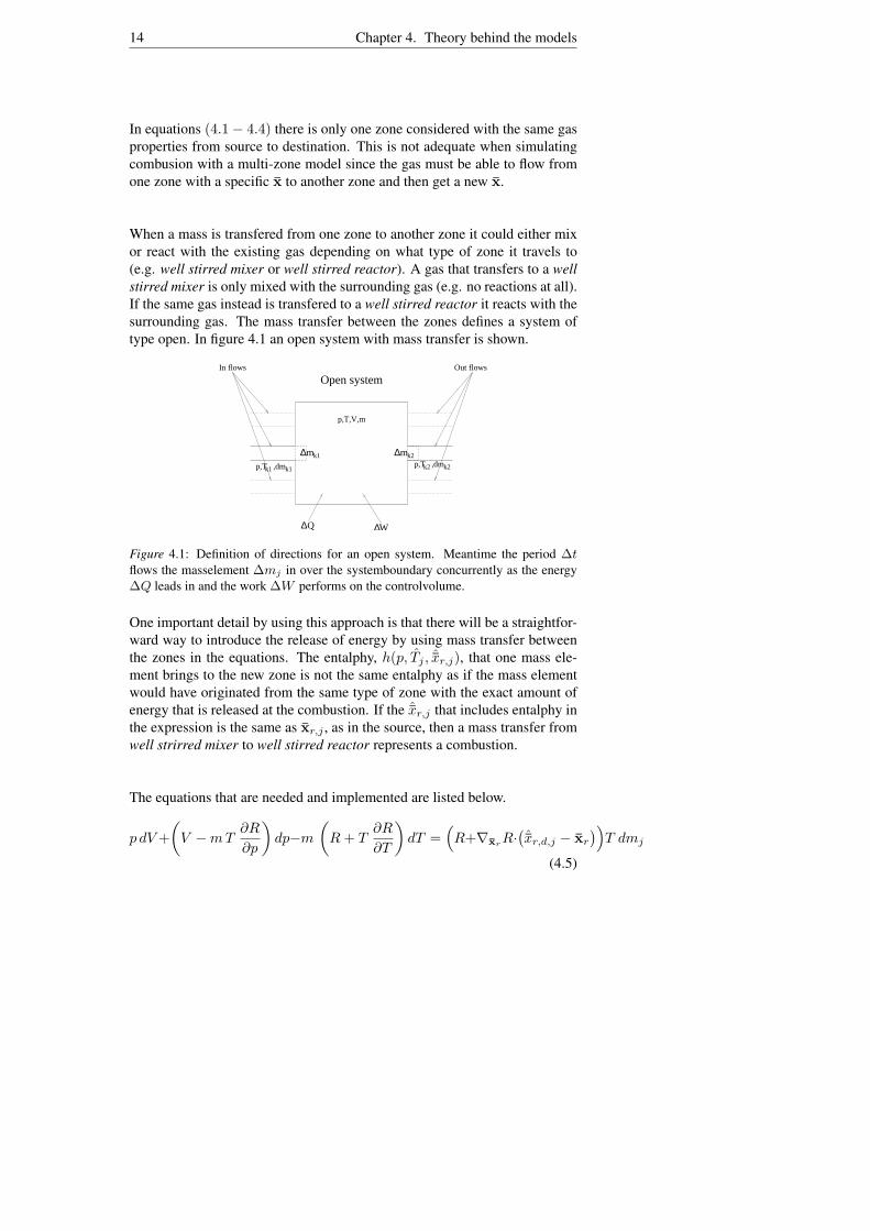
In equations (4.1− 4.4) there is only one zone considered with the same gasproperties from source to destination. This is not adequate when simulatingcombusion with a multi-zone model since the gas must be able to flow fromone zone with a specific x to another zone and then get a new x.
When a mass is transfered from one zone to another zone it could either mixor react with the existing gas depending on what type of zone it travels to(e.g. well stirred mixer or well stirred reactor). A gas that transfers to a wellstirred mixer is only mixed with the surrounding gas (e.g. no reactions at all).If the same gas instead is transfered to a well stirred reactor it reacts with thesurrounding gas. The mass transfer between the zones defines a system oftype open. In figure 4.1 an open system with mass transfer is shown.
k2∆mk1∆mp,T ,dmk1k1
p,T ,dmk2k2
∆Q ∆W
p,T,V,m
In flows Out flows
Open system
Figure 4.1: Definition of directions for an open system. Meantime the period ∆tflows the masselement ∆mj in over the systemboundary concurrently as the energy∆Q leads in and the work ∆W performs on the controlvolume.
One important detail by using this approach is that there will be a straightfor-ward way to introduce the release of energy by using mass transfer betweenthe zones in the equations. The entalphy, h(p, Tj , ˆxr,j), that one mass ele-ment brings to the new zone is not the same entalphy as if the mass elementwould have originated from the same type of zone with the exact amount ofenergy that is released at the combustion. If the ˆxr,j that includes entalphy inthe expression is the same as xr,j , as in the source, then a mass transfer fromwell strirred mixer to well stirred reactor represents a combustion.
The equations that are needed and implemented are listed below.
p dV +(
V −mT∂R
∂p
)dp−m
(R + T
∂R
∂T
)dT =
(R+∇xrR·
(ˆxr,d,j − xr
))T dmj
(4.5)

4.2. Fuel injection model 15
m cv dT+m∂u
∂pdp+pdV = dQ+
(∇xru · (xr − ˆxr,s,j) + h(p, Ts,j , ˆxr,d,j)− u
)dmj
(4.6)
dxr =xr,d,j − xr
mdmj (4.7)
Here are
χd,j ={
χj For flow from outside to inside (dmj > 0)χ For flow from inside to outside (dmj ≤ 0) (4.8)
χs,j ={
f(χj) For flow from outside to inside (dmj > 0)χ For flow from inside to outside (dmj ≤ 0) (4.9)
u = u(p, T, xr) =∑
k
xk(p, T, xr)uk(T ) (4.10)
For χ ∈ {T, xr, xk}.
0 1 0a1 p b1
c1 p d1
dpdV1
dT1
=
dV(R +∇xr
R · (ˆxr,d,j − xr
))T dmj
dQ +(∇xru · (xr − ˆxr,d,j) + h(p, Td,j , ˆxr,s,j)− u
)dmj
(4.11)there
ai = V −mT∂R
∂p
bi = −m
(R + T
∂R
∂T
)
ci = m∂u
∂p
di = m cv
4.2 Fuel injection modelThe figure 4.2 shows which signals that are sent into the submodel and whatsignals that comes out from the submodel.
Fuel Injection Submodelp,_cyl, P_rail, N m_f, u
Figure 4.2: In- and outsignals from the model
The model of fuel injection presented by Heywood [1] have been choosed and

16 Chapter 4. Theory behind the models
implemented in the total model. The timing and rate of fuel injection affectthe spray dynamics and combustion characteristics. If the pressure upstreamof the injector nozzle can be measured or estimated and assuming the flowthrough each nozzle is quasi-steady, incompressible, and one dimensional,the mass flow rate of fuel through the nozzle, ˙mf,inj , is given by:
mf,inj = CDAN
√2ρl∆p (4.12)
where AN is the nozzle minimum area, CD the discharge coefficient, ρ thedensity of liquid fuel, and ∆P the pressure drop across the nozzle. [1]
Since mf,inj = ANρlui, the fuel injection velocity at the nozzle tip ui, canbe expressed as:
ui = CD
√2∆p
ρl(4.13)
The discharge coefficient, CD, have been investigated by [2] for several en-gine operating condition. As a result of their correlation analyses, the bestcompromise between accuracy and generalization for CD is to use a functiondepending on the volume injected fuel qfuel and engine speed N .
CD = a1 − a2 · (qfuel ·N) if (qfuel ·N) ≥ 1− a1
a2
CD = 1 if (qfuel ·N) ≤ 1− a1
a2
(4.14)
Here a1 = 1.1774, a2 = 3.95 · 10−6, N is the engine speed in rpm and qfuel
is the volume injected in mm3. [2]
4.3 Fuel sprayAt the start of injection, fuel begins to penetrate into the combustion chamberand high temperature air is entrained into the spray. The hot air evaporates thefuel and beyond a fixed length, known as the break-up length, no liquid fuelexists. The liquid length shortens slightly after the start of combustion butremains relatively constant until the end of injection. Beyond the break-uplength, the rich premixed fuel and air continue to be heated until they react inthe rich premixed reaction zone.[8]
Figure 4.3 shows an general overview of the fuel spray and its flame prop-agation. The products of rich combustion continue downstream and diffuseand mix radially outward until reaching the surrounding cylinder gases. At alocation where the rich products and cylinder gases mix to produce a stoichio-metric mixture, a diffusion flame is produced. The diffusion flame surroundsthe jet in a thin turbulent sheet, which extends upstream toward the nozzle.

4.3. Fuel spray 17
Figure 4.3: General view of an quasi-steady diesel combustion plume [8].
Soot is burned out and NOx is produced on the outside of the diffusion flame,where temperatures are high and oxygen and nitrogen are abundant.[8]
Figure 4.4 shows the liquid phase and vapour phase of dme1 in different
Figure 4.4: How liquid and vapour phase propagates in time.
conditions and how they propagates in time. The rail pressure was set to 400bar and the injection duration was 3 ms. This figure shows in a distinct waythe fuel spray behaviour with both liquid and vapour phase. [12]
4.3.1 Fuel spray submodelFigure 4.5 shows which signals that are sent into the submodel and what sig-nals that comes out from the submodel.
1Dimethyl ether

18 Chapter 4. Theory behind the models
Fuel Spray Submodelp_cyl, p_rail,
t_inj_start, Nm_ae
Figure 4.5: In- and outsignals from the fuel spray submodel
The fuel spray submodel describes the fuel motion from the nozzle hole intothe combustion chamber. In every time step the model predicts the spray tippenetration sspray and the spray velocity Uspray . It also predicts the mass ofthe entrained air ma,e into the fuel spray.
The injected fuel is assumed to be a liquid column that is connected to theliquid-zone. The liquid column travels through the nozzle hole exit at a con-stant velocity U0 into the cylinder before the fuel spray breakup time, tb,occurs. This relation is given by the following equations:
U0 = CD
√2∆p
ρl(4.15)
tb = 4.351ρl · dn
C2D
√ρa∆p
(4.16)
Where CD is the discharge coefficient of the fuel injector, ∆p is the pressuredrop through the nozzle hole given in [Pa], dn is the nozzle hole diameter in[mm], ρl is the density of the fuel and ρa is the air density in the air-zone.
After the break-up time, t ≥ tb, the fuel is assumed to be atomized into finedroplets. Then there will be a descending velocity of the fuel spray, Uspray:
Uspray =2.952
(∆p
ρa
) 14
√dn
t(4.17)
To get the fuel spray break-up length, sb, and the spray tip penetration sspray
are the two equations (4.15) and (4.17) integrated. The break-up length isdefined as the length where the fuel spray liquid column atomizes into finedroplets and the spray tip penetration is the total length of the fuel spray thatreaches into the combustion chamber. The equations for fuel break-up lengthand spray tip penetration is given by:
sb(0 < t < tb) = U0 · t = CD
√2∆p
ρl· t (4.18)
sspray(t ≥ tb) =2.952
(∆p
ρa
) 14 √
dn · t (4.19)
The mass of the entrained air, ma,e is described by the rate of air that entrainsthe atomized fuel which leads to the fuel droplets to evaporate. By using

4.4. Fuel evaporation submodel 19
the conservation of the momentum the prediction of the entrained air can bedescribed by the following equation:
ma,e = −∫ t
0mf,inj(t) dt · U0
(Uspray(t))2· Uspray(t) (4.20)
Where mf,inj is the mass of the injected fuel. The integral describes thecumulative fuel mass injected and Uspray is the gradient of the fuel sprayvelocity. For a more detailed description see appendix A1. [4], [2]
4.4 Fuel evaporation submodelFigure 4.6 shows which signals that are sent into the submodel and whatsignals that comes out from the submodel. The evaporation submodel de-
Fuel Evaporation Submodelp_O2, m_f_inj m_fp
Figure 4.6: In- and outsignals from the fuel evaporation submodel
scribes the evaporation process with a semi-empirical model proposed byWhitehouse and Way [3]. With this model approach some precision is lostdue to the fact that the fuel atomization and vaporization are neglected. Fuelprepared-rate is only considered in this model.
The fuel is prepared after it has atomized and evaporated and then micro-mixed with the entrained air. The prepared mass flow is depending on theinjected fuel at that time, on the entrained air (partial oxygen pressure in theprepared-zone) as well on the amount of fuel that is injected but not yet pre-pared. Following equation gives the relation between these dependencies:
mf,p(t) = C1 · 180ω
π·(∫ t
0
mf,inj(t) dt
) 13
(pO2(t))0.4 ·
·(∫ t
0
mf,inj(t) dt−∫ t
0
mf,p(t) dt
) 23
(4.21)
where ω is engine speed in[
rads
], pO2 is the partial oxygen pressure in the air-
zone in [bar] and C1 is a constant assumed equal to 0.035[
bar−0.4
deg
]. [2], [3]
4.5 Combustion submodelFigure 4.7 shows which signals that are sent into the submodel and what sig-nals that comes out from the submodel. The combustion submodel also uses

20 Chapter 4. Theory behind the models
Fuel Combustion Submodelp_O2, T_mean, m_fp m_fb
Figure 4.7: In- and outsignals from the combustion submodel
an semi-empirical model that is strongly connected to the fuel evaporationsubmodel. The mass of the burned fuel, mf,b is predicted by this model.There are two equations describing the rate of combustion. First is the rateof combustion, mf,b, and the second is the mean gas temperature of the threezones.
mf,b(t) =C2 · pO2
N ′ ·√
Tmean(t)· 180ω
π· e
(− TA
T (t)
) ∫ t
0
(mf,p(t)− mf,b(t)) dt
(4.22)
Tmean(t) =∑
k Ti(t) ·mi(t)∑k mi(t)
(4.23)
Here ω is the engine speed in[
rads
], pO2 is the partial oxygen pressure of the
air-zone in [bar], N ′ is the engine speed in [rps]. C2 and TA is assumed tobe equal to 1.2 · 1010
[K0.5
bars
]and 16500 [K]. Ti and mi are the temperature
and mass for the zone i = a, p, b.[2]
In the early stages of combustion the preparation rate, mf,p, is greater thanthe burning rate, mf,b, and with an accumulation of prepared fuel it resultsin a premixed combustion process. When the energy of the premixed com-bustion comes to an end, the evaporation and combustion rates are equal andresulting in a mixing-controlled combustion process [3].
4.6 Heat transfer submodelFigure 4.8 shows which signals that are sent into the submodel and whatsignals that comes out from the submodel. Two types of heat transfer are
Thermodynamic Submodelp, T, m, phi dp, dT, dphi
Figure 4.8: In- and outsignals from the heat transfer submodel
discussed in this model; convective heat transfer and radiative heat transfer.The most part of the heat transfer in internal combustion engines comes fromconvection. This is when heat is transfered through fluids in motion or a fluidand solid surface in relative motion. The forced convection is used when themotions are produced by forces other than gravity. In this case there is forced

4.6. Heat transfer submodel 21
convection between the in-cylinder gases and the cylinder head, valves, cylin-der walls and piston during the different phases. The heat transfer caused byradiation occurs from the high temperature combustion gases and hot parti-cles in the flame region to the combustion chamber walls. The concept ofheat transfer by radiation is based on the emission and absoption of electro-magnetic waves.[1]
In the burned-zone there are both convective and radiative heat transfer. Thetotal heat transfer in the burned-zone is calculated by the sum as follow:
Q = Qc + Qr (4.24)
The convective heat transfer is described by Newons law of cooling:
Qc = hcA (T − Tw) Cc (4.25)
Here T is the temperature in the zone, Tw is the in-cylinder wall tempera-ture, Cc is calibration parameter, A is the in-cylinder area and hc is given byWoschnis correlation as:
hc = 0.013 ·p0.8
(C1up + C2
(p−pm)TrVprVr
)0.8
B0.2 · T 0.55(4.26)
Here the constants are set to C1 = 2.28 and C2 = 0 during the compression-phase. During the combustion-phase the constants are set as C1 = 2.28 andC2 = 3.24 · 10−3. The other constants and parameters can be seen in table4.6.
Constant Description Unitup Mean piston speed m
sB Cylinder bore [m]T Temperature [K]pr Reference pressure [Pa]Vr Reference volume [m3]Tr Reference Temperature [K]p Fired pressure [Pa]p0 Motored pressure [Pa]C1 Constant [−]C2 Constant [ m
sK ]
The radiative heat transfer is described by using Stefan-Boltzmann law:
Qr = σA(T 4
b − T 4w
)Cr (4.27)
Where σ is Stefan-Boltzmanns constant, Cr is a calibration parameter and Tb
is the mean gas temperature in the burned-zone.

Chapter 5
Implementation
This chapter will describe how the model was implemented into the Mat-lab/Simulink environment. Matlab is a numerical computing environmentbut also a programming language. Simulink is a tool in Matlab for modeling,simulating and analyzing dynamic systems.
5.1 General view
The entire model consists of all submodels presented in previous chapter andthese submodels are implemented in Simulink and a few as S-functions. Tosimplify the work to implement our multi-zone model has a package calledpsPack1 been used. Further information about psPack is presented in sec-tion 5.5. The submodels that have been implemented in Simulink containsinformation that are used by the S-functions2 that handles compression andcombustion.
5.2 Simulink
Simulink is the environment where all the submodels, presented in the Modeltheory chapter, was put together to a working unit. Below, in figure 5.1, anexample is shown on how the implementation in our model is made, in thiscase the fuel spray submodel. To the left in the figure is the submodel com-municating with all other submodels presented (the top layer). The right partof the figure shows how the fuel spray submodel is built with more submodelsthat represents different equations (4.15, 4.16, 4.17) in the model.
1Engine simulation tool developed at Vehicular systems at LiTH2Internal function in simulink, often written in C- code
22

5.3. S-functions 23
Fuel Spray
after_break_up
Goto24
m_dot_ae
Goto23
p_rail
p_cyl
fuel_injected
t_inj,start
air_density
burn_completed
C_D
m_dot_a,e
after break-up
Fuel Spray Submodel
[C_D]
From65
[air_density]
From6
[fuel_injected_part]
From44
[t_inj_start]
From43
[comb_enable]
From39
[p_cyl]
From36
[burn_completed]
From33
-C-0:0
Constant4
2
after break-up
1
m_dot_a,eProduct
m_finj
U_0
U_ab
m_dot_a,e
Equation_22
p_rail
p_cyl
t_inj,start
air_density
U_ab
Equation_20
p_rail
p_cyl
C_D
air_density
t_b
Equation_19
p_rail
p_cyl
C_D
U_0
Equation_18
t_b
t_inj,start
after_break-up
before_break-up
Break-up length
Enable
7
C_D
6
burn_completed
5
air_density
4
t_inj,start
3
fuel_injected
2
p_cyl
1
p_rail
Figure 5.1: A general view of the model to demonstrate how the model is implementedwith the different layers in simulink.
5.3 S-functions
In the final model several S-functions have been used. These have been codedin the m-language and are implemented as Level 2 M-file S-Functions. Themain S-functions are those who handles the compression and combustion.These S-functions calculates the thermal properties, pressure, temperaturesand volumes for the different zones. Some of this information is then feededback to submodels. There are also S-functions that handles the fuel injectionsystem.
5.4 Solver
To solve the differential equations is a stiff ode3 solver used. The problemis stiff if the solution being sought is varying slowly, but there exists nearbysolutions that vary rapidly, so the numerical method must take small steps toobtain satisfactory results.
5.5 psPack
This is a simulation tool that initally was designed for simulation of SI-engines. This package has been stripped down and only the necessary func-tions are used. In the psPack-menu changes can be made in a few engineparameters such as geometry and engine speed. psPack is allso used to calcu-late thermal properties for the burned gas. It uses a table where it is lookingup the desired thermal property for the current pressure p, temperature T andmass fraction of fuel and air in the zone. This package is developed for Mat-lab/Simulink.
3Ordinary Differential Equation

24 Chapter 5. Implementation
5.5.1 Thermal PropertiesTo calculate the desired thermal property some arguments are sent to thepsPack function, psThermProp, that is needed to interpolate in the tables.As mentioned above it needs p, T and mass fraction of fuel and air for thespecific zone. To simplify the call of the thermal property function4 the massfraction are divided as a vector Xgc that consists of the fraction of unburnedand burned mass of fuel and air. It can be seen in equation 5.1:
Xgc =(
xf,u xa,u xf,b xa,b
)(5.1)
where xf,u and xa,u stands for the mass fraction in an unburned zone and xf,b
and xa,b stands for the same in the burned zone. In our setup of zones there arean air-zone, prepared-zone and a burned-zone. The air-zone is considered asair that is unburned and the prepared-zone is considered as vaporized fuel thatalso is unburned. In the burned-zone air and vaporized fuel have reacted andthere is a mixture of burned fuel and air. Initially there exists a small fractionof burned fuel and air due to residual gas from previously combustion. Inequation 5.2 it is shown what the setup of the zones looks like.
Xgc =
Xgc,a
Xgc,p
Xgc,b
=
0 xa,u 0 0xf,u 0 0 00 0 xf,b xa,b
(5.2)
where row one is the air-zone, row two is the prepared-zone and row three isthe burned-zone.
4the function is called psThermProp() and is a part of psPack

Chapter 6
Validation
In this chapter the validation steps is presented. Validation of the submodelshave been carried out in two steps. Both when the submodels are separateunits and when they have been put togehther to one unit.
6.1 Comments about the Validation
The important content of the model is that it should predict torque in a correctway. Unfortunately it is not possible to validate the total model in an goodway because the lack of engine measurement data. Although validations ofsome of the submodels are presented in this chapter. When validations arenot possible, experiments have been performed to show that the submodelsprobably act as it supposed to. With the measurement data thats availablecan the different submodels behavior be studied in detail. If the submodelsbehavior is concurrent with the measurement it is probably a good indicationthat the total model also will concur.
6.2 Fuel injection
The fuel injection is described, as equation (4.12), and is very dependentof the amount of fuel injected hence the parameter CD change as equation(4.14). A test was formed to show how the parameter CD affects the massflow rate at the injection. The test setup can be seen in table 6.1. Figure 6.1shows the control signal, for the different cases, plotted in the same figureas fuel mass flow rate. As the injected mass increases the parameter CD
changes. These phenomena can be seen as when the first part of the fuelis injected it does not encounter any major resistance. When the amount offuel increases in the cylinder the later part of the injected fuel encounters aresistance so that it bumps into the aldready injected fuel and therefore slows
25

26 Chapter 6. Validation
Injection law set nr Rail pressure Injected fuel N1 800 [bar] 32.9 [mg] 2500 [rpm]1 1000 [bar] 36.4 [mg] 2500 [rpm]1 1200 [bar] 39.4 [mg] 2500 [rpm]
Table 6.1: Table of fuel injection test setup
down the fuel mass flow rate. The resistance that is increased comes from themodel of CD that is described by equation (4.14).
−15 −10 −5 0 5 10 150
0.1
0.2
0.3
0.4
0.5
0.6
0.7
0.8
0.9
1Injection control signal and injected fuel mass flow
Con
trol
sig
nal
theta [deg]−15 −10 −5 0 5 10 15
0
0.01
0.02
0.03
0.04
0.05
0.06
Fue
l mas
s flo
w [k
g/s]
800 bar1000 bar1200 bar
Figure 6.1: Fuel injection control signal and mass flow rate that shows the changes inCD for different injection pressures. The decrease in CD can be seen in the decreaseof the mass flow after about 2 deg.
6.3 Fuel spray validationTo validate the spray penetration correlation, experimental data collected byDan et al. [9] were compared with the implemented model predictions. Theinjection conditions and ambient conditions of the experiment are summa-rized in Table 6.2 The injector nozzle has a mini-sac volume design for highinjection pressure. The injection pressure was varied from 55 MPa to 120MPa. In figure 6.2 and 6.3 simulations are compared to the measurementsof the spray tip penetration as a function of time from start of injection andinjection pressure.
In figure 6.2, the measured spray penetration for an injection pressure of 120MPa is compared with the simulated data from the model. It shows that theimplemented model over predicts the spray tip penetration. When the injec-tion pressure is lower, in this case 55 MPa, the model has a better accuracy

6.3. Fuel spray validation 27
Parameter value/specHole diameter [mm] 0.2Hole length [mm] 1.1Number of holes [-] 1Discharge coefficient of the hole [-] 0.66Injection pressure [MPa] 55, 120Ambient pressure [MPa] 1.5Ambient temperature [K] 293Ambient density [ kg
m3 ] 17.3Ambient viscosity [·10−6Pa · s] 17.5
Table 6.2: Experimental setup for the fuel spray validation.
but it still over predicts. This result can be seen in figure 6.3 . This over-prediction probably comes from the disregard of the ambient viscosity in ourmodel that is used in the experimental setup.
0 0.5 1 1.5 2 2.5
x 10−3
0.01
0.02
0.03
0.04
0.05
0.06
0.07
0.08
0.09
0.1Injection with a rail−pressure at 120 MPa
Time after injection [s]
Spr
ay ti
p pe
netr
atio
n [m
]
SimulationExperimental
Figure 6.2: Spray tip penetration as function of time with fuel injection pressure 120MPa. As can be seen the model overpredicts the penetration length slightly.
In figure 6.4 it is shown how the length of the spray tip varies with differentsets of rail-pressure. The liquid length is the fuel spray break-up length andis shown as the solid line in the figure. The length of the dropplet basedspray is the dotted length and the total fuel spray penetration length is thesolid and dotted line together. In this simulation was a simulation time of 1.4millisecond used and the rail pressure was in the four cases 60, 80, 100, 120MPa.

28 Chapter 6. Validation
0 0.5 1 1.5 2 2.5
x 10−3
0.01
0.02
0.03
0.04
0.05
0.06
0.07
0.08Injection with a rail−pressure at 55 MPa
Time after injection [s]
Spr
ay ti
p pe
netr
atio
n [m
]
SimulationExperimental
Figure 6.3: Spray tip penetration as function of time with fuel injection pressure 55MPa. Here it also shown that the model sligthly overpredict the penetration length.
0 0.01 0.02 0.03 0.04 0.05 0.06 0.07 0.08 0.09
1
2
3
4
Spray tip penetration [m]
Tes
t Nr:
Length of spray tip
Figure 6.4: Spray tip length, for different injection pressures. From the top: 120, 100,80, 60 MPa The solid line represents liquid length. As expected the penetration islarger for higher pressures.
6.4 Fuel evaporation model
To validate the fuel evaporation model the injected fuel mass and the massof the evaporated fuel are plotted in the same plot. Figure 6.5 shows theinjection and evaporation of fuel with only a main injection. It is shownthat the evaporation process looks like a first order system and this seems tobe correct when a comparison are made between these plots and the plotspresented in the Salerno rapport [2]. In figure 6.6 is a new simulation madewith the difference that both pre- and main injection is used.

6.4. Fuel evaporation model 29
0.023 0.0235 0.024 0.0245 0.025 0.0255 0.0260
0.5
1
1.5
2
2.5
3
3.5
4x 10
−5 Injected and evaporated fuel (Injection law nr:1 )
Time [s]
Mas
s [k
g]
Fuel mass injectedFuel mass evaporated
Figure 6.5: Fuel injection and evaporation, main injection (injection law nr 1). Theshape of the evaporated mass is consistent with a first order system and the result issimilar to the result in [2].
0.0225 0.023 0.0235 0.024 0.0245 0.025 0.0255 0.0260
0.5
1
1.5
2
2.5
3
3.5
4
4.5x 10
−5 Injected and evaporated fuel (Injection law nr:2 )
Time [s]
Mas
s [k
g]
Fuel mass injectedFuel mass evaporated
Figure 6.6: Fuel injection and evaporation, pre + main injection (injection law nr 2).When using multiple injections the evaporated mass is still consistent with a first ordersystem.
In the following figure it’s presented how the rate of evaporation varies duringthe injection. In figure 6.7 the rate for both injection law one and two isplotted, see Table 6.5 for more information.

30 Chapter 6. Validation
0.0225 0.023 0.0235 0.024 0.0245 0.025 0.0255 0.0260
0.005
0.01
0.015
0.02
0.025
0.03
0.035
0.04Fuel evaporation rate (Injection law nr: 1 & 2 )
Time [s]
Mas
srat
e [k
g/s]
Injection law 1Injection law 2
Figure 6.7: Fuel evaporation rate for injection law nr 1 plotted with injection law 2.This shows how the fuel evaporation rate varies during two different types of injec-tions.
6.5 Evaporation and combustion submodel
In the model the atomization of fuel into droplets, vaporization of the fuel,entrainment of air and micromixing of fuel and air are joint together and isknown as preparation of fuel according to the equations (4.21,4.22). At thestart of the combustion the fuel burning rate is lower than the preparation rate.As the prepared fuel is accumulated it causes an increase in the burning rate.Then, as the combustion proceeds, the burning rate increases faster than thepreparation rate. When the prepared fuel is depleted the burning rate is de-creasing. This is a result of premixed combustion process and the burningrate is controlled by the chemical kinetics.[3]
To validate the premixing combustion process a test setup in table 6.3 wasused.
Start of injection Fuel injectedθ = 4.76 deg BTDC 21.56 [mg]
Table 6.3: Test setup for evaporatin and combustion validation.
In figure 6.8 it’s shown that this premixed behaviour starts at 4 [deg] BTDCand ends at 4 [deg] ATDC. After the premixed behaviour is completed themixing controlled combustion starts. As a result of the mixing controlledcombustion process the combustion and preparation rate keeps equal to the
6.5. Evaporation and combustion submodel 31
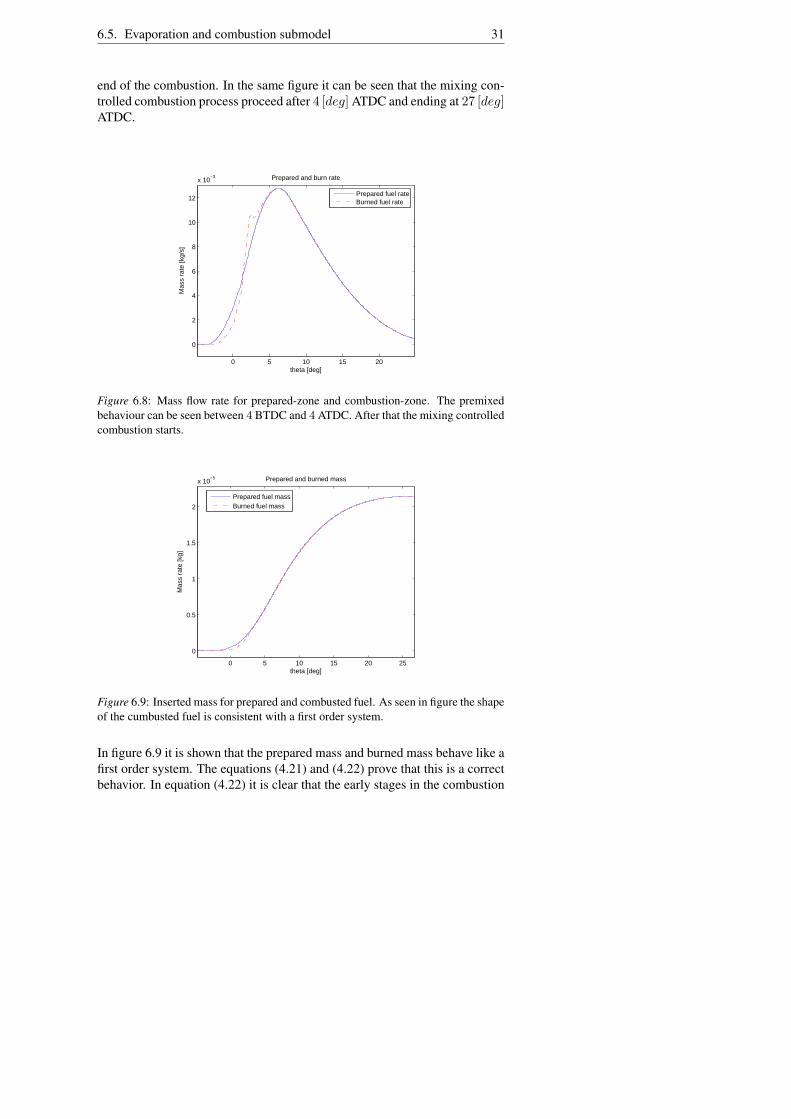
end of the combustion. In the same figure it can be seen that the mixing con-trolled combustion process proceed after 4 [deg] ATDC and ending at 27 [deg]ATDC.
0 5 10 15 20
0
2
4
6
8
10
12
x 10−3 Prepared and burn rate
theta [deg]
Mas
s ra
te [k
g/s]
Prepared fuel rateBurned fuel rate
Figure 6.8: Mass flow rate for prepared-zone and combustion-zone. The premixedbehaviour can be seen between 4 BTDC and 4 ATDC. After that the mixing controlledcombustion starts.
0 5 10 15 20 25
0
0.5
1
1.5
2
x 10−5 Prepared and burned mass
theta [deg]
Mas
s ra
te [k
g]
Prepared fuel massBurned fuel mass
Figure 6.9: Inserted mass for prepared and combusted fuel. As seen in figure the shapeof the cumbusted fuel is consistent with a first order system.
In figure 6.9 it is shown that the prepared mass and burned mass behave like afirst order system. The equations (4.21) and (4.22) prove that this is a correctbehavior. In equation (4.22) it is clear that the early stages in the combustion

32 Chapter 6. Validation
is controlled by an Arrhenius 1 like part. This part describes the tempera-ture dependece of the rate of chemical reaction. It can also be considered torepresent the ignition delay time. The constant C2 also controls the ignitiondelay time. In the simulation of the burning rate is the end of combustionconsidered as when the burned fuel fraction reaches 0.9995, as described inequation (6.1):
mf,b
mf,inj≥ 0.9995 (6.1)
6.6 Heat transfer model
In this section the implemented heat transfer model is validated. In table6.3 the setup for this validation is presented. Figure 6.10 shows how theconvective and radiative heat transfer varies during the cumbustion process.Lack of validation data will force to validate the model just by looking at thefundamental appearance of the heat transfer curves. The figure also showsthat the convective heat transfer stands for the largest part of the total heattransfer. When the combustion starts, just before TDC, the radiative heattransfer increases, and is at most about 30 percent of the total heat transfer.
−60 −40 −20 0 20 40 60 80 1000
2000
4000
6000
8000
10000
12000
14000Heat transfer
theta [deg]
dQ [W
/(m
2 K)]
Convective heat transferRadiative heat transferTotal heat transfer
Figure 6.10: Total heat transfer for a simulation. In figure it is show that the largestpart for the heat transfer originates from convective heat transfer.
1The Arrhenius equation is a simple, but remarkably accurate, formula for the temperaturedependence of the rate constant, and therefore rate, of a chemical reaction

6.7. Thermal properties 33
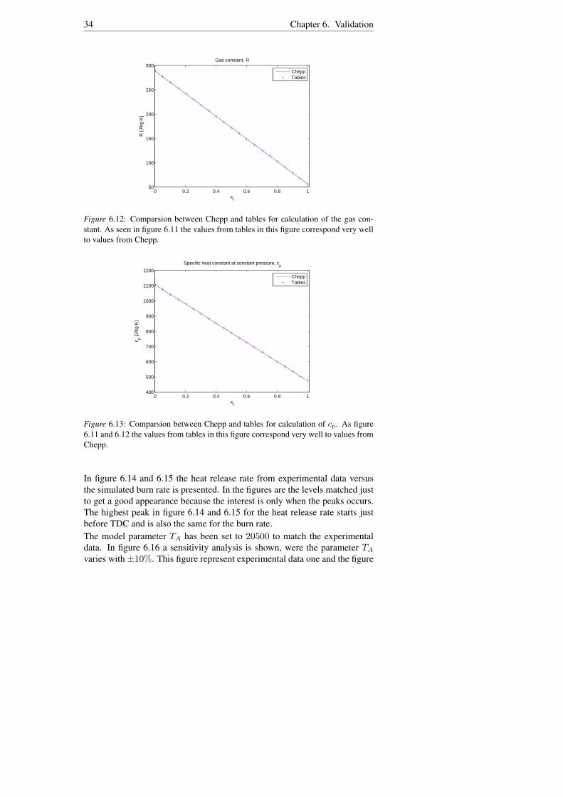
6.7 Thermal propertiesOne important part of model accuracy is to have correct values for the thermalproperties of the different zones. There exist a program called Chepp2 whichcalculates the thermal properties for differents types of zones. Unfortunatelythis program could not be used in the final product. Tables are used as a re-placement to obtain the desired thermal property for the specific mass fractionof air and fuel (xf,u, xa,u, xf,b, xa,b), T and p. If some value is going out ofbound the tables extrapolates.
In figure 6.11 6.12 6.13 it is shown that the table calculations fit the cal-culations produced from Chepp. These calculations have been made for anunburned zone where xf vary from 0 to 1. To to get a clearer view the calcu-lations for the tables have been downsampled.
0 0.2 0.4 0.6 0.8 10
1
2
3
4
5
6x 10
5 Enthalpy, h
xf
h [J
/kg]
CheppTables
Figure 6.11: Comparsion between Chepp and tables for calculation of enthalpy. It isshown that the values from generated from tables correspond very well to the valuesproduced from Chepp.
6.8 Heat release analysisIn this section two experiment are made to validate the heat release. The heatrelease rate for the experiment is given by real measurments from GM. Theheat release for the simulated model is approximated with the fuel burn ratee.g. mfb. In table 6.4 the model parameters that is used in the simulation ispresented.
2Chemical Equilibrium Program, developed at Vehicular systems by Lars Eriksson
34 Chapter 6. Validation
0 0.2 0.4 0.6 0.8 150
100
150
200
250
300Gas constant, R
xf
R [J
/kg
K]
CheppTables
Figure 6.12: Comparsion between Chepp and tables for calculation of the gas con-stant. As seen in figure 6.11 the values from tables in this figure correspond very wellto values from Chepp.
0 0.2 0.4 0.6 0.8 1400
500
600
700
800
900
1000
1100
1200
Specific heat constant at constant pressure, cp
xf
c p [J/k
g K
]
CheppTables
Figure 6.13: Comparsion between Chepp and tables for calculation of cp. As figure6.11 and 6.12 the values from tables in this figure correspond very well to values fromChepp.
In figure 6.14 and 6.15 the heat release rate from experimental data versusthe simulated burn rate is presented. In the figures are the levels matched justto get a good appearance because the interest is only when the peaks occurs.The highest peak in figure 6.14 and 6.15 for the heat release rate starts justbefore TDC and is also the same for the burn rate.The model parameter TA has been set to 20500 to match the experimentaldata. In figure 6.16 a sensitivity analysis is shown, were the parameter TA
varies with ±10%. This figure represent experimental data one and the figure

6.8. Heat release analysis 35
Variable Value UnitTim 325 [K]Tres 440,480 [K]xres 33 [%]TA 20500 [K]
Table 6.4: Setup for heat release experiment one and two.
−40 −30 −20 −10 0 10 20 30 400
20
40
60
80
100
120
140
160
180
200
θ [deg]
Heat release vs burned rate
Heat release from experimentBurned rate from simulation
Figure 6.14: Heat release for experiment one. As can be seen in figure the timing ofheat release and the burned-rate is matched good, around TDC.
−40 −30 −20 −10 0 10 20 30 400
20
40
60
80
100
120
140
160
180
200
θ [deg]
Heat release vs burned rate
Heat release from experimentBurned rate from simulation
Figure 6.15: Heat release for experiment two. As can be seen in figure the timing ofheat release and the burned-rate is matched good, around TDC.
for experimental data two is located in Appendix B. It shows that an increasein the parameter TA postpone the first burn rate peak and a decrease in the
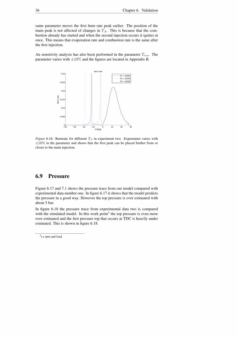
36 Chapter 6. Validation
same parameter moves the first burn rate peak earlier. The position of themain peak is not affected of changes in TA. This is because that the com-bustion already has started and when the second injection occurs it ignites atonce. This means that evaporation rate and combustion rate is the same afterthe first injection.
An sensitivity analysis has also been performed in the parameter Tres. Theparameter varies with ±10% and the figures are located in Appendix B.
−40 −30 −20 −10 0 10 20 300
0.005
0.01
0.015
0.02
0.025
0.03
θ [deg]
Bur
n ra
te
Burn rate
TA = 20500TA = 22550TA = 18450
Figure 6.16: Burnrate for different TA in experiment two. Experminet varies with±10% in the parameter and shows that the first peak can be placed further from orcloser to the main injection.
6.9 Pressure
Figure 6.17 and 7.1 shows the pressure trace from our model compared withexperimental data number one. In figure 6.17 it shows that the model predictsthe pressure in a good way. However the top pressure is over estimated withabout 5 bar.
In figure 6.18 the pressure trace from experimental data two is comparedwith the simulated model. In this work point3 the top pressure is even moreover estimated and the first pressure top that occurs at TDC is heavily underestimated. This is shown in figure 6.18.
3i.e rpm and load

6.10. In-cylinder temperature 37
−300 −200 −100 0 100 200 3000
20
40
60
80
100
120
140Cylinder pressure
θ [deg]
Pre
ssur
e [b
ar]
Experimental pressureSimulated pressure
Figure 6.17: Pressure-trace for experiment one. It is shown that the simulated pressureis slightly under predicted at TDC and slightly over predicted a few degrees after TDC.
−300 −200 −100 0 100 200 3000
20
40
60
80
100
120
140Cylinder pressure
θ [deg]
Pre
ssur
e [b
ar]
Experimental pressureSimulated pressure
Figure 6.18: Pressure-trace for experimental setup two. The under and over predictionof the simulated pressure is a bit larger than seen in figure 6.17.
6.10 In-cylinder temperature
To show the effects of pre-injection a test set was constructed, see table 6.5.
In figure 6.19 the temperature in the burned-zone is plotted against the crankangle, evidencing an minor increase of the maximum temperature in the testcase with only one main injection. In the presence of pre and main injection,test case 2, the maximum temperature is reduced. This reduction is achieveddue to the reduced mass of fuel of the main injection, although the sameamount of injected fuel is the same in both test cases.

38 Chapter 6. Validation
Injection type Inj 1 Inj 2
Only main -{
θstart=7 deg BTDCminj=15.37[mg]
}
Pre- and main{
θstart=25.7 deg BTDCminj1=2.76[mg]
} {θstart=7 deg BTDCminj2=12.65[mg]
}
Table 6.5: Table of injection law sets. The two different injections has the same totalamount of injected fuel.
0 5 10 15 20 25 30
1800
1900
2000
2100
2200
2300
2400
2500
Temperature in burned zone
θ [deg]
Tem
pera
ture
[K]
Main injectionPre− and main injection
Figure 6.19: Difference between temperature in the burned zone. It is shown that ainjection law with pre + main injection may reduce the high temperature.
The IMEP4 is almost the same for the two cases (14.12, 14.5) bar. This is ev-idencing that the occurrence of pre-injection may reduce the maximum tem-perature while keeping almost the same IMEP, with benfits of lower NOx
emissions. These is the same conclusions that is made in (Arise et al., 2005)[2].
4Indicated Mean Effective Pressure

Chapter 7
Results and Conclusions
In this chapter the results and conclusions that can be recognised are pre-sented.
7.1 ResultsBelow are data from our model presented and compared with experimentaldata. Two figures are also shown to help illustrate the performance of themodel. In table 7.1 it is shown that our model can predict the torque duringone cycle that only differ 0.7 % with experimental data (Experimental setupone). In table 7.1 it is shown that our model gives a mean square error between0.36 - 0.80 Nm.
Experimental setup Measurement Simulated ExperimentalOne Torque [Nm] 59.9881 59.5284One IMEP [Bar] 10.7443 11.1063Two Torque [Nm] 53.7677 54.9965Two IMEP [Bar] 10.3045 10.5152
Table 7.1: Results presented for both experiment one and two.
Experimental setup Measurement ResultOne Mean fault [Nm] 0.362064Two Mean fault [Nm] 0.801828
Table 7.2: Results presented for both experiment one and two.
Figures 7.1 and 7.2 shows a comparison between measurement data and ex-perimental data for the two different setups. This is presented with the help of
39

40 Chapter 7. Results and Conclusions
pV-diagrams. The figures shows that the model gives a good approximationof the pressure during a whole combustion cycle.
0.5 1 1.5 2 2.5 3 3.5 4 4.5 5
x 10−4
0
20
40
60
80
100
120
Volume [m3]
Pre
ssur
e [b
ar]
Pressure versus volume
ExperimentSimulated
Figure 7.1: Pressure versus volume (pV-plot) for experiment one. In this pV-plot theover prediction of top-pressure is shown.
0.5 1 1.5 2 2.5 3 3.5 4 4.5 5
x 10−4
0
20
40
60
80
100
120
Volume [m3]
Pre
ssur
e [b
ar]
Pressure versus volume
ExperimentSimulated
Figure 7.2: Pressure versus volume (pV-plot) for experiment two. In this pV-plot theover prediction of top-pressure is shown.
7.2 Conclusions
• A model that can predict the engine torque has been implemented.

7.3. Future work 41
• The validation in the two engine operating-points gives a good resultwhen comparing the implemented model and the engine measurementdata.
• Since a complete validation not has been possible to accomplish thedifferent submodels has been investigated separately. The submodelsthat were possible to validate have been validated with good result.
• For those submodels that not have been possible to validate experi-ments have been constructed to show that the submodel is very likelyto behave in a correct manner.
• A sensitivity analysis has been performed for some of the ingoing modelparameters.
• Together with the sensitivity analysis and the investigation of the ingo-ing submodels the results show that the parts that need more validationis fuel injection and heat transfer and while the the models for evapo-ration, combustion and fuel spray indicates a satisfying result.
7.3 Future workThe existing model that has been presented in this thesis can be further mod-ified and improve in the following items:
• Gas exchange model. To get the full pressure trace it is necessary tohave an accurate gas exchange model.
• Swirl model. To get a more accurate model of the fuel spray distribu-tion it should be considered to model the swirl factor. The swirl factoris a measurement of how turbulent the airflow is in the combustionchamber.
• Advanced model of fuel spray. Another step to increase accuracy inthe model is to divide the fuel spray into several zones and considerdroplet distribution. This is a more advanced fuel spray model and isproposed by Jung, Assanis [4].
• Wall wetting. There may occur injections where the injected fuel hitsthe in-cylinder wall and cools down which prevents the evaporizationprocess to happen.

42 Chapter 7. Results and Conclusions
• Cylinder wall temperature Examine how the changes in the in-cylinderwall temperature effects the combustion process.
• Parameter identification To enhance the accuracy in the model furtherwork in tuning and verifying the parameters must be done.
If some of these improvements is done the complexity increases and thereforethe computational time and simulation time will increase.

Chapter 8
References
[1] John B. Heywood. Internal Combustion Engine Fundamentals. McGraw-Hill Book Co, 1988.
[2] C. Pianese G. Rizzo A. Caraceni P. Cioffi G. Flauti I. Arsie. Thermo-dynamic modeling of jet formation and combustion in common rail multi-jetdiesel engines. SAE Thechnical Papers Series 2005-01-1121, 2005.
[3] J. I. Ramos. Internal Combustion Engine Modeling. Hemisphere Pub-lishing Corporation, 1989.
[4] Dohoy Jung and Dennis N. Assanis. Multi-Zone DI Diesel Spray Com-bustion Model for Cycle Simulation Studies of Engine Performance and Emis-sions. SAE Technical Papers Series 2001-01-1246, 2001.
[5] L. Eriksson Y. Nilsson. A new formulation of multizone combustion en-gine models. Internal technical report. Department of Electrical Engineering,Linkopings University.
[6] L. Eriksson L Nielsen. Vehicular Systems. Technical report. Departmentof Electrical Engineering, Linkopings University, 2006.
[7] C. F. Taylor. The Internal-Combustion Engine in Theory and Practice,Revised Edition. The M.I.T press, Seventh printing, 1995.
[8] C. Argachoy. A. P. Pimenta. Phenomenological Model of Particulate Mat-ter Emission from Direct Injection Diesel Engines. Technical Paper. 2005.
[9] J. Senda H. Fujimoto T. Dan. S. Takagishi. Effect of ambient gas prop-erties for characteristics of non-reacting diesel fuel spray. SAE TechnicalPaper Series 9703552, 1997.
43

44 Chapter 8. References
[10] Nationalencyklopedin, 2007
[11] http : //auto.howstuffworks.com/diesel1.htm,October2008
[12] Y. Kim, J. Lim, and K. Min A study of the dimethyl ether spray character-istics and ignition delay School of Mechanical and Aerospace Engineering,Seoul National University, April 2007
[13] P. Oberg A DAE Formulation and it’s Numerical Solution for Multi-Zonethermodynamic models Technical report in progress. Department of Electri-cal Engineering, Linkopings University, 2008

Notation
Symbols used in the report.
Variables and parametersCD Discharge coefficient [-]m Mass kg
mf,b Mass of burned fuel kgmf,p Mass of prepared fuel kg
mf,inj Mass of fuel injected kgma,e Mass of air entrained kgN Engine speed rev/sN ′ Engine speed rad/s
patm Atmospheric normal pressure Paprail Rail Pressure Papcyl Cylinder Pressure PaR Gas constant J/(kgK)
Sbreak Break-up length mt Time from start of injection s
tbreak Fuel sprey break-up time stinj,d Fuel sprey break-up time s
T Temperature KTw Cyllinder wall temperatur KV Volume m3
45
Appendix A
Derivation of airentrainment rate andthermodynamic model
In this chapter the derivation of air entrainment rate and thermodynamic modelthat is used in the report is presented.
A.1 Air entrainment rateThe prediction of the entrained air is based on the conservation of momentum.It assumes that the initial momentum imparted by the fuel flow at the nozzleexit is equal to the sum of the momentum of the unburned and liquid zone as:
mf,inj · U0 = (mf,inj + ma,e)Uspray (A.1)
where mf,inj is the fuel injected, ma,e is the entrained air, U0 is the fuel flowvelocity at the nozzle exit considered constant value and Uspray is the fuelspray velocity. Equation A.1 can be rewritten as:
ma,e = mf,inj
(U0
1Uspray
− 1)
(A.2)
Then by differentiating equation A.2 with resepect to time, the air entrainmentrate come out as:
ma,e = −∫ t
0mf,inj(t) dt · U0
(Uspray(t))2· Uspray(t) (A.3)
which is the expression we use in air entrainment section.
46

A.2. Thermodynamic Equations 47
A.2 Thermodynamic Equations
A.2.1 Energy at equilibrium
The change in energy for an open system are described by the equations be-low. Note that the function for the different parts xk can vary from zone tozone and that xj,k is used to denote that it is the xk-function for the source jthats regarded. The index b,e denote beginning and end respectively.
∆U = ∆W + ∆Q (A.4)
Ub = m∑
k
xk(pb, Tb, xr,b)uk(Tb) + ∆mj
∑
k
xj,k(pb, Tj , ˆxr,j)uk(Tj)
(A.5)Ue = (m + ∆mj)
∑
k
xk(pe, Te, xr,e)uk(Te) =
= (m + ∆mj)∑
k
xk(pb + ∆p, Tb + ∆T, xr,b + ∆xr)uk(Tb + ∆T ) =
= (m + ∆mj)∑
k
(xk(pb, Tb, xr,b) +
∂xk
∂p∆p +
∂xk
∂T∆T+
+∇xrxk ·∆xr + O(∆2)) (
uk(Tb) +∂uk
∂T∆T + O(∆2)
)=
= m∑
k
xk(pb, Tb, xr,b)uk(Tb) + m∑
k
(∂xk
∂p∆p +
∂xk
∂T∆T +∇xrxk ·∆xr
)uk(Tb)+
+ m∑
k
xk(pb, Tb, xr,b)∂uk
∂T∆T + ∆mj
∑
k
xk(pb, Tb, xr,b)uk(Tb) + O(∆2)
(A.6)
∆U = Ue − Ub = m∑
k
(∂xk
∂p∆p +
∂xk
∂T∆T +∇xrxk ·∆xr
)uk(Tb)+
+ m∑
k
xk(pb, Tb, xr,b)∂uk
∂T∆T+
+ ∆mj
∑
k
(xk(pb.Tb, xr,b)uk(Tb)− xj,k(pb, Tj , ˆxr,j)uk(Tj)
)
(A.7)
Divide with ∆t, and let ∆t → 0, dump dt, replace {}b with {} and separatethe work done by the gas on the zone and the work originating from the in-ternal change of volume.

48Appendix A. Derivation of air entrainment rate and thermodynamic model
Hence:dU = dQ− pdV + dmj p vj (A.8)
dU = m∑
k
(∂xk
∂pdp +
∂xk
∂TdT +∇xr
xk · dxr
)uk(T )+
+ m∑
k
xk(p, T, xr)∂uk
∂TdT+
+ dmj
∑
k
(xk(p.T, xr)uk(T )− xj,k(p, Tj , ˆxr,j)uk(Tj)
)(A.9)
There
χj ={
χj For flow from outside to inside (dmj > 0)χ For flow from inside to outside (dmj ≤ 0)
For χ ∈ {T, xr, xk}.
A.2.2 Energy with a frozen mixtureThe difference between an equlibriumstate mixture and a frozen mixture isthe xk function in the zone. For a frozen mixture the xk is not dependent onthe pressure nor the temperature but it is dependent on the particles that flowsin.
In the same way as above in the equilibrium state we have:
∆U = ∆W + ∆QUb = m∑
k
xk,buk(Tb) + ∆mj
∑
k
xj,kuk(Tj) (A.10)
Ue = (m + ∆mj)∑
k
xk,euk(Te) = (m + ∆mj)∑
k
(xk,b + ∆xk)uk(Tb + ∆T ) =
= (m + ∆mj)∑
k
(xk,b + ∆xk)(
uk(Tb) +∂uk
∂T∆T + O(∆2)
)=
= m∑
k
xk,buk(Tb) + m∑
k
xk,b∂uk
∂T∆T+
+ m∑
k
∆xkuk(Tb) + ∆mj
∑
k
xk,buk(Tb) + O(∆2)
(A.11)
∆U = Ue − Ub = m∑
k
xk,b∂uk
∂T∆T + m
∑
k
∆xkuk(Tb)+
+ ∆mj
∑
k
(xk,buk(Tb)− xj,kuk(Tj)
)+ O(∆2)
(A.12)

A.2. Thermodynamic Equations 49
∆xk = xk,f−xk,b =mxk,b + ∆mj xj,k
m + ∆mj− (m + ∆mj)xk,b
m + ∆mj=
∆mj(xj,k − xk,b)m + ∆mj
(A.13)Divide with ∆t, and let ∆t → 0, dump dt, replace {}b with {} and separatethe work done by the gas on the zone and the work originating from the in-ternal change of volume.
Hence:dU = dQ− pdV + dmj p vj (A.14)
dU = m∑
k
dxkuk(T )+m∑
k
xk∂uk
∂TdT+dmj
∑
k
(xkuk(T )− xj,kuk(Tj)
)
(A.15)
dxk =1m
(xj,k − xk)dmj (A.16)
Here are
χj ={
χj For flow from outside to inside (dmj > 0)χ For flow from inside to outside (dmj ≤ 0) (A.17)
For χ ∈ {T, xr, xk}.
A.2.3 State equation - the ideal gas lawFor both the well stirred reactor- and the well stirred mixer -case the stateequation looks like as follows:
pV = n(p, T, x)RTn =
∑k nk =
∑k xk
mMk
}=⇒
pV = m∑
k
xk(p, T, xr)RMk
T = mR(x(p, T, xr))T(A.18)
The following relations can now be considered:
pdV + V dp = R(x(p, T, xr))Tdmj + mR(x(p, T, xr))dT + mTdR(A.19)
there
dR =∂R
∂pdp +
∂R
∂TdT +∇xrR · dxr =
=∂R
∂pdp +
∂R
∂TdT +∇xrR · 1
m(ˆxr,j − xr)dmj
(A.20)
That leads to:
pdV +V dp = R Tdmj+mR dT+T
(m
∂R
∂pdp + m
∂R
∂TdT +∇xrR · (ˆxr,j − xr)dmj
)
(A.21)Equation A.21 is used as state equation for both well stirred reactor and wellstirred reactor.

Appendix B
Sensitivity plots
This chapter presents a sensitivity analysis of the two parameters Tres andTA.
−40 −30 −20 −10 0 10 20 300
0.005
0.01
0.015
0.02
0.025
0.03
θ [deg]
Bur
n ra
te
Burn rate
T
res = 480
Tres
= 528 K
Tres
= 432 K
Figure B.1: Burnrate for different Tres in experiment one. Variation in parameter is±10%. It is shown that temperature of the residual gas is affecting the position for thefirst peak of burn-rate.
50

51
−40 −20 0 20 40 6020
40
60
80
100
120
θ [deg]
Pre
ssur
e [b
ar]
Cylinder pressure
T
res = 480 K
Tres
= 528 K
Tres
= 432 K
Figure B.2: Pressure for different Tres in experiment one. Variation in the parameter is±10%. It can be seen that a lower residual gas temperature can delay the combustion,raise the top pressure and also hold the pressure slightly higher after the top pressure.
−40 −20 0 20 40 6020
30
40
50
60
70
80
90
100
110
120
130
θ [deg]
Pre
ssur
e [b
ar]
Cylinder pressure
TA = 20500TA = 22550TA = 18450
Figure B.3: Pressure for different TA in experiment one. Variation in the parameter is±10%. Here it is shown that the parameter is affecting the timing of the combustion.The top pressure is almost the same for the three cases.

52 Appendix B. Sensitivity plots
−40 −30 −20 −10 0 10 20 300
0.005
0.01
0.015
0.02
0.025
0.03
θ [deg]
Bur
n ra
te
Burn rate
T
res = 480
Tres
= 528 K
Tres
= 432 K
Figure B.4: Burnrate for different Tres in experiment two. It is shown that temperatureof the residual gas is affecting the position for the first peak of burn-rate.
−40 −20 0 20 40 6020
40
60
80
100
120
θ [deg]
Pre
ssur
e [b
ar]
Cylinder pressure
T
res = 480 K
Tres
= 528 K
Tres
= 432 K
Figure B.5: Pressure for different Tres in experiment two. Variation in the parameteris±10%. It can be seen that a higher residual gas temperature can start the combustionearlier, decrease the top pressure and also hold the pressure slightly lower after the toppressure.

53
−40 −30 −20 −10 0 10 20 300
0.005
0.01
0.015
0.02
0.025
0.03
θ [deg]
Bur
n ra
te
Burn rate
TA = 20500TA = 22550TA = 18450
Figure B.6: Burnrate for different TA in experiment two. Experminet varies with±10% in the parameter and shows that the first peak can be placed further from orcloser to the main injection.
−40 −20 0 20 40 6020
30
40
50
60
70
80
90
100
110
120
130
θ [deg]
Pre
ssur
e [b
ar]
Cylinder pressure
TA = 20500TA = 22550TA = 18450
Figure B.7: Pressure for different TA in experiment two. Variation in the parameter is±10%. Here it is shown that the parameter is affecting the timing of the combustion.The top pressure is almost the same for the three cases.

54

Copyright
SvenskaDetta dokument halls tillgangligt pa Internet - eller dess framtida ersattare -under en langre tid fran publiceringsdatum under forutsattning att inga extra-ordinara omstandigheter uppstar.
Tillgang till dokumentet innebar tillstand for var och en att lasa, ladda ner,skriva ut enstaka kopior for enskilt bruk och att anvanda det oforandrat for ic-kekommersiell forskning och for undervisning. Overforing av upphovsrattenvid en senare tidpunkt kan inte upphava detta tillstand. All annan anvandningav dokumentet kraver upphovsmannens medgivande. For att garantera aktheten,sakerheten och tillgangligheten finns det losningar av teknisk och administra-tiv art.
Upphovsmannens ideella ratt innefattar ratt att bli namnd som upphovs-man i den omfattning som god sed kraver vid anvandning av dokumentet paovan beskrivna satt samt skydd mot att dokumentet andras eller presenterasi sadan form eller i sadant sammanhang som ar krankande for upphovsman-nens litterara eller konstnarliga anseende eller egenart.
For ytterligare information om Linkoping University Electronic Press seforlagets hemsida: http://www.ep.liu.se/
EnglishThe publishers will keep this document online on the Internet - or its possiblereplacement - for a considerable time from the date of publication barringexceptional circumstances.
The online availability of the document implies a permanent permissionfor anyone to read, to download, to print out single copies for your own useand to use it unchanged for any non-commercial research and educationalpurpose. Subsequent transfers of copyright cannot revoke this permission.All other uses of the document are conditional on the consent of the copy-right owner. The publisher has taken technical and administrative measuresto assure authenticity, security and accessibility.
According to intellectual property law the author has the right to be men-tioned when his/her work is accessed as described above and to be protectedagainst infringement.
For additional information about the Linkoping University Electronic Pressand its procedures for publication and for assurance of document integrity,please refer to its WWW home page: http://www.ep.liu.se/
c© Fredrik Jones, Christoffer JezekLinkoping, June 11, 2008