MATH 162: Calculus IIFramework for Mon., Jan. 29

Review of Differentiation and Integration

Differentiation

Definition of derivative f ′(x):

limh→0

f(x + h)− f(x)

hor lim

y→x

f(y)− f(x)

y − x.

Differentiation rules:

1. Sum/Difference rule: If f , g are differentiable at x0, then

(f ± g)′(x0) = f ′(x0)± g′(x0).

2. Product rule: If f , g are differentiable at x0, then

(fg)′(x0) = f ′(x0)g(x0) + f(x0)g′(x0).

3. Quotient rule: If f , g are differentiable at x0, and g(x0) 6= 0, then(f

g

)′

(x0) =f ′(x0)g(x0)− f(x0)g

′(x0)

[g(x0)]2.

4. Chain rule: If g is differentiable at x0, and f is differentiable at g(x0), then

(f ◦ g)′(x0) = f ′(g(x0))g′(x0).

This rule may also be expressed as

dy

dx

∣∣∣x=x0

=

(dy

du

∣∣∣u=u(x0)

) (du

dx

∣∣∣x=x0

).

Implicit differentiation is a consequence of the chain rule. For instance, if y is reallydependent upon x (i.e., y = y(x)), and if u = y3, then

d

dx(y3) =

du

dx=

du

dy

dy

dx=

d

dy(y3)y′(x) = 3y2y′.

Practice: Find

d

dx

(x

y

),

d

dx(x2√y), and

d

dx[y cos(xy)].

MATH 162—Framework for Mon., Jan. 29 Review of Differentiation and Integration

Integration

The definite integral

• the area problem

• Riemann sums

• definition

Fundamental Theorem of Calculus:

I: Suppose f is continuous on [a, b]. Then the function given by F (x) :=∫ x

af(t) dt is

continuous on [a, b] and differentiable on (a, b), with derivative

F ′(x) =d

dx

∫ x

a

f(t) dt = f(x).

II: Suppose that F (x) is continuous on the interval [a, b] and that F ′(x) = f(x) for alla < x < b. Then ∫ b

a

f(x) dx = F (b)− F (a).

Remarks:

• Part I says there is always a formal antiderivative on (a, b) to continuous f . A verticalshift of one antiderivative results in another antiderivative (so, if one exists, infinitelymany do). But if an antiderivative is to pass through a particular point (an initialvalue problem), there is often just one satisfying this additional criterion.

• Part II indicates the definite integral is equal to the total change in any (and all)antiderivatives.

The average value of f over [a, b] is defined to be

1

b− a

∫ b

a

f(x) dx,

when this integral exists.

Integration by substitution:

• Counterpart to the chain rule (Q: What rules for integration correspond to the otherdifferentiation rules?)

• Examples:

1.

∫e3x dx

2

MATH 162—Framework for Mon., Jan. 29 Review of Differentiation and Integration

2.

∫ 5

0

dx

2x + 1

3.

∫ √π/2

0

2x cos(x2) dx

4.

∫ln x

xdx

5.

∫dx

1 + (x− 3)2

6.

∫dx

x√

4x2 − 1

7.

∫cos(3x) sin(3x) dx

8.

∫arctan(2x)

1 + 4x2dx

9.

∫tanm x sec2 x dx

10.

∫tan x dx (worth extra practice)

11.

∫sec x dx (worth extra practice)

3

MATH 162: Calculus IIFramework for Tues., Jan. 30

Integration by Parts

Integration by parts formula: ∫u dv = uv −

∫v du

Remarks

• Counterpart to product rule for differentiation

• Applicable for definite integrals as well:∫ b

a

u dv = uv∣∣∣ba−

∫ b

a

v du.

• Technique used when integrands have the form:

– p(x)eax, p(x)eax, where p(x) is a polynomial, a a constantLet u be the polynomial part; number of iterations equals degree of p

– p(x) cos(bx), p(x) sin(bx), where p(x) is a polynomial, b a constantLet u be the polynomial part; number of iterations equals degree of p

– eax cos(bx), eax sin(bx), where a, b are constantsNo rule for which part u equals; requires 2 iterations and algebra

Some integrals (less obviously) done by parts:

•∫

ln x dx (see p. 450)

•∫

arccos x dx (and other inverse fns; see p. 454)

•∫

sec3 x dx (see p. 459)

MATH 162: Calculus IIFramework for Wed., Jan. 31

Trigonometric Integrals

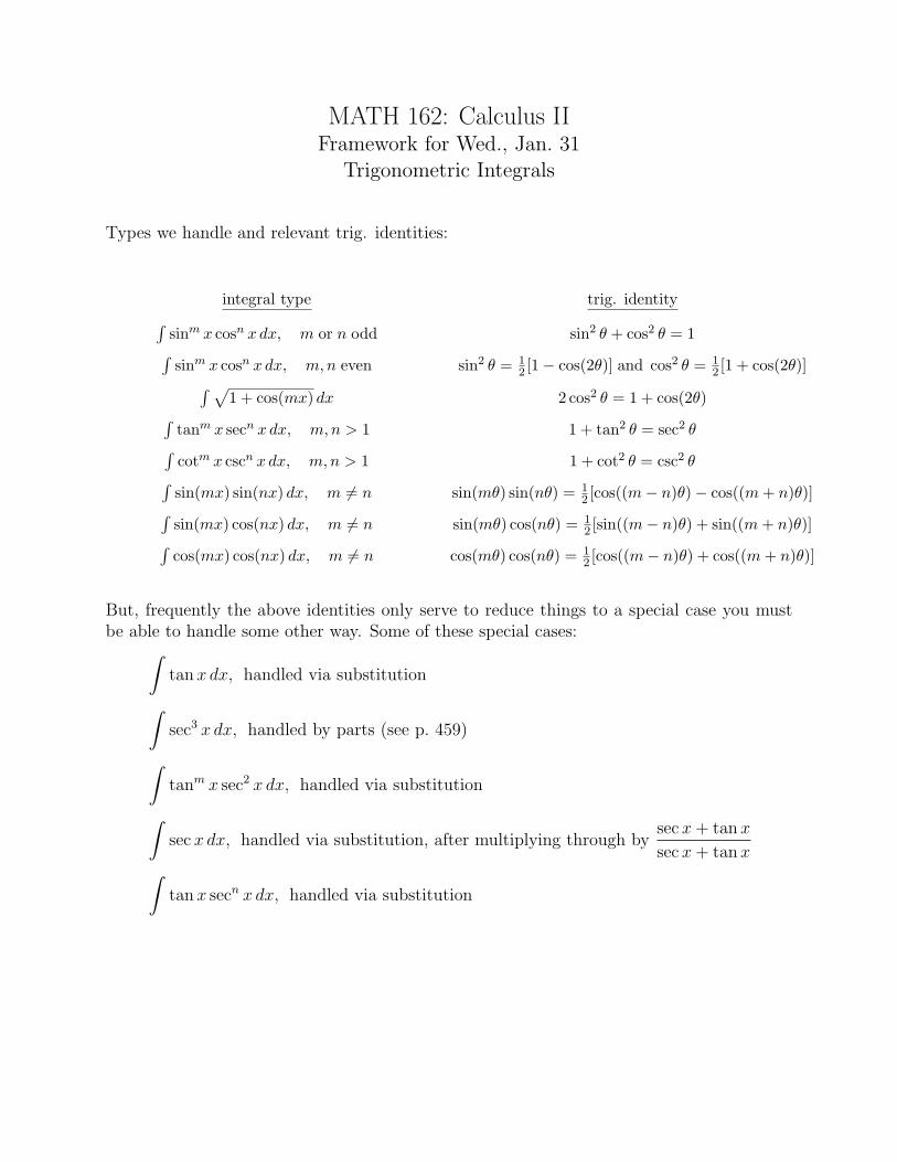
Types we handle and relevant trig. identities:

integral type trig. identity∫sinm x cosn x dx, m or n odd sin2 θ + cos2 θ = 1∫sinm x cosn x dx, m, n even sin2 θ = 1

2 [1− cos(2θ)] and cos2 θ = 12 [1 + cos(2θ)]∫ √

1 + cos(mx) dx 2 cos2 θ = 1 + cos(2θ)∫tanm x secn x dx, m, n > 1 1 + tan2 θ = sec2 θ∫cotm x cscn x dx, m, n > 1 1 + cot2 θ = csc2 θ∫sin(mx) sin(nx) dx, m 6= n sin(mθ) sin(nθ) = 1

2 [cos((m− n)θ)− cos((m + n)θ)]∫sin(mx) cos(nx) dx, m 6= n sin(mθ) cos(nθ) = 1

2 [sin((m− n)θ) + sin((m + n)θ)]∫cos(mx) cos(nx) dx, m 6= n cos(mθ) cos(nθ) = 1

2 [cos((m− n)θ) + cos((m + n)θ)]

But, frequently the above identities only serve to reduce things to a special case you mustbe able to handle some other way. Some of these special cases:∫

tan x dx, handled via substitution∫sec3 x dx, handled by parts (see p. 459)∫tanm x sec2 x dx, handled via substitution∫sec x dx, handled via substitution, after multiplying through by

sec x + tan x

sec x + tan x∫tan x secn x dx, handled via substitution

MATH 162: Calculus IIFramework for Fri., Feb. 2

Trigonometric Substitutions

Trigonometric substitution

• a technique used in integration

• useful most often when integrands involve (a2 + x2)m, (a2− x2)m or (x2− a2)m, wherea and m are constants. m is often, but not exclusively, equal to 1/2.Note: To get one of these forms, often completion of a square is required.

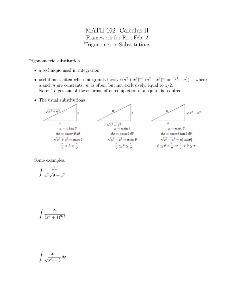
• The usual substitutions

Some examples:∫dx

x2√

9− x2

∫dx

(x2 + 1)3/2

∫x√

x2 − 3dx

MATH 162: Calculus IIFramework for Mon., Feb. 5

Integrals using Partial Fraction Expansion

Definition: A rational function is a function that is the ratio of polynomials.

Examples:2x

x2 + 6

x2 − 1

(x2 + 3x + 1)(x− 2)2

1√x + 7

Definition: A quadratic (2nd-degree) polynomial function with real coefficients is said tobe irreducible (over the reals) if it has no real roots.

A quadratic polynomial is reducible if and only if it may be written as the product of linear(1st-degree polynomial) factors with real coefficients

Examples:

x2 + 4x + 3

x2 + 4x + 5

Partial fraction expansion

• Reverses process of “combining rational fns. into one”

– Input: a rational fn. Output: simpler rational fns. that sum to input fn.

– degree of numerator in input fn. must be less than or equal to degree of denomi-nator (You may have to use long division to make this so.)

– denominator of input fn. must be factored completely (i.e., into linear and quadraticpolynomials)

• Why a “technique of integration”?

• leaves you with integrals that you must be able to evaluate by other means. Someexamples: ∫

5

2(x− 5)dx

∫2

(3x + 1)3dx

∫x + 1

(x2 + 4)2dx

MATH 162: Calculus IIFramework for Wed., Feb. 7

Numerical Integration

Numerical approximations to definite integrals

• Riemann (rectangle) sums already give us approximations

Main types: left-hand, right-hand and midpoint rules

• Question: Why rectangles?

– trapezoids

∗ Area of a trapezoid with bases b1, b2, height h

∗ Approximation to

∫ b

a

f(x) dx using n steps all of width ∆x = (b − a)/n

(Trapezoid Rule)

∗ Remarkable fact: Trapezoid rule does not improve over midpoint rule.

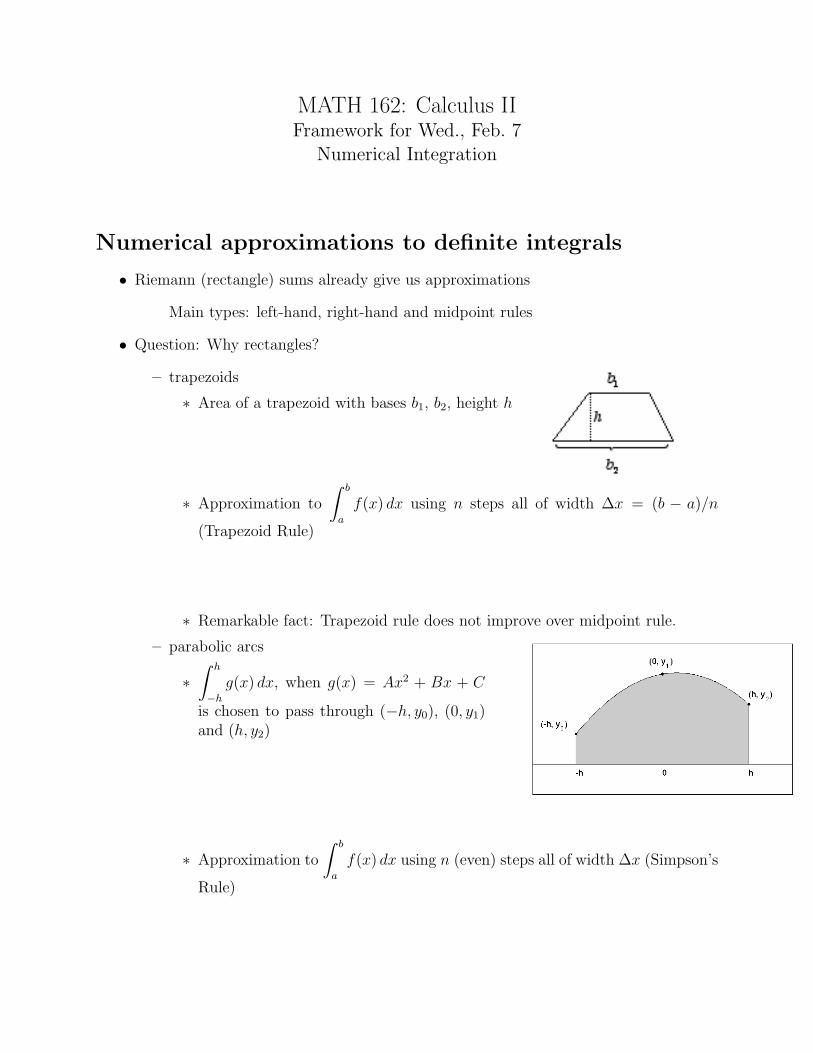
– parabolic arcs

∗∫ h

−h

g(x) dx, when g(x) = Ax2 + Bx + C

is chosen to pass through (−h, y0), (0, y1)and (h, y2)

∗ Approximation to

∫ b

a

f(x) dx using n (even) steps all of width ∆x (Simpson’s

Rule)

MATH 162—Framework for Wed., Feb. 7 Numerical Integration

• Error bounds

– No such thing available for a general integrand f

– Formulas (available when f is sufficiently differentiable)

∗ Trapezoid Rule. Suppose f ′′ is continuous throughout [a, b], and |f ′′(x)| ≤M for all x ∈ [a, b]. Then the error ET in using the Trapezoid rule with n

steps to approximate

∫ b

a

f(x) dx satisfies

|ET | ≤M(b− a)3

12n2.

∗ Simpson’s Rule. Suppose f (4) is continuous throughout [a, b], and |f (4)(x)| ≤M for all x ∈ [a, b]. Then the error ES in using Simpson’s rule with n steps

to approximate

∫ b

a

f(x) dx satisfies

|ES| ≤M(b− a)5

180n4.

– Use

∗ For a given n, gives an upper bound on your error

∗ If a desired upper bound on error is sought, may be used to determine a priorihow many steps to use

2

MATH 162: Calculus IIFramework for Fri., Feb. 9

Improper Integrals

Thus far in MATH 161/162, definite integrals

∫ b

a

f(x) dx have:

• been over regions of integration which were finite in length (i.e., a 6= −∞ and b 6= ∞)

• involved integrands f which are finite througout the region of integration

Q: How would we make sense of definite (improper, as they are called) integrals that violateone or both of these assumptions?

A: As limits (or sums of limits), when they exist, of definite integrals.

• When all of the limits involved exist, the integral is said to converge.

• When even one of the limits involved does not exist, the integral is said to diverge.

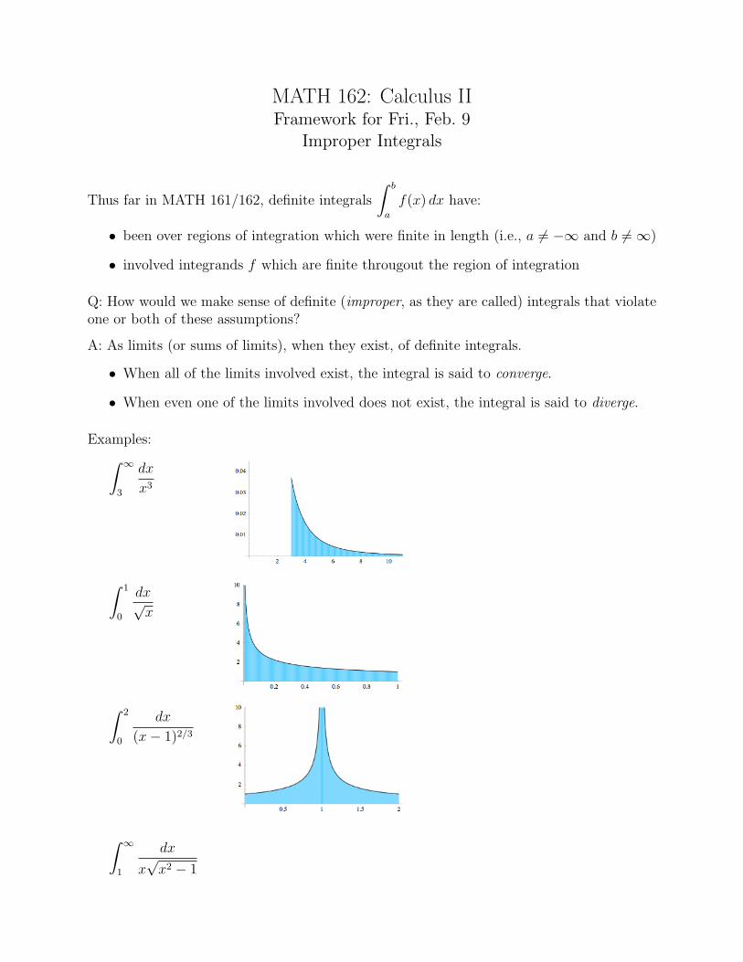
Examples:∫ ∞

3

dx

x3

∫ 1

0

dx√x

∫ 2

0

dx

(x− 1)2/3

∫ ∞

1

dx

x√

x2 − 1

MATH 162—Framework for Fri., Feb. 9 Improper Integrals

Evaluating them:∫ 0

−∞ex dx

∫ 1

0

ln x dx

∫ ∞

1

dx

xp

∫ ∞

−∞

dx

1 + x2

Even when an improper integral cannot be evaluated exactly, one might be able to determineif it converges or not. One of several possible theorems which address this issue:

Theorem (Direct Comparison Test): Suppose f , g satisfy 0 ≤ f(x) ≤ g(x) for allx ≥ a. Then

(i)

∫ ∞

a

f(x) dx converges if

∫ ∞

a

g(x) dx converges.

(ii)

∫ ∞

a

g(x) dx diverges if

∫ ∞

a

f(x) dx diverges.

2

MATH 162: Calculus IIFramework for Tues., Feb. 13

Introduction to Series

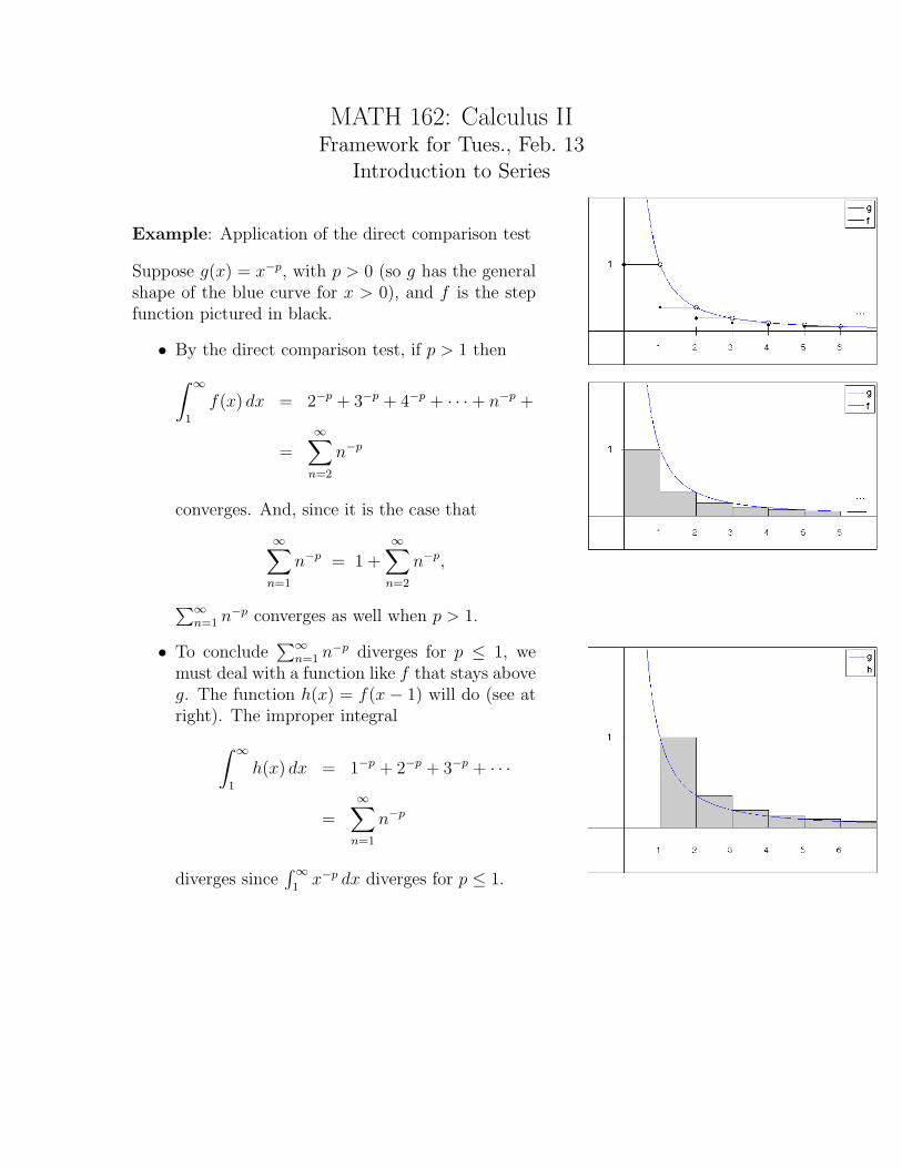
Example: Application of the direct comparison test

Suppose g(x) = x−p, with p > 0 (so g has the generalshape of the blue curve for x > 0), and f is the stepfunction pictured in black.

• By the direct comparison test, if p > 1 then∫ ∞

1

f(x) dx = 2−p + 3−p + 4−p + · · ·+ n−p + · · ·

=∞∑

n=2

n−p

converges. And, since it is the case that

∞∑n=1

n−p = 1 +∞∑

n=2

n−p,

∑∞n=1 n−p converges as well when p > 1.

• To conclude∑∞

n=1 n−p diverges for p ≤ 1, wemust deal with a function like f that stays aboveg. The function h(x) = f(x − 1) will do (see atright). The improper integral∫ ∞

1

h(x) dx = 1−p + 2−p + 3−p + · · ·

=∞∑

n=1

n−p

diverges since∫∞

1x−p dx diverges for p ≤ 1.

MATH 162—Framework for Tues., Feb. 13 Introduction to Series

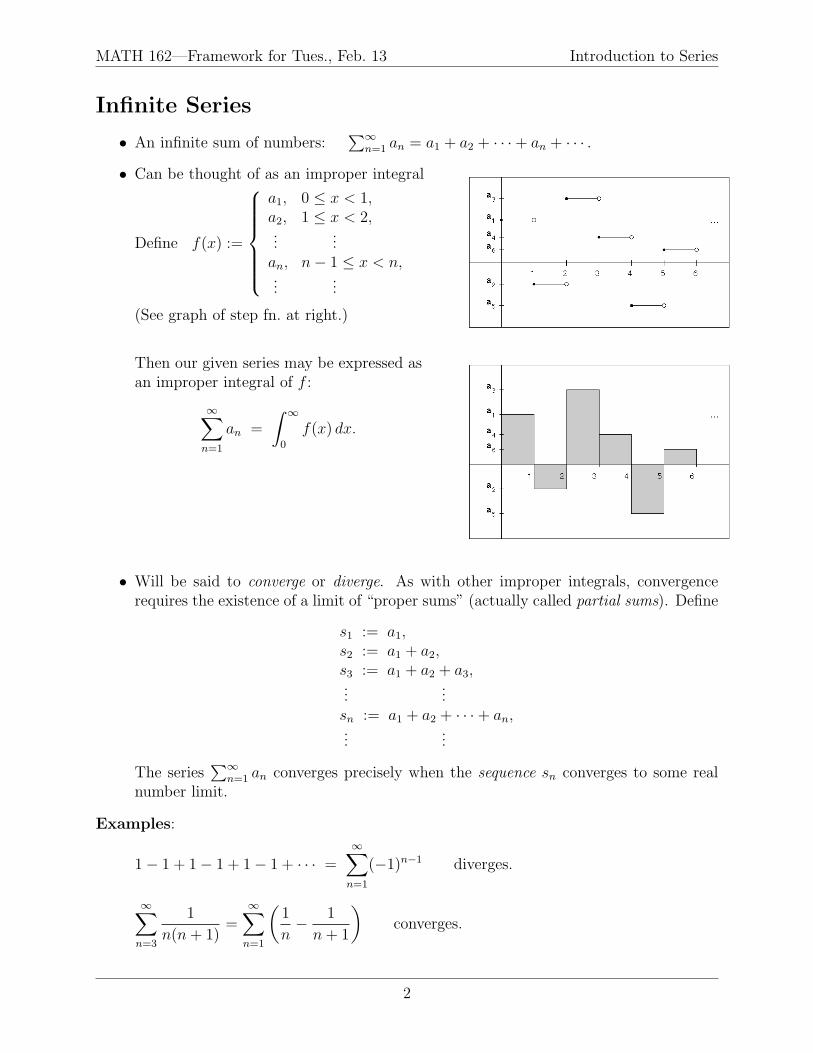
Infinite Series

• An infinite sum of numbers:∑∞

n=1 an = a1 + a2 + · · ·+ an + · · · .

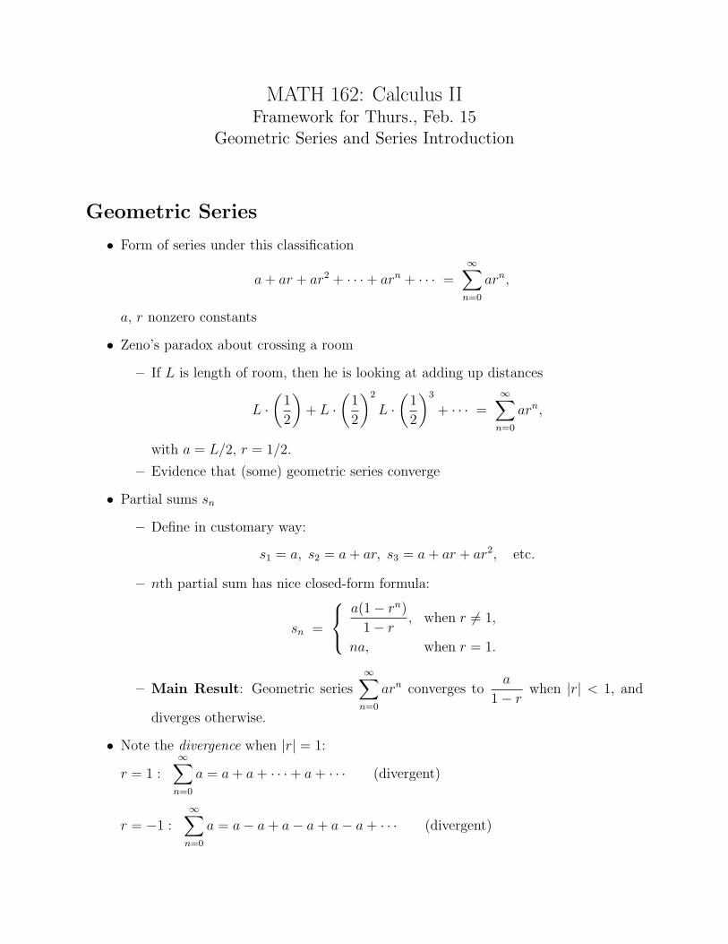
• Can be thought of as an improper integral:

Define f(x) :=

a1, 0 ≤ x < 1,a2, 1 ≤ x < 2,...

...an, n− 1 ≤ x < n,...

...

(See graph of step fn. at right.)

Then our given series may be expressed asan improper integral of f :

∞∑n=1

an =

∫ ∞

0

f(x) dx.

• Will be said to converge or diverge. As with other improper integrals, convergencerequires the existence of a limit of “proper sums” (actually called partial sums). Define

s1 := a1,s2 := a1 + a2,s3 := a1 + a2 + a3,...

...sn := a1 + a2 + · · ·+ an,...

...

The series∑∞

n=1 an converges precisely when the sequence sn converges to some realnumber limit.

Examples:

1− 1 + 1− 1 + 1− 1 + · · · =∞∑

n=1

(−1)n−1 diverges.

∞∑n=3

1

n(n + 1)=

∞∑n=1

(1

n− 1

n + 1

)converges.

2

MATH 162: Calculus IIFramework for Thurs., Feb. 15

Geometric Series and Series Introduction

Geometric Series

• Form of series under this classification

a + ar + ar2 + · · ·+ arn + · · · =∞∑

n=0

arn,

a, r nonzero constants

• Zeno’s paradox about crossing a room

– If L is length of room, then he is looking at adding up distances

L ·(

1

2

)+ L ·

(1

2

)2

L ·(

1

2

)3

+ · · · =∞∑

n=0

arn,

with a = L/2, r = 1/2.

– Evidence that (some) geometric series converge

• Partial sums sn

– Define in customary way:

s1 = a, s2 = a + ar, s3 = a + ar + ar2, etc.

– nth partial sum has nice closed-form formula:

sn =

a(1− rn)

1− r, when r 6= 1,

na, when r = 1.

– Main Result: Geometric series∞∑

n=0

arn converges toa

1− rwhen |r| < 1, and

diverges otherwise.

• Note the divergence when |r| = 1:

r = 1 :∞∑

n=0

a = a + a + · · ·+ a + · · · (divergent)

r = −1 :∞∑

n=0

a = a− a + a− a + a− a + · · · (divergent)

MATH 162—Framework for Thurs., Feb. 15 Geometric Series and Series Introduction

Remarks concerning infinite series (general, not just geometric ones)∞∑

n=1

an:

1. Convergence relies on the partial sums sn := a1+· · ·+an approaching a limit as n →∞

2. Assessing the limit of partial sums directly requires a nice closed-form expression forsn. Such an expression exists only in rare cases, such as the following examples we’vealready done

Geometric series:∞∑

n=0

arn

“Telescoping series”:∞∑

n=1

(1

n− 1

n + 1

)3. When no closed-form expression for sn is available, determining if limit exists is usually

more difficult.

Example:∞∑

n=1

(−1)n−1

np, p ≥ 0

4. Systematic tests can help

• Some of the tests that have been developed (’*’ indicate ones we will study)

– *nth-term test for divergence (p. 519)

– integral test (p. 525): formalization of the approach we used to determine

which p-series∞∑

n=1

n−p converge/diverge

– direct comparison test (p. 529): practically a restatement of the one ofthe same name for improper integrals

– limit comparison test (p. 530): did not do comparable result for improperintegrals

– *ratio test (p. 533)

– root test (p. 535)

– alternating series test (p. 538): formalization of the approach we used to

show∞∑

n=1

(−1)n−1

npconverges for p ≥ 0

– *absolute convergence test (p. 540)

• Must be cognizant of

– the situations in which a test may be applied

– what conclusions may and may not be drawn from such tests

2

MATH 162: Calculus IIFramework for Fri., Feb. 16

Absolute and Conditional Convergence

p-Series Results Revisited

• Results we have shown: The series whose terms are all positive

∞∑n=1

n−p = 1 + 2−p + 3−p + 4−p + · · · (1)

converges for p > 1, and diverges for p ≤ 1. The series with alternating signs

∞∑n=1

(−1)n−1n−p = 1− 2−p + 3−p − 4−p + · · · (2)

converges for p > 0, and diverges for p ≤ 0.

• The above results apply narrowly—only to series in the forms (1) and (2) respectively.Thus, nothing we have learned tells us whether

1 +1

2− 1

3+

1

4− 1

5− 1

6+

1

7+

1

8− 1

9+ · · ·

converges.

• The “borderline” case of (1), the one with p = 1,

∞∑n=1

n−1 = 1 +1

2+

1

3+ · · ·+ 1

n+ · · · (3)

is divergent, and has been named the harmonic series.

• When the convergence/divergence of a series∑

an is known, then the convergence/divergenceof certain modified forms of that series can be known as well. In particular,

– Any nonzero multiple of a series that converges (resp. diverges) will also converge(resp. diverge). Thus,

1

3+

1

6+

1

9+

1

12+ · · · =

1

3

∞∑n=1

n−1,

diverges, being a multiple of the harmonic series (3).

MATH 162—Framework for Fri., Feb. 16 Absolute and Conditional Convergence

– Suppose∑

an is a series whose convergence/divergence is known. Any serieswhich has the same “tail” as that of

∑an will converge (resp. diverge) based on

what∑

an does. For instance, since we know

∞∑n=1

(−1)n−1n−1/2 = 1− 1√2

+1√3− 1

2+

1√5− 1√

6+ · · ·

converges, we can conclude

∞∑n=4

(−1)n−1n−1/2 = −1

2+

1√5− 1√

6+ · · ·

and

b1 + b2 + · · ·+ b50 +1√3− 1

2+

1√5− 1√

6+ · · ·

converge as well. Here b1, . . . , b50 is any arbitrary list of 50 numbers. Theimportant thing is not the values of these bj’s, but that there are only finitelymany (in this case, 50) of them.

Absolute and Conditional Convergence

Definition: Let∑

an be a convergent series. If the corresponding series∑

|an| in whichevery term has been made positive diverges, then the original series

∑an is said to be

conditionally convergent.

Example: The series∞∑

n=1

(−1)nn−1 = 1−1/2+1/3−1/4+ · · · is conditionally convergent.

Definition: Let∑

an be a given series (i.e., one for which the values of the terms aj areknown). If the corresponding series

∑|an| with all positive terms converges, then the original

series∑

an is said to be absolutely convergent.

Theorem (Absolute Convergence Test): All absolutely convergent series are convergent.

Example: The series

11

3+

11

6− 11

12+

11

24− 11

48− 11

96− 11

192+ · · ·

is absolutely convergent, since

11

3+

11

6+

11

12+

11

24+

11

48+ · · · =

∞∑n=0

(11

3

) (1

2

)n

converges (being geometric, with r = 1/2). By the absolute convergence test, the originalseries converges as well.

2

MATH 162: Calculus IIFramework for Mon., Feb. 19

The Ratio Test

Several Ideas Coming Together

• Power fns.: ones of form x−p.

– Identification. The base x varies, while the exponent (−p) remains fixed. Thesefns. grow without bound as x → ∞ when p < 0, and approach zero as x → ∞when p > 0.

– Improper integrals. Only in the case p > 0 might we hope∫∞

1x−p dx converges.

Our finding is that, in actuality,∫∞

1x−p dx converges only when p > 1. That is,

only when p > 1 do such fns. approach 0 quickly enough so that the stated integralconverges. Our corresponding finding for series:

∑∞n=1 n−p converges for p > 1

and diverges for p ≤ 1.

• Exponential fns.: ones of form bx

– Identification. The base b remains fixed, and the exponent x varies. Suchfns. grow without bound as x → ∞ when b > 1; they approach zero as x → ∞when 0 < b < 1.

– Improper integrals. When 0 < b < 1, the exponential bx decays to zero fasterthan any power fn. xp with p > 0. Not surprisingly, then,∫ ∞

a

bx dx

(a any real number) converges for any value of b in (0, 1). The correspondingtypes of series are geometric series

∞∑n=0

rn

which we know converge for −1 < r < 1, and diverge for |r| ≥ 1.

• It’s the tail that matters. The “fate” of a series∑

an (in terms of whether or notit converges) does not depend on its first few, say 100 trillion or so, terms, but on thetail (the remaining infinitely many terms).

MATH 162—Framework for Mon., Feb. 19 The Ratio Test

The Ratio Test

The previous facts point to the following conjecture concerning series:

Given some series∑

an, if it may be determined that, eventually, the termsshrink in magnitude at least as quickly as an exponential decay function, thenthe series should converge.

There might be several ways to formulate this conjecture into a mathematical statement.One way, which has been proved (so it is a theorem), is:

Theorem (Ratio test, p. 533): Let∑

an be a series whose terms an > 0 (all positive),and suppose limn→∞ an+1/an = ρ (i.e., suppose that this limit exists; we’ll call it ρ).

(i) If ρ < 1, the series∑

an converges.

(ii) If ρ > 1, the series∑

an diverges.

Note: If ρ = 1, this test does not allow us to draw a conclusion either way.

Examples:

∞∑n=1

2n

n23n

∞∑n=1

1

n

∞∑n=1

1

n2

When a series∑

an has negative terms, we may apply the ratio test to∑|an|. If the test

reveals that∑|an| converges, then so does

∑an by the absolute convergence test.

Example: Determine those x-values for which the series converges.

(a)∞∑

n=0

(3x− 2)n

n3n

(b)∞∑

n=0

xn

n!

(c)∞∑

n=0

n!xn

2

MATH 162: Calculus IIFramework for Tues., Feb. 20Introduction to Power Series

Definition: A function of x which takes the series form

∞∑n=0

cn(x− a)n = c0 + c1(x− a) + c2(x− a)2 + c3(x− a)3 + · · · (1)

is called a power series about x = a. The number a is called the center, and the coefficientsc0, c1, c2, . . . are constants.

Remarks:

• As for any function, a power series has a domain. The acceptable inputs x to a powerfunction are those x for which the series converges.

• If it were not for the coefficients cj (if, say, each cj = 1), a power series would lookgeometric. Indeed, the geometric series

∞∑n=0

xn = 1 + x + x2 + x3 + · · · (2)

is a power series about x = 0, that is known to converge to (1−x)−1 when −1 < x < 1and to diverge when |x| ≥ 1. So, the domain of power series (2) is (−1, 1).

More generally, for a special type of power series about x = a with coefficients cj = βj

(i.e., whose coefficients are ascending powers of some fixed number β)

∞∑n=0

βn(x− a)n = 1 + β(x− a) + β2(x− a)2 + β3(x− a)3 + · · · , (3)

we have that this series

converges to1

1− β(x− a)when |β(x−a)| < 1, that is, for a− 1

|β|< x < a +

1

|β|,

and diverges when |(x− a)| ≥ 1

|β|.

Thus, the domain of series (3) is (a− 1/|β|, a + 1/|β|).

• In the most general case, where the coefficients cj in (1) do not, in general, equal βj

for some number β, the determination of the domain usually requires

MATH 162—Framework for Tues., Feb. 20 Introduction to Power Series

1. the use of the ratio test on the series∑∞

n=0 |cn(x− a)n|. That is, one looks at

limn→∞

|cn+1||x− a|n+1

|cn||x− a|n=

(lim

n→∞

|cn+1||cn|

)|x− a|.

If limn→∞ |cn+1|/|cn| exists, and if we let

ρ =

(lim

n→∞

|cn+1||cn|

)|x− a|,

then part (i) of the ratio test imposes constraints on what values x may take.Specifically, we generally wind up with a number R ≥ 0, called the radius ofconvergence, for which the series (1)

converges if x is inside the open interval (a−R, a + R), and

diverges if |x−a| > R (i.e., if x is outside the closed interval [a−R, a+R]).

In those cases where limn→∞ |cn+1|/|cn| = 0, the value of R := +∞, and whenthis happens there is no need to proceed to step 2.

2. the determination (by some other means than the ratio test) of whether the seriesconverges when |x− a| = R (i.e., at the points x = a±R).

The upshot is that the domain of a power series whose radius of convergence R isnonzero is always an interval, an interval that has x = a at its center and, in the caseR 6= +∞, may include one or both of its endpoints x = a ± R. For this reason thedomain of a power series is usually called its interval of convergence.

Example: Determine the interval of convergence for

(a)∞∑

n=0

(3x− 2)n

n3n

(b)∞∑

n=0

xn

n!

(c)∞∑

n=0

n!xn

(d)∞∑

n=0

xn3n

n3/2

2

MATH 162—Framework for Tues., Feb. 20 Introduction to Power Series

Power Series Expressions for Some Fns. (building new series from known ones)

We know that, for |x| < 1, the fn. f(x) = 1/(1− x) may be expressed as a power series:

1

1− x=

∞∑n=0

xn, |x| < 1.

Thus, we may express similar-looking fns. as power series:

1

1− 3x=

∞∑n=0

(3x)n =∞∑

n=0

3nxn, |3x| < 1 ⇒ −1

3< x <

1

3

1

2− x=

1

2· 1

1− (x/2)=

1

2

∞∑n=0

(x

2

)xn =

∞∑n=0

xn

2n+1,

∣∣∣x2

∣∣∣ < 1 ⇒ −2 < x < 2.

x3

1− x= x3 · 1

1− x= x3

∞∑n=0

xn =∞∑

n=0

xn+3, −1 < x < 1.

1

1 + x=

1

1− (−x)=

∞∑n=0

[(−1)x]n =∞∑

n=0

(−1)nxn, | − x| < 1 ⇒ −1 < x < 1.

1

1 + x2=

∞∑n=0

(−1)n(x2)n =∞∑

n=0

(−1)nx2n, |x2| < 1 ⇒ −1 < x < 1.

All of the above are power series about x = 0. We show how the 2nd one (in the above listof 5) could also be written as a power series centered around x = 1:

1

2− x=

1

1− (x− 1)=

∞∑n=0

(x− 1)n, |x− 1| < 1 ⇒ 0 < x < 2.

3

MATH 162: Calculus IIFramework for Wed., Feb. 21

Differentiation and Integration of Power Series

While power series are allowed to have nonzero numbers as centers, for today’s results wewill assume all power series we discuss are centered about x = 0; that is, are of the form

∞∑n=0

cnxn = c0 + c1x + c2x

2 + c3x3 + · · · . (1)

We will also assume each has a positive radius of convergence R > 0, so that the seriesconverges at least for those x satisfying −R < x < R.

Differentiation of Power Series about x = 0

Theorem (Term-by-Term Differentiation, p. 549): Let f(x) take the form of the powerseries in (1), with radius of convergence R > 0. Then the series

∞∑n=1

ncnxn−1

converges for all x satisfying −R < x < R, and

f ′(x) =∞∑

n=1

ncnxn−1, for all x satisfying −R < x < R.

Remarks:

• Since the hypotheses of this theorem now apply to f ′(x), we can continue to differentiatethe series to find derivatives of f of all orders, convergent at least on the interval−R < x < R. For instance,

f ′′(x) =∞∑

n=2

n(n− 1)cnxn−2 = (2 · 1)c2 + (3 · 2)c3x + (4 · 3)c4x

2 + · · ·

f ′′′(x) =∞∑

n=3

n(n− 1)(n− 2)cnxn−3 = (3 · 2 · 1)c3 + (4 · 3 · 2)c4x + (5 · 4 · 3)c5x

2 + · · ·

......

f (j)(x) =∞∑

n=j

n(n− 1)(n− 2) · · · (n− j + 1)cnxn−j

= j! cj + [(j + 1)j · · · 2] cj+1x + [(j + 2)(j + 1) · · · 3] cj+2x2 + · · · .

MATH 162—Framework for Wed., Feb. 21 Differentiation and Integration of Power Series

• The easiest place to evaluate a power series is at its center. In particular, if f has theform (1), we may evaluate f and all of its derivatives at zero to get:

f(0) = c0,

f ′(0) = c1,

f ′′(0) = (2 · 1) c2 ⇒ c2 =1

2f ′′(0),

f ′′′(0) = (3 · 2 · 1) c3 ⇒ c3 =1

3!f ′′′(0),

and so on. So, we arrive at the following relationship between the coefficients cj andthe derivatives of f at the center:

Corollary: Let f(x) be defined by the power series (1). Then

cn =f (n)(0)

n!, for all n = 0, 1, 2, . . . .

Example: We know that f(x) = (1− x)−1 has the power series representation∑∞

n=0 xn forx in the interval (−1, 1). By the term-by-term differentiation theorem, f ′(x) = (1−x)−2 hasthe power series representation

1

(1− x)2=

d

dx

(∞∑

n=0

xn

)=

d

dx

(1 + x + x2 + x3 + · · ·

)=

d

dx(1) +

d

dx(x) +

d

dx(x2) +

d

dx(x3) + · · · (the theorem justifies this step)

= 0 + 1 + 2x + 3x2 + 4x3 + · · ·

=∞∑

n=1

nxn−1,

with this series representation holding at least for −1 < x < 1.

Integration of Power Series about x = 0

If we can differentiate a series expression for f term-by-term in order to arrive at a seriesexpression for f ′, it may not be surprising that we may integrate a series term-by-term aswell.

Theorem (Term-by-Term Integration, p. 550): Suppose that f(x) is defined by thepower series (1) and the radius of convergence R > 0. Then∫ x

0

f(t) dt =∞∑

n=0

cn

n + 1xn+1, for all x satisfying −R < x < R.

2

MATH 162—Framework for Wed., Feb. 21 Differentiation and Integration of Power Series

Example: We know that f(x) = (1+x)−1 has the power series representation∑∞

n=0(−1)nxn

for x in the interval (−1, 1). Moreover,∫ x

0

dt

1 + t=[ln |1 + t|

]x0

= ln |1 + x|.

By the term-by-term integration theorem, for −1 < x < 1 we also have∫ x

0

dt

1 + t=

∫ x

0

(∞∑

n=0

(−1)ntn

)dt =

∫ x

0

(1− t + t2 − t3 + t4 − t5 + · · · ) dt

=

∫ x

0

dt−∫ x

0

t dt +

∫ x

0

t2 dt−∫ x

0

t3 dt + · · · (the theorem justifies this step)

=∞∑

n=0

(−1)n

(∫ x

0

tn dt

)

=∞∑

n=0

(−1)n

n + 1

[tn+1

]x0

=∞∑

n=0

(−1)n

n + 1xn+1

= x− 1

2x2 +

1

3x3 − 1

4x4 + · · · .

That is,∞∑

n=0

(−1)n

n + 1xn+1 = ln(1 + x),

at least for all x in the interval −1 < x < 1. In fact, though the theorem does not go sofar as to guarantee convergence at the value x = 1, since the series on the left converges atx = 1 (Why?), one might suspect that

1− 1

2+

1

3− 1

4+ · · · = ln 2.

This, indeed, is the case.

Example: Use the power series representation for (1+x2)−1 about zero to get a power seriesrepresentation for arctan x.

3

MATH 162: Calculus IIFramework for Fri., Feb. 23

Taylor Series

In the section on power series, we seemed to be

• interested in finding power series expressions for various functions f ,

• but able to find such series only when the function f , or some order derivative/antiderivativeof f , looked enough like (1− x)−1 to make this feasible.

Our goal today is to find series expressions for important functions that are not so closelylinked to (1− x)−1. First, a definition:

Definition: Suppose f is a function which has derivatives of all orders at x = a. The Taylorseries for f at x = a is

∞∑n=0

f (n)(a)

n!(x− a)n.

What this definition says is that, for appropriate f , we may construct a power series aboutx = a employing the values of derivatives f (n)(a) in the coefficients. As of yet, no assertionthat this power series actually equals f has been made. (See note 2 below.)

Some important notes:

1. The Taylor series, like any power series, has a radius of convergence R, which may bezero.

2. Even if the radius of convergence R > 0, the function defined by the Taylor series of fmight not equal f except at the single location x = a.

3. But, if R > 0, then for many “nice” functions f , the Taylor series for f equals f on itsentire interval of convergence.

4. If we stop the sum at the term containing (x − a)n (i.e., consider the partial sum of

the series that includes as its last term the one with (x− a) to the nth power), we get

a polynomial of nth degree. This polynomial is called the Taylor polynomial of ordern for f at x = a.

5. If a = 0, then the Taylor series is called the MacLaurin series of f.

6. If f equals any power series about x = a at all, then that series must be the Taylorseries.

MATH 162—Framework for Fri., Feb. 23 Taylor Series

Some favorite Taylor series (all of these are MacLaurin series)

1

1− x=

∞∑n=0

xn

= 1 + x + x2 + · · ·+ xn + · · · , −1 < x < 1

ex =∞∑

n=0

xn

n!

= 1 + x +x2

2+

x3

3!+ · · ·+ xn

n!+ · · · , −∞ < x < ∞

sin x =∞∑

n=0

(−1)n x2n+1

(2n + 1)!

= x− x3

3!+

x5

5!+ · · ·+ (−1)n x2n+1

(2n + 1)!+ · · · , −∞ < x < ∞

cos x =∞∑

n=0

(−1)n x2n

(2n)!

= 1− x2

2!+

x4

4!+ · · ·+ (−1)n x2n

(2n)!+ · · · , −∞ < x < ∞

arctan x =∞∑

n=0

(−1)n x2n+1

(2n + 1)

= x− x3

3+

x5

5+ · · ·+ (−1)n x2n+1

2n + 1+ · · · , −1 ≤ x ≤ 1

ln(1 + x) =∞∑

n=1

(−1)n+1xn

n

= x− x2

2+

x3

3+ · · ·+ (−1)n+1xn

n+ · · · , −1 < x ≤ 1

As with expressions that were similar to (1−x)−1, we may substitute into these power seriesto get power series expressions for other, related functions.

Example: The MacLaurin series converging to exp(−x2) is

exp(−x2) = 1− x2 +x4

2− x6

3!+

x8

4!+ · · ·+ (−1)n x2n

n!+ · · · .

2

MATH 162: Calculus IIFramework for Mon., Feb. 26Convergence of Taylor Series

Today’s Goal: To determine if a function equals its power series.

In a remark from the last class, it was stated that, while a certain function f may allow theconstruction of a Taylor series about x = a with positive radius of convergence, one may notassume this Taylor series converges to f . In our “favorite Taylor series” (see the frameworkfor that day), however, the convergence of the MacLaurin series for (1− x)−1, arctan x andln(1 + x) to their respective functions throughout their intervals of convergence has alreadybeen established. What has yet to be established is whether the MacLaurin series for ex,cos x and sin x converge to their respective functions.

The Remainder

Suppose f has (n + 1) derivatives throughout an interval I around x = a. Under these

conditions, we can write down the nth-order Taylor polynomial for f about x = a:

Pn,a(x) = f(a) + f ′(a)(x− a) +f ′′(a)

2!(x− a)2 +

f ′′′(a)

3!(x− a)3 + · · ·+ f (n)(a)

n!(x− a)n,

Here the subscript a has been added to indicate that this polynomial is about x = a. Thediscrepancy between the function and its Taylor polynomial is called the remainder term:

Rn,a(x) := f(x)− Pn,a(x).

Theorem (Lagrange): Suppose f , Pn,a and Rn,a are as described above, and that x (fixed)is a number in the interval I. Then there is a number t between a and x such that

Rn,a(x) =f (n+1)(t)

(n + 1)!(x− a)n+1.

Example: We can use Lagrange’s theorem to show that sin x is equal to its MacLaurinseries for every real number x. For any (fixed) x, the theorem guarantees the existence of anumber t between 0 and x such that

|Rn,0(x)| =| sin(n+1)(t)|

(n + 1)!|x|n+1 ≤ |x|n+1

(n + 1)!→ 0 as n →∞.

Thus,lim

n→∞Pn,0(x) = lim

n→∞[sin x−Rn,0(x)] = sin x− lim

n→∞Rn,0(x) = sin x,

which says that the sequence of partial sums of the MacLaurin series for the sine functionconverges to sine at x. Since we did not assume anything special about the x involved inthis calculation, the result holds for any real x.

MATH 162—Framework for Mon., Feb. 26 Convergence of Taylor Series

A similar type of argument may be used to establish that the MacLaurin series for ex

converges to ex for all real x, and that the MacLaurin series for cos x converges to cos x forall real x.

Example (a weird function): Let f be defined by the formula

f(x) :=

{e−1/x2

, x 6= 0,

0, x = 0.

It can be shown that f (n)(0) = 0 for all integer n ≥ 0. The MacLaurin series for f is thus

∞∑n=0

0

n!xn = 0,

the zero function (not even an infinite series, so of course it converges for all x). A graph off appears in Figure 8.14 on p. 558 of the text. It may not be obvious from the picture, butwhile f(0) = 0, for all other choices of x, f(x) > 0. Hence, the only place its MacLaurinseries equals f is at x = 0.

2

MATH 162: Calculus IIFramework for Tues., Feb. 27

Functions of Multiple Variables

Definition: A function (or function of n variables) f is a rule that assigns to each orderedn-tuple of real numbers (x1, x2, . . . , xn) in a certain set D a real number f(x1, x2, . . . , xn).The set D is called the domain of the function.

Example: Most real-life functions are, in fact, functions of multiple variables. Here aresome:

1. v(r, h) = πr2h

2. d(x, y, z) =√

x2 + y2 + z2

3. g(m1, m2, R) = Gm1m2/R2 (G is a constant)

4. P (n, T, V ) = nRT/V (R is a constant)

Of course, one can hold fixed the values of all but one of the input variables and therebycreate a function of a single variable. For instance, the way the volume of a right-circularcylinder whose height is 3 varies with its radius is given by the formula

V (r) = 3πr2, r ≥ 0.

Graphing

Functions of a single variable

To graph a function of a single variable requires two coordinate axes. When we writey = f(x), it is implied that x is a possible input and the y-value is the corresponding output.We think of the domain (the set of all possible inputs) of f as consisting of some part of thereal line, the graph of f (often called a “curve”) as having a point at location (x, f(x)) foreach x in the domain of f . Keep in mind that, given an arbitrary equation involving x andy, it is not always the case that

(i) we want to make y be the dependent variable, and

(ii) if we do solve for y, the result is a function.

Example: x2 + y2 = 4

MATH 162—Framework for Tues., Feb. 27 Functions of Multiple Variables

Functions of multiple variables

We have the following analogies for functions of multiple variables:

• When nothing explicit is said about the inputs to a function of multiple variables, wetake the domain to be as inclusive as possible.

Examples:

f(x, y) =√

xy

f(x, y) = xy(x2 + y)−1

• The graphs of functions of n variables are n-dimensional objects drawn in a coordinateframe involving (n + 1) mutually-perpendicular coordinate axes. (Think of a curvewhich is the graph of y = f(x) as a 1-dimensional object weaving through 2-dimensionalspace.)

As a corollary: It is not possible to produce the graph of a function of 3 or morevariables. A possible work-around: level sets.

Definition: Let f be a function of n variables, and c be a real number. The set ofall n-tuples (x1, . . . , xn) for which f(x1, . . . , xn) = c is called the c level set of f.

Examples:

f(x, y) = y2 − x2

f(x, y, z) = z − x2 − 2y2

• Not every equation involving x, y and z yields z as a single function of x and y.

Examples:

x− y2 − z2 = 0

x2 + y2 + z2 = 4

• One may assume a missing variable is implied and takes on all real values.

Example: The meaning of x = 1 in 1, 2 and 3 dimensions.

One may need more than one equation/inequality to describe certain regions of space.

Example: x2 + (y − 1)2 ≤ 1, z = −1

2

MATH 162: Calculus IIFramework for Wed., Feb. 28

Limits and Continuity

Today’s Goal: To understand the meaning of limits and continuity of functions of 2 and 3variables.

Geometry of the Domain Space

Definition: (Distance in R3): Suppose that (x1, y1, z1) and (x2, y2, z2) are points in R3. Thedistance between these two points is√

(x1 − x2)2 + (y1 − y2)2 + (z1 − z2)2.

If our two points have the same z-value (for instance, if they both lie in the xy-plane), thenthe distance between them is just√

(x1 − x2)2 + (y1 − y2)2.

We employ these definitions for distance in R2, R3 to define circles, disks, spheres and balls.

Definition: A circle in R2 centered at (a, b) with radius r is the set of points (x, y) satisfying

(x− a)2 + (y − b)2 = r2.

Given such a circle C, the set of all points on or inside C is a closed disk. The set of pointsinside but not on C is an open disk.

Definition: A sphere in R3 centered at (a, b, c) with radius r is the set of points (x, y, z)satisfying

(x− a)2 + (y − b)2 + (z − c)2 = r2.

The inside of a sphere is called a ball, and can be closed or open depending on whether the(whole) sphere is included.

Open intervals in R are sets of the form a < x < b (also written using interval notation(a, b)), where neither endpoint a, b is included in the set. One observation about such sets isthat, if you take any x ∈ (a, b), there is a value of r > 0, perhaps quite small, for which theinterval (x− r, x + r) is wholly contained inside (a, b). We build on that idea when definingvarious kinds of subsets of R2.

MATH 162—Framework for Wed., Feb. 28 Limits and Continuity

Definition: Let R be a region of the xy-plane and (x0, y0) a point (perhaps in R, perhapsnot). We call (x0, y0) an interior point of R if there is an open disk of positive radius centeredat (x0, y0) such that every point in this disk lies inside R.

We call (x0, y0) a boundary point of R if every disk with positive radius centered at (x0, y0)contains both a point that is in R and a point that isn’t in R.

The region R is said to be open if all points in R are interior points of R.

The region R is said to be closed if all boundary points of R are in R.

The region R is said to be bounded if it lies entirely inside a disk of finite radius.

Examples:

1. An open disk is open. A closed disk is closed. For both, the boundary points are thosefound on the enclosing circle.

2. The upper half-plane R consisting of points (x, y) for which y > 0 is an open, un-bounded set. The boundary points of R are precisely those points found along thex-axis, none of which are contained in R.

3. If y = f(x) is a continuous function on the interval a ≤ x ≤ b, then the graph of f isa closed, bounded set made up entirely of boundary points.

4. The set of points (x, y) satisfying x ≥ 0, y ≥ 0 and y < x + 1 is bounded, but neitheropen nor closed.

5. The only nonempty region of the plane which is both open and closed is the entireplane R2.

Limits and Continuity

The idea behind the statement

lim(x,y)→(x0,y0)

f(x, y) = L

for a function f of two variables is that you can make the value of f(x, y) as close to L asyou like by focusing only on (x, y) in the domain of f which are inside an open disk centeredat (x0, y0) of some positive radius. The official definition follows.

Definition: The limit of f as (x, y) approaches (x0, y0) is L if for every ε > 0 there is acorresponding δ > 0 such that, for all (x, y) in dom(f),

if 0 <√

(x− x0)2 + (y − y0)2 < δ then |f(x, y)− L| < ε.

Remarks:

2

MATH 162—Framework for Wed., Feb. 28 Limits and Continuity

1. All the limit laws of functions of a single variable—those stated in Section 2.2—haveanalogs for functions of 2 variables. For instance, the analog to Rule 5 on p. 65 goeslike this:

Theorem: Suppose

lim(x,y)→(x0,y0)

f(x, y) = L and lim(x,y)→(x0,y0)

g(x, y) = M.

(That is, suppose both these limits exist, and call them L, M respectively.) If M 6= 0,then

lim(x,y)→(x0,y0)

f(x, y)

g(x, y)=

L

M.

2. We recall that, for a function f of a single variable and a point x0 interior to thedomain of f , the statement limx→x0 f(x) = L requires the values of f to approachL as the x-values approach x0 from both the left and the right. The requirement atinterior points (x0, y0) to the domain of a function f of 2 variables is even more strict.Any path of (x, y)-values within the domain of f traversed en route to (x0, y0) shouldproduce function values which approach L.

Example: The limits lim(x,y)→(0,0)

4xy

x2 + y2and lim

(x,y)→(0,0)

4xy2

x2 + y4do not exist.

3. One defines continuity for functions of two variables in an identical fashion as forfunctions of a single variable.

Definition: Suppose (x0, y0) is in the domain of f . We say that f is continuous at(x0, y0) if

lim(x,y)→(x0,y0)

f(x, y) = f(x0, y0)

(i.e., if this limit exists and has the same value as f(x0, y0)). We say f is continuous (orf is continuous throughout its domain) if f is continuous at each point in its domain.

Example: The functions f(x, y) :=4xy

x2 + y2and g(x, y) :=

4xy2

x2 + y4are continuous

at all points (x, y) except (0, 0).

4. The notions of distance, open and closed balls, boundary point, interior point, open andclosed sets, limits and continuity may all be generalized to functions of n variables,where n is any integer greater than 1.

3

MATH 162: Calculus IIFramework for Thurs., Mar. 1

Partial Derivatives

Today’s Goal: To understand what is meant by a partial derivative.

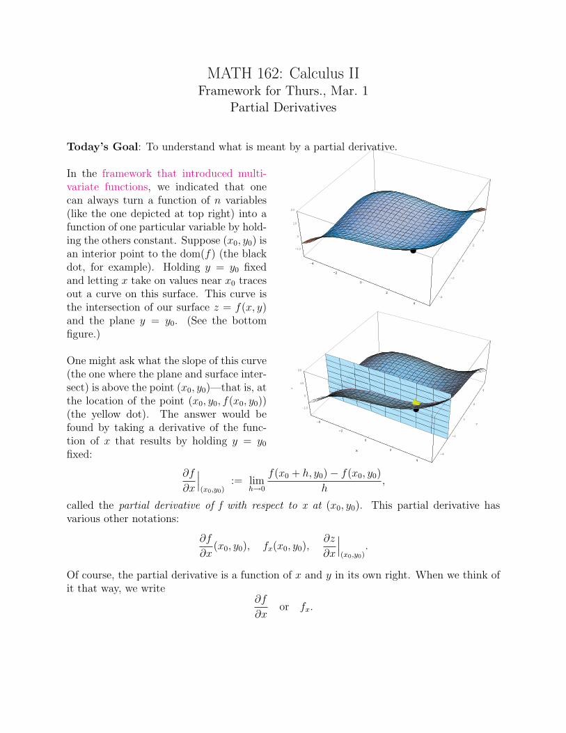
In the framework that introduced multi-variate functions, we indicated that onecan always turn a function of n variables(like the one depicted at top right) into afunction of one particular variable by hold-ing the others constant. Suppose (x0, y0) isan interior point to the dom(f) (the blackdot, for example). Holding y = y0 fixedand letting x take on values near x0 tracesout a curve on this surface. This curve isthe intersection of our surface z = f(x, y)and the plane y = y0. (See the bottomfigure.)

One might ask what the slope of this curve(the one where the plane and surface inter-sect) is above the point (x0, y0)—that is, atthe location of the point (x0, y0, f(x0, y0))(the yellow dot). The answer would befound by taking a derivative of the func-tion of x that results by holding y = y0

fixed:

-4

-2

0

2

4

-4

-2

0

2

4

-10

0

10

20

-4

-2

0

2

4

-4

-2

0

2

4

x-4

-2

0

2

4

y

-10

0

10

20

z

-4

-2

0

2

4

x

∂f

∂x

∣∣∣(x0,y0)

:= limh→0

f(x0 + h, y0)− f(x0, y0)

h,

called the partial derivative of f with respect to x at (x0, y0). This partial derivative hasvarious other notations:

∂f

∂x(x0, y0), fx(x0, y0),

∂z

∂x

∣∣∣(x0,y0)

.

Of course, the partial derivative is a function of x and y in its own right. When we think ofit that way, we write

∂f

∂xor fx.

MATH 162—Framework for Thurs., Mar. 1 Partial Derivatives

We can also take partial derivatives with respect to y (or other variables, if f is a functionof more than 2 variables). The resulting partial derivatives may be differentiated again:

∂2f

∂y2, or fyy get this by differentiating fy with respect to y.

∂2f

∂x∂y, or fyx get this by differentiating fy with respect to x.

∂2f

∂y2∂x, or fxyy get this by differentiating fx twice with respect to y.

The usual theorems that provide shortcuts to taking derivative may be applied, keeping inmind which variable(s) is being held constant.

Examples:

2x2 − y

3x− xy2

exp(x/y2)

ln(xy2)

2

MATH 162: Calculus IIFramework for Tues., Mar. 6

Differentiability

Today’s Goal: To understand the relationship between partial derivatives and continuity.

The Mixed Partial Derivatives

We have learned that the partial derivative fx at (x0, y0) may be interpreted geometricallyas providing the slope at the point (x0, y0, f(x0, y0)) along the curve that results from slicingthe surface z = f(x, y) with the plane y = y0. If one thinks of the x-axis as “facing east”,then what we are talking about is akin to standing on a patch of (possibly) hilly ground andasking what slope you would immediately experience heading eastward from your currentposition. Now imagine moving northward (i.e., in the direction of the positive y-axis), butstill determining eastward slopes. The rate at which those eastward slopes changed as youmoved northward is precisely what fxy = ∂/∂y(fx) provides.

One might ask the following question: Suppose I mark a particular spot on this hypothet-ical terrain. Then I cross over the mark twice. The first time, I do so heading northward,noting the rate of change of eastward-facing slopes as I cross (that is, fxy). The secondtime, I do so heading eastward, noting the rate at which northward-facing slopes change asI cross (i.e., fyx). Should these two rates of change be equal? There does not seem to be aparticular reason why they should be, but experimenting with various formulas f(x, y) wefind, nevertheless, that they often are.

Example: f(x, y) = cos(x2y)

This phenomenon has much to do with our natural inclination to choose “nice” functions.In general, fxy and fyx are not equal. But, under the conditions of the following theorem,they are.

Theorem: (The Mixed Derivative Theorem, p. 26) If f(x, y) and its partial derivativesfx, fy, fxy and fyx are defined throughout an open region of the plane containing the point(x0, y0), and are all continuous at (x0, y0), then

fxy(x0, y0) = fyx(x0, y0).

Differentiability and Continuity

In MATH 161, we learn

• how to differentiate a function of a single variable

MATH 162—Framework for Tues., Mar. 6 Differentiability

• at points of differentiability, the function

– is also continuous.

– looks (locally) like a straight line.

For functions of multiple variables, we have learned how to take partial derivatives, and whatthese partial derivatives represent. Unfortunately, existence of partial derivatives does not,by itself, imply continuity.

Example: For the function

f(x, y) :=

{1, if xy = 0,0, if xy 6= 0,

the partial derivatives exist at (0, 0). However, f is not continuous at (0, 0). (The graph ofthis function is given on p. 725 of your text.)

We would like functions of multiple variables, like their single-variable counterparts, to becontinuous whenever they are differentiable. In light of the previous example, we will requiremore of such a function than just “its partial derivatives exist” before we call it differentiable.

Definition: A function z = f(x, y) is said to be differentiable at (x0, y0), a point in thedomain of f , if fx(x0, y0) and fy(x0, y0) both exist, and ∆z := f(x, y)−f(x0, y0) satisfies theequation

∆z = fx(x0, y0)∆x + fy(x0, y0)∆y + ε1∆x + ε2∆y, (1)

where∆x := x− x0, ∆y := y − y0,

and ε1, ε2 → 0 as (x, y) → (x0, y0).

If we drop the terms in equation (1) that become more and more negligible as (x, y) → (x0, y0)(the ones involving ε1 and ε2), then we obtain the approximation

∆z ≈ fx(x0, y0)∆x + fy(x0, y0)∆y, (2)

orf(x, y)− f(x0, y0) ≈ fx(x0, y0)(x− x0) + fy(x0, y0)(y − y0),

orf(x, y) ≈ fx(x0, y0)(x− x0) + fy(x0, y0)(y − y0) + f(x0, y0).

The right-hand side of this last version of the approximation is in the form

Ax + By + C.

2

MATH 162—Framework for Tues., Mar. 6 Differentiability

Later in the course, we shall see that this is one form of the equation of a plane. Thus, thedefinition says that z = f(x, y) is differentiable at (x0, y0) if, locally speaking, the surface atthe point looks like (is well-approximated by) the plane

f(x0, y0) + fx(x0, y0)(x− x0) + fy(x0, y0)(y − y0).

We know (from the example above) that existence of partial derivatives at the point (x0, y0)alone is not sufficient to guarantee that a function is differentiable there. However, thefollowing theorem provides a stronger condition that guarantees it.

Theorem: Let f be be a function of 2 variables whose partial derivatives fx and fy arecontinuous throughout an open region R of the plane. Then f is differentiable at each pointof R.

Given our notion of differentiability, we may prove this analog to the theorem from MATH161 relating differentiability and continuity.

Theorem: If a function f of two variables is differentiable at (x0, y0), then f is continuousthere.

Differential Notation and Linear Approximation

For functions of one variable y = f(x), we sometimes write dy = f ′(x)dx. What does thismean?

• dx is an independent variable (think of it like ∆x)

• dy is a dependent variable, a function of both x and dx.

• This “differential notation” is another way of writing the linear approximation to f .

Now, for the function z = f(x, y), we may analogously write

dz = fx(x, y)dx + fy(x, y)dy.

Compare this to equation (2).

Example: The volume of a right circular cylinder is given by v(r, h) = πr2h. Thus

dv = 2πrh dr + πr2 dh.

Thus, if a cylinder of radius 2 in. and height 5 in. is deformed to a different cylinder, now ofradius 1.98 in. and height 5.03 in., then the approximate change in volume is

2π(2)(5)(−0.02) + π(2)2(0.03) = −0.8797

cubic inches. (The actual change is -0.8809 cubic inches.)

3

MATH 162: Calculus IIFramework for Thurs., Mar. 8

Chain Rules

Today’s Goal: To extend the chain rule to functions of multiple variables.

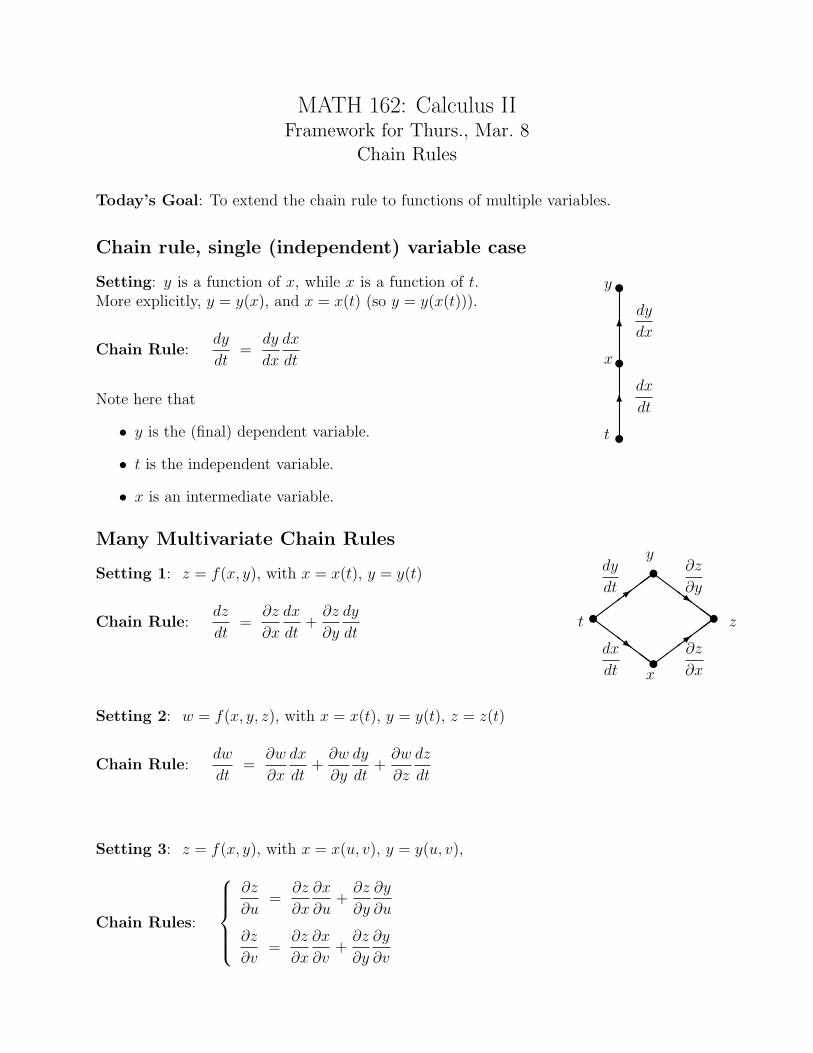
Chain rule, single (independent) variable case

Setting: y is a function of x, while x is a function of t.More explicitly, y = y(x), and x = x(t) (so y = y(x(t))).

Chain Rule:dy

dt=

dy

dx

dx

dt

Note here that

• y is the (final) dependent variable.

• t is the independent variable.

• x is an intermediate variable.

u

u

u

t

dx

dt

x

dy

dx

y

6

6

Many Multivariate Chain Rules

Setting 1: z = f(x, y), with x = x(t), y = y(t)

Chain Rule:dz

dt=

∂z

∂x

dx

dt+

∂z

∂y

dy

dt

Setting 2: w = f(x, y, z), with x = x(t), y = y(t), z = z(t)

Chain Rule:dw

dt=

∂w

∂x

dx

dt+

∂w

∂y

dy

dt+

∂w

∂z

dz

dt

Setting 3: z = f(x, y), with x = x(u, v), y = y(u, v),

Chain Rules:

∂z

∂u=

∂z

∂x

∂x

∂u+

∂z

∂y

∂y

∂u

∂z

∂v=

∂z

∂x

∂x

∂v+

∂z

∂y

∂y

∂v

t z

ydy

dt

∂z

∂y

x

dx

dt

∂z

∂x

uu

uu�

��>�

��

ZZ

Z~ZZZ

ZZ

Z~ZZZ

��

�>���

MATH 162—Framework for Thurs., Mar. 8 Chain Rules

Another Look at Implicit Differentiation

Many problems from MATH 161 in which implicit differentation was used involved equationswhich could be put in the form F (x, y) = 0. Assuming that this equation defines y implicitlyas a function of x (an assumption that is generally true), then by the chain rule

dF

dx=

∂F

∂x

dx

dx+

∂F

∂y

dy

dx= Fx + Fy

dy

dx.

This is the x-derivative of one side of the equation F (x, y) = 0. The x-derivative of the otherside is, naturally, 0. Thus, we have

Fx + Fydy

dx= 0 ⇒ dy

dx= −Fx

Fy

.

2

MATH 162: Calculus IIFramework for Fri., Mar. 9

Vectors

Today’s Goal: To understand vectors and be able to manipulate them.

Vectors in 2 and 3 Dimensions

Definition: A vector is a directed line segment. If P and Q are points in R2 or R3, then

the directed line segment from the initial point P to the terminal point Q is denoted−→PQ.

• Vector names: bold-faced letters (usually lower-case) v, or letters with arrows ~v

• There are two things that distinguish a vector v: its length and its direction. Thus,two directed line segments which are parallel, have the same length, and are orientedin the same direction (arrow pointing the same way) are considered to be the same(equal) even if their initial and terminal points are different.

• Component form: Given what was said above, any vector v may be moved rigidly soas to make its initial point be the origin. Writing (v1, v2, v3) for the resulting terminalpoint, we then say that v = 〈v1, v2, v3〉. This is called the component form of v. Thenumbers v1, v2 and v3 are the components of v.

• Equality of vectors: Two vectors are considered equal when they are equal in eachcomponent.

• If v = 〈v1, v2, v3〉 then the length (or magnitude) of v, denoted |v|, is given by

|v| :=√

v21 + v2

2 + v23.

The only vector whose length is zero is the one whose components are all zero. Wecall this the zero vector, denoting it by 0. The other vectors (the ones with nonzerolength) are collectively referred to as nonzero vectors.

Vector Operations

Vector Addition: If u = 〈u1, u2, u3〉 and v = 〈v1, v2, v3〉, we define

u + v := 〈u1 + v1, u2 + v2, u3 + v3〉 .

Scalar Multiplication: If v = 〈v1, v2, v3〉 and c is a real number (a scalar), then we define

cv := 〈cv1, cv2, cv3〉 .

MATH 162—Framework for Fri., Mar. 9 Vectors

Note that:

• Our definitions for vector addition and scalar multiplication are enough to give us thenotion of vector subtraction as well, since we may think of u− v as

u + (−1)v = 〈u1, u2, u3〉+ 〈−v1,−v2,−v3〉 = 〈u1 − v1, u2 − v2, u3 − v3〉 .

• We make sense of an expression like v/c (i.e., dividing a vector by a scalar) by thinkingof it as (1/c)v (i.e., the reciprocal of c multiplied by v). For any nonzero vector v,v/|v| is a vector whose length is 1, called the direction of v.

• No attempt has been made to define any type of multiplication (not yet) nor division(never!) between two vectors.

Unit Vectors

Any vector whose length is 1 is called a unit vector.

Example: For each v 6= 0, the directionv

|v|of v is a unit vector. Thus, in 2D, the vector

v = 〈−2, 5〉 has direction

d =〈−2, 5〉√(−2)2 + 52

=

⟨−2√29

,5√29

⟩.

We may then write v as a product of its magnitude times its direction

v =√

29d.

Standard unit vectors (the ones parallel to the coordinate axes): i := 〈1, 0, 0〉, j :=〈0, 1, 0〉, and k := 〈0, 0, 1〉.

Notice that, for v = 〈v1, v2, v3〉, it is the case that

v = v1i + v2j + v3k.

2

MATH 162: Calculus IIFramework for Mon., Mar. 12Dot Products and Projections

Today’s Goal: To define the dot product and learn of some of its properties and uses

The Dot Product

Definition: For vectors u = 〈u1, u2, u3〉 and v = 〈v1, v2, v3〉, we define the dot product of uand v to be

u ·v := u1v1 + u2v2 + u3v3.

Notes:

• The dot product u ·v is a scalar (number), not another vector.

• Properties

1. u ·v = v ·u2. c(u ·v) = (cu) ·v = u · (cv).

3. u · (v + w) = u ·v + u ·w4. 0 ·v = 0

5. v ·v = |v|2

Theorem: If u and v are nonzero vectors, then the angle θ between them satisfies

cos θ =u ·v|u||v|

.

Note that, when θ = π/2, the numerator on the right-hand side must be zero. This motivatesthe following definition.

Orthogonality

Definition: Two vectors u and v are said to be orthogonal (or perpendicular) if u ·v = 0.

Example: The zero vector 0 is orthogonal to every other vector. In 2D, the vectors 〈a, b〉and 〈−b, a〉 are orthogonal, since

〈a, b〉 · 〈−b, a〉 = (a)(−b) + (b)(a) = 0.

MATH 162—Framework for Mon., Mar. 12 Dot Products and Projections

Example: Find an equation for the plane containing the point (1, 1, 2) and perpendicularto the vector 〈A, B, C〉.

Projections

Scalar component of u in the direction of v: |u| cos θ =u ·v|v|

.

Vector projection of u onto v:

projvu :=

(scalar component of u

in direction of v

) (direction

of u

)=

(u ·v|v|

) (v

|v|

)=

u ·v|v|2

v.

Work

The work done by a constant force F acting through a displacement vector D =−→PQ is given

byW = F ·D = |F||D| cos θ,

where θ is the angle between F and D.

2

MATH 162: Calculus IIFramework for Tues., Mar. 13

Cross Products

Today’s Goal: To define the cross product and learn of some of its properties and uses

The Cross Product

Definition: For nonzero, non-parallel 3D vectors u and v, we define the cross product of uand v to be

u × v := (|u||v| sin θ)n,

where θ is the angle between u and v, and n is a unit vector perpendicular to both u andv, and in the direction determined by the “right-hand rule.”

If either u = 0 or v = 0, we define u × v = 0. Similarly, if u and v are parallel, we takeu × v = 0.

Notes:

• There is no corresponding concept for 2D vectors.

• The dot product between two vectors produces a scalar. The cross product of twovectors yields another vector.

• Properties

1. u × v = −v × u

2. i × j = k, j × k = i, k × i = j

3. (ru) × (sv) = (rs)(u × v)

4. The cross product is not associative! This means that, in general, it is not thecase that

(u × v) × w and u × (v × w)

are equal.

• The cross product u × v may be computed from the following symbolic determinant:

u × v =

∣∣∣∣∣∣i j ku1 u2 u3

v1 v2 v3

∣∣∣∣∣∣ :=

∣∣∣∣ u2 u3

v2 v3

∣∣∣∣ i − ∣∣∣∣ u1 u3

v1 v3

∣∣∣∣ j +

∣∣∣∣ u1 u2

v1 v2

∣∣∣∣k,

where u = 〈u1, u2, u3〉 and v = 〈v1, v2, v3〉.

MATH 162—Framework for Tues., Mar. 13 Cross Products

Applications

• r×F is the torque vector resulting from a force F applied at the end of a lever arm r.

• |u×v| (the length of the cross product u×v) is the area of a parallelogram determinedby u and v.

• |(u × v) ·w| (the absolute value of the scalar (u × v) ·w) is the volume of the paral-lelepiped determined by u, v and w.

• Finding normal vectors to planes.

Example: The vectors u = 〈1, 2,−1〉 and v = 〈−2, 3, 1〉

– are not parallel,

– so they determine a family of parallel planes.

Find a vector that is normal to these planes. Then determine an equation for theparticular one of these planes passing through the point (1, 1, 1).

2

MATH 162: Calculus IIFramework for Thurs., Mar. 15

Vector Functions and Differential Calculus

Today’s Goal: To understand parametrized curves and their derivatives.

In yesterday’s lab, we called a set of continuous functions over a common interval I

x = x(t),y = y(t),z = z(t),

t ∈ I, (1)

a parametrized curve. (I may be a finite interval, like I = [a, b], or one of infinite length.)Another name for a parametrized curve is path, as one may think of tracing out the locationof a particle (x(t), y(t), z(t)) at various t-values in I.

Equations of lines in space

Whereas lines in the xy-plane may be characterized by a slope, lines in xyz-space are mosteasily characterized by a vector that is parallel to the line in question. Since there areinfinitely many parallel vectors, there are infinitely many ways to describe a given line.Say we want the line passing through the point P = (x0, y0, z0) parallel to the vector v =v1i + v2j + v3k. We describe it parametrically. We might arbitrarily decide to associate thepoint P with the parameter value t = 0, and integer values of t correspond to integer leapsof length |v|:

x = x0 + v1t,y = y0 + v2t,z = z0 + v3t,

−∞ < t < ∞.

Example: Find 3 possible parametrizations of the line through (2,−1, 4) in the directionof v = −i + 2j− 2k. Make one of these parametrizations be by arc length.

The position vector

One might take the functions (1) and create from them a vector function, with x(t), y(t),and z(t) as component functions:

r(t) = x(t)i + y(t)j + z(t)k.

Following the idea that the path (1) describes the locations of a moving particle, r(t) is oftencalled a position vector—that is, when drawn in standard position (i.e., with its initial pointat the origin), the terminal point of r(t) moves so as to trace out the curve.

MATH 162—Framework for Thurs., Mar. 15 Vector Functions and Differential Calculus

Example: Equation of a line in space, vector form. For the line passing through thepoint P = (x0, y0, z0) parallel to the vector v = v1i + v2j + v3k, we have the vector form

r(t) = (x0 + v1t)i + (y0 + v2t)j + (z0 + v3t)k.

Limits and continuity of vector functions

While the following definition is not identical to the one given in the text, the two are logi-cally equivalent.

Definition: Let r(t) = x(t)i + y(t)j + z(t)k (so the component functions of r(t) are x(t),y(t) and z(t)). We say that

limt→t0

r(t) = L = L1i + L2j + L3k

precisely when each corresponding limit of the component functions

limt→t0

x(t) = L1, limt→t0

y(t) = L2, and limt→t0

z(t) = L3

holds.

We say that r(t) is continuous at t = t0 precisely when each of the component functions x(t),y(t) and z(t) are continuous at t = t0.

Example: The vector function r(t) = t/(t−1)2i+(ln t)j is continuous at all points t whereits component functions x(t) = t/(t − 1)2 and y(t) = ln t are continuous—that is for t > 0.Thus, limt→t0 r(t) exists whenever t0 > 0.

Derivatives of vector functions

Definition: A vector function r(t) = x(t)i + y(t)j + z(t)k is differentiable at t if the limit

r′(t) := lim∆t→0

r(t + ∆t)− r(t)

∆t

exists.

Notes:

• An equivalent definition to the one above would be that r(t) is differentiable at agiven t-value precisely when each of its component functions x(t), y(t) and z(t) aredifferentiable there. When this is so, we have

dr

dt= x′(t)i + y′(t)j + z′(t)k.

2

MATH 162—Framework for Thurs., Mar. 15 Vector Functions and Differential Calculus

• If a vector function r(t) is differentiable, then the derivative r′(t) is itself another vectorfunction, which may be differentiable as well. When this is so, we have

d2r

d2t= x′′(t)i + y′′(t)j + z′′(t)k.

• If the position vector function r(t) is differentiable, then dr/dt is the correspondingvelocity vector function. What we call speed is actually the length |dr/dt| of the velocityfunction.

If dr/dt is differentiable, then we call d2r/dt2 the acceleration vector function.

• One check that we have defined dot and cross products between vectors in a usefulfashion is whether they obey “product rules.” In fact, all of the rules for differentiationthat hold for scalar functions, and are appropriate to apply to vector functions, stillhold:

1.d

dtC = 0 (constant function rule)

2.d

dt[cu(t)] = cu′(t) (constant multiple rule)

3.d

dt[f(t)u(t)] = f ′(t)u(t) + f(t)u′(t) (product of scalar and vector fn.)

4.d

dt

[u(t)

f(t)

]=

f ′(t)u(t)− f(t)u′(t)

[f(t)]2(quotient of vector and scalar fn.)

5.d

dt[u(t)± v(t)] = u′(t)± v′(t) (sum and difference rules)

6.d

dt[u ·v] = u′(t) ·v(t) + u(t) ·v′(t) (dot product rule)

7.d

dt[u× v] = u′(t)× v(t) + u(t)× v′(t) (cross product rule)

8.d

dt[u(f(t))] = f ′(t)u′(f(t)) (chain rule)

3

MATH 162: Calculus IIFramework for Fri., Mar. 16

Vector Functions and Integral Calculus

Today’s Goal: To understand how to integrate vector functions.

Indefinite integrals

Recall: For scalar functions f(t),

• A function F is called an antiderivative of f on the interval I if F ′(t) = f(t) at eachpoint t ∈ I.

• Given any antiderivative F of f and any constant C, F (t)+C is also an antiderivativeof f .

• The indefinite integral ∫f(t) dt

stands for the set of all antiderivatives of f .

For a vector function r(t) = f(t)i + g(t)j + h(t)k,

• An antiderivative of r(t) on an interval I is another vector function R(t) for whichR′(t) = r(t) at each t ∈ I.

• Finding an antiderivative of r(t) comes down to finding antiderivatives for its compo-nent functions. That is, if F , G and H are antiderivatives of f , g and h on the intervalI, then

R(t) = F (t)i + G(t)j + H(t)k

is an antiderivative of r(t).

• Given any antiderivative R(t) of r(t) and any constant vector C, R(t) + C is also anantiderivative of r(t).

• The symbol ∫R(t) dt

stands for the set of all antiderivatives of r.

Example:

∫ [(1

1 + t2

)i + (sin t cos t) j +

(t√

1 + 3t2

)k

]dt

MATH 162—Framework for Fri., Mar. 16 Vector Functions and Integral Calculus

Definite Integrals

Definition: Suppose that the component functions of r(t) = f(t)i + g(t)j + h(t)k are allintegrable over the interval [a, b] (true, say, if each of f , g and h are continuous over thatinterval). Then we say the vector function r(t) is integrable over [a, b], and define its integralto be ∫ b

a

r(t) dt :=

(∫ b

a

f(t) dt

)i +

(∫ b

a

g(t) dt

)j +

(∫ b

a

h(t) dt

)k.

Since the fundamental theorem of calculus holds for the components of r(t), it holds for r(t)as well. Here we state just part II.

Theorem: If r(t) is continuous at each point of the interval [a, b] and if R is any antideriva-tive of r on [a, b], then ∫ b

a

r(t) dt = R(b)−R(a).

Application: Projectile motion

For projectiles near enough to sea level, we think of them as having constant accelerationa(t) = −gk, where g has the value 9.8 m/s2 or 32 ft/s2. Since velocity is an antiderivativeof acceleration, we may write∫ t

0

a dτ = −gtk = v(t)− v(0),

or, abbreviating v(0) by v0,v(t) = v0 − gtk.

The position r(t) is an antiderivative of velocity, so∫ t

0

v(τ) dτ = tv0 −1

2gt2k = r(t)− r(0),

or

r(t) = r0 + tv0 −1

2gt2k,

where r0 := r(0) is the initial position.

2

MATH 162: Calculus IIFramework for Mon., Mar. 26

Quadric Surfaces

Today’s Goal: To review how equations in three variables are graphed, and to identifyspecial graphs known as quadric surfaces.

What we already know: A 2nd-order polynomial in x and y takes the general form

p(x, y) = Ax2 + Bxy + Cy2 + Dx + Ey + F.

Such a polynomial is called a quadratic polynomial (in x and y).

Some special cases, usually treated in high school classes:

• Case B = C = 0, A 6= 0: p(x, y) = Ax2 + Dx + Ey + F

– The level sets of p are parabolas.

– By symmetry of argument, the level sets are parabolas opening sideways whenA = B = 0 and C 6= 0.

• Case B2 < 4AC:

– Some level sets of p are ellipses.

– When B = 0 and A = C, the ellipses are actually circles.

• Case AC < 0: Almost all level sets of p are hyperbolas.

Quadric Surfaces

Similar to the above, a quadratic polynomial in x, y and z is a 2nd-order polynomial havinggeneral form

p(x, y, z) = Ax2 + Bxy + Cy2 + Dxz + Eyz + Fz2 + Gx + Hy + Iz + J. (1)

• The graph of p would require 4 dimensions, but the level sets of p are surfaces in 3D.

• The solutions of the equation p(x, y, z) = k (k a fixed number) coincide with thek-level surface for the quadratic function p.

Definition: For a quadratic polynomial p in the form (1), the set of points (x, y, z)which satisfy the level surface equation p(x, y, z) = k is called a quadric surface.

MATH 162—Framework for Mon., Mar. 26 Quadric Surfaces

• When the coefficient F = 0 and at least one of D, E or I is nonzero, the level surfaceequation may be manipulated algebraically to solve for z as a function of x and y. Inthese cases, what we learned about graphing functions of 2 variables still applies.

Example: 9x2 − y2 − 4z = 0 (hyperbolic paraboloid)

By symmetry of argument, the level surface equation p(x, y, z) = k can be written asa function if

– A = 0 and at least one of B, D or G is nonzero, in which case x may be writtenas a function of y and z, or

– C = 0 and any one of B, E or H is nonzero, in which case y may be written as afunction of x and z.

• Even when the equation p(x, y, z) = k cannot be re-written as a function of twovariables, a good way to get an idea of the graph of the level surface is to considercross-sections:

– slices by planes parallel to the xy-plane are the result of setting z = z0.

– slices by planes parallel to the xz-plane are the result of setting y = y0.

– slices by planes parallel to the yz-plane are the result of setting x = x0.

Examples:

9x2 + y2 − 4z2 = 1 (an hyperboloid in one sheet)

9x2 + y2 − 4z2 = 0 (an elliptic cone)

9x2 − y2 − 4z2 = 1 (an hyperboloid in two sheets)

9x2 + y2 + 4z2 = 1 (an ellipsoid)

2

MATH 162: Calculus IIFramework for Tues., Mar. 27

More about Lines and Planes in Space

Today’s Goal: To review how lines and planes in space are represented, and use thesenotions to derive some useful formulas and algorithms involving points, lines and planes.

Lines and Planes

We have derived the following representations.

• Lines. The line trough point P = (x0, y0, z0) parallel to v = v1i + v2j + v3k

component form: x = x0 + v1t,y = y0 + v2t, −∞ < t < ∞,z = z0 + v3t,

vector form: r(t) = (x0 + v1t)i + (y0 + v2t)j(z0 + v3t)k, −∞ < t < ∞.

• Planes. The plane trough point P = (x0, y0, z0) perpendicular to n = ai + bj + ck

n · [(x− x0)i + (y − y0)j + (z − z0)k] = 0, or ax + by + cz = d,

where d = ax0 + by0 + cz0.

Formulas and Algorithms for Lines and Planes

• Distance from a point S to a line L.

Keys to a formula:

1. Our distance is |−→PS| sin θ, where

P is any point on line L.

2. For two vectors u and v, |u× v| = |u||v| sin θ.

From these we get

|−→PS| sin θ =

|−→PS × v||v|

,

where v is any vector parallel to line L.

````````````````````�������

uu

L

P

S

������������1

MATH 162—Framework for Tues., Mar. 27 More about Lines and Planes in Space

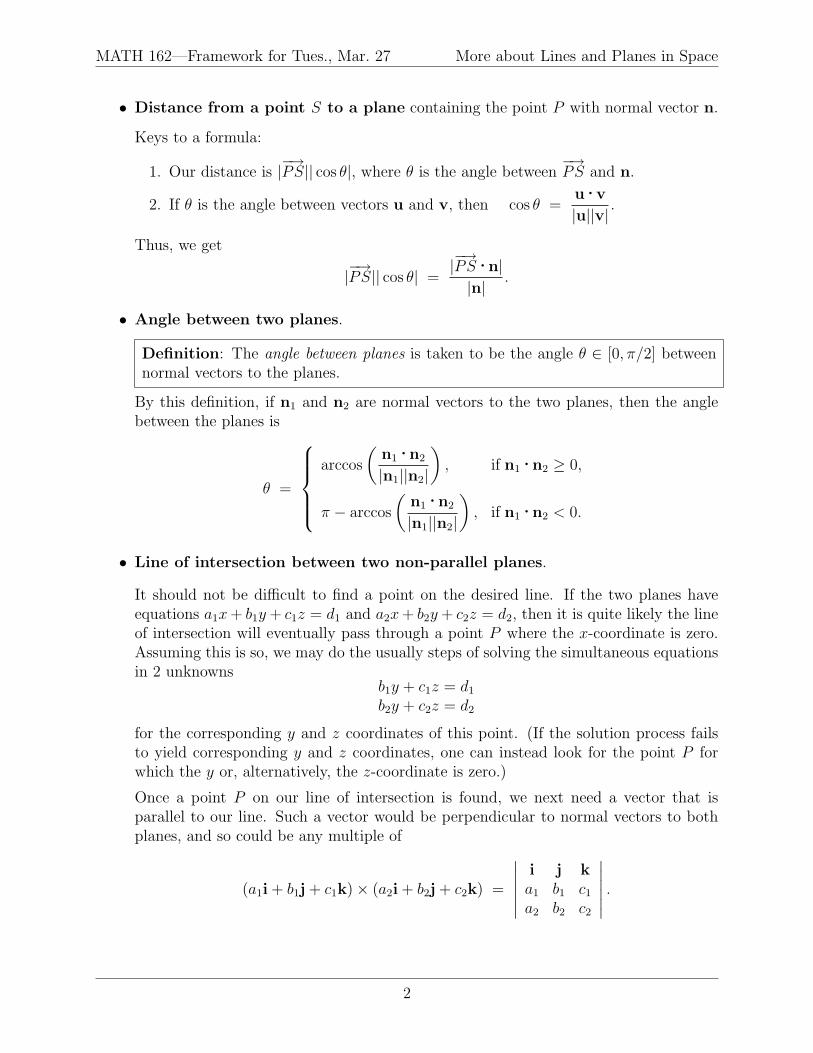
• Distance from a point S to a plane containing the point P with normal vector n.

Keys to a formula:

1. Our distance is |−→PS|| cos θ|, where θ is the angle between

−→PS and n.

2. If θ is the angle between vectors u and v, then cos θ =u ·v|u||v|

.

Thus, we get

|−→PS|| cos θ| =

|−→PS ·n||n|

.

• Angle between two planes.

Definition: The angle between planes is taken to be the angle θ ∈ [0, π/2] betweennormal vectors to the planes.

By this definition, if n1 and n2 are normal vectors to the two planes, then the anglebetween the planes is

θ =

arccos

(n1 ·n2

|n1||n2|

), if n1 ·n2 ≥ 0,

π − arccos

(n1 ·n2

|n1||n2|

), if n1 ·n2 < 0.

• Line of intersection between two non-parallel planes.

It should not be difficult to find a point on the desired line. If the two planes haveequations a1x + b1y + c1z = d1 and a2x + b2y + c2z = d2, then it is quite likely the lineof intersection will eventually pass through a point P where the x-coordinate is zero.Assuming this is so, we may do the usually steps of solving the simultaneous equationsin 2 unknowns

b1y + c1z = d1

b2y + c2z = d2

for the corresponding y and z coordinates of this point. (If the solution process failsto yield corresponding y and z coordinates, one can instead look for the point P forwhich the y or, alternatively, the z-coordinate is zero.)

Once a point P on our line of intersection is found, we next need a vector that isparallel to our line. Such a vector would be perpendicular to normal vectors to bothplanes, and so could be any multiple of

(a1i + b1j + c1k)× (a2i + b2j + c2k) =

∣∣∣∣∣∣i j ka1 b1 c1

a2 b2 c2

∣∣∣∣∣∣ .

2

MATH 162: Calculus IIFramework for Thurs., Mar. 29–Fri. Mar. 30

The Gradient Vector

Today’s Goal: To learn about the gradient vector ~∇f and its uses, where f is a functionof two or three variables.

The Gradient Vector

Suppose f is a differentiable function of two variables x and y with domain R, an open regionof the xy-plane. Suppose also that

r(t) = x(t)i + y(t)j, t ∈ I,

(where I is some interval) is a differentiable vector function (parametrized curve) with(x(t), y(t)) being a point in R for each t ∈ I. Then by the chain rule,

d

dtf(x(t), y(t)) =

∂f

∂x

dx

dt+

∂f

∂y

dy

dt

= [fxi + fyj] · [x′(t)i + y′(t)j]

= [fxi + fyj] · dr

dt. (1)

Definition: For a differentiable function f(x1, . . . , xn) of n variables, we define the gradientvector of f to be

~∇f :=

⟨∂f

∂x1

,∂f

∂x2

, . . . ,∂f

∂xn

⟩.

Remarks:

• Using this definition, the total derivative df/dt calculated in (1) above may be writtenas

df

dt= ~∇f · r′.

In particular, if r(t) = x(t)i+y(t)j+z(t)k, t ∈ (a, b) is a differentiable vector function,and if f is a function of 3 variables which is differentiable at the point (x0, y0, z0), wherex0 = x(t0), y0 = y(t0), and z0 = z(t0) for some t0 ∈ (a, b), then

df

dt

∣∣∣∣t=t0

= ~∇f(x0, y0, z0) · r′(t0).

• If f is a function of 2 variables, then ~∇f has 2 components. Thus, while the graph ofsuch an f lives in 3D, ~∇f should be thought of as a vector in the plane.

If f is a function of 3 variables, then ~∇f has 3 components, and is a vector in 3-space.

MATH 162—Framework for Thurs., Mar. 29–Fri. Mar. 30 The Gradient Vector

Speaking more generally, we may say that whilea function f(x1, . . . , xn) of n variables requiresn inputs to produce a single (numeric) output,

the corresponding gradient ~∇f produces fromthose same n inputs a vector with n compo-nents. Objects which assign to each n-tupleinput an n-vector output are known as vectorfields. The gradient is an example of a vectorfield.

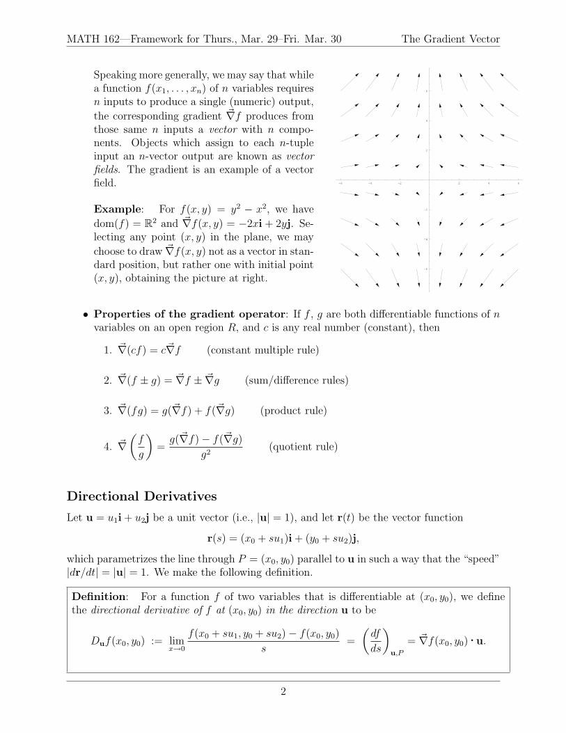
Example: For f(x, y) = y2 − x2, we have

dom(f) = R2 and ~∇f(x, y) = −2xi + 2yj. Se-lecting any point (x, y) in the plane, we may

choose to draw ~∇f(x, y) not as a vector in stan-dard position, but rather one with initial point(x, y), obtaining the picture at right.

-6 -4 -2 2 4 6

-6

-4

-2

2

4

6

• Properties of the gradient operator: If f , g are both differentiable functions of nvariables on an open region R, and c is any real number (constant), then

1. ~∇(cf) = c~∇f (constant multiple rule)

2. ~∇(f ± g) = ~∇f ± ~∇g (sum/difference rules)

3. ~∇(fg) = g(~∇f) + f(~∇g) (product rule)

4. ~∇(

f

g

)=

g(~∇f)− f(~∇g)

g2(quotient rule)

Directional Derivatives

Let u = u1i + u2j be a unit vector (i.e., |u| = 1), and let r(t) be the vector function

r(s) = (x0 + su1)i + (y0 + su2)j,

which parametrizes the line through P = (x0, y0) parallel to u in such a way that the “speed”|dr/dt| = |u| = 1. We make the following definition.

Definition: For a function f of two variables that is differentiable at (x0, y0), we definethe directional derivative of f at (x0, y0) in the direction u to be

Duf(x0, y0) := limx→0

f(x0 + su1, y0 + su2)− f(x0, y0)

s=

(df

ds

)u,P

= ~∇f(x0, y0) ·u.

2

MATH 162—Framework for Thurs., Mar. 29–Fri. Mar. 30 The Gradient Vector

Remarks:

• Special cases: the partial derivatives fx, fy themselves are derivatives in the directionsi, j respectively.

Dif = ~∇f · i = fx, and Djf = ~∇f · j = fy.

• For f a function of 2 variables, the direction of ~∇f(x, y) (namely ~∇f(x, y)/|~∇f(x, y)|)

is the direction of maximum increase, while −~∇f(x, y)/|~∇f(x, y)| is the direction ofmaximum decrease.

Proof: For any unit vector u,

Duf(x, y) = ~∇f(x, y) ·u = |~∇f(x, y)||u| cos θ = |~∇f(x, y)| cos θ,

where θ is the angle between ~∇f(x, y) and u. This directional derivative is

largest when θ = 0 (i.e., when u = ~∇f/|~∇f |) and smallest when θ = π.

• The notion of directional derivative extends naturally to functions of 3 or more vari-ables.

The Gradient and Level Sets

Suppose f(x, y) is differentiable at the point P = (x0, y0),and let k = f(x0, y0). Then the k-level curve of f con-tains (x0, y0). Suppose that we have a parametrization ofa section of this level curve containing the point (x0, y0).That is, let

• x(t) and y(t) be differentiable functions of t in anopen interval I containing t = 0,

• x0 = x(0) and y0 = x(0), and

• f(x(t), y(t)) = k for t ∈ I (that is, the parametrization gives at least a small part ofthe k-level curve of f—a part that contains the point P ).

Because we are parametrizing a level curve of f , it follows that df/dt = 0 for t ∈ I. Inparticular,

0 =df

dt

∣∣∣∣t=t0

= ~∇f(x0, y0) · [x′(t0)i + y′(t0)j].

This shows that the gradient vector at P is orthogonal to the level curve of f (or the tangentline to the level curve) through P . This is true at all points P where f is differentiable.That this result may be generalized to higher dimensions is motivation for the definition ofa tangent plane.

3

MATH 162—Framework for Thurs., Mar. 29–Fri. Mar. 30 The Gradient Vector

Tangent Planes

Definition: Let f(x, y, z) be differentiable at a point P = (x0, y0, z0) contained in the levelsurface f(x, y, z) = k. We define the tangent plane to this level surface of f at P to be the

plane containing P normal to ~∇f(x0, y0, z0).

Example: Suppose f(x, y, z) is a differentiable function at the point P = (x0, y0, z0) lyingon the level surface f(x, y, z) = k. Derive a formula for the equation of the tangent planeto this level surface of f at P . Then use it to write the equation of the tangent plane to thequadric surface

f(x, y, z) = x2 + 3y2 + 2z2 = 6

at the point (1, 1, 1).

Example: Suppose z = f(x, y) is a differentiable function at the point P = (x0, y0).Derive a formula for the equation of the tangent plane to the surface z = f(x, y) at the pointP = (x0, y0, f(x0, y0)). Use it to get the equation of the tangent plane to z = 2x2− y2 at thepoint (1, 3,−7).

4

MATH 162: Calculus IIFramework for Wed., Apr. 4

Unconstrained Optimization of Functions of 2 Variables

Today’s Goal: To be able to locate and classify local extrema for functions of two variables.

Definition: Suppose the domain of f(x, y) includes the point (a, b).

1. f(a, b) is called a local maximum (or relative maximum) value of f if f(a, b) ≥ f(x, y)for all points from dom(f) contained in some open disk (an open disk of some positive,though perhaps quite small, radius) centered at (a, b).

2. f(a, b) is called a local minimum (or relative miminum) value of f if f(a, b) ≤ f(x, y)for all points from dom(f) contained in some open disk centered at (a, b).

Remarks:

• As with functions of a single variable (think of the absolute value function), localextrema (maxima or minima) of functions f of two variables may occur at pointswhere f is not differentiable.

• When an extremum occurs at an interior point (a, b) of dom(f) where f is differentiable,one would expect f to have a horizontal tangent plane there. The equation for thetangent plane to z = f(x, y) at a point (x0, y0) where f is differentiable is

fx(x0, y0)(x− x0) + fy(x0, y0)(y − y0)− (z − z0) = 0,

orz = z0 + fx(x0, y0)(x− x0) + fy(x0, y0)(y − y0),

while the equation of a horizontal plane (one parallel to the xy-plane is) z = constant.We may, therefore, conclude:

Theorem: If f(x, y) has a local extremum at an interior point (a, b) of dom(f), andif the partial derivatives of f exist there, then

fx(a, b) = 0 and fy(a, b) = 0.

This motivates the following definition.

Definition: Let f be a function of two variables. An interior point of dom(f) where

(i) both fx and fy are zero, or

(ii) at least one of fx, fy does not exist

is called a critical point of f .

Fmwk. for Wed., Apr. 4 Unconstrained Optimization of Functions of 2 Variables

Classifying Critical Points

Just as with functions of one variable, not all critical points of f(x, y) correspond to a localextremum. On pp. 757–759 of the text, Figures 12.37 and 12.41 depict situations in which(0, 0) is a critical point corresponding to an extremum; Figure 12.40 depicts situations inwhich (0, 0) is the location of a saddle point.

Definition: Suppose f(x, y) is a differentiable function with critical point (a, b). If everyopen disk centered at (a, b) contains both domain points (x, y) for which f(x, y) > f(a, b)and domain points (x, y) for which f(x, y) < f(a, b), then f is said to have a saddle point at(a, b).

With functions of a single variable, we have several tests (the First Derivative Test and theSecond Derivative Test) for determining when a critical point corresponds to a local ex-tremum. The following theorem provides a test for those critical points of type (i) for whichf is twice continuously differentiable throughout a disk surrounding the critical point.

Theorem: Suppose that f(x, y) and its first and 2nd partial derivatives are continuous

throughout a disk centered at (a, b), and that ~∇f(a, b) = 0. Let D be given by the followingtwo-by-two determinant:

D(x, y) :=

∣∣∣∣ fxx(x, y) fxy(x, y)fxy(x, y) fyy(x, y)

∣∣∣∣ = fxxfyy − f 2xy.

Then

(i) f has a local maximum at (a, b) if fxx(a, b) < 0 and D(a, b) > 0.

(ii) f has a local minimum at (a, b) if fxx(a, b) > 0 and D(a, b) > 0.

(iii) f has a saddle point at (a, b) if D(a, b) < 0.

If D(a, b) = 0, or if D(a, b) > 0 and fxx(a, b) = 0, then this test fails to classify the criticalpoint (a, b).

Examples:

f(x, y) = x3y + 12x2 − 8y

f(x, y) =x2y2 − 8x + y

xy

f(x, y) = xy(1− x− y)

2

MATH 162: Calculus IIFramework for Mon., Apr. 9

Constrained Optimization of Functions of 2 Variables

Today’s Goal: To be able to find absolute extrema for functions of two variables on closedand bounded domains.

Definition: A function f of two variables is said to have

1. a global maximum (or absolute maximum) at the point (a, b) ∈ dom(f) if f(a, b) ≥f(x, y) for all points (x, y) in dom(f).

2. a global minimum (or absolute minimum) at the point (a, b) ∈ dom(f) if f(a, b) ≥f(x, y) for all points (x, y) in dom(f).

The value f(a, b) is correspondingly called the global (or absolute) maximum or minimumvalue of f .

Before we embark on a process of looking for absolute extrema, it would be nice to knowthat what we are looking for is out there to be found. The following theorem supplies suchan assurance in the special case that the domain of f is closed and bounded.

Theorem: (Extreme Value Theorem) Suppose f(x, y) is a continuous function on a closedand bounded region R of the xy-plane. Then there exist points (a, b) and (c, d) in R forwhich

f(a, b) ≥ f(x, y) f(c, d) ≤ f(x, y)

for all (x, y) in R.

Remarks:

• In some simple cases, it is even possible that (a, b) and (c, d) from the theorem are thesame point.

• In the theorem, we would call “continuity of f over a closed, bounded region R” assufficient conditions to guarantee that f reaches maximum and minimum values in R.It is possible for f to attain such extrema even if one or both of these conditions (the“continuity” or the “closed and boundedness of R”) is not in place.

Examples:

1. Find the maximum value of f(x, y) = 49− x2 − y2 along the line x + 3y = 10.

Framework for Mon., Apr. 9 Constrained Optimization of Functions of 2 Variables

2. Find the absolute extrema for f(x, y) = x2−y2−2x+4y on the region of the xy-planebounded below by the x-axis, above by the line y = x + 2, and on the right by the linex = 2.

3. Find the absolute extrema for f(x, y) = x2 + 2y2 on the closed disk x2 + y2 ≤ 1.

4. Find the maximum of f(x, y, z) = 36 − x2 − y2 − z2 subject to the constraintx + 4y − z = 21.

5. Find the point on the graph of z = x2 + y2 + 10 closest to the plane x + 2y − z = 0.

2

MATH 162: Calculus IIFramework for Wed., Apr. 11

Double and Iterated Integrals, Rectangular Regions

Today’s Goal: To understand the meaning of double integrals over bounded rectangularregions R of the plane, and to be able to evaluate such integrals.

Important Note: In conjunction with this framework, you should look over Section 13.1of your text.

Riemann Sums

We assume that f(x, y) is a function of 2 variables, and that R = {(x, y) ∈ R2 | a ≤ x ≤b, c ≤ y ≤ d} (i.e., R is some bounded rectangular region of the plane whose sides areparallel to the coordinate axes). Supppose we

• divide R up into n smaller rectangles, labeling them R1, R2, . . . , Rn,

• choose, from each rectangle Rk, some point (xk, yk), and

• use the symbol ∆Ak to denote the area of rectangle Rk.

Then the sumn∑

k=1

f(xk, yk)∆Ak

is called a Riemann sum of f over the region R.

Definition: The collection of smaller rectangles R1, . . . , Rn is called a partition P of R.The maximum, taken over all lengths and widths of these rectangles, is called the norm ofthe partition P , and is denoted by ‖P‖.

The function f is said to be integrable over R if the limit

lim‖P‖→0

n∑k=1

f(xk, yk)∆Ak,

taken over all partitions P of R, exists. The value of this limit, called the double integral off over R, is denoted by ∫∫

R

f(x, y) dA.

The following theorem tells us that, for certain functions, integrability is assured

Theorem: Suppose f(x, y) is a continuous function over the closed and bounded rectangleR = {(x, y ∈ R2 | a ≤ x ≤ b, c ≤ y ≤ d} in the plane. Then f is integrable over R.

Framework for Wed., Apr. 11 Double and Iterated Integrals, Rectangular Regions

Remarks

• The double integral of f over R is a definite integral, and has a numeric value.

• When f(x, y) is a nonnegative function,∫∫

Rf(x, y) dA may be interpreted as the vol-

ume under the surface z = f(x, y) over the region R in the xy-plane.

• When f(x, y) is a constant function (i.e., f has the same value, say c, for each inputpoint (x, y)), then ∫∫

R

f(x, y) dA = c · Area(R).

Iterated Integrals and Fubini’s Theorem

Except in the very special case of constant functions f , the definition of∫∫

Rf(x, y) dA does

not, by itself, provide us with much help for evaluating a double integral. (If you are view-ing this document on the web, click here for an alternate point of view, expressed by PeterA. Lindstrom of Genesee Community College.) However, the following theorem indicatesthat the double integral may be evaluated as an iterated integral.

Theorem: (Fubini) Suppose f(x, y) is continuous throughout the rectangleR = {(x, y) ∈ R2 | a ≤ x ≤ b, c ≤ y ≤ d}. Then∫∫

R

f(x, y) dA =

∫ b

a

∫ d

c

f(x, y) dy dx =

∫ d

c

∫ b

a

f(x, y) dx dy.

Examples: Evaluate the double integral, with R as specified.

1.

∫∫R

(2x + x2y) dA, where R : −2 ≤ x ≤ 2, −1 ≤ y ≤ 1.

2.

∫∫R

y sin(xy) dA, where R : 1 ≤ x ≤ 2, 0 ≤ y ≤ π.

2

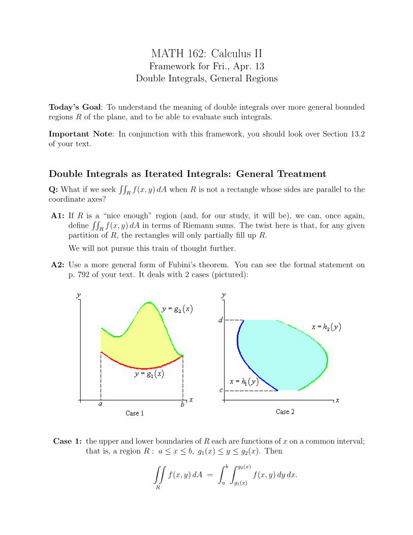
MATH 162: Calculus IIFramework for Fri., Apr. 13

Double Integrals, General Regions

Today’s Goal: To understand the meaning of double integrals over more general boundedregions R of the plane, and to be able to evaluate such integrals.

Important Note: In conjunction with this framework, you should look over Section 13.2of your text.

Double Integrals as Iterated Integrals: General Treatment

Q: What if we seek∫∫

Rf(x, y) dA when R is not a rectangle whose sides are parallel to the

coordinate axes?

A1: If R is a “nice enough” region (and, for our study, it will be), we can, once again,define

∫∫R

f(x, y) dA in terms of Riemann sums. The twist here is that, for any givenpartition of R, the rectangles will only partially fill up R.

We will not pursue this train of thought further.

A2: Use a more general form of Fubini’s theorem. You can see the formal statement onp. 792 of your text. It deals with 2 cases (pictured):

Case 1: the upper and lower boundaries of R each are functions of x on a common interval;that is, a region R : a ≤ x ≤ b, g1(x) ≤ y ≤ g2(x). Then∫∫

R

f(x, y) dA =

∫ b

a

∫ g2(x)

g1(x)

f(x, y) dy dx.

Framework for Fri., Apr. 13 Double Integrals, General Regions

Example: Evaluate∫∫

R(x + 2y) dA over the region R that lies between the

parabolas y = 2x2 and y = 1 + x2.

Case 2: the left and right boundaries of R each are functions of y on a common interval;that is, a region R : c ≤ y ≤ d, h1(x) ≤ x ≤ h2(x). Then∫∫

R

f(x, y) dA =

∫ d

c

∫ h2(y)

h1(y)

f(x, y) dx dy.

Example: Set up an integral for a function f(x, y) over the region bounded bythe y-axis and the curve x + y2 = 1.

2

MATH 162: Calculus IIFramework for Mon., Apr. 16

Applications of Double Integrals

Today’s Goal: To use double integrals meaningfully in solving problems.

Important Note: In conjunction with this framework, you should look over Section 13.3of your text.

Area

If R is a bounded region of the plane, then∫∫

RdA gives the area of R. (This is because the

volume under the curve z = 1 over the region R, while it has different units, is the same asthe area of R.)

Average Value of a Function

For y = f(x) (a function of one variable), we defined the average value of f over the interval[a, b] to be

1

b− a

∫ b

a

f(x) dx =1

length of interval [a, b]

∫ b

a

f(x) dx.

Similarly,

Definition: If f(x, y) is integrable over a region R of the plane, then the average value of fover R is defined to be

1

Area(R)

∫∫R

f(x, y) dA.

Integral of a Density

Some functions give the amount of something per unit of measurement, as in

• f(x) is the number of grams per unit length in an (idealized) 1-dimensional string.

• f(x, y) is the number of grams per unit area in an (idealized) 2-dimensional plate.

• f(x, y, z) is the number of molecules per unit volume of a certain gas.

Such functions are collectively known as densities. The examples above are 1, 2 and 3-dimensional densities respectively.

If f(x, y) gives the density (2-dimensional) of something at each point (x, y) in the regionR, then

∫∫R

f(x, y) dA is the total of that substance found in R.

MATH 162: Calculus IIFramework for Tues., Apr. 17

Triple Integrals, Rectangular Coordinates

Today’s Goal: To be able to set up and evaluate triple integrals.

Important Note: In conjunction with this framework, you should look over Section 13.5of your text.

Defining Triple Integrals

Suppose

• D is a “nice” bounded region in 3-dimensional space.

• We subdivide D, creating a partition P of D, where P consists of n “boxes” whollycontained in D.

• In the kth box (1 ≤ k ≤ n), we choose a point (xk, yk, zk).

We then look at sums of the form

n∑k=1

f(xk, yk, zk)∆Vk,

where ∆Vk denotes the volume of the kth box.

As with Riemann sums over partitions of regions of the plane, there are many functions andregions D for which the limit

lim‖P‖→0

n∑k=1

f(xk, yk, zk)∆Vk

exists, in which case we say that f is integrable over D. This limit is denoted by∫∫∫D

f(x, y, z) dV,

read as the triple integral of f over D.

Framework for Tues., Apr. 17 Triple Integrals, Rectangular Coordinates

Comparisons to Double Integrals

1. Evaluation.

Double integrals:

Here our principle tool is Fubini’s Theorem. We have two cases.

Case:

∫∫R

g(x, y) dA =

∫ b

a

∫ g2(x)

g1(x)

g(x, y) dy dx.

Here, a and b reflect the lowest and highest of a continuum of x-values en-countered in the region R, while the lower and upper boundaries of R may beidentified as functions of x.

Case:

∫∫R

g(x, y) dA =

∫ d

c

∫ h2(x)

h1(x)

g(x, y) dx dy.

Here, c and d reflect the lowest and highest of a continuum of y-values en-countered in the region R, while the left and right boundaries of R may beidentified as functions of y.

For most regions R, either case is applicable (sometimes one of the options requiresa sum of integrals instead of a single one), meaning that the double integral may bewritten in either of two orders (i.e., either with y as the inner integral, as in dy dx,or in the order dx dy).

Triple integrals:

Given a bounded region D of 3-dimensional space, the triple integral∫∫∫

Df(x, y, z) dV

may be written as an iterated integral in six different orders. Here are twoof the possibilities:

•∫∫∫

D

f(x, y, z) dV =

∫ d

c

∫ g2(y)

g1(y)

∫ h2(y,z)

h1(y,z)

f(x, y, z) dx dz dy.

Here, c and d are the lowest and highest in a continuum of y-values encounteredas one passes through the region D. For any fixed y ∈ [c, d], we imagine a2-dimensional (planar) region that results from slicing through D with a planeparallel to the xz-plane. This planar region has a starting and ending z-value,given by g1(y) and and g2(y) respectively. At the inner-most level (the inner-most integral, which is in x), y and z are held fixed while x is allowed to vary.The interval of possible x-values starts at h1(y, z) and ends at h2(y, z).

•∫∫∫

D

f(x, y, z) dV =

∫ s

r

∫ g2(z)

g1(z)

∫ h2(x,z)

h1(x,z)

f(x, y, z) dy dx dz.

The explanation of our region is similar to the above, but this time r and srepresent lowest and highest z-values encountered in D; for a fixed z, g1(z)and g2(z) give lowest and highest x-values; for both x and z fixed, h1(x, z) andh2(x, z) give lowest and highest y-values.

2

Framework for Tues., Apr. 17 Triple Integrals, Rectangular Coordinates

2. Interpretations.

(a) Areas, volumes and higher.

Double integrals:

When g(x, y) is nonnegative, the double integral∫∫

Rf(x, y) dA gives the vol-

ume under the surface z = g(x, y) over the region R of the xy-plane. If gchanges sign in the region R, then

∫∫R

g(x, y) dA represents a difference ofvolumes.

A special case is when g(x, y) ≡ 1. As we have seen∫∫

Rg(x, y) dA =

∫∫dA

gives the area of R (numerically equal to the volume under a surface over Rwhose height is uniformly 1).

Triple integrals:

When f(x, y, z) is nonnegative, we can be sure that∫∫∫

Df(x, y, z) dV is non-

negative as well. But since the graph of w = f(x, y, z) is 4-dimensional, wewould have to think of this value as a type of 4-dimensional volume (or differ-ence of volumes, if f changes sign in D).

When f(x, y) ≡ 1, then∫∫∫

Rf(x, y, z) dV =

∫∫∫dV gives the volume of the

3-dimensional region D.

(b) Average values.The average value of g(x, y) over a region R of the xy-plane was defined to be∫∫

Rg(x, y) dA/

∫∫R

dA. Similarly, we define the average value of f(x, y, z) over aregion D of 3-dimensional space to be

∫∫∫D

f(x, y, z) dV/∫∫∫

DdV .

(c) Density integrals. When g(x, y) gives the amount of a substance per unit area,then

∫∫R

g(x, y) dA tallies the amount of that substance found in a region R ofthe xy-plane. Similarly, when f(x, y, z) gives the amount of a substance per unitvolume, then

∫∫∫D

f(x, y, z) dV tallies the amount of that substance found in aregion D of 3D space.

Examples:

1. Evaluate∫∫∫

Dz dV over the region enclosed by the three coordinate planes and the

plane x + y + z = 1.

2. Find the average z-value in the region from problem 1.

3. Find limits of integration for∫∫∫

D

√x2 + z2 dy dz dx where D is the region bounded

by the paraboloid y = x2 + z2 and the plane y = 4.

4. Write a triple integral for f(x, y, z) over the region bounded by the ellipsoid 9x2+4y2+z2 = 1.

5. What solid is it for which the iterated triple integral∫ 2

0

∫ 2−y

0

∫ 4−y2

0dz dx dy gives its

volume. What do other iterated triple integrals for the same expression look like?

3

MATH 162: Calculus IIFramework for Thurs., Apr. 19

Polar Coordinates

Today’s Goal: To understand the use of polar coordinates for specifying locations on theplane.

Important Note: In conjunction with this framework, you should look over Section 9.1 ofyour text.

Coordinate Systems for the Plane

1. Rectangular coordinates Coordinate pair (x, y) indicates how far one must travelin two perpendicular directions to arrive at point.

2. Polar coordinates Coordinate pair (r, θ) indicates signed distance and bearing

• The r value (signed distance) is written first, followed by θ.

• The bearing is an angle with the positive horizontal axis, with positive anglestaken in the counterclockwise direction.

• Any polar coordinate pair (r, θ) with r = 0 specifies the origin.

• Each point has infinitely many specifications. For instance,

· · · = (−1,−π) = (1, 0) = (−1, π) = (1, 2π) = . . . .

In particular, for any point other than the origin, there are infinitely-many repre-sentations (r, θ) in polar coordinates with r > 0, and infinitely-many with r < 0.

Relationships between Rectangular/Polar Coordinates

• Rectangular to polar: If a point (x, y) is specified in rectangular coordinates, ithas a corresponding polar representation (r, θ) determined by

r =√

x2 + y2, sin θ =y√

x2 + y2and cos θ =

x√x2 + y2

.

• Polar to rectangular: If a point (r, θ) is specified in rectangular coordinates, it hasa corresponding polar representation (x, y) determined by

x = r cos θ and y = r sin θ.

Framework for Thurs., Apr. 19 Polar Coordinates

When Polar Coordinates Are Useful

Using the “rectangular to polar” conversion above, equations in x and y (and the curvesthat correspond to them) may be expressed as polar equations (equations involving polarcoordinates). Often (though not always), what was a simple equation in rectangular coor-dinates is uglier in polar coordinates. Nevertheless, even when this is the case, integrationof particular functions over particular regions is sometimes more easily carried out in polarform than in rectangular. (See examples of this in the framework for Apr. 23.)

Examples of curves in both forms:

1. Circles centered at the origin.

Rectangular form: x2 + y2 = a2 Polar form: r = ±a

2. Circles centered on coordinate axis with point of tangency at the origin.

Rectangular: x2 + (y − a)2 = a2 Polar: r = ±2a sin θ

3. Certain ellipses.

Rectangular:x2

a2+

y2

b2= 1 Polar: r =

b√1− ε2 cos2 θ

, where ε =

√1− b2

a2

4. Lines through the origin.

Rectangular: y = mx Polar: θ = c, where c = arctan m

5. Horizontal and vertical lines.

Rectangular: y = b Polar: r = b csc θ

Polar Functions

For equations in rectangular coordinates, we often express y as a function of x (i.e., treat x asindependent) when this is possible. Similarly, when it is possible to make θ the independentvariable (i.e., when a polar equation may be solved for r), we tend to prefer doing so, writingr = f(θ). The polar forms in examples 1–3 and 5 above were expressed this way.

Examples of families of polar curves of some interest:

Note: If you place your graphing calculator in polar mode, you should be able to plot anypolar curve written in the form r = f(θ). See these and other polar curves at this link.

1. Cardioids: r = a(1± cos θ) or r = a(1± sin θ)

2. Lemniscates: r2 = a2 cos(2θ), r2 = a2 sin(2θ), etc.

3. Limacons: r = a + b cos θ or r = a + b sin θ

4. Rose curves: r = a cos(bθ) or r = a sin(bθ)

5. Spirals: r = aθ, r = eaθ, etc.

2

MATH 162: Calculus IIFramework for Mon., Apr. 23

Double Integrals in Polar Coordinates

Today’s Goal: To learn the mechanics of setting up double integrals in polar coordinates,and learn to recognize situations in double integrals that may be easier in polar form.

Important Note: In conjunction with this framework, you should look over Section 13.4of your text.

Polar Rectangles

While the specific integrand f(x, y) plays a large role in how difficult it is to evaluate a doubleintegral

∫∫R

f(x, y) dA, it is the region R alone that determines what limits of integrationone uses in formulating an iterated integral. When R is the rectangular region R : a ≤ x ≤b, c ≤ y ≤ d, setting up an iterated integral is quite easy (the limits are simply the boundingx and y-values for the rectangle).

Correspondingly, if our region R is a polar rectangle

a ≤ r ≤ b, α ≤ θ ≤ β,

then it will be easy to find limits of integration for an iterated integral in polar coordinates.

Some examples of polar rectangles:

• 0 ≤ r ≤ 1, 0 ≤ θ ≤ 2π

• 1 ≤ r ≤ 2, 0 ≤ θ ≤ 2π

• 1 ≤ r ≤ 2,π

4≤ θ ≤ π

Double Integrals in Polar Coordinates over a Polar Rectangle R :r1 ≤ r ≤ r2, α ≤ θ ≤ β

• If the integrand is f(x, y) (i.e., if it is given in terms of rectangular coordinates), onemust find the appropriate expression in polar coordinates by substituting r cos θ for x,r sin θ for y.

• The dA in∫∫

Rf(x, y) dA becomes dx dy or dy dx when written as an iterated integral

in rectangular form.

In polar form, dA = r dr dθ because of the need for the area expansion factor r.

Example: Compute the volume under the hemisphere z =√

1− x2 − y2 above the polarrectangle R : 0 ≤ r ≤ 1/2, 0 ≤ θ ≤ π in the plane.

Framework for Mon., Apr. 23 Double Integrals in Polar Coordinates

Bounded Regions

Our regions of integration for double integrals are not always rectangles (neither in theusual sense, nor in the polar sense). Often the region R of integration for a double integral∫∫

Rf(x, y) dA is described as “the region bounded by the curves . . . .” In such instances,

one step in setting up an iterated integral involves finding points where the curves intersect.

Example: Find the area of the region outside the circle r = 2 and inside the circler = 4 sin θ.

More Examples

1. Find the volume of the region bounded by the paraboloid z = 10− 3x2 − 3y2 and theplane z = 4.

2. Evaluate the iterated integral

∫ 2

0

∫ √4−y2

−√

4−y2

x2y2 dx dy.

2

MATH 162: Calculus IIFramework for Thurs., Apr. 26–Fri., Apr. 27

Moments, Centers of Mass

Today’s Goal: To learn to apply the skill of setting up and evaluating triple integrals inthe context of finding centers of mass.

Important Note: In conjunction with this framework, you should look over Section 13.6of your text.

Point Masses along a Line (1D)

• Assume n masses m1, . . . , mn sit at locations x1, . . . , xn on a number line.

• Call the location x about which the total torque is zero. That is, x is the location toplace a fulcrum so that

n∑k=1

mk(xk − x) = 0.

Solving for x, we get

x =

n∑k=1

mkxk

n∑k=1

mk

=:1st moment about x = 0

total mass(1)

Continuous Mass along a Line (1D; more instructive than practical)

When

• mass is distributed throughout a continuous body (instead of being concentrated atfinitely-many distinct positions),

• ρ(x) gives the mass density (mass per unit length) inside the interval a ≤ x ≤ b,

then the total mass is ∫ b

a

ρ(x) dx.

The continuous analog to the numerator of (??) comes from the following definition:

Definition: If ρ(x) is the mass density (in mass per unit length) of a substance containedin a region a ≤ x ≤ b of 1D space, then the first moment about x = 0 is given by∫ b

a

xρ(x) dx.

Framework for Thurs., Apr. 26–Fri., Apr. 27 Moments, Centers of Mass

Using this, the corresponding center of mass is

x =

∫ b

axρ(x) dx∫ b

qρ(x) dx

(2)

Centers of Mass in 3D

Definition: If ρ(x, y, z) is the mass density (in mass per unit volume) of a substancecontained in a region D of 3D space, then the first moment about the yz-plane (x = 0) isgiven by

Myz :=

∫∫∫D

xρ(x, y, z) dV.

Similarly, the first moments about the xz and xy-planes are

Mxz :=

∫∫∫D

yρ(x, y, z) dV and Mxy :=

∫∫∫D

zρ(x, y, z) dV

respectively.

The corresponding center of mass will reside at a point (x, y, z) in space. If we denote thetotal mass in the region D by

M :=

∫∫∫D

ρ(x, y, z) dV,

then the coordinates of the center of mass are given by

x =Myz

M, y =

Mxz

M, and z =

Mxy

M. (3)

Remarks:

• One can develop formulas for the position (x, y) of the center of mass in two dimensions.In that case it is assumed ρ(x, y) gives mass density in mass per unit area, and thefirst moments My =

∫∫R

xρ(x, y) dA and Mx =∫∫

Ryρ(x, y) dA are about the x-axis and

y-axis respectively.

• When there is constant mass density ρ(x, y, z) = δ throughout the region D, thenanother name for the center of mass is the centroid. In this case,

x =Myz

M=

δ∫∫∫D

x dV∫∫∫D

δ dV=

∫∫∫D

x dV∫∫∫D

dV= avg. x-value in D.

Similar statements may be made about the other coordinates y and z of the centroid.

2

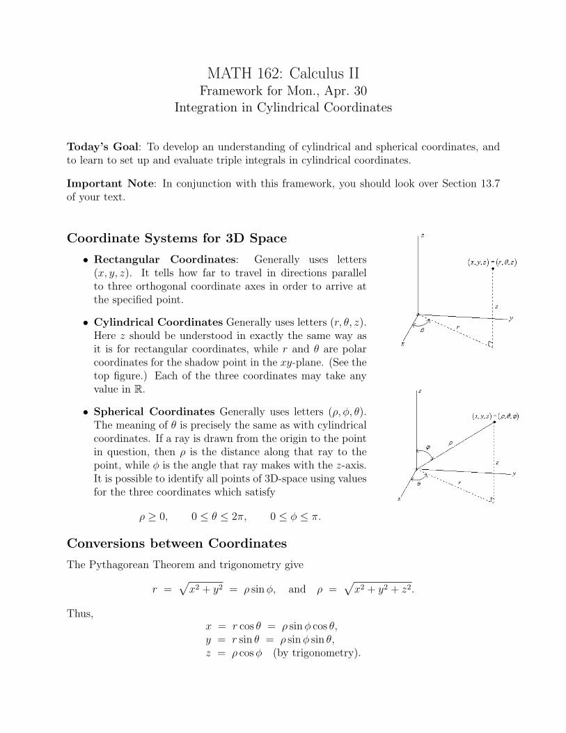
MATH 162: Calculus IIFramework for Mon., Apr. 30

Integration in Cylindrical Coordinates

Today’s Goal: To develop an understanding of cylindrical and spherical coordinates, andto learn to set up and evaluate triple integrals in cylindrical coordinates.

Important Note: In conjunction with this framework, you should look over Section 13.7of your text.

Coordinate Systems for 3D Space

• Rectangular Coordinates: Generally uses letters(x, y, z). It tells how far to travel in directions parallelto three orthogonal coordinate axes in order to arrive atthe specified point.

• Cylindrical Coordinates Generally uses letters (r, θ, z).Here z should be understood in exactly the same way asit is for rectangular coordinates, while r and θ are polarcoordinates for the shadow point in the xy-plane. (See thetop figure.) Each of the three coordinates may take anyvalue in R.

• Spherical Coordinates Generally uses letters (ρ, φ, θ).The meaning of θ is precisely the same as with cylindricalcoordinates. If a ray is drawn from the origin to the pointin question, then ρ is the distance along that ray to thepoint, while φ is the angle that ray makes with the z-axis.It is possible to identify all points of 3D-space using valuesfor the three coordinates which satisfy

ρ ≥ 0, 0 ≤ θ ≤ 2π, 0 ≤ φ ≤ π.

Conversions between Coordinates

The Pythagorean Theorem and trigonometry give

r =√

x2 + y2 = ρ sin φ, and ρ =√

x2 + y2 + z2.

Thus,x = r cos θ = ρ sin φ cos θ,y = r sin θ = ρ sin φ sin θ,z = ρ cos φ (by trigonometry).

Framework for Mon., Apr. 30 Integration in Cylindrical Coordinates

Triple Integrals in Cylindrical Coordinates

When computing the triple integral∫∫∫

Df(x, y, z) dV , one can choose any of the three

coordinate systems discussed above. Cylindrical coordinates are attractive when

• the boundary of the shadow region in the plane may be expressed nicely as a combi-nation of polar functions, and/or

• the integrand f(r cos θ, r sin θ, z) is simple.

For iterated integrals in cylindrical coordinates, the volume element is dV = r dz dr dθ, orsome permutation of this. Thus,∫∫∫

D

f(x, y, z) dV =

∫∫∫D

f(r cos θ, r sin θ, z)r dz dr dθ.

Examples:

1. Show that the volume of a sphere with radius a is what we think it should be.

2. Find the volume of a “cored apple”—a sphere of radius a from which a cylindricalregion of radius b (b < a) has been removed.

3. Find the volume of a typical cone whose radius at the base is a and whose height is h.

2

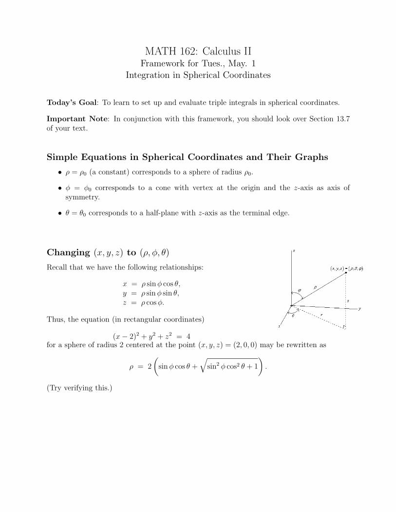
MATH 162: Calculus IIFramework for Tues., May. 1

Integration in Spherical Coordinates

Today’s Goal: To learn to set up and evaluate triple integrals in spherical coordinates.

Important Note: In conjunction with this framework, you should look over Section 13.7of your text.

Simple Equations in Spherical Coordinates and Their Graphs

• ρ = ρ0 (a constant) corresponds to a sphere of radius ρ0.

• φ = φ0 corresponds to a cone with vertex at the origin and the z-axis as axis ofsymmetry.

• θ = θ0 corresponds to a half-plane with z-axis as the terminal edge.

Changing (x, y, z) to (ρ, φ, θ)

Recall that we have the following relationships:

x = ρ sin φ cos θ,y = ρ sin φ sin θ,z = ρ cos φ.

Thus, the equation (in rectangular coordinates)

(x− 2)2 + y2 + z2 = 4for a sphere of radius 2 centered at the point (x, y, z) = (2, 0, 0) may be rewritten as

ρ = 2

(sin φ cos θ +

√sin2 φ cos2 θ + 1

).

(Try verifying this.)

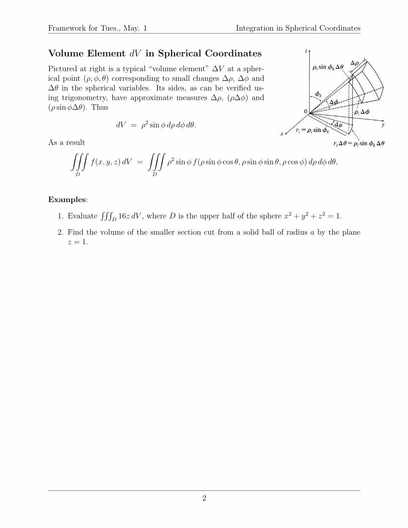
Framework for Tues., May. 1 Integration in Spherical Coordinates

Volume Element dV in Spherical Coordinates

Pictured at right is a typical “volume element” ∆V at a spher-ical point (ρ, φ, θ) corresponding to small changes ∆ρ, ∆φ and∆θ in the spherical variables. Its sides, as can be verified us-ing trigonometry, have approximate measures ∆ρ, (ρ∆φ) and(ρ sin φ∆θ). Thus

dV = ρ2 sin φ dρ dφ dθ.

As a result∫∫∫D

f(x, y, z) dV =

∫∫∫D

ρ2 sin φ f(ρ sin φ cos θ, ρ sin φ sin θ, ρ cos φ) dρ dφ dθ,

Examples:

1. Evaluate∫∫∫

D16z dV , where D is the upper half of the sphere x2 + y2 + z2 = 1.

2. Find the volume of the smaller section cut from a solid ball of radius a by the planez = 1.

2