di⁄erentiated durable goods monopolypersonal.lse.ac.uk/schirald/multicoase oa1.pdf ·...
TRANSCRIPT

.
Differentiated Durable Goods MonopolyOnline Appendix
Francesco Nava† and Pasquale Schiraldi†
October 2018
Abstract: The sections of the online appendix discuss: related product design exercises; thedetails of the example reported in Section 4 of the main text; proofs omitted from the main
text; and proofs of results included in the appendix. Results on product design establish why
horizontal product differentiation is profit-maximizing for the monopolist, and why niche
products can be optimal when multiple varieties are for sale.
†Economics Department, London School of Economics, [email protected].†Economics Department, London School of Economics, [email protected].
1 Product Design Results
This section considers the product design problem faced by a durable goods monopolist. The
monopolist assembles products from a basket of characteristics. For instance, a smartphone
producer may decide which features to include in a new line of devices (such as screen
resolution, battery size, memory, and camera), or an automobile manufacturer may choose
how to blend performance, practicality, size, and fuel effi ciency. The way these characteristics
are assembled might generate dependence and dispersion in consumers’valuations for the
varieties. Therefore, we ask how different product designs affect the profit of the monopolist.
For instance, would the monopolist prefer vertically differentiated products or horizontally
differentiated ones? Should the monopolist produce mass products with low volatility in
valuations, or niche products with high dispersion in valuations? To tackle these questions,
we study how optimal market-clearing profits are affected by the distribution of buyers’
valuations. This approach relies implicitly on Proposition 3 and is legitimate for markets in
which the monopolist can frequently revise prices. We refrain from presenting an explicit
model in which products are constructed by bundling characteristics, for the sake of brevity.
The first result fixes the marginal distribution of buyers’valuations for each variety and
asks what correlation structure between varieties maximizes the profit of the monopolist.
This approach is valid whenever production costs depend only on the marginal distribution
of valuations and not on their correlation structure. Results exploit classical contributions on
copulas (Sklar 1959) to establish that the profit-maximizing design requires full horizontal
product differentiation. Horizontal differentiation increases profits, as a strong preference
for one variety tends to be associated with a low desire for the other. This favors market
segmentation and increases profits by minimizing the value of units that are never purchased.
One may conjecture that vertical product differentiation may then be the profit-minimizing
design. However, we establish that this is not the case in general, as independent products oc-
casionally generate smaller profits than vertically differentiated ones. The other substantive
contribution analyzes how volatility in valuations affects the seller’s profits. In particular, it
asks whether the monopolist prefers a distribution of values or its mean. In a single-variety
setting, the answer is trivial, as the monopolist always dislikes variance (in one case the
product is sold at the minimum value, while in the other at the average value). However
in multi-variety settings, two opposing forces are at play. Variance increases both the infor-
mation rents of buyers, thereby hurting the monopolist, and the value of the durable good
(that is, the value of the preferred variety), thereby benefitting the monopolist. The analysis
establishes that either of the two forces can dominate, and it provides suffi cient conditions for
both scenarios. This shows why low-volatility mass products need not be an optimal design
when multiple varieties can be sold.
2

Classical Results on Copulas: Recall that Fi denotes the marginal cumulative distributionof the consumers’valuations for variety i. For the rest of the analysis, let Fi be continuous,
and let its support be the compact set Vi = [0, vi] ⊆ [0, 1].1 Before proceeding to the design
problem, we briefly review the notion of copula and some of its properties. For a more
detailed discussion of these topics, we refer to Nelsen 2006.
A function C : [0, 1]2 → [0, 1] is said to be a copula if
(1) C(k, 0) = C(0, k) = 0 for every k ∈ [0, 1];
(2) C(k, 1) = C(1, k) = k for every k ∈ [0, 1];
(3) C(x) + C(y)− C(xa, yb)− C(ya, xb) ≥ 0 for every x, y ∈ [0, 1]2 such that x ≥ y.
Let C denote the set of all copulas. Sklar’s Theorem implies that for any joint distribution
function F with continuous marginal distributions Fi for i ∈ a, b, there exists a uniquecopula C such that
F (v) = C(Fa(va), Fb(vb)) for all v ∈ Va × Vb.
A copula C can therefore be thought of as a suffi cient statistic of the dependence structure
between the two random variables. A commonly used copula exhibits no dependence between
the random variables and is associated with the joint distribution I(v) = Fa(va)Fb(vb). Two
other noteworthy copulas are known as the Frechét-Hoeffding (FH) bounds and are associated
with the two joint distributions
K(v) = minFa(va), Fb(vb);L(v) = maxFa(va) + Fb(vb)− 1, 0.
Figure 8 depicts the support of these three copulas when marginals are uniform on [0, 1]. In
a classical contribution, Frechét and Hoeffding establish that the two FH copulas bound any
other feasible copula C.
Proposition 3 Any joint distribution F consistent with the two marginals, Fa and Fb, sat-
isfies
L(v) ≤ F (v) ≤ K(v) for all v ∈ Va × Vb.
Random variables va and vb are said to be concordant if (vi − v′i)(vj − v′j) > 0 for any two
profiles v and v′ in the support of the joint distribution. The random variables are instead
1We restrict attention to the environments in which the lowest values equal 0 to make results directlycomparable to the one-variety no-gaps case where the Coase conjecture leads to 0 profits in the limit. Thecompact support assumption and the continuity assumption are convenient, but not essential.
3

said to be discordant if (vi − v′i)(vj − v′j) < 0 for any two profiles v and v′ in the support.
The FH bounds L and K characterize instances of extreme concordance and discordance,
respectively, and they are thus associated with a Kendall’s Tau of 1 and −1, respectively.2
Informally, the FH upper bound identifies the most concordant copula, as large values of one
random variable are associated with large values of the other, and small values of one with
small values of the other. Conversely, the FH lower bound identifies the most discordant
copula as large values of one random variable are associated with small values of the other,
and vice versa. For instance, if the marginal distributions are either uniform or Gaussian,
the FH bounds induce either perfect positive or perfect negative correlation between the two
random variables.
Independent FH Upper Bound FH Lower Bound
Figure 8: Three copulas for uniform marginals Fa(x) = Fb(x) = x.
The next result highlights a few well-known properties of the FH bounds that play an
important role in our product design analysis. A subset V of R2 is non-decreasing if for any
v, v′ ∈ V , va < v′a implies vb ≤ v′b. Similarly, a subset V of R2 is non-increasing if for any
v, v′ ∈ V , va < v′a implies vb ≥ v′b.
Proposition 4 The joint distribution F is equal to its:
(1) FH upper bound K if and only if its support V is a non-decreasing subset of Va × Vb;(2) FH lower bound L if and only if its support V is a non-increasing subset of Va × Vb.Moreover, random variable va is almost surely a strictly monotonic function of vb if and only
if the copula coincides with one of the FH bounds.
The result implies that it is possible to construct monotone correspondences va = k(vb)
and va = l(vb) that completely pin down the support of the FH bounds. The additional
assumptions imposed on the marginal distributions further imply that these correspondences
are functions such that k′(x) ∈ (0,∞) and l′(x) ∈ (−∞, 0) almost surely.2For any two profiles v and v′ in the support of the joint distribution, Kendall’s Tau amounts to
τ(F ) = Pr((vi − v′i)(vj − v′j) > 0
)− Pr
((vi − v′i)(vj − v′j) < 0
).
4

Product Design Results: Our product design exercises begin by analyzing how dependence(or association) between the random variables va and vb affects the optimal market-clearing
profits. By the analysis carried out in Section 4, our conclusions also identify how dependence
affects the limiting stationary equilibrium profits of the dynamic pricing game. The first
result fixes the marginal distributions Fi (postulating that any costs incurred in generating
value depends only such marginals) and asks which joint distribution compatible with such
marginals maximizes optimal market-clearing profits. Formally, let V F denote the support
of a joint distribution F , and let πF denote the optimal market-clearing profits associated
with the joint distribution F . Specifically, we solve the following problem:
maxC∈C πF s.t. F = C(Fa, Fb).
The next result establishes that optimal market-clearing profits are maximized at the FH
lower bound. Thus, the seller always benefits from selling varieties that are most discordant.
Intuitively, selling discordant varieties maximizes profits as segmenting the market guarantees
that no value is wasted on varieties that are never purchased.
Proposition 5 For any joint distribution F consistent with the two marginals, Fa and Fb,
πF ≤ πL.
The result implies that independent varieties are suboptimal since horizontal product differ-
entiation allows for more effective market segmentation. As the monopolist loses its ability
to intertemporally discriminate buyers (when the time between offers vanishes), statically
screening consumers by selling different varieties is the only option available to extract any
surplus. But such a task is most profitable when the market is segmented and values are
discordant.
The other product design contribution looks at how variance in valuations affects the
profitability of the monopolist. When a single product is for sale, the monopolist always
prefers to minimize variance, as the durable good necessarily trades at the lowest valuation
in the support. However, when multiple varieties can be sold, a trade-off emerges, since
variance increases both buyers’ information rents (which hurts profits) and total surplus
(which benefits profits) as the maximal value grows. Thus, we ask whether the monopolist
prefers a distribution F to the distribution F in which all buyers value products at the
mean of F (that is, F is a degenerate distribution with unit measure at EF (v)). The result
establishes that the answer to this question depends on the details of the measure F when
multiple varieties are for sale.
5
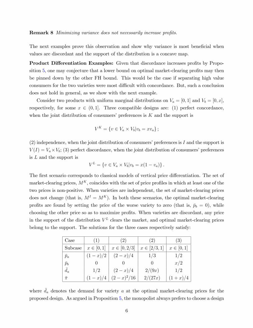
Remark 8 Minimizing variance does not necessarily increase profits.
The next examples prove this observation and show why variance is most beneficial when
values are discordant and the support of the distribution is a concave map.
Product Differentiation Examples: Given that discordance increases profits by Propo-sition 5, one may conjecture that a lower bound on optimal market-clearing profits may then
be pinned down by the other FH bound. This would be the case if separating high value
consumers for the two varieties were most diffi cult with concordance. But, such a conclusion
does not hold in general, as we show with the next example.
Consider two products with uniform marginal distributions on Va = [0, 1] and Vb = [0, x],
respectively, for some x ∈ (0, 1]. Three compatible designs are: (1) perfect concordance,
when the joint distribution of consumers’preferences is K and the support is
V K = v ∈ Va × Vb|vb = xva ;
(2) independence, when the joint distribution of consumers’preferences is I and the support is
V (I) = Va×Vb; (3) perfect discordance, when the joint distribution of consumers’preferencesis L and the support is
V L = v ∈ Va × Vb|vb = x(1− va) .
The first scenario corresponds to classical models of vertical price differentiation. The set of
market-clearing prices,MK , coincides with the set of price profiles in which at least one of the
two prices is non-positive. When varieties are independent, the set of market-clearing prices
does not change (that is, M I = MK). In both these scenarios, the optimal market-clearing
profits are found by setting the price of the worse variety to zero (that is, pb = 0), while
choosing the other price so as to maximize profits. When varieties are discordant, any price
in the support of the distribution V L clears the market, and optimal market-clearing prices
belong to the support. The solutions for the three cases respectively satisfy:
Case (1) (2) (2) (3)
Subcase x ∈ [0, 1] x ∈ [0, 2/3] x ∈ [2/3, 1] x ∈ [0, 1]
pa (1− x)/2 (2− x)/4 1/3 1/2
pb 0 0 0 x/2
da 1/2 (2− x)/4 2/(9x) 1/2
π (1− x)/4 (2− x)2/16 2/(27x) (1 + x)/4
where da denotes the demand for variety a at the optimal market-clearing prices for the
proposed design. As argued in Proposition 5, the monopolist always prefers to choose a design
6
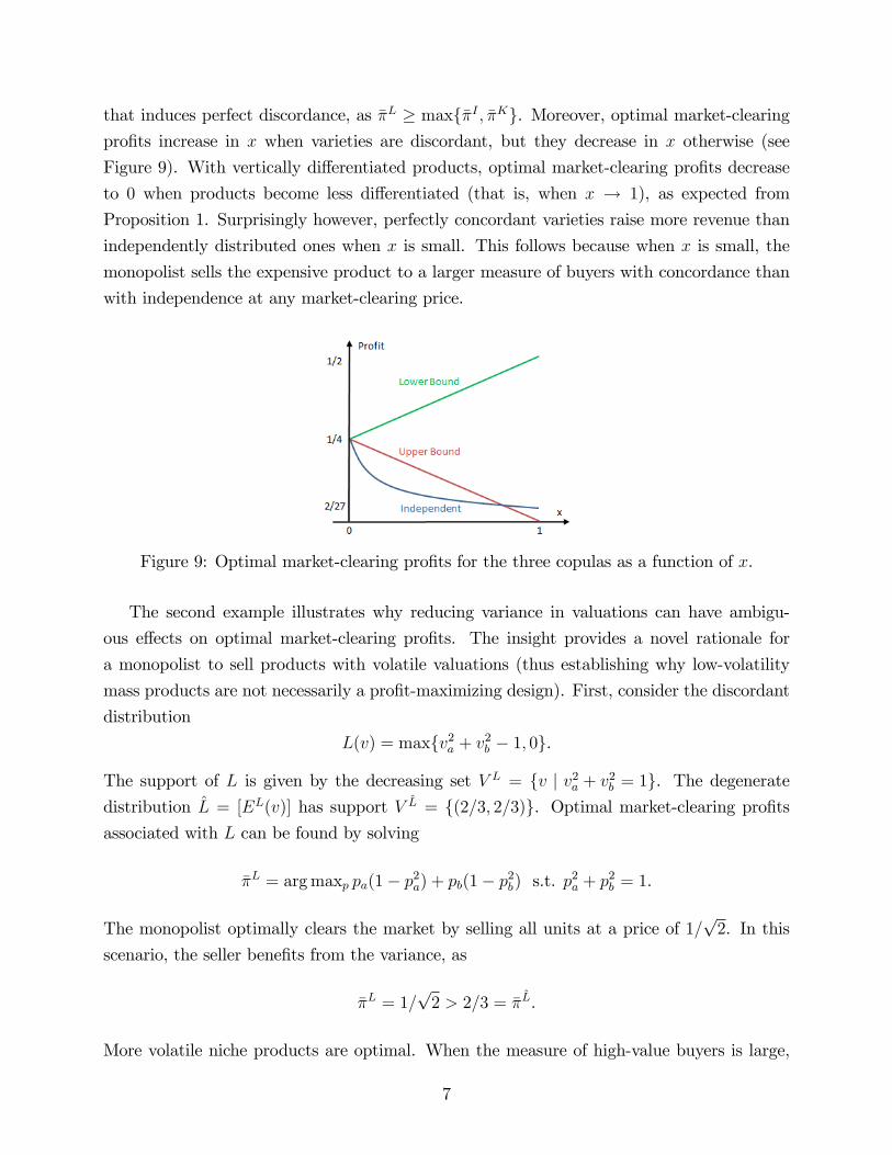
that induces perfect discordance, as πL ≥ maxπI , πK. Moreover, optimal market-clearingprofits increase in x when varieties are discordant, but they decrease in x otherwise (see
Figure 9). With vertically differentiated products, optimal market-clearing profits decrease
to 0 when products become less differentiated (that is, when x → 1), as expected from
Proposition 1. Surprisingly however, perfectly concordant varieties raise more revenue than
independently distributed ones when x is small. This follows because when x is small, the
monopolist sells the expensive product to a larger measure of buyers with concordance than
with independence at any market-clearing price.
Figure 9: Optimal market-clearing profits for the three copulas as a function of x.
The second example illustrates why reducing variance in valuations can have ambigu-
ous effects on optimal market-clearing profits. The insight provides a novel rationale for
a monopolist to sell products with volatile valuations (thus establishing why low-volatility
mass products are not necessarily a profit-maximizing design). First, consider the discordant
distribution
L(v) = maxv2a + v2
b − 1, 0.
The support of L is given by the decreasing set V L = v | v2a + v2
b = 1. The degeneratedistribution L = [EL(v)] has support V L = (2/3, 2/3). Optimal market-clearing profitsassociated with L can be found by solving
πL = arg maxp pa(1− p2a) + pb(1− p2
b) s.t. p2a + p2
b = 1.
The monopolist optimally clears the market by selling all units at a price of 1/√
2. In this
scenario, the seller benefits from the variance, as
πL = 1/√
2 > 2/3 = πL.
More volatile niche products are optimal. When the measure of high-value buyers is large,
7
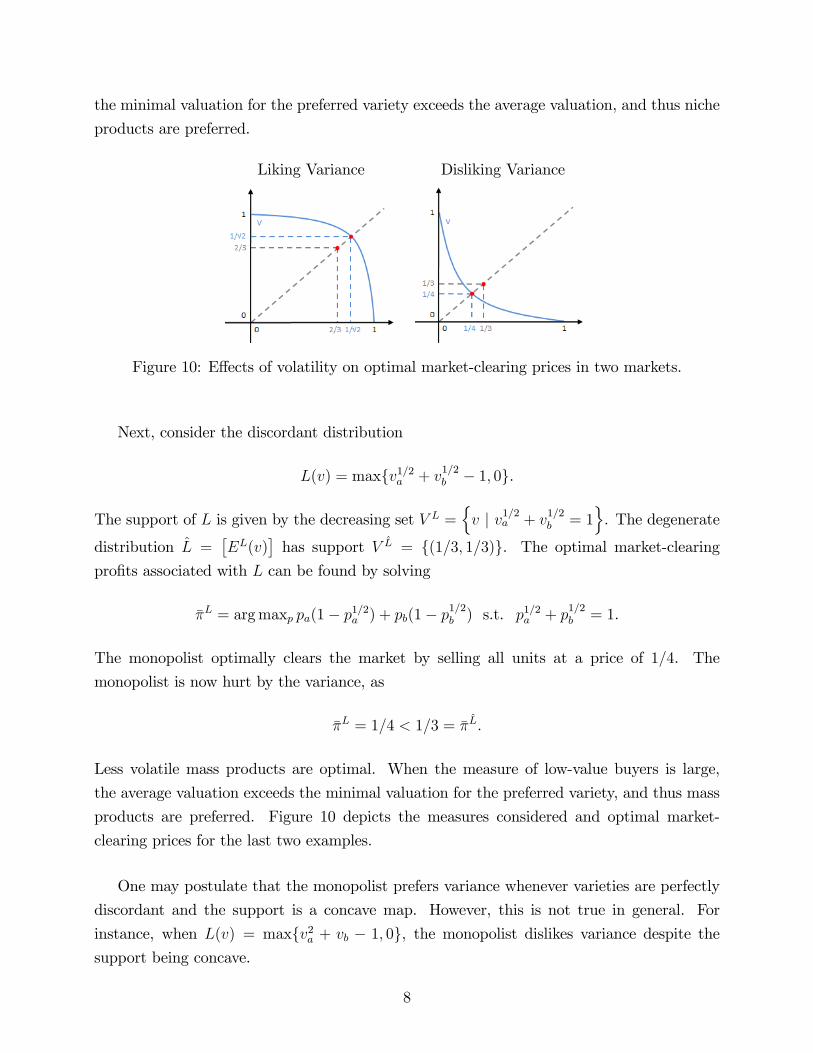
the minimal valuation for the preferred variety exceeds the average valuation, and thus niche
products are preferred.
Liking Variance Disliking Variance
Figure 10: Effects of volatility on optimal market-clearing prices in two markets.
Next, consider the discordant distribution
L(v) = maxv1/2a + v
1/2b − 1, 0.
The support of L is given by the decreasing set V L =v | v1/2
a + v1/2b = 1
. The degenerate
distribution L =[EL(v)
]has support V L = (1/3, 1/3). The optimal market-clearing
profits associated with L can be found by solving
πL = arg maxp pa(1− p1/2a ) + pb(1− p1/2
b ) s.t. p1/2a + p
1/2b = 1.
The monopolist optimally clears the market by selling all units at a price of 1/4. The
monopolist is now hurt by the variance, as
πL = 1/4 < 1/3 = πL.
Less volatile mass products are optimal. When the measure of low-value buyers is large,
the average valuation exceeds the minimal valuation for the preferred variety, and thus mass
products are preferred. Figure 10 depicts the measures considered and optimal market-
clearing prices for the last two examples.
One may postulate that the monopolist prefers variance whenever varieties are perfectly
discordant and the support is a concave map. However, this is not true in general. For
instance, when L(v) = maxv2a + vb − 1, 0, the monopolist dislikes variance despite the
support being concave.
8

2 Mixing Example
Consider a market in which δ = 3/4, and in which the support of valuations is
V = (1, 1) ∪v ∈ [0, 1]2 | vj = (1− vi)/3 for any vi ∈ [1/4, 1] & any i ∈ a, b
.
The dark blue region in Figure 11 depicts this support. As regularity is mainly needed for
existence, we consider an atomic example failing regularity for the sake of tractability. Of
course, similar conclusions would hold for regular markets in which the support is the convex
hull of V (the light blue shaded region in Figure 11) and in which almost all of the measure
is near V .
Figure 11: The support of the measure considered in the example and its convex hull.
Consider the following joint distribution on support V :
F (v) =
1 if v = (1, 1)
(6vj + 6vi − 3)/10 if vi ≥ 1/4 & vj ∈ [1/4, 1)
(18vj + 6vi − 6)/10 if vi ≥ 1/4 & vj ∈ [1− 3vi, 1/4]
0 if otherwise
.
Intuitively, such a distribution puts 1/10 of its measure on the atom at (1, 1), while 9/10 of
the measure is uniformly distributed on the rest of V . If so, the marginal distribution for
each variety amounts to
Fi(vi) =
9vi/5 if vi ∈ [0, 1/4)
(6vi + 3)/10 if vi ∈ [1/4, 1)
1 if vi = 1
.
For convenience, define the following function which identifies the larger component of the
support V :
g(x) = max1/3− x/3, 1− 3x for x ∈ [0, 1] .
9

Optimal Pricing: First consider the benchmark setting in which the monopolist can commitex-ante to a constant price profile. If so, for any p /∈M such that pi ≥ pj, the seller’s profits
would simply amount to
Π(p) = pi(9/10− Fi(pi)) + pj(1− Fj(pj)),
and the associated optimal commitment prices and profits would be equal to
p∗a = p∗b = 13/24 & Π∗ = 169/480 = 0.352.
Optimal Clearing: Then consider the alternative benchmark in which the monopolist mustset a price profile that clears the market instantaneously. Clearly, the seller would never set
prices in the interior of the market-clearing price set. Thus, if it sold variety i at price
pi ≥ 1/4, it would sell variety j at price pj = g(pi), and for any such a price profile p, profits
would amount to
Π(pi, g(pi)) = pi(9/10− Fi(pi)) + g(pi)(1/10 + Fi(pi)).
The associated optimal market-clearing prices and profits would then be equal to
pi = 5/12, pj = 7/36 & Π0 = 49/180 = 0.272.
Constructing Mixed Strategy Equilibria: We look for equilibria in which the marketclears in two periods, both varieties are sold at a common price in the first period, and
the seller randomizes with equal probability between two symmetric market-clearing price
profiles in the second period. Throughout the example, we denote by i the variety that is
sold at a higher price in the final period and by j the other variety.
We begin by constructing the equilibrium path of this symmetric mixed strategy equilib-
rium. To nest all cases, consider subgames in which a fraction 1− α of the measure at (1, 1)
has already purchased in the first period. Consider the equilibrium path active buyer set
A =[V ∩ [0, x]2
]∪ (1, 1)
for some x ∈ [1/4, 1). In subgame A, the payoff to the monopolist at any market-clearing
price p0 ∈M\M amounts to
Π(p0|A) = p0i (Fi(x)− Fi(p0
i )) + g(p0i )(α/10 + Fi(p
0i )− Fi(g(x))).
10
The subgame possesses two optimal market-clearing prices, which amount to
p0(x) = (p0i (x), p0
j(x)) = ((9− α + 12x) /48, (39 + α− 12x) /144) for i ∈ a, b .
We look for fixed points of the game in which: (1) the seller sells both varieties at a
common price p in the initial period; (2) the atom at (1, 1) purchases in the initial period;
and (3) the boundary of the active player set is determined by buyers who are indifferent
between buying the same variety today and tomorrow. Fixed point conditions in general
require that the boundary of the active player set be pinned down by the incentive constraint
maxva, vb − p = δmax
maxva, vb −
p0a(x) + p0
b(x)
2,va + vb
2−minp0
a(x), p0b(x)
.
As the boundary of the active player set x is determined by buyers who are indifferent between
buying a variety today and tomorrow,
x− p = δ(x−
(p0a(x) + p0
b(x))/2)⇒ x(p) = (64p− 11) /20.
From this, the subgame prices can be pinned down as a function of the initial price quoted
by the seller:
p0(p) = p0(x(p)) = ((16p+ 1) /20, (19− 16p) /60) .
For the atom to be willing to purchase in the initial period, it must be that 1 − p ≥δ(1− p0
j(p)), which in turn requires that p < 13/32. Finally, to have such a fixed point,
the marginal buyer must satisfy
x(p)−(p0i (p) + p0
j(p))/2 ≥ (x(p) + g(x(p))) /2− p0
j(p),
which holds for p ≥ 1/4. Therefore, such a fixed point can exist and be consistent with
equilibrium behavior provided that p < 13/32.
The previous conjectures on the structure of the equilibrium imply that the objective
function of the monopolist at the initial stage when setting the same price p for the two
varieties simply amounts to
Π(p, p) = p(19/10− 2Fi(x(p))) + δΠ(p0(p)|x(p)).
Maximizing this objective function with respect to the initial price p identifies the optimal
opening as p1 = 311/864. Since p1 < 13/32, the monopolist’s behavior in the initial stage is
consistent with buyers with value (1, 1) purchasing in the first period. At such a price, the
11

present value of profits amounts to
Π1 = 2521/8640 = 0.29178.
This profit exceeds the optimal market-clearing profit. Thus, the seller does not benefit from
clearing the market in the opening round. In the conjectured equilibrium, the monopolist
initially sells both varieties at price p1 = 311/864, then randomizes with equal probability
between two market-clearing profiles (5/12, 7/36) , (7/36, 5/12) in period 2.
Asymmetric Deviations and Consistent Beliefs: Next we construct strategies and
beliefs for asymmetric subgames in which the market is expected to clear in 2 periods. As
before, to nest all cases, let α denote the fraction of the measure at (1, 1) purchasing in the
second period. Consider asymmetric subgames in which the active buyer set satisfies
A = [V ∩ [0, xa]× [0, xb]] ∪ (1, 1),
for some vector x /∈M .3 Without loss of generality, further suppose that xi ≥ xj. In subgame
A, the payoff to the monopolist at a market-clearing price p0 ∈M\M amounts to
Π(p0|A) = p0i (Fi(xi)− Fi(p0
i )) + g(p0i )(α/10 + Fi(p
0i )− Fi(g(xj))).
In such a subgame, the optimal market-clearing prices satisfy
p0(x) = (p0i (x), p0
j(x)) =
(
9−α+18xi−6xj48
,39+α−18xi+6xj
144
)if xj ≥ 1
4(8−α+2xi−18xj
16,
3α−8−6xi+54xj16
)if xj ≤ 1
4& xi + 7xj ≥ 2 + α
18
(1− 3xj, xj) if xj ≤ 14& xi + 7xj ≤ 2 + α
18
.
Moreover, such prices are unique whenever xi > xj.
We look for fixed points of the game in which: (1) in the initial period, the seller posts
a price profile p such that pi ≥ pj; (2) the seller does not randomize in the final stage; (3)
the atom at (1, 1) purchases in the initial period; and (4) the boundary of the active player
set is determined by buyers who are indifferent between buying the same variety today and
tomorrow.
Restriction (4) requires that the boundary of the active player set be pinned down by the
two incentive constraints
xa − pa = δ(xa − p0
a(x))and xb − pb = δ
(xb − p0
b(x)),
3If x ∈M , then A must have measure zero. Thus, we neglect this scenario.
12

and it further requires that
xa − p0a(x) ≥ g(xa)− p0
b(x) and xb − p0b(x) ≥ g(xb)− p0
a(x).
As before, these conditions identify marginal buyers given the current prices, x(p), and
therefore they identify subgame prices as a function of current prices:
p0(p) = p0(x(p)) = ((5 + 24pi − 8pj) /36, (31 + 8pj − 24pi) /108) .
As restrictions (3) and (1) require that the atom purchase in the first period and that pi ≥ pj,
equilibrium further implies that 1− pj ≥ δ (1−minp0a(p), p
0b(p)).
Given the conjectures made about the fixed point, we look for equilibria in which pi ≥ pi
and xi(p) ≥ xj(p). The objective function of the monopolist at the initial stage when setting
prices for the two varieties amounts to
Π(p) = pi(9/10− Fi(xi(p))) + pj((10− a)/10− Fj(xj(p))) + δΠ(p0(p)|A(p)).
Solving this problem, we find that the opening prices set by the seller satisfy
p1 = (p1i , p
1j) = (171/416, 125/416) = (0.41106, 0.30048),
and consequently that marginal buyers satisfy
x(p1) =(xi(p
1), xj(p1))
= (63/104, 57/104) = (0.60577, 0.54808) .
The monopolist’s behavior in the initial stage is consistent with buyers with value (1, 1)
purchasing in the initial period, as
1− p1j = 291/416 > 51/104 = δ(1− p0
j).
Moreover, marginal buyers are not tempted by the other variety as
xi − p0i (x) = 27/104 ≥ −9/104 = g(xi)− p0
j(x),
xj − p0j(x) = 103/312 ≥ −61/312 = g(xj)− p0
i (x).
Thus, all fixed point conditions hold at such prices, and profits amounts to
Π1 = 479/1664 = 0.28786.
13

Profits exceed the optimal market-clearing profits, but they are smaller than the profits
attainable when clearing the market symmetrically by randomizing in the final period.
Many Periods: If the seller were allowed a third period to clear the market, the mostprofitable strategy consistent with clearing the market in exactly three periods would re-
quire: selling both varieties at a common price in the first period, p2 = (0.38033, 0.38033);
randomizing with equal probability between two price profiles in second period,
p1 ∈ (0.32663, 0.25041) , (0.25041, 0.32663) ;
setting one of two market-clearing price profiles in the third period contingent on the outcome
of the randomization in the previous period:
p0 =
(0.30097, 0.23300) if p1 = (0.32663, 0.25041)
(0.23300, 0.30097) if p1 = (0.25041, 0.32663).
Mixing would take place in the second period, as the seller always prefers to clear the market
asymmetrically once the atom has purchased,4 and because the atom necessarily purchases in
the first period in this example. Alternative strategies in which a measure of buyers purchases
goods in any one of the three periods are necessarily less profitable.
When following such a strategy, the present value of profits would amount to
Π2 = 0.29057
and would be smaller than the profits the seller was making by clearing the market symmet-
rically in two periods. Intuitively, in this example, discounting losses would dominate price
discrimination gains because buyers are suffi ciently patient. If the seller had more than three
periods in which to sell the product, a similar logic would hold, and profits would further
decline under any strategy in which a positive measure of buyers purchases products in more
than three periods.
MPE Beliefs: In any stationary equilibrium after any price history, the market clears in
at most two periods. In the notation of the proof of Proposition 2, X t = ∅ for any t > 2.
The seller never benefits by clearing the market in more than two periods if buyers’beliefs
are consistent and δ = 3/4. Moreover, given these beliefs, clearing the market in more than
two periods would be even less profitable since buyers would be more inclined to wait for a
discount if the market was expected to clear sooner.
4In any subgame in which the atom has purchased, the measure of active buyers is discordant, and clearingthe market asymmetrically maximizes the seller’s profit.
14

In the desired equilibrium, the seller stochastically clears the market in two periods. In
such an equilibrium, whenever pa = pb = p and p ∈ X1, buyers believe that the prices in the
following period will coincide with the prices they would expect if the market had to clear
symmetrically in exactly two periods. Thus, buyers expect one of the following two profiles
with equal probability:
p0(p) = (p0i (p), p
0j(p)) = ((16p+ 1) /20, (19− 16p) /60) .
Whenever pi > pj and p ∈ X1, buyers believe that the prices in the following period will
coincide with the prices they would expect if the market had to clear asymmetrically in
exactly two periods:
p0(p) = (p0i (p), p
0j(p)) = ((5 + 24pi − 8pj) /36, (31 + 8pj − 24pi) /108) .
For brevity’s sake, we omit the derivation of beliefs associated with prices in X2, while beliefs
associated with prices in X0 are trivial. By construction, these beliefs are consistent with
the seller’s strategy, and the seller’s strategy maximizes profits given these beliefs.
3 Omitted Proofs
Proof Remark 1. (1) Consider the price pg = (vg, vg). Such a price belongs to M , as for
all v ∈ V ,maxi∈a,bvi − pgi ≥ maxi∈a,b vi − vg ≥ 0.
By setting price pg, the monopolist obviously achieves a profit of vg. Thus, when va < vb,
optimal market-clearing profits weakly exceed vb and strictly exceed va.
(2) If varieties are unranked, further consider the market-clearing price profile pε = (vb +
ε, vb) for some small number ε > 0. By definition of static demand, limε→0 di(pε) ≥ F(vi > vj)
for any i ∈ a, b. As products are unranked, F(vi > vj) > 0. But if so, optimal market-
clearing profits must strictly exceed vb since da(pε) > 0 for ε suffi ciently small.
(3) If va = vb = v, again consider the market-clearing price profile pε = (v+ ε, v). Again,
it must be that limε→0 di(pε) ≥ F(vi > vj) for any i ∈ a, b. If at pε some consumers were to
purchase variety a, optimal market-clearing profits would strictly exceed v. If instead optimal
market-clearing profits were equal to v for any ε > 0, then limε→0 da(pε) = F(va > vb) = 0,
and thus va ≤ vb for any v ∈ V . A symmetric argument would then establish that vb ≤ va
for any v ∈ V . So, optimal market-clearing profits could be equal to v only if va = vb for any
v ∈ V . Similarly, if varieties were identical, any market-clearing price would set one of the
15

two prices no higher than v, as (v, v) ∈ V .(4) But if so, optimal market-clearing profits would amount v, as all players would pur-
chase the cheapest variety. Thus, profits equal 0 if and only if varieties are identical and
v = 0.
(5) If va = vb = v and (v, v) ∈ V , then vg = v. If varieties are not identical, it must be
that F(vi > vj) > 0 for some i ∈ a, b. If so, the price profile (pi, pj) = (v+ε, v) ∈M would
raise more profits than vg for ε suffi ciently small.
Proof Remark 2. To prove the first part note that by the proof of Remark 1 part (5),
the optimal market-clearing price must equal (pi, pj) = (v + ε, v) for some ε > 0 and some
i ∈ a, b. Since V is connected, v ∈ V , and (v, v) ∈ V , for any κ ∈ (0, ε) there exists a
vκ ∈ V such that
vκi − vκj = κ.
Thus, the price cannot be effi cient if ε > 0, as any buyer vκ purchases variety j despite
preferring variety i.
To prove the second part, suppose va ≤ vb. When varieties are unranked and V is
connected, effi ciency of a price (pa, pb) ∈ M requires pa = pb. Hence, the most profitable
effi cient market-clearing price must satisfy pa = pb = vb, because V is a Cartesian product.
But, such a price cannot be optimal by the proof of Remark 1 part (2).
Proof Remark 3. Assume v+a ≥ ca. Consider setting price pε = (ca, cb + ε) for some ε > 0.
Such a price belongs to M , as for all v ∈ V +,
maxi∈a,bvi − pi ≥ va − pa = va − ca ≥ 0.
When varieties are unranked, F(va − ca > vb − cb) > 0. But if so,
limε→0 db(pε) = F(va − ca > vb − cb) > 0.
Hence, optimal market-clearing profits are strictly positive for ε suffi ciently small.
Proof Remark 4. The proof is essentially identical to that of Lemma 2 in the main text.
Let M+ denote the “interior” of the market-clearing price set M+. We show that, in any
PBE, all consumers accept any price in M+ at any information set. Suppose this were not
the case. Select any equilibrium, and let P denote the set of prices that are accepted by all
buyers in any possible subgame. By contradiction, suppose that M+ is not contained in P .
As before, p ∈ P whenever mini∈a,b pi < −1. To show the latter, observe that Lemma 1 is
unaffected by costs, and that its proof, as before, implies that buyers’value functions at any
buyer-history h ∈ H are non-decreasing in v and have a modulus of continuity of less than
16

1, since for v′ ≥ v,
U(h, v′)− U(h, v) ≤ maxi∈a,b v′i − vi .
Thus, in any PBE we have that U(h, v) ≤ 1 for all v ∈ V , and that all buyers strictly preferto purchase a variety when mini∈a,b pi < −1, as
maxi∈a,b vi − pi > 1 > δU(h, v) for all h ∈ H. (1)
If so, for any ε > 0 there is a price p ∈ M+\P 6= ∅ such that
pi ≤ pi − ε & pj ≤ pj for some i implies p ∈ P . (2)
To find such a price p, let pa = infq∈M+\P qa, and for some η ∈ (0, ε) let
pb = infq∈M+\P qb s.t. qa ≤ pa + η,
where mini∈a,b pi ≥ −1 by (1). Then set p to be any price in M+\P such that p ≤ p+(η, η).
Such a price exists by definition of p for any suffi ciently small η. Moreover, (2) holds because:
(a) p ∈ P whenever pa ≤ pa− ε < pa by definition of pa; and (b) p ∈ P for any pa ≤ pa when
pb ≤ pb − ε by definition of pb.But, when ε is suffi ciently small,
maxi∈a,b vi − pi > δmaxi∈a,b vi − pi + ε ⇔ ε <1− δδ
maxi∈a,b vi − pi .
If so, all consumers would accept p at any buyer-history (p, h) ∈ H. If a type was to rejectan offer, they could agree no sooner than tomorrow, and the most they could expect any one
price to drop is ε as any further drop would lead to acceptance by all buyers. Thus, for all
v ∈ V , the continuation value satisfies
maxi∈a,b vi − pi + ε ≥ U((p, h), v).
But this in turn implies that
maxi∈a,b vi − pi > δU((p, h), v) for any h ∈ H.
As p /∈ P , the latter contradicts the definition of P and consequently establishes the result.
Since every consumer buys when prices belong to M+, the seller can secure a payoffarbitrarily
close to the optimal market-clearing profits π(A) > 0 (where A = A(h) denotes the active
player set associated with history h) by choosing a price in M+.
17

The proof of the second part of the remark essentially coincides with the proof of Propo-
sition 3 and is omitted for sake of brevity.
Proof Remark 5. First, we introduce some notation. In this setting, all buyers are active
in every period. However, the measure of values evolves over time. For any profile of values
v ∈ V , denote the residual value of an owner of variety i by
vi = (vii, vij) = (0, vj − vi).
LetRi(ht) ∈ P∗([0, 1]2) denote the measure of residual values of consumers purchasing variety
i ∈ a, b at any history ht ∈ H. Then, define the measure of values at history ht as
F(E|ht) = F(E|ht−1) +∑
i∈a,b[Ri(E|ht)−Di(E|ht)
]for any E ∈ Ω([0, 1]2).
Let V (ht) be the support of F(ht). Define the set of buyers for whom gains from trade are
positive at history ht as
A∗(ht) = v ∈ V (ht) | maxi∈a,bvi − ci > 0.
Refer to buyers in A∗(ht) as essentially active. The proof then follows along the same steps of
Remark 3. We show that in any PBE, at any history h ∈ H, the set A∗(p, h) must be empty
if p ∈ M∗, where M∗ denotes the “interior”of the market-clearing price set M∗. Suppose
this were not the case. Select any equilibrium, and let P denote those prices p such that
A∗(p, h) = ∅ after any history h. By contradiction, suppose that M∗ is not contained in P .
First, we show that p ∈ P whenever p ∈ M∗ and mini∈a,b pi < −1. As before, buyers’
value functions are non-decreasing in v and have a modulus of continuity of less than 1 at any
buyer-history h ∈ H, since an argument equivalent to Lemma 1 implies that for all v′ ≥ v,
U(h, v′)− U(h, v) ≤ maxi∈a,b v′i − vi .
Thus, in any PBE we have that U(h, v) ≤ 1 for all v ∈ V . But then, all buyers must purchasea variety when mini∈a,b pi < −1, as
maxi∈a,b
vi − pi + δU(h, vi)
> 1 > δU(h, v) for all h = (p, h) ∈ H, (3)
where U(h, vi) ≥ 0 denotes the continuation value of buyer v once the value transitions to
vi. But if so, as p ∈ M∗, for every player purchasing i we have that cj ≥ vj − vi = vij, and
similarly for every player purchasing j we have that ci ≥ vi − vi = vji . Thus, A∗(h) = ∅ and
p ∈ P .
18

By the previous argument, for any ε > 0 there is a price p ∈ M+\P 6= ∅ such that
pi ≤ pi − ε & pj ≤ pj for some i implies p ∈ P . (4)
To find such a price p, let pa = infq∈M+\P qa, and for some η ∈ (0, ε) let
pb = infq∈M+\P qb s.t. qa ≤ pa + η,
where mini∈a,b pi ≥ −1 by (3). Then set p to be any price in M+\P such that p ≤ p+(η, η).
Such a price exists by definition of p for any suffi ciently small η. Moreover, (4) holds because:
(a) p ∈ M+ given that p ∈ M+; (b) p ∈ P whenever pa ≤ pa − ε < pa by definition of pa;
and (c) p ∈ P for any pa ≤ pa when pb ≤ pb − ε by definition of pb.When ε is suffi ciently small though,
maxi∈a,b vi − pi > δmaxi∈a,b vi − pi + ε ⇔ ε <1− δδ
maxi∈a,b vi − pi .
But if ε is small, all consumers must purchase a variety at any buyer-history (p, h) = h ∈ H.If a type was to reject an offer, they could agree no sooner than tomorrow, and the most
they could expect any one price to drop is ε as any further drop would lead to acceptance
by all buyers. But in that scenario, no more trade could be expected as p − (ε, ε) ∈ P and
therefore no buyer would be essentially active. Thus, for all v ∈ V (h) the continuation value
must satisfy
maxi∈a,b vi − pi + ε ≥ U(h, v).
In turn, this implies that for any (p, h) = h ∈ H,
maxi∈a,b
vi − pi + δU(h, vi)
> δmaxi∈a,b vi − pi + ε > δU(h, v).
But then, all buyers must purchase a variety at p. As p ∈ M∗, though, the latter implies that
A∗(h) = ∅, which contradicts p /∈ P . Thus, p ∈ P and M∗ ⊆ P . As every consumer buys
when prices belong to M∗ and no more trades take place after that, the seller can always
secure a payoff arbitrarily close to the optimal market-clearing profits in M∗ by charging a
price in M∗.
The proof of the second part of the remark again coincides with the proof of Proposition
3 and is again omitted for sake of brevity.
Proof Remark 6. As the market is regular, F(A∞) = fL(A∞) for some f ∈(f, f
)and
hence L(A∞) = 0. Thus, for any v ∈ A∞ and for any v′ ∈ V such that va − vb = v′a − v′b, itmust be that v′ ≥ v. If v′ < v, then v′ ∈ A∞ by part (3) of Lemma 1. But, this would lead
19

to a contradiction when the market is regular since it would imply that L(A∞) > 0, given
that all values in a neighborhood of v′ would also remain active as v′ ∈ V .Moreover, A∞ must be an increasing set (that is, v′i > vi ⇒ v′j ≥ vj for any v, v′ ∈ A∞).
If this were not the case, buyer
v′′ = (maxva, v′a,maxvb, v′b)
would also prefer not to buy any variety by part (1) of Lemma 1 (that is, v′′ ∈ V ⇒v′′ ∈ A∞). If so, by part (3) of the Lemma 1, any buyer v ∈ V such that v < v′′ would
strictly prefer not to buy (that is, v ∈ A∞) provided that
δmaxi∈a,bv′′i − vi < mini∈a,bv′′i − vi. (5)
When the market is regular, however, V is convex, and thus there exist buyers
v(κ) = κv + (1− κ)v′ ∈ V for all κ ∈ (0, 1) .
If so, there exists a value κ such that v′′a − v′′b = va(κ)− vb(κ) and consequently v(κ) ∈ A∞.This, however, again leads to a contradiction, as L(A∞) would be strictly positive given that
a positive measure of buyers would fulfill (5) if v(κ) ∈ V .At any history h, define the floor price of variety i at date t as pti(h) = mins≤t p
si . As
F(A∞) = 0, it must be that for any equilibrium history h∞ associated withA∞, limt→∞pt(h∞) ∈
M , or else the market could not possibly clear. Thus, A∞ ⊆ M\M , as only buyers whosevalues are on the boundary of the market-clearing set M could remain active in the limit if
limt→∞pt(h∞) ∈ M , by Lemma 1 and because F(A∞) = 0. However, M\M is a decreasing
set (that is, p′i > pi ⇒ p′j ≤ pj for any p, p′ ∈M\M), as p > p′ and p ∈M imply p′ ∈ M .As A∞ is both an increasing and a decreasing set, there exists an i such that v, v′ ∈ A∞
implies vi = v′i. But if so, for all ε > 0, there must exist t suffi ciently large such that
|vi − v′i| ≤ ε for some i and for all v, v′ ∈ At.Proof Remark 7. All of the operators defined in the first part of proof of Proposition 1
are independent of s when z is suffi ciently large. That is:
Πs(A) = Π(A); Bs(A) = B(A); U s(p, v) = U(p, v); As(p, ρ|A) = A(p, ρ|A).
Furthermore, the map Π(A) is equicontinuous in A. To see this, consider any two active
player sets A′ ⊆ A ⊆ V . Let p(A) denote any degenerate distribution in B(A). It follows
that
Π(A)− Π(A′) ≤ (F(A)−F(A′)) maxi pi(A) ≤ f(L(A)− L(A′)),
20

where the first inequality follows because the seller could always set price p(A) even when it
believes that players in A′ are active; and where the second inequality follows because the
market is regular and v ≤ (1, 1) for all v ∈ V . Also, the operator A(p, ρ|A) is equicontinuous
in p and in ρ for all A ∈ K(V ), since U(ρ|v) is continuous in ρ by the proof of Lemma 1.
When vg = 0, consider a sequence of games where the measure of buyers Fn∞n=0 satisfies
fn(v) =
f(v) if v ≥ vn
0 otherwise
for a strictly positive decreasing sequence vn∞n=0 such that limn→∞ vn = v. As each of these
games displays gaps (vng ≥ maxi vni > 0), there exists a stationary equilibrium σn, αn in
each of these games by the first part of the proof of Proposition 1.
Since the sequence of functions Πn, An∞n=0 is equicontinuous, it has a uniformly conver-
gent sub-sequence converging to continuous functions Π, A. For notational ease, posit thatthe sequence actually converges to this limit. For any A ∈ K(V ), label by J(A,Π, A, σ) the
limit problem of the seller,
maxρ∈P([0,1]2)∫
[0,1]2pd(p|A) + δΠ(A(p, σ(p)|A))dρ(p),
and by Jn(A,Πn, An, σn) the same problem for the nth element of the sequence of games.
Since Jn is Lipschitz continuous in (Πn, An, σn) in the uniform topology for all A ∈ K(V ), Jnconverges to J , and the limit points of σn must converge to an equilibrium of the limit game
σ at any continuity point of σ by the theorem of the maximum. Thus, for all p ∈ [0, 1]2, we
have that
limn→∞ σn(p) = σ(p) ⇒ σ(p) ∈ B(A(p, σ(p)|A)).
Consequently, σ is an equilibrium of the limit game, and thus a WME exists even when
vg = 0.
4 Additional Proofs
Proof Proposition 5. For clarity, let dFi (p) denote the static demand for product i when
prices are p and the measure of buyers is F . Recall that for a joint distribution F , the optimal
market-clearing profits satisfy
πF = dFa (pF )pFa + (1− dFa (pF ))pFb
≥ dFa (p)pa + (1− dFa (p))pb for any p ∈M(F ),
21

where pF ∈ MF denotes the optimal market-clearing price (which exists by regularity). We
want to establish that πF ≤ πL. To do so, it suffi ces to find prices p ∈ML such that p ≥ pF
and dFa (pF ) = dLa (p). For any market-clearing price p ∈ MF such that pa ≥ pb, we have by
regularity that
dFa (p) = FF (va − vb ≥ pa − pb) .
Let V L denote the support of the distribution L. Since V L is a non-increasing set by Propo-
sition 4, va < pa implies vb ≥ pb for any v, p ∈ V L. Thus, V L ⊆ ML. Proposition 4 also
implies that for any p ∈ V L,
dLa (p) = FL (va − vb ≥ pa − pb) = FL (va − l(va) ≥ pa − l(pa)) = FL (va ≥ pa) = 1− Fa(pa),
where the second equality holds since V L is a non-increasing set, and the third holds since
l′ ≤ 0. As marginal distributions are continuous by regularity, they admit an inverse. Thus,
it is possible to find a price pa satisfying
pa = F−1a (1− dFa (pF )).
To conclude, we establish that pa ≥ pFa . By construction, it must be that
FF(va − vb ≥ pFa − pFb
)= 1− Fa(pa).
However, since pF ∈MF , it is also the case that
FF(va − vb ≥ pFa − pFb
)≤ 1− Fa(pFa ),
as va− pFa ≥ vb− pFb implies va− pFa ≥ 0 for any pF ∈MF . The last two observations together
imply that Fa(pa) ≥ Fa(pFa ), and thus pa ≥ pFa . A similar argument applies for variety b.
References
[1] Sklar, A.,1959, “Fonctions de Répartition à n Dimensions et leurs Marges”, Publications
Institut Statistique de l’Université de Paris, 8, 229-231.
22