dielectric response of interdigital chemocapacitors: the role of the sensitive layer thickness

Sensors and Actuators B 115 (2006) 69–78

Dielectric response of interdigital chemocapacitors: The roleof the sensitive layer thickness

Rui Igreja ∗, C.J. DiasDepartamento de Ciencia dos Materiais/CENIMAT, Faculdade de Ciencias e Tecnologia, Universidade Nova de Lisboa,

Campus da Caparica, 2829-516 Caparica, Portugal

Received 6 June 2005; accepted 8 August 2005Available online 30 September 2005

Abstract

The most important characteristics of a chemical sensor are its sensitivity and selectivity. In choosing a sorbent material for a chemical sensorall possible interactions with the vapour of interest should be understood if our goal is to obtain a desirable sensitivity or/and selectivity. In thiswork, an analytical model for the capacitance of interdigital capacitive sensors was used to explain the relationship between the sensor responseand its geometrical parameters. This study reveal the strong link between the sensor response (sensitivity and selectivity) and the sensor geometricprnuam©

K

1

aioscstssabobc

0d

arameters, in particular what concerns the sensitive layer (sorbent material) thickness for a given electrode geometry. The knowledge of theseelationships enables the right choice of a sensor in order to obtain the desired sensitivity and/or selectivity to a set of analytes. This can be doneot only by the correct choice of the sorbent material but as well by the right choice of its thickness and sensor geometry. On the other hand, thenderstanding of the sensor response opens the possibility of making sensors or a combination of sensors with a reduced sensitivity to unwantednalytes. The dynamic of the response was studied as well, to identify the physical process involved which can be used to understand the sensingechanisms and as well to increase the number of features to be extracted from the sensors.2005 Elsevier B.V. All rights reserved.

eywords: Interdigital chemocapacitors; Chemical sensors; Capacitive sensors

. Introduction

Typical chemocapacitors with interdigital planar electrodesre made with two comb electrodes deposited on the top of annert substrate. A dielectric film (sensitive layer) is then appliedver the electrodes. The principle of the chemical sensor pre-ented here is to measure capacitance variations resulting fromhanges in the permittivity and thickness of the chemical sen-itive layer. This principle was first used for humidity sensingransducers [1,2] and later to determine quantitatively organicolvent molecules in gas phase [3–5]. As pointed out in thesetudies, the use of a polymer as sensitive layer provides specificdvantages compared with other chemical sensors. The majorenefits are the excellent linearity of the sensor signal as a resultf the sorption of the organic molecules and the long-term sta-ility of the polymer films. As well polymers enable a goodompromise between response time, selectivity and reversibil-

∗ Corresponding author.E-mail address: [email protected] (R. Igreja).

ity. It is well known that the reversibility is associated with weakinteractions between the sensitive layer and the analyte (phys-ical sorption), which are the dominant interactions between alarge range of polymers and the majorities of organic vapours[6,7]. The low selectivity of the polymer sensitive layers are nota drawback for this sensors, since usually the identification ofvapour samples are made by an array of sensors each one witha different polymer sensitive layer.

The change in the capacitance with analyte sorption is relatedto three different processes: adsorption on the polymer surface(given rise of a new thin layer on the top of the polymer), absorp-tion into the polymer phase (changing the dielectric constant ofthe polymer) and swelling of the polymer layer:

�C = �Cad + �Cε + �Ch (1)

where �Cad, �Cε and �Ch represents the adsorption, thechange in the capacitance imposed by the change in the per-mittivity of the sensitive layer and the change in the capacitancebecause of the swelling of the sensitive layer (see Fig. 1).

The adsorption term only has significance (relative to theother terms) if the thickness of the sensitive layer is small in

925-4005/$ – see front matter © 2005 Elsevier B.V. All rights reserved.oi:10.1016/j.snb.2005.08.019

70 R. Igreja, C.J. Dias / Sensors and Actuators B 115 (2006) 69–78

Fig. 1. Partial cross-section of the chemocapacitor showing in a schematic waythe sensing principle: polymer swelling, incorporation of the analyte moleculeswithin the polymer and the presence of an adsorbed analyte layer on the to ofthe polymer layer.

relation of the sensor spatial wavelength (see Section 2.2). Thechange in the dielectric constant due to the absorption term,�Cε, can be positive if the dielectric constant of the analyte ishigher than that of the polymer layer or negative if the dielec-tric constant of the analyte is lower than that of the polymerlayer. For the same polymer/analyte pair, the magnitude of thisterm always increases with increasing thickness of the polymerlayer reaching a saturation value when the polymer thicknessis half the sensor wavelength (see Section 2.2). The swellingterm, �Ch, always makes a positive change in the capacitanceresponse since the dielectric constant of the polymer layer isalways higher than one (dielectric constant of the air layer onthe top of the polymer layer). The change on the capacitancebecause of swelling depends on the thickness of the polymerlayer, having a maximum at a point that is a function of thethickness of the polymer layer, the electrode geometry, and ofthe polymer and analyte dielectric constants. The last two termson the second member of Eq. (1) are strongly related to eachother, since the swelling is related with the amount of analytemolecules that diffuses into the polymer changing its permit-tivity. An interesting case occurs when the permittivity of theanalyte is lower than that of the polymer, given rise to responsesthat can be either positive or negative depending on the polymerthickness for a given electrode geometry.

In a previous work [8], we have shown that the capacitancefor a particular sensor configuration is a function of the dielec-tgenOhgip

2

2c

b

nique (PPC), as a weighted sum of the contributions from eachlayer that forms the capacitor, provided that the permittivity ofeach layer decrease as we move away from the electrode plane,as we have shown in a previous work [8]. For each layer, thegeometrical capacitance is only function of the metallizationratio:

η = W

W + G(2)

and the ratio between the layer thickness, h, and the spatial wave-length, λ:

r = h

λ(3)

(see Fig. 1 for details about the electrode configuration).The capacitance of the interdigital capacitor are given by (see

ref. [8] for details):

C ∼= ε0LN − 1

2

⎛⎝n−1∑

i=1

(εi − εi+1)Cg

⎛⎝η,

i∑j=1

rj

⎞⎠

+ (εn + εs)Cg(η, ∞)

⎞⎠ (4)

where Cg(η, r) is the geometric capacitance between each elec-trode and ground (electric wall half way between each electrodepetpg

C

wmm

k

wa

k

v

f

C

w

k

e

ric permittivity of the materials, the electrodes length and of twoeometric non-dimensional parameters: (i) the ratio between thelectrodes gap and finger widths; (ii) the ratio between the thick-ess of the sensitive layer and the spatial sensor wavelength.ur goal in this work is to explain these relationships with theelp of that analytical model for the capacitance, based on theseeometrical parameters of the sensor together with the exper-mental parameters from the specific interaction between eacholymer/analyte pair.

. Theory

.1. Capacitance of a multilayered sensor (partial parallelapacitance)

The overall capacitance of a multilayered chemicapacitor cane calculated by means of the parallel partial capacitance tech-

air), η the metallization ratio, N the number of electrodes, L thelectrodes length, n the number of layers, εi the relative permit-ivity of layer i, ε0 the permittivity of vacuum and εs is the relativeermittivity of the substrate. The geometrical capacitance CP isiven by:

g(η, r) = K(k)

K(k′)(5)

here K(k) is the complete elliptic integral of first kind withodulus k, and k′ is the representation of the complementaryodulus, k′ = √

1 − k2, with

= sn(K(k1)η, k1)

√k−2

1 − 1

k−21 − sn2(K(k1)η, k1)

(6)

here sn(K(K1,k1)) is the Jacobi elliptic function of modulus k1,nd

1 =[v2(0, exp(−4πr))

v3(0, exp(−4πr))

]2

, (7)

2 and v3 are, respectively, the second and the third elliptic thetaunctions [9].

For the case where r → ∞ the capacitance is given by:

P(η, ∞) = K(k∞)

K(k′∞), (8)

ith

∞ = sin(π

2η)

(9)

The approximation signal in Eq. (4) reflects the neglect of theffect of the outer fingers where the capacitance between two

R. Igreja, C.J. Dias / Sensors and Actuators B 115 (2006) 69–78 71

outer fingers is slightly different from the capacitance betweentwo interior fingers. Since in our case the number of electrodesis relatively high (N = 100) the difference between this equationand the complete equation in ref. [8] is very small (less than0.1%).

2.2. Sorption equilibrium

As pointed out, the changes in the capacitance of an interdig-ital chemocapacitor are related with the change on the thickness(because of swelling) and on the change on the permittivity of thesensitive layer. The sorption of an analyte into the polymer sen-sitive layer can be studied by two thermodynamic equilibriumstates. The initial state where the concentration of the analyte iszero and a final equilibrium state where the number of moleculesinside the polymer layer reach its final concentration which isrelated with the analyte concentration on the gas phase and withthe partition coefficient for the analyte/polymer pair (K).

The change in the polymer thickness, can be calculated by:

�h = hf − h = hνφv (10)

where v is the relative polymer volume change, h the initialpolymer thickness, hf the final polymer thickness and φv is a con-stant that depends on the specific polymer/analyte interactions(φv = 1 represents ideal swelling). Usually φv ≤ 1 dependingoc

�

cNyiotnwa

�

wlε

fipm

tE

C

r

Fig. 2. ∂C∂ε

as a function of r.

previous models (Eqs. (11)–(13)) to write a general expressionfor the change in sensor capacitance:

�C(η, r) =⎛⎝∂C

∂ε

εa − εp2εp+εa

3εp

φε + ∂C

∂rrφr

⎞⎠ v (14)

Since we have an analytical expression for the capacitance,Eq. (13), we can calculate de two partial derivatives ∂C

∂εand ∂C

∂ras shown in Figs. 2 and 3 as a function of r for η = 0.5. It shouldbe noticed that these derivatives only depend on the geometricalvariables of the sensor.

Eq. (14) predicts a sensor response proportional to v, or inother words the sensor response should be proportional to theanalyte concentration. The total change in capacitance, �C, isthe sum of the two terms ∂C

∂ε�ε (dielectric response) and ∂C

∂r�r

(swelling response), the first accounts for the change in thedielectric constant of the polymer (by the absorption of the ana-lyte molecules) and the second is related to the change in theparameter r (because of swelling). It interesting to find whichis the contribution from each one, to better understand the totalsensor response. To simplify, three different cases are consid-ered separately (i) εa εp; (ii) εa > εp; and (iii) εa < εp, and arerepresented in Fig. 4.

2.2.1. Case 1 (εa εp)

p

n the elastic properties of the polymer. In the same way, thehange on the value of the adimensionalized thickness r is:

r = rf − r = rvφv. (11)

Several models have been proposed in literature for the cal-ulation of the dielectric constant of mixtures and composites.evertheless the sorption of an analyte into a polymer are notet explained by any general model due to the specificity of thenteractions between the analytes and the polymer phase. Twof the most used models are the Maxwell model [10] (for a mix-ure of solids) and Clausius–Mossotti model [11] (mixtures ofonpolar liquids). In this study, a modified Maxwell equationas used, introducing a experimental parameter, φε, that can

ccounts for the specific interaction of the analyte/polymer pair:

ε = εf − ep = εa − εp2εp+εa

3εp

vφε (12)

here εf is the dielectric constant of the polymer layer after equi-ibrium is attained, εp is the dielectric constant of the polymer,a is the dielectric constant of the analyte and φε is a coef-cient which needs to be calculated experimentally for eacholymer/analyte pair. If φε = 1 Eq. (12) reduces to Maxwellodel for low volume fractions (v � 1) [10].For the calculation of the expected change in sensor capaci-

ance for the case of one finite layer on the top of the electrodes,q. (4) can be written as:

= ε0LN − 1

2[(εs + 1)Cg(η, ∞) + (εp − 1)Cg(η, r)] (13)

Experimentally, one is interested in the change of capacitanceather than in its absolute value and we can therefore use the

When εa εp, the swelling contribution is small when com-ared with change in the capacitance related with the change in

Fig. 3. ∂C∂r

and ∂C∂r

r as a function of r.


Fig. 4. Total response, �C, and partial contributions for the sensor response:∂C∂ε

�ε (dielectric response) and ∂C∂r

�r (swelling response).

the dielectric constant of the sensitive layer that are the dominantterm (see Fig. 4). The simulation parameters are written on thegraph. Notice that we use φv and φε equal to 1 meaning that wedo not introduce in the simulation any experimental parameters.

2.2.2. Case 2 (εa > εp)For this situation, the two contributions present similar mag-

nitudes, the contribution from the permittivity increase thecapacitance and the swelling contribution present a peak nearr = 0.15 (see Fig. 4). Obviously the total response present a peakas well, slighted shifted to the right. It is interesting to note thatfor r values near the peak the total response can be much higherthan that for high values of the parameter r. Again no experi-mental values where used on this simulation and the consideredparameters are written on the graph.

2.2.3. Case 3 (εa < εp)This are perhaps the more interesting case, since we can

model the response to be positive, negative or even zero bychoosing the right r value. As in the last cases, the swellingcontribution is positive with a peak near r = 0.15, but now thecontribution from the permittivity are negative for all values ofr. The sum of these two contributions defines a region wherethe response are positive and a region where the response arenegative. It is very interesting to note that we can obtain a nullresponse to this particular analyte by choosing the right r value(

2

faccalfε

sensitive layer. Nevertheless this case does not work for high-εanalytes (like water and ethanol) and on the other hand impliesa great control of the thickness of the polymer layer. A secondapproach (already mentioned by other authors [12]) is the pos-sibility of using two sensors with a high value of r and subtractits responses, since the response for high-ε vapours reach a satu-ration (constant) value for lower values of r than that of lower-εvapours, is possible to cancel out the response of high dielectricconstant interferants.

Another method (more general) consists on the use of twosensors with different η values. As we point out, ∂C

∂εand ∂C

∂rdepend on the metallization ratio η. This way is possible to usetwo sensors with the same polymer thickness and the same rvalue, but with a different metallization ratio (i.e. different η).The polymer can then be deposited simultaneously on both sen-sors to ensure the same thickness. Using now a combination ofthe response of the two sensors is possible to null the responseof any analyte. The advantage of this method is that can be usedfor any value of the analyte dielectric constant and it is easy tomatch the polymer thickness of both sensors by depositing thepolymer layer on both sensors at the same time.

2.2.5. Parameters φv and φε

Up to know we have used on the simulations the value of onefor the two experimental coefficients (φv and φε), which enableto understand the response of the sensor based on its geometricalpadvdt

svme

tBispt

ttp(ft

2

ba

r = 0.28 in this case).

.2.4. Cancel the response to interfering analytesIn some applications of gas sensors, the response to inter-

ering analytes like water and ethanol (e.g. the case of thepplication of this sensors in arrays to test beverages samples)an saturate the response and/or mask the presence of loweroncentration analytes which ones to detect. Since we have annalytical model to describe the sensor response, is possible toook for the possibilities to cancel the response of such inter-erants. One way was already mentioned for the case wherea < εp, where we just have to choose the right thickness of the

arameters, nevertheless the interactions between the analytesnd the polymer are not identical and different analytes interactifferently with the polymer phase. It is worth at this point toerify what is the influence of the experimental parameters (thatefine this specific interaction polymer/analyte) on the capaci-ive response of the sensor.

The parameter φv act as a proportional constant for thewelling response. In rubbery polymers, the percentage of freeolume increase due to solvent swelling (plasticizing) is mini-al at low solvent concentrations [12,13], in other words, φv is

xpected to be very close to 1.The parameter φε only changes the magnitude of the dielec-

ric response, and because of that the total response change.ecause of the specificity of each analyte/polymer interaction

s very difficult to have a general model for the dielectric con-tant of such mixtures and the introduction of a experimentalarameter is necessary to describe the behaviour of the dielec-ric constant.

The conceptual shape of the change in the capacitance withhe parameter r is a consequence of the geometric parameters ofhe sensor himself and can be derived by the analytical modelroposed. The values ∂C

∂εand ∂C

∂rare a theoretical result and Eq.

14) can be modified by the introduction of a different modelsor the change in the swelling and in the dielectric constant, buthe results should be equivalent to the ones of this work.

.3. Transient response (dynamic behaviour)

In situations where the systems shown Fickian diffusionehaviour, the number of moles of analyte within the polymer asfunction of time can be found by the integration of the solution


of the Fick’s Second Law for a one-dimensional system over thefilm thickness. Assuming a constant diffusion coefficient (D)and the right boundary conditions is [7]:

n(t)

nm= 1 − 2

θ2

∞∑n=1

exp

(−θ2 D

h2 t

)(15)

where θ = π(n − 0.5), nm is the number of moles absorbed inthe film after equilibrium. Eq. (15) can be approximated, takingonly the first term from the sum (i.e. n = 1), as:

n(t)

nm= 1 − 8

π2 exp(− t

τ

)(16)

with

τ = h2

0.25π2D(17)

where τ is the equilibrium time for the response.Different ways of finding the diffusion coefficients and equi-

librium times has already been proposed in literature, and in allof these methods a fitting of Eq. (15) (or modifications of thisequation) with experimental values was necessary.

The diffusion coefficient is constant for the same ana-lyte/polymer at a defined analyte concentration; the polymerthickness should not change the diffusion coefficient. Thismeans that the equilibrium time for any analyte/polymer pairst

n[i

o

rt

sli

τ

smt

3

3

wltAw

As sensitive layer we use a room temperature vulcanisa-tion (RTV) poly(dimethylsiloxane) (PDMS) from Dow Corn-ing (Sylgard 184). According to the information provided byDow Corning, the elastomer contains about 62% dimethylvinyl-terminated silica resin, 5.7% dimethyl methylhydrogen siloxanecross-linker, and a trace of organo-platinum catalyst. The solu-tion of silicone elastomer base and curing agent was diluted indichloromethane at a ratio of 1:1 and mixed for 5 min. Aftermixing the solution was degassed in a low vacuum chamber toremove the air bubbles. Finally, the mixture was sprayed ontothe devices using an airbrush gun (Badger model 200) with purenitrogen as carrier gas. The cure of the PDMS elastomer wasmade into two stages: first for 30 min at room temperature in adust free environment followed by 1 h at 120 ◦C to promote totalcuring and cross-linking. The thickness of the polymer layers islisted in Table 1.

3.2. Interface circuit

In order to measure the capacitance, a dedicated circuit wasmade (see Fig. 5). The excitation sinusoidal signal was appliedon an audio transformer to generate a fully differential voltage.A reference capacitor (CR) is used to compensate the capacitivecurrent, forming a half-bridge circuit with the sensor (CS). Thecommon point of the two capacitors is connected to a virtualgfaWttibftcpps

toriab

TM

S

12345

hould be proportional to the square of the polymer thickness inhe case of a Fick behaviour.

Since the Fick behaviour can be approximated to an expo-ential response, we can use a method first described by Dias14] to find its time constant (τ). This method can be appliedn this context if we plot the product of the time with derivative

f the concentration in time(t

dn(t)dt

)against the natural loga-

ithmic of time. This can be done more easily considering thatdn(t)

dt= ∂n

∂(ln(t)) .If the sensor response follows a Fick diffusion process it

hould present (in this type of plot) only one peak at the equi-ibrium time on the plot ∂n

∂(ln(t)) versus ln(t). If only absorptions present the time constant of absorption is given by:

ab = h2

0.25π2D∼= max

(∂n

∂(ln(t))

)(18)

Of course, once knowing the absorption time constant is pos-ible to estimate the diffusion coefficient using Eq. (17). Thisethod as the advantage of identify other process (e.g. adsorp-

ion), if they are present, by the appearance of other peaks.

. Experimental

.1. Sensor preparation

Sensors were made using a borosilicate glass as substrate,ith Cr/Au electrodes made by photolithographic process fol-

owed by a lift-off process with a thickness of 10/40 nm, respec-ively. Each sensor has 100 electrodes with a length of 7 mm.ll sensors will have a metallization ratio, η, of 0.5 and a spatialavelength, λ, of 200 �m.

round of a charge amplifier. The current that flows through theeedback of this charge amplifier can be balanced by means ofgain controlled amplifier connected to the reference capacitor.ith the half-bridge balanced, the in-phase signal obtained at

he output of the charge amplifier is a function of the change inhe capacitance of the sensor (VC = VIN

�CSCF

) and is frequencyndependent. The feedback resistor (RF) together with the feed-ack capacitor (CF) on the charge amplifier will set the cut-offrequency (f = RFCF

2π= 0.16 Hz) forming a high pass filter and

he gain (G = 1CF

). The output from the charge amplifier isonnected to a lock-in amplifier (Stanford Research SR830) toerform the demodulation and extract the in-phase signal com-onent. With this circuit is possible to resolve a change in theensor capacitance of 0.05 fF.

The advantage of this circuit is the ability to measure onlyhe capacitive response, neglecting any changes in resistivityr dielectric losses. This circuit can be used to measure theesponse in a broad range of frequencies and can be easily maden a small print circuit board (the lock-in can be replaced byn synchronous demodulator) if more than one sensor are toe measured at the same time. There is always the possibility

able 1easured thickness for all sensors

ensor Sensitive layer thickness (�m) r

10 ± 5 0.05 ± 0.0160 ± 5 0.30 ± 0.01

110 ± 10 0.55 ± 0.03340 ± 10 1.70 ± 0.03510 ± 10 2.55 ± 0.03


Fig. 5. Signal conditioning for the sensors.

to measure the resistive and dielectric losses by measuring thequadrature-phase signal component.

In this work, all the measurements where performed with anexcitation signal of VIN = 3 V with a frequency of 1 kHz.

3.3. Vapour generation

The organic test vapours were generated from a small bub-bler to allow the use of smaller quantities on the liquid phaseand an easy substitution of the organic to volatise. The bubblerwas immersed on the water bath with controlled temperatureand the carrier gas was pure nitrogen. As a first approxima-tion the partial pressure was calculated with Antoine equa-tion and than the system was calibrated by measuring the lossmass at a constant flux over a sufficient time. After calibra-tion the flux from the bubbler was diluted with another fluxof nitrogen to obtain the desired concentration. The total fluxon the sensor was always 150 ml/min to improve the base linedrift.

The sensors where tested in a stainless steel chamber with avolume of 150 ml. The pressure inside is the atmospheric pres-sure. The flux was incident directly on the sensor to minimizethe inhomogeneity of the analyte concentration in the beginningderived from the necessary time to change all the gas inside thechamber.

The volatile organic compounds where chosen to show both aset of different affinities with PDMS and a wide range of valuesof the permittivity. Toluene, n-octane, 1-propanol and ethylac-etate is known in literature as TOPE [15]. These four compoundshave been used to test the response of sensor arrays and elec-tronic noses either each alone or as mixtures. With n-hexane ispossible to build a set of volatiles (HTOPE, n-hexane, toluene,n-octane, 1-propanol and ethylacetate) in a way that the per-mittivity of PDMS is somewhere in the middle of this range(Table 2).

4. Results and discussion

4.1. Capacitive response

In order to study the dielectric response, five sensors withdifferent thickness of the PDMS layer were used as summa-rized in Table 1. These sensors where submitted to a constantflow of gas where the concentration of the analyte vapours areswitched from 0 to 3000 ppm and back to 0 after the equilibriumis attained. Fig. 6(top) shows the response of the analytes forthe case of sensor 1 (r = 0.05). It is possible to notice a fast timeconstant for the response build-up (attributed to the adsorption),followed by a slow process (absorption). This behaviour onlyappears for the low thickness sensitive layers (low-r). This is

TA

1-

S CHM 0.M 60D 0.B 97S 37D 1.

able 2nalyte properties

Toluene n-Octane

tructural formula C6H5 CH3 CH3 (CH2)6 CH3

olar volume (dm3 mol−1) 0.1316 0.1059olar mass (g mol−1) 92.13 114.22ensity (g cm−3) (20 ◦C) 0.86 0.80oiling point (◦C) 110.6 126aturation vapor pressure (Pa) (303 K) 4820 2430ielectric constant (εr) 1.89 2.38

Propanol Ethylacetate n-Hexane

3 CH2 CH2 OH CH3 C(=O) O CH2 CH3 CH3 (CH2)4 CH3

0 0.0748 0.0979.09 88.11 86.1880 0.902 0.659.2–97.8 76.5–77.5 68.780 15800 2460095 20.80 6.02


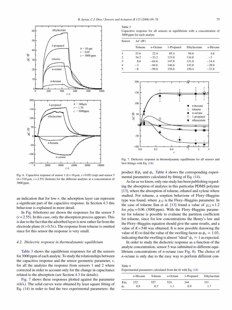
Fig. 6. Capacitive response of sensor 1 (h = 10 �m, r = 0.05) (top) and sensor 5(h = 510 �m, r = 2.55) (bottom) for the different analytes at a concentration of3000 ppm.

an indication that for low-r, the adsorption layer can representa significant part of the capacitive response. In Section 4.3 thisbehaviour is explained in more detail.

In Fig. 6(bottom) are shown the responses for the sensor 5(r = 2.55). In this case, only the absorption process appears. Thisis due to the fact that the adsorbed layer is now rather far from theelectrode plane (h > 0.5λ). The response from toluene is omittedsince for this sensor the response is very small.

4.2. Dielectric response in thermodynamic equilibrium

Table 3 shows the equilibrium responses for all the sensorsfor 3000 ppm of each analyte. To study the relationships betweenthe capacitive response and the sensor geometric parameter, r,for all the analytes the response from sensors 1 and 2 wherecorrected in order to account only for the change in capacitancerelated to the absorption (see Section 4.3 for details).

Fig. 7 shows these responses plotted against the parameterr(h/λ). The solid curves were obtained by least square fitting ofEq. (14) in order to find the two experimental parameters: the

Table 3Capacitive response for all sensors in equilibrium with a concentration of3000 ppm for each analyte

Sensor �C (fF)

Toluene n-Octane 1-Propanol Ethylacetate n-Hexane

1 53.6 22.4 85.4 94.6 4.62 34.2 −33.2 133.0 134.8 −33 8.6 −64.6 147.8 131.0 −14.44 −3 −84.6 146.6 143.8 −28.05 −8 −99.0 159.8 150.4 −23.8

Fig. 7. Dielectric response in thermodynamic equilibrium for all sensors andbest fittings with Eq. (14).

product Kφv and φε. Table 4 shows the corresponding experi-mental parameters calculated by fitting of Eq. (14).

As far as we know, only one study has been publishing regard-ing the absorption of analytes in this particular PDMS polymer[13], where the absorption of toluene, ethanol and xylene wherestudied. For toluene, a sorption behaviour of Flory–Hugginstype was found, where χ12 is the Flory–Huggins parameter. Inthe case of toluene Sun et al. [13] found a value of χ12 = 1.2for p/p0 = 0.06 (3000 ppm). With the Flory–Huggins parame-ter for toluene is possible to evaluate the partition coefficientfor toluene, since for low concentrations the Henry’s law andthe Flory–Huggins equation should give the same results, and avalue of K = 540 was obtained. It is now possible (knowing thevalue of K) to find the value of the swelling factor as φv = 1.03,indicating that the swelling is almost “ideal” φv ≈ 1 as expected.

In order to study the dielectric response as a function of theanalyte concentration, sensor 5 was submitted to different equi-librium concentrations of n-octane (see Fig. 8). The choice ofn-octane is only due to the easy way to perform different con-

Table 4Experimental parameters calculated from the fit with Eq. (14)

n-Hexane Toluene n-Octane 1-Propanol Ethylacetate

Kφv 232 557 524 344 331φε 0.8 0.3 1.1 0.9 1.7


Fig. 8. Response of sensor 3 (r = 0.55) to different concentrations of n-octane.

centration at a flux range compatible with our setup and massflow controllers in a way that the total flux in the sensor cham-ber is always 150 ml/min. Since we measure the capacitanceas a difference between the sensor and a reference capacitor,the sensitivity here is defined as ∂C

∂c, where c is the molar con-

centration of the analyte in gas phase. The sensor response isa linear function of the vapour concentration with a sensitiv-ity of slope of −0.024 fF/ppm. This means a linear sorptionisotherm in the low-concentration range (500–3000 ppm), whereis expected that Henry’s law holds. At higher concentrations,deviations from Henry’s law are expected which is typical ofvapour sorption in rubbery polymers [13]. As pointed out inSection 2.2 with our circuit is possible to resolve 0.05 fF thatin this case mean a resolution of about 2 ppm for the case ofn-octane.

4.3. Dynamic behaviour

As we can observe in Fig. 9(top), for the sensor with the lowerpolymer thickness (r = 0.05) we notice two different build-upresponse time constants, one is a fast response (few seconds)and other a slower response. For the case of the thinner poly-mer layers only the second slow time constant is observed. Thisbehaviour is explained by the fact that in the case of the lowerpolymer thickness the adsorbed layer gives a significant contri-bution to the capacitive response. In order to study the numbero(Stcacm(oo

Fig. 9. Transient response analysis and fitting the experimental points with Eq.(19). (Top) Sensor 1 (r = 0.05) for 1-propanol and (bottom) sensor 4 (r = 1.70)for 1-propanol.

plane. The method described here was used to find the sensortime constants of absorption. The sensor dynamic response isthen modulated with the following equation:

�C(t) = Aad exp

(− t

τad

)+ Aab

(− t

τab

)(19)

where the first term is related with the adsorption of the analytelayer on the top of the polymer, and the second term is relatedwith the absorption. If the absorption process follows the Ficklaw, then τab is related with the diffusion coefficient as predictedin Eq. (18). The parameters of Eq. (19) are presented in Table 5for n-hexane, 1-propanol and ethylacetate.

To evaluate the sensor response due to the absorption processwe use the values of the thick sensors, namely 110, 340 and510 �m (since the volume of the chamber can contribute to asignificative error in the case of thinner polymers).

Despite the fact that the sensor response does not show atrue Fick behaviour, mainly because the capacitance is not a

f physical phenomena present during the response build-upadsorption and absorption) we use the method described inection 2.3. As we can see in Fig. 9(bottom), for the case of

he lower polymer thickness (r = 0.05) we observe a first timeonstant of about 4 s that is attributed to the adsorption of thenalyte into the surface of the polymer layer and a second timeonstant of about 50 s that is due to the absorption of the analyteolecules into the polymer phase. For the case of a thicker layer

r = 1.7) only the absorption term is present with a time constantf 210 s. This is because the adsorption layer is very thin and cannly be noticed by the sensor if it is very close to the electrode


Table 5Experimental parameters of Eq. (19) for the case of n-hexane, 1-propanol and ethylacetate

Aad Aab

fF % τad/s fF % τab/s

h = 10 �m; r = 0.05n-Hexane 1.7 47 2.8 2.9 53 73.21-Propanol 36.3 42 2.6 49.2 56 55.2Ethylacetate 28.6 31 3.2 63.9 69 48.2

h = 60 �m; r = 0.30n-Hexane – – – – – –1-Propanol 13.1 10 6.8 105 90 43.5Ethylacetate 18.3 14 6.7 112 86 52.8

h = 110 �m; r = 0.55n-Hexane 0 0 – −68 100 91.61-Propanol 0 0 – 148 100 67.3Ethylacetate 0 0 – 132 100 53.5

h = 340 �m; r = 1.70n-Hexane 0 0 – −132 100 2631-Propanol 0 0 – 150 100 210Ethylacetate 0 0 – 146 100 170

h = 510 �m; r = 2.55n-Hexane 0 0 – −147 100 5331-Propanol 0 0 – 134 100 729Ethylacetate 0 0 – 149 100 533

linear function of the analyte concentration within the polymerphase, Fick equation is shown to be a good approximation in themajority of cases. Some responses appear to have not only onetime constant but also a distribution of time constants centeredon the time constant expected from the Fick law. For that reason,Eq. (19) can be used as an approximation for the sensors responseand an experimental diffusion coefficient can be calculated fromEqs. (18) and (19).

In Fig. 10, the time constants for n-hexane, 1-propanol andethylacetate for the sensors 4, 5 and 6 (110, 340 and 510 �m,respectively) are shown, and the values for the experimentaldiffusion coefficient are present in Table 6.

F1

Table 6Experimental diffusion coefficients calculated from Eqs. (18) and (19)

D (×106 cm2 s−1)

n-Hexane 1.61-Propanol 1.7Ethylacetate 2.2

These values are similar to the ones obtained by Sun andChen for other analytes (e.g. 1.2 × 10−6 cm2 s−1 for toluene and1.4 × 10−6 cm2 s−1 for ethanol) [13].

5. Conclusions

The strong dependence of the capacitive response with thegeometric parameters of the interdigital capacitive sensors isexplained with an analytical model. These results could be usedto build sensor arrays where one can choose the pattern responsenot only by means of the polymer type, but as well by choosingthe desired geometrical parameters. For a complete descriptionof the sensor response is necessary to know two experimentalparameters (defined here as the product Kφv and φε), never-theless this can be inferred from other studies, in particular thepartition coefficient between several polymers and analytes arealready available in the literature. Once knowing the specificinteractions between the polymer and the analytes an accuratesimulation can be made to anticipate the pattern response of aparticular sensor to a set of analytes. It should be stressed that theexperimental values are not related to the transducer mechanismbut are related with the polymer and analyte specific interactions.

Another important result that can be extrapolated from thismodel is the possibility of cancelling an unwanted response. For

ig. 10. Response time as a function of the thickness of the sensor for n-hexane,-propanol and ethylacetate.


analytes where the dielectric constant is lower than the analyte tocancel we just need to choose the right thickness for the sensitivelayer. If one uses a combination of two sensors and takes thedifferential response, it is possible to cancel the interference ofanalytes with high dielectric constant (e.g. humidity), since theresponse for εa εp reach a saturation value before the responsefor εa > εp. In this way, the differential response for analytes withhigh dielectric constant will vanish.

As well we can “play” with the sensor geometric parame-ters (e.g. η) to build a combination of sensor pairs to cancelout the response of some unwanted interferants. As well amethod used in the past for dielectric spectroscopy studies hassuccessfully apply in the sorption dynamics to find the sensorequilibrium times, making possible to account for the physicalprocess evolved.

Acknowledgment

The authors gratefully acknowledge Falko Keck for the helpin the system setup and on measurements.

References

[1] M.C. Zaratsky, J. Melcher, C.M. Cooke, Moisture sensing in transformeroil using thin-film microdielectrometry, IEEE Trans. Electron. Insul. 24(1989) 1167–1176.

[7] D.S. Ballantine, R.M. White, S.J. Martin, A.J. Ricco, E.T. Zellers, G.C.Frye, H. Wohltjen, Acoustic Wave Sensors: Theory, Design and Physico-Chemical Applications, Academic Press, San Diego, 1997.

[8] R. Igreja, C.J. Dias, Analytical evaluation of the interdigital electrodescapacitance for a multi-layered structure, Sens. Actuators A 112 (2004)291–301.

[9] M. Abramowitz, A. Stegun, Handbook of Mathematical Functions withFormulas, Graphs and Mathematical Tables, Dover, New York, 1970.

[10] A.J. Moulson, J.M. Herbert, Electroceramics: Materials Properties andApplications, Chapman and Hall, London, 1990.

[11] C.J.F. Bottcher, Theory of Electric Polarization, Elsevier, Amsterdam,1973.

[12] A.M. Kummer, A. Hierlemann, H. Baltes, Tuning sensitivity and selec-tivity of complementary metal oxide semiconductor-based capacitivechemical microsensors, Anal. Chem. 76 (2004) 2470–2477.

[13] Y. Sun, J. Chen, Sorption/desorption properties of ethanol, toluene, andxylene in poly(dimethylsiloxane) membranes, J. Appl. Polym. Sci. 51(1994) 1797–1804.

[14] C.J. Dias, Determination of a distribution of relaxation frequencies basedon experimental relaxation data, Phys. Rev. B 63 (1996) 14212–14222.

[15] S. Strathmann, Sample conditioning for multi-sensor systems, Ph.D.Thesis, Universitat Tubingen, 2001.

Biographies

Rui Igreja was born in Lisbon, Portugal in 1966. He graduated in Engi-neering Physics from Universidade Nova de Lisboa in 1992 and joined theDepartment of Physics of the same University in 1993 as Assistant Profes-sor. He obtained the MSc degree in Instrumentation, Industrial MainteinenceaiMd

CfPtpaeaa

[2] W. Qu, W. Wlodarski, A thin-film sensing element for ozone, Sens.Actuators B 64 (2000) 42–48.

[3] C. Hagleitner, A. Hierlemann, D. Lange, A. Kummer, N. Kerness, O.Brand, H. Baltes, Smart single-chip gas sensor microsystems, Nature414 (2001) 293–296.

[4] F. Josse, R. Lukas, R. Zhou, S. Schneider, D. Everhart, AC-impedance-based chemical sensors for organic solvent vapors, Sens. Actuators B36 (1996) 363–369.

[5] R. Casalini, M. Kiliziraki, D. Wood, M.C. Pety, Sensitivity of the electri-cal admittance of a polysiloxane film to organic vapors, Sens. ActuatorsB 56 (1999) 37–44.

[6] A. Hierlemann, A.J. Ricco, K. Bodenhofer, A. Dominik, W. Gopel,Conferring selectivity to chemical sensors via polymer side-chain selec-tion: thermodynamics of vapor sorption by a set of polysiloxanes onthickness-shear mode resonators, Anal. Chem. 72 (2000) 3696–3708.

nd Quality in 1998 in Universidade Nova de Lisboa. He is currently work-ng toward the PhD in chemo-capacitors for electronic nose systems in the

aterials Science Department. His fields of interest are in solid state physics,ielectrics and sensors.

.J. Dias was born in Angola in 1959. He graduated in Engineering Physicsrom Universidade Nova de Lisboa in 1982 and joined the Department ofhysics of the same University in 1985. He received the PhD degree from

he University of North Wales (Bangor) in 1994 working on ferroelectricolymer-ceramic composites. Since then he has been an auxiliary Professort Universidade Nova de Lisboa and is currently working in the Materials Sci-nce Department. His research interests include characterization of dielectricsnd their use in various applications such as sensors and actuators, acousticsnd polymer ionic materials for energy applications.

dielectric response of interdigital chemocapacitors: the role of the sensitive layer thickness

Documents