did the hilda collisional family form during the late heavy

Mon. Not. R. Astron. Soc. 414, 2716–2727 (2011) doi:10.1111/j.1365-2966.2011.18587.x

Did the Hilda collisional family form during the late heavy bombardment?

M. Broz,1� D. Vokrouhlicky,1 A. Morbidelli,2 D. Nesvorny3 and W. F. Bottke3

1Institute of Astronomy, Charles University, Prague, V Holesovickach 2, 18000 Prague 8, Czech Republic2Observatoire de la Cote d’Azur, BP 4229, 06304 Nice Cedex 4, France3Department of Space Studies, Southwest Research Institute, 1050 Walnut St., Suite 300, Boulder, CO 80302, USA

Accepted 2011 February 22. Received 2011 February 3; in original form 2011 January 5

ABSTRACTWe model the long-term evolution of the Hilda collisional family located in the 3/2mean-motion resonance with Jupiter. Its eccentricity distribution evolves mostly due to theYarkovsky/YORP effect and assuming that (i) impact disruption was isotropic and (ii) albedodistribution of small asteroids is the same as for large ones, we can estimate the age of theHilda family to be 4+0

−1 Gyr. We also calculate collisional activity in the J3/2 region. Our re-sults indicate that current collisional rates are very low for a 200-km parent body such that thenumber of expected events over gigayears is much smaller than 1.

The large age and the low probability of the collisional disruption lead us to the conclusionthat the Hilda family might have been created during the late heavy bombardment (LHB)when the collisions were much more frequent. The Hilda family may thus serve as a test oforbital behaviour of planets during the LHB. We have tested the influence of the giant-planetmigration on the distribution of the family members. The scenarios that are consistent with theobserved Hilda family are those with fast migration time-scales �0.3–3 Myr, because longertime-scales produce a family that is depleted and too much spread in eccentricity. Moreover,there is an indication that Jupiter and Saturn were no longer in a compact configuration (withperiod ratio PS/PJ > 2.09) at the time when the Hilda family was created.

Key words: methods: numerical – celestial mechanics – minor planets, asteroids: general.

1 IN T RO D U C T I O N

There are many independent lines of evidence that the orbits ofplanets of the Solar system were not the same all the time, butthat they have changed substantially over billions of years. Themajor arguments are based on the observed orbital distribution ofKuiper belt objects (Malhotra 1995; Levison et al. 2008) or smallbut non-negligible eccentricities and inclinations of the giant plan-ets (Tsiganis et al. 2005). Observations of Jupiter’s Trojans (Mor-bidelli et al. 2005), main-belt asteroids (Minton & Malhotra 2009;Morbidelli et al. 2010), the amplitudes of secular oscillations ofthe planetary orbits (Brasser et al. 2009; Morbidelli et al. 2009),or the existence of irregular moons (Nesvorny, Vokrouhlicky &Morbidelli 2007) provide important constraints for planetary mi-gration scenarios.

Asteroids are a fundamental source of information about theevolution of the planetary system. Some of the resonant groups, i.e.those which are located in the major mean-motion resonances withJupiter, might also have been influenced by planetary migration,because their current distribution does not match the map of thecurrently stable regions. For instance, there are two stable islands

�E-mail: [email protected]

denoted by A and B in the J2/1 resonance and only the B island ispopulated (Nesvorny & Ferraz-Mello 1997).

In this work we focus on the Hilda asteroid family in the 3/2resonance with Jupiter. We exploit our ability to model long-termevolution of asteroid families, which is usually dominated by theYarkovsky effect on the orbital elements (Bottke et al. 2001), of-ten coupled to the YORP effect on the spin rate and obliquity(Vokrouhlicky et al. 2006b). Chaotic diffusion in eccentricity andsometimes interactions with weak mean-motion or secular reso-nances (Vokrouhlicky et al. 2006a) also play important roles. Incase of asteroids inside strong mean-motion resonances, one hasto account for the ‘resonant’ Yarkovsky effect, which causes a sys-tematic drift in eccentricity (Broz & Vokrouhlicky 2008). This isdifferent from usual non-resonant orbits where the Yarkovsky effectcauses a drift in semimajor axis.

The Hilda collisional family – a part of the so-called Hilda groupin the 3/2 mean motion resonance with Jupiter – was already brieflydiscussed by Broz & Vokrouhlicky (2008). However, the modellingpresented in that paper was not very successful, since the resultingage of the family seemed to be too large (exceeding 4 Gyr). Thiswas an important motivation for our current work. We think thatwe missed an important mechanism in our previous model, namelyperturbations arising from the migration of the giant planets andalso an appropriate treatment of the YORP effect. Indeed, the age

C© 2011 The AuthorsMonthly Notices of the Royal Astronomical Society C© 2011 RAS

Hilda collisional family 2717

�4 Gyr suggests that the planetary migration might have played adirect role during the early evolution of the Hilda family. In thispaper we thoroughly test this hypothesis.

The paper is organized as follows. First we study the observedproperties of the J3/2 resonance population in Section 2. Our dynam-ical model of the Hilda family (without migration first) is describedin Section 3. Then we estimate the collisional activity in the J3/2 re-gion in Section 4. The results of our simulations of the giant-planetmigration are presented in Section 5. Finally, Section 6 is devotedto conclusions.

2 C U R R E N T A S T E RO I D PO P U L AT I O NI N T H E J 3 / 2 R E S O NA N C E

Asteroids located in the 3/2 mean motion resonance with Jupiterhave osculating semimajor axes around (3.96 ± 0.04) au, i.e. beyondthe main asteroid belt. Contrary to the Kirkwood gaps (associatedwith J3/1, J7/3 or J2/1 resonances), this resonance is populatedby asteroids while its neighbourhood is almost empty. The Hildacollisional family we are going to discuss in detail is a small part ofthe whole J3/2 resonant population.

Our identification procedure of the J3/2 resonant population wasdescribed in the previous paper, Broz & Vokrouhlicky (2008). Usingthe AstOrb catalogue of orbits (version JD = 245 5500.5, 2010October 31) we identified 1787 numbered and multi-oppositionbodies with the librating critical argument

σ = p + q

qλ′ − p

qλ − � , (1)

where p = 2, q = 1, λ′ is the mean longitude of Jupiter, λ the meanlongitude of the asteroid and � the longitude of perihelion of theasteroid.

In order to study the detailed distribution of the bodies libratinginside the resonance, we have to use pseudo-proper resonant ele-ments defined as approximate surfaces of sections (Roig, Nesvorny& Ferraz-Mello 2002), i.e. the intersection of the trajectory with aplane defined by

|σ | < 5◦ ,�σ

�t> 0 , |� − � ′| < 5◦ . (2)

These conditions correspond to the maximum of the semimajoraxis a over several oscillations and the minimum of the eccentric-ity e or the inclination I. We need to apply a digital filter to σ (t)prior to using equation (2), namely filter A from Quinn, Tremaine& Duncan (1991), by sampling 1 yr and with a decimation factorof 10, to suppress fast �80 yr oscillations, which would otherwisedisturb slower �280 yr oscillations associated with resonant libra-tions. Finally, we apply an averaging of the sections a, e, I over1-Myr running window and these averages are the pseudo-properelements ap, ep, Ip. The accuracy of the pseudo-proper elements isof the order of 10−4 au for ap and 10−4 for ep or sin Ip, which ismuch smaller than those of the structures we are interested in.

The overall dynamical structure of the J3/2 resonance is deter-mined by secular resonances ν5, ν6 at high eccentricities ep � 0.3and secondary resonances at lower values of ep � 0.13 (according toMorbidelli & Moons 1993; Nesvorny & Ferraz-Mello 1997; Ferraz-Mello et al. 1998; Roig & Ferraz-Mello 1999). They destabilize theorbits at the borders of a stable island. The orbits inside the islandexhibit very low chaotic diffusion rates, so bodies can remain therefor 4 Gyr (without non-gravitational perturbation).

Next we apply a hierarchical clustering method (Zappala et al.1994) to detect significant clusters. We use a standard metric in the

Figure 1. The number N of the Hilda family members versus the selectedcut-off velocity vcut-off .

pseudo-proper element space (ap, ep, sin Ip):

δv = na

√5

4

(δap

ap

)2

+ 2(δe2

p

) + 2(δ sin Ip)2 . (3)

In the following, we do not discuss the known Schubart family,which was sufficiently analysed elsewhere (Broz & Vokrouhlicky2008), but we focus on the family associated with (153) Hilda.A suitable cut-off velocity for the Hilda family seems to bevcut-off = 140 m s−1, because the number of members does notchange substantially around this value (see Fig. 1). The number ofmembers at this cut-off is 400.

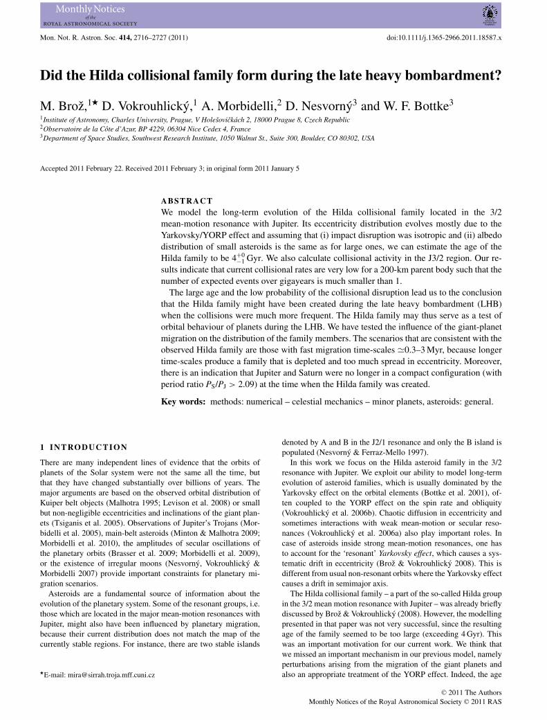
The resulting plots (ap, H), (ep, H) and (Ip, H) of the Hildafamily show very interesting features (see Fig. 2). The distributionof semimajor axis and inclination seems rather uniform and almostindependent of absolute magnitude H, but the eccentricities of smallasteroids (i.e. with high H) are clearly concentrated at the outskirtsof the family and depleted in the centre.

In order to explain the distribution of asteroids in the (ep, H) planewe have to recall that asteroids orbiting about the Sun are affectedby non-gravitational forces, mostly by the Yarkovsky/YORP effect,i.e. the recoil force/torque due to anisotropic emission of thermalradiation. We consider the concentrations in the (ep, H) plane tobe a strong indication of the ongoing Yarkovsky/YORP evolution,because they are very similar to those observed among the severalmain-belt families in the (ap, H) plane and successfully modelled byVokrouhlicky et al. (2006b). The difference between these two casesstems from the fact that the main-belt families are non-resonantand the Yarkovsky/YORP effect thus increases or decreases thesemimajor axis (depending on the actual obliquity of the spin axis),while in our resonant case, the same perturbation results instead in asystematic increase or decrease of eccentricity. A detailed modellingof the e-distribution is postponed to Section 3.5.

The central part of the (ep, H) distribution, from e = 0.17–0.23, seems rather extended. The large asteroids (H < 12.5 mag)are spread over this interval of eccentricities even though theirYarkovsky drift rates must have been small. Only 2–4 of them arelikely to be interlopers, because there is a very small number ofbackground asteroids in the surroundings of the family (see Fig. 3).We think this shape might actually be the result of the initial-size-independent perturbation that the family distribution received bythe migration of the giant planets (which we discuss in Section 5.1).

Regarding the (ap, H) distribution, the largest asteroid (153) Hildais offset with respect to the centre, but this is a natural outcome ofthe definition of the pseudo-proper elements – fragments that fallto the left of the libration centre are mapped to the right, whichcreates the offset.

The geometric albedos for Hilda family objects are poorly known.There are only six measured values for the family members: 0.064,

C© 2011 The Authors, MNRAS 414, 2716–2727Monthly Notices of the Royal Astronomical Society C© 2011 RAS

2718 M. Broz et al.

Figure 2. The Hilda family displayed in resonant semimajor axis ap (left), eccentricity ep (middle) and inclination sin Ip (right) versus absolute magnitudeH. The libration centre is located at a � 3.96 au and all the bodies are displayed to the right of it. The ‘ears’ in (ep, H), i.e. both the concentration of smallasteroids on the outskirts of the family and their depletion at the centre are very prominent here. The thin vertical lines denote the central part of the (ep, H)distribution discussed in the text. The family has 400 members at vcut-off = 140 m s−1.

Figure 3. The J3/2 region displayed in (ap, Ip) plot. A very prominentSchubart cluster (studied by Broz & Vokrouhlicky 2008) is visible aroundsin Ip

.=0.05. The close surroundings of the Hilda family, where only a lownumber of bodies is present, are highlighted by grey rectangles.

0.046, 0.038, 0.089, 0.044, 0.051 (Davis & Neese 2002). Given thesmall number of values and the possibility of selection effects, weprefer to assume that the family members have a mean value pV =0.044, which corresponds to the whole J3/2 population. The size ofthe parent body can be then estimated to be DPB = (200 ± 20) km.We employ two independent methods to determine the diameterDPB: (i) we sum the volumes of the observed bodies larger than anassumed completeness limit Dcomplete = 10 km and then we prolongthe slope of the size–frequency distribution down to D = 0 toaccount for unobservable bodies (see Broz & Vokrouhlicky 2008),which results in DPB � 185 km; (ii) we also use a geometric methoddeveloped by Tanga et al. (1998) which gives DPB � 210 km. A testwith different albedo values will be described in Section 3.6.

The size–frequency distribution N(>D) versus D of the Hildafamily is steeper than that of background J3/2 population, but shal-lower than for usual main-belt families (Fig. 4). Interestingly, theslope γ = −2.4 ± 0.1 of the distribution N(>D) = CDγ is close toa collisional equilibrium calculated by Dohnanyi (1969).

Colour data extracted from the Sloan Digital Sky Survey MovingObject Catalogue version 4 (Parker et al. 2008) confirm that theHilda family belongs to the taxonomic type C, because most ofthe spectral slopes are small. Recall that the whole J3/2 populationexhibits a bimodal distribution of slopes, i.e. it contains a mixtureof C- and D-type asteroids.

Figure 4. Cumulative size distributions of the J3/2 population and the Hildafamily. The polynomial fits of the form N(>D) = CDγ are plotted as thinlines, together with the respective values of the γ exponent. Several main-belt families are plotted for comparison: Eos (with slope γ = −2.8), Euno-mia (−5.0), Hygiea (−3.8), Koronis (−2.8), Themis (−2.9), Tirela (−3.3),Veritas (−3.4) and Vesta (−5.4).

3 TH E H I L DA FA M I LY MO D E L W I T HR A D I AT I O N FO R C E S

To understand the long-term evolution of the Hilda family, weconstruct a detailed numerical model, extending efforts in Broz& Vokrouhlicky (2008), which includes the following processes:(i) impact disruption, (ii) the Yarkovsky effect, (iii) the YORP ef-fect, (iv) collisions and spin-axis reorientations. We describe theindividual parts of the model in the following subsections.

3.1 Impact disruption

To obtain initial conditions for the family just after the breakupevent, we need a model for the ejection velocities of the fragments.We use a very simple model of an isotropic ejection from the work ofFarinella, Froeschle & Gonczi (1994). The distribution of velocities‘at infinity’ follows the function

dN (v)dv = Cv(v2 + v2esc)

−(α+1)/2dv , (4)

with the exponent α being a free parameter, C a normalizationconstant and vesc the escape velocity from the parent body, which



is determined by its size DPB and mean density ρPB as vesc =√(2/3)πGρPB DPB . The distribution is usually cut at a selected

maximum allowed velocity vmax to prevent outliers. The actualvalues of all these parameters are given in Section 3.5. Typically,the overall distribution of velocities has a peak close to the escapevelocity, which is approximately 100 m s−1 for a 200-km parentbody. The initial velocities |v| of individual bodies are generatedby a straightforward Monte Carlo code and the orientations of thevelocity vectors v in space are assigned randomly.

Here, we assume the velocity of fragments is independent of theirsize, which seems reasonable with respect to the observed uniformdistribution of the Hilda family in the (ap, H) and (Ip, H) planes(Fig. 2). We also perform tests with non-isotropic distributions inSection 3.7.

We must also select initial osculating eccentricity ei of the parentbody, initial inclination ii, as well as true anomaly f imp and argumentof perihelion ωimp at the time of impact disruption. All of these pa-rameters determine the initial shape of the synthetic ‘Hilda’ familyjust after the disruption of the parent body. Initial semimajor axis ai

is not totally free, instead it is calculated from the initial semimajoraxis of Jupiter aJi and the Kepler’s law, since the parent body has tobe confined to the J3/2 resonance.

3.2 Yarkovsky effect in a resonance

The long-term evolution of asteroid orbits is mainly driven by theYarkovsky thermal effect. The implementation of the Yarkovsky ef-fect in the SWIFT integrator was described in detail in Broz (2006).Only minor modifications of the code were necessary to incorpo-rate spin rate evolution, which is driven by the YORP effect (seeSection 3.3).

The thermal parameter we use are reasonable estimates for C/X-type bodies: ρsurf = ρbulk = 1300 kg m−3 for the surface and bulkdensities, K = 0.01 W m−1 K−1 for the surface thermal conductivity,C = 680 J kg−1 for the heat capacity, A = 0.02 for the Bond albedoand εIR = 0.95 for the thermal emissivity parameter.

We can use a standard algorithm for the calculation of theYarkovsky acceleration which results in a semimajor-axis drift incase of non-resonant bodies. The drift in eccentricity in case ofresonant bodies arises ‘automatically’ due to the gravitational partof the integrator. In Fig. 5 we can see a comparison between theexpected drift �a in semimajor axis and the resulting drift �e ineccentricity, computed for the Hilda family (see the explanation inappendix A of Broz & Vokrouhlicky 2008). The data can be approx-

Figure 5. An almost linear relation between the expected drift �a in semi-major axis and the simulated drift �e in eccentricity, computed for 360members of the Hilda family located inside the J3/2 resonance.

imated by a linear relationship, where the departures from linearityare caused mainly by interactions of drifting orbits with embeddedweak secular or secondary resonances.

Note that according to a standard solar model the young Sun wasfaint (Gudel 2007), i.e. its luminosity 4 Gyr ago was 75 per centof the current L�. We can then expect a lower insolation and conse-quently weaker thermal effects acting on asteroids. Since we assumea constant value of L� in our code, the age estimated for the Hildafamily (in Section 3.5) can be 12.5 per cent larger.

3.3 YORP effect

The magnitude of the Yarkovsky drift sensitively depends on theorientation of the spin axis with respect to the orbital plane and,to a lesser extent, on the angular velocity too. We thus have toaccount for the long-term evolution of spins of asteroids which iscontrolled by torques arising from the emission of thermal radia-tion, i.e. the YORP effect. The implementation of the YORP effectfollows Vokrouhlicky et al. (2006b). We assume the following re-lations for the rate of angular velocity and obliquity:

dω

dt= fi(ε) , i = 1, . . . , 200 , (5)

dε

dt= gi(ε)

ω, (6)

where f - and g-functions are given by Capek & Vokrouhlicky (2004)for a set of 200 shapes with mean radius R0 = 1 km, bulk densityρ0 = 2500 kg m−3, located on a circular orbit with semimajor axisa0 = 2.5 au. The shapes of the Hilda family members are not known,so we assign one of the artificial shapes (denoted by the index i)randomly to each individual asteroid. We only have to scale the f -and g-functions by the factor

c = cYORP

(a

a0

)−2 (R

R0

)−2 (ρbulk

ρ0

)−1

, (7)

where a, R, ρbulk are semimajor axis, radius and density of thesimulated body, and cYORP is a free scaling parameter, which canaccount for an additional uncertainty of the YORP model. Becausethe values of f and g were computed for only a limited set ofobliquities (with a step �ε = 30◦) we use interpolation by Hermitepolynomials (Hill 1982) of the data in Capek & Vokrouhlicky (2004)to obtain a smooth analytical function each for fi(ε) and gi(ε).

If the angular velocity approaches a critical value,

ωcrit =√

8

3πGρbulk , (8)

we assume a mass-shedding event, so we keep the orientation of thespin axis and the sense of rotation, but we reset the orbital periodP = 2π/ω to a random value from the interval (2.5, 9) h. We alsochange the assigned shape to a different one, since any change ofshape may result in a different YORP effect.

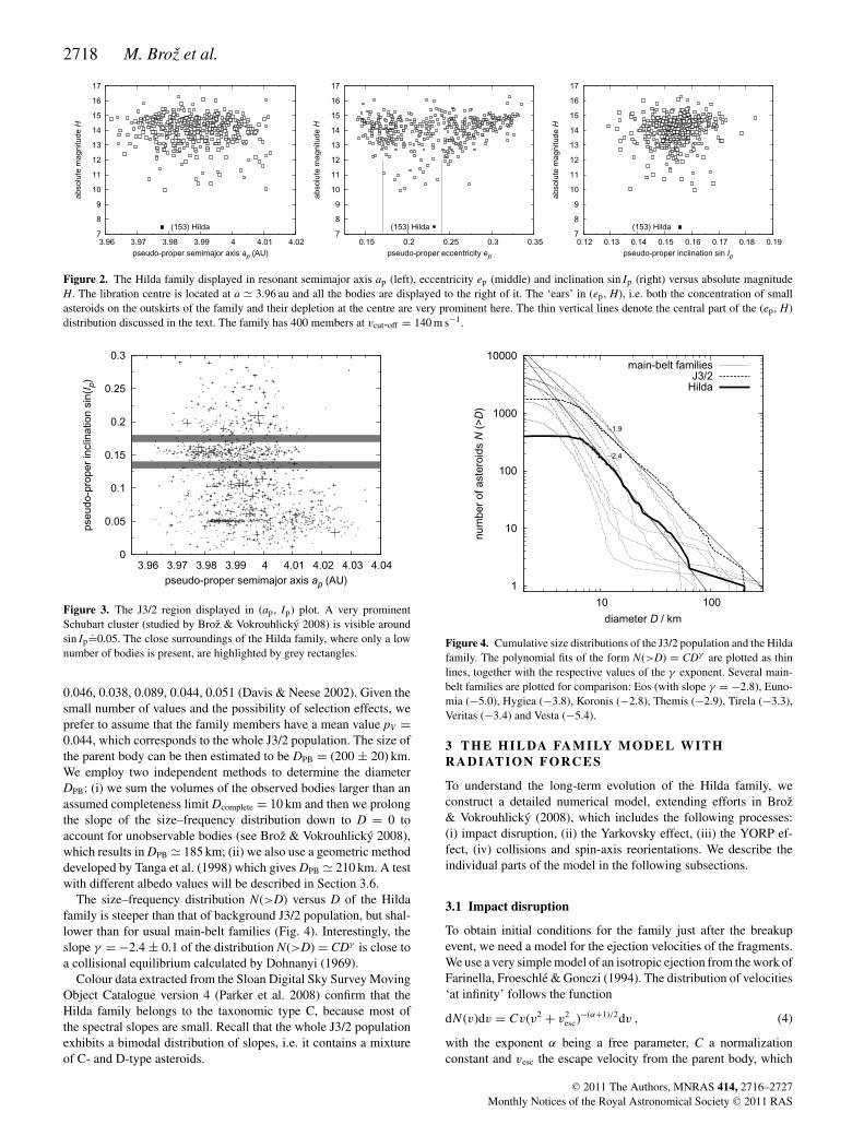
The differential equations (5) and (6) are integrated numericallyby a simple Euler integrator. The usual time-step is �t = 1000 yr.An example of the results computed by the spin integrator for theHilda family is displayed in Fig. 6. The typical time-scale of thespin-axis evolution is τYORP � 500 Myr. After � 3 times τYORP mostbodies have spin axes perpendicular to their orbits, what maximizesthe Yarkovsky drift rate of eccentricity.


2720 M. Broz et al.

Figure 6. An example of the YORP-driven evolution of obliquities (namelya z-component of the spin-axis unit vector, top panel) and angular velocitiesω (bottom panel) for the members of the synthetic ‘Hilda’ family. At thebeginning, all values of ω were selected positive and spin axes were dis-tributed isotropically. The evolution may force ω to become negative, whichsimply corresponds to an opposite orientation of the spin axis. The scalingparameter selected for this run was cYORP = 0.33.

3.4 Collisions and spin-axis reorientations

In principle, collisions may directly affect the size distribution ofthe synthetic Hilda family, but we neglect this effect because mostof the asteroids are large enough to remain intact.

However, we include spin-axis reorientations caused by col-lisions. We use an estimate of the time-scale by Farinella,Vokrouhlicky & Hartmann (1998):

τreor = B

(ω

ω0

)β1(

D

D0

)β2

, (9)

where B = 84.5 kyr, β1 = 5/6, β2 = 4/3, D0 = 2 m and ω0 cor-responds to period P = 5 h. These values are characteristic of themain belt and we use them as an upper limit of τ reor for the J3/2region. Even so, the time-scale is τ reor � 3 Gyr for the smallestobservable (D � 5 km) bodies, and reorientations are thus only ofminor importance. Note that the probability of the reorientation isenhanced when the YORP effect drives the angular velocity ω closeto zero.

3.5 Results for the Yarkovsky/YORP evolution

We start a simulation with an impact disruption of the parent bodyand create 360 fragments. Subsequent evolution of the syntheticHilda family due to the Yarkovsky/YORP effect is computed up to6 Gyr in order to estimate the time-span needed to match the ob-served family even though the family cannot be older than �4 Gyr,of course. Planets are started on their current orbits. A typical out-come of the simulation is displayed in Fig. 7.

Figure 7. Eccentricity versus absolute magnitude plot for the synthetic‘Hilda’ family just after the impact disruption (time t = 0, top panel) andafter 4 Gyr of evolution due to the Yarkovsky/YORP effect (bottom panel).There is a comparison with the observed Hilda family (grey dots).

Due to the long integration time-span and large number of bodies,we were able to compute only four simulations with the followingvalues of true anomaly and YORP efficiency:

(i) f imp = 0◦, cYORP = 0;(ii) f imp = 180◦, cYORP = 0;(iii) f imp = 0◦, cYORP = 1;(iv) f imp = 0◦, cYORP = 0.33.

The remaining parameters were fixed: ei = 0.14, ii = 7.◦8,ωimp = 30◦, α = 3.25, vmax = 300 m s−1, RPB = 93.5 km, ρPB =1300 kg m−3, pV = 0.044.

We are mainly concerned with the distribution of eccentricitiesep, because the observed family has a large spread of ep values,while the initial synthetic family is very compact. For this purposewe constructed a Kolmogorov–Smirnov test (Press et al. 1999) ofthe normalized cumulative distributions N(<e):

DKS = max0<e<1

|N (<e)syn − N (<e)obs| , (10)

which provides a measure of the difference between the syntheticHilda family, at a given time, and the observed Hilda family (seeFig. 8 for an example). The results of the KS tests are summarizedin Fig. 9 (the first four panels).

There is an easy possibility to asses the sensitivity of results withrespect to the vmax parameter too, without the need to compute thesimulation again. We simply select bodies fulfilling the conditionv < v′

max, with v′max = 200, 100 or 50 m s−1, and recompute only

the KS statistics for this subset. The results are plotted in Fig. 9 asthin lines. We can state that values lower than vmax � 100 m s−1 aresurely excluded.

As a preliminary conclusion we may say that all simulationspoint to a large age of the Hilda family. The ep-distributions aremost compatible with the observed family for ages t = (4.0 ±1.0) Gyr. This suggests that the Hilda family might have experiencedthe giant-planet migration period which is dated by the late heavybombardment to tLHB � 3.85 Gyr (Gomes et al. 2005). The large



Figure 8. Normalized cumulative distributions N(<e) of eccentricities for(i) the observed Hilda family, (ii) the synthetic ‘Hilda’ family at time t = 0(just after the impact disruption), (iii) evolved due to the Yarkovsky/YORPeffect (at time t = 3845 Myr). In this figure we show the best fit for thesimulation with parameters f imp = 0◦, cYORP = 0.33. Note that the ‘bent’shape of the observed distribution corresponds to the ‘ears’ on the (ep,H) plot (Fig. 2). There is no perturbation by planetary migration in thisparticular case.

uncertainty of the age stems from the fact that the runs including theYORP effect (cYORP ≥ 0.33) tend to produce ages at a lower limitof the interval while the YORP-less runs (with cYORP = 0) tend tothe upper limit.

3.6 Alternative hypothesis: high albedos of small asteroids

We now discuss two scenarios that further reduce the minimalage of the family: (i) high albedos of small asteroids (i.e. largerYarkovsky/YORP drift); (ii) strongly asymmetric velocity field af-ter impact (like that of the Veritas family).

Albedo is the most important unknown parameter, which canaffect results on the Yarkovsky/YORP evolution. Fernandez, Jewitt& Ziffer (2009) measured albedos of small Trojan asteroids andfound systematically larger values than those for large Trojans. Ifwe assume that the J3/2 asteroids behave similarly to Trojans, wemay try a simulation with a rather high value of geometric albedopV = 0.089 (compared to previous pV = 0.044). Moreover, wedecrease density ρbulk = 1200 kg m−3, increase maximum velocityof fragments vmax = 500 m s−1 (though the velocity distribution isstill determined by equation 4) and select true anomaly f imp = 90◦

to maximize the spread of ep values.The KS test is included in Fig. 9, panel (e). The most probable

age is (2.3 ± 0.5) Gyr in this case. However, we do not think that thesize-dependent albedo is very plausible because both large and smallfamily members should originate from the same parent body andtheir albedos, at least just after the disruption, should be similar.Nevertheless, the albedos may change to a certain degree due tospace weathering processes (Nesvorny et al. 2005). Unfortunately,we do not have enough data for small asteroids to assess a possiblealbedo difference between large and small family members.

3.7 Alternative hypothesis: strongly asymmetric velocity field

Another possibility to reduce the estimate of the family age is thatthe original velocity was highly anisotropic. A well-known examplefrom the main belt is the Veritas family. Let us assume that the

anisotropy is of the order of Veritas, i.e. approximately four timeslarger in one direction. Note that Veritas is a young family and canbe modelled precisely enough to compensate for chaotic diffusion inresonances (Nesvorny et al. 2003; Tsiganis, Knezevic & Varvoglis2007). This family is characterized by a large spread of inclinations,which corresponds to large out-of-plane components of velocities.In case of the Hilda family we multiply by 4 the radial componentsof initial velocities to maximize the dispersion of eccentricities,assuming the most favourable geometry of disruption (f imp

.= 90◦).The fit in Fig. 9, panel (f), is seemingly better at the beginning of

the simulation, but bodies on unstable orbits are quickly eliminatedand the fit gets much worse at t � 500 Myr. We can see that thesynthetic Hilda family is similar to the observed Hilda family quiteearly (at t � 2.5 Gyr); however, the best fit is at later times (t �3.5 Gyr), so there is no significant benefit compared to isotropicvelocity-distribution cases.

4 D I SRU PTI ON R ATES I N THE J 3 / 2POPULATI ON

4.1 Present collisional activity

The results presented above show that the Hilda family is old.However, the uncertainty of the age is too large to conclude whetheror not the family formed during the late heavy bombardment (LHB)period. An alternative constraint is the collisional lifetime of theparent body. If the probability that the parent body broke in the last4 Gyr in the current collisional environment is negligible, it wouldargue that the family broke during the LHB when the collisionalbombardment was much more severe. Thus, here we estimate thecollisional lifetime of the parent body.

In our case, the target (parent body) has a diameter Dtarget =200 km, a mean impact velocity V i = 4.8 km s−1 (Dahlgren 1998),and a probable strength Q�

D = 4 × 105 J kg−1 (Benz & Asphaug1999), and thus the necessary impactor size (Bottke et al. 2005) is

ddisrupt = (2Q�

D/V 2i

)1/3Dtarget � 65 km . (11)

The population of ≥65 km projectiles is dominated by main-beltbodies: nproject � 160, according to Bottke et al. (2006), and wehave only one 200-km target in the J3/2 region, so ntarget = 1. Theintrinsic collisional probability for Hilda versus main belt collisionsis Pi = 6.2 × 10−19 km−2 yr−1 (Dahlgren 1998) and the correspond-ing frequency of disruptions is

fdisrupt = Pi

D2target

4nprojectntarget � 10−12 yr−1 . (12)

Thus, over the age of the Solar system TSS � 4 Gyr (after LHB),we expect a very small number of such events nevents = TSSf disrupt �0.004.

The value of strength Q�D used above corresponds to strong tar-

gets. Though there is a theoretical possibility that the Hilda parentbody was weaker, it does not seem to us likely, because the Hildafamily is of the C taxonomic type. Thus, it is rather similar to(presumably stronger) main belt asteroids, than to (likely weaker)D-type objects. Anyway, even if we use an order of magnitude lowerstrength inferred for weak ice, Q�

D � 4 × 104 J kg−1 (see Leinhardt& Stewart 2009; Bottke et al. 2010), we obtain ddisrupt � 30 km,nproject � 360 and nevents � 0.009, so the conclusion about the lownumber of expected families remains essentially the same.


2722 M. Broz et al.

Figure 9. Kolmogorov–Smirnov tests of the synthetic ‘Hilda’ family: (a) no migration, only initial disruption (at anomaly f imp = 0◦, � i = 30◦) and subsequentYarkovsky evolution; (b) the case with f imp = 180◦; (c) including the YORP effect; (d) YORP with efficiency factor cYORP = 0.33; (e) high albedo values (i.e.small bodies); (f) strongly asymmetric velocity field. The horizontal line denotes the distance DKS = 0.165 for which the probability p(>DKS) that the twoeccentricity distributions differ by this amount equals 0.01.

4.2 The late heavy bombardment

We now compute the probability that the parent body broke duringthe LHB. We can think of two projectile populations: (i) transientdecaying cometary disc; (ii) D-type asteroids captured in the J3/2.Models like that of Levison et al. (2009) suggest that the decaytime-scale of the cometary bombardment is of the order of 10–100 Myr and the flux of impactors integrated over this time-spanmight have been 100 times larger than it is today. Higher meancollisional velocities, due to projectiles on high-e and high-i orbits,are also favourable.

In order to estimate collisional activity we use a self-consistentmodel of the cometary disc from Vokrouhlicky, Nesvorny &Levison (2008). Their N-body simulations included four giant plan-ets and 27 000 massive particles with a total mass of Mdisc = 35 M⊕.

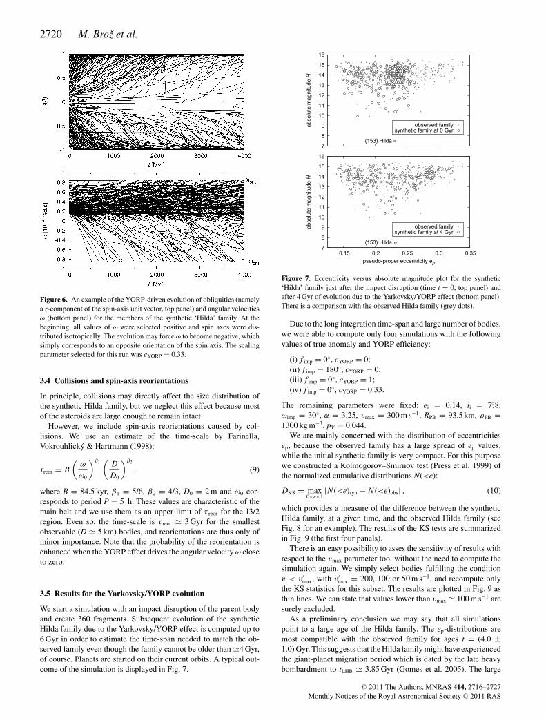
The orbital evolution was propagated by the SyMBA integrator for100 Myr. Using the output of these simulations, we calculate themean intrinsic collisional probabilities Pi(t) between the cometary-disc population (at given time t) and the current J3/2 population.We use an algorithm described in Bottke et al. (1994) for this pur-pose. Typically, the Pi reaches 2to3 × 10−21 km−2 yr−1 and thecorresponding mean impact velocities are V imp = 7–10 km s−1 (seeFig. 10).

The necessary impactor size is slightly smaller than before,ddisrupt = 40–50 km due to larger V imp. To estimate the numberof such projectiles we assume that the cometary disc had a size dis-tribution described by a broken power law with differential slopesq1 = 5.0 for D > D0, q2 = 2.5 ± 0.5 for D < D0, where the diametercorresponding to the change of slopes is D0 = 50–70 km. We thenuse the following expressions to calculate the number of bodies



Figure 10. Mean intrinsic collisional probability Pi and mean impact ve-locity V imp versus time for one of the disc simulations from Vokrouhlickyet al. (2008).

larger than the given threshold (Vokrouhlicky et al. 2008):

D1 = D0

[(q1 − 4)(4 − q2)

(q1 − 1)(q1 − q2)

Mdisc

M0

] 1q1−1

, (13)

N (>D) = q1 − 1

q2 − 1

(D1

D0

)q1−1(D0

D

)q2−1

− q1 − q2

q2 − 1

(D1

D0

)q1−1

, (14)

where M0 = π6 ρD3

0 and ρ = 1300 kg m−3. The result of this cal-culation is N(>ddisrupt)

.= 0.3 to 1.7 × 109. The actual number ofbodies in the simulation (27 000) changes in course of time andit was scaled such that initially it was equal to N(>ddisrupt). Theresulting number of events is

nevents = D2target

4ntarget

∫Pi(t) nproject(t) dt

� 0.05 to 0.2 , (15)

which is 10–50 times larger than the number found in Section 4.1.Regarding the captured D-type asteroids, they were probably not

so numerous and their impact velocities were lower but their colli-sional probabilities were larger and the population might have had asubstantially longer time-scale of decay (Levison et al. 2009). Usingthe reasonable values V i = 4.0 km s−1, ddisrupt = 70 km, nproject =5000, Pi = 2.3 × 10−18 km−2 yr−1, TLHB � 1 Gyr, we obtain thenumber of events �0.1 which is again 25 times larger than thenumber presented in Section 4.1.

We conclude that the Hilda family was likely created duringthe LHB when the collisions were much more frequent than inthe current collisional environment. We must now test whether thestructure of the family is consistent with the giant-planet migration,since it is connected with the LHB.

5 PL A N E TA RY M I G R AT I O N

At the LHB-time the planetary migration was most probably causedby the presence of a massive cometary disc. Instead of a full N-body model we use a simpler analytic migration, with an artificialdissipation applied to the planets. This is the only realistic possibilityin our case, because we need to test not only a large number ofvarious migration scenarios but also various initial configurationsof the synthetic Hilda family.

For this purpose we use a modified version of the symplecticSWIFT–RMVS3 integrator (Levison & Duncan 1994). We accountfor four giant planets and include the following dissipation term

Table 1. Free parameters of our Hilda family model.

No. Parameter Description

1 aJi Initial semimajor axis of Jupiter2 aSi Saturn3 eJi Initial eccentricity of Jupiter4 eSi Saturn5 τmig Migration time-scale6 edampJ Eccentricity damping for Jupiter7 edampS Saturn8 ei Initial eccentricity of the parent body9 ii Initial inclination

10 f imp True anomaly at the impact disruption11 ωimp Argument of perihelion12 α Slope of the velocity distribution13 vmax Maximum velocity of fragments14 RPB Radius of parent body15 ρPB Bulk density16 pV Geometric albedo of fragments17 cYORP Efficiency of the YORP effect

Table 2. Fixed (assumed) parameters of the Hilda family model. There arealso a number of less important parameters, such as the thermal ones (ρsurf ,K, C, A, εIR) or the collisional ones (B, β1, β2).

No. Parameter Description

18 aJf Final semimajor axis of Jupiter19 aSf Saturn20 N(<H) (observed) absolute magnitude distribution

applied to the planets in every time-step:

v = v

[1 + �v

v

�t

τmigexp

(− t − t0

τmig

)], (16)

where v denotes a velocity vector of a given planet, v is the absolutevalue of velocity, �t is the time-step, τmig is the selected migrationtime-scale, �v = √

GM/ai − √GM/af the required total change

of velocity (i.e. the difference of mean velocities between the initialand the final orbit), t is the time and t0 is some reference time. Ifthere are no perturbations other than (16), the semimajor axis of theplanet changes smoothly (exponentially) from the initial value ai tothe final af . We use time-step �t = 36.525 d and the total time-spanof the integration is usually equal to 3τmig when planetary orbitspractically stop to migrate.

We would like to resemble evolution of planetary orbits similar tothe Nice model so it is necessary to use an eccentricity-damping for-mula, which simulates the effects of dynamical friction (Morbidelliet al. 2010). This enables us to model a decrease of eccentricitiesof the giant planets to relatively low final values. The amount ofeccentricity damping is characterized by a parameter edamp.

Because inclinations of the planets are not very important forwhat concerns the perturbation of minor bodies (the structure ofresonances is mainly determined by planetary eccentricities), weusually start with the current values of inclination of the planets.

We admit that the analytic migration is only a crude approxima-tion of the real evolution, but we can use it as a first check to seewhich kinds of migration scenarios are allowed and which are notwith respect to the existence and structure of the Hilda family.

As a summary we present a list of free and fixed (assumed)parameters of our model in Tables 1 and 2. According to our nu-merical tests the initial configuration of Uranus and Neptune is notvery important, as these planets do not produce significant direct


2724 M. Broz et al.

perturbations on asteroids located in the J3/2 resonance. We thusdo not list the initial semimajor axes and eccentricities of Uranusand Neptune among our free parameters though we include theseplanets in our simulations.

The problem is that we cannot tune all the 17 parameters together,since the 17-dimensional space is enormous. We thus first select areasonable set of impact parameters for the family (No. 8–17 inTable 1), keep them fixed, and experiment with various values ofmigration parameters (No. 1–7). We test roughly 103 migrationscenarios. Then, in the second step, we vary impact parameters fora single (successful) migration scenario and check the sensitivity ofresults.

5.1 Results for planetary migration

In the first test we compute an evolution of the synthetic Hildafamily during planetary migration phase for the following parameterspace (these are not intervals but lists of values): aJi = (5.2806 and5.2027) au, aSi = (8.6250, 8.8250, 9.3000) au, eJi = (0.065, 0.045),eSi = (0.08, 0.05), τmig = (0.3, 3, 30, 300) Myr, edampJ = 10−11,edampS = 10−11.1 The values of aJi and aSi correspond to periodratios PS/PJ from 2.09 to 2.39 (the current value is 2.49), i.e. thegiant planets are placed already beyond the 2:1 resonance, sincethe 2:1 resonance crossing would destroy the Hilda family (Broz& Vokrouhlicky 2008). Impact parameters were fixed except f imp:ei = 0.14, ii = 7.◦8, f imp = (0◦, 180◦), ωimp = 30◦, α = 3.25, vmax =300 m s−1, RPB = 93.5 km, ρPB = 1300 kg m−3.

The synthetic Hilda family has 360 bodies in case of short simu-lations (τmig = 0.3or3 Myr). In case of longer simulations we create60 bodies only. Their absolute magnitudes (sizes) were thus selectedrandomly from 360 observed values. This is a minimum number ofbodies necessary to compare the distributions of eccentricities. Weperformed tests with larger numbers of bodies and the differencesdo not seem significant.

A comparison of the final orbits of the planets with the currentplanetary orbits shows we have to exclude some migration simula-tions (mostly those with Uranus and Neptune on compact orbits).One of the reasons for the unsuccessful scenarios is that a com-pact configuration of planets is inherently unstable. If the migrationtime-scale is too large or the eccentricity damping too low, it mayresult in a violent instability, close encounters between planets andeventually an unrealistic final configuration.

The change in the structure of the synthetic Hilda family due tomigration can be seen in Fig. 11. The family is shifted in semimajoraxis, because it moves together with the resonance with migratingJupiter. Moreover, the eccentricities are dispersed while the incli-nations are barely affected.

We have found that the eccentricity distribution is modified whensecondary resonances occur between the libration frequency f J3/2

of an asteroid in the J3/2 resonance and the frequency f 1J−2S of thecritical argument of Jupiter–Saturn 1:2 resonance (see Kortenkamp,Malhotra & Michtchenko 2004; Morbidelli et al. 2005 for the caseof Trojans):

nfJ3/2 = f1J−2S , (17)

1 In order to increase the statistics we ran simulations multiple timeswith different initial conditions for Uranus and Neptune: aUi = (18.4479,12.3170) au, aNi = (28.0691, 17.9882) au, eUi = (0.06, 0.04), eNi = (0.02,0.01).

Figure 11. A usual evolution of the synthetic ‘Hilda’ family in the pseudo-proper semimajor axis versus eccentricity plot. The initial (t = 0 Myr) andfinal stages (t = 100 Myr) are plotted. The migration time-scale was τmig =30 Myr in this particular example. We selected this longer time-scale becausesecular frequencies can then be computed more precisely (see Fig. 12). Thearrow indicates a total change of the position of the J3/2 resonance due tomigration of Jupiter.

where n is a small integer number, n = 2, 3 or 4 in our case.2 We cansee the evolution of resonant semimajor axes and the correspond-ing dominant frequencies, computed by means of periodogram, inFig. 12.

Because the resonances are localized – they act only at particularvalues of semimajor axes of planets – it is not necessary to have adense grid in aJi, aSi parameters to study the dependence of the syn-thetic Hilda family shape on aJi, aSi. Essentially, there are only threesituations when the Hilda family is strongly perturbed, otherwisethe spread in e does not change much in course of time.

A very simple test, which allows us to quickly select allowedmigration scenarios, is the number of remaining Hilda family mem-bers. We may assume that the depletion by dynamical effects wasprobably low (say 50 per cent at most), otherwise we would obtain amuch larger parent body than D � 200 km, which has a much lowerprobability of collisional disruption. The fractions of the remainingbodies N left/N initial versus initial conditions for planets are displayedin Fig. 13.

The small number of remaining bodies N left indicates that per-turbations acting on the synthetic family were too strong. It meanseither the family had to be formed later (when fewer and weakersecondary resonances are encountered) to match the observed fam-ily or this migration scenario is not allowed. The same applies to thedispersion of e-distribution (see below): if it is too large comparedto the observed Hilda family, the synthetic Hilda had to be formedlater or the scenario is not allowed. Our results indicate that

(i) a faster migration time-scale τmig � 0.3–30 Myr is preferredover slower time-scales;

(ii) Jupiter and Saturn were not in the most compact configuration(aJi = 5.2806 au, aSi = 8.6250 au) at the time when the Hilda familywas created.

5.2 A sensitivity to the impact-related parameters

Another important test was devoted to the impact parameters, whichwere varied in relatively larger steps: ei = (0.12, 0.15), ii = (6.◦8,8.◦8), f imp = (45◦, 90◦, 135◦), ωimp = (60◦, 90◦), α = (2.25, 4.25),vmax = (200, 400) m s−1, RPB = (83.5, 103.5) km, ρPB = (1000,2000) kg m−3. Note that the selected impact parameters are ratherextreme, reason that we do not expect them to ever be out of these

2 We also looked for secondary resonances connected with the 4:9, 3:7 and2:5 Jupiter–Saturn resonances, but we found no significant effects.



Figure 12. Top panel: the frequency f 1J−2S of the Jupiter–Saturn 1:2 meanmotion critical argument (thick grey curve) versus time t. The frequencychanges due to the migration of planets with the time-scale τmig = 30 Myr.We also computed dominant frequencies f J3/2 of librations in the J3/2 res-onance for three selected members of the synthetic Hilda family (blackcurves). We do not plot the frequency itself but a selected multiple of itnf J3/2. Captures in the secondary resonances of type nf J3/2 = f 1J−2S arethen clearly visible when the frequencies are equal. For the test particlenumber 1 it occurs between 4 and 10 Myr, particle 2 was captured from 21to 32 Myr and particle 3 from 54 Myr till the end of the simulation. Bottompanel: the corresponding changes of the pseudo-proper semimajor axes ap

versus time t due to the secondary resonances. The three test particles fromthe top panel are shown (black curves) together with the remaining membersof synthetic ‘Hilda’ family (grey curves). Note that some particles may bepushed to the border of the stable libration zone and then escape from theJ3/2 resonance.

bounds. The total number of simulations is 384. The migrationparameters were fixed (they correspond to one successful migrationscenario): aJi = 5.2806 au, aSi = 8.8250 au, eJi = 0.065, eSi = 0.08,τmig = 3 Myr, edampJ = 10−11, edampS = 10−11.

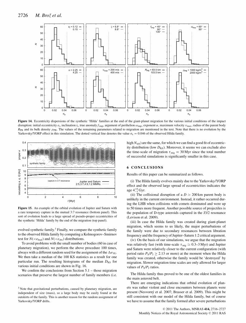
This time, we decided to use a simple quantity to discuss theresults, namely the eccentricity dispersion σe of the synthetic familyat the end of the giant-planet migration. The most frequent values ofthe dispersion are σe = 0.015–0.04 (see the histograms in Fig. 14).Further evolution by the Yarkovsky/YORP effect would increase thedispersions up to σe = 0.045–0.06, while the observed dispersionof the Hilda family is σe = 0.046.

It is notable that the histograms look similar for all the impact pa-rameters, there is even no apparent correlation between them. Theexplanation for this ‘lack of dependence’ is that the eccentricitydistribution is mainly determined by the perturbations of the giantplanets. A given planetary evolution therefore gives a characteristicvalue of σe whatever the impact parameters are. The dispersion inσe values is due to the fact that the planetary evolutions that we havecomputed change widely from one simulation to another. Thoughplanet migration was prescribed analytically, there are mutual in-teractions between planets and random captures in resonances (orjumps across resonances) which may affect the eccentricity dis-tribution of the synthetic Hilda family. An extreme case is shownin Fig. 15. In this particular simulation, Jupiter and Saturn werecaptured in the mutual 3:7 resonance for 0.5 Myr which resulted ina large eccentricity dispersion σe = 0.044 of the synthetic family.Our conclusion is that the impact parameters are less important thanthe parameters related to migration.

5.3 Matching results together

Even though we do not perform a joint integration which includesboth the planetary migration and Yarkovsky/YORP effect, we try tomatch the previous results from Sections 5.1 and 3.5. We do it by us-ing a straightforward Monte Carlo approach: (i) we take the pseudo-proper eccentricities emig of bodies at the end of planetary migrationfrom Section 5.1; (ii) we compute the total Yarkovsky/YORP drifts�eYE in eccentricity from Section 3.5; (iii) we assign every body adrift randomly (efinal = emig + �eYE) and this way we construct an

Figure 13. The number of simulations N versus the fraction of remaining bodies Nleft/Ninitial from the synthetic ‘Hilda’ family. The histograms are plotted forfour different time-scales of migration τmig and six different initial configurations of Jupiter and Saturn (aJi, aSi; we indicate period ratios PSi/PJi instead ofsemimajor axes here). The ranges of the remaining free parameters are mentioned in the text. We only plot the successful migration scenarios with �vplanets ≤2000 m s−1, where �vplanets = ∑4

1 δvi is a sum of the velocity differences δv (defined similarly as in the HCM metric, equation 3) between the final simulatedorbit of the ith planet and the currently observed one. This way we join differences in orbital elements a, e, I into a single quantity which has the dimension ofvelocity.


2726 M. Broz et al.

Figure 14. Eccentricity dispersions of the synthetic ‘Hilda’ families at the end of the giant-planet migration for the various initial conditions of the impactdisruption: initial eccentricity ei, inclination ii, true anomaly f imp, argument of perihelion ωimp, exponent α, maximum velocity vmax, radius of the parent bodyRPB and its bulk density ρPB. The values of the remaining parameters related to migration are mentioned in the text. Note that there is no evolution by theYarkovsky/YORP effect in this simulation. The dotted vertical line denotes the value σe = 0.046 of the observed Hilda family.

Figure 15. An example of the orbital evolution of Jupiter and Saturn witha rare temporary capture in the mutual 3:7 resonance (bottom panel). Thissort of evolution leads to a large spread of pseudo-proper eccentricities ofthe synthetic ‘Hilda’ family by the end of the migration (top panel).

evolved synthetic family.3 Finally, we compare the synthetic familyto the observed Hilda family by computing a Kolmogorov–Smirnovtest for N(<efinal) and N(<eobs) distributions.

To avoid problems with the small number of bodies (60 in case ofplanetary migration), we perform the above procedure 100 times,always with a different random seed for the assignment of the �eYE.We then take a median of the 100 KS statistics as a result for oneparticular run. The resulting histograms of the median DKS forvarious initial conditions are shown in Fig. 16.

We confirm the conclusions from Section 5.1 – those migrationscenarios that preserve the largest number of family members (i.e.

3 Note that gravitational perturbations, caused by planetary migration, areindependent of size (mass), so a large body may be easily found at theoutskirts of the family. This is another reason for the random assignment ofYarkovsky/YORP drifts.

high N left) are the same, for which we can find a good fit of eccentric-ity distribution (low DKS). Moreover, it seems we can exclude alsothe time-scale of migration τmig = 30 Myr since the total numberof successful simulations is significantly smaller in this case.

6 C O N C L U S I O N S

Results of this paper can be summarized as follows.

(i) The Hilda family evolves mainly due to the Yarkovsky/YORPeffect and the observed large spread of eccentricities indicates theage 4+0

−1 Gyr.(ii) The collisional disruption of a D � 200 km parent body is

unlikely in the current environment. Instead, it rather occurred dur-ing the LHB when collisions with comets dominated and were upto 50 times more frequent. Another possible source of projectiles isthe population of D-type asteroids captured in the J3/2 resonance(Levison et al. 2009).

(iii) In case the Hilda family was created during giant-planetmigration, which seems to us likely, the major perturbations ofthe family were due to secondary resonances between librationfrequency and the frequency of Jupiter–Saturn 1:2 critical argument.

(iv) On the basis of our simulations, we argue that the migrationwas relatively fast (with time-scale τmig � 0.3–3 Myr) and Jupiterand Saturn were relatively closer to the current configuration (withperiod ratio PS/PJ ≥ 2.13 or more) at the moment when the Hildafamily was created, otherwise the family would be ‘destroyed’ bymigration. Slower migration time scales are only allowed for largervalues of PS/PJ ratios.

The Hilda family thus proved to be one of the oldest families inthe main asteroid belt.

There are emerging indications that orbital evolution of plan-ets was rather violent and close encounters between planets werepresent (Nesvorny et al. 2007; Brasser et al. 2009). This might bestill consistent with our model of the Hilda family, but of coursewe have to assume that the family formed after severe perturbations



Figure 16. The number of simulations N versus the Kolmogorov–Smirnov distance DKS between the synthetic and the observed Hilda family. The simulationsdiffer by the time-scale of migration τmig and the initial conditions for Jupiter and Saturn (aJi, aSi). We only plot the successful migration scenarios with�vplanets ≤ 2000 m s−1 and the number of bodies left Nleft > Ninitial/2. The dotted vertical line denotes the distance DKS for which the probability p(>DKS)that the two eccentricity distributions differ by this amount equals 0.01.

in the J3/2 region ended. A more complicated migration scenariolike that of ‘jumping Jupiter’ (Morbidelli et al. 2010) even seemsfavourable in our case because Jupiter and Saturn very quickly reacha high period ratio (PS/PJ � 2.3, i.e. the planets are quite close totheir current orbits). Then, the perturbations acting on the J3/2 re-gion are already small and the flux of impactors becomes high justafter the jump. The Hilda family thus might have formed exactlyduring this brief period of time.

Regarding future improvements of our model, knowledge of ge-ometric albedos for a large number of small asteroids may signifi-cantly help and decrease uncertainties. The WISE infrared missionseems to be capable of obtaining these data in near future.

AC K N OW L E D G M E N T S

We thank Hal Levison for his code on eccentricity damping, DavidCapek for sending us the YORP effect data in an electronic formand an anonymous referee for constructive comments.

The work of MB and DV has been supported by the Grant Agencyof the Czech Republic (grants 205/08/P196 and 205/08/0064) andthe Research Program MSM0021620860 of the Czech Ministry ofEducation. We also acknowledge the provision of computers to usat the Observatory and Planetarium in Hradec Kralove.

REFERENCES

Benz W., Asphaug E., 1999, Icarus, 142, 5Bottke W. F., Nolan M. C., Greenberg R., Kolvoord R. A., 1994, Icarus,

107, 255Bottke W. F., Vokrouhlicky D., Broz M., Nesvorny D., Morbidelli A., 2001,

Sci, 294, 1693Bottke W. F., Durda D. D., Nesvorny D., Jedicke R., Morbidelli A.,

Vokrouhlicky D., Levison H. F., 2005, Icarus, 175, 111Bottke W. F., Nesvorny D., Grimm R. E., Morbidelli A., O’Brien D. P.,

2006, Nat, 439, 821Bottke W. F., Nesvorny D., Vokrouhlicky D., Morbidelli A., 2010, AJ, 139,

994Brasser R., Morbidelli A., Gomes R., Tsiganis K., Levison H. F., 2009,

A&A, 507, 1053Broz M., 2006, PhD thesis, Charles Univ.Broz M., Vokrouhlicky D., 2008, MNRAS, 390, 715Capek D., Vokrouhlicky D., 2004, Icarus, 172, 526Dahlgren M., 1998, A&A, 336, 1056Davis D. R., Neese C., eds, 2002, Asteroid Albedos. EAR-A-5-DDR-

ALBEDOS-V1.1. NASA Planetary Data SystemDohnanyi J. W., 1969, J. Geophys. Res., 74, 2531

Farinella P., Froeschle C., Gonczi R., 1994, in Milani A., Di Martino M.,Cellino A., eds, Asteroids, Comets, Meteors 1993. Kluwer, Dordrecht,p. 205

Farinella P., Vokrouhlicky D., Hartmann W. K., 1998, Icarus, 132, 378Fernandez Y. R., Jewitt D., Ziffer J. E., 2009, AJ, 138, 240Ferraz-Mello S., Michtchenko T. A., Nesvorny D., Roig F., Simula A., 1998,

P&SS, 46, 1425Gomes R., Levison H. F., Tsiganis K., Morbidelli A., 2005, Nat, 435, 466Gudel M., 2007, Living Rev. Solar Phys., 4, 3Hill G., 1982, Publ. Dom. Astrophys. Obser. Victoria BC, 16, 67Kortenkamp S. J., Malhotra R., Michtchenko T., 2004, Icarus, 167, 347Leinhardt Z. M., Stewart S. T., 2009, Icarus, 199, 542Levison H. F., Duncan M., 1994, Icarus, 108, 18Levison H. F., Morbidelli A., Vanlaerhoven Ch., Gomes R., Tsiganis K.,

2008, Icarus, 196, 258Levison H. F., Bottke W. F., Gounelle M., Morbidelli A., Nesvorny D.,

Tsiganis K., 2009, Nat, 460, 364Malhotra R., 1995, AJ, 110, 420Minton D. A., Malhotra R., 2009, Nat, 457, 1109Morbidelli A., Moons M., 1993, Icarus, 102, 316Morbidelli A., Levinson H. F., Tsiganis K., Gomes R., 2005, Nat, 435,

459Morbidelli A., Brasser R., Tsiganis K., Gomes R., Levison H. F., 2009,

A&A, 507, 1041Morbidelli A., Brasser R., Gomes R., Levison H. F., Tsiganis K., 2010, AJ,

140, 1391Nesvorny D., Ferraz-Mello S., 1997, Icarus, 130, 247Nesvorny D., Bottke W. F., Levison H. F., Dones L., 2003, ApJ, 591, 486Nesvorny D., Jedicke R., Whiteley R. J., Ivezic Z., 2005, Icarus, 173, 132Nesvorny D., Vokrouhlicky D., Morbidelli A., 2007, AJ, 133, 1962Parker A., Ivezic Z., Juric M., Lupton R., Sekora M. D., Kowalski A., 2008,

Icarus, 198, 138Press W. H., Teukolsky S. A., Vetterlink W. T., Flannery B. P., 1999, Nu-

merical Recipes in Fortran 77. Cambridge Univ. Press, CambridgeQuinn T. R., Tremaine S., Duncan M., 1991, AJ, 101, 2287Roig F., Ferraz-Mello S., 1999, Planet. Space Sci., 47, 653Roig F., Nesvorny D., Ferraz-Mello S., 2002, MNRAS, 335, 417Tanga P., Cellino A., Michel P., Zappata V., Paolicchi P., Dell’Oro A., 1998,

Icarus, 141, 65Tsiganis K., Gomes R., Morbidelli A., Levison H. F., 2005, Nat, 435, 459Tsiganis K., Knezevic Z., Varvoglis H., 2007, Icarus, 186, 484Vokrouhlicky D., Broz M., Bottke W. F., Nesvorny D., Morbidelli A., 2006a,

Icarus, 182, 92Vokrouhlicky D., Broz M., Bottke W. F., Nesvorny D., Morbidelli A., 2006b,

Icarus, 182, 118Vokrouhlicky D., Nesvorny D., Levison H. F., 2008, AJ, 136, 1463Zappala V., Cellino A., Farinella P., Milani A., 1994, AJ, 107, 772

This paper has been typeset from a TEX/LATEX file prepared by the author.


did the hilda collisional family form during the late heavy

Documents