diagnostics of forecasts for polar regions - ecmwf · magnusson, l: diagnostics of forecasts for...

Diagnostics of forecasts for polar regions

Linus Magnusson

ECMWF, Shinfield Park, ReadingRG2 9AX, United [email protected]

1 Introduction

European Centre for Medium-range Weather Forecasts (ECMWF) has produced global deterministic(i.e. single realization without uncertainty estimation, HRES hereafter) forecasts since 1981. Since1992, an ensemble of forecasts is run at a lower resolution to estimate forecast uncertainty and provideprobabilistic forecasts. Because all forecasts are using a global model,the polar regions are included,but the model is not specifically tuned for these areas. In this report, with afocus on the polar regions, anoverview of the improvement of the forecast quality will be given and various aspects of the ensemble(ENS) will be discussed. A study on a similar topic was presented inJung and Leutbecher(2007).

The polar regions are in many aspects different to lower latitudes. From theobservational system pointof view, the challenging environment lead to difficulties deploying in-situ based observations. Thisresults in fewer observations in the data assimilation system as well as little data to verify the forecastresults against. Regarding the atmospheric interactions, the connection between the troposphere andthe stratosphere is believed to be stronger around the poles than elsewhere and the interaction betweensnow-cover, sea-ice and the atmosphere is unique for these regions.

The aim of ensemble prediction is to forecast uncertainties and provide a basis for probabilistic forecasts.The uncertainties in the forecasts originate from uncertainties in the data assimilation (analysis) togetherwith uncertainties in the model formulation and the truncated model resolution. Inorder to simulate theforecast uncertainty, 50 perturbed forecasts are run. Each of themis initialised from a perturbed analysisto simulate the uncertainty in the initial conditions. The initial perturbations for the ECMWF ENS aregenerated from an ensemble of data assimilations (Buizzaet al., 2008; Isaksenet al., 2010) togetherwith singular vectors (Molteni et al., 1999). To simulate the model uncertainty, Stochastically PerturbedPhysical Tendencies (SPPT) scheme is used together with a stochastic backscatter scheme (Palmeret al.,2009).

The way the differences between the perturbed forecasts evolve in time depends on the flow in the atmo-sphere. In situations of high predictability, the difference between the ensemble members is expected togrow slowly with time, while uncertain conditions should result in a large spreadamong the ensemblemembers. As a first order measure of the reliability of the simulated uncertainties, the standard deviationof the ensemble should match, on average, the root-mean-square-error(RMSE) of the ensemble mean.However, this assumes that the random component of the forecast error dominates over the systematiccomponent (bias).

To simulate the uncertainties correctly, one needs to include all components that can contribute to thediversity among the ensemble members. If the model system does not include e.g a sea-ice model,the uncertainties in the atmosphere due to the sea-ice evolution will not be captured. Furthermore, ifthe model lacks variability in a component, the uncertainty will be underestimated.Another importantaspect is that the ensemble system can only simulate uncertainties larger than the grid box scale. In otherwords, small scale variability inside the box will not be captured as long as thevalue from the model

ECMWF-WWRP/THORPEX Workshop on Polar Prediction, 24 - 27 June 2013 1

MAGNUSSON, L: D IAGNOSTICS OF FORECASTS FOR POLAR REGIONS. . .

is supposed to represent the entire grid box. The latter issue is especially aproblem near the groundsurface if the grid box is inhomogeneous in properties such as land-sea,orography and snow cover.

The data in this report are based on the ECMWF IFS forecasting system. The scores are mainly basedon forecasts from 2012, when the HRES used spectal resolution TL1279 (16 km) with 91 vertical levels,and the ENS TL639 (32 km) with 62 vertical levels. We will also use the control forecast for ENS, whichis an unperturbed forecast run with the same resolution as ENS.

In Section2 the general predictability of weather in the polar regions and its developmentduring thepast 25 years. Even though the forecasts have improved in general, thesystem occasionally producesbad forecasts and such a case will be evaluated in Section3. In section4 the ability of simulating theuncertainties in the Arctic are evaluated. The effect of satellite observations on the EDA in the polarregions is presented in Section5 and the properties of the SPPT scheme in the Arctic is discussed inSection6. Finally the results are summarised in Section7.

2 Predictability in the Polar regions

In this report we define the Arctic (N.Pole hereafter) as north of 65◦N and the Antarctic as south of 65◦S(S.Pole hereafter). The northern hemisphere (N.Hem) is defined as 20◦N-90◦N and southern hemisphere(S.Hem) as 20◦S-90◦S (which both exclude the tropics).

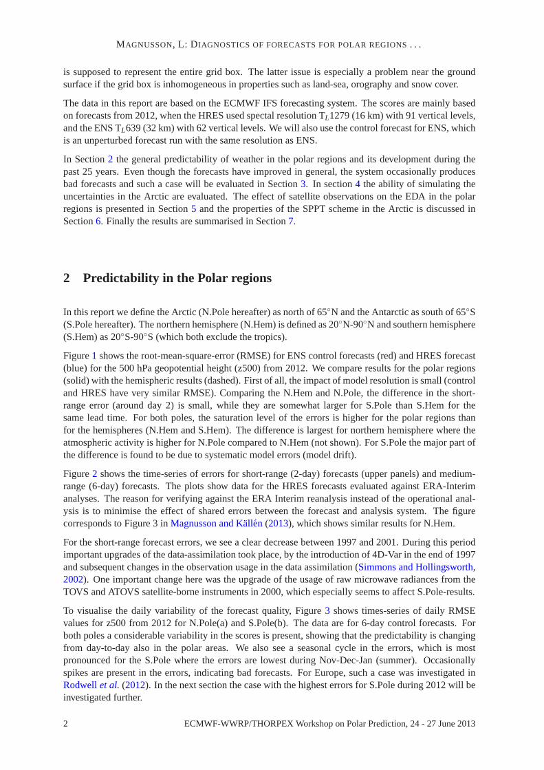
Figure1 shows the root-mean-square-error (RMSE) for ENS control forecasts (red) and HRES forecast(blue) for the 500 hPa geopotential height (z500) from 2012. We compare results for the polar regions(solid) with the hemispheric results (dashed). First of all, the impact of modelresolution is small (controland HRES have very similar RMSE). Comparing the N.Hem and N.Pole, the difference in the short-range error (around day 2) is small, while they are somewhat larger for S.Pole than S.Hem for thesame lead time. For both poles, the saturation level of the errors is higher forthe polar regions thanfor the hemispheres (N.Hem and S.Hem). The difference is largest for northern hemisphere where theatmospheric activity is higher for N.Pole compared to N.Hem (not shown). For S.Pole the major part ofthe difference is found to be due to systematic model errors (model drift).

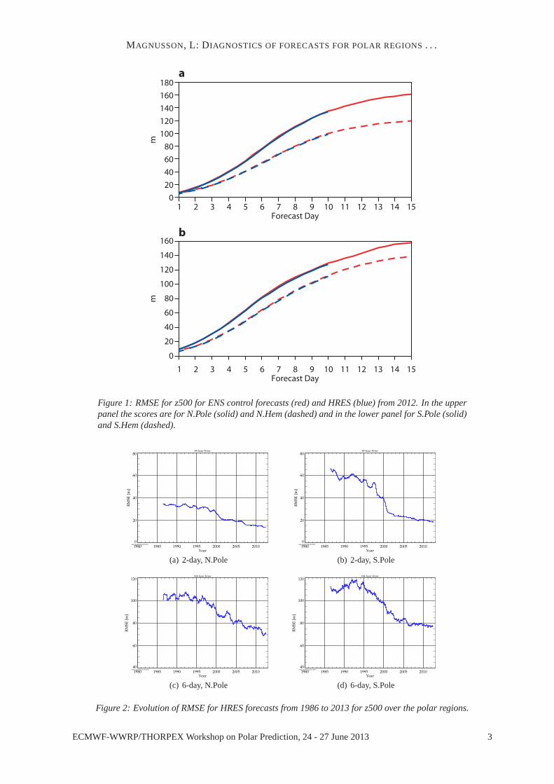
Figure2 shows the time-series of errors for short-range (2-day) forecasts (upper panels) and medium-range (6-day) forecasts. The plots show data for the HRES forecastsevaluated against ERA-Interimanalyses. The reason for verifying against the ERA Interim reanalysisinstead of the operational anal-ysis is to minimise the effect of shared errors between the forecast and analysis system. The figurecorresponds to Figure 3 inMagnusson and Kallen(2013), which shows similar results for N.Hem.

For the short-range forecast errors, we see a clear decrease between 1997 and 2001. During this periodimportant upgrades of the data-assimilation took place, by the introduction of 4D-Var in the end of 1997and subsequent changes in the observation usage in the data assimilation (Simmons and Hollingsworth,2002). One important change here was the upgrade of the usage of raw microwave radiances from theTOVS and ATOVS satellite-borne instruments in 2000, which especially seems toaffect S.Pole-results.

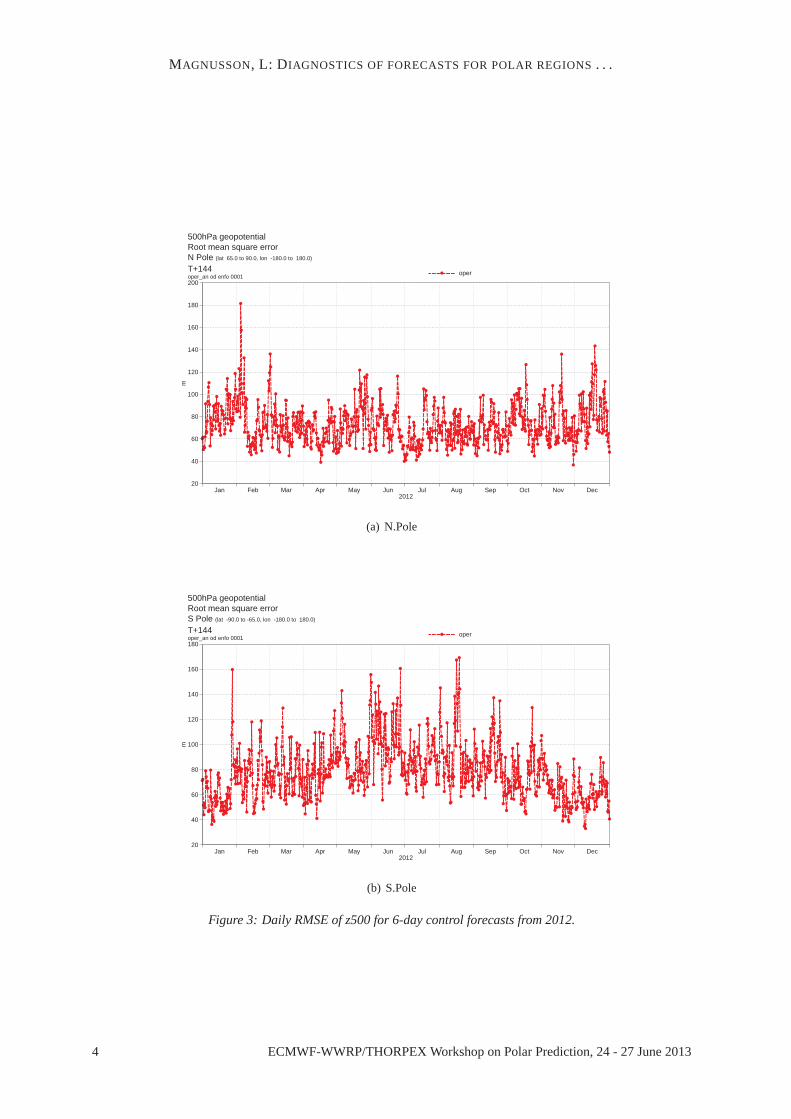
To visualise the daily variability of the forecast quality, Figure3 shows times-series of daily RMSEvalues for z500 from 2012 for N.Pole(a) and S.Pole(b). The data are for 6-day control forecasts. Forboth poles a considerable variability in the scores is present, showing that the predictability is changingfrom day-to-day also in the polar areas. We also see a seasonal cycle inthe errors, which is mostpronounced for the S.Pole where the errors are lowest during Nov-Dec-Jan (summer). Occasionallyspikes are present in the errors, indicating bad forecasts. For Europe, such a case was investigated inRodwellet al. (2012). In the next section the case with the highest errors for S.Pole during 2012 will beinvestigated further.

2 ECMWF-WWRP/THORPEX Workshop on Polar Prediction, 24 - 27 June2013


0

20

40

60

80

100

120

140

160

180

m

Forecast Day87654321 9 10 11 12 13 14 15

Forecast Day87654321 9 10 11 12 13 14 15

a

0

20

40

60

80

100

120

140

160

m

b

Figure 1: RMSE for z500 for ENS control forecasts (red) and HRES (blue) from 2012. In the upperpanel the scores are for N.Pole (solid) and N.Hem (dashed) and in the lower panel for S.Pole (solid)and S.Hem (dashed).

48-hour Error

1980 1985 1990 1995 2000 2005 2010Year

0

20

40

60

80

RM

SE

[m

]

e48_npole2) Jun 20 2013

(a) 2-day, N.Pole

48-hour Error

1980 1985 1990 1995 2000 2005 2010Year

0

20

40

60

80

RM

SE

[m

]

e48_spole2) Jun 20 2013

(b) 2-day, S.Pole

144-hour Error

1980 1985 1990 1995 2000 2005 2010Year

40

60

80

100

120

RM

SE

[m

]

e144_npole2) Jun 20 2013

(c) 6-day, N.Pole

144-hour Error

1980 1985 1990 1995 2000 2005 2010Year

40

60

80

100

120

RM

SE

[m

]

e144_spole2) Jun 20 2013

(d) 6-day, S.Pole

Figure 2: Evolution of RMSE for HRES forecasts from 1986 to 2013 for z500 over the polar regions.



20

40

60

80

100

120

140

160

180

200

m

Jan Feb Mar Apr May Jun Jul Aug Sep Oct Nov Dec2012

oper_an od enfo 0001T+144N Pole (lat 65.0 to 90.0, lon -180.0 to 180.0)

Root mean square error500hPa geopotential

oper

(a) N.Pole

20

40

60

80

100

120

140

160

180

m

Jan Feb Mar Apr May Jun Jul Aug Sep Oct Nov Dec2012

oper_an od enfo 0001T+144S Pole (lat -90.0 to -65.0, lon -180.0 to 180.0)


oper

(b) S.Pole

Figure 3: Daily RMSE of z500 for 6-day control forecasts from2012.



3 Example of a problematic forecast for the Antarctic

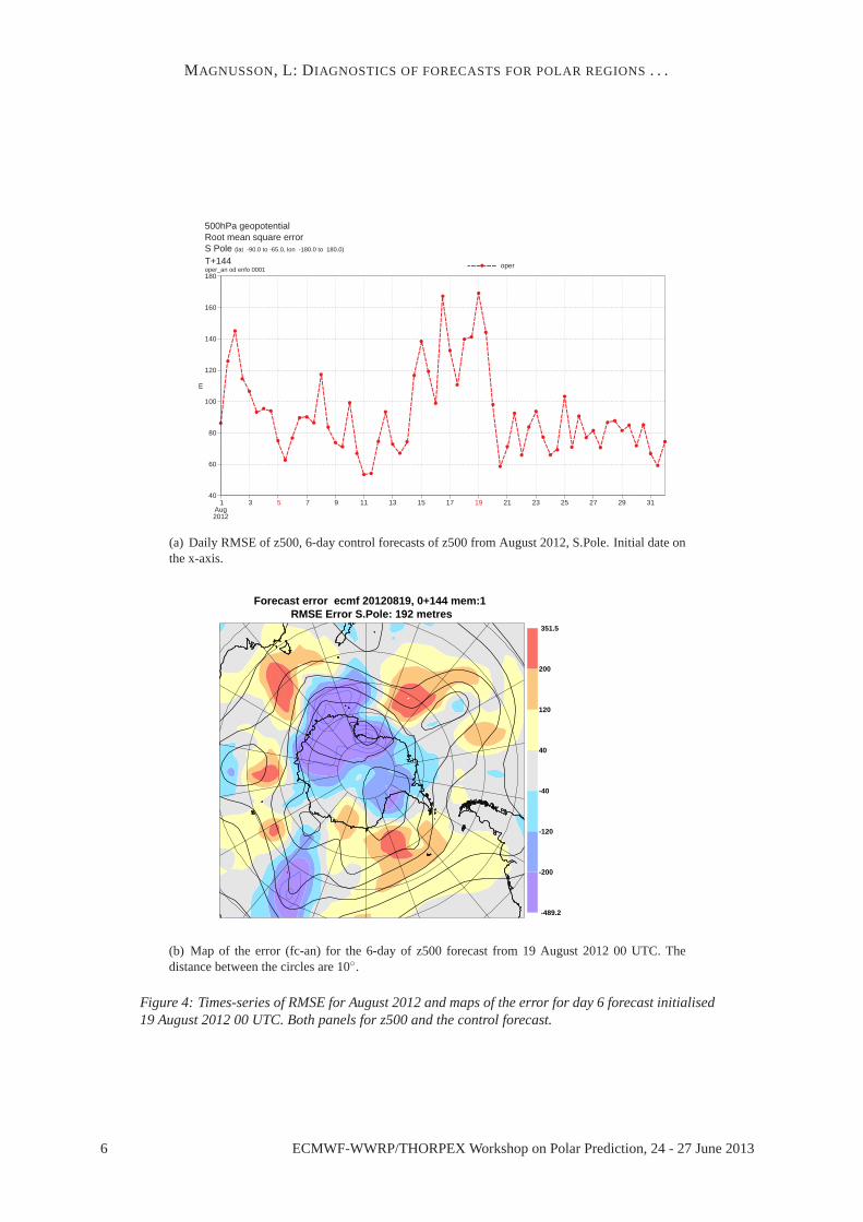
Figure4(a) shows the same as Figure3(b), but only for August 2012. Between the 15 August and 19August the forecasts resulted in a period of large errors. In Figure4(b) a map of the error (forecast-analysis) for the 6-day forecast for the 19 August 00 UTC is plotted. A large part of the Antarcticexperienced a negative error, while the error equatorward of 70◦S had a positive sign. This indicates thatit is not a single synoptic weather system causing the major part of the errorbut rather a more large-scalefeature or a combination of both.

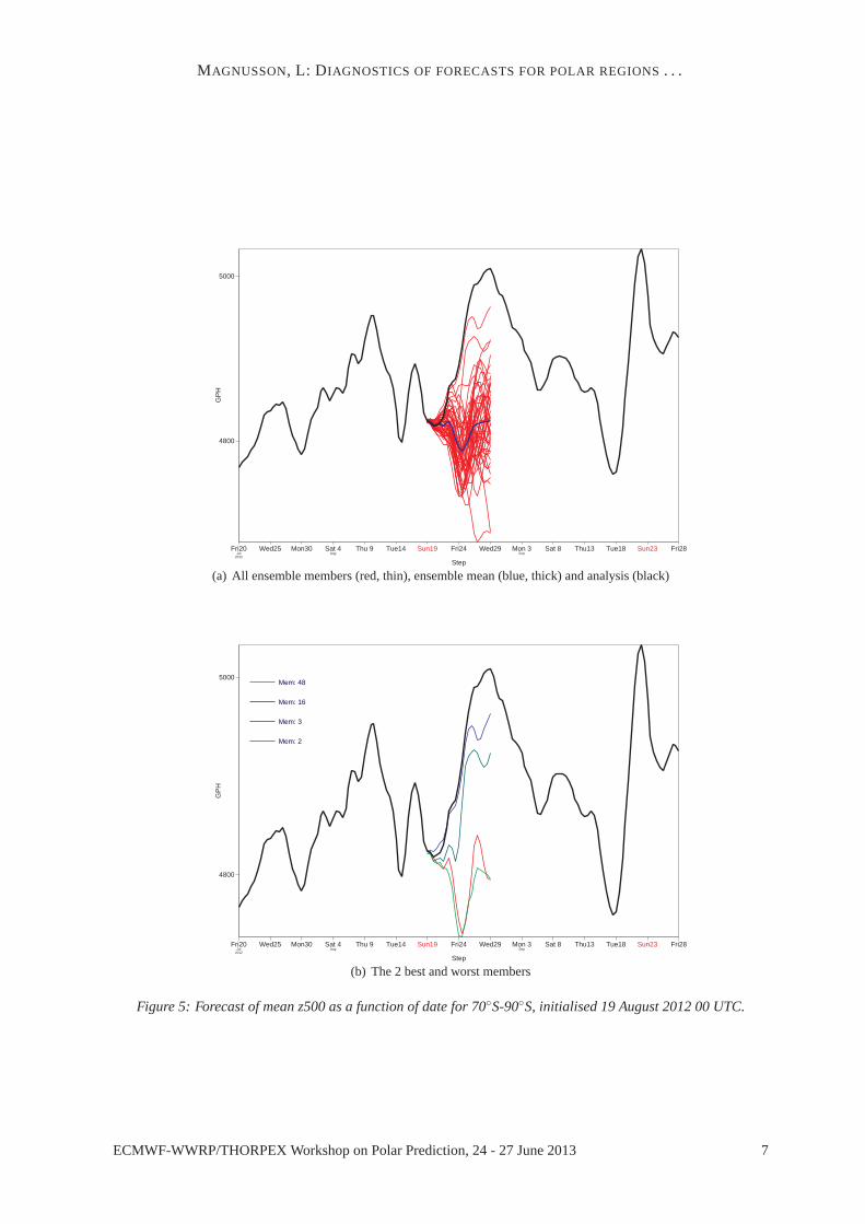
Figure5 shows the observed time-series of the mean z500 south of 70◦S. Here a rapid increase in thegeopotential height after 20 August appears, with a peak on 29 August.In the figure all ensemble mem-bers from 19 August 00 UTC are plotted (red, thin) together with the ensemble mean (blue, thick). Mostof the members did not capture the increased geopotential height, causing anegative error. However,we find a few members that at least partially captured the development in the atmosphere. In the lowerpanel the 2 best and the 2 worst members are plotted and will be analysed further.

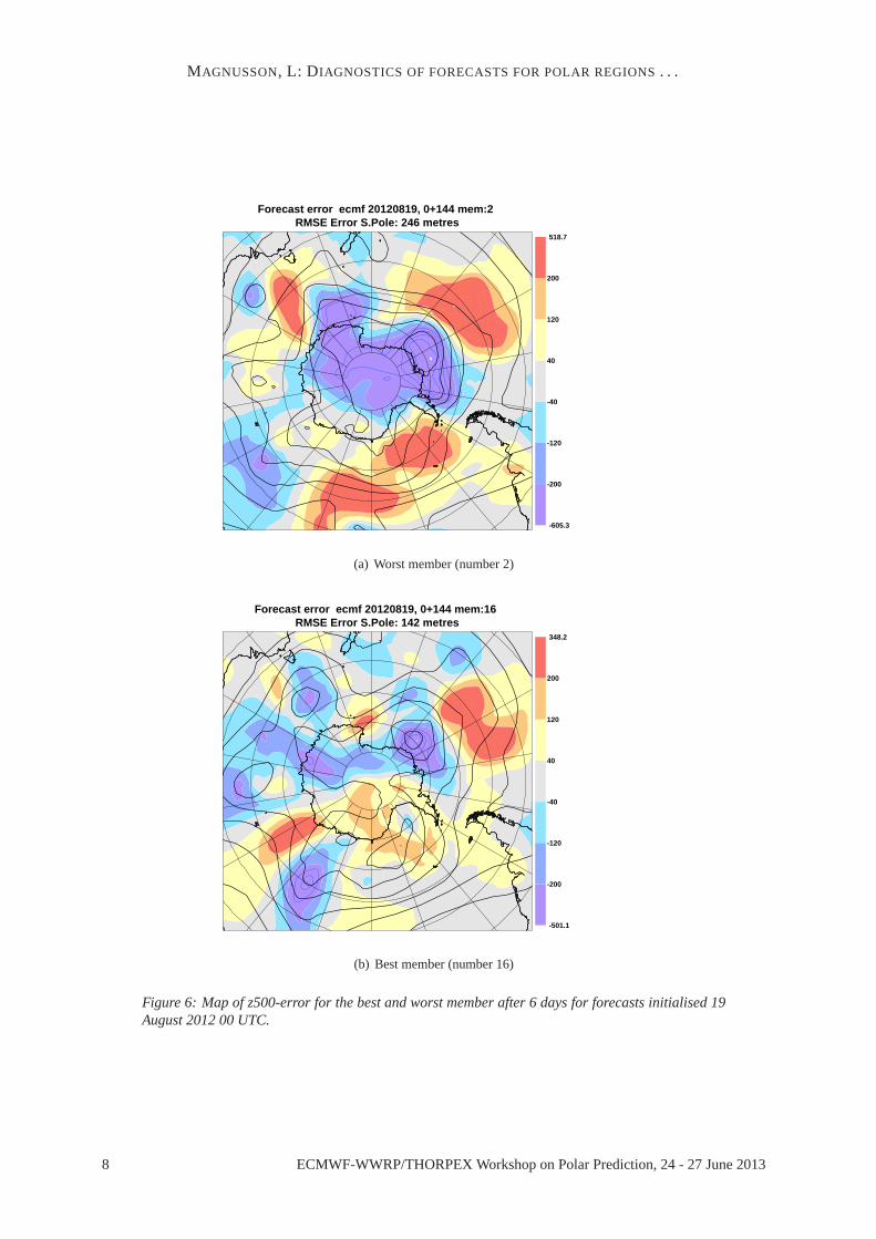
The panels in Figure6 show maps of errors for the best and the worst ensemble member from 19 August00 UTC. Here we see a large difference in the large scale, where the worst member has the negative errorover the Antarctic, while the best member does not. However, the best memberhas still large errors insynoptic scale structures.

The large-scale structure of the error for this case points to an externalforcing. Such a candidate isthe stratosphere. Anomalous evolutions in the stratosphere over Antarcticahave been investigated inthe context of ECMWF forecasts inSimmonset al. (2005). In order to investigate the evolution of thestratosphere, a Hovmoller diagram of the temperature anomaly from ERA Interim is plotted in Figure7. Here we see a warm anomaly in the stratosphere, which starts to propagatedownwards after 13August. One can suspect that this stratospheric warming influenced the troposphere. Figure8 shows theevolution for the best and worst ensemble members for the temperature at 50hPa. Here both the best andworst members captured the evolution reasonably and, if anything, the best members broke down thewarming event too early. So one could speculate that the failing developmentis due to the connectionbetween the stratosphere and the troposphere in the model.

These results suggest that the error was because the downward propagation of a stratospheric warmingevent was not well captured, although we cannot rule out other sources for the error. Most of theensemble members did not capture the evolution in the troposphere, but a fewensemble members did.A deeper investigation is needed to see what aspects of the perturbations caused the event to be bettercaptured. In general,Vitart (2013) showed that the current version of the ECMWF model has a too weakconnection between the stratosphere and the troposphere for the Arctic.This could be the case also forthe Antarctic. However, more cases of large errors needs to be investigated to see if they normallyoriginate from the stratosphere.

4 Simulating uncertainties in the Arctic

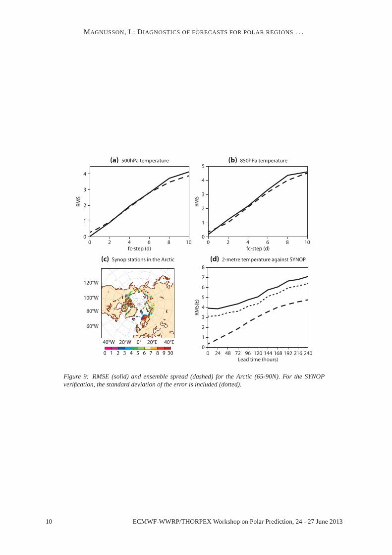
Figure9 shows the ensemble mean RMSE and the ensemble standard deviation (hereafter referred to asensemble spread) for boreal winter forecasts from 2012. For a perfect ensemble, these quantities shouldmatch each other for all lead times (seeLeutbecher and Palmer(2008)). For the temperature at 500 hPaover the Arctic (Figure9(a)), the relation holds well for all lead times. Further down in the troposphere(850 hPa, Figure9(b)), the ensemble is somewhat under-dispersive. However, in this diagnostic we havenot accounted for errors in the verification data set (Saetraet al., 2004). By accounting for these errors,it is possible that the ensemble turns out to be somewhat over-dispersive for 500 hPa temperature.

Figure9(d) shows the RMSE (solid) and ensemble standard deviation (dashed) for 2-metre temperature



40

60

80

100

120

140

160

180

m

1 3 5 7 9 11 13 15 17 19 21 23 25 27 29 31Aug2012

oper_an od enfo 0001T+144S Pole (lat -90.0 to -65.0, lon -180.0 to 180.0)


oper

(a) Daily RMSE of z500, 6-day control forecasts of z500 from August 2012, S.Pole. Initial date onthe x-axis.

RMSE Error S.Pole: 192 metresForecast error ecmf 20120819, 0+144 mem:1

-489.2

-200

-120

-40

40

120

200

351.5

(b) Map of the error (fc-an) for the 6-day of z500 forecast from 19 August 2012 00 UTC. Thedistance between the circles are 10◦.

Figure 4: Times-series of RMSE for August 2012 and maps of theerror for day 6 forecast initialised19 August 2012 00 UTC. Both panels for z500 and the control forecast.



Fri20 Wed25 Mon30 Sat 4 Thu 9 Tue14 Sun19 Fri24 Wed29 Mon 3 Sat 8 Thu13 Tue18 Sun23 Fri28Jul Aug Sep

2012

Step

4800

5000

GP

H

(a) All ensemble members (red, thin), ensemble mean (blue, thick) andanalysis (black)


2012

Step

4800

5000

GP

H

Mem: 2

Mem: 3

Mem: 16

Mem: 48

(b) The 2 best and worst members

Figure 5: Forecast of mean z500 as a function of date for 70◦S-90◦S, initialised 19 August 2012 00 UTC.




-605.3

-200

-120

-40

40

120

200

518.7

(a) Worst member (number 2)


-501.1

-200

-120

-40

40

120

200

348.2

(b) Best member (number 16)

Figure 6: Map of z500-error for the best and worst member after 6 days for forecasts initialised 19August 2012 00 UTC.



1 2 3 4 5 6 47–1–2

Mon13

Wed8

Fri3

Aug

Sun29

Tue24

Thu19Jul

Sat18

Thu23

Tue28

Sun2

Sep

Fri7

Wed12

Mon17

–3–4–5–6–28

500

200

100

50

20

10

5

2

1

Figure 7: Hovmoller diagram of the mean temperature anomaly from ERA Interim, south of 70◦S.X-axis represents time and y-axis pressure.


2012

Step

185

190

195

T (

K)

Mem: 2

Mem: 3

Mem: 16

Mem: 48

Figure 8: Mean temperature for 50 hPa south of 70◦S as a function of date. Analysis (black) andsame ensemble members as in Figure6(b).



0

1

2

3

4

RM

S

1086420fc-step (d)

1086420fc-step (d)

0

1

2

3

4

5

RM

S

50°N

70°N

90°N

60°W

80°W

100°W

120°W

0°20°W 40°E20°E40°W

0 1 2 3 4 5 6 7 8 9 30 120967248240 144 168 192 216 240Lead time (hours)

0

1

2

3

4

5

6

7

8

RM

S(E

)

(a) 500hPa temperature (b) 850hPa temperature

(c) Synop stations in the Arctic (d) 2-metre temperature against SYNOP

Figure 9: RMSE (solid) and ensemble spread (dashed) for the Arctic (65-90N). For the SYNOPverification, the standard deviation of the error is included (dotted).

10 ECMWF-WWRP/THORPEX Workshop on Polar Prediction, 24 - 27 June 2013


verified against SYNOP observations. The observation network used here is shown in Figure9(c). Forthe 2-metre temperature there is a large difference between the error and the spread. While the amplitudeof the spread has the same magnitude as for 850 hPa, the error is much larger. Several factors can play arole here. Firstly, systematic model errors will increase the error level. For example the cloud modellingis a well-known source of uncertainty (see e.gSvensson and Karlsson(2011); Karlsson and Svensson(2011)). In order to remove the effect of model bias, the standard deviation ofthe error is included inFigure9(c).

Another source of differences between observations and model data issub-grid variability. The sub-gridvariability could be due to small-scale weather features such as convectivecells, but also to sub-gridvariability in the boundary conditions. Examples of such variabilities are orography, land-sea-lake con-trasts and snow conditions. For the 2-metre temperature in the polar areas these three items constitute alarge source of variability, especially considering that many of the observation stations are located eitherclose to the sea or in low level terrain, affected by strong inversions in winter. To illustrate the problem,Figure10shows a 3-day HRES forecast from 7 February 2013 00 UTC and corresponding observationsof 2-metre temperature for the stations Tarfala and Nikkalouta in northern Sweden. The stations areseparated by 17 kilometres, but while Tarfala is located far up a steep, down-sloping valley, Nikkaluotais located in the bottom of a gentle valley. For Tarfala the temperature forecast is in good agreementwith the observations, while for Nikkalouta the forecast is about 20◦C too warm. The forecasts for bothstations are very similar. The large difference in the observed values forNikkalouta is due to a stronginversion. The inversion temporary broke up at midday on the 8 Februaryand the temperatures becamehigher than the forecast. To address the issue with strong local inversions, one needs either a muchhigher model resolution or a parametrisation of the sub-grid uncertainty. For an ensemble system, thelatter is essential in order to catch the true forecast uncertainty.

In this section we have pointed out some difficulties in diagnosing the spread inthe ensemble system. Itis hard to disentangle the the lack of spread in the ensemble system from systematic model errors andrepresentativeness errors between the model grid and the observations. If one derives the uncertaintiesin the verification data set, that component could be accounted for followingSaetraet al. (2004).

5 Impact of polar orbiting satellites on EDA standard deviation

Since June 2010, ECMWF is operationally using an ensemble of data assimilations (EDA) to generate apart of the initial perturbations for the ensemble forecasts and since May 2011 to scale the backgrounderror variances for the data assimilation system (Buizzaet al., 2008; Isaksenet al., 2010). The conceptof the EDA is illustrated in Figure11. The EDA consists of 10 independent 4DVAR data-assimilationcycles, which uses observations perturbed according to observation uncertainty. For the forecasts be-tween the assimilations (first guess forecast), the model uncertainty is simulatedby the SPPT scheme(Palmeret al., 2009).

Although the observations are perturbed, their presence should reduce the dispersion between the EDAmembers to realistic levels. The trivial example is when we do not have any observations to assimi-late, which should lead to a dispersion as large as the climatological variability after a number of dataassimilation cycles.

As discussed in Section2, the introduction of assimilation of polar orbiting satellites clearly reducedthe forecast error in the polar regions. The effects of such data are documented inMcNally (2006);Andersson(2006). In this section we investigate the impact on the EDA standard deviation (spread).For this purpose, an EDA experiment without data from polar orbiting satellites (but still using MODISAMV) was run between 10 October 2012 and 11 November 2012 (hereafter referred to as NoPol). Theexperiment has been evaluated for the impact on hurricane Sandy inMcNally et al.(2013); Magnussonet al.



Thu 7 Fri 8 Sat 9Feb2013

day

-40

-38

-36

-34

-32

-30

-28

-26

-24

-22

-20

-18

-16

-14

-12

-10

-8

-6

-4

-2

0

T2m

020

29

ObsForecast

(a) Tarfala

Thu 7 Fri 8 Sat 9Feb2013

day

-40

-38

-36

-34

-32

-30

-28

-26

-24

-22

-20

-18

-16

-14

-12

-10

-8

-6

-4

-2

0

T2m

020

36

ObsForecast

(b) Nikkaluota

Figure 10: Forecasts (from HRES) and observations of 2-metre temperature.



Figure 11: Concept of Ensemble of data assimilations.

(2013). Optimally, as the analysis error and forecast error increase with less data, the ensemble standarddeviation should do as well.

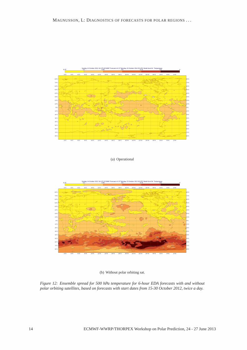
Figure12 shows the EDA spread for the temperature at 500 hPa, for the operational EDA (top panel)and the NoPol experiment (bottom panel). Without the data from the polar orbiting satellites the spreadincreases over the oceans outside the tropics (over the tropics the data from geostationary satellites aredominating). The largest difference is present in the southern hemisphere where the spread increasesby more than 3 times over some areas. The difference is much less pronounced over the Arctic. Theless difference in the Arctic could be due to more conventional observations in that region, compared toAntarctica.

Figure13 shows the verification of an ensemble experiment using EDA perturbations from the experi-ment discussed above. The experiment is initialized from HRES analysis thatalso had the polar orbitingsatellite data omitted. 8 ensemble forecasts have been run with start dates from2012-10-21 to 2012-10-28. One caveat with these results is the limited sample. The figure shows the RMSE of the ensemblemean (left panels) and the ensemble spread (right panels) for N.Pole (upper panels) and S.Pole (lowerpanels). Together with the NoPol ensemble experiment (blue) a control experiment initialised from aHRES analysis and EDA pertubations using all observations (red) is plotted. The forecasts are verifiedagainst the operational HRES analysis. For both polar regions the forecast error increased without thesatellite data. The largest change is seen for S.Pole where the 2-day error is more than doubled. Forthe ensemble spread for S.Pole, we see a similar increase, which is a clear sign that the simulation ofthe forecast uncertainty is capturing the increased forecast error caused by the loss of data. This isnot apparent for N.Pole, where the ensemble spread is similar for the two experiments, although theforecast error increased. One reason for this could be the more complex observation system over theArctic (more observations), which makes the EDA spread more sensitive to the tuning of the errors fromdifferent types of observations.

6 SSPT scheme in the polar areas

To simulate model errors, the ensemble prediction system at ECMWF uses the Stochastically PerturbedPhysics Tendency (SPPT) scheme together with the stochastic backscatterscheme (Palmeret al., 2009).The SPPT scheme perturbs the tendencies from the physics schemes in the model, which includes theconvection, cloud, radiation, vertical diffusion and dissipation. Together with the dynamics scheme(mainly advection), these tendencies give the evolution of the forecast during the integration of the



0°N

10°S

20°S

30°S

40°S

50°S

60°S

70°S

80°S

10°N

20°N

30°N

40°N

50°N

60°N

70°N

80°N

0°N

10°S

20°S

30°S

40°S

50°S

60°S

70°S

80°S

10°N

20°N

30°N

40°N

50°N

60°N

70°N

80°N

20°E 40°E 60°E 80°E 100°E 120°E 140°E 160°E 180°E 160°W 140°W 120°W 100°W 80°W 60°W 40°W 20°W


Sunday 14 October 2012 18 UTC ECMWF Forecast t+6 VT:Monday 15 October 2012 00 UTC Model level 64 Temperature 0.15 0.3 0.45 0.6 0.75 0.9 4

(a) Operational

0°N

10°S

20°S

30°S

40°S

50°S

60°S

70°S

80°S

10°N

20°N

30°N

40°N

50°N

60°N

70°N

80°N

0°N

10°S

20°S

30°S

40°S

50°S

60°S

70°S

80°S

10°N

20°N

30°N

40°N

50°N

60°N

70°N

80°N



Sunday 14 October 2012 18 UTC ECMWF Forecast t+6 VT:Monday 15 October 2012 00 UTC Model level 64 Temperature 0.15 0.3 0.45 0.6 0.75 0.9 4

(b) Without polar orbiting sat.

Figure 12: Ensemble spread for 500 hPa temperature for 6-hour EDA forecasts with and withoutpolar orbiting satellites, based on forecasts with start dates from 15-30 October 2012, twice a day.



0

200

400

600

800

1000

RM

SE

0 2 4 6 8 10fc-step (d)

2012102100-2012102800 (8)rmse_em

z500hPa, Arctic

nopol

control

(a) RMSE N.Pole

0

200

400

600

800

1000

RM

S

0 2 4 6 8 10fc-step (d)

2012102100-2012102800 (8)spread_em

z500hPa, Arctic

nopol

control

(b) Ens.Std N.Pole

0

200

400

600

800

1000

RM

SE

0 2 4 6 8 10fc-step (d)

2012102100-2012102800 (8)rmse_em

z500hPa, Antarctic

nopol

control

(c) RMSE S.Pole

0

200

400

600

800

1000

RM

S

0 2 4 6 8 10fc-step (d)

2012102100-2012102800 (8)spread_em

z500hPa, Antarctic

nopol

control

(d) Ens.Std S.Pole

Figure 13: Average RMSE of ensemble mean and ensemble spreadfor 500 hPa geopotential heightfor experiments with and without polar orbiting satellites. Forecasts initialised 21-28 October 2012,0 UTC.



290

290

330

330

330

330

370

370 370

370

410

270

310

310

310

310

350350

350350

390

390

430

290

290

330

330

330

330

370

370 370

370

410

270

310

310

310

310

350350

350350

390

390

430

290310330

350

370

290310

350

370

330

290

310290

330

350

370

310

330

350

290

(a) Convection (b) Cloud

(c) Radiation (d)Advection

(e)Vert.Di! (f) Dissip

200

500

1000

-4 -2 -1.2 -0.4 0.4 1.2 2 4 -4 -2 -1.2 -0.4 0.4 1.2 2 4

200

500

100090°S60°S30°S0°N30°N60°N90°N 90°S60°S30°S0°N30°N60°N90°N

200

500

1000

-4 -2 -1.2 -0.4 0.4 1.2 2 4 -4 -2 -1.2 -0.4 0.4 1.2 2 4

200

500

100090°S60°S30°S0°N30°N60°N90°N 90°S60°S30°S0°N30°N60°N90°N

200

500

1000

-4 -2 -1.2 -0.4 0.4 1.2 2 4 -0.1 -0.01 -0.006 -0.002 0.002 0.006 0.01 0.1

200

500

100090°S60°S30°S0°N30°N60°N90°N 90°S60°S30°S0°N30°N60°N90°N

Figure 14: Zonal average of mean temperature tendencies from forecast day 0 to 5 (mean from 7 forecasts).

model. By scaling the physical tendencies by a random number the forwardintegration of the model isslightly changed. The random numbers are generated by a pattern simulatorin order to include a spatialscale to the perturbations. The random numbers are also correlated in time. For the boundary layer andthe stratosphere no perturbations from the SPPT scheme are used.

Figure14 shows vertical cross-sections of the mean tendencies from forecast day 0 to 5 for each com-ponent, contributing to the temperature evolution. For the tropics, the dominatingtendencies are awarming by release of latent heat in convection balanced by vertical advection of air and the evaporationof clouds.

For the polar regions the dominant process in the free troposphere is the radiative cooling, which is com-pensated by advection (both horizontal and vertical). By the design of theSPPT scheme, the radiationtendencies will be the dominant contributor for the SPPT perturbations overthe Arctic. One could arguethat this process is well understood, and the uncertainty is low in the process in the free atmosphereduring the Arctic night (by the same argument the SPPT scheme is switched offin the stratosphere).For the Arctic the largest model uncertainties are constrained to the boundary layer, which is not yetperturbed by the SPPT scheme. It is plausible that the resulting lack of model perturbations lead toan under-dispersive ensemble close to the surface (together with other sources of uncertainty such assea-ice), as seen in Figure9.



7 Discussion

In this report various aspects of ECMWF forecasts in the polar regions have been discussed. Since theoperational forecasts started in 1986, the 6-day root-mean-square error (RMSE) has been reduced byabout 30 % for the polar regions. For short-range (2-day) forecast errors the reduction is much larger forthe southern hemisphere (about 60 %). The major part of the reduction took place between 1997-2001and is believed to be due to improvements in the data assimilation leading to a more efficient use ofsatellite observations.

Even though the forecasts have been improved over the years, large errors appear occasionally. In thisreport the event with the highest errors over Antarctica during 2012 was investigated. The error seemsto coincide with a sudden stratospheric warming event. To see if this is a general source of large errors,more cases need to be investigated. However,Vitart (2013) points to a too weak link between suddenstratospheric warnings and the tropospheric development (in the Arctic).This is a process that needsmore diagnostic work to understand and to monitor future model development.

The ensemble is designed for the purpose of simulating the uncertainties in the forecasts. The abilityto simulate the uncertainties has been evaluated for the polar regions by comparing the RMSE of theensemble mean and the standard deviation of the ensemble (ensemble spread). Optimally these twoquantities should match. However, this assumes that the model bias is negligible and that the uncertaintyin the validation data set is small. This may be reasonably true in the free atmosphere over well observedareas. For the Arctic, we see a good match between the quantities for the free atmosphere (t500 andt850 verified against the analysis), but a large difference when we verify 2-metre temperature againstSYNOP observations. In the Arctic during winter-time, the local variability in temperature due to stronginversions can be large. Hence, more work is needed to quantify the sub-grid variability. Without suchan estimate it is hard to decide whether the ensemble is under-dispersive or not.

For the EDA, the impact of assimilating observations from polar orbiting satelliteson the ensemblespread has been investigated. By reducing the number of observations,the error in the analysis isincreased as expected. This seems to be well simulated by the EDA for the Antarctic, while for Arcticthe ensemble spread did not increase to the same degree as the error. Thepresence of more conventionalobservations in the Arctic makes the data assimilation system more complex, and more sensitive to thetuning of the observation uncertainty.

Regarding the SPPT scheme, we recognise the problem with tapering of the perturbations in the bound-ary layer, where we have the largest uncertainties in the polar regions. Instead the perturbations originatemainly from the radiation tendency in the free atmosphere, a process that is less uncertain. Thereforemore development should be undertaken aiming to perturb the model in the boundary layer and alsoinclude the surface modelling.

In this report some key areas of future diagnostics regarding the polar areas have been highlighted, suchas the ability to obtain the correct strength in the teleconnection from the stratosphere to the troposphereand the need for a good estimate for the representativeness error. We also highlighted the impact of satel-lite observations in the EDA and the possibility to run data denial experiments forthe EDA. Regardingthe ensemble system design, the SPPT scheme is going to be revised to better target the uncertainties inthe polar regions in terms of radiation and boundary layer processes, and in the autumn of 2013, initialperturbations of the surface variables will be introduced that will potentiallyaffect the polar areas (atleast on the edge of the snow cover). Finally, the uncertainty caused by sea-ice cover is not representedin the ensemble today, hence the plans for the future also includes introductionof a dynamic sea-icemodel in the prediction system.



Acknowledgements

We would like to acknowledge Trond Iversen, Peter Bauer, Roberto Buizza, Massimo Bonavita, SimonLang, Sarah Keeley, David Richardson, Thomas Haiden and many other for valuable discussions andproviding material for this report and Anabel Bowen for help with the preparation of the figures.

References

Andersson E. 2006. Data assimilation in the Polar Regions. In:Seminar on Polar Meteorology, 4-8September 2006, ECMWF. pp. 89–102.

Buizza R, Leutbecher M, Isaksen L. 2008. Potential use of an ensembleof analyses in the ECMWFEnsemble Prediction System.Q. J. R. Met. Soc.134: 2051–2066.

Isaksen L, Bonavita M, Buizza R, Fisher M, Haseler J, Leutbecher M, Raynaud L. 2010. Ensemble ofData Assimilations at ECMWF. Technical Memorandum 636, ECMWF.

Jung T, Leutbecher M. 2007. Performance of the ECMWF forecasting system in the Arctic duringwinter.Q. J. R. Met. Soc.133: 1327–1340.

Karlsson J, Svensson G. 2011. The simulation of Arctic clouds and their influence on the winter present-day climate in the CMIP3 multi-model dataset.Clim. Dyn.36: 623–635.

Leutbecher M, Palmer TN. 2008. Ensemble forecasting.J. Computational Physics227: 3515–3539.

Magnusson L, Kallen E. 2013. Factors influencing skill improvements in the ECMWF forecastingsys-tem.Mon. Wea. Rev.141: 3142–3153.

Magnusson L, Thorpe A, Bonavita M, Lang S, McNally T, Wedi N. 2013.Evaluation of forecasts forhurricane Sandy. Technical Memorandum 699, ECMWF.

McNally T. 2006. The use of satellite data in Polar Regions. In:Seminar on Polar Meteorology, 4-8September 2006, ECMWF. pp. 103–114.

McNally T, Bonavita M, Thepaut JN. 2013. The Role of Satellite Data in the Forecasting of HurricaneSandy. Technical Memorandum 696, ECMWF.

Molteni F, Buizza R, Palmer T, Petroliagis T. 1999. The ECMWF Ensemble Prediction System: Method-ology and validation.Q. J. R. Met. Soc.122: 73–119.

Palmer T, Buizza R, Doblas-Reyes F, Jung T, Leutbecher M, Shutts G J, Steinheimer M, Weisheimer A.2009. Stochastic parametrization and model uncertainty . Technical Memorandum 598, ECMWF.

Rodwell MJ, Magnusson L, Bauer P, Bechtold P, Bonavita M, Cardinali C, Diamantakis M, EarnshawP, Garcia-Mendez A, Isaksen L, Kallen E, Klocke D, Lopez P, McNally T, Persson A, Prates F, WediN. 2012. Characteristics of occasional poor medium-range weather forecasts for Europe.Bull. Amer.Meteor. Soc.Accepted.

Saetra O, Hersbach H, Bidlot JR, Richardson DS. 2004. Effects of Observation Errors on the Statisticsfor Ensemble Spread and Reliability.Mon. Wea. Rev.132: 1487–1501.

Simmons A, Hollingsworth A. 2002. Some aspects of the improvement in skill of numerical weatherprediction.Q. J. R. Met. Soc.128: 647–677.



Simmons A, Hortal M, Kelly G, McNally A, Untch A, Uppala S. 2005. ECMWF Analyses and Forecastsof Stratospheric Winter Polar Vortex Breakup: September 2002 in the Southern Hemisphere andRelated Events.J. Atm. Sci.62: 668–689.

Svensson G, Karlsson J. 2011. On the Arctic wintertime climate in global climate model. J. Climate24:5757–5771.

Vitart F. 2013. Evolution of ECMWF sub-seasonal forecast skill scores over the past 10 years. TechnicalMemorandum 694, ECMWF.


diagnostics of forecasts for polar regions - ecmwf · magnusson, l: diagnostics of forecasts for...

Documents