Contract Report 606

Diagnostic-Feasibility Study of Lake George, Lake County, Indiana

by Raman K. Raman, Shun Dar Lin, and David L. Hullinger

Office of Water Quality Management

Wiliam C. Bogner and James A. Slowikowski Office of Hydraulics & River Mechanics

George S. Roadcap Office of Ground-Water Quality

Prepared for the City of Hammond, Indiana

November 1996

Illinois State Water Survey Chemistry and Hydrology Divisions Champaign, Illinois

A Division of the Illinois Department of Natural Resources

Diagnostic-Feasibility Study of Lake George, Lake County, Indiana

Raman K. Raman, William C. Bogner, Shun Dar Lin, James A. Slowikowski,

and and David L. Hullinger George S. Roadcap

Chemistry Division Hydrology Division

Prepared for the City of Hammond, Indiana

November 1996

Funded under

USEPA Grant #S995209-01-0 IDEM Contract #ARN92-006

#ARN92-007A

Illinois State Water Survey Champaign, Illinois

A Division of the Illinois Department of Energy and Natural Resources

ISSN 0733-3927

This report was printed on recycled and recyclable papers.

CONTENTS

Page

Executive Summary 1

Introduction 4 Lake Identification and Location 4

Acknowledgments 8

Study Area 9 Lake George and the Robertsdale Industrial Park 9 Site History 9 Climatologic Conditions 11 Geological and Soil Characteristics of the Drainage Basin 11 Drainage Area 13 Public Access to the Lake Area 15 Size and Economic Structure of Potential User Population 15 Lakes within a 50-Mile Radius 22 Point Source Waste Discharge 22

Hydrologic, Bathymetric, and Sedimentation Assessment 22 Hydrologic System 22

Surface Inflow and Outflow Conditions 22 Ground-Water Conditions around Lake George 26 Hydrologic Budget 29 Bathymetric Survey 33 Sediment and Nutrient Input Budgets 33 Lakebed Characteristics 36

Limnological Assessment 36 Materials and Methods 38 Water Quality Characteristics 51

Physical Characteristics 51 Temperature and Dissolved Oxygen 51 Secchi Disc Transparencies 56

Chemical Characteristics 56 pH and Alkalinity 56 Conductivity 62 Chloride 63 Total Suspended Solids, Volatile Suspended Solids, and

Total Dissolved Solids 63 Phosphorus 64 Nitrogen 65 Chemical Oxygen Demand 66

Page

Oil and Grease 67 Chlorophyll 67

Biological Characteristics 67 Indicator Bacteria 67 Phytoplankton 70 Zooplankton 75 Macrophytes 78 Benthic Macroinvertebrates 83

Trophic State 84 Sediment Characteristics 91

Sediment Quality Standard 91 Historical Sediment Data 94 Current Study Data 99

Surficial Sediment Data 99 Core Sediment Data 99 Nutrients 103 Particle-Size Distribution 103 White Precipitate 103 TCLP Results 103

Lake-Use Support Analysis 108 Definition 108 Lake George Use Support 109

Biological Resources and Ecological Relationships 1ll Lake Fauna 1ll Fish Flesh Analyses 112 Terrestrial Vegetation and Animal Life 113

Plant Communities 113 Sand Forest 113 Prairie 113 Marsh 114 Shrub Swamp 114

Mammals 114 Birds 115 Reptiles and Amphibians 115

Feasibility of Water Quality and Ecosystem Management in Lake George 118 Outlet Control Structure 119 Macrophyte Control 120

Sediment Removal and Sediment Tilling 120 Sediment Exposure and Desiccation 121 Lake-Bottom Sealing 121 Shading 122 Chemical Controls 122

Page

Harvesting 123 Biological Controls 124

Shallow Water Depths 125 Dredging 125

Control of Runoff and Ground-Water Leachate from Bairstow Property 128 Buffer Strip 128 Leachate Interceptor Channel 128

Objectives of Lake George Management Scheme 129 Proposed Restoration Scheme 129

Lake Deepening and Macrophyte Control 129 Control of Runoff and Leachate from the Bairstow Landfill Area 130 Lake Ecosystem Management 132

Replanting of Desirable Native Aquatic Plants 132 Addition of Physical Structures for Fish Cover 132 Fish Community Manipulation 132

Benefits Expected from Lake Management 133 Phase II Water Quality Monitoring, Schedule, and Budget 134

Monitoring Program 134 Implementation Schedule 135

Budget 135 Environmental Evaluation 135

References 138

LIST OF FIGURES

Page Figure 1. Location map of Lake George 5

Figure 2. Lake George and its immediate environment 6

Figure 3. Drainage basin of Lake George and major drainage features 14

Figure 4. Public access points and facilities 16

Figure 5. Water-level hydrographs for Lake George, Wolf Lake, and representative ground-water wells 28

Figure 6. Bathymetric map of Lake George 34

Figure 7. Particle-size distribution for Lake George bed materials 37

Figure 8. Sampling locations for water quality and sediment monitoring stations 40

Figure 9. Dissolved oxygen and temperature profiles on selected dates, north basin 53

Figure 10. Dissolved oxygen and temperature profiles on selected dates, south basin 54

Figure 11. Temporal variations in water quality characteristics, north basin 60

Figure 12. Temporal variations in water quality characteristics, south basin 61

Figure 13. Types and areal extent of macrophytes 80

Figure 14. Views of the lake taken during the macrophyte survey 82

LIST OF TABLES

Page Table 1. General Information about Lake George 7

Table 2. Parking and Public Access Points in Lake George 17 Table 3. Demographic and Economic Data for Surrounding Towns 18

Table 4a. Population and Economic Data for Areas near Lake George 19

Table 4b. General Employment Categories for Areas near Lake George 20

Table 5. Public Lakes within a 50-Mile Radius of Lake George 23

Table 6. Monthly Summary of Hydrologic Budget for Lake George,30 October 1992 to September 1993 30

Table 7. Annual Summary of the Hydrologic Budget of Lake George, October 1992 to September 1993 32

Table 8. Sediment and Nutrient Loading to Lake George 35

Table 9. Morphometric Details of Lake George 39

Table 10. Protocol for Field Data Collections in Lake George 41

Table 11. Analytical Procedures 43

Table 12. Sizes and Shapes of Zooplankton Used in Biomass Determination 47

Table 13. Sizes and Shapes of Algae Used in Biomass Determination 48

Table 14. Dissolved Oxygen and Temperature Observations in Lake George 52 Table 15. Percent Dissolved Oxygen Saturation in Lake George 55

Table 16. Water Quality Characteristics of Lake George, North Basin,57 October 1992 to September 1993 57

Table 17. Water Quality Characteristics of Lake George, South Basin, October 1992 to September 1993 58

Table 18. Summary of Water Quality Characteristics of Lake George 59

Table 19. Indicator Bacterial Densities in Lake George and Its Tributaries 69

Table 20. Algal Types and Densities, Biomass, and Chlorophyll in Lake George, North Basin, 1993 71

Table 21. Algal Types and Densities, Biomass, and Chlorophyll in Lake George, South Basin, 1993 73

Table 22. Zooplankton Densities in Lake George, North Basin, 1993 76

Table 23. Zooplankton Densities in Lake George, South Basin, 1993 77

Table 24. Macrophytes Collected at Lake George, July 23, 1993 79

Table 25. Observations in Lake George during Macrophyte Survey, July 23, 1993 81

Page Table 26. Benthic Macroinvertebrates Collected at Lake George 85

Table 27. Trophic State Index and Trophic State of Lake George, North Basin 87

Table 28. Trophic State Index and Trophic State of Lake George, South Basin 88

Table 29. Quantitative Definition of Lake Trophic State 89 Table 30. Nitrogen-Phosphorus Ratios (N/P) for Lake George

Water Samples 90 Table 31. Classification of Illinois Lake Sediments 92

Table 32. Maximum Background Concentrations of Pollutants in Indiana Streams and Lakes 93

Table 33. Criteria for Grouping Sediments into Levels of Concern 95

Table 34. Results of Slag (Soil) Analyses for Federated Metals Property, October 5-7, f988.... 96

Table 35. Sediment Quality of Lake George 97

Table 36. Extraction Results for Lake George Sediments 98

Table 37. Physical and Chemical Characteristics of Lake George Surficial Sediments, 1993 100

Table 38. Physical and Chemical Characteristics of Lake George Core Sediment Samples, 1993 101

Table 39. Particle-Size Distribution of Lake George Surficial Sediments 104

Table 40. Results of Analyses of White Precipitate from Southwest Corner of Lake George 105

Table 41. Results of Toxicity Characteristics Leaching Procedure (TCLP) 107

Table 42. Assessment of Use Support in Lake George 110

Table 43. Birds Sighted in Lake George Area 116

Table 44. Cost of Dredging in Illinois 127

Table 45. Proposed Areas and Depths of Dredging and Corresponding Volumes and Costs 131

Table 46. Proposed Implementation Schedule for Lake George Restoration 136

EXECUTIVE SUMMARY

The Illinois State Water Survey undertook a detailed and systematic 16-month diagnostic-feasibility study of Lake George beginning on July 1, 1992. The major objective of the project was to assess the present condition of the lake and recommend an integrated protection/mitigation plan for the lake and its watershed on the basis of this evaluation.

The diagnostic study was designed to delineate the existing water quality problems and other factors affecting the lake's recreational, aesthetic, and ecological qualities; to examine the causes of degradation, if any; and to identify and quantify the sources of nutrients and any pollutants flowing into the lake. The diagnostic-feasibility study was funded 70 percent by the U.S. Environmental Protection Agency (USEPA) under the Clean Lakes Program (section 314 of the Clean Water Act), with the remaining costs (30 percent) being contributed by the city of Hammond, IN.

Located in Lake County in the far northwest corner of Indiana, Lake George sits in an industrial area within the urbanized greater Chicago region. Since the mid-1970s, a 240-acre area including Lake George has been owned by the Robertsdale Foundation, the financial support organization for Calumet College of St. Joseph. The college occupies a former industrial building in the northeast corner of the property, known as Robertsdale Industrial Park.

Lake George is situated in a large lake plain that developed around the southern shore of Lake Michigan during the post-glacial period when water levels were higher. The local geology is composed of unconsolidated beach sands and lake sediments overlying glacial tills. Below the tills and roughly 85 feet from the surface is dolomite bedrock. Ground-water flow into Lake George is restricted to the uppermost unit, known as the Equality Formation, and to the man-made fill deposits that cover most of the area.

Prior to development in the late 1800s, the region was dominated by extensive wetlands, sluggish rivers, and shallow lakes. To make this region suitable for development, large areas of wetlands were filled. The two main sources of fill were slag wastes from steel production and dredgings from the deepening and channelization of the Calumet River system.

The lake presently has a very limited drainage area (374 acres) that includes the 148-acre lake, 173 acres of open soils, and 53 acres of impervious surfaces. Lake George has lost more than half of its original water surface area to filling for industrial expansion. It has also been exposed to several sources of potentially contaminated materials associated with the fill material and surrounding industries, such as the adjacent Bairstow Company and Federal Metals Corporation sites.

The hydrologic budget showed that during the one-year monitoring period, 75 percent of the inflow volume to the lake was direct precipitation on the lake surface, 13

1

percent was watershed runoff, and 12 percent was unmeasured inflow volume. Outflow volume was 66 percent evaporation, 10 percent surface runoff, and 24 percent unmeasured volume. Due to the low volume of watershed runoff, sediment and nutrient loadings from the watershed are negligible.

A bathymetric survey conducted for the study showed that the maximum water depth in the lake is 4 feet in the north basin and 3.5 feet in the south basin. Average depths were 1.8 feet and 2.2 feet for the north and south basins, respectively. Lakebed sediments were less than 0.5 feet thick in the north basin and ranged from 0.5 to 2.0 feet thick in the south basin. The higher rate of sediment influx to the south basin may be due to backflows from the outlet channel and precipitants from ground-water inflow to the lake.

The dissolved oxygen conditions in the lake were very good throughout the investigation, and at no time did anoxic conditions prevail. This is primarily because of the profuse aquatic vegetation present in the lake. Because of macrophyte competition for nutrients, phytoplankton densities were low except for one or two observations in early spring. The obnoxious blue-green algae were not dominant at any time. The benthic macroinvertebrate survey revealed that the benthos community was dominated by relatively pollution-intolerant members of the Chironomidae. The benthos in this lake is more diverse and pollution sensitive than that found in most stratified lakes.

With the exception of pH, the chemical quality characteristics for which standards are available in Indiana were all within the stipulated limits. The general-use water quality standards require pH to be in the range of 6.5 to 9.0 except for natural causes. South basin values exceeded this range in 59 percent of the observations, due mainly to the impact of runoff and leachate from the slag pile on the Bairstow property and not to algal growths. Ammonia levels met the standards at all times. Mean total phosphate concentrations in the north and south basins were 0.06 and 0.11 mg/L, respectively. Total phosphorus values found in Lake George were significantly lower than the values observed for lakes in agricultural watersheds.

Sediment inputs to the lake from the five storm drains are very low. Based on probings of the lakebed, the major sedimentation problem in the lake is associated with backflow into the lake at the outlet during storm events. This backflow originates from the roadside ditches along Calumet Avenue south of and adjacent to the lake.

Surficial and core sediment samples collected from the lake had characteristics not warranting a hazardous classification. Evaluation of the sediment characteristics using the Toxicity Characteristics Leaching Procedure indicates that metals concentrations in the leachate were all well within the regulatory limits. Consequently, no special handling or precautions need to be taken if the lake is dredged.

From the foregoing discussion, it is apparent that the major problems in the lake that need to be addressed are the deteriorated condition of the outlet structure, the

2

profusion of unbalanced aquatic macrophytes, shallow depth, and the white precipitate in the south basin caused by the slag pile leachate. The quality of fishing in the lake is largely unknown as no fish or creel surveys have been done there in the recent past. However, based on the types and densities of macrophytes found in the lake, it could be surmised that sports fisheries in the lake would be impaired.

Based on the results of this study, it is recommended that the major goals and objectives of a lake management scheme should include:

• controlling backflows into the lake at the outlet point, • improving conditions for winter fish survival, • controlling Eurasian water milfoil (Myriophylium spicatum) and preventing its re-

establishment by promoting diversity of native macrophytes, • controlling surface runoff and ground-water leachate influx from the Bairstow

property into the lake, and • enhancing aesthetic and recreational opportunities in and around the lake by

enhancing sports fisheries and fish habitat in the lake.

To accomplish these objectives, the following restoration scheme is suggested:

• reconstruction of the outlet structure, • lake deepening and macrophyte control, • controlling runoff and leachate from the Bairstow landfill area by construction of a

slurry wall containment, • managing the lake ecosystem by replanting desirable native aquatic plants, • addition of physical structures for fish cover, and • manipulation offish communities.

3

DIAGNOSTIC-FEASIBILITY STUDY OF LAKE GEORGE, LAKE COUNTY, INDIANA

INTRODUCTION

The Illinois State Water Survey (ISWS) undertook a detailed and systematic 16-month diagnostic-feasibility study of Lake George beginning on July 1, 1992. The major objective of the project was to assess the present condition of the lake and recommend an integrated protection/mitigation plan for the lake and its watershed on the basis of this evaluation.

The diagnostic study was designed to delineate the existing water quality problems and other factors affecting the lake's recreational, aesthetic, and ecological qualities; to examine the causes of degradation, if any; and to identify and quantify the sources of nutrients and any pollutants flowing into the lake. On the basis of the study findings, water quality goals were established for the lake. Alternative management techniques were then evaluated in relation to the established goals.

The diagnostic-feasibility study was funded 70 percent by the U.S. Environmental Protection Agency (USEPA) under the Clean Lakes Program (section 314 of the Clean Water Act), with the remaining costs (30 percent) being contributed by the city of Hammond, IN. The Indiana Department of Environmental Management was responsible for grant administration and management. The primary goal of the Clean Lakes Program is to protect at least one lake whose water quality is suitable for contact recreation, or to restore a degraded lake to that condition, within 25 miles of every major population center.

Lake Identification and Location

Located in Lake County in the far northwest corner of Indiana, Lake George sits (figure 1) in an industrial area within the urbanized greater Chicago region. The lake has an area of 148 acres. Since the mid-1970s, a 240-acre area including Lake George has been owned by the Robertsdale Foundation, the financial support organization for Calumet College of St. Joseph. The college occupies a former industrial building in the northeast corner of the property, known as Robertsdale Industrial Park (figure 2). A causeway (125th street) in this highly industrialized area separates the lake into north and south basins. The lake was reportedly reduced in size either by filling with sand and slag or through drainage by ditching primarily by the Jones and Laughlin Steel Company in the early 1920s. It is commonly perceived that the sediments may be contaminated with metals and other industrial pollutants because of the past industrial waste disposal practices. Other relevant information about Lake George is included in table 1.

4

Figure 1. Location map of Lake George

5

Figure 2. Lake George and its immediate environment

6

Table 1. General Information about Lake George

Lake name: Lake George State: Indiana County: Lake Nearest municipalities: Hammond, IN and Whiting, IN Latitude/Longitude 41° 40' 12"/87° 30' 05" (north basin)

41° 39' 55"/87° 30' 05" (south basin) USEPA region: V Major tributary: None Receiving water body: Lake George Canal, Indiana

Harbor Canal, and Lake Michigan Water quality standards: Title 327

Water Pollution Control Board

7

ACKNOWLEDGMENTS

This investigation was jointly sponsored and funded by the city of Hammond, IN, and the USEPA, under the Clean Lakes Program (Section 314 of the Clean Water Act). Tom Davenport and Don Roberts, USEPA Region V in Chicago, were responsible for federal administration of the project. The Indiana Department of Environmental Management was responsible for the fiscal oversight of the project. Sharen Jarzen of the Indiana Department of Environmental Management and Curtis Vosti of the city of Hammond were the project managers and contract administrators.

This final report represents the cooperative efforts of many individuals representing local, state, and federal organizations.

Most of the laboratory analytical work was done by Environmental Science and Engineering (ESE), Inc. and by PDC Technical Services, Inc., both Illinois Environmental Protection Agency-certified laboratories in Peoria, IL. Their services were very professional, timely, and commendable.

Mr. John Beckman, initially affiliated with Calumet College, provided historical information on the project site and subsequently was instrumental in identifying sources of information pertinent to the project site which were needed in the report preparation. His assistance and continued interest in the successful completion of the project are appreciated. Ms. Barbara Waxman, Northwestern Indiana Regional Planning Commission, provided information on industrial land use, demographics, and publicly owned lakes in Indiana, within a 50-mile radius of the project site. Her unflinching assistance is gratefully acknowledged.

Ms. Joy Bower, Lake County Parks, IN, provided excerpts from the TAMS Consultants, Inc. Illinois-Indiana Regional Airport site selection report, dealing specifically with the flora and fauna in the area surrounding Lake George. Mr. Bob Robertson, Indiana Department of Natural Resources, provided historical information about Lake George fisheries. Mr. Lloyd Barnett, Calumet College, provided both personal knowledge and plan drawings of the former Amoco Research Facility. And Mr. Brad Scalf, Hammond Sanitary District, provided information and access that greatly enhanced this project.

Mr. Jeff Mitzelfelt provided information about publicly owned lakes in Illinois within a 50-mile radius of Lake George. Mr. Joseph Thomas and Mr. David Dabertin provided background on the existing lake conditions. Dr. Rich Helm, ESE, Inc., provided technical and cost information concerning slurry wall construction. Mr. Peter Berrini, Cochran & Wilken, Inc., provided cost information and other details about recent dredging projects. All their valuable input to this project is gratefully acknowledged.

The authors would like to thank Robert Kay, Richard Duwelius, and Lee Watson of the U.S. Geological Survey (USGS) for their professional opinions, assistance, and

8

cooperation in permitting the ISWS to measure USGS wells and for installation of the additional well on the south side of Lake George. Thanks are also extended to Don Thomas, city of Hammond, for securing permission to install this well.

Several ISWS personnel contributed to the successful completion of the project. Nancy Johnson helped collect much of the field data. The thorough and competent manner in which she performed this work is gratefully acknowledged. Curt Benson helped collect the monthly ground-water-level measurements. Long Duong sorted the macroinvertebrates from benthic samples, and Tom Hill identified and enumerated them and evaluated the data. Rick Twait identified the macrophyte samples and determined the biomass. Davis Beuscher identified and enumerated the algae. Kingsley Allan and Tim Nathan were largely responsible for the Geographic Information System (GIS) component of this project. Wayne Wendland provided the climatological information. Linda Hascall and Dave Cox prepared illustrations. Linda Dexter, Kathleen Brown, and Lacie Jeffers prepared the draft and the final reports, which Eva Kingston and Sarah Hibbeler edited. All their efforts and assistance are gratefully acknowledged and appreciated.

Last but not the least, the authors are grateful to all the reviewers for their valuable comments and suggestions, which made this document significantly better than its initial draft.

STUDY AREA

Lake George and the Robertsdale Industrial Park

The study area is located in sections 7 and 8, Township 37 North, Range 9 West of the 2nd Principal Meridian, Lake County, IN. It is bounded (figure 2) by Calumet Avenue on the west and New York Avenue on the east and lies between the major thoroughfares, Indianapolis Boulevard and 129th Street. The area is also bounded by residential and industrial development. Figure 2 shows the lake and its immediate environment. As mentioned earlier, a causeway (125th street) divides the lake into north and south basins that are interconnected by a pipe culvert under the causeway. The figure also shows some of the significant past land uses adjoining Lake George with a potentially adverse impact on the lake's ecology. The now-defunct Federated Metals Corporation is located on the northeast corner of the lake. The Amoco Research and Development disposal site is located on the southeast corner of the lake, and the Bairstow Company slag pile is on the south side of the lake.

Site History

Strimbu (1988) has provided an excellent historical perspective of the changes that have occurred in northwestern Lake County over the past century. He states that in the last 60 years, Lake George lost more than half of its original water surface area as a result of filling for industrial expansion. According to the author, in the early 1920s Jones and

9

Laughlin Steel Company (J & L) of Pennsylvania purchased about 800 acres of property, which included Lake George and the surrounding land. J & L used the lake for much of its slag disposal. Areas that were once part of Lake George, either the lake itself or surrounding marshlands, were filled with slag, sand, and other materials. At one time, Lake George was surrounded by many thriving industries: J & L, Union Tank Line Company, Amoco Oil (Standard Oil of Indiana) research facilities, and Great Western Smelting & Refining Company. As industrial and residential development in northwest Indiana expanded rapidly during the past several decades, lakes and marshes continued to be drained and filled.

A site assessment report prepared by Carnow (1990) indicates that slag piles associated with the Federated Metals operations appear to have been dumped directly into Lake George, eventually filling part of the northeast corner of the lake. The report further states that several 55-gallon drums were visible within the slag piles on the Federated Metals property, and one partially submerged drum was observed at the shoreline of Lake George.

Several hazardous wastes were generated at the Federated Metals facility, including zinc sludge, zinc and lead fume wastes, chlorinated cleaning fluids, slags, used refractories from furnaces, degreasers, pickling liquid acids, and smelting dross. More details can be found in Carnow (1990). The company stored throughout its facility numerous waste piles, including slag wastes, which were landfilled in areas that included portions of Lake George.

Amoco Oil Company operated its Research and Development Disposal Site on the southeast side of the lake. This disposal area is reported (ibid.) to consist of two to three dozen 12- × 12- × 6-foot pits filled with materials disposed of by the research facility. The wastes included fuels, lubricants, insecticides, and low-level radioactive materials used in engine wear-and-tear studies and possible weapons and munitions investigations. Most of the waste material was barrelled, and the containers were broken or punctured prior to deposition in the pits. There is no indication that liners or a surface diversion structure were installed around this site.

The Bairstow property, about 100 acres bordering the southern shore of Lake George, was operated as a disposal site for slag, fly ash, and other waste materials generated by nearby industries from 1946 to 1980 (ibid). Approximately 4,000,000 cubic yards of slag were disposed of on the site through a contract with U.S. Steel Company. During a USEPA site investigation in 1980, approximately 100 drums partially filled with oily waste were observed on the property. The site assessment report (ibid.) describes in detail several distinctly different large stock piles of slag, fly ash, and bottom ash within this property. In November 1983, the Indiana Department of Highways developed a plan to request the use of fly ash from the Bairstow property for embankment construction. That same year, Gulf Coast Laboratories, Inc. analyzed samples collected from various locations on the property and found that the levels of metals and organics were acceptable. It is reported (ibid.) that after reviewing this and other existing data, the State of Indiana

10

Environmental Management Board determined that the bottom ash was not contaminated with hazardous waste and required that sampling and testing be conducted at frequent intervals to assure that no contaminated material was moved offsite and used for road embankments. A site inspection completed and reported by Ecology and Environment, Inc. in February 1987 indicated that approximately 2.5 million cubic yards of slag and fly ash were removed from this site for construction purposes.

In general, much of the area surrounding the lake was used for industrial waste disposal. Disposal practices were based mostly on expedience, with scant consideration given to the ecology of the lake or its environment.

Climatologic Conditions

The Chicago metropolitan area has a temperate continental climate. Warm season (March to November) climate conditions are dominated by maritime tropical air from the Gulf of Mexico. Winters can be severe and represent a distinct cold season with frequent frost and snowfall. The period from November-March is dominated by Pacific air. However, four to six times each winter, cold, dry air from the Canadian Arctic moves south, taking temperatures below 0 degrees Fahrenheit (°F).

The climate of the Chicago metropolitan area is considerably influenced by urbanization and Lake Michigan. Within a few miles of Lake Michigan, the climate is modified by lake breezes, and temperatures are wanner in winter and cooler in summer by 2 to 5°F.

Summer precipitation averages approximately 4 inches per month, mostly in the form of showers and thunderstorms. Summer winds are generally from the southwest. Snowfalls of 6 inches or more occur every other year on the average, and snowcover often persists for several weeks.

Long-term records are available from a climatological station at the University of Chicago, 12 miles northwest of the project area. These records indicate that temperatures range from -24°F to 104°F with an average annual temperature of 49.1°F. The average temperature for January, the coldest month of the year, is 31.5°F, while the average temperature for July, the wannest month of the year, is 84.2°F. Average annual precipitation is 37.33 inches, and average annual snowfall is 26.95 inches.

Geological and Soil Characteristics of the Drainage Basin

Lake George is situated in a large lake plain that developed around the southern shore of Lake Michigan during the post-glacial period when water levels were higher. The local geology is composed of unconsolidated beach sands and lake sediments overlying glacial tills. Below the tills and roughly 85 feet from the surface is dolomite bedrock. Ground-water flow into Lake George is restricted to the uppermost unit, known as the Equality Formation, and to the man-made fill deposits that cover most of the area.

11

Numerous reports have been published on the geology and hydrogeology of the Chicago region, which encompasses Lake George. The most comprehensive of these are by Bretz (1939, 1955), Suter et al. (1959), and Willman (1971). The geologic framework of the surficial deposits in northwestern Indiana is discussed in greater detail by Watson et al. (1989) and by Rosenshein and Hunn (1968).

The uppermost bedrock unit consists of up to 500 feet of Silurian-age dolomites that form a gentle, eastward sloping surface at an elevation of between 500 and 525 feet above mean sea level. This unit forms an aquifer that is widely used by municipalities south of the study area.

The deposits overlying the dolomite generally consist of two till members of the Wedron Formation. The lower Lemont drift averages 30 feet in thickness, and the upper Wadsworth Till averages 25 feet in thickness. Both of these units are described as gray silty clays with traces of sand and gravel. The Lemont drift is typically much harder and has a lower moisture content than the Wadsworth Till. The upper surface of the till gently slopes eastward, reflecting an erosional surface at the bottom of Lake Michigan immediately following glaciation.

The Equality Formation comprises beach and lacustrine sands, silts, and clays deposited on the floor of Lake Michigan during the post-glacial period. Strong currents and waves brought in sediments from the retreating glaciers and eroding shorelines to the north, forming a large sand deposit in far southeastern Chicago and northwestern Indiana known as the Dolton Sand Member (Bretz, 1955). As the Lake Michigan water level receded, low beach ridges formed parallel to the present shoreline. Remnants of the beach ridges can be found in sandy portions of the present land surface, such as in the forest preserve north of Wolf Lake.

Even though the bottom of the Dolton Sand Member is clearly defined by the surface of the till units, the thickness of the sand is difficult to map because the top of the sand unit has a very irregular surface. These irregularities are due to the natural variations in depositional processes of beaches and to quarrying and reworking during industrial development. The sand is generally 15 to 25 feet thick around Lake George. This sand deposit thickens to the east of the study area where it is known as the Calumet aquifer, with a saturated thickness greater than 45 feet (Watson et al., 1989).

Prior to development in the late 1800s, the region was dominated by extensive wetlands, sluggish rivers, and shallow lakes. To make this region suitable for development, large areas of wetlands were filled. The two main sources of fill were slag wastes from steel production and dredgings from the deepening and channelization of the Calumet River system (Colton, 1985). The lithologic logs from borings in the region show slag to be the most common fill type but also cite other types of material such as garbage, bricks, wood, metal scraps, concrete, and cinders.

12

The lithologic and hydraulic character of the fill is extremely variable for even short horizontal or vertical distances and cannot be quantified in a single description. This variability was demonstrated in the basement excavations for a group of houses that were built north of Wolf Lake. The fill material removed from one of these excavations consisted of fine reddish clays and yellowish slag, while the neighboring excavation 40 feet to the north contained pinkish slag and paving bricks, and the excavation 40 feet to the south contained what appeared to be natural topsoil. Depositional features could be seen in the sides of the excavation, indicating that the fill was dumped by truckloads and was not leveled until dumping had stopped. The underlying sand was generally at a depth of about 5 feet.

Due to the variable nature of the fill material, the soils in the region cannot be classified into typical units or associations. Some areas of natural sandy soil do occur where the old beach ridges are at the surface, such as in some of the older residential areas. The soils on land adjacent to Lake George consist almost entirely of slag, which can vary dramatically in composition and texture. Many truck- and railcar-loads of slag were dumped while still hot, forming solid masses.

Drainage Area

Definition of the Lake George drainage area is a tenuous process at best. A true surface water divide cannot be accurately defined when surface gradients are extremely low. The low relief in the area also allows the direction of stormwater flow to change with different storm conditions. Previous studies (Ralph E. Price to John N. Simpson, Indiana Department of Natural Resources Departmental Memorandum, February 1, 1980) have declared the natural drainage basin for Wolf Lake immediately northwest of the Lake George area to be undefinable.

The drainage areas for Lake George as delineated in figure 3 include areas of open drainage to the lake and likely source areas for constructed storm drains. The drainage area of the lake as shown is 374 acres. The area south of the lake along Calumet Avenue has been observed to drain into the lake regularly during heavy rains. Under normal to dry conditions, runoff from this area should flow away from Lake George.

The Lake George drainage area (figure 3) includes 53 acres of impervious surfaces associated with the Robertsdale Industrial Park and the Federated Metals facility; 173 acres of pervious surfaces draining directly into the lake; and 148 acres of lake surface. The direct drainage to the lake includes runoff from potentially hazardous fill materials at the Bairstow landfill site and the Federated Metals facility.

Runoff from the impervious surfaces (paved areas and rooftops) associated with Calumet College and the industrial park collects in a constructed storm drain system that discharges into Lake George at five outfall points. The location of these outfalls are shown in figure 3. The drainage from these impervious surfaces shows very little delay in reacting to heavy rainfall events. Flow from the outfalls is initiated soon after the start of

13

Figure 3. Drainage basin of Lake George and major drainage features 14

rainfall events, and runoff is routed quickly through the short system of storm drains. Runoff ends soon after the cessation of rainfall.

The pervious surfaces (surfaces that allow water infiltration) in the watershed react slowly to precipitation events. These areas have little or no associated surface runoff. Instead, precipitation infiltrates the soil, slag, or rubble and discharges slowly to the lake by percolating through soil layers. Runoff from these areas is more closely related to general variations in subsurface water-table levels than a particular storm event.

Public Access to the Lake Area

Lake George is situated in the midst of several urban population centers. The cities of Whiting, Hammond, and East Chicago, IN, are either within walking distance or easy and convenient driving distance (1 to 10 miles) of the lake. Hammond Transit System provides public transportation along Calumet Avenue from 6 a.m. until 6 p.m. The services are at 15-minute intervals during peak traffic hours and at 45-minute intervals during nonpeak hours. 125th Street, which divides the lake, provides very easy access from Calumet Avenue. Situated in a highly urbanized and industrialized region, the lake has an excellent network of city, state, and interstate freeways and tollways for easy access. Amtrak railroad's nearby Hammond stop is located at the intersection of Calumet Avenue and Indianapolis Boulevard.

The lake's north and south basins are easily accessible along the 125 th Street causeway, but there are no well-defined roadways or paths around the lake. Additionally, there is no boat launching ramp in either basin, but a sand-and-gravel area in the north basin facilitates launching small boats off the causeway. Launching of even small boats is difficult in the south basin. Some open spaces are located along the north shore of the north basin. The launch sites, gravel open spaces, and potential parking areas are shown in figure 4. Pertinent information on parking and access points is outlined in table 2. There is no fee charged for using the lake.

Size and Economic Structure of Potential User Population

Currently there is no mechanism for tracking the number and type of users (fishermen, boaters, hikers, bird watchers, etc.) visiting the lake site on a daily, weekly, or annual basis. The authors have noticed individuals fishing from the causeway (item 2, figure 4), and people have been observed feeding the resident population of swans. Because the potential user population is likely to be from southeastern portions of Chicago and Calumet City, IL, and from East Chicago, Hammond, and Whiting, IN, table 3 gives pertinent population and economic information for these cities. Tables 4a and 4b show population and economic data for areas within 50 miles of the lake. The potential user population, economic base, user demands/needs, etc., are overwhelming since the lake is situated in the most highly industrialized region of the Midwest. No information available indicates that any specific segments of the user population have been adversely affected by this lake's degradation.

15

16

Figure 4. Public access points and facilities

Item* Type

1 Paved open space 2 Low bank open space 3 Roadside open space

and lookout 4 Roadside open space

and lookout 5 Roadside open space

and lookout 6 Roadside open space

and lookout 7 Roadside open space

and lookout 8 Low bank open space 9. Paved open space

10. Lake shore lookout (opposite Lincoln Ave.)

11. Lake shore lookout (opposite Superior Ave.)

17

Table 2. Parking and Public Access Points in Lake George

Size, feet

350 × 290 70 × 35 70 × 6

50 × 5

60 × 7

190 × 10

120 × 8

18 × 10 Nearly circular, diameter: 140

60 × 15

30 × 15

Facility and capacity

Potential for several dozen vehicles No clearly defined parking spaces Unpaved area, parking for three vehicles

Unpaved area, parking for three vehicles

Unpaved area, parking for three vehicles

Unpaved area, parking for twelve vehicles

Unpaved area, parking for eight vehicles

No parking spaces Unmarked area, parking for several vehicles

Gravel, grassy area, parking for five vehicles

Grassy area, no parking space

* Note: Items 3-7 are gravel open spaces adjoining the causeway (125th Street) where vehicles could be parked.

Table 3. Demographic and Economic Data for Surrounding Towns

Total Population Male Female

Percent of population under 18 Percent of population over 65 Number of households Persons per household Per capita income, dollars

Calumet, IL

37,840 17,897 19,943

23.2 15.5

15,434 2.45

13,569

East Chicago, IN

33,892 16,109 17,783

30.9 13.2

12,122 2.78

9,090

Hammond, IN

84,236 40,793 43,443

26.8 14.3

32,146 2.61

11,576

Whiting, IN

5,155 2,505 2,650

23.7 17.1

2137 2.41

11,664

Source: 1990 census data (U.S. Bureau of the Census, Economic Census and Surveys Division, 1992)

18

Table 4a. Population and Economic Data for Areas near Lake George

Manufacturing Total Total

Number of Number of Value number of number of Area Population Wholesale establish- employees added establish- employees Per capita

County (sq. miles) (thousands) (thousands) ments Units (thousands) (thousands) ments (thousands) income Illinois Cook 946 5105.1 $92,995,424 9,450 26,988 491.6 $31,463,100 120,330 2,371.3 $11,176 DuPage 334 781.7 $32,087,877 1,857 3,112 67.5 $3,628,300 26,012 465.8 $21,155 Grundy 420 32.3 $198,268 44 256 2.9 $298,800 749 10.3 $14,474 Kane 521 317.5 $3,394,851 749 2,268 37.4 $2,643,600 8,305 136.0 $15,890 Kankakee 678 96.2 $530,630 111 520 7.0 $606,500 2,005 30.9 $12,142 Kendall 321 39.4 $116,513 51 68 1.4 $79,500 643 6.2 $16,115 Lake 448 516.4 $5,398,296 760 2,505 50.9 $2,920,700 13,225 208.1 $21,765 Will 837 357.3 $1,590,189 361 1,387 17.6 $1,617,300 6,497 90.2 $15,186 Indiana Jasper 560 25.0 $148,535 23 45 1.3 $53,000 601 6.1 $11,256 Lake 497 475.6 $2,462,690 379 3,226 42.1 $3,760,900 9,200 167.2 $12,663 LaPorte 598 107.1 $229,228 188 562 11.8 $654,600 2,312 36.5 $12,973 Newton 402 13.6 $61,927 13 79 - - 249 2.5 $11,925 Porter 418 128.9 $339,458 104 1,234 10.7 $1,438,300 2,451 39.2 $15,059 Sources: 1990 Census of Population and Housing Characteristics (Illinois, Indiana), Bureau of Census, U.S. Department of Commerce, 1990 Census of

Population and Housing (1990); Summary of Social, Economic, and Housing Characteristics (Illinois, Indiana), Bureau of Census, U.S. Department of Commerce (1990); Rand McNally Commercial Atlas and Marketing Guide (1993).

Table 4b. General Employment Categories for Areas near Lake George

County/county seat (Other major towns)

Illinois Cook/Chicago

DuPage/Wheaton (Naperville)

Grundy/Morris

Kane/Geneva (Aurora)

Kankakee/Kankakee

Kendall/Yorkville (Piano)

Lake/Waukegan

Employment categories

Construction; manufacturing (food and kindred products, tobacco products, textile products, lumber and wood products, furniture and fixtures, paper and allied products, printing and publishing, chemical and allied products, leather products, stone clay and glass products, primary metal industries, fabricated metal products, industrial machinery and equipment, electronic equipment, transportation equipment, instruments and related products); transportation and public utilities; wholesale trade; retail trade; finance, insurance, real estate; services (hotels and motels, automotive, motion pictures, computer and data processing, engineering and management, amusement and recreation, health, management, public relations).

Agriculture; construction; manufacturing (food products, paper products, printing and publishing, rubber and plastic products, fabricated metal products, industrial machinery and equipment, electronic products); transportation and public utilities; wholesale trade; retail trade; finance, insurance, real estate; services (hotels and motels, business, computer and data processing, health, automotive, engineering, management, public relations).

Manufacturing (chemical and allied products); transportation and public utilities; retail trade; personal services.

Construction; manufacturing (food products, furniture and fixtures, paper mills and allied products, printing and publishing, chemical products, rubber and plastic products, fabricated metal products, industrial machinery and equipment, electronic equipment; transportation and public utilities; wholesale trade; retail trade; finance, insurance, real estate; services - business, personal, health, engineering, management).

Construction; manufacturing (food and kindred products, paper and allied products, chemical and allied products; transportation and public utilities; wholesale trade; retail trade; finance, insurance, real estate; services (business, health, educational, social).

Construction; manufacturing; transportation and public utilities; wholesale trade; retail trade; services (business, auto, health, social).

Agricultural (veterinary, landscape and horticulture); construction; manufacturing (food and kindred products, paper products, printing and publishing, rubber and plastic products, fabricated metal products, industrial machine and equipment), electronic equipment; transportation and public utility; wholesale trade; retail trade; finance, insurance, real estate; services (hotels and motels, personal, business, automotive, health, engineering, management).

20

Table 4b. (Concluded)

County/county seat (Other major towns) Employment categories

Will/Joliet Agricultural services; construction; manufacturing (chemical products, rubber and plastic products, fabricated metal products, industrial machinery and equipment); transportation and public utilities; wholesale trade; retail trade; finance, insurance, real estate; services (personal, business, health, membership organizations, engineering, management).

Indiana Jasper/Rensselaer Retail trade and health services.

Lake/Crown Point Construction; manufacturing (food products, printing and publishing, chemical (Gary) products, primary metal industries, fabricated metal products, industrial

machinery and equipment); transportation and public utilities; wholesale trade; retail trade; finance, insurance, real estate; services (personal, business, health, education, social, membership organizations).

LaPorte/LaPorte Construction, manufacturing (primary metal industries, fabricated metal (Michigan City) products, industrial machinery and equipment); transportation and public

utilities; wholesale trade; retail trade; services (business, health).

Newton/Kentland Manufacturing and retail trade.

Porter/Valparaiso Construction, manufacturing (industrial machinery and equipment, printing and (Portage) publishing; transportation and public utilities; wholesale trade; retail trade;

services (business, health, membership organizations).

Sources: 1990 Census of Population and Housing Characteristics (Illinois, Indiana), Bureau of Census, U.S. Department of Commerce, 1990 Census of Population and Housing (1990); Summary of Social, Economic, and Housing Characteristics (Illinois, Indiana), Bureau of Census, U.S. Department of Commerce (1990); Rand McNally Commercial Atlas and Marketing Guide (1993).

21

Lakes within a 50-Mile Radius

There are numerous public lakes within 50 miles of Lake George. Table 5 gives the names of these lakes along with information about size, maximum depth, existence of boat ramps, and lake uses. All of these lakes provide recreational opportunities such as picnicking, fishing, boating, etc., and none is known to serve as a water supply source. A few lakes afford opportunities for camping, flood control, swimming, wildlife refuge, and waterfowl hunting. One of the world's largest freshwater bodies, Lake Michigan, lies a very short distance north of Lake George. Table 5 lists 25 that are more than 100 acres in area. Of these, nine have surface areas of 500 acres or more. It is obvious that the region is richly endowed with lacustrine resources, but at the same time the demand for water-based recreation in this highly industrialized region is increasing significantly. Hudson et al. (1992) reported that outdoor recreational activity continues to increase as more people recreate more often. Based on days of Illinois residents' participation per year, fishing has increased 125 percent and swimming 200 percent (ibid.).

Point Source Waste Discharge

There is no known point source municipal or industrial waste discharge occurring in the lake's watershed.

HYDROLOGIC, BATHYMETRIC, AND SEDIMENTATION ASSESSMENT

Hydrologic System

The hydrologic system at Lake George is composed of the following major units:

• the two main lake pools and smaller peripheral pools and wetland areas; • surface drainage from the five storm drains carrying runoff from impervious surfaces

on the Calumet College campus and the industrial park, the Federated Metals facility, and undeveloped land around the lake; and

• the regional ground-water system.

Other factors that may impact the lake's hydrology but cannot be documented include

• surface inflows to the lake from areas outside the defined drainage basin (i.e., Calumet Avenue ditch backflows) and

• localized alteration of the ground-water regime due to pumpage.

Surface Inflow and Outflow Conditions

The major surface units in the hydrologic system react in a very predictable manner. Precipitation wets surfaces and then puddles until these initial losses are met.

22

Table 5. Public Lakes within a 50-Mile Radius of Lake George

23

Area, Maximum Launching Lake acres depth, feet ramps *Lake uses

Cook County, IL Axehead Lake 17.0 31.0 F,P,R Bakers Lake 111.6 12.0 F,P,R,WLR Beck Lake 38.0 22.0 F,P,R Belleau Lake 12.0 34.0 F,P,R Bullfrog Lake 15.2 12.0 F,P,R Bussee Woods Lake 584.0 16.0 8 F,FC,P,R Horsetail Lake 11.0 24.0 F,P,R Ida Lake 10.0 16.0 F,P,R Maple Lake 55.0 22.0 F,P,R Midlothian Reservoir 25.0 14.0 F,FC,P,R Pappose Lake 18.0 10.0 F,P,R Powderhom Lake 34.5 19.0 F,P,R Sag Quarry - East Lake 13.4 17.0 F,P,R Saganashkee Slough 325.0 9.0 F,P,R Skokie Lagoons Lake 190.0 9.0 2 F,P,R Tampier Lake 160.0 16.0 F,P,R Turtlehead Lake 12.0 15.0 F,P,R Wampum Lake 35.0 14.0 F,P,R Wolf Lake 419.0 21.0 3 F,P,R, WTF

DuPage County, IL Churchill Lagoon 21.0 6.0 F,P,R Herrick Lake 19.1 10.0 BR,C,F,P,R Mallard Lake 40.0 20.0 F,P,R Mallard North Lake 10.0 15.0 F,P,R Pratts Waynewoods Lake 16.2 21.0 C,F,P,R Silver Lake 68.0 30.0 8 C,F,P,R

Grundy County, IL Dresden Lake 1,275.0 16.0 CO,F Heidecke Lake 1,955.0 60.0 3 BR,CO,F,P,

R,WTF Kane County, IL

Jericho Lake 40.0 30.0 F,P,R Mastodon Lake 22.3 12.0 F,P Pioneer Lake 6.5 13.0 F,R

Kankakee County, IL Birds Park Quarry 7.0 40.0 BR,F,R

Table 5. (Continued)

Area, Maximum Launching Lake acres depth, feet ramp *Lake uses

Lake County, IL Banks Lake 297.0 25.0 6 BR,F,P,R Diamond Lake 149.0 24.0 2 BR,F,P,R,S Fox Chain O' Lakes 6,500.0 40.0 56 BR,C,F,IF,

IS,P,R,S, WS,WTF

Gages Lake 139.0 48.0 2 BR,C,F,P,R, S

Grays Lake 79.0 19.0 F,P,R Lake Zurich 228.0 32.0 2 F,P,R Round Lake 215.0 35.0 2 F,P,R,S South Economy Gravel Pit 18.5 36.0 F,P,R Sterling Lake 73.9 29.0 F,P,R Turner Lake 34.0 10.0 C,F,P,R

Will County, IL Braidwood Lake 2,640.0 80.0 7 CO,F,WTF

Lake County, IN Fisher Pond Optimist Park Lake Oak Ridge Prairie Lake Clay Pits Lake George 270.0 14.0 MacJoy Lake Grand Boulevard Lake 40.0 Robinson Lake Independent Lake Cedar Lake 781.0 16.0 Lemon Lake Calmet Park Lake Francher Lake 10.0 40.0 WolfLake 804.0 18.0 4 B,F,IF,IS,

P,S,WS

LaPorte County, IN Clear Lake 17.0 33.0 Clear Lake 106.0 12.0 Finger Lake Fish Lake (Lower) 134.0 16.0 Fish Lake (Upper) 139.0 24.0 Hog Lake 59.0 52.0 Hudson Lake 432.0 42.0 Lancaster Lake

24

Table 5. (Concluded)

Area, Maximum Launching Lake acres depth, feet ramp *Lake uses

Lily Lake 16.0 22.0 Lower Lake Mill Pond 24.0 8.0 Orr Lake Pine Lake 564.0 48.0 Round Lake Stone Lake 125.0 36.0 Tamarack 20.0

Newton County, IN Goose Pond Swamp 20.0 J.C. Murphy Lake 1,515.0 8.0 Cory Lake Riverside Lake

Porter County, IN Chestnut Lakes Chub Lake Flint Lake 89.0 Fisher Pond Long Lake 65.0 Loomis Lake 62.0 Mud Lake Pratt Lake Round Lake Silver Lake Spectacle Lake 9.0 Wauhob Lake

Starke County, IN Bass Lake Round Lake

* BR = boat rental, C = camping, CO = cooling, F = fishing, FC = flood control, IF = ice fishing, IS = ice skating, P = picnicking, R = recreation, S = swimming, WLR = wildlife refuge, WTF = waterfowl hunting, and WS = water skiing.

Note: Blank spaces indicate that information is not readily available.

25

For impervious surfaces (paved surfaces and building roofs), infiltration potential is very low, and runoff begins when initial losses have been met. For pervious surfaces, runoff occurs only for storm events that exceed infiltration capacity. During most precipitation events, runoff occurs only from impervious surfaces.

As runoff enters the lake pools, their water levels rise, increasing the volume of water stored in those pools. This process is complicated only slightly by the restricted interflow between the lake's north and south basins. Stage data collected during the diagnostic portion of this study indicate that the water level in the south basin rises more rapidly than the level in the north basin. Pool levels are slowly equalized through the 18-inch connecting pipe through the causeway road.

Lake levels closely follow ground-water levels and may be controlled by the ground-water table during extended dry periods. The effects of ground water on the water levels of Lake George are part of a complex series of interrelationships between precipitation, local sanitary and storm sewer leakage, and water levels in Lake Michigan, Wolf Lake, and Lake George.

Surface outflows from Lake George were very low during the diagnostic monitoring period. No measurable discharge through the outflow channel was noted at any time during the study. Drainage from Lake George, if it occurs, is to the south through the area of the Cline Avenue interchange to the Lake George Canal. This has probably been the pattern for drainage from the lake since the construction of the Canal or Calumet Avenue. This has not always been the case. An 1883 map of the area in Colton (1985) appears to show drainage from Lake George through Wolf Lake and into the Calumet River. At that time water levels in Lake George were higher than at present. The 1938 USGS 15' Quadrangle sheet shows Lake George draining through the Calumet Avenue ditch to the canal and a common lake water level with Lake Michigan. Sedimentation of the Calumet Avenue ditch over the intervening years has resulted in a higher water level in Lake George than in Lake Michigan.

The balance of inflows and ouflows from the lake will be discussed in more detail in another section of this report.

Ground-Water Conditions around Lake George

To assess the impact of ground water on Lake George, monthly water-level elevations were measured in ten monitoring wells located in the surrounding Hammond and Whiting area. These wells are part of a regional monitoring well network in northern Lake County constructed by the USGS. This network was designed to obtain the data necessary to understand the regional flow system and construct a ground-water flow model, both of which are discussed in Fenelon and Watson (1993). The following conclusions from this study are especially relevant to studying the local ground-water movement around Lake George:

26

• sanitary and storm sewers located in the residential areas depress the ground-water system and limit water-level fluctuations by functioning as drains; and

• major changes in flow directions and gradients depend on major water-level fluctuations of Lake Michigan and to a lesser degree on seasonal water-level variations.

Figure 5 shows the monthly water-level readings for the period November 1992 to October 1993 for four of the USGS wells, Lake George, and Wolf Lake. The four wells, all of which have been installed in the shallow sand aquifer, were chosen either because they are the closest to the lake or because they best represent the type of ground-water interaction occurring in each direction around the lake. The Lake George water-level data are from a staff gage in the north basin. The November-March readings for the two lakes had to be interpolated because they were not taken on the same days as the ground-water readings. Readings at the Wolf Lake gage were additionally affected by waves of up to six inches. It is important to note that all of the measurements only represent what was occurring on a particular day and may not accurately portray everything that happened during an entire month.

The Wolf Lake Park well, known as USGS well E3, is located on the isthmus between Wolf Lake and Lake George near the intersection of Sheffield and Calumet Avenues. At the request of the ISWS, the USGS constructed a monitoring well in April 1993 atop the Bairstow slag pile to fill a data gap on the south side of Lake George. The third well, USGS well D21, is located roughly a half mile southeast of Lake George at the intersection of 129th Street and White Oak Avenue. This well is in a sewered area and is close to an Amoco remediation system that pumps out ground water contaminated with petroleum. Because there are no available wells north of the lake, readings from a well in a similarly sewered residential area were included to represent the possible ground-water behavior. This well, USGS well E5, is located on the grounds of Lincoln School at 143rd Street and Camero Avenue.

With the exception of the first three readings from the Wolf Lake Park well, the water levels in Lake George were higher than the surrounding ground water. This means that for the period of study, all ground-water flow was likely to be leaving the lake and entering the aquifer, with the exception of the northwest shore of the lake during the period October 1992 to January 1993. This exception may be due to artificially higher water levels caused by industrial discharges into Wolf Lake.

There are insufficient data to preclude the possible development of near-shore, ephemeral ground-water divides around Lake George after large precipitation events. These divides, which reverse the direction of flow and cause the discharge of a fairly large amount of ground water over a one-day period, have been shown to exist in very similar hydrologic settings near Lake Calumet (Duwal, 1994) and on the west shore of Wolf Lake. Depending on their height, these mounds typically become insignificant within a week without additional precipitation.

27

Figure 5. Water-level hydrographs for Lake George, Wolf Lake, and representative ground-water wells

28

The hydrographs in figure 5 show the water levels in the four wells rising and falling at the same time, indicating similar responses to precipitation. With the exception of February and July, Lake George water levels also show a very similar response. Some of the variation in the February data may be due to the interpolation mentioned earlier, while the lower ground-water levels in July are probably caused by the interception and subsequent transpiration by plants of the precipitation falling on land. Although water levels in the Lincoln School and White Oak Avenue wells have been lowered by leakage into sewers, their response to precipitation was similar to that of the other wells, possibly indicating that the sewers are not very efficient drains for the system.

Research on the discharge of ground water from a slag pile to a wetland near Lake Calumet showed that the discharge was concentrated in springs (Duwal, 1994). These springs develop where there is a significant hydraulic gradient and presumably where there is a gravelly lens in the slag. The springs may be spaced somewhat regularly and are more concentrated where there is a concave bend in the shore. Seepage-meter tests indicate that the discharge between these springs may be close to zero. Duwal (1994) also demonstrated that the hydraulic conductivity of a slag pile may be much higher than expected due to this macropore development.

Hydrologic Budget

The hydrologic budget of Lake George or any other lake system takes the general form:

Storage change = Inflows - outflows

In general, inflows to the lake include direct precipitation, watershed runoff, ground-water inflow, and pumped input. Outflows include surface evaporation, discharge at the lake outlet, ground-water outflow, and withdrawals. For Lake George, pumped inputs and withdrawals are not a factor.

Various parameters necessary to develop a hydrologic budget for Lake George were monitored for a one-year period (October 1992 to September 1993) during the diagnostic phase of the project. Table 6 presents monthly results of this monitoring.

Changes in basin storage were estimated by multiplying the monthly change in lake stage (recorded during the diagnostic monitoring site visits) by the lake surface area to determine net monthly inflow or outflow volume in acre-feet.

The volume of direct precipitation input to the lake is based on the monthly precipitation data for the Hammond Sanitary District raingage at the Robertsdale pump station. The precipitation depth was multiplied by the lake surface area to determine inflow volume in acre-feet.

29

Table 6. Monthly Summary of Hydrologic Budget for Lake George, October 1992 to September 1993

Surface Storage Net Unmeasured Month Precipitation runoff Evaporation change inflow volume

October 9.0 0.1 24.9 0.0 -15.7 15.7 November 55.7 3.0 10.6 53.4 48.2 5.2 December 37.7 3.1 4.7 64.8 36.0 28.7 January 50.5 5.7 4.7 61.0 51.5 9.5 February 12.6 0.0 7.6 0.0 4.9 -4.9 March 61.4 4.6 18.1 17.7 47.9 -30.2 April 39.9 2.0 34.1 -12.4 7.8 -20.2 May 23.1 0.0 53.5 -42.8 -30.4 -12.4 June 157.1 52.4 66.3 185.2 143.2 42.0 July 31.4 3.8 74.9 -118.1 -39.8 -78.4 August 85.5 25.7 61.2 17.1 50.0 -32.9 September 61.9 6.2 41.2 0.0 26.9 -26.9

Totals 625.7 106.6 401.8 225.7 101.1 -206.0

Note: All values expressed in terms of acre-feet (1 acre-foot = 1,232 cubic meters). A minus indicates reduction in storage or outflows from the lake.

30

Monthly evaporation rates are the long-term average monthly evaporation rates for Chicago as presented by Roberts and Stall (1967). These rates do not vary significantly from year to year, and they are representative of normal lake evaporation rates in the area. Monthly lake surface evaporation volume was determined for the study period by multiplying the long-term average monthly evaporation depth by the lake surface area.

Watershed surface runoff rates were not directly measured during this study. Surface inflow volume was evaluated by using the daily precipitation rates from the Robertsdale pump station as inputs to the Soil Conservation Service (SCS) watershed runoff algorithm. For this analysis, a Curve Number (CN) value of 95 was used for the 53 acres of impervious surfaces in the watershed, and a CN value of 50 was used for the 173 acres of pervious surfaces. Results indicated that 80 percent of the storm runoff volume to the lake originated from the impervious rooftops and paved surfaces of the industrial park and Federated Metals facility.

Ground-water inflow to the lake could not be directly measured for this analysis. Instead, ground-water impacts are included in a grouping of unmeasured inflow and outflow volumes. Since all other major inflow and outflow sources have been evaluated, the major portion of the unmeasured volume is presumed to be ground-water inflow or outflow. Other factors included in the monthly unmeasured volumes are the error factors from calculated estimates and a surface outflow volume, which is estimated in table 7 for the year.

The trend in ground-water gradients toward the lake during the monitoring period does match the trend in unmeasured volumes. Figure 5 shows that for November, December, and January, the gradient toward the lake from the Wolf Lake Park well is positive, as are the unmeasured volumes. For the rest of the period, the gradient and the unmeasured volumes are negative except for June when the gradient is almost zero and the unmeasured volume is positive. There are no corresponding data available for October. The similarity of the trend is confirmed by a regression coefficient of 0.70 calculated statistically by comparing the gradient versus the unmeasured volumes. This calculation reflects only the April-September data for which synoptic, noninterpolated water-level data were available.

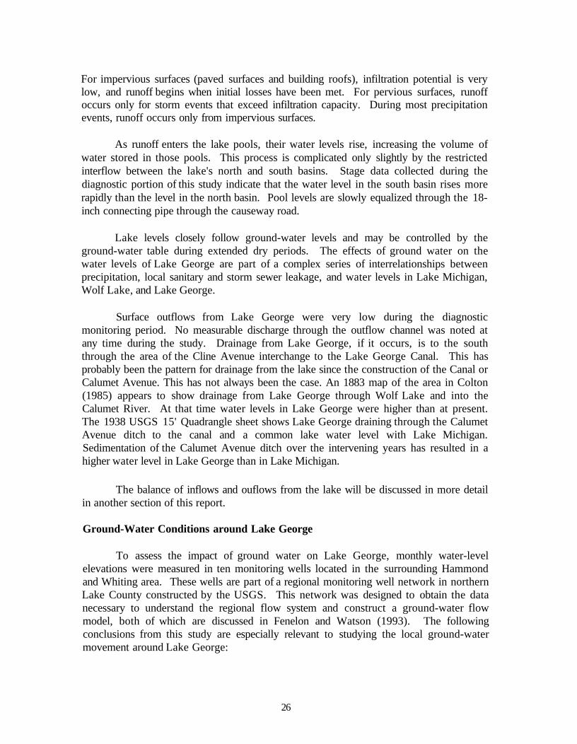
Table 7 summarizes the hydrologic budget for the one-year monitoring period. During this period, 75 percent of the inflow volume to the lake was direct precipitation on the lake surface; 13 percent was watershed runoff; and 12 percent was unmeasured inflow volume. Outflow volume was 66 percent evaporation, 10 percent surface runoff, and 24 percent unmeasured volume.

The outflow point in the southwest corner of Lake George's south basin was observed on a regular basis during the monitoring visits. Measurable flow in the discharge channel was never observed, and notes of no flow, light discharge, or, on several occasions, light inflow were used to estimate surface outflow from the lake. In table 7, an allowance of 60 acre-feet of outflow volume has been made.

31

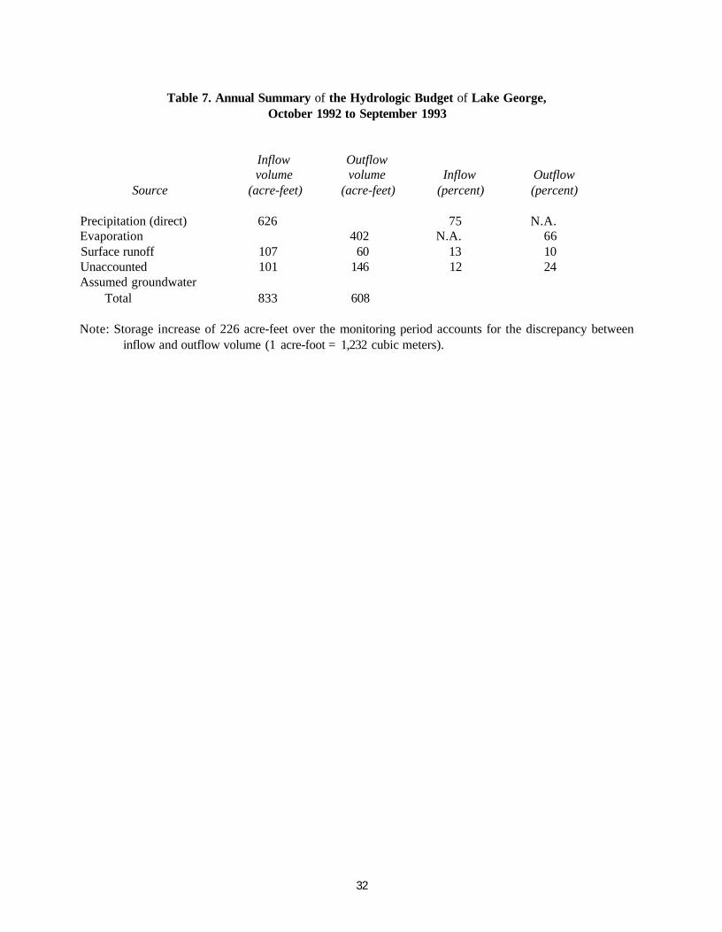
Table 7. Annual Summary of the Hydrologic Budget of Lake George, October 1992 to September 1993

Inflow Outflow volume volume Inflow Outflow

Source (acre-feet) (acre-feet) (percent) (percent)

Precipitation (direct) 626 75 N.A. Evaporation 402 N.A. 66 Surface runoff 107 60 13 10 Unaccounted 101 146 12 24 Assumed groundwater

Total 833 608

Note: Storage increase of 226 acre-feet over the monitoring period accounts for the discrepancy between inflow and outflow volume (1 acre-foot = 1,232 cubic meters).

32

Bathymetric Survey

A bathymetric survey of Lake George was conducted as part of the diagnostic study. The data were collected using a range azimuth methodology, which entailed using a surveyor to collect range azimuth data as the boat moved along a transect. As data for each surveyed point were collected, personnel in the boat would simultaneously determine the depth using a standard sounding pole calibrated to 0.1 feet. A total of 27 transects were run to collect the depth and horizontal position data: 12 transects in the north basin and 15 in the south basin.

Data collected during the field survey were processed on a Geographical Information System (GIS) using the software program TIN (Triangulated Irregular Network). The TIN data structure (Environmental Systems Research Institute, Inc., 1991) is based on two elements: points with x,y, and z values, and a series of edges joining these points to form triangles. This triangular mosaic forms a continuous faceted surface, much like a jewel. This solution satisfies the Delaunay criterion, which ensures that any point is joined to its two nearest neighbors to form a triangle. From this, the location of any point on the surface can be triangulated, providing the ability to plot depth contours and to determine volumes below a specified datum.

The TIN program generated the bathymetric contours shown in figure 6. Lake George was found to be shallow with a maximum depth of 4.0 feet in the north basin and 3.5 feet in the south basin. Average depths of 1.8 and 2.2 feet were determined for the north and south basins, respectively. The volume of the north basin was 148 acre-feet, while the south basin had a volume of 140 acre-feet. All depth and volume data have been analyzed using a pool elevation of 583 feet above mean sea level. This level corresponds to a water depth over the crowns of the interconnecting pipe of 0.76 feet in the north basin and 0.45 feet in the south basin.

Sediment and Nutrient Input Budgets

The results of stormwater inflow samples collected during the site monitoring visits were combined with the stormwater runoff volumes from the hydrologic analysis to estimate suspended sediment and nutrient loading to the lake. These results, which show that loadings to the lake are negligible, are presented in table 8. For example, the suspended sediment loading of 10 tons per year is less than 400 cubic feet of material or a volume of 10 feet × 10 feet × 4 feet deep.

For assessing the internal regeneration of nutrients from lake bottom sediments, reliance was placed on values reported in the literature. USEPA's Clean Lakes Program Guidance Manual (1980) suggests values of 0.5 to 5 g/m2/year under aerobic conditions and 10 to 20 g/m2/year under anaerobic conditions. Nurnberg (1984) compiled and reported phosphorus release rates in anoxic and oxic core tubes for lake sediments of several lakes. The release rates are indicative of adsorption of phosphorus to sediments under aerobic conditions. Generally, phosphorus release rates were found to be 2 to 10

33

Figure 6. Bathymetric map of Lake George

34

Table 8. Sediment and Nutrient Loading to Lake George

35

Inflow Annual total

Total dissolved solids 14.9 tons (13,500 Kg) Total suspended solids 10.3 tons (9,350 Kg) Total volatile solids 2.4 tons (2,180 Kg) Total inorganic nitrogen 157.7 pounds (71.5 Kg) Ammonia-nitrogen 81.6 pounds (37.0 Kg) Nitrate + nitrite-nitrogen 76.1 pounds (34.5 Kg) Total phosphate-phosphorus 20.5 pounds (9.3 Kg)

times higher under anoxic conditions compared to under aerobic conditions for the same core sediments.

Analyses of Lake George bottom sediments indicate that phosphorus concentrations were below the levels found in other lake sediments (tables 31 and 32). Assuming a phosphorus release rate of 2 mg/m2/day for the aerobic conditions that prevailed in the lake, phosphorus loading to the lake due to internal regeneration is 1.0 pound/year. The release rate assumed for Lake George is in the mid-range of values reported by Nurnberg and the low end of the range suggested in USEPA's Clean Lakes Manual.

The contribution of phosphorus from internal regeneration to the total lake loading is only 4.7 percent (1 pound in 21.5 pounds) which is much less than in lakes with agricultural setting reported by Kothandaraman and Evans (1983a, 1983b). The total annual phosphorus loading to the lake was found to be 0.016 g/m2/year and is considered excessive from the point of view of eutrophication. The actual phosphorus loading of 0.016 g/m2/year for Lake George is well within the permissible levels suggested in the literature.

Lakebed Characteristics

Lakebed conditions in Lake George were evaluated by collecting samples of bed materials from the lake bottom through dredge sampling and shallow coring. This sampling was supplemented by probing of the lake bottom with a 1-inch-diameter pole.

The bed material sampling indicated that the lakebed is composed of an organic muck surface layer covering sandy substrata. In the north basin, thickness of the surface muck layer ranged consistently from 0 to 0.5 feet. The south basin had a thicker muck deposit, ranging from 2 feet thick along the west side of the lake to 0.5 feet thick along the east shore.

Particle-size distributions of the bed material samples are presented in figure 7. These analyses show that samples from the sandy substrata are very uniform with a mean particle size of 0.2 mm, which is characteristic of fine sands.

LIMNOLOGICAL ASSESSMENT

Lake George is a remnant of a large glacial basin once part of Lake Michigan. In the wake of the industrialization of northwestern Indiana, the water body became isolated from Lake Michigan and gradually shrank due to industrial waste disposal practices used in the middle part of this century. The lake has no tributary feeding it, but has five storm drains that are ephemeral in nature. The lake has a water surface area of 148 acres with a maximum depth of 4 feet. Other pertinent morphometric details regarding the lake are included in table 9.

36

Figure 7. Particle-size distribution for Lake George bed materials

Materials and Methods

In order to assess the current conditions of the lake, specific physical, chemical, and biological characteristics were monitored during the period October 1, 1992, to October 27, 1993. The lake was monitored monthly from October-April and twice a month during the remaining period, for a total of 17 sampling visits. Because the lake's tributary creeks are ephemeral in nature, tributary samples were not collected during these regular visits to the lake; instead, additional trips were made to collect tributary samples during storm events. However, samples were collected routinely from the outflow channel on the southwest corner of the south basin.

The locations of the lake and tributary monitoring stations are shown in figure 8. In addition to periodic water sample collections, trips were made to the lake for collecting storm event samples, surficial and core sediment samples, and for collecting and identifying macrophytes and benthic organisms. Table 10 outlines the protocol for field data collections, including the type and frequency of observations required during the one-year data-gathering effort.

In situ observations for temperature and dissolved oxygen (DO) and Secchi disc transparency readings were made at lake sampling sites. An oxygen meter, Yellow Springs Instrument model 58, with a 50-foot cable and probe was standardized at the site using the saturation chamber air standardization procedure. Temperature and DO measurements were obtained in the water column at 1-foot intervals commencing from the surface.

Secchi disc transparencies were measured using an 8-inch-diameter Secchi disc, which was lowered until it disappeared from view, and the depth noted. The disc was lowered further and slowly raised until it reappeared. This depth was also noted, and the average of the two depths was recorded. Secchi disc visibility measures a lake's water transparency or its ability to allow sunlight penetration.

Samples for water chemistry analyses were collected near the surface (1 foot below) in two 500-milliliter (mL) plastic containers, one without any preservative and the other with reagent-grade sulfuric acid as preservative. These samples were kept on ice until transferred to the laboratory for analyses. Determinations for pH, phenalphthalein alkalinity, and total alkalinity were made at the site before the samples were taken to the laboratory. Samples for metals were taken in 500-mL plastic bottles containing reagent-grade nitric acid as preservative. Samples for organic analyses were collected in 1-gallon dark amber glass bottles filled to the brim without any head space. The methods and procedures involved in the analytical determinations are given in table 11.

Vertically integrated samples for chlorophyll and phytoplankton were collected using a weighted bottle sampler with a half-gallon plastic bottle. The sampler was lowered at a constant rate to a depth twice the Secchi depth, or to 2 feet above the bottom of the lake, and raised at a constant rate to the surface. For chlorophyll analysis, a measured

38

Table 9. Morphometric Details of Lake George

North basin South basin

Surface area, acres (ha) 84.16 (34.04) 64.50 (25.68) Volume, acre-feet (m3) 147.73 (182,000) 139.98 (172,500) Mean depth, feet (m) 1.76 (0.53) 2.20 (0.67) Maximum depth, feet (m) 3.99(1.22) 3.50(1.07) Length of shoreline, miles (m) 1.79(2,090) 1.46(2,360) Lake type glacial glacial

39

Figure 8. Sampling locations for water quality and sediment monitoring stations

40

Table 10. Protocol for Field Data Collections in Lake George

A. Water 1. Sites (sampling and in situ monitoring)

a. One site in each of the two water bodies b. Deepest point in each water body

2. Depths a. Dissolved oxygen/temperature profile at each site b. Sample collected at 1 foot below surface c. Chlorophyll-a - integrated sample in euphotic zone

3. Frequency a. Core parameters - bimonthly from May to September and monthly from

October to April b. Organics, metals - once

4. Parameters a. Core (samples each time monitored)

Field observations, Secchi disc transparency, dissolved oxygen/temperature profiles, pH, total alkalinity, phenolphthalein alkalinity, conductivity, chlorides, total suspended solids, volatile suspended solids, dissolved phosphorus, total phosphorus, ammonia-N, nitrate and nitrite-N, total kjeldahl nitrogen, chemical oxygen demand, and chlorophyll-a, b, c and pheophytin

b. Metals and organics Cadmium, chromium, copper, iron, lead, manganese, nickel, silver, zinc, PCBs, aldrin, dieldrin, DDT and analogs, total chlordane and isomers, endrin, methoxychlor, hexachlorocyclohexane, hexachlorobenze, and pentachlorophenol

B. Sediment 1. Sites

a. Surficial - 8 b. Core - 4

2. Frequency - replicate core and sediment samples once 3. Parameters

a. Metals listed in A.4.b. above b. Organics listed in A.4.b. above c. In addition, total phosphorus, total kjeldahl nitrogen, percent total and volatile

solids, chemical oxygen demand, total organic carbon, particle size, and density

C. Phytoplankton and zooplankton 1. Sites - same as for water 2. Depths - integrated euphotic zone, twice Secchi depth 3. Frequency - monthly from April to October 4. Parameters

a.. Identification to lowest possible taxon and enumeration b. Biovolume

41

I. In-Lake Monitoring

Table 10. (Concluded)

D. Aquatic Macrophytes 1. Sites - littoral zone, shoreline to twice Secchi depth 2. Frequency - once in summer 3. Parameters

a. Identification to lowest possible taxon b. Mapping of locations and abundance c. Biomass

E. Benthic Macroinvertebrate 1. Sites - same as for water 2. Frequency - spring turnover and peak summer stratification 3. Parameters

a. Identification to lowest possible taxon b. Biomass

F. Fecal and Total Coliforms and Fecal Streptococci 1. Sites - same as for water 2. Frequency - monthly from May to September

II. Inflows and Outflows

A. Sites 1. Storm discharges 2. Industrial discharges 3. Outflow

B. Depth integrated

C. Frequency - same as for water

D. Parameters 1. Total and volatile suspended soids, total phosphorus, ammonia-N, nitrate and nitrite-

N, for outflows and storm discharges 2. Metals and organics listed in I.A.4.b, once for outflows and storm discharges

42

Table 11. Analytical Procedures

Units of Detection Parameter Method of analysis (reference) measure limits

Temperature In situ measurement using YSI °C 0.1 °C Model 58 Dissolved Oxygen meter

Dissolved Oxygen In situ measurement using YSI mg/L O2 0.1 mg/L Model 58 DO meter

pH On site using Necter model 47 none 0.05 after collection

Alkalinity Titration of 25-mL sample using mg/L as CaCO3 1 mg/L as Necter Model 47 pH meter with CaCO3 0.02 NH 2 SO 4 to pH 8.3 (phenolphthalein alkalinity) and to pH 4.5 (total alkalinity)

Conductivity EPA 120.1 Wheatstone bridge µmho/cm 1 µmho/cm

Chloride Standard Methods 17th edition mg/L 5 mg/L 4500 CI B Argertometric

Chemical Oxygen E1A 410.4 mg/L 1 mg/L Demand Colorimetric

Chlorophyll Standard Method 17th edition, µg/L 2-7 µg/L 10200 Spectrophotometric

Ammonia-N Potentiometric, ISE mg/L 0.1 mg/L

Nitrite-N EPA 353.2 mg/L 0.10 mg/L NO2-N Colorimetric, automated Cd redn

Nitrate-N EPA 353.2 mg/L 0.10 mg/L Colorimetric, automated Cd redn

Total EPA 351.4 mg/L 0.10 mg/L Kjeldahl-N Potentiometric, mg/L ISF

after Digestion

Oil & Grease, EPA 413.2 mg/L 1.0 mg/L 1R Spectrophometric, IR

Phosphorus, EPA 365.2 mg/L 0.05 mg/L total Persulfate digestion

Ascorbic acid colorimetric

Phosphorus, EPA 365.2 mg/L 0.05 mg/L dissolved after field filtration through

0.45-u filter Persulfate Digestion ascorbic acid colorimetric

43

Table 11. (Continued)

Units of Detection Parameter Method of analysis (reference) measure limits

Total Solids EPA 160.3 mg/L 1 mg/L Gravimetric, dried at 103-105°C

Total EPA 160.1 Gravimetric mg/L 1 mg/L Dissolved Residue, filterable Solids Dry at 180°C

Total EPA 160.2 Gravimetric mg/L 1 mg/L Suspended Residue, nonfilterable Solids Dry at 103-105°C

Volatile EPA 160.4 Gravimetric mg/L 1 mg/L Suspended Ignition at 550°C Solids

Cadmium EPA 200.7, ICP µg/L <5 µg/L

Chromium EPA 200.7, ICP µg/L 10 µg/L

Copper EPA 200.7, ICP µg/L 10 µg/L

Iron EPA 200.7, ICP µg/L 100 µg/L

Lead EPA 239.2, AA Furnace µg/L 5 µg/L

Manganese EPA 200.7, ICP µg/L 10 µg/L

Nickel EPA 200.7, ICP µg/L 20 µg/L

Silver EPA 200.7, ICP µg/L 10 µg/L

Zinc EPA 200.7, ICP µg/L 20 µg/L

Arochlor-1016 SW-846/8080 µg/L 0.5 µg/L 1221 " µg/L 0.5 µg/L 1232 " µg/L 0.5 µg/L 1242 " µg/L 0.5 µg/L 1248 " µg/L 0.5 µg/L 1254 " µg/L 1.0 µg/L 1260 " µg/L 1.0 µg/L

Aldrin " µg/L 0.05 µg/L Dieldrin " µg/L 0.10 µg/L 4,4'-DDE " µg/L 0.10 µg/L Endrin " µg/L 0.10 µg/L 4,4'-DDD " µg/L 0.10 µg/L 4,4'-DDT " µg/L 0.10 µg/L Methoxychlor " µg/L 0.50 µg/L Alpha-chlordane " µg/L 0.5 µg/L Gamma chlordane " µg/L 0.5 µg/L Hexachlorobenzene " µg/L 10 µg/L

44

Table 11. (Concluded)

Parameter

a-BHC b-BHC g-BHC d-BHC Pentachlorphenol

45

Method of analysis (reference)

SW-846/8080 "

"

"

SW-846/8270

Units of measure

µg/L µg/L µg/L µg/L µg/L

Detection limits

0.05 µg/L 0.05 µg/L 0.05 µg/L 0.05 µg/L 50µg/L

amount of sample was filtered through a Fisher glass fiber filter G4 using a hand-operated vacuum pump in the shade. The chlorophyll filters were then wrapped in aluminum foil and the filtrate volume measured using a graduated cylinder. Filters were kept frozen in the laboratory until analyzed. Water samples collected from Lake George, particularly the south basin, were extremely difficult to filter. Hence, in addition to obtaining filtered samples for chlorophyll analyses, unfiltered water samples in foil-wrapped quart bottles were collected and used in the chlorophyll determinations. For algal identification and enumeration, 380-mL water subsamples were taken, preserved with 20 mL of formalin at the time of collection, and stored at room temperature until they could be examined.

Also, vertically integrated 10-liter (L) samples were collected for zooplankton identification and enumeration. The samples were filtered through a Wisconsin net, and the collected zooplankton were placed in a 250-mL bottle with 10 mL of ethyl alcohol (95 percent ethanol) and 190 mL of deionized water. In the laboratory, each sample was filtered through a 0.45-micrometer (μm) filter. The organisms were resuspended in 10 mL of deionized water. One mL of sample was placed in a Sedgwick Rafter Cell and examined using a differential contrast microscope at 100X magnification. Organisms in the five widths of the cell were counted and recorded. The sizes and shapes of various zooplankton found in water samples are given in table 12.

For algal identification and enumeration, the sample was thoroughly mixed, and a 1-mL aliquot was pipetted into a Sedgwick Rafter Cell. A differential interface contrast microscope equipped with a 10X or 20X eyepiece, 20X or 100X objective, and a Whipple disc was used for identification and counting. Five short strips were counted. The algae species were identified and classified into five main groups: blue-greens, greens, diatoms, flagellates, and desmids. For enumeration, blue-green algae were counted by trichomes. Green algae were counted by individual cells except for Actinastrum, Coelastrum, and Pediastrum, which were recorded by each colony observed. Each cell packet of Scenedesmus was counted. Diatoms were counted as one organism regardless of their grouping connections. For flagellates, a colony of Dinobryon or a single cell of Ceratium was recorded as a unit. The dimensions and shapes of various algae found in the water samples are given in table 13.

Benthic samples for macroinvertebrate examination were collected using a petite ponar dredge. Three grab samples were taken at each station for macroinvertebrate analyses. The samples were washed in a 30-mesh screen bucket, and the residue was preserved in plastic bottles containing 95 percent ethyl alcohol. In the laboratory, the samples were washed again; the organisms were picked from the bottom detritus, identified, and counted; and then the biomass was determined.

Bacterial samples from the lake and storm drams were examined for total coliform, fecai coliform, and fecal streptococcus. Procedures from Standard Methods for the Examination of' Water and Wastewater (American Public Health Association et al., 1992) were employed using 0.45-µm membrane filters in the bacterial determinations.

46

Table 12. Sizes and Shapes of Zooplankton Used in Biomass Determination

Name Shape Size (μm)

Cladocera (Water Fleas) Alona quadrangularis Spherical 500 diam. Bosmina coregoni Spherical 700 diam. Bosmina longirostris Spherical 500 diam. Daphnia laevis Spherical 2,000 diam. D. pulex Spherical 2,000 diam. D. rosea Spherical 2,000 diam.

Copepoda (Copepods) Diaptomus minutus Cylindrical 100 × 500 Eucyclops speratus Cylindrical 200 × 900

Ostracoda (Seed Shrimps) Cyclocypris forbesi Spherical 500 diam.

Rotifera (Rotifers) Ascomorpha saltans Spherical 150 diam. Horaella brehmi Spherical 200 diam.

47

Table 13. Sizes and Shapes of Algae Used in Biomass Determination

Name Shape

Blue-Greens Anabaena planctonica Flat, rectangular A. spiroides Spherical, filamentous Anacystis thermolis Spherical, colony

Aphanizomenonflos-aquae Cylindrical, filamentous Oscillatoria chlorina Cylindrical O. sp. Cylindrical

Greens Actinastrum hanztschii Spherical Closteriopsis longissima Flat, rectangular Coelastrum microporum Spherical Crucigenia rectangularis Flat, rectangular, colony

Oocystis borgei Spherical Pediastrum biradiatum Spherical P. duplex Cylindrical P. simplex Cylindrical P. tetras Spherical Scenedesmus carinatus Flat, rectangular S. dimorphus Flat, rectangular Ulothrix variabilis Cylindrical, filamentous U. zonata Flat, rectangular

Diatoms Amphiprora ornata Flat, rectangular Amphora ovalis Flat, rectangular Asterionella formosa Flat, rectangular Crucigenia rectangularis Flat, rectangular Cylotella atomus Spherical C. meneghiniana Spherical C. ocellata Spherical Cymatopleura solea Flat, rectangular Cymbella affinis Cylindrical C. prostrata Cylindrical Diatoma vulgare Flat, rectangular Diploneis smithii Cylindrical Fragilaria virescens Flat, rectangular Gomphonema olivaceum Flat, rectangular Melosira granulata Cylindrical Navicular cryptocephala Cylindrical N. cuspidata Cylindrical N. gastrum Cylindrical Neidium dubium Cylindrical Nitzschia dentecula Cylindrical

48

Size (µm)

11 × 9 10 diam., 100 5 diam., 6 to 16 in a colony 4.5 × 90 9 × 67.5 8 × 55

42 diam. 5 × 210 24 diam. 4.5 × 24, 250 in a colony 22 diam. 15 diam. 3 × 150 10x22 9 diam. 3 × 12 5 × 19 5 × 10, 10 31 × 55

44 × 60 13 × 65 2 × 125 5 × 8 4 diam. 21 diam. 11 diam. 22 × 155 12 × 60 25 × 85 11 × 45 15 × 8 9 × 88 7 × 20 12 × 60 5 × 25 22 × 120 12 × 45 12 × 33 5 × 51

Table 13. (Concluded)

Name Shape Size (µm)

Diatoms Rhoicosphenia cruvata Cylindrical 7 × 45 Stephanodiscus niagarae Spherical 52 diam. Synedra actinastroides Spherical, colony 3 diam., 55 S. acus Cylindrical 4.5 × 200 S. delicatissima Cylindrical 3 × 220 S. ulna Cylindrical 4.5 × 200 Tabellaria fenestrata Cylindrical 6 × 90

Flagellates Carteria multifilis Spherical 14 diam. Ceratium hirundinella Triangular 48 × 48 × 200 Chlamydomonas reinhardi Spherical 7 diam. Dinobryon sertularia Cylindrical 30 × 60 Eudorina elegans Flat, rectangular, colony 10 × 21, 135 Euglena gracilis Cylindrical 6 × 45 Phacus pleuronectes Cylindrical 40 × 87 Trachemonas crebea Spherical 18 diam.

Desmids Closterium sp. Flat, rectangular 20 × 110 Staurastrum comutum Flat, rectangular 18 × 32

49

The macrophyte survey of the lake was done in two stages. A reconnaissance survey of the macrophyte beds was carried out on June 23, 1993, using a boat and a GIS-generated lake map with square grids. The macrophyte beds were probed thoroughly with a garden rake to determine the presence/absence of macrophytes, type and qualitative assessment of vegetation densities (dense, medium, sparse, etc.), and so forth. Map grids helped researchers mark the boat position on the map. The reconnaissance survey enabled the delineation of the areal extent and abundance of macrophytes in the lake and the tentative selection of sites for quantitative sampling of macrophytes.

Macrophyte samples were collected at several locations with the aid of two scuba divers on July 23, 1993, using 18- or 12-inch quadrats, depending on whether the site had sparse or dense growth. At each sampling site observations were made and recorded for water depth, plant length, depth and character of the sediments, etc. All the plants within the quadrat were collected with roots intact and placed in plastic bags, which were then sealed. These samples were then examined with a stereo microscope and identified. Subsequently, the plants from each sampling site were air-dried, then dried at 105 degrees Celsius (°C) in a drying oven to constant weight, and finally weighed to determine the biomass.

Sediment samples were collected from seven sampling sites: the four locations shown in figure 8 and the three regular water quality monitoring sites. Core samples were collected either from a boat or by wading, using a 2-inch hand-driven sediment corer thrust into the lake bottom to the point of refusal. Wildco (Wildlife Supply Company, Saginaw, MI) clear plastic core-liner tube was used to collect the sediment samples, which were subsequently divided into three equal parts: top, middle, and bottom. Each of these portions was examined for heavy metals and trace organics in the laboratory.

Surficial sediment samples were collected using an epoxy-coated Petite Ponar dredge. Subsamples from these ponar samples were collected for metals, trace organics, and toxicity characteristics leaching procedure (TCLP) tests as per the Illinois Environmental Protection Agency's (IEPA's) Field Methods Manual (1987). Particle-size analyses of the surficial sediments were carried out using the hydrometer analyses procedure, American Society of Testing and Materials (ASTM) D422-63. USEPA's method 1311 (1990a), published March 29, 1990, in the Federal Register (40CFR-261), was used for the TCLP extraction of the surficial sediment sample.

50

Water Quality Characteristics

Physical Characteristics

Temperature and Dissolved Oxygen. Lakes in temperate climates undergo seasonal variations in temperature through the water column. The variations have a very significant influence on the physical, chemical, and biological characteristics of the lake ecology.

Most desirable aquatic organisms, including fish, require adequate dissolved oxygen (DO) in water to survive and proliferate. Transfer of oxygen from the atmosphere through the water surface and photosynthetic production of oxygen by algae and rooted aquatic vegetation are the principal sources of DO in lake waters. A very high oxygen concentration results in supersaturation, which can occur when oxygen production in a lake by photosynthesis exceeds diffusion of oxygen back to the atmosphere. Generally, supersaturation occurs in the top few feet of a lake's water column due to algal blooms, as well as in the vicinity of dense aquatic plant growth.

Oxygen deficiencies can arise when plant, animal, and micro- and macroscopic organisms respire at a higher rate than photosynthesis and oxygen transfer from the atmosphere. Also, decaying organic matter in the bottom sediments can exert oxygen demand far exceeding oxygen replenishment. The mud-water interfaces are known to be anoxic even in very shallow lakes in the Midwest. Winter fish kills occur in shallow lakes when snow-covered ice prevents sunlight penetration and hence decreases algal photosynthesis. If oxygen demands are greater than the oxygen resources, the lake's supply of oxygen will be depleted and fish will suffocate.

The observed DO and temperature data for the north and south basins of Lake George are shown in table 14. The maximum water temperature observed was 27.4°C on July 20, 1993, in the north basin and 28.6°C on July 6, 1994, in the south basin. The highest and lowest DO concentrations observed in the lake were 14.9 milligrams per liter (mg/L) and 3.0 mg/L. DO and temperature profiles on selected dates for the north and south basins are shown in figures 9 and 10, respectively. Percent DO saturation values for the observed DO and temperature are given in table 15. Saturation DO values were computed using the formula (Committee on Sanitary Engineering Research, 1960):

DO = 14.652-0.410022T + 0.0079910T2-0.000077774T3

where

DO = the saturation dissolved oxygen, mg/L T = water temperature, °C

A higher degree of supersaturation occurred in the south basin than in the north basin during the warm summer period. This was likely due to the dense beds of rooted

51

Table 14. Dissolved Oxygen and Temperature Observations in Lake George

North Basin

10/15/92 11/10/92 12/22/92 1/20/93 2/11/93 3/17/93 4/14/93 5/10/93 5/27/93 Depth Temp DO Temp DO Temp DO Temp DO Temp DO Temp DO Temp DO Temp DO Temp DO

0 10.6 12.7 5.1 11.9 1.8 14.8 0.8 14.0 1.0 10.9 1.2 12.9 8.6 11.6 25.1 8.1 18.6 9.0 1 10.6 12.6 5.2 11.9 1.8 14.8 2.0 14.1 2.3 12.8 1.2 13.0 8.6 11.5 25.2 8.1 18.6 9.0 2 10.6 12.6 1.9 14.9 3.3 13.8 3.0 12.1 1.3 13.0 8.6 11.5 25.2 8.1 18.6 9.0 3 1.3 13.0

6/10/93 6/22/93 7/6/93 7/20/93 8/3/93 8/18/93 9/8/93 9/28/93 Depth Temp DO Temp DO Temp DO Temp DO Temp DO Temp DO Temp DO Temp DO

0 22.8 9.6 25.7 9.4 27.4 9.0 25.0 7.7 24.8 8.8 24.9 7.3 22.1 12.1 13.8 10.4 1 22.7 9.6 25.7 9.4 27.4 9.0 25.0 7.7 24.8 8.9 24.9 7.3 22.2 12.2 13.9 10.4 2 22.7 9.1 25.7 9.4 27.4 9.0 25.0 7.7 24.8 8.9 24.9 7.3 22.3 12.1 13.9 10.4 3 21.5 9.0 25.7 9.3 27.4 9.0 25.1 7.7 24.9 7.3 13.9 10.4

South Basin

10/15/92 11/10/92 12/22/92 1/20/93 2/11/93 3/17/93 4/14/93 5/10/93 5/27/93 Depth Temp DO Temp DO Temp DO Temp DO Temp DO Temp DO Temp DO Temp DO Temp DO

0 10.7 12.3 4.8 12.2 0.2 12.1 0.9 10.5 1.0 14.3 1.4 12.1 9.1 11.6 25.3 13.9 18.6 14.8 1 10.7 12.3 4.8 12.1 0.7 12.1 1.7 10.0 1.0 14.3 1.4 12.1 9.1 11.6 25.4 14.0 18.5 12.5 2 10.7 12.2 0.8 11.8 2.5 9.6 1.0 14.3 1.4 12.1 9.1 11.6 23.2 12.8 18.2 9.4 3 0.8 11.8 2.7 9.3 1.0 14.3 1.4 12.2 9.1 11.5 22.7 11.4

6/10/93 6/22/93 7/6/93 7/20/93 8/3/93 8/18/93 9/8/93 9/28/93 Depth Temp DO Temp DO Temp DO Temp DO Temp DO Temp DO Temp DO Temp DO

0 23.9 11.3 26.0 11.5 28.6 12.1 25.7 10.9 23.0 12.3 24.8 5.9 23.0 14.4 13.4 9.8 1 21.3 11.3 26.0 11.6 28.6 11.1 24.9 8.2 24.4 11.1 24.5 4.9 21.1 12.5 13.5 9.8 2 21.1 10.1 24.5 11.1 26.1 6.2 24.6 7.8 22.8 7.4 24.4 4.4 19.8 7.4 13.6 9.8 3 20.5 9.3 23.4 7.8 25.7 4.2 24.6 6.9 22.7 5.2 24.3 3.0 19.4 6.2 13.6 9.7

Note: Depth is expressed in feet, temperature in °C, and dissolved oxygen (DO) in mg/L

Figure 9. Dissolved oxygen and temperature profiles on selected dates, north basin

53

Figure 10. Dissolved oxygen and temperature profiles on selected dates, south basin

54

Table 15. Percent Dissolved Oxygen Saturation in Lake George

North Basin

Dissolved oxygen saturation, percent Depth 10/15/92 11/10/92 12/22/92 1/20/93 2/11/93 3/17/93 4/14/93 5/10/93 5/27/93

0 113 93 106 98 76 91 99 99 97 1 113 94 106 102 93 92 99 99 97 2 113 107 103 90 92 99 99 97 3 92 103

Dissolved oxygen saturation, percent Depth 6/10/93 6/22/93 7/6/93 7/20/93 8/3/93 8/18/93 9/8/93 9/28/93

0 113 117 115 94 107 89 140 101 1 112 117 115 94 108 89 141 101 2 105 117 115 94 108 89 140 101 3 115 115 94 89 101

South Basin

Dissolved oxygen saturation, percent Depth 10/15/92 11/10/92 12/22/92 1/20/93 2/11/93 3/17/93 4/14/93 5/10/93 5/27/93

0 111 95 83 73 100 86 101 171 159 1 111 95 84 72 100 86 101 173 134 2 111 82 70 100 86 101 151 100 3 82 68 100 86 101 133

Dissolved oxygen saturation, percent Depth 6/10/93 6/22/93 7/6/93 7/20/93 8/3/93 8/18/93 9/8/93 9/28/93

0 135 143 158 135 145 72 169 94 1 129 145 145 100 134 59 142 94 2 114 134 77 95 87 53 82 95 3 101 93 52 84 61 36 68 94

Note: Depth is expressed in feet.

vegetation that existed in the south basin. The highest saturation value recorded for the south basin was 171 percent on May 10, 1993, while for the north basin it was 140 percent on September 8, 1993. The lowest saturation values recorded in the south and north basins were, respectively, 36 percent on August 18, 1993, and 76 percent on February 11, 1993. In general, the DO conditions in the lake were more than adequate for fish survival and always met the DO criteria of the Indiana Water Pollution Control Board (Title 327). Only once in each basin was the near-bottom water DO slightly lower than the criteria. No mud-water interface oxic conditions were monitored in this investigation.

Secchi Disc Transparencies. Secchi disc visibility is a measure of a lake's water transparency, which suggests the depth of light penetration into a body of water (its ability to allow sunlight penetration). Even though the Secchi disc transparency is not an actual quantitative indication of light transmission, it serves as an index and a means of comparing similar bodies of water or the same body of water at different times. Since changes in water color and turbidity in deep lakes are generally caused by aquatic flora and fauna, transparency is related to this entity. The euphotic zone or region of a lake where enough sunlight penetrates to allow photosynthetic production of oxygen by algae and aquatic plants is taken as two to three times the Secchi disc depth (USEPA, 1980).

The observed Secchi disc readings in the north and south basins, along with the data for other chemical and biological parameters, are given in tables 16 and 17, respectively. A statistical summary of all these parameters is given in table 18. Also, figures 11 and 12 give the temporal variations in these parameters for the north and south basin, respectively. Secchi disc values were lower in both basins during May-July compared to other months. It is obvious that the depth of sunlight penetration is limited by the depth of the lake and not by the turbidity caused by suspended matter.

The mean and range of Secchi disc values were 22 inches and 12 to 32 inches in the north basin and 21 inches and 11 to 36 inches in the south basin. High Secchi disc values were noted in September, while the lowest values were observed in June and July coinciding with the period of high biological growth (algae and macrophytes) in the lake. This was also the period when sustained supersaturated conditions prevailed (table 15).

Chemical Characteristics

pH and Alkalinity. It is generally considered that pH values above 8.0 in natural waters are produced by a photosynthetic rate that demands more carbon dioxide than the quantities furnished by respiration and decomposition (Mackenthun, 1969). Photosynthesis by aquatic plants uses carbon dioxide, removing it from bicarbonate, when no free carbon dioxide exists in the water column. Decomposition and respiration of biota tend to reduce pH and increase bicarbonates.

The alkalinity of a water is its capacity to accept protons, and it is generally imparted by bicarbonate, carbonate, and hydroxile components. The species makeup of alkalinity is a function of pH and mineral composition. The carbonate equilibrium, in

56

Table 16. Water Quality Characteristics of Lake George, North Basin, October 1992 to September 1993

Table 17. Water Quality Characteristics of Lake George, South Basin, October 1992 to September 1993

Table 18. Summary of Water Quality Characteristics of Lake George

North basin South basin Parameters Mean Range Mean Range

Secchi readings, inches 22 12-32 21 11-36 pH - 7.68-8.97 - 8.50-10.37 Alkalinity, mg/L as CaCO3 130 81-182 121 46-181 Conductivity, µmho/cm 723 500-1,070 691 480-1,000 Chloride, mg/L 67 42-125 71 46-130 Solids, mg/L

Total suspended solids 11 1-55 29 2-120 Volatile suspended soilds 8 <l-28 21 1-95 Total dissolved solids 376 314-466 393 282-505

Phosphorus, mg/L Total phosphate 0.06 0.02-0.22 0.11 0.02-0.30 Dissolved phosphate 0.04 0.01-0.10 0.06 0.01-0.19

Nitrogen, mg/L Ammonia 0.12 0.10-0.30 0.21 0.10-0.53 Nitrite 0.02 0.01-0.06 0.03 0.01-0.06 Nitrate 0.08 0.05-0.23 0.07 0.05-0.24 Kjeldahl 0.92 0.10-1.87 1.22 0.30-2.80

COD, mg/L 31 1-65 58 22-200 Oil and grease, mg/L <1 <l-2 <1 <l-3 Field filtered, µg/L

Chlorophyll-a 5.32 0.90-15.5 10.95 3.00-48.3 Chlorophyll-b 2.65 0.50-9.70 7.48 1.85-24.1 Chlorophyll-c 2.23 0.50-7.97 10.17 1.25-48.9 Pheophytin-a 2.20 0.50-8.68 4.84 0.50-28.5

Laboratory filtered, µg/L Chlorophyll-a 4.54 0.50-6.19 10.99 0.92-19.2 Chlorophyll-b 3.01 0.71-5.54 9.60 1.16-14.3 Chlorophyll-c 4.31 1.35-13.70 13.00 1.37-15.1 Pheophytin-a 0.97 0.50-2.50 3.31 0.50-17.4

59

Figure 11. Temporal variations in water quality characteristics, north basin

60

Figure 12. Temporal variations in water quality characteristics, south basin

61

which carbonate and bicarbonate ions and carbonic acid are in equilibrium, is the chemical system present in natural waters.

The pH of north basin water samples ranged from 7.68 to 8.97, with pH values higher than 8.0 observed from March-November. This elevated pH is attributable to photosynthesis. The DO conditions were at near-saturation or supersaturation levels. The pH levels in the south basin were higher than those observed for the north basin, ranging from 8.50 to 10.37. In addition to being at much higher DO supersaturated conditions than in the north basin, the colloidal suspended particles in the water might have caused some elevated pH observations. The colloidal particulate matter, often observed as a dense white band of swirls in the south basin, is suspected to be the result of runoff or leachate from the Bairstow slag piles entering the lake. The sediment (white precipitate) along the lake's southern shore was found to be highly alkaline in character with a measured pH of 10.9, an aspect that will be discussed in greater detail later on. The pH values observed in south basin water samples exceeded the criteria for pH < 9.0 (Indiana Water Pollution Control Board, Title 327) 10 out of 17 times.

The total alkalinity values ranged from 81 to 182 and 46 to 181 mg/L as CaCO3, in the north and south basins, respectively. Concommitant with an increase in pH due to photosynthesis, there was a significant decrease in alkalinity values in the lake. This phenomenon was very pronounced during June and July. Mean alkalinity values in the north and south basins were 130 and 121 mg/L. These waters were found to be well buffered, as is typical of Midwestern lakes.

Conductivity. Specific conductance provides a measure of a water's capacity to convey electric current and is used as an estimate of the dissolved mineral quality of water. This property is related to the total concentration of ionized substances in water and the temperature at which the measurement is made. Specific conductance is affected by such factors as the nature of dissolved substances, the relative concentrations, and the ionic strength of the water sample. The geochemistry of the drainage basin is the major factor determining the chemical constituents in the waters. Practical applications of conductivity measurements include determination of the purity of distilled or deionized water, quick determination of the variations in dissolved mineral concentrations in water samples, and estimation of dissolved ionic matter in water samples.

The mean conductivity values for the lake water samples were 723 and 691 µmho/cm at 25°C for the north and south basins, respectively. These values are much higher and nearly twice the mean values observed for Illinois lakes (Kothandaraman and Evans, 1983a, 1983b). This is probably due in part to the impact of the runoff from Bairstow slag disposal site. Temporal variations for conductivity (figures 11 and 12) indicate a general decrease during the months of June and July concommitant with the decrease in alkalinities during the same period. The areas surrounding the lake are paved and highly industrialized, and the watershed for the lake is relatively small in relation to the size of the lake. The lake waters appear to have a high mineral content exhibiting high conductivity values.

62

Chloride. Chlorides are found in practically all natural waters. They are conservative substances sometimes used as a tracer element in engineering studies of surface waters and treatment unit processes. Both sulfates and chlorides in surface waters may be of mineral origin, or they may also emanate from municipal and industrial waste discharges. Chloride and sulfate are the predominant anions causing what is known as "permanent hardness" in waters. Because of the salty taste caused by the chloride ion, it is generally limited to 250 mg/L in public water supplies.

The mean and range for chlorides in the north basin were 67 mg/L and 42 to 125 mg/L. The corresponding values for the south basin were 71 mg/L and 46 to 130 mg/L. While the south basin water was found to be mineralized to a higher degree than the north basin, the values observed in these basins are not unusual. The temporal variations in chloride (figures 11 and 12) show a very similar pattern to the variations in conductivity measurements.

Total Suspended Solids, Volatile Suspended Solids, and Total Dissolved Solids. In natural waters, dissolved solids consist mainly of carbonates, bicarbonates, sulfates, chlorides, phosphates, nitrates, calcium, magnesium, and potassium, with traces of iron, manganese, and other substances. The constituent composition of these minerals depends to a large extent on the geochemistry of the area that contributes to the surface or ground-water resource. The amount of suspended solids found in impounded waters is small compared to the amount found in streams, because solids tend to settle to the bottom in lakes. However, in shallow lakes, this aspect is greatly modified by wind and wave actions and by the type and intensity of use to which these lakes are subjected.

All salts in solution change the physical and chemical nature of the water and exert an osmotic pressure. Some have physiological as well as toxic effects. However, possible synergistic or antagonistic interactions between mixed salts in solution may cause the effects of salts in combination to be different from those of salts occurring separately.

Greeson (1971) observed that high dissolved solids content in Oneida Lake (New York) in 1967 and 1969 accompanied high algal production, while low dissolved solids content in 1968 accompanied lower algal production. He concluded that these relationships indicate that dissolved solids content is an important index of potential productivity conditions, because no element, ion, or compound is likely to be a limiting factor on algal production when the dissolved solids content is high.

Total suspended solids represent the amount of all inorganic and organic materials suspended in the water column. Typical inorganic components originate from the weathering and erosion of rocks and soils in a lake's watershed and resuspension of lake sediments. Organic components are derived from a variety of biological origins, but in a lacustrine environment they are mainly composed of algae and resuspended plant and animal material from the lake bottom. Volatile suspended solids indicate the fraction of the total suspended solids that is organic in nature.

63

Total suspended solids in the north basin ranged from 1 to 55 mg/L with a mean of 11 mg/L. These values were somewhat higher in the south basin, where the range was 2 to 120 mg/L with a mean of 29 mg/L. Volatile suspended fractions were also higher in the south basin. The total dissolved solids concentrations measured in the lake were comparable to those in the lakes evaluated by Kothandaraman and Evans (1983a, 1983b). The temporal variations for total suspended and volatile suspended solids (figures 11 and 12) indicate generally higher concentrations of volatile organic matter in the lake waters during April-July. Other than the macrophyte and algae growth during the summer months, causing the volatile suspended fraction to increase, no trend could be discerned for this parameter in the two basins. Observed dissolved solids concentrations were within the stipulated level of 750 mg/L (Indiana Pollution Control Board, Title 327).

Phosphorus. Phosphorus as phosphate may occur in surface or ground waters as a result of leaching from minerals or ores, natural processes of degradation, or agricultural drainage. Phosphorus is an essential nutrient for plant and animal growth and, like nitrogen, it passes - cycles of decomposition and photosynthesis.

Because phosphorus is essential to plant growth, it has become the focus of attention in the entire eutrophication issue. With phosphorus being singled out as probably the most limiting nutrient and the one most easily controlled by removal techniques, various facets of phosphorus chemistry and biology have been extensively studied in the natural environment.

In any ecosystem, the two aspects of interest for phosphorus dynamics are the phosphorus concentration and phosphorus flux (concentration times flow rate) as functions of time and distance. The concentration itself indicates the possible limitation that this nutrient can place on vegetative growth in the water. The phosphorus flux is a measure of phosphorus transport rate at any point in flowing waters.

Unlike nitrate-nitrogen, phosphorus applied as fertilizer is held tightly to the soil. Most of the phosphorus carried into streams and lakes from runoff over cropland will be in the particulate form adsorbed to soil particles. On the other hand, the major portion of phosphate-phosphorus emitted from municipal sewer systems is in a dissolved form. This also is true for phosphorus generated from anaerobic degradation of organic matter in the lake bottom. Consequently, the form of phosphorus, namely particulate or dissolved, is indicative of its source to a certain extent.

From his experience with Wisconsin lakes, Sawyer (1952) concluded that aquatic blooms are likely to develop in lakes during summer months when concentrations of inorganic nitrogen and inorganic phosphorus are in excess of 0.3 and 0.01 mg/L, respectively. These critical levels for nitrogen and phosphorus concentrations have been accepted and widely quoted in scientific literature.

64

Table 18 summarizes the observations for total and dissolved phosphate-phosphorus in the lake, and figures 11 and 12 depict the temporal variations in the lake's phosphorus content. The mean of observed total phosphorus in the north and south basins was 0.06 and 0.11 mg/L, several times higher than the critical level suggested by Sawyer. The phosphorus levels in the south basin are higher than in the north basin, and the temporal variations do not follow general seasonal fluctuations. The ratio of dissolved phosphorus to the total phosphorus in the lake ranged from 11 to 100 percent with a mean of 58 percent in the north basin and from 16 to 100 percent with a mean of 56 percent in the south basin. These values are comparable to those reported, 20 to 90 percent with a mean of 55 percent, for Lake Le-Aqua-Na by Kothandaraman and Evans (1983a). From the concentrations of total phosphorus and the dissolved phosphorus fractions of total phosphorus noted in Lake George, it can be concluded that phosphorus in the lake will not limit sustained high biological productivity. The lake is likely to remain eutrophic with high biological productivity.

Nitrogen. Nitrogen in natural waters is generally found in the form of nitrate, organic nitrogen, and ammonia-nitrogen. Nitrates are the end product of the aerobic stabilization of organic nitrogen, and as such they occur in polluted waters that have undergone self-purification or aerobic treatment processes. Nitrates also occur in percolating groundwater. Ammonia-nitrogen, being a constituent of the complex nitrogen cycle, results from the decomposition of nitrogenous organic matter. It can also result from municipal and industrial waste discharges to streams and lakes.

The concerns about nitrogen as a contaminant in water bodies are twofold. First, because of adverse physiological effects on infants and because the traditional water treatment processes have no effect on the removal of nitrate, concentrations of nitrate plus nitrite as nitrogen are limited to 10 mg/L in public water supplies. Second, a concentration in excess of 0.3 mg/L is considered sufficient to stimulate nuisance algal blooms (Sawyer, 1952). Indiana environmental rules (Indiana Department of Environmental Management, 1995) stipulate a limit of 10 mg/L for nitrate and values for unionized ammonia concentrations dependent on pH and temperature.

Nitrogen is one of the principal elemental constituents of amino acids, peptides, proteins, urea, and other organic matter. Various forms of nitrogen—for example, dissolved organic nitrogen and inorganic nitrogen such as ammonium, nitrate, nitrite, and elemental nitrogen—cannot be used to the same extent by different groups of aquatic plants and algae.

Vollenweider (1968) reports that in laboratory tests the two inorganic forms of ammonia and nitrate are, as a general rule, used by planktonic algae to roughly the same extent. However, Wang et al. (1973) reported that during periods of maximum algal growth under laboratory conditions, ammonium-nitrogen was the source of nitrogen preferred by planktons. In the case of higher initial concentrations of ammonium salts, yields were noted to be lower than with equivalent concentrations of nitrates (Vollenweider, 1968). This was attributed to the toxic effects of ammonium salts. The

65

use of nitrogenous organic compounds has been noted by several investigators, according to Hutchinson (1957). However, Vollenweider (1968) cautions that the direct use of organic nitrogen by planktons has not been definitely established, citing that not one of 12 amino acids tested with green algae and diatoms was a source of nitrogen when bacteria-free cultures were used. But the amino acids were completely used up after a few days when the cultures were inoculated with a mixture of bacteria isolated from water. He has opined that in view of the fact that there are always bacterial fauna active in nature, the question of the use of organic nitrogen sources is of more interest to physiology than to ecology.

The mean and range of values for ammonia, nitrite, nitrate, and Kjeldahl-nitrogen in the lake are included in table 18, and the temporal variations in these parameters are shown in figures 11 and 12. Concentrations of nitrite-nitrogen were generally very low, often below the detection limit, and these values were not plotted. The mean concentrations of ammonia-nitrogen were 0.12 and 0.21 mg/L in the north and south basins, respectively, with ranges from 0.10 to 0.30 mg/L and 0.10 to 0.53 mg/L. Even the highest observed value for ammonia-nitrogen is much lower than the 1.5 mg/L considered critical for fish in terms of ammonia toxicity. The mean inorganic nitrogen (sum of nitrate, nitrite, and ammonia) was 0.22 mg/L in the north basin and 0.31 mg/L in the south basin. These values are about the same or less than the critical value of 0.30 mg/L for nitrogen suggested by Vollenweider. For Kjeldahl nitrogen, an indicator of the relative abundance of suspended matter of organic origin (algae, zooplankton, bacteria, plant fragments, etc.), the mean and range of values were 0.92 and 0.10 to 1.87 mg/L for the north basin and 1.22 and 0.30 to 2.80 mg/L for the south basin. Considering the total nitrogen in the water samples, it is clear that a major portion, 81 percent in the north basin and 80 percent in the south basin, constitutes nitrogen of organic origin. The maximum total ammonia concentration observed for the lake was much below the Indiana Water Pollution Control Board's criteria (Title 327) for ammonia based on un-ionized ammonia as nitrogen.

Chemical Oxygen Demand. Chemical oxygen demand (COD) represents the amount of oxygen needed to oxidize all the oxidizable organic and inorganic constituents (biota and other organic matter, iron, manganous compounds, ammonia, etc.) under specified conditions. It is an indirect but efficient method of assessing the biochemical oxygen demand exerted on the oxygen resources of the water body under ambient conditions.

The mean COD values for the north and south basins were 31 and 58 mg/L, respectively, ranging from 1 to 65 mg/L and 22 to 200 mg/L. The COD of the two water samples collected in the south basin at the beginning of this investigation (October and November 1992) was very high — 200 and 133 mg/L, respectively — compared to the COD of all other samples. COD values for the other 15 samples ranged from 22 to 70 mg/L. The COD in north basin samples ranged from 11 to 65 mg/L, except for two samples collected on June 10, 1993, and September 18, 1993, which showed values of 2 mg/L or less. In general, the lake waters have a high degree of organic enrichment.

66

Oil and Grease. Water samples from both basins were monitored for oil and grease on a regular basis. Except on one occasion, the measured values were mostly below the detection limit. No oily sheen was observed on the lake surface at any time during the monitoring. Two mg/L of oil and grease was measured in the north basin on September 18, 1993, and 3 mg/L in the south basin on May 27, 1993 (tables 16 and 17). No oil residues were noted in the bottom sediments examined. Oil and grease do not appear to be a problem in the lake.

Chlorophyll. Chlorophyll a is a primary photosynthetic pigment in all oxygen-evolving photosynthetic organisms. Extraction and quantification of chlorophyll a can be used to estimate biomass or the standing crop of planktonic algae present in a body of water. Other algae pigments, particularly chlorophyll b and c, can give information on the type of algae present. Blue-green algae (Cyanophyta) contain only chlorophyll a, while both the green algae (Chlorophyta) and the euglenoids (Euglenophyta) contain chlorophyll a and c. Chlorophyll a and c are also present in the diatoms, yellow-green and yellow-brown (Chrysophyta) algae, as well as dinoflagellates (Pyrrhophyta). These accessory pigments can be used to identify the types of algae present in a lake. Pheophytin a results from the breakdown of chlorophyll a, and a large amount indicates a stressed algal population or a recent algal die-off. Because direct microscopic examination of water samples was used to identify and enumerate the type and concentrations of algae present in the water samples, the indirect method of making such assessments was not employed in this investigation.

The mean and range of values for chlorophyll a and other pigments are shown in table 18. The mean concentration of chlorophyll a in the north basin was 5.32 µg/L and ranged from 0.90 to 15.5 µg/L. In the south basin, the mean concentration was 10.95 µg/L and ranged from 3.00 to 48.3 µg/L. Although chlorophyll concentrations in the south basin were two or more times higher than those observed in the north basin, the chlorophyll values observed in the lake are typical of Midwestern lakes.

Biological Characteristics

Indicator Bacteria. Pathogenic bacteria, pathogenic protozoan cysts, and viruses have been isolated from wastewaters and natural waters. The sources of these pathogens are the feces of humans and of wild and domestic animals. Identification and enumeration of these disease-causing organisms in water and wastewater are not recommended because no single technique is currently available to isolate and identify all the pathogens. In fact, concentrations of these pathogens are generally low in water and wastewater. In addition, the methods for identification and enumeration of pathogens are labor intensive and expensive.

Instead of direct isolation and enumeration of pathogens, total coliform (TC) has long been used as an indicator of pathogen contamination of water that poses a public health risk. Fecal coliform (FC) which is more fecal-specific, has been adopted as a standard indicator of contamination in natural water in Indiana and many other states. TC

67

and/or FC are used for standards of drinking water and natural waters. Fecal streptococcus (FS) is used as a pollution indicator in Europe. The ratios of FC/FS have been employed for identifying pollution sources in the United States. Fecal streptococci are present in the intestines of warm-blooded animals and of insects, and they are present in the environment (water, soil, and vegetation) for long periods of time.

The Indiana Water Pollution Control Board stipulates in Title 327 that for recreational uses, bacteriological quality during April-October should be such that Escherichia coli (E. coli) bacteria shall not exceed 125 per 100 mL (using a membrane filter method) as a geometric mean based on not less than five samples equally spaced over a 30-day period, nor shall it exceed 235 per 100 mL in any one sample in a 30-day period.

Table 19 presents the bacterial results for the monthly in-lake monitoring in Lake George and for periodic sampling in its tributaries (LG1 - LG5, figure 8) and outflowing ditch (LGO, figure 8). Determinations for E. coli were not made in this study. The FC results obtained during the one-year monitoring period could not be evaluated with the Indiana Stream Pollution Control Board's geometric mean standard. This standard has since been superseded. The five-sample minimum was not collected over a 30-day period. However, on the basis of in-lake FC density, only one violation of the 400 FC per 100 mL limit occurred each in the north basin (November 12, 1992) and the south basin (August 4, 1993). A historic FC count of 4,000 per 100 mL was recorded on July 6, 1976, in Lake George. However, the exact sampling location was not noted by the Lake County Health Department, IN.

Table 19 suggests that the bacterial counts, especially for TC and FC at the outlet ditch (LGO), were high in July and August 1993, possibly due to rain events. This ditch connects the lake to the Lake George Canal located approximately 1 mile south of the lake. This ditch has become choked by sediment and may no longer pass flow under Cline Avenue. Surface water runoff on the north side of Cline Avenue tends to drains north along Calumet Avenue and empty into Lake George. There is one drainage culvert near the southwest corner of Lake George, which runs under Calumet Avenue and drains the trucking terminal lot immediately adjacent to the west side of Calumet Avenue. A large marshy area is also located along the western shore of Lake George's south basin. It is evident that wildlife such as muskrats, ducks, geese, and swans inhabit this area (Carnow, 1990). High bacterial counts observed in Lake George's south basin (LGS) on August 4, 1993, may have been influenced by high bacterial density in the ditch (LGO). Flow reversals in the outlet channel have often been noticed, particularly during periods of storm events.

The use of FS in conjunction with FC was first suggested by Geldreich et al. (1964). In applying the FC/FS ratio to a natural stream system, best results are obtained if the stream samples are collected within a 24-hour streamflow time of a pollution source. A series of studies (Geldreich et al., 1964; Geldreich, 1967; Geldreich and Kenner, 1969) determined that ratios greater than 4.0 are indicative of a pollution source primarily of human origin such as domestic wastewater, whereas ratios less than 0.7 suggest that the

68

Table 19. Indicator Bacterial Densities in Lake George and Its Tributaries

Total coliform, Fecal coliform, Fecal streptococcus, Station Date Time per 100 mL per 100 mL per 100 mL

LGN 11/12/92 1,500 810 150 12/21/92 100 1 nd* 1/19/93 22 nd <1 2/10/93 170 2 <1 3/16/93 100 <1 <1 4/10/93 89 15 13 5/9/93 46 4 nd 6/9/93 130 33 7 7/7/93 15 3 5 8/4/93 17:30 24 6 1 9/8/93 6 1 <1 10/27/93 57 24 3

LGS 11/12/92 82 39 41 12/21/92 30 6 5 1/19/93 nd nd nd 2/10/93 8 3 nd 3/16/93 84 nd 1 4/10/93 11 6 5 5/9/93 10 3 nd 6/9/93 - 42 3 7/7/93 21 3 11 8/4/93 1,800 1,100 92 9/8/93 25 5 nd 10/27/93 60 20 4

LGO 6/8/93 09:30 170 22 6/8/93 19:57 400 40 4 6/10/92 16:01 210 20 240 7/7/93 2,700 910 130 7/19/93 19:31 2,400 990 70 8/3/93 17:55 190,000 6,800 180 10/27/93 210 24 4

LG1 10/27/93 20 5 <1

LG2 6/8/93 09:30 640 65 1 6/10/93 15:43 Failed 13,000 180

LG3 6/8/93 09:34 630 23 1,000 6/10/93 15:43 300 110 140 7/24/93 19:41 24,000 990 580

LG4 6/8/93 09:30 13,000 2,800 9,600

LG5 6/7/93 13:10 18,000 2,100 7,800

* nd = not detected - = test foiled

69

pollution source is likely waste from warm-blooded animals other than humans (livestock, poultry, wild animals, etc.). Intermediate values between 0.7 and 4.0 represent a mixed pollution source.

Table 19 indicates that FS densities in both of Lake George's basins were generally very low (<1 per 100 mL) and even undetectable on many occasions. Geldreich et al. (1964) also suggested that the FC/FS ratio should not be used if FS densities are less than 100 per 100 mL. Inspection of table 19 shows that the FS count greater than 100 FS per 100 mL occurred only once in lake water at the north basin on November 12, 1992. The FC/FS ratio was 5.4, indicating contamination of human origin.

For storm drains during or after storm events, high bacterial densities were observed at station LGO (outlet) during June-August 1993. The June sample suggests a nonhuman warm-blooded animal pollution source, while three samples collected during July and August indicate the pollution sources are of human origin. At station LG2, the FC/FS ratio on June 10, 1993, was very high, indicating a human pollution source. The FC/FS ratio for a June 8, 1993, sample at station LG3 indicated a nonhuman pollution source; and the two samples collected at LG3 on June 10 and July 24, 1993, had FC/FS ratios of 0.78 and 1.70 (mixed pollution sources). It should be pointed out that Poly-John, a business dealing with portable toilets, is located near stations LG2 and LG3. One sample collected at stations LG4 and LG5 had an FC/FS ratio of 0.3, indicating a nonhuman pollution source.

Phytoplankton. Sampling of plankton (algae and zooplankton) communities was carried out monthly during a period from April 1993-October 1993. Algal densities (standing crops) expressed as the total number of counts per milliliter (cts/mL), frequency of occurrence, species distribution, and biomass for Lake George's north and south basins are presented in table 20 and table 21, respectively. Chlorophyll contents are also listed in the tables. Algal densities ranged from 124 to 4,022 cts/mL and from 65 to 4,347 cts/mL for the north and south basins, respectively. Highest algal densities occurred in April 1993 for both basins, then decreased with time and remained at low levels during the summer. This might be due to dense macrophyte growths in almost the entire lake. This trend of algal growth was not observed in any Illinois lakes investigated by the authors. In general, high algal counts are observed in early spring and during the summer months (Kothandaraman and Evans, 1983a, 1983b; Raman and Bogner, 1994).

There were between 7 and 12 algal species identified in each north basin sample, and from 4 to 12 in each south basin sample. There were 33 different species identified in the north basin, 32 species in the south basin, and a total of 44 different algal species identified in all 14 samples examined. These species include: 2 blue-greens (Cyanophytes), 11 greens (nonmobile Chlorophytes), 21 diatoms (Bacillariophytes), 8 flagellates (Euglenophytes), and 2 desmids. In both basins, green algae and diatoms were generally the predominant algae present, not the problem-causing blue-green algae.

70

Table 20. Algal Types and Densities, Biomass, and Chlorophyll in Lake George, North Basin, 1993

Species Blue-green

Anacystis thermolis Aphanizomenonflos-aquae

Green Coelastrum microporum Crucigenia rectangularis Oocystis borgei Pediastrum duplex P. simplex P. tetras Scenedesmids carinatus S. dimorphus Schroederia sp. Tetraedron hastatum

Diatoms Amphiprora ornata Asterionella formosa Caloneis amphisbaena Cyclotella atomus C. michiganiana Cymatopleura solea Cymbella affinis C. prostrata Diploneis smithii Hantzschia amphioxys Melosira granulata Navicula cryptocephala N. cuspidata Nitzschia clausii Pinnularia quadrate Rhopalodia gibba Surirella ovata Synedra acus S. delicatissima S.sp.

Flagellates Carteria multifilis Ceratium hirundinella Dinobryon sertularia Eudorina elegans Euglena gracilis E. viridis Glenodinium sp. Trachemonas crebea

71

Percent of

4/14 5/27 6/22 7/20 8/18 9/28 10/27 occurrence

78 14 111 14

74 4 11 8 57 88 34 29

2,090 15 38 40 57 11 4 11 43

84 4 29 4 13 29

189 19 29 851 21 48 21 38 71

4 14 74 14

11 14 2 11 29

48 14

4 14 4 14

4 14 59 14

17 14

42 14

2 14 25 14

116 13 29 3,161 14

21 14 2 8 11 43

420 84 29

34 14 221 14

11 14 74 8 4 4 57

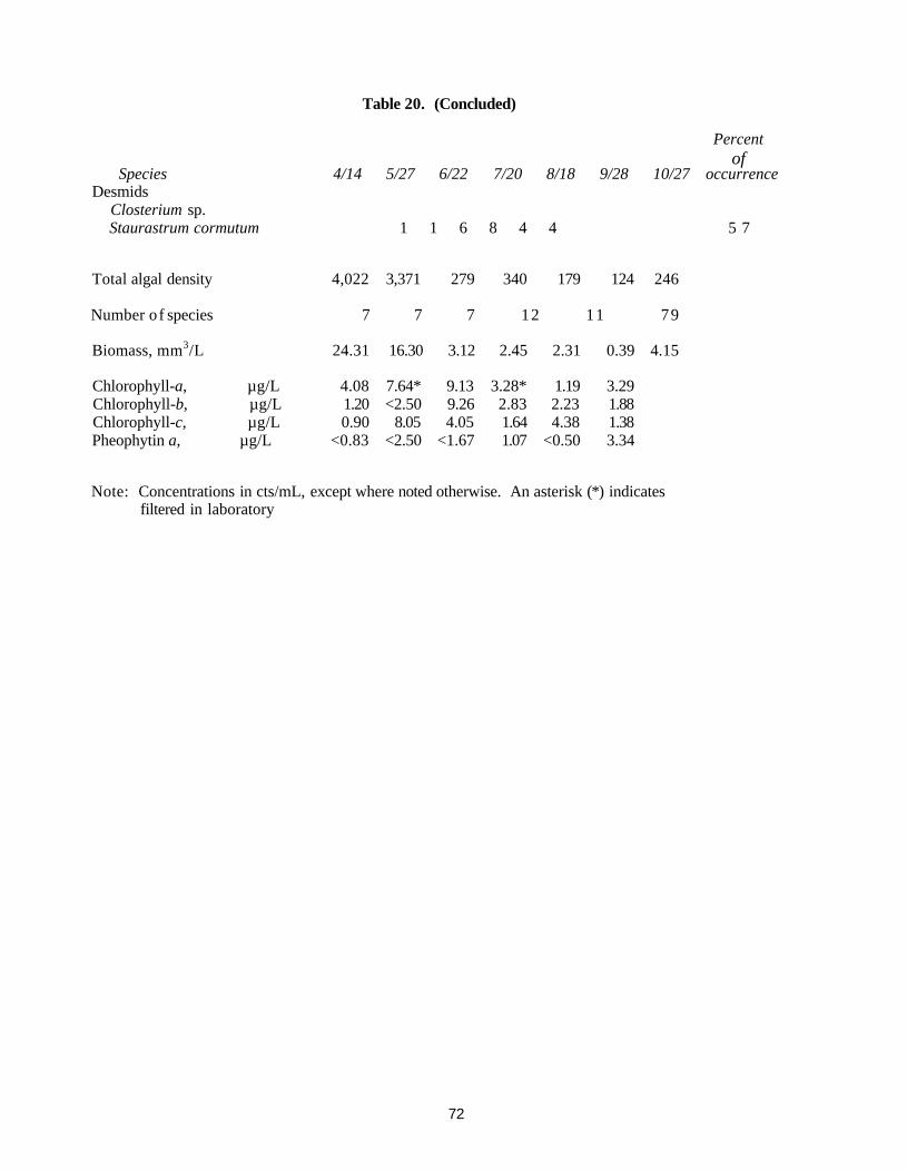
Table 20. (Concluded)

Percent of

Species 4/14 5/27 6/22 7/20 8/18 9/28 10/27 occurrence Desmids

Closterium sp. Staurastrum cormutum 1 1 6 8 4 4 5 7

Total algal density 4,022 3,371 279 340 179 124 246

Number of species 7 7 7 12 11 79

Biomass, mm3/L 24.31 16.30 3.12 2.45 2.31 0.39 4.15

Chlorophyll-a, µg/L 4.08 7.64* 9.13 3.28* 1.19 3.29 Chlorophyll-b, µg/L 1.20 <2.50 9.26 2.83 2.23 1.88 Chlorophyll-c, µg/L 0.90 8.05 4.05 1.64 4.38 1.38 Pheophytin a, µg/L <0.83 <2.50 <1.67 1.07 <0.50 3.34

Note: Concentrations in cts/mL, except where noted otherwise. An asterisk (*) indicates filtered in laboratory

72

Table 21. Algal Types and Densities, Biomass, and Chlorophyll in Lake George, South Basin, 1993

Species Blue-green

Anacystis thermolis Aphanizomenon flos-aquae

Green Coelastrum microporum Crucigenia rectangularis Oocystis borgei Pediastrum duplex P. simplex P. tetras Scenedesmus carinatus S. dimorphus Schroederia sp. Tetraedron hastatum

Diatoms Amphiprora ornata Asterionella formosa Caloneis amphisbaena Cyclotella atomus C. meneghiniana Gymatopleura solea Cymbella affinis C. prostrata Diploneis smithii Hantzschia amphioxys Melosira granulata Navicula cryptocephala N. cuspidata N. gastrum Nitzschia clausii Pinnularia quadrate Rhopalodia gibba Surirella ovata Synedra acus S. delicatissima S. sp.

Flagellates Carteria multifilis Ceratium hirundinella Dinobryon sertularia Eudorina elegans Euglena gracilis E. viridis Glenodinium sp.

73

Percent of

4/14 5/27 6/22 7/20 8/18 9/28 10/27 occurrence

116 69 122 43 29 14

6 4 29 67 14

32 8 11 29 95 38 8 23 15 44 86 42 15 8 43 21 13 29 95 143 11 59 21 21 17 100

59 14 38 6 29

2 27 8 11 57 166 14 4 14

4 14 11 48 29

11 14 59 14

11 14 6 14 4 14

13 40 29 27 14

3,791 14 40 14

8 6 29 84 34 29 21 14 32 11 29

Table 21. (Concluded)

Species Flagellates

Peridinium cinctum Trachemonas crebea

Desmids Closterium sp. Staurastrum comutum S. paradoxum

Total algal density

Number of species

Biomass, mm3/L

Chlorophyll-a, µg/L Chlorophyll-b, µg/L Chlorophyll-c, µg/L Pheophytin-a, µg/L

74

Note: Concentrations in cts/mL, except where noted otherwise. An asterisk (*) indicates filtered in laboratory.

Percent of

4/14 5/27 6/22 7/20 8/18 9/28 10/27 occurrence

6 14

2 14 8 2 29

4,347 254 65 223 237 229 395

12 6 4 10 9 11 9

10.50 1.00 0.08 2.72 1.10 2.89 3.05

5.61 0.92* 5.43 6.61* 23.1 3.86 <2.50 1.16 1.48 2.58 20.7 2.72 <2.50 1.37 2.24 3.17 23.3 2.89 <2.50 <0.50 <1.67 3.14 <0.94 <0.50

The most frequently occurring algae were Scenedesmus dimorphus (green), Pediastrum duplex (green), and Trachemonas crebea (flagellate) in the south basin; and Scenedesmus dimorphus, Oocystis borgei (green), Coelastrum microporum (green), Trachemonas crebea, and Staurastrum cornutum (desmid) in the north basin.

On April 14, 1993, Synedra delicatissima (a linear, needle-shaped diatom) was the dominant algal species in both north and south basins. A relatively high algal count was also observed in the north basin on May 27, 1994. This sample was dominated by a green alga, Crucigenia rectangularis.

Inspection of tables 20 and 21 indicates that there is no correlation between total algal density and chlorophyll a for the 14 algal samples. The reason is unknown. Chlorophyll a was found to peak on June 22, 1993, in the north basin (9.13 µg/L) and on August 18, 1993, in the south basin (23.1 µg/L).

The calculated biomass values showed a wide range in both basins. Algal biomass ranged from 0.39 to 24.31 cubic millimeters per liter (mm3/L) in the north basin and from 0.08 to 10.50 mm3/L in the south basin. The highest observed biomass occurred on April 14, 1993, in both basins (tables 20 and 21). Algal growths in the lake do not seem to be a problem, either because of the densities or the types of algae found.

Zooplankton. The term "plankton" refers to those microscopic aquatic forms having little or no resistance to currents and living free-floating and suspended in open or pelagic waters (American Public Health Association et al., 1992). Plankton can be divided into planktonic plants, phytoplankton (microscopic algae), and planktonic animals (zooplankton). The zooplankton in fresh water are comprised principally of protozoans, rotifers, cladocerans, copepods, and ostracods. Since a Wisconsin plankton net was used for collecting plankton samples, protozoans (microplanktons) were not detected. In this report, protozoans are not included in zooplankton.

Zooplankton densities in Lake George are presented in tables 22 and 23. Total observed zooplankton densities ranged from 100 to 1,400 cts/L in the north basin and from undetectable to 2,100 cts/L in the south basin. The variation of zooplankton communities for each basin showed no trend with time. Peak densities occurred on May 27, 1993, in the north basin and on June 22, 1993, in the south basin.

In the two basins, 11 zooplankton species were observed. These comprised 6 cladocerans, 2 copepods, 1 ostracod, and 2 rotifers. The dominant zooplankton were found to be either copepoda or cladocera. The dominant species for both basins were Diatomus minutus, Bosmina longirostris, and Daphnia pulex. Horaella brehmi were also found frequently in the south basin (table 23). Biovolumes of zooplanktons found in the samples were computed using the shape and size information provided in table 12, and included in tables 22 and 23 for the north and south basins, respectively.

75

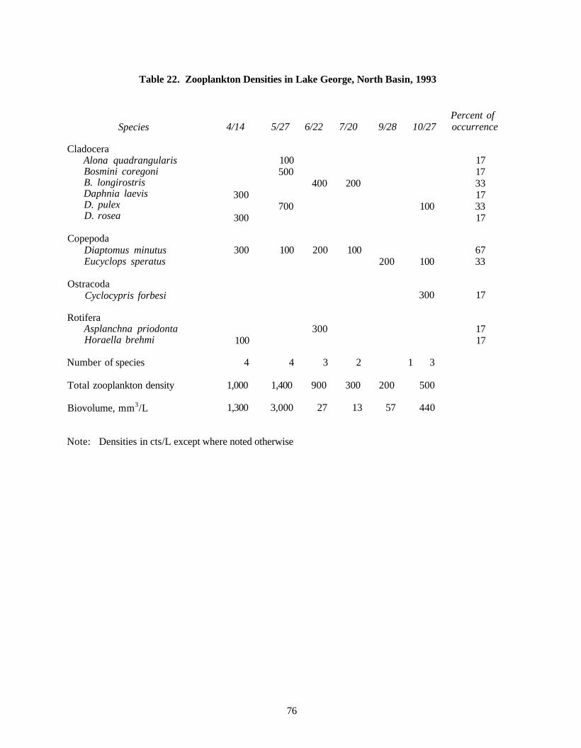
Table 22. Zooplankton Densities in Lake George, North Basin, 1993

Species

Cladocera Alona quadrangularis Bosmini coregoni B. longirostris Daphnia laevis D. pulex D. rosea

Copepoda Diaptomus minutus Eucyclops speratus

Ostracoda Cyclocypris forbesi

Rotifera Asplanchna priodonta Horaella brehmi

Number of species

Total zooplankton density

Biovolume, mm3/L

76

Note: Densities in cts/L except where noted otherwise

Percent of 4/14 5/27 6/22 7/20 9/28 10/27 occurrence

100 17 500 17

400 200 33 300 17

700 100 33 300 17

300 100 200 100 67 200 100 33

300 17

300 17 100 17

4 4 3 2 1 3

1,000 1,400 900 300 200 500

1,300 3,000 27 13 57 440

Table 23. Zooplankton Densities in Lake George, South Basin, 1993

Species

Cladocera Alona quadrangularis Bosmini coregoni B. longirostris Daphnia laevis D. pulex D. rosea

Copepoda Diaptomus minutus Eucyclops speratus

Ostracoda Cyclocypris forbesi

Rotifera Horaella brehmi

Number of species

Total zooplankton density

Biovolume, mm3/L

77

Note: Densities in cts/L except where noted otherwise

Percent of 4/14 5/27 6/22 7/20 8/18 9/28 10/27 occurrence

700 14 1,200 400 300 43

100 14 200 100 100 43

200 100 29

800 100 200 100 57 100 100 29

100 100 100 43

100 100 100 400 57

None found 4 3 4 4 6 2

1,100 2,100 800 400 1,200 200

470 82 870 430 870 420

Macrophytes. Macrophytes are commonly called aquatic vegetation (or weeds). The macrophyton consists principally of aquatic vascular flowering plants, but it also includes the aquatic mosses, liverworts, ferns, and larger macroalgae (American Public Health Association et al., 1992). Macrophytes may include submerged, emerged, and floating plants; and filamentous algae. Aquatic vegetation in lakes and ponds may beneficially and/or adversely impact the natural ecosystem. Reasonable amounts of aquatic vegetation improve water clarity by preventing shoreline erosion, stabilizing sediment, storing nutrients, and providing habitat and hiding places for many small fish (young of the year, bluegill, sunfish, etc.). They also provide food, shade, and oxygen for aquatic organisms; block water movement (wind wave); and utilize nutrients in the water, reducing the excessive growth of phytoplankton.

However, excessive growth of aquatic vegetation generally interferes with recreational activities (fishing, boating, surfing, etc.); adversely affects aquatic life (overpopulation of small fish, benthic invertebrates); causes fish kill; emits taste and odor in water due to decomposition of dense weed beds; blocks water movement and retards heat transfer, creating vertical temperature gradients; and destroys aesthetic value to the extent of decreasing the economic values of properties surrounding a lake. Under these circumstances, aquatic plants are often referred to as weeds.

The macrophyte survey was conducted on July 23, 1993. Table 24 presents the types of macrophytes observed and their biomass expressed in terms of grams of dry weight of macrophytes per square meter of lake bottom (g/m2). The locations of the quantitative macrophyte sampling stations are shown as roman numerals in figure 13. Figure 13 also plots the areal extent of macrophyte beds as determined by the reconnaissance survey and dominant species observed. The quadrat size used, water depth, sediment characteristics at the sampling location, and plant heights are described in table 25. Figure 14 shows some views of the lake taken during the macrophyte survey; the quadrat used in sample collection, the nylon bag containing the collected sample, and the dense growth in the lake interfering with boating can all be noted in this figure.

Six different species of macrophytes were found in the lake. The north basin had six and the south basin had five species of vegetation. All but one of the macrophyte species, namely spike rush found at site IV of the north basin, were found in both basins. Chara is the dominant species in the north basin, occurring in four of the five sites examined quantitatively, but occurred only at site IV in the south basin. Eurasian water milfoil (Myriophyllum spicatum) is the most dominant species in the south basin, constituting 100 percent of the vegetative mass recovered at sites I, II, and III. Only at site HI of the north basin were naiad (Najas flexilis) and Eurasian water milfoil nearly equally dominant. Engel (1990) reports these two macrophytes and chara are also commonly found in the Wisconsin lakes. Three different species were observed at the outlet of the lake (LGO). The biomass collected at site LGO was negligible. Yellow water lilies pads were found at several locations in the north basin.

78

Table 24. Macrophytes Collected at Lake George, July 23, 1993

Note: * LGO: Lake George outlet

Eurasian water milfoil 40 1 100 100 100 1 95 5

Chara 98 90 96 100 4 97 1

Naiad 5 50 2 2 1

Pondweed

Sago pondweed 2 10 2 <1 1

Broad leaf pondweed 2 3 2 3 5 1

Coontail <1 1

Spike rush 2 1

Creeping water primrose 99 1

Duckweed <1 1

Number o f taxa 2 4 3 3 1 1 1 1 3 2 3

Biomass,g/m2 74.4 84.5 143.1 120.3 43.8 221.1 232.2 163.9 56.2 40.1

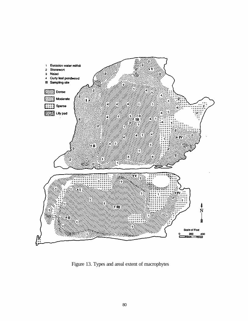
Figure 13. Types and areal extent of macrophytes

80

Table 25. Observations in Lake George during Macrophyte Survey, July 23, 1993

Size of Water Plant Station* quadrat, depth, height, (basin-site) inches feet feet Sediment characteristics

N-I 18 2.3 0.5-0.8 Black, sandy, little organic silt, no putrid odor, sediment 4" deep, firm bottom

N-n 12 2.8 0.5-0.8 Black, fine grit, sediment 3" deep, firm bottom

N-III 18 4.3 5.5 Black, organic oozy material underneath gray sand, sediment 6" deep

N-IV 18 2 Black, sandy, odorless, sediment 4" deep. (Reeds in the sample are not representative of the area. They were found only in this sampling spot)

N-V 18 23 0.3 Black, sandy, little organic silt, no putrid odor, sedi­ment 4" deep, firm bottom

S-I 12 3 4 Black, fine grit, organic silt, musty, sediment 9" deep, firm bottom below

S-II 12 3.3 4 Black, fine grit, organic silt, musty, sediment 6" deep, gritty, firm bottom below

S-III 12 4 5 Black, organic silty, muck, no putrid odor, sediment 6" deep firm bottom below

S-IV 12 2.5 0.8 Black, gritty, odorless, sediment 6" deep

S-V 18 3.5 3 Black, organic muck, loose, soft, odorless, sediment 6" deep, firm bottom

Note: *N = north basin and S = south basin

81

Figure 14. Views of the lake taken during the macrophyte survey

82

a. Quantitative sampling for macrophyte

b. Dense macrophyte growth interfering with boating

Schloesser and Manny (1984) provided guidelines for defining density of macrophyte growths in lakes. They considered growths of 20 to 80 g/m2 to be low density, 60 to 160 g/m2 medium density, and 150 to 220 g/m2 high density. Based on this scale, the north basin could be classified as experiencing medium-dense growth and the south basin as experiencing heavy growth.

Eurasian water milfoil is a non-native aquatic plant that has become a widespread problem throughout North America. It has fine, featherlike leaves and produces a dense canopied bed. It can impact extensive areas because of this dense canopy-like growth form and its highly aggressive and weedy characteristics. Eurasian water milfoil spreads both within and between lakes by the formation of vegetative autofragments, stem pieces that break off the plant through stem abscission. Dense colonies may also spread locally by the growth of root crowns. It grows entirely under water, possibly at depths of 8 to 10 feet, and it will usually become the dominant species in the lake (Pullman, 1992; Madsen, 1993).

Chara is an advanced form of algae that grows from the lake bottom with stems and branches. It feels bristly, has a musky odor, and is usually found in hard water. Common names are muskgrass and stonewart. Like Eurasian water milfoil, chara is often difficult to control even when proper herbicides are used (Illinois Department of Conservation, 1990).

Water depths at the macrophyte sampling stations ranged from 2.0 feet to 4.3 feet. At sites where chara was the dominant species, measured plant heights were between 0.3 to 0.8 feet lower than the water depths. However, plant heights at the sites where Eurasian water milfoil was dominant ranged from 3.0 to 5.5 feet taller than water depths, tending to form a thick canopy. Generally, the soft sediment in the lake was black in color and not more than 9 inches thick. No putrid odor was released when the bottom was disturbed. This soft sediment is underlain by a firm, gritty, and sandy bottom.

From the areal extent of macrophyte beds, it is estimated that approximately 90 and 85 percent of the north and south basins, respectively, were covered by macrophytes. Based on biomass data and the areal extent of macrophyte beds, it is estimated that approximately 29.3 metric tons (64,500 pounds or 32.3 tons) and 27.7 metric tons (61,000 pounds or 30.5 tons) of macrophytes existed (dry-weight basis) in the north and south basins, respectively. It is apparent that the excessive macrophyte growths in the lake adversely impact recreational opportunities such as fishing, boating, and wind surfing. Without a doubt, the massive growths of macrophytes decrease the aesthetic value of the water body.

Benthic Macroinvertebrates. Benthic macroinvertebrates are animals within the aquatic system visible to the unaided eye and capable of being retained by a U.S. Standard No. 30 mesh sieve. These common, easily collected organisms have limited mobility and are present throughout the growing season. An abundant and diverse community of

83

macroinvertebrates is important as a reliable food source for fish. Macroinvertebrates are sensitive to changes in the aquatic environment.

The benthic macroinvertebrate communities were sampled on May 11, 1993, and August 4, 1993, in both the north and south basins. These samples were taken at the regular sampling stations (LGN and LGS) representing the deepest part of each basin.

Table 26 gives the numbers of individuals, taxa, and biomass collected. In the north and south basins, the benthic population ranged from 1,090 to 171 individuals/m2

and the taxa from 7 to 3, respectively. Biomass ranged from 0.291 to 0.036 grams dry weight/m2. The May collection had the highest population, diversity, and biomass, while the August collection had the lowest. This is probably due to the emergence of matured insects and fish predation rather than low DO conditions. The differences between basins were not consistent.

The benthic community was dominated by relatively pollution-intolerant members of the Chironomidae (64%), tolerant members of Chironomus (14%), and aquatic worms (7%). A pollution-sensitive organism, Leptocella, was found during the May and August collections. The benthos in this lake is more diverse and pollution sensitive than that found in most stratified lakes. The abundant macrophytes appear to provide a more complex habitat for aquatic macroinvertebrates.

Trophic State

Eutrophication is a normal process that affects every body of water from its time of formation. As a lake ages, the degree of enrichment from nutrient materials increases. In general, the lake traps a portion of the nutrients originating in the surrounding drainage basin. In addition, precipitation, dry fallout, and ground-water inflow are the other contributing sources.

A wide variety of indices of lake trophic conditions have been proposed in the literature. These indices have been based on Secchi disc transparency; nutrient concentrations; hypolimnetic oxygen depletion; and biological parameters, including chlorophyll a, species abundance, and diversity. The USEPA (1980) suggests in its Clean Lake Program Guidance Manual the use of four parameters as trophic indicators: Secchi disc transparency, chlorophyll a, surface water total phosphorus, and total organic carbon.

In addition, the lake trophic state index (TSI) developed by Carlson (1977) on the basis of Secchi disc transparency, chlorophyll a, and surface water total phosphorus can be used to calculate a lake's trophic state. The TSI can be calculated from Secchi disc transparency (SD) in meters (m), chlorophyll a (CHL) in µg/L, and total phosphorus (TP) in µg/L as follows:

84

on the basis of SD, on the basis of CHL,

TSI = 60 - 14.4 In (SD) TSI = 9.81 In (CHL)+ 30.6

(1) (2)

Table 26. Benthic Macroinvertebrates Collected at Lake George

Organisms

Chironomus (bloodworm) Chironomidae (non-Chironomus) Chaoborus (phantom midge) Ceratopogonidae (biting midge) Caenis (mayfly) Ischnura (damselfly) Leptocella (caddis fly) PsychomiidA. (caddis fly) Tabanidae (horsefly) Oligochaeta (aquatic worm)

Total Number Total Taxa Total Dry Weight, g/m2

85

Note: Density in individuals/m2

Stations 5/11/93 8/4/93

LGN LGS LGN LGS

57 100 100 847 129 115 57

14 14

115 29

14 14 14 43 14 57 43 14 14

1,090 300 243 171 6 7 4 3

0.291 0.054 0.036 0.085

The index is based on the amount of algal biomass in surface water, using a scale of 0 to 100. Each increment of ten in the TSI represents a theoretical doubling of biomass in the lake. The advantages and disadvantages of using the TSI were discussed by Hudson et al. (1992). The accuracy of Carlson's index is often diminished by water coloration or suspended solids other than algae. Applying TSI classification to lakes that are dominated by rooted aquatic plants may indicate less eutrophication than actually exists.

The TSI values for Lake George were calculated using formulas (l)-(3) for each basin based on Secchi depth, total phosphorus, and chlorophyll a concentration of each sample. The TSI results, average values, and trophic state are listed for both basins in tables 27 and 28.

Categorizing the trophic state of a lake can be accomplished using TSI values with the information provided in table 29. Both basins of Lake George could be classified as eutrophic considering the mean Secchi depth and total phosphorus TSI and as mesotrophic considering the mean chlorophyll a TSI. However, the lake exhibited hypereutrophic tendencies in 10 of the 17 samples collected, considering only the individual Secchi depth TSI and/or total phosphorus TSI. Because of excessive macrophyte growths covering almost the whole lake bottom in both basins, the algae must compete for available nutrients. This is the case for Lake George. Hudson et al. (1992) also found that the chlorophyll a TSI was lower than the Secchi depth TSI at McCullom Lake, IL, during their 1980 and 1990 studies, when a substantial portion of the lake bottom was covered with rooted aquatic plants and Chara sp. In conclusion, the trophic state of Lake George can be considered eutrophic with a tendency toward hypereutrophy.

In order to ascertain the limiting nutrient in Lake George, ratios of total nitrogen to total phosphorus were examined. Table 30 shows the ratios of total nitrogen to total phosphorus values (N/P) of Lake George water samples. During the earlier part of this investigation—namely, from October 1992 to June 1993—the ratios were generally higher than during the latter part of the investigation. Ratios greater than 15 are considered phosphorus-limiting conditions for biological productivity in the lake. Frequent and heavy precipitation events experienced during the last three months of field sample collections resulted in more phosphorus influx to the lake from the watershed as evidenced by increased phosphorus concentrations in the lake. However, during this period concentrations of inorganic nitrogen were also less compared to the earlier period, resulting in lower N/P values. The ratio generally tended to be less than 15. The mean ratio values were 29 and 21 for the north and south basins, respectively. Even though these values indicate a phosphorus-limited condition in the lake, biological productivity and the nutrient levels in the water are high.

86

on the basis of TP, TSI=14.421n(TP) + 4.15 (3)

Table 27. Trophic State Index and Trophic State of Lake George, North Basin

Secchi depth Total Phosphorus Chlorophyll a Date inch TSI µg/L TSI µg/L TSI

10/15/92 16 73.0 60 63.4 15.50 57.4 11/10/92 17 72.2 120 73.3 14.50 56.7 12/22/92 21 68.2 40 57.5 4.96 46.2

1/20/93 28 65.0 30 53.3 1.48 34.5 2/11/93 28 65.0 20 47.5 0.90 29.8 3/17/93 27 65.5 30 53.3 1.77 36.3 4/14/93 26 66.0 80 67.5 4.08 44.3 5/10/93 12 77.2 20 47.5 3.23 42.2 5/27/93 23 67.8 30 53.3 7.64* 50.4 6/10/93 18 71.3 40 57.5 5.58 47.3 6/22/93 12 77.2 40 57.5 9.13 52.2 7/6/93 12 77.2 220 82.0 4.95* 46.2 7/20/93 12 77.2 80 67.5 3.28* 42.4 8/3/93 29 64.5 90 69.2 2.42 39.3 8/18/93 28 65.0 100 70.7 1.19 32.4 9/18/93 30 64.0 80 67.5 3.29 42.5 9/28/93 32 63.2 20 47.5 6.55 48.8

Average TSI: 69.4 60.9 44.1 Trophic State: Eutrophic Eutrophic Mesotrophic

Note: * Sample filtered in laboratory.

87

Table 28. Trophic State Index and Trophic State of Lake George, South Basin

Secchi depth Total Phosphorus Chlorophyll a Date inch TSI µg/L TSI µg/L TSI

10/15/92 11 78.5 120 73.3 48.3 68.6 11/10/92 21 68.2 30 53.3 <16.7 58.2 12/22/92 17 72.2 70 65.6 5.7 47.5

1/20/93 25 66.5 70 65.6 7.3 50.0 2/11/93 34 62.3 60 63.4 3.0 41.5 3/17/93 27 65.5 80 67.5 2.7 40.5 4/14/93 19 70.5 110 72.0 5.6 47.4 5/10/93 12 77.2 20 47.5 3.8 43.7 5/27/93 20 69.8 30 53.3 0.9* 30.0 6/10/93 18 71.3 90 69.2 4.6 45.5 6/22/93 12 77.2 50 60.7 5.4 47.3 7/6/93 18 71.3 200 80.7 12.5 55.2 7/20/93 12 77.2 130 74.4 6.6 49.1 8/3/93 21 69.2 70 65.6 12.6 55.3 8/18/93 22 67.0 220 82.0 23.1 61.4 9/18/93 30 64.0 120 73.3 90.8 52.2 9/28/93 36 61.5 50 60.7 3.9 43.7

Average TSI: 70.0 66.4 49.2 Trophic State: Eutrophic Eutrophic Mesotrophic

Note: * Sample filtered in laboratory.

88

Secchi disc transparency Chlorophyll a Total phosphorus,

Trophic State (inches) (meters) (µg/L) lake surface (µg/L) TSI

Oligotrophic >157 >4.0 <2.6 <12 <40

Mesotrophic 79-157 2.0-4.0 2.6-7.2 12-24 40-50

Eutrophic 20-79 0.5-2.0 7.2-55.5 24-96 50-70

Hypereutrophic <20 <0.5 >55.5 >96 >70

Table 29. Quantitative Definition of Lake Trophic State

89

Table 30. Nitrogen-Phosphorus Ratios (N/P) for Lake George Water Samples

North basin South basin Total Total Total Total

Sampling Nitrogen Phosphorus Nitrogen Phosphorus date (mg/L) (mg/L) N/P ratio (mg/L) (mg/L) N/P ratio

10/15/92 1.76 0.06 29 1.77 0.12 15 11/10/92 1.92 0.12 16 3.06 0.30 10 12/22/92 1.06 0.04 27 1.80 0.07 26 1/20/93 1.25 0.03 42 2.33 0.07 33 2/11/93 1.04 0.02 52 2.82 0.06 47 3/17/93 0.66 0.03 22 1.41 0.08 18 4/14/93 0.95 0.08 12 1.37 0.11 13 5/10/93 1.95 0.02 98 1.45 0.02 73 5/27/93 1.65 0.03 55 1.26 0.03 42 6/10/93 1.32 0.04 33 0.34 0.09 4 6/22/93 1.25 0.04 31 1.14 0.05 23 7/6/93 0.36 0.22 2 0.40 0.20 2 7/20/93 0.77 0.08 9 0.89 0.13 7 8/3/93 0.76 0.09 8 1.13 0.07 16 8/18/93 0.45 0.10 5 0.93 0.22 4 9/18/93 0.10 0.08 1 1.39 0.12 12 9/28/93 1.09 0.02 55 0.46 0.05 9

90

Sediment Characteristics

Lake sediment can act both as sinks and as potential pollution sources (such as phosphorus and metals) impacting lake water quality. Its metal and/or organic chemical toxicities can directly affect the presence of aquatic animals and plants on the lake bottom. Lake sediments, if and when dredged, should be carefully managed to prevent surface water and ground-water contamination.

Sediment monitoring is becoming increasingly important as a tool for detecting pollution loadings in lakes and streams. The reasons are as follows: 1) many potential toxicants are easier to assess in sediments because they accumulate there at levels far greater than those normally found in the water column; 2) sediments are less mobile than water and can be used more reliably to infer sources of pollutants; and 3) nutrients, heavy metals, and many organic compounds can become tightly bound to the fine particulate silts and clays of the sediment deposits where they remain until they are released to the overlying water and made available to the biological community through physical, chemical, or bioturbation processes. Remedial pollution mitigation projects may include the removal of contaminated sediments as a necessary step (Indiana Department of Environmental Management, 1990).

Sediment Quality Standard

While there are no regulatory agencies that promulgate sediment quality standards, sediment quality in Illinois is generally assessed using the data developed by Kelly and Hite (1981). For their study, they collected 273 individual sediment samples from 63 lakes across Illinois during the summer of 1979. On the basis of each parameter measured, they defined "elevated levels" as concentrations of one to two standard deviations greater than the mean value, and "highly elevated levels" as concentrations greater than two standard deviations from the mean. A statistical classification of Illinois lake sediment developed by Kelly and Hite is shown in table 31. It should be noted that in this classification, lake sediment data are considered to be elevated based on a statistical comparison of levels found in 1979 and not on toxicity data. Therefore, elevated or highly elevated levels of parameters do not necessarily indicate a human health risk.

In Indiana, the maximum sediment background concentrations were determined from the analyses of sediment samples from 83 "non-contaminated" sites throughout the state (Indiana Department of Environmental Management, 1990). Each sediment sample was collected from a lake or from a small stream at a location upstream of all known point sources of pollution including municipal or industrial discharges and combined sewer overflows. Aerial sources of contaminants and contamination from nonpoint urban and agricultural runoff may have impacted those sampling sites. While it is unlikely that any areas of the state are free of inputs from these sources, the background concentrations calculated are considered to represent the best possible estimate of "unpolluted" sediment in Indiana. The maximum background levels of constituents in Indiana lake and stream sediments determined by the study are shown in table 32. Sediments containing less than

91

Table 31. Classification of Illinois Lake Sediments

Below Highly Constituent normal Normal Elevated elevated

Chemical oxygen demand <32,500 32,500-162,000 162,000-226,000 >226,000 Total Kjeldahl nitrogen <1,650 1,650-5,775 5,775-7,850 >8,750 Total phosphorus <225 225-1,175 1,175-1,650 >1,650 Volatile solids (%) <5 5-13 13-17 >17 Total organic carbon <26,500 26,500-65,000 65,000-85,100 >85,100

Arsenic <27 27-41 >41 Cadmium <1.8 1.8-2.6 >2.6 Chromium <14 14-30 30-38 >38 Copper <100 100-150 >150 Iron <18,000 18,000-36,000 36,000-45,000 >45,000

Lead <15 15-100 100-150 >150 Manganese <3,000 3,000-3,900 >3,900 Mercury <0.25 0.25-0.40 >0.40 Zinc <50 50-175 175-250 >250

Note: Constituents measured in mg/kg except where otherwise noted

Source: Kelly and Hite (1981)

/92

Table 32. Maximum Background Concentrations of Pollutants in Indiana Stream and Lake Sediments

Maximum Maximum background background

Parameter (mg/kg) Parameter (mg/kg)

Aluminum 9,400 Silver <0.5 Antimony 0.49 Strontium 110 Arsenic 29 Thallium <3.8 Beryllium 0.7 Zinc 130 Boron 8.0 Phenol <0.2 Cadmium 1.0 Cyanide <0.1 Chromium 50 PCB (Total) 0.022 Cobalt 20 Chlordane 0.029 Copper 20 Dieldrin 0.033 Iron 57,000 DDT (Total) 0.020 Lead 150 BHC (Total) 0.014 Manganese 1,700 Pentachlorophenol 0.003 Mercury 0.44 Heptachlor 0.002 Nickel 21 Aldrin 0.0007 Nitrogen (TKN) 1,500 HCB <0.001 Phosphorus 610 Methoxychlor <0.001 Selenium 0.55 Endrin <0.001

93

two times the maximum background concentration for each constituent are classified as "uncontaminated."

In Indiana, lake (reservoir) or stream sediments were also grouped into four levels of concern—high, medium, low, and unknown—based on the presence and concentration of priority pollutants measured. The criteria for such groupings are listed in table 33. If background concentrations of particular contaminants found were not known, the water body was placed into the "unknown" category of concern.

Historical Sediment Data

The available historical data for soil and sediments around and in Lake George are presented in tables 34-36. Table 34 shows the toxicity characteristics leaching test (TCLP) results of slag analyses for the Federated Metals property. The concentrations of six parameters (arsenic, chromium, mercury, selenium, silver, and sulfite) determined for slag (soil) were less than the detection limits. In 54 percent (15/28) of samples, the cadmium levels exceeded the USEPA limit of 1.0 mg/L (1990a). Concentrations of lead in the leachates were generally very high (maximum 280 mg/L), with 82 percent (23/28) of the samples exceeding the regulatory limit of 5.0 mg/L.

Table 35 shows the results of sediment analyses for Lake George made by various organizations during a period from 1976-1986. The Indiana maximum background sediment levels are listed in the first column for purposes of comparison. Unfortunately, exact sampling sites in Lake George are not available, and how the samples were composited is unknown.

Inspection of table 35 reveals that the metal concentrations in the sediments collected on July 17, 1986, were extremely high in the north basin sample. The reason for this is unknown. In the north basin sample, the concentration of antimony was of high concern; cadmium, copper, lead, and zinc concentrations were of medium concern; and nickel and selenium concentrations were of low concern. Lead and copper concentrations in this sample were much above the background concentrations. Sediment quality in the south basin sample was significantly better than that in the north basin sample. Similar observations hold true for both composite sediment samples collected on April 29, 1976, and July 6, 1976 (table 35). Composite samples collected from the north basin on these dates had concentrations of cadmium, copper, and zinc at medium concern levels. Core samples collected on July 8, 1976, showed 'good" sediment quality (table 35). Surficial sediment samples taken on April 22, 1981, also showed 'good" quality, except for a low-concern level of copper concentration in the #1 (2') samples of the north basin.

Table 36 shows the results of the Extraction Procedure Toxicity Test for sediment samples collected in 1980 and 1981. The values determined were all found to be lower than the maximum regulatory limits.

94

Table 33. Indiana Criteria for Grouping Sediments into Levels of Concern

High Concern: Any contaminant present in concentrations greater than 100 times background

Medium Concern: Any contaminant present in concentrations 10 to 100 times background

Low Concern: Any contaminant present in concentrations 2 to 10 times background

Unknown Concern: Contaminants present for which background concentration has not been established

95

Table 34. Results of Slag (Soil) Analyses for Federated Metals Property, October 5-7, 1988

Toxicity Characterstics Sample Total Leaching Procedure, mg/L Cyanide, Sulfide number pH solids, % As Ba Cd Cr Pb Hg Se Ag mg/L mg/L

(Detection Value: 0.5 1.0 0.1 0.5 0.5 0.02 0.1 0.5 10 10)

1 9.7 89.5 k* 1.7 1.5 k 150 k k k k k 2 8.8 85.3 k k 2.2 k 17 k k k k k 3 7.5 78.3 k k 5.8 k 130 k k k k k 4 9.5 94.4 k 1.4 0.3 k 200 k k k k k 5 9.9 86.5 k 1.5 0.5 k 160 k k k k k 6 8.9 69.2 k k 5.2 k 140 k k k k k 7 8.9 78.8 k 1.0 1.4 k 120 k k k k k 8 9.5 83.9 k 1.0 1.2 k 220 k k k k k 9 9.2 85.6 k 1.2 1.1 k 280 k k k k k

10 9.9 95.4 k 2.6 0.5 k 140 k k k k k

11 9.1 87.5 k 1.8 1.2 k 56 k k k k k 12 8.3 85.8 k 1.0 1.3 k 140 k k k k k 13 9.6 81.1 k 2.8 k k 2.3 k k k k k 14 9.4 85.2 k 2.0 3.0 k 5.0 k k k k k 15 9.1 76.2 k 1.5 0.7 k 270 k k k k k 16 8.3 91.6 k 1.1 0.4 k 11 k k k k k 17 8.4 78.9 k 1.4 2.7 k 12 k k k k k 18 10.8 78.4 k 2.7 0.7 k 1.5 k k k k k 19 9.2 78.1 k 1.5 0.9 k 31 k k k k k 20 8.6 80.6 k 2.7 0.45 k 14 k k k k k

21 8.8 80.5 k 11 2.2 k 73 k k k k k 22 7.7 74.0 k 1.7 5.3 k 44 k k k k k 23 7.3 86.0 k 2.3 6.5 k 110 k k k k k 24 8.5 84.9 k 2.7 6.7 k 61 k k k k k 25 8.6 80.4 k 2.7 0.8 k 58 k k k k k 26 9.5 82.1 k 15 0.9 k 14 k k k k k 27 8.4 80.4 k 3.0 0.1 k 1.4 k k k k k 28 9.9 87.5 k 13 0.2 k 0.6 k k k k k

(Regulatory level: 5.0 100 1.0 5.0 5.0 0.2 1.0 5.0)

Notes: *k = less than the detection value For all samples, total hydrocarbons are < 1 mg/kg, flashpoints are > 140°F.

Source: Carnow (1990). Analyses done by ATEC Environmental Services.

96

Table 35. Sediment Quality of Lake George

4/29/76 7/6/76 7/8/76, Core sample 4/22/81, Surficial sample 7/17/86 Composite sample Composite sample North South North South Grab sample

Parameters North South North South 2.5-4.5' 6-9' 4-5.5' 8.5-10' #1 (2') #1(Sand) #2 #3 North South

BOD 59,000 70,000 724 554 COD 540 >600 1600 1150 7010 785057,000 6370 88,000 14,000 11,000 69,000 Grease & Oil 200 200 <10 <10 <50 <50 <50 <50 Total solids, % 788 823 625 792 37 40 Volatile solids, % 8 6 Antimony (0.49) 60 3.1 Arsenic (29) 0.11 <.02 0.06 0.07 10 1.3 2.7 3.3 58 8.1 Barium 68.9 71.3 74.9 24.7 72.5 5 9.5 9.0 <2.8 <2.7 Calcium 0.1 <0.1 1.3 0.4 Cadmium (1.0) 10.8 0.94 11.2 1.1 0.9 4.9 <1 <1 0.74 <0.5 0.08 0.27 26 <2.7 Chromium (50) 36.7 54.4 60 60 16.9 10.2 3.1 4.1 3.0 2.5 2.0 1.5 97 36 Copper (20) 1419 42.2 315 128 1.7 2.5 35.7 2.0 230 3.0 11.5 14 1800 54 Iron (57,000) 1870 2310 5510 2730 6500 3800 3750 3750 Lead (150) 72.4 65.6 86 56 8.4 14.8 34.4 7.2 57.5 5.3 4.7 15.5 2800 140 Manganese (1,700) 116 145 357 159 400 130 115 112 Nickel (21) 34.8 11.3 450 45 6.1 6.0 10 8 7.5 <5 <5 <5 54 6.6 Selenium (0.55) 3.7 0.55 Silver (<0.5) 1 1 0.5 <0.5 <2.1 <1.6 Thallium (<3.8) <28 <27 Zinc (130) 2413 216 1500 125 15.0 27.8 69.5 14.9 100 9 16.5 30.5 3500 260 Cyanide (<0.1) <0.05 0.1 <.26 <.26 0.00 0.00 Hexane 297 2120 81 1000 Phenol (<0.2) 0.9 6.0 PCB (0.022) <1 <1 <1 <1 <0.05 <0.05<0.05<0.05 Analyses by: Waste Lake County Williams Laboratory Measurement Indiana State

Management Health Deptartment Services Sciences Corp. Toxics Program

Notes: Values shown in parentheses in column 1 are the Indiana maximum background concentrations. Parameters are in mg/kg unless noted otherwise.

= Low concern = Medium concern = High concern

Source: Carnow (1990)

Table 36. Extraction Results for Lake George Sediments

Note: 1980 analyses by American Smelting and Refining Compnay (ASARCO), 1981 analyses by Science Corporation.

Source: Carnow (1990)

Current Study Data

During this study, the sediment samples (both surficial and core) were collected at seven sites (figure 8) on September 29, 1993. The surficial sediment samples were collected using a Petite Ponar dredge, and the core samples were taken using a 2-inch Wildco sediment corer with liner tubes. Each core sample was divided into three equal parts—top, middle, and bottom—and each portion was completely mixed and then analyzed. The results of sediment quality are presented in tables 37 and 38.

Surficial Sediment Data. For the purposes of comparison, Indiana maximum background concentrations and Illinois maximum normal concentrations are listed in table 37. It can be seen from this table that copper levels in only three surficial sediment samples taken from the north basin are at elevated levels; while the LGN1 sample is of medium-level concern, the other two samples are of low-level concern. Copper levels in the south basin may not be of any concern except in the LGS sample, which had a concentration at the lowest threshold of low-level concern. Copper levels were well below the normal concentrations observed in Illinois except for the LGN1 sample. In addition, cadmium and zinc concentrations in the LGN1 sample fall within the low-concern category. Unfortunately, copper and zinc concentrations were not determined for slag (soil) from Federated Metals property (table 34). However, cadmium levels in TCLP tests were high.

Except for copper, cadmium, and zinc, other parameters measured in sediments from Lake George were found to be in normal range.

Examination of tables 35 and 37 reveals that the concentrations of heavy metals in Lake George sediments generally decreased since 1976 studies. Historical records reveal that sediments with the worst quality characteristics were taken from the north basin on July 17, 1986. In this study, the worst sediment characteristics were found at station LGN1, and yet the sediment there was still much better than north basin sediment collected on July 17, 1986.

Core Sediment Data. As shown in table 38, silver concentration in core samples was below the detectable level. Metals levels in the top, middle, and bottom portions of core samples generally showed a similar pattern for both LGN and LGS; i.e., concentrations of metals decreased with depth. On the other hand, samples collected at the outlet (LGO) showed metals concentrations increasing with depth. The composition of the heavy metal content in the core samples collected from stations LGN1, LGN2, LGS1, and LGS2 was found to be inconsistent, with no definite trend. For purposes of comparison, Indiana maximum background concentrations for sediments are shown in the first column of table 38.

As in the surficial samples, the concentrations of copper, zinc, and cadmium in a few core samples were found to be of low-level concern (table 38). High copper levels occurred in six of the nine core subsamples in the north basin. In the south basin, low-

99

Table 37. Physical and Chemical Characteristics of Lake George Surficial Sediment Samples, 1993

Notes: LGN: Fine-grained sand with traces of medium-grained sand, traces of clay, and considerable silt LGN1: Fine-grained sand, with considerable amount of medium-grained sand, traces and small amounts of silt LGN2: Fine-grained sand with traces of medium- and coarse-grained sand, traces of clay, and some silt LGS: Silly loam LGS1: Fine-grained sand with traces of medium-grained sand, clay, and silt LGS2: Fine-grained sand with some coarse-grained sand, fine-grained gravel, and traces of medium-grained sand, silt, and clay LGO: silt

= Low concern; = Medium concern

Table 38. Physical and Chemical Characteristics of Lake George Core Sediment Samples, 1993

LGN LGN1 LGN2 Parameters* Top Middle Bottom Top Middle Bottom Top Middle Bottom

Metals, mg/kg Cadmium (1.0) 2.17 <0.50 <0.50 0.62 0.69 <0.50 0.99 0.83 0.52 Chromium (50) 1 2 . 0 0 2 . 3 1 2.75 3 . 8 1 5 . 0 4 8 . 6 2 7 . 4 5 5 . 1 0 3.43 Copper (20) 87.40 2.08 1.54 69.60 121.00 7.10 73.00 81.8 93.4 Iron (57,000) 6,910 2,710 2,830 4,210 7,730 5,970 6,450 6,780 5,420 Lead (150) 197 6.2 5.00 53.5 45.1 <5.0 86.9 85.4 89.3 Manganese (1700) 395 134 162 179 151 166 268 169 130 Nickel (21) 7.81 2.05 2.56 4.17 5.98 3.78 5.68 5.22 4.40 Silver (<0.5) < 1 . 0 0 < 1 . 0 0 <1.00 <1.00 <1.00 <1.00 <1.00 <1.00 <1.00 Zinc (130) 337.0 16.2 7.2 175.0 146.0 18.7 148.0 103.7 82.7

Other Parameters Total phosphorus-P,mg/kg (225) 49.4 72.0 31.5 21.4 34.9 88.4 102.0 233.0 191.0 Total nitrogen-N, mg/kg 950 430 420 350 1,030 350 1,200 1,310 1,250 COD, mg/kg (162,000) 55,400 16,200 39,900 3,760 120,000 8,940 43,400 49,600 75,800 Total solids, % 59.4 66.4 71.8 77.9 65.3 73.6 46.5 58.2 54.2 Volatile solids, % (13) 3 2 2 13 3 7 9 13 TOC, mg/kg (65,500) 2,800 2,900 7,300 7,800 3,300 2,000 14,000 8,800 13,000 Density, g/mL 1.51 1.78 1.81 1.92 1.58 1.92 1.38 1.59 1.53

Metals, mg/kg Cadmium 2.12 1.11 <0.50 <0.50 <0.50 <0.50 <0.50 <0.50 <0.50 Chromium 32.20 18.9 1.61 4.69 2.81 2.78 3.20 2.21 2.64 Copper 63.9 25.1 1.18 7.99 13.20 10.2 14.7 3.13 1.45 Iron 9,900 7,310 2,020 3,500 4,600 3,490 3,660 2,230 2,480 Lead 163.0 94.1 5.2 2.3 19.3 13.2 10.1 5.9 5.0 Manganese 1,010 478 108 293 190 166 128 86 109 Nickel 9.89 6.12 <2.00 2.77 2.55 2.36 <2.00 2.04 2.14 Silver <1.00 <1.00 <1.00 <1.00 <1.00 <1.00 <1.00 <1.00 <1.00 Zinc 309.0 174.0 10.0 63.7 68.8 31.4 19.8 16.9 7.9

Table 38. (Concluded)

LGS LGS1 LGS2 Parameters Top Middle Bottom Top Middle Bottom Top Middle Bottom

Other Parameters Total phosphorus-P, mg/kg 209.0 60.3 121.0 103.0 113.0 113.0 114.0 117.0 129.0 Total nitrogen-N, mg/kg 1,060 780 130 160 110 200 120 88 78 COD, mg/kg 69,300 47,000 21,000 8,040 27,300 23,400 9,580 9,260 4,260 Total solids, % 25.8 67.9 77.7 76.2 70.4 71.6 78.0 79.7 79.7 Volatile solids, % 1 7 2 1 1 1 1 1 1 1 TOC, mg/kg 19,000 9,500 1,500 1,200 10,000 3,200 3,200 9,300 2,100 Density, g/mL 1.20 1.68 1.89 1.87 1.89 1.87 1.92 1.93 1.86

LGO Top Middle Bottom

Metals, mg/kg Cadmium 1.02 1.23 1.39 Chromium 18.4 25.2 30.3 Copper 39.10 41.1 51.1 Iron 5,510 7,550 9,090 Lead 80.4 130.0 152.0 Manganese 601 756 852 Nickel 4.15 6.62 7.90 Silver <1.00 <1.00 <1.00 Zinc 163.0 242.0 294.0

Other Parameters Total phosphorus-P, mg/kg 127.0 172.0 194.0 Total nitrogen-N, mg/kg 740 540 460 COD, mg/kg 29,100 65,400 73,400 Total solids, % 19.9 19.2 32.2 Volatile solids, % 14 14 14 TOC, mg/kg 17,000 8,500 9,300 Density, g/mL 1.13 1.16 1.17 Note: * Values in parentheses are the maximum background concentrations in Indiana.

Low concern

level concern copper concentrations are limited to the top subsample at station LGS. At station LGO, concentrations of copper in the whole core sample may be considered of low concern, although the top sample did not exceed two times the background concentration of 20 mg/L.

Nutrients. Total phosphorus (TP) levels in the seven surficial sediment samples were between 141 and 199 milligrams per kilogram (mg/kg) (table 37). For seven core sediment samples, TP concentrations ranged from 21.4 mg/kg to 233 mg/kg (table 38). Only the LGN2 middle subsample exceeded the Illinois maximum normal concentration. Low TP levels were found at stations LGN and LGN1; whereas TP levels at LGN2 were higher. The average value of the 21 TP concentrations listed in table 38 is 114 mg/kg. This value is the best available estimate and can be used for calculating TP removed from Lake George, if it is dredged.

Total nitrogen levels in seven surficial sediment samples ranged from 240 mg/kg at station LGS2 to 1,360 mg/kg at LGS (table 37). For core sediments (table 38), total nitrogen levels were generally low, between 78 mg/kg at LGS2, bottom portion, and 1,310 mg/kg at LGN2, the middle portion. The average total nitrogen concentration from the 21 determinations in table 38 is 560 mg/kg. Both TP and total nitrogen in Lake George sediments are low in concentration presumably because of the absence of agricultural drainage.

Particle-Size Distribution. Table 39 shows the particle-size distribution of surficial sediments taken from Lake George. The samples were fine-grained sand with traces of silt except those from LGS and LGO, which were predominantly silty loam and silt, respectively. The sediment accumulations at sites LGS and LGO were less dense and fluffy compared to other sites, and the loose sediment accumulation at the lake's outlet (LGO) is several feet deep. No relationship could be discerned between particle size and nutrient concentrations. The phosphorus concentrations of sediment samples from LGS and LGO were similar to those determined for other sites.

White Precipitate Table 40 shows results of analyses of the white precipitate scraped from a hard substrate from the southwest corner of Lake George adjoining the Bairstow property. The white precipitate is presumed to be the result of direct runoff or leachate from the Bairstow slag disposal site. The interaction between the leachate from the slag pile and the lake waters forms colloidal precipitates, which in due course coalesce and settle to the bottom. This colloidal particulate matter caused difficulty in filtering south basin samples for chlorophyll and indicator bacteria analyses. No such difficulty was encountered with respect to the north basin samples. The precipitate sample had high pH and alkalinity values, and nearly 27 percent, by weight, was calcium and magnesium. All the other metals—cadmium, chromium, copper, iron, lead, manganese, nickel, silver, and zinc—were below the Indiana maximum background concentrations.

TCLP Results. The cornerstone of safe waste management and disposal practices is determining whether or not the waste in question is considered "hazardous." The

103

Table 39. Particle-Size Distribution of Lake George Surficial Sediments

Percent finer than sieves Sample #4 #10 #20 #40 #60 #140 #200* Description

LGN 100 100 100 98 80 22 16 Fine-grained sand with trace of medium-grained sand, consi­derable silt, and trace of clay

LGN1 100 88 84 81 69 11 10 Fine-grained sand with consi­derable medium-grained sand, small amount of silt, and trace of clay

LGN2 100 98 97 96 89 23 18 Fine-grained sand with trace of medium- and coarse-grained sand, some silt, and trace of clay

LGS 100 100 100 98 91 70 64 Silt loam LGS1 100 100 100 97 83 8 5 Fine-grained sand with trace of

medium-grained sand, clay, and silt

LGS2 82 70 69 66 53 6 5 Fine-grained sand with some coarse-grained sand, fine­grained gravel, and trace of medium-grained sand, silt, and clay

LGO 100 100 100 100 99 97 96 Silt

Note:* Sieve sizes: #4 - 4.75 mm; #10 - 2.00 mm; #20 - 0.850 mm, #40 - 0.425 mm; #60 - 0.250 mm; #140 - 0.106 mm; and #200 - 0.075 mm.

104

Table 40. Results of Analyses of White Precipitate from Southwest Corner of Lake George

Parameter Value

pH 10.9 Alkalinity 52,530 Total Aluminum 1,470 Antimony <1.6 Arsenic <3.1 Barium 186 Boron 1.25 Beryllium 0.31 Cadmium 1.8 Calcium 258,700 Chromium 11.6 Cobalt 0.62 Copper 34.4 Iron 3,310 Lead 62.5 Magnesium 11,200 Manganese 606 Nickel 2.5 Phosphorus 134 Potassium 309 Selenium <3.9 Silver <0.31 Sodium 562 Sulfur 1,440 Vanadium <0.16 Yttrium 1.25 Zinc 119 Note: Values in mg/kg except pH

105

process of determining a waste's toxicity and subsequently classifying it as "hazardous" or "nonhazardous" involves various state-of-the-art analytical procedures. The Extraction Procedure (EP) Toxicity Characteristics has been used for years.

The Toxicity Characteristics Leaching Procedure (TCLP) was driven by the Federal Resource Conservation and Recovery Act (RCRA) and its amendments. The Identification and Listing of Hazardous Waste rule was originally proposed in June 1986, designed to replace the EP Toxicity Characteristics. Over a four-year period, the USEPA has significantly changed the actual procedure; they replaced the EP Toxicity Test with the TCLP in 1990. The effective date of the TCLP rule was September 25, 1990, for all large-quantity generators, and March 29, 1991, for all small-quantity generators.

If any dredging is to be conducted in a lake, the amount of nutrient removed with the lake sediments could be estimated using the collected data. The TCLP test is intended to simulate the potential release of contaminants from sediments that might occur during dredging operations or be encountered in leachate from a disposal area containing dredged lake sediment.

Table 41 presents the concentrations of metals, polychlorinated biphenyls (PCBs), and pesticides determined by TCLP tests of six Lake George samples. Not all the parameters evaluated were required by the USEPA; only five of 30 parameters are in the TCLP regulatory list (table 41). TCLP tests indicate that concentrations of cadmium, chromium, lead, endrin, and lindane are all under the regulatory limit for the six sediments. The highest lead level was 4.33 mg/L (<5.0 mg/L limit) at station LGN.

Table 41 also shows that concentrations of 7 types of PCBs and 14 pesticides are all below the detection limits. Based on the results, sediments in Lake George are classified as "non-hazardous" material, and they would not require special handling during disposal if the lake is dredged.

106

Table 41. Results of Toxicity Characteristics Leaching Procedure (TCLP)

USEPA regulatory

LGN LGN1 LGS LGS1 LGS2 LGO limit, mg/L TCLP metals, mg/L

Cadmium 0.042 0.024 0.032 0.020 <0.005 0.016 1.0 Chromium 0.021 <0.010 0.040 0.045 <0.010 <0.010 5.0 Copper 0.013 0.367 0.039 0.076 0.095 0.025 Iron 43.9 <0.100 36.0 46.3 0.464 0.821 Lead 4.33 1.08 2.23 1.36 0.182 0.346 5.0 Manganese 12.9 2.45 28.0 19.4 5.37 17.4 Nickel 0.064 0.046 0.047 0.045 <0.020 0.039 Silver <0.010 <0.010 <0.010 <0.010 <0.010 0.025 Zinc 8.18 4.60 5.35 3.69 0.903 3.85

TCLP PCBs, mg/L Aroclor-1016 <0.0005 <0.0005 <0.0005 <0.0005 <0.0005 <0.0005 Aroclor-1221 <0.0005 <0.0005 <0.0005 <0.0005 <0.0005 <0.0005 Aroclor-1232 <0.0005 <0.0005 <0.0005 <0.0005 <0.0005 <0.0005 Aroclor-1242 <0.0005 <0.0005 <0.0005 <0.0005 <0.0005 <0.0005 Aroclor-1248 <0.0005 <0.0005 <0.0005 <0.0005 <0.0005 <0.0005 Aroclor-1254 <0.001 <0.001 <0.001 <0.001 <0.001 <0.001 Aroclor-1260 <0.001 <0.001 <0.001 <0.001 <0.001 <0.001

TCLP pesticides, mg/L Aldrin <0.04 <0.04 <0.04 <0.04 <0.04 <0.04 Dieldrin <0.002 <0.002 <0.002 <0.002 <0.002 <0.002 4,4'-DDE <0.002 <0.002 <0..002 <0.002 <0.002 <0.002 Endrin <0.002 <0.002 <0.002 <0.002 <0.002 <0.002 0.02 4,4'-DDD <0.002 <0.002 <0.002 <0.002 <0.002 <0.002 4,4'-DDT <0.002 <0.002 <0.002 <0.002 <0.002 <0.002 Methoxychlor <1.0 <1.0 <1.0 <1.0 <1.0 <1.0 Alpha-Chlordane <0.003 <0.003 <0.003 <0.003 <0.003 <0.003 Gamma-Chlordane <0.003 <0.003 <0.003 <0.003 <0.003 <0.003 BHC, Alpha <0.04 <0.04 <0.04 <0.04 <0.04 <0.04 BHC, Delta <0.04 <0.04 <0.04 <0.04 <0.04 <0.04 BHC, G (Lindane) <0.04 <0.04 <0.04 <0.04 <0.04 <0.04 0.4 Hexachlorobenzene <0.01 <0.01 <0.01 <0.01 <0.01 <0.01

Pentachlorphenol <0.50 <0.50 <0.50 <0.50 <0.50 <0.50

107

Lake-Use Support Analysis

Definition

An analysis of Lake George's use support was carried out employing the methodology developed by the IEPA (1994). The degree of support identified for each designated use indicates the ability of the lake: 1) to support a variety of high quality recreational activities, such as boating, sport fishing, swimming, and aesthetic enjoyment; 2) to support healthy aquatic life and sport fish populations; and 3) to provide adequate, long-term quality and quantity of water for public or industrial water supply (if applicable). Determination of a lake's use support is based upon the state's water quality standards as described in Subtitle C of Title 35 of the State of Illinois Administrative Code (IEPA, 1990). Each of four established use designation categories (including General Use, Public and Food Processing Water Supply, Lake Michigan, and Secondary Contact and Indigenous Aquatic Life) has a specific set of water quality standards.

For the lake uses assessed in this report, the General Use standards—primarily the 0.05 mg/L TP standard—were utilized. The TP standard has been established for the protection of aquatic life, primary-contact (e.g., swimming) and secondary-contact (e.g., boating) recreation, agriculture, and industrial uses. In addition, lake-use support is based in part on the amount of sediment, macrophytes, and algae in the lake and how these might impair designated lake uses. The following is a summary of the various classifica­tions of use impairment:

Full = full support of designated uses, minimal impairment Full/threatened = full support of designated uses, with indications of declining water quality or evidence of existing use impairment Partial/minor = partial support of designated uses, with slight impairment Partial/moderate = partial support of designated uses, with moderate impairment Nonsupport = no support of designated uses, with severe impairment

Lakes that fully support designated uses may still exhibit some impairment or have slight to moderate amounts of sediment, macrophytes, or algae in a portion of the lake (e.g., headwaters or shoreline); however, most of the lake acreage shows minimal impairment of the aquatic community and uses. It is important to emphasize that if a lake is rated as not fully supporting designated uses, it does not necessarily mean that the lake cannot be used for those purposes or that a health hazard exists. Rather, it indicates impairment in the ability of significant portions of the lake waters to support either a variety of quality recreational experiences or a balanced sport fishery. Since most lakes are multiple-use water bodies, a lake can fully support one designated use (e.g., aquatic life) but exhibit impairment of another (e.g., swimming).

Lakes that partially support designated uses have a designated use that is slightly to moderately impaired in a portion of the lake (e.g., swimming impaired by excessive aquatic macrophytes or algae, or boating impaired by sediment accumulation). So-called

108

nonsupportive lakes have a designated use that is severely impaired in a substantial portion of the lake (e.g., a large portion of the lake has so much sediment that boat ramps are virtually inaccessible, boating is nearly impossible, and fisheries are degraded). However, in other parts of the same nonsupportive lake (e.g., near a dam), the identical use may be supported. Again, nonsupport does not necessarily mean that a lake cannot support any uses, that it is a public health hazard, or that its use is prohibited.

Lake-use support and level of attainment were determined for aquatic life, recreation, swimming, and overall lake use using methodologies described in the IEPA's Illinois Water Quality Report 1992-1993 (IEPA, 1994).

The primary criterion in the aquatic life use assessment is an Aquatic Life Use Impairment Index (ALI), while the primary criterion in the recreation use assessment is a Recreation Use Impairment Index (RUT). While both indices combine ratings for TSI (Carlson, 1977) and degree of use impairment from sediment and aquatic macrophytes, each index is specifically designed for the assessed use. ALI and RUI relate directly to the TP standard of 0.05 mg/L. If a lake water sample is found to have a TP concentration at or below the standard, the lake is given a "full support" designation. The aquatic life use rating reflects the degree of attainment of the "fishable goal" of the Clean Water Act, whereas the recreation use rating reflects the degree to which pleasure boating, canoeing, and aesthetic enjoyment may be obtained at an individual lake.

The assessment of the level of support for swimming (primary-contact recreation) was based on available data using two criteria: 1) Secchi disc transparency depth data, and 2) Carlson's TSI. The swimming use rating reflects the degree of attainment of the "swimmable goal" of the Clean Water Act. A rating of "nonsupport" for swimming does not mean that a lake cannot be used or that health hazards exist. It indicates that swimming may be less desirable than at those lakes assessed as fully or partially supporting swimming.

Finally, in addition to assessing individual aquatic life, recreation, and swimming uses, the overall level of lake-use support was assessed. The overall use-support methodology aggregates the level of support attained for each of the designated uses assessed. Values assigned to each use-support attainment category are summed and averaged, and then used to assign an overall lake-use attainment value for the lake.

Lake George Use Support

Use support at Lake George is determined based on Illinois' lake-use support criteria. Table 42 presents basic information along with information on the lake's use-support assessment. Both north and south basins received the same ratings. For aquatic life, recreation, swimming, and overall use, they are classified as full/threatened, partial/moderate, partial/moderate, and partial/minor, respectively.

109

Table 42. Assessment of Use Support in Lake George

North basin South basin Use Value All points* Value Allpoints*

I. Aquatic life use 1. Mean trophic state index 58.1 40 61.9 40

2. Macrophyte impairment >70% 15 >70% 15

3. Nonvolatile suspended solids 3.6 mg/L 0 8.0 mg/L 0 Total points: 55 65

Criteria points: <75 <75

Use Support: Full/Threatened Full/Threatened

Value RUI points* Value RUI points*

II. Recreation use 1. Mean trophic state index 58.1 58 61.9 62

2. Macrophyte impairment >70% 15 >70% 15

3. Nonvolatile suspended solids 3.6 mg/L 5 8.0 mg/L 10 Total points: 78 87

Criteria points: 75 ≤RUI < 90 75 ≤RUI < 90

Use Support: Partial/Moderate Partial/Moderate

Degree of Degree of Value use support Value use support

III. Swimming use 1. Secchi depth < 24 inches 53% of time 71% of time Partial/Moderate

2. Fecal conform > 200/100 mL 8% Full 8% Full

3. Mean trophic state index 58.1 Partial/Minor 61.9 Partial/Minor

Use Support: Partial/Moderate Partial/Moderate

IV. Overall use 2.7 2.7

Use Support: Partial/Moderate Partial/Moderate

Note: *ALI: Aquatic life use impairment index and RUI: Recreation use impairment index

110

Even though the IEPA's methodology for assessing lake-use impairment indicates that Lake George has a recreational classification of partial support with moderate impairment, the lake uses were found to be severely impaired and not conducive for high quality recreational opportunities such as boating, sailing, surfing, fishing, etc. This is primarily because algal growth in Lake George waters was relatively small compared to lakes situated in agricultural watersheds. This has a significant bearing on the volatile suspended sediments and chlorophyll a concentrations in the lake. Also, the points (weight) assigned for macrophyte impairment (15 on a scale of 1 to 100 for macrophyte coverage > 70 percent of lake surface) skews the results towards chlorophyll (TSI), which is assigned much greater weight.

BIOLOGICAL RESOURCES AND ECOLOGICAL RELATIONSHIPS

Lake Fauna

There is no recorded information about fish management carried out in the lake recently. The latest fish survey in the lake was done July 28-29, 1980 (Robertson, 1980). A summary of this survey indicates that the Indiana Department of Natural Resources made two fishery samples earlier, one in 1976 and another in 1977.

In the 1980 survey, 249 fish representing 15 species were collected. Game species included bluegill, yellow perch, largemouth bass, black crappie, northern pike, and channel catfish. The types and percent distribution of fish collected during this survey were: bluegill, 27.3; lake chubsucker, 24.1; carp, 10.0, yellow perch, 8.8; brown bullhead, 6.8; largemouth bass, 6.0; golden shiner, 5.6; pumpkinseed, 3.2; yellow bullhead, 2.8; warmouth, 2.0; black crappie, 1.2; northern pike, 0.8; channel catfish, 0.4; grass pickerel, 0.4; and central mudminnow, 0.4. The range of lengths for the fish collected can also be found in the survey summary.

The survey summary also reports that the 1977 survey was conducted following a fairly severe winter kill. Based on the 1980 survey, it was concluded that the sport fishing value of the lake had improved substantially. Photographs of dead fish in the spring of 1977 indicated sport fishing to be good despite the shallow nature of the lake. Interviews with fishermen at the time of the 1980 survey also revealed that fishing for bass, northern pike, and bullhead was considered to be fair. The summary concluded with the statement, "Lake George is expected to show additional improvement in the future."

Some of Engel's observations (1988) pertaining to ecological relationships are applicable to Lake George even though no attempt was made during the current field monitoring to verify such relationships. He observed that fish under 120 mm total length were sheltered by plant beds denser than 120 g/m2. Larger bluegills and largemouth bass penetrated looser foliage and remained offshore. Macrophyte decay and plant harvesting created channels used by bass as cruising lanes. Plant-dwelling fish grazed mainly on

111

aquatic insect larvae or microcrustaceans. Submersed macrophytes selectively restricted fish movements. Small bass and bluegills (39 to 119 mm total length) sought shelter among the foliage but avoided bare areas along shore. Plant beds denser than 300 g/m2

were difficult to penetrate. It should be pointed out that Lake George has extensive and dense macrophyte beds.

Fish Flesh Analyses

The primary concern in fish flesh analyses is in regard to the possibility of the bioaccumulation of toxic substances such as mercury, organochlorine and other organic chemicals in fish that may prove detrimental to higher forms of life in the food chain, including humans, the ultimate consumer. In backing a preventive approach, the U.S. Food and Drug Administration (FDA) has adopted cancer risk assessment guidelines and guidelines for other health effects. To protect the public from such long-term health effects, states have used the FDA guidelines to establish threshold concentrations for organics and metals in fish tissues above which an advisory will be issued that the fish not be consumed. The federal action levels are:

The U.S. Fish and Wildlife Service completed recently a report titled Lake George Fish Health Assessment, Hammond, Lake County, Indiana, July 1992; Volume I - Fish Tissue Residues (Sparks, 1995). The objective of the investigation was to determine the presence of contaminants in the aquatic food chain relevant to human consumption and assess associated risks. Determinations were made for volatile organic compounds (VOCs), organochlorine pesticides, polychlorinated bipehmyls (PCBs), hexachloroenzene, and heavy metals: mercury, lead, chromium, cadmium, arsenic, selenium, and thallium.

Twelve composite skin-on fish fillets of largemouth bass (4), common carp (4), and brown bullhead (4) were analyzed for VOCs, PCBs, and hexachlorobenzene. A separate set of 12 composite skin-on fish filets were analyzed for metals. Sparks (ibid.) reported the details of fish collection and assessment, field sampling, handling, shipment procedures, and results and discussion.

The general conclusion of this investigation is that the fish tissue concentrations determined for Lake George were below FDA guidelines for human consumption. Specifically, all fish tissue samples contained mercury at levels below the FDA action level of 1.00 ppm and none of the fillet samples contained PCBs exceeding the FDA's tolerance level of 2 ppm. Sparks (ibid.) went on to point out that Lake George fish fillets were

112

Contaminants Action Levels (ppm) Heptachlor epoxide 0.3 PCBs 2.0 Chlordane 0.3 Total DDT 5.0 Dieldrin 0.3 Mercury 1.0

lower in PCBs than those found in most major river systems in Indiana and in most Lake Michigan salmons. However he pointed out that heavy metal concentrations were higher in fish liver samples than in fillets. Also, two different types of external abnormalities were observed during this fish survey. Most of the large bass seemed to have two or more large (>3 cm) external melanistic spots. Three bullhead catfish in the sampling effort were found to be missing fins. The percent of such occurrence, significance, and potential cause(s) are unknown.

Terrestrial Vegetation and Animal Life

A wealth of information is available on local plant, animal, and avian life, prepared by TAMS Consultants, Inc. (1991) as part of the site selection report for the proposed Illinois-Indiana regional airport. This inventory of natural and cultural resources is based on available existing data and field data collected over a one-year period at five of the proposed sites. Most of the information in this segment of the report was taken directly from TAMS Consultants, Inc. (1991). Only the information on avian life is specific to Lake George. Plant and animal life information pertains to Wolf Lake and Eggers Woods, which are in very close proximity to Lake George. This latter information should be considered regional rather than site-specific information.

Plant Communities

Vegetation existing at the sites (areas surrounding Wolf Lake and Eggers Woods) was categorized into ten community types: forest, prairie, savanna, dune complex, wetland, open water, primary, cave, and cultural and urban types of vegetation or land use. Field inventories of vegetation emphasized the forest, prairie, savanna, dune complex and wetland community types, plus selected cultural and urban community classes. The community classes associated with Eggers Woods and Wolf Lake are sand forest, marsh, shrub swamp, and prairie. Characteristic species for these vegetation classes are listed below in alphabetical order by genus and then by species within genera.

Sand Forest. "This forest community has 80 percent or greater canopy cover and occurs on sandy soil. Black oak (Quercus velutina) is typically the dominant tree. Associates include Pennsylvania sedge (Carex pernnsylvanica), flowering spurge (Euphorbia corollata), witch hazel (Hamamelis virginiana), woodland sunflower (Helianthus divaricates), round-headed bush clover (Lespedeza capitata), panic grass (Panicum villosissimum pseudopubescens), chokecherry (Prunus virginiana), bracken fern (Pteridium aquilinum latiusculum), white oak (Quercus alba), sassafras (Sassafras albidum), starry false Solomon's seal (Smilacina stellata), old-field goldenrod (Solidago nemoralis), showy goldenrod (Solidago speciosa), spiderwort (Tradescantia ohioensis), and early low blueberry (Vaccinium angustifolium laevifolium)."

Prairie. "Prairies occur on black soil (including clayey morainal soils), within a wide variety of soil moisture conditions. This community is distinguished from the cultural vegetation classes ... by the presence of native grassland species, including lead

113

plant (Amorpha canescens), big bluestem grass (Andropogon gerardi), little bluestem grass {Andropogon scoparius), shooting star (Dodecatheon meadia), rattlesnake master (Eryngium yuccifolium), flowering spurge (Euphorbia corollata), prairie alum root (Heuchera richardsonii), yellow star grass (Hypoxis hirsuta), round-headed bush clover (Lespedeza capitata), hoary puccoon (Litospermum canescens), switch grass (Panicum virgatum), wild quinine (Parthenium integrifolium), purple prairie clover (Petaolstemum purpureum), prairie phlox (Phlox pilosa), yellow coneflower (Ratibida pinnata), compass plant (Silphium laciniatum), prairie dock (Silphium terebinthinaceum), Indian grass (Sorghastrum nutans), prairie dropseed (Sporobolus heterolepis), porcupine grass (Stipa sported), spiderwort (Tradescantia ohioensis), and Culver's root (Veronicastrum virginicum) among many others."

Marsh. 'This emergent wetland community is usually dominated by common cattail (Typha latifolia), or common reed (Phragmites communis berlandieri). Many marshes in the Gary and Lake Calumet search areas are becoming infested with purple loosestrife (Lythrum salicaria), an aggressive non-native species. Associate marsh species include common water plantain (Alisma subcordatum), swamp milkweed (Asclepias incarnatd), blue joint grass (Calamagrostis canadensis), marsh shield fern (Dryopteris thelypteris pubescens), common boneset (Eupatorium perfoliatum), blue flag (Iris virginica shrevei), Chairmaker's rush (Scirpus americanus), great bulrush (Scirpus validus creber), water parsnip (Sium suave), and prairie cord grass (Spartina pectinata)."

Shrub Swamp. "This permanent or semipermanent wetland contains at least 50 percent shrub cover. Typical shrub species include buttonbush (Cephalanthus occidentalis), red-osier dogwood (Cornus stolonifera), silky dogwood (Cornus obliqud), [and] sandbar willow (Salix interior). Herbaceous associates include many marsh and wet prairie species, some of which are listed above. This community occurs sporadically throughout the study region."

Mammals

" Two distinctly different communities were originally present within [the general study area]; good examples of each remain intact. The black-soil prairies and marshes are inhabited by masked shrews, Sorex cinereus, deer mice, Peromyscus maniculatus, and meadow voles, Microtus pennsylvanicus. These species have survived even in severely disturbed sites, including slag-filled areas, but in such locations they coexist with the non-native house mouse, Mus musculus, and Norway rat, Rattus norvegicus. Sand savannas support species such as the gray squirrel, Sciurus carolinensis, and white-footed mouse, Peromyscus leucopus.

The rare Franklin's ground squirrel, Spern ophilus franklinii, has been trapped or observed at three locations within the Lake Calumet area. It is most often seen in dry sand prairie, but also occurs in sand savanna and black soil prairie. One of the Lake Calumet sightings was in a disturbed area where slag fill is more prevalent than soft soil." Lake

114

Calumet is in close proximity to the study lake. Details of trapping results from Eggers Woods can be found in the report by TAMS Consultants, Inc. (1991, p. 72).

During field work, some of the authors of this report have observed the presence of muskrats, beavers, racoons, oppossums, and evidence of white-tailed deer.

Birds

"Mute swans nested along the shores of Lake George, and Wood Ducks, Green-winged Teal, American Coots, American Wigeons, Canada Geese, Canvasbacks, Gadwalls, Mallards, Pied-billed Grebes, Redheads, Red-breasted Mergansers and Ring-necked Ducks were seen during spring migration. Great Blue Herons, Green-backed Herons, and Least Bitterns hunted in the marshes, and Semipalmated Plovers and Least Sandpipers foraged along the marshes' margins. A flock of Caspian Terns was seen in August at the lake. Yellow-billed and Black-billed Cuckoos were seen in the upland forest used by many migrants, including: American Redstarts, Bay-breasted Warblers, Black-and-white Warblers, Black-throated Blue Warblers, Black-throated Green Warblers, Canada Warblers, Chestnut-sided Warblers, Golden-crowned Kinglets, Magnolia Warblers, Nashville Warblers, Northern Parulas, Palm Warblers, Ruby-crowned Kinglets, Tennessee Warblers, White-crowned Sparrows, White-throated Sparrows and Yellow-rumped Warblers." Table 43 lists the types of birds sighted in Lake George, along with breeding information and status in Indiana (TAMS Consultants, Inc., 1991). Lakeside residents report that purple martins are common in the area

Reptiles and Amphibians

" Thirteen species of amphibians and reptiles occur in the vicinity of the Lake Calumet site .... Some sensitive species are believed to have disappeared from the immediate vicinity within historic times, possibly because of habitat destruction and fragmentation. The smooth green snake, Opheodrys vernalis, was once the second most abundant snake in the Lake Calumet prairies ... but now survives in only one location.

" Black soil prairie and marsh inhabitants include American toads, Bufo americanus, western chorus frogs, Pseudacris triseriata, northern leopard frogs, Rana pipiens, and plains garter snakes, Thamnophis radix. In the sand savannas near the eastern and southern edges of the site, the plains garter snake becomes less common, and the Chicago garter snake, Thamnophis sirtalis, and midland brown snake, Storeria dekayi, are the dominant species. Both types of garter snake and the brown snake are quite adaptable, and they are often abundant in urban vacant lots. They are often simple to collect in such situations because of their habit of hiding under boards, roofing shingles, sheet metal, and other human debris" (TAMS Consultants, Inc., 1991).

115

116

Table 43. (Concluded)

Note: * Breeding Status: Conf. = Confirmed, Prob. = Probable, Pos. = Possible Status : SSC = Indiana State Special Concern, WL = Indiana Watchlist

Table 43. Birds Sighted in Lake George Area

117

FEASIBILITY OF WATER QUALITY AND ECOSYSTEM MANAGEMENT IN LAKE GEORGE

As a result of the detailed and systematic study of the lake ecology covering a period of more than 12 months, an assessment of the physical, chemical, and biological characteristics of the lake water and sediment was made. Additionally, the factors affecting the lake's aesthetic and ecological qualities were assessed, and the causes of its use degradation were determined. The hydraulic, sediment, and nutrient budgets of the lake were estimated based on the data collected for precipitation, lake-level fluctuations, and the water quality characteristics of ephemeral runoffs into the lake after storm events. The investigations revealed that the primary factors adversely impacting the lake use are shallow water depths, an overabundance of unbalanced aquatic vegetation, and surface and subterranian influx of runoff and leachate from the slag pile disposal site adjoining the lake's southern border. Another factor in the use impairment is the lack of easy and safe boat access and well-defined visitor parking areas.

Dissolved oxygen conditions in the lake were very good throughout the investigation, and at no time did anoxic conditions prevail. This is primarily because of the profuse aquatic vegetation present in the lake. Because of macrophyte competition for nutrients, phytoplankton densities were low except for one or two observations in early spring. The obnoxious blue-green algae were not dominant any time. The benthic macroinvertebrate survey revealed that the benthos community was dominated by relatively pollution-intolerant members of the Chironomidae. The benthos in this lake is more diverse and pollution sensitive than that found in most stratified lakes.

The chemical quality characteristics of parameters for which standards are set either in Illinois or in Indiana were all within the stipulated limits with the exception of pH. The general-use water quality standards for pH are to be in the range of 6.5 to 9.0 except for natural causes. South basin values exceed this range in 59 percent of the observations, mainly due to the impact of runoff and leachate from the slag pile on the Bairstow property and not due to algal growths. Ammonia levels met the standards at all times. Mean total phosphate concentrations in the north and south basins were 0.06 and 0.11 mg/L, respectively.

Sediment inputs to the lake from the five storm drains are very low. Based on probings of the lakebed, the major sedimentation problem in the lake is associated with backflow into the lake at the outlet during storm events. This backflow originates from the roadside ditches along Calumet Avenue south of and adjacent to the lake.

Surficial and core sediment samples collected from the lake had characteristics not warranting a hazardous classification. Nutrient levels in the lake's sediments were found to be below the normal levels found in Illinois lake sediments. Evaluation of the sediment characteristics using the TCLP indicate that metals concentrations in the leachate were all well within the regulatory limits. Consequently, no special handling or precautions need to be taken if the lake is dredged.

118

Based on the foregoing discussion, it is apparent that the major problems in the lake which need to be addressed are the deteriorated condition of the outlet structure, the profusion of unbalanced aquatic macrophyte, shallow depth, and the white precipitate in the south basin caused by the slag pile leachate. The quality of fishing in the lake is largely unknown as no fish or creel surveys have been done for the lake in the recent past. However, based on the types and densities of macrophytes found in the lake, it could be surmised that sports fisheries in the lake would be nonexistent or marginal at best. A discussion of the means of mitigating these problems follows. Most of the information was compiled from a few excellent published reports dealing with in-lake and watershed management techniques. The most significant of these are by Cooke et al. (1986), Dunst et al. (1974), and USEPA (1973, 1988, 1990b).

Outlet Control Structure

The existing outlet from Lake George is a deteriorated earthfill draintube outlet structure that will no longer function as an effective water-level control structure. Control of the water level in the lake is due mainly to clogging of the ditch south of the lake along Calumet Avenue. Reconstruction of the outlet structure is an inexpensive but effective first step in rehabilitating the lake. Following this reconstruction, efforts should be initiated to clear the ditches from the outlet south to the Lake George Canal.

The primary purpose of the outlet structure would be to prevent storm water flow off the Calumet Avenue roadway from entering the lake. If ditches along Calumet Avenue were cleared and maintained, Calumet Avenue storm water as well as runoff from much of the Bairstow property would be effectively separated from the lake. A discharge notch in the outlet structure should be set for a control level in the lake that would not affect adjacent roadways or other facilities.

Reconstruction of the outlet structure would cost approximately $10,000. Maintenance of the roadside ditches would not be eligible for Clean Lakes Program funds and should be pursued under existing maintenance programs.

Reconstruction of the outlet control structure would result in a number of beneficial impacts to the lake. The potential for backflows from roadside ditches into the lake would be effectively eliminated; lake levels could be maintained at slightly higher levels; and an improvement and clearing project could be initiated on ditches away from the lake without destabilizing lake levels.

The outlet structure should be rebuilt to serve as a true outlet control structure when the roadside ditches are maintained and positive flow away from the lake is a reality. Establishing a positive drainage away from the lake might reduce the impacts of the Bairstow site on the lake by taking water away from the site more efficiently.

119

Macrophyte Control

Macrophytes are generally grouped into classes called emergent (such as cattails), floating leafed (water lilies), and submergents (water milfoil), plus the mats of filamentous algae that develop in weed beds. They reproduce by flowers and seeds, by asexual propagation from fragments and shoots extending from roots, or by both mechanisms. It is obvious that overabundant rooted and floating plants are a major nuisance to lake users, interfere with recreation, and detract from aesthetic values of lakes.

Available light is a significant factor in how profusely and where the plants will grow. Submergent plants will grow profusely only where underwater illumination (sunlight penetration) is sufficient. Turbid lakes and reservoirs are unlikely to have dense beds of submerged plants. The most commonly considered techniques for controlling and managing excessive weeds are discussed below.

Sediment Removal and Sediment Tilling

Sediment removal can limit submerged weed growth through deepening of the lake, thereby producing light limitation and/or by removing favorable substrate for weed growth. These techniques can also eliminate or limit plant growth through removal of roots.

Sediment removal will be discussed in detail in a subsequent subsection. The amount of sediments removed, and hence the new depth and associated light penetration, is critical to successful long-term control of rooted submerged plants. USEPA (1988) provided a criterion for determining the maximum depth of colonization (MDC) by macrophytes based on Secchi disc (SD) values. For Wisconsin, the suggested relationship is:

log MDC = 0.79 log SD + 0.25

in which MDC and SD are expressed in meters.

Adopting this empirical relationship developed for Wisconsin to Indiana and assuming the Secchi disc values in the range 6 to 10 feet, the corresponding depths to which rooted vegetation could colonize are indicated as 9.4 to 14.1 feet. This implies that in order to prevent colonization of the aquatic weeds in the lake, the lake has to be dredged to a depth of more than 9 to 14 feet, depending on the likely Secchi disc readings (i.e., 6 to 10 feet). Secchi disc data obtained in Wolf Lake concurrently with the Lake George investigation indicate that this range of Secchi disc values is within the realm of possibility, depending on the depths of the measurement sites.

Rototilling and the use of cultivation equipment are newer procedures, which are under development and testing by the British Columbia Ministry of Environment. A

120

rototiller is a bargelike machine with a hydraulically operated tillage device that can be lowered to depths of 10 to 12 feet for the purpose of tearing out roots. The purpose of this method is to stress rooted aquatic plants and to prevent the development of surfacing colonies that could cause rapid fragment dispersal or nuisance conditions. Rototilling or tillage using agricultural plows is best applied during the nongrowing season, when shoot material is minimal. Root masses may be buried, stressed, or dislodged. Containment using floating boom systems may be required or root masses may be washed into shoreline areas and raked manually or gathered by shore-based equipment. A detailed discussion of this method, including capital and operating costs, can be found elsewhere (Province of British Columbia, 1978).

The use of sediment removal for long-term control of macrophytes is effective when the source of sediments is controlled. Dredging below the lake's photic zone will prevent macrophyte growth. It is reported that rototilling to remove water milfoil is as effective as three to four harvesting operations. Costs of rototiller operations were found to be similar to herbicides and harvesting methods, but operation speed is slower.

Sediment Exposure and Desiccation

Water-level manipulation has been employed as a mechanism for enhancing the quality of certain lakes and reservoirs. The exposure of lake-bottom mud to the atmosphere reduces sediment oxygen demand and increases the oxidation state of the mud surface. This procedure may retard the movement of nutrients from the sediments to the overlying water when flooded once again. Sediment exposure can also curb sediment nutrient release by physically stabilizing the upper flocculant zone of the sediments. Lake drawdown has been investigated as a control measure for submerged rooted aquatic vegetation and as a mechanism for lake-deepening through sediment consolidation. Since there is no water-flow control system for Lake George, this is not a technically feasible alternative. Moreover, since the lake bottom is mostly composed of fine gritty sand, the method does not hold promise.

Lake-Bottom Sealing

Sediment covering to control macrophytes and sediment nutrient release has been widely used as an in-lake treatment technique. Covering of bottom sediments with sheeting material (plastic, rubber, etc.) or particulate material (sand, clay, fly ash, etc.) can prevent the exchange of nutrients from the sediments to the overlying waters either by forming a physical barrier or by increasing the capacity of surface sediments to hold nutrients.

The problem encountered when covering sediments with sheeting is the ballooning of the sheeting in the underlying sediments. Sand and other large materials tend to sink below flocculent sediments. Cooke et al. (1986) report that polyethylene sheeting has not had long-term effectiveness due to macrophyte regrowth on its surface.

121

Cooke et al. (1986) also discussed PVC-coated fiberglass screen, which they note is expensive but nontoxic and appears to give long-term macrophyte control. They report that PVC fiberglass screening (aqua screen) of size 62 apertures per square centimeter (cm2) was very effective in controlling macrophytes. Screenings with 9.9 and 39 apertures/cm2 were either ineffective or less effective than the screens with 52 apertures/cm2. Seed germination and regrowth occurred on screens after significant sedimentation had taken place (two to three years after deployment), but autumnal removal of the screens followed by repositioning in spring seemed to correct the sedimentation problem. Cost of the screen with 62 apertures/cm2 was $140 (1979 prices), for a roll 7 feet wide and 100 feet long. Unless the lake is drawn down, screening must be placed directly over vegetative growth by scuba divers and anchored with metal T-bars.

In view of the extensive macrophyte growths in Lake George, the high initial cost of $8,640 per acre for material alone (1979 prices), and the need for skilled labor to remove and reposition the screens almost annually, covering sediment with screens to control macrophytes is not economically justifiable at Lake George.

Shading

Use of dyes to suppress plant growth was first suggested in 1947 (Cooke et al., 1986). Commercial products are designed specifically to shade hydrologically closed systems such as ponds. The dye is added as a concentrate, and winds disperse it throughout the pond giving blue or aqua green color to the lake water. The manufacturers claim that the materials are effective against several species of macrophytes, including Myriophyllum (water milfoil), without toxicity to aquatic life. The mode of action is light limitation rather than direct toxicity to the plants. There is insufficient published information at this time to evaluate commercial dyes.

Chemical Controls

USEPA (1988) considers herbicide treatment as an effective, short-term management procedure to produce a rapid reduction in vegetation for periods of weeks to months. Plants are left to decompose, resulting in high demand on the lake's oxygen resources. Subsequently, new plants grow, sometimes to densities greater than before. The use of herbicides to control rooted vegetation and algae remains controversial and emotionally charged since the pros and cons of herbicides have not been well understood by proponents and opponents alike.

Chemical control of nuisance weed growths involves less labor and generally costs less. Years of testing chemical effectiveness, toxicity, and residues has weeded out questionable, hazardous materials. Now only a limited number of highly effective, approved products are available for weed control. Certain chemicals and application rates selectively control only target weed species, so the applicator has the option of treating only specific nuisance weeds. Applications can be made to areas that cannot be reached

122

by mechanical harvesters, and waters under piers and docks can be treated easily. A detailed list of various chemicals and dosage rates, and the macrophytes' responses to chemical treatments can be found in Fishery Bulletin No. 4 (Illinois Department of Conservation, 1990) and the Lake and Reservoir Restoration Guidance Manual (USEPA, 1988).

Following are some of the drawbacks to chemical control of macrophytes.

• Different chemicals are required to control different plant species. • Chemical application permits and monitoring programs are required. • Restrictions are often placed on water usage after chemical applications. • Success or failure of the treatment depends on various factors such as chemical

dosage, water temperature, pH, weather conditions, wind, and water velocity. • Toxicity and residue problems may make chemical control controversial and less

acceptable environmentally. • Decaying vegetation creates unsightly conditions in the lake. Released nutrients

become readily available for recycling. Algal blooms occur subsequent to chemical treatments.

The cost of chemical control of macrophytes is estimated to vary between $200 and $300 per acre. It is reported that herbicide treatments are expensive for what they accomplish. They produce no restorative benefit, show no carryover of effectiveness to the following season, and may require several applications per year. The short-term benefit-cost ratio can be desirably high, but the long-term benefit-cost ratio is likely to be very low (USEPA, 1988).

Also U.S. EPA (1988) considers herbicide treatment only as an effective, short-term management procedure to produce a rapid reduction in vegetation for periods of weeks to months. Plants are left to die and decompose, resulting in high demand on the lake's oxygen resources. Subsequently, new plants regrow, sometimes to densities greater than before. The U.S. EPA considers chemical control of aerophytes and algal to be a palliative approach to lake restoration. Therefore these measures are rarely eligible for financial assistance.

Harvesting

The harvesting of nuisance organisms is limited to macrophytes and some undesirable fish. The technique has been advocated as a practical means of accelerating the nutrient outflow from lake systems; however, this technique alone is deemed inadequate for lowering nutrient input to lakes receiving enrichment as a result of anthropogenic activities.

Harvesting is as effective as herbicide treatment; it is no more expensive than chemical control in the long run (USEPA, 1988); and it has several distinct advantages over herbicide treatments. Following are some of the advantages.

123

124

• The procedure is target-specific, and the time and place of harvesting are decided by lake managers.

• The nuisance vegetation is immediately removed along with a certain quantity of plant nutrients.

• No toxicants are introduced, hence no toxic residues remain. • The lake can remain open during harvesting. • The plants do not remain in the lake to decompose, utilize oxygen, and release

nutrients that may stimulate algal growth. • Harvested weeds may be used for compost, mulch, methane production, etc. • Harvesting can be easily regulated to preserve fish habitats and recreational access,

and at the same time avoid any major upset in the ecological balance. • Regrowth after harvesting is usually delayed, and reharvesting in one year tends to

inhibit regrowth in subsequent years. • The adverse impact on fish abundance is slight. • Fish growth rates may increase, and fish may increasingly turn to algae-grazers

instead of snails and insects.

The following are potential negative impacts of harvesting.

• The procedure requires high capital outlay for equipment. • The technique is energy and labor intensive. • Only relatively small areas can be treated per unit time, which may create lake-user

dissatisfaction. • Plants may fragment and spread the infestation. • Harvesting constitutes habitat removal, and with it will come a reduction in species

of the shallow area of the lake, particularly animals such as snails, insects, and worms.

• Machine breakdown can be frequent, especially if an undersized piece of equipment is employed.

The cost of harvesting depends on several factors, significant among which are equipment cost, labor, fuel, insurance, disposal, and the amount of downtime. Harvesting costs in the Midwest have ranged from $135 to $300 per acre (USEPA, 1988).

It should be noted that the Clean Lakes Program considers harvesting to be a palliative approach to lake restoration in most cases, and therefore rarely eligible for financial assistance.

Biological Controls

This approach encompasses the introduction or promotion of organisms that are inimical to the target organisms. White amur, or grass carp, has been recognized as a plant-control agent. Even though it is now permitted in Indiana for aquatic plant control,

this technique is still considered experimental and has not been successfully employed in large water bodies. Also Eurasian water milfoil is not a preferred plant food for grass carp. Hence, its utility in controlling aquatic plants in Lake George is questionable.

Shallow Water Depths

The sediment accumulations in the main body of Lake George have not been significant. Site LGO, the lake outlet, was the only location where soft organic muck accumulation was found. At all other places surveyed, the lake bottom was firm, gritty sand 6 to 9 inches below the mud-water interface. Historically, the lake has never been deeper than what it is currently. However, it should be pointed out that the lake has been filled and significantly reduced in areal extent over the past few decades. Lake deepening now could address the two major problems of the lake, namely excessive rooted vegetation and shallow water depths.

Dredging

Sediment removal in freshwater lakes is usually undertaken to increase volume, enhance overwinter fish survival, remove nutrient-rich sediments and/or hazardous materials, and reduce the abundance of rooted aquatic plants.

Advantages of sediment-removal techniques include the ability to selectively deepen parts of a lake basin, increase the lake volume, recover organically rich sediment for soil enrichment, and improve limnetic lake quality. Disadvantages include high cost, possible phosphorus release from sediment, increased phytoplankton productivity, noise, lake drawdown, temporary reduction in benthic fish food organisms, and the potential for release of toxic materials to the overlying water and for environmental degradation at the dredged material disposal site (Peterson, 1981). In addition, the nutrient content of the sediments may remain high at a considerable depth, thus making it impossible to reach a low nutrient level in sediment. Satisfactory disposal of the spoils may be very expensive. However, high quality dredge material can be used for beneficial purposes and may offset the initial high cost of dredging.

Peterson's (1981) report on the restoration of Wisconsin Spring Ponds using dredging as the management technique is one of the most thoroughly documented studies concerning the ecological effects of dredging small lakes. The purpose of the dredging was to deepen the ponds to improve fish production. Incidental to the deepening was the control of aquatic macrophytes. It is reported that even though there was a temporary decrease in the benthic organisms soon after dredging, four to five years after lake restoration the average density and biomass of fishable-size fish were substantially greater than during the predredging period.

Peterson (1981) also reports on the successful restoration of Lilly Lake (southeastern Wisconsin) by dredging. The main problems in Lilly Lake were severe shoaling, abundant aquatic plant growths, and winter fish kills. In addition to the whole

125

basin dredging, 10 percent of the 97 acres of the lake was dredged to a depth of approximately 6.0 meters (20 feet). Dredging was completed in September 1979. As of 1981, water quality had remained good, macrophytes had virtually been eliminated, and local sponsors were generally pleased with the outcome.

The city of Springfield, IL, successfully employed hydraulic dredging to dredge Lake Springfield to meet multiple objectives; namely, to deepen the shallow end of the lake in order to increase sediment retention capacity, control emergent aquatic vegetation, and enhance aesthetic and recreational opportunities. This project is considered the largest inland lake dredging project completed in the early 1990s (Cochran & Wilkin, Inc., December 1, 1994, personal communication).

Sediment removal can be accomplished either by hydraulic dredging or by exposing lake sediments for removal by conventional earth-moving equipment. Pierce (1970) describes various types of hydraulic dredging equipment and provides guidance on the engineering aspects of dredge selection. Peterson (1981) has described various grab, bucket, and clam-shell dredges; hydraulic cutterhead dredges; and specialized dredges to minimize secondary water quality impacts. Sediment removal using earth-moving equipment after lake-level drawdown was successfully used in Crystal Lake, Urbana, IL, during 1990-1991.

Lake drawdown and sediment removal using earth-moving equipment are not feasible for Lake George because no flow control devices exist for the lake. Also, excavation with drag-line devices are considered uneconomical (Cochran & Wilken, Inc., 1992). This method is more practical for small lakes or where there is a large quantity of rocks or debris. Removal and disposal of accumulated sediment are inefficient and labor intensive. Once the sediment is removed from the lake, it must be placed on a barge or truck and transported to the retention/disposal site. This repeated handling is generally not cost effective and can result in sediment losses during transfer.

Dredging costs are difficult to determine accurately and even more difficult to compare because they vary a great deal depending on a number of factors (Peterson, 1981): 1) types and quantity of sediment removed, 2) type of dredges used, 3) nature of the operational environment, 4) geographic location, and 5) mode of disposal of the dredged material. The USEPA (1980) indicates that costs of sediment removal vary widely from $0.76 to $12.00 per cubic yard.

Table 44 supplies details of dredging costs for those lakes in Illinois for which dredging has either been completed in recent years or is being contemplated in the near future. These data were obtained from Cochran & Wilken, Inc., Springfield, IL (December 1, 1994, personal communication). Similar dredging cost information for Indiana lakes was not readily available. It should be noted that the unit cost of dredging decreases with increased volume of dredging. It is also influenced by the location of the dredging project; namely, the cost is relatively high in urban centers.

126

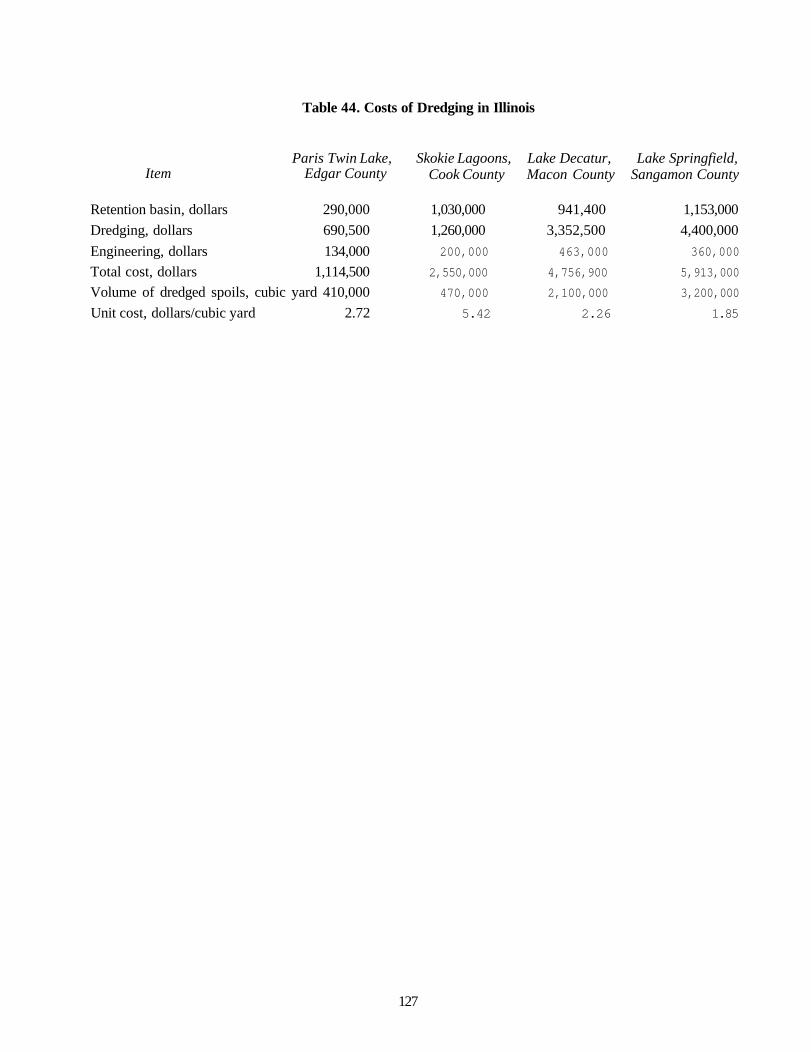
Table 44. Costs of Dredging in Illinois

Paris Twin Lake, Item Edgar County

Retention basin, dollars 290,000 Dredging, dollars 690,500 Engineering, dollars 134,000 Total cost, dollars 1,114,500 Volume of dredged spoils, cubic yard 410,000 Unit cost, dollars/cubic yard 2.72

127

Skokie Lagoons, Lake Decatur, Lake Springfield, Cook County Macon County Sangamon County

1,030,000 941,400 1,153,000 1,260,000 3,352,500 4,400,000 200,000 463,000 360,000

2,550,000 4,756,900 5,913,000 470,000 2,100,000 3,200,000

5.42 2.26 1.85

Control of Runoff and Ground-Water Leachate from Bairstow Property

Buffer Strip

Because of the inimical effects of the runoff and leachate from the Bairstow property—namely, the elevated pH observed in the south basin of the lake—and the possible deleterious impact of the physio-chemical interaction of the colloidal precipitate on the aquatic organisms (mainly fish), this aspect needs to be addressed and mitigated.

One of the mitigation methods could be similar to the scheme proposed by Atec Associates in 1984 for the Federated Metals Corporation site adjoining the lake's north basin (Carnow, 1990). The Atec closure plan is for the hazardous material area to be capped with clay and sloped to drain away from the lake to reduce infiltration and leachate generation. The nonhazardous slag area would be graded smooth and sloped to grade, and 12 inches of dune sand would be placed on the slag surface to choke off pore spaces between slag particles. Two feet of clay would be placed on top of the sand in layers, compacted to achieve permeability not to exceed 10-7 centimeters per second. After placement of the clay, 6 inches of sand would be placed followed by 6 inches of topsoil, rolled and hydroseeded to provide a grass covering cap (Carnow, 1990).

Because the slag material on the Bairstow property was found to be nonhazardous and was used earlier for highway construction, it may not be necessary or economical to render the entire tract impermeable with a compacted clay layer topped with grass cover. However, as a first step, it would be necessary to spread and even out all the slag piles, grade them smooth, and slope them away from the lake. A grass buffer at least 50 feet wide running east-west on the southern perimeter of the lake should be considered as a filter strip or sediment trap for the surface runoff. The cost of constructing the buffer strip—trucking-in top soil, spreading, harrowing, fertilizing, seeding, mulching, etc.—is estimated at $9,000 per acre of strip (Agricultural Soil Conservation Service, June 1994, personal communication).

Leachate Interceptor Channel

A less expensive and potentially more effective leachate control system than a slurry wall would consist of a ditch paralleling the southern shore of the lake and ending at the ditch along Calumet Avenue at a point below the lake's outfall. This ditch would extend three to four feet below the water table effectively intercepting most or all of the ground-water discharge into Lake George from the Bairstow site.

Sampling programs at similar sites indicate that ground water underneath slag piles is highly mineralized, has a high pH, and is reducing. When this ground water discharges into surface water, conditions drastically change and minerals such as gypsum precipitate out (much of the "White precipitate" is gypsum). These ditches also can have a very high pH. Ditches in similar slag areas near Lake Calumet have had pH values above 11.

128

To alleviate the high pH problem and encourage more precipitation, several small aerators could be placed at various points along the ditch. Because phagmites can grow in this environment, the ditch may qualify as a constructed wetland.

This interceptor channel would cost approximately $3.00 per cubic yard for construction.

OBJECTIVES OF LAKE GEORGE MANAGEMENT SCHEME

The lake is shallow and eutrophic. A very large portion is covered with dense non-native macrophytes, and the aesthetics and beneficial lake uses are severely impaired. The major goals and objectives of a lake management scheme should include:

• Selective deepening of the lake for winter fish survival. • Controlling Eurasian water milfoil (Myriophylium spicatum) and preventing its re-

establishment by promoting diversity of native macrophytes. • Controlling surface runoff and ground-water leachate influx from the Bairstow

property into the lake. • Enhancing aesthetic and recreational opportunities in and around the lake by

enhancing sports fisheries and fish habitat in the lake.

A basic eligibility requirement for Clean Lakes Program funding is that the lake be open and publicly accessible and that such access be across publicly owned land. Public access must be provided independently of a Clean Lakes project, and Section 314 funds may not be used to purchase or lease property solely to provide access. The intent of this regulation is to ensure that the benefits of a lake restoration or protection project are in fact enjoyed by the public (USEPA, 1980).

Proposed Restoration Scheme

Lake Deepening and Macrophyte Control

Dredging the lake accomplishes the multiple objectives of increasing the lake volume, removing the undesirable rooted vegetation, and providing additional space for fish winter survival. Herbicide application and harvesting and removal of macrophytes are not viable options for controlling the dominant and dense growths of Eurasian water milfoil. Hence, for the reasons discussed earlier, hydraulic dredging will be the technically and economically feasible method for eliminating the predominance of this non-native aquatic vegetation in the lake. The dredged spoil could be disposed of in a suitable containment facility.

The Illinois Department of Conservation (1986) recommends that for fish stocking and survival in small lakes and ponds in northern Illinois, the water depth must be about 10 feet in one-quarter of the water area. The authors are not aware of any published

129

criteria for water depths for winter fish survival recommended by the Indiana Department of Natural Resources. The maximum depth of macrophyte colonization is estimated to be in the range 9 to 14 feet of water depth. These two criteria, in addition to the resources available for dredging, will determine the area, depth, and volume of lake to be dredged.

Since dredging a lake is a very expensive proposition, it may not be economically feasible to dredge the entire lake. Also, because there may be uncertainties in the resources available for carrying out the dredging operations, table 45 presents different percentages of lake-bottom dredging and the corresponding estimates for dredged spoil volumes and associated costs.

Another method that has been tried for controlling water milfoil, in addition to dredging and herbicide treatments, is the rototiller technique, developed in British Columbia. However, the authors were unable to find instances in the Midwest where this technique was applied to control water milfoil or other aquatic weeds. Wisconsin does not permit rototilling as a means of controlling aquatic vegetation in its waters (Wisconsin Department of Natural Resources, April 1994, personal communication). Hence, it is proposed that in all areas where water milfoil growths were found and where the lake is not considered suitable for dredging to meet the MDC (Maximum Depth of Colonization) requirement, the area will be dredged for at least 1 foot, primarily to remove the water milfoil, roots and all.

Dense aquatic growth with water milfoil as the dominant species was found in about 40 acres of lake area in the north basin and about 37 acres in the south basin. Since this exotic, non-native vegetation is known to overpower native aquatic vegetation and upset the ecological balance in the lake system, a combination of deep dredging for fisheries enhancement and minimal dredging for eliminating water milfoil in other areas needs to be considered.

Table 45 shows that areas of deep dredging will have a water depth of at least 14 feet, and areas where dredging is needed will have 1 foot of sediment removed. Volumes of calculated dredged spoils were corrected to three significant numbers. The volume of sediment removal from the lake will vary from a total of 485,000 cubic yards to 1,552,000 cubic yards, depending on whether 10 acres or 40 acres are utilized for fisheries enhancement in each basin. Correspondingly, the costs of sediment removal are expected to vary from $2,667,500 to $6,208,000, including the costs for geotechnical and engineering services and sediment retention site construction. The overall project budget is estimated based on dredging an area of 20 acres in each basin.

Control of Runoff and Leachate from the Bairstow Landfill Area

Construction of the interceptor channel for a length of 2,500 feet along the south shore of the lake to a depth of 15 feet, with 5-foot bottom width and 2:1 side slopes would require 50,000 cubic yards of earth work at a cost of $3.00 per cubic yard or $150,000. The area of buffer strip needed to control suspended sediment runoff from the

130

Table 45. Proposed Areas and Depths of Dredging and Corresponding Volumes and Costs

Items

A. Area of deep dredging, acres Area of shallow dredging, acres Volume of dredged spoils, cubic yards Unit cost, dollars/cubic yard Total cost, dollars

B. Area of deep dredging, acres Area of shallow dredging, acres Volume of dredged spoils, cubic yards Unit cost, dollars/cubic yard Total cost, dollars

C. Area of deep dredging, acres Area of shallow dredging, acres Volume of dredged spoils, cubic yards Unit cost, dollars/cubic yard Total cost, dollars

D. Area of deep dredging, acres Area of shallow dredging acres Volume of dredged spoils, cubic yards Unit cost, dollars/cubic yards Total cost, dollars

131

North basin South basin

40 40

790,000 762,000 4.00 4.00

3,160,000 3,048,000

30 30 10 10

609,000 588,000 4.25 4.25

2,588,250 2,499,000

20 20 20 20

428,000 413,000 4.75 4.75

2,033,000 1,961,750

10 10 30 30

246,000 239,000 5.50 5.50

1,353,000 1,314,500

Bairstow property will be 2.9 (rounded to 3.0) acres for a buffer strip that is 50 feet wide. Cost of the buffer strip will be $27,000, bringing the total cost of this phase of the mitigation effort to $589,500.

Lake Ecosystem Management

Replanting of Desirable Native Aquatic Plants. To help prevent reinfestation of Eurasian water milfoil in areas where it has been controlled, it is desirable to reintroduce and re-establish native aquatic plants. The goal of aquatic plant management is to provide the appropriate amount of aquatic plants, taking into account the effects of macrophytes on fish communities and other lake uses such as boating and aesthetics. Macrophytes can help stabilize the lakebed and shoreline, reducing problems with lake shore erosion and high turbidity. Fisheries are enhanced by moderate growth of aquatic plants; the complete elimination of macrophyte beds may be as harmful as excessive plant growth.

Some desirable rooted aquatic submerged vegetation suited for Midwestern lakes are: certain broad-leaved pondweeds, Potamogeton amplifolius, P. illinoensis, P. natans, and P. richardsonii, certain narrow-leaved pondweeds, Potamogeton berchtoldii, P. foliosus, P. pectinatus, and wild celery, Vallisneria americana (Wisconsin Department Natural Resources, personal communication, November 21, 1994). Cost of materials and labor to plant aquatic plants has been reported to be approximately $3,250 per acre (Chicago Park District, 1994), reported for small park lagoons. Hudson et al. (1992) estimated the cost for planting a 5-acre area to be $8,250 for McCullom Lake in McHenry County, one of the collar counties in the Chicago region. For Lake George, considering the economy of scale, the unit cost for replanting aquatic vegetation in the lake would be about $1,500 per acre.

Addition of Physical Structures for Fish Cover. Some lakes and reservoirs lack sufficient structural features and areas for fish to hide—in particular, areas where younger, smaller fish can find cover to escape from larger fish and other predators. Without adequate cover, survival rates of young fish are often low. Structural features provide safety from predators, substrate for food organisms, and in some cases spawning habitat. Additionally, predators, which include most game species, tend to concentrate around structural features in search of prey. By concentrating fish in specific areas, the addition of fish cover, such as artificial reefs, can increase fishing success and angler satisfaction (USEPA, 1993).

Common types of physical structural habitat include docks and piers, brush piles, rock reefs, as well as constructed artificial reefs such as cribs, piping, and plastic structures. In addition to replanting native aquatic vegetation in Lake George, other artificial reef structures in adequate number and size should be considered for fisheries enhancement.

Fish Community Manipulation. Since Lake George has not been managed for sports fisheries in the past 10 to 15 years, it may be necessary to adopt and implement a

132

vigorous fish management program to enhance its recreational potential and opportunities. Fisheries management techniques involve manipulation of the fish community and other organisms that may serve as prey for, predators of, or competitors with the fish species of interest. Some significant fisheries management activities include: 1) control of undesirable fish species and stunted fish populations, 2) prey enhancements to supplement food supplies, and 3) gamefish stocking. A detailed discussion of the factors to be considered before initiating a management program can be found elsewhere (USEPA, 1993). Answers to questions such as the best species to stock, size and number of fish to stock, methods of controlling undesirable fish species, techniques for prey enhancement, managing fishing pressure and harvest, etc., can be resolved in consultation with the fisheries experts within the Indiana State's natural resources agencies.

Lake George and its watershed are within the areas of concern (AOC) identified by the International Joint Commission (IJC). The Remedial Action Plan (RAP) of the IJC is an ongoing effort to control and mitigate the effects of past waste disposal practices in the AOC. The management scheme for Lake George could be intergrated into the RAP of the DC.

A no-action option will not resolve lake problems such as the dense growth of Eurasian water milfoil in the lake, surface runoff, and ground-water leachate influx from the Bairstow property, etc. There was a strong sentiment expressed during the public meeting on September 17, 1996, to leave the lake as it is without dredging. As a minimum, it is recommended to construct the interceptor ditch and filter strip along the Bairstow property and the outlet control structure. The estimated cost for these three items amounts to $187,000.

Benefits Expected from Lake Management

Once implemented, the proposed restoration plan would provide a wide range of water quality, habitat, and recreational-use enhancement in Lake George. The dominance of Eurasian water milfoil, particularly in the south basin, interferes with boating activities and detracts from the aesthetic enjoyment of the water body because of its extensive canopy formation. Control of this non-native aquatic vegetation and re-establishment of native plantings will provide and sustain conditions for an ecological balance and desirable aquatic food chain in the ecosystem. These conditions would be vastly improved with the addition of strategically placed fish cribs and other fish structures. Selective deepening would increase fish survival over harsh winters, and sports fisheries in the lake would be improved through the proposed fisheries management activities. Overall, the aesthetic and recreational opportunities provided by the lake environment will be increased significantly.

The proposed construction of a greenway linear park extending from Calumet Avenue to Indianapolis Boulevard, much of which will adjoin Lake George on the north side, will add to the aesthetic and recreational use of the lake environment. With Hammond being one of the cities vying for a floating casino, the recent approval of river-

133

boat gaming in Indiana will attract more visitors to the area. A well-managed Lake George environment will provide additional attraction for visitors.

A report prepared by JACA Corporation (1980) for the USEPA, assessing the economic benefits derived from 28 projects in the Section 314 Clean Lakes Program, found a return in benefits of $8.30 per federal dollar expended, or $4.15 per total project dollar. The projects produced benefits in twelve categories, including recreation, aesthetics, flood control, economic development, fish and wildlife, agriculture, property value, and public health. The report also indicates that while many benefits could not be measured in monetary terms, the success of many Clean Lakes Program projects appears to have been a catalyst for other community activities.

Phase II Water Quality Monitoring, Schedule, And Budget

Monitoring Program

The following monitoring schedule will be used in evaluating the effectiveness of the in-lake management technique adopted for the lake.

The lake will be monitored for dissolved oxygen, temperature, and Secchi disc readings at the deepest locations, one in each of the north and south basins. Observations for dissolved oxygen and temperature will be made at 1-foot intervals commencing from the surface.

Water samples for chemical analyses will be taken at these deep stations from two different points: 1 foot below the water surface and 2 feet above the bottom. Analyses will be made for pH, alkalinity (phenolphthalein and total), total suspended and dissolved solids, volatile suspended solids, turbidity, total phosphorus, dissolved phosphorus, nitrate plus nitrite nitrogen, ammonia nitrogen, total Kjeldahl nitrogen, turbidity, and COD.

Integrated water samples (integrated to a depth of twice the Secchi disc depth) will be collected at each deep station for determining chlorophyll-a, b, c, and pheophytin. Integrated water samples will also be collected for algae and zooplankton identification and enumeration.

Sediment samples with an Ekman/Petite Ponar dredge from one deep and one shallow station in both the north and south basins will be examined for macroinvertebrate identification and enumeration.

Physical and chemical water quality characteristics will be monitored at biweekly intervals (May-September) and at monthly intervals (October-April). Algae and zooplankton samples will be collected at monthly intervals from May-September, and benthos will be examined once in late spring and again in mid-summer.

134

A macrophyte survey and a fish survey using an electroshock technique will be made once, approximately 12 to 18 months after the implementation of the management techniques. A fish-flesh contamination assessment is desirable.

Implementation Schedule

The proposed implementation schedule is listed in table 46, which outlines planning, design, in-lake management, and reporting phases. The proposed duration of Phase II is two-and-a-half years.

Budget. The following is a breakdown of project costs.

Dollars 1. Sediment Removal

a. Engineering design and construction inspection services; surveying, mapping, testing, and geotechnical investigation 250,000

b. Retention site preparation and construction 1,000,000 c. Sediment removal (841,000 cubic yards) 2.749.750

Total sediment removal cost 3,999,750 2. Interceptor ditch construction 150,000 3. Filter strip construction 27,000 4. Outlet control structure 10,000 5. Replanting of native vegetation 60,000 6. Removal of rough fish and restocking 50,000 7. Installation of fish cribs and artificial reefs 50,000 8. Removal and proper disposal of debris and industrial wastes from

the lake vicinity; beautification of the surrounding area 100,000 9. Post implementation lake monitoring and report preparation 200.000

Total Estimated Project Cost 4,646,750

Environmental Evaluation

This section addresses some of the environmental concerns regarding project implementation.

Will the project displace people?

The project will not displace people since all project-related activities occur in uninhabited areas.

135

Table 46. Proposed Implementation Schedule for Lake George Restoration

Will the project deface residential areas?

There are residences located on the north side of the lake. However, if hydraulic dredging is chosen as a mitigation technique, it will be considerably less noisy than drag­line equipment and earth-moving machinery. The dredged spoils are likely to be pumped to the south of the lake for disposal in the Bairstow, Inc., property. Some noise associated with cutterhead operation and pumping is unavoidable. Otherwise, no defacement of residences is anticipated.

Will the project entail changes in land-use patterns?

No land-use pattern will be affected. However, the improved aesthetics and recreational opportunities will positively impact the surrounding educational, commercial, and residential entities.

Will the project impact prime agricultural land?

No agricultural land is affected by the project.

Will the project adversely affect park land, public, or scenic land?

There will be some visual and noise impact during the transitory period of restoration activities. However, lake restoration will provide long-term enhancement of the environmental, aesthetic, and recreational values in the general area.

Will there be adverse impacts on historical, architectural, archeological, or cultural resources?

There are no significant cultural resources in the project area.

Will the project entail long-range increases in energy demand?

Once the major components of the restoration scheme are implemented, there will be no activity requiring excessive energy use in the operation and maintenance of the lake system.

Are changes in ambient air quality expected?

Because the project area is in a highly industrialized region of the state, changes in air quality due to the operation of the diesel-powered dredge may not be perceptible.

Are there any adverse effects due to chemical treatment?

No in-lake chemical treatment methods are proposed.

137

Does the management plan comply with Executive Order (E.O.) 11988 on floodplain management?

The lake restoration of Lake George does not involve any activities in floodplains and consequently does not infringe on E.O. 11988.

Will the dredged material be discharged into the waters of the United States?

It is proposed that the dredged material be disposed of in the adjoining land south of the lake. This site has historically been used for disposing slag, bottom ash, and other industrial wastes. Dredged materials will not be discharged into any waterway.

Are any adverse effects on wetlands and related resources anticipated?

No wetland or its related resources will be affected by the lake improvement activities.

Have all the feasible alternatives been considered?

All the relevant and applicable management options were considered and discussed, and appropriate suggestions and recommendations have been made.

Are there other mitigative measures required?

The pros and cons of various alternatives have been considered, and the need for no other mitigative measure should arise.

REFERENCES

American Public Health Association (APHA), American Water Works Association (AWWA), and Water Environment Federation. 1992. Standard methods for the examination of water and wastewater. 18th edition, APHA, Washington, DC.

Bretz, J.H., 1939. Geology of the Chicago region, part 1 - general. Illinois State Geological Survey Bulletin 65, Champaign, IL.

Bretz, J.H., 1955. Geology of the Chicago region, part 2 - the Pleistocene. Illinois State Geological Survey Bulletin 65, Champaign, IL.

Carlson, R.E. 1977. "A trophic state index for lakes." Limnology and Oceanography. 22(2):361-369.

Carnow, B.W. 1990. Calumet College project - toxicologic review. CCA Project No. 102179-E001, Carnow, Conibear & Associates Ltd.

138

Chicago Park District. 1994. Clean Lakes Program, Phase I Diagnostic/Feasibility Study of Douglas Park Lagoon, Garfield Park Lagoon, Lincoln Park Lagoon, and Washington Park Lagoon, Cook County, Illinois. Chicago, IL.

Cochran & Wilken, Inc., Consulting Engineers. 1992. Phase I diagnostic/feasibility study of Paris Twin Lakes, Edgar County, Illinois. Springfield, IL.

Colton, C.E., 1985. Industrial wastes in the Calumet area, 1869-1970. Illinois Hazardous Waste Research and Information Center, Research Report 001, Champaign, IL.

Committee on Sanitary Engineering Research. 1960. "Solubility of atmospheric oxygen in water." American Society of Civil Engineers, Journal of the Sanitary Engineering Division. 82(12): 1115-1130.

Cooke, G.D., E.B. Welch, S.A. Peterson, and P.R. Newroth. 1986. Lake and reservoir restoration. Ann Arbor Science Book, Butterworths, Boston, MA.

Dunst, R.C., M.B. Born, P.D. Uttormack, S.A. Smith, S.A. Nichole, J.O. Peterson, D.R. Knauer, S.L. Serns, D.R. Winter, and T.L. Wirth. 1974. Survey of lake rehabilitation techniques and experiences. Technical Bulletin No. 75, Wisconsin Department of Natural Resources, Madison, WI.

Duwal, K.G., 1994. Event-based and seasonal precipitation effects on ground water-wetlands interactions near Lake Calumet, Southeast Chicago, Illinois. University of Illinois-Chicago, Master's Thesis.

Engel, S. 1988. "The role and interactions of submersed macrophytes in a shallow Wisconsin lake." Journal of Freshwater Water Ecology. 4(3):329-341.

Engel, S. 1990. Ecosystem responses to growth and control of submerged macrophytes: A literature review. Technical Bulletin No. 170, Wisconsin Department of Natural Resources, Madison, WI.

Environmental Systems Research Institute, Inc. 1991. Surface modeling with TIN; surface analysis and display. Arc Info Users Guide.

Fenelon, J.M. and L.R. Watson. 1993. Geohydrology andwater quality of the Calumet aquifer, in the vicinity of the Grand Calumet River/Indiana Harbor Canal, Northwestern Indiana. U.S. Geological Survey, Water-Resources Investigations Report 92-4115, Indianapolis, IN.

Geldreich, E.E. 1967. "Fecal coliform concepts in stream pollution." Water and Sewage Works. 114 (R.N.):R98-R109.

139

Geldreich, E.E., H.F. Clark, and C.B. Huff. 1964. "A study of pollution indicators in a waste stabilization pond." Journal of Water Pollution Control Federation. 36(11): 1372-1379.

Geldreich, E.E., and B.A. Kenner. 1969. "Concepts of fecal streptococci in stream pollution." Journal of Water Pollution Control Federation. 41(8): R336-R352.

Greeson, P.E. 1971. Limnology of Lake Oneida with emphasis on factors contributing to algal blooms. U.S. Geological Survey, Open File Report.

Hudson, H.L., R.J. Kirschner, and J.J. Clark. 1992. Clean lakes program, phase 1 diagnostic/feasibility study of McCullom Lake, McHenry County, Illinois. Northeastern Illinois Planning Commission, Chicago, IL.

Hutchinson, G.E. 1957. A treatise on limnology, volume 1: geography, physics, and chemistry. John Wiley and Sons, Inc., New York.

Illinois Department of Conservation. 1986. Management of small lakes and ponds in Illinois. First Edition, Division of Fisheries, Springfield, IL.

Illinois Department of Conservation. 1990. Aquatic weeds and their identification and methods of control. Fishery Bulletin No. 4, Division of Fisheries, Springfield, IL.

Illinois Environmental Protection Agency. 1978. Assessment and classification of Illinois lakes. Volume II, IEPA, Springfield, IL.

Illinois Environmental Protection Agency. 1987. Quality assurance and field methods manual. Division of Water Pollution Control, Planning Section, Springfield, IL.

Illinois Environmental Protection Agency. 1990. Title 35: environmental protection, subtitle C: water pollution. State of Illinois, Rules and Regulations, Springfield, IL.

Indiana Department of Environmental Management. 1990. Indiana 305(b) report 1988-89. Office of Water Management, Indianapolis, IN.

JACA Corporation. 1980. An assessment of economic benefits of 28 projects in the Section 314 Clean Lakes Program. Fort Washington, PA.

Kelly, M.H., and R.L. Hite. 1981. Chemical analysis of surficial sediments from 63 Illinois lakes, summer 1979. Illinois Environmental Protection Agency, Springfield, IL.

Kothandaraman, V., and RL. Evans. 1983a. Diagnostic-feasibility study of Johnson Sauk Trail Lake. Illinois State Water Survey Contract Report 312, Champaign, IL.

140

Kothandaraman, V., and R.L. Evans. 1983b. Diagnostic-feasibility study of Lake Le-Aqua-Na. Illinois State Water Survey Contract Report 313, Champaign, IL.

Mackenthun, K.M. 1969. The practice of water pollution biology. U.S. Department of the Interior, Federal Water Pollution Control Administration.

Madsen, J.D. 1993. Control points in the phenological cycle of Eurasian water milfoil. Aquatic Control Research Program, Vol. A-93-1, U.S. Army Corps of Engineers, Waterways Experiment Station.

Nürnberg, G.K. 1984. The prediction of internal phsphorus load in lakes with anoxic hypolimnia. Limnology and Oceanography 29 (1): 11-124.

Peterson, S.A. 1981. Sediment removal as a lake restoration technique. EPA-600/3-81-013, U.S. Environmental Protection Agency, Corvallis, OR.

Pierce, N.D. 1970. Inland lake dredging evaluation. Technical Bulletin 46, Wisconsin Department of Natural Resources, Madison, WI.

Province of British Columbia. 1978. Information bulletin, aquatic plant management program, Okanagan Lakes. Volume IV, Ministry of the Environment, Water Investigations Branch.

Pullman, G.D. 1992. Aquatic vegetation management guidance manual, version 1. Midwest Aquatic Plant Management Society, Flint, MI.

Raman, R.K., and W.C. Bogner. 1994. Frank Holten State Park Lakes: Phase III, post-restoration monitoring. Illinois State Water Survey Contract Report 564, Champaign, IL.

Raman, R.K., and R.M. Twait. 1994. Water quality characteristics of Lake Bloomington and Lake Evergreen. Illinois State Water Survey Contract Report 569, Champaign, IL.

Rand McNally. 1993. Commerical Atlas and Marketing Guide.

Robertson, B. 1980. Lake George, Hammond. Fish Survey (File Copy), Bass Lake State Fish Hatchery, Indiana Department of Natural Resources Knox, Indiana, 3p.

Rosenshein, J.S., and J.D. Hunn. 1968. Geohydrology and groundwater potential of Lake County, Indiana. Indiana Department of Natural Resources, Division Water Resources Bulletin 31, 36 p.

Sawyer, C.N. 1952. Some aspects of phosphate in relation to lake fertilization. Sewage and Industrial Wastes. 24(6):768-776.

141

Schloesser, D.W., and B.A. Manny. 1984. Rapid qualitative method for estimating the biomass of submersed macrophytes in large water bodies. Journal Aquatic Plant Management. 22:102-104.

Sparks, D.W. 1995. Lake George fish health assessment, Hammond, Lake County, Indiana, July 1992: Volume I — fish tissue residues. U.S. Fish and Wildlife Service, Bloomington Field Office, 620 S. Walker Street, Bloomington, IN.

Strimbu, R.T. 1988. A hydrogeologic study of the ditches along Calumet Avenue between Lake George and Lake George Canal in the northwest Lakes region of Indiana. Bachelor's thesis, Indiana University Northwest, Gary, IN.

Suter, M., R.E. Bergstrom, H.F. Smith, H.E. Emrich, W.C. Walton, and T.E. Larson. 1959. Preliminary report on ground-water resources of the Chicago region, Illinois. Illinois State Geological Survey and State Water Survey Cooperative Ground-Water Report 1, Champaign, IL.

TAMS Consultants, Inc. 1991. Illinois-Indiana regional airport. Site Selection Report, Appendix E, Volume IL state of Illinois. Presented to the state of Indiana and the city of Chicago. Chicago, IL.

U.S. Bureau of the Census, Economic Census and Surveys Division. 1992. County Business Patterns, 1900, United States: Employment, Payrolls, Number and Employment, Size of Establishments by Detailed County. U.S. Government Printing Office, Washington, D.C.

U.S. Department of Commerce. 1992. 1990 Census of Population, General Population Characteristics, Illinois, Sections 1 and 2, 1990 CP-2-15. Economics and Statistics Administration, Bureau of the Census, U.S. Government Printing Office, Washington, DC.

U.S. Department of Commerce. 1992. 1990 Census of Population, Social and Economic Characteristics, Illinois, 1990 CP-1-5. Economics and Statistics Administration, Bureau of the Census, U.S. Government Printing Office, Washington, DC.

U.S. Environmental Protection Agency. 1973. Measures for the restoration and enhancement of freshwater lakes. EPA 430/9-73-005. Washington, DC.

U.S. Environmental Protection Agency. 1980. Clean Lakes Program guidance manual. EPA 440/5-81-003, Office of Water Regulation and Standards, Washington, DC.

U.S. Environmental Protection Agency. 1988. The lake and reservoir restoration guidance manual, first edition. EPA 440/5-88-002, Washington, DC.

U.S. Environmental Protection Agency. 1990a. Federal Register, 40 CFR Chapter 1 (7-1-90 edition), 261.24. Washington, DC.

142

U.S. Environmental Protection Agency. 1990b. Monitoring lake and reservoir restoration, technical supplement to the lake and reservoir restoration guidance manual. EPA 440/4-90-007, Washington, DC.

U.S. Environmental Protection Agency. 1993. Fish and fisheries management in lakes and reservoirs, technical supplement to the lake and reservoir restortion guidance manual. EPA 841-R-93-002, Water Division (WH-553), Washington, DC.

Vollenweider, R.A. 1968. Scientific fundamentals of lakes and flowing waters, with particular reference to nitrogen and phosphorus as factors in eutrophication. DAS/CSI/68.27, Organization for Economic Cooperation and Development, Paris, France.

Wang, W.C., W.T. Sullivan, and R.L. Evans. 1973. A technique for evaluating algal growth potential in Illinois surface waters. Illinois State Water Survey Report of Investigation 72, Champaign, IL.

Watson, L.R., R.J. Shedlock, K.J. Banaszak, L.D. Arihood, and P.K. Doss. 1989. Preliminary analysis of the shallow ground-water system in the vicinity of the Grand Calumet River/Indiana Harbor Canal, Northwestern Indiana. U.S. Geological Survey Open File Report 88-492.

Willman, H.B. 1971. Summary of the geology of the Chicago area. Illinois State Geological Survey Circular 160, Champaign, IL.

143