Diagnosing the Italian Disease

Bruno Pellegrino University of California Los Angeles

and

Luigi Zingales* Harvard University, NBER & CEPR

September 2014

Abstract

We try to explain why twenty years ago Italy’s labor productivity stopped growing. We find no evidence

that this slowdown is due to the introduction of the euro or to excessively protective labor regulation. By

contrast, we find that the stop is associated with small firms’ inability to rise to the challenge posed by the

Chinese competition and to Italy’s failure to take full advantage of the ICT revolution. Many institutional

features can account for this failure. Yet, a prominent one is the lack of meritocracy in managerial

selection and promotion. Familism and cronyism appear to be the ultimate causes of the Italian disease.

* Luigi Zingales gratefully acknowledges financial support from the Initiative on Global Markets at the University of Chicago Booth School of Business. We thank Robert Inklaar, Marcel Timmer, and Bart Van Ark for granting us access to additional data from the EU KLEMS dataset. We thank Carlo Altomonte and Tommaso Aquilante for granting us access to additional data from the EFIGE dataset.

2

There is a prevalent perception that Japan’s economic performance in the last two decades has been bad

(e.g. Caballero et al., 2008), so much so that these decades are often referred to as the “lost decades.” Yet,

if we look at labor productivity (rather than GDP) growth, Japan’s economic performance is far from

abysmal. In fact, during the period 1995–2011 productivity per hour worked in Japan grew at an annual

rate of 1.8%: better than Germany (1.5%) and France (1.4%) and only slightly below the United States

(2.3%). Among developed nations, the real laggard is Italy, with a growth of productivity per hour equal

to only 0.4%, which becomes 0.18% in the period 2000–2011. During the period 1995–2006, Italy fell

behind other advanced nations in labor productivity growth by a cumulative 20%. Even accounting for

lower capital accumulation, Italy’s Total Factor Productivity cumulative growth gap equals 12.8%. Thus,

Italy is the country that lost two decades, and the important question is why.

The puzzle is more perplexing because Italy, unlike Japan, did not face any major financial crisis until

the very end of this period. It did not face a persistent deflation (the average increase in the consumer

price index during this period is 2.7%) and it benefited from low and stable interest rates. In fact, it

benefited from a monetary policy sufficiently loose to fuel an overheated economy in Spain, Greece, and

Ireland. Nor was the fiscal policy that restrictive either, with an average fiscal deficit of 3.7% per year.

Finally, during this period Italy did not face any major political instability: it enjoyed the longest lasting

government of its entire post-World War II period. So what is the cause of this Italian ailment? As Figure

1 shows, the Italian slowdown in productivity growth, while much more pronounced, takes place around

the same time as the European slowdown and the U.S. acceleration. Is this slowdown just an Italian issue

or a more acute form of a European problem?

We start by analyzing whether we can attribute Italy’s lack of productivity growth to structural

deficiencies specific to Italy. Italy is specialized in relatively low-tech sectors, which are more exposed to

competition from China. On average, its firms are much smaller and we know that smaller firms tend to

be less productive (Van Ark and Monnikhof, 1996). Furthermore, Italy lags behind other developed

countries on many institutional dimensions: it ranks high in regulatory protection of labor1 (3.15 vs. an

OECD average of 2.38) and low in freedom from corruption2 (42 vs. an OECD average of 68.8), rule of

law3 (50 vs. an OECD average of 77.4), human capital4 (2.8 vs. an OECD average of 3.1), and adult

literacy5 (253 vs. an OECD average of 273).

While these factors may be able to explain why Italy is less productive overall, they are unable to

explain why productivity slowed down. When we try to predict Italy’s productivity growth in the last 15

years by using its sectorial and firm-size mix, we find that (surprisingly) Italy should have grown faster 1 OECD Employment Protection Index, 2012 2 Transparency International, Corruption Perceptions Index 2012 3 Heritage Index of Economic Freedom 2012, Property Rights component 4 Barro-Lee Human Capital index for 2010, from Penn World Tables 8.0 5 OECD Programme for the International Assessment of Adult Competencies (PIAAC), 2013

3

than average, not slower. We also find no evidence that differences in productivity growth are related to

differences in labor flexibility, either at country level or in the cross-section. In fact, we do not find any

evidence that in sectors where labor needs to be reallocated more, productivity grows more slowly in

countries where this reallocation is more difficult due to a less flexible labor market.

We find mixed results for government efficiency and human capital growth. Depending on the measure

used, the level of government efficiency and human capital growth are sometimes positively correlated

with productivity growth, but we do not find any evidence that the sectors that rely more heavily on

government inputs are more negatively affected by government inefficiency—or that sectors/countries

that are more labor-intensive benefit more from human capital gains.

These results are not that surprising since Italian economic and institutional deficiencies were present

in the 1950s and 1960s when Italy was considered an economic miracle, and persisted into the 1970s and

1980s when Italy continued to have a GDP and productivity growth above the European average.

To explain such a sudden stop in productivity growth, we need to focus on what changed in the

surrounding world in the mid- to late-1990s. The main exogenous shock is China’s entry in the World

Trade Organization (WTO) in 2001. The second shock is the introduction of the euro in 1999. The third

and final one is the information technology revolution that took place starting in the mid-1990s. Since all

these shocks are more or less contemporaneous, there is little hope of being able to separate one from the

other by relying on the timing of the change alone.

To identify the cause of the Italian Disease (as we refer to it), we need to understand why these shocks,

which hit all the other major European countries, had much more adverse effects in Italy. To this purpose,

we analyze the interaction between the shocks and the economic and institutional characteristics where

Italy stands out. If these characteristics are the culprit, they need to have similar effects even outside of

Italy.

The “Euro” and the “China” explanations are similar in that they imply the “contagion” occurred

through the trade balance. However, we fail to detect even a weak correlation between trade balance and

productivity developments. By contrast, we find evidence that productivity tends to grow faster in sectors

that are more exposed to international competition from China. Thus, far from being the culprit, China’s

competition turns out to be a driver of productivity growth. Italy, however, does not fully benefit from this

effect, which is bigger in countries and sectors where large firms are more prevalent. Italy falls behind

because its small firms cannot respond appropriately.

We also find evidence that the Italian productivity slowdown is associated with Italy’s difficulty in

taking full advantage of the Information and Communication Technology (ICT) Revolution that started in

the mid-1990s. This problem is not uniquely Italian. Using an index developed by the World Economic

Forum, we find that developed countries differ significantly in their ability to take advantage of the ICT

4

revolution. In this sense, the Italian disease is a more extreme form of a European ailment, as on average

European countries fell behind the United States in productivity growth at the onset of the ICT revolution.

Since ICT readiness tends to be highly correlated with many other institutional characteristics

(corruption, business-friendly environment, managers’ training), it is not easy, with aggregate data, to

identify which feature (or features) are responsible for the difficulties in technology adoption. For this

reason, we rely on EFIGE, a firm-level dataset. Our conjecture is that a loyalty-based promotion system

discourages the diffusion and adoption of any disruptive innovation, such as ICT. With firm-level data, we

are able to test this conjecture. We find that indeed a system of managerial selection based on loyalty

rather than competence reduces the ability to exploit the ICT revolution. This is true for all countries. Yet,

Italy stands out in this dimension. The Italian disease has a name: it is cronyism.

We are certainly not the first to point out that Italy’s productivity slowed down. In fact, this slowdown

is so well know to have become an international problem in the aftermath of the Eurozone crisis (see the

first chapter of the 2013 IMF Country Report). Yet, there is a dearth of data-based explanations.

The most prominent explanation is by Daveri and Parisi (2010), who suggest that Italy’s productivity

slowdown can be explained by a 1997 labor market reform that introduced temporary employment

contracts, producing a rightward shift to labor supply. Instead of investing in productivity-enhancing

technologies, Italian firms preferred to hire cheap, flexible labor. According to Daveri and Parisi (2010),

this tendency was exacerbated by the old age of Italian managers, which might hinder firms’ ability to

adopt new technologies. Consistent with this hypothesis, Daveri and Parisi find that among Italian firms

productivity growth between 2001 and 2003 correlates negatively with the share of temporary workers

and the age of managers. This explanation is able to account for both Italy’s dismal productivity growth

and for its strong employment growth (+11% relative to the cross-country average in 1995-2006). Yet, it

is not able to explain why Italy’s hourly labor cost (adjusted for the change in labor composition) has

increased in line with the cross-country average over the same period.

By contrast, Ciriaci and Palma (2008) attribute Italy’s productivity slowdown to the decreased

knowledge spillovers produced by the reduced demand for low-tech Italian manufacturing products. By

contrast, Bandiera et al (2008) claim that the slowdown in productivity is due to the bad performance of

the “fidelity-based” model of managerial recruiting. They do not explain, though, why such a model

generated high productivity growth until the late 1980s.

The rest of the paper proceeds as follows. Section 1 describes our data. Section 2 explores the possible

structural causes for the lack of productivity growth. Section 3 analyzes to what extent this lack of growth

can be attributed to shocks in exports. Section 4 looks at the effect of the ICT revolution. Section 5

investigates why some institutional variable might affect ICT adoption. Section 6 concludes.

5

1. Data

1.1 Main Dataset

Our main data source is the EU-KLEMS structural database (O’Mahony and Timmer, 2009). This

dataset, first made available in 2007, contains measures of value added, output, inputs, total factor

productivity, and input compensation shares at the 3-digit ISIC level for 25 European countries, Australia,

South Korea, Japan, and the United States for the period 1970-2007. This level of disaggregation makes it

possible to focus on inter-sectorial variations in productivity growth, by controlling for country-level

determinants with country fixed effects. It also allows us to study the interaction between country-specific

factors and industry-specific factors.

O’Mahony and Timmer also provide industry-level growth accounting (value added growth at constant

prices is broken down into a TFP component, an ICT-capital component, a non-ICT capital component, an

hours worked component and a human capital component).

All countries have data available for the period of interest (1995-2006). Capital formation series and

growth accounting series are unavailable for 11 countries. We also choose to drop emerging countries

(Czech Republic, Hungary, Slovenia). We do so partly due to data quality concerns and partly because

including economies at a different stage of development has a negative impact on the effectiveness of

sector controls (the sectors in which productivity and capital grow faster are not the same). This leaves 15

countries. The EU KLEMS authors have also made available their estimates of industry-level distance-to-

frontier figures in TFP terms for 11 of these countries, which we only use in some robustness tests. Thus,

all our tables are based on data from 15 countries.

We use these data at the finest sectorial decomposition for which growth accounting series are made

available—with the following three exceptions:

• In order to be able to merge some explanatory variables in the dataset that are available at industry-level, we aggregate sectors 50 to 52 (wholesale and retail trade).

• Due to dataset-specific issues regarding the attribution of real estate assets data and public sector output (see the EU KLEMS Methodology document), we use the aggregate sector 70t74 instead of 70 (real estate) and 71t74 (other business services).

• Due to long-standing issues related to the measurement of public sector input, output and productivity we drop, as customary, public sector and social services (sectors 75-99) from the analysis altogether.

Thus, all our tables are based on data from 23 sectors.

1.2 Other datasets

1.2.1. Firm Size Activity Distribution and Trade Balance Data

6

For data on firm size distribution, we rely on the OECD Structural and Demographic Business

Statistics (SDBS). We use sector-level breakdown of value added and labor input across five firm size

categories. We adjust this data to account for differences in the definition of size categories across

countries.

In order to study how trade balance shocks impact productivity, we use the OECD-WTO Trade in

Value Added (TiVA) dataset to obtain sector-level data on trade balance as a pecent of GDP, as well as

the relative growth in China’s exports.

1.2.2. Sectorial Variables

To capture “creative destruction” trends across sectors, we compute US mass layoff rates using data

from both the EU KLEMS dataset (Total Employment in 2001–2005) and the Bureau of Labor Statistics’

Displaced Workers Supplement (number of workers displaced from job held for more than three years,

average of the 2001–2003 and the 2003–2005 releases).

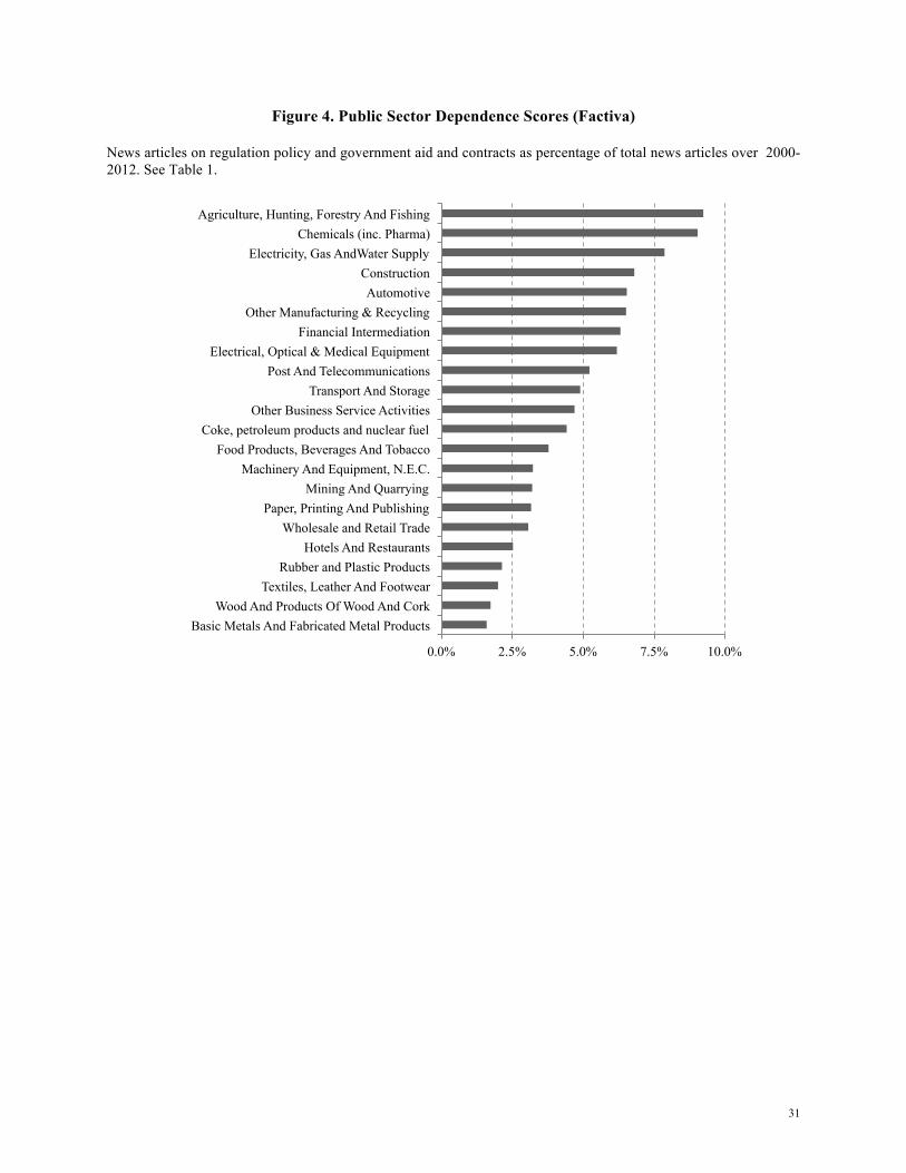
In order to measure how much each sector is dependent on the government, we count news articles in

Factiva News Search. Sectorial government dependence in each sector is defined as the ratio of total news

counts having “Government” as topic (see Table 1 for details) to total news for that sector.

Other sector variables (such as the average size of firms in the US or the accumulation of ICT capital

in Finland) have been obtained by using EU KLEMS and OECD’s SBS data (see Table 1).

1.2.3 Institutional Variables

As the main measure of labor market regulation we use the OECD’s Employment Protection

Legislation index (version 2). As an additional measure, we use the Labor Market Freedom Index,

computed by Heritage International using World Bank indicators of labor regulation strictness.

To gauge the effectiveness of judicial systems, we use “days to enforce a contract” (from the World

Bank DBIs). As a more general measure of government effectiveness, we also use the average time to

return a letter sent to a non-existent business address (which we adjust for geographical distance),

computed by Chong et al. (2012) and the performance of public schools measured as the average OECD

PISA scores for public schools.

We also use, as a measure of Human Capital, scores from OECD’s 2013 PIAAC survey of adult skills.

We use score differences between age cohorts to gauge human capital gains at country level that might

not be captured by changes in workforce composition. PIAAC is a standardized test (analogous to PISA)

aiming at assessing literacy and numeracy of adult workers across OECD and partner countries.

To capture a country’s ability to leverage the ICT revolution, we use the 2012 Networked Readiness

Index, computed by the World Economic Forum. This index, developed by Kirkman et al. (2002),

7

measures “the performance of 148 economies in leveraging information and communications

technologies to boost competitiveness and well-being.” It is built on multiple “pillars” (institutions, the

business environment, infrastructure, affordability, human capital, usage and impact, etc.).

To measure a country’s level of cronyism, we rely on two country scores contained in the 2007 Global

Competitiveness Index, by the World Economic Forum:

• In your country, to what extent do government officials show favoritism to well-connected

firms and individuals when deciding upon policies and contracts? [1 = always show favoritism;

7 = never show favoritism]

• In your country, who holds senior management positions? [1 = usually relatives or friends

without regard to merit; 7 = mostly professional managers chosen for merit and qualifications]

To measure a country’s quality of management schools we use another index from the 2007 Global

Competitiveness Index

• In your country, how would you assess the quality of business schools [1 = extremely poor—

among the worst in the world; 7 = excellent—among the best in the world]

As a hard-data alternative to the third survey, we use the sum of GMAT scores sent and received from

each country, per 100,000 head of population.

1.2.4 Firm-Level Data

To complement our analysis of EU KLEMS data in section 6, we also use a firm-level dataset, EFIGE

(European Firms in a Global Environment), developed by Altomonte and Aquilante (2012) for the think-

tank Bruegel. The dataset contains balance sheet data for over 14,000 firms from 6 European countries

(Austria, France, Germany, Hungary, Italy, Spain, UK). It also contains answers to a survey, undertaken

in 2008-2009, which covers a wide range of topics related to the firms’ operations. From this data, we use

demographic information (firm size, age, sector), data on IT usage, innovation, international activity, and

management style, as well as the authors’ estimates of firm-level total factor productivity. We combine

some of these variables to form discrete scores of IT Usage and Innovation, as well as a Performance-

Oriented Management index similar to the one computed by Bandiera et al. (2008).

In this dataset, we will use as a control the Pavitt classification, which categorizes industrial firms

according to sources of technology, requirements of the users, and appropriability regime (Pavitt 1984).

All the variables used are defined in Table 1. Table 2 provides the summary statistics.

1.3 Growth accounting methodology

We follow the EU KLEMS database authors’ methodology in assuming that firms follow a profit-

maximizing behavior in competitive markets with constant returns to scale. On the basis of these

8

relatively standard assumptions, one can decompose one-period growth in sector-level value added at

constant prices using the following formula:

(1)

where Y is Value Added, K is capital services (constant prices), H is hours worked, L is labor services

(constant prices), wL is the labor compensation share of value added (at current prices), and A is the

Solow Growth Residual, hereafter “Total Factor Productivity.” Under this accounting framework, we are

separating the effect of total hours worked from that of labor services per hour worked. Therefore, the

term can be interpreted intuitively as the contribution of the change in labor composition.

The authors use a perpetual inventory model (PIM) to estimate capital stock series across 9 different

asset classes (within each sector). As a consequence, they are able to further decompose growth in capital

services into an ICT (information and communication technology) part and a non-ICT part.

(2)

where is the share of ICT capital in total capital at current rental prices. Equation 3 depicts an

equivalent formulation of the EU KLEMS growth accounting equation, in which the left hand side is

replaced by value added per hour worked:

(3)

2. Decomposing Growth

We begin our analysis by showing how the Italian lost decades are fundamentally a productivity

problem. Figure 2 illustrates graphically the decomposition of the growth of GDP per capita at constant

prices in a cross-section of 15 countries in the period 1994–2006, according to the following formula:

Δ log GDPPopulation

= Δ log GDPHours

+Δ log HoursEmployed

+Δ log EmployedPopulation

This exercise shows very clearly that Italy’s lower GDP per capita growth is not due to a reduction in

the employed/population ratio. To the contrary, an increase in the participation rate has masked a marked

slowdown in labor productivity growth. Of the countries reported, only Spain does worse.

Δ logY = Δ log A+ 1−wL( )Δ logK +wL Δ log LH+Δ logH

#

$%

&

'(

HLwLΔ

Δ logK = wIΔ logKI + 1−wI( )Δ logKN

Iw

Δ log YH= Δ log A+ 1−wL( ) wIΔ log

KIH+ 1−wI( )Δ log KNH

#

$%

&

'(+wLΔ log

LH

9

The very first place where we can look for clues on the nature of the Italian productivity malady is the

growth accounting numbers provided directly by the dataset authors. Obviously, this growth accounting

exercise relies on some strong assumptions regarding the way that agents make production and

investment decisions. We shall try and relax some of these assumptions at a later stage.

Table 3 provides OLS results from a weighted regression of the various components of hourly labor

productivity on sector fixed effects and a dummy variable for Italy. The LHS variable in column 1 is

labor productivity. It shows that, controlling for sector fixed effects, Italy’s gap cumulated in the period

1995-2006 is 19%.

Column 2 repeats the same regression with total factor productivity as the LHS variable. The gap in

this case is 13%. Thus, the lion’s share of the productivity gap (13% out of 19%) cannot be attributed to

either slower capital accumulation or to an adverse change in the workforce mix; it is in the Solow

residual. Columns 3 to 6 show the sources of the explained component in the productivity gap. Lower

investments in ICT capital can explain a cumulative 3.0%. Lower non-ICT investments 2.5%, while

changes in the labor composition do not seem to account for much.

3. Structural Characteristics

In this section we investigate whether the Italian productivity slowdown can be explained by structural

characteristics that differentiate Italy from the other OECD countries. We first look at industrial and

institutional characteristics, then we focus on the quality of Italy’s stock of human capital.

3.1 Demographics of Italian Firms

Italy’s industrial structure has always been peculiar. Italian manufacturing firms tend to specialize in

labor-intensive, low-technology products (Wolff (1999)) and they tend to be small- or medium-sized

(OECD (2012)).

One hypothesis is that Italy specialized in sectors that just happened to have a slower productivity

growth. Another is that TFP in small firms grew more slowly during this period and that Italian slow TFP

growth is due to that. Finally, it could be an interaction between the two stories above: small firms in low-

tech sectors might have faced a particularly difficult time in recent years and that might explain Italy’s

slow TFP growth. Yet, the Italian slowdown is not concentrated in some sectors: it is common to most of

them. An exception is Post and Telecommunications, where Italian productivity grew more than the

average of the other developed countries.

To test this hypothesis formally, in Table 4, we predict Italian aggregate labor productivity growth

using the sectorial composition (column 2), size distribution (column 3), and size and sector composition

10

simultaneously (column 4). We obtain these predictions by weighting global sectors and firm size

categories by their respective shares of national employment and then applying the average growth in the

sample for that subgroup.

For most countries, the prediction is reasonably close to the actual (column 1). Four cases stand out. In

the negative domain, Italy and Spain perform much worse than expected. In the positive domain, Finland

and Sweden perform much better than expected. For Italy, the gap between actual and predicted is similar

in magnitude to the one we obtain by just comparing Italy to the cross-country average. Thus, size and

sectorial composition cannot explain any part of the Italian slowdown.

Finally, in Figure 3, we decompose the deviation of Italy’s GDP/Hour worked from the cross-country

average into a “within sectors” component, a “between sectors” component (which captures specialization

in sectors where labor productivity is higher at a global level) and a “strategic” component (which

captures specialization in sectors in which Italy enjoys a comparative advantage).

Italy’s sectorial specialization appears to have negatively affected the level of GDP/Hour worked since

the mid-1980’s. Yet, this gap did not become any worse after the mid-1990s. Once again, the effect of this

bad allocation of labor resources on productivity growth could be defined as marginal at best. What

Figure 3 shows clearly is that in the mid-1990s Italy develops a growing productivity gap within sectors,

as also shown by Table 3. This gap is responsible for Italy’s productivity slowdown.

3.2 Structural Characteristics of Italian Institutions

3.2.1 Labor Protection Regulation

One theory, particularly popular in policy circles, is that Italy’s productivity slowdown is due to

excessive labor market regulation. The simplest version of this model is that labor protection reduces

workers’ incentives, decreasing both productivity and productivity growth. While theoretically plausible,

this argument looks weak. Italy’s labor market does not appear more heavily regulated than that of

Germany, France, or Sweden. None of these countries has faced a productivity slowdown comparable to

that faced by Italy. Furthermore, the empirical evidence on the effects of labor market regulation on

productivity growth is scarce and contradictory.6

Nevertheless, to test this hypothesis, in Table 5, we regress sector-level TFP growth on sector fixed

effects and on the country-level index of labor flexibility, either the OECD one (column 1) or the World

6 The relationship between productivity growth and labor protection is positive in some studies (Nickell & Layard (1999), Koeniger (2005)), negative in others (Bassanini et al. (2008), Bassanini et al. (2009)), as well as inverse U-shaped (Belot et al. (2007)). Exploiting variations in wrongful discharge regulation across US states, Autor et al. (2007) find that discharge regulation induces excess capital deepening, raising labor productivity and simultaneously decreasing Total Factor Productivity. By using European firm-level data, Cingano et al. (2010) find that labor protection decreases both capital per worker as well as total factor productivity, and that the effect is stronger in sectors with high rates of labor reallocation.

11

Bank one (column 3). The sign of the coefficients in the two regressions is different, but neither is

statistically significant. Thus, we fail to detect any negative correlation between labor protection and

productivity growth.

A more sophisticated version of the same theory is that the negative impact of stringent labor

protection legislation on productivity growth manifests itself only when there is a strong need to

reallocate labor. When a shock (like China’s entry in the WTO) changes a country’s comparative

advantages, stringent labor protection prevents firms from efficiently re-allocating resources, negatively

impacting productivity

If this were case, we would expect labor productivity to grow more slowly in sectors where

Schumpeterian “creative destruction” is most intense precisely in those countries with more protective

labor regulation. To test this hypothesis, we follow Bassanini, Nunziata and Venn (2009), henceforth

BNV, and add, to the previous regression, an interaction effect between labor protection and sector-level

layoff rates in the United States, as an indicator of need for turnover in the sector. We also include

country fixed effects.

Regression results are presented in columns 2 and 4 of Table 5. The coefficient of the interaction

between need for labor reallocation and labor protection is negative (as expected) in column (2) and

negative (while we expected a positive) in column (4). In both cases the coefficients are not statistically

significant. Our result in column 2 differs from BNV, who find a negative and statistically significant

coefficient. The difference can be due to the sample period (ours is 1995-2006 instead of 1980-2003) or

the fact we have just one observation per country/sector, as opposed to one observation per

country/sector/year (we use cumulative Productivity growth and average Labor Protection). Since the

OECD employment protection index barely changes over time, we prefer to collapse the time dimension.

When we do the same for BNV, their result is similar to ours.

A different hypothesis is advanced by Daveri and Parisi (2010), who argue that Italy’s productivity

slowdown is due to a 1997 labor market reform that introduced temporary/part-time work. According to

Daveri and Parisi, Italian firms responded to the shock in labor supply by cutting back investment and

hiring cheap, flexible labor.

Daveri and Parisi’s mechanism works through a reduction in labor cost. Yet, we do not see any

evidence of this. For example, according to Banque de France data, hourly labor cost rose 18.4% in the

Euro Area in the years 2000-2006; the corresponding figure for Italy is actually slightly higher: 19.7%.

3.2.2 Government Inefficiency

Another favorite “culprit” for Italy’s loss of competitiveness is its inefficient public sector. The reasoning

is that an ineffective bureaucratic apparatus discourages innovation and investment. Moreover, if

12

government services are inputs in the firms’ production function, an inefficient government reduces the

marginal productivity of labor and capital and, in turn, observed TFP growth. Because taxation does not

enter this argument, in this section we are going to look at government “effectiveness” rather than

government “efficiency.”

There is a plethora of indicators for quality of government (e.g. La Porta et al (1999)). Here we

want to focus mostly on bureaucratic efficiency, separately from factors such as corruption and the rule of

law. We also want to avoid using perception-based measures of effectiveness where “hard data” is

available. We have identified three indicators that comply with these criteria:

1. The World Bank’s estimate of Days Needed to Enforce a Contract, which captures the

effectiveness of the judicial system

2. The average score of a country’s public schools in PISA 2009, which captures the

effectiveness of pre-tertiary public schools.

3. The average time needed for a letter sent to a non-existent business address in a foreign

country to be returned to the sender, as computed by Chong, LaPorta, Lopez-de-Silanes, and

Shleifer (2014).

Given the limited number of countries at our disposal, to identify a causal effect of government

effectiveness on productivity growth, we need to rely on some cross-sectional variation in the need for

government services. Because, as of today, there are no measures that quantify sectors’ dependence from

the government, we construct one by using news articles data from the Factiva News Search Database,

which pre-sorts news by sector and topics. We define “government dependence” for a sector as the

proportion of articles on a certain sector that have government policy/regulation/aid as one of their topics.

Figure 4 shows this measure of government dependence.

As an alternative indicator of the sectorial importance of the government, we use the size of a sector in

Sweden, a country where the government is large and relatively effective. We measure size in terms of

proportion of employed people and we compare it to the average.

Regression results are presented in Table 6. We start with a simple regression of productivity growth

on judicial efficiency and sector fixed effects. Countries with worse judicial efficiency (more days to

enforce a contract) experience lower productivity growth and the effect is statistically significant, in spite

of the very few degrees of freedom (we clustered the standard error at the country level). Unfortunately,

judicial efficiency is very highly correlated with lack of corruption, computer literacy, and so on so forth.

Thus, without the possibility of an interaction effect we cannot separately identify this channel from all

the other institutional factors.

13

In columns 2 and 3 we interact judicial efficiency with the two measures of how a sector depends upon

the government (always controlling for country fixed effects). In columns 2 and 3 the interaction

coefficient is positive (rather than negative) and it is not statistically significant.

In columns 4 to 9 we repeat the same exercise with the two other measures of government

effectiveness and we obtain the same result. There is no evidence that productivity grows faster in more

government-dependent sectors in countries with more efficient governments. Thus, while government

inefficiency might still be a permanent drag on Italy’s productivity, it seems unable to explain why the

latter has slowed down in the mid-1990s.

3.2.3 Human Capital

The KLEMS database provides an estimate for the contribution of the various growth components in

Value Added. As Table 3 shows, labor composition can only account for less than a tenth of Italy’s

productivity growth gap.

This result, however, could be an undesired consequence of the shortcomings of the KLEMS dataset.

Equation (1) does not incorporate changes in the quality of human capital, except for compositional

effects, i.e. the re-allocation of hours worked across age, sex, and educational attainment categories. In

particular, it does not account for country-level improvements in the stock of human capital due to

workforce training and/or to the better education of the new generations entering the labor force. A bad

educational system can slow down and possibly reduce a country’s stock of human capital: this effect

would show up in a slower TFP growth.

To test whether growth differences in TFP can be attributed to differences in human capital

accumulation ( ), we need to incorporate this effect in our growth accounting framework by amending

equation 1 in the following way:

(4)

We account for the unobserved by looking at results from the recent Program for International

Assessment of Adult Competencies (PIAAC) done by the OECD. It is similar to the more famous PISA

program, but specifically targeted to adults. The first published results provide, among other things,

estimates of average adult literacy score by country. While there is only one wave of PIAAC, we can

obtain a proxy for the rate of accumulation of by country, by taking the log difference of the average

scores for the 25-35 age band and the 45-55 age band—while controlling for other socio-demographic

factors. The implicit assumption is that PIAAC literacy scores provide a better proxy of human capital per

λ

Δ log YH= Δ log A+wKΔ log

KH+wL Δ log L

H+Δ logλ

"

#$

%

&'

λ

λ

14

worker than educational attainment. The null hypothesis is that Total Factor Productivity growth is

uncorrelated to the growth rate of (interacted with the labor compensation share).

Results from this regression are shown in Table 7. TFP growth is first regressed (column 1) on PIAAC

growth, controlling for sector fixed effects (and clustering the standard error by country). The coefficient

is positive and statistically significant. Yet, as for judicial efficiency, PIAAC growth is a country specific

factor, which correlates with many other positive characteristics of a country. To isolate this specific

factor, in column 2 we control also for country-fixed effects and focus on the interaction between PIAAC

growth and the labor compensation share. The coefficient changes sign and becomes not statistically

different from zero. Therefore, there is no evidence that the lower productivity growth is due to (omitted)

human capital accumulation.

λ

15

4. Globalization and the “Trade Balance Channel”

Having shown that the structural differences in Italy as of 1995 cannot explain the slowdown in

productivity growth, we explore the possibility that this slowdown could be due to a shock.

Unfortunately, there is no lack of candidates. In the mid- to late-1990s, two different shocks hit Italian

export sectors. The first was Italy’s entry in a common currency area, starting with the re-entry of Italian

lira in the Exchange Rate Mechanism in November 1996, which prevented any devaluation. Around the

same years, competition from China became much more intense. While China’s official entry in the WTO

occurs in 2001, trade barriers against China started falling well in advance of that.

In the short term, a decrease in external demand for Italian products can adversely affect productivity

through several channels. First, there is a scale effect. A reduction in export volumes can slow down or

reverse firm growth, harnessing TFP gains from scale and learning-by-doing. Second, a decrease in

external demand for Italian products has a negative impact on the profitability of Italian firms. To the

extent firms are liquidity constrained, this reduction in profitability can also lead to a reduction in

investments in R&D and new technologies, slowing down not only labor productivity but also TFP

growth. The third potential channel is labor adjustment costs. In the absence of growth in internal

demand, a decrease in external demand forces Italian firms to cut back production, at least temporarily. If

firms cannot easily lay off workers in response to this shock, productivity will drop, the more so the

harder it is to lay off workers (i.e., the stronger employment protection is).

All these negative effects should be short term. In the long term, if there is a permanent drop in

demand for Italian products, firms will eventually adjust or close. If they adjust, they will probably be

forced to increase productivity. If they close, the least productive firms will close first, increasing the

average productivity simply through a compositional effect. Thus, the predictions for the long term are

the opposite. While it is hard to imagine that 15 years are still the short term, we should let the data speak.

As a first step, in Table 8, we run a regression of TFP growth on the change in sector-level trade

balance (as a percentage of Value Added) during the period 1995–2005. This regression suffers of a clear

reverse causality problem. Even in the absence of a positive effect of external demand on TFP, TFP

growth is likely to have a positive impact on trade balances. Thus, a positive coefficient in this regression

cannot be considered a proof of an effect of trade balance on TFP. Yet, as column 1 shows, the coefficient

is negative and not statistically different from zero. Thus, this is evidence of a lack of casual link in either

direction.

In column 2, we interact the trade balance with the average size of firms in the United States. In the

spirit of Rajan and Zingales (1998), the idea is that the size of firms in the United States represents the

“unconstrained” optimum and thus the efficient size of firms. Thus, in sectors where the efficient firm

16

size is larger, an expansion in demand should allow firms to achieve that size more easily, increasing their

TFP. The coefficient of this interaction is positive, but it is not statistically significant.

To overcome the problem of reverse causality between productivity and trade balance, we focus on the

various channels of transmission for this effect, rather than on the reduced form. For this reason, in

columns 3 and 4 we look at the change in firm size vis-à-vis changes in the external balance. If external

demand affects productivity growth through its effects on firm’s size, then we should observe that sectors

where external demand grew less (or shrank) are also sectors where the average size of firms grew less. In

column 3 we test the direct effect, while in column 4 the change in the external balance is interacted with

the size of firms in the United States. The coefficient is positive for the direct effect and negative for the

interaction coefficient, and never statistically significant.

The second transmission channel is investment in new capital. Thus, in columns 5 and 6 we look at

whether changes in capital per hour worked are positively related to the sectorial change in external

balance. Contrary to what a causal link between TFP growth and trade would suggest, the coefficient of

capital per hour worked on changes in the external balance is negative. When we interact the change in

external balance with the capital per hour worked in the United States, we get a positive interaction

coefficient that is not statistically significant. Thus, there is no evidence for this channel.

To explore the third channel, in Table 9, we look at the relationship between TFP growth and the

interaction between labor flexibility and the relative growth of Chinese exports vis-à-vis peer countries in

the OECD-WTO TiVA database. If the slowdown in productivity is due to Chinese competition in

countries where it was difficult to lay off workers, we would expect that sectors that are more affected by

the Chinese competition should see their TFP grow relatively faster in countries with more labor

flexibility. The coefficient is indeed positive, but it is not statistically significant, regardless of the

measure of labor flexibility used.

In the long run an external shock, like China’s accession to the WTO, may have a positive impact on

productivity. Increased international competition can force firms to either ramp up their investments in

innovative technologies and products or to reorganize to achieve more efficiency. This mechanism is

outlined theoretically by Bloom, Romer, Terry and Van Reneen (2013) and comes up frequently in

business cases. If this hypothesis were true, then we would expect this effect to be stronger for larger

firms that compete internationally and have dedicated R&D and product development infrastructure.

We test this hypothesis by regressing TFP growth on Firm Size and its interaction with China’s relative

Exports growth. Both variables have a positive coefficient, which is statistically significant. This effect

suggests that in a country like Italy, where firms are small, this productivity-enhancing effect of

international competition will be dampened.

17

We shall now verify whether these findings can be reconciled with evidence from firm-level data. To

this end, we use Bruegel’s EFIGE dataset. The dataset contains information on the international and

innovative activities of firms from six European countries (including Italy). First we compute an

innovation score by counting the number of YES answers to four survey questions on R&D activity and

product/process/organizational innovation. Then, in Table 10, we estimate an ordered Probit (and Logit),

where the dependent variable is this innovation score and the RHS variable is a dummy that equals 1 for

firms that declare to be facing competition from Chinese and Indian firms plus a series of demographic

controls (country, sector, firm age, size).

This specification suffers from a potential reverse causality problem: innovative firms tend to be more

active on international markets and therefore are more likely to face competition from abroad. To address

this problem, we limit the regression to the sub-sample of firms (3,262) that report not being active

abroad. We can identify them by using one of the other variables contained in the dataset.

Consistent with our findings from the EU KLEMS dataset, firms facing competition from China and

India engage in innovative activities significantly more often than their peers that are not exposed to such

competitive pressure.

If we combine this evidence with the previous finding regarding the impact of firm size on the

relationship between Chinese competition and growth, a picture of the Italian problem starts to emerge.

Between 1995 and 2006 Italy’s export volumes underwent a slowdown similar to that of labor

productivity. Such a slowdown is almost entirely driven by low-tech manufacturing sectors, in which

Italy competes directly with China and other emerging economies. In other countries, this competition

lead firms to innovate. Less so in Italy, since the smaller average size of firms made that innovation effort

much more difficult to undertake.

5. The ICT Revolution

Besides the rise of China and the introduction of the euro, the past 20 years have also seen dramatic

progress in Information & Communication Technology (ICT). There is a vast literature describing the

impact of the so-called “ICT Revolution” on economic activity (for an overview see Cohen, Garibaldi,

and Scarpetta (2004)). While both information and communication technology existed before the mid-

1990s, it is around that time that the dramatic reduction in cost of this technology brought a change in the

way production and distribution was organized. Hence, the name “ICT revolution.” As Figure 5 shows,

after 1995 there is an acceleration in ICT investments, more pronounced in the United States and less

pronounced in Europe.

4.1 TFP and the ICT revolution

18

As Bresnahan, Brynjolfsson, and Hitt (2002) and Brynjolfsson, Hitt, and Yang (2002) have shown,

management practices, the quality of human capital, and the quality of a country’s institutions exhibit

strong complementarity with the adoption of ICT capital. As a consequence, there is wide variation in

how firms and countries “succeed” in benefiting from the ICT revolution.

Recent work by Van Ark, O’Mahony, and Timmer (2008) and Bloom, Sadun, and Van Reenen (2012),

shows that the recent productivity growth divide between the US and Europe is a consequence of

European firms’ inferior ability to take advantage of the ICT revolution. In particular, the latter study

suggests that poorer management practices are the cause of this disadvantage, raising the possibility that

the Italian disease is just an extreme form of a European disease.

To test this hypothesis, in Table 11, we regress TFP growth on country and sectors fixed effects and

an interaction between an Italy dummy and the sectorial level of ICT Capital investments (change in ICT

Capital over Hour worked) in Finland during the same period (1994-2006). Again, in the spirit of Rajan

and Zingales (1998), we choose Finland as the benchmark, since it is the most ICT-friendly country (it

ranks first in the WEF’s Networked Readiness Index). The coefficient of the interaction variable is

negative and statistically significant, providing some preliminary support for the thesis that the Italian

slowdown in productivity growth is due, at least in part, to some problems with ICT adoption.

Yet, to determine whether this finding is an Italy-specific phenomenon or an extreme version of some

broader phenomena, we first need to understand how the KLEMS TFP accounting could be affected by

cross-country differences in the productivity of ICT capital. By looking at equation (1) and separating the

ICT and non-ICT components of the capital contribution to Value Added growth, we get:

(5)

KLEMS measures the ICT share in value added as the two-period average capital compensation share

multiplied by the two-period average share of ICT capital in total capital stock. An important assumption

implicit in this calculation is that ICT capital and non-ICT capital have the same return. If this is not true

and the return of ICT and non-ICT capital varies systematically across countries, then the term

will not capture this variation, introducing a systematic bias in (4). Indeed, some recent studies (see

Brynjolfsson and Hitt (2003) and Draca, Sadun, and Van Reenen (2006)) have suggested that in the

presence of ICT capital, the Total Factor Productivity estimates based on standard growth accounting can

be way off.

To see this effect, consider an alternative formulation in which sector-level ICT capital services are

given by:

Δ logY = Δ log A+wKIΔ logKI +wKNΔ logKN +wLΔ log L

KIw

IKI Kw Δ

19

(6)

where KI is the stock of ICT capital and χ a country-level factor that can either enhance or dampen

productivity gains from ICT capital.7 If we allow for this possibility, we obtain a different TFP residual:

(7)

By combining equations (5) and (7) we obtain the following relationship between the “true” TFP

residual and the one computed under the traditional approach:

Δ log A = Δ log !A+ χ −1( ) ⋅wKIΔ logKI (8)

This expression means that if our alternative specification is correct, the Solow growth residual

calculated according to the standard methodology will contain an “error term” that is correlated to the

contribution of ICT capital. Moreover, the expression implies that the higher χ is, the more positive the

response of to will be. Therefore, we can study econometrically the effect of χ by

looking at how the cross-sectorial correlation between TFP growth and ICT capital contribution varies

across countries: if the working hypothesis is correct, this correlation will be higher in countries that are

more “ICT-friendly.”

4.2 Being “Ready” for the ICT revolution

How do we measure χ? A good “candidate” from which to begin our analysis is the Networked

Readiness Index—currently released by the World Economic Forum. Initially developed from a mix of

hard data and expert surveys by Kirkman, Osorio, and Sachs (2002), the index is intended to capture

country-level factors that can either hinder or facilitate the exploitation of ICT.

In Table 12, column 1 we present the results of a regression of TFP growth (computed under the

standard KLEMS framework) on the contribution of ICT capital to Value Added growth, both as a

standalone variable and interacted with the Networked Readiness Index. We also include country and

sector controls. This interaction term has a positive and statistically significant effect on productivity

growth, implying that ICT capital is more productive in countries that are more “network-ready.” This

result is robust to the exclusion of the ICT capital producing sector (30t33) and the exclusion of Italy. It is

7 This specification follows Dearmon and Grier (2010), who suggest that social capital and local institutions have an impact on the marginal productivity of capital.

Δ log !KI = χΔ logKI

Δ logY = Δ log !A+ χ ⋅wKIΔ logKI +wKNΔ logKN +wLΔ log L

Δ log !A wKIΔ logKKI

20

also robust to the inclusion of sector-level TFP distances from the frontier (provided upon request by the

KLEMS authors).

The Networked Readiness Index shares both the advantages and the disadvantages of other frequently

used measures of institutional quality (such as the World Bank Governance Indicators and Transparency

International’s Corruption Perceptions Index) that are computed by averaging many correlated variables.

The main advantage is that it has a fairly good signal-to-noise ratio. The main disadvantage is that it is not

clear what exactly is being measured.

4.3 Resistance to ICT Adoption

Institutional variables are highly correlated and we have a very limited set of countries. Pinpointing

precisely the cause of Italy’s failure to take full advantage of the ICT revolution is almost impossible.

Nevertheless, in this section, we try and conjecture what the root causes of this problem might be.

One hypothesis is that there is an incompatibility between the underground economy and ICT.

Underground firms might be recalcitrant to adopt ICT innovations because they want to avoid increasing

their traceability to fiscal authorities. In addition, to escape fiscal authorities underground firms tend to be

small and managed in an informal way, both factors that make it less profitable to adopt ICT technology.

Since Italy has a very large informal sector, this could be a reason why Italy fell behind.

Another possibility is that Networked Readiness might be capturing country variations in labor market

institutions. One potential reason why Italy has difficulty in adopting ICT, is that its highly regulated and

unionized labor market makes it difficult for firms to reorganize and re-train the workforce in order to

exploit new technologies.

To capture this effect, we re-run the specification outlined in section 4.2 by replacing Networked

Readiness with the size of the Shadow Economy (as computed by Schneider et al. (2012)), with the

average firm size and with Employment Protection (OECD index). As firm size varies across countries

AND sectors, this variable is also included on its own (without interaction).

Columns 2 to 4 of Table 12 show the results. The size of the Shadow economy and the degree of

Employment Protection are bad proxies for Networked Readiness and do not capture cross-country

differences in the exploitation of ICT. A similar result holds for firm size: while the variable alone is

significant, its interaction with the contribution of ICT capital is not.

4.3 Institutions, Management and ICT Adoption

Having excluded these factors, we might have a better chance of understanding the nature of Italy’s

problem with ICT adoption by analyzing the sub-components of the Networked Readiness Index. In

21

particular, we focus on i) The Political & Regulatory Environment, which measures “the extent to which

the national legal framework facilitates ICT penetration and the safe development of business activities;”

ii) The Business Readiness Index, which measures “the capacity of the business framework’s conditions

to boost entrepreneurship;” iii) Infrastructure, which captures “the development of ICT infrastructure

(including mobile network coverage, international Internet bandwidth, secure Internet servers, and

electricity production); iv) Affordability, which measures “the cost of accessing ICTs, either via mobile

telephony or fixed broadband Internet;” v) Skills, which gauges “the ability of a society to make effective

use of ICTs thanks to the existence of basic educational skills;” vi) Business Usage, which measures “the

extent of business Internet use as well as the efforts of the firms in an economy to integrate ICTs into an

internal, technology-savvy, innovation-conducive environment that generates productivity gains.”

In Table 13, we re-estimate the regression from Table 12, replacing the Networked Readiness Index

with its sub-components. When used individually all these components have a positive coefficient and for

all, except Business Readiness and Skill, the coefficient is statistically significant. When all these sub-

components are used simultaneously, the institutional environment emerges as the only statistically

significant.

In a recent Vox article, Hassan and Ottaviano (2013) have hypothesized that Italy’s malaise might be a

more extreme version of the “European” ICT malaise identified by Bloom et al. (2012). According to this

view, the modest impact of ICT on productivity is a direct consequence of poor management practices.

While this hypothesis effectively reconciles Italy’s productivity decline with existing empirical evidence

on the growth divide between the U.S. and Europe, it has two major drawbacks. First, it leaves one major

question unanswered: “why are Italian firms then so poorly managed?” Second, if we were to test this

hypothesis, we might run into a reverse-causation problem: good management practices could also

develop as a consequence of a country being ICT-friendly (see for example Brynjolfsson and Hitt (2003)).

In an attempt to endogenize management practice, we provide two alternative explanations for cross-

country differences in ICT-enabling management practices. The first potential explanation is that Italian

managers might simply be poorly trained. To test this hypothesis, we interact the contribution of ICT

capital to Value Added growth with two measures of management training. The first is an expert survey

from the Global Competitiveness Index on the perceived quality of management schools (Table 14,

column 1). The second is the logarithm of the number of GMAT scores sent or received by each country

per million of population (Table 14, column 2). As we can see from table 14, both interaction terms are

statistically insignificant.

The alternative explanation for the poor management track record of Italian firms is a direct

consequence of a promotion system based on loyalty rather than competence (Bandiera, Guiso, Prat, and

Sadun (2011), henceforth BGPS). In an environment where the legal system is painfully slow and

22

misappropriations by managers common, loyalty becomes a key attribute. An owner delegates only to

managers she consider trustworthy. For this reason, subordinates are chosen on the base of their loyalty

and not necessarily of their competence. Loyalty is often based on repeated interaction. Thus, a loyalty-

based system cannot rely on wide searches for the most talented individual. By favoring internal

candidates, this promotion system discourages the diffusion and adoption of any disruptive innovation,

such as ICT.

To measure the pervasiveness of this loyalty-based promotion system we use two questions in the

World Economic Forum Executive Surveys that are specifically about meritocracy and cronyism. The

first asks about perceived favoritism in officials’ decision making. The second is about the degree of

meritocracy in the selection of private sector managers. We average these two variables to form a proxy

for meritocracy.

When we use this proxy in Table 14, we find that has a positive and statistically significant coefficient

and an explanatory power equal to that of the Networked Readiness Index. Notably, the absolute value of

Italy’s fixed effect decreases sensibly when we use Meritocracy in place of Networked Readiness.

Although meritocracy stands out among the institutional explanatory variables that we have examined,

there is still a possibility that it does so because it correlates with some other omitted institutional factor

that it is the true driver of ICT-readiness. In order to exclude this eventuality, we need to resort to firm-

level data.

4.4 Evidence at the Firm Level

To study how firm-level IT usage and productivity are influenced by managerial practices, after

controlling for all country-level factors, we use firm-level data from the EFIGE database. The EFIGE

dataset has a short time span and does not allow us to study the dynamics of productivity growth as

KLEMS allows us to do. Yet, it allows us to observe in a much more direct way some key features of the

businesses’ organizational model.

To quantify a firm’s level of IT usage, we count the number of “yes” answers to the following

questions contained in the EFIGE survey:

• Does the firm have access to a broadband connection (high-speed transmission of digital

content)?

• Does the firm use IT systems/solutions for internal information management (e.g. SAP / CMS)?

• Does the firm use IT systems/solutions for E-commerce (e.g. SAP / CMS)?

• Does the firm use IT systems/solutions for management of the sales/purchase network?

Mimicking the methodology used by BGPS, we determine the extent to which a firm follows the

performance-based method as opposed to a fidelity-based approach by extracting the first principal

component from the following six dummy variables: 1) the firm’s CEO is part of the family controlling

23

the firm (if any); 2) the firm is family-managed; 3) management is de-centralized; 4) the firm uses

bonuses to incentivize managers; 5) the firm has sought a third-party quality certification; 6) at least one

of the firm’s executives has worked more than one year abroad.

The first two variables enter the first principal component with a negative loading. Since the absolute

magnitude of the loadings is very similar (ranging from .33 to .45), the first principal component is almost

identical to a simple average of these variables. In fact, if we were to use a simple average instead of the

principal component, the results would be the same.

Controlling for firm size, firm age, country, sector, and Pavitt classification, we regress IT usage and

Total Factor Productivity on the Performance-Oriented Management index. To benchmark our theory

against the one proposed by Daveri and Parisi, who claim that the old age of Italian managers is the

culprit, we also control for the age of the CEO. The regression results, shown in Table 15, show that firms

that follow the performance model are both significantly more likely to use IT, and have a significantly

higher Total Factor Productivity. By contrast, we find that the age of the CEO has no effect on IT usage,

while it has a positive (instead of negative), significant effect on TFP.

It is possible, albeit unlikely, that in firms where the productivity is likely to grow, the management

has more incentives to become performance-oriented. Thus, there will be a reverse causality. To show

the robustness of our results, in column 3, instead of the performance index we use a dummy for foreign

ownership. The results are the same, suggesting they are not driven by reverse causality.

These findings are not inconsistent with those from the previous section, quite the contrary. Among

firms in the EFIGE dataset, the fidelity-based model tends to be significantly more predominant among

small firms. The two theories do not seem to compete in econometric terms either. In the last regression

of Table 15, we combine the models from column 2 and from Table 10 column 4 into one single

specification: the coefficients and their standard errors are only marginally affected.

Finally, we try and quantify how much of Italy’s productivity gap can be explained by difficulties in

the adoption of ICT. Looking at the regression in Table 3, we note that almost half of the difference

between the Labor Productivity Gap (19.3%) and the Total Factor Productivity Gap (12.8%) can be

directly attributed to scarce ICT capital accumulation. In addition, when we “correct” TFP growth by

using the estimated response coefficient to the interaction of meritocracy and ICT capital contribution, the

unexplained component of Italy’s labor productivity gap drops to just about 3.5%.

The reason why lack of meritocracy can explain so much of Italy’s productivity growth gap during the

ICT revolution lies in the fact that the managerial model followed by Italian firms appears to be

profoundly different from that of other developed countries. Even after controlling for differences in firm

size, the mean performance-oriented management index for Italian firms is about 0.8 standard deviations

lower than the average for Austrian, French, German, Hungarian, Spanish, and British firms. Italy is also

24

by far the lowest ranking country in our EU KLEMS sample in terms of the meritocracy index (calculated

using WEF surveys), with a z-score of -2.72. Regardless of anything else, one must admit that there is

something troubling about the way Italian managers are selected and rewarded.

6. Conclusions

In this paper, we try to explain why Italian productivity stopped growing twenty years ago. We find no

evidence that this slowdown is due to the adoption of the euro or to the impact of Chinese competition.

We also do not find any evidence supporting the claim that excessive protection of employees is the

cause. By contrast, we find evidence that the slowdown is associated with two factors. First, the inability

of small firms (very prevalent in Italy) to rise to the challenge imposed by the Chinese competition.

Second, Italy’s failure to take full advantage of the ICT revolution. In this sense, the Italian disease is an

extreme form of the European disease: with the ICT revolution Europe’s productivity growth fell behind

the U.S. one.

Institutional variables are very highly correlated and we have a very limited set of countries, so it is

almost impossible to pinpoint precisely which aspect of the Italian environment is mostly responsible for

Italy’s failure to take full advantage of the ICT revolution. Nevertheless, the explanation most consistent

with the data is that a system of managerial selection based on loyalty rather than competence reduces the

ability to exploit the ICT revolution. In other words, familism and cronyism are the ultimate cause of the

Italian disease.

25

References

Aghion, Philippe, Alberto F. Alesina, and Francesco Trebbi. "Democracy, technology, and growth." (2007).

Autor, David H., William R. Kerr, and Adriana D. Kugler. 2007. “Do Employment Protections Reduce Productivity? Evidence from U.S. States.” Economic Journal 117 (6): 189–217.

van Ark, Bart, Robert Inklaar, and Robert H. McGuckin. "’Changing Gear: Productivity, ICT and Service Industries: Europe and the United States." The Industrial Dynamics of the New Digital Economy, Edward Elgar, Cheltenham (2003): 56-99.

van Ark, Bart, Robert Inklaar, and Robert H. McGuckin. "ICT and Productivity in Europe and the United States Where Do the Differences Come From?." CESifo Economic Studies 49, no. 3 (2003): 295-318.

van Ark, Bart, Mary O'Mahony, and Marcel P. Timmer. "The productivity gap between Europe and the United States: trends and causes." The Journal of Economic Perspectives 22, no. 1 (2008): 25-44.

van Ark, B. and E. Monnikhof (1996), "Size Distribution of Output and Employment: A Data Set for Manufacturing Industries in Five OECD Countries, 1960s-1990", OECD Economics Department Working Papers, No. 166, OECD Publishing, 1996.

Bandiera, Oriana, Luigi Guiso, Andrea Prat, and Raffaella Sadun, (2008) “Italian managers: fidelity or performance?” in T. Boeri, A. Merlo and A. Prat “The ruling class; management and politics in modern Italy”, Oxford, New York: Oxford University Press.

Barro, Robert J. "Economic Growth in a Cross Section of Countries." The Quarterly Journal of Economics 106, no. 2 (1991): 407-443.

Bassanini, Andrea and Danielle Venn. 2007. “Assessing the Impact of Labour Market Policies on Productivity: A Difference-in-Differences Approach.” OECD Social, Employment, and Migration Working Paper No. 54. Paris.

Bassanini, Andrea, Luca Nunziata, and Danielle Venn. 2009. “Job Protection Legislation and Productivity Growth in OECD Countries.” Economic Policy. 24 (58): 349-402.

Belot, Michèle, Jan Boone, and Jan van Ours. 2007. “Welfare Improving Employment Protection.” Economica. 74: 381-396.

Bloom, Nicholas, Raffaella Sadun, and John Van Reenen. "Americans Do IT Better: US Multinationals and the Productivity Miracle." The American Economic Review 102, no. 1 (2012): 167-201.

Bloom, Nicholas, Paul Romer, Stephen Terry, and John Van Reenen. "A trapped factors model of innovation." (2013).

Bresnahan, Timothy F., Erik Brynjolfsson, and Lorin M. Hitt. "Information technology, workplace organization, and the demand for skilled labor: Firm-level evidence." The Quarterly Journal of Economics 117.1 (2002): 339-376.

Brynjolfsson, Erik, and Lorin M. Hitt. "Computing productivity: Firm-level evidence." Review of economics and statistics 85, no. 4 (2003): 793-808.

26

Brynjolfsson, Erik, Lorin M. Hitt, and Shinkyu Yang. "Intangible assets: Computers and organizational capital." Brookings papers on economic activity 2002, no. 1 (2002): 137-198.

Bugamelli, Matteo, and Patrizio Pagano*. "Barriers to Investment in ICT." Applied Economics 36, no. 20 (2004): 2275-2286.

Caballero, Ricardo J., Takeo Hoshi, and Anil K. Kashyap. Zombie lending and depressed restructuring in Japan. No. w12129. National Bureau of Economic Research, 2006.

Chong, Alberto, Rafael LaPorta, Florencio Lopez-de-Silanes, and Andrei Shleifer (2014), "Letter Grading Government Efficiency". Journal of the European Economic Association, 12: 277–299.

Cingano, Federico, Marco Leonardi, Julian Messina, and Giovanni Pica. 2010. "The Effects of Employment Protection Legislation and Financial Market Imperfections on Investment: Evidence from a Firm-Level Panel of EU Countries." Economic Policy. 25 (61): 117- 163.

Codogno, Lorenzo. "Two Italian Puzzles: Are Productivity Growth and Competitiveness Really so Depressed?." Government of the Italian Republic (Italy)-Ministry of Economy and Finance-Department of the Treasury Working Paper Collection (2009).

Cohen, Daniel, Pietro Garibaldi, and Stefano Scarpetta. "The ICT Revolution: Productivity Differences and the Digital Divide." (2004).

Daveri, Francesco, and Cecilia Jona-Lasinio. "Italy's Decline: Getting the Facts Right." Giornale degli Economisti e Annali di Economia 64, no. 4 (2005): 365-410.

Daveri, Francesco, and Maria Laura Parisi. “Experience, innovation and productivity: Empirical evidence from Italy's slowdown”. CESifo, Center for Economic Studies & Ifo Institute for economic research, 2010.

Dearmon, Jacob, and Kevin Grier. "Trust and development." Journal of Economic Behavior & Organization 71, no. 2 (2009): 210-220.

Dew-Becker, Ian, and Robert J. Gordon. The role of labor market changes in the slowdown of European productivity growth. No. w13840. National Bureau of Economic Research, 2008.

Draca, Mirko, Raffaella Sadun, and John Van Reenen. Productivity and ICT: A Review of the Evidence. No. dp0749. Centre for Economic Performance, LSE, 2006.

Evans, Peter, and James E. Rauch. "Bureaucracy and growth: a cross-national analysis of the effects of" Weberian" state structures on economic growth." American Sociological Review (1999): 748-765.

Fabiani, Silvia, Fabiano Schivardi, and Sandro Trento. "ICT adoption in Italian manufacturing: firm-level evidence." Industrial and Corporate Change 14, no. 2 (2005): 225-249.

Glaeser, Edward L., Rafael La Porta, Florencio Lopez-de-Silanes, and Andrei Shleifer. "Do institutions cause growth?." Journal of economic Growth 9, no. 3 (2004): 271-303.

Hassan, Fadi, and Gianmarco Ottaviano. "Productivity in Italy: The great unlearning." article published on VoxEU 30 (2012).

27

Inklaar, Robert, Mary O'Mahony, and Marcel Timmer. "ICT and Europe's productivity performance industry-level growth account comparisons with the United States." Review of Income and Wealth 51, no. 4 (2005): 505-536.

Jona-Lasinio, Cecilia, and Giovanna Vallanti. “Reforms, labour market functioning and productivity dynamics: a sectoral analysis for Italy”. Working Papers No. 10. Department of the Treasury, Ministry of the Economy and of Finance, 2013.

Koeniger, Winfried. 2005. “Dismissal Costs and Innovation.” Economics Letters. 88 (1): 79– 84.

Kirkman, Geoffrey S., Carlos A. Osorio, and Jeffrey D. Sachs. "The Networked Readiness Index: Measuring the Preparedness of Nations for the Networked World." The Global Information Technology Report 2001–2002 4 (2002): 20.

Nickell, Stephen J. and Richard Layard. 1999. “Labour Market Institutions and Economic Performance.” in Ashenfelter and Card (eds.). Handbook of Labor Economics. Vol 3C. 3029-3084

O'Mahony, Mary, and Marcel P. Timmer. "Output, input and productivity measures at the industry level: The EU KLEMS database*." The Economic Journal 119, no. 538 (2009): F374-F403.

OECD (2012), Financing SMEs and Entrepreneurs 2012: An OECD Scoreboard, OECD Publishing.

Parisi, Maria Laura, Fabio Schiantarelli, and Alessandro Sembenelli. "Productivity, innovation and R&D: Micro evidence for Italy." European Economic Review 50, no. 8 (2006): 2037-2061.

Pavitt, K. (1984). "Sectoral patterns of technical change: towards a taxonomy and a theory". Research Policy 13: 343–373.

Quatraro, Francesco. "ICT capital and services complementarities: the Italian evidence." Applied Economics 43, no. 20 (2011): 2603-2613.

Tiffin, Andrew, European Productivity, Innovation and Competitiveness: The Case of Italy (May 2014). IMF Working Paper No. 14/79.

Wolff, Edward N. "Specialization and productivity performance in low-, medium-, and high-tech manufacturing industries." In International and inter-area comparisons of income, output, and prices, pp. 419-452. University of Chicago Press, 1999.

Zagler, Martin, and Georg Dürnecker. "Fiscal policy and economic growth." Journal of economic surveys

28

Figure 1. GDP per Hour Worked (2005 PPP$)

This chart shows the evolution of PPP-converted GDP per hour worked (in 2005 U.S. dollars) in the United States, Italy, and the EU15 (excluding Luxembourg, Greece and Portugal). Levels in 2005 International Dollars from Penn World Tables. Trend from EU KLEMS.

25!

27.5!

30!

32.5!

35!

37.5!

40!

42.5!

45!

47.5!

50!

52.5!

1983! 1985! 1987! 1989! 1991! 1993! 1995! 1997! 1999! 2001! 2003! 2005!

2005

$ p

er h

our!

EU!

Italy!

US!

29

Figure 2. Growth in GDP / Capita (1994–2006)

This chart shows the breakdown of log growth in GDP per capita at constant prices between 1994 and 2006 into 3 components. Data is sourced from the International Labor Comparisons program of the Bureau of Labor Statistics.

-15% -10%

-5% 0% 5%

10% 15% 20% 25% 30% 35% 40% 45% 50% 55% 60% 65% 70% 75% 80% 85%

Hour Worked/Employee

Employment/Population

GDP/Hour

GDP p.Capita

30

Figure 3. Factoring Italy’s Labor Productivity Gap

In this chart, we factor the log difference in labor productivity between Italy and the cross-country average into 3 components: 1) a “Within Sectors” productivity component which is not affected by compositional effects; 2) A “Between Sectors” effect, which captures allocation of labor units to sectors in which labor productivity is higher across all countries; 3) a “Strategic” effect, which captures specialization in sectors in which Italy has a competitive advantage. Sectors 45 and 70t74 are excluded.

-40%

-35%

-30%

-25%

-20%

-15%

-10%

-5%

+0%

+5%

1988

1989

1990

1991

1992

1993

1994

1995

1996

1997

1998

1999

2000

2001

2002

2003

2004

2005

2006

Between Sectors

Strategic

Within Sectors

Total

31

Figure 4. Public Sector Dependence Scores (Factiva)

News articles on regulation policy and government aid and contracts as percentage of total news articles over 2000-2012. See Table 1.

0.0% 2.5% 5.0% 7.5% 10.0%

Basic Metals And Fabricated Metal Products Wood And Products Of Wood And Cork

Textiles, Leather And Footwear Rubber and Plastic Products

Hotels And Restaurants Wholesale and Retail Trade

Paper, Printing And Publishing Mining And Quarrying

Machinery And Equipment, N.E.C. Food Products, Beverages And Tobacco

Coke, petroleum products and nuclear fuel Other Business Service Activities

Transport And Storage Post And Telecommunications

Electrical, Optical & Medical Equipment Financial Intermediation

Other Manufacturing & Recycling Automotive

Construction Electricity, Gas AndWater Supply

Chemicals (inc. Pharma) Agriculture, Hunting, Forestry And Fishing

32

Figure 5. The ICT Revolution

This chart shows the evolution of the IT stock per hours worked expressed in 2000 US$. Source: Bloom, Sadun, and Van Reneen 2012.

33

Table 1. Variables Description

Variable Description Source

Average Firm Size Relative to U.S. Sectors. Estimated using within-sector employment distribution across firm size categories.

OECD Structural Business Statistics

CEO Age Age of current CEO/Company Head in years, grouped in 7 categories: <25, 26-35, 36-45, 46-55, 56-65, 66-75, >75. Increase of 1 represents +10 years.

Bruegel-Unicredit EFIGE

Days to Enforce a Contract

Natural Logarithm of the Average number of days needed to enforce a contract (from the Doing Business Indicators)

World Bank, 2007

Days to Get a Letter Back

Logarithm of average number of days needed to get a mis-addressed letter back. Residual from a regression on log distance (in miles).

Chong et al., 2014

Employment Protection

OECD’s Employment Protection Legislation Index (version 2). Earliest available data point in the 1998-2008 period.

OECD.Stat

Performance Oriented

Management

First principal component of the following 6 dummy variables: • Family-Managed: firm share of managers related to the controlling

family is higher than the national average • CEO is the individual who controls the firm or is a member of the

controlling family • Decentralized management: managers can take autonomous decisions in

some business areas • Managers are also rewarded with a bonus • The firm has gone through any quality certification • Any of your executives worked abroad for at least 1 year

Bruegel-Unicredit EFIGE

Finland Δlog ICT Capital/Hour

Growth in ICT Capital per Hour in Finnish Sectors, 1994–2006 EU KLEMS

Foreign Competition Dummy indicating whether firm faces competition from abroad. Bruegel-Unicredit EFIGE Foreign Ownership Dummy indicating whether firm is owned by a foreign group. Bruegel-Unicredit EFIGE

GMAT Scores Natural Logarithm of the number of GMAT submitted to and received from country, divided by total Population

GMAC 2008

Government Dependence

Ratio Government-Related News to Total Sector News. Articles of 2000–2012 from Bloomberg, Dow Jones, Financial Times, Reuters, Thomson Financial, Wall Street Journal.

Factiva News Search

ICT Capital Contribution

Contribution of ICT Capital to growth in Value added in 1994–2006. It is defined as the 2-period average compensation share of capital in value added (estimated by subtracting labor compensation from value added) times the growth in ICT capital

EU KLEMS

Innovation

Sum of “YES” answers to the following 4 survey questions • Firm carried out product innovation in years 2007–2009 • Firm carried out process innovation in years 2007–2009 • Product/process innovation implied organizational innovation • Firm employs people in R&D functions

Bruegel-Unicredit EFIGE

IT Usage Sum of “YES” answers to the following 4 survey questions on whether the firm has access to/uses • Broadband connection • IT systems for internal information management • IT systems for E-commerce • IT systems for management of the sales/purchase network

Bruegel-Unicredit EFIGE

Labor Compensation Share

Labor Compensation Share of Value Added (average 1995–2006) EU KLEMS

34

Labor Freedom “Labor” component of the Heritage-WSJ 2012 Index Economic Freedom, based on World bank indicators of labor market regulation.

Heritage / World Bank

log TFP Logarithm of Total Factor Productivity (average 2001–2009). Estimated by EFIGE authors using balance sheet data using the procedure described by Levinsohn and Petrin (2003).

Bruegel-Unicredit EFIGE

Management Schools

Global Competitiveness Index Expert Survey (2007): 5.05 Quality of Management Schools

World Economic Forum, 2007

Meritocracy Average of 2 Global Competitiveness Index Expert Surveys (2007): 1.07 (Favoritism in Public Officials' Decision Making) and 7.07 (Reliance on Professional Management)

World Economic Forum, 2007

Networked Readiness

Networked Readiness Index—headline index. The index is computed by the World Economic Forum by combining both hard data and expert surveys.

World Economic Forum 2012

NRI Affordability Sub-index (Pillar 4) of the 2012 Networked Readiness Index (see above) World Economic Forum 2012 NRI Business Environment

Sub-index (Pillar 2) of the 2012 Networked Readiness Index (see above) World Economic Forum 2012

NRI Business Usage Sub-index (Pillar 7) of the 2012 Networked Readiness Index (see above) World Economic Forum 2012 NRI Human Capital Sub-index (Pillar 5) of the 2012 Networked Readiness Index (see above) World Economic Forum 2012 NRI Infrastructure Sub-index (Pillar 3) of the 2012 Networked Readiness Index (see above) World Economic Forum 2012

NRI Institutions Sub-index (Pillar 1) of the 2012 Networked Readiness Index (see above) World Economic Forum 2012 PIAAC Average Average of Average Literacy and Numeracy PIAAC Scores OECD Skills Outlook 2013

PISA Public Schools Average PISA Score in Public Schools (e.g.Belgium and France, all schools)

OECD 2009

Shadow Economy Shadow Economy, % of GDP (average in 1999–2006) Schneider & Buehn, 2012 Sweden Sector Size Sector Size (in terms of total employed) in Sweden relative to cross-country

average EU KLEMS

TFP Gap Distance-to-Frontier Total Factor Productivity (in log) EU KLEMS Authors U.S. Capital/Hour Capital / Hour Worked in U.S. Sectors (average 1995–2006) EU KLEMS

U.S. Firm Size Average Firm size in U.S. Sectors (average 1995–2006) OECD Structural Business Statistics

U.S. Layoff Rate

Workers Displaced in the two following 3 years from jobs held for at least 3 year (from BLS Displaced Workers Supplement) divided by Total Employed (from EU KLEMS). Average of ‘01–‘03 and ‘03–’05 releases.

Bureau of Labor Statistics

Δ Trade Surplus % VA

Change in Trade Surplus as % of Sector Value Added. Trade surplus by sector as % of GDP sourced from the OECD-WTO TiVA and divided by Value Added as % of GDP from the EU KLEMS.

OECD-WTO TiVA / EU KLEMS

Δlog Capital/Hour Log Growth in Capital/Hour Worked (1995–2006) EU KLEMS Δlog China Exports Growth of $ value of China exports (1995–2005), relative to total exports of

countries in the OECD-WTO TiVA dataset OECD-WTO Trade in Value

Added Δlog Firm Size Log Growth in Average Firm Size (1995–2006) OECD Structural Business

Statistics Δlog PIAAC Log difference in PIAAC literacy scores between the 25-35 years old cohort

and the 45-55 years old cohort—adjusted for other socio-demographic factors (sex, educational attainment and race).

OECD Skills Outlook 2013

Δlog TFP Solow growth residual (Total factor productivity growth) over 1995–2006 computed by the authors of the EU KLEMS.

EU KLEMS

35

Table 2. Descriptive Statistics

Variable Mean Median SD Min Max

Average Firm Size -0.55 -0.54 0.51 -2.26 0.92

Days to Enforce a Contract 0.41 0.29 0.34 0.00 1.39

Days to Get a Letter Back -0.62 -0.61 0.46 -1.38 -0.03

Employment Protection 2.38 2.64 0.61 1.00 3.15

Finland Δlog ICT Capital/Hour 13.33 13.21 0.53 12.49 14.90

GMAT Scores 1.52 1.29 1.18 0.67 5.46

Government Dependence 0.05 0.05 0.02 0.02 0.09

ICT Capital Contribution 0.06 0.04 0.06 -0.03 0.46

Labor Compensation Share 0.63 0.67 0.18 0.06 1.00

Labor Freedom 71.07 73.60 16.44 48.70 99.90

log TFP -1.09 -.96 1.27 -10.30 1.75 Management Schools 5.45 5.54 0.52 4.34 6.16

Meritocracy 5.03 5.10 0.66 3.23 5.76

NRI Affordability 5.59 5.72 0.63 3.97 6.38

NRI Business Environment 4.86 5.01 0.36 3.99 5.32

NRI Business Usage 5.27 5.39 0.73 3.82 6.22

NRI Human Capital 5.87 5.88 0.35 5.07 6.51

NRI Infrastructure 6.06 6.09 0.59 4.78 6.90

NRI Institutions 5.17 5.33 0.61 3.50 5.86

Networked Readiness 5.28 5.29 0.46 4.17 5.94

PIAAC Average 270.17 272.00 12.63 248.50 292.00

PISA Public Schools 501.13 497.00 19.69 473.33 543.67

Shadow Economy 16.15 15.84 5.05 8.66 27.05

Sweden Sector Size 1.16 1.03 0.46 0.31 2.26

TFP Gap -0.28 -0.25 0.21 -0.91 0.00

U.S. Capital/Hour 21.71 13.26 24.07 3.08 115.06

U.S. Firm Size 66.23 48.09 45.81 12.41 175.89

U.S. Layoff Rate 0.06 0.04 0.04 0.01 0.15

Δ Trade Surplus % VA 0.00 0.00 0.00 -0.01 0.01

Δlog Capital/Hour 0.49 0.46 0.32 -0.43 1.78

Δlog China Exports 0.95 1.10 1.01 -1.18 2.55

Δlog Firm Size -0.06 0.00 0.35 -1.78 0.97

Δlog PIAAC 0.03 0.03 0.02 0.00 0.07

Δlog TFP 0.14 0.10 0.34 -1.43 2.44

36

Table 3. Italy’s labor productivity growth gap (decomposed)

This table reports OLS coefficients from a weighted regression of Labor Productivity growth in 1995–2006, and each of its components, on sector-fixed effects and a dummy for Italy. Observations are weighted using hours worked. Labor productivity is measured as Value added (in constant prices) per hour worked. Observations are weighted by hours worked. Total Factor Productivity and factor contributions are calculated using the following growth accounting formula (where A is the Solow growth residual, H is hours worked, KI and KN are ICT and non-ICT capital services, L is labor services and the w’s are the respective compensation shares of production inputs in value added). The various contributions appear in the table header in the same order as they as they do the formula. The Last term can be interpreted as the contribution of labor composition. See Table 1 for details.

Δ log YH= Δ log A+wKIΔ log

KIH+wKNΔ log

KNH

+wLΔ logLH

Δ Labor

Productivity (1)

Δ Total Factor Productivity

(2)

ICT Capital Contribution

(3)

Non-ICT Capital Contribution

(4)

Contribution of Labor Composition

(5)

Italy Dummy -.193*** (.036)

-.128*** (.037)

-.030*** (.007)

-.025* (.013)

-.008* (-.005)

Sector Fixed Effects ! ! ! ! !

Observations 345 345 345 345 345

R-squared .708 .621 .663 .226 .221

37

Table 4. Labor Productivity growth: actual v/s predicted

This table shows actual versus predicted Growth in Value added (at constant prices) per hour worked in 1995–2006. Predicted growth is calculated by weighting productivity growth in global sectors and/or firm size classes using national labor shares (in hours worked). Sector-level Value Added at constant prices and hours worked come from the EU KLEMS dataset. Sector-level firm size shares of Value added and labor are obtained from the OECD Structural Business Statistics Database. Labor shares have been adjusted to take into account the different size class definitions across countries.

Country Actual Predicted (Sector)

Predicted (Size)

Predicted (Sector & Size)

Australia 30.0% 18.0% 21.8% 22.6%

Austria 22.8% 20.7% 20.0% 23.1%

Belgium 13.8% 18.3% 20.3% 21.0%

Denmark 11.4% 20.6% 19.0% 21.6%

Finland 32.0% 23.4% 20.2% 25.1%

France 20.5% 18.9% 20.0% 19.5%

Germany 19.9% 20.3% 18.3% 21.5%

Ireland 36.2% 23.5% 19.5% 24.4%

Italy 1.8% 20.9% 27.0% 30.0%

Japan 24.8% 19.9% 23.0% 25.9%

Netherlands 22.8% 17.4% 18.8% 16.4%

Spain 2.1% 18.6% 24.4% 24.2%

Sweden 37.6% 21.0% 20.2% 23.9%

United Kingdom 28.0% 16.6% 18.2% 16.3%

United States 16.9% 18.0% 14.4% 11.7%

38

Table 5. TFP growth and Labor Market Regulation This table reports OLS coefficients from four regressions of sector-level Total Factor Productivity growth on country-level measures of labor market regulation. Each variable is first used without sector interactions and with country-clustered standard errors, then with a sector interaction and country fixed effects. The sector interaction is the job loss rate in the United States, computed by combining EU KLEMS data with BLS Data (Displaced Workers Supplement 2004 and 2006). Note that a higher employment protection corresponds to STRICTER labor market regulation, while a higher Labor Freedom value is associated with LESS STRICT regulation. See Table 1 for detailed variable description. To allow for comparisons of coefficients from the various regressions, labor regulation measures have been standardized and layoff rates have been divided by their sample mean.

(1) (2) (3) (4)

Employment Protection .001 (.025)

Employment Protection × US Layoff Rate -.028 (.024)

Labor Freedom -.030 (.034)

Labor Freedom × US Layoff Rate -.002 (.026)

Country-Fixed Effects ! !

Sector-Fixed Effects ! ! ! !

Country-clustered SEs ! !

Observations 345 255 345 255

R-squared .237 .446 .246 . 442

*significant at 10% confidence, **significant at 5% confidence, ***significant at 1% confidence

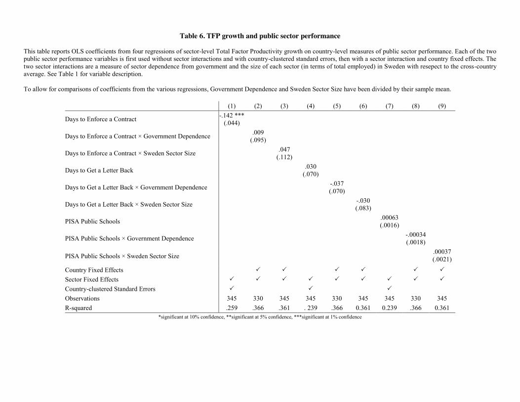
Table 6. TFP growth and public sector performance

This table reports OLS coefficients from four regressions of sector-level Total Factor Productivity growth on country-level measures of public sector performance. Each of the two public sector performance variables is first used without sector interactions and with country-clustered standard errors, then with a sector interaction and country fixed effects. The two sector interactions are a measure of sector dependence from government and the size of each sector (in terms of total employed) in Sweden with resepect to the cross-country average. See Table 1 for variable description. To allow for comparisons of coefficients from the various regressions, Government Dependence and Sweden Sector Size have been divided by their sample mean.

(1) (2) (3) (4) (5) (6) (7) (8) (9)

Days to Enforce a Contract -.142 *** (.044)

Days to Enforce a Contract × Government Dependence .009 (.095)

Days to Enforce a Contract × Sweden Sector Size .047 (.112)

Days to Get a Letter Back .030 (.070)

Days to Get a Letter Back × Government Dependence -.037 (.070)

Days to Get a Letter Back × Sweden Sector Size -.030 (.083)

PISA Public Schools .00063 (.0016)

PISA Public Schools × Government Dependence -.00034 (.0018)

PISA Public Schools × Sweden Sector Size

.00037

(.0021) Country Fixed Effects 3 3 3 3 3 3 Sector Fixed Effects 3 3 3 3 3 3 3 3 3 Country-clustered Standard Errors 3 3 3 Observations 345 330 345 345 330 345 345 330 345 R-squared .259 .366 .361 . 239 .366 0.361 0.239 .366 0.361

*significant at 10% confidence, **significant at 5% confidence, ***significant at 1% confidence

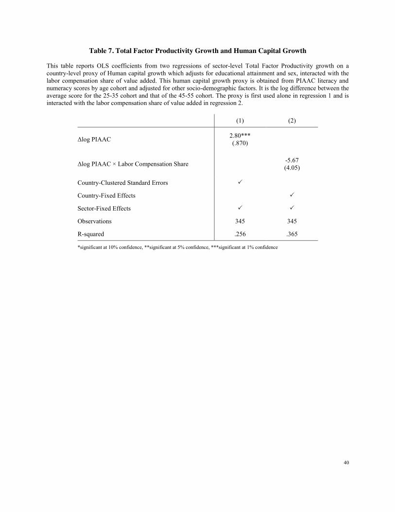
40

Table 7. Total Factor Productivity Growth and Human Capital Growth This table reports OLS coefficients from two regressions of sector-level Total Factor Productivity growth on a country-level proxy of Human capital growth which adjusts for educational attainment and sex, interacted with the labor compensation share of value added. This human capital growth proxy is obtained from PIAAC literacy and numeracy scores by age cohort and adjusted for other socio-demographic factors. It is the log difference between the average score for the 25-35 cohort and that of the 45-55 cohort. The proxy is first used alone in regression 1 and is interacted with the labor compensation share of value added in regression 2.

(1) (2)

Δlog  PIAAC 2.80*** (.870)

Δlog  PIAAC  × Labor Compensation Share -5.67 (4.05)

Country-Clustered Standard Errors 3

Country-Fixed Effects 3

Sector-Fixed Effects 3 3

Observations 345 345

R-squared .256 .365

*significant at 10% confidence, **significant at 5% confidence, ***significant at 1% confidence

41

Table 8. Capital Accumulation, Firm Size Growth and the Trade Balance This table reports OLS coefficients. In the first two regressions, the dependent variable is growth in TFP between 1994 and 2006. In regressions 3 and 4, the dependent variable is growth in average firm size during the same period. In the last two regressions, the dependent variable is growth in capital per hour worked during the same period. The explanatory variables are: i) change in sector-level trade balance (as a percentage of Value Added) in 1995–2005; ii) change in the trade balance interacted with a measure of average U.S. firm size; iii) change in the trade balance interacted with average U.S. capital per hour worked. Standard errors are reported in brackets. Because the sector definition is coarser for OECD TiVA (Trade in Value Added) data than for EU KLEMS, we use clustered standard errors; each combination of country and TiVA sector identifies one cluster. To allow for comparisons of coefficients from the various regressions US Firm Size and US Capital/Hour have been divided by their sample mean.

Δlog  TFP Δlog  Firm  Size Δlog  Capital/Hour

(1) (2) (3) (4) (5) (6)

Δ Trade Surplus %VA -.007 (.007)

-.013 (.020)

.005 (.008)

.032 (.025)

-.009* (.005)

-.013 (.012)

Δ Trade Surplus %VA × US Firm Size .005

(.014)

-.021 (.017)

Δ Trade Surplus %VA × US Capital/Hour .005 (.015)

Country-Fixed Effects 3 3 3 3 3 3 Sector-Fixed Effects 3 3 3 3 3 3 Errors clustered by Country and TiVA Sector 3 3 3 3 3 3 Observations 345 345 345 345 345 345 R-squared .363 .363 .508 .513 .407 .407 *significant at 10% confidence, **significant at 5% confidence, ***significant at 1% confidence

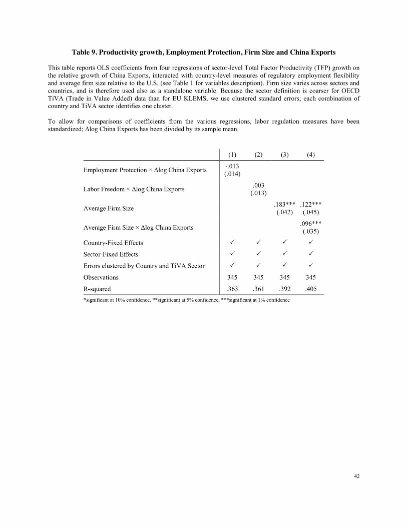
42

Table 9. Productivity growth, Employment Protection, Firm Size and China Exports This table reports OLS coefficients from four regressions of sector-level Total Factor Productivity (TFP) growth on the relative growth of China Exports, interacted with country-level measures of regulatory employment flexibility and average firm size relative to the U.S. (see Table 1 for variables description). Firm size varies across sectors and countries, and is therefore used also as a standalone variable. Because the sector definition is coarser for OECD TiVA (Trade in Value Added) data than for EU KLEMS, we use clustered standard errors; each combination of country and TiVA sector identifies one cluster. To allow for comparisons of coefficients from the various regressions, labor regulation measures have been standardized; Δlog China Exports has been divided by its sample mean.

(1) (2) (3) (4)

Employment Protection × Δlog China Exports -.013 (.014)

Labor Freedom × Δlog China Exports .003 (.013)

Average Firm Size .183*** (.042)

.122*** (.045)

Average Firm Size × Δlog China Exports .096*** (.035)

Country-Fixed Effects 3 3 3 3

Sector-Fixed Effects 3 3 3 3

Errors clustered by Country and TiVA Sector 3 3 3 3

Observations 345 345 345 345

R-squared .363 .361 .392 .405 *significant at 10% confidence, **significant at 5% confidence, ***significant at 1% confidence

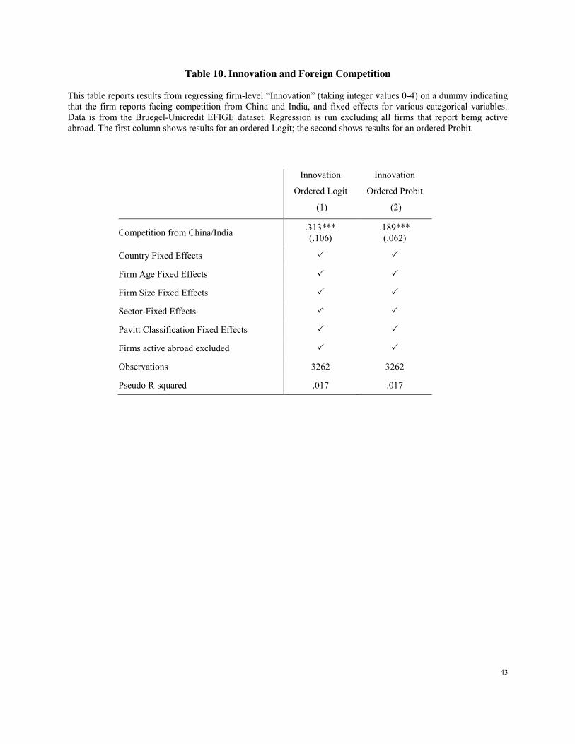
43

Table 10. Innovation and Foreign Competition This table reports results from regressing firm-level  “Innovation”  (taking  integer  values  0-4) on a dummy indicating that the firm reports facing competition from China and India, and fixed effects for various categorical variables. Data is from the Bruegel-Unicredit EFIGE dataset. Regression is run excluding all firms that report being active abroad. The first column shows results for an ordered Logit; the second shows results for an ordered Probit.

Innovation

Ordered Logit

(1)

Innovation

Ordered Probit

(2)

Competition from China/India .313*** (.106)

.189*** (.062)

Country Fixed Effects 3 3

Firm Age Fixed Effects 3 3

Firm Size Fixed Effects 3 3

Sector-Fixed Effects 3 3

Pavitt Classification Fixed Effects 3 3

Firms active abroad excluded 3 3

Observations 3262 3262

Pseudo R-squared .017 .017

44

Table 11. Productivity growth and ICT capital growth This table reports OLS coefficients from a regression of Total Factor Productivity growth on country/sector effects and ICT capital stock / hour worked growth in Finland sectors, interacted with a dummy for Italy. Finland Δlog ICT Capital/Hour has been divided by its sample mean.

(1)

Finland  Δlog  ICT  Capital/Hour × Italy Dummy -.400*** (.118)

Country-Fixed Effects 3 Sector-Fixed Effects 3 Observations 345 R-squared .384 *significant at 10% confidence, **significant at 5% confidence, ***significant at 1% confidence

45

Table 12. Productivity growth, ICT capital accumulation and Networked Readiness

This table reports OLS coefficients from regressions of sector-level Total Factor Productivity growth during the period 1995–2006 on the contribution of ICT capital to the growth in value added, interacted (in turn) with the Networked Readiness Index (regression 1), the Size of the Shadow Economy (Schneider et al. (2012)) (regression 2), Average Firm Size relative to the US (3), the   OECD’s   Employment   Protection   Legislation   Index   (4). Since average firm size varies across countries and sectors, it also appears in regression 3 as a standalone variable. See Table 1 for variables description. NRI has been standardized to allow for easier comparisons with regression coefficients in table 13.

(1) (2) (3) (4)

ICT Capital Contribution -.215 (.427)

.192 (.403)

.326 (.477)

.113 (.416)

Average Firm Size .171*** (.059)

ICT Capital Contribution × Networked Readiness .900*** (.338)

ICT Capital Contribution × Shadow Economy -.065 (.303)

ICT Capital Contribution × Average Firm Size .210 (.623)

ICT Capital Contribution × Employment Protection -.216 (.278)

Country-Fixed Effects 3 3 3 3 Sector-Fixed Effects 3 3 3 3 Observations 345 345 345 345 R-squared .376 .362 .393 .363

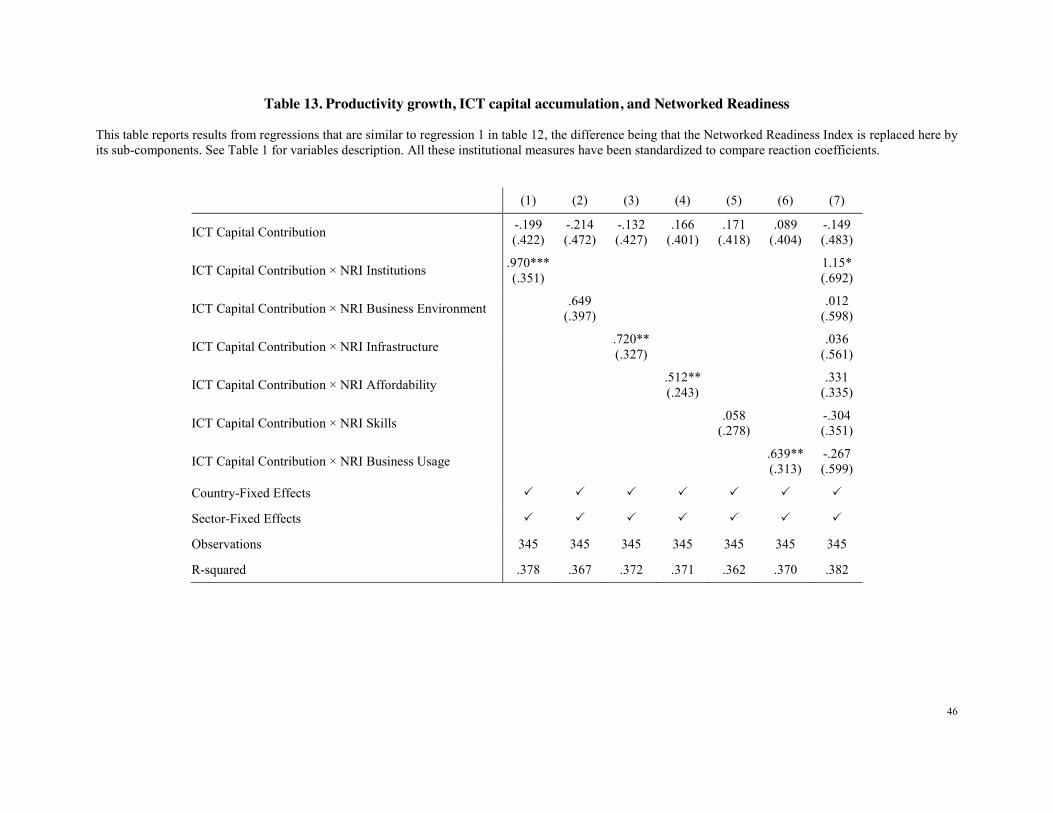
46

Table 13. Productivity growth, ICT capital accumulation, and Networked Readiness This table reports results from regressions that are similar to regression 1 in table 12, the difference being that the Networked Readiness Index is replaced here by its sub-components. See Table 1 for variables description. All these institutional measures have been standardized to compare reaction coefficients.

(1) (2) (3) (4) (5) (6) (7)

ICT Capital Contribution -.199 (.422)

-.214 (.472)

-.132 (.427)

.166 (.401)

.171 (.418)

.089 (.404)

-.149 (.483)

ICT Capital Contribution × NRI Institutions .970*** (.351) 1.15*

(.692)

ICT Capital Contribution × NRI Business Environment .649 (.397) .012

(.598)

ICT Capital Contribution × NRI Infrastructure .720** (.327) .036

(.561)

ICT Capital Contribution × NRI Affordability .512** (.243) .331

(.335)

ICT Capital Contribution × NRI Skills .058 (.278) -.304

(.351)

ICT Capital Contribution × NRI Business Usage .639** (.313)

-.267 (.599)

Country-Fixed Effects 3 3 3 3 3 3 3

Sector-Fixed Effects 3 3 3 3 3 3 3

Observations 345 345 345 345 345 345 345

R-squared .378 .367 .372 .371 .362 .370 .382

47

Table 14. Productivity growth, ICT capital accumulation and Management Columns 1-3 of this table report results from regressions that are similar to regression 1 in table 12, the difference being that the Networked Readiness Index is here replaced by measures of management quality and perceptions of meritocracy and cronyism. See Table 1 for variables description. All these measures have been standardized to compare reaction coefficients. Column 4 combines the specification of Column 3 and Table 9, column 4. Because the sector definition is coarser for OECD TiVA (Trade in Value Added) data than for EU KLEMS, we use clustered standard errors in regression 4; each combination of country and TiVA sector identifies one cluster

(1) (2) (3) (4)

ICT Capital Contribution .198 (.403)

.306 (.418)

-.157 (.420)

-.124 (.629)

Average Firm Size .106** (.046)

ICT Capital Contribution × GMAT Scores -.194 (.264)

ICT Capital Contribution × Management Schools -.336 (.346)

ICT Capital Contribution × Meritocracy .977*** (.365)

.956*** (.338)

Average Firm Size × log China Export .105*** (.035)

Country-Fixed Effects 3 3 3 3

Sector-Fixed Effects 3 3 3 3

Errors clustered by Country and TiVA Sector 3

Observations 345 345 345 345

R-squared .363 .363 .376 .420

'

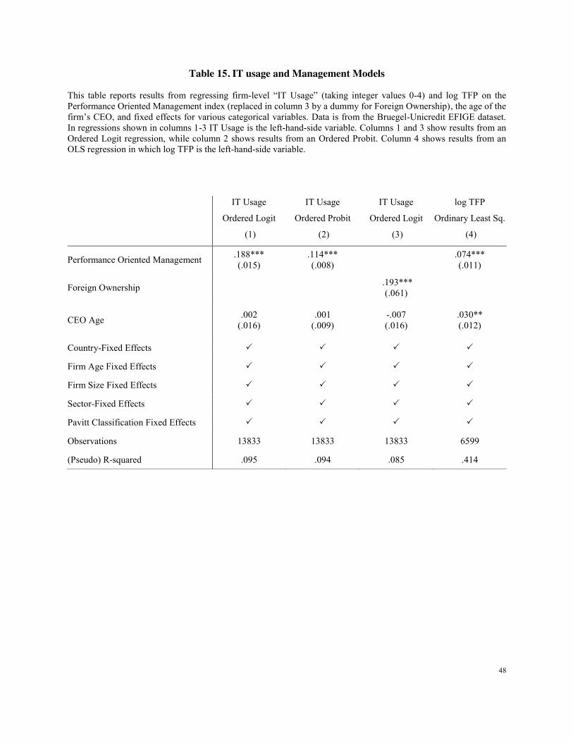
48

Table 15. IT usage and Management Models This table reports results from regressing firm-level   “IT  Usage” (taking integer values 0-4) and log TFP on the Performance Oriented Management index (replaced in column 3 by a dummy for Foreign Ownership), the age of the firm’s  CEO,  and fixed effects for various categorical variables. Data is from the Bruegel-Unicredit EFIGE dataset. In regressions shown in columns 1-3 IT Usage is the left-hand-side variable. Columns 1 and 3 show results from an Ordered Logit regression, while column 2 shows results from an Ordered Probit. Column 4 shows results from an OLS regression in which log TFP is the left-hand-side variable.

IT Usage

Ordered Logit

(1)

IT Usage

Ordered Probit

(2)

IT Usage

Ordered Logit

(3)

log TFP

Ordinary Least Sq.

(4)

Performance Oriented Management .188*** (.015)

.114*** (.008)

.074*** (.011)

Foreign Ownership .193*** (.061)

CEO Age .002 (.016)

.001 (.009)

-.007 (.016)

.030** (.012)

Country-Fixed Effects 3 3 3 3

Firm Age Fixed Effects 3 3 3 3

Firm Size Fixed Effects 3 3 3 3

Sector-Fixed Effects 3 3 3 3

Pavitt Classification Fixed Effects 3 3 3 3

Observations 13833 13833 13833 6599

(Pseudo) R-squared .095 .094 .085 .414