第13章 运动分析（Motion Analysis）

李厚强，周文罡

中国科学技术大学

Outline

2-D motion model 2-D motion vs. optical flow Optical flow equation and ambiguity in motion estimation General methodologies in motion estimation Pixel-based motion estimation Block-based motion estimation Multiresolution motion estimation Phase Correlation Method Global motion estimation Region-based motion estimation Motion Segmentation

13.1 2-D Motion Model

Camera projection 3D motion Projection of 3-D motion 2D motion due to rigid object motion

Projective mapping

Approximation of projective mapping Affine model Bilinear model

Pinhole Camera

Cameracenter

Imageplane

2-Dimage

3-Dpoint

The image of an object is reversed from its 3-D position. The object appears smaller when it is farther away.

Pinhole Camera Model: Perspective Projection

ZyxZ

YFy

Z

XFx

Z

Y

F

y

Z

X

F

x

torelatedinversely are ,

,,

All points in this ray will have the same image

Approximate Model: Orthographic Projection

When the object is very far ( )

,

Can be used as long as the depth variation within the object is small

compared to the distance of the object.

Z

x X y Y

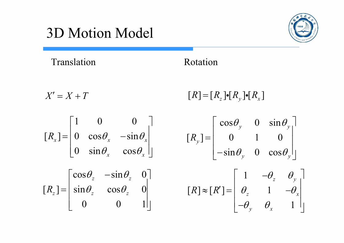
3D Motion Model

Translation Rotation

X X T [ ] [ ] [ ] [ ]z y xR R R R

1 0 0

[ ] 0 cos sin

0 sin cosx x x

x x

R

cos 0 sin

[ ] 0 1 0

sin 0 cos

y y

y

y y

R

cos sin 0

[ ] sin cos 0

0 0 1

z z

z z zR

1

[ ] [ ] 1

1

z y

z x

y x

R R

Rigid Object Motion

zyxzyx TTT ,,:;,,:][;)]([' TRCTCXRX :center object the wrt.ntranslatio and Rotation

Flexible Object Motion

Two ways to describe Decompose into multiple, but connected rigid

sub-objects

Global motion plus local motion in sub-objects Eg. Human body consists of many parts each

undergo a rigid motion

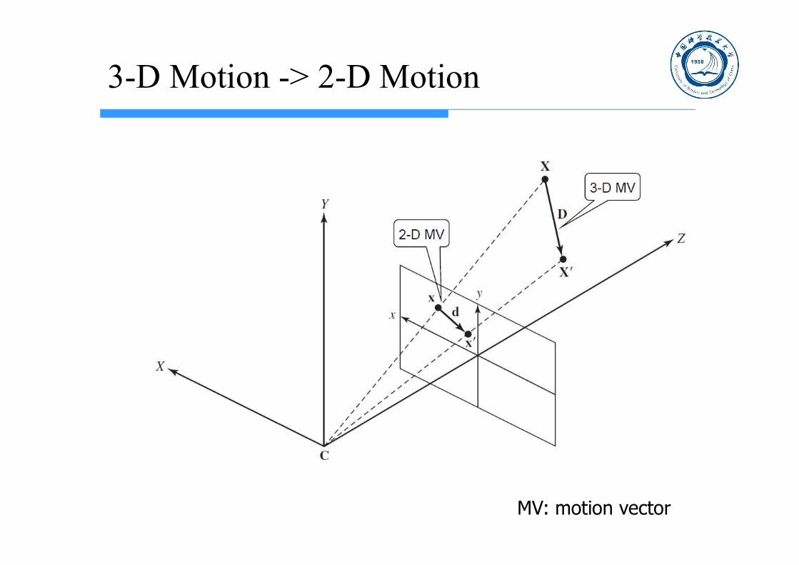
3-D Motion -> 2-D Motion

2-D MV

3-D MV

MV: motion vector

Definition and Notation

3D motion vector

1 2( ; , ) [ , , ]TX Y ZD X t t X X D D D

2D motion vector

1 2( ; , ) [ , ]Tx yX X Xd t t d d

Mapping function

1 2( ; , )X Xw t t

( )( )X X Xw d

Flow vector

,T

yxdd d

Vt t t

Sample of Motion Field

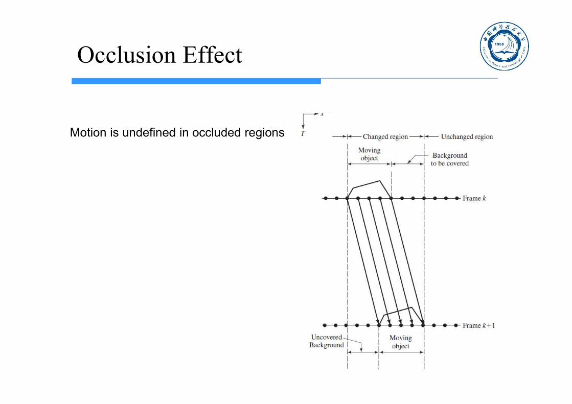
Occlusion Effect

Motion is undefined in occluded regions

Typical Camera Motions

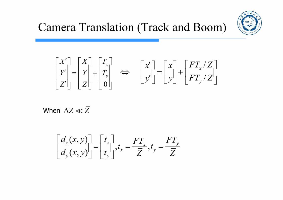
Camera Translation (Track and Boom)

0

x

y

X X T

Y Y T

Z Z

/

/x

y

FT Zx x

FT Zy y

When Z Z

( , ), ,

( , )x x yx

x yy y

d x y t FTFTt t

d x y t Z Z

Camera Pan and Tilt

Z Z

1 0

[ ][ ] [ ][ ] 0 1

1

y

x y x y x

y x

X X

Y R R Y R R

Z Z

If , then ,x yY Z X Z

( , )

( , )

x y

y x

d x y F

d x y F

Camera Zoom and Roll

cos sin 1

sin cos 1

z z z

z z z

x x x

y y y

( , )

( , )x z

y z

d x y y

d x y x

( , ) (1 )( / )

( , ) (1 )

x

y

d x yx x xF F

d x yy y y

Zoom

Roll

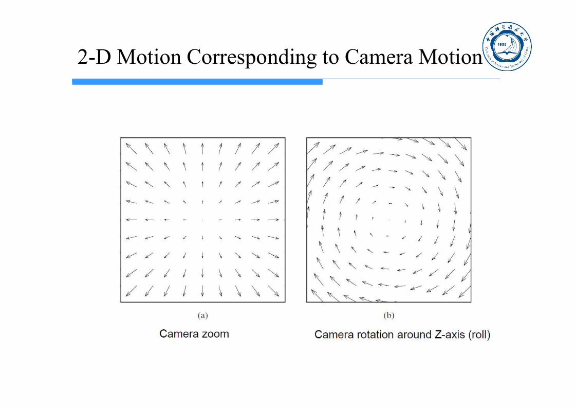
2-D Motion Corresponding to Camera Motion

Camera zoom Camera rotation around Z-axis (roll)

Four-Parameter Model

1 2 3

2 1 4

cos sin

sin cos

y xz z

x yz z

x F tx

y F ty

c c cx

c c cy

Consider a camera that goes through translation, pan, tilt, zoom, and rotation in sequence

This mapping function has four parameters, and is a special case of the affine mapping, which has 6 parameters.

Geometric Mapping

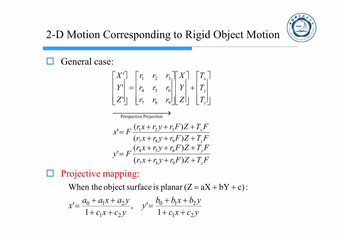
2-D Motion Corresponding to Rigid Object Motion

General case:

Projective mapping:

FTZFryrxr

FTZFryrxrFy

FTZFryrxr

FTZFryrxrFx

T

T

T

Z

Y

X

rrr

rrr

rrr

Z

Y

X

z

y

z

x

z

y

x

)(

)('

)(

)('

'

'

'

987

654

987

321

Projection ePerspectiv

987

654

321

ycxc

ybxbby

ycxc

yaxaax

21

210

21

210

1',

1'

:c)bYaX(Zplanar is surfaceobject When the

Projective Mapping

Two features of projective mapping:• Chirping: increasing perceived spatial frequency for far away objects• Converging (Keystone): parallel lines converge in distance

Affine and Bilinear Model

Affine (6 parameters):

Good for mapping triangles to triangles

Bilinear (8 parameters):

Good for mapping blocks to quadrangles

ybxbb

yaxaa

yxd

yxd

y

x

210

210

),(

),(

xybybxbb

xyayaxaa

yxd

yxd

y

x

3210

3210

),(

),(

Motion Field Corresponding to Different 2-D Motion Models

Translation

Bilinear Perspective

Affine

13.2 2-D Motion vs. Optical Flow

• 2-D Motion: Projection of 3-D motion, depending on 3D object motion and projection operator

• Optical flow: “Perceived” 2-D motion based on changes in image pattern, also depends on illumination and object surface texture

On the left, a sphere is rotating under a constant ambient illumination, but the observed image does not change.

On the right, a point light source is rotating around a stationary sphere, causing the highlight point on the sphere to rotate.

13.3 Optical Flow Equation

When illumination condition is unknown, the best one can do it is to estimate optical flow.

Constant intensity assumption -> Optical flow equation

0or 0or 0

:equation flow optical thehave we two,above theCompare

),,(),,(

:expansion sTaylor' using But,

),,(),,(

:"assumptionintensity constant "Under

ttv

yv

xd

td

yd

x

dy

dy

dx

tyxdtdydx

tyxdtdydx

Tyxtyx

tyxtyx

tyx

v

How to use the optical equation

),1,1(),1,(),,1(),,(4

1

)1,1,1()1,1,()1,,1()1,,(4

1

tyxftyxftyxftyxf

tyxftyxftyxftyxff t

)1,1,()1,,(),1,(),,(4

1

)1,1,1()1,,1(),1,1(),,1(4

1

tyxftyxftyxftyxf

tyxftyxftyxftyxff x

Ambiguities in Motion Estimation

Optical flow equation only constrains the flow vector in the

gradient direction

The flow vector in the tangent direction ( ) is under-determined

In regions with constant brightness ( ), the flow is indeterminate Motion estimation is unreliable in regions with flat texture, more reliable near

edges

nv

0

0

n n t t

n

v v

vt

v e e

tv

The Aperture Problem

??

?

13.4 General Considerations for Motion Estimation

Two categories of approaches: Feature based (more often used in object tracking, 3D

reconstruction from 2D)

Intensity based (based on constant intensity assumption) (more often used for motion compensated prediction, required in video coding, frame interpolation) -> Our focus

Three important questions How to represent the motion field?

What criteria to use to estimate motion parameters?

How to search motion parameters?

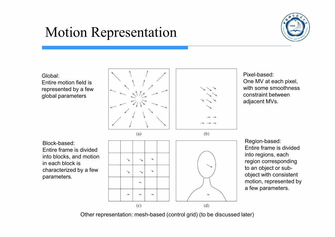
Motion Representation

Global:Entire motion field is represented by a few global parameters

Pixel-based:One MV at each pixel, with some smoothness constraint between adjacent MVs.

Region-based:Entire frame is divided into regions, each region corresponding to an object or sub-object with consistent motion, represented by a few parameters.

Block-based:Entire frame is divided into blocks, and motion in each block is characterized by a few parameters.

Other representation: mesh-based (control grid) (to be discussed later)

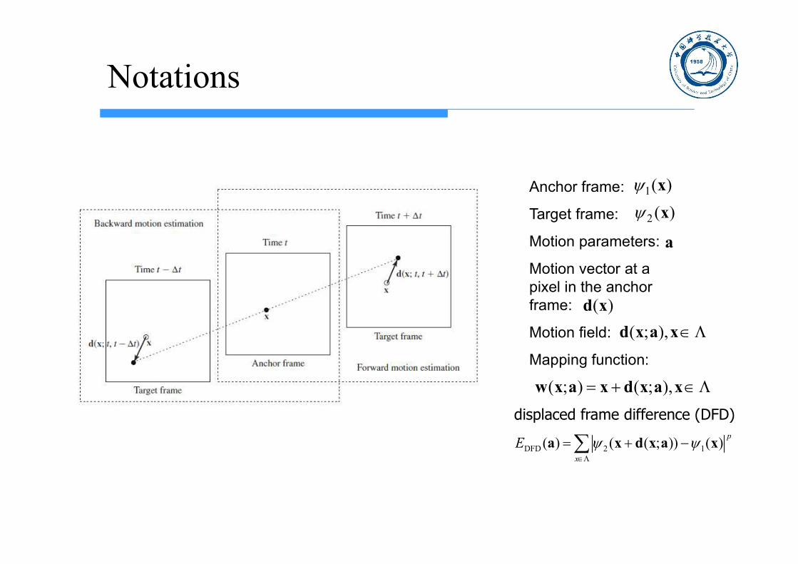
Notations

Anchor frame:

Target frame:

Motion parameters:

Motion vector at a pixel in the anchor frame:

Motion field:

Mapping function:

)(1 x)(2 x

)(xd

xaxd ),;(

a

xaxdxaxw ),;();(

displaced frame difference (DFD)

DFD 2 1( ) ( ( ; )) ( )p

x

E

a x d x a x

Motion Estimation Criterion

To minimize the displaced frame difference (DFD)

To satisfy the optical flow equation

To impose additional smoothness constraint using regularization technique (important in pixel- and block-based representation)

Bayesian (MAP) criterion: to maximize the a posteriori probability

MSE :2 MAD;:1

min)());(()( 12DFD

Pp

Ex

pxaxdxa

min)()();()()( 122OF x

pTE xxaxdxa

max),( 12 dDP

min)()(

);();()(

DFD

2

aa

aydaxdax y

ssDFD

Ns

EwEw

Ex

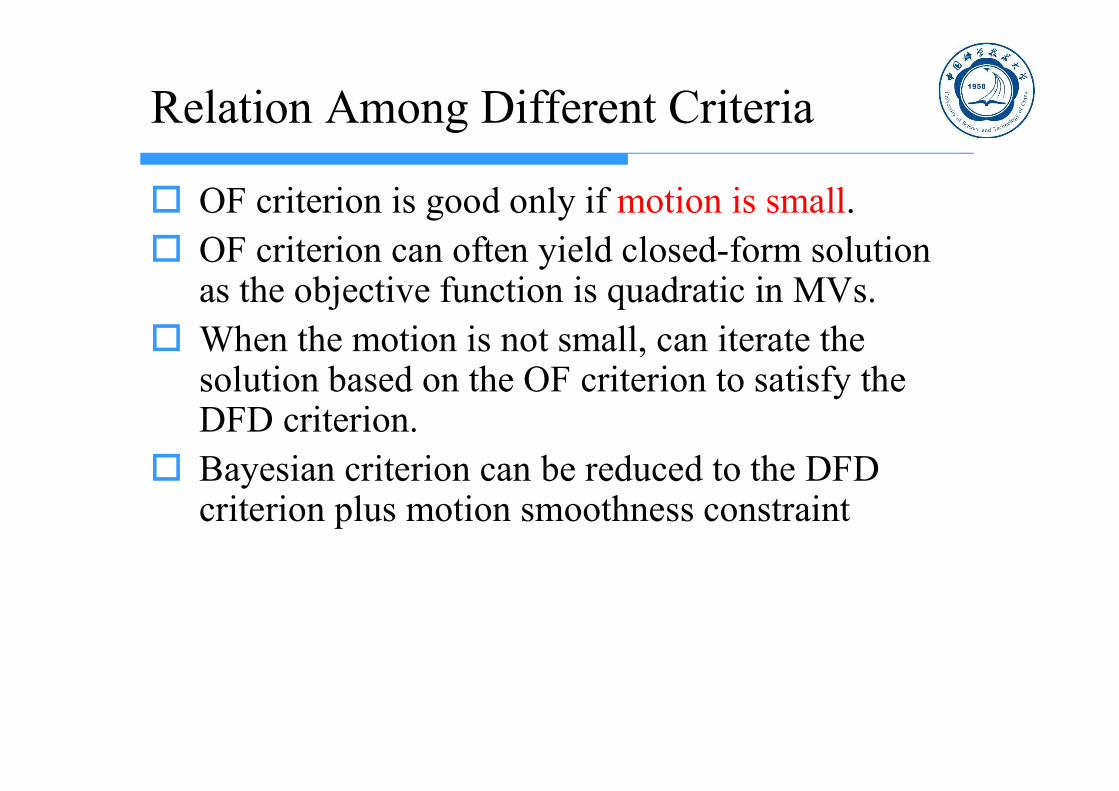
Relation Among Different Criteria

OF criterion is good only if motion is small. OF criterion can often yield closed-form solution

as the objective function is quadratic in MVs. When the motion is not small, can iterate the

solution based on the OF criterion to satisfy the DFD criterion.

Bayesian criterion can be reduced to the DFD criterion plus motion smoothness constraint

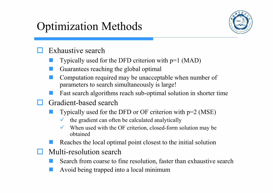
Optimization Methods

Exhaustive search Typically used for the DFD criterion with p=1 (MAD) Guarantees reaching the global optimal Computation required may be unacceptable when number of

parameters to search simultaneously is large! Fast search algorithms reach sub-optimal solution in shorter time

Gradient-based search Typically used for the DFD or OF criterion with p=2 (MSE)

the gradient can often be calculated analytically When used with the OF criterion, closed-form solution may be

obtained

Reaches the local optimal point closest to the initial solution

Multi-resolution search Search from coarse to fine resolution, faster than exhaustive search Avoid being trapped into a local minimum

13.5 Pixel-Based Motion Estimation

Horn-Schunck method OF + smoothness criterion

Multipoint neighborhood method Assuming every pixel in a small block surrounding a

pixel has the same MV

Pel-recurrsive method MV for a current pel is updated from those of its

previous pels, so that the MV does not need to be coded Developed for early generation of video coder

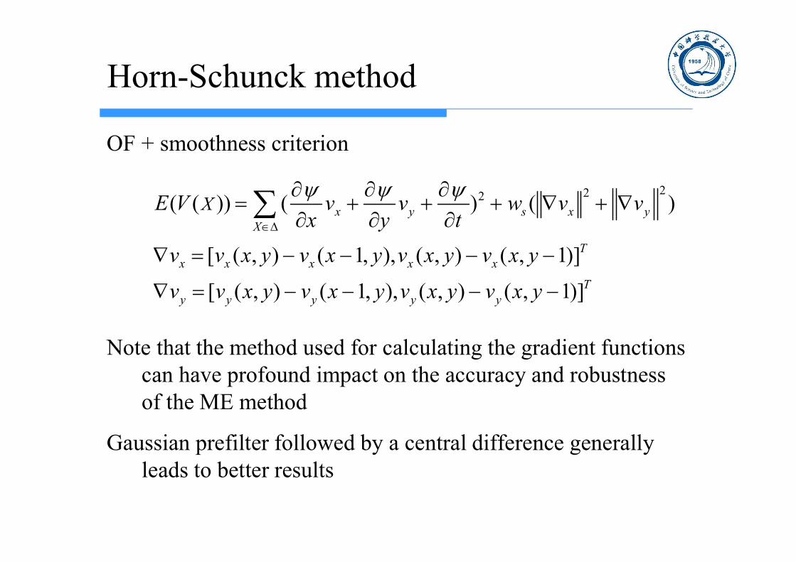
Horn-Schunck method

OF + smoothness criterion

Note that the method used for calculating the gradient functions can have profound impact on the accuracy and robustness of the ME method

Gaussian prefilter followed by a central difference generally leads to better results

222( ( )) ( ) ( )

[ ( , ) ( 1, ), ( , ) ( , 1)]

[ ( , ) ( 1, ), ( , ) ( , 1)]

x y s x yX

Tx x x x x

Ty y y y y

XE V v v w v vx y t

v v x y v x y v x y v x y

v v x y v x y v x y v x y

Multipoint Neighborhood Method

Estimate the MV at each pixel independently, by minimizing the DFD error over a neighborhood surrounding this pixel

Every pixel in the neighborhood is assumed to have the same MV

Minimizing function:

Optimization method: Exhaustive search (feasible as one only needs to search one MV at

a time) Need to select appropriate search range and search step-size

Gradient-based method

min)()()()()(

212nDFD

nBnwE

xx

xdxxd

13.6 Block-Based Motion Estimation: Overview

Assume all pixels in a block undergo a coherent motion, and search for the motion parameters for each block independently

Block matching algorithm (BMA): assume translational motion, 1 MV per block (2 parameter) Exhaustive BMA (EBMA)

Fast algorithms

Deformable block matching algorithm (DBMA): allow more complex motion (affine, bilinear)

Block Matching Algorithm

Overview: Assume all pixels in a block undergo a translation, denoted by a

single MV Estimate the MV for each block independently, by minimizing the

DFD error over this block

Minimizing function:

Optimization method: Exhaustive search (feasible as one only needs to search one MV at

a time), using MAD criterion (p=1) Fast search algorithms Integer vs. fractional pel accuracy search

min)()()( 12mDFD mB

pmE

x

xdxd

Exhaustive Block Matching Algorithm (EBMA)

Complexity of Integer-Pel EBMA

Assumption Image size: MxM Block size: NxN Search range: (-R,R) in each dimension Search stepsize: 1 pixel (assuming integer MV)

Operation counts (1 operation=1 “-”, 1 “abs”, 1 “+”): Each candidate position: Each block going through all candidates: Entire frame:

Independent of block size!

Example: M=512, N=16, R=16, 30 fps Total operation count = 2.85x10^8/frame*30 =8.55x10^9/second

Regular structure suitable for VLSI implementation Challenging for software-only implementation

2 2(2 1)R N2 2 2 2 2( / ) (2 1) (2 1)M N R N M R

2N

Fractional Accuracy EBMA

Real MV may not always be multiples of pixels. To allow sub-pixel MV, the search stepsize must be less than 1 pixel

Half-pel EBMA: stepsize=1/2 pixel in both dimension Difficulty:

Target frame only have integer pels

Solution: Interpolate the target frame by factor of two before searching Bilinear interpolation is typically used

Complexity:

4 times of integer-pel, plus additional operations for interpolation.

Fast algorithms: Search in integer precisions first, then refine in a small search region in

half-pel accuracy.

Half-Pel Accuracy EBMA

Bilinear Interpolation

(x+1,y)(x,y)

(x+1,y+1)(x,y+!)

(2x,2y) (2x+1,2y)

(2x,2y+1) (2x+1,2y+1)

O[2x,2y]=I[x,y]O[2x+1,2y]=(I[x,y]+I[x+1,y])/2O[2x,2y+1]=(I[x,y]+I[x+1,y])/2O[2x+1,2y+1]=(I[x,y]+I[x+1,y]+I[x,y+1]+I[x+1,y+1])/4

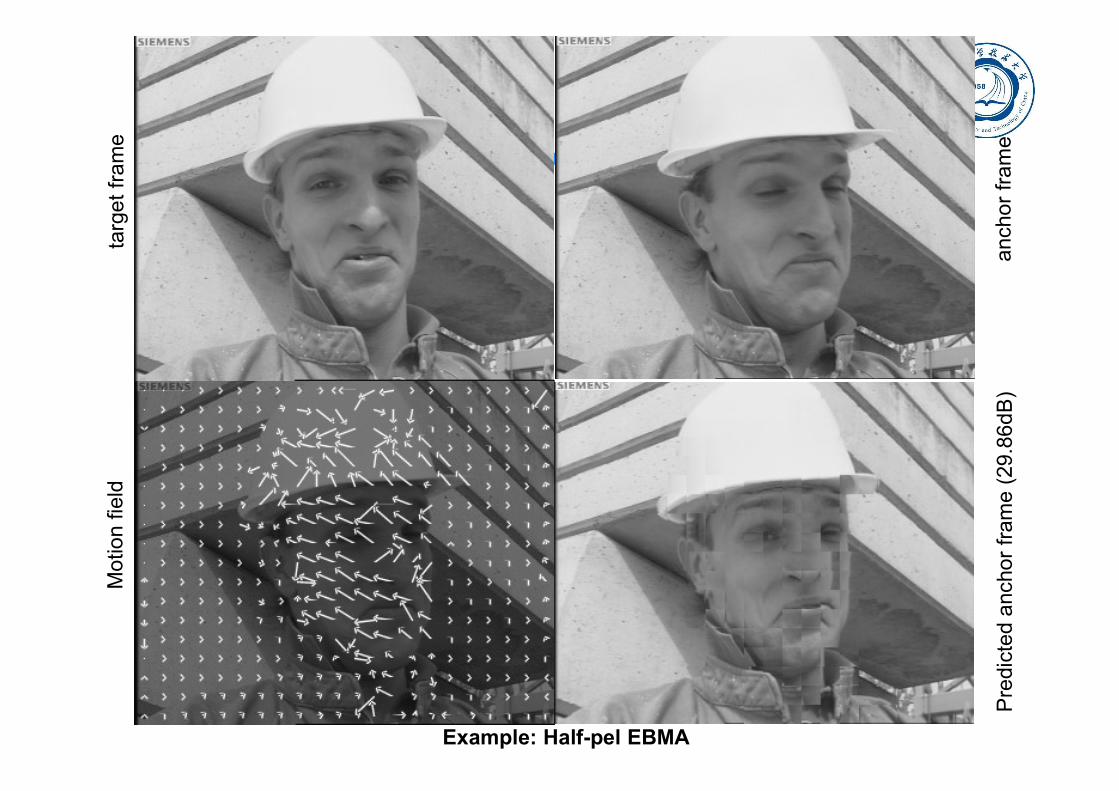
Pre

dict

ed

anc

hor

fram

e (2

9.8

6d

B)

anc

hor

fra

me

targ

et

fra

me

Mo

tion

fie

ld

Example: Half-pel EBMA

Fast Algorithms for BMA

Key idea to reduce the computation in EBMA: Reduce # of search candidates:

Only search for those that are likely to produce small errors. Predict possible remaining candidates, based on previous search result

Simplify the error measure (DFD) to reduce the computation involved for each candidate

Classical fast algorithms Three-step 2D-log

Many new fast algorithms have been developed since then Some suitable for software implementation, others for VLSI

implementation (memory access, etc)

Three-step Search Method

R0: initial search step

Search step L

2 0log 1L R

Total number:8L+1

For example

R=32

EBMA:4225 = (2R+1)2

3Step:41 = 8*5+1

Problems with EBMA

Blocking effect (discontinuity across block boundary) in the predicted image Because the block-wise translation model is not accurate Real motion in a block may be more complicated than translation

Fix: Deformable BMA

There may be multiple objects with different motions in a block Fix:

region-based motion estimation mesh-based using adaptive mesh

Intensity changes may be due to illumination effect Should compensate for illumination effect before applying “constant

intensity assumption”

Problems with EBMA (Cntd)

Motion field somewhat chaotic because MVs are estimated independently from block to block Fix:

Imposing smoothness constraint explicitly Multi-resolution approach Mesh-based motion estimation

Wrong MV in the flat region because motion is indeterminate when spatial gradient is near zero Ideally, should use non-regular partition Fix: region based motion estimation

Requires tremendous computation! Fix:

fast algorithms Multi-resolution

13.7 Multi-resolution Motion Estimation

Problems with BMA Unless exhaustive search is used, the solution may not be global

minimum Exhaustive search requires extremely large computation Block wise translation motion model is not always appropriate

Multiresolution approach Aim to solve the first two problems First estimate the motion in a coarse resolution over low-pass

filtered, down-sampled image pair Can usually lead to a solution close to the true motion field

Then modify the initial solution in successively finer resolution within a small search range Reduce the computation

Can be applied to different motion representations, but we will focus on its application to BMA

Hierarchical Block Matching Algorithm (HBMA)

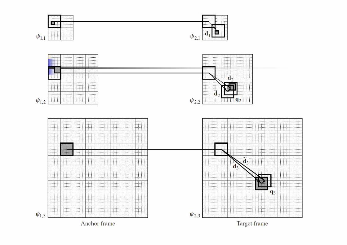
Hierarchical Block Matching Algorithm (HBMA)

Number of levels: L

lth level image:

Interpolation operator:

Error function:

Update motion vector:

MV at lth level prediction:

Total motion:

, ( ), , 1,2t l lX X t

1( ) ( ( ))l lX Xd du

2, 1,| ( ( ) ( )) ( ) |l

pl l l l

X

X X X Xd q

( ) ( ) ( )l l lX X Xd d q

1 2 1 0)( ) ( ( ( ) ( ( ) ( ( ) ( )) ))l L L LX X X X X Xd q q q q du u u

, , 1, / 2 , / 2 1, / 2 , / 2( ) ( ( )) 2 ( )l m n l m n l m nX X Xd d du

Pre

dict

ed

anc

hor

fram

e (2

9.8

6d

B)

anc

hor

fra

me

targ

et

fra

me

Mo

tion

fie

ld

Example: Half-pel EBMA

Computation Requirement of HBMA

Assumption Image size: MxM; Block size: NxN at every level; Levels: L

Search range: 1st level: R/2^(L-1) (Equivalent to R in L-th level) Other levels: R/2^(L-l) (can be smaller)

Operation counts for EBMA image size M, block size N, search range R # operations:

Operation counts at l-th level (Image size: M/2L-l)

Total operation count

Saving factor:

22)2(

1

21244

3

112/22/ RMRM L

L

l

LlL

21212/22/ LlL RM

22 12 RM

)3(12);2(343 )2( LLL

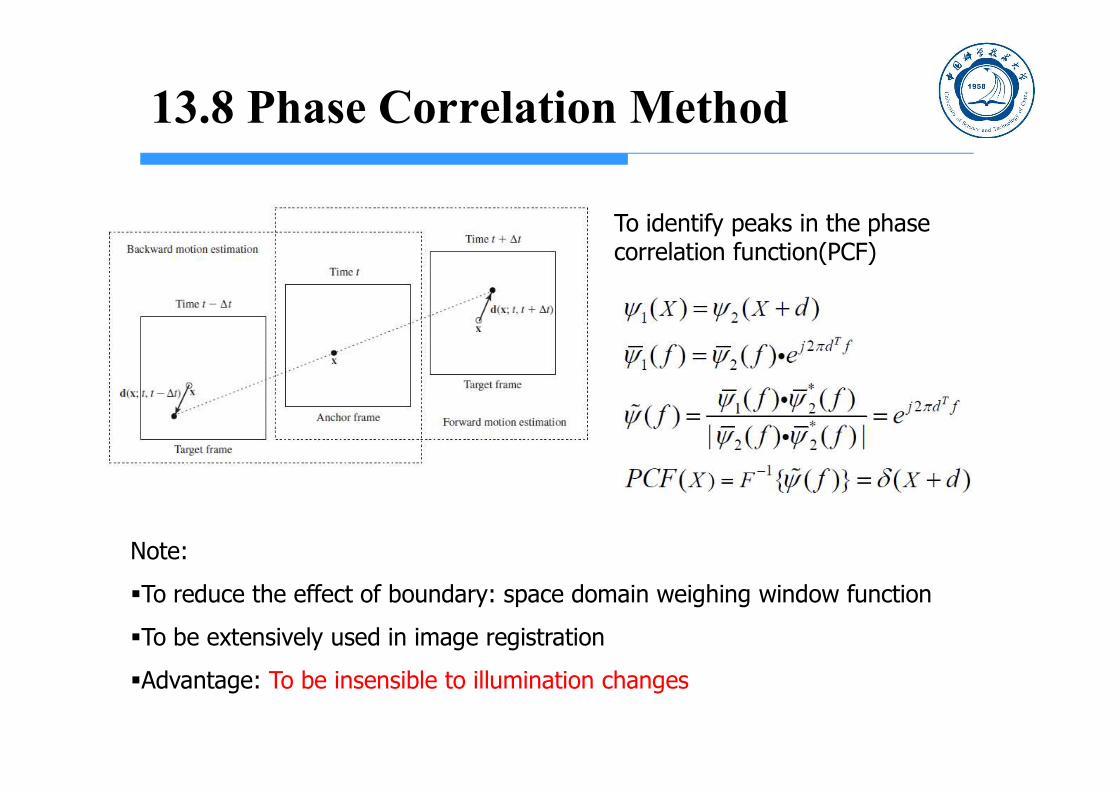
13.8 Phase Correlation Method

To identify peaks in the phase correlation function(PCF)

1 2

21 2

*21 2

*2 2

1)

( ) ( )

( ) ( )

( ) ( )( )

| ( ) ( ) |

( { ( )} ( )

T

T

j d f

j d f

X X

X F X

d

f f e

f ff e

f f

PCF f d

Note:

To reduce the effect of boundary: space domain weighing window function

To be extensively used in image registration

Advantage: To be insensible to illumination changes

13.9 Global Motion Estimation

Global motion: Camera moving over a stationary scene

Most projected camera motions can be captured by affine mapping!

The scene moves in its entirety --- a rare event! Typically, the scene can be decomposed into several major regions, each

moving differently (region-based motion estimation)

If there is indeed a global motion, or the region undergoing a coherent motion has been determined, we can determine the motion parameters Direct estimation Indirect estimation

When a majority of pixels (but not all) undergo a coherent motion, one can iteratively determine the motion parameters and the pixels undergoing this motion Robust estimator

Direct Estimation

Parameterize the DFD error in terms of the motion parameters, and estimate these parameters by minimizing the DFD error

Ex: Affine motion:

T

nn

nn

ny

nxbbbaaa

ybxbb

yaxaa

d

d],,,,,[,

);(

);(210210

210

210

a

ax

ax

Exhaustive search or gradient descent method can be used to find athat minimizes EDFD

Weighting wn coefficients depend on the importance of pixel xn.

Indirect Estimation

First find the dense motion field using pixel-based or block-based approach (e.g. EBMA)

Then parameterize the resulting motion field using the motion model through least squares fitting

nTnnn

Tnn

nnT

nnfit

nn

nnn

nn

nnnfit

ww

wE

yx

yx

wE

dAAAa

daAAa

A

aAaxd

daxd

][][][

0)]([][

1000

0001][

,][);(

:motion Affine

));((

1

2

Weighting wn coefficients depend on the accuracy of estimated motion at xn.

Robust Estimator

Essence: iteratively removing “outlier” pixels.

1. Set the region to include all pixels in a frame

2. Apply the direct or indirect method method over all pixels in the region

3. Evaluate errors (EDFD or Efit) at all pixels in the region

4. Eliminate “outlier” pixels with large errors

5. Repeat steps 2-4 for the remaining pixels in the region

Details: Hard threshold vs. soft threshold

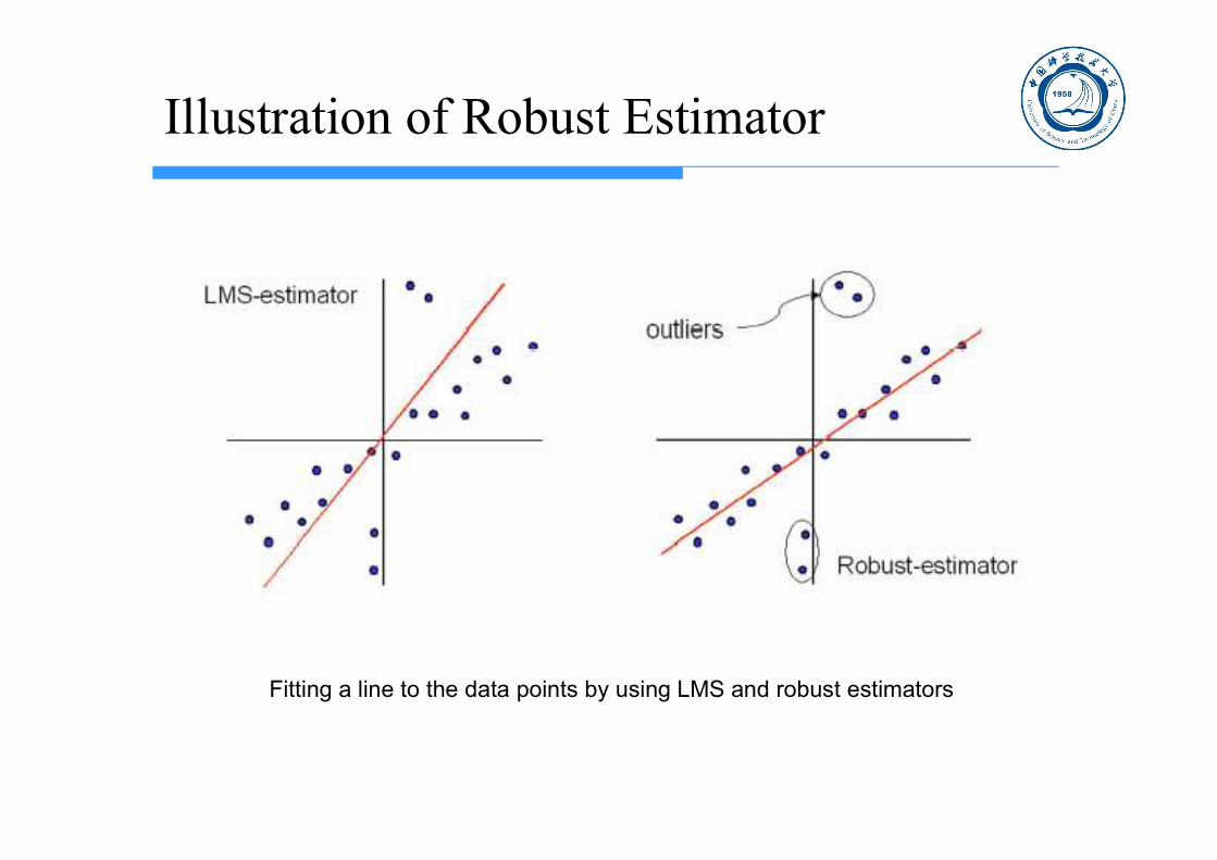
Illustration of Robust Estimator

Fitting a line to the data points by using LMS and robust estimators

13.10 Region-Based Motion Estimation

Assumption: the scene consists of multiple objects, with the region corresponding to each object (or sub-object) having a coherent motion Physically more correct than block-based, mesh-based, global motion

model

Method: Region First: Segment the frame into multiple regions based on

texture/edges, then estimate motion in each region using the global motion estimation method

Motion First: Estimate a dense motion field, then segment the motion field so that motion in each region can be accurately modeled by a single set of parameters

Joint region-segmentation and motion estimation: iterate the two processes

13.11 Motion Segmentation

WHY OBJECT MOTION SEGMENTATION Help improve optical flow estimation with multiple motion

Help improve 3D motion and structure estimation

Object recognition

Object tracking

Object based video coding

Object based editing (synthetic transfiguration)

Image vs Motion Segmentation

Segmentation is based on a feature (vector). e.g. image segmentation usually based upon the grayscale, color or

texture

Application of standard image segmentation methods directly to motion segmentation (i.e. using the velocity vector as feature) may not be useful, since 3D motion usually generates spatially varying optical flow fields. e.g. within a purely rotating object there is no flow at the center of

rotation and the magnitude of the flow vectors increase as the distance of the points from the center of rotation increase.

Motion segmentation needs to be based on some parametric description of the motion field.

2D Optical Flow Estimation and Segmentation

A realistic scene generally contains multiple motion

Smoothness constraints cannot be imposed across motion boundaries

MOTION SEGMENTATION METHODS

Direction method Thresholding for change detection

Segmentation based on motion model Modified Hough Transform

Parameter clustering approach

Bayesian segmentation

Dominant motion approach

Simultaneous estimation and segmentation

Summary

Fundamentals: 2-D Motion Corresponding to Camera Motion

Projective mapping, Affine mapping

Optical flow equation Derived from constant intensity and small motion assumption Ambiguity in motion estimation

How to represent motion: Pixel-based, block-based, region-based, global, etc.

Estimation criterion: DFD (constant intensity) OF (constant intensity + small motion) Bayesian (MAP, DFD + motion smoothness)

Search method: Exhaustive search, gradient-descent, multi-resolution

Basic techniques: Pixel-based motion estimation Block-based motion estimation

EBMA, integer-pel vs. half-pel accuracy, Fast algorithms

More advanced techniques Multiresolution approach

Avoid local minima, smooth motion field, reduced computation

Phase Correlation Method Global motion estimation

Good for estimating camera motion

Region-based motion estimation More physically correct: allow different motion in each sub-object

region

Motion Segmentation

Summary

Reference

A. M. Tekalp. Digital Video Processing. 清华大学出版社，1998.

Yao Wang etc. Video Processing and Communications. 清华大学出版社，2002.