di usion of a passive scalar from a no-slip boundary into
TRANSCRIPT

J. Fluid Mech. (1998), vol. 372, pp. 119–163. Printed in the United Kingdom
c© 1998 Cambridge University Press
119
Diffusion of a passive scalar froma no-slip boundary into a two-dimensional
chaotic advection field
By S. G H O S H1†, A. L E O N A R D2 AND S. W I G G I N S3
1Chemical Engineering, California Institute of Technology, Pasadena, CA 91125, USA2Graduate Aeronautical Laboratories, California Institute of Technology, Pasadena, CA 91125, USA
3Applied Mechanics, California Institute of Technology, Pasadena, CA 91125, USA
(Received 10 June 1994 and in revised form 12 May 1998)
Using a time-periodic perturbation of a two-dimensional steady separation bubble ona plane no-slip boundary to generate chaotic particle trajectories in a localized regionof an unbounded boundary layer flow, we study the impact of various geometricalstructures that arise naturally in chaotic advection fields on the transport of a passivescalar from a local ‘hot spot’ on the no-slip boundary. We consider here the fulladvection-diffusion problem, though attention is restricted to the case of small scalardiffusion, or large Peclet number. In this regime, a certain one-dimensional unstablemanifold is shown to be the dominant organizing structure in the distribution of thepassive scalar. In general, it is found that the chaotic structures in the flow stronglyinfluence the scalar distribution while, in contrast, the flux of passive scalar from thelocalized active no-slip surface is, to dominant order, independent of the overlyingchaotic advection. Increasing the intensity of the chaotic advection by perturbing thevelocity field further away from integrability results in more non-uniform scalar dis-tributions, unlike the case in bounded flows where the chaotic advection leads to rapidhomogenization of diffusive tracer. In the region of chaotic particle motion the scalardistribution attains an asymptotic state which is time-periodic, with the period thesame as that of the time-dependent advection field. Some of these results are under-stood by using the shadowing property from dynamical systems theory. The shadowingproperty allows us to relate the advection-diffusion solution at large Peclet numbersto a fictitious zero-diffusivity or frozen-field solution, corresponding to infinitely largePeclet number. The zero-diffusivity solution is an unphysical quantity, but is foundto be a powerful heuristic tool in understanding the role of small scalar diffusion. Anovel feature in this problem is that the chaotic advection field is adjacent to a no-slipboundary. The interaction between the necessarily non-hyperbolic particle dynamics ina thin near-wall region and the strongly hyperbolic dynamics in the overlying chaoticadvection field is found to have important consequences on the scalar distribution;that this is indeed the case is shown using shadowing. Comparisons are made through-out with the flux and the distributions of the passive scalar for the advection-diffusionproblem corresponding to the steady, unperturbed, integrable advection field.
† Present address: ARCO Exploration and Production Technology, Plano, TX 75075 USA.

120 S. Ghosh, A. Leonard and S. Wiggins
1. IntroductionThe kinematics of a perfect or non-diffusive tracer is purely advective. In other
words, perfect tracer particles will follow the pathlines of the flow. The dispersion ofthese particles is then directly related to the fluid particle trajectories and, in Eckart’sterminology (see Eckart 1948), is called ‘stirring’. Given some initial distribution ofperfect tracer particles, how this distribution evolves in time is entirely dependent onthe dynamics of particle motion in the flow, and therefore the associated transportissues are often best understood using the global geometrical viewpoint of dynamicalsystems theory. In stirring by chaotic advection (Aref 1984), the individual particletrajectories might be very complicated, but the underlying geometrical structuressuch as invariant manifolds and homoclinic/heteroclinic tangles provide a dynamicaltemplate that in certain cases considerably simplifies questions related to the transportor dispersion of particles (e.g. see Wiggins 1992). A more realistic scalar impuritywill, however, undergo both advection and diffusion. Thus the time-evolution of somegiven initial scalar field will be dictated not only by the purely fluid-mechanical stirringprocess but also by the generally slower process of molecular diffusion of the nowdiffusive tracer, which is called ‘mixing’ (Eckart 1948). In the Lagrangian framework,the kinematics of a diffusive tracer has a Brownian-motion component in addition tothe advective component due to the fluid motion, and tracer particles no longer followthe pathlines of the flow. That raises several fundamental questions regarding the roleof the underlying geometrical structures in the transport of a passive scalar and themanner in which they influence the time-evolution of a scalar field, particularly atsmall scalar diffusivities. Moreover, scalar advection in chaotic flows creates fine-scale structure since the attendant strong stretching and folding operations resultin arbitrarily small striation thicknesses (Aref & Jones 1989; Jones 1991), so thateven asymptotically small diffusivity cannot be ignored. It is therefore also a matterof considerable practical importance to incorporate small scalar diffusion. Amongother considerations is the relationship between the stirring and mixing processes, inparticular how small scalar diffusion affects the zero-diffusivity solution correspondingto pure advection.
An important isssue which has been mostly ignored in the existing literature is thetransport of a passive scalar from an active no-slip boundary into a chaotic advectionfield, even though heat and mass transfer from stationary surfaces is common inengineering applications. A stagnation point (or fixed point) is called hyperbolic ifthe velocity field expanded about the stagnation point has no eigen-values with zeroreal part. The linear part of the velocity field expanded about any stagnation point onthe no-slip boundary has zero eigen-values, and therefore every point on the no-slipboundary is non-hyperbolic. The non-hyperbolicity of the stagnation points on a no-slip boundary makes analysis difficult. Further, stirring, by itself, becomes meaninglesssince diffusion is essential for ‘lifting’ heat or a passive impurity from the active no-slip surface. Given these complications, it is not clear how the geometrical structuresin a chaotic advection field adjacent to an active no-slip surface can influence thetime-dependent distribution of the scalar field as the scalar impurity diffuses intothe flow. Our objective is to investigate some of these issues using a simple two-dimensional time-periodic separation bubble with chaotic particle trajectories, over aplane stationary surface.
We use a method devised by Perry & Chong (1986 a) to obtain a simple Taylor-series representation of a chaotic separation bubble which is also an asymptoticallyexact solution of the Navier–Stokes and continuity equations, close to the origin ofthe series-expansion. The method relies on the availability of a sufficient number oftopological constraints (Perry & Chong 1986 a) and is therefore particularly well-suited to study steady two- and three-dimensional separated flows (Perry & Chong

Diffusion of a passive scalar into a advection field 121
1986 a; Tobak & Peake 1982; Dallmann 1988) on account of their readily availabletopological features such as location and stability-type of stagnation points, loca-tion of points of zero shear stress on the no-slip boundary, angles of separationand attachment, etc. Our scheme is to construct a low-order series-representationof a steady two-dimensional separation bubble at a plane wall and then introducetime-periodic terms to obtain an unsteady bubble with chaotic particle trajectories,such that the representation satisfies incompressibility and remains an asymptoticallyexact solution of the now time-dependent Navier–Stokes equations. The truncatedseries-solution constitutes a simple time-periodic perturbation of an integrable dy-namical system. There are methods (Perry & Chong 1986 a) for testing the accuracyof a truncated series-solution over any given region of the flow, but we will notconcern ourselves with identifying a domain of applicability of the series-solutionsince attention will be mostly confined to regions close to the origin of the expansion.Only a localized portion of the plane wall is considered as an active surface suchthat finite-time distributions of the scalar field remain confined near the origin of theseries-expansion.
The relative importance of advection versus diffusion is measured by the Pecletnumber, which is the ratio of the diffusion and advection time-scales. We are interestedin the regime of small scalar diffusion, or more precisely, the regime where the diffusiontime-scale is much greater than the advection time-scale, which means large Pecletnumbers. At large Peclet numbers, the scalar advection-diffusion problem is besttackled by random-walk methods based on the theory of Brownian motion (Wang& Uhlenbeck 1945), and we develop numerical implementations of these methodsto solve for the time-dependent scalar field. These computations show clearly thatfor scalar transport with small scalar diffusivity, the unstable manifold of a saddlepoint on the boundary corresponding to zero shear stress is the organizing structurein the distribution of the scalar field, and the time evolution of the scalar field canbe understood in terms of the structure of the unstable manifold. This is a centraltheme throughout this paper. In addition we use a different numerical method, theWiener bundle method, to compute values of the scalar field. This serves as a checkof our random walk methods, and also sets the stage for our application of themethod of shadowing from dynamical systems theory. We introduce a fictitious ‘zero-diffusivity’ solution as a heuristic tool in demonstrating the role of the underlyinggeometrical structures in the flow and in interpreting the role of slow mixing asa local smoothing of fine-scale structure in the scalar field, created by the stirringprocess.
The hyperbolic invariant set (Smale 1967) associated with Smale horseshoes (Smale1967) is the prototype of a chaotic dynamical system, and the shadowing lemma(Bowen 1975) from dynamical systems theory is one of the fundamental results forthe dynamics on a hyperbolic invariant set. Recent work of Klapper (1992 a) has usedshadowing theory (Anosov 1967; Bowen 1975) to study the small-diffusivity scalaradvection-diffusion problem. Asymptotic results were obtained for the restricted classof uniformly hyperbolic systems, and therefore apply to typical chaotic processes inonly a non-rigorous sense. Justification (Klapper 1992 a) for its validity is based onexisting numerical evidence (Hammel, Yorke & Grebogi 1987, 1988; Grebogi et al.1990) that typical chaotic dynamical processes have the shadowing property. In arough sense, a dynamical system that has the shadowing property is guaranteed tohave a deterministic orbit that remains close to any noisy orbit with bounded noise,where how ‘close’ depends on the noise level. The shadowing property has been usedpreviously to reduce bounded additive noise in orbits generated by chaotic dynamical

122 S. Ghosh, A. Leonard and S. Wiggins
systems (Hammel 1990; Farmer & Sidorowich 1991). That the shadowing propertycan be used to treat scalar diffusion is not surprising since diffusion can be regardedas a noisy component in the kinematics of a diffusive tracer.
We use these ideas to develop a qualitative understanding of our random-walksolutions of the time-dependent scalar field and the interplay between the stirring andmixing processes. It is found that increased chaotic advection produces more localizedand non-uniform distributions, even in regions of the flow that have no islands ofstability bounded by invariant closed curves; near integrability, such curves will beprovided by Kolmogorov–Arnold–Moser (KAM) tori and island bands, but as oneperturbs the dynamical system further away from integrability there are no survivinginvariant closed curves, and we choose such a parameter-regime to emphasize ourresult. The phenomenon contrasts sharply with that in the case of chaotic advection inbounded domains where the chaotic particle motion promotes rapid homogenization(Jones 1991) of diffusive tracer, giving rise to an asymptotically uniform scalardistribution. Reasons for this phenomenon are sought using shadowing theory. Themethod of shadowing also helps us understand that the form of the asymptoticdistribution and the time-scale over which it is attained is also intimately linkedwith the geometrical structures in the flow, and the connection is made explicitby considering the details of exact dynamical trajectories that ‘shadow’ the ‘noisy’Wiener trajectories of a diffusive tracer. We also show how the presence of the planewall and the consequent regular dynamics of particles in a narrow near-wall regionstrongly influences the time-evolution of the scalar field, thus underlining the role ofnon-hyperbolicity at the wall. In engineering applications the flux of a passive scalar,integrated over the active surface, is a quantity of considerable practical importance;our computations show it is largely independent of the details of the chaotic advection-diffusion phenomena above the wall, for the class of flows considered. Perturbationarguments in the thermal boundary layer adjacent to the active no-slip surface furtherclarify this issue.
The organization of this paper is as follows. In § 2 we construct an approximaterepresentation of a chaotic separation bubble over a plane wall. In § 3 we set upthe scalar advection-diffusion problem. Numerical schemes are developed to obtainfinite-time solutions of the large-Peclet-number or small-diffusivity advection-diffusionproblem. In § 4, a ‘zero-diffusivity’ solution is constructed by solving for the scalarfield in the thermal boundary layer at the wall at small time and treating this as an‘initial distribution’ of perfect tracers which is subsequently stirred but not mixed bychaotic advection. In § 5 we apply shadowing theory to our scalar advection-diffusionproblem. We end with a discussion and concluding remarks in § 6.
2. Time-periodic separation bubble at a plane wallWe first construct a viscous, incompressible, two-dimensional flow that has the
topology of a steady separation bubble at a plane wall in the form of a Taylor-seriesexpansion from a point on the no-slip boundary. The construction suggests ways inwhich time-dependent terms can be introduced in the vector field such that one obtainsan asymptotically exact representation of a time-periodic bubble with chaotic particletrajectories. The advantage of the Taylor-series expansion method (Perry & Chong1986 a) is that one can generate boundary layer flows, especially separation patternswith desired topological features, as local Taylor-series expansions to arbitrary order,without regard to the outer inviscid flow. The method assumes the solutions of thecontinuity and Navier–Stokes equations for incompressible flow are smooth.
Diffusion of a passive scalar into a advection field 123
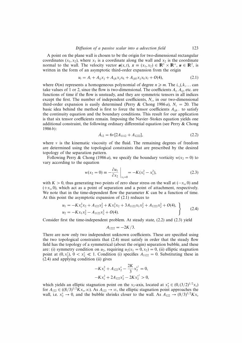
A point on the plane wall is chosen to be the origin for two-dimensional rectangularcoordinates (x1, x2), where x1 is a coordinate along the wall and x2 is the coordinatenormal to the wall. The velocity vector u(x, t), x ≡ (x1, x2) ∈ R1 × R+, u ∈ R2, iswritten in the form of an asymptotic third-order expansion from the origin
ui = Ai + Aijxj + Aijkxjxk + Aijklxjxkxl + O(4), (2.1)
where O(m) represents a homogeneous polynomial of degree n > m. The i, j, k, . . . cantake values of 1 or 2, since the flow is two-dimensional. The coefficients Ai, Aij , etc. arefunctions of time if the flow is unsteady, and they are symmetric tensors in all indicesexcept the first. The number of independent coefficients, Nc, in our two-dimensionalthird-order expansion is easily determined (Perry & Chong 1986 a), Nc = 20. Thebasic idea behind the method is first to force the tensor coefficients Aijk··· to satisfythe continuity equation and the boundary conditions. This result for our applicationis that six tensor coefficients remain. Imposing the Navier–Stokes equation yields oneadditional constraint, the following ordinary differential equation (see Perry & Chong1986 b):
A12 = 6ν[2A1112 + A1222], (2.2)
where ν is the kinematic viscosity of the fluid. The remaining degrees of freedomare determined using the topological constraints that are prescribed by the desiredtopology of the separation pattern.
Following Perry & Chong (1986 a), we specify the boundary vorticity w(x2 = 0) tovary according to the equation
w(x2 = 0) ≡ −∂u1
∂x2
∣∣∣∣x2=0
= −K(x21 − x2
s ), (2.3)
with K > 0, thus generating two points of zero shear stress on the wall at (−xs, 0) and(+xs, 0), which act as a point of separation and a point of attachment, respectively.We note that in the time-dependent flow the parameter K can be a function of time.At this point the asymptotic expansion of (2.1) reduces to
u1 = −Kx2s x2 + A122x
22 +Kx2
1x2 + 3A1122x1x22 + A1222x
32 + O(4),
u2 = −Kx1x22 − A1122x
32 + O(4).
}(2.4)
Consider first the time-independent problem. At steady state, (2.2) and (2.3) yield
A1222 = −2K/3.
There are now only two independent unknown coefficients. These are specified usingthe two topological constraints that (2.4) must satisfy in order that the steady flowfield has the topology of a symmetrical (about the origin) separation bubble, and theseare: (i) symmetry condition on u2, requiring u2(x1 = 0, x2) = 0, (ii) elliptic stagnationpoint at (0, x∗2), 0 < x∗2 � 1. Condition (i) specifies A1122 = 0. Substituting these in(2.4) and applying condition (ii) gives
−Kx2s + A122x
∗2 −
2K
3x∗
2
2 = 0,
−Kx2s + 2A122x
∗2 − 2Kx∗
2
2 > 0,
which yields an elliptic stagnation point on the x2-axis, located at x∗2 ∈ (0, (3/2)1/2xs)for A122 ∈ ((8/3)1/2Kxs,∞). As A122 →∞, the elliptic stagnation point approaches thewall, i.e. x∗2 → 0, and the bubble shrinks closer to the wall. As A122 → (8/3)1/2Kxs
124 S. Ghosh, A. Leonard and S. Wiggins
from above, x∗2 → (3/2)1/2xs from below and the bubble grows in size. For A122 <(8/3)1/2Kxs, there are no stagnation points in the entire domain of the flow. We notethat for A122 ∈ ((8/3)1/2Kxs,∞) there is also a hyperbolic stagnation point or saddlelocated at (0, x2), and x2 ∈ ((3/2)1/2xs,∞); as A122 → ∞, x2 → ∞ and the separationbetween the two stagnation points is maximum, while as A122 → (8/3)1/2Kxs fromabove, x2 → (3/2)1/2xs from above so that at A122 = (8/3)1/2Kxs the hyperbolic andelliptic stagnation points coalesce and disappear as A122 decreases below (8/3)1/2Kxs.At A122 = 3Kxs, the elliptic stagnation point is located at (0, 0.3625). The hyperbolicstagnation point or saddle is located at (0, 4.1374). It is therefore sufficiently far awayfrom the wall to have no bearing on passive scalar transport close to the wall andis ignored hereafter. With this choice of A122, the time-independent velocity field iscompletely specified,
u1 = −Kx2s x2 + 3Kxsx
22 +Kx2
1x2 − 23Kx3
2 + O(4),
u2 = −Kx1x22 + O(4),
}(2.5)
and is a low-order approximation of a steady two-dimensional separation bubble at aplane wall. By varying the coefficient A122, the size of the steady separation bubble canbe varied with important consequences on the associated advection-diffusion problem,and is the subject of § 3.6. At present we continue with our choice of A122 = 3Kxs.The streamlines (or pathlines) corresponding to the steady velocity field of (2.5) areshown in figure 1. From a dynamical systems viewpoint, the phase space of (2.5)has a heteroclinic connection ψh between the point of separation and the point ofattachment, separating bounded and unbounded motion, where ψh is the value of thetime-independent stream function (obtained below) on the separatrix. Introducing atime-periodic perturbation in (2.5) is expected to destroy this degenerate structure,giving rise to chaotic particle motion. An obvious way is to break the symmetry in thesteady state. To do so we let A1122(t) = Kβ sin(ωt). The remaining coefficients are leftunchanged. From (2.2), K remains independent of t and hence all remaining tensorcoefficients are also time-independent. Non-dimensionalizing, ui → uiKx
3s , xi → xixs,
t→ t/Kx2s , ω → ωKx2
s , the time-dependent velocity field becomes
u1 = −x2 + 3x22 + x2
1x2 − 23x3
2 + 3βx1x22 sin(ωt) + O(4),
u2 = −x1x22 − βx3
2 sin(ωt) + O(4).
}(2.6)
The stream function ψ is easily obtained,
ψ(x1, x2, t) = −x22
2+ x3
2 +x2
1x22
2− x4
2
6+ βx1x
32 sin(ωt) + O(5). (2.7)
Truncated to third order, (2.6) can be expressed in the form
u(x, t) = fu(x) + βgu(x) sin(ωt), (2.8)
where fu ≡ (fu1 , fu2) = (−x2 + 3x2
2 + x21x2 − 2
3x3
2, −x1x22), g
u ≡ (gu1 , gu2) = (3x1x
22, −x3
2),and β can be considered as the perturbation amplitude, while ω is the frequency ofthe perturbation. The associated Poincare map or time-T map, T = 2π/ω, whichis defined in the usual way in § 3, shows highly irregular motion in the bubbleregion indicating chaotic particle trajectories. In physical terms, the time-periodicperturbation in (2.8) that leads to bubble break-up and chaotic trajectories in theviscous boundary layer can be attributed to an oscillatory outer inviscid flow. Inparticular, it should be noted that the chaotic advection field of (2.8) does not arisefrom any inherent oscillatory instability in the equations of motion at large Reynolds

Diffusion of a passive scalar into a advection field 125
whx2
x1 p+
(+1,0)p–
(–1,0)
Figure 1. Streamlines for the steady two-dimensional separation bubble at a plane wall,obtained using (2.5).
number but, instead, arises from an external forcing presumably caused by the outerinviscid flow. The Reynolds number, Re = Kx4
s /ν, for our boundary layer flow isarbitrary, though it must be noted that the region of accuracy of the truncated seriessolution shrinks as the Reynolds number is increased (Perry & Chong 1986 a).
Finally, there are alternative schemes for introducing a time-periodic perturbationin (2.5) such that the time-dependent velocity field remains an asymptotically exactsolution of the Navier–Stokes and continuity equations, and again gives rise to chaoticparticle trajectories; there is of course no unique representation of a two-dimensionalchaotic advection field adjacent to a no-slip boundary. However we shall show that thequalitative aspects of the associated passive scalar advection-diffusion problem dependprimarily on certain generic structures in these chaotic advection fields, regardless ofthe specific form of the equations giving rise to the chaotic particle motion. Section3.5 deals with this issue by considering an alternative local representation of a chaoticadvection field.
3. Advection-diffusion of a passive scalar at small diffusivity or large Pecletnumber
A localized portion of the plane no-slip boundary is considered as an active surface.In the case of heat transfer, the active surface can be considered as a local ‘hot spot’at the wall and is modelled as a local step change in temperature with the step placedsymmetrically about the unperturbed bubble. At time t = 0 the temperature has adimensionless value of unity at the wall over the dimensionless interval x1 ∈ [−1.5, 1.5]and is zero everywhere else on the wall and in the fluid. The temperature distributionat the wall is maintained externally and serves as a time-independent boundarycondition as heat diffuses from the wall and into the fluid. Non-dimensionalizing timet using the advection time-scale 1/Kx2
s gives the familiar evolution equation for theadvection-diffusion of a scalar field θ(x, t), which can be considered as temperature,
∂θ
∂t+ u · ∇θ =
1
Pe∇2θ, (3.1)

126 S. Ghosh, A. Leonard and S. Wiggins
where the Peclet number Pe = Kx4s /D, with D the scalar diffusivity. The advecting
two-dimensional velocity field u(x, t) is given by (2.8). The following initial andboundary conditions:
θ(x1, x2 > 0, t = 0) = 0,
θ(x1, x2 = 0, t) = 1−H(|x1| − 1.5),
θ(|x1| → ∞, x2 > 0, t) = 0,
θ(x1, x2 →∞, t) = 0,
with (x1, x2) ∈ R1×R1, completely specify the advection-diffusion problem. H(·) is theHeaviside step function. In the absence of scalar diffusion the deterministic Lagrangianmotion of a passive scalar is described by the velocity field. Two-dimensional time-periodic flows have been studied extensively using a dynamical systems approach (e.g.see Wiggins 1992) and the geometrical structures that arise naturally in the domainof the flow, such as invariant manifolds, homoclinic/heteroclinic tangles, hyperbolicinvariant sets and KAM tori are well known. However, it is still far from clear howthese structures influence the transport and distribution of a passive scalar in thepresence of scalar diffusion. Our model problem provides a convenient frameworkfor understanding some of the transport issues that arise naturally in such flows. Thedomain of interest is the flow region immediately above the active portion of the walland since we will be making frequent reference to this region, we loosely term it asthe ‘bubble-region’.
In the context of dynamical systems theory, the velocity field of (2.8) is a time-periodic perturbation of a planar Hamiltonian vector field, where the stream functionof (2.7) plays the role of the Hamiltonian. The analysis of the global structure ofthe flow is most clearly carried out by studying the associated Poincare map, whichis the time-T map obtained by considering the discrete motion of points in time-intervals of one period T of the perturbation, and since the perturbation is alsoHamiltonian the Poincare map is area-preserving. In this case one would expectSmale horseshoes, resonance bands and KAM tori to arise in the phase space of (2.8),which is also the physical space of the flow. However, from the dynamical systemsviewpoint, our problem is non-generic because every point on the no-slip boundary isa non-hyperbolic stagnation point, despite the fact that it is a commonly encounteredsituation in fluid flows. Consequently, the mathematical theorems (see Wiggins 1990,1992) proving existence of chaotic dynamics do not apply. For the case of hyperbolicstagnation points the existence of stable and unstable manifolds is familiar, butthe non-hyperbolic case requires special consideration. In the unperturbed (β = 0)integrable system, the bubble has a point of separation, denoted by p−, a point ofattachment, denoted by p+, and a heteroclinic connection ψh between p− and p+. Thepoints p+ ≡ (+1, 0) and p− ≡ (−1, 0), which are the points of zero shear stress on thewall, are non-hyperbolic stagnation points. The standard scheme of introducing thephase of the periodic perturbation in (2.8) gives an autonomous vector field
x = fu(x) + βgu(x) sin(φ),
φ = ω,
where the phase space of the autonomous system is now R2 × S1. For β = 0, whenviewed in the three-dimensional phase space R2 × S1, p+ and p− become periodic

Diffusion of a passive scalar into a advection field 127
orbits
γ±(t) = (p±, φ(t) = ωt),
with a two-dimensional stable and two-dimensional unstable manifold respectively,denoted by Ws(γ+(t)) and Wu(γ−(t)). Therefore, Ws(γ+(t)) and Wu(γ−(t)) coincidealong a two-dimensional heteroclinic manifold, Γγ . For β 6= 0, it is easily verifiedfrom (2.8) that p± persist as the points of zero shear stress on the wall, whichimplies p±β = p± (Ghosh 1994; Shariff, Pulliam & Ottino 1991), and hence the
periodic orbits for β 6= 0 are γ±β (t) = γ±(t). However, we note that the invariantmanifold theorem (see Theorem 4.1, Hirsch, Pugh & Shub 1977) for the persistenceof normally hyperbolic invariant manifolds and the persistence and smoothness oftheir stable and unstable manifolds (at sufficiently small β) does not apply to γ±(t);in our problem, persistence of the invariant manifolds is decided by computationof the corresponding invariant manifolds of the associated Poincare map, which weshall define momentarily. Assuming Ws(γ+(t)) and Wu(γ−(t)) persist for β 6= 0, thestable and unstable manifolds of γ+
β (t) and γ−β (t), denoted by Ws(γ+β (t)) and Wu(γ−β (t))
respectively, will generically not coincide. The Poincare map is defined as a globalcross-section in the usual way,
Pφβ : Σφ → Σφ,
(x1(φ), x2(φ)) 7→ (x1(φ+ 2π), x2(φ+ 2π)).
The intersection with Σφ of the stable and unstable manifolds of γ+β (t) and γ−β (t)
respectively are denoted as
Wsβ(φ) ≡Ws(γ+
β (t)) ∩ Σφ,
Wuβ (φ) ≡Wu(γ−β (t)) ∩ Σφ.
Rom-Kedar, Leonard & Wiggins (1990) considered the transport of a passive scalar inthe absence of scalar diffusion in a similar problem and found the unstable manifold,i.e. Wu
β (φ), as the dominant organizing structure. They considered the evolution of anarbitrary blob of fluid under several iterations of the Poincare map and showed thatthe unstable manifold behaves in some sense as an attractor since neighbourhoods ofWu
β (φ) are stretched along Wuβ (φ) and flattened in a complementary direction under
forward iterations of P φβ . Of course, because of the area-preserving property of P φ
β
that derives from the incompressibility of the fluid, Wuβ (φ) is not an attractor in
the usual sense. Our main goal in this section is to motivate the following: for scalartransport with small scalar diffusivity, the unstable manifold Wu
β (φ) continues to be theorganizing structure in the distribution of the scalar field and the time evolution of thescalar field for the β 6= 0 case can be understood in terms of the structure of Wu
β (φ).Additionally, there are other important considerations, some of which have beenoutlined in the Introduction: for example the role of hyperbolicity and the strongstretching and folding properties characteristic of chaotic advection fields, the roleof non-hyperbolicity at the wall, the asymptotic state of the scalar distribution, etc.,and to what extent they contribute to our understanding of the advection-diffusionprocess and its interplay with the geometrical structures in the flow. As a first steptowards investigating these issues, finite-time distributions of the scalar field areobtained by solving (3.1) numerically. We confine our attention entirely to the case ofsmall scalar diffusivity, or large Peclet number; large scalar diffusivity would result
128 S. Ghosh, A. Leonard and S. Wiggins
in a diffusively dominant advection-diffusion process, in which case the role of thegeometrical structures in the flow can be expected to be less prominent.
3.1. A random-walk scheme for solving the advection-diffusion equation
The singular limit of large Peclet number is not easily tackled by any numericalscheme that embraces the Eulerian approach and tries to solve the partial differentialequation of (3.1) directly. At large Pe, a thermal boundary layer will form in thevicinity of the active surface of thickness proportional to Pe−1/3 (see § 3.4), whichplaces severe constraints on the spatial resolution obtainable in the boundary layer ina finite-difference solution of (3.1) at large Pe. In contrast, a random-walk solutionuses a Lagrangian approach based on the stochastic differential corresponding to thescalar advection-diffusion equation. Saffman (1959) used a random-walk approachto study the effects of molecular diffusion on the transport of a passive scalar inflow through porous media. Chorin (1973) extended the random-walk approach tonumerical solutions of the vorticity diffusion equation corresponding to the Navier–Stokes equations for incompressible flow in two space dimensions at large Reynoldsnumbers, where the problem is complicated by the fact that the vorticity is not apassive scalar. Since we require solutions to (3.1) at Peclet numbers so large thatfinite-difference methods are difficult to apply, a random-walk or Brownian motionscheme is developed below for solving the scalar advection-diffusion problem.
The active boundary is imagined to be a constant temperature bath. The physicalprocess of diffusion of passive scalar from the active portion of the plane boundaryinto the flow is imitated by numerically simulating a constant temperature bath. Thebath has width identical to the extent of the active surface and depth chosen accordingto the Peclet number. At t = 0, N points are randomly distributed in the bath atlocations r0
i = (x01i, x
02i), i = 1, ..., N, N large, each of mass 1/Nd where Nd = N/Abath
is the number density of the randomly distributed points, and Abath is the area of theconstant temperature bath. The evolution of temperature in the bath is governed bythe simple transient diffusion equation
∂θ
∂t=
1
Pe∇2θ, (3.2)
with initial data θ(x, t = 0) = 1 and adiabatic boundary conditions, which of coursehas solution θ(x, t) = 1. The probabilistic interpretation of the transient diffusionequation with given initial data is well known (Chandrasekhar 1943). For a brief surveywith view to applications in numerical schemes based on random-walk methods, seeChorin & Marsden (1979). The stochastic differential corresponding to (3.2) is simply
dx = (2/Pe)1/2dWt,
where Wt is a two-dimensional Wiener process (Arnold 1974). Hence, in every time-step ∆t, the points may be advanced according to
x1n+1i = x1
ni + η, x2
n+1i = x2
ni + ξ, n = 0, 1, . . . ,
where η, ξ are Gaussianly distributed random variables, each with mean zero andvariance 2∆t/Pe, and x1
ni ≡ x1i(n∆t), x2
ni ≡ x2i(n∆t). Except for the boundary that
coincides with the wall, the remaining three boundaries of the constant temperaturebath behave as adiabatic surfaces and are therefore treated as perfectly reflectingboundaries (Chandrasekhar 1943). As for the wall, when a point jumps across thewall and into the domain of the flow, a new point of identical mass is created at thereflection point inside the bath. To ensure that the reflection point is almost always

Diffusion of a passive scalar into a advection field 129
– i.e. with probability arbitrarily close to unity – inside the bath, it is sufficient tochoose the depth of the bath as 10σ where σ is the standard deviation of the Gaussian‘jumps’. In every time-step, a constant number density Nd of randomly distributedpoints of masses 1/Nd is maintained inside the bath and it therefore simulates aconstant temperature bath. Points that jump across the wall, from the bath andinto the domain of the flow, have trajectories generated by the stochastic differentialcorresponding to (3.1)
dx = udt+ (2/Pe)1/2dWt. (3.3)
A point in the domain of the flow, i.e. at location r0 = (x01, x
02) with x0
2 > 0, is thereforeadvanced according to
xn+11 = xn1 + ∆xn1 + η, xn+1
2 = xn2 + ∆xn2 + ξ, (3.4)
where
xn1 = x1(n∆t), xn2 = x2(n∆t), ∆xn1 =
∫ (n+1)∆t
n∆t
u1dt, ∆xn2 =
∫ (n+1)∆t
n∆t
u2dt,
and η, ξ are Gaussianly distributed random variables as before; the velocity field isintegrated using fourth-order Runge–Kutta scheme. The Gaussianly distributed ran-dom variables η and ξ are obtained from uniformly distributed computer-generatedpseudo-random numbers using standard algorithms based on the Box–Mueller trans-formation (e.g. see Press et al. 1986). The increment (∆xn1,∆x
n2) is the deterministic
jump in a time-step ∆t arising from the continuum velocity of a fluid particle, while(η, ξ) is a random component describing the Brownian motion of the molecules. Forthe advection-diffusion process in the domain of the flow, the wall specifies a constanttemperature boundary condition and can therefore be treated as a perfectly absorb-ing boundary (Chandrasekhar 1943). Hence, trajectories generated by (3.3) that crossthe wall, which is signalled by xn2 6 0, are terminated. After n steps, the expecteddistribution of mass on the upper half-plane, x2 > 0, gives the temperature field attime t = n∆t. Therefore the temperature at time t at a point (x1, x2), x2 > 0, is givenby
θ(x1, x2, t) = limN→∞
number of points contained in I1(x1)× I2(x2) at time t
NdAbox,
where I1(x1) = [x1 − 12∆x1, x1 + 1
2∆x1], I2(x2) = [x2 − 1
2∆x2, x2 + 1
2∆x2], I1(x1)× I2(x2)
is the Cartesian product of the two closed intervals, and Abox = ∆x1∆x2. The fluxacross the wall, integrated over the active portion of the wall, is given by the expectedrate at which points cross the active portion of the wall (Chandrasekhar 1943). Thewall-integrated flux Jw at time t = n∆t is simply
Jw(t) = limN→∞
∆N(n)
Nd∆t,
where ∆N(n) is the net number of points crossing the active portion of the wall atthe nth time-step. Therefore ∆N(n) is the number of points that jump from the bathand into the flow at the nth time-step minus the number of points in the domain ofthe flow that jump across the active surface at the nth time-step and are terminated.We compute the wall-integrated flux averaged over time T = 2k∆t, which is given by
〈Jw(t)〉T = limN→∞
∆N(n, k)
Nd(2k∆t),
where ∆N(n, k) is the net number of points crossing the active surface in 2k time-steps,

130 S. Ghosh, A. Leonard and S. Wiggins
from time (n− k)∆t to (n+ k)∆t. Therefore 〈Jw(t)〉T is in fact
〈Jw(t)〉T =1
T
∫ t+T/2
t−T/2
(∫ x1=1.5
x1=−1.5
− 1
Pe
∂θ
∂x2
(x1, x2, s)∣∣∣x2=0
dx1
)ds.
Standard error-estimation techniques (Ghosh 1994) show the error in the computedscalar field θ(x1, x2, t) is O((NdAbox)
−1/2). The consequent slow convergence, which istypical of random-walk methods, requires that N be very large especially when highspatial resolution, i.e. small ∆x1∆x2 or small Abox, is desired. In our computations Nis O(106). However, it is not hard to realize that the random-walk scheme describedabove is ideally suited for parallel computation and an implementation of the methodon a parallel computer like the 512 node Intel Touchstone Delta reduces computationtime by several orders of magnitude. In fact, our code can use any number ofcompute nodes and proceeds in parallel by distributing N equally among the numberof available nodes, with an absolute minimum of node interactions. We note thatthere are alternative random-walk schemes that can be formulated for our advection-diffusion problem, but these were discarded in favour of the scheme described aboveon account of the ease with which the computations can be rendered parallel.
3.2. The Wiener bundle method
The results obtained using the random-walk method above were verified by comparingthe solution of the scalar field at several points in the domain of interest againstpoint values computed using an independent numerical scheme also based on thetheory of Brownian motion, called the Wiener bundle method. The method has beenused previously to study heat conduction problems (Haji-Sheikh & Sparrow 1967), totreat the advection-diffusion of magnetic field in magnetohydrodynamics (Molchanov,Ruzmaikin & Sokolov 1985; Klapper 1992 b), and in the study of chaotic advectionof scalars (Klapper 1992 a). While the Wiener bundle method is generally inefficientfor whole field computations, it has the unique advantage of allowing calculation ofthe scalar value at a single point without calculating the whole field. Therefore, whenonly a few point values are desired the method offers a distinct advantage over othernumerical schemes. The Wiener bundle method will also be used in § 5 to gain usefulinsights into the small diffusivity scalar advection-diffusion problem, and we thereforeoutline it briefly. The method is also called a pseudo-Lagrangian method since it is ageneralization of the Lagrangian solution for zero diffusivity. At Pe = ∞, i.e. for thecase of zero-diffusivity, (3.1) is solved by considering θ as constant along pathlinesin the flow. Hence θ(x(x0, t), t) = θ(x0, t0), t > t0, where x(x0, t) is the Lagrangianvariable defined by dx = udt, x(x0, t0) = x0. The zero-diffusivity Lagrangian solutioncan be generalized to the case of non-zero diffusivity, i.e. finite Pe, by averaging overa bundle of random (Wiener) trajectories. A Wiener trajectory is generated using thestochastic differential of (3.3). Therefore, starting at a point x at time t and integratingbackwards in time using (3.3) yields a ‘bundle’ of Wiener trajectories, each of whichstarts from a random point x0 at initial time t0 and reaches x at time t. Each Wienertrajectory ‘carries’ with it the scalar value θ of the point from which it originates,just as in the zero-diffusivity Lagrangian solution, and an expectation taken over thebundle of Wiener trajectories determines θ(x, t). The Wiener bundle solution of (3.1)is given by
θ(x, t) = 〈θ(x0, t0)〉, (3.5)

Diffusion of a passive scalar into a advection field 131
x2
y2
p
(a)0.6
0.5
0.4
0.3
0.2
0.1
0–1.0 –0.5 0 0.5 1.0 1.5
x1
0.6
0.5
0.4
0.3
0.2
0.1
0–1.0 –0.5 0 0.5 1.0 1.5
x1
–1.5
(b)
y1
Figure 2. The unstable manifold Wuβ at ω = 0.72 and (a) β = 0.6, (b) β = 0.2.
where the average is taken over all Wiener trajectories starting at a random point x0
and ending at a given non-random point x in time t− t0. It is easy to verify that (3.5)is indeed a solution of (3.1). For a rigorous proof, see McKean (1969).
3.3. Scalar distributions – numerical simulation results
The unstable manifold of p− for the Poincare map corresponding to the cross-section
φ = 0, Pβ ≡ P φ=0β , denoted Wu
β ≡Wuβ (φ = 0), is computed for two different values of
the perturbation amplitude, β = 0.2, 0.6, keeping the frequency of the perturbationfixed at ω = 0.72, and these are shown in figure 2. Finite-time distributions of thescalar field at Pe = 2.5 × 10⁴ are obtained numerically on the 512 node Intel Deltausing the random-walk method for whole field computations described earlier. Thescalar field is computed at several times that are integral multiples of the perturbationperiod at again β = 0.2, 0.6, and these are displayed in figures 3(a–d), 4(a–d). Thetime-evolution of the scalar field is also obtained for β = 0, i.e. for the steady bubble,at the same Pe for the sake of comparison and is shown in figure 5(a–d). For thesteady bubble the asymptotic or long-time scalar field distribution is expected tobe uniform in the circulation or core region of the bubble (Batchelor 1956; Pan &Acrivos 1968), while there will be boundary layers along the wall and straddling theseparatrix, ψh. The diffusive time-scale, being of the order of the Peclet number, isvery large and since the asymptotic distribution is attained over the diffusion time-scale (Rhines & Young 1983) it would take a prohibitively long-time computationto reproduce the expected asymptotic distribution. However, it is clear from figure5(a–d) that the distribution of the scalar field for the case of steady (β = 0) advectionis tending to the expected asymptotic distribution as t increases. Comparing figures 3,4 with figure 5, it is clearly evident that the evolution of the scalar field for the β 6= 0case is markedly different from the β = 0 case. Comparisons of figure 3(a–d) withfigure 2(a), and figure 4(a–d) with figure 2(b) shows the dominating role of Wu
β in thetime-evolution of the scalar field. We note that for the parameter values consideredhere the size of KAM islands is negligible and, as far as the distribution of the scalarfield is concerned, Wu
β (φ) is the main organizing structure over the entire domain ofthe flow with the exception of a narrow near-wall boundary layer, as is evident fromfigures 3, 4.

132 S. Ghosh, A. Leonard and S. Wiggins
x2
(a)
0.6
0.5
0.4
0.3
0.2
0.1
–1.0 –0.5 0 0.5 1.0 1.5
x1
0.6
0.5
0.4
0.3
0.2
0.1
–1.0 –0.5 0 0.5 1.0 1.5
x1
(b)
x2
0.950.850.750.650.550.450.350.250.150.05
h
x2
(c)
0.6
0.5
0.4
0.3
0.2
0.1
–1.0 –0.5 0 0.5 1.0 1.5
0.6
0.5
0.4
0.3
0.2
0.1
–1.0 –0.5 0 0.5 1.0 1.5
(d)
x2
Figure 3. Scalar field for β = 0.6, ω = 0.72, Pe = 2.5× 10⁴, at (a) t = 5T , (b) t = 10T ,(c) t = 20T , (d) t = 30T , T = 2π/ω.
Notice further that the distribution of the scalar field is more uniform andwidespread for the near-integrable system (figure 4) in contrast to the case withlarger β (figure 3). Comparing figure 3 with figure 4, it is also evident that at largerβ an asymptotic distribution is attained in shorter time. To further pursue this point,the perturbation amplitude in the chaotic advection field is pushed higher to β = 0.8while retaining ω = 0.72, and the scalar field is displayed in figure 6(a–d). The scalarfield is almost entirely localized around the unstable manifold of p− and an asymp-totic distribution is attained in even shorter time. We make a few remarks: chaoticadvection is usually associated with improved stirring (Aref 1984; Khakhar & Ottino1986) and, consequently, improved mixing (Jones 1991). For chaotic advection inbounded domains this results in rapid homogenization of the scalar field, irrespectiveof the initial distribution; the asymptotic distribution is uniform and the time-scale forhomogenization goes as the logarithm (Jones 1991) of the Peclet number, in contrast

Diffusion of a passive scalar into a advection field 133
x2
(a)
0.6
0.5
0.4
0.3
0.2
0.1
x1
0.6
0.5
0.4
0.3
0.2
0.1
x1
(b)
x2
0.950.850.750.650.550.450.350.250.150.05
h
x2
(c)
0.6
0.5
0.4
0.3
0.2
0.1
0.6
0.5
0.4
0.3
0.2
0.1
(d)
x2
–1.0 –0.5 0 0.5 1.0 1.5–1.5 –1.0 –0.5 0 0.5 1.0 1.5–1.5
–1.0 –0.5 0 0.5 1.0 1.5–1.5 –1.0 –0.5 0 0.5 1.0 1.5–1.5
Figure 4. Scalar field for β = 0.2, ω = 0.72, Pe = 2.5× 10⁴, at (a) t = 5T , (b) t = 10T ,(c) t = 20T , (d) t = 30T , T = 2π/ω.
to the case when particle trajectories are regular and the time-scale of homogenizationis linear (Rhines & Young 1983) in Pe. However, because of the unbounded natureof the flow being considered here, the scalar distribution of course never attains ahomogenized state. Indeed, as the chaotic particle motion becomes more widespread(i.e. at larger β) the scalar distribution becomes more localized and non-uniform.Therefore, while the time-scale of homogenization is a useful measure of efficiency ofmixing in bounded domains, in unbounded flows there is no analogous physical basisfor defining an efficiency of mixing. Below we consider the case with surviving KAMtori enclosing the core region of the bubble.
Increasing the frequency ω of the perturbation dramatically changes the structureof the unstable manifold Wu
β , which now does not sweep out the entire bubble region.Appearing in the core region of the bubble are KAM tori and island bands which areimpenetrable by the unstable manifold, and Wu
β is no longer the dominant organizing

134 S. Ghosh, A. Leonard and S. Wiggins
x2
(a)
0.6
0.5
0.4
0.3
0.2
0.1
x1
0.6
0.5
0.4
0.3
0.2
0.1
x1
(b)
x2
0.950.850.750.650.550.450.350.250.150.05
h
x2
(c)
0.6
0.5
0.4
0.3
0.2
0.1
0.6
0.5
0.4
0.3
0.2
0.1
(d)
x2
–1.0 –0.5 0 0.5 1.0 1.5–1.5 –1.0 –0.5 0 0.5 1.0 1.5–1.5
–1.0 –0.5 0 0.5 1.0 1.5–1.5 –1.0 –0.5 0 0.5 1.0 1.5–1.5
Figure 5. Scalar field for the steady separation bubble, for Pe = 2.5× 10⁴, at (a) t = 5T ,(b) t = 10T , (c) t = 20T , (d) t = 60T , T same as in figures 3, 4.
structure in the time-evolution of the scalar field, though it does influence the scalardistribution in regions swept by Wu
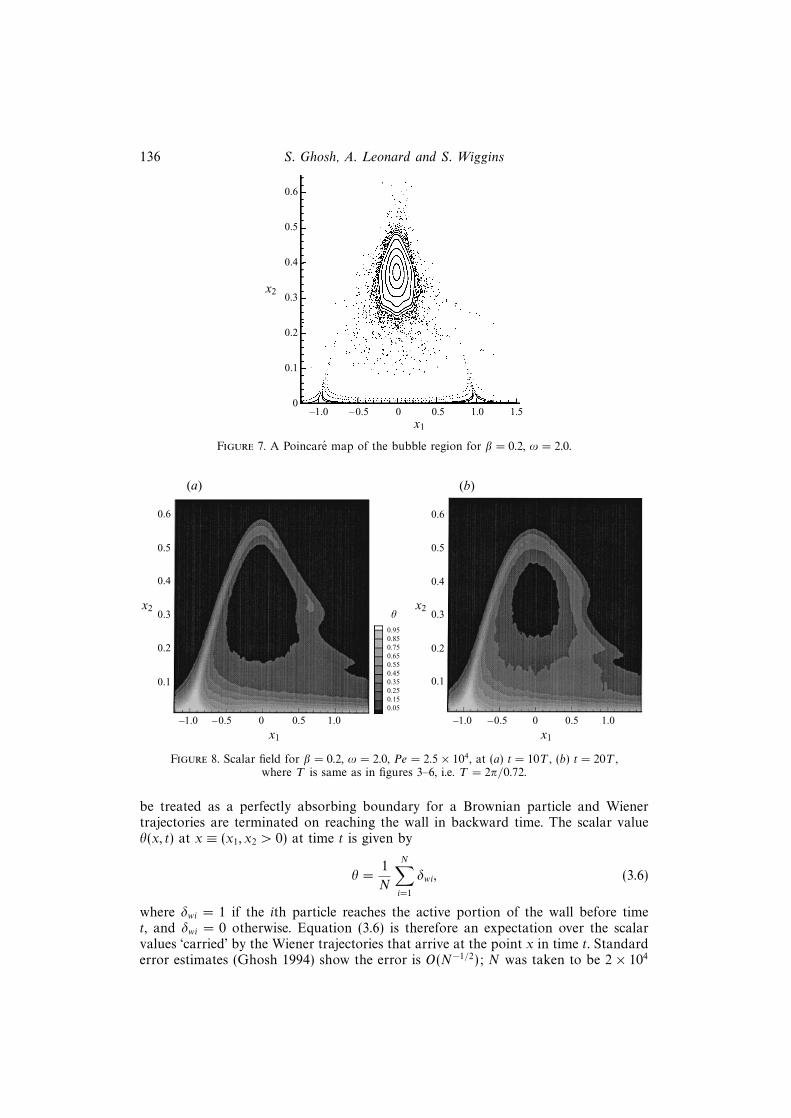
β . In figure 7 a Poincare map of the time-periodicchaotic advection field is obtained at β = 0.2, ω = 2.0, showing the structure of theKAM tori and island bands. In figure 8 we compute the scalar field at β = 0.2 andperturbation frequency increased to ω = 2.0, while Pe is again taken to be 2.5× 10⁴;to compare with previous results, the time-dependent distribution is obtained at thesame times as before. Notice that we are no longer evaluating the scalar field at timesthat are integral multiples of the perturbation period corresponding to ω = 2.0, andtherefore the t in figure 8 correspond to different cross-sections φ; as φ changes, sodoes the geometrical structure of Wu
β (φ), which in turn influences the distribution of
the passive scalar in regions swept by Wuβ (φ). But in the core region of the bubble the
KAM tori play a role not unlike closed streamlines in the steady bubble as transport

Diffusion of a passive scalar into a advection field 135
x2
(a)
0.6
0.5
0.4
0.3
0.2
0.1
x1
0.6
0.5
0.4
0.3
0.2
0.1
x1
(b)
x2
0.950.850.750.650.550.450.350.250.150.05
h
x2
(c)
0.6
0.5
0.4
0.3
0.2
0.1
0.6
0.5
0.4
0.3
0.2
0.1
(d)
x2
–1.0 –0.5 0 0.5 1.0 1.5 –1.0 –0.5 0 0.5 1.0 1.5
–1.0 –0.5 0 0.5 1.0 1.5 –1.0 –0.5 0 0.5 1.0 1.5
Figure 6. Scalar field for β = 0.8, ω = 0.72, Pe = 2.5× 10⁴, at (a) t = 5T , (b) t = 10T ,(c) t = 20T , (d) t = 30T , T = 2π/ω.
across a KAM torus is possible by scalar diffusion only, and the time-evolution ofthe scalar field in this core region resembles closely that in the steady-bubble case.Nothing can be said though about the nature of the asymptotic distribution in thiscase.
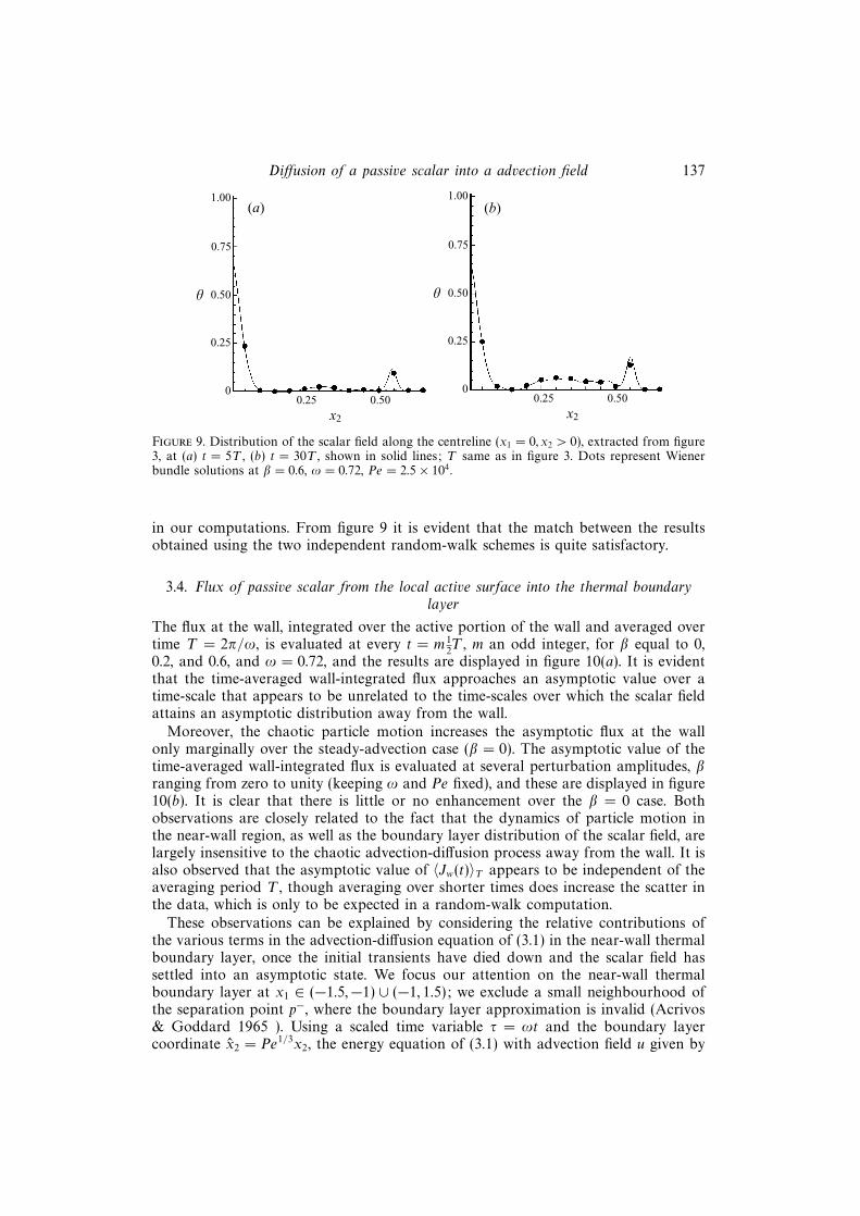
We conclude this section with a verification of the results obtained from the wholefield computations, using the Wiener bundle method. Centreline profiles of the scalarfield along (x1 = 0, x2 > 0) were extracted from figure 3(a, d), and these are plottedas solid lines in figure 9. Point values of the scalar field were obtained at the same tusing the Wiener bundle method and these are also displayed in figure 9. The scalarvalue at a point on the centreline is obtained by integrating backwards in time acollection N of ‘particles’ that are located at the given x ≡ (x1 = 0, x2 > 0) at timet, using the stochastic differential of (3.3). As was mentioned earlier, the wall can
136 S. Ghosh, A. Leonard and S. Wiggins
x1
x2
0.6
0.5
0.4
0.3
0.2
0.1
0–1.0 –0.5 0 0.5 1.0 1.5
Figure 7. A Poincare map of the bubble region for β = 0.2, ω = 2.0.
(a)
x1
0.6
0.5
0.4
0.3
0.2
0.1
x1
(b)
x2
0.950.850.750.650.550.450.350.250.150.05
h
–1.0 –0.5 0 0.5 1.0
0.6
0.5
0.4
0.3
0.2
0.1
x2
–1.0 –0.5 0 0.5 1.0
Figure 8. Scalar field for β = 0.2, ω = 2.0, Pe = 2.5× 10⁴, at (a) t = 10T , (b) t = 20T ,where T is same as in figures 3–6, i.e. T = 2π/0.72.
be treated as a perfectly absorbing boundary for a Brownian particle and Wienertrajectories are terminated on reaching the wall in backward time. The scalar valueθ(x, t) at x ≡ (x1, x2 > 0) at time t is given by
θ =1
N
N∑i=1
δwi, (3.6)
where δwi = 1 if the ith particle reaches the active portion of the wall before timet, and δwi = 0 otherwise. Equation (3.6) is therefore an expectation over the scalarvalues ‘carried’ by the Wiener trajectories that arrive at the point x in time t. Standarderror estimates (Ghosh 1994) show the error is O(N−1/2); N was taken to be 2× 10⁴
Diffusion of a passive scalar into a advection field 137
(a)
0.25
0
x2
(b)
h
0.25
0.50
0.75
1.00
0.50
0.25
0
x2
h
0.25
0.50
0.75
1.00
0.50
Figure 9. Distribution of the scalar field along the centreline (x1 = 0, x2 > 0), extracted from figure3, at (a) t = 5T , (b) t = 30T , shown in solid lines; T same as in figure 3. Dots represent Wienerbundle solutions at β = 0.6, ω = 0.72, Pe = 2.5× 10⁴.
in our computations. From figure 9 it is evident that the match between the resultsobtained using the two independent random-walk schemes is quite satisfactory.
3.4. Flux of passive scalar from the local active surface into the thermal boundarylayer
The flux at the wall, integrated over the active portion of the wall and averaged overtime T = 2π/ω, is evaluated at every t = m 1
2T , m an odd integer, for β equal to 0,
0.2, and 0.6, and ω = 0.72, and the results are displayed in figure 10(a). It is evidentthat the time-averaged wall-integrated flux approaches an asymptotic value over atime-scale that appears to be unrelated to the time-scales over which the scalar fieldattains an asymptotic distribution away from the wall.
Moreover, the chaotic particle motion increases the asymptotic flux at the wallonly marginally over the steady-advection case (β = 0). The asymptotic value of thetime-averaged wall-integrated flux is evaluated at several perturbation amplitudes, βranging from zero to unity (keeping ω and Pe fixed), and these are displayed in figure10(b). It is clear that there is little or no enhancement over the β = 0 case. Bothobservations are closely related to the fact that the dynamics of particle motion inthe near-wall region, as well as the boundary layer distribution of the scalar field, arelargely insensitive to the chaotic advection-diffusion process away from the wall. It isalso observed that the asymptotic value of 〈Jw(t)〉T appears to be independent of theaveraging period T , though averaging over shorter times does increase the scatter inthe data, which is only to be expected in a random-walk computation.
These observations can be explained by considering the relative contributions ofthe various terms in the advection-diffusion equation of (3.1) in the near-wall thermalboundary layer, once the initial transients have died down and the scalar field hassettled into an asymptotic state. We focus our attention on the near-wall thermalboundary layer at x1 ∈ (−1.5,−1) ∪ (−1, 1.5); we exclude a small neighbourhood ofthe separation point p−, where the boundary layer approximation is invalid (Acrivos& Goddard 1965 ). Using a scaled time variable τ = ωt and the boundary layercoordinate x2 = Pe1/3x2, the energy equation of (3.1) with advection field u given by

138 S. Ghosh, A. Leonard and S. Wiggins
(a)
0.0025
0 30
(b)
252015105
0.0050
0.0075
0.0100
b=0
b=0.2
b=0.6
t/T
©Jw(t)ªT
0.005
©Jw(t)ªT
0.004
0.003
0.002
0.001
0 0.25 0.50 0.75 1.00
b
Figure 10. Time-averaged wall-integrated flux 〈Jw(t)〉T for β = 0, 0.2 and 0.6 and asymptotic〈Jw(t)〉T at several β ∈ [0, 1], for ω = 0.72, Pe = 2.5× 10⁴, and T = 2π/ω.
(2.8) becomes
η∂θ
∂τ+ (x1
2 − 1)x2
∂θ
∂x1
− x1x22
∂θ
∂x2
− ∂2θ
∂x22
+ O(Pe−1/3) = 0, (3.7)
where η = ω/Pe−1/3. For large η, (3.7) is clearly a singular perturbation problem.We shall restrict attention to the following subcase of η → ∞: ω fixed and Pe → ∞.

Diffusion of a passive scalar into a advection field 139
Introducing the small parameter γ = η−1/2 in (3.7) gives
∂θ
∂τ+ γ2
[(x1
2 − 1)x2
∂θ
∂x1
− x1x22
∂θ
∂x2
]= γ2 ∂
2θ
∂x22
+ O(γ4). (3.8)
In an inner boundary layer of thickness (ωPe)−1/2, the first and third terms of (3.8)will be in balance. We shall seek asymptotic solutions in the outer and inner regionsin the form of a power series in γ. Typically, these solutions would be linked by themethod of matched asymptotic solutions. However, we shall only look at the form ofthe solutions in the outer and inner regions and the matching conditions between thetwo solutions in order to extract useful order estimates. A full asymptotically matchedsolution will not be attempted becuse of the difficulty in applying a matching conditionat the separation point p− (at x1 = −1), linking the solution in the thermal boundarylayer with the thermal wake along the unstable manifold.
With θ = θ(τ, x1, x2) denoting the outer representation, we substitute the ansatz
θ =
∞∑n=0
γnθn, (3.9)
in (3.8) and on equating like powers of γ, we obtain for the first five terms:
∂θn
∂τ=
0, n = 0, 1
Ξ(n, x1, x2), n = 2, 3
Ξ(n, x1, x2)− 3ωx22(1 + x1β sin τ)
∂θ0
∂x1
+ ωx23β sin(τ)
∂θ0
∂x2
, n = 4
where
Ξ(n, x1, x2) =∂2θ(n−2)
∂x22− (x1
2 − 1)x2
∂θ(n−2)
∂x1
+ x1x22 ∂θ(n−2)
∂x2
.
We expect steady-state oscillations in the temperature field in the near-wall thermalboundary layer owing to the steady-state oscillations in the local wall shear (Pedley1972); this is confirmed by the numerically obtained temperature time-series infigure 11(a). Thus we cannot allow secular terms in the temperature field that wouldgrow indefinitely with time. Inspecting the first five terms in the expansion givenabove, we find that no time-periodic solutions are possible for the first four terms of(3.9), and therefore require
∂θn
∂τ= 0, n < 4.
Then the time-dependent component of (3.9) is (at most) O(γ4) which, in terms ofthe Peclet number, is O(Pe−2/3). We note that for the Peclet number at which thetemperature time-series of figure 11(a) was obtained, Pe−1/3 = 0.03; since figure 11(a)was obtained at (x1, x2) = (0, 0.04), the result of figure 11(a) can be considered to berepresentative of the temperature field in the outer region. We also confirm the weakPe−2/3 scaling of the steady-state temperature oscillations by repeating the numericalcomputation of figure 11(a) at two different Peclet numbers, and the results aredisplayed in figure 11(b).
We mention in passing that the asymptotic analysis, of course, does not applyaway from the wall and the asymptotic scalar distribution is not necessarily time-independent, even to dominant order. Time-series obtained at a point in the bubble

140 S. Ghosh, A. Leonard and S. Wiggins
(a)
0.25
0
(b)
h
5
0.50
0.75
1.00
10
0.25
0
h
5
0.50
0.75
1.00
10
t/T t/T15 20 15 20
(i)
(ii)
Figure 11. Time-series using the Wiener bundle method, at (x1, x2) = (0, 0.04), for β = 0.6,ω = 0.72 and (a) Pe = 2.5× 10⁴; (b) Pe = 125 (i), Pe = 103 (ii).
0.25
0
h
5
0.50
10
t/T15 20
Figure 12. Time-series using the Wiener bundle method, at (x1, x2) = (−0.547, 0.321) ∈Wuβ ,
for β = 0.6, ω = 0.72, Pe = 2.5× 10⁴.
region away from the wall (see figure 12) shows large O(1) time-periodic fluctuationsabout an asymptotic mean value, in sharp contrast to figure 11(a).
To dominant order, the instantaneous wall-integrated flux is given by
Jw(t) = Pe−2/3
∫ 1.5
−1.5
∂θ
∂x2
∣∣∣x2→0
dx1.
It can be shown (Ghosh 1994) that the contribution to the instantaneous wall-integrated flux from the thermal boundary layer region in the vicinity of the separationpoint p− can be ignored to dominant order, and therefore does not appear in theexpression above.
To obtain estimates of the heat flux from the wall, it is essential to consider theinner region. Let ξ = γ−1x2 be a suitably scaled inner variable. With θ = Θ(τ, x1, ξ)denoting the inner representation, we substitute the ansatz
Θ =
∞∑n=0
γnΘn,
in (3.8) and on equating like powers of γ, we obtain a transient diffusion equation for
Diffusion of a passive scalar into a advection field 141
the first two terms:∂Θn
∂τ− ∂2Θn
∂ξ2= 0, n = 0, 1. (3.10)
‘Diffusing solutions’ of (3.10), which are solutions in terms of the similarity variableξ2/τ, are ruled out since they apply only to the transient state and not the asymp-totic steady-state oscillations that are of interest here. Then, a consideration of theasymptotic matching condition at ξ →∞ yields easily
Θ0 = 1, Θ1 = Cξ, (3.11)
where use was made of the fact that θ0(x1, x2 → 0) must be of the form 1 + a0h(β)with h(β) → 0 as β → 0, since the outer solution must approach the steady solutionat all x2 and γ as the amplitude β of the time-periodic perturbation approaches zero;rejecting the diffusing solution at zeroth order requires a0 = 0, while the constant Cin (3.11) is obtained from the asymptotic matching at ξ →∞ (see Pedley 1972). From(3.11) we obtain easily that the wall-integrated flux is O(Pe−2/3), identical to the steadycase. The marginal enhancement observed in figure 10(b) is interpreted as a weaksecond-order effect. We also note that the asymptotic instantaneous wall-integratedflux, Jw(t), is time-independent to dominant order, which accounts for the observedfeature that the asymptotic time-averaged wall integrated flux, 〈Jw(t)〉T , is largelyinsensitive to the averaging period T.
In physical terms, the introduction of a time-periodic perturbation to the advectionfield can cause an enhancement in the heat flux from the wall in two ways: onedue to the oscillating wall shear, and another due to the chaotic advection in thebubble region above the thermal boundary layer, which causes the destruction ofthe separatrix boundary layer and the constant temperature recirculation bubble,allowing heat to escape more rapidly from the boundary layer into the overlyingbubble region. But as the analysis above shows, neither of these is a dominant ordereffect. Their influence at lower orders is not captured by our analysis above.
3.5. Case with oscillating points of zero shear stress
Results obtained by Shariff et al. (1991) show that for two-dimensional time-periodicincompressible flows adjacent to a plane no-slip boundary, the necessary conditionfor a point on the no-slip boundary (x∗1, 0) to have a one-dimensional stable/unstablemanifold for the corresponding Poincare map, with the manifold emanating withnon-zero slope, is the following:∫ T
0
∂u1
∂x2
(x1 = x∗1, x2 = 0)dt = 0, (3.12)
where x1 is the coordinate along the boundary, x2 is the coordinate normal to theboundary, and u1 is the x1-component of the velocity field, i.e. the time-averagedshear stress must vanish at the manifold emanation points. Here we point out itsconsequences on the scalar distribution in the context of our advection-diffusionproblem.
To this end, we first set-up a chaotic advection field which has oscillating pointsof zero shear stress on the no-slip boundary. The time-periodic velocity field of (2.8)has two points of zero shear stress on the no-slip boundary at all times, given byx1 = ±1, i.e. the points of zero shear stress are independent of time t. The point (−1, 0)corresponds to the separation point p−, while (+1, 0) corresponds to the attachment
point p+. For the corresponding Poincare map P φβ , p− and p+ are the only points on

142 S. Ghosh, A. Leonard and S. Wiggins
the no-slip boundary having one-dimensional unstable/stable manifolds, irrespectiveof the cross-section φ. Consider now a time-periodic perturbation of (2.5) that notonly generates chaotic particle trajectories in the bubble region but also creates twopoints of zero shear stress on the no-slip boundary that are not time-independent,but instead oscillate periodically about x1 = ±1. This is achieved easily by adding anappropriate perturbation term to (2.3); the boundary vorticity in the time-dependentflow is made to vary according to the equation
w(x2 = 0) ≡ −∂u1
∂x2
∣∣∣∣x2=0
= −K(x21 − x2
s + βx1xs sin(ωt)).
The appropriately non-dimensionalized velocity field, truncated again to third-order,is given by
u1 = −x2 + 3x22 + x2
1x2 − 23x3
2 + βx1x2 sin(ωt),
u2 = −x1x22 −
β
2x2
2 sin(ωt),
(3.13)
which is again an asymptotically exact solution of the Navier–Stokes and continuityequations close to the origin of the expansion. The points of zero shear stress on theno-slip boundary (x1, 0) are now given by
x1 = ±1− β
2sin(ωt) + O(β2).
However, applying Shariff et al.’s result of (3.12), for the Poincare map Pφβ corre-
sponding to the velocity field of (3.13) the only points on the no-slip boundary (x∗1, 0)having a one-dimensional stable/unstable manifold are located at x∗1 = ±1. Noticethat the necessary condition of (3.12) is independent of the cross-section or phase φ of
the Poincare map P φβ , which implies that though the points of zero shear stress on the
no-slip boundary oscillate in a time-periodic manner, the manifold emanation points
are time-independent and remain the same for every P φβ , irrespective of φ. Therefore,
while the unstable manifold Wuβ (φ) changes structure with φ, the manifold emanation
point or separation point remains stationary at the wall. This property becomes trans-parent from numerical simulation results of figure 13(a–c) for the scalar distributioncomputed at times that are not integral multiples of the period T = 2π/ω of the time-periodic velocity field of (3.13) and therefore correspond to different cross-sections φ.Thus, despite the fact that (3.13) and (2.8) are very different chaotic advection fields,the scalar distributions for the associated advection-diffusion problem at large Pecletnumbers share the same qualitative features owing to the similarity in the underlyinggeometrical structures in the two cases. This further reinforces the importance of theunderlying geometrical structures in determining the scalar distribution in chaoticadvection fields.
The asymptotic time-averaged wall-integrated flux 〈Jw(t)〉T again shows weak en-hancement over the steady-advection case, which is not surprising following ourdiscussion in § 3.4. Temperature time-series in the thermal boundary layer indicateweak time-dependence as before, attributed to the absence of time-dependent struc-tures in the near-wall region in the sense of oscillating manifold emanation points. Theabsence of such time-dependent structures is the likely cause of the lack of enhancedtransport usually associated with turbulent flows. Moreover, it should be clear fromequation (3.12) that every time-periodic two-dimensional velocity field will have time-independent manifold emanation points at the no-slip boundary. Finally, we note that

Diffusion of a passive scalar into a advection field 143
x2
(a)
0.6
0.5
0.4
0.3
0.2
0.1
x1
0.6
0.5
0.4
0.3
0.2
0.1
x1
(b)
x2
0.950.850.750.650.550.450.350.250.150.05
h
–1.0 –0.5 0 0.5 1.0 –1.0 –0.5 0 0.5 1.0 1.51.5
x2
(c)
0.6
0.5
0.4
0.3
0.2
0.1
x1
–1.0 –0.5 0 0.5 1.0 1.5
Figure 13. Scalar field corresponding to the chaotic advection field of (3.13), for β = 0.4, ω = 0.65,Pe = 2.5× 10⁴, at (a) t = 5.25T , (b) t = 5.75T , (c) t = 6T , T = 2π/ω.
it might be possible to generate time-dependent structures in the near-wall region fortwo-dimensional chaotic advection fields with more complicated time-dependences, inparticular quasi-periodic time-dependence.
3.6. Impact of changing bubble size
The size of the steady separation bubble can be varied by varying the coefficient A122
in the time-independent velocity field of (2.4); A122 must lie within the appropriatelimits given in § 2. Introducing a time-periodic perturbation as in (2.6) and truncatingthe series expansion to third-order gives a chaotic advection field identical to (2.8)with time-independent component fu(x), expressed now in terms of the unspecifiedcoefficient A122,
fu ≡ (fu1 , fu2) =
(−x2 +
A122
Kxsx2
2 + x21x2 − 2
3x3
2,−x1x22
). (3.14)

144 S. Ghosh, A. Leonard and S. Wiggins
x2
(a)
0.25
x1 x1
(b)
0.950.850.750.650.550.450.350.250.150.05
h
–1.0 –0.5 0 0.5 1.0 –1.0 –0.5 0 0.5 1.0 1.51.5
0.50
x2 0.25
0.50
Figure 14. Scalar field corresponding to the chaotic advection field with time-independent compo-nent (3.14), for A122 = 4.5Kxs, with β = 0.5, ω = 0.5, Pe = 2.5 × 10⁴, at (a) t = 10T , (b) t = 20T ,T = 2π/ω.
x2
(a)
x1 x1
(b)
x2
0.950.850.750.650.550.450.350.250.150.05
h
–1.0 –0.5 0 0.5 1.0 –1.0 –0.5 0 0.5 1.0 1.51.5
0.25
0.50
0.75
1.00
0.25
0.50
0.75
1.00
Figure 15. Scalar field corresponding to the chaotic advection field with time-independent compo-nent (3.14), for A122 = 2Kxs, with β = 0.5, ω = 0.5, Pe = 2.5 × 10⁴, at (a) t = 10T , (b) t = 20T ,T = 2π/ω.
We consider here the effect of variations in the coefficient A122 on the chaoticadvection field above and, consequently, on the scalar distribution in the associatedadvection-diffusion problem.
Thus far we have presented numerical simulation results for A122 = 3Kxs. Time-dependent scalar distributions are now computed at two different values of thecoefficient A122: in figure 14(a, b), scalar distributions are obtained for A122 = 4.5Kxs,while in figure 15(a, b) the scalar distributions are obtained for A122 = 2Kxs, with theperturbation parameters β, ω and the Peclet number Pe identical in the two cases.Evidently, there is a sharp qualitative difference in the scalar distributions for thetwo cases. It is observed that at smaller A122, the unstable manifold Wu
β (φ) plays amore dominant organizing role in the distribution of the passive scalar. Moreover,the distributions are more localized and non-uniform at smaller A122. Following ourarguments in § 3.4, it is not surprising that the wall-integrated flux is observed to belargely insensitive to variations in A122, as long as A122 is not too large.

Diffusion of a passive scalar into a advection field 145
While for β = 0, i.e. for steady advection, the value of A122 determines the sizeof the separation bubble, for β 6= 0 but β small, A122 determines the location of theheteroclinic tangle formed by the intersections of the stable and unstable manifolds,
Wsβ(φ) and Wu
β (φ) respectively, of the Poincare map Pφβ corresponding to the time-
periodic chaotic advection field. In fact, it is a simple consequence of Gronwall’s lemma
(e.g. see Wiggins 1990) that trajectories under P φβ with initial position on Wu
β (φ) withinO(β) of the separation point p−, must remain O(β) close to the unperturbed separatrixψh for small β, until they enter a small neighbourhood of the attachment point p+.Then, since A122 determines the shape of the separatrix ψh, it strongly influencesthe shape of the unstable manifold Wu
β (φ). Moreover, variations in A122 cause sharpvariations in the stretching properties of the chaotic advection field, evidence of whichwill be presented later; the lower the value of A122 (A122 > (8/3)1/2Kxs), the greater thestretching and contraction rates – precise definitions are given in § 5 – in the chaoticbubble region. These two factors account for vastly different scalar distributions atdifferent A122. To what extent these advection-diffusion phenomena at small scalardiffusivity can be understood in terms of the dynamics under (2.8) is the content ofthe following sections.
4. The zero-diffusivity solution and its relation to the solution at smallscalar diffusivity
Given some initial distribution of a scalar field one can construct a zero-diffusivitysolution, also called the frozen-field solution, at any t > 0 by treating θ as a materialinvariant. It might be expected that the effect of small scalar diffusion is to smoothout any fine-scale structure in the zero-diffusivity solution. Recent work of Klapper(1992 a) has contributed strongly towards this description. If small scalar diffusiondoes no more than smooth out the fine variations in the zero-diffusivity solution,the distribution of the scalar field at small scalar diffusivity should retain the grossfeatures of the zero-diffusivity solution. However, our problem is complicated by thefact that the zero-diffusivity solution, i.e. the solution of (3.1) at Pe = ∞, is triviallyzero over the entire domain of the flow. We therefore interpret the zero-diffusivitysolution in the following sense: for Pe → ∞, Pe however large, there is alwaysa thermal boundary layer near the active portion of the wall which is diffusivelydominant and where diffusion may not be ignored. For t = t0 sufficiently small, asolution in the boundary layer is easily obtained, which is used as an ‘initial profile’,θ(x, t = t0), to obtain a ‘zero-diffusivity’ solution in the rest of the domain at t > t0 bysetting the scalar diffusivity to be exactly zero and treating θ as a material invariantfor all t > t0. The construction is artificial, but it proves to be a useful artifice inunderstanding not only the role of the unstable manifold as a organizing structurebut also the role of small scalar diffusion as a local smoothing of fine-scale structurein the frozen field.
In the boundary layer at the wall, for t sufficiently small the normal coordinatex2 < O(1) for all x1. If the lateral coordinate x1 is O(1), the advective term in (3.1),u ·∇θ, is O(x2), and therefore there is a time t sufficiently small such that the advectiveterm cannot match ∂θ/∂t and will not contribute to dominant order. Moreover,for x2 � x1, diffusion in the normal direction dominates over diffusion parallel tothe wall. Hence, at small t the dominant balance argument is straightforward: thetransient term ∂θ/∂t must be balanced by diffusion normal to the wall. In physicalterms, for small t, in particular t so small that advection is negligible in comparison to

146 S. Ghosh, A. Leonard and S. Wiggins
transverse diffusion over a narrow boundary layer at the wall, the advection-diffusionequation in the boundary layer must reduce to a simple transient diffusion equationwith solution θ(x1, x2, t) independent of the lateral coordinate x1. We rescale time,t → Pe−αt, α > 0. Balancing appropriate terms in (3.1) gives x2 = O(Pe−(α+1)/2).Rescaling the normal coordinate in the near-wall boundary layer, x2 → Pe−(α+1)/2x2
gives a simple transient diffusion equation, to dominant order:
∂θ
∂t=∂2θ
∂x22
,
with initial and boundary conditions
θ(t→ 0) = 0,
θ(x2 → 0) = 1,
θ(x2 →∞) = 0,
which has the familiar error function solution, expressed now in the unscaled coordi-nates,
θ(x1, x2, t) = 1− 2
π1/2
∫ Pe1/2x2
2t1/2
0
e−s2
ds. (4.1)
The exact scaling factor α remains undetermined. The dominant balance argument isnot expected to hold near the separation point p− where advection is not dominantlyparallel to the wall. But, for large Pe, this advection-diffusion regime will be ofnegligible size and may be ignored. Comparison with the exact Wiener bundle solutionfor β = 0.6, ω = 0.72, and Pe = 2.5 × 10⁴ along the centreline (x1 = 0, x2 > 0) atseveral t (see figure 16) shows that the error function solution of (4.1) tracks thetime-evolution of the scalar field in the boundary layer all the way up to aboutt ≈ 10, but deteriorates rapidly at larger times.
Using the error function solution of (4.1) for Pe = 2.5× 10⁴ and t = t0 sufficientlysmall as the ‘initial distribution’ θ(x, t = t0), the ‘zero-diffusivity’ solution is obtainedat several t > t0, excluding of course the thin near-wall boundary-layer region (seefigures 17, 18). Henceforth, it will be understood that by ‘zero-diffusivity’ solution wemean θ(x, t > t0) obtained using the ‘initial distribution’ described above. It is evidentfrom figures 17 and 18 that the initial distribution, which is confined to the near-wallregion, is wrapped around Wu
β (φ) as time progresses; as usual the numerical resultsare obtained at t = NT for several N, i.e. at times that are integral multiples of theperiod T of the velocity field, so that φ = 0 and comparisons can be made with Wu
β
of figure 2. This result can be understood in simple terms by examining the dynamicsof points in the near-wall region under forward iterations of the Poincare map Pβ .Consider the heteroclinic tangle formed by the intersections of Ws
β and Wuβ . If they
intersect once, they must intersect a countably infinite number of times since theirintersection points, called heteroclinic points (see Wiggins 1992), asymptote to theattachment point p+ in forward time and to the separation point p− in backwardtime, and therefore constitute a doubly asymptotic set. Moreover, if they intersecttransversely, there exists a countable infinity of transverse heteroclinic points. This isdue to the fact that transversal intersections are preserved under diffeomorphisms andPβ , being the time-T map derived from a smooth flow, is a diffeomorphism. Hencethe presence of the plane wall and the accumulation of transverse heteroclinic pointsclose to p−, in terms of arclength along Wu
β , forces segments of Wsβ to accumulate at

Diffusion of a passive scalar into a advection field 147
1.00
0.75
0.50
0.25
0.0250 0.050 0.075 0.100
(c)(b)
(a)
x2
h
o: t =T/2
x : t =T
+ : t =2T
Figure 16. Wiener bundle solutions (symbols) at several points along the centreline (x1 = 0, x2 > 0)at several times and for β = 0.6, ω = 0.72, Pe = 2.5×10⁴, are compared to the small-time analyticalsolution of (4.1) at the same Pe (solid lines). (a) t = T/2, (b) t = T , (c) t = 2T , T = 2π/ω.
the wall, giving rise to the familiar trellis-type structure studied originally by Poincare(e.g. see Easton 1986). This is demonstrated by the heteroclinic tangle over the wall,obtained in figure 19 for β = 0.6, ω = 0.72.
Integration errors near the no-slip boundary makes resolution of the tangle dif-ficult, but the afore-mentioned trellis-type structure of the tangle is clearly evident.Now consider the countable infinity of transverse heteroclinic points pi, i ∈ Z , thataccumulate on p− in the sense described above. As segments of Ws
β densely fill outthe near-wall region Rw ≡ (−1.5, 1 − ε1) × (0, ε2), 0 < ε1, ε2 � 1, ε1 → 0 as ε2 → 0,every open neighbourhood of any point in Rw has points lying on a segment of Ws
β
or on the stable manifold through some pi, where the stable manifold through pi isthe set of points that converge asymptotically to the trajectory of pi under forwarditerations of Pβ . Since points on Ws
β converge asymptotically in forward time, and thepi are mapped to transverse heteroclinic points under Pβ , points in Rw are swept intoa thin neighbourhood of Wu
β under forward iterations of Pβ , which accounts for thenature of the zero-diffusivity solution observed in figures 17, 18. Moreover, because ofthe asymptotic convergence of points on Ws
β , the zero-diffusivity solution will have asteep gradient in the local stable direction which, for a transverse heteroclinic point, isthe direction of the tangent to Ws
β at that point and is complementary to the tangentdirection of Wu
β at that point. This is verified by extracting from figure 17 the scalardistribution in directions tangent and normal to Wu
β at a point p ∈ Wuβ , i.e. along
Tp(Wuβ ) and Np(W
uβ ), which are displayed in figure 20.
We make a slight digression to address a technical point. While figure 19 does supply
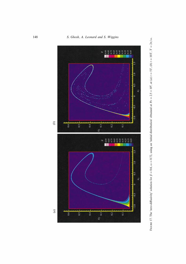
148 S. Ghosh, A. Leonard and S. Wiggins
0.6
0.5
0.4
0.3
0.2
0.1
–1.0
–0.5
00.
51.
01.
5
x 1
0.95
0.85
0.75
0.65
0.55
0.45
0.35
0.25
0.15
0.05h
x 2
(a)
0.6
0.5
0.4
0.3
0.2
0.1
–1.0
–0.5
00.
51.
01.
5
x 1
0.95
0.85
0.75
0.65
0.55
0.45
0.35
0.25
0.15
0.05h
x 2
(b)
Figure17.
Th
e‘z
ero
-diff
usi
vit
y’
solu
tion
forβ
=0.6
,ω
=0.7
2,
usi
ng
an
‘in
itia
ld
istr
ibu
tion
’ob
tain
edat
Pe
=2.5×
10
4,
at
(a)t
=5T
,(b
)t
=10T
,T
=2π/ω
.

Diffusion of a passive scalar into a advection field 149
0.6
0.5
0.4
0.3
0.2
0.1
–1.0
–0.
50
0.5
1.0
1.5
x 1
0.95
0.85
0.75
0.65
0.55
0.45
0.35
0.25
0.15
0.05h
x 2
(a)
0.6
0.5
0.4
0.3
0.2
0.1 –1
.5–1
.00
0.5
1.0
1.5
x 1
0.95
0.85
0.75
0.65
0.55
0.45
0.35
0.25
0.15
0.05h
x 2
(b)
–1.5
–0.
5
Figure18.T
he
‘zer
o-d
iffu
sivit
y’so
luti
on
forβ
=0.2
,ω
=0.7
2,u
sin
gan
‘in
itia
ld
istr
ibu
tion
’ob
tain
edat
Pe
=2.5×
10
4,at
(a)t
=5T
,(b
)t
=10T
,T
=2π/ω
.

150 S. Ghosh, A. Leonard and S. Wiggins
0.025
–1.00
0.50
x1
–1.5 –0.5 1.0 1.5
0.050
0.075
0.100
0.125
0.150
x2
Figure 19. Heteroclinic tangle near the wall for β = 0.6, ω = 0.72.
0.50
0.25
0 0.01 0.02 0.03 0.04
(a) (b)
h
0.50
0.25
0 0.01 0.02 0.03 0.04
h
Distance along Np(Wub )Distance along Tp(W
ub )
Figure 20. Distribution of the scalar field at t = 10T in the zero-diffusivity solution of figure 17along (a) Tp(W
uβ ), (b) Np(W
uβ ), p = (−0.547, 0.321) ∈Wu
β . The point p is plotted in figure 2 (a).
numerical evidence of transversal intersections of Wsβ and Wu
β , analytical verificationcan also be obtained using the Melnikov function (Wiggins 1992) which gives a signedmeasure of the distance between Ws
β(φ) and Wuβ (φ). Assuming smoothness of Ws
β(φ)
and Wuβ (φ), Melnikov’s theory can be used to obtain the following Melnikov function
for our problem, including complications due to the non-hyperbolicity of p− and p+
(e.g. see Camassa & Wiggins 1991 and Ghosh 1994):
M(τ) = A(ω) sin(ωτ),
where τ parametrizes the heteroclinic connection ψh, and
A(ω) =
∫ +∞
−∞(fu1g
u2 − fu2gu1)(xh(t)) cos(ωt)dt,
where fu ≡ (fu1 , fu2) and gu ≡ (gu1 , g
u2) are from the velocity field of (2.8), and xh(t) is
the heteroclinic orbit. For A(ω) 6= 0, it is a straightforward conclusion that Wsβ and
Wuβ do intersect transversely (Wiggins 1990). The variation of A(ω) with ω is shown
in figure 21. We also note that the perturbation frequency ω was chosen to be 0.72

Diffusion of a passive scalar into a advection field 151
0.100
0.075
0.050
0.025
0 0.5 1.0 1.5 2.0 2.5 3.0
x
A(x)
Figure 21. Variation of amplitude A of the Melnikov function with perturbation frequency ω.
in our computations since A(ω) is maximum at ω = 0.72; it is desirable to have largeA(ω) since the width of the chaotic layer increases with A(ω) (Ghosh, Chang & Sen1992). Moreover, it is evident from figure 21 that the distance between the stable andunstable manifolds falls rapidly as ω is increased beyond 0.72 and for such ω, Ws
β
and Wuβ do not sweep out the entire bubble region; this is certainly true for ω = 2.0.
Thus the zero-diffusivity solution at t > t0 pulls the boundary layer distribution att = t0 into a narrow distribution along the unstable manifold of p−, Wu
β (φ), where
the variation of the scalar field along Wuβ (φ) is much smaller than in transverse
directions. The physical picture arising from comparing figures 17(a, b), 18(a, b) withfigures 3(a, b), 4(a, b) respectively is that the zero-diffusivity solution creates fine-scalestructure that is confined to the vicinity of Wu
β (φ) and small scalar diffusion onlysmooths out the fine variations, thus allowing the unstable manifold to continue to bethe dominant organizing structure everywhere except in a narrow diffusively-dominantnear-wall boundary layer. In the following section we develop an understanding ofthis qualitative picture using recent results (Klapper 1992 a) based on the shadowingtheory of chaotic hyperbolic sets.
5. Application of shadowing theory to the small diffusivity problemKlapper (1992 a) has shown how shadowing theory from deterministic dynamical
systems theory can be used to study the small diffusivity problem. We apply hisapproach to our problem, where it enables us to understand:
(1) the role of diffusion as a smoothing of the zero-diffusivity solution at smalldiffusivity,
(2) the approach of the scalar field to an asymptotic state over an intermediatetime scale,
(3) the observed increase in non-uniformity of the scalar field as the perturbationis increased,
(4) the role of the unstable manifold of p− as the geometric structure in the flowgoverning the spatial distribution of the scalar field.
We now describe the method. We consider a discrete-time formulation in whichinstantaneous advection, given by the Poincare map P
φβ , is alternated with pulses of
diffusion over time T . Therefore, a diffusive tracer located at x0 at initial time t0 is

152 S. Ghosh, A. Leonard and S. Wiggins
advanced according to
xn+1 = f(xn) + ρT , n = 0, 1, . . . , (5.1)
with ρT ≡ (ηT , ξT ), where ηT , ξT are Gaussianly distributed random variables, each
with mean zero and variance 2T/Pe, diffeomorphism f ≡ Pφβ , and the cross-section
φ is determined by φ = ωt0 (mod 2π).
The shadowing lemma applies to the deterministic part of (5.1), i.e. the map f.Strictly speaking, it only applies in a region where every point has a one-dimensionalexponentially attracting direction and a one-dimensional exponentially expandingdirection, and the angle between these two directions is bounded away from zero.Regions having this property are called hyperbolic sets, and we will denote such aregion by Λ. The shadowing lemma (Bowen 1975) states that for each δ > 0 thereis an ε > 0, such that every trajectory {xi}mi=n in Λ satisfying |xi+1 − f(xi)| < ε forall n 6 i 6 m (called an ε-pseudo-orbit) is δ-traced by an exact trajectory {yi}mi=nin Λ (called the shadowing trajectory), i.e. yi+1 = f(yi) and |xi − yi| 6 δ for alln 6 i 6 m, where n = −∞ and m = +∞ is permitted. For Λ ⊂ R2, | · | can betaken to be the standard Euclidean norm on the plane. If the shadowing lemma canbe applied (a question that we will address more completely after we describe themethod), the picture we have in mind is that the ε-pseudo-orbits represent diffusiveor Wiener trajectories. Then the shadowing lemma implies that such trajectories areapproximated by deterministic trajectories.
In what follows, we assume that the dynamics at every point can indeed bedecomposed into a stable and unstable direction. Consider then a diffusive tracerlocated at xN and travelling backwards under (5.1), i.e.
xn−1 = f−1(xn) + ρT , n ∈ [1, N]. (5.2)
Therefore (5.2) generates a bundle or cloud of Wiener trajectories, each of whichstarts at a random ‘Wiener initial point’ x0 at iteration zero or t = t0 and arrivesat the fixed non-random point xN in N forward iterations. Now, every Wienertrajectory generated by (5.2) has a noisy deviate ρT at each iterate which is typicallyO((T/Pe)1/2). Because of the Gaussian tail, ρT can become unbounded in somerealizations, but the probability of such an event can be made arbitrarily small forany finite number of realizations by taking Pe large enough and thus forcing thevariance of the noisy deviates to be as small as desired. More precisely, given anε > 0, choosing Pe sufficiently large ensures that the sample paths of (5.2), withprobability arbitrarily close to unity, have noisy deviates that are bounded fromabove by ε at every time-step over finite time-intervals. Therefore, at large Pe almostall Wiener trajectories {xn}0n=N generated by (5.2) are ε-pseudo-orbits, and these willbe shadowed as long as the trajectory is confined to regions of the flow where theshadowing property holds. Notice the difficulty in extending the argument to infinitetimes: as N → ∞, every Wiener trajectory will, with probability one, experience alarge noise event even at arbitrarily large Pe and cannot be shadowed. However,it is irrelevant to our problem since we are interested in only finite-time results.Recall from (3.5) that computing the Wiener bundle solution for the scalar value atthe point xN at time t requires taking an expectation over this bundle of Wienertrajectories. Since the exact distribution of Wiener trajectories is difficult to obtain inan arbitrary flow, the method might seem to offer little additional insight. However,chaotic flows with the shadowing property and the associated hyperbolic structure

Diffusion of a passive scalar into a advection field 153
provide a means of representing the distribution of Wiener trajectories in terms ofexact shadow trajectories in a convenient way (Klapper 1992 a).
Consider the Wiener trajectory {xn}0n=N generated using (5.2). The first noisy back-ward iterate of xN is O((T/Pe)1/2) close to f−1(xN). In the next backward iterate,the component of xN−1 in the local unstable direction of f−1(xN) is contracted ex-ponentially under f−1 and therefore xN−2 remains O((T/Pe)1/2) close to the stablemanifold of f−2(xN). Continuing in this way, the Nth noisy backward iterate ofxN , x0 is O((T/Pe)1/2) close to the stable manifold through f−N(xN), which is alsothe Nth preimage of the stable manifold through xN . Denoting the stable manifoldthrough xN as Ws(xN), the hyperbolic structure of the dynamics pulls the cloudof Wiener trajectories released at xN into an O((T/Pe)1/2) neighbourhood (whichcan be imagined as a tube or sausage of thickness O((T/Pe)1/2) ) of f−N(Ws(xN))in N backward time-steps. The observation is crucial and was first made by A. D.Gilbert (see Klapper 1992 b). From (3.5), the Wiener bundle solution at xN at timet = NT + t0 is therefore an appropriately weighted average of the initial field distri-bution θ(x, t0) in an O((T/Pe)1/2) neighbourhood of the Nth preimage of the stablemanifold through xN . If θ(x, t0) is continuous, assuming all Wiener initial points, i.e.the x0, lie on f−N(Ws(xN)) causes an error of O((T/Pe)1/2) in θ(xN, t = NT + t0), andcan be ignored. Thus the assumed hyperbolic structure of the dynamics leads to animportant dimensional reduction in the problem, since obtaining the Wiener bundleaverage of (3.5) now requires computing the distribution of Wiener initial points interms of arclength along the one-dimensional manifold f−N(Ws(xN)). Note, however,that the variance of this distribution can be O(1); due to the fast (asymptoticallyexponential) convergence of points on the stable manifold in forward time, the noisybackward iterates xN−n can quickly move an O(1) distance away from f−n(xN) interms of arclength along f−n(Ws(xN)), even for very large Pe. Therefore, the aver-aging might have to be carried out over a O(1) length of f−N(Ws(xN)). But, sincef−N(Ws(xN)) is not an embedding in R2 it is not a submanifold of R2 and can be avery complicated geometric object, in which case no major simplification is achieved.The shadowing property offers a way around this problem. From the shadowinglemma and our discussion above, almost every Wiener trajectory is δ-shadowed byan exact trajectory and δ can be chosen arbitrarily small provided Pe is sufficientlylarge. A Wiener trajectory {xn}0n=N and the corresponding exact shadow trajectory
{yn}0n=N will pick up the same scalar value to O(δ) and therefore the contributionto the Wiener bundle average of (3.5) by θ(x0, t0) can be replaced by θ(y0, t0) withasymptotically small error. It should be clear that the y0 must lie on f−N(Ws(xN));otherwise, since the component in the unstable direction is exponentially expandedin forward time, forward iterates of y0 (under the deterministic map, f ) will movequickly away from the preimages of the stable manifold through xN and cannotremain close to {xn}0n=N . The advantage gained is the following: the distribution ofWiener initial points over f−N(Ws(xN)) can be mapped back to Ws(xN) under fN ,since the Wiener trajectories can be replaced by exact trajectories of fN to O(δ),yielding the appropriate weighting law for averaging the zero-diffusivity solution overWs(xN). Since points on f−N(Ws(xN)) converge exponentially under fN as N → ∞,the variance of the distribution over f−N(Ws(xN)) is also asymptotically exponen-tially contracted under fN , which is an important simplification since Ws(xN) can bereplaced by a straight line Es(xN) in the local stable direction at xN . Therefore, theWiener bundle average of the initial field θ(x, t0) over an O((T/Pe)1/2) neighbour-hood of f−N(Ws(xN)) is asymptotically replaced by a properly weighted average of

154 S. Ghosh, A. Leonard and S. Wiggins
the zero-diffusivity solution over Es(xN) in the Wiener bundle solution of (3.5) at xN
at t = NT + t0. Klapper (1992 a) showed that the asymptotic (Pe →∞) weighting lawfor averaging the zero-diffusivity solution over Es(xN) is Gaussian, with zero meanand variance
σ2N =
2T
Pe
N∑n=1
(1
λn
)2
, (5.3)
where λn > 1 is the expansion factor of f−n along the local stable direction at xN .The λn are easily expressed in terms of the local expansion rates at every iterate. Letfn be the restriction of f−1 to Ws(f−n+1(xN)) and introduce Fn = fn ◦ fn−1 ◦ · · · ◦ f1;Fn maps Ws(xN) onto Ws(f−n(xN)). Then λn is simply
λn ≡ dFn
∣∣∣xN
= dfn
∣∣∣f−n+1(xN )
◦ dfn−1
∣∣∣f−(n−1)+1(xN )
◦ · · · ◦ df1
∣∣∣xN,
= βn ◦ βn−1 ◦ · · · ◦ β1,
where βi = dfi
∣∣∣f−i+1(xN )
is the expansion factor of f−1 in the local stable direction of
f−i+1(xN).Finally, we discuss conditions under which the shadowing lemma applies. The
result would appear to be useful only in the special case of uniformly hyperbolic oreverywhere hyperbolic (Farmer & Sidorowich 1991) dynamical systems (also calledAnosov dynamical systems) in which at each point the dynamics can be decomposedinto local stable and unstable directions and the stable and unstable manifolds alwaysintersect transversely, i.e. there are no homoclinic tangencies (Farmer & Sidorowich1991). However, work of Klapper (1992 a) has indicated that making the assumptionthat the shadowing property holds in non-uniformly hyperbolic systems such as ourscan lead to useful insights into the small-diffusivity scalar advection-diffusion problem.Our work also confirms this hope, and we support this with numerical simulationsthat enable us to determine when shadowing breaks down (i.e. when homoclinictangencies occur). A detailed numerical study of this for our problem can be foundin the thesis of Ghosh (1994).
5.1. Comparison of shadowing and the Wiener bundle methods
In figure 22(a) 104 Wiener trajectories starting at p1 = (0.25, 0.455) are generated using(5.2) by advancing backward in time up to a length of time 5T , for β = 0.6, ω = 0.72,and Pe = 106, to obtain the distribution of Wiener initial points in the domain ofinterest, which is the bubble region or the flow region above the active portion of thewall. An equal number of points is distributed uniformly along the stable directionat p1 up to a length 3σ on either side of p1, where σ is the standard deviation ofthe Gaussianly distributed shadowing trajectories, computed for the same parametervalues as above, using (5.3). These are integrated backwards up to a length of time 5Tusing the velocity field of (2.8) to obtain the preimage of the stable manifold throughp1, and is shown in figure 22(b). It is evident that most of the mass of the distributionof Wiener initial points is confined to a small neighbourhood of the preimage of thestable manifold through p1. These results illustrate the usefulness of the shadowingproperty.
5.2. Smoothing of the zero-diffusivity solution by diffusion at small scalar diffusivity
Due to the hyperbolic character of the dynamics in chaotic flows, the fine-scaledirection (or the scalar gradient) at a point in the zero-diffusivity solution will be,

Diffusion of a passive scalar into a advection field 155
0.6
0.5
0.4
0.3
0.2
0.1
0–1.5 –1.0 –0.5 0 0.5 1.0
x1
x2
p1
(a)0.6
0.5
0.4
0.3
0.2
0.1
0–1.5 –1.0 –0.5 0 0.5 1.0
x1
x2
p1
(b)
Figure 22. (a) Distribution of 104 Wiener initial points that arrive at the point p1 = (0.25, 0.455) intime t = 5T . Relevant parameter values are β = 0.6, ω = 0.72, Pe = 106, and T = 2π/ω. (b) 104
points lined up along the stable direction at p1 = (0.25, 0.455) up to a length 3σ on either side of p1
and integrated backwards for a length of time 5T , where σ = 0.0015 and is computed using (5.3)for parameter values identical to (a).
roughly speaking, in the local stable direction (Klapper 1992 a). For a point p onthe unstable manifold of p−, p ∈ Wu
β (φ), the local unstable direction is Tp(Wuβ (φ)),
while the local stable direction is in general complementary to Tp(Wuβ (φ)), unless p
is a point of homoclinic tangency; not surprisingly, scalar profiles extracted alongTp(W
uβ ) and in the direction orthogonal to Tp(W
uβ ) are strikingly different (see figure
20). Therefore, as long as the shadowing property holds, adding small scalar diffusionwill smooth fine-scale structure in the zero-diffusivity solution around p ∈ Wu
β (φ).
Since the zero-diffusivity distribution is almost entirely confined along Wuβ (φ), adding
small scalar diffusion only smears out the zero-diffusivity solution about Wuβ (φ).
5.3. Further considerations of the zero-diffusivity solution
Before we can apply shadowing theory to determine the effects of small diffusivity,we need to continue our analysis and characterization of the zero-diffusivity solutionbegun in § 4. From both theoretical arguments and numerical evidence presentedin § 4, it is clear that the zero-diffusivity solution away from the wall is confinedentirely to the vicinity of the unstable manifold of p− , Wu
β , and therefore it will besufficient to consider the dynamics of points in the vicinity of Wu
β even for the full
advection-diffusion problem. Let Rw = (−1.5, 1) × (0, ε1), where ε1 = O(Pe−(α+1)/2).Therefore Rw is the thin near-wall region in which the ‘initial’ distribution θ(x, t0) isnon-zero. Let θfr denote the zero-diffusivity or frozen-field solution. Consider a point
x in the vicinity of Wuβ , and let {xn}0n=N be the exact dynamical trajectory through x
under backward iterations of f, i.e. xN ≡ x. Then, θfr(x, t = NT + t0) 6= 0 if and only
if f−N(xN) ≡ x0 ∈ Rw . Let x ∈ Ws(y), where y ∈ Wuβ , and let {yn}0n=N be the exact
dynamical trajectory through y under backward iterates of f, yN ≡ y. Moreover, letN1 be defined such that for N > N1(ε1, y), |f−N(yN)− p−| < ε1, where recall that p−
156 S. Ghosh, A. Leonard and S. Wiggins
is the point of separation on the no-slip boundary. Then, if x0 ∈ Rw ,
|x0 − y0| ' λN |x− y|, (5.4)
where the segment of Ws(y0) in Rw is being approximated as a straight line and|x − y| is assumed small; λN is the expansion factor of f−N along the local stabledirection of y ∈Wu
β . Therefore θfr(y, t = NT + t0) 6= 0 for all N > N1(ε1, y) and from(5.4), the width of the zero-diffusivity solution at y will be O(1/λN), where by ‘width’we mean the length over which the zero-diffusivity solution is non-zero in the localstable direction at y.
Since the exact dynamical trajectory through a point on the unstable manifoldy ∈ Wu
β under backward iterations of f approaches the separation point p− and,since p− is a non-hyperbolic stagnation point, the local expansion rates or βn alongthe backward trajectory approach unity. In fact one can show that (Ghosh 1994)(βN − 1) 6 ε0 for all N > N0 where N0 depends on ε0and y. A verification is providedby numerical computations presented below (see figure 23).
Now, choosing ε0 very small, N0 > N1(ε1, y). Since for all N > N0
λN = (βN ◦ · · · ◦ βN0+1) ◦ λN0,
it easily follows that
λN 6 (1 + ε0)(N−N0)λN0
. (5.5)
Hence for all finite N > N0
λN06 λN 6 λN0
+ O(ε0).
There is therefore an intermediate time-scale specified by (N − N0) < O(1/ε0) overwhich λN is infinitesimally close to λN0
and the width of the zero-diffusivity solutionat y is O(1/λN0
). We note that though the right-hand side of (5.5) diverges for N →∞,this limit is irrelevant to our discussion since shadowing theory applies only on finitetime-scales. The zero-diffusivity solution is therefore O(1/λN1
) wide at y ∈ Wuβ when
it first appears at N = N1, but shrinks to an asymptotic width of O(1/λN0) as N
increases beyond N0; of course since N0 > N1, λN0> λN1
.Owing to the non-hyperbolicity of p−, backward iterates of y approach p− very
slowly. Since backward iterates of x ∈Ws(y), O(1/λN0) close to y, lie on segments of
f−N(Ws(y)) that are approximately parallel to the wall, their x2-coordinate varies veryslowly with N for N large. Again, this can be made precise by considering the localrepresentation of f−1 in the vicinity of any point on the no-slip boundary (Ghosh1994). Therefore the backward iterates pick-up approximately the same scalar valuefrom the ‘initial’ distribution in Rw . It is therefore concluded that on an intermediatetime-scale specified by N0 < N < N0 + O(1/ε0) the zero-diffusivity solution at y, andin an O(1/λN0
) vicinity of y along the local stable direction at y, does not changeappreciably and can be said to have attained an asymptotic frozen-field distribution.
5.4. The small-diffusivity solution
From the viewpoint being considered here, the scalar value at a point in the bubbleregion, in the presence of small scalar diffusion, depends on twin factors: firstly, thezero-diffusivity distribution in the local stable direction at that point built-up by theunderlying chaotic advection discussed above and secondly, the local shape of theasymptotic weighting function imposed by the smoothing process of scalar diffusion.We consider now the latter.
It is clear that if the role of small scalar diffusion is a local smoothing of scalar

Diffusion of a passive scalar into a advection field 157
gradient built-up in the zero-diffusivity solution, then the scalar value at a pointin the presence of small scalar diffusion will be zero if the zero-diffusivity solutionis also zero at that point and in a neighbourhood of that point; the size of thisneighbourhood will of course depend on the variance of the smoothing function, andfrom (5.3) it is evident that for finite-times and large Pe, the size will be asymptoticallysmall.
In addition, for all N > N0, and for all x ∈Ws(y) such that x is O(1/λN0) close to
y, the variance of the Gaussian weighting function of (5.3) satisfies
σ2N 6
2T
Pe
[N0∑n=1
1
λ2n
+
(N −N0
λ2N0
)],
where use has been made of the fact that λn is a non-decreasing function of n. Formost points in the bubble-region away from the wall λN0
is large. Therefore again,for all finite N > N0,
σ2N06 σ2
N 6 σ2N0
+ O
(1
λ2N0
),
i.e. σ2N is infinitesimally close to σ2
N0over the intermediate time-scale specified by
(N−N0) < O(1/λ2N0
) and can be said to have attained an asymptotic value. It followsthen that the scalar distribution in the vicinity of y ∈ Wu
β , in the presence of smallscalar diffusion, will not change by any appreciable amount over an intermediate time-scale and can be said to have attained an asymptotic distribution. In fact, at largerperturbation amplitude β, the λn are larger (see figure 23) and the asymptotic values,λN0
and σ2N0
, are attained in shorter time, i.e. N0 decreases with β. This can explain thenumerically observed feature that the asymptotic scalar distribution is attained over ashorter time-scale at larger perturbation amplitudes (compare figure 4 with figure 6).Since the arguments hold for any cross-section φ and any y ∈Wu
β (φ), the scalar fieldin the entire bubble region will attain an asymptotic distribution. Moreover, at anyparticular point the asymptotic scalar value will be time-periodic and will have thesame period as the period T of the advection field. Numerically obtained time-seriesin figure 11(b) support this prediction.
5.5. Effect of local expansion rates
We consider next the effect of an increase in local expansion rates. Fix y ∈ Wuβ , let
y ≡ yN , N > N1, and suppose N1(ε1, y) is unchanged while the βn are increased.Increasing βn results in larger λN , which means a ‘thinner’ zero-diffusivity distributionat y. Further, from (5.3), larger λn yield smaller σ2
N , and hence the scalar distributionat y, in the presence of scalar diffusion, is confined even closer to Wu
β . Therefore, as thedynamics becomes more strongly hyperbolic, the zero-diffusivity solution is wrapped moretightly around Wu
β and diffusion is less effective as a smoothing process. Together, theyaccount for the localized and non-uniform distributions obtained at larger perturbationamplitudes. Of course we have no method for increasing βn without changing β, andconsequently changing the geometrical structure of Wu
β . We cannot then considera fixed y and examine the effect of increasing the βn. The only alternative is tocompare y, lying on Wu
β corresponding to different β, that have approximately thesame N1(ε1, y) for given ε1. To examine this situation, we choose three representativey: y1 ∈ Wu
β=0.2, y2 ∈ Wuβ=0.6, y3 ∈ Wu
β=0.8, all with the same N1(ε1, y) for ε1 small. We
choose yi ≡ yNi , with N = 10, i = 1, 2, 3, i.e. we are considering t = 10T + t0. Infigure 23 we plot βn, n ∈ [1, 10], for all three cases; for given yi, βn is the expansion

158 S. Ghosh, A. Leonard and S. Wiggins
15
10
5
01 2 3 4 5 6 7 8 9 10
(a)
(b)
(c)
n
bn
Figure 23. Local expansion rates, βn, at points on the exact trajectory {yni }0n=N , N = 10, i = 1, 2, 3,
and (a) yN1 = (0.55, 0.1649) ∈Wuβ=0.2, (b) yN2 = (0.5, 0.152 88) ∈Wu
β=0.6, (c) yN3 = (0.5, 0.1476) ∈Wuβ=0.8.
The perturbation frequency ω = 0.72 in all three cases. The points yN1 and yN2 are plotted in figures2(b) and (a) respectively.
factor of f−1 in the local stable direction of f−n+1(yi). Evidently, at larger β, the βnand consequently the λn are larger on account of the increased hyperbolicity of thedynamics under the Poincare map f ≡ Pβ . Not surprisingly the βn approach unity asn increases and preimages of yi approach the non-hyperbolic separation point p−.
Another method for increasing on average the local expansion rates in the chaoticbubble region is by modulating appropriately the coefficient A122 in the time-independent component fu(x) of the velocity field, given by (3.14). That this isindeed the case is shown by computing the local expansion rates or βn along thebackward dynamical trajectory (under f−1) through two representative points yA, yBlying on the unstable manifolds WA, WB respectively, where WA ≡ Wu
β for β = 0.5,ω = 0.5 and A122 = 4.5Kxs while WB ≡ Wu
β for β = 0.5, ω = 0.5 and A122 = 2Kxs,and again N1(ε1, yA) ' N1(ε1, yB). Note that the perturbation parameters β, ω arechosen to be identical to those in figures 14 and 15. The numerical results, displayedin figure 24, show that the local expansion rates for A122 = 2Kxs are significantlyhigher than that for A122 = 4.5Kxs. Lowering A122 not only increases the size of theunperturbed bubble and consequently the size of the chaotic bubble region in theassociated time-periodically perturbed flow, but also increases on average the localexpansion rates. Then, following our discussion above, it is expected that the scalardistribution would become more non-uniform and localized about Wu
β at lower A122.This explains the observations made in § 3.6 regarding the sharp qualitative differencebetween the scalar distributions of figures 14(a, b) and 15(a, b) corresponding to twodifferent values of the coefficient A122. We note that the perturbation parameters β,ω were chosen in a manner such that for both values of A122 considered here, thecorresponding Poincare maps have no KAM tori enclosing the core region of thebubble. In fact, the surviving KAM tori are of negligible size in both cases. Further,

Diffusion of a passive scalar into a advection field 159
10
01 2 3 4 5 6 7 8 9 10
(a)
(b)
n
bn 20
30
40
Figure 24. Local expansion rates, βn, at points on the exact trajectory {ynA,B}0n=N , N = 10, and
(a) yNA = (0.50352, 0.11174) ∈ WA, (b) yNB = (−0.30030, 0.58182) ∈ WB . Case (a) corresponds toA122 = 4.5Kxs and case (b) corresponds to A122 = 2Kxs, where A122 is the coefficient in (3.14). Theperturbation parameters are β = 0.5, ω = 0.5 in both cases.
the value of ω = 0.5 turns out to be close to the values of the perturbation frequencyat which the amplitude A(ω) of the Melnikov’s function (see § 4) is maximum ineither case; the value of ω at which A(ω) is maximum is of course different fordifferent A122, but are fortunately not widely separated for the two A122 consideredhere.
5.6. Distribution along the unstable manifold
We consider finally how the distribution varies, at a fixed time t = NT + t0, as onemoves further away from p− in terms of arclength along Wu
β . As y ∈ Wuβ moves
away from p− in terms of arclength along Wuβ , N1(ε1, y) increases and the zero-
diffusivity solution attains a non-zero value at y at a later time. Consider two pointsy1, y2 ∈ Wu
β , where y1 <l y2, i.e. y1 is closer to p− in terms of arclength alongWu
β . Fix N > N1(ε1, y2) > N1(ε1, y1). Now, our numerical simulations show that thelocal expansion rates or βn in general decrease monotonically along each backwardtrajectory {yn}0n=N on Wu
β ; this fact is evident from figure 23. On a cautionary notewe add that this may be violated if the backward trajectory through y ∈ Wu
β passesthrough regions with homoclinic tangencies, since these regions are also characterizedby weak stretching; figure 24 shows one such case where the monotonic decreasein βn is violated in one iterate. Since f−n(y1) <l f
−n(y2) for all n ∈ [0, N] and, aslong as βn decreases monotonically as p− is approached along Wu
β , λn(y1) < λn(y2),where λn(yi) is the expansion factor of f−n along the stable direction of yi. ThereforeλN(y1) < λN(y2), and the zero-diffusivity distribution at y2 is thinner than at y1. Fur-ther, because of the larger λn(y2), σ
2N(y2) < σ2
N(y1). Therefore a thinner zero-diffusivitydistribution at y2 is smoothed against a Gaussian with smaller variance, which meansthe scalar distribution about Wu
β , in the presence of scalar diffusion, should in general

160 S. Ghosh, A. Leonard and S. Wiggins
narrow down as one moves further away from p− in terms of arclength along Wuβ ;
note that there is a (weak) gradient in the zero-diffusivity solution along Wuβ (see
figure 20 a), and θfr(y2, t = NT + t0) < θfr(y1, t = NT + t0). From figures 3(a–d)and 6(a–d) it is evident that the numerical simulation results agree with the predic-tions made above, with the exception of regions where the manifold Wu
β has largecurvature. Since these are also the regions where homoclinic tangencies are likely(Farmer & Sidorowich 1991), the discrepancy is not entirely surprising. Note thatsince Wu
β is not a submanifold of R2, segments of Wuβ wind back infinitesimally
close to each other such that the distributions along them may overlap, which canmake verification of the previous prediction difficult (e.g. see figure 4). Also, forpoints y ∈ Wu
β that are far away from p− in terms of arclength along Wuβ , the
backward trajectory through y is bound to pass through weakly stretched regionsas Wu
β has a folded structure with several segments of large curvature signallingthe likelihood of homoclinic tangencies, and for these points the theory becomesuncertain owing to likely violations in the assumption of monotonic decrease in βnalong the backward trajectory {yn}0n=N . The predictions are therefore more likelyto hold for the situation in figures 3(a–d) and 6(a–d) where the scalar distributionremains localized along Wu
β up to only a relatively short distance in terms of ar-clength along p− as opposed to that in figure 4. The arguments given above remainunchanged if N1(ε1, y) is replaced by N0(ε0, y), and therefore the conclusions areidentical for the asymptotic scalar distribution. Moreover, since N0(ε0, y) increasesas y ∈ Wu
β moves away from p− in terms of arclength along Wuβ , the asymptotic
distribution is attained over a longer time at points further away from p− in termsof arclength along Wu
β . Finally, as N0 increases, the asymptotic value of the stan-dard deviation of the Gaussian weighting function will become much greater thanthe asymptotic width of the zero-diffusivity solution about Wu
β , i.e. σN0� O(1/λN0
),in which case a Gaussian smoothing of the zero-diffusivity solution will be nearlyzero, and therefore the asymptotic scalar distribution, in the presence of small scalardiffusion, will tend to zero as one moves far away from p− in terms of arclengthalong Wu
β . Comparing figure 2(a) with figure 3(d) shows that such is indeed thecase.
We refrain from making any quantitative comparisons between scalar values ob-tained from our random-walk schemes and that predicted using the asymptoticshadowing result of (5.3). The main difficulty is the arbitrariness involved in choosingt0, which is the cut-off time for the boundary layer solution of § 4 and determines the‘initial’ distribution for the fictitious zero-diffusivity solution. While the zero-diffusivitysolution thus constructed offers a convenient heuristic tool for examining the roleof small scalar diffusion, it seems difficult to extract any quantitative informationfrom it. Moreover, due to the abundance of homoclinic tangencies in the near-wallregion there is a lack of good (small δ) deterministic shadowing (Ghosh 1994), andquantitative results based on (5.3) are likely to be unsatisfactory.
For the case with surviving KAM tori enclosing the core region of the bubble, thepresence of invariant closed curves as well as the islands of stability enclosed withinprecludes the possibility of applying shadowing theory. In fact, the theory becomesuncertain whenever there are invariant curves since Wiener trajectories crossinginvariant curves will not be shadowed (Klapper 1992 a) and diffusion can produceeffects that will not be captured by the shadowing theory. For the cases consideredin this section, the flow-domain has no invariant curves and is very much the basisfor arguing that shadowing theory will continue to give the correct qualitative resultseven when small δ shadowing is unlikely.

Diffusion of a passive scalar into a advection field 161
6. ConclusionsWe have examined scalar advection-diffusion in a two-dimensional flow with chaotic
particle trajectories adjacent to an active no-slip surface at the limit of large Pecletnumber or small scalar diffusivity using results from dynamical systems theory. Theflow field was constructed in the form of a Taylor series expansion satisfying theno-slip boundary condition and consistent with the Navier–Stokes equations. Anunstable manifold emanating from a point of zero time-averaged shear stress on theno-slip boundary is found to play a dominant role in the advection-diffusion of passivescalar from the boundary, particularly when the underlying chaotic particle motionis widespread and the dynamics in the flow has a pronounced hyperbolic character.It is found that the increased hyperbolicity results in scalar distributions that arelocalized entirely along the unstable manifold with sharp scalar gradients. Introducinga fictitious zero-diffusivity solution provides an understanding of the relationshipbetween the stirring and mixing processes and shadowing theory gives a nice physicaldescription of the role of small scalar diffusion as a local smoothing of fine scalevariations created by the stirring process. A novel feature in this problem is thepresence of the no-slip boundary and the interaction between the non-hyperbolicity atthe boundary and the strongly hyperbolic character of the overlying chaotic advectionin the bubble-region of the flow. The non-hyperbolicity at the boundary is found toplay an important role in the advection-diffusion process and strongly influences thetime-evolution of the scalar field. The wall-integrated flux remains O(Pe−2/3) evenin the chaotic-advection case. Introducing a time-periodic perturbation in the steadyadvection field, again with low-order polynomial behaviour in space, introduces onlyweak time and space dependence in the near-wall thermal boundary layer after theinitial transients have died down, resulting in weak enhancement in the asymptoticflux over the steady-advection case. The absence of near-wall structures that havestrong temporal and spatial fluctuations parallel to the wall is the likely cause for theobserved weak time-dependence in the thermal boundary layer, and the consequentlack of enhanced transport usually associated with turbulent flows. Our numericalsimulation results show that in the presence of widespread chaotic particle motion thescalar distribution attains an asymptotic distribution over a time-scale that is muchshorter than the time-scale over which an asymptotic distribution is attained in thesteady flow. Moreover, this asymptotic distribution is found to be time-periodic withthe same period as that of the chaotic advection field.
We would like to acknowledge the parallel computing facilities made generouslyavailable by the Center for Advanced Computing Research at Caltech. This researchwas supported by a grant from the Air Force Office of Scientific Research, GrantNo. AFOSR-91-0241 and by a grant from the Office of Naval Research, Grant No.N00014-97-1-0071.
REFERENCES
Acrivos, A. & Goddard, J. D. 1965 Asymptotic expansions for laminar foced-convection heat andmass transfer. Part 1. Low speed flows J. Fluid Mech. 23, 273.
Anosov, D. V. 1967 Geodesic flows on closed Riemannian manifolds with negative curvature. Proc.Steklov Inst. Math. 90, 1 (Am. Math. Soc. translation 1969).
Aref, H. 1984 Stirring by chaotic advection. J. Fluid Mech. 143, 1.
Aref, H. & Jones, S. W. 1989 Enhanced separation of diffusing particles by chaotic advection. Phys.Fluids A 1, 470.
Arnold, L. 1974 Stochastic Differential Equations. Wiley.

162 S. Ghosh, A. Leonard and S. Wiggins
Batchelor, G. K. 1956 Steady laminar flow with closed streamlines at large Reynolds number.J. Fluid Mech. 1, 177.
Bowen, R. 1975 ω-limit sets for Axiom A diffeomorphisms. J. Diffl Equat. 18, 333.
Camassa, R. & Wiggins, S. 1991 Chaotic advection in a Rayleigh-Benard flow. Phys. Rev. A 43,774.
Chandrasekhar, S. 1943 Stochastic problems in Physics and Astronomy. Rev. Mod. Phys. 15, 1.
Chorin, A. J. 1973 Numerical study of slightly viscous flow. J. Fluid Mech. 57, 785.
Chorin, A. J. & Marsden, J. E. 1979 A Mathematical Introduction to Fluid Mechanics. Springer.
Dallmann, U. 1988 Three-dimensional vortex structures and vorticity topology. Fluid Dyn. Res. 3,183.
Easton, R. W. 1986 Trellises formed by stable and unstable manifolds in the plane. Trans. Am.Math. Soc. 294(2), 719.
Eckart, C. 1948 An analysis of the stirring and mixing processes in incompressible fluids. J. Mar.Res. 7, 265.
Farmer, J. D. & Sidorowich, J. J. 1991 Optimal shadowing and noise reduction. Physica D 47,373.
Ghosh, S. 1994 The role of various geometrical structures in scalar advection-diffusion. PhD thesis,California Institute of Technology.
Ghosh, S., Chang, H.-C. & Sen, M. 1992 Heat-transfer enhancement due to slender recirculationand chaotic transport between counter-rotating eccentric cylinders. J. Fluid Mech. 238, 119.
Grebogi, C., Hammel, S. M., Yorke, J. A. & Sauer, T. 1990 Shadowing of physical trajectories inchaotic dynamics: containment and refinement. Phys. Rev. Lett. 65, 1527.
Haji-Sheikh, A. & Sparrow, E. M. 1967 The solution of heat conduction problems by probabilitymethods. Trans ASME C J. Heat Transfer 89, 121.
Hammel, S. M. 1990 A noise reduction method for chaotic systems. Phys. Lett. A 148, 421.
Hammel, S. M., Yorke, J. A. & Grebogi, C. 1987 Do numerical orbits of chaotic dynamicalprocesses represent true orbits? J. Complexity 3, 136.
Hammel, S. M., Yorke, J. A. & Grebogi, C. 1988 Numerical orbits of chaotic processes representtrue orbits. Bull. Am. Math. Soc. 19, 465.
Hirsch, M. W., Pugh, C. C. & Shub,M. 1977 Invariant Manifolds. Springer Lecture Notes inMathematics, Vol. 583. Springer.
Jones, S. W. 1991 The enhancement of mixing by chaotic advection. Phys. Fluids A 3, 1081.
Khakhar, D. V. & Ottino, J. M. 1986 Fluid mixing (stretching) by time-periodic sequences ofweak flows. Phys. Fluids 29, 3503.
Klapper, I. 1992 a Shadowing and the role of small diffusivity in the chaotic advection of scalars.Phys. Fluids A 4, 861.
Klapper, I. 1992 b A study of fast dynamo action in chaotic helical cells. J. Fluid Mech. 239, 359.
McKean, H. P. 1969 Stochastic Integrals. Academic.
Molchanov, S. A., Ruzmaikin, A. A. & Sokolov, D. D. 1985 Kinematic dynamo action in randomflow. Sov. Phys. Usp. 28, 307.
Pan, F. Y. & Acrivos, A. 1968 Heat transfer at high Peclet number in regions of closed streamlines.Intl J. Heat Mass Transfer 11, 439.
Pedley, T. J. 1972 On the forced heat transfer from a hot film embedded in the wall in two-dimensional unsteady flow. J. Fluid Mech. 55, 329.
Perry, A. E. & Chong, M. S. 1986 a A series-expansion study of the Navier–Stokes equations withapplications to three-dimensional separation patterns. J. Fluid Mech. 173, 203.
Perry, A. E. & Chong, M. S. 1986 b A series-expansion study of the Navier-Stokes equationswith applications to three-dimensional separation patterns – a detailed treatment. Rep. FM-17.Mech. Engng Dept., University of Melbourne.
Press, W. H., Flannery, B. P., Teukolsky, S. A. & Vetterling, W. T. 1986 Numerical Recipes.Cambridge University Press.
Rhines, P. B. & Young, W. R. 1983 How rapidly is a passive scalar mixed within closed streamlines?J. Fluid Mech. 133, 133.
Rom-Kedar, V., Leonard, A. & Wiggins, S. 1990 An analytical study of transport, mixing, andchaos in an unsteady vortical flow. J. Fluid Mech. 214, 347.
Saffman, P. G. 1959 A theory of dispersion in porous medium. J. Fluid Mech. 6, 321.

Diffusion of a passive scalar into a advection field 163
Shariff, K., Pulliam, T. H. & Ottino, J. M. 1991 A dynamical systems analysis of kinematics inthe time-periodic wake of a circular cylinder. Lectures Appl. Math. 28, 613.
Smale, S. 1967 Differentiable dynamical systems. Bull. Am. Math. Soc. 73, 747.
Tobak, M. & Peake, D. J. 1982 Topology of three-dimensional separated flows. Ann. Rev. FluidMech. 14, 61.
Wang, M. C. & Uhlenbeck, G. E. 1945 On the theory of the Brownian motion II. Rev. Mod. Phys.17, 323.
Wiggins, S. 1990 Introduction to Applied Nonlinear Dynamical Systems and Chaos. Springer.
Wiggins, S. 1992 Chaotic Transport in Dynamical Systems. Springer.