di erential equations - theory and applications - … · have applications in di erential...
TRANSCRIPT

Differential Equations
- Theory and Applications -
Version: Fall 2017
Andras Domokos , PhD
California State University, Sacramento

Contents
Chapter 0. Introduction 3
Chapter 1. Calculus review. Differentiation and integration rules. 41.1. Derivatives 41.2. Antiderivatives and Indefinite Integrals 71.3. Definite Integrals 11
Chapter 2. Introduction to Differential Equations 152.1. Definitions 152.2. Initial value problems 202.3. Classifications of DEs 232.4. Examples of DEs modelling real-life phenomena 25
Chapter 3. First order differential equations solvable by analytical methods 273.1. Differential equations with separable variables 273.2. First order linear differential equations 313.3. Bernoulli’s differential equations 363.4. Non-linear homogeneous differential equations 383.5. Differential equations of the form y′(t) = f(at+ by(t) + c). 403.6. Second order differential equations reducible to first order differential equations 42
Chapter 4. General theory of differential equations of first order 454.1. Slope fields (or direction fields) 454.1.1. Autonomous first order differential equations. 494.2. Existence and uniqueness of solutions for initial value problems 534.3. The method of successive approximations 594.4. Numerical methods for Differential equations 624.4.1. The Euler’s method 624.4.2. The improved Euler (or Heun) method 674.4.3. The fourth order Runge-Kutta method 684.4.4. NDSolve command in Mathematica 71
Chapter 5. Higher order linear differential equations 755.1. General theory 755.2. Linear and homogeneous DEs with constant coefficients 785.3. Linear and non-homogeneous DEs with constant coefficients 815.3.1. Variation of parameters for second order linear equations 815.3.2. The undetermined coefficients method and the superposition principle 825.3.3. Use Mathematica to solve higher order DEs 85
1

5.4. The Cauchy-Euler DE 88
Chapter 6. Solving linear differential equations with the Laplace transform 916.1. Definition and properties of the Laplace transform 916.2. Further properties of the Laplace transform. Transforms of the Heaviside
function and the Dirac Delta function 966.2.1. Translation on the s-axis 966.2.2. Derivatives of the Laplace transform 966.2.3. The Laplace transform of the unit step function and of piecewise continuous
functions 976.2.4. The Dirac Delta function 1006.3. The inverse Laplace transform 1026.3.1. Calculate the Laplace transform and inverse Laplace transform using
Mathematica 1046.4. Solving IVPs of linear DEs with the Laplace transform 1066.4.1. Solving differential equations using Mathematica and the Laplace transform 1106.5. Solving systems of first order linear differential equations with the Laplace
transform 1146.5.1. Using Mathematica to solve systems of DEs 115
Chapter 7. Appendix: Mathematica files 117
2

CHAPTER 0
Introduction
This textbook covers the material for the undergraduate Differential Equations courseat California State University Sacramento. Although there might be issues related just toa particular campus, I believe that the presentation shown here is useful to a general audience.
First, let’s see the particular issues. This is a 3 unit class, taught 3 times 50 minutes(or 2 times 75 minutes) per week during a semester of 15 weeks. Most of the students arescience majors, including mathematics, physics and engineering. Many of the students aretransfer students, who took the prerequisite classes - Precalculus, Calculus 1 and 2 - at othercampuses, so there is a wide range of mathematical knowledge and maturity.
At the beginning of every semester a week of review of calculus, especially differentiationand integration rules, proved to be necessary.
The Linear Algebra course is not a prerequisite for this class, and within the time frameallowed, it is difficult to spend time on covering the complete fundamentals regarding opera-tions with matrices, eigenvalues and eigenvectors. Also, there is no computer lab componentfor this course. These are not optimal starting points for this class and I hope that thecoming years will bring some changes.
Secondly, let’s talk about some general issues. Almost all of my students were used togetting the 1000+ pages textbooks for their earlier courses. Over the years these huge text-books killed the habits of taking time to read them, focus on the details and understandingthe definitions and theorems describing the main ideas. The most frequent question I do getis: ”We see what is the material, but how much of it we have to know for the exam?” Theanswer - ”All of it.” - usually brings out a big sign of disbelief.
Differential Equations is a very important mathematical subject from both theoreticaland practical perspectives.
The theoretical importance is given by the fact that most pure mathematics theorieshave applications in Differential Equations. For students, all the prerequisite knowledge istested in this class.
The practical importance is given by the fact that the most important time dependentscientific, social and economical problems are described by differential, partial differentialand stochastic differential equations. The bridge between Nature or Universe and us is pro-vided by mathematical modeling, which is the process of finding the correct mathematicalequations describing a certain problem. This process might start with experimental mea-surements and analysis, which lead to certain equations, in our case differential equations.Then, these differential equations are solved and their solutions tested for agreement to ex-perimental results. In this process we generate some solutions, which have the role to predict
3

the future behavior of the analyzed problem.
In general, regarding the future, there is no solution manual and here comes another issue.Most of my students were used to having solution manuals for their mathematics classes andchecking whether the solution is right or wrong was reduced to comparison with the answersin the solution manual. However, this eliminates the need to completely understand whatwe are doing and whether the answer really makes sense.
Differential Equations is probably one of the best classes which can make us understandthat Nature does not provide us with a complete solution manual. We usually have to findsome approximate answers and we are also left with the task of predicting how accuratethese answers are, without knowing the correct answer.
For this reason, there will be NO SOLUTION MANUAL posted. I request the studentsto check the correctness of their answers by applying the theoretical methods shown in class,but also by using a computer software in the campus computer labs. The available softwareis Mathematica, which could be substituted off campus by Wolfram Alpha. There are manymathematical softwares, like Maple, Matlab, Octave, and you are free to use whichever isavailable to you. The most important thing is to actively participate in the teaching-learningprocess and based on the information presented in class, create your own way of checkingyour answers. The answers given by computers might be in a different form than the onesobtained on paper, but it is a good challenge to compare them. You must develop intuition,theoretical and computer knowledge to be able to test and decide whether a solution iscorrect or wrong.
4

CHAPTER 1
Calculus review. Differentiation and integration rules.
1.1. Derivatives
Definition 1.1.1. Consider a function y : I → R, where I is an interval on the real lineR. We say that the function y has a derivative at t0 ∈ I if the limit
limt∈I, t→t0
y(t)− y(t0)
t− t0
exists and it is finite. In the case when the derivative exists, we use the notation
y′(t0) = limt∈I, t→t0
y(t)− y(t0)
t− t0.
Other notations for the derivative of function y at t0 can be dydt
(t0) or ddty(t0).
In case t0 is one of the endpoints of the interval I, then the above limits become one sidedlimits.If the derivative exists at every t0 ∈ I, then y′(t) is a new function, called the derivativefunction.If y′(t) has a derivative function, then we call it the second derivative of the function y(t)and denote it by y′′(t).For higher order derivatives we use the notations y′′′(t), y(4)(t), ... , y(n)(t), or dn
dtny(t).
Interpretations and applications of the derivative:
(1) y′(t0) is the instantaneous rate of change of the function y at t0.(2) y′(t0) is the slope of the tangent line to the curve y = y(t), t ∈ I at the point
(t0, y(t0)).(3) If the function y has a local maximum (minimum) at t0, which is in the interior of
I, and y is differentiable at t0, then y′(t0) = 0. However, y′(t0) might not be zero ift0 is one of the endpoints.
(4) If y′(t) ≥ 0 for every t ∈ I, then the function y is increasing on I.(5) If y′(t) ≤ 0 for every t ∈ I, then the function y is decreasing on I.(6) If y′′(t) ≥ 0 for every t ∈ I, then the function y is concave-up on I.(7) If y′′(t) ≤ 0 for every t ∈ I, then the function y is concave-down on I.
4

Derivatives of the most used elementary functions:
(tn)′ = ntn−1
(at)′ = at ln a , (et)′ = et , (ln t)′ =1
t(sin t)′ = cos t , (cos t)′ = − sin t , (tan t)′ = sec2 t
(arcsin t)′ =1√
1− t2, (arccos t)′ =
−1√1− t2
, (arctan t)′ =1
1 + t2.
Differentiation Rules: In the following rules y and z are differentiable functions on aninterval I, t ∈ I and c ∈ R.
(1) (y(t) + z(t)
)′= y′(t) + z′(t) .
(2) (c · y(t)
)′= c · y′(t) .
(3) (y(t) · z(t)
)′= y′(t) · z(t) + y(t) · z′(t) .
(4) (y(t)
z(t)
)′=y′(t) · z(t)− y(t) · z′(t)
z2(t), if z(t) 6= 0 .
(5) (y(z(t)
))′= y′
(z(t)
)· z′(t) .
Examples:
(t2 − 3t+ 5)′ = 2t− 3(t3 · e2t
)′= 3t2 · e2t + t3 · 2e2t(
tan t)′
=
(sin t
cos t
)′=
cos t · cos t− sin t · (− sin t)
cos2 t=
1
cos2 t(√1 + t2
)′=
1
2(1 + t2)−
12 · 2t =
t√1 + t2(
arctan(t2))′
=1
1 + t4· 2t =
2t
1 + t4
Note: To define functions, calculate derivatives and plot graphs with Mathematica, seeChapter 8.
5

Homework exercises:
(1) Find the derivatives of the following functions:
(a) f(t) = 2t3 + 5t2 − 3t− 4
(b) f(t) = t2 et3
(c) f(t) = sin t · cos t
(d) f(t) =t2 − 1
t3 + 8
(e) f(t) =3√
4t2 + 1
(f) f(t) = t arcsin 3t
(g) f(t) =t√t2 + 1
(h) f(t) = (2t+ 1) ln t
(i) f(t) = (tan t)2 · sec t .
(2) Graph the following functions. Find the domain, the horizontal and vertical asymptotes,local minima and maxima and intervals where the following functions are decreasing or in-creasing, convex or concave.Check your answers by graphing the functions with Mathematica.
(a) f(t) = t3 − 4t .
(b) f(t) =2t− 4
t2 − 6t+ 5.
(c) f(t) = ln t− 2t .
(d) f(t) =et
t.
(e) f(t) = te−t2
.
(f) f(t) = arctan t .
(g) f(t) = 3 sin(2t) + 1 .
6

1.2. Antiderivatives and Indefinite Integrals
Definition 1.2.1. Let y : I → R be a function. A differentiable function Y : I → R iscalled an antiderivative of the function y on the interval I if
Y ′(t) = y(t) , for all t ∈ I .The set (or collection) of all the antiderivatives of y is denoted by∫
y(t) dt
and called the indefinite integral of the function y.
Examples:
(a)
y : R→ R , y(t) = 2t , Y (t) = t2 ,
∫2t dt = t2 + c .
(b)
y : (−1, 1)→ R , y(t) =1√
1− t2, Y (t) = arcsin t ,∫
1√1− t2
dt = arcsin t+ c .
Integration Rules:
(1) Linearity, the sum rule.∫y(t) + z(t) dt =
∫y(t) dt+
∫z(t) dt = Y (t) + Z(t) + c .
(2) Linearity, the constant multiple rule.∫a · y(t) dt = a
∫y(t) dt = a Y (t) + c .
(3) Integrals of some elementary functions:∫tn dt =
tn+1
n+ 1+ c, n 6= −1.∫
1
tdt = ln|t|+ c∫et dt = et + c∫
sin t dt = − cos t+ c∫cos t dt = sin t+ c∫
tan t dt = ln|sec t|+ c
7

∫sec t dt = ln|sec t+ tan t|+ c∫
1
t2 + a2dt =
1
aarctan
(t
a
)+ c∫
1√a2 − t2
dt = arcsin
(t
a
)+ c .
(3) The substitution rule : u = z(t), du = z′(t) dt,∫y(z(t)
)· z′(t) dt =
∫y(u) du = Y (u) + c = Y (z(t)) + c .
Example: Use u = t3 + 1 and du = 3t2dt to get∫t2√t3 + 1
dt =
∫1√u
1
3du =
2
3
√u+ c =
2
3
√t3 + 1 + c .
(4) The integration by parts.∫y(t)z(t) dt = y(t)Z(t)−
∫y′(t)Z(t) dt .
Example: ∫te2t dt = t
e2t
2−∫
1e2t
2dt =
te2t
2− e2t
4+ c .
(5) Trigonometric substitutions.
(a) For integrals containing√a2 + t2 use t = a · tan θ.
Example. Use t = 2 tan θ and dt = 2 sec2 θ dθ to get∫1
t2√t2 + 4
dt =
∫cos θ
4 sin2 θdθ = − 1
4 sin θ+ c = −
√t2 + 4
4t+ c .
(b) For integrals containing√a2 − t2 use t = a · sin θ.
(c) For integrals containing√t2 − a2 use t = a · sec θ.
(6) Trigonometric integrals.
(a) For integrals of the form∫
sinn(t) cos2k+1(t) dt use the substitution u = sin t.Example. Use u = sin t and du = cos t dt to get∫
sin2 t cos3 t dt =
∫u2(1− u2) du =
u3
3− u5
5+ c =
sin3 t
3− sin5 t
5+ c .
(b) For integrals of the form∫
cosn(t) sin2k+1(t) dt use the substitution u = cos t.
(c) For integrals of the form∫
sin2n(t) cos2k(t) dt use the double angle formulascos2(t) = 1
2(1 + cos(2t)) and sin2(t) = 1
2(1− cos(2t)).
8

The double angle formulas follow from the following two trigonometric identities:
cos2 t+ sin2 t = 1
cos2 t− sin2 t = cos(2t) .
(d) For integrals of the form∫
tann(t) sec2k(t) dt use the substitution u = tan t.
(e) For integrals of the form∫
tan2k+1(t) secn(t) dt use the substitution u = sec t.Example. Use u = sec t and du = sec t tan t dt to get∫
tan3(t) sec2(t) dt =
∫(u2 − 1)u du =
u4
4− u2
2+ c =
sec4(t)
4− sec2(t)
2+ c .
(7) Integration by partial fraction decompositions. Some examples:(a)
2t+ 3
(t− 1)(t+ 2)=
A
t− 1+
B
t+ 2, A =
5
3, B =
1
3∫2t+ 3
(t− 1)(t+ 2)dt =
5
3ln|t− 1|+ 1
3ln|t+ 2| .
(b)t2 + t+ 2
t(t+ 1)2=A
t+
B
t+ 1+
C
(t+ 1)2, A = 2, B = −1, C = −2∫
t2 + t+ 2
t(t+ 1)2dt = 2 ln|t| − ln|t− 1|+ 2
t+ 2.
(c)2t− 19
(t+ 3)(t2 + 16)=
A
t+ 3+Bt+ C
t2 + 16, A = −1, B = 1, C = −1
∫2t− 19
(t+ 3)(t2 + 16)dt = − ln|t+ 3|+ 1
2ln(t2 + 16)− 1
4arctan
(t
4
)+ c .
Note: To calculate integrals with Mathematica, see Chapter 8.
9

Homework exercises: Calculate the following integrals. Check your answers by differ-entiation and also by using Mathematica. For instructions, see Chapter 8.
(1)
∫(2t3 − 3t2 + 2t− 5) dt
(2)
∫t
1 + t2dt
(3)
∫t2et
3
dt
(4)
∫(t2 + t+ 1)et dt
(5)
∫t sin t dt
(6)
∫1
t2√
9− t2dt
(7)
∫1√
t2 − 25dt
(8)
∫1√
4t2 + 1dt
(9)
∫sin5 t · cos2 t dt
(10)
∫tan3 t · sec4 t dt
(11)
∫cos4 t dt
(12)
∫1
t2 − 1dt
(13)
∫t+ 1
t2 + 4t+ 3dt
(14)
∫t2 − 1
t3 + tdt
(15)
∫5t2 + 20t+ 6
t3 + 2t2 + tdt
(16)
∫ln t dt
(17)
∫t ln t dt
10
1.3. Definite Integrals
Definition 1.3.1. Consider a bounded function y : [a, b] → R. For a partition of theinterval [a, b],
P ={a = t0 < t1 < ... < tn = b
},
and sample points tk−1 ≤ t∗k ≤ tk , 1 ≤ k ≤ n, define the Riemann-sum
S(y, P ) =n∑k=1
y(t∗k) (tk − tk−1
).
The norm of the partition P is defined as the length of the largest subinterval [tk−1, tk].If the Riemann-sums have a well-defined finite limit as the norm of the partition P tends to0, then we say that the function y is Riemann-integrable on [a, b] and we denote this definiteintegral by ∫ b
a
y(t) dt .
The set of Riemann-integrable functions on [a, b] includes, among others, the continuousfunctions and, also the bounded functions with finitely many jump discontinuities.
Geometrical interpretation of the definite integral:∫ bay(t) dt is the net area bounded by the t-axis, t = a, t = b and the graph of the
function y. Net area means the difference of the area above and the area below the t-axis.If we want the total area bounded by the t-axis, t = a, t = b and the graph of the function
y, we have to calculate∫ ba|y(t)| dt. In particular, if y(t) ≥ 0 for all t ∈ [a, b], then the total
area is given by∫ bay(t) dt.
The Fundamental Theorem of Calculus (FTC):
Theorem 1.3.1. If y : [a, b]→ R is a Riemann-integrable function on [a, b] and Y is anantiderivative function of y on [a, b], then∫ b
a
y(t) dt = Y (b)− Y (a) .
Corollary to the FTC:
Corollary 1.3.1. If y is a continuous function on [a, b], then the function
Y (t) =
∫ t
a
y(s) ds
is an antiderivative of y, and hence
d
dt
(∫ t
a
y(s) ds
)= y(t) , a ≤ t ≤ b .
11

Note. The integration rules for indefinite integrals apply for definite integrals. Just, wehave to take care of the lower and upper limits of integrations.
Examples. (a) We can use the substitution u = t2 with du = 2tdt to calculate thefollowing definite integral:
∫ 2
0
2tet2
dt =
∫ 4
0
eu du = eu∣∣∣40
= e4 − 1 .
(b)
∫ π2
0
sin2 t · cos3 t dt =
∫ π2
0
sin2 t · cos2 t · cos t dt
=
∫ π2
0
sin2 t · (1− sin2 t) · cos t dt
u = sin t , du = cos t dt
=
∫ 1
0
u2(1− u2) du =
∫ 1
0
u2 − u4 du =
=u3
3− u5
5
∣∣∣∣∣1
0
=1
3− 1
5=
2
15.
Homework exercises: Calculate the following definite integrals. Check your answerswith Mathematica. For instructions, see Chapter 8.
(1)
∫ 2
0
(t3 − t+ 1) dt
(2)
∫ 3
2
1
t2dt
(3)
∫ 4
3
1
t ln tdt
(4)
∫ 1
0
t
1 + t2dt
(5)
∫ 1
0
1√4− t2
dt
(6)
∫ π
0
t sin(2t) dt
(7)
∫ 1
0
t2 et dt
12

(8)
∫ 2
√3
t2 − 3
tdt
(9)
∫ π/3
π/6
cos3 t√sin t
dt
(10)
∫ 2
1
t+ 1
t(t2 + 1)dt
(11)
∫ 0
−2
t
t2 − 6t+ 8dt
(12)
∫ 1
0
1
t2 + 2t+ 5dt
(13)
∫ 2
1
1
t3 + 2t2 + tdt
13


CHAPTER 2
Introduction to Differential Equations
2.1. Definitions
Definition 2.1.1. A differential equation (DE) is an equation in which an unknownfunction y(t) appears together with some of its derivatives.
In general, a DE can be written as
F (t, y(t), y′(t), ..., y(n)(t)) = 0 , t ∈ I .Examples:
(a)y′′(t)− 2y′(t) + y(t)− t2 = 0 , t ∈ (−1, 1) .
(b)
y(4)(t) · y′(t)− y(t) = 2t+ 1 , t ≥ 0 .
(c)ety′(t)
1 + y2(t)= 5 , t ∈ R .
(d) Calculating the indefinite integral∫
2t dt is the same as solving the DE y′(t) = 2t.Both problems ask for those functions, which have derivative equal to 2t.
Definition 2.1.2. The order of a DE is defined by the highest derivative present inthe equation.
Examples.(a) The DE y′′(t)− (y′(t))3 + 5y6(t) = et has order 2.(b) The DE y(4)(t)− y′(t) = 0 has order 4.
Normal form of a DE. If the DE can be solved in the highest order derivative, then wesay that we have obtained its normal form, which can be written as:
y(n)(t) = f(t, y(t), y′(t), ..., y(n−1)(t)) , t ∈ I .Examples.
(a) The DEt2y′′(t)− ty′(t) + y(t) = et , t ∈ [1, 2]
can be written in the following normal form:
y′′(t) =1
ty′(t)− 1
t2y(t) +
1
t2et , t ∈ [1, 2] .
15
This normal form was obtained by dividing the DE by t2. However, if we consider the inter-val [−1, 1], dividing by t2, which becomes 0 for t = 0, makes the normal form not defined onthe entire interval [−1, 1].
(b) The DE
ey′(t) + y′(t) = (t+ 1)y(t) , t ∈ [0, 1]
cannot be solved in y′(t), so it cannot be written in normal form.
Definition 2.1.3. A system of differential equations (SDEs) is formed by a numberof differential equations involving more than one unknown functions and their derivatives.
Example of a SDEs: {y′(t) = y(t) + z(t)z′(t) = y(t)− z(t) , t ∈ R .
Note. Every higher order DE can be rewritten as a first order SDEs. This is very importantfor studying the existence of solutions and their numerical approximations.
Example.Consider the second order DE y′′(t) = y(t) and introduce the function z(t) = y′(t). Now wecan write the SDEs {
y′(t) = z(t)z′(t) = y(t) ,
which has a pair of solutions (y(t), z(t)), in which the first component is the same as thesolution of the original second order DE and the second component is the derivative of it.Solving the SDEs is equivalent to solving the DE.
Definition 2.1.4. A solution of a DE on an interval I is a function y = y(t) which,when substituted into the DE, satisfies the equation identically on the interval I.
Examples of solutions.
(a) y(t) = cos t is a solution of y′′(t) + y(t) = 0 on (−∞,+∞). To verify this we have toobserve that y′′(t) = − cos t, and hence we get
− cos t+ cos t = 0 , for each t ∈ (−∞,+∞) ,
which means that the y(t) = cos t satisfies the DE identically on (−∞,+∞).But, observe also that it is not the only solution. y2(t) = sin t is another solution. Moreover,any function of the form y(t) = a cos t+ b sin t is a solution.
(b) y(t) =√
1− t2 is a solution of the DE y′(t) · y(t) + t = 0 on the interval (−1, 1), butit is not a solution on any interval larger than (−1, 1).
Explicit and implicit solutions. Functions can be defined explicitly or implicitly. There-fore, solutions of DEs, which are functions, can be obtained explicitly or implicitly and,
16

hence, we can talk about explicit or implicit solutions. The above examples are all explicitsolutions.For an example of an implicit solution consider the equation
t2 + y(t) + y3(t) = 5 ,
which defines the function y(t) implicitly. If we use implicit differentiation, we get the DE
2t+ y′(t) + 3y2(t) y′(t) = 0 ,
which has the same function y(t), as an implicitly defined solution.
Indefinite integrals: When we calculate the indefinite integral∫
2t dt, we actually solvethe DE y′(t) = 2t. All the solutions are in the form t2 + c, where the parameter c can beany real number. We can write this as y(t) = t2 + c, and the meaning is that we have aone-parameter family of solutions, which is the same as the family of all the antiderivativesof 2t.
In general, DEs tend to have infinitely many solutions, but the general situation is muchmore complex.
Families of solutions:If the solutions of a DE depend on parameters c1, ..., ck, then we call them a k-parameterfamily of solutions.
Singular solutions of DE.A solution of a DE, which is not part of any family of solutions is called singular solution.
Examples of solutions for DEs.
(a) y′(t)− y(t) = 0 has solutions of the form y(t) = cet. Therefore, we have a one-parameterfamily of solutions and, as we will see later, all solutions are part of this family.
(b) y′′(t)− y(t) = 0 has a two-parameter family of solutions of the form y(t) = c1et + c2e
−t.
(c) y′(t) = t√y(t) has a one-parameter family of solutions y(t) =
(14t2 + c
)2, but also a
solution y(t) = 0, which is not part of this family.
(d) (y′(t))2 + (y(t))2 = 0 has exactly one solution, the constant function y(t) = 0.
(e) (y′(t)2 + (y(t))2 = −1 does not have any solutions.
Solution curve of a DE.
The graph of a solution of a DE is called a solution curve.For example, y1(t) = et, y2(t) = 0.5et and y3(t) = −0.4et are solutions of y′(t) − y(t) = 0,so their graphs, which are the curves with equations y = et, y = 0.5et and y = −0.4et are
17

solution curves.
Homework exercises.
1. Find the order of the following DEs:
(a) y′′′(t) + t2y′′(t)− y(t) = t4 .
(b) y(4)(t) + y′(t)− y5(t) = 0 .
(c) (1− t3)y′′(t) + ety′(t)−√
1 + ty(t) = 4 .
(d) t3 y′(t) + y(t) = sin t .
(e)y(t)
1 + (y′(t))2= 2 .
(f)√y′′(t) + t2 = y′(t) .
2. Find the normal form of the following DEs:
(a) (1 + t2)y′′(t) + ty′(t)− 5y(t) = t3 + 4 .
(b) y(t)y′(t) + t = 1 .
(c)√y′(t) + 4 + y(t)− t = 0 .
18

3. Rewrite the following DEs as systems of first order DEs.
(a) y′′(t) + 2y′(t) + y(t) = t .
(b) t3y′′′(t)− 2t2y′′(t) + 3t3y′(t)− 4t4y(t) = 0 .
(c) y′′(t)− y(t) = t .
(d) y′′′(t) + 2y′(t) + t2y(t) = et .
4. Verify whether the indicated function is a solution of the given DE or not.
(a) y′′(t) + 4y′(t) + 3y(t) = 0 , y(t) = e−3t , t ∈ R .(b) y′′(t)− 4y′(t) + 3y(t) = 0 , y(t) = e−3t , t ∈ R .
(c) (4− t2)y′(t) + 2ty(t) = 0 , y(t) =1
4− t2, −2 < t < 2 .
(d) (4− t2)y′(t)− 2ty(t) = 0 , y(t) =1
4− t2, −2 < t < 2 .
(e) t2y′′(t)− 6y(t) = 0 , y(t) =1
t2, t > 0 .
(f) t2y′′(t)− 6y(t) = 0 , y(t) =1
t2, t < 0 .
(g) t2y′′(t) + 6y(t) = 0 , y(t) =1
t2, t > 0 .
(h) t2y′′(t)− 6y(t) = 0 , y(t) =1
t2, −1 < t < 1 .
5. Verify whether the indicated family of functions is a family of solutions of the given DEor not. In case of solutions, plot three different integral curves.
(a) y′′(t) + y(t) = 1 , y(t) = c cos t+ d sin t+ 1 .
(b) y′′(t)− y(t) = 2 , y(t) = c et + d e−t − 2 .
(c) y′′(t) + 6y′(t) + 9y(t) = 0 , y(t) = c e3t + d te3t .
(d) y′′(t)− 6y′(t) + 9y(t) = 0 , y(t) = c e3t + d te3t .
(e) y′(t)− y(t) + y2(t) = 0 , y(t) =c et
1 + c et.
(f) y′(t) + y(t) + y2(t) = 0 , y(t) =c et
1 + c et.
6. Verify that the equationy3 − t2y = 5
forms a implicit solution of the DE
y′(t) =2ty(t)
3y2(t)− t2.
19

2.2. Initial value problems
Consider an nth-order DE, F (t, y(t), y′(t), ..., y(n)(t)) = 0 , t ∈ I , and fix t0 ∈ I.
A system of initial conditions is a system of the form
y(t0) = α0 , y′(t0) = α1 , ..., y
(n−1)(t0) = αn−1 ,
where α0, α1, ..., αn−1 are n given numbers.
Initial Value Problems (IVP). The problem which combines a DE and a system of initialconditions is called an Initial Value Problem:
(IV P )
F (t, y(t), y′(t), ..., y(n)(t)) = 0 , t ∈ Iy(t0) = α0
y′(t0) = α1
.........y(n−1)(t0) = αn−1
General solution of a DE: A n-parameter family of solutions of a nth-order DE is calleda general solution if for every system of initial conditions a member of that family solves thecorresponding IVP.
Example. Consider the Initial Value Problem:
(IV P )
y′′(t)− y(t) = 0 , −∞ < t <∞y(0) = 1y′(0) = 2 .
The initial condition y(0) = 1 tells that the solution must go through the point (0, 1),while the condition y′(0) = 2 indicates that the slope of the tangent line to the solutioncurve at (0,1) must be 2.
The 2-parameter family of solutions
y(t) = cet + de−t ,
is a general solution of the DE. The initial conditions lead to the linear system of equations{c+ d = 1c− d = 2 .
Solving this system of linear equations gives c = 3/2 and d = −1/2. Therefore, this IVPhas a unique solution of the form
y(t) =3
2et − 1
2e−t .
20

Homework exercises:
1. Consider the general solution
y(t) = c cos(2t) + d sin(2t)
of the DE
y′′(t) + 4y(t) = 0 , t ∈ R .
Determine the values of the parameters using the following initial conditions:
(a) y(0) = 0 , y′(0) = 0 .
(b) y(0) = 1 , y′(0) = 0 .
(c) y(0) = 0 , y′(0) = 1 .
(d) y(π
4) = 2 , y′(
π
4) = 1 .
(e) y(π
3) = −1 , y′(
π
3) = 1 .
2. Consider the family of solutions
y(t) = tan(t2 + c) ,
of the DE
y′(t) = 2t(1 + y2(t)) .
21

Determine the values of the parameters using the following initial conditions and determinethe domain of the corresponding function. How many solutions do you have?
(a) y(0) = 0 .
(b) y(0) = 1 .
(c) y(1) = −1 .
3. Consider the family of solutions
y(t) = − 1
t+ c
of the DEy′(t) = y2(t) , −2 < t < 2 .
Determine the values of the parameters using the following systems of initial conditions andcompare the domain of the corresponding function to the interval (−2, 2).
(a) y(0) = 0 .
(b) y(0) = 1 .
(c) y(1) = −1 .
(d) y(1.5) = 3 .
(e) y(−0.5) = 4 .
22
2.3. Classifications of DEs
We will use the following two classifications of DEs:
- By order: As we discussed in the previous section, the order of a DE is the order of thehighest derivative present in the equation. So, we can talk about DEs of order one, two,three and so on.
- By linearity: A DE of the form
an(t) y(n)(t) + an−1(t) y(n−1)(t) + ...+ a1(t) y
′(t) + a0(t) y(t) = f(t) ,
where the functions an(t), ..., a0(t) are given and act as coefficients of the derivatives of theunknown function and f(t) is the function on the right hand side, is called a linear DE oforder n.DEs in any other form are called non-linear.
Examples.
(1) The DE
(t3 + 1)y′′(t) + sin(t) · y′(t)− 5y(t) = et
is a linear DE of order 2.
(2) The DE
(t3 + 1)y′′(t) + sin(y′(t))− 5y(t) = et
is a non-linear DE of order 2.
(3) The DE
y′(t) + y2(t) = t+ 1
is non-linear and of first order.
(4) The DE
y′′′ + 3y′′(t) · y′(t)− ty(t) = 1
is non-linear and of third order.
23

Homework exercises:Determine whether the following DEs are linear or nonlinear and find their orders.
(1)√t2 + 4 y′′(t)− 5y′(t) +
1
ty(t) = t3 + 1 .
(2) y(t) · y′(t)− 2t = 0 .
(3) y′(t) =y(t)
t.
(4) y′(t) =t
y(t).
(5) y′′′(t)− y′(t) = 1 .
(6) y′′(t) + 4y′(t) + 3y(t) = 2t+ 1 .
(7)√y′(t) + 1− y(t) = 0 .
(8) y′′(t) + (t− 1)y′(t) + tan(y(t)) = 0 .
(9) cos(t) · y′′′(t)− y′(t) = t2 .
(10) y′(t) + ey(t) = t .
24

2.4. Examples of DEs modelling real-life phenomena
(1) Radioactive decayIt is known that a radioactive material decomposes at a rate proportional to the amountpresent at the current time. This can be expressed as a DE
M ′(t) = kM(t) , 0 ≤ t ,
where M(t) is the mass of the radioactive material present after time t.As we will see later, the solutions of this first order, linear DE are of the form
M(t) = cekt .
The constant k is determined experimentally by the half-life of the radioactive material,while the parameter c is determined by the initial condition
M(0) = M0 ,
which describes the amount of the material present at time t = 0.
(2) Population dynamics.In 1798 the English economist Thomas Malthus proposed that a population grows at a rateproportional to its size. This leads to the same DE as in the case of radioactive decay:
N ′(t) = kN(t) , t ≥ 0 .
Notice that the radioactive decay has the same DE as this model of population dynamics.However, in the case of the radioactive decay the solution is accurate on long time periods,while in the case of the population dynamics only on a short term, except an idealistic situ-ation of an isolated population with unlimited resources.
For a demonstration of this model see:
http://demonstrations.wolfram.com/ContinuousExponentialGrowth/
In a more realistic scenario, the growth rate depends on the size of the populations aswell as on external environmental factors, like limited resources. One possible scenario leadsto the logistic DE
N ′(t) = αN(t)(β −N(t)
),
where β > 0 is the carrying capacity of the environment.
For a demonstration of this model see:http://demonstrations.wolfram.com/LogisticEquation/
If more than one species interact within the same environment, then we need systemsto describe their behavior. In case of two animal species, where the first species eats onlyvegetation and the second species eats the first species, we are lead to the Lotka-Volterraprey-predator model: {
x′(t) = −ax(t) + bx(t) y(t)y′(t) = dy(t)− cx(t) y(t) ,
25

where a, b, c, d are positive constants and the functions x(t), y(t) describe the number of thepopulation of the two species.
For a demonstration of the two species model check:http://demonstrations.wolfram.com/PredatorPreyModel/
For a more realistic model see:http://demonstrations.wolfram.com/PredatorPreyEcosystemARealTimeAgentBasedSimulation/
(3) Series RLC electric circuits.The DE describing the state of an electric circuit comes from Kirchhoff’s second law ofelectricity, which says that the sum of the voltage drops around the circuit must add up tothe electromotive force. In case of a circuit containing an inductor, a capacitor and a resistor,we denote by L, R, C the inductance, resistance and capacitance. The DE describing thiscircuit is
L q′′(t) +Rq′(t) +1
Cq(t) = E(t) ,
where q(t) is the charge on the capacitor and E(t) is the impressed voltage at time t.
For a demonstration of a series RLC circuit check:http://demonstrations.wolfram.com/SeriesRLCCircuits/
(4) Mass-Spring systems.The DE describing a vertical, free mass-spring system follows from Hooke’s law and has theform
my′′(t) + ky(t) = 0 , t ≥ 0 ,
where y(t) is the the vertical displacement measured from the natural length of the spring,m is the mass attached to the spring and k is the proportionality constant of the spring.However, if we assume that damping forces proportional to the velocity act on the mass-spring system, then we have the DE
my′′(t) + δy′(t) + ky(t) = 0 ,
where δ > 0 is the damping constant.To have unique solutions, we have to give, as initial conditions, the initial height and theinitial velocity at which the spring is released.
For a demonstration on this problem check:http://demonstrations.wolfram.com/FreeVibrationsOfASpringMassDamperSystem/
26
CHAPTER 3
First order differential equations solvable by analytical methods
In this chapter we present several types of first order DEs, which can be solved byalgebraic manipulations and integrations.
3.1. Differential equations with separable variables
DEs with separable variables have the form
y′(t) = f(t) · g(y(t)) .
We simplify the way we write these equations in order to separate the variables:
y′ = f(t) · g(y) .
Then replace y′ by dydt
dy
dt= f(t) · g(y) ,
and getdy
g(y)= f(t) dt .
Integrate the left side with respect to y and the right side with respect to t to obtain anequation of the form
G(y) = F (t) + c .
This is the implicit form of the solution. Solving this equation in y gives the solution inexplicit form.
Examples.
(1) Solve the DE
y′ =t
y, −5 < t < 5 .
Solution:dy
dt=t
y
y dy = t dt
y2
2=t2
2+ c
y2 = t2 + c , solution in implicit form
y(t) = ±√t2 + c , two families of solutions.
27
(2) Solve the IVP
y′ =t
y, y(0) = −2 .
First we solve the DE as in Example 1 and get
y(t) = ±√t2 + c .
The initial condition shows that we have to use the family of solutions with negative signand get
y(0) = −√c = −2 ,
which gives c = 4. Therefore, the solution is
y(t) = −√t2 + 4 .
(3) Solve the DEy′ = t
√y , t ∈ R .
For separating the variables we need to divide the DE by√y, which possibly excludes the
constant function y(t) ≡ 0 from the family of solutions we get. However, if we substitutethe constant 0 function into the DE, we get the identity 0 = 0, which shows that y(t) ≡ 0 isa solution. Later we will see that it is a singular solution.
dy√y
= t dt
2√y =
t2
2+ c
y(t) =
(t2
4+c
2
)2
Observing that c2
is just playing the role of an arbitrary constant, to simplify the form ofthe solutions, we can replace it by c. In conclusion, we have the one-parameter family ofsolutions
y(t) =
(t2
4+ c
)2
.
In this family no particular value of c gives the constant 0 function, hence y(t) ≡ 0 is notmember of this family, and therefore it is a singular solution.
Solving DEs and IVPs with ”Mathematica”.In this section we solve the DE y′(t) = 2ty(t) analytically. The solutions of DEs by numericalmethods will be shown in Section 4.4.
Start with the Mathematica input line:
DSolve[y’[t] == 2*t*y[t], y[t], t]
The answer is given as
y[t] -> et2C[1],
28
which means that the family of solutions is
y(t) = cet2
.
If we want to solve the IVPy′(t) = 2ty(t) , y(1) = 2 ,
then we use the input line
DSolve[{y’[t] == 2*t*y[t],y[1]==2}, y[t], t] .
The answer is
y[t] -> 2e−1+t2
which means that the solution is
y(t) = 2e−1+t2
=2
eet
2
,
and hence c = 2e.
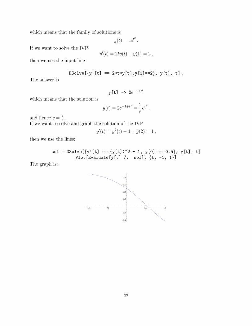
If we want to solve and graph the solution of the IVP
y′(t) = y2(t)− 1 , y(2) = 1 ,
then we use the lines:
sol = DSolve[{y’[t] == (y[t])^2 - 1, y[0] == 0.5}, y[t], t]
Plot[Evaluate[y[t] /. sol], {t, -1, 1}]The graph is:
-1.0 -0.5 0.5 1.0
-0.4
-0.2
0.2
0.4
0.6
0.8
29

Homework Exercises.
1. Solve the following DEs and IVPs. For the IVPs, give the largest interval on which thesolution is defined and graph the solution curve.
(1) y′ =y
t, t > 0 .
(2) y′ = ty , y(0) = 1 .
(3) y′ = y2 − 9 , t ∈ R .
(4) y′ = t√
4− y2 , t ∈ R
(5) y′ + 2ty2 = 0 , y(1) =1
5.
(6) y′ =ty
t2 − 1, t > 1 .
(7) y′ =ty
t2 − 1,−1 < t < 1 .
(8) y′ =ty
t2 − 1, y(2) = 0.5 .
(9) y′ = y tan t ,−π2< t <
π
2.
(10) y′ =2t
ln y, y(2) = 1 .
2. Assume that an epidemic spreads in a city with population 100, 000 at a rate proportionalto the product of the number of people already infected and the number of people susceptible,but not yet infected. This can be modeled by the logistic DE
y′(t) = 10−6 y(t)(50, 000− y(t)) , t ≥ 0 ,
where y(t) is the number of people already infected and t is the number of hours. Assumingthat at t = 0, the number of people already infected was 1, 000, estimate the number of theinfected people after 10 hours. Graph the solution curve. What is limt→∞ y(t)?
30

3.2. First order linear differential equations
The first order linear differential equations have the general form of
a(t)y′(t) + b(t)y(t) = f(t) . (3.2.1)
If the function f on the right hand side is constantly 0, then we say that the equation ishomogeneous. Otherwise, it is non-homogeneous.The following steps are required to solve a first order linear DE:
Step 1.Given a non-homogeneous linear DE (3.2.1), first we solve the corresponding homogeneousDE
a(t)y′(t) + b(t)y(t) = 0 . (3.2.2)
We solve it as a separable DE.
a(t)y′ = −b(t)ydy
y= − b(t)
a(t). (3.2.3)
Let’s stop for a moment. The division by y, shows that, as in the previous section, wehave to check, by substitution into (3.2.2), that the constant function y(t) ≡ 0 is a solution.Indeed, it is, but as we will see later that it is not a singular solution, because it is a memberof the family of solutions we get.
Also, the division by a(t), shows that the domain of the solutions has to exclude thenumbers t for which a(t) becomes 0.
Using the notation
u(t) + c =
∫− b(t)a(t)
dt ,
the integration of (3.2.3) leads to
ln |y| = u(t) + c .
By exponentiating both sides we get that
eln |y| = eu(t)+c = eu(t) · ec ,
and by replacing the positive constant ec to a general constant c, we get that
y(t) = c eu(t) .
In conclusion, the family of solutions of the homogeneous linear DE (3.2.2) always has thegeneral form
yh(t) = c z(t) .
Note that, for c = 0, the constant 0 function is a member of this family of solutions.Step 2.We need a so-called particular solution of the non-homogeneous linear DE, which will befound by the variation of parameters method. We search for the particular solution as
yp(t) = c(t)z(t) ,
31

where c(t) is an unknown function and z(t) is taken from Step 1.Substitute yp(t) into the non-homogeneous equation (3.2.1):
a(t)(c′(t)z(t) + c(t)z′(t)
)+ b(t)c(t)z(t) = f(t) .
Rearrange this equation as
a(t)c′(t)z(t) + c(t)[a(t)z′(t) + b(t)z(t)
]= f(t) ,
and use the fact that z(t) is a solution of the homogeneous equation, which makes theexpression inside the square brackets be 0. Hence,
c′(t) =f(t)
a(t)z(t),
and therefore c(t) is an antiderivative of f(t)a(t)z(t)
. Once c(t) is determined, we get yp(t).
Step 3.Finally, the solution of the non-homogeneous linear DE (3.2.1) looks like
y(t) = yh(t) + yp(t) .
Note. This method is not valid for non-linear differential equations. In particular, it cannotbe used to solve the DE y′ + ty2 = t .
Example. Solve the DE
y′ − 2ty = t .
Step 1.
y′ − 2ty = 0
dy
dt= 2ty
dy
y= 2t dt
ln |y| = t2 + c
|y| = et2+c
yh(t) = cet2
32

Step 2.
yp(t) = c(t)et2
y′p(t) = c′(t)et2
+ c(t)2tet2
c′(t)et2
+ c(t)2tet2 − 2tc(t)et
2
= t
c′(t)et2
= t
c′(t) = te−t2
c(t) =
∫te−t
2
dt = −1
2e−t
2
yp(t) = −1
2e−t
2
et2
= −1
2
Step 3.
y(t) = cet2 − 1
2.
Homework Exercises.
1. Solve the following DEs and IVPs. For the IVPs, give the largest interval on which thesolution is defined and graph the solution curve.
(1) y′ − 4y = 0 , t ∈ R .(2) y′ − 4y = 0 , y(0) = −1 .
(3) y′ + 2y = et , t ∈ R ..(4) y′ + 3y = e5t , y(0) = 5.
(5) y′ +2
t+ 1y = 3t , t > −1 .
33
(6) y′ + tan t y = 2 sin t cos t , y(0) = 1.
(7) y′ + 3t2y = t2 , t ∈ R .(8) t2y′ + ty = 1 , t < 0 .
(9) cos t y′ + sin t y = 1 , 0 < t <π
2.
(10) cos t y′ + sin t y = 1 , y(π
4) = 1 .
(11) y′ + 2ty = te−t2
, t ∈ R .(12) (1− t2)y′ − 2ty = e−t , t > 1 .
(13) (1− t2)y′ − 2ty = e−t , −1 < t < 1 .
(14) y′ + tan t y = cos t , y(0) = 0 .
(15) (1 + t2)y′ + 4ty =2
1 + t2, y(0) = 1 .
2. The plutonium 239 disintegrates according to the DE:
A′(t) = k A(t) ,
where k = −0.0000286728, and A(t) is the amount of plutonium 239 present after t numberof years. If at the present time we have an amount of 10kg, then estimate the amount leftafter 100 years.
3. The C-14 carbon isotope - which is used in carbon dating of fossils - disintegrates accordingto
A′(t) = k A(t) ,
where k = −0.00012378, and A(t) is the amount present after t number of years. If wemeasure that 50% of the C − 14 is left, how old is the fossil?
4. A population of bacteria in a culture grows according to the differential equation
N ′(t) = k N(t) ,
where k = 0.5, and N(t) is the number of bacteria present after t hours. If at present timewe approximately 5000 bacteria, estimate their number after 10 hours.
5. Consider the problem of a free falling object with mass M . Assume that only gravity andair resistance act upon the object. Let us suppose that the air resistance is proportional tothe velocity v(t) of the object. Newton’s second law of motion gives the DE
Mv′(t) = Mg − kv(t) , t ≥ 0 .
More exactly, this is a first order linear DE with constant coefficients:
Mv′(t) + kv(t) = Mg , t ≥ 0 .
Suppose that 2 objects with mass M1 = 10 kg and M2 = 20kg are released from an altitudeof 3000 meters with initial vertical velocity 0. Suppose that the constant k = 0.5 for both
34

objects. Answer the following questions:(a) Calculate the velocities v1(t) and v2(t) of the two objects.(b) What is their terminal (highest) velocity?(c) Which object is falling faster?(d) What is their speed after 5 seconds?
6. Visit:http://demonstrations.wolfram.com/LinearFirstOrderDifferentialEquation/
35

3.3. Bernoulli’s differential equations
Bernoulli’s differential equations have the form
y′ + a(t)y = b(t)yk ,
where k 6= 0 and k 6= 1. This is a non-linear equation, which will be changed to a linear one.
Changing the non-linear DE into a linear DE.Divide the equation by yk and get
y−k y′ + a(t)y1−k = b(t) .
Introduce a new functionz(t) = y1−k(t) ,
for whichz′(t) = (1− k) · y−k(t) · y′(t) .
Therefore, the non-linear Bernoulli’s DE is changed to
1
1− kz′ + a(t)z = b(t) ,
which is a first order linear DE in the unknown function z(t).
Solve the first order linear DE in z(t).This is done according to the Steps 1, 2 and 3 from the previous section.
Return to y(t). Write
y(t) = z(t)1
1−k ,
which is the solution of the Bernoulli’s DE.
Example. Solve the DE
y′ +1
ty = t2y2 , t > 0 .
Solution:Changing the non-linear DE into a linear DE.Divide the DE by y2:
y−2y′ +1
ty−1 = t2 .
Introduce
z(t) = (y(t))−1 =1
y(t).
Then, z′ = (−1)y−2 y′ and the linear DE in z looks like
−z′ + 1
tz = t2 .
Solve the first order linear DE in z(t).Step 1.
−z′ + 1
tz = 0
36

dz
z=dt
tln |z| = ln |t|+ c
zh(t) = c t .
Step 2. Search the particular solution in the form zp(t) = c(t) · t.By substituting zp(t) into the DE of z(t) gives c′(t) = −t, which gives c(t) = − t2
2and hence
zp(t) = −t3
2.
Step 3.
z(t) = ct− t3
2.
Return to y(t).
y(t) =1
ct− t3
2
.
Homework Exercises. Solve the following DEs and IVPs. For the IVPs, give the largestinterval on which the solution is defined and graph the solution curve.
(1) ty′ − y =−t3
y2, t > 0 .
(2) ty′ − y =−t3
y2, y(1) = 2 .
(3) y′ + y =1√y, y(0) = 4 .
(4) y′ + y =1√y, y(0) = −4 .
(5) ty′ + y = t2y2 , t < 0 .
(6) t2y′ − 2ty = 3y4 , y(1) =1
2.
(7) ty′ − (1 + t)y = ty2 , t > 0.
(8) 3y2y′ + 2y3 = et , −1 < t < 1.
(9) − 2t2y′ + ty = 5y3 , t < 0.
(10)−2t2y′
y3+
t
y2= 5 , t > 0.
(11) − 2t2y′ + ty = 5y3 , y(−1) = 0 .
(12) y′ − ty = t√y3 , y(1) = 4 .
37

3.4. Non-linear homogeneous differential equations
The non-linear part of the title has the meaning to distinguish between the earlier studiedlinear homogeneous DEs and the ones in this section. Note, that, while most of the DEs inthis section are non-linear, there are linear DEs which are homogeneous in this non-linearsense.
The non-linear homogeneous differential equations have the form
y′ = f(yt
).
We can solve them by introducing a new function
z(t) =y(t)
t.
Hence,y(t) = tz(t)
andy′ = z + tz′ .
The new DE in z isz + tz′ = f(z) ,
which is always a DE with separable variable. After solving this DE in z, we can get y(t)from the equation y(t) = t z(t).
Example. Solve the DEt2y′ − y2 − yt = 0 , t > 0 .
Solution:Dividing the equation by t2 gives:
y′ =(yt
)2+y
t.
Then,
z =y
ty = tz
y′ = z + tz′
z + tz′ = z2 + z
tdz
dt= z2
dz
z2=dt
t, z 6= 0
Note: z(t) = 0 is excluded from the solutions, so we have to check, by substitution, whetherit is a solution or not. It turns out that it is a solution.
−1
z= ln t+ c
z =−1
ln t+ c38
Not that z(t) = 0 is not part of this family, so it is a singular solution.Therefore, the solutions of this problem can be organized in a one-parameter family ofsolutions
y =−t
ln t+ c,
and a singular solutiony(t) ≡ 0 .
Homework Exercises. Solve the following DEs and IVPs. For the IVPs, give the largestinterval on which the solution is defined and graph the solution curve.
(1) ty′ − y + t = 0 , 0 < t < 2 .
(2) ty′ − y + t = 0 , y(1) = 2 .
(3) ty′ − y + t = 0 , y(0) = 2 .
(4) (y − 2t)y′ + t = 0 , −1 < t < 1 .
(5) t2y′ + y2 + yt = 0 , t < 0.
(6) y′ =t+ 3y
3t+ y, t > 0
(7) ty′ = y +√t2 − y2 , t > 0
(8) ty2y′ = y3 − t3 , y(1) = 3 .
(9) (t2 + 2y2)y′ = ty , y(−1) = 1 .
(10) ty3 y′ = y4 + t4 , t > 0 .
(11) y′ =t3 + y3
ty2, y(1) = 3 .
39

3.5. Differential equations of the form y′(t) = f(at+ by(t) + c).
In these equations a, b, c are constant and we introduce the function
z(t) = at+ by(t) + c .
Then
z′ = a+ by′ ,
and, in z, we get a DE with separable variables:
z′ = bf(z) + a .
We solve this equation and get z(t), from which we obtain y(t).Example.Solve the DE
y′ = (4t+ y + 3)2 .
Solution:
z = 4t+ y + 3
z′ = 4 + y′
y′ = z′ − 4
z′ − 4 = z2
dz
dt= 4 + z2
dz
z2 + 4= dt
1
2arctan
z
2= t+ c
arctanz
2= 2t+ c
z
2= tan(2t+ c)
z = 2 tan(2t+ c)
4t+ y + 3 = 2 tan(2t+ c)
y = 2 tan(2t+ c)− 4t− 3
40

Homework Exercises.
Solve the following DEs and IVPs. For the IVPs, give the largest interval on which thesolution is defined and graph the solution curve.
(1) y′ = cos(t+ y) , −π < t < π.
(2) y′ = cos(t+ y) , y(0) =π
4(3) y′ = 1 + ey−t+5 , t > 0 .
(4) y′ =1− t− yt+ y
, y(0) = −1.
(5) y′ =1− t− yt+ y
, y(1) = −1.
(6) y′ =3t+ 2y
3t+ 2y + 2, y(−1) = −1
(7) y′ =3t+ 2y
3t+ 2y + 2, y(0) = −1
41
3.6. Second order differential equations reducible to first order differentialequations
We will solve second order differential equations which contain just y′′ and y′, and no y.These equations have the general form form f(t, y′, y′′) = 0.If we introduce the function z = y′, then we get a first order DE in z: f(t, z, z′) = 0. Oncewe get z, the solution y is found by integration.
Example.Solve the IVP:
y′′ + 3y′ = e2t , y(0) = 1, y′(0) = 0 .
Solution:Introducing the function z = y′ we get the linear DE in z:
z′ + 3z = e2t .
Solving this equation in z gives:
z(t) = ce−3t +1
5e2t .
Integrating z leads to
y(t) =−c3e−3t +
1
10e2t + d .
The initial conditions give the system
{ −c3
+ 110
+ d = 1c+ 1
5= 0 .
Solving this system in c and d gives c = −15
and d = 56.
Therefore, the solution of the IVP is
y(t) =1
15e−3t +
1
10e2t +
5
6.
42

Homework Exercises. Solve the following DEs and IVPs.
(1) ty′′ + 3y′ = 0 , t > 0 .
(2) ty′′ + 3y′ = 0 , y(1) = 1 , y′(1) = 2 .
(3) y′′ = (y′)2 , y(0) = 1 , y′(0) = −1
e.
(4) t4y′′ + t3y′ = 4 , t > 0 .
(5) t4y′′ + t3y′ = 4 , t < 0 .
(6) y′′ + 3y′ = e2t , y(0) = 4 , y′(0) = 0 .
(7) 2y′y′′ = 1 + (y′)2 .
(8) y′′ =3t2y′
1 + t3.
43


CHAPTER 4
General theory of differential equations of first order
4.1. Slope fields (or direction fields)
Consider a first order DE in normal form
y′(t) = f(t, y(t)) , t ∈ I .
If y : I → R is a solution to this DE, then at any point t0 ∈ I, the value of f(t0, y(t0)) is theslope to the graph of the function y, which is a solution curve to the DE.Therefore, if we show a rectangular grid in the ty-coordinate system and evaluate f(t, y) atthe points in the grid, then we have graphical information about where solution curves areheading, without actually solving the DE.
Definition 4.1.1. A slope field of a DE is a rectangular grid with slopes, as arrowspointing left, drawn at each point of the grid.
Example. This example shows how to draw a slope field manually. Consider the DE
y′ = t− y .
Draw first a grid in the ty-coordinate system for t = −2,−1, 0, 1, 2 and y = −2,−1, 0, 1, 2
� � �-�-�
-�
-�
�
�
�
�
The right hand side to the DE gives the function f(t, y) = t − y. Evaluate this functionat each point of the grid and show the results as slopes at the corresponding points. Forexample, f(2, 1) = 1 gives a slope 1 at the point (2, 1). Continuing in this way we get thefollowing slope field.
45

�
�
�
�
� � �-�-�
-�
-�
Based on the slope field we can get graphical information about solution curves. If we choosean initial point, then we can draw an approximative solution curve on the graph by followingthe slopes in the slope field. The following graph shows the slope field and solution curvefor the IVP {
y′ = t− yy(−1) = 0.5 .
�
�
�
�
� �-�-�
-�
-�
Of course, if the slope field is filled with more slopes, our information about solution curvesis more complete.Mathematica can graph a slope field in the following way. The role of the cosine arctangentand the sine arctangent is to restrict the length of each vector to one.
VectorPlot[{Cos[ArcTan[t - y]], Sin[ArcTan[t - y]]}, {t, -2, 2},{y, -2, 2}, PlotRange->{{-2.5, 3}, {-2.5, 2.5}}, Axes -> True,
VectorStyle -> Arrowheads[0.02]]
46

We can add to the slope field the solution curve starting at (−2, 1), which shows how solutioncurves follow the slopes.
Show[VectorPlot[{Cos[ArcTan[t - y]], Sin[ArcTan[t - y]]}, {t, -2, 2},{y, -2, 2}, PlotRange -> {{-2.5, 3}, {-2.5, 2.5}}, Axes->True,
VectorStyle -> Arrowheads[0.015]], Plot[4*Exp[-t - 2] + t - 1, {t, -2, 2},PlotStyle -> Red]]
47

Also, there is the option of using StreamPlot.
More slope fields can be found athttp://demonstrations.wolfram.com/SlopeFields/.
48

4.1.1. Autonomous first order differential equations.
First order DEs in the form
y′(t) = f(y(t)) ,
or shortly
y′ = f(y) ,
are called autonomous first order DEs. Their slope fields show equal slopes along horizontalgrid lines. For example, lets have a look at the slope field of
y′ = y2 − 1 .
Definition 4.1.2. A phase portrait for a first order DE is a slope field with severalsolution curves, showing the most important qualitative properties of solutions.
Definition 4.1.3. Critical numbers (or points) for an autonomous first order DEare numbers c such that f(c) = 0.
Definition 4.1.4. Equilibrium solutions are the constant functions y(t) = c, corre-sponding to the critical numbers c.
Example. Consider the DE
y′ = y2 − 1 .
In this case f(y) = y2− 1 and the critical numbers correspond to the solutions of y2− 1 = 0,which are ±1. Hence the critical numbers are c = −1 and c = 1, while the equilibriumsolutions are y(t) = −1 and y(t) = 1. The phase portrait in this case looks like:
49

Classifications of equilibrium solutions:
(a) We call an equilibrium solution y(t) = c attractor (or asymptotically stable) if for anyother solution z(t) which starts from a position sufficiently close to c, we have limt→∞ z(t) = c.
(b) We call an equilibrium solution y(t) = c repeller (or unstable) if any other solution z(t)starting any close to c moves away from it as t→∞.
(c) We call an equilibrium solution y(t) = c semi-stable if it is an attractor from one sideand repeller from the other side.
Example. Let us look at the phase portrait of y′ = y2(y2 − 1).
The y(t) = 1 is a repeller, y(t) = 0 is semi-stable and y(t) = −1 is an attractor.
50
Homework Exercises.
1. Sketch slope fields and approximate solution curves for the given DEs and initial condi-tions:
(a)y′ = t+ y , y(−1) = 2 , y(0) = −1 .
(b)y′ = t− y , y(−1) = 2 , y(0) = −1 .
(c)
y′ =t
y, y(1) = 1 , y(0) = −1 .
(d)y′ = |t| − |y| , y(−1) = 0 , y(0) = 1 .
(e)y′ = y2 − t, y(0) = 0 , y(0) = 0.6 , y(0) = 0.8 .
(f)y′ = t(y + 1) , y(0) = 0 , y(1) = −1 .
(g)y′ = y sin t , y(0) = 0 , y(π) = 1 .
(h)
y′ =t
t2 + 1, y(0) = 0 , y(0) = 1 .
(i)
y′ =1
t2 + y2, y(1) = 0 , y(−1) = 0 .
(j)
y′ =1
|t|+ |y|, y(1) = 0 , y(−1) = 0 .
(k)
y′ =1
t+ y, y(1) = 0 , y(−1) = 0 .
2. For the following autonomous DEs sketch a phase-portrait, find the critical numbers,equilibrium solutions and classify them:
(a)y′ = y2 − y4 .
(b)y′ = (y − 1)2 .
(c)y′ = y4 − y .
(d)y′ = sin y .
51

(e)y′ = ye−y .
(f)y′ = y(4− y2) .
(g)y′ = y3 − 8y2 + 12y .
(h)y′ = y3 − 3y2 − 2y + 4 .
(i)y′ = y4 − 8y2 + 16 .
(j)y′ = y4 − 8y3 + 16y2 .
(k)y′ = y2 + 5y + 6 .
(l)y′ = y2 + 1 .
(m)
y′ =y2 − 9
y.
3. Suppose that the following DE models the pressure within a container:
y′ = y4 − 7y3 + 6y2 .
(a) Find the critical points, equilibrium solutions and classify them. Draw the phase por-trait.(b) If the pressure at t = 0 is 4, will it increase or decrease in the future? How much can itchange on long term?
4. Look at the DE in Exercise 2. in Section 3.1.(a) Find the critical points, equilibrium solutions and classify them. Draw the phase por-trait.(b) If at t = 0 the number of infected people is 15,000, will this number increase or decreasein the future? How much can it change on long term?
52

4.2. Existence and uniqueness of solutions for initial value problems
In this section we study the existence and uniqueness of solutions for IVPs. We will dothis by analyzing the right hand side of first order DEs in normal form, but without solvingthe DEs in the way we did in Chapter 3. This is an important issue, because many DEscannot be analytically solved and before we use the numerical methods from Section 4.4, wemust be sure that the numerical methods lead to a valid approximate solution. We will seethat disregarding this issue might lead to incorrect or incomplete answers.
Consider the IVP {y′ = f(t, y)y(t0) = y0 ,
(4.2.4)
where
(t, y) ∈ [t0 − a, t0 + a]× [y0 − b, y0 + b] = Ra,b .
By this we assume that the function f(t, y), as a function of two variables t and y, is definedon the rectangle Ra,b.
The question we can ask is under what conditions does the IVP have a solution curvethrough the point (t0, y0). The following two theorems give existence and uniqueness answers,based on the properties of f(t, y) inside the rectangle Ra,b. We use the following numbers:
M = Maximum of |f(t, y)| when (t,y) belongs to Ra,b ,
and
h = min{a, bM} .
We will apply the following two theorems.
Theorem 4.2.1 (Picard-Lindelof Existence and Uniqueness Theorem). If the functionf(t, y) and its partial derivative with respect to y, ∂f
∂y(t, y), are continuous on the rectangle
Ra,b, then there exists a unique solution y : [t0−h, t0+h]→ [y0−b, y0+b] of the IVP (4.2.4).
Theorem 4.2.2 (Peano’s Existence Theorem). If the function f(t, y) is continuous inboth the t and y variables on Ra,b, then the IVP (4.2.4) has at least one solutiony : [t0 − h, t0 + h]→ [y0 − b, y0 + b].
53

The following graph shows that, while we check the properties of f(t, y) inside the redrectangle, we can assure the existence of a solution curve inside a smaller blue rectangle.
Our main goal is to apply, if possible, the Picard-Lindelof Existence and Uniqueness Theo-rem.
Example 1. Consider the IVP: y′ = −yt
y(1) = 2 .
For this probem we have t0 = 1, y0 = 2 and
f(t, y) = −yt,∂f
∂y(t, y) = −1
t.
Both functions are continuous everywhere, except at the points for which t = 0. We willchoose the number a > 0 in such a way to avoid t = 0. Any number 0 < a < 1 is goodfor this purpose. With the choice of a = 0.5, the variable t belongs to the interval [0.5, 1.5],hence it cannot be 0. For the choice of b > 0 we don’t have any restrictions, so for simplicitylet us use b = 1. This means that the variable y belongs to the interval [1, 3]. The rectangleRa,b has the form
R0.5,1 = [0.5, 1.5]× [1, 3] .
To calculate M , we would need to use optimization methods for functions with two vari-ables, which is part of Calculus 3 and it is not a prerequisite for this class. Hence, we will usesimple logical arguments, like a fraction is the largest, when the numerator is the largest andthe denominator is the smallest. Then M = 3
0.5= 6 and h = min{0.5, 1
6} = 1
6. Therefore,
the Picard-Lindelof Existence and Uniqueness Theorem guarantees the existence of a uniquesolution y :
[56, 76
]→ [1, 3].
54

Observation. As you can notice from the graph, the solution curve probably continuesoutside of the interval [5/6, 7/6] and stays within the red rectangle. This means that thenumber h provided by the Picard-Lindelof Existence and Uniqueness Theorem is not optimal.Let’s have glimpse on how a more detailed analysis can extend the solution curve outsideof the interval [5/6, 7/6], but still within the rectangle [0.5, 1.5] × [1, 3]. The IVP of thisexample can be rewritten as
y(t) = 2 +
∫ t
1
−y(s)
sds .
If we want to check where does the solution curve exit the red rectangle, we have to evaluate|y(t)− 2| and see when it reaches 1.
|y(t)− 2| =∣∣∣∣∫ t
1
−y(s)
sds
∣∣∣∣ ≤ ∫ t
1
y(s)
sds .
At this stage, in the proof of Picard-Lindelof Existence and Uniqueness Theorem we calculatethe maximum of |f(t, y)| = y
tover the red rectangle, which means that we assume 0.5 ≤ s ≤
1.5 and 1 ≤ y(s) ≤ 3, which gives
|y(t)− 2| ≤ 3
0.5· h ≤ 1 ,
and this leads to h = 16. However, it is enough to consider the maximum of y
tover a smaller
rectangle [1− h, 1 + h]× [1, 3], defined by a variable h, and this gives
|y(t)− 2| ≤ 3
1− h· h ≤ 1 ,
which leads to h = 14, which is a better result.
It is a good exercise to try finding the optimal h, without solving the DE. As an indicationof what is happening, we can show a combination of the slope field from Section 4.1 and thegraph from this section.
55
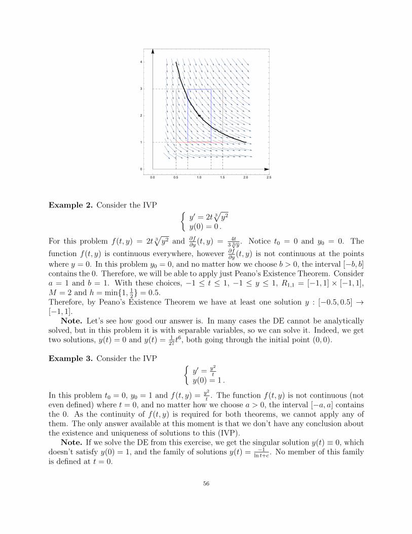
Example 2. Consider the IVP {y′ = 2t 3
√y2
y(0) = 0 .
For this problem f(t, y) = 2t 3√y2 and ∂f
∂y(t, y) = 4t
3 3√y. Notice t0 = 0 and y0 = 0. The
function f(t, y) is continuous everywhere, however ∂f∂y
(t, y) is not continuous at the points
where y = 0. In this problem y0 = 0, and no matter how we choose b > 0, the interval [−b, b]contains the 0. Therefore, we will be able to apply just Peano’s Existence Theorem. Considera = 1 and b = 1. With these choices, −1 ≤ t ≤ 1, −1 ≤ y ≤ 1, R1,1 = [−1, 1] × [−1, 1],M = 2 and h = min{1, 1
2} = 0.5.
Therefore, by Peano’s Existence Theorem we have at least one solution y : [−0.5, 0.5] →[−1, 1].
Note. Let’s see how good our answer is. In many cases the DE cannot be analyticallysolved, but in this problem it is with separable variables, so we can solve it. Indeed, we gettwo solutions, y(t) = 0 and y(t) = 1
27t6, both going through the initial point (0, 0).
Example 3. Consider the IVP {y′ = y2
ty(0) = 1 .
In this problem t0 = 0, y0 = 1 and f(t, y) = y2
t. The function f(t, y) is not continuous (not
even defined) where t = 0, and no matter how we choose a > 0, the interval [−a, a] containsthe 0. As the continuity of f(t, y) is required for both theorems, we cannot apply any ofthem. The only answer available at this moment is that we don’t have any conclusion aboutthe existence and uniqueness of solutions to this (IVP).
Note. If we solve the DE from this exercise, we get the singular solution y(t) ≡ 0, whichdoesn’t satisfy y(0) = 1, and the family of solutions y(t) = −1
ln t+c. No member of this family
is defined at t = 0.
56

Example 4. This examples shows that we cannot blindly trust the answers given by com-puters. Consider the IVP {
y′ = 2t√y
y(0) = 0.16 .
The initial point is (t0, y0) = (0, 0.16) and the function f(t, y) = 2t√y and its partial
derivative ∂f∂y
(t, y) = t√y
are continuous on the rectangle R1,0.08 = [−1, 1]× [0.08, 0.24], so by
the Picard-Lindelof Existence and Uniqueness Theorem we should have we have a uniquesolution going through the initial point (0, 0.16). However, Mathematica gives two solutions.
If we add the slope field to the graph, we see that the decreasing curvey = 0.25(0.64 − 1.6t2 + t4) = 0.25(t2 − 0.8)2 doesn’t fit and it is the result of a softwaremistake.
57

Homework Exercises.
(1) Check the existence and uniqueness of solutions for the following IVPs. Sketch therectangle Ra,b. In case of existence or existence and uniqueness of the solution draw anapproximate solution curve through the initial point.
(a) (t− 1)y′ = y2 + t , y(0) = 1 .
(b) (t− 1)y′ = y2 + t , y(1) = 0 .
(c) y′ =√y2 − 4 , y(1) = 2 .
(d) y′ =√y2 − 4 , y(1) = 3 .
(e) y′ =3√ty + y2 , y(0) = 3 .
(f) (t2 + y2)y′ = y + 1 , y(1) = 1 .
(g) y′ = ty2 + 3 , y(0) = 2 .
(h) y′ =ty
t2 − 1, y(0) = 1 .
(i) t2y′ + ty = 1 , y(3) = 1 .
(j) t2y′ + ty = 1 , y(0) = 1 .
(k) ty2y′ = y3 − t3 , y(1) = 1 .
(2) Return to exercise 2 from Section 2.2. Do we have a unique solution for the IVPs? Why?
58

4.3. The method of successive approximations
This is a theoretical method, which is used to prove the existence and uniqueness theorem.Although, practically not as useful as the numerical methods from the next section, it offersgreat insight to the theory of initial value problems.Consider the IVP {
y′ = f(t, y)y(t0) = y0 ,
(4.3.5)
and assume that we can use the PIcard-Lindelof Existence and Uniqueness theorem to assurethat we have a unique solution y : [t0 − h, t0 + h] → [y0 − b, y0 + b]. Integrate both sides ofthe DE from t to t0: ∫ t
t0
y′(s)ds =
∫ t
t0
f(s, y(s)) ds .
By the Fundamental Theorem of Calculus we get that
y(t)− y(t0) =
∫ t
t0
f(s, y(s)) ds ,
and hence any solution of the IVP (4.3.5) satisfies the equation
y(t) =
∫ t
t0
f(s, y(s)) ds+ y0 . (4.3.6)
We will use an iteration, called the succesive approximation of the solution, for (4.3.6):
y1(t) =
∫ t
t0
f(s, y0) ds+ y0
y2(t) =
∫ t
t0
f(s, y1(s)) ds+ y0
..................................
yn(t) =
∫ t
t0
f(s, yn−1(s)) ds+ y0 (4.3.7)
......................................
As n → ∞ the sequence of functions yn(t) converges uniformly to a function y(t) on theinterval [t0 − h, t0 + h]. Therefore, in the equation (4.3.7) we can let n→∞ and get that
y(t) =
∫ t
t0
f(s, y(s)) ds+ y0 ,
which means that y(t) is the unique solution of the IVP (4.3.5).
Example. Consider the IVP {y′ = yy(0) = 1 ,
The solution y(t) satsfies the integral equation
y(t) =
∫ t
0
y(s) ds+ 1 .
59
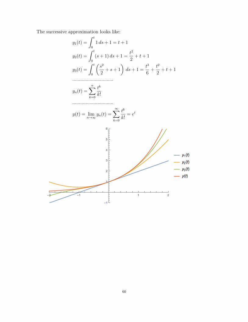
The successive approximation looks like:
y1(t) =
∫ t
0
1 ds+ 1 = t+ 1
y2(t) =
∫ t
0
(s+ 1) ds+ 1 =t2
2+ t+ 1
y3(t) =
∫ t
0
(s2
2+ s+ 1
)ds+ 1 =
t3
6+t2
2+ t+ 1
...............................
yn(t) =n∑k=0
tk
k!
...............................
y(t) = limn→∞
yn(t) =∞∑k=0
tk
k!= et
60
Homework Exercises.
Calculate the first 3 terms of the method of successive approximations. Substitute y3(t) intothe DE and verify how close y3(t) is to be a solution.Optional: Try finding (not always easy or even possible) the formula for yn(t) and thencalculate the solution as y(t) = limn→∞ yn(t) .
(1) y′ = −y , y(0) = 2 .
(2) y′ = 3y , y(0) = 1 .
(3) y′ = 2ty , y(0) = 1 .
(4) y′ = y − t , y(0) = 2 .
(5) y′ =t√t2 + 1
, y(0) = 2 .
(6) y′ = y2 , y(0) = 1 .
(7) y′ + 2ty2 = 0 , y(0) = 1 .
(8) y′ = y + t , y(0) = 0 .
(9) y′ = ty2 − 1 , y(0) = 1 .
(10) y′ =ty√t2 + 1
, y(0) = 2 .
61

4.4. Numerical methods for Differential equations
4.4.1. The Euler’s method. Consider again the IVP{y′ = f(t, y)y(t0) = y0 .
Suppose that, as in the statement of the existence and uniqueness theorem, f and ∂f∂y
are
continuous on Ra,b. Hence, we have a unique solution defined on [t0 − h, t0 + h].
The following method, called Euler’s method, provides the simplest numerical approxi-mation of the solution. By numerical approximation we mean some algebraical calculationsusing f(t, y), which is the right hand side of the DE.
Choose a small step ε > 0. We will determine approximate values of the solution at thefollowing points:
t1 = t0 + ε ,
t2 = t1 + ε = t0 + 2ε ,
.......................................
tn = t0 + n ε ,
................................
For each tn we define a number yn which approximates the exact value of the solution y(tn).We write this approximation as yn ≈ y(tn).
Let us start with
y1 = y0 + f(t0, y0)ε .
By the fact that the slope of the solution curve at (t0, y0) is f(t0, y0) we can use the linearapproximation of functions by their first order Taylor polynomial to conclude that y(t1) ≈ y1.Continue the process by setting
y2 = y1 + f(t1, y1)ε
y3 = y2 + f(t2, y2)ε
..................................
yn+1 = yn + f(tn, yn)ε .
The calculated points (t0, y0), (t1, y1), ... (tn, yn) can be connected by line segments to givea continuous curve, which is an approximation of the solution curve.
Example. Consider the IVP {y′ = 4t
√y
y(0) = 0.16 ,. (4.4.8)
62

We want to find an approximation of the solution on the interval [0, 1]. First, let us select astep size ε = 0.25. We use
f(t, y) = 4t√y
and
t0 = 0 , y0 = 0.16 .
Starting the first round of calculations, t1 = 0.25 and y1 = 0.16 + (4 · 0 ·√
0.16) · 0.25 = 0.16.
t1 = 0.25 , y1 = 0.16 .
Continuing with the second round, t2 = 0.5 and y2 = 0.16 + (4 · 0.25 ·√
0.16) · 0.25 = 0.26.
t2 = 0.5 , y2 = 0.26 .
In similar ways,
t3 = 0.75 , y3 = 0.5149 .
and
t4 = 1 , y4 = 1.053 .
In this way we found that,
y(0) = 0.16, y(0.25) ≈ 0.16, y(0.5) ≈ 0.26, y(0.75) ≈ 0.5149, y(1) ≈ 1.053 .
We can use Mathematica to generate these numbers:
For comparison, let us calculate the exact values using the exact solution y(t) = (t2+0.4)2.Note that, in general, we don’t know the exact solution.
y(0) = 0.16 , compared to y0 = 16
y(0.25) = (0.252 + 0.4)2 = 0.2139 , compared to y1 = 0.16
y(0.5) = (0.52 + 0.4)2 = 0.4225 , compared to y2 = 0.26
y(0.75) = (0.752 + 0.4)2 = 0.9264 , compared to y3 = 0.5149
y(1) = (1 + 0.4)2 = 1.96 , compared to y4 = 1.053
63
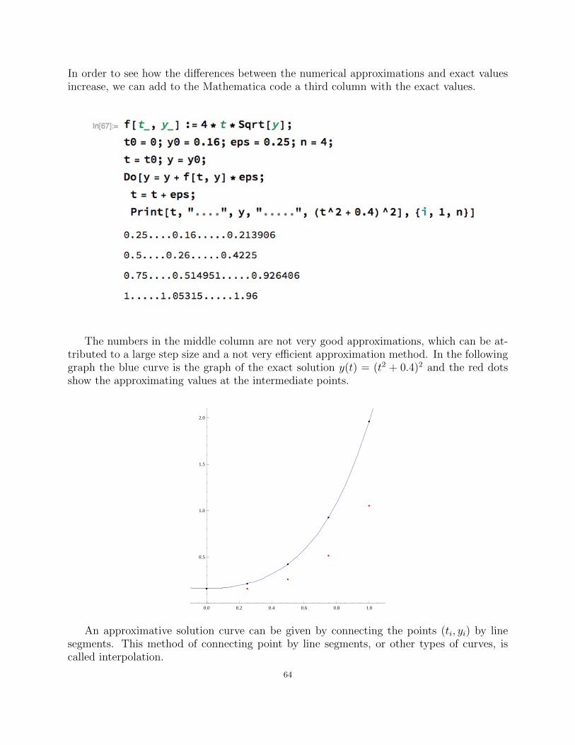
In order to see how the differences between the numerical approximations and exact valuesincrease, we can add to the Mathematica code a third column with the exact values.
The numbers in the middle column are not very good approximations, which can be at-tributed to a large step size and a not very efficient approximation method. In the followinggraph the blue curve is the graph of the exact solution y(t) = (t2 + 0.4)2 and the red dotsshow the approximating values at the intermediate points.
0.0 0.2 0.4 0.6 0.8 1.0
0.5
1.0
1.5
2.0
An approximative solution curve can be given by connecting the points (ti, yi) by linesegments. This method of connecting point by line segments, or other types of curves, iscalled interpolation.
64

0.0 0.2 0.4 0.6 0.8 1.0
0.5
1.0
1.5
2.0
Smoother interpolation curves are available, too:
0.0 0.2 0.4 0.6 0.8 1.0
0.5
1.0
1.5
2.0
As yn is just an approximation of the exact value y(tn), we call the quantity
errn = |y(tn)− yn| ,
the error of the approximation at tn. Let us try to estimate errn.The following calculations show the power of theoretical mathematics in finding the size ofthe error, without knowing the exact solution.Suppose that both partial derivatives of f(t, y) are continuous on the rectangle Ra,b. Then,the unique solution y(t) of the IVP has a continuous second order derivative on [t0−h, t0+h]and
y′′(t) =∂f
∂t(t, y(t)) +
∂f
∂y(t, y(t)) y′(t) .
65

Hence, |y′′(t)| will have a finite maximum M2 ≥ 0 over the interval [t0 − h, t0 + h]. UsingTaylor’s theorem we get that
y(t1) = y(t0) + y′(t0)ε+ y′′(t∗)ε2
2,
for some t0 ≤ t∗ ≤ t1. But, by Euler’s method y1 = y(t0) + y′(t0)ε, which gives
|y(t1)− y1| ≤M2
2ε2 .
These calculation show that at each step we pick up a local error of order ε2. But, we needhε
steps to cover the interval from t0 to t0 + h, so we can expect that the global error to beof order one less than the local error:
h
ε
M
2ε2 = C ε ,
This means that
|y(tn)− yn| ≤ C ε .
To improve the approximation of the solution we have two options: use smaller steps orimprove the numerical method.
First, let us use a smaller step size ε = 0.1. We let Mathematica do the calculations and,as before, the second column contains the numerical approximations and the third columnthe exact values.
As we can see, y10 = 1.53032 is much closer to the exact value of y(1) = 1.96 than the earlier1.053, which was calculated with a step size of 0.25.
66

4.4.2. The improved Euler (or Heun) method.
The previously introduced Euler method tends to underestimate the exact values in a caseof a concave-up solution. To get a better approximation we will use an improved method,which is of a predictor-corrector type. This means that we approximate y′(tn) by averagingthe slopes at the current and the following intermediate points.To find yn+1, we will calculate first an intermediate value y∗n+1:
y∗n+1 = yn + f(tn, yn) · ε ,
and then
yn+1 = yn +f(tn, yn) + f(tn+1, y
∗n+1)
2· ε .
For the same IVP (4.4.8) as before, with step size ε = 0.25, the calculated values are:
t0 = 0 , y0 = 0.16 .
t1 = 0.25 , y∗1 = 0.16 + 4 · 0 ·√
0.16 · 0.25 = 0.16
y1 = 0.16 + 0.25 · 4 · 0 ·√
0.16 + 4 · 0.25 ·√
0.16
2= 0.21
t1 = 0.25 , y1 = 0.21 .
t2 = 0.5 , y∗2 = 0.21 + 0.25 · (4 · 0.25 ·√
0.21) = 0.3245
y2 = 0.21 + 0.25 · 4 · 0.25 ·√
0.21 + 4 · 0.5 ·√
3245
2= 0.4096
t2 = 0.5 , y2 = 0.4096 .
t3 = 0.75 , y∗3 = 0.7296 , y3 = 0.8899
t3 = 0.75 , y3 = 0.8899 .
t4 = 1 , y∗4 = 1.5974 , y4 = 1.8756
t4 = 1 , y4 = 1.8756 .
Therefore,
y(1) ≈ 1.8756 .
Mathematica can be programmed in the following way. As before, the middle column con-tains the numerical approximations and the third column contains the exact values.
67
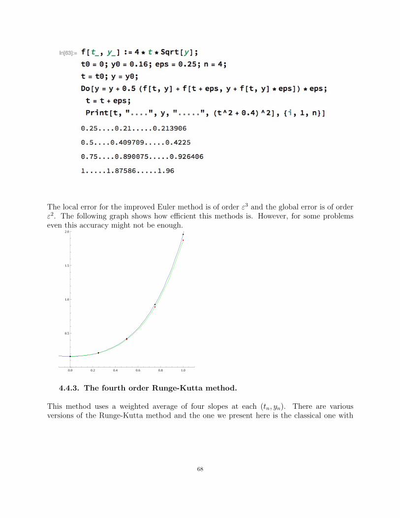
The local error for the improved Euler method is of order ε3 and the global error is of orderε2. The following graph shows how efficient this methods is. However, for some problemseven this accuracy might not be enough.
0.0 0.2 0.4 0.6 0.8 1.0
0.5
1.0
1.5
2.0
4.4.3. The fourth order Runge-Kutta method.
This method uses a weighted average of four slopes at each (tn, yn). There are variousversions of the Runge-Kutta method and the one we present here is the classical one with
68

the average of four slopes. The general formula is the following.
s1 = f(tn, yn)
s2 = f(tn +
ε
2, yn +
s12ε)
s3 = f(tn +
ε
2, yn +
s22ε)
s4 = f (tn + ε , yn + s3 ε)
yn+1 = yn +s1 + 2s2 + 2s3 + s4
6ε
For the IVP (4.4.8) studied earlier, let us use a step twice as large as for the Euler and Heunmethods: ε = 0.5. Remember that f(t, y) = 4t
√y.
Then for the first step we get the following results:
s1 = f(0, 0.16) = 0
s2 = f(0.25, 0.16) = 0.4
s3 = f
(0.25, 0.16 +
0.4
2· 0.5
)= 0.509902
s4 = f (0.5, 0.16 + 0.509902 · 0.5) = 1.28833
y1 = 0.16 +0 + 2 · 0.4 + 2 · 0.509902 + 1.28833
60.5 = 0.419011
For the second step we get the following results:
s1 = f(0.5, 0.419011) = 1.29452
s2 = f
(0.75, 0.419011 +
1.29462
20.5
)= 2.58534
s3 = f
(0.75, 0.419011 +
2.58534
20.5
)= 3.09647
s4 = f (1, 0.419011 + 0.309647 · 0.5) = 5.61034
y2 = 0.419011 +1.29462 + 2 · 2.58534 + 2 · 0.3.09647 + 5.61034
60.5 = 1.94138
We can see that with just 2 steps the Runge-Kutta method gives better approximation ofy(1) than the Heun method with 4 step and the Euler method with 10 steps.The local error of the Runge-Kutta method is of order ε5, while the global error is of orderε4.
69

Connecting the calculated points with line segments leads to the following graph.
0.0 0.2 0.4 0.6 0.8 1.0
0.5
1.0
1.5
2.0
As you notice, even if the calculated points are on the exact solution curve, connectingthem with line segments doesn’t match the exact solution curve at other places. We canimprove this by selecting a smaller step size, or use a smoother interpolation curve as in thenext graph.
0.0 0.2 0.4 0.6 0.8 1.0
0.5
1.0
1.5
2.0
To further compare the approximation methods from this section, you can watch the follow-ing demonstration:http://demonstrations.wolfram.com/NumericalMethodsForDifferentialEquations/
70

4.4.4. NDSolve command in Mathematica.
We can use the NDSolve command to get a numerical solution to an IVP. The expressionsgiving the solution looks as:NDSolve[{y’[t] == 4*t*Sqrt[y[t]], y[0] == 0.16}, y[t], {t, 0, 1}]If we want to get approximate values and graph of the solution then we assign a function tothe numerical solution in the follwing way:sol = NDSolve[y’[t] == 4*t*Sqrt[y[t]], y[0] == 0.16, y[t], t, 0, 1]
q[t ] := Evaluate[y[t] /. sol]
The function q[t] is the approximate numerical solution of our problem. If we want to getthe the approximate value of the solution for the input t = 0.75, then we just writeq[0.75], which gives 0.926402, an answer very close to the exact one 0.962406.We can graph the solution with the command linePlot[q[t],{t,0,1}] .
71

More examples for numerical approximations.
Example 1. This example shows what could happen if the IVP has multiple solutions.Consider the IVP {
y′ = 4t√y
y(0) = 0 ,. (4.4.9)
The problem arises from the fact that there are two solutions. NDSolve gives the constanty(t) ≡ 0 function as a solution, while DSolve gives the function y(t) = t4 as the solution.However, for more complicated DEs, DSolve might not provide an answer and we wouldloose information about other solutions.
Example 2. For the following IVP analytic solutions are not possible and DSolve doesn’tprovide any answers. We can use only NDSolve, but we have to check that we can apply thePicard-Lindelof Existence and Uniqueness Theorem before we start the computations.Consider the IVP {
y′ = y2 − 3√t
y(0) = 1 ,. (4.4.10)
72

Using the Picard-Lindelof Existence and Uniqueness Theorem for a = 1 and b = 1 leads toa unique solution y : [−0.2, 0.2]→ [0, 2]. NDSolve leads to the following graph.
The graph shows no erratic behavior of the solution and therefore, probably, its domaincan be extended. Trying to extend it from [−0.2, 0.2] to [−2, 2] leads to the following message.
The message shows that around t = 1.35 some problems arise. Let’s try the domain[−1.3, 1.3].
The graph shows that at about t = 1.35 a possibly vertical asymptote shows up, hencethe solution cannot be extended further to the right. However, it could be extended to theleft.
73
Homework Exercises.
(1) Use each of the Euler, Heun and Runge-Kutta methods to approximate y(t) on theinterval [1, 2] using a step size ε = 0.5, where y(t) is the solution of the IVP{
y′ = t+ yy(1) = 0 .
(2) Use each of the Euler, Heun and Runge-Kutta methods to approximate y(0.5) after twosteps, where y(t) is the solution of the IVP{
y′ = −tyy(0) = 1 .
(3) Use each of the Euler, Heun and Runge-Kutta methods to approximate y(1) after twosteps, where y(t) is the solution of the IVP{
y′ = t− yy(0) = 1 .
(4) Use the Heun method to approximate y(1) with step sizes ε = 0.25 and ε = 0.1, wherey(t) is the solution of the IVP {
y′ = y2
y(0) = 2 .
What are your conclusions?
(5) Use the Euler method to approximate y(1.5) with step sizes ε = 0.25 and ε = 0.1, wherey(t) is the solution of the IVP {
y′ = 3y2/3
y(1) = 0 .
What might go wrong and why?
(6) Use each of the Euler, Heun and Runge-Kutta methods to approximate y(2.2) using astep size ε = 0.4, where y(t) is the solution of the IVP{
y′ = t2
+ y4
y(1) = 4 .
Note: Check your answers for the Homework Exercises with Mathematica by using boththe DSolve and the NDSolve.
74
CHAPTER 5
Higher order linear differential equations
5.1. General theory
A nth-order linear DE has the form
an(t) y(n)(t) + an−1(t) y(n−1)(t) + · · ·+ a1(t) y
′(t) + a0(t) y(t) = g(t) , t ∈ I , (5.1.1)
where the unknown function is y(t) and the coefficients are the functions ak(t), 0 ≤ k ≤ n.
Example. In the case of
(t3 − 1) y(4)(t) +√t2 + 4 y′′′(t)− sin t y′(t) + y(t) = et , 1 < t <∞ ,
a4(t) = t3 − 1, a3(t) =√t2 + 4, a2(t) = 0, a1(t) = − sin t, a0(t) = 1 and g(t) = et.
The general solution of a nth-order linear DE has the form
y(t) = yh(t) + yp(t) ,
where yh(t) is a n-parameter family of solutions of the linear and homogeneous DE
an(t) y(n)(t) + an−1(t) y(n−1)(t) + · · ·+ a1(t) y
′(t) + a0(t) y(t) = 0 , t ∈ I , (5.1.2)
and yp(t) is a particular solution of the non-homogeneous DE (5.1.1). As a n-parameterfamily of solutions, yh(t) has to be determined as
yh(t) = c1y1(t) + · · ·+ cnyn(t) ,
where y1(t) , · · · yn(t) are solutions of the linear and homogeneous DE (5.1.2).However, not every choice of n solutions is suitable. We must choose linearly independentsolutions, which means that if
c1y1(t) + · · ·+ cnyn(t) = 0 , for every t ∈ I ,then each parameter must be 0:
c1 = · · · = cn = 0 .
To analytically check the linear independence of solutions, we must check the Wronskiandeterminant is not identically zero:
W (y1(t) , y2(t) , · · · yn(t)) =
∣∣∣∣∣∣∣∣∣∣y1(t) y2(t) · · · yn(t)y′1(t) y′2(t) · · · y′n(t). . · · · .. . · · · .
y(n−11 (t) y
(n−1)2 (t) · · · y
(n−1)n (t)
∣∣∣∣∣∣∣∣∣∣6= 0 ,
for at least one t ∈ I.
75

Note: Determinants are calculated in the following way:∣∣∣∣ a bc d
∣∣∣∣ = ad− bc ,
∣∣∣∣∣∣a b cd e fg h i
∣∣∣∣∣∣ = a ·∣∣∣∣ e fh i
∣∣∣∣− b · ∣∣∣∣ d fg i
∣∣∣∣+ c ·∣∣∣∣ d eg h
∣∣∣∣ .Higher order determinants are calculated in a similar way by expanding them using the firstrow, and thus reducing the calculations to determinants of one size less.
Definition. The functions y1(t), · · · , yn(t) form a Fundamental Set of Solutions (shortlyFSS) of the linear and homogeneous DE (5.1.2) if:
1. Each function is a solution.2. They are linearly independent.
The following theorem gives us a method to check whether n functions form a FSS or not.
Theorem 5.1.1. If the functions y1(t), · · · , yn(t) are solutions of the linear and homoge-neous DE (5.1.2) and W (y1(t), · · · , yn(t)) 6= 0 for at least one t ∈ I, then they are linearlyindependent and form a FSS.
Examples:(1) Let us show that the functions y1(t) = t and y2(t) = t3 form a FSS for the DE
t2 y′′ − 3t y′ + 3 y = 0 , t ∈ (0,+∞) .
First, let us check that the two functions are solutions. By substituting y1(t) = t into theDE we get
t2 · 0− 3t · 1 + 3t = 0 ,
which leads to 0 = 0. Repeat the process for y2(t) = t3, too.Then
W (t, t3) =
∣∣∣∣ t t3
1 3t2
∣∣∣∣ = 3t3 − t3 = 2t2 ,
which is not zero for any (would be enough to check just for one) t > 0. Therefore, y1(t) = tand y2(t) = t3 form a FSS.However, if we want to see whether z1(t) = t and z2 = 5t form a FSS, then we can checkthat they are solutions, but
W (t, 5t) =
∣∣∣∣ t 5t1 5
∣∣∣∣ = 5t− 5t = 0 ,
which shows that they are not linearly independent. Therefore, they do not form a FSS.
Regarding the existence and uniqueness of solutions for IVPs corresponding to linear DEswe have the following theorem.
76
Theorem 5.1.2. Consider the IVP an(t)y(n)(t) + an−1(t)y(n−1)(t) + · · ·+ a0(t)y(t) = g(t) , t ∈ [α, β]
y(t0) = y0, y′(t0) = y1, · · · , y(n−1)(t0) = yn−1 ,
where t0 ∈ [α, β] is a fixed point.If the functions an(t), · · · , a0(t), g(t) are continuous on the interval [α, β] and an(t) 6= 0 forany α ≤ t ≤ β, then the IVP has a unique solution on the entire interval [α, β].
Homework Exercises.(1) Determine whether the given functions form a FSS of the corresponding linear andhomogeneous DE.
(a) cos 5t , sin 5t , y′′ + 25y = 0 , t ∈ R.(b) e5t , e−5t , y′′ + 25y′ = 0 , t ∈ R.(c) e5t , e−5t , y′′ − 25y = 0 , t ∈ R.
(d)1
t, t , t2 , t3y′′′ + t2y′′ − 2ty′ + 2y = 0 , t > 0 .
(e) t2 − t , t , t2 , t3y′′′ + t2y′′ − 2ty′ + 2y = 0 , t < 0 .
(f) e3t , te3t , y′′ − 6y′ + 9y = 0 , t ∈ R.(g) 1 , cos 2t , sin 2t , y′′′ + 4y′ = 0 , t ∈ R.(h) e−t , e4t , y′′ − 3y′ − 4y = 0 , t ∈ R.(i) et , cos t , sin t , y′′′ − y′′ + y′ − y = 0 , t ∈ R.
(2) Determine the intervals on which IVPs corresponding to the given DEs have uniquesolutions:
(a) (t2 − 9) y′′′ + sin t y′′ − y = t.
(b) cos t y′ + 3y = et.
(c) y′′ +√
1− t2 y′ + ln t y = 0.
(d) y(4) − y′′ = t3.
(e) t3 y′′′ − 5t2 y′′ + ty′ − 5y = t+ 2.
77
5.2. Linear and homogeneous DEs with constant coefficients
The linear and homogeneous DEs with constant coefficients have the form
an y(n)(t) + an−1 y
(n−1)(t) + · · ·+ a1 y′(t) + a0 y(t) = 0 , (5.2.1)
where the coefficients an, an−1, · · · , a1, a0 are real numbers and an 6= 0.We would like to find which functions of the form y(t) = ert are solutions of the DE (5.2.1).Substituting y(t) = ert in the DE (5.2.1) gives(
an rn + an−1 r
n−1 + · · ·+ a1 r + a0
)ert = 0 .
Therefore, we have the following theorem:
Theorem 5.2.1. If r is a solution of the polynomial equation
an rn + an−1 r
n−1 + · · ·+ a1 r + a0 = 0 , (5.2.2)
then y(t) = ert is a solution of the DE (5.2.1).
Equation (5.2.2) is called the characteristic equation of the DE (5.2.1). Every nth-orderpolynomial equation has n real or complex solutions.
We will assign to each solution r of the characteristic equation (5.2.2) a solutionof the DE (5.2.1). In this process we have to distinguish the following cases.
Simple real solution: If r is a simple real solution of (5.2.2), then we assign to it thefunction
ert .
Repeated real solutions: If r is a real solution repeated k times, then we assign to it ksolutions:
ert, tert, · · · , tk−1ert .Simple complex solution: If r = a+ ib is a complex solution of (5.2.2), then a− ib is alsoa solutions, so we assign to r two solutions
eat cos(bt) , eat sin(bt) .
Repeated complex solutions: If r = a + ib is a complex solution of (5.2.2) repeated ktimes, then we assign to it k pairs of solutions
eat cos(bt) , eat sin(bt) , teat cos(bt) , teat sin(bt) , · · · tk−1eat cos(bt) , tk−1eat sin(bt) .
We finalize the theory of this section by the following theorem.
Theorem 5.2.2. If we assign to each solution of the characteristic equation a solution ofthe linear and homogeneous DE (5.2.1) in the ways shown above, then we get a fundamentalset of solutions.
78

Examples.
1. Solve the DE:
y′′ − 9y = 0 .
The characteristic equation r2 − 9 = 0 has the solutions
r1 = 3 , r2 = −3 .
The functions assigned to them are
y1(t) = e3t , y2(t) = e−3t .
These two functions form a FSS, so the general solution has the form
y(t) = c1e3t + c2e
−3t .
2. Solve the DE:
y′′ + 9y = 0 .
The characteristic equation r2 + 9 = 0 has the solutions
r1 = 3i , r2 = −3i .
The functions assigned to them are
y1(t) = cos(3t) , y2(t) = sin(3t) .
These two functions form a FSS, so the general solution has the form
y(t) = c1 cos(3t) + c2 sin(3t) .
3. Solve the DE:
y′′′ + 4y′′ + 4y′ = 0 .
The characteristic equation r3 + 4r2 + 4r = 0 has the solutions
r1 = 0 , r2 = r3 = −2 .
The functions assigned to them are
y1(t) = 1 , y2(t) = e−2t , y3(t) = te−2t
These three functions form a FSS, so the general solution has the form
y(t) = c1 + c2e−2t + c3te
−2t .
4. Solve the IVP:
y′′ − 4y′ + 13y = 0 , y(0) = 0 , y′(0) = 3 .
The characteristic equation r2 − 4r + 13 = 0 has the solutions
r1 = 2 + 3i , r2 = 2− 3i .
79

The functions assigned to them are
y1(t) = e2t cos(3t) , y2(t) = e2t sin(3t) .
These two functions form a FSS, so the general solution of the DE has the form
y(t) = c1e2t cos(3t) + c2e
2t sin(3t) .
Using the initial conditions we get c1 = 0 and c2 = 1, and, therefore, the unique solution ofthe IVP is
y(t) = e2t sin(3t) .
Homework Exercises. Solve the following DEs and IVPs:
1. 2y′ − 5y = 0.
2. y′′ + 4y′ + 3y = 0, y(1) = 0, y′(1) = 2e−3.
3. y′′′ + y = 0.
4. y(4) − 16y = 0.
5. y′′′ + 5y′′ = 0.
6. y′′′ − y′′ + 4y′ − 4y = 0.
7. y′′′ − 5y′′ + 3y′ + y = 0.
8. y′′ − 8y′ + 16y = 0.
9. y′′′ − y′′ + y′ − y = 0, y(0) = 0, y′(0) = 1, y′′(0) = −1.
10. y(4) − 5y′′ + 4y = 0.
11. y(4) + 5y′′ + 4y = 0.
12. y(4) − 50y′′ + 625y = 0.
13. y′′′ + y′′ + y′ = 0.
14. y′′ − 6y′ + 13y = 0.
15. y′′′ − 3y′′ + 4y′ − 2y = 0.
80

5.3. Linear and non-homogeneous DEs with constant coefficients
The previous section provided methods to find yh, so we are left to find a particular solutionyp. Two methods will be presented.
5.3.1. Variation of parameters for second order linear equations.
Variation of parameters can be used for any linear DE, as long as we know a FSS of thehomogeneous equation. Here we will present it just for second order linear DEs.
Consider the DE
a2 y′′(t) + a1 y
′(t) + a0 y(t) = g(t) ,
where a2, a1, a0 are real numbers, a2 6= 0 and g(t) is not the constant zero function.Let us assume that we already obtained the solution of the homogeneous DE
a2 y′′ + a1 y
′ + a0 y = 0 ,
and it has the form
yh(t) = c1 y1(t) + c2 y2(t) .
The variation of parameters method means that we are looking for the particular solutionin the form
yp(t) = c1(t) y1(t) + c2(t) y2(t) ,
where the c1(t) and c2(t) are unknown functions left to be determined. By requesting thatyp(t) be a solution of the non-homogeneous DE, we get the system{
c′1(t) y1(t) + c′2(t) y2(t) = 0
c′1(t) y′1(t) + c′2(t) y
′2(t) = g(t)
a2.
Solving this system gives c′1(t) and c′2(t). By integrating them we get c1(t) and c2(t), andfrom here we find yp(t). The final solution is given by y(t) = yh(t) + yp(t).
Example: Solve the DE
y′′ − 3y′ + 2y = e5t .
Step 1. The homogeneous equation
y′′ − 3y′ + 2y = 0
has the characteristic equation
r2 − 3r + 2 = 0 ,
which has the solutions r1 = 1 and r2 = 2. The FSS assigned to them is formed by thefunctions y1(t) = et and y2(t) = e2t. Therefore,
yh(t) = c1 et + c2 e
2t .
Step 2. We search the particular solution in the form
yp(t) = c1(t) et + c2(t) e
2t ,
81

and this leads to the system {c′1(t) e
t + c′2(t) e2t = 0
c′1(t) et + c′2(t) 2e2t = e5t .
Subtracting the first equation from the second gives
c′2(t)e2t = e5t ,
and hence c′2(t) = e3t and c2(t) = 13e3t. Substituting e3t for c′2(t) in the first equation gives
c′1(t) = −e4t and hence c1(t) = −14e4t.
Therefore,
yp(t) = −1
4e4tet +
1
3e3te2t =
1
12e5t .
Step 3. The complete solution is
y(t) = c1 et + c2 e
2t +1
12e5t .
5.3.2. The undetermined coefficients method and the superposition principle.
The undetermined coefficients method applies if the function g(t) on the right hand side ofthe DE has one of the following forms:
1. If g(t) = P (t)eαt, where P (t) is a polynomial of degree m and α is not a solution of thecharacteristic equation, then we search yp(t) in the following form
yp(t) = (bmtm + · · ·+ b1t+ b0)e
αt ,
where the unknown coefficients bm, · · · , b1, b0 are determined by substituting yp(t) in thenon-homogeneous DE.
2. If g(t) = P (t)eαt, where P (t) is a polynomial of degree m and α is a solution of thecharacteristic equation repeated k-times, then we search yp(t) in the following form
yp(t) = tk(bmtm + · · ·+ b1t+ b0)e
αt ,
where the unknown coefficients bm, · · · , b1, b0 are determined by substituting yp(t) in thenon-homogeneous DE.
3. If g(t) = P (t)eαt cos(βt) + Q(t)eαt sin(βt), where P (t) and Q(t) are a polynomials ofdegree at most m and α+ iβ is not a solution of the characteristic equation, then we searchyp(t) in the following form
yp(t) = (bmtm + · · ·+ b1t+ b0)e
αt cos(βt) + (dmtm + · · · d1t+ d0)e
αt sin(βt) ,
where the unknown coefficients bm, · · · , b1, b0, dm, · · · , d1, d0 are determined by substitutingyp(t) in the non-homogeneous DE.
82

4. If g(t) = P (t)eαt cos(βt) + Q(t)eαt sin(βt), where P (t) and Q(t) are a polynomials ofdegree at most m and α + iβ is a solution of the characteristic equation repeated k-times,then we search yp(t) in the following form
yp(t) = tk(bmtm + · · ·+ b1t+ b0)e
αt cos(βt) + tk(dmtm + · · · d1t+ d0)e
αt sin(βt) ,
where the unknown coefficients bm, · · · , b1, b0, dm, · · · , d1, d0 are determined by substitutingyp(t) in the non-homogeneous DE.
In the following examples we focus just on finding yp and ask the reader to complete thedetails of finding yh.
Example 1. Solve the DEy′′ − y′ − 2y = 2t+ 3 .
Step 1. Using the method from Section 5.2 we get yh(t) = c1e2t + c2e
−t.Step 2. In this exercise g(t) = (2t + 3)e0 t and α = 0, which is not a solution of thecharacteristic equation r2 − r − 2 = 0. So, we search for yp(t) in the form
yp(t) = (b1t+ b0)e0 t = b1t+ b0 .
Substituting yp(t) into the DE leads to
−b1 − 2b1t− 2b0 = 2t+ 3 ,
which can be rearranged as−2b1t− 2b0 − b1 = 2t+ 3 .
The two sides must be identically the same, so we have −2b1 = 2 and −2b0 − b1 = 3, whichgives b1 = −1 and b0 = −1, and hence yp(t) = −t− 1.Step 3. The final form of the solution is
y(t) = c1e2t + c2e
−t − t− 1 .
Example 2. Solve the DEy′′ − y′ = 2t+ 3 .
Step 1. Using the method from Section 5.2 we obtain yh(t) = c1 + c2et.
Step 2. In this exercise g(t) = (2t+ 3)e0 t and α = 0, which is a simple (k = 1) solution ofthe characteristic equation r2 − r = 0. So, we search for yp(t) in the form
yp(t) = t(b1t+ b0)e0 t = b1t
2 + b0t .
Substituting yp(t) into the DE leads to
2b1 − 2b1t− b0 = 2t+ 3 ,
which can be rearranged as−2b1t+ 2b1 − b0 = 2t+ 3 .
The two sides must be identically the same, so we have −2b1 = 2 and 2b1 − b0 = 3, whichgives b1 = −1 and b0 = −5 and hence yp(t) = −t2 − 5t.Step 3. The final form of the solution is
y(t) = c1 + c2et − t2 − 5t .
83

Example 3. Solve the DEy′′′ + y′′ − y′ − y = 4 cos t .
Step 1. Using the method from Section 5.2 we obtain yh(t) = c1et + c2e
−t + c3te−t.
Step 2. In this exercise, g(t) = 4e0t cos t and α + iβ = i, which is not a solution of the thecharacteristic equation. So, we search yp(t) in the form
yp(t) = a cos t+ b sin t .
By substituting yp(t) into the DE and grouping the similar terms we get that
(2a− 2b) sin t+ (−2a− 2b) cos t = 4 cos t ,
which leads to the system {2a− 2b = 0−2a− 2b = 4 .
This gives a = b = −1 and therefore yp(t) = − cos t− sin t.Step 3. The final form of the solution is
y(t) = c1et + c2e
−t + c3te−t − cos t− sin t .
The superposition principle:This method works just in the case of linear DEs. If the right hand side is the sum of kfunctions,
g(t) = g1(t) + · · ·+ gk(t) ,
then we search the particular solution as
yp(t) = yp1(t) + · · ·+ ypk(t) ,
where each function is a particular solution of the corresponding term of the right hand side.
Example 4.. Consider the linear DE:
y′′ + 4y = tet − 24e2t .
Step 1. Solving the homogeneous equation gives yh(t) = c1 cos(2t) + c2 sin(2t) .Step 2. We search the particular solution in the form yp(t) = (at+b)et+de2t. By substitutingyp(t) into the DE we get
(5at+ 5b+ 2a)et + 8de2t = tet − 24e2t ,
which gives the system 5a = 15b+ 2a = 0
8d = −24 .
Hence, a = 15, b = − 2
25, d = −3 and yp(t) = (1
5t− 2
25)et − 3e2t.
Step 3. The final form of the solution is
y(t) = c1 cos(2t) + c2 sin(2t) + (1
5t− 2
25)et − 3e2t .
84

5.3.3. Use Mathematica to solve higher order DEs.
The FullSimplify command can be really useful in simplifying the solutions to a form similarto what we get without the use of computers.
Homework exercises.
1. Solve the following DEs and IVPs:
1. y′ − 3y = 6.
2. y′′ − 4y′ + 3y = et sin(2t), y(0) = 0, y′(0) = 1.
3. y′′′ + y = t+ e−2t.
4. y(4) − 16y = t2 + t.
5. y′′′ + 5y′′ = t+ 3.
6. y′′′ − y′′ + 4y′ − 4y = sin(2t).
7. 4y′′ + 5y′ + y = 1et
.
8. y′′ + y = tan t.
9. y′′ + y = cos t.
10. y′′ + y = te−2t.
11. y′′ + 9y = 1sin(3t)
.
12. y′′ + 3y′ + 2y = 11+et
.
13. y′′ + 3y′ + 2y = 1+et
et.
85

14. y′′ + 3y′ + 2y = t2 .
15. y(4) − 5y′′ + 4y = et.
16. y(4) − 5y′′ + 4y = e3t.
17. y(4) + 5y′′ + 4y = cos(2t)− sin(2t).
18. y(4) − 50y′′ + 625y = 125.
19. y′′ + 2y′ + y = 1tet
.
2. The vertical displacement from its natural length of a spring-mass system is described by
y′′(t) + 2y′(t) + 10y(t) = 0 ,
where the time t is measured in seconds.Describe the position of the mass after 20 seconds if the initial position is 0 and initial ve-locity is −1 m/s.
3. Find the charge q(t) on the capacitor in a series RLC circuit which is modeled by theIVP
1
8q′′ + 5q′ + 500q = 0V , q(0) = 0C , q′(0) = 20A .
Find the charge after 3 seconds.
4. Find the charge q(t) on the capacitor in a series RLC circuit which is modeled by theIVP
5
3q′′ + 10q′ + 30q = 110V , q(0) = 0C , q′(0) = 2A .
What is the charge after 1 second? What is the long term behavior of q(t)?
5. (a) Find the charge q(t) on the capacitor in a series RLC circuit which is modeled by theIVP
1
10q′′ + 2q′ + 100q = cos(10t) + sin(10t)V , q(0) = 0C , q′(0) = 0A .
(b) Use DSolve to find q(t), plot it and estimate the maximum charge during the first second.
86

6. Consider the problem of a free falling object with mass M . Assume that only gravityand air resistance act upon the object.
(a) As a first model, let us suppose that the air resistance is proportional to the velocity v(t)of the object. Newton’s second law of motion gives the DE
Mv′(t) = Mg − kv(t) , t ≥ 0 .
More exactly, this is a first order linear DE with constant coefficients:
Mv′(t) + kv(t) = Mg , t ≥ 0 .
Suppose that 2 objects with mass M1 = 10 kg and M2 = 20kg are released from an altitudeof 3000 meters with initial vertical velocity 0. Suppose that the constant k = 0.5 for bothobjects. Answer the following questions:(i) Calculate the velocities v1(t) and v2(t) of the two objects.(ii) What are their terminal (highest) velocities?(iii) Which object is falling faster?(iv) What are their speeds after 5 seconds?
(b) (Optional) The role of this exercise is to show that another mathematical model mightlead to a much more difficult DE. In certain cases, the air resistance can be modeled as
Fair = C · 0.5 · ρ · v(t)2 · A ,where C is the drag coefficient, ρ is the air density, and A is the reference area of the object.C and A are constants, but the air density depends on air temperature and pressure whichvary with altitude. A simple function modeling air density is the following
ρ(y) = 1.2− 0.00011y ,
where y is the elevation above see level. This function is obtained by supposing that the airis dry, the temperature at see level is 20◦C and is dropping at a rate of 6◦C per 1000 meters.If an object with mass of 10kg is released at 3000 meters and we denote by s(t) = 3000−y(t)the distance the object dropped until time t, then we get the a DE of the form
10s′′(t) + C · A · (0.87 + 0.00011s(t)) · (s′(t))2 = 100 ,
which is a second order non-linear differential equation.Use DSolve and NDSolve to estimate the altitude and velocity of the object after 10 seconds.
87

5.4. The Cauchy-Euler DE
The Cauchy-Euler DE has the form
an · tn · y(n)(t) + an−1 · tn−1 · y(n−1)(t) + · · ·+ a1 · t · y′(t) + a0 · y(t) = g(t) , (5.4.1)
which has to be solved for t < 0 or t > 0. This is a linear DE with non-constant coefficientsand we will reduce it to a linear DE with constant coefficients. In order to achieve this, weuse the substitutions
t = ex or x = ln t , if t > 0 ,
andt = −ex or x = ln(−t) , if t < 0 .
Let us consider the t > 0 case.We have to substitute the derivatives in t with derivatives in x. Using the chain rule we getthat
dy
dt=dy
dx
dx
dt=dy
dx
1
t=dy
dxe−x .
Furthermore,
d2y
dt2=
d
dt
(dy
dt
)=
d
dx
(dy
dxe−x)e−x =
(d2y
dx2− dy
dx
)e−2x ,
and
d3y
dt3=
d
dt
(d2y
dt2
)=
d
dx
((d2y
dx2− dy
dx
)e−2x
)e−x =
(d3y
dx3− 3
d2y
dx2+ 2
dy
dx
)e−3x .
If we continue in this way, we can express any derivative in t in terms of derivatives in x andby substituting them into the equation (5.4.1), we obtain a linear differential equation withconstant coefficients.
Example Solve the following DE:
t3y′′′ + 5t2y′′ + 7ty′ + 8y = 2 ln t , t > 0 .
Let us use the substitution t = ex and get
e3x(d3y
dx3− 3
d2y
dx2+ 2
dy
dx
)e−3x + 5e2x
(d2y
dx2− dy
dx
)e−2x + 7ex
dy
dxe−x + 8y = 2x
The exponential functions are canceling each other, so we get
d3y
dx3+ 2
d2y
dx2+ 4
dy
dx+ 8y = 2x .
Solving this DE according to the methods from the previous sections gives
y(x) = c1e−2x + c2 cos(2x) + c3 sin(2x) +
1
4x− 1
8.
We get the final form of the solution by substituting x = ln t in the previous line:
y(t) = c1t−2 + c2 cos(2 ln t) + c3 sin(2 ln t) +
1
4ln t− 1
8.
88

Homework Exercises.
Solve the following DEs and IVPs.
1. t2y′′ − ty′ + y = sin(ln t) , t > 0.
2. t3y′′′ − 6y = 2t+ 3 , t > 0 .
3. t2y′′ + ty′ + y = 0 , y(1) = 1 , y′(1) = 2 .
4. t2y′′ + ty′ − y = 1t, t > 0 .
5. t3y′′′ − 6ty′ + 12y = t2 , t > 0 .
6. t2y′′ − ty′ + 5y = 2 ln t+ t , t > 0 .
7. t3y′ − 3t2y = 1 , t > 0 .
8. t3y′′′ − 6ty′ + 12y = t2 , t < 0 .
89

CHAPTER 6
Solving linear differential equations with the Laplace transform
6.1. Definition and properties of the Laplace transform
The Laplace transform changes a linear DE into an algebraical equation, which can be solvedby algebraical methods. Finally, the algebraical solution is transformed back into a solutionof the original DE.As an addition to the methods presented in the previous chapter, the Laplace transform willhelp us to solve linear DEs with discontinuous right hand sides.
Definition 6.1.1. We say that a function y : [0,+∞) → R is piecewise continuouson [0,∞) if limt→0+ y(t) exists and y(t) is continuous on every interval of finite length [0, b],except maybe a finite number of points, where the function has jump discontinuities.
Definition 6.1.2. We say the function y : [0,+∞)→ R is of exponential order c ≥ 0if there are positive constants M and T such that
|y(t)| ≤Mect , for all t ≥ T .
Definition 6.1.3. Consider a function y : [0,+∞)→ R, which is piecewise continuouson [0,+∞) and is of exponential order c. The Laplace transform of the function y(t) isdefined as
L[y(t)](s) =
∫ ∞0
e−sty(t) dt , s > c . (6.1.1)
Properties of the Laplace transform:
Existence: The Laplace transform is an improper integral, which could converge or divergedepending on the value of s.However, if the function y(t) is piecewise continuous on [0,+∞) and of exponential order c,then the improper integral converges for s > c, so L[y(t)](s) exists and is finite.
Linearity: Suppose that λ ∈ R and the functions y(t) and z(t) are piecewise continuous on[0,+∞) and of exponential order c. Then for all s > c we have:
L[y(t) + z(t)](s) = L[y(t)](s) + L[z(t)](s)
L[λy(t)](s) = λL[y(t)](s) .
The linearity of the Laplace transform makes it compatible with linear differential equations.
91

Laplace transforms of elementary functions :
(1) L[1](s) =1
s, s > 0.
(2) L[tn](s) =n!
sn+1, s > 0 , n ∈ N.
(3) L[eat](s) =1
s− a, s > a.
(4) L[sin(bt)](s) =b
s2 + b2, s > 0.
(5) L[cos(bt)](s) =s
s2 + b2, s > 0.
(6) L[sinh(bt)](s) =b
s2 − b2, s > |b|.
(7) L[cosh(bt)](s) =s
s2 − b2, s > |b|.
Let us prove these these formulas.
(1) If s > 0 then
L[1](s) =
∫ ∞0
e−ts dt = −e−ts
s
∣∣∣∞0
=1
s.
(2)
L[t](s) =
∫ ∞0
e−ts t dt = −te−ts
s
∣∣∣∞0
+1
s
∫ ∞0
e−ts dt =1
s2.
L[t2](s) =
∫ ∞0
e−ts t2 dt = −t2e−ts
s
∣∣∣∞0
+2
s
∫ ∞0
e−ts t dt =2
s3.
By mathematical induction, if n ≥ 2,
L[tn](s) =
∫ ∞0
e−ts tn dt = −tne−ts
s
∣∣∣∞0
+n
sL[tn−1](s) =
n!
sn+1.
(3) If s > a, then
L[eat](s) =
∫ ∞0
e−ts eatdt =
∫ ∞0
e−t(s−a) dt = −e−t(s−a)
s− a
∣∣∣∞0
=1
s− a.
92

(4) If s > 0, then
L[sin(bt)](s) =
∫ ∞0
e−ts sin(bt) dt
= −e−ts sin(bt)
s
∣∣∣∞0
+b
s
∫ ∞0
e−ts cos(bt) dt
= −be−ts cos(bt)
s2
∣∣∣∞0− b2
s2
∫ ∞0
e−ts sin(bt) dt
=b
s2− b2
s2L[sin(bt)](s) .
Therefore,
L[sin(bt)](s) =b
s2 + b2.
(5) It is similar to (4).
(6) If s > |b|, then
L[sinh(bt)](s) = L[ebt − e−bt
2
](s) =
1
2
(L[ebt](s)− L[e−bt](s)
)=
1
2
(1
s− b− 1
s+ b
)=
b
s2 − b2.
(7) If s > |b|, then
L[cosh(bt)](s) = L[ebt + e−bt
2
](s) =
1
2
(L[ebt](s) + L[e−bt](s)
)=
1
2
(1
s− b+
1
s+ b
)=
s
s2 − b2.
Homework Exercises.
1. Which of the following functions are of exponential order c? Find c, if the answer is yes.(a)
y(t) = 5t2 + 2t+ 1 .
(b)
y(t) = sin(3t) .
(c)
y(t) = 4 e2t .
(d)
y(t) = et2
.
93
(e)
y(t) =
{2 if t = 31t−3 if t 6= 3 .
(f)
y(t) = cos t e3t .
(g)
y(t) = e−5t .
2. Which of the following functions are piecewise continuous on [0,+∞)?(a)
y(t) = t2 et .
(b)
y(t) =
{0 if t = 41t−4 if t 6= 4 .
(c)
y(t) =
{0 if 0 ≤ t < 51t−4 if t ≥ 5 .
(d)
y(t) =
{0 if t = 0sin 1
tif t > 0 .
(e)
y(t) = btc , the integer part of t .
3. Which of the functions from exercises 1 and 2 are both of exponential order c and piece-wise continuous on [0,+∞)?
4. Find the Laplace transforms of the following functions and give the interval on which theLaplace transforms are defined:
(a)
y(t) = 2t+ 3 .
(b)
y(t) = t2 + 2t+ 1 .
(c)
y(t) = (cos t+ sin t)2 .
(d)
y(t) = t2 + e4t .
(e)
y(t) =(1 + e3t
)2.
94
(f)y(t) = sinh2 t .
(g)
y(t) =t2 + 5t+ 6
t+ 2.
(h)y(t) = sin(5t) + cos(5t) .
(i)y(t) = e−2t + 3e2t .
(j)y(t) = cos2(t) .
(h)
y(t) =
{0 if 0 ≤ t < 1t if t ≥ 1 .
95

6.2. Further properties of the Laplace transform. Transforms of the Heavisidefunction and the Dirac Delta function
6.2.1. Translation on the s-axis.
If the function y(t) is piecewise continuous on [0,+∞) and of exponential order c, then
L[eat y(t)](s) = L[y(t)] (s− a) , if s > a+ c . (6.2.2)
We can prove this formula in the following way:
L[eat y(t)](s) =
∫ ∞0
e−ts eat y(t) dt =
∫ ∞0
e−t(s−a) y(t) dt
= L[y(t)](s− a) .
Examples:
(1)
L[e2t t3](s) = L[t3] (s− 2) =3!
s4
∣∣∣∣∣s→s−2
=6
(s− 2)4, if s > 2 .
(2)
L[e−t cos(2t)](s) = L[cos(2t)] (s+ 1) =s
s2 + 4
∣∣∣∣∣s→s+1
=s+ 1
(s+ 1)2 + 4, if s > 0 .
6.2.2. Derivatives of the Laplace transform.
For simplcity of notations, the Laplace transform of a function denoted by a lower case letterwill be denoted by the same upper case letter. For example:
L[y(t)] (s) = Y (s) .
To find a formula for Y (n)(s) we start with Y ′(s) and give some explanations.
Y ′(s) =d
ds
∫ ∞0
e−ts y(t) dt =
∫ ∞0
d
dse−ts y(t) dt
=
∫ ∞0
(−t)e−ts y(t) dt = −L[ty(t)](s) .
Hence,L[ty(t)](s) = −Y ′(s) ,
and continuing this process, by mathematical induction, we get that for any n ∈ N we have
L[tn y(t)] = (−1)n Y (n)(s) . (6.2.3)
As you can see, the process of calculating the derivatives of Y (s) involves differentiating un-der the integral sign, which requires the use of uniform convergence of the improper integrals
96

∫∞0e−ts y(t) dt in s for s ≥ c+ ε, where ε > 0 symbolizes any small positive number.
Examples.(1)
L[t2](s) = L[t2 · 1](s) =d2
ds2
(1
s
)=
2
s3.
(2)
L[t3e2t](s) = − d3
ds3
(1
s− 2
)=
6
(s− 2)3.
(3)
L[t sin t](s) = − d
ds
(1
s2 + 1
)=
2s
(s2 + 1)2.
6.2.3. The Laplace transform of the unit step function and of piecewise con-tinuous functions.
The unit step function is frequently used to model the turning ”off” and ”on” of externalforces and it is defined by:
ua(t) =
{0 if 0 ≤ t < a1 if t ≥ a .
With the aid of the unit step function we can rewrite the piecewise continuous functionsin a form suitable for the Laplace transform. Let’s see two examples:
Consider
f(t) =
{0 , if 0 ≤ t < 2t− 3 , if t ≥ 2 .
97

We can write
f(t) = (t− 3) u2(t) .
Consider now
g(t) =
{t2 , if 0 ≤ t < 10 , if t ≥ 1 .
Then,
g(t) = t2 − t2 u1(t) .
For another piecewise continuous function consider
f(t) =
0 , if 0 ≤ t < 13 , if 1 ≤ t < 20 , if t ≥ 2
98

we havef(t) = 3u1(t)− 3u2(t) .
Let’s continue by calculating the Laplace transforms of these piecewise continuous functions.
L[ua(t)] (s) =
∫ ∞a
e−ts dt = −e−ts
s
∣∣∣∣∣∞
a
=e−as
s.
In general,
L[f(t− a)ua(t)] (s) =
∫ ∞a
e−τs f(τ − a) dτ
t = τ − a , dt = dτ
=
∫ ∞0
e−(t+a)s f(t) dt =
∫ ∞0
e−as e−ts f(t) dt = e−as∫ ∞0
e−ts f(t) dt
= e−as L[f(t)](s) .
Therefore,
L[f(t− a)ua(t)] (s) = e−as L[f(t)](s) . (6.2.4)
Examples.
(1)
L[(t− 2)u2(t)] (s) = e−2s L[t] (s) =e−2s
s2.
(2)
L[et−3u3(t)] (s) = e−3s L[et] (s) =e−3s
s− 1.
(3)
L[(t− 3) u2(t)] (s) = L[(t− 2) u2(t)− u2(t)] (s)
= L[(t− 2) u2(t)] (s)− L[u2(t)] (s)
= e−2s L[t] (s)− e−2s
s=e−2s
s2− e−2s
s=
1− ss2
e−2s .
99

(4)
L[(t2 + 1) u1(t)] (s)
= L[(t− 1)2 + 2(t− 1) + 2) u1(t)] (s)
= L[(t− 1)2 u1(t)] (s) + 2L[(t− 1)u1(t)] (s) + 2L[u1(t)] (s)
= e−s L[t2] (s) + 2e−s L[t] (s) + 2e−s
s
=
(2
s3+
2
s2+
2
s
)e−s .
6.2.4. The Dirac Delta function. The Dirac Delta function describes forces of largemagnitude acting only for a very short time. Actually it is not a function, it is a distribution,or generalized function, but a description of the distributions theory is beyond the level ofthis course. Hence, we will just define the Dirac function in an elementary way and give itsLaplace transform.
For a ≥ 0 define
δa(t) =
{+∞ , if t = a
0 , if t 6= a ,
and formally require ∫ ∞−∞
δa(t) dt = 1 .
We will use the notation δ(t) instead of δ0(t).
The Laplace transform of the Dirac Delta function is given by
L[δa(t)] (s) = e−as . (6.2.5)
Hence,
L[δ(t)] (s) = 1 . (6.2.6)
Homework Exercises.
Find the Laplace transforms of the following functions:
(1) et sin t
(2) e−t cos t
100

(3) e3tt2
(4) t cosh t
(5) t2 − 3tet
(6) t2e3t
(7) e−2t sin 4t+ 3t
(8) (t− 3)u3(t)
(9) (t− 3)2 u3(t)
(10) sin(t− π) uπ(t)
(11) sin2 t
(12) cos2(3t)
(13) 10δ3(t)
(14) sin t+ δπ(t)
(15) (t− 2)3 u2(t) + δ2(t)
101

6.3. The inverse Laplace transform
By Lerch’s theorem, if two piecewise continuous functions have the same Laplace transform,then they can differ just at the discontinuity points. By assuming that at discontinuitypoints we consider the right hand side limit as the value of the function at that point, wefind that the Laplace transform is a one-to-one transformation. Therefore, we can define itsinverse transformation, which reverses the effect of the Laplace transform.
Definition 6.3.1. If Y (s) = L[y(t)] (s) then define
L−1 [Y (s)] (t) = y(t) .
Note: The inverse Laplace transform is linear, which means that
L−1[Y (s) + Z(s)] (t) = L−1[Y (s)] (t) + L−1[Z(s)] (t) = y(t) + z(t) ,
and
L−1[aY (s)] (t) = a L−1[Y (s)] (t) = a y(t) .
Examples:
(1)
L−1[
1
s
](t) = 1 .
(2)
L−1[
1
s3
](t) =
1
2t2 .
(3)
L−1[
1
s− 5
](t) = e5t .
(4)
L−1[
s
s2 + 4
](t) = cos(2t) .
(5)
L−1[
s+ 3
(s+ 3)2 + 4
](t) = e−3t cos(2t) .
102

(6)
L−1[
s
(s+ 3)2 + 4
](t) = L−1
[s+ 3− 3
(s+ 3)2 + 4
](t)
= L−1[
s+ 3
(s+ 3)2 + 4− 3
(s+ 3)2 + 4
](t)
= L−1[
s+ 3
(s+ 3)2 + 4
](t)− 3
2L−1
[2
(s+ 3)2 + 4
](t)
= e−3t cos(2t)− 3
2e−3t sin(2t) .
(7)
L−1[
1
(s− 5)2
](t) = te5t .
(8)
L−1[e−2s
s
](t) = u2(t) .
(9)
L−1[e−2s
1
s− 5
](t) = e5(t−2) u2(t) .
(10)
L−1 [1] (t) = δ(t) .
(11)
L−1[e−3s
](t) = δ3(t) .
For the next exercise we have to use partial fraction decomposition.
(12)
L−1[
2s2 + s+ 2
s3 + s2 + 2s+ 2
](t) = L−1
[2s2 + s+ 2
(s+ 1)(s2 + 2)
](t)
= L−1[
1
s+ 1+
s
s2 + 2
](t)
= L−1[
1
s+ 1
](t) + L−1
[s
s2 + 2
](t)
= e−t + cos(√
2t) .
103

6.3.1. Calculate the Laplace transform and inverse Laplace transform usingMathematica.
To calculate the Laplace transform we can use the following commands:
LaplaceTransform[Sin[t], t, s]
For the inverse Laplace transform we can use:
InverseLaplaceTransform[1/(1 + s), s, t]
Homework Exercises.
Find the inverse Laplace transforms of the following functions:
(1)
Y (s) = s−5 .
(2)
Y (s) =(s− 3)2
s5.
(3)
Y (s) =
(3
s+
1
s2
)2
.
(4)
Y (s) =3
s− 2.
(5)
Y (s) =1
2s+ 1.
(6)
Y (s) =5
s2 + 36.
(7)
Y (s) =−3s
s2 + 1.
(8)
Y (s) =s
4s2 + 1.
(9)
Y (s) =2s+ 4
s2 + 9.
(10)
Y (s) =1
s2 + 2s+ 10.
104
(11)
Y (s) =1
s2 + 3s− 10.
(12)
Y (s) =1
s4 + 5s2 + 6.
(13)
Y (s) =3
(s− 2)4.
(14)
Y (s) =s
(s+ 1)2.
(15)
Y (s) =1
s(s+ 1)2.
(16)
Y (s) =e−s
s2.
(17)
Y (s) =e−2s
s2 + s.
(18)
Y (s) =e−πs
s2 + 4.
(19)
Y (s) =s e−sπ/4
s2 + 4.
(20)
Y (s) =s
(s2 + 9)2.
105

6.4. Solving IVPs of linear DEs with the Laplace transform
Laplace transforms of the derivatives.
If y(t), y′(t), · · · , y(n−1)(t) are continuous on [0,+∞), are of exponential order c and y(n)(t)is piecewise continuous on [0,+∞), then
L[y(n)(t)](s) = snL[y(t)](s)− sn−1 y(0)− sn−2 y′(0)− · · · − s y(n−2)(0)− y(n−1)(0) .
To see how this works, let us start calculating L[y′(t)](s) using integration by parts. Forsimplicity, let us work with these improper integrals as with the usual definite integrals, butwe should not forget that this is possible, because our assumptions make these improperintegrals convergent. Also, by the exponential order c of the function y(t) we know that fors > c we have limt→∞ e
−sty(t) = 0.
L[y′(t)](s) =
∫ ∞0
e−ts y′(t) dt
= e−tsy(t)∣∣∣∞0
+ s
∫ ∞0
e−ts y(t) dt
= −y(0) + sL[y(t)](s) .
We can continue to evaluate higher order derivatives in the following way:
L[y′′(t)](s) =
∫ ∞0
e−ts y′′(t) dt
= e−tsy′(t)∣∣∣∞0
+ s
∫ ∞0
e−ts y′(t) dt
= −y′(0)− sy(0) + s2 L[y(t)](s) .
You should pay close attention to Example 1. This is an easy exercise, but the more com-plicated ones follow exactly the same steps.
Example 1.
Solve the IVP
y′ − 2y = 6 , y(0) = 1 .
This is a linear DE with constant coefficients, so we can apply the Laplace transform to bothsides of the equation:
L[y′(t)− 2y(t)] (s) = L[6] (s) .
By the linearity of the Laplace transform we get
L[y′(t)] (s)− 2L[y(t)] (s) = L[6] (s) .
106
We use the notation Y (s) = L[y(t)] (s) and by the formula for the transformation of deriva-tives we get
sY (s)− 1− 2Y (s) =6
s.
Solving this equation in Y (s) gives:
Y (s) =s+ 6
s(s− 2).
The partial fraction decomposition of the right hand side gives:
Y (s) =4
s− 2− 3
s.
Now we apply the inverse Laplace transform to both sides:
L−1[Y (s)] (t) = L−1[
4
s− 2− 3
s
](t) .
The linearity of the inverse transform gives:
y(t) = 4L−1[
1
s− 2
](t)− 3L−1
[1
s
](t) .
Hence, we get the final form of the solution
y(t) = 4e−2t − 3 .
Example 2.
Solve the IVPy′′ − 2y′ + 2y = 0 , y(0) = 1 , y′(0) = 2 .
Using the Laplace transform we get that
s2Y (s)− s− 2− 2(sY (s)− 1
)+ 2Y (s) = 0 .
Solving this equation in Y (s) gives
Y (s) =s
s2 − 2s+ 2.
The denominator cannot be factored, so we have to complete the square and then find theinverse Laplace transform.
y(t) = L−1[
s
s2 − 2s+ 2
](t) = L−1
[s
(s− 1)2 + 1
](t)
= L−1[
s− 1
(s− 1)2 + 1
](t) + L−1
[1
(s− 1)2 + 1
](t)
= et cos t+ et sin t
107

Example 3.
Let’s see what is happening when we solve the same DE, but without the initial conditions.The DE is:
y′′ − 2y′ + 2y = 0 .
For the unspecified initial conditions we use undetermined numbers y(0) = a and y′(0) = b.Applying the Laplace transform to the DE leads to
s2Y (s)− as− b− 2(sY (s)− a
)+ 2Y (s) = 0 .
Solving this equation in Y (s) gives
Y (s) =as+ b− 2a
s2 − 2s+ 2.
Therefore,
y(t) = L−1[as+ b− 2a
s2 − 2s+ 2
](t)
= L−1[
as− a(s− 1)2 + 1
](t) + L−1
[b− a
(s− 1)2 + 1
](t)
= aet cos t+ (b− a)et sin t
Renaming a = c1 and b− a = c2 we get the general solution
y(t) = c1 et cos t+ c2 e
t sin t .
Example 4.
Solve the IVP y′′ − 4y′ + 4y = t3e2t , y(0) = 6 , y′(0) = −2.Using the Laplace transform we get that
s2Y (s)− 6s+ 2− 4sY (s) + 24 + 4Y (s) =6
(s− 2)4.
Therefore,
(s2 − 4s+ 4)Y (s) = 6s− 26 +6
(s− 2)4.
Hence,
Y (s) =6s− 26
(s− 2)2+
6
(s− 2)6
=6(s− 2)
(s− 2)2− 14
(s− 2)2+
6
(s− 2)6
=6
s− 2− 14
(s− 2)2+
6
(s− 2)6.
108

By the inverse Laplace transform we get that
y(t) = 6e2t − 14te2t +1
20t5e2t .
Example 5.
Solve the DE
y′′ + y = f(t) =
{0 , if 0 ≤ t < 13 , if t ≥ 1
with initial conditions y(0) = 0 and y′(0) = 1.
We can write f(t) = 3u1(t) and then apply the Laplace transform to the differentialequation. We get
s2Y (s)− 1 + Y (s) = 3e−s
s,
which leads to
Y (s) = 3e−s1
s(s2 + 1)+
1
s2 + 1.
Partial fraction decomposition gives
Y (s) = 3e−s(
1
s− s
s2 + 1
)+
1
s2 + 1
= 3e−s1
s− 3e−s
s
s2 + 1+
1
s2 + 1.
The inverse Laplace transform provides now the answer
y(t) = 3u1(t)− 3 cos(t− 1)u1(t) + sin t .
Example 6.
Solve the IVP
y′′ + 3y′ + 2y = et + δ5(t) , y(0) = 1 , y′(0) = 0 .
Applying the Laplace transform gives
s2Y (s)− s+ 3Y (s)− 3 + 2Y (s) =1
s− 1+ e−5s .
Hence,
Y (s) =1
(s− 1)(s+ 1)(s+ 2)+
e−5s
(s+ 1)(s+ 2)+
s+ 3
(s+ 1)(s+ 2).
109

The partial fraction decompositions give
Y (s) =1/6
s− 1− 1/2
s+ 1+
1/3
s+ 2
+e−5s
s+ 1− e−5s
s+ 2
+2
s+ 1− 1
s+ 2
Hence,
Y (s) =1/6
s− 1+
3/2
s+ 1− 2/3
s+ 2+
e−5s
s+ 1− e−5s
s+ 2.
The inverse Laplace transform gives
y(s) =1
6et +
3
2e−t − 2
3e−2t + e−(t−5)u5(t)− e−2(t−5)u5(t) .
6.4.1. Solving differential equations using Mathematica and the Laplace trans-form.
Let us solve the following IVP:
y′′ + 3y′ + 2y = e2t cos t , y(0) = 1 , y′(0) = −1 .
First, let’s give a name to the DE:
diffeq = y’’[t] + 3*y’[t] + 2*y[t] == Exp[2*t]*Cos[t]
Then, we transform this DE with the Laplace transform:
transeq = LaplaceTransform[diffeq, t, s] /. {y[0] -> 1, y’[0] -> -1,
LaplaceTransform[y[t], t, s] -> Y}
Now, we solve the transformed equation
sol = Solve[transeq, Y] ,
and name the solution as
Z = Y /. sol
The inverse Laplace transform gives now the final solution. The FullSimplify is needed tochange the complex exponential form into a real expression.The solution function can be defined with
DEsol[t ]: = FullSimplify[InverseLaplaceTransform[Z, s, t]] .
110
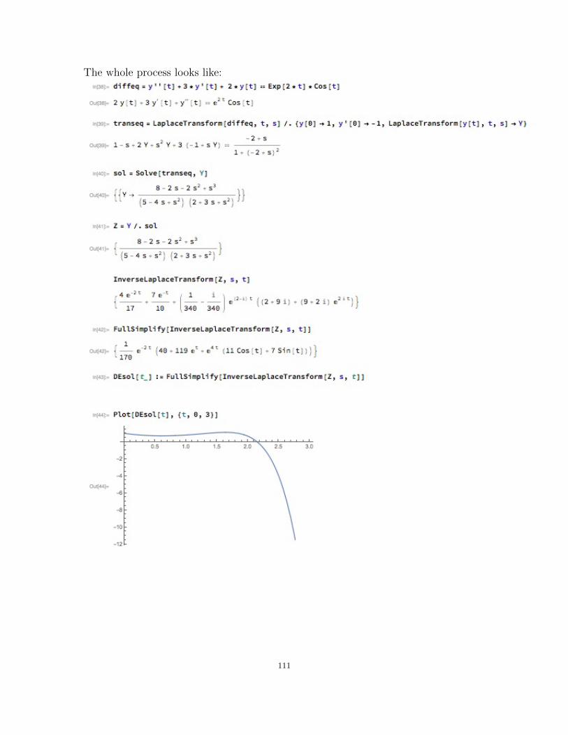
The whole process looks like:
111
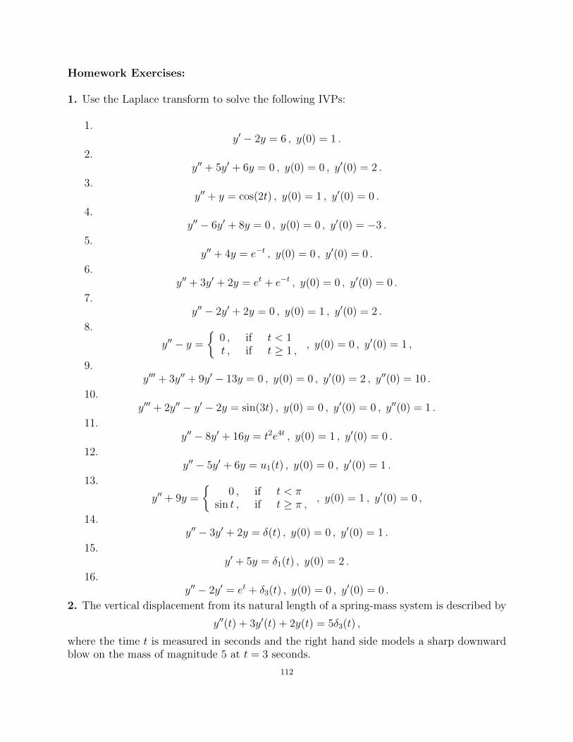
Homework Exercises:
1. Use the Laplace transform to solve the following IVPs:
1.y′ − 2y = 6 , y(0) = 1 .
2.y′′ + 5y′ + 6y = 0 , y(0) = 0 , y′(0) = 2 .
3.y′′ + y = cos(2t) , y(0) = 1 , y′(0) = 0 .
4.y′′ − 6y′ + 8y = 0 , y(0) = 0 , y′(0) = −3 .
5.y′′ + 4y = e−t , y(0) = 0 , y′(0) = 0 .
6.y′′ + 3y′ + 2y = et + e−t , y(0) = 0 , y′(0) = 0 .
7.y′′ − 2y′ + 2y = 0 , y(0) = 1 , y′(0) = 2 .
8.
y′′ − y =
{0 , if t < 1t , if t ≥ 1 ,
, y(0) = 0 , y′(0) = 1 ,
9.y′′′ + 3y′′ + 9y′ − 13y = 0 , y(0) = 0 , y′(0) = 2 , y′′(0) = 10 .
10.y′′′ + 2y′′ − y′ − 2y = sin(3t) , y(0) = 0 , y′(0) = 0 , y′′(0) = 1 .
11.y′′ − 8y′ + 16y = t2e4t , y(0) = 1 , y′(0) = 0 .
12.y′′ − 5y′ + 6y = u1(t) , y(0) = 0 , y′(0) = 1 .
13.
y′′ + 9y =
{0 , if t < π
sin t , if t ≥ π ,, y(0) = 1 , y′(0) = 0 ,
14.y′′ − 3y′ + 2y = δ(t) , y(0) = 0 , y′(0) = 1 .
15.y′ + 5y = δ1(t) , y(0) = 2 .
16.y′′ − 2y′ = et + δ3(t) , y(0) = 0 , y′(0) = 0 .
2. The vertical displacement from its natural length of a spring-mass system is described by
y′′(t) + 3y′(t) + 2y(t) = 5δ3(t) ,
where the time t is measured in seconds and the right hand side models a sharp downwardblow on the mass of magnitude 5 at t = 3 seconds.
112

Describe the position of the mass after 10 seconds, if the mass is released 0.2m above theequilibrium position.
3. The charge q(t) on the capacitor in an series RLC circuit is given by the DE
1
8q′′ + 5q′ + 500q = E(t) , q(0) = 0C , q′(0) = 20A ,
where
E(t) =
{0, if 0 ≤ t < 10π
100(sin(50t) + cos(50t)), if t ≥ 10π.
Find q(40).
113

6.5. Solving systems of first order linear differential equations with the Laplacetransform
With the Laplace transform we can solve systems of linear differential equations with constantcoefficients, too, No extra preparation is needed.Let’s solve the following system of differential equations:{
y′(t) = 2y(t) + 3z(t)z′(t) = 2y(t) + z(t)
(6.5.7)
with the initial conditions y(0) = 1, z(0) = 4.
We apply the Laplace transform to the DEs and for simplicity we write Y and Z instead ofY (s) and Z(s). {
sY − 1 = 2Y + 3ZsZ − 4 = 2Y + Z .
By rearranging the terms we get that{(s− 2)Y − 3Z = 1−2Y + (s− 1)Z = 4 .
(6.5.8)
We can eliminate Z by multiplying the first equation by (s − 1), the second equation by 3and then adding them. In this way we get that
Y (s) =s+ 11
(s− 4)(s+ 1).
The partial fraction decomposition leads to
Y (s) =3
s− 4− 2
s+ 1,
and therefore, by the inverse Laplace transform, we obtain that
y(t) = 3e4t − 2e−t .
Solving the first equation of the system (6.5.8) in Z leads to
Z =(s− 2)Y
3− 1
3=s− 2
s− 4− 2
3
s− 2
s+ 1− 1
3
=1 +2
s− 4− 2
3
(1− 3
s+ 1
)− 1
3
=2
s− 4+
2
s+ 1.
So, by the inverse Laplace transform we get that
z(t) = 2e4t + 2e−t .
Therefore, system (6.5.7) has the following pair of solutions
y(t) = 3e4t − 2e−t
z(t) = 2e4t + 2e−t
114
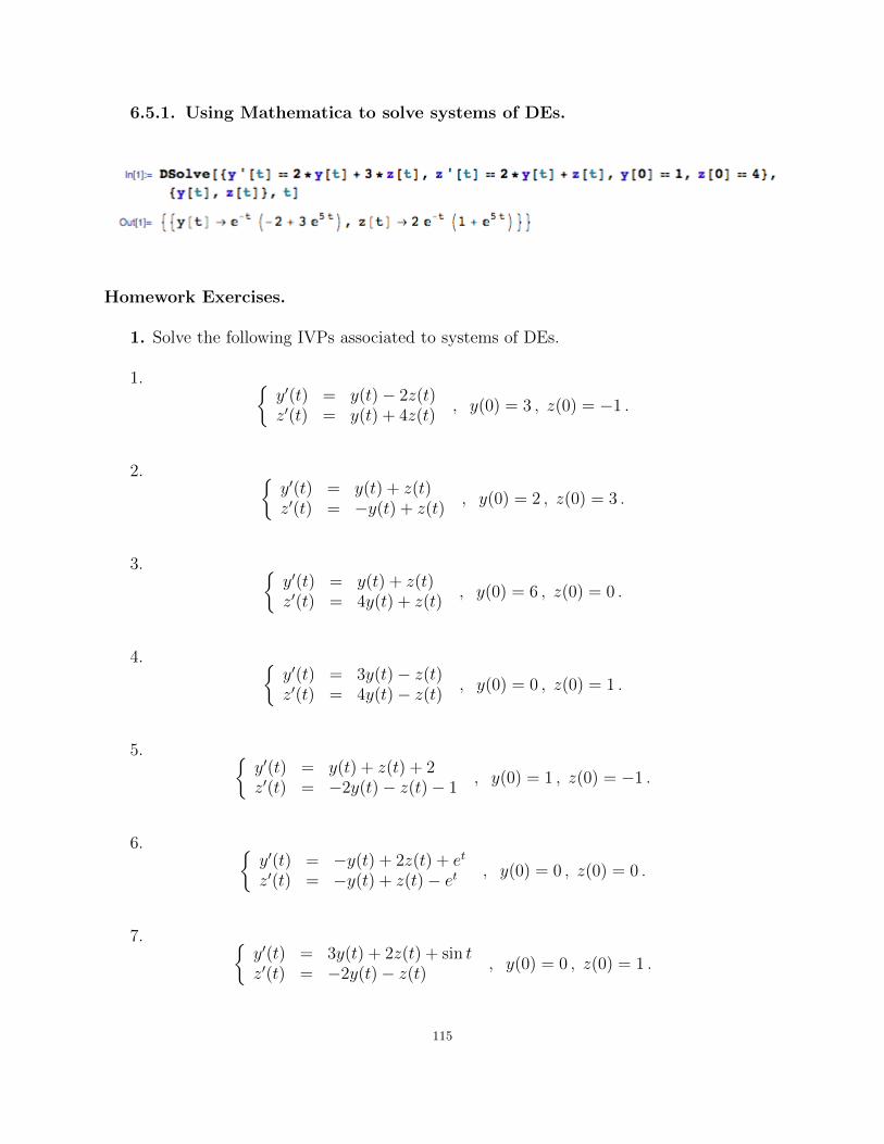
6.5.1. Using Mathematica to solve systems of DEs.
Homework Exercises.
1. Solve the following IVPs associated to systems of DEs.
1. {y′(t) = y(t)− 2z(t)z′(t) = y(t) + 4z(t)
, y(0) = 3 , z(0) = −1 .
2. {y′(t) = y(t) + z(t)z′(t) = −y(t) + z(t)
, y(0) = 2 , z(0) = 3 .
3. {y′(t) = y(t) + z(t)z′(t) = 4y(t) + z(t)
, y(0) = 6 , z(0) = 0 .
4. {y′(t) = 3y(t)− z(t)z′(t) = 4y(t)− z(t)
, y(0) = 0 , z(0) = 1 .
5. {y′(t) = y(t) + z(t) + 2z′(t) = −2y(t)− z(t)− 1
, y(0) = 1 , z(0) = −1 .
6. {y′(t) = −y(t) + 2z(t) + et
z′(t) = −y(t) + z(t)− et , y(0) = 0 , z(0) = 0 .
7. {y′(t) = 3y(t) + 2z(t) + sin tz′(t) = −2y(t)− z(t)
, y(0) = 0 , z(0) = 1 .
115

8. {y′(t) = 2y(t)− z(t) + et
z′(t) = 3y(t)− 2z(t) + 4t, y(0) = 1 , z(0) = 2 .
9. {y′(t) = 2z(t) + 2z′(t) = y(t) + 3z(t) + e−t
, y(0) = 0 , z(0) = 0 .
10. {y′(t) = 2y(t) + 2z(t) + et
z′(t) = y(t) + 3z(t) + 4t.
2. Suppose that we have two tanks with salt water. Fresh water flows into the first tankand is stirred with the existing salt water. The mixture flows into the second tank and afterwell-stirred, part of the outflow flows back into the first tank. We denote by y(t) and z(t)the amount of salt in the two tanks. Knowing the rate of flows, measured in gallon/hour,suppose that we obtained the following system of DEs:{
y′(t) = −y(t) + 4z(t)z′(t) = y(t)− z(t)
.
Find out the salt present in the two tanks after 3 hours, if the initial amounts were y(0) = 100and z(0) = 200 pounds.
116

CHAPTER 7
Appendix: Mathematica files
117

Derivatives and plots with Mathematica
Define the function:
In[1]:= f@t_D := t � Ht^2 - 1L
Two options to calculate the derivative:
In[2]:= f'@tD
Out[2]= -
2 t2
I-1 + t2M2+
1
-1 + t2
In[3]:= D@f@tD, tD
Out[3]= -
2 t2
I-1 + t2M2+
1
-1 + t2
Simplify the expression if needed:
In[4]:= FullSimplify@f'@tDD
Out[4]= -
1 + t2
I-1 + t2M2
Graph the function f(t) on the interval [-5,5]:
In[5]:= Plot@f@tD, 8t, -5, 5<D
Out[5]=-4 -2 2 4
-2
-1
1
2
118
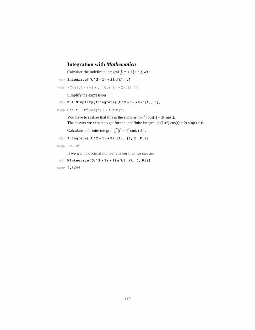
Integration with Mathematica
Calculate the indefinite integral Ù It2 + 1M sinHtL â t :
In[1]:= Integrate@Ht^2 + 1L * Sin@tD, tD
Out[1]= -Cos@tD - I-2 + t2M Cos@tD + 2 t Sin@tD
Simplify the expression
In[2]:= FullSimplify@Integrate@Ht^2 + 1L * Sin@tD, tDD
Out[2]= Cos@tD - t2 Cos@tD + 2 t Sin@tD
You have to realize that this is the same as (1-t2) cos(t) + 2t sin(t).The answer we expect to get for the indefinite integral is (1-t2) cos(t) + 2t sin(t) + c.
Calculate a definite integral Ù0þIt2 + 1M sinHtL â t :
In[3]:= Integrate@Ht^2 + 1L * Sin@tD, 8t, 0, Pi<D
Out[3]= -2 + Π2
If we want a decimal number answer than we can use
In[4]:= NIntegrate@Ht^2 + 1L * Sin@tD, 8t, 0, Pi<D
Out[4]= 7.8696
119
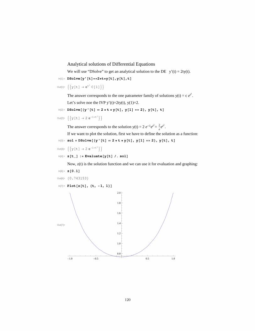
Analytical solutions of Differential Equations
We will use “DSolve” to get an analytical solution to the DE y’(t) = 2ty(t).
In[1]:= DSolve @y' @t D==2∗t ∗y@t D,y @t D,t D
Out[1]= 99y@tD → �t2C@1D==
The answer corresponds to the one patrameter family of solutions y(t) = c et2.
Let’s solve noe the IVP y’(t)=2ty(t), y(1)=2.
In[2]:= DSolve @8y ' @t D � 2 ∗ t ∗ y@t D, y @1D == 2<, y @t D, t D
Out[2]= 99y@tD → 2 �−1+t2==
The answer corresponds to the solution y(t) = 2 e-1et2= 2
eet2.
If we want to plot the solution, first we have to define the solution as a function:
In[3]:= sol = DSolve @8y ' @t D � 2 ∗ t ∗ y@t D, y @1D == 2<, y @t D, t D
Out[3]= 99y@tD → 2 �−1+t2==
In[4]:= z@t_ D : = Evaluate @y@t D ê. sol D
Now, z(t) is the solution function and we can use it for evaluation and graphing:
In[6]:= [email protected] D
Out[6]= 80.743153<
In[7]:= Plot @z@t D, 8t, −1, 1 <D
Out[7]=
-1.0 -0.5 0.5 1.0
0.8
1.0
1.2
1.4
1.6
1.8
2.0
120

Numerical Solutions of Differential Equations with Mathematica
We will solve numerically the IVP y’(t)=4t yHtL , y(0)=0.16.
In[2]:= sol = NDSolve@8y'@tD � 4 * t * Sqrt@y@tDD, y@0D � 0.16<, y@tD, 8t, 0, 1<D
Out[2]= 88y@tD ® InterpolatingFunction@880., 1.<<, <>D@tD<<
In[3]:= q@t_D := Evaluate@y@tD �. solD
In[4]:= [email protected]
Out[4]= 80.926402<
In[5]:= Plot@q@tD, 8t, 0, 1<D
Out[5]=
0.2 0.4 0.6 0.8 1.0
0.5
1.0
1.5
2.0
121

The Laplace transform and inverse Laplace transform of functions.
In[23]:= LaplaceTransform@Sin@tD, t, sD
Out[23]=
1
1 + s2
In[25]:= LaplaceTransform@t^2 * Exp@3 * tD + t, t, sD
Out[25]=
2
H-3 + sL3
+1
s2
In[27]:= InverseLaplaceTransform@1 � H1 + sL, s, tD
Out[27]= ã-t
In[28]:= InverseLaplaceTransform@Exp@-sD � s, s, tD
Out[28]= HeavisideTheta@-1 + tD
HeavisideTheta is the unit step function, so HeavisideTheta[-1+t]=u1HtL.
In[29]:= Plot@HeavisideTheta@-1 + tD, 8t, 0, 3<D
Out[29]=
0.5 1.0 1.5 2.0 2.5 3.0
0.2
0.4
0.6
0.8
1.0
In[30]:= InverseLaplaceTransform@1, s, tD
Out[30]= DiracDelta@tD
In[31]:= InverseLaplaceTransform@Exp@-3 * sD, s, tD
Out[31]= DiracDelta@-3 + tD
With our notations DiracDelta[-3+t]=u3HtL.
122

Solving IVPs with the Laplace transform.
Let’s solve the IVP y’’+3y’+2y=e2 t
+cos(t), y(0)=1, y’(0)=-1.
In[8]:= diffeq = y''@tD + 3 * y'@tD + 2 * y@tD � Exp@2 * tD * Cos@tD
Out[8]= 2 y@tD + 3 y¢@tD + y
¢¢@tD � ã2 t
Cos@tD
In[9]:= transeq = LaplaceTransform@diffeq, t, sD �.
8y@0D ® 1, y'@0D ® -1, LaplaceTransform@y@tD, t, sD ® Y<
Out[9]= 1 - s + 2 Y + s2
Y + 3 H-1 + s YL �-2 + s
1 + H-2 + sL2
In[10]:= sol = Solve@transeq, YD
Out[10]= ::Y ®8 - 2 s - 2 s
2 + s3
I5 - 4 s + s2M I2 + 3 s + s
2M>>
In[11]:= Z = Y �. sol
Out[11]= :8 - 2 s - 2 s
2 + s3
I5 - 4 s + s2M I2 + 3 s + s
2M>
In[12]:= InverseLaplaceTransform@Z, s, tD
Out[12]= :4 ã-2 t
17
+7 ã-t
10
+1
340
-ä
340
ãH2-äL t IH2 + 9 äL + H9 + 2 äL ã
2 ä tM>
In[13]:= FullSimplify@InverseLaplaceTransform@Z, s, tDD
Out[13]= :1
170
ã-2 t I40 + 119 ã
t+ ã
4 t H11 Cos@tD + 7 Sin@tDLM>
In[16]:= DEsol@t_D := FullSimplify@InverseLaplaceTransform@Z, s, tDD
In[18]:= N@DEsol@1DD
Out[18]= 80.803708<
123