dhi-wasy software feflowfeflow.info/fileadmin/feflow6/feflow_6.0_tutorial.pdf · dhi-wasy software...

DHI-WASY Software

FEFLOW®

6Finite Element Subsurface Flow

& Transport Simulation System

Installation Guide & Demonstration Exercise

2

Copyright notice:

No part of this manual may be photocopied, reproduced, or translated without written permission ofthe developer and distributor DHI-WASY GmbH.

Copyright © 2010 DHI-WASY GmbH Berlin – all rights reserved.

DHI-WASY, FEFLOW and WGEO are registered trademarks of DHI-WASY GmbH.

DHI-WASY GmbH

Waltersdorfer Straße 105, 12526 Berlin, Germany

Phone: +49-(0)30-67 99 98-0,

Fax: +49-(0)30-67 99 98-99

E-Mail: [email protected]

Internet: www.feflow.info

www.dhigroup.com

3

FEFLOW 6

I Installation Guide 4

I.1 Introduction 4

I.2 Installing FEFLOW (Windows) 5

l.2.1 Introduction 5

I.2.2 System recommendations 6

I.2.3 FEFLOW Installation 6

I.2.4 Demo Data Installation 7

l.2.5 Installation of the X server

Exceed 2006 7

l.2.6 Installation of the Network License

Manager NetLM 8

I.2.7 License installation 8

I.3 Installing FEFLOW (Linux) 9

I.4 Installation Packages 10

II Demonstration Exercise 11

II.1 Introduction 11

II.1.1 About FEFLOW 11

II.1.2 Scope and Structure 11

II.1.3 Terms and Notations 12

II.1.4 Requirements 12

II.1.5 Model Scenario 13

II.2 Getting Started 14

II.2.1 Starting FEFLOW 14

II.2.2 The FEFLOW 6 User Interface 14

II.3 Geometry 15

II.3.1 Maps and Model Bounds 15

II.3.2 Supermesh 16

II.3.3 Finite element-mesh 19

II.3.4 Expansion to 3D 21

II.4 Problem settings 28

II.5 Model Parameters 30

II.5.1 Initial conditions 30

II.5.2 Boundary conditions 32

II.5.3 Material properties 37

II.6 Simulation 39

II.7 Flow Transport Model 42

II.7.1 Problem settings 42

II.7.2 Initial Conditions 44

II.7.3 Boundary conditions 45

II.7.4 Material properties 46

II.7.5 Vertical resolution 46

II.7.6 Reference data 48

II.7.7 Simulation Run 49

II.7.8 Postprocessing 50

Contents

4Installation Guide & Demonstration Exercise

I.1 Introduction

The FEFLOW simulation package contains the fol-lowing main programs along with additional soft-ware tools:

FEFLOW® 6.0

Interactive finite-element simulation system formodeling 3D and 2D flow, mass and heat trans-port processes in ground water and the vadosezone.

FEFLOW is provided on DVD for the following platforms:

32-bit operating systems

• Windows XP, Vista, 7, Server 2003, Server 2008

• Linux: CentOS 4.6 (RedHat family), OpenSUSE11.0 (SUSE family), Ubuntu 8.04 (Debian fam-ily)

64-bit operating systems

• Windows XP x64 Edition, Vista x64 Edition,7 x64 Edition, Server 2003 x64 Edition,Server 2008 x64 Edition

• Linux: CentOS 4.4 (RedHat family), OpenSUSE11.0 (SUSE family), Ubuntu 8.04 (Debian fam-ily)

FEFLOW for other Linux distributions may be avail-able for download from the FEFLOW websitewww.feflow.info. If you need FEFLOW for anotherLinux distribution, please do not hesitate to con-tact us at [email protected]!

For evaluation purposes, it is possible to obtain afully functional but time-limited license from DHI-WASY, one of the DHI offices, or from your local FEFLOW distributor.

FEFLOW® ViewerFEFLOW Viewer is free software for visualizingFEFLOW models and results and for postprocess-ing purposes. FEFLOW Viewer is installed withFEFLOW.

WGEO® 6.0

WGEO® is a sophisticated georeferencing,geoimaging and coordinate transformation soft-ware developed by DHI-WASY GmbH. A licensefor WGEO® Basis and the flexible 7-parametertransformation comes with each FEFLOW licenseand is installed automatically.

WGEO® is provided for the Windows platform.

I Installation Guide

5

IFEFLOW 6

I.2 Installing FEFLOW (Windows)

I.2.1 Introduction

FEFLOW 6 Standard provides powerful state-of-the-art editing and visualization tools for mostkinds of applications. As some of the lesser usedfunctionality for data input is not yet implementedin FEFLOW 6 Standard, FEFLOW 6 Classic is pro-vided as a fallback. Convenient tools make it easyto switch between the two types of user interface.

The FEFLOW 6 Classic requires an X server runningon display number 10 for proper operation. DHI-WASY recommends to use Hummingbird Exceed2006 for this purpose, a customized version ofwhich is available on the FEFLOW DVD. It may onlybe used in conjunction with FEFLOW.

To run FEFLOW in single-seat mode, the DHI-WASYLicense Manager NetLM has to be installed locally.Only NetLM has to be installed on network licenseservers, distributing FEFLOW licenses to clients inthe network.

So a typical FEFLOW installation on a Windowsoperating system consists of four steps:

• Installation of FEFLOW and additional programs

• Installation of the demo data package

• Installation of the X server Exceed 2006 (onlyneeded for running FEFLOW 6 Classic)

• Installation of the DHI-WASY license managerNetLM

After inserting the DVD into the DVD drive, anoverview of the DVD contents is shown automat-ically. If autostart is disabled, run Starter.exe fromthe windows directory on the DVD.

The hyperlinks in the overview can be used to startthe different parts of the FEFLOW installation, toview the documentation and example movies, andto install third-party software.

FEFLOW is automatically installed as a 32 bit ver-sion on 32 bit systems, and as 32 and 64 bit ver-sions on 64 bit operating systems.


IInstallation Guide

I.2.2 System recommendations

The following system specifications are recom-mended as a minimum configuration. Thememory requirements depend on the size andcomplexity of the actual model to be simula-ted.• 512 MB RAM

• 450 MB of disk space

• Screen resolution of 1280 x 1024 or higher forFEFLOW 6 Classic

• Separate graphics card with up-to-date graph-ics driver

I.2.3 FEFLOW Installation

Start the Windows Installer by clicking on thehyperlink FEFLOW Program Files. Click Next aftereach step to proceed to the next step.

1. A Welcome screen appears first.

2. In the next step, the License Agreement has tobe accepted. Please read it carefully before pro-ceeding with the installation.

3. In the License window, choose Demo for testingFEFLOW without a license. Select Client if thelicense to be used is installed on a remotelicense server (Network License) and type in thename or IP number of the license server. ChooseServer if a Single Seat License is to be used or ifthe machine is intended to act as a license serverfor a Network License.

7

IFEFLOW 6

4. Select the packages to install. Details about thepackages can be found on the right of the win-dow and on page 10 of this booklet. Thedefault installation location is C:\ProgramFiles\WASY\FEFLOW 6.0. For specifying a dif-ferent destination directory, click Browse.

5. Start the installation or go back to change thesettings.

6. FEFLOW is installed. This may take several min-utes.

7. Finish the installation by clicking Finish.

I.2.4 Demo Data Installation

The demo data installation is started by clicking onthe hyperlink FEFLOW Demo Data.

I.2.5 Installation of the X server Exceed 2006

Before installing Hummingbird Exceed forFEFLOW, we recommend to manually deinstall allprevious versions of Exceed.


IInstallation Guide

Start the installation by clicking on the corre-sponding hyperlink. The setup installs all parts ofExceed 2006 (version 11) required for runningFEFLOW. The basic X server settings are cus-tomized for running FEFLOW.

Terminal Server installationOn Terminal Server, the installation of Exceed2006 has to be performed in a different way:Follow the procedure described inConnectivityInstallation.pdf (Chapter 3, Installationon a Terminal Server), located in the win-dows\exceed directory of the FEFLOW DVD.

I.2.6 Installation of the NetworkLicense Manager NetLM

Before installing the Network License ManagerNetLM we recommend to deinstall all previousversions of NetLM.

The installation is started by clicking on the hyper-link License Manager NetLM. Follow the instructionsin the installation dialog.

There is only onedongle for each copy of FEFLOW.

If the dongle is lost, it canonly be replaced by purcha-sing a new license of FEFLOW!

I.2.7 License installation

This step can be skipped for working in Demomode only. All license installations have to be donewith administrator privileges.

Make sure that the firewall allows (local) TCP/IPconnections on port 1800.

• Install the dongle (hardware lock) on the USBport or parallel port resp. Start the DHI-WASYLicense Administration tool by clicking on theWASY License Administration entry in the AllPrograms\WASY group of the Windows start menu.

license information in comparison to the infor-mation provided on the license sheet. The infor-mation has to be identical in all details.

• Click OK to close the License Administration dia-log.

• Choose FEFLOW 6.0 from the WASY programgroup or double click on the desktop icon tostart FEFLOW.

Using a Network License for FEFLOW, the WASYLicense Manager can be installed on any computerwithin the network (LAN or WAN) without thecomplete FEFLOW installation. Clients need TCP/IPconnection on port 1800 to have access to thelicense server.

I.3 Installing FEFLOW (Linux)

• Browse to the linux directory on the DVD.

• Browse to the sub directory corresponding toyour Linux distribution.

• For a full installation, use the following com-mand: rpm -i *.rpm

• For deinstalling all WASY packages, use rpm -

e ‘rpm -qa | grep ’^wasy-’‘

• Note that you may need root privileges to per-form these commands.

9

IFEFLOW 6

• In the tree view on the left side, select Donglelicense in the FEFLOW 6.0 branch. In theHostname or IP address field, insert localhost ifthe dongle is installed locally, or insert the nameor the IP number of the remote license man-ager.

• Click Connect. Check whether the numberreturned in the field HOSTID is identical to thenumber on the FEFLOW license sheet. In casethat multiple dongles of the same brand areconnected, a HOSTID mismatch may occur. Inthis case remove all dongles except the DHI-WASY dongle.

• Switch to the Licenses tab and enter the licenseinformation from the FEFLOW license sheet. Thelicense information can be pasted from the clip-board if the license has been received digitally.Copy the selected section in the license docu-ment to the clipboard and use on the Pastelicense from clipboard button to insert all thelicense information at once. Please also makesure that the same license type as on the licensesheet is selected:

• Single seat license – FEFLOW can be run onlyon the computer the dongle is attached to.

• Network license – FEFLOW can be used on anycomputer connected to the license server viaTCP/IP network (LAN or WAN/internet).

• Click Install. A message box indicates that thelicense has been successfully installed. If theinstallation was not successful, check all the

For the version,please note thatyou have to use

“6.0x” because your licenseis valid for all sub-versionsof FEFLOW 6.0.

For the 64 bit ver-sion of FEFLOW, aHASP HL USB

dongle is required. If you donot already have such adongle, please contact yourFEFLOW distributor or DHI-WASY for a dongleexchange!


IWGEO

Georeferencing, geoimaging and transformationsoftware - a WGEO license is installed automati-cally.

• WGEO help - online help system

• German Transformations - coordinate transfor-mation routines for Germany (may require sep-arate licensing)

• Desktop shortcut icon - WGEO icon on theWindows desktop

Plot Assistant

GIS-like software for producing plots with FEFLOWdata.

Data Tools

Scripts for data checking and format conversion.

In the demo data installation there are the follow-ing packages:

• Examples - example models

• Exercise - data for the demonstration exercise

• Tutorial - data for the tutorials (User Manual)

• Benchmarks - benchmark models

Installation Guide

I.4 Installation Packages• Packages for installation can be selected during

the first installation or by re-running the instal-lation in Modify mode.

• A description for each package is shown in theright part of the Select feature dialog of theinstallation by selecting one of the packages.

• The following packages are available:

FEFLOW

FEFLOW program files - required for runningFEFLOW

• Help - FEFLOW help system

• Interface Manager SDK - development kit forthe open programming interface IFM (requiredfor plug-in development)

• Desktop shortcut icon - WGEO icon on theWindows desktop

WGEO Basis islicensed automa-tically with

FEFLOW. If a license dialogshow up, just click onCancel.

11

FEFLOW 6

II.1 Introduction

II.1.1 About FEFLOW

FEFLOW (Finite Element subsurface FLOW andtransport system) is an interactive groundwatermodeling system for

• three-dimensional and two-dimensional

• areal and cross-sectional (horizontal, vertical oraxisymmetric)

• fluid density-coupled, also thermohaline, oruncoupled

• variably saturated

• transient or steady state

• flow, mass and heat transport

• reactive multi-species transport

in subsurface water resources with or without oneor multiple free surfaces.

FEFLOW can be efficiently used to describe thespatial and temporal distribution and reactions ofgroundwater contaminants, to model geothermalprocesses, to estimate the duration and traveltimes of chemical species in aquifers, to plan anddesign remediation strategies and interceptiontechniques, and to assist in designing alternativesand effective monitoring schemes.

Sophisticated interfaces to GIS and CAD data as wellas simple text formats are provided.

The option to use and develop user-specific plug-ins via the programming interface (InterfaceManager IFM) allows the addition of external codeor even external programs to FEFLOW.

FEFLOW is available for WINDOWS systems as wellas for different Linux distributions.

Since its first appearance in 1979 FEFLOW hasbeen continuously extended and improved. It isconsistently maintained and further developed bya team of experts at DHI-WASY. FEFLOW is usedworldwide as a high-end groundwater modelingtool at universities, research institutes, governmentagencies and engineering companies.

For additional information about FEFLOW pleasedo not hesitate to contact your local DHI office,one of the FEFLOW distributors, DHI-WASY, orhave a look at the FEFLOW web sitehttp://www.feflow.info.

II.1.2 Scope and Structure

This exercise provides a step-by-step descriptionof the setup, simulation, and post processing of athree-dimensional flow and transport model basedon (simplyfied) real-world data, showing thephilosopy and handling of the FEFLOW user inter-face.

II Demonstration Exercise


IIDemonstration Exercise

You can skip anyof the steps in thisexercise by loading

already prepared files atcertain stages. These filesare not necessarily ready torun in the simulator.

The demonstration exercise is not intended as anintroduction to groundwater modeling itself.Therefore, some background knowledge ofgroundwater modeling is required, or commonliterature should be consulted in parallel.

The exercise covers the following work steps:

• Import of background maps

• Definition of the basic model geometry

• Generation of a 2D finite-element mesh

• Expansion of the mesh to 3D

• Setup of a steady-state flow and transient trans-port model, including initial conditions, bound-ary conditions and material properties

• Import of GIS data and regionalization

• Simulation run

• Results visualization and post processing

II.1.3 Terms and Notations

In addition to the verbal description of the requiredscreen actions this exercise makes use of someicons. They are intended to assist in relating thewritten description to the graphical informationprovided by FEFLOW. The icons refer to the kindof setting to be done:

main menu

context menu

toolbar

panel

button

input box for text or numbers

switch toggle

radio button

checkbox

All file names are printed in bold red, map namesare printed in red, numbers to be input in boldgreen. Keyboard keys are referenced in <italic>style. All required files are available in the FEFLOWdemo data. The symbol indicates an inter-mediary stage where either a prepared file can beloaded to resume this exercise or - if working witha license - the model can be saved. Thus the exer-cise does not have to be done in one step even indemo mode.

II.1.4 Requirements If not already done, please install the FEFLOW soft-ware including the demo data package. A license isnot necessary to run this tutorial (FEFLOW can be runin demo mode).The latest version of FEFLOW can be downloadedfrom the website www.feflow.info. In case of anyproblems or additional questions please do not hes-itate to contact the FEFLOW technical support ([email protected] ).

For following theexercise, the demodata files for

FEFLOW have to be instal-led. The demo data instal-lation package is availableon the FEFLOW DVD aswell as on the FEFLOW website for download.

13

IIFEFLOW 6

II.1.5 Model Scenario

A fictitious contaminant has been detected nearthe small town of Friedrichshagen, in the south-east of Berlin, Germany. An increasing concentra-tion of nitrate can be observed in two water supplywells. There are two potential sources of the con-tamination: The first are abandoned sewage fieldsclose to a waste-water treatment plant located inan industrial area northeast of town. The otherpossible source is an abandoned waste-disposalsite further east.

A three-dimensional groundwater flow and con-taminant transport model is set up to evaluate theoverall threat to groundwater quality, and to quan-tify the potential pollution. First, the model domainneeds to be defined. The town is surrounded bymany natural flow boundaries, such as rivers andlakes. There are two small rivers that run north-south on either side of Friedrichshagen that canact as the eastern and western boundaries. Thelake Müggelsee can limit the model domain to thesouth. The northern boundary is chosen along aneast-west hydraulic contour line of groundwaterlevel north of the two potential sources of the con-tamination.

The geology of the study area is comprised ofQuaternary sediments. The hydrogeologic systemcontains two main aquifers separated by anaquitard. The top hydrostratigraphic unit is con-sidered to be a sandy unconfined aquifer up to 7meters thick. The second aquifer located belowthe clayey aquitard has an average thickness ofapproximately 30 meters.

The northern part of the model area is primarilyused for agriculture, whereas the southern portionis dominated by forest. In both parts, significanturbanized areas exist.



II.2 Getting Started

II.2.1 Starting FEFLOW

On Windows Systems• Start FEFLOW 6.0 via the corresponding desk-

top icon or the startup menu entry.

On Linux Systems• Type feflow60q in a console window and press

<Enter> .

If no FEFLOW license is available, FEFLOW askswhether to start in demo mode. The demo modedoes not allow loading and saving of files withmore than 500 nodes, and it does not allow toexecute the simulation run. Specially prepareddemo files coming with FEFLOW are an exception.Such files are provided for this example so that themodel setup can be interrupted and picked upagain, and the simulation runs can be performed.

II.2.2 FEFLOW 6 User Interface

The user interface components are organized in amain menu, toolbars, panels, view windows, anddialogs.

While the main menu is always visible, the otherparts of the interface can be customized, addingor hiding particular toolbars and panels by using

the menu command View > Panelsand View > Toolbars, respectively. Please keepin mind that not all panels and toolbars are dis-played by default. Thus this exersice may requireto access a function in a toolbar or panel that isnot visible at that moment. The toolbar or panelhas to be added then.

View windows display a certain type of view onthe model and its properties. There are four dif-ferent types of view windows: Supermesh view, FE-Slice view, 3D view and Cross-Section view. Differentkinds of tools are linked to the different view types.

View windows can be closed via the correspon-ding button in the view frame. New view windowscan be opened by selecting Window > Newand choosing the respective view window type.

The last type of user interface component relevantfor the exercise are diagrams. Looking very simi-lar to panels, they contain plots of time curves.Missing diagram windows can be added to theuser interface by opening View > Diagram from

the menu and choosing the required diagramfrom the list.

Last, but not least it might be worth to mentionthat all steps done in FEFLOW can be undone andredone via the corresponding toolbar buttons.There is no limit on the number of undo steps.

II.3 Geometry

II.3.1 Maps and Model Bounds

When FEFLOW starts, by default a new docu-ment is opened. A new document can also be

created using the menu command File >

New or the New button in the Standardtoolbar.

The first step of model setup is the definition ofthe Initial Domain Bounds. This can be done man-ually, or by loading georeferenced maps.

All necessary files for this exercise are provided withthe FEFLOW Demo Data package and are locatedin the project folder demo/exercise/standard. Themap files are found in the subdirectoryimport+export.

Click on Load map(s). Load all the followingmaps at once (by holding <Ctrl> on the keyboard)to ensure that FEFLOW uses the bounding box ofall the maps to define the initial domain bounds.

15

IIFEFLOW 6

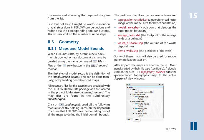
The particular map files that are needed now are:

• topography_rectified.tif (a georeferenced rasterimage of the model area for better orientation)

• model_area.shp (a polygon that denotes theouter model boundary)

• sewage_fields.dxf (the footprint of the sewagefields as a polygon)

• waste_disposal.shp (the outline of the wastedisposal site)

• demo_wells.shp (the positions of the wells)

Some of these maps will also be used for modelparameterization later on.

After import, the maps are listed in the Mapspanel, sorted by their file type (see figure). A doubleclick on the Geo-TIFF topography_rectified adds thegeoreferenced topographic map to the activeSupermesh view window.



Except for the map sewage-fields, all other maps areESRI shape files. These vector files occupy their ownbranch in the tree, each with a default map layer.Double-click on all the Default layer entries to addthe visualization layers of the shape files to theSupermesh view.

Now have a closer look at a second panel, theView Components panel. This panel lists the com-

ponents that are currently plotted in the active viewwindow.

When having double-clicked on the maps in theMaps panel, the maps have been added to the

tree in the View Components panel.

The drawing order of maps can be modified bydragging them with the mouse to another posi-tion in the tree (this might become necessary asthe model area polygon may overlay the polygonsof the mass sources). The topmost map is drawnon top.

To switch a map on and off, the checkbox in frontof the map name can be checked/unchecked.Checking/unchecking the checkbox of an entirebranch all the maps in this branch become visi-ble/invisible at the same time.

The topographic map has mainly been loaded forproviding a regional context. For more clarity, itcan be switched off before starting with the fol-lowing operations. Make sure that the other mapsare visible.

II.3.2 Supermesh

In the simplest case, the supermesh contains a def-inition of the outer model boundary. In addition,geometrical features such as the position of pump-ing wells, the limits of areas with different prop-erties or the courses of rivers can be included tobe considered for the generation of the finite-ele-ment mesh. Additionally, the polygons, lines andpoints specified in the supermesh can be used lateron to assign boundary conditions or material prop-erties.

17

IIFEFLOW 6

As mentioned above, a supermesh may containthree types of features:

• polygons

• lines

• points

At least one polygon has to be created to definethe model area boundaries.

The editing tools are found in the Mesh Editortoolbar:

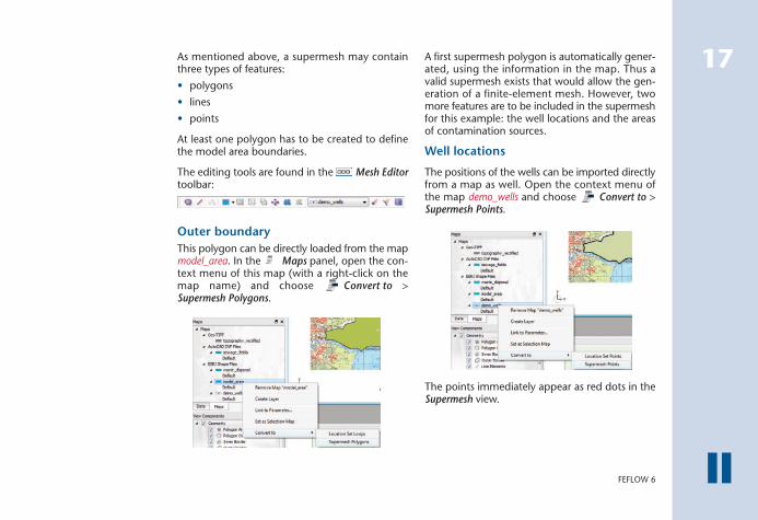
Outer boundary

This polygon can be directly loaded from the mapmodel_area. In the Maps panel, open the con-text menu of this map (with a right-click on themap name) and choose Convert to >Supermesh Polygons.

A first supermesh polygon is automatically gener-ated, using the information in the map. Thus avalid supermesh exists that would allow the gen-eration of a finite-element mesh. However, twomore features are to be included in the supermeshfor this example: the well locations and the areasof contamination sources.

Well locations

The positions of the wells can be imported directlyfrom a map as well. Open the context menu ofthe map demo_wells and choose Convert to >Supermesh Points.

The points immediately appear as red dots in theSupermesh view.


II

exercise_fri1.smh

Contamination sources

The estimated source areas of the contaminationsare to be represented in the supermesh by poly-gons. To avoid overlapping of polygons (which isnot allowed at any editing stage), the initial poly-gon covering the entire model area is partitionedmanually.

Click on Split Polygons. This tool allows to splitan existing polygon along a polyline to be drawn.Here, it is used to separate the two areas of con-tamination sources from the existing polygon.

Demonstration Exercise

Start with the eastern source of contamination (theformer waste-disposal site).

The splitting has to start and end at an alreadyexisting polygon border (but not necessarily atalready existing polygon nodes). As the contami-nation sources are located completely inside themodel area, two cuts are necessary when carvingthe new polygon from the existing one.

By selecting the map waste_disposal from the drop-down list in the Mesh Editor toolbar and acti-vating Snap to points, a snapping mode isemployed for the geometrical information in thecorresponding background map. The mouse cur-sor snaps to the exact position of the polygon mapnodes when clicking close to them. This allows foraccurate digitizing.

19

IIFEFLOW 6

The first cut starts on anarbitrary point on themodel boundary, thengoing half-way around thecontamination source andreturning to the modelboundary on the other side(see figure, red arrows). Thesecond cut completes thepolygon by cutting along

the missing part of the border of the outline of thewaste disposal (see figure, green arrows).

For the next step, select the map sewage_fields forsnapping in the dropdown list in the

Mesh Editor toolbar.

In the same way as before the polygon for thesewage fields, the western source of contamina-tion, is created. Use the Split Polygons tool tocreate polygon borders along its outline.

An example supermesh setup for both the disposalsite and the sewage fields is shown in the follow-ing figure.

Corrections

Accidently created polygons, lines, or points canbe selected by using the Select tool. They canbe deleted hitting <Del> on the keyboard.

Misplaced nodes in polygons or lines can beremoved during digitizing by going back to thelast correct node of the feature and clicking on it.

The position of a point can be corrected after apolygon or line has been finished by using the

Move node tool to shift its position (the snap-ping mode can be used here as well).

exercise_fri2.smh

II.3.3 Finite element-mesh

Once the outer boundary and other geometricalconstraints have been defined in the supermesh,the finite-element mesh can be generated.

All necessary tools can be found in theMesh Generator toolbar.

First, one of the mesh generation algorithms pro-vided by FEFLOW is chosen from the drop-downlist in the Mesh Generator toolbar.

For this example, choose Gridbuilder. Click

Generate Mesh to start mesh generation.

Zooming func-tions can be usedat any time. Press

and hold the right mousebutton, move the mouseup/down). Pan by pressingand holding the mousewheel and moving themouse to any direction.Also the mouse wheel maybe used for zooming.


IISwitch to the Supermesh view again to see the

Mesh Generation toolbar. If the view has beenaccidentally closed, re-open it bychoosing Window > New > Supermesh Viewfrom the menu.

Click on Generator Properties to open theGenerator Properties dialog.

Activate the Polygon gradation option bychecking the corresponding box and set a refine-ment level of 20 (the maximum). As only the poly-gon borders adjacent to the contamination sourcesneed refinement, this operation is to be appliedonly to Selected polygon or line-addin edges.


A new FE-Slice view is automatically opened,depicting the resulting finite-element mesh.

For our purpose, especially for the simulation ofcontaminant transport, this initially generatedmesh does not seem to be appropriate. A finer spa-tial resolution is required.

Activate the Supermesh view again so that theMesh Generator and Supermesh toolbar

become visible again.

In the Mesh Generator toolbar, enter 6000as the Total Number and hit Generate Meshagain. The finite-element mesh in the FE-Slice viewis updated, showing a much finer discretizationnow.

Local refinement

First, special attention should be paid to the areasof the contamination sources. At their borders, theoccurrence of high concentration gradients is likely,possibly requiring an even finer spatial resolutionto avoid oscillations in the solution. Consequently,the mesh needs local refinement along the poly-gon outlines.

Second, at the pumping wells steep hydraulic gra-dients are expected at the center of the well cone.To realistically represent these, fine discretizationis necessary, too.

Besides refine-ment along poly-gon borders,

FEFLOW also provides themeans to edit the desiredrelative mesh density on apolygon-by-polygon basis.

21

IIFEFLOW 6

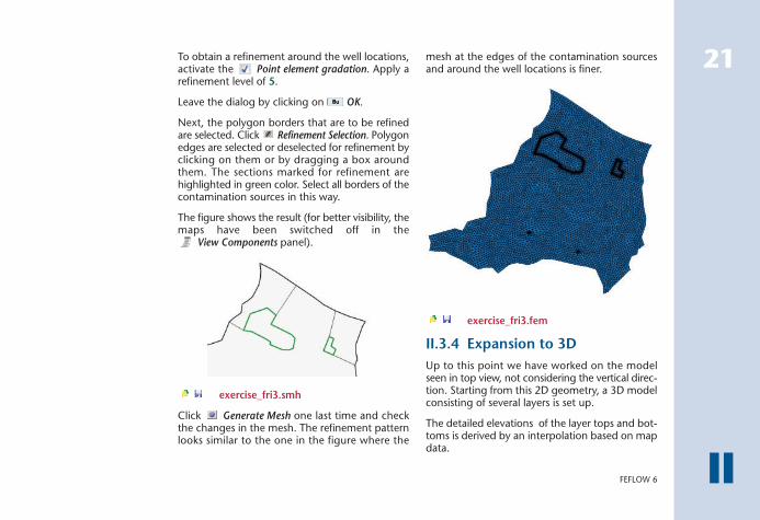
To obtain a refinement around the well locations,activate the Point element gradation. Apply arefinement level of 5.

Leave the dialog by clicking on OK.

Next, the polygon borders that are to be refinedare selected. Click Refinement Selection. Polygonedges are selected or deselected for refinement byclicking on them or by dragging a box aroundthem. The sections marked for refinement arehighlighted in green color. Select all borders of thecontamination sources in this way.

The figure shows the result (for better visibility, themaps have been switched off in the

View Components panel).

exercise_fri3.smh

Click Generate Mesh one last time and checkthe changes in the mesh. The refinement patternlooks similar to the one in the figure where the

mesh at the edges of the contamination sourcesand around the well locations is finer.

exercise_fri3.fem

II.3.4 Expansion to 3D

Up to this point we have worked on the modelseen in top view, not considering the vertical direc-tion. Starting from this 2D geometry, a 3D modelconsisting of several layers is set up.

The detailed elevations of the layer tops and bot-toms is derived by an interpolation based on mapdata.


IIFor this example, three geological layers are con-sidered for the model. An upper aquifer is limitedby the ground surface on top and by an aquitardat the bottom. A second aquifer is situated belowthe aquitard, underlain by a low permeable unitof unknown thickness. This underlying strati-graphic layer is assumed to be impervious and isnot part of the simulation.

FEFLOW distinguishes between layers and slices in3D. Layers are three-dimensional bodies that typ-ically represent geological formations like aquifersand aquitards. The interfaces between layers, aswell as the top and bottom model boundary arecalled slices.

In a first step, the numbers of layers and slices aredefined. The actual stratigraphic data are appliedin a second step afterwards.

Initial 3D Setup

Open Edit > 3D Layer Configuration.

In the upper left corner of the dialog, a text fieldshows the current number of layers (1). Increasethis value to 3 and hit <Enter>. This makesFEFLOW switch the model geometry to 3D, themodel containing 3 layers. The number of slicesautomatically changes to 3 + 1 = 4 . By default,the top slice has a spatially constant elevation of0 m. The other slices are placed below with a dis-tance of 1 m each.

With these default elevations that are close to theexpected real-world elevations, there is danger thatthe slices would temporarily intersect during theslice-wise assignment of elevations. FEFLOW doesat no time allow an intersection of slices and thus


23

IIFEFLOW 6

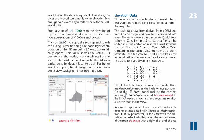
would reject the data assignment. Therefore, theslices are moved temporarily to an elevation lowenough to prevent any interference with the real-world data.

Enter a value of -1000 m to the elevation oftop slice input box and hit <Enter>. The slices arenow at elevations of -1000 m and below.

Click on Ok to apply the settings and to exitthe dialog. After finishing the basic layer confi-guration of the 3D model, a 3D view automati-cally opens. This view shows the actual 3Dgeometry of the model, now containing 4 planarslices with a distance of 1 m each. The 3D viewbackground by default is set to black. For bettervisibility in print, for all images in this exercise awhite view background has been applied.

exercise_fri4.fem

Elevation DataThis raw geometry now has to be formed into itsreal shape by regionalizing elevation data fromthe map files.

The basic data have been derived from a DEM andfrom borehole logs, and have been combined intoa text file (extension dat, tab separated) with fourcolumns: X, Y, Ele, and Slice. Such a file can beedited in a text editor, or in spreadsheet softwaresuch as Microsoft Excel or Open Office Calc.Containing the target slice number as a pointattribute, the file can be used as the basis forregionalization of elevations for all slices at once.The elevations are given in meters ASL.

The file has to be loaded as a map before its attrib-ute data can be used as the basis for interpolation.Go to the Maps panel and use the contextmenu ( Add Map(s)...) to add elevations.dat tothe list of loaded maps. It is not necessary to visu-alize the map in the view.

As a next step, the attribute values of the data fileneed to be associated with (linked to) their respec-tive FEFLOW parameter, in this case with the ele-vation. In order to do this, open the context menuof the map elevations with a right click and choose

Click on Add Link to establish a connectionbetween the values in the relief map and the ele-vation data, or - alternatively - double click onElevation to set the link.

The new link carries all the properties that can bedefined for the data transfer from the map to themesh nodes.

By default, FEFLOW expects elevation data to bein the unit meters, which is correct in this case.

FEFLOW only applies two-dimensional interpola-tion. To separate data for the different slices, select


IILink to Parameter… For a *.dat file containing

multiple columns, it is usually necessary to definethe respective columns containing X and Y coor-dinates etc. As elevations.dat uses default columnheaders (X, Y), these are automatically recognizedby FEFLOW and no specific column binding isrequired. Thus the Parameter Association dialog isdirectly opened.

On the left-hand side of the dialog, the availableattributes of the map are listed. Select the entryEle with a mouse click.

On the right-hand side, a tree view contains allavailable FEFLOW parameters that can be associ-ated with the data. In this tree, open theProcess Variables > Elevation branch and click onElevation.


In this exercise,different file typesare used as data

source at the differentstages of modelling toshow the number ofoptions. In practical proj-ects, it may be preferred tostore basic data in one filetype, e.g., shp when usingGIS.

25

IIFEFLOW 6

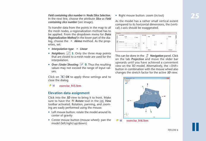
Field containing slice number in Node/Slice Selection.In the next line, choose the attribute Slice as Fieldcontaining slice number (see image).

To transfer data from the points in the map to allthe mesh nodes, a regionalization method has tobe applied. From the dropdown menu for DataRegionalization Method in the lower part of the dia-log, choose the Akima method. As the prop-erties, set:

• Interpolation type: Linear

• Neighbors: 3. Only the three map pointsthat are closest to a mesh node are used for theinterpolation.

• Over-/Under Shooting: 0. Thus the resultingvalues may not exceed the range of input val-ues.

Click on OK to apply these settings and toclose the dialog.

exercise_fri5.fem

Elevation data assignment

Click into the 3D view to bring it to front. Makesure to have the Rotate tool in the Viewtoolbar activated. Rotation, panning, and zoom-ing are easily performed using the mouse:

• Left mouse button: rotate the model around itscenter of gravity

• Center mouse button (mouse wheel): pan themodel (left/right/up/down)

• Right mouse button: zoom (in/out)

As the model has a rather small vertical extentcompared to its horizontal dimensions, the (verti-cal) z-axis should be exaggerated.

This can be done in the Navigation panel. Clickon the tab Projection and move the slider barupwards until you have achieved a convenientview on the 3D model. Alternatively, the <Shift>button in combination with the mouse wheel alsochanges the stretch factor for the active 3D view.

exercise_fri6.fem


II• Hereby, in the Editor toolbar, the map ele-

vation is automatically set as data source in theinput box and the model property Elevation isactivated as parameter. Note that also Elevationhas been chosen in the Data panel and isnow shown in bold letters.

• Click Put value in the Editor toolbar toapply the new elevation data to all nodes.

In the 3D view the node elevations are immedi-ately updated.

Click on Clear Selection in the Selection tool-bar.

The result looks as shown in the figure below.Probadly the Scaling has to be adjusted again( Navigation panel > Projection tab or <Shift> -mouse wheel) to account for the changed verticalextent.


As a next step, the target locations of the dataassignment have to be defined, i.e., all nodes inthe mesh have to be selected.

Click on Select All in the Selection toolbar.

To finally assign the elevation data by regionaliza-tion from map data to the selected nodes, twomore steps are required:

• In the Maps panel, open the branch Maps> ASCII Tables > elevation. UnderLinked Attributes, double-click on Ele -> Elevation.

Additionalselection optionsare described in

detail in the FEFLOW helpsystem.

27

IIFEFLOW 6

exercise_fri7.fem

3D MapsAs an example for a three-dimensional map, a sim-ple representation of the sewage plant is loaded.Add the map file sewage_plant.shp in the

Maps panel via Add map(s). Go to the 3D view and double-click on the layerDefault of sewage_plant. The footprint of the build-ings and clarifiers is shown on top of the modelsomewhat north of the sewage fields.

Choose Edit Properties in the context menu ofthe Default layer. In the upcoming Map Properties dialog, activate

Draw 3D Data and click Apply Changes.

Optionally use the other settings in the dialog toclassify the features, adjust colors and outline style. The structures are shown in 3D on the model top.They are vertically exaggerated with the model.

Reset the stretch factor in the Navigationpanel to return to real elevations display.


IIII.4 Problem settings

FEFLOW provides the means to simulate a num-ber of different physical processes in different spa-tial and temporal dimensions, ranging from simple2D steady-state flow models to transient, unsatu-rated, density-coupled reactive transport models.As the input parameters depend on the modeltype, the general problem settings are done at thebeginning.

Go to Edit > Problem Settings to open theProblem Settings dialog, where all general set-

tings related to the current model are done.

All these settings are organized in thematic pagescontrolled by a tree view on the left-hand side ofthe dialog.

Problem class

The principal type of the FEFLOW model is definedon the Problem Class page.

Below the Problem title (which is not mandatoryto be modified) one of two general types of prob-lems – saturated media and unsaturated/variablysaturated media is chosen.

By default saturated media is selected, applyingDarcy’s equation. Though saturated media isselected, the model is able to account for phreaticconditions.

The second option - unsaturated model - wouldlead to Richards’ equation being applied, beingcapable of accounting for both saturated andunsaturated conditions within one model. In thisparticular case, it is not expected that consideringthe unsaturated/variably saturated zone in detailwould change the model result to an extent thatwould justify the additional effort in parametriza-tion and numerical effort for the solution.

Keep the default setting (Saturated Media) for thisexercise.


29

IIFEFLOW 6

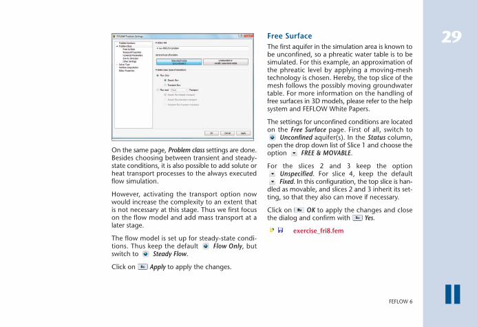
On the same page, Problem class settings are done.Besides choosing between transient and steady-state conditions, it is also possible to add solute orheat transport processes to the always executedflow simulation.

However, activating the transport option nowwould increase the complexity to an extent thatis not necessary at this stage. Thus we first focuson the flow model and add mass transport at alater stage.

The flow model is set up for steady-state condi-tions. Thus keep the default Flow Only, butswitch to Steady Flow.

Click on Apply to apply the changes.

Free Surface

The first aquifer in the simulation area is known tobe unconfined, so a phreatic water table is to besimulated. For this example, an approximation ofthe phreatic level by applying a moving-meshtechnology is chosen. Hereby, the top slice of themesh follows the possibly moving groundwatertable. For more information on the handling offree surfaces in 3D models, please refer to the helpsystem and FEFLOW White Papers.

The settings for unconfined conditions are locatedon the Free Surface page. First of all, switch to

Unconfined aquifer(s). In the Status column,open the drop down list of Slice 1 and choose theoption FREE & MOVABLE.

For the slices 2 and 3 keep the optionUnspecified. For slice 4, keep the defaultFixed. In this configuration, the top slice is han-

dled as movable, and slices 2 and 3 inherit its set-ting, so that they also can move if necessary.

Click on OK to apply the changes and closethe dialog and confirm with Yes.

exercise_fri8.fem


IIII.5 Model Parameters

In the following sections, the physical propertiesof the study area are applied to the finite-elementmodel.

The respective parameters are found in theData panel. The parameters are organized in

four main branches in the tree view:

• Process Variables

• Boundary Conditions

• Material Properties

• Reference Data

II.5.1 Initial conditions

For a transient simulation we need initial condi-tions as starting conditions at time zero of the sim-ulation. Inital conditions are set as process variablesfor the beginning of the simulation. Averagegroundwater levels derived from several observa-tion wells are provided in a text file.

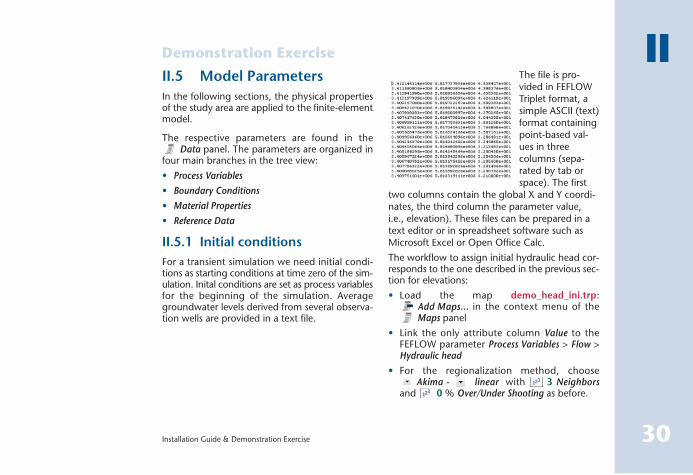
The file is pro-vided in FEFLOWTriplet format, asimple ASCII (text)format containingpoint-based val-ues in threecolumns (sepa-rated by tab orspace). The first

two columns contain the global X and Y coordi-nates, the third column the parameter value,i.e., elevation). These files can be prepared in atext editor or in spreadsheet software such asMicrosoft Excel or Open Office Calc.

The workflow to assign initial hydraulic head cor-responds to the one described in the previous sec-tion for elevations:

• Load the map demo_head_ini.trp:Add Maps... in the context menu of theMaps panel

• Link the only attribute column Value to theFEFLOW parameter Process Variables > Flow >Hydraulic head

• For the regionalization method, chooseAkima - linear with 3 Neighbors

and 0 % Over/Under Shooting as before.


exercise_fri9.fem

• Close the Parameter Association dialog by click-ing on OK.

• Select all nodes at once by a single click on theSelect All button in the Selection toolbar

while having the 3D view active.

• In the Maps panel double-click on Maps >ASCII Triplet Files > demo_head_ini > Linked attrib-utes > Value -> Hydraulic head.

• Click on Put value in the Editor toolbarto execute the interpolation and set the initialhead values.

• Click on Clear Selection.

As a result, a head distribution is shown in the viewwith colors representing heads around 32 m at thesouthern border and 46 m at the northern border.A legend is shown in the upper left corner of theview.

31

IIFEFLOW 6


IIII.5.2 Boundary conditions

As a next step, appropriate boundary conditionsare applied. For the sake of simplicity, they will bekept in a rather simple way:

• Southern border: The lake Müggelsee com-pletely controls the head along the southernboundary. The lake water level of 32.1 m is usedas the value for a 1st kind (Dirichlet) hydraulic-head boundary condition.

• Northern border: As there is no natural bound-ary condition like a water divide close to theboundary, a head contour line will be usedinstead (fixed head = 46 m).

• Western and eastern border: Two small rivers(the Fredersdorfer Mühlenfließ and theNeuenhagener Mühlenfließ) form the bound-ary at the western and eastern limits of themodel. As they follow roughly the groundwa-ter flow direction, we assume these heavilyclogged creeks to represent boundary stream-lines. No exchange of water is expected over this boundary and therefore ano-flow boundary condition is assumed.

• Finally, two wells, each with a pumping rate of1,000 m³/d, are located in the southern part ofthe model. These stand for a number of largewell galleries in reality.

The boundary conditions are not derived from amap (even though this would be possible), butentered manually.

Manual editing is often easier if being done in a2D top view. Thus switch to the FE-Slice view. Ifyou have accidentally closed it, a new view can beopened via Window > FE-Slice view.

FE-Slice view

This view type always shows a single slice or layer.Browsing between the slices is easiest by hittingthe <Pg Up> and <Pg Down> keys, respectively.Alternatively, the layer/slice to be seen in the viewcan be directly selected in the Spatial Unitspanel.

The recommended tool for navigation in the FE-Slice view is the Pan tool in the View tool-bar. The mouse buttons are associated with thefollowing functions:

• Left and center mouse button: pan

• Right mouse button: zoom (in/out)

• Mouse wheel: zoom (in/out) in steps

Northern Boundary

Zoom to the northern boundary.

For the FE-Slice view, the Selection toolbar pro-vides additional tools for selecting nodes compared


33

IIFEFLOW 6

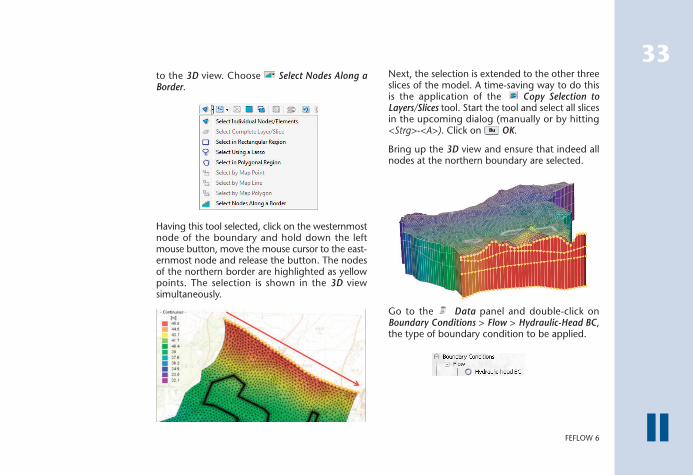
to the 3D view. Choose Select Nodes Along aBorder.

Having this tool selected, click on the westernmostnode of the boundary and hold down the leftmouse button, move the mouse cursor to the east-ernmost node and release the button. The nodesof the northern border are highlighted as yellowpoints. The selection is shown in the 3D viewsimultaneously.

Next, the selection is extended to the other threeslices of the model. A time-saving way to do thisis the application of the Copy Selection toLayers/Slices tool. Start the tool and select all slicesin the upcoming dialog (manually or by hitting<Strg>-<A>). Click on OK.

Bring up the 3D view and ensure that indeed allnodes at the northern boundary are selected.

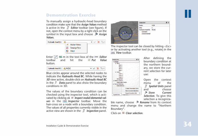
Go to the Data panel and double-click onBoundary Conditions > Flow > Hydraulic-Head BC,the type of boundary condition to be applied.


IITo manually assign a hydraulic-head boundarycondition make sure that the Assign Values methodis active in the Editor toolbar (see figure). Ifnot, open the context menu by a right click on thesymbol in the input box and choose AssignValues.

Enter 46 m in the text box of the Editortoolbar and hit the Put Valuebutton.

Blue circles appear around the selected nodes toindicate the Hydraulic-Head BC. While having the3D view active, double-click on Hydraulic-Head BCin the Data panel to also show the boundaryconditions in 3D.

The values of the boundary condition can bechecked using the inspector tool, which is acti-vated by clicking ok Inspect nodal/elemental val-ues in the Inspector toolbar. Move thehair-cross on a node with a boundary condition.The values of all properties currently visible in theactive view are shown in the Inspection panel.

The inspector tool can be closed by hitting <Esc>or by activating another tool (e.g., rotate) in the

View toolbar.

After defining theboundary condition atthe northern bound-ary, we store the cur-rent selection for lateruse:

Open the contextmenu of the

Spatial Units paneland choose

Store CurrentSelection. To give thisselection a recogniza-

ble name, choose Rename from its contextmenu and change the name to “NorthernBoundary”.

Click on Clear selection.


• Clear selection afterwards.

exercise_fri11.fem

Remaining outer boundaries

At nodes without an explicit boundary condition,FEFLOW automatically applies a no-flow condition.Therefore, no further action is required for thewestern, eastern, top and bottom model bound-aries, which are assumed to be impervious exceptfor groundwater recharge to be added later.

Pumping wells

The wells are to be set in the southern part of thestudy area based on the map demo_wells. They areassumed to be screened throughout the wholedepth of the model.

35

IIFEFLOW 6

exercise_fri10.fem

Southern Boundary

The assignment of boundary conditions along thesouthern boundary is done in the same way:

• In the FE-Slice view, zoom/pan to the southernborder.

• Select nodes along a border.

• Copy the selection to all slices .

• Switch to the 3D view and check that the selection is set correctly.

• Make sure that Hydraulic-Head BC in theData panel is still active.

• Type 32.1 m in the input box of theEditor toolbar and click Put Value.

• Store the selection and rename it to “SouthernBoundary” for later use.


IIGo to the FE-Slice view and browse to the slice 4(<Pg Down>), where the well screen bottoms arelocated. To select the well nodes, make use of thecorresponding map and select nodes close to themap points:

• Double-click on demo_wells in Maps panel.

• Input 1 m in the input box of the SnapDistance toolbar.

• Click on Select by all map geometries in theSelection toolbar.

• Double-click Boundary Conditions > Well BC inthe Data panel. In the Editor toolbarenter 1000 m³/d and click Put Value orhit <Enter>.

So far, the pumping wells are set on the bottomslice, pumping water from the second aquifer. Toconsider a well screen across all layers, additionalwell boundary conditions are defined at the samelocation on the other slices. This makes FEFLOWto connect these boundary conditions by a high-conductive finite element.

Clear Selection and browse to slice 3. Select thewell locations again by clicking on Select by allmap geometries and Copy selection to slices 1and 2. Enter 0 m³/d and click Put Value.

Clear Selection.

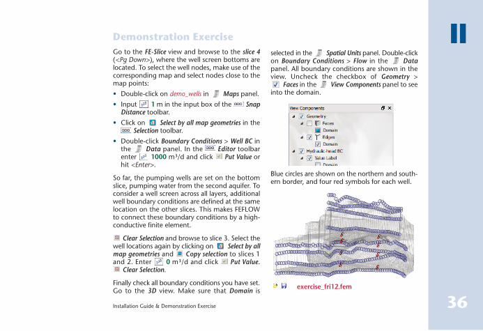
Finally check all boundary conditions you have set.Go to the 3D view. Make sure that Domain is


selected in the Spatial Units panel. Double-clickon Boundary Conditions > Flow in the Datapanel. All boundary conditions are shown in theview. Uncheck the checkbox of Geometry >

Faces in the View Components panel to seeinto the domain.

Blue circles are shown on the northern and south-ern border, and four red symbols for each well.

exercise_fri12.fem

37

IIFEFLOW 6

II.5.3 Material properties

Groundwater recharge

Although groundwater recharge from the math-ematical point of view is rather a boundary con-dition, it is handled as a material property inFEFLOW. In a 3D model, the respective parameterto be set is In/Outflow on top/bottom.

The input procedures for material properties arecompletely analogous to the ones for process vari-ables and boundary conditions; the only excep-tion is that material properties are assigned toelements instead of nodes:

• Go to the 3D view.

• Activate In/Outflow on top/bottom in theData panel with a double-click.

• Choose the Select Complete Layer/Slice toolin the Selection toolbar and select the toplayer by clicking on it.

• Add the map year_rec.shp to the Mapspanel. This map is a polygon shape file con-taining the recharge data for different polygonsin the study area. The unit of the values in thefile is 10-4 m/d.

• Open the context menu of the map with aright-click and choose Link to Parameter…

• Link the data field Mean_Year in the file to theFEFLOW parameter In/Outflow on top/bottom(in material properties).

• Close the dialog by clicking on OK.

• Double click on … > year_rec > Linked Attributes> MEAN_YEAR -> In/Outflow on top/bottom

• Click on Put Value in the Editor toolbar.

exercise_fri13.fem

Conductivity

For this exercise, isotropic materials are assumed,i.e., conductivity does not depend on flow direc-tion.

Add the map conduc2d.shp to the Maps

panel ( Add maps(s)). This shape file containspoint-based conductivity values for the topaquifer in 10-4 m/s.


IIAssociate ( Link to Parameter…) the attributecolumn CONDUCT to the FEFLOW parametersKxx, Kyy and Kzz by defining three links. For

each single link, choose Akima, Linear,

with Neighbors 3 and 0 % Over-/UnderShooting. To select one of the links for editing itsproperties, click on it.

Double-click on Conductivity [Kxx], then press<Ctrl> and double click on Conductivity [Kyy]

and Conductivity [Kzz] in the Data panel.If the top layer is no longer selected, choose the

Select Complete Layer/Slice tool in the

Selection toolbar and select it.

Switch the input tool in the Editor toolbar to

Maps input (with a right-click on the icon inthe input box). Make sure that conduc2d is set asthe map in the input box and assign the data by

clicking Put Value.

Clear selection and select the elements in the

second layer applying Select CompleteLayer/Slice again.

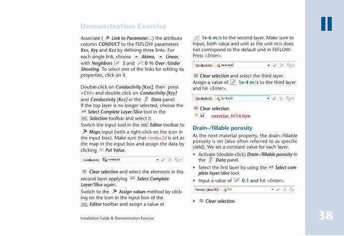
Switch to the Assign values method by click-ing on the icon in the input box of the

Editor toolbar and assign a value of


1e-6 m/s to the second layer. Make sure toinput, both value and unit as the unit m/s doesnot correspond to the default unit in FEFLOW.Press <Enter>.

Clear selection and select the third layer.

Assign a value of 1e-4 m/s to the third layerand hit <Enter>.

Clear selection.

exercise_fri14.fem

Drain-/fillable porosity

As the next material property, the drain-/fillableporosity is set (also often referred to as specificyield). We set a constant value for each layer.

• Activate (double-click) Drain-/fillable porosity inthe Data panel.

• Select the first layer by using the Select com-plete layer/slice tool.

• Input a value of 0.1 and hit <Enter>.

• Clear selection.

exercise_fri15.fem

II.6 Simulation

The flow part of the flow and transport model iscomplete. It is worth the time doing a test run nowto ensure that the flow model is set up correctly.

In case that FEFLOW is run in licensed mode, savethe model to be able to return to the initial prop-erties later! If running FEFLOW in demo mode, thismodel cannot be saved as the number of nodesper slice exceeds the allowed maximum of 500.Please use the prepared file in this case.

exercise_fri15.fem

Starting the simulator

To run the simulation, click Start in theSimulator toolbar.

The simulation is run in steady-state mode. As themodel is unconfined, the system is solved itera-tively, taking into account that the saturated thick-ness of unconfined layers depends on the actualsolution for hydraulic head. The Error Norm Historydiagram provides information about the remain-ing error in each simulation iteration. The simula-tion stops after eight iterations, the error reachingvalues below the defined error criterion.

39

IIFEFLOW 6

• Select the second layer by using the Selectcomplete layer/slice tool.

• Assign 0.01 to the selection.


• Select the third layer by using the Select com-plete layer/slice tool.

• Assign 0.2 to the selection.


The result with the element faces turned on againin the View Components panel is shown in thefigure.

All other material properties are used with theirrespective default values in this exercise.

It is recommendedto save the filebefore starting

the simulation (if workingwith a license). During thesimulation, the processvariables will change andyou would lose the initialconditions of the model.

The budget shows inflows in red, outflows inblue for the different boundary condition typesand the areal sources and sinks (groundwaterrecharge). The Balance value as the sum of allwater flows is sufficiently small to accept thesolution as steady state.


IIDuring and after simulation the run, all visualiza-tion tools in FEFLOW can be used to monitor thesimulation results.

For example, go to the Data panel and dou-ble-click on Process Variables > Flow > Hydraulichead for visualization of the resulting hydraulichead distribution.

When visualizing results in the 3D view, especiallyat the beginning of the simulation vertical meshmovement caused by the free & movable modecan be observed. The top of the model alwaysexactly matches the water table elevation.

Budget

To check whether the model indeed has reachedan equilibrium state, the overall water balance canbe calculated. The Budget panel provides themeans for this.

If it has been closed accidentally, open theBudget panel via View > Panels > Budget

Panel.

Check the Active checkbox to activate thebudget calculation. The budgeting is turned offby default as it can cause significant computationaleffort, especially when being done at each timestep during a simulation run.


On computerswith multi-coreCPUs or multiple

CPUs the simulation resultand budget result may beslightly different in eachrun - even with identicalinput parameters. This isdue to possibly differentsummation order whenusing parallelization.

41

IIFEFLOW 6

Pathlines

One way to visualize the flow field is the plottingof pathlines.

Pathlines are calculated by tracking the path of vir-tual particles that are released at certain startingpoints (called seeds).

In our case, multiple pathlines are released fromall the nodes in the areas of the contaminationsources.

First, a selection is created containing all the nodeson the model top within the contamination sourceareas.

Go to the FE-Slice view and browse to slice 1.

In the Data panel make sure that Hydraulichead or any other nodal property is active toensure the nodal selection mode rather than theelemental one.

Set the Snap distance in the Snap Distance tool-bar to 1 m.

Activate (double-click) the map waste_disposal inthe Maps panel. Choose the tool Select byMap Polygon from the dropdown menu in the

Selections toolbar. With a click into the waste-disposal area the nodes of the contaminationsource are added to the selection.

Repeat the steps for the sewage_fields map. Theresult looks like this:

Go to the 3D view and uncheck Geometry > Facesin the View Components panel. Without thisstep the opaque element faces around the outermodel domain would conceal the pathlineslocated inside the model.

In the Spatial Units panel, click on CurrentSelection > Node selection.

In the Data panel double-click on ProcessVariables > Flow > Pathlines > Forward.

After a short time for computation, the pathlinesare shown in the 3D view.


II

From the result it can be seen that the western wellis certainly influenced by the sewage treatmentplant. The eastern well seems not to be influencedby either contamination source. However, thestreamline-based evaluation does take into accountany mixing processes due to dispersion.

For this purpose, a transport model is needed.


II.7 Flow and Transport Model

When the flow model has been run, the processvariable Hydraulic head has changed. After the run,it does not contain the initial conditions any more,but the final results. In addition, the moving meshtechnique has changed the elevation of the slices.

Therefore before starting to add the mass trans-port properties, the previously saved model has tobe loaded again to return to the original model.

exercise_fri15.fem

II.7.1 Problem settings

Problem class

From the preliminary pathline analysis based onthe results of the flow model it is obvious that thecontamination sources are located within thecatchment zone of the production wells. To beable to provide quantitative estimations, the modelis extended to a flow and mass transport model.

To change the problem class, go to Edit >Problem Settings and open the Problem Settings dia-log. In Problem Class, select Flow and MassTransport and Steady flow/transient transport.

Confirm with Apply.

Time Stepping

In a transient model temporal discretization has tobe defined. The corresponding settings can befound on the Temporal Properties page.

By default, FEFLOW uses an automatic time-stepcontrol scheme. Hereby, an appropriate time-steplength is determined internally by monitoring thechanges in the primary variables (hydraulic headin a flow simulation).

Switch to the Forward Euler / Backward Euler(FE/BE) time-integration scheme for improvingmodel stability.

Enter a value of 7300 days in the Final Timeinput box.

Click on Apply.

43

IIFEFLOW 6

Numerical Parameters

On the Numerical Parameters page, turn on the

Upwinding option Shock capturing. This dam-pening technique helps to suppress numericaloscillations at steep concentration gradients withonly a minimum of additional dispersion.

Click on OK to apply the changes and to closethe Problem Settings dialog, and confirm by click-ing on Yes.

exercise_fri16.fem

II.7.2 Initial conditions

Switch to the 3D view. Double-click on ProcessVariables > Mass transport > Mass Concentration inthe Data panel. The 3D view shows the defaultinitial concentration of 0 mg/l, representing freshwater. No changes are necessary for the back-ground concentration.

Contamination sources

The contamination sources are represented by ahigher initial concentration in the areas of thewastewater treatment plant and the landfill withinthe first aquifer.

First, a selection of the nodes belonging to thecontamination source is needed.

Go to the FE-Slice view and browse to slice 1.Double-click on Process Variables > Mass transport> Mass Concentration in the Data panel. In the

Maps panel, activate (double-click) the mapwaste_disposal. Make sure the Snap distance is setto 1 m in the Snap Distance toolbar. Click

Select by All Map Geometries in theSelections toolbar.

Repeat the same steps with the sewage_fields mapto add also these nodes to the selection.

The contamination in both areas is found to reachdown to the top of the aquitard. Use Copy



Selection to Slices/Layers to copy the selection toslice 2.

The initial concentrations in these areas are to beinterpolated from observation data.

Go to the Maps panel and add the map fileconc_init.shp.

Associate ( Link to Parameter…) the attributecolumn CONC to the FEFLOW parameter ProcessVariables > Mass transport > Mass concentration bydefining the link. Choose Inverse Distance asthe Data Regionalization Method and use 4Neighbors and Exponent of 2.

Click on OK.

Double-click on CONC -> Mass concentration in theMaps panel and assign the values by clicking

on Put Value.

Clear selection.

exercise_fri17.fem

Do not forget toselect theDomain entryagain in the

Spatial Units panel beforecontinuing (otherwise nomodel properties can beplotted in the active view)!

Boundary constraint conditions

As stated before, water entering the model at thenorthern or southern border is fresh water.Depending on the actual flow direction, however,at these boundaries also outflow is possible. In thiscase, a free outflow of contaminated water is tobe preferred over a fixed concentration.

This requires a dynamic change of the mass trans-port boundary condition depending on the flowdirection, which can be implemented by intro-ducing a boundary constraint condition.

A constraint in our case is used to limit the flux ata 1st kind boundary condition (fixed head/con-centration/temperature) to a minimum or maxi-mum value. For this exercise, the constraint is setto limit the mass flux to a minimum value of 0 g/d,applying the concentration boundary conditiononly for inflowing water.

The constraints are technically applied in the sameway as boundary conditions. However, for the sakeof clarity, the constraint conditions are not shownby default as properties in the data panel andhave to be added first:

In the Data panel, open the context menu ofBoundary Conditions > Mass transport > Mass-Concentration BC and choose Add Constraint >Min. mass-flow constraint.

45

IIFEFLOW 6

II.7.3 Boundary Conditions

Northern and southern boundary

Any water entering the domain through the north-ern or southern boundary is fresh water with aconcentration of 0 mg/l. Therefore a fixed con-centration of 0 mg/l is assigned as a boundarycondition at these locations.

Go to the Spatial Units panel and open thecontext menu of the previously stored node selec-tion Northern Boundary. Choose Add to currentselection.

Repeat these steps with the node selectionSouthern Boundary.

In the 3D view all nodes along both borders areshown as selected. Click on Domain in the

Spatial Units panel.

Double-click on Boundary Conditions > MassTransport > Mass-Concentration BC in the Datapanel. In the Editor toolbar, ensure that theAssign Values mode is active, input a value of

0 mg/l and click Put Value.

Blue circles indicate that fist kind boundary con-ditions are set, similar to the flow boundary con-ditions.



Expand the tree view and activate (double-click)Min. mass-flow constraint and assign 0 g/d toall the selected nodes with <Enter>. The minimumconstraint is indicated by a bar below the associ-ated boundary condition symbol.

Clear selection.

exercise_fri18.fem

II.7.4 Material properties

To simplify the data input, the porosity effectivefor mass transport processes is assumed to be20 % throughout the model.

Go to the 3D view and activate (double click)Material Properties > Mass transport > Porosity inthe Data panel.

Select all elements of the model. The easiest wayto do this is to click Select All in the Selectiontoolbar.

Input a value of 0.2 in the Editor toolbarand hit <Enter>.

Repeat these steps for the longitudinal dispersiv-ity (Material Properties > Mass transport >Longitudinal dispersivity, 70 m) and for the trans-verse dispersivity (Material Properties > Mass trans-port > Transverse dispersivity, 7 m) for all elementsof the model.

Clear selection.

exercise_fri19.fem

II.7.5 Vertical resolution

To ensure a correct representation of low flowvelocities in the aquitard as a basis for transportsimulation, this model layer has to be further sub-divided.

A good choice to minimize errors due to the nodalnature of the calculated velocity field is to applythin layers on top and bottom of the aquitard.

Algebraic signsare handled dif-ferently for

Constraint and BoundaryCondi tions: For ConstraintConditions inflows are posi-tive (+), outflows are nega-tive (-). For BoundaryConditions Inflows arenegative (-), outflows arepositive (+).

47

IIFEFLOW 6

The two additional slices are placed within theaquitard with a distance of 10 cm to the aquitardtop and bottom.

Go to Edit > 3D Layer Configuration.

Type a value of 0.1 m in the Distance input boxand - for inserting the first additional slice - choosethe option lower slice.

Increase the Number of layers in the input box inthe upper left corner of the dialog by one (to 4).Press <Enter>. The Slice placement dialog is opened.

In this list, choose where the first new slice is beinginserted. The slice numbers refer to the NEW sliceconfiguration. Select New slice 3 and click onOK.

The new slice is inserted into the model with theslice number 3. Set its status to Fixed, check-ing the checkbox.

The next slice is to be inserted 0.1 m below thesecond slice. Change the option to upper slice.

Increase the Number of layers to 5 and hit<Enter>.

In the upcoming Slice Partitioner dialog, select Newslice 3 again and click on OK.

The aquitard has been divided into three layers.To ensure that the data is transferred correctly fromthe old to the new slices and layers, the Data Flowlists on the right of the 3D Layer Configurator areused.

There are two lists that provide control over thedata flow between the previous and the new slicesand layers. The upper control called Data flow forslices describes the data flow of the process vari-ables, boundary conditions, and nodal selectionsfrom the old slices to the new ones. The old slicesare shown as number buttons in the left column,the new ones in the right column. The data flowis symbolized by lines connecting the old with thenew slices. The lower list, Data flow for layersdescribes the data flow for all material data andfor elemental selections.

The nodal parameters of the old slice 2 are inher-ited to the new slices 2 and 3, while the informa-tion from the old slice 3 is to be inherited by slices4 and 5.



FEFLOW suggests to transfer the properties fromold slice 2 to slices 2 – 4. In order to change this,double click on the button 5 in the new column.Change this entry to 4 – 5.

As a result, the link from old slice 2 points to newslices 2-3 and from old slice 3 to new slices 4-5.

The data flow in the lower list for the materialproperties describes the same data characteristicsfrom the old bottom layer (lower aquifer) to thenew layers 2, 3 and 4. No changes are necessary.

Click on OK to exit the 3D Layer Configuratorand to apply the changes to the model.

exercise_fri20.fem

II.7.6 Reference data

Observation points

A network of observation wells exists in the studyarea. For a later comparison between measuredand calculated data, the concentration develop-ment over time at these monitoring points isshown and logged during the simulation.

The X-Y locations of the observation wells as wellas their respective relation to a certain depth (slicenumber) are contained in the shape fileobs_points.shp. Add this map to the Mapspanel ( Add map... from the context menu).

Go to the FE-Slice view. Open the context menuof the map obs_points and choose Convert to >Observation Points.

In the following dialog, the attribute columns ofthe map are associated to the properties of theobservation points. Choose the field SLICE forthe Slice Number and TITLE for the Label. ForNode Number choose <no node>.

Click on OK to create the set of observationpoints. Click on Set/Clear Observation Points inthe Observation Point toolbar to show theimported observation points in the view.

49

IIFEFLOW 6

exercise_fri21.fem

II.7.7 Simulation Run

If working with a licensed version of FEFLOW, theresults can be saved to a file during the simulationrun. Click on Record in the Simulator tool-bar. Activate Save complete results (DAC file). Bydefault, the results file (*.dac) is saved with thesame name as the current model in a subdirectoryresults. Confirm by clicking OK.

If running FEFLOW in demo mode, it is not possi-ble to save the results file, and only the preparedfile can be run.

exercise_fri21.fem

To run the model, click Start in theSimulator toolbar. The simulation takes approx-

imately 15 minutes on a system with 2GB RAMand an Intel Core Duo processor.

The current simulation time is displayed in thedropdown box of the Simulator toolbar.



In the Time Steps diagram (which can be openedvia View > Diagrams if not already shown) theactual time step length versus total simulation timeis plotted. The mostly steady conditions lead to asteadily increasing time step length.

The simulation stops after 7,300 days (the finaltime that has been set in the Problem Settings dia-log before).

Click Stop to leave the simulator.

II.7.8 Postprocessing

Load the recorded results file.

exercise_fri21.dac

Cross-sections

Process variables and material properties can bevisualized in cross-section views.

In our case, we are interested in the vertical distri-bution of the contamination along the contami-nation plumes.

The cross section is based on a 2D Surface Line.Switch to the FE-Slice view and open its contextmenu. Choose Tool > Draw a Surface (2D) Line.

Click on the waste-water treatment plant (the con-tamination source in the north-west) to define thestarting point of the line here. The line is extendedby adding points with a mouse click. Follow theflow path to the western well and further to thelake Müggelsee. Finish the line with a double click.

Repeat these steps for the waste dump (the east-ern contamination source). The final result shouldlook like this:

51

IIFEFLOW 6

In the Spatial Units panel, two new entriesSurface Locations > 2D Polyline #1 / #2 have beenadded.

Open the context menu of 2D Polyline #1 andchoose Cross-Section View.

A cross-section view along the line is opened.

In the Navigation panel, go to the Projectiontab and push up the lever to exaggerate the z-axis.



Isosurfaces

Go to the 3D view. Make sure that Domain is

selected in the Spatial Units panel. In the

Data panel, double-click on Mass concentra-tion to show this parameter in the view. In the

View Components panel, uncheck Faces

and Mass concentration > Continuous. Check

Mass concentration > Isosurfaces > Domain.One isosurface for an average concentration isshown. To edit the isosurface visualization properties,

double-click on Isosurfaces. The Properties

panel comes to front. Switch to the Custom

mode and click on Edit. Specify two values,

10 mg/l and 20 mg/l. Close the dialog

by clicking OK, and click Apply in the

Properties panel. The isosurface visualizationis changed to reflect the newly set concentrati-ons.This completes the demonstration exercise.Additional tutorials are available in the UserManual.

dhi-wasy software feflowfeflow.info/fileadmin/feflow6/feflow_6.0_tutorial.pdf · dhi-wasy software...

Documents