dhanalakshmi srinivasan - dscedsce.ac.in/mech_notes/sem 5/me 6511- dynamics laboratory.pdf ·...
TRANSCRIPT
DHANALAKSHMI SRINIVASAN COLLEGE OF ENGINEERING
COIMBATORE
zzzz
DEPARTMENT OF MECHANICAL ENGINEERING
Subject Code & Title
ME6511 DYNAMICS LABORATORY
Name :
Roll No :
Degree & Branch :
Subject Code &Title :
Year &Semester :

1
Ex. No: 01 Date :

2

3
4
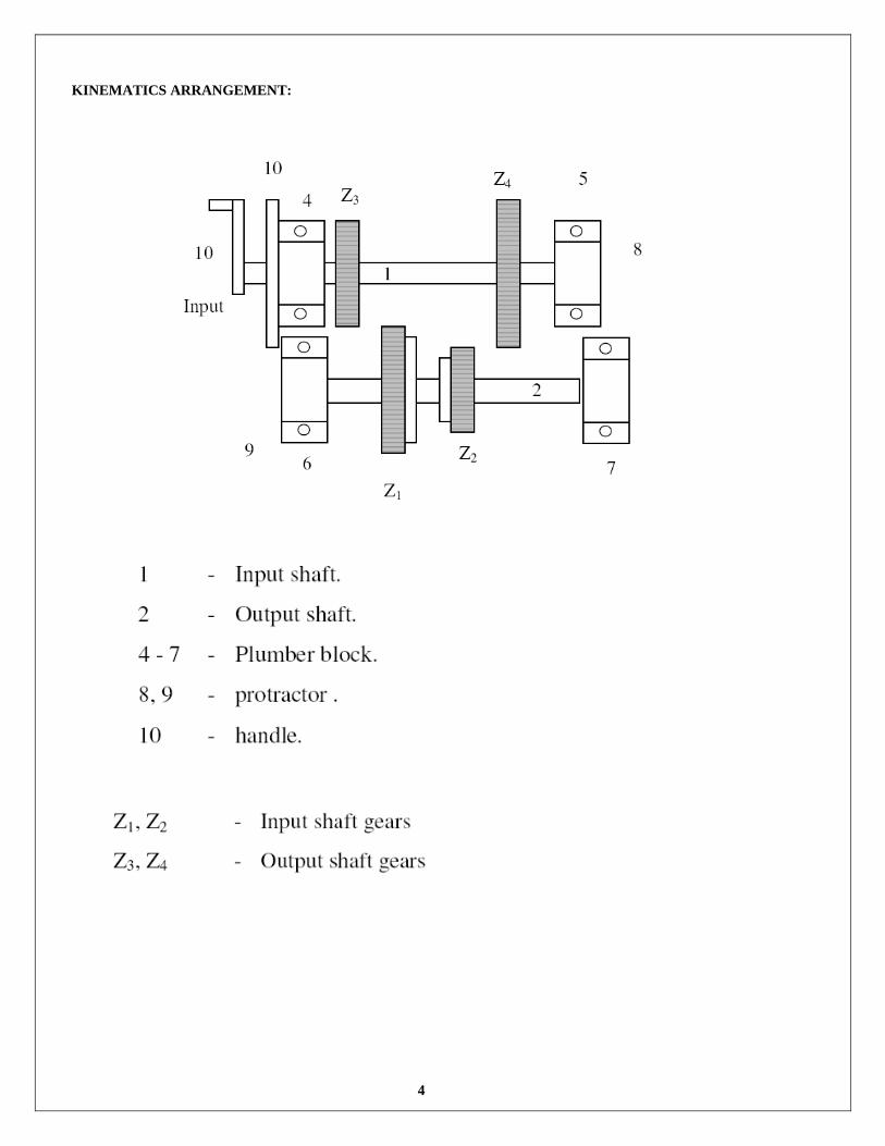
KINEMATICS ARRANGEMENT:
5
SIMPLE GEAR TRAIN
EX.NO:02
DATE:
AIM:
To draw the speed diagram / Ray diagram by using the simple gear train.
APPARATUS REQUIRED:
Experimental setup.
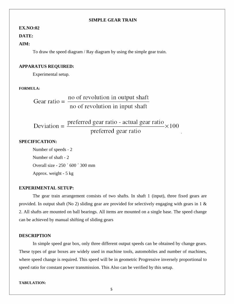
FORMULA:
´
SPECIFICATION:
Number of speeds - 2
Number of shaft - 2
Overall size - 250 ´ 600 ´ 300 mm
Approx. weight - 5 kg
EXPERIMENTAL SETUP:
The gear train arrangement consists of two shafts. In shaft 1 (input), three fixed gears are
provided. In output shaft (No 2) sliding gear are provided for selectively engaging with gears in 1 &
2. All shafts are mounted on ball bearings. All items are mounted on a single base. The speed change
can be achieved by manual shifting of sliding gears
DESCRIPTION
In simple speed gear box, only three different output speeds can be obtained by change gears.
These types of gear boxes are widely used in machine tools, automobiles and number of machines,
where speed change is required. This speed will be in geometric Progressive inversely proportional to
speed ratio for constant power transmission. This Also can be verified by this setup.
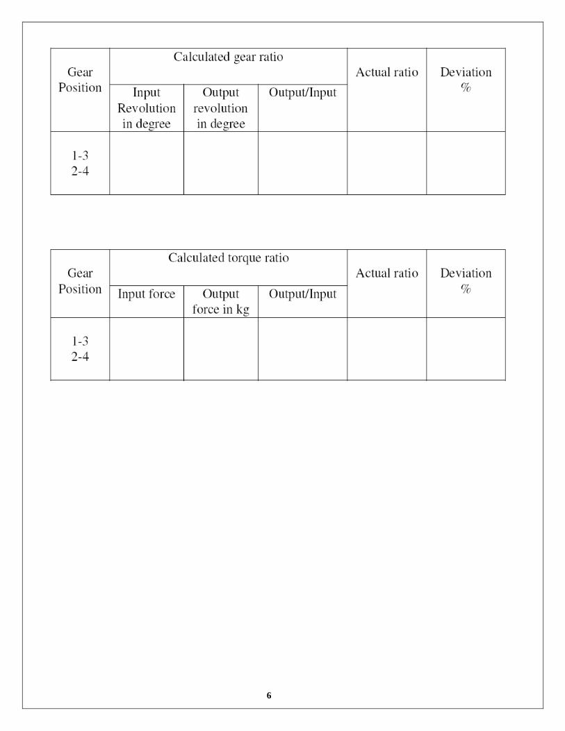
TABULATION:
6

7
TESTING PROCEDURE:
1) Check the sliding gear is perfectly meshed with its meshing gear.
2) Check the number of teeth for the all gear.
3) Check the bearings, shafts and key positions.
4) Check the gear numbers are perfectly.
EXPERIMENTAL PROCEDURE:
1) Count the number of teeth in each gear.
2) Calculate module of gears, Verify that it is same for all the gears.
3) Module = outer diameter of any gear teeth/ (number of teeth + 2)
4) Measure center distance between the shafts. Eg. Center distance of shaft
1- 2 = ((40 m) + (20 m))/2.
5) Estimate gear ratio (output rev/ input rev) in each combination 1-3, 2-4, etc.
6) Set different position of 1/3 and 2/4, give and revolution to output shaft and Measure output
revolutions. Estimate gear ratio and verify with calculated values.
RESULT:
Thus the Speed Ratio and Torque ratio where Calculated.

8
KINEMATICS ARRANGEMENTS:
9
COMPOUND GEAR TRAIN EX.NO:03
DATE:
AIM:
To draw the speed diagram / Ray diagram by using the gear train.
APPARATUS REQUIRED:
Experimental setup.
FORMULA:
SPECIFICATION:
Number of speeds - 9
Number of shaft - 2
Overall size - 600 ´ 300 ´ 300 mm
Approx. weight - 10 kg
Resolution - 1° for angular measurement.
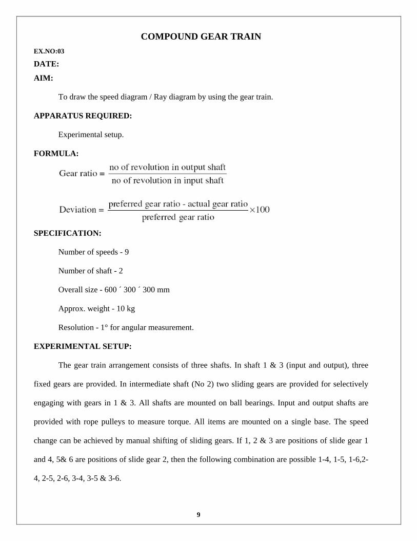
EXPERIMENTAL SETUP:
The gear train arrangement consists of three shafts. In shaft 1 & 3 (input and output), three
fixed gears are provided. In intermediate shaft (No 2) two sliding gears are provided for selectively
engaging with gears in 1 & 3. All shafts are mounted on ball bearings. Input and output shafts are
provided with rope pulleys to measure torque. All items are mounted on a single base. The speed
change can be achieved by manual shifting of sliding gears. If 1, 2 & 3 are positions of slide gear 1
and 4, 5& 6 are positions of slide gear 2, then the following combination are possible 1-4, 1-5, 1-6,2-
4, 2-5, 2-6, 3-4, 3-5 & 3-6.
10
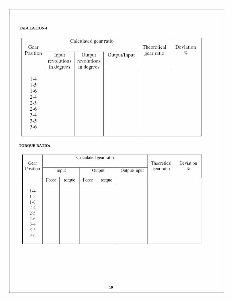
TABULATION-I
TORQUE RATIO:
11
DESCRIPTION
In multi speed gear box, different output speeds can be obtained by change gears. With two
numbers of 3 positions sliding gear in intermediate shaft 3 × 3 = 9 different speeds can be obtained in
the output shaft for a constant input shaft speed. These types of gear boxes are widely used in
machine tools, automobiles and number of machines, where speed change is required. This speed will
be in geometric progressive inversely proportional to speed ratio for constant power transmission.
This also can be verified by this setup.
TESTING PROCEDURE:
1) Check the sliding gear is perfectly meshed with its meshing gear.
2) Check the number of teeth for the all gear.
3) Check the bearings, shafts and key positions.
4) Check the gear numbers are perfectly.
EXPERIMENTAL PROCEDURE:
1) Count the number of teeth in each gear.
2) Calculate module of gears, Verify that it is same for all the gears.
Module = outer diameter of any gear teeth/ (number of teeth + 2)
3) Measure center distance between the shafts. Eg., Center distance of shaft
1- 2 = ((40 × m) + (20 × m))/2.
4) Estimate gear ratio (output rev/ input rev) in each combination 1-4, 1-5, 1-6,etc.,
5) Set different position of 1|2|3 and 4|5|6, give and revolution to output shaft and measure
output revolutions. Estimate gear ratio and verify with calculated values.
6) Draw speed diagram
7) do for torque ration

12

13
RESULT:
Thus the speed ratio and torque ratio are found for the gear train and compared with its
actual value.
14
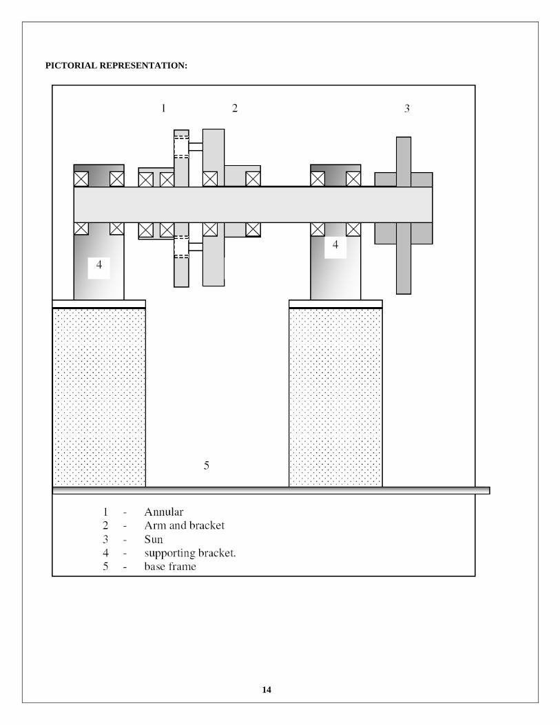
PICTORIAL REPRESENTATION:
15
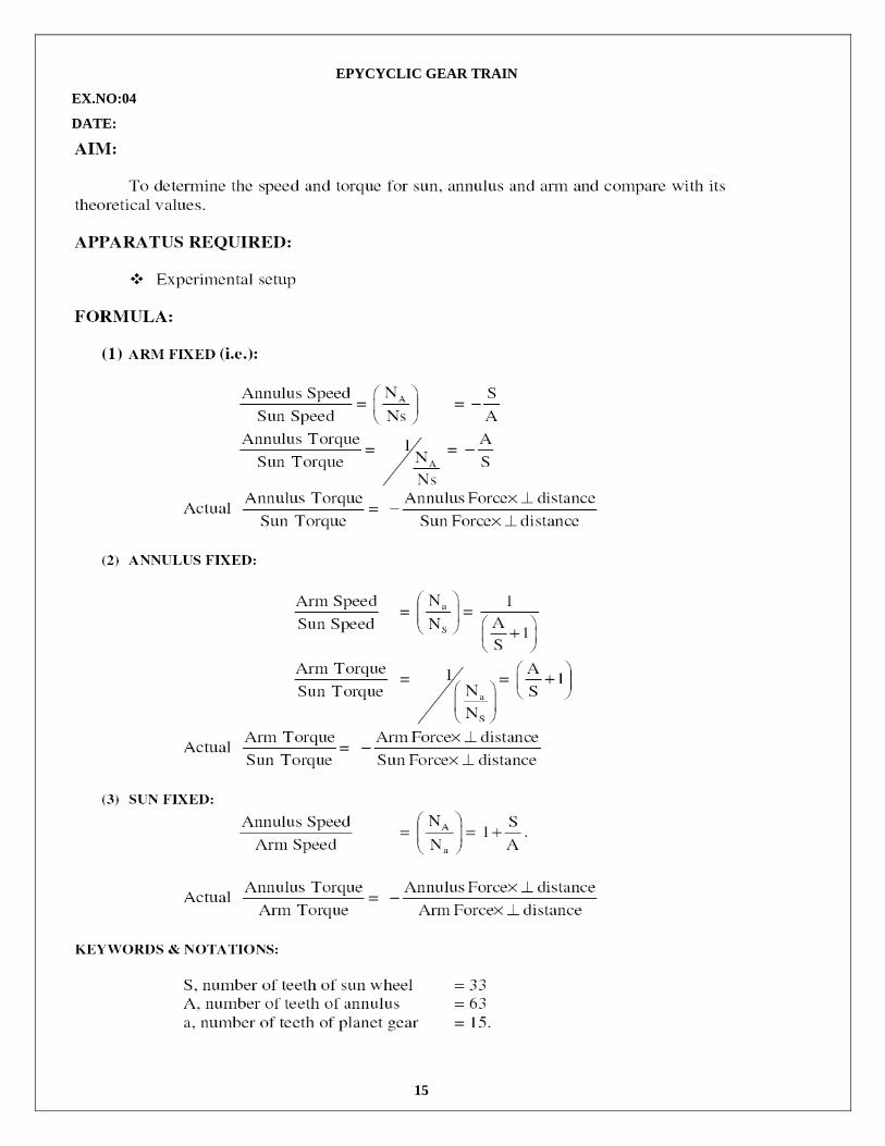
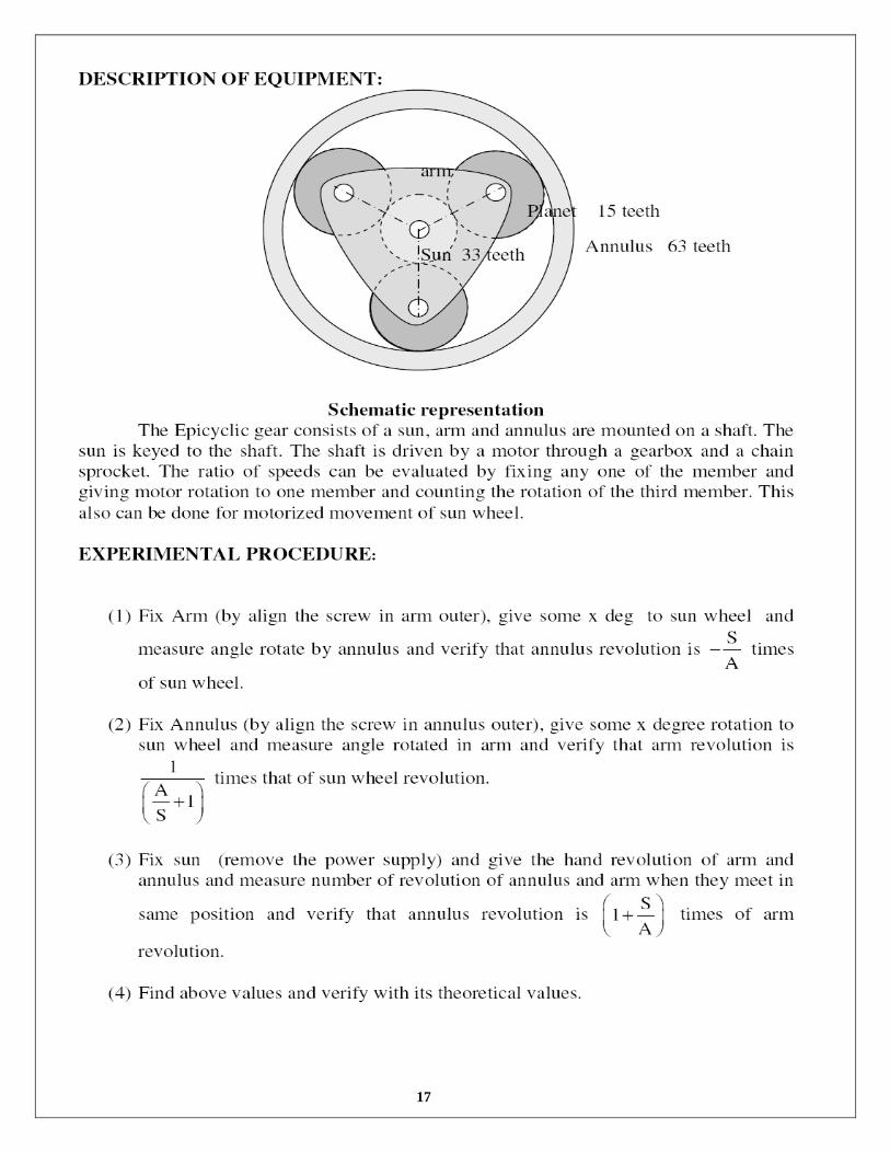
EPYCYCLIC GEAR TRAIN
EX.NO:04
DATE:

16
17

18

19
RESULT:
Thus the sun, annulus and arm speeds ratio are determined by experimentation in
epicyclic gearbox and compared with its theoretical values.

20
21
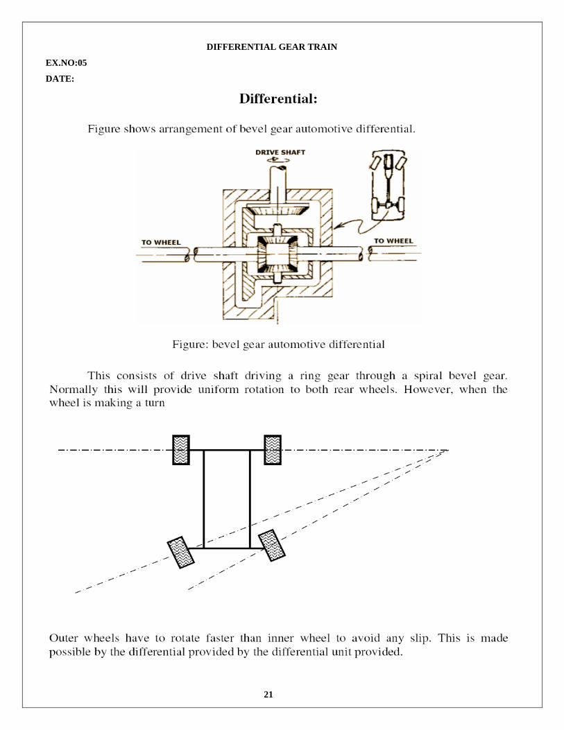
DIFFERENTIAL GEAR TRAIN
EX.NO:05
DATE:
22
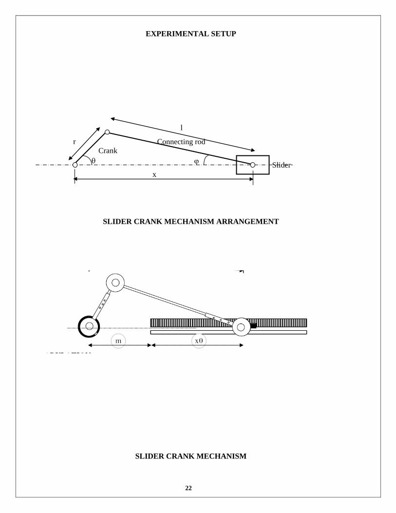
EXPERIMENTAL SETUP
SLIDER CRANK MECHANISM ARRANGEMENT
SLIDER CRANK MECHANISM
θ ϕ
x
l
r Crank
Connecting rod
Slider

23
EX.NO:06
DATE:
INTRODUCTION:
Slider crank chain is a form of four bar mechanism in which length of one of the link
is infinity. In this case reciprocating motion is converted into rotary motion and vice versa. Examples
of such applications are in I.C engines. Reciprocating pumps, power presses etc. The relation between
motions of links is required to establish kinematics motion and also for analysis of inertia forces. The
relation between position and velocity of links can be evaluated by analytical method and
experimental method.
Experimental method is by making model of mechanism and analyzing its moments by
physical measurements and analysis.
AIM:
To find the angular velocity of connecting rod, slider velocity, slider acceleration and compare
with its theoretical value.
APPARATUS REQUIRED:
Slider crank setup
Allen Key
Scale
SPECIFICATION:
Crank length - (50 – 80) mm
Connecting rod - (180 – 250) mm
Slider stroke - (100 – 200) mm
Resolution of measurement - 1 mm for slider
- 0.1o for crank angle
Overall size - 300 × 600 × 50 mm
Weight - 3 kg approximately

24
TABULATION:
Crank angle ( θ )
Measured value
from scale
(x0)
Distance between
crank centre and slider
( x ) = m + x0
Angle between slider and
connecting rod
ϕ = sin-1 r cosl
θ
in °
0
10
20
30
40
50
60
70
80
90
100
110
120
130
140
150
160
170
180
Observation:

25
TESTING PROCEDURE:
This model consists of a slider crank mechanism with the following features.
(a) Crank length is adjustable
(b) Connecting rod length is adjustable
(c) Crank and connecting rod ends are hinged by ball bearings
(d) Angular position of crank can be measured to an accuracy of 0.1o
(e) Slider position can be measured to accuracy of 1 mm.
To check it and correct if the correction is needed.
EXPERIMENTAL PROCEDURE:
(1) Set length of crank( r ) and connecting rod ( l ) .
(2) Ensure zero reading in crank angle for outer dead centre of crank.
(3) Measure value of position of slider ‘x’ for various values of crank angle ‘θ’, from 0, 10, 20 ---
180o.
(4) Calculate inclination of connecting rod ϕ = 1 r sinsinl
− θ
for various values ofθ.
(5) Plot graphs θ – x and θ - ϕ .
(6) Find slope of θ - x curve at the required point dxdθ
.
(7) Velocity of slider = dx dx d dxdt d dt d
θ= × = ω
θ θ compare with calculated value (assume
value of ω = 10 rev/min).
(8) Calculate velocity of slider for any one angle, θ
sin 2x r sin2n
lwhere nr
• θ = ω θ +
=

26

27
9. Angular velocity of connecting rod CR cosn cos
ω θ=
ω ϕ
Where ωCR is angular velocity of connecting rod.
ω Is angular velocity of crank?
10. This can be calculated for a particular value of θ and can be compared with slope of graph,
ddϕθ
,
ωCR = ddϕθ
RESULT:
Thus angular velocity is verified and this theoretical value is compared with its practical
value.

28
EXPERIMENTAL SETUP
1
2
3
4
7 6
1, 2, 3, 4 - Links. 6, 7 - Angle protractors Note. 2, 3, 4 are telescopic limits

29
CRANK ROCKER MECHANISM
EX.NO:07
DATE:
INTRODUCTION:
Four bar linkage forms core mechanism for most of the machines. Even complicated
mechanism can be split into number of four bar mechanisms. The problems of four bar mechanism
namely analysis and synthesis can be solved by graphical, analytical and experimental means.
Graphical methods include finding out velocity and acceleration of a point or link by drawing
velocity and acceleration diagram.
Using relative velocity method or instantaneous center method.
Analytical methods include vector approach, trigonometrically method or complex algebra
method. Experimental method is by constructing a model and analyzing the motion by measurements.
AIM:
To determine the angular velocity ratio ω4/ω2 and ω3/ω2 for various angular position of
crank for the given link sizes.
APPARATUS REQUIRED:
Four bar mechanism setup
Lens
Allen Key
Divider
FORMULA:
1. Angle between link 2 & 3 θ3( )4 4 2 21
1 2 2 4 4
r sin r sintan
r r cos r cos− θ − θ
= − θ + θ
2. Velocity ratio ( 4
2
ωω
) between link 2 and 4 ( )( )
2 3 24
2 4 3 4
r sin )r sin
θ − θω=
ω θ − θ
3. Velocity ratio ( 3
2
ωω
) between link 2 and 3. ( )( )
2 4 23
2 3 3 4
r sin )r sin
θ − θω=
ω θ − θ.

30
OBSERVATION:
Length of the fixed link =
Radius of the Crank =
Length of the Connecting rod =
Length of Rocker =
TABULATION
S.No θ2 θ4 θ3( )4 4 2 21
1 2 2 4 4
r sin r sintan
r r cos r cos− θ − θ
= − θ + θ ( )
( )2 3 24
2 4 3 4
r sin )r sin
θ − θω=
ω θ − θ ( )
( )2 4 23
2 3 3 4
r sin )r sin
θ − θω=
ω θ − θ

31
SPECIFICATION:
Crank length -80 – 120 mm
Coupler length -180 – 320 mm
Racker length -130 – 220 mm
Overall size -600 × 300 mm
Approximate weight- 2 kg
Resolution -0.1°
TESTING PROCEDURE:
1. Check the position of the grub screw in crank.
2. And also check the position of the coupler and Racker.
3. Check the Angular position of crank and Racker can be measured to an accuracy of 0.1°.
DESCRIPTION:
The experimental set consists of a four bar mechanism model having the following features.
(1) Two links are fixed on to a board. The distance between the pivots is considered as length
of fixed link 1.
(2) Each moving link is telescopic type and its length can be varied by grub screw provided.
(3) Hinges are provided with ball bearings to reduce error due to clearance.
(4) Angular position of links 2 (crank) and 4 (rocker) can be measured to a resolution of 0.1o
by venire protractors.
(5) The links are in two planes so that complete rotation of crank is possible.

32

33
EXPERIMENTAL PROCEDURE:
1. Adjust the length link 2, 3 and 4 as per requirement.
2. Links are numbered in anti clockwise starting with fixed link as 1. Ensure that θ2 is zero when
link 2 coincided with link 1.
3. Measure value of θ4 for various values of θ2, 0, 10 , 20, . . . 180°.
4. Calculate θ3( )4 4 2 21
1 2 2 4 4
r sin r sintan
r r cos r cos− θ − θ
= − θ + θ
5. Calculate 4
2
ωω
from following formula. ( )( )
2 3 24
2 4 3 4
r sin )r sin
θ − θω=
ω θ − θ
6. Similarly verify angular velocity ratio ( 3
2
ωω
) between link 2 and 3. ( )( )
2 4 23
2 3 3 4
r sin )r sin
θ − θω=
ω θ − θ.
7. Also calculate above three terms (step 4, 5, 6) in graphical method (or any analytical method)
and compare with above actual value.
RESULT:
Thus the angular velocity of 4
2
ωω
and 3
2
ωω
found out and compared with graphical value.

34
The inclination between shafts can be varied and measured.

35
KINEMATICS OF UNIVERSAL JOINTS
EX.NO:08
DATE:
INTRODUCTION:
Universal joint (or Hooke’s joint) can transmit power between inclined axes. If α
is the inclination between the input and output shaft then, angular velocity of output shaft,
Where, ω is the angular velocity of input shaft.
And θ is the angle turned by input shaft.
It can be seen from the above equation, is not constant and varies as a function of θ. This
will introduce angular acceleration and hence inertia torque and stresses due to that uniform velocity
ratio (or no angular acceleration) can be achieved by introduction of one more universal coupling in
the same sense to give angular velocity of output shaft for all values of θ.
An experimental set up is made to verify the above.
AIM:
To determine the angular velocity ratio for single and double joints.
APPARATUS REQUIRED:
Experimental setup
TESTING PROCEDURE:
Check the joints are perfectly
Check the marking scale is correctly or not
Check the initial corrections
EXPERIMENTAL SETUP:
The setup consists of two numbers of universal joints joined by a spline shaft. The whole
system is mounted on three Plummer blocks.
Provision is made to measure angular position of input shaft, intermediate shaft and output
shaft.

36

37
FORMULA
1. Angular velocity ratio in single joint
2. Experimental velocity ratio in single joint
Where ω2 ,ω1- angular velocity of output & input shaft.
α is angle between two shafts,
θ is angle of turns in input shaft
EXPERIMENTAL PROCEDURE
1. Keep α = 0 initially, Measure, values of θ2 and θ3 for various values of θ1 Starting from 0 to
360° with increment of 15°.
2. Move output shaft for particular value to give the α = 25° and do the step 2.
3. Calculate dθ2 and also experimental angular velocity ratio, .
4. Calculate theoretical angular velocity ratio,
5. Draw graph between following data in same graph sheet.
θ1 Vs experimental & theoretical angular velocity ratio
6. Do this for α = 30°, 35°, 40° and verify the values with the theoretical one.
RESULT:
Thus the angular velocity ratio of single and double joints is determined.

38
TABULATION:
S.No Mass of the Object ‘Kg’
Time period for one oscillation
without mass ‘t1’ in sec
Time period for one
oscillation with mass ‘t2’ in sec
Mass moment of inertia of beam I1 in
‘Kg m2’
Mass moment of inertia of unknown object I2 in’Kg m2’
39
CONNECTING ROD AND FLYWHEEL BY COMPOUND PENDULUM
EX.NO:09
DATE:
AIM:
To determine the mass moment of inertia of unknown objects like connecting rod and
flywheel by oscillation of compound pendulum.
APPARATUS REQUIRED:
1. Experimental setup
2. connecting rod
3. Flywheel
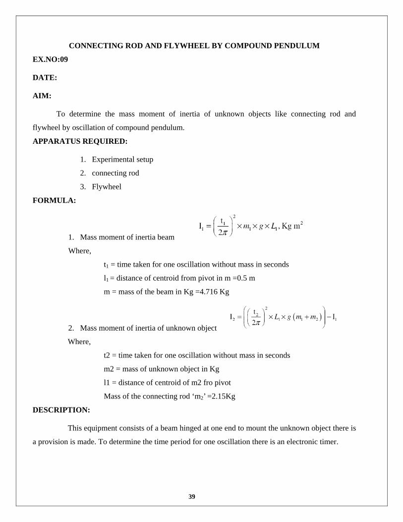
FORMULA:
1. Mass moment of inertia beam
Where,
t1 = time taken for one oscillation without mass in seconds
l1 = distance of centroid from pivot in m =0.5 m
m = mass of the beam in Kg =4.716 Kg
2. Mass moment of inertia of unknown object
Where,
t2 = time taken for one oscillation without mass in seconds
m2 = mass of unknown object in Kg
l1 = distance of centroid of m2 fro pivot
Mass of the connecting rod ‘m2’ =2.15Kg
DESCRIPTION:
This equipment consists of a beam hinged at one end to mount the unknown object there is
a provision is made. To determine the time period for one oscillation there is an electronic timer.

40
41
PROCEDURE:
1. When there is no mass attached to the beam determine the time period for one oscillation t1
from the electronic timer.
2. Now calculate the moment of inertia of the beam using the formula I1 = (t1/2π)2 (l1mg).
3. Fix the object whose moment of inertia is to be determined by coinciding the centre of gravity
of object with centre of gravity of beam.
4. Give a small pull to the beam and determine the time period for one oscillation t2 using
electronic timer.
5. Calculate the moment of inertia of unknown object by using the formula
I2 = {(t2/2π) 2(m+m2)l1g}-I1-m2l12
RESULT:
Thus the mass moment of inertia of connecting rod and flywheel are determined by using
oscillation of compound pendulum.
42
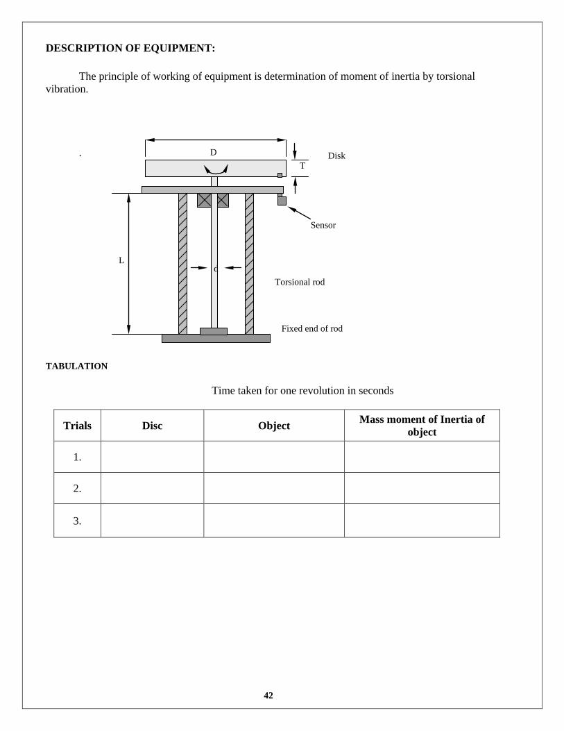
DESCRIPTION OF EQUIPMENT:
The principle of working of equipment is determination of moment of inertia by torsional vibration.
. TABULATION Time taken for one revolution in seconds
Trials Disc Object Mass moment of Inertia of object
1.
2.
3.
D T
d L
Sensor
Disk
Torsional rod
Fixed end of rod

43
TURN TABLE EX.NO:10 DATE:
AIM:
To determine moment of inertia of unknown member by using the torsional apparatus.
APPARATUS REQUIRED:
1. Experimental setup
2. connecting rod
FORMULA USED:
1. Mass Moment of Inertia of Disc I1 =212
qt4π
2. Mass Moment of Inertia of Object I2 = 222
qt4π
– I1
Where – I1 is mass moment of inertia of Disc
I2 is mass moment of inertia of object (flywheel, connecting rod)
T1 is time taken for one oscillation of disc
T1 is time taken for one oscillation of disc with object
q is torsional stiffness of the rod.
3. Torsional stiffness of rod q = GJL
G – Modulus of rigidity
J – Polar moment of inertia = 4d32π
Where d is wire dia = 6.1 mm
L – Length of the polish rod = 660 mm

44

45
EXPERIMENTAL PROCEDURE:
The following are the procedure adapted in the determination of moment of inertia of a
member.
(1) Give angular twist to the disc and measure period (t1) for one oscillation.
(2) Find out the mass moment of inertia of the disc using formula I1 =212
qt4π
.
(3) Compare with theoretical value of the disc using the formula
Mass moment of inertia of disc, = 2rm
2
(4) Take an object Place it on centre of marking and find out time taken for one oscillation (t2).
(5) Find out the mass moment of inertia of the disc and test object using formula given
I2 = 222
qt4π
– I1
RESULT:
Thus torsional oscillation equipment is tested and also mass moment of inertia of unknown
object is found out.

46
SCHEMATIC REPRESENTATION OF GYROSCOPE COUPLE:
TABULATION:
S.No Spin speed N
(rpm)
Weight W
(N)
Angle of Precession
‘dϕ’
Time required
for Precession
‘dt’ (sec)
Gyroscopic
Couple T(Nm)
Degrees radians
47
GYROSCOPIC COUPLE
EX.NO:11
DATE:
AIM:
To determine the gyroscope Couple Effect.
APPARATUS REQUIRED:
Gyroscope
Digital speed controller
Weights
Stopwatch
FORMULA:
1. Mass Moment of Inertia (I) = mr2/4 Kg-m2
2. Angular Velocity (ω) = 2πN /60 rad/sec
3. Precision angular Velocity (ωp)= dϕ/dt rad/sec
4. Gyroscopic couple (T) = I ω ωp
Where,
M-Mass of Rotor Kg
R-Radius of the Rotor Disc m
N-Spindle Speed rpm
Dϕ-Angular Speed rad
ω-Angular Velocity rad/s
dt-time required for precession s
PROCEDURE:
The spinning body exerts a torque or couple in such a direction which tends to make the axis
of spin to coincide with that of the precession.
To study the rule of gyroscopic behavior, the following procedure is adopted.
1. Balance the initial horizontal position of the rotor.
2. Start the motor. By turning the regulator Knob increase the voltage until a designed constant
speed is obtained.

48
OBSERVATION:
Weight of the rotor (W) = 2.7 Kg or 2.7×9.81 N
Disc rotor diameter (d) = 20 cm
Rotor Thickness (t) = 10 cm
MODEL CALCULATION:
49
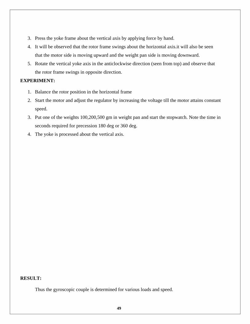
3. Press the yoke frame about the vertical axis by applying force by hand.
4. It will be observed that the rotor frame swings about the horizontal axis.it will also be seen
that the motor side is moving upward and the weight pan side is moving downward.
5. Rotate the vertical yoke axis in the anticlockwise direction (seen from top) and observe that
the rotor frame swings in opposite direction.
EXPERIMENT:
1. Balance the rotor position in the horizontal frame
2. Start the motor and adjust the regulator by increasing the voltage till the motor attains constant
speed.
3. Put one of the weights 100,200,500 gm in weight pan and start the stopwatch. Note the time in
seconds required for precession 180 deg or 360 deg.
4. The yoke is processed about the vertical axis.
RESULT:
Thus the gyroscopic couple is determined for various loads and speed.

50

51
UNIVERSAL GOVERNOR APPARATUS
EX.NO:12
DATE:
AIM:
To determine the radius of rotation, Centrifugal force, Sensitivity, effort, power and draw the
characteristics Curves of Watt, Porter, Proell and Hartnell governor.
APPARATUS REQUIRED:
Proell,Porter and Hartnell Governor
Digital Electronic Control Unit
Tachometer
FORMULA:
1. Governor Height (h) = ho – X/2 (mm)
2. Radius of Rotation (r) = √ly2-h2 (mm)
3. Centrifugal Force (f)= mω2r (N)
4. Sensitivity (s) = 2(N2-N1)/(N2+N1)
5. Percentage Increase in Speed (c) = (N2-N1)/ N1×100
6. Governor Effort (e) = [c(m+M)g] (N)
7. Governor Power (p) = ex (N-mm)
Where,
N2, N1 are maximum and minimum speed respectively
x= Sleeve displacement, m=mass of the ball in kg, r=radius of rotation
DESCRIPTION:
The drive unit consists of a DC electronic motor connected through belt and pulley
arrangement. Motor and test set up mounted on a M.S fabricated fram.The governor spindle is driven
by motor through V-belt and is supported in a ball bearing.
The optional governor mechanism can be mounted on spindle. Digital speed is controlled by
the electronic control unit. A rpm indicate with sensor is to determine the speed. A graduated scale is
fixed to the sleeved and guided in vertical direction.
The centre sleeve of the porter, proell and Hartnell governors incorporates a weight sleeve to
which weights may be added.

52
DIAGRAMATICAL REPRESENTATION OF WATT GOVERNOR:
TABULATION:
S.No Sleeve
Displacement (X) ‘mm’
Height of the
Governor (h) ‘mm’
Speed (N)
‘rpm’
Radius of
rotation (r)
‘mm’
Centrifugal force ‘F’
Sensitivity (s)
Effort (e) ‘N’
Power (P)
‘Nmm’

53
Graph:
1. Speed Vs Sleeve Displacement
2. Centrifugal Force Vs Radius of Rotation

54
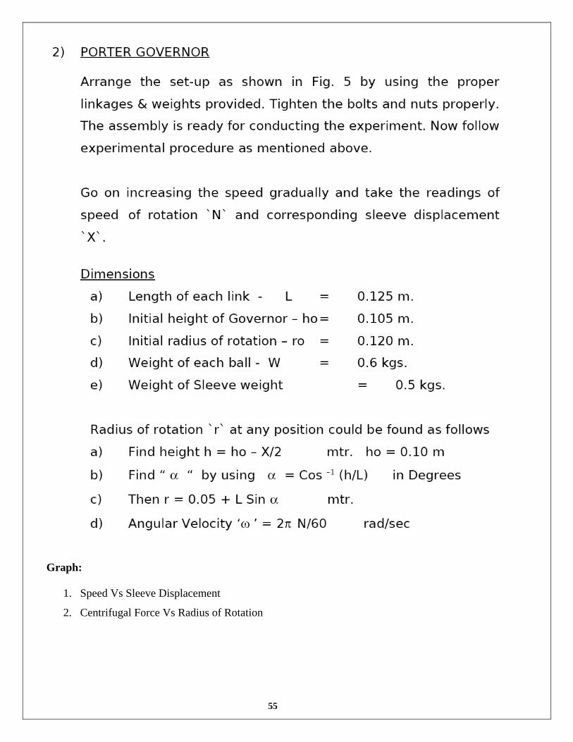
DIAGRAMATICAL REPRESENTATION OF PORTER GOVERNOR:
TABULATION:
S.No Sleeve
Displacement (X) ‘mm’
Height of the
Governor (h) ‘mm’
Speed (N)
‘rpm’
Radius (r)
‘mm’
Centrifugal force ‘N’
Sensitivity (s)
Effort (e) ‘N’
Power (P)
‘Nmm’
55
Graph:
1. Speed Vs Sleeve Displacement
2. Centrifugal Force Vs Radius of Rotation
56
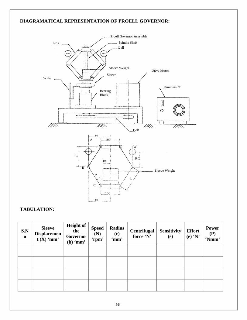
DIAGRAMATICAL REPRESENTATION OF PROELL GOVERNOR:
TABULATION:
S.No
Sleeve Displacement (X) ‘mm’
Height of the
Governor (h) ‘mm’
Speed (N)
‘rpm’
Radius (r)
‘mm’
Centrifugal force ‘N’
Sensitivity (s)
Effort (e) ‘N’
Power (P)
‘Nmm’

57
Graph:
1. Speed Vs Sleeve Displacement
2. Centrifugal Force Vs Radius of Rotation
58
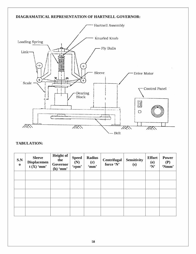
DIAGRAMATICAL REPRESENTATION OF HARTNELL GOVERNOR:
TABULATION:
S.No
Sleeve Displacement (X) ‘mm’
Height of the
Governor (h) ‘mm’
Speed (N)
‘rpm’
Radius (r)
‘mm’
Centrifugal force ‘N’
Sensitivity (s)
Effort (e) ‘N’
Power (P)
‘Nmm’

59
Graph:
1. Speed Vs Sleeve Displacement
2. Centrifugal Force Vs Radius of Rotation

60
61
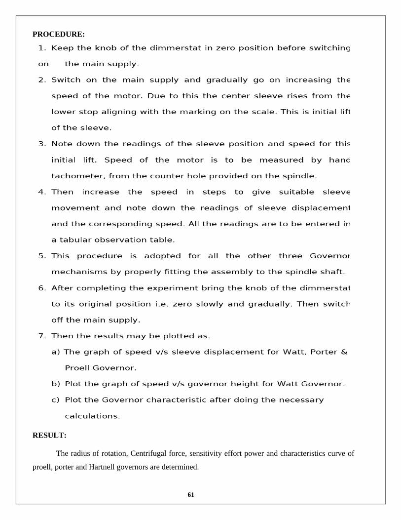
PROCEDURE:
RESULT:
The radius of rotation, Centrifugal force, sensitivity effort power and characteristics curve of
proell, porter and Hartnell governors are determined.
62
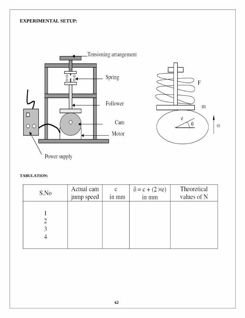
EXPERIMENTAL SETUP:
TABULATION:
63
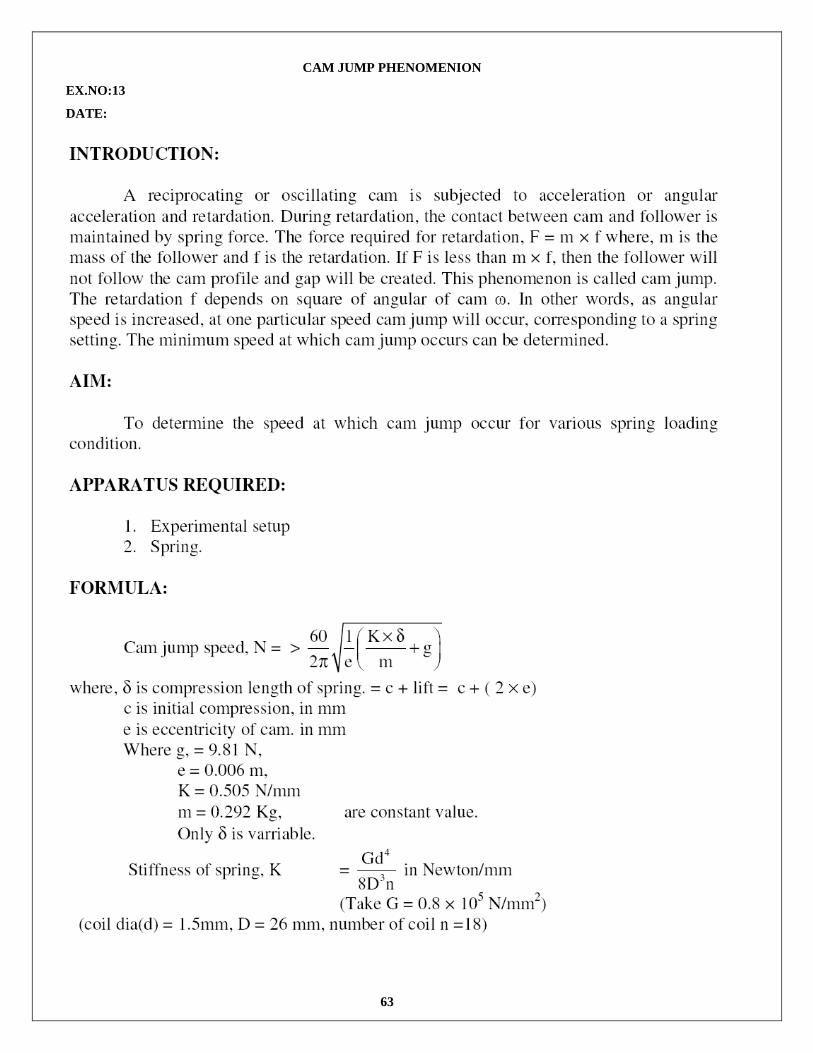
CAM JUMP PHENOMENION
EX.NO:13
DATE:

64
OBSERVATION: Diameter of the Coil = Mean Diameter of the spring = Number of turns = Modulus of Rigidity =

65
RESULT:
Thus the speed is determined by the cam jump occur.

66

67
CAM STUDY MODEL

68

69
SINGLE DEGREE FREEDOM SYSTEM EX.NO:14 DATE:

70
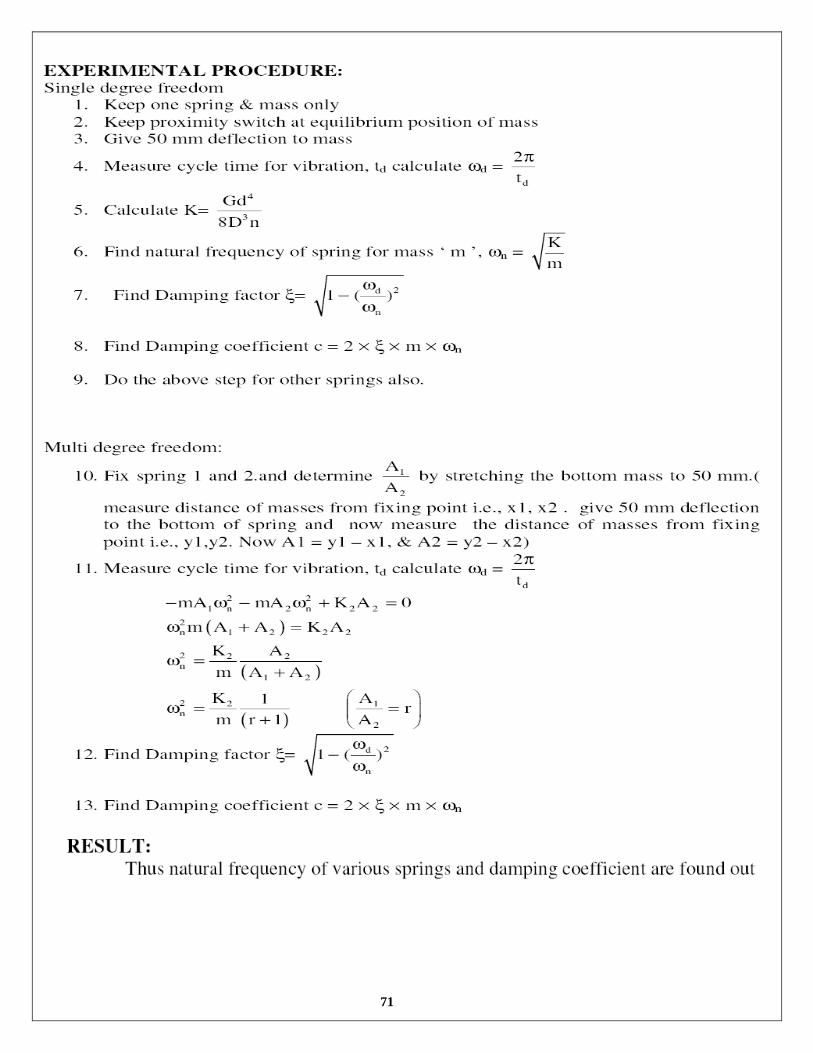
71

72
OBSERVATION:
Diameter of the shaft =
Vibrating Length =
Density of the shaft =
Modulus of the Elasticity =
TABULATION:
S.No
Shaft
Diameter
‘mm’
Vibrating
Length
‘mm’
Whirling
speed ‘rpm’
Deflection
‘m’
Whirling speed rad/sec
Theoretical Experimental
73
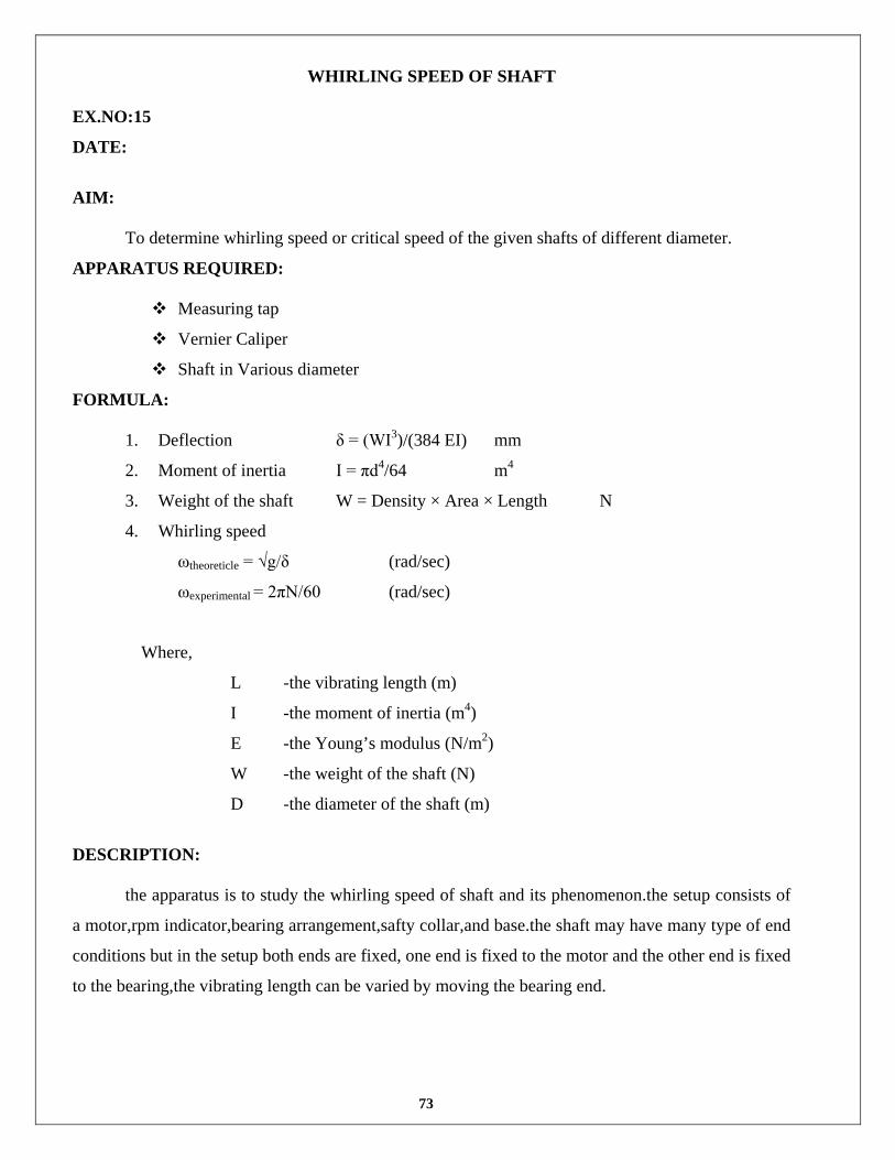
WHIRLING SPEED OF SHAFT EX.NO:15
DATE:
AIM:
To determine whirling speed or critical speed of the given shafts of different diameter.
APPARATUS REQUIRED:
Measuring tap
Vernier Caliper
Shaft in Various diameter
FORMULA:
1. Deflection δ = (WI3)/(384 EI) mm
2. Moment of inertia I = πd4/64 m4
3. Weight of the shaft W = Density × Area × Length N
4. Whirling speed
ωtheoreticle = √g/δ (rad/sec)
ωexperimental = 2πN/60 (rad/sec)
Where,
L -the vibrating length (m)
I -the moment of inertia (m4)
E -the Young’s modulus (N/m2)
W -the weight of the shaft (N)
D -the diameter of the shaft (m)
DESCRIPTION:
the apparatus is to study the whirling speed of shaft and its phenomenon.the setup consists of
a motor,rpm indicator,bearing arrangement,safty collar,and base.the shaft may have many type of end
conditions but in the setup both ends are fixed, one end is fixed to the motor and the other end is fixed
to the bearing,the vibrating length can be varied by moving the bearing end.

74

75
PROCEDURE:
1. Mild steel shaft is fixed in the setup.
2. The shaft length can be adjusted by the movement of the bearing holder.
3. Motor is switched on.
4. The shaft is allowed to rotate until it touches the safety collar, then the rpm is noted by a
digital indicator.
5. Similarly observe another two readings for different length.
6. From the above observation the readings for different length.
7. Similarly repeat the same procedure for the shafts of various diameters.
RESULT:
The critical speed of given shafts of different diameter are determined and compared with
theoretical value.

76
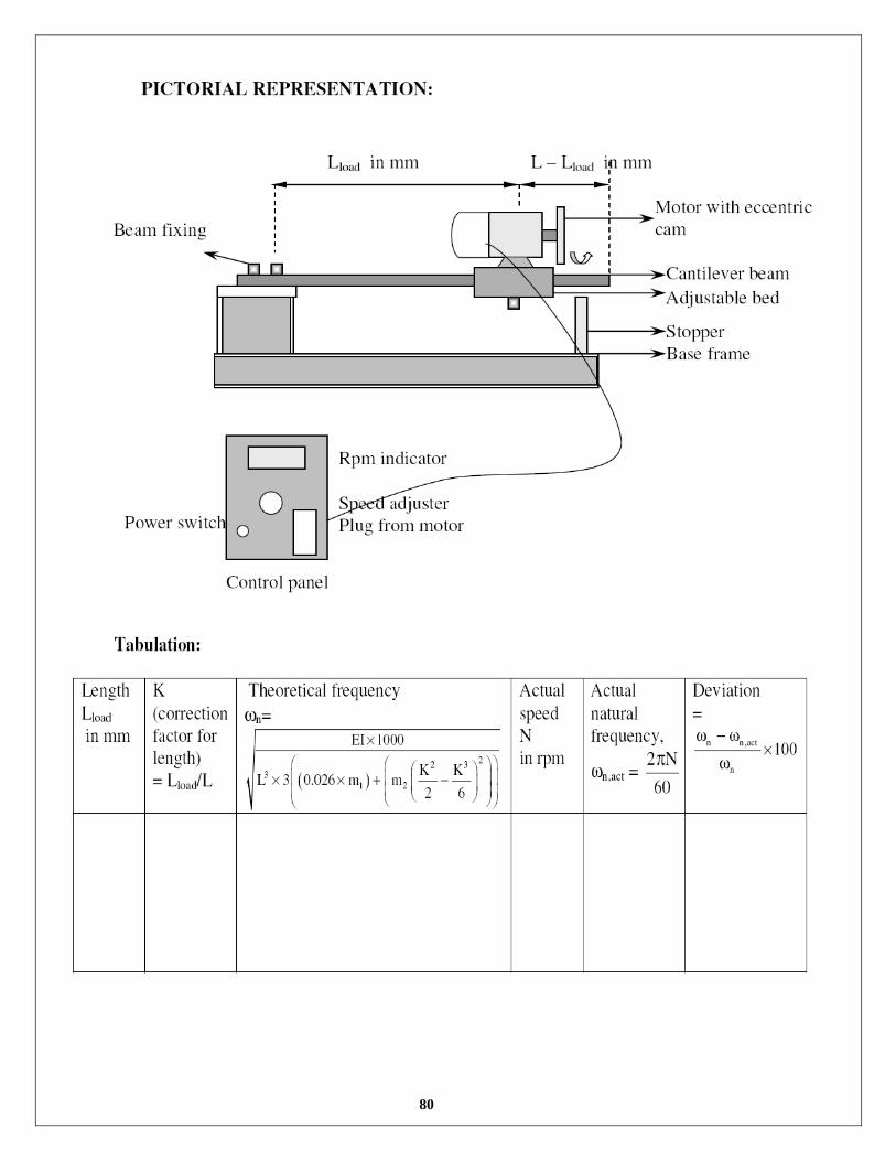
PICTORIAL REPRESENTATION:
77
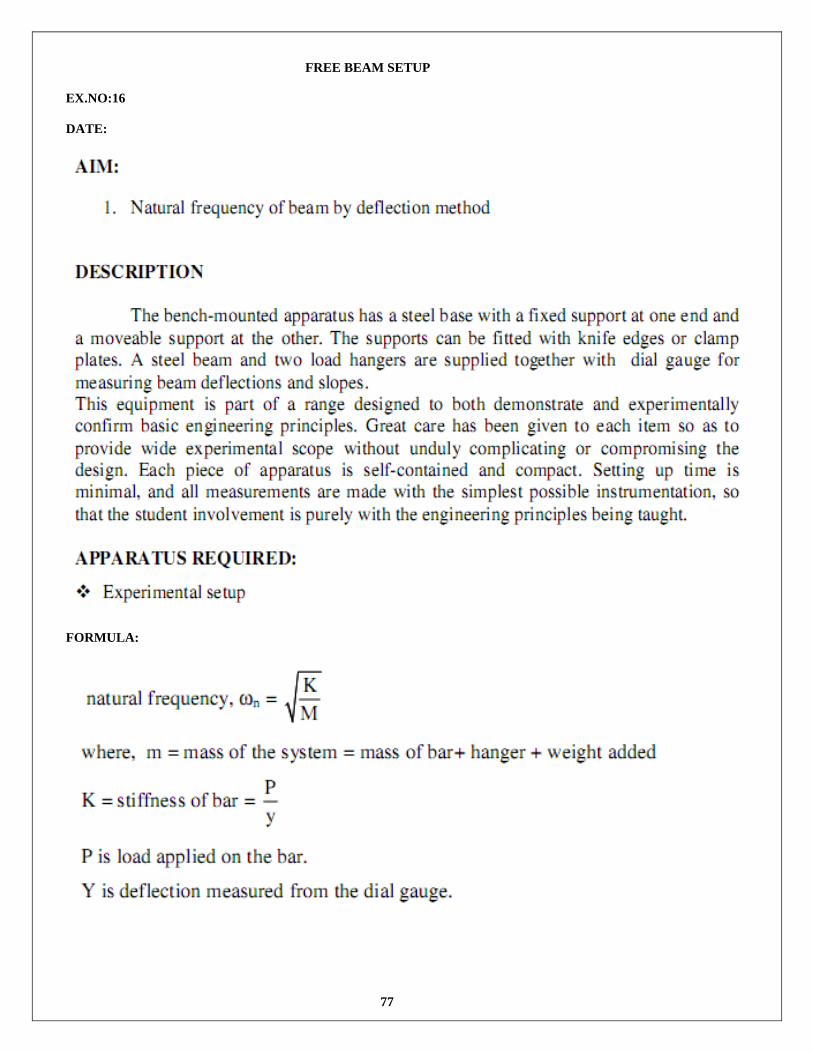
FREE BEAM SETUP
EX.NO:16
DATE:
FORMULA:

78
TABULATION:

79
EXPERIMENTAL PROCEDURE:
80
81
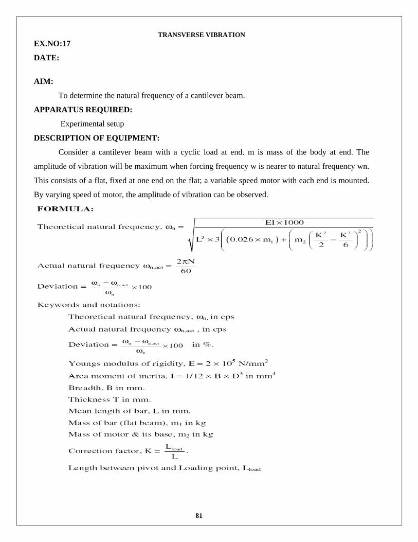
TRANSVERSE VIBRATION EX.NO:17
DATE:
AIM:
To determine the natural frequency of a cantilever beam.
APPARATUS REQUIRED:
Experimental setup
DESCRIPTION OF EQUIPMENT:
Consider a cantilever beam with a cyclic load at end. m is mass of the body at end. The
amplitude of vibration will be maximum when forcing frequency w is nearer to natural frequency wn.
This consists of a flat, fixed at one end on the flat; a variable speed motor with each end is mounted.
By varying speed of motor, the amplitude of vibration can be observed.

82

83
EXPERIMENTAL PROCEDURE:
1. Measure cross section of beam.
2. Weigh the mass on the beam.
3. Fix at known distance and vary the speed of motor.
4. Observe speed at which amplitude is maximum.
5. (Do not run at this speed for long time) (at natural frequency stage the motor
6. Takes more power, so variation speed / variation of voltage is very low.)
7. Increase speed for this and ensure that amplitude is less at higher speed.
8. Do this for various values of ‘L’ and compare with calculated value.
9. calculate theoretical frequency wn
10. Find actual frequency of the system wn,act = 2pN/60.
11. Compare theoretical with actual value.
Remarks:
Following reasons causes variation of natural frequency between theoretical and experimental.
1. Fixing bolt is also act as spring.
2. Damping factor of material of the flat.
RESULT: Thus the natural frequency and critical speed is determined by given vibration table.
84
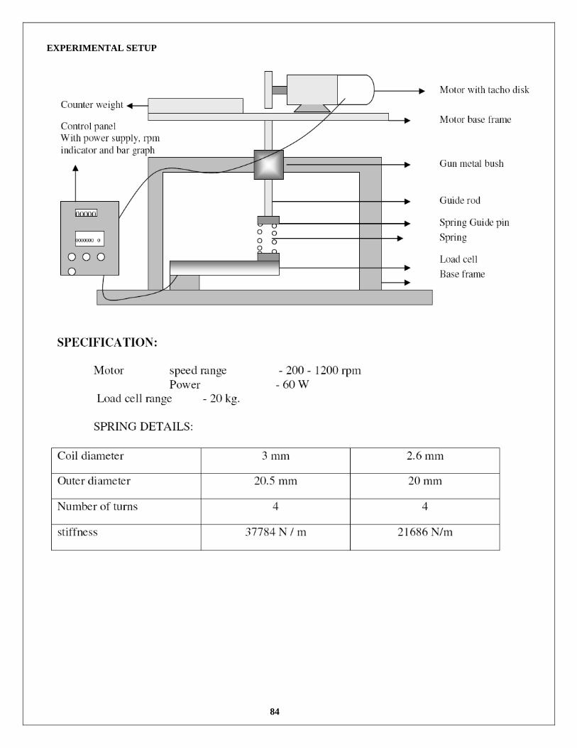
EXPERIMENTAL SETUP
85
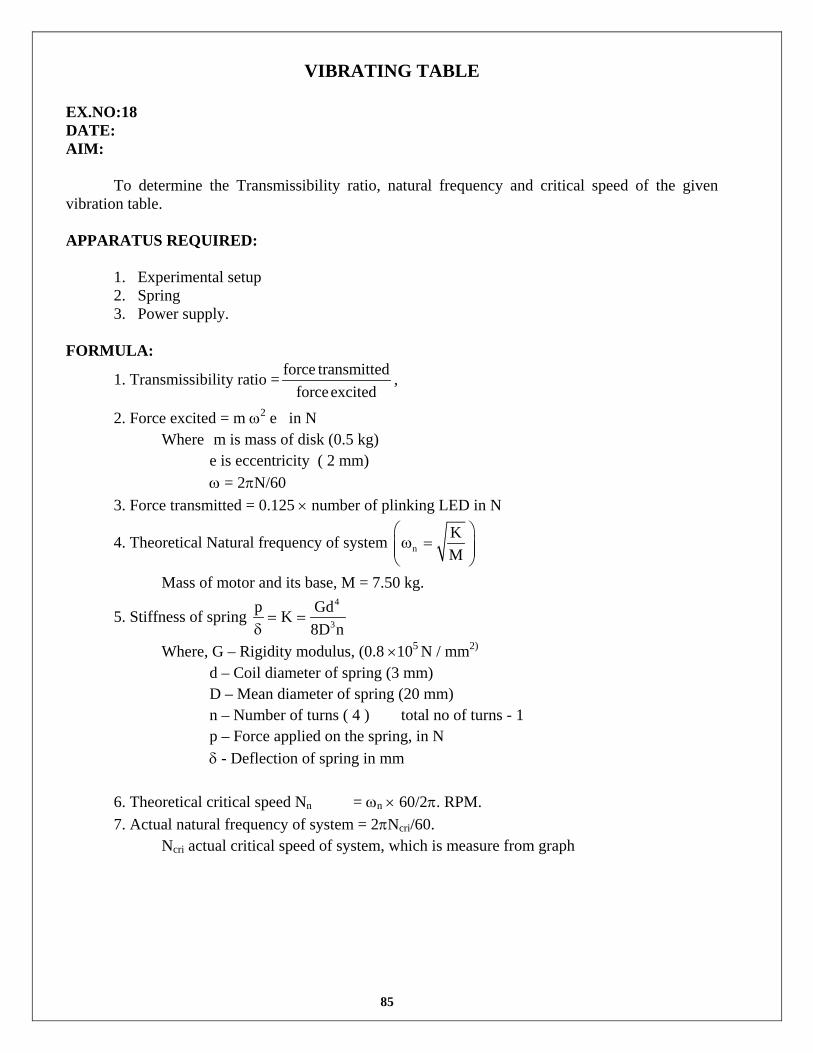
VIBRATING TABLE EX.NO:18 DATE: AIM: To determine the Transmissibility ratio, natural frequency and critical speed of the given vibration table. APPARATUS REQUIRED:
1. Experimental setup 2. Spring 3. Power supply.
FORMULA:
1. Transmissibility ratio = force transmittedforceexcited
,
2. Force excited = m ω2 e in N Where m is mass of disk (0.5 kg)
e is eccentricity ( 2 mm) ω = 2πN/60
3. Force transmitted = 0.125 × number of plinking LED in N
4. Theoretical Natural frequency of system nKM
ω =
Mass of motor and its base, M = 7.50 kg.
5. Stiffness of spring 4
3
p GdK8D n
= =δ
Where, G – Rigidity modulus, (0.8 ×10⁵ N / mm2) d – Coil diameter of spring (3 mm)
D – Mean diameter of spring (20 mm) n – Number of turns ( 4 ) total no of turns - 1
p – Force applied on the spring, in N δ - Deflection of spring in mm 6. Theoretical critical speed Nn = ωn × 60/2π. RPM. 7. Actual natural frequency of system = 2πNcri/60. Ncri actual critical speed of system, which is measure from graph

86
TABULATION:
S.NO Speed of the motor
no of plinking LED
Force transmitted In N
Force excited In N
Transmissibility ratio T
In N

87

88
EXPERIMENTAL PROCEDURE:
1. Take out motor with unbalance wheel, guide rod etc and weigh in a balance M = 7.50 kg.
2. Measure dimension of spring used for vibration isolation, d, D, n, free length etc.
3. Calculate stiffness of spring Calculate natural frequency Ensure that this is within 1200 rpm and Fix the
spring on the table
4. Set the value in bar graph is as zero. (switch off all led including zero indicator)
5. Then increase the speed of the motor and check the system in vibration mode or not. If no vibration (oscillation)
on spring then adjust the counter weight added or spring location.
6. Then now run the motor in 200 rpm. Now increase the speed of motor. Simultaneously note the speed of motor
for each increasing of blinking LED.
7. Find force excited = m ω2 e
8. Find force transmitted = 0.125 × number of plinking LED
9. Find transmissibility ratio = force transmitted
forceexcited
10. Plot transmissibility Vo speed
11. Determine Nc where transmissibility is maximum.
12. Calculate ωe = c2 N60π
and compare with natural frequency ωn
13. After reaching all (8) LED, increase the speed for additional 200 rpm.
14. then now reduce the motor, now also Simultaneously note the speed of motor for each increasing of blinking
LED Note values of force transmitted as a function of speed (N).
15. Do the same experiment with different spring as a function of speed (N)
RESULT: Thus the natural frequency and critical speed is determined by given vibration table.
89
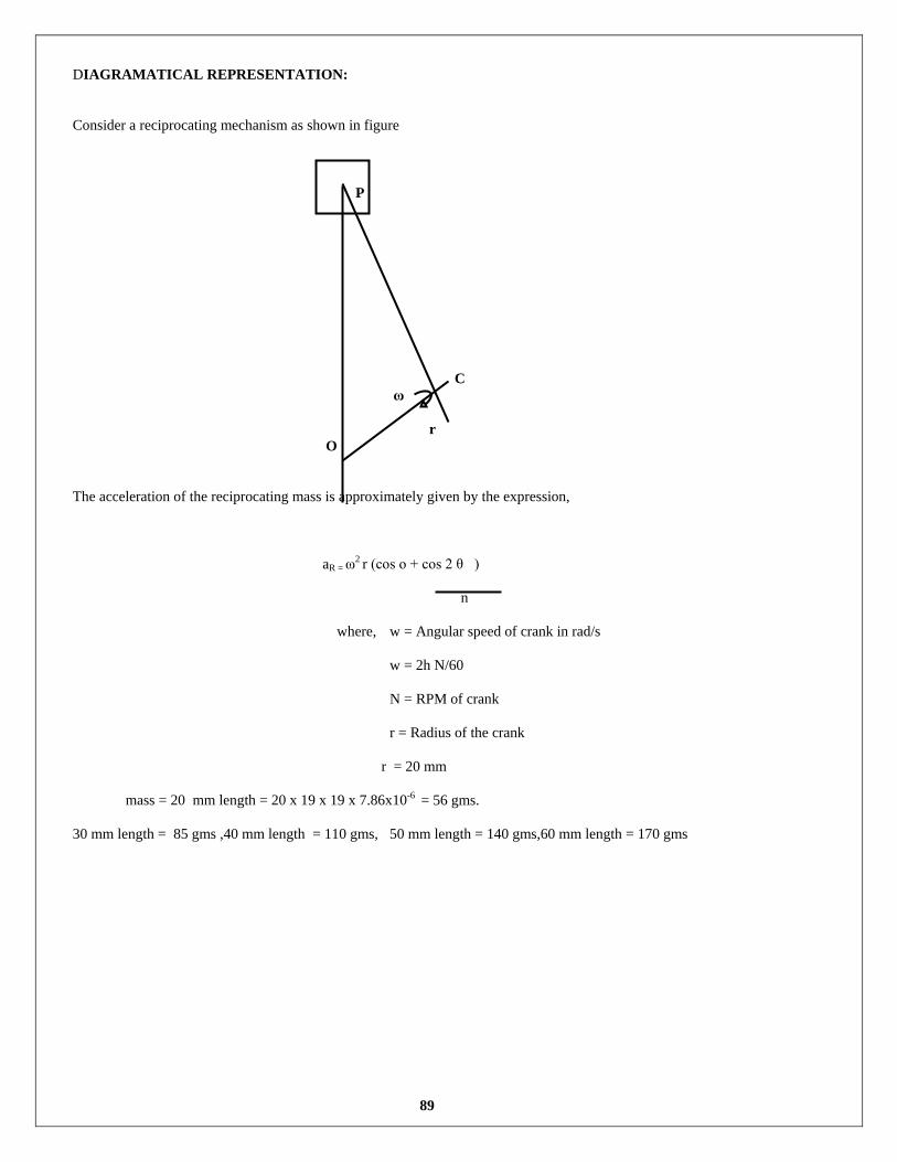
DIAGRAMATICAL REPRESENTATION: Consider a reciprocating mechanism as shown in figure P C
ω
r O The acceleration of the reciprocating mass is approximately given by the expression,
aR = ω2 r (cos o + cos 2 θ )
n
where, w = Angular speed of crank in rad/s
w = 2h N/60
N = RPM of crank
r = Radius of the crank
r = 20 mm
mass = 20 mm length = 20 x 19 x 19 x 7.86x10-6 = 56 gms.
30 mm length = 85 gms ,40 mm length = 110 gms, 50 mm length = 140 gms,60 mm length = 170 gms
90
BALANCING OF RECIPROCATING MASS
EX.NO:19
DATE:
AIM:
Balancing the reciprocating mass in various speeds.
EXPERIMENTATION
1. Run the equipment without rotating balancing mass and measure the unbalance in vertical direction.
2. Add balancing mass at ‘r’ opposite to crank pin with β = 0.2, 0.4, 0.6, 0.8 & 1.0 and measure unbalance in
vertical direction.
3. Verify that the unbalance vertical force is increased when adding weights to compensate the vertical balancing.
4. Also check vibration is increased in according to the speed.

91
TABULATION:
Mass added
FH in ----------- rpm FV
Visual movement
FH----------- rpm
FV Visual
movement
No of blinking LED
load on horizontal
No of blinking LED
load on horizontal
92
PROCEDURE:
RESULT:
Thus the changes in horizontal vibration are vise versa to vertical vibration when the reciprocating mass is under
balancing.
93
BALANCING ROTATING MASSES EX.NO:20 DATE: AIM
To determine the balancing mass of the rotor connected in the crank shaft. CONDITIONS FOR COMPLETE BALANCING:
In order to have complete balance or several masses in different plans the two
conditions must be satisfied.
1. Resultant (Centrifugal force must be zewr) 2. Resultant couple must be zero.
APPARATUS REQUIRED
1. Dynamic Balancing Crankshaft model
2. Tacho meter 3. Scale and protractor.
PROCEDURE:
1. The dynamic model of crankshaft is run at the rated speed.
2. The known mass is placed at the required angular position. 3. The eccentricity of the masses is measured. 4. The distance between the reference plane to the rotating plane masses are measured. 5. Draw the couple and force polygon and find the unknown mass and angular position of
the balanced mass. 6. The shaft is run at same speed and check the balance. 7. To draw the force polygon and couple polygon and find unknown masses for given
condition.

94
TABULATION:
S.NO
Plane
Mass (Kg)
Radius (Metre)
Centrifugal Force, (Kgm)
Dist from A, length (m)
Couple (Kg*m*m)
1
A
2
B
3
C
4
D