Developments in Model-Based County Level Estimation of Agricultural

Cash Rental Rates

Michael E. Bellow1, Nathan Cruze1, Andreea L. Erciulescu1, 2

1National Agricultural Statistics Service, 1400 Independence Ave., SW, Washington, DC 20250 2National Institute of Statistical Sciences, P.O. Box 14006, Research Triangle Park, NC 27709

Abstract

Estimates of agricultural cash rental rates at different geographic levels are used for rental agreement formulation, farm program administration and other applications. The USDA's National Agricultural Statistics Service (NASS) has been producing estimates of average cash rental rates at the state level since 1997. In 2009, the agency fully implemented an annual Cash Rents Survey (CRS) to obtain estimates of average cash rental rates for counties with at least 20,000 acres of cropland or pastureland in three land use categories. Since sample sizes for a number of counties were too small for reliable direct estimation, NASS developed a model-based estimation method (implemented in 2013) that incorporates auxiliary information and involves separate area-level modeling of the average and difference of rental rates over two survey years. With the 2014 Farm Bill specifying that the survey be conducted "no less frequently than every other year", the current focus is on evaluating how this estimator would perform with survey data from two years apart (when the survey is skipped in the intervening year). We describe the results of an empirical study addressing that question and discuss future directions for research.

Key Words: model-based estimation, best linear unbiased predictor, Cash Rents Survey

1. Introduction

Timely and accurate estimation of cash rental rates at the individual county level is a key initiative of the United States Department of Agriculture’s National Agricultural Statistics Service (NASS). The user community for such estimates includes farm operators and renters, state and federal government agencies as well as universities and other research organizations. For example, operators use county-level cash rents estimates in decision-making related to the renting and leasing of their farmland. The USDA’s Farm Service Agency (FSA) utilizes these figures to determine market-based rates for administering programs such as the Conservation Reserve Program (CRP), while an agronomics researcher could employ them in carrying out studies evaluating the relationships between cash rental rates and other economic variables. NASS only publishes estimates of rental rates and not separate total rented acres or total rent series.

Due in large part to the importance of county-level estimates of cash rental rates in the administration of the CRP, the 2008 Farm Bill mandated that NASS conduct an annual survey of cash rents and publish estimates for all counties in the U.S. having 20,000 or more acres of cropland plus pasture. Separate estimates were stipulated for the following three land use categories: 1) non-irrigated cropland, 2) irrigated cropland, and 3) permanent pasture. NASS implemented the Cash Rents Survey (CRS) in 2009 and conducted it on an annual basis until 2014. Because of budgetary

2773

considerations, the 2014 Farm Bill relaxed the earlier requirement by specifying that the CRS be carried out at least once every two years in all U.S. states with the exception of Alaska.

The target population for the CRS is the set of all agricultural operations that have rented land in any of the categories on a cash basis or will do so over the current crop year (which in some cases crosses two calendar years). The survey does not attempt to obtain information about land rented for a share of the crop, on a fee per head basis, per pound of grain or by animal unit month (AUM), land rented free of charge or land that includes buildings (e.g., barns). Data collection takes place from late February until the end of June.

Of the counties in the U.S. (excluding Alaska), 2,764 (89 percent) had 20,000 or more acres of combined cropland and pasture according to the 2012 Census of Agriculture. NASS has published at least one county estimate of cash rental rate in 93 to 95 percent of such counties each year although some land use practices may be underserved.

About a month after state-level estimates of cash rental rates are released, estimates are published for counties as well as agricultural statistics districts, which are sets of counties in geographic proximity and generally having similar agricultural practices. For purposes of internal consistency, appropriately weighted sums of county estimates must agree with the state-level and district-level estimates. Official cash rents estimates are produced by NASS through the review process of the Agricultural Statistics Board (ASB). The commodity specialists and statisticians of the ASB review several distinct estimates of acreage rented and rent expense, including the direct estimates of cash rental rates obtained from the CRS, model-based estimates and other auxiliary information. The ASB seeks to set estimates for all counties with at least one positive report of acreage rented on a cash basis. Since the official statistics are the result of a board review process, accompanying measures of variability are not published.

Because direct estimates of county-level cash rental rates computed from the CRS are often unstable due to the small realized sample sizes, NASS has explored model-based approaches involving auxiliary variables, such as total value of production and county-level crop yield estimates. Since rental rates from the current and previous year are often highly correlated despite differences between the sets of respondents in both years, it was believed that gains in efficiency could be achieved by using information from both survey years. Computational expediency was obtainable by reducing a bivariate model to two separate univariate components.

To that end, Berg, Cecere and Ghosh (2014) proposed a univariate area-level model that involves fitting two sets of survey-based direct estimates, the first constructed as the average of the direct estimates of cash rental rates for two survey years and the second as the difference (i.e., change) of the same direct estimates for the same two survey years. Their model can be described as an extension of the well-known Fay-Herriot model (Fay and Herriot, 1979). An assumption of orthogonality between the residuals of the two submodels simplifies the computation of estimates and mean-squared errors. The associated estimation method was tested on survey and auxiliary data from 2010-11 and found to be more efficient than direct estimation. In the remainder of this paper, the term BCG refers to the model developed by Berg, Cecere and Ghosh and its associated estimator.

Berg et al. (2014) devised an index combining information from multiple covariates and constructed synthetic estimates of sampling variances using a hierarchical model so as to obtain a variance estimator less variable and less correlated with estimators of means when compared to the

2774

sampling variance (extensions are constructed for samples of size one). They applied the two-stage benchmarking procedure developed by Ghosh and Steorts (2013) to the county estimates for consistency with official state-level and district-level figures. NASS began using estimates computed via the BCG method (based on two consecutive years of survey data) for operational county-level cash rents estimation in 2013.

Since this method was developed and tested at a time when the CRS was required to be conducted every year, there was no initial exploration of how it would be affected if survey data from two non-consecutive years were used. Due to the relaxed requirement of the 2014 Farm Bill and the likelihood that this survey will be carried out on an irregular basis in the foreseeable future, NASS decided to resume its research efforts in model-based cash rents estimation in 2016. The objective was to evaluate the BCG method using survey and auxiliary data over a three-year period for which survey data were available. Estimation was based on two pairs of survey years: 1) 2013 and 2014 (consecutive years), and 2) 2012 and 2014 (skipped year). Although the CRS was conducted in 2013, we carried out the BCG estimation procedure for the (2012, 2014) scenario as if it had been skipped that year (to emulate the likely future situation) and compared the results for the two cases.

Section 2 describes the BCG methodology in detail. In Section 3, model fit and estimation performance for the consecutive years vs. skipped year scenarios are compared. Section 4 provides a summary and discussion of possible avenues for future research.

2. Methodology

The Cash Rents Survey employs a stratified systematic sample design with a national sample size of approximately 225,000 agricultural operations. On the questionnaire, respondents are asked whether any land was or will be rented for cash during the current crop year and, if so, the total acres rented and cash rent per acre or total dollars paid for each of the three land use categories (non-irrigated cropland, irrigated cropland and pasture). Direct estimates are computed as weighted sums over sampled units, where the weights are the product of response rates and inverses of selection probabilities.

The univariate area-level model for cash rental rates proposed by Berg et al. (2014) can be expressed as follows:

(𝜃𝑖,𝑡−𝑝 , 𝜃𝑖,𝑡) = (𝜃𝑖 , 𝜃𝑖) + (−0.5∆𝑖 , 0.5∆𝑖), (2.1)

where:

p = gap between the two survey years (‘1’ in original BCG modeling),

𝜃𝑖,𝑠 = mean cash rental rate for county i in year s (s = t-p or t),

𝜃𝑖 = two-year (t-p and t) average of cash rental rates for county i, and

∆𝑖 = change in cash rental rate for county i from year t-p to t.

The model for the two-year average is:

�̂�𝑖 = 𝜃𝑖 + 𝑒𝑖 ;

2775

𝜃𝑖 = 𝒙′𝒊,𝒂𝜷𝒂 + 𝑢𝑖 ,

where:

�̂�𝑖 = direct estimate of two-year average rental rate for county i,

𝒙𝒊,𝒂 = vector of covariates for the average in county i, and

𝜷𝒂 = vector of fixed effects parameters for the average.

The error terms {𝑒𝑖} are assumed to be independent with mean 0 and variances {𝜎𝑒𝑖2 } , while the

{𝑢𝑖} are assumed independent with mean 0 and common variance 𝜎𝑢2 (and independent of the {𝑒𝑖}).

The model for the difference between the two years is:

�̂�𝑖 = ∆𝑖 + i ;

∆𝑖= 𝒙′𝒊,𝒅𝜷𝒅 + 𝑣𝑖 ,

where:

�̂�𝑖 = direct estimate of two-year difference between cash rental rates for county i,

𝒙𝒊,𝒅 = vector of covariates for the difference in county i, and

𝜷𝒅 = vector of fixed effects parameters for the difference.

The {i} are assumed to be independent with mean 0 and variances 𝜎𝑓𝑖2 , while the {𝑣𝑖} are assumed

independent with mean 0 and common variance 𝜎𝑣2 (and independent of the {i}).

The parameters 𝜷𝒂 , 𝜷𝒅 , 𝜎𝑢2 and 𝜎𝑣

2 are generally unknown but can be estimated using techniques such as method of moments (MOM), maximum likelihood or Bayesian analysis (NASS currently employs MOM since the other methods require distributional assumptions). A jackknife method and Taylor series expansion are used to derive direct estimates of sampling variances for all counties with a sample size of at least two in each survey year. This estimator is approximately unbiased, but may have a large variance (especially in counties with small sample sizes) and significant correlation with direct estimators of means for certain states and land uses. To address these concerns, Berg et al. (2014) developed an alternative procedure for estimating the sampling variances of the average and difference based on a hierarchical model.

The following three types of available auxiliary information are used in fitting the model:

1) Total value of (agricultural) production (TVP), 2) Official county-level crop yield estimates, and 3) National Commodity Crop Productivity Indexes (NCCPI).

The Census of Agriculture, conducted by NASS twice each decade in years ending in ‘2’ and ‘7’, provides estimates of TVP at the county level. NASS publishes county-level crop yield estimates on an annual basis. Due to the sparsity of yield data for certain crops in a number of states, use of yield data for specific crops as covariates in estimation models can be challenging. Berg et al.

2776

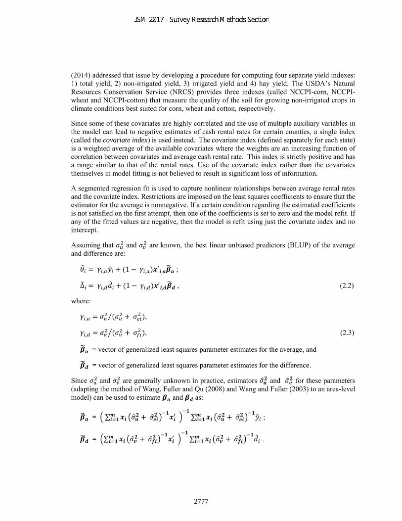
(2014) addressed that issue by developing a procedure for computing four separate yield indexes: 1) total yield, 2) non-irrigated yield, 3) irrigated yield and 4) hay yield. The USDA’s Natural Resources Conservation Service (NRCS) provides three indexes (called NCCPI-corn, NCCPI-wheat and NCCPI-cotton) that measure the quality of the soil for growing non-irrigated crops in climate conditions best suited for corn, wheat and cotton, respectively.

Since some of these covariates are highly correlated and the use of multiple auxiliary variables in the model can lead to negative estimates of cash rental rates for certain counties, a single index (called the covariate index) is used instead. The covariate index (defined separately for each state) is a weighted average of the available covariates where the weights are an increasing function of correlation between covariates and average cash rental rate. This index is strictly positive and has a range similar to that of the rental rates. Use of the covariate index rather than the covariates themselves in model fitting is not believed to result in significant loss of information.

A segmented regression fit is used to capture nonlinear relationships between average rental rates and the covariate index. Restrictions are imposed on the least squares coefficients to ensure that the estimator for the average is nonnegative. If a certain condition regarding the estimated coefficients is not satisfied on the first attempt, then one of the coefficients is set to zero and the model refit. If any of the fitted values are negative, then the model is refit using just the covariate index and no intercept.

Assuming that 𝜎𝑢2 and 𝜎𝑣

2 are known, the best linear unbiased predictors (BLUP) of the average and difference are:

�̃�𝑖 = 𝛾𝑖,𝑎�̂�𝑖 + (1 − 𝛾𝑖,𝑎)𝒙′𝒊,𝒂�̃�𝒂 ;

∆̃𝑖 = 𝛾𝑖,𝑑�̂�𝑖 + (1 − 𝛾𝑖,𝑑)𝒙′𝒊,𝒅�̃�𝒅 , (2.2)

where:

𝛾𝑖,𝑎 = 𝜎𝑢2 (𝜎𝑢

2 + 𝜎𝑒𝑖2 )⁄ ,

𝛾𝑖,𝑑 = 𝜎𝑣2 (𝜎𝑣

2 + 𝜎𝑓𝑖2 )⁄ , (2.3)

�̃�𝒂 = vector of generalized least squares parameter estimates for the average, and

�̃�𝒅 = vector of generalized least squares parameter estimates for the difference.

Since 𝜎𝑢2 and 𝜎𝑣

2 are generally unknown in practice, estimators �̂�𝒖𝟐 and �̂�𝒗

𝟐 for these parameters (adapting the method of Wang, Fuller and Qu (2008) and Wang and Fuller (2003) to an area-level model) can be used to estimate 𝜷𝒂 and 𝜷𝒅 as:

�̂�𝒂 = ( ∑ 𝒙𝒊𝒎𝒊=𝟏 (�̂�𝒖

𝟐 + �̂�𝒆𝒊𝟐 )

−𝟏𝒙𝒊

′ )−𝟏

∑ 𝒙𝒊𝒎𝒊=𝟏 (�̂�𝒖

𝟐 + �̂�𝒆𝒊𝟐 )

−𝟏�̂�𝑖 ;

�̂�𝒅 = (∑ 𝒙𝒊𝒎𝒊=𝟏 (�̂�𝒗

𝟐 + �̂�𝒇𝒊𝟐 )

−𝟏𝒙𝒊

′ )−𝟏

∑ 𝒙𝒊𝒎𝒊=𝟏 (�̂�𝒗

𝟐 + �̂�𝒇𝒊𝟐 )

−𝟏�̂�𝑖 .

2777

The shrinkage parameters 𝛾𝑖,𝑎 and 𝛾𝑖,𝑑 are estimated by replacing 𝜎𝑢2 and 𝜎𝑣

2 in expression (2.3) with their estimates. Approximate best linear unbiased predictors of 𝜃𝑖 and ∆𝑖 are then obtained via replacement of �̃�𝒂 and �̃�𝒅 with �̂�𝒂 and �̂�𝒅 , and 𝛾𝑖,𝑎 and 𝛾𝑖,𝑑 with their estimates in (2.2):

𝜃𝑖 = 𝛾𝑖,𝑎�̂�𝑖 + (1 − 𝛾𝑖,𝑎 )𝒙′𝒊,𝒂�̂�𝒂 ;

∆̂𝑖= 𝛾𝑖,𝑑�̂�𝑖 + (1 − 𝛾𝑖,𝑑 )𝒙′𝒊,𝒅�̂�𝒅 . (2.4)

The model assumes that the direct estimate for the current year exists, i.e. at least one survey respondent in county i provided acreage and rent information. If the direct estimate for the earlier survey year does not exist, �̂�𝑖 is set to the current year’s direct estimate. The predictor of the difference takes into account multi-year respondents, survey design and outliers.

Since the covariate index does not correlate nearly as strongly with year-to-year changes in cash rental rates as it does with two-year averages, the Akaike information criterion (AIC) is applied to determine whether or not it should be used in the difference model for a given state or group of states. If the covariate index is not used, 𝒙𝒊,𝒅 is set to ‘1’ in (2.2) so that an intercept-only model is fit.

The model-based county-level estimators of cash rental rates for the two survey years are then obtained by combining the estimators of average and difference in the manner of (2.1):

𝜃𝑖,𝑡 = 𝜃𝑖 + 0.5∆̂𝑖 ,

𝜃𝑖,𝑡−𝑝 = 𝜃𝑖 - 0.5∆̂𝑖 .

The estimator 𝜃𝑖,𝑡 is of primary interest to NASS, although 𝜃𝑖,𝑡−𝑝 is available as well.

Berg et al. (2014) also derived estimators of the mean squared errors of the predictors of the average and difference, respectively. Under the assumption that the residuals for the average and difference models are uncorrelated, the MSE of the model-based estimator of cash rental rates (for either year) can be estimated by:

𝑀𝑆�̂�𝑖 = 𝑀𝑆�̂�𝑖,𝑎 + 0.25𝑀𝑆�̂�𝑖,𝑑 ,

where:

𝑀𝑆�̂�𝑖,𝑎 = estimator of MSE for the average,

𝑀𝑆�̂�𝑖,𝑑 = estimator of MSE for the difference.

The cash rents model is run separately in 34 states. The remaining 15 states (other than Alaska which is not part of the cash rents program) are placed in the following groups:

1) Arizona, Nevada; 2) Connecticut, Maine, Massachusetts, New Hampshire, Rhode Island, Vermont; 3) Delaware, Maryland; 4) New Jersey, New York, Pennsylvania; and 5) Montana, Wyoming.

2778

Note that all five groups consist of states in geographic proximity. Estimates of cash rental rates for all counties in a group are derived via a combined model fit.

As mentioned earlier, the model-based county-level cash rents estimates are benchmarked for consistency with official state-level and district-level values using the two-stage method of Ghosh and Steorts (2013). The state-level estimates are released before the start of the county estimation process. The BCG estimator of mean-squared error does not account for benchmarking effects.

An area of concern with this model has been the presence of occasional negative estimates (especially for irrigated cropland and pasture). Since the model-based estimates of the average are assured of being non-negative, these negative values are caused by either large changes in the difference model or benchmarking.

3. Empirical Evaluation

The area-level model developed by Berg et al. (2014) was evaluated with regard to model fit and estimation accuracy using Cash Rents Survey from 2012, 2013 and 2014 in conjunction with auxiliary data. The primary objective was to compare model-based estimates of 2014 cash rental rates under two scenarios: 1) consecutive-years of CRS data (2013 and 2014) as used in production and 2) a counter-factual skip-year scenario using 2012 and 2014 data. The latter case emulates the situation where the survey is not conducted in a given year so that estimation for the following year must use data from surveys conducted two years apart. In the remainder of this section, the two scenarios are sometimes referred to as model-C (for consecutive) and model-S (for skipped), respectively.

We begin by examining model fit. As mentioned earlier, the difference model only uses the covariate index if a condition involving the AIC is satisfied. When the model-based indications of cash rental rates were generated for use in 2014 operational estimation, the covariate indices were computed using crop yield data from the six year period 2004-2009 and total value of production figures obtained from the 2007 Census of Agriculture so those same indices were used in this study. Figure 1 is a set of three maps showing for each land use type the states for which the covariate index was used in difference modeling for: 1) neither the consecutive years nor skipped year cases (tan), 2) only the consecutive years case (orange), only the skipped year case (yellow) and 4) both cases (green). Note the relatively small number of states (especially for pasture) where the AIC allowed use of the covariate index.

We wish to assess the degree to which the assumption of orthogonality (i.e., zero correlation) of the residuals for average vs. difference is satisfied. Figures 2 through 4 show combined (over all states and groups of states for which the model was fit) scatterplots of standardized residuals vs. fitted values for the average and difference models (𝒙′

𝒊,𝒂�̂�𝒂 and 𝒙′𝒊,𝒅�̂�𝒅 in expression (2.4) for non-

irrigated cropland, irrigated cropland and pasture, respectively. The standardized residuals are computed as:

𝑟𝑖,𝑎 = (�̂�𝑖 − 𝒙′𝒊,𝒂�̂�𝒂 ) (�̂�𝒖

𝟐 + �̂�𝒆𝒊𝟐 )1/2⁄ ;

𝑟𝑖,𝑑 = (�̂�𝑖 − 𝒙′𝒊,𝒅�̂�𝒅 ) (�̂�𝒖

𝟐 + �̂�fi𝟐 )1/2⁄ ,

where the terms on the right-hand side are defined in Section 2. The residuals for model-C and model-S are superimposed on the same graph for each land use type. Notice that in all six plots the

2779

residuals appear to be symmetric about zero (although some skewness is apparent in the ones for average).

Figure 1. States where the Covariate Index was Used in Difference Modeling

Non-Irrigated Irrigated

Pasture

Since the model errors are not assumed to be normally distributed, Kendall’s Tau () coefficients between the standardized residuals for average and difference were computed for each land use/state combination over states where the model was fit. Table 1 shows for each land use type (with model-C and model-S) the minimum, median and maximum values of and of its absolute value. The absolute value is used because large negative values of suggest equally significant departures from orthogonality as large positive ones. Note that ranged from -0.337 to 0.511 and its median value with model-S for non-irrigated (0.153) was appreciably greater than zero.

2780

Figure 2. Standardized Residuals vs. Fitted Values for Non-Irrigated Cropland (All Estimated Counties)

Average Difference

Figure 3. Standardized Residuals vs. Fitted Values for Irrigated Cropland (All Estimated Counties)

Average Difference

Figure 4. Standardized Residuals vs. Fitted Values for Pasture (All Estimated Counties)

Average Difference

G

2781

Table 1. Summary Statistics on Kendall’s Tau Coefficients between Standardized Residuals of Average and Difference Models

Land Usage Number of

States

Measure Statistic Model-C Model-S

Non-Irrigated

46 Minimum -0.183 -0.144 Median 0.074 0.153 Maximum 0.511 0.5

|| Minimum 0.002 0.0004 Median 0.086 0.153 Maximum 0.511 0.5

Irrigated 41 Minimum -0.273 -0.211 Median 0.036 0.061 Maximum 0.289 0.27

|| Minimum 0 0.01 Median 0.054 0.088 Maximum 0.289 0.27

Pasture 42 Minimum -0.337 -0.248 Median 0.016 0.038 Maximum 0.186 0.304

|| Minimum 0.006 0.004 Median 0.088 0.08 Maximum 0.337 0.304

For each of the three land use types, a ‘typical’ state was selected, i.e., one for which the absolute value of Kendall’s Tau coefficient between standardized residuals of differences and averages was close to the corresponding median value (shown in Table 1). Figures 5 through 7 show the residuals of differences plotted against those of the averages for South Dakota (non-irrigated), Mississippi (irrigated) and Kansas (pasture). The graphs for the consecutive years and skipped year scenarios appear side-by-side for ease of comparison. Note that some degree of relationship (possibly non-linear) between the two sets of residuals is suggested by all six plots. For example, there’s clearly higher variability of the difference residuals for positive than negative values of the residuals for average in the model-S plot for Kansas, while upward trends are noticeable in the model-C plot for Mississippi and all three model-S plots. Note also that only the plots for South Dakota depict a situation where the covariate index was used in the model fit for the difference (see Figure 1).

The nonparametric test of association based on Kendall’s Tau was applied for each land use/state combination. The maps in Figure 8 depict the test results, showing for each land use category the states where the null hypothesis of zero association (as measured by Kendall’s Tau) between residuals for average and difference was rejected at the 𝛼 = 0.05 level for 1) both model-C and model-S (red), 2) just model-C (orange), 3) just model-S (yellow) and 4) neither model (green).

2782

Figure 5. Standardized Residuals of Difference vs. Average for Non-Irrigated Cropland in South Dakota

Model-C Model-S

Figure 6. Standardized Residuals of Difference vs. Average for Irrigated Cropland in Mississippi

Model-C Model-S

Figure 7. Standardized Residuals of Difference vs. Average for Pasture in Kansas

Model-C Model-S

2783

States where the model was either not run or there was insufficient data for a valid test (e.g., fewer than five counties were estimated) are indicated by tan. Of the ‘typical’ states depicted in Figures 5 through 7, the null hypothesis of zero association between the average and difference residuals was accepted with model-C but rejected with model-S for South Dakota (non-irrigated), while it was accepted in both scenarios for Mississippi (irrigated) and Kansas (pasture). Overall, the test showed significant association in more states for the non-irrigated category than for either irrigated or pasture and in more states for model-S than model-C. The set of five contiguous centrally located states (Nebraska, Iowa, Missouri, Arkansas and Tennessee) where significant association was detected in both scenarios for pasture is also noteworthy.

Figure 8. Results of Kendall’s Tests of Association between Average and Difference Residuals (Legends Refer to Null Hypothesis that = 0)

Non-Irrigated Irrigated

Pasture

2784

We compared deviations of model-C and model-S county-level cash rents estimates and corresponding official estimates of cash rental rates for 2014 published by NASS. While the official figures are not being used as a gold standard, the degree of agreement between these numbers and the model-based estimates is still of interest. The following four metrics (computed at the state level) are used in the comparisons:

1) Mean Absolute Deviation (MAD) – mean of absolute values of county-level deviations from official estimates:

𝑀𝐴𝐷 = (1

𝑛𝑐) ∑ |𝜗𝑖𝑡

𝑛𝑐𝑖=1 − 𝑦𝑖𝑡

(𝑜𝑓𝑓)| ,

where:

𝜗𝑖𝑡 = an estimate (model-C, model-S or direct) of cash rental rate for county i in year t,

𝑦𝑖𝑡(𝑜𝑓𝑓) = NASS official estimate of cash rental rate for county i in year t, and

𝑛𝑐 = number of estimated counties in state.

2) Mean Absolute Relative Deviation (MARD) – mean of ratios between absolute deviations and official estimates: 𝑀𝐴𝑅𝐷 = (

1

𝑛𝑐) ∑ |𝜗𝑖𝑡 − 𝑦𝑖𝑡

(𝑜𝑓𝑓)| 𝑦𝑖𝑡

(𝑜𝑓𝑓)⁄

𝑛𝑐𝑖=1 .

3) Root Mean-Squared Deviation (RMSD) – square root of mean of squared deviations from

official estimates:

RMSD = [(1

𝑛𝑐) ∑ (𝜗𝑖𝑡 − 𝑦𝑖𝑡

(𝑜𝑓𝑓))2𝑛𝑐

𝑖=1 ]1/2

.

4) Root Mean-Square Relative Deviation (RMSRD) – square root of mean of squared ratios

between absolute deviations and official estimates:

RMSRD = [(1

𝑛𝑐) ∑ (

𝜗𝑖𝑡−𝑦𝑖𝑡(𝑜𝑓𝑓)

𝑦𝑖𝑡(𝑜𝑓𝑓) )2𝑛𝑐

𝑖=1 ]

1/2

.

Figure 9 is a set of plots showing MARD and RMSRD for model-C (vertical axis) vs. model-S (horizontal axis) for each land usage. Since these two metrics are based on relative deviations, they can be compared directly across states. A majority of points falling below the ‘y=x’ line (for example, the two ‘non-irrigated’ plots) suggest closer proximity to official figures for model-C than model-S. Note also the outliers in all of the plots.

Table 2 shows for each metric the number and percent of states where it was lower for model-C than model-S. Note that: 1) all four metrics were lower in more states for model-C than model-S for both non-irrigated and irrigated cropland, and 2) all four metrics were higher for model-C than model-S in either more states or the same number of states for pasture.

2785

Figure 9. MARD and RMSRD for Model-C vs. Model-S

MARD (Non-Irrigated) RMSRD (Non-Irrigated)

MARD (Irrigated) RMSRD (Irrigated)

MARD (Pasture) RMSRD (Pasture)

2786

Table 2. Number and Percent of States where Metrics on Deviations from Official Estimates Lower for Model-C than Model-S

Land

Use

Type

Metric

MAD

MARD RMSD RMSRD

Number Percent Number Percent Number Percent Number Percent Non-Irrigated

29 63.0 36 78.3 28 60.9 34 73.9

Irrigated 22 53.7 23 56.1 21 51.2 22 53.7 Pasture 19 45.2 19 45.2 20 47.6 21 50

Table 3 provides a similar comparison for variability of the direct, model-C and model-S estimators based on minimum, median and maximum MSEs (over counties) in each state. Note that model-S displayed more favorable properties than model-C in terms of MSE for all three land usages. The model-based estimates of MSE never exceed corresponding synthetic variances and are not always smaller than summary variances from the CRS.

Another factor of interest is the effect of sample size on estimator properties. Figure 10 shows (for all states combined) the differences between the model-C and model-S estimates vs. the sample size from the 2014 CRS for the three land use categories. Note the overall decrease in the magnitude of the differences as the sample size increases. This is due mainly to the shrinkage factors in the model for average tending toward one as the sample size increases in both the consecutive and skipped year cases so that the model estimates are close to the corresponding direct estimates. Figure 11 depicts the effect of sample size on variability (again, for all states combined), showing the MSEs of both model-C and model-S falling considerably with increasing sample size.

In Section 2 the presence of occasional negative estimates with the BCG model was mentioned. Table 4 shows the three use/state combinations where negative estimates were generated for 2014 in either the consecutive years or skipped year scenario. Note that there were only seven counties with negative estimates for model-S compared with twelve for model-C. All of the unbenchmarked estimates in the irrigated category for Ohio and Pennsylvania were non-negative so the benchmarking process caused the final BCG estimates for three counties in Ohio and eight in Pennsylvania to be negative in one or both scenarios. The unbenchmarked estimate for the county in Virginia with a negative benchmarked estimate was also negative.

Table 3. Number and Percent of States where Metrics on Mean-Squared Error Lower for Model-C than Model-S

Land

Usage

Minimum Median Maximum

Number Percent Number Percent Number Percent Non-Irrigated

18 38.3 11 23.4 20 42.6

Irrigated 25 53.2 18 38.3 23 48.9 Pasture 21 44.7 21 44.7 20 42.6

2787

Figure 10. Difference between Model-C and Model-S Estimates vs. 2014 Sample Size

Non-Irrigated Irrigated* Pasture

* - some outliers not shown

Figure 11. Model Mean-Squared Error vs. 2014 Sample Size

Non-Irrigated Irrigated Pasture

i

Table 4. Statistics on Counties with Negative Benchmarked Model-Based Cash Rents Estimates for 2014

Land Use

Type

State Model-C Model-S

No. of Counties Percent No. of Counties Percent Irrigated Ohio 3 9.1 3 9.1

Pennsylvania 8 27.6 4 13.8 Pasture Virginia 1 1.2 0 0.0

2788

4. Summary and Future Work

The univariate area-level model for cash rental rates developed by Berg et al. (2014) was evaluated using Cash Rents Survey and auxiliary data from 2012-2014. Of particular interest was a comparison between the consecutive years and skipped year scenarios in terms of model fit and estimator performance as the survey will not be conducted every year in the foreseeable future.

The evaluation of model fit showed some noticeable departures from the assumption (made and later relaxed in Berg et al. (2014)) that residuals for the average and difference are uncorrelated. The land use category for which Kendall’s Tau test showed significant association for the most states was non-irrigated cropland. There was a group of five contiguous states in the central US where the test showed significant association in both the consecutive years and skipped year case for pasture.

In terms of estimator performance, model-C tracked the official estimates more closely overall than model-S for non-irrigated and irrigated cropland but less closely for pasture while mean-squared errors tended to be lower for model-S. Discrepancies between model-C and model-S as well as the MSEs of both estimators tended to diminish with increasing 2014 sample size. A small number of negative estimates of cash rental rates was observed in both scenarios (mainly for irrigated cropland) although fewer with model-S than model-C.

The ultimate goal is for NASS to have an accurate and reliable model-based estimator of cash rental rates to use in the setting of official estimates. The method needs to be effective in the situation where the CRS is not conducted in a given year so that non-consecutive years of survey data are used. Issues that remain to be addressed include the instability of difference estimates, data sparseness and nonresponse, covariate effectiveness and the impact of weighting and benchmarking.

Potential areas for future research include: 1) covariate selection (are there alternative auxiliary variables that could be useful in certain situations, e.g., where the covariate index is not used in model fitting due to the built-in AIC criterion?, 2) alternative benchmarking methods, 3) application of spatial modeling, e.g., the spatial Fay-Herriot model (Pratesi and Salvati, 2008), 4) different choices of state groupings, and 5) generalized variance functions (currently used in an effort to reduce the estimated variance of the direct estimator’s variance and the correlation between direct estimates and their variances).

With regard to item 1, since (as mentioned in Section 3) yield data from the current or previous year were not used in the computation of the covariate indexes in our empirical study, it would be interesting to conduct similar analyses with more current values of the indexes and compare results. Concerning item 2, the effect of using official acreage figures instead of survey acreages in the construction of benchmarking weights for the rental rates would be of interest as well as the contribution of the benchmarking adjustment to MSEs of final estimates and the impact of benchmarking on percentage of negative model-based estimates in both the consecutive years and skipped year scenarios. A simple benchmarking adjustment following model fit and estimation may reduce the number of negative estimates since the sign of the estimates would not change under ratio adjustment whereas it could change with the current procedure.

2789

5. References

Berg, E., Cecere, W. and Ghosh, M. (2014). “Small Area Estimation for County-Level Farmland and Cash Rental Rates”, Journal of Survey Statistics and Methodology, 2, 1-37.

Fay, R.E. and Herriot, R.A. (1979). “Estimates of Income for Small Places: An Application of James-Stein Procedures to Census Data”, Journal of the American Statistical Association, 74, 269-277.

Ghosh, M. and Steorts, R.C. (2013). “Two-Stage Bayesian Benchmarking as Applied to Small Area Estimation”, TEST, 22, 670-687.

Pratesi, M. and Salvati, N. (2008). “Small Area Estimation: the EBLUP Estimator Based on Spatially Correlated Random Area Effects”, Statistical Methods and Applications, 17(1), 113-141.

U.S. Dept. of Agriculture, National Agricultural Statistics Service, Agricultural Statistics Board (2016). “2016 Cash Rents Survey Interviewer’s Manual”, NASS internal document.

Wang, J., and Fuller, W.A. (2003). “The Mean Squared Error of Small Area Predictors Constructed with Estimated Area Variances”, Journal of the American Statistical Association, 98, 716-23.

Wang, J., Fuller, W.A. and Qu, Y. (2008). “Small Area Estimation under a Restriction”, Survey

Methodology, 32, 29-36.

2790