development of wireless pebble for packed bed heat

University of New MexicoUNM Digital Repository

Nuclear Engineering ETDs Engineering ETDs

Spring 1-31-2019

DEVELOPMENT OF WIRELESS PEBBLE FORPACKED BED HEAT TRANSFERMEASUREMENTS AND MACHINELEARNING-AIDED ACCIDENT DIAGNOSISFOR LOSS OF FLOW ACCIDENT (LOFA)Dongjune ChangUniversity of New Mexico

Follow this and additional works at: https://digitalrepository.unm.edu/ne_etds

Part of the Nuclear Engineering Commons

This Thesis is brought to you for free and open access by the Engineering ETDs at UNM Digital Repository. It has been accepted for inclusion inNuclear Engineering ETDs by an authorized administrator of UNM Digital Repository. For more information, please contact [email protected].

Recommended CitationChang, Dongjune. "DEVELOPMENT OF WIRELESS PEBBLE FOR PACKED BED HEAT TRANSFER MEASUREMENTS ANDMACHINE LEARNING-AIDED ACCIDENT DIAGNOSIS FOR LOSS OF FLOW ACCIDENT (LOFA)." (2019).https://digitalrepository.unm.edu/ne_etds/81

https://digitalrepository.unm.edu?utm_source=digitalrepository.unm.edu%2Fne_etds%2F81&utm_medium=PDF&utm_campaign=PDFCoverPages

https://digitalrepository.unm.edu/ne_etds?utm_source=digitalrepository.unm.edu%2Fne_etds%2F81&utm_medium=PDF&utm_campaign=PDFCoverPages

https://digitalrepository.unm.edu/eng_etds?utm_source=digitalrepository.unm.edu%2Fne_etds%2F81&utm_medium=PDF&utm_campaign=PDFCoverPages

https://digitalrepository.unm.edu/ne_etds?utm_source=digitalrepository.unm.edu%2Fne_etds%2F81&utm_medium=PDF&utm_campaign=PDFCoverPages

http://network.bepress.com/hgg/discipline/314?utm_source=digitalrepository.unm.edu%2Fne_etds%2F81&utm_medium=PDF&utm_campaign=PDFCoverPages

https://digitalrepository.unm.edu/ne_etds/81?utm_source=digitalrepository.unm.edu%2Fne_etds%2F81&utm_medium=PDF&utm_campaign=PDFCoverPages

mailto:[email protected]

i

Dongjune Chang Candidate

Nuclear Engineering

Department

This thesis is approved, and it is acceptable in quality and form for publication:

Approved by the Thesis Committee:

Prof. Youho Lee, Chairperson

Prof. Cassiano R. E. de Oliveira

Prof. Sang Lee

ii

DEVELOPMENT OF WIRELESS PEBBLE FOR PACKED BED

HEAT TRANSFER MEASUREMENTS AND MACHINE

LEARNING-AIDED ACCIDENT DIAGNOSIS FOR LOSS OF

FLOW ACCIDENT (LOFA)

by

DONGJUNE CHANG

B.S., Mechanical Engineering & Mathematical Science, KAIST, Daejeon, 2010

M.S., Mechanical Engineering, KAIST, Daejeon, 2012

THESIS

Submitted in Partial Fulfillment of the

Requirements for the Degree of

Master of Science

Nuclear Engineering

The University of New Mexico

Albuquerque, New Mexico

May 2019

iii

ACKNOWLEDGMENT

I wish to acknowledge the University of New Mexico’s Nuclear Engineering

Department for funding this research and providing the means by which I was able to

complete my education at UNM. I would also like to acknowledge my research and

academic advisor and the chair of the thesis committee, Dr. Youho Lee, Assistant Professor

of Nuclear Engineering, because we were able to start two new kinds of studies that did

not exist in the nuclear field. Many thanks are due to other members of the committee,

including Dr. Sang Lee, Assistant Professor of Department of Mechanical Engineering,

and Dr. Cassiano R. E. de Oliveira, Assistant Professor of Department of Mechanical

Engineering for their helpful suggestions and valuable feedback and comments.

I appreciate the help I received from two lab research assistant professors, Dr. Maolong

Liu and Dr. Amir Ali, and from Dr. Seong Gu Kim and my graduate student colleagues,

Soon Lee, David Weitzel, and Mingfu He, who are working on related topics.

Special thanks are due to the members of my family, especially my wife Seoyeong Kim.

Dad, mom and sister Suhyeon who helped me when I was in economic difficulties and

confusion were also very grateful. I could not have achieved this without their patience,

support, understanding, and hope for better things to come.

iv

Development of Wireless Pebble for Packed Bed Heat Transfer

Measurements and Machine Learning-Aided Accident Diagnosis for

Loss of Flow Accident (LOFA) by

Dongjune Chang

B.S., Mechanical Engineering & Mathematical Science, KAIST, 2010,

M.S., Mechanical Engineering, KAIST, 2012,

M.S., Nuclear Engineering, University of New Mexico, 2019

ABSTRACT

In the first study, a novel wireless pebble for scale experiments is developed, and a

simple heat transfer experiment is conducted to determine the difference in the local heat

transfer coefficient. Based on the fact that the use of Dowtherm A between approximately

57–87 °C is an alternative to the normal use of the FliBe temperature range of 600–700°C,

a new-concept wireless device in a scaled experiment is introduced. This device consists

of a 63.5 mm diameter metal shell and contains a built-in customized circuit board and

battery for driving temperature measurements and wireless data transfer. The circuit board

used for receiving temperature measurements from several type K thermocouples is based

on the ATmega328 microprocessor (MCU). This board collects temperature at multiple

points and send data to the receiver wirelessly. Also, the results from the experiment on

the wireless communication between multiple devices are presented. The single wireless

pebble did not change the value of the averaged heat transfer coefficient, even when the

airflow rate changed and the attachment structure of Thermocouple (TC) was changed.

Because the averaged heat transfer coefficient did not change significantly in the

v

orientation of the internal heater, it could easily expand into several wireless pebbles.

Lastly, the demonstration of three multiple wireless pebbles indicates that our suggested

wireless pebbles can greatly help to estimate the local heat transfer coefficient. The results

of the validation process will be extended to multiple wireless pebbles in future packed

pebble-beds. This research is applicable to a case study for scaled experiments with packed

pebble-beds for fluoride salt-cooled high-temperature reactors. We expect that this study

will provide an experimental basis for pebbles for those who wish to use a non-invasive

wireless device, which offer a powerful approach to investigating heat transfer coefficients

in a non-invasive manner and to designing randomly packed configurations for further

studies.

In the second study, a prediction of accident diagnosis using machine learning was

performed. The simple case of an unprotected loss of flow accident (LOFA) was selected

for simulation for a fuel pin at the start of different flow rates. The obtained outlet

temperatures were used to identify the relationship between peak fuel temperatures and

flow rate changes using a support vector machine (SVM). The SVM, trained with the core

outlet temperature, provided an accurate prediction (R2 > 0.9) for changes in mass flow

rate and peak surface temperature cladding in the early phase of LOFA transience (~0.5 s),

unless the amount of training data was limited.

This illustrates that the key accident features are reflected well in the reactor core’s

early response (i.e., core outlet temperature). This implies two possibilities. The first is to

implement a different diagnostic framework from the current behavioral response to a

prolonged progression of the accident. The second is to provide effective guidance for

accident mitigation strategies in the early stages of accident progression.

vi

The high predictability (i.e., R2 > 0.9) presented in the early phase of unprotected

LOFA shows that the core outlet temperature is strongly correlated with both the change

in flow rate and the peak surface cladding temperature throughout the entire transience.

This strong correlation between different physical parameters allows for the possibility of

interdependent detector systems by reducing the traditional boundaries of physical location

and physical quantities in accident response and progress detection.

vii

Table of Contents

ACKNOWLEDGMENT ................................................................................................. iii

ABSTRACT ...................................................................................................................... iv

Table of Contents ............................................................................................................ vii

List of Figures .................................................................................................................. xii

List of Tables .................................................................................................................. xvi

1. Introduction ....................................................................................................................1

1.1 Wireless pebble research......................................................................................... 1

1.2 Machine learning-aided nuclear accident diagnosis research ................................. 6

1.3 Research objective and thesis organization ............................................................ 9

2. Design and development of the wireless device for scaled FHR experiments ............10

2.1 Pebble components ............................................................................................... 10

2.1.1 Main circuit module ........................................................................................ 10

2.1.2 Wireless modules ............................................................................................ 11

2.1.3 Sensor module ................................................................................................. 12

2.1.4 External induction heating .............................................................................. 14

2.1.5 Internal heater module .................................................................................... 14

2.1.6 Software architecture ...................................................................................... 16

2.2 Wireless pebble assembly ..................................................................................... 18

2.2.1 First prototype ................................................................................................. 18

2.2.2 Final prototype ................................................................................................ 18

2.3 Preliminary experiments for verifying basic functions of wireless pebble........... 22

2.3.1 Verification experiments for single wireless pebble and two pebbles under

induction heating ....................................................................................................... 22

2.3.2 Verification experiments for three wireless pebbles under internal heating ... 30

3. Validation of wireless device for scaled FHR experiments .........................................33

3.1 Experimental Setup ............................................................................................... 33

3.1.1 Four Nusselt number correlations for comparing heat transfer coefficients ... 36

3.1.2 Two configurations for TC attachment positions ........................................... 38

3.2 Wireless measurements with change in volume flow rate .................................... 40

3.3 Effect of locations of TCs ..................................................................................... 40

3.4 Effect of internal heater orientation ...................................................................... 43

viii

3.5 Demonstration of multiple wireless pebbles ......................................................... 44

4. Analysis of a PWR fuel pin during unprotected LOFA ...............................................46

4.1 SVM for LOFA ..................................................................................................... 47

4.2 MARS simulation results for a nuclear fuel pin during an unprotected LOFA .... 50

5. Machine learning aided analysis of PWR fuel pin during unprotected LOFA ............56

5.1 Prediction of the flow rate change inm (t) using coolant outlet temperature Tout(t)

57

5.2 Prediction of the peak cladding temperature using coolant outlet temperature

Tout(t) ............................................................................................................................. 59

6. Discussions ..................................................................................................................61

6.1 Wireless device for heat transfer coefficient of scaled experiments ..................... 61

6.2 Implications for SVM-aided LOFA diagnosis ...................................................... 62

6.2.1 Instantaneous accident diagnosis .................................................................... 62

6.2.2 Guidance for accident mitigation strategies .................................................... 63

6.2.3 Strongly correlated response ........................................................................... 63

7. Conclusion and Future works ......................................................................................64

8. References ....................................................................................................................66

Appendix A: Commercial products selected .....................................................................72

Appendix B: List of Publications Related to Work ...........................................................73

xii

List of Figures

Figure 1.1 Conceptual design of the proposed pebble experiment adopting a wireless

communication method: (a) Block diagram of the wireless pebble and receiver. A single

wireless pebble should contain the main circuit module, wireless module, sensor modules,

and internal heater module. The receiver has a wireless module and can receive data from

each wireless pebble. (b) The experiments with coolant flow use multiple devices for

wireless measurement. ........................................................................................................ 5

Figure 1.2 Prandtl numbers of FLiBe and Dowtherm A at various temperatures [4]. ....... 5

Figure 1.3 Significance of Tout during a LOFA resulting from min (t) ................................ 8

Figure 1.4 Schematic of a typical accident analysis method, and an accident diagnosis

method................................................................................................................................. 8

Figure 2.1 (a) Micro metal conductive (MMC) yarn (b) Heating fabric knitted by MMC

yarn (c) Heating pad with film polyimide (Appendix A.3) .............................................. 15

Figure 2.2 (a) Basic software architecture native to ATmega328P, Arduino-based C++ (b)

Produce-consumer design pattern (C#, LABVIEW) (c) GUI Applications ..................... 17

Figure 2.3 First implementation of a wireless pebble. Two thermocouples (TC) are used to

obtain the surface temperatures of the pebble................................................................... 19

Figure 2.4 Customized circuit prototype (one-board system). (a) Front (b) Rear ............ 20

Figure 2.5 Wireless pebble assembly. (a) The ATmega328P-based customized printed

circuit board (PCB) includes all the circuits of the wireless pebble. The RF modules

nRF24L01 are mounted on the customized board, and six measurement TCs and wireless

charger modules are connected to the board. (b) The six thermocouples attached on the

inner surface of the shell sphere can measure six different points on the surface. The

xiii

internal heater attached to the inner surface of the sphere is the fabric heating element. (c)

This inner heater forms a vertical crossing of the two bands in a symmetrical manner. (d)

Two different purposes of the battery are related: 1) operating all circuits, and 2) operating

all stacks in parallel for the internal heating element. (e) The top view of the wireless pebble,

with all the modules fitted properly in the two stainless steel hemispheres. (f) The wireless

pebble assembly has an outer diameter of 63.5 mm and an inner diameter of 57.4 mm .. 21

Figure 2.6 Experimental setup for collecting temperature data wirelessly under induction

heating ............................................................................................................................... 24

Figure 2.7 Trends in temperature data received from a surrogate pebble. Conditions: (a) 12

V, 0.49 A, 28 external temperature, (b) 12 V, 0.48 A, 29 , (c) 13 V, 0.53 A, 27 ,

(d) 13 V, 0.53 A, 32 , (e)14 V, 0.49 A, 27 , (f) 14V, 0.57 A, 27 , (g) 16 V, 0.66 A,

28 , (h) 16 V, 0.66 A, 32 .......................................................................................... 25

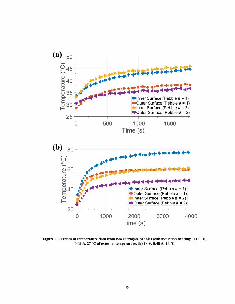
Figure 2.8 Trends of temperature data from two surrogate pebbles with induction heating:

(a) 15 V, 0.49 A, 27 of external temperature, (b) 18 V, 0.48 A, 28 ....................... 26

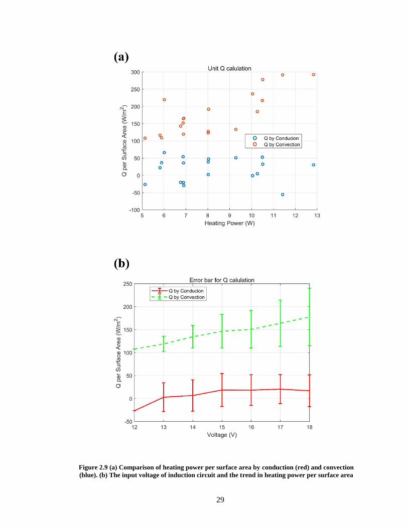
Figure 2.9 (a) Comparison of heating power per surface area by conduction (red) and

convection (blue). (b) The input voltage of induction circuit and the trend in heating power

per surface area ................................................................................................................. 29

Figure 2.10 Graph showing trend of temperature data received from three wireless pebbles

........................................................................................................................................... 32

Figure 3.1 (a) Overall heat transfer experiment configuration of the air flowing over a

single wireless pebble (b) Simple model for heat transfer through energy-balanced

equations (c) An installed experimental facility ............................................................... 34

xiv

Figure 3.2 Two different TC attachment configurations. (a) Symmetrical: upper plane (TC

#1 to TC #4) and lower plane (TC #5 and TC # 6) (b) Asymmetrical: top (TC # 1), bottom

(TC # 6), front (TC #3), left (TC #2), and TC #4 and TC #5 on the upper and lower planes

as defined in configuration (a), respectively. .................................................................... 39

Figure 3.3 Eight temperature profiles (TC #1–TC #6, and inlet, outlet) and comparison of

heat transfer coefficients at low (12 SCFH, (a) and (d)), medium (15 SCFH, (b) and (e)),

and high (18 SCFH, (c) and (f)) flow rates ....................................................................... 41

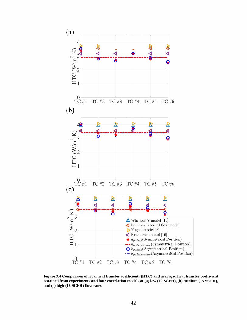
Figure 3.4 Comparison of local heat transfer coefficients (HTC) and averaged heat transfer

coefficient obtained from experiments and four correlation models at (a) low (12 SCFH),

(b) medium (15 SCFH), and (c) high (18 SCFH) flow rates ............................................ 42

Figure 3.5 Experimental setup of multiple wireless pebble experiments. Three different

pebble ID numbers (index numbers) were set to identify the different pebbles. In the heat

transfer experiment of the packed bed system, the pebbles with ID=3, ID=4 and ID=5 were

placed at the bottom, middle, and top, respectively. Each bulk temperature measurement

near the target surface temperature depended on the corresponding geometric location. 45

Figure 4.1 SVM with kernel function (a) linear kernel (b) Gaussian RBF kernel ............ 49

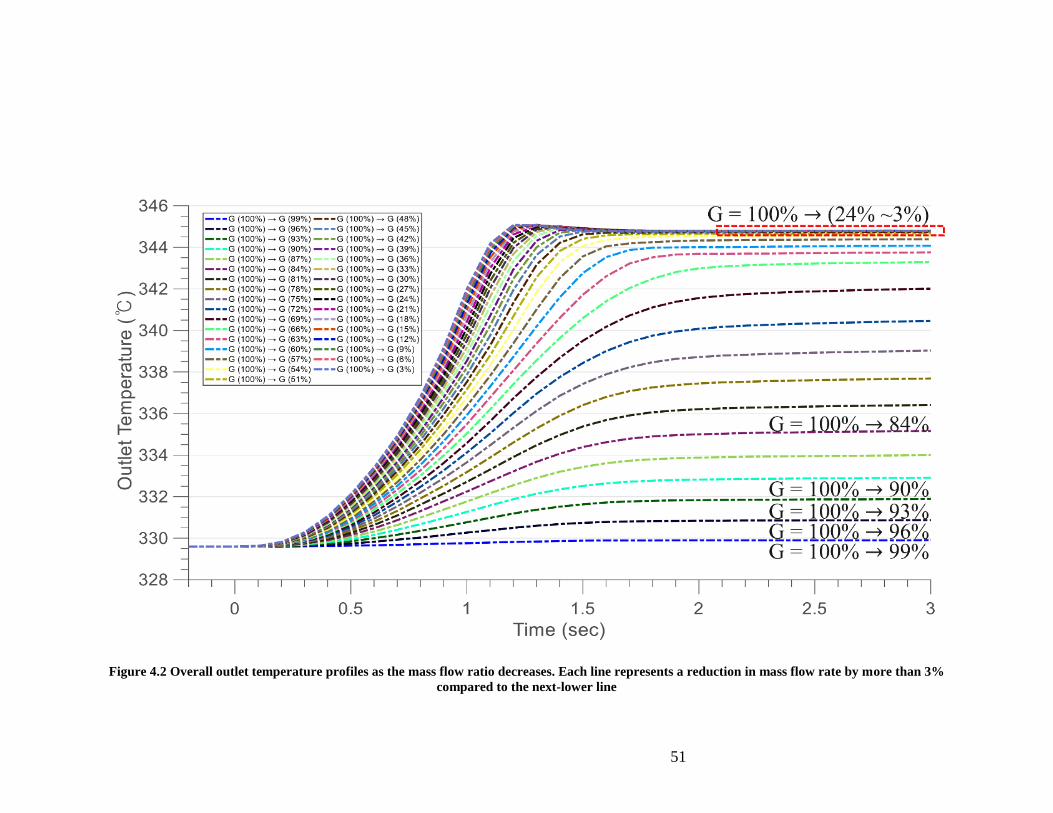
Figure 4.2 Overall outlet temperature profiles as the mass flow ratio decreases. Each line

represents a reduction in mass flow rate by more than 3% compared to the next-lower line

........................................................................................................................................... 51

Figure 4.3 Difference in flow regimes and coefficients of heat transfer due to a decrease in

the G ratio from G100% to (a),(b) G99 %; (c) and (d) G23%; and (e) and (f) G3%; ...... 53

Figure 4.4 Difference in local fuel peak temperatures according to changed inlet mass flux

(G) from G100% to G a% ................................................................................................. 55

xv

Figure 5.1 Prediction accuracy of flow rate change (G) using core outlet temperature, with

respect to the amount of training data. 10% training data ratio represents approximately 9

out of a total 97 data sets. The LOFA transient time is fixed to 3.0 s. (a) R2, (b) MSE ... 58

Figure 5.2 Prediction accuracy of flow rate change (G) using core outlet temperature, with

respect to LOFA transient time. 10% training data ratio represents ~9 out of total 97 data

sets. (a) R2, (b) MSE ......................................................................................................... 58

Figure 5.3 Prediction accuracy of peak fuel temperatures using core outlet temperature,

with respect to the number of training data. A 10% training data ratio represents

approximately 9 data out of total 97 data sets. The LOFA transient time is fixed at 3.0 s.

(a) R2, (b) MSE ................................................................................................................. 60

Figure 5.4 Prediction accuracy of peak cladding outer surface temperature using core outlet

temperature, with respect to LOFA transient time. 10% training data ratio represents

approximately 9 out of total 97 data sets. (a) R2, (b) MSE ............................................... 60

xvi

List of Tables

Table 2.1 Configuration of data packet protocol for each wireless pebble. (a) Transmitter

data packet (b) Receiver data packet (c) Temperature data packet in transmitter and receiver

........................................................................................................................................... 13

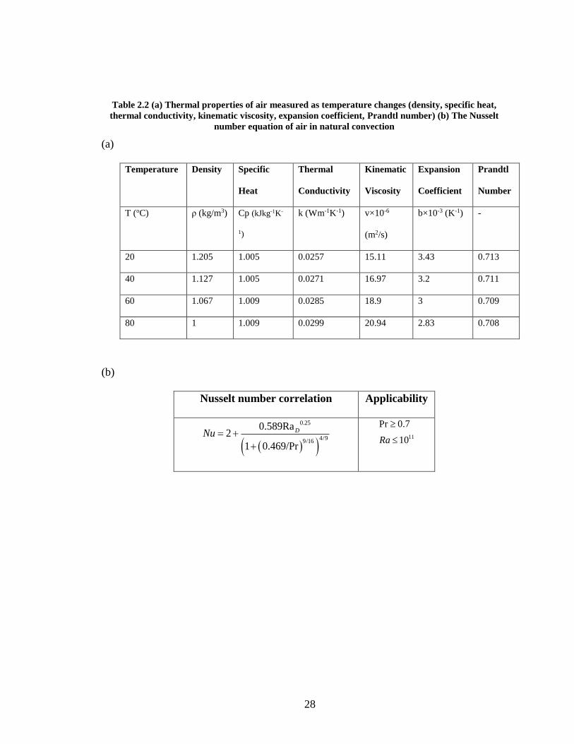
Table 2.2 (a) Thermal properties of air measured as temperature changes (density, specific

heat, thermal conductivity, kinematic viscosity, expansion coefficient, Prandtl number) (b)

The Nusselt number equation of air in natural convection ............................................... 28

Table 2.3 Expected lifetime of batteries as relevant parameters ...................................... 31

Table 3.1 Nusselt number correlations of Whitaker’s model [3], the model of modified

laminar internal flow, Yuge’s model [4], and Kramers’s model [5] ................................ 37

Table 3.2 Comparison of averaged heat transfer coefficient ,pebble average

h obtained from

experiments, and four correlation models ......................................................................... 43


h obtained from

experiments and four correlation models using multiple wireless pebbles ...................... 45

Table 4.1 Geometry parameters for the reference PWR fuel pin ..................................... 46

Table 4.2 Operational parameters for PWR pin simulation .............................................. 46

1

1. Introduction This paper presents two in-depth studies on two independent topics in nuclear engineering.

The first study introduces a new methodology to measure local heat transfer coefficients

using wireless devices in a scaled heat transfer experiment, and the other one is a diagnostic

study of a simple nuclear accident case using machine learning. These two different topics

have a common purpose in the safety analysis of nuclear reactors, but they are intended for

different nuclear applications, which are molten-salt reactors and pressurized water

reactors (PWRs), respectively. In this section, the author will briefly introduce what

motivates each research initiative and what the relevant research is.

1.1 Wireless pebble research

The key technical challenge in chemical and nuclear engineering [1], [4], [6]–[11] has

been the efficient and extensive correlation equations of heat transfer coefficients in

pebble-bed systems. The Nusselt number correlations of individual heat transfer models

have been shown in many experimental studies [8], [10]–[13] to predict the heat transfer

in packed beds. Subsequent to the particle-liquid heat transfer approach in Wakao and

Kaguei [10], considerable effort and experimental work was carried out, showing changes

in experimental correlation based on several related parameters, such as the Prandtl number,

the Reynolds number, and bed porosity. Until recently, most of the literature, which has

usually studied chemical and catalytic applications, was primarily concerned with

predicting the pebble-bed core temperature distribution. Also, these studies usually rely on

calculating the overall heat transfer of all pebbles, rather than finding the value of the heat

transfer coefficient of an individual pebble.

2

However, unlike chemical applications, nuclear engineering requires safety standards

that can eliminate potential safety risks. Recent studies [14]–[16] have reported that there

is a measurable difference between the surface temperatures of packed bed systems,

suggesting that the statistical heat transfer distribution due to the random placement of

pebbles should be considered. Thus, different heat transfer problems, such as local hot

spots due to “random packaging,” have been carefully considered in the nuclear

engineering field. In addition, the measurement or calculation of overall values does not

ensure that all the different heat transfer coefficients at all locations are free from problems.

Fluoride salt-cooled high temperature reactors (FHR) are one of the applications

experiencing this problem. Many studies related to packed pebble-beds for FHRs have

widely conducted owing to the reactor’s passive safety features under atmospheric pressure,

pool type configuration, and higher thermal efficiency compared to conventional nuclear

systems. However, its performance and safety rely heavily on the hydraulic thermal

information at its core, such as different local flow profiles, and heat transfers around

spherical fuels due to random packing density. The local heat transfer effect of this scheme

should be carefully investigated to meet the challenge of finding an adequate model for

fluid flow, heat transfer, and structural analysis.

Many research projects have started to define the problems that occur locally by

increasing the number of thermocouples (TCs) around the heat test sections. Nazari [14]

and Huddar [15] reported well-defined and successful experiments. Another group [16]

used heat flux sensors in order to evaluate heat generation. Even though they have

considered problems related to random packing, there are several limitations. First, the TCs

used in those studies were invasive TCs that interacted with the coolant fluid. Also, due to

3

the limited number of TCs, it was difficult to cover the local hot spots, and this leads to a

loss of statistical information for randomly packed pebbles. In this case, there may be

significant uncertainty with regard to reactor core temperature predictions.

The first study suggests a new device that measures temperatures at multiple points

wirelessly and enables us to estimate local heat transfer coefficients in randomly packed

pebbles. The usage of a wireless module, unlike the conventional method of using wires,

aids the measurement of temperatures in a non-invasive fashion. This approach leads

improves on invasive temperature-measurement methods and overcomes the limited

number of TCs along the test sections. For this reason, this approach is quite different from

that of previous experimental studies. Furthermore, the wireless device can be used to

determine the statistical distribution of temperature, and the heat transfer performance of

randomly packed spherical fuels. Figure 1.1 illustrates the conceptual design of the

suggested wireless device in the packed-bed system. We call a single device a “wireless

pebble.”

The wireless pebble has numerous potential applications, such in a packed pebble-bed

for the FHR in extensive scaled research experiments. Scarlat discussed the alternative of

using ‘Dowtherm A’ instead of FLiBe, the molten salt coolant used in FHR, by pointing

out that both coolants match the Prandtl number in a specific temperature range [2], [7], as

shown in Figure 1.2. If one can match its Reynolds number easily in a scaled experiment,

the use of Dowtherm A between approximately 57 and 87 is an alternative to the

temperature range of 600-700 of FLiBe its normal operation. As the wireless module

can operate properly below 85 , the maximum operational criterion of an electric circuit,

our suggested wireless device both measures local temperatures non-invasively and helps

4

the statistical analysis of heat transfer in scaled experiments of packed pebble-beds for

FHRs.

In this paper, the development and validation of a non-invasive wireless device for

pebble-bed temperature measurements will be described. These suggested devices may

offer a powerful approach to investigating heat transfer coefficients in a non-invasive

manner and designing randomly packed configurations for further studies.

5

Figure 1.1 Conceptual design of the proposed pebble experiment adopting a wireless communication

method: (a) Block diagram of the wireless pebble and receiver. A single wireless pebble should

contain the main circuit module, wireless module, sensor modules, and internal heater module. The

receiver has a wireless module and can receive data from each wireless pebble. (b) The experiments

with coolant flow use multiple devices for wireless measurement.

Figure 1.2 Prandtl numbers of FLiBe and Dowtherm A at various temperatures [4].

6

1.2 Machine learning-aided nuclear accident diagnosis research

A loss of flow accident (LOFA) is a design-based accident that causes a loss of

designed reactor coolability due to pump failure during operation. In recent years, an

increasing number of studies have been conducted to analyze nuclear accidents with

machine-learning technology [17]–[23]. In the field of fault diagnosis for nuclear power

plants, operational support systems with artificial intelligence have been developed to help

operators mitigate failures. Specifically, fuzzy logic techniques for predicting failure

scenarios in nuclear systems [21], [24], and probabilistic support vector machines (SVMs)

for monitoring the state of components in nuclear power plants [23] have been studied.

Kim et al. (2015) used an SVM to classify break position and size in the case of loss of

coolant accidents. Fernandez et al. (2017) used an artificial neural network (ANN) with

multiple sensors to evaluate the ability to predict system behavior during various core

power inputs and a LOFA. Machine learning has also been used to advance the prediction

of various two-phase flow phenomena, including flow-regime transitions [25], the

modeling of pressurization in a PWR by ANN [26], and critical heat flux (CHF) predictions

[27].

Recent advances in machine learning suggest it can be applied to unprotected LOFA

analysis and prediction. As a first step, this study used an SVM and transient reactor outlet

temperature input to investigate the predictability of loss of reactor core flow upon a reactor

pump outage. The results, in terms of predictability, address the possibility of establishing

a relationship between flow change and readily measurable reactor core outlet temperature.

This, in turn, implies the feasibility of advanced accident diagnosis by removing the

traditional boundary between different, yet strongly correlated, physical quantities. As a

7

next step, the author used an SVM to investigate the correlation between local fuel

temperature (i.e., peak cladding and centerline temperature) and reactor outlet temperature

during an unprotected LOFA. The author then explored the predictability of unmeasurable

local temperature using readily measurable temperatures, advancing the predictability of

reactor core damage during a LOFA. This study represents an initial attempt to remove the

boundaries between different physical quantities (i.e., change in flow rate and core outlet

temperature), and between different locations (i.e., local fuel temperature and core outlet

temperature) during a LOFA.

In this study, reactor core outlet temperature, Tout, is the primary parameter of interest.

With constitutive models, obtained transient Tout (t) can be seen as an outcome of continuity,

momentum, and energy balance, which are related to the transient flow change, min (t), and

local temperature information Tlocal (t), such as the fuel peak temperature, as illustrated in

Figure 1.3.

The relationship between Tout (t) and min (t) is not straightforward; the energy transfer

rate from fuel to coolant during transient flow is affected by the energy deposition rate on

the fuel structures. Energy transfer during transience is determined together with continuity

and momentum, all of which are coupled to constitutive equations and correlations.

Nuclear system codes such as RELAP5-3D and MARS mechanistically solve these

coupled equations in a forward direction, as shown in Figure 2. Accident diagnosis tackles

the problem in the opposite direction by using a measurable response parameter, Tout, to

find the cause of the transience, min (t). This reversed process can best be executed by

finding the inverse operator of the forward process.

8

Figure 1.3 Significance of Tout during a LOFA resulting from min (t)

Figure 1.4 Schematic of a typical accident analysis method, and an accident diagnosis method

9

In this study, the author obtains the inverse operator by training an SVM with the

change in min (t) and the Tout (t) obtained from a MARS simulation. Tout (t) is chosen as the

primary response parameter of interest because it contains information for the transient loss

of flow and is a readily measurable parameter during reactor accidents.

1.3 Research objective and thesis organization

In this study, the author attempts to transfer new technologies from other fields to nuclear

engineering, such as wireless devices and machine learning. Through the application of

these new technologies, a heat transfer experiment using wireless communication and a

possible accident diagnosis process using machine learning are described.

The thesis is organized as follows. Chapter 2 and Chapter 3 cover the development and

verification of wireless pebbles, and Chapter 4 and Chapter 5 present a machine learning-

aided case study, pressurized water reactors (PWR) pin. Lastly, Chapter 6 discusses the

importance and implications of this paper.

10

2. Design and development of the wireless device for scaled FHR experiments

In this chapter, the design and development of the wireless pebble are described. The

wireless device requires specific design conditions. Each wireless pebble has the following

requirements:

1) Measured temperatures can be transmitted wirelessly.

2) The surface temperature of the all circuits must remain at a temperature below 85.

3) All modules should be small enough to be enclosed inside the wireless device.

4) The internal heating element should be capable of heating uniformly to a constant

power over the surface.

The cover of the wireless pebble is made of thin metallic steel with a spherical shape.

This is beneficial for the heat transfer between the inside and the outside of the pebble. A

fabric-based internal heat source to supply constant heat inside the device is considered.

This method has the advantage of easily calculating power by using the voltage and

resistance across the heating element.

2.1 Pebble components

2.1.1 Main circuit module

Each wireless device basically requires a wireless module, a programmable

microcontroller unit (MCU), and peripherals for temperature measurement, such as TCs

and their amplifiers. While TCs measure temperatures as small levels of voltages, their

amplifiers digitize the temperature signal and convert it into a readable format compatible

with serial peripheral interface (SPI) relay.

11

Each MCU in the wireless device is programmed to obtain temperature information

converted to readable format and transmit this information to the designated receiver

through the wireless module. Each receiver has a wireless module capable of collecting

informative data from up to five individual wireless devices, which are finally exchanged

via RS232 input to the PC and stored in the data acquisition (DAQ) system. Multiple

receivers can collect data from multiple wireless devices. The Arduino Pro Mini (3.3V), a

smaller version of the embedded ATmega328 (Appendix A.4) at approximately 18 x 33

mm, was adopted as the main MCU to reduce the final size of the wireless device.

2.1.2 Wireless modules

Wireless communication has become an essential technology for portable devices such as

smartphones, tablet PCs, and laptops. It transmits information or power between two or

more nodes connected by an electrical conductor. The radio wave is the most common

wireless technology, and there are many allowable distances from a few meters to hundreds

of kilometers. The nRF24L01 module, an ultra-low power integrated circuit from Nordic

Semiconductor (Appendix A.1), was selected because it is small, low-power, SPI-

compatible, and can transmit and receive on the worldwide 2.4–2.5 GHz ISM band.

Additionally, the ShockBurst™ technology embedded in the nRF24L01 provides

automatic response, transmission, and reception of up to 32 payload bytes to the device.

As the number of wireless devices increases, it is crucial to carefully consider how to

configure important data packets. This is because the configuration can affect the high

reception rate of data packets between each wireless device and the receiver.

Each wireless device has a unique pebble identification number (ID) and transmits

information about its six different inner surface temperatures to the receiver using the

12

nRF24L01. Because the nRF24L01 module can send only 32 payload bytes of data at a

time, the length of the data packet sent from a single device is limited to 32 bytes. The

detailed configuration of the data packet protocol for the wireless pebble is shown in Table

2.1. Unlike the data packet configuration of the transmitter, that of the receiver includes

the time at which the packet arrived on the basis of receiver time. This is to identify the

order in which packets from different wireless pebbles arrive. Thus, the received data from

the various pebbles are easily identified based on the time received at the receiver.

Each set of temperature data is displayed up to the first decimal point. For the user’s

convenience, each temperature value is multiplied by 10, and then converted to a

hexadecimal value that occupies only 3 bytes. For example, if the first piece of temperature

data is 25.7 °C, it is converted to 257, and 25710 = 10116 . Likewise, if the second

temperature is 42.7 °C, it is converted to 427 and 42710 = 1AB16 , and then the

corresponding hex value is 1AB. If the measured value exceeds FFF16, it is fixed to FFF16

and maintains its data size, 3 bytes.

2.1.3 Sensor module

To measure the temperatures, many bundles of 5TC-GG-K-36 (Appendix A.5) type K

insulated TCs were chosen. Each TC could measure the temperature from -200 °C to

700 °C with an accuracy of ±2 °C. As the TC’s electromotive force is small and sensitive,

an amplifier was used to identify the measured temperatures. The amplifier for the TCs,

the MAX31855K breakout board from SparkFun, was selected (Appendix A.2). The

breakout board digitizes the temperature value and sends it to the other side via the SPI

interface.

13

Table 2.1 Configuration of data packet protocol for each wireless pebble. (a) Transmitter data packet

(b) Receiver data packet (c) Temperature data packet in transmitter and receiver

(a)

Contents Start code Delimiter ID Delimiter DATA

Check

sum

Delimiter

End

code

Number

of bytes

1 1 1 1 24 1 1 1

Data

type

Char String Char String

Char &

String

Char String Char

Value 0x02 , , , 0x03

(b)

DATA

Contents TC #1 Delimiter TC #2 Delimiter … TC #6 Delimiter

Number of bytes 3 1 3 1 … 3 1

Data type

Hexa

Char

String

Hexa

Char

String …

Hexa

Char

String

Value , , … ,

(c)

Contents

Start

code

Delimiter ID Delimiter DATA

Check

sum

Relative

Time

Delimiter

End

code

Number

of bytes

1 1 1 1 24 1

-

1 1

Data

type

Char String

Cha

r

String

Char &

String

Char

String

String Char

Value 0x02 , , , 0x03

14

2.1.4 External induction heating

Initially, induction heating was considered as the heating method. It is a method of heating

a metal object by using electromagnetic induction. When a current is supplied to a coil, an

eddy current is generated on the surface of a shallow metal sphere, raising its surface

temperature. The induced heat is not constant on the spherical surface but can be used for

preliminary tests to check the influence of the induced heat and the operation of the wireless

module. A module with a 1000-watt, zero voltage switching (ZVS), low-voltage induction

heating board and wound coils induced heat successfully.

2.1.5 Internal heater module

Although external induction heating does not generate heat uniformly, an induction

heating element inside is free from this limitation. To generate uniform heat on the surface

of the pebbles, a fabric-based heating material made by WireKinetics Corp. was used

(Appendix A.3). The fabric module was made with textile-type micro-metal conductive

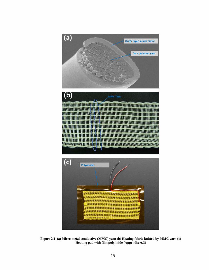
(MMC) yarn fibers. As shown in Figure 2.1(a), the fabric heating material is composed of

micro-metal lines and many polymer yarns. It has 0.9–4.0 ohms/meter of electric resistance.

The pitch range of the MMC fibers can be defined from 2 mm to 100 mm, and the

performance of the heating fiber is determined by the pitch. The fabric heating material

broadly covers the S-shaped micro-metal (Figure 2.1(b)) to help distribute heat in a uniform

way and is internally attached inside the surface of the two hemispheres. The heating

material requires a 3.5–12 V DC power supply. The heating pad is equipped with a yellow

sticker, which is an insulation film called polyimide (PI). This film maintains close contact

between the heating material and the inner surface of the pebble to reduce contact resistance,

as shown in Figure 2.1(c).

15

Figure 2.1 (a) Micro metal conductive (MMC) yarn (b) Heating fabric knitted by MMC yarn (c)

Heating pad with film polyimide (Appendix A.3)

16

2.1.6 Software architecture

This section discusses software architecture. First, the Arduino-based C++ script is

uploaded to the MCU, and the classes used in the script are used in both the receiver's script

and the GUI application. This is to integrate into one source code. The overall software

layer category is divided into three major categories. 1) Device management (serial

communication); 2) Data receiver controller by produce-consumer design pattern; 3) GUI

application (data saving and settings). The PC GUI is designed to receive data from more

than 100 wireless pebbles.

In Figure 2.2, Class basepacket is a class that can receive data using the packet described

above, and the wireless device class is an interface implemented by using the concept of

inheritance within this base packet class. Class wirelessdevice has two child classes, one

for the wireless receiver and one for the wireless transmitter. Thus, one complete program

is in Arduino-based C ++ on ATmega 328P, and a wireless receiver class is included with

the GUI programs in C# and LABVIEW. The produce-consumer design pattern, which is

a commonly used design pattern, is used in this GUI program, which provides a way to

manage data effectively. This pattern is helpful for managing external data from, such as

that transmitted by serial communication.

17

(c)

Figure 2.2 (a) Basic software architecture native to ATmega328P, Arduino-based C++ (b) Produce-

consumer design pattern (C#, LABVIEW) (c) GUI Applications

18

2.2 Wireless pebble assembly

2.2.1 First prototype

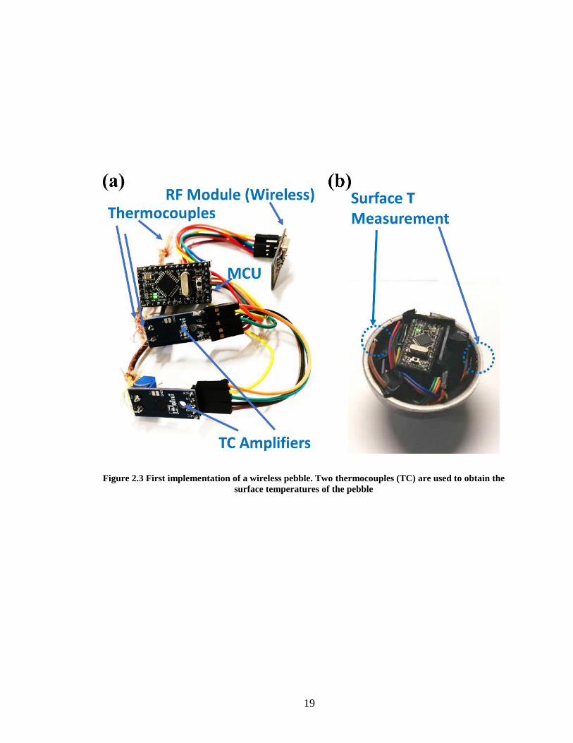
The first prototype of the wireless pebble was developed as shown in Figure 2.3. This

device is designed to check the normal operation of components or confirm the basic

functions through a combination of commercial products. The commercial products

include 1) the smallest MCU, the ATMega328 Pro Mini, 2) The radio frequency (RF)

module nRF24L01, a wireless module, 3) MAX31855K TC amplifier, 4) two TCs. The

two TCs were attached first to measure the temperature inside and outside the surface. In

the following sections, several simple preliminary experiments on the three wireless

pebbles are presented.

2.2.2 Final prototype

In the first porotype, most of the modules or components were connected by wires.

However, a more compact design was required to increase the number of temperature

measurement points on the wireless pebble. However, due to the limited space inside the

sphere, the wireless pebble needed to be miniaturized. Also, because the structure measured

temperature at only two points that were not symmetrical, marble gravel could cause some

spatial errors when used in gravel packing systems. For this reason, a wireless pebble was

designed to be smallest in size after having a single customized circuit system capable of

measuring up to six temperatures. Figure 2.4 shows a customized circuit prototype (one-

board system) that includes an MCU, six TC amplifiers, and a socket for inserting an RF

module, etc. TC #1 to TC #6, shown in Figure 2.4 (a), are sockets designed to plug in and

fix 6 TCs.

19

Figure 2.3 First implementation of a wireless pebble. Two thermocouples (TC) are used to obtain the

surface temperatures of the pebble

20

Figure 2.4 Customized circuit prototype (one-board system). (a) Front (b) Rear

21

Figure 2.5 Wireless pebble assembly. (a) The ATmega328P-based customized printed circuit board (PCB) includes all the circuits of the wireless pebble.

The RF modules nRF24L01 are mounted on the customized board, and six measurement TCs and wireless charger modules are connected to the board.

(b) The six thermocouples attached on the inner surface of the shell sphere can measure six different points on the surface. The internal heater attached

to the inner surface of the sphere is the fabric heating element. (c) This inner heater forms a vertical crossing of the two bands in a symmetrical manner.

(d) Two different purposes of the battery are related: 1) operating all circuits, and 2) operating all stacks in parallel for the internal heating element. (e)

The top view of the wireless pebble, with all the modules fitted properly in the two stainless steel hemispheres. (f) The wireless pebble assembly has an

outer diameter of 63.5 mm and an inner diameter of 57.4 mm

22

Figure 2.5 shows the fabricated board and its assemblies. For a compact design, the circuits

in all the modules, such as ATmega328 and the amplifier, were combined and customized,

mounting the RF module nRF24L01. The program modules for the robust wireless

communication of multiple pebbles were designed and tested. In Figure 2.5(a) and (b), the

six TCs TC#1 to TC#6 are attached at six different inner surface locations of the wireless

pebble. The optional function of the wireless charger is designed to charge the battery

effectively. The internal heater forms a vertical crossing of two bands so as to be as

symmetrical as possible, as shown in Figure 2.5(c). The first Li-polymer battery for

operating all circuits is connected to the fabricated board, and the secondary Li-polymer

battery, stacked in parallel with the internal heating element, is inserted into the remaining

space inside the sphere (Figure 2.5(d)). In essence, the cover of the wireless pebble,

consisting of two hemispherical shells, is intended to be made of stainless steel for its high

thermal conductivity. Figure 2.5(e) shows that the fabricated board, TCs, and batteries are

well-placed inside the shell of the sphere. Finally, when this part is combined with the

sphere, the outer diameter of the sphere is 63.5 mm and the inner diameter is 57.4 mm, as

shown in Figure 2.5(f).

2.3 Preliminary experiments for verifying basic functions of wireless pebble

2.3.1 Verification experiments for single wireless pebble and two pebbles under induction heating

The purpose of these experiments is to examine the measurements and the wireless

communication of the wireless pebbles under induction heating or internal heating. Figure

2.6 represents the experimental setup for three wireless pebbles placed on an element under

induction heating. The covers of the three prototypes in Figure 2.5 were closed, and the

23

prototypes were placed on the induction coil of a commercial induction heater. This section

focuses on verifying the rise in temperature, and whether the data transmission through the

receiver operated normally.

Two measurement points inside and outside the shell of each pebble were used to

determine how much heat was generated by the thin shell. The test condition varied the

input voltage of the inductive power supply from 12 V to 16 V. Figure 2.7 and Figure 2.8

show the temperature change of single wireless pebbles, and the result of using two

wireless pebbles, respectively. Both devices used the same inductor coil, but the steady-

state temperature was different.

24

Figure 2.6 Experimental setup for collecting temperature data wirelessly under induction heating

25

Figure 2.7 Trends in temperature data received from a surrogate pebble. Conditions: (a) 12 V, 0.49

A, 28 external temperature, (b) 12 V, 0.48 A, 29 , (c) 13 V, 0.53 A, 27 , (d) 13 V, 0.53 A, 32 ,

(e)14 V, 0.49 A, 27 , (f) 14V, 0.57 A, 27 , (g) 16 V, 0.66 A, 28 , (h) 16 V, 0.66 A, 32

26

Figure 2.8 Trends of temperature data from two surrogate pebbles with induction heating: (a) 15 V,

0.49 A, 27 of external temperature, (b) 18 V, 0.48 A, 28

27

The heating power induced by induction heating was estimated for both conditions in the

above experiments. The estimated power provided a baseline for the thermal energy that

each wireless pebble had versus the voltage provided by induction heating. There were two

methods used: 1) calculating with the assumption that the ball is heated by natural air

convection, 2) calculating the heat exchanged through the conduction of stainless steel.

Using the air thermal properties and Nusselt number equations correlated in Table 2.2,

the Nusselt number and the heat transfer coefficient were first derived, and the heating

power (Q) divided by the cross-sectional area was calculated to obtain an estimation of the

magnitude of the heating induced through induction in one wireless pebble, as shown in

Figure 2.9.

From these preliminary results, it was concluded that it would be difficult to prove the

uniformity of heating power for the situation where the wireless pebble is placed in

different positions in space. Two heating methods, induction heating, and internal fabric-

based heating were considered to provide remote heating for the pebbles.

28

Table 2.2 (a) Thermal properties of air measured as temperature changes (density, specific heat,

thermal conductivity, kinematic viscosity, expansion coefficient, Prandtl number) (b) The Nusselt

number equation of air in natural convection

(a)

Temperature Density Specific

Heat

Thermal

Conductivity

Kinematic

Viscosity

Expansion

Coefficient

Prandtl

Number

T (oC) ρ (kg/m3) Cp (kJkg-1K-

1)

k (Wm-1K-1) v×10-6

(m2/s)

b×10-3 (K-1) -

20 1.205 1.005 0.0257 15.11 3.43 0.713

40 1.127 1.005 0.0271 16.97 3.2 0.711

60 1.067 1.009 0.0285 18.9 3 0.709

80 1 1.009 0.0299 20.94 2.83 0.708

(b)

Nusselt number correlation Applicability

( )( )

0.25

4/99/16

0.589Ra2

1 0.469/Pr

DNu = +

+ 11

Pr 0.7

10Ra

29

Figure 2.9 (a) Comparison of heating power per surface area by conduction (red) and convection

(blue). (b) The input voltage of induction circuit and the trend in heating power per surface area

30

2.3.2 Verification experiments for three wireless pebbles under internal heating

In fact, an inductor does not provide uniform heat over the surfaces of the spherical

pebbles because of the non-uniform magnetic field affecting the metallic shell. Even if the

induction heater provided a nearly uniform current to the shell structure, there are more

difficult problems to resolve. If the shape of the inductor coil is changed to another type,

such as a flip type or a spiral type, all the components surrounding the inductor should be

changed. The capacity of the power supply and the current provided to the coil will be

changed as the design of the inductor coil as well.

In this experiment, fabric heating was used to heat three wireless pebbles. The graph in

Figure 2.10 shows the peak in the time range between 200 s and 500s. The “ID = 1” means

the first pebble ID, and “Inner” and “Outer” indicate the inner and outer surface

temperature of each wireless pebble. After the pebbles reach their peak temperature, the

3.7 V battery in the pebbles all seemed to be fully discharged. The estimated resistance of

the fabric heater is approximately 10 ohms. If the 7.4 V battery is used, 740 mA of current

flows in the fabric heating material, which means that a 150 mAh Li-polymer battery would

last 720 s (12 min), approximately. Considering the internal resistance, the lifetime of a 7.4

V battery would be less than 720 s.

In the case of using a fabric-based heating pad, supplying uniform heat flux from the inner

side of the sphere surface is possible. In addition, one can easily estimate the amount of

heat generated from the heating pad because the electric resistance of the fabric material is

measurable, and the amount of current can be calculated. Because the fabric material is a

metal material, its resistance is proportional to its length and cross-sectional area. In Table

3, the parameters related to battery life are listed. Increased resistance of the heating pad

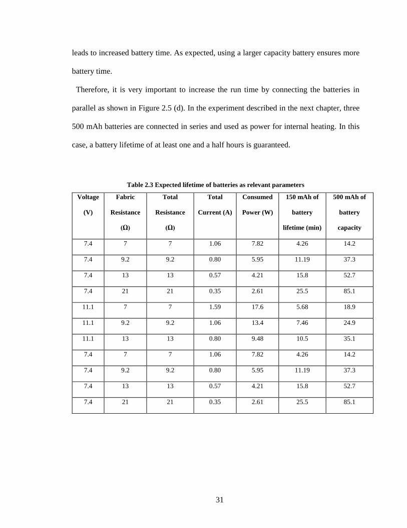
31

leads to increased battery time. As expected, using a larger capacity battery ensures more

battery time.

Therefore, it is very important to increase the run time by connecting the batteries in

parallel as shown in Figure 2.5 (d). In the experiment described in the next chapter, three

500 mAh batteries are connected in series and used as power for internal heating. In this

case, a battery lifetime of at least one and a half hours is guaranteed.

Table 2.3 Expected lifetime of batteries as relevant parameters

Voltage

(V)

Fabric

Resistance

(Ω)

Total

Resistance

(Ω)

Total

Current (A)

Consumed

Power (W)

150 mAh of

battery

lifetime (min)

500 mAh of

battery

capacity

7.4 7 7 1.06 7.82 4.26 14.2

7.4 9.2 9.2 0.80 5.95 11.19 37.3

7.4 13 13 0.57 4.21 15.8 52.7

7.4 21 21 0.35 2.61 25.5 85.1

11.1 7 7 1.59 17.6 5.68 18.9

11.1 9.2 9.2 1.06 13.4 7.46 24.9

11.1 13 13 0.80 9.48 10.5 35.1

7.4 7 7 1.06 7.82 4.26 14.2

7.4 9.2 9.2 0.80 5.95 11.19 37.3

7.4 13 13 0.57 4.21 15.8 52.7

7.4 21 21 0.35 2.61 25.5 85.1

32

Figure 2.10 Graph showing trend of temperature data received from three wireless pebbles

33

3. Validation of wireless device for scaled FHR experiments

In this section, the local heat transfer coefficients of the developed wireless pebble are

calculated with an airflow heat transfer experiment and compared with values in the

literature. Many research projects [3], [4], [11] have actively studied Nusselt numbers in

different heat transfer environments. Because these studies are based on various

correlations, the heat transfer coefficient attained from each correlation equation can be

compared with the local heat transfer coefficients computed from our experimental

apparatus by measuring the surface temperatures of the wireless pebbles. The validation

process for a single pebble relies on 1) the airflow rate of change, 2) the location of the TC

attachment, and 3) the orientation of the internal heater, 4) the heat transfer coefficients in

multiple wireless pebbles are subsequently demonstrated. The validation process results

will be extended to multiple wireless pebbles in future packed pebble-beds.

3.1 Experimental Setup

A heat transfer experiment with air flowing over the sphere of the pebbles was conducted

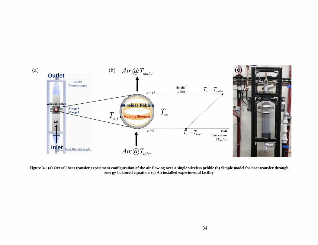
to validate the feasibility of the wireless pebble. In the test facility, as shown in Figure 3.1

(a) and (c), the air flows along a vertically erected cylindrical tube, from the bottom inlet

to the top outlet, at a controlled volume flow rate while the wireless pebble located between

flange 1 and flange 2 is placed in order to estimate the local heat transfer coefficient through

wirelessly collected pebble temperatures. Also, the heating element inside the wireless

pebble, which heats the surface of the pebble and increases the temperature of the outlet,

creates heat transfer between the surface and the air flowing from the inlet to the outlet.

34

Figure 3.1 (a) Overall heat transfer experiment configuration of the air flowing over a single wireless pebble (b) Simple model for heat transfer through

energy-balanced equations (c) An installed experimental facility

35

When the heat transfer flow reaches a steady state, the increased temperature of the outlet

of the plant is gradually balanced by this heat transfer process. The following Eq. (3.1)–

(3.5) relating to the local heat transfer coefficient h are determined by the energy balance

equation in a steady state. Here, the bulk temperature T is simply assumed to change

linearly in relation to z, which is the distance from the bottom of the wireless pebble in the

direction of airflow. Full insulation of the facility helps to ensure the heat energy produced

by the wireless pebble is converted into increased air temperature at the outlet.

Because the temperature of six inner surfaces is measured directly at the position of

attachment of the six TCs in the wireless pebbles, the corresponding surface temperatures

,S iT for 1, ,6i = can easily be estimated using simple heat transfer equations. Now, six

local heat transfer coefficients (,pebble i

h , for 1, ,6i = ) can be calculated, and, finally, the

averaged heat transfer coefficients can be obtained by averaging these six coefficients.

( )sphere p outlet inletQ mc T T= − (3.1)

( )( )outlet inlet inlet

zT f z T T T

D= = − + (3.2)

( ),

,

convection

pebble i

S i

Qh

A T T

=−

for 1, ,6i = (3.3)

sphere convectionQ Q (3.4)

, ,

1

6pebble average pebble i

i

h h= (3.5)

where m is the air mass flow rate, p

c is the specific air heat, D is the wireless pebble

diameter, z is the distance from the bottom of the wireless pebble in the airflow direction,

36

A is the surface area where the heat is transferred to the wireless pebble, sphere

Q is the heat

obtained from the flowing air in a facility system, convection

Q is the heat generated in a wireless

pebble to be heat-exchanged by convection, ,pebble i

h is the heat transfer coefficient at the

corresponding outer surface at the ith temperature measurement position, and ,pebble average

h is

the average value of the heat transfer coefficients at the outer surface corresponding to the

six temperature measurement positions. Furthermore, inletT , outlet

T , ,S i

T , and T are the

temperatures at the inlet and outlet, the outer surface temperature corresponding to the ith

measured inner surface temperature, and the bulk temperature of flowing air, respectively.

3.1.1 Four Nusselt number correlations for comparing heat transfer coefficients

The four different Nusselt number correlations from [3]–[5] were taken and summarized

in Table 3.1 to compare the heat transfer coefficients. The Whitaker model [3] was first

selected for the forced convection flow empirical equations for heated spheres. Second,

assuming that the sphere in the cylindrical tube is a two-concenter cylindrical tube at sphere

height, the hydraulic diameter can be set in the modified laminar internal flow model. Third,

Yuge [4] conducted heat transfer experiments for forced convection of airflow. Fourth,

Kramers [5] performed a steady experiment on airflow with a relatively small Reynolds

number on a sphere approximately 1 mm in diameter. In section 3.2, the performance of

the wireless pebble is verified step by step through the comparison between the heat

transfer coefficient of the wireless pebble surface and the heat transfer coefficient derived

from these four Nusselt numerical correlations.

37

Table 3.1 Nusselt number correlations of Whitaker’s model [3], the model of modified laminar

internal flow, Yuge’s model [4], and Kramers’s model [5]

Authors Medium Nusselt number Correlation Applicability

Whitaker’s model [15] Air 0.252

0.5 0.532 0.4Re 0.06Re Prw

Nu

= + +

D

0.71 Pr 380

3.5 e 7.6104

1.0 / 3.2w

R

Model of modified

laminar internal flow

Air 4.36Nu = -

Yuge’s model [2] Air 0.52 0.493ReNu = + 10 Re 1000

Pr 0.715

=

Kramers’s model [16] Air 0.2 0.31 0.50.42Pr 0.57Pr ReNu = + 0.4 Re 2100

0.71 Pr 380

38

3.1.2 Two configurations for TC attachment positions

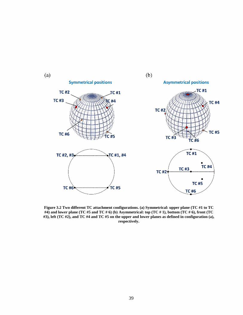
To further analyze how the location of the TCs affects the result, it is necessary to

differentiate the configuration of the TC attachment locations on the inside surface of the

wireless pebble. In the first symmetrical TC configuration, as shown in Figure 3.2 (a), the

upper plane, in which TC #1 to TC #4 are placed on the four vertices, and the lower plane,

in which TC #5 to TC #6 are placed on the diagonals, are the same parallel distance from

the center of a cross-section (upper and lower, respectively) of the wireless pebble.

The second asymmetric TC configuration in Figure 3.2 (b), on the other hand, consists of

placement in the top (TC #1) and bottom (TC #6) of the sphere, and the front (TC #3) and

the left (TC #2) in its center cross-section, and two TCs (TC #4 and TC #5) on the upper

and lower planes as defined in configuration (a), respectively.

39

Figure 3.2 Two different TC attachment configurations. (a) Symmetrical: upper plane (TC #1 to TC

#4) and lower plane (TC #5 and TC # 6) (b) Asymmetrical: top (TC # 1), bottom (TC # 6), front (TC

#3), left (TC #2), and TC #4 and TC #5 on the upper and lower planes as defined in configuration (a),

respectively.

40

3.2 Wireless measurements with change in volume flow rate

In this section, the author first investigates how well the device can measure temperature.

The airflow facility described in the previous section was used in measuring the wireless

pebble’s six internal surface temperatures (TC #1–TC #6) and the inlet and outlet

temperatures under varying airflow rates. The first symmetric TC configuration was

adopted here. Three different volume flow rates were used: low (12 standard cubic feet per

hour (SCFH)), medium (15 SCFH), and high (18 SCFH). Figure 3.3 (a)–(c) shows six

temperatures, and inlet and outlet temperatures, and Figure 3.3 (d)–(f) shows the heat

transfer coefficients obtained from the steady state temperature information compared with

the four Nusselt number correlations described in Section 3.1.

3.3 Effect of locations of TCs

Two similar airflow experiments were conducted to evaluate the effect of TC locations,

as in Section 3.2, using two different single wireless pebbles, one with a symmetrical TC

configuration and the other with an asymmetrical TC configuration. The flow rate

increased from Figure 3.4(a) to (c) from 12 SCFH to 18 SCFH but the three average values

,pebble averageh from Figure 3.4(d) to (f) were almost identical. As a result, the author concluded

that there was no significant difference between the values from the literature and

experiments depending on where the TC was attached.

41

Figure 3.3 Eight temperature profiles (TC #1–TC #6, and inlet, outlet) and comparison of heat transfer coefficients at low (12 SCFH, (a) and (d)), medium

(15 SCFH, (b) and (e)), and high (18 SCFH, (c) and (f)) flow rates

42

Figure 3.4 Comparison of local heat transfer coefficients (HTC) and averaged heat transfer coefficient

obtained from experiments and four correlation models at (a) low (12 SCFH), (b) medium (15 SCFH),

and (c) high (18 SCFH) flow rates

43

3.4 Effect of internal heater orientation

The author examination of the effect of the internal heater orientation is presented in this

section. Three different experiments were conducted to differentiate the random three-

dimensional orientation of a single wireless pebble, whereas the local h value, ,pebble i

h , and

the average h value, ,pebble average

h , were obtained on the basis of steady state temperature

information. Table 3.2 shows a statistical analysis of the mean heat transfer coefficient (M,

,pebble averageh ) ± standard deviation (SD) and minimum (in the column Min) and maximum (in

the column Max) values of each experiment’s six heat transfer coefficients (,pebble i

h for

1, ,6i = ) relative to the heat transfer coefficient derived from the four correlation models

referred to in Section 3.1. There was no significant difference in the error range in the

average calculation of ,pebble average

h depending on where the internal heater was placed. This

means that it is possible to extend from one pebble to several pebbles, as there was no

significant difference in the calculation if multiple wireless pebbles were randomly placed.


h obtained from experiments,

and four correlation models

Internal Heater Orientation Experiments Four Correlation Models

Random

Orientation

N M±SD Min Max Whitaker

[15]

Laminar

internal flow

Yuge

[2]

Kramers

[16]

#1 6 2.96±0.56 2.20 3.63

3.93 3.55 4.07 3.53 #2 6 3.34±0.41 2.77 3.94

#3 6 2.76±0.54 2.01 3.36

44

3.5 Demonstration of multiple wireless pebbles

Finally, an experiment with three identical symmetrical TC configurations was performed

on several wireless pebbles. In this case, three wireless pebbles were placed in the same

experimental facility, and heat transfer experiments were performed until a stable state was

reached. Figure 3.5 shows the configuration of the three wireless pebbles. Each pebble has

a different ID; that is, the pebble with ID= 3 is at the bottom, ID= 4 is at the center, and

ID= 5 is at the top. The geometric arrangement revealed that the bulk temperature at the

bottom of ID=5 was slightly lower than the bulk temperature at the bottom of ID=4, which

means that the local bulk temperature depended on the location of the pebble.

Table 3.3 shows a statistical analysis of the mean heat transfer coefficient (M, ,pebble average

h ) ±

SD and minimum and maximum values of six heat transfer coefficients ,pebble i

h for

1, ,6i = per experiment compared with the heat transfer coefficient derived from the four

correlation models. As can be seen from the results, the values of the averaged ,pebble average

h of

pebbles of ID=5 and ID=3 were considerably different, even though the bulk temperature

distribution was considered.

The result shows the average values,pebble average

h of the ID=5 and ID=3 pebbles were

significantly different, although the bulk temperature distribution was considered. In other

words, there were evidently differences in the average heat transfer coefficients ,pebble average

h

between the pebbles, which implies that the average heat transfer coefficients of locally

positioned pebbles can differ significantly when extended to the packed pebble-bed system.

45


h obtained from experiments

and four correlation models using multiple wireless pebbles

Multiple Wireless Pebble Experiment Four Correlation Models

Pebble

(ID, location)

N M±SD Min Max Whitaker

[15]

Laminar

internal flow

Yuge

[2]

Kramers

[16]

3, Bottom 6 3.79±0.24 3.52 4.19

3.93 3.55 4.07 3.53 4, Middle 6 3.09±0.49 2.45 3.76

5, Top 6 2.96±0.44 2.35 3.60

Figure 3.5 Experimental setup of multiple wireless pebble experiments. Three different pebble ID

numbers (index numbers) were set to identify the different pebbles. In the heat transfer experiment

of the packed bed system, the pebbles with ID=3, ID=4 and ID=5 were placed at the bottom, middle,

and top, respectively. Each bulk temperature measurement near the target surface temperature

depended on the corresponding geometric location.

46

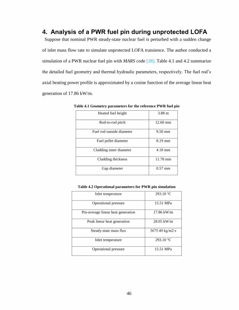
4. Analysis of a PWR fuel pin during unprotected LOFA Suppose that nominal PWR steady-state nuclear fuel is perturbed with a sudden change

of inlet mass flow rate to simulate unprotected LOFA transience. The author conducted a

simulation of a PWR nuclear fuel pin with MARS code [28]. Table 4.1 and 4.2 summarize

the detailed fuel geometry and thermal hydraulic parameters, respectively. The fuel rod’s

axial heating power profile is approximated by a cosine function of the average linear heat

generation of 17.86 kW/m.

Table 4.1 Geometry parameters for the reference PWR fuel pin

Heated fuel height 3.88 m

Rod-to-rod pitch 12.60 mm

Fuel rod outside diameter 9.50 mm

Fuel pellet diameter 8.19 mm

Cladding inner diameter 4.18 mm

Cladding thickness 11.78 mm

Gap diameter 0.57 mm

Table 4.2 Operational parameters for PWR pin simulation

Inlet temperature 293.10

Operational pressure 15.51 MPa

Pin-average linear heat generation 17.86 kW/m

Peak linear heat generation 28.05 kW/m

Steady-state mass flux 3675.40 kg/m2∙s

Inlet temperature 293.10

Operational pressure 15.51 MPa

47

A total of 97 independent MARS simulation cases were created to simulate an unprotected

LOFA by suddenly reducing the flow rate to only 3% of the nominal steady-state flow rate

(i.e., 100% → 3%). Transient outlet temperatures and local fuel temperatures for each

simulated case were reported for SVM training.

4.1 SVM for LOFA

SVM algorithms have become a widely used as a classification method since the

introduction of Cortes and Vapnik (1995). They offer many benefits for the classification

of patterns and model regression [30]–[35]. The first SVM algorithm was intended to

classify where the new point belongs to.. The given data points belong to two

classes , where the class label of point 𝑥𝑖 is for 𝑖 = 1, ⋯ 𝑛. An SVM finds the

hyperplane 𝒘, also called the decision boundary, that best separates the data points in the

training set by the class labels 1, −1. The governing equation of an SVM is formulated

as follows:

To minimize , subject to . (4.1)

This constrained optimization problem is reorganized into:

To minimize , subject to . (4.2)

After the gradient of its Lagrangian multiplier L is set to zero in relation to 𝒘 and b, the

equation becomes:

(4.3)

, . (4.4)

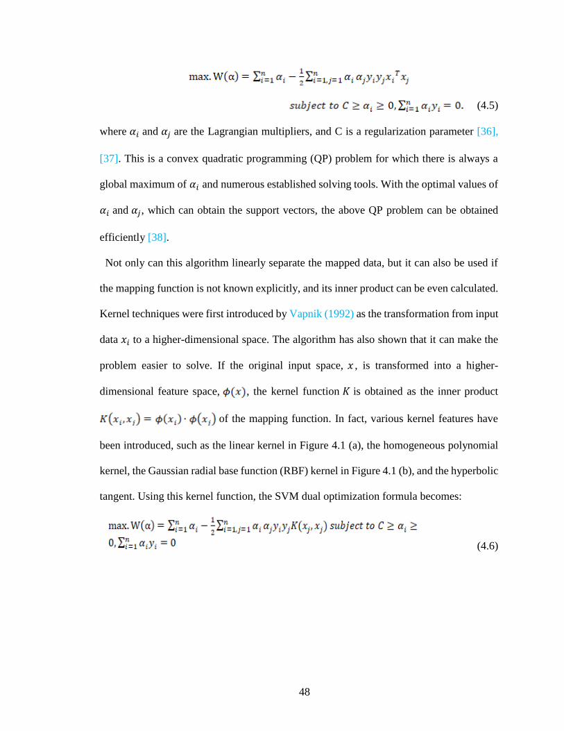
Then the dual optimization form for an SVM is obtained:

48

(4.5)

where 𝛼𝑖 and 𝛼𝑗 are the Lagrangian multipliers, and C is a regularization parameter [36],

[37]. This is a convex quadratic programming (QP) problem for which there is always a

global maximum of 𝛼𝑖 and numerous established solving tools. With the optimal values of

𝛼𝑖 and 𝛼𝑗, which can obtain the support vectors, the above QP problem can be obtained

efficiently [38].

Not only can this algorithm linearly separate the mapped data, but it can also be used if

the mapping function is not known explicitly, and its inner product can be even calculated.

Kernel techniques were first introduced by Vapnik (1992) as the transformation from input

data 𝑥𝑖 to a higher-dimensional space. The algorithm has also shown that it can make the

problem easier to solve. If the original input space, 𝑥 , is transformed into a higher-

dimensional feature space, , the kernel function 𝐾 is obtained as the inner product

of the mapping function. In fact, various kernel features have

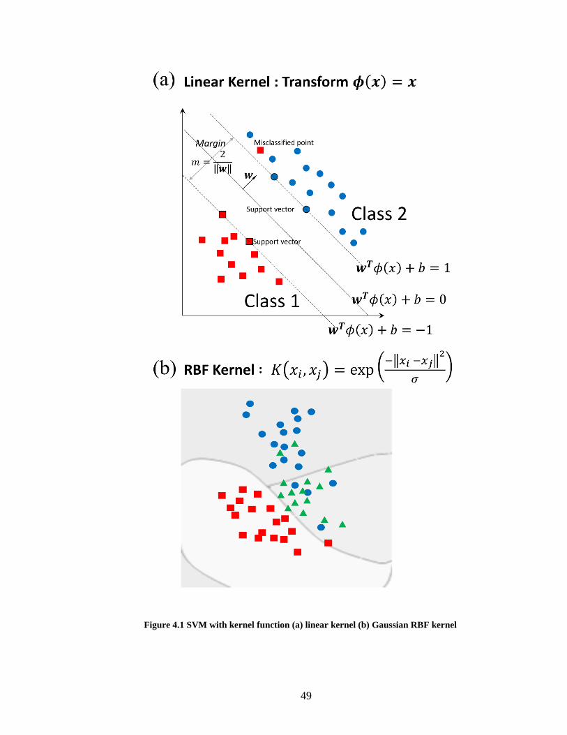
been introduced, such as the linear kernel in Figure 4.1 (a), the homogeneous polynomial

kernel, the Gaussian radial base function (RBF) kernel in Figure 4.1 (b), and the hyperbolic

tangent. Using this kernel function, the SVM dual optimization formula becomes:

(4.6)

49

Figure 4.1 SVM with kernel function (a) linear kernel (b) Gaussian RBF kernel

50

Hsu and Lin (2002a and 2002b) initiated comparisons of methods for multi-class vector

support machines and compared numerous multi-class SVMs, such as BSM and LIBSVM.

How to effectively extend a multi-class SVM is an ongoing problem that is beyond the

scope of this study. Here, an error-correcting output code (ECOC) model [42] was used.

This algorithm used the 𝐾(𝐾 − 1) / 2 binary SVM model, and a “one-versus-one” coding

design in which K is the number of unique class labels. In an ECOC strategy, a classifier

can be created to target classifications between different sub-sets. This means that these

subsets can divide the main problem of classification into tasks of sub-classification. The

author created an SVM training template with an ECOC model and a Gaussian RBF linear

kernel for predictions based on MARS simulated results.

4.2 MARS simulation results for a nuclear fuel pin during an unprotected LOFA

A reduced flow rate increases the outlet temperature. Figure 4.2 illustrates the transience

of outlet temperature in flow reduction test cases. As soon as flow reduction starts, the

outlet temperature tends toward a new equilibrium. The rate at which it achieves

equilibrium is determined by the heat transfer rates coupled with continuity, momentum,

and energy balance with constitutive equations. In Figure 4.2, mass flow (G) is defined as

the mass flow rate divided by flow area, and mass flow ratio (G ratio) is defined as the

mass flow rate ratio after and before the occurrence. Because the flow area is the same

before and after the events, the G ratio reflects how G changes.

51

Figure 4.2 Overall outlet temperature profiles as the mass flow ratio decreases. Each line represents a reduction in mass flow rate by more than 3%

compared to the next-lower line

52

As the outlet flow temperature escalates, the fuel surface undergoes a change in heat

transfer mode due to overheating. Figure 4.3 (a), (b), and (c) show different flow regimes

along the height of the fuel rod under LOFA due to different flow reductions. An increasing

drop in flow rate eventually causes an appreciable two-phase heat transfer, characterized

by a nucleate, transition, and film (post-CHF) boiling regime. The higher bulk fluid

temperature toward the end of the flow channel, in conjunction with the cosine power

profile, leads to the onset of film boiling (at the occurrence of CHF) in the upper half of

the fuel rod.

The changes in heat transfer rates result from changes in heat transfer modes. Figure 4.3

(d), (e), and (f) indicate heat transfer coefficients along height of the fuel with respect to

LOFA duration. If film boiling is generated, heat transfer rates, expressed as heat transfer

coefficients, deteriorate.

Such dynamic heat transfer rate evolutions associated with boiling mode changes

influence the rate of energy transfer to the bulk fluid, which is highly related to the rate at

which the outlet flow temperature finds a new equilibrium, as shown in Figure 4.3.

Consequently, the rate of increase of outlet flow temperature Tout during a LOFA contains

information concerning changes in the dynamic heat transfer rate.

53

Figure 4.3 Difference in flow regimes and coefficients of heat transfer due to a decrease in the G ratio

from G100% to (a),(b) G99 %; (c) and (d) G23%; and (e) and (f) G3%;

54

The peak fuel and cladding temperatures during LOFA transience are linked to the

reduced flow rate. Figure 4.4 represents the peak fuel and cladding temperatures during

LOFA transience with respect to the reduced inlet G. The peak temperature is insensitive

to flow rate reduction up to the threshold point. However, if the threshold is surpassed, the

flow rate decreases. The reduced flow rate at these thresholds is a case in which the flow

is sufficiently low to cause the onset of film boiling.

Reducing the flow rate beyond this point will further lower the heat transfer rate, thus

increasing the fuel and cladding temperature. The results presented indicate that local peak

fuel and cladding temperatures can be predicted by determining the predicted reduced flow

at the outlet flow rate. As a result, peak local fuel and cladding temperatures can be

predicted using only the measurable outlet flow temperature as input.

The above relationship between different physical quantities during an unprotected LOFA

suggests that an inverse operator can be found for accident diagnosis (Figure 1.4). In this

study, an SVM trained with MARS simulation results is used for finding the inverse

operator of the accident diagnosis.

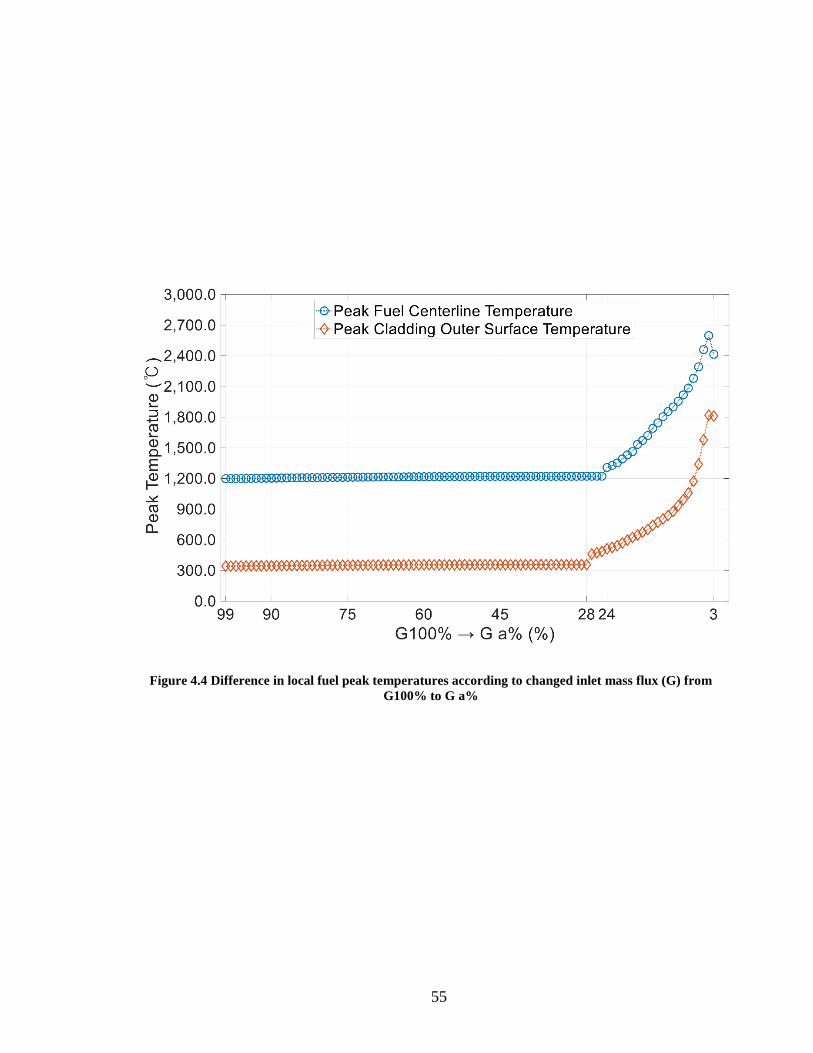
55

Figure 4.4 Difference in local fuel peak temperatures according to changed inlet mass flux (G) from

G100% to G a%

56

5. Machine learning aided analysis of PWR fuel pin during unprotected LOFA

In the previous section, the author simulated the change in different parameters in

accordance with a sudden 97% reduction in mass flow rate via MARS simulation. The SVM

was then trained with MARS results to correlate the following physical quantities:

(1) Tout(t) and changed inlet mass flux (G)

(2) Tout(t) and peak fuel and cladding temperature

Tout(t) is treated as a vector in a time series. Because Tout(t) achieved a new equilibrium

within 3 s (Figure 4.2), the data in the SVM multi-class input was limited to 3 s of

transience. An SVM can divide data into training sets and test sets, as with most machine

learning algorithms. The author built an SVM model with training sets and tested it by

quantifying the error with a test set for the model. In this study, the author used two metrics

to quantify the error, such as mean square error (MSE) and the coefficient of determination

( 2R ), defined in Eq. (5.1) and (5.2), respectively.

( )( )

2

12

2

1

( , ) 1

n

ii

n

ii

y yR y y

y y

=

=

−= −

−

.(5.1)

( )2

1

1( , )

n

iiMSE y y y y

n == − (5.2)

where n is the number of observations, 𝑦𝑖 is the actual value, and and are the prediction

and averaged value, respectively. In order to create an SVM model for (1), the parameter

G ratio (defined in Section 4) and its corresponding Tout(t) became the label and the data

for the SVM training data set, respectively. Similarly, for an SVM model for (2), the peak

fuel (or cladding temperature) and its corresponding Tout(t) became the label and the data

for the SVM training data set, respectively. The effects of the amount if training data and

57

the transient time of the LOFA on the prediction accuracy are examined for each model.

For the sensitivity of the amount of training data, 29 evenly distributed MARS simulation

results were fixed for the tests, while the number of training data sets was randomly

selected and gradually increased from 9 to 68. The transient time of the MARS simulation

was set to 3.0 s in this case. For this transient time sensitivity of the LOFA, the results of

the MARS simulation used for SVM training increased gradually from 0.5 to 3.0 s.

5.1 Prediction of the flow rate change inm (t) using coolant outlet

temperature Tout(t)

The accuracy of the prediction for flow rate increases with the amount of training data

(Figure 5.1). The results show that including 20 percent or more of the training data, or 19

of a total 97 data sets, produces 99 percent accuracy or better for the prediction. In a similar

manner, when the training data ratio increased, the MSE approached zero. This implies that

there is no need for a large amount of training data to build an SVM relationship between

mass flow rate and core outlet temperature.

Figure 5.2 shows the LOFA transient time sensitivity for the prediction accuracy of flow

rate change using the core outlet temperature. The prediction accuracy of the flow rate

change increased with the increase in LOFA transient time. In the first 0.5 s of LOFA

transient time, the prediction accuracy reaches its maximum value for all tested training

data ratios. When the amount of training data was less than or near 10% of the entire data

set, the saturated accuracy dropped to 0.9 in terms of R2. This demonstrates that if the

training data ratio is higher than 20%, the SVM model trained with the core outlet

temperature gives a highly accurate (R2 = 0.99) prediction for the flow rate changes in the

first 0.5 s of the LOFA transient time. This suggests that SVM can instantaneously give an

accurate prediction of flow rate change upon the occurrence of transience.

58

Figure 5.1 Prediction accuracy of flow rate change (G) using core outlet temperature, with respect to

the amount of training data. 10% training data ratio represents approximately 9 out of a total 97

data sets. The LOFA transient time is fixed to 3.0 s. (a) R2, (b) MSE

Figure 5.2 Prediction accuracy of flow rate change (G) using core outlet temperature, with respect to

LOFA transient time. 10% training data ratio represents ~9 out of total 97 data sets. (a) R2, (b) MSE

59

5.2 Prediction of the peak cladding temperature using coolant outlet temperature Tout(t)

Furthermore, Figure 5.3 illustrates the predictability (R2 and MSE) of peak fuel and

cladding temperature using the coolant outlet temperature. In Figure 5.3, it is clearly

evident that the SVM model can only provide accurate predictions for cladding and fuel

surface temperatures, whereas the fuel centerline temperature is difficult to correlate with

the core outlet temperature. This means that the core damage initiated by cladding

degradation can be predicted by using the core outlet temperature.

The effect of LOFA transient time on the predictability of the peak cladding outer surface

temperature is investigated as shown in Figure 5.4. After approximately 0.5 s, if the number

of training data is sufficient, the prediction provides relatively high accuracy (> 0.8). Here,

9 (10% in training data ratio) is shown to be the minimum number of training data sets, as

can be inferred in Figure 5.4. LOFA transient temporal sensitivities explain that the

extended transient effects are necessarily more accurate (i.e., 20, 30, and 40% of the

training data ratio in Figure 5.4). This implies that in the early stages of the unprotected

LOFA, changes in the core outlet temperature contain information that is most relevant to

the peak cladding outer surface temperature of the entire transience.

60

Figure 5.3 Prediction accuracy of peak fuel temperatures using core outlet temperature, with respect

to the number of training data. A 10% training data ratio represents approximately 9 data out of

total 97 data sets. The LOFA transient time is fixed at 3.0 s. (a) R2, (b) MSE

Figure 5.4 Prediction accuracy of peak cladding outer surface temperature using core outlet

temperature, with respect to LOFA transient time. 10% training data ratio represents approximately

9 out of total 97 data sets. (a) R2, (b) MSE

61

6. Discussions

6.1 Wireless device for heat transfer coefficient of scaled experiments

The author carried out several wireless pebble and simple heat transfer experiments in

chapter 3. This study shows in scaled experiments that the local heat transfer coefficient

through the implementation of the wireless pebble and simple heat transfer experiments

can be quite different. To conclude this, a series of experimental steps were taken.

First, the single wireless pebble did not change the average heat transfer coefficient even

when the airflow rate changed and the TC connection structure changed. In addition,

because the average coefficient for heat transfer did not change significantly according to

the orientation of the internal heater, it could easily be expanded to several wireless pebbles.

Lastly, the experiment with three wireless pebbles demonstrated that the wireless pebbles

we proposed could greatly help estimate the local heat transfer coefficient.

In particular, this study can be used in the FHR application of an advanced nuclear reactor

because the use of Dowtherm A offers practical advantages for conducting scaled

experiments.

To design an efficiently scaled experiment for a very large number of packed bed systems,

the number of receivers should be increased. There is one principal challenge: as the

number increases, the time needed to achieve a stable state can increase, which affects the

duration of the battery. This type of problem can be solved by heating the pebbles to

increase the initial surface temperatures. This allows the pebbles to reach a stable state

quickly, regardless of battery performance.

In summary, the author expects that this study will provide an experimental basis for

those who need to measure local temperatures in a non-invasive manner, providing a solid

62

approach to investigation of non-invasive heat transfer coefficients and randomly packaged

configurations in further studies.

In addition, this study not only helps to ensure proper nuclear safety in the future, such as

local hot spots due to the random packing of a large number of wireless pebbles, but also

serves as a guide to the statistical distribution of local heat transfer coefficients for

multiple-pebble systems.

6.2 Implications for SVM-aided LOFA diagnosis

6.2.1 Instantaneous accident diagnosis

It is noteworthy that all the results and analyses presented demonstrate high predictability

of flow change and peak fuel temperatures in the early phase of unprotected LOFA (i.e.,

the first 0.5 s of LOFA transience). This implies that the key accident characteristics are

well reflected in the early response to changes in the core parameter (i.e., core outlet

temperature). This refers to the possibility of a different intelligent diagnostic framework

for accidents than in current practice, depending on the reactor behavior response over

prolonged accident progression.

With SVM, however, the early or almost immediate reactor parameters can tell the cause

and consequences of unprotected LOFA. This may indicate that SVM-aided accident

diagnosis, when combined with current practices, can lead to comprehensive accident

diagnoses and reactor safety analyses taking advantage of rich information inherent in

accident progression from start to finish. However, the accurate detection of the reactor

core's instantaneous response will require advanced core instrumentation technology.

63

6.2.2 Guidance for accident mitigation strategies

Note that the cases presented are limited to non-protected LOFA. The proven ability to

instantly predict the resulting peak fuel temperature and thus the core damage provide an

effective guideline for accident mitigation strategies. In other words, SVM can be used to

inform reactor operators of the latent consequences of accidents in the early phase of the

accident, which can help them choose strategies for coping with accidents.

6.2.3 Strongly correlated response

It is remarkable that even with a limited number of training data, the presented SVM

models can achieve exceptionally high prediction accuracy (i.e., R2 > 0.9). This shows

clearly that many parameters of reactor response, including those presented in this study,

such as Tout vs ∆𝐺, and Tout vs Tcladding, peak, are strongly correlated. By means of such strong

correlations, one can have access to information that is not directly measurable, such as the

initiation of core damage. Consequently, the traditional boundaries of physical locations

and physical quantities in accident response and progression detection can be pushed,

allowing interdependent detector systems to be made available.

64

7. Conclusion and Future works In the first study, the accident analysis and accident diagnosis for a nuclear fuel pin during

an unprotected LOFA were investigated. In terms of “Accident analysis,” MARS, one of

the system codes, was used to simulate the changes in physical parameters according to the

change in flow during unprotected LOFA. There were the physical parameters we are

interested in: 1) core outlet temperatures, 2) flow regimes, 3) heat transfer coefficients of

the coolant, and 4) local fuel peak temperatures. In our case study of an unprotected LOFA,

the SVM helped to obtain each inverse operator of accident diagnosis in physical quantities:

1) Tout(t) and changed inlet mass flux (G) 2) Tout(t) and peak fuel and cladding temperature

Along the models made by SVM, we have found that the important results. In terms of

“Accident Diagnosis”, the strongly correlated parameters were found: even with a limited

number of training data, the presented SVM models can achieve exceptionally high

prediction accuracy (i.e., R2 > 0.9). Also, to predict mass flux (G) given Tout(t), the key

accident features are well reflected in the early response to changes in the core parameter

(i.e., core outlet temperature). Using Tout(t), the high predictive accuracy of peak cladding

outer surface temperature also means the core damage can provide an effective guideline

for accident mitigation strategies.

In my opinion, this result can be expanded to analyze some more complex cases in the

future. One example is the Reactivity Insertion Accident (RIA) or Loss of Coolant

Accident (LOCA) in the design-basis accident (DBA) condition of the water reactor fuel

behavior. In fact, the greatest reason why SVM is used in this paper is that the SVM

suggests an optimal solution, but other methods such as the ANN and its extensions can be

used when one can look at his extensive research area. In recent years, studies on deep

learning and reinforcement learning are actively underway. Therefore, if appropriate

65

insights and algorithms are combined, the calculation and prediction for the accident

diagnosis in the early phase may be possible.

In the second study, the wireless pebble was designed and developed. The main idea was

originated from that Dowtherm A initiates to make the temperature range of interest below

100 °C. Also, it can be demonstrated that the number of pebbles can be extended into

applicable for scaled experiments for FliBe. This result provides an experimental basis for

those who need to measure local temperatures in a non-invasive manner. In addition, this

result serves as a guide to the statistical distribution of local heat transfer coefficients for

multiple pebble systems. Lastly, this result helps us ensure proper nuclear safety, such as

local hot spots due to the random packing of a large number of wireless pebbles in the

future. In the future work of the second study, it is possible to increase the number of

wireless pebbles, but at the same time, it is necessary to stabilize the initial heating method

in advance. Although the wireless charger that has been developed so far is installed, it is

necessary to examine whether it is charging even when the temperature rises. If the number

increases, the time to reach the steady-state will be relatively long. Also, software for the

real-time check of communication status should be developed when the number is

increased to 100. Theoretically, there will be many trial and error in practice if it is possible.

Therefore, the problem of battery and careful attention to communication will be the most

important in future research.

66

8. References [1] J. Yang, J. Wang, S. Bu, M. Zeng, Q. Wang, and A. Nakayama, “Experimental

analysis of forced convective heat transfer in novel structured packed beds of

particles,” Chem. Eng. Sci., vol. 71, pp. 126–137, 2012.

[2] R. O. Scarlat and P. F. Peterson, “The current status of fluoride salt cooled high

temperature reactor (FHR) technology and its overlap with HIF target chamber

concepts,” Nucl. Instruments Methods Phys. Res. Sect. A Accel. Spectrometers,

Detect. Assoc. Equip., vol. 733, pp. 57–64, 2014.

[3] S. Whitaker, “Forced convection heat transfer correlations for flow in pipes, past

flat plates, single cylinders, single spheres, and for flow in packed beds and tube

bundles,” AIChE J., vol. 18, no. 2, pp. 361–371, 1972.

[4] T. Yuge, “Experiments on heat transfer from spheres including combined natural

and forced convection,” J. Heat Transfer, vol. 82, no. 3, pp. 214–220, 1960.

[5] H. Kramers, “Heat transfer from spheres to flowing media,” physica, vol. 12, no. 2–

3, pp. 61–80, 1946.

[6] T. D. Eastop and C. Smith, “HEAT-TRANSFER FROM A SPHERE TO AN AIR

STREAM AT SUB-CRITICAL REYNOLDS-NUMBERS,” Trans. Inst. Chem. Eng.

Chem. Eng., vol. 50, no. 1, p. 26, 1972.

[7] N. Zweibaum, Z. Guo, J. C. Kendrick, and P. F. Peterson, “Design of the Compact

Integral Effects Test Facility and Validation of Best-Estimate Models for Fluoride

Salt–Cooled High-Temperature Reactors,” Nucl. Technol., vol. 196, no. 3, 2016.

67

[8] Wilson M. and H. Jacobs, “A Numerical Solution of the Heat Transfer from a

DenseArray of Spherical Particles,” in ANS Proc. National Heat Transfer

Conference, 1993, vol. 7, pp. 225–233.

[9] J. B. Will, N. P. Kruyt, and C. H. Venner, “An experimental study of forced

convective heat transfer from smooth, solid spheres,” Int. J. Heat Mass Transf., vol.

109, pp. 1059–1067, 2017.

[10] N. Wakao and S. Kagei, Heat and mass transfer in packed beds, vol. 1. Taylor &

Francis, 1982.

[11] G. C. Vliet and G. Leppert, “Forced convection heat transfer from an isothermal

sphere to water,” J. Heat Transfer, vol. 83, no. 2, pp. 163–170, 1961.

[12] W. E. Ranz, W. R. Marshall, and others, “Evaporation from drops,” Chem. Eng.

Prog, vol. 48, no. 3, pp. 141–146, 1952.

[13] J. A. Lewis and W. H. Gauvin, “Motion of particles entrained in a plasma jet,”

AIChE J., vol. 19, no. 5, pp. 982–990, 1973.

[14] M. Nazari, D. J. Vahid, R. K. Saray, and Y. Mahmoudi, “Experimental investigation

of heat transfer and second law analysis in a pebble bed channel with internal heat

generation,” Int. J. Heat Mass Transf., vol. 114, pp. 688–702, 2017.

[15] L. Huddar, J. C. Kendrick, C. Poresky, X. Wang, and P. F. Peterson, “Application

of frequency response methods in separate and integral effects tests for molten salt

cooled and fueled reactors,” Nucl. Eng. Des., vol. 329, pp. 3–11, 2018.

[16] R. S. Abdulmohsin and M. H. Al-Dahhan, “Characteristics of convective heat

transport in a packed pebble-bed reactor,” Nucl. Eng. Des., vol. 284, pp. 143–152,

2015.

68

[17] M. V. de Oliveira and J. C. S. de Almeida, “Application of artificial intelligence

techniques in modeling and control of a nuclear power plant pressurizer system,”

Prog. Nucl. Energy, vol. 63, pp. 71–85, 2013.

[18] M. He and Y. Lee, “Application of machine learning for prediction of critical heat

flux: Support vector machine for data-driven CHF look-up table construction based

on sparingly distributed training data points,” Nucl. Eng. Des., vol. 338, pp. 189–

198, 2018.

[19] M. G. Na, W. S. Park, and D. H. Lim, “Detection and Diagnostics of Loss of Coolant

Accidents Using Support Vector Machines,” IEEE Trans. Nucl. Sci., vol. 55, no. 1,

pp. 628–636, 2008.

[20] M. G. Fernandez, A. Tokuhiro, K. Welter, and Q. Wu, “Nuclear energy system’s

behavior and decision making using machine learning,” Nucl. Eng. Des., vol. 324,

pp. 27–34, 2017.

[21] E. Zio, F. Di Maio, and M. Stasi, “A data-driven approach for predicting failure

scenarios in nuclear systems,” Ann. Nucl. Energy, vol. 37, no. 4, pp. 482–491, 2010.

[22] S. G. Kim, Y. G. No, and P. H. Seong, “Prediction of severe accident occurrence

time using support vector machines,” Nucl. Eng. Technol., vol. 47, no. 1, pp. 74–84,

2015.

[23] J. Liu, R. Seraoui, V. Vitelli, and E. Zio, “Nuclear power plant components

condition monitoring by probabilistic support vector machine,” Ann. Nucl. Energy,

vol. 56, pp. 23–33, 2013.

[24] J. W. Hines, D. J. Wrest, and R. E. Uhrig, “Signal Validation Using an Adaptive

Neural Fuzzy Inference System,” Nucl. Technol., vol. 119, no. 2, pp. 181–193, 1997.

69

[25] M. Lokanathan and T. Hibiki, “Flow regime, void fraction and interfacial area

transport and characteristics of co-current downward two-phase flow,” Nucl. Eng.

Des., vol. 307, pp. 39–63, 2016.

[26] M. V. de Oliveira and J. C. S. de Almeida, “Application of artificial intelligence

techniques in modeling and control of a nuclear power plant pressurizer system,”

Prog. Nucl. Energy, vol. 63, pp. 71–85, 2013.

[27] M. He and Y. Lee, “Application of machine learning for prediction of critical heat

flux: Support vector machine for data-driven CHF look-up table construction based

on sparingly distributed training data points,” Nucl. Eng. Des., vol. 338, pp. 189–

198, 2018.

[28] W. J. Lee, B. D. Chung, J. J. Jeong, K. S. Ha, and M. K. Chung, “Development of

multi-dimensional realistic thermal-hydraulic system analysis code, MARS 1.3 and

its verification,” 1998.

[29] C. Cortes and V. Vapnik, “Support vector machine [J],” Mach. Learn., vol. 20, no.

3, pp. 273–297, 1995.

[30] V. Vapnik, “The support vector method of function estimation,” in Nonlinear

Modeling, Springer, 1998, pp. 55–85.

[31] T. Evgeniou, M. Pontil, and T. Poggio, “Regularization networks and support vector

machines,” Adv. Comput. Math., vol. 13, no. 1, p. 1, 2000.

[32] G. Guo, S. Z. Li, and K. Chan, “Face recognition by support vector machines,” in

Automatic Face and Gesture Recognition, 2000. Proceedings. Fourth IEEE

International Conference on, 2000, pp. 196–201.

70

[33] T. S. Furey, N. Cristianini, N. Duffy, D. W. Bednarski, M. Schummer, and D.

Haussler, “Support vector machine classification and validation of cancer tissue

samples using microarray expression data,” Bioinformatics, vol. 16, no. 10, pp. 906–

914, 2000.

[34] M. P. S. Brown et al., “Knowledge-based analysis of microarray gene expression

data by using support vector machines,” Proc. Natl. Acad. Sci., vol. 97, no. 1, pp.

262–267, 2000.

[35] E. Tuba and N. Bacanin, “An algorithm for handwritten digit recognition using

projection histograms and SVM classifier,” in Telecommunications Forum Telfor

(TELFOR), 2015 23rd, 2015, pp. 464–467.

[36] A. J. Smola and B. Schölkopf, “A tutorial on support vector regression,” Stat.

Comput., vol. 14, no. 3, pp. 199–222, 2004.

[37] S. R. Gunn and others, “Support vector machines for classification and regression,”

ISIS Tech. Rep., vol. 14, no. 1, pp. 5–16, 1998.

[38] H. Drucker, C. J. C. Burges, L. Kaufman, A. J. Smola, and V. Vapnik, “Support

vector regression machines,” in Advances in neural information processing systems,

1997, pp. 155–161.

[39] V. Vapnik, “Principles of risk minimization for learning theory,” in Advances in

neural information processing systems, 1992, pp. 831–838.

[40] C.-W. Hsu and C.-J. Lin, “A simple decomposition method for support vector

machines,” Mach. Learn., vol. 46, no. 1–3, pp. 291–314, 2002.

[41] C.-W. Hsu and C.-J. Lin, “A comparison of methods for multiclass support vector

machines,” IEEE Trans. Neural Networks, vol. 13, no. 2, pp. 415–425, 2002.

71

[42] S. Escalera, O. Pujol, and P. Radeva, “On the decoding process in ternary error-

correcting output codes,” IEEE Trans. Pattern Anal. Mach. Intell., vol. 32, no. 1, pp.

120–134, 2010.

72

Appendix A: Commercial products selected

[1] nRF24L01, Single Chip 2.4GHz Transceiver, manufactured by Nordic

Semiconductor.

URL:

https://www.nordicsemi.com/eng/content/download/2730/34105/file/nRF24L01_Product

_Specification_v2_0.pdf

[2] Thermocouple breakout board of MAX31855, manufactured by Sparkfun.

URL: https://cdn.sparkfun.com/datasheets/Sensors/Temp/MAX31855K.pdf

[3] MMC yarn and ‘Ultra Heating Fabric’, manufactured by Wirekinetics Co., Ltd.

URL :https://www.wirekinetics.com/web/award/upload/files/Fundamental%20of%20Hea

ting.pdf

[4] ATmega 328/P, manufactured by Microchip Technology Inc.

URL: http://ww1.microchip.com/downloads/en/DeviceDoc/Atmel-42735-8-bit-AVR-

Microcontroller-ATmega328-328P_Datasheet.pdf

[5] 5TC-GG-K-30-36, thermocouples manufactured by OMEGA Engineering Inc.

URL :https://www.omega.com/pptst/5TC.html

https://www.nordicsemi.com/eng/content/download/2730/34105/file/nRF24L01_Product_Specification_v2_0.pdf

https://www.nordicsemi.com/eng/content/download/2730/34105/file/nRF24L01_Product_Specification_v2_0.pdf

https://cdn.sparkfun.com/datasheets/Sensors/Temp/MAX31855K.pdf

https://www.wirekinetics.com/web/award/upload/files/Fundamental%20of%20Heating.pdf

https://www.wirekinetics.com/web/award/upload/files/Fundamental%20of%20Heating.pdf

73

Appendix B: List of Publications Related to Work [1] Dongjune Chang, Youho Lee, “Development and validation of wireless pebbles

for pebble-bed temperature measurement: non-invasive heat transfer coefficient

measurements of flowing air over a sphere”, International Journal of Heat and Mass

Transfer (under review)

[2] Dongjune Chang, Maolong Liu, Youho Lee, “Accident Diagnosis of a PWR Fuel

Pin during Unprotected Loss of Flow Accident with Support Vector Machine”, Nuclear

Engineering Design (under review)

[3] Dongjune Chang, Maolong Liu, Youho Lee, “Analysis of Transient flow change

Aided by a Support Vector Machine method”, Nuclear Technology, March. 2019 (in

preparation)

[4] Dongjune Chang, Youho Lee, “Preliminary experiments of Wireless Advanced

Instrumentation toward Packed Pebble Heat Transfer”, Embedded Topical Meeting On

Advances in Thermal Hydraulics, Ath 2018, Held At the American Nuclear Society 2018

Annual Meeting. Nov. 2018

[5] Dongjune Chang, Maolong Liu, Youho Lee, “Analysis of Transient flow change

Aided by a Support Vector Machine method”, Embedded Topical Meeting On Advances in

Thermal Hydraulics, Ath 2018, Held At the American Nuclear Society 2018 Annual

Meeting. Nov. 2018 (Recommended for submission to a future special issue of Nuclear

Technology for peer-reviewed publication from American Nuclear Society)

development of wireless pebble for packed bed heat

Documents