development of topographic factor modeling for application

Chapter 4

Development of Topographic FactorModeling for Application in Soil Erosion Models

Anna Hoffmann Oliveira,Mayesse Aparecida da Silva,Marx Leandro Naves Silva, Nilton Curi,Gustavo Klinke Neto andDiego Antonio França de Freitas

Additional information is available at the end of the chapter

http://dx.doi.org/10.5772/54439

1. Introduction

The fast changes in soil use and higher vegetal resource demands favor the triggering of watererosion that needs to have its rates expressed in space and time for the proper adaptation ofcontrol practices and resources for agricultural planning. The physical processes of disaggre‐gation, transport and soil deposition that define the erosive process are hydrologically directedand the movement of the water on the soil undergoes the interference of the topography,climate, soil class and land use, so that the studies regarding the theme are based on the intenseexperimentation of the effects of the variations of these factors on the sediment production.The estimate of the topographic variables, although benefitted by automatic generation andspatial distribution made possible by the Geographical Information Systems (GIS’s), is thetarget of controversy related to the formulation of algorithms for this end, so that its three-dimensional calculation is not a current procedure in the geoprocessing programs [1].

Given the scope of the process, the topographic modeling in the erosion analyses can differ interms of complexity, processes considered and data required for model use and calibration,which can be empirical, physical and conceptual [2]. In the empirical models most used, suchas USLE (Universal Soil Loss Equation) [3] and the revised version of USLE (Revised UniversalSoil Loss Equation - RUSLE) [4], the topographic factor is expressed by the association of thesteepness and the length of the slope called, respectively, factors S and L. Considering theproper formulation of USLE and its adaptation to the work context in the Digital Elevation

© 2013 Oliveira et al.; licensee InTech. This is an open access article distributed under the terms of theCreative Commons Attribution License (http://creativecommons.org/licenses/by/3.0), which permitsunrestricted use, distribution, and reproduction in any medium, provided the original work is properly cited.

Model (DEM), obviously the advantages associated to DEM derive almost entirely on issuesrelated to the topographic LS factor, because it can be evaluated with the aid of DEM and wherethe precision of the extracted parameters can become apparent [5].

An aspect that hinders the estimate of appropriate topographic factor (LS) values for applica‐tions in GIS and results in high limitation in the use of the USLE and RUSLE erosion models[6, 7] are the dynamics of the erosive process in complex reliefs and hydrographic basins, sinceUSLE was primarily developed for the prediction of the erosion in not very accentuated anduniform slope stretches, in other words, not considering if they are concave, convex [8], or incombination. The limitation of the empirical modeling in the soil loss estimates in complexprofiles impelled the development of conceptual models (or semi-empirical), such RUSLE 3Dand USPED (Unit Stream Power Erosion and Deposition) [9]. Derived from USLE, thesemodels intend to represent their advancements by adding a physical basis that tries to relatethe morphology of the relief and the erosion defining parameters.

In this sense, given the strategic need for generation and diffusion of algorithms for automaticmapping of the topographic variables used in the operationalization of the digital analyses ofwater erosion, the objective of the present chapter was to conduct a review of the topographicfactor development in erosion equations applied in computational geoprocessing systems,with prominence for USLE and RUSLE, addressing the main theories and algorithms used inthe digital treatment of the data.

2. Digital Elevation Model (DEM)

In the landscape, the topography determines the behavior of the surface runoff, the phase ofthe hydrologic cycle that is most directly associated to the water erosion and that requires arigorous and effective analysis throughout its entire extension, make possible with the use ofdigital elevation models (DEM). The analyses developed on a DEM allow: to visualize themodel in planar geometric projection; generating gray scale images, shaded images andthematic images; calculating fill (embankment) and cut volumes; conducting profile analyseson predetermined trajectories; and generating derivative maps, such as steepness andexposure maps, drainage maps, contour maps and visibility maps. Products of the analysescan even be integrated with other geographical data types aiming at the development of severalgeoprocessing applications, such as urban and rural planning, agricultural suitability analyses,risk area determination, environmental impact report generation [10], elaboration of digitalsoil maps, as well as maps of soil attributes such as soil organic matter content [11], amongothers. Therefore, DEM should faithfully represent the relief allowing to capture the topo‐graphic variations presented.

The elaboration and creation of a DEM, indispensable for the representation of a real surfaceon the computer, can be represented by analytical equations or a network (grid) of points, ina way that transmits the spatial characteristics of the land to the user [12]. Therefore, theinformation contained before in specific points (vectors) are transformed into a continuousspatial distribution of the relief (raster), enabling new inferences about the local relief. Different

Soil Processes and Current Trends in Quality Assessment112

methods exist for the interpolation of the data and DEM generation, which are built throughregular rectangular grids, such as the Topogrid [13], or triangulated irregular networks (TIN)[14]. For the choice of efficient DEM in the evaluation of the erosive process, an intensepreliminary analysis of information, from a hydrologic point of view, is recommended,because the development of the water erosion occurs in response to the manner the watermoves through and on the landscape [15].

The geomorphological and hydrological consistency of a DEM is reached when the matriximage faithfully represents the relief features, such as the hydrographic basin watershed,thalwegs and concave and convex elements, and it assures the convergence of the surfacerunoff for the mapped drainage network. In this sense, several water erosion analysis andmodeling works have used the TIN model [16-18], as well as the Topogrid model [19-21] forDEM generation. In a research conducted with the objective of defining the drainage networkin a sub-basin [22], the original contour curves (scale 1:10.000) were compared to the curvesgenerated by DEM's of the Topogrid, linear TIN and TIN natural neighbor interpolators. Ahigher Topogrid hydrological consistency was observed verified in the better continuity of thecontour curves and higher drainage area and watershed detailing, resulting in a smalleramount of flat areas and in more detailed drainage pathways. The authors emphasized thatall of the generated models have high reliability due to the precise topographic surveys datafrom which they originated, a fact also observed by [15, 18]. Starting from this same comparisonamong interpolators, other works [23, 24] made similar observations regarding the behaviorand reliability of the models.

The precision of the data collection will influence the quality of the corresponding digitalmodel and the choice of the database to be used in the construction of DEM becomes funda‐mental. Such data can be derived from contour curves, elevation points, photogrammetricanalysis from aerial photography, information collected by stereoscopic satellite images, orradar [25, 26]. The digital database can result from a digitized manual survey obtained throughdirect readout digital equipment (total stations, topographic GPS), or by remote sensingequipment (radar, laser) in which different DEM generation models can be applied supplyingDEM's with varying precision [26]. The spatial distribution and the amount of errors propa‐gated can vary according to the spatial resolution, therefore, the effect of the spatial resolutionon supplying useful information for the determination of an appropriate resolution should beinvestigated [27]. The higher the scale of a map, the higher detail it presents, and to the contrary,the lower the scale in a map, the higher the degree of generalization seen which increases theminimum cartographic area of the land [27]. With better horizontal resolution DEM’s, it ispossible to include more relief roughness aspects, reducing the length of the slope straight linesegments and increasing the accuracy of the L and S factors [18].

The evolution of the geographical information systems and the growing availability of betterquality radar images enabled the obtaining of terrain elevation models (DEM) with increas‐ingly better spatial resolutions. However, data surveys considered as having high precision(below 10 meters of resolution) still possess high costs, limiting their use in research. Currently,the most widely used digital database for the generation of DEM’s originates from of thedigitization of topographic maps or those obtained by remote sensing maintaining their

Development of Topographic Factor Modeling for Application in Soil Erosion Modelshttp://dx.doi.org/10.5772/54439

113

original precision. Because the influence of the pixel size has a significant weight in the analysesderived from DEM’s, the choice of the spatial resolution proportional to the scale of the primarydata must have certain considerations, among them, the original contour curve scale and thecharacteristics of the mapped relief. For instance, with a minimum horizontal distance betweenthe curves on the order of 20 m, the spatial resolution of 15 m can be shown appropriate forthe detailing of the relief presented in the original base, considering that lower resolutionswould tend to generate erroneous information (nonexistent), while higher resolutions wouldnot detail the relief in a satisfactory way [11]. Furthermore, a sufficient spatial resolution cannotonly depend on the aimed information and/or the precision used in the collection of thisinformation, but also on the topography. In areas where simple hillsides exist with flattopography, a coarse resolution (> 20 m) may not lead to major errors in hydrographic basins,being able to be used with little uncertainty. In a complex topography, with accentuated slopes,a coarse resolution can result in great uncertainty, and a better resolution could be necessary.

Along those lines, studies have been developed seeking to define the best DEM resolution thatis capable of precisely representing the variations of the relief, thus reducing the uncertaintiesof the erosion prediction models that need topographic modeling. In Slovakia, the S factorderived from a MED with 50 m resolution, obtained from digitized contours of the topographicmaps in a 1:50.000 scale, promoted a sufficient level of detail for this type of regional evaluationand the spatial resolution selected reflected the scale of the primary data [28]. To determinethe resolution of DEM when the objective is to promote an impartial average global estimate,the global variance of the LS factor can be used [29].

The local variance of a cell measure the average local space variability, while the globalvariance measures the global variation of the estimates showing a considerable difference ofbehavior with the increase of the DEM resolution. Thus, in [29] the objective of the researchwas to evaluate the appropriate DEM resolution for the spatial prediction of the LS factor. Adecrease of the global variation of the LS values obtained in the 30 by 100 meter resolution inDEM was observed, followed by a stabilization after 100 m. The local average variance andsemivariance of a cell increased with the 30 by 50 m resolution and it decreased after 50 m. Thehighest local variance and semivariance of a cell was at the 50 m resolution and thus it couldbe considered appropriate for the necessary detailing of the spatial information (distributionand variability) for the LS factor prediction [29].

A study developed in Thailand analyzed the influence of the spatial resolution on the resultsof the LS factor [30]. Two DEM resolutions extracted from a SRTM (Shuttle Radar TopographyMission) radar image with 90 m of resolution (original image resolution) and 30 m (resamplingof the 90 m resolution) were appraised. The grid size change affected the steepness values,compromising the L and S factor values, since the L factor depends on the grid size and thesteepness and the S factor only on the steepness. When affecting the L and S factors, theresolution also affected the sediment transport ratio. The best sediment production estimateswere observed in DEM with resolution of 30 m. A fundamental observation is made by theauthors of the study, who highlight that the better results of the 30 m resolution compared tothe 90 m using the USLE methodology, is probably due to fact this resolution is closer to the22.4 m slope length, the length used in the derivation of the USLE relationships. Another study


[31] compared SRTM radar images with spatial a resolution of 90 x 90 m and digitizedhypsometric curves to determine the topographic factor. The highest detail was obtained bythe SRTM images that evidenced lower LS ranges. They concluded that the difference occurreddue to the higher detailing in plane areas, where LS is lower (ramp height lower than 40 m,with low steepness).

3. Water erosion modeling

3.1. USLE and RUSLE empirical modeling

The empirical models are the simplest ones, generally possessing less data and lower compu‐tational base than the physical and conceptual ones. The empirical models normally have ahigh aggregation of time and space and are based on analyses of the erosion process usingstatistic techniques. For this reason, they are particularly useful as the first step to identify thesediment sources. Universal Soil Loss Equation (USLE) and Revised Universal Soil LossEquation (RUSLE) have been the most used models in the world for predicting erosionprocesses due to their simplicity and the availability of information.

The topographic factor is the most sensitive parameter of USLE/RUSLE in the soil losspredictions, where a higher relative effect of the steepness factor is observed in a simpleanalysis of sensitivity. However, an interaction of the steepness (S) and the slope length(L) exists and, LS being used as the “only” parameter in the sensitivity analysis, its influ‐ence is even higher on the soil loss than the remaining parameters, including L and S in‐dividually [32]. By definition, the slope length (L) is the distance from the point of originof the surface flow to the point where each slope gradient (S) decreases enough for thebeginning of deposition or when the flow comes to concentrate in a defined channel [3].The soil losses increase with the increase of the slope length and steepness, conditionswhere the surface flow reaches high-speeds.

The procedure to obtain the slope length was originally manual in these models, which maybe adapted to GIS framework. It initially consists of slope length identification throughinformation plans of slope steepness and classified aspects, such as the exposition anglebetween the slopes and the north. From each rill slope or polygon, the average slope steepness(degrees) and the altitude are calculated [33, 34]. It is possible to calculate the slope lengththrough the following equation [33]:

sina=

DHL (1)

Where L is slope length (m); DH is altitude difference (m); and α is average slope steepness(degrees).

The slope angle α corresponds to the inverse of the tangent angle that may be calculateddividing sin α (altitude difference) by cos α (distance between level curves and/or quoted


115

points). The α angle of a surface defined by two points (A and B) is calculated with thehorizontal as show in Figure 1 [35].

Figure 1. Trigonometric variables in the calculation of the slope.

The slope length (L) and slope steepness (S) factors of the USLE were developed for uniformslopes based on empirical models, which means that they use dependent field measurements.For USLE/RUSLE, they are calculated from the comparison with a ramp length of 22.1 m and9% slope with the use of a factor m for different steepness classes [3].

The L factor can also be obtained by pixel size in the DEM. If one size of the pixel is considerateas flow length, an equal value is determined for the flown length; therefore it is assumed thatthe inclination is composed by segments of equal dimensions, consequently with differentinclinations, which is not true. However, this approach is considerably feasible if a pixel ofsuitable dimension is used [36]. A study developed in Thailand evaluated two DEM resolu‐tions and observed better results from 30 m resolution using USLE methodology due to thefact that this one is closer to 22.1 m slope length, which is used for the derivation of modelrelations [30].

The calculation methodology of LS factors proposed by the USLE was improved in theequation revision, named RUSLE [4], considered more extensive than the previous model. TheL factor, in both USLE and RUSLE, is expressed as [3]:

22.1

mlæ ö

= ç ÷è ø

L (2)

Where L is slope length effect on soil loss standardized for 22.1 m length; λ is field slope length(m); and m is slope length exponent.


In the USLE, the m recommend value is from 0.2 to 0.5 for slope levels lower than 1%; 1-3%;3.5-4.5%; and 5% or more, respectively. Therefore, if a slope gradient is higher than 5%, slopelength factor do not change with slope inclination. However, in the RUSLE, m continues toincrease with slope inclination (Equation 3). Thus, in the RUSLE, the slope length effect is afunction of the erosion ratio of rill to interrill [36].

(1 )m b

b=

+(3)

0.8

sin0.0896

3(sin ) 0.56

q

bq

æ öç ÷è ø=

é ù+ë û

(4)

Where β is ratio of rill to interrill erosion; and θ is slope angle.

Researchers observed that the m = 0.5 exponent of USLE is better adapted for very accentuateslopes [37]. When the slope increases from 9% to 60%, the m exponent increases from 0.5 to0.71. The slope length exponent, m, is 0.7 for a 50% slope with 60 m length and a moremoderated ratio of rill and interrill erosion. When the 0.7 factor is used, the RUSLE predictsan addition of 22% of soil loss than the USLE (m = 0.5) through a 60 m of length slope. Whenthe slope is lower than 9%, the USLE will predict a higher soil loss than RUSLE and, beingsteeper than 9%, the RUSLE will predict a higher soil loss than USLE. The higher differenceoccurs in much accentuated slopes.

The equation used in the USLE slope factor (S) (Equation 5) was modified to obtain moreaccurate results in RUSLE model (Equation 6), probably due to changes in the slope factor [34,38], which depends on the slope angle Ө.

265.4sin 4.56sin 0.0654S q q= + + (5)

10.8sin 0.03, for <9% or 16.8sin 0.50S Sq q q= + = - (6)

3.1.1. USLE and RUSLE limitations

The restrictions of the USLE and RUSLE empirical models frequently occur because neitherexamines the hydrologic phenomena in their geographical context, using a simplified repre‐sentation of spatial elements that assumes the hydrographic basin as uniform [39]. Manymethods have been developed seeking to include complex slopes, common in a context ofhydrographic basins [40]. In a comparison of several manual methods it was concluded thatthere is no obviously better method [41]. The errors of the empirical models are producedbecause the water erosion, being a hydrologically driven process, is not evaluated in relationto the surface runoff [42-45]. In the soil loss estimates using the USLE and RUSLE models thesurface runoff is not considered in a direct way, though they indirectly consider that the flow


117

transports the eroded sediment and the concentration of sediments depends on the kineticenergy level of the rain, in the sample space of a parcel [44]. Thus, the surface runoff in theempirical models is a primitive factor. This presupposition limits the potential of these modelsin predicting erosive factor changes, on the scale of basins or drainage systems, which arefavored in models based on physical and semi-empirical processes where the surface runoffconstitutes a fundamental factor in the water erosion prediction.

For local conservation planning, the LS factor is usually estimated or calculated from lengthand inclination measurements in the field [6], or even through manual procedures on carto‐graphic bases, making the procedure very difficult and slow due to the difficulty of individu‐alization of each slope [1]. The measurement of the ramp length is made from the evaluatedpoint in relation to the watershed. Besides possessing the difficulty of locating the watershed,this procedure considers the straight line distance until the watershed, concealing the impor‐tance of the relief form, because the erosion is affected by the torrent that comes from the wholecontribution area. These labor intensive in-field measurements rendered the soil erosionmodeling obviously unviable on a regional scale [6] leading to the determination of the ramplength based on the estimate of an average value for hydrographic basins, which is anoversimplification of the true situation [7]. Furthermore, an underestimate of LS values,obtained manually, and consequently also of the erosion risk is observed when compared tothe irregular slopes considered in automated models [46].

A second shortcoming of these models is the evaluation of only the erosion, without sedimentdeposition prediction [47]. When adopting an average rate for an entire slope or hydrographicbasin, addressing the erosion using the USLE and RUSLE models does not offer any informa‐tion as to the sources and sinks of the erosion materials. In spite of the methodology of dividingcomplex landscapes into series of semi-homogeneous planes used by these models, to providesome consideration as to the convexity and concavity of the inclination, the erosion is onlycalculated along the flow in a rectilinear manner, without full consideration of the convergenceand divergence flow influence [45]. No approach adequately supplies spatially distributedinformation on the erosion necessary for effective control of the erosion and sediments. Thus,on a hydrographic basin or landscape scale, the spatial distribution of the soil erosion predictedby such models will distort the current conditions and will tend to overestimate the erosion[47, 48]. Some studies mention overestimates in lower soil losses and underestimates for thehigh losses using the USLE and RUSLE models [44, 49, 50]. As a solution, studies recommendto first identify those portions of the landscape subject to the deposition and to exclude themfrom the analysis when applying the USLE and RUSLE models [9].

USLE was related to GIS due to the advantages of handling great amounts of spatial data. Untilthe middle of the 1990’s, a great limitation in the use of the USLE and RUSLE erosion modelson a regional landscape scale was the difficulty in estimating appropriate LS factor values forapplications in GIS [7], since such models evaluate the effects of the topography on the erosionin a two-dimensional way. In that context, the use of models distributed in space came torepresent a powerful environmental analysis tool, highlighting soil erosion by water on thehydrographic basin scale.


3.2. Conceptual modeling

The conceptual methods incorporate the impact of different erosive processes throughempirical parameters [51] usually obtained through calibration with observed data, such asflow discharge and sediment concentration [52]. Therefore, these models represent theprocesses within the scale in which they were simulated [53]. It is noteworthy, particularly ona large scale, to mention that deposition patterns and sediment residence time are still littleunderstood in a way that the erosion prediction and the sediment deposition rates on thesescales are based, usually, on empirical or semi-empirical studies that are applied in a uniformway throughout the whole area [54].

The semi-empirical LS factor explains the double phenomenon of drainage convergence andfurrow [27]. The result of the LS factor thus comes to be equivalent to the traditional LS factoron flat surfaces, but with the advantage of being applicable to slopes with complex geometries[55-57]. When substituting the empirical topographic factor by the semi-empirical one in USLE,the laminar and concentrated flow in complex terrains is considered in the spatial distributionof the erosion, making the estimate more precise.

In the conceptual models the slope length factor is substituted by the upstream contributionarea [9, 46, 55, 56] whose modeling conducted in the digital elevation model (DEM) allows todetermine the drainage network considering the direction of the surface runoff and theaccumulated flow. For each cell, the contribution area upstream is obtained from DEM initiallycalculating the steepness and aspect maps, building the water flow paths later. The upstreamcontribution area map is determined from the water flow path lines and the DEM spatialresolution. The precision of the model is related to the uncertainty of the empirical parametersused in the LS factor equation, the accuracy and resolution of DEM and to the methods forderivation of the topographical variables related to LS, such as steepness, aspect and contri‐bution area [27]. In that way, the topographical LS factor can be finally obtained.

Incorporating this concept, an equation modified to compute the LS factor in the form of finitedifference in a grid of cells representing a segment of the hillside was derived [46]. Anothermodel, called RUSLE 3D (Revised Universal Soil Loss Equation 3D) presented a simple andcontinuous form of the LS factor equation considering the impact of the convergent flow [9].Also considering the contribution area, the USPED model (Unit Stream Power Erosion andDeposition) was developed from the drainage force unit theory [56, 57] for analysis of theerosion and deposition.

3.2.1. Contribution area modeling

The modeling of the contribution area is conducted resorting to DEM, because it containsinformation that allows to determine the surface runoff network. As such, based on DEM, theflow direction and the accumulated flow and the steepness are determined. The area ofcontribution of each cell (pixel) of DEM, considering a grid of cells, is its own area plus thearea of the upstream neighbors that possess some drained fraction for the pixel in question.The contribution area (A) of a specific grid of cells is calculated from the product of theaccumulated flow (χ) and the area of each cell (η) [58]:


119

A ch= (7)

The determination of the accumulated drainage areas (or accumulated flow), which allows thesimulation of the hydrographic network, are defined based exclusively on the flow directions.The accumulated flow represents the amount of rain that will drain through each cell,supposing that all of the rain become torrents and there is no interception, evapotranspiration,or loss of underground water. Each pixel receives a value corresponding to the sum of theareas of all of the pixels whose drainage contributed to the analyzed pixel [59].

The flow direction defines the flow path of water, as well as sediments and nutrients, in areasadjacent to the lower altitude points in all of the positions in the hydrographic basin [60].Independent of the magnitude of the rain event, the flow algorithm in a GIS establishes a one-dimensional flow network connecting each cell with other cells of the hydrographic basin inDEM until the point where the whole surface runoff generated inside the hydrographic basinmeets, defined as the mouth [61]. As such, the hydrological relationships are built betweendifferent points within a hydrographic basin, topographical continuity being necessary so thatfunctional drainage exists [62].

The estimate of the flow direction is based on the physical principle that the mass of controlledgravity proceed in the direction of the most accentuated slope. The slope is characterizedidentifying the plane tangent to the topographical surface in the center of the cell. Themaximum plane elevation change rate characterizes the inclination gradient, while thecorrespondent cardinal direction of this larger difference is the aspect [63] (Figure 2).

Figure 2. Code of flow direction in analogy to cardinal points generated on the aspect map.

Many algorithms have been developed to consider the contribution area. The flow directionmethods, profoundly different, are classified in: concentrative, also called single direction oreight directions, that transfer the whole source pixel matter to the downstream pixel in question[59, 64-68]; and dispersive or multiple direction, that divide the matter of the source cell amongseveral receptors [63, 66, 69-73]. That means that, while those of single flow consider all of the


slopes as concave or parallel, the multiples also differentiate the convex ones [46]. In watererosion analysis, the most thoroughly used methods are the concentrative [1, 7, 29, 47, 74-81].

The first and simpler method to specify the flow direction attributes the flow of each pixel toone of their eight neighbors, be it adjacent or diagonal, in the direction of the steepest hillsideslope. This method, designated Deterministic 8 Algorithm (D8), is based on the fact that the wa‐ter can move in 8 possible directions, as demonstrated in Figure 2 (8 flow directions) [64]. TheD8 approach has disadvantages arising from the determination of the flow distributed equallyin only one of the eight possible directions, separate by 45˚, that is expressed in parallel (or con‐vergent) flow patterns in the directions of the cardinal or diagonal points, intermediate valuesnot being possible [60]. In a complex topography, however, the divergent flow frequently canoccur causing a significant impact on the delimitation of the basin contribution area [80].

Is suggested to overcome these random flow direction attribution problems for one of the de‐scending neighbors, with the probability proportional to the slope [65]. Other flow directionmethods [69, 70] have also been suggested in an attempt to solve the limitations of D8. These at‐tribute a fractional flow to each smaller neighbor, proportional to the slope (or, in the case of theFreeman method, inclination to an exponent) for that neighbor. The multiple flow directionmethod, here designated by MS (based on multiple slope directions), have the disadvantagethat the pixel flow is dispersed for all of the neighboring pixels with lower elevation.

An algorithm was developed using the aspect associated to each pixel to specify the flowdirections [71]. The flow is directed as if it was a ball rolling on a plane, liberated from thecenter of each cell grid. This plane is suited to the elevation of the corners of the pixel, and suchcorner elevations are estimated by the average of the elevations of the central elevation of theadjacent pixels. This procedure has the advantage of continually specifying the flow direction(an angle between 0 and 2π) without dispersion. Extending the ideas of the previous meth‐odology, a group of elaborated procedures was presented called Demon [66]. Griddedelevation values are used as pixel corners, instead of limiting to the center, and a plane surfaceis formed for each pixel. The authors recognize the flow as two uniform dimensional originsalong the area of the pixel, instead of flow paths drawn from the center of each pixel. Theupstream area is evaluated through the construction of detailed flow tubes. It is presupposedthat a local plane adjustment for each pixel requires approximation because only three pointsare necessary to determine a plane. The best adjustment plane, in general, cannot cross thefour elevations in the corners, leading to a surface representation discontinuity on the edgesof the pixel. The local plane adjustment for specific combinations can lead to inconsistent ordeduced flow directions that are a problem in the Lea and Demon methods [63].

Being such, a new procedure to represent the flow directions and calculation of the upstreamareas using a grid based DEM was suggested, see reference [63], called infinite D or D∞. TheD∞ method calculates the water flow direction according to the steepness of the terrain,distributing the flow proportionally among the neighboring cells. This procedure continuallyspecifies the flow direction (an angle between 0 and 2π) taken in the most accentuated hillsideslope, distributing it among the eight facets generate by a 3 x 3 pixel mesh that contains theanalyzed pixel in the center. These facets avoid the approximation involved in the planeadjustment and the influence of neighbors with higher altitudes on the upstream water flow


121

[82]. When the direction does not follow one of the cardinal (0, π/2, π, 3π/2) or diagonal (π/4,3π/4, 5π/4, 7π/4) directions, the accumulated flow is calculated from the flow contribution ofa pixel between the two upstream pixels according to the proximity of the flow angle in relationto a right angle for the central pixel. A great advantage of the method D∞ is in considering theform of the divergent surface, in other words, the flow also becomes divergent [83]. Comparingresults of the statistical tests and map influence and dependence analysis on the calculation ofthe upstream area in DEM, a better performance of the D∞ method was observed in relationto the D8, MS and Lea methods, being comparable to Demon, but overcoming its problems offrequent inconsistencies [63].

On defining the drainage directions, it is expected that the resulting drainage network islocated within the river channel. Depending on the method used, significant DEM differencesin the distribution of the contribution area are obtained. Figure 3 presents the accumulatedflow map using the D8 and D∞ methods. As the D8 method routes the whole flow to the cellof higher gradient, rectilinear drainage lines are observed. In turn, the D∞ method, since itconsiders a proportional distribution among the pixels according to the steepness, does notpresent the characteristic angular tracings of the flow path restriction.

Using low and high resolution DEM assay data examples, differences are more notable withthe increase of the DEM data resolution, especially on the slopes scale [63]. Furthermore, thedrainage direction determination methods can produce different results that do not alwaysagree with the reality, mainly when applied in plane areas [60, 84, 85], because they dependon the treatment that each algorithm gives to these regions.

Figure 3. The accumulated flow by the D8 and D-infinity (D∞) methods. (Source: Elaborated by the authors).

Seeking to define a hydrologically consistent digital elevation model and to obtain a sub-basindrainage network, a study [22] tested the D8 [64] and D∞ [63] methods. In the analysis of themean error between the observed and estimated drainage, the D∞ method provided higherdrainage pathway detailing and agreement among the drainage networks. The D8 methodprovoked errors in the orientation of the drainage network matrix.


The inability of the single direction method (D8) to simulate the flow direction along theinclination of the hillside was also noted [60], which emphasized best performance of themultiple direction method (D∞). The same observations were made in erosive process spatialdistribution analysis studies [20, 83, 86-88]. These results were even verified in a study whosepurpose was the modeling of the topographic factor [46], which opted for the multiple flowdirection method due to its better adjustment in the erosive process analyses.

3.2.2. Desmet & Govers algorithm

The great disadvantage observed in the USLE/RUSLE models is the two-dimensional evalu‐ation used to determine the effects of the topography. In these models, the landscape has beengenerically treated as homogeneous, with plane characteristics. The first research that devel‐oped a procedure for the soil loss calculation capable to consider the slope form divided theirregular slopes into a limited number of uniform segments was [89]. Continuing this study,weights were attributed for the slope stretches according to their convexity or concavity [3].

Extending the study of [89], the upstream contribution area concept was introduced for thecalculation of the L factor [46] that was applied to the RUSLE LS factor equations [90, 91]. Forthe calculation of the contribution area, a multiple flow direction algorithm was used [70]. TheL factor is expressed according to the equation:

( ) ( )1 12, ,

, 2, (22.13 )

m m

i j in i j in

i j m m mi j

A D AL

D x

+ +

- -

+

é ù+ -ê úë û=é ùë û

(8)

Where Li,j is the slope length factor of a cell with coordinates (i, j); Ai,j-in is the contribution areaof a cell with coordinates (i, j) (m2); D = is the cell grid size (m); xi,j is the flow direction value,obtaining the equation x = senα+ cosα, where α is the flow direction angle; m is the coefficientthat assumes the values: 0.5, if S ≥ 5% (S the steepness degree); 0.4, if 3% ≤ S < 5%; 0.3, if 1% ≤S < 3%; and 0.2, if S < 1%.

For the steepness calculation, the following algorithm was employed [92]:

2 2ij x yG G G= + (9)

Where Gx and Gy are, respectively, the gradient in the direction x (m/m) and the gradient inthe direction y (m/m).

The LS factor for a grid of cells can be thus obtained by the insertion of Li,j and Gij in the LSfactor equations of the chosen USLE or RUSLE approach.

This algorithm makes calculations of the steepness, flow direction and the amount of flow thataccumulated upstream from a pixel for each pixel [46]. As such, the pixel to pixel topographicalfactor is calculated along complex slopes. As result, it is possible to define where there is signifi‐


123

cant distance from the watershed and where there is flow convergence (concave slopes), as wellas high steepness, where the LS value tends to be high. In compensation, that value is low in theinterfluves (hill tops and plateaus), because the slope length and the steepness are reduced.

The method is not limited to express the sediment transport capacity by the runoff, but it alsoconsiders the surface flow, the ramp geometry - if concave or convex - and the erosion way [94].Comparing the results obtained in the automatic method [46] and manual one [3], a researchwork [94] verified similar LS values in areas of low steepness. However, in the case of complexslopes, in more sloping areas, the LS values generated by the Desmet & Govers algorithm [46]were significantly superior. That can probably be explained by the assimilation of the conver‐gence and by the respective flow accumulation of this method, which does not occur with theWischmeier & Smith method [3].

Refining the method of Desmet & Govers, another study [80] incorporated an infinite flowdirection model (D∞) and additional methods to isolate the slope length factor. Such methodcan be applied in situations where a complex topography can influence the surface runoff pathand where the excessively long slope lengths, calculated from DEM, can be in need of newlandscape detailing. The authors validated the method by the comparison of the statisticaldistribution of the LS values in GIS with the LS distribution, calculated from field observationdata, providing support for applicability of the GIS method to obtain spatial heterogeneity andLS factor magnitude. The evaluation in GIS presented statistical distributions of the LS factorvalues very similar to those described in the field data, supplying strong support for the useof GIS based methods to represent the spatial heterogeneity and LS factor magnitude for thefirst time.

3.2.3. RUSLE–3D

From Equation 8, derived by Desmet & Govers, an LS factor equation was generated that isused by the RUSLE 3D model [9]. The model includes irregular hillsides integrating a widespectrum of hillside convexities and concavities and it incorporates the contribution area A forthe determination of the LS factor:

2 2ij x yG G G= + (10)

Where A(r) is the upstream contribution area (m2); β(r) is the slope inclination angle (degrees);and m and n are flow type dependent parameters.

Typical m values are 0.4-0.6 and for n 1-1.3. The exponents for the runoff and slope terms inthe soil detachment and sediment transport equations reflect the interaction among differentflow, detachment and soil transport types. Figure 4 shows the spatial pattern of the topographicpotential by RUSLE-3D with different values for the exponent m. For laminar flow (m = 0.1),the detachment and transport of sediments increase relatively little with the amount of water.This type of flow is typical for areas with good plant covering, but also for a severely compacted


soil, where the compacting prevents the detachment and formation of furrows. The value ofthe exponent m of this flow is low, represented by the contribution area [51].

In case the area presents both flow types, usually due to the spatial variability of soil use andproperties, an m value=0.4 balances the impact of the surface laminar and turbulent flow andit supplies average satisfactory results [51] (Figure 4). When furrow and gully erosion indegraded soils vulnerable to the formation of deep furrows prevails, there are high water flowturbulence conditions and higher water impact, reflecting in a high exponent (m=0.6). Thedense vegetation impedes the creation of furrows and maintains a dispersed water flow, whilein situations of bare soil, the detachment caused by the flow turbulence increase leads to theformation of furrows [51].

Figure 4. LS factor of RUSLE-3D with m value of = 0.1 for laminar flow; m = 0.4 for laminar and concentrated flowimpact; and m = 0.6 for high flow impact in the erosion pattern. (Source: Elaborated by the authors).

The exponent of the spatial variable based on the covering can vary seeking to increase thenegative impact of the disturbed areas and to reduce the impact in vegetated areas [51]. Forinstance, for forest m=0.2, for pasture m=0.4, for degraded pasture m=0.5 and for degradedareas m=0.6. In a study of these coefficient calibrations for two hydrographic sub-basins withforest vegetation, pastures and native field (prairie) in Mexico [95], the estimated value for mwas 0.49. In the evaluation of the water erosion in forest systems [17] the value adopted forthe coefficient was 0.4. In a hydrographic sub-basin with prevalence of native forest inAustralia, the coefficient m=0.6 was considered more representative [96]. It was observed thatthe m value is low (m=0.1) when sediment detachment and transport increase relatively littlewith the amount of water. Thus, the geometric properties of the topography (slope, curvatures)play a more important role in the evolution of the soil detachment and erosion/depositionpattern than the water flow pattern [95].

The RUSLE model supplies an exponent m expressed in function of the slope angle that reflectsthe predominating dispersed flow in plane hillsides of gentle slope, while the flow in accen‐tuated slopes is more turbulent. However, in the RUSLE-3D model this exponent supplies


125

satisfactory results only for short segments. The formula for m based on the slope can resultin values of 0.8 or higher in longer slopes. For slopes with hundreds of meters in length or forthe concentrated flow this exponent predicts extremely high erosion rates in RUSLE-3D dueto the contribution area [51]. As such, the RUSLE equation for the variable m was developedfor the slope length and traditional field applications, and therefore it is not recommended foruse as contribution area without evaluating the results through field measurements.

Considering this question, a study conducted the calibration of the m and n parametersthrough the comparison of the result of each soil loss estimated by the different coefficients,with the soil losses obtained in sample portions inserted in an analyzed sub-basin [48]. Jointanalysis the values that presented good performance in relation to the mean error and meandifference for the soil loss estimates were determined. The obtained results, m=0.5 and n=1.0,correspond to those mentioned in [51] (m=0.4 and n=1.0) for areas with high spatial variabilityof use and soil properties under which both flow types, laminar and concentrated, occur. Infact, the forest use is predominant in the sub-basin and so the laminar flow is favored. At thesame time, the high variability of soils and their respective properties also influenced by therelief can generate concentrated flows.

3.2.4. USPED

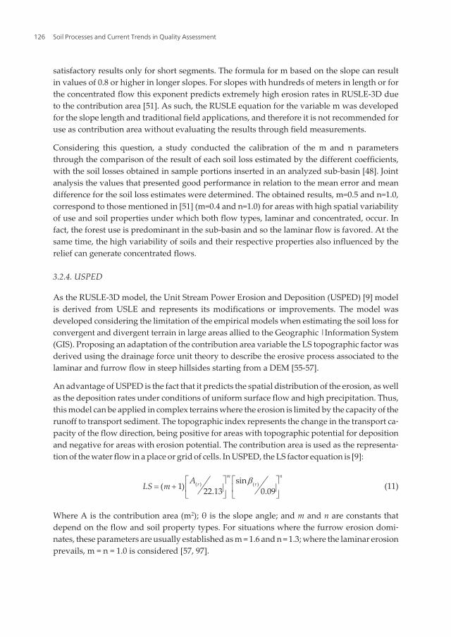
As the RUSLE-3D model, the Unit Stream Power Erosion and Deposition (USPED) [9] modelis derived from USLE and represents its modifications or improvements. The model wasdeveloped considering the limitation of the empirical models when estimating the soil loss forconvergent and divergent terrain in large areas allied to the Geographic |Information System(GIS). Proposing an adaptation of the contribution area variable the LS topographic factor wasderived using the drainage force unit theory to describe the erosive process associated to thelaminar and furrow flow in steep hillsides starting from a DEM [55-57].

An advantage of USPED is the fact that it predicts the spatial distribution of the erosion, as wellas the deposition rates under conditions of uniform surface flow and high precipitation. Thus,this model can be applied in complex terrains where the erosion is limited by the capacity of therunoff to transport sediment. The topographic index represents the change in the transport ca‐pacity of the flow direction, being positive for areas with topographic potential for depositionand negative for areas with erosion potential. The contribution area is used as the representa‐tion of the water flow in a place or grid of cells. In USPED, the LS factor equation is [9]:

( ) ( )sin( 1) 22.13 0.09

m nr rALS m bé ù é ù

= + ê ú ê úë û ë û

(11)

Where A is the contribution area (m2); θ is the slope angle; and m and n are constants thatdepend on the flow and soil property types. For situations where the furrow erosion domi‐nates, these parameters are usually established as m = 1.6 and n = 1.3; where the laminar erosionprevails, m = n = 1.0 is considered [57, 97].


In this model, the water erosion in a DEM cell is dependent on the surface runoff in this cellthat in turn depends on the upstream drainage area. When substituting the slope length theupstream contribution area generates the erosion network calculated as the convergence ofthe sediment flow and the deposition network obtained by the alteration in the sedimenttransport capacity.

Due to USPED computing divergence of the sediment flow, the impact of the exponents ismore complex when compared to RUSLE 3D [51]. In USPED the water flow exponent controlsthe ratio between the erosion extension and deposition, reflecting the fact that the turbulentflow can transport sediments and the impact of the concentrated erosion will be wider than ifthe flow was dispersed throughout the vegetation. Figure 5 shows the spatial pattern oftopographic potential by USPED with different values for the exponent m. For m = 1, a case ofdispersed laminar flow and deposition along the hillside. With m = 1.4 we have the case of theinfluence of both flow types, laminar and in furrows, on the erosion and deposition, with thedeposition beginning in the lower third of the hillside and gullying beginning in headwaterareas. For m=1.6, furrows and concentrated flows prevail beginning with great force in theheadwater areas and turning the erosion even longer and wider with potential for gullying.In this situation, the extension of the deposition areas is even more reduced.

Figure 5. Spatial pattern of topographic potential for erosion and deposition by USPED with m=1.0; m=1.4; andm=1.6. (Source: Elaborated by the authors).

The variation of the LS factor coefficients of USPED interferes in the soil loss estimates byvarying with the relief forms, plant covering and erosive processes. For this reason, the valueof the exponents has been documented and established for different climates and areas. Forthe United States, the value suggested for n in [98] varies from 0.3 to 2.0. In laminar erosionsituations the coefficient n=1.0 prevails and where the erosion in furrows is dominant, n=1.3.For a hydrographic basin of forest and agricultural use in Italy, the values adopted were m=n=1[99], as well as in [95] after the calibration of these parameters. In the identification of the miningimpact in an agricultural area of India, the coefficients m=1.6 and n=1.3 were adopted [100],


127

while in Poland, they opted for m=1.4 and n=1.2 for two hydrographic basins with the presenceof intense erosive processes [101]. In a sub-basin of forest use located in Brazil, the coefficientsm=n=1.0 were determined [48].

As the conceptual models reflect the physical processes that govern the system describing themwith empirical relationships, various quantitative evaluation studies of erosion risk inhydrographic basins have opted for the association of the USLE model with an LS factor thatreflects the expected surface drainage according to the topography, in order to reach soil lossestimates closer to reality [1, 55, 56, 77, 79, 102-104]. The analysis of the erosion risk in a sub-basin was conducted evaluating the performance of four topographic factor models (USLE,RUSLE, RUSLE 3D and USPED) in the USLE model [48]. The USPED (0.1286 ton ha-1) andRUSLE 3D (0.0668 ton ha-1) models did not present statistical differences in relation to the fieldlosses (0.1354 ton ha-1) and they generated a water erosion distribution meditated by theaccumulated flow, while the LS factors of RUSLE (2.74 ton ha-1) and USLE (3.65 ton ha-1)overestimated the soil losses [48]. The model considered most efficient in the modeling of theerosion was USPED. This model represented the erosive process in a broad manner whenestimating potential erosion and deposition areas, thus allowing to more precisely define thepriority areas for conservationist practices under different management sceneries, agreeingwith other studies [51, 99]. The advantages of USPED related to the possibility of predictingthe spatial distribution of the erosion as well as the deposition rates were stood out in [105],after its comparison with the LS factor of RUSLE 3D. In this context, several research worksare opting for the use of the USPED model [9, 45, 51, 98-100, 106, 107].

4. Models in real environmental scenarios

Application these topographic models in the real environmental scenarios have permittedmore accuracy and faster estimate of soil erosion in different regions, reliefs and land uses thanmanual methods. This way, studies have tried to figure out better results applying differentLS factor in the water erosion models to estimate and understand this process on watersheds.

LS RUSLE was utilized by [38] in the USLE model to estimate water erosion distributioncaused by forest ecosystems in a small watershed and generating soil loss predictionmaps according different land use situations. This same LS factor was used in USLEmodel by [108] allowing identification of the water erosion potential in a watershed for‐ested with eucalyptus and by [109] to estimate of the sediment delivery ratio in a water‐shed upstream from the hydroelectricity plants.

[110] applied USPED to identify the influence of changing land use on erosion and sedimen‐tation in different land use situations in watershed. [48] applied USLE, RUSLE 3D and USPEDin a small watershed for predicting water erosion by eucalyptus plantation founding bestresults for USPED model. USPED and RUSLE were also applied for assessing the impact ofsoil erosion/deposition on the archaeological surface at the archaeological site in Greece andUSPED presented better results [111]. Using USPED, [112] presented a modeling approach toimplement the support practices factor using geographic systems information where data are


unavailable and they concluded that USPED with adequate support practices permit to reduceerosion process.

Thus, considering the erosion problems in the world and data available efforts have been doneto improve erosion models.

5. Final considerations

The analysis and obtaining of the topographic factors conducted in the digital environ‐ment has become a fundamental piece in erosion model progress, because they addressthe systematic analyses from specific Geographical Information Systems (GIS’s) tools, aswell as allow the empirical processing of the data through adaptations of analogical tech‐niques, thus maintaining researcher interpretation. The analysis of the topography in GIenables the analyses of the landscape on a large scale, considers the effects of the topo‐graphical complexity more fully in the soil erosion, makes the data processing easier andfaster and reduces the relative cost. It is stood out that the reliability of these estimates isdirectly related to the precision of the topographic surveys used for the derivation of thedigital elevation model (DEM).

Evolution of LS factor driven by advanced technology allows the application of differenttopographic models in the USLE/RUSLE equations modernizing, and improving the estimateof those models. In semi-empirical algorithms, where the contribution area constitutes thecentral concept, advantages include application in slopes of complex geometries, representa‐tion of the surface runoff paths and incorporation of the convergent and divergent flow impactby calibration of empirical coefficients that allow to indicate the qualitative and quantitativeeffects of the changes in the land use without demanding large spatial and temporal databases.Such models, besides determining the erosion areas on a hydrographic basin level, in the caseof the USPED model, even allows to determine the deposition areas, including the erosiveprocess to its full extent.

Author details

Anna Hoffmann Oliveira1*, Mayesse Aparecida da Silva1,2, Marx Leandro Naves Silva1,Nilton Curi1, Gustavo Klinke Neto3 and Diego Antonio França de Freitas1

*Address all correspondence to: [email protected]

1 Soil Science Department, Federal University of Lavras, Lavras, MG, Brazil

2 CAPES and CNPq (Visiting scholar) scholarships, Brazil

3 Vitaramae Environmental Consulting Ltd., Lavras, MG, Brazil


129

References

[1] Bloise, G.L.F.; Carvalho Júnior, O.A.; Reatto, A.; Guimarães, R.F.; Martins, E.S.;Carvalho, A.P.F. Avaliação da suscetibilidade natural à erosão dos solos da Bacia doOlaria – DF. Planaltina: Embrapa Cerrados, 2001. 33 p. (Boletim de pesquisa e desenvolvi‐mento)

[2] Merritt, W.S.; Letcher, R.A.; Jakeman, A.J. A review of erosion and sediment transportmodels. Environmental Modelling & Software, Camberra, v. 18, p. 761-799, 2003.

[3] Wischmeier, W. H.; D. D. Smith. Predicting rainfall erosion losses; a guide to consevationplanning. Washington: USDA, 1978. Departament of Agriculture. 58 p. (AgricultureHandbook n. 537).

[4] Renard K.G.; Foster G.A.; Weesies D.A.; Mccool D.K.; Yoder, D.C. Predicting soilerosion by water: a guide to conservation planning with the revised universal soil lossequation (RUSLE). 1997. Agriculture handbook No. 703. USDA, Washington, DC.

[5] Ferrero, V. O. Hidrologia computacional y modelos digitales del terreno: teoría, práctica yfilosofía de una nueva forma de análisis hidrológico. [S.l.: s.n.], 2004. 364 p. Disponível em:<http://www.gabrielortiz.com/descargas/Hidrologia_Computacio‐nal_MDT_SIG.pdf>. Acesso em: 2 dez. 2010.

[6] Hickey, R. Slope angle and slope length solutions for GIS. Cartography, 2000. vol. 29, n.1, pp. 1-8.

[7] Van Remortel, R.D.; Maichle, R.W.; Hickey, R.J. Computing the LS factor for theRevisedUniversal Soil Loss Equation through array-based slope processing of digitalelevation data using a C++ executable. Computers & Geosciences, 2004: 30, 1043–1053.

[8] Bertoni, J.; Lombardi Neto, F. Conservação do solo. São Paulo: Ícone, 2005. 355p.

[9] Mitasova, H.; Hofierka, J.; Zlocha, M.; Iverson, L.R. Modelling topographic potentialfor erosion and deposition using GIS. International Journal Geographical InformationSystem, 1996. 10: 629– 641.

[10] Felgueiras, C. A.; "Análises sobre Modelos Digitais de Terreno em Ambiente deSistemas de Informação Geográfica". VIII Simpósio Latinoamericano de Percepción Remotay Sistemas de Información Espacial. Sesión Poster. Mérida, Venezuela, 2 a 7 de Novembrode 1997.

[11] Oliveira, A.H.; Silva, M.A. Da; Silva, M.L.N.; Avanzi, J.C.; Curi, N.; Lima, G.C.; Pereira,P.H. Caracterização ambiental e predição dos teores de matéria orgânica do solo naSub-Bacia do Salto, Extrema, MG. Semina: Ciências Agrárias, 2012a. 33: (1)143-154.

[12] Camara, G.; Souza, R.C.M.; Freitas, U.M.; Garrido, J. Spring: Integrating remote sensingand GIS by object-oriented data modeling. Computers & Graphics, 20: (3) 395-403, 1996.

[13] Hutchinson, M. F. A new procedure for gridding elevation and stream line data withautomatic removal of spurious pits. Journal of Hydrology, 1989. 106: (3-4)211-232.


[14] Câmara, G.; Davis. C.; Monteiro, A.M.; D’alge, J.C. Introdução à Ciência da Geoinforma‐ção. São José dos Campos, INPE, 2001.

[15] Chagas, C. S.; Fernandes Filho, E.I.; Rocha, M.F.; Carvalho Júnior, W. De; Souza Neto,N.C. Avaliação de modelos digitais de elevação para aplicação em um mapeamentodigital de solos. Revista Brasileira de Engenharia Agrícola e Ambiental, 2010. 14: (2)218-226.

[16] Ferraz, S. F. B.; Marson, J.C.; Fontana, C.R.; Lima, W.P. Uso de indicadores hidrológicospara classificação de trechos de estradas florestais quanto ao escoamento superficial.Scientia Forestalis, 2007. (75)39-4.

[17] Ferreira, A.G.; Gonçalves, A.C.; Dias, S.S. Avaliação da Sustentabilidade dos SistemasFlorestais em Função da Erosão. Silva Lusitana, 2008. 55 - 67.

[18] Liu H.; Fohrer, N.; Hörmann, G.; Kiesel. J. Suitability of S factor algorithms for soil lossestimation at gently sloped landscapes. Catena, 2009. 77: 248–255.

[19] Freitas, L.F. De; Carvalho Júnior, O.A. De; Guimarães, R.F.; Gomes, R.A.T.; Martins,E.S.; Gomes-Loebmann, D. Determinação do potencial de erosão a partir da utilizaçãoda EUPS na bacia do Rio Preto. Espaço & Geografia, 2007. 10: (2)431:452.

[20] Mata, C.L.; Carvalho Júnior, O.A. De; Carvalho, A.P.F. De; Gomes, R.A.T.; Martins, E.S.;Guimarães, R.F. Avaliação multitemporal da susceptibilidade erosiva na bacia do rioUrucuia (MG) por meio da Equação Universal de Perda de Solos. Revista Brasileira deGeomorfologia, 2007. 8: (2)57-71.

[21] Bilaşco, Ş.; Horvath, C.; Cocean, P.; Sorocovschi, V.; Oncu, M. Implementation of theUSLE model using GIS techniques. Case study the Someşean plateau. Carpathian Journalof Earth and Environmental Sciences, 2009. 4: (2)123 – 132.

[22] Oliveira, A.H.; Silva, M.L.N.; Curi, N.; Klinke Neto, G.; Silva, M.A. da; Araújo, E.F.Consistência hidrológica de modelos de elevação digital (MED) para avaliação daerosão hídrica na Sub-bacia hidrográfica do horto florestal Terra Dura, Eldorado doSul, RS. Revista Brasileira de Ciência do Solo, 2012b. 36: (4)1259-1267.

[23] Zeilhofer, P. Modelação de relevo e obtenção de parâmetros fisiográficos na Bacia doRio Cuiabá. Revista Brasileira de Recursos Hídricos, 2001. 6: (3)95-109.

[24] Redivo, A.L.; Guimarães, R.F.; Ramos, V.M.; Carvalho Júnior; Martins, E.S. Comparaçãoentre diferentes interpoladores na delimitação de bacias hidrográficas. Documentos/EmbrapaCerrados, 2002. 20p.

[25] Aronoff, S. Geographic information systems: A managment perspective. WDL Publications,Otawa, 1989. 294 p.

[26] Hutchinson, M.F.; Gallant, J.C. Digital elevation models and representation of terrainshape. In: WILSON, J.P.; GALLANT, J.C. (ed.). Terrain analysis: Principles and applica‐tions. New York: John Wiley & Sons, 2000. p.29-50.


131

[27] Gertner, G.; Wang, G.; Fang, S.; Anderson, A.B. Effect and uncertainty of digitalelevation model spatial resolutions on predicting the topographical factor for soil lossestimation. Journal of Soil and Water Conservation, 2002. 57: (3)164-174.

[28] Cebecauer, T.; Hofierka, J. The consequences of land-cover changes on soil erosiondistribution in Slovakia. Geomorphology, 2008. 98: 187–198.

[29] Wang, G.; Gertner, G.; Parysow, P.; Anderson, A. Spatial prediction and uncertaintyassessment of topographic factor for revised universal soil loss equation using digitalelevation models. Journal of Photogrammetry & Remote Sensing, 2001. 56: 65–80.

[30] Bhattarai, R.; Dutta, D. Estimation of Soil Erosion and Sediment Yield Using GIS atCatchment Scale. Water Resources Management, 2007. 21: 1635–1647.

[31] Fornelos L.F.; Neves S.M.A.S. Uso de modelos digitais de elevação (mde) gerados apartir de imagens de radar interferométrico (SRTM) na estimativa de perdas de solo.Revista Brasileira de Cartografia, 2007. 59(01).

[32] Truman, C.C.; Wauchope, R.D.; Sumner, H.R.; Davis, J.G.; Gascho, G.J., Hook, J.E.;Chandler, L.D.; Johnson, A.W. Slope length effects on runoff and sediment delivery.Journal of Soil and Water Conservation, 2001. 56: (3)249.

[33] Rocha, J.V.; Lombardi Neto, F.; Bacellar, A.A.A. Metodologia para determinação dofator comprimento de rampa (L) para a Equação Universal de Perdas de Solo. Cadernode Informações Georreferenciadas (CIG), 1997. 1: (2).

[34] Silva, A.M.; Mello, C.R.; Curi, N.; Oliveira, P.M. Simulação da variabilidade espacialda erosão hídrica em uma sub-bacia hidrográfica de Latossolos no sul de Minas Gerais.Revista Brasileira de Ciência do Solo, 2008. 32: 2125-2134.

[35] Bateira, C. Cálculo e cartografia automática dos declives: Novas tecnologias versuslelhos problemas. Revista da Faculdade de Letras – Geografia. Porto / Portugal. v. XII/XIII, ,1996/7, pp. 125-143.

[36] Ismail, J.; Ravichandran, S. Using Remote Sensing and GIS. Water Resources Manage‐ment, 2008. 22: 83-102.

[37] Liu, B.Y.; Nearing, M.A.; Shi, P.J.; Jia, Z.W. Slope length effects on soil loss for steepslopes. In: Stott, D.E.; Mohtar, R.H., Steinhardt, G.C. Sustaining the Global Farm, 2001.784-788.

[38] Silva, M.A. Da; Silva, M.L.N.; Curi, N. L.; Norton, D.; Avanzi, J.C.; Oliveira, A.H.; Lima,G.C. (2010) - Water erosion modeling in a watershed under forest cultivation throughthe USLE model. In: Proceedings 19th World Congress of Soil Science. Brisbane, Australia,IUSS, p. 173-176.

[39] Tucci, C. E. M. Modelos hidrológicos. Porto Alegre: Ed. Universidade, UFRGS, 1998. 669p.

[40] Wilson, J.P. Estimating the topographic factor in the universal soil loss equation forwatersheds. Journal of Soil and Water Conservation, 1986. 41: 179-184.


[41] Griffin, M.L.; Beasley, D.B.; Fletcher, J.J.; Foster, G.R. Estimating soil loss on topo‐graphically nonuniform field and farm units. Journal of Soil and Water Conservation, 1988.43: 326-331.

[42] Kandel, D.D., Western, A.W., Grayson, R.B.; Turral, H.N. Process parameterization andtemporal scaling in surface runoff and erosion modelling. Hydrological Processes, 2004.18: 1423-1446.

[43] Kinnell, P.I.A. Slope length factor for applying the USLE-M to erosion in grid cells. SoilTillage Research, 2001. 58: 11–17.

[44] Kinnell, P.I.A. Why the universal soil loss equation and the revised version of it do notpredict event erosion well. Hydrological Processes, 2005. 19: 851–854.

[45] Warren, S.D.; Mitasova, H.; Hohmann, M.G.; Landsberger, S.; Iskander, F.Y.; Ruzycki,T.S.; Senseman, G.M. Validation of a 3-D enhancement of the Universal Soil LossEquation for prediction of soil erosion and sediment deposition. Catena, 2005. 64:281-296.

[46] Desmet, P.J.J.; Govers, G. A GIS procedure for automatically calculating the USLE LSfactor on topographically complex landscape units. Journal of Soil and Water Conserva‐tion, 1996. 51: 427–433.

[47] Van Remortel, R., Hamilton, M.; Hickey, R. Estimating the LS factor for RUSLE throughiterative slope length processing of digital elevation data. Cartography, 2001. 30:(1)27-35.

[48] Oliveira, A.H. Erosão hídrica e seus componentes na sub-bacia hidrográfica do horto florestalTerra Dura, Eldorado do Sul, RS. PhD thesis. Universidade Federal de Lavras, 2011.

[49] Risse, L.M.; Nearing, M.A.; Nicks, A.D., Laften, J.M. Error assessment in the universalsoil loss equation. Soil Science Society of America Journal, 1993. 57: 825–833.

[50] Rapp, J.F.; Lopes, V.L.; Renard, K.G. Comparing soil erosion estimates from Rusle andUsle on natural runoff plots. In: Aschough II, J.C., Flanagan D.C. (eds). Proceedings ofInternational Symposium Soil Erosion Research for the 21st Century, Jan. 3–5, Honolulu, HI.American Society Agricultural Engineers: St Joseph, MI; p. 24–27. 2001.

[51] Mitasova, H.; Mitas, L.; Brown, W.M.; Johnston, D. Terrain modeling and Soil ErosionSimulation: applications for Ft. Hood Report for USA CERL. University of Illinois, Urbana-Champaign, IL. 2001.

[52] Zhou, Q.; Liu, X. Error assessment of grid-based flow routing algorithms used inhydrological models. International Journal of Geographic Information Science, 2002. 16:(8)819-842.

[53] Arnold, J.G. SWAT: Soil and Water Assessment Tool / User's Manual, USDA-ARS. 1996.

[54] Lu, H., Moran, C., Prosser, I.; Sivapalan, M. Modelling sediment delivery ratio basedon physical principles. In: Pahl-Wostl, C.; Schmidt, S.; Jakeman, T. (Editors), Interna‐


133

tional Congress: "Complexity and Integrated Resources Management". Osnabrueck: Inter‐national Environmental Modelling and Software Society, p. 600, 2004.

[55] Moore I.D.; Burch, G.J. Modeling erosion and deposition. Topographic effects.Transactions of the America, Science Agricultural Engineering, 1986. 29: 1624-1640.

[56] Moore, I.D., Burch, G.J. Physical basis of the length-slope factor in the universal soilloss equation. Soil Science Society of America Journal, 1986. 50: 1294-1298.

[57] Moore, I.D.; Wilson, J.P. Length-slope factors for Revised Universal Soil Loss Equation(RUSLE): simplified method of estimation. Journal of Soil and Water Conservation, 1992.47: (5)423-428.

[58] Moore, I.D., Turner, A.K., Wilson, J.P., Jenson, S. K.; Band, L. E. Gis and land surfacesubsurface process. In: Goodchild, M.F.; Bradley, O. Environmental Modeling with GIS.Parks & Louis T. Steyaert (eds), 1993. pp. 196-230.

[59] Jenson, S. K.; Domingue, J. O. Extracting topographic structure from digital elevationdata for geographic information system analysis. Photogrammetric Engineering andRemote Sensing, 1988. 54: (11)1593-1600.

[60] Nardi, F.; Grimaldi, S.; Santini, M.; Petroselli, A.; Ubertini, L. Hydrogeomorphicproperties of simulated drainage patterns using digital elevation models: the flat areaissue. Hydrological Sciences Journal, 2008. 53: (6)1176-1193.

[61] Maidment, D. R., Oliveira, F., Calver, A., Eatherall, A. and Fraczek, W. Unit Hydro‐graph Derived From A Spatially Distributed Velocity Field. Hydrological Processes, 1996.10: 833-844.

[62] Rennó, C.D.; Nobre, A.D.; Cuartas, L.A.; Soares, J.V.; Hodnett, M.G.; Tomasella, J.;Waterloo, M.J.H. A new terrain descriptor using SRTM-DEM: Mapping terra-firmerainforest environments in Amazonia. Remote Sensing of Environment, 2008. 112:3469-3481.

[63] Tarboton, D. G. A new method for the determination of flow directions and upslopeareas in the grid digital elevation models. Water Resources Research, 1997. 33: (2)309- 319.

[64] O’callaghan, J.F.; Mark, D.M. The extraction of drainage networks from digitalelevation data. Computer Vision Graphics Image Processing, 1984. 28: 323–344.

[65] Fairfield, J.; Leymarie, P. Drainage networks from grid digital elevation models. WaterResources Research, 1991. 27: (5) 709-717.

[66] Costa-Cabral, M.C.; Burges, S. J. Digital elevation model networks (DEMON): A modelof flow over hillslopes for computation of contributing and dispersal areas. WaterResources Research, 1994. 30: (6)1681-1692.

[67] Garbrecht, J.; Martz, L.W. The assignment of drainage direction over flat surfaces inraster digital elevation models. Journal of Hydrology, 1997. 193:204-213.


[68] Orlandini, S.; Moretti, G.; Franchini, M.; Aldighieri, B.; Testa, B. Path-based methodsfor the determination of nondispersive drainage directions in grid-based digitalelevation models. Water Resources Research, 2003. 39: (6)1144.

[69] Freeman, T.G. Calculating catchment area with divergent flow based on a regular grid.Computers & Geosciences, 1991. 17: 413–422.

[70] Quinn, P.; Beven, K.; Chevallier, P.; Planchon, O. The prediction of hillslope flow pathsfor distributed hydrological modeling using digital terrain models. HydrologicalProcesses, 1991. 5: 59-79.

[71] Lea, N.L. An aspect driven kinematic routing algorithm. In: Overland Flow: Hydraulicsand Erosion Mechanics, Eds. PARSONS, A.J.; Abrahams, A.D. Chapman & Hall, NewYork, USA. 1992.

[72] Lindsay, J.B. A physically based model for calculating contributing area on hillslopesand along valley bottoms. Water Resources Research, 2003. 39: (12)1332.

[73] Seibert, J., Mcglynn, B.L. A new triangular multiple flow direction algorithm forcomputing upslope areas from gridded digital elevation models. Water ResourcesResearch, 2007. 43.

[74] Rieke-Zapp, D.H.; Nearing, M.A. Slope Shape Effects on Erosion: A Laboratory Study.Soil Science Society American Journal, 2005. 69: 1463–1471.

[75] Mendes, C.A.B.; Ordoñez, J.E.S.; Grehs, S.A. Arcabouço de modelo hidrológico deescala continental utilizando-se a topologia da rede de drenagem simulada: aplicaçãona Bacia Hidrográfica Amazônica. Geografia, 2006. 15: (2)21-49.

[76] Patriche, C.V.; Capatana, V.C.; Stoica, D.L. Aspects regarding soil erosion spatialmodeling using the USLE / RUSLE within GIS. Geographia Technica, 2006. 2: 87-97.

[77] Efe, R.; Ekinci, D.; Cürebal Erosion analysis of Sahin Creek watershed (NW of Turkey)using GIS based on RUSLE (3d) method. Journal of Applied Sciences, 2008. 8: (1)49-58.

[78] Ferreira, A.G.; Gonçalves, A.C.; Dias, S.S. Avaliação da Sustentabilidade dos SistemasFlorestais em Função da Erosão. Silva Lusitana, 2008. (n. especial) 55 - 67.

[79] Ozcan, A.U.; Erpul, G.; Basaran, M.; Erdogan, H.E. Use of USLE/GIS technologyintegrated with geostatistics to assess soil erosion risk in different lan uses of IndagiMountain Pass-Çankiri, Turkey. Environmental Geology, 2008. 53: 1731-1741.

[80] Winchell, M.F.; Jackson, S.H.; Wadley, A.M.; Srinivasan, R. Extension and validationof a geographic information system-based method for calculating the Revised Univer‐sal Soil Loss Equation length-slope factor for erosion risk assessments in large water‐sheds. Journal of Soil and Water Conservation, 2008. 63: (3)105-111.

[81] Zhang, Q.; Wang, L.; Wu, Fa-qi. GIS-Based Assessment of Soil Erosion at Nihe GouCatchment. Agricultural Sciences in China, 2008. 7: (6)746-753.


135

[82] Tarboton, D.G.; Mohammed, I.N. Terrain analysis using digital elevation models. TauDEM,version 5.0. Software. 2010.

[83] Bogaart, P.W.; Troch, P.A. Curvature distribution within hillslopes and catchments andits effect on the hydrological response. Hydrology and Earth System Sciences, 2006. 10:925–936.

[84] Ramos, V.M.; Guimarães, R.F.; Redivo, A.L.; Carvalho Júnior, O.A. De; Fernandese,N.F.; Gomes, R.A.T. Avaliação de metodologias de determinação do cálculo de áreasde contribuição. Revista Brasileira de Geomorfologia, 2003. 4: (2)41-49.

[85] Buarque, D.C.; Fan, F.M.; Paz, A.R. Da; Collischonn, W. Comparação de Métodos paraDefinir Direções de Escoamento a partir de Modelos Digitais de Elevação. RevistaBrasileira de Recursos Hídricos, 2009. 14: (2)91-103.

[86] Günter, A.; Seibert, J.; Uhlenbrook, S. Modeling spatial patterns of saturated areas: Anevaluation of different terrain indices. Water Resources Research, 2004. 40: 5114.

[87] Pan, F.; Peters-Lidard, C.D.; Sale, M.J.; King, A.W. A comparison of geographicalinformation systemsbased algorithms for computing the TOPMODEL topographicindex. Water Resources Research, 2004. 40: 6303, 2004.

[88] Erskine, R.H.T.R.G.; Ramirez, J.A.; Macdonald, L.H. Comparison of grid-basedalgorithms for computing upslope contributing area. Water Resources Research, 2006.42:9416.

[89] Foster, G.R.; W.H., Wischmeier. Evaluating irregular slopes for soil loss prediction.Transactions of ASAE, 1974. 17: 305-309.

[90] Mccool, D.K., Brown, L.C.; Foster, G.R.. Revised slope steepness factor for the UniversalSoil Loss Equation. 1987. Transactions of the ASAE, vol. 30, pp. 1387-1396.

[91] Mccool, D.K., Foster, G.R.; Mutchler, C.K.; Meyer, L.D. Revised slope length factor forthe Universal Soil Loss Equation. 1989. Transactions of the ASAE, vol. 32, pp. 1571-1576.

[92] Zevenbergen, L.W.; Thorne, C.R. Quantitative analysis of land surface topography.Earth Surface Processes and Lnadforms, 1987. 12: 475.

[93] Carvalho Junior, O.A.; Guimarães, R.F. Implementação em ambiente computacional eanálise de emprego da área de contribuição no cálculo do fator topográfico (LS) daUSLE. In: Simpósio Nacional de Controle da Erosão, 7. Anais... Goiânia, 2001. (CD-ROM).

[94] Silva, V.C. Cálculo automático do fator topográfico (LS) da EUPS, na Bacia do RioParacatu. Pesquisa Agropecuária Tropical, 2003. 33: (1)29-34.

[95] Suárez, M.C.G. Metodologia de cálculo del factor topográfico, LS, integrado em los modelosRUSLE y USPED. Aplicación em Arroio Del Lugar, Guadalajara (España). 2008. Universi‐dad Politécnica de Madrid, Madri. 391 p. (Tese de Doutorado)


[96] Simms, A.D.; Woodroffe, C.D.; Jones, B.G. Application of RUSLE for Erosion Manage‐ment in a Coastal Catchment, Southern NSW. In: Proceedings of MODSIM 2003.Townsville, Queensland, Australia, p. 678-683, 2003.

[97] Foster, G.R. Comment on “Length-slope factors for the Revised Universal Soil LossEquation: simplified method of estimation”. Journal of Soil and Water Conservation. 1994.49: 171–173.

[98] Pricope, N.G. Assessment of Spatial Patterns of Sediment Transport and Delivery forSoil and Water Conservation Programs. Journal of Spatial Hydrology, 2009. 9: (1)21-46.

[99] Pistocchi, A.; Cassani, G.; Zani, O. Use of the USPED model for mapping soil erosionand managing best land conservation practices. In: Rizzoli, A. E.; Jakeman, A. J. (eds.).Integrated Assessment and Decision Support, Proceedings of the First Biennial Meeting of theInternational Environmental Modelling and Software Society, v. 1, 2002. pp. 163-168.Disponível em: <iEMSs, 2002. http://www.iemss.org/iemss2002/proceedings/>.

[100] Kandrika, S.; Dwivedi, R.S. Assessment of the impact of mining on agricultural landusing erosion-deposition model and space borne multispectral data. Journal of SpatialHydrology, 2003. 3: (2).

[101] Drzewiecki, W.; Mularz, S. Model USPED jako narzędzie prognozowania efektówerozji i depozycji materiału glebowego. In: Annals of Geomatics (Associação Polonesa deInformação Espacial), 2005. 3: (2)52–54.

[102] Andrade, A.C.; Leal, L.R.; Carvalho Júnior, O.A.; Martins, E.S.; Reatto, A. Estudo dosprocessos erosivos na Bacia do Rio Grande (BA) como subsídio ao planejamento agroecológico.Planaltina, DF: Embrapa Cerrados, 2002. 26 p. Boletim técnico n. 63.

[103] Erdogan, E.H.; Erpul, G.; Bayramin, İ. Use of USLE/GIS Methodology for PredictingSoil Loss in a Semiarid Agricultural Watershed. Environmental Monitoring and Assess‐ment, 2007. 131: 153–161.

[104] Jain, M.; Kothyari, U.C. Estimation of soil erosion and sediment yield using GIS.Hydrological Science Journal, 2000. 45: (5)771-786.

[105] Saavedra, C.P.; Mannaerts, C.M. Erosion estimation in an Andean catchment combin‐ing coarse and fine resolution satellite imagery. In: Proceedings of the 31st InternationalSymposium on Remote Sensing of Environment: global monitoring for sustainability andsecurity. Saint Petersburg, 20-24 June, 2005. 4 p.

[106] Liu, J.; Liu, S.; Tieszen, L.; Chen, M. Estimating soil erosion using the USPED modeland consecutive remotely sensed land cover observations. Proceedings of the 2007summer computer simulation conference, San Diego, 2007.

[107] Alimohammadi, A.; Sheshangosht, S.; Soltani, M.J. Evaluation of relations betweenDEM-Based USPED Model Output and Satellite-based spectral indices. In: ConferenceProceedings of Map India 2006. Anais… Disponível em: <http://www.gisdevelop‐ment.net/proceedings/mapindia/2006/index.htm>.


137

[108] Avanzi, J. C. Soil properties, condition and soil losses for south and east Brazilian forestareas. PhD thesis. Universidade Federal de Lavras, 2009.

[109] Beskow S.; Mello, C. R.; Norton, L. D.; Curi, N.; Viola, M. R.; Avanzi, J. C. Soil erosionprediction in the Grande River Basin, Brazil using distributed modeling. Catena, 2009.79: 49-59.http://www.sciencedirect.com/science/article/B6VCG-4WKJ5JC-1/2/fb138c9c89ca86d834b52c3124987424 (accessed 19 October 2012).

[110] Leh, M.; Bajwa, S.; Chaubey, I. Impact of land use change on erosion risk: an integratedRemote sensing, geographic information system and modeling methodology. LandDegradation & Development, 2011. https://engineering.purdue.edu/ecohydrology/Pubs/2011%20LDD%20Leh-Bajwa-Chaubey.pdf. (accessed 19 October 2012).

[111] Gouma, M.; Wijngaarden, G. J. V.; Soetens, S. Assessing the effects of geomorp hologicalprocesse son archaeologic al densities: a GIS case stud y on Zakynth os Island, Greece.Journal of Archaeological Science, 2011. 38: 2714-2725

[112] Pelacani, S.; Märker, M.; Rodolfi, G. Simulation of soil erosion and deposition in achanging land use: A modelling approach to implement the support practice factor.Geomorphology, 2008. 99: 329 – 340


development of topographic factor modeling for application

Documents