development of the methodology and application to … · •universidad politecnica de madrid...

Modelling SequentialBiosphere Systemsunder Climate Changef o r R a d i o a c t i v eW a s t e D i s p o s a l

EC-CONTRACT : FIKW-CT-2000-00024

Deliverable D8b :

Development of thephysical/statistical downscalingmethodology and applicationto climate model CLIMBERfor BIOCLIM Workpackage 3.

Simulation of the future evolution of the biosphere system using the hierarchical strategy

2 0 0 3

Work package 3:

RESTRICTED‘All property rights and copyrights are reserved. Any communication or reproduction of this document, and any communication or use of itscontent without explicit authorization is prohibited. Any infringement to this rule is illegal and entitles to claim damages from the infringer,without prejudice to any other right incase of granting a patent of registration in the field or intellectual property.’

Foreword

Work package 1 will consolidate the needs of the European agencies of the consortium and summarise how environmental change has been treated to date in performance assessments.

Work packages 2 and 3 will develop two innovative and complementary strategies for representing time series of long term climate change using different methods to analyse extreme climate conditions (the hierarchical strategy) and a continuous climate simulation over more than the next glacial-interglacial cycle (the integrated strategy).

Work package 4 will explore and evaluate the potential effects of climate change on the nature of the biosphere systems.

Work package 5 will disseminate information on the results obtained from the three year project among the international community for further use.

The project brings together a number of representatives from both European radioactive waste managementorganisations which have national responsibilities for the safe disposal of radioactive waste, either asdisposers or regulators, and several highly experienced climate research teams, which are listed below.

The BIOCLIM project on modelling sequential BIOsphere systems under CLIMate change for radioactivewaste disposal is part of the EURATOM fifth European framework programme. The project was launched inOctober 2000 for a three-year period. The project aims at providing a scientific basis and practicalmethodology for assessing the possible long term impacts on the safety of radioactive waste repositoriesin deep formations due to climate and environmental change. Five work packages have been identified tofulfil the project objectives:

•Agence Nationale pour la Gestion des Déchets Radioactifs (Andra), France – J. Brulhet, D.Texier

•Commissariat à l’Energie Atomique/ Laboratoire des Sciences du Climat et de l’Environnement (CEA/LSCE) France – N. de Noblet, D. Paillard, D.Lunt, P.Marbaix, M. Kageyama

•United Kingdom Nirex Limited (NIREX), UK – P. Degnan

•Gesellschaft für Anlagen und Reaktorsicherheit mbH (GRS), Germany – A. Becker

•Empresa Nacional de Residuos Radioactivos S.A. (ENRESA), Spain – A. Cortés

•Centro de Investigaciones Energeticas, Medioambientales y Tecnologicas (CIEMAT), Spain – A. Aguero, L. Lomba, P. Pinedo, F. Recreo, C. Ruiz,

•Universidad Politecnica de Madrid Escuela Tecnica Superior de Ingenieros de Minas (UPM-ETSIMM), Spain – M. Lucini , J.E. Ortiz, T. Torres

•Nuclear Research Institute Rez, plc - Ustav jaderneho vyzkumu Rez a.s. (NRI), Czech Republic – A. Laciok

•Université catholique de Louvain/ Institut d’Astronomie et de Géophysique Georges Lemaître (UCL/ASTR), Belgium – A. Berger, M.F. Loutre

•The Environment Agency of England and Wales (EA), UK - R. Yearsley, N. Reynard

•University of East Anglia (UEA), UK – C. Goodess, J. Palutikof

BIOCLIM is supported by a Technical Secretariat provided by Enviros Consulting Ltd, with other technical support provided by Quintessa Ltd and Mike Thorneand Associates Ltd.

For this report, deliverable D8b of the BIOCLIM project, the main contributor is the climate modelling group of the CEA/LSCE.

Public should be aware that BIOCLIM material is working material.

BIOCLIM, Deliverable D8b

Content List1 - Introduction and objectives 6

2 - CLIMBER outputs and the downscaling issue 82.1. - Basic data 8

2.1.1 - Climatology 82.1.2 - CLIMBER model 8

2.2. - Physical-statistical method principles 102.3. - Physically based predictors 11

2.3.1 - Continentality 122.3.2 - Mountains 14

2.4. - Calibration of the downscaling method 172.4.1 - Temperature 172.4.2 - Precipitation 22

3 - Downscaling for the BIOCLIM future scenarios 283.1. - Time series for the sites 29

3.1.1 - Natural scenario – model / downscaling comparison 293.1.2 - Fossil fuel scenarios 32

3.2. - Snapshots 36

4 - Conclusions 39

5 - References 41

APPENDIX 1 : Data product 43

1. Introduction and objectives

The overall aim of BIOCLIM is to assess thepossible long term impacts due to climatechange on the safety of radioactive waste

repositories in deep formations. This aim is addressedthrough the following specific objectives:

• Development of practical and innovative strategies forrepresenting sequential climatic changes to thegeosphere-biosphere system for existing sites overcentral Europe, addressing the timescale of onemillion years, which is relevant to the geologicaldisposal of radioactive waste.

• Exploration and evaluation of the potential effects ofclimate change on the nature of the biospheresystems used to assess the environmental impact.

• Dissemination of information on the newmethodologies and the results obtained from theproject among the international waste managementcommunity for use in performance assessments ofpotential or planned radioactive waste repositories.

This deliverable has the following specific motivationsand objectives:

Its main aim is to provide time series of climaticvariables at the high resolution as needed byperformance assessment (PA) of radioactive wasterepositories, on the basis of coarse output from theCLIMBER-GREMLINS climate model.

The climatological variables studied here are long-term(monthly) mean temperature and precipitation, asthese are the main variables of interest forperformance assessment (see Ref.1, section 3.2).CLIMBER-GREMLINS is an earth-system model ofintermediate complexity (EMIC), designed for longclimate simulations (glacial cycles). Thus, this modelhas a coarse resolution (about 50 degrees in longitude)and other limitations which are sketched in this report(further details are provided in Ref.2). For the purpose

of performance assessment, the climatologicalvariables are required at scales pertinent for theknowledge of the conditions at the depository site. Inthis work, the final resolution is that of the bestavailable global gridded present-day climatology, whichis 1/6 degree in both longitude and latitude (this willbe called “regional scale” here, although it is areasonable approximation of local (site) temperatureand precipitation when there is no complex localtopography).

To obtain climate-change information at this highresolution on the basis of the climate model outputs, a2-step downscaling method is designed. First, physicalconsiderations are used to define variables which areexpected to have links which climatological values(i.e. predictors, such as continentality); secondly astatistical model is used to find the links between thesevariables and the high-resolution climatology oftemperature and precipitation. Thus the method istermed as “physical/statistical” : it involves physicallybased assumptions to compute predictors from modelvariables and then relies on statistics to find empiricallinks between these predictors and the climatology.

The simple connection of coarse model results toregional values can not be done on a purely empiricalway because the model does not provide enoughinformation – it is both too coarse and simplified. Thisis why we first need to find these “physically based”relations between large scale model outputs andregional scale predictors. This is a solution to thespecific problem of downscaling from an intermediatecomplexity model such as CLIMBER. There are severalother types of downscaling methodologies, such hasthe dynamical (model) and rule-based methodpresented in other BIOCLIM deliverables. A specificity ofthe present method is to attempt to use physicalconsiderations in the downscaling while a detailed“dynamical” approach is out of reach because



p. 6/7CLIMBER only (or mainly) provides the average climate.By contrast, an input of time-variability at various scales(preferably up to meteorological events) is necessaryfor a more dynamical approach (see e.g. Ref.3 ; Ref.4).

This report is organised as follows:

Section 2 relates to the design and validation of themethod, while section 3 reports the application to

BIOCLIM simulations. We first present the employeddata sources, which are the model results and theobserved climatology (subsection 2.1). We thenpresent the principles of the downscaling method (2.2),the formulation of the predictors (2.3) and thecalibration of the statistical model, including results forthe last glacial maximum (2.4). In section 3, the resultsare first presented as time series for each site (3.1),then as maps at specific times, or snapshots (3.2).

2. CLIMBER outputs andthe downscaling issue


Climatological data is a key element in this work,because it will be used to statistically estimatethe parameters of the empirical part of our

method. These high resolution observation-based datawill also serve as a guide to find which kind of «physicalinformation» we may want to add to coarse climatemodel outputs in order to provide regional details, as itwill appear later. As the CLIMBER model itself does notrepresent day to day variability nor year to year changes,we seek a monthly climatology. We need at least

precipitation and temperature on land areas, at a highspatial resolution. This is conveniently provided by therecent, 10’ resolution (1/6 degree) global griddedclimatology from the Climate Research Unit [Ref.5],which proved more trustworthy than formerly availabledata (during our preliminary tests). The correspondingtemperatures for January and July are plotted on figure1. The resolution of that dataset will be the targetresolution of our downscaling, i.e. all our data will becomputed or interpolated on that grid.

2.1. - Basic data

2.1.1. - Climatology

The climate model, CLIMBER2.3 [Ref.6] isdescribed in deliverable D7 (Ref.2, section2.1.2). It has a coarse longitudinal-latitudinal

grid: each atmospheric grid box is 51° in longitude and10° in latitude. Also important for our application, it isan “intermediate complexity model”: with comparison

to 3D general circulation models, it includes lessexplicit representations of atmospheric features, thusrelying on more parametrisations. In particular, itdoesn’t represent mid-latitude low pressure systems,but accounts for their effects on the meridional heattransport. Thus it ignores the variability at the time

2.1.2. - CLIMBER model

Figure 1 : Monthly mean temperature climatology (CRU 10’ data, see text)

January July


scale of meteorological events (e.g. winds associatedwith low pressure systems) and also at the time scaleof a few years, in particular the North AtlanticOscillation (NAO).

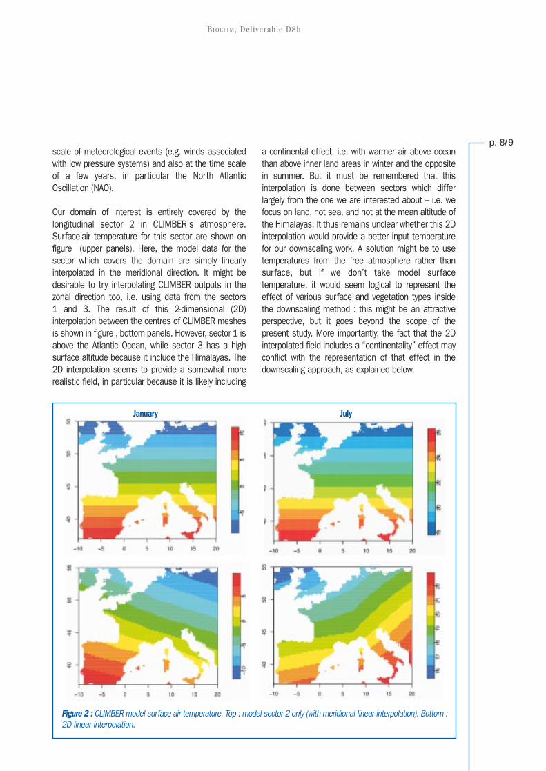
Our domain of interest is entirely covered by thelongitudinal sector 2 in CLIMBER’s atmosphere.Surface-air temperature for this sector are shown onfigure (upper panels). Here, the model data for thesector which covers the domain are simply linearlyinterpolated in the meridional direction. It might bedesirable to try interpolating CLIMBER outputs in thezonal direction too, i.e. using data from the sectors1 and 3. The result of this 2-dimensional (2D)interpolation between the centres of CLIMBER meshesis shown in figure , bottom panels. However, sector 1 isabove the Atlantic Ocean, while sector 3 has a highsurface altitude because it include the Himalayas. The2D interpolation seems to provide a somewhat morerealistic field, in particular because it is likely including

a continental effect, i.e. with warmer air above oceanthan above inner land areas in winter and the oppositein summer. But it must be remembered that thisinterpolation is done between sectors which differlargely from the one we are interested about – i.e. wefocus on land, not sea, and not at the mean altitude ofthe Himalayas. It thus remains unclear whether this 2Dinterpolation would provide a better input temperaturefor our downscaling work. A solution might be to usetemperatures from the free atmosphere rather thansurface, but if we don’t take model surfacetemperature, it would seem logical to represent theeffect of various surface and vegetation types insidethe downscaling method : this might be an attractiveperspective, but it goes beyond the scope of thepresent study. More importantly, the fact that the 2Dinterpolated field includes a “continentality” effect mayconflict with the representation of that effect in thedownscaling approach, as explained below.

p. 8/9

Figure 2 : CLIMBER model surface air temperature. Top : model sector 2 only (with meridional linear interpolation). Bottom :2D linear interpolation.

January July


2.2. - Physical-statistical method principles

A s described above, there are much more detailsin the real climatology than in our model data, atvarious geographical scales. Some statistical

approaches rely on an essentially empirical method toconnect the coarse model results to high resolutionvariables. But these methods usually take model inputswhich contain more information than what we canobtain from an EMIC such as CLIMBER. Whenlarge-scale meteorological conditions are known, thesecan be connected to regional patterns of precipitationand temperature on a either a statistical basis(empirical approach, see e.g. Ref.7) or a dynamicalbasis (model or desaggregation scheme, see e.g.Ref.4). But in the context of this climate model, we onlyhave monthly climatological means. On the other hand,observed data of good quality on most of Europe areonly available for present-day conditions. In summarywe have little information on time variability at allscales, from meteorological to climate state changes.

In this context, trying to connect regional temperatureand precipitation to large scale information using onlystatistics would have severe limitations : we don’t haveenough data to calibrate empirical relations in a waywhich could be reliably applied to climate change onlong periods. Our aim is than to find “physically based”relations between regional and large scales whichmight supplement the statistical approach. Theserelations have to be robust, i.e. be independent of theclimate state (past, present, future). In addition, therelations will provide insight on the climate changeissue only if these involve input data for which we knowthe value at the desired time, such as sea-level orclimate model variables.

Before going into the details of these additionalphysical relations, it is now necessary to introduce thestatistical model. The input variables, or predictors, arethe data for which climate changes value are known(either directly from the climate model or usingadditional “physical” hypothesis). The statistical modelis thus a link (regression function) between these

predictors and the desired output, or predictand - heretemperature or precipitation. A quite flexible model isthe Generalized Additive Model (GAM), in which thepredictand is expressed as a sum of smooth (spline)functions of each predictor, including linear terms ifdesired :

where Y is the predictand, X j are the predictors, bo andbj are constants, ƒj are spline functions and ε is themodel error.A very simple statistical model will now illustrate themethod and serve as a guide for further development :

where Τ is the high-resolution temperature field, ƒ(zs) isa smooth function of the land surface height zs , ΤM isthe interpolated climate model surface temperature,which is decomposed in its geographical domain1

-averaged value ΤM and the deviation from this mean :

The deviation from the mean, ∆ΤM , mainly representsthe meridional temperature gradient from CLIMBER,because this model is very coarse and we use datafrom only one longitudinal sector, as shown in figure(top panels).

We are thus constructing a regression function relativeto the link between land surface height and large-scaletemperature gradient from the climate model, andregional temperature on the other hand. The regressionfunction (the spline ƒ(zs) and the coefficient bΤ) isprovided by the implementation of the GAM model inthe R software [Ref.8].

This regression describes the geographical variabilityfor a given month. As our final objective is climatechange downscaling, the regression must also bemeaningful in climate change conditions. The first stepin this direction is the inclusion of the large scale

(3)

1 The geographical domain is the “domain of interest” shown e.g. on figure 1.


gradient from the climate model : we suggest thatchanges in the modelled gradient have something“real”, i.e. that if the model gives a larger/smallergradient, it is reasonable that the statistical predictionalso involves that change in the gradient. By doing itthis way, we assume that the link between CLIMBER’sgradient and the high resolution temperature issomewhat robust, i.e. that if the gradient is smaller inthe reality than in the climate model, this will also betrue, and possibly in the same ratio (the regression

coefficient) in a changed climate. As we only have onereference climate state (the present), we have noinformation about the link between the domain meantemperature in the model and in the reality. Therefore,we can only decide that changes in the mean modeltemperature are included in the downscaling output;that’s why we just add the mean temperature ΤM, whichis thus not included in the estimated regressionfunction.

It is now interesting to have a look at the ability of oursimple regression to represent the actual variance oftemperature in the domain. Topography and north-southgradient already explain a substantial part of thegeographical variability, so that our regression functionproduces maps which partly looks like the climatology.The difference between the regression and the actualtemperature, i.e. the statistical model error ε, is plottedon figure. These maps reveal the “missing information”

in the simple statistical model. The dominant “missing”feature is continentality : in winter, the map shows thatto match the climatology, eastern parts of the domainshould be colder while western ones should be warmer,and the contrary is seen for summer. The simpleregression also lacks other effects, of which some areprobably connected with secondary effects of mountainranges (e.g. the Rhone valley, the Po plain).

I n this section, we try to define physically-soundrelations between large and regional large scales tosupplement the statistical approach based on

climatology. These relations have to be robust, i.e.

reliably apply to climate change. The obtained regionalvariables are meant to be used as inputs of thestatistical downscaling model, or predictors.

p. 10/11

Figure 3 : Difference between actual surface-air temperature climatology and a very simple regression based solely ontopography and coarse climate model temperature.

January July

2.3. - Physically based predictors


Continentality is a major feature of geographicalclimate variability. Continental, eastern Europehas a larger Temperature seasonal cycle (cold

winters, hot summers) than coastal regions. Broadlyspeaking, the temperature variability over land areas ismitigated in regions which receive maritime air moredirectly and frequently, in connection with cyclonicactivity. This also impacts precipitation, with innercontinental areas becoming dryer than those moreinfluenced by the seas.

Predictors are computed from climate model outputs.The employed climate model variables must beselected so that these bring pertinent informationabout climate change, to make the predictor as usefuland robust as possible. In the case of continentalitycomputation, possible “input” variables are :

• coast line, which is influenced by sea-level, drivenitself by the modelled continental ice amount.

• modelled wind, connected with arrival of air massesover the continent.

Two kinds of “continentality predictors” will be designedin this study. The first one uses the modelled wind togain some information on how air masses come to thecontinent, and therefore will be called “advectivecontinentality”. As mentioned above (section 2.1.2),CLIMBER does only contain a limited representation ofwind, which relates to monthly means and doesn’texplicitly include cyclonic and lower scale circulations.In the model, this is supplemented by a representationof mean energy and moisture transport by the non-represented motions. A comparison of these outputswith climatological values suggested that the meanwind is quite correct. As our aim is to gain someinformation about how and from where air masses arecoming to the continent, the “transport” model outputseems less interesting, and was not used : it does nottell us much about incoming air masses (e.g. cold aircoming from the North as the same effect as warmair coming from the south).

2.3.1. - Continentality

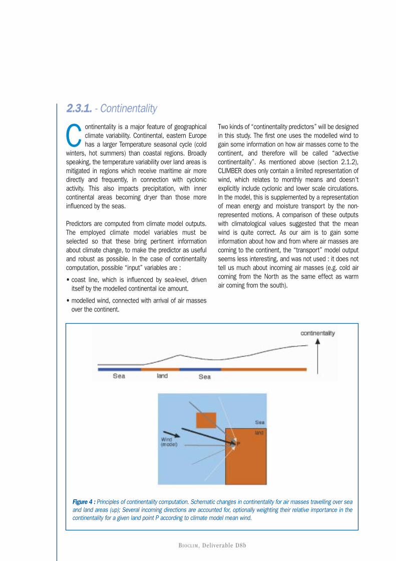
Figure 4 : Principles of continentality computation. Schematic changes in continentality for air masses travelling over seaand land areas (up); Several incoming directions are accounted for, optionally weighting their relative importance in thecontinentality for a given land point P according to climate model mean wind.


p. 12/13Consider air masses coming from several direction tothe land point for which continentality is to be computed(P). Each incoming direction thus have a contributionto overall continentality at P, as sketched on figure .This contribution is calculated using the followingassumption : an air mass becomes progressivelycontinental (maritime) as it travels over land (ocean).The rate of this changes towards continental / maritimeconditions is assumed to be a constant fraction (τ) perunit time, i.e. the change in continentality during dt time is :

where is the continentality (between 0 = sea limit, 1 = land

limit), ico = 0 over sea, 1 over land

,in which dx isthe element of

the distance travelled by the air mass during dt, U is themean wind norm (from CLIMBER), lo/Uo is the distance/ wind ratio corresponding to fractional change of 2 ofthe continentality predictor, currently set to

Therefore, the wind speed enters the computation in afirst way : due to the fact that the continentality changefraction is constant in time, over a given distance thecontinentality will change following the inverse of thewind speed (faster wind means less “residence time”,thus less “adjustment” to a given surface type). Tocomplete the computation of continentality at a givenpoint, we must first integrate the continentality changeover each “incoming air mass path”,

To complete, it is necessary to decide the respectiveweight of each path direction. As mentioned, we havelittle knowledge of the actual motion of air masses, andit seems reasonable to rely on simple assumptions,because we have no physical basis to build a morecomplex scheme. Minimal requirements seems to (1)give more weight to path directions which matches thedirection of the mean wind, and (2) give zero weight topaths which are in opposition with the mean wind, i.e.

represents an air-mass travelling against the wind (thiswould be inconsistent with our above assumptions forthe continentality change over a given path; however,such behaviour is not impossible in practice and shouldbe accounted for in the other continentality index). Asimple way to achieve this is to use the scalar productof the mean wind and the path direction unitvector (we have integrated this over each path, butthis is unimportant since the model mean wind doesn’tchange much because the scale is coarse):

The weighted average of the contributions from allpaths gives the continentality at the desired point :

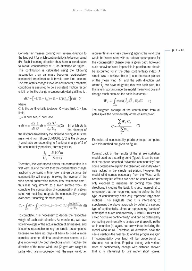
Examples of continentality predictor maps computedwith this method are given on figure.

Coming back on the results of the simple statisticalmodel used as a starting point (figure), it can be seenthat the above described “advective continentality” hassome potential to explain the observed variability whichwas lacking in the simple regression. However, themodel wind comes essentially from the West, whilecontinentality-like effects are seen on coast which areonly exposed to maritime air coming from otherdirections, including the East. It is also interesting toremember that the mean wind used to define the firsttype of continentality does only represent large-scalemotions. This suggests that it is interesting tosupplement the above approach by defining a secondtype of continentality, aimed at representing “random”atmospheric fluxes unresolved by CLIMBER. This will becalled “diffusive continentality” and can be obtained bycomputing continentality changes along specific pathsas in equation (4) again, but now without including themodel wind at all. Therefore, all directions have thesame weight in the final result, and the progressive gainin continentality over land will be proportional todistance, not to time. Empirical testing with variousrates of continentality change with distance showedthat it is interesting to use rather short scales,

(4)

(5)

(6)

(7)


suggesting that most larger scale effects arerepresented in the “advective” continentality. Thisis consistent with (although not a necessaryconsequence of) the idea of including scalesunresolved by the climate model. In this study, thedistance corresponding to 50% change towardscontinent or sea conditions is 150 km.

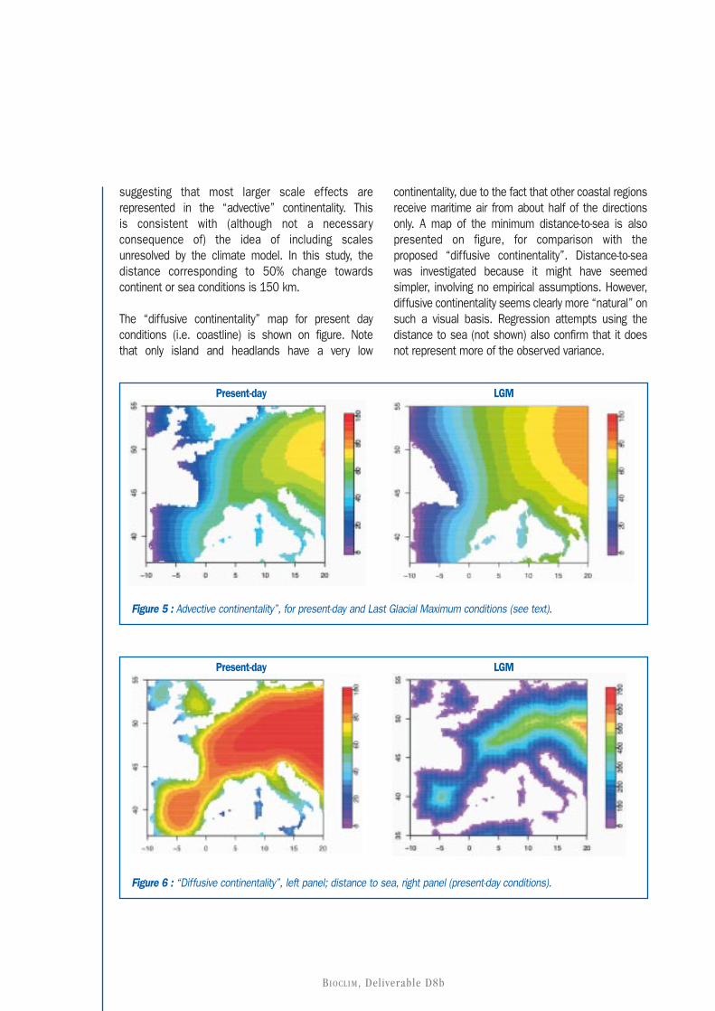
The “diffusive continentality” map for present dayconditions (i.e. coastline) is shown on figure. Notethat only island and headlands have a very low

continentality, due to the fact that other coastal regionsreceive maritime air from about half of the directionsonly. A map of the minimum distance-to-sea is alsopresented on figure, for comparison with theproposed “diffusive continentality”. Distance-to-seawas investigated because it might have seemedsimpler, involving no empirical assumptions. However,diffusive continentality seems clearly more “natural” onsuch a visual basis. Regression attempts using thedistance to sea (not shown) also confirm that it doesnot represent more of the observed variance.

Figure 5 : Advective continentality”, for present-day and Last Glacial Maximum conditions (see text).

Present-day LGM

Figure 6 : “Diffusive continentality”, left panel; distance to sea, right panel (present-day conditions).

Present-day LGM


p.14/15

Agood deal of the European climate is connectedwith surface elevation. Several topography-based predictors are thus designed here. These

are constructed from the ETOPO5 surface elevationmap [Ref.9].

Temperature is almost directly linked to elevation itself.The quantitative link is not easy to obtain, though,specifically when it comes to finding climate changeinformation based on CLIMBER outputs. A possibility isto re-compute near-surface temperature for severalheight in each (coarse) model grid box, as proposed forthe coupling of CLIMBER and its ice-sheet model (seeRef.2, section 2.3.2). Another approach is the verticaltemperature gradient from the free atmosphere (lapse-rate) provided by CLIMBER. The rationale behind thischoice is that mountains are rather small within the gridbox, and that from an empirical point of view, the impactof altitude on temperature is indeed about the same asin the free atmosphere. This second approach is usedin the present work because initial tests suggested thatit was more appropriate for our domain, but the firstapproach should remain open to investigation in anyfurther study. In practice, the predictor is the product ofthe lapse-rate obtained from CLIMBER by the highresolution surface elevation, as shown for an examplecase on figurea.

As we are working on a grid, with a certain resolution(10 minutes, coming from the climatology), we mayexpect that the climate variables, specificallyprecipitation, are impacted by higher resolutiontopographical features. A potential predictor is thus thestandard deviation of surface height, shown on figureb.While such variable is constant at the time scale of ourstudy, it may explain a part of the geographical variancein our climate fields, so that its inclusion in thestatistical model might be useful.

The next topography-related predictor shall be referredto as “mountain masking”. The aim is to account forthe impact of mountains on the regional climate of theregions which lie downstream from the mountains withrespect to the main incoming air masses. There are twopossible mechanisms for this “masking” :- part of the incoming air flow may be diverted by themountain,

- the characteristics of air masses which went up themountain may have changed in the process, inparticular dried up due to Foehn effect.

These effects are at least partly similar to an increaseof the continentality in the “masked” area (figure , toppanel). In this study, the corresponding predictor iscomputed separately of the continentality, but in asimilar way. As for continentality, several incoming airmasses directions are considered, with the sameweighting as before. The main change here is that the“masking index” increase only when the “hypotheticalair mass” is going up. In practice, the computation isbased on the difference between the height of thesurface at each point along the “hypothetical air mass”track and the height of the target location. An exampleof the resulting maps is given on figurec.

The last predictor is connected with the lifting of airmasses over topography, with a potential link toincreased precipitation (figure , bottom panel). In thisstudy, only the mean zonal wind is accounted for,and multiplied by the mean east-west slope overapproximately 100 km. Only upward trends areretained, while the effect of downward mean motion isassumed to be represented by the “masking” predictorpresented above. An example of the resulting maps isgiven on figured.

2.3.2. - Mountains


Figure 7 : Mountain-related predictors, present-day conditions (January).

a. topography / lapse-rate effect (C)

Figure 8 : Principles of the computation of predictors related to secondary mountain effects.

b. subgrid elevation deviation (m)

c. “mountain masking” d. “upslope” effect


p. 16/172.4. - Calibration of the downscaling method

B eing based on a regression, the method worksin two steps : first the regression function isdefined as a best fit to available (present-day)

data, secondly it is applied to predict high-resolutionclimate based on the corresponding changes in thecoarse climate model. As the first step, or calibration,is based on minimizing the difference between theregression values and the present-day climatology,using corresponding input values, it needs present-dayvalues for the predictors. These predictors being basedon CLIMBER model values, a specific simulation

starting from the pre-industrial conditions was run untilconditions approximately matching those of the late20th century. The end of this simulation provides the“present-day” model outputs, which are consistent withthe climatology.

The statistical models used for the downscaling oftemperature and precipitations will now be presented.Results for the Last Glacial Maximum (LGM, 21 kyr BP)will serve as an application example and anindependent validation opportunity.

A few different sets of predictors, as well asvarious changes in the design of thesepredictors (e.g. length scales involved in the

computation of continentality), where tested during thisproject. The following statistical model represents ourbest selection of predictors for the temperature field:

in which the various terms are based on the abovedescribed predictors :Ca advective continentalityCd diffusive continentalityµ mountain masking effect (not included for summer

months because it did not explain a significant part of the variance in that case)

Υ lapse-rate effectƒca , ƒcd , ƒµ , ƒΥ are spline functions with only 3 knots,which results into high smoothness, i.e. the functionscan not be very complex. The objective is to allow thecontribution of each term to be somewhat non-linear,because it’s difficult to build physical predictors whichwould provide a simple linear contribution totemperature or precipitation maps. However, thecontributions can not be too complex, because thiswould introduce a kind of “overfitting” : the statisticalmodel would not represent a link between ourpredictors and observations, it would just produce anarbitrary and meaningless fit to the data.

The most simple way to use the presented downscalingapproach is to calibrate the statistical model using datafor a single month in the year, then apply it to the same

month of a climate change scenario. The regressionitself relates to the geographical variability, and is thusstationary in time. In turn, the computation of thepredictors is assumed to have a physical basis, andthus some robustness regarding the long-term time-variability. For example, if the coastline moves, thecontinentality predictor will change, and its contributionto local temperature will change accordingly (thisaspect being assumed stationary). However, ourcurrent design of the predictors does not include anyinput related with the seasonal cycle: e.g. continentalityis computed, but the impact of continentality ontemperature is highly season-dependent : it might bedesired to predict this link on the basis of climatemodel data. But using such seasonal-cycle relatedinformation from the climate model would introducemore complexity in the method, possibly bringinguncertainty. This did not appear to be desirable in thecontext of a first downscaling method for the CLIMBERmodel.

Nevertheless, some partial accounting for month-to-month changes is possible : rather than calibrating themodel for 1 month, it can be calibrated using themonths preceding and following the month of interest.This has two kinds of advantages:• it provides a validation opportunity for the method. If

the month of interest is not used for the calibration,it is interesting to compare the prediction of themethod for this month to the actual climatology,because these data are partly independent. A goodmatching between these maps suggests that the

2.4.1. - Temperature

(8)


method is at least making an acceptable use of themodel data to make a prediction in different conditions.It doesn’t suffice to validate the method in the climatechange context, but it is a satisfying first test.

• some gain, possibly minor, might be expected inrobustness. For climate change prediction, threemonths can be used at the calibration stage : thetarget month and its two neighbours. This mayinclude more “diversity” in the calibration data thanjust one month would do. Although the regression willmatch the climatology of the target month lessclosely, it is not evidently worse: in fact more data areused, both from the model and the climatology, sothat this may help cancelling random errors.

The practical implementation of this 2 or 3-monthscalibration is simple but not immediate: the large-scalemodel temperature gradient (∆ΤΜ) needs to becomputed on the basis of the mean temperature ofeach month. To put it shortly, the monthly meanaverage temperatures do not enter the statistical

model, and the final output temperature is obtained byadding the climate model mean for the target month.

Figure presents results for temperature in January. Themethod is calibrated using the climatology and modeloutputs for December and February. The temperatureprediction based on equation 8 for January is reportedon panel 9b, and compares favourably with thecorresponding climatology on panel 9a. The explainedvariance is 95.2%, confirming that the designedpredictors are appropriate. The difference betweenthe climatology and regression, or model error, ispresented on panel 9c. This can be compared to theerror obtained with a calibration based on the monthof January itself.

The corresponding maps for temperature in July arepresented on figure . The explained variance is less thanin January (90.7%), as shown by the comparison betweenclimatology and model fit output (panels a, b and c).

Figure 9 : Calibration and validation for temperature (°C) in January (see text).

a. Climatology b. Regression

c. Climatology - regression d. Climatology – reg. based on January


p. 18/19

Figure 10 : Calibration for temperature in January: contribution of each term based on spline function to the regression(additive model). Abscissa : predictor. Ordinate: contribution in Celsius (zero mean is imposed).

a. lapse-rate effect (ƒƒΥΥ ) b. advective continentality (ƒƒca)

c. diffusive continentality (ƒƒcd) d. mountain masking effect (ƒƒµµ )


Figure 11 : Calibration and validation for temperature (°C) in July (see text; please note that the colour-temperaturecorrespondence is not identical in the two bottom plots).

a. Climatology b. Regression

c. Climatology - regression d. Climatology – reg. based on July

As the CLIMBER modelling and the downscalingmethod are aimed at providing results for widelydifferent climates, the Last Glacial Maximum (LGM) isan interesting test period. Last Glacial Maximumsurface air temperature in January is reported onfigure. The first two panels (a and b) are based on the3-month calibration explained above, and represent ourbest estimate for the LGM temperature and itsdifference to present conditions. The correspondingsea level change, due to the growth of continental icesheets, is –128 m. Consequently, the coastline is alsovery different in northern Europe. Panel c shows theLGM temperature anomaly computed with CLIMBERalone (with linear interpolation). The downscalingmethod (panel b) provides significantly different results,in particular over England and Italy (respectively warmer

and colder than CLIMBER values). The details of thedownscaling method does not seem to have largeimpacts on the results. In particular, using a calibrationon January only rather than 3 months (JJA) does almostnot modify the result (panel d). Another test is toremove the diffusive continentality predictor from theregression (panel e). The result is modified in a ratherexpected way, with the disappearance of low distanceeffects of coastline changes around England. This givessome idea of the uncertainty of the method : while theresults should be better when the diffusivecontinentality is included, this predictor clearly fails toreproduce certain details of the actual temperaturechange in the coastal region (see figure). It is thusinteresting to see how this predictor influence theresults.


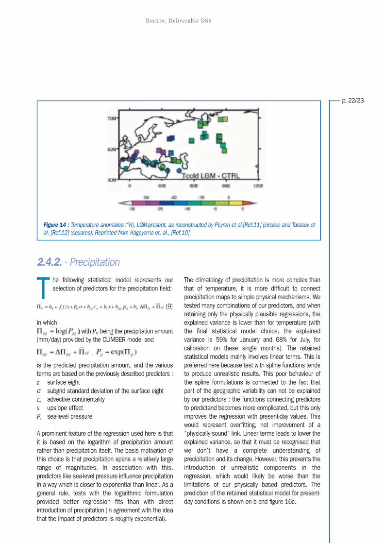
Temperature reconstructions for the LGM are available,mainly on the basis of pollen data. However, thetemperature is available only at certain locations andthe values are still the object of research aimed atimproving their reliability. The reconstruction shownhere (figure 2) was used in the framework of thePaleoclimate Model Intercomparison Project (PMIP),and presented in [Ref.10]. Temperatures anomalies

(LGM-present) for January over European sites rangebetween approximately –10 and –30°C. This is clearlybelow all values obtained here. The downscaling doesnot significantly improve the comparability of simulatedresults to the reconstruction. However, there are only afew sites for which temperature data is provided whichfalls inside the BIOCLIM domain, so that no conclusionscan be drawn at the moment.

p. 20/21

Figure 12 : Last Glacial Maximum, January near-surface temperature (°C). a. LGM, b. predicted difference between LGMand present, c. CLIMBER interpolated, d. predicted difference when the calibration is based on January only (others useDJF). e. predicted difference when diffusive continentality is not included in the regression.

b. difference, DJF calibration c. difference, CLIMBER

d. difference, January calibration e. difference, no diffusive continentality

a. LGM


Figure 13 : LGM-July temperature, as on figure 12

a. LGM

d. difference, July calibration

b. difference, JJA calibration c. difference, CLIMBER


Figure 14 : Temperature anomalies (°K), LGM-present, as reconstructed by Peyron et al.[Ref.11] (circles) and Tarasov etal. [Ref.12] (squares). Reprinted from Kageyama et. al., [Ref.10].

The following statistical model represents ourselection of predictors for the precipitation field:

in which , with PM being the precipitation amount

(mm/day) provided by the CLIMBER model and

,

is the predicted precipitation amount, and the variousterms are based on the previously described predictors :z surface eightσ subgrid standard deviation of the surface eightca advective continentalitys upslope effectPsl sea-level pressure

A prominent feature of the regression used here is thatit is based on the logarithm of precipitation amountrather than precipitation itself. The basis motivation ofthis choice is that precipitation spans a relatively largerange of magnitudes. In association with this,predictors like sea-level pressure influence precipitationin a way which is closer to exponential than linear. As ageneral rule, tests with the logarithmic formulationprovided better regression fits than with directintroduction of precipitation (in agreement with the ideathat the impact of predictors is roughly exponential).

The climatology of precipitation is more complex thanthat of temperature, it is more difficult to connectprecipitation maps to simple physical mechanisms. Wetested many combinations of our predictors, and whenretaining only the physically plausible regressions, theexplained variance is lower than for temperature (withthe final statistical model choice, the explainedvariance is 59% for January and 68% for July, forcalibration on these single months). The retainedstatistical models mainly involves linear terms. This ispreferred here because test with spline functions tendsto produce unrealistic results. This poor behaviour ofthe spline formulations is connected to the fact thatpart of the geographic variability can not be explainedby our predictors : the functions connecting predictorsto predictand becomes more complicated, but this onlyimproves the regression with present-day values. Thiswould represent overfitting, not improvement of a“physically sound” link. Linear terms leads to lower theexplained variance, so that it must be recognised thatwe don’t have a complete understanding ofprecipitation and its change. However, this prevents theintroduction of unrealistic components in theregression, which would likely be worse than thelimitations of our physically based predictors. Theprediction of the retained statistical model for present-day conditions is shown on b and figure 16c.

2.4.2. - Precipitation

(9)

p.22/23

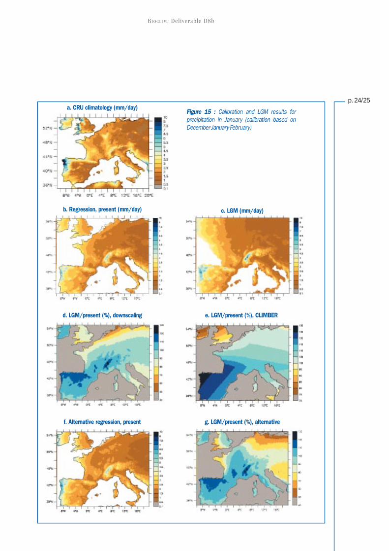
As an example of method-related uncertainty, one ofthe tests with another regression equation is presentedhere. This one is connected with the representation ofprecipitation peaks near the western coasts in January.The above regression underestimates this maxima(figure 15d). The alternative consists in replacing thelinear advective continentality term by a more complexone based on a spline function (figure 15f).. This givesmore freedom to the statistical model, which indeedbetter represents the coastal precipitation maximum(unfortunately, the diffusive continentality provedunsuitable for this purpose). As mentioned above, isprobable that relying on complex fitted functions likethis involves some “overfitting”, so that the statisticalmodel does not entirely represent real physical linksbetween predictors and precipitation. The practicalconsequence is that we regard the climate changeresults obtained with the “alternative” regression(figure 15g) as less reliable than the standard result(figure 15d), but more importantly, the differencebetween those two represents a typical uncertainty ofthe method.

It is interesting to note that there is theoretical risk ofoverfitting related to the combination of coarse modeldata. When two very coarse fields are used, inparticular precipitation and sea-level-pressure fromCLIMBER as here, the linear combination of these fields

can indeed provide any requested large scale gradient(each coarse input field approximately represent a largescale gradient, and if these are not collinear, theircombination gives any other gradient). In other words,any set of two model variables should explain asignificant part of the domain-wide variability, so thatthe fact that such predictors contribute to increase theexplained variance is not a proof that it forms a valuablestatistical model. In the case of model precipitation andsea-level pressure, there are however good reasonsto use these variable as predictors. Higher meanpressure is indeed associated with lower precipitation,connected with the presence of less low pressuresystems in the area and/or air subsidence.

Last, a fraction of the unexplained variance maypossibly be due to inaccuracies in the climatologicaldata. Details of the climatology may indeed still bequestioned, specifically for precipitation over mountainregions. This is shown by the difference between the1/2 deg climatology and the new 1/6 deg CRUclimatologies on figure 16 a and b: there are significantdifferences near the alps, at scales much larger thanthe grids (more detailed information over the Alps isavailable form the MAP project, but accessing thesedata was not planed in the framework of this projectand is not clearly needed because no BIOCLIM sites arelocated in that region).



p.24/25

Figure 15 : Calibration and LGM results forprecipitation in January (calibration based onDecember-January-February)

a. CRU climatology (mm/day)

b. Regression, present (mm/day) c. LGM (mm/day)

d. LGM/present (%), downscaling e. LGM/present (%), CLIMBER

f. Alternative regression, present g. LGM/present (%), alternative


Figure 16 : Calibration and LGM results for July (calibration based on June-July-August)

a. CRU climatology – 1/2 deg (mm/day) b. CRU climatology – 1/6 deg (mm/day)

c. Regression, present (mm/day) d. LGM (mm/day)

e. LGM/present (%), downscaling f. LGM/present (%), CLIMBER


p.26/27

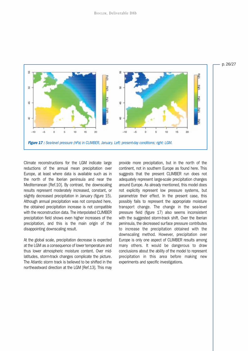
Figure 17 : Sea-level pressure (hPa) in CLIMBER, January. Left: present-day conditions; right: LGM.

Climate reconstructions for the LGM indicate largereductions of the annual mean precipitation overEurope, at least where data is available such as inthe north of the Iberian peninsula and near theMediterranean [Ref.10]. By contrast, the downscalingresults represent moderately increased, constant, orslightly decreased precipitation in January (figure 15).Although annual precipitation was not computed here,the obtained precipitation increase is not compatiblewith the reconstruction data. The interpolated CLIMBERprecipitation field shows even higher increases of theprecipitation, and this is the main origin of thedisappointing downscaling result.

At the global scale, precipitation decrease is expectedat the LGM as a consequence of lower temperature andthus lower atmospheric moisture content. Over mid-latitudes, storm-track changes complicate the picture.The Atlantic storm track is believed to be shifted in thenortheastward direction at the LGM [Ref.13]. This may

provide more precipitation, but in the north of thecontinent, not in southern Europe as found here. Thissuggests that the present CLIMBER run does notadequately represent large-scale precipitation changesaround Europe. As already mentioned, this model doesnot explicitly represent low pressure systems, butparametrize their effect. In the present case, thispossibly fails to represent the appropriate moisturetransport change. The change in the sea-levelpressure field (figure 17) also seems inconsistentwith the suggested storm-track shift. Over the Iberianpeninsula, the decreased surface pressure contributesto increase the precipitation obtained with thedownscaling method. However, precipitation overEurope is only one aspect of CLIMBER results amongmany others. It would be dangerous to drawconclusions about the ability of the model to representprecipitation in this area before making newexperiments and specific investigations.

3. Downscaling forthe BIOCLIM future scenarios


Several simulations covering the next 200 kyrwere performed by two climate models, asreported in deliverable D7. In this report, we

apply the presented downscaling method to the resultsof CLIMBER-GREMLINS. In summary, the simulations

correspond to a scenario of the natural CO2 variations(A4a), a scenario including a moderate fossil fuelcontribution (B3) and a scenario including a high fossilfuel contribution (B4). The corresponding CO2 time-series are remembered on figure 18.

Figure 18 : CO2 concentration (ppmv) asa function of time (decades). Naturalscenario (A4a, black), Fossil fuel (B3,blue) and high fossil fuel (B4, purple).

Figure 19 : Sea-level (m) computed for the natural (A4a) and moderate fossil fuel contribution (B3) scenarios (referencelevel : present-day conditions).


p.28/29The sea-level is estimated from the ice northern-hemisphere ice volume computed by CLIMBER. Thechanges in Antarctic ice volume are not included herebecause these are not modelled. However, theAntarctic component is much smaller than that of thenorthern hemisphere, so that the approximation isacceptable for computing the sea-level in the present

context. The sea level is estimated as (N.H. ice volume at a given time – present-day icevolume) x (2.2 m / 106 km3)

This estimate gives a satisfactory value for the lastglacial maximum (-129 m). The resulting sea-levelheight is shown on figure 19.

We first present detailed results for the naturalscenario, explaining how these were obtained. In a next

step, summarized results are presented for the fossil-fuel scenarios.

3.1. - Time series for the sites

T he downscaling methodology was applied on themodel outputs for the three 200 kyr scenarios,providing output on the 1/6 degree grid used for

the downscaling (as above). This output was computedonly for the points which belongs to a BIOCLIM site. The

definition of the BIOCLIM sites used here is given intable 1. In this section, the results are presented assimple statistics based on the outputs on each site(site minimum, maximum, and mean).

Table 1: Definition of the BIOCLIM sites within this report. The temperature and precipitation columns provides climatologicalmean values (“present-day” CRU climatology used as a reference for downscaling)

Site Site name Latitude Longitude Temperature PrecipitationNo (from – to) (from – to) Jan July Jan July

1 Czech Republic 48.9 – 49.5 15.0E – 15.6E -3.3 16.5 1.35 2.582 Germany 52.0 – 52.6 10.0E – 11.0E 0.3 17.3 1.60 2.223 France (Bure) 48.3 – 48.9 5.3E – 6.0E 0.9 17.7 2.73 2.184 Spain - Toledo 38.0 – 41.8 6.5W – 1.5W 5.1 23.0 1.64 0.475 Spain - Padul 36.7 – 37.3 4.0W – 3.4W 5.5 23.5 2.03 0.396 Spain - Cullar 37.3 – 37.9 2.9W – 2.3W 5.8 23.3 1.68 0.437 Central England 51.6 – 54.8 2.8W – 0.0 3.1 15.4 2.45 1.91

While the initial downscaling output is availableover each gridpoint (1/6 degree), we haveonly present mean, minimum and maximum

values over the sites (however all results are availablefor all scenarios and site grid-points, see appendix 1).

The available results are :

• downscaling output (“uncorrected”)

• corrected downscaling output, obtained as follows :For temperature, the difference between climatologyand present-day downscaling output is added to theoutput from the downscaling for the scenario (i.e. thepresent-day downscaling error is removed, giving thecorrect value for the present climate, but thiscorrection is maintained constant under climatechange conditions while the actual model error isunknown for all future times).

3.1.1. - Natural scenario – model / downscaling comparison


For precipitation, the ratio of climatological and predicted values is used to correct the downscaling scenario, by multiplying the downscaled precipitation by the correction ratio (rather than adding a constantlike for temperature). Thus if the model downscalingmethod predicts a 50% increase in precipitation, wejust compute future precip as being 50% more thanpresent-day climatology (not 50% more than present-day downscaling output, nor adding the precipitationincrement from the downscaling to climatology)

• model: linearly interpolated CLIMBER output,provided for comparison.

• corrected model output. The corrected model valueis the interpolated CLIMBER result with a correctiondone as for downscaling above: the time-mean valueis corrected so that model-mean matches theclimatological mean for present climate (additivecorrection for temp, multiplication for precipitation).This provides a fair comparison of model values todownscaling: while absolute model results do rarelyreproduce the climatological mean with a highaccuracy, the model is expected to provide anacceptable (large-scale) climate-change signal.

A selection of the results for the natural scenario (A4a)is presented in figures 20 (temperature) and 21(precipitation). The meaning of each curve issummarised on figure 22. Site-mean values areprovided for model, downscaling and correcteddownscaling, as defined above. Site minimum andmaximum are provided only for corrected downscaling,as this is the most important output for practicalapplications. The four last sites (in Spain and England)show larger differences between minimum andmaximum values because the site area is larger, andsometimes because topography is more complex.While looking at the results, it is important to note thatthe present-day values are never plotted on the

graphics : these begin with the first climate modeloutput, that is after 1000 years from CLIMBER run start(pre-industrial). To compare future values with presentday ones, the climatological values are provided in table1 (those values are used to calibrate both thedownscaling method and the “corrected values”introduced above).

For temperature, the difference between correcteddownscaling mean and model mean values are quitesmall, not exceeding 1-2°K in both January and July.

The results for precipitation are more surprising. Theresults of the downscaling outputs are largely differentfrom the model results, and the downscaling alsoprovides a larger time variability. For present day, boththe corrected model and corrected downscaling valuesare equal and matches the climatology. Therefore, thedifferences between these two time-series is only aconsequence of the long-term time variability. The“correction” methodology, based on a multiplication bya constant factor as explained above, may explainsome aspects of the results, but not many (uncorrectedvalues are also shown). As a general rule, time-variability seems quite low in the model. By contrast,the variability found in the downscaling output is highlyunexpected. Downscaling outputs goes up to more than200% of the model output. In addition, there arecircumstances for which the time variability showsphase oppositions between model and downscalingvalues. While it is unclear that the model itself is betterat this scale, downscaling values should be consideredvery prudently. A possible origin for the large increasesin the mean and variability of precipitation is the sea-level pressure term used in the downscaling. While thedownscaling methodology has been developedcarefully, it is only a first version of a rather newmethod; it still needs more validation, and this wouldlikely suggest improvements.


p.30/31

Figure 20 : Natural scenario for the next 200 kyr – temperatures (°K). Legend is given by figure 22.

Site

1 Czech Republic

2 Germany

3 France

4 Spain - Toledo

5 Spain - Padul

6 Spain - Cullar

7 Central England

January July


Figure 21 : Natural scenario for the next 200 kyr : precipitation (mm/day). Legend is given by figure 22

Site

1 Czech Republic

2 Germany

3 France

4 Spain - Toledo

5 Spain - Padul

6 Spain - Cullar

7 Central England

January July


p.32/33

Figure 22 : Legend for the natural scenario time series (figures 20 and 21).The data types are defined in text. Minimum/maximum/mean values refer tostatistics over the site areas.

F igures 23 and 24 show site-mean downscaledtemperature and precipitation for the threestudied scenarios. As in the previous section, all

graphics start after 1000 years of CLIMBER run, andthe corresponding present-day value is the climatologygiven in table 1 (i.e. these are “corrected” downscalingoutputs, as defined in the previous section).

For temperature, specifically in January, the maindifference between the natural and anthropogenic (B3and B4) scenarios is connected with an abrupttemperature increase in CLIMBER. This abrupt eventdoes not happens at the same time in theanthropogenic and fossil fuel scenarios. The event isprobably connected with changes in the thermohalinecirculation (see Ref.2). There are only rather minordifferences between scenarios B3 and B4 (less than1°K, decreasing with time).

For precipitation, the reliability of the downscalingmethod is unclear, due to the unexpected resultsobtained for the natural scenario in the previoussection. In January, the long-term decreasing trendfound in the natural scenario (e.g. for the German site)appears as much weaker, almost suppressed, in thefossil-fuel scenarios. Thus, precipitation is muchheavier for the fossil fuel cases in January. By contrast,precipitation is generally lower for the fossil fuelscenarios in July; in itself, this is not surprising forfuture climate experiments. However, a curious featureof these plots is that the difference between the naturaland anthropogenic runs is increasing with time forseveral cases, e.g. German site in January or Englandsite in July. Since the downscaling method itself is time-independent, this effect should be attributed toCLIMBER – possibly with an exaggerated amplificationdue to the downscaling methodology.

3.1.2. - Fossil fuel scenarios


Figure 23 : Comparison of scenarios for the next 200 kyr : temperature (°K). Natural scenario (A4a, red line); fossil fuelscenario (B3, black line); high fossil fuel scenario (B4, green line)

Site

1 Czech Republic

2 Germany

3 France

4 Spain - Toledo

5 Spain - Padul

6 Spain - Cullar

7 Central England

January July


p.34/35

Figure 24 : Comparison of scenarios for the next 200 kyr : precipitation (mm/day). Natural scenario (A4a, red line); fossilfuel scenario (B3, black line); high fossil fuel scenario (B4, green line).

Site

1 Czech Republic

2 Germany

3 France

4 Spain - Toledo

5 Spain - Padul

6 Spain - Cullar

7 Central England

January July


3.2. - Snapshots

T he downscaling method was applied on all landpoints of the domain for two specific yearsselected and used in other BIOCLIM work-

packages : + 67 kyr (case E) and +178 kyr (case F) from

run B3. The temperature and precipitation change,found with the GCM are remembered in table 2 (valuesaveraged over Europe, taken from [Ref.14].

Table 2: Summary of results from deliverable D4 – GCM simulations (IPSL_CM4_D model) which corresponds to the snapshotspresented here, averaged over Europe. The values are mean temperature (K) and precipitation (%) changes for winter andsummer.

Snapshot DJF JJA

∆TDJF ∆TJJA

∆PDJF ∆PJJA

“E” -0.024 +2.4+1.6 -6.8

“F” -0.87 -0.33+5.3 +1.3

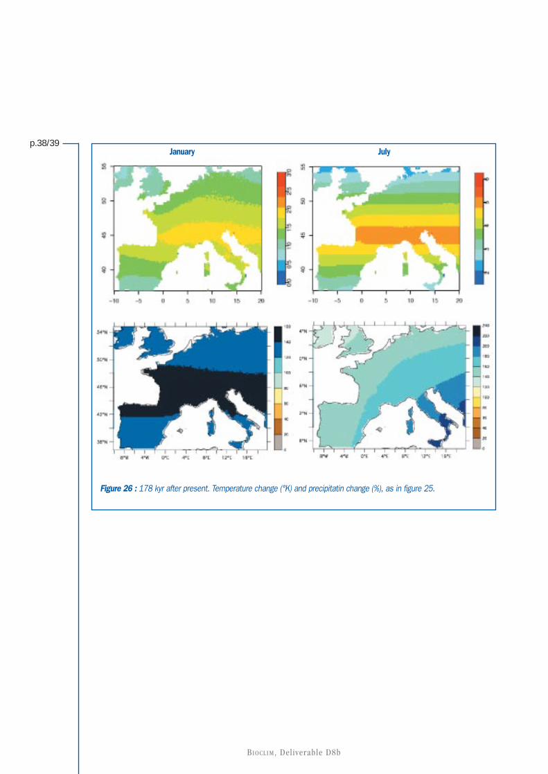
The downscaling results are presented in figures 25(+67 kyr) and 26 (+178 kyr). There are no significantregional features in these temperature andprecipitation change fields. This does not means thatthe downscaling method is wrong : it is accounting forthe regional variations in the fields for a given time, itjust did not find local effects of the climate change. Thedownscaling outputs are nevertheless not identical tothe simple linear interpolation of CLIMBER results (notshown here), and may be more realistic. However, thenear absence of regional or local details is ratherdisappointing. Sea level did not change much inscenario B3 (a few meters, see figure 19), so it couldnot have a large effect (it is probably responsible for afew “odd” points in the temperature plots, near thecoasts). Mountains might have provided more

interesting effects, connected with mechanisms suchhas “masking” or lapse rate changes (section 2.3), butsuch effects where at most very weak.

For precipitation, the large increase found in the timeseries over the sites shows again here. As explained insection 3.1.1, this increase is rather surprising and cannot be given a high confidence without more researchand general validation of the method. However, it isimportant to note that CLIMBER itself shows largeprecipitation increases for the present snapshots.When linear interpolation is used instead ofdownscaling, the precipitation change goes up to 200%but with a partly different geographical repartition andcovering a smaller area (not shown).


p.36/37

Figure 25 : 67 kyr after present.Temperature change (°K, above) and precipitation change (%, below).Changes are relativeto present-day (end of the XX century). Grey areas are under sea-level at that time (and not in present day)

January July


p.38/39

Figure 26 : 178 kyr after present. Temperature change (°K) and precipitatin change (%), as in figure 25.

January July


4. Conclusion

This repor t presents a downscalingmethodology designed to provide highresolution temperature and precipitation data

on the basis of outputs from the intermediatecomplexity model CLIMBER-GREMLINS. The methodprovides a link between the coarse climate modeloutputs and the regional (or local) climate dataneeded for performance assessment of radioactivewaste repositories.

To obtain climate-change information at 1/6 degreeresolution on the basis of the climate modeloutputs, the downscaling method works in 2-steps.First, physical considerations are used to definevariables (predictors) which are expected to havelinks which climatological values; secondly, ageneralized additive statistical model is used to findthe links between these variables and the high-resolution climatology of temperature andprecipitation. Thus the method is termed as“physical/statistical” : it involves physically basedassumptions to compute predictors from modelvariables and then relies on statistics to findempirical links between these predictors and theclimatology. These “physically based assumptions”are necessary because the climate data areprovided by an intermediate complexity model,which gives only limited information about spaceand time variability: it provides coarse data whichcan not be directly linked to regional climate changeby a statistical model calibrated on present-dayclimatology (but other downscaling strategies arealso be applicable, such as in Ref.15.

The predictors which have been computedfrom CLIMBER outputs and physically-basedassumptions are : continentality (with advective anddiffusive variants), vertical temperature gradient,effects of mountains (masking, Foehn-like upslopeeffect).

The method is new. It has been successfully appliedto CLIMBER, providing outputs for the BIOCLIMscenarios. The conception of the method wascareful : many tests with different sets of predictorshave been conducted (only the most interestingones where repor ted here). However, fur therresearch and improvement will still be possible inthe future. A potential area for improvement is thetreatment of the seasonal cycle: in the currentversion, there is no predictor related with theseasonal cycle, while in practice the impact ofcontinentality on temperature is highly season-dependent. In more general sense, the waycontinentality affects land temperature in themethod also need further investigations, with a viewto account for temperature contrasts between seaand land in CLIMBER. While this may seem easy, itwill need a careful look at CLIMBER outputs indifferent climate states. Knowing which variablescan be useful and how it might be used is notimmediate, because due to the simplified nature ofthe climate model, variables such as SSTs may nothave the degree of realism required for direct use inthe downscaling process. The limited comparisonwith reconstructions for the last glacial maximumdid not show advantages of the application ofdownscaling. This may have several origins,including the climate model and the precision of thepast climate reconstructions, so that this also callsfor more research in the future.

Monthly mean temperature and precipitation arepresented for 3 scenarios for the next 200 kyr(natural and fossil fuel cases). These variables aremainly shown as time series of site-mean valuesplus maps a two specific times, while more datais available in numeric form (see appendix). Fortemperature, the downscaling results are expectedto have some realism, and may be interesting touse for performance assessment – at least as an


p.40/41 alternative to more direct CLIMBER-GREMLINSoutputs. The downscaling results for precipitationshould be considered more prudently. Largeincreases are shown in the future both in the modeland downscaling results (up to about 200%),but the downscaling procedure provides highprecipitation amounts over larger parts of Europe,as well as other surprising results. While it wasinteresting to obtain complete results with this newmethod, this clearly opens the way for furtherresearch.

ACKNOWLEDGMENTSWe thank the Climate Research Unit (U.K.) formaking the high-resolution climatology used inthis study available for research (dataset CRUCL2.0, described in New et al., 2002; availableon http://www.cru.uea.ac.uk/cru/data ).


5. References

Ref. 1: BIOCLIM Report D10-12 (2003) Development and application of a methodology for taking climate-driven environmental change into account in PAs. Available on www.andra.fr/bioclim.

Ref. 2: BIOCLIM Report D7 (2003) Continuous climate evolution scenarios over western Europe (1000km scale). Available on www.andra.fr/bioclim.

Ref. 3: Houghton, J. T., Y. Ding, D. J. Griggs, M. Nogueur, P. J. van der Linden, X. Dai, K. Raskell, and C. A. Johnson (eds.), IPCC 2001:climate change 2001: The Scientific Basis. Contribution of Working Group 1 to the third assessment report of Intergovernmental Pannel for Climate Change. Cambridge University Press, Cambridge, United Kingdom and New York, USA,881 pp., 2001.

Ref. 4: Brasseur O., H. Gallée, J.-D. Creutin, T. Lebel, P. Marbaix, High resolution simulations of precipitation over the Alps with the perspective of coupling hydrological models. Advances in Global Change Research: “Climatic change: implications for the hydrological cycle and for water management”, pp. 75-100, Kluwer Academic Publishers, 2002.

Ref. 5: New, M., D. Lister, M. Hulme, I. Makin, A high-resolution data set of surface climate over global land areas. Climate Research, 21, 1-25, 2002.

Ref. 6: Petoukhov, V., A. Ganopolski, V. Brovkin, M. Claussen, A. Eliseev, C. Kubatzki, S. Rahmstorf, CLIMBER-2: a climate system model of intermediate complexity. Climate Dynamics, 16, 1-17, 2000.

Ref. 7: Mearns, L., Bogardi, I., Giorgi, F., Matyasovszky, I., and Palecki, M. Comparison of climate change scenarios generated from regional climate model experiments and statistical downscaling. Journal of Geophysical Research, 104(6), 6603-6621, 1999.

Ref. 8: R Development Core Team, A language and environment for statistical computing, edited by the R foundation for statistical computing, Vienna, Austria, http://www.R-project.org, 2003.

Ref. 9: NOAA, ETOPO5,data announcement 88-MGG-02, digital relief of the surface of the earth. Available from NOAA, National Geophysical Data Center, 1988.

Ref. 10: Kageyama, M., O. Peyron, S. Pinot, P. Tarasov, J.Guiot, S.Joussaume, G. Ramstein, The last glacial maximum climate over Europe and western Siberia : a PMIP comparison between models and data. Climate Dynamics, 17, 23-43, 2001.

Ref. 11: Peryron O, Guiot J, Cheddadi R, Tarasov P, Reille M, de Beaulieu J-L, Bottema S, Andrieu V, Climate reconstruction in Europe for 18 000 yr B.P. from pollen data. Quat Res 49,183-196, 1998.

Ref. 12: Tarasov PE, O Peyronm J Guiot, S Brewer, VS Volkova, LG Bewusko, NI Dorofeyuk, EV Kvavadze, IM Osipova, NK Panova, Last glacial maximum climate of the former Soviet Union and Mongolia reconstructed from pollen and macro-fossil data. Climate Dynamics, 15,227-240, 1999.


p.42/43 Ref. 13: Kageyama, M., F. D'Andrea, G. Ramstein, P. J. Valdes, R. Vautard, 1999. Weather regimes in past climate Atmospheric General Circulation Model simulations, Clim. Dyn. 15, 773-793

Ref. 14: BIOCLIM Report D4/5 (2003). Global climatic characteristics, including vegetation and seasonal cycles over Europe, for snapshots over the next 200,000 years. Available on www.andra.fr/bioclim.

Ref. 15: BIOCLIM Report D8a (2003a) Development of the rule-based downscaling methodology for BIOCLIM Workpackage 3. Available on www.andra.fr/bioclim.


Appendix 1 : Data productThe temperature and precipitation time series (200 kyr starting from present) have been made available to theBIOCLIM community on the Buisness Collaborator web site (http://cobweb.businesscollaborator.com/bc/bc.cgi).The provided values are those presented in the graphics of section 3.1 in this report. Data is thus available for eachBIOCLIM site, for scenario A4a and B3 (at least). A simple ASCII format is used, and can be read with commonlyused software. There are two basic types of files : “raw” results contain values (temperature and precipitation) overeach downscaling-grid points, and the regular output provides simple statistics on these values (e.g. site mean, maxand min for the interpolated CLIMBER output, climatology, downscaling output). There is thus somewhat more dataregarding the time series than shown in the report. The detailed description of the files and their organization isprovided with the files.

For further information contact:

BIOCLIM project co-ordinator, Delphine Texier

ANDRA, DS/MG (Direction Scientifique - Service Milieu Géologique

Parc de la Croix Blanche - 1/7, rue Jean-Monnet - 92298 Châtenay-Malabry Cedex - FRANCETél.: +33 1 46 11 83 10

e-mail: [email protected] site: www.andra.fr/bioclim/

© A

ndra

- Ja

nvie

r 20

04 -

Con

cept

ion

grap

hiqu

e : V

ince

nt G

RÉG

OIR

E

development of the methodology and application to … · •universidad politecnica de madrid...

Documents