development of the danish lraic model for fixed networks...2019© axon partners group 6 1....
TRANSCRIPT

Development of the Danish LRAIC model for fixed networks
Model Reference Paper – Consultation Document
1 July 2019

2019© Axon Partners Group 1

2019© Axon Partners Group 2
Contents
1. Introduction ................................................................................................... 6
1.1. Context ....................................................................................................... 6
1.2. Structure of the document ............................................................................ 7
1.3. The public consultation process ...................................................................... 8
2. Costing Methodology ........................................................................................ 10
2.1. Cost orientation methodologies available to DBA ............................................ 10
2.1.1. Legal Context ...................................................................................... 10
2.1.2. LRAIC methodology.............................................................................. 11
2.1.2.1. Definition of LRAIC .......................................................................... 11
2.1.2.2. The bottom-up approach ................................................................. 12
2.1.3. Relevant cost standard ......................................................................... 12
2.1.3.1. Summary of the asset valuation approaches ...................................... 18
2.1.3.2. Practical implementation of EC’s recommendations ............................. 18
2.2. Focus on LRAIC .......................................................................................... 20
2.2.1. LRAIC ................................................................................................. 20
2.2.2. Defining the Increment ......................................................................... 21
2.2.3. Implications of LRAIC ........................................................................... 22
2.3. Time horizon of the cost model .................................................................... 23
3. Networks to be modelled .................................................................................. 25
3.1. Scope of the model and definition of the increment ........................................ 25
3.1.1. Introduction to the model’s networks and increment ................................ 25
3.1.2. The core network ................................................................................. 25
3.1.3. The access network .............................................................................. 26

2019© Axon Partners Group 3
3.1.4. Scope of the networks .......................................................................... 28
3.1.5. Modelled operator ............................................................................... 29
3.2. Services .................................................................................................... 30
3.2.1. Routing factors .................................................................................... 33
3.3. Technologies to be modelled ........................................................................ 34
3.3.1. Core switching technologies .................................................................. 34
3.3.2. Core transmission technologies .............................................................. 34
3.3.2.1. Transmission technologies ............................................................... 35
3.3.2.2. Optical transmission systems in the network ...................................... 35
3.3.3. Access technologies ............................................................................. 35
3.3.4. Degree of optimisation ......................................................................... 36
3.4. Network demand ........................................................................................ 36
3.5. Network coverage costs .............................................................................. 37
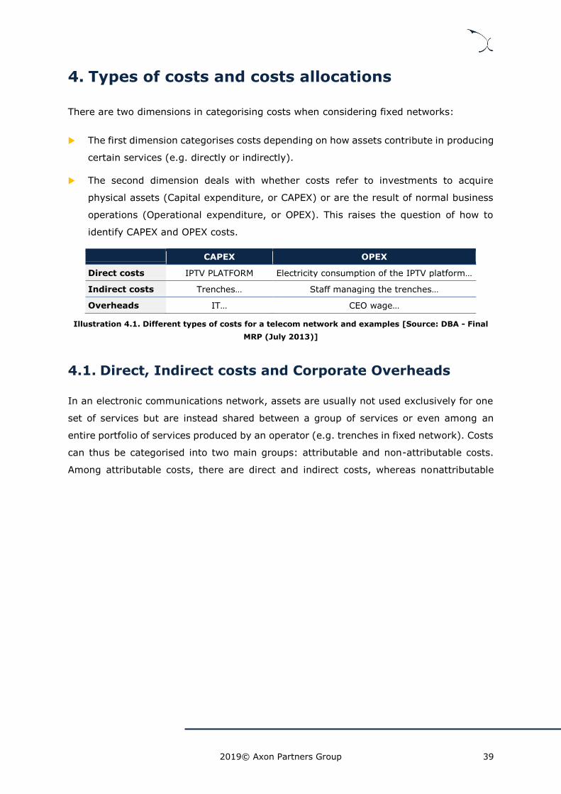
4. Types of costs and costs allocations ................................................................... 39
4.1. Direct, Indirect costs and Corporate Overheads ............................................. 39
4.1.1. Direct Network Costs ............................................................................ 41
4.1.2. Joint and network common costs ........................................................... 41
4.1.3. Corporate overheads ............................................................................ 43
4.2. CAPEX assessment ..................................................................................... 44
4.2.1. Equipment Prices ................................................................................. 45
4.3. OPEX assessment ....................................................................................... 45
4.4. Depreciation Methodologies ......................................................................... 47
4.4.1. Standard Annuity ................................................................................. 48
4.4.2. Tilted annuity ...................................................................................... 49
4.4.3. Full economic depreciation .................................................................... 51

2019© Axon Partners Group 4
4.5. Cost of Capital ........................................................................................... 54
4.6. The cost of working capital .......................................................................... 54
5. Model implementation ...................................................................................... 56
5.1. Service Demand ......................................................................................... 58
5.1.1. Broadband and TV services ................................................................... 59
5.1.2. Leased Lines ....................................................................................... 59
5.1.3. Access services .................................................................................... 59
5.2. Network Demand ....................................................................................... 60
5.2.1. The calculation of demand drivers .......................................................... 60
5.2.2. Busy hour information .......................................................................... 61
5.2.3. Adjustments for the grade of service ...................................................... 62
5.3. Network hierarchy ...................................................................................... 62
5.3.1. The Scorched Node Assumption ............................................................. 62
5.3.2. The Hierarchy of the “Exchanges” .......................................................... 63
5.3.2.1. The highest layer of the “exchanges” ................................................ 65
5.3.2.2. The other layers of the hierarchy ...................................................... 65
5.4. Network dimensioning ................................................................................ 66
5.4.1. Modelling tools .................................................................................... 66
5.4.2. Access network ................................................................................... 67
5.4.2.1. Geomarketing data ......................................................................... 67
5.4.2.2. Roll-out of the network .................................................................... 70
5.4.2.3. Access network dimensioning ........................................................... 74
5.4.3. Core and transmission networks ............................................................ 77
5.4.3.1. Dimensioning of the active transmission elements .............................. 77
5.4.3.2. Dimensioning of the civil infrastructure for the transmission network .... 77
2019© Axon Partners Group 5
5.4.3.3. Dimensioning of the core platforms ................................................... 79
5.5. Costing the Network ................................................................................... 79
5.6. Allocation of costs to services ...................................................................... 79
5.6.1. Allocation of shared costs of civil infrastructure ....................................... 80
5.6.2. Allocation of costs to access services ...................................................... 81
5.7. Ancillary services ....................................................................................... 81
6. Model outputs ................................................................................................. 89
6.1. Geographical De-Averaging ......................................................................... 89
6.2. Level of Detail............................................................................................ 90
6.3. Charging basis ........................................................................................... 91
7. LRAIC model validation and update process ........................................................ 92
7.1. Top-down validation ................................................................................... 92
7.2. Update process .......................................................................................... 92
8. Appendix ........................................................................................................ 94
8.1. List of criteria ............................................................................................ 94
8.1.1. Comparison of BU criteria with respect to the MRP from July 2013 ........... 100
8.2. Template to comment ............................................................................... 110
8.3. List of acronyms ...................................................................................... 112

2019© Axon Partners Group 6
1. Introduction
1.1. Context
The telecommunications market in Denmark is ruled under the Danish
Telecommunications Act1 (hereinafter, the Act). Its main purpose is to promote an efficient
and innovative market for electronic communications networks and services for the benefit
of end-users.
The Act lays out in its fifth chapter the guidelines for the sector specific regulation in the
telecommunications market, detailing how the analyses of the competitive situation should
be performed, including markets definition, the identification of providers with Significant
Market Power (SMP) and the potential obligations that could be imposed to regulate
providers with SMP.
Particularly, the Act outlines that it is the Danish Business Authority (Erhvervsstyrelsen)
(i.e. the DBA) duty to analyse the relevant markets and assess the potential obligations
to be imposed on SMP operators. The analysis carried out by DBA for the relevant
wholesale broadband markets (current market 3A and market 3B) resulted, since 2003,
in a price control obligation on the access network services of the SMP. The enforcement
of this obligation is performed through the LRAIC model.
Since LRAIC costs were first calculated in 2003, the model developed by DBA has been
subject to a number of revisions and updates, in line with market developments. The latest
major update of the cost model took place in 2013, with a small update in 2017 that made
the model capable of excluding geographical areas from the cost calculation to allow the
model to exclude areas where price regulation has been lifted. However, the relevant
changes that have occurred since then in the fixed Danish market require a new update
of the fixed LRAIC model to make sure it is representative of the current situation and can
fulfil DBA’s regulatory needs. This is the reason behind the update of this Model Reference
Paper (hereinafter, the ‘MRP’).
DBA has chosen Axon Partners Group (hereinafter, ‘Axon’) to assist DBA in this project.
This document constitutes the draft Model Reference Paper, which will set the roadmap
for the update of the model.
1 https://www.retsinformation.dk/forms/r0710.aspx?id=161319, Act no. 128, 7th February 2014 with amendments (Teleloven).

2019© Axon Partners Group 7
At this point, the document seeks comments from the industry through a public
consultation process. The feedback received from stakeholders will be considered in the
development of the final MRP.
This MRP has been prepared based on the existing methodological guidelines followed by
DBA, as reflected in the MRP from July 20132. The geographical adjustment from
November 20173 has also been taken into consideration when drafting this document.
1.2. Structure of the document
This document has been built starting from the final MRP published in July 2013. The
sections included are as follows:
Section 1: Introduction
Section 2: Costing Methodology
Section 3: Networks to be modelled
Section 4: Types of costs and costs allocations
Section 5: Model implementation
Section 6: Model outputs
Section 7: LRAIC model validation and update process
Section 8: Appendix
In order to facilitate the review of sections 2-7 (both included), the July 2013 MRP has
been taken as a reference, highlighting all the changes introduced in track changes.
Therefore, if a specific paragraph in the sections below is not marked in track changes,
stakeholders should understand that it remains identical as in the July 2013 MRP.
Additionally, the following notes should be taken into account in the assessment of the
track changes introduced:
When sections from the July 2013 MRP have been removed from this new version,
only the section titles have been left in this document and they appear as removed in
track changes. The body of these sections has been removed without track changes
in order to ease the reading of this document.
2 DBA, Final Model Reference Paper, July 2013. Link: https://erhvervsstyrelsen.dk/sites/default/files/2019-03/Metodepapir01_lraic_mrp_final.pdf 3 DBA, Specification Document, November 2017. Link: https://erhvervsstyrelsen.dk/sites/default/files/2019-03/GB_modeldokumentation_180119.pdf (see grey adjustments).

2019© Axon Partners Group 8
The order of some sections from the July 2013 MRP has been switched in this new
version to maximise the consistency of this document. This is especially the case in
the contents of section ‘5 Model implementation’. Therefore, we have included at the
beginning of this section a table summarising how the contents of the July 2013 MRP
have been mapped into this new version of the MRP.
Track changes are not shown in footnotes for practicality reasons.
1.3. The public consultation process
This public consultation is conducted by DBA within the framework of its competences from
the Act.
In this document, DBA puts into public consultation the proposal regarding the principles
and methodology that will drive the definition of the LRAIC model for fixed networks.
Stakeholders are invited to submit their comments in reply to the relevant questions issued
in this document by making use of the template to comment included in section ‘8.2
Template to comment’ of this document.
The public consultation is launched on Monday 1 July 2019 and it will end on
Friday 30 August 2019. Responses should be submitted in English and
electronic form before the end of the public consultation.
The consultation responses from the industry may be published in full and outlining the
corporate name of the respondent by DBA. In case the responses contain confidential
information that should not be published, operators are responsible of reporting a separate
version of the document removing any information that shall be considered confidential
for publication.
Responses should be submitted to the following email addresses: [email protected] and
[email protected]. During the public consultation, DBA may provide clarifications to
questions issued by interested parties which must be submitted by e-mail to the same
email address.
The present text does not bind DBA as to the content of the subsequent regulation.
DBA is open to receive and consider the reasoned views and documented comments on
all these matters. DBA expects respondents to support their comments with any relevant
justifications. DBA may not consider comments that are not properly justified.

2019© Axon Partners Group 9
DBA will assume that if a stakeholder does not answer a specific question, the stakeholder
is accepting the approach presented to such question under the present paper.

2019© Axon Partners Group 10
2. Costing Methodology
2.1. Cost orientation methodologies available to DBA
2.1.1. Legal Context
As part of its responsibilities in monitoring the telecommunications companies, and in
particular in regulating the network access price control, DBA can require service providers
with Significant Market Power (SMP) to meet certain pricing requirements.
According to the Price Control Order4, DBA can choose between several price control
methods when it comes to determining regulated prices:
"Specification of pricing requirements, cf. section 46(1) of the Act on Electronic
Communications Networks and Services, shall be based on one or more of the
following price control methods:
1. The long-run average incremental cost (LRAIC) method
2. Historic costs
3. Retail minus
4. Requirement of reasonable prices”
DBA has currently determined maximum wholesale prices for TDC, which has been
designated as an SMP operator, in a number of fixed network markets5, including:
Wholesale market for fixed-network termination (market 1)6;
Wholesale market for local access (market 3A)
Wholesale market for central access (market 3B).
As a consequence, when choosing among cost orientation methods, DBA can select
between two alternatives: “LRAIC” and “historic costs”. Normally LRAIC would be using
current cost/forward looking cost but as LRAIC in principle is a method to distribute cost
between services, it could in theory be based on historical costs (partly or fully). As per
the MRP published by DBA in 2013, the LRAIC costing approach is to be adopted in the
implementation of the fixed LRAIC model in Denmark.
4 DBA, Executive Order on Price Control Methods, dated 27 April 2011. 5 European Commission, Commission Recommendation on relevant product and service markets within the electronic communications sector susceptible to ex ante regulation, dated 9 October 2014. 6 Several other operators are LRAIC-based regulated for market 1.

2019© Axon Partners Group 11
2.1.2. LRAIC methodology
2.1.2.1. Definition of LRAIC
LRAIC is “the long run average incremental cost of providing either an increment or
decrement of output, which should be measured on a forward-looking basis”.
The LRAIC approach enables one to mimic the level of costs in a competitive and
contestable market:
“Long-run incremental costs (LRIC) based on an efficient deployment of a modern
asset reflect the level of costs that would occur in a competitive and contestable
market. Competition ensures that operators achieve a normal profit and normal return
over the lifetime of their investments (i.e. in the long run). Contestability ensures that
existing providers charge prices that reflect the costs of supply in a market that can be
entered by new players using modern technology.
Together these ensure that inefficiently incurred costs are not recoverable and require a
forward-looking assessment of an operator’s cost recovery (as a potential new entrant is
unconstrained by historical cost recovery).”
In Denmark, the Price Control Order supports the use of the LRAIC method stating that:
“(1) Where the LRAIC pricing method is used; the total price for a network access
product may not exceed the sum of the long-run average incremental costs
associated with the network access product in question.
(2) Only efficiently incurred costs may be included, using efficient modern
technologies.”7
Further, as determined in EC’s 2013 Recommendation8, replacement costs should be
considered when determining the cost base of the model (see section ‘2.1.3 Relevant cost
standard’).
7 DBA, Executive Order on Price Control Methods (Section 3 Networks to be modelled), dated 27 April 2011. 8 EC, Commission Recommendation on consistent non-discrimination obligations and costing methodologies to promote competition and enhance the broadband investment, dated 11 September 2013.
2019© Axon Partners Group 12
2.1.2.2. The bottom-up approach
From 2013, the implementation of the fixed LRAIC model has been shifted to a full bottom-
up methodology.9
Bottom-up models use demand data as a starting point and model an efficient network,
using economic and engineering principles, which is capable of serving that level of
demand. Under a bottom-up approach, the model (re)builds a (hypothetical) reasonably
efficient network, reflecting to a certain extent the network of the modelled operator. The
network is modelled accordingly, in order to deliver electronic communications services
and to satisfy the demand for these services. The bottom-up results will be reconciled with
data from the SMP operator(s).
2.1.3. Relevant cost standard
Key area of discussion below: Cost base to be adopted in the cost model.
There are two cost standards for asset valuation commonly accepted by NRAs and
international institutions (e.g. ITU, EC) in the development of cost models:
Historical Cost Accounting (HCA) is the average price paid historically by an
operator to acquire an asset, based on its financial registries.
Current Cost Accounting (CCA) reflects the current and expected market value of
the assets.
Although current cost accounting has been broadly accepted by most NRAs in the
development of Bottom-Up models for mobile networks, there have been several
discussions among regulators on the suitability of valuating fixed operators’ civil
infrastructure (for instance copper access network, civil works and ducts) according to
Current Cost Accounting, as it may lead to an overestimation of access services’ costs.
In this sense, in its 2005 Copper Statement10, Ofcom concluded, referring to civil
infrastructure assets, that “The value of the RAV (Regulatory Asset Value) is set to equal
the closing HCA value for the pre 1st August 1997 assets for the 2004/5 financial year”
9 The alternative to a bottom up model is a top down model. With top-down (TD) modeling, cost inputs are taken from the operator’s accounting data and are allocated to different services on the basis of the causality relation between costs and services. 10 Ofcom, Valuing copper access – Final statement, dated 18 August 2005
2019© Axon Partners Group 13
whereas it approved the “use of current cost accounting as at present for assets deployed
from 1st August 1997 onwards”.
In similar fashion, the EC’s Recommendation of 2013 ‘on consistent non-discrimination
obligations and costing methodologies to promote competition and enhance the broadband
investment environment’11 establishes clear guidelines in order to avoid such over-
recovery of civil engineering related costs. Particularly, the EC’s Recommendation of 2013
states that:
“(33) Valuation of the assets of such an NGA network at current costs best reflects
the underlying competitive process and, in particular, the replicability of the assets.
(34) Unlike assets such as the technical equipment and the transmission medium
(for example fibre), civil engineering assets (for example ducts, trenches and poles)
are assets that are unlikely to be replicated. Technological change and the level of
competition and retail demand are not expected to allow alternative operators to
deploy a parallel civil engineering infrastructure, at least where the legacy civil
engineering infrastructure assets can be reused for deploying an NGA network.
(35) In the recommended costing methodology the Regulatory Asset Base (RAB)
corresponding to the reusable legacy civil engineering assets is valued at current
costs, taking account of the assets’ elapsed economic life and thus of the costs
already recovered by the regulated SMP operator. This approach sends efficient
market entry signals for build or buy decisions and avoids the risk of a cost over-
recovery for reusable legacy civil infrastructure. An over-recovery of costs would
not be justified to ensure efficient entry and preserve the incentives to invest
because the build option is not economically feasible for this asset category.
(36) The indexation method would be applied to calculate current costs for the RAB
corresponding to the reusable legacy civil engineering assets. This method is
preferred due to its practicability, robustness and transparency. It would rely on
historical data on expenditure, accumulated depreciation and asset disposal, to the
extent that these are available from the regulated SMP operator’s statutory and
regulatory accounts and financial reports and on a publicly available price index
such as the retail price index.
11 EC, Recommendation on consistent non-discrimination obligations and costing methodologies to promote competition and enhance the broadband investment environment, dated 11 September 2013

2019© Axon Partners Group 14
(37) Therefore, the initial RAB corresponding to the reusable legacy civil
engineering assets would be set at the regulatory accounting value, net of the
accumulated depreciation at the time of calculation and indexed by an appropriate
price index, such as the retail price index.
(38) The initial RAB would then be locked-in and rolled forward from one regulatory
period to the next. The locking-in of the RAB ensures that once a non-replicable
reusable legacy civil engineering asset is fully depreciated, this asset is no longer
part of the RAB and therefore no longer represents a cost for the access seeker, in
the same way as it is no longer a cost for the SMP operator. Such an approach
would further ensure adequate remuneration for the SMP operator and at the same
time provide regulatory certainty for both the SMP operator and access seekers
over time.”
Based on the previous directives and recommendations from the European Commission,
it becomes apparent that current costs should be used to reflect the regulatory value of
most assets. Nevertheless, the EC’s 2013 Recommendation provides room for adjustments
to account for the accumulated depreciation of the reusable civil engineering assets. This
is derived from the EC’s understanding that, unlike active equipment and the transmission
medium (e.g. fibre), civil infrastructure assets are unlikely to be replicated.
While DBA agrees that the active equipment could be indeed replicated (i.e. deployment
of their own assets could be economically feasible for an access seeker), it could be argued
that in order for the transmission medium to be replicable, an access seeker must be able
to rely on the underlying civil infrastructure of the access provider (i.e. civil infrastructure
has to be reusable). Therefore, a necessary condition to allow the replicability of the
transmission medium is that access seekers can access the underground access network
of the infrastructure operator, for instance, through ducts. Otherwise, the transmission
medium should be considered not to be replicable and thus, it should also be valued at
current costs net of cumulated depreciation.
Given the technical complexities resulting from it, the EC’s 2013 Recommendation requires
a careful assessment, especially in countries such as Denmark, where multiple access
networks coexist (copper, fibre and coax). Depending on the architecture and network
topology, different circumstances may apply that need to be assessed on their own.
Additionally, it is worth noting that, according to the EC’s Digital Agenda12, NGA networks
12 EC, Broadband Coverage in Europe 2017, dated 6 June 2018.
2019© Axon Partners Group 15
can rely on copper, fibre and coax, as they include FTTH, FTTB, Cable DOCSIS 3.0/3.1,
VDSL solutions with at least 30 Mbps of download speed.
Further, one of the main regulatory inputs of the model will be the European Electronic
Communications Code (EECC). This text introduces the concept of “Very High Capacity
Networks” (VHCN)13 as:
“An electronic communications network which consists wholly of optical fibre
elements at least up to the distribution point at the serving location, or an electronic
communications network which is capable of delivering, under usual peak-time
conditions, similar network performance in terms of available downlink and uplink
bandwidth, resilience, error-related parameters, and latency and its variation.”
DBA’s assessment of the situation applicable to each access network with regards to
NGA/VHCN is presented in the paragraphs below.
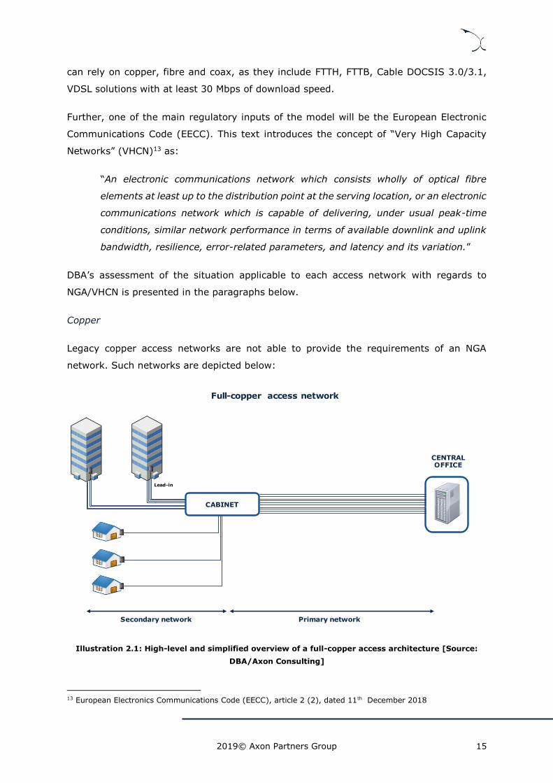
Copper
Legacy copper access networks are not able to provide the requirements of an NGA
network. Such networks are depicted below:
Illustration 2.1: High-level and simplified overview of a full-copper access architecture [Source:
DBA/Axon Consulting]
13 European Electronics Communications Code (EECC), article 2 (2), dated 11th December 2018
CENTRAL OFFICE
Secondary network Primary network
Full-copper access network
Lead-in
CABINET

2019© Axon Partners Group 16
However, thanks to the technological evolutions achieved over the last few years, they
can be upgraded to reach the status of NGA. Besides upgrades in the active equipment,
the main improvements involve rolling out fibre closer to the end user, thus shortening
the copper loop and improving the capabilities of the network. Depending on the point to
which the fibre is rolled out, the topology can take the shape of "Fibre To The Cabinet”
(FTTC), as shown in the illustration below:
Illustration 2.2. High-level and simplified overview of an FTTC access architecture [Source: Axon
Consulting]
In all the cases mentioned, the final part reaching the end-user is copper based. However,
depending on the location of the street cabinet, copper networks can, in some instances
be considered to be VHCN.
Parts of the legacy copper access networks are actually being reused to deploy NGA
networks. This includes the access copper and civil infrastructure that has not been
replaced by fibre. Further, it could be the case that the civil infrastructure that was
previously used to host copper cables is now hosting fibre cables.
At the same time, it is widely accepted that an access seeker would not deploy parallel
copper cables to those of the access provider. In practice, the deployment of copper cables
itself would not be replicable, as it is highly unlikely that the economics of these networks
would allow cost-recovery if they were built today. Therefore, it could be concluded that
copper access cables are not replicable by access seekers.
Secondary network Primary network
FTTC access network
Lead-in
CABINET
Fibre
CENTRAL OFFICE
2019© Axon Partners Group 17
Based on the previous considerations, copper cable assets and their related civil
infrastructure should be “valued at current costs, taking account of the assets’ elapsed
economic life and thus of the costs already recovered by the regulated SMP operator”, as
per the EC’s 2013 recommendation, (35) on page 5.
Fibre
Fibre to the home (FTTH) networks are to be considered as NGA/VHCN from inception.
Consequently, the particularities specified in the EC’s 2013 Recommendation do not apply
to these assets.
The only exception to this norm takes place when the underlying civil infrastructure used
to deploy the FTTH network is already reused from pre-existing infrastructure previously
employed in other access networks (e.g. copper). In these cases, the same considerations
outlined above for the reusable civil infrastructure apply.
Coax
Legacy coaxial networks were initially deployed to provide TV services to end users. As
technology and customer-needs evolved, coax networks were upgraded to allow the
provision of broadband services. Currently, DOCSIS 3.0 and DOCSIS 3.1 are considered
as NGA networks.
As in copper networks, besides improving the features of its active elements, fibre
deployments were introduced to complement coax, leading to the so-called Hybrid Coaxial
Fibre networks (HFC). The handover point between the coaxial and fibre cables is often
denominated as the Optical Node, which is being moved closer to the customer by
operators to enhance the capabilities of such networks. In the cases where the optical
node is located close enough to the customer, HFC networks can be considered as VHCN.
As a result of the previous considerations, a similar argument to the one used for copper
networks could be followed. This is, coax cables and their underlying infrastructure are
being reused for NGA/VHCN networks.
One caveat to this parallelism is the fact that coaxial networks are typically left outside
the scope of EU regulations. Particularly, EU Regulations on the definition of the Regulatory
Asset Base were focused on other access technologies (i.e. fibre networks built on top of
legacy copper networks) due to their prevalence in EU markets over other access networks
such as coax. However, nothing in these regulations excludes, in a legally binding or
otherwise convincing manner, their relevance as guidance for the design of a bottom-up
model for HFC networks, at least as regards the principles of such regulatory exercise.

2019© Axon Partners Group 18
Moreover, considering a different alternative to the one applicable for copper access would
be, at most, arbitrary and would harm the overarching regulatory obligation of
technological neutrality in the regulation of competition, unless there are clear technical
or other objective reasons justifying a deviation.
Therefore, the same approach presented above for copper access related assets will also
be adopted for coaxial assets. This is, coaxial cable assets and their related civil
infrastructure should be “valued at current costs, taking account of the assets’ elapsed
economic life and thus of the costs already recovered by the regulated SMP operator” cf.
the EC’s 2013 Recommendation.
2.1.3.1. Summary of the asset valuation approaches
The following table presents a summary of the asset valuation approaches that should be
followed for each of the network elements considered in the different access networks.
Network Valuation should account for
fully depreciated assets Valuation should not account for fully
depreciated assets
Copper networks
✓ Copper cable. ✓ Civil infrastructure used to
hold copper cables. ✓ Existing civil infrastructure
used to deploy fibre.
Fibre cable used to substitute copper cable.
New civil infrastructure used to deploy new fibre cable.
Non-access assets.
Fibre networks
✓ Civil infrastructure reused from legacy networks.
Fibre cable New civil infrastructure. Non-access assets.
Coax networks
✓ Coax cable. ✓ Civil infrastructure used to
hold coax cables. ✓ Existing civil infrastructure
used to deploy fibre cable.
Fibre cable used to substitute coax cable.
New civil infrastructure used to deploy new fibre cable.
Non-access assets.
Illustration 2.3: Summary of asset valuation approaches [Source: Axon Consulting]
Question 1: Do you agree with the cost standards to be considered to determine the
cost base of the model? Do you agree with the list of assets in which the EC’s 2013
recommendation shall be applied (i.e. in which asset valuation should account for fully
depreciated assets)?
If you don’t agree, please justify your position and provide supporting information and
references.
2.1.3.2. Practical implementation of EC’s recommendations
The EC’s 2013 recommendation specifies that the set of assets highlighted in Illustration
2.3, should be “valued at current costs, taking account of the assets’ elapsed economic

2019© Axon Partners Group 19
life and thus of the costs already recovered by the regulated SMP operator”. The European
Electronic Communications Code (EECC) further reinforces the indications provided in the
EC’s 2013 recommendation on this particular subject.
In order to implement this directive, it is firstly important to identify the costs that have
already been recovered by the modelled operator. This involves two main considerations:
Fully depreciated assets still in use. These refer to the assets that no longer
generate any depreciation costs but are still being used by an operator. This is likely
to be the result of a misalignment between the financial useful life considered for an
asset and its technical useful life. These fully depreciated assets (which do not
generate costs to the modelled operator) should not be considered to avoid an
overvaluation of the Regulatory Asset Base.
Accumulated depreciation of assets that are not fully depreciated. In this case,
a part of the assets’ costs has already been recovered by the modelled operator.
However, whenever continuity of depreciation charges is ensured (for instance, when
based on straight line depreciation) this factor should not play a role, as the
depreciation charge should be equivalent over the years. Therefore, the net book value
of these assets will be depreciated as it has been over the last years in the operator’s
financial statements.
Taking the previous two elements into consideration, the following steps shall be adopted
to determine the proper cost references under the EC’s 2013 recommendation:
Step 1: Identify the volume of network elements (km of cables, km of ducts, number
of poles, etc.) deployed in the network based on the technical registries of the
operator.
Step 2: Extract the gross book value (GBV) of the assets that still generate costs (i.e.
assets that are not fully depreciated) from the financial accounts of the operator (Fixed
Asset Registry).
Step 3: Calculate an adjusted Gross Replacement Cost (GRC), aligned with EC’s
recommendation, of these assets based on an indexation methodology using, for
Key area of discussion below: Methodology to implement the EC’s 2013
Recommendation to calculate the cost base of the reusable legacy assets.
2019© Axon Partners Group 20
instance, the construction cost index for civil engineering projects reported by the
Statbank14.
Step 4: Divide the adjusted-GRC obtained in Step 3 by the number of units identified
in Step 1 to get the reference unit price of the asset.
Main criterion 1: A Current Cost valuation should be adopted to set the unit costs of
the assets in the Bottom-Up cost model. Nevertheless, the GRC originated from fully
depreciated assets should not be taken into consideration for the reusable legacy assets
presented in Illustration 2.3.
Question 2: Do you agree with methodology described to implement the EC’s
recommendation to calculate the cost base of the reusable legacy assets?
If you don’t agree, please justify your position and provide supporting information and
references.
2.2. Focus on LRAIC
2.2.1. LRAIC
As defined by DBA, “LRAIC is the long run average incremental cost of providing either an
increment or decrement of output, which should be measured on a forward-looking basis”.
Long run is understood as a time horizon, in which all inputs including the cost of
equipment are allowed to vary as a consequence of market demand. Average denotes that
the costs connected to the production of the relevant service (within the costs of providing
the whole increment) are divided by the corresponding total traffic in order to return an
estimate of the average incremental costs of the service. There are several definitions of
the term increment, which is why this subject is discussed in detail below (see section
‘2.2.2 Defining the Increment’).
The definition of forward-looking costs depends on the time frame considered and on the
asset valuation methodology selected, which is outlined in section ‘2.1.3 Relevant cost
standard’.
14 Index - BYG61: Construction cost indices for civil engineering projects (2015=100) by index type and unit Source: Statbank. Link: https://www.statbank.dk/statbank5a/SelectVarVal/Define.asp?MainTable=BYG61&PLanguage=1&PXSId=0&wsid=cftree

2019© Axon Partners Group 21
2.2.2. Defining the Increment
Incremental costs are the costs of providing either an increment of output when other
increments of demand are unchanged.
Increments can be defined in a number of ways. Possible definitions of the increment
include:
marginal unit of demand for a service;
total demand for a service;
total demand for a group of services;
total demand for all services.
The illustration below illustrates these different definitions for the case of a company
producing 5 different services (A to E):
Illustration 2.4: Illustration of possible increment definitions [Source: DBA - Final MRP (July 2013)]
The larger the increment, the larger the share of joint and common costs is accounted for.
For example (see Illustration 2.4):
2019© Axon Partners Group 22
If service A is the increment, no joint and common costs are taken into account;
If the increment is service A, B and C together, a share of costs that are joint to
services A, B and C are taken into account.
Calculating the costs based on small increments means that the calculated incremental
costs benefit to a great extent from the network economies of scale (as it would support
no or limited share of joint and common costs).
In the opposite case, the adoption of a large increment (for instance, in the case of a fixed
network, all services using the access network) means that all services benefit to the same
extent from economies of scale. In these cases, all services bear a share of joint and
common costs.
2.2.3. Implications of LRAIC
LRAIC results in prices that are above marginal cost. The existence of fixed costs means
that charging prices on the basis of marginal costs does not allow the SMP operator(s) to
recover the cost of investments in its network, even when its costs are efficiently incurred.
Setting prices using LRAIC permits the recovery of intra-increment fixed costs, in the
process of promoting forward-looking investment decisions. It might also reduce market
distortions. If prices were based on marginal cost, the SMP operator(s) would have to
recover many shared/fixed costs from its other (non-regulated) services, which might
distort the competition process in favour of other competing operators in those markets.
Even all-service increment LRAIC-prices does not permit the SMP operator(s) to recover
inter-increment common costs. In order to allow full recovery of efficiently incurred costs,
an adjustment to LRAIC should be applied to take account of such common costs.
Finally, it should be noted that since LRAIC is a forward-looking concept, the optimised
network should be modelled as if it was already in place. This means that no migration
costs (additional costs associated with moving from the existing network to the optimised
network) should be included.
Main criterion 2: The LRAIC model should be based on forward-looking long run
average incremental costs. No migration costs should be included. The LRAIC model
should allow coverage of common costs. These costs should be shown separately.

2019© Axon Partners Group 23
2.3. Time horizon of the cost model
Key area of discussion below: Period of time to be considered in the cost model
Given that the unit costs of services are calculated depending on the demand at a specific
point in time, the period of time modelled will be crucial in the scope of the possible
analyses of the model’s results.
Fixed networks have been well-established in Denmark for many years, covering the vast
majority of the population. In order to take into consideration the existing roll-out of fixed
networks, obtain a precise valuation of civil infrastructure assets, and to be able to
calibrate the model, it is deemed necessary that the time frame considered shall begin in
the past. Nevertheless, DBA does not consider it essential to go back to the take-up stages
of fixed networks, as it would add complexity to the modelling process. On the contrary,
DBA considers that a time frame starting in the year 2018 would suffice to achieve the
objectives previously described.
With regards to the definition of the final year of the time frame, DBA has a strict
requirement to obtain the service provisioning costs for 5 years from 2021. However, room
for two additional years should be considered to ease DBA’s first updates of the model.
This means that, at least, the model should produce results until 2028. Additionally, the
implementation of economic depreciation (see section ‘4.4 Depreciation Methodologies’),
requires demand to be defined, at least, throughout the useful life of the assets. Given
that the civil infrastructure of fixed networks can last up to 40-50 years, the model should
include a time-frame period that goes until 2070. It is worth noting, however, that the
inputs and network dimensioning algorithms will be defined only for the 2018-2028 period.
This is, only the calculations related to the implementation of economic depreciation will
be extended until 2070.
Main criterion 3: The model will calculate the service provisioning costs from 2018 to
2028. 2018 will be the base year of the model. Additionally, it will incorporate a time-
frame up to 2070 to properly implement the economic depreciation algorithms.
Question 3: Do you agree with the need for the model to produce results for the period
between 2018 and 2028?
If you don’t agree, please justify your position and provide supporting information and
references.
2019© Axon Partners Group 24
Question 4: Do you agree that the model should include a time-frame up to 2070 to
ensure a proper implementation of the economic depreciation methodology?
If you don’t agree, please justify your position and provide supporting information and
references.
2019© Axon Partners Group 25
3. Networks to be modelled
3.1. Scope of the model and definition of the increment
3.1.1. Introduction to the model’s networks and increment
Key area of discussion below: Definition of the increment(s)
Several services require an estimate of the costs of the traffic-sensitive parts of the
network (e.g. traffic component of the bitstream access “BSA”), while others require an
estimate of the costs of the line-sensitive parts (e.g. lease of non-equipped infrastructure
sections and other sub-elements in access networks “raw copper” including sub-loops).
However, there is no need to separate the core and access models or increments in order
to achieve this objective.
Particularly, the costs associated to access services and the costs associated to traffic/core
services are clearly delimited. This means that all network costs can be attributed either
to access or traffic/core services in a causal manner which, in turn, implies that there are
no network costs that should be shared between these groups of services. As a result,
having separate increments for these services would have no impact whatsoever over
having a single increment, while increasing the complexity of the model.
Main criterion 4: A single model will be built, with a single increment comprising all
access and traffic services. Costs of ancillary services (such as co-location, activation
and interconnection points) will be calculated stand-alone as they are not directly
related to the main network topology or architecture as such.
Question 5: Do you agree that a single increment comprising the demand of all the
modelled services should be considered?
If you don’t agree, please justify your position and provide supporting information and
references.
3.1.2. The core network
Costs in the core network are driven by the volume of traffic whereas costs in the access
network are mainly driven by the number of lines (active and inactive). As volumes will

2019© Axon Partners Group 26
increase with the number of subscribers (active lines), the number of active lines and the
volume of traffic will be correlated to some degree.
Assets within the core network typically include:
DSLAMs, OLTs or CMTS except line cards;
Backbone/core routers;
Transmission links between the exchanges;
Optical fibre and trenching between all levels of core node locations.
It should be noted that in the case of FTTC, the DSLAMs located at the level of the street
cabinet, even if physically in the access network, are considered as part of the core
network (see section 5.4 Network dimensioning).
3.1.3. The access network
Key area of discussion below: Definition of the access networks to be included in the
model.
As defined above, costs in the access network typically depend on the number of
customers, but not on the amount of traffic (except for the cable-TV network). Consistent
with this, an alternative definition of the access network is that it allows the customer to
send and receive traffic.
Both definitions suggest that the access network includes all cable and trenching costs
associated with customer lines between the customer’s premises and the concentrator.
Furthermore, the definitions suggest that the access network includes the line card within
the DSLAM/OLT/CMTS. This is consistent with the first view since line card requirements
are generally driven by the number of subscribers or, more accurately, by the subscriber
requirements for lines. It is also consistent with the second view since the line card is an
essential part in sending and receiving traffic.
Assets within the access network include:
The final drop wire to the customer’s premise (although the cost associated with this
drop wire, or its activation, might be captured through the connection charge);
The trenching (in some cases ducted) between the final connection point and the
remote or host DSLAM/OLT/CMTS;

2019© Axon Partners Group 27
Copper, coax and optical fibre cables in this part of the network;
Other assets such as manholes, poles and overhead cables (if used); and
Line cards in the DSLAM/OLT/CMTS.
The model should enable to take into account the costs of the different access
configurations, including:
Copper
• Copper-only access
• FTTC (Fibre-To-The-Cabinet);
FTTH
• PON15 (Passive Optical Networks)
• PTP (Point To Point)
Cable-TV
• FTTN (Fibre-To-The-Node)
• FTTC (Fibre-To-The-Cabinet)
Question 6: Do you agree that copper (copper-only and FTTC), FTTH (PON and PTP)
and coax (FTTN and FTTC) access networks should be modelled?
If you don’t agree, please justify your position and provide supporting information and
references.
The model should make it possible to clearly identify non-traffic sensitive costs which are
only subscriber-related. This would include, for example, the junction to the dedicated
cable to the premise, the dedicated cable to the premise, and the network termination
point within the premise.
Key area of discussion below: Treatment of subscribers’ access costs in coax cable
networks.
In the particular case of coax networks, part of the elements considered in the access
network (e.g. amplifiers and splitters) are not only driven by the number of lines but also
by traffic volumes. These costs that are dependent on the traffic constraints shall not be
considered in the calculation of subscriber related costs for coax networks.
15 PON networks include, among others, GPON (Gigabyte Passive Optical Networks).

2019© Axon Partners Group 28
Therefore, coax subscribers’ access costs should receive costs from coax cables and civil
infrastructure assets only.
Supporting criterion 1: For the cable-TV network, the model should enable to clearly
isolate the cost of those assets uniquely associated with individual subscribers. These
costs are specific to the passive access network for cable-TV and will include only the
civil infrastructure and the coax cables.
Question 7: Do you agree that only civil infrastructure and coax cable related costs
should be allocated to subscribers’ access services in coax networks?
If you don’t agree, please justify your position and provide supporting information and
references.
3.1.4. Scope of the networks
As described above, the demarcation between access and core networks should be set at
the line card. If the number of subscriber lines is increased while the volume of traffic is
held constant the number of line cards will increase. If, on the other hand, the volume of
traffic is increased while the number of lines is held constant the number of line cards will
not generally change. The cost of line cards therefore depends on the number of
subscribers, in common with the access network, and not the volume of traffic, unlike the
core network.
2019© Axon Partners Group 29
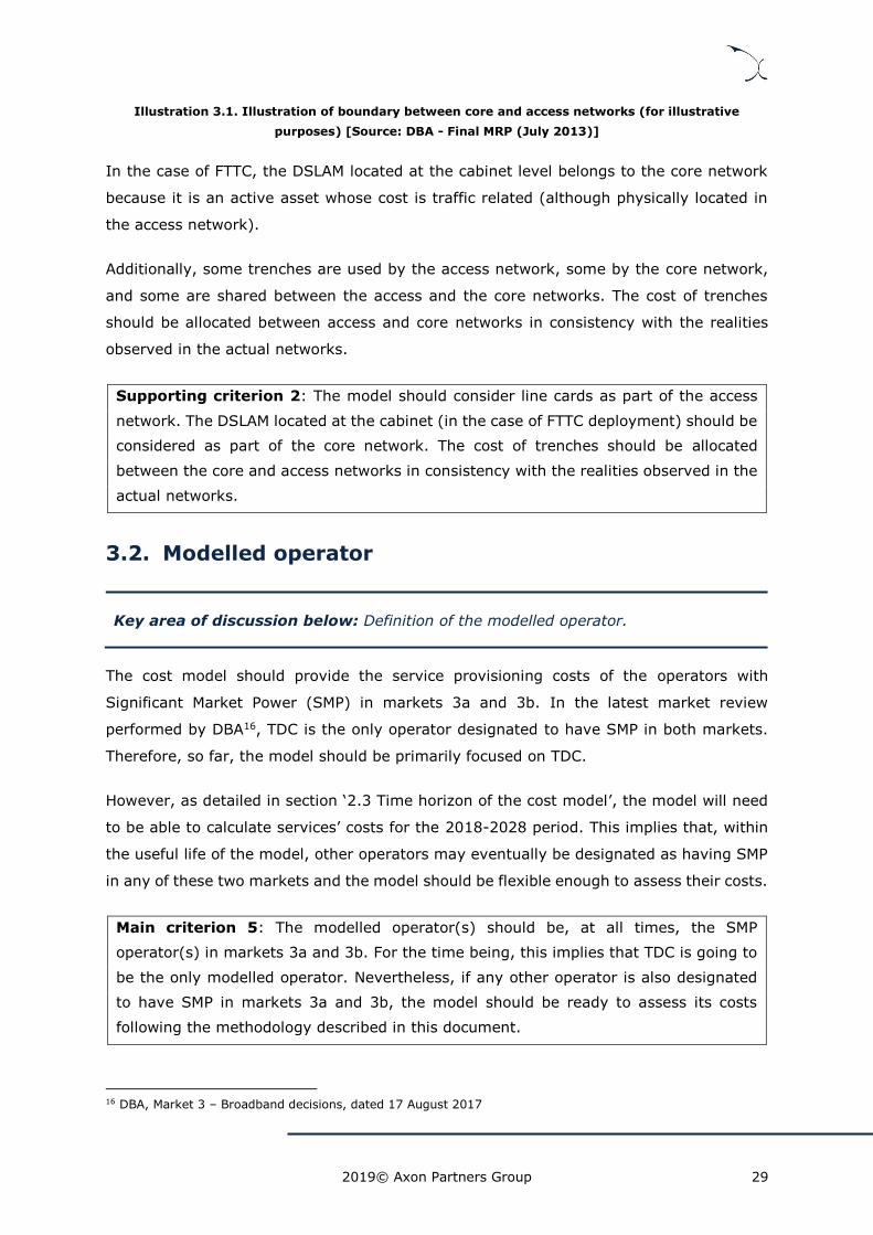
Illustration 3.1. Illustration of boundary between core and access networks (for illustrative
purposes) [Source: DBA - Final MRP (July 2013)]
In the case of FTTC, the DSLAM located at the cabinet level belongs to the core network
because it is an active asset whose cost is traffic related (although physically located in
the access network).
Additionally, some trenches are used by the access network, some by the core network,
and some are shared between the access and the core networks. The cost of trenches
should be allocated between access and core networks in consistency with the realities
observed in the actual networks.
Supporting criterion 2: The model should consider line cards as part of the access
network. The DSLAM located at the cabinet (in the case of FTTC deployment) should be
considered as part of the core network. The cost of trenches should be allocated
between the core and access networks in consistency with the realities observed in the
actual networks.
3.2. Modelled operator
Key area of discussion below: Definition of the modelled operator.
The cost model should provide the service provisioning costs of the operators with
Significant Market Power (SMP) in markets 3a and 3b. In the latest market review
performed by DBA16, TDC is the only operator designated to have SMP in both markets.
Therefore, so far, the model should be primarily focused on TDC.
However, as detailed in section ‘2.3 Time horizon of the cost model’, the model will need
to be able to calculate services’ costs for the 2018-2028 period. This implies that, within
the useful life of the model, other operators may eventually be designated as having SMP
in any of these two markets and the model should be flexible enough to assess their costs.
Main criterion 5: The modelled operator(s) should be, at all times, the SMP
operator(s) in markets 3a and 3b. For the time being, this implies that TDC is going to
be the only modelled operator. Nevertheless, if any other operator is also designated
to have SMP in markets 3a and 3b, the model should be ready to assess its costs
following the methodology described in this document.
16 DBA, Market 3 – Broadband decisions, dated 17 August 2017

2019© Axon Partners Group 30
Question 8: Do you agree that the modelled operator should be defined in accordance
to the SMP operator(s) in markets 3a and 3b?
If you don’t agree, please justify your position and provide supporting information and
references.
3.3. Services
Key area of discussion below: Definition of the services to be included in the model.
This section describes the list of services that should be included in the LRAIC model. In
addition, an introduction to the role that routing factors play in the cost allocation to
services is presented later in this section.
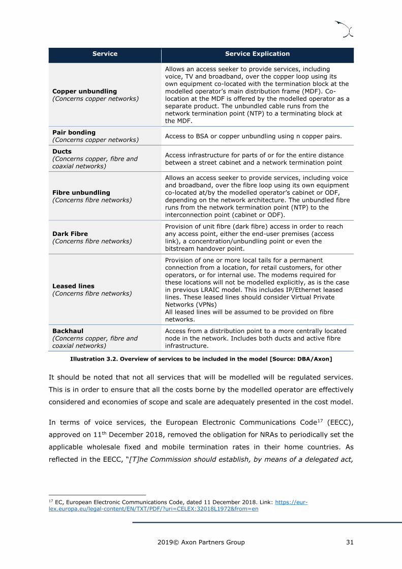
It should be noted that all services relevant for cost calculation should be included in the
model. A high-level overview of the list of services is presented below:
Service Service Explication
Retail access (Concerns copper, fibre and coaxial networks)
Provision of a line suitable for voice/broadband/TV services and sold through the modelled operator’s retail arm. One or more of these services may be provided over the same line. Retail access services will be included separately for each access technology (copper, fibre and coax).
Broadband to own customers (Concerns copper, fibre and coaxial networks)
Provision of broadband services to the own retail customers of the modelled operator(s). These services will be included separately for each access technology (copper, fibre and coax) and will be split per
broadband speed.
IPTV and video services
(Concerns copper, fibre and coaxial networks)
Provision of IPTV and other video services to end users.
VULA/BSA
(Concerns copper, fibre and coaxial networks)
Provision of a data service to an end user, where a connection of specific quality can be set up from the subscriber to an access point in the modelled operator’s network, from where the access seeker can route traffic to its own network. The modelled operator carries traffic over the access line and ensures transmission up to the access point.
This access service will be included separately for each access technology (copper, fibre and coax). The applicable
variants (for instance, based on the relevant access point) of the service will be included for each technology, namely:
VULA/BSA – POI0
VULA/BSA – POI1
VULA/BSA – POI2
VULA/BSA – POI3
2019© Axon Partners Group 31
Service Service Explication
Copper unbundling (Concerns copper networks)
Allows an access seeker to provide services, including voice, TV and broadband, over the copper loop using its own equipment co-located with the termination block at the
modelled operator’s main distribution frame (MDF). Co-location at the MDF is offered by the modelled operator as a separate product. The unbundled cable runs from the network termination point (NTP) to a terminating block at the MDF.
Pair bonding (Concerns copper networks)
Access to BSA or copper unbundling using n copper pairs.
Ducts (Concerns copper, fibre and coaxial networks)
Access infrastructure for parts of or for the entire distance between a street cabinet and a network termination point
Fibre unbundling
(Concerns fibre networks)
Allows an access seeker to provide services, including voice and broadband, over the fibre loop using its own equipment
co-located at/by the modelled operator’s cabinet or ODF,
depending on the network architecture. The unbundled fibre runs from the network termination point (NTP) to the interconnection point (cabinet or ODF).
Dark Fibre (Concerns fibre networks)
Provision of unit fibre (dark fibre) access in order to reach any access point, either the end-user premises (access link), a concentration/unbundling point or even the bitstream handover point.
Leased lines (Concerns fibre networks)
Provision of one or more local tails for a permanent connection from a location, for retail customers, for other operators, or for internal use. The modems required for these locations will not be modelled explicitly, as is the case
in previous LRAIC model. This includes IP/Ethernet leased lines. These leased lines should consider Virtual Private Networks (VPNs) All leased lines will be assumed to be provided on fibre
networks.
Backhaul (Concerns copper, fibre and coaxial networks)
Access from a distribution point to a more centrally located node in the network. Includes both ducts and active fibre infrastructure.
Illustration 3.2. Overview of services to be included in the model [Source: DBA/Axon]
It should be noted that not all services that will be modelled will be regulated services.
This is in order to ensure that all the costs borne by the modelled operator are effectively
considered and economies of scope and scale are adequately presented in the cost model.
In terms of voice services, the European Electronic Communications Code17 (EECC),
approved on 11th December 2018, removed the obligation for NRAs to periodically set the
applicable wholesale fixed and mobile termination rates in their home countries. As
reflected in the EECC, “[T]he Commission should establish, by means of a delegated act,
17 EC, European Electronic Communications Code, dated 11 December 2018. Link: https://eur-lex.europa.eu/legal-content/EN/TXT/PDF/?uri=CELEX:32018L1972&from=en
2019© Axon Partners Group 32
a single maximum voice termination rate for mobile services and a single maximum voice
termination rate for fixed services that apply Union-wide.”
Despite the absence of a regulatory need to calculate voice services’ costs, it could be
argued that their consideration in the LRAIC model could be necessary to ensure a proper
allocation of common costs to the different services. If voice services are not modelled,
there could be criticism that the common costs that should be allocated to these services
would be allocated to other services instead, thus overestimating their costs. On the other
hand, DBA recognises that, in the absence of a regulatory need to calculate voice services’
costs, removing them from the model would make the model less complicated and reduce
both data collection and model updating processes for both the industry and DBA.
In order to assess the impact of not including voice services in the calculation of other
services’ costs, an international benchmark of the share of common costs that are
allocated to voice services in four Bottom-Up models18 was performed. The results of this
analysis showed that, out of the four references consulted, the percentage of common
costs allocated to voice services was never higher than 0.8% with an average of roughly
0.5%. Additionally, this percentage is even expected to decrease further in the future as
broadband speeds increase (thus receiving a higher share of common costs) while the
number of voice subscriptions presumably will continue to decline. This implies that
removing voice services from the model will have a negligible impact on the results
obtained for the regulated services.
Main criterion 6: The model should include all relevant access, broadband leased line,
TV and ancillary services.
Main criterion 7: The model will not include voice services. Including voice services in
the model would complicate the model with a negligible impact on the cost calculation
of regulated services. Consistently, voice-specific core platforms (e.g. MGW) will not be
modelled either.
Supporting criterion 3: When dimensioning the network, the leased-lines traffic
volume should include leased lines provided to retail customers, to other operators and
to the network operator. Leased lines used by the network operator should not be
double counted. The model should not calculate the costs of leased lines explicitly.
Leased lines should only be included for dimensioning of the network and for ensuring
that a fair amount of costs is allocated to leased line services as well.
18 These included the models developed by the NRAs from Denmark, Belgium, Norway and Portugal.
2019© Axon Partners Group 33
Supporting criterion 4: For PTP, both an unbundling product at the ODF and a BSA
product will be modelled. For PON, both an unbundling product at the splitter and a BSA
product will be modelled.
Supporting criterion 519: Bitstream services in coaxial networks should be aligned
with the current wholesale commercial offers in the market.
Question 9: Do you agree that all the relevant access, broadband, TV, leased lines,
and transmission services for each technology should be included in the cost model?
If you don’t agree, please justify your position and provide supporting information and
references.
Question 10: Do you agree that voice services do not need to be included in the model?
If you don’t agree, please justify your position and provide supporting information and
references.
3.3.1. Routing factors
Routing factors are a way of measuring, in equivalent terms, the usage of the assets by
the different services. They are particularly important when dimensioning and allocating
the costs of the core network because they are a measure of the intensity to which different
services use different network elements.
Routing factors play two pivotal roles in cost models, namely:
in assisting to put the volume measures for broadband services, leased lines and data
services in the network on a common basis;
in determining costs per network element/cost category and, in turn, the cost of
individual services.
The routing factors are comprised of two main parameters:
Usage Factors. These are defined as the average frequency that a particular service
uses a given network element (e.g. the number of times a broadband connection uses
an IP router).
Conversion Factors. They are responsible of converting the demand of the different
services into equivalent units in consistency with the dimensioning driver of the
19 This criterion is specific to the cable-TV passive access network model

2019© Axon Partners Group 34
network elements. For instance, even though two broadband services with different
broadband speeds are both measured in “number of lines”, in order to properly
allocate the costs of the transmission assets (which are dimensioned based on Mbps)
the demand of the two services needs to be expressed in Mbps.
Routing factors may be easier to identify for some services than for others. Alternative
methodologies may need to be developed for some services to quantify their use of
different elements of the core network.
For the access network, routing factors are also required in order to capture the right
scope of costs for each service. As an example, for a wholesale product giving access to
the local loop (from the end-user to the Central Office), the routing factors corresponding
to higher-level layers of the network would need to be set to zero.
Supporting criterion 6: The model should show, for each service, routing factors or,
if not possible, a consistent alternative measure of how, on average, each service uses
the core network and the access network. The model should also be flexible enough to
allow for changes in routing factors / alternative measures.
3.4. Technologies to be modelled
3.4.1. Core switching technologies
IP is the packet switching technology that is used in modern telecommunication networks.
Next Generation Networks (NGNs) based on an all-IP core are rolled out in various
European countries (both by incumbent and alternative operators), where networks are
capable of handling all of the services previously routed across circuit switched networks.
This is also the technology that was only included in the previous LRAIC model. It does
not appear necessary to modify this.
Supporting criterion 7: The model should only include IP packet switch technology.
3.4.2. Core transmission technologies
There are two main concerns when choosing the technology to be used in the transport
network:
the configuration of the various available transmission technologies; and

2019© Axon Partners Group 35
the extent of optical transmission systems in the network.
3.4.2.1. Transmission technologies
In an NGN, there is no need for SDH transmission. The necessary functionality can be
provided by the IP switching/routing equipment itself.
Supporting criterion 8: The model should not include SDH.
3.4.2.2. Optical transmission systems in the network
Improvements in laser technology have increased the capacity of optical fibre. Dense
wavelength division multiplexing (DWDM) allows the combination of a number of
wavelengths on a fibre so the capacity of a single fibre is increased even more.
From a top-down perspective, an all-IP network might well incorporate a considerable
amount of DWDM equipment. However, it is most likely that this has occurred due to
historical reasons of limited fibre availability within existing trenches and ducts. Choosing
between digging up the streets to install additional fibre optic cables or installing DWDM
equipment at relevant node locations, the latter option will probably prove to be more cost
effective in most circumstances.
Nevertheless, from a bottom-up perspective, the number of fibres in each
cable/duct/trench becomes a variable and thus no longer act as a constraint on the
network design. Furthermore, the cost of rolling out more fibre cables (or cables with more
fibres) is more cost efficient than installing DWDM.
There is however one case where the use of DWDM could be necessary in the LRAIC model
which is for long distances. In this case, even a new operator building a new network
would require DWDM.
Supporting criterion 9: The model should not include DWDM equipment in the core
network, except for long distances.
3.4.3. Access technologies
In Denmark, as with most countries, the line from the customer to the closest exchange
usually consists of a twisted copper pair with the individual pairs aggregated into larger
cables at street cabinets for carriage to exchanges.
2019© Axon Partners Group 36
Since almost all the loops’ capacity is provided on copper pairs, solutions have sought to
increase the amount of data/traffic that can be transmitted over a copper pair, such as
xDSL technologies. Increasing data rates come at the expense of a reduction in the
transmission distance; the twisted pair copper cables have to be shorter in length to the
extent that active equipment (generally DSLAMs) is deployed at street cabinet locations.
There are other techniques that can offer improved services at the local loop.
Hybrid fibre coax: This uses fibre to a primary cross connect point (PCP) and then
coaxial cable to the end-user. This is e.g. used for cable-TV distribution.
Fibre direct to the customer: Historically, this used to be limited to business customers
with large line capacity requirements. However, currently, fibre connections are
common place. Two network architectures may be rolled out:
• a PTP (point to point) architecture: the fibre is deployed using a tree
topology with a dedicated fibre for each customer premise.
• a PON (passive optical network) architecture: the fibre is deployed using a
tree topology but the fibres are not dedicated to a premise. The fibres are
split so that several premises share the same fibre between the exchange
point and the splitter.
Supporting criterion 10: The model should include both PTP and PON network
architectures for FTTH networks.
3.4.4. Degree of optimisation
Supporting criterion 11: The choice of technology and degree of optimisation is
subject to the scorched-node assumption and the requirement that the modelled
network as a minimum should be capable of providing comparable quality of service as
currently available on the modelled operator’s network, and be able to provide
functionality comparable to that of the existing services.
3.5. Network demand
Key area of discussion below: Demand levels to be considered in the modelled
operator's network.
One of the main characteristics of Denmark’s fixed telecom market is the presence of
overlapping access networks owned by the infrastructure providers. For instance, TDC’s
2019© Axon Partners Group 37
copper network is present (almost) wherever and TDC has deployed cable-TV. In practice,
the copper, cable-TV and the fibre networks could be seen as a parallel deployment having
a shared use of civil engineering and accommodation. However, it appears that, contrary
to some other European countries, FTTH, cable-TV and copper networks do not share the
same trenches. This appears to be due to historical reasons since, from a technical point
of view, nothing prevents the three networks to be hosted in a same trench, using different
ducts, as it is the case in other countries where cable-TV, copper and FTTH networks can
be hosted in same trenches.
The LRAIC approach implemented in this project aims at mimicking the level of costs in a
competitive and contestable market (see section ‘2.1 Cost orientation methodologies
available to DBA’) in order to send the right build/buy signals, while ensuring that the
efficiently-incurred costs of the modelled operator are adequately recovered.
As such, and while making sure the proper cost reference is taken into account for the
assets that are not considered to be replicable by an access seeker (see section ‘2.1.3
Relevant cost standard’), each access network should support the demand of the services
provided over it.
Main criterion 8: The LRAIC model should assume that each access network
technology supports its actual demand.
Question 11: Do you agree that demand levels considered in the dimensioning of each
access network should satisfy the actual demand for that specific network?
If you don’t agree, please justify your position and provide supporting information and
references.
3.6. Network coverage costs
In the access network, not all premises have an active subscription enabling to recover
the costs of the associated access line. In practice, several situations can occur. These
include:
premises passed, i.e. those within reach of the primary and secondary cable
networks;
premises connected, i.e. those to where a final drop cable has been deployed;
premises which have an active subscription, i.e. those over which costs are
recovered.
2019© Axon Partners Group 38
Rolling out a network by only deploying the network for active customers would be highly
inefficient in the long run. In this regard, operators can follow different alternatives to
deploy (and decommission) the drop wires and infrastructure to improve their efficiency.
For instance, it is common that in buildings with several households, drop wires are
deployed from the building basement to all households even if some households do not
host an active customer.
As a consequence, access networks in the LRAIC model should reflect the realities of the
SMP operator(s) on the deployment (and decommission) of drop wires and infrastructure,
as long as the strategy followed is considered to be representative of an efficient operator.
Supporting criterion 12: The cost of passing all the premises within an area should
be modelled. Drop wires should be deployed (or decommissioned) in the model based
on the strategies followed by SMP operator(s), as long as these are considered to be
representative of an efficient operator.
2019© Axon Partners Group 39
4. Types of costs and costs allocations
There are two dimensions in categorising costs when considering fixed networks:
The first dimension categorises costs depending on how assets contribute in producing
certain services (e.g. directly or indirectly).
The second dimension deals with whether costs refer to investments to acquire
physical assets (Capital expenditure, or CAPEX) or are the result of normal business
operations (Operational expenditure, or OPEX). This raises the question of how to
identify CAPEX and OPEX costs.
CAPEX OPEX
Direct costs IPTV PLATFORM Electricity consumption of the IPTV platform…
Indirect costs Trenches… Staff managing the trenches…
Overheads IT… CEO wage…
Illustration 4.1. Different types of costs for a telecom network and examples [Source: DBA - Final
MRP (July 2013)]
4.1. Direct, Indirect costs and Corporate Overheads
In an electronic communications network, assets are usually not used exclusively for one
set of services but are instead shared between a group of services or even among an
entire portfolio of services produced by an operator (e.g. trenches in fixed network). Costs
can thus be categorised into two main groups: attributable and non-attributable costs.
Among attributable costs, there are direct and indirect costs, whereas nonattributable

2019© Axon Partners Group 40
costs consist of only corporate overheads. Indirect costs consist of joint and common
network costs20.
Illustration 4.2: Different types of costs in an operator’s costs [Source: DBA - Final MRP (July
2013)]
The definition of each sub-group of cost is given below.
Direct costs: these costs are directly related to the production of a given service.
They would cease to exist if the service was to be terminated. They are therefore
directly attributable costs that have an unambiguous causal relationship with the
considered service
Joint and common network costs: these costs cannot be specifically allocated to
one service; they are incurred when producing a given set of services. They are
indirectly attributable costs that have an unambiguous cause-effect relationship with
the considered group of services.
Corporate overheads (also known as “non-network common costs”):
Overhead costs are costs that are incurred to operate a telecommunications company
but that are not directly incurred to provide a core and access network. Examples
include human resources, legal, and planning departments. These costs cannot be
attributed in a non-arbitrary way (non-attributable costs). They are shared by the
entire portfolio of services.
As a general rule, it can be considered that when an operator produces several services,
it is less expensive to jointly produce these services than to produce them separately: the
total cost of producing several services is lower than the sum of the stand-alone costs.
Joint and common costs, therefore, consist of economies of scope achieved by an operator.
20 Sometimes, corporate overheads are categorised also as indirect costs because by definition they are not direct costs.
2019© Axon Partners Group 41
When trying to assess the cost of a service, its joint and common network costs raise the
question of how to allocate them among the different services produced by the operator.
Joint and common costs are prevalent in telecommunications networks. Several network
elements are not specific to a given service but are required to provide a set of services.
The allocation of network costs between different services is a key issue for network
costing because telecommunications networks support and share many services
(broadband, IPTV, leased lines, etc.).
Joint and common cost allocation is a complex and critical task as different methods can
lead to different unit costs for a given service. The following sections will present various
cost allocation approaches for indirect costs and the special case of corporate overheads.
4.1.1. Direct Network Costs
Direct network costs refer to those cost categories required in the network to carry the
dimensioned capacity. Direct network costs in the exchange network include, but are not
necessarily limited to, ports, processor cards (including software) and associated operating
costs.
Supporting criterion 13: The LRAIC model will present the total direct network costs
of the different network elements separately for CAPEX and OPEX.
4.1.2. Joint and network common costs
Indirect network cost categories include items such as accommodation, installation,
provision of power and air-conditioning, and support systems. Ideally, these costs should
be considered in the model, through the use of a “mark-up” on the direct network costs
as an approximation (see section ‘4.3 OPEX assessment’).
Installation costs can usually be provided by operators and/or manufacturers or can be
derived/estimated as a percentage of the investment costs.
Support systems are likely to include equipment specific operation/management systems
and also more generic network management systems. For the former, specific costs might
be available either from the modelled operator (for equipment currently used by the
operator) and/or from the manufacturers. For the latter, estimates might well need to be
made based on systems currently in use by the modelled operator and also, perhaps, by
other operators within Denmark. International benchmarking might also be useful with
respect to such generic network management systems.
2019© Axon Partners Group 42
The costs of accommodation could be estimated in the model in two ways - the first is to
use a mark-up, the second is to look at the accommodation requirements of a modelled
equipment, on a number-of-square-metres basis, and the cost per square metre for such
accommodation in different parts of the country. The latter approach should be adopted
wherever practical to estimate the costs of accommodation.
Supporting criterion 14: The LRAIC model should consider indirect costs, such as
accommodation, costs of installation, support systems, power, and cooling.
Different allocation keys can be envisaged for the allocation of indirect costs. The choice
of the allocation can lead to very different unit costs for a given service.
In cost modelling, two types of cost allocation families are generally considered:
proportional rules cost allocation families (technical allocation) or game-theory rules cost
allocation families (economical allocation):
Proportional rules (technical allocation): capacity-based allocation, Moriarty, and
residual benefit.
Game-theory rules (economic allocation): Shapley-Shubik, nucleolus.
Each allocation rule has its advantages and drawbacks. The capacity-based allocation rule
is the rule that is generally used by regulatory authorities for allocating joint and common
network costs. This approach has the advantage of being more easily implementable in a
bottom-up model.
In particular, the capacity-based allocation rule allocates common and joint costs to the
services based on the network capacity required by each service at the busiest hour21.
This rule is the one traditionally used by DBA as it follows the cost drivers (networks are
dimensioned to support the peak of traffic). As the traditional rule, the capacity-based
allocation rule should be implemented in the model.
Other alternatives based on game-theory rules suppose a more theoretical approach. The
use of these alternatives is often debatable and, while they are much more complex to
implement and review, they do not necessarily provide more accurate results.
Main criterion 9: Capacity-based allocation for joint and common network costs
should be implemented in the LRAIC model.
21 Period during which the maximum total traffic load occurs.

2019© Axon Partners Group 43
4.1.3. Corporate overheads
In addition to network costs, an operator faces non-network common costs such as the
costs of maintaining a corporate office which are incurred to support all functions and
activities. Examples of these costs include costs associated with corporate headquarters,
senior management and internal audit.
Identifying the impact of an increment on corporate overheads is a very complex task.
These costs are potentially material and should be recovered if relevant22. According to
BEREC, the method traditionally used by NRAs to allocate these costs is the EPMU
approach23:
“In a regulatory environment it is accepted that all services should bear, in addition
to their incremental cost, a reasonable proportion of the common costs. The
preferred method of allocating common costs is Equal Proportionate Mark- Up
(EPMU).”
Under the EPMU approach, each service is allocated a share of the common costs in
proportion to that service’s share of total attributable costs.
22 DBA, Article 6.2.3 of the Accounting Separation Regulation limits un-attributable cost to less than 10% of overall costs, dated 2 August 2004. 23 EC, ERG common position: Guidelines for implementing the Commission Recommendation C (2005) 3480 on Accounting Separation & Cost Accounting Systems under the regulatory framework for electronic communications, dated 19 September 2005.

2019© Axon Partners Group 44
Illustration 4.3. Numerical example of the EPMU method (for illustrative purpose only) [Source:
DBA - Final MRP (July 2013)]
While the EPMU approach is relatively simple to implement, the main drawback of this
approach is that it does not take into account efficiency considerations24.
This approach has traditionally been used in previous LRAIC models developed in Denmark
and other European countries.
Main criterion 10: Corporate overheads costs should be allocated on the basis of the
EPMU approach.
4.2. CAPEX assessment
CAPEX are costs incurred when a telecom operator invests in equipment and/or designs
and implements the network infrastructure. The equipment includes for example the
DSLAMs, the routers, the switches, and the entire core network equipment, whereas the
24 “Ramsey-Boiteux” is an alternative to the EPMU approach. With this approach, the size of the mark-up on each service is inversely proportional to the price elasticity of demand for that service, as this minimises the consumption-distorting effect of raising prices above marginal cost (see Laffont and Tirole, 2001, Competition in Telecommunications, Cambridge: MIT Press, for more detailed on Ramsey-Boiteux pricing). This approach tends to maximise the welfare but is rarely implemented in practice due to the difficulty to calculate price elasticities.

2019© Axon Partners Group 45
costs for the design and implementation of the network infrastructure can be site
acquisition and civil works.
In the LRAIC model, CAPEX is derived from the service demand through engineering
principles and the equipment prices.
4.2.1. Equipment Prices
Equipment prices are likely to vary between operators for a number of reasons including
differences in underlying network structure, specification, business focus, bargaining
power and bargaining ability. Where significant differences exist between the cost
estimates provided by different operators, clarification may be needed to ensure that the
estimates refer to equipment with equivalent specifications.
Moreover, based on their scale, some operators could be expected to have stronger
bargaining power than others. The model should take this into account.
Main criterion 11: Prices used in the model should reflect those that an efficient
operator would face.
4.3. OPEX assessment
Key area of discussion below: Determination of assets’ operational costs.
OPEX are costs incurred as a result of an operator performing its normal business
operations. The OPEX to be taken into account for the LRAIC model is network driven, i.e.
the costs associated with the operation of the network, transmission, site rentals,
operation and maintenance.
Several methods of operating cost assessment are possible, the choice of which depends
on the goal of the modeller and the availability of data.
a. Top-down assessment: as in the norm of top-down modelling, OPEX costs are
based on the operator’s actual costs and can be obtained directly from the
operator’s accounting records. This type of approach is not necessarily in line with
bottom-up cost models except if the operator’s costs are efficiently defrayed;
b. Top-down assessment with potential efficiency adjustments: as explained
earlier, top-down modelling reflects the actual costs incurred by an operator, but it
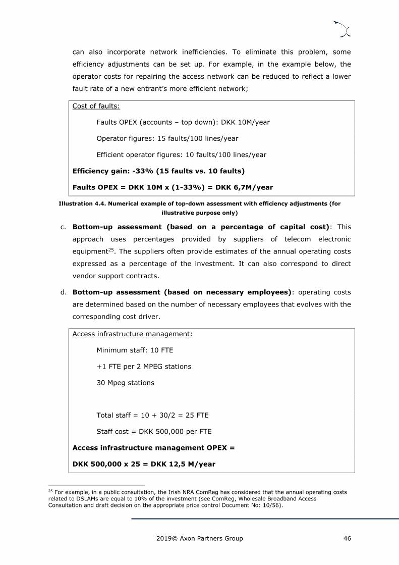
2019© Axon Partners Group 46
can also incorporate network inefficiencies. To eliminate this problem, some
efficiency adjustments can be set up. For example, in the example below, the
operator costs for repairing the access network can be reduced to reflect a lower
fault rate of a new entrant’s more efficient network;
Cost of faults:
Faults OPEX (accounts – top down): DKK 10M/year
Operator figures: 15 faults/100 lines/year
Efficient operator figures: 10 faults/100 lines/year
Efficiency gain: -33% (15 faults vs. 10 faults)
Faults OPEX = DKK 10M x (1-33%) = DKK 6,7M/year
Illustration 4.4. Numerical example of top-down assessment with efficiency adjustments (for
illustrative purpose only)
c. Bottom-up assessment (based on a percentage of capital cost): This
approach uses percentages provided by suppliers of telecom electronic
equipment25. The suppliers often provide estimates of the annual operating costs
expressed as a percentage of the investment. It can also correspond to direct
vendor support contracts.
d. Bottom-up assessment (based on necessary employees): operating costs
are determined based on the number of necessary employees that evolves with the
corresponding cost driver.
Access infrastructure management:
Minimum staff: 10 FTE
+1 FTE per 2 MPEG stations
30 Mpeg stations
Total staff = 10 + 30/2 = 25 FTE
Staff cost = DKK 500,000 per FTE
Access infrastructure management OPEX =
DKK 500,000 x 25 = DKK 12,5 M/year
25 For example, in a public consultation, the Irish NRA ComReg has considered that the annual operating costs related to DSLAMs are equal to 10% of the investment (see ComReg, Wholesale Broadband Access Consultation and draft decision on the appropriate price control Document No: 10/56).

2019© Axon Partners Group 47
e. True bottom-up assessment: this approach consists in calculating the network’s
requirements (in energy, cooling, square meters) and to conduct a bottom up
assessment of OPEX (e.g. energy cost = kWh requirement for all networks elements
x kWh price);
f. Benchmarking: this way of assessment involves collecting and analysing OPEX
mark-ups used by NRAs in other comparable countries.
Approaches b, c, d and e tend to model the efficient costs of an operator. However,
approaches b, d and e rely on many assumptions that are challenging to predict accurately
(e.g. staff needed to maintain the network element, efficiency gain, etc.). The DBA/Axon
team believes that alternative c, bottom-up assessment (based on a percentage of capital
cost), is the best option because:
1. It strikes a reasonable balance between accuracy, the number of assumptions
required and comparability against international references.
2. Provides easy reviewing mechanisms (i.e. there is broad consensus in the industry
on the common range OpEx should represented over CapEx)
3. Ensures consistency with the approach generally used in the current version of
DBA’s fixed LRAIC model.
Main criterion 12: Operating costs should be calculated using a bottom-up
assessment based on a percentage of capital cost.
Question 12: Do you agree that operating costs should be calculated using a bottom-
up assessment based on a percentage of capital costs?
If you don’t agree, please justify your position and provide supporting information and
references.
4.4. Depreciation Methodologies
Key area of discussion below: Depreciation methodologies to be considered in the
model.
An important element of a LRAIC model is the estimation of the annual cost associated
with assets. Annuities measure both the depreciation charge and the capital charge
associated to the assets.

2019© Axon Partners Group 48
An annuity is the annual payment which, when discounted at an appropriate cost of capital
and summed over the asset lifetime, gives the replacement cost for an asset. The
alternative approach sometimes used is economic depreciation. This involves measuring
the depreciation charge as the annual change in the net present value (NPV) of an asset,
adjusted for factors such as changes in output profile or prices, overhead cost and the cost
of capital
Three traditional annuities formulas will be presented in this section: the standard annuity
(4.4.1), the tilted annuity (4.4.2)and the full economic depreciation (4.4.3).
4.4.1. Standard Annuity
The use of this method is appropriate when asset prices and volumes of outputs produced
by an asset are stable. The standard annuity approach consists of calculating an annual
charge A called annuity, which is identical every year and which respects the following
equation:
𝐼 =𝐴
(1 + ω)+
𝐴
(1 + ω)2+ ⋯ +
𝐴
(1 + ω)𝑛
Then, A can be written as follows:26
𝐴 = 𝐼 ×ω
1 − (1
1 + ω)𝑛
where ω is the cost of capital, I the investment, n the asset life.
26 This formula assumes that the operator begins generating revenues from the asset one year after investment is completed.

2019© Axon Partners Group 49
The standard annuity approach calculates an increasing depreciation charge and a
decreasing return on capital employed in such a way that the annuity remains stable over
time.
Illustration 4.5. Asset renewal (year 11) at a higher price under standard annuity method (discontinuity) [Source: DBA - Final MRP (July 2013)]
4.4.2. Tilted annuity
The tilted annuity formula is probably the most widespread depreciation formula used for
regulatory purposes. It incorporates a tilt which enables the calculation of annuities that
evolve in line with asset price changes: if an asset price increases by say 5% per annum,
annuities will also increase by 5% per annum, as illustrated in Illustration 4.6.

2019© Axon Partners Group 50
Such a formula sends appropriate ‘build or buy’ signals to market players. It also allows
replicating the annual charges that would be faced by an operator in a competitive market.
Illustration 4.6. Annuities with the tilted annuity method - Asset renewal (year 11) under tilted annuity method – Asset price increase of 5% per annum (continuity) [Source: DBA - Final MRP
(July 2013)]
A tilted annuity can be calculated on the basis of the following formula:
𝐴𝑡 = 𝑝𝑡 ×∑ (1 + ω)j × 𝐼𝑗
𝑛𝑗=1
∑ (1 + ω)j × 𝑝𝑗𝑛𝑗=1
This can be written as follows:
𝐴𝑡 = 𝐼 ×(ω − 𝑝) × (1 + 𝑝)𝑡
1 − (1 + 𝑝1 + ω)
𝑛
Where ω is the cost of capital, I the investment, t the year considered, n the asset life, p
the tilt (price trend of the asset in the long term) and 𝐴𝑡 the annuity of year t27.This
formula is derived by the same equation as the one provided in the beginning of this
section28 but with the following relationship between each annuity:
27 This annuity is calculated by assuming that the first annual cost recovery is happening one year after the investment is made. If the time between the moment the first annuity happens, and the investment is paid is
one year lower (respectively one year higher), then the annuity should be multiplied by a (1 + ω)−1
(respectively ((1 + ω)).
28 𝐼 = ∑𝐴𝑖
(1+ω)𝑖𝑛𝑖=1

2019© Axon Partners Group 51
𝐴𝑡 = 𝐴𝑡−1 × (1 + 𝑝)
which means that annuities are evolving with asset prices.
Even more important, tilted annuities allow a smooth evolution of annual cost despite price
changes and investment cycles. At the end of the useful life of an asset, i.e. when the
asset needs to be renewed, the annuities calculated with the tilted annuity method will be
similar just before and just after the renewal of the asset (as shown in the illustration
above). Therefore, annuities evolve without the discontinuities which are one of the main
drawbacks of the standard annuity approach. If the volume of output produced by an asset
is stable, then the tilted annuity is a good approximation for economic depreciation.
However, the tilted annuity may not be a good proxy for economic depreciation when the
volume of outputs produced by an asset is not stable. This may be the case for new
services (which have a logistic curve) or when demand is evolving fast (see example
below).
Illustration 4.7. Example of unit cost derived on the basis of the tilted annuity formula when the
number of output produced by an asset is increasing [Source: DBA - Final MRP (July 2013)]
In this case, a full economic depreciation method can be used.
4.4.3. Full economic depreciation
It is possible to modify the tilted annuity formula to compute annuities that take into
account the evolution of the number of outputs produced by assets. This is referred to as
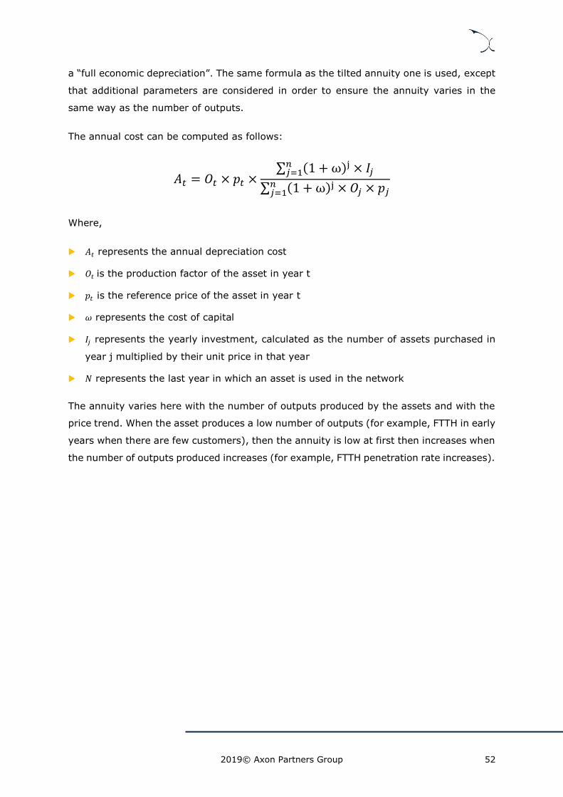
2019© Axon Partners Group 52
a “full economic depreciation”. The same formula as the tilted annuity one is used, except
that additional parameters are considered in order to ensure the annuity varies in the
same way as the number of outputs.
The annual cost can be computed as follows:
𝐴𝑡 = 𝑂𝑡 × 𝑝𝑡 ×∑ (1 + ω)j × 𝐼𝑗
𝑛𝑗=1
∑ (1 + ω)j × 𝑂𝑗 × 𝑝𝑗𝑛𝑗=1
Where,
𝐴𝑡 represents the annual depreciation cost
𝑂𝑡 is the production factor of the asset in year t
𝑝𝑡 is the reference price of the asset in year t
𝜔 represents the cost of capital
𝐼𝑗 represents the yearly investment, calculated as the number of assets purchased in
year j multiplied by their unit price in that year
𝑁 represents the last year in which an asset is used in the network
The annuity varies here with the number of outputs produced by the assets and with the
price trend. When the asset produces a low number of outputs (for example, FTTH in early
years when there are few customers), then the annuity is low at first then increases when
the number of outputs produced increases (for example, FTTH penetration rate increases).
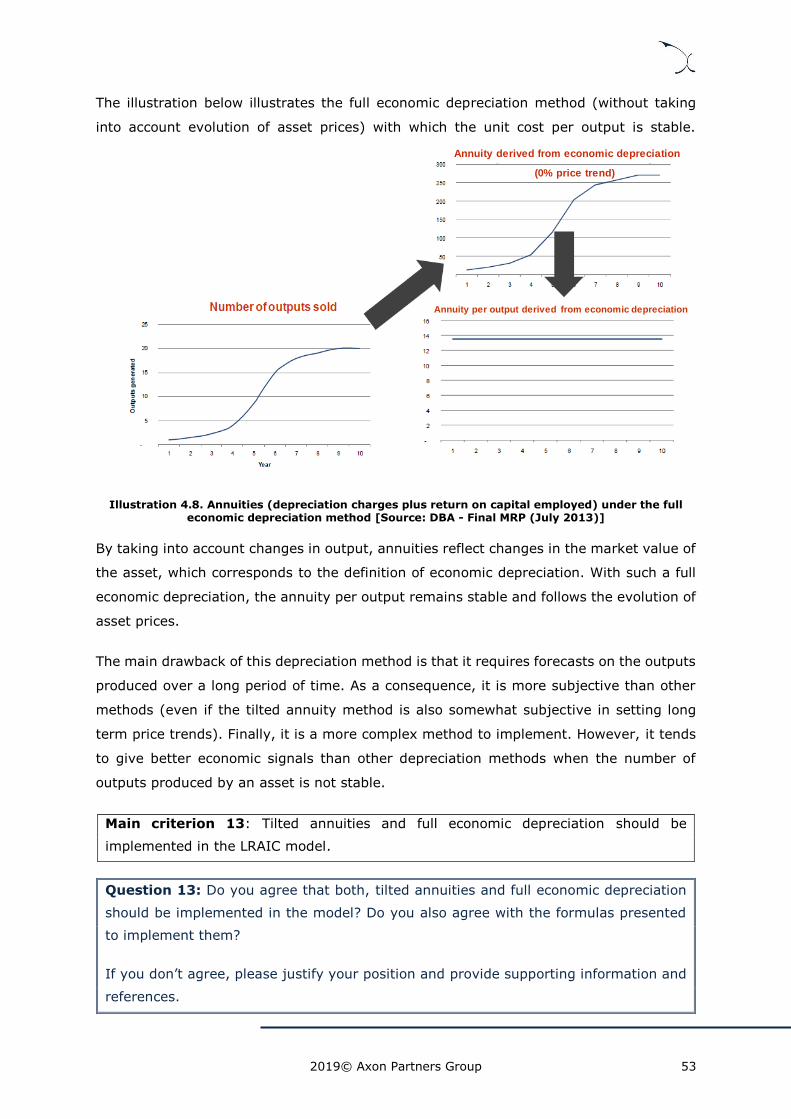
2019© Axon Partners Group 53
The illustration below illustrates the full economic depreciation method (without taking
into account evolution of asset prices) with which the unit cost per output is stable.
Illustration 4.8. Annuities (depreciation charges plus return on capital employed) under the full economic depreciation method [Source: DBA - Final MRP (July 2013)]
By taking into account changes in output, annuities reflect changes in the market value of
the asset, which corresponds to the definition of economic depreciation. With such a full
economic depreciation, the annuity per output remains stable and follows the evolution of
asset prices.
The main drawback of this depreciation method is that it requires forecasts on the outputs
produced over a long period of time. As a consequence, it is more subjective than other
methods (even if the tilted annuity method is also somewhat subjective in setting long
term price trends). Finally, it is a more complex method to implement. However, it tends
to give better economic signals than other depreciation methods when the number of
outputs produced by an asset is not stable.
Main criterion 13: Tilted annuities and full economic depreciation should be
implemented in the LRAIC model.
Question 13: Do you agree that both, tilted annuities and full economic depreciation
should be implemented in the model? Do you also agree with the formulas presented
to implement them?
If you don’t agree, please justify your position and provide supporting information and
references.
Annuity per output derived from economic depreciation
Annuity derived from economic depreciation
(0% price trend)

2019© Axon Partners Group 54
4.5. Cost of Capital
When an operator invests in an asset, it must be able to recover the appropriate costs of
financing this investment: on the one hand, it supports the cost of equity as measured by
the returns that shareholders require for this investment and on the other hand, it supports
the cost of debt if the investment is also financed by debt. In regulation, these financial
costs are typically recovered through the use of a “weighted average cost of capital”
(“WACC”). The cost of capital reflects the opportunity cost of funds invested in the asset,
and is incorporated into the cost model by multiplying the WACC by the capital employed
or through the application of an annuity formula which combines the calculation of both
the return on capital and the depreciation charge.
WACC values to be considered in the model shall be based on the latest decisions published
by DBA.
Main criterion 14: WACC values considered in the cost model should be aligned with the
up to date decisions determined by DBA.
Further, as detailed by the EC in the EECC,
“Where the national regulatory authorities consider price control obligations to be
appropriate, they shall allow the undertaking a reasonable rate of return on
adequate capital employed, taking into account any risks specific to a particular
new investment network project.”
Therefore, if deemed appropriate, an NGA premium may be considered under specific
circumstances to account for risks specifics to particular investments.
Supporting criterion 15: The LRAIC model should have the possibility of including a
risk premium for NGA/VHCN networks.
4.6. The cost of working capital
Key area of discussion below: Consideration of working capital in the cost model.
The activity of an electronic communications operator requires or generates cash for
everyday operations: this amount of cash is defined as “working capital”. The working
capital is calculated as the WACC times the difference between current assets minus
current liabilities. Working capital may either be positive (i.e. generate a cost) or negative
(i.e. generate revenues), depending on the financial situation of the operator.

2019© Axon Partners Group 55
Based on an assessment of the working capital situation of the current SMP operator in
Denmark, we have concluded that there is not a clear cost of working capital associated
to the provision of the services to be included in the cost model. In particular, not even
the likely sign of the working capital is known (i.e. whether it could represent a cost or a
revenue to the modelled operator). Therefore, given the uncertainties surrounding this
input, and the unlikelihood of getting access to detailed financial information to accurately
assess working capital, a conservative approach consisting of not including working capital
in the model is preferred.
Supporting criterion 16: The LRAIC model should not include working capital
costs/revenues in the light of the financial data extracted from the current SMP
operator).
Question 14: Do you agree that working capital should not be considered in the cost
model?
If you don’t agree, please justify your position and provide supporting information and
references.

2019© Axon Partners Group 56
5. Model implementation
IMPORTANT NOTE: There has been a major restructuring of this section when
compared with the July 2013 MRP due to the decision to integrate both the access and
core models into a single fixed LRAIC cost model. While, for the most part, the text
included in the July 2013 MRP has been maintained, the sections have been restructured
in order to improve the flow of this section. The following table includes a comparison
of the sections included in the July 2013 MRP and the current version of this document.
Section in previous MRP Section in this document
4 Models Implementation 5. Model implementation
4.1 Modelling Guidelines 5.1. Service Demand
4.1.1 Estimating Demand 5.1. Service Demand
4.1.2 Equipping the Network 5.4.2. Access network
4.1.3 Costing the Network 5.5. Costing the Network
4.1.4 Costing Services 5.6. Allocation of costs to services
4.2 Optimisation in the LRAIC Model 5.3.1. The Scorched Node Assumption and 5.2.4. An optimized and resilient network
4.2.1 The Scorched Node Assumption 5.3.1. The Scorched Node Assumption
4.2.2 Guidelines on Optimisation 5.2.4. An optimized and resilient network
4.3 Modelling Access 5.4.1. Modelling tools
4.3.1 Estimating Demand 5.1. Service Demand
4.3.2 Equipping the Network 5.4.2. Access network
4.3.2.1 Geomarketing data 5.4.2.1.Geomarketing data
4.3.2.2 Roll-out of the network 5.4.2.2. Roll-out of the network
4.3.2.3 Network Dimensioning 5.4.2.3. Access dimensioning
4.3.3 Costing the network 5.5. Costing the Network
4.3.3.1 Costing capital expenditures 5.5. Costing the Network
4.3.3.2 Costing operating expenditures 5.5. Costing the Network
4.3.4 Costing Services 5.6.2. Allocation of costs to access services
4.4 Modelling Core Included in subsections below
4.4.1 Demand Over the Core Network Included in subsections below
4.4.1.1 Estimation of End-User Demand 5.1. Service Demand
4.4.1.2 Estimating Dimensioned Demand 5.2.1. demand drivers
4.4.1.3 The Hierarchy of the “Exchanges” 5.3.2. The Hierarchy of the “Exchanges”
4.4.1.4 Equipment at each node 5.3.2. The Hierarchy of the “Exchanges”
4.4.1.5 Direct network Costs 4.1.1. Direct Network Costs
4.4.1.6 Indirect network 4.1.2. Joint and network common costs
4.4.2 Modelling Transmission 5.4.3.1. Dimensioning of the active transmission elements
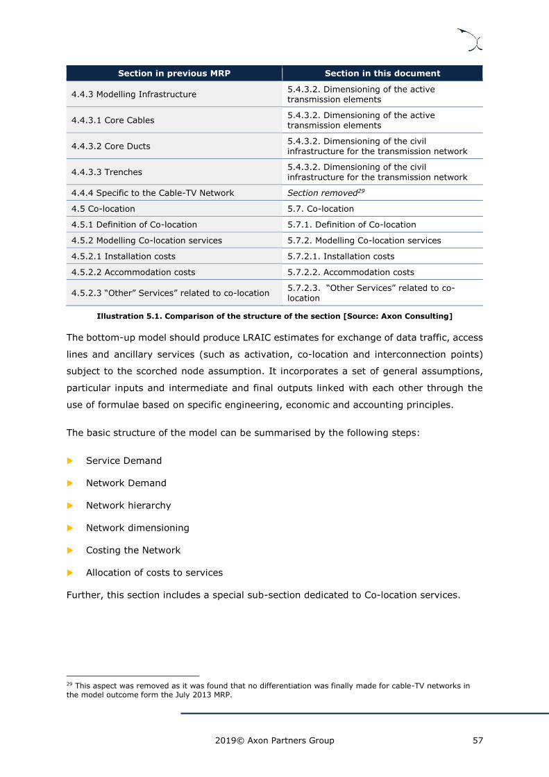
2019© Axon Partners Group 57
Section in previous MRP Section in this document
4.4.3 Modelling Infrastructure 5.4.3.2. Dimensioning of the active transmission elements
4.4.3.1 Core Cables 5.4.3.2. Dimensioning of the active transmission elements
4.4.3.2 Core Ducts 5.4.3.2. Dimensioning of the civil infrastructure for the transmission network
4.4.3.3 Trenches 5.4.3.2. Dimensioning of the civil
infrastructure for the transmission network
4.4.4 Specific to the Cable-TV Network Section removed29
4.5 Co-location 5.7. Co-location
4.5.1 Definition of Co-location 5.7.1. Definition of Co-location
4.5.2 Modelling Co-location services 5.7.2. Modelling Co-location services
4.5.2.1 Installation costs 5.7.2.1. Installation costs
4.5.2.2 Accommodation costs 5.7.2.2. Accommodation costs
4.5.2.3 “Other” Services” related to co-location 5.7.2.3. “Other Services” related to co-
location
Illustration 5.1. Comparison of the structure of the section [Source: Axon Consulting]
The bottom-up model should produce LRAIC estimates for exchange of data traffic, access
lines and ancillary services (such as activation, co-location and interconnection points)
subject to the scorched node assumption. It incorporates a set of general assumptions,
particular inputs and intermediate and final outputs linked with each other through the
use of formulae based on specific engineering, economic and accounting principles.
The basic structure of the model can be summarised by the following steps:
Service Demand
Network Demand
Network hierarchy
Network dimensioning
Costing the Network
Allocation of costs to services
Further, this section includes a special sub-section dedicated to Co-location services.
29 This aspect was removed as it was found that no differentiation was finally made for cable-TV networks in the model outcome form the July 2013 MRP.

2019© Axon Partners Group 58
5.1. Service Demand
The main source of information on the current level of demand in Denmark will be the
fixed network operators. The model will include the demand for the services listed in
section ‘3.3 Services’, which includes wholesale and retail services. .
Supporting criterion 17: The starting point when building the bottom-up model is the
level of demand in Denmark for all the modelled services.
The demand for each modelled service will be introduced from the reference year (2018)
until the final year considered in the model (2028) in the corresponding units (e.g. lines
for access services or Mbps for bitstream capacity services).
In order to define the demand inputs until 2028, forecasts will be requested from operators
which will be complemented by a regression analysis based on historical trends to be
performed by the DBA.
Supporting criterion 18: The LRAIC model will include demand forecasts until 2028
for the modelled services.
Question 15: Do you agree that the model should include demand forecasts until
2028?
If you don’t agree, please justify your position and provide supporting information and
references.
The following paragraphs describe the approach to be adopted with regards to the
definition of the demand inputs for each of the key categories of services to be modelled:
Broadband and TV services
Leased Lines
Access services
Key area of discussion below: Extent of the demand forecasts to be included in the
model.
2019© Axon Partners Group 59
5.1.1. Broadband and TV services
As a minimum, the model should be able to identify the number of customers for each of
the major broadband service speeds.
Supporting criterion 19: The LRAIC model should have the capability to be able to
show the demand for each major broadband service speed in terms of the number of
customers.
Further, demand for other services that run over the IP network, such as multicast IPTV
or Video on Demand, should also be considered in terms of number of customers and/or
services provided (e.g. number of TV channels).
Supporting criterion 20: Demand for TV services such as Multicast-IPTV and Video
On Demand should be included in the model.
5.1.2. Leased Lines
The model should show the total demand of leased lines circuits in terms of number of
circuits by capacity bandwidths.
The use of the core network by leased lines is likely to vary significantly across the network
as leased lines are more likely to be requested either within or between large towns and
cities and less likely within/between small towns and villages. Thus, information should be
sought on how the amount of leased line capacity sold varies across the different regions
of the country and by hierarchical level within the network.
Supporting criterion 21: The LRAIC model should show the demand of number of
leased lines by volume and bandwidth. Information should be sought on how the
amount of leased line capacity sold varies across the different regions of the country
and by hierarchical level within the network.
5.1.3. Access services
Demand of access services will include the number of active access lines associated to
each technology. These lines will be disaggregated for the different services presented in
section ‘3.3 Services’.

2019© Axon Partners Group 60
5.2. Network Demand
Once the service demand has been specified, the model will need to express it in network
terms to properly run the dimensioning algorithms.
The conversion of demand at service level to network level involves the following relevant
considerations:
Demand drivers
Busy hour information
Adjustments for the grade of service
5.2.1. The calculation of demand drivers
Service demand is insufficient to dimension the network because traffic will flow through
the network in different ways and thus some network elements will be utilized more than
others for the same service demand.
Further, demand from the different services may be considered in different units.
Therefore, in order to perform an accurate dimensioning process, the service demand must
be converted to a common driver (e.g. Mbps).
There are two main ways which may be used in order to assess how end-user demand
results in specific network element demand across the network:
Demand on a route by route basis. This consists of estimating the traffic flowing over
the network on a route by route basis. The amount of traffic originating from each
node of the network is computed aggregating the amount of traffic from all the lines
directly or indirectly connected to that node.
Usage factors. Usage factors are defined as the average frequency that a particular
service uses a given network element.
DBA recommends that usage factors are used as the default method to distribute the
forward-looking level of demand over the different parts of the network. Route-by-route
demand might be more suitable in certain cases, for example with regard to high speed
leased lines.
Supporting criterion 22: The usage factors used for the determination of the demand
drivers in the model need to be consistent with the underlying network architecture.

2019© Axon Partners Group 61
5.2.2. Busy hour information
Although information on traffic is generally collected on an annual basis, the network will
need to be dimensioned to carry the traffic flowing in the “busy hour” subject to required
blocking margins (“busy-hour” traffic). The LRAIC model will need to take account of
demand on different days of the week and in different months of the year, but not traffic
surges caused by special events such New Year’s Eve. It should be noted that “busy-hour”
can vary in different parts of the network and for different services (for example,
broadband usage). This will be captured in the model by considering that the capacity
required by each service is equal to the contribution of each service to the total network
busy hour.
Illustration 5.2. Busy hours occur at different times of the day for the different services [Source:
DBA - Final MRP (July 2013)]
Information on the busy hour will need to be sourced from the operators for all relevant
services.
For non-contended services, such as leased lines, the full capacity should be assumed to
be used even though in practice the customer is unlikely to utilise that capacity on a 24/7
basis.
Supporting criterion 23: The LRAIC model should clearly identify busy-hour
information for all relevant traffic. The LRAIC model should also be flexible enough to

2019© Axon Partners Group 62
allow for changes in these figures. Information on the busy hour will need to be sourced
from the operators for all relevant services.
5.2.3. Adjustments for the grade of service
For real-time traffic flowing over the IP network, additional adjustments are likely to be
necessary to take account of the need to prioritise such traffic as it flows across the
network.
The LRAIC model should demonstrate that the modelled network provides services at an
appropriate level of quality for an efficient modelled operator, particularly for real time
traffic (such as VoIP and IPTV) and non-contended (“leased lines’) traffic.
Supporting criterion 24: The LRAIC model should demonstrate that the modelled
network provides services at an appropriate level of quality for an efficient modelled
operator, particularly for real time traffic (such as IPTV) and non-contended (“leased
lines”) traffic.
5.3. Network hierarchy
5.3.1. The Scorched Node Assumption
DBA interprets the Scorched Node constraint such that when modelling an “optimally
structured network” under the scorched node assumption the locations for equipment are
constrained by the existing number of sites and their existing locations. However, the
scorched node assumption does not imply that the transport network - cables, duct/trench
etc. - is fixed. Nor does the assumption imply that the same number and type of equipment
should be placed at each of these geographical locations.
Supporting criterion 25: The LRAIC model should show the costs of a network with
an efficient configuration operated by an efficient company, based on the latest proven
technological solutions and an optimally structured organisation. However, the starting
point should be the existing geographic network architecture in the modelled operator’s
network. This implies that equipment should be placed at the existing geographical
locations of the modelled operator’s network nodes (the scorched node assumption).

2019© Axon Partners Group 63
The following list of equipment meets for example the basic definition of a node within an
all-IP network30:
A DSLAM/OLT/CMTS;
A Layer 2 Ethernet switch; and
A Layer 3 IP router.
Whatever type of node is used, the boundary between the core and access networks will
remain at the line card situated at the relevant exchange, with the line card included in
the costs of the access network.
5.3.2. The Hierarchy of the “Exchanges”
The LRAIC model is to adopt an “all-IP” network. Although such networks are often thought
of as comprising a mesh-like structure, such that packets can find lots of ways through
the network, in practice an operator will still organise the network using a hierarchical
approach.
A typical four-layer hierarchy might comprise the following layers:
Core Routers. These represent the second level of IP routing within the network and
again would typically be installed in a ring (or more likely two rings) configuration with
a number of Edge Routers feeding into two (for dual parenting reasons) Core Routers.
Edge Routers. These represent the first level of IP routing within the network and
would typically be installed in rings, with a number of Aggregation switches feeding
into two (for dual parenting reasons) Edge Routers on a ring.
Aggregation switches. These are managed Ethernet switches, used to group together
a number of DSLAMs/OLTs/cable-TV equipment and also to form high capacity rings
in dense (typically business) urban areas.
DSLAMs or other access equipment (such as OLTs, CMTS nodes, etc.). The DSLAMs
represent the layer at which the customer typically connects (via a DSLAM line card).
Within a Next Generation Network, the DSLAMs are commonly referred to as MSANs
(Multi-Service Access Nodes)
30 For the core network only
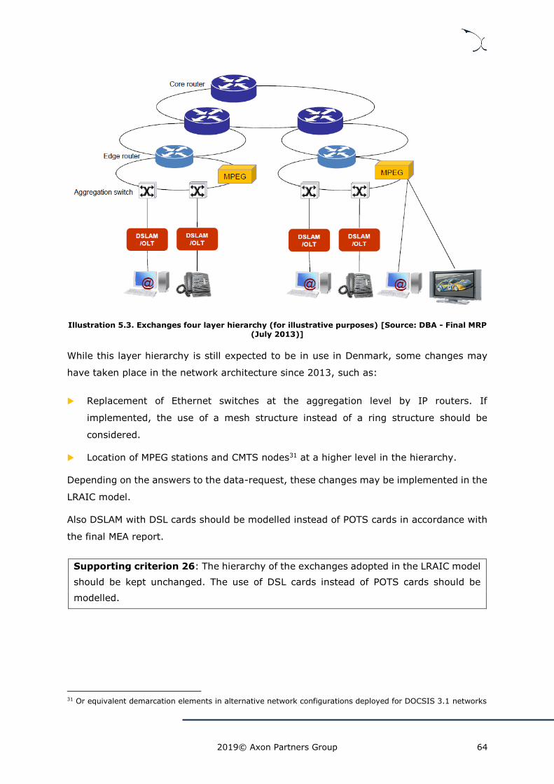
2019© Axon Partners Group 64
Illustration 5.3. Exchanges four layer hierarchy (for illustrative purposes) [Source: DBA - Final MRP
(July 2013)]
While this layer hierarchy is still expected to be in use in Denmark, some changes may
have taken place in the network architecture since 2013, such as:
Replacement of Ethernet switches at the aggregation level by IP routers. If
implemented, the use of a mesh structure instead of a ring structure should be
considered.
Location of MPEG stations and CMTS nodes31 at a higher level in the hierarchy.
Depending on the answers to the data-request, these changes may be implemented in the
LRAIC model.
Also DSLAM with DSL cards should be modelled instead of POTS cards in accordance with
the final MEA report.
Supporting criterion 26: The hierarchy of the exchanges adopted in the LRAIC model
should be kept unchanged. The use of DSL cards instead of POTS cards should be
modelled.
31 Or equivalent demarcation elements in alternative network configurations deployed for DOCSIS 3.1 networks
2019© Axon Partners Group 65
5.3.2.1. The highest layer of the “exchanges”
The first step in the modelling process will be to model the top layer of the exchanges in
the core network, which in an IP network would typically represent the Core Routers.
There are several ways to determine the number of nodes in this layer of the hierarchy.
The number of core routers in the modelled operator’s network.
The calculated peak traffic needs and how this might impact the size of the equipment
for differing numbers of highest level nodes. If too few nodes are chosen, then the
peak traffic levels might mean that multiple core routers will need to be sited at the
same location. If this occurs, then it might be more resilient to locate the equipment
at multiple sites.
International experience, the experience of other operators within Denmark, and the
need for highest level interconnect could also be used to help determine the
appropriate number and size of these “highest level” core router sites.
5.3.2.2. The other layers of the hierarchy
Once the number of sites at the highest layer of the hierarchy has been estimated, the
remaining sites will need to be allocated to the other layers of the hierarchy. Similar
analysis needs to be carried out as for the highest level in the hierarchy (see the above
bullets).
In addition, the final choice might need to take account of:
cost: the cost of serving a certain threshold of customers. The cost will need to include
not only the cost of the equipment, but also other costs such as installation, operating
costs, accommodation, and power and network management.
impact on other parts of the network: the LRAIC model should be able to show the
cost implications of the chosen mix on other parts of the network, e.g. transmission
equipment, fibre or trenching.
security: the implications on the quality of service should also be taken into account.
For example, the ability of the network to cope with the breakdown of equipment
located at one site.
practicability: the chosen mix must be technically feasible. This means that the
equipment must be able to handle the increasing amount of traffic and there must be
sufficient higher level nodes to host in an effective manner all of the DSLAMs/MSANs.

2019© Axon Partners Group 66
It also means that the distances between interconnected equipment must take
account of the maximum distances for un-repeated fibre optic communications and
thus the need to include repeaters on long distance routes.
consistency with the evolution of electronic communications networks: the optimised
sites must be consistent with the general evolution of network design in Denmark and
around the world. That is, it must be flexible enough to allow for developments such
as the growth of the Internet and moves to unbundled subloops.
Supporting criterion 27: The hierarchical design adopted in the LRAIC model
considers the following factors: cost, the impact on other parts of the network, security,
technical feasibility, and consistency with the evolution of the telecoms networks.
5.4. Network dimensioning
5.4.1. Modelling tools
Cost assessments in fixed networks, particularly in their access segment, are heavily
influenced by the civil infrastructure needs. It is, therefore, key to rely on accurate
dimensioning tools to ensure that these network assets are precisely dimensioned based
on the specific location of the households as well as the modelled operator’s nodes.
To achieve this objective, a database software for static calculations related to the
geographical analyses will be developed. As described in section ‘5.4.2.3 Access network
dimensioning’, the access segment should be modelled at the section level (i.e. portion of
a road located in between two road crossroads). For a country the size of Denmark, it is
expected to have several hundred thousands of sections. A database of this size cannot
be recorded in an Excel file. This is why DBA intends to use similarly to the current model,
a database software to handle these calculations. However, to facilitate the understanding
of the costing of the network, Microsoft Excel will be used for all other purposes (e.g. to
cost the network and to calculate the results).
Supporting criterion 28: The LRAIC cost model will be based on a database software
and Microsoft Excel. The usage of database solutions will be limited to the geographical
assessment of the access network to facilitate the review and understanding of the
LRAIC model by stakeholders.

2019© Axon Partners Group 67
5.4.2. Access network
Equipping the access network consists in assessing the type of equipment and the quantity
that should be rolled out. This should be carried out through three main phases:
Geomarketing data;
Roll-out of the network
Access dimensioning.
These phases are described in the sections hereafter.
5.4.2.1. Geomarketing data
Geomarketing data are topographical and demographical data. These are specific to each
country.
It is first necessary to locate the nodes of the different access networks following the
scorched node approach using the X;Y geographic coordinates of the modelled operator.
These nodes are:
The MDFs for the copper access network;
The ODFs for the FTTH access network;
The MPEG stations, or equivalent demarcation points for DOCSIS 3.1 networks (if
applicable) for the cable-TV access network.
To each node is associated a coverage area. The coverage area is the area in which all the
buildings are connected to the corresponding network node. These coverage areas should
be based on a theoretical split of the country (still using the nodes of the operators) using
the Voronoi decomposition. This approach, while theoretical, closely resembles the realities
that would be faced by a generic efficient operator. The Voronoi approach, should be
adjusted in order to make sure there is no standalone street in any coverage area (the
road network in each Voronoi area should be a convex network). The Voronoi
decomposition should therefore be computed using the distance based on the road
network (i.e. the distance between two points should be the sum of the lengths of the road
sections located in-between the two points and following the shortest path) instead of the
crow-fly distance32.
32 This adjusted Voronoi decomposition is consistent with reality as the access network cables tend to follow the road network.
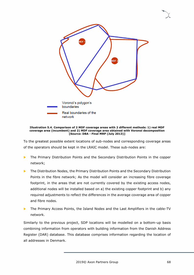
2019© Axon Partners Group 68
Illustration 5.4. Comparison of 2 MDF coverage areas with 2 different methods: 1) real MDF coverage area (incumbent) and 2) MDF coverage area obtained with Voronoi decomposition
[Source: DBA - Final MRP (July 2013)]
To the greatest possible extent locations of sub-nodes and corresponding coverage areas
of the operators should be kept in the LRAIC model. These sub-nodes are:
The Primary Distribution Points and the Secondary Distribution Points in the copper
network;
The Distribution Nodes, the Primary Distribution Points and the Secondary Distribution
Points in the fibre network; As the model will consider an increasing fibre coverage
footprint, in the areas that are not currently covered by the existing access nodes,
additional nodes will be installed based on a) the existing copper footprint and b) any
required adjustments to reflect the differences in the average coverage area of copper
and fibre nodes.
The Primary Access Points, the Island Nodes and the Last Amplifiers in the cable-TV
network.
Similarly to the previous project, SDP locations will be modelled on a bottom-up basis
combining information from operators with building information from the Danish Address
Register (DAR) database. This database comprises information regarding the location of
all addresses in Denmark.

2019© Axon Partners Group 69
Main criterion 15: The LRAIC model should use as much as possible locations (X;Y
geographic coordinates) of each network node of the operators.
The coverage areas should be based on the area where the relevant operators have rolled
out their network.
Main criterion 16: The model should use the coverage areas of the modelled operator.
Knowing that electronic communications networks follow streets/roads (contrary to
electric networks that can sometimes cross fields and roads to reach a point with a minimal
distance), the second type of data necessary is data concerning the road/street network.
The road network data should be collected from official agencies, such as the DAR. More
precisely, it is the network of road sections that should be the level of granularity used for
the modelling as this level enables to dimension all the network elements without the need
of any projection.
Illustration 5.5. Example of road sections (all are not highlighted in red) in Copenhagen [Source: DBA - Final MRP (July 2013)]
Supporting criterion 29: The LRAIC model should use the road network database
provided by the DAR.
Data concerning buildings that have an access connection is necessary in order to be able
to dimension the network. These data should include building locations and number of
households per building.

2019© Axon Partners Group 70
The location of buildings is used to find out where the access network should be rolled out.
The number of households per building allows an accurate dimensioning of the different
elements of the access network as the trench sizes are derived from the cable sizes which
are derived directly from the total number of households.
The building data should be collected from DAR databases. Similar sources were used in
the previous revision of the LRAIC model.
Supporting criterion 30: The LRAIC model should use the data on buildings provided
by DAR or equivalent sources if not available.
5.4.2.2. Roll-out of the network
The network deployment is carried out according to the operators’ network architecture:
Illustration 5.6. Networks architecture (for illustrative purpose)33 [Source: DBA - Final MRP (July 2013)]
The access copper network is made of four parts:
The part between the MDF and the PDP (Primary Distribution Point) called “E-Side”;
The part between the PDP and the SDP (Secondary Distribution Point) called “D-Side”;
33 The cable-TV architecture shown in the figure is a typical architecture nevertheless other network architectures exist that should be taken into account when modeling the cable-TV access network.

2019© Axon Partners Group 71
The part between the SDP and the FDP (Final Distribution Point) is also part of the “D-
Side”;
The part between the FDP and the customer premises called “final drop”.
The FTTC network is following the same architecture as the copper network, the only
difference being a fibre cable is rolled out on the E-Side of the network instead of a copper
cable.
There are two configurations for the FTTH access network:
A point-to-point architecture (PTP);
A point-to-point architecture (PON).
The PTP network is made of four parts:
The part between the ODF and the PDP (Primary Distribution Point);
The part between the PDP and the SDP (Secondary Distribution Point);
The part between the SDP and the FDP (Final Distribution Point);
The part between the FDP and the customer premises called “final drop”.
The PON network is made of four parts:
The part between the ODF and the PDP (Primary Distribution Point);
The part between the PDP and the SDP (Secondary Distribution Point);
The part between the SDP and the FDP (Final Distribution Point);
The part between the FDP and the customer premises called “final drop”.
The cable-TV network is made of five parts:
The part between the MPEG station34 and the PAP (Primary Access Network);
The part between the PAP and the IN (Island Node);
The part between the IN and the LA (Last Amplifier);
The part between the LA and the DP (Distribution Point);
The part between the LA and the customer premises called “final drop”.
34 Or equivalent demarcation point for DOCSIS 3.1 networks
2019© Axon Partners Group 72
Supporting criterion 31: The LRAIC model should use the operators’ networks
hierarchies. However, as regards fibre access network, PTP should be modelled with the
same hierarchy as other access networks.
The network roll out is carried out by first connecting the main node to the primary
subnodes which are then if possible connected to the secondary sub-nodes and then
subsequently to buildings.
For example, the copper network is made of three parts as explained above. The MDFs
are first connected to each Primary Distribution Points located in their coverage area. Then
the Primary Distribution Points are then connected to each Secondary Distribution Points
located in their coverage areas. Finally, the Secondary Distribution Points are connected
(via FDPs) to the buildings located in their coverage areas. Possibly, depending on
operators’ rules, some buildings may be directly connected to the MDFs or to the Primary
Distribution Points.
For each part of the network, it is possible to determine the exact shortest path (among
all paths following the road network). This shortest path should be the network path.
Determining this shortest path is carried out by the “shortest path algorithm”.
It is to be noted that shortest paths calculations are conducted on a “per road section
basis”. It is assumed that the FDP will be located in the same road section as the buildings
it connects (this should be the case in the vast majority of cases). As a consequence, the
“FDP-building” path does not require a shortest path calculation to be performed but rather
an assumption on the distance of this link.
Supporting criterion 32: The LRAIC model should use the “shortest path algorithm”
to connect two nodes together by following the real Danish road and street network.
For illustrative purpose, the illustration below represents a node area (in blue) of an access
network with two street cabinets (two sub-nodes), purple and red, corresponding to three
groups of buildings. This network is thus made of two parts:
The part between the node and the street cabinet;

2019© Axon Partners Group 73
The part between the street cabinet and the building.
Illustration 5.7. A node area and the shortest path possible between street cabinets and building
groups [Source: DBA - Final MRP (July 2013)]
In this example, the road sections part of the coverage area of the purple street cabinet
are in purple and the road sections part of the coverage area of the red street cabinet are
in red. This is to illustrate which road sections are connected to either the purple or red
street cabinet.
Once the road sections and their corresponding street cabinet are identified, the “shortest
path algorithm” is then implemented to get the following paths:
The shortest path between each building and its corresponding street cabinet
(depending on the road on which the building is located);
The shortest path between each street cabinet and the node.

2019© Axon Partners Group 74
Illustration 5.8. Configuration of the shortest possible path for E-side and D-side [Source: DBA - Final MRP (July 2013)]
By means of this algorithm, for each network path (MDF to PDP for example), the
road/street sections that are to be followed (identified for example by a number) are
identified.
5.4.2.3. Access network dimensioning
Using the road network database and the shortest path algorithm, it is possible to
determine exactly on each section which network elements should be rolled out in every
part of the country:
The shortest path algorithm defines the path of each cable:
Example: In the next illustration, the shortest path has been identified for several road
sections.
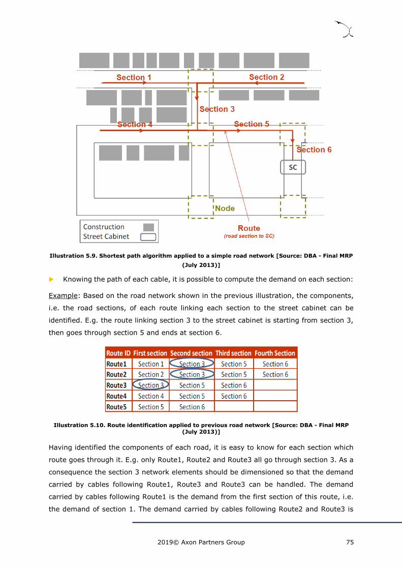
2019© Axon Partners Group 75
Illustration 5.9. Shortest path algorithm applied to a simple road network [Source: DBA - Final MRP
(July 2013)]
Knowing the path of each cable, it is possible to compute the demand on each section:
Example: Based on the road network shown in the previous illustration, the components,
i.e. the road sections, of each route linking each section to the street cabinet can be
identified. E.g. the route linking section 3 to the street cabinet is starting from section 3,
then goes through section 5 and ends at section 6.
Illustration 5.10. Route identification applied to previous road network [Source: DBA - Final MRP (July 2013)]
Having identified the components of each road, it is easy to know for each section which
route goes through it. E.g. only Route1, Route2 and Route3 all go through section 3. As a
consequence the section 3 network elements should be dimensioned so that the demand
carried by cables following Route1, Route3 and Route3 can be handled. The demand
carried by cables following Route1 is the demand from the first section of this route, i.e.
the demand of section 1. The demand carried by cables following Route2 and Route3 is

2019© Axon Partners Group 76
likewise respectively the demand of section 2 and section 3. Therefore, the network
elements located on section 3 should handle the demand of section 1, section 2 and section
3.
Knowing the demand and using the network dimensioning rules (such as spare
capacity), it is possible to assess exactly the number of copper pairs/fibres/cables
needed on each section;
Using the list of available cables, it is therefore possible to assess the number and the
size of the cables that need to be rolled out on each section;
The number of ducts and then the size of the trenches are directly derived from the
number of cables rolled out. However, these do not depend only on the cables rolled
out for the access network but depend also on the cables rolled out for the core
network. Indeed the core cables are sometimes sharing the same trenches and
potentially the same ducts as the cables rolled out for the access network. It is
therefore necessary to dimension the infrastructure part of the core network at the
section level.
The dimensioning of the core network infrastructure is detailed in section ‘5.4.3 Core and
transmission networks’.
Other elements are also dimensioned at the section level:
One piece of jointing equipment is installed for each cable at each crossroad (so at
the beginning of each section as a section is the part of a road located between two
crossroads). Indeed, a piece of jointing equipment is needed at each crossroad either
to cross the road or to turn;
One piece of jointing equipment is installed for each cable if the distance between two
jointing equipment installed by the previous rules exceeds a threshold set according
to operators’ rules.
Knowing the locations of the jointing equipment, it is then possible to compute the
number of chambers required as a piece of jointing equipment should be installed in
a chamber in case the network is underground (on a pole if the network is aerial).
Supporting criterion 33: The access and transmission networks should be
dimensioned at section level.

2019© Axon Partners Group 77
5.4.3. Core and transmission networks
5.4.3.1. Dimensioning of the active transmission elements
Within an all-IP core network there is no need for SDH/PDH transport networks.
Specific equipment for data transport, rather than switching/routing, is therefore likely to
be limited to the use of repeaters on long distance routes.
Microwave links should be avoided wherever practical due to the relatively limited data
carrying capacity of such links compared to fibre optic cable.
Supporting criterion 34: Repeaters should only be used on long distance routes. Any
use of microwave links within the core network will also need to be justified.
5.4.3.2. Dimensioning of the civil infrastructure for the transmission network
Modelling infrastructure is a very important part of modelling the transmission network
because the infrastructure is likely to be the most expensive part, accounting for up to 80
percent of the investment in an all-IP transmission network. It can also be a contentious
exercise since the same assets are used to support a large number of different services,
implying significant shared and common costs which will need to be allocated.
In this section, the infrastructure category is defined to include all trench, duct and fibre
optic cables (and ancillary items such as manholes, fibre splicing trays etc.).
Supporting criterion 35: The LRAIC model should identify infrastructure costs
associated with the transmission network. The model should identify separately the
costs of cable, duct and trenches.
Core cables
Contrary to the access network, the core network includes often resilient routes.
Furthermore, the path followed by the core cables may not be the shortest path between
two core nodes and resilient cables are often following different paths. This is generally
due to the specificities of each country and is therefore more difficult to model properly
from a bottom-up perspective. Moreover, these paths may not follow the road network or
may follow some roads that the access network is not following such as highways.
The first step of modelling the core infrastructure is therefore to collect a digitalised map
of the core cables network from the operator. With this map, it is possible to count the

2019© Axon Partners Group 78
number of core cables located in each section in Denmark or to determine the list of
connections between core sites.
In accordance with section ‘5.4 Network dimensioning’ the number of fibres per cable
should be calculated using bottom-up demand for fibre (this is possible for fibre cables
that goes out existing sites of the network), existing configurations and assessment of the
impact of DWDM in the need for fibre in the modelled operator’s network.
The length of each cable on each section should be determined on the basis of the shortest
path algorithm. To apply this algorithm the list of physical connections between sites of
the core network (including resilient connections) will be requested to the modelled
operator.
Supporting criterion 36: The core cables network data (list of connections between
core sites) should be collected from the modelled operator.
Core ducts
Knowing the number and size of core cables located in each section in Denmark, the
number of ducts (and possibly micro-ducts or sub-ducts, depending on the engineering
principles used) required per section is derived.
The length of each duct should be the length of the section.
Supporting criterion 37: The length and the cost of the core ducts should be derived
from the core cables calculations.
Trenches
Trenches should be constructed wherever a core cable is rolled out (only one trench on
one section even if multiple cables are rolled out).
The trenches are shared between the core network and the access network as explained
in section ‘5.6 Allocation of costs to services’.
Supporting criterion 38: The LRAIC model should show the amount of duct and
trench that is common to the core and the access network and any other utility. It
should show also the amount of duct and trench specific to the core network and to the
access network.

2019© Axon Partners Group 79
5.4.3.3. Dimensioning of the core platforms
Core platforms required to provide the modelled services will be included in the model. In
order to perform the dimensioning of these platforms, the model will rely on the capacity
of the typical platforms installed by the modelled operator and the demand requirements
that these elements shall satisfy.
5.5. Costing the Network
Having dimensioned the network, i.e. having assessed for each section which and how
many elements are needed, it is possible now to calculate the cost of the network.
Calculating the cost of the network includes estimating the level of the capital expenditures
and the operating expenditures separately for each type of network element:
Capital expenditures: Based on the number of network elements of a given type
required for each year, the model will assess the associated investment levels. These
investments shall be annualised for each type of network element based on the
methodologies determined in section ‘4.4 Depreciation Methodologies’ This cost
category will include both, depreciation and cost of capital charges.
Operational expenditures: The total operational expenditures for each type of
network element for a given year can be calculated by multiplying the unitary yearly
OpEx by the number of network elements required for that given year.
Once these costs have been calculated for the whole network, these are ready to be
allocated to services.
5.6. Allocation of costs to services
The final step in the process will be to calculate the costs for various services under
scrutiny. Based on the hypothetical network that has been built, the model needs to
calculate the LRAIC costs attributable to each of the various services.
This means that all of the different cost categories - direct network costs, indirect network
costs, operating costs and overheads - will be aggregated into network elements that will
form the “building blocks” when calculating the costs of the services.
The cost categories that fall under the heading direct network costs should be sufficiently
disaggregated that each cost category has only one cost driver. For example, a DSLAM
consists of both line cards and concentrating functionality, and therefore its costs depend
2019© Axon Partners Group 80
on subscribers and traffic. Therefore, there should be at least two cost categories, the
costs of line cards and the costs of concentrating functionality (this can theoretically be
split into more than one cost category depending on the modularity of the equipment
acquired), instead of a single cost category measuring the total cost of the equipment.
Supporting criterion 39: The LRAIC model should identify cost categories such that
there is only one exogenous cost driver for each. The model should aggregate, in a
clear manner, the cost of network elements used in the modelled services such that it
is clear how the overall cost of a particular service is comprised of the cost of individual
network elements.
The allocation of the network costs to services will be based on the methodologies
described in section 4.1 Direct, Indirect costs and Corporate Overheads.
However, for the sake of clarity, the paragraphs below describe the specific approach to
be adopted with regards to two areas of special relevance for the model:
Allocation of shared costs of civil infrastructure
Allocation of costs to access services
5.6.1. Allocation of shared costs of civil infrastructure
Key area of discussion below: Allocation of civil infrastructure costs from access and
transmission networks.
As detailed in section ‘5.4 Network dimensioning’, civil infrastructure is commonly shared
between access and core/transmission networks. It is therefore necessary to define a
specific allocation methodology to disaggregate the costs of these elements between the
access and core networks (and, therefore, between the services provided in each of them).
Based on the information available at road section level for both ducts and trenches,
including the identification of the presence or not of cables rolled out for the access
network and the core/transmission network, the costs of that road section will be allocated
between access and core networks. Particularly, this allocation will be performed by
splitting the costs of the trenches and ducts proportionally to the length occupied by the
core and access assets.
If there are only access cables in one section then 100% of the trench costs should be
allocated to the access network and reciprocally, if in one section, there are only core
cables, then 100% of the trench costs should be allocated to the core network. Same rules

2019© Axon Partners Group 81
can be used for sharing with other types of networks (such as electricity, water or mobile
telecom networks).
Main criterion 17: The cost of shared assets (trenches and possibly ducts) between
the access and the core networks should be split based on the total surface (area)
occupied by the cables they use.
Question 16: Do you agree with the proposed allocation mechanism to split the costs
of shared assets between access and core networks?
If you don’t agree, please justify your position and provide supporting information and
references.
5.6.2. Allocation of costs to access services
The model will calculate the costs of access services based on the costs that are line-
dependant.
For that purpose, the sum of annualised capital expenditures and operating costs will be
divided by the appropriate number of active lines.
The LRAIC model will have the ability to assess the costs at different geographical levels
which will enable the comparison of the cost distribution over the country (see section ‘6.1
Geographical De-Averaging’).
Supporting criterion 40: The LRAIC model should compute a cost per line for each
geographical level by dividing the sum of the annualised capital expenditures and the
operating costs by the appropriate number of present active lines.
5.7. Ancillary services
Ancillary services refer to ad-hoc services that support the provision of the main services
defined in section ‘3.3 Services’ such as VULA, bitstream or local loop unbundling. For
instance, typically, the initiation of the provision of a new bitstream service requires a one-
off activation/installation service or activity as well as a co-location to interconnect the
equipment of the access seekers.
Given that these ancillary services are an intrinsic part of any reference offer, the fixed
LRAIC model should be capable of determining their costs. However, differently from the
main services defined in section ‘3.3 Services’, a bottom-up calculation is not the most

2019© Axon Partners Group 82
appropriate approach to determine the costs of the ancillary services, as these are mostly
based on one-time actions (e.g. activations), or recurrent processes which should be
analysed from a top-down perspective (e.g. space occupied for co-location).
Therefore, a specific calculation module will be included in the fixed LRAIC model, which
will not be directly connected to the cost calculations performed for the services defined
in section ‘3.3 Services’ to determine the costs of the ancillary services. The main inputs
for the calculation of the costs of the ancillary services will be:
The time (measured in man-hours) required from internal and external employees to
carry out the one-time actions.
The man-hour cost of the internal and external employees involved in the execution
of the one-time actions.
The cost of other necessary resources (e.g. materials, systems, etc.) involved in the
provision of the service.
The model should include all the relevant ancillary services based on DBA’s regulatory
needs. The full list of ancillary services (along with the main service associated) to be
included in the model is presented in the following table.
Main Service Ancillary service
LLU New Installation- Unassisted
LLU New Installation- Engineer assisted
LLU Inquiry
LLU New setup
LLU Physical rearrangement
LLU Change to trunk number
LLU Visit by technician
LLU Cancellation-fee II
LLU Calculation of attenuation on the line
LLU Unproductive fault handling
LLU Raw copper -full loop: migration to full loop from BSA
LLU Raw copper -full loop: migration to full loop from Shared Raw Copper, full loop
LLU NTP
LLU NTP incl. Drilling
Shared LLU New Installation- Unassisted
Shared LLU New Installation- Engineer assisted
Shared LLU Inquiry
Shared LLU New setup

2019© Axon Partners Group 83
Main Service Ancillary service
Shared LLU Physical rearrangement
Shared LLU Change of trunk number
Shared LLU Visit by technician
Shared LLU Cancellation-fee II
Shared LLU Calculation of attenuation on the line
Shared LLU Unproductive fault handling
Shared LLU Shared raw copper -full loop: migration to shared full loop
from BSA with telephony
Shared LLU NTP
Shared LLU NTP incl. Drilling
LLU sub loop New Installation- Unassisted
LLU sub loop New Installation- Engineer assisted
LLU sub loop Inquiry
LLU sub loop New setup
LLU sub loop Physical rearrangement
LLU sub loop Change to trunk number
LLU sub loop Visit by technician
LLU sub loop Cancellation-fee II
LLU sub loop Calculation of attenuation on the line
LLU sub loop Unproductive fault handling
LLU sub loop Raw copper -sub loop: migration to sub loop from BSA
LLU sub loop Raw copper -sub loop: migration to sub loop from Raw Copper, full loop
LLU sub loop Raw copper -sub loop: migration to sub loop from Shared Raw Copper, full loop
LLU sub loop Raw copper -sub loop: migration to sub loop from Shared Raw Copper, sub loop
LLU sub loop NTP
LLU sub loop NTP incl. Drilling
Shared LLU sub loop New Installation- Unassisted
Shared LLU sub loop New Installation- Engineer assisted
Shared LLU sub loop Inquiry
Shared LLU sub loop New setup
Shared LLU sub loop Physical rearrangement
Shared LLU sub loop Change of trunk number
Shared LLU sub loop Visit by technician
Shared LLU sub loop Cancellation-fee II
Shared LLU sub loop Calculation of attenuation on the line
Shared LLU sub loop Unproductive fault handling
Shared LLU sub loop Shared raw copper -sub loop: migration to sub loop from BSA

2019© Axon Partners Group 84
Main Service Ancillary service
Shared LLU sub loop Shared raw copper -sub loop: migration to sub loop from Shared Raw Copper, full loop
Shared LLU sub loop NTP
Shared LLU sub loop NTP incl. Drilling
BSA/VULA New Installation- Unassisted
BSA/VULA New Installation- Engineer assisted
BSA/VULA Reactivated installation- Unassisted
BSA/VULA Reactivated installation- Engineer assisted
BSA/VULA Additional work for a new installation of "BSA without co-
production
BSA/VULA Conversion from BSA online to BSA without co-production
BSA/VULA Conversion from ATM BSA to BSA/VULA
BSA/VULA Installation of Multichannel
BSA/VULA Change of speed BSA
BSA/VULA Migration to BSA/VULA with telephony from BSA/VULA without telephony
BSA/VULA Migration to BSA/VULA from Raw Copper, full loop
BSA/VULA Migration to BSA/VULA from Shared Raw Copper, full loop
BSA/VULA NTP
BSA/VULA NTP incl. Drilling
Co-location in technical house Co-location in technical house
Co-location in technical house Multiplexing - setup
Co-location in technical house Multiplexing - annual cost
Resources other services Setup of pre-selection
Resources other services Implementation of prefix for pre-selection
Resources other services Local POI - Installation
Resources other services Local POI - Management
Resources other services Interconnection capacity (2 Mbit/s port/30-group) - Setup
Resources other services Interconnection capacity (2 Mbit/s port/30-group) - Annual
cost
Resources other services Supervised access
Resources other services New Installation, Street Cabinet Backhaul - duct
Resources other services New Installation, Street Cabinet Backhaul - dark fibre
Resources other services New Installation, Bitstream Transport
Resources other services New Installation, Multicast - first channel
Resources other services New Installation, Multicast - additional channel
LLU Re-establishing trunks
LLU Cancellation fee II
LLU Calculation of attenuation on the line
LLU Migration of 30 or more connections in a project
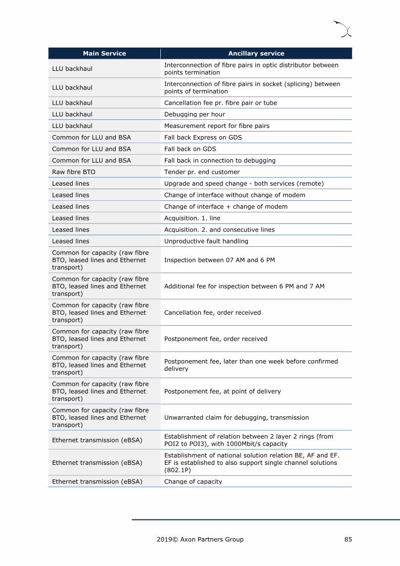
2019© Axon Partners Group 85
Main Service Ancillary service
LLU backhaul Interconnection of fibre pairs in optic distributor between points termination
LLU backhaul Interconnection of fibre pairs in socket (splicing) between points of termination
LLU backhaul Cancellation fee pr. fibre pair or tube
LLU backhaul Debugging per hour
LLU backhaul Measurement report for fibre pairs
Common for LLU and BSA Fall back Express on GDS
Common for LLU and BSA Fall back on GDS
Common for LLU and BSA Fall back in connection to debugging
Raw fibre BTO Tender pr. end customer
Leased lines Upgrade and speed change - both services (remote)
Leased lines Change of interface without change of modem
Leased lines Change of interface + change of modem
Leased lines Acquisition. 1. line
Leased lines Acquisition. 2. and consecutive lines
Leased lines Unproductive fault handling
Common for capacity (raw fibre BTO, leased lines and Ethernet transport)
Inspection between 07 AM and 6 PM
Common for capacity (raw fibre BTO, leased lines and Ethernet
transport)
Additional fee for inspection between 6 PM and 7 AM
Common for capacity (raw fibre
BTO, leased lines and Ethernet
transport)
Cancellation fee, order received
Common for capacity (raw fibre
BTO, leased lines and Ethernet transport)
Postponement fee, order received
Common for capacity (raw fibre BTO, leased lines and Ethernet transport)
Postponement fee, later than one week before confirmed delivery
Common for capacity (raw fibre BTO, leased lines and Ethernet transport)
Postponement fee, at point of delivery
Common for capacity (raw fibre BTO, leased lines and Ethernet transport)
Unwarranted claim for debugging, transmission
Ethernet transmission (eBSA) Establishment of relation between 2 layer 2 rings (from
POI2 to POI3), with 1000Mbit/s capacity
Ethernet transmission (eBSA) Establishment of national solution relation BE, AF and EF. EF is established to also support single channel solutions (802.1P)
Ethernet transmission (eBSA) Change of capacity

2019© Axon Partners Group 86
Main Service Ancillary service
Bit Stream Access (eBSA og common for eBSA, VULA and Fibre BSA)
Change of speed
Bit Stream Access (eBSA og common for eBSA, VULA and Fibre BSA)
Move
Bit Stream Access (eBSA og common for eBSA, VULA and Fibre BSA)
Conversion GDS between PSTN and ISDN
Bit Stream Access (eBSA og common for eBSA, VULA and Fibre BSA)
Unproductive visit (Technician)
Bit Stream Access (eBSA og common for eBSA, VULA and Fibre BSA)
Cancellation
Bit Stream Access (eBSA og common for eBSA, VULA and Fibre BSA)
Mac addresses 32/64
Bit Stream Access (eBSA og common for eBSA, VULA and
Fibre BSA)
Conversion between eBSA and ATM BSA
Bit Stream Access (eBSA og
common for eBSA, VULA and Fibre BSA)
POI GE Switch-port
Bit Stream Access specifically for Multicast
Specification of parameters in multicast setup in relation to the establishing a customer
Bit Stream Access specifically for
Multicast Implementation of specific customer.
Co-location Inquiry
Co-location Offer
Co-location Trunk cables PDS 2*cat.5 Installation
Co-location Trunk cables PDS 2*cat.5 per 10 m
Co-location Trunk cables PDS 10*cat.5 Installation
Co-location Trunk cables PDS 10*cat.5 per 10 m
Co-location Trunk cables 12 fibre pair (sm) Installation
Co-location Trunk cables 12 fibre pair (sm) per 10 m
Co-location Internal cabling mm PDS 2*cat.5 Installation
Co-location Internal cabling mm PDS 2*cat.5 per 10 m
Co-location Internal cabling mm PDS 10*cat.5 Installation
Co-location Internal cabling mm PDS 10*cat.5 per 10 m
Co-location Internal cabling mm 12 fibre pair (sm) Installation
Co-location Internal cabling mm 12 fibre pair (sm) per 10 m
Co-location Internal cabling mm 8 Coax pair Installation
Co-location Internal cabling mm 8 Coax pair per 10 m
Co-location Internal cabling mm 24 coax pair Installation

2019© Axon Partners Group 87
Main Service Ancillary service
Co-location Internal cabling mm 24 coax pair per 10 m
Co-location Internal cabling mm 100 copper pair Installation
Co-location Internal cabling mm 100 copper pair per 10 m
Co-location Internal cabling mm 3*100 copper pair Installation
Co-location Internal cabling mm 3*100 copper pair per 10 m
Co-location Internal cabling in-span fibre Installation
Co-location Internal cabling in-span fibre per 10 m
Co-location Technical house led/cover - delivery of led/cover
Co-location Technical closet in technical house - installation
Co-location Technical closet in technical house - Monitoring and battery check
Co-location Technical closet in technical house - 48 VDC 100W. Installation of point outlet with cable and fuse
Co-location Technical closet in technical house 48 VDC 100W - Each year inclu. Utilities
Co-location, specifically for closets Delivery and installation of DSL closet without co-production
Co-location, specifically for closets Delivery and installation of DSL closet with co-production
Co-location, specifically for closets 230 VAC, 4A supply incl. Fuse and monitoring device
Co-location, specifically for closets 1x100 pair cables and fibre trunk incl. Digging and termination of 1x100 copper pairs and 4 fibres
Co-location, specifically for closets 1x100 pair cable with termination at TDC
Co-location, specifically for closets Fibre trunk with termination of 4 fibres i distributor at TDC
Co-location, specifically for closets Fibre trunk with termination of 4 fibres in socket (splicing) at TDC
Common for LLU and BSA Manuel order
Exchange of traffic Pre fix for switched interconnection, basic fee, implementation
Exchange of traffic Pre fix for switched interconnection, per central, implementation
Exchange of traffic Pre fix with same routing as established pre fix from same operator for switched interconnection, per central, implementation
Exchange of traffic Pre fix for switched interconnection, per central, change
Exchange of traffic Pre fix with same routing as established pre fix from same
operator for switched interconnection, per central, change
Exchange of traffic Pre fix for local interconnection, per central, change
Colocation Hourly rate for re-registration of co-location, e.g. from quarterly to monthly payment of rent
Cables Processing of inquiry on cables, per hour

2019© Axon Partners Group 88
Main Service Ancillary service
LLU Additional fee for cable distributor
Fibre BSA Digging/blowing per meter, above 30 meters, per meter
Resources Co-location specific site cost
Room fit-out
Resources Co-location specific site cost
Cable trenches
Resources Power Power Installation (1 * 48 VCD 16 A)
Resources Power Power Installation (1 * 48 VDC 30 A)
Resources Power Power Installation (1 * 48 VDC 60 A)
Resources Power Power Installation (1 * 230 VAC 10 A)
Resources Power Power Installation (1 * 230 VAC 10 A service socket)
Resources Power Shift to another power-product
Resources Power Power Usage (1 * 48 VCD 16 A)
Resources Power Power Usage (1 * 48 VDC 30 A)
Resources Power Power Usage (1 * 48 VDC 60 A)
Resources Power Power Usage (1 * 230 VAC 10 A)
Resources Power Power Usage (1 * 230 VAC 10 A service socket)
Resources Land Outdoor space - Land
Resources Land Indoor space - Buildings
PSTN Unproductive fault handling
Illustration 5.1. List of ancillary services [Source: Axon Consulting]

2019© Axon Partners Group 89
6. Model outputs
6.1. Geographical De-Averaging
Key area of discussion below: Level of disaggregation of the results to be produced
by the model.
Costs are likely to differ significantly between areas in the access network; variations are
likely to be smaller, in relative terms, for the core network. In addition, it is quite difficult
to measure costs by area in the core network since, for example, transmission links may
pass through more than one type of area.
Focusing on the access example, there are at least three reasons for differences in costs
by area:
trenching/ducting costs are likely to be higher in urban than rural areas;
distances between the exchange and the customer tend to be shorter in urban than
in rural areas; and
cables tend to carry more pairs in urban than rural areas.
The first factor would result in higher access costs in urban areas; the latter two factors in
lower costs. In overall terms the last two factors are likely to dominate, implying lower
access costs in urban areas. The difference could be significant.
In this regard the model shall be aligned with the regulatory needs of DBA. Particularly, in
the latest analysis of markets 3a and 3b, DBA lifted the price regulation obligations
applicable to TDC for fibre-related services in some specific areas of Denmark, introducing
a geographical disaggregation of the regulatory obligations imposed.
Therefore, the model shall be able to calculate the costs stemming from regulated areas
only. While so far, the distinction between regulated and deregulated is performed at
postal code level, the model should be able to accommodate other levels of disaggregation
(e.g. central office or even household level).
The default level of disaggregation of the results should include:
Disaggregation per geotype (e.g. urban, suburban and rural). This disaggregation will
be at DSLAM/OLT/CMTS level in order to ensure all access elements belong to a single
geotype. The disaggregation of the country per geotype will be based on the density
of buildings.

2019© Axon Partners Group 90
Disaggregation between regulated and non-regulated areas.
Disaggregation at regional level. This disaggregation will be based on the five regions
in Denmark (Hovedstaden, Midtjylland, Nordjylland, Sjælland and Syddanmark) to
ensure transmission costs are adequately represented.
Disaggregation between single-dwelling and multi-dwelling buildings.
Main criterion 18: The model will provide results at different levels of disaggregation
(geotype, regulated/deregulated areas, regions, single/multi dwelling units) as well as
nationwide. The model will also provide room to calculate costs at a higher level of
detail (e.g. central office or even household level) on an ad-hoc basis.
Question 17: Do you agree that the model should be able to provide results at different
levels of disaggregation (geotype, regulated/deregulated areas, regions, single/multi
dwelling units)?
If you don’t agree, please justify your position and provide supporting information and
references.
6.2. Level of Detail
The model should also seek to identify operating and asset costs separately. Only those
operating costs necessary to bring an asset into working for its intended use, such as
transport, installation and commissioning should be capitalised.
Supporting criterion 41: Costs related to assets can include capitalised operating
costs (“own work capitalised").
The results of the LRAIC model are service costs. In order to facilitate the understanding
and review of the LRAIC model, it is relevant to show not only service costs but also costs
of the service components. For example, rather than showing only the cost of a VULA/BSA
wholesale line, it could be very relevant to show also the cost components of this service,
such as the cost of the civil infrastructure, the cost of fibre, the cost of the splitters, etc.
Supporting criterion 42: The LRAIC model should have the ability to show not only
the cost of the services but also the cost of the components involved in the provision of
these services.
2019© Axon Partners Group 91
6.3. Charging basis
Several charging bases can be used to cost a given service. These charging bases include
(but are not limited to):
DKK per kbps (capacity-based charging);
DKK per line per month
For each service, the charging basis must be selected in order to provide the different
stakeholders with the appropriate incentives. It is also preferable for the charging basis to
be consistent with the cost drivers of the service. For instance, if BSA was priced on a ‘per
minute’ basis, it would not be in line with cost drivers (capacity). In addition, the charging
basis has to be compliant with the applicable legal and regulatory provisions.
Supporting criterion 43: The charging basis should be as consistent as possible with
the cost drivers of the service.

2019© Axon Partners Group 92
7. LRAIC model validation and update process
7.1. Top-down validation
The LRAIC model is based on a bottom-up approach. However, a top-down validation can
still be conducted in order to increase the robustness of the final costing results.
The outputs of the bottom-up model should be compared with modelled operator data.
This is a two-stage process:
calibrate the model assets in order to have output volumes that are broadly in line
with those of the modelled operator(s) (e.g. trench kilometres, cables kilometres);
broadly compare the model expenditures (separately for CAPEX and OPEX).
Where considered reasonably efficient, the model’s total CAPEX and OPEX should reflect
those of the modelled operator. This reconciliation should be performed with the highest
level of granularity possible, making sure that the cost items compared in the bottom-up
and the accounts have a comparable scope.
As a consequence, the data request will include some top-down information enabling to
perform the top-down validation.
Supporting criterion 44: Information to aid a top-down validation will be requested
from the modelled operator(s). The validation will include both a calibration of assets
and a reconciliation of the cost base. For the avoidance of doubt, information to aid a
top-down validation is limited to top-down asset information and cost data, which is
distinct from a top-down cost model based on operator accounts.
7.2. Update process
LRAIC models are forward-looking models which include some forecasts: forecasts on the
number of users, on the traffic, on the unit costs, etc. In order to inform DBA on the
evolution of service costs in the future and in particular in order to verify the extent to
which regulated prices evolve in line with underlying costs, a regular update of the LRAIC
model is necessary. DBA intends to carry out annual updates.
Such updates can be a lengthy process and require significant time for both DBA but mainly
the modelled operator. In order to facilitate the update of the LRAIC model, it is proposed
to create a template spreadsheet listing key inputs of the LRAIC model which need regular
updates. This template spreadsheet should be easily linked to a file system so that

2019© Axon Partners Group 93
including the new inputs into the LRAIC model is not a lengthy process. This will also
enable the modelled operator to collect updated data in a more automated way.
The LRAIC development process should therefore include the building of a template
spreadsheet enabling easier and more automated updates of the LRAIC model.
Supporting criterion 45: The LRAIC development process should include the building
of a template spreadsheet enabling easier and more automated updates of the LRAIC
model.
Question 18: Do you agree with the remaining criteria defined in the MRP for which
no specific questions have been asked to the industry?
If you don’t agree, please justify your position and provide supporting information and
references.

2019© Axon Partners Group 94
8. Appendix
8.1. List of criteria
The criteria for the LRAIC model set out by DBA are listed below, differentiating between
main and supporting criteria.
Main criteria
Main criterion 1: A Current Cost valuation should be adopted to set the unit costs of the
assets in the Bottom-Up cost model. Nevertheless, the GRC originated from fully
depreciated assets should not be taken into consideration for the reusable legacy assets
presented in Illustration 2.3.
Main criterion 2: The LRAIC model should be based on forward-looking long run average
incremental costs. No migration costs should be included. The LRAIC model should allow
coverage of common costs. These costs should be shown separately.
Main criterion 3: The model will calculate the service provisioning costs from 2018 to
2028. 2018 will be the base year of the model. Additionally, it will incorporate a time-
frame up to 2070 to properly implement the economic depreciation algorithms.
Main criterion 4: A single model will be built, with a single increment comprising all
access and traffic services. Costs of ancillary services (such as co-location, activation and
interconnection points) will be calculated stand-alone as they are not directly related to
the main network topology or architecture as such.
Main criterion 6: The model should include all relevant access, broadband leased line,
TV and ancillary services.
Main criterion 7: The model will not include voice services. Including voice services in
the model would complicate the model with a negligible impact on the cost calculation of
regulated services. Consistently, voice-specific core platforms (e.g. MGW) will not be
modelled either.
Main criterion 8: The LRAIC model should assume that each access network technology
supports its actual demand.
Main criterion 9: Capacity-based allocation for joint and common network costs should
be implemented in the LRAIC model.

2019© Axon Partners Group 95
Main criterion 10: Corporate overheads costs should be allocated on the basis of the
EPMU approach.
Main criterion 11: Prices used in the model should reflect those that an efficient operator
would face.
Main criterion 12: Operating costs should be calculated using a bottom-up assessment
based on a percentage of capital cost.
Main criterion 13: Tilted annuities and full economic depreciation should be implemented
in the LRAIC model.
Main criterion 14: WACC values considered in the cost model should be aligned with the
up to date decisions determined by DBA.
Main criterion 15: The LRAIC model should use as much as possible locations (X;Y
geographic coordinates) of each network node of the operators.
Main criterion 16: The model should use the coverage areas of the modelled operator.
Main criterion 17: The cost of shared assets (trenches and possibly ducts) between the
access and the core networks should be split based on the total surface (area) occupied
by the cables they use.
Main criterion 18: The model will provide results at different levels of disaggregation
(geotype, regulated/deregulated areas, regions, single/multi dwelling units) as well as
nationwide. The model will also provide room to calculate costs at a higher level of detail
(e.g. central office or even household level) on an ad-hoc basis.
Supporting criterion
Supporting criterion 1: For the cable-TV network, the model should enable to clearly
isolate the cost of those assets uniquely associated with individual subscribers. These costs
are specific to the passive access network for cable-TV and will include only the civil
infrastructure and the coax cables.
Supporting criterion 2: The model should consider line cards as part of the access
network. The DSLAM located at the cabinet (in the case of FTTC deployment) should be
considered as part of the core network. The cost of trenches should be allocated between
the core and access networks in consistency with the realities observed in the actual
networks.
2019© Axon Partners Group 96
Supporting criterion 3: When dimensioning the network, the leased-lines traffic volume
should include leased lines provided to retail customers, to other operators and to the
network operator. Leased lines used by the network operator should not be double
counted. The model should not calculate the costs of leased lines explicitly. Leased lines
should only be included for dimensioning of the network and for ensuring that a fair
amount of costs is allocated to leased line services as well.
Supporting criterion 4: For PTP, both an unbundling product at the ODF and a BSA
product will be modelled. For PON, both an unbundling product at the splitter and a BSA
product will be modelled.
Supporting criterion 5: Bitstream services in coaxial networks should be aligned with
the current wholesale commercial offers in the market.
Supporting criterion 6: The model should show, for each service, routing factors or, if
not possible, a consistent alternative measure of how, on average, each service uses the
core network and the access network. The model should also be flexible enough to allow
for changes in routing factors / alternative measures.
Supporting criterion 7: The model should only include IP packet switch technology.
Supporting criterion 8: The model should not include SDH.
Supporting criterion 9: The model should not include DWDM equipment in the core
network, except for long distances.
Supporting criterion 10: The model should include both PTP and PON network
architectures for FTTH networks.
Supporting criterion 11: The choice of technology and degree of optimisation is subject
to the scorched-node assumption and the requirement that the modelled network as a
minimum should be capable of providing comparable quality of service as currently
available on the modelled operator’s network, and be able to provide functionality
comparable to that of the existing services.
Supporting criterion 12: The cost of passing all the premises within an area should be
modelled. Drop wires should be deployed (or decommissioned) in the model based on the
strategies followed by SMP operator(s), as long as these are considered to be
representative of an efficient operator.

2019© Axon Partners Group 97
Supporting criterion 13: The LRAIC model will present the total direct network costs of
the different network elements separately for CAPEX and OPEX.
Supporting criterion 14: The LRAIC model should consider indirect costs, such as
accommodation, costs of installation, support systems, power, and cooling.
Supporting criterion 15: The LRAIC model should have the possibility of including a risk
premium for NGA/VHCN networks.
Supporting criterion 16: The LRAIC model should not include working capital
costs/revenues in the light of the financial data extracted from the current SMP operator).
Supporting criterion 17: The starting point when building the bottom-up model is the
level of demand in Denmark for all the modelled services.
Supporting criterion 18: The LRAIC model will include demand forecasts until 2028 for
the modelled services.
Supporting criterion 19: The LRAIC model should have the capability to be able to show
the demand for each major broadband service speed in terms of the number of customers.
Supporting criterion 20: Demand for TV services such as Multicast-IPTV and Video On
Demand should be included in the model.
Supporting criterion 21: The LRAIC model should show the demand of number of leased
lines by volume and bandwidth. Information should be sought on how the amount of leased
line capacity sold varies across the different regions of the country and by hierarchical
level within the network.
Supporting criterion 22: The usage factors used for the determination of the demand
drivers in the model need to be consistent with the underlying network architecture.
Supporting criterion 23: The LRAIC model should clearly identify busy-hour information
for all relevant traffic. The LRAIC model should also be flexible enough to allow for changes
in these figures. Information on the busy hour will need to be sourced from the operators
for all relevant services.
Supporting criterion 24: The LRAIC model should demonstrate that the modelled
network provides services at an appropriate level of quality for an efficient modelled
operator, particularly for real time traffic (such as IPTV) and non-contended (“leased
lines”) traffic.

2019© Axon Partners Group 98
Supporting criterion 25: The LRAIC model should show the costs of a network with an
efficient configuration operated by an efficient company, based on the latest proven
technological solutions and an optimally structured organisation. However, the starting
point should be the existing geographic network architecture in the modelled operator’s
network. This implies that equipment should be placed at the existing geographical
locations of the modelled operator’s network nodes (the scorched node assumption).
Supporting criterion 26: The hierarchy of the exchanges adopted in the LRAIC model
should be kept unchanged. The use of DSL cards instead of POTS cards should be
modelled.
Supporting criterion 27: The hierarchical design adopted in the LRAIC model considers
the following factors: cost, the impact on other parts of the network, security, technical
feasibility, and consistency with the evolution of the telecoms networks.
Supporting criterion 28: The LRAIC cost model will be based on a database software
and Microsoft Excel. The usage of database solutions will be limited to the geographical
assessment of the access network to facilitate the review and understanding of the LRAIC
model by stakeholders.
Supporting criterion 29: The LRAIC model should use the road network database
provided by the DAR.
Supporting criterion 30: The LRAIC model should use the data on buildings provided by
DAR or equivalent sources if not available.
Supporting criterion 31: The LRAIC model should use the operators’ networks
hierarchies. However, as regards fibre access network, PTP should be modelled with the
same hierarchy as other access networks.
Supporting criterion 32: The LRAIC model should use the “shortest path algorithm” to
connect two nodes together by following the real Danish road and street network.
Supporting criterion 33: The access and transmission networks should be dimensioned
at section level.
Supporting criterion 34: Repeaters should only be used on long distance routes. Any
use of microwave links within the core network will also need to be justified.
2019© Axon Partners Group 99
Supporting criterion 35: The LRAIC model should identify infrastructure costs associated
with the transmission network. The model should identify separately the costs of cable,
duct and trenches.
Supporting criterion 36: The core cables network data (list of connections between core
sites) should be collected from the modelled operator.
Supporting criterion 37: The length and the cost of the core ducts should be derived
from the core cables calculations.
Supporting criterion 38: The LRAIC model should show the amount of duct and trench
that is common to the core and the access network and any other utility. It should show
also the amount of duct and trench specific to the core network and to the access network.
Supporting criterion 39: The LRAIC model should identify cost categories such that
there is only one exogenous cost driver for each. The model should aggregate, in a clear
manner, the cost of network elements used in the modelled services such that it is clear
how the overall cost of a particular service is comprised of the cost of individual network
elements.
Supporting criterion 40: The LRAIC model should compute a cost per line for each
geographical level by dividing the sum of the annualised capital expenditures and the
operating costs by the appropriate number of present active lines.
Supporting criterion 41: Costs related to assets can include capitalised operating costs
(“own work capitalised").
Supporting criterion 42: The LRAIC model should have the ability to show not only the
cost of the services but also the cost of the components involved in the provision of these
services.
Supporting criterion 43: The charging basis should be as consistent as possible with the
cost drivers of the service.
Supporting criterion 44: Information to aid a top-down validation will be requested from
the modelled operator(s). The validation will include both a calibration of assets and a
reconciliation of the cost base. For the avoidance of doubt, information to aid a top-down
validation is limited to top-down asset information and cost data, which is distinct from a
top-down cost model based on operator accounts.

2019© Axon Partners Group 100
Supporting criterion 45: The LRAIC development process should include the building of
a template spreadsheet enabling easier and more automated updates of the LRAIC model.
8.1.1. Comparison of BU criteria with respect to the MRP from July
2013
The table below presents, for each of the BU criteria included in the 2013 MRP, the
corresponding criteria in the current document.
BU Criteria (MRP from July 2013) BU Criteria (Current)
Criterion BU 1: The LRAIC model should
include the ability to use historic cost information for some assets.
Main criterion 1: A Current Cost valuation should be adopted to set the unit costs of the assets in the Bottom-Up cost model.
Nevertheless, the GRC originated from fully depreciated assets should not be taken into
consideration for the reusable legacy assets presented in Illustration 2.3.
Criterion BU 2: The LRAIC model should be based on forward-looking long run average incremental costs. No migration costs should be included. The LRAIC model should allow coverage of common costs. These costs should be shown separately.
Main criterion 2: The LRAIC model should be based on forward-looking long run average incremental costs. No migration costs should be included. The LRAIC model should allow coverage of common costs. These costs should be shown separately.
Criterion BU 3: The LRAIC model should be able to calculate the wholesale call termination cost on the basis of the pure LRIC approach.
The applied method will be similar to the one implemented in the latest version of the LRAIC model.
BU Criterion removed from the MRP
Criterion BU 4: Access and core networks should be modelled separately.
Main criterion 4: A single model will be built, with a single increment comprising all access and traffic services. Costs of ancillary services (such as co-location, activation and interconnection points) will be calculated stand-alone as they are not directly related to the
main network topology or architecture as such.
Criterion BU 5: For the core network, the increment should include all services that use the core network. For the access network, the increment should include all services that use the access network. The LRAIC of co-location is the cost incurred in providing co-location services.
BU Criterion removed from the MRP
Criterion BU 6: For the cable-TV network, the model should enable to clearly isolate the cost of those assets uniquely associated with individual subscribers.
Supporting criterion 1: For the cable-TV
network, the model should enable to clearly
isolate the cost of those assets uniquely associated with individual subscribers. These costs are specific to the passive access network for cable-TV and will include only the civil infrastructure and the coax cables.

2019© Axon Partners Group 101
BU Criteria (MRP from July 2013) BU Criteria (Current)
Criterion BU 7: The models should include line cards in the access increment. The DSLAM located at the cabinet (in the case of FTTC deployment) should be considered as part of the core network. The cost of trenches should be assessed in the access model but corresponding costs should then be allocated
between the core and access networks.
Supporting criterion 2: The model should consider line cards as part of the access network. The DSLAM located at the cabinet (in the case of FTTC deployment) should be considered as part of the core network. The cost of trenches should be allocated between the core and access networks in consistency with
the realities observed in the actual networks.
Criterion BU 8: The LRAIC models should
include all services on the copper, cable and FTTH networks. This includes voice, broadband, TV and leased lines services.
BU Criterion removed from the MRP
Criterion BU 9: The models should include all relevant voice and broadband services.
Main criterion 6: The model should include all relevant access, broadband leased line, TV and ancillary services.
Criterion BU 10: When dimensioning the network, the leased-lines traffic volume should include leased lines provided to retail customers, to other operators and to the network operator.
Supporting criterion 3: When dimensioning the network, the leased-lines traffic volume should include leased lines provided to retail customers, to other operators and to the network operator. Leased lines used by the
network operator should not be double counted. The model should not calculate the costs of leased lines explicitly. Leased lines should only be included for dimensioning of the network and for ensuring that a fair amount of costs is allocated to leased line services as well.
Criterion BU 11: The models should include all the “other services”.
BU Criterion removed from the MRP
Criterion BU 12: The model should include all the relevant copper access services.
Main criterion 6: The model should include all relevant access, broadband leased line, TV and
ancillary services.
Criterion BU 13: For PTP, both an unbundling product at the ODF and a BSA product will be modelled. For PON, both an unbundling product at the splitter and a BSA product will
be modelled.
Supporting criterion 4: For PTP, both an
unbundling product at the ODF and a BSA product will be modelled. For PON, both an unbundling product at the splitter and a BSA product will be modelled.
Criterion BU 14: Both bitstream services cited in DBA’s decision for market 5 will be modelled for the cable-TV network. The modelling will reflect the strategy of an efficient operator
building a new cable-TV network. Centralised BSA will be modelled as a combination of de-centralised BSA and an IP transport product. The inclusion/exclusion of CPE from the model scope should be in line with the scope of TDC wholesale offers: if bitstream offers do not
include the CPE then it should not be taken
into account in the model. Currently, the cable-TV regulation is being reviewed by DBA. The model must be able to reflect outcomes of this review.
Supporting criterion 5: Bitstream services in coaxial networks should be aligned with the current wholesale commercial offers in the market.

2019© Axon Partners Group 102
BU Criteria (MRP from July 2013) BU Criteria (Current)
Criterion BU 15: The models should show, for each service, routing factors or, if not possible, a consistent alternative measure of how, on average, each service uses the core network and the access network. The models should also be flexible enough to allow for changes in
routing factors / alternative measures.
Supporting criterion 6: The model should show, for each service, routing factors or, if not possible, a consistent alternative measure of how, on average, each service uses the core network and the access network. The model should also be flexible enough to allow for changes in routing factors / alternative
measures.
Criterion BU 16: The models should only include IP packet switch technology.
Supporting criterion 7: The model should only include IP packet switch technology.
Criterion BU 17: The models should not include SDH.
Supporting criterion 8: The model should not include SDH.
Criterion BU 18: The models should include microwave at a small extent.
BU Criterion removed from the MRP
Criterion BU 19: The models should not include
DWDM equipment in the core network, except for long distances.
Supporting criterion 9: The model should not include DWDM equipment in the core network, except for long distances.
Criterion BU 20: The models should include both PTP and PON network architectures for FTTH networks.
Supporting criterion 10: The model should include both PTP and PON network architectures for FTTH networks.
Criterion BU 21: The choice of technology and degree of optimisation is subject to the scorched-node assumption and the requirement that the modelled network as a
minimum should be capable of providing
comparable quality of service as currently available on the SMP operator’s network, and be able to provide functionality comparable to that of the existing products and services.
Supporting criterion 11: The choice of technology and degree of optimisation is
subject to the scorched-node assumption and the requirement that the modelled network as a minimum should be capable of providing comparable quality of service as currently
available on the modelled operator’s network, and be able to provide functionality comparable
to that of the existing services.
Criterion BU 22: The LRAIC model should
assume that each access network technology supports 100% of TDC’s local fixed network present demand in terms of active subscriptions (i.e. 100% of the “copper + cable-TV + fibre” demand).
Main criterion 8: The LRAIC model should assume that each access network technology supports its actual demand.
Criterion BU 23: The cost of passing all the premises within an area should be modelled. Drop wires should be deployed for active
customers but also for some inactive customers to reflect the natural level of churn and to reflect the fact that in buildings with
several accommodations it is more efficient to deploy drop wires to all accommodations at once even if some accommodations host inactive customers. Corresponding costs
should be recovered over the subset of connected locations assumed to have an active subscription.
Supporting criterion 12: The cost of passing all the premises within an area should be modelled. Drop wires should be deployed (or decommissioned) in the model based on the
strategies followed by SMP operator(s), as long as these are considered to be representative of an efficient operator.

2019© Axon Partners Group 103
BU Criteria (MRP from July 2013) BU Criteria (Current)
Criterion BU 24: The starting point when building the LRAIC model for the core network is the level of demand in TDC’s network for all the services using the copper, cable-TV and fibre access networks.
BU Criterion removed from the MRP
Criterion BU 25: Both the capacity-based and the Shapley-Shubik allocation rules for joint and common network costs should be implemented in the LRAIC models.
Main criterion 9: Capacity-based allocation for joint and common network costs should be implemented in the LRAIC model.
Criterion BU 26: Corporate overheads costs should be allocated on the basis of the EPMU approach.
Main criterion 10: Corporate overheads costs should be allocated on the basis of the EPMU
approach.
Criterion BU 27: Prices used in the models should reflect those that an efficient operator
with the bargaining power of an SMP operator would face.
Main criterion 11: Prices used in the model should reflect those that an efficient operator
would face.
Criterion BU 28: Initially, model cost inputs should be based on the latest available information and traffic and subscription data will subsequently be updated to reflect 2014. In subsequent years, the base year of the
model will be adjusted accordingly.
BU Criterion removed from the MRP
Criterion BU 29: The models should use a
Modern Equivalent Asset concept to estimate current costs. Replacement cost in the model should correspond to the cost of buying new equipment in the base year.
BU Criterion removed from the MRP
Criterion BU 30: Operating costs should be calculated using one of the following approaches depending on their feasibility (e.g.
information availability): Top-down assessment with potential efficiency
adjustments, bottom-up assessment based on a percentage of capital cost, bottom-up assessment based on necessary employees, true bottom-up assessment.
Main criterion 12: Operating costs should be calculated using a bottom-up assessment based on a percentage of capital cost.
Criterion BU 31: Tilted annuities and full economic depreciation (where volumes of outputs can change significantly) should be used in the LRAIC model. However, as in the access network, demand is supposed to be
fairly stable (see §3.4.1), only tilted annuities will be implemented.
Main criterion 13: Tilted annuities and full economic depreciation should be implemented in the LRAIC model.
Criterion BU 32: The LRAIC model should include the facility for separate WACCs for the core, copper, cable-TV and fibre networks. A
review of the cost of capital to be applied as part of the pricing decisions will be undertaken and will be issued for consultation to industry as part of this process.
Fejl! Henvisningskilde ikke fundet. Main criterion 14: WACC values considered in
the cost model should be aligned with the up to date decisions determined by DBA.
Criterion BU 33: The LRAIC model should have the possibility of including a risk premium for
NGA networks.
Supporting criterion 15: The LRAIC model should have the possibility of including a risk
premium for NGA/VHCN networks.

2019© Axon Partners Group 104
BU Criteria (MRP from July 2013) BU Criteria (Current)
Criterion BU 34: Like for working capital generated by CAPEX, which should be taken into account through depreciation formulas, the cost of working capital related to network OPEX should be included in the LRAIC model if significant.
Supporting criterion 16: The LRAIC model should not include working capital costs/revenues in the light of the financial data extracted from the current SMP operator).
Criterion BU 35: The starting point when building the bottom-up model is the level of demand in Denmark for all the services using
the access and the core network of an SMP operator along with an allowance for growth.
Supporting criterion 17: The starting point when building the bottom-up model is the level of demand in Denmark for all the modelled
services.
Criterion BU 36: The LRAIC model should show the costs of a network with an efficient configuration operated by an efficient
company, based on the latest proven technological solutions and an optimally
structured organisation. However, the starting point should be the existing geographic network architecture in the SMP operator’s network. This implies that equipment should be placed at the existing geographical
locations of the SMP operator’s network nodes (the scorched node assumption).
Supporting criterion 25: The LRAIC model should show the costs of a network with an efficient configuration operated by an efficient company, based on the latest proven technological solutions and an optimally
structured organisation. However, the starting point should be the existing geographic network
architecture in the modelled operator’s network. This implies that equipment should be placed at the existing geographical locations of the modelled operator’s network nodes (the scorched node assumption).
Criterion BU 37: The LRAIC model should utilise a technically feasible network based on packet switched, IP, technology. The quality
level, functionality and other characteristics of the modelled network should however correspond to the voice interconnection products that the SMP operator’s network is designed for.
BU Criterion removed from the MRP
Criterion BU 38: The model must be able to demonstrate that the optimized network can carry the dimensioned traffic with a sufficient level of resilience.
BU Criterion removed from the MRP
Criterion BU 39: The LRAIC model needs to demonstrate that the optimized network
provides services at a level of quality and functionality, which as a minimum meets the level that the SMP operator offers today to interconnecting operators and end-users.
BU Criterion removed from the MRP
Criterion BU 40: Although the model will be based on an “all-IP” network, it will still need to interconnect with TDM networks. Thus the costs of interconnecting with such networks (media gateways) should be included as well
as IP-IP interconnection elements.
BU Criterion removed from the MRP
Criterion BU 41: The LRAIC access network cost model will be based on both Microsoft Access and Microsoft Excel but Microsoft Access should be used to a minimum extent to facilitate the review and understanding of the LRAIC model by stakeholders.
Supporting criterion 28: The LRAIC cost model
will be based on a database software and Microsoft Excel. The usage of database solutions will be limited to the geographical assessment of the access network to facilitate the review and understanding of the LRAIC model by stakeholders.

2019© Axon Partners Group 105
BU Criteria (MRP from July 2013) BU Criteria (Current)
Criterion BU 42: The LRAIC model should be capable of handling demand forecasts for the relevant services.
Supporting criterion 18: The LRAIC model will include demand forecasts until 2028 for the modelled services.
Criterion BU 43: The LRAIC model should use
as much as possible locations (X;Y geographic coordinates) and coverage areas of each network node of the operators.
Main criterion 15: The LRAIC model should use as much as possible locations (X;Y geographic coordinates) of each network node of the operators.
Criterion BU 44: The model should use the coverage areas of: TDC for the nationwide
copper network, TDC for the cable-TV network and respectively TDC’s copper network and existing FTTH network for the FTTH network.
Main criterion 16: The model should use the
coverage areas of the modelled operator.
Criterion BU 45: The LRAIC model should use
the road network database provided by a GPS
data provider or by KMS.
Supporting criterion 29: The LRAIC model
should use the road network database provided by the DAR.
Criterion BU 46: The LRAIC model should use the data on buildings provided by KMS or equivalent sources if not available.
Supporting criterion 30: The LRAIC model should use the data on buildings provided by DAR or equivalent sources if not available.
Criterion BU 47: The LRAIC model should use the operators’ networks hierarchies.
Supporting criterion 31: The LRAIC model should use the operators’ networks hierarchies.
However, as regards fibre access network, PTP should be modelled with the same hierarchy as other access networks.
Criterion BU 48: The LRAIC model should use
the “shortest path algorithm” to connect two
nodes together by following the real Danish road and street network.
Supporting criterion 32: The LRAIC model should use the “shortest path algorithm” to connect two nodes together by following the
real Danish road and street network.
Criterion BU 49: The access network should be dimensioned at the section level. The transmission part of the core network should
also be dimensioned at the section level.
Supporting criterion 33: The access and transmission networks should be dimensioned at section level.
Criterion BU 50: The cost of shared assets
(trenches and possibly ducts) between the access and the core networks should be split between the two networks using one of the three rules described above, depending on network specifics.
Main criterion 17: The cost of shared assets
(trenches and possibly ducts) between the access and the core networks should be split based on the total surface (area) occupied by the cables they use.
Criterion BU 51: The LRAIC model should compute a cost per line for each network at the national level and at the MDF/ODF/MPEG level by dividing the sum of the annualised
capital expenditures and the operating costs by the appropriate number of present active lines.
Supporting criterion 40: The LRAIC model should compute a cost per line for each geographical level by dividing the sum of the annualised capital expenditures and the
operating costs by the appropriate number of present active lines.

2019© Axon Partners Group 106
BU Criteria (MRP from July 2013) BU Criteria (Current)
Criterion BU 52: The LRAIC model should show the anticipated growth per annum for each service with the modelled networks dimensioned appropriately. The model should be flexible enough to allow for changes in margins for growth. Forecasts will provide insights on how costs are likely to evolve in
the future.
BU Criterion removed from the MRP
Criterion BU 53: When measuring the current
level of voice traffic, the LRAIC model should take account of unsuccessful calls and ringing time which are not charged and, therefore, not included in traffic statistics.
BU Criterion removed from the MRP
Criterion BU 54: The LRAIC model should have the capability to be able to show the demand for each major broadband service tier, both in
terms of the number of customers and also in terms of the monthly download usage.
Supporting criterion 19: The LRAIC model should have the capability to be able to show the demand for each major broadband service
speed in terms of the number of customers.
Criterion BU 55: The LRAIC model should show the demand of number of leased lines by
volume and bandwidth. Information should be sought on how the amount of leased line capacity sold varies across the different regions of the country and by hierarchical level within the network. For this purpose, a detailed list of the SMP leased lines with their features (speed, contention rate, locations of
the ends of the leased line) may be needed.
Supporting criterion 21: The LRAIC model
should show the demand of number of leased lines by volume and bandwidth. Information should be sought on how the amount of leased line capacity sold varies across the different regions of the country and by hierarchical level within the network.
Criterion BU 56: Demand for other services
should be shown by different categories of services and, within each category, by different capacity bandwidths. Particular
attention should be placed on platforms provided for other data services, and on new, high-growth services that already utilize the SMP operator’s existing IP network. Modelling
of multicast IPTV should reflect work conducted in the multicast working group.
BU Criterion removed from the MRP
Criterion BU 57: The routing factors used in the model need to be consistent with the underlying network architecture. The LRAIC model should separately identify, for each service, routing factors for the switching and the transport network.
Supporting criterion 22: The usage factors used for the determination of the demand drivers in the model need to be consistent with the
underlying network architecture.
Criterion BU 58: The LRAIC model should clearly identify busy-hour information for all relevant traffic. The LRAIC model should also
be flexible enough to allow for changes in
these figures. Information on the busy hour will need to be sourced from the SMP operator for all relevant services. Busy hour will be required for each service separately (for the Shapley-Shubik approach) and for all services
together too.
Supporting criterion 23: The LRAIC model should clearly identify busy-hour information
for all relevant traffic. The LRAIC model should
also be flexible enough to allow for changes in these figures. Information on the busy hour will need to be sourced from the operators for all relevant services.

2019© Axon Partners Group 107
BU Criteria (MRP from July 2013) BU Criteria (Current)
Criterion BU 59: The LRAIC model should demonstrate that the modelled network provides services at an appropriate level of quality for an efficient SMP operator, particularly for real time traffic (such as VoIP and IPTV) and non-contended (“leased lines”) traffic.
Supporting criterion 24: The LRAIC model should demonstrate that the modelled network provides services at an appropriate level of quality for an efficient modelled operator, particularly for real time traffic (such as IPTV) and non-contended (“leased lines”) traffic.
Criterion BU 60: The LRAIC model should show how service-specific requirements for
resilience have been taken into account both in the modelled network architecture and in the sizing of the network elements.
BU Criterion removed from the MRP
Criterion BU 61: The hierarchy of the exchanges adopted in the LRAIC model should be kept unchanged. The use of DSL cards instead of POTS cards should be modeled.
Depending on the answers to the data-request, additional changes related to
aggregation switches and MPEG stations and CMTS locations may need to be implemented.
Supporting criterion 26: The hierarchy of the
exchanges adopted in the LRAIC model should be kept unchanged. The use of DSL cards
instead of POTS cards should be modelled.
Criterion BU 62: The hierarchical design adopted in the LRAIC model should have regard to the following factors: cost, the
impact on other parts of the network, security, technical feasibility, and consistency with the evolution of the telecoms networks.
Supporting criterion 27: The hierarchical design adopted in the LRAIC model considers the following factors: cost, the impact on other parts of the network, security, technical feasibility, and consistency with the evolution of the telecoms networks.
Criterion BU 63: The LRAIC model will need to show the annualised direct network costs and
the associated operating costs making up the relevant network elements.
BU Criterion removed from the MRP
Criterion BU 64: The LRAIC model should
estimate the costs of accommodation by looking at the square metre requirements of modelled equipment and also the costs of equipment space in different parts of the country. This will also enable accommodation costs to be allocated in a cost-causal way.
Costs of installation, support systems, accommodation, power, and cooling should be shown separately within the model.
BU Criterion removed from the MRP
Criterion BU 65: Repeaters should only be used on long distance routes. Any use of microwave links within the core network will also need to be justified.
Supporting criterion 34: Repeaters should only be used on long distance routes. Any use of microwave links within the core network will also need to be justified.
Criterion BU 66: The LRAIC model should
identify infrastructure costs associated with
the different assets used in different parts of the network. The model should identify separately the costs of cable, duct and trenches.
Supporting criterion 35: The LRAIC model
should identify infrastructure costs associated
with the transmission network. The model should identify separately the costs of cable, duct and trenches.

2019© Axon Partners Group 108
BU Criteria (MRP from July 2013) BU Criteria (Current)
Criterion BU 67: The core cables network data (list of connections between core sites) should be collected from the SMP operator.
Supporting criterion 36: The core cables network data (list of connections between core sites) should be collected from the modelled operator.
Criterion BU 68: The length and the cost of the core ducts should be derived from the core cables calculations.
Supporting criterion 37: The length and the cost of the core ducts should be derived from the core cables calculations.
Criterion BU 69: The LRAIC model should show the amount of duct and trench that is common to the core and the access network and any other utility. It should show also the amount of duct and trench specific to the core network
and to the access network.
Supporting criterion 38: The LRAIC model should show the amount of duct and trench that
is common to the core and the access network and any other utility. It should show also the amount of duct and trench specific to the core network and to the access network.
Criterion BU 70: The LRAIC model should isolate the part of the core network located between the exchange nodes (e.g. DSLAM/OLT) and the MPEG stations level in
order to be able to allocate the cost related to the copper and the FTTH networks only.
BU Criterion removed from the MRP
Criterion BU 71: Estimates of installation costs should take into account room build and the additional equipment required. These will both depend on the type of unbundling under consideration (fully unbundling or shared access), a forecast of the number of operators seeking access to access lines and the kind of
services (cooling, security etc.) that the SMP operator is requested to provide. Any user specific installation costs should be shown
separately from room build and other general installation costs.
BU Criterion removed from the MRP
Criterion BU 72: Estimates of accommodation costs should be on a per square meter basis. When appropriate, these costs should vary by location. Common site costs should be
allocated to access, core and co-location services. These costs should not vary by location unless differences can be justified.
BU Criterion removed from the MRP
Criterion BU 73: Estimates of work processes and tasks should be based on the time spent by administrative personnel, academic personnel and technicians and on the relevant hourly rates. Each should be shown separately.
BU Criterion removed from the MRP
Criterion BU 74: The model should avoid
double counting tasks shared between
different services.
BU Criterion removed from the MRP
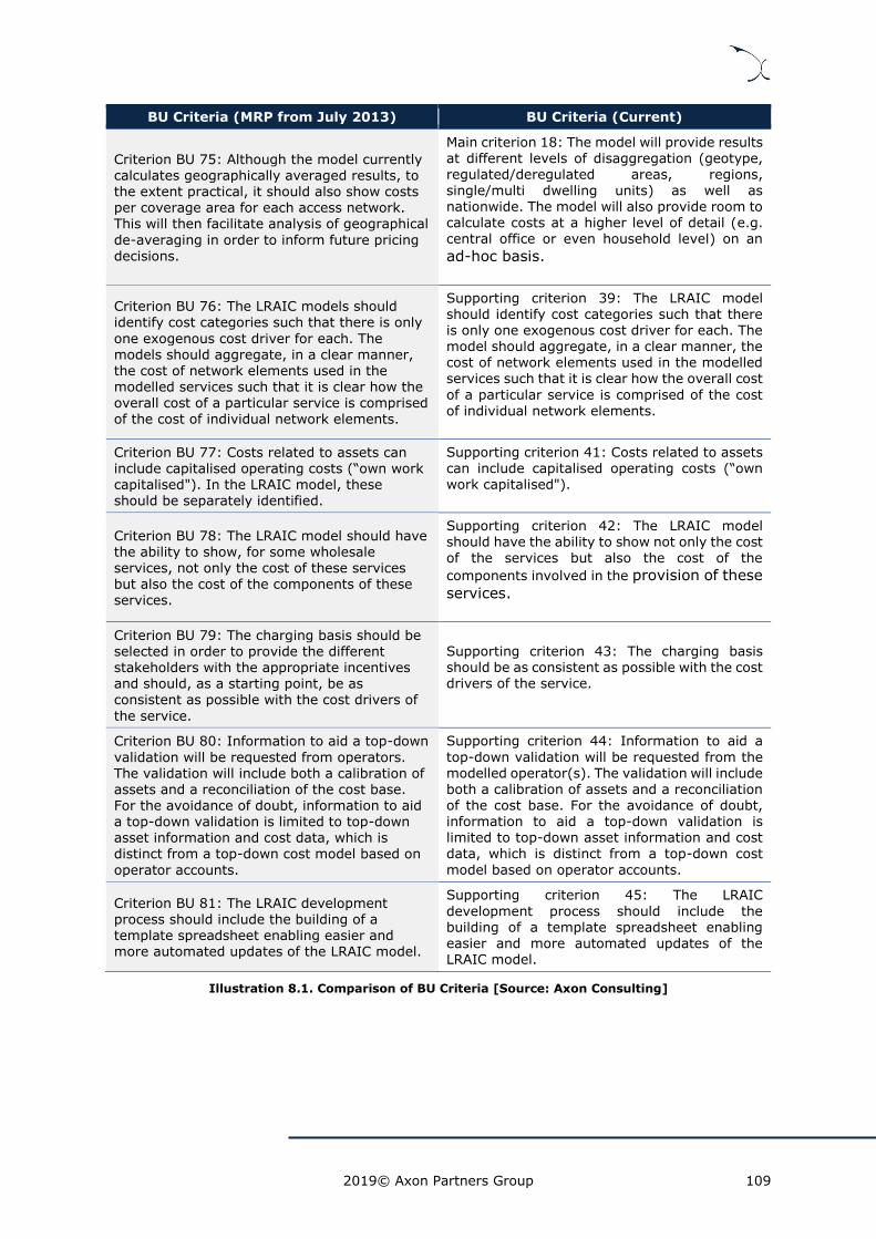
2019© Axon Partners Group 109
BU Criteria (MRP from July 2013) BU Criteria (Current)
Criterion BU 75: Although the model currently calculates geographically averaged results, to the extent practical, it should also show costs per coverage area for each access network. This will then facilitate analysis of geographical
de-averaging in order to inform future pricing decisions.
Main criterion 18: The model will provide results at different levels of disaggregation (geotype, regulated/deregulated areas, regions, single/multi dwelling units) as well as nationwide. The model will also provide room to calculate costs at a higher level of detail (e.g. central office or even household level) on an
ad-hoc basis.
Criterion BU 76: The LRAIC models should identify cost categories such that there is only
one exogenous cost driver for each. The models should aggregate, in a clear manner, the cost of network elements used in the modelled services such that it is clear how the overall cost of a particular service is comprised
of the cost of individual network elements.
Supporting criterion 39: The LRAIC model should identify cost categories such that there is only one exogenous cost driver for each. The model should aggregate, in a clear manner, the cost of network elements used in the modelled services such that it is clear how the overall cost
of a particular service is comprised of the cost
of individual network elements.
Criterion BU 77: Costs related to assets can include capitalised operating costs (“own work capitalised"). In the LRAIC model, these should be separately identified.
Supporting criterion 41: Costs related to assets can include capitalised operating costs (“own work capitalised").
Criterion BU 78: The LRAIC model should have the ability to show, for some wholesale services, not only the cost of these services but also the cost of the components of these services.
Supporting criterion 42: The LRAIC model should have the ability to show not only the cost of the services but also the cost of the
components involved in the provision of these
services.
Criterion BU 79: The charging basis should be selected in order to provide the different stakeholders with the appropriate incentives and should, as a starting point, be as
consistent as possible with the cost drivers of
the service.
Supporting criterion 43: The charging basis should be as consistent as possible with the cost drivers of the service.
Criterion BU 80: Information to aid a top-down
validation will be requested from operators. The validation will include both a calibration of assets and a reconciliation of the cost base. For the avoidance of doubt, information to aid a top-down validation is limited to top-down asset information and cost data, which is distinct from a top-down cost model based on
operator accounts.
Supporting criterion 44: Information to aid a
top-down validation will be requested from the modelled operator(s). The validation will include both a calibration of assets and a reconciliation of the cost base. For the avoidance of doubt, information to aid a top-down validation is limited to top-down asset information and cost data, which is distinct from a top-down cost
model based on operator accounts.
Criterion BU 81: The LRAIC development process should include the building of a template spreadsheet enabling easier and more automated updates of the LRAIC model.
Supporting criterion 45: The LRAIC
development process should include the building of a template spreadsheet enabling easier and more automated updates of the LRAIC model.
Illustration 8.1. Comparison of BU Criteria [Source: Axon Consulting]

2019© Axon Partners Group 110
8.2. Template to comment
In order to participate in this consultation process, stakeholders have to provide their
comments through the template included below. While stakeholders may, at their will,
provide comments beyond the scope of this table, DBA will give priority to the feedback
provided under the scope of the template below:
Question Position (Agree / Partially Agree /
Disagree) Justification
Question 1: Do you agree with the cost standards to be considered to determine the cost base of the model? Do you agree with the list of assets in which the EC’s 2013 recommendation shall be applied (i.e. in which
asset valuation should account for fully depreciated assets)?
If you don’t agree, please justify your position and provide supporting information and
references.
Question 2: Do you agree with methodology described to implement the EC’s recommendation to calculate the cost base of
the reusable legacy assets?
If you don’t agree, please justify your position
and provide supporting information and references.
Question 3: Do you agree with the need for the model to produce results for the period between 2018 and 2028?
If you don’t agree, please justify your position
and provide supporting information and references.
Question 4: Do you agree that the model should include a time-frame up to 2070 to ensure a proper implementation of the economic depreciation methodology?
If you don’t agree, please justify your position and provide supporting information and references.
Question 5: Do you agree that a single increment comprising the demand of all the modelled services should be considered?
If you don’t agree, please justify your position and provide supporting information and references.
Question 6: Do you agree that copper
(copper-only and FTTC), FTTH (PON and PTP) and coax (FTTN and FTTC) access networks should be modelled?
If you don’t agree, please justify your position and provide supporting information and references.

2019© Axon Partners Group 111
Question Position (Agree / Partially Agree /
Disagree) Justification
Question 7: Do you agree that only civil infrastructure and coax cable related costs should be allocated to subscribers’ access
services in coax networks?
If you don’t agree, please justify your position and provide supporting information and
references.
Question 8: Do you agree that the modelled operator should be defined in accordance to
the SMP operator(s) in markets 3a and 3b?
If you don’t agree, please justify your position
and provide supporting information and references.
Question 9: Do you agree that all the relevant access, broadband, TV, leased lines, and
transmission services for each technology should be included in the cost model?
If you don’t agree, please justify your position and provide supporting information and references.
Question 10: Do you agree that voice services do not need to be included in the model?
If you don’t agree, please justify your position and provide supporting information and references.
Question 11: Do you agree that demand levels considered in the dimensioning of each access network should satisfy the actual demand for that specific network?
If you don’t agree, please justify your position
and provide supporting information and
references.
Question 12: Do you agree that operating costs should be calculated using a bottom-up assessment based on a percentage of capital costs?
If you don’t agree, please justify your position and provide supporting information and
references.
Question 13: Do you agree that both, tilted annuities and full economic depreciation should be implemented in the model? Do you
also agree with the formulas presented to implement them?
If you don’t agree, please justify your position and provide supporting information and
references.
Question 14: Do you agree that working capital should not be considered in the cost model?
If you don’t agree, please justify your position and provide supporting information and references.

2019© Axon Partners Group 112
Question Position (Agree / Partially Agree /
Disagree) Justification
Question 15: Do you agree that the model should include demand forecasts until 2028?
If you don’t agree, please justify your position and provide supporting information and references.
Question 16: Do you agree with the proposed allocation mechanism to split the costs of shared assets between access and core networks?
If you don’t agree, please justify your position and provide supporting information and
references.
Question 17: Do you agree that the model should be able to provide results at different levels of disaggregation (geotype,
regulated/deregulated areas, regions, single/multi dwelling units)?
If you don’t agree, please justify your position and provide supporting information and references.
Question 18: Do you agree with the remaining criteria defined in the MRP for which no specific questions have been asked to the industry?
If you don’t agree, please justify your position and provide supporting information and references.
Illustration 8.2: Template to comment to the consultation process for the MRP [Source: Axon
Consulting]
8.3. List of acronyms
BSA Bitstream Access
BU Bottom-Up
BU-LRAIC Bottom-up Long-run Average Incremental Costs
CAPEX Capital expenditure
CMTS Cable Model Termination System
CPE Customer Premises Equipment
DBA Danish Business Authority
DKK Danish Krone
DN Distribution Node
DP Distribution Point
DSLAM Digital Subscriber Line Access Multiplexer
DWDM Dense wavelength division multiplexing
EC European Commission
EPMU Equal Proportionate Mark-Up

2019© Axon Partners Group 113
FDP Final Distribution Point
FTTC Fibre To The Cabinet
FTTH Fibre To The Home
GPON Gigabyte Passive Optical Networks
GPS Global Positioning System
IMS IP Multimedia Subsystem
IN Island Node
IP Internet Protocol
ITU International Telecommunication Union
Kbps Kilobit per second
LA Last Amplifier
LRAIC Long-run average incremental cost
LRIC Long-run incremental costs
Mbps Megabit per second
MDF Main Distribution Frame
MEA Modern Equivalent Asset
MPEG Moving Picture Expert Group
MRP Model Reference Paper
MSAN Multi-Service Access Nodes
NGA Next Generation Access
NGN Next Generation Network
NRAs National Regulatory Authorities
ODF Optical Distribution Frame
OLT Optical Line Terminal
OPEX Operational expenditure
PAP Primary Access Point
PCP Primary cross connect Point
PDH Plesiochronous Digital Heriarchy
PDP Primary Distribution Point
PON Passive Optical Network
POTS Plain Old Telephone Service
PSTN Public Switched Telephone Network
PTP Point to Point
SDH Synchronous Digital Hierarchy
SDP Secondary Distribution Point
SMP Significant Market Power
TD-LRAIC Top-down Long-run Average Incremental Costs
TDM Time Division Multiplexing

2019© Axon Partners Group 114
VoD Video On Demand
VoIP Voice over IP
WACC Weighted Average Cost of Capital
xDSL Digital Subscriber Line