development of the bicycle compatibility index: a level of service
TRANSCRIPT

Publication No. FHWA-RD-98-072December 1998
Development of the Bicycle Compatibility Index
http://209.207.159.179/development/98072/ [9/22/2000 1:37:00 PM]

Acknowledgments
The authors of this report wish to acknowledge the following individualswhose assistance with site selection, participant recruitment, andlogistical arrangements was invaluable in the conduct of this researchstudy:
Mr. Arthur Ross - Pedestrian & Bicycle Coordinator (Madison,Wisconsin)
Mr. Tom Huber - Pedestrian & Bicycle Coordinator (WisconsinDepartment of Transportation)
Mr. Mike Dornfeld - Bicycle Coordinator (Washington State Departmentof Transportation)
Mr. Rick Waring - Former Pedestrian & Bicycle Coordinator (Austin,Texas)
Ms. Dianne Bishop - Bicycle Coordinator (Eugene, Oregon)
Mr. Glenn Grigg - Former City Traffic Engineer (Cupertino, California)
Ms. Linda Dixon - Policy Specialist (University of Delaware)
Ms. Marcie Stenmark - Former Bicycle Coordinator (Gainesville,Florida)
Acknowledgements
http://209.207.159.179/development/98072/ack/ack.html [9/22/2000 1:37:02 PM]

Table of Contents
Chapter 1- Introduction
BackgroundBicycle stress levelBicycle level of serviceObjectives and scopeOrganization of the report
Chapter 2 - Development and validation of the methodology
Site selectionVideo productionVideo surveyField surveyData analysisConclusions
Chapter 3 - Data collection
Site selectionField data collectionVideo productionVideo survey
Chapter 4 - Data analysis
Effect of bicyclist experienceRegional evaluationModel developmentModel sensitivitySpecial circumstancesLevel of service criteria
Chapter 5 - Intersection pilot study
Site selectionData collectionVideo productionVideo surveyData analysis
Chapter 6 - Summary & conclusions
Summary of resultsConclusions
Table of Contents
http://209.207.159.179/development/98072/TOC/toc.html (1 of 6) [9/22/2000 1:37:02 PM]

Application example
Appendix A - Literature review
Bicycle safety index ratingFlorida roadway condition indexBicycle interaction hazard scoreConclusions
Appendix B - Pilot study data analysis
Appendix C - Survey instruments
Appendix D - English units BCI model
References
List of Figures
Figure 1. Practitioners need a tool that will allow them to determine thecompatibility of their roadways for bicycling.
Figure 2. The pilot study focused on roadways with various curb lanewidths, exclusive of bicycle lanes and paved shoulders, since this wasthe variable believed to be the most difficult for viewers to discern fromthe video.
Figure 3. High-volume multilane pilot study site with an 85th percentilespeed of 55 km/h and a curb lane width of 3.4 m.
Figure 4. Low-volume two-lane pilot study site with an 85th percentilespeed of 48 km/h and a curb lane width of 5.5 m.
Figure 5. The camera was positioned on the curb as close to the lane aspossible at a height of 1.4 to 1.5 m with the lens aimed parallel to theroadway.
Figure 6. Participants in the field survey of the pilot study stood adjacentto the direction of travel of interest and indicated how comfortable theywould be riding a bicycle under the conditions observed.
Figure 7. Sites included in the video survey were filmed in sixcities/regional areas located throughout the United States.
Figure 8. The sites selected for the video survey included a broad rangeand an extensive combination of geometric and operationalcharacteristics, as illustrated by these four locations.
Table of Contents
http://209.207.159.179/development/98072/TOC/toc.html (2 of 6) [9/22/2000 1:37:02 PM]

Figure 9. At locations with on-street parking, the camera was positionedat the left edge of the parking lane as close to the travel lane as possibleat a height of 1.4 to 1.5 m with the lens aimed parallel to the roadway.
Figure 10. Supplemental video clips were included on the video surveytape to examine the effects of large trucks and buses on bicyclists’comfort levels.
Figure 11. The video survey was conducted in three cities and included202 participants with the characteristics shown.
Figure 12. Mean comfort level ratings by type of bicyclist for the fourvariables rated in the video survey.
Figure 13. Mean comfort level ratings by State for the four variablesrated in the video survey.
Figure 14. Change (increase) in the overall mean comfort level ratingsby type of bicyclist for the special circumstances evaluated in the videosurvey.
Figure 15. Distribution of mean overall comfort level ratings used inestablishing level of service (LOS) designations.
Figure 16. The maneuver selected for evaluation of the use of the videomethodology at intersections was the bicyclist traveling straight throughthe intersection in the presence of right-turning traffic.
Figure 17. Examples of sites included in the intersection pilot study.
Figure 18. For the intersection study, the camera was positionedupstream of the intersection to allow participants to observe the approachspeeds and lane-changing behaviors of motorists.
Figure 19. Sites with high volumes of right-turning traffic sometimescontained extremely long auxiliary turn lanes, which made viewing theintersection proper difficult.
Figure 20. The intersection index increased significantly (indicating alower level of comfort) if the bicyclist was required to shift to the left toproceed straight through the intersection.
Figure 21. Proposed geometric design options for the reconstruction of aminor arterial.
Figure 22. A completed questionnaire.
Table of Contents
http://209.207.159.179/development/98072/TOC/toc.html (3 of 6) [9/22/2000 1:37:02 PM]

Figure 23. Pilot survey instructions.
Figure 24. Rating scale used in the pilot study.
Figure 25. Examples of completed field survey forms.
Figure 26. Completed video editing form.
Figure 27. Video survey instructions for rating midblock segments.
Figure 28. Video survey instructions for rating intersections.
Figure 29. Rating scale used in the primary data collection effort.
Figure 30. Example of a completed video survey form for midblocksegments.
Figure 31. Example of completed video survey forms for intersections.
List of Tables
Table 1. Example of stress levels developed by the Geelong BikeplanTeam.
Table 2. Suggested interpretation of bicycle stress levels.
Table 3. Quantitative geometric and operational values developed andassigned to each stress level.
Table 4. Distribution of sites selected for the pilot study by lane widthand 85th percentile speed.
Table 5. Number of sites selected for the video survey stratified by typeof facility, speed, lane width, and number of lanes.
Table 6. Characteristics of bicyclist groups used in the analysis.
Table 7. Variables included in the regression modeling analysis.
Table 8. Bicycle Compatibility Index (BCI) models for all bicyclists andfor the three groups of bicyclists by experience level.
Table 9. Ranges of variables included in the regression model.
Table 10. Example of the effects of variable changes within the BicycleCompatibility Index (BCI) model.
Table 11. Adjustment factors for large truck volumes.
Table 12. Adjustment factors for on-street parking turnover.
Table of Contents
http://209.207.159.179/development/98072/TOC/toc.html (4 of 6) [9/22/2000 1:37:02 PM]

Table 13. Bicycle Compatibility Index (BCI) ranges associated withlevel of service (LOS) designations.
Table 14. Number of sites selected for the intersection study stratified byright-turn volume and type of approach lane.
Table 15. Variables included in the regression modeling analysis ofintersections.
Table 16. Bicycle Compatibility Index (BCI) model, variable definitions,and adjustment factors.
Table 17. Bicycle Compatibility Index (BCI) ranges associated withlevel of service (LOS) designations and compatibility level qualifiers.
Table 18. Bicycle Compatibility Index (BCI) computations and levels ofservice (LOS) associated with the geometric design options in theexample.
Table 19. Bicycle safety index rating (BSIR) model.
Table 20. Rating classifications for the bicycle safety index rating(BSIR).
Table 21. Modified pavement and location factors used in the Floridaroadway condition index.
Table 22. Roadway condition index (RCI) model.
Table 23. Modified roadway condition index (MRCI) model.
Table 24. Comparison of the bicycle safety index rating (BSIR) modeland the roadway condition index (RCI) model.
Table 25. Interaction hazard score (IHS) model.
Table 26. Bicycle level of service (BLOS) model.
Table 27. Field (OFR) vs. video (OVR) overall ratings for the combinedsubject by location sample.
Table 28. Level of agreement in the field (OFR) vs. video (OVR) overallratings.
Table 29. Field (WFR) vs. video (WVR) width ratings for the combinedsubject by location sample.
Table 30. Level of agreement in the field (WFR) vs. video (WVR) widthratings.
Table of Contents
http://209.207.159.179/development/98072/TOC/toc.html (5 of 6) [9/22/2000 1:37:02 PM]

Table 31. Field (VFR) vs. video (VVR) volume ratings for the combinedsubject by location sample.
Table 32. Level of agreement in field (VFR) vs. video (VVR) volumeratings.
Table 33. Field (SFR) vs. video (SVR) speed ratings for the combinedsubject by location sample.
Table 34. Level of agreement in field (SFR) vs. speed (SVR) speedratings.
Table 35. Geometric and operational characteristics of the pilot studysites.
Table 36. English units version of the Bicycle Compatibility Index (BCI)model.
Table of Contents
http://209.207.159.179/development/98072/TOC/toc.html (6 of 6) [9/22/2000 1:37:02 PM]

Technical Report Documentation Page
1. Report No.
FHWA-RD-98-072
2. GovernmentAccession No.
3. Recipient's Catalog No.
4. Title and Subtitle
DEVELOPMENT OF THE BICYCLECOMPATIBILITY INDEX: A LEVELOF SERVICE CONCEPT
Final Report
5. Report Date
December 1998
6. Performing OrganizationCode
7. Author(s) David L. Harkey, Donald W.Reinfurt, Matthew Knuiman,
J.Richard Stewart, and Alex Sorton
8. Performing OrganizationReport No.
9. Performing Organization Name and Address
University of North Carolina
Highway Safety Research Center
730 Airport Road, CB #3430
Chapel Hill, NC 27599
10. Work Unit No. (TRAIS)
NCP4A4C
11. Contract or Grant No.
DTFH61-92-C-00138
12. Sponsoring Agency Name and Address
Office of Safety and Traffic OperationsResearch & Development
Federal Highway Administration
6300 Georgetown Pike
McLean, VA 22101-2296
13. Type of Report andPeriod Covered
Final Report
January 1995 - May1998
14. Sponsoring Agency Code
Technical Report
http://209.207.159.179/development/98072/techrep/techrep.html (1 of 3) [9/22/2000 1:37:03 PM]

15. Supplementary Notes
Contracting Officer’s Technical Representative (COTR): Carol TanEsse, HSR-20
Subcontractor: Northwestern University Traffic Institute
16. Abstract
Presently, there is no methodology widely accepted by engineers,planners, or bicycle coordinators that will allow them to determinehow compatible a roadway is for allowing efficient operation of bothbicycles and motor vehicles. Determining how existing trafficoperations and geometric conditions impact a bicyclist’s decision touse or not use a specific roadway is the first step in determining thebicycle compatibility of the roadway. This research effort wasundertaken to develop a methodology for deriving a bicyclecompatibility index (BCI) that could be used by practitioners toevaluate the capability of specific roadways to accommodate bothmotorists and bicyclists. The BCI methodology was developed forurban and suburban roadway segments (i.e., midblock locations thatare exclusive of major intersections) and incorporated those variableswhich bicyclists typically use to assess the "bicycle friendliness" of aroadway (e.g., curb lane width, traffic volume, and vehicle speeds).The developed tool will allow practitioners to evaluate existingfacilities in order to determine what improvements may be requiredas well as to determine the geometric and operational requirementsfor new facilities.
Also discussed in this report is the application of the developedmethodology used for rating midblock segments to intersections andan assessment of the validity of such an approach for rating thebicycle compatibility of intersections.
In addition to this final report, there is a companion report titled TheBicycle Compatibility Index: A Level of Service Concept,Implementation Manual (FHWA-RD-98-095) that contains appliedexamples of the BCI methodology.
17. Key Words:
Bicycle compatibility, level ofservice, bicycle operations,geometric design, bicycleplanning
18. Distribution Statement
No restrictions. This document isavailable to the public through theNational Technical InformationService, Springfield, Virginia22161.
Technical Report
http://209.207.159.179/development/98072/techrep/techrep.html (2 of 3) [9/22/2000 1:37:03 PM]

19. Security Classif. (ofthis report)
Unclassified
20. Security Classif.(of this page)
Unclassified
21. No. ofPages
94
22. Price
Form DOT F 1700.7 (8-72) Reproduction of form and completed page is authorized
Technical Report
http://209.207.159.179/development/98072/techrep/techrep.html (3 of 3) [9/22/2000 1:37:03 PM]

1. Introduction
Background
Bicycle stress level
Bicycle level of service
Objectives and scope
Organization of the report
Introduction
http://209.207.159.179/development/98072/ch01/ch01.html [9/22/2000 1:37:04 PM]
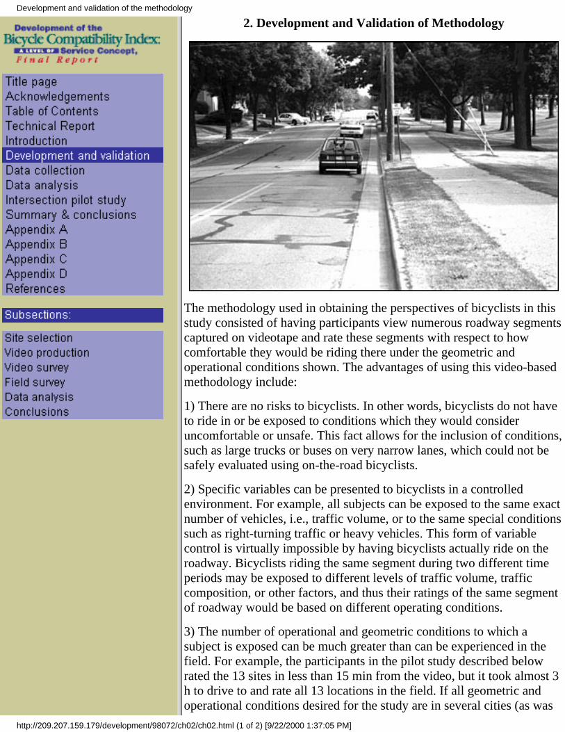
2. Development and Validation of Methodology
The methodology used in obtaining the perspectives of bicyclists in thisstudy consisted of having participants view numerous roadway segmentscaptured on videotape and rate these segments with respect to howcomfortable they would be riding there under the geometric andoperational conditions shown. The advantages of using this video-basedmethodology include:
1) There are no risks to bicyclists. In other words, bicyclists do not haveto ride in or be exposed to conditions which they would consideruncomfortable or unsafe. This fact allows for the inclusion of conditions,such as large trucks or buses on very narrow lanes, which could not besafely evaluated using on-the-road bicyclists.
2) Specific variables can be presented to bicyclists in a controlledenvironment. For example, all subjects can be exposed to the same exactnumber of vehicles, i.e., traffic volume, or to the same special conditionssuch as right-turning traffic or heavy vehicles. This form of variablecontrol is virtually impossible by having bicyclists actually ride on theroadway. Bicyclists riding the same segment during two different timeperiods may be exposed to different levels of traffic volume, trafficcomposition, or other factors, and thus their ratings of the same segmentof roadway would be based on different operating conditions.
3) The number of operational and geometric conditions to which asubject is exposed can be much greater than can be experienced in thefield. For example, the participants in the pilot study described belowrated the 13 sites in less than 15 min from the video, but it took almost 3h to drive to and rate all 13 locations in the field. If all geometric andoperational conditions desired for the study are in several cities (as was
Development and validation of the methodology
http://209.207.159.179/development/98072/ch02/ch02.html (1 of 2) [9/22/2000 1:37:05 PM]

the case in this effort), it is simply impractical to present all conditions tothe same group of bicyclists.
4) The same set of geometric and operational conditions can beexamined and rated by bicyclists in several municipalities. Thisadvantage allows for the direct comparison of ratings between bicyclistsin different regions of the country or communities that may vary in termsof bicycling facilities or bicycle "friendliness."
This application of videotape technology to obtain ratings frombicyclists was used by Sorton and Walsh in several bicycle researchefforts and was shown to produce consistent rating results from onestudy to the next.7 However, there had never been any formal validationof the video methodology. Prior to proceeding with this methodology inthe full-scale data collection effort of this research study, a pilot studywas undertaken with the primary objective of validating the videotechnique, i.e., determining how well the participants’ comfort ratings ofvarious geometric, traffic volume, and speed conditions recorded whenwatching a videotape compared with the participants’ comfort ratingswhen seeing the locations in the field. There were also several secondaryobjectives, including evaluating camera positions, determining theamount of videotape to shoot at a given site, determining the length ofvideo clips necessary for an individual to make definitive ratings, andexploring different rating scales.
Site selection
Video production
Video survey
Field survey
Data analysis
Conclusions
Development and validation of the methodology
http://209.207.159.179/development/98072/ch02/ch02.html (2 of 2) [9/22/2000 1:37:05 PM]

3. Data Collection
Site selection
Field data collection
Video production
Video survey
Data collection
http://209.207.159.179/development/98072/ch03/ch03.html [9/22/2000 1:37:06 PM]

4. Data Analysis
The two primary questions addressed by the analysis of the datacollected under this project were focused on the development of thebicycle compatibility index (BCI) model:
Can the comfort level ratings of bicyclists be used to develop a BCImodel that can be used by bicycle coordinators, transportationplanners, traffic engineers, and others to evaluate the capability ofspecific roadway segments to accommodate both motorists andbicyclists in their jurisdiction?
If so, what roadway and traffic operations variables are needed asinput for this index?
In addition to these primary questions, several secondary questions werealso addressed as part of the analysis, including:
1) Are there differences in the comfort level ratings of experiencedriders vs. casual riders with respect to any of the roadway or trafficoperations variables?
2) Do bicyclists in different geographic regions have the sameperceptions of bicycle compatibility; i.e., are there differences in thecomfort level ratings of bicyclists in the three survey cities?
3) What are the interrelationships between the variables being rated bythe respondents; i.e., what interactions are important in making theratings?
Effect of bicyclist experience
Regional evaluation
Model development
Model sensitivity
Special Circumstances
Level of service criteria
Data analysis
http://209.207.159.179/development/98072/ch04/ch04.html [9/22/2000 1:37:06 PM]

5. Intersection Pilot Study
The secondary objective of this research effort was to apply the video methodology used forrating midblock roadway segments to intersections and assess whether such an approach wasvalid for rating the bicycle compatibility of intersections. The goal of this limited effort wasnot to completely develop a BCI model for intersections but rather to determine if the videotechnique showed promise for application to intersections. Thus, the scope of this pilot studyfor intersections was limited to one maneuver that bicyclists typically make at an intersection.The maneuver selected was a bicyclist traveling straight through an intersection in thepresence of right-turning traffic (see figure 16).
Site selection
Data collection
Video production
Video survey
Data analysis
Intersection pilot study
http://209.207.159.179/development/98072/ch05/ch05.html [9/22/2000 1:37:07 PM]

6. Summary and Conclusions
Summary of results
Conclusions
Application example
Summary & conclusions
http://209.207.159.179/development/98072/ch06/ch06.html [9/22/2000 1:37:08 PM]

Appendix A - Literature review
In recent years, several models have been developed in an attempt toassociate roadway geometrics and vehicle operations with bicycle safetyand/or operations. This appendix provides a discussion of each of thesemodels. The efforts discussed here were progressive in nature with eachconcurrent effort essentially building on what had been done in theprevious study. To better understand how the models were developedand how they relate to one another, the discussion is presented inchronological order.
Bicycle safety index rating
Florida roadway condition index
Bicycle interaction hazard score
Conclusions
Appendix A
http://209.207.159.179/development/98072/appa/appa.html [9/22/2000 1:37:08 PM]

Appendix B - Pilot study data analysis
As previously noted in chapter 2, the primary objective of the pilot study in thisresearch effort was to validate the video methodology, i.e., determine how well theparticipants’ comfort ratings assigned when watching locations on a videotapematched the participants’ ratings when viewing the same locations in the field. Inchapter 2, a summary of the results of the data analysis was provided. A moreextensive discussion of the statistical analysis is provided in this appendix.
Since each of the 24 participants (subjects) viewed the 13 sites both from thevideotape and in the field, the most stable and reliable analyses are based on the312 (24 × 13) combined pairs (video vs. field) of observations. Thus, the analysisfocuses on the combined sample of comfort ratings, including the overall rating aswell as those related to curb lane width, volume, and speed of traffic.
However, analyses were also carried out by subject to examine: 1) possible biases(e.g., generally rating the video slightly higher than the field observation); 2)consistency (i.e., providing essentially the same ratings for each pair of matchedvideo clips); and 3) order of presentation differences (i.e., differences between theparticipants who saw the video first followed by the field observations vs. thosewho saw the field sites first followed by the video). Finally, the ratings by site wereinvestigated to see if the participants’ ratings between the field and video weremore consistent for some sites compared with others and, if so, to determine thecharacteristics of those sites where the participants were less consistent in theirratings.
The basic data for this study consisted of a sample of matched pair comfort ratings(field vs. video) for each of 24 participants. As noted in chapter 2, there were twovideo clips of the same site in the survey, each with a different traffic volume. Oneof the clips contained the "uniform" volume condition while the other clipcontained the "representative" volume condition. Since the objective of this analysiswas to directly compare the ratings between field and video observations, the videoclip that most closely matched the field volume observed by each participant wasused as the matching clip. As such the data can best be represented by contingencytables with rows (i) representing the field ratings (i = 1, 2, ..., 6) and columns (j)representing the video ratings (j = 1, 2, ..., 6). Further, the ratings can be defined asfollows:
OFR(i)= overall field rating
OVR(j)= overall video rating
WFR(i)= width field rating
WVR(j)= width video ratingVFR(i)= volume field rating
VVR(j)= volume video rating
SFR(i)= speed field rating
SVR(j)= speed video rating
If there were perfect agreement between the field and video ratings (e.g., OFR(i) ºOVR(j)), then all pairs of overall ratings would fall along the main diagonal of thecontingency table (or matrix). If the video ratings were consistently somewhat
Appendix B
http://209.207.159.179/development/98072/appb/appb.html (1 of 7) [9/22/2000 1:37:10 PM]

higher than the field ratings (e.g., OFR(i) < OVR(j)) or vice versa, the pairs ofoverall ratings would consistently fall above or below the main diagonal of thecontingency table, respectively. The following analyses examined these possiblerelationships.
The results of the field vs. video overall ratings for the 312 subject-by-locationpairs are shown in table 27. Note first that the column marginal distribution for thevideo (namely, 5.5%, 23.4%, ..., 2.2%) is similar to the row marginal distributionfor the field ratings (namely, 6.7%, 21.8%, ..., 4.2%). This suggests that, overall,the video ratings are reasonably reliable predictors of the field ratings. Table 28indicates the degree of agreement between the field and video overall ratings. In36.9 percent of the sample, there is perfect agreement whereas in 85.3 percent ofthe cases, the ratings differ by no more than one level. And in 96.8 percent of thepairs, the difference is two levels or less. Also note that when OFR is not equal toOVR, the field rating is more often higher (36.6% = 26.0 + 7.7 + 2.9) than the videorating (26.5% = 22.4 + 3.8 + 0.3). Such is not the case, however, with the speed orvolume ratings discussed later.
Cohen’s k (kappa) statistic is a nonparametric measure of the degree of agreementamong pairs of ratings that is appropriate to further quantify these relationships.21
The results of calculating Cohen’s k and the natural extension to near diagonal cellsare also shown in table 28. For the perfect agreement condition (main diagonal), theCohen’s k is 0.19, which indicates a "fair" level of agreement between the field andvideo ratings. The extended Cohen’s k for the video rating being within one level ofthe field rating is 0.62, which suggests "substantial" agreement.
Appendix B
http://209.207.159.179/development/98072/appb/appb.html (2 of 7) [9/22/2000 1:37:10 PM]

The corresponding results for ratings based on curb lane width (W), speed (S), andtraffic volume (V) are presented in tables 29 through 34, respectively. For the mostpart, the results are quite similar to those for the overall ratings. The row andcolumn marginal distributions are quite similar for each of the three variables,indicating that the video ratings for each variable are fairly reliable predictors of thefield ratings.
For the curb lane width variable, the field rating (WFR) is within one level of thevideo rating (WVR) for 39.4 percent of the pairs and the corresponding Cohen’s kis 0.25, indicating a fair level of agreement. In 81.1 percent of the cases, the ratingsdiffer by no more than one level, and the corresponding extended Cohen’s k is 0.60,indicating a substantial level of agreement. Similar to the overall ratings, the fieldrating for curb lane width was more often higher (40.4% = 27.6 + 9.0 + 3.8) thanthe video rating (19.8% = 14.1 + 5.1 + 0.6) when the ratings were not equal.
The results for the traffic volume variable indicate that 30.8 percent of the samplepairs match, with a corresponding Cohen’s k of 0.11, indicating a fair level ofagreement. In 82.4 percent of the cases, the ratings differ by no more than one level,and the corresponding Cohen’s k is 0.55, indicating a substantial level ofagreement. In contrast to the overall and curb lane width results, the video rating forvolume was more often higher (37.5% = 28.5 + 7.7 + 1.3) than the field rating(31.4% = 23.1 + 7.7 + 1.3) when the ratings were not equal.
Appendix B
http://209.207.159.179/development/98072/appb/appb.html (3 of 7) [9/22/2000 1:37:10 PM]

The results for the speed variable produced the highest match rate (43.6 percent)between the sample pairs of the four variables examined. The correspondingCohen’s k was 0.23, again indicating a fair level of agreement. In 87.2 percent ofthe cases, the ratings differ by no more than one level, and the correspondingCohen’s k was 0.59, again indicating a substantial level of agreement. Similar to theresults for the volume variable, the video rating for speed was more often higher(33.0% = 25.0 + 7.4 + 0.6) than the field rating (23.4% = 18.6 + 4.2 + 0.6) when theratings were not equal.
Chi-square tests of marginal homogeneity (i.e., similar marginal distributions forfield ratings and video ratings) showed the distributions to be most similar for thespeed and volume ratings (p > 0.25 and p > 0.10, respectively) and reasonablysimilar for the overall ratings (p = 0.06). However, due to the large differencesbetween field and video ratings at levels 3 and 4 for the curb lane width ratings, thevideo and field ratings distributions for this variable did differ significantly (p <0.01). For the most part, the various video ratings distributions did reflect the fieldratings distributions, confirming earlier results that examined the levels ofagreement between the ratings.
The analysis just discussed examined the ratings of all participants across all sites.The results are considerably more variable with respect to participants (N=24)across sites and with respect to sites (N=13) across participants. Thus, a pairedcomparison t-test was undertaken to explore these specific aspects. The primaryinterest here is not only in the significance of the test, but also in the sign of the teststatistic. A positive sign (+) suggests that the video rating was generally lower thanthe field rating while a negative sign (-) suggests that the field rating was generallylower than the video rating. A non-significant test statistic suggests that, withinpairs, the field and video ratings do not differ. With respect to the overall ratings,21 of 24 subjects had non-significant (at a = 0.05) t-statistics across sites. With 16out of 23 being positive (one case where t=0), the tests suggest that the subjectstended to give slightly higher ratings when viewing the sites in the field whencompared with viewing the same sites on the video.
Appendix B
http://209.207.159.179/development/98072/appb/appb.html (4 of 7) [9/22/2000 1:37:10 PM]

With respect to the overall ratings, 21 of 24 subjects had non-significant (at a =0.05) t-statistics across sites. With 16 out of 23 being positive (one case where t =0), the tests suggest that the subjects tended to give slightly higher ratings whenviewing the sites in the field when compared with viewing the same sites on thevideo.
As previously noted in chapter 2, half of the 24 subjects viewed the video first andthen went to the site whereas the other half visited the site first. There were no cleardifferences in these two groups with respect to whether they rated the field scenehigher or lower than the video clip as judged by the significance or sign (+ or -) ofthe corresponding t-statistics.
Similar results were seen when comparing the field and video ratings for curb lanewidth, volume, and speed by subject. The main difference was that while subjectstended to rate the field view slightly higher than the video clip for both the overalland width variables, the opposite was true for the volume and speed variables. Thisresult is similar to what was found in the analysis of the 312 combined pairs.
One of the objectives of the pilot study was to determine how consistentparticipants were in rating the same conditions. To achieve this objective, therewere 26 identical pairs of video clips included in the video survey. The videoratings for the 26 matched clips were compared. Here the rows of the contingencytable represented the overall rating of each of the 24 subjects for the first time the
Appendix B
http://209.207.159.179/development/98072/appb/appb.html (5 of 7) [9/22/2000 1:37:10 PM]

clip was shown while the columns of the table represented the ratings of thesubjects for the second time the same scene was displayed. For the overall ratings,20 of the 26 had non-significant t-tests suggesting consistent ratings. And 20 of 25had a positive sign (one case where t = 0), indicating that the rating was slightlyhigher for the second clip. The results were most similar for the width, volume, andspeed ratings.
The final analysis issue dealt with strength of agreement between the field andvideo ratings on a site-by-site basis in an attempt to determine if there werecharacteristics of certain sites that led to inconsistencies in the video vs. fieldratings. Using paired comparisons t-tests for both the overall comfort ratings andratings based on the width of the curb lane, 5 out of 13 tests in both cases indicatedsignificance (at a = 0.05), suggesting some differences in the video vs. field ratingsfor five sites. The curb lane widths, speeds, and traffic volumes for all 13 sites areshown in table 35. The sites with significant t-statistics (sites 6, 7, 8, 10, and 13) donot appear, as a group, to result in any consistent pattern with respect to any of thevariables, which is greatly different from the remaining eight sites that producedconsistent ratings.
Appendix B
http://209.207.159.179/development/98072/appb/appb.html (6 of 7) [9/22/2000 1:37:10 PM]

However, further examination of the field observation data revealed that a largenumber of participants viewed site number 8 in the field when there was anunusually low traffic volume. This fact may have resulted in the significantly lowerfield rating for this site. The other four sites had significantly higher field ratings.At three of these four locations (sites 7, 10, and 13), more than half of theparticipants observed either a truck or bus during the field rating period, which mayhave produced a higher rating than the video clip of those sites since no trucks orbuses were included in the primary video clips; at only one of the eightnonsignificant sites did that many participants observe a truck or bus. Finally, thefourth location with a significantly higher field rating was the site with thenarrowest lane width (3.1 m), which may have simply been more intimidating in thefield compared with video than the larger lane widths.
Appendix B
http://209.207.159.179/development/98072/appb/appb.html (7 of 7) [9/22/2000 1:37:10 PM]

Appendix C - Survey Instruments
This appendix contains the forms, instructions, and rating scales used in the data collection efforts in boththe pilot study and the primary research effort. Figure 22 is an example of a completed questionnaire (withthe name omitted); this questionnaire was completed by all study participants and used to assess theirexperience levels as bicyclists. Figure 23 shows the instructions used during the pilot study for both thefield survey and video survey; the accompanying rating scale is shown in figure 24. Examples of completeddata collection forms from the pilot effort are provided in figure 25.
Figure 26 is an example of a completed video editing form that was used to record volumes for 10-sintervals over the 15-min taping period; it was from this form that the video clips were selected. Theinstructions used for the video survey of midblock segments in the primary data collection effort areprovided in figure 27. The instructions used for the intersection survey are shown in figure 28; one set is forthe individuals who were asked to rate five variables while the other set is for those who rated only onevariable. The rating scale used for both surveys is shown in figure 29. Examples of completed datacollection forms from each type of survey are provided in figures 30 and 31.
Figure 22. A completed questionnaire.
Appendix C
http://209.207.159.179/development/98072/appc/appc.html (1 of 9) [9/22/2000 1:37:12 PM]

BICYCLE COMPATIBILITY INDEX STUDYVIDEO SURVEY INSTRUCTIONS - MADISON, WI
In a moment, you are going to watch a videotape which contains 60clips showing different roadway conditions. As you watch each clip,I want you to pay particular attention to three specific aspects(illustrate with a videotape):
o the amount of traffic going in the direction away from you,
o the speed of this traffic, and
o the width or space available to you to ride your bicycle in this samedirection.
As you look at each video clip, I want you to indicate howcompatible or good you think the road is for bicycling. In otherwords, I want you to rate each roadway with respect to howcomfortable you would be riding there, where comfort is defined bythe level of risk you would feel as a bicyclist. The scale you aregoing to use in rating these segments is in front of you. It isnumerically ordered in terms of the level of perceived risk. If you seethe roadway condition as presenting virtually no risk to you as abicyclist, you would rate the condition as a "1." If you see theroadway condition as presenting a risk that is so high that you wouldnever ride under that condition, you would rate the condition as a "6."If you see the roadway condition as something between these twoextremes, use the values from 2 to 5 to indicate your level ofperceived risk.
As you can see on the rating sheet, there are four columns; one forvolume (or amount of traffic), one for speed, one for lane width, andone for overall. As you view each video clip, I want you to provide aperceived risk rating of 1 to 6, as we just discussed, for each of thethree conditions shown in that particular clip (volume, speed, andwidth of the lane in which you would be riding), each oneindependently of the other two conditions. For example, as you arewatching the clip, I want you to provide a rating of 1 to 6 withrespect to the amount of risk you feel the traffic volume on thatroadway presents to you as a bicyclist. Then you will provide a ratingof 1 to 6 based on the amount of risk you feel from the speed of thetraffic. Next you will provide a rating of 1 to 6 based on the amountof risk you feel from the width of the curb lane or space available toride your bicycle in the road. Finally, you will provide a rating of 1 to6 for the roadway as a whole which should represent your perceivedrisk based on the three measures just noted plus any other measuresthat you may consider important in determining your level of risk asa bicyclist. You may rate the volume, speed, and lane width in anyorder. The overall rating should be done last.
Each video clip is approximately 40 seconds in length. When thereare 10 seconds remaining, a beep will be heard. During these last 10seconds, you should complete the ratings for that roadway. Betweenconsecutive video clips, there will be approximately 5 seconds inwhich the screen is blank. During each blank screen, I will indicatewhich numbered video clip is about to be shown.
Before we begin, are there any questions?
Appendix C
http://209.207.159.179/development/98072/appc/appc.html (2 of 9) [9/22/2000 1:37:12 PM]

BICYCLE COMPATIBILITY INDEX STUDYFIELD SURVEY INSTRUCTIONS - MADISON, WI
This morning, we are going to several specific sites onroadways here in Madison. When we get to a site, I will parkthe van and we will proceed to a location along the roadside.When we reach that location, I want you to pay particularattention to three specific aspects (illustrate with a videotape):
o the amount of traffic going in the direction away from you,
o the speed of this traffic, and
o the width or space available to you to ride your bicycle in thissame direction.
As you examine the roadway, I want you to indicate howcompatible or good you think the road is for bicycling. In otherwords, I want you to rate each roadway with respect to howcomfortable you would be riding there, where comfort isdefined by the level of risk you would feel as a bicyclist. Thescale you are going to use in rating these segments is in front ofyou. It is numerically ordered in terms of the level of perceivedrisk. If you see the roadway condition as presenting virtually norisk to you as a bicyclist, you would rate the condition as a "1."If you see the roadway condition as presenting a risk that is sohigh that you would never ride under that condition, you wouldrate the condition as a"6." If you see the roadway condition assomething between these two extremes, use the values from 2to 5 to indicate your level of perceived risk.
As you can see on the rating sheet, there are four columns; onefor volume (or amount of traffic), one for speed, one for lanewidth, and one for overall. As you examine each roadway, Iwant you to provide a perceived risk rating of 1 to 6, as we justdiscussed, for each of the three conditions presently existing onthe roadway (volume, speed, and width), each oneindependently of the other two conditions. For example, as youexamining the roadway, I want you to provide a rating of 1 to 6with respect to the amount of risk you feel the traffic volumeon that roadway presents to you as a bicyclist. Then you willprovide a rating of 1 to 6 based on the amount of risk you feelfrom the speed of the traffic. Next you will provide a rating of1 to 6 based on the amount of risk you feel from the width ofthe curb lane or space available to ride your bicycle in the road.Finally, you will provide a rating of 1 to 6 for the roadway as awhole which should represent your perceived risk based on thethree measures just noted plus any other measures that you mayconsider important in determining your level of risk as abicyclist. You may rate the volume, speed, and lane width inany order. The overall rating should be done last.
We will spend no more than 2 minutes at each roadwaylocation. We will then return to the van and proceed to the nextlocation.
Before we go to the van, are there any questions?
Figure 23. Pilot survey instructions.
Appendix C
http://209.207.159.179/development/98072/appc/appc.html (3 of 9) [9/22/2000 1:37:12 PM]

BICYCLE COMPATIBILITY INDEX STUDY
VIDEO/FIELD SURVEY RATING SCALE -MADISON, WI
PERCEIVED RISK
1 - VIRTUALLY NO RISK
2
3
4
5
6-UNACCEPTABLY HIGH RISK
Figure 24. Rating scale used in the pilot study.
Figure 25. Examples of completed field survey forms.
Appendix C
http://209.207.159.179/development/98072/appc/appc.html (4 of 9) [9/22/2000 1:37:12 PM]
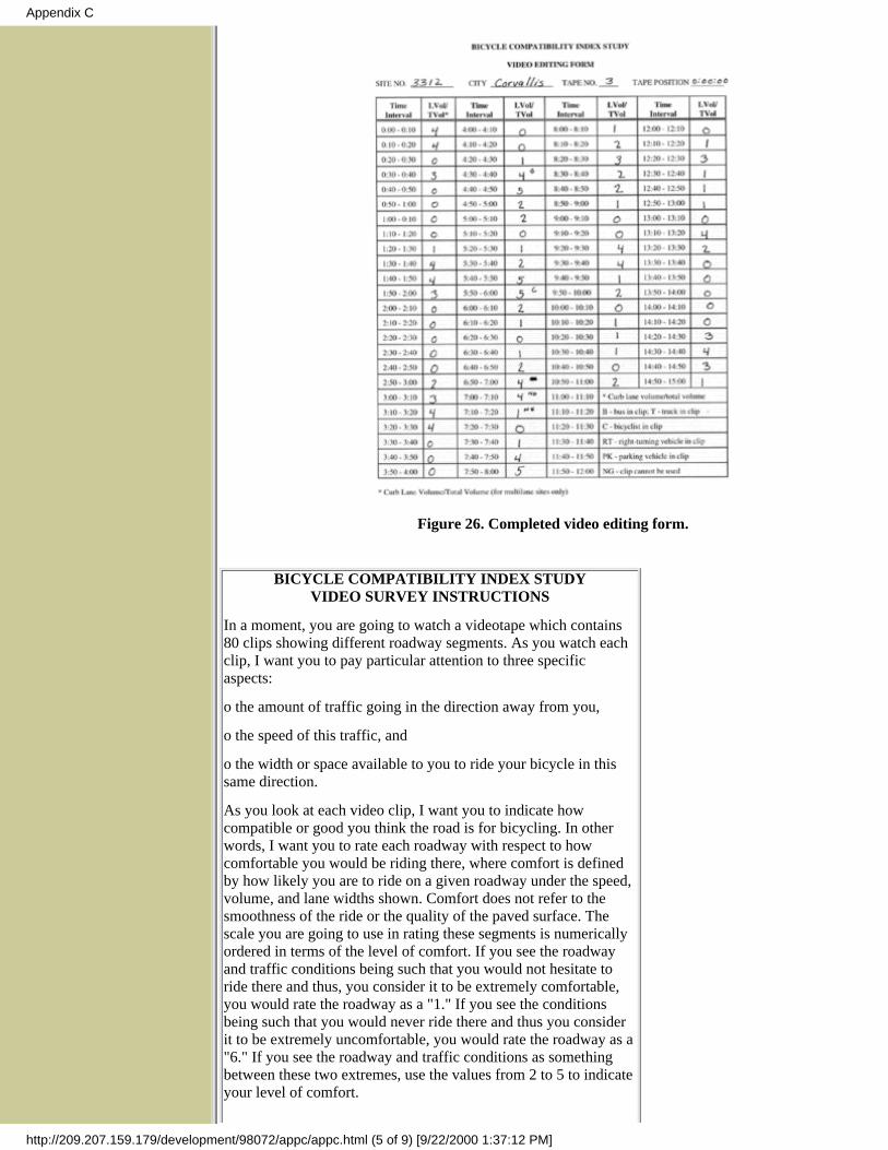
Figure 26. Completed video editing form.
BICYCLE COMPATIBILITY INDEX STUDYVIDEO SURVEY INSTRUCTIONS
In a moment, you are going to watch a videotape which contains80 clips showing different roadway segments. As you watch eachclip, I want you to pay particular attention to three specificaspects:
o the amount of traffic going in the direction away from you,
o the speed of this traffic, and
o the width or space available to you to ride your bicycle in thissame direction.
As you look at each video clip, I want you to indicate howcompatible or good you think the road is for bicycling. In otherwords, I want you to rate each roadway with respect to howcomfortable you would be riding there, where comfort is definedby how likely you are to ride on a given roadway under the speed,volume, and lane widths shown. Comfort does not refer to thesmoothness of the ride or the quality of the paved surface. Thescale you are going to use in rating these segments is numericallyordered in terms of the level of comfort. If you see the roadwayand traffic conditions being such that you would not hesitate toride there and thus, you consider it to be extremely comfortable,you would rate the roadway as a "1." If you see the conditionsbeing such that you would never ride there and thus you considerit to be extremely uncomfortable, you would rate the roadway as a"6." If you see the roadway and traffic conditions as somethingbetween these two extremes, use the values from 2 to 5 to indicateyour level of comfort.
Appendix C
http://209.207.159.179/development/98072/appc/appc.html (5 of 9) [9/22/2000 1:37:12 PM]

As you can see on the rating sheet, there are four columns; one forvolume (or amount of traffic), one for speed, one for lane width,and one for overall. As you view each video clip, I want you toprovide a comfort level rating of 1 to 6, as we just discussed, foreach of the three conditions shown in that particular clip (volume,speed, and width of the lane in which you would be riding). Forexample, as you are watching the clip, I want you to provide arating of 1 to 6 with respect to how comfortable you would feel asa bicyclist considering the number of vehicles on that roadway.Then you will provide a rating of 1 to 6 based on how comfortableyou would feel considering the speed of the traffic. Next you willprovide a rating of 1 to 6 based on how comfortable you wouldfeel considering the space available to you to ride your bicycle inthe road. Finally, you will provide a rating of 1 to 6 for theroadway as a whole which should represent your overall comfortlevel based on the three measures just noted plus any othermeasures that you may consider important in determining yourcomfort level as a bicyclist. You may rate the volume, speed, andlane width in any order. The overall rating should be done last.
Each video clip is approximately 40 seconds in length. When thereare 10 seconds remaining, you will hear a beep. During these last10 seconds, you should complete the ratings for that roadway.Between consecutive video clips, there will be approximately 5seconds in which the screen is black, with the exception of anumber in the upper left-hand corner identifying the upcomingclip.
Before we begin, are there any questions?
Figure 27. Video survey instructions for rating midblock segments.
BICYCLE COMPATIBILITY INDEX STUDYINTERSECTION VIDEO SURVEY INSTRUCTIONS
Now you are going to watch a videotape which contains 19 clipsshowing different intersections. As you look at each video clip, Iwant you to indicate how compatible or good you think theintersection is for through bicyclists. In other words, I want you torate each roadway with respect to how comfortable you would beriding straight through the intersection in the presence of theright-turning traffic, where comfort is defined by how likely you areto ride through that intersection under the roadway and trafficconditions shown. Again, comfort does not refer to the smoothnessof the ride or the quality of the paved surface. You will use the samescale as before. If you see the roadway and traffic conditions asbeing such that you would not hesitate to ride through theintersection and thus, you consider it to be extremely comfortable,you would rate the intersection as a "1." If you see the conditions asbeing such that you would never ride through the intersection, andthus you consider it to be extremely uncomfortable, you would ratethe intersection as a "6." If you see the roadway and trafficconditions as something between these two extremes, use the valuesfrom 2 to 5 to indicate your level of comfort.
Each video clip is approximately 40 seconds in length. When thereare 10 seconds remaining, you will hear a beep. During these last 10seconds, you should complete the ratings for that roadway. Betweenconsecutive video clips, there will be approximately 5 seconds inwhich the screen is black, with the exception of a number in theupper left-hand corner identifying the upcoming clip.
Before we begin, are there any questions?
Appendix C
http://209.207.159.179/development/98072/appc/appc.html (6 of 9) [9/22/2000 1:37:12 PM]

BICYCLE COMPATIBILITY INDEX STUDYINTERSECTION VIDEO SURVEY INSTRUCTIONS
Now you are going to watch a videotape which contains 19 clipsshowing different intersections. As you watch each clip, I want youto pay particular attention to four specific aspects:
the amount of right-turning traffic,●
the speed of this traffic on the approach to the intersection,●
the space available to you to ride your bicycle through thisintersection, and
●
the clarity of any signs and markings indicating appropriatepaths for bicyclists and/or motorists
●
As you look at each video clip, I want you to indicate howcompatible or good you think the intersection is for throughbicyclists. In other words, I want you to rate each roadway withrespect to how comfortable you would be riding straight through theintersection in the presence of the right-turning traffic, wherecomfort is defined by how likely you are to ride through thatintersection under the speed, volume, and other conditions shown.Again, comfort does not refer to the smoothness of the ride or thequality of the paved surface. You will use the same scale as before.If you see the roadway and traffic conditions being such that youwould not hesitate to ride through the intersection and thus, youconsider it to be extremely comfortable, you would rate theintersection as a "1." If you see the conditions being such that youwould never ride through the intersection, and thus you consider itto be extremely uncomfortable, you would rate the intersection as a"6." If you see the roadway and traffic conditions as somethingbetween these two extremes, use the values from 2 to 5 to indicateyour level of comfort.
As you can see on the rating sheet, there are five columns; one forright-turning volume (or amount of traffic), one for approach speed,one for available space, one for signs and markings, and one foroverall. As you view each video clip, I want you to provide acomfort level rating of 1 to 6, as we just discussed, for each of theconditions shown in that particular clip. For example, as you arewatching the clip, I want you to provide a rating of 1 to 6 withrespect to how comfortable you are with the signs and markingsindicating appropriate paths for bicyclists and motorists. Then youwill provide a rating of 1 to 6 with respect to how comfortable youwould feel as a bicyclist considering the number of right-turningvehicles at that intersection. Next you will provide a rating of 1 to 6based on how comfortable you would feel considering the speed ofthe traffic approaching the intersection. Then you will provide arating of 1 to 6 based on how comfortable you would feelconsidering the space available to you to ride your bicycle throughthe intersection. Finally, you will provide a rating of 1 to 6 for theroadway as a whole which should represent your overall comfortlevel based on the four measures just noted plus any other measuresthat you may consider important in determining your comfort levelas a bicyclist. You may rate the volume, speed, available space andsigns/markings in any order. The overall rating should be done last.
Each video clip is approximately 40 seconds in length. When thereare 10 seconds remaining, you will hear a beep. During these last 10seconds, you should complete the ratings for that roadway. Betweenconsecutive video clips, there will be approximately 5 seconds inwhich the screen is black, with the exception of a number in the
Appendix C
http://209.207.159.179/development/98072/appc/appc.html (7 of 9) [9/22/2000 1:37:12 PM]
upper left-hand corner identifying the upcoming clip.
Before we begin, are there any questions?
Figure 28. Video survey instructions for rating intersections.
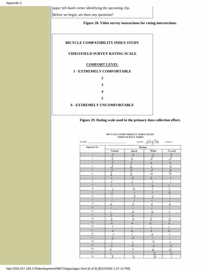
BICYCLE COMPATIBILITY INDEX STUDY
VIDEO/FIELD SURVEY RATING SCALE
COMFORT LEVEL
1 - EXTREMELY COMFORTABLE
2
3
4
5
6 - EXTREMELY UNCOMFORTABLE
Figure 29. Rating scale used in the primary data collection effort.
Appendix C
http://209.207.159.179/development/98072/appc/appc.html (8 of 9) [9/22/2000 1:37:12 PM]

Figure 30. Example of a completed video survey form for midblock segments.
Figure 31. Example of completed video survey forms for intersections.
Appendix C
http://209.207.159.179/development/98072/appc/appc.html (9 of 9) [9/22/2000 1:37:12 PM]

Appendix D - English Units BCI Model
While many States and municipalities have converted to the metricsystem of measurement, other localities still employ the English systemor the geometric and operational information contained in the data basesis in English units. For these reasons, an English units version of the BCImodel is provided in table 36.
Table 36. English units version of the Bicycle Compatibility Index(BCI) model.
BCI = 3.67 - 0.966BL - 0.125BLW - 0.152CLW + 0.002CLV +0.0004OLV
+ 0.035SPD + 0.506PKG - 0.264AREA + AF
where:
BL = presence of a bicycle laneor paved
shoulder > 3.0 ft
no = 0
yes = 1
BLW = bicycle lane (or pavedshoulder) width
ft (to the nearest tenth)
CLW = curb lane width
ft (to the nearest tenth)
CLV = curb lane volume
vph in one direction
OLV = other lane(s) volume -same direction
vph
SPD = 85th percentile speed oftraffic
mi/h
PKG = presence of a parkinglane with more than
30 percent occupancy
no = 0
yes = 1
AREA = type of roadsidedevelopment
residential = 1
other type = 0
AF = ft + fp + frt
where:
ft = adjustment factor for truckvolumes
(see below)
fp = adjustment factor for parkingturnover
(see below)
frt = adjustment factor forright-turn volumes
Appendix D
http://209.207.159.179/development/98072/appd/appd.html (1 of 2) [9/22/2000 1:37:13 PM]

(see below)
Adjustment Factors
Hourly CurbLane
Large TruckVolume1
ft
Parking Time
Limit (min)
fp
> 120
60 - 119
30-59
20-29
10-19
< 10
0.5
0.4
0.3
0.2
0.1
0.0
< 15
16 - 30
31 - 60
61 - 120
121 - 240
241- 480
> 480
0.6
0.5
0.4
0.3
0.2
0.1
0.0
Hourly Right-
Turn Volume2
frt
> 270
< 270
0.1
0.0
1 Large trucks are defined as all vehicles with six or more tires.2 Includes total number of right turns into driveways or minor intersections along aroadway segment.
Appendix D
http://209.207.159.179/development/98072/appd/appd.html (2 of 2) [9/22/2000 1:37:13 PM]

References
1. The National Bicycling and Walking Study, Report No.FHWA-PD-94-023, Federal Highway Administration, Washington, DC,1994.
2. J. Davis, Bicycle Safety Evaluation, Auburn University, City ofChattanooga, and Chattanooga-Hamilton County Regional PlanningCommission, Chattanooga, TN, June 1987.
3. B. Epperson, "Evaluating the Suitability of Roadways for BicycleUse: Towards a Cycling Level of Service," Transportation ResearchRecord 1438, Transportation Research Board, Washington, DC, 1994.
4. B.W. Landis, "Bicycle Interaction Hazard Score: A TheoreticalModel," Transportation Research Record 1438, Transportation ResearchBoard, Washington, DC, 1994.
5. W.C. Wilkinson, A. Clarke, B. Epperson, & R. Knoblauch, SelectingRoadway Design Treatments to Accomodate Bicycles, Report No.FHWA-RD-92-073, Federal Highway Administration, Washington, DC,1994.
6. Geelong Planning Committee, Geelong Bikeplan, Geelong, Australia,1978.
7. A. Sorton and T. Walsh, "Bicycle Stress Level as a Tool to EvaluateUrban and Suburban Bicycle Compatibility", Transportation ResearchRecord 1438, Transportation Research Board, Washington, DC, 1994.
8. Highway Capacity Manual, Special Report 209, TransportationResearch Board, Washington, DC, 1994.
9. D.L. Harkey and J.R. Stewart, "Evaluation of Shared-Use Facilitiesfor Bicycles and Motor Vehicles," Transportation Research Record1578, Transportation Research Board, Washington, DC, 1997.
10. L. Breiman, J. Friedman, R. Olshen, and C. Stone, Classification andRegression Trees, Wadsworth International Group, Belmont, CA, 1984.
11. Cupertino Pedestrian/Bicycle Safe Way to School Program, City ofCupertino, Cupertino, CA, 1978.
12. D.L. Harkey, H.D. Robertson, and S.E. Davis, "Assessment ofCurrent Speed Zoning Criteria," Transportation Research Record 1281,Transportation Research Board, 1990.
13. M.R. Parker, Comparison of Speed Zoning Procedures and TheirEffectiveness, Final Report, Michigan Department of Transportation,Lansing, MI, September 1992.
14. D.T. Smith, Jr., Safety and Locational Criteria for Bicycle Facilities,
References
http://209.207.159.179/development/98072/ref/ref.html (1 of 2) [9/22/2000 1:37:13 PM]

Final Report, Publication No. FHWA-RD-75-112, Federal HighwayAdministration, Washington, DC, February 1976.
15. K.D. Cross and G. Fisher, Identification of Specific Problems andCountermeasure Approaches to Enhance Bicycle Safety, AnacapaSciences, Inc., Santa Barbara, CA, 1977.
16. Guide for the Development of New Bicycle Facilities, AmericanAssociation of State Highway and Transportation Officials, Washington,DC, 1981.
17. J. Forester, Cycling Traffic Engineering Handbook, Custom CycleFitments, Palo Alto, CA, 1977.
18. K.G. Courage, A. Vallim, and D.P. Reaves, Inductive Loop DetectorConfiguration Study, University of Florida Transportation ResearchCenter, Gainesville, FL, February 1985
19. W.W. Hunter, J.C. Stutts, W.E. Pein, and C.L. Cox, Pedestrian andBicycle Crash Types of the Early 1990s, Publication No.FHWA-RD-95-163, Federal Highway Administration, Washington, DC,June 1996.
20. B.W. Landis, V.R. Vattikuti, and M.T. Brannick, "Real-time HumanPerceptions: Toward a Bicycle Level of Service," TransportationResearch Record 1578, Transportation Research Board, Washington,DC, 1997.
21. J.R. Landis and G.G. Koch, "The measurement of observeragreement for categorical data," Biometrics, Volume 33, pp.159-174,1977.
References
http://209.207.159.179/development/98072/ref/ref.html (2 of 2) [9/22/2000 1:37:13 PM]
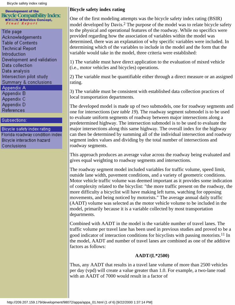
Bicycle safety index rating
One of the first modeling attempts was the bicycle safety index rating (BSIR)model developed by Davis.2 The purpose of the model was to relate bicycle safetyto the physical and operational features of the roadway. While no specifics wereprovided regarding how the association of variables within the model wasdetermined, there was an explanation of why specific variables were included. Indetermining which of the variables to include in the model and the form that thevariable would take in the model, three criteria were established:
1) The variable must have direct application to the evaluation of mixed vehicle(i.e., motor vehicles and bicycles) operations.
2) The variable must be quantifiable either through a direct measure or an assignedrating.
3) The variable must be consistent with established data collection practices oflocal transportation departments.
The developed model is made up of two submodels, one for roadway segments andone for intersections (see table 19). The roadway segment submodel is to be usedto evaluate uniform segments of roadway between major intersections along apredetermined highway. The intersection submodel is to be used to evaluate themajor intersections along this same highway. The overall index for the highwaycan then be determined by summing all of the individual intersection and roadwaysegment index values and dividing by the total number of intersections androadway segments.
This approach produces an average value across the roadway being evaluated andgives equal weighting to roadway segments and intersections.
The roadway segment model included variables for traffic volume, speed limit,outside lane width, pavement conditions, and a variety of geometric conditions.Motor vehicle traffic volume was deemed important as it provides some indicationof complexity related to the bicyclist: "the more traffic present on the roadway, themore difficulty a bicyclist will have making left turns, watching for opposingmovements, and being noticed by motorists." The average annual daily traffic(AADT) volume was selected as the motor vehicle volume to be included in themodel, primarily because it is a variable collected by most transportationdepartments.
Combined with AADT in the model is the variable number of travel lanes. Thetraffic volume per travel lane has been used in previous studies and proved to be agood indicator of interaction conditions for bicyclists with passing motorists.11 Inthe model, AADT and number of travel lanes are combined as one of the additivefactors as follows:
AADT/(L*2500)
Thus, any AADT that results in a travel lane volume of more than 2500 vehiclesper day (vpd) will create a value greater than 1.0. For example, a two-lane roadwith an AADT of 7000 would result in a factor of
Bicycle safety index rating
http://209.207.159.179/development/98072/appa/appa_01.html (1 of 6) [9/22/2000 1:37:14 PM]

1.4. In contrast, a roadway segment with a travel lane volume of less than 2500 vpdwill result in a value less than 1.0. The speed limit of the roadway was alsoincluded in the model for two reasons. First, it was believed that speed limitprovided some reasonable indicator of the design speed of the roadway. Secondand more importantly, it was believed to provide some indication of travel speedsof motor vehicles, which directly relates to the speed differential between motoristsand bicyclists. While these reasons for using speed limit are sound and the need forsome measure of motor vehicle speed is needed in the model, the reasoning doesnot necessarily hold true for all roadways. In a recent Federal HighwayAdministration (FHWA) study, 85th percentile speeds on a variety of rural andurban, two-lane and multilane roadways was found to be from 6 to 14 mi/h over theposted speed limit.12 This is not surprising considering the number of factors thatare often considered when a speed limit is set. Another recent study found that
Bicycle safety index rating
http://209.207.159.179/development/98072/appa/appa_01.html (2 of 6) [9/22/2000 1:37:14 PM]

while the 85th percentile speed is often used as the principal criterion, engineeringjudgment and the consideration of other factors often results in the establishment ofarbitrary speed limits that do not reflect travel speeds.13
The additive factor containing the speed limit variable within the model waswritten as follows:
S/35
From previous research, it had been shown that speed differentials betweenmotorists and bicyclists remain fairly constant (between 10 and 15 mi/h) up tomotor vehicle speeds of approximately 35 mi/h.14 In another study, it was shownthat more than 50 percent of all bicycle fatalities occurred on roadways with postedspeed limits greater than 35 mi/h.15 Thus, 35 mi/h was selected as the denominatorin the speed limit factor within the model. Any roadways with a speed limit of 35would produce a factor of 1.0; speed limits of 30 and lower would produce factorsless than 1.0 and posted speed limits of 40 and higher would produce factorsgreater than 1.0.
The outside or curb lane width was the next variable included in the model. Thisvariable was included since it determines the travel space available for bicyclingwithin the roadway and the space available for an overtaking motorist who desiresto remain in the curb lane during the maneuver. Curb lane widths of 14 ft werecited from two sources as being the desirable width to provide safe bicyclingconditions.16,17 The variable is presented in the model as follows:
(14-W)/2
As noted in the variable definitions presented with the model above, any lane widthgreater than 14 ft will still use a value of 14 ft within the model, i.e., 14 ft is themaximum value that can be used in the model. Based on this definition, any lanewidth greater than or equal to 14 ft will produce a factor of zero. One problem withthis restriction is that no benefit is gained from curb lane widths of 15 ft or greater.If larger values were used, a negative value would be produced, which wouldreduce the index value. Lane widths less than 14 ft will produce positive values thatwill add to the index. For example, a lane width of 12 ft would produce a positivefactor of 1.0.
Pavement condition was the next variable included in the model. This variable wasincluded because defects or irregularities in the paved surface can affect thecomfort and safety of bicyclists. As noted in the variable definitions presented withthe model above, eight different conditions are provided to define detrimentalpavement surfaces. Each of these conditions has a value assigned to it. Anexplanation of how these values were derived was not provided. An examination ofthe values, however, does seem to indicate that some degree of relative importancewas assigned within the factor itself. For example, potholes, rough edges, anddrainage grates are perhaps the most dangerous to bicyclists and, thus, wereassigned the largest value (0.75). Patching, weathering, and curb and gutter on theother hand, are not nearly as problematic for bicyclists and were assigned a valueof 0.25. The other conditions (rough railroad crossings and cracking) wereconsidered to fall in between the two extremes and were assigned a value of 0.50.
The last factor in the model is the location factor, which incorporates a variety ofmeasures related to both geometrics and operations along a roadway segment.
Bicycle safety index rating
http://209.207.159.179/development/98072/appa/appa_01.html (3 of 6) [9/22/2000 1:37:14 PM]

Those for bicyclists were assigned a positive value while those conditions whichpotentially improve bicycle safety were assigned a negative value. For example,parking along the roadside, grades, restricted sight distances, and driveways allreceived positive values. Paved shoulders and physical medians received negativevalues. As with the pavement factor, no detailed explanation was given regardinghow these assigned values were derived, but there does seem to be relativeimportance among the operational and geometric conditions present within thefactor. The condition perceived to be the most beneficial was the presence of apaved shoulder, with a value of -0.75, while the condition perceived to create thegreatest safety hazard was angle parking, with a value of 0.75.
As with the roadway segment model, traffic volume was deemed important at theintersection because it provides some indication of the level of complexity. Thefirst factor is intended to simply provide a number relative to the total enteringvolume at a given intersection. If this volume is greater than 10,000 vpd, the factorwill be greater than 1.0, indicating a more difficult intersection for the bicyclist.The second volume-related factor is intended to provide some indication of thelevel of difficulty that would be experienced by a bicyclist on a low-volume streetcrossing a high-volume street or vice versa. As an example, assume a bicyclist on astreet with an entering volume of 20,000 vpd is crossing a street with an enteringvolume of 5,000 vpd. The factor for these conditions becomes 1.6. If the bicyclist ison the low-volume roadway and is crossing the high-volume street, the factorbecomes 0.4. Intuitively, this factor appears to provide an opposite result of what isexpected; in most cases, exclusive of signalization and geometrics, one wouldhypothesize that it would be more difficult for the bicyclist to cross thehigh-volume roadway than the low-volume roadway. Again, there is no explanationregarding the development of these factors. Thus, a full understanding of what theauthor intended the factor to represent is difficult.
The geometrics variable is the next factor included in the model. This variable wasintended to quantify the traffic maneuver complexity of the intersection. Thenumber of lanes and type of lane are the predominant variables included in thisfactor, with a right-turn lane being given the highest value of 0.75. This probablyreflects the fact that the provision of such a lane for motor vehicles produces aweaving situation for motorists turning right and bicyclists proceeding through theintersection. Restricted sight distance and substandard curb radii are also geometricvariables that should be considered as part of the factor.
The last factor in the intersection model is the signalization factor. These factorsare intended to indicate how signal operations at a specific intersection may impactupon the safety of the bicyclists. If a signal is actuated, it is considered to have anegative impact on bicycling safety resulting from the fact that bicyclists oftencannot be detected by the detection loops.18 This fact, in turn, can result in thebicyclist crossing against the light and putting him or herself in a dangeroussituation. If the clearance interval is sub-standard, i.e., not long enough forbicyclists, a value of 0.75 is used. A value of less than 4.0 s is consideredsubstandard in the model. Finally, if permissive left turns are allowed or ifright-turn arrows are present, conditions are present that may require motorists toyield to bicyclists, which may create a hazardous situation.
A case study using the developed models was conducted in Chattanooga,Tennessee. A total of seven roadways consisting of 21 uniform segments and 29major intersections were included in the study. The appropriate indexes were
Bicycle safety index rating
http://209.207.159.179/development/98072/appa/appa_01.html (4 of 6) [9/22/2000 1:37:14 PM]

computed for each segment and intersection and then combined to form the overallindex rating (BSIR) for each roadway. The ratings produced for the sevenroadways ranged from 4.46 to 6.54. Relative comparisons were made between eachindividual rating and the other six ratings. On the basis of the author’s knowledgeof the roadways selected and the ratings produced from the models, a classificationscheme was developed to define bicycle operation based on the BSIR values (seetable 20). Of the seven roadways included in the case study, two were classified as"good," three were classified as "fair," and two were classified as "poor."
Table 20. Rating classifications for the bicycle safety index rating (BSIR).3
IndexRange
Classification Description
0 to 4 Excellent Denotes a roadway extremelyfavorable for safe bicycle operation.
4 to 5 Good Refers to roadway conditions stillconducive to safe bicycle operation,but not quite as unrestricted as in theexcellent case.
5 to 6 Fair Pertains to roadway conditions ofmarginal desirability for safe bicycleoperation.
6 or above Poor Indicates roadway conditions ofquestionable desirability for bicycleoperation.
As notedby theauthor,
these indexes are not definitive values, but instead assign general designations toroadways that can be used in determining bicycle routes, preparing bicycle maps,or prioritizing improvements for bicycling. While this study provides a goodstarting point for examining specific variables that may be important to bicycleoperations, it was not able to conclusively define how important specific variableswere to either bicycle safety or operations. First, there was no bicycle accidentanalysis conducted on any of the segments included in the case study. Thus, theterm bicycle "safety" index rating is misleading. While there is no argument thatmany of the factors included may impact upon the safety of bicyclists operatingconcurrently with motor vehicles, the validation of how these factors actuallyimpact upon safety was not performed. Second, the classification schemedeveloped was based entirely on the relative differences in the indexes producedand the author’s knowledge of the routes. This method of developing aclassification scheme is problematic from the standpoint that: 1) it relies on thesubjective judgment of the author to establish the scale of what is consideredexcellent, good, fair, or poor; and 2) the classification scheme may not betransferable to other cities or even other locations within the city since the relativedifferences between the sites used played a large part in establishing the scheme.
Finally, there is the problem of combining the results from the two submodels intoa single rating. Since the final result was simply an average of all intersection andsegment values produced for the roadway, it was assumed that roadway segments
Bicycle safety index rating
http://209.207.159.179/development/98072/appa/appa_01.html (5 of 6) [9/22/2000 1:37:14 PM]

are equivalent to intersections in terms of safety or operational difficulty for thebicyclist. Recent work has shown that 50.4 percent of all bicycle accidents occur atintersections or are intersection related.19 An additional 21.4 percent of the bicycleaccidents occur at other types of junctions, such as driveways. These resultsindicate a need to perhaps weight intersections significantly more when combiningresults. It is also possible that the two scenarios, intersections and segments, cannotbe combined; they are simply too different in terms of the maneuvers required, thetype and number of conflicts encountered, and the overall geometric andoperational conditions.
Bicycle safety index rating
http://209.207.159.179/development/98072/appa/appa_01.html (6 of 6) [9/22/2000 1:37:14 PM]

Florida roadway condition index
In 1991, the bicycle programs in Broward County and Hollywood, Florida, wereinterested in developing objective ratings for their roadway system as it related tobicycle operations. The BSIR, discussed above, was used as the evaluation tool withsome minor changes. First, only the roadway segment portion of the BSIR was usedin the evaluation. Intersections were not rated as part of this effort, and eachroadway segment between two intersections maintained a single rating (i.e., ratingsfor two or more roadway segments were not combined into a single weightedvalue). Second, the values used for some of the pavement and location factors weremodified in an attempt to reduce the weight of these factors within the model. Anexamination of the results from the Chattanooga case study revealed that, onaverage, the pavement and location factors accounted for 30 percent of the BSIR.The revised values are shown in table 21.3
The next change was for the Hollywood model only; the model was modified toplace greater weight on those segments where narrow lanes and high motor vehiclespeeds occurred simultaneously. This was done by multiplying the speed limit termby the lane width term. The speed limit used in the denominator was also reducedfrom 35 mi/h to 30 mi/h, again increasing the weighting of the speed factors.Finally, the traffic volume in the denominator was increased to from 2500 to 3100,which, in turn, reduced the weight of the traffic volume factor. The resulting modelwas termed the roadway condition index (RCI), reflecting the fact that it was anindicator of conditions rather than a predictor of crashes, and took the form shownin table 22.
Florida roadway condition index
http://209.207.159.179/development/98072/appa/appa_02.html (1 of 3) [9/22/2000 1:37:15 PM]

Since Hollywood is located within Broward County, a number of roadways wererated using both models. Percent differences in the actual values produced rangedfrom 0 to 19 percent, with the modified BSI model, used in Broward County,normally producing higher values than the RCI model, used in Hollywood. As notedby the author, the RCI model was more sensitive to changes in lane width and speedand less sensitive to changes in AADT. This effect should have been expectedconsidering the modifications made to the model.
One goal that was achieved in the results from both models was the reduction in thecontribution of the pavement and location factors to the overall rating. In BrowardCounty, the modified BSIR, which included only changes in the values assigned tothe various conditions, resulted in an 11 percent contribution to the index rating byboth factors. In Hollywood, the two factors contributed only 9 percent to the RCIrating.
An attempt to use the RCI model to predict crashes was also undertaken. Bicyclecrashes over a 20-month period in Hollywood were linked to specific roadwaysegments and ranked from one to five, depending on severity (with five being fatal).Sums were computed for each segment and divided by the length of the segment,resulting in an accident frequency per mile weighted by severity. The analysisconducted showed the RCI model to explain only 18 percent of the variation in thecrash scores between roadway segments. The first reason for this poor result maysimply be the means by which the crash measure was expressed. A much better wayto describe the crash would be in terms of "per bicycle miles ridden" or "per numberof motor vehicle encounters per mile" or some other exposure measure. The lack ofbicycle exposure data on the roadway segments was the principal reason noted bythe authors in explaining the poor results of the analysis.
In 1993, the RCI model was modified and applied in Dade County, Florida (seetable 23). The only variable not previously defined is HV, which is the percentageof heavy vehicles in the traffic stream and is expressed as a decimal. The values anddescriptive terms for the pavement and location variables were simplified. Thepavement surface was rated as either excellent, good, fair, or poor and assignedvalues of 0, 1, 2, and 3, respectively. The location factor was defined solely in termsof cross-traffic generation, which was either little, moderate, or heavy with values of1, 2, and 3, respectively.
Florida roadway condition index
http://209.207.159.179/development/98072/appa/appa_02.html (2 of 3) [9/22/2000 1:37:15 PM]

The change in the arrangement of terms in the model produced similar values to theprevious version, but changed the weighting of terms within the model. Thepavement and location factors in the modified version were less of a factor in theoverall index. Additional roadway width beyond 14 ft was now included in thepavement width term as a positive factor. Finally, the terms for lane width, speed,and traffic volume were multiplied in an attempt to increase the interaction betweenthe terms, which is more representative of the real world. This multiplicative formatalso allowed for the use of an exponential scalar. The value of 1.8 was used in themodel to accentuate changes in the index at the top and bottom of the ranges, whichimproved the fit to low-volume roads while not significantly affecting highervolume locations. Even with the changes in assigned values and modifications tothe model equations, there was still the need to interpret the index ratings producedby the various models and develop a classification scheme to identify the variouslevels at which roads were and were not compatible for bicycling operations. Aswith the BSIR, this development of such a scheme seemed to be subjective, basedon the individual or collective knowledge of bicycle researchers, coordinators, andpossibly others, and the relative results produced by the models. For the RCI model,the classification scheme was simply shifted down by one number from what hadbeen developed for the BSIR model (see table 24). The descriptions for theclassifications remained the same as previously shown in table 20. For the MRCImodel used in Dade County, the classifications as well as the descriptions weremodified. A roadway segment with a value between 0 and 4.0 was determined toprovide an adequate level of service for less experienced bicyclists or children. Arating of 5.0 or lower was considered to provide an adequate level of service formore experienced bicyclists.
Florida roadway condition index
http://209.207.159.179/development/98072/appa/appa_02.html (3 of 3) [9/22/2000 1:37:15 PM]

Bicycle interaction hazard score
The interaction hazard score (IHS) was the next model developed and was basedheavily on the prior models.4 The model was developed in an attempt to overcometwo problems noted with the previous models: 1) the substantial subjectivity used inestimating the values of some of the variables, and 2) the lack of consideration ofthe exposure variables. It is not clear what is meant by exposure. This could be thelevel of bicycling on a particular roadway, expressed as a volume or number ofbicycle miles ridden, or it could be the number of hazards to which the bicyclist isexposed along a route.
In deciding which variables to include in the model, all on-road bicycle interactionswere divided into two distinct groups. The first group was termed the "longitudinalroadway environment" and included variables that affect the bicyclist’s perceptionof hazard. Variables in this group included volume, speed, and size of the motorvehicles using the shared roadway, proximity of the bicyclist to these vehicles, andpavement condition of the travel lane for the bicyclist. The second group wastermed the "transverse roadway environment" and included variables that representuncontrolled vehicular movements that may present a hazard to the bicyclist on theshared roadway. Variables in this group included frequency of driveways andon-street parking presence and turnover.
Combining some of the terms from the prior models with some additional terms toaccount for the variables just mentioned, the IHS model took the form shown intable 25.
Once the model was developed, baseline conditions for a two-lane minor arterialwere used for calibration. Coefficients for a1, a2, and a3 were established to be 0.01,
Bicycle interaction hazard score
http://209.207.159.179/development/98072/appa/appa_03.html (1 of 2) [9/22/2000 1:37:16 PM]

0.01, and 0.024, respectively. These coefficients resulted in the speed factorproducing 79 percent of the model’s value. The pavement condition factor and theland use/curb cut factor produced 13 percent and 8 percent of the equation’s value,respectively. A sensitivity analysis was also conducted to show how changes in aspecific variable affected the overall value of the model. This analysis wasperformed for each variable and compared with the baseline conditions establishedfor the two-lane minor arterial. The author concludes that the values established forthe coefficients and the results of the sensitivity analysis are valid on the basis ofinterviews with bicyclists and group meetings. However, no results from any ofthese meetings or interviews were provided to assess the actual validity. Thus, itappears that the goal of eliminating subjectivity from the modeling process was nottotally achieved within the IHS. It is also not clear whether the goal of increasingconsideration for exposure was met. As previously noted, the author did notexplicitly define exposure. If the goal was to improve the use of bicycle exposuremeasures within the model, such as bicycle volumes, the model was unsuccessful.However, if exposure was defined as potential hazards to the bicyclist, then themodel did tend to include measures that were directly applicable and moreobjective when compared with previous models.
Bicycle interaction hazard score
http://209.207.159.179/development/98072/appa/appa_03.html (2 of 2) [9/22/2000 1:37:16 PM]

Conclusions
All of the models discussed here were good attempts at trying to definebicycle operations (and sometimes safety) under varying roadwayconditions. Altogether, there were five different models described, with eachone building on what had been done in the previous efforts. As eachsuccessive model was developed, there seemed to be a desire to remove thesubjectivity from the process. Unfortunately, this was never totally achieved.In all cases, there was the need to interpret the various indexes produced anddecide what the breakpoints were that separated a roadway with goodbicycling operations from one that was excellent or fair or poor. The meansof accomplishing this in each case was to produce the index ratings,examine them in relation to each other and, based primarily on the "street"knowledge of the author with regard to which roadways he thought weregood and bad for bicycling, establish the subjective breakpoints in theclassification scheme.
It should be noted that the authors did recognize the need to further validatetheir work. The primary suggestion from two of the authors was toincorporate the opinions of bicyclists regarding perceived hazards and ridingcomfort.3,4 Several means of accomplishing this goal were suggested,including:
having bicyclists actually ride on a number of different roadways;1.
having bicyclists complete questionnaires or participate in roadsideinterviews designed to quantify different types of hazards;
2.
having the bicyclists view videotapes of different roadway segmentsand evaluate them in much the same way as they would if they wereriding the segment.; or
3.
observing which routes bicyclist choose in going from an origin to adestination and how long they are willing to ride on each specificroadway segment.
4.
In this research effort, it was the video technique that was adapted fromprior work by Sorton and Walsh and validated as discussed in chapter 2.Another research effort recently conducted adopted the approach of havingbicyclists ride in the roadway on a limited number of segments.20 As in thiseffort, the subjects in that study also provided "comfort" ratings on asix-point scale for each of the segments ridden, exclusive of intersections.
The bicycle level of service (BLOS) model developed from the bicyclists’surveys is shown in table 26. The model had an R2-value of 0.73 andincorporated a number of variables related to geometrics, operations, andtrip generation characteristics. While there are some differences betweenthis model and the BCI model with respect to significant terms, the primaryterms of width, presence or absence of a bicycle lane, traffic volume, andmotor vehicle speed, are present in both. However, the BLOS modelcontains a number of additional variables that would not be readily availableto most practitioners (e.g., pavement condition rating and detailed land-useinformation); obtaining such data could be cost-prohibitive for some
Conclusions
http://209.207.159.179/development/98072/appa/appa_04.html (1 of 2) [9/22/2000 1:37:18 PM]

agencies. The BCI model developed in the current research study attemptedto be sensitive to this issue, and thus minimizes the amount of additionaldata that may be required.
One of the major differences between the BCI model and the BLOS modelis the inclusion of the term pavement condition in the BLOS model. Thedevelopers of the model insist that this variable is critical to determining thequality of service for bicyclists. The authors of this report do not disagreewith that statement, but take the position that bicycle routes should not beestablished on the basis of that criterion. Instead, the geometric andoperations variables identified as significant in the BCI model should beused for establishing bicycle level of service and subsequently appropriateroutes. The surface quality of those routes on the bicycle network shouldthen be maintained to minimize hazards and provide a quality ride forbicyclists.
Conclusions
http://209.207.159.179/development/98072/appa/appa_04.html (2 of 2) [9/22/2000 1:37:18 PM]

Summary of results
The primary objective of this research effort was to develop an instrument thatwould allow bicycle coordinators, transportation planners, traffic engineers, andothers to evaluate the capability of specific roadways in their communities toaccommodate both motorists and bicyclists. The tool developed is the bicyclecompatibility index (BCI), which incorporates the geometric and operationalvariables considered by adult bicyclists to be important in terms of their comfortlevel when riding on streets in the presence of motor vehicle traffic. Note: The BCImodel is not necessarily appropriate for evaluating the compatibility of roadwaysfor youth bicyclists.
The approach used in developing the BCI was to obtain the perspectives ofbicyclists by having them view numerous roadway segments captured on videotapeand rate those segments with respect to how comfortable they would be ridingthere under the geometric and operational conditions shown. The reliability of theresults obtained using this video technique of data collection with respect toreflecting on-street comfort levels was validated in a pilot study (see chapter 2).The procedure used offered several advantages over other forms of data collection,including minimizing the risk to bicyclists, maximizing the range of roadwayconditions to which the bicyclists could be exposed, and controlling the variablesevaluated by the bicyclists.
Using the perspectives of over 200 study participants in three locations (Olympia,WA; Austin, TX; and Chapel Hill, NC), the BCI model was developed for allbicyclists, as shown in table 16 (see appendix D for the equivalent English unitsversion of the model). This model predicts the overall comfort level rating of abicyclist using the eight significant (at p < 0.01) variables shown and an adjustmentfactor (AF) to account for three additional operational characteristics. The basicmodel (excluding the adjustment factor) has an R2-value of 0.89, indicating that 89percent of the variance in the index or comfort level of the bicyclist is explained bythe eight variables included in the model. In other words, the model is a reliablepredictor of the expected comfort level of bicyclists on the basis of these eightvariables describing the geometric and operational conditions of the roadway. Thevariable with the largest effect on the index is the presence or absence of a bicyclelane or paved shoulder that is at least 0.9 m wide (BL); the presence of a bicyclelane (paved shoulder) reduces the index by almost a full point, indicating anincreased level of comfort for the bicyclist. Increasing the width of the bicycle laneor paved shoulder (BLW) or the curb lane (CLW) also reduces the index as doesthe presence of residential development along the roadside (AREA). On the otherhand, an increase in traffic volume (CLV and OLV) or motor vehicle speeds(SPD) increases the index, indicating a lower level of comfort for the bicyclist. Thepresence of on-street parking (PKG) also increases the index.
In addition to the primary variables included in the BCI model, three additionalvariables defining specific operating conditions were also examined. Thesesupplemental variables were identified during the pilot phase of the study as havinga potential impact on the comfort level of bicyclists and included the presence of:1) large trucks or buses, 2) vehicles turning right into driveways or minorintersections,
Summary of results
http://209.207.159.179/development/98072/ch06/ch06_01.html (1 of 5) [9/22/2000 1:37:19 PM]

1Large trucks are defined as all vehicles with six or more tires.
2Includes total number of right turns into driveways or minor intersections along aroadway segment.
Or 3) vehicles pulling into or out of on-street parking spaces. An analysis of theoverall comfort level ratings made when viewing video clips illustrating theseconditions showed all three of these variables to significantly increase the comfortlevel rating, thus indicating a lower level of comfort when these conditions werepresent. For all bicyclists, the overall mean rating increased by 0.50 when largetrucks or buses were present. When there were vehicles pulling into or out ofparking spaces, the average rating increased by 0.60. And finally, the presence ofright-turning vehicles resulted in an increase in the mean rating of 0.10
Summary of results
http://209.207.159.179/development/98072/ch06/ch06_01.html (2 of 5) [9/22/2000 1:37:19 PM]

While the presence of these three specific operating conditions was not evaluatedacross all possible combinations of geometrics and operations, the results of thelimited sample do indicate a need for adjustment to the BCI model when largetrucks or buses are present, when there is a high number of vehicles pulling into orout of on-street parking spaces, or when there is a high volume of right-turningvehicles. Thus, a series of adjustment factors that can be added to the model havebeen developed for each of these scenarios (see table 16). These factors weredeveloped on the basis of the theory that the conditions shown to the surveyparticipants represented worst-case scenarios and, subsequently, the increase in theoverall mean comfort level rating represented the maximum adjustment that wouldbe required (see chapter 4 for a detailed discussion).
It should be noted that one variable not included in the development of the BCImodel was the grade of the roadway. Results from a preliminary effort showed thatchanges in grade of 2 percent or less were not distinguishable on the video. Theadvantages of using video, which included not exposing bicyclists to high-riskconditions, incorporating a much larger sample of sites, and controlling specificvariables to ensure that all subjects were exposed to identical conditions, werebelieved to outweigh the absence of this one variable. It is also believed that thevariables having the most significant effect on the bicycle compatibility of aroadway have been included in the BCI model. Specifically, the variables of width,speed, volume, and on-street parking were shown to have the greatest impact onthe index. At this time, the impact of grade relative to these and the othersignificant variables included in the model is unknown but may be determined infuture research efforts.
Once the BCI model was developed, bicycle level of service (LOS) criteria wereestablished on the basis of the distribution of the participants’ mean comfort levelratings. Currently, there are no LOS criteria provided in the Highway CapacityManual. However, the definition of the LOS according to the manual is founded onthe concept of users’ perception of qualitative measures that characterize theoperational conditions of the roadway. Two of the terms used in the manual todescribe LOS are comfort/convenience and freedom to maneuver; both of theseitems are applicable to bicyclists and are directly reflected in the BCI since therating scale used by the study participants was a direct indication of comfort level.Thus, using the distribution of participant comfort level ratings across all sitesincluded in this study, LOS designations were established for LOS A through LOSF, as shown in table 17. LOS A (represented by an index £ 1.50) indicates that aroadway is extremely compatible (or comfortable) for the average adult bicyclistwhile LOS F (represented by an index > 5.30) is an indicator that the roadway isextremely incompatible (or uncomfortable) for the average adult bicyclist.
In developing the BCI model, several other issues were addressed, including theeffect of bicycling experience level on perceived comfort levels. Using the resultsfrom a questionnaire completed by the participants, the bicyclists were stratifiedinto three groups based on their riding habits such as number of bicycle trips/wkand types of facilities used (e.g., major roadways vs. bicycle paths). A comparisonof the comfort level ratings of these three groups showed that "casual recreational"bicyclists produced a significantly higher overall mean comfort level rating (3.1)across all sites than "experienced recreational" or "experienced commuter"bicyclists (2.7 and 2.6, respectively). As a result of these differences, separate BCImodels were produced for each of the three groups in addition to the model for all
Summary of results
http://209.207.159.179/development/98072/ch06/ch06_01.html (3 of 5) [9/22/2000 1:37:19 PM]

bicyclists (see table 8 in chapter 4). However, in real-world applications, it is mostlikely that bicyclists of all experience levels will ride or have the opportunity toride on any given segment of roadway. Thus, it is recommended that the BCImodel developed for all bicyclists and shown in table 16 be used withoutmodification for most applications. The LOS designations shown in table 17were developed on the basis of this model and thus, are only applicable toresults produced with the "all bicyclists" model. Thus, use of the model forcasual recreational bicyclists or other specific groups of bicyclists in conjunctionwith these LOS designations is not appropriate.
1Qualifiers for compatibility level pertain to the average adult bicyclist.
Instead, a different approach that can be used to ensure that facilities meet thedesired comfort levels of casual bicyclists is to simply design for a higher level ofservice. As noted in chapter 4, the casual bicyclist model is likely to result in BCIvalues that are 0.14 to 0.38 greater than the model for all bicyclists. The differencein BCI values between LOS designations are, on average, 1.0 (see table 17). Bydesigning for a higher LOS (e.g., LOS B rather than LOS C) on a facility known toproduce a high number of casual bicyclists, the necessary comfort level for thisgroup of bicyclists can be achieved with the model for all bicyclists. It should benoted that where casual bicyclists are expected, the facility should always bedesigned at LOS C or better.
Another issue addressed was that of possible regional differences in the perceptionsof bicyclists. If bicyclists in different geographical regions of the country perceivecomfort levels differently, then separate models would need to be developed toreflect these differences. An analysis of the comfort level ratings across subjects inthe three survey cities showed no differences in the mean comfort levels for thefour variables rated (speed, volume, width, and overall). This lack of differencesindicates that the perceptions of individuals with respect to bicycle compatibilityare the same in the three regions where the survey was conducted, and that the BCImodel should be applicable across all regions of the country.
It is important to note again that the BCI model developed is for midblock streetsegments only and is primarily intended for use on "through" streets. In otherwords, the ratings do not account for major intersections along the route where thebicyclist may encounter a stop sign or traffic signal. A secondary objective of thisresearch effort was to apply the developed methodology used for rating midblock
Summary of results
http://209.207.159.179/development/98072/ch06/ch06_01.html (4 of 5) [9/22/2000 1:37:19 PM]

roadway segments to intersections and assess whether such an approach was validfor rating the bicycle compatibility of intersections. In a limited effort, bicyclistswere asked to rate a series of intersections with respect to how comfortable theywere riding through the intersection in the presence of right-turning traffic. Therelationship between these ratings and the geometric and operational conditions ofthe intersection was determined through regression modeling. By including onlythose variables or combinations of variables that were significant (at p £ 0.01), thefollowing model (R2 = 0.81) was developed:
BCI(INT) = 2.22 – 0.76BL + 0.49SHIFT + 0.003RVOL + 0.001TVOL
Similar to the BCI model for midblock segments, the variable having the greatestimpact was the presence or absence of a bicycle lane (BL) on the approach to theintersection. The presence of such a lane dramatically reduces the index value,indicating a higher level of comfort. The remaining variables in the model allproduce increases in the index, indicating a lower level of comfort, with the mostsignificant of these conditions being when a bicyclist has to shift to the left acrossan auxiliary right-turn lane to proceed straight through the intersection.
Overall, the results of this limited effort for intersections was positive and showedthat the video methodology used to obtain bicyclists’ perspectives can be a reliablemeans for producing a compatibility index for intersections. However, futureresearch needs to be conducted in which the scope of the study is expanded toinclude the full range of possible intersection maneuvers by bicyclists and the fullrange of geometric and operational conditions that can be expected inurban/suburban settings.
Summary of results
http://209.207.159.179/development/98072/ch06/ch06_01.html (5 of 5) [9/22/2000 1:37:19 PM]

Conclusions
The BCI model and the subsequent LOS designations provide bicyclecoordinators, transportation planners, traffic engineers, and others thecapability to assess their roadways with respect to compatibility forshared-use operations by motorists and bicyclists. The tool also allowspractitioners to better plan for and design roadways that are bicyclecompatible. Specifically, the BCI model can be used for the followingapplications:
• Operational Evaluation - Existing roadways can be evaluated using theBCI model to determine the bicycle LOS present on all segments. Thistype of evaluation may be useful in several ways. First, a bicyclecompatibility map can be produced for the bicycling public to indicatethe LOS they can expect on each roadway segment. Second, roadwaysegments or "links" being considered for inclusion in the bicyclenetwork system can be evaluated to determine which segments are themost compatible for bicyclists. In addition, "weak links" in the bicyclenetwork system can be determined, and prioritization of sites needingimprovements can be established on the basis of the index values.Finally, alternative treatments (e.g., addition of a bicycle lane vs.removal of parking) for improving the bicycle compatibility of aroadway can be evaluated using the BCI model.
• Design - New roadways or roadways that are being re-designed orretrofitted can be assessed to determine if they are bicycle compatible.The planned geometric parameters and predicted or known operationalparameters can be used as inputs to the model to produce the BCI valueand determine the bicycle LOS that can be expected on the roadway. Ifthe roadway does not meet the desired LOS, the model can be used toevaluate changes in the design necessary to improve the bicycle LOS(see example below).
• Planning - Data from long-range planning forecasts can be used toassess the bicycle compatibility of roadways in the future using projectedvolumes and planned roadway improvements. The model provides theuser with a mechanism to quantitatively define and assess long-rangebicycle transportation plans.
Conclusion
http://209.207.159.179/development/98072/ch06/ch06_02.html [9/22/2000 1:37:20 PM]

Application example
Provided below is a brief example of how the BCI model can be applied in the assessment of designalternatives for a roadway that is being planned for reconstruction. A minor arterial that connects asuburban area to the major arterial used for commuting into and out of downtown is being widened fromtwo lanes to four because of a projected increase in volumes. The development along the roadside is acombination of retail businesses and light commercial industries. The current average annual daily traffic(AADT) on the roadway is 10,000 vehicles per day (vpd) with 2 percent truck traffic, and the projectedAADT in five years is 16,000 vpd with the same percentage of trucks. Motor vehicle speeds on the facilitycurrently have an 85th percentile of 50 km/h; with the additional lanes, this value is expected to increaseslightly to 55 km/h. The original proposed highway department design (see figure 21) within the 20.0-mright-of-way included 3.6-m wide lanes, a 1.0-m wide planting strip on each side, and 1.8-m widesidewalks. No paved shoulders or bicycle lanes were included in the design.
Using the BCI model, the bicycle LOS for the proposed route can be determined as follows. First, theprojected AADT of 16,000 vpd must be converted into an hourly volume. The highest hourly volume onthis roadway is during the peak hour with 10 percent of the AADT (1,600 vehicles) traveling in bothdirections during this hour. It is also known that the directional split during the peak hour is 70/30, i.e., 70percent of the vehicles are traveling in one direction during the peak hour. Thus, 1120 vph (0.7 x 1600) isthe directional volume to be used. Since this volume will be distributed across two lanes with 60 percent ofthe traffic in the curb lane, two final calculations are made to determine the lane volumes as follows:
Curb lane volume (CLV)
= 1120 x 0.6 = 672
Other lane volume (OLV)
= 1120 x 0.4 = 448
Table 18. Bicycle Compatibility Index (BCI) computations and levels of service (LOS) associatedwith the geometric design options in the example.
Application example
http://209.207.159.179/development/98072/ch06/ch06_03.html (1 of 2) [9/22/2000 1:37:20 PM]

DesignOption
BCI Model Variables BCI LOS
BL BLW CLW CLV OLV SPD PKG AREA AF
OriginalProposal
0 0.0 3.6 672 448 55 0 0 0.1 4.71 E
Wide CurbLane
0 0.0 4.6 672 448 55 0 0 0.1 4.21 D
BicycleLane
1 1.2 3.6 672 448 55 0 0 0.1 3.24 C
Calculations
DesignOption
3.67 - 0.966BL - 0.410BLW - 0.498CLW + 0.002CLV + 0.0004OLV + 0.022SPD +0.506PKG - 0.264AREA + AF
OriginalProposal
3.67 - 0.966(0) - 0.410(0.0) - 0.498(3.6) + 0.002(672) + 0.0004(448) + 0.022(55) +0.506(0) - 0.264(0) + 0.1
Wide CurbLane
3.67 - 0.966(0) - 0.410(0.0) - 0.498(4.6) + 0.002(672) + 0.0004(448) + 0.022(55) +0.506(0) - 0.264(0) + 0.1
BicycleLane
3.67 - 0.966(1) - 0.410(1.2) - 0.498(3.6) + 0.002(672) + 0.0004(448) + 0.022(55) +0.506(0) - 0.264(0) + 0.1
The truck traffic on the roadway was projected to be 2 percent of the AADT. Using the same assumptionsfor directional splits and lane distributions, the number of trucks per hour in the curb lane becomes 13(0.02 x 672). From table 16, the adjustment factor (ft)for this level of truck volume is 0.10.
Using this information and the other data provided, the BCI for the original proposed design wascomputed as shown in table 18. The calculated BCI was 4.71 which, based on the LOS criteria shown intable 17, results in a bicycle LOS E or a very low level of compatibility for bicycling.
Since this particular roadway presently accommodates a fair volume of commuting bicyclists and is animportant link in the bicycle network, it is desired to provide bicycle LOS C or better. Thus, two optionaldesigns are proposed that fit within the 20.0-m-wide right-of-way. The first option is the wide curb lanedesign in which the planting strip is eliminated and the curb lanes are increased to 4.6 m in width; all otherdimensions remain the same. As shown in table 18, this design results in a BCI of 4.21, which isequivalent to LOS D and indicates a moderately low level of compatibility for bicycling. While this is animprovement, it does not increase the LOS to the desired level.
The second optional design incorporates a 1.2-m-wide bicycle lane, as shown in figure 22. Again, theplanting strip has been eliminated and the original sidewalk width is maintained. The curb lane widths of3.6 m are also maintained, but the interior lanes are reduced slightly to 3.4 m. The BCI for this option iscomputed to be 3.24, as shown in table 18. This value equates to LOS C, which indicates a moderatelyhigh level of compatibility for bicycling and meets the desired bicycle LOS requirements for the roadway.
This example was provided to illustrate the practical use of the BCI model in evaluating alternativedesigns to ultimately arrive at a design that could be considered "bicycle friendly." Other examplesassociated with various aspects of planning and design issues as well as detailed instructions on how toapply the model can be found in the companion report to this document, titled The Bicycle CompatibilityIndex: A Level of Service Concept, Implementation Manual.
Application example
http://209.207.159.179/development/98072/ch06/ch06_03.html (2 of 2) [9/22/2000 1:37:20 PM]

Site selection
The sites selected for the intersection study were located in several of thesame cites as the selected roadway segments. As with the midblockroadway segments, a matrix (see table 14) that stratified several of thegeometric and operational variables was developed to ensure that thesites selected represented the range of variables a bicyclist mayencounter in performing this maneuver in an urban or suburbanenvironment. The bicycle lane facilities were separated from thestandard/wide curb lane facilities and the right-turn traffic volumeswere separated into two categories. Another stratification variable usedfor those facilities with a bicycle lane on the approach was whether ornot the bicyclist had to shift to the left, across an auxiliary right-turnlane, to travel straight through the intersection. The number of sitesselected in each of the cells is shown in table 14, with the total numberbeing 19. Shown in figure 17 are four of the intersection sites illustratingthe range of conditions included in the evaluation.
High Volumehigh-speedintersectionwithchannelizedright-turn laneon theapproach.
Site selection
http://209.207.159.179/development/98072/ch05/ch05_01.html (1 of 3) [9/22/2000 1:37:22 PM]

High-volume,low-speedintersection withunique combinedright-turn/bicyclelane
Low-volume,low-speedintersectionwith bicyclelane separatedfrom motorvehicle lanes bywide-dashedstriping
Low-volume,low-speedintersection withtypical sharedthrough andright-turn laneformotor vehicles(i.e., no separateright-turn lane)and no bicyclelane.
Site selection
http://209.207.159.179/development/98072/ch05/ch05_01.html (2 of 3) [9/22/2000 1:37:22 PM]

Figure 17. Examples of sites included in the intersection pilot study
Site selection
http://209.207.159.179/development/98072/ch05/ch05_01.html (3 of 3) [9/22/2000 1:37:22 PM]

Data collection
The procedures followed for collecting data for the intersection locationswere similar to those followed for the midblock roadway segments (seechapter 3). The one exception pertained to the filming of theintersection. For the midblock locations, the camera was positionedalong a tangent section of roadway, aimed parallel to the roadway, andset to "record" passing traffic conditions for 15 min. At the intersection,the camera had to be positioned upstream of the intersection at a pointthat would allow participants to observe the speed of approaching trafficas well as the lane-changing behavior of traffic into auxiliary right-turnlanes (see figure 18). In some cases, the auxiliary lanes were extremelylong. With the camera positioned upstream of the beginning of theauxiliary lane, it made viewing the detailed configuration of theintersection difficult (see figure 19). Thus, at the start of filming for eachlocation, the camera was zoomed out to show a close-up of theintersection and then slowly zoomed in to the normal (non-zoom)position for the 15 min of filming. This zooming sequence for eachintersection was added prior to the 40-s clip used for rating theintersection.
Figure 18. For the intersection study, the camera was positionedupstream of the intersection to allow participants to observe the
approach speeds and lane-changing behaviors of motorists.
Data collection
http://209.207.159.179/development/98072/ch05/ch05_02.html (1 of 2) [9/22/2000 1:37:23 PM]

Figure 19. Sites with high volumes of right-turning traffic sometimescontained extremely long auxiliary turn lanes, which made viewing
the intersection proper difficult.
Data collection
http://209.207.159.179/development/98072/ch05/ch05_02.html (2 of 2) [9/22/2000 1:37:23 PM]

Video production
The production of the video for the survey followed the same proceduresdescribed in chapter 3 for the production of the video for the midblockroadway segments. The only difference was in the volume counted andused to select representative video clips. For the midblock locations, thetraffic volume of interest was the curb lane volume; for the intersectionlocations, it was the right-turning traffic volume. Thus, the equation usedin conjunction with the right-turn volume counts for selectingrepresentative intervals was as follows:
Vrt = (Vtrt/15 min)(40 s/60 s)
where:
Vrt = representative right-turn volume for the 40-s interval,and
Vtrt = total right-turn volume observed during the 15 min ofvideotape.
Video production
http://209.207.159.179/development/98072/ch05/ch05_03.html [9/22/2000 1:37:23 PM]

Video survey
The video survey for the intersections included the same individuals inthe same cities who participated in the roadway segment survey. Oncethe roadway segment survey was completed each evening, theparticipants were provided with new rating forms and a new set ofinstructions (see appendix C). They were instructed to rate each of the 19intersections using the same six-point scale with respect to howcomfortable they would be riding a bicycle through the intersectionshown in the presence of the right-turning traffic and the other conditionsshown.
The variables for which ratings were provided differed for approximatelyhalf of the participants. It had been hypothesized in the early stages ofthe study that the participants would make one overall comfort levelrating, and that the significant geometric and operational variables wouldbe reflected in that rating. This approach differed from that of having theparticipants provide not only an overall rating, but ratings for othervariables believed to be important in terms of assessing the bicyclecompatibility of an intersection. In the latter case, it was possible that theoverall rating was influenced by the rating of one or more of the othervariables.
Using these two approaches, an additional experiment was carried outwithin this intersection study. Approximately half of the participantsprovided a single overall comfort level rating for the bicycle maneuver inquestion. The remaining participants provided not only an overall rating,but also comfort level ratings based on four other factors. These factorsincluded the volume of right-turning traffic, the speed of approachingtraffic, the width or space available to them to maneuver through theintersection, and the clarity of signs and markings to guide the motoristand bicyclist through the intersection.
Video survey
http://209.207.159.179/development/98072/ch05/ch05_04.html [9/22/2000 1:37:24 PM]

Data analysis
The analysis of the video survey data focused on the development of a model topredict the bicycle compatibility of intersections with respect to the maneuverselected for this pilot study. The objective of the analysis was to determine if thevideo methodology could be applied at intersections and produce results thatcould be used to assess the bicycle compatibility of intersections.
Differences in overall comfort level ratings between subjects were examined bycomputing an average overall rating score (across intersections) for each subject.A regression tree model was then developed using the CART (Classification AndRegression Tree) procedure to identify subgroups of subjects over which theoverall ratings differed consistently.10 Independent variables in this modelincluded the questionnaire item responses and a variable indicating whether ornot the subject provided a single overall rating or an overall rating plus the otherfour ratings.
The results of this analysis were quite consistent with those of the midblockanalysis in that the primary subdivision of subjects was between those who madea large percentage of their trips for commuting purposes on major city streetsversus those who primarily rode for recreation largely on more minor streets withless traffic and lower speeds or on bicycle paths. The average comfort ratings forthese two groups were 3.49 and 4.10, respectively. It was also of interest to notethat consistent differences in overall scores were not found between thosesubjects who provided the single overall rating versus those who also providedthe additional ratings.
As with the roadway segment analysis, regression models were used toinvestigate relationships between intersection characteristics and comfort levelratings. The geometric and operational variables collected in the field or from thevideo and included in the regression modeling are shown in table 15. To estimatethe effects of these characteristics on the overall comfort level ratings, means andvariances of the overall ratings were computed for each intersection across allsubjects. A weighted regression model, where each case was weighted by theinverse of its variance, was then developed using the mean overall rating as theresponse variable and the intersection characteristics as independent variables.Using combinations of the independent variables and eliminating all variablesand combinations that were not significant at the p < 0.01 level, the resultingregression model is expressed as follows:
BCI(INT) =2.22 - 0.76BL+ 0.49SHIFT
+ 0.003RVOL + 0.001TVOL
The variable having the greatest impact on the index was the presence or absenceof a bicycle lane approaching the intersection. If a bicycle lane (BL) is present,the index is reduced by 0.76, indicating a higher level of comfort. Another of thesignificant variables was SHIFT, which indicates if the bicyclist had to shift tothe left across an auxiliary lane to continue straight through the intersection. Ifthis scenario exists (see example in figure 20), the index increases by almost halfa point (0.49), indicating that bicyclists are less comfortable when this maneuveris required. The other significant variables were the right-turn volume (RVOL)and the total approach volume (TVOL); both of these variables increase the
Data analysis
http://209.207.159.179/development/98072/ch05/ch05_05.html (1 of 3) [9/22/2000 1:37:25 PM]

index as volumes increase, again indicating a decrease in the comfort level ofbicyclists with higher traffic volumes. For each 100-vph increase in right-turnvolumes, the index increases by 0.30; for each such increase in total approachvolumes, the index increases by 0.10.
The model developed had an R2-value of 0.81, indicating that 81 percent of thevariance in the index value is explained by the four variables included in theequation. Thus, the use of these four variables can produce an index value that isa reliable predictor of a bicyclist’s comfort level with performing the maneuverstudied, i.e., continuing straight through the intersection in the presence ofright-turning traffic. It appears then that this model is a good indicator of thebicycle compatibility of an intersection for that particular maneuver. These resultsalso indicate that the use of the video methodology at intersections can be areliable means of developing a compatibility index for intersections. However,more research is needed to fully develop an intersection index, including anexpansion of the scope of bicycle maneuvers and intersection characteristics.
Data analysis
http://209.207.159.179/development/98072/ch05/ch05_05.html (2 of 3) [9/22/2000 1:37:25 PM]

Figure 20. The intersection index increased significantly (indicating a lowerlevel of comfort) if the bicyclist was required to shift to the left to proceed
straight through the intersection.
Data analysis
http://209.207.159.179/development/98072/ch05/ch05_05.html (3 of 3) [9/22/2000 1:37:25 PM]

Effect of bicyclist experience
In the prior research effort conducted by Sorton and Walsh, the experience level of thebicyclist significantly affected the comfort level of the bicyclist.7 For example, whenasked to rate their comfort level with respect to curb lane width (on a five-point scale),the experienced riders produced a mean value of 3.00 while the casual riders produceda higher mean rating of 3.34, indicating less comfort with the widths provided. Similarresults were found with respect to the motor vehicle speed and traffic volumevariables.
From these past results, it was reasonable to hypothesize that differences in experiencelevels would also be reflected in the comfort level ratings of participants in this study.Specifically, those bicyclists with the most experience would be most comfortablewith the geometric and operating conditions shown and thus would have lower ratingswhen compared with the less experienced bicyclists.
The first step in evaluating the experience levels of bicyclists on the comfort levelratings was to produce clusters of bicyclists with similar experience. The responses tothe questionnaire completed by the participants served as the mechanism to producesuch groups. The final question on the questionnaire asked participants to classifythemselves into one of two specified categories according to their experience riding onurban and suburban streets. A total of 60 percent stated that they were "comfortableriding under most traffic conditions, including major streets with busy traffic andhigher speeds."
A logistic regression analysis of this response on other questionnaire responsesindicated that the self-classification of ‘comfortable riding under most conditions’ waspositively associated with male gender, percent of cycling on major streets, and milesper week that they typically ride. With the exception of these factors, theself-classification of experience did not appear to be related to other experienceresponse variables and thus was not used as the sole criterion in developing groups byexperience level.
Instead, cluster analyses were performed to determine clusters or homogeneous groupsof bicyclists. Two-cluster and three- cluster models were fitted using the centroidmethod of ‘distance’ between clusters. The analyses produced clusters according to amultivariate score based on all variables. While the definition of each cluster could notbe simply defined, the results did provide insight into which variables are mostimportant in terms of assessing experience level. Those variables included trippurpose, number of trips/wk, distance ridden/wk, and types of facilities used.Ultimately, these exploratory cluster analysis results were used as the basis fordefining three homogeneous groups (see table 6) of bicyclists as follows:
1) Experienced Commuter Bicyclists
Bicyclists in this group make the largest percentage of their trips (60 percent) for thepurpose of commuting to/from school or work. This group also rides more days/wkthan the other groups, longer distances, and makes more trips/wk. They also tend toride on major streets more often than the other groups.
2) Experienced Recreational Bicyclists
Bicyclists in this group make 80 percent of their trips for the purpose of recreation orexercise. They tend to ride fewer days/wk than experienced commuter bicyclists butmore days/wk than casual recreational bicyclists. This same trend is also true fornumber of trips/wk and distances ridden/wk. Finally, bicyclists in this group are less
Effect of bicyclist experience
http://209.207.159.179/development/98072/ch04/ch04_01.html (1 of 4) [9/22/2000 1:37:27 PM]

likely than experienced commuter bicyclists to ride on major streets but more likely toride on bicycle paths.
3) Casual Recreational Bicyclists
Bicyclists in this group are similar to experienced recreational bicyclists in that theymake the largest percentage of their trips (70 percent) for recreational/exercisepurposes. However, this group rides the fewest days/wk, makes the fewest number oftrips/wk, and rides the fewest number of mi/wk. This group also rides the least amountof their trips on major streets and the most on bicycle paths when compared with theother groups.
As previously described in chapter 3, each participant provided four ratings on a scaleof one (extremely comfortable) to six (extremely uncomfortable) for four variables:width (or space available to ride), speed of traffic, volume of traffic, and overall.Shown in figure 12 are the mean comfort level ratings for each of these variables andeach group of bicyclists. For all four variables rated, the experienced recreationalbicyclists and the experienced commuter bicyclists had identical or very similar meanvalues. On the other hand, the casual recreational bicyclists had slightly higher meanratings when compared with the other groups, confirming what had previously beenfound by Sorton and Walsh.7 The differences ranged from a low of 0.3 to a high of 0.5.While these higher mean ratings by the one group of bicyclists were significantlydifferent from the other groups for all four variables rated, it is questionable as towhether these differences can be considered practical. These differences also raise thequestion of how to develop and apply the BCI model in the real world where bicyclistsof all levels may be riding on a given roadway. This issue is addressed in more detaillater in this chapter.
Effect of bicyclist experience
http://209.207.159.179/development/98072/ch04/ch04_01.html (2 of 4) [9/22/2000 1:37:27 PM]

Effect of bicyclist experience
http://209.207.159.179/development/98072/ch04/ch04_01.html (3 of 4) [9/22/2000 1:37:27 PM]

Effect of bicyclist experience
http://209.207.159.179/development/98072/ch04/ch04_01.html (4 of 4) [9/22/2000 1:37:27 PM]

Regional evaluation
One concern with the development of any model that is based on the perceptions ofindividuals is that these perceptions may differ depending on the geographic region. Ifthis is true, then separate models must be developed for the various regions where suchdifferences occur. Thus prior to any model development in this study, the ratings fromthe three survey cities (Olympia, WA; Austin, TX; and Chapel Hill, NC) werecompared. The distribution of bicyclists by type (experienced commuter vs. experiencedrecreational vs. casual recreational) was similar in the three regions. As shown in figure13, there were virtually no differences between locations in the comfort level ratings ofany of the variables. A statistical evaluation of the data confirmed the apparent lack ofdifferences, indicating that the groups participating in the three States generallyperceived comfort level, and thus bicycle compatibility, in the same way across thesix-point rating scale.
Regional evaluation
http://209.207.159.179/development/98072/ch04/ch04_02.html [9/22/2000 1:37:27 PM]

Model development
Determining the key roadway and traffic variables that may influence abicyclist’s decision to ride or not ride on a given roadway andincorporating those variables into a model was the primary objective ofthe data analysis. The analysis approach was to use regression modelingto determine all main effects, search for significant square andinteraction terms, and ultimately eliminate all variables that were notsignificant at the level of p < 0.01. Thus, the variable selection strategyconsidered each candidate independent variable equally. Those thatappeared in the final model were the ones that were significantly andindependently related to the ratings (or outcome variable) after all othervariables were taken into account.
The geometric and operational variables collected in the field or from thevideo clips and included in the regression modeling are shown in table 7.Using these variables as independent variables and the mean rating foreach roadway segment (across subjects) as the response variable,regression models were developed to predict the overall comfort level ofbicyclists. Models were developed for all bicyclists as well as for thethree separate groups of bicyclists previously defined. Shown in table 8are the four models developed. Three of the four models include thesame eight significant variables; only the model for the experiencedcommuter bicyclist is different in that respect. For that particular model,the variables of bicycle lane width (BLW) and type of roadsidedevelopment (AREA) were not significant, but the simple presence of abicycle lane or paved shoulder accounts for a much greater decrease inthe index value, somewhat offsetting the effects of these variables in theother models.
As noted previously in this chapter, the mean comfort level ratings forcasual recreational bicyclists were significantly greater than for the othergroups of bicyclists. For that reason, models were produced separatelyfor each of the groups, as shown in table 8. In general, the model forcasual riders begins with a slightly higher intercept value (3.83 vs. 3.62and 3.65 for the experienced groups) and the coefficients for eachsignificant variable result in a greater impact on the BCI for this group.For example, with all other variables held constant, each km/h increasein the 85th percentile speed increases the index by 0.026 for casual ridersand 0.021 for experienced riders. While this increase appears to be verysmall, the cumulative effect over all variables in the model will generallyincrease the BCI more for casual bicyclists than for all bicyclists. Themagnitude of this increase depends on the geometric and operationalcharacteristics of the roadway. As examples, consider the two sites inthis study that produced the lowest and highest BCI values for allbicyclists at 1.19 and 5.60, respectively. Using the model for the casualrecreational bicyclist, these same sites produce values of 1.33 and 5.98,respectively. Thus, the BCI model for casual bicyclists can be expected
Model development
http://209.207.159.179/development/98072/ch04/ch04_03.html (1 of 5) [9/22/2000 1:37:29 PM]

to produce BCI values that are typically between 0.14 (= 1.33 - 1.19) and0.38 (= 5.98 - 5.60) greater than the values produced by the model for allbicyclists.
VariableName
Description Variable Codes/Units
NL Number of lanes Both directions (2through 8)
DT Number of traveldirections
One-way street = 1
Two-way street = 2
CLW Curb lane width Meters, to the nearesttenth
BL Presence of a bicyclelane or paved shoulder
No = 0
Yes = 1
BLW Bicycle lane (pavedshoulder) width
Meters, to the nearesttenth
CLV Curb lane volume Hourly volume
OLV Other lane(s) volume -same direction
Hourly volume
SPD 85th percentile speed Km/h
SL Speed limit Km/h
PKG Presence of a parkinglane with at least 30percent of the spacesoccupied
No = 0
Yes = 1
GP Presence of a gutterpan
No = 0
Yes = 1
GPW Gutter pan width Meters, to the nearesttenth
Model development
http://209.207.159.179/development/98072/ch04/ch04_03.html (2 of 5) [9/22/2000 1:37:29 PM]

MED Presence of a median No = 0
Yes = 1
TWLTL Presence of atwo-way-left-turn lane
No = 0
Yes = 1
DWD Driveway density 0 driveways/100 m = 1
1 - 3 driveways/100 m= 2
> 3 driveways/100 m =3
SW Presence of sidewalks No = 0
Yes = 1
SWS Sidewalk separatedfrom roadway
No = 0
Yes = 1
AREA Type of roadsidedevelopment
Residential = 1
Other type = 2
Table 7. Variables included in the regression modeling analysis.
More important than the differences between the models developed for
Model development
http://209.207.159.179/development/98072/ch04/ch04_03.html (3 of 5) [9/22/2000 1:37:29 PM]

the various experience levels is the application of the appropriate modelin the real world. The most probable scenario is that bicyclists of allexperience levels will be riding on a particular segment of roadway, andthus the bicycle compatibility of that roadway should be determined onthe basis of the average skills of all bicyclists. Thus, it is recommendedthat the model developed for all bicyclists be used for most applications;use of the model for the casual recreational bicyclist should only be donewhen the practitioner knows that the majority of the riders along aspecific route are indeed casual bicyclists.
Further examination of the model for all bicyclists reveals that thevariable having the greatest effect on the BCI is the presence or absenceof a bicycle lane (or paved shoulder). If a bicycle lane or paved shoulder(BL) is present and all other variables in the model are held constant, theindex is reduced by 0.966, indicating a higher level of comfort.Similarly, as the width of the roadway increases and all other variablesare held constant, so does the comfort level of the bicyclist. For eachmeter of bicycle lane or paved shoulder present (BLW), the index isreduced by 0.410; for each meter of curb lane width (CLW), the index isreduced by 0.498.
The range of conditions included in the development of the modelshould be representative of most urban and suburban roadwayconditions. However, since the sites included in the developmentcontained a limited range of widths, volumes, and speeds, the modelshould not be extrapolated beyond the values shown in table 9. Forexample, the model is only appropriate for bicycle lane or pavedshoulder widths between 0.9 and 2.4 m and curb lane widths between 3.0and 5.6 m.
Variables that increase the BCI and thus have a negative effect on thecomfort level of bicyclists include speed, volume, and on-street parking.In each example that follows, it is assumed that, with the exception ofthe variable under consideration (e.g., on-street parking), all othervariables in the model are being held constant. With respect to the
Model development
http://209.207.159.179/development/98072/ch04/ch04_03.html (4 of 5) [9/22/2000 1:37:29 PM]

latter, the presence of on-street parking (PKG) increases the BCI by0.506, indicating a high degree of discomfort by bicyclists having to passparked vehicles. As the speed of motor vehicle traffic increases (SPD),so does the BCI value; for each km/h increase in the 85th percentilespeed, the index increases by 0.022. This same pattern is true withrespect to traffic volume; for each 100 vehicles per hour (vph) increasein volume in the curb lane (CLV), the BCI increases by 0.20. Onmultilane roads, a similar increase in same-direction volume in lanesother than the curb lane (OLV) increases the BCI by 0.04.
Model development
http://209.207.159.179/development/98072/ch04/ch04_03.html (5 of 5) [9/22/2000 1:37:29 PM]

Model sensitivity
To better understand the effects that changes in the variables within the model canhave on the BCI value, an example is provided in table 10 and described below. Acondition that is typical in an urban environment has been established as thebaseline condition. This particular street segment is a two-lane road in acommercially developed area with a peak-hour volume of traffic in the curb laneequivalent to 250 vph. The lane widths are 3.4 m, and the 85th percentile speed oftraffic along this segment is 56 km/h. Under these conditions, the BCI is 3.68. Ifthis same street were in a residentially developed area, the BCI would be 3.42 or7.2 percent less. If this street segment contained on-street parking, the BCI wouldbe 4.19 or 13.8 percent greater. If the segment were a multilane street withcomparable volumes in the lanes other than the curb lane, the index increases byjust 1.6 percent to 3.74.
Changes or improvements to the baseline conditions of the roadway segment interms of motor vehicle speeds, traffic volumes, and lane widths can alsodramatically change the BCI. As shown in table 10, an increase in the lane widthof 0.3 m decreases the index by 4.1 percent to 3.53. Similar reductions can beachieved by reducing the 85th percentile speeds by 8 km/h or the traffic volumeby 100 vph. The most dramatic effect occurs with the addition of a 1.2-m bicyclelane to the existing facility; this change reduces the BCI value by almost 40percent to 2.22.
Model sensitivity
http://209.207.159.179/development/98072/ch04/ch04_04.html [9/22/2000 1:37:29 PM]

Special circumstances
During the pilot phase of this study, several variables other than those traditionallythought of as important (e.g., lane width, speed , and volume) were identified as beingimportant to the comfort level of bicyclists. These variables included the presence ofheavy trucks or buses, vehicles turning right into driveways, and vehicles pulling into orout of on-street parking spaces. As a result, several video clips illustrating these specialcircumstances were included in the survey.
The clips illustrating these scenarios were taken from the same roadways for whichrepresentative clips had been previously selected for inclusion in the survey. Thus,comfort level ratings were obtained for the representative clip and for the clip showingthe special circumstances of interest. The analysis focused on the differences in theratings between the "representative" clips and the "special circumstances" clips. Theresults (see figure 14) showed that all three special circumstances studied producedhigher overall mean comfort level ratings (indicating a lower level of comfort) whencompared with the representative conditions. The circumstance that resulted in thelargest increase in the mean rating (0.60 increase for the group containing all bicyclists)was vehicles pulling into or out of on-street parking spaces. The effect of large trucks orbuses resulted in a very similar increase of 0.50 for all bicyclists. The scenario showingthe least effect, but still significant, was vehicles turning right into driveways. Thissituation resulted in an increase of 0.1 for all bicyclists.
The results in figure 14 are also shown for each of the three groups of bicyclists. For thescenarios of large trucks/buses and right-turning vehicles, there are virtually nodifferences in the changes in mean ratings between the groups. In other words, the effectof these two special circumstances on comfort level is similar, regardless of experiencelevel. However, for vehicles pulling into or out of parking spaces, there are significantdifferences between the groups of bicyclists, with casual riders being the leastcomfortable of the three groups (0.9 increase in the overall mean comfort level ratingcompared with 0.7 and 0.5 for experienced recreational and experienced commuterbicyclists, respectively). As discussed in the previous section, the use of the index valuefor all bicyclists is most appropriate unless it is known that the large majority ofbicyclists using a given facility are indeed, for example, casual bicyclists.
Special circumstances
http://209.207.159.179/development/98072/ch04/ch04_05.html (1 of 4) [9/22/2000 1:37:30 PM]

Overall, the results from these special circumstances indicate that bicyclists areimpacted by each of these scenarios to varying degrees. Thus, if the roadway segmentbeing evaluated has a significant number of large trucks or buses, or a high volume ofright-turning vehicles, or a high number of vehicles pulling into or out of on-streetparking spaces, the BCI should be adjusted to account for these situations. While thesample of sites with these special conditions provided evidence of the effect on thecomfort level of bicyclists, the range of operational and geometric characteristics overwhich these conditions were evaluated did not allow for analytical development ofadjustment factors.
Instead, a more qualitative approach was taken to develop adjustment factors for each ofthe three variables. The first step in this approach was to examine the volume of events(e.g., number of large trucks or buses) shown to the participants during the 40-s videoclips and determine if the volume could be considered high, low, or somewhere inbetween. The theory here is that the volume of events will be correlated with an increasein the mean comfort level rating. For example, if the number of large trucks (or buses)seen in the 40-s video clip can be considered a high volume of trucks, then the increasein the mean comfort level rating shown in the analysis (i.e., 0.50 for all bicyclists)would be the maximum adjustment factor applied to the BCI model. For truck volumeslower than those included in the video clips, smaller adjustment factors could then bedeveloped.
The first variable to which this approach was applied was the presence of large trucks orbuses. The number of trucks traveling in the curb lane during the 40-s video clipsillustrating this condition was, on average, 1.7; this equates to 153 trucks/h in the curblane, which can be considered a high volume of trucks for urban/suburban streets.Another means of expressing this effect is in terms of passing interactions; 153 trucks/hequates to a truck passing a bicyclist, on average, every 24 s, which is quite often. Infact, a truck passing a bicyclist every 30 s or less (equivalent to 120 trucks or more per
Special circumstances
http://209.207.159.179/development/98072/ch04/ch04_05.html (2 of 4) [9/22/2000 1:37:30 PM]

hour) might be considered extremely uncomfortable for a bicyclist. Thus, the increase inthe mean overall comfort level rating of 0.50 should be considered the maximumadjustment factor for large truck/bus presence and applied when the volume of trucks is120/h or more. On the other end of the scale, a truck passing a bicyclist less often thanonce every 6 min, on average, equivalent to less than 10 trucks/h, could be considered anon-factor (relative to the other roadway conditions) in terms of the comfort level of abicyclist. For this low level of truck volume, no adjustment factor should be applied tothe BCI model. By interpolating between these two extremes for average time betweenbicycle/truck interactions, a series of truck adjustment factors based on interaction timesand equivalent hourly truck volumes in the curb lane has been developed, as shown intable 11.
For roadways with on-street parking, the issue related to comfort level is the frequencyof parking turnover. The video clips in which vehicles were pulling into or out ofparking spaces showed, on average, 1.5 vehicles performing such a maneuver over the40-s period; this equates to 135 vph pulling into or out of on-street parking spaces. Thisnumber represents an extremely high parking turnover rate, and thus the increase in themean overall comfort level rating of 0.6 for parking conditions should be the maximumadjustment that needs to be made for parking turnover. In most cases, parking turnoveris directly correlated with the time limits placed on parking spaces and typically, theshortest duration of on-street parking that is found is 15 min. Thus, if the duration ofparking allowed is 15 min or less, an adjustment factor of 0.60 should be used. On theother end of the scale, if the parking duration allowed is more than 8 h, there will bevery little turnover; thus, no adjustment should be made to the BCI value. Byinterpolating between these two extremes, adjustment factors were developed forparking turnover for sites with on-street parking, as shown in table 12.
Finally, the video clips showing right-turning vehicles averages three vehicles turningright in 40s; this equates to 270 right-turning vehicles in an hour which, again, is arelatively high number. Since the increase in the overall mean comfort level rating forthis particular variable was only 0.10 for all bicyclists, the adjustment factor will be
Special circumstances
http://209.207.159.179/development/98072/ch04/ch04_05.html (3 of 4) [9/22/2000 1:37:30 PM]

equal to that value and applied only when right-turn volumes into driveways or minorintersections along a midblock segment are equal to or greater than 270 vph.
Special circumstances
http://209.207.159.179/development/98072/ch04/ch04_05.html (4 of 4) [9/22/2000 1:37:30 PM]

Level of service criteria
Presently, the Highway Capacity Manual does not define level of service (LOS) criteria for bicycles. Forother modes of transportation, however, the term LOS is used to characterize the operational conditions ofa roadway with six designations (LOS A through LOS F). The descriptive terms in the written definitionof LOS include speed and travel time, comfort/convenience, traffic interruptions, and freedom tomaneuver. While this concept and the subsequent defining terms were originally developed for motorvehicle applications, the qualitative descriptors of comfort/convenience and freedom to maneuver aremost applicable to bicyclists traveling on the roadway in the presence of motor vehicles.
The LOS definition also states that it is the user’s perception of the operational conditions within thetraffic stream that dictates the ranges of qualitative measures included in each LOS designation. Theperceived comfort level of bicyclists within a given set of operating conditions on the roadway is exactlywhat the BCI model produces. Thus for bicycle LOS, the measure of effectiveness (MOE) should be theBCI. Subsequently, each LOS designation should be defined by a range of values produced by the model.To remain consistent with the Highway Capacity Manual, six LOS designations (A through F) should bedefined. A discussion of how these ranges were developed follows.
As a starting point, the distribution of overall mean comfort level ratings (averaged across all subjects) bysite was examined. The site with the lowest rating produced a mean of 1.24; the site with the highestrating resulted in a mean of 5.49. The conditions included in the video survey and rated by the participantsincluded a broad range of conditions. These sites were selected to range from environments that would becomfortable for every adult bicyclist to those that would not be comfortable for even the most experiencedcommuter bicyclist. Likewise, the participants in the study ranged from the very timid casual bicyclistwho might ride once a month and only on off-street facilities to the most savvy experienced commuterwho rode every single day in all types of traffic conditions. With this in mind, the extreme values notedabove (1.24 and 5.49) are believed to represent the extremes that might be expected in practice. Shown infigure 15 is a line drawn between these two extreme points, which approximates the distribution ofparticipant scores. On the lower end of the scale, the extreme value of 1.24 represents the point at whichvirtually all bicyclists feel comfortable riding under a given set of roadway conditions. On the upper end,the extreme value of 5.49 represents the opposite, i.e., the point at which virtually no bicyclists feelcomfortable riding. In between these extremes, percentiles along the line can then be selected and used torepresent the breakpoints between the various LOS designations. While the selection of these breakpointsis arbitrary (as are the breakpoints used in the Highway Capacity Manual for other LOS designations),they have been chosen to reflect the full range of site conditions and bicycling experience levels present inmost urban and suburban areas.
Level of service criteria
http://209.207.159.179/development/98072/ch04/ch04_06.html (1 of 2) [9/22/2000 1:37:31 PM]

The 50th percentile along the line corresponds to a mean overall rating of 3.40. Since there are six levelsof service (A through F), the rating corresponding to the 50th percentile (3.40) was selected as thebreakpoint in the middle of the scale between LOS C and LOS D (see table 13).
The breakpoints between the other levels were selected to reflect a slightly greater concentration of scoressurrounding the 50th percentile and a very low concentration at the extremes. Extending 25 percent fromeither side of the 50th percentile results in a 75th percentile along the line corresponding to a mean overallrating of 4.40 and a 25th percentile corresponding to a value of 2.30. These values were selected as thebreakpoints between LOS D and LOS E, and LOS C and LOS B, respectively.
To define the breakpoint between LOS E and LOS F, the 95th percentile was selected. From figure 15,this percentile corresponds to the mean overall rating of 5.30. On the other end of the scale, the 5thpercentile was selected as the breakpoint between LOS A and LOS B, equivalent to a mean overall ratingof 1.50. Note, the LOS designations were established using the BCI model for all bicyclists (see table8). It is not appropriate to use the results from models for specific experience levels (i.e.,experienced commuter vs. experienced recreational vs. casual recreational) with these LOSdesignations. A more complete discussion of how to use these LOS designations in cases where it isknown that the majority of bicyclists using a particular route are indeed "casual" is provided in chapter 6.
Level of service criteria
http://209.207.159.179/development/98072/ch04/ch04_06.html (2 of 2) [9/22/2000 1:37:31 PM]

Site selection
The sites that were filmed and included in the study were selected in severalcities within five distinct regions of the country, as shown in figure 7. Thesecities represent a range of geographic conditions present in the United Statesand included:
•Eugene and Corvallis, Oregon.
•Cupertino, Palo Alto, Santa Clara, and San Jose, California.
•Gainesville, Florida.
•Madison, Wisconsin.
•Raleigh and Durham, North Carolina.
Many of these cities have a variety of on-street bicycle facilities that range inwidths, traffic volumes, and motor vehicle speeds. This variety in facility typesmade it feasible to maximize the range of conditions included in the videosurvey.
Figure 7. Sites included in the video survey were filmed in cities/regionalareas located throughout the United States.
Prior to selecting the sites, a matrix was developed that stratified several of thegeometric and operational characteristics (see table 5). The intent of the matrixwas to ensure that the sites selected did indeed represent the variety ofconditions a bicyclist may encounter in an urban/suburban environment. As astarting point, bicycle lane/paved shoulder facilities were separated fromstandard/wide curb lane facilities. Bicycle lane facilities and paved shoulderfacilities were grouped into a single category for two reasons. First, the twofacility types are indistinguishable from each other on video unless thepavement markings or signs designating the bicycle lane are visible in the videoframe. Being able to always incorporate a bicycle lane marking or sign into thevideo frame was not possible since these signs and markings are sometimesspaced at very large intervals or are at locations where the filming could not be
Site selection
http://209.207.159.179/development/98072/ch03/ch03_01.html (1 of 4) [9/22/2000 1:37:33 PM]

done (e.g, directly in front of a shopping center driveway or in the middle of ahorizontal curve). Second, prior research has shown that midblock interactionsbetween motorists and bicyclists on bicycle lanes and paved shoulders areessentially identical; in other words, the two parties operate their vehicles in thesame manner in the presence of each other regardless of facility type.9 Othervariables that were used as site selection criteria included vehicle speed,number of lanes, and lane or shoulder width. As indicated in the table, twolevels for each of these variables were used to further stratify the sites.
FacilityType
Bicycle Lane/PavedShoulder (m)
Standard/Wide Curb Lane(m)
85th%tileSpeed
< 56 km/h > 56 km/h < 56 km/h > 56 km/h
LaneWidth(m)*
<1.2
>1.2
<1.2
>1.2
< 4.3 > 4.3 < 4.3 > 4.3
Two-Lane 5 6 4 5 4 3 3 3
Multilane 1 2 7 9 4 3 4 4
Table 5. Number of sites selected for the video survey stratified by type offacility, speed, lane width, and number of lanes.
Altogether, 67 sites were selected for inclusion in the video survey. The numberof sites in each of the matrix cells is shown in table 5. The geometric andoperational characteristics also ranged considerably across the 67 sites andincluded: 1) curb lane widths from 3.0 to 5.6 m; 2) motor vehicle 85thpercentile speeds from 40 to 89 km/h; traffic volumes from 2,000 to 60,000vehicles/day, and 4) bicycle lane/paved shoulder widths from 0.9 to 2.4 m.Other characteristics that varied included number of intersecting driveways,type of roadside development (e.g., residential, commercial, etc.), type of street(e.g., arterial, collector, etc.), number of through travel lanes, and the presenceor absence of gutter pans, sidewalks, and medians. Within several of these cells,sites with on-street parking were also selected to examine the effect of suchdesigns on bicyclists’ comfort levels. Shown in figure 8 are four of the studysites illustrating the range of roadway conditions.
Multilane arterial with atwo-way left-turn lane.85th percentile speed = 77km/hcurb lane width = 3.7 mpaved shoulder width =0.9 mAADT = 26,500
Site selection
http://209.207.159.179/development/98072/ch03/ch03_01.html (2 of 4) [9/22/2000 1:37:33 PM]

vehicles/day
Undivided multilanearterial adjacent to theUniversity of Florida.
85th percentile speed =48 km/h
curb lane width = 4.6 mAADT = 38,500
vehicles/dayno gutter pan
Two-lane collector inresidential area.85th percentile speed =48 km/hcurb lane width = 4.1 mbicycle lane width = 1.2mAADT = 8,000vehicles/day
Two-lanecollector nearOregon State
University withon-street parking.
85th percentilespeed = 48 km/h
curb lane width =3.8 m
bicycle lanewidth = 1.2 m
parking lanewidth = 2.4 m
AADT = 16,000 vehicles/day
Figure 8. The sites selected for the video survey included a broad rangeand an extensive combination of geometric and operational characteristics,
Site selection
http://209.207.159.179/development/98072/ch03/ch03_01.html (3 of 4) [9/22/2000 1:37:33 PM]

as illustrated by these four locations.
Site selection
http://209.207.159.179/development/98072/ch03/ch03_01.html (4 of 4) [9/22/2000 1:37:33 PM]

Field data collection
The data collection effort in this study was conducted in three phases.The first phase included videotaping the selected street segments andcollecting supplemental geometric or operations data. The second phaseincluded reducing the collected video data into a format that could beused in the video survey and preparing the survey videotape. The finalphase included the video survey and reducing the survey responses into aformat for the analysis.
The procedures followed for filming each location were developed in thepilot study, as described in chapter 2, and are briefly reiterated here. Ateach of the selected roadway segments, 15 min of video were recorded.All sites were filmed during off-peak hours (between 9 AM and 4 PM) tomake the data collection as efficient as possible and, at the same time, toprovide the widest range of volume conditions. It was determined duringthe pilot study that within 15 min of videotape from a given location,there were a number of 40-s intervals that could have been selected toreflect various volume conditions, from almost no traffic to rathercongested conditions. The video camera was positioned at the sameheight at each location, namely between 1.4 and 1.5 m above the roadsurface to be representative of the eye height of a bicyclist. At locationswithout parking, the camera was positioned on the curb as close to thelane as possible and aimed parallel to the roadway (previously shown infigure 5 in chapter 2). At locations with on-street parking, the camerawas positioned at the left edge of the parking lane as close to the travellane as possible (see figure 9). Again it was aimed so that it was parallelto the roadway. In addition to the videotaping at each location,supplemental geometric or traffic operations data were also collected,including additional speed data, confirmation of lane widths, and specificpavement marking information.
Field data collection
http://209.207.159.179/development/98072/ch03/ch03_02.html (1 of 2) [9/22/2000 1:37:35 PM]

Figure 9. At locations with on-street parking, the camera waspositioned at the left edge of the parking lane as close to the travel
lane as possible at a height of 1.4 to 1.5 m with the lens aimedparallel to the roadway.
Field data collection
http://209.207.159.179/development/98072/ch03/ch03_02.html (2 of 2) [9/22/2000 1:37:35 PM]

Video production
After the videotaping was completed for each set of roadway segmentsin each city, the video editing began, which consisted of viewing each15-min video and selecting specific 40-s intervals that best conveyed thevariables of interest. (A 40-s interval was determined to provide anadequate amount of time for an individual to rate the roadway and trafficconditions of interest in the pilot study.) The first step in this process wasto record the curb lane volumes and total volumes for each 10-s periodthroughout the entire 15 min of videotape for each location. Any 10-sintervals containing heavy trucks, buses, or bicycles were also noted (seeappendix C for an example of a completed form). The truck and busintervals were identified so that specific heavy vehicle clips could beincluded in the survey that would allow for a comparison of the samesites with and without heavy vehicles in the scene. The intervals withheavy right-turning volumes and vehicles pulling into or out of on-streetparking spaces were noted for similar reasons.
Intervals with bicyclists in the scene were also noted and discarded fortwo reasons. First, it would not have been feasible to obtain video of alllocations with traffic stream bicyclists. Second, and more importantly,the ratings of a given roadway segment by a subject should be based onthe subject’s own interpretation of conditions and should not beinfluenced by the fact that an unknown bicyclist with an unknown skilllevel is riding on the roadway.
Once the volume counts were completed, representative 40-s intervalswere selected for each site that contained passenger vehicles and lighttrucks only. Determining how many vehicles should be included in therepresentative interval was done using the following equation:
Vr = (Vt/15 min)(40 s/60 s)
where:
Vr = representative curb lane volume for the 40-s interval,and
Vt = total curb lane volume observed during the 15 min ofvideotape.
The selection of any supplemental intervals, e.g., ones with heavyvehicles, was done after all representative intervals were selected. Thetype and number of supplemental intervals selected included:
•Large trucks and buses - Seven clips were selected that included avariety of large trucks and/or buses. An example of one of the sitesincluded in the survey where trucks and buses were prevalent is shownin figure 10.
Video production
http://209.207.159.179/development/98072/ch03/ch03_03.html (1 of 2) [9/22/2000 1:37:36 PM]

•Right-turning vehicles - Two clips were selected that included a highvolume of traffic turning right into driveways or minor intersectionsalong the block.
•Parking vehicles - Two clips were selected that included vehiclespulling into or out of on-street parallel parking spaces.
•Practice clips - Two clips were selected to help the subjects getacclimated to the process and to indicate the range of conditions thatcould be anticipated. One of the clips was a high-volume, high-speedscenario with a moderate lane width while the other was a low-speed,low-volume condition with a bicycle lane.
Figure 10. Supplemental video clips were included on the videosurvey tape to examine the effects of large trucks and buses on
bicyclists' comfort levels.
Once representative 40-s intervals and the supplemental 40-s intervalswere selected for all sites, the process of copying these intervals to thevideo survey tape began. With the exception of the practice clips, the40-s clips were placed onto the survey tape in random order whileensuring that no representative clip and special condition clip from thesame site appeared sequentially. Each 40-s clip was copied onto thesurvey tape with 5 s of blank tape placed between consecutive clips. Thenumber of the upcoming clip was then placed in the 5-s blank intervalsas an aid to any participant who may have lost track of the appropriateclip number during the survey. An audible beep was also added to eachvideo clip and placed on the tape so it could be heard when there were 10s left on each 40-s clip; this beep reminded the subjects that they neededto complete their ratings of the segment shown.
Video production
http://209.207.159.179/development/98072/ch03/ch03_03.html (2 of 2) [9/22/2000 1:37:36 PM]
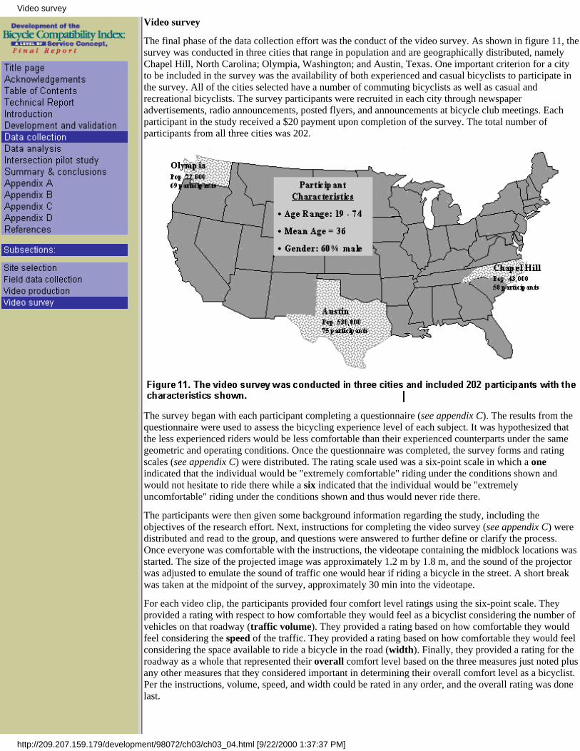
Video survey
The final phase of the data collection effort was the conduct of the video survey. As shown in figure 11, thesurvey was conducted in three cities that range in population and are geographically distributed, namelyChapel Hill, North Carolina; Olympia, Washington; and Austin, Texas. One important criterion for a cityto be included in the survey was the availability of both experienced and casual bicyclists to participate inthe survey. All of the cities selected have a number of commuting bicyclists as well as casual andrecreational bicyclists. The survey participants were recruited in each city through newspaperadvertisements, radio announcements, posted flyers, and announcements at bicycle club meetings. Eachparticipant in the study received a $20 payment upon completion of the survey. The total number ofparticipants from all three cities was 202.
The survey began with each participant completing a questionnaire (see appendix C). The results from thequestionnaire were used to assess the bicycling experience level of each subject. It was hypothesized thatthe less experienced riders would be less comfortable than their experienced counterparts under the samegeometric and operating conditions. Once the questionnaire was completed, the survey forms and ratingscales (see appendix C) were distributed. The rating scale used was a six-point scale in which a oneindicated that the individual would be "extremely comfortable" riding under the conditions shown andwould not hesitate to ride there while a six indicated that the individual would be "extremelyuncomfortable" riding under the conditions shown and thus would never ride there.
The participants were then given some background information regarding the study, including theobjectives of the research effort. Next, instructions for completing the video survey (see appendix C) weredistributed and read to the group, and questions were answered to further define or clarify the process.Once everyone was comfortable with the instructions, the videotape containing the midblock locations wasstarted. The size of the projected image was approximately 1.2 m by 1.8 m, and the sound of the projectorwas adjusted to emulate the sound of traffic one would hear if riding a bicycle in the street. A short breakwas taken at the midpoint of the survey, approximately 30 min into the videotape.
For each video clip, the participants provided four comfort level ratings using the six-point scale. Theyprovided a rating with respect to how comfortable they would feel as a bicyclist considering the number ofvehicles on that roadway (traffic volume). They provided a rating based on how comfortable they wouldfeel considering the speed of the traffic. They provided a rating based on how comfortable they would feelconsidering the space available to ride a bicycle in the road (width). Finally, they provided a rating for theroadway as a whole that represented their overall comfort level based on the three measures just noted plusany other measures that they considered important in determining their overall comfort level as a bicyclist.Per the instructions, volume, speed, and width could be rated in any order, and the overall rating was donelast.
Video survey
http://209.207.159.179/development/98072/ch03/ch03_04.html [9/22/2000 1:37:37 PM]

Site selection
With limited resources and an objective of comparing participants’ratings from watching a videotape with their ratings from seeing thelocations in the field, only those conditions believed to be the mostdifficult to discern on the videotape were included in the pilot effort.Preliminary observations by project staff showed that differences inmotor vehicle speeds and volumes were relatively easy to recognize onthe videotape. Similarly, it was easy to determine the differencesbetween cross-sections with and without a paved shoulder or bicyclelane. The most difficult of the cross-section elements to determine fromthe videotape was lane width when there was no paved shoulder orbicycle lane. Thus, the pilot study included only roadway segments withstandard or wide curb lanes and no paved shoulders or bicycle lanes, i.e.,the most difficult situations for viewers to differentiate (see figure 2).
Figure 2. The pilot study focused on roadways with various curb lanewidths, exlcusive of bicycle lanes and paved shoulders, since this was te
variable believed to be most difficult for viewers to discern from thevideo.
The pilot survey was conducted in Madison, Wisconsin. After examiningseveral potential sites and collecting speed data to determine the 85thpercentile speeds, 13 locations were selected for inclusion in the pilotsurvey. The distribution of sites by lane width and 85th percentile speedis shown in table 4. The geometric and operational characteristicsassociated with each location are shown in table 35 in appendix B. Curblane widths ranged from 3.1 m to 5.5 m; 85th percentile speeds rangedfrom 48 to 72 km/h; and traffic volumes ranged from 3,550 to 26,650vehicles/day. The sites selected also represented an extensive range of
Site selection
http://209.207.159.179/development/98072/ch02/ch02_01.html (1 of 3) [9/22/2000 1:37:38 PM]

combinations of these variables, from low-speed, low-volume,narrow-lane locations to high-speed, high-volume, wide-lane locations.Examples of two of the selected sites are shown in figures 3 and 4.
85th %tile
Speed
Lane Width (m)
< 3.4 3.7 - 4.0 > 4.3
< 56 km/h 3 1 3
> 56 km/h 2 2 2
Table 4. Distribution of sites selected for the pilot study by lane widthand 85th percentile speed.
Figure 3. High-volume multilane pilot study site with an 85th percentilespeed of 55 km/h and a curb lane width of 3.4 m.
Site selection
http://209.207.159.179/development/98072/ch02/ch02_01.html (2 of 3) [9/22/2000 1:37:38 PM]

Figure 4. Low-volume two-lane pilot study site with an 85th percentilespeed of 48 km/h and a curb lane width of 5.5 m.
Site selection
http://209.207.159.179/development/98072/ch02/ch02_01.html (3 of 3) [9/22/2000 1:37:38 PM]
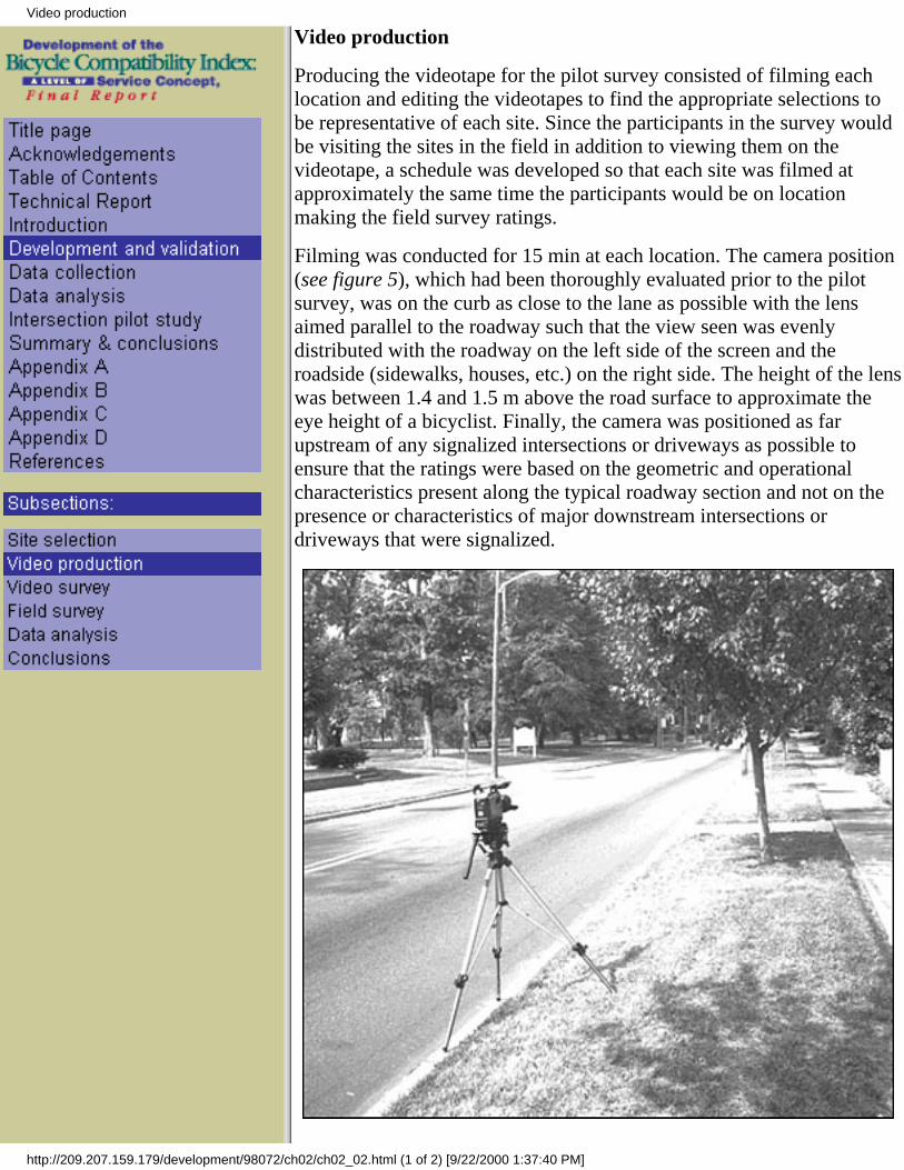
Video production
Producing the videotape for the pilot survey consisted of filming eachlocation and editing the videotapes to find the appropriate selections tobe representative of each site. Since the participants in the survey wouldbe visiting the sites in the field in addition to viewing them on thevideotape, a schedule was developed so that each site was filmed atapproximately the same time the participants would be on locationmaking the field survey ratings.
Filming was conducted for 15 min at each location. The camera position(see figure 5), which had been thoroughly evaluated prior to the pilotsurvey, was on the curb as close to the lane as possible with the lensaimed parallel to the roadway such that the view seen was evenlydistributed with the roadway on the left side of the screen and theroadside (sidewalks, houses, etc.) on the right side. The height of the lenswas between 1.4 and 1.5 m above the road surface to approximate theeye height of a bicyclist. Finally, the camera was positioned as farupstream of any signalized intersections or driveways as possible toensure that the ratings were based on the geometric and operationalcharacteristics present along the typical roadway section and not on thepresence or characteristics of major downstream intersections ordriveways that were signalized.
Video production
http://209.207.159.179/development/98072/ch02/ch02_02.html (1 of 2) [9/22/2000 1:37:40 PM]

Figure 5. The camera was positioned on the curb as close to the lane aspossible at a height of 1.4 to 1.5 m with the lens aimed parallel to the
roadway.
Once the videotaping was completed, curb lane volumes and totalvolumes were counted and recorded for each 10-s period throughout theentire 15 min of videotape for each location. Two 40-s intervalsrepresenting different volume conditions were then selected for each site.The two volume conditions for each site included one that was the most"representative" of conditions during the 15 min of taping and one thatincluded exactly 4 vehicles passing in the curb lane during 40 s,equivalent to 360 vehicles/h/ lane.
This selection process resulted in a "representative volume" 40-ssegment and a "uniform volume" 40-s segment for each of the 13 sites.These 26 segments were included on the survey video twice, whichwould allow for the examination of how consistent the participants werein rating the same roadway conditions. In addition to these 52 clips (26 x2), there were two clips at the beginning that were provided as practiceclips and would not be used in the evaluation. With the exception of thetwo practice clips, the various clips were randomly ordered forplacement on the survey videotape, ensuring that the same location neverappeared in two sequential clips. Each 40-s clip of interest was thencopied onto the survey tape with 5 s of blank tape placed betweenconsecutive clips. The number of each consecutive clip was then placedin the 5-s blank intervals; these numbers were added as an aid to anyparticipant who lost their place during the survey. An audible beep alsowas added to each of the clips; the beep was placed on the tape such thatit could be heard when there were 10 s left of the 40-s clip and providedan indication to the participants that they needed to complete theirratings within the next 10 s.
Video production
http://209.207.159.179/development/98072/ch02/ch02_02.html (2 of 2) [9/22/2000 1:37:40 PM]

Video survey
The schedules for the participants were arranged such that half of the 24participants would complete the video survey first and then the fieldsurvey. The other half would complete the field survey first and then thevideo survey. This approach allowed for an examination of anydifferences that may have resulted due to the order of completing thesurvey.
The video survey was conducted each of four evenings over a 2-h period,with the number of participants ranging from three to eight per evening.The participants began
by filling out a questionnaire (see appendix C) that was intended toprovide an indication of experience level with regard to riding on urbanand suburban streets. In the prior work by Sorton and Walsh, it had beenshown that less experienced bicyclists tended to have higher ratings, i.e.,be less comfortable, than more experienced bicyclists.7 Thus, it was alsopossible that these differences in perception by experience level may bea factor in any differences between the video survey ratings and the fieldratings.
Once the questionnaire was completed, the survey forms and ratingscales (see appendix C) were distributed, and the participants were thengiven some background information regarding the study and told theobjectives of the research effort. Instructions for completing the videosurvey were then read to the group (see appendix C) and questions wereanswered to clarify or further define the process. Once everyone wascomfortable with the process, the videotape was started. The size of theprojected image was approximately 1.2 m by 1.8 m, and the sound of theprojector was adjusted to emulate the sound of traffic one would hearwhen riding a bicycle on the roadway.
Video survey
http://209.207.159.179/development/98072/ch02/ch02_03.html [9/22/2000 1:37:40 PM]

Field survey
The field survey was conducted over a 4-h period each of four mornings,with the number of participants ranging from four to eight per morning.The participants were given clipboards containing the survey forms andrating scales (see appendix C) when they arrived at the meeting site. Theparticipants were then given some background information regarding thestudy and told the objectives of the research effort. Instructions forcompleting the field survey were then read to the group (see appendix C)and questions were answered to clarify or further define the process.Once everyone was comfortable with the process, the participants weretaken to each of the 13 locations, in the order that was established priorto the videotaping, to make the ratings. At each site, the van was parkedand everyone, as a group, walked to the point where they were toobserve the traffic and roadway conditions. This observation point wasthe same location where the camera had been positioned to ensure thatconditions were being observed in the field and on the video from thesame vantage point. The participants were told which direction of trafficto observe (the direction closest to them) and instructed to make theirratings based on what they observed during the next 2 min. During this2-min period, a traffic count was done in order to have a record of thevolumes and types of vehicles being observed by the participants onvarious days. A typical group making the ratings from the roadsidevantage point at one of the locations is shown in figure 6.
Figure 6. Participants in the field survey of the pilot study stoodadjacent to the direction of travel of interest and indicated howcomfortable they would be riding a bicycle under the condtions
observed.
Field survey
http://209.207.159.179/development/98072/ch02/ch02_04.html [9/22/2000 1:37:41 PM]

Data analysis
As previously noted, the primary objective of this pilot study was tovalidate the video methodology, i.e., determine how well theparticipants’ comfort ratings recorded when watching the video matchedthe participants’ ratings when viewing the location in the field. Sinceeach of the 24 participants (subjects) viewed the 13 sites both from thevideotape and in the field, the most stable and reliable analyses are basedon the 312 (24 × 13) combined pairs (video vs. field) of observations.Thus, the analysis primarily focused on the combined sample of comfortratings, including the overall rating as well as those related to curb lanewidth, traffic volume, and traffic speed. For brevity, only a summary ofthe results is provided below; a complete discussion of the statisticalanalysis is provided in appendix B.
The results of the analyses indicated that the participants’ video ratingsmatched reasonably well to the field ratings for all four variablesexamined (overall, speed, curb lane width, and volume). The number ofexact matches for the 312 site-by-participant pairs ranged from 30.8percent to 43.6 percent, depending on the variable. However, thepercentage of pairs that differed by no more than one rating levelincreased dramatically and ranged from 81.1 to 87.2 percent. Thesenumbers and the corresponding statistics produced as part of the analysisindicate that the great majority of the video and field ratings were insubstantial agreement.
It should also be noted that for all variables examined, there were veryfew values in the extremes of the contingency tables. For example, therewere no sites where any participant rated any variable as a one from thevideo and a six in the field or vice versa. Similarly, there were almost nocases where variables rated as a two under one scenario were rated as afive under the other scenario. This lack of extremes, or conversely theconcentration of values along the main diagonal, is another indicator ofthe reliability of the video methodology to accurately reflect the fieldcomfort ratings of bicyclists.
Data analysis
http://209.207.159.179/development/98072/ch02/ch02_05.html [9/22/2000 1:37:42 PM]

Conclusions
Overall, the results from the data analysis showed the videomethodology to be a valid technique for obtaining realistic perspectivesof bicyclists pertaining to comfort levels under varying roadwayconditions. The pilot study was also used as a proving ground for thesurvey procedures and provided insight into other issues that wereincorporated into the full-scale data collection effort. Some of the moreimportant issues and the resulting consequences for the study included:
• The video survey procedures employed were very efficient and resultedin no problems. Similarly, the procedures employed in the videotaping,editing, and production of the survey tape resulted in a quality product.Thus, the same procedures were carried forward to the larger study.
• At the conclusion of the video survey, participants were asked todiscuss the variables other than volume, speed, and curb lane width thatinfluenced their comfort ratings. The variables that were commonly citedincluded presence of large trucks or buses, heavy right-turning traffic,and number of driveways in the scene. Thus, these variables wereexamined in greater detail in the full-scale effort.
• During the initial stages of this study, considerable thought anddiscussion went into the development of the rating scale to reflect thebicyclists’ level of comfort. The project team ultimately decided that thestudy participants should be evaluating their level of comfort as it relatedto their perceived level of risk. Thus, a six-level scale was used in thepilot study, where a rating of one implied that the condition of interest(e.g., lane width, speed of traffic, or traffic volume) represented virtuallyno risk and a rating of six implied that the condition representedunacceptably high risk. Discussions with the participants in the pilotstudy after the survey was completed indicated that the majority of thesubjects thought that "perceived risk" accurately reflected their comfortlevel. However, a few of the more experienced bicyclists preferred ascale with less of a safety connotation. The one term that the moreexperienced riders seemed to like was "tolerance." A rating of one in thiscase would indicate that the condition of interest would be tolerated foran unlimited amount of time while a six would indicate that thecondition of interest would not be tolerated for any length of time.
The preferred alternative, however, was to simply use "comfort level" asthe rating term with some qualifying statements to indicate that comfortdoes not refer to the smoothness of the ride. Thus, for the full-scale datacollection effort, a six-point scale incorporating "comfort level" wasdeveloped and used (see chapter 3). The most important factor in thedevelopment and use of any rating scale was that it was understood andinterpreted the same way by all participants. The simplicity of the term"comfort level" was believed to have the best chance of achieving thislevel of understanding and uniform interpretation.
Conclusions
http://209.207.159.179/development/98072/ch02/ch02_06.html (1 of 2) [9/22/2000 1:37:43 PM]

Conclusions
http://209.207.159.179/development/98072/ch02/ch02_06.html (2 of 2) [9/22/2000 1:37:43 PM]

1. Introduction
Background
The goals of the United States Department of Transportation (USDOT)as stated in the National Bicycling and Walking Study are: 1) to doublethe number of trips made by bicycling and walking, and 2) tosimultaneously reduce by 10 percent the number of pedestrians andbicyclists killed or injured in traffic crashes.1 Meeting the first of thesegoals will require a substantial increase in the number of trips made bybicyclists using on-road or shared facilities. This increased exposurecould, in turn, jeopardize the second goal of improved safety unlesscareful consideration is given to the needs of both bicyclists and motorvehicle operators in the enhancement of existing roadways ordevelopment of new roadways. To develop or improve roadways forshared use by these two modes of transportation, one must begin byevaluating existing roadways and determining what is considered"user-friendly" from the perspective of the bicyclist.
Presently, there is no methodology widely accepted by engineers,planners, or bicycle coordinators that will allow them to determine howcompatible a roadway is for allowing efficient operation of both bicyclesand motor vehicles (see figure 1). Determining how existing trafficoperations and geometric conditions impact a bicyclist’s decision to useor not use a specific roadway is the first step in determining the bicyclecompatibility of the roadway.
Figure 1. Practitioners need a tool that will allow them to determine thecompatibility of their roadways for bicycling.
Background
http://209.207.159.179/development/98072/ch01/ch01_01.html (1 of 2) [9/22/2000 1:37:44 PM]

In recent years, several studies have been undertaken to develop somesystematic means of measuring the operational condition of roadways forbicycling (see appendix A for a detailed discussion). These efforts haveincluded the development of models based on the geometrics of roadwaysegments and intersections, pavement conditions, traffic volumes, speedlimits, and other variables. Each of these models produces an index thatcan be compared with a subjectively developed rating scale to assess thespecific roadway segment or intersection.2,3,4 Another effort developed aseries of recommended lane, shoulder, and bicycle lane widths that aresubjectively assigned on the basis of traffic volumes, motor vehicleoperating speeds, type of bicyclist, and other variables.5
The one missing element in each of these studies is the lack ofrecognition of the bicyclists’ perspectives. After all, these are theindividuals who will ultimately decide if a roadway meets their personalcomfort level for riding in the presence of motor vehicle traffic.
Background
http://209.207.159.179/development/98072/ch01/ch01_01.html (2 of 2) [9/22/2000 1:37:44 PM]

Bicycle stress level
In 1978, the Geelong Bikeplan Team in Australia understood theimportance of the bicyclist’s perspective and incorporated it into aconcept known as the bicycle stress level to better define the bicyclingsuitability of roadways from the viewpoint of the bicyclist.6 This conceptwas developed, in part, on the assumption that bicyclists not only want tominimize the physical effort required when choosing a roadway on whichto ride, but that they also want to minimize the mental effort, or stress,that results from conflict with motor vehicles, interaction with heavyvehicles, and having to concentrate for long periods of time while ridingon high-volume and high-speed roadways.
The team members drew upon their personal bicycling experience withspecific roadways to quantitatively define the concept. The variablesconsidered to have the most impact on the stress level of a bicyclist werecurb lane width, motor vehicle speed, and traffic volume. For variouscombinations of these three variables, team members assigned valuesfrom one to five to reflect the amount of stress they experienced whenriding under those conditions. A value of one indicated a very low levelof stress while a five indicated a very high level. Shown in table 1 areexamples of the stress levels developed. While these values are subjective(based on the experience of team members), it was the first attempt to usethe perspective of the bicyclist to assess the compatibility of roadways forbicycling.
Bicycle stress level
http://209.207.159.179/development/98072/ch01/ch01_02.html (1 of 4) [9/22/2000 1:37:45 PM]

In 1994, Sorton and Walsh used the bicycle stress level concept in aneffort to relate bicyclists’ perspectives on various types of roadways tospecific geometric and traffic operating conditions.7 Their projectrepresented the first attempt to gather perspectives from persons otherthan research team members; thus, the results were not based solely onthe subjective interpretations of researchers.
In a small-scale research effort employing segments of videotape fromdifferent street environments, three groups of bicyclists (experienced,casual, and youth) were asked to rate several urban and suburbanroadway segments with varying degrees of traffic volume, motor vehiclespeeds, and curb lane, shoulder, or bicycle lane widths. The ratings wereto reflect the level of stress they would experience (i.e., howuncomfortable they would be) riding on a specific segment with respectto each of the variables noted above. The scale used for rating thesegments and the authors’ interpretation of the scale is shown in table 2.At the extremes, a stress level of one indicates that all types of bicyclists(older than age 10) could safely be accommodated on the facility, whileat stress level five, virtually no bicyclists would ride on the roadway.
Table 2. Suggested interpretation of bicycle stress levels (7)
Bicycle stress level
http://209.207.159.179/development/98072/ch01/ch01_02.html (2 of 4) [9/22/2000 1:37:45 PM]

StressLevel
Interpretation
1-VeryLow
Street is reasonably safe for all types of bicyclists(except children under 10).
2-Low Street can accommodate experienced and casualbicyclists, and/or may need altering1 or havecompensating conditions2 to fit youth bicyclists.
3-Moderate Street can accommodate experienced bicyclists, and/orcontains compensating conditions to accommodatecasual bicyclists. Not recommended for youthbicyclists.
4-High Street may need altering and/or have compensatingconditions to accommodate experienced bicyclists. Notrecommended for casual or youth bicyclists.
5-VeryHigh
Street may not be suitable for bicycle use.
For each of the three variables rated, the authors developed quantitativevalues that they believed to be associated with each stress level. This stepinvolved examining the engineering literature for empirical data relatedto the operations of bicycles or motor vehicles, determining the endpoints for each variable that would be considered low and high stresssituations for the bicyclist, and then interpolating between these points toassign quantitative values to the other stress levels. The values developedand assigned to each of the stress levels are shown in table 3.
Bicycle stress level
http://209.207.159.179/development/98072/ch01/ch01_02.html (3 of 4) [9/22/2000 1:37:45 PM]
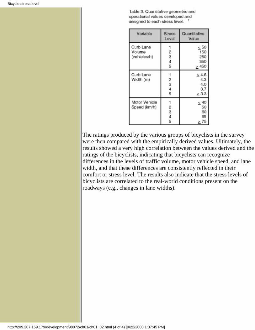
The ratings produced by the various groups of bicyclists in the surveywere then compared with the empirically derived values. Ultimately, theresults showed a very high correlation between the values derived and theratings of the bicyclists, indicating that bicyclists can recognizedifferences in the levels of traffic volume, motor vehicle speed, and lanewidth, and that these differences are consistently reflected in theircomfort or stress level. The results also indicate that the stress levels ofbicyclists are correlated to the real-world conditions present on theroadways (e.g., changes in lane widths).
Bicycle stress level
http://209.207.159.179/development/98072/ch01/ch01_02.html (4 of 4) [9/22/2000 1:37:45 PM]

Bicycle level of service
The Highway Capacity Manual defines levels of service (LOS) as"...qualitative measures that characterize operational conditions within atraffic stream and their perception by motorists and passengers."8
The terms used in describing each LOS (designated as A through F, withLOS A being the most desirable) include speed and travel time, freedomto maneuver, comfort/convenience, and traffic interruptions.
The concept of LOS was introduced to qualify the operationalcharacteristics associated with various levels of vehicles or personspassing a given point during a specified time period. For this reason,LOS in reality is a qualifier of conditions related to vehicle or personthrough-put rather than a qualifier of conditions related to individualcomfort level. This fact is revealed by examining the measures ofeffectiveness (MOE’s) used to define the ranges of LOS for varioustypes of facilities. For freeways, the MOE is density (passengercars/mi/h); for signalized intersections, the MOE is average stoppeddelay (s/vehicle); and for arterials, the MOE is average travel speed(mi/h). Each of these MOE’s is directly related to vehicle through-put.
For bicycles, LOS criteria are not defined in the Highway CapacityManual. The discussion on bicycles is primarily limited to the impact ofbicycles on motor vehicle LOS. If the implied definition of LOS (i.e., asrelated to vehicle through-put) is used, there are very few on-streetfacilities in the United States where LOS criteria would be neededsimply because of the low bicycle volumes. However, the descriptiveterms for LOS used in the written definition are applicable to bicycletransportation. For a bicyclist, the qualitative terms comfort andconvenience and freedom to maneuver are critical factors with respect todetermining their quality of service on a given facility.
Referring back to the definition for LOS, the user’s perception of theoperational conditions is an important element in terms of assigning aLOS designation to a facility. The bicycle stress level conceptincorporates the perceptions of bicyclists to assess the bicyclecompatibility of roadways on a five-point scale. In many ways, eachpoint on the scale can be thought of as representing a different LOS forbicyclists. For example, a roadway with a very low stress level would beconsidered by bicyclists to offer a high degree of comfort, which wouldbe represented by the LOS A designation.
In the current study, the bicycle compatibility index (BCI) reflects thecomfort levels of bicyclists on the basis of observed geometric andoperational conditions on a variety of roadways. The correlation of thesecomfort levels with the conditions of the roadway in the development ofthe BCI model allows the user to determine bicycle LOS for roadwaysegments by incorporating these geometric and operational
Bicycle level of service
http://209.207.159.179/development/98072/ch01/ch01_03.html (1 of 2) [9/22/2000 1:37:45 PM]

characteristics into the model. A complete discussion of the BCI modeland subsequent LOS designations is provided in chapter 4.
Bicycle level of service
http://209.207.159.179/development/98072/ch01/ch01_03.html (2 of 2) [9/22/2000 1:37:45 PM]

Objectives and scope
The primary objective of the current study was to develop amethodology for deriving a bicycle compatibility index (BCI) that couldbe used by bicycle coordinators, transportation planners, trafficengineers, and others to evaluate the capability of specific roadways toaccommodate both motorists and bicyclists. The BCI methodology wasdeveloped for urban and suburban roadway segments ( i.e., midblocklocations that are exclusive of intersections) and incorporated thosevariables that bicyclists typically use to assess the "bicycle friendliness"of a roadway (e.g., curb lane width, traffic volume, and vehicle speeds).
A secondary objective of this study was to apply the developedmethodology used for rating midblock segments to intersections andassess whether such an approach was valid for rating the bicyclecompatibility of intersections. As with the roadway segmentmethodology, those variables used by bicyclists to assess the "bicyclefriendliness" of intersections were identified, and a limited amount ofdata were collected and analyzed to assess the effectiveness of themethodology.
This research effort expanded upon the work of Sorton and Walsh andthe Geelong Bikeplan Team to produce a practical instrument that can beused by practitioners to predict bicyclists’ perceptions of a specificroadway environment and ultimately determine the level of bicyclecompatibility that exists on roadways within their jurisdictions. Thedeveloped tool will allow practitioners to evaluate existing facilities inorder to determine what improvements may be required as well as todetermine the geometric and operational requirements for new facilitiesto achieve the desired level of bicycle service.
Objectives and scope
http://209.207.159.179/development/98072/ch01/ch01_04.html [9/22/2000 1:37:45 PM]

Organization of the report
The results of this research effort are provided in two separate reports.This final report contains the comprehensive results of the study. Thesecond report is the implementation manual and provides practitioners aguide on how to apply the BCI methodology in response to planning andengineering issues.
In this final report, chapter 2 contains the development and validation ofthe research methodology, including the results of the pilot study.Chapter 3 discusses the data collection efforts while chapter 4 providesdetails on the data analysis. In chapter 5, the application of the developedmethodology to intersections is discussed. Finally, a summary of theresults, conclusions, and an applied example are provided in chapter 6.There are also four appendices, one of which includes a detailedliterature review of those few studies that have attempted to modelbicycle safety or bicycle operating conditions on the basis of roadwaygeometrics, traffic conditions, and other variables.
Organization of the report
http://209.207.159.179/development/98072/ch01/ch01_05.html [9/22/2000 1:37:46 PM]