DEVELOPMENT OF SIMULATION SOFTWARE - FROM SIMPLE ODE MODELLING TO STRUCTURAL DYNAMIC SYSTEMS

Felix Breitenecker

Institute for Analysis and Scientific Computing, Dept. Mathematical Modelling and Simulation Vienna University of Technology

1040 Vienna, Austria E-mail: Felix.Breitenecker@tuwien.ac.at

KEYWORDS Simulation software, simulation systems, object-oriented simulation, CSSL standard, Modelica standard, state space approach, dynamic structures, UML, physical modelling, structural dynamic systems ABSTRACT

This contribution presents development and trends of simulation software, from the simple structures for ‘static’ explicit ODE models to modelling of structural dynamic systems with DAEs. Simulation emerged in the 1960’ in order to be able to analyse nonlinear dynamic system and to synthesize nonlinear control systems. Since that time simulation as problem solving tool has been developed towards the third pillar of science (be-neath theory and experiment), and simultaneously simu-lation software has been developed further on. The paper first follows roots in the CSSL standard for simulation languages, from simple ODE modelling structures to discrete elements in ODE modelling, using the classical state space approach. Next, the extensions from explicit state space description to implicit model descriptions and their consequences for numerical algo-rithms and for structure of simulators are discussed, like DAE solvers and implicit model translation. Besides DAE modelling, state event description and state event handling has become a key feature for simulators – sketched by a state event classification and options for implementation. In the following, the last major steps of the development are presented: a-causal physical modelling, the new Modelica standard for ODE and DAE modelling, state chart and structural dynamic systems. Physical model-ling and Modelica is outlined by examples, and for structural dynamic systems a new approach by means of internal and external events is presented – together com-fortable state chart descriptions based on UML-RT. The last section reviews state-of-the-art simulators for availability of extended and structural features neces-sary for these last developments: DAE modelling, a-causal physical modelling, state events, Modelica mod-elling, state chart modelling, structural decomposition for structural dynamic systems, and related features. At the end, a table summarises and compares the availabil-ity of structural approaches and features.

CSSL STRUCTURE IN CONTINUOUS SIMULATION

Simulation supported various developments in engi-neering and other areas, and simulation groups and so-cieties were founded. One main effort of such groups was to standardise digital simulation programs and to work with a new basis: not any longer simulating the analog computer, but a self-standing structure for simu-lation systems. There were some unsuccessful attempts, but in 1968, the CSSL Standard became the milestone in the development: it unified the concepts and language structures of the available simulation programs, it de-fined a structure for the model, and it describes minimal features for a runtime environment. The CSSL standard suggests structures and features for a model frame and for an experimental frame. This dis-tinction is based on Zeigler’s concept of a strict separa-tion of these two frames. Model frame and experimental frame are the user interfaces for the heart of the simula-tion system, for the simulator kernel or simulation en-gine. A translator maps the model description of the model frame into state space notation, which is used by the simulation engine solving the system governing ODEs. This basic structure of a simulator is illustrated in Figure 1; an extended structure with service of dis-crete elements is given in Figure 3. In principle, in CSSL’s model frame, a system can be described in three different ways, as an interconnection of blocks, by mathematical expressions, and by conven-tional programming constructs as in FORTRAN or C. Mathematical basis is for the simulation engine is the state space description

00 )(),,),(),(()( xtxpttutxftx rrrrrr&r == ,

which is used by the ODE solvers of the simulation en-gine. Any kind of textual model formulation, of graphi-cal blocks or structured mathematical description or host languages constructs must be transformed to an internal state equation of the structure given above, so that the vector of derivatives ),,,( ptuxf rrrr

can be calcu-lated for a certain time instant ),),(),(( pttutxff iiiii

rrrrr= .

This vector of derivates is fed into an ODE solver in order to calculate a state update ),.(1 hfxx iii

rrr Φ=+ , h stepsize (all controlled by the simulation engine).

Proceedings 22nd European Conference on Modelling andSimulation ©ECMS Loucas S. Louca, Yiorgos Chrysanthou,Zuzana Oplatková, Khalid Al-Begain (Editors)ISBN: 978-0-9553018-5-8 / ISBN: 978-0-9553018-6-5 (CD)

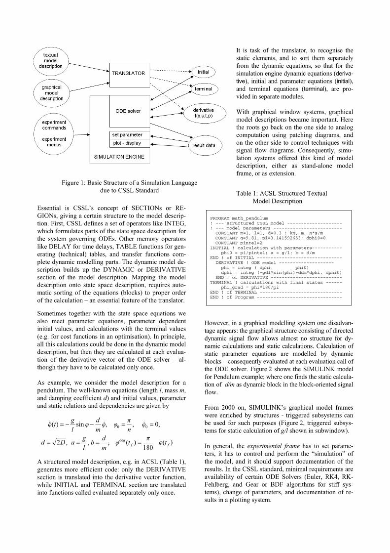
Essential is CSSL’s concept of SECTIONs or RE-GIONs, giving a certain structure to the model descrip-tion. First, CSSL defines a set of operators like INTEG, which formulates parts of the state space description for the system governing ODEs. Other memory operators like DELAY for time delays, TABLE functions for gen-erating (technical) tables, and transfer functions com-plete dynamic modelling parts. The dynamic model de-scription builds up the DYNAMIC or DERIVATIVE section of the model description. Mapping the model description onto state space description, requires auto-matic sorting of the equations (blocks) to proper order of the calculation – an essential feature of the translator. Sometimes together with the state space equations we also meet parameter equations, parameter dependent initial values, and calculations with the terminal values (e.g. for cost functions in an optimisation). In principle, all this calculations could be done in the dynamic model description, but then they are calculated at each evalua-tion of the derivative vector of the ODE solver – al-though they have to be calculated only once. As example, we consider the model description for a pendulum. The well-known equations (length l, mass m, and damping coefficient d) and initial values, parameter and static relations and dependencies are given by

)(180

)(,,,2

,0,,sin)(

deg

00

ff tφπtφmdb

lgaDd

φnπφφ

mdφ

lgtφ

====

==−−=

&

&&&&

A structured model description, e.g. in ACSL (Table 1), generates more efficient code: only the DERIVATIVE section is translated into the derivative vector function, while INITIAL and TERMINAL section are translated into functions called evaluated separately only once.

It is task of the translator, to recognise the static elements, and to sort them separately from the dynamic equations, so that for the simulation engine dynamic equations (deriva-tive), initial and parameter equations (initial), and terminal equations (terminal), are pro-vided in separate modules. With graphical window systems, graphical model descriptions became important. Here the roots go back on the one side to analog computation using patching diagrams, and on the other side to control techniques with signal flow diagrams. Consequently, simu-lation systems offered this kind of model description, either as stand-alone model frame, or as extension.

Table 1: ACSL Structured Textual Model Description

PROGRAM math_pendulum ! --- structured CSSL model -------------------- ! --- model parameters ------------------------- CONSTANT m=1, l=1, d=0.3 ! kg, m, N*s/m CONSTANT g=9.81, pi=3.141592653; dphi0=0 CONSTANT pintel=2

INITIAL ! calculation with parameters----------- phi0 = pi/pintel; a = g/l; b = d/m END ! of INITIAL ------------------------------- DERIVATIVE ! ODE model -------------------- phi = integ ( dphi, phi0) dphi = integ (-gdl*sin(phi)-ddm*dphi, dphi0) END ! of DERIVATIVE -------------------------- TERMINAL ! calculations with final states ------ phi_grad = phi*180/pi END ! of TERMINAL ------------------------------ END ! of Program -------------------------------

However, in a graphical modelling system one disadvan-tage appears: the graphical structure consisting of directed dynamic signal flow allows almost no structure for dy-namic calculations and static calculations. Calculation of static parameter equations are modelled by dynamic blocks – consequently evaluated at each evaluation call of the ODE solver. Figure 2 shows the SIMULINK model for Pendulum example; where one finds the static calcula-tion of d/m as dynamic block in the block-oriented signal flow. From 2000 on, SIMULINK’s graphical model frames were enriched by structures - triggered subsystems can be used for such purposes (Figure 2, triggered subsys-tems for static calculation of g/l shown in subwindow). In general, the experimental frame has to set parame-ters, it has to control and perform the “simulation” of the model, and it should support documentation of the results. In the CSSL standard, minimal requirements are availability of certain ODE Solvers (Euler, RK4, RK-Fehlberg, and Gear or BDF algorithms for stiff sys-tems), change of parameters, and documentation of re-sults in a plotting system.

Figure 1: Basic Structure of a Simulation Language due to CSSL Standard

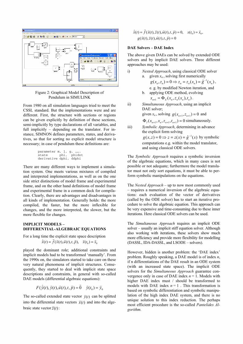
Figure 2: Graphical Model Description of Pendulum in SIMULINK

From 1980 on all simulation languages tried to meet the CSSL standard. But the implementations were and are different. First, the structure with sections or regions can be given explicitly by definition of these sections, semi-implicitly by type declarations of all variables, and full implicitly – depending on the translator. For in-stance, SIMNON defines parameters, states, and deriva-tives, so that for sorting no explicit model structure is necessary; in case of pendulum these definitions are:

parameter m, l, g, ……. state phi, phidot derivative dphi, ddphi

There are many different ways to implement a simula-tion system. One meets various mixtures of compiled and interpreted implementations, as well as on the one side strict distinctions of model frame and experimental frame, and on the other hand definitions of model frame and experimental frame in a common deck for compila-tion. Clearly, there are advantages and disadvantages in all kinds of implementation. Generally holds: the more compiled, the faster, but the more inflexible for changes, and the more interpreted, the slower, but the more flexible for changes. IMPLICIT MODELS – DIFFERENTIAL-ALGEBRAIC EQUATIONS

For a long time the explicit state space description 00 )(),,),(),(()( xtxpttutxftx rrrrrr

&r ==

played the dominant role; additional constraints and implicit models had to be transformed ‘manually’. From the 1990s on, the simulators started to take care on these very natural phenomena of implicit structures. Conse-quently, they started to deal with implicit state space descriptions and constraints, in general with so-called DAE models (differential algebraic equations):

00 )(0),),(),(),(( ytypttutytyF rrrrrr&r ==

The so-called extended state vector )(tyr can be splitted into the differential state vectors )(txr and into the alge-braic state vector )(tzr :

0),),(),(),((,)(,0),),(),(),(()( 00

====

pttutztxgxtxpttutztxftx

rrrr

rrrrrr&r

DAE Solvers – DAE Index

The above given DAEs can be solved by extended ODE solvers and by implicit DAE solvers. Three different approaches may be used:

i) Nested Approach, using classical ODE solver a. given xn , solving first numerically

)(ˆ)(0),( 1nnnnnn xgxzzzxg −==⇒= ,

e. g. by modified Newton iteration, and b. applying ODE method, evolving

)),(,(1 nnnnEn txzxx Φ=+ . ii) Simultaneous Approach, using an implicit

DAE solver; given xn , solving 0),( 11 =++ nn zxg and

0),,,( 111 =Φ +++ nnnnI tzxx simultaneously. iii) Symbolic Approach, determining in advance

the explicit form solving )(ˆ)(0),( 1 xgxzzzxg −==⇒= by symbolic

computations e.g. within the model translator, and using classical ODE solvers.

The Symbolic Approach requires a symbolic inversion of the algebraic equations, which in many cases is not possible or not adequate; furthermore the model transla-tor must not only sort equations, it must be able to per-form symbolic manipulations on the equations. The Nested Approach – up to now most commonly used – requires a numerical inversion of the algebraic equa-tions: each evaluation of the vector of derivatives (called by the ODE solver) has to start an iterative pro-cedure to solve the algebraic equation. This approach can be very expensive and time-consuming due to these inner iterations. Here classical ODE solvers can be used. The Simultaneous Approach requires an implicit ODE solver – usually an implicit stiff equation solver. Although also working with iterations, these solvers show much more efficiency and provide more flexibility for modelling (DASSL, IDA-DASSL, and LSODE – solvers). However, hidden is another problem: the ‘DAE index’ problem. Roughly speaking, a DAE model is of index n, if n differentiations of the DAE result in an ODE system (with an increased state space). The implicit ODE solvers for the Simultaneous Approach guarantee con-vergence only in case of DAE index n = 1. Models with higher DAE index must / should be transformed to models with DAE index n = 1 . This transformation is based on symbolic differentiation and symbolic manipu-lation of the high index DAE system, and there is no unique solution to this index reduction. The perhaps most efficient procedure is the so-called Pantelides Al-gorithm.

Unfortunately, in case of mechanical systems modelling and in case of process technology modelling indeed DAE models with DAE index n = 3 may occur, so that index reduction may be necessary. Index reduction is a new challenge for the translator of simulators, and still point of discussion. In graphical model descriptions, implicit model struc-tures are known since long time as algebraic loops: the directed graph of signals has one or more signal feed-back loops without any memory operator (integrator, delay, etc). Again, in evaluating the problem of sorting occurs, and the model translator cannot build up the sequence for calculating the derivative vector. Some simulators, e.g. SIMULINK, recognise algebraic loops and treat them as implicit models. When a graphical model contains an algebraic loop, SIMULINK calls a loop solving routine at each time step - SIMULINK makes use of the Nested Approach described before. This procedure works well in case of models with DAE index n = 1, for higher index problems may occur. In object-oriented simulation systems, like in Dymola, physical a-causal modelling plays an important role, which results in DAEs with sometimes higher index. These systems put emphasis on index reduction (in the translator) to DAEs with index n = 1 in order to apply implicit ODE solvers (Simultaneous Approach DISCRETE ELEMENTS IN CONTINUOUS SIMULATION

The CSSL standard also defines segments for discrete actions, first mainly used for modelling discrete control. So-called DISCRETE regions or sec-tions manage the communication be-tween discrete and continuous world and compute the discrete model parts. In graphical model description, dis-crete controllers and the time delay could be modelled by a z-transfer block. New versions of e.g. SIMULINK and Scicos offer for more complex discrete model parts trig-gered submodels, which can be exe-cuted only at one time instant, con-trolled by a logical trigger signal. For incorporating discrete actions, the simulation engine must interrupt the ODE solver and handle the event. For generality, efficient implementations set up and handle event lists, repre-senting the time instants of discrete actions and the calculations associated with the action, where in-between consecutive discrete actions the ODE solver is to be called.

In order to incorporate DAEs and discrete elements, the simulator’s translator must now extract from the model description the dynamic differential equations (deriva-tive), the dynamic algebraic equations (algebraic), and the events (event i) with static algebraic equations and event time, as given in Figure 3 (extended structure of a simulation language due to CSSL standard). In princi-ple, initial equations, parameter equations and terminal equations (initial, terminal) are special cases of events at time t = 0 and terminal time. Some simulators make use of a modified structure, which puts all discrete actions into one event module, where CASE - constructs distin-guish between the different events. State Events in Continuous Models

Much more complicated, but defined in CSSL, are the so-called state events. Here, a discrete action takes place at a time instant, which is not known in advance, it is only known as a function of the states.

As example, we consider the pendulum with constraints (Constrained Pendulum). If the pendulum is swinging, it may hit a pin positioned at angle ϕp with distance lp from the point of suspension. In this case, the pendulum swings on with the position of the pin as the point of rotation. The shortened length is ls = l - lp. and the an-gular velocity ϕ& is changed at position ϕp from ϕ& to sll /ϕ& , etc. These discontinuous changes are state events, not known in advance. For such state events, the classical state space descrip-tion is extended by the so-called state event function

)),(),(( ptutxh rrr , the zero of which determines the event:

Figure 3: Extended Structure of a Simulation System due to Extensions of the CSSL Standard with Discrete Elements and with DAE Models.

0),),(),((),,),(),(()(

==

tptutxhtptutxftx

rrr

rrrrr

In this notation, the model for Constrained Pendulum is given by

0),(

,sin,

121

21221

=−=

−−==

phmd

lg

ϕϕϕϕ

ϕϕϕϕϕ &&

The example involves two different events: change of length parameter (SE-P), and change of state (SE-S), i.e. angle velocity). Generally, state events (SE) can be classified in four types:

Type 1 – parameters change discontinuously (SE-P), Type 2 - inputs change discontinuously (SE-I), Type 3 - states change discontinuously (SE-S), and Type 4 - state vector dimension changes (SE-D),

including total change of model equations. State events type 1 (SE-P) could also be formulated by means of IF-THEN-ELSE constructs and by switches in graphical model descriptions, without synchronisation with the ODE solver. The necessity of a state event for-mulation depends on the accuracy wanted. Big changes in parameters may cause problems for ODE solvers with stepsize control. State events of type 3 (SE-S) are essential state events. They must be located, transformed into a time event, and modelled in discrete model parts. State events of type 4 (SE-D) are also essential ones. In principle, they are associated with hybrid modelling: models following each other in consecutive order build up a sequence of dynamic processes. And consequently, the structure of the model itself is dynamic; these so-called structural dynamic systems are at present (2008) discussion of extensions to Modelica, see next chapters. State Event Handling

The handling of a state event requires four steps: i. Detection of the event, usually by checking the

change of the sign of h(x) within the solver step over [ti, ti+1]

ii. Localisation of the event by a proper algorithm determining the time t* when the event occurs and performing the last solver step over [ti, t*]

iii. Service of the event: calculating / setting new parameters, inputs and states; switching to new equations

iv. Restart of the ODE solver at time t* with solver step over [ t*= ti+1, ti+2]

State events are facing simulators with severe problems. Up to now, the simulation engine had to call independent algorithms, now a root finder for the state event function h needs results from the ODE solver, and the ODE solver calls the root finder by checking the sign of h.

For finding the root of the state event function h(x), ei-ther interpolative algorithms (MATLAB/Simulink) or iterative algorithms are used (ACSL, Dymola). Figure 3 (extended structure of a simulation language due to CSSL standard) also shows the necessary exten-sions for incorporating state events. The simulator’s translator must extract from the model description addi-tionally the state event functions (state event j) with the associated event action – only one state event shown in the figure). In the simulator kernel, the static event man-agement must be made dynamically: state events are dynamically handled and transformed to time events. In principle, the kernel of the simulation engine has be-come an event handler, managing a complex event list with feedbacks. It is to be noted, that different state events may influence each other, if they are close in time – in worst case, the event finders run in a deadlock. Again, modified implementations are found. It makes sense to separate the module for state event function and the module for the associated event – which may be a single module, or which may be put into a common time event module. In case of a structural change of the system equations (state event of type 4 – SE-D), simulators usually can manage only fixed structures of the state space. The technique used is to ‘freeze’ the states that are bound by conditions causing the event. In case of a complete change of equations, both systems are calculated to-gether, freezing one according to the event. One way around is to make use of the experimental frame: the simulation engine only detects and localises the event, and updates the system until the event time. Then control is given back to the experimental frame. The state event is now serviced in the experimental frame, using features of the environment. Then a new simulation run is restarted (modelling of the structural changes in the experimental frame).

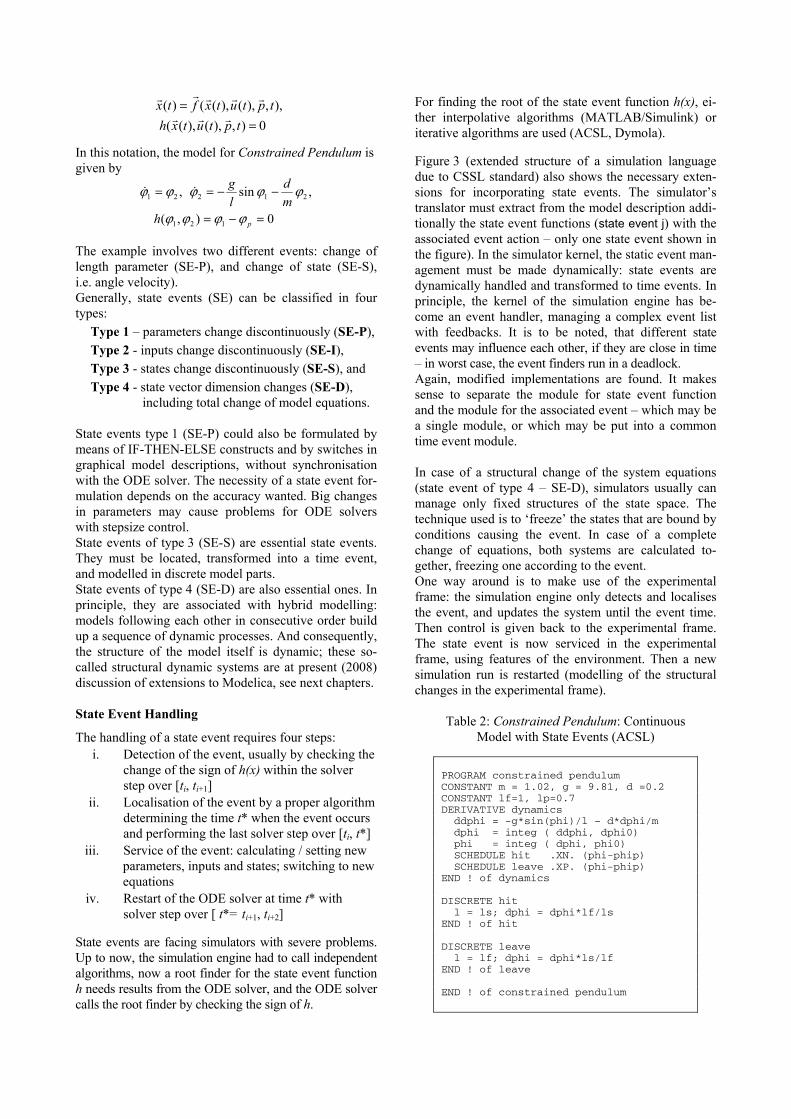
Table 2: Constrained Pendulum: Continuous Model with State Events (ACSL)

PROGRAM constrained pendulum CONSTANT m = 1.02, g = 9.81, d =0.2 CONSTANT lf=1, lp=0.7 DERIVATIVE dynamics ddphi = -g*sin(phi)/l – d*dphi/m dphi = integ ( ddphi, dphi0) phi = integ ( dphi, phi0) SCHEDULE hit .XN. (phi-phip) SCHEDULE leave .XP. (phi-phip) END ! of dynamics DISCRETE hit l = ls; dphi = dphi*lf/ls END ! of hit DISCRETE leave l = lf; dphi = dphi*ls/lf END ! of leave END ! of constrained pendulum

The Constrained Pendulum example involves a state event of type 1 (SE-P) and type 3 (SE-S). A classical ACSL model description works with two discrete sec-tions hit and leave, representing the two different modes, both called from the dynamic equations in the derivative section (Table 2). Dymola defines events and their scheduling implicitly by WHEN – or IF - constructs in the dynamic model description, in case of the discussed example e.g. by

WHEN phi-phip=0 AND phi>phip THEN l = ls; dphi = dphi*lf/ls

In case of more complex event descriptions, the WHEN – or IF – clauses are put into an ALGORITHM section similar to ACSL’s DISCRETE section. In graphical model descriptions, we again are faced with the problem that calculations at discrete time in-stants are difficult to formulate. For the detection of the event, SIMULINK provides the HIT CROSSING block (in new Simulink version implicitly defined). This block starts state event detection (interpolation method) depending on the input, the state event function, and outputs a trigger signal, which may call a triggered sub-system servicing the event. Extended Features of Simulators

Discrete elements with time events and state events and DAEs may change the structure of the model. Explicit type-4 state events (SE-D) and implicit algebraic condi-tions in DAEs may change the model essentially or may make a need for a different model. In mechanical sys-tems, these changes are equivalent to a change in the degree of mechanical or physical freedom. Event description (ED), state event handling (SEH) and DAE support (DAE) with or without index reduction (IR) became desirable structural features of simulators, supported directly or indirectly. Table 3 compares the availability of these features in the MATLAB / Simu-link System, in ACSL and in Dymola. Table 3: Comparison of Simulators’ Extended Features

(Event Handling and DAE Modelling)

MS

- Mod

el

Sorti

ng

ED -E

vent

D

escr

iptio

n SH

E - S

tate

Ev

ent H

an-

dlin

g D

AE

- DA

E

Solv

er

IR -

Inde

x

Red

uctio

n

MATLAB no no (yes) (yes) no Simulink yes (yes) (yes) (yes) no MATLAB / Simulink yes yes yes (yes) no

ACSL yes yes yes yes no

Dymola yes yes yes yes yes

In Table 3, the availability of features is indicated by ‘yes’ and ‘no’; a ‘yes’ in parenthesis ‘(yes)’ means, that the feature is complex to use. MS - ‘Model Sorting’, is a standard feature of a simulator – but missing in MAT-LAB (in principle, MATLAB cannot be called a simula-tor). On the other hand, MATLAB’s ODE solvers offer limited features for DAEs (systems with mass matrix) and an integration stop on event condition, so that SHE and DAE get a (‘yes’). In Simulink, event descriptions are possible by means of triggered subsystems, so that ED gets a ‘(yes)’ because of complexity. A combination of MATLAB and Simulink suggest putting the event description and handling at MATLAB level, so that ED and SHE get both a ‘yes’. DAE solving is based on modified ODE solvers, using the nested approach (see before), so DE gets only a ‘(yes)’ for all MATLAB/Simulink combinations.

ACSL is a classical simulator with sophisticated state event handling, and since version 10 (2001) DAEs can be modelled directly by the residuum construct, and they are solved by the DASSL algorithm (a well-known direct DAE solver, based on the simultaneous ap-proach), or by modified ODE solvers (nested approach) – so ‘yes’ for ED, SHE, and DAE. In case of DAE in-dex n = 1, the DASSL algorithm guarantees conver-gence, in case of higher index integration may fail. ACSL does not perform index reduction (IR ‘no’).

Dymola is a modern simulator, implemented in C, and based on physical modelling. Model description may be given by implicit laws, symbolic manipulations extract a proper ODE or DAE state space system, with index re-duction for high index DAE systems – all extended fea-tures are available. Dymola started a new area in model-ling and simulation of continuous and hybrid systems. FROM CSSL TO MODELICA AND VHDL-AMS

In the 1990s, many attempts have been made to improve and to extend the CSSL structure, especially for the task of mathematical modelling. The basic problem was the state space description, which limited the construction of modular and flexible modelling libraries. Two devel-opments helped to overcome this problem. On model-ling level, the idea of physical modelling gave new in-put, and on implementation level, the object-oriented view helped to leave the constraints of input/output re-lations. In physical modelling, a typical procedure for modelling is to cut a system into subsystems and to account for the behaviour at the interfaces. Balances of mass, energy and momentum and material equations model each sub-system. The complete model is obtained by combining the descriptions of the subsystems and the interfaces. This approach requires a modelling paradigm different to classical input/output modelling. A model is consid-ered as a constraint between system variables, which leads naturally to DAE descriptions. The approach is very convenient for building reusable model libraries.

In 1996, the situation was thus similar to the mid 1960s when CSSL was defined as a unification of the tech-niques and ideas of many different simulation programs. An international effort was initiated in September 1996 for bringing together expertise in object-oriented physi-cal modelling (port based modelling) and defining a modern uniform modelling language – mainly driven by the developers of Dymola. The new modelling language is called Modelica. Mode-lica is intended for modelling within many application domains such as electrical circuits, multibody systems, drive trains, hydraulics, thermodynamical systems, and chemical processes etc. It supports several modelling formalisms: ordinary differential equations, differential-algebraic equations, bond graphs, finite state automata, and Petri nets etc. Modelica is intended to serve as a standard format so that models arising in different do-mains can be exchanged between tools and users. Modelica is a not a simulator, Modelica is a modelling language, supporting and generating mathematical mo-dels in physical domains. When the development of Modelica started, also a competitive development, the extension of VHDL towards VHDL-AMS was initiated. Both modelling languages aimed for general-purpose use, but VHDL-AMS mainly addresses circuit design, and Modelica covers the broader area of physical mod-elling; modelling constructs such as Petri nets and finite automata could broaden the application area, as soon as suitable simulators can read the model definitions. Modelica offers a textual and graphical modelling con-cept, where the connections of physical blocks are bidi-rectional physical couplings, and not directed flow. An example demonstrates how drive trains are mod-elled. The drive train consists of four inertias and three clutches, where the clutches are controlled by input sig-nals (Figure 4). The graphical model layout corresponds with a textual model representation, shown in Table 4 (abbreviated, simplified).

Figure 4: Graphical Modelica Model for Coupled Clutches

Table 4: Textual Modelica Model for Coupled Clutches

encapsulated model CoupledClutches; "Drive train" parameter SI.Frequency freqHz=0.2; …. Rotational.Inertia J1(J=1,phi(ic=0),w(ic=10)); Rotational.Torque torque; Rotational.Clutch clutch1(peak=1.1, fn_max=20); Rotational.Inertia J3(J=1); …………………………………… equation connect(sin1.outPort, torque.inPort); connect(torque.flange_b, J1.flange_a); connect(J1.flange_b, clutch1.flange_a); …………………………………….. connect(step2.outPort, clutch3.inPort); end CoupledClutches;

The translator from Modelica into the target simulator must not only be able to sort equations, it must be able to process the implicit equations symbolically and to perform DAE index reduction (or a way around). Up to now – similar to VHDL-AMS – some simulation systems understand Modelica (2008; generic – new simulator with Modelica modelling, extension - Mode-lica modelling interface for existing simulator):

• Dymola from Dynasim (generic), • MathModelica from MathCore

Engineering (generic) • SimulationX from ISI (generic/extension) • Scilab/Scicos (extension) • MapleSim (extension, announced) • Open Modelica - since 2004 the University of

Lyngby develops an provides an open Modelica simulation environment (generic),

• Mosilab - Fraunhofer Gesellschaft develops a generic Modelica simulator, which supports dynamic variable structures (generic)

• Dymola / Modelica blocks in Simulink As Modelica also incorporates graphical model ele-ments, the user may choose between textual modelling, graphical modelling, and modelling using elements from an application library. Furthermore, graphical and textual modelling may be mixed in various kinds. The minimal modelling environment is a text editor; a com-fortable modelling environment offers a graphical mod-elling editor. The Constrained Pendulum example can be formulated in Modelica textually as a physical law for angular ac-celeration. The event with parameter change is put into an algorithm section, defining and scheduling the parameter event SE-P (Table 5). As instead of angular velocity, the tangential velocity is used as state variable, the second state event SE-S ‘vanishes’.

Table 5: Textual Modelica Model for Constrained Pendulum

equation /*pendulum*/ v = length*der(phi); vdot = der(v); mass*vdot/length + mass*g*sin(phi) +damping*v = 0; algorithm if (phi<=phipin) then length:=ls; end if; if (phi>phipin) then length:=l1; end if;

Modelica allows combining textual and graphical mod-elling. For the Constrained Pendulum example, the ba-sic physical dynamics could be modelled graphically with joint and mass elements, and the event of length change is described in an algorithm section, with variables interfacing to the predefined variables in the graphical model part (Figure 5).

algorithm if (revolute1.phi <= phipin then revolute1.length:=ls; end if; if (revolute1.phi < phipin then revolute1.length:=ll; end if;

Figure 5: Mixed Graphical and Textual Dymola

Model for Constrained Pendulum MODELLING WITH STATE CHARTS

In the end of the 1990s, computer science initiated a new development for modelling discontinuous changes. The Unified Modelling Language (UML) is one of the most important standards for specification and design of object oriented systems. This standard was tuned for real time applications in the form of a new proposal, UML Real-Time (UML-RT). By means of UML-RT, objects can hold the dynamic behaviour of an ODE. In 1999, a simulation research group at the Technical University of St. Petersburg used this approach in com-bination with a hybrid state machine for the develop-ment of a hybrid simulator (MVS), from 2000 on avail-able commercially as simulator AnyLogic. The model-ling language of AnyLogic is an extension of UML-RT; the main building block is the Active Object. Active objects have internal structure and behaviour, and allow encapsulating of other objects to any desired depth. Rela-tionships between active objects set up the hybrid model. Active objects interact with their surroundings solely through boundary objects: ports for discrete communi-cation, and variables for continuous communication (Figure 6). The activities within an object are usually de-fined by state charts (extended state machine). While dis-crete model parts are described by means of state charts, events, timers and messages, the continuous model parts are described by means of ODEs and DAEs in CSSL-type notation and with state charts within an object. An AnyLogic implementation of the well-known Bounc-ing Ball example shows a simple use of state chart model-ling (Figure 7). The model equations are defined in the active object ball, together with the state chart ball.main. This state chart describes the interruption of the state flight (without any equations) by the event bounce (SE-P and SE-S event) defined by condition and action.

Figure 6: Active Objects with Connectors - Discrete

Messages (Rectangles) and Continuous Signals (Triangles

Figure 7: AnyLogic Model for the Bouncing Ball AnyLogic influenced further developments for hybrid and structural dynamic systems, and led to a discussion in the Modelica community with respect to a proper implementation of state charts in Modelica. The princi-ple question is, whether state charts are to be seen as comfortable way to describe complex WHEN – and IF – constructs, being part of the model, or whether state charts control different models from a higher level. At present (2008) a free Modelica state chart library ‘emu-lates’ state charts by Boolean variables and IF – THEN – ELSE constructs. A further problem is the fact, that the state chart notation is not really standardised; Any-Logic makes use of the Harel state chart type. An AnyLogic implementation for the Constrained Pen-dulum may follow the implementation for the bouncing ball (Figure 8). An primary active object (Constrained Pendulum)‘holds’ the equations for the pendulum, to-gether with a state chart (main) switching between short and long pendulum. The state chart nodes are empty; the arcs define the events (Figure 8). Internally, Any-Logic restarts at each hit the same pendulum model (trivial hybrid decomposition).

Figure 8: AnyLogic model for Constrained

Pendulum, Simple Implementation HYBRID AND STRUCTURAL-DYNAMIC SYSTEMS

Continuous simulation and discrete simulation have different roots, but they are using the same method, the analysis in the time domain. During the last decades a broad variety of model frames (model descriptions) has been developed.

In continuous and hybrid simulation, the explicit or im-plicit state space description is used as common de-nominator. This state space may be described textually, or by signal-oriented graphic blocks (e.g. SIMULINK), or by physically based block descriptions (Modelica, VHDL-AMS). In discrete simulation, we meet very different tech-niques for the model frame. Application-oriented flow diagrams, network diagrams, state diagrams, etc. allow describing complex behaviour of event-driven dynam-ics. Usually these descriptions are mapped to an event-based description. On the other side, the simulator ker-nel is similar for discrete and continuous simulators. The model description is mapped to an event list with adequate update functions of the states within state up-date events. In discrete simulation, the states are usually the status variables of servers and queues in the model, and state update is simple increase or decrease by in-crements; complex logic conditions may accompany the scheduling of events. In continuous simulation the state space is based of various laws used in the application area, and usually defined by differential-algebraic equa-tions. DAE solvers generate a grid for the approximation of the solutions. This grid drives an event list with state update events using complex formula depending on the chosen DAE solver and on the defined DAE. Additional time events and state events are inserted into the global event list. Hybrid systems often come together with a change of the dimension of the state space, then called structural-dynamic systems. The dynamic change of the state space is caused by a state event of type SE-D. In con-trary to state events SE-P and SE-S, states and deriva-tives may change continuously and differentiable in case of structural change. In principle, structural-dynamic systems can be seen from two extreme view-points. The one says, in a maximal state space, state events switch on and off algebraic conditions, which freeze certain states for certain periods. The other one says that a global discrete state space controls local models with fixed state spaces, whereby the local mod-els may be also discrete or static.

These viewpoints derive two different approaches for structural dynamic systems modelling, the

• maximal state space, and the • hybrid decomposition.

Maximal State Space for Structural-Dynamic Systems – Internal Events

Most implementations of physically based model de-scriptions support a big monolithic model description, derived from laws, ODEs, DAEs, state event functions and internal events. The state space is maximal and static, index reduction in combination with constraints keep a consistent state space. For instance, Dymola, OpenModelica, and VHDL-AMS follow this approach.

This approach can be classified with respect to event implementation. The approach handles all events of any kind (SE-P, SE-S, and SE-D) within the ODE solver frame, also events which change the state space dimen-sion (change of degree of freedoms) – consequently called internal events.

Using the classical state chart notation, internal state events I-SE caused by the model schedule the model itself, with usually different re-initialisations (depending on the event type I-SE-P, I-SES, I-SE-D; Figure 9). For instance, VHDL-AMS and Dymola follow this approach, han-dling also DAE models with index higher than 1;

Figure 9: State Chart Control for Internal Events of one Model

discrete model parts are only supported at event level. ACSL and MATLAB / Simulink generate also a maxi-mal state space. Hybrid Decomposition for Structural-Dynamic Systems – External Events

The hybrid decomposition approach makes use of ex-ternal events (E-SE), which control the sequence and the serial coupling of one model or of more models. A convenient tool for switching between models is a state chart, driven by the external events – which itself are generated by the models. Following e.g. the UML-RT notation, control for continuous models and for discrete actions can by modelled by state charts. Figure 10 shows the hybrid coupling of two models, which may be extended to an arbitrary number of models, with pos-sible events E-SE-P, E-SE-S, and ESE-D. As special case, this technique may be also used for serial condi-tional ‘execution’ of one model – Figure 11 (only for SE-P and SE-S). This approach additionally allows not only dynamically changing state spaces, but also different model types, like ODEs, linear ODEs (to be analysed by linear the-ory), PDEs, etc. to be processed in serial or also in par-allel, so that also co-simulation can be formulated based on external events.

Figure 11: State Chart Control for External

Events for two Models

Figure 12: State Chart Control for External Events for one Model

The approach allows handling all events also outside the ODE solver frame. After an event, a very new model can be started. This procedure may make sense especially in case of events of type SE-D and SE-S. As consequence, consecutive models of different state spaces may be used. Figure 12 shows a structure for a simulator supporting structural dynamic modelling and simulation. The figure summarises the outlined ideas by extending the CSSL structure by control model, external events and multiple models. The main extension is that the translator gener-ates not only one DAE model; he generates several DAE models from the (sub)model descriptions, and external events from the connection model, controlling the model execution sequence in the highest level of the dynamic event list.

There, all (sub)models may be precompiled, or the new recent state space may be determined and translated to a DAE system in case of the external event (interpretative technique). Clearly, not only ODE solver can make use of the model descriptions (derivatives), but also eigenvalue analysis and steady state calculation may be used and other analysis algorithms. Furthermore, complex ex-periments can be controlled by external events schedul-ing the same model in a loop. Mixed Approach with Internal and External Events

A simulator structure as proposed in Figure 12 is a very general one, because it allows as well external as ell as internal events, so that hybrid coupling with variable state models of any kind with internal and external events is

possible (Figure 13).

Both approaches have advantages and disadvan-tages. The classical Dy-mola approach generates a fast simulation, because of the monolithic pro-gram. However, the state space is static. Further-more, Modelica centres on physical modelling. A hybrid approach handles separate model parts and must control the external events. Consequently, two levels of programs have to be generated: dynamic mod-els, and a control program – today’s implementations are interpretative and not compiling, so that simula-tion times increase - but the overall state space is indeed dynamic. A challenge for the future lies in the combination of both approaches. The main ideas are:

• Moderate hybrid decomposition

• External and in-ternal events

• Efficient imple-mentation of models and con-trol

Figure 12: Structure for a Simulation System with External State Events E-SE and

Classical Internal State Events I-SE for Controlling Different Models

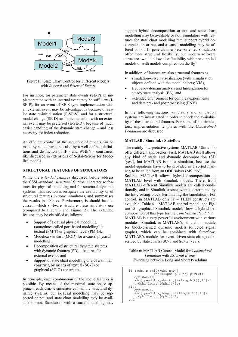
Figure13: State Chart Control for Different Models with Internal and External Events

For instance, for parameter state events (SE-P) an im-plementation with an internal event may be sufficient (I-SE-P), for an event of SE-S type implementation with an external event may be advantageous because of eas-ier state re-initialisation (E-SE-S), and for a structural model change (SE-D) an implementation with an exter-nal event may be preferred (E-SE-D), because of much easier handling of the dynamic state change – and less necessity for index reduction. An efficient control of the sequence of models can be made by state charts, but also by a well-defined defini-tions and distinction of IF - and WHEN - constructs, like discussed in extensions of Scilab/Scicos for Mode-lica models. STRUCTURAL FEATURES OF SIMULATORS

While the extended features discussed before address the CSSL-standard, structural features characterise fea-tures for physical modelling and for structural dynamic systems. This section investigates the availability or of structural features in some simulators, and summarises the results in table xx. Furthermore, is should be dis-cussed, which software structure these simulators use (compared to Figure 3 and Figure 12). The extended features may be classified as follows:

• Support of a-causal physical modelling (sometimes called port-based modelling) at textual (PM-T) or graphical level (PM-G),

• Modelica standard (MOD) for a-causal physical modelling ,

• Decomposition of structural dynamic systems with dynamic features (SD) – features for external events, and

• Support of state chart modelling or a of a similar construct, by means of textual (SC-T) or graphical (SC-G) constructs.

In principle, each combination of the above features is possible. By means of the maximal state space ap-proach, each classic simulator can handle structural dy-namic systems, but a-causal modelling may be sup-ported or not, and state chart modelling may be avail-able or not. Simulators with a-causal modelling may

support hybrid decomposition or not, and state chart modelling may be available or not. Simulators with fea-tures for state chart modelling may support hybrid de-composition or not, and a-causal modelling may be of-fered or not. In general, interpreter-oriented simulators offer more structural flexibility, but modern software structures would allow also flexibility with precompiled models or with models compiled ‘on the fly’. In addition, of interest are also structural features as • simulation-driven visualisation (with visualisation

objects defined with the model objects; VIS), • frequency domain analysis and linearization for

steady state analysis (FA), and • extended environment for complex experiments

and data pre- and postprocessing (ENV). In the following sections, simulators and simulation systems are investigated in order to check the availabil-ity of these structural features. For some of the simula-tors, implementation templates with the Constrained Pendulum are discussed. MATLAB / Simulink / Stateflow

The mainly interpretative systems MATLAB / Simulink offer different approaches. First, MATLAB itself allows any kind of static and dynamic decomposition (SD ‘yes’), but MATLAB is not a simulator, because the model equations have to be provided in a sorted man-ner, to be called from an ODE solver (MS ‘no’). Second, MATLAB allows hybrid decomposition at MATLAB level with Simulink models. There, from MATLAB different Simulink models are called condi-tionally, and in Simulink, a state event is determined by the hit-crossing block (terminating the simulation). For control, in MATLAB only IF – THEN constructs are available. Table 6 – MATLAB control model, and Fig-ure 15– graphical Simulink model, show a hybrid de-composition of this type for the Constrained Pendulum. MATLAB is a very powerful environment with various modules. Simulink is MATLAB’s simulation module for block-oriented dynamic models (directed signal graphs), which can be combined with Stateflow, MATLAB’s module for event-driven state changes de-scribed by state charts (SC-T and SC-G ‘yes’).

Table 6: MATLAB Control Model for Constrained Pendulum with External Events

Switching between Long and Short Pendulum

if ((phi_p-phi0)*phi_p<0 | (phi0==phi_p & phi_p*v>0)) dphi0=v/ls; sim('pendulum_short',[t(length(t)),10]); v=dphi(length(dphi))*ls; else dphi0=v/l; sim('pendulum_long',[t(length(t)),10]); v=dphi(length(dphi))*l; end

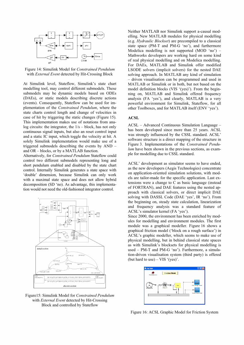
Figure 14: Simulink Model for Constrained Pendulum with External Event detected by Hit-Crossing Block

At Simulink level, Stateflow, Simulink’s state chart modelling tool, may control different submodels. These submodels may be dynamic models based on ODEs (DAEs), or static models describing discrete actions (events). Consequently, Stateflow can be used for im-plementation of the Constrained Pendulum, where the state charts control length and change of velocities in case of hit by triggering the static changes (Figure 15). This implementation makes use of notations from ana-log circuits: the integrator, the 1/s – block, has not only continuous signal inputs, but also an reset control input and a static IC input, which toggle the velocity at hit. A solely Simulink implementation would make use of a triggered submodels describing the events by AND – and OR – blocks, or by a MATLAB function. Alternatively, for Constrained Pendulum Stateflow could control two different submodels representing long and short pendulum enabled and disabled by the state chart control. Internally Simulink generates a state space with ‘double’ dimension, because Simulink can only work with a maximal state space and does not allow hybrid decomposition (SD ‘no). As advantage, this implementa-tion would not need the old-fashioned integrator control.

Figure15: Simulink Model for Constrained Pendulum with External Event detected by Hit-Crossing

Block and controlled by Stateflow

Neither MATLAB nor Simulink support a-causal mod-elling. New MATLAB modules for physical modelling (e.g. Hydraulic Blockset) are precompiled to a classical state space (PM-T and PM-G ‘no’), and furthermore Modelica modelling is not supported (MOD ‘no’) – Mathworks developers are working hard on some kind of real physical modelling and on Modelica modelling. For DAEs, MATLAB and Simulink offer modified LSODE solvers (implicit solvers) for the nested DAE solving approach. In MATLAB any kind of simulation – driven visualisation can be programmed and used in MATLAB or Simulink or in both, but not based on the model definition blocks (VIS ‘(yes)’). From the begin-ning on, MATLAB and Simulink offered frequency analysis (FA ‘yes’), and clearly, MATLAB is a very powerful environment for Simulink, Stateflow, for all other Toolboxes, and for MATLAB itself (ENV ‘yes’). ACSL

ACSL – Advanced Continuous Simulation Language – has been developed since more than 25 years. ACSL was strongly influenced by the CSSL standard. ACSL’ software structure is a direct mapping of the structure in Figure 3. Implementations of the Constrained Pendu-lum have been shown in the previous sections, as exam-ple for modelling due to CSSL standard. ACSL’ development as simulator seems to have ended, as the new developers (Aegis Technologies) concentrate on application-oriented simulation solutions, with mod-els are tailor-made for the specific application. Last ex-tensions were a change to C as basic language (instead of FORTRAN), and DAE features using the nested ap-proach with classical solvers, or direct implicit DAE solving with DASSL Code (DAE ‘yes’, IR ‘no’). From the beginning on, steady state calculation, linearization and frequency analysis was a standard feature of ACSL’s simulator kernel (FA ‘yes’). Since 2000, the environment has been enriched by mod-ules for modelling and environment modules. The first module was a graphical modeller. Figure 16 shows a graphical friction model (‘block on a rough surface’) in ACSL’s graphic modeller, which seems to make use of physical modelling, but in behind classical state spaces as with Simulink’s blocksets for physical modelling is used – PM-T and PM-G ‘no’). Furthermore, a simula-tion-driven visualisation system (third party) is offered (but hard to use) – VIS ‘(yes)’.

Figure 16: ACSL Graphic Model for Friction System

A very interesting module is an extended environment called ACSLMath. ACSLMath was intended to have same features as MATLAB; available is only a subset, but powerful enough for an extended environment (ENV ‘yes’), which can be used for hybrid decomposi-tion of a structural dynamic model in almost the same way than MATLAB does (SD ‘yes’). Unfortunately the development of ACSLMath has been stopped. In gen-eral, there is no intention to make a-causal physical modelling available, also Modelica is not found in the developers’ plans (PM-T, PM-G, and MOD ‘no’). Dymola

Dymola has partly been discussed in a section before, together with an implementation for the Constrained Pen-dulum example (Dymola standard implementation, Fig-ure 5, Table 5). Dymola, introduced by F. E. Cellier as a-causal modelling language, and developed to a simulator by H. Elmquist, can be called the mother of Modelica. Dymola is based on a-causal physical modelling and ini-tiated Modelica; consequently, it fully supports Modelica these structural features (PM-T, PM-G, and MOD ‘yes’). Together with the model objects, also graphical objects may be defined, so that simulation based pseudo-3D visu-alisation is available (VIS ‘yes’). A key feature of Dy-mola is the very sophisticated index reduction by the modified Pantelides algorithm, so Dymola handles any DAE system, also with higher index, with bravura (DAE and IR ‘yes’). For DAE solving, modified DASSL algo-rithms are used. In software structure, Dymola is similar to ACSL, using an extended CSSL structure as given in Figure 3 – with the modification that all discrete actions are put into one event module, where CASE - constructs distinguish between the different events (this structure is based on the first simulator engine Dymola used, the DS-Block System of DLR Oberpfaffenhofen). Dymola comes with a graphical modelling and basic simulation environment, and provides a simple script language as extended environment; new releases offer also optimisation, as built-in function of the simulator. Furthermore, based on Modelica’s matrix functions some task of an environment can be performed – so ENV (‘yes’) – available, but complex/uncomfortable. Dymola offers also a Modelica – compatible state chart library, which allows to model complex conditions (in-ternally translated into IF – THEN – ELSE or WHEN constructs - SC-T and SC-G ‘(yes)’). Figure 17 shows an implementation of the Constrained Pendulum using this library. Up to now (2008) the Modelica definition says nothing about structural dynamic systems, and Dymola builds up a maximal state space. And up to now, Modelica does not directly define state charts, and in Dymola a state chart library in basic Modelica notation is avail-able, but working only with internal events within the maximal state space (SD ‘no’).

Figure17: Graphical Dymola Model for Constrained Pendulum with Internal Events Managed by Elements of Dymola’s State Chart Library

For Modelica extension, a working group on hybrid systems has been implemented, in order to discuss and standardise hybrid constructs like state charts, and hy-brid decompositions (independent submodels). Another interesting and remarkable development started in 2006 – Modelica’s basic static calculation features be-come notable. These basic features include any kind of vector and matrix operations, and they can be extended by Modelica’s generic extension mechanism. In principle, ‘static’ Modelica defines a MATLAB-like language. Simulators being capable of understanding Modelica, must consequently also support these static calculations (without any DAE around) – so that each Modelica simu-lator becomes a ‘Mini-MATLAB’. In Dymola, such cal-culations may be performed in a textual Dymola consist-ing only of an algorithmic section, without any time ad-vance from the simulator kernel. MathModelica

MathModelica, developed by MathCoreAB, was the second simulation system, which understood Modelica modelling. MathModelica is an integrated interactive development, from modelling via simulation to analysis and code integration. As furthermore the MathModelica translator is very similar to Dymola’s model translator, clearly all related features are available, including index reduction and use of implicit solvers like DASSL (all DAE, IR, PM-T, PM-G and MOD ‘yes’). Figure 18 shows a drive train model set up with Math-Modelica’s Mechanics Package (Modelica modelling) – due to the Modelica standard this model looks almost exactly like the model in Dymola, SimulationX, etc.

Figure 18: MathModelica Model for a Drive Train

MathModelica follows a software model different to CSSL standard. The user interface consists of a graphical model editor and notebooks. There, a simulation center controls and documents experiments in the time domain. Documentation, mathematical type setting, and symbolic formula manipulation are provided via Mathematica, as well as Mathematica acts as extended environment for MathModelica (ENV ‘yes’) – performing any kind of analysis and visualisation (FA and VIS ‘yes’). By means of the Mathematica environment, also a hybrid decompo-sition of structural dynamic systems is possible, with the same technique like in MATLAB (SD – ‘yes’). Mosilab Since 2004, Fraunhofer Gesellschaft Dresden develops a generic simulator Mosilab, which also initiates an exten-sion to Modelica: multiple models controlled by state automata, coupled in serial and in parallel. Furthermore, Mosilab puts emphasis on co-simulation and simulator coupling, whereby for interfacing the same constructs are used than for hybrid decomposition. Mosilab is a generic Modelica simulator, so all basic features are met (ED, SEH, DAE, PM-T, and PM-G ‘yes’, and MOD ‘(yes)’ – because of subset implementation at present, 2008). For DAE solving, variants of IDA-DASSL solver are used. Mosilab implements extended state chart modelling, which may be translated directly due to Modelica stan-dard into equivalent IF – THEN constructs, or which can control different models and model executions (SC-T, SC-G, and SD ‘yes’). At state chart level, state events of type SE-D control the switching between different mod-els and service the events (E-SE-D). State events affect-ing a state variable (SE-S type) can be modelled at this external level (E-SE-S type), or also as classic internal event (I-SE-S). Mosilab translates each model separately, and generates a main simulation program out of state charts, controlling the call of the precompiled models and passing data between the models, so that the software model of Mosilab follows the structure in Figure 12. The textual and graphical constructs for the state charts are modifications of state chart modelling in AnyLogic. Mosilab is in developing, so it supports only a subset of Modelica, and index reduction has not been implemented yet, so that MOD gets a ‘(yes)’ in parenthesis, and IR gets a ‘(no)’ – indicating that the feature is not available at present (2008), but is scheduled for the future. Index re-duction at present not available in Mosilab, but planned (IR ‘(no)’) - has become topic of discussion: case studies show, that hybrid decomposition of structural dynamic systems results mainly in DAE systems of index n = 1, so that index reduction may be bypassed (except models with contact problems). Mosilab allows very different approaches for modelling and simulation tasks, to be discussed with the Con-strained Pendulum example. Three different modelling approaches reflect the distinction between internal and external events as discussed before.

Mosilab Standard Modelica Model. In a standard Mode-lica approach, the Constrained Pendulum is defined in the MOSILAB equation layer as implicit law; the state event, which appears every time when the rope of the pendulum hits or ‘leaves’ the pin, is modelled in an algorithm section with if (or when) – conditions (Table 7).

Table 7: Mosilab Model for Constrained Pendulum – Standard Modelica Approach

with Internal Events (I-SE-P)

equation /*pendulum*/ v = l1*der(phi); vdot = der(v); mass*vdot/l1 + mass*g*sin(phi)+damping*v = 0; algorithm if (phi<=phipin) then length:=ls; end if; if (phi>phipin) then length:=l1; end if; end

Mosilab I-SE-P Model with State Charts. MOSILAB’s state chart approach models discrete elements by state charts, which may be used instead of IF - or WHEN - clauses, with much higher flexibility and readability in case of complex conditions. There, Boolean variables define the status of the system and are managed by the state chart. Table 8 shows a Mosilab implementation of the Constrained Pendulum: the state charts initialise the system (initial state) and manage switching between long and short pendulum, by changing the length ap-propriately.

Table 8: Mosilab Model for Constrained Pendulum – State Chart Model with Internal Events (I-SE-P)

event Boolean lengthen(start=false), shorten(start = false); equation lengthen=(phi>phipin); shorten=(phi<=phipin); equation /*pendulum*/ v = l1*der(phi); vdot = der(v); mass*vdot/l1 + mass*g*sin(phi)+damping*v= 0; statechart state LengthSwitch extends State; State Short,Long,Initial(isInitial=true); transition Initial -> Long end transition; transition Long -> Short event shorten action length := ls; end transition; transition Short -> Long event lengthen action length := l1; end transition; end LengthSwitch;

From the modelling point of view, this description is equivalent to the aforementioned description with IF - clauses. The Mosilab translator clearly generates there an implementation with different internal equations. Mosilab E-SE-P Model. Mosilab’s state chart construct is not only a good alternative to IF - or WHEN - clauses within one model, it offers also the possibility to switch between structural different models. This very powerful feature allows any kind of hybrid composition of mod-els with different state spaces and of different type (from ODEs to PDEs, etc.). Table 9 shows a Mosilab implementation of the Constrained Pendulum making use of two different pendulum models, controlled exter-nally by a state chart. Clearly, in case of this simple model, different models would not be necessary.

Here, the system is decomposed into two different mod-els, Short pendulum model, and Long pendulum model, controlled by a state chart. The model descrip-tion (Table 9) defines now first the two pendulum mod-els, and then the event as before. The state chart creates first instances of both pendulum models during the ini-tial state (new). The transitions organise the switching between the pendulums (remove, add). The connect statements are used for mapping local to global state.

Table 9: Mosilab Model for Constrained Pendulum – State Chart Switching between Different Pendulums

Models by External Events (E-SE-P)

model Long equation mass*vdot/l1 + mass*g*sin(phi)+damping*v = 0; end Long;

model Short equation mass*vdot/ls + mass*g*sin(phi)+damping*v = 0; end Short;

event discrete Boolean lengthen(start=true), shorten(start = false); equation lengthen = (phi>phipin);shorten=(phi<=phipin);

statechart state ChangePendulum extends State; State Short,Long,startState(isInitial=true);

transition startState -> Long action L:=new Long(); K:=new Short(); add(L); end transition;

transition Long->Short event shorten action disconnect ….; remove(L); add(K); connect … end transition;

transition Short -> Long event lengthen action disconnect …; remove(K); add(L); connect …… end transition; end ChangePendulum;

Mosilab offers also strong support for simulator cou-pling (e.g. MATLAB) and time-synchronised coupling of external programs. This feature may be used for any kind of visualisation not based the model definition (VIS ‘(yes)’). External events driven by external states charts open pos-sibilities, which were not planned at begin of Mosilab development, but which became obvious during devel-opment. It turned out, that complex experiments can be defined and performed by means of external state charts - as well as a simple parameter loop, which makes use of the same model in each state change (change of parameter value). Furthermore, at level of the ‘main’ model, any kind of static calculations due to Modelica standard should be possible. There, Mosilab mixes model frame and experimental frame and sets up a common extended environment (ENV ‘yes’), where also frequency analysis can be implemented (FA ‘(no)’). Open Modelica The goal of the Open Modelica project is to create a complete Modelica modelling, compilation and simula-tion environment based on free software distributed in binary and source code form.

Figure 19: Software Modules of Open Modelica. The whole OpenModelica environment consists of open software (Figure 19): OMC – the Open Modelica Com-piler translates Modelica models (with index reduction); OMShell as interactive session handler is a minimal ex-periment frame; Modelica models may be set up by a simple text editor or by a graphical model editor (here, for teaching purposes the model editor of MathMode-lica is allowed to be used!); the purpose of OMNote-book is to provide an advanced Modelica environment and teaching tool; the DrModelica notebook provides all the examples from P. Fritzson's book on Modelica; the other modules support environment interfacing and Open Modelica development.

Open Modelica is a generic Modelica simulator, so all basic features are met (ED, SEH, DAE, PM-T, PM-G, IR and MOD ‘yes’; for DAE solving, variants of DASSL solver are used). P. Fritzson, the initiator of Open Mode-lica puts emphasis on discrete events and hybrid model-ling, so documentation comes with clear advice for use of IF – and WHEN – clauses in Modelica, and with state chart modules in DrModelica – so SC-T gets ‘yes’. Fig-ure 20 shows the equivalence of a state chart and the cor-rect definition as Modelica submodel. For graphical state chart modelling the experimental Modelica state chart library can be used – so SC-G ‘(yes)’. The notebook features allow interfaces and extensions of any kind, e.g. for data visualisation and frequency analysis – FA and VIS ‘(yes)’; they allow also for controlled ex-ecutive of different models, so that hybrid decomposition of structural dynamic systems is possible – SD ‘(yes)’.

partial model SimpleBacklash Boolean backward, slack, forward; parameter …… equation phi_dev = phi_rel - phi_rel0; backward = phi_rel < -b/2; forward = phi_rel > b/2; slack = not (backward or forward); tau = if forward then c*(phi_dev – b/2) else (if backward then c*(phi_dev + b/2) else 0); end SimpleBacklash

Figure 20: OpenModelica State Chart Modelling

SimulationX

SimulationX is a new Modelica simulator developed by ITI simulation, Dresden. This almost generic Modelica simulator is based on ITI’s simulation system ITI-SIM, where the generic IT-SIM modelling frame has been re-placed by Modelica modelling. From the very beginning on, ITI-SIM concentrated on physical modelling, with a theoretical background from power graphs and bond graphs. Figure 21 shows graphical physical modelling in ITI-SIM – very similar to Modelica graphical modelling. The simulation engine from ITI-SIM drives also Simula-tionX, using a sophisticated implicit integration scheme, with state event handling. Consequently, all features f related to physical modelling are available: (ED, SEH, DAE, PM-T, PM-G, and MOD ‘yes’; index reduction is not really implemented – IR ‘(no)’. State chart constructs are not directly supported (SC-T ‘no’), but due to Modelica compatibility the Modelica state chart library can be used (SC-G – ‘(yes)’. Simula-tionX (and ITI-SIM) put emphasis on physical applica-tion – oriented modelling and simulation, so frequency analysis is directly supported in the simulation environ-ment (FA – ‘yes’), which offers via additional modules (e.g. interfaces to multibody systems) connectivity to ex-ternal systems (ENV – ‘(yes)’). The simulation engine drives also pseudo-3D visualisation (VIS – ‘yes’).

Figure 21: Physical Modelling in ITI-SIM / SimulationX AnyLogic

AnyLogic – already discussed in a previous section) is based on hybrid automata (SC-T and SC-G - ‘yes’). Consequently, hybrid decomposition and control by external events is possible (ED, SD ‘yes’). AnyLogic can deal partly with implicit systems (only nested ap-proach, DAE ‘(yes)’), but does not support a-causal modelling (PM-T, PM-G - ‘no’) and does not support Modelica (MOD - ‘no’). Furthermore, new versions of AnyLogic concentrate more on discrete modelling and modelling with System Dynamics, whereby state event detection has been sorted out (SEH ‘(no)’. On the other hand, AnyLogic offers many other modelling para-digms, as System Dynamics, Agent-based Simulation, DEVS modelling and simulation. AnyLogic is Java-based and provides simulation-driven visualisation and animation of model objects (VIS ‘yes’) and can also generate Java web applets. In AnyLogic, various implementations for the Con-strained Pendulum are possible. A classical implementa-tion is given in Figure 8, following classical textual ODE modelling, whereby instead of IF – THEN clauses a state chart is used for switching (I-SE-P, I-SE-S).

Equations Constrained Pendulum parameter … end Constrained pendulum Equations Short d(alpha)/dt = omega d(omega)/dt =(-g*sin(alpha)-mu*omega)/ls Change eventLong; (alpha>=alphaN)||(alpha<=alphaN) Action; omega=omega*ls/ll; stop end Short Equations Long d(alpha)/dt = omega d(omega)/dt =(-g*sin(alpha)-mu*omega)/ll Change eventShort (alpha>=alphaN)||(alpha<=alphaN) Action; omega=omega*ll/ls; stop end Long

Figure 21: AnyLogic Model for Constrained Pendulum, Hybrid Model Decomposition with

two Pendulum Models and External Events AnyLogic E-SE-P Model with State Charts. A hybrid de-composed model may make use of two different models, each defined in substate / submodel Short and Long. – both part of a state chart switching between these sub-models. The events defined at the arcs stop the actual model, set new initial conditions and start the alternative model (Figure 21).

AnyLogic E-SE-P Model with Parallel Models. Any-Logic works interpretatively, after each external event state equations are tracked and sorted anew for the new state space. This makes it possible, to decompose model not only in serial, but also in parallel. In Constrained Pendulum example, the ODE for the angle, which is not effected by the events, may be put in the main model, together with transformation to Cartesian coordinates (Figure 22), which seems to run in parallel with differ-ent velocity equations.

Equations Constrained Pendulum d(alpha)/dt = omega x = l*sin(alpha); y = l*cos(alpha) end Constrained pendulum Equations Short d(omega)/dt =(-g*sin(alpha)-mu*omega)/ls Change eventLong (alpha>=alphaN)||(alpha<=alphaN) Action; omega=omega*ls/ll; stop end Short Equations Long d(omega)/dt =(-g*sin(alpha)-mu*omega)/ll Change eventShort (alpha>=alphaN)||(alpha<=alphaN) Action; omega=omega*ll/ls; stop end Long

Figure 22 AnyLogic Model for Constrained Pendulum, Hybrid Model Decomposition with Two Models for

Angular Velocity and Overall Model for Angle

From software engineering view, AnyLogic is a pro-gramming environment for Java, with special features for ODE simulation. At each level Java code can be entered, and Java modules linked and called. The main module may be arbitrarily extended by Java code, stat-ing not only the (predefined) simulation engine, but also frequency analysis packages, etc., with programming effort – so ENV ‘(yes)’ Model Vision Studium MVS

Model Vision Studium (MVS) – is an integrated graphical environment for modelling and simulation of complex dynamical systems. Development of MVS started in the 1990ies at Technical University of St. Petersburg; for end of 2008, an English version is announced. Basis of MVS are hybrid state charts (SC-T, SC-G - ‘yes’), allowing any parallel, serial, and conditional com-bination of continuous models, described by DAEs, and controlled and interrupted by state events (ED, SHE - ‘yes’). State models itself are objects to be instantiated in various kinds, so that structural dynamic systems of any kind can be modelled (SD - ‘yes’). Textual physical and DAE modelling is supported by an editor capable of edit-ing mathematical formula (DAE and PM-T ‘yes’, PM-G no), but no Modelica compatibility (MOD – ‘no’). For MVS, a subset of UML Real Time was chosen and extended to state chart activities (Java – based). Other modules (simulation kernel, environment) are linked modules (e.g. C-modules), e.g. Java-base simulation driven visualisation (VIS - ‘yes’). In principle, MVS and AnyLogic have been developed in parallel. The continu-ous elements in AnyLogic have been taken from MVS, because AnyLogic started as pure discrete simulator. State charts are similar to AnyLogic, consisting of differ-ent implicit state space descriptions – and also defining complex experiments (calling different models; ENV – ‘yes), but without frequency analysis (FA – ‘no’). As example, two states pendulum and flight, and a state chart handling the external event of type E-SE-D (Fig-ure 23) describe a breaking pendulum.

Figure 23: MVS Model for Breaking Pendulum - Hybrid Model Decomposition into Pendulum

and Flight Model

SCILAB / SCICOS

Scilab is a scientific software package for numerical computations with a powerful open computing envi-ronment for engineering and scientific applications. Scilab is open source software. Scilab is now the re-sponsibility of the Scilab Consortium, launched in May 2003. Scicos is a graphical dynamical system modeller and simulator toolbox included in Scilab. Scilab / Scicos is an open source alternative to MAT-LAB / Simulink, developed in France. Consequently, Scilab as MATLAB – like tool has nearly the same fea-tures than MATLAB: no equation sorting– MS – ‘no’!; DE, IR, PM-T, PM-G, MOD, SC-T, and SC-G – ‘no’; SEH, DAE, and VIS – ‘(yes)’, remarkably – SD, FA and ENV – ‘yes’. Similarly, Scicos has extended fea-tures ED, SEH, and DAE – ‘yes’. The developers of Scicos started early with a kind of physical modelling – Figure 24 shows an electrical modelling palette of Scicos (PM-T, PM-G – yes). They are working on extensions in two directions: • extending the model description by full Modelica

models (textually and graphically) – - so MOD and IR ‘(yes)’ (subset)

• refining the IF-THEN-ELSE – and WHEN – clause introducing different classes of associated events, resulting ‘state chart clauses’ - so SC-T – ‘yes’

In Scicos, the Modelica state chart library allows graphical state chart modelling. Standalone Scicos has no features for frequency analysis, structural decomposition and ex-tended environment (FA, SD, ENV – ‘no’), but limited visualisatisation (VIS – ‘(yes)’); Scicos controlled by Scilab has all these features (VIS, FA, SD, ENV – ‘yes’).

Figure 24: Scicos Physical Modelling Palette for Electrical Applications

Maple

Maple – developed by Maplesoft, Canada, is working on a toolbox MapleSim, which will understand Mode-lica models (PM-T, PM-G, and MOD – ‘yes’). Maple acts as environment and provides sophisticated DAE solvers, as well as symbolic algorithms for index reduc-tion (DAE, IR, ENV, VIS, FA – ‘yes’). In development are constructs for events and event han-dling (ED – ‘yes)’, SEH – ‘(no)’); textual state chart modelling has not been discussed yet, graphical state chat notation may com from the experimental Modelica state chart library (SC-T – ‘no’, SC-G – ‘(yes)’).

Availability of Structural Features

Table 10 provides an availability comparison of the dis-cussed features within the presented simulators. Clearly such comparison must be incomplete, and using simple ‘yes’ and ‘no’ might be too simple. Consequently, it should be a hint for further detailed feature comparison. REFERENCES

As a really adequate reference list, with details on structures, features, and detailed developments and background would cover again 10 pages, alternatively the list is restricted to only few main sources. For information modelling approaches, it is referred to the journal SNE – Simulation News, where regularly benchmarks, also for Modelica modelling, are published (http: sne.argesim.org, ww.argesim.org). For simulator information, see webpages of distributors / developers.

F. Breitenecker F., and I. Troch. 2004. ‘Simulation Software – Development and Trends’. In Modelling and Simulation of Dynamic Systems / Control Systems, Robotics, and Auto-mation. H. Unbehauen, I. Troch, and F. Breitenecker (Eds.). Encyclopedia of Life Support Systems (EOLSS), UNESCO, Eolss Publishers, Oxford ,UK, www.eolss.net.

Cellier, F.E. (1991). Continuous System Modeling. Springer, New York.

Cellier, F.E., and E. Kofman. 2006. Continuous System Simulation. Springer, New York.

Fritzson, P. 2005. Principles of Object-Oriented Modeling and Simulation with Modelica. Wiley IEEE Press.

Fritzson, P., F.E.Cellier, C. Nytsch-Geusen, D. Broman, and M. Cebulla, Eds. 2007. EOOLT'2007 - Proc. 1st Intl. Workshop on Equation-based Object-oriented Languages and Tools. TU Berlin Forschungsberichte, Vol. 2007-11.

Nytsch-Geusen C., and P. Schwarz. 2005. ‘MOSILAB: Development of a Modelica based generic simulation tool supporting model structural dynamics’. In Proc. 4th Intern. Modelica Conference, G. Schmitz (Ed.), Modelica Association - www.modelica.org, 527 – 535.

Strauss J. C. 1967. ‘The SCi continuous system simulation language (CSSL)’. Simulation 9, SCS Publ. 281-303.

AUTHOR BIOGRAPHIES

Felix Breitenecker studied ‘Applied Mathematics’ and acts as professor for Mathematical Modelling and Simulation at Vienna University of Technology. He covers a broad research area, from mathematical modelling to simulator development, from DES via numerical mathematics to symbolic computation, from biomedical and mechanical simula-

tion to process simulation. He is active in various simulation societies: president and past president of EUROSIM since 1992, board member and president of the German Simulation Society ASIM, member of INFORMS, SCS, etc. He has pub-lished about 250 scientific publications, and he is author of two books and editor of 22 books. Since 1995, he is Editor in Chief of the journal Simulation News Europe.

MS

- Mod

el

Sorti

ng

ED -E

vent

D

escr

iptio

n

SEH

-Sta

te E

vent

H

andl

ing

DA

E - D

AE

So

lver

IR -

Inde

x

Red

uctio

n

PM-T

- Ph

ysic

al

Mod

ellin

g -T

ext

PM-G

- Ph

ysic

al

Mod

ellin

g -G

raph

ics

VIS

– ‘O

nlie

’ -

Vis

ualis

atio

n

MO

D –

Mod

elic

a M

odel

ling

SC-T

– S

tate

Cha

rt –

Mod

ellin

g - T

ext

SC-G

– S

tate

Cha

rt

Mod

ellin

g - G

raph

ics

SD –

Stru

ctur

al D

y-na

mic

Sys

tem

s

FA –

Fre

quen

cy

Ana

lysi

s

ENV

– E

xten

ded

En-

viro

nmen

t

MATLAB no no (yes) (yes) no no no (yes) no no no yes yes yes Simulink yes (yes) (yes) (yes) no no (no) (yes) no no no no yes (yes) MATLAB / Simulink yes yes yes (yes) no no (no) (yes) no no no yes yes yes

Simulink / Stateflow yes yes yes (yes) no no (no) (yes) no (yes) yes no yes (yes)

ACSL yes yes yes yes no no (no) (yes) no no no no yes yes Dymola yes yes yes yes yes yes yes yes yes (yes) (yes) no (no) (yes) MathModelica yes yes yes yes yes yes yes (yes) yes (no) (yes) no (no) (no) MathModelica / Mathematica yes yes yes yes yes yes yes yes yes (no) (yes) yes yes yes

Mosilab yes yes yes yes (no) yes yes (no) (yes) yes yes yes no (yes) Open Modelica yes yes yes yes yes yes (no) (no) yes (no) (yes) no no no SimulationX yes yes yes yes yes yes yes yes yes (no) (yes) no yes (yes) AnyLogic yes yes (yes) (yes) no no no yes no yes yes yes no no Model Vision yes yes yes yes yes yes no yes no yes yes yes yes no Scilab no no (yes) (yes) no no no (yes) no no no yes yes yes Scicos yes (yes) yes yes (yes) yes yes (yes) (yes) yes (yes) no no no Scilab/ Scicos yes yes yes yes (yes) yes yes (yes) (yes) yes (yes) yes yes yes (MapleSim) yes (yes) (yes) yes yes yes yes yes yes no no (yes) (yes) yes

Table 10: Availability of Structural Features in Simulators - DAEs, State Events, Modelica Notation, Structural Decomposition, and Related Features