development of risk models for florida's bridge management
TRANSCRIPT

FINAL REPORT
Development of Risk Models for Florida's Bridge
Management System
(Reuters)
Contract No. BDK83 977-11
John O. Sobanjo
Florida State University
Department of Civil and Environmental Engineering
2525 Pottsdamer St.
Tallahassee, FL 32310
Paul D. Thompson
Consultant
17035 NE 28th Place
Bellevue, WA 98008
Prepared for:
State Maintenance Office
Florida Department of Transportation
Tallahassee, FL 32309
June 2013

Final Report ii
Disclaimer
The opinions, findings, and conclusions expressed in this publication are those of the
authors and not necessarily those of the Florida Department of Transportation (FDOT),
the U.S. Department of Transportation (USDOT), or Federal Highway Administration
(FHWA).

Final Report iii
SI* (MODERN METRIC) CONVERSION FACTORS
APPROXIMATE CONVERSIONS TO SI UNITS
SYMBOL WHEN YOU KNOW MULTIPLY BY TO FIND SYMBOL
LENGTH
in Inches 25.4 millimeters mm
ft Feet 0.305 meters m
yd Yards 0.914 meters m
mi Miles 1.61 kilometers km
SYMBOL WHEN YOU KNOW MULTIPLY BY TO FIND SYMBOL
AREA
in2 Square inches 645.2 square millimeters mm
2
ft2 Square feet 0.093 square meters m
2
yd2 square yard 0.836 square meters m
2
ac acres 0.405 hectares ha
mi2 square miles 2.59 square kilometers km
2
SYMBOL WHEN YOU KNOW MULTIPLY BY TO FIND SYMBOL
VOLUME
fl oz fluid ounces 29.57 milliliters mL
gal gallons 3.785 liters L
ft3 cubic feet 0.028 cubic meters m
3
yd3 cubic yards 0.765 cubic meters m
3
NOTE: volumes greater than 1000 L shall be shown in m3
SYMBOL WHEN YOU KNOW MULTIPLY BY TO FIND SYMBOL
MASS
oz ounces 28.35 grams g
lb pounds 0.454 kilograms kg
T short tons (2000 lb) 0.907 megagrams (or "metric ton")
Mg (or "t")
SYMBOL WHEN YOU KNOW MULTIPLY BY TO FIND SYMBOL
TEMPERATURE (exact degrees) oF Fahrenheit 5 (F-32)/9 or (F-32)/1.8 Celsius
oC
SYMBOL WHEN YOU KNOW MULTIPLY BY TO FIND SYMBOL
ILLUMINATION
fc foot-candles 10.76 lux lx
fl foot-Lamberts 3.426 candela/m2 cd/m
2
SYMBOL WHEN YOU KNOW MULTIPLY BY TO FIND SYMBOL
FORCE and PRESSURE or STRESS
lbf poundforce 4.45 newtons N
lbf/in2 poundforce per square inch 6.89 kilopascals kPa
*SI is the symbol for the International System of Units. Appropriate rounding should be made to comply with Section 4 of ASTM E380. (Revised March 2003).

Final Report iv
APPROXIMATE CONVERSIONS FROM SI UNITS
SYMBOL WHEN YOU KNOW MULTIPLY BY TO FIND SYMBOL
LENGTH
mm millimeters 0.039 inches in
m Meters 3.28 feet ft
m Meters 1.09 yards yd
km kilometers 0.621 miles mi
SYMBOL WHEN YOU KNOW MULTIPLY BY TO FIND SYMBOL
AREA
mm2 square millimeters 0.0016 square inches in
2
m2 square meters 10.764 square feet ft
2
m2 square meters 1.195 square yards yd
2
ha Hectares 2.47 acres ac
km2 square kilometers 0.386 square miles mi
2
SYMBOL WHEN YOU KNOW MULTIPLY BY TO FIND SYMBOL
VOLUME
mL milliliters 0.034 fluid ounces fl oz
L Liters 0.264 gallons gal
m3 cubic meters 35.314 cubic feet ft
3
m3 cubic meters 1.307 cubic yards yd
3
SYMBOL WHEN YOU KNOW MULTIPLY BY TO FIND SYMBOL
MASS
g Grams 0.035 ounces oz
kg kilograms 2.202 pounds lb
Mg (or "t") megagrams (or "metric ton")
1.103 short tons (2000 lb)
T
SYMBOL WHEN YOU KNOW MULTIPLY BY TO FIND SYMBOL
TEMPERATURE (exact degrees) oC Celsius 1.8C+32 Fahrenheit
oF
SYMBOL WHEN YOU KNOW MULTIPLY BY TO FIND SYMBOL
ILLUMINATION
lx Lux 0.0929 foot-candles fc
cd/m2 candela/m
2 0.2919 foot-Lamberts fl
SYMBOL WHEN YOU KNOW MULTIPLY BY TO FIND SYMBOL
FORCE and PRESSURE or STRESS
N Newtons 0.225 poundforce lbf
kPa kilopascals 0.145 poundforce per square inch
lbf/in2
*SI is the symbol for the International System of Units. Appropriate rounding should be made to comply with Section
4 of ASTM E380. (Revised March 2003).

Final Report v
Technical Report Documentation Page 1. Report No.
2. Government Accession No.
3. Recipient's Catalog No.
4. Title and Subtitle
Development of Risk Models for Florida's Bridge Management System 5. Report Date
June 2013
6. Performing Organization Code
7. Author(s)
John O. Sobanjo and Paul D. Thompson 8. Performing Organization Report No.
9. Performing Organization Name and Address
Florida State University Paul D. Thompson
Department of Civil Engineering Consultant
2525 Pottsdamer St. 17035 NE 28th Place,
Tallahassee, FL 32310 Bellevue, WA 98008
10. Work Unit No. (TRAIS)
11. Contract or Grant No.
BDK83 977-11
12. Sponsoring Agency Name and Address
Florida Department of Transportation
Research Center, MS 30
605 Suwannee Street
Tallahassee, FL 32310
13. Type of Report and Period Covered
Final Report
July 2010 – July 2013
14. Sponsoring Agency Code
15. Supplementary Notes
Prepared in cooperation with the Federal Highway Administration
16. Abstract
Florida Department of Transportation (FDOT) has been actively implementing the American Association of State Highway
Transportation Officials (AASHTO) Pontis Bridge Management System (BMS), recently renamed AASHTOWare Bridge
Management (BrM), to support network-level and project-level decision making in the headquarters and district offices.
This system is an integral part of a Department-wide effort to improve the quality of asset management information provided
to decision makers. With the success of FDOT‟s previous research efforts, it was necessary to extend bridge management
tools and processes to an area that is receiving increasing attention nationally: risk management. The state of Florida is
exposed to risk on its bridges from many natural and man-made hazards, including hurricanes, tornadoes, flooding and
scour, and wildfires, as well as advanced deterioration, fatigue, collisions, and overloads.
This study developed a comprehensive framework and components of a risk model for these listed hazards. For each hazard,
historical data were utilized to develop risk assessment models which predicted the likelihood of such events and also
quantified the consequences of the hazard event. Sources of data with several years of recorded events included the
following: the Department‟s databases on bridge inventory and inspection; District‟s records of damage after hazards;
NOAA‟s climatic data; FEMA; and the Florida Department of Forestry.
The research identified the types of bridges (design type and material type) and specific bridge elements that are most
vulnerable to damage under the hazard events. The overall risk model was used to identify the top 20 bridges that are most
vulnerable under each of the hazard types. Finally, recommendations are presented as well as modifications to the Project
Level Analysis Tool (PLAT).
17. Key Words
Bridges, risk, hurricanes, tornadoes, wildfires, scour,
deterioration, fatigue.
18. Distribution Statement
This document is available to the public through the
National Technical Information Service, Springfield,
Virginia, 22161.
19. Security Classif. (of this report)
Unclassified 20. Security Classif. (of this page)
Unclassified 21. No. of Pages
298 22. Price

Final Report vi
Acknowledgements
The authors wish to express their sincere appreciation to the Florida Department of Transportation
(FDOT) for funding this research, especially to Mr. Richard Kerr, the Project Manager. Special thanks
are also extended to the FDOT District State Maintenance Engineers for their support and provision of
pertinent information, and to the Florida Department of Forestry for providing the historical data on
wildfire events in Florida.

Final Report vii
Likelihood (of hazard)
Co
nse
qu
en
ce
(to
str
uctu
re)
Impact (on public and environment)
Executive summary
The FDOT has been actively implementing the American Association of State Highway Transportation
Officials (AASHTO) Bridge Management Software (BrM) to support network-level and project-level
decision making in the headquarters and district offices. The BrM, formerly known as Pontis, is an
integral part of a FDOT-wide effort to improve the quality of asset management information provided to
decision makers. The credibility and usefulness of this information is also essential for satisfaction of the
requirements of the Government Accounting Standards Board Statement 34 (GASB 34) regarding the
reporting of capital assets. Previous FDOT research has identified analytical needs for implementation of
the economic models of the BrM, and has made significant progress in the development of these models.
With the success of these research efforts, it was necessary to extend bridge management tools and
processes to an area that is receiving increasing attention nationally: risk management. Incorporation of
risk assessment and risk management is now being nationally recognized as an improvement to the
Pontis.
The bridges in the state of Florida are exposed to risks from many natural and man-made hazards,
including hurricanes, tornadoes, flooding and scour, and wildfires, as well as advanced deterioration,
fatigue, collisions, and overloads. At the beginning of this study, a review of the current management
tools within the FDOT showed that risk management is not being implemented, except for a study done
on the application of risk
analysis to the project delivery
system. In this study, hazards
were assessed in terms of their
likelihoods, as well as the
consequences to the structure
and the impact on the public
and environment.
The major accomplishments of
this study are summarized in
the following paragraphs.
Hazards identification in Florida Based on review of historical records of hazard events at both national and state levels, it was concluded
the predominant natural hazard in Florida is the hurricane, followed by wildfires, tornadoes, flooding,
and scour. Earthquake history in Florida was reviewed, and it was found that the hazard is not common in
recent times. There are recorded earthquake events of significant intensity in the 1890s and 1990s, but
many of them were doubted as being natural earthquakes. Given the high traffic of vehicles, especially
those of trucks, on the roadways and vessels on the waterways in Florida, the risk due to collisions,
which may also result in fire incidents, was found to also constitute a significant risk to Florida bridges.
Lastly, the natural aging of bridges and the associated deterioration make significant the risk of fatigue
and advanced deterioration.
Risk models for hurricanes
From published Hazards United States (HAZUS) hurricane maps from FEMA and data from other
sources of previous research on hurricane winds, GIS and other analytical tools were used to establish the
probability distributions of hurricane wind speeds at Florida bridge locations. By classifying these speeds
into hurricane categories (according to the Saffir-Simpson scale) at each bridge location, the probability
(likelihood) of having a designated hurricane category wind within a specified period of time was
estimated assuming the exponential distribution of times between occurrence of events. It was observed

Final Report viii
-0.02000
0.00000
0.02000
0.04000
0.06000
0.08000
0.10000
0.12000
0 1 2 3 4 5 6
An
nu
al p
rob
abil
ity
Hurricane Category
that overall, the mean annual probabilities of hazard events decrease with increase in hurricane intensity
(category). As expected, the coastal bridges on Florida‟s northwest panhandle and bridges south of the
Tampa area have significant exposure to hurricane categories 1, 2 and 3, with the Florida Keys being the
only area with significant chances of categories 4 and 5.
Consequences of hurricanes were reviewed based on the most recent experience of Florida, which was
primarily from 2004 to 2006; other recent hurricanes have not really affected Florida in terms of damage
to the bridges. The most significant the damage was to the I-10 Escambia Bay Bridges due to Hurricane
Ivan in 2006. Other experiences from outside Florida, including those of Hurricanes Katrina and Ike,
were also studied in detail to learn what consequences may be applicable to Florida bridges. Data from
Florida‟s inspection after the hurricane events were analyzed to identify which bridge elements were
most vulnerable to damage as well as the agency costs of repairs and roadway closure durations. Based
on the methodology developed in this study, the top 20 bridges vulnerable to hurricanes were identified.
Risk models for tornadoes
Data were obtained from the National Weather Service GIS Data Portal for tornado events recorded as
occurring in Florida from 1950 to 2010,
categorized using the Fujita scale.
Applying GIS and other analytical tools
to these data, estimates were made of
likelihood of occurrence of tornadoes at
Florida bridge locations. The first
approach was to identify how many
tornado touch-downs occurred within a
one-mile buffer of specific bridges, using
this statistic to estimate annual
occurrence of tornadoes in that vicinity.
The other approach involved using the
data recorded on occurrence of tornadoes
in each county for the same 1950 to 2010
time period, i.e., establishing annual
rates of tornadoes for each county.

Final Report ix
Assuming Poisson occurrence of tornadoes, the probability (likelihood) of occurrence by category was
estimated for each bridge location. In the results, it was observed that many bridges (both coastal and
inland) in Florida are exposed to the risk of tornadoes, with the mean annual probabilities (about 2%
across the categories) being comparable to that of the occurrence of hurricane category 2. It should be
noted also that tornadoes sometimes accompany hurricanes.
In terms of the consequences, there was limited data available for damage on Florida bridges due to
tornadoes. But from damage reported elsewhere, it was identified that bridges with long spans should be
considered very susceptible, particularly narrow, and high level truss. Also, movable bridge elements,
and other bridge non-structural elements such as signs, railings, etc., were identified as being very
susceptible to damage from the strong winds. Based on the methodology developed in this study, the top
20 bridges vulnerable to tornadoes were identified.
Risk models for wildfires
A detailed data set on historical wildfires (both GIS shapefile formats and databases), with date range of
1980 to 2010, was obtained from the Florida Department of Forestry. These data were analyzed to
estimate the likelihood of wildfire occurrence within 1 mile of each Florida bridge. Another set of data
from NOAA was also obtained,
indicating wildfire occurrence
in each Florida county for the
period 1996 to 2010. Each set
of data produced annual rates
of wildfire occurrence near the
bridges and in each county.
Assuming Poisson process for
the events, as for the hurricane
and tornado hazards, the
probability was calculated for
the occurrence of wildfire near
Florida bridges.
If a wildfire engulfs a bridge, the damage that occurs is
dependent on the bridge material. Timber is the most
vulnerable, followed by steel and then concrete. Since
the wildfire intensity is much less than that of, say, a
fuel tanker explosion, serious damage may be restricted
to specific bridge elements, such as structural timber
and non-structural elements such as railings, signs,
lighting, etc. rather than total destruction. Though the
data available for wildfire damage on Florida bridges
are limited, it can be reasonably assumed that road
closures constitute the biggest threat to roadways and
bridges, rather than physical member damage. Based
on the methodology developed in this study, the top 20
bridges vulnerable to wildfires were identified.

Final Report x
Risk models for floods
Much of Florida is at low elevations at or near sea level. Coupled with the state‟s frequent experience
with hurricanes and tropical storms, flooding is a common occurrence at Florida bridges in riverine and
tidal locations. To assess the likelihood of flooding at bridge locations, two sets of GIS data were
acquired: one from the FEMA Map Office and the other from the Florida Geographic Data Library
(FGDL). Using GIS tools, Florida bridges were assigned risk levels as follows: high risk zones with 100-
year floods, i.e., their annual rate of occurrence is 1/100 or 1%; moderate risk or 500-year floods, with
their annual rate of 0.2%; and the moderate-to-low-risk zones considered to be outside the flood plains,
or in other words, have zero annual rate of occurrence. Estimating the likelihood of flooding is most
accurately done on a bridge-by-bridge basis, where the detailed hydrology and hydraulics data for the
specific location can be critically analyzed. For the objectives of this research, use of the FEMA flood
data was deemed adequate. The consequences of flooding could not be well quantified in this study due
to lack of historical data on flooding effects on bridges. But the observed damage to Florida bridges due
to hurricanes was partially used to infer the damage expected from flooding. The vulnerability of bridge
elements to damage during flooding varies, with channel elements being most vulnerable, followed by
culverts, approach slabs, slope protection, walls, footings, and movable bridge elements. Based on the
methodology developed in this study, the top 20 bridges vulnerable to floods were identified.
Risk models for scour
The occurrence of scour is associated with hurricanes and floods, thus scour may be classified as a
secondary, or consequential hazard rather than a primary hazard. Nevertheless, the increased scour
resulting from hurricanes and floods is a real hazard to Florida bridges and must be considered. Two
approaches were considered in predicting scour at bridge locations. The first one is an elaborate
mechanistic approach which is well described in the Florida Scour Manual and other publications where
the soil properties, hydraulic data, bridge geometric attributes, and other pertinent data are utilized,
through various equations to estimate the scour depth. The other approach is primarily empirical, where
National Bridge Inventory (NBI) data are used, with a bit of theoretical consideration, to establish the
likelihood of scour and the risks. The latter has been made popular by the FHWA, as evidenced in the
HYRISK Software and also the Unknown Foundation Procedure Manual for Florida Bridges. Some
historical data on river elevations, basically in the form of hydrographs (gauge heights and discharge) are
available for some Florida locations at NOAA‟s National Weather Service website and linked USGS
websites. In this study, it was demonstrated how this data can be used to predict the probability of scour
by associating the overtopping frequency with scour vulnerability. Unfortunately, many of the data sites
have incomplete data or data that are only provisional and not validated yet. This detailed type of
information can be and are assumed to have been used by the bridge inspectors to assess the overtopping
frequency at each bridge location for entry into the NBI Item 71 Waterway adequacy. Moreover, the
FDOT Districts and State Drainage Office will have access to more accurate and complete flood data for
assessing the overtopping frequency. Also the Pontis database‟s userbrg table has a field (scrrating)
which is a good estimate of the likelihood of occurrence of scour.
Risk models for vehicle or vessel collisions and bridge overloads
Vehicular crashes on bridge roadways, including collisions with bridge elements constitute real hazards,
and various studies have been conducted to identify
reasons for vessels colliding with bridge members in the
waterways. The former type of accident has been
known to result in significant fire hazard, especially
when trucks carrying flammable materials are involved,
for example, fuel tankers. To estimate the likelihood of
these occurrences, various models were developed and
some suggested for future development. Vehicular
crash rates were estimated, including annual crash

Final Report xi
probabilities for trucks. The Florida vehicle classification scheme was applied to identify the proportion
of the traffic stream that would be fuel tankers; this refines the probability of truck crashes that may
result in fire at the bridge location. There is a limitation in this approach due to the unavailability of such
vehicle classification data for all roadways in Florida. Collision risks were estimated for vehicles and
trucks, as well as consequences expected based on historical records of crashes at Florida bridge
locations. Specific types of collisions considered also included those due to roadway surface accidents,
over-height vehicle collisions, and vessel impact collisions. Using the parameters suggested in the
AASHTO Specifications for Vessel Collision Design of Bridges, a methodology was developed and
suggested for predicting likelihood of vessel impacts on the Florida bridge substructures. Based on the
methodology developed in this study, the top 20 bridges vulnerable to collisions and bridge over-height
cases were identified.
Risk models for bridge advanced deterioration
A common and general concern of risk management is the unavoidable disruption of service due to the
need to respond proactively to impending hazards. If bridge maintenance is deferred for a prolonged
period, the condition of the structure reaches a point where the agency is forced to take action to ensure
safe mobility. The action may be posting, closure, strengthening, or partial or complete replacement. All
of these actions disrupt service, forcing road users to expend more time and fuel in congestion or detours.
They also force the agency to expend public funds on the action. This study developed tools to identify
opportunities where the agency can apply strategic preventive maintenance actions and postpone the need
for more expensive forced activities. By analyzing Florida bridge inventory data, service disruptions were
correlated to the deteriorated condition of the bridge to develop a disruption likelihood model. The
condition of the bridge was represented by a decay index formulated from a two-stage process modeled
on the concept of the bridge health index. By computing the life cycle costs of service disruption, a
cumulative risk profile was formulated and used to modify the Project Level Analysis Tool (PLAT). The
analysis also produced, as a by-product, the data necessary to compute failure probabilities for Pontis 4.5.
Based on the methodology developed in this study, the top 20 bridges vulnerable to advanced
deterioration were identified.
Risk models for bridge fatigue
Fatigue is a deterioration process where a material flaw, initially microscopic in size, develops into a
larger defect and eventually a crack. This occurs because of a concentration of stress in the vicinity of the
flaw, which is cyclically applied by the passage of live loads on the structure or by distortion of the
structure. The crack grows, and this situation may quickly lead to complete failure of the structural
member. For bridge management analysis, fatigue of structural steel is of great significance. In this study,
risk was measured using the product of likelihood and consequence, and described as vulnerability to
fatigue cracking as the applicable hazard. A risk mitigation action, crack repair, is developed in order to
reduce the likelihood of member failure. Replacement of the superstructure (or of the entire bridge) is an
action which can restore the fatigue life of the structure, while resilience is the remaining fatigue life of
the bridge. Based on Florida data, 519 structures were identified as requiring fracture-critical inspections.
The likelihood of cracking was estimated using an adaptation of the approach described in the National
Cooperative Highway Research Program (NCHRP) Report 495, which is based on the AASHTO fatigue
life model. Consequences were also computed in terms of agency costs and impact to road users. Based
on the methodology developed in this study, the top 20 bridges vulnerable to fatigue were identified.

Final Report xii
TABLE OF CONTENTS
Disclaimer ii
SI* (Modern metric) conversion factors iii
Technical report documentation page v
Acknowledgements vi
Executive summary vii
List of Tables xvi
List of Figures xix
1. Introduction 1
1.1. Research objectives 1
1.2. Framework and definitions 2
1.2.1. Service disruption 2
1.2.2. Elements of risk 3
1.2.3. Alternative performance measures 4
1.2.4. Available data 5
1.3. Literature review 5
1.3.1. Thompson et al. (2012) 6
1.3.2. Consolazio et al. (2010) 7
1.4. Risk assessment: hazards identification 7
1.4.1. Hazards in Florida 8
1.5. References 14
2. Hurricanes 16
2.1. Hurricane-related studies 17
2.2. Risk assessment: likelihood estimates for hurricanes 29
2.2.1. The Saffir-Simpson Hurricane Wind Scale 29
2.2.2. Hurricane map data 30
2.2.3. Analysis of hurricane wind data 30
2.2.4. Hurricane models: special case of coastal bridges 34
2.3. Risk assessment: consequences of hurricane hazard 40
2.3.1. Lessons learned from previous hurricanes 40
2.3.2. Agency costs of damage 50
2.3.3. Evaluation of element damage 54
2.3.4. Costs of repair 56
2.3.5. User costs associated with hurricanes 61
2.3.5.1. Preliminary network traffic analysis of roadway and bridges in
Tampa Bay area 62
2.4. Summary 67
2.5. References 76
3. Tornadoes 78
3.1. Risk assessment: likelihood estimates for tornadoes 78

Final Report xiii
3.1.1. Analysis of tornado data 81
3.2. Risk assessment: consequences of tornadoes 82
3.2.1. Lessons learned from previous tornadoes 82
3.3. Summary 86
3.4. References 89
4. Wildfires 90
4.1. Risk assessment: likelihood estimates for wildfires 90
4.2. Risk assessment: consequences of wildfires 94
4.3. Summary 95
4.4. References 98
5. Floods 99
5.1. Risk assessment: likelihood estimates for floods 99
5.2. Risk assessment: consequences of floods 103
5.2.1. Lessons learned from previous floods 104
5.3. Summary 106
5.4. References 109
6. Scour 110
6.1. Risk assessment: likelihood estimates for scour 110
6.1.1. Use of hydraulics data to estimate scour likelihood 110
6.1.2. Use of NBI data to estimate scour likelihood 113
6.1.3. Overview of bridge scour likelihood estimates 115
6.2. The risk assessment model: consequences of scour 116
6.3. Summary 116
6.4. References 117
7. Accidents (vehicle or vessel collision) and bridge overloads 118
7.1. Risk assessment: likelihood estimates for collisions/overloads 118
7.1.1. Roadway accidents involving trucks 118
7.1.1.1. Predicted accident counts 124
7.1.2. Vessel impact accidents 129
7.1.3. Vehicle overweight hazard 132
7.1.3.1. Likelihood of vehicle weight violation 132
7.1.3.2. Likelihood of reduced operating rating due to age 134
7.2. Risk assessment: consequences of accidents and overloads 142
7.2.1. Prior reports on consequences 142
7.2.2. Estimate of consequences 146
7.2.2.1. Roadway crashes 150
7.2.2.2. Vehicular over-height crashes (under-route roadways) 152
7.2.2.3. Vessel impact crashes 154
7.2.2.4. Agency costs of accidents 156
7.3. Summary 160
7.4. References 164

Final Report xiv
8. Advanced deterioration 165
8.1. Identifying service disruptions related to condition 165
8.2. Identifying deteriorated conditions related to risk 166
8.3. Central office bridges 166
8.4. Classifying the reason for demolition or replacement 168
8.5. Likelihood of service disruption 170
8.5.1. Effect of condition 170
8.5.2. Potential explanatory variables 172
8.5.3. Model form 173
8.5.4. Data filtering 174
8.5.5. Estimation and model evaluation 175
8.6. Model results 176
8.6.1. Decay index 176
8.6.2. Disruption likelihood model 178
8.6.3. Life cycle cost of service disruption 180
8.6.4. PLAT modification 180
8.6.5. Cumulative disruption 180
8.6.6. Pontis failure probability 182
8.7. References 184
9. Fatigue 185
9.1. Level of detail 185
9.2. Elements of fatigue risk 186
9.3. Categories of fatigue-prone details 187
9.4. Redundancy 188
9.5. Available data 189
9.6. Identifying structures of interest 191
9.7. Likelihood of cracking 191
9.7.1. AASHTO fatigue life model 191
9.7.2. Truck traffic volume and growth 193
9.7.3. Accounting for uncertainty 195
9.7.4. Computing likelihood: step by step 195
9.8. Consequence of cracking 197
9.9. Impact of cracking 200
9.10. Final risk model 200
9.11. Analysis of FDOT structures of interest 201
9.12. References 202
10. Summary of Methods for PLAT 203
10.1. General approach 203
10.1.1. Projects and benefits 204
10.1.2. Predicting risk on one bridge 205
10.1.3. Significance of the risk index 207
10.1.4. Unknown parameters and model calibration 207

Final Report xv
10.2. Hurricanes 211
10.3. Tornadoes 212
10.4. Wildfires 212
10.5. Floods and scour 214
10.6. Vessel collisions 214
10.7. Overloads 215
10.8. Over-height collisions 216
10.9. Other truck collisions 217
10.10. Advanced deterioration 218
10.11. Fatigue 220
10.12. References 225
Appendix A1: Estimates of hurricanes‟ likelihood 227
Appendix A2: Estimates of tornadoes‟ likelihood 237
Appendix A3: Estimates of wildfires‟ likelihood 243
Appendix A4: Estimates of floods‟ likelihood 247
Appendix A5: Consequences of hazards 250
A5.1 References 268
Appendix A6: Vulnerability to storm surge and wave loading 269
A6.1 References 276

Final Report xvi
LIST OF TABLES
Table 1.1. Recent history of Florida hurricanes (FEMA 2011) 8
Table 1.2. Recent history of Florida tornadoes (FEMA 2011) 9
Table 1.3. Recent history of Florida fires (FEMA 2011) 9
Table 1.4. Recent history of Florida severe and tropical storms (FEMA 2011) 10
Table 1.5. Recent history of Florida flooding (FEMA 2011) 11
Table 1.6. Breakdown of natural hazards in Florida based on recent history 11
Table 2.1. Hurricane classification: The Saffir–Simpson hurricane wind scale (NOAA 2012) 16
Table 2.2. Damage state definitions and descriptions (Stearns and Padgett, 2011) 20
Table 2.3. Partial listing from summary of damaged bridges in Houston/Galveston region
(Stearns and Padgett, 2011) 21
Table 2.4. Qualitative damage state descriptions defined by amending HAZUS for typical
hurricane-induced bridge damage (Stearns and Padgett, 2011) 26
Table 2.5. Sample hurricane map data (wind speeds and return periods) for bridges 30
Table 2.6. Hurricane occurrence in different regions of Florida (Le and Brown, 2008) 32
Table 2.7. Estimated peak storm surge heights in Florida (Sheppard and Miller, 2003) 35
Table 2.8. Reported bridge damage from Hurricane Ike 44
Table 2.9. Levels of bridge damage from Hurricane Ike 44
Table 2.10. Summary of structures by element types damaged during hazards in Florida 51
Table 2.11. Established scheme for classifying levels of damage to structures during
hurricane hazards in Florida 52
Table 2.12. Damage effects of hurricanes on Element No. 396 Abutment Slope Protection 55
Table 2.13. Damage effects of hurricanes on Element No. 290 Channel 56
Table 2.14. Summary of bridge repair costs due to hurricane damage in Florida 57
Table 2.15. Bridge repair costs at damage levels in Hurricane Katrina outside Florida
(Padgett et al., 2008) 57
Table 2.16. Variation in age of bridge elements affected by hurricanes 58
Table 2.17. No. of bridges by district location and bridge ownership of elements affected
by hurricanes 59
Table 2.18. No. of bridges by superstructure materials type for elements affected by hurricanes 59
Table 2.19. No. of bridges by superstructure design type for elements affected by hurricanes 60
Table 2.20. Summary of bridge road closure durations due to hurricanes in Florida 61
Table 2.22. Levels of vulnerability of non-coastal bridge elements to hurricane damage 69
Table 2.23. Levels of vulnerability of coastal bridge elements to hurricane damage 72
Table 2.24. General vulnerability to hurricane damage for coastal bridges by design and
material types 75
Table 3.1. Tornado classification: The Fujita Scale (NOAA 2011) 78
Table 3.2. Levels of vulnerability of bridge elements to damage from tornadoes and strong winds 87
Table 3.3. Levels of vulnerability of bridge types to damage from tornadoes and strong winds 88
Table 4.1. Sample data for wildfire occurrence near bridge locations 91
Table 4.2. Levels of vulnerability of bridge elements to damage from wildfires 96
Table 4.3. Levels of vulnerability of bridge types to damage from wildfires 97
Table 5.1. Assignment of flood zone descriptions 101
Table 5.2. Sample data for flood high risk level for bridge locations 102
Table 5.3. Sample data for flood moderate risk level for bridge locations 102

Final Report xvii
Table 5.4. Sample data for flood moderate-to-low risk level for bridge locations 102
Table 5.5. Summary of bridge locations by county in flood risk categories 103
Table 5.6. Levels of vulnerability of bridge elements to damage from flooding 107
Table 5.7. Levels of vulnerability of bridge types to damage from flooding 108
Table 6.1. Flood categories at Suwannee River at White Springs 111
Table 6.2. Historical crests (gauge heights) at Suwannee River at White Springs 112
Table 6.3. Flood categories at Aucilla River at Lamont 112
Table 6.4. Historical crests (gauge heights) at Aucilla River at Lamont 113
Table 6.5. NBI Item 71 Waterway adequacy and implied annual probability of
bridge overtopping 114
Table 6.6. Annual probability of flood overtopping at bridge locations 114
Table 6.7. Pontis table userbrg definition for scour rating evaluation (scrrating field) 115
Table 6.8. Summary of scour (overtopping) likelihood estimates on Florida bridges 115
Table 6.9. State-maintained bridges with scour (overtopping) likelihood estimate of 0.5 115
Table 6.10. State-maintained bridges with scour (overtopping) likelihood estimate
of 0.1 (ADT ≥ 15000) 116
Table 7.1. Intermediate variables for accident model 119
Table 7.2. Parameters and statistics of Thompson (1999) model 119
Table 7.3. The FHWA Vehicle Classification Scheme F 120
Table 7.4. FDOT‟s vehicle classification scheme 121
Table 7.5. Sample bridge and vehicle classification data 123
Table 7.6. Statistics summary of bridge accident parameters 124
Table 7.7. Bridges with greater than 1 x 10⁻⁶
annual probability of vehicle accident 127
Table 7.8. Revised probability of truck accidents involving fire 129
Table 7.9. Summary on vehicle weight violations on Florida b ridges, 2007 - 2008 133
Table 7.10. Estimate of the likelihood of reduction in operating rating relative to bridge age 134
Table 7.11. Summary of bridges by element types damaged during fire hazards in Florida 147
Table 7.12. Established scheme for classifying levels of damage to structures during fire
hazards in Florida 148
Table 7.13. Types of crashes on bridges 149
Table 7.14. Effect of roadway crashes on bridge elements 151
Table 7.15. Established damage levels to bridges due to roadway crashes 151
Table 7.16. Established damage levels to bridges due to vehicular over-height crashes 153
Table 7.17. Levels of damage on Bridges from vehicular over-height crashes 153
Table 7.18. Effect of vehicular over-height crashes on bridge elements 153
Table 7.19. Established damage levels to bridges due to vessel impact crashes 155
Table 7.20. Effect of vessel impact crashes on bridge elements 155
Table 7.21. Summary of bridge accidents repair costs from FDOT‟s MMS Cost Data 156
Table 7.22. Summary of repair total costs for bridge elements after accidents 158
Table 7.23. Summary of repair unit costs for bridge elements after accidents 159
Table 7.24. Levels of vulnerability of bridge elements to damage from truck collisions 161
Table 7.25. Levels of vulnerability of bridge elements to damage from vessel collisions 162
Table 7.26. Levels of vulnerability of bridge elements to damage from overhead collisions 163
Table 8.1. Summary of service disruptions 166
Table 8.2. Structure design types in FDOT District 9 167
Table 8.3. Primary cause of bridge retirement 169
Table 8.4. Example of Markovian deterioration 171
Table 8.5. Frequency of service disruption for ranges of condition (in percent) 171
Table 8.6. Frequency of service disruption by functional class 172

Final Report xviii
Table 8.7. Frequency of service disruption by ADT range 172
Table 8.8. Frequency of service disruption by material type (based on NBI item 43A) 173
Table 8.9. Final coefficients for the decay index 177
Table 8.10. Coefficients and distribution parameters of the final model 179
Table 8.11. Computed Pontis failure probabilities 183
Table 9.1. Summary of fracture criticality and fatigue 189
Table 9.2. Fracture criticality or fatigue, by design type 190
Table 9.3. Fatigue model parameters 192
Table 9.4. Typical fatigue repairs on steel superstructures from NCHRP 495 199
Table 10.1. Risk allocation results 209
Table 10.2. Coefficients and distribution parameters for the hazard model 219
Table 10.3. Coefficients for the decay index 220
Table 10.4. Fatigue model parameters 222
Table A2.1. County-based likelihood (annual rates) of tornado events in Florida (14-yr. data) 241
Table A2.2. County-based likelihood (probability) of tornado events in Florida (14-yr. data) 242
Table A3.1. County-based likelihood of wildfire events in Florida (60-yr. data) 246
Table A5.1. Summary of structures replaced or posted due to hazards (“Central Office” Bridges) 251 Table A5.2. Summary of hazard impacts (with costs or road closure) on bridges in Florida 253 Table A5.3. Summary of damage to Florida bridges and repair costs during Hurricane Wilma 256
Table A5.4. Summary of bridges (non-Florida) damaged during Hurricane Katrina
(Padgett et al., 2008) 257 Table A5.5. Summary of fire hazard impacts on structures in Florida 258 Table A5.6. Summary of bridges (non-Florida) damaged in fire hazards 264
Table A5.7. Cost data from MMS on bridge accident repairs 265
Table A6.1. Computation of bridge vulnerability to storm surge and wave loading
(Sheppard and Dompe, 2006) 272

Final Report xix
LIST OF FIGURES
Figure 1.1. Risk as the product of likelihood, consequence, and impact of hazards 3
Figure 1.2. Framework for quantifying risk 4
Figure 1.3. National seismic hazard map 2008 (USGS 2011b) 13
Figure 1.4. Seismic hazard map for Florida (USGS 2011b) 13
Figure 2.1. Bridge approach undermined by scour due to Hurricane Ike (Stearns and Padgett, 2011) 18
Figure 2.2. Deck displacement due to storm surge and waves (Stearns and Padgett, 2011) 18
Figure 2.3. Deck displacement due to storm surge and waves (Stearns and Padgett, 2011) 19
Figure 2.4. Illustration of common failure modes in bridge damage during hurricane event
(Stearns and Padgett, 2011) 20
Figure 2.5. US-90 Biloxi-Ocean Springs Bridge showing the primary mode of failure in severely
damaged bridges: span unseating due to storm surge-induced loading
(Padgett et al., 2008) 22
Figure 2.6. Damage to bent caps: (a) bridge parapet; (b) due to storm surge
(Padgett et al., 2008) 23
Figure 2.7. Misaligned span due to barge impact on the I-10 Bridge at Pascagoula, Miss.:
(a) resulting pier damage; (b) (courtesy of MDOT) (Padgett et al., 2008) 24
Figure 2.8. Abutment and approach damage from scour and erosion: (a) courtesy of MDOT;
(b) courtesy of LADOT (Padgett et al., 2008) 25
Figure 2.9. Damaged bridges relative to storm surge contours: (a) Louisiana;
(b) Mississippi (adapted from FEMA 2006) (Padgett et al., 2008) 27
Figure 2.10. Cumulative probability distribution of wind speeds for Structure ID 154403 31
Figure 2.11. Probability distribution of wind speeds at Structure ID 154403 32
Figure 2.12. Annual probabilities of hurricanes (bubble plot) at Florida bridge locations 34
Figure 2.13. Storm surge heights in coastal areas of Escambia, Santa Rosa, Okaloosa,
Walton, and Bay counties 38
Figure 2.14. Storm surge heights in coastal areas of Pinellas, Hillsborough, Manatee,
and Sarasota counties 38
Figure 2.15. Storm surge heights in coastal areas of Miami-Dade, Broward, and
Palm Beach Counties 39
Figure 2.16. Storm surge heights in coastal areas of Nassau, Duval, and St. Johns counties 39
Figure 2.17. Coastal locations with estimated storm surge heights in Florida 40
Figure 2.18. Hurricane experience for Florida in the year 2004 (Pavlov 2005) 41
Figure 2.19. Damage to bridge approach slabs in Florida during 2004 hurricane season
(Pavlov 2005) 41
Figure 2.20. Damage to sign structures in Florida during the 2004 hurricane season (Pavlov 2005) 42
Figure 2.21. Damage to the decks, superstructure, and substructures on I-10 Escambia Bay
Bridge after Hurricane Ivan (Maxey 2006) 42
Figure 2.22. Damage to the Mud Creek Bridge after Hurricane Frances (Danielsen 2012) 43
Figure 2.23. Slope failures at bridge bents after Hurricane Jeanne (Danielsen 2012) 43
Figure 2.24. Bridges over Biloxi Bay: (a) two bridges severely damaged but parallel railroad bridge
remained standing; (b) lateral restraints (Gilberto et al., 2007) 46
Figure 2.25. Bearing restraint details for US 90 Highway Bridge over Biloxi Bay
(Gilberto et al., 2007) 47
Figure 2.26. Railroad bridge over Biloxi Bay with close-spaced girders and large
concrete shear keys (Gilberto et al., 2007) 48
Figure 2.27. Cross-section details of railroad bridge over Biloxi Bay (Gilberto et al., 2007) 48

Final Report xx
Figure 2.28. Empty steel shipping container lodged against columns supporting roof
(Gilberto et al., 2007) 49
Figure 2.29. Levels of damage to bridges for hurricane categories 53
Figure 2.30. Levels of damage on sign structures for hurricane categories 53
Figure 2.31. Comparison of bridge channel ratings before and after hurricane hazard events 54
Figure 2.32. Mean costs of bridge repair or replacement due to Hurricane Katrina outside Florida
(Not showing two movable bridges with complete damage at $275.5 m)
(Padgett et al., 2008) 58
Figure 2.33. Variation in ages of Florida bridge elements affected by hurricanes 59
Figure 2.34. Variation in max. spans on Florida bridges with channel scour due to hurricanes 60
Figure 2.35. Variation in no. of main spans on Florida bridges with channel scour due to hurricanes 60
Figure 2.36. Map layout of the Tampa Bay area 62
Figure 2.37. Sample aerial photographs used to identify intersections and interchanges 63
Figure 2.38. Traffic volumes at nodes and links on the Tampa Bay area roadway network 64
Figure 2.39. Fully-operational network (90 minutes of simulation) 65
Figure 2.40. SR-60 and US-92 closure on network (90 minutes of simulation) 65
Figure 2.41. SR-60 closure on network (90 minutes of simulation) 66
Figure 2.42. US-92 closure on network (90 minutes of simulation) 66
Figure 2.43. I-275 closure on network (90 minutes of simulation) 67
Figure 3.1. Tornado touchdown points in the United States (1950 – 2010) (NOAA 2011). 79
Figure 3.2. Tornado lift points in the United States (1950 – 2010) (NOAA 2011) 79
Figure 3.3. Tornado tracks in the United States (1950 – 2010) (NOAA 2011) 79
Figure 3.4. Bridges in Leon County within one mile of a recorded tornado touchdown point 80
Figure 3.5. Bridges in Pasco county within one mile of recorded tornado touch down points 80
Figure 3.6. Mean annual probabilities of hazard events at Florida bridge locations 82
Figure 3.7. Examples of tornado projectiles (Pierce et al., 2009) 83
Figure 3.8. Damage to the Kinzua Railroad Bridge from tornado in McKean County, Pennsylvania.
in 2003 (McKean 2011) 84
Figure 3.9. Damage to railroad bridge from tornado in Monticello, Indiana, 1974
(Monticello 2011) 84
Figure 3.10. Variation in maximum span lengths of state-maintained bridges
(truss, suspension or stayed girder) 85
Figure 3.11. Variation in vertical underclearances for state-maintained bridges
(truss, suspension or stayed girder) with maximum span lengths > 40 m. 86
Figure 4.1. Bridges in Suwannee County within one mile of recorded wildfire locations 91
Figure 4.2. Frequency of wildfire incidents near bridge locations 92
Figure 4.3. Annual rates of wildfire incidents near bridge locations 92
Figure 4.4. Mean annual probabilities of wildfire events at Florida bridge locations 93
Figure 4.5. Active wildfires in Florida in 2007 (Unified 2007) 94
Figure 4.6. The ten case study fire locations (Morton et al., 2003) 95
Figure 5.1. The Ashhurst Bridge, Manawatu, New Zealand (Seville and Metcalfe, 2005) 104
Figure 5.2. Variation in average span lengths of Florida‟s state-maintained bridges 106
Figure 6.1. Recent hydrograph for Suwannee River at White Springs (NOAA 2012) 111
Figure 6.2. Recent hydrograph for Aucilla River at Lamont (NOAA 2012) 112
Figure 7.1. FHWA vehicle classification scheme 121
Figure 7.2. Typical fuel tankers using the highways 122

Final Report xxi
Figure 7.3. Variation in predicted number of annual accidents on Florida bridges 124
Figure 7.4. Variation in annual accidents per million daily vehicles on Florida bridges 125
Figure 7.5. Variation in annual probability of accidents on Florida bridges 126
Figure 7.6. Variation in vehicle weight violations on Florida bridges 133
Figure 7.7. Deterioration trends for bridge operating ratings on functional class 1 roadways 135
Figure 7.8. Deterioration trends for bridge operating ratings on functional class 2 roadways 136
Figure 7.9. Deterioration trends for bridge operating ratings on functional class 6 roadways 137
Figure 7.10. Deterioration trends for bridge operating ratings on functional class 7, 8,
and 9 roadways 138
Figure 7.11. Deterioration trends for bridge operating ratings on functional class 11 roadways 139
Figure 7.12. Deterioration trends for bridge operating ratings on functional class 12 roadways 139
Figure 7.13. Deterioration trends for bridge operating ratings on functional class 14 roadways 140
Figure 7.14. Deterioration trends for bridge operating ratings on functional class 16 roadways 141
Figure 7.15. Deterioration trends for bridge operating ratings on functional class 17 roadways 142
Figure 7.16. Deterioration trends for bridge operating ratings on functional class 19 roadways 142
Figure 7.17. Accident reconstruction diagram for fire-related tractor trailer crash on CR 651
in Florida (Lessard 2010) 143
Figure 7.18. Detailed display of damage to the bridge elements (Lessard 2010) 144
Figure 7.19. San Francisco Oakland Bay Bridge after fire damage 144
Figure 7.20. Puyallup River Bridge Railroad tanker fire (Stoddard 2004) 145
Figure 7.21. Fire consumption of timber bridge, Washington State – WSDOT 146
Figure 7.22. Levels of fire damage to bridges 149
Figure 7.23. Frequency of roadway, over-height, and vessel impact crashes at specific
bridge locations 150
Figure 7.24. Probability of damage on bridge elements during roadway crashes
(240 elements/207 crashes) 152
Figure 7.25. Probability of damage on bridge elements during vehicular over-height crashes
(164 elements/154 crashes) 154
Figure 7.26. Probability of damage on bridge elements during vessel impact crashes
(44 elements/31 crashes) 155
Figure 7.27. Variation in bridge accidents repair costs 156
Figure 7.28. Variation in bridge beam accidents repair costs 157
Figure 7.29. Variation in repair costs for bridge accidents at levels of damage for
Element No. 109 160
Figure 8.1. Schematic depiction of a hazard model 174
Figure 8.2. Example of model estimation tableau, for steel bridges 175
Figure 8.3. Final hazard functions (“estimated”) plotted with binned observations
(“actual”) in percent 179
Figure 8.4. Cumulative disruption probability 181
Figure 9.1. Framework for quantifying risk 186
Figure 10.1. Basic ingredients of risk analysis in PLAT 203
Figure 10.2. Allocation of risk based on historical events 204
Figure 10.3. Life cycle activity profile for risk 205
Figure 10.4. Example of a few bridges from the risk summary model 210
Figure 10.5. Top 20 bridges vulnerable to hurricanes (sorted by agency risk cost) 212
Figure 10.6. Top 20 bridges vulnerable to tornadoes 213
Figure 10.7. Top 20 bridges vulnerable to wildfire 213
Figure 10.8. Top 20 bridges vulnerable to floods and scour 214
Figure 10.9. Top 20 bridges vulnerable to vessel collisions 215

Final Report xxii
Figure 10.10. Top 20 bridges vulnerable to overloads 216
Figure 10.11. Top 20 bridges vulnerable to over-height collisions 217
Figure 10.12. Top 20 bridges vulnerable to other truck collisions 218
Figure 10.13. Top 20 bridges vulnerable to advanced deterioration 220
Figure 10.14. Top 20 bridges vulnerable to fatigue 224
Figure A1.1. Bridges with hurricane category 1 probability (1 year) >= 0.04
(Max. Prob. = 0.095) 228
Figure A1.2. Bridges with hurricane category 1 probability (1 year) = 0.095 229
Figure A1.3. Bridges with hurricane category 2 probability (1 year) = 0.049 230
Figure A1.4. Bridges with hurricane category 3 probability (1 year) = 0.0198 231
Figure A1.5. Bridges with hurricane category 4 probability (1 year) = 0.0198 232
Figure A1.6. Bridges with hurricane category 5 probability (1 year) = 0.00499 233
Figure A1.7. Bridges with hurricane category 3 probability (at least 1 event in10 years)
>= 0.15 (Max. Prob. = 0.18) 234
Figure A1.8. Bridges damaged during hurricanes in Florida 235
Figure A1.9. Bridges damaged during hurricanes in Florida relative to category 3 probability
(at least 1 event within 10 years) >= 9%. 236
Figure A2.1. Bridges with tornado probability (1 year) >= 0.1 (Max. Prob. =0.25) 238
Figure A2.2. Bridges with tornado probability (at least 1 event in10 years) >= 0.25
(Max. Prob. = 0.95) 239
Figure A2.3. Bridges with tornado probability (at least 1 event in10 years) >= 0.5
(Max. Prob. = 0.95) 240
Figure A3.1. Bridges with wildfire probability (1 year) >= 0.5 (Max. Prob. =0.99) 244
Figure A3.2. Bridges with wildfire probability (at least 1 event in10 years) >= 0.75
(Max. Prob. = 0.99) 245
Figure A4.1. Bridges with flooding probability (1 year) = 0.01 (High Risk) 248
Figure A4.2. Bridges with flooding probability (1 year) = 0.002 (Moderate Risk) 249
Figure A5.1. Sample completed survey questionnaire for bridge damage 252
Figure A6.1. Force components during storm surge and wave loading a bridge superstructure. 271
Figure A6.2. Image of user‟s guide sheet in FCDB network analysis spreadsheet 273
Figure A6.3. Image of bridge parameters sheet of FCDB network analysis spreadsheet 274
Figure A6.4. Image of wave parameters calculation sheet of FCBD network analysis
spreadsheet 274
Figure A6.5. Image of wave vulnerability index of FCDB network analysis spreadsheet 275

Final Report Page No. 1
1. Introduction
The FDOT has been actively implementing the American Association of State Highway Transportation
Officials (AASHTO) Bridge Management Software (BrM) to support network-level and project-level
decision making in the headquarters and district offices. The BrM was formerly known as Pontis BMS,
and FDOT is still using the Pontis database for its BMS operations. Thus Pontis will be used to reference
the FDOT BMS throughout this report. Pontis is an integral part of a FDOT-wide effort to improve the
quality of asset management information provided to decision makers. The credibility and usefulness of
this information is also essential for satisfaction of the requirements of the Government Accounting
Standards Board Statement 34 (GASB 34) regarding the reporting of capital assets.
Previous FDOT research has identified analytical needs for implementation of the economic models of
the Pontis BMS, and has made significant progress in the development of these models. With the success
of these research efforts, it is now proposed to extend bridge management tools and processes to an area
that is receiving increasing attention nationally: risk management.
The state of Florida is exposed to many natural and man-made hazards, including hurricanes, tornadoes,
flooding, landslides, and wildfires. With highway bridges and other structural elements constituting
important lifelines on the transportation network, it is very important to incorporate these risks into the
decision-making processes at the FDOT. For example, in 2004, Hurricane Ivan damaged the Interstate-10
Escambia Bay Bridge, in Pensacola, Florida, resulting in enormous agency and user costs to the people of
Florida and the nation as a whole. The Pontis inspection records also indicate some of the damages from
this hurricane to sign structures. Hurricanes can produce violent winds, tornadoes, storm surge, and
floods. Many bridges in Florida are vulnerable to both coastal and riverine flooding. Landslides, best
described as earth flows on slopes due to gravity, may block or damage bridge channels and slope
pavements, and worsen a flooding situation. Wildfires may also constitute a hazard to bridge structural
elements, especially structural steel superstructures and substructures. Additional risks that are being
considered include fatigue, scour, over-height truck impact, ship impact, and overloads. Generally, in
addition to the natural and man-made hazards, two other types of risks are considered: vulnerability of
the structure and users due to advanced deterioration; and also risk to users due to substandard roadway
width. Also, incorporation of risk assessment and risk management is now being nationally recognized as
an improvement to Pontis.
A review of the current management tools within the FDOT shows that risk management is not being
implemented, except for a study done on the application of risks analysis to the project delivery system.
1.1. Research objectives Risk assessment is a process to estimate the likelihood and consequences of an identified hazard, while
risk management considers the warrants, costs, and benefits of mitigating actions. The main goal of the
proposed research was therefore, to develop a framework and also implement risk assessment and risk
management models in the Florida Pontis BMS.
An important deliverable of this research was a framework of a transportation asset risk model that can
be applied to other transportation assets (pavements, culverts, guardrails, signs, etc.) and decision making
cases in the FDOT, including the Offices of Planning, Design, Traffic, and to some extent, Structures.
The research also provided useful data, analytical tools, and a report describing the methodology and

Final Report Page No. 2
updating procedures for future use by the FDOT. These are not available for use by the headquarters
Maintenance Office and by the District Structures Maintenance Engineers (DSMEs) in the FDOT‟s
maintenance planning processes, and will be of great interest to the entire national bridge management
community beyond Florida.
The specific objectives are listed as follows:
Conduct an extensive literature review, internationally, and national, including a review of the
FDOT‟s management practices to identify any prior and current application of risk assessment
and risk management techniques.
Develop a risk assessment model, including formally identifying the types of hazards, the
relevant adverse events that could occur, estimating the likelihood of these events, and also
estimating the consequences of each adverse event.
Develop performance measures based on a methodology that would scale the risk to a hazard
value function.
Identify risk mitigation actions for each type of hazard identified and modeled.
Develop guidelines for a new risk assessment process based on the results of the study, including
recommendations for any changes in the bridge inspection process.
Modify the Florida Project Level Analysis Tool (PLAT) and Network Level Analysis Tool
(NAT) to incorporate the new risk models and the utility function as a prioritization criterion.
Prepare the project final report describing the study methods and results, as well as
recommendations for implementation of the results and for future research.
1.2. Framework and definitions FDOT has a variety of means at its disposal to manage risk in the structure inventory. The present study
is concerned primary with the use of project selection and programming decisions to control risk. But
risk can also be managed through design, maintenance, and operational decisions. For example:
Modern bridges are often provided with structural redundancy as a design principle, so fracture
of any one member is less likely to cause catastrophic failure (a design decision).
If a bridge is found to have damage affecting its load-bearing capacity, certain emergency
maintenance actions, such as cribbing or carbon fiber wrapping, can sometimes be used in order
to restore its capacity (a maintenance decision).
If it is not cost-effective to restore a bridge‟s load-bearing capacity, then the bridge may be
posted to restrict the usage of the structure to ensure safety (an operational decision).
If an extreme natural hazard event, such as a hurricane, is underway, a vulnerable bridge may be
closed until the hazard has passed (an operational decision).
A complete and efficient risk management strategy combines all of these tools. Because of these and
other available measures, the sudden failure of a bridge under traffic is extremely rare. Nonetheless,
certain hazards still present a safety concern, including earthquakes, tornadoes, vehicular and vessel
collisions, and sudden fracture or buckling on non-redundant structures.
1.2.1. Service disruption A much more common and general concern of risk management is the unavoidable disruption of service
due to the need to respond pro-actively to impending hazards. If bridge maintenance is deferred for a

Final Report Page No. 3
prolonged period, the condition of the structure reaches a point where the agency is forced to take action
to ensure safe mobility. The action may be posting, closing, strengthening, or partial or complete
replacement. All of these actions disrupt service, forcing road users to expend more time and fuel in
congestion or detours. They also force the agency to expend public funds on the action. Of course, the
sudden damage or destruction of a structure due to a natural extreme event is also a form of service
disruption, having especially severe consequences and impacts.
One of the key life cycle tradeoffs in bridge management is the possibility of strategic preventive
maintenance actions to postpone the need for more expensive forced activities. A purpose of Pontis and
the PLAT is to identify these opportunities. Accurate evaluation of preventive activities requires the use
of tools to quantify the negative impacts of allowing conditions to deteriorate.
1.2.2. Elements of risk In general, a risk analysis model consists of three elements (Figure 1):
Likelihood model, quantifying the probability that a hazard will arise and cause an actual
disruption of service.
Consequence model, quantifying the direct effect of the hazard on the structure, including the
agency response, and its immediate agency cost, that is forced by the hazard.
Impact model, quantifying the indirect effect of the hazard on the public and the environment.
While the public may not be aware of deteriorated conditions that necessitate action, they are still
impacted by congestion and detours that result from the agency response to the hazard.
In the framework introduced here, likelihood is expressed as a probability, in percent. Consequence is
expressed as a choice of agency action, or a set of choices, with an estimate or expected value of cost.
Impact will be expressed in the form of social cost, the sum of agency, user, and (when appropriate) non-
user costs. An alternative to social cost is to use a unitless utility function as a means of setting priorities
among alternative investments. Since Florida DOT has historically relied on user cost in its bridge
management decision making processes, the preference is to continue to express project benefits in this
way if possible.
The current memorandum, responding as it does to Tasks 2 and 3 of the study, focuses on the likelihood
element of the risk model. Later tasks will address consequences and impact.
Likelihood (of hazard)
Co
nse
qu
en
ce
(to
str
uctu
re)
Impact (on public and environment)
Figure 1.1. Risk as the product of likelihood, consequence, and impact of hazards

Final Report Page No. 4
1.2.3. Alternative performance measures When concepts of risk are used in communications with stakeholders and the public, they are easily and
incorrectly confused with unsafe conditions. As a result, agencies rarely use the term “risk” directly when
presenting assessments and needs, especially at the asset level. It is desirable to emphasize that
operational policies and procedures are in place to prevent a hazard from becoming an unsafe condition.
It is more accurate to present risk as the possibility of service disruption, which may be caused by
deterioration, by exogenous hazards (hurricanes, fires, etc.), or by operational procedures necessary to
maintain safety.
At the asset level, risk management is often measured using the product of likelihood and consequence,
and described as vulnerability of an asset to exogenous hazards. Risk mitigation actions are developed in
order to reduce either the likelihood, or consequence, or both. These reduce the vulnerability of the asset,
or increase its resilience. Most performance measures in asset management are expressed as positive
qualities of the asset, such that it is desired to increase the value of the performance measure or prevent
the decline of the measure over time. Thus, it is common to use “resilience” as a measure of risk
avoidance in asset management (Exhibit 2).
Desired reliability
Service disrupted
Examplebridge
123456
100%
0%
Resilience
Vulnerability
0%
100%
$ 0 $ max
Resilience after risk mitigationResilience in current state
Maximum value ofconsequence and impact(agency plus user cost)
Excess user and agency cost
Benefit of risk mitigation
Figure 1.2. Framework for quantifying risk
At the network level, all three components of risk (likelihood, consequence, and impact) are necessary in
order to fully describe the quantity to be managed, and to set priorities among alternative investments.
“Risk” is less easily confused with “lack of safety” at the network level, and so is somewhat more
commonly used at the network level. However, it is also common to speak of the vulnerability or
resilience of the transportation network as a whole. “Resilience” is often preferred because it is defined
in a positive direction in the same manner as most other network level asset management performance
measures.
For the present study, it is desired to express performance in the form of economic measures if possible.
Therefore, a lack of resilience, at either the asset level or the network level, will be expressed as an
excess social cost. The social cost framework for risk management works in the same way as the
functional improvement framework presently used in Florida (Thompson et al., 1999). It is not necessary
to quantify total social costs of the transportation network, but only the excess social costs that arise
because of resilience that is below desired levels.

Final Report Page No. 5
When resilience of an asset is increased due to risk mitigation actions, the result is a marginal decrease in
expected value of social cost. This marginal social cost may include travel time, vehicle operating costs,
and accident costs. (It may also include non-user costs such as those related to air quality, but this is
beyond the scope of the present study.) The positive contribution of a risk mitigation action will therefore
be measured as user benefit, defined as a marginal reduction in expected social cost.
1.2.4. Available data The risk model to be developed is derived as a network level model, in that it is meant to be a general
model that can be applied to the wide range of structures in the inventory. Therefore the model must rely
on comprehensive data sources, and not on anecdotal descriptions of hazards. This is especially
problematic when structural failures are relatively uncommon and each failure is unique. There is no
laboratory where a scientific sample of bridges can be allowed to deteriorate to failure under realistic
conditions of weather and traffic. Similarly, highly deteriorated conditions in the Florida inventory are
uncommon and are routinely avoided by active management processes.
Florida‟s Pontis database is the only comprehensive source of data on historical conditions and events of
service disruption. Therefore a resourceful data mining of Pontis is necessary to develop the required
models.
1.3. Literature review Various documented studies and articles related to analysis of hazards on bridges are presented here, first
in general terms, and then in details for some specific pertinent studies.
Using user costs and accident risk during the construction phases, Corotis et al. (2010) presented a risk-
based analysis of Colorado bridges to identify key factors that would explain the differences between the
various structure types. Adey et al. (2003) presented a methodology on determining the optimal
intervention for inadequate levels of service due to multiple environmental hazards to be used for bridge
management strategies. Zayed et al. (2007) proposed and developed a risk index (R) for risk assessment
and prioritization of bridges with unknown foundations to assist bridge managers. Zayed et al. (2007)
provided practitioners with risk parameters and factors for the evaluation and ranking of bridges. Primary
risk parameters including but not limited to the bridge type, cost, bridge geometry, substructure system,
bridge age, design life of bridge, type of bridge foundation, bridge conditions, potential loss of life, soil
characteristics, average daily traffic (ADT) and average annual daily traffic (AADT), scour, seismic
vulnerability, value of lost time, detour length, what the bridge passes over (water or land or both) were
collected from ten bridges in the states of Florida, Indiana and New York for evaluation in the case study.
In the event of an emergency, the New Zealand Defense Emergency Management (CDEM) Act (2002)
requires that road networks be functional to the fullest possible extent. Seville et al. (2005) carried out a
research study which focuses on the challenge of assessing the risk of road closures for the State
Highway network. They considered risk as a function of the following: the likelihood and magnitude of a
hazard event; the vulnerability of the road network to damage from that event; and the social,
environmental and economic impacts of any damage or disruption to the road network and subsequent
traffic flows, summed over the full spectrum of hazards and hazard magnitudes capable of impacting on
the road network.
Seville et al. (2005) suggests a framework that uses a walkthrough scenario approach, in which hazard
events in New Zealand are randomly simulated over a period of time, using a Geographical Information

Final Report Page No. 6
System (GIS) analysis. Ayyub et al. (2009) developed an analytic and probabilistic risk analysis
methodology for protected hurricane-prone regions to assist decision and policy makers. Ideas on
developing the risk and vulnerabilities of bridges in Florida due to both man-made and natural disasters
were developed by Lachance (2005) and Lazlo (2008). The model used data including statistical bridge
data, weather data compiled from hurricane and tornado history in Florida, and Flood data. Lazlo (2008)
and Lachance (2005) applied Geographic Information System (GIS) analysis methods to transportation
management while introducing methods of risk management to develop an infrastructural management
system. The results from Lachance (2005) and Lazlo (2008) were very general and in some cases limited
to data from one county.
Pinelli et al. (2004) presented a model for predicting damage after a hurricane but for residential
buildings and not for highway bridges. The model is based on defined damage modes for buildings and
the Monte Carlo simulations of hurricane wind speeds on engineering numerical models of the building
types. Stewart (2010) reviewed risk-based approaches and describes risk acceptability (based on fatality
risks, failure probabilities, and net benefit assessment) and cost-effectiveness of protective measures for
infrastructure. The decision support framework considers hazard and threat probabilities, value of human
life, physical and indirect damages, risk reduction, and protective measure costs. An example application
is given for a bridge over an inland waterway where the hazard is ship impact.
The aging and deterioration of bridges was considered by Padgett et al. (2010) in the risk analysis of
bridges subjected to earthquake and hurricane hazards where the bridge elements experience seismic and
surge/wave loading respectively. Mackie (2010) described for bridges experiencing seismic events, the
sensitivity of the probabilistic repair cost and time metrics to changes in repair quantities, unit costs,
production rates, and correlation at the demand and damage levels. With focus on coastal bridges, Ataei
(2010) presented the use of bridge fragility to assess the risk to the bridges posed by hurricane-induced
storm surge and wave. Efforts are discussed on the development of probabilistic models of the bridge
vulnerability subjected to hurricane scenarios, and sensitivity studies are presented on the significance of
varying hazard and bridge parameters on the dynamic response of coastal bridges.
Fragility curves or functions are typically developed for specific bridge elements subjected to damage
resulting from hazards such as earthquake (Choe et al., 2010; Sullivan and Nielson, 2010; Alipour et al.,
2010; Ramanathan et al., 2010; Seo and Linzell, 2010). According to Ramanathan et al. (2010), fragility
curves are condition probability estimates of the likelihood that a structure will meet or exceed a
specified level of damage for a given ground motion intensity measure. These curves could be developed
from expert opinions, empirical data, and analytical methods. Maconochie (2010) incorporates concepts
from risk-based asset management, as well as reliability theories. The model was designed to be utilized
by transportation agencies for effective management of their programs “by providing a systematic risk-
based perspective to investment decision making.” Instead of creating a model for the failure of a bridge,
Maconochie (2010) creates a model that predicts the mean time to a service interruption (situation that
causes a bridge owner to perform emergency acts and/or restricts the use) of the bridge.
1.3.1. Thompson et al. (2012) Thompson et al. (2012) described the development of a tool, the Bridge Replacement and Improvement
Management (BRIM) system, to rank potential bridge projects by directly considering the risk of an
interruption to service in Minnesota DOT‟s long term planning process. The database in the tool will
help project stakeholders to understand how the DOT prioritizes and programs bridge projects for future
contracts. The database and tool contain a risk assessment model to provide a consistent rating and
ranking of Minnesota bridges using the principles of risk management. The BRIM consists of a set of risk
evaluation models that consider the major natural and man-made hazards affecting the bridge inventory:

Final Report Page No. 7
advanced deterioration of deck, superstructure, and substructure; scour; fracture criticality; fatigue;
overweight and over-height trucks.
1.3.2. Consolazio et al. (2010) The focus of this article is further developing the probability of collapse expressions for bridge piers
subject to barge impact loading. During the collision of a traveling water vessel, such as a large barge,
with a structural component of a bridge, there is a large horizontal force transferred into the bridge
superstructure that could possibly cause structural collapse. This article develops and improves
expressions measuring the probability of structural collapse due to this type of collision. These
probabilistic collapse expressions developed in this study are meant to serve as an aid in the design of
bridges for vessel collision. Through the use of probability analysis, along with the aid of finite element
analysis of barge-pier collision simulations, the authors propose new structural component designs to
better withstand vessel impact at the critical impact locations they have determined.
Now although vessel impact is not an environmental hazard, it poses a very serious hazard to coastal
bridges and needs to be addressed. Also, the methods for the development of the probability expressions
for vessel collision can be very similar to those of environmental hazards. The paper quantifies the
probability of vessel impact on structural elements of bridges that traverse waterways, specifically, the
collapse of bridge piers from vessel impact, not just the general collapse of the entire structure like in the
previous articles. The authors go into elaborate detail in developing various finite element models of the
bridge piers and the barge-bow representing the vessel that induces the impact, providing detailed results
of deformation and collision forces.
One of the major components of this paper is further developing the relationship between vessel impact
deformation and the damage inflicted on the structural components of the bridge. This also provides
insight into how much detail can be put into developing probability expressions, which under similar
methodology, can assist in dealing with risk due to environmental hazards.
One very direct and important application of this paper‟s methodology is how the authors went about
identifying which bridges to look at. In other words, the approach they took to select what spectrum of
bridges to select to undergo study. In this article, it is shown that there is great importance in selecting a
set of bridge cases that represent a wide range of bridge types. Many other articles in this literature
review apply a method in which only bridges of a certain category are addressed. For example, there are
other journals mentioned in this review that focus on addressing the risk a bridge is vulnerable to
structural damage from storm surges experienced in hurricanes. The only bridges of interest in
addressing that specific environmental hazard were low elevation, concrete slab and girder bridges that
cross coastal waterways.
1.4. Risk assessment: hazards identification In general, civil infrastructures are exposed to the following hazards: Scour, Flood (coastal and riverine);
Earthquake; Fatigue/Fracture; Impact (vehicular and vessel); Advanced deterioration; Vehicular crash
(substandard width or alignment); Hurricane; Tornado; Landslide; Wildfire; and Other (e.g. Terrorism).
The first step taken in developing the risk assessment model was by formally identifying the types of
hazards, the relevant adverse events that could occur, and the likelihood of these events.

Final Report Page No. 8
1.4.1. Hazards in Florida According to the FEMA (2011) website, the recent history of nationally-declared disasters resulting from
natural hazards in Florida is listed below in Tables 1.1 to 1.5. Most are related to hurricanes, severe
storms, tornadoes, and flooding while a few fire hazards have occurred in recent times. Table 1.6 shows a
summarized breakdown of the various types of natural hazards as they affect bridges. Not shown in Table
1.6, is another set of hazards including those due to impact to the bridge superstructure by vehicles (e.g.,
fuel tankers) or to bridge substructures by vessels on waterways. These two types of hazard will be
classified Man-made hazards (Unintentional). Nothing is mentioned about seismic-related (earthquakes)
disasters in Florida, but this category of natural hazard will be discussed later in terms of its history in
Florida.
Table 1.1. Recent history of Florida hurricanes (FEMA 2011)
Year Date Disaster Classification
2008 10/27 Hurricane Gustav Category 4
2005 10/24 Hurricane Wilma Category 3
2005 08/28 Hurricane Katrina Category 3
2005 07/10 Hurricane Dennis Category 3
2004 09/26 Hurricane Jeanne Category 3
2004 09/16 Hurricane Ivan Category 3
2004 09/04 Hurricane Frances Category 2
2004 08/13 Hurricane Charley and Tropical Storm Bonnie Category 4
1999 10/20 Hurricane Irene Category 2
1999 09/22 Hurricane Floyd Category 2
1998 09/28 Hurricane Georges Category 2
1998 09/04 Hurricane Earl Category 2
1995 10/04 Hurricane Opal Category 3
1995 08/10 Hurricane Erin Category 2
1992 08/24 Hurricane Andrew Category 5
1985 12/03 Hurricane Kate Category 3
1985 09/12 Hurricane Elena Category 3
1979 09/13 Hurricane Frederic Category 3
1968 11/07 Hurricane Gladys Category 1
1965 09/14 Hurricane Betsy Category 3

Final Report Page No. 9
Table 1.2. Recent history of Florida tornadoes (FEMA 2011)
Year Date Disaster
2007 02/08 Severe Storms, Tornadoes, and Flooding
2007 02/03 Severe Storms and Tornadoes
2003 04/25 Tornado
1998 02/12 Severe Thunderstorms, Tornadoes and Flooding
1998 01/06 Tornadoes
1994 11/28 Tropical Storm Gordon, Heavy Rain, Tornadoes, Flooding
1993 03/13 Tornadoes, Flooding, High Winds, Tides, Freezing
1992 10/08 Flooding, Severe Storm, Tornadoes
1979 05/15 Severe Storm, Flooding, Tornadoes
Table 1.3. Recent history of Florida fires (FEMA 2011)
Year Date Incident
2009 5/21 Martin County Fire Complex*
2008 5/21 Brevard Fire Complex*
2007 6/27 Okeechobee Fire Complex*
2007 5/9 Caloosahatchee Fire Complex*
2007 5/8 Black Creek Fire*
2007 5/7 Suwannee Fire Complex*
2007 5/2 Deland Fire Complex*
2007 3/26 53 Big Pine Fire*
2006 5/15 Volusia Fire Complex*
1998 06/18 Florida Extreme Fire Hazard
*Fire Management Assistance Declarations

Final Report Page No. 10
Table 1.4. Recent history of Florida severe and tropical storms (FEMA 2011)
Year Date Disaster
2009 05/27 Severe Storm, Tornadoes, and Straight-line Winds
2009 04/21 Severe Storm, Tornadoes, and Straight-line Winds
2007 02/08 Severe Storm, Tornadoes, and Flooding
2007 02/03 Severe Storm and Tornadoes
2003 07/29 Severe Storm and Flooding
2001 09/28 Tropical Storm Gabrielle
2001 06/17 Tropical Storm Allison
2000 10/03 Tropical Storm
1998 11/06 Tropical Storm Mitch
1998 02/12 Severe Thunderstorms, Tornadoes and Flooding
1996 10/15 Severe Storm/Flooding
1995 10/27 Severe Storm, Flooding
1994 11/28 Tropical Storm Gordon, Heavy Rain, Tornadoes, Flooding
1994 07/10 Severe Storm, Flooding, Tropical Storm Alberto
1992 10/08 Flooding, Severe Storm, Tornadoes
1992 08/14 Flooding, Severe Storm
1990 04/03 Flooding, Severe Storm
1982 07/07 Severe Storm, Flooding
1979 09/29 Severe Storm, Flooding
1979 05/15 Severe Storm, Tornadoes, Flooding
1973 05/26 Severe Storm, Flooding

Final Report Page No. 11
Table 1.5. Recent history of Florida flooding (FEMA 2011)
Year Date Disaster
2007 02/08 Severe Storm, Tornadoes, and Flooding
2003 07/29 Severe Storm and Flooding
2000 10/04 Heavy Rains And Flooding
1998 02/12 Severe Thunderstorms, Tornadoes and Flooding
1996 10/15 Severe Storm/Flooding
1995 10/27 Severe Storm, Flooding
1994 11/28 Tropical Storm Gordon, Heavy Rain, Tornadoes, Flooding
1994 07/10 Severe Storm, Flooding, Tropical Storm Alberto
1993 03/13 Tornadoes, Flooding, High Winds, Tides, Freezing
1992 10/08 Flooding, Severe Storm, Tornadoes
1992 08/14 Flooding, Severe Storm
1990 04/03 Flooding, Severe Storm
1982 07/07 Severe Storm, Flooding
1979 09/29 Severe Storm, Flooding
1979 05/15 Severe Storm, Tornadoes, Flooding
1975 09/26 High Winds, Heavy Rains, Flooding
1975 08/22 Flooding
1973 05/26 Severe Storm, Flooding
1970 07/03 Heavy Rains, Flooding
1953 10/22 Flood
Table 1.6. Breakdown of natural hazards in Florida based on recent history
Natural Hazard Specific Types Potential effects on bridge
structure
1. Tropical Cyclone Hurricanes/ Severe and Tropical
Storms
Excessive wind forces
Storm surge waves
Tornadoes Excessive wind forces
Flooding (Coastal)/Landslides Channel erosion/deposit
Slope failure
Scour
Debris impact
Approach slab undermining
2. Flooding (Riverine)/ Landslides Channel erosion/deposit
Slope failure
Scour
Debris impact
3. Tornadoes (Inland) Excessive wind forces
4. Seismic (Earthquake/Tsunami) N/A N/A
5. Fire Wildfire Extreme material
temperature

Final Report Page No. 12
According to USGS (2011a) Florida is not usually a state that commonly experiences earthquakes,
though some minor shocks have been recorded in the state. It was stated that only one of these shocks
caused damage. There have been other recorded shocks but of doubtful seismic origin. In January 1879, a
shock occurred near St. Augustine, in the northeast part of the state. This is the largest earthquake
recorded to have been centered in Florida. The tremors and shocks were felt as far as Daytona Beach,
Tampa, north and central Florida, and at Savannah, Georgia. In January 1880, two strong earthquakes
were centered in Cuba that sent severe shock waves through Key West, Florida. A famous shock
occurred in Charleston, South Carolina, in August 1886 that was felt throughout northern Florida,
including strong aftershocks that occurred in September, October and November 1886. Jacksonville
experienced a slight shock and a minor earthquake in June 1893 and October 1900, respectively. In
Captiva Island, in the Gulf of Fort Myers, an apparent earthquake, though accompanied by sounds like
distant heavy explosions, was experienced in November 1948. In November 1952, Quincy, near
Tallahassee, experienced a slight tremor but with no serious effects noted. Some shocks of doubtful
seismic origins are recorded for the Everglades-La Belle-Fort Myers area in July 1930, Tampa in
December 1940, and the Miami - Everglades - Fort Myers area in January 1942. Most authorities
attribute these incidents to some sort of explosion.
Also posted on the website is an article by Mott (1981) indicating that slight tremors have been felt in
various parts of Florida as follows: November 1952 in Lake City and Quincy; March 1953 in Orlando; in
1973 in central Florida; in December 1973 in Seminole and Orange counties; in 1975 around Daytona
Beach; and in October 1977, an Earthquake Seismograph Station became operational at the University of
Florida, with another tremor recorded in November 1977 over the Florida Peninsular.
National Seismic Hazard Maps are developed by the U.S. Geological Survey (USGS) to display
earthquake ground motions for various probability levels across the United States and are applied in
seismic provisions of building codes, insurance rate structures, risk assessments, and other public policy
(USGS 2011b). The maps are derived from seismic hazard curves calculated on a grid of sites across the
United States that describe the frequency of exceeding a set of ground motions. The most recent version
available on the USGS website is for 2008 and is shown in Figure 1.3 for the entire United States, and
specifically for the state of Florida in Figure 1.4, including the probabilities of exceeding given ground
motion accelerations.

Final Report Page No. 13
Figure 1.3. National seismic hazard map 2008 (USGS 2011b)
Figure 1.4. Seismic hazard map for Florida (USGS 2011b)

Final Report Page No. 14
1.5. References Adey B, Hajdin R, and Brühwiler E., (2003). “Risk-based approach to the determination of optimal
interventions for bridges affected by multiple hazards,” Engineering Structures, Volume 25, Issue 7,
June, pp 903–912.
Alipour, A, Shafei, B, Shinozuka, M. (2010). “Evaluation of Uncertainties Associated with Design of
Highway Bridges Considering the Effects of Scouring and Earthquake,” 2010 Structures Congress and
the 19th Analysis and Computation Specialty Conference, pp 288-297.
Ataei, Navid, Stearns, Matthew, and Padgett, Jamie E., (2010). “Response Sensitivity for Probabilistic
Damage Assessment of Coastal Bridges Under Surge and Wave Loading,” Transportation Research
Record: Journal of the Transportation Research Board, Issue 2202, pp 93-101.
Ayyub. B.M., Foster J., and McGill W.L. (2009). “Risk Analysis of a Protected Hurricane-Prone Region.
I: Model Development.” Natural Hazards Review, American Society of Civil Engineering Vol: 10, Issue
2, pp. 38-53.
Choe, Do-Eun, Gardoni, Paolo, and Rosowsky, David, (2010). “Fragility Increment Functions for
Deteriorating Reinforced Concrete Bridge Columns,” Journal of Engineering Mechanics, Volume 136,
Issue 8, pp 969-978.
Consolazio, Gary R., Davidson, Michael T., and Getter, Daniel J., (2010). “Vessel Crushing and
Structural Collapse Relationships for Bridge Design,” University of Florida, Gainesville; Florida
Department of Transportation, 231p.
Corotis, Ross B., Beams, Bill, and Hattan, David E., (2010). “Comprehensive Risk Analysis for
Structure Type Selection,” University of Colorado, Boulder; Colorado Department of Transportation;
Federal Highway Administration, 64p.
Seville, Erica, and Metcalfe, Joseph, (2005). “Developing a hazard risk assessment framework for the
New Zealand State Highway Network.” Land Transport New Zealand Research Report 276. 80pp.
FEMA, (2011). Florida Disaster History, Accessed May 2011 from the website address
http://www.fema.gov/news/disasters_state.fema?id=12
Lachance, Michelle, (2005). “Risk and liability analysis modeling for hurricane damage on Florida
bridges: a geographical information system,” Unpublished M.S. Thesis, Florida State University.
Lazo. E. (2008). “Risk and Vulnerability Analysis of Civil Infrastructure: A Florida Bridges Case Study,”
Unpublished M.S. Thesis, Florida State University.
Mackie, K R. (2010). “Sensitivities in Repair Cost and Repair Time Metrics for Seismic Bridge
Response,” 2010 Structures Congress and the 19th Analysis and Computation Specialty Conference; pp
201-212.
Maconochie, James, (2010). “U.S. Highway Bridge Risk Model -- Development, Summary Results, and
Applications for Federal and State Transportation Agencies,” TRB 89th Annual Meeting Compendium of
Papers DVD, Transportation Research Board Annual Meeting 2010 Paper #10-3324.

Final Report Page No. 15
Mott Charles J., (1981). “Earthquake History of Florida: 1727 to 1981,” Division of Science and
Mathematics, St. Petersburg Junior College, Clearwater, Florida 33515. Posted on the web at
http://earthquake.usgs.gov/earthquakes/states/florida/florida_eq_history.php
Padgett, J. E., Ghosh, J., and Ataei, N., (2010). “Sensitivity of Dynamic Response of Bridges under
Multiple Hazards to Aging Parameters,” 2010 Structures Congress and the 19th Analysis and
Computation Specialty Conference, pp 1-12.
Pinelli, Jean-Paul, Simiu, Emil, Gurley, Kurt, Subramanian, Chelakara, Zhang, Liang, Cope, Anne,
Filliben, James J., and Hamid, Shahid, (2004). “Hurricane Damage Prediction Model for Residential
Structures,” Journal of Structural Engineering, ASCE, Vol. 130, No. 11, November 1, 1685 – 1691.
Ramanathan, Karthik, DesRoches, Reginald, and Padgett, Jamie Ellen. (2010). “Analytical Fragility
Curves for Multispan Continuous Steel Girder Bridges in Moderate Seismic Zones,” Transportation
Research Record: Journal of the Transportation Research Board, Issue 2202, pp 173-182.
Seo, Junwon, and Linzell, Daniel G., (2010). “Probabilistic Vulnerability Scenarios for Horizontally
Curved Steel I-Girder Bridges Under Earthquake Loads,” Transportation Research Record: Journal of the
Transportation Research Board, Issue 2202, pp 206-211.
Stewart, Mark G. (2010). “Acceptable Risk Criteria for Infrastructure Protection,” International Journal
of Protective Structures, Volume 1, Issue 1, pp 23-40.
Sullivan, I., and Nielson, B. G., (2010). “Sensitivity Analysis of Seismic Fragility Curves for Skewed
Multi-Span Simply Supported Steel Girder Bridges,” 2010 Structures Congress and the 19th Analysis
and Computation Specialty Conference, pp 226-237.
Thompson, Paul D., Najafi, Fazil, Soares, Roberto, and Choung, Hong Jae., (1999). “Florida DOT Pontis
User Cost Study,” Final report prepared for the Florida Department of Transportation.
Thompson, Paul D., Rogers, Hal, and Thomas, Dustin, (2012). “Risk based bridge planning in
Minnesota,” Unpublished research report, submitted to Minnesota Department of Transportation.
U.S. Geological Survey (USGSa), Florida‟s earthquake history and data, Accessed May 2011, from
website address: http://earthquake.usgs.gov/earthquakes/states/index.php?regionID=9
U.S. Geological Survey (USGSb), Seismic Hazard Map 2008, Accessed May 2011, from website
address: http://earthquake.usgs.gov/earthquakes/states/florida/hazards.php
Zayed, T., Minchin, R.E., Boyd, A.J, Gary R.S, and McVay M.C. (2007). “Model for the Physical Risk
Assessment of Bridges with Unknown Foundation.” The Journal of Performance of Constructed
Facilities. American Society of Civil Engineering. Vol: 21, Issue 1, pp. 44-52.

Final Report Page No. 16
2. Hurricanes
Over half of the hurricane-related damage in the United States occurs in the state of Florida, and with
approximately 85% of the rapidly increasing population situated on or near the 1,900 km of coastline,
Florida losses will continue to mount in proportion to coastal population density (Pinelli et al., 2004).
Florida has quite a history with hurricanes and thus gets the majority of the news and appears that it is a
major state in the path of Hurricanes. The typical classification scheme for hurricanes is on the Saffir–
Simpson Hurricane Wind Scale shown in Table 2.1, based on the 3-sec. sustained wind speeds, and
relating the speeds to damage to physical properties. This classification scheme is described in more
details later in this report.
Table 2.1. Hurricane Classification – The Saffir–Simpson Hurricane Wind Scale (NOAA 2012) Category Wind Speed
mph (km/h)
Storm surge
ft (m)
Type of Damage
1 74 – 95
(119-153)
4 - 5
(1.2-1.5)
Very dangerous winds will produce some damage: Well-
constructed frame homes could have damage to roof,
shingles, vinyl siding and gutters. Large branches of trees
will snap and shallowly rooted trees may be toppled.
Extensive damage to power lines and poles likely will result
in power outages that could last a few to several days.
2 96 – 110
(154-177)
6 - 8
(1.8-2.4)
Extremely dangerous winds will cause extensive damage:
Well-constructed frame homes could sustain major roof and
siding damage. Many shallowly rooted trees will be snapped
or uprooted and block numerous roads. Near-total power loss
is expected with outages that could last from several days to
weeks.
3
(Major)
111-129
(178-208)
9 – 12
(2.7-3.7)
Devastating damage will occur: Well-built framed homes
may incur major damage or removal of roof decking and
gable ends. Many trees will be snapped or uprooted, blocking
numerous roads. Electricity and water will be unavailable for
several days to weeks after the storm passes.
4
(Major)
130 – 156
(209-251)
13 – 18
(4.0–5.5)
Catastrophic damage will occur: Well-built framed homes
can sustain severe damage with loss of most of the roof
structure and/or some exterior walls. Most trees will be
snapped or uprooted and power poles downed. Fallen trees
and power poles will isolate residential areas. Power outages
will last weeks to possibly months. Most of the area will be
uninhabitable for weeks or months.
5
(Major)
>156
(>251)
>18
(>5.5)
Catastrophic damage will occur: A high percentage of
framed homes will be destroyed, with total roof failure and
wall collapse. Fallen trees and power poles will isolate
residential areas. Power outages will last for weeks to
possibly months. Most of the area will be uninhabitable for
weeks or months.
During a hurricane, bridge structures suffer from a variety of damage, impact damage from floating
debris, as well as erosion around the substructure due to storm surge and increased levels of floodwaters

Final Report Page No. 17
at a bridge site and scour, which is considered the most common form of hurricane damage to bridges.
There are two types of scour hazards: scour as an extreme event hazard (from floods and hurricanes); and
scour as a long-term cumulative hazard (from steady stream flow especially during the spring runoff
season). The extreme event type of scour is usually associated with the cause of the event such as
hurricane damage), while the long-term type of scour is merely called “scour” in common usage. The
combined effects of these damages often lead to “the deterioration of rip rap by the abutments,
undermining of bridge approaches, and damage to the areas behind the wing walls of many structures.”
(Stearns and Padgett, 2011). Impact Damage on bridges is usually caused as storm surge and floodwaters
collect large amount of debris, causing considerable amounts of damage to local bridges. Many bridges
had debris resting against the superstructure which affected post-event functionality, while others
suffered visible structural damage due to debris impacts (Stearns and Padgett, 2011).
Storm surge and wave loading also accompany hurricanes when the combined storm surge and waves rise
to a level at or above the bottom of the bridge superstructure, the deck is subjected to uplift and
transverse forces that can cause severe damage to the structure. The forces acting on the bridge are
comprised of both a hydrodynamic and a hydrostatic component. The drag force, inertial force, and
buoyancy force make up the hydrostatic component of the force, and the slamming force caused by
trapped air effects makes up the hydrodynamic component (Sheppard and Marin, 2009). Given the
limited connection capacity provided between many bridge superstructures and substructures, this
loading can shift or even completely displace the deck of the bridge.
The following section presents some notable documented studies related to hurricanes and their impacts
on bridges.
2.1. Hurricane-related studies Stearns and Padgett (2011) presented some analyses of the damage to bridges in the Houston/Galveston
region of Texas observed after Hurricane Ike. This hurricane originated off the coast of Africa, impacting
islands in the Bahamas and Cuba before making landfall in the upper Texas coast on September 13, 2008
as a category 2 hurricane. In addition to post-event inspections, data were collected from consultants,
Texas DOT, and through interviews of bridge owners. Using hindcast data developed by other
researchers at University of Texas at Austin, for Hurricane Ike, surge and wave heights generated by the
hurricane were identified at the damaged bridge locations. It was revealed that the peak storm surge level
and wave heights were significant at various locations. Some non-coastal rural (inland) bridges not in the
surge zone also suffered scour/impact damage, probably due to flooding associated with the hurricane. It
was observed that many of the damaged bridges were either timber bridges or low-clearance water-
crossing bridges. About half of these bridges were damaged or completely destroyed by the storm surge
and wave loading, while the other half experienced damage due to scour around abutments and wing
walls, as well as impact damage from debris (shown in the form of spalling and chipping of concrete).
In terms of the scour damage, it was noted that the combined effect of the storm surge, flooding,
increased water levels and flow often led to the deterioration of rip rap by the abutments, undermining of
bridge approaches, and damage to the areas behind the wing walls of many structures. As shown Figure
2.1, the damage to the approach also displaced the superstructure on a particular bridge multiple inches
below its original height.

Final Report Page No. 18
Figure 2.1. Bridge approach undermined by scour due to Hurricane Ike (Stearns and Padgett, 2011)
As an example of the impact damage, debris was observed to have bent guardrails on a bridge. Due to
storm surge height, estimated as 12.9 feet with 3.1-foot waves at a timber bridge location, the bridge deck
was displaced completely off the timber support structure, as shown in Figure 2.2. The bridge deck and
the support bent connections were inadequate to resist the uplift forces, and they were ripped from the
support columns. Another location with storm surge of 14.2 feet with 5.5-foot waves, had the deck and
support bents missing, with only the support piers from the structure remaining (Figure 2.3).
Figure 2.2. Deck displacement due to storm surge and waves (Stearns and Padgett, 2011)

Final Report Page No. 19
Figure 2.3. Deck displacement due to storm surge and waves (Stearns and Padgett, 2011)
Three major highway bridges were affected by Hurricane Ike. One of these bridges was a concrete box
girder bridge with five spans on concrete pile substructure constructed in 1984. The bridge deck, 72.5
feet wide, consisted of 18 pre-stressed concrete box girders, each 1.67 feet thick with a 3-inch finish
grade of asphalt on top. The end spans of the bridge were 45 feet long, and the middle three spans were
50 feet long. The support bents and abutments for the structure rested on 12 spiral-bound concrete piles.
The NBI condition ratings in 2008 were “Very Good” for deck, “Good” for superstructure and
substructure, and “Satisfactory” for the channel. The bridge had a deck clearance of approximately 5.3
feet over mean water elevation, and during Hurricane Ike the bridge was subjected to a 15-foot surge
with 5-foot waves. The bridge suffered major shifting of many of the sections of the bridge and complete
loss of some of the sections, yielding displacement in four of the five spans. It was revealed during site
visits that minimal spalling had occurred on the bent beams along with complete loss of most connections
between superstructure and substructure. The other major bridge had concrete slab on steel girders for
some spans and timber girders for others. This bridge experienced shifting of some spans due to the
storm surge and wave loading. The third major bridge was a concrete slab bridge with a movable bascule
section in the main span. The major damage observed were due to erosion to the approach roadway,
riprap, and support columns. The bascule also suffered severe damage to its fenders.
The levels of damage were defined, as shown in Table 2.2 where for example, “Light damage” implies
when there is visible repairable damage that does not affect structural strength. As shown partially in
Table 2.3, the damage observed include the following: approach slab/erosion; deck unseated; deck
displaced; electrical failure; spalling; adjacent roadway: inundation and flooding.

Final Report Page No. 20
Figure 2.4. Illustration of common failure modes in bridge damage during hurricane event (Source
Stearns and Padgett, 2011)
Table 2.2. Damage state definitions and descriptions (Stearns and Padgett, 2011).
Damage state Description
Light Some repairable damage to the superstructure. No immediate danger.
Medium Minor damage to the superstructure and possibly substructure of the
bridge. Possible loss of structural integrity.
Heavy Major damage to entire bridge structure. Severe loss of structural
integrity, posing public danger.
Destroyed Bridge structure unusable or missing.

Final Report Page No. 21
Table 2.3. Partial listing from summary of damaged bridges in Houston/Galveston region (Stearns et al.,
2011).
Padgett et al. (2008) presented a very detailed review of bridge damage and repair efforts resulting from
the Hurricane Katrina, collecting data related to 44 bridges, with an overall cost to repair or replace the
bridges totaling about $1 billion. In general, it was observed that storm surge was severe in the coastal
areas, with most damage done to superstructures but also cases of scour damage, inundation of electrical
and mechanical equipment, and some wind damage (Padgett et al., 2008).
Starting with the damage due to surge-induced loading, the most severe failure mode was unseating of
individual spans, particularly low-elevation spans. Specifically, this includes the following: deck
displacement; spans shift but with no complete loss of support, but leading to pounding and damage to
abutments, bent caps, and girders; bearing damage along with the deck displacement and span shifting;
and loss of or damage to parapets on the bridge decks due to a combination of the storm surge and wind
loading. The damaged spans were those with elevation at or below estimated peak storm surge levels.
The types of bridges affected were traditional fixed bridges, with continuous spans, simply-supported
spans, and movable bridges with fixed portions experiencing storm surges.
Impact damage was also reported, due to barges, oil drilling platforms, tug boats, and other debris. The
damage modes were described as span misalignment, damage to fascia girders (spalling of concrete and
breaking of prestressing strands), damage to fenders, and pile damage. Scour damage was presented in
terms of scour and erosion of abutment, slope failure, and undermining of bridge approach. Damage due
to water inundation primarily affected movable bridges with damage in the flowing modes: on submerged

Final Report Page No. 22
electrical and mechanical equipment (not designed for extended wetting or submersion in rushing flood
water); debris accumulation affecting functioning of mechanical gears; bent pivots; fractured mechanical
parts; and damage to traffic control gates. The water inundation destroyed lift motors and electrical
systems, disabling the bridge. It was stated that 80% of emergency repair costs on a particular bridge was
for replacement of the electronics damaged by water inundation.
High winds from the hurricane may actually worsen the damage modes described above, increasing the
potential for impact and debris; facilitating larger surges, waves, and horizontal pounding. The high
winds would also cause structural damage to operator houses and machinery housing in movable bridges,
as well as cause damage to the electrical cables on the towers of the movable bridge.
Figure 2.5. US-90 Biloxi-Ocean Springs Bridge showing the primary mode of failure in severely
damaged bridges: span unseating due to storm surge-induced loading (Padgett et al., 2008)

Final Report Page No. 23
a.
b.
Figure. 2.6. Damage to bent caps (a); bridge parapet (b) due to storm surge (Padgett et al., 2008)

Final Report Page No. 24
a.
b.
Figure 2.7. Misaligned span due to barge impact on the I-10 Bridge at Pascagoula, Miss. (a), resulting
pier damage (b) (courtesy of MDOT) (Padgett et al., 2008)

Final Report Page No. 25
a.
b.
Figure 2.8. Abutment and approach damage from scour and erosion (a) courtesy of MDOT; (b) courtesy
of LADOT (Padgett et al., 2008)
In describing the damaged states of the bridges, the FEMA table is shown in Table 2.4. The qualitative
descriptions used for discriminating slight, moderate, extensive, and complete damage for bridges
presented in HAZUS from seismic events are used in this study with additional descriptions included for
more hurricane-specific damage (FEMA 2003).

Final Report Page No. 26
Table 2.4. Qualitative damage state descriptions defined by amending HAZUS for typical hurricane-
induced bridge damage Stearns and Padgett, 2011)

Final Report Page No. 27
a.
b.
Figure 2.9. Damaged bridges relative to storm surge contours in (a) Louisiana; (b) Mississippi (Padgett et
al., 2008)
The repair and replacement cost was initially expensive for emergency repairs needed to restore
immediate functionality of the bridges, especially with a higher priority on the Interstate-10 bridges
before addressing the local bridges. Major damage and replacement projects were let out as contract bids
while minor damage was often repaired in house (by state DOTs). Repair costs were reported as ranging
from an estimated $275 million for replacement of the Biloxi-Ocean Springs Bridge carrying US-90 in
Mississippi, to less than $1,000 for minor repairs of damaged operator houses on movable bridges in
Louisiana. The cost estimates were assumed based on the findings of the TLCEE (2006) reconnaissance
using preliminary DOT inspection reports and estimates, costs of work completed to date, and bid
estimates.
It was found that slightly damaged bridges (all movable bridges found in Louisiana that typically suffered
slight damage to the operator house and to gates and signals) had repair costs of less than $10,000. For
bridges in the extensive damage state, there was more variation in the repair costs, ranging from $25,000
to nearly $7.7 million. The repair or replacement costs of completely damaged bridges ranged from $1.9
million to $275 million, depending upon the size of the bridge, number of the spans, etc. Though the size

Final Report Page No. 28
of the bridge may have also been a factor, it was shown that the repair or replacement costs are directly
related to the level of damage on the bridge.
The main focus of Padgett et al. (2009)‟s article is to use empirical data from bridge damage during
recent Hurricanes to develop probabilistic bridge vulnerability estimates through statistical analysis.
This article is intended to be an initial step towards risk assessment of coastal bridges and highway
systems subjected to hurricane or storm surge events. The dataset collected in order to perform the
statistical analysis of the bridge damage during hurricane uses the 2005 Hurricane Katrina
reconnaissance which the results are presented in Padgett‟s Bridge Damage and Repair Costs from
Hurricane Katrina. Data was also collected from the national bridge inventory database for locating
bridge numbers, characteristics, and geographic coordinates for the damaged bridges as well as for the
total bridge set within the surge region. Surge estimates developed by FEMA were also used. Surge
elevations were interpolated from GIS from the surge contours. The last dataset employed in this study is
the output of a Katrina hindcast developed by researchers at the University of Notre Dame which was
used to estimate water velocity and wind speed estimates experienced during the storm.
With this empirical data, the author develops estimates of the conditional probability of meeting or
exceeding different damage states, given the surge elevation at that location. Padgett then makes point
estimates of exceedance probabilities for the undamaged bridges in the region by directly comparing the
hazard at the damaged bridge locations relative to the undamaged bridges. In order to make the
comparison between the damaged bridges and the undamaged ones, a homogeneous bridge sample is
required. In this article all low-elevation, multi-span, simply supported, concrete water crossing bridges
were chosen. By doing this, the author develops damage probability matrices which are then presented in
the form of fragility curves. The author states that the fragility curves developed can be used in
validation of future analytical studies that simulate bridge damage from surge and wave action in
hurricanes. Possible uncertainty in the fragility curves can be due to both the limited damage data
available from the Katrina bridge inventory data and also bias from the specific storm and characteristics.
The author states “Regression analysis using this information provides the first set of fragility curves for
bridges subjected to hurricane induced storm surge hazards. These statements of conditional probability
of failure can be used in estimating damage potential for similar coastal bridges, validating their use for
an estimate for future coastal bridge damage in other areas, given the predicted storm surge heights are
known.
Hayes (2008) addresses risk based hazard to Delaware‟s coastal bridges based on the coastal bridge
hurricane storm surge model developed by Max Sheppard (Sheppard and Miller, 2003). The journal
assesses vulnerability of coastal bridges to storm surge and wave forces of Delaware‟s bridge inventory
based on the work of Florida hurricane studies. The study performs trial assessments on 3 Delaware
coastal bridges based on the three-level vulnerability analysis procedure developed by Max Sheppard and
Ocean Engineering Associates, Inc (OEA) for Florida‟s coastal bridges and to see how applicable this
procedure is for coastal bridges on the Middle Atlantic coast. In this analysis method, initially, a level I
analysis (most conservative and simple) is performed, and if there exists a significant threat, a higher
level (II or III) analysis would be warranted and performed (according to the article, Level II and III
analyses shall be conducted by a qualified coastal engineer).
After implementing this method on the three case study bridges chosen along Delaware‟s coastline, it
was shown that all of these bridges were assumed to be non-vulnerable to damage from storm surge
waves from hurricanes according to the criteria presented in Max Sheppard‟s method. The article will
prove a useful example for applying this storm surge vulnerability assessment on Florida‟s coastal
bridges and may also prove insightful in developing a method to apply this analysis approach to a
network system of coastal bridges in Florida‟s bridge database.

Final Report Page No. 29
The relevant applicable codes used in this article are AASHTO LRFD Bridge Design Specifications,
Shore Protection Manual of the US Army, Coastal Engineering Manual, and Max Sheppard‟s Guide
Specifications for Bridges Vulnerable to Coastal Storms. An important criterion for bridges at risk
defined by this method is that “Vertical clearances of highway bridges should be sufficient to provide at
least 1 ft of clearance over the 100-yr design wave crest elevation, which includes the design storm water
elevation.”
2.2. Risk assessment: likelihood estimates for hurricanes It is important to be able to forecast the future occurrence of these hazards near bridge locations.
Towards this goal, historical data is needed in order to develop probabilistic models for such forecasts or
prediction. This section presents results of the efforts to collect the pertinent data and also analyze them
as inputs towards the development of risk assessment models for the hurricane hazard.
2.2.1. The Saffir-Simpson hurricane wind scale Though mentioned briefly in the previous section, the Saffir-Sampson scale is described here again,
based on NOAA (2012), as it relates to the hurricane categories. It is a 1 to 5 categorization based on the
hurricane's intensity at the indicated time. The scale has been an excellent tool for alerting the public
about the possible impacts of various intensity hurricanes, providing examples of the type of damage and
impacts in the United States associated with winds of the indicated intensity. The maximum sustained
surface wind speed (peak 1-minute wind at the standard meteorological observation height of 10 m [33
ft] over unobstructed exposure) associated with the cyclone is the determining factor in the scale. The
historical examples provided in each of the categories correspond with the observed or estimated
maximum wind speeds from the hurricane experienced at the location indicated. These do not necessarily
correspond with the peak intensity reached by the system during its lifetime. It is also important to note
that peak 1-minute winds in a hurricane are believed to diminish by one category within a short distance,
perhaps a kilometer of the coastline. For example, Hurricane Wilma made landfall in 2005 in southwest
Florida as a Category 3 hurricane. Even though this hurricane only took four hours to traverse the
peninsula, the winds experienced by most Miami-Dade, Broward, and Palm Beach County communities
were Category 1 to Category 2 conditions. However, exceptions to this generalization are certainly
possible.
The scale does not address the potential for other hurricane-related impacts, such as storm surge, rainfall-
induced floods, and tornadoes. It should also be noted that these wind-caused damage general
descriptions are to some degree dependent upon the local building codes in effect and how well and how
long they have been enforced. For example, building codes enacted during the 2000s in Florida, North
Carolina and South Carolina are likely to reduce the damage to newer structures from that described
below. However, for a long time to come, the majority of the building stock in existence on the coast will
not have been built to higher code. Hurricane wind damage is also very dependent upon other factors,
such as duration of high winds, change of wind direction, and age of structures.
Earlier versions of this scale – known as the Saffir-Simpson Hurricane Scale – incorporated central
pressure and storm surge as components of the categories. The central pressure was used during the
1970s and 1980s as a proxy for the winds as accurate wind speed intensity measurements from aircraft
reconnaissance were not routinely available for hurricanes until 1990. Storm surge was also quantified by
category in the earliest published versions of the scale dating back to 1972. However, hurricane size
(extent of hurricane-force winds), local bathymetry (depth of near-shore waters), topography, the
hurricane‟s forward speed and angle to the coast also affect the surge that is produced. For example, the
very large Hurricane Ike (with hurricane force winds extending as much as 125 mi from the center) in
2008 made landfall in Texas as a Category 2 hurricane and had peak storm surge values of about 20 ft. In

Final Report Page No. 30
contrast, tiny Hurricane Charley (with hurricane force winds extending at most 25 mi from the center)
struck Florida in 2004 as a Category 4 hurricane and produced a peak storm surge of only about 7 ft.
These storm surge values were substantially outside of the ranges suggested in the original scale. Thus to
help reduce public confusion about the impacts associated with the various hurricane categories as well
as to provide a more scientifically defensible scale, the storm surge ranges, flooding impact and central
pressure statements are being removed from the scale and only peak winds are employed in this revised
version -- the Saffir-Simpson Hurricane Wind Scale as shown in Table 2.1
2.2.2. Hurricane map data The primary source of data for the hurricane winds was the Federal Emergency Management Agency‟s
(FEMA) HAZUS software program. The HAZUS has extensive national data for three natural hazards –
earthquake, hurricane, and floods. A request was made to FEMA, and the software was obtained (free),
along with the pertinent historical data. Running the program generates hurricane maps in a Geographic
Information System (GIS) format for desired regions in the U.S., in this case, Florida. The map layers
show hurricane wind speeds corresponding to various return periods for specific census tracts in the
state. A return period simply means the time between reoccurrence of the wind speed. For example, a
wind speed of 98 mph at a return period of 20 years in a census tract implies that the tract will experience
such a wind once every 20 years.
Using ESRI ArcGIS 9.3, simple spatial join commands were used in the ArcToolBox to query the
overlay between the Hurricane GIS layer and the Florida DOT bridge GIS layer. The intersection of the
layers yielded the bridges (Structure ID, roadway ID, Roadside (C, L, or R),) lying in each census tract,
acquiring the listed hurricane wind attributes (wind speeds at return periods ranging from 10 years to
1000 years). A sample of merged data is shown in Table 2.5 below. For some few cases such as Structure
IDs 150055, and 156701 in Table 2.51, where two or three tracts, contribute to the wind data at a bridge
location, an average is taken of the wind speeds at each return period. Typically, these are adjoining
tracts and the values are very close.
Table 2.5. Sample hurricane map data (wind speeds and return periods) for bridges
ROADWAY ROAD_SIDE STRUCTURE_ tract 10 20 50 100 200 500 1000
15150000 C 150055 12103024902 68.6 83.3 100.3 111.4 121.7 135.6 143.4
15150000 C 150055 12103024905 68.7 83.2 100.3 111.3 121.4 134.9 143.3
15240000 C 150125 12103024902 68.6 83.3 100.3 111.4 121.7 135.6 143.4
15061000 C 150177 12103024904 68.8 83.4 100.3 111.4 121.5 134.8 143.6
15008500 C 154203 12103025401 68.6 82.8 99.5 110.3 119.7 132.6 142.2
15514000 C 154207 12103025401 68.6 82.8 99.5 110.3 119.7 132.6 142.2
15504000 C 154403 12103024901 68.8 83.5 100.5 111.6 121.9 135.4 143.4
15000114 C 154406 12103024901 68.8 83.5 100.5 111.6 121.9 135.4 143.4
15000444 C 156701 12103024904 68.8 83.4 100.3 111.4 121.5 134.8 143.6
15000444 C 156701 12103024905 68.7 83.2 100.3 111.3 121.4 134.9 143.3
15000444 C 156701 12103024906 68.7 83.3 100.4 111.5 121.7 135.3 143.3
wind speeds (mph) at return periods (yr.)
2.2.3. Analysis of hurricane wind data Li and Ellingwood (2006) stated that the two-parameter Weibull distribution provided a reasonable and
appropriate fit to the probability distribution of hurricane winds, making validating to the earlier similar
results from Vickery et al. (2000), Peterka and Shahid (1998), and Batts et al. (1980). The Weibull

Final Report Page No. 31
cumulative distribution function (CDF), defined based on the scale and shape parameters, u and α,
respectively, is given as
uvvVPvFV exp1)()( 2.1
According to Li and Ellingwood (2006), using wind maps such as provided in the FEMA‟s HAZUS data,
the parameters u and α are location-specific and can be determined from the relationship between wind
speed, vT , and return period, T , where
1
1lnT
uvT 2.2
Using two pairs of variables wind speed, vT , and return period, T, for example v20 and v1000
corresponding to return periods 20 years‟ and 1000 years respectively, the Weibull parameters can be
estimated using equation 2.2 above. First the shape parameter α is estimated as follows.
501ln
10001ln
1
ln
ln50
1000
v
v
Then the scale parameter u is estimated using one of the pairs of variables, for example,
1
1000
10001ln
v
u
The main use of such Weibull functions will be for simulation of probable wind speeds at the specific
locations. For example, based on the HAZUS map data, the variability of hurricane winds at structure ID
154403 with the data shown in Table 2.5 was estimated as a Weibull distribution with shape and scale
parameters equal to 1.495 and 39.433 respectively. The distribution plots are shown in Figures 2.10 and
2.11. The probability of exceeding 110 mph wind speed at this bridge location is approximately 0.01.
0
0.1
0.2
0.3
0.4
0.5
0.6
0.7
0.8
0.9
1
0 20 40 60 80 100 120 140 160
Cu
m. p
rob
abili
ty
Wind Speed (mph)
Figure 2.10. Cumulative probability distribution of wind speeds for Structure ID 154403

Final Report Page No. 32
0
0.002
0.004
0.006
0.008
0.01
0.012
0.014
0.016
0.018
0.02
0 20 40 60 80 100 120 140 160
Pro
bab
ility
Wind speed (mph)
Figure 2.11. Probability distribution of wind speeds at Structure ID 154403
In this study, the wind speed will not be simulated. Rather the interest is in estimating future probability
of hurricane occurrence. Regarding timed-based predictions, it can be assumed that exponential
distributions will reasonably fit the time between occurrences of hurricane category winds at each
location. The number of hurricane storms arriving at a specific coastal location in one year can be
assumed to follow the Poisson distribution (Kobayashi et al., 2003; Le and Brown 2008), with Kriebel
(1982) indicating from hurricane data, an example of λ, the average number of storms per year being 0.7
at Panama City, Florida. Le and Brown (2008) reported that the average annual hurricane occurrence
varied from about 0.04 in the northeastern part of Florida to about 0.3 in the northwest region.
Considering Florida in terms of four regions: northwest, southwest, southeast, and northeast, the
hurricane occurrences in these regions can be quite different. Based on land falling hurricanes during the
period from 1851 to 2005, Le and Brown (2008) reported the occurrences in the Florida regions as shown
in Table 2.6. It can be seen that the northwest region of Florida has experienced the most while northeast
region has experienced the fewest, with southwest and southeast experiencing about the same and more
likely to see categories 4 and 5 storms than any other region.
Table 2.6. Hurricane occurrence in different regions of Florida (Le and Brown 2008)
Based on the previous studies (Kobayashi et al., 2003; Le and Brown 2008;Kriebel 1982, and Le and
Brown 2008) just described in the last two paragraphs, the number of storms arriving at a location in one
year can be assumed to follow the Poisson distribution defined as
!
)exp(
nP
n
n
2.3

Final Report Page No. 33
where Pn = the probability of having n storms per year, and
λ = mean rate or an average number of storms per year.
The recurrence time or time between two consecutive occurrences of an event in a Poisson process can
be expressed in a probability distribution of function of T, such that
ttTPtFT exp1)()( 2.4
Where λ = mean occurrence rate as defined earlier, and the mean recurrence time, is referred to as the
return period = 1/ λ.
From published HAZUS hurricane maps, the return times (years) are provided for various hurricane wind
speeds. By classifying these speeds into hurricane categories (according to the Saffir-Simpson scale) at
various locations, the return periods can be assigned to each specific hurricane category at each bridge
location. Using the return period, the exponential distributions can be developed as briefly explained
above. The probability of having a designated hurricane category wind within a specified period of time
can therefore be estimated using equation 2.4.
As an example, considering the Structure ID 154403 from Table 2.5, the average annual rate λ for
hurricane categories 1, 2, 3, and 4 are estimated as 0.05, 0.02. 0.01 and 0.002 respectively. Using
equation 2.4, the probability of the bridge experiencing a hurricane of category 1 within the next one year
is estimated as
1*05.0exp1)1()1( TPFT or 0.04877.
Similarly, the probabilities for hurricane categories 2, 3, and 4 within one year at this bridge can be
shown to be equal to 0.0198, 0.00995, and 0.00200 respectively, while category 5 has zero probability of
occurrence. If desired for long-term planning, the probabilities of hurricanes within next 10 years can
also be estimated, for example, for category 1,
10*05.0exp1)10()10( TPFT or 0.3935.
Similarly, the probabilities for hurricane categories 2, 3, and 4 within 10 years at this bridge can be
shown to be equal to 0.1813, 0.0952, and 0.0198 respectively, while category 5 has zero probability of
occurrence.
Estimates of the likelihoods of hurricane occurrence near Florida bridges are presented in more details in
Appendix A1 but summarized here for hurricane categories in Figure 2.12. The mean annual probabilities
of hazard events decrease with increase in the hurricane intensity (category).

Final Report Page No. 34
-0.02000
0.00000
0.02000
0.04000
0.06000
0.08000
0.10000
0.12000
0 1 2 3 4 5 6
An
nu
al p
rob
abil
ity
Hurricane Category
Figure 2.12. Annual probabilities of hurricanes (bubble plot) at Florida bridge locations
2.2.4. Hurricane models – special case of coastal bridges The prediction model for hurricane occurrence at a bridge location has been presented earlier but of
interest is also the effect of storm surge and wave loading that accompany hurricanes. This is a
secondary effect of hurricane events that cannot be realistically predicted at coastal bridge locations. The
closest to a prediction is to use the surge elevation data of coastal areas where these bridges are located.
Sheppard and Miller (2003) developed design storm surge hydrographs for the Florida coast. This report
listed recommended values for peak storm surge heights and corresponding likelihoods (50 year, 100
year, and 500 years occurrence) at various locations as summarized in Table 2.7, along with the GPS
coordinates. Though the precision of the coordinates cannot be ascertained, it can be assumed reasonable.
Using the latitude/longitude information from this list, a shape layer was developed in the GIS and
overlaid on the Florida state-maintained coastal bridges. Shown in Figures 2.13 to 2.15 are the storm
surge heights at selected coastal locations with the labels showing the 100 yr frequency estimates in feet.
The bridges in the vicinity of these height locations can be easily identified.
Figure 2.16 shows (highlighted in lighter color) the coastal locations with estimated surge heights equal
or greater than 13 feet. It should be noted that knowing the estimated storm surge height is not sufficient
to predict the effects of surge-related hurricane events. These estimates have to be used in analyses to
evaluate the adequacy of the available clearance below the lowest superstructure member of the bridge
and the underlying water. In other words, information on storm surge heights can provide a rough
knowledge on the expected intensity at certain bridge locations and it will be more useful in estimating
the consequences and impacts of hurricanes, rather than in predicting their storm surge-related
occurrence or magnitude.
A preliminary study on the vulnerability of coastal bridges to storm surges and wave loading is presented
in Appendix A6.

Final Report Page No. 35
Table 2.7. Estimated peak storm surge heights in Florida (Sheppard and Miller, 2003)
Peak Storm Surge Heights (ft, NGVD)
50-yr 100-yr 500-yr
101 Escambia W, Esc. 30.28 87.52 9.8 11.4 15.3
102 Pensacola Bay, Esc. 30.32 87.27 9.7 11.0 14.3
103 Pensacola Bch, Esc. 30.35 87.07 9.4 10.8 13.9
104 Eglin AFB, Esc. 30.38 86.87 9.2 10.7 13.8
301 Eglin AFB, Oka. 30.40 86.63 9.9 11.2 13.0
302 Destin W, Oka. 30.39 86.60 10.2 11.4 13.7
303 Destin E, Oka. 30.38 86.40 10.2 11.4 13.7
401 Miramar Bch, Wal. 30.37 86.35 9.8 11.4 14.2
402 Grayton Bch, Wal. 30.33 86.16 9.4 11.2 14.1
403 Inlet Bch, Wal. 30.29 86.05 8.9 10.5 13.6
501 Hollywood Bch, Bay 30.27 85.99 10.6 11.9 14.8
502 Panama City, Bay 30.10 85.69 11.0 12.2 15.1
503 Mexico Bch, Bay 29.93 85.39 10.7 12.0 15.0
600 Beacon Hill, Gulf 29.92 85.38 10.1 11.7 16.3
601 St Joseph Pt, Gulf 29.85 85.41 8.0 9.3 12.6
602 St Joseph Park, Gulf 29.76 85.40 7.7 8.8 11.9
603 Cape San Blas, Gulf 29.68 85.37 9.3 11.1 16.0
604 McNeils, Gulf 29.68 85.30 10.8 12.4 16.9
605 Indian Pass, Gulf 29.68 85.25 11.0 12.6 17.0
701 St Vincent Is, Fra. 29.59 85.05 10.1 12.0 14.7
702 West Pass, Fra. 29.63 84.93 10.2 12.1 15.1
703 Sikes Cut, Fra. 29.68 84.81 10.2 12.3 15.4
704 St George Is, Fra. 29.75 84.71 10.5 12.6 16.0
705 Dog Is, Fra. 29.80 84.59 11.5 13.0 16.4
706 Alligator Hbr, Fra. 29.90 84.35 12.2 14.7 18.7
801 Lighthouse Pt, Wak. 29.93 84.29 13.1 14.7 17.3
802 Shell Pt, Wak. 29.96 84.23 13.3 15.1 17.3
803 Goose Creek Bay, Wak. 30.00 84.17 13.5 15.3 17.8
804 Whale Is, Wak. 30.03 84.12 13.9 15.3 18.1
805 Palmetto Is, Wak. 30.07 84.06 14.2 15.5 18.3
806 Little Redfish Pt, Wak. 30.10 84.00 13.9 15.2 17.9
1001 Stake Pt, Tay. 30.00 83.80 13.6 14.9 17.7
1002 Deadman Bay, Tay. 29.60 83.50 13.4 14.6 17.5
1101 Horseshoe Bch, Dix. 29.40 83.25 13.1 14.3 17.2
1102 Suwannee River, Dix. 29.30 83.10 12.8 14.0 17.0
1201 Cedar Key, Levy 29.15 83.00 12.6 13.7 15.5
1202 Waccasassa River, Levy 29.15 82.83 12.3 13.3 16.0
1301 Crystal River, Cit. 28.88 82.64 12.0 13.0 15.9
1302 Homasassa Bay, Cit. 28.75 82.64 11.7 12.7 15.8
Latitude
(deg N)
Longitude
(deg W)Location Ref No.

Final Report Page No. 36
Table 2.7. Estimated peak storm surge heights in Florida (Sheppard and Miller, 2003) Cont‟d)
Peak Storm Surge Heights (ft, NGVD)
50-yr 100-yr 500-yr
1303 Chassahowitzka Bay, Cit. 28.65 82.64 11.5 12.4 15.6
1401 Little Pine Is Bay, Her. 28.50 82.64 11.2 12.1 15.5
1501 Port Richey, Pas. 28.25 82.75 10.9 11.8 15.4
1601 Anclote River, Pin. 28.08 82.83 9.5 11.5 15.3
1602 Hurricane Pass, Pin. 27.89 82.85 8.5 10.1 13.4
1603 St Pete Bch, Pin. 27.73 82.74 9.9 11.5 14.7
1604 Bunces Pass, Pin. 27.62 82.72 8.5 9.9 13.1
1701 Tampa Bay, Man. 27.54 82.74 11.0 12.3 15.0
1702 Bradenton Bch, Man. 27.46 82.70 11.1 12.5 15.0
1703 Longboat Key, Man. 27.39 82.64 11.3 12.8 15.7
1801 Longboat Key, Sar. 27.38 82.64 11.4 12.9 16.0
1802 Venice Inlet, Sar. 27.17 82.49 11.3 12.6 15.6
1803 Manasota, Sar. 26.95 82.38 11.7 13.1 15.5
1901 Manasota, Cha 26.95 82.38 11.7 13.1 15.5
1902 Don Pedro Is, Char. 26.89 82.33 11.5 12.9 15.0
1903 Gasparilla Pass, Char. 26.81 82.28 11.4 12.7 15.0
2001 Gasparilla Is, Lee 26.79 82.27 10.7 12.5 15.4
2002 Captiva Pass, Lee 26.65 82.25 10.6 12.2 14.7
2003 Captiva, Lee 26.52 82.19 10.6 12.2 14.9
2004 Sanibel Is, Lee 26.42 82.09 11.6 13.4 16.2
2005 Ft Myers Bch, Lee 26.43 81.91 12.9 14.8 17.4
2006 Bonita Bch, Lee 26.34 81.85 12.9 14.7 17.9
2101 Wiggins Pass, Col. 26.32 81.84 13.1 15.2 18.9
2102 Doctors Pass, Col. 26.19 81.82 12.2 14.1 17.5
2103 Keewaydin Is, Col. 26.06 81.79 11.5 13.1 16.3
2104 Naples, Col. 25.92 81.73 11.5 12.9 15.1
2201 Highland Pt., Mon. 25.50 81.20 11.6 13.0 15.5
2202 Shark Pt, Mon. 25.30 81.20 11.7 13.2 15.8
2203 Key West, Mon. 24.70 81.40 11.7 13.3 16.2
2204 Big Pine Key, Mon. 24.80 80.80 11.8 13.5 16.5
2205 Long Key, Mon. 25.10 80.40 11.9 13.6 16.9
2206 Key Largo, Mon. 25.25 80.30 12.0 13.7 17.3
2207 N. Key Largo, Mon. 25.10 80.40 12.1 13.9 17.6
2301 Key Biscayne, Dade 25.68 80.16 12.1 14.0 18.0
2302 Miami Bch, Dade 25.83 80.12 10.8 13.6 17.7
2303 Bakers Haulover, Dade 25.95 80.12 11.4 13.5 17.6
2401 Hollywood, Bro. 26.03 80.11 11.4 13.6 16.9
Latitude
(deg N)
Longitude
(deg W)Ref No. Location

Final Report Page No. 37
Table 2.7. Estimated peak storm surge heights in Florida (Sheppard and Miller, 2003) (Cont‟d)
Peak Storm Surge Heights (ft, NGVD)
50-yr 100-yr 500-yr
2402 Ft Lauderdale, Bro. 26.06 80.11 11.2 13.1 17.2
2403 Pompano Bch, Bro. 26.22 80.09 10.9 12.5 17.1
2501 Boca Raton, Palm. 26.33 80.07 9.9 11.6 14.6
2502 Boynton Inlet, Palm. 26.53 80.05 9.9 11.5 15.0
2503 Lake Worth Inlet, Palm. 26.76 80.04 9.7 11.1 15.0
2504 Jupiter Inlet, Palm. 26.96 80.08 9.8 11.2 15.4
2601 Blowing Rocks, Mar. 27.01 80.09 10.3 11.2 12.6
2602 St. Lucie Inlet, Mar. 27.15 80.15 10.8 11.6 13.0
2603 Jensen Bch, Mar. 27.26 80.20 11.1 11.9 13.5
2701 Jensen Bch Park, StL. 27.27 80.20 10.4 11.4 13.3
2702 Ft Pierce Inlet S, StL. 27.42 80.27 10.8 12.1 13.9
2703 Ft Pierce Inlet N, StL. 27.54 80.32 11.1 12.3 14.7
2801 Vero Bch, Ind. 27.58 80.33 10.2 11.5 13.9
2802 Indian R Shores, Ind. 27.74 80.38 10.0 11.3 13.4
2803 Sebastian Inlet, Ind. 27.84 80.44 9.9 11.2 13.4
2901 Sebastian Bch, Bre. 27.91 80.47 10.2 11.6 14.2
2902 Satellite Bch, Bre. 28.18 80.59 9.8 11.1 13.7
2903 Cocoa Bch, Bre. 27.58 80.33 9.4 10.7 13.3
2904 Cape Canaveral, Bre. 28.50 80.50 9.4 10.9 14.0
2905 N Cape Canaveral, Bre. 28.80 80.65 9.5 11.0 14.7
3001 New Smyrne Bch, Vol. 28.88 80.79 9.5 11.2 15.4
3002 Daytona Bch, Vol. 29.15 80.97 8.8 10.6 15.8
3003 N. Penisula Rec., Vol. 29.43 81.10 9.2 11.3 15.7
3101 Flagler Bch, Flag. 29.44 81.10 8.7 10.7 15.2
3102 Painters Hill, Flag. 29.54 81.16 9.4 11.8 16.7
3103 Marineland, Flag. 29.67 81.21 9.8 12.6 18.3
3201 Matanzas Inlet, StJ. 29.70 81.22 9.2 12.3 16.3
3202 St. Augustine Inlet, StJ. 29.96 81.31 9.6 12.3 16.9
3203 Ponte Vedra Bch, StJ. 30.23 81.37 10.4 13.1 18.9
3301 Lake Duval, Duv. 30.26 81.38 10.5 13.2 17.8
3302 Manhattan Bch, Duv. 30.36 81.40 10.5 13.2 17.9
3303 Little Talbot Is, Duv. 30.48 81.41 10.6 13.1 17.8
3401 Nassau Sound, Nas. 30.54 81.44 11.1 13.2 18.8
3402 Fernandina Bch, Nas. 30.70 81.43 11.6 13.7 19.9
3403 St. Marys Ent., Nas. 30.71 81.43 11.9 13.9 20.2
Ref No. Location
Latitude
(deg N)
Longitude
(deg W)

Final Report Page No. 38
Figure 2.13. Storm surge heights in coastal areas of Escambia, Santa Rosa, Okaloosa, Walton, and Bay
counties
Figure 2.14. Storm surge heights in coastal areas of Pinellas, Hillsborough, Manatee, and Sarasota
counties

Final Report Page No. 39
Figure 2.15. Storm surge heights in coastal areas of Miami-Dade, Broward, and Palm Beach counties
Figure 2.16. Storm surge heights in coastal areas of Nassau, Duval, and St. Johns counties

Final Report Page No. 40
Figure 2.17. Coastal locations with estimated storm surge heights in Florida
2.3. Risk assessment: consequences of hurricane hazard When hazards occur on bridges, the consequences consist of damage for which the agency is directly
responsible (i.e., physical damage to the bridge, which will require repairs or replacement efforts) and
other types of consequences related to public user costs (user delays, vehicle operations, and accidents).
This section will address only the agency costs-related consequences. But first, it is important to note that
the extent of the consequences or impact of hazards on bridges is dependent on attributes related to the
bridge and its location. This can be referred to as the vulnerability or susceptibility of the bridge to
damage from the particular hazard. For instance, bridges located on the coast are more vulnerable to
damage from flooding, hurricane storm surge and wave loading than those bridges located inland, away
from the coasts. This measure of vulnerability can be used to enhance the overall estimate of risk of the
bridge to a particular hazard. In the examples given above, a bridge that is already very vulnerable will
have a higher overall risk than another (less vulnerable) bridge that is exposed to the same likelihood
estimate of occurrence of the particular hazard
2.3.1. Lessons learned from previous hurricanes From the historical records reviewed, the year 2004 was the busiest in Florida for hurricanes, with four
hurricanes making landfall in Florida (Figure 2.18). Damages to bridges and sign structures were
observed in Florida as demonstrated in the two examples shown in Figures 2.19 and 2.20.

Final Report Page No. 41
Figure 2.18. Hurricane experience for Florida in the year 2004 (Pavlov 2005)
Figure 2.19. Damage to bridge approach slabs in Florida during 2004 hurricane season (Pavlov 2005)

Final Report Page No. 42
Figure 2.20. Damage to sign structures in Florida during the 2004 hurricane season (Pavlov 2005)
Maxey (2006) and Sheppard and Dompe (2006) described the damage to the I-10 Escambia bay bridge
due to Hurricane Ivan, with. Maxey (2006) describing the damages as follows: Westbound bridge (Phase
1): 12 spans destroyed; 19 spans misaligned; and 7 bents replaced; Eastbound bridge (Phase 2): 51 spans
destroyed; 33 spans misaligned; and 25 bents replaced. Some of the damages are illustrated in Figure
2.21.
After Hurricane Francis in 2004, according to Danielsen (2012), Mud Creek Bridge (ID 940005) suffered
damages including 20 feet of scour under bridge, and the approach slab and bulkhead were undermined
and destroyed (Figure 2.22). After hurricane Jeanne, slope failures were observed around end bents at
three bridges (E. Lyons Bridge; Lake Worth Bridge; and Roosevelt Bascule Bridge) with example shown
in Figure 4.3.
Figure 2.21. Damage to the decks, superstructure, and substructures on I-10 Escambia Bay Bridge after
Hurricane Ivan (Maxey 2006)

Final Report Page No. 43
Figure 2.22. Damage to the Mud Creek Bridge after Hurricane Frances (Danielsen 2012)
Figure 2.23. Slope failures at bridge bents after Hurricane Jeanne (Danielsen 2012)
As discussed in the literature review sections of this report, some lessons were also learned from other
hurricane events that occurred outside Florida. These are presented in the following paragraphs.
According to Stearns and Padgett (2011), Hurricane Ike landed on September 13, 2008 in Texas, causing
severe damage to the infrastructure in Houston/Galveston area. Data were collected for timber and major
bridges from post-assessment surveys and reconnaissance reports, and a study of the failure modes of
structures. Generally, the damage is described as being due to the following processes: inundation of
bridge decks and superstructures; debris impact; erosion of abutment support; and erosion of approaches.
Most severely damaged were timber bridges with low clearance over water. Of the 53 damaged bridges
evaluated, 26 were observed to be damaged due to storm surge and wave loading, 25 bridges experienced
scour around abutments and wing walls, while impact damage from debris affected four bridges. Peak
storm surge level was found to be greater than 14 feet and wave heights more than 5 feet at most
damaged locations. It was also observed that 17 rural bridges located inland, away from the surge zones,
also experienced damage, primarily in the form of scour and impact damage. This is due to increased
water flow rates and flooding.
For the timber bridges, various modes of failure were observed. Scour led to degradation of riprap on the
abutments, undermining of the bridge approaches, and damage to areas behind the wing walls. Debris
impact damages were seen on guardrails while tree trucks also impacted bridge piers and bents. Storm
surge and wave loading caused shifting and complete unseating of bridge decks. One of the failures
observed on the major bridges was loss of connection between the superstructure and substructure due to

Final Report Page No. 44
storm surge and wave loading, accompanied by failure of post-tensioning cable between girders. It should
be noted though that the cables were already corroded before the hurricane. The adjacent roadway was
also undermined and swept away. A major bridge, consisting of concrete slab and movable sections, was
observed to be damaged at the approaches, fender (near bascule), and with severe erosion around the
support columns. The damages are briefly summarized and categorized in Table 2.8, and levels of
damage explained in Table 2.9.
Table 2.8. Reported bridge damages from Hurricane Ike
Subsctructure Superstructure Destroyed Heavy Medium Light
Timber Timber Deck unseated (24)
Scour (8), Scour and
Impact (2)
Scour (1), Scour and
Impact (1)
Timber Steel
Scour (2), Scour and
Impact (1) Impact (1)
Timber and Steel Timber Impact (1)
Concrete, Steel,
and Timber Steel and Concrete Deck displaced (1)
Steel Steel Scour (2)
Concrete Concrete Deck unseated (1) Scour (3)
Scour (1), Scour and
Electrical (1)
Scour (2), Spalling (1),
Scour and spalling (1)
Level of Damage
No. of bridges indicated in parenthesis (e.g., 24)
Bridge Type
Table 2.9. Levels of bridge damages from Hurricane Ike Damage State Description
Light Some repairable damages to the superstructures. No immediate danger.
Medium
Minor damage to the superstrucure and possibly to the bridge. Possible loss of
structural integrity.
Heavy
Major damage to entire bridge structure. Severe loss of structural integrity, posing
public danger.
Destroyed Bridge structure unusable or missing.
Potential risk mitigation measures include the following: replacing timber bridges with concrete bridge
structures that have increased capacity and higher clearance; use of grated decks; use of air vents in
bridge diaphragms; improved connectivity or vertical restraint elements between superstrucure and
substrucure; use of transverse/shear keys to prevent lateral shifting; continuous span designs; increased
span elevation; and erosion mitigation at approaches and abutments. In case of applying shear keys or
restrianing cables to existing bridges, the design of the susbstructure has to be verified to carry the
applied loads or upgraded as necessary. One suggested method of upgrade is to use fuses in new
connection such that the connection would fail in a moderate event, with the deck and superstructure
washed away but saving the substructure for reuse. Bridge approaches, abutments, and foundations
should be evaluated for vulnerability to damage from erosion and scour due to flooding. Adequate
mitigation may be needed in the form of riprap, wingwalls, or other protective measures.
For coastal bridges with low clearance over water, the lessons learned are as follows:
Timber bridges are vulnerable to complete destruction from storm surge and wave loading, with
the main mode of failure being deck unseating.
Timber bridges in coastal vicinity (inland) are vulnerable to medium and heavy levels of damage
from scour and impact.
Bridges with steel and timber members are subject to scour and impact damage from light to
heavy levels of damage.

Final Report Page No. 45
Bridges with concrete, steel and timber members are subject to heavy damage involving deck
displacement.
Steel bridges may suffer heavy damage from scour.
Concrete bridges are vulnearable to complete damage from storm surge and wave loading, with
the mode of failure being deck unseating. They are also subject to light to heavy damage from
scour, medium damage to electrical components, and light damage in the form of spalling.
From a similar report on Hurricane Katrina by Padgett et al. (2008), described earlier, the following
information can be summarized:
Storm surge was severe in the coastal areas, with most damage done to superstructures due to
unseating of individual spans, particularly low-elevation spans.
o deck displacement
o span shift without complete loss of support, but leading to pounding and damage to
abutments, bent caps, and girders
o bearing damage along with deck displacement and span shifting
o loss of or damage to parapets on the bridge decks due to a combination of the storm
surge and wind loading
Scour damage
o scour and erosion of abutment
o slope failure
o undermining of bridge approach.
Impact damage from barges, oil drilling platforms, tug boats, and other debris.
o span misalignment
o damage to fascia girders (spalling of concrete and breaking of prestressing strands)
o damage to fenders
o pile damage.
Inundation of electrical and mechanical equipment, primarily affecting movable bridges.
o damage on submerged electrical and mechanical equipment (not designed for extended
wetting or immersion in rushing flood water)
o debris accumulation affecting functioning of mechanical gears
o bent pivots
o fractured mechanical parts
o damage to traffic control gates
o damage to lift motors and electrical systems, disabling the bridge. It was stated that 80%
of emergency repair costs on a particular bridge were for replacement of the electronics
damaged by water inundation.
High winds from the hurricane may increase the potential for impact and debris, facilitating
larger surges, waves, and horizontal pounding.
o structural damage to operator houses and machinery housing in movable bridges
o damage to the electrical cables on the towers of the movable bridge.
The damaged spans were those with elevation at or below estimated peak storm surge levels.
The types of bridges affected were traditional fixed bridges, with continuous spans, simply-
supported spans, and movable bridges with fixed portions experiencing storm surges.
From this report by Padgett et al. (2008), the following criteria can be set and applied to Florida bridges:

Final Report Page No. 46
Extensive damage can result from impact to fixed and movable bridges, in this case, the moving
object may be a barge. Railings/guardrails are suceptible to debris impact damage.
Deck movements (from storm surge and wave loading) can cause moderate, extensive, or
complete damage to fixed and movable bridges.
Scour can cause moderate, extensive or complete damage to fixed and movable bridges.
Winds are associated with slight, moderate, and extensive levels of damage in movable bridges.
Damage to electrical and mechanical components accompany moderate, extensive and complete
levels of damage in movable bridges.
Gilberto et al. (2007) reported that bridges were subjected to direct vertical and horizontal hydraulic
forces, as well as being hit by large surge-borne debris such as vessels and large containers. Fast-moving
water undermined bridge piers and caused flooding of mechanical and control rooms of moveable
bridges. It was shown that provision of lateral support such as shear blocks prevented significant damage,
as illustrated in Figure 2.24 where the railroad bridge piers with shear did not lose any spans across
Biloxi Bay, but the nearby two parallel bridges (without lateral supports for spans) lost several spans.
a. b.
Figure 2.24. Bridges over Biloxi Bay: (a) two bridges severely damaged but parallel railroad bridge
remained standing (b) lateral restraints (Gilberto et al., 2007).
Although a bridge was several miles inland, the impact from barges displaced the bridge superstructure
about four feet to the north and tipped piers, causing a vertical drop of several inches. Spans of a
particular bridge were pushed laterally off their bearings, evidently by a blockage of surge borne debris.
There was also a case of a bridge suffering impact damage from an oil platform which broke loose from
its mooring.
Also on movable bridges, the control and mechanical rooms were typically flooded, and the highly
conductive and corrosive salt water damaged electrical and mechanical bridge controls, leaving them
stuck either in the open or closed position.
Lessons learned from Gilberto et al. (2007) can be summarized as follows:
Bridges with lateral restraints have a better chance of avoiding deck and superstructure damage
(unseating or shifting) due to hurricane storm surge and wave loading.

Final Report Page No. 47
Impact damage, especially from heavy objects such as barges and loose oil platforms, can be
severe enough to damage or displace the superstructure and tip the piers.
Surge borne debris can also displace or shift superstructure spans
Flooding on movable bridges may lead to highly conductive and corrosive salt water damaging
electrical and mechanical bridge controls, leaving them stuck either in the open or closed
position.
Robertson et al. (2007) reported that while Hurricane Katrina may have made landfall as a Category 3
hurricane in the Louisiana/Mississippi border, the storm surge and wave action developed while it was
Category 5 in the Gulf of Mexico may not have lost strength rapidly as assumed. For bridges completely
submerged in the storm surge, the superstructure‟s self weight was reduced, as well as development of
buoyancy due to trapped air. This led to significant hydrostatic uplift forces. Buoyancy is greatly
influenced by the deck/superstructure geometry (bulb tee girder, double tee girder, etc.) because of the
capability to trap air. It was shown that immersion in seawater reduces the effective self-weight of
concrete members from around 23.54 kN/m3 (150 lb/ ft3) to 13.49 kN/m3 (86 lb/ ft3), and flotation was
generated on the spans from air trapped below the bridge deck or slab system, between the girders,
transverse bridging, and end bulkheads.
For a particular bridge, the bearings supporting the girders at the pier bents provided no restraint against
uplift and only nominal resistance against lateral movement (Figure 2.25). Being a low seismic zone, the
region was not expected to make design provisions for lateral restraint or ties to prevent uplift. For some
bridges, the friction induced by gravity load, and small steel angles, were the only physical restraint
against lateral movement.
Figure 2.25. Bearing restraint details for US 90 Highway Bridge over Biloxi Bay (Gilberto et al., 2007).
A particular railroad bridge lost its entire railway‟s tracks, sleepers, and ballast, but the prestressed
concrete bridge girders and deck remained intact (Figures 2.26 and 2.27). This performance was
attributed to the reduced hydrodynamic uplift due to the small width of the bridge deck and the relatively
small volume of entrapped air because of the closely spaced girders. The estimated wave-induced
hydrodynamic uplift is estimated and the hydrostatic uplift (buoyancy) on the submerged deck was less
than the deck self-weight. This bridge also had lateral restraint provided by concrete shear keys on either
side of the girders at each support pier. This was adequate to resist the lateral hydrodynamic loads.

Final Report Page No. 48
Figure 2.26. Railroad Bridge over Biloxi Bay with close-spaced girders and large concrete shear keys
(Gilberto et al., 2007).
Figure 2.27. Cross-section details of Railroad Bridge over Biloxi Bay (Gilberto et al., 2007).
Extensive scour was observed around bridge abutments and piers, with two types of mechanisms
identified: shear-induced scour due to pickup and transport of sediments by the flowing water and debris;
and liquefaction-induced scour due to soil instability as a result of pore pressure gradients within the
sediment bed. The latter occurs during a storm surge event, when the vertical effective stress between
soil particles is reduced to nearly zero due to phase difference (i.e., time lag) between pore-pressure
variation in the soil and water pressure variation on the bed surface. This mechanism is enhanced by the
rapid drawdown as the surge water recedes. Scour occurs very rapidly under such conditions because the
soil loses almost all of its shear strength and thus behaves like a viscous liquid, which can be transported
easily by the flowing fluid. Wave-induced liquefaction of the soil may occur more in sandy soils.
Provision of thin slope pavement may help by preventing shear-induced scour and postponing occurrence

Final Report Page No. 49
of the liquefaction. But the sandy soil is still susceptible to liquefaction-induced scour particularly during
wave drawdown or ebb-surge.
There were signs of damage from debris impact, including those from floating casino barges, industrial
barges, shipping containers, and 18-wheeler trucks. It was demonstrated that a 4,600 ton barge with a
modest speed of 5 mph, and a 0.03 sec. impact duration will have an impulsive force acting on the
structure of approximately 120,000 kips.
Water-damming by floating barriers was also identified as a source of damage to piers and columns, but
demonstrated in Figure 2.28 for columns in a building. The process involves significant drag and inertia
forces developed when large debris such as a shipping container becomes lodged between columns,
creating disruption in the flow field.
Figure 2.28. Empty steel shipping container lodged against columns supporting roof (Gilberto et al.,
2007)
Lessons learned and applicable to this FDOT bridge risk study include the following:
For low-lying bridges, the superstructure can be lifted up by a combination of hydrostatic (from
submersion) and hydrodynamic (from waves) forces and then displaced laterally by the
hydrodynamic forces from surge and waves.
The design type of bridge deck and superstructure will dictate the effects mentioned above
(girders, deck slab, shear keys, etc.). Simply supported spans would be more vulnerable than
continuous ones; Bulb tee beams will more vulnerable than deck slabs or box girders; existence
of lateral restraints (shear keys) will improve resistance of the bridge superstructure.
Using knowledge on the mechanism behind the scour process (shear-induced scour and wave-
induced liquefaction of the soil), the extent of scour damage may be predictable. Presence of
concrete slope pavement may slow down shear-induced scour while non-sandy soils will perform
relatively better under the abutment and approach roadway. Backfills behind abutments and
approach slabs should consider soil stabilization.
Debris impact forces are very significant on the bridge substructure elements, particularly from
large debris such as heavy barges, shipping containers, etc. Water-damming effects also
introduce drag forces on bridge piers when the debris becomes lodged in between the piers.
Bridges can be evaluated for the impact forces under the AASHTO Guide for Vessel Impact

Final Report Page No. 50
Guide. Only coastal bridges and inlet bridges to be evaluated for the debris (barge) impacts. Span
lengths of bridge piers may also be used as criterion to predict likelihood of debris damming, i.e.,
short spans are more susceptible.
2.3.2. Agency costs of damage
When hazards occur on bridges, the consequences consist of damage for which the agency is directly
responsible (i.e., physical damage to the bridge, which will require repairs or replacement efforts) and
other types of consequences related to public user costs (user delays, vehicle operations, and accidents)
This section is focused on determining the agency cost of repair or replacement. Data to support this
analysis were obtained from Pontis and from a questionnaire survey distributed among FDOT‟s bridge
engineers (DSMEs). In Pontis, the inspevnt.insptype field is used to identify inspections done after
hazards such as vehicular or vessel accidents (code =”L”) and also after natural hazards such as
hurricanes (code = “M”). A special district code (known as “central office bridges”) indicates bridge
records that have been removed from the routine inspection process, usually because the bridge was
retired or replaced. Table A5.1 in Appendix A5 shows a list of such bridges that have been retired or
replaced due to extreme events, as identified in Pontis. The survey questionnaires served as a useful
method of eliciting hard-to-find detailed information about the hazard events and their impacts on the
structures. A sample completed questionnaire is shown in Figure A5.1 in Appendix A5.
In this study, we reviewed all described damages in the inspectors‟ comments in Pontis and in the survey
results to develop a database of the impact of the hazard events on each structure identified. The
pertinent information derived included the following: district location; date of hazard event (or
inspection date); structure ID; brief description of hazard; bridge elements damaged; described costs of
repair; estimated costs of repair; number of roadway lanes closed; duration of roadway closure; and other
comments. Table A5.2 in Appendix A5 shows a summary of the results, but limited to those structures
with cost or roadway closure duration estimates available. After an analysis of the damage data, a
summary of the count of damages, by specific bridge element or bridge component type, is presented in
Table 2.10.
A new field was added to the Pontis and survey results to reflect the level of damage on each structure.
As background, a review was done on various existing criteria, especially FEMA‟s for hurricanes and
earthquakes. There are no formal criteria for such classification for Florida bridges, and the only one
reported in literature is an adaptation by Padgett et al. (2008) of the FEMA table for bridges damaged
during hurricanes. A review of all the described damages due to floods and hurricanes on Florida
structures was utilized to develop the scheme shown in Table 2.11, showing the criteria used in
classifying damage experienced by Florida structures during the hazard events.
This set of criteria was then used to assign levels of damage observed on the structures in each event, as
summarized in Figure 2.29 for bridges and in Figure 2.30 for sign structures. The intensity of the
hurricane, as indicated by the category, did not appear to strongly influence the extent of damage. The
records showed that except for the two bridges damaged in Florida during Hurricane Ivan, i.e., the two I-
10 Escambia bridges, which were completely destroyed, other hurricane damages were mostly at
moderate or slight levels. The sign structures showed mostly moderate damage under hurricane
categories 1, 2, and 3. Hurricane category 4 caused mostly complete damage to the sign structures (about
50%) while moderate damage was seen on about 35%, and the remaining sign structures were equally
divided between extensive and slight damage.
A more detailed analysis of the damage to bridge elements is presented in the next section of this report.

Final Report 51
Table 2.10. Summary of structures by element types damaged during hazards in Florida
Element Type
Total for
Each
Element
Hurricane
Katrina
(Cat 1)
Hurricane
Frances
(Cat 2)
Hurricane
Rita (Cat
2)
Hurricane
Wilma
(Cat 3)
Hurricane
Dennis
(Cat 3)
Hurricane
Erin
(Cat 3)
Hurricane
Jeanne
(Cat 3)
Hurricane
Charley
(Cat 4)
Hurricane/
Tropical
Storm Fay
Average
per
Hurricane
Decks and Slabs 9 1 2 2 3 1 0.9
Columns and Piles 14 1 4 3 5 1 1.4
Pier Walls and Abutments 4 1 3 0.4
Substructures, incl. Caps and Footings 3 1 1 1 0.3
Culvert 3 2 1 0.3
Channel, Scour, incl. Pile Scour 219 2 28 2 131 42 9 4 21.8
Approach Slab 24 1 10 1 5 2 3 1 1 2.4
Railing 12 1 2 7 2 1.2
Fender and Dolphin 19 2 11 5 1 1.9
Abutment Slope Protection 53 7 6 11 4 21 4 5.3
Bulkhead and Seawall 5 3 2 0.5
Wingwall, Retaining Wall, and MSE Walls 13 1 8 2 2 1.3
Sign Horizontal Member (Elem 487) 263 36 7 205 8 7 26.3
Sign Vertical Member (Elem 488) 53 3 4 43 2 2 5.4
Sign Foundation (Elem 489) 135 3 1 116 3 12 13.5
Navigational Lights (Elem 580) 23 1 13 5 4 2.3
Operator Facility (Elem 581) 32 1 28 3 3.2
Warning Gates (Elem 591) 22 1 20 1 2.2
Traffic Signal (Elem 592) 22 1 19 2 2.2
Small signs ("weight limit", "Bridge Ahead", etc.) 45 42 3 4.5
Street Lights and Light Fixtures 17 16 1 1.7
Guardrails, Barrier and Handrails 2 2 0.2
Totals 992 52 81 9 679 6 3 112 40 10
No. of Structures Affected
Note: Not included is the damage by Hurricane Ivan to two I-10 Escambia Bridges.

Final Report 52
Table 2.11. Established scheme for classifying levels of damage to structures during hurricane hazards in Florida
Hazard Type Slight Moderate Extensive CompleteHurricanes (Bridges) Debris (tree logs, boats, etc.), insignificant
scour, minor damage to channel, and damage to
non-structural elements such as street l ights,
luminaires, lamps, mounted lights, small signs,
and rail ings. Poses no serious structural
problem. Structure may need minor repairs.
Washouts at embankments/approach slabs and
damage to slope protection system. Overtopping due
to flood (deck/slab or culvert damage) and
significant scour. Moderate damages, including
undermining, to abutments, columns, piles, caps,
footings, channel, and bulkhead. Moderate damages
to fenders, navigational l ights, warning gates, traffic
signals, operator facil ities, electrical conduit,
cables, PLCs, transformers, and equipment. Poses
serious structural/functional problems. Structure is
repairable.
Extensive damage to culvert, deck,
superstructure, substructure, and pertinent
bridge elements. Structure is repairable.
Poses serious structural/functional
problems. May require full replacement of
structural component(s).
Severe damage to all or critical
structural and non-structural
components. Structure need to be
completely replaced.
Hurricanes (Sign Structures) Minor damages such as loss of sign panels,
twisting of luminaires, etc. Poses no serious
structural problem. Structure may need minor
repairs.
Loss of horizontal members, and minor cracks on
foundation. Moderate damage to horizontal, vertical
members, or foundation. Poses serious
structural/functional problems. Structure is
repairable.
Extensive damage to panels, chords,
trusses, and foundation. Poses serious
structural/functional problems. Structure
is repairable. May require full replacement
of structural component(s).
Severe damage to all or critical
structural components. Structure
need to be completely replaced.
Levels of Damage

Final Report Page No. 53
0.0
0.1
0.2
0.3
0.4
0.5
0.6
0.7
0.8
0.9
1.0
Hurricane Charley (Cat 4) (15 bridges)
Hurricane Dennis (Cat 3) (4 bridges)
Hurricane Frances (Cat 2) (52 bridges)
Hurricane Jeanne (Cat 3) (76 bridges)
Hurricane Katrina (Cat 1) (7 bridges)
Hurricane Wilma (Cat 3) (247 bridges)
Hurricane/Tropical Storm Fay (9 bridges)
% o
f b
rid
ges
Hurricane category
Slight
Moderate
Extensive
Complete
Figure 2.29. Levels of damage to bridges for Hurricane categories *Note: Not included is the damage by Hurricane Ivan to two I-10 Escambia Bridges costing $243 million to repair.
0.0
0.1
0.2
0.3
0.4
0.5
0.6
0.7
0.8
0.9
1.0
Hurricane Charley (Cat 4) (14 signs)
Hurricane Frances (Cat 2) (8 signs)
Hurricane Jeanne (Cat 3) (14 signs)
Hurricane Katrina (Cat 1) (42 signs)
Hurricane Wilma (Cat 3) (302 signs)
% o
f b
rid
ges
Hurricane Category
Slight
Moderate
Extensive
Complete
Figure 2.30. Levels of damage on sign structures for hurricane categories

Final Report Page No. 54
2.3.3. Evaluation of element damage In quantifying the damage done to the bridge elements by hurricanes and associated floods, the bridge
inventory data for identified elements in the hazard event data in Table 2.11 were retrieved from the
Pontis database. Specifically, the hazard event data (with event dates, etc.) were merged with bridge,
roadway, and inspevent tables‟ data from Pontis. An estimate was made for each bridge record of the
difference between hazard event dates and the inspection dates in the inspevent table. These date
differences were used to separate inspections into those done before and after the hazard event. By
sorting by bridge IDs and dates of inspection, the closest inspections to the hazard event dates were
identified and used to create two tables, one for inspections done before the hazard event and the other
for inspections after the hazard. The same process was then repeated, but using the Pontis eleminsp table
instead of the inspevent table. This yielded more detailed element-based inspection data.
One of the elements evaluated was Element No. 396 Abutment slope protection. In the NBI condition
data records, the closest rating to measuring conditions of this element (the abutment slope) is the NBI
Item 61 Channel rating. By definition from FDOT (2011) .. “…this item reflects the overall physical
condition associated with the flow of water through the bridge or culvert, including evaluation of stream
stability and the condition of the channel, riprap, slope protection, etc. Particular concern is mentioned
about signs of excessive water velocity which may affect undermining of slope protection or footings,
erosion of banks and realignment of the stream which may result in immediate or potential problems.
Thus this is a very good measure of scour damages…” A review was done of the data before and after
the hazard events as explained above, using bridges identified as being damaged in their abutment slope
protection. As shown in Figure 2.31, the changes in the NBI Item 61 Channel ratings for the affected
bridges were observed to indicate that some rapid deterioration had occurred, though the specific change
between condition ratings could not be ascertained. It appears the damages were done to bridges in
condition ratings 7 and 8.
0
5
10
15
20
25
30
2 3 4 5 6 7 8 9
No
. of
bri
dge
s
channel rating
Insp. Before Hazard Insp. After Hazard
Figure 2.31. Comparison of bridge channel ratings before and after hurricane hazard events

Final Report Page No. 55
The next effort was to use the element inspection data (elemisnp) as explained above, which gave more
detailed inspection data. This time the bridges damaged at their abutment slope protection elements are
directly identifiable in the records as Element No. 396. Specific hazard events were evaluated and the
change in state condition data observed as shown in Table 2.12. Looking at the element quantity in each
condition state, it could be seen that during Hurricane Dennis, the damage to the elements appears to be
very negligible. Hurricanes Frances and Tropical Storm Fay showed slight damages while Hurricane
Wilma showed more significant damages. Hurricanes Jeanne and Rita showed no damage, with data for
Hurricane Jeanne actually showing addition of element quantity after the hurricane. Overall for the
affected bridges, the damages for the abutment slope protection are portrayed in the last two rows of
Table 2.12 in a quantified form of the changes in the condition states of the element. While the exact
transitions cannot be ascertained directly, unless by looking at each bridge, it could be seen that some
bridge elements lost element portions in the state 1 condition to worse condition states.
Table 2.12. Damage effects of hurricanes on Element No. 396 Abutment Slope Protection
Another consequence observed on Florida bridges due to hurricanes and flooding was damage to
channels in the form of scour. In this case a detailed evaluation of the element inspection data for the
channel element (a Florida custom element) was conducted as done above for the abutment slope
protection. The results are shown in Table 2.13, this time with additional variations by the environmental
classification of the elements. Significant damage can be observed as having occurred to the elements
during Hurricane Frances while Hurricanes Jeanne and Wilma suffered slight damages. Hurricanes
Charley, Katrina and Rita did not show any damage to the channels. Overall there is a reasonable damage
to the elements‟ condition, where there is an obvious reduction of element quantities from condition state
1 and increase in the quantities for the worse condition states.
Inspection
Before/ After
Hazard
Element
Quantity (SF)
% in
State 1
Quantity
in State 1
% in
State 2
Quantity
in State 2
% in
State 3
Quantity
in State 3
% in
State 4
Quantity
in State 4
% in
State 5
Quantity
in State 5
Hurricane Dennis
3 Before 3718.3 1.00 3718.3 0.00 0.0 0.00 0.0 0.00 0.0 0.00 0.0
3 After 3718.3 1.00 3704.3 0.00 13.9 0.00 0.0 0.00 0.0 0.00 0.0
Hurricane Frances
7 Before 3709.9 0.69 2546.9 0.30 1105.0 0.02 58.0 0.00 0.0 0.00 0.0
7 After 3709.9 0.63 2326.3 0.30 1100.4 0.06 206.6 0.02 76.6 0.00 0.0
Hurricane Jeanne
14 Before 5476.8 0.79 4336.3 0.01 47.8 0.10 540.1 0.10 552.6 0.00 0.0
14 After 5996.5 0.84 5066.5 0.00 29.9 0.06 353.7 0.09 546.4 0.00 0.0
Hurricane Rita
6 Before 4936.2 0.94 4654.1 0.03 160.1 0.02 94.1 0.01 27.9 0.00 0.0
6 After 4936.2 0.95 4701.2 0.02 74.6 0.03 132.5 0.01 27.9 0.00 0.0
Hurricane Wilma
9 Before 3827.2 0.98 3739.5 0.00 17.3 0.02 70.4 0.00 0.0 0.00 0.0
9 After 3827.2 0.79 3035.7 0.03 111.9 0.07 261.5 0.11 418.1 0.00 0.0
Hurricane/Tropical Storm Fay
14 Before 943.1 1.00 943.1 0.00 0.0 0.00 0.0 0.00 0.0 0.00 0.0
14 After 943.1 0.99 936.7 0.00 2.4 0.00 3.9 0.00 0.0 0.00 0.0
All hazards 53 Before 22611.4 88.18 19938.0 5.88 1330.2 3.37 762.6 2.57 580.5 0.00 0.0
53 After 23131.1 85.47 19770.8 5.76 1333.1 4.14 958.2 4.62 1068.9 0.00 0.0
# During hurricane Jeanne, three bridges show increase in quantity from before to after, in amounts of about 240, 260, and 16 units.
Hurricane Name/
No. of elements

Final Report Page No. 56
Table 2.13. Damage effects of hurricanes on Element No. 290 Channel Inspection
Before/
After
Hazard
Element
Quantity
(EA)
% in
State 1
Quantity
in State 1
% in
State 2
Quantity
in State 2
% in
State 3
Quantity
in State 3
% in
State 4
Quantity
in State 4
% in
State 5
Quantity
in State 5
Hurricane Charley
3 Before 3 33.3 1 66.7 2 0.0 0 0.0 0 0.0 0
After 3 33.3 1 66.7 2 0.0 0 0.0 0 0.0 0
4 Before 6 33.3 2 50.0 3 0.0 0 16.7 1 0.0 0
After 6 33.3 2 50.0 3 0.0 0 16.7 1 0.0 0
All environments Before 9 33.3 3 55.6 5 0.0 0 11.1 1 0.0 0
After 9 33.3 3 55.6 5 0.0 0 11.1 1 0.0 0
Hurricane Frances
3 Before 16 68.8 11 31.3 5 0.0 0 0.0 0 0.0 0
After 16 37.5 6 50.0 8 6.3 1 6.3 1 0.0 0
4 Before 12 83.3 10 16.7 2 0.0 0 0.0 0 0.0 0
After 12 50.0 6 25.0 3 25.0 3 0.0 0 0.0 0
All environments Before 28 75.0 21 25.0 7 0.0 0 0.0 0 0.0 0
After 28 42.9 12 39.3 11 14.3 4 3.6 1 0.0 0
Hurricane Jeanne
3 Before 13 15.4 2 76.9 10 7.7 1 0.0 0 0.0 0
After 13 15.4 2 69.2 9 15.4 2 0.0 0 0.0 0
4 Before 26 61.5 16 23.1 6 7.7 2 7.7 2 0.0 0
After 26 53.8 14 30.8 8 11.5 3 3.8 1 0.0 0
All environments Before 39 46.2 18 41.0 16 7.7 3 5.1 2 0.0 0
After 39 41.0 16 43.6 17 12.8 5 2.6 1 0.0 0
Hurricane Katrina
4 Before 2 50.0 1 50.0 1 0.0 0 0.0 0 0.0 0
After 2 50.0 1 50.0 1 0.0 0 0.0 0 0.0 0
Hurricane Rita
4 Before 2 100.0 2 0.0 0 0.0 0 0.0 0 0.0 0
After 2 100.0 2 0.0 0 0.0 0 0.0 0 0.0 0
Hurricane Wilma
3 Before 36 77.8 28 22.2 8 0.0 0 0.0 0 0.0 0
After 36 72.2 26 25.0 9 2.8 1 0.0 0 0.0 0
4 Before 96 68.8 66 28.1 27 3.1 3 0.0 0 0.0 0
After 96 64.6 62 32.3 31 3.1 3 0.0 0 0.0 0
All environments Before 132 71.2 94 26.5 35 2.3 3 0.0 0 0.0 0
After 132 66.7 88 30.3 40 3.0 4 0.0 0 0.0 0
All hazards Before 212 65.6 139 30.2 64 2.8 6 1.4 3 0.0 0
All environments After 212 57.5 122 34.9 74 6.1 13 1.4 3 0.0 0
Hurricane Name/
Environment
2.3.4. Costs of repair The collected data on costs for repairs due hurricane damage are summarized in Table 2.14 for Florida
bridges. The data size is somewhat small to make any strong statistical conclusions or inferences. The
mean cost per bridge damaged during hurricanes does not correlate directly with the intensity or category
of the hurricane. Looking at bridges damaged during Hurricane Wilma, in which there is a reasonable
size of the dataset (33), it can be seen that it cost an average of about $21,000 to repair the damage, with
a range of between $1,000 and $77,300. It should be noted that the data on the graphs does not include
Hurricane Ivan (Cat 3) which destroyed two bridges (Escambia I-10 bridges ID 480213 and 480214) at a
replacement cost of $243 million.

Final Report Page No. 57
Table 2.14. Summary of bridge repair costs due to hurricane damage in Florida
Hurricane Category (No. of bridges
affected) Bridges
No. of Costs
Available Mean Cost ($) Std. Dev. ($) Min. Cost ($) Max. Cost ($)
Hurricane Frances (Cat 2) (52 bridges) 52 2 405,606 557,757 11,212 800,000
Hurricane Rita (Cat 2) (6 bridges) 6 6 206,008 195,883 11,000 455,070
Hurricane Dennis (Cat 3) (4 bridges) 4 4 47,988 16,410 33,000 66,000
Hurricane Wilma (Cat 3) (247 bridges) 247 33 21,085 17,747 1,000 77,300
Tropical Storm Fay (9 bridges) 9 9 229,507 183,806 26,417 524,676 *Note: Not included is the damage by Hurricane Ivan to two I-10 Escambia Bridges costing $243 million to repair.
A further breakdown of the costs indicated that two bridges at moderate levels of damage during
Hurricane Frances (Category 2) cost an average of $405,606 to repair, while six bridges with similar
levels of damage during Hurricane Rita (Category 2) cost about $206,000 on average. During Hurricane
Wilma (Category 3), three bridges with slight damages were observed to cost an average of $10,333 to
repair while 30 bridges at moderate level of damage cost $22,160. For Hurricane Dennis, also category 3,
the four bridges damaged at moderate levels, cost an average of $47,988 to repair. Tropical Storm Fay
also caused moderate levels of damage to nine bridges, costing an average of $229,507 to repair. It
should be noted again, that the two I-10 Escambia Bridges were extensively damaged during Hurricane
Ivan and cost $243 m to repair. Though the Florida repair cost data does not have many bridges that were
extensively or completely damaged, the costs for slight and moderate damages are comparable to the
costs reported by Padgett et al. (2008) for damage to bridges during Hurricane Katrina in the states of
Alabama, Louisiana, and Mississippi. The cost data from Padgett et al. (2008) was further analyzed and
summarized in Table 2.15 and Figure 2.32. More detailed cost data on hurricane damages are provided in
Appendix A5.
Table 2.15. Bridge repair costs at damage levels in Hurricane Katrina outside Florida (Padgett et al.,
2008)
Damage level and bridge type Mean Cost ($) Min Cost ($) Max Cost ($) Std Dev ($)
Coeff. of
variation Count
Slight Damage 2,778 1,000 9,000 894 0.322 9
Moderate Damage 112,500 25,000 200,000 35,018 0.311 6
Moderate damage movable bridges 146,429 25,000 350,000 45,023 0.307 7
Moderate damage fixed bridges 2,023,333 10,000 6,000,000 1,988,386 0.983 3
Extensive damage movable bridges 1,839,063 25,000 7,700,000 554,682 0.302 16
Extensive damage fixed bridges 2,110,000 500,000 5,800,000 1,237,646 0.587 4
Complete damage movable bridges 275,500,000 275,000,000 276,000,000 500,000 0.002 2
Complete damage fixed bridges 11,133,333 1,500,000 30,000,000 9,434,040 0.847 3
All are due to wind only and movable bridges in Louisiana; All cases due to wind only except for one.

Final Report Page No. 58
$2,778
$2,023,333 $2,110,000
$11,133,333
$146,429
$1,839,063
0
2,000,000
4,000,000
6,000,000
8,000,000
10,000,000
12,000,000
14,000,000
Slight damage movable bridges(9)
Moderate damage fixed bridges (3)
Extensive damage fixed bridges (4)
Complete damage fixed bridges (3)
Moderate damage movable bridges (7)
Extensive damage movable bridges (16)
Me
an c
ost
($)
Damage Level and Bridge Type
Figure 2.32. Mean costs of bridge repair or replacement due to Hurricane Katrina outside Florida (Not
Showing two movable bridges with complete damage at $275.5 m) (Padgett et al., 2008)
Also investigated were the effects of age on the cost of damage suffered by bridge elements. Table 2.16
below shows average ages at which the elements suffered hurricane damage. Given the large standard
deviation values in the results, it is difficult to make a distinct separation among the ages at which the
bridge elements suffered damage during hurricanes. The approach slabs appear to be damaged in
relatively older bridges of an average of 39 years, while the abutment slope protection and channel /pile
(scour) appear to suffer damage at the age of about 32 years. Hurricane Wilma appeared to be an
exception for the channel/pier scour where bridges were damaged at a relatively lower age of about 30
years. The variation in ages for each bridge element or deficiency is shown in Figure 2.33.
Table 2.16. Variation in age of bridge elements affected by hurricanes Mean Standard Deviation Median Count
Channel, Scour, incl. Pile Scour
All Hurricane Events 32.1 14.1 31.0 222
Hurricane Charley 37.7 16.5 34.0 9
Hurricane Frances 39.8 18.1 41.0 28
Hurricane Jeanne 33.6 14.7 33.5 42
Hurricane Wilma 29.4 11.7 27.0 131
Abutment Slope Protection
All Hurricane Events 32.3 13.0 31.5 54
Approach Slab
All Hurricane Events 39.2 15.0 39.5 24
Bridge Element/Deficiency

Final Report Page No. 59
0
10
20
30
40
50
60
70
80
10 20 30 40 50 60 70 80 90 100
No
. of
Bri
dge
s
Age of Bridge (yrs.)
Abutment Slope Protection Approach Slab Channel/Pile Scour
Figure 2.33. Variation in ages of Florida bridge elements affected by hurricanes
In terms of geographic location, most of the damage observed on the channel/Pile scour, abutment slope
protection, and approach slab, occurred in Districts 1 and 4. These damages also occurred mostly on
state-maintained bridges. Abutment slope protection is damaged more on prestressed concrete, multi-
beam or multi-girder bridges than any other types. The approach slab seems to be predominantly
damaged on slab types of bridges. These conclusions are based on the results summarized in Tables 2.17
to 2.19. The influence of bridge span length and count on element damage is explored in the histograms
in Figures 2.34 and 2.35. The channel/pier scour damage appeared to have occurred on bridges with
lower (maximum) span lengths, and low number of major spans. There are limitations to these
conclusions given the small data set and also the need to compare the statistical pattern with that of the
original bridge inventory not affected by hurricanes.
Table 2.17. No. of bridges by district location and bridge ownership of elements affected by hurricanes
Bridge Element/Deficiency 1 2 3 4 5 6 7 1 2 3 4
Channel, Scour, incl. Pile Scour 140 9 0 47 20 3 3 113 58 1 50
Abutment Slope Protection 13 2 0 21 6 10 2 47 4 2 1
Approach Slab 5 1 0 14 1 3 0 12 5 0 7
District Located Owner Code
Table 2.18. No. of bridges by superstructure materials type for elements affected by hurricanes
Bridge Element/Deficiency Concrete
Concrete
Continuous Steel
Steel
Continuous
Prestressed
Concrete
Prestressed
Concrete
Continuous
Abutment Slope Protection 7 2 10 0 34 1
Approach Slab 11 1 2 1 9 0
Materialmain Code

Final Report Page No. 60
Table 2.19. No. of bridges by superstructure design type for elements affected by hurricanes
Bridge Element/Deficiency Slab
Multi-beam
or Multi-
girder
Tee Beam,
or Double
Tee Beam
Movable -
Bascule
Segmental
Box Girder
Channel
Beam
Abutment Slope Protection 8 39 2 3 2 0
Approach Slab 12 7 1 1 1 2
DesignMain Code
0
20
40
60
80
100
120
140
10 20 30 40 50 60 70 80 90 100
No
. of
Bri
dge
s
Max. Span (m)
Figure 2.34. Variation in max. spans on Florida bridges with channel scour due to hurricanes
0
20
40
60
80
100
120
140
160
180
200
1 2 3 4 5 6 7 8 9 10
No
. of
Bri
dge
s
No. of main spans (10 or less == 92.8%)
Figure 2.35. Variation in no. of main spans on Florida bridges with channel scour due to hurricanes

Final Report Page No. 61
2.3.5. User costs associated with hurricanes
Apart from the agency costs to repair the damage to the bridge elements from the hurricane hazard, the
public users also incur some costs from the inconvenience or unavailability of the bridge for use. These
costs are termed the user costs. One of the variables necessary to estimate such costs is the duration of
roadway closures on the bridge when the hazard events occur.
Overall, data on duration of hurricane-related roadway closures were limited; the available data are
summarized in Table 2.20.
Table 2.20. Summary of bridge road closure durations due to hurricanes in Florida
Hazard Type No. of Bridges No. of Closures Mean Std. Dev. Min. Max.
Hurricane Charley (Cat 4) 15
Hurricane Dennis (Cat 3) 4 1 24 24 24
Hurricane Erin (Flood) (Cat 1) 1
Hurricane Frances (Cat 2) 52
Hurricane Georges (Cat 4) 1 1 24 24 24
Hurricane Jeanne (Cat 3) 78 1 16 16 16
Hurricane Katrina (Cat 1) 7
Hurricane Rita (Cat 2) 6
Hurricane Wilma (Cat 3) 247
Hurricane/Tropical Storm Fay 9 1 24 24 24
TOTALS 420 4
Bridge Closure (Hours)
Very little information on roadway closures is available from published news. According to SERT
(2005), due to Hurricane Dennis, there were road and bridge closures on the following routes: Hwy 98
from SR 65 east to Carrabelle, in Franklin county, closed due to wash out; Stumphole (C.R. 30-E) at
Cape San Blas from S.R. 30A to St. Joseph State Park, in Gulf County, open to local traffic only; U.S. 98
from Okaloosa Island to Destin in Okaloosa County was closed. Tolls were suspended on the Mid-Bay
and Garcon Point Bridges in Florida‟s panhandle. Also according to FEMA report on damage during
Jeanne/Frances, the Sunshine Skyway Bridge was closed due to high winds. Flooding also led to several
road closures and 106 tornadoes were attributed to Hurricane Frances.
It can thus be generally assumed that bridges will be closed both for precautionary measures and also due
to physical damage to the bridge elements. Table 2.20 indicates one or two days of road closure duration.
Using these assumed durations, existing models that were developed for Florida bridges from previous
studies can be used to estimate user costs, i.e., costs associated with user delays and vehicle operations.
When multiple bridges in an area are affected by a single event, it may be necessary to take a network
approach, estimating the impact of the bridges‟ closures on the network of roadways that connect them,
rather than isolating each bridge‟s user costs. This can be primarily done through traffic simulation of the
roadway network, using vehicle volume data and other pertinent attributes of the roadways. Scenarios are
then created on the network to see the impacts of closures of certain segments of the roadways. The
results were evaluated in terms of resulting estimated vehicle delays. Such preliminary network analysis
was done using traffic data and roadway network of the Tampa Bay area in Florida.

Final Report Page No. 62
2.3.5.1. Preliminary network traffic analysis of roadway and bridges in Tampa Bay Area
The network simulations of the Tampa Bay area bridges evaluate the lengthy delays and high user costs
that occur from a prolonged closure of the bridges. The simulations were created to understand how
bridge closures from extensive hurricane damage would impact are traffic and see if the results justify
extensive retrofitting of any of the bridges to prevent closure.
Figure 2.36. Map layout of the Tampa Bay area
The corridor chosen for the network simulation of bay area traffic near Tampa and St. Petersburg Florida
is bounded by US-19 to the west, Curlew Rd, Tampa Rd, and W Hillsborough Avenue to the north, Dale
Mabry Highway to the East, and Gandy Boulevard North to the south (Figure 2.36). The bridges on the
three roadways (US-92, I-275, and SR-60) are being assessed for additional delays occurring if they were
to be critically damaged during a hurricane.
The traffic simulations and data were created using CORSIM , a traffic simulation software program. The
network was created from connecting links, which function as the roads, using nodes, which function as
intersections. The majority of the data necessary to create a functioning and accurate network was taken
from GIS layers provided by the FDOT Planning Office. The framework of the network of roadways was
created using the GIS measure tool and the CORSIM‟s x,y coordinate system. The GIS ArcMap provides
some information about interchange shape but satellite maps from Google Earth were utilized for the
creation of more accurate interchange shapes (Figure 2.37). A similar method was used for link lane data.
Some of this data is provided by FDOT GIS data and this information was supplemented by Google
Earth satellite maps.

Final Report Page No. 63
Figure 2.37. Sample aerial photographs used to identify intersections and interchanges
Once the network was created, numerous amounts of data were required to create accurate simulations,
the most important being the traffic volumes. Volume data can only be entered at entry nodes in the
CORSIM network. This pertinent information such as the directional volumes was derived by
appropriately adjusting the AADT provided by FDOT GIS data by the roadway K-factor and D-factor.
The interior roadway volumes are simulated by manipulating the relative turn volumes at each node in
the network. In order to be as accurate as possible, a Microsoft Excel program was created to estimate the
volume of traffic each road experiences as the relative turn volumes are manipulated (Figure 2.38).
Given the preliminary nature of this network impact study, the relative turn ratios at intersections was not
the most accurate. But the direct link volumes are accurate. Some other situations unaccounted for are the
effects of businesses and neighborhoods on the traffic but it is assumed that these are reflected to some
extent on the recorded traffic volumes. CORSIM requires information on which turn movements are
signalized and the cycle lengths. Once the turn volume data was entered into the nodes, the only
information needed was for signalized intersections, the inclusion of left and/or right turn pockets, the
lengths of the left/right turn pockets, and freeway acceleration/deceleration lane lengths. Since no data

Final Report Page No. 64
was available, reasonable assumptions were made on the data to provide best traffic flow during the fully
operational condition.
Figure 2.38. Traffic volumes at nodes and links on the Tampa bay area roadway network
Once the fully operation condition network, coded Tampa Bay Bridges, was created, certain turn volumes
were changed to effectively “close” a bridge. Traffic was not allowed to enter links that led to the bridge
and all traffic was diverted off of roadways that provided through traffic to the bridge. Four different
networks were created: The “I-275 Bridge Closed” scenario, the “US-92 Bridge Closed” scenario, the
“SR-60 Bridge Closed” scenario, and the “US-92 and SR-60 Bridges Closed” scenario. CORSIM then
evaluates each network for delay and provides an animated simulation of each network. One
complication is that the I-275 simulation causes so much backup on the freeway links that some of the
simulation vehicles “miss” their turns and end up traveling on the “closed” bridge. The percentage of
traffic that this occurs with is minor. The simulations as a whole show that the closure of any of the
bridges will cause some significant delays but none as severe as when the I-275 bridge is closed.
The results, though with limitations as described above are shown in the following figures, with the
captions explaining the specific output.

Final Report Page No. 65
Figure 2.39. Fully operational network (90 minutes of simulation)
Medium delay on eastbound I-275 bridge. Minor delays occurring on links carrying incoming traffic into
intersections.
Figure 2.40. SR-60 and US-92 closure on network (90 minutes of simulation)
Significant higher delays occurring in northern surface streets where only medium delays were in fully
operational. I-275 Bridge experiencing extreme eastbound delay.

Final Report Page No. 66
Figure 2.41. SR-60 closure on network (90 minutes of simulation)
Northern routes which serve as closest detour experiencing high to extreme delay. More significant than
fully operational.
Figure 2.42. US-92 closure on network (90 minutes of simulation)
I-275 bridge eastbound experiencing extreme delay. Intersections close to the closed bridge receiving
heavy delay.

Final Report Page No. 67
Figure 2.43. I-275 closure on network (90 minutes of simulation)
Extreme delay located on interchanges to I-275. Increased intensity of delay compared with the fully
operational network.
2.4. Summary The vulnerability of bridge elements to hurricane hazards are summarized in Tables 2.22 and 2.23 while
the levels of damage to the bridge in general by virtue of design and material type are shown in Table
2.24. During hurricanes, the data collected in this study show that culverts, channel (scour incl. pile
scour), sign structures, movable bridge elements, small signs, street lights, guardrails, barriers, and
handrails are most vulnerable to damage. But consideration of reported damage to coastal bridges from
Hurricane Ivan (I-10 Escambia Bay Bridges) and Hurricane Katrina (Padgett et al., 2008) would make
almost all bridge elements significantly vulnerable.
There was a need to separate the coastal bridges from the non-coastal bridges mainly because the extents
of damage from hurricanes are very different for the two cases. The storm surge and wave loading effects
of the hurricanes affects only the coastal bridges, resulting in specific types of damage, which are more
pronounced than damage known to occur on non-coastal bridges. Most of the damages observed from
Florida records were for hurricane categories one to three.
For the bridge elements recorded as being damaged on non-coastal bridges, the level of damage at
hurricane category 3 was adopted for both categories one and two. For the more severe hurricane
categories four and five, the level of damage was estimated as being one unit and two units, respectively,
above damage level observed for category three (Table 2.22). For certain elements not specifically
identified as damaged in the Florida records, some adjustments were made, to use the level of damage
observed for similar elements. For instance, pile jackets is expected to experience the same level of
damage as substructure elements like walls, for which there was a record of damage. Traffic arms and
signs are expected to be damaged like sign structures. Minimum level (1) of damage was assigned to

Final Report Page No. 68
elements expected to suffer little damage (e.g., joints and bearings on non-coastal bridges), while
elements which are not expected to suffer damage at all (e.g., girders on non-coastal bridges), were
assigned the value of 0.5, just to avoid elements with zero levels of vulnerability. This is based on
observed damage on Florida bridges and publications elsewhere on hurricane damage to bridges. Most
movable bridge elements damaged in Florida were at level 5 (extreme level) with one element at level 2;
these were mostly coastal bridges. But even for non-coastal bridges, damage by inundation is very
common and many movable bridge elements are very vulnerable to damage at the extreme level. In
particular, the operator facility of movable bridges can easily be damaged during hurricanes.
For coastal bridges, the damage data on categories four to five is very limited for Florida bridges as
mentioned earlier, but the data from outside Florida, as reported in various publications, were used to
establish the vulnerability levels. Other than the case of the Escambia Bridges in Florida, many reported
cases from Texas, Louisiana, and Alabama were used, including Hurricanes Ivan and Katrina. These
cases were all category three hurricanes, but the damages were very pronounced. The levels of damage
observed in the category three was adopted for category two but reduced by one unit for category one; for
categories four and five, the level of vulnerability was increased by one unit, if the level at category
three was not 5 already (Table 2.23). In terms of bridge superstructure design type and material type, the
vulnerability of coastal bridges to damage from hurricanes is shown in Table 2.24. The empty cells in the
table indicate where the design and material type of bridge does not exist. One example from the
information in this table is that non-continuous, slab and girder/beam design types for timber and
concrete coastal bridges are the most vulnerable to damage from hurricanes.
Costs associated with the repair and replacement of bridge elements or entire bridges were presented in
this report, including costs from other reports for hazards outside Florida. Where the data were available,
repair costs at the various levels of damage were estimated in terms of the average total costs or unit
costs.

Final Report Page No. 69
Table 2.22. Levels of vulnerability of non-coastal bridge elements to hurricane damage
Element key Element short decription
Hurricane
Cat 1
Hurricane
Cat 2
Hurricane
Cat 3
Hurricane
Cat 4
Hurricane
Cat 5
12 Bare Concrete Deck 1 1 1 2 2
13 Unp Conc Deck/AC Ovl 1 1 1 2 2
28 Steel Deck/Open Grid 1 1 1 2 2
29 Steel Deck/Conc Grid 1 1 1 2 2
30 Corrug/Orthotpc Deck 1 1 1 2 2
31 Timber Deck 1 1 1 2 2
32 Timber Deck/AC Ovly 1 1 1 2 2
38 Bare Concrete Slab 1 1 1 2 2
39 Unp Conc Slab/AC Ovl 1 1 1 2 2
54 Timber Slab 1 1 1 2 2
55 Timber Slab/AC Ovly 1 1 1 2 2
98 Conc Deck on PC Pane 1 1 1 2 2
99 PS Conc Slab 1 1 1 2 2
101 Unpnt Stl Box Girder 0.5 0.5 0.5 2 2
102 Paint Stl Box Girder 0.5 0.5 0.5 2 2
104 P/S Conc Box Girder 0.5 0.5 0.5 2 2
105 R/Conc Box Girder 0.5 0.5 0.5 2 2
106 Unpnt Stl Opn Girder 0.5 0.5 0.5 2 2
107 Paint Stl Opn Girder 0.5 0.5 0.5 2 2
109 P/S Conc Open Girder 0.5 0.5 0.5 2 2
110 R/Conc Open Girder 0.5 0.5 0.5 2 2
111 Timber Open Girder 0.5 0.5 0.5 2 2
112 Unpnt Stl Stringer 0.5 0.5 0.5 2 2
113 Paint Stl Stringer 0.5 0.5 0.5 2 2
115 P/S Conc Stringer 0.5 0.5 0.5 2 2
116 R/Conc Stringer 0.5 0.5 0.5 2 2
117 Timber Stringer 0.5 0.5 0.5 2 2
120 U/Stl Thru Truss/Bot 0.5 0.5 0.5 2 2
121 P/Stl Thru Truss/Bot 0.5 0.5 0.5 2 2
125 U/Stl Thru Truss/Top 0.5 0.5 0.5 2 2
126 P/Stl Thru Truss/Top 0.5 0.5 0.5 2 2
130 Unpnt Stl Deck Truss 0.5 0.5 0.5 2 2
131 Paint Stl Deck Truss 0.5 0.5 0.5 2 2
135 Timber Truss/Arch 0.5 0.5 0.5 2 2
140 Unpnt Stl Arch 0.5 0.5 0.5 2 2
141 Paint Stl Arch 0.5 0.5 0.5 2 2
143 P/S Conc Arch 0.5 0.5 0.5 2 2
144 R/Conc Arch 0.5 0.5 0.5 2 2
145 Other Arch 0.5 0.5 0.5 2 2
146 Misc Cable Uncoated 0.5 0.5 0.5 2 2
147 Misc Cable Coated 0.5 0.5 0.5 2 2
151 Unpnt Stl Floor Beam 0.5 0.5 0.5 2 2
152 Paint Stl Floor Beam 0.5 0.5 0.5 2 2
154 P/S Conc Floor Beam 0.5 0.5 0.5 2 2
155 R/Conc Floor Beam 0.5 0.5 0.5 2 2
156 Timber Floor Beam 0.5 0.5 0.5 2 2
160 Unpnt Stl Pin/Hanger 0.5 0.5 0.5 2 2
161 Paint Stl Pin/Hanger 0.5 0.5 0.5 2 2
201 Unpnt Stl Column 1 1 1 2 2
202 Paint Stl Column 1 1 1 2 2
204 P/S Conc Column 1 1 1 2 2
205 R/Conc Column 1 1 1 2 2
206 Timber Column 1 1 1 2 2
207 P/S Conc Holl Pile 1 1 1 2 2
210 R/Conc Pier Wall 2 2 2 3 3
* Level of vulnerability: 5 - Extremely High; 4 - Very High; 3 - High; 2 - Moderate; 1 - Low; 0 - Negligible) min of 0.5 indicated
for those elements with no data of damages observed.

Final Report Page No. 70
Table 2.22. Levels of vulnerability of non-coastal bridge elements to hurricane damage (Cont‟d)
Element key Element short decription
Hurricane
Cat 1
Hurricane
Cat 2
Hurricane
Cat 3
Hurricane
Cat 4
Hurricane
Cat 5
211 Other Mtl Pier Wall 2 2 2 3 3
215 R/Conc Abutment 2 2 2 3 3
216 Timber Abutment 2 2 2 3 3
217 Other Mtl Abutment 2 2 2 3 3
220 R/C Sub Pile Cap/Ftg 1 1 1 2 2
230 Unpnt Stl Cap 1 1 1 2 2
231 Paint Stl Cap 1 1 1 2 2
233 P/S Conc Cap 1 1 1 2 2
234 R/Conc Cap 1 1 1 2 2
235 Timber Cap 1 1 1 2 2
240 Metal Culvert 3 3 3 4 4
241 Concrete Culvert 3 3 3 4 4
242 Timber Culvert 3 3 3 4 4
243 Misc Culvert 3 3 3 4 4
290 Channel 3 3 3 4 4
298 Pile Jacket Bare 2 2 2 3 3
299 Pile Jacket/Cath Pro 2 2 2 3 3
300 Strip Seal Exp Joint 1 1 1 2 2
301 Pourable Joint Seal 1 1 1 2 2
302 Compressn Joint Seal 1 1 1 2 2
303 Assembly Joint/Seal 1 1 1 2 2
304 Open Expansion Joint 1 1 1 2 2
310 Elastomeric Bearing 1 1 1 2 2
311 Moveable Bearing 1 1 1 2 2
312 Enclosed Bearing 1 1 1 2 2
313 Fixed Bearing 1 1 1 2 2
314 Pot Bearing 1 1 1 2 2
315 Disk Bearing 1 1 1 2 2
320 P/S Conc Appr Slab 2 2 2 3 3
321 R/Conc Approach Slab 2 2 2 3 3
330 Metal Rail Uncoated 2 2 2 3 3
331 Conc Bridge Railing 2 2 2 3 3
332 Timb Bridge Railing 2 2 2 3 3
333 Other Bridge Railing 2 2 2 3 3
334 Metal Rail Coated 2 2 2 3 3
356 Steel Fatigue SmFlag 0 0 0 0 0
357 Pack Rust Smart Flag 0 0 0 0 0
358 Deck Cracking SmFlag 0 0 0 0 0
359 Soffit Smart Flag 0 0 0 0 0
360 Settlement SmFlag 0 0 0 0 0
361 Scour Smart Flag 0 0 0 0 0
362 Traf Impact SmFlag 0 0 0 0 0
363 Section Loss SmFlag 0 0 0 0 0
369 Sub.Sect Loss SmFlag 0 0 0 0 0
370 Alert Smart Flag 0 0 0 0 0
386 Fender/Dolphin Uncoa 2 2 2 3 3
387 P/S Fender/Dolphin 2 2 2 3 3
388 R/Conc Fender/Dolphi 2 2 2 3 3
389 Timber Fender/Dolphi 2 2 2 3 3
390 Other Fender/Dolphin 2 2 2 3 3
393 Blkhd Sewl Metal Unc 2 2 2 3 3
394 R/Conc Abut Slope Pr 2 2 2 3 3
395 Timber Abut Slope Pr 2 2 2 3 3
396 Other Abut Slope Pro 2 2 2 3 3
397 Drain. Syst Metal 1 1 1 2 2
398 Drain. Syst Other 1 1 1 2 2
399 Other Xpansion Joint 1 1 1 2 2
* Level of vulnerability: 5 - Extremely High; 4 - Very High; 3 - High; 2 - Moderate; 1 - Low; 0 - Negligible) min of 0.5 indicated
for those elements with no data of damages observed.

Final Report Page No. 71
Table 2.22. Levels of vulnerability of non-coastal bridge elements to hurricane damage (Cont‟d)
Element key Element short decription
Hurricane
Cat 1
Hurricane
Cat 2
Hurricane
Cat 3
Hurricane
Cat 4
Hurricane
Cat 5
474 Walls Uncoated 3 3 3 4 4
475 R/Conc Walls 3 3 3 4 4
476 Timber Walls 3 3 3 4 4
477 Other Walls 3 3 3 4 4
478 MSE Walls 3 3 3 4 4
480 Mast Arm Found 4 4 4 5 5
481 Paint Mast Arm Vert 4 4 4 5 5
482 Galvan Mast Arm Vert 4 4 4 5 5
483 Other Mast Arm Vert 4 4 4 5 5
484 Paint Mast Arm Horzn 4 4 4 5 5
485 Galvan Mast Arm Horz 4 4 4 5 5
486 Other Mast Arm Horzn 4 4 4 5 5
487 Sign Member Horiz 4 4 4 5 5
488 Sign Member Vertical 4 4 4 5 5
489 Sign Foundation 5 5 5 5 5
495 Uncoat High Mast L. 4 4 4 5 5
496 Painted High Mast L. 4 4 4 5 5
497 Galvan. High Mast L. 4 4 4 5 5
498 Other High Mast L.P. 4 4 4 5 5
499 H. M. L. P. Found. 4 4 4 5 5
540 Open Gearing 2 2 2 3 3
541 Speed Reducers 2 2 2 3 3
542 Shafts 2 2 2 3 3
543 Shaft Brgs and Coupl 2 2 2 3 3
544 Brakes 2 2 2 3 3
545 Emergency Drive 2 2 2 3 3
546 Span Drive Motors 2 2 2 3 3
547 Hydraulic Power Unit 2 2 2 3 3
548 Hydraulic Piping Sys 2 2 2 3 3
549 Hydraulic Cylinders 2 2 2 3 3
550 Hopkins Frame 2 2 2 3 3
560 Locks 2 2 2 3 3
561 Live Load Shoes 2 2 2 3 3
562 Counterweight Suppor 2 2 2 3 3
563 Acc Ladd & Plat 2 2 2 3 3
564 Counterweight 2 2 2 3 3
565 Trun/Str and Cur Trk 2 2 2 3 3
570 Transformers 2 2 2 3 3
571 Submarine Cable 2 2 2 3 3
572 Conduit & Junc. Box 2 2 2 3 3
573 PLCs 2 2 2 3 3
574 Control Console 2 2 2 3 3
580 Navigational Lights 2 2 2 3 3
581 Operator Facilities 5 5 5 5 5
582 Lift Bridge Spec. Eq 2 2 2 3 3
583 Swing Bridge Spec. E 2 2 2 3 3
590 Resistance Barriers 2 2 2 3 3
591 Warning Gates 5 5 5 5 5
592 Traffic Signals 5 5 5 5 5
* Level of vulnerability: 5 - Extremely High; 4 - Very High; 3 - High; 2 - Moderate; 1 - Low; 0 - Negligible) min of 0.5 indicated
for those elements with no data of damages observed.

Final Report Page No. 72
Table 2.23. Levels of vulnerability of coastal bridge elements to hurricane damage.
Element key Element short decription
Hurricane
Cat 1
Hurricane
Cat 2
Hurricane
Cat 3
Hurricane
Cat 4
Hurricane
Cat 5
12 Bare Concrete Deck 4 5 5 5 5
13 Unp Conc Deck/AC Ovl 4 5 5 5 5
28 Steel Deck/Open Grid 4 5 5 5 5
29 Steel Deck/Conc Grid 4 5 5 5 5
30 Corrug/Orthotpc Deck 4 5 5 5 5
31 Timber Deck 4 5 5 5 5
32 Timber Deck/AC Ovly 4 5 5 5 5
38 Bare Concrete Slab 4 5 5 5 5
39 Unp Conc Slab/AC Ovl 4 5 5 5 5
54 Timber Slab 4 5 5 5 5
55 Timber Slab/AC Ovly 4 5 5 5 5
98 Conc Deck on PC Pane 4 5 5 5 5
99 PS Conc Slab 4 5 5 5 5
101 Unpnt Stl Box Girder 4 5 5 5 5
102 Paint Stl Box Girder 4 5 5 5 5
104 P/S Conc Box Girder 4 5 5 5 5
105 R/Conc Box Girder 4 5 5 5 5
106 Unpnt Stl Opn Girder 4 5 5 5 5
107 Paint Stl Opn Girder 4 5 5 5 5
109 P/S Conc Open Girder 4 5 5 5 5
110 R/Conc Open Girder 4 5 5 5 5
111 Timber Open Girder 4 5 5 5 5
112 Unpnt Stl Stringer 4 5 5 5 5
113 Paint Stl Stringer 4 5 5 5 5
115 P/S Conc Stringer 4 5 5 5 5
116 R/Conc Stringer 4 5 5 5 5
117 Timber Stringer 4 5 5 5 5
120 U/Stl Thru Truss/Bot 3 4 4 5 5
121 P/Stl Thru Truss/Bot 3 4 4 5 5
125 U/Stl Thru Truss/Top 3 4 4 5 5
126 P/Stl Thru Truss/Top 3 4 4 5 5
130 Unpnt Stl Deck Truss 3 4 4 5 5
131 Paint Stl Deck Truss 3 4 4 5 5
135 Timber Truss/Arch 3 4 4 5 5
140 Unpnt Stl Arch 3 4 4 5 5
141 Paint Stl Arch 3 4 4 5 5
143 P/S Conc Arch 3 4 4 5 5
144 R/Conc Arch 3 4 4 5 5
145 Other Arch 3 4 4 5 5
146 Misc Cable Uncoated 3 4 4 5 5
147 Misc Cable Coated 3 4 4 5 5
151 Unpnt Stl Floor Beam 4 5 5 5 5
152 Paint Stl Floor Beam 4 5 5 5 5
154 P/S Conc Floor Beam 4 5 5 5 5
155 R/Conc Floor Beam 4 5 5 5 5
156 Timber Floor Beam 4 5 5 5 5
160 Unpnt Stl Pin/Hanger 4 5 5 5 5
161 Paint Stl Pin/Hanger 4 5 5 5 5
201 Unpnt Stl Column 2 3 3 4 4
202 Paint Stl Column 2 3 3 4 4
204 P/S Conc Column 2 3 3 4 4
205 R/Conc Column 2 3 3 4 4
206 Timber Column 2 3 3 4 4
207 P/S Conc Holl Pile 2 3 3 4 4
210 R/Conc Pier Wall 2 3 3 4 4
* Level of vulnerability: 5 - Extremely High; 4 - Very High; 3 - High; 2 - Moderate; 1 - Low; 0 - Negligible) min of 0.5
indicated for those elements with no data of damages observed.

Final Report Page No. 73
Table 2.23. Levels of vulnerability of coastal bridge elements to hurricane damage (Cont‟d)
Element key Element short decription
Hurricane
Cat 1
Hurricane
Cat 2
Hurricane
Cat 3
Hurricane
Cat 4
Hurricane
Cat 5
211 Other Mtl Pier Wall 2 3 3 4 4
215 R/Conc Abutment 2 3 3 4 4
216 Timber Abutment 2 3 3 4 4
217 Other Mtl Abutment 2 3 3 4 4
220 R/C Sub Pile Cap/Ftg 2 3 3 4 4
230 Unpnt Stl Cap 2 3 3 4 4
231 Paint Stl Cap 2 3 3 4 4
233 P/S Conc Cap 2 3 3 4 4
234 R/Conc Cap 2 3 3 4 4
235 Timber Cap 2 3 3 4 4
240 Metal Culvert 3 4 4 5 5
241 Concrete Culvert 3 4 4 5 5
242 Timber Culvert 3 4 4 5 5
243 Misc Culvert 3 4 4 5 5
290 Channel 4 5 5 5 5
298 Pile Jacket Bare 3 4 4 5 5
299 Pile Jacket/Cath Pro 3 4 4 5 5
300 Strip Seal Exp Joint 3 4 4 5 5
301 Pourable Joint Seal 3 4 4 5 5
302 Compressn Joint Seal 3 4 4 5 5
303 Assembly Joint/Seal 3 4 4 5 5
304 Open Expansion Joint 3 4 4 5 5
310 Elastomeric Bearing 3 4 4 5 5
311 Moveable Bearing 3 4 4 5 5
312 Enclosed Bearing 3 4 4 5 5
313 Fixed Bearing 3 4 4 5 5
314 Pot Bearing 3 4 4 5 5
315 Disk Bearing 3 4 4 5 5
320 P/S Conc Appr Slab 4 5 5 5 5
321 R/Conc Approach Slab 4 5 5 5 5
330 Metal Rail Uncoated 4 5 5 5 5
331 Conc Bridge Railing 4 5 5 5 5
332 Timb Bridge Railing 4 5 5 5 5
333 Other Bridge Railing 4 5 5 5 5
334 Metal Rail Coated 4 5 5 5 5
356 Steel Fatigue SmFlag 0 0 0 0 0
357 Pack Rust Smart Flag 0 0 0 0 0
358 Deck Cracking SmFlag 0 0 0 0 0
359 Soffit Smart Flag 0 0 0 0 0
360 Settlement SmFlag 0 0 0 0 0
361 Scour Smart Flag 0 0 0 0 0
362 Traf Impact SmFlag 0 0 0 0 0
363 Section Loss SmFlag 0 0 0 0 0
369 Sub.Sect Loss SmFlag 0 0 0 0 0
370 Alert Smart Flag 0 0 0 0 0
386 Fender/Dolphin Uncoa 4 5 5 5 5
387 P/S Fender/Dolphin 4 5 5 5 5
388 R/Conc Fender/Dolphi 4 5 5 5 5
389 Timber Fender/Dolphi 4 5 5 5 5
390 Other Fender/Dolphin 4 5 5 5 5
393 Blkhd Sewl Metal Unc 4 5 5 5 5
394 R/Conc Abut Slope Pr 4 5 5 5 5
395 Timber Abut Slope Pr 4 5 5 5 5
396 Other Abut Slope Pro 4 5 5 5 5
397 Drain. Syst Metal 3 4 4 5 5
398 Drain. Syst Other 3 4 4 5 5
399 Other Xpansion Joint 3 4 4 5 5
474 Walls Uncoated 3 4 4 5 5
* Level of vulnerability: 5 - Extremely High; 4 - Very High; 3 - High; 2 - Moderate; 1 - Low; 0 - Negligible) min of 0.5
indicated for those elements with no data of damages observed.

Final Report Page No. 74
Table 2.23. Levels of vulnerability of coastal bridge elements to hurricane damage (Cont‟d)
Element key Element short decription
Hurricane
Cat 1
Hurricane
Cat 2
Hurricane
Cat 3
Hurricane
Cat 4
Hurricane
Cat 5
475 R/Conc Walls 3 4 4 5 5
476 Timber Walls 3 4 4 5 5
477 Other Walls 3 4 4 5 5
478 MSE Walls 3 4 4 5 5
480 Mast Arm Found 3 4 4 5 5
481 Paint Mast Arm Vert 3 4 4 5 5
482 Galvan Mast Arm Vert 3 4 4 5 5
483 Other Mast Arm Vert 3 4 4 5 5
484 Paint Mast Arm Horzn 3 4 4 5 5
485 Galvan Mast Arm Horz 3 4 4 5 5
486 Other Mast Arm Horzn 3 4 4 5 5
487 Sign Member Horiz 3 4 4 5 5
488 Sign Member Vertical 3 4 4 5 5
489 Sign Foundation 3 4 4 5 5
495 Uncoat High Mast L. 3 4 4 5 5
496 Painted High Mast L. 3 4 4 5 5
497 Galvan. High Mast L. 3 4 4 5 5
498 Other High Mast L.P. 3 4 4 5 5
499 H. M. L. P. Found. 3 4 4 5 5
540 Open Gearing 3 4 4 5 5
541 Speed Reducers 3 4 4 5 5
542 Shafts 3 4 4 5 5
543 Shaft Brgs and Coupl 3 4 4 5 5
544 Brakes 3 4 4 5 5
545 Emergency Drive 3 4 4 5 5
546 Span Drive Motors 3 4 4 5 5
547 Hydraulic Power Unit 3 4 4 5 5
548 Hydraulic Piping Sys 3 4 4 5 5
549 Hydraulic Cylinders 3 4 4 5 5
550 Hopkins Frame 3 4 4 5 5
560 Locks 3 4 4 5 5
561 Live Load Shoes 3 4 4 5 5
562 Counterweight Suppor 3 4 4 5 5
563 Acc Ladd & Plat 3 4 4 5 5
564 Counterweight 3 4 4 5 5
565 Trun/Str and Cur Trk 3 4 4 5 5
570 Transformers 3 4 4 5 5
571 Submarine Cable 3 4 4 5 5
572 Conduit & Junc. Box 3 4 4 5 5
573 PLCs 3 4 4 5 5
574 Control Console 3 4 4 5 5
580 Navigational Lights 3 4 4 5 5
581 Operator Facilities 3 4 4 5 5
582 Lift Bridge Spec. Eq 3 4 4 5 5
583 Swing Bridge Spec. E 3 4 4 5 5
590 Resistance Barriers 3 4 4 5 5
591 Warning Gates 3 4 4 5 5
592 Traffic Signals 3 4 4 5 5
* Level of vulnerability: 5 - Extremely High; 4 - Very High; 3 - High; 2 - Moderate; 1 - Low; 0 - Negligible) min of 0.5
indicated for those elements with no data of damages observed.

Final Report Page No. 75
Superstructure design type Concrete
Concrete
Continuous Steel
Steel
Continuous
Prestressed
concrete
Prestressed
concrete
continuous
Wood or
Timber Masonry
Aluminum,
Wrought
Iron, or Cast
Iron
Slab 5 3 5 3 5
Stringer/MultiBeam/Girder 5 3 3 2 5 3 5
Girder & Floorbeam 5 3 3 2 5 3 5
Tee Beam 5 3 3 2 5 3 5
Box Beam or Girders - Multiple 5 3 3 2 5 3 5
Box Beam/Girders - Single or Spread 5 3 3 2 5 3 5
Frame (except frame culverts)
Orthotropic
Truss - Deck
Truss - Thru
Arch - Deck 2
Arch - Thru 2
Suspension 2
Stayed Girder 2
Movable - Lift 4 3
Movable - Bascule 4 3
Movable - Swing 4 3
Tunnel
Culvert 4 4 4 4 4 4
Mixed Types
Segmental Box Girder 4
Channel Beam 4
* Level of vulnerability: 5 - Extremely High; 4 - Very High; 3 - High; 2 - Moderate; 1 - Low; 0 - Negligible)
Superstructure material type
Table 2.24. General vulnerability to hurricane damage for coastal bridges by design and material types

Final Report Page No. 76
2.5. References Batts, M.E, Cordes, M. R., Russell, L. R., Shaver, J. R., and Simiu, E., (1980). “Hurricane wind speeds in
the United States,” Report No. BSS-124. Washington (DC): Nat. Bureau of Standards, U.S. Department
of Commerce.
Danielsen, (2012), Report on FDOT District 4 Bridge damages from Hurricanes, Florida Department of
Transportation, Tallahassee, Florida.
Gilberto, Mosqueda, Porter, Keith A., O‟Connor, Jerome, and McAnany, Paul, (2007). “Damage to
Engineered Buildings and Bridges in the Wake of Hurricane Katrina,” Proceedings, Forensic Engineering
Symposium, ASCE Structures Congress, 11 pp.
Hayes, Matthew. (2008)."Assessing the Vulnerability of Delaware's Coastal Bridges to Hurricane
Forces." Unpublished Master‟s Thesis, University of Delaware.
Kobayashi, Nobuhisa, Pozueta, Beatriz, and Melby Jeffrey A., (2003). “Performance of Coastal
Structures against Sequences of Hurricanes,” Journal of Waterway, Port, Coastal, and Ocean
Engineering, ASCE, Vol. 129, No. 5, September 1, 219 – 228.
Kriebel, D.L., (1982). "Beach and Dune Response to Hurricanes," Unpublished M.S. Thesis, University
of Delaware.
Le, Xu, and Brown Richard E., (2008). “A Hurricane Simulation Method for Florida Utility Damage and
Risk Assessment,” IEEE.
Li and Ellingwood, (2006). “Hurricane damage to residential construction in the US: Importance of
uncertainty modeling in risk assessment,” Engineering Structures 28, 1009–1018.
Maxey, Dan, (2006). “Emergency repair of the I-10 Escambia Bay Bridge,” FICE/FDOT Design
Conference, Parsons Transportation Group, Florida.
National Oceanic and Atmospheric Administration (NOAA), (2012). National Climatic Data
Center, Website: http://www.ncdc.noaa.gov/oa/satellite/satelliteseye/educational/saffir.html, Accessed
2012.
Padgett, J. E., DesRoches, R., Nielson, B. G., Yashinsky, M., Kwon, O.-S., Burdette, N., and Tavera, E.
(2008). "Bridge Damage and Repairs from Hurricane Katrina," ASCE Journal of Bridge Engineering,
Vol. 13 No. 1, pp. 6-14, January.
Padgett, Jamie, Spiller, April, and Candase, Arnold, (2009). "Statistical analysis of coastal bridge
vulnerability based on empirical evidence from Hurricane Katrina." Structure and Infrastructure
Engineering.
Padgett, J. E., Ghosh, J., and Ataei, N., (2010). “Sensitivity of Dynamic Response of Bridges under
Multiple Hazards to Aging Parameters,” Structures Congress and the 19th Analysis and Computation
Specialty Conference, pp 1-12.
Pavlov, Andre, (2005). “Hurricane Damage to Transportation Structures -- Lessons Learned and Design
Changes,” FDOT Construction Conference, Florida Department of Transportation, Tallahassee, Florida.

Final Report Page No. 77
Peterka, J. A., and Shahid S., (1998). “Design gust wind speed in the United States,” Journal of
Structural Engineering, ASCE 1998; 124 (2):207–14.
Pinelli, Jean-Paul, Simiu, Emil, Gurley, Kurt, Subramanian, Chelakara, Zhang, Liang, Cope, Anne,
Filliben, James J., and Shahid, Hamid, (2004). “Hurricane Damage Prediction Model for Residential
Structures,” Journal of Structural Engineering, ASCE, Vol. 130, No. 11, November 1, 1685 – 1691.
Robertson, Ian N., Riggs, H. Ronald, Yam, Solomon C. S., and Young, Yin Lu, (2007). “Lessons from
Hurricane Katrina Storm Surge on Bridges and Buildings, ASCE‟s Journal of Waterway, Port, Coastal,
and Ocean Engineering, Vol. 133, No. 6, November 1, 2007, p 463 – 483.
Sheppard, Max and Dompe, Phil. (2006). “A method for screening existing bridges for surge/wave
loading vulnerability,” FDOT Design Conference, Florida Department of Transportation, Tallahassee.
Sheppard, Max, and Marin, Justin. (2009)."Wave Loading on Bridge Decks." Final Report, Florida
Department of Transportation, FDOT Contract Number BD54d-58, December, 177 pp.
Sheppard D. Max and Miller William Jr., (2003). “Design storm surge hydrographs for the Florida
coast,” Final Report, Florida Department of Transportation, FDOT Contract Number BC-354 RWPO 70,
September, 140 pp.
Stearns, Matthew, and Padgett, Jamie E., (2011) “Impact of 2008 hurricane Ike on bridge infrastructure
in the Houston/Galveston region," ASCE Journal of Performance of Constructed Facilities, Vol. 13 No.
1, pp. 6-14.
Technical Lifelines Council for Earthquake Engineering (TLCEE). (2006). “Hurricane Katrina:
Performance of transportation systems.” R. Des Ruches, ed., ASCE Technical Council on Lifeline
Earthquake Engineering Monograph No. 29, American Society of Civil Engineers, June.
Vickery, P. J., Skirl, P. F., Stickle, A. C., and Teasdale, L. A., (2000). “Simulation of hurricane risk in the
United States using empirical track modeling technique.” Journal of Structural Engineering, ASCE 2000,
126(10):1222–37.

Final Report Page No. 78
3. Tornadoes
In Florida, tornadoes can occur at any time of the year. Tornadoes can form on their own, or they can
accompany hurricanes and tropical storms. Generally, weather patterns produce the strongest tornadoes
between February and May. The extent or strength of a tornado is typically indicated using the Fujita
scale as shown in Table 3.1.
Table 3.1. Tornado Classification: The Fujita Scale (NOAA 2011)
Category
(F-Number)
Wind Speed
mph (km/h)
Intensity
Description
Type of Damage
0 40 - 72 Gale Tornado Minor structural damage. Tree branches break
off, and small trees are uprooted. Damages
large signs boards.
1 73 - 112 Moderate Tornado Hurricane wind like speed. Roofs ripped off
houses, and mobile homes are overturned.
Cars are pushed off the road and attached
garages might be destroyed.
2 113-157 Significant Tornado Extensive damage. Roofs torn off frame
houses. Mobile homes destroyed. Trains‟ box
cars turned over. Large trees torn from the
ground and snapped. Light objects become
deadly missiles.
3 158 - 206 Severe Tornado Roofs of well built houses are ripped off.
Numerous trees ripped out of the earth. Trains
are overturned.
4 207 - 260 Devastating Tornado Well build houses are totally destroyed. Newly
build houses are thrown considerable
distances. Cars thrown and other large objects
become missiles.
5 261 - 318 Incredible Tornado Well built houses are torn out of the ground
and thrown great distances. Trees become
debarked, and car size missiles fly up to one
hundred meters. Steel reinforced concrete
structures are badly damaged.
6 319 - 379 Inconceivable
Tornado
Winds at these speeds are highly unlikely, but
if a tornado this big did occur, the wreckage
would be so great it would be unidentifiable.
Everything would be destroyed.
3.1. Risk assessment: likelihood estimates for tornadoes Tornado data are available from the National Weather Service GIS Data Portal. These data include
tornados in the years 1950 to 2010, and hail and wind from 1955 to 2010, in shapefile and Personal
Database File formats. The data were prepared in a USA Contiguous Lambert Conformal Conic
projection with North American Datum 1983. Figures 3.1 to 3.3 show the national display of Tornado
touchdowns, lift points, and tracks respectively.

Final Report Page No. 79
Figure 3.1. Tornado Touchdown Points in the United States (1950 – 2010) (NOAA 2011).
Figure 3.2. Tornado Lift Points in the United States (1950 – 2010) (NOAA 2011).
Figure 3.3. Tornado Tracks in the United States (1950 – 2010) (NOAA 2011).
The tornado data in these three formats were downloaded for the state of Florida. Each tornado record
indicates important information including the date, time, the Fujita Scale (measure of strength), injuries,

Final Report Page No. 80
fatalities, width, and length. Using ESRI ArcGIS 9.3, simple spatial join commands were used in the
ArcToolBox to query the overlay between the Tornado GIS layer and the Florida DOT bridge GIS layer.
Using a buffer of 1 mile, the recorded locations of tornadoes near each bridge were identified and the
bridge assigned the tornado and its attributes. The 1 mile value as buffer was chosen arbitrarily because
the widths of tornados can vary significantly, up to 2.5 miles.
Shown below in figure 3.4 is the identified set of tornadoes historically recorded within one mile of a
bridge in a specific area of Leon County. Another bridge is shown in Figure 3.5 with two tornado points
in Pasco County.
Figure 3.4. Bridges in leon county within one mile of a recorded tornado touch down point.
Figure 3.5. Bridges in Pasco county within one mile of recorded tornado touch down points.

Final Report Page No. 81
3.1.1. Analysis of Tornado data As described in detail earlier for hurricanes, it will also be assumed that tornadoes touch down at specific
locations according to the Poisson distribution. Thus what is needed is the average annual occurrence
rate at each bridge location. From the spatially merged data of the tornado and bridge GIS layers, the
mean rate is obtained by dividing the frequency or total number of occurrences of tornadoes near the
bridge, by the total duration of the data observation, i.e. 60 years, from 1950 to 2010. It was observed
that 1301 of the 2231 bridges affected by tornados historically, had experienced only one such incident in
the 60 years of observation. There were 788 bridges with between 2 and 5 tornado touch downs during
the 60 years while only 64 has 10 or more tornado experiences. In considering only bridges experiencing
tornadoes with Fujita scale greater than F1, the frequency was reduced, with 51 of 443 bridges having
had more than one of such tornadoes within 60 years. Only two bridges have experienced more than two
of those tornado categories in 60 years.
Using the same methodology applied above to hurricane wind occurrence, the probability of occurrence
can be predicted for tornadoes also. Let us consider that for example, the Structure ID 154403 used for
illustration under the hurricane wind analysis. Within the period of 60 years, 5 tornadoes are recorded to
have occurred in the vicinity of this particular bridge location. This implies the mean occurrence rate, or
λ = 5/60 or 0.083.
According to equation 2.4 presented in the section of this report on hurricanes, the probability that there
will be a tornado at this location within a year is given as
1*083.0exp1)1()1( TPFT or 0.0796.
Also, the probability of having a tornado within the next 10 years at this bridge location is estimated as
10*083.0exp1)10()1( TPFT or 0.564.
Another approach taken in estimating the likelihood of tornado occurrence was using recorded history of
tornado events in each county in Florida (NOAA 2011). It was observed that the data had a range of 60
years, dated from March 16, 1950 to August 30, 2010. For category of Tornado, the count of occurrence
in each county was determined and divided by the 60-year time span to estimate the mean occurrence
rate, or λ as described above. Using the same equations demonstrated above, the probabilities of
occurrence of tornadoes within one and 10 years can be estimated.
Estimates of the likelihoods of tornado occurrence near Florida bridges are presented in more detail in
Appendix A2. In comparison with other common natural hazards such as hurricanes and wildfires,
estimates of the likelihood of tornado occurrence are summarized here for various categories in Figure
3.6. The mean annual probabilities of hazard events appear to decrease with increase in the tornado
intensity (category).

Final Report Page No. 82
0.063
0.0230.010 0.003 0.001
0.287
0.026 0.019 0.017 0.017 0.017
0
0.05
0.1
0.15
0.2
0.25
0.3
0.35
Hu
rric
ane
Cat
ego
ry1
Hu
rric
ane
Cat
ego
ry2
Hu
rric
ane
Cat
ego
ry3
Hu
rric
ane
Cat
ego
ry4
Hu
rric
ane
Cat
ego
ry5
Wild
Fire
Torn
ado
F0
Torn
ado
F1
Torn
ado
F2
Torn
ado
F3
Torn
ado
F2
or
gre
ate
r
An
nu
al p
rob
abil
ity
Hazard Type
Figure 3.6. Mean annual probabilities of hazard events at Florida bridge locations
3.2. Risk assessment: consequences of tornadoes
Tornado is one of the most dangerous and damaging types of natural hazard in the United States, as they
cause loss of lives and considerable property damage. Tornados often create and transport large amounts
of debris that can be ejected at high velocities.
3.2.1. Lessons learned from previous tornadoes Tornado is one of the most dangerous and damaging types of natural hazard in the United States, as they
cause loss of lives and considerable property damage. Tornados often create and transport large amounts
of debris that can be ejected at high velocities. Pierce et al (2009) states that “According to eyewitness
reports and documented damage assessments, some of the largest objects that have been lifted and
transported by tornados include refrigerators and pianos, fertilizer tanks and propane tanks, cars, vans,
farm wagons, school buses, and tractor-trailers. For instance, an empty fertilizer tank weighing 26,000
pounds was moved about 3,900 feet during a tornado that passed through Lubbock, Texas in May 1970
(Figure 3.7).

Final Report Page No. 83
Figure 3.7. Examples of tornado projectiles (Pierce et al., 2009)
Due to the development of modern building methods, materials and construction techniques, the span
lengths of flexible structures such as suspension and cable-stayed bridges, have been increased to record
setting levels. The susceptibility to wind actions of these large bridges is increasing accordingly. The
original Tacoma Narrows Bridge in Washington State, opened to traffic in July 1940, was the third
largest suspension bridge in the U.S at the time of construction. Failure occurred on the bridge only four
months after its opening to the public due to strong winds. The collapse of the bridge shocked and
intrigued bridge engineers to conduct various scientific investigations on bridge aerodynamics.
Long-span bridges are more susceptible to wind actions. It has been known that tornado-induced strong
winds have much higher turbulence intensity than that of moderate winds, and a high intensity tornado is
mainly composed of turbulent winds, and therefore during its occurrence, it is more likely to cause major
damage to long span bridges as opposed to short spanned bridges.
The effect of strong winds on different types of bridges can be reviewed by classifying bridges into five
categories; beam, truss, arch, suspension, cable stayed girder, and movable bridges. It has been observed
that out of the five aforementioned bridge types, long truss beams located high above the ground level are
most vulnerable to strong winds. Some bridge elements on movable bridges are very susceptible to
damage from strong winds. The first element is the operator facility because it is more or less a building,
and buildings are known to be very vulnerable to tornadoes and hurricane strong winds. Other vulnerable
elements on the movable bridges include the navigational lights, signs, etc.
Many literatures state that generally, long spanned bridges are more susceptible to the effects of strong
winds than shorter spanned ones. For tornado hazards which also involve strong winds, another bridge
attribute that should be considered in assigning influence factors is the vertical underclearance. Many
bridges which were reported as being completely destroyed during tornadoes were truss bridges that were
highly elevated along the spans with very high underclearances. An example is the tornado observed in
McKean County, in Pennsylvania, on July 21, 2003, which completely damaged the Kinzua Bridge
(Figure 3.8) (McKean 2011). The winds associated with the tornado were estimated to be over 94 mph.
It was also concluded that tall trestle bent viaducts was vulnerable to catastrophic collapse in extreme
wind events because the anchor bolt systems have been either designed improperly or weakened through
corrosion or fatigue.
A tornado also tore through Monticello, Indiana on April 31, 1974, with strong winds pushing four spans
of a Penn Central Transportation Company railroad bridge off their piers (Figure 3.9) (Monticello 2011).
The bridge deck width was small, being a one-track railroad.

Final Report Page No. 84
a. before b. after
Figure 3.8. Damage to the Kinzua Railroad Bridge from tornado in McKean County, Pennsylvania in
2003 (McKean 2011)
Figure 3.9. Damage to Railroad Bridge from tornado in Monticello, Indiana in 1974 (Monticello 2011)
The main lessons learned on bridges susceptible to damage from strong winds due to hurricanes and
tornadoes, include the following:
Bridges with spans greater than 150 ft should be considered very susceptible particularly those
bridges of the truss types with high underclearances.
Elements on the movable bridges are also susceptible to damages
Using the current Pontis database again, a review was done on Florida‟s state-maintained bridges which
are classified by design as truss, suspension, or stayed girder (using NBI Item No. 42B designmain). This

Final Report Page No. 85
filter resulted in 144 bridges. The maximum span length of each bridge was considered as the main
attribute for wind-susceptibility. Of the 144 bridges, about 72% have maximum spans of 40 m or less
while about 24% have maximum spans between 40m and 160 m (Figure 3.10). The remaining 4% have
maximum span lengths between 160 m and 400 m.
0%
20%
40%
60%
80%
100%
0
20
40
60
80
100
120
0 -
40
40
-8
0
80
-1
20
12
0 -
16
0
16
0 -
20
0
20
0 -
24
0
24
0 -
28
0
28
0 -
32
0
32
0 -
36
0
36
0 -
40
0
No
. of
bri
dge
s
Max. span of bridge (m)
Frequency
Cumulative %
Figure 3.10. Variation in maximum span lengths of state-maintained bridges (truss, suspension or stayed
girder)
Among these design type of bridges, those with maximum spans greater than 40 m (40 bridges) were
further reviewed for their vertical underclearances. The results are illustrated in Figure 3.11. Of these 40
bridges, 75% or 30 bridges have vertical underclearance greater than 4 m, with one bridge, about 40 m
maximum span, having a clearance of 11.5 m (Bridge ID 469017, GRAND PANAMA RESORT,
Pedestrian overpass, on US98A SR30A). Nine of these 40 bridges have vertical underclearance over 6
m, and seven of them are pedestrian overpasses while the other two carry the facility “SR-228 (HART
BDG.)” crossing over St. Johns River. It appears that the issue of extreme combinations of long span and
vertical underclearance on truss, suspension or stayed girder bridges may not be a major concern, as the
slightly serious cases identified are for non-vehicular carrying bridges. In other words, based on the
consideration of the pertinent bridge attributes, the common tornadoes (up to F4) and strong winds may
not really threaten the existing bridge inventory, if the bridges are in good physical conditions.

Final Report Page No. 86
0%
20%
40%
60%
80%
100%
0
5
10
15
20
25
0 0 - 2 2 - 4 4 - 6 6 - 8 8 - 10 10 - 12 12 - 14 14 - 16
No
. of
bri
dge
s
Vertical underclearance (m)
Frequency
Cumulative %
Figure 3.11. Variation in vertical underclearances for state-maintained bridges (truss, suspension or
stayed girder) with maximum span lengths > 40 m.
3.3. Summary
No data were available on Florida bridges regarding damage during tornadoes but the literature review
and some damages observed under hurricanes suggests that, as shown in Tables 3.2 and 3.3, some
elements and bridge types are more vulnerable than others. For instance, signs, railings, and movable
bridge elements are very vulnerable. Also truss bridges and/or narrow deck bridges with high
underclearances are very vulnerable to severe damage under tornadoes and strong winds.

Final Report Page No. 87
Table 3.2. Levels of vulnerability of bridge elements to damage from tornadoes and strong winds. Element
key Element short decription Vulnerability
Element
key Element short decription Vulnerability
Element
key Element short decription Vulnerability
12 Bare Concrete Deck 1 216 Timber Abutment 2 476 Timber Walls 3
13 Unp Conc Deck/AC Ovl 1 217 Other Mtl Abutment 1 477 Other Walls 2
28 Steel Deck/Open Grid 1 220 R/C Sub Pile Cap/Ftg 1 478 MSE Walls 2
29 Steel Deck/Conc Grid 1 230 Unpnt Stl Cap 1 480 Mast Arm Found 4
30 Corrug/Orthotpc Deck 1 231 Paint Stl Cap 1 481 Paint Mast Arm Vert 4
31 Timber Deck 2 233 P/S Conc Cap 1 482 Galvan Mast Arm Vert 4
32 Timber Deck/AC Ovly 2 234 R/Conc Cap 1 483 Other Mast Arm Vert 4
38 Bare Concrete Slab 1 235 Timber Cap 2 484 Paint Mast Arm Horzn 4
39 Unp Conc Slab/AC Ovl 1 240 Metal Culvert 1 485 Galvan Mast Arm Horz 4
54 Timber Slab 2 241 Concrete Culvert 1 486 Other Mast Arm Horzn 4
55 Timber Slab/AC Ovly 2 242 Timber Culvert 3 487 Sign Member Horiz 4
98 Conc Deck on PC Pane 1 243 Misc Culvert 2 488 Sign Member Vertical 4
99 PS Conc Slab 1 290 Channel 3 489 Sign Foundation 4
101 Unpnt Stl Box Girder 1 298 Pile Jacket Bare 3 495 Uncoat High Mast L. 4
102 Paint Stl Box Girder 1 299 Pile Jacket/Cath Pro 3 496 Painted High Mast L. 4
104 P/S Conc Box Girder 1 300 Strip Seal Exp Joint 2 497 Galvan. High Mast L. 4
105 R/Conc Box Girder 1 301 Pourable Joint Seal 2 498 Other High Mast L.P. 4
106 Unpnt Stl Opn Girder 2 302 Compressn Joint Seal 2 499 H. M. L. P. Found. 4
107 Paint Stl Opn Girder 2 303 Assembly Joint/Seal 2 540 Open Gearing 3
109 P/S Conc Open Girder 1 304 Open Expansion Joint 2 541 Speed Reducers 3
110 R/Conc Open Girder 1 310 Elastomeric Bearing 2 542 Shafts 3
111 Timber Open Girder 2 311 Moveable Bearing 2 543 Shaft Brgs and Coupl 3
112 Unpnt Stl Stringer 3 312 Enclosed Bearing 2 544 Brakes 3
113 Paint Stl Stringer 2 313 Fixed Bearing 2 545 Emergency Drive 3
115 P/S Conc Stringer 2 314 Pot Bearing 2 546 Span Drive Motors 3
116 R/Conc Stringer 2 315 Disk Bearing 2 547 Hydraulic Power Unit 3
117 Timber Stringer 3 320 P/S Conc Appr Slab 1 548 Hydraulic Piping Sys 3
120 U/Stl Thru Truss/Bot 4 321 R/Conc Approach Slab 1 549 Hydraulic Cylinders 3
121 P/Stl Thru Truss/Bot 4 330 Metal Rail Uncoated 4 550 Hopkins Frame 3
125 U/Stl Thru Truss/Top 4 331 Conc Bridge Railing 4 560 Locks 3
126 P/Stl Thru Truss/Top 4 332 Timb Bridge Railing 4 561 Live Load Shoes 3
130 Unpnt Stl Deck Truss 4 333 Other Bridge Railing 4 562 Counterweight Suppor 3
131 Paint Stl Deck Truss 4 334 Metal Rail Coated 4 563 Acc Ladd & Plat 3
135 Timber Truss/Arch 2 356 Steel Fatigue SmFlag 564 Counterweight 3
140 Unpnt Stl Arch 2 357 Pack Rust Smart Flag 565 Trun/Str and Cur Trk 3
141 Paint Stl Arch 2 358 Deck Cracking SmFlag 570 Transformers 3
143 P/S Conc Arch 1 359 Soffit Smart Flag 571 Submarine Cable 3
144 R/Conc Arch 1 360 Settlement SmFlag 572 Conduit & Junc. Box 3
145 Other Arch 1 361 Scour Smart Flag 573 PLCs 3
146 Misc Cable Uncoated 4 362 Traf Impact SmFlag 574 Control Console 3
147 Misc Cable Coated 4 363 Section Loss SmFlag 580 Navigational Lights 4
151 Unpnt Stl Floor Beam 3 369 Sub.Sect Loss SmFlag 581 Operator Facilities 4
152 Paint Stl Floor Beam 3 370 Alert Smart Flag 582 Lift Bridge Spec. Eq 3
154 P/S Conc Floor Beam 2 386 Fender/Dolphin Uncoa 2 583 Swing Bridge Spec. E 3
155 R/Conc Floor Beam 2 387 P/S Fender/Dolphin 2 590 Resistance Barriers 3
156 Timber Floor Beam 3 388 R/Conc Fender/Dolphi 2 591 Warning Gates 4
160 Unpnt Stl Pin/Hanger 3 389 Timber Fender/Dolphi 2 592 Traffic Signals 4
161 Paint Stl Pin/Hanger 3 390 Other Fender/Dolphin 2
201 Unpnt Stl Column 3 393 Blkhd Sewl Metal Unc 2
202 Paint Stl Column 3 394 R/Conc Abut Slope Pr 2
204 P/S Conc Column 2 395 Timber Abut Slope Pr 3
205 R/Conc Column 2 396 Other Abut Slope Pro 2
206 Timber Column 3 397 Drain. Syst Metal 2
207 P/S Conc Holl Pile 2 398 Drain. Syst Other 2
210 R/Conc Pier Wall 1 399 Other Xpansion Joint 2
211 Other Mtl Pier Wall 1 474 Walls Uncoated 2
215 R/Conc Abutment 1 475 R/Conc Walls 2
* Level of vulnerability: 5 - Extremely High; 4 - Very High; 3 - High; 2 - Moderate; 1 - Low; 0 - Negligible); to avoid zero vulnerability, min of 1 indicated for those elements with no data of damages
observed.

Final Report Page No. 88
Table 3.3. Levels of vulnerability of bridge types to damage from tornadoes and strong winds.
Superstructure design - main unit
Low
underclearance
High
underclearance
Slab 1 2
Stringer/MultiBeam/Girder 1 2
Girder & Floorbeam 1 2
Tee Beam 1 2
Box Beam or Girders - Multiple 1 2
Box Beam/Girders - Single or Spread 1 2
Frame (except frame culverts) 1 2
Orthotropic 1 2
Truss - Deck 4 5
Truss - Thru 4 5
Arch - Deck 1 2
Arch - Thru 1 2
Suspension 4 4
Stayed Girder 4 4
Movable - Lift 3 4
Movable - Bascule 3 4
Movable - Swing 3 4
Tunnel 2 4
Culvert 2 3
Mixed Types 2 2
Segmental Box Girder 1 2
Channel Beam 1 2
* Level of vulnerability: 5 - Extremely High; 4 - Very High; 3 - High; 2 - Moderate; 1 - Low; 0 -
Negligible); to avoid zero vulnerability, min of 1 indicated for those elements with no data of
damages observed.

Final Report Page No. 89
3.4. References
National Oceanic and Atmospheric Administration (NOAA), (2011). National Climatic Data Center,
Website: http://www.ncdc.noaa.gov Accessed 2011.
Pierce, C., Jenkins, J., and Joseph, L. (2009) Ground Damage Assessment from Tornado-Borne
Projectiles. Forensic Engineering 2009: pp. 709-718.
McKean, (2001). Collapse of the Kinzua Bridge, Accessed May 2011, from
http://www.dcnr.state.pa.us/info/kinzuabridgereport/kinzua.html and
http://www.dcnr.state.pa.us/stateparks/parks/kinzuabridge.aspx
Monticello, (2011). Collapse of a Penn Central Transportation Company railroad bridge, Accessed May,
from (http://www.april31974.com/indiana_tornado_data.htm)

Final Report Page No. 90
4. Wildfires
Florida is regularly subjected to wildfires. The fires often occur during the intense heat of summer, but
can occur at any time during the year. During a drought, even a small spark - such as from a discarded
cigarette - can quickly become a massive wildfire, and Florida's frequent, intense lightning storms make
conditions even more dangerous.
Fires can easily lead to road closures in Florida. This is due, in part, to the fact that fire is a very
important part of Florida's ecosystem; many native plants will burn and regenerate quite easily. In rural
areas, huge walls of quickly moving flames and smoke can make roads impassable. Even a distant fire
can lead to road closures, as blowing smoke can quickly reduce visibility to just a few feet and make
driving extremely dangerous. On January 9, 2008, a thick mix of fog and smoke led to a catastrophic 70-
vehicle pileup on Interstate 4 in Polk County.
Muck Fires are common in Florida. In much of Florida, the ground beneath the top layer of soil is made
up of loose, organic material, which is known as "muck." When a fire on the surface burns down into the
muck, the organic material can ignite, producing a stubborn, smelly blaze. This blaze, a muck fire, can
leave embers smoldering underground long after the surface fire has been extinguished. The muck fire
can spread underground, burning tree roots, and making trees unstable. The trees can then fall on
firefighters or other people in the area. Containing a muck fire can be very difficult for firefighters.
Falling trees and destabilized ground can make it nearly impossible to bring firefighting equipment into a
forested area where a muck fire is burning. Also, in order to extinguish a muck fire, the ground must be
thoroughly soaked. This can require the earth to be turned over so that water can better reach burning
areas of muck.
Smoke is likely to be the major source of disruption to a road and bridge network, as it will cover a much
larger area than the actual fire itself. Even if a fire lasts for a duration of weeks, it is unlikely a bridge
network will be affected for the total length of this time as the fire front will constantly be moving and
the wind direction will change throughout the course of the fire. This means that, while multiple roads
could be closed in the course of a fire, it is unlikely that these closures will coincide with each other, and
hence the impact of wildfires will, in most areas, be minimized by the availability of alternative routes.
Fire may also melt and burn the surface of the road and damage roadside furniture such as delineators,
signs, barriers and more. The level of service provided will be reduced accordingly until repairs and
replacement are complete, but the duration of total closure is likely to be small relative to other hazards.
4.1. Risk assessment: likelihood estimates for wildfires A detailed set of historical wildfires with date range of 1980 to 2010 was obtained from the Florida
Department of Forestry. The data were available in both GIS shapefile formats and databases. Each
wildfire record indicates important information, including the date, fuel type, and fire cause. Using ESRI
ArcGIS 9.3, simple spatial join commands were used in the ArcToolBox to query the overlay between
the Wildfire GIS layer and the Florida DOT bridge GIS layer. Using a buffer of 1 mile, the recorded
locations of wildfire near each bridge were identified, and the bridge was assigned the wildfire event and
its attributes. The 1-mile value as buffer was chosen arbitrarily. Sample data for the wildfire records are
shown in Table 4.1.
As shown in Figure 4.1, three bridges (Structure Nos. 370016, 370013, and 370027) located in Suwannee
county have the enclosed wildfire locations as indicated. The selected fire spots are highlighted. It should

Final Report Page No. 91
be noted that some of these fire locations have repeated information, i.e., multiple incidents for one point.
A detailed list has been generated indicating for each bridge the assigned risk of flood has described
above.
Table 4.1. Sample data for wildfire occurrence near bridge locations. ROADWAY ROAD_SIDE STRUCTURE_ YEAR START_DATE FUEL_TYPE FIRE_CAUSE
01010000 C 010045 1981 19810326 7 5
01010101 C 010050 1981 19810603 1 1
01075000 L 010059 1981 19810111 1 5
01075000 R 010060 1981 19810111 1 5
01060000 C 010061 1981 19810307 1 5
01060000 C 010061 1981 19811221 5 5
01060000 C 010062 1981 19810321 1 5
01060000 C 010063 1981 19810321 1 5
01511000 C 010066 1981 19810207 5 5
01511000 C 010066 1981 19810603 1 1
01040000 L 010067 1981 19810118 1 5
01040000 L 010067 1981 19810203 5 5
01040000 L 010067 1981 19810203 5 5
01040000 R 010068 1981 19810118 1 5
01040000 R 010068 1981 19810203 5 5
Figure 4.1. Bridges in Suwannee county within one mile of recorded wildfire locations
As described in detail above for the other natural hazards, it will also be assumed that wildfires occur at
specific locations according to the Poisson distribution. Thus what is needed is the average annual
occurrence rate at each bridge location. From the spatially merged data of the wildfire and bridge GIS
layers, the mean rate is obtained by dividing the frequency or total number of occurrences of wildfires
near the bridge, by the total duration of the data observation, i.e. 30 years, from 1980 to 2010. As shown
in Figures 4.2 and 4.3, it was observed that 538 of the 6637 bridges affected by wildfires historically had

Final Report Page No. 92
experienced more than one such incident per year in the 30 years of observation. There were 16 bridges
with more than three wildfires per year during the 30 years while only 3 had more than four per year.
0
500
1000
1500
2000
2500
30005
10
15
20
25
30
35
40
45
50
55
60
65
70
75
80
85
90
95
10
0
10
5
11
0
11
5
12
0
12
5
13
0
13
5
14
0
14
5
15
0
15
5
No
. of
bri
dge
s
No. of wildfire incidents
Figure 4.2. Frequency of wildfire incidents near bridge locations (1980 to 2010)
0
500
1000
1500
2000
2500
3000
3500
0.2
5
0.5
0.7
5 1
1.2
5
1.5
1.7
5 2
2.2
5
2.5
2.7
5 3
3.2
5
3.5
3.7
5 4
4.2
5
4.5
4.7
5 5
5.2
5
5.5
5.7
5 6
No
. of
bri
dge
s
Annual rate of wildfire incidents
Figure 4.3. Annual rates of wildfire incidents near bridge locations(1980 to 2010)
Using the same methodology applied above to hurricane wind occurrence, the probability of occurrence
can be predicted for tornadoes also. Let us consider that for example, the Structure ID 154403 used for
illustration under the hurricane wind analysis. Within the period of 30 years, only one wildfire was
recorded to have occurred in the vicinity of this particular bridge location. This implies the mean

Final Report Page No. 93
occurrence rate, or λ = 1/30 or 0.033. According to equation 3.4 the probability that there will be a
wildfire at this location within a year is given as
1*033.0exp1)1()1( TPFT or 0.03246.
Also, the long-term probability of having a wildfire, within the next 10 years, at this bridge location is
estimated as
10*033.0exp1)10()1( TPFT or 0.2811.
The estimates of the likelihood of wildfire occurrence are summarized here for various categories in
Figure 4.4. Looking the skewed distribution of the annual probabilities (Figure 4.4), it is obvious that
Florida experiences a lot of wildfire events, with majority of the bridge locations experiencing up to 60%
of occurrence every year. The mean annual probabilities of hazard events appear to decrease with
increase in the tornado intensity (category).
Another approach taken in estimating the likelihood of wildfire occurrence was using recorded history of
wildfire events in each county in Florida (NOAA 2011). It was observed that the data ranged in date from
March 4, 1996 to December 21, 2010, implying a range of 14 years. The count of occurrence in each
county was determined and divided by the 14 years time span to estimate the mean occurrence rate, or λ
as described above. Using the same equations demonstrated above, the probabilities of occurrence of
tornadoes within one and 10 years can be estimated.
Estimates of the likelihoods of wildfire occurrence near Florida bridges are presented in more details in
Appendix A3. It should be noted that the intensity of the wildfire cannot be readily ascertained form
these historical records, so the model indicates just the occurrence of the wildfire event.
0
200
400
600
800
1000
1200
0 0.05 0.1 0.15 0.2 0.25 0.3 0.35 0.4 0.45 0.5 0.55 0.6 0.65 0.7 0.75 0.8 0.85 0.9 0.95 1
No
. of
bri
dge
s
Annual probability
Figure 4.4. Mean annual probabilities of wildfire events at Florida bridge locations

Final Report Page No. 94
4.2. Risk assessment: consequences of wildfires When hazards occur on bridges, the consequences consist of damage for which the agency is directly
responsible (i.e., physical damage to the bridge, which will require repairs or replacement efforts) and
other types of consequences related to public user costs (user delays, vehicle operations, and accidents).
But first, it is important to note that the extent of the consequences or impact of hazards on bridges is
dependent on attributes related to the bridge and its location. This can be referred to as the vulnerability
or susceptibility of the bridge to damage from the particular hazard. If a wildfire engulfs a bridge, the
damage that occurs is dependent on the bridge material. Timber is most vulnerable, followed by steel and
then concrete.
Since the wildfire intensity is much less than that of fire, say from a fuel tanker explosion, serious
damage may be restricted to certain specific bridge elements, such as timber structural and non-structural
elements, railings, signs, lightings, and other non-structural elements. The more pronounced impact of
wildfire will be in terms of user costs.
According to Unified (2007), during a case of wildfire in Florida in 2007, it was stated that the driving
conditions became dangerous in Baker and Columbia counties which had large areas of active wildfires
(Figure 4.4). There was deployment of “Smoke on the Road” signs, with several road closures and
detours. There were road closures on various roads in impacted areas, including US-441 from I-10 to SR-
6 in Columbia County. Other roads that were open but subject to closure included I-75 from
Georgia/Florida state border to Lake City, and I-10 from Live Oak to Sanderson. The same report stated
that other approach roadways and bridges may be closed, including neighboring detours, especially in
areas where visibility-deteriorates rapidly due to smoke.
Figure 4.5. Active wildfires in Florida in 2007 (Unified 2007)
Also Morton et al. (2003) presented 10 case studies done on national scope to show the impacts of
wildfires. The locations of the case study fire event are shown in Figure 4.5. It was stated in this report
that wildfires are very active in Florida. The case discussed for Florida was the Calton fire in Sarasota
County in 2001, covering 6000 acres. This event led to the closure of 3.5 mile stretch of I-75 for 12 hours
(from late afternoon to early morning), with traffic backups.

Final Report Page No. 95
The “Double Trouble” fire in New Jersey also led to closure of a 24-mile stretch of the middle of the
Garden State Parkway (Toll-road) for 12 hours in 2002, with an estimated direct cost of $15,000, not
including lost toll revenue. The Garden State Parkway parallels the New Jersey coastline and carries a
large portion of the north-south non-commercial traffic in New Jersey. In June 2002, The Parkway
generated toll revenues totaled more than $17.3 million, or nearly 50 million car-uses. It was stated that
the timing of the closure, a Sunday afternoon during the summer months, when many vacationers visit
the New Jersey Shore, was a major inconvenience.
Another wildfire incident, the Battle Creek fire burned 12,420 acres of the Black Hills National Forest
and private lands in South Dakota in 2002. The fire burned within one mile of Mount Rushmore National
Memorial, and the possibility of damage to Mount Rushmore elevated Battle Creek to a Class 1 fire and
to the number one priority fire in America in August 2002. The fire incident led to the closure of Hwy 16
for 3 days, at a cost to $18,000 to the South Dakota DOT.
This report showed that the structures that are seriously damaged in wildfires are buildings.
Figure 4.6. The ten case study fire locations (Morton et al., 2003)
Though the case studies are limited in terms of the number, it can be reasonably assumed that road
closures constitute the most threat to roadways and bridges, rather than physical member damage. It also
seems that major roadways (Interstates and Principal arterials) are closed for about 12 hrs to one day due
to the typical urgent responses. On the other hand, local roads may take longer to open after closure, say
three days or slightly more.
4.3. Summary
Methods were used to estimate the probability of the occurrence of wildfire events near a bridge and also
in the county where the bridge is located. Though the model does not indicate the intensity of the
wildfire, these events are very common in Florida with many bridges likely to experience it in its vicinity.
The consequences of wildfire event will be most severe on local roads in terms of agency and user costs,
particularly for timber material bridges.
As shown in Table 4.2, the vulnerability of bridge elements to damage during wildfire vary, with timber
elements being most vulnerable, followed by joints, bearings, railings, and movable bridge elements.

Final Report Page No. 96
Depending on the wildfire intensity, the different bridge design and material types may experience
different levels of vulnerability to damage. Table 4.3 shows that timber superstructures are most
vulnerable followed by steel structural members. Continuous superstructures may also transmit the
effects of the wildfire faster than non-continuous designs.
Table 4.2. Levels of vulnerability of bridge elements to damage from wildfires Element
key Element short decription Vulnerability
Element
key Element short decription Vulnerability
Element
key Element short decription Vulnerability
12 Bare Concrete Deck 1 216 Timber Abutment 5 476 Timber Walls 5
13 Unp Conc Deck/AC Ovl 1 217 Other Mtl Abutment 4 477 Other Walls 4
28 Steel Deck/Open Grid 1 220 R/C Sub Pile Cap/Ftg 1 478 MSE Walls 2
29 Steel Deck/Conc Grid 1 230 Unpnt Stl Cap 2 480 Mast Arm Found 2
30 Corrug/Orthotpc Deck 1 231 Paint Stl Cap 2 481 Paint Mast Arm Vert 2
31 Timber Deck 5 233 P/S Conc Cap 1 482 Galvan Mast Arm Vert 2
32 Timber Deck/AC Ovly 5 234 R/Conc Cap 1 483 Other Mast Arm Vert 2
38 Bare Concrete Slab 1 235 Timber Cap 5 484 Paint Mast Arm Horzn 2
39 Unp Conc Slab/AC Ovl 1 240 Metal Culvert 2 485 Galvan Mast Arm Horz 2
54 Timber Slab 5 241 Concrete Culvert 1 486 Other Mast Arm Horzn 2
55 Timber Slab/AC Ovly 5 242 Timber Culvert 5 487 Sign Member Horiz 2
98 Conc Deck on PC Pane 1 243 Misc Culvert 4 488 Sign Member Vertical 2
99 PS Conc Slab 1 290 Channel 2 489 Sign Foundation 2
101 Unpnt Stl Box Girder 2 298 Pile Jacket Bare 2 495 Uncoat High Mast L. 2
102 Paint Stl Box Girder 2 299 Pile Jacket/Cath Pro 2 496 Painted High Mast L. 2
104 P/S Conc Box Girder 1 300 Strip Seal Exp Joint 4 497 Galvan. High Mast L. 2
105 R/Conc Box Girder 1 301 Pourable Joint Seal 4 498 Other High Mast L.P. 2
106 Unpnt Stl Opn Girder 2 302 Compressn Joint Seal 4 499 H. M. L. P. Found. 2
107 Paint Stl Opn Girder 2 303 Assembly Joint/Seal 4 540 Open Gearing 3
109 P/S Conc Open Girder 1 304 Open Expansion Joint 4 541 Speed Reducers 3
110 R/Conc Open Girder 1 310 Elastomeric Bearing 4 542 Shafts 3
111 Timber Open Girder 5 311 Moveable Bearing 4 543 Shaft Brgs and Coupl 3
112 Unpnt Stl Stringer 2 312 Enclosed Bearing 4 544 Brakes 3
113 Paint Stl Stringer 2 313 Fixed Bearing 4 545 Emergency Drive 3
115 P/S Conc Stringer 1 314 Pot Bearing 4 546 Span Drive Motors 3
116 R/Conc Stringer 1 315 Disk Bearing 4 547 Hydraulic Power Unit 3
117 Timber Stringer 5 320 P/S Conc Appr Slab 1 548 Hydraulic Piping Sys 3
120 U/Stl Thru Truss/Bot 2 321 R/Conc Approach Slab 1 549 Hydraulic Cylinders 3
121 P/Stl Thru Truss/Bot 2 330 Metal Rail Uncoated 3 550 Hopkins Frame 3
125 U/Stl Thru Truss/Top 2 331 Conc Bridge Railing 2 560 Locks 3
126 P/Stl Thru Truss/Top 2 332 Timb Bridge Railing 5 561 Live Load Shoes 3
130 Unpnt Stl Deck Truss 2 333 Other Bridge Railing 4 562 Counterweight Suppor 3
131 Paint Stl Deck Truss 2 334 Metal Rail Coated 3 563 Acc Ladd & Plat 3
135 Timber Truss/Arch 5 356 Steel Fatigue SmFlag 564 Counterweight 3
140 Unpnt Stl Arch 2 357 Pack Rust Smart Flag 565 Trun/Str and Cur Trk 3
141 Paint Stl Arch 2 358 Deck Cracking SmFlag 570 Transformers 3
143 P/S Conc Arch 1 359 Soffit Smart Flag 571 Submarine Cable 3
144 R/Conc Arch 1 360 Settlement SmFlag 572 Conduit & Junc. Box 3
145 Other Arch 4 361 Scour Smart Flag 573 PLCs 3
146 Misc Cable Uncoated 2 362 Traf Impact SmFlag 574 Control Console 3
147 Misc Cable Coated 2 363 Section Loss SmFlag 580 Navigational Lights 3
151 Unpnt Stl Floor Beam 2 369 Sub.Sect Loss SmFlag 581 Operator Facilities 3
152 Paint Stl Floor Beam 2 370 Alert Smart Flag 582 Lift Bridge Spec. Eq 3
154 P/S Conc Floor Beam 1 386 Fender/Dolphin Uncoa 2 583 Swing Bridge Spec. E 3
155 R/Conc Floor Beam 1 387 P/S Fender/Dolphin 2 590 Resistance Barriers 3
156 Timber Floor Beam 5 388 R/Conc Fender/Dolphi 1 591 Warning Gates 3
160 Unpnt Stl Pin/Hanger 2 389 Timber Fender/Dolphi 5 592 Traffic Signals 3
161 Paint Stl Pin/Hanger 2 390 Other Fender/Dolphin 4
201 Unpnt Stl Column 2 393 Blkhd Sewl Metal Unc 1
202 Paint Stl Column 2 394 R/Conc Abut Slope Pr 1
204 P/S Conc Column 1 395 Timber Abut Slope Pr 5
205 R/Conc Column 1 396 Other Abut Slope Pro 4
206 Timber Column 5 397 Drain. Syst Metal 3
207 P/S Conc Holl Pile 1 398 Drain. Syst Other 3
210 R/Conc Pier Wall 1 399 Other Xpansion Joint 4
211 Other Mtl Pier Wall 4 474 Walls Uncoated 4
215 R/Conc Abutment 1 475 R/Conc Walls 1
* Level of vulnerability: 5 - Extremely High; 4 - Very High; 3 - High; 2 - Moderate; 1 - Low; 0 - Negligible); to avoid zero vulnerability, min of 1 indicated for those elements with no data of
damages observed.

Final Report Page No. 97
Table 4.3. Levels of vulnerability of bridge types to damage from wildfires
Superstructure design type Concrete
Concrete
Continuous Steel
Steel
Continuous
Prestressed
concrete
Prestressed
concrete
continuous
Wood or
Timber Masonry
Aluminum,
Wrought
Iron, or Cast
Iron
Slab 3 3 3 3 5
Stringer/MultiBeam/Girder 3 3 4 4 3 3 5
Girder & Floorbeam 3 3 4 4 3 3 5
Tee Beam 3 3 4 4 3 3
Box Beam or Girders - Multiple 3 3 3 3
Box Beam/Girders - Single or Spread 3 3 3 3
Frame (except frame culverts)
Orthotropic
Truss - Deck 4 4
Truss - Thru 4 4
Arch - Deck 3
Arch - Thru 3
Suspension 4 4
Stayed Girder 4 4
Movable - Lift 3 3 4 4
Movable - Bascule 3 3 4 4
Movable - Swing 3 3 4 4
Tunnel
Culvert
Mixed Types
Segmental Box Girder 3 3 3 3
Channel Beam 4 4
* some cells are blank because the bridge type will not exist, e.g., there is no Masonry suspension bridge.
* Level of vulnerability: 5 - Extremely High; 4 - Very High; 3 - High; 2 - Moderate; 1 - Low; 0 - Negligible); min of 1 assigned to bridge types with estimated zero level of vulnerability. Also assumes hurricane
categories 3 and above.

Final Report Page No. 98
4.4. References
Douglas C. Morton, Megan E. Roessing, Ann E. Camp, and Mary L. Tyrrell, (2003). Assessing the
Environmental, Social, and Economic Impacts of Wildfire, GISF Research Paper 001, Global Institute of
Sustainable Forestry, Forest Health Initiative, School of Forestry & Environmental Studies, Yale
University.
National Oceanic and Atmospheric Administration (NOAA), (2011). National Climatic Data Center,
Website: http://www.ncdc.noaa.gov Accessed 2011.
State Emergency Response Team (SERT), (2005). Florida: Hurricane Dennis‟s statewide response
briefing sheet, July 12, 2005, Accessed 2012 from www.FloridaDisaster.org.
Unified, (2007). Command Briefing Jointly by FEMA, FL Dept. of Agriculture, State Emergency
Response Team (SERT), and Forest Service May 18, 2007, Accessed 2012 from
www.FloridaDisaster.org.

Final Report Page No. 99
5. Floods
Because so much of Florida is at or near sea level, flooding is a common problem. Even a minor flood
can be a disaster for the people who are forced to cope with it. Quickly-rising water can cause millions of
dollars of damage to homes and businesses. Flooding is caused by factors as discussed in the following
paragraphs.
Hurricanes and tropical storms can bring significant storm surges, which can flood large areas. Even a
Category 2 hurricane brings a storm surge of at least six feet above normal. A major hurricane can bring
a storm surge of twice that, or even more. For Floridians who live only a few feet above sea level, this
can be a major problem. If a storm surge occurs at high tide, the effects can be devastating.
Florida regularly experiences strong thunderstorms, especially in summer, leading to heavy rains. These
storms can produce great amounts of rain very quickly. If drainage systems are unable to keep up with the
water levels, flooding occurs. Even when there is adequate drainage in one area, the water may flow into
a river, and the sudden rise in the river level may flood a different area.
Florida's low-lying, populated areas are often divided into flood zones. These zones detail which places
are likely to be affected by different categories of hurricanes and tropical storms and when residents
should be ready to evacuate. Emergency-management officials use these zones to simplify the incredibly
difficult process of hurricane evacuations.
Bridges on the Florida State Highway network are prone to several different modes of failure during a
flooding event. These include collapse caused by scouring of the piers, hydraulic loading on the piers,
hydraulic loading on the bridge deck, erosion of the abutments, as well as debris such as large trees or
logs carried by the flood waters striking the piers. Although bridge designs incorporate features to reduce
the chances of failure, designing bridges to withstand the most extreme flooding events is not generally a
viable option. The uncertainty that surrounds return periods for different flooding events means that it is
possible that the designer of a bridge ensured that the bridge could sustain floods that were believed to
have a return period of 100 years where in reality the return period could be much shorter.
5.1. Risk assessment: likelihood estimates for floods Two sources were utilized for the acquisition of Flood GIS data: the FEMA Map office and the Florida
Geographic Data Library (FGDL). The FGDL is a collection of Geospatial Data compiled by the
University of Florida GeoPlan Center with support from the Florida Department of Transportation
(FGDL 2011). GIS data available in FGDL are collected from various state, federal, and other agencies
(data sources) who are data stewards, producers, or publishers. According to metadata described in
FGDL (2011), the flood GIS dataset contains information about the flood hazards within zones used by
the Federal Emergency Management Agency (FEMA) to designate the Special Flood Hazard Area
(SFHA) and for insurance rating purposes. These data represent the flood hazard areas that are or will be
depicted on the Flood Insurance Rate Map (FIRM). There is one polygon for each contiguous flood zone
designated. This information is required for all draft Digital Flood Insurance Rate Maps. The Digital
Flood Insurance Rate Map (DFIRM) Database depicts flood risk information and supporting data used to
develop the risk data. The primary risk classifications used are the 1-percent-annual-chance flood event
(100 year), the 0.2-percent-annual-chance flood event (500 year), and areas of minimal flood risk. The
DFIRM Database is derived from the following: Flood Insurance Studies (FISs), previously published

Final Report Page No. 100
Flood Insurance Rate Maps (FIRMs) – both published by FEMA, flood hazard analyses performed in
support of the FISs and FIRMs, and new mapping data, where available.
Also, the FIRM is the basis for floodplain management, mitigation, and insurance activities for the
National Flood Insurance Program (NFIP). Insurance applications include enforcement of the mandatory
purchase requirement of the Flood Disaster Protection Act, which "... requires the purchase of flood
insurance by property owners who are being assisted by Federal programs or by Federally supervised,
regulated or insured agencies or institutions in the acquisition or improvement of land facilities located or
to be located in identified areas having special flood hazards," Section 2 (b) (4) of the Flood Disaster
Protection Act of 1973. In addition to the identification of Special Flood Hazard Areas (SFHAs), the risk
zones shown on the FIRMs are the basis for the establishment of premium rates for flood coverage
offered through the NFIP. The DFIRM Database presents the flood risk information depicted on the
FIRM in a digital format suitable for use in electronic mapping applications. The DFIRM database is a
subset of the Digital FIS database that serves to archive the information collected during the FIS.
Limited by availability from FEMA, the data is restricted to the following counties: Alachua, Baker, Bay,
Charlotte, Columbia, Dixie, Escambia, Flagler, Gadsden, Gilchrist, Gulf, Hamilton, Hillsborough,
Holmes, Jackson, Lafayette, Lake, Lee, Leon, Madison, Marion, Miami-Dade, Monroe, Nassau,
Okaloosa, Orange, Osceola, Pinellas, Santa Rosa, Seminole, St. Johns, Suwannee, Taylor, Union,
Volusia, and Walton.
The most important information in the GIS attribute database table is the designated field “FLD_ZONE”
which is coded by FEMA to imply the risk level of the particular zone, in terms of the percentage
probability of flooding, as shown in Table 5.1.
Based on these Flood zone designations, the FGDL dataset added a new field to indicate the flood risks
as follows: High risk - coastal areas (Zones V, VE, and V1 – 30; High risk areas (Zones A, AE, A1-A30,
AH, AO, AR, and A99); Moderate to low risk areas (Zones B, C, and X, with insurance purchase not
required in these zones); and Undetermined (Zone D).
The flood in the high risk zones are 100-year floods, i.e., their annual rate of occurrence is 1/100 or 1%.
The moderate risk floods are 500-year floods, or their annual rate is 0.2% while the moderate-to-low-risk
zones are considered to be outside the flood plains, or in other words, have zero annual rate of
occurrence.
Using ESRI ArcGIS 9.3, simple spatial join commands were used in the ArcToolBox to query the
overlay between the flood GIS layer and the Florida DOT bridge GIS layer. The intersection of the layers
yielded the bridges lying in each of the listed risk categories. The result was produced in terms of
Structure ID, roadway ID, Roadside (C, L, or R), and county of location. A detailed list has been
generated indicating for each bridge the assigned risk of flood as described above.

Final Report Page No. 101
Table 5.1. Assignment of flood zone descriptions FLD_ZONE Description A Zone A is the flood insurance rate zone that corresponds to the 1-percent annual chance
floodplains that are determined in the Flood Insurance Study by approximate methods of analysis.
Because detailed hydraulic analyses are not performed for such areas, no Base Flood Elevations or
depths are shown within this zone. Mandatory flood insurance purchase requirements apply.
AE and A1-
A30
Zones AE and A1-A30 are the flood insurance rate zones that correspond to the 1-percent annual
chance floodplains that are determined in the Flood Insurance Study by detailed methods of
analysis. In most instances, Base Flood Elevations derived from the detailed hydraulic analyses
are shown at selected intervals within this zone. Mandatory flood insurance purchase requirements
apply.
AH Zone AH is the flood insurance rate zone that corresponds to the areas of 1-percent annual chance
shallow flooding with a constant water-surface elevation (usually areas of ponding) where average
depths are between 1 and 3 feet. The Base Flood Elevations derived from the detailed hydraulic
analyses are shown at selected intervals within this zone. Mandatory flood insurance purchase
requirements apply.
AO Zone AO is the flood insurance rate zone that corresponds to the areas of 1-percent shallow
flooding (usually sheet flow on sloping terrain) where average depths are between 1 and 3 feet.
Average flood depths derived from the detailed hydraulic analyses are shown within this zone. In
addition, alluvial fan flood hazards are shown as Zone AO on the Flood Insurance Rate Map.
Mandatory flood insurance purchase
AR Zone AR is the flood insurance rate zone used to depict areas protected from flood hazards by
flood control structures, such as a levee, that are being restored. FEMA will consider using the
Zone AR designation for a community if the flood protection system has been deemed restorable
by a Federal agency in consultation with a local project sponsor; a minimum level of flood
protection is still provided to the community by the system; and restoration of the flood protection
system is scheduled to begin within a designated time period and in accordance with a progress
plan negotiated between the community and FEMA. Mandatory purchase requirements for flood
insurance will apply in Zone AR, but the rate will not exceed the rate for an unnumbered Zone A
if the structure is built in compliance with Zone AR floodplain management regulations.
A99 Zone A99 is the flood insurance rate zone that corresponds to areas within the 1-percent annual
chance floodplain that will be protected by a Federal flood protection system where construction
has reached specified statutory milestones. No Base Flood Elevations or depths are shown within
this zone. Mandatory flood insurance purchase requirements apply.
D The Zone D designation is used for areas where there are possible but undetermined flood
hazards. In areas designated as Zone D, no analysis of flood hazards has been conducted.
Mandatory flood insurance purchase requirements do not apply, but coverage is available. The
flood insurance rates for properties in Zone D are commensurate with the uncertainty of the flood
risk.
V Zone V is the flood insurance rate zone that corresponds to areas within the 1-percent annual
chance coastal floodplains that have additional hazards associated with storm waves. Because
approximate hydraulic analyses are performed for such areas, no Base Flood Elevations are shown
within this zone. Mandatory flood insurance purchase requirements apply.
VE Zone VE is the flood insurance rate zone that corresponds to areas within the 1-percent annual
chance coastal floodplain that have additional hazards associated with storm waves. Base Flood
Elevations derived from the detailed hydraulic analyses are shown at selected intervals within this
zone. Mandatory flood insurance purchase requirements apply.
B, C, and X Zones B, C, and X are the flood insurance rate zones that correspond to areas outside the 1-
percent annual chance floodplain, areas of 1-percent annual chance sheet flow flooding where
average depths are less than 1 foot, areas of 1-percent annual chance stream flooding where the
contributing drainage area is less than 1 square mile, or areas protected from the 1-percent annual
chance flood by levees. No Base Flood Elevations or depths are shown within this zone. Insurance
purchase is not required in these zones.
0.2 pct annual
chance flood
hazard
Areas with a 0.2% annual chance of flooding (500 year).

Final Report Page No. 102
The flood data has already being classified into risk categories by virtue of the flood zones that the bridge
falls. Sample data are shown in Tables 5.2 to 5.4.
Table 5.2. Sample data for flood high risk level for bridge locations ROADWAY ROAD_SIDE STRUCTURE_ COUNTY FLOODPLAIN RISK_LEVEL DESCRIPT
26040000 C 260006 ALACHUA 100-YEAR FLOODPLAIN HIGH RISK AREAS INSIDE SPECIAL FLOOD HAZARD AREA
26530500 C 264138 ALACHUA 100-YEAR FLOODPLAIN HIGH RISK AREAS INSIDE SPECIAL FLOOD HAZARD AREA
26000013 C 262501 ALACHUA 100-YEAR FLOODPLAIN HIGH RISK AREAS INSIDE SPECIAL FLOOD HAZARD AREA
26250000 C 260940 ALACHUA 100-YEAR FLOODPLAIN HIGH RISK AREAS INSIDE SPECIAL FLOOD HAZARD AREA
26506001 C 264875 ALACHUA 100-YEAR FLOODPLAIN HIGH RISK AREAS INSIDE SPECIAL FLOOD HAZARD AREA
26260000 R 260081 ALACHUA 100-YEAR FLOODPLAIN HIGH RISK AREAS INSIDE SPECIAL FLOOD HAZARD AREA
26080000 R 260103 ALACHUA 100-YEAR FLOODPLAIN HIGH RISK AREAS INSIDE SPECIAL FLOOD HAZARD AREA
26508000 C 260016 ALACHUA 100-YEAR FLOODPLAIN HIGH RISK AREAS INSIDE SPECIAL FLOOD HAZARD AREA
26110000 C 260025 ALACHUA 100-YEAR FLOODPLAIN HIGH RISK AREAS INSIDE SPECIAL FLOOD HAZARD AREA
26000001 C 264146 ALACHUA 100-YEAR FLOODPLAIN HIGH RISK AREAS INSIDE SPECIAL FLOOD HAZARD AREA
26060000 C 260045 ALACHUA 100-YEAR FLOODPLAIN HIGH RISK AREAS INSIDE SPECIAL FLOOD HAZARD AREA
26510000 C 260051 ALACHUA 100-YEAR FLOODPLAIN HIGH RISK AREAS INSIDE SPECIAL FLOOD HAZARD AREA
Table 5.3. Sample data for flood moderate risk level for bridge locations ROADWAY ROAD_SIDE STRUCTURE_ FLOODPLAIN COUNTY RISK_LEVEL DESCRIPT
01000078 C 014118 500-YEAR FLOODPLAIN CHARLOTTE MODERATE RISK AREAS OUTSIDE SPECIAL FLOOD HAZARD AREA
10130000 L 100068 500-YEAR FLOODPLAIN HILLSBOROUGH MODERATE RISK AREAS OUTSIDE SPECIAL FLOOD HAZARD AREA
10270004 C 100087 500-YEAR FLOODPLAIN HILLSBOROUGH MODERATE RISK AREAS OUTSIDE SPECIAL FLOOD HAZARD AREA
10140000 C 100094 500-YEAR FLOODPLAIN HILLSBOROUGH MODERATE RISK AREAS OUTSIDE SPECIAL FLOOD HAZARD AREA
10270000 C 100095 500-YEAR FLOODPLAIN HILLSBOROUGH MODERATE RISK AREAS OUTSIDE SPECIAL FLOOD HAZARD AREA
10270000 C 100294 500-YEAR FLOODPLAIN HILLSBOROUGH MODERATE RISK AREAS OUTSIDE SPECIAL FLOOD HAZARD AREA
10190009 C 100295 500-YEAR FLOODPLAIN HILLSBOROUGH MODERATE RISK AREAS OUTSIDE SPECIAL FLOOD HAZARD AREA
10270000 C 100297 500-YEAR FLOODPLAIN HILLSBOROUGH MODERATE RISK AREAS OUTSIDE SPECIAL FLOOD HAZARD AREA
10130001 R 100300 500-YEAR FLOODPLAIN HILLSBOROUGH MODERATE RISK AREAS OUTSIDE SPECIAL FLOOD HAZARD AREA
10150000 C 100335 500-YEAR FLOODPLAIN HILLSBOROUGH MODERATE RISK AREAS OUTSIDE SPECIAL FLOOD HAZARD AREA
10130001 L 100585 500-YEAR FLOODPLAIN HILLSBOROUGH MODERATE RISK AREAS OUTSIDE SPECIAL FLOOD HAZARD AREA
10270113 C 100674 500-YEAR FLOODPLAIN HILLSBOROUGH MODERATE RISK AREAS OUTSIDE SPECIAL FLOOD HAZARD AREA
10270114 C 100675 500-YEAR FLOODPLAIN HILLSBOROUGH MODERATE RISK AREAS OUTSIDE SPECIAL FLOOD HAZARD AREA
Table 5.4. Sample data for flood moderate-to-low risk level for bridge locations ROADWAY ROAD_SIDE STRUCTURE_ FLOODPLAIN COUNTY RISK_LEVEL DESCRIPT
01075000 L 010069 OUTSIDE FLOODPLAIN CHARLOTTE MODERATE TO LOW RISK AREAS OUTSIDE SPECIAL FLOOD HAZARD AREA
01075000 R 010070 OUTSIDE FLOODPLAIN CHARLOTTE MODERATE TO LOW RISK AREAS OUTSIDE SPECIAL FLOOD HAZARD AREA
01075000 L 010071 OUTSIDE FLOODPLAIN CHARLOTTE MODERATE TO LOW RISK AREAS OUTSIDE SPECIAL FLOOD HAZARD AREA
01075000 R 010072 OUTSIDE FLOODPLAIN CHARLOTTE MODERATE TO LOW RISK AREAS OUTSIDE SPECIAL FLOOD HAZARD AREA
01075000 L 010073 OUTSIDE FLOODPLAIN CHARLOTTE MODERATE TO LOW RISK AREAS OUTSIDE SPECIAL FLOOD HAZARD AREA
01075000 R 010074 OUTSIDE FLOODPLAIN CHARLOTTE MODERATE TO LOW RISK AREAS OUTSIDE SPECIAL FLOOD HAZARD AREA
01075000 L 010082 OUTSIDE FLOODPLAIN CHARLOTTE MODERATE TO LOW RISK AREAS OUTSIDE SPECIAL FLOOD HAZARD AREA
01075000 R 010083 OUTSIDE FLOODPLAIN CHARLOTTE MODERATE TO LOW RISK AREAS OUTSIDE SPECIAL FLOOD HAZARD AREA
01000089 C 014103 OUTSIDE FLOODPLAIN CHARLOTTE MODERATE TO LOW RISK AREAS OUTSIDE SPECIAL FLOOD HAZARD AREA
01530000 C 014115 OUTSIDE FLOODPLAIN CHARLOTTE MODERATE TO LOW RISK AREAS OUTSIDE SPECIAL FLOOD HAZARD AREA
02010000 C 020026 OUTSIDE FLOODPLAIN MARION MODERATE TO LOW RISK AREAS OUTSIDE SPECIAL FLOOD HAZARD AREA
10040000 C 100001 OUTSIDE FLOODPLAIN HILLSBOROUGH MODERATE TO LOW RISK AREAS OUTSIDE SPECIAL FLOOD HAZARD AREA
Below in Table 5.5 is the summary of all the bridges by county, with indication of the risk levels. The
annual occurrence rate λ is also shown. Appendix A4 shows more details on the estimates of flooding
likelihood on Florida bridges. As demonstrated earlier for hurricanes and tornadoes, the events can be
assumed to be a Poisson process and the probability of future occurrence can be predicted using the
equations presented.

Final Report Page No. 103
Table 5.5. Summary of bridges location by county in flood risk categories
High-Risk
(λ = 0.01)
High-Risk Coastal
(λ = 0.01)
Moderate-Risk
(λ = 0.02)
Moderate-To-
Low-Risk
(λ = 0.0)
ALACHUA 32 0 2 34
BAKER 34 0 1 35
BAY 72 8 3 20
CHARLOTTE 64 4 1 16
COLUMBIA 37 0 0 37
DIXIE 35 6 0 4
ESCAMBIA 85 6 4 108
FLAGLER 28 0 5 25
GADSDEN 57 0 1 37
GILCHRIST 4 0 1 0
GULF 31 1 0 4
HAMILTON 24 0 1 17
HILLSBOROUGH 259 2 18 419
HOLMES 126 0 7 59
JACKSON 80 0 5 17
LAFAYETTE 13 0 0 0
LAKE 36 0 0 59
LEE 92 13 17 93
LEON 55 0 3 57
MADISON 31 0 3 18
MARION 23 0 3 46
MIAMI-DADE 620 10 27 534
MONROE 61 40 5 2
NASSAU 45 1 12 38
OKALOOSA 85 3 2 48
ORANGE 105 0 3 508
OSCEOLA 85 0 8 81
PINELLAS 151 32 31 115
SANTA ROSA 103 11 7 55
SEMINOLE 22 0 9 80
ST. JOHNS 47 1 4 32
SUWANNEE 21 0 0 18
TAYLOR 46 4 1 10
UNION 19 0 0 5
VOLUSIA 88 0 16 69
WALTON 101 1 0 42
TOTALS 2817 143 200 2742
NO. OF BRIDGES IN RISK CATEGORY
COUNTY
5.2. Risk assessment: consequences of floods When hazards occur on bridges, the consequences consist of damage for which the agency is directly
responsible (i.e., physical damage to the bridge, which will require repairs or replacement efforts) and
other types of consequences related to public user costs (user delays, vehicle operations, and accidents).
This section will address only the agency costs-related consequences. But first, it is important to note that
the extent of the consequences or impact of hazards on bridges is dependent on attributes related to the

Final Report Page No. 104
bridge and its location. This can be referred to as the vulnerability or susceptibility of the bridge to
damage from the particular hazard. For instance, bridges located on the coast are more vulnerable to
damage from flooding, hurricane storm surge and wave loading than those bridges located inland, away
from the coasts. This measure of vulnerability can be used to enhance the overall estimate of risk of the
bridge to a particular hazard. In the examples given above, a bridge that is already very vulnerable will
have a higher overall risk than another (less vulnerable) bridge that is exposed to the same likelihood
estimate of occurrence of the particular hazard.
5.2.1. Lessons learned from previous floods According to the U.S. Geological Survey (USGS), flooding causes more death and property damage than
any other natural occurring hazard, with three-quarters of all federal disaster declarations due at least in
part to a flooding event. Bridges are prone to several different failure modes during a flood. They include
collapse caused by scouring of the piers, hydraulic loading on the piers, hydraulic loading on the bridge
deck, erosion of the abutments, as well as debris such as large trees or logs carried by the flood waters
striking the piers (Seville and Metcalfe ,2005) (Figure 5.1). Due to the effects of flooding, it is expected
that coastal bridges will experience higher consequences of flooding than mainland bridges.
Figure 5.1. The Ashhurst Bridge, Manawatu, New Zealand (Seville and Metcalfe, 2005)
According to Stearns and Padgett (2011), Hurricane Ike landed on September 13, 2008 in Texas, causing
severe damage to the infrastructure in Houston/Galveston area. Data were collected for timber and major
bridges from post-assessment surveys and reconnaissance reports, and a study of the failure modes of
structures. Generally, the damage is described as being due to the following processes: inundation of
bridge decks and superstructures; debris impact; erosion of abutment support; and erosion of approaches.
Most severely damaged were timber bridges with low clearance over water. Of the 53 damaged bridges
evaluated, 26 were observed to be damaged due to storm surge and wave loading, 25 bridges experienced
scour around abutments and wing walls, while impact damage from debris affected four bridges. Peak
storm surge level was found to be greater than 14 feet and wave heights more than 5 feet at most
damaged locations. It was also observed that 17 rural bridges located inland, away from the surge zones,
also experienced damage, primarily in the form of scour and impact damage. This is due to increased
water flow rates and flooding.

Final Report Page No. 105
From a similar report on Hurricane Katrina by Padgett et al. (2008), it was stated that, among other noted
damages, there was inundation of electrical and mechanical equipment, primarily affecting movable
bridges. There was damage on submerged electrical and mechanical equipment because they were not
designed for extended wetting or immersion in rushing flood water. Gilberto et al. (2007) reported that
during Katrina, fast-moving water undermined bridge piers and caused flooding of mechanical and
control rooms of moveable bridges, and that flooding on movable bridges may lead to highly conductive
and corrosive salt water damaging electrical and mechanical bridge controls, leaving them stuck either in
the open or closed position.
In a flooding event, waterborne debris including trees, bushes, and occasionally manmade materials often
accumulate on bridges or make direct impact (force) on the bridge elements. Shapes and sizes of debris
accumulation can vary from a small cluster of debris on a bridge pier to a near complete blockage of the
bridge waterway opening (Lagasse et al., 2010). These accumulations cause obstruction, constrictions,
redirection of flow though the bridge openings or excessive scour at bridge foundations.
There are too many variables that have to be considered to be able to get an accurate probability of a
bridge being impacted by debris in the event of a flood. They include the magnitude of the flood, the
location of the bridge, the amount of grounded objects around the bridge, the weight of the objects
around the bridge, and lots more. This makes it almost impossible to be able to predict the possibility of
debris impact on a bridge. Due to the excessive number of variables, debris influence factors will solely
be based on the bridge features.
All debris impact predictions take into account the width of a pier as a factor that contributes to
likelihood of a pier being hit by debris. The factor is because a larger width is more prone than a smaller
one. Another factor that can contribute to failure of a pier by debris impact is spacing between the piers.
A smaller space is more likely to cause large debris to be trapped between the piers; this in turn increases
the resistance of water flow, ultimately resulting in higher damage to the pier. Based on this assumption
it can be concluded that bridges with longer spans will have a smaller probability of having debris strike
the piers that bridges with smaller span lengths. For example, a 400 meters long bridge with five spans
and four columns will have a higher likelihood of debris impact than a 400 meters long, four-span bridge
with three columns. Using the total length of the bridge divided by the total number of spans, the average
length of the spans can be determined. It can be arbitrarily assumed that bridges with average clear spans
less than 20 m will considered more susceptible than those with spans more than 20 m. Thus bridges with
average spans of 20 meters and less may be considered as having influence factor of 1, while those with
lengths greater than 20 meters are assigned influence factors of 0.8.
Analysis of the current Pontis database for Florida‟s state-maintained bridges (owner codes 1, 31, and 33)
was done to evaluate the variation in the span lengths. These are bridges coded as being over any form
of waterway, including highway-waterway, railroad-waterway, etc. (NBI Item No. 42 – service under).
The number of approach spans and main spans were added together to get the total number of spans.
Then the bridge length was divided by the number of spans to estimate an average span length for the
bridge. The variation in the overall data for average span lengths is shown in Figure 5.2. It could be seen
that about 83% of the bridges have an average span less than or equal to 20 m, and about 55% have an
average span length of 10 m or less. This indicates that debris impact potential may be a major concern
on Florida state-maintained bridges, especially for those in the coastal areas or riverine areas with high
likelihoods of hurricane and flooding.

Final Report Page No. 106
0%
20%
40%
60%
80%
100%
0
200
400
600
800
1000
1200
1400
16000
-5
5 -
10
10
-1
5
15
-2
0
20
-2
5
25
-3
0
30
-3
5
35
-4
0
40
-4
5
45
-5
0
50
-5
5
55
-6
0
60
-6
5
65
-7
0
70
-7
5
75
-8
0
80
-8
5
85
-9
0
90
-9
5
95
-1
00
> 1
00
No
. of
bri
dge
s
Avg. span of bridge (m)
Frequency
Cumulative %
Figure 5.2. Variation in average span lengths of Florida‟s state-maintained bridges
5.3. Summary
Estimating the likelihood of flooding is most accurately done on a bridge-by-bridge basis, where the
detailed hydrology and hydraulics data for the specific location will be critically analyzed. For the
objectives of this research, use of the FEMA flood data may be adequate, with the results presented
above. The consequences of flooding could not be well quantified in this study due to lack of historical
data on flooding effects on bridges. But the observed damage on Florida bridges due to hurricanes can be
partially used to infer the damage expected from flooding.
As shown in Table 5.6, the vulnerability of bridge elements to damage during flooding vary, with
channel elements being most vulnerable, followed by culverts, approach slabs, slope protection, walls,
footings, and movable bridge elements. Based on the average span of the bridge, the vulnerability to
damage from flooding may differ. Short spans are more vulnerable than longer spans due to the
constriction and faster speed of water flow in the former, with the potential of debris impact also higher
in short span bridges. Table 5.7 shows this vulnerability for the various bridge types.

Final Report Page No. 107
Table 5.6. Levels of vulnerability of bridge elements to damage from flooding
Element
key Element short decription Vulnerability
Element
key Element short decription Vulnerability
Element
key Element short decription Vulnerability
12 Bare Concrete Deck 1 216 Timber Abutment 3 476 Timber Walls 4
13 Unp Conc Deck/AC Ovl 1 217 Other Mtl Abutment 3 477 Other Walls 4
28 Steel Deck/Open Grid 1 220 R/C Sub Pile Cap/Ftg 4 478 MSE Walls 4
29 Steel Deck/Conc Grid 1 230 Unpnt Stl Cap 3 480 Mast Arm Found 2
30 Corrug/Orthotpc Deck 1 231 Paint Stl Cap 3 481 Paint Mast Arm Vert 1
31 Timber Deck 2 233 P/S Conc Cap 3 482 Galvan Mast Arm Vert 1
32 Timber Deck/AC Ovly 2 234 R/Conc Cap 3 483 Other Mast Arm Vert 1
38 Bare Concrete Slab 1 235 Timber Cap 3 484 Paint Mast Arm Horzn 1
39 Unp Conc Slab/AC Ovl 1 240 Metal Culvert 4 485 Galvan Mast Arm Horz 1
54 Timber Slab 2 241 Concrete Culvert 4 486 Other Mast Arm Horzn 1
55 Timber Slab/AC Ovly 2 242 Timber Culvert 4 487 Sign Member Horiz 1
98 Conc Deck on PC Pane 1 243 Misc Culvert 4 488 Sign Member Vertical 1
99 PS Conc Slab 1 290 Channel 5 489 Sign Foundation 2
101 Unpnt Stl Box Girder 2 298 Pile Jacket Bare 4 495 Uncoat High Mast L. 1
102 Paint Stl Box Girder 2 299 Pile Jacket/Cath Pro 4 496 Painted High Mast L. 1
104 P/S Conc Box Girder 1 300 Strip Seal Exp Joint 3 497 Galvan. High Mast L. 1
105 R/Conc Box Girder 1 301 Pourable Joint Seal 3 498 Other High Mast L.P. 1
106 Unpnt Stl Opn Girder 2 302 Compressn Joint Seal 3 499 H. M. L. P. Found. 2
107 Paint Stl Opn Girder 2 303 Assembly Joint/Seal 3 540 Open Gearing 4
109 P/S Conc Open Girder 1 304 Open Expansion Joint 3 541 Speed Reducers 4
110 R/Conc Open Girder 1 310 Elastomeric Bearing 3 542 Shafts 4
111 Timber Open Girder 2 311 Moveable Bearing 3 543 Shaft Brgs and Coupl 4
112 Unpnt Stl Stringer 2 312 Enclosed Bearing 3 544 Brakes 4
113 Paint Stl Stringer 2 313 Fixed Bearing 3 545 Emergency Drive 4
115 P/S Conc Stringer 1 314 Pot Bearing 3 546 Span Drive Motors 4
116 R/Conc Stringer 1 315 Disk Bearing 3 547 Hydraulic Power Unit 4
117 Timber Stringer 2 320 P/S Conc Appr Slab 4 548 Hydraulic Piping Sys 4
120 U/Stl Thru Truss/Bot 2 321 R/Conc Approach Slab 4 549 Hydraulic Cylinders 4
121 P/Stl Thru Truss/Bot 2 330 Metal Rail Uncoated 1 550 Hopkins Frame 4
125 U/Stl Thru Truss/Top 2 331 Conc Bridge Railing 1 560 Locks 4
126 P/Stl Thru Truss/Top 2 332 Timb Bridge Railing 1 561 Live Load Shoes 4
130 Unpnt Stl Deck Truss 2 333 Other Bridge Railing 1 562 Counterweight Suppor 4
131 Paint Stl Deck Truss 2 334 Metal Rail Coated 1 563 Acc Ladd & Plat 4
135 Timber Truss/Arch 2 356 Steel Fatigue SmFlag 564 Counterweight 4
140 Unpnt Stl Arch 2 357 Pack Rust Smart Flag 565 Trun/Str and Cur Trk 4
141 Paint Stl Arch 2 358 Deck Cracking SmFlag 570 Transformers 4
143 P/S Conc Arch 1 359 Soffit Smart Flag 571 Submarine Cable 4
144 R/Conc Arch 1 360 Settlement SmFlag 572 Conduit & Junc. Box 4
145 Other Arch 2 361 Scour Smart Flag 573 PLCs 4
146 Misc Cable Uncoated 3 362 Traf Impact SmFlag 574 Control Console 4
147 Misc Cable Coated 3 363 Section Loss SmFlag 580 Navigational Lights 4
151 Unpnt Stl Floor Beam 2 369 Sub.Sect Loss SmFlag 581 Operator Facilities 4
152 Paint Stl Floor Beam 2 370 Alert Smart Flag 582 Lift Bridge Spec. Eq 4
154 P/S Conc Floor Beam 1 386 Fender/Dolphin Uncoa 3 583 Swing Bridge Spec. E 4
155 R/Conc Floor Beam 1 387 P/S Fender/Dolphin 3 590 Resistance Barriers 4
156 Timber Floor Beam 2 388 R/Conc Fender/Dolphi 3 591 Warning Gates 4
160 Unpnt Stl Pin/Hanger 2 389 Timber Fender/Dolphi 3 592 Traffic Signals 4
161 Paint Stl Pin/Hanger 2 390 Other Fender/Dolphin 3
201 Unpnt Stl Column 2 393 Blkhd Sewl Metal Unc 3
202 Paint Stl Column 2 394 R/Conc Abut Slope Pr 4
204 P/S Conc Column 1 395 Timber Abut Slope Pr 4
205 R/Conc Column 1 396 Other Abut Slope Pro 4
206 Timber Column 2 397 Drain. Syst Metal 3
207 P/S Conc Holl Pile 3 398 Drain. Syst Other 3
210 R/Conc Pier Wall 3 399 Other Xpansion Joint 3
211 Other Mtl Pier Wall 3 474 Walls Uncoated 4
215 R/Conc Abutment 3 475 R/Conc Walls 4
* Level of vulnerability: 5 - Extremely High; 4 - Very High; 3 - High; 2 - Moderate; 1 - Low; 0 - Negligible); to avoid zero vulnerability, min of 1 indicated for those elements with no data of
damages observed.

Final Report Page No. 108
Table 5.7. Levels of vulnerability of bridge types to damage from flooding
Superstructure design - main unit
Short average
span
Long average
span
Slab 4 2
Stringer/MultiBeam/Girder 4 2
Girder & Floorbeam 4 2
Tee Beam 4 2
Box Beam or Girders - Multiple 4 2
Box Beam/Girders - Single or Spread 4 2
Frame (except frame culverts) 4 2
Orthotropic 4 2
Truss - Deck 4 2
Truss - Thru 4 2
Arch - Deck 4 2
Arch - Thru 1 1
Suspension 4 2
Stayed Girder 4 2
Movable - Lift 4 2
Movable - Bascule 4 2
Movable - Swing 4 2
Tunnel 4 2
Culvert 4 2
Mixed Types 4 2
Segmental Box Girder 4 2
Channel Beam 4 2
* Level of vulnerability: 5 - Extremely High; 4 - Very High; 3 - High; 2 - Moderate; 1 - Low; 0 - Negligible); to avoid zero
vulnerability, min of 1 indicated for those elements with no data of damages observed.

Final Report Page No. 109
5.4. References
Florida Geographic Data Library (FGDL), (2011). Geospatial Data by the University of Florida GeoPlan
Center, Support from the Florida Department of Transportation, Accessed 2011 from website
http://www.fgdl.org/
Gilberto, Mosqueda, Porter, Keith, A., O‟Connor, Jerome, and McAnany, Paul, (2007). “Damage to
Engineered Buildings and Bridges in the Wake of Hurricane Katrina,” Proceedings, Forensic Engineering
Symposium, ASCE Structures Congress, 11 pp.
Lagasse, P. F., Zevenbergen, L. W., and Clopper, P. E., (2010). “Impacts of Debris on Bridge Pier
Scour,” ASCE Conference Proceedings 392, 85.
Padgett, J. E., DesRoches, R., Nielson, B. G., Yashinsky, M., Kwon, O.-S., Burdette, N., and Tavera, E.
(2008) "Bridge Damage and Repairs from Hurricane Katrina," ASCE Journal of Bridge Engineering,
Vol. 13 No. 1, pp. 6-14, January.
Seville Erica, and Metcalfe Joseph, (2005). “Developing a hazard risk assessment framework for the New
Zealand State Highway Network.” Land Transport New Zealand Research Report 276. 80pp.
Stearns, Matthew, and Padgett, Jamie E., (2011) “Impact of 2008 hurricane Ike on bridge infrastructure
in the Houston/Galveston region," ASCE Journal of Performance of Constructed Facilities, Vol. 13 No.
1, pp. 6-14.

Final Report Page No. 110
6. Scour
The occurrence of scour is associated with hurricanes and floods and there are two approaches to
predicting scour at bridge locations. First, an elaborate mechanistic approach is available and well
described in the Florida Scour Manual and other publications where the soil properties, hydraulic data,
bridge geometric attributes, and other pertinent data are utilized, through various equations to estimate
the scour depth. These equations are derived based on both theoretical and laboratory considerations. The
other approach is primarily empirical, where bridge inventory data (NBI) are used, with a bit of
theoretical considerations, to establish likelihood of scour and the risks. The latter has been made popular
by the FHWA, as evidenced in the HYRISK Software and also the Unknown Foundation Procedure
manual for Florida bridges. Stein et al. (1999) appeared to be the main author of the HYRISK approach
which uses mainly NBI data and some consideration of hydraulic principles, to derive the methodology.
As will be discussed in the following sections, a link can be reasonably assumed to exist between the two
approaches of using detailed theoretical basis, and the empirical method.
6.1. Risk assessment: likelihood estimates for scour The approach by Stein et al. (1999) seems to be acceptable by FHWA in estimating the probability of
failure due to scour. Though based on some subjective estimates, it is simple and direct approach which
goes beyond the estimates of likelihood as described above. It computes the probability of failure based
on the flow depth and scour vulnerability, as well as the overtopping frequency and scour vulnerability.
By combining the probability of failure with the associated replacement and user costs, an estimate is
obtained for the overall risk at the bridge due to scour.
6.1.1. Use of hydraulics data to estimate scour likelihood An excellent method of estimating the probability of scour is the use of detailed hydrology and
hydraulics data. Some historical data on river elevations, basically in the form of hydrographs (gauge
heights and discharge) are available for some Florida locations at NOAA‟s National Weather Service
website and linked USGS websites (e.g., NOAA‟s Advanced Hydrologic Prediction Service
http://water.weather.gov/ahps/). For example, a recent hydrograph at a gauge location near Lake City and
Live Oak in Florida is shown in Figure 6.1 for Suwannee River at White Springs near the I-10 and I-75
highways.

Final Report Page No. 111
Figure 6.1. Recent hydrograph for Suwannee River at White Springs (NOAA 2012)
The flood impacts of the gauge readings are listed in Table 6.1 with the historical crests in Table 6.2.
The gauge datum is 48.54 ft. A comparison of the flood elevation data with the existing bridge deck
elevation will indicate the overtopping events at the bridge. In this case, I-75 and the railroad bridge must
have been closed in 1973 due to flooding (Table 6.2).
Unfortunately many of the data sites have incomplete data or data that are only provisional and not
validated yet. Thus the study cannot go into a detailed approach of estimating overtopping frequency for
each bridge using the hydrographs. This type of information can be and are assumed to have been used
by the bridge inspectors to assess the overtopping frequency at each bridge location for entry into the
NBI Item 71 Waterway adequacy. Moreover, the FDOT Districts and State drainage office will have
access to more accurate and complete flood data for assessing the overtopping frequency.
Table 6.1. Flood categories at Suwannee River at White Springs
Flood Category
Flood Stage
(ft.) Flood impacts
Major Flood 88.00 I-75 will be closed.
Major Flood 86.50 The railroad bridge at the gage site floods.
Moderate 81.00
Area known as Suwannee Valley is inundated and
secondary roads are closed. Flooding begins at Stephen
F. Foster State Park.
Moderate 80.00
Water begins to enter homes and secondary roads
become flooded.
Minor 77.00
Action 73.00

Final Report Page No. 112
Table 6.2. Historical crests (gauge heights) at Suwannee River at White Springs
Date
Gauge
Height
(ft.) Date
Gauge
Height
(ft.)
04/30/1928 79.13 04/10/1973 88.02
10/01/1928 82.44 04/10/1984 85.40
01/05/1942 78.78 04/18/1984 81.48
09/25/1945 81.74 02/21/1986 80.67
04/05/1948 85.19 03/20/1991 79.79
03/22/1959 83.15 01/31/1998 77.3
09/17/1964 84.36 02/27/1998 84.86
04/20/1966 79.33 10/03/2004 84.00
09/30/1970 79.44
Another example is also shown for a recent hydrograph at a gauge location near Tallahassee, Florida in
Figure 6.2 for Aucilla River at Lamont near the US 27 roadway. The flood impacts of the gauge readings
are listed in Table 6.3 with the historical crests in Table 6.4. In this case, historically, it appears that no
major flooding that affected US 27 has occurred but lowland flooding affected houses in 1973, 1985 and
1986 (Table 6.4).
Figure 6.2. Recent hydrograph for Aucilla River at Lamont (NOAA 2012)
Table 6.3. Flood categories at Aucilla River at Lamont
Flood Category
Flood Stage
(ft.) Description
Major Flood 20
Major flood damage will occur. Water will reach U S
Highway 27.
Moderate Flood 14
A few houses near U S Highway 27 will flood.
Widespread lowland flooding will occur. Water will
approach a few houses on U S Highway 27.
Flood 9 Minor lowland flooding begins.

Final Report Page No. 113
Table 6.4. Historical crests (gauge heights) at Aucilla River at Lamont
Date
Gauge
Height
(ft.) Date
Gauge
Height
(ft.) Date
Gauge
Height
(ft.)
09/18/1957 14.90 04/04/1987 12.19 04/16/2003 9.54
03/18/1959 13.00 03/11/1988 11.18 06/09/2003 9.72
04/08/1973 16.57 09/12/1988 9.80 06/23/2003 9.38
12/07/1976 11.10 02/23/1990 10.69 07/05/2003 8.86
03/16/1978 10.60 02/03/1991 13.90 08/18/2003 9.81
03/04/1979 10.00 03/08/1991 14.86 04/08/2005 13.17
04/09/1984 14.53 08/08/1991 11.10 08/26/2008 12.10
09/08/1985 9.48 02/27/1992 9.86
02/16/1986 13.99 12/20/1995 12.00
6.1.2. Use of NBI data to estimate scour likelihood The objective here is to estimate the likelihood of scour at the bridge locations, so the approach to be
followed in the study will involve using the NBI Item 71 (Waterway Adequacy), as similarly done in the
Stein et al (1999)‟s methodology. The NBI data fields are subjective in nature but some of the entries
related to scour are based on the bridge engineer/inspectors assessment and/or analyses of the situation,
some of which will involve detailed scour analyses. According to the FDOT BMS Coding Guide, the
entries for Item 71 are based on historical data and input from the District Drainage Engineer.
NBI Item 71 appraises the waterway opening under the bridge with respect to passage of flow, with
regards to chances of overtopping (frequency), relative to the functional classification of the roadways
being carried by the bridge, as well as a consideration of possible traffic delays resulting from occurrence
of the flooding. The frequencies of bridge overtopping were categorized as follows: Remote (greater
than 100 years); Slight (11 to 100 years); Occasional (3 to 10 years); and Frequent (less than 3 years).
Stein et al (1999) simplified these return periods to indicate the frequencies, respectively as 100 years, 50
years, 10 years, and 2 years. Table 6.5 shows the definition and explanation of NBI Item 71, including
the implied annual probability of each rating.
Using Florida‟s functional class definition on the roadways, Table 6.5 further illustrates the same
information. Except for functional classes 8,9,17, and 19 (Minor collectors and locals), the estimates are
the same for all functional classes. It can be argued that without information on the geometrical and
hydraulic attributes of the bridge, the functional classes should influence only the vulnerability or
consequences of the scour rather than the probability of its occurrence. In other words, it is reasonable to
apply one set of probability distribution relative to the waterway adequacy rating of the bridge, i.e.,
P(Overtopping) =
These probabilities can be used to predict the likelihood of bridge scour, though it should be compared
with the estimates separately done for flooding and hurricane events at the bridge sites, as these events
also cause scour. The main concern is not to double-count these situations.
While the NBI Item 113 (Scour Critical) is very important, it is used to evaluate the vulnerability of the
bridge to scour as it expresses the current conditions, but not to estimate the likelihood of scour
occurrence. Stein et al (1999) utilized this information to estimate the probability of failure and the
overall risk due to scour. Another scour data is available is the scrrating field (userbrg table in the Pontis
{0.50 0.10 0.10 0.10 0.02 0.02 0.02 0.01}

Final Report Page No. 114
database) which rates the scour at each bridge location according to definition shown in Table 6.7. But
again, it should be noted that these ratings are risks, based on a combination of the likelihoods and
consequences of the scour occurrence. With focus on just the estimate of likelihood of occurrence of
scour, the scrrating data can be used as the desired probabilities. The annual probability of bridge
overtopping is shown in Table 6.6.
Table 6.5. NBI Item 71 Waterway adequacy and implied annual probability of bridge overtopping
Principal Arterials -
Interstates, Freeways, or
Expressways
Principal and Minor
Arterials and Major
Collectors
Minor Collectors
and Locals Description Code
Chance of
Overtopping
Annual
Probability
N N N Bridge not over a waterway. N/A N/A
9 9 9
Bridge deck and roadway approaches
above flood water elevations (highwater).
Chance of overtopping is remote. Remote 0.01
8 8 8 Bridge deck above roadway approaches.
Slight chance of overtopping roadway Slight 0.02
6 6 7 Slight chance of overtopping bridge deck
and roadway approaches. Slight 0.02
4 5 6
Bridge deck above roadway approaches.
Occasional overtopping of roadway
approaches with insignificant traffic delays. Occasional 0.10
3 4 5
Bridge deck above roadway approaches.
Occasional overtopping of roadway
approacheswith significant traffic delays. Occasional 0.10
2 3 4 Occasional overtopping of bridge deck and
roadway approaches with significant traffic Occasional 0.10
2 2 3 Frequent overtopping of bridge deck and
roadway approaches with significant traffic Frequent 0.50
2 2 2 Occasional or frequent overtopping of
bridge deck and roadway approaches with Frequent 0.50
0 0 0 Bridge closed.
Table 6.6. Annual probability of flood overtopping at bridge locations
0 2 3 4 5 6 7 8 9 N
Rural
Principal Arterial –
Interstate1 0.50 0.10 0.10 0.10 0.02 0.02 0.02 0.01 N
Principal Arterial – Other 2 0.50 0.10 0.10 0.10 0.02 0.02 0.02 0.01 N
Minor Arterial 6 0.50 0.10 0.10 0.10 0.02 0.02 0.02 0.01 N
Major Collector 7 0.50 0.10 0.10 0.10 0.02 0.02 0.02 0.01 N
Minor Collector 8 0.50 0.50 0.10 0.10 0.10 0.02 0.02 0.01 N
Local 9 0.50 0.50 0.10 0.10 0.10 0.02 0.02 0.01 N
Urban
Principal Arterial –
Interstate11 0.50 0.10 0.10 0.10 0.02 0.02 0.02 0.01 N
Principal Arterial - Other
Freeways or Expressways 12 0.50 0.10 0.10 0.10 0.02 0.02 0.02 0.01 N
Other Principal Arterial 14 0.50 0.10 0.10 0.10 0.02 0.02 0.02 0.01 N
Minor Arterial 16 0.50 0.10 0.10 0.10 0.02 0.02 0.02 0.01 N
Collector 17 0.50 0.50 0.10 0.10 0.10 0.02 0.02 0.01 N
Local 19 0.50 0.50 0.10 0.10 0.10 0.02 0.02 0.01 N
Waterway Adequacy (NBI Item 71)
Fu
ncti
on
al
Cla
ss (
NB
I It
em
26
)
Bri
dg
e C
lose
d

Final Report Page No. 115
Table 6.7. Pontis table userbrg definition for scour rating evaluation (scrrating field)
Code Description
@ Unknown
! Not applicable
1 Low Risk - Low
2 Low Risk - Medium
3 Low Risk - High
4 Scour Susceptible - Low
5 Scour Susceptible - Medium
6 Scour Susceptible - High
7 Scour Critical
8
Minimal Risk - Notes: Bridge with NBI item 113 coded “U”
(Unknown Foundation) and a Lifetime Risk Cost < $15,000 based
on Unknown Foundation Procedural Manual.
9
Low Risk Unknown - Notes: Bridge with NBI item 113 coded “U” (Unknown Foundation), and a Lifetime Risk Cost > $15,000,
and foundation determined to be Low Risk by calculations
performed based on Unknown Foundation Procedural Manual.
6.1.3. Overview of bridge scour likelihood estimates Applying the methodology described above (Table 6.6) to the Florida bridge inventory, with focus on
state-maintained bridges, the estimates of scour likelihoods are summarized in Table 6.8. Further review
of the results also shows the list of four bridges with very high estimates of likelihood (50% annual
probability) in Table 6.9 while bridges with high estimates (10% annual probability) are shown in Table
6.10. The latter table is illustrated with bridges carrying greater than or equal to 15000 vehicles per day,
to emphasize their functional importance. From these summaries it could be observed that most of the
bridges (about 70%) have 2% or less chances of overtopping every year or once every 50 years while
about 6% have may experience the overtopping once every 10 years. A very few (four) bridges have a
serious exposure to the likelihood of bridge overtopping; only one of the bridges have a significant
amount of daily traffic going over it.
Table 6.8. Summary of scour (overtopping) likelihood estimates on Florida bridges
Annual Probability of Overtopping
No. of
Bridges
% of
Bridges
0.01 216 6.5%
0.02 2112 63.3%
0.10 210 6.3%
0.50 4 0.1%
N (Bridge not over waterway) 792 23.7%
Closed 4 0.1%
Totals 3338
Table 6.9. State-maintained bridges with scour (overtopping) likelihood estimate of 0.5
BRKEY Feature Intersected Facility Carried
Functional
class
Average
Daily
Traffic
(ADT)
Year of
ADT
%ADT
Truck
Waterway
Adequacy
Rating
Scour
Critical
Rating*
Substructure
Rating
Channel
Rating
Culvert
Rating
Year
built
No. of
Main
Spans
Bridge
length
264144 HERRION BAYOU US98 SR30 09 51 2001 0 2 U 3 3 N 1965 8 60.96
157840 ROCKY CREEK SR-121 16 18420 2003 5 2 3 6 7 N 1963 2 7.00
045001 SHARP BEND CANAL US-27 (SR-25) 19 100 1984 0 3 6 3 3 N 1961 2 6.70
726601 B23 CANAL IRR SR-93 (I-75)SB 19 151 2010 5 3 U 5 6 N 1967 3 36.61
* U -- Unknown foundation

Final Report Page No. 116
Table 6.10. State-maintained bridges with scour (overtopping) likelihood estimate of 0.1 (ADT ≥ 15000)
BRKEY Feature Intersected Facility Carried
Functional
class
Average
Daily
Traffic
(ADT)
Year of
ADT
%ADT
Truck
Waterway
Adequacy
Rating
Scour
Critical
Rating*
Substructure
Rating
Channel
Rating
Culvert
Rating
Year
built
No. of
Main
Spans
Bridge
length
570012 BROWARD RIVER SR-105 (HECKSCHER) 02 45000 2008 4 5 8 N 8 7 1948 1 180.40
780022 DRAINAGE DITCH SR91 TPK 134.1 02 17900 2010 2 5 8 N 7 6 1957 3 9.00
010037 AINGER CREEK SR-776 06 23500 1993 15 5 6 6 6 N 1954 5 22.90
120108 Clay Gully N. Branch SR56 06 27000 2010 8 5 8 N 7 7 2009 8 16.76
150235 BIG SLOUGH CANAL I-75 SB 14 59500 2010 3 4 8 7 7 N 1981 9 164.59
160084 MOCCASIN CREEK SR-2 14 18600 2010 7 5 8 N 6 5 1951 5 38.10
120067 CYPRESS CREEK I-75 SB 16 23500 1996 5 4 6 N 5 5 1963 3 47.76
157820 YELLOW WATER BRANCH US-301 (SR-200) 16 18420 2003 5 3 6 7 7 N 1965 2 6.40
480137 East Dog Creek I10 SR8 16 19750 2010 6 5 8 8 8 N 1970 2 6.31
754014 CANAL C-111 SR 5 / US-1 16 16777 1992 5 5 U 6 8 N 2010 3 71.02
754066 MIA Canal/Okeechobee RD SR 934 WB (870989) 16 18118 2002 5 5 8 7 7 N 2005 3 138.00
780003 DRAINAGE CANAL US441-SR15 16 16000 2010 3 4 8 7 6 N 1950 3 13.70
105624 TERRA CEIA BAY US-19/SR-55SB 17 22000 2009 10 5 8 7 7 N 1954 7 103.00
724073 Spruce Creek N. Relief US-1 NB 17 21601 2010 50 6 U 7 6 N 2001 7 65.20
724351 Nova Canal Big Tree Road 17 31531 2010 10 5 8 N 5 6 1988 3 9.45
724379 Nova Road Canal Sixth St. 19 33121 2004 2 5 8 N 6 6 1959 1 7.32
* U -- Unknown foundation
N -- Not applicable
6.2. The risk assessment model: consequences of scour The consequences of scour on the bridge have been reported under the section for hurricanes in this
report.
6.3. Summary Some methods have been presented on estimating the likelihood of scour. Actually, scour is not an event
but the consequence of other hazard events such as hurricanes and flooding. So most of the discussions
presented under hurricanes and flooding can be applied to the occurrence of scour on the bridges.

Final Report Page No. 117
6.4. References Stein, S. M., Young, G. K., Trent, R. E., and Pearson, D. R. (1999). “Prioritizing Scour Vulnerable
Bridges Using Risk. Journal of Infrastructure Systems, American Society of Civil Engineers (ASCE,
New York, NY.
National Oceanic and Atmospheric Administration (NOAA), (2012). National Weather Service
and Advanced Hydrologic Prediction Service. Website: http://water.weather.gov/ahps/
Accessed 2012.

Final Report Page No. 118
7. Accidents (vehicle or vessel collision) and bridge overloads
As mentioned earlier in this report, there is another set of hazards including those due to impact to the
bridge superstructure by vehicles (e.g., fuel tankers) or to bridge substructures by vessels on waterways.
These impacts are known to sometimes result in fire hazards. In addition, there is a likelihood of hazard
due to overload vehicles traversing the bridges. These types of hazard will be classified Man-made
(Unintentional) hazards.
7.1. Risk assessment: likelihood estimates for collisions/overloads Roadway accidents are the main sources of vehicle-bridge collisions while some studies have identified
various reasons for vessels colliding with bridge members in the waterways. To estimate the likelihood of
such occurrences, various models have to reviewed and developed, as described in the following
sections.
7.1.1. Roadway accidents involving trucks The occurrence of accidents or crashes on the highway has been modeled by various research studies,
and two particular studies have been conducted in the past on Florida bridges (Thompson et al. 1999; and
Sobanjo and Thompson, 2011). Roadway crashes can result in vehicle damage, injuries to vehicle
occupants, damage to bridge elements, and involvement of fire. With focus on the crashes particularly
involving fuel tankers, which may result in fire hazards, it is important to be able to predict the
probability of having such crashes at a bridge location. The first step will be to be able to predict the
annual count of crashes at each bridge. Both models in Thompson et al. (1999) and Sobanjo and
Thompson (2011) are capable of doing this.
But first, it worth it to mention a study that was conducted in Texas very recently on the truck impacts on
bridge piers (Buth et al. 2010). In this study, a risk analysis methodology was developed for vehicle-
bridge column/abutment collisions. Example accidents (19) involving collision of trucks with bridge
piers are presented from various locations nationwide (10 sites from Texas). Collapse of the bridge
occurred in four out of the 19 cases reviewed, while the remaining 15 had pier damage ranging from
minor to extensive levels. Of the 15 bridges with pier damage (no bridge collapse), there were two cases
with fire incidents.
The Texas study can be broken down into two sections. First a detailed Finite Element Analysis of
vehicle impact on rigid piers was done, with the impact forces quantified through simulation. Secondly, a
crash risk model was developed to estimate the probability of a truck hitting a bridge pair. In the crash
model, the probability of crash was predicted using approximated Poisson distribution models. The crash
data for four years was utilized, including information on Run-Off-Road (ROR) crashes for trucks.
The following parameters were defined in order to estimate the crash probability:
1. The probability of a truck ROR crash (PT_ROR) =
No. of truck RORs on 1 mile segment of roadway/No. of opportunities in AADT on 1
mile segment roadway.
The denominator is equal to the total no. of trucks using the mile segment in four years,
i.e., 4* Truck AADT*365.
2. The probability of truck hitting bridge pier (THBP), given that it ROR (PTHBP|T_ROR) =
No. of trucks hitting bridge pier/No. of truck ROR crashes.

Final Report Page No. 119
3. The probability of truck hitting bridge pier (PTHBP) = (PTHBP|T_ROR)* (PT_ROR)
A similar but not exact approach will be followed in estimating probability of crashes at bridge locations
in Florida. An accident risk model was developed by Thompson et al. (1999) using historical crash data,
in which crashes at bridge sites are mentioned to be strongly affected by narrowness of the bridge
(defined as the ratio of the number of lanes (lanes) to the roadway width (roadwidth) on the bridge),
approach alignment (appralign), deck condition (dkrating), functional classification (funclass), bridge
length (length), and traffic volume (Average daily Traffic or ADT). Based on the Thompson et al.‟s
(1999) original model the annual count of crashes E(y) at each bridge location can be predicted. Tables
7.1 and 7.2 describe the intermediate variables and the required coefficients for the model.
Table 7.1. Intermediate variables for accident model
Name Formula Range in data set
UrbanArterial funcclass=14 or 16 true or false
AlignLE6 appralign<=6 true or false
Narrowness lanes/roadwidth 0.06-0.36
ADT 1 to 324,806
BadDeck dkrating<=6 true or false
Table 7.2. Parameters and statistics of Thompson et al. (1999) model
For bridge where Variable Coefficient Std.Error t value
UrbanArterial=false Constant -377.3701 66.0689 -5.7118
UrbanArterial=true Constant 886.0098 109.9613 8.2835
All bridges lanes*length 0.7323 0.0455 16.1039
AlignLE6=false and BadDeck=false Narrowness*ADT 0.3904 0.0087 44.9273
AlignLE6=true and BadDeck=false Narrowness*ADT 0.5031 0.0194 25.8690
AlignLE6=false and BadDeck=true Narrowness*ADT 0.4531 0.0257 17.6592
AlignLE6=true and BadDeck=true Narrowness*ADT 0.7899 0.0556 14.2052
Using the Average Daily Traffic (ADT), and assuming 365 days per year, the probability of crash at a
bridge location, PCrash is estimated as a ratio of the annual count of crashes, E(y), to the opportunities of
such crashes in one year, i.e.,
(1)
This will generate estimates of roadway crashes generally, but for the case of crashes involving fuel
tankers, another approach was tried where the vehicle classification scheme was utilized. The idea here
is that the fuel tankers can be identified as some specific vehicle classes and those more specific counts
of trucks using the roadway can be used to estimate the crashes involving trucks that could cause such
fire incidents. The FHWA vehicle classification scheme is shown in Tables 7.3 and 7.4 and Figure 7.1. A
brief literature review and Internet search for types of fuel tankers showed that most are in vehicle class
10 (Figure 7.2), while very few may occasionally be in classes 8 and 9.

Final Report Page No. 120
Table 7.3. The FHWA vehicle classification scheme F
Class Vehicle Type Description
1 Motorcycles
All two- or three-wheeled motorized vehicles. Typical vehicles in this
category have saddle type seats and are steered by handle bars rather than
wheels. This category includes motorcycles, motor scooters, mopeds,
motor-powered bicycles, and three-wheeled motorcycles
2 Passenger cars
All sedans, coupes, and station wagons manufactured primarily for the
purpose of carrying passengers and including those passenger cars
pulling recreational or other light trailers
3Four tire, single
unit
All two-axle, four-tire, vehicles other than passenger cars. Included in
this classification are pickups, panels, vans, and other vehicles such as
campers, motor homes, ambulances, hearses, carryalls, and minibuses.
Other two-axle, four-tire single unit vehicles pulling recreational or other
light trailers are included in this classification
4 BusesAll vehicles manufactured as traditional passenger-carrying buses with
two axles and six tires or three or more axles.
5Two axle, six tire
single unit
All vehicles on a single frame including trucks, camping and recreational
vehicles, motor homes, etc., having two axles and dual rear wheels
6Three axle,
single unit
All vehicles on a single frame including trucks, camping and recreational
vehicles, motor homes, etc., having three axles
7Four or more
axle, single unit
All trucks on a single frame with four or more axles
8Four or less axle
single trailer
All vehicles with four or less axles consisting of twounits, one of which is
a tractor or straight truck power unit
9Five axle, single
trailer
All five-axle vehicles consisting of two units, one of which is a tractor or
straight truck power unit
10Six or more axle,
single trailer
All vehicles with six or more axles consisting of two units, one of which is
a tractor or straight truck power unit
11Five or less axle,
multi trailer
All vehicles with five or less axles consisting of three or more units, one of
which is a tractor or straight truck power unit
12Six axle, multi
trailer
All six-axle vehicles consisting of three or more units, one of which is a
tractor or straight truck power unit
13
Seven or more
axle, multi
trailer
All vehicles with seven or more axles consisting of three or more units,
one of which is a tractor or straight truck power unit.

Final Report Page No. 121
Figure 7.1. FHWA vehicle classification scheme
Table 7.4. FDOT‟s vehicle classification scheme
CLASS DESCRIPTION
01 MOTORCYCLES
02 CARS
03 PICK-UPS AND VANS
04 BUSES
05 2-AXLE, SINGLE UNIT TRUCKS
06 3-AXLE, SINGLE UNIT TRUCKS
07 4-AXLE, SINGLE UNIT TRUCKS
08 2-AXL TRCTR W/ 1 OR 2-AXL TRLR, 3-AXL TRCTR W/ 1-AXL TRLR
09 3-AXLE TRACTOR W/ 2-AXLE TRLR
10 3-AXLE TRACTOR W/ 3-AXLE TRLR
11 5-AXLE MULTI-TRLR
12 6-AXLE MULTI-TRLR
13 ANY 7 OR MORE AXLE
14 NOT USED
15 OTHER

Final Report Page No. 122
Figure 7.2. Typical fuel tankers using the highways
The probability of a fuel tanker (FT) being involved in a roadway crash, PCrashFT can be interpreted as a
probability of a roadway crash, PCrash, and a fuel tanker being on the roadway, or estimated as
(2)
Where,
PFT =Probability of a fuel tanker being on the roadway, which is basically the proportion of the
traffic volume that are fuel tankers.
The FDOT collects traffic data at many locations on the Florida highways, including the Portable Traffic
Monitoring Sites (PTMS). The data from the PTMS are unique in that they contain information such as
traffic volume, speed, vehicle class, etc. Our research is interested in the vehicle classification data.
The Shapefile GIS data for the PTMS is available on the Florida Department of Transportation‟s website,
showing the different locations of PTMS in Florida. Information in the shapefile included AADT, year,
cosite (a data field for location ID of PTMS), but not the information for the vehicle classes. Data on
vehicle classes was obtained from a different FDOT source, the Traffic Data DVD from the FDOT‟s
Planning Division. This data also contained cosite information, which was used to merge the data with
the PTMS GIS shapefile. Using spatial join tools in the GIS, the nearest PTMS location to the bridge was
identified and the revised PTMS data merged with information from the bridge data. All the selected
PTMS locations were directly on the same roadway as the bridges and very close to the bridge starting or
ending points. Sample data are shown in Table 7.5. It should be noted that this information is not
available for all the bridge sites; only 564 bridges have the vehicle classification data.

Final Report Page No. 123
Table 7.5. Sample bridge and vehicle classification data Structure
ID
Data
Year
Cosite
No.
Vehicle
Class 01
Vehicle
Class 02
Vehicle
Class 03
Vehicle
Class 04
Vehicle
Class 05
Vehicle
Class 06
Vehicle
Class 07
Vehicle
Class 08
Vehicle
Class 09
Vehicle
Class 10
Vehicle
Class 11
Vehicle
Class 12
Vehicle
Class 13
Vehicle
Class 14
Vehicle
Class 15
020002 2010 025008 1.01 68.19 24.55 0.27 2.63 0.43 0.05 1.98 0.81 0.06 0 0 0.01 0 0
040055 2010 040004 0.46 33.78 29.27 0.33 7.76 3.31 1.72 7.39 13.23 1.13 0.43 0.63 0.56 0 0
100012 2010 100010 0.91 64.53 24.72 0.23 4.15 0.94 0.03 1.81 2.6 0.04 0.03 0 0.01 0 0
100038 2010 105603 0.92 53.51 24.51 0.92 5.15 1.29 0.82 1.86 10.76 0.25 0 0 0 0 0
100103 2010 100010 0.91 64.53 24.72 0.23 4.15 0.94 0.03 1.81 2.6 0.04 0.03 0 0.01 0 0
100592 2010 100010 0.91 64.53 24.72 0.23 4.15 0.94 0.03 1.81 2.6 0.04 0.03 0 0.01 0 0
110002 2010 111002 1.29 45.62 13.54 1.85 9.1 2.34 0.14 3.7 16.74 1.75 0.06 0.21 0.08 0 3.57
120061 2010 120068 0.44 60.54 25.97 0.13 3.93 1.77 0.37 1.88 4.59 0.25 0 0 0.13 0 0
120165 2010 120086 0.6 55.61 29.9 0.23 5.07 1.03 0.2 2.96 3.99 0.25 0.08 0.02 0.05 0 0
120186 2010 120086 0.6 55.61 29.9 0.23 5.07 1.03 0.2 2.96 3.99 0.25 0.08 0.02 0.05 0 0
140020 2010 145603 0.54 76.64 18.33 0.07 1.71 0.49 0.12 1.21 0.77 0.06 0 0 0.05 0 0
150107 2010 150062 0.25 78.76 15.23 0.59 2.22 0.35 0.05 0.91 1.57 0.04 0.03 0 0 0 0
150210 2010 150062 0.25 78.76 15.23 0.59 2.22 0.35 0.05 0.91 1.57 0.04 0.03 0 0 0 0
150255 2010 150077 0.34 76.69 15.9 1.09 2.96 0.65 0.07 0.82 1.34 0.04 0.1 0 0 0 0
160220 2010 160138 0.49 71.56 21.62 0.06 2.25 0.69 0.06 1.17 1.84 0.04 0.05 0.04 0.12 0 0
180021 2010 180118 0.24 61.81 18.47 1.18 3.92 1.59 0.66 2.74 8.34 0.98 0.05 0 0.02 0 0
260006 2010 260248 0.91 56.72 36.27 0.09 1.39 0.45 0.01 1.08 2.96 0.06 0.02 0.03 0 0 0
490032 2010 491502 0.73 57.47 32.51 0.94 5.3 0.47 0.03 1.62 0.84 0.06 0 0 0.02 0 0
490100 2010 490125 0.68 59.94 29.6 0.43 4.8 1.48 0.03 2.74 0.22 0.06 0 0 0.03 0 0
510052 2010 511503 0.79 64.71 27.48 0.59 2.97 0.75 0.06 1.36 1.25 0.04 0 0 0 0 0
510063 2010 511604 0.92 57.12 29.8 0.77 4.27 0.81 0.15 1.9 4.14 0.06 0 0 0.04 0 0
540006 2010 542001 0.32 56.09 18.38 0.96 2.93 0.52 0.11 2.04 17.43 0.25 0.54 0.37 0.06 0 0
540049 2010 542001 0.32 56.09 18.38 0.96 2.93 0.52 0.11 2.04 17.43 0.25 0.54 0.37 0.06 0 0
540061 2010 540235 0.67 58.55 29.79 0.35 4.71 0.82 0.03 1.46 3.57 0.06 0 0 0 0 0
550008 2010 550214 0.71 69.08 23.84 0.82 3.25 0.44 0 1.17 0.65 0.04 0 0 0 0 0
554146 2010 553073 0.84 66.08 28.72 0.39 2.73 0.31 0.08 0.62 0.17 0.06 0 0 0 0 0
570044 2010 570088 0.29 68.21 25.39 0.42 3.18 0.69 0.12 0.59 1.04 0.04 0.02 0 0 0 0
570045 2010 570088 0.29 68.21 25.39 0.42 3.18 0.69 0.12 0.59 1.04 0.04 0.02 0 0 0 0
570071 2010 570088 0.29 68.21 25.39 0.42 3.18 0.69 0.12 0.59 1.04 0.04 0.02 0 0 0 0
570073 2010 570088 0.29 68.21 25.39 0.42 3.18 0.69 0.12 0.59 1.04 0.04 0.02 0 0 0 0
720214 2010 720899 0.26 67.85 24.21 0.32 1.71 0.68 0.07 0.73 3.83 0.04 0.21 0.07 0 0 0.01
720263 2010 720899 0.26 67.85 24.21 0.32 1.71 0.68 0.07 0.73 3.83 0.04 0.21 0.07 0 0 0.01
750002 2010 750480 0.39 64.11 26.71 0.92 5.34 0.52 0.06 0.67 1.14 0.04 0.06 0 0.01 0 0.03
750167 2010 750480 0.39 64.11 26.71 0.92 5.34 0.52 0.06 0.67 1.14 0.04 0.06 0 0.01 0 0.03
750552 2010 750480 0.39 64.11 26.71 0.92 5.34 0.52 0.06 0.67 1.14 0.04 0.06 0 0.01 0 0.03
860003 2010 860346 0.44 85.89 9.61 0.36 1.17 0.45 0.44 0.21 0.31 0.25 0 0 0.05 0 0.83
860029 2010 860478 0.43 82.94 14.5 0.84 0.87 0.08 0.01 0.09 0.17 0.06 0 0 0 0 0
860035 2010 860429 0.75 79.25 16.42 0.76 2.1 0.19 0.02 0.35 0.09 0.04 0 0 0 0 0.02
860134 2010 860478 0.43 82.94 14.5 0.84 0.87 0.08 0.01 0.09 0.17 0.06 0 0 0 0 0
860622 2010 860429 0.75 79.25 16.42 0.76 2.1 0.19 0.02 0.35 0.09 0.04 0 0 0 0 0.02
860623 2010 860429 0.75 79.25 16.42 0.76 2.1 0.19 0.02 0.35 0.09 0.04 0 0 0 0 0.02
870631 2010 872539 0.23 85.08 11.47 0.98 1.42 0.48 0 0.15 0.11 0.06 0 0 0.01 0 0.01
870633 2010 871116 0.17 71.02 22.62 0.54 4.62 0.22 0.01 0.57 0.23 0 0 0 0 0 0
870785 2010 872572 0.78 19.61 2.33 75.73 1.36 0.19 0 0 0 0 0 0 0 0 0
870786 2010 872571 0.38 19.27 2.48 75.19 2.1 0.57 0 0 0 0 0 0 0 0 0
870787 2010 872570 0.25 41.23 2.47 54.57 0.74 0.74 0 0 0 0 0 0 0 0 0
890113 2010 890044 0.54 77.17 19.22 0.05 1.46 0.07 0 0.88 0.04 0 0 0 0.01 0 0.55
900095 2010 900623 2.63 68.63 18.05 1.04 5.32 0.54 0.44 1.54 1.72 0 0.08 0.01 0 0 0
900096 2010 900623 2.63 68.63 18.05 1.04 5.32 0.54 0.44 1.54 1.72 0 0.08 0.01 0 0 0
920001 2010 920314 0.85 75.93 15.51 0.23 2 1.94 0.23 0.89 2.16 0.25 0 0 0 0 0
920199 2010 920058 1.26 48 15.13 0.33 3.48 1.72 0.27 3.3 24.68 0.71 0.16 0.34 0.63 0 0
920200 2010 920058 1.26 48 15.13 0.33 3.48 1.72 0.27 3.3 24.68 0.71 0.16 0.34 0.63 0 0
934924 2010 930680 1.6 89.76 6.27 0.15 1.91 0.09 0.09 0.11 0.01 0 0 0 0.01 0 0
940003 2010 940719 2.48 84.21 9.47 0.12 1.52 0.62 0.42 0.94 0.19 0.04 0 0 0 0 0
940004 2010 940719 2.48 84.21 9.47 0.12 1.52 0.62 0.42 0.94 0.19 0.04 0 0 0 0 0
940084 2010 940719 2.48 84.21 9.47 0.12 1.52 0.62 0.42 0.94 0.19 0.04 0 0 0 0 0
940085 2010 940719 2.48 84.21 9.47 0.12 1.52 0.62 0.42 0.94 0.19 0.04 0 0 0 0 0
944008 2010 948528 0.76 62.66 24.4 1.94 3.41 0.14 0.3 5.18 0.18 0.39 0.09 0.24 0.32 0 0

Final Report Page No. 124
7.1.1.1. Predicted accident counts
The Thompson et al. (1999) model was applied to Florida‟s state-maintained bridges, considering 4651
bridges in total, after the necessary filtering of the data. As shown in Table 7.6, the predicted accident
counts at specific bridge sites varied from a minimum of zero to 31.9 with an average of 1.5 for all
vehicles. For trucks the corresponding values were a range of zero to just over six and an average of
almost zero (0.1). The overall variation in the predicted annual accidents at bridge locations is shown in
Figure 7.3. About 73% of the bridges have two or fewer vehicle accidents predicted for annual
occurrence while 95% have six or fewer crashes. Over 10 crashes annually were estimated for 78 bridges,
or just over 1.6% of the bridges considered. Using the predicted count of accidents and the traffic
volume, a conventional estimate of risk, the annual accidents per million daily vehicles (aamdv) was also
estimated. The variation is shown in Figure 7.4.
Table 7.6. Statistics summary of bridge accident parameters
Parameter Mean
Standard
devia tion Minimum Maximum Count
Annual Vehicle Accident Count 1.5 2.4 0 31.9 4651
Annual Accidents Per Million Daily Vehicles 388.5 12873.6 0 864513.6 4651
Annual Truck Accident Count 0.1 0.3 0 6.1 4651
Truck Annual Accidents Per Million Daily Vehicles 22.3 803.2 0 53304.9 4651
Prob. of Annual Vehicle Accidents (x 10 ) 1.064 35.270 0 2368.530 4651
Prob. of Annual Truck Accidents (x 10 ) 0.061 2.200 0 146.041 4651
0
500
1000
1500
2000
2500
3000
3500
0 2 4 6 8 10
12
14
16
18
20
22
24
26
28
30
32
No
. of
bri
dge
s
Annual count of accidents
all vehicles
trucks
Figure 7.3. Variation in predicted number of annual accidents on Florida bridges

Final Report Page No. 125
0
500
1000
1500
2000
2500
3000
0
40
80
12
0
16
0
20
0
24
0
28
0
32
0
36
0
40
0
44
0
48
0
52
0
56
0
60
0
No
. of
bri
dge
s
Annual accidents per million daily veh (aamdv)
all vehicles
trucks
Figure 7.4. Variation in annual accidents per million daily vehicles on Florida bridges
Next the probability of an accident occurring on the bridge was estimated as a ratio of the predicted
annual crash count, to the number of vehicles exposed to the accident (ADT x 365), i.e., using equation 1
explained earlier. From the bridge data analyzed, results for those bridges with more than 1 x 10⁻⁶
annual
probability of accident are summarized in Table 7.7. The estimated probabilities for all vehicles varied
from a minimum of zero to maximum of 2368.5 x 10-6
, and an average of 1.06 x 10⁻⁶
(Table 7.6). About
66% of the bridges considered have a probability of 2 x 10⁻⁶
or less of having roadway crashes involving
all vehicles, or less than 1 in half a million chances. It was identified that 150 bridges have more than a
probability of 10 x 10-6
of having roadway crashes. The variations are shown in Figure 7.5.
The probability of roadway crash involving a truck was estimated as simply a product of the probability
of roadway crash and the probability of trucks being in the traffic stream, i.e., using equation 2 stated
earlier. The percentage truck in the ADT was used as the probability of the trucks being in the traffic.
Since some bridge records indicate zero truck percentage, these bridges will have zero probability of a
truck being involved in a roadway crash. For accidents involving trucks, the probability of accident at
bridge locations ranged from zero to 146.04 x 10⁻⁶
, and an average of 0.06 x 10⁻⁶
with the variation shown
in Figure 7.5. For accidents involving trucks, most bridges (99.4%) have a probability 2 x 10⁻⁶
or less of
annual occurrence. For a comparison, the TTI study on truck impact crashes on bridge piers, the
probabilities of crash where truck runs off road were estimated as 3.799 x 10⁻⁷
and 2.986 x 10⁻⁷
respectively, for undivided and divided roadways (Butt et al., 2010).

Final Report Page No. 126
0
500
1000
1500
2000
2500
3000
35000 2 4 6 8 10
12
14
16
18
20
22
24
26
28
30
32
34
36
38
40
42
44
No
. of
bri
dge
s
Annual accident probability (x10-6)
trucks
all vehicles
Figure 7.5. Variation in annual probability of accidents on Florida bridges
The last approach considered was to identify the types of trucks responsible for most fire accidents,
specifically assumed to be fuel tankers, i.e., vehicle class 10, and apply their probabilities of being in the
traffic stream. Obviously this will make the already low probability estimates, even smaller. But it is
something that should be considered. For example, the bridges with IDs 150036, 150252, and 170083
from Table 7.7, have data on the vehicle classification. The truck percentage of vehicle class 10 (fuel
tankers) are respectively 0.02%, 0.02% and 0.07% respectively for these three bridges. These are much
lower than the overall percentage trucks (all trucks) of 3%, 6% and 8% respectively for the three bridges.
A revision of the estimated probability of truck in crash can now be done using the percentage of the
traffic that is fuel tankers, i.e., vehicle class 10. As shown in Table 7.8, for bridge IDs 150036, 150252,
and 170083, the original estimated accident risk (truck annual accidents per million daily vehicles) were
0.009 x10⁻⁶
, 0.012 x10⁻⁶
, and 0.017 x10⁻⁶
respectively. But now with the vehicle class data, the revised
estimates are 0.000002 x10⁻⁶
, 0.000002 x10⁻⁶
, and 0.000012 x10⁻⁶
respectively, showing a significant
reduction in the likelihood of such event.

Final Report Page No. 127
Table 7.7. Bridges with greater than 1 x 10⁻⁶
annual probability of vehicle accident
Bridge ID Facility
Functional
Class
Percent
truck
Year
Built
Total
ADT for
2012
Annual
Vehicle
Accident
Count
Annual
Accidents Per
Million Daily
Vehicles
Annual Truck
Accident
Count
Truck Annual
Accidents Per
Million Daily
Vehicles
Prob. of Annual
Vehicle Accidents
(x 10 )
Prob. of Annual
Truck Accidents
(x 10 )
024022 SR-951(COLLIER BL) 08 5 1969 1048 0.4 425.4 0.0 21.3 1.165 0.058
105400 SR 684 (Cortez Rd) 19 0 1956 1860 1.0 541.5 0.0 0.0 1.484 0.000
150004 SR60 WB 16 5 1999 2190 1.0 460.2 0.1 23.0 1.261 0.063
554036 US-17 (SR-15) 07 1 1971 101 0.5 4603.4 0.0 46.0 12.612 0.126
554050 US-17 NB (SR-15) 07 3 1973 727 0.3 444.6 0.0 13.3 1.218 0.037
574130 SR-109A (CESERY) 09 0 1966 25 0.1 2279.3 0.0 0.0 6.245 0.000
580816 SR-109(UNIVERSITY) 09 0 1983 105 0.1 648.3 0.0 0.0 1.776 0.000
580817 I-295 SB (SR-9A) 09 0 1994 63 0.4 5779.1 0.0 0.0 15.833 0.000
584016 SR-228 (LEG E) 09 0 1967 58 0.0 634.4 0.0 0.0 1.738 0.000
584025 SR-228 08 0 1967 74 0.5 6550.9 0.0 0.0 17.948 0.000
584048 SR-202 EB (JTB) 09 1 1988 42 0.7 15479.5 0.0 154.8 42.410 0.424
584060 I-295 (9A)DAMES PT 09 0 1989 63 2.0 31601.0 0.0 0.0 86.578 0.000
584115 I-95 NB (SR-9) 09 6 1992 348 0.4 1013.4 0.0 60.8 2.776 0.167
584130 SR-105 NB 09 0 1994 21 0.0 680.1 0.0 0.0 1.863 0.000
584132 SR-13 SB (ACOSTA) 09 0 1991 70 0.4 5355.6 0.0 0.0 14.673 0.000
584133 SR-13 NB (ACOSTA) 09 1 1991 132 0.4 2862.5 0.0 28.6 7.842 0.078
584140 SB ACOSTA N. LEG H 09 0 1991 85 0.1 694.3 0.0 0.0 1.902 0.000
584142 NB ACOSTA N. LEG G 09 0 1991 48 0.4 7486.5 0.0 0.0 20.511 0.000
584146 US-17 ACOSTA LEG K 09 0 1991 51 0.0 692.1 0.0 0.0 1.896 0.000
584189 SR-9A SB 09 0 2005 45 0.6 12216.2 0.0 0.0 33.469 0.000
584190 SR-9A NB 09 0 2005 96 0.6 5789.6 0.0 0.0 15.862 0.000
584198 I-95 (SR-9)NB & SB 09 0 2003 96 0.6 6362.0 0.0 0.0 17.430 0.000
584200 I-95 (SR-9) 09 0 2003 51 0.8 14772.9 0.0 0.0 40.474 0.000
584201 I-95 (SR-9) 09 5 2003 107 0.7 6601.8 0.0 330.1 18.087 0.904
584214 I-95SB to I-295SB 09 0 2004 20 0.5 25891.2 0.0 0.0 70.935 0.000
585001 I-95NB TO I-295NB 17 1 2005 301 0.8 2671.2 0.0 26.7 7.318 0.073
590021 SR-116 E.B. & W.B. 07 2 2003 1057 0.4 384.3 0.0 7.7 1.053 0.021
590023 SR-116 E.B. & W.B. 07 17 2003 2523 1.4 543.3 0.2 92.4 1.488 0.253
590039 SR-10 W.B. 02 9 2000 2418 1.1 448.4 0.1 40.4 1.228 0.111
594001 SR-202 WB TO SR-9A 09 0 2007 48 0.0 615.2 0.0 0.0 1.685 0.000
600006 US-90 EB (SR-212) 08 8 2009 1472 0.6 438.7 0.1 35.1 1.202 0.096
720642 SR-312 EB 17 5 1976 9570 4.5 469.0 0.2 23.4 1.285 0.064
180941 US98 SR30 09 1 2006 1 1.0 864513.6 0.0 8645.1 2368.530 23.685
184000 US98 SR30 09 5 2003 348 1.5 4240.4 0.1 212.0 11.618 0.581
260101 SR 20 14 3 1998 31015 14.7 472.7 0.4 14.2 1.295 0.039
270006 US98 SR30 16 18 1960 11039 15.8 1429.8 2.8 257.4 3.917 0.705
280032 I110 SR8A 07 8 2007 443 0.4 984.1 0.0 78.7 2.696 0.216
280046 I10 SR8 07 5 2006 631 5.9 9290.3 0.3 464.5 25.453 1.273
290083 US98 SR30 06 9 1988 3259 1.5 460.6 0.1 41.5 1.262 0.114
290084 US98 SR30 07 10 1988 1315 6.1 4615.0 0.6 461.5 12.644 1.264
290085 US98 SR30 07 3 1990 666 2.4 3573.7 0.1 107.2 9.791 0.294
290086 SR 300 01 23 2003 23656 15.7 662.4 3.6 152.4 1.815 0.417
320015 I 10, SR 8 08 5 1978 335 2.2 6426.5 0.1 321.3 17.607 0.880
320025 I 10 SR 8 08 10 1975 266 0.1 500.9 0.0 50.1 1.372 0.137
320026 I10 SR8 08 10 1975 266 0.1 434.6 0.0 43.5 1.191 0.119
320047 US27 SR63 07 22 2000 527 0.3 546.6 0.1 120.3 1.498 0.329
320050 US27 SR63 08 10 2001 163 0.2 1503.5 0.0 150.4 4.119 0.412
380037 US 90 SR 10 07 5 1959 579 0.4 733.2 0.0 36.7 2.009 0.100
480105 SR20 08 1 1972 278 0.3 1195.1 0.0 12.0 3.274 0.033
490838 I10 SR8 09 5 1997 26 0.3 12127.5 0.0 606.4 33.226 1.661
490839 I10 SR8 09 5 1997 26 0.3 12124.0 0.0 606.2 33.216 1.661
520082 US331 SR83 08 0 1991 979 3.0 3112.5 0.0 0.0 8.527 0.000
534007 I10 SR8 08 1 1973 201 0.5 2658.1 0.0 26.6 7.283 0.073
734066 I-595 to NB I-95 19 2 1969 1014 0.4 383.5 0.0 7.7 1.051 0.021
734080 SB A1A to WB 820 14 2 1976 239 1.1 4655.0 0.0 93.1 12.753 0.255
735502 SB I-95 14 5 1975 116 1.0 8712.6 0.1 435.6 23.870 1.194
744001 WB I-595 (SR-862) 09 0 1987 52 0.7 13616.7 0.0 0.0 37.306 0.000

Final Report Page No. 128
Table 7.7. Bridges with greater than 1 x 10⁻⁶
annual probability of vehicle accident (Cont‟d)
Bridge ID Facility
Functional
Class
Percent
truck
Year
Built
Total
ADT for
2012
Annual
Vehicle
Accident
Count
Annual
Accidents Per
Million Daily
Vehicles
Annual Truck
Accident
Count
Truck Annual
Accidents Per
Million Daily
Vehicles
Prob. of Annual
Vehicle Accidents
(x 10 )
Prob. of Annual
Truck Accidents
(x 10 )
744006 EB I-595 (SR-862) 09 0 1987 33 1.8 54521.5 0.0 0.0 149.374 0.000
744007 SB I-95 to I-595 07 5 1987 453 0.5 1207.2 0.0 60.4 3.307 0.165
744009 NB I-95 (SR-9) 07 5 1988 233 0.5 2243.6 0.0 112.2 6.147 0.307
864092 NB I-95 (SR-9) 16 5 1982 1816 1.2 651.0 0.1 32.5 1.784 0.089
864093 SB I-95 (SR 9) 16 5 1982 1816 1.2 666.1 0.1 33.3 1.825 0.091
864104 St Lucie West Blvd 16 5 1989 4360 1.7 387.2 0.1 19.4 1.061 0.053
157127 I-75 19 3 1966 568 1.7 2952.8 0.1 88.6 8.090 0.243
544067 SR-404 EB 09 0 1971 52 0.1 2632.7 0.0 0.0 7.213 0.000
710027 SR-426 16 10 1979 3155 1.6 499.9 0.2 50.0 1.370 0.137
714048 Central Fl Parkway 09 10 1990 159 0.2 1215.1 0.0 121.5 3.329 0.333
720026 SR-417 SB 14 24 1993 4191 1.8 419.5 0.4 100.7 1.149 0.276
724055 SR-44 19 25 1990 369 0.8 2043.9 0.2 511.0 5.600 1.400
724115 SR-430 WB 17 2 1997 1365 0.8 590.0 0.0 11.8 1.616 0.032
724116 SR-430 EB 19 5 1997 1000 0.8 752.5 0.0 37.6 2.062 0.103
724151 US-92 WB 17 5 2001 9598 3.6 370.4 0.2 18.5 1.015 0.051
724153 US-92 EB 19 3 2001 2103 1.2 589.6 0.0 17.7 1.615 0.048
724175 I-4 WB 19 15 2002 2198 0.9 415.9 0.1 62.4 1.139 0.171
794038 CA Ramp 16 5 2007 5309 2.1 400.2 0.1 20.0 1.096 0.055
750556 S MIAMI AVE-I95 NB 11 4 1968 2839 1.4 489.7 0.1 19.6 1.342 0.054
750607 SR-826 WB 12 14 1989 2734 2.9 1057.0 0.4 148.0 2.896 0.405
750801 E/B SR 41 - A1A 09 0 1995 3 0.2 52581.5 0.0 0.0 144.059 0.000
754009 I-95NB HOV(870774) 09 5 1994 28 0.7 23825.3 0.0 1191.3 65.275 3.264
784058 SR-5 (US-1) NB 09 5 1972 159 2.6 16629.5 0.1 831.5 45.560 2.278
784064 SR 5 (US 1) 19 5 1979 309 0.2 744.2 0.0 37.2 2.039 0.102
784065 US 1 (SR 5) 19 1 1979 257 0.6 2223.7 0.0 22.2 6.092 0.061
100381 SR618A (CROSSTOWN) 16 3 2006 11079 9.1 822.8 0.3 24.7 2.254 0.068
124078 I-275 SB (SR 93) 19 2 1980 506 1.6 3194.2 0.0 63.9 8.751 0.175
124079 I 275 NB 09 1 1980 102 1.6 16161.9 0.0 161.6 44.279 0.443
124080 I-275 NB TO I-375 09 1 1977 116 0.1 706.3 0.0 7.1 1.935 0.019
124133 SR 580 EB 17 2 1988 3524 1.9 529.6 0.0 10.6 1.451 0.029
124906 I 275 SB 09 1 1991 261 6.7 25806.6 0.1 258.1 70.703 0.707
124909 I-275 SB 19 3 1994 786 1.0 1240.5 0.0 37.2 3.399 0.102
124910 I-275 NB 17 2 1992 2074 1.1 537.3 0.0 10.7 1.472 0.029
125007 SR 679 19 0 2001 95 0.3 2989.2 0.0 0.0 8.190 0.000
134046 PINELLAS TRAIL 08 10 1999 772 0.4 461.2 0.0 46.1 1.263 0.126
144035 SR 570 POLK WB 6.6 16 5 1998 2301 1.2 525.0 0.1 26.3 1.438 0.072
750077 SR91 WB TPK 55.2 14 5 1990 3200 1.7 519.3 0.1 26.0 1.423 0.071
750515 SR821 HEFT NB 12.4 14 3 1972 2198 1.1 512.1 0.0 15.4 1.403 0.042
134117 SR-60A 14 1 1954 1536 1.0 651.5 0.0 6.5 1.785 0.018
156710 I-75 19 5 1966 1162 1.8 1536.4 0.1 76.8 4.209 0.210
184055 US98 SR30 Westbd 07 5 -1 592 0.5 846.7 0.0 42.3 2.320 0.116
262502 US90 CERVANTES ST 08 10 1940 269 0.1 427.1 0.0 42.7 1.170 0.117
300008 US 98 SR 30 02 9 1935 2103 2.4 1124.2 0.2 101.2 3.080 0.277
370017 US 90 SR 10 07 10 1938 564 1.1 1873.1 0.1 187.3 5.132 0.513
490025 I 10 SR 8 06 16 1968 731 5.7 7849.3 0.9 1255.9 21.505 3.441
490028 I 10 SR 8 02 11 1968 1682 1.0 612.4 0.1 67.4 1.678 0.185
490801 I 10 SR 8 09 25 1968 75 2.7 35511.8 0.7 8877.9 97.293 24.323
490807 I10 SR8 09 5 1968 26 0.3 10625.2 0.0 531.3 29.110 1.456
494000 SR87 08 2 2008 301 1.8 5891.2 0.0 117.8 16.140 0.323
520047 US-331 SR-83 01 32 1940 8464 4.1 481.2 1.3 154.0 1.318 0.422
560804 SR-13 09 5 1921 26 0.3 10299.2 0.0 515.0 28.217 1.411
570028 SR-105 (FT.GEORGE) 07 2 1949 252 0.2 822.2 0.0 16.4 2.253 0.045
574009 I-95 (SR-9) 09 1 1958 101 0.5 4533.1 0.0 45.3 12.419 0.124
584158 I95 09 2 2007 603 1.3 2098.1 0.0 42.0 5.748 0.115
720489 I-4 14 1 1959 2103 1.1 508.6 0.0 5.1 1.393 0.014
720490 I-4 14 1 1959 1998 1.0 514.1 0.0 5.1 1.408 0.014
724236 Ramp GE 09 10 2009 216 0.1 484.7 0.0 48.5 1.328 0.133
790141 US-92 14 50 1938 9 0.9 106609.7 0.5 53304.9 292.082 146.041

Final Report Page No. 129
Table 7.8. Revised probability of truck accidents involving fire
Bridge ID Facility
Functional
Class
Percent
truck
Year
Built
Total
ADT for
2012
Annual
Vehicle
Accident
Count
Annual
Accidents Per
Million Daily
Vehicles
Annual
Truck
Accident
Count
Prob. of Annual
Truck Accidents
(x 10 )
Percent vehicle
class 10 (fuel
tankers?)
Revised Prob. of
Annual Truck
Accidents (x 10 )
150036 SR-60 14 3 1941 82532 8.8 107.0 0.3 0.009 0.02 0.000002
150252 US-41 (SR-45) 11 6 1923 132998 9.7 72.7 0.6 0.012 0.02 0.000002
170083 US-19 (SR-20) 11 8 1958 135883 10.6 78.2 0.9 0.017 0.07 0.000012
7.1.2. Vessel impact accidents
It is very important to estimate of the likelihood of bridge elements, especially substructures, getting
impacted by vessels. To understand the existing methods for designing or evaluating bridges for vessel
impacts, two documents were reviewed – the AASHTO Specifications for Vessel Collision Design of
Bridges (AASHTO 2009); and report on a recent research about vessel impacts on Florida bridges by
Consolazio et al. (2010). The former explains the design and evaluation methods for bridges while the
latter performed a finite element modeling of the bridge, recommending some improvements to the
AASHTO code.
The focus of Consolazio et al. (2010) is further developing the probability of collapse expressions for
bridge piers subject to barge impact loading. During the collision of a traveling water vessel, such as a
large barge, with a structural component of a bridge, there is a large horizontal force transferred into the
bridge superstructure that could possibly cause structural collapse. This article develops and improves
expressions measuring the probability of structural collapse due to this type of collision. These
probabilistic collapse expressions developed in this study are meant to serve as an aid in the design of
bridges for vessel collision. Through the use of probability analysis, along with the aid of finite element
analysis of barge-pier collision simulations, the authors propose new structural component designs to
better withstand vessel impact at the critical impact locations they have determined.
Now although vessel impact is not an environmental hazard, it poses a very serious hazard to coastal
bridges and needs to be addressed. Also, the methods for the development of the probability expressions
for vessel collision can be very similar to those of environmental hazards. The paper quantifies the
probability of vessel impact on structural elements of bridges that traverse waterways, specifically, the
collapse of bridge piers from vessel impact, not just the general collapse of the entire structure like in the
previous articles. The authors go into elaborate detail in developing various finite element models of the
bridge piers and the barge-bow representing the vessel that induces the impact, providing detailed results
of deformation and collision forces.
One of the major components of this paper is further developing the relationship between vessel impact
deformation and the damage inflicted on the structural components of the bridge. This also provides
insight into how much detail can be put into developing probability expressions, which under similar
methodology, can assist in dealing with risk due to environmental hazards.
One very direct and important application of this paper‟s methodology is how the authors went about
identifying which bridges to look at. In other words, the approach they took to select what spectrum of
bridges to choose for study. In this article, it is shown that there is great importance in selecting a set of
bridge cases that represent a wide range of bridge types. Many other articles in this literature review
apply a method in which only bridges of a certain category are addressed. For example, there are other
journals mentioned in this review that focus on addressing the risk a bridge is vulnerable to structural
damage from storm surges experienced in hurricanes. The only bridges of interest in addressing that

Final Report Page No. 130
specific environmental hazard were low elevation, concrete slab and girder bridges that cross coastal
waterways
The 1980 collapse of the Sunshine Skyway Bridge led to the decision to consider vessel collision risk in
the design of bridges, providing for the analysis of existing bridges to determine their vulnerability and
potential for retrofit: “bridge structures to be designed to prevent collapse of the superstructure by
considering the size and type of fleet,…., available water depth, vessel speed, structure response, risk of
collision, and operational classification of bridge.” There are three recommended methods for designing
or evaluating bridges with regard to vessel collision. Method I is very detailed, involving the selection of
design vessel, but maybe too detailed for consideration as a network-based methodology. The Method II
risk analysis, which appears more suitable for network-based application, is recommended for existing
bridges in a procedure based on estimated annual frequency of collapse. This estimate is used to identify
and rank high risk bridges, and prioritize vulnerable bridges for potential rehabilitation, retrofit, pier
protection, or replacement. The bridges vulnerable to ship and barge impacts are typically located in
coastal areas and along inlet waterways. The Method III analysis involves the evaluation of the benefits
of risk reduction efforts relative to the costs of bridge strengthening or protection system; this method is
also suitable for network risk of bridges, particularly, if combined with Method II.
According to the AASHTO Guide (2009) from 1960 to 2002 (42 years), 31 major collapses are reported
worldwide, with loss of 342 lives; 17 of these collapses occurred in the US resulting in loss of 35 lives.
Many vessel collisions caused damage varying from very minor to significant levels but do not
necessarily result in bridge collapse or loss of life. Based on a study by the US Coast Guard in 2003, of
the 2692 vessel accidents observed between 1992 and 2001, there was no fatality involved, only
61caused bridge damage in excess of $500,000 while 1703 of these accidents caused very minor damage
with no repair costs.
The factors identified as contributing to the bridge vulnerability to vessel collision includes its location
relating to the alignment of the navigation channel, nearness to waterfront docks, as well as the adequacy
of the span (length) over the navigation channel. Poorly sited bridges on unusual bends or turns are
vulnerable as well as bridges with short spans over the navigation channel.
The AASHTO Guide (2009) discussed the risk analysis involving extreme event combinations of scour
and vessel collision. Two load cases were mentioned: 1) Minimum impact load from vessel collision
combined with the long-term scour; and 2) maximum impact load combined with half of the predicted
long-term scour. The argument was made that based on historical records, merchant ships or barges do
not transit during storms or extreme events, thus vessel impact would probably never occur during
hurricanes or storms. Also among the 31 bridges observed to have collapsed worldwide, none was
mentioned to have scour concerns.
Bridges are also given an operational classification: Critical/Essential bridges; and typical bridges. The
former are bridges that are located on the STRAHNET routes (NBI Item 100), and they must function
after impact from a design vessel whose probability of occurrence is smaller than for typical bridges.
Their locations always indicate high vehicle volumes (potential of high loss of lives), and connection to
civil defense, police, fire department, and health facilities.
The annual frequency of bridge elements collapse (AF) is defined as
AF = N*PA*PG*PC*PF (3)
Where,
N = Annual frequency of vessel by type and size
PA = Probability of aberrancy

Final Report Page No. 131
PG = Geometric probability
PC = Probability of collapse
PF = Protection factor
PA is further defined as
PA = BR*RB*RC*RXC*RD
Where,
BR = Empirical values used for barges and ships
RB = Factor depending on geometry of location
RC = Factor depending on velocity of current parallel to vessel path
RXC = Correction factor for X-currents acting perpendicular to the vessel path
RD = Correction factor for vessel traffic density
The Geometric Probability (PG) is the conditional probability that a vessel will hit a bridge pier or span
given that it has lost control (aberrant) in the vicinity of the bridge. It is determined based on the pier
dimensions and vessel width. The Probability of Collapse (PC) is based on the ratio of bridge‟s lateral
capacity to the collision impact load. PF is estimated as the fraction of the bridge elements not protected.
If there is no protection, PF = 1.0; if there is 100% protection, PF = 0.0; and if say there is 70%
protection (e.g., use of dolphins), PF = 0.3.
The Method III analysis evaluates of the benefits of risk reduction efforts relative to the costs of bridge
strengthening or a protection system. This is estimated as a discounted present worth of the expected
disruption costs due to the bridge collapse from vessel collision,
PW = AF*DC*(discount factor)
(4)
Where,
PW = present worth of the disruption cost,
AF = Annual frequency of bridge collapse
DC = Disruption costs associated with bridge collapse (pier replacement cost, span
replacement cost, motorist inconvenience cost, and port interruption cost),
g = real annual rate of growth of disruption costs (as decimal, 2%/yr. = 0.02)
i = discount rate (as decimal, 4%/yr. = 0.04),
Y = design life of bridge (years)
The disruption cost associated with the collapse of the bridge is computed as
DC = PRC + SRC + MIC + PIC
Where
DC = disruption cost,
PRC = pier replacement cost,
SRC = span replacement cost,
MIC = motorist inconvenience cost, and
PIC = port interruption cost
Method III may be useful in the risk study for mitigation analyses, i.e., comparing PW above to the cost
of a mitigation effort (strengthening, adding a pier protection system, etc.)

Final Report Page No. 132
The challenge for network level evaluation of vessel impact risk is the availability of the input
parameters needed to estimate the annual frequency of collapse (AF). It is necessary to know which data
are already available in Pontis or in local district records. It is recommended that FDOT districts develop
a database (coastal and inlet bridges) of pertinent information required to perform the Method II analyses
on a network basis. The primary parameter to be estimated is the Annual Frequency of bridge collapse,
AF defined above. The AASHTO Guide specifications have established the following acceptance criteria
for bridge collapses associated with vessel collisions: AF = 0.0001 per year for critical/essential bridges
(AF<= 0.01 in 100 years or one failure every 10,000 years); and AF=0.001 for typical bridges (AF<= 0.1
in 100 years or one failure every 1,000 years).
Another question of interest is to identify which bridges are essential or critical. It appears that those on
the STRAHNET routes (NBI Item 100) qualify for this class. According to FDOT (2012), the Strategic
Highway Network (STRAHNET) is a designation given to roads that provide “defense access, continuity,
and emergency capabilities for movements of personnel and equipment in both peace and war.”
STRAHNET includes Routes (for long-distance travel) and Connectors (to connect individual
installations to the Routes).
STRAHNET Routes include all of the Interstate highways and the following additional routes: HIGHWAY ROUTE
NUMBERS
ROUTE DESCRIPTION APPROX.
MILEAGE
INSTALLATIONS ALONG
THE CORRIDOR
US 231 From the Alabama / Florida
state border to US 98 in
Panama City.
66 Tyndall AFB
FL 91 (Florida Turnpike), FL
528 (Bee Line Expressway)
Take FL 91 from I-75 south of
Ocala to FL 528 in Orlando.
Then take FL 528 to FL 401 at
Cape Canaveral.
106 Cape Canaveral, Patrick AFB
FL 826, US 1 Take FL 826 from I-95 at
Biscayne Gardens in Miami to
US 1 in southern Miami. Then
take US 1 to Key West.
171 Key West Naval Complex
STRAHNET Connectors have been defined for Priority 1, Priority 2, and Priority 3 military installations.
Only the connectors for Priority 1 and 2 installations are shown in the STRAHNET Atlas, and only those
connectors are also on the National Highway System. The main national source of information on
STRAHNET is at the DOD Web page at https://www.tea.army.mil/pubs/res/dod/pmd/STRAHNET.htm
7.1.3. Vehicle overweight hazard To estimate the likelihood of a bridge experiencing vehicles that are over the legal weight allowed, two
approaches are presented. The first approach involves the recorded data of vehicle weight violations on
bridges while the other uses bridge operating ratings, a measure of the bridge vehicle gross weight
capacity.
7.1.3.1. Likelihood of vehicle weight violation
This approach uses data provided by FDOT on the vehicle weight violations on Florida bridges for the
time period January 1, 2007 through December 31, 2008, i.e., two years. The data included information
as follows: Total Penalty ($); Weight Penalty ($); Date of Citation; Scale City; Violation Type; Actual
Weight; and Legal Weight. From this data, containing 322 records, estimates were made of the excess
weight recorded over the bridge‟s legal weight limit. A summary of the data and the resulting overweight,
as a fraction of the legal weight, are shown in Table 7.8 and Figure 7.6. If the data is assumed to be
complete for Florida bridges, then it can be assumed that during the period of two years, the 6500 state-
maintained bridges on Florida roadways experienced overweight situations 322 times or 161 annually. In
other words, the annual probability of excess weight over the legal limit on each bridge is the ratio 161 to

Final Report Page No. 133
6500 or 0.025. If more explicit data are available, for instance on specific bridges, then the probability
estimate can be refined further.
From Figure 7.6 an estimate can be made of the likelihood of getting an amount of excess weight beyond
the legal weight on the bridge. For example, there is a 67% likelihood of the vehicle weight exceeding
up to an amount same as the legal weight, while 86% of the vehicles will exceed the legal weight by an
amount up to two times the legal weight. The data was fitted to a lognormal distribution with the location
parameter (μ) and the scale parameter (σ), being estimated as -0.46978 and 0.98629 respectively. The
goodness of fit was defined with a reasonable Anderson Darling value of 0.6281. The parameters μ and σ
were used to estimate the expected value as 1.02, slightly higher than the arithmetic mean of 0.962 shown
in Table 7.9. In other words, vehicle weights on bridges are expected to be excessive by an amount equal
to about the legal weight.
It is necessary to again note some limitations in using the results. First, the data on the overweight
violations only represent those truckers that get caught, so the number of overweight loads would be
higher than shown. In addition, using the average assume that each overweight truck is only crossing one
bridge. They would probably be crossing multiple bridges. Therefore, the number of bridges
experiencing overweight loads would actually be significantly higher that shown in the report.
Table 7.9. Summary on vehicle weight violations on Florida bridges (2007 to 2008)
Vehicle Parameters Mean Std Dev Min. Max. Count
Legal Weight on Bridge (lb) 25074.5 11111.5 10000 68000 322
Actual Weight (lb) 45452.6 19396.1 14800 158200 322
Excess Over Weight (lb) 20378.1 16989.7 400 142200 322
Ratio of Excess to Legal Weight 0.962 0.978 0.006 8.888 322
0%
20%
40%
60%
80%
100%
0
20
40
60
80
100
120
140
0.0
0.5
1.0
1.5
2.0
2.5
3.0
3.5
4.0
4.5
5.0
5.5
6.0
6.5
7.0
7.5
8.0
8.5
9.0
Mo
re
No
. of
Bri
dge
s
Relative Excess Overweight*
Frequency Cumulative %
* Ratio of excess weight to bridge legal weight
Figure 7.6. Variation in vehicle weight violations on Florida bridges

Final Report Page No. 134
7.1.3.2. Likelihood of reduced operating rating due to age
Based on bridge data for state-maintained bridges that have no record of reconstruction, simple
deterioration models are developed for operating ratings relative to the bridge age. Using the functional
class designations and the types of material in the superstructure, the various rates of deterioration for the
operating rating is summarized in Table 7.10. The regression models for the various sets of bridges are
shown in Figures 7.7 to 7.16. The predicted operating rating at a desired age can then be compared to
threshold rating (legal load or 35 tons). The blank entries in Table 7.9 are for where there is inadequate
data to formulate the regression model while the last column shows the results for all materials in each
functional class. By identifying which sets of bridges deteriorate fast, a more detailed model
(probabilistic model) can be developed for predicting “overweight” based on the 30 tons legal load, i.e.,
predicting age when legal load will be exceeded.
Table 7.10. Estimate of the likelihood of reduction in operating rating relative to bridge age
Functional class Concrete
Concrete
continuous Steel
Steel
continuous
Prestressed
concrete*
Prestressed
concrete
continuous*
All material
types
Rural Principal Arterial -
Interstate Slight None None
Rural Principal Arterial - Other
Very
Significant
Very
Significant None Moderate Slight Moderate
Rural Minor Arterial Moderate
Very
Significant None Moderate Significant Slight Moderate
Rural Major Collector Significant
Very
Significant Moderate
Rural Minor Collector Significant Slight
Rural Local
Very
Significant
Very
Significant
Urban Principal Arterial -
Interstate None None None None None None None
Urban Principal Arterial - Other
Freeways or Expressways Significant Significant
Very
Significant
Very
Significant
Very
Significant
Urban Other Principal Arterial Significant
Very
Significant Moderate None Moderate None Moderate
Urban Minor Arterial
Very
Significant Significant Significant None Slight Slight Moderate
Urban Collector Moderate Moderate Moderate Moderate Moderate Moderate Moderate
Urban Local Significant Significant Significant Significant Significant Significant Significant
* Post-tensioned concrete coded as prestressed concrete.
Superstructure material type

Final Report Page No. 135
y = -0.1147x + 93.07R² = 0.0021
0
50
100
150
200
250
0 10 20 30 40 50 60
Op
era
tin
g ra
tin
g (T
on
s)
Age at rating (yrs)
ORLOAD: func1 matl1
y = 0.3667x + 47.933R² = 0.1027
0
10
20
30
40
50
60
70
80
90
100
0 5 10 15 20 25 30 35
Op
era
tin
g ra
tin
g (T
on
s)
Age at rating (yrs)
ORLOAD: func1 matl2
y = 0.098x + 67.244R² = 0.0064
0
20
40
60
80
100
120
0 10 20 30 40 50 60
Op
era
tin
g ra
tin
g (T
on
s)
Age at rating (yrs)
ORLOAD: func1 matl5
y = 0.5264x + 59.743R² = 0.1053
0
50
100
150
200
250
0 10 20 30 40 50 60
Op
era
tin
g ra
tin
g (T
on
s)
Age at rating (yrs)
ORLOAD: func1 matlall
Figure 7.7. Deterioration trends for bridge operating ratings on functional class 1 roadways

Final Report Page No. 136
y = -0.4663x + 78.053R² = 0.1443
0
20
40
60
80
100
120
0 10 20 30 40 50 60 70 80
Op
era
tin
g ra
tin
g (T
on
s)
Age at rating (yrs)
ORLOAD: func2 matl1
y = -0.7375x + 72.067R² = 0.1695
0
20
40
60
80
100
120
0 5 10 15 20 25 30 35
Op
era
tin
g ra
tin
g (T
on
s)
Age at rating (yrs)
ORLOAD: func2 matl2
y = 0.2007x + 53.209R² = 0.0299
0
20
40
60
80
100
120
0 10 20 30 40 50 60 70
Op
era
tin
g ra
tin
g (T
on
s)
Age at rating (yrs)
ORLOAD: func2 matl3
y = -0.1767x + 67.543R² = 0.0261
0
20
40
60
80
100
120
0 10 20 30 40 50 60
Op
era
tin
g ra
tin
g (T
on
s)
Age at rating (yrs)
ORLOAD: func2 matl5
y = -0.0836x + 69.889R² = 0.0022
0
20
40
60
80
100
120
0 5 10 15 20 25 30 35
Op
era
tin
g ra
tin
g (T
on
s)
Age at rating (yrs)
ORLOAD: func2 matl6
y = -0.2777x + 70.66R² = 0.0738
0
20
40
60
80
100
120
0 10 20 30 40 50 60 70 80
Op
era
tin
g ra
tin
g (T
on
s)
Age at rating (yrs)
ORLOAD: func2 matlall
Figure 7.8. Deterioration trends for bridge operating ratings on functional class 2 roadways

Final Report Page No. 137
y = -0.1896x + 73.477R² = 0.039
0
20
40
60
80
100
120
140
0 20 40 60 80 100
Op
era
tin
g ra
tin
g (T
on
s)
Age at rating (yrs)
ORLOAD: func6 matl1
y = -0.5712x + 72.918R² = 0.1514
0
20
40
60
80
100
120
0 10 20 30 40 50
Op
era
tin
g ra
tin
g (T
on
s)
Age at rating (yrs)
ORLOAD: func6 matl2
y = 0.1651x + 41.928R² = 0.0114
0
20
40
60
80
100
120
0 10 20 30 40 50 60 70
Op
era
tin
g ra
tin
g (T
on
s)
Age at rating (yrs)
ORLOAD: func6 matl3
y = -0.1689x + 67.563R² = 0.0492
0
20
40
60
80
100
120
0 10 20 30 40 50 60 70
Op
era
tin
g ra
tin
g (T
on
s)
Age at rating (yrs)
ORLOAD: func6 matl4
y = -0.2991x + 67.524R² = 0.0865
0
20
40
60
80
100
120
0 10 20 30 40 50 60
Op
era
tin
g ra
tin
g (T
on
s)
Age at rating (yrs)
ORLOAD: func6 matl5
y = -0.111x + 71.194R² = 0.0086
0
20
40
60
80
100
120
0 5 10 15 20 25 30 35 40
Op
era
tin
g ra
tin
g (T
on
s)
Age at rating (yrs)
ORLOAD: func6 matl6
y = -0.2221x + 70.209R² = 0.0577
0
20
40
60
80
100
120
140
0 20 40 60 80 100
Op
era
tin
g ra
tin
g (T
on
s)
Age at rating (yrs)
ORLOAD: func6 matlall
Figure 7.9. Deterioration trends for bridge operating ratings on functional class 6 roadways

Final Report Page No. 138
y = -0.3458x + 76.224R² = 0.1414
0
20
40
60
80
100
120
0 10 20 30 40 50 60 70
Op
era
tin
g ra
tin
g (T
on
s)
Age at rating (yrs)
ORLOAD: func7 matl1
y = -0.409x + 68.021R² = 0.1333
0
20
40
60
80
100
120
0 10 20 30 40 50 60
Op
era
tin
g ra
tin
g (T
on
s)
Age at rating (yrs)
ORLOAD: func7 matl5
y = -0.2879x + 69.157R² = 0.0901
0
20
40
60
80
100
120
0 10 20 30 40 50 60 70
Op
era
tin
g ra
tin
g (T
on
s)
Age at rating (yrs)
ORLOAD: func7 matlall
a. Deterioration trends for bridge operating ratings on functional class 7 roadways
y = -0.2639x + 68.984R² = 0.0291
0
20
40
60
80
100
120
0 10 20 30 40 50
Op
era
tin
g ra
tin
g (T
on
s)
Age at rating (yrs)
ORLOAD: func8 matl5
y = -0.1512x + 65.913R² = 0.0113
0
20
40
60
80
100
120
0 10 20 30 40 50
Op
era
tin
g ra
tin
g (T
on
s)
Age at rating (yrs)
ORLOAD: func8 matlall
b. Deterioration trends for bridge operating ratings on functional class 8 roadways
y = -0.4999x + 72.495R² = 0.1152
0
20
40
60
80
100
120
0 10 20 30 40 50 60
Op
era
tin
g ra
tin
g (T
on
s)
Age at rating (yrs)
ORLOAD: func9 matl5
y = -0.4467x + 69.735R² = 0.1158
0
20
40
60
80
100
120
0 10 20 30 40 50 60
Op
era
tin
g ra
tin
g (T
on
s)
Age at rating (yrs)
ORLOAD: func9 matlall
c. Deterioration trends for bridge operating ratings on functional class 8 roadways
Figure 7.10. Deterioration trends for bridge operating ratings on functional class 7, 8, and 9 roadways

Final Report Page No. 139
y = 0.098x + 63.702R² = 0.0055
0
20
40
60
80
100
120
0 10 20 30 40 50 60
Op
era
tin
g ra
tin
g (T
on
s)
Age at rating (yrs)
ORLOAD: func11 matl all
Figure 7.11. Deterioration trends for bridge operating ratings on functional class 11 roadways
y = -0.2875x + 74.566R² = 0.0883
0
20
40
60
80
100
120
0 10 20 30 40 50 60 70
Op
era
tin
g ra
tin
g (T
on
s)
Age at rating (yrs)
ORLOAD: func12 matl 1
y = -0.3359x + 72.104R² = 0.1084
0
20
40
60
80
100
120
0 10 20 30 40 50 60 70
Op
era
tin
g ra
tin
g (T
on
s)
Age at rating (yrs)
ORLOAD: func12 matl 3
y = -0.4126x + 66.105R² = 0.1869
0
20
40
60
80
100
120
0 10 20 30 40 50 60 70
Op
era
tin
g ra
tin
g (T
on
s)
Age at rating (yrs)
ORLOAD: func12 matl 4
y = -0.6325x + 70.597R² = 0.2095
0
20
40
60
80
100
120
0 10 20 30 40 50 60
Op
era
tin
g ra
tin
g (T
on
s)
Age at rating (yrs)
ORLOAD: func12 matl 5
y = -0.5532x + 70.292R² = 0.1905
0
20
40
60
80
100
120
0 10 20 30 40 50 60 70
Op
era
tin
g ra
tin
g (T
on
s)
Age at rating (yrs)
ORLOAD: func12 matl all
Figure 7.12. Deterioration trends for bridge operating ratings on functional class 12 roadways

Final Report Page No. 140
y = -0.2317x + 78.953R² = 0.0607
0
20
40
60
80
100
120
0 20 40 60 80 100
Op
era
tin
g ra
tin
g (T
on
s)
Age at rating (yrs)
ORLOAD: func14 matl 1
y = -0.4461x + 71.765R² = 0.0822
0
20
40
60
80
100
120
0 10 20 30 40 50
Op
era
tin
g ra
tin
g (T
on
s)
Age at rating (yrs)
ORLOAD: func14 matl 2
y = -0.171x + 62.648R² = 0.0586
0
20
40
60
80
100
120
0 10 20 30 40 50 60 70 80
Op
era
tin
g ra
tin
g (T
on
s)
Age at rating (yrs)
ORLOAD: func14 matl 3
y = 0.0172x + 60.997R² = 0.0005
0
20
40
60
80
100
120
0 10 20 30 40 50 60
Op
era
tin
g ra
tin
g (T
on
s)
Age at rating (yrs)
ORLOAD: func14 matl 4
y = -0.1783x + 67.388R² = 0.0255
0
20
40
60
80
100
120
0 10 20 30 40 50 60
Op
era
tin
g ra
tin
g (T
on
s)
Age at rating (yrs)
ORLOAD: func14 matl 5
y = -0.0489x + 69.687R² = 0.0006
0
20
40
60
80
100
120
0 5 10 15 20 25 30
Op
era
tin
g ra
tin
g (T
on
s)
Age at rating (yrs)
ORLOAD: func14 matl 6
y = -0.1363x + 68.679R² = 0.0188
0
20
40
60
80
100
120
0 20 40 60 80 100
Op
era
tin
g ra
tin
g (T
on
s)
Age at rating (yrs)
ORLOAD: func14 matl all
Figure 7.13. Deterioration trends for bridge operating ratings on functional class 14 roadways

Final Report Page No. 141
y = -0.4342x + 86.253R² = 0.1617
0
20
40
60
80
100
120
0 10 20 30 40 50 60 70 80
Op
era
tin
g ra
tin
g (T
on
s)
Age at rating (yrs)
ORLOAD: func16 matl 1
y = -0.2329x + 69.302R² = 0.0447
0
10
20
30
40
50
60
70
80
90
100
0 10 20 30 40 50
Op
era
tin
g ra
tin
g (T
on
s)
Age at rating (yrs)
ORLOAD: func16 matl 2
y = -0.2337x + 59.168R² = 0.0778
0
20
40
60
80
100
120
0 10 20 30 40 50 60 70 80
Op
era
tin
g ra
tin
g (T
on
s)
Age at rating (yrs)
ORLOAD: func16 matl 3
y = 0.0683x + 56.863R² = 0.0032
0
20
40
60
80
100
120
0 10 20 30 40 50 60
Op
era
tin
g ra
tin
g (T
on
s)
Age at rating (yrs)
ORLOAD: func16 matl 4
y = -0.0769x + 63.963R² = 0.0058
0
20
40
60
80
100
120
0 10 20 30 40 50 60
Op
era
tin
g ra
tin
g (T
on
s)
Age at rating (yrs)
ORLOAD: func16 matl 5
y = -0.1356x + 59.425R² = 0.0069
0
10
20
30
40
50
60
70
80
90
100
0 5 10 15 20 25 30
Op
era
tin
g ra
tin
g (T
on
s)
Age at rating (yrs)
ORLOAD: func16 matl 6
y = -0.1343x + 66.269R² = 0.0175
0
20
40
60
80
100
120
0 10 20 30 40 50 60 70 80
Op
era
tin
g ra
tin
g (T
on
s)
Age at rating (yrs)
ORLOAD: func16 matl all
Figure 7.14. Deterioration trends for bridge operating ratings on functional class 16 roadways

Final Report Page No. 142
y = -0.275x + 65.117R² = 0.0861
0
20
40
60
80
100
120
0 10 20 30 40 50 60 70 80
Op
era
tin
g ra
tin
g (T
on
s)
Age at rating (yrs)
ORLOAD: func17 matl all
Figure 7.15. Deterioration trends for bridge operating ratings on functional class 17 roadways
y = -0.3167x + 72.161R² = 0.0626
0
20
40
60
80
100
120
0 10 20 30 40 50 60
Op
era
tin
g ra
tin
g (T
on
s)
Age at rating (yrs)
ORLOAD: func19 matl all
ORLOAD
Linear (ORLOAD)
Figure 7.16. Deterioration trends for bridge operating ratings on functional class 19 roadways
7.2. Risk assessment: consequences of accidents and overloads When hazards occur on bridges, the consequences consist of damage for which the agency is directly
responsible (i.e., physical damage to the bridge, which will require repairs or replacement efforts) and
other types of consequences related to public user costs (user delays, vehicle operations, and accidents).
But first, it is important to note that the extent of the consequences or impact of hazards on bridges is
dependent on attributes related to the bridge and its location. This can be referred to as the vulnerability
or susceptibility of the bridge to damage from the particular hazard. For instance, a timber bridge is more
susceptible to damage during fire from roadway fuel tanker accidents than a reinforced concrete bridge.
This measure of vulnerability can be used to enhance the overall estimate of risk of the bridge to a
particular hazard. In the examples given above, a bridge that is already very vulnerable will have a higher
overall risk than another (less vulnerable) bridge that is exposed to the same likelihood estimate of
occurrence of the particular hazard.
It should be noted also that bridges are exposed to fire hazards, with some from minor causes such as
electrical equipment malfunctions on movable bridges, vagrants starting fire under the bridge, and
wildfires (covered earlier in this report). But the major fire events on bridges have been observed to come
from vehicular (truck) accidents. Thus they are presented in this chapter of the report.
7.2.1. Prior reports on consequences As reported by Lessard (2010), an accident occurred on CR 561 in Lake County, Florida on Monday
December 14, 2009 causing fire to an overpass bridge (ID 110070) on the Turnpike highway. A rough

Final Report Page No. 143
sketch of the accident reconstruction diagram is shown in Figure 7.17. This is basically a roadway
vehicular accident occurring on the underpass of a bridge, and resulting in fire because it involved a
tractor trailer that was carrying flammable material.
Figure 7.17. Accident reconstruction diagram for fire-related tractor trailer crash on CR 651 in Florida
(Lessard 2010)
The damages, partially shown in Figure 7.18, were summarized as follows. On the concrete deck, there
were large delaminations with exposed steel, widespread Map Cracking, and areas of Concrete
“softness”, easily removed when struck with hammer. Prestressed Concrete Beams had delaminations
and strand Exposure along length (5 of 7 beams), and cracking and “softness” along exposed surfaces
(webs and flanges). Bearing Pads (Pier 2) appeared “brittle” and flake easily when hit with hammer. Pier
Caps and Columns had delaminations with areas of exposed steel. Spans 1 and 3 had Localized hollow
areas at beam ends (five to six locations).
The FDOT‟s immediate project mission was outlined as follows: Restore Turnpike NB Traffic ASAP by
constructing Traffic Diversion with one northbound lane on the southbound bridge; Repair NB Turnpike
Bridge 110070 by replacing Span 2 Superstructure; Repair / Strengthen Substructure (Pier Columns and
Caps); and Misc. Repairs to Spans 1 and 3. Perform traffic Management by providing 24/7 Roadway.
Response through site; Coordinating with Other Agencies; and perform Public Outreach with provision
of public Information, Media Briefings, etc.

Final Report Page No. 144
Figure 7.18. Detailed display of damage to the bridge elements (Lessard 2010)
A study by the New York State Department of Transportation was cited in Kodur et al. (2010) in which
reports show that in the U.S., there are three times more bridges that collapse because of a fire as
opposed to seismic issues. The majority of fires that occur on a bridge itself are the result of tanker truck
collision. If fire engulfs a bridge, the damage that occurs is dependent on the bridge material. Timber is
most vulnerable, followed by steel and then concrete.
On April 29, 2007 in Oakland, California, a speeding tanker overturned, dumping 8600 gallons of
gasoline which in turn caused an intense fire on I-880 (Figure 7.19). The bridge collapsed after
approximately 22 minutes of sustained fire loading. Temperatures during the fire were believed to have
reached 2000°F (1100°C). The failure was as a result of the softening of bolts in the connections and
girders which caused large deformations resulting in the deck pulling off of its supports (Kodur et al.
2010).
Figure 7.19. San Francisco Oakland Bay Bridge after fire damage
Whenever a bridge is affected by a fire, the bridge is usually closed for an indefinite period of time by the
owners regardless of the fire‟s intensity, so material samples can be tested.

Final Report Page No. 145
On December 11, 2002, a railroad tanker collision caused a fire under the Puyallup River Bridge, a
prestressed concrete girder bridge that consumed 30,000 gallons of Methyl Alcohol (Figure 7.20). A high
flame temperature was maintained for about an hour, and span 8 was completely engulfed by the fire.
Road closures occurred on the interstate freeway and remained closed pending an all night structural
inspection. The bridge displayed no unusual deflections or misalignments and was reopened on
December 12th to commuter traffic and legal weight trucks, excluding overweight trucks which were re-
routed.
Figure 7.20. Puyallup River Bridge Railroad tanker fire (Stoddard 2004)
Fire damage to the bridge included a 2” deep concrete spalls that exposed the spiral reinforcement for a
full height of the pier on Pier 9. Further analysis showed delaminations within the concrete core inside
the spiral cage and vertical reinforcement. All the girders were damaged in Span 8, and there were
concrete spalls in the top flange and webs of girders (Stoddard 2004).
Timber bridges are used because of the low cost, ease of construction, the reliability of performance, and
sometimes aesthetics to match the environment in which the bridge is built in. Although through
advances in technology, wooden and timber bridges are being built with the ability to withstand certain
temperatures of fire, there are a lot of bridges that were built before the availability of such technologies,
and therefore usually in the event of a wooded or timber bridge coming in physical contact with fire,
there is usually a total loss of the bridge structure (Figure 7.21). Modern technological design
implementations try to ensure that when a larger structural timber is exposed to fire, there is some delay
as it chars and eventually flames. As the burning continues, the charred layer has an insulative effect,
and the burning slows to an average rate of about 1/40 inch (0.6mm) per minute (or 1 ½ (38mm) per
hour), for average structural timber species. These slow rates of fire penetration mean that timber
structural members subjected to fire maintain a high percentage of their original strength for considerable
periods of time (vermontlocalroads.org).

Final Report Page No. 146
Figure 7.21. Fire consumption of timber bridge Washington State – WSDOT
The main lesson learned about consequences of fire is that steel and timber bridges are more susceptible
to severe damage from fire hazard while concrete bridges may suffer moderate /severe damages. It can be
reasonably assumed that timber bridges would suffer the most among the three types of bridges.
7.2.2. Estimate of consequences
As described in the section for hurricane hazards, a review of the inspectors‟ comments in Pontis and in
the survey results was performed to develop a database of the impact of the hazard events on each
structure identified. Table A5.2 in Appendix A5 shows a summary of the results, but limited to those
structures with cost or roadway closure duration estimates available. After an analysis of the fire damage
data, a summary of the count of damages, by specific bridge element or bridge component type, is
presented in Table 7.11. It could be seen that the elements that suffer most damage were the deck and
superstructure elements, followed by the columns/piles and substructures.
A review of all the described damages due to fire on Florida bridges was utilized to develop the scheme
shown in Table 7.12, showing the criteria used in classifying damages experienced by Florida structures
during the fire hazard events. This set of criteria was then used to assign levels of fire damage observed
on the structures in each event, as summarized in Figure 7.22. Here it is seen that most of the bridges
(almost 80%) suffered slight damage, with fewer than 10% having moderate damage, while almost 20%
suffered the extensive level of damage. These bridges with extensive damage were all from vehicular
accidents on the roadway. From the records available, no bridge was completely replaced due to fire
damage. A complete list of the fire damages on the bridges as well as the extent of damage and
associated costs (if available) is shown in Table A5.5 of appendix A5. For comparison, the information
on damage from fire as reported for bridges outside Florida is shown in Table A5.6.
Records showed that cost of repairs on fire-damaged bridges in Florida were as follows: for a bridge
damaged at moderate level it cost $410,000; and for six bridges damaged extensively, it costs $89,852,
$375,000, $477,794, $477,794, $1,917,100, and $2,300,000 to repair each bridge. It can be summarized
that showed bridges that suffered moderate damage from fire, cost $410,000 per bridge to repair while
those at extensive damage cost $939,590 per bridge. In terms of roadway closures resulting from fire
events on Florida bridges, there was limited data available. It was reported form six cases of fire events
that the average closure duration was 179 hours ranging from six hours to 576 hours. These were all from
vehicle accidents-caused fires.

Final Report Page No. 147
Table 7.11. Summary of bridges by element types damaged during fire hazards in Florida
Element Type
No. of Bridge
elements affected
Decks and Slabs 20
Superstructure 19
Columns and Piles 15
Pier Walls and Abutments 7
Substructures, incl. Caps and Footings 11
Expansion Joint 2
Bearings 4
Drainage System 4
Railing 7
Fender and Dolphin 5
Abutment Slope Protection 1
Bulkhead and Seawall 1
Conduit (Elem 572) 1
Control (Elem 574) 1
Navigtional Lights (Elem 580) 3

Final Report Page No. 148
Table 7.12. Established scheme for classifying levels of damage to structures during fire hazards in Florida
Hazard Type Slight Moderate Extensive CompleteFire Damages such as paint peeling, black soot
coloring, charring, small-sized spalls,
delaminations (no exposed steel) on structural
elements, damages to non-structural elements
such as railings. Poses no serious structural
problems. Includes minor fire damage to
planks/stringers, andelectrical conduit/wiring
on fenders. Maybe due to vehicular crashes,
electrical fire (fenders), wildfires, gunfires, or
vagrants setting fires under bridge. Structure
may need minor repairs.
Damages such as moderate size spalls, extensive
surface scaling, and delamination on large areas
(with exposed steel) on structural elements. Poses
serious structural problems. Structure is repairable.
Severe damage to deck, beams, caps, and
columns, including widespread spalling,
strand loss (prestressed concrete) and
major section loss. Damage may include
non-structural elements (signs, railings,
etc.). Structure is repairable. Poses serious
structural/functional problems. May
require partial or full replacement of
bridge span(s).
Severe damage to all or critical
structural and non-structural
components. Structure need to be
completely replaced.
Levels of Damage

Final Report Page No. 149
0.0
0.2
0.4
0.6
0.8
1.0
Slight Moderate Extensive Complete
% o
f b
rid
ges
Level of Damage
Figure 7.22. Levels of fire damage to bridges
A review of documented accident inspections on bridges (Pontis inspevent table) also revealed various
types of accidents that could be classified into three categories: roadway (surface) crashes, over-height
crashes, and vessel impacts. The roadway crashes imply those crashes that occurred on the traveling
surface of the roadway, while over-height crashes mean those involving vehicles that had heights higher
than or equal to the available underclearance at the bridges. The vessel impacts are for the cases where
vessels (barges, boats, ship, etc.) on the waterway impacted the bridge substructure elements.
The Pontis inspevent table data was reviewed, with emphasis on the inspector‟s notes field, to ascertain
and compile for each bridge record, pertinent information as follows: BRKEY (bridge ID), date, time,
type of accident, elements inspected, deck/deck overhang/slab Damage, beam damage, barrier damage,
guardrail/railing damage, column damage, fire involved, barge impact/fender damage, movable bridge
damage, sign/electrical damage, misc. damage, MMS Ref#, no damage, no repair requested, comments,
and inspection date. A total of 398 bridge records have been reviewed and the results summarized in the
following sections, with Table 7.13 showing the breakdown into the types of accidents. The dates and
times were indicated on most of the crash records but for a very few records with no date and time
indicated, the inspection date was assumed for the date. The crash records data had dates in the range of
12/16/1998 to 7/8/2008.
Table 7.13. Types of crashes on bridges
Accident Type
Number of
crashes
% of
crashes
Roadway crash 207 52.0%
Roadway (Under-route) crash 1 0.3%
Vehicle Overheight crash 154 38.7%
Vessel Impact crash 31 7.8%
Unknown (Vehicular Impact) 2 0.5%
Fire (Fender) 3 0.8%
Total 398
Also reviewed was the frequency of each type of crash at specific bridges, as shown in Figure 7.23. Most
bridges experienced only one roadway crash within the period of observation, but there were multiple
occurrences at some bridges. Two bridges each experienced more than 10 crashes. For over-height

Final Report Page No. 150
crashes, most of the bridges specifically experienced one crash during the observation period, while three
had over 10 crashes each. Most bridges experienced only one vessel impact crash while one bridge
experienced 12 crashes.
0
10
20
30
40
50
60
1 2 3 4 5 6 7 8 9 10 More
No
. of
bri
dge
s
No. of crashes
Vessel
Overheight
Roadway
Figure 7.23. Frequency of roadway, over-height, and vessel impact crashes at specific bridge locations
7.2.2.1. Roadway crashes
The consequences of roadway crashes on bridges can be estimated as affecting various element types as
shown in Table 7.14. It appears that truss members and railing elements are most affected by roadway
crashes.
It was difficult to establish the damage levels of roadway crashes based on the limited information. But
some rough inferences can be made. Examples of the roadway crashes are shown in Table 7.15 in a set of
criteria that could be used to classify damage levels. Of the 207 crashes, 29 or 14% had clear indication
that there was no damage or that there was no need for repairs. Fire was involved in eight (about 4%) of
the crashes, with two cases having severe damage to beams, and three crashes causing severe damage to
piers, columns, and caps. For 107 of the 207 crashes (about 52%), in which MMS reference numbers
were indicated, this may imply that there was an effort to do some repairs. Such crashes can be assumed
to have caused moderate level damage.
Though not the ideal statistical situation, the data in Table 7.14 can be approximated as the probability of
a bridge element being damaged in a roadway crash, as illustrated in Figure 7.24 Again, it could be seen
that handrails, bridge rails, and railings, in general, are damaged about half of the time during roadway
crashes; truss members and parts of deck or slab are also affected at about 16% and 7% of the time.

Final Report Page No. 151
Table 7.14. Effect of roadway crashes on bridge elements
Element Type Affected
No. of element in
crashes
% of all elements
in crashes
Decks and Slabs 16 6.7%
Beams: Girders and Stringers 4 1.7%
Truss 39 16.3%
Columns 7 2.9%
Abutment and Walls 7 2.9%
Caps 5 2.1%
Channel 3 1.3%
Joint/Seal 3 1.3%
Bearing 2 0.8%
Approach Slab 4 1.7%
Handrail/Bridge rail/Railing 117 48.8%
Dolphin 1 0.4%
Slope Protection 1 0.4%
Sign/Sign Structure 1 0.4%
Moveable bridge elements 7 2.9%
Guardrail 5 2.1%
Barrier 13 5.4%
Fence 1 0.4%
Wingwall and backwall 4 1.7%
Totals all elements in crashes 240
Core Elements
Non-core Elements
Table 7.15. Established damage levels to bridges due to roadway crashes
Level of Damage Bridge ID Incident Description Elements Affected Comments MMS No.
Severe 130103
a tanker truck southbound on I-75
crashed into the US-301 median,
burning spans 39 and 40 and pier 40.
12, 302, 331, 109,
310, 205 and 234
Spans 39-40 are totally
unrepairable.
Moderate 390009
unknown vehicle traveling South on SR-
121 struck the guardrail transition areas
at the Northwest and Southwest corners
of the structure. This impact caused
damage to the concrete bridge railing,
guardrail, backwall at Abutment 1, and
the curb drainage inlet next to the North
approach slab. 331, 334, 215, 321 9190721
Minor 720184
vehicle traveling northbound on I-95
struck the median barrier wall in Spans
1, 2 and 3. There are minor surface
spalls at the top of the median barrier
wall in Spans 1, 2, and 3. Barrier
no repairs are being
requested.
FDOT's Maintenance Management System (MMS): work order prepared for repair.

Final Report Page No. 152
6.7%1.7%
16.3%
2.9% 2.9% 2.1% 1.3% 1.3% 0.8% 1.7%
48.8%
0.4% 0.4% 0.4% 2.9% 2.1% 5.4%0.4% 1.7%
0.0
0.2
0.4
0.6
0.8
1.0
Dec
ks a
nd S
labs
Be
am
s: G
ird
ers
an
d S
trin
ge
rs
Trus
s
Col
umns
Abu
tmen
t an
d W
alls
Cap
s
Ch
ann
el
Join
t/Se
al
Bea
ring
Ap
pro
ach
Sla
b
Ha
nd
rail/
Bri
dg
e r
ail/
Ra
ilin
g
Do
lph
in
Slop
e Pr
otec
tion
Sign
/Sig
n St
ruct
ure
Mo
veab
le b
rid
ge e
lem
ents
Gu
ard
rail
Bar
rier
Fen
ce
Win
gwal
l and
bac
kwal
l
Pro
bab
ility
of D
amag
e
Bridge Element Type
Figure 7.24. Probability of damage on bridge elements during roadway crashes (240 elements/207
crashes)
7.2.2.2. Vehicular over-height crashes (under-route roadways)
Over-height crashes are the vehicular crashes where vehicles, mostly trucks traveling on the roadway
under a bridge, are too high for the bridge underclearance. Truck height histograms from prior FDOT
BMS studies may be helpful to estimate the likelihood of vehicular over-height crashes, but recognizing
that most over-height trucks successfully find alternative routes. Examples of the damage levels as
observed in the data are shown in Table 7.16, and the number of bridge crashes at each level is shown in
Table 7.17. Of the 154 recorded bridge over-height crashes, about 60% resulted in moderate damage to
the bridge elements while about 30% of the bridges suffered minor or no damage. Only two bridge
crashes resulted in extreme level damage.
A summary of the bridge elements affected by this type of crash is shown in Table 7.18 and Figure 7.25.
As expected, the beams and girders are most affected while the deck or slab may be occasionally
affected.

Final Report Page No. 153
Table 7.16. Established damage levels to bridges due to vehicular over-height crashes
Level of Damage Bridge ID Incident Description Elements Affected Comments MMS No.
Severe 010088
track hoe mounted on a semi rig lowboy
trailer traveling northbound struck this
bridge at span 5 south side, midspan.
The collision severely damaged the
span necessitating closure of Rampart
Blvd over I-75 by first responders. The
roadway underneath also sustained
some damage. 98, 109
Moderate 720092
northbound long-bed dump truck struck
and damaged/destroyed 2 of 6 beams
in Span 3. 109 9190714
Minor 720177
unknown overheight vehicle traveling
westbound on 20th St. struck Beams 2-1,
2-2, 2-4, 2-6, 2-14, 2-16, 2-18, 2-20 and 2-
24. The bottom east flange of these
beams have spalls averaging 12 in. x 4
in. x 1/2 in. with no exposed steel. Beams no repairs are requested
No Damage 290082
an overheight vehicle was reported to
be stuck under one of the overpasses at
I-75 and US-441 in Columbia County.
Beams 2-9 and 2-1appeared to have
the most recent damage which
consisted of minor scrapes on bottom
flange, over outside lane, of Northbound
441. 109
No damage. No evidence
of damage/debris on under
route roadway.
FDOT's Maintenance Management System (MMS): work order prepared for repair.
Table 7.17. Levels of damage on Bridges from vehicular over-height crashes Level of damage No. of bridge crashes % of bridge crashes
No Damage 5 3.2%
Minor 43 27.9%
Moderate 90 58.4%
Severe 2 1.3%
Unknown 14 9.1%
Totals all crashes 154
Table 7.18. Effect of vehicular over-height crashes on bridge elements
Element Type Affected
No. of element in
crashes
% of all elements
in crashes
Core Deck and Slab 12 7.4%
Beam: Girder and Stringer 137 84.0%
Column 1 0.6%
Abutment/Retaining Walls 1 0.6%
Bearing 1 0.6%
Railing 5 3.1%
Signs, Electrical conduit/junction box. 6 3.7%
Totals all elements in crashes 163

Final Report Page No. 154
7.4%
84.0%
0.6% 0.6% 0.6% 3.1% 3.7%
0.0
0.2
0.4
0.6
0.8
1.0
De
ck a
nd
Sla
b
Bea
m: G
ird
er a
nd
Str
inge
r
Co
lum
n
Abu
tmen
t/R
etai
ning
Wal
ls
Bea
ring
Rai
ling
Sign
s, E
lect
rica
l con
duit
/jun
ctio
n bo
x.
Pro
bab
ility
of D
amag
e
Bridge Element Type
Figure 7.25. Probability of damage on bridge elements during vehicular over-height crashes (164
elements/154 crashes)
7.2.2.3. Vessel impact crashes
Due to the limited size of the data on vessel impact crashes, set it was difficult to establish a level of
damage to assess the crash cost, but examples of such levels from the data are shown in Table 7.17. It
was observed that of the 31 bridge vessel impact crashes recorded, 26 bridges had their fenders affected,
with one case demanding a “declaration of emergency” for removal of damaged portions of the fender
system; this could be classified as a severe damage. Most damages to the fenders were described
typically as “damage solely to the fender system and consists of broken piling, horizontal wales, catwalk
planks, and misalignment of the west fender…” “..struck and damaged the north and south fenders; The
southwest fender was destroyed..” The plan to repair, as indicated by MMS numbers on the records, was
also noticed on 16 cases of fender damage. In terms of the bridge elements affected, the fenders were
clearly identified as the predominant element (Table 7.20 and Figure 7.26), being affected about 60% of
the time. Conduit and junction boxes, as well as navigational lights are also slightly affected, in about
14% of the time.

Final Report Page No. 155
Table 7.19. Established damage levels to bridges due to vessel impact crashes
Level of Damage Bridge ID Incident Description Elements Affected Comments MMS No.
Severe 720061
a northbound barge and tug "Miss
Sarah" struck and damaged the Fender
System. The impacted areas were in
good condition prior to this accident.
The U.S.C.G. investigated this accident.
A Declaration of Emergency was issued
on 10/21/04 for removal of damage in
the navigational channel to the Fender
System. 386, 572, 580 9190624
Moderate 720069
a northbound tug boat "Coption Muller"
pushing 2 barges struck and damaged
the southwest fender. fender 9190528
Minor 720005
a barge and tug "Bull Dog" scraped the
south fender. No damaged noted. No
incident report was sent and no repairs
requested. fender no repairs requested.
FDOT's Maintenance Management System (MMS): work order prepared for repair.
Table 7.20. Effect of vessel impact crashes on bridge elements
Element Type Affected
No. of element in
crashes
% of all elements in
crashes
Core Deck overhang 1 2.3%
Railing 1 2.3%
Beam: girder, bascule span, chord 3 6.8%
Fender 26 59.1%
Conduit & Junc. Box 6 13.6%
Navigational Lights 6 13.6%
Platform 1 2.3%
Totals all elements in crashes 44
2.3% 2.3%6.8%
59.1%
13.6% 13.6%
2.3%
0.0
0.2
0.4
0.6
0.8
1.0
De
ck o
verh
an
g
Rai
ling
Be
am
: gir
de
r, b
asc
ule
sp
an
, ch
ord
Fen
der
Co
nd
uit
& J
un
c. B
ox
Nav
igat
iona
l Lig
hts
Plat
form
Pro
bab
ility
of D
amag
e
Bridge Element Type
Figure 7.26. Probability of damage on bridge elements during vessel impact crashes (44 elements/31
crashes)

Final Report Page No. 156
7.2.2.4. Agency costs of accidents
Many of the crash records indicated the MMS numbers associated with the repairs of bridge damage.
Unfortunately, the available MMS cost data did not have any of the MMS numbers shown on the data.
All the MMS numbers started with “9” and none of the available MMS data (from just prior FDOT BMS
study on costs) started with “9.” Apparently this MMS numbers indicated inspection effort after the
accidents and not the repair effort itself. Available MMS cost data were reviewed using the MMS
Activity No. 888, used for “Bridge Damage Repairs” and defined as being done for accident repairs. The
repair activities were verified in the activity description of each repair done. Some estimates were
derived for the total cost of damage repairs done at each bridge, based on the limited data (100 bridge
repairs recorded for this MMS activity number).
The summary is shown in Table 7.21 for the major types of repairs observed in the data and illustrated in
Figures 7.27 and 7.28. Bridge beam repair costs are shown because this was the most common type of
repair found in the data. Overall there is considerable variation in the costs as indicated by the standard
deviations and coefficients of variation. This is not unexpected given that there are many unknown
variables behind the costs of these repair activities. But it could be seen that 80% of all bridge accident
repairs cost less than about $2,000, while the same percentage costs about $1,600 for bridge beam
accident repairs. A detailed list of the repair costs is shown in Appendix A5.
Table 7.21. Summary of bridge accidents repair costs from FDOT‟s MMS Cost Data
Bridge Element Type Mean Cost ($) Min Cost ($) Max Cost ($) Std Dev ($)
Coeff. Of
variation Count
Barrier 2,578.41 310.45 6,460.00 2,333.83 0.91 6
Beam 1,203.80 16.64 8,530.13 1,686.86 1.40 41
Fender 1,272.28 51.16 4,224.89 1,993.72 1.57 4
Guardrail/Handrail/Post 1,440.48 33.21 8,045.78 2,081.27 1.44 28
All Bridge Elements 1,307.70 14.55 8,530.13 1,844.27 1.41 100
0%
20%
40%
60%
80%
100%
0
5
10
15
20
25
30
0
400
800
1200
1600
2000
2400
2800
3200
3600
4000
4400
4800
5200
5600
6000
6400
6800
7200
7600
8000
8400
9000
No
. o
f o
f b
rid
ges (
100 t
ota
l)
Repair cost ($)
No. of bridges Cumulative %
Figure 7.27. Variation in bridge accidents repair costs

Final Report Page No. 157
0%
20%
40%
60%
80%
100%
0
1
2
3
4
5
6
7
8
9
0
400
800
1200
1600
2000
2400
2800
3200
3600
4000
4400
4800
5200
5600
6000
6400
6800
7200
7600
8000
8400
9000
No
. o
f o
f b
rid
ges (
41 t
ota
l)
Repair cost ($)
No. of bridges Cumulative %
Figure 7.28. Variation in bridge beam accidents repair costs
Additional efforts were made to obtain agency costs of repairs at FDOT. Based on FDOT District Two
data for 322 bridge accidents, the following results in Tables 7.22 and 7.23 and Figure 7.29 were
estimated. The task description was used to assign a perceived level of damage from the accident, i.e.,
negligible, slight, moderate, or severe. This can be considered subjective. Cost summaries at each level of
damage observed were estimated for each bridge element in the records. It should be noted that these
costs had no specific dates assigned to them, but the data was for bridge repairs done from 2002 to 2012.
For elements measured in linear feet or square feet, the unit costs are directly useful, but in most cases
the total costs are more applicable, especially where the unit of measure is man-hours. Also, although
there are a few matches of the bridge IDs on the cost data with those of the accident inspection list, there
is no certainty in the dates of occurrence. There is a limitation in terms of small population size for many
elements but generally, it could be seen that the costs of repair correlate roughly with the extent of
damage on the bridge element.

Final Report Page No. 158
Table 7.22. Summary of repair total costs for bridge elements after accidents
Bridge element no. Damage level mean ($) stdev ($) min ($) max ($) count
12 slight 1,002.11 NA 1,002.11 1,002.11 1
12 moderate 1,312.85 498.87 776.10 1,762.33 3
107 moderate 772.75 471.57 271.10 1,379.91 6
109 negligible 1,598.48 1,127.77 690.27 2,860.81 3
109 slight 1,165.91 1,582.89 142.95 4,629.87 7
109 moderate 3,085.51 3,579.48 18.85 17,418.25 48
109 severe 2,042.07 872.98 962.68 3,366.02 6
121 moderate 129.97 20.70 109.91 161.87 5
121 moderate 186.08 NA 186.08 186.08 1
205 moderate 3,959.59 NA 3,959.59 3,959.59 1
215 moderate 717.46 822.90 135.58 1,299.34 2
234 slight 562.40 NA 562.40 562.40 1
301 moderate 365.95 NA 365.95 365.95 1
321 moderate 275.70 NA 275.70 275.70 1
330 moderate 529.25 543.18 9.94 3,344.42 38
331 slight 486.66 265.75 298.74 674.57 2
331 moderate 2,703.80 2,594.38 16.31 13,431.80 54
333 moderate 2,478.94 2,628.92 254.01 11,277.61 22
334 moderate 712.00 627.99 18.10 1,542.94 4
386 moderate 3,100.50 4,053.35 497.29 7,770.65 3
387 moderate 539.74 481.76 8.60 948.54 3
394 moderate 1,563.15 1,580.63 339.08 3,315.47 5
396 moderate 910.47 NA 910.47 910.47 1
475 moderate 920.38 1,343.66 94.25 2,926.42 4
482 moderate 704.79 NA 704.79 704.79 1
487 moderate 2,145.15 NA 2,145.15 2,145.15 1
489 slight 433.83 NA 433.83 433.83 1
489 moderate 195.61 NA 195.61 195.61 1
563 moderate 1,495.85 176.56 1,371.00 1,620.70 2
572 moderate 329.03 388.52 8.60 1,234.04 12
580 moderate 309.29 401.46 27.36 1,080.11 6
railings, guardrails & handrails moderate 3,270.79 2,608.82 461.69 6,988.64 7
Signs and gates moderate 2,453.64 2,922.90 163.24 6,294.58 4

Final Report Page No. 159
Table 7.23. Summary of repair unit costs for bridge elements after accidents
Bridge element Damage level unit mean ($) stdev ($) min ($) max ($) count
12 slight SF 0.46 NA 0.46 0.46 1
12 moderate SF 180.05 69.71 125.88 258.70 3
107 moderate MH 28.55 2.19 25.82 31.67 6
109 negligible MH 49.31 32.51 27.61 86.69 3
109 slight MH 61.05 99.25 16.93 285.90 7
109 moderate MH 37.57 46.14 17.93 345.76 48
109 severe MH 27.31 4.15 19.85 31.95 6
121 moderate MH 31.23 3.38 28.29 36.64 5
121 moderate MH 18.61 NA 18.61 18.61 1
205 moderate MH 21.70 NA 21.70 21.70 1
215 moderate MH 26.98 4.45 23.84 30.13 2
234 slight MH 22.27 NA 22.27 22.27 1
301 moderate LF 91.49 NA 91.49 91.49 1
321 moderate SF 275.70 NA 275.70 275.70 1
330 moderate LF 22.98 38.21 1.74 222.96 37
331 slight LF NA NA NA NA 0
331 moderate LF 115.24 130.01 8.40 854.05 47
333 moderate LF 53.60 38.79 4.10 132.26 21
334 moderate LF 41.61 25.13 16.83 67.08 3
386 moderate MH 28.54 3.07 26.70 32.08 3
387 moderate MH 32.87 1.66 31.10 34.40 3
394 moderate MH 34.11 33.23 9.41 92.04 5
396 moderate MH 10.65 NA 10.65 10.65 1
475 moderate MH 26.73 1.84 25.00 29.22 4
482 moderate MH 35.24 NA 35.24 35.24 1
487 moderate UN 71.51 NA 71.51 71.51 1
489 slight UN 144.61 NA 144.61 144.61 1
489 moderate UN 195.61 NA 195.61 195.61 1
563 moderate MH 36.09 4.87 32.64 39.53 2
572 moderate MH 31.74 3.84 25.37 37.88 12
580 moderate MH 64.67 35.11 24.69 121.40 6
railings, guardrails & handrails moderate LF 102.12 92.59 9.62 240.99 7
Signs and gates moderate MH 27.16 3.34 23.81 31.70 4
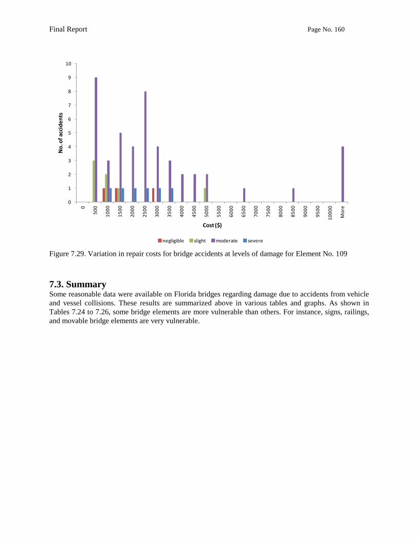
Final Report Page No. 160
0
1
2
3
4
5
6
7
8
9
10
0
50
0
10
00
15
00
20
00
25
00
30
00
35
00
40
00
45
00
50
00
55
00
60
00
65
00
70
00
75
00
80
00
85
00
90
00
95
00
10
00
0
Mo
re
No
. of
acci
de
nts
Cost ($)
negligible slight moderate severe
Figure 7.29. Variation in repair costs for bridge accidents at levels of damage for Element No. 109
7.3. Summary
Some reasonable data were available on Florida bridges regarding damage due to accidents from vehicle
and vessel collisions. These results are summarized above in various tables and graphs. As shown in
Tables 7.24 to 7.26, some bridge elements are more vulnerable than others. For instance, signs, railings,
and movable bridge elements are very vulnerable.

Final Report Page No. 161
Table 7.24. Levels of vulnerability of bridge elements to damage from truck collisions Element
key Element short decription Vulnerability
Element
key Element short decription Vulnerability
Element
key Element short decription Vulnerability
12 Bare Concrete Deck 3 216 Timber Abutment 2 476 Timber Walls 2
13 Unp Conc Deck/AC Ovl 3 217 Other Mtl Abutment 2 477 Other Walls 2
28 Steel Deck/Open Grid 3 220 R/C Sub Pile Cap/Ftg 1 478 MSE Walls 2
29 Steel Deck/Conc Grid 3 230 Unpnt Stl Cap 1 480 Mast Arm Found 1
30 Corrug/Orthotpc Deck 3 231 Paint Stl Cap 1 481 Paint Mast Arm Vert 1
31 Timber Deck 3 233 P/S Conc Cap 1 482 Galvan Mast Arm Vert 1
32 Timber Deck/AC Ovly 3 234 R/Conc Cap 1 483 Other Mast Arm Vert 1
38 Bare Concrete Slab 3 235 Timber Cap 1 484 Paint Mast Arm Horzn 1
39 Unp Conc Slab/AC Ovl 3 240 Metal Culvert 1 485 Galvan Mast Arm Horz 1
54 Timber Slab 3 241 Concrete Culvert 0 486 Other Mast Arm Horzn 1
55 Timber Slab/AC Ovly 3 242 Timber Culvert 0 487 Sign Member Horiz 1
98 Conc Deck on PC Pane 3 243 Misc Culvert 0 488 Sign Member Vertical 1
99 PS Conc Slab 3 290 Channel 1 489 Sign Foundation 1
101 Unpnt Stl Box Girder 5 298 Pile Jacket Bare 1 495 Uncoat High Mast L. 1
102 Paint Stl Box Girder 5 299 Pile Jacket/Cath Pro 1 496 Painted High Mast L. 1
104 P/S Conc Box Girder 5 300 Strip Seal Exp Joint 3 497 Galvan. High Mast L. 1
105 R/Conc Box Girder 5 301 Pourable Joint Seal 3 498 Other High Mast L.P. 1
106 Unpnt Stl Opn Girder 5 302 Compressn Joint Seal 3 499 H. M. L. P. Found. 1
107 Paint Stl Opn Girder 5 303 Assembly Joint/Seal 3 540 Open Gearing 1
109 P/S Conc Open Girder 5 304 Open Expansion Joint 3 541 Speed Reducers 1
110 R/Conc Open Girder 5 310 Elastomeric Bearing 3 542 Shafts 1
111 Timber Open Girder 5 311 Moveable Bearing 3 543 Shaft Brgs and Coupl 1
112 Unpnt Stl Stringer 5 312 Enclosed Bearing 3 544 Brakes 1
113 Paint Stl Stringer 5 313 Fixed Bearing 3 545 Emergency Drive 1
115 P/S Conc Stringer 5 314 Pot Bearing 3 546 Span Drive Motors 1
116 R/Conc Stringer 5 315 Disk Bearing 3 547 Hydraulic Power Unit 1
117 Timber Stringer 5 320 P/S Conc Appr Slab 1 548 Hydraulic Piping Sys 1
120 U/Stl Thru Truss/Bot 3 321 R/Conc Approach Slab 1 549 Hydraulic Cylinders 1
121 P/Stl Thru Truss/Bot 3 330 Metal Rail Uncoated 3 550 Hopkins Frame 1
125 U/Stl Thru Truss/Top 3 331 Conc Bridge Railing 3 560 Locks 1
126 P/Stl Thru Truss/Top 3 332 Timb Bridge Railing 3 561 Live Load Shoes 1
130 Unpnt Stl Deck Truss 3 333 Other Bridge Railing 3 562 Counterweight Suppor 1
131 Paint Stl Deck Truss 3 334 Metal Rail Coated 3 563 Acc Ladd & Plat 1
135 Timber Truss/Arch 3 356 Steel Fatigue SmFlag 0 564 Counterweight 1
140 Unpnt Stl Arch 3 357 Pack Rust Smart Flag 0 565 Trun/Str and Cur Trk 1
141 Paint Stl Arch 3 358 Deck Cracking SmFlag 0 570 Transformers 1
143 P/S Conc Arch 3 359 Soffit Smart Flag 0 571 Submarine Cable 1
144 R/Conc Arch 3 360 Settlement SmFlag 0 572 Conduit & Junc. Box 1
145 Other Arch 3 361 Scour Smart Flag 0 573 PLCs 1
146 Misc Cable Uncoated 3 362 Traf Impact SmFlag 0 574 Control Console 1
147 Misc Cable Coated 3 363 Section Loss SmFlag 0 580 Navigational Lights 1
151 Unpnt Stl Floor Beam 3 369 Sub.Sect Loss SmFlag 0 581 Operator Facilities 1
152 Paint Stl Floor Beam 3 370 Alert Smart Flag 0 582 Lift Bridge Spec. Eq 1
154 P/S Conc Floor Beam 3 386 Fender/Dolphin Uncoa 0 583 Swing Bridge Spec. E 1
155 R/Conc Floor Beam 5 387 P/S Fender/Dolphin 0 590 Resistance Barriers 1
156 Timber Floor Beam 5 388 R/Conc Fender/Dolphi 0 591 Warning Gates 1
160 Unpnt Stl Pin/Hanger 3 389 Timber Fender/Dolphi 0 592 Traffic Signals 1
161 Paint Stl Pin/Hanger 3 390 Other Fender/Dolphin 0
201 Unpnt Stl Column 3 393 Blkhd Sewl Metal Unc 0
202 Paint Stl Column 3 394 R/Conc Abut Slope Pr 2
204 P/S Conc Column 3 395 Timber Abut Slope Pr 2
205 R/Conc Column 3 396 Other Abut Slope Pro 2
206 Timber Column 3 397 Drain. Syst Metal 1
207 P/S Conc Holl Pile 1 398 Drain. Syst Other 1
210 R/Conc Pier Wall 1 399 Other Xpansion Joint 1
211 Other Mtl Pier Wall 1 474 Walls Uncoated 1
215 R/Conc Abutment 2 475 R/Conc Walls 2
* Level of vulnerability: 5 - Extremely High; 4 - Very High; 3 - High; 2 - Moderate; 1 - Low; 0 - Negligible); to avoid zero vulnerability, min of 1 indicated for those elements with no data of damages
observed.

Final Report Page No. 162
Table 7.25. Levels of vulnerability of bridge elements to damage from vessel collisions Element
key Element short decription Vulnerability
Element
key Element short decription Vulnerability
Element
key Element short decription Vulnerability
12 Bare Concrete Deck 1 216 Timber Abutment 1 476 Timber Walls 0
13 Unp Conc Deck/AC Ovl 1 217 Other Mtl Abutment 1 477 Other Walls 0
28 Steel Deck/Open Grid 1 220 R/C Sub Pile Cap/Ftg 1 478 MSE Walls 0
29 Steel Deck/Conc Grid 1 230 Unpnt Stl Cap 1 480 Mast Arm Found 0
30 Corrug/Orthotpc Deck 1 231 Paint Stl Cap 1 481 Paint Mast Arm Vert 0
31 Timber Deck 1 233 P/S Conc Cap 1 482 Galvan Mast Arm Vert 0
32 Timber Deck/AC Ovly 1 234 R/Conc Cap 1 483 Other Mast Arm Vert 0
38 Bare Concrete Slab 1 235 Timber Cap 1 484 Paint Mast Arm Horzn 0
39 Unp Conc Slab/AC Ovl 1 240 Metal Culvert 1 485 Galvan Mast Arm Horz 0
54 Timber Slab 1 241 Concrete Culvert 1 486 Other Mast Arm Horzn 0
55 Timber Slab/AC Ovly 1 242 Timber Culvert 1 487 Sign Member Horiz 0
98 Conc Deck on PC Pane 1 243 Misc Culvert 1 488 Sign Member Vertical 0
99 PS Conc Slab 1 290 Channel 1 489 Sign Foundation 0
101 Unpnt Stl Box Girder 2 298 Pile Jacket Bare 1 495 Uncoat High Mast L. 0
102 Paint Stl Box Girder 2 299 Pile Jacket/Cath Pro 1 496 Painted High Mast L. 0
104 P/S Conc Box Girder 2 300 Strip Seal Exp Joint 1 497 Galvan. High Mast L. 0
105 R/Conc Box Girder 2 301 Pourable Joint Seal 1 498 Other High Mast L.P. 0
106 Unpnt Stl Opn Girder 2 302 Compressn Joint Seal 1 499 H. M. L. P. Found. 0
107 Paint Stl Opn Girder 2 303 Assembly Joint/Seal 1 540 Open Gearing 1
109 P/S Conc Open Girder 2 304 Open Expansion Joint 1 541 Speed Reducers 1
110 R/Conc Open Girder 2 310 Elastomeric Bearing 1 542 Shafts 1
111 Timber Open Girder 2 311 Moveable Bearing 1 543 Shaft Brgs and Coupl 1
112 Unpnt Stl Stringer 2 312 Enclosed Bearing 1 544 Brakes 1
113 Paint Stl Stringer 2 313 Fixed Bearing 1 545 Emergency Drive 1
115 P/S Conc Stringer 2 314 Pot Bearing 1 546 Span Drive Motors 1
116 R/Conc Stringer 2 315 Disk Bearing 1 547 Hydraulic Power Unit 1
117 Timber Stringer 2 320 P/S Conc Appr Slab 1 548 Hydraulic Piping Sys 1
120 U/Stl Thru Truss/Bot 1 321 R/Conc Approach Slab 1 549 Hydraulic Cylinders 1
121 P/Stl Thru Truss/Bot 1 330 Metal Rail Uncoated 1 550 Hopkins Frame 1
125 U/Stl Thru Truss/Top 1 331 Conc Bridge Railing 1 560 Locks 1
126 P/Stl Thru Truss/Top 1 332 Timb Bridge Railing 1 561 Live Load Shoes 1
130 Unpnt Stl Deck Truss 1 333 Other Bridge Railing 1 562 Counterweight Suppor 1
131 Paint Stl Deck Truss 1 334 Metal Rail Coated 1 563 Acc Ladd & Plat 1
135 Timber Truss/Arch 1 356 Steel Fatigue SmFlag 0 564 Counterweight 1
140 Unpnt Stl Arch 1 357 Pack Rust Smart Flag 0 565 Trun/Str and Cur Trk 1
141 Paint Stl Arch 1 358 Deck Cracking SmFlag 0 570 Transformers 1
143 P/S Conc Arch 1 359 Soffit Smart Flag 0 571 Submarine Cable 1
144 R/Conc Arch 1 360 Settlement SmFlag 0 572 Conduit & Junc. Box 2
145 Other Arch 1 361 Scour Smart Flag 0 573 PLCs 1
146 Misc Cable Uncoated 1 362 Traf Impact SmFlag 0 574 Control Console 1
147 Misc Cable Coated 1 363 Section Loss SmFlag 0 580 Navigational Lights 2
151 Unpnt Stl Floor Beam 1 369 Sub.Sect Loss SmFlag 0 581 Operator Facilities 1
152 Paint Stl Floor Beam 1 370 Alert Smart Flag 0 582 Lift Bridge Spec. Eq 1
154 P/S Conc Floor Beam 1 386 Fender/Dolphin Uncoa 5 583 Swing Bridge Spec. E 1
155 R/Conc Floor Beam 1 387 P/S Fender/Dolphin 5 590 Resistance Barriers 1
156 Timber Floor Beam 1 388 R/Conc Fender/Dolphi 5 591 Warning Gates 1
160 Unpnt Stl Pin/Hanger 1 389 Timber Fender/Dolphi 5 592 Traffic Signals 1
161 Paint Stl Pin/Hanger 1 390 Other Fender/Dolphin 5
201 Unpnt Stl Column 1 393 Blkhd Sewl Metal Unc 1
202 Paint Stl Column 1 394 R/Conc Abut Slope Pr 1
204 P/S Conc Column 1 395 Timber Abut Slope Pr 1
205 R/Conc Column 1 396 Other Abut Slope Pro 1
206 Timber Column 1 397 Drain. Syst Metal 0
207 P/S Conc Holl Pile 1 398 Drain. Syst Other 0
210 R/Conc Pier Wall 1 399 Other Xpansion Joint 0
211 Other Mtl Pier Wall 1 474 Walls Uncoated 0
215 R/Conc Abutment 1 475 R/Conc Walls 0
* Level of vulnerability: 5 - Extremely High; 4 - Very High; 3 - High; 2 - Moderate; 1 - Low; 0 - Negligible); to avoid zero vulnerability, min of 1 indicated for those elements with no data of damages
observed.

Final Report Page No. 163
Table 7.26. Levels of vulnerability of bridge elements to damage from overhead collisions Element
key Element short decription Vulnerability
Element
key Element short decription Vulnerability
Element
key Element short decription Vulnerability
12 Bare Concrete Deck 3 216 Timber Abutment 1 476 Timber Walls 1
13 Unp Conc Deck/AC Ovl 3 217 Other Mtl Abutment 1 477 Other Walls 1
28 Steel Deck/Open Grid 3 220 R/C Sub Pile Cap/Ftg 1 478 MSE Walls 1
29 Steel Deck/Conc Grid 3 230 Unpnt Stl Cap 1 480 Mast Arm Found 0
30 Corrug/Orthotpc Deck 3 231 Paint Stl Cap 1 481 Paint Mast Arm Vert 0
31 Timber Deck 3 233 P/S Conc Cap 1 482 Galvan Mast Arm Vert 0
32 Timber Deck/AC Ovly 3 234 R/Conc Cap 1 483 Other Mast Arm Vert 0
38 Bare Concrete Slab 3 235 Timber Cap 1 484 Paint Mast Arm Horzn 0
39 Unp Conc Slab/AC Ovl 3 240 Metal Culvert 1 485 Galvan Mast Arm Horz 0
54 Timber Slab 3 241 Concrete Culvert 0 486 Other Mast Arm Horzn 0
55 Timber Slab/AC Ovly 3 242 Timber Culvert 0 487 Sign Member Horiz 0
98 Conc Deck on PC Pane 3 243 Misc Culvert 0 488 Sign Member Vertical 0
99 PS Conc Slab 3 290 Channel 1 489 Sign Foundation 0
101 Unpnt Stl Box Girder 5 298 Pile Jacket Bare 1 495 Uncoat High Mast L. 0
102 Paint Stl Box Girder 5 299 Pile Jacket/Cath Pro 1 496 Painted High Mast L. 0
104 P/S Conc Box Girder 5 300 Strip Seal Exp Joint 3 497 Galvan. High Mast L. 0
105 R/Conc Box Girder 5 301 Pourable Joint Seal 3 498 Other High Mast L.P. 0
106 Unpnt Stl Opn Girder 5 302 Compressn Joint Seal 3 499 H. M. L. P. Found. 0
107 Paint Stl Opn Girder 5 303 Assembly Joint/Seal 3 540 Open Gearing 0
109 P/S Conc Open Girder 5 304 Open Expansion Joint 3 541 Speed Reducers 0
110 R/Conc Open Girder 5 310 Elastomeric Bearing 3 542 Shafts 0
111 Timber Open Girder 5 311 Moveable Bearing 3 543 Shaft Brgs and Coupl 0
112 Unpnt Stl Stringer 5 312 Enclosed Bearing 3 544 Brakes 0
113 Paint Stl Stringer 5 313 Fixed Bearing 3 545 Emergency Drive 0
115 P/S Conc Stringer 5 314 Pot Bearing 3 546 Span Drive Motors 0
116 R/Conc Stringer 5 315 Disk Bearing 3 547 Hydraulic Power Unit 0
117 Timber Stringer 5 320 P/S Conc Appr Slab 1 548 Hydraulic Piping Sys 0
120 U/Stl Thru Truss/Bot 3 321 R/Conc Approach Slab 1 549 Hydraulic Cylinders 0
121 P/Stl Thru Truss/Bot 3 330 Metal Rail Uncoated 3 550 Hopkins Frame 0
125 U/Stl Thru Truss/Top 3 331 Conc Bridge Railing 3 560 Locks 0
126 P/Stl Thru Truss/Top 3 332 Timb Bridge Railing 3 561 Live Load Shoes 0
130 Unpnt Stl Deck Truss 3 333 Other Bridge Railing 3 562 Counterweight Suppor 0
131 Paint Stl Deck Truss 3 334 Metal Rail Coated 3 563 Acc Ladd & Plat 0
135 Timber Truss/Arch 3 356 Steel Fatigue SmFlag 0 564 Counterweight 0
140 Unpnt Stl Arch 3 357 Pack Rust Smart Flag 0 565 Trun/Str and Cur Trk 0
141 Paint Stl Arch 3 358 Deck Cracking SmFlag 0 570 Transformers 0
143 P/S Conc Arch 3 359 Soffit Smart Flag 0 571 Submarine Cable 0
144 R/Conc Arch 3 360 Settlement SmFlag 0 572 Conduit & Junc. Box 0
145 Other Arch 3 361 Scour Smart Flag 0 573 PLCs 0
146 Misc Cable Uncoated 3 362 Traf Impact SmFlag 0 574 Control Console 0
147 Misc Cable Coated 3 363 Section Loss SmFlag 0 580 Navigational Lights 0
151 Unpnt Stl Floor Beam 3 369 Sub.Sect Loss SmFlag 0 581 Operator Facilities 0
152 Paint Stl Floor Beam 3 370 Alert Smart Flag 0 582 Lift Bridge Spec. Eq 0
154 P/S Conc Floor Beam 3 386 Fender/Dolphin Uncoa 0 583 Swing Bridge Spec. E 0
155 R/Conc Floor Beam 5 387 P/S Fender/Dolphin 0 590 Resistance Barriers 0
156 Timber Floor Beam 5 388 R/Conc Fender/Dolphi 0 591 Warning Gates 0
160 Unpnt Stl Pin/Hanger 3 389 Timber Fender/Dolphi 0 592 Traffic Signals 0
161 Paint Stl Pin/Hanger 3 390 Other Fender/Dolphin 0
201 Unpnt Stl Column 3 393 Blkhd Sewl Metal Unc 0
202 Paint Stl Column 3 394 R/Conc Abut Slope Pr 1
204 P/S Conc Column 3 395 Timber Abut Slope Pr 1
205 R/Conc Column 3 396 Other Abut Slope Pro 1
206 Timber Column 3 397 Drain. Syst Metal 1
207 P/S Conc Holl Pile 1 398 Drain. Syst Other 1
210 R/Conc Pier Wall 1 399 Other Xpansion Joint 1
211 Other Mtl Pier Wall 1 474 Walls Uncoated 1
215 R/Conc Abutment 1 475 R/Conc Walls 1
* Level of vulnerability: 5 - Extremely High; 4 - Very High; 3 - High; 2 - Moderate; 1 - Low; 0 - Negligible); to avoid zero vulnerability, min of 1 indicated for those elements with no data of damages
observed.

Final Report Page No. 164
7.4. References
American Association of State Highway and Transportation Officials. AASHTO, (2009). Design
Specifications for Bridges Vulnerable to Coastal Storms. Washington, D.C.
Buth, C. Eugene, Williams, William F., Brackin, Michael S., Lord, Dominique, Geedipally, Srinivas R.,
and Abu-Odeh, Akram Y., “Analysis of large truck collisions with bridge piers: phase 1. Report of
guidelines for designing b ridge piers and abutments for vehicle collisions,” Report No. FHWA/TX-10/9-
4973-1, Texas Transportation Institute, Texas Department of Transportation, and the Federal Highway
Administration, May 2010, 186 pp.
Consolazio, Gary R., Davidson, Michael, T., Getter, and Daniel, J., (2010). Vessel Crushing and
Structural Collapse Relationships for Bridge Design. University of Florida, Gainesville; Florida
Department of Transportation, 231p.
FDOT, (2012). Guide to STRAHNET, Accessed Feb. 2012 from the website at Florida Department of
Transportation (FDOT): http://www.dot.state.fl.us/planning/statistics/hwydata/strahnetguide.pdf
Kodur, V., Gu, L., and Garlock, M., (2010) "Review and Assessment of Fire Hazard in Bridges."
Transportation Research Record: Journal of the Transportation Research Board No. 2172 (2010): 23-29
Lessard, Aran, (2010). Bridge Fire – Lake County on MP 282 – Turnpike over CR 561, South Eastern
Bridge Preservation Partnership (SEBPP) Meeting, Orlando, Florida, 2010.
Sobanjo, John, and Thompson, Paul., (2011). Enhancement of the FDOT's Project Level and Network
Level Bridge Management Analysis Tools (Final Report, Research Contract No. BDK83 977-01). Florida
Department of Transportation, Tallahassee, Florida.
Stoddard, Richard, (2004). “Inspection and Repair of a Fire Damaged Prestressed Girder Bridge, Report
No. IBC-04-17, Washington State DOT, Olympia, WA.
Thompson, P. D., Soares, R., Choung, H. J., Najafi, F. T., and Choung, H. J., (1999) “Development Of
User Cost Data For Florida's Bridge Management System,” WPI 0510855, Final Rept, UF No. 4910-
4504-606-12, State Proj 99700-3554-119. Contract #: BB-262, 53 p.

Final Report Page No. 165
8. Advanced Deterioration
A common and general concern of risk management is the unavoidable disruption of service due to the
need to respond pro-actively to impending hazards. If bridge maintenance is deferred for a prolonged
period, the condition of the structure reaches a point where the agency is forced to take action to ensure
safe mobility. The action may be posting, closure, strengthening, or partial or complete replacement. All
of these actions disrupt service, forcing road users to expend more time and fuel in congestion or detours.
They also force the agency to expend public funds on the action.
One of the key life cycle tradeoffs in bridge management is the possibility of strategic preventive
maintenance actions to postpone the need for more expensive forced activities. A purpose of Pontis and
the PLAT is to identify these opportunities. Accurate evaluation of preventive activities requires the use
of tools to quantify the negative impacts of allowing conditions to deteriorate. There is no laboratory
where a scientific sample of bridges can be allowed to deteriorate to failure under realistic conditions of
weather and traffic. Similarly, highly deteriorated conditions in the Florida inventory are uncommon and
are routinely avoided by active management processes.
Florida‟s Pontis database is the only comprehensive source of data on historical conditions and events of
service disruption. Therefore a resourceful data mining of Pontis is necessary to develop the required
models.
8.1. Identifying service disruptions related to condition While there are many ways in which bridge characteristics can interfere with mobility, the Pontis
database offers three types of service disruption that can be specifically related to condition:
Evidence of bridge closure or replacement, provided by the assignment of a bridge to fictitious
“District 9 – Central Office.” FDOT never deletes a structure from the Pontis database, but
instead assigns it to District 9 when it is no longer required to be in the active inventory, usually
because it has been demolished.
Evidence of bridge reconstruction, from National Bridge Inventory (NBI) item 106 – Year
reconstructed. This is defined as the most recent year in which the bridge underwent work
eligible for Federal funding (regardless of how actually funded). This can include total
replacement, superstructure replacement, and functional improvements such as widening.
Operational status of posted or closed, based on a value of NBI item 41 of B, D, E, K, P, or R.
This information is comprehensive for bridges, but not for other types of structures, such as sign
structures, high-mast light poles, and mast arms. This is because non-bridge structures were added to
Pontis relatively recently and do not yet have a long time series of data. As a result, it was necessary to
remove non-bridge structures from the analysis. This reduced the number of structures in the data set
from 31,166 to 15,548.
Table 8.1 summarizes the events of service disruption, potentially related to condition, identified in the
analysis. For an inspection to be listed in the table, it must have at least one deck, superstructure, or
substructure element in the worst or second-worst condition state. This represents 27% of the 97,416
bridge inspections in the database. A bridge inspection is classified as Retired if it is the last element
inspection that was recorded before the bridge was moved to District 9. It is classified as Rebuilt if it is
the last element inspection recorded before the year indicated in NBI item 106. It is classified as Posted if
the operational status indicates posting or closure in the following inspection but not in the current
inspection. These definitions arose from the statistical analysis described later in this report.

Final Report Page No. 166
Table 8.1. Summary of service disruptions
Material Inspections Number of events Percent of inspections
Retired Rebuilt Posted Retired Rebuilt Posted
Reinforced concrete 9057 175 110 54 1.9 1.2 0.6
Prestressed concrete 9865 193 208 51 2.0 2.1 0.5
Steel 4810 143 86 47 3.0 1.8 1.0
Timber 2802 150 58 8 5.4 2.1 0.3
It can be seen in Table 8.1 that the types of service disruptions can vary substantially by material type, as
determined from NBI item 43.
8.2. Identifying deteriorated conditions related to risk In the Florida Bridge Inspection Manual, as in the AASHTO CoRe Element Manual (AASHTO 2001),
the definition of the final (worst) condition state of each structural element includes words such as,
“Deterioration is sufficient to warrant structural review to ascertain the impact on the ultimate strength
and/or serviceability of either the element or the bridge.” This wording indicates the possibility of service
disruption in the worst condition state, at least for the primary load-bearing elements.
An analysis of replacement, reconstruction, posting, and closure of bridges in the Florida inventory found
that even a tiny fraction of an element in the worst condition state was highly correlated with service
disruption, and that a significant fraction of bridges underwent a service disruption even with no
elements in their worst condition states. A detailed analysis of central office bridges (next chapter) found
that it was also necessary to consider the fraction of primary elements in the second-to-worst condition
state in order to obtain a more complete picture of the motivations for posting, reconstruction, and
replacement.
In the analyses described in the remainder of this report, each model was tested for significance of the
second-to-worst condition state, to see if it was necessary to consider these moderately-deteriorated
elements. In almost every case, these elements played a necessary role in obtaining strong statistical
results. This may indicate a significantly proactive FDOT response to advanced deterioration.
8.3. Central office bridges As of August 2011, the FDOT Pontis database contains 5,033 structures in District 9, of which 3,213 are
bridges (Table 8.2). Known as “central office bridges,” these are structures whose data are not actively
maintained for inspection, operations, or planning purposes. Nevertheless, they are retained in Pontis for
a variety of other reasons, including possible use in special studies such as the current one. Most of these
are structures that were previously in service, but were retired or replaced. The reasons for these
retirements or replacements are especially relevant to efforts to quantify the likelihood and consequences
of risk factors such as advanced deterioration, fatigue, storms, collisions, and scour. As part of the study,
an effort was made to identify the reasons for bridges to be classified as “central office bridges.”
Sign structures, high-mast light poles, and traffic signal mast arms are relatively recent additions to the
Pontis database, unlikely to have enough data yet to reliably quantify cause-and-effect relationships. As a
result, it was decided to omit them from the analysis. To ensure that the data set would have roadway-on
data and element inspection data, structures lacking these records were omitted.
In many cases FDOT staff add a new bridge in the central office to reserve a bridge ID for a structure that
is not yet built, or not yet open to traffic. Appendix A of the FDOT Coding Guide (FDOT 2011)
describes the data items required for these structures. Nearly all of these structures lack element
inspection data.

Final Report Page No. 167
Table 8.2. Structure design types in District 9
Design type Count
-1 Unknown (P) 75
0 Other (NBI) 298
1 Slab 718
2 Stringer/Girder 1494
3 Girder-Floorbeam 55
4 Tee Beam 202
6 Single/Spread Box 23
7 Frame 1
9 Truss-Deck 1
10 Truss-Thru 18
11 Arch-Deck 24
12 Arch-Thru 3
15 Movable - Lift 4
16 Movable-Bascule 46
17 Movable-Swing 4
18 Tunnel 1
19 Culvert 265
20 Mixed types 2
21 Segmental Box Girder 3
22 Channel Beam 51
89 Sign-Monotube-Cantilever 1
91 Sign-Cantilever 910
92 Sign-Span 361
93 Sign-Butterfly 44
94 Sign-Cable 152
96 High Mast Light 270
97 Traffic Signal Mast Arm 7
Total 5033
In addition, occasionally a bridge will be assigned to the central office in Pontis if it is found to be open
only to private use, or does not satisfy NBI length requirements, or for other administrative reasons. This
may occur without any physical change happening at the bridge site. A total of 70 bridges were found to
be in District 9 for this reason. After removing these structures, a total of 1,480 bridges remained in the
data set for further analysis.

Final Report Page No. 168
8.4. Classifying the reason for demolition or replacement It is desired to classify these remaining bridges according to the likely reason(s) that each bridge was
removed or replaced. The most common reasons include:
A roadway section or intersection is widened or reconfigured to increase access, capacity or
safety.
The condition of a bridge has deteriorated to the point where there is an actual or imminent effect
on serviceability for legal loads, or where the danger of fracture or other types of sudden failure
is unacceptably high.
A bridge is damaged by the cumulative effect of scour on its foundations, to the point where
there is actual or imminent effect on serviceability.
A bridge presents a safety or access issue because of narrowness, impaired vertical clearance, or
low load capacity not caused by active deterioration.
A bridge is no longer needed because the feature under it is removed, or the bridge‟s traffic-
carrying role is no longer required.
A bridge is damaged or destroyed by a hurricane, flood, vehicle or vessel collision, or other
extreme event.
It is possible for there to be a combination of reasons, particularly a combination of deterioration and
functional needs. Some of the reasons are relevant to risk analysis, while others are not.
The Pontis database provides several types of evidence that can assist in this classification:
Year built or reconstructed (NBI items 27 or 106);
National Bridge Inventory (NBI) condition assessments for deck, superstructure, substructure,
and culvert (Items 58, 59, 60, and 62);
NBI assessments of channel condition, waterway adequacy, and scour criticality (Items 61, 71,
and 113);
NBI indication of the requirement for fracture critical inspections (Item 92A);
Element inspection data, particularly the percentage of elements in their worst and second-worst
defined condition states;
Operating rating (NBI item 64);
Route number and milepost (NBI items 5 and 11), which is especially useful for identifying
groups of bridges that are all replaced at the same time along a route for functional reasons;
Number of lanes on the bridge (NBI item 28A);
Comments that are logged with the bridge record or with inspection records.
Ultimately each bridge was classified using judgment, based on the preponderance of the available data.
The most important factors turned out to be:
Comments entered in the database directly explaining what happened to the bridge and why;
For bridges with an identified replacement structure, a change in the number of lanes was taken
as a strong indicator of functional reasons for the replacement;
An NBI condition assessment of 4 or below, or any element (from among the deck,
superstructure, or substructure primary load-bearing elements) in the worst condition state, were
taken as strong indicators of condition reasons for bridge replacement, especially when in
combination with reduced operating ratings;
Indicators of severe channel deterioration, waterway inadequacy, scour criticality, or fracture
criticality were taken as indicators that extreme events, or the possibility of such hazards, may
have contributed to the decision to replace a bridge. In addition, some of the bridges had specific
mentions of hurricane damage in their final inspection records.

Final Report Page No. 169
It should be noted that none of these information sources is necessarily authoritative. In many cases there
are engineering reports and detailed inspection reports outside of Pontis that provide a deeper
justification for replacement. The current analysis seeks network-wide risk estimates, and therefore
places higher priority on breadth and comprehensiveness across the inventory, rather than depth of
analysis for any specific bridges.
The interpretation of the data is in the context of knowing with certainty that the bridge was replaced or
retired: the effect is known and the cause is imputed. For example, if a two-lane bridge in bad condition
is replaced by another two-lane bridge, there is a presumption that the bad condition must have
contributed to the replacement decision. The converse is usually not true: if a bridge is in bad condition,
it usually is not immediately replaced. Instead, it might be repaired or more closely monitored. The risk
factor of interest in this study is the small but non-zero likelihood that none of the less extreme options
will suffice, and that immediate replacement or load restriction will be necessary, thus interrupting
normal service on the bridge.
Table 8.3 shows the results of this classification analysis. In this table, each retired or replaced bridge is
classified by what is believed to be the primary reason for retirement, using the logic described above.
This information was added to the userbrdg table in the researchers‟ Pontis database for further use.
Table 8.3. Primary cause of bridge retirement
Reason Count
? Unknown, unable to determine reason 440
C Cracking, fatigue, fracture criticality 8
D Deterioration of structural elements 327
F Functional, roadway project, add lanes 650
H Hurricane damage 18
V Vehicle/vessel collision 2
W Washout, scour, flood 35
Total 1480
It can be seen that in 440 cases there was not enough information in Pontis to enable useful speculation
about the cause of bridge retirement. However, in all of these cases there were no condition assessments
of 4 or below, no primary elements in their worst condition states, and no indication of vulnerability to
extreme events. In many cases these structures have one or more primary elements in their second-worst
condition state, indicating that condition may have played a role. Functional requirements may also have
played a role.
In many cases replacement of a bridge may be motivated by a combination of reasons. For example, in 54
of the cases where deterioration was viewed as the primary reason for replacement, the replacement
bridge had a different number of lanes than the original structure.
One of the most useful indicators of the reason for bridge retirement, was the set of data available about
the bridge that replaced it. The Pontis data item userbrdg.repl_strct_id was added in February 2008 to
enable this type of analysis. Prior to that date, the replacement structure had been sporadically noted in
bridge or inspection comments. To improve the usefulness of this information, the replacement bridge ID
was extracted from all comments where it was noted, and used to further populate the repl_strct_id
column in the database. This added 642 data points, for a total of 913 bridges whose replacement bridge
id was known, out of the 1480 bridges in the analysis. Of the remaining bridges, some were replaced by
an unknown bridge ID, and others were not replaced at all.

Final Report Page No. 170
An SQL update script for the 642 replacement structure ids can be provided for FDOT use if desired.
8.5. Likelihood of service disruption To develop a predictive model of the likelihood of service disruption, a regression analysis was
conducted to estimate the probability of replacement, reconstruction, and operational restriction, as a
function of element condition. The analysis attempted to find and quantify a cause-and-effect relationship
between advanced deterioration and service disruption.
In order to make the analysis possible using a Pontis data set, the incidence of service disruption was
approximated by recorded instances of bridge retirement, replacement, reconstruction, and posting. It was
recognized that condition is not the only reason for these activities. It was expected therefore that a
significant amount of statistical “noise” would be present in the models, and it was important to select
model formulations that would isolate the effect of condition and avoid bias caused by non-condition-
related influences on agency decisions.
8.5.1. Effect of condition It is desired that the risk model to be developed have the ability to work with the results of deterioration
models, to show how the risk of service disruption may increase as condition worsens. A previous FDOT
study of deterioration showed that reliable deterioration models can be developed for element condition
states, but that the forecasting of National Bridge Inventory (NBI) condition ratings was indirect and
much less precise (Sobanjo and Thompson 2011). Therefore a statistical relationship with element
condition states is desired.
When bridge element deterioration is forecast using Markovian models, a small but non-zero fraction
appears in the worst condition state relatively early in the element‟s life. Table 8.4 shows a typical
example of deterioration based on a Markov transition probability matrix. It can be seen that the percent
in the worst condition state (state 5 in this example) is non-zero after only three years of deterioration.
Obviously the risk of service disruption cannot be considered to be elevated when so little deterioration
has taken place. From this reasoning, it follows that small amounts of deterioration should be associated
with very small amounts of risk, and that risk should smoothly increase with further deterioration.
Table 8.5 shows the frequency of retirement, reconstruction, and posting for deteriorated bridges for
various ranges of condition. In this table the inspections counted as “Decayed” are those that were moved
to District 9 for deterioration or for unknown reasons (codes “D” or “?”). The rows in this table represent
ranges of the percent found to be in the worst (left side) or second-worst (right side) condition state for
the element in worst condition. The left side of the table shows that the probability of a bridge being
Rebuilt is already 3.13 percent even after a tiny percentage (more than zero but less than one-tenth of one
percent) is found in the worst condition state. As expected, the risk increases as higher amounts are
found. The right side of the table shows that the risk is lower but still significant for the second-worst
condition state. Experimental regression models also confirmed that it is necessary to consider the
second-worst condition state in order to have a risk model with reasonable behavior.
Table 8.5 also hints that the increase in risk is not linear with worsening condition, but is more closely
tied to the log of condition. The regression analysis presented later in this chapter shows that there is a
good reason for this to be the case.

Final Report Page No. 171
Table 8.4. Example of Markovian deterioration
Markov transition probability matrix
State State probability in one year
Today 1 2 3 4 5 Probability of state k next year: for all k
1 95.3 4.6 0.1 0.0 0.0
2 0 93.2 3.9 1.9 1.0 j is the condition state this year and x is the fraction in state j
3 0 0 89.4 7.3 3.3 p is the transition probability from j to k
4 0 0 0 82.8 17.2
5 0 0 0 0 100
Future condition forecasts
Percent by condition state Percent by condition state
Year 1 2 3 4 5 Year 1 2 3 4 5
0 100 0.0 0.0 0.0 0.0 25 30.0 28.1 10.1 6.8 25.0
1 95.3 4.6 0.1 0.0 0.0 26 28.6 27.6 10.1 6.9 26.8
2 90.8 8.7 0.4 0.1 0.0 27 27.3 27.0 10.2 7.0 28.6
3 86.6 12.3 0.8 0.3 0.2 28 26.0 26.4 10.2 7.1 30.4
4 82.5 15.4 1.2 0.5 0.4 29 24.8 25.8 10.1 7.1 32.2
5 78.6 18.2 1.8 0.8 0.6 30 23.6 25.2 10.1 7.1 34.0
6 74.9 20.5 2.4 1.1 1.0 31 22.5 24.6 10.0 7.1 35.8
7 71.4 22.6 3.0 1.5 1.5 32 21.4 23.9 9.9 7.1 37.6
8 68.0 24.3 3.6 1.9 2.1 33 20.4 23.3 9.8 7.0 39.4
9 64.8 25.8 4.3 2.3 2.8 34 19.5 22.6 9.7 7.0 41.2
10 61.8 27.0 4.9 2.7 3.6 35 18.5 22.0 9.6 6.9 42.9
11 58.9 28.0 5.5 3.1 4.5 36 17.7 21.4 9.5 6.9 44.7
12 56.1 28.8 6.1 3.5 5.5 37 16.8 20.7 9.3 6.8 46.4
13 53.5 29.5 6.6 3.9 6.6 38 16.1 20.1 9.1 6.7 48.0
14 51.0 29.9 7.1 4.3 7.7 39 15.3 19.5 9.0 6.6 49.7
15 48.6 30.2 7.6 4.6 9.0 40 14.6 18.8 8.8 6.5 51.3 << Median life expectancy
16 46.3 30.4 8.0 5.0 10.4 41 13.9 18.2 8.6 6.4 52.9
17 44.1 30.5 8.4 5.3 11.8 42 13.2 17.6 8.4 6.2 54.5
18 42.0 30.4 8.7 5.5 13.3 43 12.6 17.0 8.2 6.1 56.0
19 40.1 30.3 9.0 5.8 14.8 44 12.0 16.5 8.0 6.0 57.5
20 38.2 30.1 9.3 6.0 16.4 45 11.5 15.9 7.8 5.9 58.9
21 36.4 29.8 9.5 6.3 18.1 46 10.9 15.3 7.6 5.7 60.4
22 34.7 29.4 9.7 6.4 19.7 47 10.4 14.8 7.4 5.6 61.8
23 33.0 29.0 9.9 6.6 21.5 48 9.9 14.3 7.2 5.5 63.1
24 31.5 28.6 10.0 6.7 23.2 49 9.5 13.8 7.0 5.3 64.4
25 30.0 28.1 10.1 6.8 25.0 50 9.0 13.3 6.8 5.2 65.7
j
jkjk pxy
Table 8.5. Frequency of service disruption for ranges of condition (in percent)
Range Worst element in its worst condition state Worst element in 2nd-worst condition state
Count Decayed Rebuilt Posted Total Count Decayed Rebuilt Posted Total
0.0<0.1 32 0.00 3.13 0.00 3.13 228 0.44 3.95 0.00 4.39
0.1-0.5 200 0.50 3.00 0.50 4.00 948 0.11 1.48 0.11 1.69
0.5<1.0 212 1.42 1.42 0.94 3.77 1255 0.80 1.51 0.40 2.71
1<5 1071 1.96 2.61 0.09 4.67 5232 0.88 1.85 0.59 3.33
5<10 738 2.98 1.49 1.22 5.69 2556 1.13 1.68 0.74 3.56
10<50 1182 5.41 2.37 0.93 8.71 5061 1.64 1.70 0.81 4.15
50<100 1227 5.38 1.55 1.06 7.99 8454 1.77 1.87 0.53 4.18

Final Report Page No. 172
8.5.2. Potential explanatory variables Table 8.6 shows the variation in service disruptions by functional class of the roadway on each bridge.
Bridges carrying more important functional classes are more likely to be replaced or reconstructed when
they reach poor condition, and less likely to be posted.
Table 8.6. Frequency of service disruption by functional class
Functional class Count Decayed Rebuilt Posted Total
01 Rural Interstate 573 0.00 2.27 0.00 2.27
02 Rural Other Princ 1706 2.17 1.47 0.12 3.75
06 Rural Minor Arterial 1103 2.63 1.09 0.45 4.17
07 Rural Mjr Collector 2058 1.26 0.39 0.63 2.28
08 Rural min Collector 1446 0.69 0.62 0.69 2.01
09 Rural Local 4359 2.84 1.33 0.76 4.93
11 Urban Interstate 1567 0.32 6.89 0.38 7.59
12 Urban Fwy/Expwy 1088 0.55 3.95 0.00 4.50
14 Urban Other Princ 2449 1.10 2.12 0.29 3.51
16 Urban Minor Arterial 2574 1.13 1.17 0.93 3.22
17 Urban Collector 2530 0.83 1.78 0.87 3.48
19 Urban Local 3250 1.02 1.11 0.86 2.98
Table 8.7 shows how the frequency of service disruptions does not exhibit a clear overall pattern when
bridges are grouped by traffic volume. The lowest-volume bridges are more likely to be retired, while
the highest volume bridges are more likely to be reconstructed. The incidence of posting increases as
volume decreases, but this is because of condition rather than because of traffic volume.
Table 8.7. Frequency of service disruption by ADT range
Range of ADT Count %Bad* Decayed Rebuilt Posted Total
0<100 2678 49.94 3.40 1.27 0.64 5.30
100<500 3043 48.64 1.64 1.18 1.02 3.84
500<1000 1741 47.18 0.69 0.80 0.86 2.35
1000<5000 5441 46.54 1.31 0.99 0.74 3.03
5000<10000 2836 41.11 1.34 1.23 0.81 3.39
10000<50000 7389 34.40 1.04 2.33 0.30 3.67
50000+ 1578 21.58 0.51 5.96 0.13 6.59
*Percent of the worst element in the worst or 2nd-worst condition state
Analysis of disruption frequency by bridge design type (NBI item 43) did not show any clear
relationships, but the analysis by material type was very clear, as shown in Table 8.8. Most of the timber
bridges that are in deteriorated condition are already posted for reasons unrelated to condition, so the
incidence of posting is even higher than the table would suggest.

Final Report Page No. 173
Table 8.8. Frequency of service disruption by material type (based on NBI item 43A)
Material Count Decayed Rebuilt Posted Total
Concrete - Prestressed 9108 0.82 2.18 0.53 3.54
Concrete - Reinforced 8397 1.05 1.25 0.60 2.90
Steel 4551 1.80 1.80 0.99 4.59
Timber 2650 3.85 2.00 0.26 6.11
8.5.3. Model form Regression models were developed for a variety of functional forms that might be justified by the
problem structure. The model types and their rationale are:
Constant probability. This model assumes that a bridge has a fixed probability of service disruption if
any of its elements reaches its worst or second-worst condition state. Such a model works fairly well
when only bridge decks are considered, because they are inspected as “eaches”. In the historical database
of inspections, a bridge deck has either 100% or 0% in the target condition state. Unfortunately, this
model lacked explanatory power for elements that are not inspected as “eaches”. Also, the forecasts
output by a Markovian model are not limited to 100% or 0%. In addition, it was considered unreasonable
that a tiny fraction in a deteriorated condition state should yield the same disruption probability as a
much larger fraction in that state.
Linear probability. This model assumes that a bridge‟s probability of service disruption is linearly
proportional to the fraction and/or probability of the deteriorated condition state. This model form is
implicit in Pontis, where the proportional relationship is represented by the “failure probability,” and is
also used in the PLAT. The regression analysis showed that the linear model was a reasonable
approximation for some of the materials and some of the disruption types, but could readily be improved
upon by other model forms. It is the only model form currently accepted by Pontis, however.
Weibull model. This model assumes that the probability of disruption is related to bridge age, using a
Weibull distribution. A variation of the model uses a measure of condition, such as health index, as a
proxy for age. This is the same model that proved to be very effective in describing the onset of
deterioration, in the previous FDOT study. There would be an attractive consistency and symmetry if the
end of a bridge‟s life could be described using the same model as the beginning of its life. Unfortunately,
the Weibull form did not work well for the risk model. Determining the actual effective age of a bridge is
inexact, introducing a considerable amount of error because of unknown past rehabilitation work. Health
index was a poor proxy that did not produce compelling goodness-of-fit statistics from the regression
model.
Lognormal model. Like the Weibull model, this model also assumes that the probability of disruption is
related to age, and uses condition as a proxy for age. However, it models condition as the result of a
multiplicative process (multiplying a transition probability by itself some unknown number of times),
such that the predictive variable can be expressed as the log of the fraction in the deteriorated condition
state. This model has the theoretical attractiveness that it fits the phenomenon being modeled in a very
intuitive way. Moreover, it was the only model form that consistently produced strong goodness-of-fit
measures in the regression analysis.
The lognormal model is very commonly used in reliability analysis in combination with Markov models,
and is common in many fields where compound rates of change are used. For example, the Black-Scholes
model for pricing of financial instruments is based on the lognormal distribution.

Final Report Page No. 174
Using these alternative model forms in the regression analysis, models were attempted using either the
worst condition state, or a combination of the worst and second-worst states, or using a weighted sum of
the worst and second-worst states. Models were developed separately for each type of disruption
(retirement, reconstruction, or posting), and for combinations of the disruption types. Explanatory
variables were investigated in various reasonable configurations, including constant “dummy” variables
for material and functional class, and variations on ADT suggested by the exploratory data analysis.
Model stratification was also investigated in place of the use of dummy variables.
In the development of this type of statistical model, censoring is a significant issue. In a population of
several thousand bridges, only a relatively small fraction are close to the end of their lives. The remaining
bridges will eventually reach this point at an unknown time in the future. Future life extension activity
may postpone this eventuality for a considerable length of time. It is significant to know that certain
bridges have reached various stages of advanced deterioration without encountering any service
disruption, so this valuable information should not be discarded.
To ensure that the model estimation process is unbiased while still making maximum use of censored
data, the analysis was organized in the form of a hazard model. A hazard model estimates the
instantaneous probability, at a given condition level, that a service disruption will occur (Figure 8.1).
Hazard function(instantaneous probabilityor height of distribution)
Deteriorating condition
Probability that disruption has occurred
Figure 8.1. Schematic depiction of a hazard model
When the analysis is organized as a hazard model, the unit of analysis is the inspection, rather than the
bridge. Rather than following each bridge through its life to find out when replacement, reconstruction,
or posting occurs, the process looks at each inspection to see what happens immediately afterward,
before the next inspection. The possibilities are that the bridge may be retired, reconstructed, or posted;
or it is possible (and most likely) that no disruption will happen at all.
8.5.4. Data filtering In the estimation data set, inspections were included only if they contain at least one element in the worst
or second-worst condition state, from among deck, superstructure, and substructure elements (those with
elemkey<300). It is assumed that the disruption probability is zero if no primary load-bearing elements
are in deteriorated states. In addition:
Inspections having the inspkey value of „STRT‟ were omitted since they represent FDOT‟s initial
experiments with element inspection in the mid-1990s, which have questionable accuracy.
Inspections after 7/1/2009 were omitted, to provide an opportunity to examine the following
inspection for posting data. This ensures that the hazard model is not censored.
Certain additional quality control checks were performed, such as ensuring that element
quantities are non-zero.
The final data set used in model estimation had 26,534 bridge inspections.

Final Report Page No. 175
8.5.5. Estimation and model evaluation The Weibull and lognormal models were estimated using an iterative maximum likelihood estimation
procedure, similar to what was used in the previous study for the onset of deterioration. Excel‟s Solver
module provided the fitting procedure. It was configured to maximize the sum of a log-likelihood
function for the normal distribution, a measure of the probability of the observed data arising, given the
model under investigation.
To facilitate visualization and evaluation, a procedure was developed to group the data points into bins.
A tableau using 20 bins of equal population provided the most consistent results. Figure 8.2 shows an
example, for steel bridges.
Model parameters Bin Count DecayIx ActCnt EstCnt Actual EstimatedX2-modelX2-uniform
SpW 40 C1 1 1E-06 0 0.0 0.000 0.000 0.00 10.91
SbW 40 0 240 0.01669 3 5.8 1.250 2.400 1.32 5.74
DkX 0.5 1 241 0.05823 8 7.8 3.320 3.248 0.00 0.78
SpX 0.5 2 240 0.10813 10 8.5 4.167 3.548 0.26 0.08
SbX 0.5 3 241 0.17639 12 9.0 4.979 3.735 1.00 0.11
c -0.00014 4 240 0.27524 15 9.3 6.250 3.869 3.52 1.53
b 0.001962 5 241 0.43885 9 9.6 3.734 3.971 0.03 0.33
a 3000 6 241 0.65789 6 9.7 2.490 4.035 1.43 2.21
μ 15.5453 7 240 0.91264 8 9.8 3.333 4.071 0.32 0.78
σ 3.997625 8 241 1.24123 7 9.9 2.905 4.098 0.84 1.40
Std Dev 0.207604 9 240 1.76118 8 9.9 3.333 4.132 0.37 0.78
Sum Log LF 737.1525 10 241 2.48915 12 10.1 4.979 4.179 0.37 0.11
C1 -5.6E-08 11 241 3.5524 6 10.3 2.490 4.265 1.78 2.21
C2 0.213828 12 240 4.62675 7 10.5 2.917 4.369 1.16 1.40
13 241 6.07297 14 10.9 5.809 4.531 0.87 0.87
Population 4812 14 240 7.99632 13 11.5 5.417 4.774 0.21 0.40
Disruptions 218 15 241 10.1107 6 12.2 2.490 5.067 3.16 2.21
Avg rate 4.53 16 241 12.0712 18 12.9 7.469 5.356 2.01 4.61
X2-model 28.49 17 240 15.1367 15 14.0 6.250 5.832 0.07 1.53
X2-uniform 73.07 18 241 19.4858 27 15.8 11.203 6.540 8.01 23.73
19 239 29.8487 14 19.9 5.858 8.337 1.76 0.87
C2 1 100 0.21383 0.2 21.383 21.383 0.00 10.49
0
5
10
15
20
25
0.01 0.1 1 10 100
Pro
bab
ility
of
serv
ice
dis
rup
tio
n
Decay index (log scale)
Steel
Actual
Estimated
Figure 8.2. Example of model estimation tableau, for steel bridges

Final Report Page No. 176
In addition to the 20 bins, the model had two control points. One control point was set at a very small but
non-zero level of deterioration, and constrained to produce a hazard probability of zero at that point. This
was to ensure a smooth risk transition as a bridge deteriorates under a Markov model. A second control
point was set at a condition level where 100% of deck, superstructure, and substructure elements were in
their worst condition state. This control point was constrained to ensure that the hazard function never
exceeded 100% probability of service disruption.
The choice of 20 as the number of bins was made to ensure that nearly all bins have at least 5 instances
of service disruption. This was necessary in order to ensure the usefulness of a chi-squared test for
goodness of fit. The Pearson‟s chi-square statistic was calculated from equation 8-1.
(8-1)
Where Oi = the observed number of disruptions in the ith bin
Ei = the predicted number of disruptions according to the model
N = the total number of bins (20)
While this statistic has limited usefulness as an absolute measure of goodness-of-fit, it is very useful in
combination with graphic visualization for comparing two or more alternative models. It aided in the
search for the most representative model specification.
8.6. Model results Maximum likelihood estimation using Excel‟s Solver is a very general iterative search method that makes
few assumptions about the model being developed. This is valuable when there is a desire to investigate
several very different model forms. The same estimation framework was adapted to all of the
combinations of model formulation alternatives discussed above. The Chi-squared test enabled a fair
comparison among all of them. For consistency, the constant (average) probability model was computed
for every formulation and used as a baseline against which each new model was compared. For a model
to be a useful improvement over simpler models, it would need to produce a significantly lower chi-
squared value.
The model estimation process determined that the best statistical properties were achieved if reinforced
concrete, prestressed concrete, steel, and timber models were developed entirely separately (as classified
by NBI item 43A), using the same functional form but with different model coefficients. Therefore these
results are reported separately in the following sections. This is reflective of the fact that these four
material categories have very different repair and rehabilitation possibilities when bridges reach a highly
deteriorated state.
8.6.1. Decay index One of the key questions to be addressed in the modeling process was the means of describing bridge
condition at the bridge level, as built up from the element level. The maximum likelihood estimation
process was adapted to investigate the various alternatives to see which formulation and model
coefficients would consistently yield the best predictions of service disruption frequency. The best results
came from a two-stage process modeled on the concept of the bridge health index (Shepard and Johnson
2001). Since the formulation emphasized the two worst condition states of each element and gave a value
of 100 to the worst possible condition, it was termed the Decay Index. The decay index is computed
using equation 8-2.

Final Report Page No. 177
(8-2)
Where = Fraction of element e observed or forecast to be in condition state s
= Quantity of element e on the bridge
= Unit replacement cost of element e
= Relative weight (importance) of component c (Table 10.3)
= Relative weight (importance) of condition state s of component c
Equation 8-2 is organized into three components, deck, superstructure, and substructure. Current element
value, total element value, and decay index are computed separately for each component, before being
combined into the bridge-level Decay Index. The three components are combined as a weighted average,
using Wc as the weight. This weight is determined in the model estimation process as the weighting that
is most predictive of service disruptions. Since a bridge may have more than one element in a given
component, the CEV and TEV are computed separately for each element before being used in the
computation of Decay Index at the component level.
Equation 8-2 considers two condition states for each element. First it considers the worst defined state,
which may be either state 4 or state 5 in the element inspection manual. (All elements having
elemkey<300 have at least 4 condition states.) The worst condition state is always given full weight, wc1
= 1.0. Second the model considers the second-worst condition state, which is either state 3 or state 4 in
the element inspection manual. The weight of this state is determined in the model estimation process
and must be less than or equal to 1.0.
The component and condition state weights were developed as a part of the same process used in
selecting a disruption model. Their optimal values did vary with different model formulations. One
model selection criterion was to give preference to models that used intuitively reasonable weights of
components and condition states, which were as consistent as possible across components. In the final
stages of model estimation, the weights were constrained to round numbers in order to improve the ease
of use of the product. Table 8.9 shows the final weights.
Table 8.9. Final coefficients for the decay index
Component weights 2nd
-worst state
Material Deck Super Substr Deck Super Substr
Concrete – prestressed 20% 40% 40% 50% 50% 50%
Concrete – reinforced 20% 40% 40% 50% 50% 50%
Steel 20% 40% 40% 50% 50% 50%
Timber 40% 40% 20% 10% 50% 50%

Final Report Page No. 178
The models were not very sensitive to variations of any of these weights within a tolerance of 10-20
percentage points. The loss of predictive power was insignificant in constraining concrete and steel to
use the same round-number weights. Only timber bridges showed significantly different behavior that
could not be fit with the same parameters as other bridges. All of the models performed badly if the
weight of the second-worst state was set to zero.
8.6.2. Disruption likelihood model The disruption likelihood model predicts the probability of a service disruption as a function of decay
index. The three types of service disruptions (bridge retirement, reconstruction, and restriction) were
investigated separately and in various combinations. The simplest and most robust model was found to be
a combination of all three types of disruption into the same model.
It was found that the choice of the type of agency response to deteriorated conditions was a difficult
phenomenon to model with any of the available data other than material type. As a result, modeling the
three types of disruption separately gave in each case an incomplete picture of the agency response to
deteriorated conditions, which failed to produce reliable predictive models. It was only when the three
responses were combined into a single model that a clear and consistent picture emerged.
As described above, four alternative model forms were evaluated, each with a valid intuitive rationale. It
turned out that a combination of the linear and lognormal models produced consistently strong chi-
squared evaluations with the actual data. The final model for service disruption in a given inspection is
described in equation 8-3.
(8-3)
where: D = decay index as computed below
ln(D) = natural logarithm of the decay index
μ = mean of ln(D) (Table 8.10)
σ = standard deviation of ln(D) (Table 8.10)
φ((ln(D)-μ)/σ) = probability density function of the normal distribution
= NORMDIST(ln(D),μ,σ,FALSE) in Excel
((ln(D)-μ)/σ) = cumulative distribution function of the normal distribution
= NORMDIST(ln(D),μ,σ,TRUE) in Excel
a,b,c = regression coefficients (Table 8.10)
Note that the exact value of the probability density function, and an approximation of the cumulative
distribution function, can both be computed using standard formulas. But it is simplest to use the built-in
Excel functions. In this formulation, ln(D) is conceptualized as roughly proportional to the length of time
spent in the worst or second-worst condition states. The first term of the equation, with regression
coefficient a, is the textbook hazard function of a lognormal probability distribution, representing the
cause-and-effect relationship between advanced deterioration and service disruption. The second term in
the equation, with the coefficient b, represents a linear growth of disruption probability with advancing
deterioration. It was found to represent a period of increasing risk where a bridge might be posted and
monitored, while waiting for funding for bridge reconstruction or replacement.
The coefficients a and c are not strictly necessary for this model. The value of a is related to the values of
b, μ, and σ and merely provides convenient scaling. The value of c is always near zero in the best-fit
models. However, these coefficients were found to aid the Excel solution algorithm in avoiding

Final Report Page No. 179
numerical problems while searching for an optimal model. Table 8.10 shows the final coefficients and
parameters of the models. Figure 8.3 shows the models graphically.
Table 8.10. Coefficients and distribution parameters of the final model
Coefficients Distribution
Material a b c Concrete – prestressed 3000 0.00199 0 15.461 3.982
Concrete – reinforced 3000 0.00047 0 15.385 3.928
Steel 3000 0.00196 0 15.545 3.998
Timber 3000 0.00539 0 15.077 3.902
0
5
10
15
20
25
0.01 0.1 1 10 100
Pro
bab
ility
of
serv
ice
dis
rup
tio
n
Decay index (log scale)
Reinforced concrete
Actual
Estimated
0
5
10
15
20
25
0.01 0.1 1 10 100
Pro
bab
ility
of
serv
ice
dis
rup
tio
n
Decay index (log scale)
Prestressed concrete
Actual
Estimated
0
5
10
15
20
25
0.01 0.1 1 10 100
Pro
bab
ility
of
serv
ice
dis
rup
tio
n
Decay index (log scale)
Steel
Actual
Estimated
0
10
20
30
40
50
60
0.01 0.1 1 10 100
Pro
bab
ility
of
serv
ice
dis
rup
tio
n
Decay index (log scale)
Timber
Actual
Estimated
Figure 8.3. Final hazard functions (“estimated”) plotted with binned observations (“actual”) in percent
In this regression analysis, the lognormal probability distribution is unknown because the vast majority of
data are on just the left tail of the distribution. This is why the parameters μ and σ must be estimated
rather than computed directly. A significant fraction of Florida bridges are replaced or reconstructed
relatively soon after significant quantities of elements reach the worst condition state. But for bridges
that are not addressed right away, the linear model provides the longer-term pattern of increasing risk.

Final Report Page No. 180
8.6.3. Life cycle cost of service disruption In a life cycle cost model, the hazard function provides the likelihood that service will be disrupted by
bridge replacement, reconstruction, or posting. In a year-by-year simulation of future costs, the life cycle
cost of service disruption can be computed using equation 8-4.
(8-4)
where: discrate = discount rate = 1/(1-i) where i is the real interest rate
y = year of the condition forecast (number of years to discount)
D = decay index (equation 8-2) computed from forecast element conditions
= disruption probability for the forecast decay index D (equation 8-3)
impact = total social cost (agency+user+nonuser) of a full service disruption
As long as no deck, superstructure, or substructure elements on a bridge are in their worst or second-
worst condition state, there is no risk of service disruption and the life cycle disruption cost is zero.
When Markovian deterioration causes an element to enter its second-worst condition state, the decay
index will be very small, and the disruption index will also be very small. The decay index builds up
more quickly when elements begin to enter their worst condition state. Table 8.4 above shows the typical
buildup of conditions in the worst condition states with a Markovian model. Most of the Florida
deterioration models build up more slowly than the example in Table 8.4.
As the binned data points in Figure 8.3 show, relatively few bridges in the Florida inventory, even at the
local level, are allowed to deteriorate past a decay index in the 10-20 range without receiving some sort
of maintenance. This is the area where the risk of service disruption starts to build up more rapidly. If
maintenance is not performed and deterioration continues, the risk of service disruption becomes a
significant part of the life cycle cost of the bridge. This creates a substantial penalty for deferred bridge
maintenance.
If a bridge is not maintained for a very long time, the decay index approaches 100 asymptotically under
Markovian deterioration. The hazard function continues to increase (moderated by the discount rate), and
life cycle cost continues to build up without limit. As a result, there is no need for a “minimum failure
cost” when this model is used, because it is always optimal to intervene at some point sooner or later in
the deterioration process.
8.6.4. PLAT modification The Project Level Analysis Tool (PLAT) currently contains a “failure risk” model based on the Pontis
failure probability. This acts as a penalty for allowing a bridge to deteriorate excessively. It is
recommended that the disruption likelihood model replace the failure risk model in the PLAT software.
This will improve the realism of the life cycle cost analysis. The framework described earlier in this
memorandum will also accommodate the remainder of the risk analysis being prepared under this current
study.
8.6.5. Cumulative disruption For certain applications it may be useful to estimate the total life cycle cost impact of the buildup of risk
on a bridge that is allowed to deteriorate. In a full-scale analysis such as PLAT, the buildup can be
computed year by year as described earlier, which is the most precise way to do it. For a quicker analysis,
however, the cumulative hazard function can be used.
The cumulative disruption probability at a particular level of deterioration Di=D, based on equation 3
above, is the area under the hazard function curve up to decay index D. This is shown in equation 8-5.

Final Report Page No. 181
(8-5)
With c=0 and a=3000 this integral works out to equation 8-6.
(8-6)
where: Di = decay index as computed in equation 2 in inspection i
ln(Di) = natural logarithm of the decay index
μ = mean of ln(Di)
σ = standard deviation of ln(Di)
φ((ln(Di)-μ)/σ) = probability density function of the normal distribution
= NORMDIST(ln(Di),μ,σ,FALSE) in Excel
Φ((ln(Di)-μ)/σ) = cumulative distribution function of the normal distribution
= NORMDIST(ln(Di),μ,σ,TRUE) in Excel
a,b,c = regression coefficients
Figure 8.4 shows equation 8-6 graphically. The cumulative disruption probability is the total fraction of
service disruption consequences to be recognized in a life cycle cost model, if condition reaches a given
level of decay index. As conditions deteriorate, the cumulative likelihood of disruption becomes higher
and can exceed 1.0 if the bridge is not replaced. This model is based on condition, not time, and does not
consider discounting. Depending on the application, approximations of the effect of discounting and
deterioration rates can be developed to scale the cumulative disruption model appropriately.
0.0001
0.001
0.01
0.1
1
10
0.01 0.1 1 10 100
Like
liho
od
of
serv
ice
dis
rup
tio
n (
log
scal
e)
Decay index (log scale)
PS
RC
Steel
Timber
Figure 8.4. Cumulative disruption probability

Final Report Page No. 182
8.6.6. Pontis failure probability The analysis for this report produced, as a by-product, the data necessary to compute failure probabilities
for Pontis. Pontis is more rigid than PLAT in its risk analysis and has some very specific requirements
for the failure probability, which differ from the assumptions made up to this point:
Failure probability only applies to elements in their worst condition state. The second-worst state
cannot play a role.
Each element accounts for failure separately from all other elements.
The failure probability model cannot depend on any bridge level data. It can rely only on the type
of element and the fraction in the worst condition state.
The model must be linear. The probability of a bridge failure is a direct multiple of the fraction
in the worst condition state.
For the purpose of this analysis, it is valid to define the Pontis term “failure” in the same way that service
disruptions are defined for the risk analysis. So the same three disruption types are used, computed in the
same way:
Evidence of bridge closure or replacement, provided by the assignment of a bridge to fictitious
“District 9 – Central Office.” The reason for bridge retirement must be deterioration or an
unknown reason (reason codes “D” and “?”), thus omitting bridges replaced for functional or
administrative reasons.
Evidence of bridge reconstruction, from National Bridge Inventory (NBI) item 106 – Year
reconstructed. This is defined as the most recent year in which the bridge underwent work
eligible for Federal funding (regardless of how actually funded). This can include total
replacement, superstructure replacement, and functional improvements such as widening.
Operational status of posted or closed as of the following inspection, based on a value of NBI
item 41 of B, D, E, K, P, or R, provided that the bridge is not already posted in the current
inspection.
To compute the failure probability, a data set was prepared of element inspections having a non-zero
quantity in the element‟s worst condition state. Element inspections were excluded if they had a zero
quantity, had an inspkey value of „STRT‟, or took place after 7/1/2009 (since some of these would not
yet have a follow-up inspection in the database used in the analysis). All element types were included.
Element types were grouped into categories, mainly by material and role in the bridge structure. The
purpose was to ensure valid sample sizes while combining elements likely to have similar failure
probabilities. For each category, the failure probability is computed as in equation 8-7.
(8-7)
where: Faili = 1 if the bridge suffered service disruption before the next inspection, 0 otherwise
PWi = fraction in the worst condition state in element inspection i
Table 8-11 shows the results of this computation. An SQL UPDATE script will be provided so FDOT
can enter these results into the condumdl table in the Pontis database.

Final Report Page No. 183
Table 8-11. Computed Pontis failure probabilities
Material Count of element inspections Failure
Probability Total Failed* Worst**
Deck/Slab 356 43 356 12.1
Steel 1148 82 386 21.2
Concrete 3357 151 783 19.3
Other 4146 299 1322 22.6
Joint 13860 474 8219 5.8
Bearing 901 39 370 10.6
Appurtenance 4172 172 1451 11.9
Smart 380 35 380 9.2
Movable 1957 118 1433 8.2
* Bridges replaced, rebuilt, or posted before next inspection
** Total of fraction in the worst condition state

Final Report Page No. 184
8.7. References AASHTO. (2001). AASHTO Guide for Commonly-Recognized (CoRe) Structural Elements, Interim
revision to the 1997 document. Washington: American Association of State Highway and Transportation
Officials.
FDOT. (2011). Bridge Management System Coding Guide. Florida Department of Transportation.
Shepard, R.W., and Johnson, M.B., (2001). California Bridge Health Index: A Diagnostic Tool to
Maximize Bridge Longevity, Investment. TR News 215, available online at
http://onlinepubs.trb.org/Onlinepubs/trnews/trnews215full.pdf.
Sobanjo, John O. and Thompson, Paul, D. (2011). Enhancement of the FDOT‟s Project Level and
Network Level Bridge Management Analysis Tools. Final Report Contract BDK83 977-01, Florida
Department of Transportation.
Thompson, Paul D., Fazil T. Najafi, Roberto Soares, and Hong Jae Choung, (1999). Florida DOT Pontis
User Cost Study, Final Report, Florida Department of Transportation.

Final Report Page No. 185
9. Fatigue
Fatigue is a deterioration process where a material flaw, initially microscopic in size, develops
into a larger defect and eventually a crack. This occurs because of a concentration of stress in the
vicinity of the flaw, which is cyclically applied by the passage of live loads on the structure, or by
distortion of the structure. As the crack grows, the stress concentration becomes more severe,
which may further accelerate the growth of the crack. This unstable situation may quickly cause
complete failure of the structural member (Yen et al., 1990).
For bridge management analysis, fatigue of structural steel is of great significance. This may occur on
any steel members that are primarily under tension. Steel members and their connections are modeled as
having a finite, quantifiable, probabilistic limit on the number of cyclical loadings they may endure
before the probability of the onset of cracking becomes unacceptable. Based on traffic studies, structural
analysis, and empirical research, each member and connection is designed so that its fatigue life is not
reached prior to its design life (AASHTO 2012).
9.1. Level of detail Fatigue design of bridges is heavily focused on the connections between steel members, because these
welded, riveted, or bolted details are often associated with stress concentrations and construction defects.
The fatigue resistance at a given location is dependent on forces and their variation under live loads at
the given location, member sizes, fastener and weld characteristics, and quality assurance processes.
These are designed and managed during the design and construction phases of a bridge‟s life with great
attention to detail.
Once a bridge is placed into service, the characteristics that affect fatigue resistance are subject to a
variety of changes, which are difficult to measure and track in an economical way. The weight and
composition of traffic may differ from design assumptions, as may temperature changes, winds, and other
live loads. Development of material defects is a random variable, as is the discovery of such defects. The
fatigue life of a structure as a whole is influenced by the fatigue life characteristics of many individual
details.
A bridge management system generally does not have reliable access to the structural computations that
affect design detailing, nor to a comprehensive condition survey of design details on in-service bridges.
Therefore a risk analysis in bridge management is necessarily less rigorous, using simplifying
assumptions to reduce data requirements.
For guidance on the identification of reasonable simplifications, this study relies especially on the
framework of NCHRP Report 495, “Effect of Truck Weight on Bridge Network Costs” (Fu et al., 2003).
Although Report 495 was developed for an entirely different purpose (analysis of increased truck weight
limits on routes or networks), it relies on the AASHTO fatigue life model, which is an integral part of
current bridge design and maintenance practices across the nation. In a manner similar to Report 495, the
current study uses the following simplifications:
Each bridge is represented by its most critical fatigue-prone details, with criticality determined
both by the category of detail, and the effective stress range.
A very rough determination is made, based on available Pontis data, of whether each bridge is
likely to have highly fatigue-prone details. It is assumed that the FDOT will be able to refine this
determination later as a part of implementing the new model.

Final Report Page No. 186
Similarly, a default stress range assumption for critical details is made for initial analysis. It is
assumed that once the most significant bridges are identified by the initial analysis, the stress
ranges can be refined further for individual structures, using the FDOT‟s routine load rating
procedures.
Fracture criticality is assessed in a very cursory way from NBI data, but can be refined later
where needed.
Traffic growth is assumed to follow a continuous geometric progression as described by the
applicable NBI traffic count fields.
The likelihood of fatigue cracking is modeled using a simple probability distribution derived
from the AASHTO fatigue life model.
A simple cost and effectiveness model is used in order to quantify consequences and impacts,
using a set of prototypical repair options.
Given the combined effect of these assumptions, the initial modeling results may be useful primarily as a
screening tool, to identify the bridges most in need of further analysis. However, the framework permits
refinement so the addition of a few additional data items can provide a much more precise risk
assessment.
9.2. Elements of fatigue risk In this study, risk is measured using the product of likelihood and consequence, and described as
vulnerability to fatigue cracking as the applicable hazard. A risk mitigation action, crack repair, is
developed in order to reduce the likelihood of member failure. Replacement of the superstructure (or of
the entire bridge) is an action which can restore the fatigue life of the structure. Resilience is the
remaining fatigue life of the bridge. (Figure 9.1).
Desired reliability
Service disrupted
Examplebridge
123456
100%
0%
Resilience
Vulnerability
0%
100%
$ 0 $ max
Resilience after risk mitigationResilience in current state
Maximum value ofconsequence and impact(agency plus user cost)
Excess user and agency cost
Benefit of risk mitigation
Figure 9.1. Framework for quantifying risk
Since it is desired to express performance in the form of economic measures if possible, a lack of
resilience, at either the asset level or the network level, will be expressed as an excess social cost. For
redundant structures, the social cost is merely the probabilistic agency cost of crack repairs. For non-
redundant structures, a user cost of traffic disruption is also applied, to represent the possibility that a
bridge may need to be restricted while repairs are underway. When resilience is increased due to
superstructure replacement, the result is a decrease in expected value of social cost. The positive
contribution of a risk mitigation action will therefore be measured as a social benefit.

Final Report Page No. 187
9.3. Categories of fatigue-prone details Bridge inspectors are trained to recognize a variety of fatigue-prone details, which may receive special
attention for condition evaluation. The details are described in categories as follows (Ryan et al., 2012).
Category A includes “base metal” or plain material with rolled or cleaned surfaces, away from welded,
riveted or bolted connections. This condition has the best fatigue resistance. It is not common practice to
examine these base metal regions for fatigue cracks unless the regions are susceptible to distortion,
because cracks usually develop at nearby connection details with lower fatigue strength categories.
Category B includes the following welded structural details and high strength bolted joints:
Longitudinal continuous welds in built-up plates and shapes.
Transverse full penetration groove welds with weld reinforcement ground smooth and weld
soundness established by non-destructive testing (NDT).
Groove welded attachments with a transition radius not less than 610 mm (24 inches).
High strength bolted connections.
Category B' includes details similar to those of Category B, but found to be more sensitive to fatigue:
Longitudinal continuous welds in built-up plates and shapes not detailed in Category B.
Transverse full penetration groove welds with reinforcement ground smooth to provide straight
transition in width or thickness, slopes of transition not steeper than 1 to 2.5, and base metal
A514 or A517.
Category C and C' includes transverse stiffeners, very short attachments, and transverse groove welds
with reinforcement not removed.
Base metal at welds connecting transverse stiffeners or vertical gusset plates to connection and
gusset plates of girder webs or flanges.
Transverse full penetration groove welds, weld reinforcement not removed, but with weld
soundness established by NDT.
Groove or fillet welded horizontal gusset or attachment, the length of which (in the direction of
the main member) is less than 50 mm (2 inches).
Groove welded attachments 150 to 610 mm (6 to 24 inches) in length with transition radius.
Intersecting plates connected by fillet welds with the discontinuous plate not more than 13 mm
(½ inch) thick.
Shear connectors.
Category D includes welded short attachments, welded connections with sharp transition curves, and
riveted joints.
Welded attachments with a short groove or fillet weld in the direction of the main member
between 50 and 100 mm (2 and 4 inches) long but less than 12 times the plate thickness.
Groove welded attachments with transition radius between 50 and 150 mm (2 and 6 inches).
Groove welded attachments with unequal plate thickness, weld perpendicular to attachment,
weld reinforcement removed, and a transition radius of at least 50 mm (2 inches).
Longitudinally loaded fillet weld with length in the direction of stress of 50 to 100 mm (2 to 4
inches).
Riveted connections, net section.
Category E and E' includes details that have the lowest fatigue strength in comparison to those in other
categories. Generally, for welded details in this group with the same configurations, Category E' applies
if the flange plate thickness exceeds 20 mm (0.8 inch) or if the attachment plate thickness is 25 mm (1
inch) or more.

Final Report Page No. 188
Ends of partial length cover plates on girder or beam flanges.
Welded attachment, with groove or fillet weld in the direction of the main members, more than
100 mm (4 inches) or 12 times the plate thickness.
Welded attachment with curved transition radius.
Welded attachment with loads transverse to welds.
Intermittent fillet welds
Shear stress on the throat of a fillet weld (Formerly classified Category F)
Deck plate at the connection to floorbeam web.
Of all the details, those in Categories E and E‟ are the most susceptible to fatigue crack growth. These
details should be closely examined at every inspection. NCHRP Report 495 (Fu et al., 2003) recommends
that categories E and E‟ be emphasized for evaluation of fatigue life and costs, but provides the
capability to include other categories if desired. The AASHTO LRFD Design Spec and the AASHTO
Manual for Bridge Evaluation (AASHTO 2011) provide fatigue life and resistance factors for all of these
categories.
The categorization of fatigue details has a significant effect on the likelihood of the onset of cracking.
Details in the more fatigue-prone categories are able to withstand fewer loading cycles at any given stress
range.
9.4. Redundancy Redundancy in a structure provides more load paths or elements of support than are necessary for
stability. Thus, if one load path is interrupted, the alternative paths are able to pick up this load without
instability or failure. Redundancy primarily influences the consequences of fatigue: in a non-redundant
structure a fatigue crack can lead to significantly larger risk to road users. There are three types of
redundancy:
Load path redundancy typically exists if a bridge has three or more main load-carrying members
between substructure supports. In some cases more than three members may be required for
stability. This is determined by structural analysis.
Structural redundancy may exist if there is continuity of a load path from span to span, typically
over three or more spans. If one of the middle spans is broken, the adjacent spans may be able to
pick up the load without loss of stability.
Internal redundancy may exist if a member consists of three or more elements, mechanically
connected to provide alternative load paths. Riveted box shapes in truss members often exhibit
internal redundancy, as do wire ropes.
A bridge is fracture critical if it contains at least one fracture-critical member in tension. A member is
fracture critical if its failure would cause a “collapse,” defined as a change in the bridge geometry that
would render it unfit for use. Usually only load path redundancy is considered when making a
determination of fracture criticality of a bridge.
When a fatigue crack occurs in a known location, a determination can be made about the consequences of
the crack in terms of any of the three types of redundancy. However, in a risk analysis the location of
future cracks is unknown, so it is impossible to be certain whether a future crack would be protected by
structural or internal redundancy. Therefore, only load-path redundancy is considered.
Similarly, not all cracks in a fracture-critical member necessarily have consequences to bridge users, in
terms of restricting service. This of course would depend on the location and severity of the crack.
However, since these characteristics are unknown in a risk analysis, a conservative approach assumes
that all such cracks have consequences to road users, or will have consequences within a short time if not
repaired.

Final Report Page No. 189
9.5. Available data Fatigue and fracture criticality have been identified as a significant issue on a relatively small number of
Florida‟s bridges. Table 9.1 summarizes the data available. A total of 519 structures have been identified
as requiring fracture-critical inspections, according to NBI item 92AA (Pontis field inspevnt.fcinspreq).
Table 9.1. Summary of fracture criticality and fatigue
Bridges Fatigue smart flags
Fracture critical inspection required:
Fracture-critical configurations Y N Y N
A Steel 1- or 2-grider systems 206 17 24 1
B Pin and hanger systems 1 1 0 0
C Steel bent caps in tension 59 1 1 0
D Steel trusses 87 17 1 0
F Suspension or cable struc 1 2 0 0
G Steel box girders 74 3 3 0
J Horizontally-curved girders 2 2 0 0
L Electroslag welding 52 21 0 0
O Super/sub integral framing 7 0 0 0
P Tied arches 1 0 0 0
None 29 30583 0 66
Total 519 30647 29 67
FDOT also maintains the Pontis field bridge.fc_detail, which indicates bridge configurations lacking
load-path redundancy, which are potentially fracture critical. A total of 554 bridges have this indication.
In addition, FDOT uses smart flag 356 to indicate observed fatigue cracking. Only 96 bridges have this
flag in their most recent inspection, and most of these do not have fracture critical configurations or
fracture critical inspections. The Pontis database does not have any information on fatigue detail
categories, nor stress ranges at critical locations.
Of bridges that have either fracture-critical configurations or inspections, 68% are on the state highway
system. Table 9.2 shows the breakdown by structure design type. All of the high-mast light poles in this
group are there because of electroslag welding, with 71% having fracture critical inspections required.
Of the 96 structures with fatigue smart flags, 2 are in state 3 and 27 in state 2, of which only 4 are
bridges. The rest of the smart flags are in state 1.

Final Report Page No. 190
Table 9.2. Fracture criticality or fatigue, by design type
Design type (main)
Fracture
critical
bridges*
Fatigue
smart
flags
0 Other (NBI) 3 0
1 Slab 10 0
2 Stringer/Girder 56 14
3 Girder-Floorbeam 43 3
4 Tee Beam 5 0
6 Single/Spread Box 98 3
7 Frame 2 0
9 Truss-Deck 1 0
10 Truss-Thru 90 0
12 Arch-Thru 1 0
13 Suspension 2 0
14 Stayed Girder 1 0
15 Movable - Lift 7 0
16 Movable-Bascule 175 22
17 Movable-Swing 12 1
22 Channel Beam 1 0
91 Sign-Cantilever 0 19
92 Sign-Span 1 31
93 Sign-Butterfly 0 2
96 High Mast Light 73 1
97 Traffic Signal Mast Arm 2 0
Total 583 96
* Structures with fracture critical inspections or fracture critical
configurations identified

Final Report Page No. 191
9.6. Identifying structures of interest
Appendix A of NCHRP Report 495 (Fu et al., 2003) identifies several common fatigue-prone bridge
details that are especially likely to affect fatigue life. These details can exist on any type of bridge, not
limited to bridges having fracture-critical configurations or inspections.
End welds of partial-length coverplates. Commonly found on rolled-beam bridges built before
1975.
Termination of longitudinal web stiffeners. Common on plate girder bridges with spans longer
than 130 feet.
Longitudinal connection plates. Common on bridges with spans longer than 150 feet, built before
1980.
Other types of details can also be critical for fatigue life, particularly category E or E‟ details. In general,
any steel bridge with truck traffic on it, built before 1980, could potentially have fatigue details that are
near the end of their fatigue life. Non-bridge structures are not included, since the fatigue life model
depends on truck volume as a critical input. Excluding district 9 (retired bridges) and bridges missing
data in critical fields (adttotal, adtyear, yearbuilt, truckpct (if funcclass is also missing), trafficdir, and
lanes), there are 518 such bridges in the Pontis database. In addition, there are 12 bridges not designated
as steel in NBI items 43 or 44, but marked as requiring fracture critical inspections in NBI item 92. So
the total number of bridges of interest is 530.
It is likely that a significant fraction of these bridges have an infinite (or very long) fatigue life, and
therefore no fatigue risk, due to:
Lack of fatigue-prone details.
Low stress ranges on all fatigue-prone details.
Low truck volume.
For screening purposes, all of these bridges will be included. However, the fatigue risk analysis readily
eliminates most of them from further concern due to low truck volume or relatively young age.
9.7. Likelihood of cracking The recommended risk assessment methodology uses an adaptation of the approach described in NCHRP
Report 495, which is based on the AASHTO fatigue life model. The methodology uses the probability
distribution implicit in the AASHTO model to quantify the risk of new crack development.
Consequences are defined as repair actions that are necessary to arrest or repair cracks, to ensure that
each crack doesn‟t grow and become a fracture. The expected value of agency and user costs is then a
measure of risk.
9.7.1. AASHTO fatigue life model AASHTO‟s fatigue life model was first developed in NCHRP Project 12-28(03) and published in Report
299 (Moses et al., 1987). It was first codified in the 1990 AASHTO Guide Specification for Fatigue
Evaluation of Existing Steel Bridges. With minor revisions, the model was carried over to AASHTO‟s
current Manual for Bridge Evaluation (MBE, AASHTO 2011, section 7.2.5). In the AASHTO model the
total finite fatigue life of a fatigue-prone detail, in years, is determined as
(9-1)

Final Report Page No. 192
where = Resistance factor for evaluation or mean fatigue life from MBE table 7.2.5.2-1
= Detail category constant, from LRFD design spec table 6.6.1.2.5-1
= Number of stress range cycles per truck passage, from LRFD table 6.6.1.2.5-2
= Average number of trucks per day in a single lane averaged over the fatigue life
= Effective stress range, estimated from structural analysis or in situ measurement
The resistance factor for mean fatigue life was calibrated for the mean (and median, since the distribution
is symmetrical) of the probability density function of the natural log of fatigue lifespans observed in the
research data set. It provides the expected value of time until the onset of cracking for a given detail, and
varies according to the fatigue detail category. For evaluation fatigue life, the resistance factor is
determined from the same probability density function, but taken one standard deviation earlier than the
mean fatigue life, where the probability of failure (onset of cracking in the given detail) is 16 percent.
These are tabulated in Table 9.3.
Table 9.3. Fatigue model parameters
Fatigue
Category (ksi3)
A 2.8 1.7 2.50 E+10
B 2.0 1.4 1.20 E+10
B‟ 2.4 1.5 6.10 E+09
C 1.3 1.2 4.39 E+09
C‟ 1.3 1.2 4.39 E+09
D 1.6 1.3 2.20 E+09
E 1.6 1.3 1.10 E+09
E‟ 2.5 1.6 3.90 E+08
In order to adapt the AASHTO model to a network-wide risk evaluation process, it is necessary to make
certain simplifications to accommodate the data available for risk assessment. To do this, the following
definitions are used:
= Mean age at onset of cracking (years), an estimate of Y in equation 9-1.
= Resistance factor (unitless) for detail category identified by subscript and for the mean of
the log fatigue life distribution, equal to in equation 9-1.
= Empirical fatigue constant for detail category identified by subscript (ksi to the third
power), equal to in equation 9-1.
= Number of stress range cycles per truck passage, simplified to be 1.0 for bridges having
maximum span length (bridge.maxspan) of greater than 12m (39.372 feet), and 2.0 for shorter-
span bridges, an estimate of n in equation 9-1.
= Average annual single-lane truck volume estimated over the mean expected fatigue life of the
bridge, equal to 365 × (ADTT)SL (trucks per year).
= Effective stress range at the detail to be analyzed (ksi), including any applicable load
factor as described in MBE section 7.2.2.
With these slightly refined definitions, the basic equation for mean fatigue life is

Final Report Page No. 193
(9-2)
This equation is quite sensitive to stress range, and also sensitive to the fatigue detail category. Because
of this sensitivity, as well as the scarcity of data on fatigue details, it should be adequate to select the one
most critical detail on each bridge.
A group of District Structure Maintenance Engineers (DSMEs) was polled by email to gain insight into
reasonable default values for the fatigue detail category and stress range. It was found that fatigue details
in the E and E‟ categories with cracking problems are extremely rare, and are typically under some form
of monitoring in order to reduce their risk. It was decided therefore to use category D as more typical for
newly-discovered fatigue problems.
A conservative default value of 5 ksi was selected for the stress range. Stress ranges can vary widely, so
bridges found to have significant risk should be evaluated to assign a more accurate detail category and
stress range.
The definition of TA above is easy to use only if future traffic volume is constant. If traffic is forecast to
grow over time, then the fatigue life will be shorter. The analysis then requires a refinement to take into
account the fact that fatigue life depends on TA, which in turn depends on fatigue life. The next section
describes how this can be handled.
9.7.2. Truck traffic volume and growth Pontis provides, for each bridge roadway, a past traffic count and a future one. This enables the
calculation of a growth factor. Most bridges in the Florida inventory have a growth projection assigned to
them. The traffic counts are for all lanes in both directions. A truck percentage is usually given
separately. With this set of data, the cumulative traffic over a bridge‟s fatigue life can be computed as the
area under a traffic growth curve defined as a geometric progression. Then the annual average single-lane
truck volume over the mean fatigue life is:
(9-3)
Where = Mean fatigue life as computed in Equation 9-2.
= Single-lane truck volume in the first year of the bridge‟s life, computed below.
= Index of age of the bridge.
g = Traffic growth factor, as computed below.
In equation 9-3 the growth factor can be determined from Pontis data, as follows:
(9-4)
where all of the symbols are fields in the Pontis roadway table. If adttotal is zero or missing, the bridge
should not be included in the fatigue analysis. If any of the other variables are zero or missing, a growth
factor of g = 1.0 can be assumed.
The first-year truck volume is determined from the latest traffic count and the growth factor, and adjusted
to estimate the maximum single-lane volume:
(9-5)

Final Report Page No. 194
where adttotal, adtyear, and truckpct are in the Pontis roadway table, and yearbuilt is in the Pontis
bridge table. If truckpct is missing, the AASHTO LRFD spec provides the following default values in
Table C3.6.1.4.2-1:
Functional class 01 (rural interstate) 20
Functional classes 02-11 (all other rural, and urban interstate) 15
Functional classes 12-19 (all other urban) 10
If any other fields are missing, the bridge should be excluded from the analysis. SLF is the single-lane
factor, based on LRFD spec table 3.6.1.4.2.1, as follows:
If trafficdir=3 or lanes=1 1.000
If trafficdir=1 and lanes=2 0.850
If trafficdir=1 and lanes>2 0.800
If trafficdir=2 and lanes=2 or 3 0.500
If trafficdir=2 and lanes=4 or 5 0.425
If trafficdir=2 and lanes>5 0.400
where trafficdir and lanes are in the Pontis roadway table. If either of these database fields are missing or
zero, the bridge should be excluded from the analysis.
The summation of the geometric progression in equation 3 above can be transformed using basic calculus
to yield a simpler version:
(9-6)
Substituting equation 9-6 into equation 9-2 and rearranging gives the following equation:
(9-7)
This can be simplified and rearranged to
(9-8)
Taking the log of both sides and rearranging gives an expression for mean fatigue life under a constant
rate of traffic growth
(9-9)
This equation has two special cases to be handled. If traffic volume is constant (no growth), then g = 1,
rendering equation 9-9 singular. In this case TA = T1, so
(9-10)

Final Report Page No. 195
If the argument of the log function in the numerator of equation 9-9 is less than or equal to zero, the
equation becomes undefined. This can occur with a negative growth rate (g < 1), and corresponds to the
situation where traffic volume is falling so rapidly that it never reaches the fatigue limit. In this case the
fatigue life is infinite, and there is no fatigue risk.
9.7.3. Accounting for uncertainty At any given time, the likelihood of the onset of cracking is modeled using a probability density function
developed in NCHRP Report 299 (Moses et al., 1987). The model form assumes that the failure
probability is normally distributed with ln(Age). AM is an estimate of the mean (and median) fatigue life
for this distribution, and the report also provides a method for computing the evaluation fatigue life as
one standard deviation of ln(Age) sooner. Using the transformations described in the preceding section,
the evaluation fatigue life can be computed as
(9-11)
(9-12)
where all variables are as defined above, and and given in Table 9.3 above. As with the
computation of mean fatigue life, the evaluation fatigue life is infinite, and fatigue risk is zero, if the
argument of the log function in the numerator of equation 9-12 is less than or equal to zero.
As a bridge ages, the probability of failure (onset of a crack) increases. When the age reaches AE, the
failure probability is about 16%; when it reaches AM, the probability is 50% (AASHTO 2011, comment
on section 7.2.5.1). If a crack is repaired, but nothing is done to prevent further cracks (such as bridge
replacement), the probability is unchanged, and subsequently continues to increase with further aging.
Therefore the cumulative probability function for the lognormal distribution is an appropriate estimate of
crack probability.
Since the risk model is to be implemented in Excel, the simplest way to compute the lognormal
distribution is to use the LOGNORMDIST worksheet function. At a given age A, the probability of
cracking is
(9-13)
where the first argument is age, the second is the mean of the natural log of age in the probability
distribution, and the third is the standard deviation of the distribution. In all of the arguments, age is
normalized by dividing by AM, which is why the mean is ln(AM/AM) = 0. The standard deviation is
computed as ln(AM/AM) - ln(AE/AM), which reduces to ln(AM/AE).
9.7.4. Computing likelihood, step by step The recommended approach for the likelihood model consists of two phases: a screening phase to
determine which bridges merit further scrutiny; and a refinement phase to ensure that the fatigue details
are accurate, for the bridges of greatest concern. The step-by-step process is described as follows.
Step 1. Create a list of all of the bridges of interest, using the methodology described in Section 1.6
above. The following SQL query will perform this function to populate the accompanying Excel file:

Final Report Page No. 196
SELECT br.*,ie.flag356,ie.truss
FROM
(SELECT b.brkey,yearbuilt,designmain,designappr,mainspans,appspans,
maxspan*3.281 as maxspan,funcclass,
bypasslen/1.609 as bypasslen,det_speed/1.609 as det_speed,
adttotal,adtyear,adtfuture,adtfutyear,truckpct,trafficdir,lanes,
facility,featint,fc_detail,i.fcinspreq
FROM bridge b,roadway r,inspevnt i
WHERE b.brkey=r.brkey and on_under='1' and district<>'09'
and i.brkey=b.brkey and i.inspkey=
(SELECT max(ii.inspkey)
FROM inspevnt ii
WHERE ii.brkey=b.brkey and ii.inspdate=
(SELECT max(iii.inspdate)
FROM inspevnt iii
WHERE iii.brkey=b.brkey))
and ((materialmain in ('3','4')
and 1*designmain>=2 and 1*designmain<=17)
or (materialappr in ('3','4')
and 1*designappr>=2 and 1*designappr<=17)
or i.fcinspreq='Y')
and yearbuilt<1980 and adttotal>0 and adtyear>0
and yearbuilt>0 and trafficdir>'0' and lanes>0
and not (truckpct<0 and 1*funcclass<1)
and truckpct<>0) br
LEFT JOIN
(SELECT e.brkey,
max(if elemkey=356 then
if qtystate5>0 then 5 else if qtystate4>0 then 4
else if qtystate3>0 then 3 else if qtystate2>0 then 2
else 1 endif endif endif endif else 0 endif) flag356,
max(if elemkey in (120,121,125,126,130,131,135) then 1 else 0
endif) truss
FROM inspevnt i, eleminsp e
WHERE e.brkey=i.brkey and i.inspkey=
(SELECT max(ii.inspkey)
FROM inspevnt ii
WHERE ii.brkey=e.brkey and ii.inspdate=
(SELECT max(iii.inspdate)
FROM inspevnt iii
WHERE iii.brkey=e.brkey))
GROUP BY e.brkey) ie
ON br.brkey=ie.brkey
ORDER BY br.brkey

Final Report Page No. 197
This query produces all of its results in US Customary units.
In the 2011 Pontis database used in this research, there are 530 bridges meeting these criteria. The main
data-related issue noted was that 25 of the bridges have truckpct=0 and are therefore omitted from the list
even though they meet all the other criteria. These bridges are shown in a separate worksheet in the
accompanying Excel file.
Step 2. Determine , , and from Table 9.3, assuming that the critical detail on each bridge is of
category D unless better information is available. Also determine C (stress range cycles per truck
passage) as it is defined for equation 9-2.
Step 3. Compute g and T1 as described in equations 9-4 and 9-5.
Step 4. Compute AM using equations 9-9 and 9-10. Note the special cases described for those equations.
Step 5. Compute AE using equations 9-11 and 9-12. Note the special cases described for those equations.
Step 6. Compute Pf(A) using equation 9-13. Sort the bridges by this cracking probability in descending
order, to indicate the relative priority of a more detailed investigation.
Step 7. For the highest priority bridges in the step 6 list, consult Virtis or other load rating or design files
to determine an appropriate fatigue detail category and critical stress range. Also review the fracture
criticality indicator, which is used to determine whether the bridge is sensitive in terms of road user
impacts of cracking.
Step 8. Repeat the preceding steps using the more accurate fatigue data.
At Step 6 in this process, out of the 530 bridges, there are 36 with at least a 50% probability of cracking,
62 with at least a 16% probability, and 92 with at least 1% probability. This might indicate the number of
bridges needing a closer look to refine the fatigue detail category and stress range.
It is recommended that three fields be added to the Pontis userbrdg table, for the critical fatigue detail
category, stress range, and user impact sensitivity. This will make it possible to retain the data over time
for use in PLAT.
9.8. Consequence of cracking Once a fatigue crack appears, it is standard operating procedure to schedule a repair action within a
reasonable time frame. The cost and urgency of the repair can vary widely depending on the type and
severity of the crack, its location on the structure, traffic conditions, difficulty of access, and many other
factors. In a risk analysis, the particular characteristics of each repair are impossible to predict. Therefore
it is necessary to define a broadly typical repair action based on available data, which can include the
detail category, type of structure, number and length of spans. Since the likelihood model is probabilistic,
the agency cost portion of the risk assessment is computed as
(9-14)
where is the crack probability computed in the previous section.
Appendix A of NCHRP Report 495 (Fu et al., 2003) provides some useful guidance for estimating
fatigue repair costs. The following analysis builds on this information to adapt it to the data available in a
risk analysis. FDOT‟s Maintenance Management System does not provide cost data specifically
associated with fatigue repairs. However, input from the District Structure Maintenance Engineers has
been helpful in refining the estimates.

Final Report Page No. 198
The recommended framework for estimating costs allows the repair cost to vary by type of bridge,
fatigue category, and size of bridge. Since the main and approach units can have different structure types,
they are estimated separately and then combined. However, only one fatigue category is used to represent
the entire structure. The cost formula is as follows:
(9-15)
where:
= Total agency cost (dollars) of repair of all fatigue cracks on a bridge in a year, given that at
least one crack has been observed.
= Span multiplier, indicating the number of cracks repaired per span in a typical year‟s fatigue
repairs on a typical bridge. A value of 0.2 produces average estimated repair costs consistent
with the guidance provided by the DSMEs. In addition to making the model sensitive to the
length of the bridge, this multiplier also reflects the typically more difficult access found on
longer bridges.
= Number of spans in unit u. For this purpose a bridge has one main unit and may have one
approach unit. Pontis provides separate data for number of spans (mainspans and appspans)
and structure design type (designmain and designappr) for the main and approach units.
= Cost impact factor (unitless), which depends on the fatigue detail category , the design type
of unit u, and the maximum span length on the bridge
= Agency cost, in dollars, of repairing one typical crack on a bridge with fatigue details of
category on unit u, given the design type of unit u
= Indirect cost, in dollars, per crack repaired, consisting of traffic control, access, and
mobilization
NCHRP Report 495 (Fu et al., 2003) documents eight common fatigue repairs on steel superstructures.
The authors selected a typical bridge for each repair, and prepared a cost estimate to respond to one
crack. They also indicated the variance of costs with span length, as a cost impact factor. Table 9.4
summarizes this information.
The FDOT Pontis database doesn‟t have enough detail to assign a specific type of repair according to this
table. However, the repairs can be associated with detail categories and structure design types, as
suggested in Table 9.4. Using some engineering judgment about the relative likelihood of the different
repairs, some average unit costs can be developed. In addition, since the repair costs were estimated in
1999, they need to be updated to 2013 dollars. This reasoning gives the following suggested repair costs:
Trusses or non-trusses, category D $2000
Non-trusses, category E or E‟ 4400
Trusses, category E or E‟ 5200
The ENR Construction Cost Index was used for the inflation computation, providing a multiplier of 1.54.
A cost of zero is suggested for the other fatigue categories in the fatigue risk computation. Truss
structures (typical designmain or designappr values of 9, 10, 15, 17) are distinguished from non-trusses
(designmain or designappr values of 2, 3, 4, 5, 6, 7, 8, 11, 12, 13, 14,16). It was found that the more
difficult access found with truss structures was already largely reflected in the span multiplier.

Final Report Page No. 199
Table 9.4. Typical fatigue repairs on steel superstructures from NCHRP 495
Repair Detail
Detail
cate-
gory
Found
on
trusses
Found
on non-
trusses
Repair
cost
($/crack)
Range of
cost
impact
factors
B1 Welds of partial-length coverplates E N Y 775 0.71-1.64
B2 Transverse connection plates welded to the tension flange E Y Y 2445 0.75-2.03
B3 Welded transverse stiffener C N Y 340 1.0
B4 Termination of welded longitudinal web stiffener B N Y 360 1.0
B5A Welded longitudinal connection plates - bottom flange E Y Y 3415 0.75-2.03
B5B Welded longitudinal connection plates - web E Y Y 4015 0.75-2.03
B6 Riveted truss members D Y N 1075 0.75-1.2
B7 Riveted built-up girder or floorbeam D N Y 1380 0.51-2.7
NCHRP Report 495 (Fu et al., 2003) provides cost impact factors to reflect the higher costs on long-span
bridges. Pontis provides only the maximum span length for the bridge as a whole (bridge.maxspan),
without distinguishing main unit from approach. So that is the information used in the recommended risk
model. The following cost impact factors are suggested:
For trusses with fatigue detail category D:
Up to 120 feet in span 0.75
Up to 200 feet in span 1.00
Greater spans 1.20
For non-trusses with fatigue detail category D:
Up to 65 feet in span 0.51
Up to 100 feet in span 1.00
Up to 120 feet in span 1.33
Up to 140 feet in span 1.70
Up to 160 feet in span 2.16
Greater spans 2.70
For trusses or non-trusses with fatigue detail category E or E‟:
Up to 100 feet in span 0.75
Up to 120 feet in span 1.00
Up to 140 feet in span 1.28
Up to 160 feet in span 1.63
Greater spans 2.03
The report also provides a separate allowance for indirect costs, described as incorporating traffic control
and access, typically $1000 per repair. Allowing for inflation, an indirect cost of $1500 per crack is
suggested.
Using these parameters, an average total estimated project cost for fatigue detail category D was $22,500
for trusses and $13,500 for other bridges.

Final Report Page No. 200
9.9. Impact of cracking It is recommended that the impact of fatigue cracking on road users be limited to fracture-critical bridges.
For such bridges, it may be necessary to limit traffic while a repair is accomplished. To provide
reasonably typical user costs, it is assumed that all trucks are forced to use the detour route for a period
of 8 days while repairs are made, based on DSME guidance.
The recommended user cost model is similar to the one used in the 1999 FDOT User Cost Study
(Thompson et al., 1999) and the 2003 failure cost analysis (Thompson 2003). It is calculated as follows:
(9-16)
where:
= Vehicle operating cost per detour distance. In 1999 this was estimated as $0.27/km. Updated
to 2013 dollars with the consumer price index (using a factor of 1.3828), and converted to US
Customary units (1.609 km per mile), this value is 60 cents per mile.
= Detour distance, in miles, from the Pontis field roadway.bypasslen.
= Travel time cost per hour of detour. Updated to 2013 dollars, this cost is $36.55.
= Detour speed, in miles per hour. This is provided in Pontis in the roadway.det_speed field.
= Duration of the repair action. A default value of 8 days is recommended.
= Average daily truck traffic for the analysis year. This can be computed using the
information developed for the likelihood model above.
(9-17)
where g is the growth factor computed in equation 3a, and year is the analysis year. The fields adttotal
and adtyear are taken from the Pontis roadway table for the roadway on the bridge.
With these parameters, the average estimated user cost during fatigue repair projects was $67,600.
9.10. Final risk model Given the likelihood, consequence, and impact models already described, the final social cost of fatigue
risk is computed from
(9-18)
Where = Cracking probability from equation 9-13.
= Repair cost from equation 9-15.
= User cost from equation 9-16.

Final Report Page No. 201
9.11. Analysis of FDOT structures of interest Accompanying this report is an Excel file that implements the methods described here. Since it contains
all relevant bridges in the FDOT inventory, it can be used to gauge the overall effect of the various input
parameters. The key inputs are highlighted in yellow in the spreadsheet. The key results for evaluation
are the probability of cracking, and the final cost numbers: agency cost, user cost, and total risk cost for
each bridge (columns highlighted with orange).
Using the recommended model parameters, the total social cost of fatigue risk in the 530-bridge data set
is $1.9 million. For the 92 bridges having at least a 1% probability of cracking, the average risk cost is
$20,400 per bridge.

Final Report Page No. 202
9.12. References AASHTO. (2011). The Manual for Bridge Evaluation: Second Edition. American Association of State
Highway and Transportation Officials.
AASHTO, (2012). AASHTO LRFD Bridge Design Specifications. American Association of State
Highway and Transportation Officials. Various editions in SI and US Customary units have been
published from 1994 to 2012.
Fu, Gongkang, Feng, Jihang, Dekelbab, Waseem, Moses, Fred, Cohen, Harry, Mertz, Dennis, and
Thompson, Paul, D., (2003). Effect of Truck Weight on Bridge Network Costs. National Cooperative
Highway Research Program Report 495, Transportation Research Board of the National Academies.
Moses, Fred, Schilling, C.G., and Raju, K.S., (1987). Fatigue evaluation procedures for steel bridges.
National Cooperative Highway Research Program Report 299, Transportation Research Board of the
National Academies (out of print).
Ryan, Thomas W., J. Eric Mann, Zachary M. Chill, and Bryan T. Ott., (2012). Bridge Inspector‟s
Reference Manual. US Federal Highway Administration Report FHWA-NHI-12-049.
Thompson, Paul D., Fazil T. Najafi, Roberto Soares, and Hong Jae Choung, (1999). Florida DOT Pontis
User Cost Study: Final Report, Florida Department of Transportation.
Thompson, Paul D. (2003). Failure cost analysis for Pontis. Memorandum to Richard Kerr, Florida
Department of Transportation.
Yen, Ben T., Huang, T.I., Lai, Lung-Yang, and Fisher, John W., (1990). Manual for Inspecting Bridges
for Fatigue Damage Conditions. Report FHWA-PA-89-022, prepared for the Pennsylvania Department of
Transportation by Lehigh University.

Final Report Page No. 203
10. Summary of Methods for PLAT
Florida DOT implements the products of its bridge management research in the Project Level Analysis
Tool (PLAT; Sobanjo and Thompson, 2004; and Sobanjo and Thompson, 20042011), an Excel
spreadsheet model built on the AASHTOWare Pontis database (Cambridge 2003). The PLAT, in turn,
contributes estimates of cost and effects to the Network Analysis Tool (NAT; Sobanjo and Thompson,
2007), which is used for priority setting and programming of bridge work on a district and statewide
basis.
Philosophically, the performance management approach taken in the PLAT and NAT is to attempt to
quantify all costs and benefits in dollar terms at the project and network levels. Each project may affect
transportation system performance in a variety of ways: initial cost, life cycle cost, safety, mobility, and
risk. These project benefits are considered together in a multi-objective optimization framework (Patidar
et al., 2007). In the FDOT models, the utility function for this multi-objective framework is social cost,
consisting of agency, user, and non-user costs.
Previous FDOT studies have quantified initial and life cycle costs, safety, and mobility, using social costs
to measure ongoing performance and project benefits. The current study measures risk in the same
framework.
10.1. General approach A variety of bad things can happen to good bridges in Florida: hurricanes, tornadoes, wildfires, floods,
collisions, advanced deterioration, and fatigue. The causes are, at least in part, outside agency control and
subject to random external factors. They are considered to be hazards, which are quantified in terms of
the likelihood of hazard occurrence. All of these hazards can cause a bridge to be damaged or destroyed,
delivering a consequence to the agency (the cost to repair or replace the structure) and an impact on the
public (disruption of transportation service and of the larger economy). Figure 10.1 shows the basic
ingredients.
Hazard Consequence Impact
Resilience built into structure
Operational strategies
Agency costsUser and non-
user costs
Random event
Figure 10.1. Basic ingredients of risk analysis in PLAT
Hazards are modeled probabilistically. At a given bridge site, the hazard can strike with various levels of
severity that can be forecast only with a broad concept of probability distribution. An F2 tornado 500 feet
wide may touch down near a bridge, pass 1000 feet from the structure, and do no damage. The same

Final Report Page No. 204
tornado with stronger winds or a slight variation in its path, may destroy the same bridge. Tornadoes can
happen anywhere in Florida, and do occasionally damage bridges. It is impossible to forecast future
events on one given bridge, but it is possible to quantify a general level of risk based on regional records
of tornado occurrence and statewide tornado damage.
Once a hazard strikes, the damage to the structure and impact on the public are also probabilistic, subject
to a limited degree of agency control. A wildfire near a bridge may engulf and destroy the structure, or
may cause varying levels of repairable damage, or may spare the structure and merely disrupt traffic with
a pall of smoke. Efforts by emergency crews to save the structure or to minimize the impact on traffic
have varying effectiveness, depending on random factors. When a hurricane strikes, the FDOT may close
bridges pre-emptively to protect life, even if the bridge is not ultimately damaged.
10.1.1. Projects and benefits For bridge management purposes, the main decision variable in the risk analysis is the selection and
timing of programmed actions to increase the resilience of the FDOT‟s structures, thus indirectly
influencing the social costs caused by hazards. The controllable costs of structure resilience and
operational strategies, are combined with the more random future outputs of agency, user, and non-user
costs due to hazards, to produce forecasts of life cycle costs.
When a risk mitigation or replacement action is being considered as a way of increasing structure
resilience, it is impossible to know what future benefits, if any, may accrue to that specific project. For
example, when a bridge pier in the center of a river is reinforced with rip-rap, it is impossible to know
whether a severe flood will occur during the life of that improvement, it is impossible to know whether
such a flood would be able to damage the unimproved bridge foundation, and it is impossible to know
whether the rip-rap will be effective in preventing damage. It is known that these events happen
somewhere in the state every year, and every year a few structures are damaged or destroyed.
In risk analysis, the regional or statewide historical records of hazards, consequences, and impacts are
summarized and used as a gross indication of future risk. This risk is allocated to specific bridges in a
way that is reflective of structure resilience and significance. A bridge is assigned more risk if it has less
resilience, if it is expensive to replace, or if it is used by a large number of people (Figure 10.2).
Allocate risk to specific bridges
Bridge 1
Bridge 2
Bridge 3
Random historical events
Fuzzy picture of future risk
Resilience
Size Utilization
Figure 10.2. Allocation of risk based on historical events
Using this perspective, risk is spread uniformly among bridges, and from year to year over time. Risk
may gradually increase over time because of traffic growth and deterioration. If a risk mitigation or
replacement action takes place, resilience improves and risk is reduced for the time subsequent to the
action (Figure 10.3). The life cycle cost (LCC) of this scenario is the sum of discounted social costs
incurred throughout the life of the crossing served by this bridge. Risk-related costs are high without the
mitigation action, and lower once the action is applied. The action itself also has a cost. If the life cycle

Final Report Page No. 205
that includes the action has lower total LCC than a life cycle without the action, then it is attractive to
perform the work.
Time
Risk mitigation action Risk cost if action taken
Risk cost if nothing done
Risk cost before the
action
Figure 10.3. Life cycle activity profile for risk
For project selection purposes in any given year, LCC can be computed for a variety of feasible actions,
including doing nothing, to select the action which minimizes LCC. The total benefit of a project is the
savings in LCC relative to doing nothing.
If a project is delayed, this lengthens the period of higher risk costs, and thus increases LCC. The benefit
of accelerating a project by one year is the one-year savings in life cycle cost. In a priority programming
context where a limited budget must be allocated among projects each year, the best projects are those
which would save the most in risk costs, relative to each dollar spent, if they are done this year rather
than waiting another year.
10.1.2. Predicting risk on one bridge In the Project Level Analysis Tool, the reason for predicting risk is to develop a reasonable and
consistent basis for selecting and prioritizing projects. The available data are fairly limited, as the earlier
chapters of this report have shown. In some cases it is necessary to apply judgmental parameters or rules
of thumb to provide reasonableness and consistency in the absence of hard data. For many types of risk,
it is necessary to estimate key parameters by a process of calibration, fitting the data in a manner that
agrees with statewide damage and disruption estimates.
In this context, the risk analysis does not try to forecast specific events and responses on a given bridge,
but instead looks for the most objective and consistent method of allocating risk that is sensitive to
possible mitigation actions.
In any kind of forecasting model, it is important to separate long-term trends from short-term statistical
noise. The fact that a tornado hit a specific bridge in the past, does not mean that particular bridge is
more susceptible than the other bridges near it. Historical risk data are inherently “lumpy,” and therefore
must be smoothed geographically, over time, and within bridge types, in order to make reasonable
forecasts. Smoothing can be done by classifying bridges into families or geographic groups, or by fitting
statistical models to bridge characteristics. The selection of appropriate smoothing methods may depend
on the availability of data and models, and on a judgmental assessment of reasonable variation within the
inventory.
Consistent with the philosophy discussed above, risk for one hazard on one bridge in one year is modeled
as a social cost as follows:

Final Report Page No. 206
(10-1)
Where = Hazard likelihood probability of severity level s
= Consequence probability of class c, given severity level s
= Degree of damage in class c, given severity level s
= Agency cost of recovery, per unit of , for class c and severity level s
= User and non-user costs, per unit of , from class c and severity level s
This equation reflects the idea that a hazard may occur at various levels of severity, and each level of
severity can produce a spectrum of consequences. The specifics of each event determine a quantity of
damage to the bridge. This damage, in turn, produces agency and user/non-user costs in proportion to the
quantity of damage.
To set up a suitable risk allocation process, it is useful to divide up the degree-of-damage expression into
two parts:
(10-2)
Where D = Maximum level of potential damage the hazard can do
= Fraction of potential damage that is realized in class c and severity s
So D is an indication of the strength of the hazard, while is an indication of the vulnerability (lack of
resilience) of the bridge.
Now it is useful to divide up the social cost equation into three parts that can be analyzed separately.
First, a unitless risk index that quantifies the combined effect of the probability distributions of severity
and consequence, and their relative damage levels:
(10-3)
Next is the agency cost consequence of one unit of the risk index, which reflects the cost of repairing or
replacing the bridge and recovering from an extreme event. This can be expressed as a function of bridge
replacement cost as follows:
(10-4)
Where = Recovery cost, as a multiple of replacement cost, for one unit of damage
= Replacement cost of the bridge, in dollars
Here is a scaling constant that is the same for every bridge. As would be expected, larger bridges are
assigned more risk, because they cost more to repair or replace. Replacement cost is computed by
multiplying bridge deck area by the average cost per square foot for bridge replacement.

Final Report Page No. 207
Finally comes the user cost of one unit of the risk index, which reflects the inconvenience and harm to
users and non-users of an extreme event. This can be expressed as a function of the maximum daily
detour cost as follows:
(10-5)
Where = User/non-user cost, as a multiple of one days‟ detour cost, for one unit of damage
= User cost of detouring all traffic around the bridge for a day, in dollars
The daily detour cost is computed using the same methods PLAT already uses for its user cost model
(Thompson et al 1999), based on traffic volume, detour distance, and detour speed. Bridges with higher
volumes or longer detours are assigned more risk because the total amount of user inconvenience is
greater, in the event of a service disruption. The formula for this cost is:
(10-6)
Where = Average daily traffic forecast for the year to be analyzed
= Unit vehicle operating cost per mile ($0.60 in 2013 dollars, or $0.37/km)
= Unit travel time cost per hour ($36.55 in 2013 dollars)
BL = Bypass length in miles (NBI item 19, or roadway.bypasslen in Pontis)
BS = Bypass speed in mph (roadway.det_speed in Pontis)
With these substitutions, the risk cost in equation 10-1 can be computed as:
(10-7)
Which is simply the expected value of agency cost plus the expected value of user cost.
10.1.3. Significance of the risk index The risk index can be understood simply as the likelihood of a hazard times the consequence of the
hazard. It is expressed in a way that does not depend on the size or utilization of the bridge. Hazard
likelihood can very often be developed from historical data, as earlier chapters have shown. Sometimes
(as for hurricanes) it can even be developed separately by severity level.
The consequence assessment for each hazard should depend on bridge characteristics that give it more or
less vulnerability to the hazard. Any available data about vulnerability or resilience should be taken into
account, at the bridge, roadway, or element levels. For example, wildfire consequences may depend on
structure type, materials, and age.
For a given hazard on a given bridge, the value of the risk index X can be computed from the
probabilities and damage levels shown in the equation above, if such data are available. However, any of
these variables can be estimated or even provided from expert judgment if appropriate data are absent. In
fact, the risk index itself can be assigned using judgment if there is no better basis for computing it.
Fortunately, the analysis described in this report does provide more objective methods for computing X
for each hazard. Later sections of this chapter describe how the analysis has been adapted for each
hazard.
10.1.4. Unknown parameters and model calibration
Since the risk index X is a unitless quantity, it is up to the parameters and to act as scaling
factors to relate the expected degree of consequences to actual cost of physical damage or user
inconvenience. In fact, the risk index X can be developed on any scale as long as the parameter D is

Final Report Page No. 208
adjusted correctly for the same scale. For example, X could indicate risk on a scale of 1 to 5, 0 to 100, or
even an unlimited scale (if it is a physical quantity such as truck traffic volume). It is necessary to
calibrate and to make the total statewide agency and user costs add up to historically
defensible totals of annual hazard-related losses.
Another way of looking at this is that the historical statewide average annual hazard loss is a control
total. The parameters and should be set so that the sum of all risk costs over the entire bridge
inventory, equal the control totals. The risk index X is a criterion to allocate the control total among the
bridges in the inventory, which is why the calibration process is called risk allocation. This not much
different from the very common method of cost allocation used in financial planning.
From equations 10-4 and 10-7, if agency risk costs are summed over the entire inventory, then the
statewide annual agency cost of the hazard is computed by summing over all bridges b as follows:
(10-8)
And therefore, if SAC can be estimated from historical records, we have
(10-9)
Similarly, if we can obtain an estimate of statewide annual user cost of the hazard, SUC, we can estimate:
(10-10)
An estimate of SUC can be computed by estimating the average annual number of bridge-days of closure,
and then multiplying by the statewide average of .
As a part of this study, a spreadsheet model was created in order to compute the and parameters
by means of risk allocation. It works with a complete inventory of bridges, defined as all structures in
Pontis with servtypon<=”9” and district<>”09”. From the historical research presented earlier in this
report, the following inputs are entered:
Estimates of hazard likelihood by bridge (for natural hazards), or computations of hazard
probability (for the hazards where this is possible). In some cases (e.g. floods) the bridge-level
estimates are used, while in other cases (e.g. tornadoes) the averages are smoothed by district.
The rationale is explained in later sections of this chapter.
Estimates of relative consequences by bridge and by element, typically on a scale of 1 to 5. In
some cases the consequences are computed from available bridge data, while in other cases the
scale is assigned, using judgment informed by the historical research, for categories of structures.
Unit replacement cost per square foot of existing bridge deck. The analysis does not consider
deck expansion since it is measuring existing risk, not measuring the benefits of higher capacity.
Statewide annual average agency cost for damage recovery, based on historical records for the
subject hazard, in millions of dollars.
Statewide annual average number of bridge-days of closure due to the subject hazard, estimated
from historical records.

Final Report Page No. 209
The spreadsheet then allocates the total hazard costs among the bridges according to their risk index and
magnitude, to estimate the and parameters. These parameters are then used in the PLAT to
compute the life cycle costs and benefits of risk mitigation or replacement, using the equations given
above. Table 10.1 summarizes the inputs and results of the analysis, and Figure 10.4 shows portions of
the risk parameters tables.
The following sections describe the specific methods for computing the risk index and risk cost for the
specific hazards addressed in the study.
Table 10.1. Risk allocation results
Hazard
Annual
historical
agency
cost ($M)
Annual
bridge
days of
disruption
Annual
historical
user cost
($k)
Total
annual
hazard
cost ($M)
Agency
cost
factor
1/DcA
User
cost
factor
1/DcU
Hurricane 1,185 100 11,325 12,510 30,699.6 107.0
Tornado 200 5 566 766 1,981.7 18.2
Wildfire 500 20 2,265 2,765 20,659.0 120.3
Flood 427 112 12,684 13,111 685.2 0.8
Vessel collision 100 1 113 213 324.4 2.8
Over-height collision 500 10 1,132 1,632 76.6 0.5
Overload 300 3 340 640 2,690.3 25.4
Truck crashes 300 20 2,265 2,565 1,156.4 3.4
Advanced deterioration 283,000 3,000 339,741 622,741 3.1 0.1
Fatigue 997 52 5,891 6,888 * *
* The risk allocation process was not used for fatigue

Final Report Page No. 210
General risk analysis parameters
Parameter Hurricane Tornado Wildfire Flood Vessel Height Weight Crash Decay Fatigue
Typical year 1990 1990 1990 1990 1990 1990
Typical factor 1 1 1 1 1 1
Reference year 1955 1955 1955 1955 1955 1955
Reference factor 2 2 2 2 1.5 1.2
Total of risk index 7237.11 67.71 2808.26 110.95 1.02 3.25 35.02 32.36 162.56 46.56
Annual historical damage cost ($k) 1185 200 500 427 100 500 300 300 283000
Total of risk index × replacement cost 36379038 396333 10329483 292561 32444 38294 807076 346931 870742 1057474
Checksum - total agency risk cost ($k) 1185 200 500 427 100 500 300 300 283000 997
Annual bridge-days of closure 100 5 20 112 1 10 3 20 3000
Annual user cost of hazard ($k) 11325 566 2265 12684 113 1132 340 2265 339741 0
Total of risk index × user cost 1211376 10293 272470 9781 322 562 8643 7616 22207 7639
Checksum - total user risk cost ($k) 11325 566 2265 12684 113 1132 340 2265 339741 5891
Agency cost factor (1/(DcA)) 30699.6 1981.7 20659.0 685.2 324.4 76.6 2690.3 1156.4 3.1
User cost factor (1/(DcU)) 107.0 18.2 120.3 0.8 2.8 0.5 25.4 3.4 0.1
Tornado Long bridge threshold (ft) 150
High underclearance threshold (ft) 30
Flood Avg span length cutoff (ft) 65.62
Vessel Number of bridges over navigation 394
Number of collisions per year 1.5
Fatigue Default fatigue category D
Default fatigue stress range (ksi) 5
Span multiplier - main unit 0.2
Span multiplier - approach unit 0.2
Fatigue crack repair, category D ($) 2000
Non-trusses, E or E' 4400
Trusses, E or E' 5200
Indirect cost of fatigue repairs ($) 1500
Duration of fatigue repair (days) 8
Bridge general vulnerability Coastal hurricane vulnerability by Superstructure material - main unit (NBI 43A)
0 1 2 3 4 5 6 7 8 9
Superstructure design - main unit Other RC RCC St StC PC PCC Wood Mas Alum
0 Other
1 Slab 5 3 1 1 5 3 5 1 1
2 Stringer/MultiBeam/Girder 5 3 3 2 5 3 5 1 1
3 Girder & Floorbeam 5 3 3 2 5 3 5 1 1
4 Tee Beam 5 3 3 2 5 3 5 1 1
5 Box Beam or Girders - Multiple 5 3 3 2 5 3 5 1 1
6 Box Beam/Girders - Single or Spread 5 3 3 2 5 3 5 1 1
7 Frame (except frame culverts) 1 1 1 1 1 1 1 1 1
8 Orthotropic 1 1 1 1 1 1 1 1 1
9 Truss - Deck 1 1 1 1 1 1 1 1 1
10 Truss - Thru 1 1 1 1 1 1 1 1 1
11 Arch - Deck 1 1 1 1 1 1 1 2 1
12 Arch - Thru 1 1 1 1 1 1 1 2 1
13 Suspension 1 1 1 2 1 1 1 1 1
14 Stayed Girder 1 1 1 2 1 1 1 1 1
15 Movable - Lift 1 1 4 3 1 1 1 1 1
16 Movable - Bascule 1 1 4 3 1 1 1 1 1
17 Movable - Sw ing 1 1 4 3 1 1 1 1 1
18 Tunnel 1 1 1 1 1 1 1 1 1
19 Culvert 4 1 4 1 4 1 4 4 4
20 Mixed Types 1 1 1 1 1 1 1 1 1
21 Segmental Box Girder 4 1 1 1 1 1 1 1 1
22 Channel Beam 4 1 1 1 1 1 1 1 1
Figure 10.4. Example of a few portions of the risk parameters tables

Final Report Page No. 211
10.2. Hurricanes
The hurricane likelihood model is prepared from geographic data on historical hurricane occurrence in
the five categories on the Saffir-Simpson scale. This data source is already geographically smoothed, and
reflects the fact that wind speeds are typically much higher on the coast than inland. One of the primary
hurricane damage processes, storm surge, is also a coastal phenomenon.
In each of the five wind categories, consequence estimates were prepared for each element on a 0-5 scale,
with 5 being the most severe. Structure design types (NBI items 43A and 43B) were also given relative
consequence scores. In addition, consequences were scaled according to bridge age and scour criticality.
Together, these explanatory variables reflect several different damage processes and causes of
vulnerability to winds and storm surge. The relative values were assigned judgmentally after extensive
review of historical records, as discussed earlier in this report.
Following equation 10-3 but taking the availability of data into account, the risk index is computed as
follows:
(10-11)
Where = Likelihood probability for hurricane category s
= Element vulnerability score, averaged over all elements on the bridge, for category s
= General vulnerability score based on structure design and material (NBI item 43)
= Vulnerability score based on scour criticality (NBI item 113)
= Vulnerability score based on age of the bridge (computed from NBI item 27)
If is missing for a given bridge, it is provided from district or statewide averages. Specific
probabilities were developed for 8413 of the 12139 bridges in the inventory.
All of the vulnerability scores are statewide parameters that are assigned to each category or element
using expert judgment, informed by a study of historical damage reports. In most cases they are initially
assessed on a scale of 0 to 5, then scaled so they have a value of 1.0 for a “typical” bridge in the
inventory, by adding 1 and dividing by 3. The correct score is then automatically assigned to each bridge
or element based on the characteristics found in the inventory.
Age-based vulnerability is a linear function of bridge age, computed as follows:
(10-12)
Where y = Base year, when the age-based vulnerability score is set to 1
Y = Year the bridge was built
m = Slope of the line
b = Vulnerability factor in the base year, which is 1.0
The parameters of this line are set using expert judgment to reflect the improvement in risk-based design
methods over time.
Detailed data on the likelihood and consequence parameters, and results for every bridge in the
inventory, can be found in the spreadsheets delivered with this report.

Final Report Page No. 212
Hurricane and flood likelihood Hurricane
Bridge
keyCat 1 Cat 2 Cat 3 Cat 4 Cat 5
Scour
vuln
Age
vuln
Coastal
bridge
Design
vuln
Element
vuln and
likelihd
Hazard
prob
(%)
Risk
index
Agency
cost
($k)
User
cost
($k)
brkey hurrp
1
hurrp
2
hurrp
3
hurrp
4
hurrp
5
Scour
vulnH
Age
vulnH
Coastal
H
Des
VulnH
Elem
VulnH
Haz
probH
Risk
indexH
Agcy
costH
User
costH
150107 0.0488 0.0198 0.0050 0.0020 0.0010 0.400 1.886 TRUE 2.000 0.410 7.656 3.0563 25.36 1.58
100300 0.0488 0.0198 0.0100 0.0020 0.0010 1.200 1.429 TRUE 2.000 0.422 8.152 4.6332 24.38 0.56
150189 0.0488 0.0198 0.0100 0.0020 0.0010 0.400 1.114 TRUE 0.667 0.422 8.152 0.6110 17.41 15.18
720518 0.0488 0.0100 0.0050 0.0010 0.0010 1.200 1.029 TRUE 0.667 0.399 6.571 1.0967 16.88 10.63
720343 0.0488 0.0100 0.0050 0.0010 0.0010 0.400 1.571 TRUE 1.333 0.394 6.571 1.6631 16.20 1.32
720249 0.0488 0.0100 0.0050 0.0010 0.0010 0.400 1.571 TRUE 1.333 0.394 6.571 1.6630 16.20 1.32
870592 0.0952 0.0488 0.0198 0.0100 0.0020 0.400 1.029 TRUE 1.667 0.575 17.568 1.6712 13.62 0.54
480035 0.0952 0.0050 0.0198 0.0050 0.0010 0.400 1.857 TRUE 1.000 0.486 12.594 1.6456 13.41 32.47
720076 0.0488 0.0100 0.0050 0.0010 0.0010 1.200 2.057 TRUE 0.667 0.400 6.571 2.1945 12.86 12.52
150210 0.0488 0.0198 0.0050 0.0020 0.0010 0.400 0.971 TRUE 1.333 0.416 7.656 1.0568 10.17 0.55
900101 0.0952 0.0488 0.0198 0.0100 0.0050 0.400 1.229 TRUE 0.667 0.547 17.867 0.7758 8.96 16.61
490032 0.0488 0.0100 0.0050 0.0010 0.0010 0.400 1.057 TRUE 2.000 0.398 6.571 1.6862 8.57 13.80
900020 0.0952 0.0488 0.0198 0.0100 0.0050 0.400 3.229 TRUE 1.333 0.549 17.867 4.0848 8.56 0.09
010106 0.0488 0.0198 0.0100 0.0050 0.0010 0.400 0.629 TRUE 2.000 0.427 8.451 1.0400 8.22 3.62
880077 0.0952 0.0050 0.0198 0.0050 0.0010 0.400 1.314 TRUE 2.000 0.479 12.594 2.3098 7.77 2.09
154259 0.0488 0.0198 0.0050 0.0020 0.0010 0.400 0.914 TRUE 2.000 0.416 7.656 1.4917 7.47 0.62
154260 0.0488 0.0198 0.0050 0.0020 0.0010 0.400 0.914 TRUE 2.000 0.415 7.656 1.4897 7.46 0.65
900016 0.0952 0.0488 0.0198 0.0100 0.0050 0.400 1.514 TRUE 2.000 0.553 17.867 2.8865 6.90 0.04
900045 0.0952 0.0488 0.0198 0.0100 0.0050 0.400 1.514 TRUE 2.000 0.549 17.867 2.8756 6.87 0.03
139003 0.0000 0.0000 0.0000 0.0000 0.0000 0.400 1.686 TRUE 2.000 0.397 6.123 2.6876 6.73 3.13
Figure 10.5. Top 20 bridges vulnerable to hurricanes (sorted by agency risk cost)
10.3. Tornadoes Tornado likelihood was developed from historical records of tornado paths. A bridge is associated with a
particular tornado if the hazard passed within one mile of it. Even though tornadoes are common in
Florida and can happen anywhere in the state, they are not common enough to produce a smooth
probability distribution. Therefore, the historical incidence of tornadoes was accumulated by district in
order to produce a more reasonable forecast of future tornado probability for any particular bridge.
Consequences of tornadoes were graded on a 0-5 scale by structure design type (NBI 43B) and by range
of underclearance. Bridges with higher underclearances have been found to have an increased incidence
of severe tornado damage in the historical record. Since design methods for wind loads have improved
over the past few decades, age of each bridge was also used as a consideration in the risk allocation.
10.4. Wildfires Wildfires were modeled in a manner quite similar to tornadoes. While they are very common across
Florida, it was still necessary to smooth the historical data in order to have consistent predictions of
future event likelihood.

Final Report Page No. 213
Tornado
Bridge
key
Element
vuln
Age
vuln
Under
clear
(m)
Design
vuln
Hazard
prob
(%)
Risk
index
Agency
cost
($k)
User
cost
($k)
brkey Elem
VulnT
Age
vulnT
UClrT Des
vulnT
Haz
probT
Risk
indexT
Agcy
costT
User
costT
150189 0.994 1.114 53.340 1.667 1.045 0.0193 8.52 2.82
870592 1.174 1.029 9.388 1.667 1.488 0.0299 3.78 0.06
900101 0.990 1.229 19.812 1.000 1.488 0.0181 3.24 2.28
720518 1.032 1.029 53.340 1.667 0.762 0.0135 3.22 0.77
720076 1.117 2.057 46.330 2.000 0.762 0.0350 3.18 1.18
150107 0.970 1.886 13.076 1.000 1.045 0.0191 2.46 0.06
720343 1.024 1.571 19.812 1.000 0.762 0.0123 1.85 0.06
720249 1.012 1.571 19.812 1.000 0.762 0.0121 1.83 0.06
480035 1.013 1.857 15.240 1.000 0.654 0.0123 1.55 1.43
150210 1.018 0.971 14.874 1.000 1.045 0.0103 1.54 0.03
720107 1.131 1.657 42.885 2.000 0.762 0.0286 1.52 0.43
870453 0.973 1.657 22.860 1.000 1.488 0.0240 1.24 1.29
100300 1.017 1.429 13.381 1.000 1.045 0.0152 1.24 0.01
870356 0.930 1.657 22.860 1.000 1.488 0.0229 1.04 0.29
470029 1.101 2.486 15.850 2.000 0.654 0.0358 1.04 0.02
870301 1.000 1.886 16.673 1.000 1.488 0.0281 0.93 2.67
860478 0.909 1.086 5.060 0.667 1.310 0.0086 0.92 0.22
880077 0.984 1.314 19.812 1.000 1.310 0.0169 0.88 0.09
900020 0.824 3.229 6.096 0.667 1.488 0.0264 0.86 0.00
870077 1.000 1.943 10.668 1.000 1.488 0.0289 0.82 0.93
Figure 10.6. Top 20 bridges vulnerable to tornadoes
Wildfire
Bridge
key
Element
vuln
Age
vuln
Design
vuln
Hazard
prob
(%)
Risk
index
Agency
cost
($k)
User
cost
($k)
brkey Elem
VulnW
Age
vulnW
Des
vulnW
Haz
probW
Risk
indexW
Agcy
costW
User
costW
720343 1.095 1.571 1.667 20.263 0.5813 8.41 0.41
720249 1.062 1.571 1.667 20.263 0.5635 8.15 0.40
480035 1.067 1.857 1.667 17.625 0.5819 7.05 10.21
720076 1.126 2.057 1.667 20.263 0.7824 6.81 3.97
720114 1.035 1.657 1.667 20.263 0.5793 3.26 0.07
720107 1.095 1.657 1.667 20.263 0.6130 3.13 1.38
150107 0.970 1.886 1.333 9.243 0.2254 2.78 0.10
760043 1.139 1.371 1.667 20.263 0.5275 2.46 17.51
570091 1.039 0.914 1.333 17.625 0.2233 2.29 1.12
870592 1.188 1.029 1.667 9.268 0.1887 2.29 0.05
900101 0.843 1.229 1.333 9.268 0.1280 2.20 2.44
180940 0.972 1.686 1.333 15.700 0.3431 2.11 0.81
470029 1.014 2.486 1.667 17.625 0.7408 2.06 0.05
120002 1.107 1.800 1.667 15.308 0.5082 1.95 0.84
780056 1.107 1.829 1.667 20.263 0.6834 1.94 2.65
720153 1.098 1.886 1.667 20.263 0.6993 1.84 2.28
490100 0.967 0.629 1.333 17.625 0.1428 1.81 0.73
490032 0.961 1.057 1.333 17.625 0.2387 1.80 1.74
580174 1.020 0.743 1.333 17.625 0.1780 1.76 0.14
720518 1.097 1.029 0.333 20.263 0.0762 1.74 0.66
Figure 10.7. Top 20 bridges vulnerable to wildfire

Final Report Page No. 214
10.5. Floods and scour Unlike many other states, most occurrences of scour in Florida are associated with hurricanes or
flooding, and rarely occur independently of those extreme events. As a result, both categories of risk
were combined and modeled as flooding events in this analysis. Floods are localized phenomena that
occur in areas of low elevation, so the location of a bridge relative to a flood plain was the most
significant factor in assessing hazard likelihood.
For a flood to damage a bridge by scour, it is necessary for a substructure unit to be in the water, at least
during flood events. A bridge may also be damaged by changes in the river channel, which may erode the
river bank and wash out the approach or expose the abutment foundation. Bridges may also be damaged
by hydraulic pressure on the structure, or by impact of water-borne debris with the structure. Several
available data items therefore contribute to the consequence assessment: superstructure design type,
average span length, channel condition (NBI item 61), scour criticality (NBI item 113), and bridge age.
Flood
Bridge
key
Scour
vuln
Element
vuln
Age
vuln
Bridge
over
w ater
Avg
span
(m)
Design
vuln
Channel
vuln
Hazard
prob
(%)
Risk
index
Agency
cost
($k)
User
cost
($k)
brkey Scour
vulnF
Elem
VulnF
Age
vulnF
Over
waterF
Avg
spanF
Des
vulnF
Chan
vulnF
Haz
probF
Risk
indexF
Agcy
costF
User
costF
150189 1.200 1.172 1.114 TRUE 37.673 1.000 0.400 2.000 0.0125 16.01 43.22
480045 2.000 1.263 1.943 TRUE 13.337 1.667 1.600 2.995 0.3920 15.39 66.66
720076 2.000 1.216 2.057 TRUE 34.585 1.000 0.800 1.139 0.0456 11.97 36.09
100332 1.200 1.236 1.429 TRUE 23.585 1.000 0.800 2.995 0.0508 8.36 5.41
720518 2.000 1.269 1.029 TRUE 33.453 1.000 0.400 1.139 0.0119 8.20 15.98
150107 1.200 1.273 1.886 TRUE 15.071 1.667 0.400 0.995 0.0191 7.10 1.37
100300 2.000 1.333 1.429 TRUE 15.302 1.667 0.400 0.995 0.0253 5.96 0.43
010050 1.200 1.211 1.400 TRUE 21.388 1.000 0.800 2.995 0.0487 5.64 1.38
870592 1.200 1.396 1.029 TRUE 269.786 1.000 0.800 0.995 0.0137 5.01 0.62
720343 1.200 1.310 1.571 TRUE 23.108 1.000 0.400 1.139 0.0112 4.91 1.24
720249 1.200 1.309 1.571 TRUE 23.108 1.000 0.400 1.139 0.0112 4.91 1.24
120028 2.000 1.298 1.714 TRUE 16.561 1.667 0.800 2.995 0.1777 4.23 37.70
580951 2.000 1.247 1.857 TRUE 18.207 1.667 1.600 0.995 0.1229 4.16 55.11
570091 1.200 1.373 0.914 TRUE 41.645 1.000 0.400 1.995 0.0120 3.72 9.40
900101 1.200 1.078 1.229 TRUE 41.100 1.000 0.400 0.995 0.0063 3.28 18.79
180940 1.200 1.250 1.686 TRUE 12.773 1.667 0.400 1.007 0.0170 3.15 6.28
150210 1.200 1.351 0.971 TRUE 43.659 1.000 0.400 0.995 0.0063 2.70 0.45
100333 1.200 1.205 1.429 TRUE 22.714 1.000 0.800 0.995 0.0164 2.67 8.12
700184 1.200 1.200 1.057 TRUE 44.227 1.000 0.800 2.000 0.0244 2.41 15.00
480035 0.400 1.307 1.857 TRUE 18.549 1.667 0.400 0.995 0.0064 2.35 17.62
Figure 10.8. Top 20 bridges vulnerable to floods and scour
10.6. Vessel collisions Although vessel collision is a very real concern in Florida, there is minimal data available about vessel
traffic under bridges. As a result, it was necessary to assign an equal risk likelihood to all bridges having
navigable waterways and requiring pier protection. The pier protection data item (NBI item 111) was
used to distinguish consequences. Newer bridges are designed for vessel impact, while older bridges are
not, especially before 1985.

Final Report Page No. 215
Vessel collision
Bridge
key
Element
vuln
Age
vuln
Design
vuln
Hazard
prob
(%)
Risk
index
Agency
cost
($k)
User
cost
($k)
brkey Elem
VulnV
Age
vulnV
Des
vulnV
Haz
probV
Risk
indexV
Agcy
costV
User
costV
100100 0.684 3.400 2.000 0.381 0.0177 0.32 0.71
874161 0.730 2.900 1.667 0.381 0.0134 0.23 0.33
470029 0.681 2.567 2.000 0.381 0.0133 2.13 0.03
150036 0.667 2.133 2.000 0.381 0.0108 0.14 2.49
864028 0.762 2.900 1.000 0.381 0.0084 0.03 0.09
874459 0.750 2.933 1.000 0.381 0.0084 0.50 0.35
100218 0.667 1.600 2.000 0.381 0.0081 0.09 0.14
105503 0.705 2.967 1.000 0.381 0.0080 0.13 0.03
860001 0.741 2.800 1.000 0.381 0.0079 0.04 0.41
874135 0.728 2.833 1.000 0.381 0.0079 0.02 0.08
890003 0.716 1.700 1.667 0.381 0.0077 0.25 0.01
930072 0.738 2.667 1.000 0.381 0.0075 0.04 3.23
900003 0.684 1.400 2.000 0.381 0.0073 0.52 0.02
900016 0.667 1.433 2.000 0.381 0.0073 1.48 0.00
900045 0.667 1.433 2.000 0.381 0.0073 1.48 0.00
874134 0.818 2.200 1.000 0.381 0.0069 0.01 0.03
120001 0.727 2.467 1.000 0.381 0.0068 0.02 0.09
930157 0.691 2.567 1.000 0.381 0.0068 0.61 0.17
480001 0.778 2.200 1.000 0.381 0.0065 0.10 0.29
900078 0.690 1.233 2.000 0.381 0.0065 0.06 0.03
Figure 10.9. Top 20 bridges vulnerable to vessel collisions
10.7. Overloads The hazard probability for truck overloads was assumed to be proportional to the fraction of trucks
detoured due to operating rating limits. This fraction can be computed using a truck weight model
developed in an earlier study with Florida weigh-in-motion data (Sobanjo and Thompson, 2004). The
percent of trucks detoured is:
For bridges carrying interstate highways:
OR<10000 100
OR<80000 102.24 - (8.982E-5)*OR - (1.4336E-8)*OR^2
OR<91000 18.976 - (2.083E-4)*OR
OR higher 0
For all other functional classes:
OR<3725 100
OR<85000 107.26 - (1.9743E-3)*OR + (6.5265E-9)*OR^2 + (2.2256E-14)*OR^3
OR higher 0
Where OR is the operating rating of the bridge, in pounds (NBI item 66).
This percentage is multiplied by average daily traffic and truck percent to yield an estimate of the number
of trucks unable to use the bridge. It is assumed that some unknown fraction of these trucks will fail to
detour, and an unknown fraction of those will overload the bridge, causing its damage or destruction. No
effort is necessary to determine these fractions, since the calibration process will include an appropriate
scale in the D parameter.
The consequence model for overloads considers the superstructure condition (NBI item 59) and bridge
age as influential variables.

Final Report Page No. 216
Overheight truck
Bridge
key
Fraction
trucks
detour
Truck
fraction
of ADT
ADT
under
bridge
Element
vuln
Hazard
prob
(relatve)
Risk
index
Agency
cost
($k)
User
cost
($k)
brkey Detr
fracC
Truck
fracC
ADT
undC
Elem
VulnC
Haz
probC
Risk
indexC
Agcy
costC
User
costC
874635 0.000 0.000 30488 1.133 36.166 0.4099 295.50 32.47
870099 0.039 0.090 36477 0.970 71.665 0.6949 29.68 49.82
870453 0.000 0.030 11513 0.973 1.552 0.0151 20.24 29.84
870237 0.000 0.020 8416 1.053 16.525 0.1739 19.95 49.98
930157 0.006 0.030 15308 0.776 4.806 0.0373 15.89 6.89
870472 0.031 0.050 3045 1.156 4.760 0.0550 13.15 211.10
870455 0.000 0.010 1781 1.133 3.068 0.0348 11.17 104.75
870332 0.000 0.050 10856 1.167 4.712 0.0550 7.18 78.14
870434 0.000 0.050 12446 1.091 4.116 0.0449 4.41 21.06
870366 0.000 0.110 3124 1.156 1.301 0.0150 4.22 2.75
870352 0.001 0.100 14935 1.019 1.760 0.0179 4.13 10.97
860237 0.000 0.060 245393 1.028 3.344 0.0344 3.28 44.72
550941 0.020 0.060 12004 1.056 12.250 0.1293 2.96 20.07
860341 0.000 0.040 160279 1.111 1.456 0.0162 2.89 6.40
870456 0.000 0.400 6873 1.137 1.330 0.0151 2.86 3.24
870370 0.000 0.060 99565 1.137 3.844 0.0437 2.62 34.15
109907 0.013 0.050 12684 1.216 8.348 0.1015 2.59 15.99
130103 0.000 0.010 107 0.979 0.296 0.0029 2.18 0.27
109908 0.010 0.050 12684 1.216 6.637 0.0807 2.09 12.72
870474 0.000 0.010 1060 1.233 0.607 0.0075 2.07 6.65
Figure 10.10. Top 20 bridges vulnerable to overloads
10.8. Over-height collisions The hazard probability for over-height truck collisions was assumed to be proportional to the fraction of
trucks detoured due to vertical clearance restrictions. This fraction can be computed using a truck height
model developed in an earlier Florida study using laser truck counting equipment (Sobanjo and
Thompson, 2004). The percent of trucks detoured is:
For bridges carrying interstate highways:
VC<9.65 100
VC<13 855.91 - 223.43*VC + 22.199*VC^2 - 0.74236*VC^3
VC<14 (1.0956E+56)*VC^(-48.683)
VC<16.1 14.567 - 0.9046*VC
VC higher 0
For all other functional classes:
VC<7.3 100
VC<13.5 -26.275 + 34.692*VC - 2.3894*VC^2
VC<14 138.86 - 9.886*VC
VC higher 0
Where VC is the vertical clearance over the roadway, in feet (NBI item 10). This can apply to roadways
under a bridge or on it, if vertical clearance is restricted.
This percentage is multiplied by average daily traffic and truck percent to yield an estimate of the number
of trucks unable to use the bridge. It is assumed that some unknown fraction of these trucks will fail to
detour, and an unknown fraction of those will strike the bridge, causing its damage or destruction. No
effort is necessary to determine these fractions, since the calibration process will include an appropriate
scale in the D parameter.

Final Report Page No. 217
The consequence model for over-height truck collisions considers only the types of elements present on
the bridge.
Overweight truck
Bridge
key
Fraction
trucks
detour
Design
vuln
Element
vuln
Age
vuln
Hazard
prob
(relatve)
Risk
index
Agency
cost
($k)
User
cost
($k)
brkey Detr
fracL
Des
vulnL
Elem
VulnL
Age
vulnL
Haz
probL
Risk
indexL
Agcy
costL
User
costL
150189 0.021 0.667 1.394 1.057 59.570 0.5854 190.37 61.17
480163 0.058 0.667 1.400 1.143 54.219 0.5783 18.34 0.51
720163 0.009 0.667 1.463 1.500 49.171 0.7194 14.02 11.12
480164 0.026 0.667 1.396 1.143 24.376 0.2592 8.63 0.82
720249 0.001 0.667 1.432 1.286 4.617 0.0567 6.30 0.19
720343 0.001 0.667 1.417 1.286 4.617 0.0561 6.23 0.19
874459 0.023 1.000 1.274 1.900 32.001 0.7745 6.22 4.65
720076 0.001 1.000 1.423 1.529 2.642 0.0575 3.84 1.38
724214 0.022 1.333 1.410 1.471 33.863 0.9369 2.82 1.47
720107 0.002 1.000 1.429 1.329 2.994 0.0568 2.23 0.60
750244 0.009 0.667 1.389 1.243 56.811 0.6538 1.84 4.41
870975 0.002 0.667 1.394 0.771 28.753 0.2061 1.56 0.84
460019 0.004 1.000 1.333 1.357 4.278 0.0774 1.36 6.33
930094 0.018 1.000 1.306 1.571 20.551 0.4216 1.22 2.50
720164 0.013 0.667 1.436 1.443 33.472 0.4623 0.90 4.13
750242 0.004 0.667 1.389 1.243 28.069 0.3230 0.89 2.12
724312 0.061 1.333 1.481 1.414 10.525 0.2940 0.76 0.00
724304 0.024 1.333 1.333 1.414 4.085 0.1027 0.72 0.01
794003 0.005 1.333 1.295 1.514 5.341 0.1396 0.70 0.40
930428 0.005 0.667 1.394 0.971 20.502 0.1851 0.70 2.81
Figure 10.11. Top 20 bridges vulnerable to over-height collisions
10.9. Other truck collisions A bridge can be damaged by other types of truck collisions on or under the bridge. This is especially a
problem with fuel tanker trucks, which can ignite and damage the bridge by fire. The hazard probability
for truck collisions is assumed to be proportional to the truck accident risk computed by the FDOT
accident risk model (Thompson et al., 1999). This model, developed using a regression analysis of bridge
characteristics and crash statistics, computes accident risk as follows:
Expected truck accidents per year = Truck percent * (Term1 + Term2 + Term3)/1000, where:
Term1 = 886.0098 for urban arterials (functional class 14 or 16), or -377.3701 otherwise
Term2 = 0.7323*lanes*length
Term3 = coef3*lanes/roadwidth*adt
Where “length” is the structure length in meters (NBI item 49) and “lanes” is the number of lanes (NBI
item 28). For roadways under the bridge, “length” is the bridge deck width (NBI item 52) in meters.
“Roadwidth” is the traveled way width in meters (NBI item 51) and “adt” is the average daily traffic
forecast for the year being analyzed. The coefficient on term3 takes the following values based on
approach alignment and deck condition:
If approach <= “6” and deck <=”6” 0.7899
If approach <= “6” and deck >”6” 0.5031
If approach > “6” and deck <=”6” 0.4531
If approach > “6” and deck >”6” 0.3904
Note that this model was developed for metric data.

Final Report Page No. 218
For the consequence model, bridge age and structure type (NBI 43A and 43B) are considered significant,
since newer bridges have more fire protection (such as standoff barriers), and certain structure types and
materials are more resistant to fires.
Truck crash
Bridge
key
Func
classLanes
Road
length
(m)
Road
w idth
(m)
ADT
Truck
fraction
of ADT
Accidnt
model
term 1
Accidnt
model
term 2
Accidnt
model
term 3
Predict
acci-
dents
Design
vuln
Element
vuln
Age
vuln
Hazard
prob
(relatve)
Risk
index
Agency
cost
($k)
User
cost
($k)
brkey FCX LanesX LenX Road
widthX
ADTX Truck
fracX
Term1
X
Term2
X
Term3
X
Acc
cntX
Des
vulnX
Elem
VulnX
Age
vulnX
Haz
probX
Risk
indexX
Agcy
costX
User
costX
860478 11 8 1772.1 41.5 108879 0.27 -377.4 10381.5 8197.4 4.914 1.333 1.152 1.017 4.915 0.0768 13.99 10.56
720249 11 4 4968.3 20.7 67151 0.11 -377.4 14553.1 5872.1 2.205 1.667 1.074 1.114 2.205 0.0440 11.37 1.11
720343 11 4 4968.3 20.7 67151 0.11 -377.4 14553.1 5872.1 2.205 1.667 1.071 1.114 2.205 0.0439 11.35 1.11
900101 2 2 10932.5 11.0 13928 0.09 -377.4 16011.7 991.3 1.496 1.333 1.078 1.046 1.496 0.0225 6.90 15.32
100806 12 3 5181.9 17.0 24318 0.08 -377.4 11384.1 1671.6 1.014 1.333 1.022 0.909 1.905 0.0236 5.36 1.47
010106 11 6 2451.6 34.1 58032 0.13 -377.4 10771.7 3981.9 1.869 1.333 0.967 0.926 1.869 0.0223 4.68 2.47
150189 11 4 6668.1 24.4 55821 0.07 -377.4 19532.2 3574.9 1.591 0.333 1.139 1.023 1.591 0.0062 4.67 4.88
150107 11 4 4837.8 17.8 76824 0.06 -377.4 14170.9 7822.2 1.297 1.333 1.030 1.177 1.297 0.0210 4.62 0.34
480213 11 3 4212.3 17.1 27634 0.15 -377.4 9254.1 1896.1 1.616 1.333 1.074 0.909 1.616 0.0210 3.83 0.18
480214 11 3 4186.8 17.1 27634 0.15 -377.4 9198.1 1896.1 1.608 1.333 1.071 0.903 1.608 0.0207 3.75 2.89
150210 11 4 4846.2 21.0 76824 0.06 -377.4 14195.5 5712.5 1.172 1.333 0.930 0.994 1.172 0.0144 3.69 0.24
480035 14 4 4767.1 17.4 55341 0.03 886.0 13963.7 5772.9 0.619 1.667 1.093 1.171 0.619 0.0132 2.86 8.29
100333 12 2 2998.3 12.1 18239 0.07 -377.4 4391.3 1369.3 0.377 1.667 1.099 1.086 1.379 0.0274 2.64 3.11
490100 7 2 6565.9 13.4 3758 0.10 -377.4 9616.5 218.8 0.946 1.333 1.000 0.926 0.946 0.0117 2.64 2.15
870373 11 2 1223.5 11.6 68810 0.03 -377.4 1791.9 5383.8 0.204 1.333 1.204 1.114 3.507 0.0627 2.34 2.70
100332 12 2 3042.5 11.6 18239 0.07 -377.4 4456.0 1427.0 0.385 1.667 1.122 1.086 1.113 0.0226 2.21 0.55
180940 1 4 1366.7 34.5 44871 0.20 -377.4 4003.3 2030.8 1.131 1.333 1.139 1.137 1.131 0.0195 2.15 1.66
750114 12 6 1028.9 16.2 60796 0.13 -377.4 4520.8 10193.0 1.864 1.333 1.120 1.097 3.033 0.0497 2.13 2.91
870575 12 2 1206.7 11.6 68810 0.03 -377.4 1767.3 5383.8 0.203 1.333 1.175 1.114 3.164 0.0553 2.01 1.94
750064 11 11 456.3 45.7 174649 0.06 -377.4 3675.6 19039.1 1.340 1.333 1.154 1.166 1.471 0.0264 1.87 2.11
Figure 10.12. Top 20 bridges vulnerable to other truck collisions
10.10. Advanced deterioration The hazard likelihood for advanced deterioration is estimated from forecast condition, using the
following formula:
(10-21)
where: D = decay index as computed below
ln(D) = natural logarithm of the decay index
μ = mean of ln(D) (Table 10.2)
σ = standard deviation of ln(D) (Table 10.2)
φ((ln(D)-μ)/σ) = probability density function of the normal distribution
= NORMDIST(ln(D),μ,σ,FALSE) in Excel
((ln(D)-μ)/σ) = cumulative distribution function of the normal distribution
= NORMDIST(ln(D),μ,σ,TRUE) in Excel
a,b,c = regression coefficients (Table 10.2)

Final Report Page No. 219
Table 10.2. Coefficients and distribution parameters for the hazard model
Coefficients Distribution
Material a b c Concrete – prestressed 3000 0.00199 0 15.461 3.982
Concrete – reinforced 3000 0.00047 0 15.385 3.928
Steel 3000 0.00196 0 15.545 3.998
Timber 3000 0.00539 0 15.077 3.902
The regression coefficients and statistical distribution parameters in the model vary by NBI item 43A,
main unit structure material type.
The decay index is similar to the health index (Shepard and Johnson, 2001), but focuses on the worst two
condition states of each element. The rationale and development process for it are described in the earlier
chapter on advanced deterioration. It is computed from current or forecast element-level condition as
follows:
(10-22)
Where = Fraction of element e observed or forecast to be in condition state s
= Quantity of element e on the bridge
= Unit replacement cost of element e
= Relative weight (importance) of component c (Table 10.3)
= Relative weight (importance) of condition state s of component c
This equation is organized into three components, deck, superstructure, and substructure. The three
components are combined as a weighted average, using Wc as the weight. The equation considers two
condition states for each element. The worst condition state is always given full weight, wc1=1.0. The
second-worst state is tabulated in Table 10.2. The coefficients vary by NBI main unit material (item
43A).
The consequence measure for advanced deterioration is structure replacement, rehabilitation, or posting.
From the historical record, approximately 55 bridges per year are replaced due to advanced deterioration
(statewide, including local bridges); 39 are rehabilitated, and 13 are posted. Using average agency and
user costs as described earlier, this represents a total agency cost of $283 million and a total user cost of
$331 million. These results are used in the risk allocation process to determine the appropriate scaling
constants for the model.

Final Report Page No. 220
Table 10.3. Coefficients for the decay index
Component weights 2nd
-worst state
Material Deck Super Substr Deck Super Substr
Concrete – prestressed 20% 40% 40% 50% 50% 50%
Concrete – reinforced 20% 40% 40% 50% 50% 50%
Steel 20% 40% 40% 50% 50% 50%
Timber 40% 40% 20% 10% 50% 50%
Advanced deterioration
Bridge
key
Coef
B
Mean
of
distrib
StDev
of
distrib
Decay
index
Hazard
prob
Risk
index
Agency
cost ($k)
User
cost
($k)
brkey CoefBD MuD SigmaD Decay
indexD
Haz
probD
Risk
indexD
Agcy
costD
User
costD
150189 0.002 15.461 3.982 0.424 4.091 0.0409 11631.23 1663.49
720518 0.002 15.461 3.982 0.188 3.868 0.0387 5939.20 613.51
900101 0.002 15.461 3.982 3.704 4.421 0.0442 5095.33 1549.07
720249 0.002 15.545 3.998 0.861 4.080 0.0408 3965.06 52.98
720343 0.002 15.545 3.998 0.595 4.037 0.0404 3923.11 52.42
150107 0.002 15.461 3.982 4.453 4.495 0.0449 3721.28 37.93
480035 0.002 15.545 3.998 0.490 4.008 0.0401 3258.30 1294.09
150210 0.002 15.461 3.982 0.063 3.387 0.0339 3250.72 28.72
720076 0.002 15.545 3.998 12.270 5.400 0.0540 3157.21 504.28
010106 0.002 15.461 3.982 0.136 3.747 0.0375 2955.16 213.18
870592 0.002 15.545 3.998 0.047 3.169 0.0317 2578.09 16.91
900020 0.002 15.545 3.998 49.689 11.928 0.1193 2493.99 4.44
570091 0.002 15.461 3.982 0.100 3.617 0.0362 2493.85 333.62
100300 0.002 15.461 3.982 0.945 4.208 0.0421 2209.58 8.38
154259 0.002 15.461 3.982 0.859 4.198 0.0420 2097.75 28.38
100585 0.002 15.461 3.982 0.825 4.193 0.0419 2088.61 8.35
900094 0.002 15.461 3.982 2.064 4.290 0.0429 1682.78 1431.63
460113 0.002 15.461 3.982 0.129 3.726 0.0373 1647.10 25.93
154260 0.002 15.461 3.982 0.050 3.265 0.0327 1631.61 23.32
124096 0.002 15.461 3.982 0.058 3.345 0.0334 1626.92 373.93
Figure 10.13. Top 20 bridges vulnerable to advanced deterioration
10.11. Fatigue The fatigue model, like the advanced deterioration model, directly estimates the probability of damage to
a bridge. As a result, it is not necessary to use a risk allocation process. The earlier chapter on fatigue
provides a method for computing likelihood, consequence, and impact. This is included in the risk
analysis if any of the following are true:
Main unit material (NBI 43A) is 3 or 4 (steel superstructure) and design type (NBI 43b) is
between 2 and 17 inclusive;
Approach unit material (NBI 44A) is 3 or 4 (steel superstructure) and design type (NBI 44b) is
between 2 and 17 inclusive;

Final Report Page No. 221
Fracture critical inspections are required on the bridge (NBI 92AA)
The bridge is excluded from the analysis if it was built during or after the year 1980, or if key traffic and
truck data are missing or zero.
The social cost of the risk is computed from:
(10-23)
Where = Probability of fatigue cracking
= Repair cost when a crack is found
= User cost when a crack is found
The probability of cracking is estimated using an adaptation of the AASHTO fatigue life model, using a
lognormal distribution with respect to age of the bridge. It is computed as:
(10-24)
Where = Age of the bridge in the year being analyzed
= Mean age at the onset of cracking (years)
= Evaluation fatigue life (one standard deviation sooner than AM)
= Resistance factor (unitless) for fatigue category and mean life from Table 10.4
= Resistance factor (unitless) for fatigue category and evaluation life from Table 10.4

Final Report Page No. 222
= Empirical fatigue constant ( ) for fatigue category from Table 10.4
C = Number of stress range cycles per truck passage
1.0 if maximum span length (bridge.maxspan)>12m
2.0 otherwise
S = Effective stress range (ksi) at the critical detail
= Single-lane truck volume in the first year of the bridge‟s life (explained below)
g = Traffic growth factor (explained below)
For this analysis, the appropriate fatigue detail category and stress range for the critical detail can be
specified individually for each bridge. By default, the model assumes category D with a conservative
stress range of 5 ksi.
Table 10.4. Fatigue model parameters
Fatigue
Category (ksi3)
A 2.8 1.7 2.50 E+10
B 2.0 1.4 1.20 E+10
B‟ 2.4 1.5 6.10 E+09
C 1.3 1.2 4.39 E+09
C‟ 1.3 1.2 4.39 E+09
D 1.6 1.3 2.20 E+09
E 1.6 1.3 1.10 E+09
E‟ 2.5 1.6 3.90 E+08
The growth factor g can be determined from Pontis data, as follows:
(10-25)
where all of the symbols are fields in the Pontis roadway table. If adttotal is zero or missing, the bridge
should not be included in the fatigue analysis. If any of the other variables are zero or missing, a growth
factor of g=1.0 can be assumed.
The first-year truck volume is determined from the latest traffic count and the growth factor, and adjusted
to estimate the maximum single-lane volume:
(10-26)
where adttotal, adtyear, and truckpct are in the Pontis roadway table, and yearbuilt is in the Pontis bridge
table. If truckpct is missing, the AASHTO LRFD spec provides the following default values:
Functional class 01 (rural interstate) 20
Functional classes 02-11 (all other rural, and urban interstate) 15
Functional classes 12-19 (all other urban) 10

Final Report Page No. 223
If any other fields are missing, the bridge should be excluded from the analysis. SLF is the single-lane
factor, as follows:
If trafficdir=3 or lanes=1 1.000
If trafficdir=1 and lanes=2 0.850
If trafficdir=1 and lanes>2 0.800
If trafficdir=2 and lanes=2 or 3 0.500
If trafficdir=2 and lanes=4 or 5 0.425
If trafficdir=2 and lanes>5 0.400
where trafficdir and lanes are in the Pontis roadway table. If either of these database fields are missing or
zero, the bridge should be excluded from the analysis.
Agency consequences of fatigue are estimated from typical crack repair costs. Total agency cost (dollars)
of repair of all fatigue cracks on a bridge in a year, given that at least one crack has been observed, is
computed from this formula:
(10-27)
where: = Bridge unit (main or approach)
= Span multiplier, cracks per span in a typical fatigue repair, default value = 0.2
= Number of spans in unit u
= Cost impact factor (unitless) for category (see below)
= Agency cost, in dollars, of repairing one typical crack (see below)
= Indirect cost, dollars per crack (traffic control, access, and mobilization) = $1500
The research described earlier in this report found an appropriate costing methodology in NCHRP Report
495 (Fu et al., 2003) and updated the metrics. The recommended cost impact factors are as follows:
For trusses with fatigue detail category D:
Up to 120 feet in span 0.75
Up to 200 feet in span 1.00
Greater spans 1.20
For non-trusses with fatigue detail category D:
Up to 65 feet in span 0.51
Up to 100 feet in span 1.00
Up to 120 feet in span 1.33
Up to 140 feet in span 1.70
Up to 160 feet in span 2.16
Greater spans 2.70
For trusses or non-trusses with fatigue detail category E or E‟:
Up to 100 feet in span 0.75
Up to 120 feet in span 1.00
Up to 140 feet in span 1.28
Up to 160 feet in span 1.63
Greater spans 2.03
The unit costs recommended for 2013 dollars are as follows:

Final Report Page No. 224
Trusses or non-trusses, category D $2000
Non-trusses, category E or E‟ 4400
Trusses, category E or E‟ 5200
The user impact of fatigue cracking is estimated to entail the detour of all trucks for an average of 8 days,
based on FDOT‟s experience. Thus the formula is:
(10-28)
where: = Maximum daily detour cost, from equation 10-6
= Truck percent in the traffic stream
Fatigue
Bridge
key
Has
fatigue
risk
Cycles
per
truck
Grow th
factor
Single
lane
factor
First
year
ADT
Mean
life
Eval
life
Main
unit is
truss
Cost
impact
factor
Agcy
cost
main
Appr
unit is
truss
Cost
impact
factor
Agcy
cost
appr
Hazard
prob
(%)
Risk
index
Agency
cost
($k)
User
cost
($k)
brkey Has
fatigue
riskS
CycS Growth
factorS
SLFS T1S Mean
lifeS
Eval
lifeS
Truss
mainS
CIF
mainS
AC
mainS
Truss
apprS
CIF
apprS
AC
apprS
Haz
probS
Risk
indexS
Agcy
costS
User
costS
720249 TRUE 1 1.025 0.800 716529 27.6 23.7 FALSE 2.700 4140 FALSE 2.700 292560 99.808 0.9981 296.13 74.54
720343 TRUE 1 1.025 0.800 716529 27.6 23.7 FALSE 2.700 4140 FALSE 2.700 292560 99.808 0.9981 296.13 74.54
124044 TRUE 1 1.002 0.850 1055174 25.9 21.2 FALSE 1.700 2940 FALSE 1.700 48020 99.945 0.9994 50.93 27.03
120084 TRUE 1 1.025 0.850 491193 35.8 31.1 FALSE 2.700 4140 FALSE 2.700 81420 58.937 0.5894 50.43 13.46
120083 TRUE 1 1.025 0.850 491193 35.8 31.1 FALSE 2.700 4140 FALSE 2.700 81420 58.937 0.5894 50.43 13.46
720163 TRUE 1 1.025 0.400 388837 41.6 36.5 FALSE 2.700 1380 FALSE 2.700 22080 99.383 0.9938 23.32 343.82
720153 TRUE 1 1.025 0.400 344744 44.8 39.4 FALSE 1.700 980 FALSE 1.700 19600 92.699 0.9270 19.08 203.21
870077 TRUE 1 1.025 0.400 229956 56.4 50.3 FALSE 1.330 2496 FALSE 1.330 28288 47.570 0.4757 14.64 200.01
740089 TRUE 1 1.025 0.800 1118244 19.7 16.7 FALSE 2.160 3492 FALSE 2.160 10476 100.000 1.0000 13.97 108.10
870591 TRUE 1 1.021 1.000 550431 35.2 30.3 FALSE 1.000 4200 FALSE 1.000 4200 94.797 0.9480 7.96 117.41
105500 TRUE 1 1.003 0.800 1578746 17.5 14.3 FALSE 1.330 832 FALSE 1.330 6656 100.000 1.0000 7.49 165.47
105606 TRUE 2 1.004 0.800 535442 25.1 20.6 FALSE 0.510 4032 FALSE 0.510 3024 100.000 1.0000 7.06 80.35
720348 TRUE 1 1.025 0.800 647012 29.7 25.6 FALSE 1.330 832 FALSE 1.330 5824 98.961 0.9896 6.59 24.10
720154 TRUE 1 1.025 0.400 336217 45.5 40.0 FALSE 2.160 1164 FALSE 2.160 5820 93.187 0.9319 6.51 206.83
720259 TRUE 1 1.025 0.800 647012 29.7 25.6 FALSE 1.330 832 FALSE 1.330 4160 98.961 0.9896 4.94 24.10
860198 TRUE 1 1.025 0.800 960035 22.2 18.9 FALSE 2.160 2328 FALSE 2.160 2328 99.974 0.9997 4.65 57.17
860128 TRUE 1 1.025 0.800 960035 22.2 18.9 FALSE 2.160 2328 FALSE 2.160 2328 99.974 0.9997 4.65 70.61
870237 TRUE 1 1.025 0.850 246884 54.3 48.3 FALSE 2.160 8148 FALSE 2.160 4656 35.770 0.3577 4.58 24.47
870407 TRUE 1 1.025 0.800 565237 32.6 28.2 FALSE 1.700 4900 FALSE 1.700 0 91.972 0.9197 4.51 57.19
720200 TRUE 1 1.025 0.850 408906 40.3 35.3 FALSE 1.330 4160 FALSE 1.330 0 97.066 0.9707 4.04 46.39
Figure 10.14. Top 20 bridges vulnerable to fatigue

Final Report Page No. 225
10.12. References AASHTO, (2001). AASHTO Guide for Commonly-Recognized (CoRe) Structural Elements, Interim
revision to the 1997 document. Washington: American Association of State Highway and Transportation
Officials, 2001.
AASHTO, (2011). The Manual for Bridge Evaluation: Second Edition. American Association of State
Highway and Transportation Officials. 2011.
AASHTO, (2012). AASHTO LRFD Bridge Design Specifications. American Association of State
Highway and Transportation Officials. Various editions in SI and US Customary units have been
published from 1994 to 2012.
Cambridge Systematics, Inc.. (2003). Pontis 4.3 Users Manual and Technical Manual. American
Association of State Highway and Transportation Officials, Washington.
FDOT, (2011). Bridge Management System Coding Guide. Florida Department of Transportation, 2011.
Shepard, R.W., and Johnson, M.B., (2001). California Bridge Health Index: A Diagnostic Tool to
Maximize Bridge Longevity, Investment. TR News 215, available online at
http://onlinepubs.trb.org/Onlinepubs/trnews/trnews215full.pdf.
Fu, Gongkang, Feng, Jihang, Dekelbab, Waseem, Moses, Fred, Cohen, Harry, Mertz, Dennis, and
Thompson, Paul, D., (2003). Effect of Truck Weight on Bridge Network Costs. National Cooperative
Highway Research Program Report 495, Transportation Research Board of the National Academies.
Moses, Fred, Schilling, C.G., and Raju, K.S., (1987).. Fatigue evaluation procedures for steel bridges.
National Cooperative Highway Research Program Report 299, Transportation Research Board of the
National Academies (out of print).
Patidar, V., Labi, S., Sinha, K.C., and Thompson, P.D., (2007). Multi-objective optimization for bridge
management systems. National Cooperative Highway Research Program Report 590. Washington:
Transportation Research Board of the National Academies.
Ryan, Thomas W., J. Eric Mann, Zachary M. Chill, and Bryan T. Ott., (2012). Bridge Inspector‟s
Reference Manual. US Federal Highway Administration Report FHWA-NHI-12-049.
Sobanjo, John O., and Thompson, Paul, D., (2001). Development of Agency Maintenance, Repair, and
Rehabilitation (MR&R) Cost Data for Florida's Bridge Management System. Florida Department of
Transportation, Contract BB-879.
Sobanjo, John O., and Thompson, Paul, D., (2004). Project Planning Models for Florida's Bridge
Management System. Final Report, Contract No. BC-352-9. Tallahassee: Florida Department of
Transportation.
Sobanjo, John O., and Thompson, Paul, D., (2007). Decision Support for Bridge Programming and
Budgeting. Final Report, Contract No. BC-543-9. Tallahassee: Florida Department of Transportation.
Sobanjo, John O. and Thompson, Paul, D., (2011). Enhancement of the FDOT‟s Project Level and
Network Level Bridge Management Analysis Tools. Florida Department of Transportation Contract
BDK83 977-01.
Thompson, Paul D., Fazil T. Najafi, Roberto Soares, and Hong Jae Choung, (1999). Florida DOT Pontis
User Cost Study: Final Report, Florida Department of Transportation.

Final Report Page No. 226
Thompson, Paul D., (2003). Failure cost analysis for Pontis. Memorandum to Richard Kerr, Florida
Department of Transportation.
Yen, Ben T., Huang, T.I., Lai, Lung-Yang, and Fisher, John W., (1990). Manual for Inspecting Bridges
for Fatigue Damage Conditions. Report FHWA-PA-89-022, prepared for the Pennsylvania Department of
Transportation by Lehigh University.

Final Report Page No. 227
Appendix A1: Estimates of hurricanes’ likelihood

Final Report Page No. 228
Figure A1.1. Bridges with hurricane category 1 probability (1 year) >= 0.04 (max. prob. = 0.095)

Final Report Page No. 229
Figure A1.2. Bridges with hurricane category 1 probability (1 year) = 0.095

Final Report Page No. 230
Figure A1.3. Bridges with hurricane category 2 probability (1 year) = 0.049

Final Report Page No. 231
Figure A1.4. Bridges with hurricane category 3 probability (1 year) = 0.0198

Final Report Page No. 232
Figure A1.5. Bridges with hurricane category 4 probability (1 year) = 0.0198

Final Report Page No. 233
Figure A1.6. Bridges with hurricane category 5 probability (1 year) = 0.00499
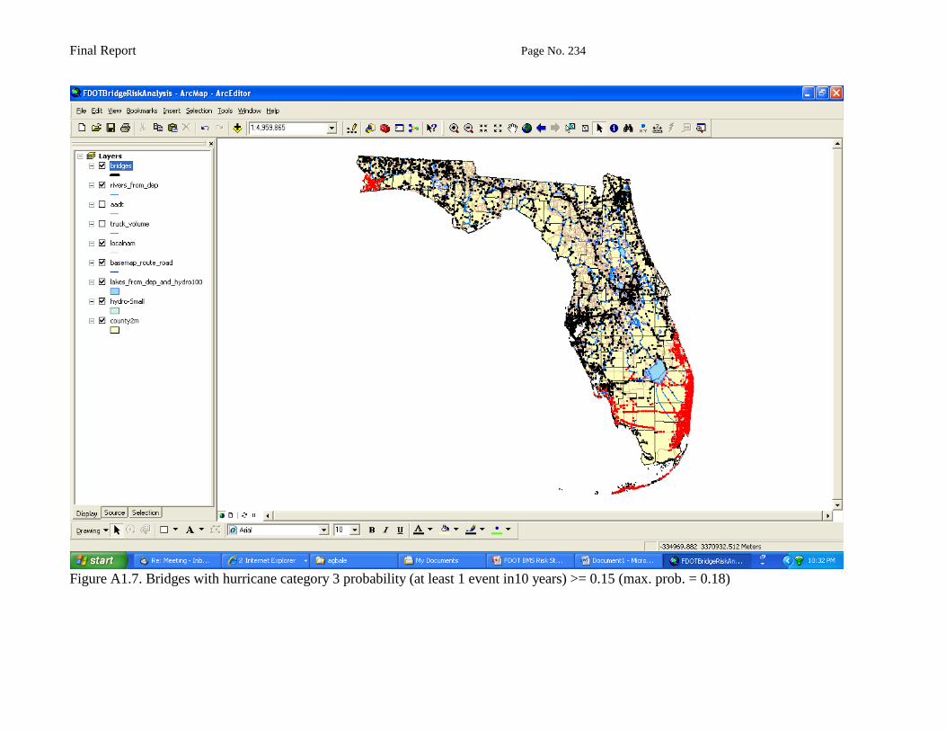
Final Report Page No. 234
Figure A1.7. Bridges with hurricane category 3 probability (at least 1 event in10 years) >= 0.15 (max. prob. = 0.18)

Final Report Page No. 235
Figure A1.8. Bridges damaged during hurricanes in Florida.

Final Report Page No. 236
Figure A1.9. Bridges damaged during hurricanes in Florida relative to category 3 probability (at least 1 event within 10 years) >= 9%.

Final Report Page No. 237
Appendix A2: Estimates of tornadoes ‘likelihood

Final Report Page No. 238
Figure A2.1. Bridges with tornado probability (1 year) >= 0.1 (max. prob. = 0.25)

Final Report Page No. 239
Figure A2.2. Bridges with tornado probability (at least 1 event in10 years) >= 0.25 (max. prob. = 0.95)

Final Report Page No. 240
Figure A2.3. Bridges with tornado probability (at least 1 event in10 years) >= 0.5 (max. prob. = 0.95)

Final Report Page No. 241
Table A2.1. County-based likelihood (annual rates) of tornado events in Florida (14-yr. data)
Count Annual rates Counts Annual rates Count Annual rates Counts Annual rates Counts Annual rates Counts Annual rates
Alachua 20 0.333 13 0.217 8 0.133 0 0.000 0 0.000 8 0.133
Baker 8 0.133 1 0.017 2 0.033 0 0.000 0 0.000 2 0.033
Bay 27 0.450 27 0.450 12 0.200 1 0.017 0 0.000 13 0.217
Bradford 7 0.117 8 0.133 1 0.017 0 0.000 0 0.000 1 0.017
Brevard 57 0.950 37 0.617 15 0.250 3 0.050 0 0.000 18 0.300
Broward 74 1.233 28 0.467 7 0.117 3 0.050 0 0.000 10 0.167
Calhoun 4 0.067 6 0.100 7 0.117 0 0.000 0 0.000 7 0.117
Charlotte 40 0.667 6 0.100 4 0.067 0 0.000 0 0.000 4 0.067
Citrus 33 0.550 11 0.183 2 0.033 1 0.017 0 0.000 3 0.050
Clay 6 0.100 10 0.167 6 0.100 0 0.000 0 0.000 6 0.100
Collier 41 0.683 12 0.200 3 0.050 0 0.000 0 0.000 3 0.050
Columbia 10 0.167 5 0.083 4 0.067 1 0.017 0 0.000 5 0.083
De Soto 25 0.417 5 0.083 3 0.050 0 0.000 0 0.000 3 0.050
Dixie 2 0.033 1 0.017 0 0.000 0 0.000 0 0.000 0 0.000
Duval 38 0.633 17 0.283 8 0.133 0 0.000 0 0.000 8 0.133
Escambia 47 0.783 27 0.450 9 0.150 3 0.050 0 0.000 12 0.200
Flagler 17 0.283 2 0.033 2 0.033 0 0.000 0 0.000 2 0.033
Franklin 20 0.333 13 0.217 4 0.067 0 0.000 0 0.000 4 0.067
Gadsden 5 0.083 13 0.217 10 0.167 0 0.000 0 0.000 10 0.167
Gilchrist 1 0.017 0 0.000 2 0.033 0 0.000 0 0.000 2 0.033
Glades 11 0.183 3 0.050 1 0.017 0 0.000 0 0.000 1 0.017
Gulf 19 0.317 5 0.083 3 0.050 0 0.000 0 0.000 3 0.050
Hamilton 4 0.067 2 0.033 2 0.033 0 0.000 0 0.000 2 0.033
Hardee 14 0.233 4 0.067 0 0.000 0 0.000 0 0.000 0 0.000
Hendry 13 0.217 8 0.133 3 0.050 0 0.000 0 0.000 3 0.050
Hernando 26 0.433 7 0.117 0 0.000 0 0.000 0 0.000 0 0.000
Highlands 24 0.400 13 0.217 3 0.050 0 0.000 0 0.000 3 0.050
Hillsborough 74 1.233 43 0.717 14 0.233 0 0.000 0 0.000 14 0.233
Holmes 7 0.117 5 0.083 3 0.050 0 0.000 0 0.000 3 0.050
Indian River 13 0.217 6 0.100 2 0.033 0 0.000 0 0.000 2 0.033
Jackson 13 0.217 16 0.267 5 0.083 0 0.000 0 0.000 5 0.083
Jefferson 7 0.117 5 0.083 0 0.000 0 0.000 0 0.000 0 0.000
Lafayette 4 0.067 3 0.050 2 0.033 1 0.017 0 0.000 3 0.050
Lake 22 0.367 19 0.317 7 0.117 3 0.050 0 0.000 10 0.167
Lee 74 1.233 21 0.350 11 0.183 0 0.000 0 0.000 11 0.183
Leon 13 0.217 3 0.050 5 0.083 0 0.000 0 0.000 5 0.083
Levy 13 0.217 7 0.117 2 0.033 0 0.000 0 0.000 2 0.033
Liberty 4 0.067 5 0.083 0 0.000 0 0.000 0 0.000 0 0.000
Madison 6 0.100 8 0.133 2 0.033 1 0.017 0 0.000 3 0.050
Manatee 54 0.900 16 0.267 6 0.100 1 0.017 0 0.000 7 0.117
Marion 23 0.383 22 0.367 9 0.150 1 0.017 0 0.000 10 0.167
Martin 19 0.317 4 0.067 3 0.050 1 0.017 0 0.000 4 0.067
Miami Dade 101 1.683 24 0.400 6 0.100 1 0.017 0 0.000 7 0.117
Monroe 41 0.683 15 0.250 6 0.100 0 0.000 0 0.000 6 0.100
Nassau 21 0.350 5 0.083 0 0.000 0 0.000 0 0.000 0 0.000
Okaloosa 57 0.950 19 0.317 14 0.233 1 0.017 0 0.000 15 0.250
Okeechobee 12 0.200 4 0.067 3 0.050 0 0.000 0 0.000 3 0.050
Orange 26 0.433 19 0.317 9 0.150 3 0.050 0 0.000 12 0.200
Osceola 16 0.267 12 0.200 3 0.050 1 0.017 1 0.017 5 0.083
Palm Beach 105 1.750 37 0.617 9 0.150 1 0.017 0 0.000 10 0.167
Pasco 56 0.933 19 0.317 6 0.100 0 0.000 0 0.000 6 0.100
Pinellas 71 1.183 32 0.533 12 0.200 2 0.033 1 0.017 15 0.250
Polk 97 1.617 39 0.650 12 0.200 0 0.000 2 0.033 14 0.233
Putnam 33 0.550 8 0.133 3 0.050 0 0.000 0 0.000 3 0.050
Santa Rosa 38 0.633 19 0.317 5 0.083 1 0.017 0 0.000 6 0.100
Sarasota 42 0.700 23 0.383 8 0.133 1 0.017 0 0.000 9 0.150
Seminole 12 0.200 9 0.150 5 0.083 1 0.017 0 0.000 6 0.100
St. Johns 38 0.633 5 0.083 5 0.083 2 0.033 0 0.000 7 0.117
St. Lucie 24 0.400 7 0.117 2 0.033 2 0.033 0 0.000 4 0.067
Sumter 8 0.133 1 0.017 3 0.050 1 0.017 0 0.000 4 0.067
Suwannee 20 0.333 14 0.233 6 0.100 0 0.000 0 0.000 6 0.100
Taylor 5 0.083 5 0.083 4 0.067 0 0.000 0 0.000 4 0.067
Union 3 0.050 3 0.050 0 0.000 0 0.000 0 0.000 0 0.000
Volusia 59 0.983 21 0.350 12 0.200 4 0.067 0 0.000 16 0.267
Wakulla 8 0.133 6 0.100 1 0.017 0 0.000 0 0.000 1 0.017
Walton 25 0.417 14 0.233 4 0.067 1 0.017 0 0.000 5 0.083
Washington 8 0.133 14 0.233 1 0.017 0 0.000 0 0.000 1 0.017
Totals 1865 841 331 42 4 377
County
F3 Tornado F4 Tornado F2 or Greater F0 Tornado F1 Tornado F2 Tornado

Final Report Page No. 242
Table A2.2. County-based likelihood (probability) of tornado events in Florida (14-yr. data)
F0 F1 F2 F3 F4 >= F2 F0 F1 F2 F3 F4 >= F2
Alachua 0.283 0.195 0.125 0.000 0.000 0.125 0.964 0.885 0.736 0.000 0.000 0.736
Baker 0.125 0.017 0.033 0.000 0.000 0.033 0.736 0.154 0.283 0.000 0.000 0.283
Bay 0.362 0.362 0.181 0.017 0.000 0.195 0.989 0.989 0.865 0.154 0.000 0.885
Bradford 0.110 0.125 0.017 0.000 0.000 0.017 0.689 0.736 0.154 0.000 0.000 0.154
Brevard 0.613 0.460 0.221 0.049 0.000 0.259 1.000 0.998 0.918 0.393 0.000 0.950
Broward 0.709 0.373 0.110 0.049 0.000 0.154 1.000 0.991 0.689 0.393 0.000 0.811
Calhoun 0.064 0.095 0.110 0.000 0.000 0.110 0.487 0.632 0.689 0.000 0.000 0.689
Charlotte 0.487 0.095 0.064 0.000 0.000 0.064 0.999 0.632 0.487 0.000 0.000 0.487
Citrus 0.423 0.168 0.033 0.017 0.000 0.049 0.996 0.840 0.283 0.154 0.000 0.393
Clay 0.095 0.154 0.095 0.000 0.000 0.095 0.632 0.811 0.632 0.000 0.000 0.632
Collier 0.495 0.181 0.049 0.000 0.000 0.049 0.999 0.865 0.393 0.000 0.000 0.393
Columbia 0.154 0.080 0.064 0.017 0.000 0.080 0.811 0.565 0.487 0.154 0.000 0.565
De Soto 0.341 0.080 0.049 0.000 0.000 0.049 0.984 0.565 0.393 0.000 0.000 0.393
Dixie 0.033 0.017 0.000 0.000 0.000 0.000 0.283 0.154 0.000 0.000 0.000 0.000
Duval 0.469 0.247 0.125 0.000 0.000 0.125 0.998 0.941 0.736 0.000 0.000 0.736
Escambia 0.543 0.362 0.139 0.049 0.000 0.181 1.000 0.989 0.777 0.393 0.000 0.865
Flagler 0.247 0.033 0.033 0.000 0.000 0.033 0.941 0.283 0.283 0.000 0.000 0.283
Franklin 0.283 0.195 0.064 0.000 0.000 0.064 0.964 0.885 0.487 0.000 0.000 0.487
Gadsden 0.080 0.195 0.154 0.000 0.000 0.154 0.565 0.885 0.811 0.000 0.000 0.811
Gilchrist 0.017 0.000 0.033 0.000 0.000 0.033 0.154 0.000 0.283 0.000 0.000 0.283
Glades 0.168 0.049 0.017 0.000 0.000 0.017 0.840 0.393 0.154 0.000 0.000 0.154
Gulf 0.271 0.080 0.049 0.000 0.000 0.049 0.958 0.565 0.393 0.000 0.000 0.393
Hamilton 0.064 0.033 0.033 0.000 0.000 0.033 0.487 0.283 0.283 0.000 0.000 0.283
Hardee 0.208 0.064 0.000 0.000 0.000 0.000 0.903 0.487 0.000 0.000 0.000 0.000
Hendry 0.195 0.125 0.049 0.000 0.000 0.049 0.885 0.736 0.393 0.000 0.000 0.393
Hernando 0.352 0.110 0.000 0.000 0.000 0.000 0.987 0.689 0.000 0.000 0.000 0.000
Highlands 0.330 0.195 0.049 0.000 0.000 0.049 0.982 0.885 0.393 0.000 0.000 0.393
Hillsborough 0.709 0.512 0.208 0.000 0.000 0.208 1.000 0.999 0.903 0.000 0.000 0.903
Holmes 0.110 0.080 0.049 0.000 0.000 0.049 0.689 0.565 0.393 0.000 0.000 0.393
Indian River 0.195 0.095 0.033 0.000 0.000 0.033 0.885 0.632 0.283 0.000 0.000 0.283
Jackson 0.195 0.234 0.080 0.000 0.000 0.080 0.885 0.931 0.565 0.000 0.000 0.565
Jefferson 0.110 0.080 0.000 0.000 0.000 0.000 0.689 0.565 0.000 0.000 0.000 0.000
Lafayette 0.064 0.049 0.033 0.017 0.000 0.049 0.487 0.393 0.283 0.154 0.000 0.393
Lake 0.307 0.271 0.110 0.049 0.000 0.154 0.974 0.958 0.689 0.393 0.000 0.811
Lee 0.709 0.295 0.168 0.000 0.000 0.168 1.000 0.970 0.840 0.000 0.000 0.840
Leon 0.195 0.049 0.080 0.000 0.000 0.080 0.885 0.393 0.565 0.000 0.000 0.565
Levy 0.195 0.110 0.033 0.000 0.000 0.033 0.885 0.689 0.283 0.000 0.000 0.283
Liberty 0.064 0.080 0.000 0.000 0.000 0.000 0.487 0.565 0.000 0.000 0.000 0.000
Madison 0.095 0.125 0.033 0.017 0.000 0.049 0.632 0.736 0.283 0.154 0.000 0.393
Manatee 0.593 0.234 0.095 0.017 0.000 0.110 1.000 0.931 0.632 0.154 0.000 0.689
Marion 0.318 0.307 0.139 0.017 0.000 0.154 0.978 0.974 0.777 0.154 0.000 0.811
Martin 0.271 0.064 0.049 0.017 0.000 0.064 0.958 0.487 0.393 0.154 0.000 0.487
Miami Dade 0.814 0.330 0.095 0.017 0.000 0.110 1.000 0.982 0.632 0.154 0.000 0.689
Monroe 0.495 0.221 0.095 0.000 0.000 0.095 0.999 0.918 0.632 0.000 0.000 0.632
Nassau 0.295 0.080 0.000 0.000 0.000 0.000 0.970 0.565 0.000 0.000 0.000 0.000
Okaloosa 0.613 0.271 0.208 0.017 0.000 0.221 1.000 0.958 0.903 0.154 0.000 0.918
Okeechobee 0.181 0.064 0.049 0.000 0.000 0.049 0.865 0.487 0.393 0.000 0.000 0.393
Orange 0.352 0.271 0.139 0.049 0.000 0.181 0.987 0.958 0.777 0.393 0.000 0.865
Osceola 0.234 0.181 0.049 0.017 0.017 0.080 0.931 0.865 0.393 0.154 0.154 0.565
Palm Beach 0.826 0.460 0.139 0.017 0.000 0.154 1.000 0.998 0.777 0.154 0.000 0.811
Pasco 0.607 0.271 0.095 0.000 0.000 0.095 1.000 0.958 0.632 0.000 0.000 0.632
Pinellas 0.694 0.413 0.181 0.033 0.017 0.221 1.000 0.995 0.865 0.283 0.154 0.918
Polk 0.801 0.478 0.181 0.000 0.033 0.208 1.000 0.998 0.865 0.000 0.283 0.903
Putnam 0.423 0.125 0.049 0.000 0.000 0.049 0.996 0.736 0.393 0.000 0.000 0.393
Santa Rosa 0.469 0.271 0.080 0.017 0.000 0.095 0.998 0.958 0.565 0.154 0.000 0.632
Sarasota 0.503 0.318 0.125 0.017 0.000 0.139 0.999 0.978 0.736 0.154 0.000 0.777
Seminole 0.181 0.139 0.080 0.017 0.000 0.095 0.865 0.777 0.565 0.154 0.000 0.632
St. Johns 0.469 0.080 0.080 0.033 0.000 0.110 0.998 0.565 0.565 0.283 0.000 0.689
St. Lucie 0.330 0.110 0.033 0.033 0.000 0.064 0.982 0.689 0.283 0.283 0.000 0.487
Sumter 0.125 0.017 0.049 0.017 0.000 0.064 0.736 0.154 0.393 0.154 0.000 0.487
Suwannee 0.283 0.208 0.095 0.000 0.000 0.095 0.964 0.903 0.632 0.000 0.000 0.632
Taylor 0.080 0.080 0.064 0.000 0.000 0.064 0.565 0.565 0.487 0.000 0.000 0.487
Union 0.049 0.049 0.000 0.000 0.000 0.000 0.393 0.393 0.000 0.000 0.000 0.000
Volusia 0.626 0.295 0.181 0.064 0.000 0.234 1.000 0.970 0.865 0.487 0.000 0.931
Wakulla 0.125 0.095 0.017 0.000 0.000 0.017 0.736 0.632 0.154 0.000 0.000 0.154
Walton 0.341 0.208 0.064 0.017 0.000 0.080 0.984 0.903 0.487 0.154 0.000 0.565
Washington 0.125 0.208 0.017 0.000 0.000 0.017 0.736 0.903 0.154 0.000 0.000 0.154
Probability of occurrence within 10 yearsProbability of occurrence within 1 year
County

Final Report Page No. 243
Appendix A3: Estimates of wildfires’ likelihood

Final Report Page No. 244
Figure A3.1. Bridges with wildfire probability (1 year) >= 0.5 (max. prob. = 0.99)

Final Report Page No. 245
Figure A3.2. Bridges with wildfire probability (at least 1 event in10 years) >= 0.75 (max. prob. = 0.99)

Final Report Page No. 246
Table A3.1. County-based likelihood of wildfire events in Florida (60-yr. data)
County Counts Annual rates
Probability of
occurrence within
1 year
Probability of
occurrence within
10 years
Alachua 14 1.000 0.632 1.000
Baker 7 0.500 0.393 0.993
Bay 8 0.571 0.435 0.997
Bradford 2 0.143 0.133 0.760
Brevard 2 0.143 0.133 0.760
Broward 9 0.643 0.474 0.998
Calhoun 1 0.071 0.069 0.510
Charlotte 5 0.357 0.300 0.972
Citrus 2 0.143 0.133 0.760
Clay 4 0.286 0.249 0.943
Collier 13 0.929 0.605 1.000
Columbia 8 0.571 0.435 0.997
De Soto 1 0.071 0.069 0.510
Dixie 1 0.071 0.069 0.510
Duval 4 0.286 0.249 0.943
Escambia 1 0.071 0.069 0.510
Flagler 8 0.571 0.435 0.997
Franklin 3 0.214 0.193 0.883
Gadsden 0 0.000 0.000 0.000
Gilchrist 3 0.214 0.193 0.883
Glades 7 0.500 0.393 0.993
Gulf 5 0.357 0.300 0.972
Hamilton 3 0.214 0.193 0.883
Hardee 0 0.000 0.000 0.000
Hendry 7 0.500 0.393 0.993
Hernando 1 0.071 0.069 0.510
Highlands 1 0.071 0.069 0.510
Hillsborough 3 0.214 0.193 0.883
Holmes 0 0.000 0.000 0.000
Indian River 0 0.000 0.000 0.000
Jackson 0 0.000 0.000 0.000
Jefferson 0 0.000 0.000 0.000
Lafayette 5 0.357 0.300 0.972
Lake 0 0.000 0.000 0.000
Lee 12 0.857 0.576 1.000
Leon 0 0.000 0.000 0.000
Levy 0 0.000 0.000 0.000
Liberty 6 0.429 0.349 0.986
Madison 1 0.071 0.069 0.510
Manatee 1 0.071 0.069 0.510
Marion 20 1.429 0.760 1.000
Martin 0 0.000 0.000 0.000
Miami Dade 15 1.071 0.657 1.000
Monroe 1 0.071 0.069 0.510
Nassau 11 0.786 0.544 1.000
Okaloosa 0 0.000 0.000 0.000
Okeechobee 0 0.000 0.000 0.000
Orange 0 0.000 0.000 0.000
Osceola 0 0.000 0.000 0.000
Palm Beach 8 0.571 0.435 0.997
Pasco 0 0.000 0.000 0.000
Pinellas 1 0.071 0.069 0.510
Polk 11 0.786 0.544 1.000
Putnam 19 1.357 0.743 1.000
Santa Rosa 0 0.000 0.000 0.000
Sarasota 6 0.429 0.349 0.986
Seminole 1 0.071 0.069 0.510
St. Johns 4 0.286 0.249 0.943
St. Lucie 1 0.071 0.069 0.510
Sumter 0 0.000 0.000 0.000
Suwannee 1 0.071 0.069 0.510
Taylor 3 0.214 0.193 0.883
Union 3 0.214 0.193 0.883
Volusia 1 0.071 0.069 0.510
Wakulla 5 0.357 0.300 0.972
Walton 2 0.143 0.133 0.760
Washington 0 0.000 0.000 0.000
Totals 261

Final Report Page No. 247
Appendix A4: Estimates of floods’ likelihood

Final Report Page No. 248
Figure A4.1. Bridges with flooding probability (1 year) = 0.01 (high risk)

Final Report Page No. 249
Figure A4.2. Bridges with flooding probability (1 year) = 0.002 (moderate risk)

Final Report Page No. 250
Appendix A5: Consequences of hazards

Final Report Page No. 251
Table A5.1. Summary of structures replaced or posted due to hazards (“Central Office” Bridges)
No.Structure
IDHazard Type Hazard Description/Consequences
Year
Built
Final
Inspection
Date
1 530006 Flood Scour concerns. Bridge replaced. 1972 8/8/2005
2 530019 Flood Scour concerns. Bridge replaced. 1972 4/19/2006
3 574073 Flood Extreme flood damage. Bridge deck and superstructure not pile-
supported.Bridge closed.
1984 2/9/2010
4 590022 Flood Flood: Closure of the bridge is recommended during near
overtopping events, or if any additional scour occurs or evidence
of settlement is found. Bridge replaced.
1956 2/2/2010
5 710058 Flood Scour concerns. Bridge replaced. 1986 11/19/2008
6 710059 Flood Scour concerns. Bridge replaced. 1986 11/19/2008
7 720062 Flood Scour concerns. Roadway overtopping. 1949 6/4/2009
8 039002 Hurricane Hurricane damage and bad general condition: bridge closed and
replaced.
1969 11/3/2005
9 489549 Hurricane Hurricane-related deficiencies. 7/13/2005
10 589503 Hurricane Hurricane-related deficiencies. 7/12/2005
11 48S544 Hurricane Hurricane-related deficiencies. 7/13/2005
12 79S019 Hurricane Frances Hurricane Frances damage. Removed. 9/8/2004
13 79S054 Hurricane Frances Hurricane Frances damage. Removed. 9/8/2004
14 94S602 Hurricane Frances Hurricane Frances damage. Removed. 9/16/2004
15
480213 Hurricane Ivan*
Hurricane Ivan caused severe damage to the eastbound I-10
bridge. Damage to deck, superstructure and substructure. Both
parallel bridges replaced. 1968 9/16/2004#
16
480214 Hurricane Ivan*
Hurricane Ivan caused severe damage to the eastbound I-10
bridge. Damage to deck, superstructure and substructure. Both
parallel bridges replaced. 1968 9/16/2004#
17 75S532 Hurricane Jeanne Hurricane Jeanne damage. Total loss. 2001 9/29/2004
18 704049 Hurricane Wilma Hurricane Wilma: Boat impact and pile/cap damages. Bridge
Posted.
1949 3/25/2010
19 12S205 Hurricane Wilma Hurricane Wilma damage. Sign replaced. 1996 9/9/2006
20 86S027 Hurricane Wilma Hurricane Wilma damage. Sign replaced. 1995 9/13/2005
21 86S042 Hurricane Wilma Hurricane Wilma damage. Removed. 1987 8/26/2005
22 86S060 Hurricane Wilma Hurricane Wilma damage. Removed. 1993 8/26/2005
23 86S468 Hurricane Wilma Hurricane Wilma damage. Removed. 7/13/2005
24 86S469 Hurricane Wilma Hurricane Wilma damage. Removed. 7/13/2005
25 86S719 Hurricane Wilma Hurricane Wilma damage. Sign replaced. 12/9/2005
26 93S210 Hurricane Wilma Hurricane Wilma damage. Sign replaced. 11/9/2005
27 93S472 Hurricane Wilma Hurricane Wilma damage. Sign replaced. 10/31/2007
28 720166 Vehicular Impact Vehicle accident impact on bridge. Damaged girders and other
non-impact related deficiencies. Bridge replaced.
1957 3/26/2009
29 72S081 Vehicular Impact Vehicle accident impact damage. Removed. 2/25/2004
30 72S126 Vehicular Impact Vehicle accident impact damage. Removed. 7/14/2004
31 72S391 Vehicular Impact Vehicle accident impact damage. Removed. 4/22/2004
# Date of Hurricane; inspection date not available.
* Not shown in the Central Office Bridge list; Cost to replace the two parallel bridges (480213 and 480214) was l isted as
$243 mill ion (http://www.roadtraffic-technology.com/projects/i-10/).

Final Report Page No. 252
Figure A5.1. Sample completed survey questionnaire for bridge damage

Final Report Page No. 253
Table A5.2. Summary of hazard impacts (with costs or road closure) on bridges in Florida
District
Hazard Event
Type
Hazard Date
(or Inspection
date) Bridge ID Description of the Hazard Bridge Elements Damaged Described Costs of Repair Costs of Repair
No. of
Lanes
Closed
Duration
of Closure
(Hours) Other Comments
Turnpike Fire 12/14/2009 110070
Vehicle fire occurring underneath Turnpike
Bridge Structure 110070 resulting in
structural damage and subsequent repairs.
reinf. conc. deck, prestr.
conc. Beams, reinf. conc.
Substructure
Structural Repair Cost: $981.0 K
Traffic Diversion Cost: $825.5 K
Hazardous Waste Mitigation
Cost: $28.5 K
Misc. Support Services: $82.1 K
$1,917,100 2 244
Detour and roadway diversion
established to accommodate repair
work.
1&7 Fire 6/4/2008 130103This bridge was damaged due to fire form a
tanker truck accident on 06/04/08.12, 109, 205, 234 Repair cost was about $4.5M. $4,500,000 3 384
Southbound traffic on I-75 was directed
to Northbound bridge during the repair.
1&7 Fire 3/28/2007 150124A tanker truck crashed on the ramp and
caught on fire.
12, 109, 205, 234, 301, 302,
303, 310, 331, 398$2,300,000 2 576
The ramp was closed during the
reconstruction. The cost show does not
include DOT costs or by other parties.
Minor superstructure damage occurred
to Bridge 150158 for Pontis elements 12,
301, 331, 398, 310, 205, and 234. The
cost shown above includes the repairs to
that bridge as well.
6 Fire 10/3/2002 870363Fuel tanker truck lost control while exiting
I-95 to SR-836 in Miami.
underdeck, expansion
joints , drainage gutters,
girders, bearings, columns,
caps, substructure
Two bridges cost $955,588 $477,794 3 14
6 Fire 10/3/2002 870364Fuel tanker truck lost control while exiting
I-95 to SR-836 in Miami.
underdeck, expansion
joints , drainage gutters,
girders, bearings, columns,
caps, substructure
Two bridges cost $955,588 $477,794 3 14
6 Fire 11/6/2006 870439
Fuel tanker truck lost control while driving
on I-95 South Bound over NW 132 Street in
Miami-Dade County .
underdeck, girders,
columns, caps, bearings,
expansion joints, drainage
gutters
$375,000 N/A N/A
6 Fire 10/2/2005 900101 Fuel Tanker Truck Accident on the Seven
Mile Bridge.12, 331 $89,852 2 15
4 Fire 940133 smoke and fire damage to bridge deck, beams $410,000
6 Hurricane Dennis 7/10/2005 900091 Hurricane Dennis 321, 396 $33,000 N/A N/A
6 Hurricane Dennis 7/10/2005 900098 Hurricane Dennis. 396 $57,750 N/A N/A
6 Hurricane Dennis 7/10/2005 900108 Hurricane Dennis. 396 $66,000 N/A N/A
6 Hurricane Dennis 7/10/2005 900115 Hurricane Dennis 321, 396 $35,200 N/A N/A
1&7Hurricane
Frances9/5/2004 150138
Fender and Fender Lighting Damage from
Hurricane Frances390, 580 $11,212 0 0
The total shown includes the cost
submitted by the asset maintenance
contractor for repair of fender.
4Hurricane
Frances9/8/2004 940005
failed north approach roadway; washed
out area; wingwall undermining. Scour and
damage to approach slab and bulkhead
321, 393, scour $800,000

Final Report Page No. 254
Table A5.2. Summary of hazard impacts (with costs or road closure) on bridges in Florida (Cont‟d)
District
Hazard Event
Type
Hazard Date
(or Inspection
date) Bridge ID Description of the Hazard Bridge Elements Damaged Described Costs of Repair Costs of Repair
No. of
Lanes
Closed
Duration
of Closure
(Hours) Other Comments
2Hurricane
Jeanne/Flood9/28/2004 780056
Extremely high water led to over-topping of
the South bulkhead and subsequent
washout.
321, 396 $26,070 1 16 Two-way, two lane traffic.
6 Hurricane Rita 9/20/2005 900078 Hurricane Rita 290, 396 $11,000 N/A N/A
6 Hurricane Rita 9/20/2005 900089 Hurricane Rita. 290, 396 $85,140 N/A N/A
6 Hurricane Rita 9/20/2005 900094 Hurricane Rita. 396 $57,400 N/A N/A
6 Hurricane Rita 9/20/2005 900095 Hurricane Rita. 321, 396 $187,440 N/A N/A
6 Hurricane Rita 9/20/2005 900096 Hurricane Rita. 396 $440,000 N/A N/A
6 Hurricane Rita 9/20/2005 900126 Hurricane Rita 396 $455,070 N/A N/A
4 Hurricane Wilma 12/14/2005 860008 small sign $1,000
4 Hurricane Wilma 12/14/2005 860011 580, 591, 592 $15,000
4 Hurricane Wilma 12/14/2005 860018 581, street l ight $77,300
4 Hurricane Wilma 12/14/2005 860038 581, 591, street l ight $9,000
4 Hurricane Wilma 12/14/2005 860043 581, 591, 592 $15,000
4 Hurricane Wilma 12/14/2005 860060386, 580, 591, 592, street
l ight$15,000
4 Hurricane Wilma 12/14/2005 860061 386 $60,000
4 Hurricane Wilma 12/14/2005 860144386, 580, 581, 592, street
l ight$10,000
4 Hurricane Wilma 12/14/2005 860146 581, 592 $20,000
4 Hurricane Wilma 12/14/2005 860157 581, 592, street l ight $13,000
4 Hurricane Wilma 12/14/2005 860230 small sign, 580, 581 $7,000
4 Hurricane Wilma 12/14/2005 860466 581, 591, 592 $13,000
4 Hurricane Wilma 12/14/2005 860618 581, 591 $19,500
4 Hurricane Wilma 12/14/2005 860622 386, 581, 591, 592 $66,000
4 Hurricane Wilma 12/14/2005 860623 581 $28,000
4 Hurricane Wilma 12/14/2005 860920 581, 592 $6,000
4 Hurricane Wilma 12/14/2005 860941 592 $2,000
4 Hurricane Wilma 12/14/2005 890003581, 592, small sign, street
l ight$15,000
4 Hurricane Wilma 12/14/2005 890150 386, 580 $35,000
4 Hurricane Wilma 12/14/2005 890151 580 $2,000
4 Hurricane Wilma 12/14/2005 890158 386, 580 $21,500
6 Hurricane Wilma 10/24/2005 900107 Hurricane Wilma scour/piles $16,500 N/A N/A
4 Hurricane Wilma 12/15/2005 930004 street l ight, 591, 592 $6,000
4 Hurricane Wilma 12/15/2005 930060 386, 591, street l ight $42,000
4 Hurricane Wilma 12/15/2005 930064 581, 591 $17,000
4 Hurricane Wilma 12/15/2005 930097 386, 581, 591, street l ight $19,500
4 Hurricane Wilma 12/15/2005 930104 small sign, 581, 591, 592 $15,000
4 Hurricane Wilma 12/15/2005 930154small sign, 581, 591, street
l ight$20,000
4 Hurricane Wilma 12/15/2005 930157386, 580, 581, 591, street
l ight$24,800
4 Hurricane Wilma 12/15/2005 930370 581, 591, street l ight $28,500
4 Hurricane Wilma 12/15/2005 930453 581, 591, street l ight $25,200
4 Hurricane Wilma 12/15/2005 930454 591, 592, street l ight $7,000
4 Hurricane Wilma 12/15/2005 930506 small sign, 581, 591, 592 $24,000
1&7Hurricane/Tropic
al Storm Fay 10/20/2008 910003
This bridge was damaged due to tropical
storm Fay which affected the area with
heavy rains.
241
Repair construction cost was
$276,990. Miscellaneous cost
such as design and
construction engineering
inspection cost was $26,250.
$303,240

Final Report Page No. 255
Table A5.2. Summary of hazard impacts (with costs or road closure) on bridges in Florida (Cont‟d)
District
Hazard Event
Type
Hazard Date
(or Inspection
date) Bridge ID Description of the Hazard Bridge Elements Damaged Described Costs of Repair Costs of Repair
No. of
Lanes
Closed
Duration
of Closure
(Hours) Other Comments
1&7Hurricane/Tropic
al Storm Fay 10/20/2008 910006
This bridge was damaged due to tropical
storm Fay which affected the area with
heavy rains.
396
Repair construction cost was
$117,160. Miscellaneous cost
such as design and
construction engineering
inspection cost was $22,715.
$139,875There is no closure information at this
time.
1&7Hurricane/Tropic
al Storm Fay 10/20/2008 910065
This bridge was damaged due to tropical
storm Fay which affected the area with
heavy rains.
396
Repair construction cost was
$125,482. Miscellaneous cost
such as design and
construction engineering
inspection cost was $21,482.
$146,964There is no closure information at this
time.
1&7Hurricane/Tropic
al Storm Fay 10/20/2008 910066
This bridge was damaged due to tropical
storm Fay which affected the area with
heavy rains.
396
Repair construction cost was
$26,483. Miscellaneous cost
such as design and
construction engineering
inspection cost was $14,519.
$41,002
1&7Hurricane/Tropic
al Storm Fay 10/20/2008 910081
This bridge was damaged due to tropical
storm Fay which affected the area with
heavy rains.
396
Repair construction cost was
$16,007. Miscellaneous cost
such as design and
construction engineering
inspection cost was $10,410.
$26,417There is no closure information at this
time.
1&7Tropical Storm
Fay (Flood)10/20/2008 054003
This bridge was damaged due to tropical
storm Fay which affected the area with
heavy rains.
290
Repair construction cost was
$391,295. Misc. cost (design
and construction engineering
inspection) was $60,616.
$451,911 2 24
This road was periodically closed from
9/11/08 through 10/07/08 for few hours
at a time to accommodate repair
construction. The 24 hours lane closure
noted above is an estimate of the total
closure.
1&7Tropical Storm
Fay (Flood)10/20/2008 914001
This bridge was damaged due to tropical
storm Fay which affected the area with
heavy rains.
290, 321
Repair construction cost was
$62,839. Miscellaneous cost
such as design and
construction engineering
inspection cost was $18,275.
$81,114 0 0
1&7Tropical Storm
Fay (Flood)10/20/2008 914002
This bridge was damaged due to tropical
storm Fay which affected the area with
heavy rains.
290
Repair construction cost was
$462,825. Miscellaneous cost
such as design and
construction engineering
inspection cost was $61,851.
$524,676 2 960
The exact closure time is undeterminable
at this time. This road was closed for at
least 40 days.
1&7Tropical Storm
Fay (Flood)10/20/2008 914007
This bridge was damaged due to tropical
storm Fay which affected the area with
heavy rains.
290
Repair construction cost was
$306,503. Miscellaneous cost
such as design and
construction engineering
inspection cost was $43,860.
$350,363 2 792
This road was closed for at least 33
days. The exact closure time is not
available at his time.
**Note: There are more records but shown here are the ones with costs or durations of closure.

Final Report Page No. 256
Table A5.3. Summary of damage to Florida bridges and repair costs during Hurricane Wilma
District
Hazard Date
(or Inspection Bridge ID Description of Damage or Repair Needs
Level of
Damage
Costs of
Repair
4 12/14/2005 860008 Repair signs Slight $1,000
4 12/14/2005 860623 Repair lights. Slight $28,000
4 12/14/2005 860941 Repair traffic signal. Slight $2,000
4 12/14/2005 860011 Repair traffic signals, barrier gate, navigation lights, and traffic gate. Moderate $15,000
4 12/14/2005 860018Repair/replace street light poles, repair street light, roof, speaker in tenderhouse
and A/C.Moderate $77,300
4 12/14/2005 860038Replace bridgehouse mirros, repair street light, tenderhouse roof, traffic gate, and
repair/replace street light feed.Moderate $9,000
4 12/14/2005 860043Repair computer, signs, traffic light, gate, PA amps/horns, fender gauge light,
emergency light in tenderhouse.Moderate $15,000
4 12/14/2005 860060Repair traffic signals, gate, handrail and sidewalk (boat impact), fender gauge light,
street light, navigation light, signs and fender handrail (boat impact)Moderate $15,000
4 12/14/2005 860061 Repair fender. Moderate $60,000
4 12/14/2005 860144Repair traffic signal, street lights, pedestrian signs, navigation lights, A/C
compressor, and repalce fender guage light.Moderate $10,000
4 12/14/2005 860146 Repair traffic signals and twisted light poles of the tenderhouse. Moderate $20,000
4 12/14/2005 860157Repair traffic signal, replace the following: (pedestrian) sign, broken fuel gauge,
tender house light, street light arm and head, and repair damaged A/C.Moderate $13,000
4 12/14/2005 860230Repair tenderhouse windows, emergency lights, marine roadio, memergency lights,
telephone, PA speaker, navigation lights, and "bridge ahead" sign.Moderate $7,000
4 12/14/2005 860466Repair traffic signals, replace gate and sidewalk, repair generator room door,
transformer, windows, fender handrials, and control power units.Moderate $13,000
4 12/14/2005 860618Repair gate, bridge house, electrical panel, PA bracket, sump pump and soffet
flashing.Moderate $19,500
4 12/14/2005 860622Repair tenderhouse, repalce marine radio antenna, repqair insulation, roof, display,
blinds, speaker, PA amps/horn, rpeiar light fxtures, navigation light, gates, traffic Moderate $66,000
4 12/14/2005 860920 Repair traffic signal, tenderhouse mirror, and diesel generator. Moderate $6,000
4 12/14/2005 890003Repair "Drawbridge Ahead" sign, traffic signlas, bridgehouse roof, window, and
street lights.Moderate $15,000
4 12/14/2005 890150Replace missing navigation lights, vertical clearance gauges, and fender system
(incl. conduit).Moderate $35,000
4 12/14/2005 890151 Replace span and fender navigation lights. Moderate $2,000
4 12/14/2005 890158 Repair vertical clearance gauge, repalce nagivation lights, and repair fender. Moderate $21,500
6 10/24/2005 900107 Scour holes around seven of the bridge piles. Holes approximately 5 ft x 5 ft x 4 ft. Moderate $16,500
4 12/15/2005 930004 Repair street light, traffic light, and traffic gates. Moderate $6,000
4 12/15/2005 930060
Repair traffic gate, barrier gate, street lights, fender (planks missing, gauge light
missing), CCTV system (camera missing), PA system horns/amp, waether station,
traffic lights, and "Bridge Ahead" sign.
Moderate $42,000
4 12/15/2005 930064Repair CCTV system on traffic pole, traffic gate, ATS Voltmeter, and water in fule fill
basin.Moderate $17,000
4 12/15/2005 930097Repair traffic gate (electrical damage), street light (pole), fender access ladder, fuel
tank platform, and marine radio antenna.Moderate $19,500
4 12/15/2005 930104
Repair "Bridge Ahead" sign, traffic signal, barrier gates, span swing light,
tenderhouse roof, trafic light, ceiling tiles (tenderhouse), marine radio antenna,
and fender (electrical conduit, planks, and clearance gauage).
Moderate $15,000
4 12/15/2005 930154Repair "Bridge Ahead" sign, bridgehouse window, ceiling fan, window blinds, traffic
gate, elcetrical service (feed) to street lights.Moderate $20,000
4 12/15/2005 930157Repair street light poles, traffic light, traffic gate, fender, bridgedhouse roof,
navigation light, and CCTV system.Moderate $24,800
4 12/15/2005 930370Repair traffic signals, street lights, traffic gates, traffic light, PLC, door (wind), A/C in
tenderhouse, radiator leaks, and bridgehouse street light.Moderate $28,500
4 12/15/2005 930453Repair/replace street light poles, repair traffic and barrier gates, traffic light sign,
gate, and roof.Moderate $25,200
4 12/15/2005 930454 Repair traffic signal light, traffic gate, and street light. Moderate $7,000
4 12/15/2005 930506Repair traffic gate, bridge house mirror, traffic signals, street lights, signs,
tenderhouse entry gate, and center median grating.Moderate $24,000

Final Report Page No. 257
Table A5.4. Summary of bridges (non-Florida) damaged during hurricane Katrina (Padgett et al., 2008) Bridge Name Roadway
Carried
Bridge
Type
Damage
State
Damage
Source
Cost Estimate Surge
Elevation
(m)
Comments
Alabama
BayouLaBatre Hwy 188 Fixed Moderate SC $10,000 —
Dauphin Island Parkway 193 Fixed Moderate I,SC $6,000,000 —
Cochrane Africatown USA US-90 Fixed Extensive I $1,000,000 — Cost reported as $1.7 million
in Hitchcock et al. (2008)
Mobile Delta Causeway I-10 Fixed Extensive D $1,140,000 —
Louisiana
Bayou DesAllemands LA-631 Movable Slight W $3,000 0.98
Bayou Dulac LA-57 Movable Slight W $1,000 1.16
Country Club LA-3127 Movable Slight W $1,000 0.91
Galliano LA-308 Movable Slight W $5,000 1.95
Golden Meadow LA-308 Movable Slight W $9,000 1.95
Harvey Canal LA-18 Movable Slight W $2,000 3.54
Houma Navigation Canal LA-661 Movable Slight W $1,000 0.91
Lockport Company Canal LA-1 Movable Slight W $2,000 0.91
PresqueIsle @Bayou Petite Caillou LA-24 Movable Slight W $1,000 —
Belle Chase LA-23 Movable Moderate W $200,000 4.08
Claiborne LA-39 Movable Moderate W $40,000 —
Intracoastal Waterway @Larose LA-1 Movable Moderate W $170,000 1.34
Perez LA-23 Movable Moderate W $200,000 —
Seabrook LocalRoad Movable Moderate W $25,000 3.11
St.Bernard Canal LA-46 Movable Moderate W $40,000 —
West Pearl River US-90 Movable Moderate EM,SC,W $350,000 4.6
Bayou Barataria LA-302 Movable Extensive EM $50,000 1.16
Bayou Lafourche @Leeville LA-1 Movable Extensive SC,W $1,600,000 2.13
Bayou Liberty LA-433 Movable Extensive EM,W $1,500,000 3.47
Bonfouca LA-433 Movable Extensive EM,W $200,000 3.57
Caminada Bay LA-1 Fixed Extensive D,SC $500,000 2.44
Chef Menteur US-90 Movable Extensive EM,SC $3,600,000 3.96
Doullut Canal LA-11 Movable Extensive EM,W $700,000 3.44
East Pearl River US-90 Movable Extensive EM,SC,W $400,000 4.6
Inner Harbor Navigation Canal Florida Ave. Movable Extensive EM,I,W $500,000 1.01
NorthDraw—LakePontchartrain US-11 Movable Extensive EM $50,000 4.02
Rigolets Pass US-90 Movable Extensive EM,SC,W $2,000,000 4.6
Rigolets Pass–Under Construction US-90 Movable Extensive I,W $1,700,000 4.6
Tchefuncte River Madisonville LA-22 Movable Extensive EM,SC,W $25,000 2.32
US11 @Lake Pontchartrain US-11 Movable Extensive EM,SC,W $6,000,000 4.02
Yscloskey LA-46 Movable Extensive EM,SC,W $900,000 5.12
Lake Pontchartrain I-10 Fixed Complete D,SC $30,000,000 4.02
Pontchartrain Causeway LA-Causeway Fixed Complete D,SC $1,500,000 2.77
Mississippi
David V.LaRosa W.WittmanRd. Fixed Moderate D $60,000 7.5
Biloxi Back Bay I-110 Movable Extensive I $2,500,000 6.22
I-10 Pascagoula River I-10 Fixed Extensive D,I $5,800,000 4.57
Popps Ferry PoppsFerryRd. Movable Extensive D,EM $7,700,000 5.82
Biloxi-Ocean Springs US-90 Movable Complete D,EM $275,000,000 6.58
US-90 Bay St.Louis US-90 Movable Complete D,EM $276,000,000 5.58
US-90 Henderson Point US-90 Fixed Complete D $1,900,000 7.01
Note: — indicates no available surge estimate. Damage key: D = Deck Movement, EM = Electrical Mechanical, I = Impact, SC = Scour, W = Wind.

Final Report Page No. 258
Table A5.5. Summary of fire hazard impacts on structures in Florida
District
Hazard Date
(or Inspection
date) Bridge ID Description of Damage or Repair Needs Level of Damage Costs of Repair
Turnpike 12/14/2009 110070
Excessive heat exposure to various structural components
of bridge including reinforced concrete substructure,
prestresssed concrete beams and reinforced concrete
bridge deck. Extensive $1,917,100
1&7 6/4/2008 130103
Element 109 - Prestressed concrete open girder, element
205 - reinforced concrete columns, element 234 -
reinforced concrete cap and element 12 - concrete deck
were damaged due to fire. Beams in spans 39 and 40 were
severely damaged with major section loss and some
complete strand loss. Spans 39 and 40 were severely
damaged by fire and experienced widespread shallow
spalling. Three columns in bent 40 had section loss and the
bent cap had major fire damage. Extensive $4,500,000
1&7 3/28/2007 150124
Damage included substructure damage, replacement of
one full span of the bridge and partial replacement of an
adjacent span. Span 9 was replaced. The Pontis elements
affected are: 12 - Bare Concrete Deck; 301 - Pourable Joint
Seal; 302 - Compression Joint Seal; 303 - Assembly Joint
Seal; 331 - Concrete Bridge Railing; 109 - Prestress
Concrete Girder; 398 - Drain System; 310 - Elastomeric
Bearing; 205 - Reinforced Concrete Column; and 234 -
Reinforced Concrete Cap. A sign attached to the right
barrier was impacted by the fire. Extensive $2,300,000
2 3/31/2009 260062
There is a 28 in. x 22 in. x 1/2 in. spall in the backwall of
Abutment 1, adjacent to Beam 1-1. This appears to be due
to a fire having been set on the cap and poses no problem
at this time. Slight
2 4/1/2002 280012
There is a spalled area, 22 in. diameter x 1 in. deep, on top
of the cap at Abutment 1, between Beams 1-3 and 1-4, due
to heat from a fire that was built on top of the cap. Poses
no problem at this time. Slight
2 10/18/2007 290076
CS 4 = There are areas of fire damage (charring) at the
beam ends at abutment 1 due to fires on the caps (Refer to
photo 7 on Addendum page A-6) Slight
2 12/3/2003 340042
There is a spalled area 22" diameter x 1" deep on top of
the cap at Abutment 1 between Beams 1-3 and 1-4 due to
heat from a fire that was built on top of the cap. Slight
2 11/24/2009 340042
There is a spalled area, 22 in. diameter x 1 in. deep, on top
of the cap at Abutment 1, between Beams 1-3 and 1-4, due
to heat from a fire that was built on top of the cap. Poses
no problem at this time. Slight
2 5/7/2008 340043
Stringer 4-5 has minor fire damage in an isolated area in
the top face at the near end. Also, there are deep splits in
the left and right faces. Slight
2 4/12/2011 370023
Previously Reported Deficiencies:
CS2: There is evidence of a past fire on the east side of the
structure. There is discoloration and corrosion on the
columns, diagonals, and base plates. (Refer to Photo 4).Slight
2 8/11/2005 380030
Six planks and 2m of top wale at the west fender, near the
center navigation light, are fire damaged. Slight

Final Report Page No. 259
Table A5.5. Summary of fire hazard impacts on structures in Florida (Cont‟d)
District
Hazard Date
(or Inspection
date) Bridge ID Description of Damage or Repair Needs Level of Damage Costs of Repair
5 1/21/2011 700017
On 01/21/2011, a traffic accident involving a gasoline
tanker truck occurred at the east approach of this structure
and twin structure, Bridge No. 700017.
Extreme heat and severe fire damage occurred to the
superstructure and substructure elements in Span 2, Span
3, at Pier 3 and Abutment 4. Refer to photos 1 through 3.
Immediate action is being taken to replace the damaged
superstructure and substructure components. The
structure is scheduled to be open to the traveling public in
approximately 35 days. Extensive
2 10/18/2010 720022
INCIDENTAL:
Two fires have taken place adjacent to the west face of the
crash wall at pier 2 between columns
1 and 2 & 3 and 4. The crash wall is spalled at each location
for an area of approximately
8'L x 6' H x 1"D. No exposed steel seen. The fire appears to
have been started with debris collected by vagrants. NEW.
See photo 7. Slight
2 6/12/2002 720053
There are three fender panels with slight fire damage
adjacent to Pier 9 (north fender panels 5, 6, & 8). See
accident report dated 6/3/91. Slight
2 10/29/2003 720055
Column 6-3 has a 26" x 22" x 1" spall on the west face next
to the groundline. This area is due to fire and poses no
problem. Column 7-3 and 7-4 has two minor incipient spall
on the bottom SE corner.Slight
2 3/17/2004 720076
Due to an electrical fire, the 3rd and 4th catwalk panels of
the west fender have been damaged. The 3rd panel has
fifteen 2 in. x 10 in. x 36 in. deckboards and two 10 in. x 3
1/2 in. x 12 ft. 6 in. deck stringers heavily damaged. The
4th panel has six deckboards and a 60 in. area of damaged
deck stringers. See Photos 1 and 2 attached for views.
Due to fire damage, temporary fender lights have been
installed on the west fender. The electrical conduit and
wiring has been destroyed by fire in a 17 ft. 6 in. area on
the northwest fender. Slight
2 2/19/2009 720076
Approximately a 10 ft. diameter area of the inside
Westbound travel lane, mid-span of Span 30, exhibits
charred areas and random shallow surface spalls due to a
vehicle fire. See Photo 1 attached for view. Poses no
problem at this time. The inside barrier was also charred
adjacent to this area. Slight
2 4/28/2011 720089
Due to vehicular impact, the right aluminum barrier rail in
Span 3 was damaged in an 18 ft. long area and the
roadway, approximately 40 ft. North of the North approach
slab, exhibits fire damage, due to vehicular fire. Slight
2 9/29/2003 720107
PREVIOUS CORRECTIVE ACTION:
The previously reported missing navigation light and fire-
damaged conduit on the north end of the Pier 2 fender
have been replaced and are currently in good condition.Slight
2 6/30/2005 720107
At Pile Clusters 2 and 3, the wales along the east face are
chard from past fire damage.
Slight

Final Report Page No. 260
Table A5.5. Summary of fire hazard impacts on structures in Florida (Cont‟d)
District
Hazard Date
(or Inspection
date) Bridge ID Description of Damage or Repair Needs Level of Damage Costs of Repair
2 5/11/2009 720137
The west face of Bent 2 cap has staining of black soot from
the vehicle fire under Span 1. The outside face of the left
and right barriers in Span 1 are covered with black soot
from the vehicle fire under Span 1. End Bent 1 cap is
covered with black soot from the vehicle fire under Span
1. The underside of all 11 slab units in Span 1 is covered
with black soot from the vehicle fire that took place under
Span 1. Refer to photo 2. The only slab units showing any
damage as a result of the fire are Slab Units 1-9, 1-10 and 1-
11. Slight
2 4/24/2008 720165
INCIDENTAL:
Two fires have taken place adjacent to the west face of the
crash wall at pier 2 between columns
1 and 2 & 3 and 4. The crash wall is spalled at each location
for an area of approximately
8'L x 6' H x 1"D. No exposed steel seen. The fire appears to
have been started with debris collected
by vagrants. NEW. See photo 7. Slight
2 6/11/2008 720170
Beam 1-7, East face and Beam 1-8 West face, smoke
stained due to fire at Abutment 1. Charred area
(apparently due to vehicular fire), right emergency lane,
Span 5 which has surface scaling and delamination in 10 ft.
diameter area.
Smoke stained (due to fire) between Beams 1-7 and 1-8
over Abutment 1, extending out to intermediate
diaphragm. Beam 1-7, East face and Beam 1-8 West face,
smoke stained due to fire at Abutment 1. Slight
2 6/9/2004 720172
The cap at Abutment 1 has minor fire damage between
Beams 1-3 and 1-4. Beam 1-3 over Abutment 1 has minor
spalling in the area of the diaphragm and poured beam
end due to fires set on top of the abutment cap. Span 2
has several beams which have been impacted by
overheight vehicles. The deck underside of Span 1
between Beams 1-3 and 1-4 is heavily sooted due to fires
being built on top of Abutment 1. Beam 1-3 over
Abutment 1 has minor spalling in the area of the
diaphragm and poured beam end due to fires set on top of
the abutment cap. Span 2 has several beams which have
been impacted by overheight vehicles. The cap at
Abutment 1 has minor pop-out spalls due to fire damage Slight

Final Report Page No. 261
Table A5.5. Summary of fire hazard impacts on structures in Florida (Cont‟d)
District
Hazard Date
(or Inspection
date) Bridge ID Description of Damage or Repair Needs Level of Damage Costs of Repair
2 12/21/2009 720226
The base of the right barrier in Spans 2 and 3 exhibit up to
moderate size pop-out spalls due to vehicular fire, up to
11 in. high x 78 ft. long area. See Photos 2 and 3 attached
for view. Due to vehicular fire, deck top in Spans 2 and 3
exhibit minor pop-out spalls in a 22 ft. x 9 ft. area in the
right emergency lane. These spalls are up to 18 in. long x
up to 2 in. x 1/4 in. deep. See Photos 1 and 3 attached for
typical/overall view. The base of the right barrier in Spans
2 and 3 exhibit up to moderate size spalls, up to 11 in. high
along a 78 ft. long area. (See Photo 1 for view). These
conditions are due to a car fire on the structure. Slight
2 11/24/2009 720239
Power resistors mounted to the top plate are heating and
causing burning on insulation of the adjacent conductors
and terminal block, creating a fire hazard. Slight
2 4/20/2007 720249
The south shoulder in Spans 103, 114 and 200 has up to 8ft.
x 6ft. x 1in. fire damage spalls. Refer to photo 2 on page 20
in the Appendix. The previously noted similar spalls in
Spans 102 and 104 were not observed during this
inspection.
Slight
2 4/29/2004 720263
CS3> The anchor bolt nuts of the handrail stanchions are
missing in random locations. The aluminum handrails
exhibit numerous areas of gunfire related damage. Slight
2 3/18/2003 720333
There is a 4' x 1 3/4" x 1/2" spall on the west side of
Column 2-6 due to vehicular impact and fire. See Photo 1
for view of spall attached. There is a 39" x 12" x 4" spall
with 2" of exposed reinforcing steel in left bottom corner
of the cap at Pier 2 between Columns 2-5 and 2-6 (used
ZRC). This spall appears to be due to vehicle fire below
cap. See Photo 2 for view of spall attached. There is a 48
in. x 19 in. x 1/2 in. spall on the West side of Column 2-6
due to vehicular impact and fire. Slight
2 8/18/2008 720343
Several shallow surface spalls exist in deck top of Span 119
in a 5 ft. x 3 ft. area in the left emergency strip, the result
of vehicular (motorcycle) fire damage. See Photos 1 and 2,
attached. Concrete sounded with a hammer in this area
and returned a solid report. This condition poses no
problem at this time. The following other conditions were
noted in the deck top:
The north shoulder in Spans 7, 27, 105, 119 and 149 has up
to 6ft. long x 4ft. wide x 1in. deep fire damage spalls.
Refer to photo 2 on page 18 in the Appendix. There is
minor damage to the left bridge rail in Span 41 due to a Slight
2 8/3/2005 720370
Light fire damage was noted in the deck top in the right
emergency strip of Span 14 near Bent 14 where a minor
shallow spall exists, but this and the surrounding area
provided a solid report when sounded with a hammer and
poses no problem at this time. Slight

Final Report Page No. 262
Table A5.5. Summary of fire hazard impacts on structures in Florida (Cont‟d)
District
Hazard Date
(or Inspection
date) Bridge ID Description of Damage or Repair Needs Level of Damage Costs of Repair
2 6/9/2010 740129
CS3: The lower northeast edge of pier 5 cap has a 10ft x
10in x 4in delamination/spall with exposed steel due to
fire damage which also damaged the column -NEW. Refer
to Photo 10. P3 WO The north and east faces of column 5
have an 8ft x 6ft x 3in fire related spall with exposed steel.
The cap is also damaged -NEW. Refer to Photo 8. P3 WO Moderate
2 12/7/2004 760002
Column 27-1, two spalls, averaging 10" x 10" x 3" deep on
the south face.
These spalls are located within 8 ft. of the groundline and
ZRC was used. They appear to be due to firearm discharge
(see Photos 12 and 13 for typical view). Slight
2 3/10/2011 780035
North face, bottom edge of Column 5-1, has a 28 in. x 20
1/2 in. x 2 in. spall due to fire damage. Poses no problem. Slight
2 6/15/2010 780097
Pile 15-4 has a 2 ft. 3 in. x 13 in. incipient spall, Northeast
corner, with two minor spalls up to 1 ft. 9 in. x 8 in. x 5/8 in.
deep due to heat from a fire. Slight
2 3/20/2006 780099
North face, bottom edge of Column 5-1 has a 28" x 20 1/2"
x 2" spall due to fire damage. Poses no problem. Slight
6 10/3/2002 870363
The tanker rolled off the exit ramp and exploded upon
impact in the parking lot of the Miami-Dade County
Women's Detention Center, burning a least 10 cars. The
incident caused extensive fire damage to the
substructure, including girders, underdeck, columns, caps,
bearings, expansion joints and drainage gutters. Extensive $477,794
6 10/3/2002 870364
The tanker rolled off the exit ramp and exploded upon
impact in the parking lot of the Miami-Dade County
Women's Detention Center, burning a least 10 cars. The
incident caused extensive fire damage to the
substructure, including girders, underdeck, columns, caps,
bearings, expansion joints and drainage gutters. Extensive $477,794
6 11/6/2006 870439
The gasoline tanker struck the west barrier and fell onto
the parking lot below causing a severe explosion. A large
fire ensued which was extinguished in approximately 20
minutes. There were intermittent concrete spalls with no
expose steel on the girders, underdeck, columns, caps,
bearings, expansion joints and drainage gutters. Extensive $375,000
6 10/2/2005 900101
On 10/03/2005 an accident occurred on the Seven Mile
Bridge with a fuel tank truck damaging section of the
bridge deck at spans #14 and 15. The concrete deck surface
along bridge segments 14-7 & 14-8 along with 15-1
presented intermitting delamination throughout the
deck. Including concrete delamination to the bridge
railing system along both sides of span 14-7, 14-8 & 15-
1. All the concrete delamination was as a result of the
intense heat along the interior faces of the concrete
railing and the deck surface. Extensive $89,852
Turnpike 1/12/2010 920027
Excessive heat exposure to various structural components
of bridge including reinforced concrete substructure,
prestresssed concrete beams and reinforced concrete
bridge deck. Extensive
4 940133
Repair 3 beams of Span 3 (beams 3-3, 3-4 and 3-5) with
Carbon Fiber and restore the underside deck of 2 bays
(possible 3rd bay if determined area is affected). MOT
provided by Ranger Construction Moderate $410,000
2 1/19/2005 720061 Minor fender damage; impact & fire Slight
2 9/29/2003 720107 Fender damage & navigational light damage Slight

Final Report Page No. 263
Table A5.5. Summary of fire hazard impacts on structures in Florida (Cont‟d)
District
Hazard Date
(or Inspection
date) Bridge ID Description of Damage or Repair Needs Level of Damage Costs of Repair
2 2/22/2003 720395
Fire damage resulted in spalls to Beams 2-5 and 2-6. West
face of Beam 2-5 exhibits 13" x 2" x 1/2" spall on upper
flange and 58" x 6" x 1 1/2" spall on lower flange. See
Photo 1 attached. Slight
2 1/15/2002 720400
There is a 3.0 m x 2.0 m area at N. end of Beam 4-3 over
Abutment 5 that has heavy soot and paint peeling which
was caused by a fire at top of slope. The diaphragm over
Abutment 5 between Beams 4-2 & 4-3 has heavy soot &
peeled paint due to fire. Slight
2 2/25/2002 720503
Box Girder 1, over Abutment 1 has approximately 37.1
square meters of paint which has blistered and peeled
due to fire damage inside of box. There is no active
corrosion within the blistered area. Several anchor bolts
for the box girders are bent laterally and resting against Slight
2 4/10/2003 720506
Column 2-4 also has a spall at the groundline, north side,
measuring 38" x 28" x 2 1/2" (no exposed steel) which
appears to be due to fire, posing no problem at this time. Slight
2 3/7/2011 720518
Vehicular fire damage in Span 31, left side, right
Southbound and emergency lanes adjacent to Bent 31, in a
20 ft. x 8 ft. 6 in. area. See Photo 1 attached for overall
view. There are four areas up to 6 ft. x 3 ft. x up to 1 in.
deep delaminated/pop-out spalls, no exposed steel. See
Photo 2 attached for view. Moderate
2 3/19/2003 720535
There are several minor surface spalls in right lane of
Spans 2, 3, and 4, possibly due to some type of object
being dragged across the structure. There is a 12' x 6' x
3/4" pop-out spall in the deck in Span 3 due to fire
damage. There are no cracks or exposed steel due to the
fire, and poses no problem at this time. There is an 18 ft. x
15 in. x up to 1 in. spall in the right barrier wall of Span 3
due to fire damage, but poses no problem at this time. Slight
2 11/3/2003 720553
Both 1 1/2" fiber optic conduit mounted to the north
abutment cap was burnt and destroyed in an 8'' area. See
Photo 1 for view. There was also minor surface spalls on
north abutment cap. This was due to fire beneath
structure. Repairs have been made by ITS, therefore, no
repairs are being requested. Slight
2 3/20/2007 720670
Beams 10-1 thru 10-6 at the abutment has vulgar graffiti,
located in the webs and the diaphragms. See Photo 1
attached for typical view. Vagrants are living under the
structure and are utilizing fires in certain areas. Slight
2 9/4/2005 720692
Beam 17-2 exhibits 1 in. diameter minor pop-out spalls
freckling the surface of the lower flange, 10 ft. North of
Bent 17, due to a vehicular fire. This incident was
inspected on 09/04/05. Posing no problem at this time.
See Photo 4 attached for view. Slight
2 2/4/2008 729002
The beams in Spans 1, 2 and 11 are blackened from fires.
No obvious structural damage was observed as a result of
the fires. A stolen car which was set on fire at the north
end of Pier 2 blackened the underside of Spans 1 and 2.
Fires set by transients at the east end of the bridge have
blackened the underside of Span 11. No obvious signs of
structural damage were seen at either of the locations. Slight

Final Report Page No. 264
Table A5.6. Summary of bridges (non-Florida) damaged in fire hazards
Bridge and Location Date Fire Event Type Damage DescriptionEstimated Cost
of DamageNotes/References
Bridge over I-75 near Hazel
Park, Michigan
7/15/2009 Gasoline tanker struck an overpass
on I-75.
Complete collapse of bridge, which
fell on freeway below.
N/A
Source: Kodur et al. (2010)
Big Four Bridge, Louisville,
Kentucky
5/7/2008 Electrical problem in the lighting
system; took 2 1/2 hours to control
Minor structural damage, resulting in
large amount of debris on the bridge.
N/A
Source: Kodur et al. (2010)
I-80 - 880 interchange in
Oakland, California
4/29/2007 Gasoline tanker crashed. A 228-m section of the interchange
collapsed.
N/A
Source: Kodur et al. (2010)
Bill Williams River Bridge,
Arizona
7/28/2006 Gasoline tanker overturned. Beam, concrete girders, and
underside of deck were damaged.
N/A
Source: Kodur et al. (2010)
I-95 Howard Avenue Overpass
in Bridgeport, Connecticut
3/26/2003 Car struck a truck carrying 8,000
gallons of heating oil.
Collapse of the south bound lanes
and partial collapse of the northbound
N/A
Source: Kodur et al. (2010)
I-80W-I-580E ramp in
Emeryville, California
2/5/1995 Gasoline tanker crashed. Deck, guardrail, and some ancillary
facilities were damaged
N/A
Source: Kodur et al. (2010)
Puyallup River Bridge,
Washington
12/11/2002 A railroad tanker collision caused a
fire under a prestressed girder bridge
The bridge experienced fire damage
to the south face of both columns at
Pier 9. Fire also damaged all 15 lines
of girders in Span 8.
$870,000 Estimated cost of repair and
replacement was both
approximately $870,000.
Source: Stoddard (2004)
East- and westbound bridges
carrying I-465 traffic over a
ramp for I-69.
10/22/2009 A truck hauling a trailer of liquefied
propane lost control and crashed
beneath the east- and westbound
bridges.
The explosion and subsequent fire did
not negatively impact the overall load
distribution nor adversely alter the
behavior of the bridge.
N/A Source: Brandt et al. (2011)
I-65 North overpass bridge in
Birmingham, Alabama
7/5/2002 A vehicle crashed into a tanker truck
that was carrying 9,000 gallons of
fuel
$3,396,421 Bridge Replacement: Contact
Amount = $2,096,421 plus
Bonus. Source: Hitchcock et
al. (2008)
I-20/59 North bridge at the
interchange of I-65 and I-20/59
10/21/2004 A 9,000 gallon fuel tanker truck
crashed under the I-20/59 north
bridge at the interchange of I-65 and I-
20/59
$6,743,000 Affected approximately
245,000 vehicles per day.
Estimated daily user cost of
$200,000. Source: Hitchcock
et al. (2008)

Final Report Page No. 265
Table A5.7. Cost data from MMS on bridge accident repairs
Site No.
Date
Reported Bridge ID ACT
Unit of
Measure Activity Description
Estimated
Units
Total
Cost ($)
Date
Completed Type of Bridge Element
8886001 3/30/1994 500052 888 MH Repair spalls on beams with dry pack gun 7 8,530.13 4/18/1994 Beam
8886002 3/30/1994 500054 888 MH Repair spalls on beams with dry pack gun 3 4,199.71 4/6/1994 Beam
8886001 1/11/1995 720068 888 MH Repair the damage caused by barge hit at fender. 20 4,224.89 3/15/1995 Fender
8886001 4/11/1995 030078 888 MH
Replace damaged handrail post NO. 2 on the right
side of span 4. 15 113.27 8/15/1996 Railing/Handrail
8886002 4/12/1995 290071 888 MH BRIDGE ACCIDENT. 100 6,041.17 7/10/1995 Unknown
8886006 5/31/1995 260056 888 MH BRIDGE ACCIDENT. 100 0.00 Unknown
8886003 5/31/1995 290071 888 MH BRIDGE ACCIDENT. 100 0.00 Unknown
8886007 5/31/1995 290071 888 MH BRIDGE ACCIDENT. 100 377.38 5/26/1995 Unknown
8886005 5/31/1995 320039 888 MH BRIDGE ACCIDENT. 100 0.00 12/28/1995 Unknown
8886009 5/31/1995 320039 888 MH BRIDGE ACCIDENT. 100 51.43 5/21/1995 Unknown
8886004 5/31/1995 320046 888 MH BRIDGE ACCIDENT. 100 0.00 Unknown
8886008 5/31/1995 320046 888 MH BRIDGE ACCIDENT. 100 93.77 5/21/1995 Unknown
8886003 9/11/1995 480061 888 MH REPAIR BEAMS 3-1 3-2 3-3 WITH DRI PACKET 1 832.35 1/9/1996 Beam
8886001 3/1/1996 100138 888 MH
Repair the damaged area caused by vehicle inpact
span 2 beam 1. 4 1,059.98 4/18/1996 Beam
8886010 4/24/1996 290082 888 MH
Splice the broken strands in the bottom flange of
Beam VI Span 3. 6 426.50 6/20/1996 Beam
8886011 4/24/1996 290082 888 MH
Repair the spalled area in the bottom flange of
Beam VI Span 3. 8 16.64 12/16/1996 Beam
8886017 5/30/1996 720060 888 MH Repair the spalled areas on the handrail. 24 0.00 7/1/1996 Railing/Handrail
8886019 5/30/1996 720061 888 MH
Replace aluminum handrail beams 7.3 ft in Span 5
and 8.4 ft in Span 6. 4 299.54 7/24/1996 Railing/Handrail
8886015 5/30/1996 720071 888 MH Patch Handrail Posts east side Spans 3 4 and 5. 15 382.66 7/2/1996 Railing/Handrail
8886016 5/30/1996 720153 888 MH Remove fire soot on west barrier Spans 15 and 16. 8 750.00 10/29/1996 barrier
8886014 5/30/1996 720186 888 MH Repair the spalled areas on Beam I and II in Span 2. 6 454.11 6/12/1996 Beam
8886013 5/30/1996 720206 888 MH
Repair the spalled areas of Beam I II and V in
Span 3. 80 350.00 10/29/1996 Beam
8886018 5/30/1996 720307 888 MH
Repair the spalled areas on Beams IX and X in
Span 2. 12 1,646.00 10/31/1996 Beam
8886012 5/30/1996 780070 888 MH
Repair 16.1LF damag.handrail R.side Span 5.
Repair spalled/crack.area deck ovrhang und.2nd
post Pr5. 160 16.73 2/6/1997 Handrail/deck
8886022 6/18/1996 720072 888 MH
Repair spalled concrete under Post 2 in Span 2 on
left side. 6 271.36 7/24/1996 RailPost
8886023 6/18/1996 720072 888 MH
Replace concrete Posts 2/ 3/ and 4 in Span 2 and
concrete Handrail Beams between Posts 2/ 3/ 4. 12 0.00 4/16/1996 Handrail
8886021 6/18/1996 720175 888 MH
Patch spalled area in Span 2 over Pier 3 in Lane 3 of
northbound roadway. 6 101.00 8/25/1996 Unknown
8886020 6/18/1996 780007 888 MH
Repair Post 3 on the right side of Span 4. Also repair
Post 2 on the right side of Span 5. 15 357.21 7/25/1996 Unknown
8886024 6/20/1996 380011 888 MH
Repair spalled area in the sidewalk on the left side
over Abutment 4. 10 282.46 6/25/1996 Unknown
8886025 6/20/1996 380011 888 MH
Repour the guardrail anchor block at the northwest
end of structure. 25 1,056.25 6/27/1996 Guardrail
8886026 6/20/1996 380011 888 MH
Seal the vertical crack in the northwest wing wall and
back wall at Abutment 4. 2 189.71 6/25/1996 Wingwall/Backwall
8886002 6/27/1996 080021 888 LF
Repaired spalled area on beam as the result of
vehicle accident. 40 0.00 Beam
8886028 7/15/1996 270057 888 MH Repair spalled areas in Beam VII/VIII and IX/Span 2. 40 286.33 8/1/1996 Beam
8886029 7/15/1996 380053 888 MH SEE INSTRUCTIONS. 40 14.55 11/4/1996 Unknown
8886030 7/15/1996 720103 888 MH Repair the spalled beam Span 2. 12 145.02 12/10/1996 Beam
8886031 7/15/1996 740054 888 MH
Repair spalled areas on handrail post in Spans
11/12/13 and top rail in Span 12. 40 6,369.35 11/7/1996 Handrail
8886032 7/15/1996 740055 888 MH
Repair spalled area in deck overhang/replace 2
destroyed handrail posts and beams/repair spall. 40 0.00 6/26/1996 Deck/RailPost/Beam
8886033 7/15/1996 780056 888 MH
Replace 9 ft. of aluminum handrail/replace 2
sheared bolts/patch spall on right side/Span 13. 10 635.23 10/8/1996 Handrail
8886034 7/15/1996 780096 888 MH
Pressure wash Beams and Deck (underside) in
Span 2. 20 1,276.80 10/29/1996 Beam/Deck
8886035 7/30/1996 380011 888 MH
Repair the gouged areas in asphalt surface of deck
and south approaching roadway. 10 31.65 8/7/1996
Deck/Approach
roadway
8886038 7/30/1996 720163 888 MH Repair spalled area on handrail. 8 278.09 2/2/1997 Handrail
8886037 7/30/1996 720309 888 MH Repair the spalled areas on the beams, Span 2. 10 550.00 2/27/1997 Beam
8886036 7/30/1996 720361 888 MH Repair the spalled bottom flange Beam IV, Span 3. 8 814.64 10/21/1996 Beam

Final Report Page No. 266
Table A5.7. Cost data from MMS on bridge accident repairs (cont‟d)
Site No.
Date
Reported Bridge ID ACT
Unit of
Measure Activity Description
Estimated
Units
Total
Cost ($)
Date
Completed Type of Bridge Element
8886042 8/1/1996 720242 888 MH Patch spalled beams, Span 3. 6 292.10 11/19/1996 Beam
8886041 8/1/1996 720315 888 MH Patch the spalled beams, Span 3. 6 469.42 11/18/1996 Beam
8886043 9/9/1996 390001 888 MH
Repair damaged curb and handrail on right side of
Span 22. 80 174.25 10/28/1996 Handrail
8886045 9/9/1996 720156 888 MH
Patch spalls under posts 1-3/repair spalled post and
handrail, west side, Span 22. 56 2,110.70 12/16/1996 Handrail
8886044 9/9/1996 720272 888 MH
Repair damaged handrail and deck overhang on
left side of Spans 1 and 2. 100 0.00 8/1/1996 Handrail/deck
8886004 10/9/1996 100177 888 MH
Repair spalls on beams 2-5 and 2-6, midspan, and
beam 1-1, south end. 16 1,117.22 10/25/1996 Beam
8886003 10/9/1996 100183 888 MH
Repair the damaged area caused by vehicle inpact
span 2 beam 1. 4 1,405.78 6/16/1997 Beam
8886005 10/9/1996 100189 888 LF
Repair Spalls with exposed Reinforced strands on
beams span 2 70 569.79 10/24/1996 Beam
8886047 12/3/1996 290039 888 MH
Repair spalled area on east side of Beam 3-7 and 3-
9. 100 100.91 1/27/1997 Beam
8886048 12/3/1996 290059 888 MH Repair spalled area on east side of Beam 3-1. 100 50.46 1/27/1997 Beam
8886046 12/3/1996 720069 888 MH
Repair cracked/damaged handrail left side Span
6/Spans 7/8 S. side. 120 1,848.30 3/12/1997 Handrail
8886052 12/16/1996 290061 888 MH
Repair as needed spalled beams in Span 3 of
Bridge Numbers 290061 and 290064. 40 786.52 2/11/1997 Beam
8886053 12/16/1996 720022 888 MH
Repair damaged aluminum pedestrian handrail on
west side of Span 16. 20 429.30 1/7/1997 Handrail
8886050 12/16/1996 720306 888 MH Repair cracked/spalled handrail, east side, span 2. 20 88.69 4/15/1997 Handrail
8886051 12/16/1996 740008 888 MH
Repl. deter. nuts holding E/W guide to lower chord
and pin holding wedge in guide NW corner 10 71.25 4/22/1997 Truss
8886049 12/16/1996 780007 888 MH Repair/repour concrete handrail over Bent 4. 40 8,045.78 2/19/1997 Handrail
8886006 12/17/1996 100223 888 MH
Repair damaged handrail caused by vehicle
impact. SB South end of Structure 1 1,470.73 2/24/1997 Handrail
8886055 2/10/1997 720177 888 MH
Splice severed strand, patch spalled areas and
surface patch all cracks in Beams 1-1 and 1-2. 81 1,054.54 3/11/1997 Beam
8886056 2/10/1997 720216 888 MH
Repair the spalled areas on Beams 3-1, 3-2 and 3-3
with exposed cable. 40 3,500.00 5/13/1997 Beam
8886057 2/10/1997 780045 888 MH Repair spalled areas on Beams 2-1, 2-2, 2-3 100 1,250.00 4/29/1997 Beam
8886058 2/10/1997 780090 888 MH
Re-secure vertical timber at south end of east
fender. 4 735.67 2/24/1997 Fender
8886059 2/10/1997 780090 888 MH
Replace missing navigational clearance gauge and
repair broken conduit at south end of east fender. 6 51.16 3/26/1997 Fender
8886060 3/31/1997 260079 888 MH Repair spall on Beams 2-8 thru 2-12. 80 1,258.45 5/29/1997 Beam
8886061 3/31/1997 720022 888 MH
Reweld aluminum handrail posts (2) to base plates
east side, Span 16 over pier 16. 10 33.21 7/28/1997 Handrail
8886002 4/29/1997 160021 888 3
Repair collision damage on posts 4 & 5 in span 1 left
side. 3 240.44 11/30/1997 RailPost
8886062 4/29/1997 260079 888 MH
Repair the spalled areas on the beams with
exposed cables. 40 193.49 9/8/1997 Beam
8886064 4/29/1997 720022 888 MH
Replace the damaged aluminum handrail/brackets
Span 16, left side. 8 231.60 6/19/1997 Handrail
8886063 4/29/1997 720496 888 MH
Patch the spalls on the west side and underside of
the flat slab, Span 6. 32 1,000.00 11/10/1997 Slab
8886065 7/3/1997 720022 888 MH
Reweld handrail posts to baseplates right side of
Span 16 between L-3 and L-4. 10 169.96 2/26/1998 Handrail
8886068 7/3/1997 720022 888 MH
REPLACE THE DAMAGED HANDRAIL IN SPAN 16
BETWEEN L-6AND L-7 ON THE WEST SIDE. 10 228.49 9/9/1997 Handrail
8886066 7/3/1997 720069 888 MH
Repair concrete Posts 6 and 7 in Span 6. Patch
spalls on concrete Post 8. 40 3,583.10 8/28/1997 Post
8886067 7/3/1997 720343 888 MH Repair spalled barrier over Bent 39. 20 310.45 9/11/1997 barrier
8886069 7/30/1997 780056 888 MH
Repair parapet,replace sheared bracket and
section of handrail,Span 17,replace one section
handrail, 40 680.95 1/21/1998 Parapet/Handrail
8886070 9/30/1997 290061 888 MH
Repair the spalled area in the bottom flange of
Beam 2-1 and Beams 2-3 through 2-10. 40 376.80 12/8/1997 Beam
8886071 9/30/1997 290064 888 MH
Repair the spalled area in the bottom flange of
Beams 2-8, 2-9 and 2-10. 40 156.27 12/8/1997 Beam
8886074 10/21/1997 720071 888 MH
Repair cracked/spalled sidewalk west
side/Repair/repour damaged bridge rail Spans 1
and 2. 20 1,288.16 11/6/1997 Sidewalk/Bridge rail
8886075 10/21/1997 720122 888 MH
Repair spalled areas on south bottom flange of
Beams 2-1 through 2-3. 10 423.44 12/17/1997 Beam
8886076 10/21/1997 729001 888 MH
Shift north end of Span 3 back into proper position.
Repair spall on east end of cap over Bent 3. 40 2,654.42 10/29/1997 Cap

Final Report Page No. 267
Table A5.7. Cost data from MMS on bridge accident repairs (cont‟d)
Site No.
Date
Reported Bridge ID ACT
Unit of
Measure Activity Description
Estimated
Units
Total
Cost ($)
Date
Completed Type of Bridge Element
8886077 10/21/1997 780067 888 MH Repair spalled areas on beams. 40 200.47 12/4/1997 Beam
8886078 12/2/1997 723450 888 MH
Install two bolts either side of damaged bolt/reattach
loose ground wire/repl bottom strut. 80 538.83 8/11/1998 Unknown
8886079 12/8/1997 720069 888 MH Repair damaged right handrail in Spans 5 and 6. 80 1,711.35 3/4/1998 Handrail
8886080 12/8/1997 720184 888 MH
Repair the damaged right handrail and spalled deck
overhang in Span 2. 80 4,943.87 2/23/1998 Handrail/Deck
8886081 12/8/1997 780074 888 MH
Repair damaged handrail and parapet on left side
of Span 7. 40 569.09 12/31/1997 Handrail/Parapet
8886082 1/27/1998 720156 888 MH
Repair or replace vertical clearance tide gauge
northeast fender. 12 77.41 11/3/1998 Fender
8886083 4/16/1998 260057 888 MH Repair the spalls in concrete Beams 2-1 through 2-5. 20 900.00 12/2/1998 Beam
8886084 4/16/1998 260082 888 MH Repair the spalls in concrete Beams 2-6 through 2-8. 20 200.00 12/2/1998 Beam
8886087 4/16/1998 720069 888 MH
Repair 8th handrail post & deck overhang base of
post Span4, right side. 80 222.95 9/14/1998 Handrail/deck
8886085 4/16/1998 740031 888 MH
Repair sidewalk beneath Handrail Post 7 Span 2,
west side. 40 949.02 10/14/1998 Sidewalk
8886086 4/16/1998 740031 888 MH
Repair Handrail Posts 6, 7 and 8 and rail, Span 2
west side. 40 663.39 9/8/1998 Handrail/rail
8886088 7/13/1998 270047 888 MH Repair spalled area on Beam 2-1, 2-2 and 2-3. 40 603.69 9/9/1998 Beam
8886089 7/13/1998 270057 888 MH Repair spalled areas on Beams 2-6 through 2-9. 20 55.12 9/14/1998 Beam
8886090 7/30/1998 370009 888 MH
Repair spalled barrier wall NW guardrail attachment
and destroyed slope pav ement NE radius section. 60 18.42 10/28/1998
Barrier Guardrail/Slope
Protection
8886093 9/15/1998 720174 888 MH Repair all the spalled beams in Span 2. 160 2,580.00 11/5/1998 Beam
8886092 9/15/1998 720177 888 MH Repair the spalls on Beams 2-22, 2-23 and 2-24. 40 2,900.00 12/7/1998 Beam
8886091 9/15/1998 720206 888 MH
Repair spalled areas with exposed cable on Beams
2-1 and 2-5. 40 5,373.79 7/28/1999 Beam
8886096 10/23/1998 720011 888 MH
Repair the damaged barrier in median on the bridge
in Span 25. 10 6,460.00 3/2/1999 Barrier
8886095 10/23/1998 720069 888 MH
Repair the damaged post on the south side of Span
6, (Post 7). 10 1,350.12 5/26/1999 Post
8886094 10/23/1998 720083 888 MH
Repair the spalled area on the beam with exposed
cable (Beam 2-10). 40 272.44 6/15/1999 Beam
8886097 10/23/1998 760028 888 MH
Repair the spalled areas in the damaged barrier
wall in Spans 1, 7, 8 and 9. 10 2,050.00 5/21/1999 Barrier
8886098 11/13/1998 720079 888 MH
Spot paint underside of all bottom flanges and north
side of web on Beam 2- 1. 20 288.06 7/22/1999 Beam
8886099 11/13/1998 720509 888 MH Repair the spalls in the left Barrier, Spans 64 and 65. 20 1,700.00 1/6/1999 Barrier
8886100 3/19/1999 720201 888 MH
Repair the aluminum and concrete handrail in Span
2, west side. 1 1,206.55 7/7/1999 Handrail
8886101 6/21/1999 780018 888 MH
Splice broken cables and patch spalls in Beams 3-2
& 3-5. P=2 1 0.00 7/7/1999 Beam
8886103 6/29/1999 720371 888 MH
Repair the spalled barrier on the right side of Spans
8, 9, 10 and left side of 13. p=2 (888 ADR) 1 4,200.00 9/29/1999 Barrier
8886104 6/29/1999 780075 888 MH Repour the handrail, left side, Span 6. (888 ADR) P=2 1 6,091.67 9/27/1999 Handrail
8886105 7/20/1999 720177 888 MH
Repair spalled area 1.5 m x 0.3 m x 0.03 m with
exposed steel, Beam 2-24. p=3 (888 ADR) El. 109 1 3,112.06 5/3/2000 Beam
8886001 3/29/2001 790102 888 MH
Clean and patch spalls with exposed prestress
strands in span 2 BEAM V SPAN 3 BEAM I. 1 553.56 4/19/2001 Beam

Final Report Page No. 268
A5.1. References Brandt, T., Varma, A., Rankin, B., Marcu S., Connor R., Harries K. (2011). Effects of Fire Damage on
the Structural Properties of Steel Bridge Elements. The Pennsylvania Department of Transportation.
FHWA-PA-2011-009-PIT011.
Kodur, V., Gu, L., Garlock, M. (2010). Review and Assessment of Fire Hazard in Bridges.
Transportation Research Record: Journal of the Transportation Research Board, 2172: 23-29.
Padgett, J. E., DesRoches, R., Nielson, B. G., Yashinsky, M., Kwon, O.-S., Burdette, N., Tavera, E.
(2008). "Bridge Damage and Repairs from Hurricane Katrina," ASCE Journal of Bridge Engineering,
Vol. 13 No. 1, pp. 6-14, January.
Stoddard, R. (2004). Inspection and Repair of a Fire Damaged Prestressed Girder Bridge. Washington
State Department of Transportation (DOT), Olympia, WA.
Hitchcock, Wilbur A., Nunez, Sandra, and Watson, Stephanie V.. (2008). Emergency Reconstruction of
Critical Transportation Infrastructure. The University of Alabama at Birmingham. UTCA Report Number
06211.

Final Report Page No. 269
Appendix A6: Vulnerability to storm surge and wave loading

Final Report Page No. 270
While hurricanes are known for damage to infrastructures due to the accompanying strong winds, coastal
structures are particularly vulnerable to damage from storm surges and wave loading. This section
presents the effort on this research study to evaluate coastal bridges for vulnerability to storm surge and
wave loading damages during hurricanes. The results can be regarded as preliminary as no validated
models were developed.
In order to study the impact and risk of coastal bridges susceptible to hurricane storm surges, it was be
necessary to review the current pertinent design and evaluation guidelines. Sheppard and others have
developed methodologies (AASHTO Guide Specs) to assess coastal bridges for vulnerability to hurricane
forces, especially for Florida bridges. Sheppard (2011) presented a useful model using 52 bridges in a
pilot study conducted in the Tampa, Florida area (FDOT District 7). These are results from an ongoing
project on AASHTO Guide Specifications for Bridges Vulnerable to Coastal Storms (done by Modjeski
& Masters, Inc. and OEA). AASHTO Guide Specifications for Bridges Vulnerable to Coastal Storms
requires that:
“the vertical clearance of highway bridges should be sufficient to provide at least 1 ft. of clearance
over the 100-yr. design wave crest elevation, which includes the design storm elevation.”
Sheppard (2011) demonstrated that a current AASHTO specification on storm surges and waves has
three levels of conformance (Levels I, II, and III).
Level I: simplest and least accurate (conservative); based on wind speed, surge height, etc.
Level II: uses improved data through simulation.
Level III: Used of advanced numerical simulation.
Hayes (2008) in a master‟s thesis work applied the same model to three bridges in Delaware but uses the
vertical clearance as the only criterion. A proprietary computer program was developed by OEA to
evaluate equations, generate force and moment data and develop parametric equations (Figure A6.1). The
following input is required to apply the force/moment equations: superstructure type, dimensions,
elevation; and design water elevation, wave height and period. The output is obtained as follows:
maximum vertical force and associated horizontal force and overturning moment; maximum horizontal
force and associated vertical force and overturning moment; maximum overturning moment and
associated; vertical and horizontal forces.

Final Report Page No. 271
Figure A6.1. Force components during storm surge and wave loading a bridge superstructure.
According to Sheppard (2011), the current FDOT Criteria for Classifying Bridge Vulnerability to Coastal
Storms are as follows:
“Extremely Critical” – Design to withstand surge/wave forces to the strength limit state (1.75
load factor)
“Critical” – Design to withstand surge/wave forces to the extreme event limit state (no load
factor)
Or “Non-Critical.”
Sheppard and Dompe (2006) also discussed a study with the objective to develop a screening criterion
and a procedure to identify all bridges in an area that might possibly be vulnerable; screen out those
bridges that do not need further analysis; analyze potentially susceptible bridges; compute surge/wave
and resistive forces; and compute structural response. Sheppard and Dompe (2006) narrated the
procedure in details and presented the computation of a “Wave Vulnerability Classification Index” as
W*P(SS+E+B+S+C) using the variable defined in the table below. The results vary from 0 to 16 and
bridges with Indices ≥ 5 need further analysis.

Final Report Page No. 272
Table A6.1. Computation of bridge vulnerability to storm surge and wave loading (Sheppard and Dompe,
2006)
One of the largest limitations in existence in the ongoing study of bridge vulnerability to hurricane-
induced storm surges is the lack of ability to apply the analysis for each bridge case study to the entire
network of coastal bridges in each state. It would be beneficial to identify on the network of Florida
roadways, the coastal bridges in existence that are considered to be at high risk to being damaged from
storm surge and wave loading during a hurricane. This will help develop a priority ranking for
mitigation. The two major bridge database resources currently available are the National Bridge
Inventory (NBI) database compiled by the Federal Highway Administration (FHWA) and the AASHTO‟s
Pontis Database. However, both databases lack the required information necessary to perform a storm
surge risk analysis, i.e., data such as the fetch length, the average water depth over the fetch length,
vertical clearance of the lowest superstructure member above the water, the base design wind speed, and
the 100-Year SWL given in ft-NAVD. Currently in the analyses, the superstructure elevations have to be
obtained from engineering drawings and the fetch lengths must be manually determined either from
Geographical Information Systems (GIS) plots from the US Army Corp or FEMA.
It is recommended that a database Florida Coastal Bridge Database (FCBD), be established for all coastal
bridges that will contain all the pertinent data needed for the network evaluation for storm surge and
wave loading effects during hurricanes. This database can be interfaced with the proposed Excel
spreadsheet presented in the following paragraphs, for evaluation of the bridges. More details on the
development of the spreadsheet and its application to the I-10 Escambia Bridge as a case study are
presented in Stanford (2012), an unpublished master‟s degree thesis from Florida State University.
Following the methodology presented by Sheppard and Dompe (2006), the Microsoft Excel spreadsheet
was developed based on the AASHTO Level I analysis, to enhance a quick evaluation of coastal bridges.
The rest of this section consists of screen shot images of the different sheets from the sample spreadsheet
analyzer. There are a total of four sheets in the spreadsheet program. The first sheet is the User‟s Guide
of the program; this sheet explains how to use the software and what the other sheets are within the
program.

Final Report Page No. 273
Figure A6.2. Image of user‟s guide sheet in FCDB network analysis spreadsheet
The following sheets in the program, as explained in the User‟s Guide, are the input and calculation
sheets of the software. The Bridge Parameters sheet is where all the information from the Florida
Coastal Database will be imported. The Wave Parameters and the Wave Vulnerability Index Sheets are
calculations sheets where equations are programmed into the cell columns and output the values
corresponding to the data field category. These two sheets are where the results of the analysis will be
available. These three remaining input and calculation sheets are shown below.

Final Report Page No. 274
Figure A6.3. Image of bridge parameters sheet of FCDB network analysis spreadsheet
Figure A6.4. Image of wave parameters calculation sheet of FCBD network analysis spreadsheet

Final Report Page No. 275
Figure A6.5. Image of wave vulnerability index of FCDB network analysis spreadsheet

Final Report Page No. 276
A6.1. References Hayes, Matthew. (2008). "Assessing the Vulnerability of Delaware's Coastal Bridges to Hurricane
Forces." Unpublished master‟s degree thesis, University of Delaware, Delaware.
Sheppard, Max. (2011). “Design guides for bridges vulnerable to coastal storms,” Presentation at 2011
Louisiana Transportation Conference, Louisiana.
Sheppard, Max and Dompe, Phil. (2006). “A method for screening existing bridges for surge/wave
loading vulnerability,” FDOT Design Conference, Florida Department of Transportation, Tallahassee.
Stanford, Scott. (2012). “Risk assessment of Florida‟s coastal bridges exposed to hurricane-induced
storm surge wave forces,” Unpublished master‟s degree thesis, Florida State University, Tallahassee.