development of radio frequency identification...
TRANSCRIPT

1
DEVELOPMENT OF RADIO FREQUENCY IDENTIFICATION (RFID) TEMPERATURE TRACKING SYSTEMS FOR FOOD SUPPLY CHAINS
By
CECILIA R. AMADOR
A DISSERTATION PRESENTED TO THE GRADUATE SCHOOL OF THE UNIVERSITY OF FLORIDA IN PARTIAL FULFILLMENT
OF THE REQUIREMENTS FOR THE DEGREE OF DOCTOR OF PHILOSOPHY
UNIVERSITY OF FLORIDA
2010

2
© 2010 Cecilia R. Amador

3
To Patty Amador (My mentor, my hero, my guardian angel)

4
ACKNOWLEDGMENTS
I would like to express my deepest gratitude to my former advisor, Dr. Jean-Pierre Emond,
for his guidance, support, example and trust; and for giving me the great opportunity of pursuing
my research in an exciting new area. I would also like to thank my current advisor, Dr. Ray
Bucklin, for all his guidance and advice; your assistance has been invaluable in these last
months. In addition, I would like to express my sincere gratitude to my committee members Dr.
Cecilia do Nascimento Nunes, Dr. Jeffrey Brecht, Dr. Allen Wysocki, Dr. Daniel Engels, Dr.
Joseph Geunes, and Dr. James Leary for their support, advice and assistance.
I would like to thank the United States Department of Defense and Motorola, Inc. for
funding this research; as well as the members of Franwell, Inc., who provided me part of the
equipment used.
I would also like to thank Dr. Ismail Uysal for his extremely valuable advice and
assistance with the DoD project. Additionally, I would like to thank all the wonderful faculty and
staff at the Agricultural and Biological Engineering Department at UF, particularly to my good
friend Billy Duckworth, whose help and support was essential in the completion of the
experiments involved in this research.
Thank you to my wonderful parents and siblings for believing in me since the very
beginning; I would be nothing without your unconditional love, support, encouragement and
example. Patrica, thank you for watching over me from above and for guiding me every step of
the way; I know I’ll never be alone. Thank you to Tere and Felix, you have been a source of
support, love, happiness and motivation beyond words. Thank you to Magalie for being my
“partner in crime” and for being a truly great friend. Thank you to Erdem for always having the
right words; to Elliot for his tremendous help during these years; to Alan for always making me
smile; and to all my current and former lab mates, who have been a joy to be around and to work

5
with. Thank you to Pedro, Sharon and Lacey for understanding and loving me at home. To the
members of my Peruvian family in Gainesville, thank you for your love and encouragement. My
deepest thank you to Ceci and Guillermo for behaving as my “big siblings” and always having
the best advice available for me. Thank you to Mari, Dane, Betsi, Karol, Juanca, Isa, Marce,
Raul, Kathy, Milton, Jose, Daniel, Alonso, Wendy-Maria, Nadia, Chris, Alexis and Ingrid; for
always being by my side even though we are thousands of miles apart.
I would also like to thank Dr. Arthur Teixeira, for changing my life for the best ten years
ago; to him and his wife Marjorie, my most sincere gratitude for having opened your hearts to
me when I truly mostly needed it.
And last, but never least, I would like to thank God for his love and for all the many
blessings he has granted me. Thank you Lord for this unique opportunity and for giving me the
strength to complete it.
6
TABLE OF CONTENTS
ACKNOWLEDGMENTS.................................................................................................................... 4
page
LIST OF TABLES.............................................................................................................................. 11
LIST OF FIGURES ............................................................................................................................ 14
LIST OF ABBREVIATIONS ............................................................................................................ 16
ABSTRACT ........................................................................................................................................ 17
CHAPTER
1 INTRODUCTION....................................................................................................................... 19
2 LITERATURE REVIEW ........................................................................................................... 22
Temperature Management in Food and Produce Supply Chains ............................................. 22 The Pineapple Supply Chain ...................................................................................................... 23 Cold Chain ................................................................................................................................... 24 Precooling .................................................................................................................................... 25
Forced-Air Cooling.............................................................................................................. 26 Hydrocooling ....................................................................................................................... 27 Vacuum Cooling .................................................................................................................. 29 Ice Cooling ........................................................................................................................... 29 Room Cooling ...................................................................................................................... 31
Short Term Storage ..................................................................................................................... 31 Transportation Systems............................................................................................................... 32
Temperature Control............................................................................................................ 32 Heat Loads ........................................................................................................................... 32
Internal heat loads ........................................................................................................ 33 External heat loads ....................................................................................................... 33 Residual heat loads ....................................................................................................... 33
Air Circulation Systems ...................................................................................................... 34 Top-air delivery system ............................................................................................... 34 Bottom-air delivery system ......................................................................................... 34
Main Transportation Modes ................................................................................................ 35 Overland transport by trucks ....................................................................................... 35 Overland transport by railcars ..................................................................................... 36 Marine transport ........................................................................................................... 36 Conventional ships ....................................................................................................... 37 Container ships ............................................................................................................. 38 Intermodal transport ..................................................................................................... 40 Airfreight transport....................................................................................................... 40
Temperature Variations during Transport .......................................................................... 41
7
Temperature Measurement Devices........................................................................................... 43 Thermocouples ..................................................................................................................... 44 Resistance Temperature Detectors (RTD) ......................................................................... 44 Thermistors (Thermal Resistors or Bulk Semiconductor Sensors) .................................. 46 Radiation Thermometers (Pyrometers) .............................................................................. 46 Non-Electric Thermometers ................................................................................................ 47
Radio Frequency Identification (RFID) ..................................................................................... 48 Industrial-Scientific-Medical (ISM) Bands........................................................................ 49 Carrier Frequency ................................................................................................................ 49
Low frequency (LF) ..................................................................................................... 50 High frequency (HF) .................................................................................................... 50 Ultra high frequency (UHF) ........................................................................................ 50 Microwave frequency .................................................................................................. 51
Materials Hindering the Signal ........................................................................................... 51 Multipath Effect ................................................................................................................... 53 RFID System Components .................................................................................................. 54
RFID tags ...................................................................................................................... 54 Classes of RFID tags .................................................................................................... 54 EPCTM tag classifications ............................................................................................. 55
RFID Reader ........................................................................................................................ 56 Stationary reader .......................................................................................................... 56 Handheld reader ........................................................................................................... 56
Reader Antenna.................................................................................................................... 57 Antenna footprint ......................................................................................................... 57 Antenna polarization .................................................................................................... 58 Linear polarized antenna .............................................................................................. 58 Circular polarized antenna ........................................................................................... 58
Information Processing Software ....................................................................................... 59 RFID Applications ............................................................................................................... 59 Applications of RFID in the Produce Industry .................................................................. 59
Identification................................................................................................................. 60 Trace back ..................................................................................................................... 60 Process system traceability .......................................................................................... 62 Opportunities of RFID usage in the produce industry ............................................... 62 Challenges for the application of RFID in the produce industry .............................. 64
3 APPLICATION OF RFID TECHNOLOGIES IN THE TEMPERATURE MAPPING OF THE PINEAPPLE SUPPLY CHAIN .................................................................................. 70
Introduction ................................................................................................................................. 70 Materials and Methods ................................................................................................................ 71
Experimental Design ........................................................................................................... 71 Statistical Analysis............................................................................................................... 73
Results and Discussion ............................................................................................................... 74 RFID Sensor Performance versus Conventional Methods................................................ 74 RFID Temperature Tags with Probe versus RFID Temperature Tags without Probe
and Their Utilization along the Supply Chain................................................................ 76

8
Level of Instrumentation ..................................................................................................... 78 Conclusions ................................................................................................................................. 79
4 EVALUATION OF SENSOR READABILITY AND THERMAL RELEVANCE FOR RFID TEMPERATURE TRACKING ....................................................................................... 88
Introduction ................................................................................................................................. 88 Materials and Methods ................................................................................................................ 91
Relevance Study .................................................................................................................. 91 Readability Study................................................................................................................. 92
Tag placement .............................................................................................................. 92 Equipment configuration ............................................................................................. 93
Results and Discussion ............................................................................................................... 93 Relevance Study .................................................................................................................. 93
Temperature distribution.............................................................................................. 93 Eighty five percent location ......................................................................................... 94
Readability Study................................................................................................................. 97 Conclusions ............................................................................................................................... 100
5 DEVELOPMENT OF RFID TEMPERATURE TRACKING SYSTEMS FOR COMBAT FEEDING LOGISTICS ......................................................................................... 106
Introduction ............................................................................................................................... 106 Materials and Methods .............................................................................................................. 109
Relevance Study ................................................................................................................ 109 Readability Study............................................................................................................... 110
Fixed system ............................................................................................................... 110 Handheld system ........................................................................................................ 110
Temperature Profile Estimator .......................................................................................... 111 Results and Discussion ............................................................................................................. 113
Relevance Study ................................................................................................................ 113 Readability Study............................................................................................................... 116
Fixed system ............................................................................................................... 116 Handheld system ........................................................................................................ 118
Temperature Profile Estimator .......................................................................................... 120 Conclusion ................................................................................................................................. 122
6 DEVELOPMENT OF A LOAD MANAGEMENT SYSTEM FOR COMBAT FEEDING LOGISTICS BASED ON SHELF-LIFE PREDICTION SOFTWARE ............. 133
Introduction ............................................................................................................................... 133 Materials and Methods .............................................................................................................. 135
Development of the Software ........................................................................................... 135 Application of the Shelf-Life Software ............................................................................ 138 Statistical Analysis............................................................................................................. 139
Results and Discussion ............................................................................................................. 139 Development of the Software ........................................................................................... 139

9
Maximum Amount of Weeks of Shelf-Life at the Deployment Areas .......................... 140 Differences between Acceptability Estimates for FSR Meals ........................................ 141 Differences between Acceptability Estimates at Different Sensor Locations ............... 142
Conclusions ............................................................................................................................... 143
7 RETURN ON INVESTMENT (ROI) DETERMINATION FOR THE DEPLOYMENT OF A RFID-BASED LOAD MANAGEMENT SYSTEM IN COMBAT FEEDING LOGISTICS ............................................................................................................................... 149
Introduction ............................................................................................................................... 149 Return on Investment (ROI) Analysis ..................................................................................... 150
Estimation of RFID Deployment Costs............................................................................ 150 Estimation of the Benefits resulting from the RFID and Load Management System
Implementation .............................................................................................................. 153 Estimation of FSR demand in Afghanistan and Iraq ............................................... 153 Estimation of FSR pallets lost to thermal abuse ...................................................... 154 Estimation of the economic loss of the FSR pallets lost to thermal abuse ............. 155 Estimation of FSR pallets sent in emergency shipments ......................................... 155 Estimation of the economic loss avoided by the load management system ........... 156
Return on Investment (ROI) Estimation .......................................................................... 156 Conclusion ................................................................................................................................. 157
8 CONCLUSIONS ....................................................................................................................... 163
For Products Prone to Low and High Temperature Abuse (Case 1) .............................. 164 For Products Susceptible to High Temperature Abuse (Case 2) .................................... 164 For Shelf Stable Products (Case 3) ................................................................................... 165
APPENDIX
A ANALYSIS OF THE VARIABILITY AND COLD CHAIN PERFORMANCE FOR CROWNLESS PINEAPPLE WITH RESPECT TO TRANSPORTATION METHODS, LOCATION WITHIN THE CARGO, AND PACKAGING ................................................. 166
Introduction ............................................................................................................................... 166 Materials and Methods .............................................................................................................. 168
Experimental Design ......................................................................................................... 168 Statistical Analysis............................................................................................................. 170 High Temperature Abuse (HTA) and Low Temperature Abuse (LTA) Risk
Estimation ....................................................................................................................... 170 High temperature abuse (HTA) analysis .................................................................. 170 Low temperature abuse (LTA) analysis.................................................................... 171
Results and Discussion ............................................................................................................. 171 Temperature Profiles of Pineapples using Different Combinations of Packaging,
Transportation Methods and Locations in the Cargo Environment (Sea Container and Truck Trailer). ......................................................................................................... 171
10
High Temperature Abuse (HTA) and Low Temperature Abuse (LTA) Risk Estimation ....................................................................................................................... 173
High temperature abuse (HTA) analysis .................................................................. 173 Refrigerated truck trailer/open holds ....................................................................... 174 Sea container .............................................................................................................. 178 Low temperature abuse (LTA) analysis.................................................................... 180 Refrigerated truck trailer/open holds ....................................................................... 181 Sea containers ............................................................................................................ 182
Conclusions ............................................................................................................................... 183 Further work .............................................................................................................................. 184
B RECOMMENDED LEVEL OF RFID INSTRUMENTATION FOR THE CROWNLESS PINEAPPLE SUPPLY CHAIN WHEN THIS USES THE REFRIGERATED TRUCK/OPEN HOLD TRANSPORTATION METHOD .................... 197
C AMBIENT TEMPERATURE PROFILES FOR THE THERMAL RELEVANCE STUDY OF A PALLET OF SPHERICAL BOTTLES OF WATER.................................... 198
D TEMPERATURE PROFILE USED AS WORST CASE SCENARIO FOR FSR SHIPMENTS ............................................................................................................................. 209
LIST OF REFERENCES ................................................................................................................. 210
BIOGRAPHICAL SKETCH ........................................................................................................... 223
11
LIST OF TABLES
Table
page
2-1 Thermocouple properties according to their ISA classification .......................................... 67
2-2 Temperature ranges for common metals used in RTDs. ..................................................... 68
2-3 List of RF properties of some materials................................................................................ 68
2-4 EPCTM tag classification. ....................................................................................................... 69
3-1 Comparison of features between RFID tags and the HOBO® sensor. ............................... 83
3-2 GLM results when comparing data from HOBO® and ThermaProbe tags ....................... 85
3-3 Comparison of HOBO® and ThermaProbe RF RFID tags temperatures. ......................... 85
3-4 GLM results when comparing data from ThermAssure RF and ILR i-Q 32T. .................. 86
4-1 RFID reader configuration................................................................................................... 102
4-2 Average temperature differentials present at the pallet level. ........................................... 102
4-3 Average temperature differentials present at the RPC level.............................................. 102
4-4 Likelihood of gathering 85% of temperatures in the intervals calculated. ....................... 103
4-5 Readability in the points of relevance (PoR) for Configuration α−Ι. ............................... 105
4-6 Readability in the points of relevance (PoR) for Configuration β. ................................... 105
5-1 RFID reader configuration................................................................................................... 124
5-2 Likelihood of gathering 85% of the temperatures in the 16°C range proposed. .............. 126
5-3 Likelihood of gathering 85% of the temperatures when using the PoRs.. ....................... 127
5-4 Maximum readability of both PoRs for Configuration α with the fixed system. ............ 128
5-5 Maximum readability of both PoRs in Configuration β with the fixed system ............... 129
5-6 Readability for the fixed system in positions “b” and “c”. ................................................ 129
5-7 Readability of four tag positions using the handheld reader. ............................................ 130
6-1 Fitting curves for the acceptability of the shelf-life limiting items ................................... 146
6-2 Final acceptability score predicted by the software. .......................................................... 146
12
6-3 Means and SDs of the combination of the 3 FSR meals at all temperature profiles. ...... 147
6-4 GLM of the acceptability scores for Profile 1 and its related profiles. ............................. 147
6-5 GLM of the acceptability scores for Profile 2 and its related profiles .............................. 147
6-6 GLM of the acceptability scores for Profile 3 and its related profiles .............................. 148
6-7 Means and SDs for each meal when combining 3 temperature profiles .......................... 148
7-1 Hardware and software costs for each work station. ......................................................... 158
7-2 Yearly costs of RFID tags.................................................................................................... 159
7-3 Cost of the project during the first year of operation. ........................................................ 159
7-4 Cost of the project during the second and fourth year of operation. ................................. 159
7-5 Cost of the project during the third and fifth year of operation. ....................................... 160
7-6 Yearly costs of the project. .................................................................................................. 160
7-7 Distribution of U.S. troops in the zone of conflict studied. ............................................... 160
7-8 Estimated number of FSR eaten daily in the zone of conflict studied. ............................. 160
7-9 Estimated demand for FSRs in the zone of conflict studied. ............................................ 161
7-10 Actual demand for FSRs in the zone of conflict studied. .................................................. 161
7-11 Estimations of yearly pallet losses. ..................................................................................... 161
7-12 Maritime shipping costs for FSR loads according to its destination................................. 161
7-13 Total cost of a lost pallet according to its final destination. .............................................. 162
7-14 Amount of product sent as yearly emergency shipments. ................................................. 162
7-15 Amount of money destined to yearly emergency shipments............................................. 162
7-16 Yearly savings created by the proposed system. ................................................................ 162
A-1 GLM comparing the refrigerated truck trailer/open holds with a sea container. ............. 186
A-2 GLM comparing three positions inside the sea container. ................................................ 187
A-3 GLM comparing refrigerated holds inside a vessel. .......................................................... 187
A-4 Percentage of time of HTA exposure in refrigerated truck trailer/open holds ................. 188
13
A-5 Risk of HTA exposure in the refrigerated truck trailer/open hold combination. ............. 188
A-6 Risk of HTA exposure according to packaging in refrigerated truck /open holds........... 189
A-7 Temperatures along the supply chain in refrigerated truck trailer/open holds ................. 189
A-8 Percentage of time of HTA exposure in sea containers. .................................................... 190
A-9 Risk of HTAexposure in sea containers. ............................................................................ 190
A-10 Risk of HTAexposure according to packaging in the sea containers. .............................. 191
A-11 Temperatures along the supply chain in using sea containers........................................... 193
A-12 Percentage of time of LTA exposure in refrigerated truck trailer/open holds ................. 195
A-13 Risk of LTA exposure in the refrigerated truck trailer/open hold combination............... 195
A-14 Risk of LTA exposure according to packaging in refrigerated truck/open holds ............ 195
A-15 Percentage of time of LTA exposure in sea containers. .................................................... 196
A-16 Risk of LTA exposure in sea containers. ............................................................................ 196
A-17 Risk of LTA exposure according to packaging in sea containers ..................................... 196
C-1 Ambient temperature profiles in the 0.5 h/0.5 h heating and cooling episodes. .............. 198
C-2 Ambient temperature profiles in the 1 h/1 h heating and cooling episodes. .................... 199
C-3 Ambient temperature profiles in the 2 h/2 h heating and cooling episodes. .................... 201
C-4 Ambient temperature profiles in the 4 h/4 h heating and cooling episodes. .................... 204
D-1 Maximum temperatures from a combat feeding shipment from the U.S. to Kuwait. ...... 209

14
LIST OF FIGURES
Figure
page
3-1 Placement of the HOBO temperature sensors in the experimental pallets. ........................ 81
3-2 RFID tags used during the trial. ............................................................................................ 81
3-3 Placement of the RFID temperature sensors in the experimental pallets. .......................... 82
3-4 Ambient temperatures obtained by the ALB-2484RFID tag. ............................................. 84
3-5 Ambient temperatures obtained by ThermAssure RF and ILR i-Q 32T ............................ 84
3-6 Temperature profiles from RFID tags with probe and without probe in RPCs. ................ 86
3-7 Temperature profiles from RFID tags with probe and without probe in boxes. ................ 87
3-8 Temperature profiles from HOBO sensors in 3 areas of a pallet with boxes ..................... 87
4-1 Area of pallet instrumented ................................................................................................. 101
4-2 Top view of the depth of tag placement for each configuration. ...................................... 102
4-3 Location of the points of relevance in one half of the pallet. ............................................ 103
4-4 Top view of the placement of the RFID tags in the pallet. ................................................ 104
4-5 Vertical view of the location of the RFID tags in Configuration α-I ............................... 104
4-6 Vertical view of the location of the RFID tags in Configuration β. ................................. 105
5-1 Three-dimensional view of the FSR packets instrumented in each box. .......................... 124
5-2 Pallet and antenna position at an antenna distance of 2 m ................................................ 124
5-3 Tag placement in the outside of the pallet for both configurations................................... 125
5-4 Tag placement in the surface of the wooden pallet in Configuration β. ........................... 125
5-5 A typical resistor-capacitor circuit. ..................................................................................... 126
5-6 Locations of the Points of Relevance (PoR) detected in the pallet. .................................. 127
5-7 Locations of the RFID tags during the readability study for Configuration α ................. 128
5-8 Temperatures in PoR A changing with respect to ambient temperatures ......................... 130
5-9 Temperatures in PoR B changing with respect to ambient temperatures ......................... 131
15
5-10 Ambient temperatures and measured and estimated temperatures in PoR A ................... 131
5-11 Ambient temperatures and measured and estimated temperatures in PoR B ................... 132
6-1 Screenshot of the final Shelf-Life Prediction Software passing the load ......................... 145
6-2 Screenshot of the final Shelf-Life Prediction Software rejecting the load ....................... 145
A-1 Placement of the HOBO temperature sensors in the experimental pallets. ...................... 185
A-2 Position of the experimental pallets in the cargo areas ...................................................... 185
A-3 Schematic of the loading pattern inside the refrigerated cargo vessel. ............................. 186
A-4 Ambient air temperature profile inside the sea container .................................................. 192
A-5 Temperature profiles presenting an air short-circuiting pattern ........................................ 194
16
LIST OF ABBREVIATIONS
DoD United States of America Department of Defense
EPC Electronic Product Code
FSR First Strike Rations
HF high frequency
HTA high temperature abuse
ISO International Standards Organization
LF low frequency
LTA low temperature abuse
MRE Meal, Ready-to-eat
PoR point of relevance
RF radio frequency
RFID radio frequency identification
RPC reusable plastic container
SLLI shelf-life limiting item
UHF ultra-high frequency

17
Abstract of Dissertation Presented to the Graduate School of the University of Florida in Partial Fulfillment of the Requirements for the Degree of Doctor of Philosophy
DEVELOPMENT OF RADIO FREQUENCY IDENTIFICATION (RFID) TEMPERATURE
TRACKING SYSTEMS FOR FOOD SUPPLY CHAINS
By
Cecilia R. Amador
August 2010
Chair: Ray Bucklin Major: Agricultural and Biological Engineering
Food items require temperature controlled supply chains since exposure to certain
temperature conditions can diminish product quality and create safety threats. Temperature
tracking systems should then be in place in order to monitor the temperature management along
their supply chains. Radio frequency identification (RFID) has been suggested as having the
potential to become an enhanced temperature tracking method; yet, very few studies have
explored the subject in depth. Furthermore, practical details about its application, such as the
proper use of RFID tags with probe and without them, how to surpass environmental interactions
taking place along the supply chain or how to achieve relevant monitoring keeping the costs
down, and the economic benefit it will bring to the food industry still remain unclear. The
following work aims to offer insight on these matters and to create viable applications for the
technology in real-life food supply chains.
Four objectives were established: 1) To compare the performance of RFID temperature
tags versus conventional temperature tracking methods in a food supply chain; 2) To compare
the utilization of RFID temperature tags with probe and without them along a food supply chain;
3) To determine the level of instrumentation (amount of sensors and the best locations for their
placement) of an efficient temperature tracking system in three different scenarios for food

18
supply chains (For products prone to low and high temperature abuse, for products susceptible to
high temperature abuse, and for shelf-stable products); and 4) To create the business case for a
RFID temperature tracking system when combined with shelf-life prediction software by
performing an economic analysis in one of the systems previously designed.
In order to achieve the first three objectives, a shipping trial was performed with crownless
pineapples; while spherical water bottles mimicking produce and First Strike Rations (FSRs)
were subjected to thermal relevance and readability studies for the third one. Additionally,
software material allowing temperature estimations inside the pallet of FSRs and shelf-life
prediction were developed as support material for objectives three and four. Finally, a return on
investment (ROI) study was performed for a load management system based on the final
monitoring system developed for FSRs.
Results indicate that, although analogous with respect to accuracy in the temperature
measurements, RFID systems are superior as temperature tracking method to conventional
methods. In addition, RFID tags with probe are important to monitor the critical points of the
load, which are the areas of the load where temperature abuse is most likely to occur inside the
product; while RFID tags without probes are relevant during monitoring of ambient conditions
during storage and transportation. Also, a monitoring system for crownless pineapples was
designed, which in some cases involved the use of more than one tag per pallet. Moreover, RFID
monitoring systems were also designed for loads of certain varieties of produce such as apples,
oranges, pomegranates, passion fruit and tangerines, and for FSRs; but these allowed the use of
only one tag per pallet. Lastly, the Return on Investment (ROI) analysis of the RFID-based load
management system designed for FSRs was calculated to be 719.49%; which proved that this
technology can be an important tool for value generation in food supply chains.

19
CHAPTER 1 INTRODUCTION
Globalization has promoted the expansion of the trade of food and produce worldwide.
Many of these products now have to travel longer distances than before in order to reach their
final markets. Consumers currently have the opportunity to eat year-round products that use to be
considered seasonal, or that were not present in their area before (Kader, 2002). As new flavors
are introduced into their diet, offering a high-quality product becomes one most effective ways to
gain customer loyalty and guard the economic interests of the companies involved in the
business.
Achieving this expected quality, however, requires meeting the challenge of controlling the
environmental conditions surrounding the load all along handling, transport, distribution, and
retail operations (Moureh et al., 2002). Managing the temperature of the product, in particular, is
the most important factor for maintaining the product’s quality and extending its shelf-life
(Jedermann et al., 2008). Bad temperature management can accelerate a wide array of
deterioration processes and microbial growth; which in some cases can lead to food safety threats
for the public (Potter and Hotchkiss, 1998; James, 2006). Consequently, it is imperative for the
industry to counter with mechanisms that actively monitor the temperature conditions food
products are exposed to during their supply chains.
Radio Frequency Identification (RFID) is a wireless auto-identification technology that has
been mentioned as having the potential to become an enhanced method for temperature tracking
(Mermelstein, 2002; Karkkainen, 2003; Gaukler and Seifert, 2007). Comparisons amongst
different kinds of RFID temperature sensors and between this and other sensing methods have
only taken place recently (Ruiz-Garcia, 2008; Jedermann et al., 2007). However, further
performance analysis and evaluation are required in order to determine their superiority as a
20
sensing method and the suitability of systems with and without probes for particular food supply
chain applications.
The use of RFID for temperature tracking purposes in food supply chains has two main
challenges. First, the lack of robustness of the most common RFID systems for supply chain
applications around products containing high amounts of water, such as produce, or in
environments containing metal, which are frequently encountered at different stages of food
supply chains (Dobkin and Weigand, 2005; Redemske and Fletcher, 2005; Gaukler and Seifert,
2007; Hartvanyi and Marek, 2007; Sivakumar and Deavours, 2008). And second, the possibility
of increasing the costs along the supply chain by using this type of sensors (Edwards, 2007),
which drives the need for efficient instrumentation. Therefore, real-life implementations of RFID
temperature tracking systems in food supply chains must surpass any negative interaction with
the load and its environment and keep sensing costs to a minimum while still providing relevant
temperature information.
Current RFID systems offer fast collection of data and the software processing capabilities
necessary for real-time decision making in food supply chains. Emond and Nicometo (2006)
proposed their use in the application of the concept of ‘‘First Expires First Out’’ (FEFO) in
supply chain and logistic operations, which can be achieved by using estimates of the remaining
shelf-life of the product. Load management systems able to provide recommendations given the
status of the load’s quality can be then produced by combining the temperature data collected by
RFID systems with shelf-life prediction software, and create efficiencies all along the supply
chains.
A RFID temperature tracking system empowered with shelf-life prediction software can
become a powerful tool for the food industry. Yet, the level of profit generated by its
21
implementation will vary with the particularities of the food supply chain. Economic studies are
then important in order to determine whether the financial benefits obtained by applying these
systems in real-life surpass the investment and operating costs involved in them (Banks et al.,
2007).
As can be seen, even though RFID temperature tracking seems to offer great possibilities
for the food industry, the details involved in its application and the real benefits it will bring to
food supply chains still remain unclear. The following work aims to offer insight on these
matters and to create viable applications for the technology in real-life food supply chains.
The objectives of the research presented in this dissertation were:
1. To study the use of RFID in temperature monitoring by comparing the performance of RFID
temperature tags versus conventional temperature tracking methods in a food supply chain.
2. To compare the utilization of RFID temperature tags with probe versus RFID temperature
tags without probes along a food supply chain.
3. To determine the level of instrumentation (amount of sensors and the best locations for their
placement) of an efficient RFID temperature tracking system at the pallet and cargo level in
three different scenarios for food supply chains:
• For products prone to low and high temperature abuse (Case 1). • For products susceptible to high temperature abuse (Case 2). • For shelf stable products (Case 3). 4. To create the business case for a RFID temperature tracking system when combined with
shelf-life prediction software by performing an economic analysis in one of the systems
previously designed.
22
CHAPTER 2 LITERATURE REVIEW
Temperature Management in Food and Produce Supply Chains
Temperature is one of the most important factors in food deterioration for it promotes
biochemical, chemical and physical changes and enzymatic reactions. The growth of pathogens
and decay organisms is highly temperature dependent, thus temperature management is
imperative in food safety and quality maintenance. In addition, inadequate temperature
conditions during storage could also contribute to the product’s degradation by hastening other
enzymatic and nonenzymatic reactions such as lipid oxidation and emulsion breaking.
Furthermore, physical changes such as moisture loss can have economic implications by
promoting the loss of saleable weight while at the same time reducing the product’s shelf-life
(Potter and Hotchkiss, 1998; James, 2006).
In the case of produce, keeping optimal temperatures will also generate physiological
changes, such as reducing the commodity’s respiration rate and thus, delaying its senescence
(Shewfelt and Prussia, 1993). The Q10 value is an indicator of the effect of temperature rise in
produce metabolism. Values of 2 to 3 are common for most produce, and denote a two to three-
fold increase in the produce respiration rate once the product’s temperature has increased 10ºC
(Nunes et al., 1995; Shewfelt and Bruckner, 2000; Thompson, 2003). Storage at lower
temperatures also implies a reduction in produce transpiration and water loss (Shewfelt and
Bruckner, 2000; DeEll et al., 2003; Proulx et al., 2005). Finally, Kader (2002) asserts that
temperature also impacts the effect of ethylene, reduced oxygen and elevated carbon dioxide in
produce.
When temperature is not properly managed, it can generate physiological disorders in
produce. For example, chilling injury (CI) develops after exposing chilling-sensitive produce to

23
temperatures below their threshold, which damages membranes and promotes cellular
breakdown (Nunes et al., 2003b). CI creates a wide variety of symptoms, though some of them
might not manifest themselves until the product is exposed to higher temperatures (Shewfelt and
Prussia, 1993; Thompson, 2003). Another physiological disorder, freezing injury takes place
when the commodity is overcooled and ice crystals form inside its cells (Hui et al., 2003;
Thompson, 2003). According to Thompson (2003), in order to avoid these disorders, produce
handling and storage should take place at temperatures just over their threshold temperatures for
chilling and freezing injury. Lastly, high-temperature injury can be the product of either long
exposure to temperatures within the 30-40ºC range, or to short exposure to even higher
temperatures (Shewfelt and Prussia, 1993).
In conclusion, proper temperature management along food and produce supply chains will
delay the deterioration of the product, extending its shelf-life and maintaining its economic value
along the chain.
The Pineapple Supply Chain
Pineapple is the second most important tropical fruit in the world. Around 21 million tons
of pineapples were produced worldwide in 2007. Twelve percent of these were devoted
exclusively to the international fresh market, a business of more than 2 USD billion dollars
(FAO, 2009). Central America (Costa Rica, Panama) and the Philippines are the biggest sources
of fruit; while the US is the top importer, having reached its levels of consumption to 2.16 kg of
fresh pineapple per capita in 2007 (USDA, 2010).
International commerce of fresh pineapples requires highly efficient temperature controlled
supply chains. Due to the sensitivity of this product to chilling injury, temperatures must remain
within a specific range at all times (7°C to 12°C), avoiding exposures to temperatures lower than
the products’ threshold (Abdullah et al., 2000; Acedo et al., 2004). However, exposure to higher

24
temperatures than the ones recommended for its storage will accelerate the senescence and decay
rates of the load (Mohammed et al., 1995). Poor temperature management during pineapple
shipments will then result in postharvest losses and in poor product quality; which generates
lower customer satisfaction and impacts the produce companies with economic losses and lack
of public credibility (Nunes, 2008; Machado et al., 2009; Nunes et al., 2009).
During the last years, the fresh pineapple trade has been positively affected by the use of
the fruit in the fresh-cut industry, which can import either pineapples with crown or crownless
(Gonzalez-Aguilar et al., 2004). Crownless pineapples facilitate fresh-cut operations; however,
their postharvest management becomes more challenging, since the wounding left by crown
removal increases metabolic activities and promotes senescence and decay in the fruit. Given the
direct relationship between temperature and these processes, adequate temperature management
in crownless pineapples is then of the uttermost importance.
Cold Chain
Perishables such as produce, pharmaceuticals, meat, and dairy products require
temperature control along their supply chains in order to avoid safety hazards and market loss.
Their temperature requirements will vary according to the biology and nature of the product; for
example, certain pharmaceutical items require storage temperatures of 2 to 8 °C, while certain
tropical crops require minimum temperatures of 7.2 °C.
Cold chain is a term that describes a supply chain that provides the best temperature
conditions required to maintain the initial quality of the product and prolong its shelf-life, at all
times. As mentioned before, proper temperature control slows down the rate of quality loss.
According to Sargent (1988), the cold chain should not be broken after the initial cooling of the
product; while Nunes et al. (2003a) explains that short interruptions in the cold chain can
generate a fast decline in product quality. Thompson et al. (1998) affirms that, in the case of

25
produce, the product condition at the market stage will be the result of the sum of all the quality
losses that took place in prior stages of the cold chain.
Precooling
In produce supply chains, the cold chain starts with the rapid removal of field heat after
harvest and before storage and/or transport. This is performed in a process called precooling. By
dropping the temperature of the produce to the approximately optimum storage and/or
transportation temperature, the metabolism and deterioration rates of the product diminish as
well as the moisture loss, reducing postharvest losses (Miller et al., 2001; Brosnan and Sun,
2001; Dincer, 2003).
Delays before precooling should be avoided since, as mentioned before, temperature can
have a significant impact on fresh produce quality and market life. For example, Thompson et al.
(1998) reports that a delay of only 2 hours at 30°C/86°F before precooling was enough to cause
decay and severe bruising symptoms which generated a loss in strawberry quality. Anderson
(2010) affirms that rapid cooling is particularly important for products with high respiration rates
such as sweet corn, where deterioration and market loss could be considerably avoided if the
product is subjected to proper temperature management.
According to Sargent (1988), the rate of heat transfer or the cooling rate, is critical for the
efficient removal of field heat; and is dependent upon three factors: time, temperature and
contact. Therefore, in order to achieve maximum cooling, the product has to remain inside the
precooler for enough time. In addition, the cooling medium (air, water, etc.) must be maintained
at constant temperature all along the cooling process. And lastly, the design of the primary and
secondary packaging of the product should allow intimate contact between the cooling medium
and the surfaces of the individual pieces of produce.
26
There are different methods used for precooling. The factors that play into the selection
process are: the rate of cooling required, compatibility of the method with the product to be
cooled, subsequent storage and shipping conditions, and equipment and operating cost (Talbot
and Chau, 1991).
Forced-air cooling is one of the most common methods; being used for many fruits, fruit-
type vegetables and cut flowers. However, when products tolerate water contact, hydro-cooling
is a viable option. This method uses water as the cooling medium and requires the use of water-
resistant packaging. It is commonly used for root, stem and flower-type vegetables, melons and
some tree fruits. Crops such as leafy vegetables, can use vacuum and water spray vacuum-
cooling. And finally, package icing cools and maintains product temperature by means of
crushed ice and is used for a small amount of produce, amongst them broccoli (Thompson,
2004).
Forced-Air Cooling
In this method, the pallets are placed in a cold room, and cold air is forced to flow through
the inside of each container. According to Meana (2005), this allows the air to remove the heat
directly from the surface of the product by forced-convective contact. This process creates a
pressure differential across the containers producing a driving force through container openings
and individual pieces of commodity (Tutar et al., 2009). The cold air then goes though the path
of least resistance, which should be present inside the primary packaging of the product and not
around it (Talbot et al., 1992).
The cooling rate of this precooling method is determined by the available refrigeration
capacity, the heat transfer capacity of cooling air, and the heat transfer parameters. For example,
cooling rates could be hindered when the product is packed in large bulk bins or tight cartons
because of the apparent conduction resistance existent. And, in such cases, respiratory heat might

27
even raise the internal temperature of the load. Yet in most cases, the first two factors are the
most relevant, particularly when the product exposes a large surface to the air flow. In addition,
the temperature difference between the product and the cooling air, as well as the velocity of the
air passing through the products are the main elements influencing the heat transfer rate from the
product to the air stream (Dincer, 2003).
The efficiency of forced-air cooling is determined by process time and product temperature
uniformity. Ventilated packaging favors rapid and uniform cooling. The airflow inside the
packaging is a strong factor in the heat transfer taking place. Effective venting is then necessary
to maximize cooling efficiency. Tutar et al., 2009 mentions that a compromise between container
structure and venting areas should be reached. Thus, packaging integrity has to exist even though
openings large enough to avoid hampering airflow are distributed along the bottom and the walls
of the container. According to Wang and Tunpun (1968) and Mitchell et al. (1971) boxes should
have about 5% sidewall vent area; nonetheless, Dincer (2003) recommends a minimum of 6% of
the total face area of a carton on the incoming air side as acceptable.
The main advantages of using forced-air cooling are its simplicity, economy, sanitation,
and the fact that it is relatively noncorrosive to the equipment (Dincer, 2003). Its main
disadvantage is that it causes some moisture loss during cooling which could be significant for
produce with a low transpiration coefficient. This moisture loss is correlated to the difference
between initial and final product temperatures and can be reduced at the expense of longer
cooling times by wrapping product in plastic or packing it in bags (Thompson et al., 2002).
Hydrocooling
Cooling is accomplished by moving cold water around produce with a shower system or
by immersing produce directly in cold water (Thompson et al., 1998). These can be flow-through
or batch systems (Dincer, 2003). The produce can be cooled in bins or be in bulk before packing

28
or already be in their primary containers after the packing process. According to Vigneault et al.
(2004) this system involves less capital cost than the other cooling methods; generates faster
cooling rates than forced air and liquid-ice; uniformly distributes the electric-power demand by
creating a heat sink in ice; avoids water loss in produce, and may also increase the water content
in some commodities.
Efficient hydrocooling depends upon the adequate flow of water over the produce surface,
which is between 10 to 17 L s-1 m-2 (Thompson et al., 2002), and on the uniformity of the water
distribution. Efficient hydrocooling will then highly depend on the design of the container and
the stacking arrangement of the produce. In addition, cooling efficiency will also be affected by
other factors, such as the water distribution inside the containers and the amount of water leaving
the container by flowing through the side-walls (Vigneault et al., 2004).
Dincer (2003) reports that flow-through cooling systems are reasonably effective but leave
“hot spots” throughout the load, especially in loads of sweet corn and celery that are packed in
wire-bound crates; while batch systems have slower cooling rates.
Packages for hydro-cooled produce must allow vertical water flow and must resist water
contact. Thompson (2004) indicates that the best packaging for hydrocooling are plastic or wood
containers; however, corrugated boxes can also be used if they have been previously wax–
dipped.
According to Sargent (1988), lots of attention should be paid to the sanitation of the
hydrocooling water, since this is reused for cooling all along the shift. If proper care is not taken,
decay-free produce can be inoculated by the decay organisms from previous loads. Additionally,
the same author also mentions that two of the main features of hydrocooled produce are that
these are resistant to contact with water-borne pathogens and manage to withstand the force of
29
the water drench. Thompson et al. (1998) suggests minimizing the levels of decay organisms by
obtaining the water from a clean source and treating it (usually with hypochlorous acid from
sodium hypochlorite or gaseous chlorine).
Vacuum Cooling
This is the most rapid method of precooling and it is extremely effective for products that
posses both a large surface to mass ratio (leafy vegetables), and an ability to release internal
water readily (Dincer, 2003). This method is based on the principle that the boiling point of
water lowers as atmospheric pressure is reduced (Sargent, 1988). It achieves cooling by causing
water to rapidly evaporate from a product; generating a water loss of 1%, close to 6°C (11°F) of
product cooling. Vacuum cooling units reduce the atmospheric pressure of 101 kPa to 0.6 kPa
(Thompson et al., 1998).
Spraying the produce with water before vacuum cooling minimizes the product moisture
loss, which can range from 2 to 4% of its weight (Thompson, 2004). Prewetting is especially
useful in products with high initial temperatures or that can absorb substantial amounts of the
added water on their surfaces before the vacuum is applied (Dincer, 2003).
Vacuum coolers are very energy efficient; so, one of their main advantages is their speed
and economy. In addition, they also reduce the cost of labor, packaging and the amount of
product damaged (Thompson et al., 1998; Dincer, 2003). Their main disadvantage is the need for
a high capital investment (Sargent, 1988).
Ice Cooling
This method can be used for precooling and also for temperature maintenance during
transport. Ice requires a substantial amount of heat to change phase from solid to liquid, hence, it
has a higher level of heat capacity when compared to water (Sargent, 1988). When the product
contacts the ice, the heat it has accumulated is absorbed by the ice, which consequently melts.
30
This also allows the maintenance of high levels of relative humidity (Sargent, 1988). According
to Anderson (2010), there are different variations of ice cooling, such as top-icing and package
icing.
Top-icing involves the placement of finely crushed ice over the top of a package of
produce before this one is closed (Sargent, 1988). It is commonly used now as a complement to
other cooling methods (Brosnan and Sun, 2001). Top-icing is relatively cheap with respect to
other cooling methods; however, the fact that the ice is not uniformly distributed throughout the
container can end in slow cooling rates (Sargent, 1988). Cortbaoui (2005) adds that top-icing is
less efficient in the lower layers of the product, where the ice source is farther away.
Package icing allows a more uniform distribution of crushed ice throughout the package,
and thus allows a faster and more uniform cooling (Cortbaoui, 2005). Dincer (2003) explains
than, this method’s advantage is its simplicity and effectiveness if applied properly, it’s
disadvantage is that it is labor intensive.
Dincer (2003) also mentions that, ice-slush, a modification of top-icing containing a
mixture of cold water and ice, is also simple and effective if applied properly. Talbot et al.
(1991) add that slush-ice allows a wider distribution of the ice due to its liquid nature; facilitating
conductive heat transfer.
The main advantage of this method is the high relative humidity environment, which
hinders moisture loss in the product. Its disadvantages are that it has high capital and operating
costs, it requires a package that can withstand constant water contact, it increases considerably
the weight on the package, and that the melt water can damage neighboring produce (Thompson,
2004).

31
Room Cooling
Although not a precooling method, room cooling is still used in some places whenever the
aforementioned precooling methods are not available. According to Meana (2005), room cooling
is the simplest method for precooling, since it only needs a refrigerated room with proper cooling
capacity. This is used mostly in products with relatively long shelf-life (such as potatoes and
onions), as a step prior to storage. These are inside loosely stacked packaging in the cooling
room, allowing for ventilation in the side of the containers (Thompson et al., 1998; Thompson et
al., 2002). Other relevant factors are the presence of proper package venting and good air flow in
the room so the cold air can past near and through each package. When these are accomplished,
most products will cool in less than 24 hours. According to Thompson et al. (1998), poor room
air flow, tightly stacked product, and poor box venting will extend cooling to many days.
Most of the internal heat load of the package needs to be transferred by conduction to the
surface so that the cold air can remove it by convection. As a result, the cooling rate of this
method is very slow when compared to other precooling methods (Meana, 2005).
According to Cortbaoui (2005), the advantages of room cooling include its low labor and
equipment cost. Yet, as mentioned before, since its cooling rates are low, this method is
appropriate for products with a low respiration rate and those who are not affected by slow
cooling such as onion or potatoes (Sargent et al., 1988). Dincer (2003), states that, if not
controlled properly, room cooling can end up creating moisture loss issues in the product.
Short Term Storage
Once cooled, produce will gain temperature rapidly when exposed to warmer
environments. Therefore, it is necessary to place it in temperature controlled environments along
its supply chain, so optimum conditions are kept and product quality is preserved as much as
possible.
32
Cold rooms then become a suitable storage area before refrigerated transport operations. It
is recommended to precool the product and avoid loading it warm into refrigerated transport
systems. These systems do not possess the refrigeration capacity needed to bring the temperature
down to optimum transport conditions, and so, the product can be exposed to high temperature
abuse for long amounts of time (Thompson et al., 1998).
Storage facilities should remain around ±1ºC of the desired temperature for the produce
stored. According to Kader (2002), temperatures below the optimal range for a given commodity
can cause freezing or chilling injury; while temperatures above it can shorten its shelf-life.
Transportation Systems
Temperature Control
One of the most important features for transportation systems used in a cold chain
management is their capacity to control temperature. There are many methods available to
maintain optimal temperatures in transport vehicles. Mechanical refrigeration, ice cooling, and
cryogenic cooling are the most common. Yet, the most widespread method worldwide is
mechanical refrigeration. This is used in road, rail, marine, and intermodal transport.
In mechanical refrigeration systems, it is very important to control frost accumulation on
the evaporator coils, for it reduces the cooling capacity of refrigeration units. Defrosting these
coils requires using electric heaters or hot refrigerant gas. During the defrost cycle, airflow is
stopped to prevent the movement of the heat produced in the coils towards the produce (Hui et
al., 2003).
Heat Loads
The refrigeration system used in a transport vehicle must remove all heat entering the
vehicle from the outside, all heat generated within the vehicle, and any heat contained in the
vehicle itself (Hui et al., 2003). For cooling capacity calculations, it is recommended using
33
extreme environmental circumstances encountered along the supply chain. According to
Vigneault et al. (2009) the estimations of total cooling capacity can be simplified by adding all
heat loads and multiplying the result by a safety factor. In addition, transportation of produce in
cold weathers requires the use of heating systems to prevent chilling and freezing injuries.
Internal heat loads
These include respiratory heat generated by the produce and any field heat that remains
within the produce at the beginning of the transportation process. If produce is not adequately
precooled or if it has gained heat from loading areas, then its internal heat load is larger.
External heat loads
The external heat loads include all the heat that enters the vehicle from the outside. This
can do so through conduction, convection, air infiltration, as well as by radiation (Vigneault et
al., 2009). Heat is conducted through the floor, walls, and ceiling of the vehicle; while warm air
infiltrates into it through small holes, cracks, drainage holes, broken door seals, and when the
doors are opened unnecessarily. Infiltration is by far the most copious source of external heat
load in refrigerated trailers. Finally, solar radiation also has an effect on internal temperatures.
For example, studies have found that the cooling requirements of stationary vehicles increased
by 20% after exposure to sunlight for several hours (Hui et al., 1993).
Residual heat loads
These include any heat initially contained in the transport vehicle or any heat load not
included as internal or external loads. The most common source is the heat present in the air and
surfaces inside the transport vehicle; as well as any remaining heat in boxes, pallets and devices
used to secure the load (Vigneault et al., 2009).

34
Air Circulation Systems
The air circulation system plays a major role in ensuring temperature control, for it is used
to distribute cool air around and through the cargo. Vigneault (2009) explains that good air
circulation allows the transfer of heat from the cargo and the environment surrounding it, to the
refrigeration unit. Moreover, if this air does not get evenly distributed along the load,
overheating or overcooling of the product can take place.
There are two different types of air delivery systems commonly used in mechanically
refrigerated semitrailers, intermodal containers, and railcars: Top-air and bottom-air.
Top-air delivery system
This is the air circulation method commonly encountered in refrigerated semitrailers and
railcars. In this system the refrigeration unit blows cold air all along the ceiling from the front to
the end of the trailer. While the cold air is flowing above the load some of it also moves
downward along the side walls. Once it reaches the back end of the trailer, the cold air goes
downward and comes back along the floor, underneath the cargo. When it reaches the front, the
air flows upward and returns to the refrigeration unit (Heap et al., 1998; Hui et al., 2003;
Vigneault et al., 2009).
Bottom-air delivery system
The bottom-air delivery system is used in intermodal and sea containers. In it, most air
movement is vertical, as the refrigeration system blows cold air through the T-beam floor of the
container. The air flows from the front to the rear of the vehicle and is forced upward through the
cargo. When air reaches the rear of the container, it flows up between the load and the rear doors
to the ceiling and then returns to the refrigeration unit, in the front through the bulkhead
openings (Heap et al., 1998; Hui et al., 2003; Vigneault et al., 2009).

35
Kader (2002) recommends using a stowage pattern that forces refrigerated air to flow
through and around the packages and do not allow air to bypass around the pallet units. Along
the same lines, Vigneault et al. (2009) suggests employing pallets, boxes and inner packaging
with enough venting and airspaces to allow vertical airflow through the pallet load.
Main Transportation Modes
According to Peleg (1985), some of the many factors involved in choosing an optimal
transportation chain are as follows: distances to markets; cost per ton-kilometer; types and
varieties of produce; and climatic conditions en route requiring refrigeration, ventilated cooling,
or heating for prevention of freezing. Additional constraints are types of packaging used, types of
available handling techniques, and unitizing methods (pallets, slip sheets, intermodal containers,
etc.).
Overland transport by trucks
This is by far the most popular mode of overland fresh produce transportation. There are
two types of vehicles used in highway transport: refrigerated semitrailers and intermodal
containers. Refrigerated semitrailers can be classified as intermodal transport vehicles. Detached
from the tractors the semi-trailers can be transported on railroad flatcars, driven right into sea
vessels, or simply hauled by a tractor-trailer on the highway. They are available in lengths of 12
m, 13.7 m, 14.6 m, or 16.2 m; and most of them use mechanical refrigeration (Hui et al., 2003).
In addition, new units can provide heat when the trailer is operated in ambient conditions colder
than the set point temperature (Kader, 2002).
Most of the heat that the refrigeration unit removes comes from heat conducted across the
walls and from air leaking into the trailer. Therefore, if the product is not center-loaded it will be
warmed when in contact with the walls. Controlled atmospheres are not applied in highway
36
trailers because these are not airtight enough; yet, modified atmospheres can be achieved when
using semi-permeable films around the packages or pallet (Kader, 2002).
Overland transport by railcars
The main advantages of overland rail transport are fast service to distant points and better
efficiency in terms of diesel fuel per ton-kilometer; also, the lack of traffic (Peleg, 1985). They
are mostly used to transport potatoes, citrus fruits, onions, carrots, and other lesser perishable
commodities (Kader, 2002). According to Hui et al. (2003), four different vehicles can be used
for rail transport: The ice-refrigerated railcar, the mechanically refrigerated railcar, the
refrigerated semitrailer on flatcar (“piggy-back”), and the intermodal container on flatcar.
In mechanically refrigerated railcars the cold air is distributed vertically downward through
the load from the ceiling or from wall flues on side walls and the far end of the car. In both
systems, warm air returns to the refrigeration unit through the floor ducts (Huit et al., 2003).
Their refrigeration systems use an electric motor that is powered by a diesel generator which can
be detached and allow the connection of the railcar to electricity (Kader, 2002).
Apart from refrigeration, heating equipment may also be required for winter transport of
fresh produce in cold climates. Insulated standard boxcars and artificial heating can be used to
protect from chilling and freezing injuries (Peleg, 1985).
These rail cars are suitable for modified atmosphere transportation. However, since they
are very airtight, unintended atmospheric modification can take place in them if drain vents are
clogged or water in them freezes in the winter (Kader, 2002).
Marine transport
This method is generally selected for intercontinental shipments since it is the most
economical mode of transportation over long distances and the most energy efficient one too,
especially when large volume is involved (Peleg, 1985; Heap et al., 1998; Hui et al., 2003). A

37
typical modern middle size reefer ship will have a capacity of approximately 12,000 m3, divided
into around 4 holds, 8 temperature zones and 12 to 16 cargo chambers (Stera, 1999). The main
difference between using containers or refrigerated ships is their cargo-carrying capacity: A
container can carry about 1,000 to 1,500 packages, while a refrigerated ship has capacity of
about 350,000 packages (Kader, 2002). Travel times, however, are generally longer, often
around 1 to 4 weeks; but produce being shipped overseas may spend on board even 5 to 6 weeks.
Thus, good temperature and humidity control is essential.
Thompson (2003) states that produce for exportation is generally transported in
temperature-controlled cargo space be it in “break bulk” (conventional refrigerated ships) or in
containers or “reefers” (container ships).
Conventional ships
These are completely insulated vessels and have a series of holds; each one divided into
three to five cargo areas. Generally, each cargo compartment will have its own refrigeration coil
and fresh air ventilation with independent temperature control (Heap et al., 1998). These ships
can carry refrigerated goods, frozen foods, and nonperishable items in different holds or rooms at
the same time. They mostly use the break bulk system (Hui et al., 2003).
Break bulk refers to a system of transport where individual boxes or pallets of produce are
stacked directly in the hold of the ship. Yet, most produce has been palletized before shipping
and remains palletized along the supply chain. Thompson (2003) mentions that the main benefits
of palletization are the reduction of handling which then reduces labor costs and damage to the
product.
The method of stacking cargo in the hold is critical for the maintenance of optimal
temperatures. Spaces must be left between rows, stacks, or layers, so that the upward circulating
air can reach one or more surfaces of each shipping container (Peleg, 1985; Hui et al., 2003).
38
Refrigerated ships are loaded in open docks and expose produce to the elements (heat,
freezing temperatures, or rain). This is especially problematic in ships that use a common
refrigeration system for two compartment levels, because the refrigeration system is not operated
until both compartments are loaded (Kader, 2002).
Smale (2004) explains that there are two common systems of air distribution in reefer
holds: The longitudinal air delivery system and the Robson system. Yet, with respect to their
interaction with the load, their effect is similar since both of them provide bottom-air delivery
systems in the cargo area.
Due to their exposure to the elements during loading, it is expected that produce
transported in cargo holds regain some of the temperature lost during precooling operations.
Hence, the ship must have sufficient refrigeration capacity and air circulation to lower the
temperature of the cargo (Hui et al., 2003).
Reefer holds are less affected by infiltration heat and to the frosting of their evaporator
coils when compared to reefers. However, both of these systems share the need for renewal of
refrigerated air as a mean to avoid the build-up of respiratory products in produce shipments
(Smale, 2004).
Container ships
Container ships have specially designed holds that have vertical guides to stack containers
below the deck. These can be stacked six to nine high below deck, and three to four high above
deck. Protection from the sun to those carried on deck may be given with an upper layer of non-
refrigerated containers. One of the main benefits of this type of ship is that they require minimal
handling of the container’s cargo; and as such, give fewer opportunities to break cold chain when
compared to the break-bulk system. Therefore, the quality of the produce transported in reefers at

39
the port of destination should be better than when this is handled by the break-bulk system in
conventional refrigerated ships (Hui et al., 2003; Smale, 2004).
Mechanically refrigerated containers or reefers are insulated containers usually equipped
with a recessed refrigeration unit (Thompson, 2003; Hui et al., 2003). Many of these run on a
diesel engine during highway or rail travel and then are plugged on shipboard to operate with an
electric motor. Reefers are generally carried on deck to ensure that there is sufficient air to
remove the heat rejected by the refrigeration unit’s condenser (Hui et al., 2003).
Air circulations rates both in vessels and in reefers are high right after loading the cargo as
part of the initial cool-down. Once the product is cooled to the optimal transport temperature and
the refrigerated air has been properly distributed along the cargo space, the system switches to
lower air circulation rates in order to reduce refrigeration load and power consumption (Smale,
2004).
The refrigeration capacity of a reefer depends on ambient temperature, insulation quality,
respiration rate of the cargo, initial temperature of the cargo, the rate of fresh air exchange and
leakage (Smale, 2004). Irreversible damage and loss of product quality can be caused by small
periods of equipment malfunction; thus continuous monitoring of the temperature and the
functioning of the entire cooling system should take place all along the chain (Ruiz-Garcia,
2008).
Heat leakage in a insulated container will be about 22 W K-1 for newer 6.1 m (20 ft) ones,
but some containers specially made for fresh fruit will have thinner insulation with a heat
leakage of around 35 W K-1. Values for 12.2 m (40 ft) containers are approximately double
these figures. Insulation efficiency reduces with time by about 3-5% per year (Heap, 1989;
40
Smale, 2004). Some reefer containers are suitable for modified atmospheres and controlled
atmospheres usage during produce transport (Thompson, 2003).
Intermodal transport
Intermodal freight transport allows the movement of goods in a cargo unit by successive modes
of transport with no handling of the goods themselves during changes in transport modes.
According to Ruiz-Garcia (2008), intermodality is characterized by the transferability of the
transported items between modes and a unique system of administration and billing.
Intermodality is important because it promotes continuity in the cold chain. Additionally, it
allows handling the product without breaking up the cargo, which results in reduced shipping
costs and less damage to the produce (Hui et al., 2003).
Sea containers are the most common type of equipment used in intermodal transport. There
are two general size classes: 20 ft (6.1 m) and 40 ft (12.2 m). Specifications can be found in the
ISO standard 668 (Smale, 2004).
Airfreight transport
This method is generally used to carry, over long distances, produce that has a short shelf-
life and therefore cannot withstand the trip through road, rail, or sea. Air transport is more
expensive than other transportation methods; however, it gives a quicker return on the capital
that is tied up during transportation (Hui et al., 2003). According to Kader (2002) air
transportation provides poor temperature control when compared to the other transportation
methods. In addition, great concern is paid to the high environmental costs and the carbon
footprint related to transporting produce via air cargo (Thompson, 2003).
Cargo is generally stacked in unit load devices (ULDs) before the time of loading the
aircraft. The two main categories of ULDs are aircraft pallets and aircraft containers. Intermodal

41
containers, traveling with their refrigeration units off can also fit in certain freight aircrafts (Heap
et al., 1998; Hui et al., 2003).
Aircraft cargo holds are also pressurized, just like passenger cabins, at less than sea level
pressure. At high altitudes, outside air temperatures can be as low as -55ºC or -60ºC, but the
inside cargo ambient temperature ranges from 5ºC-25ºC (Heap et al.,1998). According to Hui et
al. (2003), certain wide-bodied aircraft now have temperature controlled holds during the flight
(i.e. at normal cruising altitude up to 7ºC on a hot day). However, Kader (2002) asserts that most
air transport containers are not refrigerated and provide minimal air circulation. Furthermore,
Nunes et al. (2006) states that the temperatures inside the containers are around 18 ºC because
the cargo holds are generally fitted to accommodate warm-blooded animals.
Since mechanical refrigeration systems are not generally used on aircraft containers (Peleg,
1985); flexible insulating material is used as cover for the ULDs as a mean to delay the warming
of the produce (Hui et al., 2003).
One of the main problems with air transport of produce is that at high altitudes, air
humidity in planes is extremely low and can cause product dehydration if the product is not
packaged correctly or placed in a fairly airtight box (Kader, 2002).
Staging at departure and destination airports can represent additional breaks in the cold
chain due to the fact that these areas are generally not refrigerated; thus, endangering the final
quality of the product (Kader, 2002).
Temperature Variations during Transport
Recommendations for food transports allow deviations of ±0.5°C from the set point
(Jedermann and Lang, 2007). However, environmental temperature can differ from each other
depending in the location of the logger, packing material, or heat dissipation of the product
42
(Verboven et al., 2005) and there is a broad variance in the speed of temperature changes,
depending on the transport conditions (Jedermann and Lang, 2007)
Once an optimal set-point temperature for transportation has been established, achieving
proper temperature management depends on several factors. Packaging design and materials, for
example, can hasten or hinder the heat transfer process, and dramatically affect the temperature
distribution inside the pallets and throughout the cargo environments (Smale, 2004).
With produce, respiratory heat generation can pose problems, causing the cartons in the
centre of a pallet to be significantly warmer than those on the outside of the pallet (Tanner and
Amos, 2003). Such temperature variability can lead to variable quality at out-turn, which in turn
can lead to marketing problems. But packaging design provides a relatively simple means by
which these processes can be controlled, so packaging becomes a major factor in determining the
rate of heat and mass transfer during refrigerated storage and transport of horticultural products.
The traditional approach to dealing with respiratory heat has been to design cartons with open
vents; however the vents are usually designed to facilitate horizontal airflow despite vertical
airflow being the standard configuration in transport systems (Smale, 2004).
In the majority of food refrigeration systems, heat is transferred primarily by convection;
therefore, the temperature and its homogeneity are directly governed by the patterns of airflow.
Most of the time, non-uniform airflow is one of the major causes of temperature variability. For
sensitive products, this level of temperature variability may have significant food quality and
safety implications (Smale et al., 2006).
Previous research (Billing et al., 1993; Billing et al., 1995; Amos, 2001; Tanner and Amos,
2003; Moureh and Flick, 2004; Punt and Huysamer, 2005; Rodriguez-Bermejo et al., 2007) has
described the existence of spatial and time-based temperature variability both inside pallets of
43
produce, and in the cargo areas that harbored them along their supply chains. For example, Punt
and Huysamer (2005) discovered temperature differentials of about 4.5ºC in air temperature at
the pallet level in plum shipments.
Research performed by Billing et al (1993, 1995) and Smale (2004) also reported the
existence of temperature gradients within loads of produce during transportation in refrigerated
sea containers and vessels. Tanner and Amos (2003), found delivery air temperatures that varied
across the width of a container severely enough to result in air temperatures capable of freezing
the cargo. They also discovered significant time-based temperature variability during the
shipment, particularly between defrosts and in the time period corresponding to travel over the
equator.
In addition, studies in refrigerated trucks (Meffert and Van Nieuwenhuizen, 1973; Gogüs
and Yavuzturk, 1974; Lenker et al., 1985; Bennhamias, 1993; Le Blanc et al., 1994; Moureh et
al., 2002; Finn and Brennan, 2003; Tapsoba et al., 2006; and Moureh et al., 2009) have
discovered the existence of “hot spots” in the rear part of these vehicles created by poor
ventilation because of uneven air distribution and air short-circuiting around the front of the
truck.
Temperature Measurement Devices
There are many kinds of temperature sensors in the market. The easiest way to classify
them is either as contact or non-contact temperature measurement devices. Contact sensors
measure their own temperature; but they obtain the temperature of the object they are in contact
with by assuming that the two are in thermal equilibrium and there is no heat flow between them.
Noncontact temperature sensors generally measure the thermal radiant power of the infrared or
optical radiation that they receive from a known or calculated area on its surface, or a known or

44
calculated volume within it (Temperatures, 2010). Following are described the most popular
temperature measurement devices in the market.
Thermocouples
A thermocouple is a thermoelectric temperature sensor that consists on two different kind
of wires joined together at the probe tip (measurement junction) and extended to the reference
junction where a known temperature is recorded. According to Efunda (2010), the temperature
difference between the probe tip and the reference junction is detected by measuring the change
in voltage at the reference junction. Then, the absolute temperature reading is obtained by
combining the information of the known reference temperature and the difference of temperature
between probe tip and the reference.
There are different types of thermocouples based on the different combinations of metals
or calibrations. The four most common calibrations are J, K, T and E, which are base-metal
thermocouples and can be used up to about 1000°C (1832°F). There are high temperature
calibrations R, S and B, which are noble-metal thermocouples and can be used up to about
2000°C (3632°F). Each calibration has a different temperature range and environment, although
the maximum temperature varies with the diameter of the wire used in the thermocouple. Even
though the thermocouple calibration determines the temperature range, the maximum range is
also limited by the diameter of the thermocouple wire, which means that a very thin
thermocouple may not reach the full temperature range (Efunda, 2010; Omega, 2010). Table 2-1
provides a summary of basic thermocouple properties.
Resistance Temperature Detectors (RTD)
Resistance temperature detectors or resistance thermometers are devices that measure
temperature based on the premise that the resistance of metals increases with temperature
(Michalski et al., 2001). Therefore, measurements are obtained by correlating the resistance of
45
the RTD element with temperature. Most RTD elements consist of a length of fine coiled wire
wrapped around a ceramic or glass core. The element is usually quite fragile, so it is often placed
inside a sheathed probe to protect it. The RTD element is made from a pure material whose
resistance at various temperatures has been documented and has a predictable change in
resistance as the temperature changes (Omega, 2010). They are active devices requiring an
electrical current to produce a voltage drop across the sensor that can be then measured by a
calibrated read-out device (Temperatures, 2010).
The resistance of commercially available RTDs ranges from 10 to 25,000 Ω. The most
common are 100, 200, and 1000 Ω strain-free platinum (>99.999%) probes and 10 Ω copper
probes. On a general basis, the higher the resistance, the less affected the RTD will be due to
small resistance/voltage fluctuations in the lead wires and circuit. Some of the common metals
used in RTDs include platinum, copper, nickel, BalcoTM (70% Ni-30% Fe), and tungsten
(Efunda, 2010). Table 2-2 lists their temperature ranges.
Platinum RTDs (also called PRTs and PRT100s) are the most popular RTD type. These are
nearly linear over a wide range of temperatures and some are small enough to have response
times of a fraction of a second. PRTs are among the most precise temperature sensors available
with resolution and measurement uncertainties or ±0.1 °C or better (Temperatures, 2010).
RTDs are usually encapsulated in probes for temperature sensing and measurement with an
external indicator, controller or transmitter, or enclosed inside other devices where they measure
temperature as a part of the device's function, such as a temperature controllers or precision
thermostats (Temperatures, 2010).
46
Thermistors (Thermal Resistors or Bulk Semiconductor Sensors)
According to Michalski et al. (2001) thermistors are non-linear, temperature dependent
resistors with a high resistance temperature coefficient. Only thermistors with a negative
temperature coefficient are used for temperature measurements. Unlike an RTD's metal probe
where the resistance increases with temperature, the thermistor uses ceramic semiconducting
materials which respond inversely with temperature (Efunda, 2010). The resistance is measured
by passing a small, measured direct current (dc) through it and measuring the voltage drop
produced (Temperatures, 2010).
Typical thermistor sensors can measure temperatures across the range of -40 ~ 150
±0.35°C (-40 ~ 302 ±0.63°F). A thermistor probe can take the shape of a bead, washer, disk, or
rod. Typical operation resistances are in the kΩ range, although the actual resistance may range
from several MΩ to several Ω (Efunda, 2010).
Radiation Thermometers (Pyrometers)
A Pyrometer, is a non-contact temperature sensor that detects an object's surface
temperature by measuring the temperature of the electromagnetic radiation (infrared or visible)
emitted from the object (Efunda, 2010). This group of sensors includes both spot measuring
devices in addition to line measuring radiation thermometers, which produce one-dimensional
and can sometimes produce two-dimensional temperature distributions, and thermal imaging, or
area measuring, thermometers which measure over an area from which the resulting image can
be displayed as a two-dimensional temperature map of the region viewed (Temperatures, 2010).
According to Efunda (2010) pyrometers manipulate the fact that all objects above absolute
zero temperature 0°K (-273.15°C; -459.67°F) radiate and absorb thermal energy. Then, if the
relationship between the radiation intensity and wavelength and the temperature can be
47
established, the temperature can be found from the radiation. Pyrometers are then essentially
photodetectors which are capable of absorbing energy, or measuring the electromagnetic wave
intensity, at a particular wavelength or within a certain range of wavelengths.
Common pyrometers include: Optical Pyrometers, which are designed for thermal
radiation in the visible spectrum; and Infrared Pyrometers, which are designed to detect thermal
radiation in the infrared region (0.75 ~ 1000 µm; 30 µin ~ 0.04 in) usually 2 ~ 14 µm (80 ~ 550
µin) (Efunda, 2010). According to Omega (2010), the most basic design of an infrared pyrometer
consists of a lens to focus the infrared (IR) energy on to a detector, which converts the energy to
an electrical signal that can be displayed in units of temperature after being compensated for
ambient temperature variation.
Pyrometers allow the measurement of temperatures in applications where conventional
sensors cannot be employed, such as in cases dealing with moving objects or where non-contact
measurements are required because of contamination or hazardous reasons, where distances are
too great, or where the temperatures to be measured are too high for thermocouples or other
contact sensors (Omega, 2010).
Non-Electric Thermometers
These temperature sensors are the ones most recognized by the general public. There are
three main kinds: Liquid-in-glass thermometers, bimetallic thermometers and manometric
thermometers.
Liquid-in-glass thermometers are based upon the temperature dependant variation of the
volume of the liquid which is used. The thermometer consists of a liquid filled bulb connected to
a thin capillary where the temperature scale is shown. Common liquids employed include
mercury, ethanol, toluene and pentane (Michalski et al., 2001).

48
Bimetallic thermometers are also called bimetallic strips. They are used to convert
temperature change into mechanical displacement. This displacement may be coupled to a switch
for simple on-off function, to a needle of an indicator, or to a position detector for electronic
output (Capgo, 2010). The strip consists of two strips of different metals which expand at
different rates as they are heated. These metals are joined together throughout their length by
riveting, brazing or welding. The different expansions force the flat strip to bend one way if
heated, and in the opposite direction if cooled below its initial temperature. The metal with the
higher coefficient of thermal expansion is on the outer side of the curve when the strip is heated
and on the inner side when cooled (Wikipedia, 2010). In some applications the bimetal strip is
used in the flat form, but in others it may be coiled to make it more compact and sensitive, with
temperature changes causing the coil to tighten or unwind. The most common application of
bimetallic strips is being the on/off switch of thermostats; they are also used in strip chart
recorders (Capgo, 2010).
According to Michalski et al. (2001), manometric thermometers can be divided into
volume or variable pressure type. Variable volume thermometers are liquid filled units that
generate the movement of the pointer indicating the temperature measurement due to the liquid’s
expansion when the temperature increases, while the variable pressure type generates
measurements depending upon the thermometric behavior of the vapors and gases they enclose.
Radio Frequency Identification (RFID)
Radio Frequency Identification (RFID) is an automatic identification (Auto-ID) technology
that allows the identification of physical objects by employing tags attached to these that
communicate information about them wirelessly through radio waves to a reader. According to
Banks (2007), the basic principle is not much different than that of a barcode: Encoding an
49
identifier number in a machine-readable form that can be accessed quickly and reliably, with no
human translation. However, unlike bar codes, RFID does not require line-of-sight.
A RFID system consists of four elements: RFID tags, RFID readers, reader antennas, and
information processing software (Thyagaraja, 2007). The reader sends radio frequency (RF)
waves through its antenna and collects the RF waves emitted or reflected from the tag. The
information, such as a unique serial number for every tag, is carried with these RF waves.
Industrial-Scientific-Medical (ISM) Bands
Radio waves are part of the electromagnetic spectrum which use is regulated by
governments around the world. Governments have then assigned different uses for the various
parts of this spectrum (Angeles, 2005). Industrial-Scientific-Medical (ISM) bands are special
license-free bands that have been set aside by regulatory bodies across the world and are
available for use in all countries. Anyone can use unlicensed frequencies as long as they follow
the rules of transmission and broadcast (Sweeney, 2005). By using ISM bands RFID system
operators can avoid licensing processes; but, will still have to follow closely the ISM rules on the
use of the band, limits on radiated power, and tolerance of interference (Hunt et al., 2007).
Carrier Frequency
Carrier frequency is the center of a particular RF bandwidth. For instance, a 915 MHz
carrier frequency with a 10 MHz bandwidth encompasses bands from 910 to 920 MHz (Reed,
2009). Common standard frequencies include 135 kHz, 13.56 MHz, 868–870 MHz and 2.45
GHz. The frequency determines read range, the ability of the wave to penetrate objects and data
transfer rate. Higher frequencies have longer read range but less penetrating ability. They can
also accommodate higher data rates, thus using less power per unit of data (Angeles, 2005; Reed,
2009). Yet, these systems need more power to transmit the same distance as systems using lower

50
frequencies, a design trade-off. Lower frequency devices have less read range, and slower
communication speed, but good penetrating ability (Watts et al., 2002).
Following is the description of the main characteristics of different RFID systems
associated to specific frequency bands:
Low frequency (LF)
LF ranges from 30 KHz and 300 KHz. A typical LF RFID system operates at 125 KHz or
134.2 KHz. These systems use inductive coupling as communication method. LF waves perform
very well in environments containing metals, liquids, dirt, snow, or mud (Lahiri, 2006; Roussos,
2006). However, according to Dagdelen (2007) and Leong et al. (2006) they have longer read
times (with data rates, on the order of Kbits/s), higher costs, and larger tag sizes. Nonetheless,
one of its advantages is that this range is accepted worldwide.
High frequency (HF)
These systems use frequencies ranging from 3 MHz to 30 MHz. The ISM band commonly
used in HF RFID systems is 13.56 MHz. HF also uses inductive coupling as communication
method. HF waves can penetrate through water, yet metallic objects are still problematic
(Dagdelen, 2007). In addition, they present longer read times compared to other systems. The HF
frequency range is also accepted worldwide (Lahiri, 2006).
Ultra high frequency (UHF)
The UHF band ranges from 300 MHz to 1 GHz. According to Dagdelen (2007), in this
frequency range RFID systems communicate through electromagnetic coupling (backscattering,
for example). The UHF frequency band has a number of advantages. This frequency range
provides fast reading rates and offers longer reading distances than other RFID frequencies
(Sivakumar and Deavours, 2008). In addition, greater transmitter power is permitted at UHF
frequencies than at microwave frequencies, such as 2.4 GHz (Redemske and Fletcher, 2005).

51
Systems operating in the high UHF range (915 MHz in the US, 868 MHz in Europe) are highly
affected by the presence of metals and liquids in their surroundings (Leong et al., 2006);
nevertheless, low UHF frequencies such as 315 MHz and 433 MHz perform better under the
same conditions. The UHF range is not accepted worldwide; each country has restrictions with
respect to which UHF frequencies are allowed within their territory.
Microwave frequency
Microwave frequency ranges upward from 1 GHz. RFID systems operate either at 2.45
GHz or 5.8 GHz. They also use electromagnetic coupling as communication method. They
possess the fastest data-transfer rates between the tag and the reader (reaching up to the Mbit/s
range); and are the most affected with respect to the existence of metals or liquids in their
surroundings. The 2.4 GHz frequency band belongs to the ISM band, and therefore it is accepted
worldwide (Lahiri, 2006).
Materials Hindering the Signal
According to Lahiri (2006), materials can be grouped within three classes with respect to
the way they affect the radio waves propagating through them (Table 2-3). RF-lucent materials
to a certain frequency allow radio waves at this frequency pass through it without any substantial
loss of energy. RF-opaque materials block, reflect, and scatter RF waves. And finally, RF-
absorbent materials allow the radio waves to propagate through them but with significant loss of
energy.
The RF-absorbent or RF-opaque property of a material depends on the operating
frequency. So, a material that is RF-absorbent at a certain frequency could be RF-lucent at a
different frequency. For example, water and metal are RF-lucent at low frequencies while at the
highest ones (UHF, Microwave) they turn into RF-absorbent and RF-opaque materials,
respectively.
52
Metal is an electromagnetic reflector and radio signals cannot penetrate it (Roussos, 2006).
This situation prevents the tag from absorbing enough energy from the reader, since the metallic
material holds most of it, therefore detuning the operating resonant frequency at which the tag
was supposed to operate (Banks et al., 2007; Reed, 2009). As a result, metal will not only block
communication if placed between a tag and an interrogator; but it can also affect the operation
and characteristics of the antennas located nearby (Hunt et al., 2007). A proposed solution for
tagging metallic items is to either use antennas with precise tuning or to employ tags mounted on
a foam platform, which avoids the direct contact with the metal (Banks et al., 2007).
Liquid materials such as soap, water, or salty solutions are RF-absorbent in the UHF and
Microwave frequency ranges, and diminish the functionality of the RFID systems (Leong et al.,
2006; Roussos, 2006; Aroor and Deavours, 2007; Banks et al., 2007; Sivakumar and Deavours,
2008). These materials absorb considerable amounts of the energy of the radio waves arriving to
the transponder, thus reducing the available energy necessary to operate the tag. If there is severe
absorption, the transponder will not be able to capture the necessary energy to operate and the
reader will not detect its signal (Banks et al., 2007; Reed, 2009).
Banks et al. (2007) also states that the differences in the impact of RF-absorbent or RF-
opaque objects on HF and UHF derive from the ratio of the wavelength to the object size. The
author also proposes a classification of the object based on its dimensions relative to the
wavelength:
Rayleigh range. The wavelength is much larger than the object dimensions. So, for objects
smaller than half the wavelength, the reflection is minimal and metal would not interfere in the
normal operation of a tag.
53
Optical range. The wavelength is smaller than the object size. In this case a metal would
appear fully "visible'' to an RF signal.
Environmental factors also play a very important role in RFID system performance. Wind,
rain, electric motors, machinery etc. are some factors that need to be considered when trying to
achieve higher readability. For example, Ultra High Frequency (UHF) radio waves are impacted
much more by wind, snow, rain and sun than High Frequency (HF) tags. In addition, direct
sunlight on the chip also alters the read rates significantly. Furthermore, the presence of other
radio sources such as cell phones and mobile radios, and the existence of electrical motors in the
surroundings can also have a dramatic effect on the system’s performance. Finally, RF waves
can also receive interference generated by electrostatic discharge (ESD), which is a sudden flow
of electrical current through a material that is an insulator under normal circumstances (Lahiri,
2006; Potdar et al., 2007).
Multipath Effect
A "multipath effect'' is created by the reflection of the RF signal on RF reflecting objects
when these are present in large amounts in the operating environment (Banerjee et al., 2007;
Bankst et al., 2007). It happens because the reflected RF waves get scattered and take different
propagation paths and phases after the original RF waves hit the metal. These different phases
will then create interference amongst signals (Banks et al., 2007). Reed (2009) adds that in
addition to phase changes, polarization alterations in the wave will also take place.
Lahiri (2006) explains that the reflected waves can arrive at the reader antenna at different
times through different paths. Sometimes these waves are in phase, matching precisely with the
original antenna signal’s wave pattern; and thus, enhancing the original antenna signal. This
event is called constructive interference and is responsible for the protrusions in the antenna
patterns. On the other hand, when the waves arrive out of phase, as the exact opposite of the
54
original antenna wave pattern, destructive interference arises as these waves cancel each other
out. This results in the creation of nulls in the antenna pattern.
RFID System Components
As aforementioned, a RFID system consists of RFID tags, RFID readers, reader antennas,
and information processing software.
RFID tags
A RFID tag is a device that can store and transmit data to a reader in a contactless manner
using radio waves (Lahiri, 2006). RFID tags have both a microchip and an antenna. The
microchip is used to store object information such as a unique ID; while the antenna enables the
microchip to transmit information to the reader, which transforms information to a digital format
compatible with computers (Angeles, 2005). According to Banks et al. (2007) RFID tags can
also contain memory that provides the ability to record information sent by the reader.
In addition, some tags also contain batteries, and their existence and purpose give origin to
a way of classification.
Classes of RFID tags
Based on their powering mechanisms for transmission and their emission behavior, there
are four kinds of RFID tags: passive, semi-passive, active and semi-active tags.
Passive tags are unable to emit signal unless energized by a RFID reader, have no internal
power supply and are inexpensive (Mündlein et al., 2004). They also have a range of operation
(in terms of the distance from the reader) limited to only a few meters (Banks, 2007).
Semi-passive tags contain a battery that only powers their logic parts (such as sensors). It
is necessary the stimulation of the RFID reader for them to transmit a signal (Amador et al.,
2009). They have a longer range of readability when compared to a passive tag (Angeles, 2005).

55
Active tags need a power source (battery) to power on their own (Clarke et al., 2006;
Kapoor, 2008). These tags constantly emit. Their main advantage is the fact that they have larger
read ranges compared to passive tags and can carry sensors (Chamberlain, 2006). However, they
have higher costs and big sizes compared to the passive and semi-passive systems.
Semi-active tags, which are quite similar to active tags, but do not continuously emit;
instead, they are often activated manually (Dagdelen, 2007). They have an extended battery life
compared to active tags and have a longer read range than any passive or semi-passive system.
Their drawback is having costs and sizes similar to the active tags.
EPCTM tag classifications
Tags can also be classified by the standards created by EPCglobal, Inc. (Table 2-4). This
institution has defined six classes for RFID tags (0 to 5). According to Banks et al. (2007),
classes have greater capability as their number increase. Class 0 to 3 generally include passive
tags, while class 4 describes active tags, and class 5 consists of tag readers and active tags that
can read data from other tags Following is this author’s description of the classes:
Class 0/Class 1. These classes provide the basic RF passive capability. Class 0 is factory-
programmed. Beyond class 0, including class 1, the tags are user-programmable.
Class 2. Additional functionality is added, such as encryption and read-write RF memory.
Class 3. Batteries that will power logic component of the tag are found on board. Class 3
provides longer range and broadband communications
Class 4. Active tags are part of the definition of class 4 tags. Peer-to-peer communications
and additional sensing are also included.
Class 5. Class 5 tags contain enough power to activate other tags and could be effectively
classified as a reader.
56
RFID Reader
Readers (or Interrogators) are the electronic components that transmit and/or receive the
radio frequency waves used to communicate with the tags (Banks et al., 2007). They generate
signals that provide power for passive and semi-passive tags as well as interrogate the tags. A tag
captures the energy it receives from a reader to supply its own power (when possible) and then
carries out commands sent by the reader, the easiest one being sending its ID. Upon receiving
information from a tag, the reader decodes the information in its decoding software and then
transmits it to the information management system (Want, 2006; Thyagaraja, 2007). Angeles
(2005) explains that the technical characteristics of the reader are highly important because the
read range of the tag depends in part on both the reader’s power and the frequency used to
communicate.
Lahiri (2006) proposes the following classification of readers based on its mobility:
• Stationary • Handheld
Stationary reader
A stationary or fixed reader is what its name implies. Fixed-position interrogators can be
mounted in dock doors, along conveyor belts, and in doorways to track the movement of objects
through any facility (Hunt et al., 2007).
Handheld reader
A handheld reader is a mobile reader that a user can operate as a handheld unit. It generally
has built-in antenna(s) (Lahiri, 2006). Hand-held readers allow the deployment of RFID systems
in locations where it's not feasible to install fixed-position interrogators (Hunt et al., 2007).
57
Reader Antenna
The antenna is a separate device that is physically attached to a reader. Its main goal is to
provide a communication channel between the reader and the tags, sending and receiving RF
signals from them.
According to Reed (2009), transmitting antennas must radiate so that the receiving antenna
in the tag can accept the signal. RF signals lose energy with distance, so enough power must be
directed to the area where a receiver is located. Transmission power is applied to a device’s
antenna in order to generate electromagnetic energy in the form of RF waves. For a given
transmitter power, a low-frequency signal is able to travel farther than a high-frequency signal.
Following is a description of two of the main technical characteristics for antennas:
Antenna Footprint and Antenna Polarization.
Antenna footprint
An antenna footprint or antenna pattern is a three-dimensional region shaped like an
ellipsoid or a balloon projecting out of the front of the antenna where the antenna’s energy is
most effective. The footprints of the reader’s antennas govern the read zone of a reader; and
within this range tag readings are easily obtained. The footprint of an antenna generally has
protrusions surrounded by dead zones (or nulls), so it is never a perfect ellipsoid. Since readings
near these areas lack robustness, it is recommended to keep the tags inside the main ellipsoid-
shaped region (Lahiri, 2006).
Null spots can also occur from the detuning of tags, which occurs when two tags are placed
in close proximity to one another or in close proximity to liquids, metals, and other materials
with a high dielectric permittivity (Hunt et al., 2007).

58
Antenna polarization
Propagation is the direction and path that a radio wave travels, and polarization describes
the electric field vector along the propagation path (Reed, 2009). Dagdelen (2007) defines it as
the orientation of the electric field of the wave. Antenna polarization and the angle at which the
tag is presented to the reader greatly impact the readability of a tag, its reading distance and the
reading robustness of the system (Lahiri, 2006). Most antennas radiate via either linear or
circular polarization.
According to Reed (2009), antennas are designed to have a particular polarization. Using
the analogy of a thread on a nut and bolt, the author explains how antennas and RF waves must
match to work together in wireless communications. For example, an antenna with right-hand
circular polarization would have difficulty receiving a reverse-polarized signal. Consequently,
optimized antenna orientation promotes the best wireless communication performance.
Linear polarized antenna
Linear polarization takes place when the electric field is aligned in a single plane (Reed,
2009). These waves have only one energy field and the antenna’s radiation pattern remains in the
same plane at all times. Dagdelen (2007) explains that linear polarization can be vertically or
horizontally oriented depending on the propagation direction with respect to the earth surface.
Thus, a linear polarized antenna will be sensitive to tag orientation with respect to its polarization
direction. Finally, when compared to circular polarized antennas, linear polarized ones present a
narrower radiation beam with a longer read range (Lahiri, 2006).
Circular polarized antenna
A circularly polarized antenna radiates an electric field which is the sum of two fields that
have equal amplitude and magnitude with a 90° phase difference (Dagdelen, 2007). These two
components form a spiraling field vector, which rotates and completes a full 360° within one

59
wavelength (Dagdelen, 2007; Reed, 2009). Circularly polarized antennas can have a clockwise
rotation or a counter clockwise one. The main benefit of these antennas is that they are largely
unaffected by tag orientation. Circular polarized antennas can read tags in a wider area compared
to linear polarized antennas because they have a wider radiation beam (Lahiri, 2006).
Information Processing Software
In a RFID system software is critical for filtering and analyzing data as well as integrating
RFID technology into backend databases (Thyagaraja, 2007). According to Banks et al. (2007),
middleware is the software component that transforms low level RFID hardware information
coming from the readers to usable event information. Hunt et al. (2007) states that middleware
plays an important role in the quality and usability of the information produced by RFID systems
because it allows the transmission of data between the RFID networks and the IT systems within
an organization. According to Clarke et al. (2006), legacy systems can be used to make
instantaneous decisions based on the incoming data from the RF readers; for example, triggering
replenishment when an order causes inventory to drop to the reorder point.
RFID Applications
Some of the current applications of RFID are: Supply chain automation, inventory
management, parcel and postal tracking, access control, airport luggage, self check-out, and
medical ID bracelets, automatic toll collection, retail parking access, retail stock management,
library book tracking, vehicle immobilization, theft prevention systems, livestock tracking,
environmental monitoring, and tracking exact timing in sports events (Griffin et al., 2005; Potdar
et al., 2007).
Applications of RFID in the Produce Industry
RFID offers three major applications suited for the produce packing industry:
Identification, Trace Back and Process System Traceability.
60
Identification
According to Panos and Freed (2007), the majority of the produce facilities in the US have
minimal information systems capabilities, being most of their logistic operations still
documented on paper. Nonetheless, some members of this industry use automatic data collection
through bar code systems (pallet tags) in order to identify the products being moved along the
supply chain. This feature facilitates the inventory management of all parties involved, increases
their inventory accuracy and enhances the visibility of the products throughout the chain.
RFID provides a faster alternative to bar code systems because it does not require line-of-
sight between the tag and the reader and can collect the information of many tags at the same
time. It also reduces labor costs and allows the storage of bigger amounts of information than the
ones currently contained in the bar code. Taking these benefits into account, in 2003 the U.S.
Department of Defense mandated all of its suppliers to comply with RFID tagging at both the
pallet and case levels. In a similar fashion and almost at the same time, Wal-Mart also demanded
its main suppliers to execute the same command; having by 2008 incorporated all of their 15,000
suppliers into it. In the supermarket arena, Metro AG, in Germany, has also introduced the
pallet/case RFID tagging into its daily business.
RFID also provides protection against imitation products. Using non-reprogrammable
RFID tags, information about where that product was harvested or processed can be stored and
remain intact until the end of the supply chain, which could be important for products with
denomination of origin, certifications or an established branding that the consumer perceives as
an added value.
Trace back
Opara (2003) explains that the traceability in an agricultural and food supply chains
contributes to the demonstration of the transparency of the chain, adding value to the overall

61
quality management system by providing the communication linkage for identifying, verifying
and isolating sources of noncompliance to agreed standards and customer expectations.
In the last decade the produce industry has seen an increased need to perform quick and
effective trace back processes. Trace back directives in this industry were put into action due to
the U. S. Bioterrorism Act of 2002, which requires that every handler of food products
establishes and maintains records to document the movement of its products both one step
forward and one step back through the supply chain (Produce Marketing Association, 2008).
In recent years, some of the food safety recalls experienced have tested this system and
showed the imminent need for better trace back mechanisms along the supply chain, able to
determine the origin of the product in a small period of time and in an even more specific way.
Additionally, in October of 2008, the Country of Origin Labeling (COOL) regulations
were set into place. Such directives require that information about the country where the product
was harvested accurately reaches the retailer and the consumer as a mean of providing more
information to the customer during the purchase process.
When combined with proper software applications, RFID offers a quick and effective way
of storing, maintaining and retrieving the information needed during trace back operations across
all the stages of the supply chain; being able to satisfy all the regulations and needs attached to
the produce business. Furthermore, it facilitates and improves the recall process by providing
tools to all the parties involved to aim at only affected products for disposal, leaving acceptable
and safe ones in their inventories. And finally, as in the previous analysis, the use of non-
reprogrammable tags (write once, read many times) provides the opportunity of securing the
information of the origin of the product, which protects the customer by preventing intentional or
unintentional mislabeling.
62
Process system traceability
According to Bollen and Riden (2006), process system traceability involves the ability to
verify any processing and postharvest activities and treatments, such as washing, drenches and
dips, storage conditions, additives or chemicals used and temperature conditions within the
supply chain. Keeping track of some of this information will not only facilitate monitoring the
compliance to current certifications (GAP, EUREPGAP, HACCP, Organic, etc), but will also
provide a tool for tracing back quality issues that might arise during the supply chain.
Although suggested, very little research has been done with regards to the application of
RFID in process traceability, especially on the monitoring of the ambient conditions surrounding
food products along the supply chain. Being perishable, produce’s final quality and shelf-life is
determined mostly due to their interaction with these conditions (relative humidity, temperature,
etc) and therefore, there is a valid economic rationale behind monitoring them. As mentioned
before, proper temperature management of produce shipments also reduces the risk associated
with pathogenic bacteria survival and growth, which is highly important in order to avoid any
food safety concern and possible economically devastating recall scenarios.
Semi-passive, semi-active and active tags possess logic compounds within their structure.
These logic compounds can be sensors, and with them RFID systems are enabled to record
ambient measurements in conjunction with identification product codes and origin information.
RFID technology currently offers tags with temperature, moisture and vibration sensors
(Montalbano Technologies, 2008) and the incorporation of gas sensors is under development
(Abada et al., 2007; Vergara et al., 2007).
Opportunities of RFID usage in the produce industry
There are many opportunities for the produce industry when adding RFID to their
operations. First of all, as will be demonstrated by the research results presented in this

63
dissertation, with regards to cold chain monitoring, RFID sensors posses ample advantages
compared to traditional methods of temperature tracking which will translate into cost reductions
and increased profits throughout the supply chain. Their fast and simple instrumentation and data
recovery allow the use of less manpower for these duties, reducing labor costs and delays in
packing lines and warehouse management procedures. In addition, because RFID temperature
sensors supply vital information about the product’s temperature abuse, they will become a
powerful decision-making tool for suppliers and retailers, assisting in the application of the
concept of “First Expires First Out” (FEFO) in supply chain and logistic operations (Emond and
Nicometo, 2006).
This breakthrough idea will be put into practice because of the incorporation of shelf-life
modeling into RFID data processing software. Distribution centers all around the world will be
able to automatically retrieve the thermal history of each pallet entering their facilities, while at
the same time obtaining an accurate estimate of the remaining shelf-life of the products in those
pallets based on the temperatures they experienced until that point in the supply chain (Emond
and Nicometo, 2006). As a consequence, informed decisions will be made with regards to the
products future: The produce with longer shelf-life will be sent to distant locations or remain in
storage while the one with shorter shelf-life will either be destined to near-by stores or discarded,
according to the amount of shelf-life it still possess.
Furthermore, RFID temperature tags also provide something impossible to attain with
conventional temperature tracking methods: the reading and reprogramming of the sensors when
they are already into place. This is a point of high importance when considering the need for
real-time remote monitoring in food supply chains, which is becoming possible with the
combination of RFID and other wireless technologies. Once this is fully achieved and combined

64
with shelf-life prediction software, as described before, companies will be able to make logistic
decisions during the product’s transport process; redirecting product to their customers based on
the amount of temperature abuse suffered by the load, its remaining shelf-life, and the distance
between the vehicle containing the load (truck, ship, plane, train) and their customers.
The increased visibility obtained with the RFID systems during cold chain operations will
aid in process control by detecting failures in the links of the chain, and will provide a rationale
behind process improvement actions. All agents involved (retailers, producers, distributors) will
then be able to set up better standards and improve their temperature management. The resulting
enhanced cold chain will reduce the product waste in the shape of rejections at the distribution
center (DC) level and losses at the DC and the retailer store level.
From a sustainability point of view, better cold chains imply a reduction in waste: from
packaging (from the tossed product), to fuel (used to operate the packing line during their
packaging, to force air cool it and to keep the products subjected to temperature abuse somewhat
cold during its failed cold chain), to the product itself and all the factors involved in its
generation (pesticides, land, water, etc).
All of these reductions plus the ones in manpower will generate a decrease in costs for the
different areas of the produce supply chain. In addition, profit will be generated along this by
adding value to the product offered with improved quality, safety and consistency. Better
produce will then increase customer satisfaction and, in consequence, brand loyalty to both
retailers and producers (if applicable).
Challenges for the application of RFID in the produce industry
The implementation of RFID technologies in the produce industry is in its infancy and,
therefore, still presents some challenges. From a technical perspective, the most important one
for cold chain applications is the fact that the current RFID systems designed for temperature

65
tracking work either in the frequencies that can not work near products containing high amounts
of water (such as produce) or in frequencies that have short reading ranges, which makes them
unsuitable for portal applications in warehouses and distribution centers.
Another technical challenge is the use of multiple frequencies around the globe. Even
though organizations such as the International Association for Standardization (ISO) and EPC
Global are working towards creating standards promoting global parity for specific RFID
applications; the different regulations with respect to frequency ranges allocated for RFID
commercial purposes, vary according to the country and complicate global RFID ventures. For
example, UHF tags sent in a shipment from the U.S. (with a UHF frequency allocation between
902–928 MHz) will be able to be read in Europe (frequency allocation of 865–868 MHz) if used
EPC Global Gen-2 standards (which call for readers to be able to read along the entire UHF
spectrum) but will not be able to be reprogrammed and sent back with a shipment.
Cost is also one of the restrictive factors for RFID temperature tracking implementation.
The use of semi-passive, semi-active and active tags able to perform data collection and the
infrastructure necessary to perform the readings throughout the cold chain considerably surpass
the cost of conventional temperature monitoring methods in the market. Yet, the implementation
of protocols able to reduce the level of instrumentation, along with the imminent reduction in the
manufacturing costs of data-logging RFID tags, could increase the competitiveness of these
systems in the near future.
Passive RFID systems are mostly in use in the produce industry for product identification
and trace back due to the U.S. Department of Defense (DoD) and Wal-Mart mandates. These
systems are not as expensive as the ones employed for temperature tracking and are more likely
to be purchased by companies. However, the allocation of funding by the DoD to projects

66
involving temperature tracking, such as those described in this dissertation, indicate a tendency
leaning towards the combination of ID applications and environmental monitoring along the
supply chain, which could possibly lead to new mandates for its suppliers (including the produce
industry) involving the use of this type of technology in the near future.

67
Table 2-1. Thermocouple properties according to their ISA (Instrument Society of America) classification.
ISA Class
Material (+ & -)
Temperature range °C (°F)
Sensitivity at 25°C (77°F) µV/°C (µV/°F)
Error* Application**
E Chromel & Constantan (Ni-Cr & Cu-Ni)
-270~1000 (-450~1800)
60.9 (38.3)
LT:±1.67°C(±3°F) HT:±0.5%
I,O
J Iron & Constantan (Fe & Cu-Ni)
-210~1200 (-350~2200)
51.7 (28.7)
LT:±2.2~1.1°C(±4~2°F) HT:±0.375~0.75%
I,O,R,V
K Chromel & Alumel (Ni-Cr & Ni-Al)
-270~1350 (-450~2500)
40.6 (22.6)
LT:±2.2~1.1°C(±4~2°F) HT:±0.375~0.75%
I,O
T Copper & Constantan (Cu & Cu-Ni)
-270~400 (-450~750)
40.6 (22.6)
LT:±1~2% HT:±1.5% or ±0.42°C(±0.75°F)
I,O,R,V
R Platinum & 87% Platinum/ 13% Rhodium (Pt & Pt-Rh)
-50~1750 (-60~3200)
6 (3.3)
LT:±2.8°C(±5°F) HT:±0.5%
I,O
S Platinum & 90% Platinum/ 10% Rhodium (Pt & Pt-Rh)
-50~1750 (-60~3200)
6 (3.3)
LT:±2.8°C(±5°F) HT:±0.5%
I,O
B 70% Platinum/ 30% Rhodium & 94% Platinum/ 6% Rhodium (Pt-Rh & Pt-Rh)
-50~1750 (-60~3200)
6 (3.3)
LT:±2.8°C(±5°F) HT:±0.5%
I,O
*: LT = Low temperature range, HT = High temperature range **: I = Inert media, O = Oxidizing media, R = Reducing media, V = Vacuum Constantan, Alumel, and Chromel are trade names of their respective owners. Source: Efunda.com, 2010.
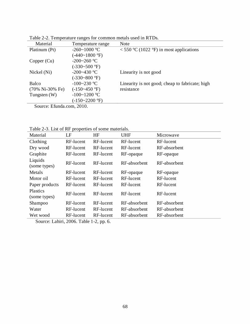
68
Table 2-2. Temperature ranges for common metals used in RTDs. Material Temperature range Note Platinum (Pt) -260~1000 °C
(-440~1800 °F) < 550 °C (1022 °F) in most applications
Copper (Cu) -200~260 °C (-330~500 °F)
Nickel (Ni) -200~430 °C (-330~800 °F)
Linearity is not good
Balco (70% Ni-30% Fe)
-100~230 °C (-150~450 °F)
Linearity is not good; cheap to fabricate; high resistance
Tungsten (W) -100~1200 °C (-150~2200 °F)
Source: Efunda.com, 2010.
Table 2-3. List of RF properties of some materials. Material LF HF UHF Microwave Clothing RF-lucent RF-lucent RF-lucent RF-lucent Dry wood RF-lucent RF-lucent RF-lucent RF-absorbent Graphite RF-lucent RF-lucent RF-opaque RF-opaque Liquids (some types) RF-lucent RF-lucent RF-absorbent RF-absorbent
Metals RF-lucent RF-lucent RF-opaque RF-opaque Motor oil RF-lucent RF-lucent RF-lucent RF-lucent Paper products RF-lucent RF-lucent RF-lucent RF-lucent Plastics (some types) RF-lucent RF-lucent RF-lucent RF-lucent
Shampoo RF-lucent RF-lucent RF-absorbent RF-absorbent Water RF-lucent RF-lucent RF-absorbent RF-absorbent Wet wood RF-lucent RF-lucent RF-absorbent RF-absorbent Source: Lahiri, 2006. Table 1-2, pp. 6.

69
Table 2-4. EPCTM tag classification. Class Power Range Memory Communication Peripherals Cost 0 None < 3 m 1 to 96 bits, Read
Only Backscatter None Low
1 None < 3 m 1 to 96 bits, Read/Write Once
Backscatter None Low
2 None < 3 m 1 to 96 bits, Read/Write
Backscatter Security Medium
3 Battery assisted < 100m < 100 Kilobytes, Read/Write
Backscatter Security, Sensors High
4 Battery assisted < 300m < 100 Kilobytes Read/Write
Active Transmission
Security, Sensor High
5 Battery assisted, AC/DC connection
Unlimited Unlimited, Read/Write
Active Transmission
Security, sensors, can communicate with other tags
Very High
Source: Banks et al., 2007. Table 3-1, pp. 69.

70
CHAPTER 3 APPLICATION OF RFID TECHNOLOGIES IN THE TEMPERATURE MAPPING OF THE
PINEAPPLE SUPPLY CHAIN
Introduction
RFID applications within the food supply chain have been mostly proposed in order to
satisfy the need for identification and trace back mechanisms (Jones, 2006; Wang et al., 2006;
Asimakopoulos et al., 2007; Montrucchio et al., 2007; Panos and Freed, 2007). Although
suggested, very little research has been done with regards to the application of RFID in process
traceability, especially on the monitoring of the ambient conditions surrounding food products
along the supply chain (Mermelstein, 2002; Karkkainen, 2003; Gaukler and Seifert, 2007).
RFID systems present many advantages for temperature monitoring and tracking. One of
them is the reduced amount of instrumentation labor required. RFID does not entail manual
scanning and hundreds of RFID tags can be downloaded into a computer at one time without
ever requiring line of sight between the tags and the reader (Karkkainen, 2003). This saves
considerable time and man-hours and decreases the number of errors that can occur with manual
systems (Thompson et al., 2005). RFID tags can be read from significant distances (especially
the active variety) and at fast speed, which favors its application in supply chain operations
without generating delays (Raza et al., 1999). According to the kind of tag, they can also record
more than 13,000 data points at different time intervals (up to 4.50 years of continuous logging)
(Identec Solutions Inc., 2007); ensuring the performance of the sensor in long-duration supply
chains.
Ruiz-Garcia et al. (2008) explain that these wireless sensors can be embedded within the
load which brings their readings closer to the true in situ properties of perishable products.
However, ambient temperature recordings throughout the load will differ from the ones
measured in the core of the product and within themselves according to the ambient conditions

71
of the surrounding area. Results obtained by this research show evidence to support that,
compared to temperature sensors with probe, the limitation of probeless RFID systems lies on
their failure to provide accurate temperature readings in some of the critical points of the load,
where temperature abuse is likely to occur. Still, their use could be appropriate if the
corresponding relationship between their output and the temperature of the product located in the
critical point is established. Therefore, the different scenarios for the utilization of RFID tags
with and without probes in the temperature mapping of supply chains have to be determined.
Cost being one of the current restrictive factors for RFID temperature tracking
implementation in real-life supply chains, it has been proposed that tagging should be done at the
transport-unit level (Karkkainen, 2003). Nonetheless, the cost of placing these tags in transport
cartons might surpass the level of investment a food company is willing to put into temperature
tracking; therefore, it is important to minimize the amount of RFID equipment used and the
resulting economic investment per load.
The objectives of this work were: 1) To study the use of RFID in the temperature
monitoring of a load of crownless pineapples packed in two kinds of primary packages by
comparing the performance of RFID temperature tags versus conventional temperature tracking
methods, as well as RFID temperature tags with probe versus RFID temperature tags without
probes and their utilization along the supply chain; and 2) To determine the level of
instrumentation necessary for proper temperature monitoring in this supply chain.
Materials and Methods
Experimental Design
The initial part of the experiment took place at a pineapple packing house in the Pacific
coast of Costa Rica. Eighteen primary packages containing six crownless pineapples each were
instrumented with temperature sensors before the palletizing process. Nine of these primary

72
packages were corrugated boxes (trays; 0.58 m x 0.39 m x 0.14 m) and nine were reusable plastic
containers (RPC; 0.59 m x 0.39 m x 0.20 m). In each package, one fruit was probed with a probe
attached to a HOBO temperature sensor (HOBO® Series H8; TMC6-HA and TMC6-HD probes,
Onset Computer Corporation, MA) so as to obtain their mass average temperature at a sampling
rate of 5.00 minutes. The probes were installed at 0.04 m of depth at the center of the fruit. The
packages were then placed in three different areas of their corresponding pallet: The upper
corner, the core at the central layer (seventh from the bottom up) and the lower corner (Figure 3-
1). The position of the probed pineapples depended on the location of the primary package in the
pallet. For the top and the bottom packages, the pineapple corresponding to the corner was
probed; while for the box placed at the core, it was the fifth pineapple from left to right.
Four kinds of RFID Temperature Sensors were also placed in each one of the six pallets
studied (Figure 3-2). These RFID tags were: ThermAssure RF (Evidencia, TN), ALB-2484
(Alien Technology, CA), ThermaProbe RF (Evidencia, TN), and ILR i-Q 32T (Identec
Solutions, TX). Both ThermAssure RF and ThermaProbe RF tags worked at a frequency of
13.56 MHz, while the ALB-2484 worked at 2.4 GHz and the ILR i-Q 32T at 915 MHz. The three
RFID sensors initially mentioned are semi-passive tags (also known as battery assisted passive
tags), which are RFID tags that contain a battery that powers their logic parts but are unable to
emit a signal unless energized by a RFID reader. On the other hand, ILR i-Q 32T, is an active
tag. Active tags are able to make use of their battery not only to power their logic parts but also
to actively broadcast a signal.
One RFID sensor of each kind was placed at the exterior of the central layer of the pallet;
but only the first three mentioned recorded ambient temperatures (Figure 3-3). The ThermaProbe
RF (Evidencia, TN) sensor was recording the mass average temperature of the probed pineapple

73
in the package placed in the core of the pallet. Based on results obtained in preliminary trials
conducted for temperature mapping, the sampling rate for all RFID temperature tags was set in
5.00 minutes.
After forced air cooling and nine hours in refrigerated storage, the two sets of pallets were
placed inside one refrigerated 12.20 m container in three specific locations: Front, Middle and
Back. The container had one row of pineapples packed in corrugated boxes and one row with a
mixed load of fruit packed in RPCs (the three pallets being studied) and corrugated boxes. The
set point of the container was 7.50°C.
Once filled, the container was sent to the Port of Limon in the Atlantic coast of Costa Rica
through land transportation. Two days after its arrival it was shipped to Florida (US) through a
carrier ship. The Temperature/Time readings from both kinds of sensors were obtained until the
shipment reached the company’s distribution center in the coasts of Florida three days later.
Statistical Analysis
A Generalized Linear Model (GLM) with a Gamma family was used in order to determine
the effects of the time, the sensor and packaging employed on the temperatures recordings
obtained (Freund and Wilson, 2003). It was also used to determine the equality of means of the
temperatures obtained with the different kinds of sensors.
In addition, a Student’s t-Test was performed in order to compare the means of the
temperature deltas between the sensors. Significance was accepted at level α=0.05 in all cases.
Statistical analyses were computed using R 2.7.2 (The R Foundation for Statistical Computing.,
Wiedner Hauptstrabe 8-10/1071 1040 Vienna, Austria).
74
Results and Discussion
RFID Sensor Performance versus Conventional Methods
The major difference noticed within both kinds of sensors was the time required for the
instrumentation of the load (Table 3-1). The RFID systems allowed a faster setup because of the
little time taken while programming the sensor and their ease of placement in the load.
The main factors in the speed of programming of the RFID systems were the amount of
tags read at once by the readers and the user-friendliness of the software employed. The fastest
was the ILR i-Q 32T system (19.09 s ± 3.15; mean ± SD) which, because of its active nature,
allowed the distant reading of all the tags at the same time, facilitating a remote activation
process. This tag was followed by the ThermAssure RF and ThermaProbe RF sensors (21.50 s ±
2.43; mean ± SD), semi-passive RFID tags using the same software and hardware, which
required a closer interaction with the readers and could only be read one by one. The user-
friendliness of the software employed was decisive in the programming time of the semi-passive
ALB-2484 (47.68 s ± 6.36; mean ± SD) tags, which, unlike the others, had management software
with poor interface and took the longest to be activated even though all the tags were able to be
read at once.
On the other hand, HOBO sensors required a lengthier period of time during programming
(53.71 s ± 3.92; mean ± SD) and had to be wired to the computer which made impossible any
sensor re-programming or reading once the pallets were instrumented.
As far as the ease of setup in the load, ThermaProbe RF tags were as difficult to handle as
HOBO sensors because their probe also needed to be placed in a specific location inside the
pallet. All other RFID sensors were quite easy to place; however, amongst all, some of them
were more convenient than others. For example, due to their small size and thickness (0.05 m x
0.05 m x 0.04 m) and light weight (6 g), handling the ThermAssure RF and ThermaProbe RF
75
sensors was better than dealing with the bigger and thicker ALB-2484; problem quite evident at
the time of taping them to the exterior of the pallet of corrugated boxes. Even less convenient
were the big ILR i-Q 32T sensors, which could not be taped and had to be placed inside the
primary packages at all times. During the setup of RPCs, the sensors that were easier to place on
the package (because they fit in the slot included in the package design) were the ThermaProbe
RF and ThermAssure RF tags; while the other two were secured using the same method as in the
previous package.
When comparing the results obtained with the ThermaProbe RF RFID tag and the HOBO
sensor placed in the pineapple of the core of the pallet the statistical analysis (Table 3-2) showed
significant differences between the sensors’ readings (P = 5.66e-03). The ThermaProbe RF RFID
tag consistently produced higher values in all pallets, being more evident in the case of the ones
using corrugated boxes as packaging (Table 3-3). This phenomenon could be explained by the
difference in accuracies of the sensors used (± 0.50°C HOBO, ±0.10°C ThermaProbe RF). As far
as RFID sensor performance, only two of the ambient ones (ThermAssure RF and ILR i-Q 32T)
were able to provide readings point by point. ALB-2484 RFID tags only supplied a final graphic
with the temperature profile, but did not allowed access to the data for further comparison. The
three temperature profiles had the same shape in each pallet (Figure 3-4). However, for both
kinds of packaging, comparison of the curves obtained with ThermAssure RF and ILR i-Q 32T
sensors showed that the former had higher values most of the time (Figures 3-4, 3-5 and 3-6).
The statistical analysis (Table 3-4) later on showed that there were significant differences
between the readings of both sensors (P < 1.55e-07). The maximum delta obtained between these
in each pallet reached up to 2.70°C in the pallets with corrugated boxes. This temperature
difference was most likely due to the fact that the bulky ILR i-Q 32T sensor was placed on the
76
vent inside the pineapple box and not on the surface of the box like the ThermAssure RF and
therefore, was subjected to different airflow exposure. In the pallet with RPCs, even though still
present, the temperature differentials between the ThermAssure RF and the ILR i-Q 32T tags
were reduced considerably with respect to the values obtained with corrugated boxes due to the
increased ventilation characteristic of RPCs.
Measured against the conventional methods for temperature tracking, such as handheld
thermometers and datalogging systems like the HOBO and iButton sensors, RFID sensors
provide ample advantages. Their fast and simple instrumentation and data recovery allow the use
of less manpower for these duties, reducing labor costs and delays in packing lines and
warehouse management procedures. In addition, because RFID temperature sensors supply vital
information about the product’s temperature abuse, they will become a powerful decision-
making tool for suppliers and retailers, assisting in the application of the concept of “First
Expires First Out” (FEFO) in supply chain and logistic operations (Emond and Nicometto,
2006). Furthermore, RFID temperature tags also provide something impossible to attain with
conventional methods: The reading and reprogramming of the sensors when they are already into
place. This last point is of high importance when considering the need for real-time remote
monitoring in food supply chains, which in the near future will become possible with the
combination of RFID and other wireless technologies.
RFID Temperature Tags with Probe versus RFID Temperature Tags without Probe and Their Utilization along the Supply Chain
Ambient readings with RFID sensors without probes present a wide difference with those
obtained by the ThermaProbe RF sensor in the pineapple of the core of the pallets. The biggest
deltas happened mostly during the forced air cooling period, reaching absolute values of up to
16.60°C (6.00 ± 2.75; mean, SD) for corrugated boxes and 16.50°C (4.96 ± 0.63; mean, SD) for
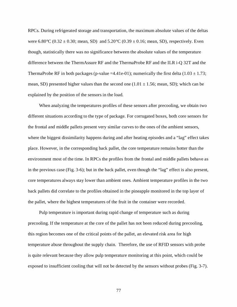
77
RPCs. During refrigerated storage and transportation, the maximum absolute values of the deltas
were 6.80°C (0.32 ± 0.30; mean, SD) and 5.20°C (0.39 ± 0.16; mean, SD), respectively. Even
though, statistically there was no significance between the absolute values of the temperature
difference between the ThermAssure RF and the ThermaProbe RF and the ILR i-Q 32T and the
ThermaProbe RF in both packages (p-value =4.41e-01); numerically the first delta (1.03 ± 1.73;
mean, SD) presented higher values than the second one (1.01 ± 1.56; mean, SD); which can be
explained by the position of the sensors in the load.
When analyzing the temperatures profiles of these sensors after precooling, we obtain two
different situations according to the type of package. For corrugated boxes, both core sensors for
the frontal and middle pallets present very similar curves to the ones of the ambient sensors,
where the biggest dissimilarity happens during and after heating episodes and a “lag” effect takes
place. However, in the corresponding back pallet, the core temperature remains hotter than the
environment most of the time. In RPCs the profiles from the frontal and middle pallets behave as
in the previous case (Fig. 3-6); but in the back pallet, even though the “lag” effect is also present,
core temperatures always stay lower than ambient ones. Ambient temperature profiles in the two
back pallets did correlate to the profiles obtained in the pineapple monitored in the top layer of
the pallet, where the highest temperatures of the fruit in the container were recorded.
Pulp temperature is important during rapid change of temperature such as during
precooling. If the temperature at the core of the pallet has not been reduced during precooling,
this region becomes one of the critical points of the pallet, an elevated risk area for high
temperature abuse throughout the supply chain. Therefore, the use of RFID sensors with probe
is quite relevant because they allow pulp temperature monitoring at this point, which could be
exposed to insufficient cooling that will not be detected by the sensors without probes (Fig. 3-7).

78
Also worthy of monitoring are certain regions where the pineapple would be at risk of low
temperature abuse and its manifestation, chilling injury, during transportation and refrigerated
storage. Results of the temperature mapping performed in this trial suggest that the fruit in the
lowest layers of the pallets will be more at risk to such conditions (Fig. 3-8).
However, no specific correlation could be deducted between the readings of the pulp
temperatures (measured with HOBO sensors) in these areas and the ambient temperatures
recorded. Consequently, in order to determine the temperature in these critical points, employing
RFID temperature tags with probe is suggested.
RFID temperature tags with probe are then necessary during precooling operations and
could also be required during transportation and refrigerated storage if there is an interest in
monitoring and preventing chilling injury occurrences. As mentioned previously, during
transportation and refrigerated storage, ambient RFID tags will prove useful in showing the
behavior of the fruit subjected to the highest temperatures in the load. Therefore, an efficient
temperature tracking system for this supply chain could make use of the potential of combining
these two RFID systems for a comprehensive temperature abuse analysis.
The development of a RFID temperature tag with a probe, able to record both ambient and
probed temperatures simultaneously is proposed as a way of ensuring proper temperature
tracking along precooling, storage and transportation operations. Its use will reduce the amounts
of instrumentation and investment required if two RFID sensors with probes, one for the core (or
for the bottom, if monitored) and one for a fruit located in the upper layer of the pallet were
employed.
Level of Instrumentation
Proper monitoring is achieved with one sensor per pallet, if necessary, according to the
location of the pallet during forced air cooling and inside the container. Probeless tags are

79
recommended for monitoring High Temperature Abuse (HTA) in the top of the pallets placed in
the back of the container. Tags with probe are suggested for detecting HTA in the center of the
pallets and Low Temperature Abuse (LTA) in the bottom of the pallets of RPCs in the front of
the container.
Conclusions
The application of RFID temperature monitoring was studied in a commercial shipment of
crownless pineapples packed in corrugated boxes and reusable plastic containers from Costa
Rica to the U.S.. A comparison between the performance of a conventional method (HOBO
sensors) and RFID temperature tags showed that both methods are analogous with regards to
accuracy, but RFID systems have a superior performance because they allow quick
instrumentation and data recovery, and the possibility of accessing the sensor program and data
at any point of the supply chain without line of sight. Although observed, differences between
the pulp temperatures taken by the RFID sensor with probe and the HOBO sensors, and between
the external RFID tags can be disregarded due to factors such as the accuracy and the placement
of the sensors. In addition, the use of RFID tags with probe was justified by its role in
determining the efficiency of the precooling operations and in tracking areas prone to chilling
injury during transportation and refrigerated storage; while the RFID tags without probe proved
most useful during high temperature abuse monitoring along transportation and refrigerated
storage. The creation of a RFID sensor with a probe, able to record both ambient and probed
temperatures simultaneously is suggested as a way of gathering the benefits of both systems and
ensuring proper temperature tracking along precooling, storage and transportation operations.
Future work in this area is needed in order to determine the readability of RFID
temperature sensors that use different frequencies along a variety of distances, pallet and primary

80
package locations and kinds of food products. Also necessary is the development of more
convenient sensors and portable readers in regards to their size and shape.
Finally, recommendations were given with respect to the instrumentation level required for
a RFID temperature tracking system for this supply chain.
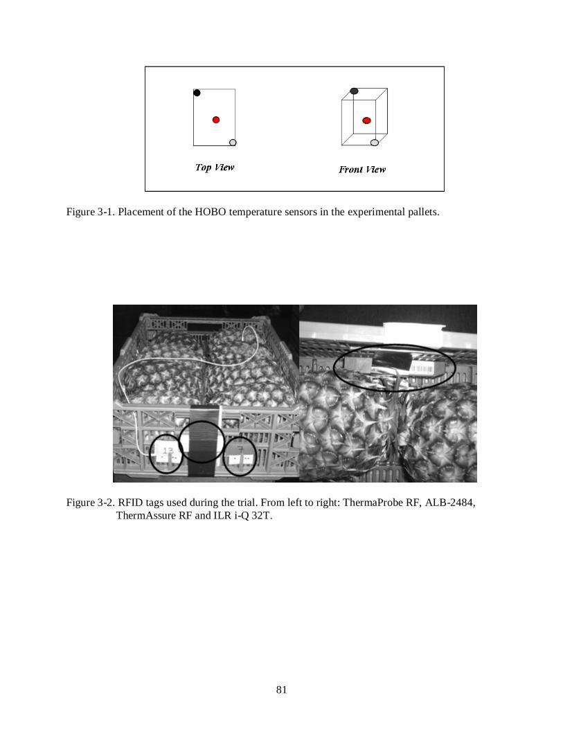
81
Figure 3-1. Placement of the HOBO temperature sensors in the experimental pallets.
Figure 3-2. RFID tags used during the trial. From left to right: ThermaProbe RF, ALB-2484, ThermAssure RF and ILR i-Q 32T.
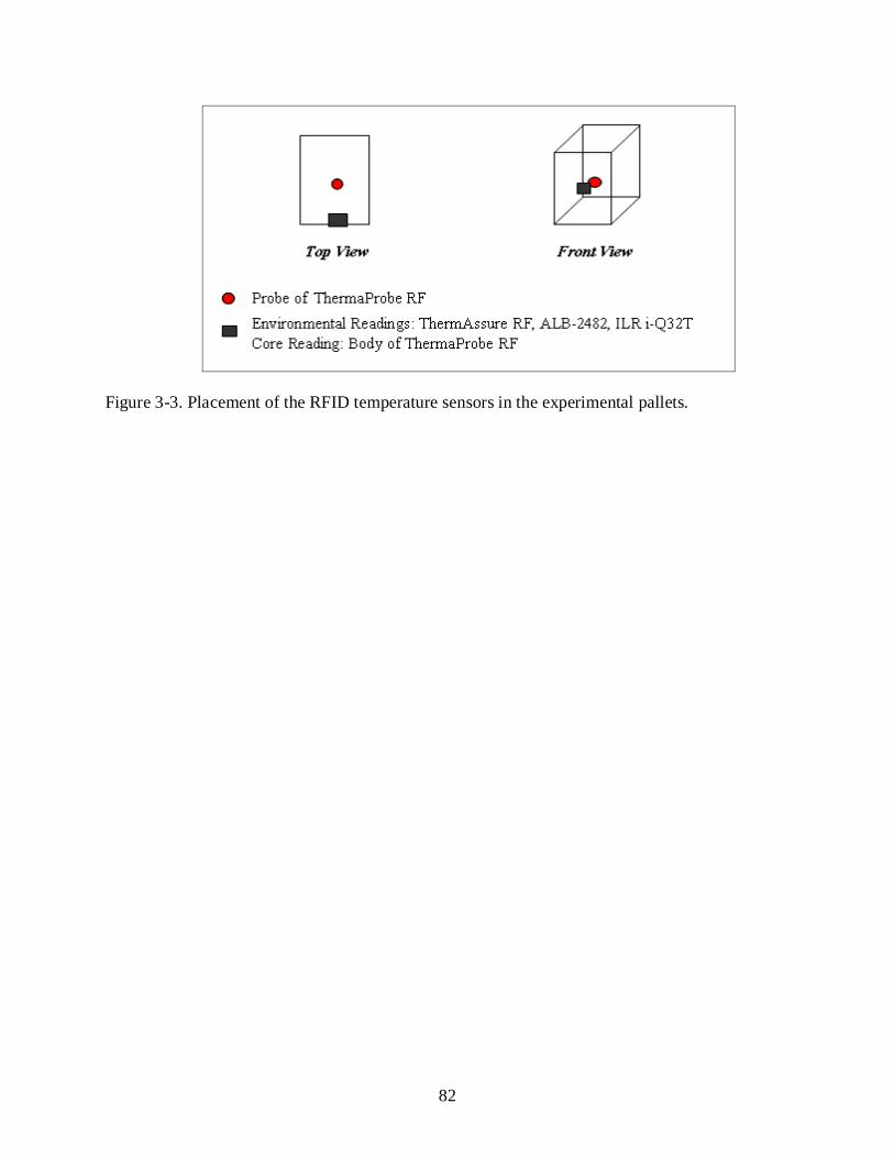
82
Figure 3-3. Placement of the RFID temperature sensors in the experimental pallets.

83
Table 3-1. Comparison of the features of the RFID temperature tracking systems analyzed and a traditional temperature monitoring system (HOBO Sensor).
Features ILR i-Q 32T
ThermAssure RF
ThermaProbe RF
ALB-2484
HOBO® Sensor
Programming time
(Mean ± SD)
19.09 s ± 3.15
21.50 s ± 2.43
21.50 s ± 2.43
47.68 s ± 6.36
53.71 s ± 3.92
Detects all sensors at once Yes No No Yes No
User-friendly software Yes Yes Yes No Yes
Allows distant interaction between the reader or computer and the sensor
Yes No No Yes No
Requires placing a probe in the load No No Yes No Yes
Easy to handle and affix to the packaging No Yes Yes No No
Software facilitates data management and analysis
Yes Yes Yes No Yes

84
Figure 3-4. Ambient temperature recordings obtained by the ALB-2484RFID tag placed in a pallet with corrugated boxes.
Figure 3-5. Ambient temperature recordings obtained by two RFID tags placed in a pallet with corrugated boxes: ThermAssure RF and ILR i-Q 32T.

85
Table 3-2. Results of the Generalized Linear Model for the Effects of the Sensor, Time Step and Packaging when comparing the temperatures (°C) obtained with the HOBO® sensor and the ThermaProbe RF RFID tag placed at the core of pallets with corrugated boxes or reusable plastic containers in the sea container.
Estimate Std. Error t Value P (Intercept) 5.74e-02 9.03e-04 63.50 < 2e-16
Sensor -1.40e-03 5.05e-04 -2.76 5.66e-03
Time Step 3.01e-05 8.57e-07 35.11 < 2e-16
Packaging 1.29e-02 2.88e-04 44.89 < 2e-16
Sensor: Time Step -2.23e-06 5.36e-07 -4.15 3.35e-05
Table 3-3. Comparison between the temperatures (°C) obtained with the HOBO® sensor and the
ThermaProbe RF RFID tag placed at the core of pallets with corrugated boxes according to their position in the sea container.
Container Position Front Middle Back
HOBO® Sensor
ThermaProbe RF
HOBO® Sensor
ThermaProbe RF
HOBO® Sensor
ThermaProbe RF
Mean 10.39 10.89 10.91 11.33 12.51 12.71 Standard Deviation 4.11 4.10 3.97 3.95 3.57 3.55

86
Table 3-4. Results of the Generalized Linear Model for the Effects of the Sensor, Time Step and Packaging when comparing the temperatures (°C) obtained with the ThermAssure RF and the ILR i-Q 32T RFID tags recording ambient temperatures on pallets with corrugated boxes or reusable plastic containers in the sea container.
Estimate Std. Error t Value P (Intercept) 6.07e-02 9.20e-04 65.96 < 2e-16
Sensor 2.75e-03 5.23e-04 5.25 1.55e-07
Time Step 2.07e-05 8.53e-07 24.20 < 2e-16
Packaging 7.75e-03 2.93e-04 26.41 < 2e-16
Sensor: Time Step 2.75e-06 5.48e-07 5.01 5.47e-07
Figure 3-6. Temperature profiles obtained by RFID tags with probe and without probe in the central layer of a pallet with RPCs.
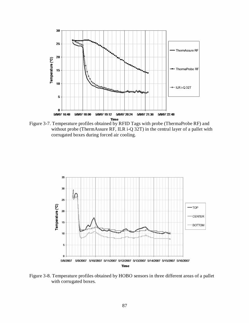
87
Figure 3-7. Temperature profiles obtained by RFID Tags with probe (ThermaProbe RF) and
without probe (ThermAssure RF, ILR i-Q 32T) in the central layer of a pallet with corrugated boxes during forced air cooling.
Figure 3-8. Temperature profiles obtained by HOBO sensors in three different areas of a pallet with corrugated boxes.
88
CHAPTER 4
EVALUATION OF SENSOR READABILITY AND THERMAL RELEVANCE FOR RFID TEMPERATURE TRACKING
Introduction
Technological advances have enabled precise traceability and visibility mechanisms within
temperature controlled supply chains. The existence of these technologies is driving a
requirement for precise traceability in perishable goods chains, such as the food and
pharmaceutical supply chains (Bollen, 2005; Ames, 2006; Metzger et al., 2007; Panos and Freed,
2007; Zhen-hua et al., 2007; Jedermann et al., 2008). RFID technology has been suggested as a
solution to address this need since it can store both pedigree and temperature/time information
and transmit it even as the product is in transit (Forcinio, 2004; Smith, 2005; Wyld, 2006; Leake,
2007). As discussed in the previous chapter, as a temperature tracking method, RFID has shown
superior performance when compared to traditional monitoring devices since it can surpass the
simplicity problems that these encounter during real-life fast-paced supply chains, while
maintaining their levels of accuracy. In spite of the promises it holds, the implementation of
RFID in this particular area is still in its infancy and, therefore, still presents some challenges.
A major hurdle for RFID’s application in food supply chains is that, based upon the
frequency used, certain environmental factors, such as water and the presence of metal, affect the
RF signal (Dobkin and Weigand, 2005; Redemske and Fletcher, 2005; Gaukler and Seifert,
2007; Hartvanyi and Marek, 2007; Sivakumar and Deavours, 2008). Current RFID systems for
temperature tracking present in the market operate either in the frequencies with reduced
readability near loads of perishable products with high water content such as produce (915 MHz,
868 MHz), or in frequencies that have short reading ranges (13.56 MHz), which makes them
unsuitable for portal applications in warehouses and distribution centers.

89
Cost is also an important barrier for industry implementations (Edwards, 2007). Battery
assisted passive and active tags used in temperature monitoring are considerably more expensive
than passive solutions used for asset tracking and represent a higher level of investment for
companies. Therefore, based on the discussions from the previous chapter, any feasible real-life
application has to utilize efficient instrumentation within the different levels of aggregation of
the load, allowing the minimization of the number of tags used without compromising the
accuracy of the system.
Within the different frequencies, there are two kinds of RFID temperature tags available in
the market: Tags with a probe and probeless tags. Tags with a probe are more suitable for
temperature monitoring inside the pallet and the product. This is mostly because these tags can
be read on the outside of the pallet; while reading a probeless tag implies surpassing the possible
interactions existent inside the pallet between the packaging/product and the RF waves, which
could turn into a very difficult matter. In addition, using a probeless tag for monitoring inside the
product complicates the instrumentation process (cut, open and insert; instead of only inserting a
probe); and could also pose a safety and quality threat if there is considerable discharge of
biological material into the load.
As discussed in the previous chapter, in produce industry applications the use of RFID tags
with a probe played an important role in monitoring the efficiency of precooling operations;
while RFID tags without a probe proved useful during transportation and refrigerated storage.
This study also demonstrated that the limitation of probeless RFID systems placed on the outer
surface of the pallet lies on their failure to consistently provide temperature readings close to
many of those in the critical points of the load, which are the areas of the load where temperature
abuse is most likely to occur inside the product. An example of this disparity is given when these
90
probeless tags register rapid temperature changes, which, if taken as reference, may mislead on
the actual product temperature in these locations.
Some perishable products (such as certain pharmaceuticals and chilling sensitive produce)
require the monitoring of the critical points of their loads because they can not afford being
subjected to any temperature abuse, since reaching threshold temperatures would seriously
impair their safety and integrity; consequently, RFID systems using tags with a probe would be
the most adequate solution for their temperature tracking needs. Nonetheless, measuring the
temperature in the critical points of the load offers disadvantages when trying to determine the
total amount of temperature abuse suffered by the entire product placed in a pallet. Since these
points are the areas more prone to it, the values they provide are the extremes and will not reflect
the average thermal history of the pallet. For many perishables’ operations, where certain
temperature excursions are allowed without posing a major threat to the product, it is the level of
thermal abuse in this other temperature profile what matters at the receiving end.
Placing a minimum amount of temperature data-loggers in relevant locations able to
describe the majority of the temperatures present in the entire pallet seems like a reasonable
option in order to obtain a broader perspective of the thermal reality of the load throughout the
supply chain, while taking into account real-life cost constraints. If the acquisition of internal
product temperature is not required, probeless RFID temperature tags could be used for this kind
of monitoring as long as, once placed in the thermally relevant areas during packing and
palletizing, they surpass any negative interaction with the load’s content and its environment and
get to be read either in transit or through portal applications during the end stages of the
distribution process.

91
The objectives of the research presented in this chapter were: To find a relevant location
able to provide a temperature reading representing eighty five percent of the temperatures
present in a pallet of bottles of water mimicking high-water content produce subjected to heating
and cooling episodes commonly encountered during loading/unloading operations in produce
supply chains. And second, to assess the readability and read range of a commercially available
RFID system when a battery assisted passive tag is placed in this thermally relevant position so
as to determine whether it would be read at the required distance for the supply chain.
Materials and Methods
Two studies were performed. A relevance study designed to find the thermally relevant
positions of the load was initially done. Then, a readability study able to detect the level of
readability of battery assisted passive tags and the reading ranges of the RFID system obtained
when placing these tags in the relevant positions found in the previous study was completed.
Relevance Study
The thermal relevance of different locations inside a pallet of bottles of water was studied
for conditions similar to the ones present during produce loading/unloading operations. Half a
pallet with 2160 bottles of water packed in 30 reusable plastic containers (RPC) was
instrumented with thermocouples previously calibrated in an ice bath (Figure 4-1). Spherical
bottles (“Aquapod”, Zephyrhills, 0.33 L) were used, mimicking circular shaped high-water
content produce such as oranges. The pallet consisted of six layers with five reusable plastic
containers (SmartCrate® GP 6419; 0.60 m x 0.40 m x 0.20 m, PP; IPL Inc., Saint-Damien,
Quebec, Canada) each; and each RPC contained a total of three layers of 24 bottles in a four by
six configuration. The 126 instrumented bottles provided a three-dimensional perspective for the
examination of the heat transfer process along the reusable plastic containers (RPC) and the half
pallet analyzed (Figure 4-1). The temperature of the pallet was initially stabilized by keeping it
92
overnight in a cold room at 4.00°C. The next morning, the pallet was moved from the cold
storage to the outside of the building, where it was exposed to ambient temperatures for a
specific amount of time (either 4.00, 2.00, 1.00 or 0.50 hours). It was stored once again in the
cold room and recordings were taken for the same amount of time it was exposed to ambient
temperatures (4.00, 2.00, 1.00 or 0.50 hours, respectively). Quantitative analysis was performed
using quintiles in Microsoft® Excel (Microsoft Corporation, Redmont, WA).
Readability Study
The readability of Class 3 battery assisted passive tags (BAP) was tested in two sides of the
pallet using the Intelleflex™ DK900 (Intelleflex Coorporation, Santa Clara, CA) RFID system
operating at 915 MHz. The pallet was located in an environment mimicking the unloading area
of a distribution center, in open air surroundings but with a sea container and metallic doors
nearby. The placement of the tags was determined by the results of the relevance study. Tags had
to be placed in one of the 1.22 m sides (Configuration α-I) and in both 1.02 m sides
(Configuration β), but since these had a similar layout only one of them was considered for this
testing. Each side was studied independently. The antennas were positioned in the middle point
of the front of the side being read. Readings were obtained using four different antenna distances
(0.50 m, 1.00 m, 2.50 m and 5.00 m) with respect to the pallet.
Tag placement
The placement of the tag inside the load could be a determinant factor in the readability of
the system and its resulting reading range. In this trial, the depth of tag placement varied with the
side configuration. For the area studied in configuration β it was 0.12 m, equivalent to the width
of two bottles. For configuration α-I it was set to 0.14 m, the height of one bottle. Figure 4-2

93
illustrates the end point of the internal layers in the configurations studied. The RFID tags were
set along the red lines.
Equipment configuration
In order to maximize the read range of the Class 3 tags inside the pallet, reader power was
set at its maximum and air interface data rates were set at their minimum. Since our research was
targeted towards portal applications, the reader’s inventory configuration was set in “portal”.
Table 4-1 summarizes the reader’s configuration.
Once set up, the system was run in three occasions; in each one, about 100 attempts of
communicating with each one of the tags were made. The level of readability of the tags was
determined by averaging the percentage of times a tag was read with respect to the attempts
made of contacting it.
Results and Discussion
Relevance Study
Temperature distribution
The temperature differentials were quite significant at the pallet level and sometimes also
at the RPC level. In addition, the magnitude of these differentials increased with the duration of
the heating/cooling episode. For example, for the longest one (4.00 hours/4.00 hours), the
temperature deltas were an average of 20.00°C (± 5.00°C, standard deviation) at the pallet level
and an average of 10.70°C (± 2.60°C, standard deviation) at the RPC level. Tables 4-2 and 4-3
summarize the average temperature differentials present at the pallet and RPC level, respectively.
As expected, the hottest temperatures were obtained near the top layer and the external
walls of the pallet; where exposure to solar radiation and environmental conditions was direct.
The coldest temperatures were recorded near the center of the pallet and at the bottom. Similar
trends in pallet temperature distribution had been previously reported by Jedermann and Lang

94
(2007). The core of the pallet was insulated by the external layers surrounding it; and its
temperature change was slow because heat transfer happened mostly due to conduction (poor air
circulation generated low convection). The bottom of the pallet remained cold also due to the
poor air circulation happening underneath the wooden pallet and reduced exposure to solar
radiation.
It is important to mention that this temperature distribution might change according to the
shape, weight, size and composition of the product being handled; as the heat transfer varies
according to them. With regards to this last issue, the product’s water content will be decisive,
because it is directly related to the product’s capacity to experience faster temperature changes.
Additionally, the shape and the size of the product will also determine the amount of air flow
present inside the pallet and could facilitate the insulation of the inner layers.
Moreover, the environmental factors in existence will contribute to these changes in
temperature too (i.e.: an increase in wind speed and/or air moisture content will facilitate the heat
exchange and raise temperature faster). Nevertheless, the current experiment was set up with
bottles full of water and conducted under the North Central Florida summer precisely because it
represents the worst case scenario for a perishable product’s cold chain, where most of the
conditions existent will encourage the quickest temperature gain possible. Hence, it is expected
that in most real life cases the temperature differentials in loads of produce packed in the same
density and similar in weight, shape, and size to the bottles of water will be less than the ones
reported in this research when subjected to comparable circumstances.
Eighty five percent location
The high variability of the temperature readings indicate that the initial target set for an
optimal location is difficult to determine. The thermal variability existent in the pallet increased
with the duration of the heating or cooling episode. It was then suggested to use the location that
95
has a temperature (n) that will be the middle point of an interval that gathers the temperature
readings of 85.00% of the measured locations. The proposed range for the time periods used is
[n-6.00, n+6.00]; a total of 12.00°C of temperature differential. The likelihood of gathering
85.00% of the temperature readings in this interval varies according to the duration of the
heating/cooling episode, decreasing as the heating/cooling episode increases in time:
• For 0.50/0.50 hours: 100.00% • For 1.00/1.00 hours: 96.00% • For 2.00/2.00 hours: 64.00% • For 4.00/4.00 hours: 42.00%
Comparisons were made between the temperature profile of this hypothetical point and the
ones obtained in the trials. Three locations in the pallet were then considered Points of Relevance
(PoR) and suitable for sensor placement (where temperature “n” will be recorded):
• Point A: Layer 9 (Row 3), X= 14.00, Y=9.00. • Point B: Layer 13 (Row 5), X=8.00, Y=1.00. • Point C: Layer 18 (Row 6), X=14.00, Y=1.00.
Where the layers move along the vertical axis (Z) and are labelled, along rows, in an
ascending way from the top to the bottom. Figure 4-3 illustrates the places where these three
points are located. It is necessary to indicate that, because of thermal symmetry, the
recommended thermally relevant points will be located in its equivalent position on the other
side of the pallet.
Analysis of the likelihood of gathering 85.00% of the temperature readings of the pallet
using these points as middle points for the interval was conducted (Table 4-4). Comparing these
estimates, point B would be the best for temperature monitoring because it has the highest values
in the first three exposure times, which are more likely to occur along the supply chain than the
last one. Point A would follow in preference and then point C. The selection of one of the
96
proposed locations for temperature monitoring will depend not only in this estimate but also on
the readability of the RF signal.
The produce industry works with two main packages: RPCs (used in this trial) and
corrugated boxes. Considering the fact that corrugated boxes generally allow less air flow and
delay the heat transfer process when compared to RPCs, it is expected that the results obtained in
this study would also be applicable to products packed in them as long as the packing density
(amount of units per box) is maintained.
The intrinsic variability of having a range of 12.00°C that includes 85.00% of the
temperatures of the pallet could be more or less detrimental on determining the condition of the
produce depending on how its respiration rate reacts to the rise of temperature. Overall, the more
sensitive the produce is to temperature increase, the more quality problems are expected in it. In
consequence, it would be advised to avoid using this methodology for produce with high
temperature quotient (Q10) values (Saltveit, 2003).
Transition times will vary widely with the specifics of a particular supply chain. On
average, they would not surpass the one hour limit during land or container loading/unloading
operations. However, for marine hold loading/unloading operations the situation changes, having
on average a one and a half hour span. Given that the level of relevance of the suggested
locations decreases with the amount of time of the heating/cooling episode, it is recommended
that this temperature monitoring system is used mostly for produce transported either by
refrigerated truck, or in a sea container, or in a combination of both methods.
It is important to remember that this system is designed solely for products of similar
characteristics to the spherical bottles of water employed and which storage temperature is
around 4.00°C; therefore, it could prove useful for produce such as apples, oranges,
97
pomegranate, passion fruit or tangerines. Further research is recommended in order to determine
if the thermally relevant locations identified in this work could also be used for products with
storage temperatures different than 4.00°C (tomatoes, limes, etc).
Readability Study
The three locations found as thermally relevant in the previous study (“PoR”) were tested
for readability. Special considerations were taken since a sensor placed in any of the sides has
the risk of not being read by the system if it is used as the entry port for the forklift. This will
occur because of the strong interaction of the RF waves emitted by the tag and the metal of the
forklift, which might hinder the communication process with the antennas. In addition, the
forklift could also shield the signal from the antenna to the tags, thereby, preventing
communication with them. Even though it would be feasible to mark the specific side where the
tag is present, this would complicate the handling of the pallet at the receiving end, where the
RFID system will be in place. Since point C is located in the bottom corner of the lowest row of
product on both of the β sides (varying from left to right corner according to the side chosen), it
was decided that both these locations and the nearest ones in the α-I side (where the corner is
completed) needed to be tested for RFID readability in case reading the β sides of the pallet was
unsuccessful because of forklift interaction. Tags were then placed in these positions, aiming
towards the corresponding face being read, in the first internal layer of all sides (Figures 4-4, 4-5
and 4-6).
In configuration α-I two out of the three tags tested were read, while in configuration β
only one of the two tags set up was detected. In the first configuration, the tag placed in the PoR
A was read at antenna distances of 0.50 m and 1.00 m. In addition, the tag corresponding to PoR
C placed on the left of this side (C1) was only found with a 2.50 m reading distance. Finally, in

98
configuration β the tag placed in PoR B was never detected and only the tag in C3 (PoR C in this
side) was read at antenna distances of 1.00 m, 2.50 m and 5.00 m.
The highest level of readability found in configuration α-I was 7.90% (± 0.01, standard
deviation) and belonged to PoR A at a reading distance of 0.50 m. Its counterpart in side β was
point C3 at a reading distance of 5.00 m with 95.59% (± 0.02, standard deviation) of readability.
Tables 4-5 and 4-6 summarize the average readability values for the PoRs detected in each
configuration at different reading ranges.
The results obtained can be explained in part by the findings of Fletcher et al. (2005) who
analyzed the signal propagation of 915 MHz waves through water. Their research indicates that
the strength of the RF signal depends not only on the amount of water it has to go through, but
also on the period of the sinusoidal wave and the point on it inherent to each water depth. Under
their analysis the period of this wave lasts approximately 0.04 m; and therefore, the lowest signal
strength will be located in amounts of depth of water multiple of four. In the current study, point
B, which is located in the middle of the β side, had no readability and point A, on the α-I side,
obtained some readability at two antenna distances. In the first case the RF wave had to
propagate through 0.12 m of water, where the signal will decrease at its maximum; while in point
A the signal had to go through 0.14 m of water, the middle point of the period between 0.12 m
and 0.16 m, at the peak of the RF wave. Therefore, it is logical to expect higher readability
during this particular point than at 0.12 m of depth. It can be then said that the bottle orientation
and the side configuration it determined influenced the level of readability of the tags.
Side configuration seemed to have played a less relevant role in the case of point C3,
where according to the previous discussion readability should have been hindered. A possible
explanation for this behaviour lies with the fact that there were no bottles of water on one of the

99
sides of the C3 tag. Compared to the center of that side, where point B was located, C3 had more
contact with open air, which facilitated the propagation of the signal and allowed larger reading
ranges. In contrast, for point C2, it is believed that any readability advantage generated by the
side configuration and the presence of air was cancelled by the reflection of the RF waves over
the surface of the sea container located near its right side.
These readability results indicate that the temperature monitoring of the load could take
place in PoRs placed either at the α-I side of the pallet (point A) or at any of the β sides (point
C3). However, in order to maximize the consistency of readings and reading range flexibility,
the use of this last point in configuration β is highly recommended.
The success of this preferred system depends on the protocol used for forklift loading. It
requires that all pallets are loaded on the forklift on the α side, so as to avoid marking the side
where the tag is placed, putting special attention during the loading of the forklifts (so the side
with the sensor is not in contact with it), or placing the antennas on an angle on top of the portal
(which might reduce the readability obtained with this setup). In this case, placing the sensor on
point C3 would only require installing antennas on both sides of the portal, so that the tag could
be read in any of the lateral sides of the pallet on the forklift.
It is also worth mentioning that since this system can work with antenna distances of 1.00
m, 2.50 m and 5.00 m, it can accommodate relatively small and large entry areas with portal
dimensions from 3.20 m up to 11.20 m of width.
Taking into account that for certain exposure times the likelihood of gathering 85.00% of
the pallet temperatures in the interval corresponding to point A is bigger than its analogue for
point C3 (Table 4-2); a compromise between the combination readability/reading range and
system accuracy is necessary.

100
Even though the current study was designed for portal applications, the use of forklift
readers could also be adequate for data retrieval during loading/unloading operations. Further
research determining the readability of the PoRs found in this study using forklift reading
systems is recommended.
Conclusions
It is feasible to perform relevant temperature monitoring using a single RFID tag per pallet
for loads of certain varieties of produce such as apples, oranges, pomegranates, passion fruit and
tangerines.

101
A
B
Figure 4-1. Area of pallet instrumented. A) Top view. B) Three-dimensional view of the bottles instrumented in each row.

102
Figure 4-2. Top view of the depth of tag placement for each configuration.
Table 4-1. RFID reader configuration.
Protocol Power (dBm)
Q value
TX Ant
RX Ant
Forward link
Reverse link Inventory BS type
C3 30.00 4.00 1.00 1.00 8.00 kbps 8.00 kbps portal fsk Table 4-2. Average temperature differentials present at the pallet level. Exposure time (hours)
Average temperature differential
Standard deviation
0.50/0.50 11.95 2.90 1.00/1.00 13.01 3.30 2.00/2.00 16.68 4.10 4.00/4.00 20.07 5.03
Table 4-3. Average temperature differentials present at the RPC level. Exposure time (hours)
Average temperature differential
Standard deviation
0.50/0.50 7.15 0.98 1.00/1.00 7.54 1.30 2.00/2.00 8.85 2.01 4.00/4.00 10.71 2.60

103
Figure 4-3. Location of the points of relevance in one half of the pallet.
Table 4-4. Likelihood of gathering 85.00% of the pallet temperatures inside the intervals
calculated using these locations. Exposure time (hours)
Location Point A Point B Point C
0.50/0.50 100.00% 100.00% 100.00% 1.00/1.00 82.35% 92.15% 74.50% 2.00/2.00 63.26% 63.26% 62.24% 4.00/4.00 41.14% 39.06% 42.18%

104
Figure 4-4. Top view of the placement of the RFID tags in the pallet.
Figure 4-5. Vertical view of the location of the RFID tags inside the pallet in Configuration α-I.
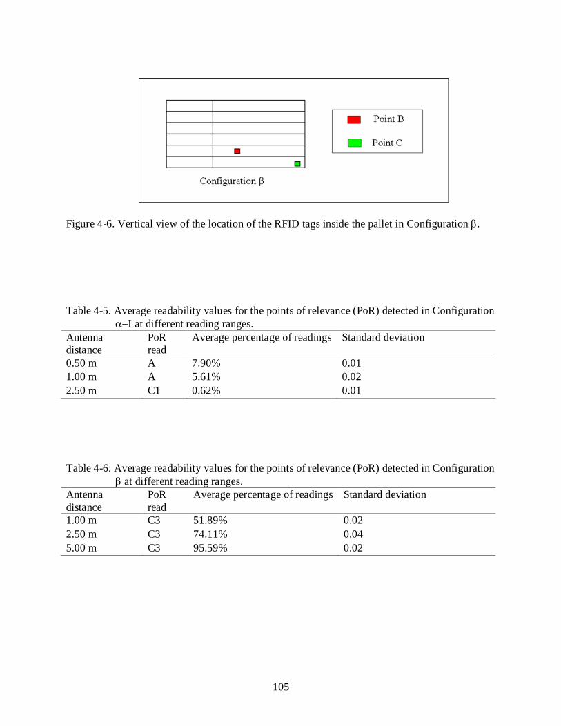
105
Figure 4-6. Vertical view of the location of the RFID tags inside the pallet in Configuration β.
Table 4-5. Average readability values for the points of relevance (PoR) detected in Configuration
α−Ι at different reading ranges. Antenna distance
PoR read
Average percentage of readings Standard deviation
0.50 m A 7.90% 0.01 1.00 m A 5.61% 0.02 2.50 m C1 0.62% 0.01 Table 4-6. Average readability values for the points of relevance (PoR) detected in Configuration
β at different reading ranges. Antenna distance
PoR read
Average percentage of readings Standard deviation
1.00 m C3 51.89% 0.02 2.50 m C3 74.11% 0.04 5.00 m C3 95.59% 0.02
106
CHAPTER 5 DEVELOPMENT OF RFID TEMPERATURE TRACKING SYSTEMS FOR COMBAT
FEEDING LOGISTICS
Introduction
Current U.S. Military operations require the deployment of millions of men and women
around the world. Daily, the Department of Defense (DoD) feeds more than two million people,
becoming one of the largest foodservice providers in the globe. In the field, during warfare
operations, the use of shelf-stable Meals, Ready-to-Eat (MRE) has provided for many years a
viable option for combat feeding without the time and temperature constraints imposed by most
perishable food supply chains. First Strike Rations (FSR) were first introduced into the mix of
shelf-stable military feeding by the DoD in 2008 as a way of reducing the waste of food existent
with MREs and the weight Warfighters had to carry, while still fulfilling their nutritional
requirements. Unlike MREs, that provide sustainment on a meal-basis, FSRs are able to supply
the soldier the energy requirements of the entirety of the day (DoD Live, 2009).
Being shelf-stable, FSRs are able to withstand a wide range of temperatures along their
supply chain. Nonetheless, once their temperature thresholds have been surpassed (26.67°C), the
deterioration rate of the product is accelerated, reducing considerably its expected shelf-life
(DoD Live, 2009). High temperature abuse could not only generate nutritional changes in it, such
as the loss of certain vitamins, and sensory changes in color, texture and flavour, which impact
the acceptability of the product (Ross et al., 1985; Ross et al., 1987; Narayan et al., 1997; Ross et
al., 1997; Shaw et al., 1997; Natress et al., 2009); but could also favor the development of
spoilage microorganisms and dangerous pathogenic growth (Banwart, 1989; Ng et al., 2002).
Taking into account the fact that shelf-stable meals are transported without refrigeration, and the
wide array of environmental conditions encountered along combat feeding logistics, it is then
imperative to monitor the temperature conditions of FSR loads along their supply chains. If
107
inadequate temperature management of FSRs is not discovered in a timely manner, their
consumption could diminish the nutritional status of the military forces deployed, affect their
morale, and, moreover, pose a food safety thread for them. Therefore, a reliable temperature
tracking system must be in place during combat feeding logistic operations in order to detect the
thermal abuse of FSR loads.
Radio Frequency Identification (RFID) is a wireless auto-id technology that has recently
gained popularity as an asset tracking tool, mostly due to the DoD and Wal-Mart’s initiative to
use it for this purpose in their supply chains since 2005. In food supply chains, RFID’s potential
lies in the possibility of a conjoint collection of pedigree data and time/temperature information
able to satisfy the current needs of the industry for trace-back and process traceability
(Karkkainen, 2003; Gaukler and Seifert, 2007; Montrucchio et al., 2007; Perez-Aloe et al.,
2007). Furthermore, results presented in Chapter 3 indicate that RFID temperature tracking
performs better when compared to conventional temperature tracking systems; providing similar
accuracy while increasing the simplicity of the sensing system.
However the promises RFID holds in food supply chains; in each implementation, there
are two major hurdles that need to be surpassed: Applying the technology in a cost-efficient way,
and obtaining consistent readings. In order to achieve the first one, and reduce the cost of the
implementation; the use of sensor-enabled battery-assisted passive tags (BAP) and active tags
has to be minimized across the load without compromising the accuracy of the system.
Moreover, as presented in the previous chapter, if the thermal and perishability characteristics of
the product being handled permit it, this can be easily obtained by monitoring only the relevant
locations able to provide a general view of the thermal reality of the load or its Points of
Relevance (PoR). Attaining consistent readings, nonetheless, is a more complicated matter; for it
108
depends considerably on surpassing the interactions between the systems’ radio frequency (RF)
waves and the product and its environment. Previous studies by Dobkin and Weigand (2005),
Redemske and Fletcher (2005), and Hartvanyi and Marek (2007) have detailed how, depending
on its frequency, the radio frequency (RF) signal is affected by the presence of water or metal in
the environment. In the ultra high frequency (UHF) spectrum, for example, where most supply
chain management applications take place, water absorbs the energy of the RF wave, decreasing
communication between the antennas and the tags; while metal acts as a reflector, which
sometimes can facilitate or hinder this process (Sydänheimo et al., 2006; Lazaro et al., 2009).
Solutions for this problem will then depend on many factors particular to each implementation
case, such as the class and configuration of the equipment being used, the reading range
available, the components, packaging, and level of aggregation of the product handled, and the
presence of any element in the surroundings that might interact with the system (metallic
forklifts, sea containers, etc).
If a RFID temperature tracking system is deployed in the military, monitoring the
immediate ambient temperature surrounding the pallets of FSRs would simplify the
instrumentation process and reduce the amount of labor involved in this task. Furthermore,
negative interactions between the RF waves and the metallic components of the meals’
packaging could be avoided, increasing the robustness of the system. Yet, data collected from the
surface of the pallet could be quite distant from the temperatures obtained in its Points of
Relevance (PoR), which are the best indicative of the thermal reality and the status of the load.
Therefore, a software tool able to estimate the temperature profiles in the PoRs of the pallet
based upon ambient temperature readings could be needed in order to facilitate the
implementation and accuracy of a RFID temperature tracking system for FSRs.
109
The objective of this research was to develop two RFID temperature tracking systems for
FSR logistics by: 1) Finding a thermally relevant location able to represent 85% of the
temperatures present inside a pallet of FSRs when subjected to heating and cooling conditions
similar to the ones faced along its supply chains; 2) Determining the level of readability of two
commercially available RFID systems using a battery assisted passive tag in this thermally
relevant position; and 3) To develop a software tool able to estimate the temperature profile of
the thermally relevant position using as input ambient temperature readings.
Materials and Methods
Relevance Study
A pallet of 432 FSR packets (0.20 m x 0.14 m x 0.09 m) packed in 48 boxes was
instrumented with thermocouples previously calibrated in an ice bath. The pallet consisted of
four layers of twelve corrugated boxes (0.42 m x 0.26 m x 0.23 m); and each box contained three
layers of FSR packets (four in the bottom, three in the middle, and two in the top), with a total of
nine per box. The 142 packets instrumented provided a three-dimensional perspective for the
examination of the heat transfer process along the boxes (Figure 5-1) and the pallet. After
instrumentation, the pallet was stored in a temperature controlled chamber. A series of heating
episodes followed by cooling ones were staged inside it, with room temperatures ranging from
60.00ºC to -35.00ºC, respectively. Before each heating/cooling episode pallet temperature was
stabilized at 25.00ºC. There were eight heating/cooling episodes with different durations: six
hours of heating/six hours of cooling, eight hours of heating/eight hours of cooling, nine hours of
heating/15.00 hours of cooling, 18.00 hours of heating/18.00 hours of cooling, 1.00 day of
heating/1.00 day of cooling, 2.00 days of heating/2.00 days of cooling, 3.00 days of heating/3.00
days of cooling, and 4.00 days of heating/4.00 days of cooling. Quantitative analysis was
performed using quintiles in Microsoft® Excel (Microsoft Corporation, Redmont, WA).

110
Readability Study
Fixed system
Two sides of the pallet were tested for readability of class 3 battery assisted passive tags
(BAP) using the Intelleflex™ DK900 (Intelleflex Coorporation, Santa Clara, CA) RFID system
operating at 915 MHz. The pallet was located inside a sea container, near the door, in the middle
of it wide-wise (Figure 5-2). The container had open air surroundings and a metallic door near
by. The placement of the tags was determined by the results of the relevance study. Since the
four sides of the pallet could be represented by one of the 1.22 m sides (Configuration α) and
one of the 1.02 m sides (Configuration β), only these two were tested. Each side was studied
independently. The antennas were positioned in the middle point of the front of the side being
read. Readings were obtained using six different antenna distances (0.50 m, 1.00 m, 1.50 m, 2.00
m, 2.50 m, and 3.00 m) with respect to the pallet.
Equipment configuration. In order to maximize the read range of the Class 3 tags inside
the pallet, reader output power was set at its maximum and air interface data rates were set at
their minimum. Table 5-1 summarizes the reader’s configuration. Once set up, the system was
run in five occasions; in each one, 200 attempts of communicating with each one of the tags were
made. The level of readability of the tags was determined by averaging the percentage of times a
tag was read with respect to the attempts made of contacting it.
Handheld system
As in the previous case, two sides of the pallet were tested for readability. The tags used
were Caen EASY2LOG® Mod. A927Z (Caen RFID Srl., Viareggio, Italy), also class 3 battery
assisted passive tags (BAP) working at 915 MHz. The pallet placement, the sides analyzed and
the surrounding environment were the same as in the past trial. Readings were taken
independently for each side of the pallet with the Motorola MC3090-Z handheld reader
111
(Motorola, Inc., Holtsville, NY). The equipment was configured to read EPC Gen 2 tags at 27.00
dBm. It was not possible to perform other changes in the configuration of the reader.
Two kinds of readings were taken: Inside and outside the pallet. For readings inside the pallet,
the tags were placed in the same locations as in the trial with the fixed system. For readings
outside the pallet, for both side configurations, one tag was placed on the side wall of the top
layer of product, facing the opening for the sea container’s door (Figure 5-3). In addition, for
configuration β, a different tag was also placed in the middle of the surface of the wooden pallet
facing the back of the container (Figure 5-4). These readings were also taken independently. The
operator holding the reader was then standing in the middle point of the front of the side being
read. The movement of the operator’s body and the arm holding the reader while collecting data
were different for each kind of test.
For example, in order to obtain readings in the interior of the pallet, the operator did the
following: He bent his arm at the height of his chest, then extended it and pointed it upwards and
downwards. He then held the reader at the height of his chest; and bent his knees pointing his
arm towards the pallet. Finally, he returned to the initial position. For external readings, the
methodology was more direct: The operator simply extended his arm and pointed upwards or
downwards towards the tag.
As in the experiment with the fixed system, six different reading ranges were tested with
respect to the pallet (0.50 m, 1.00 m, 1.50 m, 2.00 m, 2.50 m, and 3.00 m).
Temperature Profile Estimator
After analysis of the data obtained in the relevance study it was decided that a model using
a capacitive effect should be applied for the estimation of the temperature profiles in the
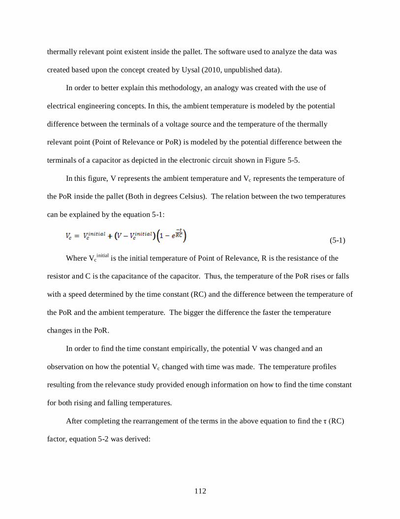
112
thermally relevant point existent inside the pallet. The software used to analyze the data was
created based upon the concept created by Uysal (2010, unpublished data).
In order to better explain this methodology, an analogy was created with the use of
electrical engineering concepts. In this, the ambient temperature is modeled by the potential
difference between the terminals of a voltage source and the temperature of the thermally
relevant point (Point of Relevance or PoR) is modeled by the potential difference between the
terminals of a capacitor as depicted in the electronic circuit shown in Figure 5-5.
In this figure, V represents the ambient temperature and Vc represents the temperature of
the PoR inside the pallet (Both in degrees Celsius). The relation between the two temperatures
can be explained by the equation 5-1:
(5-1)
Where Vcinitial is the initial temperature of Point of Relevance, R is the resistance of the
resistor and C is the capacitance of the capacitor. Thus, the temperature of the PoR rises or falls
with a speed determined by the time constant (RC) and the difference between the temperature of
the PoR and the ambient temperature. The bigger the difference the faster the temperature
changes in the PoR.
In order to find the time constant empirically, the potential V was changed and an
observation on how the potential Vc changed with time was made. The temperature profiles
resulting from the relevance study provided enough information on how to find the time constant
for both rising and falling temperatures.
After completing the rearrangement of the terms in the above equation to find the τ (RC)
factor, equation 5-2 was derived:

113
(5-2)
Hence, if the ambient and the initial temperature in the PoR are known, and also the temperature
in the PoR a given time “t”; it becomes trivial to calculate the time constant. Unlike the
electronic circuit described above, it was possible to have a different time constant for the
heating and cooling cycles due to the way the experiments were designed.
Calculations and graphics were performed in Matlab® (The MathWorks, Inc.; Natick,
MA).
Results and Discussion
Relevance Study
No thermally relevant position representing 85.00% of the temperatures of the pallet was
detected. A great level of temperature variability was present in the load. This was mostly
because of the existence of high temperature differentials due to heat accumulation in the middle
of the boxes after the warming episodes. Even though the temperature differentials within boxes
and along the pallet were quite significant in all trials, at the end of the 3.00 d/3.00 d and 4.00
d/4.00 d ones these were reduced considerably because the pallet was reaching thermal
equilibrium.
An approach already employed in the previous chapter of using a location that has a
temperature (n) that represents the middle point of an interval that gathers the temperature
readings of 85.00% of the measured locations was proposed. The suggested range was [n+8.00,
n-8.00]; a total of 16.00°C of temperature differential. Table 5-2 displays the likelihood of
gathering 85.00% of the temperature readings in this interval for each heating/cooling episode.
No particular trend was found between this particular likelihood and the duration of the episodes.

114
The temperature profiles obtained in the trials were then compared to the one
corresponding to this hypothetical location; resulting in the determination of two Points of
Relevance (PoR), where the temperature “n” was recorded and where the sensors of the
projected system would be placed.
• Point A: Layer 2 (Row 1), X= 11.00, Y= 5.00. • Point B: Layer 4 (Row 2), X= 4.00, Y= 1.00.
Where the layers move along the vertical axis (Z) and are labeled, along rows, in an
ascending way from the top to the bottom. The locations of these points are represented in Figure
5-6. Although not shown in the graphic, it is important to remark that, because of thermal
symmetry, these thermally relevant locations will also be present in their equivalent positions on
the other sides of the pallet (along the X and Y axis).
The likelihood of gathering 85.00% of the measured temperatures of the pallet within the
16.00°C interval that uses these points as middle point was then calculated (Table 5-3).
As can be seen, Point B gives a higher likelihood during most of the short and middle
duration episodes (up to 1.00 d/1.00 d), while Point A performs better during the longest trials.
Still, the selection of the best PoR for temperature monitoring will not only depend in this
estimate but also on the level of readability of the RF signal obtained in these locations.
Current U.S. military operations have a focal interest the Middle East. Therefore, the results
obtained in this relevance study have to be applicable to the varied conditions of such
environment. A review of the year-round weather conditions of Baghdad and Kabul (BBC,
2010b) show the existence of considerable temperature differentials, which average 34.50ºC, and
can reach up to 44.00°C during certain fall and winter months. These differentials will also
depend on where the FSRs are stored, and in which phase of the transportation process is the
load. For example, if the pallets are transported by land to be placed inside a cave, the

115
differentials could be greater, because the temperatures inside this will be considerably lower
than the ones registered by the weather services. Likewise, these temperature differentials could
decrease if the load is being transported by sea, and protected from solar radiation. From a heat
transfer perspective, the worst case scenario for a temperature tracking system similar to the one
being designed is when the temperatures in the pallets are quite variable, due to a high
temperature differential between the pallet and the environment. The temperature differential of
95.00°C used in these trials represents then, an extreme situation very rare to find under normal
circumstances; but that gives a safety factor even for the outlier observations encountered in real-
life situations. Consequently, it is expected that under normal supply chain conditions, the
likelihood of gathering 85.00% of the temperature readings present in the pallet within the
16.00°C range proposed when using the PoRs found as middle points of this interval will
increase.
The use of a 16.00°C temperature range as a reference for quality and shelf-life
assessments along this supply chain will not be a major concern, because FSRs are shelf-stable
products. However, if a component of the ration has a characteristic particularly sensitive to heat
or cold (degradation of vitamins, color and texture changes, etc) that might happen within that
range under ordinary storage and transport conditions; then, a higher level of quality variability
in the pallet is expected, and the application of this system could derive in the incorrect
acceptance of a faulty load. As well, a stronger level of sampling and quality control of the load
before acceptance should be established when exposure to high temperatures (over 26.67°C) is
recorded. Mainly, because the 15.00% of temperatures inside the pallet that are not represented
by this temperature tracking system might promote pathogen growth, and create food safety
hazards for the troops.
116
Readability Study
Fixed system
Figure 5-7 shows the placement of the tags for Configuration α (1.22 m). These were placed
both in the PoRs found, as in their thermally equivalent positions inside the pallet. For
Configuration β, the pallet was rotated 90° clockwise. Configuration α provided the highest
number of tags read: A minimum of five for each distance (a, b, c, d, e), and six during two of
the repetitions held at one meter. With Configuration β, four tags were read during the first five
distances tested (b, c, d, e), but only three were recorded at three meters (b, c, e). The location
with the highest readability of PoR A was position “e”; whereas for PoR B, the highest reading
percentages were distributed in locations “b” and “c” in Configurations α and β respectively.
Tables 5-4 and 5-5 summarize the highest readability levels for each PoR in each one of the
configurations studied at different reading ranges.
In Configuration α the best reading distance for PoR A is 1 m, and for PoR B is either 2.00
m or 2.50 m. In configuration β, this distance is 2.00 m for both PoRs. These results are quite
positive when considering the metallic environment that surrounded the pallet; and the fact that
the quad-laminate packaging of the components of the FSRs in direct contact with the tags
contained a layer of foil. Furthermore, the high density of the FSR packets inside the boxes
restricted the existence of air pockets able to propagate the RF signal and favor tag/reader
communication. Since metallic objects reflect RF waves, problems arise whenever the tags need
to harvest energy in order to backscatter its information (Sydänheimo et al., 2006). Mo et al.,
(2007) also reported that whenever there is a metallic object near an antenna, this can change the
antenna’s radiation pattern, input impedance, radiation efficiency, and resonant frequency; which
can decrease the performance of the RFID system. Additionally, Lázaro et al. (2009) accounts

117
that, although challenging, the presence of metallic surfaces near UHF RFID applications can
also generate constructive wave interference, and aid the RF system. Nonetheless, a study
performed by Laniel et al. (2009) described the existence of signal attenuation at 915 MHz inside
a metallic sea container due to path loss, such as multi-path and scattering. Taking into account
that the tags utilized in the trial were not designed to work in metallic environments, the
existence of favourable results in this readability study could be explained by a combination of
factors such as the use of maximum reader output power, and the existence of overall
constructive interference.
The system being designed will be used during container unloading operations; and the
readings will be taken moments before the pallet is removed from the container by the forklift.
Consequently, the space needed between the doors of the container and the antennas must allow
the transit of a forklift loaded with a pallet. So, 3.00 m, the maximum antenna distance tested,
will be chosen. At this distance, the readability of PoR A is less than PoR B; thus, the latter will
be the thermally relevant point monitored. Given that the orientation of the pallet inside the
container might vary according to the stowage pattern used at the time of loading, the RFID tag
in this location must be read from any of the two configurations studied. Locations “b” and “c”
are the only two points of PoR B read at 3.00 m, which are equivalent to each other depending
on the rotation of the pallet with respect to the sea container. As a result, instrumenting the pallet
in any of them will achieve the systems’ goal. Table 5-6 shows the readability values of these
positions.
As can be seen, the maximum amount of readability existent in the system is 82.00% while
its minimum is 32.60%. Since both tags were detected in all cases, this last value does not imply
that the tag will not be read; it only indicates that the reader will take a longer period of time

118
detecting it. Obtaining 32.60% of the 200 reader communication attempts at that particular
antenna distance took less than two minutes; so, reading the tag only once will take less than
that. However, even if detecting the tag takes two full minutes; this amount of time fits perfectly
into this phase of the FSR supply chain, as it uses the dead time when the forklifts are
transporting the pallets to their destination after unloading them from the container. Besides, if
the readings are done when the forklifts are far away, there are fewer opportunities for negative
interactions between its metallic surface and the RF waves.
Handheld system
Before reporting and discussing the results, it is important to mention that the system did not
allow the estimation of tag readability as percentage of reads from the total number of attempts
to communicate with that tag. Therefore, readability had to be estimated using the percentage of
readings of a particular tag from the total number of tag readings. So, the presence of other Class
1 Gen 2 tags detectable by the reader nearby influenced the result greatly. Since there were some
tags in the surroundings, these were read along with the CAEN tags. Yet in all the experiments
performed with the handheld reader, the impact of these tags on the results diminished with
reading distances. Even so, these results do not give a complete depiction of the robustness of the
communication existent between tag and reader at different distances; but they do, however,
allow a comparison between the readability obtained between the five trials performed: Two
attempting to read tags placed in all the PoRs, two trying to read the tag on the surface of the
FSR load, and one attempting to read the tag on the surface of the wooden pallet structure.
Two PoR locations were initially read in Configuration α at 0.50 m of reading distance.
These were points b and d, having a percentage of readings of 3.27% and 11.73%, respectively.
Nevertheless, at distances higher than 0.50 m the system could only detect point d. In

119
Configuration β only point b was read, and very weakly (0.09% in percentage of readings). Thus,
only point d in Configuration α will be taken into account in the comparison of the RFID
systems.
As can be seen in Table 5-7 the lowest readability results at all distances were obtained by
point d; which shows the strong impact that the metallic components of the packaging and the
metal surfaces of the sea container had on the signal. This phenomenon was expected, given the
fact that this model of Caen tag was not designed for applications in metallic environments; and,
as aforementioned, this element can affect greatly the operation of the system. Differences in tag
design between the Caen system and the Intelleflex system; as well as other technical
considerations, such as reader power output and antenna size and pattern might have played an
important role in their performances. Equalizing some of these variables might present a more
accurate panorama and allow proper comparisons.
The tag placed on the surface of the wooden structure of the pallet had the highest level of
readability at every single reading distance. There are two possible causes for this: First, these
tags were in contact with wood, which does not reflect RF waves, and not with the FSR boxes
full of packages with metal in their structure. And second, the angle of the reader antenna and the
location of the tag might have determined reflection patterns different than those in the other tag
positions, which created a less detrimental multipath effect.
The results corresponding to the tags placed on the surface of the FSR load are relatively
similar, though Configuration β seems to provide more robust readings than α. This is most
likely also product of different multipath effects.
Even though conclusions cannot be made with respect to the robustness of the systems
with respect to antenna distances, the use of those higher than 1.50 m is not recommended. This,
120
is due to the fact that it was observed that the speed of reading of the systems was inversely
proportional to the reading distance, and that obtaining readings at 2.00 m and more took a
considerable amount of time. Since the use of a handheld reader during unloading operations will
require its operator to move constantly towards the pallets and back, in order to avoid the
upcoming forklifts, high speed readings are desirable. Consequently, antenna distances of 1.50 m
are recommended as a way of combining the tag read velocity with the minimization of the
distance the operator will have to walk to read each pallet.
The temperatures obtained by the tag in this handheld system will later become the input
data for the temperature profile estimator; and after being processed, will give origin the
temperatures obtained in PoR B.
Temperature Profile Estimator
The temperatures in the Points of Relevance A and B (labeled also as 20-alpha and 36-
prime in the figures) showed a capacitor effect to rapidly changing temperature by slow
heating/cooling cycles (Figures 5-8 and 5-9). Therefore, the temperatures rose and decayed with
a time constant that can be determined from the eight trials from the relevance study, and can
subsequently be modeled to estimate the temperature in the PoRs given the ambient temperature.
The model was the applied by first estimating the time constants for the heating and
cooling processes for each trial. As an example, the calculations corresponding to the constant
for the 4.00 days heating period were performed for PoR A (τrising).
In this experiment, the average ambient temperature sat at 60.50ºC. If t=0.00 is defined as
the time PoR A’s temperature started to increase from 24.60ºC, then a second temperature point-
time pair can be chosen to calculate the time constant. For this example, at t=76.00 hours the
temperature of PoR A reached 60.00ºC, and this point was then used in the calculations below
where T represents temperature whereas t represents time.
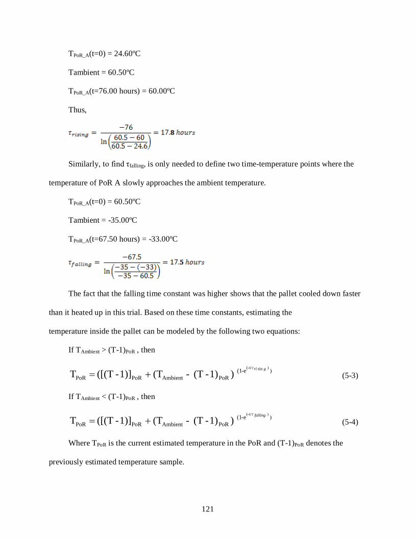
121
TPoR_A(t=0) = 24.60ºC
Tambient = 60.50ºC
TPoR_A(t=76.00 hours) = 60.00ºC
Thus,
Similarly, to find τfalling, is only needed to define two time-temperature points where the
temperature of PoR A slowly approaches the ambient temperature.
TPoR_A(t=0) = 60.50ºC
Tambient = -35.00ºC
TPoR_A(t=67.50 hours) = -33.00ºC
The fact that the falling time constant was higher shows that the pallet cooled down faster
than it heated up in this trial. Based on these time constants, estimating the
temperature inside the pallet can be modeled by the following two equations:
If TAmbient > (T-1)PoR , then
))
+=gri sin(-t/e-(1
PoRAmbientPoRPoR )1)-(T - (T 1)]-([(T Tτ
(5-3)
If TAmbient < (T-1)PoR , then
))
+=fallingτ(-t/e-(1
PoRAmbientPoRPoR )1)-(T - (T 1)]-([(T T (5-4)
Where TPoR is the current estimated temperature in the PoR and (T-1)PoR denotes the
previously estimated temperature sample.
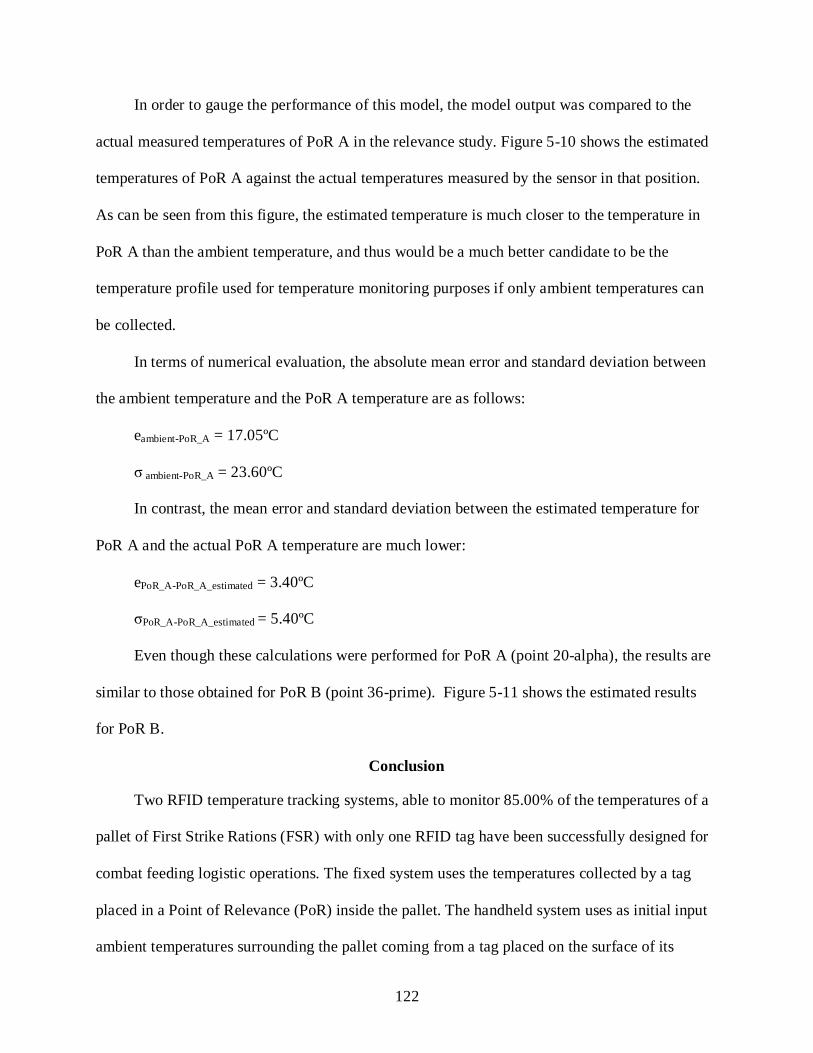
122
In order to gauge the performance of this model, the model output was compared to the
actual measured temperatures of PoR A in the relevance study. Figure 5-10 shows the estimated
temperatures of PoR A against the actual temperatures measured by the sensor in that position.
As can be seen from this figure, the estimated temperature is much closer to the temperature in
PoR A than the ambient temperature, and thus would be a much better candidate to be the
temperature profile used for temperature monitoring purposes if only ambient temperatures can
be collected.
In terms of numerical evaluation, the absolute mean error and standard deviation between
the ambient temperature and the PoR A temperature are as follows:
eambient-PoR_A = 17.05ºC
σ ambient-PoR_A = 23.60ºC
In contrast, the mean error and standard deviation between the estimated temperature for
PoR A and the actual PoR A temperature are much lower:
ePoR_A-PoR_A_estimated = 3.40ºC
σPoR_A-PoR_A_estimated = 5.40ºC
Even though these calculations were performed for PoR A (point 20-alpha), the results are
similar to those obtained for PoR B (point 36-prime). Figure 5-11 shows the estimated results
for PoR B.
Conclusion
Two RFID temperature tracking systems, able to monitor 85.00% of the temperatures of a
pallet of First Strike Rations (FSR) with only one RFID tag have been successfully designed for
combat feeding logistic operations. The fixed system uses the temperatures collected by a tag
placed in a Point of Relevance (PoR) inside the pallet. The handheld system uses as initial input
ambient temperatures surrounding the pallet coming from a tag placed on the surface of its

123
wooden structure, but with the help of a software tool is able to estimate the temperatures in the
PoR monitored by the fixed system.
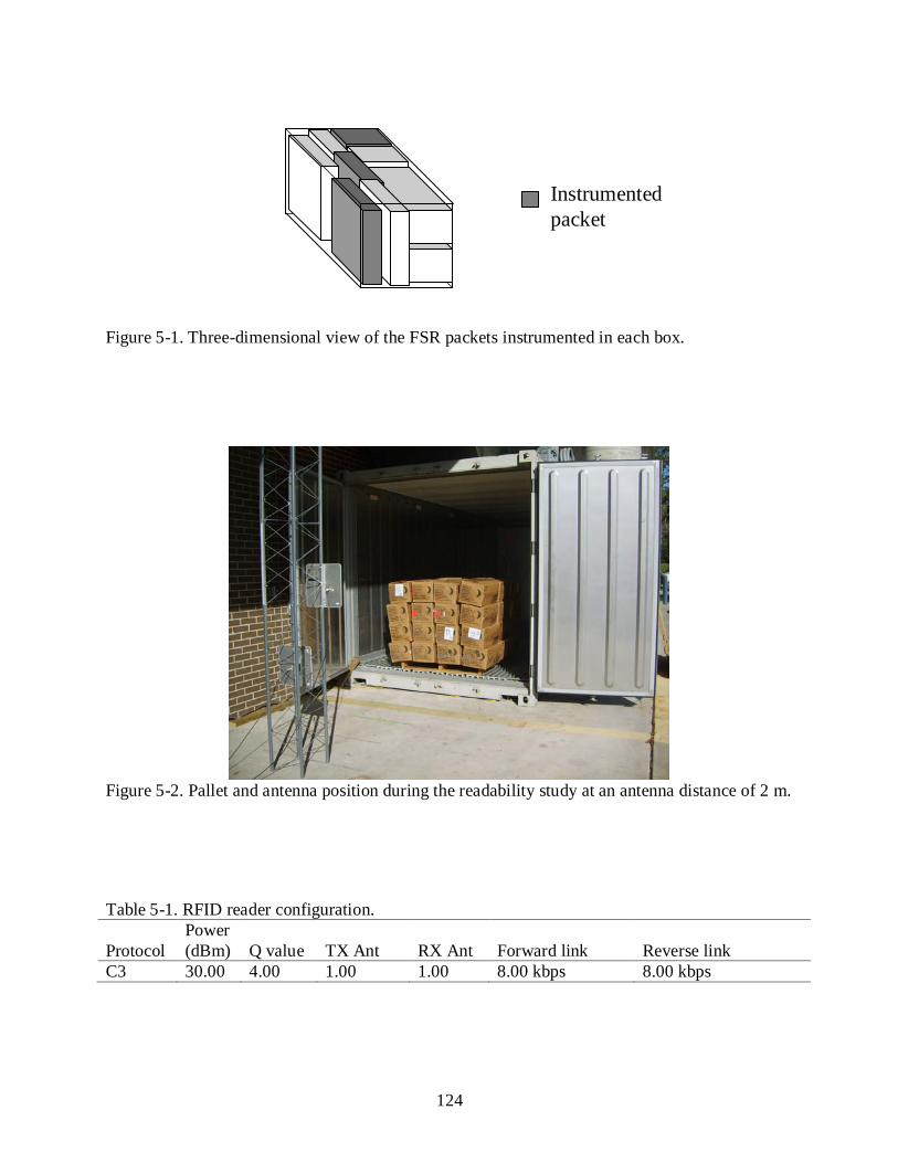
124
Figure 5-1. Three-dimensional view of the FSR packets instrumented in each box.
Figure 5-2. Pallet and antenna position during the readability study at an antenna distance of 2 m.
Table 5-1. RFID reader configuration.
Protocol Power (dBm) Q value TX Ant RX Ant Forward link Reverse link
C3 30.00 4.00 1.00 1.00 8.00 kbps 8.00 kbps
Instrumented packet
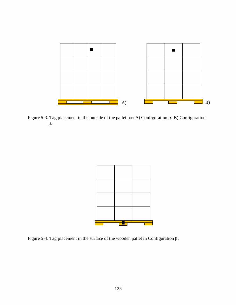
125
Figure 5-3. Tag placement in the outside of the pallet for: A) Configuration α. B) Configuration β.
Figure 5-4. Tag placement in the surface of the wooden pallet in Configuration β.
A) B)
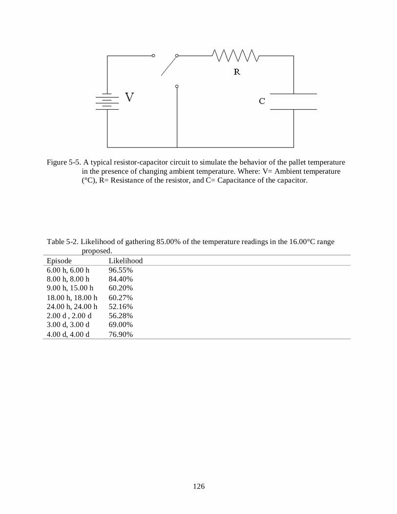
126
Figure 5-5. A typical resistor-capacitor circuit to simulate the behavior of the pallet temperature in the presence of changing ambient temperature. Where: V= Ambient temperature (°C), R= Resistance of the resistor, and C= Capacitance of the capacitor.
Table 5-2. Likelihood of gathering 85.00% of the temperature readings in the 16.00°C range
proposed. Episode Likelihood 6.00 h, 6.00 h 96.55% 8.00 h, 8.00 h 84.40% 9.00 h, 15.00 h 60.20% 18.00 h, 18.00 h 60.27% 24.00 h, 24.00 h 52.16% 2.00 d , 2.00 d 56.28% 3.00 d, 3.00 d 69.00% 4.00 d, 4.00 d 76.90%

127
Figure 5-6. Locations of the Points of Relevance (PoR) detected in the pallet.
Table 5-3. Likelihood of gathering 85.00% of the temperature readings in the 16.00°C range
proposed when using the Points of Relevance (PoR) found as the interval’s middle points.
Episode Point A Point B 6.00 h, 6.00 h 72.58% 85.23% 8.00 h, 8.00 h 41.24% 35.00% 9.00 h, 15.00 h 63.41% 74.78% 18.00 h, 18.00 h 32.15% 48.58% 1.00 d, 1.00 d 23.87% 32.45% 2.00 d, 2.00 d 49.89% 44.76% 3.00 d, 3.00 d 42.32% 32.27% 4.00 d, 4.00 d 58.07% 43.11%
B
A
X
Y
Z
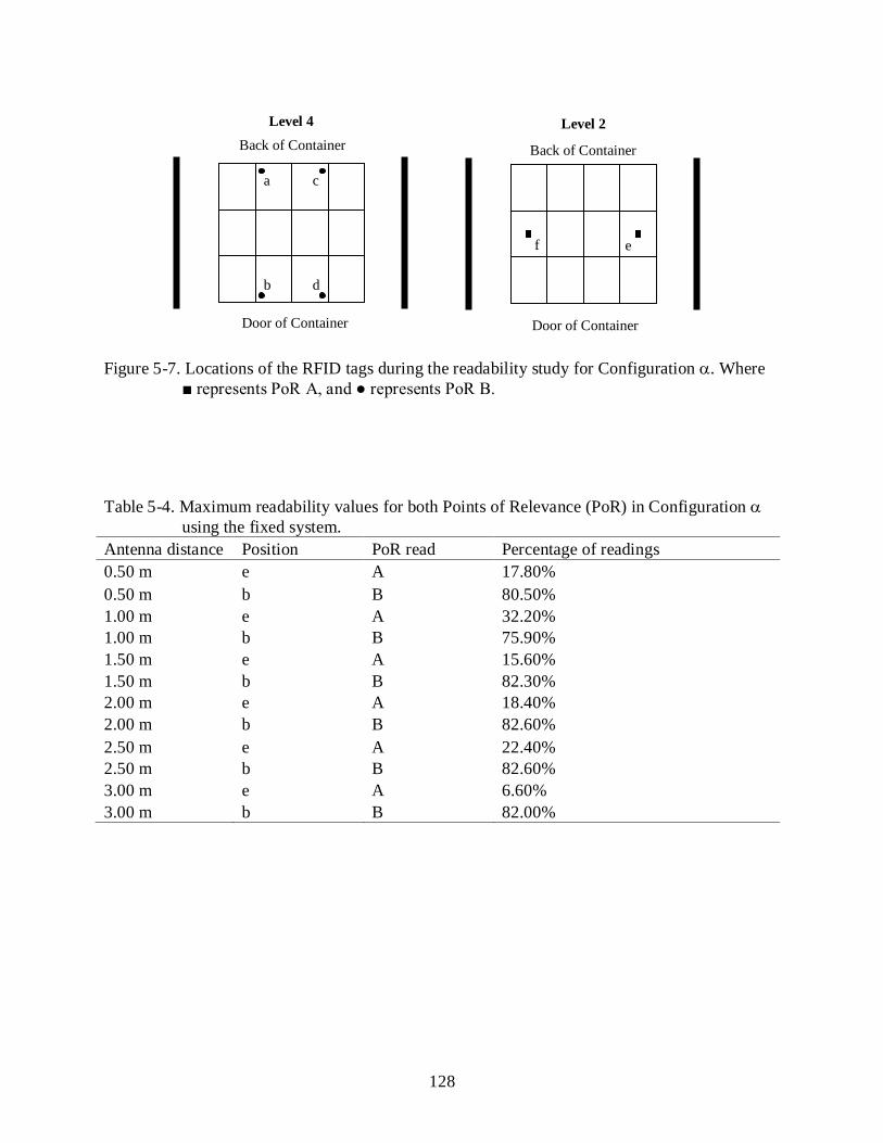
128
Figure 5-7. Locations of the RFID tags during the readability study for Configuration α. Where represents PoR A, and represents PoR B.
Table 5-4. Maximum readability values for both Points of Relevance (PoR) in Configuration α
using the fixed system. Antenna distance Position PoR read Percentage of readings 0.50 m e A 17.80% 0.50 m b B 80.50% 1.00 m e A 32.20% 1.00 m b B 75.90% 1.50 m e A 15.60% 1.50 m b B 82.30% 2.00 m e A 18.40% 2.00 m b B 82.60% 2.50 m e A 22.40% 2.50 m b B 82.60% 3.00 m e A 6.60% 3.00 m b B 82.00%
f e
Door of Container
Back of Container
Level 2
b d
a c
Door of Container
Back of Container
Level 4

129
Table 5-5. Maximum readability values for both Points of Relevance (PoR) in Configuration β using the fixed system.
Antenna distance Position PoR read Percentage of readings 0.50 m e A 69.50% 0.50 m c B 47.80% 1.00 m e A 52.40% 1.00 m c B 69.40% 1.50 m e A 45.00% 1.50 m c B 78.40% 2.00 m e A 70.50% 2.00 m c B 88.10% 2.50 m e A 28.50% 2.50 m c B 68.80% 3.00 m e A 25.60% 3.00 m c B 74.90%
Table 5-6. Readability values using the fixed system of positions “b” and “c” throughout the pallet.
Configuration Position Percentage of readings α b 82.00% α c 62.60% β b 32.60% β c 74.90%
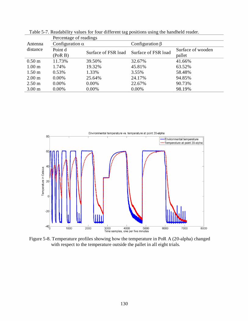
130
Table 5-7. Readability values for four different tag positions using the handheld reader.
Antenna distance
Percentage of readings Configuration α Configuration β Point d (PoR B) Surface of FSR load Surface of FSR load Surface of wooden
pallet 0.50 m 11.73% 39.50% 32.67% 41.66% 1.00 m 1.74% 19.32% 45.81% 63.52% 1.50 m 0.53% 1.33% 3.55% 58.48% 2.00 m 0.00% 25.64% 24.17% 94.85% 2.50 m 0.00% 0.00% 22.67% 90.73% 3.00 m 0.00% 0.00% 0.00% 98.19%
Figure 5-8. Temperature profiles showing how the temperature in PoR A (20-alpha) changed
with respect to the temperature outside the pallet in all eight trials.

131
Figure 5-9. Temperature profiles showing how the temperature in PoR B (36-prime) changed with the temperature outside the pallet in all eight trials.
Figure 5-10. Comparison of ambient temperatures, temperatures measured in PoR A and the estimated pallet temperatures for PoR A (point 20-alpha).

132
Figure 5-11. Comparison of ambient temperatures, temperatures measured in PoR B and the estimated temperatures for PoR B (point 36-prime).
133
CHAPTER 6 DEVELOPMENT OF A LOAD MANAGEMENT SYSTEM FOR COMBAT FEEDING
LOGISTICS BASED ON SHELF-LIFE PREDICTION SOFTWARE
Introduction
Combat feeding during military campaigns has represented a challenge for armies
throughout history. The lack of refrigeration and the possibility of limited food supply in the
field have driven some of the biggest developments in food conservation and processing; the
most remarkable being canning. During the last fifty years, technological efforts have been
aimed towards developing safe and nutritious foods able to withstand the rigorous aspects of
military supply chains. And so, in 1993 the U.S. Department of Defense (DoD) created a
successful set of meal-based shelf-stable products named Meals, Ready-to-Eat (MRE) able to
defy most of the time and temperature limitations existent in food distribution and storage, and
suitable for their logistics.
Sometime after their introduction, feedback from the field indicated that soldiers were
opening the MRE packs, and only taking with them and eating certain elements of these in order
to reduce the amount of weight carried. This not only generated big amounts of food waste, but
also endangered the nutritional status of the troops. A new shelf-stable product called First Strike
Rations (FSR) was then designed to take on the place of MREs in assault operations. With it,
Warfighters could bring a lightweight load with enough food to fulfill their nutritional
requirements for a whole day during fast-paced maneuvers (DoD Live, 2009).
A First Strike Ration (FSR), although shelf-stable, will still deteriorate faster if its storage
temperature of 26.67°C has been exceeded (DoD Live, 2009). Exposure to high temperatures
accelerates negative changes in the meals’ sensory attributes, which influence its level of
acceptability. In addition, storage of FSRs under these environmental conditions could affect
adversely the health status of the troops, by promoting nutritional changes, and the growth of

134
spoilage and pathogenic microorganisms in their meals (Ross et al., 1985; Ross et al., 1987;
Banwart, 1989; Narayan et al., 1997; Ross et al., 1997; Shaw et al., 1997; Ng et al., 2002;
Natress et al., 2009). Consequently, high temperature abuse will diminish the shelf-life of FSRs
and, in some cases, significantly.
Since the majority of current U.S. military operations takes place in desert areas where
high temperatures are reached and the loads of FSRs do not move along environmentally
controlled supply chains, there are many opportunities for high temperature abuse. In the
previous chapter the use of RFID temperature tracking systems as a way of monitoring the
conditions of these loads and detecting thermal abuse was proposed. However, during fast-paced
military deployments, the data collected in these could be difficult to decipher; since the
temperature profiles recorded are by no means a stand alone indicative of the remaining shelf-life
of the product. Therefore, a load management system that uses a software tool able to decode
such data, providing intelligible information about the shelf-life status of the product and giving
recommendations on the actions required with respect to the load is needed.
The main step in the creation of such software is the selection of an appropriate model for
the prediction of the FSR’s shelf-life. There have been a number of studies on modeling the
shelf-life of food products. Many of them are based in variations of the Arrhenius equation,
which describes the kinetics of simple chemical reactions as dependant on temperature
conditions (Hertog et al., 1999; Brody, 2003; Giannakourou and Taoukis, 2003; Hough et al.,
2006). Also popular is the use of predictive microbiology models, such as the Gompertz
equation, as a mean of determining the deterioration and safety thresholds limiting shelf-life
(Labuza and Fu, 1993; Zwietering et al., 1993; McMeekin and Ross, 1996; Riva et al., 2001;
Corbo et al., 2006). Less common are empirical models, which are built upon experimental data
135
obtained in the laboratory setting (Wilcke, 1992; Jacxsens et al., 2002; Nunes et al., 2004).
According to van Boekel (2008), these models are able to describe closely complicated
temperature-dependent reactions existing in food within the parameter region on which they are
based. Given the variety of the nature of products inside FSRs and the complexity of the
reactions existent within them, an empirical model would then be the best option for shelf-life
prediction.
The application of the load management system proposed also relies in the quality of the
temperature data collected. Taking into account the sampling methodologies previously
developed for this particular supply chain in the last chapter, it is necessary to determine whether
variations in the sensor locations proposed in these will alter the shelf-life estimations. Likewise,
it is also important for the system to determine whether the pallet is changing its shelf-life
uniformly or if some of its contents (meals) are doing so at a higher rate than others.
The objectives of this research were: 1) Developing software able to predict the shelf-life
of pallets of FSRs under current supply chain environmental conditions. 2) To establish the
maximum amount of weeks of shelf-life possible for FSRs during storage in the deployment
areas in a real-life case. 3) To determine whether there are significant differences in the predicted
acceptability scores when comparing three kinds of FSR meals. 4) To determine whether there
are significant differences in the predicted acceptability scores of FSRs when comparing
temperature sampling locations in the pallet.
Materials and Methods
Development of the Software
The first step in the development of the software was collecting the information necessary
in order to create the shelf-life prediction models. Since all boxes present in the pallet of FSR
studied contained the same three menu options, each menu was analyzed in order to determine
136
which one of its items deteriorated faster. These would then be considered the shelf-life limiting
items (SLLI) for the pallet. The following were the results of this preliminary testing (Nunes et
al., 2010, unpublished data): In Menu 1, the SLLI was the Bacon Cheddar Sandwich; in Menu 2,
the Italian Style Sandwich; and in Menu 3, the Zapplesauce.
These products were then subjected to controlled storage at two different temperatures
(48.89°C or 120.00°F, and 60.00°C or 140.00°F). Since the easiest way to determine the shelf-
life of the product during a real-life military deployment is the level of acceptability for
consumption, this attribute would then be considered in the model as the limiting quality factor
in the shelf-life of FSRs. Thus, sensory analysis was performed on each product/temperature
combination at different storage times. The scale for the acceptability evaluations was from 1 to
9; being 1 the worst acceptability score and 9 the best acceptability score. A score of 4 was
considered the limit value of acceptability fit for consumption.
Curves were then created when plotting the acceptability for consumption versus the weeks
of storage. For each temperature, the resulting curve was fitted into a third order polynomial
equation.
A third curve was built for all products in order to describe the deterioration behavior of
these at their ideal storage temperature of 26.67°C (80.00°F). Due to the fact that similar storage
tests under this temperature were not finished by the time of the completion of this study, it was
assumed that each product started with an initial quality equal to the average initial quality they
presented for the first two temperatures considered. It was also assumed that the limit of
acceptability of consumption for all products (a score equal to 4.00) was reached at 104.00
weeks (2.00 years) of storage under 26.67°C (80.00°F). Given that only the initial and final
acceptability values were given, the resulting curves were only first order polynomial curves.

137
The software was then designed by integrating the resulting relationships into a task
automating system called macro within the Microsoft® Visual Basic (Microsoft Corporation,
Redmond, Washington, 1975-2010) platform. The inputs for the program were the initial
acceptability scores of each one of the menus (also referred to as initial quality scores), the
number of temperature data points collected along the shipment, and their corresponding
temperatures in degrees Fahrenheit. Since the temperature profiles for combat feeding logistics
provided by the U.S. Department of Defense contained only one data point per day, the number
of data points in the software equaled the number of days when temperature information was
collected.
The rationale behind the model is as follows. For each product, the system estimates the
time value corresponding to the initial quality score along each one of the set curves (26.70°C,
48.89°C and 60.00°C). It then adds up the amount of time passed between the data points (in this
example, one day) and estimates the acceptability score related to that new time in the set curves.
The resulting quality score after subjecting the product to a certain period of time at the initial
temperature will be calculated by interpolating between the acceptability values given at 26.70°C
(80.00°F) and 48.89°C (120.00°F), if the initial temperature is between them; or between
48.89°C (120.00°F) and 60.00°C (140.00°F) if the temperature falls within this range. This is the
final acceptability score for that data point, and it will be used as the initial quality for the next
iteration.
Once all iterations are completed and the last acceptability value has been estimated for
each product; the system provides these as outputs. In addition, it also averages these final
quality scores and provides an average acceptability for the pallet. Finally, depending on the
status of this particular value with respect to the minimum acceptability level for consumption
138
for all products (4.00), a window displays “Pass” or “Discard” indicating the required action
regarding the pallet.
Application of the Shelf-Life Software
Ambient temperature profiles were developed using the information collected in previous
trials performed by the U.S. Department of Defense (DoD) on shipments from the U.S. to
Kuwait. A temperature profile was created based on worst-case scenario ambient conditions
recorded during those trials. This was generated by taking the maximum temperatures registered
in 17 non-refrigerated sea containers during 39.00 days where environmental monitoring of the
shipment and storage periods was performed.
Additionally, two other temperature profiles were developed also for ambient
temperatures. All of them had as initial input the temperature profile described before plus one or
two extra weeks of data of hypothetical temperature information corresponding to the storage
phase in the Middle East. These data points were created by repeating in each week the
temperatures obtained originally in the trials under this storage stage.
The following is the description of the ambient temperature profiles created:
• Profile 1: Original shipment information (storage in the US + marine shipment + 1.00 week of storage in the Middle East).
• Profile 2: Original shipment information + 1.00 week of storage in the Middle East.
• Profile 3: Original shipment information + 2.00 weeks of storage in the Middle East.
All ambient temperature profiles were assumed to be recorded in the outside wall of the
pallet; in the first location considered for the temperature sensor. The second and third sensor
positions corresponded to the locations of the Points of Relevance (PoR) A and B from the
research work described in the previous chapter.

139
Temperature profiles for PoR A and B were then obtained by entering the three
temperature profiles corresponding to the ambient conditions into the temperature profile
estimator presented in the aforementioned study.
Once all temperature profiles were estimated, these were entered into the software
individually. For all cases, the system was set up using as initial quality values the initial
acceptability scores obtained by the Shelf-Life Limiting Items in the sensory analysis employed
for the development of the model (7.85 for Menu 1; 7.90 for Menu 2; and 8.00 for Menu 3).
Once run, the resulting information was collected.
Statistical Analysis
The normality of the data was verified with the Anderson-Darling test. A Generalized
Linear Model (GLM) with a Gaussian family was used in order to determine the effects of the
position of the temperature sensor and the kind of meal studied (Freund and Wilson, 2003). It
was also used to determine the equality of means of the acceptability score predictions obtained
with the different combinations of sensor positions and meals. Significance was accepted at level
α=0.05. Statistical analyses were computed using R 2.7.2 (The R Foundation for Statistical
Computing., Wiedner Hauptstrabe 8-10/1071 1040 Vienna, Austria).
Results and Discussion
Development of the Software
The model used to construct the software was developed based in a set of equations
relating acceptability scores and time at different temperatures for each one of the SLLIs. Table
6-1 summarizes these relationships and their coefficients of determination (R2).
As can be seen, most of the equations presented had coefficients of determination close to
one; which indicates that the results obtained with these relationships were very close to the
original input data coming from sensory analysis.

140
In the case of the fitting curves for 26.67°C (80.00°F), the lack of experimental data points
could be promoting the simplification of a more complex polynomial relationship into only a
first order polynomial equation. So, the model estimations for temperatures within the 26.67°C
(80.00°F) and 48.89°C (120.00°F) range could have a certain level of inaccuracy. Yet, once the
experimental data is available and the resulting curve is subjected to regression, this software
could be easily updated for model improvement.
The best way to determine whether the current or future versions of this software are
indeed accurate is by validating the model. This would allow a comparison of the calculated
acceptability scores versus the ones obtained by sensory evaluations in product subjected to a
particular temperature profile during a real-life supply chain. Anderson (2010) used this
methodology as a tool for concluding that empirical models are better suited for shelf-life
prediction than theoretical models in sweet corn cold chains. Likewise, this process could assist
in the determination of errors and minimization of them in this software; and thus it is necessary
as future work.
In addition, a feature indicating the amount of shelf-life in weeks left in the pallet given the
latest temperature pattern could be particularly useful in the field; and should also be pursued in
the future.
Finally, Figures 6-1 and 6-2 present the two recommendation scenarios in the final
software product.
Maximum Amount of Weeks of Shelf-Life at the Deployment Areas
The results indicate that for all sensor positions, all the meals in the pallet of FSR have less
than three weeks of shelf-life at storage conditions in the deployment area (Table 6-2). Thus, in
order to avoid any risks, it would be recommended to distribute and consume the entire product
present in the load around the two week period, when all products are still over the acceptability
141
threshold score of four. An optimization could be made in order to determine the particular
amount of days of shelf-life (within 14.00 and 21.00), but it was considered more appropriate, to
facilitate the load handling in-situ, giving the recommendations to the Warfighters in weeks.
It is important to remark that the temperature profile employed was the worst case scenario
in the set of shipments studied previously by the DoD. Within these shipments there was a high
level of variability in the temperature profiles recorded depending on the position of the
container on the ship and the position of the sensor inside the container. So, even under similar
environmental conditions, the level of variability in temperature profiles was wide and thus,
possibly the acceptability scores of the load and its expected shelf-life.
In addition, these shelf-life results could differ considerably according to the weather
patterns. For example, if in real-life the temperatures increase more than the ones used in this
simulation; then, the product will probably have less acceptability scores than the ones obtained,
and could also reach its acceptability threshold after just one or two weeks of storage at the
deployment area. Since the temperature profiles provided by the DoD correspond to operations
in the months of September and October, it is expected that the shelf-life of the load gets reduced
during the months of July and August, at the peak of the summer. Likewise, if the ambient
temperatures are lower, the amount of shelf-life of the product could be extended, particularly
during the winter and fall months.
Therefore, given the high level of variability in temperature profiles and environmental
conditions, it is important to perform this kind of shelf-life analysis for every single shipment
received throughout the year.
Differences between Acceptability Estimates for FSR Meals
Table 6-3 shows the averages and standard deviations of the three meals combined for each
one of the ambient temperature profiles and its related profiles. As can be seen, standard
142
deviation values are between the range of ±0.11 and ±0.26. These values increase with respect to
the amount of time spent in storage at the deployment area, which is probably related to the
acceleration of the products’ degradation rates at increased amounts of high temperature abuse.
Statistical analysis of all the profiles shows that there are no significant differences
between the acceptability scores for FSR Meals for all sensor positions (P = 0.65; P=0.76;
P=0.58). Tables 6-4, 6-5 and 6-6 summarize the GLM Analysis performed when using as input
for the model Profiles 1, 2 and 3 and their related profiles for PoRs A and B.
These results imply that the degradation of the acceptability in the load takes place
uniformly. Thus, using an average of the final acceptability scores of the three meals is a viable
option to indicate the overall state of the pallet.
Differences between Acceptability Estimates at Different Sensor Locations
When analyzing the resulting data of combining the acceptability scores of all the
temperature profiles obtained at different sensor positions given a particular ambient temperature
profile (Table 6-7), it is very clear that the levels of variability of their original scores were very
low. The standard deviations in this case range from ±0.01 to ±0.02.
Further statistical analysis (Tables 6-4, 6-5, and 6-6) using a Generalized Linear Model
shows that there are no significant differences between the acceptability scores obtained when
placing the temperature sensor in the three different locations studied. This means that with
regards to shelf-life estimations, placing the sensor outside the pallet recording ambient
temperature is the same as recording product temperature inside the pallet at the points of
relevance A and B. As was found in the previous chapter, working with these two locations
allowed a thermally relevant instrumentation, where most of the temperatures in the pallet were
represented.

143
This finding creates a strong practical implication for the military, since it would reduce
considerably their instrumentation times and labor costs at the warehouse stage given that instead
of setting up the sensors inside the loads, they can just place these on the surface of them.
Moreover, when using RFID sensors, installing them on the outside of the pallet will increase the
readability of the tag and reduce the negative effects of the interactions between the
radiofrequency waves and the metallic packaging of the FSRs; facilitating their initial
programming and the data retrieval process at the receiving end.
Yet, before implementing a sampling system using ambient temperatures, these results
should be repeated using a full set of data points with smaller data collection intervals. Since the
temperature profiles available for this study had only one daily reading, the temperature profile
estimator used to develop the curves corresponding to PoR A and B used this as the timeframe
for the heat transfer process inside the pallet. However, data with smaller collection intervals
could provide a more dynamic idea of the temperature change process and take into account
other temperature variations along the day that might modify the initial resulting temperature
profiles for both relevant points. Consequently, it is necessary further research to determine if
this phenomenon would change the final acceptability scores of the load and if this will have a
negative or positive effect on the current estimates.
Conclusions
A load management system for First Strike Rations that uses a software tool able to
provide recommendations on the actions required with respect to the load and acceptability
scores based on shelf-life prediction models and the temperature history of the shipment was
developed. This was applied given a real-life temperature profile and it was found that the pallets
corresponding to that shipment had less than three weeks of shelf-life during their storage at the
deployment area. In addition, it was determined that using an average of the final acceptability

144
scores of the three meals as an indication of the overall state of the pallet is viable. Finally, it was
established that relevant temperature sampling for shelf-life prediction purposes can take place
outside the pallet.

145
Figure 6-1. Screenshot of the final shelf-life prediction software recommending passing the load.
Figure 6-2. Screenshot of the final shelf-life prediction software recommending rejecting the
load.

146
Table 6-1. Fitting curves describing the acceptability of the shelf-life limiting items as a function of time at three different temperatures. Where “y” is the acceptability score and “x” is the amount of time spent at a particular temperature.
Menu Shelf-life limiting item (SLLI) Temperature (ºC) Equation R2 1 Bacon Cheddar Sandwich 26.67 y = -0.037x + 7.85 1.000 2 Italian Style Sandwich 26.67 y = -0.037x + 7.85 1.000 3 Zapplesauce 26.67 y = -0.037x + 7.85 1.000 1 Bacon Cheddar Sandwich 48.89 y = -0.0345x3 + 0.3248x2 - 1.3912x + 7.9255 1.000 2 Italian Style Sandwich 48.89 y = -0.0174x3 + 0.1936x2 - 1.2079x + 7.9353 1.000 3 Zapplesauce 48.89 y = -0.0055x3 + 0.1374x2 - 1.3228x + 7.95 1.000 1 Bacon Cheddar Sandwich 60.00 y = -0.104x3 + 1.0545x2 - 3.7997x + 7.7235 0.989 2 Italian Style Sandwich 60.00 y = -0.0681x3 + 0.7681x2 - 3.2935x + 7.8207 0.999 3 Zapplesauce 60.00 y = -0.1197x3 + 1.2223x2 - 4.1828x + 7.8832 0.990 Table 6-2. Final acceptability score predicted by the software.
Sensor location
Profile 1 Profile 2 Profile 3 Meal 1 Meal 2 Meal 3 Pallet Meal 1 Meal 2 Meal 3 Pallet Meal 1 Meal 2 Meal 3 Pallet
Environment 5.49 5.56 5.34 5.46 4.52 4.70 4.36 4.53 3.37 3.87 3.75 3.66 Point A 5.53 5.59 5.36 5.49 4.56 4.72 4.38 4.55 3.40 3.89 3.76 3.68 Point B 5.53 5.59 5.36 5.49 4.56 4.72 4.38 4.55 3.40 3.89 3.76 3.68 Action Pass Pass Pass Pass Pass Pass Pass Pass Discard Discard Discard Discard
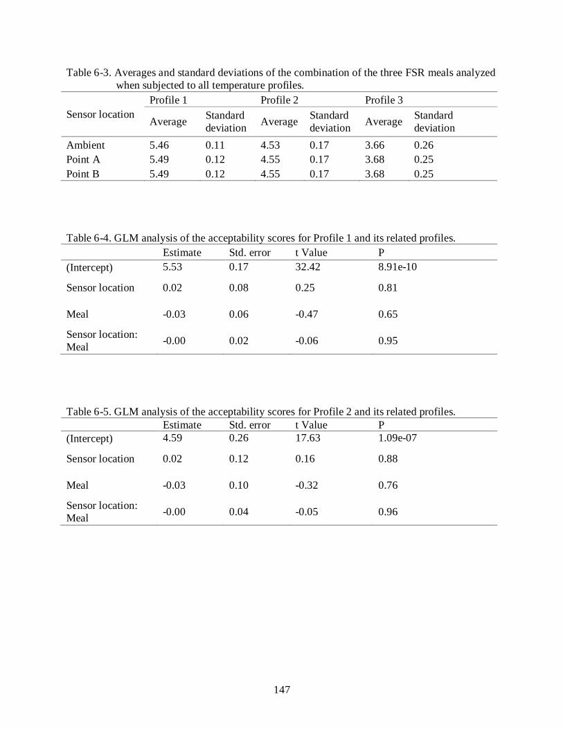
147
Table 6-3. Averages and standard deviations of the combination of the three FSR meals analyzed when subjected to all temperature profiles.
Sensor location Profile 1 Profile 2 Profile 3
Average Standard deviation Average Standard
deviation Average Standard deviation
Ambient 5.46 0.11 4.53 0.17 3.66 0.26 Point A 5.49 0.12 4.55 0.17 3.68 0.25 Point B 5.49 0.12 4.55 0.17 3.68 0.25 Table 6-4. GLM analysis of the acceptability scores for Profile 1 and its related profiles. Estimate Std. error t Value P (Intercept) 5.53 0.17 32.42 8.91e-10
Sensor location 0.02 0.08 0.25 0.81
Meal -0.03 0.06 -0.47 0.65
Sensor location: Meal -0.00 0.02 -0.06 0.95
Table 6-5. GLM analysis of the acceptability scores for Profile 2 and its related profiles. Estimate Std. error t Value P (Intercept) 4.59 0.26 17.63 1.09e-07
Sensor location 0.02 0.12 0.16 0.88
Meal -0.03 0.10 -0.32 0.76
Sensor location: Meal -0.00 0.04 -0.05 0.96

148
Table 6-6. GLM analysis of the acceptability scores for Profile 3 and its related profiles. Estimate Std. error t Value P (Intercept) 3.46 0.36 9.43 1.31e-05
Sensor location 0.02 0.17 0.10 0.92
Meal 0.08 0.13 0.57 0.58
Sensor location: Meal -0.00 0.06 -0.04 0.97
Table 6-7. Averages and standard deviations for each meal when combining the three temperature profiles analyzed.
Profile 1 Profile 2 Profile 3 Meal 1 Meal 2 Meal 3 Meal 1 Meal 2 Meal 3 Meal 1 Meal 2 Meal 3
Average 5.52 5.58 5.35 4.55 4.71 4.37 3.39 3.88 3.75 Standard deviation 0.02 0.02 0.01 0.02 0.01 0.01 0.02 0.01 0.01
149
CHAPTER 7 RETURN ON INVESTMENT (ROI) DETERMINATION FOR THE DEPLOYMENT OF A
RFID-BASED LOAD MANAGEMENT SYSTEM IN COMBAT FEEDING LOGISTICS
Introduction
The particularities of dealing with perishable inventory have been studied for many years
(Nahmias, 1982; Goyal and Giri, 2001; Bogataj et al., 2005; Ferguson and Ketzenberg, 2006).
RFID has been recently suggested as a new tool for obtaining operational efficiencies in the
supply chains of perishables as a mean of obtaining stock level transparency and improving the
application of inventory retrieval policies such as “First In First Out” (FIFO) and “Last In First
Out” (LIFO) (Kärkkäinen, 2003; Chande et al., 2005; Broekmeulen and van Donselaar, 2007).
However, the need for combining this information with the thermal history of the load due to
safety and quality concerns (Giannakourou and Taoukis, 2003; Sahin et al., 2007) opened the
door for the application of sensor-enabled RFID tags and the possibility of sorting the products
based on the amount of thermal abuse suffered during the supply chain and its impact in product
quality (Ilic et al., 2009).
Consequently, it has been suggested empowering RFID temperature tracking systems with
shelf-life prediction models in order to improve sorting at the distribution center and store level
(Emond and Nicometo, 2006; Jedermann et al., 2008; Ilic et al., 2009). Based on the shelf-life
information collected for each pallet or load, FIFO and LIFO could be replaced by a “First
Expired First Out” (FEFO) retrieval policy, that reduces the economic loss and quality and safety
concerns generated by handling expired product in the supply chain.
In the previous chapters, a relevant and feasible instrumentation protocol for RFID
environmental monitoring of First Strike Rations (FSR) logistics was created; and the resulting
RFID temperature tracking system has been combined with shelf-life models in order to build a
load management system. The aim of this system is achieving a FEFO management of the FSR

150
inventory based upon the product’s acceptability values in two combat zones: Iraq and
Afghanistan. It is believed that if applied, the FSR loss generated by thermal abuse during pallet
transport will be reduced and great savings will be achieved. However, the costs of the
deployment of such system are considerable; hence, a proper economic analysis of the benefits
of this implementation must be performed in order to make the final decision with regards to its
application.
The objective of the research presented in this chapter was to develop the business case for
the deployment of a load management system for FSRs, resulting from the combination of RFID
temperature tracking and shelf-life prediction software, applied during combat feeding logistics
operations by determining its return on investment (ROI).
Return on Investment (ROI) Analysis
This analysis works within a five year time frame due to the fact that by that time,
improved RFID systems might be available and thus, an update of the whole proposed system
could be in order.
The suggested deployment implies the installation of 50 RFID stations along Afghanistan
and Iraq. Based on the current and future distribution of Warfighters in the field, it was
determined that thirty four of the work stations will be located in Afghanistan and sixteen in Iraq.
Estimation of RFID Deployment Costs
In order to determine the cost of the deployment, yearly cost analyses were performed.
During the initial year, the cost of numerous factors were included: The hardware and software
for each work station, the RFID tags, the backup hardware and software for all work stations,
maintenance and training, and integration costs. Most of the costs included in this study were
obtained from quotes from real companies; while some, such as the cost of the shelf-life
software, were estimated based on similar applications encountered in real-life situations.
151
The core of each work station included a hand-held RFID reader, a laptop computer and a
wireless Smart Label printer. The reader would then be used to read the tags placed in each pallet
of the container, collecting inventory information as well as providing shelf-life estimations for
those with temperature sensing capabilities. The information collected by the reader would later
on be broadcasted either through Bluetooth® or Wi-Fi 802.11 a/b/g to the laptop computer,
which would gather it and add this information to the back-end system of the U.S. Department of
Defense (DoD) through a secure internet connection. The wireless Smart Label printer would be
used as a back up system, in case any passive RFID tag used for inventory management traveling
with the shipment needs to be replaced due to damage or failure. Additionally, the printer would
create Smart Labels containing the approximate acceptability values of a pallet at the time of
arrival using the average acceptability scores of the load, whenever the pallet’s temperature
RFID tag suffers damage in transit. This action, although does not assure the proper use of the
information gathered and cannot aid in further data collection with respect to environmental
monitoring, provides more resources to the people in charge of distributing the meals, allowing
them to make a more informed decision.
Different kinds of software will be necessary in order to operate the work stations. Some of
those used in typical inventory management practices using wireless RFID readers have been
included, as well as the shelf-life prediction software developed in the previous chapter, the
drivers for the printer, and the program necessary for the creation of labels. Other software
applications necessary to link each work station and the data gathered in them with the back-end
system of the DoD are included in the price of the integration.
In addition, a five-year service plan for each reader offered by Motorola, that extends
normal wear and tear repair coverage to include accidental breakage of cracked plastics, broken
152
screens, keypads and more has also been added into the initial cost. Table 7-1 offers a detailed
description of the hardware and software related items needed for each work station and their
costs.
The cost of tags was estimated by adding the number of temperature tags needed for
temperature tracking plus a safety stock of 15.00% which would replace all the tags that
malfunction or are damaged before being deployed. Also included was the cost of the passive
tags used by the wireless printers in each work station (Table 7-2). It is important to mention that
the number of temperature tags required for temperature tracking was based on results that will
be reported later on in this document on the yearly demand for FSRs in Afghanistan and Iraq.
Also included in the initial investment was the purchase of backup hardware and software
which, as its name states, is available in case the ones deployed are inoperable or being subjected
to repairs. This cost was estimated to be 10.00% of the total initial hardware and software sales
price. System maintenance and employee training were calculated as 25.00% of this particular
price too; while the cost of integration was assumed to be 2.50 million dollars. Table 7-3 presents
the costs estimated for the first year of the project; which total around 3.9 million dollars.
There were three recurring costs present in every year of the analysis: The cost of tags, the
cost of maintenance and training and the cost of system replacement. This last factor gathered all
the expenses generated when changing damaged elements of the work stations permanently and
has been taken to be 25.00% of the initial cost for hardware and software for all work stations.
Two additional costs were taken into account for the beginning of years three and five: The
replacement of both reader and printer batteries. These need to be changed because of the end of
their lifespan after two years of activity. Table 7-4 presents the costs incurred at the beginning of
the second and fourth years of operation; while Table 7-5 shows the costs for the third and fifth
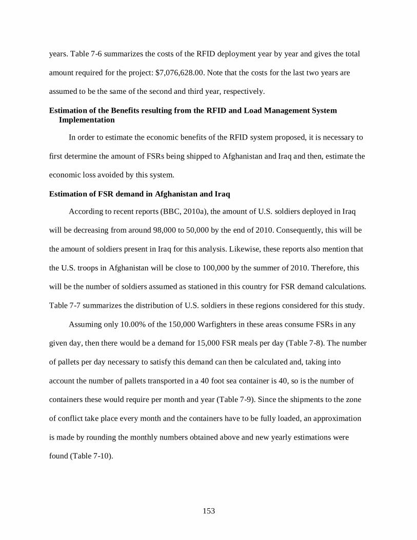
153
years. Table 7-6 summarizes the costs of the RFID deployment year by year and gives the total
amount required for the project: $7,076,628.00. Note that the costs for the last two years are
assumed to be the same of the second and third year, respectively.
Estimation of the Benefits resulting from the RFID and Load Management System Implementation
In order to estimate the economic benefits of the RFID system proposed, it is necessary to
first determine the amount of FSRs being shipped to Afghanistan and Iraq and then, estimate the
economic loss avoided by this system.
Estimation of FSR demand in Afghanistan and Iraq
According to recent reports (BBC, 2010a), the amount of U.S. soldiers deployed in Iraq
will be decreasing from around 98,000 to 50,000 by the end of 2010. Consequently, this will be
the amount of soldiers present in Iraq for this analysis. Likewise, these reports also mention that
the U.S. troops in Afghanistan will be close to 100,000 by the summer of 2010. Therefore, this
will be the number of soldiers assumed as stationed in this country for FSR demand calculations.
Table 7-7 summarizes the distribution of U.S. soldiers in these regions considered for this study.
Assuming only 10.00% of the 150,000 Warfighters in these areas consume FSRs in any
given day, then there would be a demand for 15,000 FSR meals per day (Table 7-8). The number
of pallets per day necessary to satisfy this demand can then be calculated and, taking into
account the number of pallets transported in a 40 foot sea container is 40, so is the number of
containers these would require per month and year (Table 7-9). Since the shipments to the zone
of conflict take place every month and the containers have to be fully loaded, an approximation
is made by rounding the monthly numbers obtained above and new yearly estimations were
found (Table 7-10).
154
Since military deployments of this magnitude require the use of safety factors for their
combat feeding operations in case there are any problems with their shipments, a 15.00% of the
total number of yearly containers was added in order to obtain the grand total of FSR pallet
demand (Table 7-10). The safety stock will be stored in areas of the field less prone to
temperature abuse, where conditions are favorable for the maintenance of product stability and
deterioration rates are reduced (i.e. in caves), and deployed whenever necessary to cover for
damaged product.
Estimation of FSR pallets lost to thermal abuse
The results obtained in the previous chapter indicate that, in one of the worst-case
scenarios of environmental conditions studied by the military (the profile used as the basis for
the shelf-life studies in Chapter 6), the handling of FSR containers allows a shelf-life of between
two and three weeks in these combat zones. Since transport between the port of Karachi
(Pakistan) towards Afghanistan and transport amongst the port of Umm Qasr in Iraq towards
other strategic areas in this country can take between three to eight days, an average of five days
will be taken as land transportation time in both cases. Therefore, based upon these assumptions,
the remaining shelf-life of the pallets once they have arrived to their destination will be of
approximately 1.5 weeks. Yet, this particular case is an extreme and does not represent a
common situation; so, an extra week of shelf-life will be considered as a way of accounting for
this factor. Consequently, the remaining shelf-life after the pallets have arrived to their final
destination will be considered of about 2.5 weeks. Since the shipment must last for a whole
month, some FSR pallets will have to be stored after this deadline, in order to be eaten during the
third and fourth week of the month. Yet, if the product is expired and is not suitable for
consumption, the load must be discarded, generating economic loss. So, if the pallets that would
be consumed during the last 1.5 weeks of the month have been thermally abused, about 37.5% of

155
the total monthly shipment could be classified as loss. However, since there is no certainty all of
them would be subjected to extreme environmental conditions, only half of this percentage
(18.75% of the total monthly pallet shipment) was taken into account as a conservative estimate
for pallet losses in the upcoming calculations.
Given the fact that even with the implementation of the load management system
suggested some pallets might still be deemed as lost due to exposure to extreme circumstances
during transit, the efficiency of the system has been considered only 50.00%. Table 7-11
summarizes the estimations of yearly pallet losses (pallets mishandled) and the resulting pallet
losses avoided once the proposed system is into place.
Estimation of the economic loss of the FSR pallets lost to thermal abuse
Two factors were taken into account in order to calculate this estimate. First, the cost of the
pallet of FSRs; and second, the cost of the maritime shipment from Philadelphia, PA to the two
receiving ports: Karachi in Pakistan (en route to Afghanistan) and Umm Qasr in Iraq. The cost of
land transportation and handling from these ports up to the final destinations was not included
due to the high variability existent in their locations given the nature of combat operations. Table
7-12 presents the estimation of the total costs of maritime shipment per pallet and container
according to the country of final reception. Finally, Table 7-13 shows the calculated economic
loss of a pallet sent to each one of the combat zones: $ 5,102.95 for Iraq and $ 5,069.26 for
Afghanistan.
Estimation of FSR pallets sent in emergency shipments
Since the number of pallets lost to thermal abuse surpass that of the safety stock,
emergency shipments with more FSRs are necessary in order to feed the troops once the initial
inventory has been depleted. Table 7-14 presents the amount of yearly containers devoted to this
purpose and Table 7-15 the amount of money allocated to yearly emergency shipments.

156
Estimation of the economic loss avoided by the load management system
The economic loss avoided by the proposed system will be the amount of money saved by
the DoD once this system is deployed. The calculations were done by multiplying the amount of
pallets that the system will allocate before expiration and prevent from becoming a loss with the
economic loss per pallet given its country of destination. Additional savings will derive from
eliminating the emergency shipments, since the resulting pallet loss levels after the
implementation of the system can easily be covered by the yearly FSR safety stock. Table 7-16
summarizes the results obtained. The aggregate for both items totals $11,761,779.72 per year;
and, consequently, the amount saved during the five years of its initial operation will reach
$58,808,898.63.
Return on Investment (ROI) Estimation
The ROI was determined by replacing the corresponding data in Equation 7-1. The current
discount rate given by the U.S. Federal Reserve (0.75%) was used for the calculations (Wall
Street Journal, 2010).
1
)1(
)1(
0
0 −
+
+=
∑
∑
=
=n
tt
n
tt
DVi
DVt
ROI (7-1)
Where Vi is the investment required by the project at the end of the time period t, Vt is the
monetary yield of the project at the end of time period t, n is the number of periods in the
analysis (5), t is the iterative time period; and D is the discount rate for the time value of money
(0.75%).
157
After performing the calculations, the return on investment of the project was estimated to
be 719.49%; which provided a solid financial reason for the project’s implementation.
Furthermore, the savings offered by the first year of operation of the system could pay for more
than all the costs of the deployment; allowing a net gain for the DoD during the next four years
of operation.
Conclusion
Based upon the business case presented, the deployment of a load management system for
combat feeding logistics founded on the combination of a RFID temperature tracking system
with shelf-life prediction software allows a return on investment of 719.49% during the initial
five years of operation; making its deployment a sound economic decision capable of generating
considerable amount of value in the supply chain.

158
Table 7-1. Hardware and software costs for each work station. Item Number of units Unit price Total price Reader Mc3090 Z reader 1.00 2647.10 $2,647.00 Lithium baterry pack (x2) 2.00 78.40 $157.00 4 Slot battery charger 1.00 140.00 $140.00 AC Line cord for power supplies 1.00 15.80 $16.00 Universal power supply 1.00 43.50 $44.00 Protective boot 3.00 6.00 $18.00 Holster 1.00 47.63 $48.00 Belt for holster 1.00 21.00 $21.00 Screen protectors 5.00 9.00 $45.00 Subtotal reader $3,135.00 Laptop computer HP Pavilion dv7t Select Edition series 1.00 949.99 $950.00 Subtotal laptop computer $950.00 Smart Label printer RP4T mobile printer 1.00 2566.00 $2,566.00 Vehicle charger 1.00 89.10 $89.00 Li-Ion quad charger for RP4T batteries 1.00 375.24 $375.00 Spare battery 1.00 160.00 $160.00 USB-A to PC cable 1.00 23.00 $23.00 Softcase 1.00 85.00 $85.00 Pinhead cleaning pens 3.00 40.00 $120.00 Subtotal Smart Label printer $3,418.00 Software Inventory management software 1.00 1590.00 $1,590.00 I/C Host interface 1.00 1495.00 $1,495.00 MJD nexus 1.00 995.00 $995.00 Shelf-life software 1.00 1600.00 $1,600.00 Label Vista software 1.00 69.00 $69.00 Zebra Designer Pro software 1.00 200.00 $200.00 Subtotal software $5,949.00 Other Service Pack for 5 years for MC3090 Z reader (Motorola) 1.00 613.20 $613.00 Subtotal other $613.00 Total $14,065.00

159
Table 7-2. Yearly costs of RFID tags. Tag Number of units/Year Unit price Total price Caen RFID - A927Z In transit 14880.00 25.00 $372,000.00 Safety stock 2232.00 25.00 $55,800.00 Subtotal Caen RFID -A927Z 17112.00 25.00 $427,800.00 Avery AD-233 Rolls x 1000 tags 50.00 200.00 $10,000.00 Subtotal Avery AD-233 $10,000.00 Total $437,800.00 Table 7-3. Cost of the project during the first year of operation. Item Number of units Unit price Total Work station hardware + software 50.00 $14,065.00 $703,268.00 Backup hardware + software $70,327.00 Maintenance + training $175,817.00 Tags $437,800.00 Integration $2,500,000.00 Total $3,887,212.00 Table 7-4. Cost of the project during the second and fourth year of operation. Item Total System replacement $175,817.00 Maintenance + training $175,817.00 Tags $437,800.00 Total $789,434.00
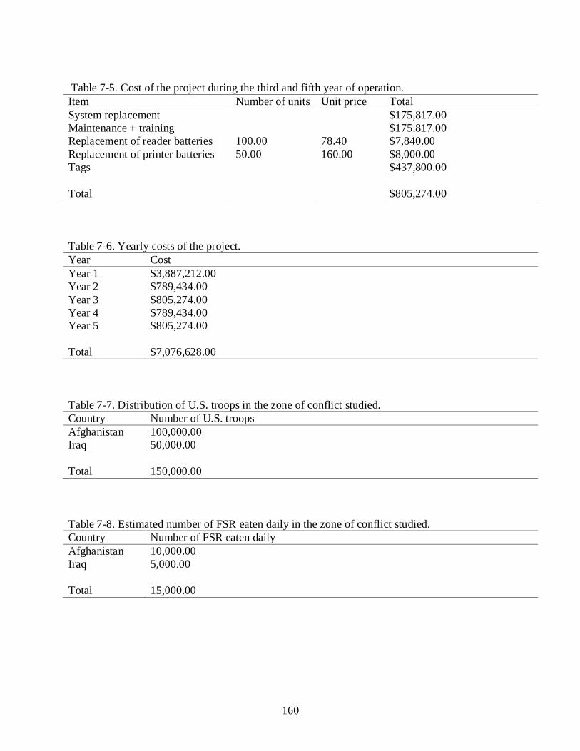
160
Table 7-5. Cost of the project during the third and fifth year of operation. Item Number of units Unit price Total System replacement $175,817.00 Maintenance + training $175,817.00 Replacement of reader batteries 100.00 78.40 $7,840.00 Replacement of printer batteries 50.00 160.00 $8,000.00 Tags $437,800.00 Total $805,274.00 Table 7-6. Yearly costs of the project. Year Cost Year 1 $3,887,212.00 Year 2 $789,434.00 Year 3 $805,274.00 Year 4 $789,434.00 Year 5 $805,274.00 Total $7,076,628.00 Table 7-7. Distribution of U.S. troops in the zone of conflict studied. Country Number of U.S. troops Afghanistan 100,000.00 Iraq 50,000.00 Total 150,000.00 Table 7-8. Estimated number of FSR eaten daily in the zone of conflict studied. Country Number of FSR eaten daily Afghanistan 10,000.00 Iraq 5,000.00 Total 15,000.00
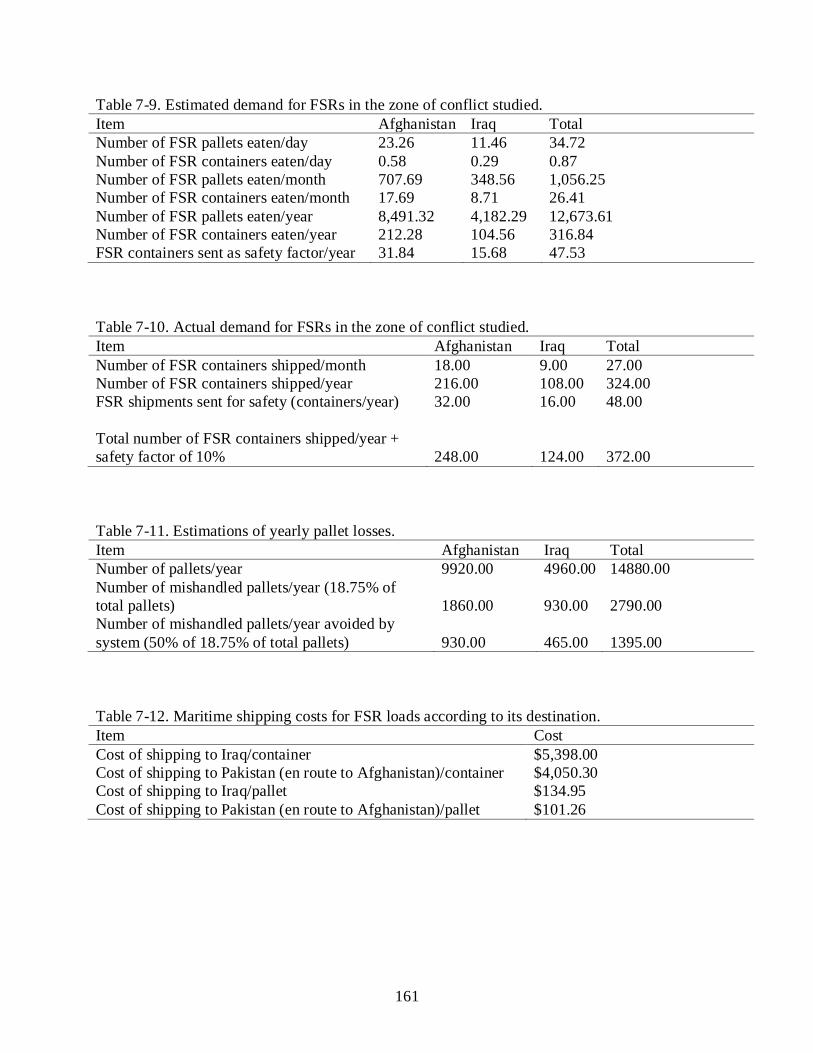
161
Table 7-9. Estimated demand for FSRs in the zone of conflict studied. Item Afghanistan Iraq Total Number of FSR pallets eaten/day 23.26 11.46 34.72 Number of FSR containers eaten/day 0.58 0.29 0.87 Number of FSR pallets eaten/month 707.69 348.56 1,056.25 Number of FSR containers eaten/month 17.69 8.71 26.41 Number of FSR pallets eaten/year 8,491.32 4,182.29 12,673.61 Number of FSR containers eaten/year 212.28 104.56 316.84 FSR containers sent as safety factor/year 31.84 15.68 47.53 Table 7-10. Actual demand for FSRs in the zone of conflict studied. Item Afghanistan Iraq Total Number of FSR containers shipped/month 18.00 9.00 27.00 Number of FSR containers shipped/year 216.00 108.00 324.00 FSR shipments sent for safety (containers/year) 32.00 16.00 48.00 Total number of FSR containers shipped/year + safety factor of 10% 248.00 124.00 372.00 Table 7-11. Estimations of yearly pallet losses. Item Afghanistan Iraq Total Number of pallets/year 9920.00 4960.00 14880.00 Number of mishandled pallets/year (18.75% of total pallets) 1860.00 930.00 2790.00 Number of mishandled pallets/year avoided by system (50% of 18.75% of total pallets) 930.00 465.00 1395.00 Table 7-12. Maritime shipping costs for FSR loads according to its destination. Item Cost Cost of shipping to Iraq/container $5,398.00 Cost of shipping to Pakistan (en route to Afghanistan)/container $4,050.30 Cost of shipping to Iraq/pallet $134.95 Cost of shipping to Pakistan (en route to Afghanistan)/pallet $101.26
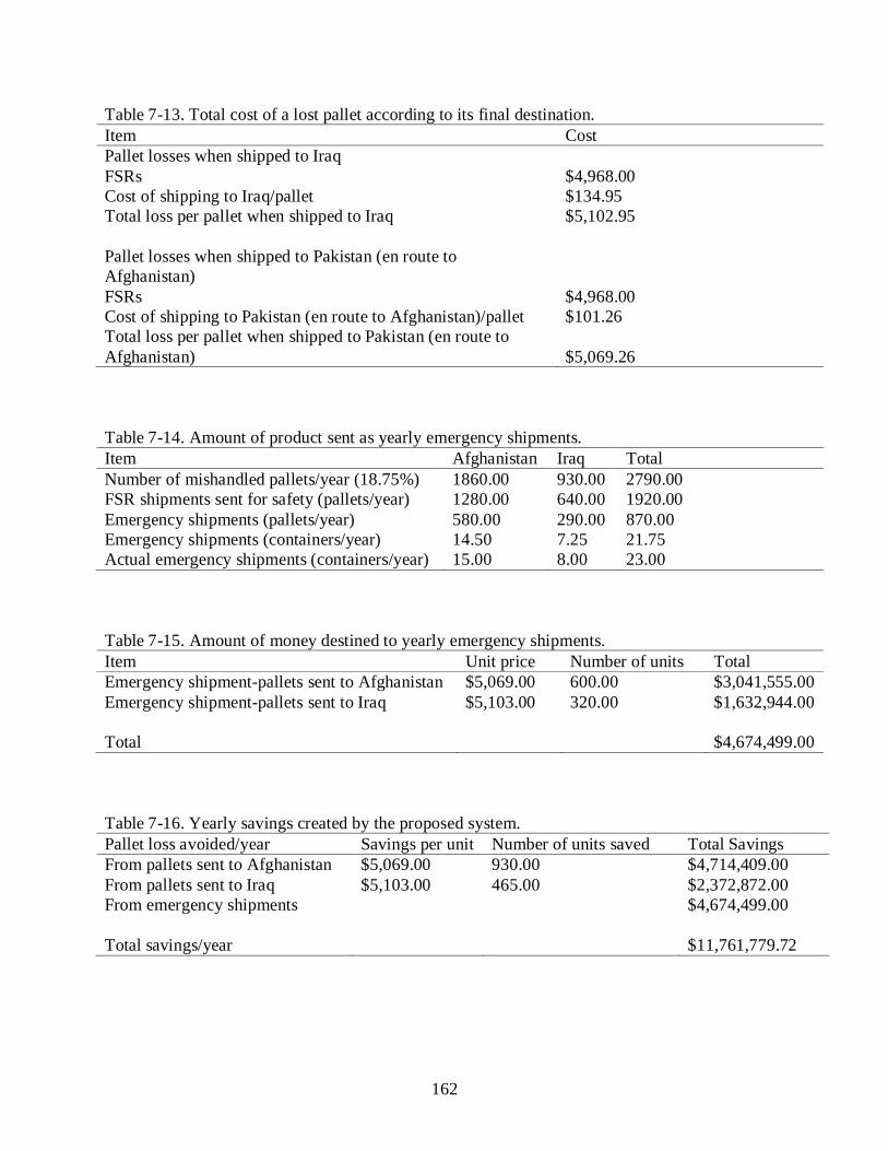
162
Table 7-13. Total cost of a lost pallet according to its final destination. Item Cost Pallet losses when shipped to Iraq FSRs $4,968.00 Cost of shipping to Iraq/pallet $134.95 Total loss per pallet when shipped to Iraq $5,102.95 Pallet losses when shipped to Pakistan (en route to Afghanistan) FSRs $4,968.00 Cost of shipping to Pakistan (en route to Afghanistan)/pallet $101.26 Total loss per pallet when shipped to Pakistan (en route to Afghanistan) $5,069.26 Table 7-14. Amount of product sent as yearly emergency shipments. Item Afghanistan Iraq Total Number of mishandled pallets/year (18.75%) 1860.00 930.00 2790.00 FSR shipments sent for safety (pallets/year) 1280.00 640.00 1920.00 Emergency shipments (pallets/year) 580.00 290.00 870.00 Emergency shipments (containers/year) 14.50 7.25 21.75 Actual emergency shipments (containers/year) 15.00 8.00 23.00 Table 7-15. Amount of money destined to yearly emergency shipments. Item Unit price Number of units Total Emergency shipment-pallets sent to Afghanistan $5,069.00 600.00 $3,041,555.00 Emergency shipment-pallets sent to Iraq $5,103.00 320.00 $1,632,944.00 Total $4,674,499.00 Table 7-16. Yearly savings created by the proposed system. Pallet loss avoided/year Savings per unit Number of units saved Total Savings From pallets sent to Afghanistan $5,069.00 930.00 $4,714,409.00 From pallets sent to Iraq $5,103.00 465.00 $2,372,872.00 From emergency shipments $4,674,499.00 Total savings/year $11,761,779.72

163
CHAPTER 8 CONCLUSIONS
The first objective in this research was to study the use of RFID in temperature monitoring
by comparing the performance of RFID temperature tags versus conventional temperature
tracking methods in a food supply chain. The supply chain chosen for such purpose was that of
crownless pineapples traveling from Costa Rica to the US. The results of the study indicate that,
although analogous with respect to accuracy in the temperature measurements, RFID systems are
superior as temperature tracking method to conventional methods such as HOBO sensors. The
main reasons behind this are the fact that RFID systems allow quick instrumentation and data
recovery, and offer the possibility of accessing the sensor program and data at any point of the
supply chain without line of sight.
The second objective of this work was to compare the utilization of RFID temperature tags
with probe versus RFID temperature tags without probes along a food supply chain. The same
supply chain studied for the first objective was chosen for this comparison. After completing the
trial, it was established that RFID tags with probe were important for determining the efficiency
of precooling operations and for tracking low temperature abuse (LTA) during transportation in
sea containers and refrigerated storage. RFID tags without probe were found most useful during
high temperature abuse (HTA) monitoring in transportation in sea containers and refrigerated
storage. In other words, RFID tags with probe are important to monitor the critical points of the
load, which are the areas of the load where temperature abuse is most likely to occur inside the
product; while RFID tags without probes are relevant during monitoring of ambient conditions
during storage and transportation. Finally, recommendations were given with respect to the
creation of a RFID sensor with a probe, able to record both ambient and probed temperatures
simultaneously.

164
The third objective of this research was to determine the level of instrumentation (amount
of sensors and the best locations for their placement) of an efficient RFID temperature tracking
system at the pallet and cargo level in three different scenarios for food supply chains. These
were: For products prone to low and high temperature abuse (Case 1); for products susceptible to
high temperature abuse (Case 2); and for shelf stable products (Case 3). Following are the
conclusions for each one of the cases studied.
For Products Prone to Low and High Temperature Abuse (Case 1)
In this case, the supply chain of crownless pineapples from Costa Rica to the US
transported by sea containers was also used. Proper monitoring was obtained using one sensor
per pallet, if necessary, according to the location of the pallet during forced air cooling and inside
the container. It is suggested to place ambient probeless tags in the top of the pallets placed in the
back of the container as a way to monitor High Temperature Abuse (HTA). For additional HTA
watch, tags with probe were recommended for the center of the pallets prone to suffer
insufficient precooling. Finally, tags with probe were also proposed for monitoring Low
Temperature Abuse (LTA) in the bottom of the pallets of RPCs in the front of the container.
For Products Susceptible to High Temperature Abuse (Case 2)
Relevant temperature monitoring using a single RFID tag per pallet for loads of certain
varieties of produce such as apples, oranges, pomegranates, passion fruit and tangerines was
achieved. In order to determine the total amount of HTA suffered by the entirety of the pallet, a
probeless RFID sensor had to be placed in a thermally relevant position or Point of Relevance
(PoR) able to describe the temperatures of 85.00% of the temperatures of the pallet. The sensor
was placed after the first layer of product in one of the bottom corners of one of the 1.02 m
smaller pallet sides, although the system can work in any of these sides.
165
For Shelf Stable Products (Case 3)
Two RFID temperature tracking systems for First Strike Rations (FSR) were developed for
combat feeding logistics. Relevant temperatures were obtained by monitoring 85.00% of the
temperatures of the pallet with only one probeless RFID tag placed in a PoR. In the fixed RFID
system the tag was placed near to the surface of the second row (from top to bottom) of boxes in
one of the 1.22 m sides of the pallet (although the system can also work in the other 1.22 m side).
In the handheld system the tag was placed on the surface of the pallet’s wooden structure; yet its
initial readings were transformed into the temperatures obtained at the PoR monitored by the
fixed system with the help of a software tool.
The final objective of this research was to create the business case for a RFID temperature
tracking system when combined with shelf-life prediction software by performing an economic
analysis in one of the systems previously designed. In order to do so, a load management system
for First Strike Rations that uses a software tool able to provide recommendations on the actions
required with respect to the load and acceptability scores based on shelf-life prediction models
and the temperature history of the shipment was developed. The return on investment (ROI) of a
scenario created from real-life conditions was estimated to be 719.49%. This proves that, for this
particular deployment, the potential economic benefits of this technology surpass greatly its
costs; making it a worthy investment. And most importantly, it also shows the fact that RFID
temperature tracking systems can be the foundation of an important tool for value generation in
food supply chains.

166
APPENDIX A
ANALYSIS OF THE VARIABILITY AND COLD CHAIN PERFORMANCE FOR CROWNLESS PINEAPPLE WITH RESPECT TO TRANSPORTATION METHODS,
LOCATION WITHIN THE CARGO, AND PACKAGING
Introduction
Pineapple is the second most important tropical fruit in the world. Around 21 million tons
of pineapples were produced worldwide in 2007 (FAO, 2009); 12% of these were devoted
exclusively to the international fresh market, a business of more than 2 billion USD. Central
America (i.e., Costa Rica and Panama) and the Philippines are the biggest sources of exported
fruit; while the US is the top importer, having reached a level of consumption in 2007 of 2.16 kg
of fresh pineapple per capita (USDA, 2010).
International commerce of fresh pineapples requires highly efficient temperature controlled
supply chains. Due to the sensitivity of this product to chilling injury, temperatures must remain
within a specific range at all times, avoiding exposures to temperatures lower than the products’
threshold (Abdullah et al., 2000; Acedo et al., 2004). However, exposure to higher temperatures
than those recommended for pineapple storage (7°C to 12°C; Paull, 1993) will accelerate the
senescence and decay rates of the load (Mohammed and Wickham, 1995). Poor temperature
management during pineapple shipments will then result in postharvest losses and in poor
product quality; which generates lower customer satisfaction and impacts the produce companies
with economic losses and lack of public credibility (Nunes, 2008; Machado et al., 2009; Nunes et
al., 2009).
During recent years, the fresh pineapple trade has been positively affected by the use of the
fruit by the fresh-cut industry, which can import either pineapples with crown (i.e., bracts on the
fruit) or crownless (Gonzalez-Aguilar et al., 2004). Crownless pineapples facilitate fresh-cut
operations; however, their postharvest management becomes more challenging, since the

167
wounding left by crown removal increases metabolic activities and promotes senescence and
decay in the fruit. Given the direct relationship between temperature and these processes,
adequate temperature management in crownless pineapples is of the uttermost importance.
Proper temperature management for pineapples begins with prompt transport of harvested
fruit from the field to the packing and cooling facility. Pineapples are usually packed into cartons
or other containers and the containers stacked on pallets at ambient temperature conditions. The
pallets of pineapples are then promptly cooled using forced air cooling to near the established
temperature for storage and transportation. For forced air cooling to be efficient, the pineapple
containers must be properly designed to facilitate the flow of refrigerated air through vent holes
from one side of a pallet to the opposite side. Cooled pallets of pineapples are subsequently
transferred to refrigerated rooms to complete the cooling process to reach a final temperature for
transport and for temporary storage prior to transport.
Once an optimal set-point temperature for transportation has been established, achieving
proper temperature management depends on several factors. The air flow pattern and
refrigeration capacity of sea containers and in truck trailers is very different. Sea containers have
greater refrigeration capacity than trailers and utilize bottom air delivery, which entails delivery
of refrigerated air under the floor of the container, from which it moves in a vertical direction
through the cargo. Refrigerated trailers utilize top air delivery, in which air moves from the front,
top part of the trailer along the top of the cargo to the back, door area. The air then returns to the
reefer unit through and underneath the cargo. Furthermore, the airflow pattern in the holds of
refrigerated cargo vessels is from bottom to top. Packaging design and materials can hasten or
hinder the heat transfer process, and dramatically affect the temperature distribution inside the
pallets and throughout the cargo environments (Smale, 2004). For pineapples, this means that
168
packaging must be designed to facilitate both horizontal air flow (for forced air cooling and
refrigerated trailers) and vertical air flow (for sea containers and refrigerated cargo vessel holds).
Stowage patterns must also accommodate the air flow design of the transport equipment being
used. The existence of spatial and time-based temperature variability, both inside pallets of
produce and in the cargo areas that harbored them along their supply chains, has been described
in previous research reports (Billing et al., 1993; Billing et al., 1995; Amos, 2001; Tanner and
Amos, 2003; Moureh and Flick, 2004; Punt and Huysamer, 2005; Rodriguez-Bermejo et al.,
2007) . Since deviations like these could potentially increase the risk of temperature abuse on the
load, any attempt to optimize a produce cold chain will require that these factors and their
possible interactions be taken into account.
The objectives of this research were to determine if there are significant differences in the
temperature profiles of pineapples handled using different combinations of packaging and
transportation methods, or among different locations in the cargo; and to estimate the risk of
exposure to high temperature abuse (HTA) and the development of chilling injury due to
exposure to low temperature abuse (LTA) in the fruit among these different parameters, based on
duration of exposure to deleterious temperatures and thermal history. It is expected that, as a
result of this study, the produce industry will be able to recognize which one of the
package/transportation method combinations synergize when trying to design an efficient
crownless pineapple supply chain that will secure high-quality produce.
Materials and Methods
Experimental Design
At a pineapple packinghouse in the Pacific coast region of Costa Rica, two samples of
primary packages of crownless pineapples were instrumented with temperature sensors before
palletizing. Both samples consisted of 9 primary packages containing six ‘MD-2’ pineapples
169
each. These primary packages were corrugated cartons (trays; 0.58 m x 0.39 m x 0.14 m) and
reusable plastic containers (RPC; 0.59 m x 0.39 m x 0.20 m). In each package, one fruit was
instrumented with a probe attached to a HOBO temperature sensor and datalogger (HOBO®
Series H8; TMC6-HA and TMC6-HD probes, Onset Computer Corporation, MA) in order to
obtain their mass average temperature at a sampling rate of one measurement per 5 min. All the
probes were installed in the center of the fruit, at a depth of 0.04 m. The packages were then
placed in three different regions of their corresponding pallet: the upper corner, the core at the
central layer (seventh from the bottom up) and the lower corner (Figure A-1). The location of the
instrumented pineapples depended on the position of the primary package within the pallet. For
the top and the bottom packages, the pineapple corresponding to the corner was instrumented;
while for the package placed at the core, it was the fifth pineapple from left to right.
The pallets were forced air cooled using 6.5ºC air to an average pulp temperature of
10.5ºC. The pallets were kept for 9 hours in refrigerated storage at 11.5ºC after forced air cooling
was completed. Then, three pallets of each set were loaded into a 12.19 m refrigerated sea
container or into a 16.15 m refrigerated truck trailer. The pallets were placed in three specific
locations (front, middle and back) in each one of the cargo areas (Figure A-2). Both of these
environments were arranged with one row of pineapples packed in corrugated cartons, and one
row with a mixed load of fruit packed in RPCs (the pallets being studied) and corrugated cartons.
The sea container and truck trailer temperature set points were programmed to 7.5ºC. Once
filled, the sea container and the trailer were taken to the Port of Limon on the Atlantic coast of
Costa Rica by land. Two days after their arrival at the port, the sea container and the pallets from
the truck trailer were loaded onto a cargo vessel. The pallets transported by truck were placed in
pairs containing one of each set (corrugated cartons and RPCs), in two different holds (1 and 2);
170
and inside one of the holds (2), on two decks (A and B). The temperature set point of the holds
was also established at 7.5 ºC. A schematic of the loading pattern can be seen in Figure A-3. The
sea container remained sealed and after the holds were closed, it was placed on the deck of the
vessel. Once fully loaded, the vessel was sent to Port Manatee (FL), where the sensors were
retrieved 3 days later.
Statistical Analysis
A Generalized Linear Model (GLM) procedure with a Gamma family was used in order to
determine the effects of time, packaging, location within the cargo, and transportation method
employed on the temperature within the pineapple loads (Freund and Wilson, 2003). The same
statistical procedure was also used to determine the equality of means of the temperatures
obtained with the different combinations of transportation method, location in the cargo area, and
packaging. Significance was accepted at level α=0.05. Statistical analyses were computed using
R 2.7.2 (The R Foundation for Statistical Computing., Wiedner Hauptstrabe 8-10/1071 1040
Vienna, Austria).
High Temperature Abuse (HTA) and Low Temperature Abuse (LTA) Risk Estimation
Risk levels were defined as the following percentages of positives from the total number of
temperature readings considered for the specific thermal abuse studied: “High risk” at values
equal to or more than 70% positives; “Medium risk” at values from 40%to less than 70%
positives; and “Low risk” at values of less than 40% positives.
High temperature abuse (HTA) analysis
Three intensity levels of exposure to high temperature abuse (HTA) were defined. These
were established based on the temperatures at which the respiration rate of a pineapple stored at
7 ºC (the optimal storage temperature for this variety of pineapple is 7.23 ºC or 45 ºF; Saenz and
D’Alolio, 2007) would approximately double (HTA No. 1: >12 ºC), triple (HTA No. 2: > 15 ºC),
171
or quadruple (HTA No. 3: > 17 ºC) (Dull et al., 1967). HTA No. 1 was considered the least
intense exposure, while HTA No.3 was considered the most intense exposure. The values of
HTA given represent the percentage of time when the fruit were exposed to these temperatures
with respect to the total duration of the storage and transport operations analyzed.
Low temperature abuse (LTA) analysis
Only one level of exposure to low temperature abuse (LTA) were defined. This LTA level
was created by adding the 0.5 ºC error margin of the HOBO® sensors to the chilling injury
threshold temperature for pineapple (i.e., 7.23 ºC). As in the HTA analysis, the values of LTA
given represent the amount of time when the fruit were exposed to LTA temperatures with
respect to the total duration of the storage and transport operations as a percentage.
Results and Discussion
Temperature Profiles of Pineapples using Different Combinations of Packaging, Transportation Methods and Locations in the Cargo Environment (Sea Container and Truck Trailer).
Significant differences were found in the majority of the temperature profiles with regards
to transportation method, position within the cargo environment, packaging, and the resulting
combinations. However, at the bottom of the pallets no significant differences were obtained
with regards to the transportation method employed, and the placement inside the container
(Tables A-1 and A-2). In addition, no significant differences were obtained due to packaging at
the top of the pallets loaded in the open holds (Table A-3). Overall, the transportation method
(truck trailer or sea container), the position inside the cargo environment analyzed (back, middle
and front) and the type of packaging (corrugated or RPC) had a significant effect on the
temperature profiles measured during handling and shipping of crownless pineapple from the
Pacific coast of Costa Rica to the U.S..
172
In addition, there was significant variability in the temperature profiles of crownless
pineapples shipped from the Pacific coast of Costa Rica to the U.S.. The lack of consistency in
the environmental and physical conditions during handling could result in the delivery of loads
of pineapples with variable quality, which could not only limit the usage of the fruit, but also the
shelf-life and the final quality of the fresh-cut products.
Prior research performed by Billing et al (1993, 1995), Smale (2004), and Punt and
Huysamer (2005) already reported the existence of temperature gradients within loads of produce
during transportation in refrigerated sea containers and vessels. While these studies aimed to
quantify the magnitude of the gradients, they did not provide an overall statistical comparison of
the temperature management throughout the whole supply chain.
The lack of significant differences in temperature profiles at the bottom layer of the pallets
with regards to the transportation method employed could be explained by the fact that both sea
containers and open holds use bottom-air delivery systems. However, it would also indicate that
the effect of the temperature management during the land transportation period, when truck
trailers with top-air delivery systems were used, was minimal. Furthermore, it suggests that the
thermal effect of the exposure to ambient conditions of the same set of pallets during the process
of loading and unloading the vessel was not a significant factor in determining the temperature
profiles.
The lack of significant differences in temperature profiles at the bottom of the pallets with
respect to placement inside the container could suggest the existence of uniform airflow along
the length of the container. Even though this observation argues against the occurrence of any air
short-circuiting phenomenon inside the container; in order to obtain a conclusion on this matter,

173
additional analysis of the temperature profiles of the fruit located in the bottom layer of the
pallets transported in sea containers is discussed later.
The lack of significant differences in temperature profiles at the top of the pallets
transported in open holds when comparing type of packaging could be explained by the fact that
these cartons and RPCs are heavily affected by solar radiation when they are loaded onto the
vessel. Therefore, the bulk of the heat transfer during this period of time could have taken place
through the top surface of the cartons and RPCs, not through the horizontal vents; the shape, size
and amount of these being one of the key dissimilarities between the two types of packages.
However, further analysis of thermal abuse incidence, duration, and intensity is required in order
to determine whether this was indeed occurring.
Similar statistical analysis procedures have been successfully used by Amador et al. (2009)
to compare the performance of sensors during temperature tracking of pineapple shipments.
Even though the procedure used constitutes an effective tool to determine the statistical
variability of the temperature profiles of pineapples along this supply chain, it fails to provide the
information needed to detect the occurrence and timing of temperature abuses that could lead to
quality deterioration of the fruit. And so, this analysis can not solely lead to process
improvement in the cold chain.
High Temperature Abuse (HTA) and Low Temperature Abuse (LTA) Risk Estimation
Following are the results of the estimations of thermal abuse risk corresponding to the trial.
High temperature abuse (HTA) analysis
The results indicate that exposure to HTA occurred more often in the load in the truck
trailer/open hold combination; but lasted longer when using the sea container (Tables A-4 to A-
11).
174
Refrigerated truck trailer/open holds
Table A-4 displays the percentages of time that the instrumented fruit spent over the limits
of the different levels of HTA during the pineapple cold chain, while Tables A-5 and A-6 present
a summary of the degree of HTA risks existing in the locations of the instrumented pallets, and
according to the packaging type employed. Overall, there was a high risk of exposure to HTA
No. 1 (T ≥ 12°C), which was more predominant in the top layers of the load. This phenomenon
is quite understandable, taking into account that the top area of the pallets is exposed to direct
solar radiation during the processes of loading and unloading the vessel. Furthermore, since the
refrigeration units in the holds did not start until the deck’s surface area had been completely
filled; the pineapples were exposed to direct sunlight without any forced convection cooling for
1.5 to 2.5 hours. Considering that the loading/unloading of the vessel took place all day long, this
allowed the top layers of fruit to reach even higher temperatures when the sun was at its peak.
The top layers of the pallets placed on Deck 1A constitute a good example of this situation. That
is, the maximum temperatures for these pallets were recorded when loaded onto the vessel
around noon, and surpassed any of the maximum temperatures registered in the other pallets,
which were exposed to ambient conditions at sunset and night time (Table A-7). The exposure to
midday temperatures and the resulting heat accumulation in the fruit transported in this particular
deck most likely generated the higher HTA No. 3 incidence in this layer (Table A-4).
It is also worthy of mention that there was a high risk of HTA No. 2 and medium risk of
HTA No. 3 in the top layers of the pallets, making this particular area most likely to be
responsible for deterioration of fruit quality (Table A-4). In addition, there was also high risk of
HTA No. 1 in the center and the bottom of the pallets, which may be related to inefficient forced
air cooling operations and exposure to ambient temperatures, respectively.
175
When comparing the effect of packaging type on the incidence, duration, and intensity of
HTA and, according to the position of the fruit inside the pallet (Tables A-4, A-5 and A-7), there
were two main phenomena taking place. The first one was on the top layer, where the incidences
of HTA No. 2 and No. 3 were considerably higher in RPCs; even though the amount of HTA No.
1 was comparable for both kinds of packaging. Compared to the corrugated cartons, RPCs
allowed greater air exchange due to their vast surface area devoted to vents; which is quite
desirable for situations such as forced-air cooling, cold storage or transportation under
refrigeration. However, these results indicate that this feature may have been a liability during
the loading/unloading process, because it favored the intrusion of warmer air into the pallets. So,
the fruit packed in RPCs in the top layer were exposed to higher temperatures than the fruit
packed in corrugated cartons located in the same area because the heat transfer process was more
extensive in the RPCs, taking place not only through the surface of the primary packages, but
also through its vents.
The second phenomenon took place in the core of the pallet, where HTA No.1 was more
predominant in corrugated cartons than in RPCs. This pattern could be explained by the fact that
corrugated cartons restrict more airflow than RPCs and hinder pre-cooling operations. This is
mostly due to the differences between them in the shape, size, and quantity of the vents for
horizontal air flow. Hence, since the refrigeration equipment used during shipping was designed
to maintain temperature instead of reducing it, there was heat accumulation in the load
throughout the whole journey. Table A-7 shows the temperatures obtained after pre-cooling and
the amount of heat removed from each one of the positions within the analyzed pallets. The
target final forced air cooling temperature was 10.5 ºC. Therefore, in all cases, the fruit packed in
RPCs achieved lower final pre-cooling temperatures and were closer to the target temperature
176
than the fruit in corrugated cartons. This fact is in agreement with previous research on the
influence of packaging in cooling operations for pineapples, papayas and mangoes
(Chonhenchob and Singh, 2003a; Chonhenchob and Singh, 2003b; Chonhenchob et al., 2008).
A good example of the importance of adequate pre-cooling was the fruit in corrugated
cartons in the center of the pallet that were shipped in the Middle/2A combination (Table A-7).
In this case, the pineapples were exposed to temperatures that would presumably have, on
average, doubled the respiratory metabolism during the entirety of the voyage. Furthermore, the
level of heat accumulation was such that during more than 25% of the shipping time, the fruit
reached temperatures that would presumably have tripled the respiration rate, accelerating the
pineapple fruit metabolism and its quality deterioration (Mohamed and Wickham, 1995).
The effect of position within the cargo environment in HTA was not entirely clear when
using the current quantitative analysis as a basis. A detailed review of the temperature profiles of
the pallets allowed the determination of the thermal behavior of the load in the two stages studied
(data not shown). In the first stage, during land transportation by refrigerated truck, the
temperatures obtained along the length of the cargo area were strongly correlated with the
expected trend given the top air delivery system airflow pattern. Regardless of the packaging
used, the pallets at the front of the trailer experienced colder temperatures than the pallets placed
in the middle and in the back of the trailer. Even though, in the case of RPCs, the temperatures
recorded in middle and back positions inside the refrigerated trailer had similar values, for
corrugated cartons the temperature differential between positions was approximately 2 ºC higher
in the back pallet than in the middle pallet, at almost all times. Earlier studies (Meffert and Van
Nieuwenhuizen, 1973; Gogüs and Yavuzturk, 1974; Lenker et al., 1985; Bennahmias and
Labonne, 1993; Le Blanc et al., 1994; Finn and Brennan, 2003; and Moureh et al., 2009) have

177
reported the existence of “hot spots” in the rear of refrigerated trailers created by f uneven air
distribution. In addition, in the present study, the temperature profiles for the bottom layers for
both kinds of packaging showed that the product placed in the front pallet was colder than that of
product placed in the middle and back positions. However, because of its proximity to the air-
return area, the front pallet location was expected to have the highest temperatures under uniform
airflow conditions. So, this phenomenon could only indicate the existence of air short-circuiting
around the front of the trailer, which favored the formation of the “hot spots” found at the rear
(Moureh et al., 2002; Finn and Brennan, 2003; Tapsoba et al., 2006).This was more evident for
RPCs, for which the air encounters less resistance to its flow than for corrugated cartons. In this
particular case, temperature differentials between the bottom layers of the pallet in front with
respect to the temperature differentials in the middle and the back of the refrigerated truck
reached more than 5 ºC. Finally, even though there was uneven air and temperature distribution
along the length of the trailer, their influence on the incidence of HTA No. 1 in the load was
small, since only the fruit in the bottom of the middle pallet packed in RPCs were exposed to
HTA No. 1 during the land stage of this transportation process (data not shown).
As previously discussed, the effect of carrying the pineapples in the hold of the cargo
vessel on the exposure of the pineapples to HTA was more related to the time of loading onto the
vessel and to the amount of heat accumulated by the produce during this process, than to the
position in the hold itself. Once the cargo had lost the heat that had accumulated during loading,
the temperatures in all the pallets were stable for the remainder of the voyage. In the case of
Hold 2, the pallets on Decks A and B displayed the pattern expected given the set-up of the
equipment (Smale, 2004). In this pattern the product in the lower deck (B) always presented
lower temperatures than its counterpart in the upper deck (A) (data not shown), since the same
178
refrigeration unit was used for the entire hold, along with a bottom-air delivery system that
connected both decks. During this period of time, temperatures in Hold 1A were within the
temperature ranges of both Deck A and Deck B in Hold 2. Unlike the first part of the marine
transportation process, this stage did not have a major impact on the exposure of the load to
HTA.
Sea container
In general, there was a medium risk of HTA No. 1 in the fruit transported by sea container
(Tables A-8, A-9 and A-10). However, this risk varied greatly depending on the location of the
produce analyzed. Thus, the top and central layers showed a high HTA risk, while the bottom
layers showed no risk (Table A-9). With respect to HTA No. 2, there was an overall low HTA
risk in the cargo, but a high HTA risk in the top layers. Finally, there was a low risk of HTA No.
3 in the load as a whole, along with a high HTA preponderance in the top layers.
The existence of a propensity toward fruit HTA exposure was not only related to the
airflow pattern inside the container, which will be discussed later, but also due to the fact that the
pineapple fruit endured three major episodes during which the container was deprived of the
energy necessary to run its refrigeration unit during the transportation process (Figure A-4). Due
to loss of the feed of cold air, the container was more vulnerable to heat accumulation due to the
respiratory heat of the cargo, exposure to solar radiation, leaks in the walls and doors of the
container, and to convection heat transfer from the environment.
The first of these episodes lasted 7 hours and occurred when the container was being
transported to the port, and was crossing a mountainous area with low ambient temperatures.
This was most likely and intentional act performed by the transportation company in order to
reduce their fuel costs. As a consequence, pineapples packed in both kinds of packaging suffered
from HTA No. 1 in the top and the central layers of the pallets (Table A-10). Moreover, these top
179
layers were also exposed to HTA No. 2 and in some cases to HTA No. 3. The second episode
took place for 6 hours, when the container was in the process of being loaded onto the vessel.
Then, the top layers of the pallets with both types of packaging were subjected to HTA No. 1.
Lastly, the third event occurred in the middle of the voyage of the vessel, and lasted about 20
hours. Once again, regardless of the primary package (corrugated or RPC), the product placed in
the top layer faced HTA No. 1. Overall, the top layers were exposed to thermal abuse between
24.4% and 42.7% of the total duration of the journey while the center was exposed to thermal
abuse for a maximum of 29.7% of the total journey (Table A-8). Finally, also worthy of attention
was the fact that regardless of the kind of packaging used, no HTA was registered in the bottom
layer of the pallets.
With respect to the effect of packaging on HTA, there were also two situations that took
place based on the area of the pallet being studied. Similar to the analysis of loads transported in
truck trailers and cargo holds, in the top layers, the use of RPCs favored an increase of fruit
temperature, subjecting it to HTA No. 3. Nevertheless, and unlike the previous case, the heating
of the pineapples took place when they were protected from the elements by the container,
during the periods of time when the refrigeration equipment was turned off. Under these
conditions, the forced convection cooling stopped, and the warm air rose to the top of the
container due buoyancy forces. Then, that warm air came in contact with some of the fruit in the
top layer through the vents of the RPCs while it remained isolated from the product in corrugated
cartons precisely because of their lack of vents. In addition, the effect of heat accumulation
inside corrugated cartons in the central layers of the pallets was also present and it was seen even
more clearly than for the truck trailer/open hold combination. Once again, a review of the
temperatures obtained after pre-cooling (Table A-11) confirmed that the pineapples packed in
180
RPCs were properly pre-cooled, while the pineapples packed in corrugated cartons were not.
Furthermore, the center of both kinds of pallets seemed to be the area where the temperature
differences between pallets reached its highest values. As a result, the temperature differential
inside the corrugated cartons was between 2 and 3 ºC higher than the target temperature of the
pre-cooling operation. This situation was then magnified by the lack of constant ventilation
inside the container, exposing the core product of the pallet located at its rear to HTA No. 1 for
over 29% of the time of travel (Table A-8).
In order to determine the effect of the position within the container on temperature
management, the temperature profiles of the pallets were examined. Regardless of the kind of
packaging, the lowest temperatures in the top layer of the pallets when the refrigeration unit was
running were obtained for the pallets in the front of the container. Given that this area was the
closest to the air-return for the bottom-air delivery system, it was expected to be the warmest
spot when adequate airflow exists. Other temperature profiles were then reviewed in order to
detect the possibility of air short-circuiting. A typical case of this anomaly would also involve
occurrence of higher temperatures in the back of the container, which was the case in almost
every one of the locations measured (Figure A-5). After further analysis, it was determined that
this phenomenon did not really affect the incidence of HTA No. 1 in the load but, once this HTA
had originated due to the disconnection of the refrigeration unit, the air short-circuiting
prolonged the HTA duration in the rear of the container once the unit was turned on.
Low temperature abuse (LTA) analysis
Exposure to LTA was found to occur more often in the truck trailer/open hold
transportation, but it lasted longer in the sea container, surpassing in some locations more than
60% of the traveling time. Meanwhile, the truck trailer/open hold combination had a more

181
intense exposure to LTA, since lower temperature values were recorded compared to those
registered in the sea container.
Refrigerated truck trailer/open holds
Overall, there was a high risk of exposure to LTA in the refrigerated truck trailer/open hold
combination (Tables A-12 and A-13). This exposure was mostly concentrated in the bottom and
central layers of the pallets, also high risk areas, while the top layers only presented medium risk
of LTA.
When analyzing the effect of packaging on LTA incidence and duration in the Front/1A
pallets, there was not much of a difference between the use of corrugated cartons and RPCs.
However, an examination of the other two positions showed that the pineapples packed in RPCs
were subjected to LTA for longer periods of time, especially in the center of the pallet. Thus, it
seems that the number of vents in RPCs increased the level of penetration of low temperature air
in the pallets (Table A-14).
The uniformity of the incidence and duration of LTA in the Frontl/1A pallets was due to
the combined effect of short-circuiting in the truck trailer, by which the majority of top-delivered
cold air went through the pallets placed in the front of the trailer with high speeds and the bottom
air delivery system in the vessel, which affected mostly the bottom layers. Furthermore, the
exposure to LTA of the pallets placed in the center and back of the trailer took only place when
these pallets were inside the refrigerated holds. Therefore, the fruit located in the top and central
layers of the front pallets in the trailer were more prone to exposure to LTA during land
transport, while similar pallets in the other positions and all the packages placed in the bottom
layers of pallets were subject to LTA during sea transportation. Overall, exposure to LTA was
correlated with the position of the cargo in the truck trailer and the airflow pattern in it. Yet, LTA
182
also had a strong relationship with the location of the fruit in the pallet, especially when the fruit
were subjected to the bottom air delivery system in the vessel.
The magnitude of the development of chilling injury (CI) symptoms in pineapples is
strongly dependent on the combination of the temperature (i.e., the lower the temperature the
more severe the symptoms) and the duration of the exposure (i.e., the longer the exposure the
more severe the symptoms). In addition, these symptoms often, and sometimes only, become
apparent after transferring the fruit from the chilling temperatures to warmer temperatures
(Saltveit and Morris, 1990). However, if the fruit are subjected to intermittent warming (removed
from chilling temperatures before irreversible, harmful changes have started, and then exposed to
warmer temperatures), its resistance to CI can actually increase when later returned to chilling
temperatures (Akamine et al., 1975; Saltveit and Morris, 1990). In the present study, some of the
pineapple fruit transported through the refrigerated truck trailer/open hold combination were first
exposed to chilling temperatures (LTA) while in the trailer, and then to ambient temperatures
when loaded onto the vessel. They were later on exposed again to chilling temperatures when
inside the open hold of the vessel. Further research is recommended in order to determine the
possibility of the existence of a positive intermittent warming effect on the fruit when using this
transportation method, in case the exposure to chilling temperatures at the truck trailer level does
not generate irreversible CI. If found, this intermittent warming effect would make the use of
refrigerated truck trailers/open holds and RPCs quite adequate for this particular supply chain.
Sea containers
Table A-15 shows that the central and bottom layers of the pallets with RPCs were
exposed to LTA for prolonged periods of time (approximately 58 and 73% of the total shipping
time for the central and bottom layers, respectively). However, while there was no risk of LTA in
the top layer of the pallets for the pineapples transported in the container, and their central and
183
bottom layers showed low risk of LTA (Table A-16). In addition, the use of corrugated cartons
seemed to exert a shielding effect against LTA, whereas the use of RPCs seemed to favor the risk
of LTA in the bottom and central layers of the pallets (Table A-17).
The effect of position within the container also influenced the exposure of pineapple fruit
packed in RPCs to LTA. Since the sea container had a bottom-air delivery system and there was
also air short-circuiting within it, the bottom and central layers of the center and especially the
front pallets with RPCs received the majority of the cold airflow. The air traveled more easily
through the RPCs compared with the corrugated cartons because the RPCs offered the path of
least resistance. Thus, stagnant areas (i.e., no air flow) occurred in the corrugated cartons and at
the back of the container. Consequently, in the pallets with corrugated cartons, no effect with
respect to the position in the cargo area could be detected. So, exposure to LTA in the sea
container was strongly related to the position of the fruit within the pallet, to the position of the
pallet in the cargo environment, and also to the airflow pattern characteristic of a mixed load of
RPCs and corrugated cartons, which promoted air short-circuiting.
Unlike in the refrigerated truck trailer/open hold case, transportation in sea containers does
not offer the possibility of an intermittent warming effect at any point in the shipping process.
Consequently, the continuous exposure of the fruit to LTA could possibly cause the development
of chilling injury in pineapples.
Conclusions
Overall, there were significant differences in the temperature profiles obtained from the
different transportation method/location in cargo/packaging combinations in the majority of
cases. Irregardless of the transportation system used, the areas of the pallet that showed the
highest risk of high temperature abuse (HTA) were the top layers followed by the center layers,
whereas the bottom and center layers displayed the highest risk of low temperature abuse (LTA).

184
Although present, the effect of pallet position inside the cargo area on pineapple thermal
handling was mostly relevant in the case of exposure to LTA in sea containers. It was also
determined that whenever inappropriate temperature control existed during transportation
corrugated cartons offered more protection from temperature abuse than RPCs due to slower heat
transfer with the cartons. Moreover, the refrigerated truck trailer/open hold combination
increased the intensity (peaks and dips) of exposure to HTA and LTA, with a large volume of
product being affected, while transporting the fruit in the sea container increased the duration of
the exposures to HTA and LTA. Thus, the use of corrugated cartons and refrigerated sea
containers for handling and transportation of crownless pineapples from Costa Rica to U.S. can
be recommended as this combination minimized the amount of product exposed to HTA and
LTA.
Further work
A comprehensive quality study should be completed in order to determine the extent of the
effect of the exposure to HTA and LTA documented in this study on pineapple shelf life and
overall quality, and to determine whether there is an intermittent warming protection effect with
regard to chilling injury when using RPCs in refrigerated truck trailer/open hold transportation.
In addition, corrugated carton should be redesigned in order to reduce the HTA exposure due to
inefficient pre-cooling that was documented here.

185
Top View Front View
Figure A-1. Placement of the HOBO temperature sensors in the experimental pallets.
Figure A-2. Position of the experimental pallets in the cargo areas (14-m refrigerated truck trailer and 12-m sea container). Pallets depicted in dark color correspond to those containing corrugated cartons; while the lighter ones represent pallets containing reusable plastic containers (RPCs).
Sea Container
Door
Front Middle Back
Refrigerated Truck
Door
Front Middle Back
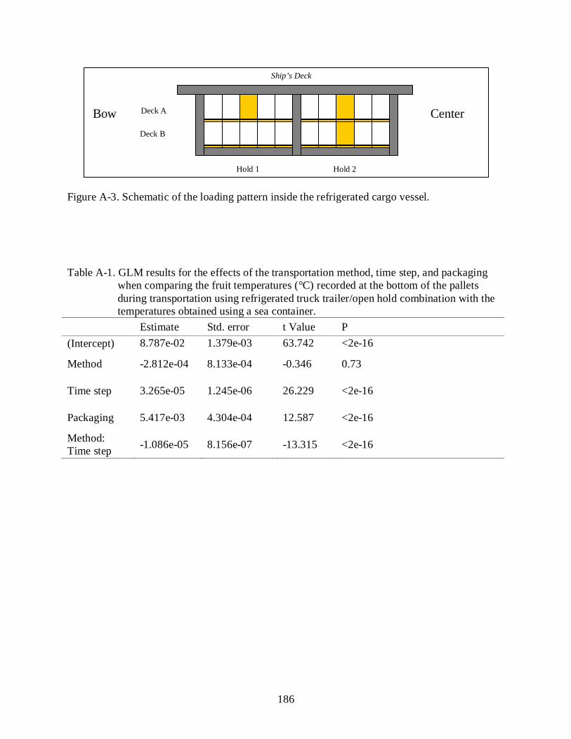
186
Figure A-3. Schematic of the loading pattern inside the refrigerated cargo vessel.
Table A-1. GLM results for the effects of the transportation method, time step, and packaging when comparing the fruit temperatures (°C) recorded at the bottom of the pallets during transportation using refrigerated truck trailer/open hold combination with the temperatures obtained using a sea container.
Estimate Std. error t Value P (Intercept) 8.787e-02 1.379e-03 63.742 <2e-16
Method -2.812e-04 8.133e-04 -0.346 0.73
Time step 3.265e-05 1.245e-06 26.229 <2e-16
Packaging 5.417e-03 4.304e-04 12.587 <2e-16
Method: Time step -1.086e-05 8.156e-07 -13.315 <2e-16
Hold 1 Hold 2
Deck A
Deck B
Ship’s Deck
Bow Center

187
Table A-2. GLM results for the effects of position, time step and packaging when comparing the
fruit temperatures (°C) recorded at the bottom of the pallets during transportation in the three positions (back, middle and front) inside the sea container.
Estimate Std. error t Value P (Intercept) 8.765e-02 1.157e-03 75.782 <2e-16
Position -1.705e-05 5.466e-04 -0.031 0.9751
Time step 2.366e-05 1.086e-06 21.789 <2e-16
Packaging 5.395e-03 4.133e-04 13.054 <2e-16
Position: Time step -1.019e-06 5.555e-07 -1.834 0.0667
Table A-3. GLM results for the effects of the hold, time step and packaging when comparing the
fruit temperatures (°C) recorded at the top of the pallets during transportation in the holds of the refrigerated vessel.
Estimate Std. error t Value P (Intercept) 1.104e-01 1.781e-03 61.958 <2e-16
Hold -1.057e-02 6.990e-04 -15.121 <2e-16
Time step -2.289e-05 1.417e-06 -16.156 <2e-16
Packaging -9.425e-05 5.735e-04 -0.164 0.87
Hold: Time step 1.193e-05 6.571e-07 18.159 <2e-16

188
Table A-4. Percentage (%) of transportation time during which pineapples were exposed to different high temperature abuse (HTA) scenarios when using the refrigerated truck trailer/open hold combination.
Front/1A Middle/2A Back/2B Top Center Bottom Top Center Bottom Top Center Bottom Corr RPC Corr RPC Corr RPC Corr RPC Corr RPC Corr RPC Corr RPC Corr RPC Corr RPC
HTA No.1 (T ≥ 12°C)
19.9 20.3 3.5 4.3 7.9 - 24.1 26.3 100.0 6.2 DS 20.6 28.2 22.1 11.8 - 5.2 4.2
HTA No.2 (T ≥ 15°C) 7.9 9.5 - - - - 3.3 8.0 26.8 - DS - 0.6 10.7 - - - -
HTA No.3 (T ≥ 17°C) 4.5 6.4 - - - - 2.3 - - DS - - - - - - -
DS: Defective sensor Table A-5. Risk of fruit exposure to different high temperature abuse (HTA) scenarios according to the position of the fruit in the
pallet when using the refrigerated truck trailer/open hold combination. Overall Top Center Bottom
HTA No.1 (T ≥ 12°C) H H H H
HTA No.2 (T ≥ 15°C) M H L N
HTA No.3 (T ≥ 17°C) L M N N
H = High, M = Medium, L = Low, and N = None.
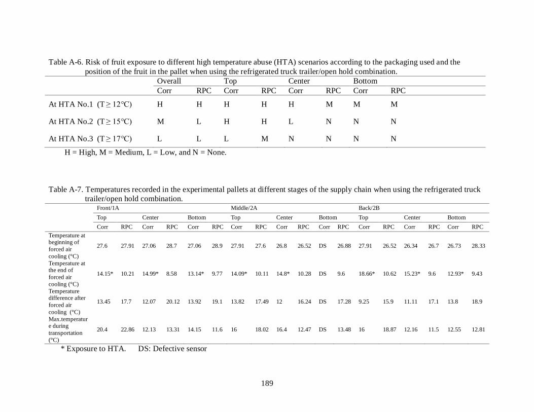
189
Table A-6. Risk of fruit exposure to different high temperature abuse (HTA) scenarios according to the packaging used and the
position of the fruit in the pallet when using the refrigerated truck trailer/open hold combination.
Overall Top Center Bottom Corr RPC Corr RPC Corr RPC Corr RPC
At HTA No.1 (T ≥ 12°C) H H H H H M M M
At HTA No.2 (T ≥ 15°C) M L H H L N N N
At HTA No.3 (T ≥ 17°C) L L L M N N N N
H = High, M = Medium, L = Low, and N = None. Table A-7. Temperatures recorded in the experimental pallets at different stages of the supply chain when using the refrigerated truck
trailer/open hold combination.
Front/1A Middle/2A Back/2B Top Center Bottom Top Center Bottom Top Center Bottom Corr RPC Corr RPC Corr RPC Corr RPC Corr RPC Corr RPC Corr RPC Corr RPC Corr RPC
Temperature at beginning of forced air cooling (°C)
27.6 27.91 27.06 28.7 27.06 28.9 27.91 27.6 26.8 26.52 DS 26.88 27.91 26.52 26.34 26.7 26.73 28.33
Temperature at the end of forced air cooling (°C)
14.15* 10.21 14.99* 8.58 13.14* 9.77 14.09* 10.11 14.8* 10.28 DS 9.6 18.66* 10.62 15.23* 9.6 12.93* 9.43
Temperature difference after forced air cooling (°C)
13.45 17.7 12.07 20.12 13.92 19.1 13.82 17.49 12 16.24 DS 17.28 9.25 15.9 11.11 17.1 13.8 18.9
Max.temperature during transportation (°C)
20.4 22.86 12.13 13.31 14.15 11.6 16 18.02 16.4 12.47 DS 13.48 16 18.87 12.16 11.5 12.55 12.81
* Exposure to HTA. DS: Defective sensor
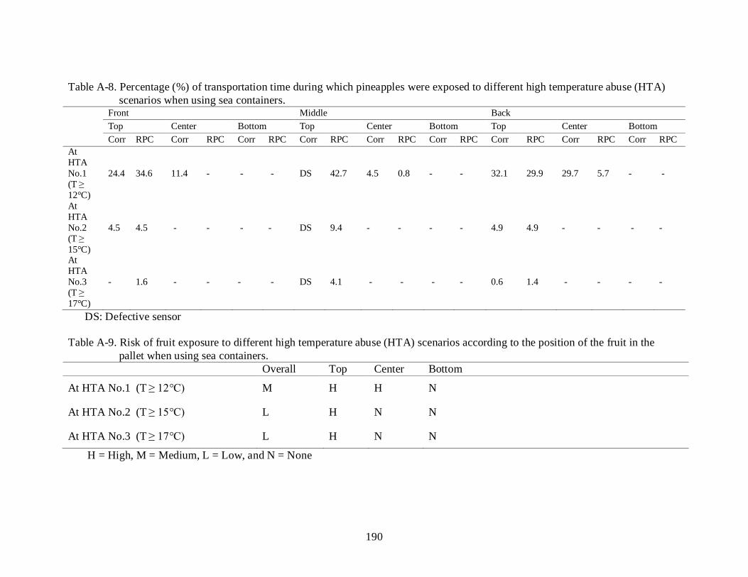
190
Table A-8. Percentage (%) of transportation time during which pineapples were exposed to different high temperature abuse (HTA)
scenarios when using sea containers.
Front Middle Back Top Center Bottom Top Center Bottom Top Center Bottom Corr RPC Corr RPC Corr RPC Corr RPC Corr RPC Corr RPC Corr RPC Corr RPC Corr RPC
At HTA No.1 (T ≥ 12°C)
24.4 34.6 11.4 - - - DS 42.7 4.5 0.8 - - 32.1 29.9 29.7 5.7 - -
At HTA No.2 (T ≥ 15°C)
4.5 4.5 - - - - DS 9.4 - - - - 4.9 4.9 - - - -
At HTA No.3 (T ≥ 17°C)
- 1.6 - - - - DS 4.1 - - - - 0.6 1.4 - - - -
DS: Defective sensor Table A-9. Risk of fruit exposure to different high temperature abuse (HTA) scenarios according to the position of the fruit in the
pallet when using sea containers. Overall Top Center Bottom
At HTA No.1 (T ≥ 12°C) M H H N
At HTA No.2 (T ≥ 15°C) L H N N
At HTA No.3 (T ≥ 17°C) L H N N
H = High, M = Medium, L = Low, and N = None

191
Table A-10. Risk of fruit exposure to different high temperature abuse (HTA) scenarios according to the type of packaging used and the position of the fruit in the pallet when using sea containers.
Overall Top Center Bottom Corr RPC Corr RPC Corr RPC Corr RPC At HTA No.1 (T ≥ 12°C) H M H H H M N N
At HTA No.2 (T ≥ 15°C) M M H H N N N N
At HTA No.3 (T ≥ 17°C) L M M H N N N N
H = High, M = Medium, L = Low, and N = None.
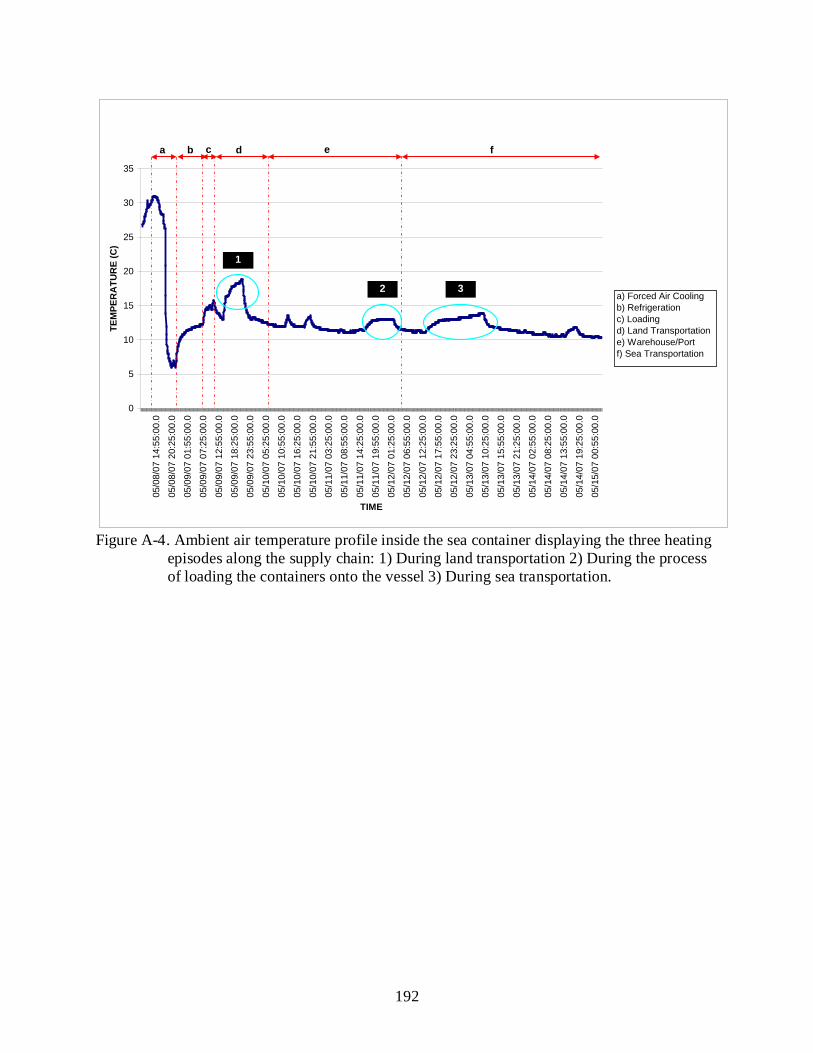
192
0
5
10
15
20
25
30
3505
/08/
07 1
4:55
:00.
0
05/0
8/07
20:
25:0
0.0
05/0
9/07
01:
55:0
0.0
05/0
9/07
07:
25:0
0.0
05/0
9/07
12:
55:0
0.0
05/0
9/07
18:
25:0
0.0
05/0
9/07
23:
55:0
0.0
05/1
0/07
05:
25:0
0.0
05/1
0/07
10:
55:0
0.0
05/1
0/07
16:
25:0
0.0
05/1
0/07
21:
55:0
0.0
05/1
1/07
03:
25:0
0.0
05/1
1/07
08:
55:0
0.0
05/1
1/07
14:
25:0
0.0
05/1
1/07
19:
55:0
0.0
05/1
2/07
01:
25:0
0.0
05/1
2/07
06:
55:0
0.0
05/1
2/07
12:
25:0
0.0
05/1
2/07
17:
55:0
0.0
05/1
2/07
23:
25:0
0.0
05/1
3/07
04:
55:0
0.0
05/1
3/07
10:
25:0
0.0
05/1
3/07
15:
55:0
0.0
05/1
3/07
21:
25:0
0.0
05/1
4/07
02:
55:0
0.0
05/1
4/07
08:
25:0
0.0
05/1
4/07
13:
55:0
0.0
05/1
4/07
19:
25:0
0.0
05/1
5/07
00:
55:0
0.0
TIME
TEM
PER
ATU
RE
(C)
a
a) Forced Air Coolingb) Refrigerationc) Loadingd) Land Transportatione) Warehouse/Portf) Sea Transportation
b c d e f
1
2 3
Figure A-4. Ambient air temperature profile inside the sea container displaying the three heating
episodes along the supply chain: 1) During land transportation 2) During the process of loading the containers onto the vessel 3) During sea transportation.
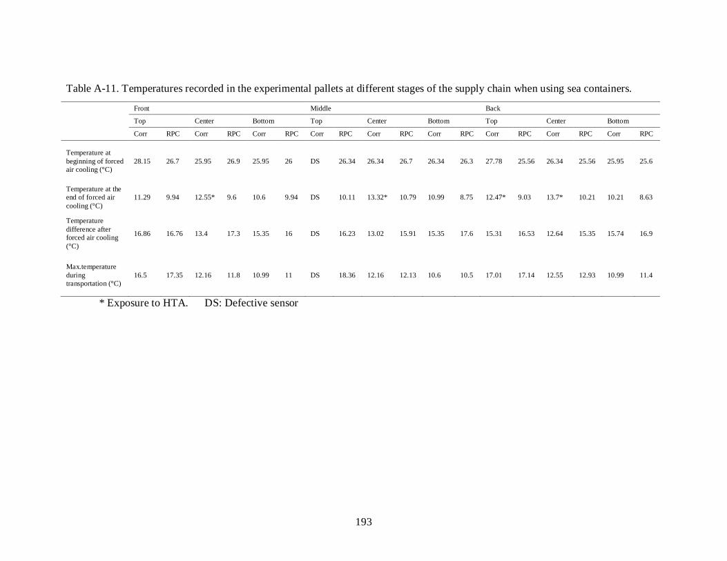
193
Table A-11. Temperatures recorded in the experimental pallets at different stages of the supply chain when using sea containers.
* Exposure to HTA. DS: Defective sensor
Front Middle Back
Top Center Bottom Top Center Bottom Top Center Bottom
Corr RPC Corr RPC Corr RPC Corr RPC Corr RPC Corr RPC Corr RPC Corr RPC Corr RPC
Temperature at beginning of forced air cooling (°C)
28.15 26.7 25.95 26.9 25.95 26 DS 26.34 26.34 26.7 26.34 26.3 27.78 25.56 26.34 25.56 25.95 25.6
Temperature at the end of forced air cooling (°C)
11.29 9.94 12.55* 9.6 10.6 9.94 DS 10.11 13.32* 10.79 10.99 8.75 12.47* 9.03 13.7* 10.21 10.21 8.63
Temperature difference after forced air cooling (°C)
16.86 16.76 13.4 17.3 15.35 16 DS 16.23 13.02 15.91 15.35 17.6 15.31 16.53 12.64 15.35 15.74 16.9
Max.temperature during transportation (°C)
16.5 17.35 12.16 11.8 10.99 11 DS 18.36 12.16 12.13 10.6 10.5 17.01 17.14 12.55 12.93 10.99 11.4
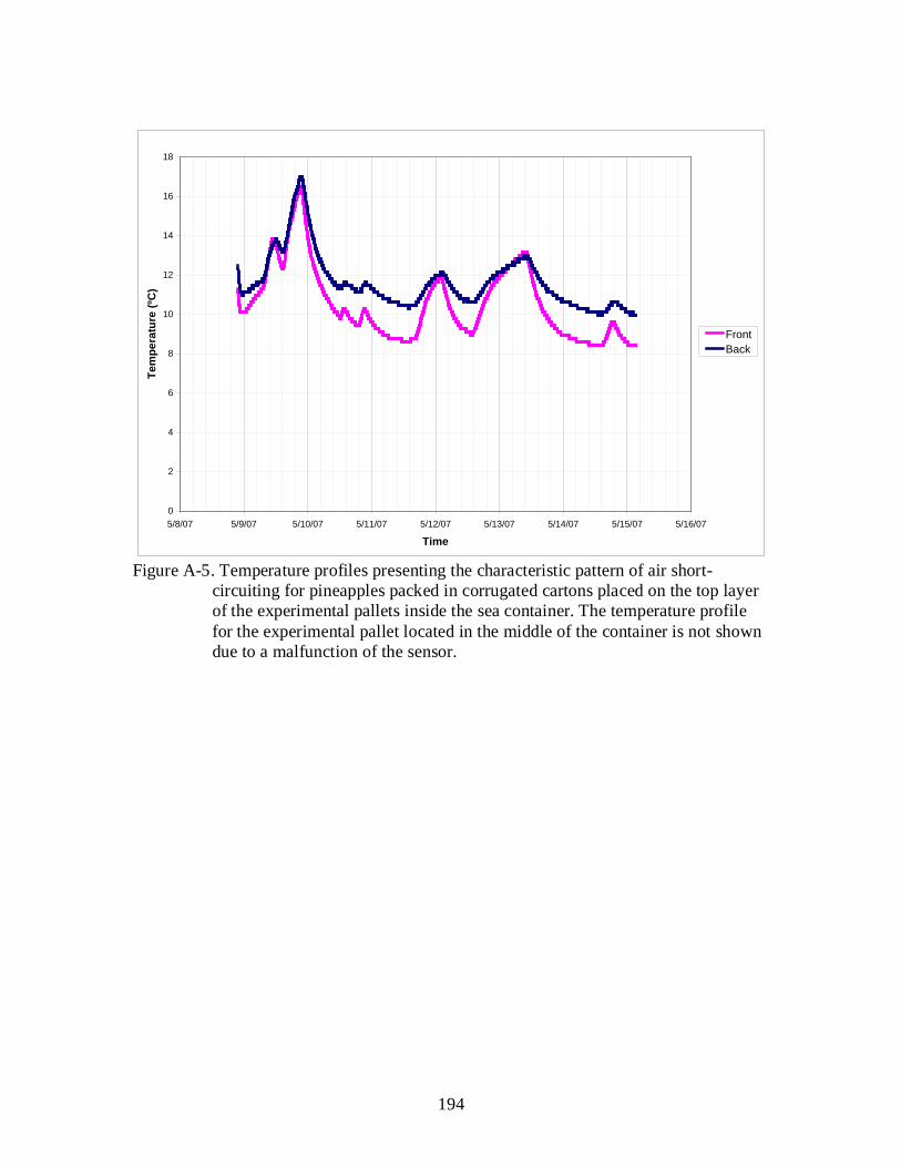
194
0
2
4
6
8
10
12
14
16
18
5/8/07 5/9/07 5/10/07 5/11/07 5/12/07 5/13/07 5/14/07 5/15/07 5/16/07
Time
Tem
pera
ture
(ºC
)
FrontBack
Figure A-5. Temperature profiles presenting the characteristic pattern of air short-
circuiting for pineapples packed in corrugated cartons placed on the top layer of the experimental pallets inside the sea container. The temperature profile for the experimental pallet located in the middle of the container is not shown due to a malfunction of the sensor.
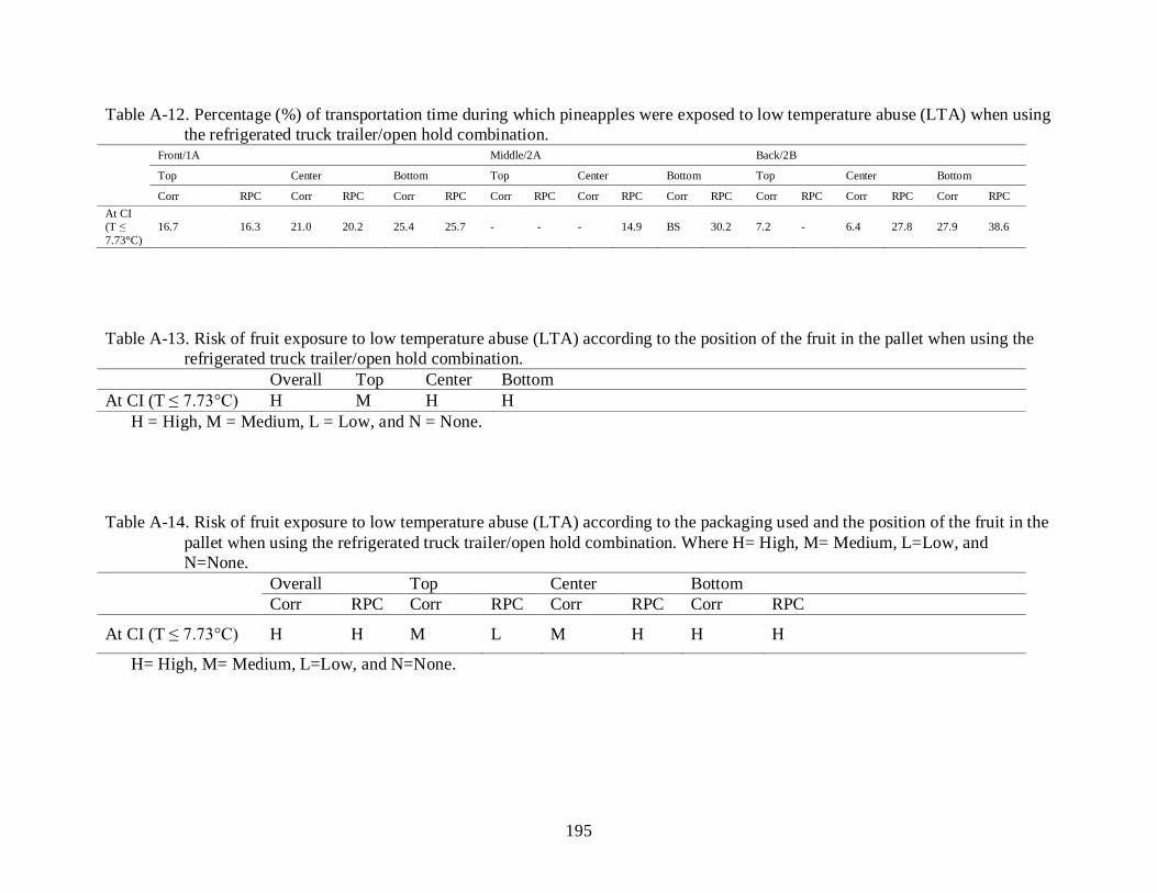
195
Table A-12. Percentage (%) of transportation time during which pineapples were exposed to low temperature abuse (LTA) when using the refrigerated truck trailer/open hold combination.
Front/1A Middle/2A Back/2B
Top Center Bottom Top Center Bottom Top Center Bottom
Corr RPC Corr RPC Corr RPC Corr RPC Corr RPC Corr RPC Corr RPC Corr RPC Corr RPC At CI (T ≤ 7.73°C)
16.7 16.3 21.0 20.2 25.4 25.7 - - - 14.9 BS 30.2 7.2 - 6.4 27.8 27.9 38.6
Table A-13. Risk of fruit exposure to low temperature abuse (LTA) according to the position of the fruit in the pallet when using the
refrigerated truck trailer/open hold combination. Overall Top Center Bottom At CI (T ≤ 7.73°C) H M H H H = High, M = Medium, L = Low, and N = None. Table A-14. Risk of fruit exposure to low temperature abuse (LTA) according to the packaging used and the position of the fruit in the
pallet when using the refrigerated truck trailer/open hold combination. Where H= High, M= Medium, L=Low, and N=None.
Overall Top Center Bottom Corr RPC Corr RPC Corr RPC Corr RPC
At CI (T ≤ 7.73°C) H H M L M H H H
H= High, M= Medium, L=Low, and N=None.

196
Table A-15. Percentage (%) of transportation time during which the pineapples were exposed to low temperature abuse (LTA) when
using the sea containers.
Front Middle Back Top Center Bottom Top Center Bottom Top Center Bottom Corr RPC Corr RPC Corr RPC Corr RPC Corr RPC Corr RPC Corr RPC Corr RPC Corr RPC
At CI (T ≤ 7.73°C)
- - - 58.1 - 72.7 - - - 29.7 - 62.6 - - - - - -
Table A-16. Risk of fruit exposure to low temperature abuse (LTA) according to the position of the fruit in the pallet when using sea
containers. Overall Top Center Bottom At CI (T ≤ 7.73°C) L N L L H= High, M= Medium, L=Low, and N=None. Table A-17. Risk of fruit exposure to low temperature abuse (LTA) according to the packaging used and the position of the fruit in the
pallet when using sea containers.
Overall Top Center Bottom Corr RPC Corr RPC Corr RPC Corr RPC
At CI (T ≤ 7.73°C) N M N N N M N M
H= High, M= Medium, L=Low, and N=None.

197
APPENDIX B
RECOMMENDED LEVEL OF RFID INSTRUMENTATION FOR THE CROWNLESS PINEAPPLE SUPPLY CHAIN WHEN THIS USES THE REFRIGERATED TRUCK/OPEN
HOLD TRANSPORTATION METHOD
Proper monitoring is achieved recording two or three temperatures per pallet, according to
the location of the pallet during forced air cooling. In order to monitor HTA, ambient probeless
tags are recommended for the top layers of the pallets and tags with probe are advised for their
center. Furthermore, tags with probe are also suggested to observe LTA in the bottom layers of
the pallets. In this case, no areas are specified as specific tag locations at the cargo level.
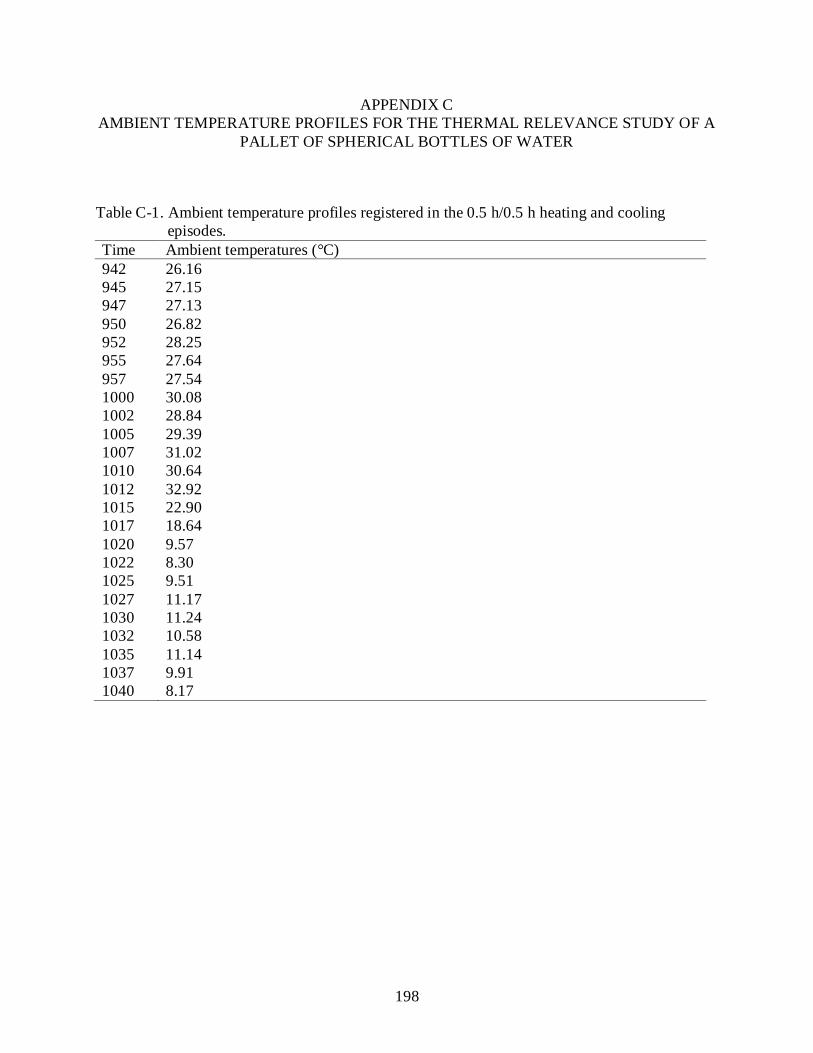
198
APPENDIX C AMBIENT TEMPERATURE PROFILES FOR THE THERMAL RELEVANCE STUDY OF A
PALLET OF SPHERICAL BOTTLES OF WATER
Table C-1. Ambient temperature profiles registered in the 0.5 h/0.5 h heating and cooling episodes.
Time Ambient temperatures (°C) 942 26.16 945 27.15 947 27.13 950 26.82 952 28.25 955 27.64 957 27.54 1000 30.08 1002 28.84 1005 29.39 1007 31.02 1010 30.64 1012 32.92 1015 22.90 1017 18.64 1020 9.57 1022 8.30 1025 9.51 1027 11.17 1030 11.24 1032 10.58 1035 11.14 1037 9.91 1040 8.17

199
Table C-2. Ambient temperature profiles registered in the 1 h/1 h heating and cooling episodes. Time Ambient temperatures (°C) 937 16.94 940 30.06 942 34.25 945 28.14 947 17.68 950 18.47 952 19.46 955 18.88 957 18.85 1000 28.05 1002 18.64 1005 21.25 1007 18.91 1010 19.07 1012 19.35 1015 19.35 1017 21.35 1020 21.15 1022 20.34 1025 23.36 1027 19.75 1030 21.02 1032 18.86 1035 20.93 1037 21.65 1040 28.76 1042 23.41 1045 15.16 1047 11.03 1050 9.73 1052 9.14 1055 8.41 1057 8.74 1100 8.28 1102 7.88 1105 7.54 1107 7.24 1110 6.93 1112 6.84 1115 6.41 1117 6.27 1120 6.08 1122 5.94 1125 5.71

200
Table C-2. Continued. Time Ambient temperatures (°C) 1127 5.73 1130 5.72 1132 5.34 1135 5.37 1137 5.53 1140 5.30 1142 5.35
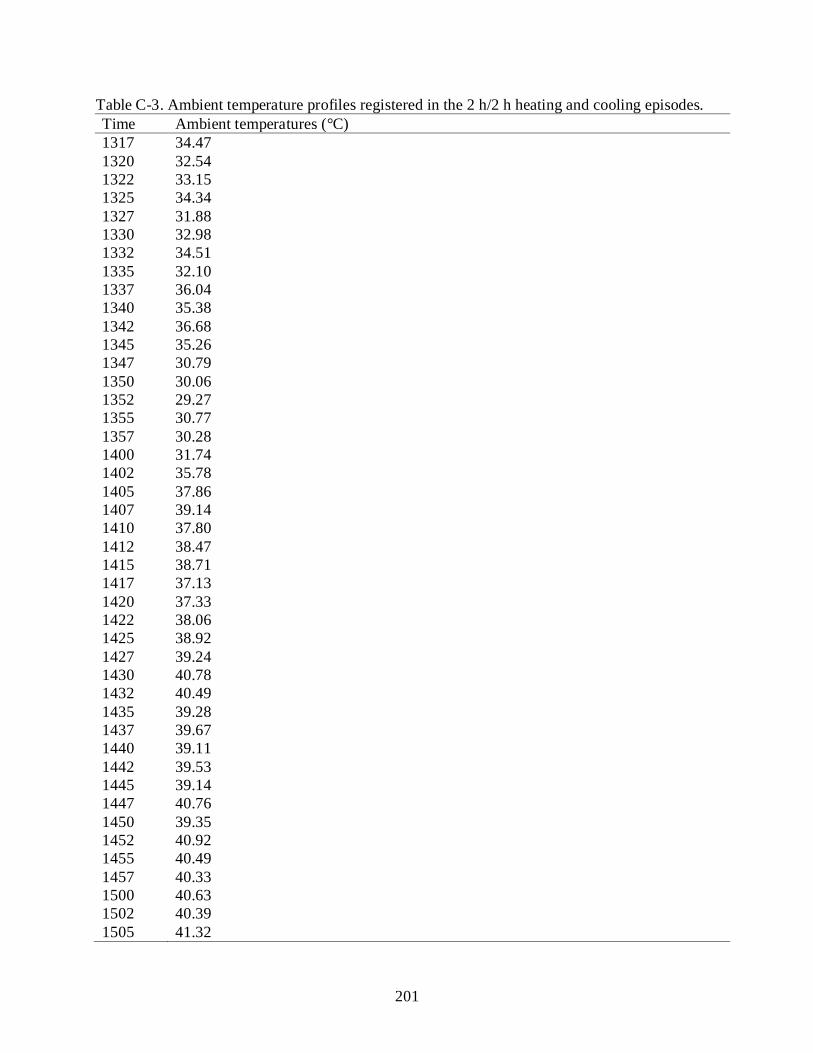
201
Table C-3. Ambient temperature profiles registered in the 2 h/2 h heating and cooling episodes. Time Ambient temperatures (°C) 1317 34.47 1320 32.54 1322 33.15 1325 34.34 1327 31.88 1330 32.98 1332 34.51 1335 32.10 1337 36.04 1340 35.38 1342 36.68 1345 35.26 1347 30.79 1350 30.06 1352 29.27 1355 30.77 1357 30.28 1400 31.74 1402 35.78 1405 37.86 1407 39.14 1410 37.80 1412 38.47 1415 38.71 1417 37.13 1420 37.33 1422 38.06 1425 38.92 1427 39.24 1430 40.78 1432 40.49 1435 39.28 1437 39.67 1440 39.11 1442 39.53 1445 39.14 1447 40.76 1450 39.35 1452 40.92 1455 40.49 1457 40.33 1500 40.63 1502 40.39 1505 41.32
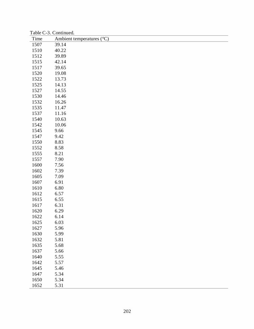
202
Table C-3. Continued. Time Ambient temperatures (°C) 1507 39.14 1510 40.22 1512 39.89 1515 42.14 1517 39.65 1520 19.08 1522 13.73 1525 14.13 1527 14.55 1530 14.46 1532 16.26 1535 11.47 1537 11.16 1540 10.63 1542 10.06 1545 9.66 1547 9.42 1550 8.83 1552 8.58 1555 8.21 1557 7.90 1600 7.56 1602 7.39 1605 7.09 1607 6.91 1610 6.80 1612 6.57 1615 6.55 1617 6.31 1620 6.29 1622 6.14 1625 6.03 1627 5.96 1630 5.99 1632 5.81 1635 5.68 1637 5.66 1640 5.55 1642 5.57 1645 5.46 1647 5.34 1650 5.34 1652 5.31
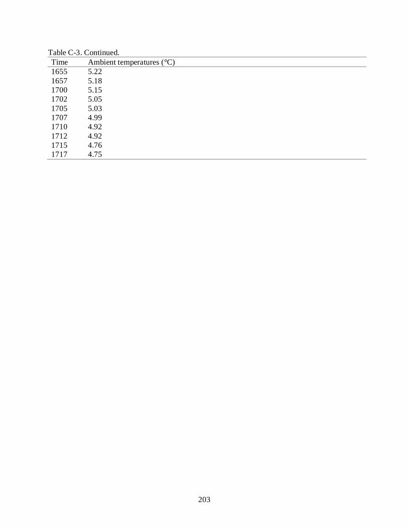
203
Table C-3. Continued. Time Ambient temperatures (°C) 1655 5.22 1657 5.18 1700 5.15 1702 5.05 1705 5.03 1707 4.99 1710 4.92 1712 4.92 1715 4.76 1717 4.75

204
Table C-4. Ambient temperature profiles registered in the 4 h/4 h heating and cooling episodes. Time Ambient temperatures (°C) 1022 7.20 1025 7.50 1027 7.61 1030 7.68 1032 7.67 1035 7.75 1037 7.82 1040 7.80 1042 7.77 1045 7.74 1047 7.65 1050 7.60 1052 7.58 1055 7.60 1057 7.67 1100 7.69 1102 7.69 1105 7.61 1107 7.59 1110 7.55 1112 7.58 1115 7.65 1117 7.68 1120 7.74 1122 7.69 1125 7.66 1127 7.61 1130 7.54 1132 7.53 1135 7.56 1137 7.61 1140 7.69 1142 7.70 1145 7.76 1147 7.80 1150 7.83 1152 7.91 1155 8.10 1157 8.17 1200 8.22 1202 8.23 1205 8.28 1207 8.33 1210 8.35

205
Table C-4. Continued. Time Ambient temperatures (°C) 1212 8.46 1215 8.57 1217 8.69 1220 8.83 1222 8.90 1225 8.94 1227 9.01 1230 9.08 1232 9.19 1235 9.28 1237 9.41 1240 9.52 1242 9.70 1245 9.80 1247 9.91 1250 10.01 1252 10.07 1255 10.18 1257 10.30 1300 10.33 1302 10.34 1305 10.39 1307 10.46 1310 10.55 1312 10.64 1315 10.65 1317 10.71 1320 10.75 1322 10.73 1325 10.81 1327 10.86 1330 10.92 1332 10.96 1335 11.02 1337 11.03 1340 11.06 1342 11.11 1345 11.11 1347 11.15 1350 11.22 1352 11.35 1355 11.44 1357 11.49

206
Table C-4. Continued. Time Ambient temperatures (°C) 1400 11.58 1402 11.66 1405 11.74 1407 11.82 1410 11.96 1412 12.01 1415 12.09 1417 12.13 1420 12.19 1422 12.27 1425 12.33 1427 12.41 1430 12.44 1432 12.53 1435 12.65 1437 12.63 1440 12.63 1442 12.25 1445 11.61 1447 11.06 1450 10.82 1452 10.69 1455 10.53 1457 10.32 1500 10.30 1502 10.66 1505 10.57 1507 10.58 1510 10.49 1512 10.41 1515 10.55 1517 10.73 1520 10.81 1522 10.86 1525 10.91 1527 10.90 1530 10.90 1532 10.85 1535 10.87 1537 10.86 1540 10.84 1542 10.84 1545 10.85
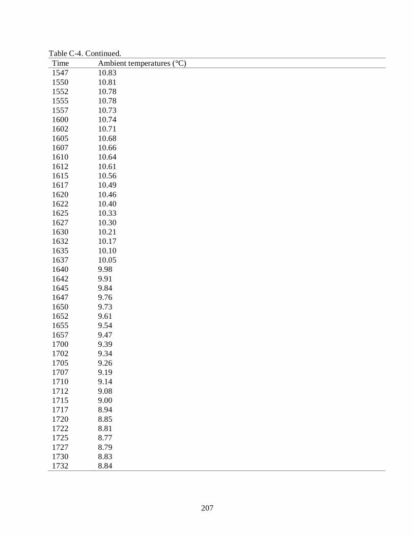
207
Table C-4. Continued. Time Ambient temperatures (°C) 1547 10.83 1550 10.81 1552 10.78 1555 10.78 1557 10.73 1600 10.74 1602 10.71 1605 10.68 1607 10.66 1610 10.64 1612 10.61 1615 10.56 1617 10.49 1620 10.46 1622 10.40 1625 10.33 1627 10.30 1630 10.21 1632 10.17 1635 10.10 1637 10.05 1640 9.98 1642 9.91 1645 9.84 1647 9.76 1650 9.73 1652 9.61 1655 9.54 1657 9.47 1700 9.39 1702 9.34 1705 9.26 1707 9.19 1710 9.14 1712 9.08 1715 9.00 1717 8.94 1720 8.85 1722 8.81 1725 8.77 1727 8.79 1730 8.83 1732 8.84
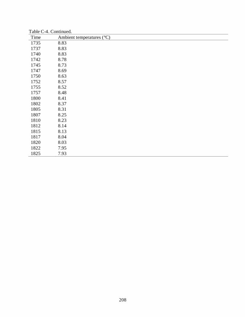
208
Table C-4. Continued. Time Ambient temperatures (°C) 1735 8.83 1737 8.83 1740 8.83 1742 8.78 1745 8.73 1747 8.69 1750 8.63 1752 8.57 1755 8.52 1757 8.48 1800 8.41 1802 8.37 1805 8.31 1807 8.25 1810 8.23 1812 8.14 1815 8.13 1817 8.04 1820 8.03 1822 7.95 1825 7.93

209
APPENDIX D TEMPERATURE PROFILE USED AS WORST CASE SCENARIO FOR FSR SHIPMENTS
Table D-1. Maximum daily temperatures obtained in a combat feeding shipment from the U.S. to Kuwait.
Days Temperatures (°F) 1 104 2 104 3 91.4 4 107.6 5 82.4 6 73.4 7 73.4 8 96.8 9 89.6 10 91.4 11 91.4 12 91.4 13 87.8 14 86 15 86 16 86 17 87.8 18 89.6 19 95 20 96.8 21 102.2 22 102.2 23 102.2 24 102.2 25 100.4 26 96.8 27 100.4 28 100.4 29 118.4 30 114.8 31 120.2 32 129.2 33 122 34 125.6 35 131 36 122 37 122 38 125.6 39 129.2
210
LIST OF REFERENCES
Abada, E., Zampolli, S., Marcoc, S., Scorzoni, A., Mazzolai, B. et al., 2007. Flexible tag microlab development: Gas sensors integration in RFID flexible tags for food logistic. Sensors and Actuators B 127, 2-7.
Abdullah, H., Rohaya, M.A., Rosli, H., Mohamed Selamat, M., 2000. Handling and transportation trial of pineapple by sea shipment from Malaysia to the United Kingdom. Acta Horticulturae 529, 317-327.
Acedo, A., Akinaga, T., Tanabez, T., 2004. Inhibition of chilling injury and quality changes in pineapple fruit with prestorage heat treatment. Journal of Food, Agriculture and Environment 2, 81-86.
Akamine, E.K., Goo, T., Steepy, T., Greidanus, T., Iwaoka, N., 1975. Control of endogenous brown spot of fresh pineapple in postharvest handling. Journal of the American Society for Horticultural Science 100, 60-65.
Amador, C., Emond, J.P., Nunes, M.C.N., 2009. Application of RFID Technologies in the Temperature Mapping of the Pineapple Supply Chain. Journal of Sensing and Instrumentation for Food Quality and Safety 3 (1), 26-33.
Amador, C., Emond, J.P., 2010. Evaluation of sensor readability and thermal relevance for RFID temperature tracking. Computers and Electronics in Agriculture 73 (1), 84-90.
Ames, H., 2006. Authentication from a Cold Chain Perspective. Pharmaceutical Commerce. July/August 2006.
Amos, N.D., 2001. Factors affecting fruit temperature maintenance within refrigerated containers. Proceedings of the IRHACE Annual Conf. Vol I, 7-10.
Anderson, K. E., 2010. Development of a simulator for sweet corn cold chain distribution. M.Sc. Thesis. University of Florida, Agricultural and Biological Engineering.
Angeles, R., 2005. RFID Technologies: Supply-Chain Applications and Implementation Issues. Information Systems Management, Vol. 22 (1), 51-65.
Aroor, S. R., Deavours, D. D., 2007. Evaluation of the state of passive UHF RFID: An experimental approach. IEEE Systems Journal 1 (2), 168–176.
Asimakopoulos, G., Spiros Louvros, G., Triantafillou, V., 2007. METATRO: A Real Time RFID enabled haulage monitoring system for perishable comestibles. Paper Presented at the IEEE Conference on Emerging Technologies and Factory Automation (ETFA), Patras, Greece.
Banerjee S.R., Jesme, R., Sainati, R.A., 2007. Performance Analysis of Short Range UHF Propagation as Applicable to Passive RFID. Paper Presented at 2007 IEEE International Conference on RFID, Grapevine, TX.
211
Banks, J., Pachano, M., Thompson, L., Hanny, D., 2007. RFID Applied. John Wiley & Sons, Inc., Hoboken.
Banwart, GJ., 1989. Basic food microbiology, 2. Van Nostrand Reinhold, New York.
BBC, 2010a. BBC News: US troops in Afghanistan outnumber those in Iraq. British Broadcasting Corporation. Available at: http://news.bbc.co.uk/2/hi/world/us_and_canada/10151175.stm. Accessed July 6th, 2010.
BBC, 2010b. World Weather: Average Conditions. British Broadcasting Corporation. Available at: http://www.bbc.co.uk/weather/world/city_guides. Accessed February 5th 2010.
Bennahmias, R., Labonne, G., 1993. Etude de la distribution de l'air et de la dispersion des tempe´ratures dans une semi-remorque frigorifique. Proceedings of the I.I.R Commissions C2, D1 et D2/3, Fez, Morocco, 241-256.
Billing, D.P., Hayes, A.J., McDonald, B., 1993. Performance of refrigerated ships carrying New Zealand produce. Refrigeration Science and Technology 3, 546-554.
Billing, D.P., Hayes, A.J., McDonald, B., 1995. Temperature and airflow characteristics in reefer vessels carrying New Zealand produce. Proceedings of the 19th International Congress of Refrigeration, La Haye, Netherlands, Vol II, 485-492.
Bogataj, M., Bogataj, L., Vodopivec, R., 2005. Stability of perishable goods in cold logistic chains. International Journal of Production Economics 93-94 (1), 345-356.
Bollen, F., 2005. Traceability in Fresh Produce Supply Chains. Acta Horticulturae 687, 279-288.
Bollen, F., Riden, C., 2006. Traceability in Postharvest Quality Management. International Journal of Postharvest Technology and Innovation 1 (1), 93-96.
Brody, A.L., 2003. Predicting packaged food shelf life. Food Technology 57(4), 100-102.
Broekmeulen, R.A.C.M., Van Donselaar, K.H., 2007. A Replenishment policy for a perishable inventory system based on estimated aging and retrieval behavior. Working Paper, Department of Technology Management, University of Eindhoven, Eindhoven, Netherlands.
Brosnan, T., Sun, D., 2001. Precooling techniques and applications for horticultural products – A review. International Journal of Refrigeration 24, 154-170.
Brown, D., 2007. RFID Implementation. Mc Graw Hill, New York.
Capgo, 2010. Introduction to Bimetallic Temperature Sensors. Capgo Pty Ltd. Available at: http://www.capgo.com/Resources/Temperature/BiMet/BiMetallic.html. Accessed June 28th, 2010.
Chamberlain, J., 2006. IBM WebSphere RFID Handbook: A Solution Guide. IBM Redbooks.

212
Chande, A., Dhekane, S., Hemachandra, N., Rangaraj, N., 2005. Perishable inventory management and dynamic pricing using RFID technology. Sadhana 30 (2), 445-462.
Chonhenchob, V., Kamhangwong, D., Singh, S.P., 2008. Comparison of reusable and single-use plastic and paper shipping containers for distribution of fresh pineapples. Packaging Technology and Science 21, 73-83.
Chonhenchob, V., Singh, S.P., 2003a. A comparison of corrugated boxes and reusable plastic containers for mango distribution. Packaging Technology and Science 16, 231-237.
Chonhenchob, V., Singh, S.P. 2003b. Packaging performance comparison for distribution and export of papaya fruit. Packaging Technology and Science 18, 125-131.
Clarke, R.H., Twede, D., Tazelaar, J.R., Boyer, K.K., 2006. Radio Frequency Identification (RFID) performance: The effect of tag orientation and package contents. Packaging Technology and Science 19, 45-54.
Corbo, M. R., Del Nobile, M.A., Sinigaglia, M., 2006. A novel approach for calculating shelf-life of minimally processed vegetables. International Journal of Food Microbiology 106, 69-73.
Cortbaoui, P., 2005. Assessment of Precooling Technologies for Sweetcorn. M. Sc. Thesis. McGill University, Bioresource Engineering.
Dagdelen, D., 2007. Improving the Readability of RFID tagged Pharmaceutical Products and Food Supplements inside a Modified Sealed Tote. M.Sc. Thesis, University of Florida, Food Science and Human Nutrition Department.
DeEll, J.R., Prange, R.K., Peppelenbos, H.W., 2003. Postharvest Physiology of Fresh Fruits and Vegetables. In: Chakraverty, A., Mujumdra, A.S., Vijaya Raghavan, G.S., Ramaswamy, H.S. (Eds.), Handbook of Postharvest Technology: Cereals, Fruits, Vegetables, Tea, and Spices. Marcel Dekker, Inc., New York, pp. 455-484.
Dinçer, I., 2003. Heat Transfer in Food Cooling Applications. Taylor & Francis, Washington, D.C.
Dobkin, D., Weigand, S., 2005. Environmental effects on RFID tag antennas. Paper Presented at the 2005 IEEE MTT-S International Microwave Symposium, Long Beach, CA.
DoD Live., 2009. Armed with science: First Strike Rations offer fast food on the go. US Department of Defense. Available at: http://www.dodlive.mil/index.php/2009/11/first-strike-rations-offer-fast-food-on-the-go. Accessed 2nd February 2010.
Dull, G., Young, R., Biale, J., 1967. Respiratory patterns in fruit of pineapple, Ananas comosus, detached at different stages of development. Physiologia Plantarum 20, 1059-1065.
Edwards, J., 2007. Cold Chain Heats Up RFID Adoption. RFID Journal. March/April 2007.

213
Efunda, 2010. Temperature Sensors. eFunda, Inc. Available at: http://www.efunda.com/designstandards/sensors/thermocouples/thmcple_intro.cfm. Accessed June 28th, 2010.
Emond, J.P., Nicometo, M., 2006. Shelf-life prediction and FEFO inventory management with RFID. Presentation in the Cool Chain Association Workshop: Temperature Measurements - When, Where and How? Knivsta, Sweden. Available at: www.coolchain.org/uploads/MikeNicometo-CCAStockholmNov06.pdf. Accessed January 15th 2008.
Ferguson, M. E., Ketzenberg M.E., 2006. Information sharing to improve retail product freshness of perishables. Production and Operations Management 15 (1), 57-73.
Finn, D.P., Brennan, S.L., 2003. Sensitivity analysis using CFD of air distribution in transport refrigeration containers. Paper Presented at the 21st International Congress of Refrigeration, Washington, DC.
Fletcher, R., Marti, U., Redemske, R., 2005. Study of UHF RFID Signal Propagation through Complex Media. Paper Presented at the 2005 IEEE Antennas and Propagation Society International Symposium, Washington, DC.
Food and Agriculture Organization, 2009. FAOSTAT. Available at http://faostat.fao.org/. Accessed November 30th, 2009.
Forcinio, H., 2004. Packaging Helps Protect Temperature-Sensitive Products. Pharmaceutical Technology 28 (3), 36-42.
Freund, R., Wilson, W., 2003. Statistical Methods, 2. Academic Press, San Diego.
Gaukler, G., Seifert, R.W., 2007. Applications of RFID in Supply Chains. In: Jung, H., Chen, F., Jeong, B. (Eds.), Trends in Supply Chain Design and Management: Technologies and Methodologies. Springer-Verlag, London, pp. 29-49.
Giannakourou, M. C., Taoukis, P.S., 2003. Application of a TTI-based distribution management system for quality optimization of frozen vegetables at the consumer end. Journal of Food Science 68, 201-209.
Gogüs, A.Y., Yavuzturk, S.,1974. Temperature pull-down and distribution in refrigerated trailers. Paper Presented at I.I.R commissions D2, Wageningen, Netherlands.
Gonzalez-Aguilar, G.A., Ruiz-Cruz, S., Cruz-Valenzuela, R., Rodriguez-Felix, A., Wang, CY., 2004. Physiological and quality changes of fresh-cut pineapple treated with anti-browning agents. Lebensmittel-Wissenschaft und-Technologie 37, 369-376.
Goyal, S.K., Giri, B.C., 2001. Recent trends in modeling of deteriorating inventory. European Journal of Operational Research 134 (1), 1-16.
214
Griffin, J.D., Durgin, G.D., Haldi, A., Kippelen, B., 2005. Radio link budgets for 915 MHz RFID antennas placed on various objects. Paper Presented at 2005 Texas Wireless Symposium, Austin, TX.
Hartvanyi, T., Marek, J., 2007. RFID Applications in the Supply Chain. Paper Presented at 2007 RFID Eurasia, Istanbul, Turkey.
Heap, R.D., Kierstan, M., Ford, G., 1998. Food Transportation. Blackie Academic and Professional, London.
Heap, R.D., 1989. Design and performance of insulated and refrigerated ISO intermodal containers. International Journal of Refrigeration 12, 137-145.
Hertog, M.L.A.T.M., Boerrigter, H.A.M., Boogaard, G.J.P.M., van den Tijskens, L.M.M., van Schaik, A.C.R., 1999. Predicting keeping quality of strawberries (cv. ‘Elsanta’) packed under modified atmospheres: an integrated model approach. Postharvest Biology and Technology 15, 1–12.
Hough, G., Garittaa, L., Gómez, G., 2006. Sensory shelf-life predictions by survival analysis accelerated storage models. Journal of Food Quality and Preference 17 (6), 468-473.
Hui, C.K.P., LeBlanc, D.I., Vigneault, C., DeEll, J.R., Sotocinal, S.A., 2003. Transportation and Handling of Fresh Fruits and Vegetables. In: Chakraverty, A., Mujumdra, A.S., Vijaya Raghavan, G.S., Ramaswamy, H.S. (Eds.), Handbook of Postharvest Technology: Cereals, Fruits, Vegetables, Tea, and Spices. Marcel Dekker, Inc., New York, pp. 555-584.
Hunt, V.D., Puglia, A., Puglia, M., 2007. RFID: A Guide to Radio Frequency Identification. Wiley-Interscience, Hoboken.
Identec Solutions Inc., 2007. Active UHF Tag i-Q32T. Version 1.2. Identec Solutions Inc., Addison.
Ilic, A., Schuster, E. W., Staake, T., Fleisch, E. 2009. Sensors in Retailing: Reducing the Quality Uncertainty of Perishable Goods. Working Paper, Bits to Energy Lab, Information Management Department, ETH Zurich, Zurich, Switzerland.
Jacksens, L., Devlieghere, F., Debevere, J., 2002. Temperature dependence of shelf-life as affected by microbial proliferation and sensory quality of equilibrium modified atmosphere package fresh produce. Postharvest Biology and Technology 26, 59-73.
James, S.J., 2006. Principles of Food Refrigeration and Freezing. In: Hui, Y.H. (Ed.), Handbook of Food Science, Technology, and Engineering, Vol. 3. CRC Press, Boston.
Jedermann, R., Emond, J.P., Lang, W., 2008. Shelf life prediction by intelligent RFID. In: Haasis, H.D., Kreowski, H.J., Scholz-Reiter, B. (Eds.), Dynamics in Logistics: Proceedings of the First International Conference LDIC 2007. Springer-Verlag, Berlin Heidelberg, pp. 231-240.
215
Jedermann, R., Lang, W., 2007. Semi-passive RFID and beyond: steps towards automated quality tracing in the food chain. International Journal of Radio Frequency Identification Technology and Applications 1 (3), 247-259.
Jedermann, R., Stein, K., Becker, M., Lang, W., 2008. UHF-RFID in the Food Chain - From Identification to Smart Labels. Paper Presented at Cold Chain Manangement: 3rd International Workshop, Bonn, Germany.
Jones, P., 2006. Networked RFID for use in the Food Chain. Paper Presented at the IEEE Conference on Emerging Technologies and Factory Automation (ETFA). Prague, Czech Republic.
Kader, A.A., 2002. Postharvest Technology of Horticultural Crops. University of California-Division of Agriculture and Natural Resources, Oakland.
Kapoor, G., 2008. Secure Ownership Transfer and Authentication Protocols for Radio Frequency Identification (RFID). Ph.D. Thesis, University of Florida, Department of Business Administration.
Karkkainen, M., 2003. Increasing efficiency in the supply chain for short shelf life goods using RFID tagging. International Journal of Retail and Distribution Management, 31 (10), 529-536.
Labuza, T.P., Fu, B., 1993. Growth kinetics for shelf-life prediction: theory and practice. Journal of Industrial Microbiology 12, 309-23.
Lahiri, S., 2006. RFID Sourcebook. IBM Press, Upper Saddle River.
Laniel, M., Emond, J.P., Altunbas, A.E., 2009. RFID behavior study in enclosed marine container for real time temperature tracking. Journal of Sensing and Instrumentation for Food Quality and Safety 3 (1), 34–40.
Lázaro, A., Girbau, D. Salinas, D., 2009. Radio link budgets for UHF RFID on multipath environments. IEEE Transactions on Antennas and Propagation 57 (4), 1241-1251.
Leake, L., 2007. The Search for Shelf Life Solutions. Food Technology 61 (11), 66-70.
LeBlanc, D., Beaulieu, C., Lawrence, R., Stark, R., 1994. Evaluation of temperature variation of frozen foods during tranportation. The Refrigeration Research Foundation Information Bulletin, Bethesda, MD.
Lenker, D.H., Wooddruff, D.W., Kindya, W.G., Carson, E.A., Kasmire, R.F., Hinsch, R.T., 1985. Design criteria for the air distribution systems of refrigerated vans. ASAE Papers 28 (6), 2089-2097.
Leong, K. S., Ng, M. L., Cole, P. H., 2006. Dual-frequency antenna design for RFID application. Paper Presented at the 21st International Technical Conference on Circuits/Systems, Computers and Communications (ITC-CSCC 2006), Chiang Mai, Thailand.

216
Machado, F.L.C., Alves, R.E., Figueiredo, R.W., Teixeira, A.S., 2009. Quality maintenance of ripe pineapple as affected by application of wax associated to 1-Methylcyclopropene. Acta Horticulturae 822, 261-268.
McMeekin, T.A., Ross, T., 1996. Shelf life prediction: status and future possibilities. International Journal of Food Microbiology 33, 65-83.
Meana, M.B., 2005. Forced-Air Cooling Of Strawberries in Reusable Plastic Containers. M.E. Thesis, University of Florida, Agricultural and Biological Engineering Department.
Meffert, H.F.T., Van Nieuwenhuizen, G., 1973. Temperature distribution in refrigerated vehicles. Proceedings of the I.I.R Commissions D1, D2 and D3, Barcelona, Spain.
Mermelstein, N. H., 2002. A look into the future of food science and technology. Food Technology 56 (1), 48-55.
Metzger, C., Michahelles, F., Fleisch, E., 2007. Ambient Energy Scavenging for Sensor-Equipped RFID Tags in the Cold Chain. Lecture Notes in Computer Science 4793, 255-269.
Michalski, L., Eckersdorf, K., Kucharski, J., McGhee, J., 2001. Temperature Measurement. John Wiley and Sons, Inc., Chichester.
Miller, W.M., Dou, H., Talbot, M., 2001. Evaluation of refrigerated conditions and fruit quality in cooling fresh Florida citrus. Proceedings of the Florida State Hort. Soc. 114, 181-185.
Mitchell, F. G., Parsons, R. A., Mayer, G., 1971. Cooling trials with plastic tray pack nectarines in various containers. California Agriculture. 25(9):13-15.
Mo, L.F., Zhang, H.J. 2007. RFID antenna near the surface of metal. Paper Presented at the International Symposium on Microwave, Antenna, Propagation and EMC Technologies for Wireless Communications, Hangzhou, China.
Mohammed, M., Wickham, L., 1995. Biochemical changes and sensory evaluations in pineapple during storage at refrigerated and non-refrigerated temperatures. Acta Horticulturae 425, 571-580.
Montalbano Technology., 2008. MT Product Family. Available at http://www.montalbanotechnology.com/index.htm. Accessed on October 15th, 2008.
Montrucchio, G.F., Rebaudengo, M., Sanchez, E.R., 2007. Analysis of a RFID-based information system for tracking and tracing in an agri-food chain. Paper Presented at 2007 RFID Eurasia, Istanbul, Turkey.
Moureh, J., Flick, D., 2004. Airflow pattern and temperature distribution in a typical refrigerated truck configuration loaded with pallets. International Journal of Refrigeration 27 (5), 464-474.
217
Moureh, J., Menia, N., Flick, D., 2002. Numerical and experimental study of airflow in a typical refrigerated truck configuration loaded with pallets. Computers and Electronics in Agriculture 34, 25-42.
Moureh, J., Tapsoba, S., Derens, E., Flick, D., 2009. Air velocity characteristics within vented pallets loaded in a refrigerated vehicle with and without air ducts. International Journal of Refrigeration 32, 220-234.
Mündlein, M., Nicolics J., Brandl M., 2004. Packaging Concept for a Miniaturized Wirelessly Interrogable Temperature Logger. Proceedings of the 2004 International Spring Seminar on Electronics Technology (ISSE) Vol. 1, 68–73.
Nahmias, S., 1982. Perishable inventory theory: A review. Operations Research 30 (4), 680-708.
Narayan, K., Porcella, C., Shaw, C.P., 1997. The Effect of high-temperature storage on the digestibility of carbohydrates in pouch bread. Natick, Mass: US Army Soldier Systems Command, Natick Research, Develoment and Engineering Center.
Nattress, D., Bennett, A., Canniff, M., Aylward, J., Moody, S., LaBrode, A., 2009. Improved storage stability of meal ready-to-eat cheese spread under heat-stressing conditions. US Army Soldier Systems Command, Natick Research, Develoment and Engineering Center, Natick, MA.
Ng, T.N., Viard, E., Caipo, M.L., Duffy, S., Schaffner, D.W., 2002. Expansion and validation of a predictive model for the growth of Bacillus Stearothermophilus in military rations. Journal of Food Science 67 (5), 1872 - 1878.
Nunes, M.C.N., 2008. Color Atlas of Postharvest Quality of Fruits and Vegetables. Blackwell Publishing Ltd., Ames.
Nunes, M.C.N., 2010. Quality curves for First Strike Rations (FSR) as a function of the storage temperature. Unpublished report. Food Science and Human Nutrition Department, University of Florida, Gainesville, FL.
Nunes, M.C.N., Brecht, J.K., Sargent, S.A., Morais, A.M.M.B., 1995. Effects of delays to cooling and wrapping on strawberry quality (cv. Sweet Charlie). Food Control 6 (6), 323-328.
Nunes, M.C.N., Emond, J. P., Brecht J.K., 2003a. Quality of strawberries as affected by temperature abuse during ground, in-flight and retail handling operations. Acta Horticulturae 604, 239-246.
Nunes, M.C.N., Emond, J. P., Brecht, J.K., 2004. Quality curves for highbush blueberries as a function of the storage temperature. Small Fruits Review 3, 423-440.
Nunes, M.C.N., Emond, J.P., Brecht, J.K., 2006. Brief deviations from set point temperatures during normal airport handling operations negatively affect the quality of papaya (Carica papaya) fruit. Postharvest Biology and Technology 41(3), 328-340.
218
Nunes, M.C.N., Emond, J.P., Rauth, M., Dea, S., Chau, K.V., 2009. Environmental conditions encountered during typical consumer retail display affect fruit and vegetable quality and waste. Postharvest Biology and Technology 51, 232-241.
Nunes, M.C.N., Proulx, E., Emond, J.P., 2003b. Quality characteristics of “Horn of Plenty” and “Medallion” yellow summer squash as a function of storage temperature. Acta Horticulturae 628, 607-614.
Omega, 2010. Technical Reference. Omega Engineering, Inc. Available at: http://www.omega.com/techref/. Accessed June 28th, 2010.
Opara, L., 2003. Traceability in agriculture and food supply chain: a review of basic concepts, technological implications, and future prospects. Journal of Food, Agriculture and Environment, 1 (1), 101- 106.
Paull, R.E, 1993. Pineapple and papaya. In: Seymour, G., Taylor, J., Tucker, G. (Eds.), Biochemistry of Fruit Ripening. Chapman & Hall, London, pp. 291-323.
Panos, R. C., Freed, T., 2007. The Benefits of Automatic Data Collection in the Fresh Produce Supply Chain. Paper Presented at the 3rd Annual IEEE Conference on Automation Science and Engineering, Scottsdale, AZ.
Peleg, K., 1985. Produce Handling, Packaging and Distribution. Avi Publishing Company, Inc., Westport.
Perez-Aloe, R., Valverde, J.M., Lara, A., Carrillo, J.M., Roa, I., Gonzalez, J., 2007. Application of RFID tags for the overall traceability of products in cheese industries. Paper Presented at 2007 RFID Eurasia, Istanbul, Turkey.
Potdar, V., Hayati, P., Chang, E., 2007. Improving RFID Read Rate Reliability by a Systematic Error Detection Approach. Paper Presented at 2007 RFID Eurasia, Istanbul, Turkey.
Potter, N.N., Hotchkiss, J.H., 1998. Food Science. Springer-Verlag, New York.
Produce Marketing Association., 2008. Traceability Frequent Asked Questions. Available at www.pma.com/view_document.cfm?docID=221. Accessed on October 20th, 2008.
Proulx, E., Nunes, M.C.N., Emond, J.P., 2005. Quality attributes limiting papaya postharvest life at chilling and non-chilling temperatures. Proceedings of the Florida State Hort. Soc. 118, 389-395.
Punt, H., Huysamer, M., 2005. Temperature variances in a 12 m integral reefer container carrying plums under a dual temperature shipping regime. Acta Horticulturae 687, 289-296.
Raza, N., Bradshaw, V., Hague, M., 1999. Applications of RFID Technology. Paper Presented at the IEEE Colloquium on RFID Technology, London, UK.
219
Redemske, R., Fletcher, R., 2005. Design of UHF RFID Emulators with Applications to RFID Testing and Data Transport. Paper Presented at the 4th IEEE Workshop on Automatic Identification Advanced Technologies, Buffalo, NY.
Reed, S. 2009. Physical Aspects of Applying Wireless Sensors: Short range, UHF radio waves and antennas in natural environments. Resource (January/February).
Riva, M., Pranzetti, L., Galli, A., 2001. Effect of storage temperature on microbiological quality and shelf-life of ready to use salads. Annals of Microbiology 51, 39-52.
Rodriguez-Bermejo, J., Barreiro, P., Robla, J.I., Ruiz-Garcia, L., 2007. Thermal study of a transport container. Journal of Food Engineering 80, 517-527.
Ross, E.W., Klicka, M., Kalick, J., Branagan, M.T., 1985. Acceptance of a military ration after 24-month storage. Journal of Food Science 50 (1), 178-181.
Ross, E.W., Klicka, M., Kalick, J., Branagan, M.T., 1987. A time-temperature model for sensory acceptance of a military ration. Journal of Food Science 52 (6), 1712 - 1717.
Ross, E.W., Shaw, C.P., Friel, M., 1997. Color measurement as predictor of consumer ratings of military ration items. Journal of Food Quality 20 (5), 427-439.
Roussos, G., 2006. Enabling RFID in retail. IEEE Computer 39 (3), 25–30.
Ruiz-Garcia, L., 2008. Development of Monitoring Applications for Refrigerated Perishable Goods Transportation. Ph.D. Thesis, Universidad Politecnica de Madrid, Escuela Tecnica Superior de Ingenieros Agronomos.
Ruiz-Garcia, L., Barreiro, P., Robla, J.I., 2008. Performance of ZigBee-Based wireless sensor nodes for real-time monitoring of fruit logistics. Journal of Food Engineering 87 (3), 405-415.
Saenz, A., D’Alolio, O., 2007. Referencias tecnicas de manejo pre y postcosecha en piña, cultivar MD-2. San Jose, Costa Rica: Consejo Nacional de Produccion del Gobierno de Costa Rica, Direccion de Calidad Agricola.
Sahin, E., Babaï, M.Z., Dallery, Y., Vaillant, R., 2007. Ensuring supply chain safety through time temperature integrators. The International Journal of Logistics Management 18 (1), 102-124.
Saltveit, M. E., Morris, L.L., 1990. Overview on chilling injury of horticultural crops. In: Wang, C. (Ed.), Chilling Injury of Horticultural Crops. CRC Press, Boca Raton, pp. 3-16.
Saltveit, M., 2003. Temperature Extremes. In: Brecht, J., Weichmann, J. (Eds.), Postharvest Physiology and Pathology of Vegetables. CRC Press, Boca Raton, pp. 457-484.
Sargent, S.A., Talbot, M.T., Brecht, J.K., 1988. Evaluating precooling methods for vegetable packinghouse operations. Proceedings of the Florida State Hort. Soc. 101, 175-182.

220
Shaw, C.P., Kluter, R. A., Morse, M., Engell, D., 1997. The effects of fluctuating temperature storage on the acceptibility of meal, ready-to-eat components. Natick, Mass: US Army Soldier Systems Command, Natick Research, Develoment and Engineering Center.
Shewfelt, R. L., Bruckner, B., 2000. Fruit and Vegetable Quality: An Integrated View. Technomic Publishing, Lancaster.
Shewfelt, R.L., Prussia, S.E., 1993. Postharvest Handling: A Systems Approach. Academic Press, San Diego.
Sivakumar, M., Deavours, D., 2008. A Dual-Resonant Microstrip Antenna for Paperboard in the Cold Chain. Paper Presented at the 2008 IEEE Sarnoff Symposium, Princeton, NJ.
Smale, N. J., 2004. Mathematical Modelling of Airflow in Shipping Systems: Model Development and Testing. Ph.D. Thesis, Massey University, Food Technology Department.
Smale, N.J., Moureh, J., Cortella, G., 2006. A review of numerical models of airflow in refrigerated food applications. International Journal of Refrigeration, 29 (6), 911-930.
Smith, J., 2005. Specialized Logistics for a Longer Perishable Supply Chain. World Trade Magazine 18 (11), 46-51.
Stera, A.C., 1999. Long distance refrigerated transport into the third millennium. Proceedings of the 20th International Congress of Refrigeration Vol 4, 1-18.
Sweeney, P.J., 2005. RFID for Dummies. Wiley Publishing, Inc., Hoboken.
Sydänheimo, L., Ukkonen, L., Kivikoski, M., 2006. Effects of size and shape of metallic objects on performance of passive radio frequency identification. International Journal of Advanced Manufacturing Technology 30, 897–905.
Talbot T.M., Sargent, S.A., Brecht, J.K., 1991. Cooling Florida Sweet Corn. In: Circular 941. Extension Service-Institute of Food and Agricultural Sciences, University of Florida, Gainesville, pp. 1-21.
Talbot, M.T., Baird, C.D., Sargent, S.A., Brecht, J.K., 1992. Improving Forced-Air Cooler Performance. In: Circular AE 108. Extension Service-Institute of Food and Agricultural Sciences, University of Florida, Gainesville.
Talbot, M.T., Chau, K.V., 1991. Precooling of Strawberries. In: Circular 942. Extension Service-Institute of Food and Agricultural Sciences, University of Florida, Gainesville.
Tanner, D. J., Amos, N. D., 2003. Temperature variability during shipments of fresh produce. Acta Horticulturae 599, 193-204.
Tapsoba, M., Moureh, J., Flick, D., 2006. Airflow patterns in an enclosure loaded with slotted pallets. International Journal of Refrigeration 29, 899-910.
221
Temperatures, 2010. Temperature Sensor Types. Temperatures.com, Inc. Available at: http://www.temperatures.com/sensors.html. Accessed June 28th, 2010.
Thompson, A.K., 2003. Fruit and Vegetables: Harvesting, Handling and Storage. Blackwell Publishing Ltd., Oxford.
Thompson, J., 2004. Pre-cooling and storage facilities. The Commercial Storage of Fruits, Vegetables, and Florist and Nursery Stocks. In: Agriculture Handbook 66. USDA, Washington, D.C.
Thompson, J., Mitchell, F., Rumsey, T., Kasmire, R., Crisosto, C., 2002. Commercial Cooling of Fruits, Vegetables, and Flowers, Revised Edition. University of California-Division of Agriculture and Natural Resources, Oakland.
Thompson, J.F., Mitchell, F.G., Rumsey, T.R., Kasmire, R.F., Crisosto, C.C., 1998. Commercial Cooling of Fruits, Vegetables, and Flowers. University of California-Division of Agriculture and Natural Resources, Oakland.
Thompson, M., Sylvia, G., Morrissey, M.T., 2005. Seafood Traceability in the United States: Current Trends, System Design, and Potential Applications. Comprehensive Reviews in Food Science and Food Safety. 4 (1), 1-7.
Thyagaraja, K., 2007. GatorPacker: A worker productivity monitoring system using RFID (Radio Frequency Identification) technology. M.Sc. Thesis, University of Florida, Agricultural and Biological Engineering Department.
Tutar, M., Erdogdu, F., Toka, B., 2009. Computational modeling of airflow patterns and heat transfer prediction through stacked layers' products in a vented box during cooling. International Journal of Refrigeration 32 (2), 295-306.
United States Department of Agriculture/Economic Research Service, 2010. Food availability-Spreadsheets: Fresh fruits. Available at http://www.ers.usda.gov/Data/FoodConsumption/FoodAvailSpreadsheets.htm, Accessed on January 16th, 2010.
Uysal, I., 2010. Development of models for a temperature profile estimator. Unpublished report. Agricultural and Biological Engineering Department, University of Florida, Gainesville, FL.
van Boekel, M.A.J.S., 2008. Kinetic Modeling of Food Quality: A Critical Review. Comprehensive Reviews in Food Science and Food Safety 7, 144-158.
Verboven, P., Tijskens, E., Ramon, H., Nicolaï, B.M., 2005. Virtual filling and airflow simulation of boxes with horticultural products. Acta Horticulturae 687, 47-54.
Vergara, A., Llobet, E., Ramirez, J. L., Ivanova, P. et al., 2007. An RFID reader with onboard sensing capability for monitoring fruit quality. Sensors and Actuators B 127, 143-149.
222
Vigneault, C., Goyette, B., Markarian, N.R., Hui, C.K.P., Côté, S., Charles, M.T., Émond, J.P., 2004. Plastic container opening area for optimum hydrocooling. Canadian Biosystems Engineering 46, 3.41.
Vigneault, C., Wu, S., Thompson, J.F., Hui, K.P.C., Leblanc, D.L., 2009. Transportation of Fresh Horticultural Produce. In: Benkeblia, N., Shiomi, N. (Eds.), Postharvest Technologies for Horticultural Crops, Vol. 2. Research Signpost, Kerala, pp. 1-24.
Wall Street Journal, 2010. Money Rates. Dow Jones & Company, Inc. Available at: http://online.wsj.com/mdc/public/page/2_3020-moneyrate.html. Accessed July 7th, 2010.
Wang, J.K., Tunpun, K., 1968. Forced-air cooling of tomatoes in cartons. Transactions of the American Society of Agricultural Engineers 12, 804–806.
Wang, N., Zhang, N., Wang, M., 2006. Wireless sensors in agriculture and food industry-Recent development and future perspective. Computers and Electronics in Agriculture 50 (1), 1-14.
Want, R., 2006. An introduction to RFID technology. Pervasive Computing (January/March).
Watts, A., Miller, P., Godwin, D., 2002. Applications of RFID (Radio Frequency Identification) in Agriculture. Pesticide Outlook (December).
Wikipedia, 2010. Bimetallic Strip. Wikimedia Foundation, Inc. Available at: http://en.wikipedia.org/wiki/Bi-metallic_strip#Applications. Accessed June 28th, 2010.
Wilcke, C., 1992. Model for predicting storability and internal quality of apples. Acta Horticulturae 313, 115-124.
Wyld, D., 2006. RFID: The Right Frequency for Government. The IBM Center for the Business of Government. Washington, D.C.
Zhen-hua, D., Jin-tao, L., Bo, F., 2007. Radio Frequency Identification in Food Supervision. Paper Presented at the 9th International Conference on Advanced Communication Technology, Gangwon-Do, South Korea.
Zwietering, M. H., Wijtzes, T., De Wit, J. C., Van’t Riet, K., 1993. A decision support system for prediction of microbial spoilage in foods. Journal of Industrial Microbiology and Biotechnology 12 (3-5), 324-329.

223
BIOGRAPHICAL SKETCH
Cecilia Amador was born in 1980 in Lima, Peru. She attended the Universidad Nacional
Agraria La Molina (UNALM), where she received her bachelor’s degree in food industries in
2003. In 2005 she began her Master of Science program at the Agricultural and Biological
Engineering Department at the University of Florida, and completed it in December 2006, under
the direction of Dr. Jean-Pierre Emond. In order to continue her work with Dr. Emond, she was
admitted into the doctoral program at UF in the winter of 2007. As a graduate student in the
UF/IFAS Center for Food Distribution and Retailing (CFDR), she has been involved in projects
related to cold chain, RFID technologies and postharvest management. In addition, during her
years of graduate school at UF, she has also served as the vice-president of the Graduate Student
Council (GSC), as a senator in UF’s Student Government, and as the president of the Hispanic
Graduate and Professional Student Association (HGSA).