development of planning-stage models for analyzing...

Development of Planning-Stage Models for AnalyzingContinuous Flow Intersections

Xianfeng Yang1; Gang-Len Chang, M.ASCE2; Saed Rahwanji3; and Yang Lu, Ph.D.4

Abstract: Despite the increasing use of continuous-flow intersections (CFIs) to contend with the congestion caused by heavy through andleft-turn traffic flows, a reliable and convenient tool for the traffic community to identify potential deficiencies of a CFI’s design is not yetavailable. This is due to the unique geometric feature of CFI, which comprises one primary intersection and several crossover intersections.The interdependent relationship between traffic delays and queues at a CFI with five closely spaced intersections cannot be fully capturedwith the existing analysis models, which were developed primarily for conventional intersections. In response to such a need, this studypresents a comprehensive analysis for the overall CFI delay, identifies the potential queue spillback locations, and develops a set of planning-stage models for the CFI design geometry. To facilitate the application of these proposed models, this paper also includes a case study of a CFIat the intersection of MD 4 and MD 235 constructed by the Maryland State Highway Administration. DOI: 10.1061/(ASCE)TE.1943-5436.0000596. © 2013 American Society of Civil Engineers.

CE Database subject headings: Intersections; Geometry; Traffic engineering.

Author keywords: Continuous-flow intersection; Geometric features; Planning model; Link length design.

Introduction

The continuous-flow intersection (CFI) has attracted increasingattention during recent years. The main benefit of a CFI is the elimi-nation of the conflict between left-turn and opposing through trafficby relocating the left-turn bay a significant distance upstream of theprimary intersection so that the through and left-turn flows canmove concurrently. With the presence of left-turn crossovers, a fullCFI design, with its primary and crossover intersections, generallyleads to a larger footprint than a typical conventional intersection.For a full CFI design, the primary intersection is located at thecenter, where four crossover intersections, also known as “leftcrossovers,” are placed respectively on four approaching legs. Sucha design allows all intersections in the CFI to operate with a two-phase signal.

Due to the increasing applications of CFI over recent years,some fundamental issues associated with its operational efficiencyand capacity have emerged as priority research subjects of the traf-fic community. For example, Goldblatt et al. (1994) showed that thebenefits of CFIs are particularly pronounced when the volumes to

some approaches exceed the capacity of a conventional intersec-tion. Using simulation data from CORSIM, Hummer (1998a, b)and Reid (1999, 2001) compared the performance of seven differ-ent unconventional designs with a conventional intersection underheavy left-turn volumes and indicated that the CFI has great poten-tial to accommodate the heavy demand that has a high percentageof left-turn volume. Jagannathan (2004) carried out a series of stud-ies on the delays that occur at CFIs based on both the simulationand regression results.

In a later study, Cheong et al. (2008) compared the perfor-mances of several CFIs under balanced and unbalanced volumeconditions and reported that switching a conventional intersectionto CFI can reduce the total delay approximately by 60–85%. Kimet al. (2007) applied their concepts to selected locations for CFIdesign. El Esawey and Sayed (2007) reported similar results andfurther argued that the capacity improvement of a CFI design isinsensitive to an increase in the left-turn volume ratio. A field studyby Pitaksringkarn (2005) also confirmed that a CFI design canreduce the intersection delays and queues by 64 and 61%, respec-tively, during peak hours. A report published by the FederalHighway Administration (Hughes et al. 2010) offers a comprehen-sive review of the geometric features, safety performance, opera-tional efficiency, and construction cost of different CFI designs.

In summary, existing studies, such as El Esawey and Sayed(2007), Hildebrand (2007), and Inman (2009), have consistentlyconcluded that CFI outperforms conventional intersection, espe-cially under the high traffic demand and high left-turn volumescenarios. Nevertheless, many critical issues associated with CFIsremain to be investigated. For instance, although many studiesreported significant reductions in delays, the critical contributingfactors and their respective impacts on such performance improve-ment is not yet well identified. The correlation between intersectiondelay and key geometric features, such as bay length, was not stud-ied. In fact, a CFI can be viewed as a small network comprising fiveintersection nodes and several interconnected links. Hence, the de-lays associated with different traffic movements are affected notonly by the volume-to-capacity ratio at each intersection, but also

1Ph.D. Candidate, Dept. of Civil and Environmental Engineering,Univ. of Maryland, 1173 Glenn L. Martin Hall, College Park, MD 20742(corresponding author). E-mail: [email protected]

2Professor, Dept. of Civil and Environmental Engineering, Univ. ofMaryland, 1173 Glenn L. Martin Hall, College Park, MD 20742. E-mail:[email protected]

3Assistant Division Chief, Office of Traffic and Safety, MarylandState Highway Administration, 7491 Connelley Dr., Hanover, MD 21076.E-mail: [email protected]

4Dept. of Civil and Environmental Engineering, Univ. of Maryland,1173 Glenn L. Martin Hall, College Park, MD 20742. E-mail: [email protected]

Note. This manuscript was submitted on January 16, 2013; approved onJune 18, 2013; published online on June 20, 2013. Discussion period openuntil April 1, 2014; separate discussions must be submitted for individualpapers. This paper is part of the Journal of Transportation Engineering,Vol. 139, No. 11, November 1, 2013. © ASCE, ISSN 0733-947X/2013/11-1124-1132/$25.00.

1124 / JOURNAL OF TRANSPORTATION ENGINEERING © ASCE / NOVEMBER 2013

J. Transp. Eng. 2013.139:1124-1132.

Dow

nloa

ded

from

asc

elib

rary

.org

by

Uni

vers

ity o

f M

aryl

and

on 0

2/04

/14.

Cop

yrig

ht A

SCE

. For

per

sona

l use

onl

y; a

ll ri

ghts

res

erve

d.

http://dx.doi.org/10.1061/(ASCE)TE.1943-5436.0000596




by the queue lengths along all associated links. Although ElEsawey and Sayed (2007) pointed out that the improved capacityby CFI may be related to its unique geometric layout, no sub-sequent research is available along this direction.

The rest of this paper is organized as follows: the “PerformanceAnalysis” section introduces the data set for simulation experi-ments and performs the delay analysis for a full CFI design. “QueueLength Estimation” presents a set of regression models for thequeue length estimation. “Model Application Process” discussesthe proposed planning and evaluation process, and “Case Study”studies a real-world case. The final section summarizes the conclu-sions and ongoing research.

Performance Analysis

Despite the fact that existing studies have generally concludedthe superior performance of CFIs over conventional intersections,identification of critical contributing factors remains an ongoingresearch issue. This paper presents preliminary investigation resultson this subject using field data along with simulation analysis. Theprimary purpose is to produce a set of statistical models for evalu-ation of a CFI design under various projected traffic demands at itsplanning stage.

Experimental Design

Recognizing that a simulation system is useful only if it canfaithfully reflect the behaviors of its target driving populations,the simulation calibration is an essential step in this study. A typicalcalibration procedure includes (1) data collection, (2) selection ofthe calibration objective function, (3) selection of key parameters tobe calibrated, and (4) searching for the optimal values of thoseparameters.

This study has conducted a field study at a CFI intersection (theintersection of MD 210 and MD 228 in Maryland). The calibrationof simulation parameters is performed by minimizing the followingobjective function:

min1

N

XNi¼1

ðQbi −QsiÞ2 ð1Þ

where Qbi = observed maximum queue length at cycle i; Qsi =simulated maximum queue length at cycle i; and N = numberof cycles observed.

The simulator calibration was conducted with a standard geneticalgorithm (GA). Table 1 summarizes the primary driving behaviorparameters of VISSIM after calibration with the field data.

To generate the experimental data with the calibrated simulator,four scenarios with different geometric parameters are used to in-vestigate impact on a CFI’s performance. Table 2 summarizes thegeometric parameters adopted in the simulation experiments.

Incoming traffic demands are generated from the most upstreamend of those four CFI legs, where the simulation employs thePoisson process for traffic arrivals. A total of 600 volume setsare randomly generated for each scenario and simulated withVISSIM. To reduce the output variation due to the stochastic proper-ties of microscopic simulation, each demand scenario has beensimulated for 30 replications under different initial random seeds.The simulation duration for each case is set to be 2 h, and the trafficflow rates remain unchanged within this time frame.

Delay Analysis of CFI

Jagannathan (2004) derived the following delay model for CFI,assuming an exponential relation between average delay and trafficvolumes:

d ¼ exp

�a0 þ

�Xij

aijXij

��104

�ð2Þ

where Xij = flow rates from approach i and movement group j.However, the experimental data reveals that the average delaydepends not only on traffic flow rates but also on the ratio betweenthe maximum queue length and its corresponding link length at theintersection.

Fig. 1 plotted the average delay per vehicle against severalpotential contributing factors. Fig. 1(a) shows the relationshipbetween the average delay and the total demand, revealing that boththe mean value and the variance of delay increase linearly withthe total intersection volume. Fig. 1(b) presents the relationshipbetween average delay and the average critical lane volume of CFI.The critical lane volume (CLV) is an indicator of the total conflict-ing flows within an intersection. Because a full CFI consists of fivesubintersections, one can measure the congestion level of such asmall signalized network with the arithmetic mean of CLV fromeach subintersection. Fig. 1(b) shows a clear exponential relationbetween the average delay and average CLV. The variance of theaverage delay also increases with CLV, where the distribution ofdelays becomes widely spread at the high volume range.

Fig. 1(c) illustrates the relationship between the average delayand queuing size within a CFI. The QL ratio is defined as the ratiobetween the maximum queue length and the available bay (or link)length, as shown in Eq. (3):

QL ratio ¼ Maximum queue lengthBay length

ð3Þ

If the QL ratio of a bay is less than 1, it indicates that the designcan provide a sufficient storage capacity to accommodate all vol-umes approaching the target bay. In contrast, if it is greater than 1,queue spillback may incur at that link due to insufficient bay

Table 1. Driving Behavior Parameters of VISSIM

Parameters Value

Maximum acceleration 2:99 m=s2 (9.8 ft=s2)Desired acceleration 1:89 m=s2 (6.2 ft=s2)Look-ahead distance 0 ∼ 250 mProbability of temporary lack of attention 10%Duration of temporary lack of attention 0.3 sAverage stand-still distance 2.32 m

Table 2. Geometric Parameters Used in Simulation Experiments

Geometric parameters A B C D

Left-turn crossover spacing 61 m (200 ft) 91 m (300 ft) 122 m (400 ft) 152 m (500 ft)Left-turn bay length 76 m (250 ft) 107 m (350 ft) 137 m (450 ft) 168 m (550 ft)Right-turn bay length 91 m (300 ft) 91 m (300 ft) 91 m (300 ft) 91 m (300 ft)

JOURNAL OF TRANSPORTATION ENGINEERING © ASCE / NOVEMBER 2013 / 1125

J. Transp. Eng. 2013.139:1124-1132.

Dow

nloa

ded

from

asc

elib

rary

.org

by

Uni

vers

ity o

f M

aryl

and

on 0

2/04

/14.

Cop

yrig

ht A

SCE

. For

per

sona

l use

onl

y; a

ll ri

ghts

res

erve

d.

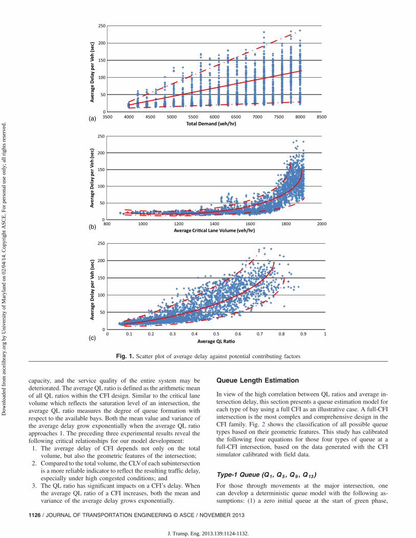
capacity, and the service quality of the entire system may bedeteriorated. The average QL ratio is defined as the arithmetic meanof all QL ratios within the CFI design. Similar to the critical lanevolume which reflects the saturation level of an intersection, theaverage QL ratio measures the degree of queue formation withrespect to the available bays. Both the mean value and variance ofthe average delay grow exponentially when the average QL ratioapproaches 1. The preceding three experimental results reveal thefollowing critical relationships for our model development:1. The average delay of CFI depends not only on the total

volume, but also the geometric features of the intersection;2. Compared to the total volume, the CLVof each subintersection

is a more reliable indicator to reflect the resulting traffic delay,especially under high congested conditions; and

3. The QL ratio has significant impacts on a CFI’s delay. Whenthe average QL ratio of a CFI increases, both the mean andvariance of the average delay grows exponentially.

Queue Length Estimation

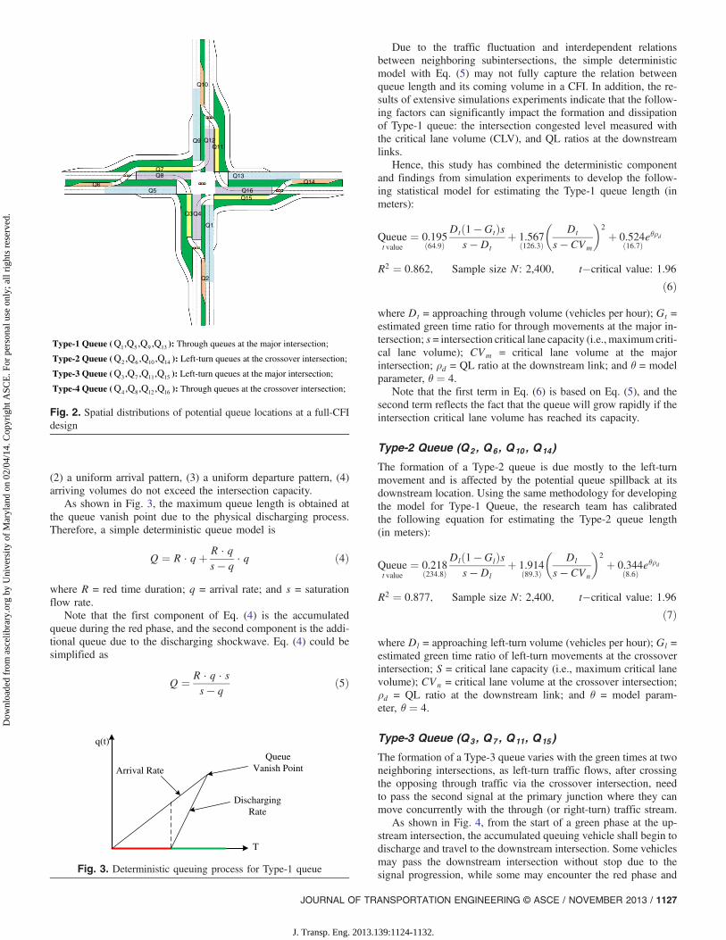
In view of the high correlation between QL ratios and average in-tersection delay, this section presents a queue estimation model foreach type of bay using a full CFI as an illustrative case. A full-CFIintersection is the most complex and comprehensive design in theCFI family. Fig. 2 shows the classification of all possible queuetypes based on their geometric features. This study has calibratedthe following four equations for those four types of queue at afull-CFI intersection, based on the data generated with the CFIsimulator calibrated with field data.

Type-1 Queue (Q1, Q5 , Q9 , Q13 )

For those through movements at the major intersection, onecan develop a deterministic queue model with the following as-sumptions: (1) a zero initial queue at the start of green phase,

0

50

100

150

200

250

3500 4000 4500 5000 5500 6000 6500 7000 7500 8000 8500

Ave

rage

Del

ay p

er V

eh (s

ec)

Total Demand (veh/hr)

0

50

100

150

200

250

800 1000 1200 1400 1600 1800 2000

Aver

age

Del

ay p

er V

eh (s

ec)

Average Cri�cal Lane Volume (veh/hr)

0

50

100

150

200

250

0 0.1 0.2 0.3 0.4 0.5 0.6 0.7 0.8 0.9 1

Ave

rage

Del

ay p

er V

eh (s

ec)

Average QL Ra�o

(a)

(b)

(c)

Fig. 1. Scatter plot of average delay against potential contributing factors


J. Transp. Eng. 2013.139:1124-1132.

Dow

nloa

ded

from

asc

elib

rary

.org

by

Uni

vers

ity o

f M

aryl

and

on 0

2/04

/14.

Cop

yrig

ht A

SCE

. For

per

sona

l use

onl

y; a

ll ri

ghts

res

erve

d.

(2) a uniform arrival pattern, (3) a uniform departure pattern, (4)arriving volumes do not exceed the intersection capacity.

As shown in Fig. 3, the maximum queue length is obtained atthe queue vanish point due to the physical discharging process.Therefore, a simple deterministic queue model is

Q ¼ R · qþ R · qs − q

· q ð4Þ

where R = red time duration; q = arrival rate; and s = saturationflow rate.

Note that the first component of Eq. (4) is the accumulatedqueue during the red phase, and the second component is the addi-tional queue due to the discharging shockwave. Eq. (4) could besimplified as

Q ¼ R · q · ss − q

ð5Þ

Due to the traffic fluctuation and interdependent relationsbetween neighboring subintersections, the simple deterministicmodel with Eq. (5) may not fully capture the relation betweenqueue length and its coming volume in a CFI. In addition, the re-sults of extensive simulations experiments indicate that the follow-ing factors can significantly impact the formation and dissipationof Type-1 queue: the intersection congested level measured withthe critical lane volume (CLV), and QL ratios at the downstreamlinks.

Hence, this study has combined the deterministic componentand findings from simulation experiments to develop the follow-ing statistical model for estimating the Type-1 queue length (inmeters):

Queuet value

¼ 0.195ð64.9Þ

Dtð1 − GtÞss −Dt

þ 1.567ð126.3Þ

�Dt

s − CVm

�2

þ 0.524eθρdð16.7Þ

R2 ¼ 0.862; Sample size N∶ 2,400; t�critical value∶ 1.96ð6Þ

where Dt = approaching through volume (vehicles per hour); Gt =estimated green time ratio for through movements at the major in-tersection; s= intersection critical lane capacity (i.e., maximumcriti-cal lane volume); CVm = critical lane volume at the majorintersection; ρd = QL ratio at the downstream link; and θ = modelparameter, θ ¼ 4.

Note that the first term in Eq. (6) is based on Eq. (5), and thesecond term reflects the fact that the queue will grow rapidly if theintersection critical lane volume has reached its capacity.

Type-2 Queue (Q2 , Q6 , Q10 , Q14)

The formation of a Type-2 queue is due mostly to the left-turnmovement and is affected by the potential queue spillback at itsdownstream location. Using the same methodology for developingthe model for Type-1 Queue, the research team has calibratedthe following equation for estimating the Type-2 queue length(in meters):

Queuet value

¼ 0.218ð234.8Þ

Dlð1 − GlÞss −Dl

þ 1.914ð89.3Þ

�Dl

s − CVn

�2

þ 0.344eθρdð8.6Þ


where Dl = approaching left-turn volume (vehicles per hour); Gl =estimated green time ratio of left-turn movements at the crossoverintersection; S = critical lane capacity (i.e., maximum critical lanevolume); CVn = critical lane volume at the crossover intersection;ρd = QL ratio at the downstream link; and θ = model param-eter, θ ¼ 4.

Type-3 Queue (Q3 , Q7 , Q11, Q15 )

The formation of a Type-3 queue varies with the green times at twoneighboring intersections, as left-turn traffic flows, after crossingthe opposing through traffic via the crossover intersection, needto pass the second signal at the primary junction where they canmove concurrently with the through (or right-turn) traffic stream.

As shown in Fig. 4, from the start of a green phase at the up-stream intersection, the accumulated queuing vehicle shall begin todischarge and travel to the downstream intersection. Some vehiclesmay pass the downstream intersection without stop due to thesignal progression, while some may encounter the red phase and

Type-1 Queue ( 1 5 9 13Q ,Q ,Q ,Q ): Through queues at the major intersection;

Type-2 Queue ( 2 6 10 14Q ,Q ,Q ,Q ): Left-turn queues at the crossover intersection;

Type-3 Queue ( 3 7 11 15Q ,Q ,Q ,Q ): Left-turn queues at the major intersection;

Type-4 Queue ( 4 8 12 16Q ,Q ,Q ,Q ): Through queues at the crossover intersection;

Q1

Q2

Q3Q4

Q5Q6

Q7Q8

Q9

Q10

Q11Q12

Q13Q14

Q15Q16

Fig. 2. Spatial distributions of potential queue locations at a full-CFIdesign

T

q(t)

Discharging Rate

Queue Vanish PointArrival Rate

Fig. 3. Deterministic queuing process for Type-1 queue


J. Transp. Eng. 2013.139:1124-1132.

Dow

nloa

ded

from

asc

elib

rary

.org

by

Uni

vers

ity o

f M

aryl

and

on 0

2/04

/14.

Cop

yrig

ht A

SCE

. For

per

sona

l use

onl

y; a

ll ri

ghts

res

erve

d.

contribute to the queue formation. Also, both the green ratio atdownstream intersection and the QL ratio at downstream linkcan significantly influence the queue length. Hence, one canconstruct the Type-3 queue model with the following three primarycomponents:• Impacts due to the queue at the upstream intersection;• Impact of the downstream red time; and• Impacts due to the downstream QL ratio.

The calibrated regression model with the preceding key compo-nents for the Type-3 queue length (in meters) is given by

Queuet value

¼ 0.101ð17.8Þ

Dlð1 − GuÞsðs −DlÞ

þ 0.128ð15.6Þ

Dlð1 −GdÞ þ 0.22eθρdð7.27Þ


where Dl = approaching left-turn volume (vehicles per hour); Gu =estimated green time ratio of left-turn movements at crossover in-tersections; Gd = estimated green time ratio of left-turn movementsat the major intersection; S = critical lane capacity (i.e., maximumcritical lane volume); ρd = QL ratio at the downstream link; and θ =model parameter, θ ¼ 4.

Type-4 Queue (Q4 , Q8 , Q12 , Q16 )

Similar to the Type-1 queue, key factors such as the incomingdemand to the target approach, the green time ratio, and the inter-section congested level measured with the CLV can collectivelydetermine the formation of Type-4 queue. By including all thesefactors, this study proposes the following model for estimatingthe Type-4 queue length (in meters):

Queuet value

¼ 0.153ð61.7Þ

ðDtþDlÞð1 − GtÞss − ðDtþDlÞ

þ 0.189ð56.3Þ

�DtþDl

s − CVn

�2


where Dt = incoming south (north) bound through volume(vehicles per hour); Dl = incoming west (east) bound left-turn

volume (vehicles per hour); CVn = critical lane volume at thecrossover intersection; Gt = green time ratio for the through move-ment at the crossover intersection; and S = critical lane capacity(i.e., maximum critical lane volume).

Stability Tests of Queue Models

To further investigate the statistical property of the queue formulasderived from regression, two types of statistical tests have beenperformed: the Shapiro-Wilk test of normality and the Chow testof model stability. The Shapiro-Wilk test is employed to confirmthe estimation error of each queue model follows a normaldistribution. As shown in Table 3, all queue models, consistent withthe normality test criterion, reflect that the residuals of regressionequations follow a normal distribution.

To evaluate the model’s stability, the Chow test has also beenapplied to verify that the coefficients of regression equations donot vary with the sample size. To do so, the original data set of800 samples has been divided into two subgroups with n1 ¼600 and n2 ¼ 200 samples, and the Chow test statistics as follows:

F ¼ ½P e2p − ðP e21 þP

e22Þ�=KðP e21 þ

Pe22Þ=ðn1þn2 − 2KÞ ð10Þ

whereP

e2p,P

e21,P

e22 = sum of residual square of the regressionmodel fitted with the original, group 1, and group 2 data sets,respectively; K = number of parameters in regression; and the testresults are summarized in Table 4.

The result of stability tests reflects that all estimated modelparameters are statistically stable, implying that the estimatedqueue lengths with the proposed models are statistically reliablefor use at the planning stage.

Model Application Process

As discussed previously, the occurrence of blockage at CFI maylead to a significant delay increase, and consequently a reductionof its operational benefits. With the queue estimation models, aplanning process is proposed to help engineers in design of a CFI’slink length, and to prevent the potential queue spillback.

Demand Pattern and Signal Settings

To apply the proposed queue estimation models, one shall first setthe signal timings based on the projected demand level. To reflectthe traffic fluctuation over time, a set of demand intervals are de-fined to represent the upper-bound and lower bound of the possible

T

q(t)

Queue Vanish Point

Queue at upstream intersection

Upstream intersection

Downstream intersection

Fig. 4. Deterministic queuing trajectory for Type-3 queue

Table 3. Shapiro-Wilk Normality Test Results

MetricType-1queue

Type-2queue

Type-3queue

Type-4queue

W test statistic 0.9855 0.9767 0.9983 0.9972P-value 1.45 × 10−17 1.72 × 10−22 1.63 × 10−3 1.38 × 10−5

Table 4. Chow Test Results

Queue model Test statistic F value (5%) Pass?

Type 1 2.37 2.62 YesType 2 2.19 2.62 YesType 3 2.59 2.62 YesType 4 2.93 3.01 Yes


J. Transp. Eng. 2013.139:1124-1132.

Dow

nloa

ded

from

asc

elib

rary

.org

by

Uni

vers

ity o

f M

aryl

and

on 0

2/04

/14.

Cop

yrig

ht A

SCE

. For

per

sona

l use

onl

y; a

ll ri

ghts

res

erve

d.

demand patterns. And the actual demand pattern becomes a randomvalue within the given demand intervals.

D ¼ fλi;∀ig ð11Þ

where λi = demand interval and λi ¼ ½λi;λi�.Due to the unique geometric features of CFIs, the number of

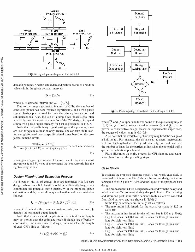
conflicted points has been reduced significantly, and a two-phasesignal phasing plan is used for both the primary intersection andsubintersections. Also, the use of a simple two-phase signal planis actually one of the primary benefits of the CFI design. A typicalsimple two-phase signal strategy for CFI is presented in Fig. 5.

Note that the preliminary signal settings at the planning stageare used for queue estimation only. Hence, one can take the follow-ing straightforward way to specify signal times based on the pro-jected demand level:

gi ¼maxfλi;λj;j∈Vig

maxfλi;λj;j∈Vgþmaxfλi;λj;j∈=Vg for each intersection j

ð12Þ

where gi = assigned green ratio of the movement i; λi = demand ofmovement i; and Vi = set of movements that concurrently has theright-of-way with i.

Design Planning and Evaluation Process

As shown in Fig. 2, 16 critical links are identified in a full CFIdesign, where each link length should be sufficiently long to ac-commodate the potential traffic queues. With the proposed queueestimation models, the resulting queue length could be estimated asfollows:

Qi ¼ fðλi;giÞ ¼ ½fðλi; giÞ; fðλi; giÞ� ð13Þ

where fð⋅Þ indicates the queue estimation model, and interval Qidenotes the estimated queue length.

Note that in a real-world application, the actual queue lengthmay be shorter than the estimated result if signals are effectivelycoordinated. For a conservative design, one can select the lengthof each CFI’s link as follows:

Li ≥ Qi þ μðQi −QiÞ ð14Þ

whereQi andQi = upper and lower bound of the queue length; μ ∈ð0; 1Þ and μ is used to select the value between Qi and Qi so as toprevent a conservative design. Based on experimental experience,the suggested value range is 0.6–0.9.

Also note that the available right-of-way may limit the design ofa link length. For instance, the distance to adjacent intersectionswill limit the length of a CFI’s leg. Alternatively, one could increasethe number of lanes for the particular link when the potential trafficqueue exceeds its upper bound.

Fig. 6 illustrates the entire process for CFI planning and evalu-ation, based on all the preceding steps.

Case Study

To evaluate the proposed planning model, a real-world case study ispresented in this section. Fig. 7 shows the current design at the in-tersection of MD 4 and MD 235 and the layout of the proposed CFIdesign.

The proposed full CFI is designed to contend with the heavy andunbalanced traffic volumes during the peak hours. The morningand afternoon peak hour traffic demands to this site were collectedfrom field surveys and are shown in Table 5.

Some key parameters are initially set as follows:• The maximum link length for the crossover space is 122 m

(400 ft);• The maximum link length for the left-turn bay is 135 m (450 ft);• Leg 1: 2 lanes for left-turn link, 3 lanes for through link and 1

lane for right-turn link;• Leg 2: 1 lanes for left-turn link, 1 lanes for through link and 1

lane for right-turn link;• Leg 3: 1 lanes for left-turn link, 3 lanes for through link and 1

lane for right-turn link;

Fig. 5. Signal phase diagram of a full CFI

Fig. 6. Planning-stage flowchart for the design of CFI


J. Transp. Eng. 2013.139:1124-1132.

Dow

nloa

ded

from

asc

elib

rary

.org

by

Uni

vers

ity o

f M

aryl

and

on 0

2/04

/14.

Cop

yrig

ht A

SCE

. For

per

sona

l use

onl

y; a

ll ri

ghts

res

erve

d.

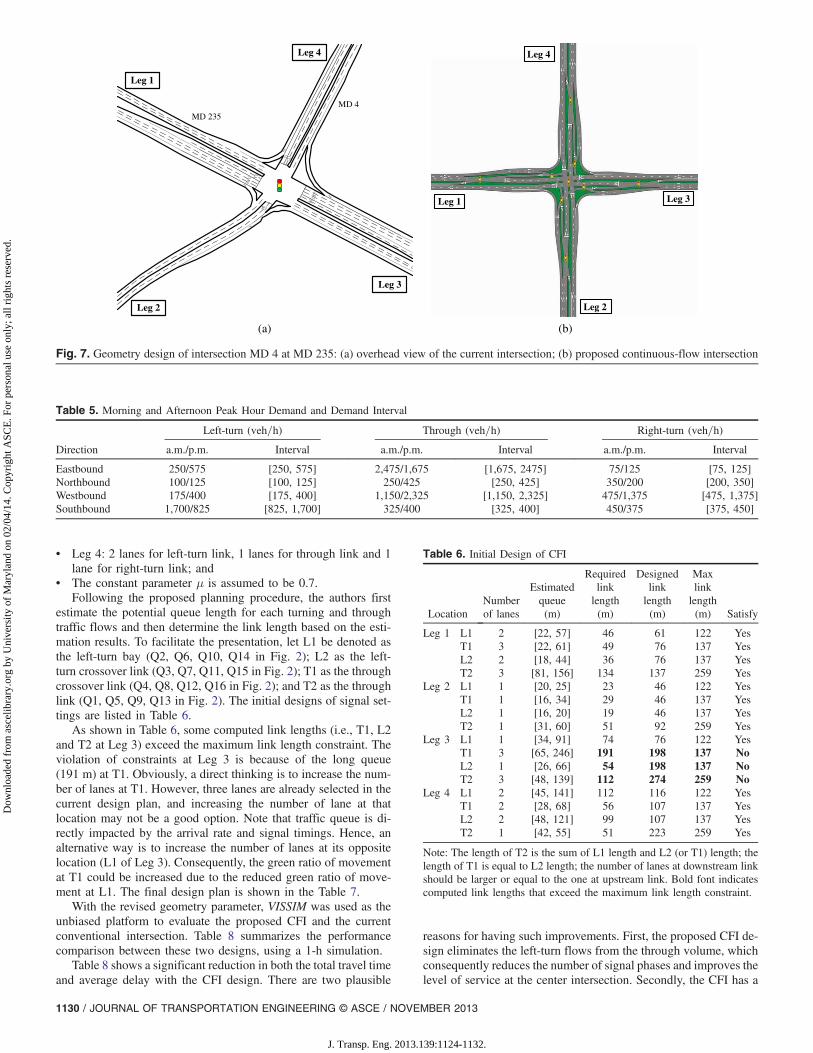
• Leg 4: 2 lanes for left-turn link, 1 lanes for through link and 1lane for right-turn link; and

• The constant parameter μ is assumed to be 0.7.Following the proposed planning procedure, the authors first

estimate the potential queue length for each turning and throughtraffic flows and then determine the link length based on the esti-mation results. To facilitate the presentation, let L1 be denoted asthe left-turn bay (Q2, Q6, Q10, Q14 in Fig. 2); L2 as the left-turn crossover link (Q3, Q7, Q11, Q15 in Fig. 2); T1 as the throughcrossover link (Q4, Q8, Q12, Q16 in Fig. 2); and T2 as the throughlink (Q1, Q5, Q9, Q13 in Fig. 2). The initial designs of signal set-tings are listed in Table 6.

As shown in Table 6, some computed link lengths (i.e., T1, L2and T2 at Leg 3) exceed the maximum link length constraint. Theviolation of constraints at Leg 3 is because of the long queue(191 m) at T1. Obviously, a direct thinking is to increase the num-ber of lanes at T1. However, three lanes are already selected in thecurrent design plan, and increasing the number of lane at thatlocation may not be a good option. Note that traffic queue is di-rectly impacted by the arrival rate and signal timings. Hence, analternative way is to increase the number of lanes at its oppositelocation (L1 of Leg 3). Consequently, the green ratio of movementat T1 could be increased due to the reduced green ratio of move-ment at L1. The final design plan is shown in the Table 7.

With the revised geometry parameter, VISSIM was used as theunbiased platform to evaluate the proposed CFI and the currentconventional intersection. Table 8 summarizes the performancecomparison between these two designs, using a 1-h simulation.

Table 8 shows a significant reduction in both the total travel timeand average delay with the CFI design. There are two plausible

reasons for having such improvements. First, the proposed CFI de-sign eliminates the left-turn flows from the through volume, whichconsequently reduces the number of signal phases and improves thelevel of service at the center intersection. Secondly, the CFI has a

(a) (b)

MD 4

MD 235

Leg 1

Leg 2

Leg 3

Leg 4

Leg 2

Leg 3Leg 1

Leg 4

Fig. 7. Geometry design of intersection MD 4 at MD 235: (a) overhead view of the current intersection; (b) proposed continuous-flow intersection

Table 5. Morning and Afternoon Peak Hour Demand and Demand Interval

Direction

Left-turn (veh=h) Through (veh=h) Right-turn (veh=h)

a.m./p.m. Interval a.m./p.m. Interval a.m./p.m. Interval

Eastbound 250/575 [250, 575] 2,475/1,675 [1,675, 2475] 75/125 [75, 125]Northbound 100/125 [100, 125] 250/425 [250, 425] 350/200 [200, 350]Westbound 175/400 [175, 400] 1,150/2,325 [1,150, 2,325] 475/1,375 [475, 1,375]Southbound 1,700/825 [825, 1,700] 325/400 [325, 400] 450/375 [375, 450]

Table 6. Initial Design of CFI

LocationNumberof lanes

Estimatedqueue(m)

Requiredlinklength(m)

Designedlinklength(m)

Maxlinklength(m) Satisfy

Leg 1 L1 2 [22, 57] 46 61 122 YesT1 3 [22, 61] 49 76 137 YesL2 2 [18, 44] 36 76 137 YesT2 3 [81, 156] 134 137 259 Yes


Leg 3 L1 1 [34, 91] 74 76 122 YesT1 3 [65, 246] 191 198 137 NoL2 1 [26, 66] 54 198 137 NoT2 3 [48, 139] 112 274 259 No


Note: The length of T2 is the sum of L1 length and L2 (or T1) length; thelength of T1 is equal to L2 length; the number of lanes at downstream linkshould be larger or equal to the one at upstream link. Bold font indicatescomputed link lengths that exceed the maximum link length constraint.


J. Transp. Eng. 2013.139:1124-1132.

Dow

nloa

ded

from

asc

elib

rary

.org

by

Uni

vers

ity o

f M

aryl

and

on 0

2/04

/14.

Cop

yrig

ht A

SCE

. For

per

sona

l use

onl

y; a

ll ri

ghts

res

erve

d.

larger geometry layout to prevent the occurrence of queue spill-backs. However, the reduction of average number of stops is notquite significant, due to the increased number of intersections.The measure of effectiveness (MOEs) improvement of CFI clearlyshows the potential effectiveness of the proposed planning models.

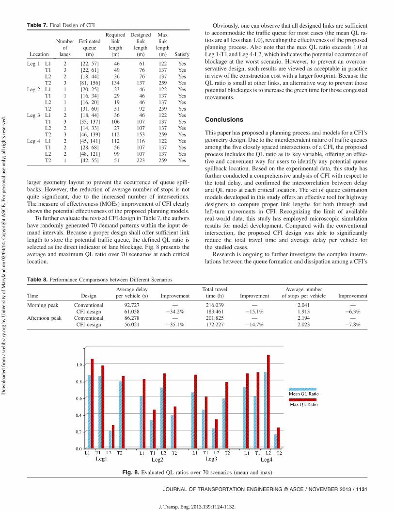
To further evaluate the revised CFI design in Table 7, the authorshave randomly generated 70 demand patterns within the input de-mand intervals. Because a proper design shall offer sufficient linklength to store the potential traffic queue, the defined QL ratio isselected as the direct indicator of lane blockage. Fig. 8 presents theaverage and maximum QL ratio over 70 scenarios at each criticallocation.

Obviously, one can observe that all designed links are sufficientto accommodate the traffic queue for most cases (the mean QL ra-tios are all less than 1.0), revealing the effectiveness of the proposedplanning process. Also note that the max QL ratio exceeds 1.0 atLeg 1-T1 and Leg 4-L2, which indicates the potential occurrence ofblockage at the worst scenario. However, to prevent an overcon-servative design, such results are viewed as acceptable in practicein view of the construction cost with a larger footprint. Because theQL ratio is small at other links, an alternative way to prevent thosepotential blockages is to increase the green time for those congestedmovements.

Conclusions

This paper has proposed a planning process and models for a CFI’sgeometry design. Due to the interdependent nature of traffic queuesamong the five closely spaced intersections of a CFI, the proposedprocess includes the QL ratio as its key variable, offering an effec-tive and convenient way for users to identify any potential queuespillback location. Based on the experimental data, this study hasfurther conducted a comprehensive analysis of CFI with respect tothe total delay, and confirmed the intercorrelation between delayand QL ratio at each critical location. The set of queue estimationmodels developed in this study offers an effective tool for highwaydesigners to compute proper link lengths for both through andleft-turn movements in CFI. Recognizing the limit of availablereal-world data, this study has employed microscopic simulationresults for model development. Compared with the conventionalintersection, the proposed CFI design was able to significantlyreduce the total travel time and average delay per vehicle forthe studied cases.

Research is ongoing to further investigate the complex interre-lations between the queue formation and dissipation among a CFI’s

Table 7. Final Design of CFI

Location

Numberof

lanes

Estimatedqueue(m)

Requiredlinklength(m)

Designedlinklength(m)

Maxlinklength(m) Satisfy





Table 8. Performance Comparisons between Different Scenarios

Time DesignAverage delayper vehicle (s) Improvement

Total traveltime (h) Improvement

Average numberof stops per vehicle Improvement

Morning peak Conventional 92.727 — 216.039 — 2.041 —CFI design 61.058 −34.2% 183.461 −15.1% 1.913 −6.3%

Afternoon peak Conventional 86.278 — 201.825 — 2.194 —CFI design 56.021 −35.1% 172.227 −14.7% 2.023 −7.8%

Fig. 8. Evaluated QL ratios over 70 scenarios (mean and max)


J. Transp. Eng. 2013.139:1124-1132.

Dow

nloa

ded

from

asc

elib

rary

.org

by

Uni

vers

ity o

f M

aryl

and

on 0

2/04

/14.

Cop

yrig

ht A

SCE

. For

per

sona

l use

onl

y; a

ll ri

ghts

res

erve

d.

five intersections under various signal control plans. The results ofdelay and queue analyses at the operational level can also serve asthe basis for development of signal optimization model for CFI.

Acknowledgments

The data support from the Maryland State Highway Administrationis greatly appreciated.

References

Cheong, S., Rahwanji, S., and Chang, G. L. (2008). “Comparison ofthree unconventional arterial intersection designs: continuous flowintersection, parallel flow intersection, and upstream signalizedcrossover.” 11th Int. IEEE Conf. New York.

El Esawey, M., and Sayed, T. (2007). “Comparison of two unconventionalintersection schemes.” Transportation Research Record No. 2023,Transportation Research Board, Washington, DC, 10–19.

Goldblatt, R., Mier, F., and Friedman, J. (1994). “Continuous flow inter-section.” J. Inst. Transport. Eng., 64(7), 34–42.

Hildebrand, T. E. (2007). “Unconventional intersection designs for improv-ing through traffic along the arterial road.” Ph.D. Thesis, Dept. of Civiland Environmental Engineering, Florida State Univ., Tallahassee, FL.

Hughes, W., Jagannathan, R., Sengupta, D., and Hummer, J. (2010).“Alternative intersections/interchanges: Information report (AIIR).”

FHWA-HRT-09-060, Federal Highway Administration, Washington,DC, 7–70.

Hummer, J. E. (1998a). “Unconventional left-turn alternative for urban andsuburban arterials: Part One.” ITE Journal, 68(9), 26–29.

Hummer, J. E. (1998b). “Unconventional left-turn alternative for urban andsuburban arterials: Part Two.” ITE J. Web, 101–106.

Inman, V. W. (2009). “Evaluation of signs and markings for partialcontinuous flow intersectionS.” Transportation Research Record2138, Transportation Research Board, Washington, DC, 66–74.

Jagannathan, R., and Bared, J. G. (2004). “Design and operational perfor-mance of crossover displaced left-turn intersections.” TransportationResearch Record 1981, Transportation Research Board, Washington,DC, 86–96.

Kim, M., Lai, X., Chang, G. L., and Rahwanji, S. (2007). “Unconventionalarterial designs initiatives.” IEEE Conf. on Intelligent TransportationSystems, Seattle.

Pitaksringkarn, J. P. (2005). “Measures of effectiveness for continuous flowintersection: A Maryland intersection case study.” ITE 2005 AnnualMeeting and Exhibit Compendium of Technical Papers, Institute ofTransportation Engineers, ARRB Group, Australia.

Reid, J. D., and Hummer, J. E. (1999). “Analyzing system travel time inarterial corridors with unconventional designs using microscopicsimulation.” Transportation Research Record 1678, TransportationResearch Board, Washington, DC, 208–215.

Reid, J. D., and Hummer, J. E. (2001). “Travel time comparisons betweenseven unconventional arterial intersection designs.” TransportationResearch Record 1751, Transportation Research Board, Washington,DC, 55–56.


J. Transp. Eng. 2013.139:1124-1132.

Dow

nloa

ded

from

asc

elib

rary

.org

by

Uni

vers

ity o

f M

aryl

and

on 0

2/04

/14.

Cop

yrig

ht A

SCE

. For

per

sona

l use

onl

y; a

ll ri

ghts

res

erve

d.

development of planning-stage models for analyzing...

Documents