i

DEVELOPMENT OF MICRO-GRINDING MECHANICS AND MACHINE TOOLS

A Dissertation Presented to

The Academic Faculty

By

Hyung Wook Park

In Partial Fulfillment of the Requirements for the Degree

of Doctor of Philosophy in the George W. Woodruff School of Mechanical Engineering

Georgia Institute of Technology April, 2008

ii

DEVELOPMENT OF MICRO-GRINDING MECHANICS AND MACHINE TOOLS

Approved by: Dr. Steven Y. Liang, Advisor George W. Woodruff School of Mechanical Engineering Georgia Institute of Technology

Dr. Chen Zhou H. Milton Stewart School of Industrial and Systems Engineering Georgia Institute of Technology

Dr. Steven Danyluk George W. Woodruff School of Mechanical Engineering Georgia Institute of Technology

Dr. Paul Griffin H. Milton Stewart School of Industrial and Systems Engineering Georgia Institute of Technology

Dr. Shreyes N. Melkote George W. Woodruff School of Mechanical Engineering Georgia Institute of Technology

Date Approved: 12/19/2007

iii

ACKNOWLEDGEMENTS

I would, first of all, like to thank my advisor Dr. Steven Y. Liang for all the

support, guidance and encouragement throughout the course of my graduate study. I

would also like to thank the members of my thesis committee, Professors Shreyes

Melkote, Steven Danyluk, Chen Zhou and Paul Griffin. Thanks are also due to Steven

Sheffield for his assistance in conducting my experiments. I would also like to thank all

the support staff in MARC and ME for all their help especially John Morehouse, Pam

Rountree, Glenda Johnson, Trudy Allen and Wanda Joefield.

I would like to thank my colleagues, Siva, Ramesh Singh, Sathyan Subbiah,

Jiann-Cherng Su, Kuan-Ming Li, Adam Cardi, Carl Hanna, Qiulin Xie, Injoong Kim,

Sangil and Haiyan Deng for their help and support during my stay at Georgia Tech.

Finally, I would like to thank my family and my wife, Jinae lee, for their love,

support, encouragement and understanding throughout my graduate study. This thesis

would not be possible without them.

iv

TABLE OF CONTENTS

ACKNOWLEDGEMENTS............................................................................................... iii

LIST OF TABLES........................................................................................................... viii

LIST OF FIGURES ............................................................................................................ x

LIST OF SYMBOLS ....................................................................................................... xvi

SUMMARY...................................................................................................................... xx

CHAPTER 1. INTRODUCTION ....................................................................................... 1

1.1 Background ........................................................................................................... 1

1.2 Research objective ................................................................................................ 5

1.3 Dissertation organization ...................................................................................... 6

CHAPTER 2. LITERATURE REVIEW ............................................................................ 9

2.1 Micro/meso-scale machine tools........................................................................... 9

2.1.1 Current developments on microscale machine tools ................................... 10

2.1.2 Technical review of component technologies.............................................. 13

2.1.3 Design methodology of microscale machine tools ...................................... 14

2.2 Introduction of the micro-grinding process ........................................................ 16

2.2.1 Modeling in the grinding process ................................................................ 17

2.2.2 Modeling of thermal effects in grinding ...................................................... 20

2.2.3 Characterization of grinding wheel topography .......................................... 23

2.3 Micromachining process..................................................................................... 26

2.3.1 Size effect in micromachining ..................................................................... 27

2.3.2 Crystallographic effects ............................................................................... 29

2.4 Summary............................................................................................................. 31

v

CHAPTER 3. MODELING OF MICRO-GRINDING FORCES AND THERMAL

EFFECTS.......................................................................................................................... 33

3.1 Introduction......................................................................................................... 33

3.2 Modeling the single grit interaction in micro-grinding....................................... 34

3.2.1 Modeling of Chip Formation Forces in individual grits .............................. 34

3.2.2 Prediction of the ploughing Force................................................................ 39

3.2.3 Shear angle in the single grit interaction...................................................... 42

3.3 Material model in micro-grinding....................................................................... 44

3.3.1 Material model of conventional flow stress................................................. 44

3.3.2 Material model considering the crystallographic effects ............................. 48

3.3.3 Material properties of Al 6061-T6............................................................... 50

3.4 Analysis of the single grit force model behavior ................................................ 52

3.5 Modeling of thermal effects in micro-grinding .................................................. 55

3.6 Calibration of heat partition ratio to the workpiece ............................................ 58

3.7 Summary............................................................................................................. 62

CHAPTER 4. CHARACTERIZING THE TOPOGRAPHY OF A MICRO-GRINDING

WHEEL............................................................................................................................. 64

4.1 Introduction......................................................................................................... 64

4.2 Electroplated grinding wheel .............................................................................. 65

4.3 Characterizing micro-grinding topography......................................................... 66

4.3.1 Optical method for the micro-grinding wheel topography .......................... 66

4.3.2 Direct method for micro-grinding wheel topography.................................. 69

4.4 Comparison between optical and direct methods ............................................... 76

vi

4.5 Dynamic cutting edge density............................................................................. 79

4.6 Summary............................................................................................................. 82

CHAPTER 5. COMPARISON BETWEEN THEORETICAL AND EXPERIMENTAL

COMPUTATIONS ........................................................................................................... 84

5.1 Introduction......................................................................................................... 84

5.2 Comprehensive model of micro-grinding forces ................................................ 85

5.2.1 Sensitivity analysis of a comprehensive model ........................................... 86

5.3. Experiment of micro-structure characterization ................................................ 88

5.3.1 Experiment for measuring the grain size ..................................................... 88

5.3.2 Grain boundary misorientation of Al 6061 T6 ............................................ 93

5.3.3 Contribution of the effects of microstructure............................................... 95

5.4 Experiment set-up of micro-grinding.................................................................. 97

5.5 Sensitivity analysis of experimental data.......................................................... 101

5.6 Model validation ............................................................................................... 104

5.6.1 Identification of parameter effects ............................................................. 105

5.6.2 Comparisons between experiment data and predictions............................ 108

5.6.3 Assessment of the effects of temperature .................................................. 115

5.7 Summary........................................................................................................... 116

CHAPTER 6. MULTI-OBJECTIVE OPTIMIZATION OF MICROSCALE MACHINE

TOOLS............................................................................................................................ 118

6.1 Introduction....................................................................................................... 118

6.2 Structural performance evaluation.................................................................... 120

6.2.1 Static stiffness evaluation .......................................................................... 120

vii

6.2.2 Thermal stiffness evaluation ...................................................................... 122

6.2.3 Dynamic characteristic evaluation............................................................. 124

6.3 Experimental analysis ....................................................................................... 127

6.3.1 Identification of dynamic parameters ........................................................ 131

6.4 Evaluation of machine performance using FEM .............................................. 133

6.5 Volumetric error evaluation.............................................................................. 137

6.6 Mathematical computation................................................................................ 140

6.7 Summary........................................................................................................... 145

CHAPTER 7. CONCLUSIONS AND RECOMMENDATIONS.................................. 147

7.1 Summary........................................................................................................... 147

7.2 Contributions and Conclusions ......................................................................... 148

7.3 Recommendations............................................................................................. 151

7.3.1 Modeling of the micro-grinding wheel wear ............................................. 152

7.3.2 Analysis of the space between grit behavior.............................................. 152

7.3.3 Predictive modeling of surface roughness ................................................. 152

7.3.4 Optimization of the micro-grinding process .............................................. 153

7.3.5 Performance evaluation techniques of miniaturized machine tools .......... 153

REFERENCES ............................................................................................................... 154

VITA............................................................................................................................... 163

viii

LIST OF TABLES

Table 1-1: Characteristics of the micro-grinding process................................................... 4

Table 2-1: Category of previous works ............................................................................ 16

Table 3-1: Material constants of Johnson-Cook model of Al 6061-T6[85] ..................... 50

Table 3-2: Material properties of Al 6061-T6 .................................................................. 50

Table 3-3: Key properties of microstructure of Al 6061-T6............................................. 51

Table 3-4: Estimated heat partition ratios to the workpiece ............................................. 61

Table 3-5: Thermal properties of CBN............................................................................. 61

Table 4-1: Profiles of section cuts of CBN 85002-BM worn and fresh wheels ............... 74

Table 4-2: Estimation of the size of grits for fresh and worn tools .................................. 76

Table 4-3: Summary of computations for static cutting density....................................... 77

Table 4-4: Regression results of dynamic cutting edge density ....................................... 82

Table 5-1: Input factor levels for sensitivity analysis....................................................... 86

Table 5-2: L9 orthogonal matrix of the Taguchi method ............................................... 102

Table 6-1: Dimensions of the miniaturized milling machine ......................................... 128

Table 6-2: Values of spring and damping parameters .................................................... 132

Table 6-3: Natural frequencies and damping ratios of experimental analysis and modeling

......................................................................................................................................... 132

Table 6-4: Summary of structure modes......................................................................... 136

Table 6-5: Natural frequencies and damping ratios of experimentaldata and FEM analysis

......................................................................................................................................... 136

Table 6-6: Magnitudes of other parameters at the optimal point of the analytical models

......................................................................................................................................... 142

ix

Table 6-7: Magnitudes of other parameters at the optimal point of FEM computations 142

Table 6-8: Experimental data of Aerotech positioning table .......................................... 144

Table 6-9: Results of the modified penalty function ...................................................... 144

x

LIST OF FIGURES

Figure 1-1: Disciplinary areas for various micro manufacturing by Liang [1]................... 1

Figure 1-2: Fabrication of microscale parts using conventional and micro grinding ......... 2

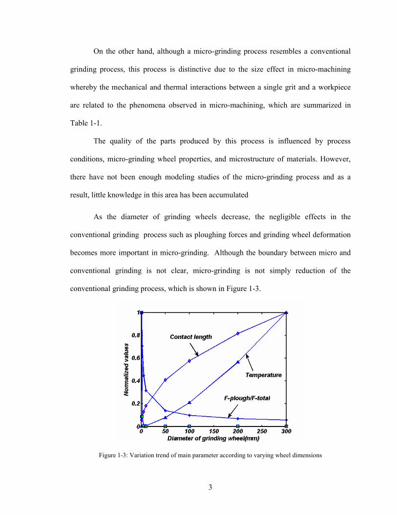
Figure 1-3: Variation trend of main parameter according to varying wheel dimensions ... 3

Figure 1-4: Flow chart of thesis organization ..................................................................... 8

Figure 2-1: Installation space of various machine tool..................................................... 11

Figure 2-2: (a) Machined grooves[11] and (b) 2nd generation UIUC Miniature Machine

Tool[8] .............................................................................................................................. 12

Figure 2-3: (a) 100 µm micro milling cutter and (b) 250µm micro grinding wheel ........ 14

Figure 2-4: (a) Ductile extrusion ahead of the grit by Shaw[28], (b) Chip formation

process with a high negative angle by Komanduri [30] ................................................... 19

Figure 2-5: A stylus trace of a grinding wheel surface..................................................... 25

Figure 2-6: Image of the wheel topography by interferometer[51] ................................. 26

Figure 2-7: Comparison between conventional and micromachining processes[62] ....... 30

Figure 2-8: (a) Variation of cutting forces corresponding with the grain boundary of Al

alloy [66]and (b) FE model of heterogeneous materials[67] ............................................ 31

Figure 3-1: A mechanical interaction of the single grit in micro-grinding....................... 35

Figure 3-2: Illustration of the geometric configuration on the spherical shape grit ......... 38

Figure 3-3: Simplification of the plough effects into a spherical indentation .................. 40

Figure 3-4: (a) Schematic of hard sphere sliding on a softer material and (b) Ploughing

friction coefficient as a function of the ratio of the depth of cut to the tool nose radius .. 42

Figure 3-5: Main effects plot for the shear angle predictions........................................... 44

xi

Figure 3-6: (a)Geometry model (b) process variation according different depths of cut by

Manjunathaiah and Endres[83] ......................................................................................... 46

Figure 3-7: Variation in vicker’s microhardness with d-1/2 for Al-Mg alloys[87].......... 51

Figure 3-8: Breakdown of single grit force in normal direction for Grit size= 43µm,

Vw=1mm/sec, and spindle RPM=60000 .......................................................................... 52

Figure 3-9: Breakdown of single grit force in tangential direction for Grit size= 43µm,

Vw=1mm/sec, and spindle RPM=60000 .......................................................................... 53

Figure 3-10: (a) Forces trend of the single grit in normal and tangential directions for

1 / secwV mm= and (b) force configuration........................................................................ 54

Figure 3-11: Schematic of the micro-grinding thermal model ......................................... 56

Figure 3-12: Microchips at 20µm depth of cut in micro-grinding.................................... 59

Figure 3-13: Temperature matching technique................................................................. 59

Figure 3-14: Experiment configuration for measuring the surface temperature............... 60

Figure 3-15: Comparison between experimentally calibrated values and analytical

predictions......................................................................................................................... 62

Figure 4-1: Illustration of CBN grinding wheel and (b) SEM picture for 120 grit by Shi

and Malkin[95].................................................................................................................. 65

Figure 4-2: Illustration of 85002-BM electroplated CBN wheel...................................... 66

Figure 4-3: (a) Example of replication on a lead plate and (b) measured profile of an

imprinted lead plate........................................................................................................... 67

Figure 4-4: (a) Imported ZYGO optical image in MATLAB software, (b) Computed

static cutting edge density in Case 1, (c) Case 2, (d) Case3, (e) Case4, and (f) Case 5.... 68

xii

Figure 4-5: (a) Illustration of a prepared sample and (b) Flowchart of the proposed direct

method............................................................................................................................... 70

Figure 4-6: Section profiles of (a) fresh and (b) worn micro-grinding wheels................. 71

Figure 4-7: Circle fitting in MATLAB software .............................................................. 73

Figure 4-8: Estimated diameter of micro-grinding wheels ............................................... 73

Figure 4-9: Calibration of the grit size on (a) fresh and (b) worn micro-grinding wheels 74

Figure 4-10: (a) Fitted normal distributions of new and worn micro-grinding wheels and

(b) Plot of the mean grit diameter versus the grit number ................................................ 75

Figure 4-11: Schematic illustration of extension for the extracted profile data ............... 76

Figure 4-12: Comparison between the optical and direct methods................................... 78

Figure 4-13: (a) Tracing and (b) illustration of dynamic cutting edges............................ 80

Figure 4-14: Dynamic density of cutting edges for

1 / secwV mm= , 10 / secwV mm= , 20 / secwV mm= , and 30 / secwV mm= in the direct method......... 81

Figure 4-15: Ratio variation of dynamic cutting edge density to static cutting edge density

for varying workpiece speed in direct method.................................................................. 81

Figure 5-1: Illustration of the predictive model of the micro-grinding forces.................. 86

Figure 5-2: Main effect plots of (a) Fy and (b) Fx............................................................ 87

Figure 5-3: Scheme of the prepared Al 6061-T6 sample.................................................. 89

Figure 5-4: Processed images in (a) sample position 1, (b) sample position 2, (c) sample

position 3, and (d) sample position 4 ................................................................................ 89

Figure 5-5: Illustration of the line intercept method for measuring the size of grains ..... 90

Figure 5-6: Experimental data of the average grain size .................................................. 91

Figure 5-7: Extracted log-normal distribution of Al 6061 T6 .......................................... 93

xiii

Figure 5-8: The density function for the angle of misorientation..................................... 94

Figure 5-9: Grain boundary misorientation of AL 6061-T6 by Kang et al.[91]............... 94

Figure 5-10: (a) The breakdowns of shear stresses computed and (b) shear stress along

depths of cut for 1wV mm= , grit size=43µm, and 60000RPM rpm= ................................... 96

Figure 5-11: The trend of the model output for varying depths of cut and grain sizes .... 97

Figure 5-12: Schematic of (a) a miniaturized machine tool and (b) Illustration of

experiment configuration .................................................................................................. 98

Figure 5-13: Detail schematic of surface micro-grinding................................................. 99

Figure 5-14: Pure force signal for 20µm depth of cut and spindle RPM 60000rpm ...... 100

Figure 5-15: FFT analysis of (a) section 1 and (b) section 2 in Figure 5-14 .................. 100

Figure 5-16: Experimental data of the micro-grinding forces at 60000rpm and 20µm

depth of cut ..................................................................................................................... 101

Figure 5-17: Normal and tangential forces for cases1-9................................................. 102

Figure 5-18: Main effect plot of (a) normal forces and (b) tangential forces ................. 103

Figure 5-19: Micro-grinding forces for varying depths of cut for sec/1mmVw = ......... 104

Figure 5-20: Comparisons of (a) tangential and (b) normal forces for varying feedrates

......................................................................................................................................... 105

Figure 5-21: Comparisons of (a) tangential and (b) normal forces for different sizes of the

micro-grinding wheel...................................................................................................... 107

Figure 5-22: Comparison between experimental data and predictions for (a) tangential

(Fx) and (b) normal forces (Fy) of 85001-BM ( 0.75ed mm≈ ) for 1 /secwV mm= ......... 109

Figure 5-23: Comparison between experimental data and predictions for (a) tangential

(Fx) and (b) normal forces (Fy) of 85002-BM ( 1.00ed mm≈ ) for 1 /secwV mm= ............... 110

xiv

Figure 5-24: Comparison between experimental data and predictions for (a) tangential

(Fx) and (b) normal forces (Fy) of 85003-BM ( 1.25ed mm≈ ) for 1 /secwV mm= ................ 111

Figure 5-25: Comparison between experimental data and predictions for (a) tangential

(Fx) and (b) normal forces (Fy) of 85002-BM ( 1.00ed mm≈ ) for 10 /secwV mm= .............. 113

Figure 5-26: Comparison between experimental data and predictions for (a) tangential

(Fx) and (b) normal forces (Fy) of 85002-BM ( 1.00ed mm≈ ) for 30 /secwV mm= ............. 114

Figure 5-27: Temperature rise on the shear plane accord to the depth of cut for 60000rpm

and 1 /secwV mm= .............................................................................................................. 116

Figure 6-1: Proposed design strategy.............................................................................. 119

Figure 6-2: Simplified machine structure model ............................................................ 121

Figure 6-3: (a) Static and (b) Thermal Stiffness of the miniaturized milling machine, and

(c) temperature distribution during machine operation .................................................. 123

Figure 6-4: Machine configuration and masses of machine components....................... 124

Figure 6-5: Three degree of freedom lumped parameter model ..................................... 126

Figure 6-6: Contribution of Rayleigh damping parameters ............................................ 127

Figure 6-7: Illustration of the miniaturized milling machine with variable dimensions 128

Figure 6-8: (a) Original shape and (b) FFT analysis of output signals from accelerometer

sensors in case 1.............................................................................................................. 129

Figure 6-9: (a) Illustration of sensor positions, (b) the hammer impact, (c) the FRF of the

case 1 and (d) the case 2 in the y direction ..................................................................... 130

Figure 6-10: Comparisons between experimental data and modeling values in terms of (a)

1st natural frequency and (b) damping ratio .................................................................... 133

Figure 6-11: FEM analysis of (a) static and (b) thermal deformation ............................ 134

xv

Figure 6-12: comparisons of (a) static and (b) thermal stiffness .................................... 135

Figure 6-13: (a)1st, (b)2nd ,(c) 3rd , and (d) 4th modes of machine tool structure ............ 136

Figure 6-14: Schematic diagram of (a) the miniaturized machine tool and (b) chain

representation.................................................................................................................. 138

Figure 6-15: Assessment of optimal dimensions of the miniaturized milling machine . 141

Figure 6-16: A comparison between the analytical models and FEM computations ..... 143

Figure 6-17: The sensitivity analysis of weighing factors .............................................. 145

xvi

LIST OF SYMBOLS

r cutting edge radius

mt minimum undeformed chip thickness

crα critical rake angle

sα effective rake angle

0t undeformed chip thickness

τ shear strength

ϕ angle of inclination

iβ instantaneous friction angle

iα instantaneous friction angle

iφ nominal friction angle

,cg xF , ,cg yF chip formation forces per grit

,cg xdF , ,cg ydF differential chip formation forces per grit

,pg xF , ,pg yF ploughing forces per grit in the normal and tangential directions

brinellF Brinell hardness force

HB Brinell hardness

pµ ploughing friction coefficient

w width of indentation

D ball diameter

b diameter of the impression

Α,Β,C ,m ,n Johnson-Cook model coefficients

xvii

nφ , nα nominal shear and rake angles

sl length of a shear plane

oxleyC Oxley’s constant

shV shear velocity

wV feedrate

sV grinding velocity

ε ,ε strain and strain rate

,γ γ shear strain and strain rate

,chip workυ υ volume ratios of the chip and workpiece deformation

v Poisson ratio

M Taylor factor

contα material’s constant

bgb burger vector of dislocations

ρt total dislocation density

ρ0 dislocation density in the volume between boundaries

ρb dislocation density per unit volume

dD average grain diameter

k constant of the geometry boundary

HPK Hall-Petch coefficient

G shear modulus

avθ average misorientation

xviii

ed diameter of the micro-grinding wheel

, oq q heat flux

Tm melting point of material

To environment temperature

T material temperature

cl contact length

Rr roughness factor

Rw heat partition ratio to the workpiece

Rs heat partition ratio to the micro-grinding wheel

ce process specific energy

ce energy to melt the workpiece materials

gk grit thermal conductivity

ck thermal conductivity

ρ density

c specific heat

sC static grit density

dC dynamic grit density

gc constant of the dynamic effect

infeedθ infeed angle

,s sA k constants of regression

( )E X expectation

xix

( )Var X variance

E modulus of elasticity

I moment of inertia

, ,b b bA B C constants of machine dimensions

tα thermal expansion coefficient

[ ]M mass matrix

[ ]C damping matrix

[ ]K joint stiffness matrix

[ ( )]G w receptance matrix

ω rotational frequency

,R Rα β constants of Rayleigh damping model

iξ damping ratio

niω rotational frequency in mode i

, ,ei ei eiα β γ rotation errors

, ,xei yei zeiδ δ δ translation errors

iC weighing factor

xx

SUMMARY

Micro-grinding with microscale machine tools is a micro-machining process in

precision manufacturing of microscale parts such as micro sensors, micro actuators,

micro fluidic devices, and micro machine parts. Mechanical micro-machining generally

consists of various material removal processes. Micro-grinding of these processes is

typically the final process step and it provides a competitive edge over other fabrication

processes. The quality of the parts produced by this process is affected by process

conditions, micro-grinding wheel properties, and microstructure of materials. Although a

micro-grinding process resembles a traditional grinding process, this process is

distinctive due to the size effect in micro-machining because the mechanical and thermal

interactions between a single grit and a workpiece are related to the phenomena observed

in micro-machining. However, there have not been enough modeling studies of the

micro-grinding process and as a result, little knowledge base on this area has been

accumulated.

In this study, the new predictive model for the micro-grinding process was

developed by consolidating mechanical and thermal effects within the single grit

interaction model at microscale material removal. The size effect of micro-machining

was also included in the proposed model. In order to assess thermal effects, the heat

partition ratio was experimentally calibrated and compared with the prediction of the

Hahn model. Then, on the basis of this predictive model, a comparison between

experimental data and analytical predictions was conducted in view of the overall micro-

grinding forces in the x and y directions. Although there are deviations in the predicted

xxi

micro-grinding forces at low depths of cut, these differences are reduced as the depth of

cut increases. On the other hand, the optimization of micro machine tools was performed

on the basis of the proposed design strategy. Individual mathematical modeling of key

parameters such as volumetric error, machine working space, and static, thermal, and

dynamic stiffness were conducted and supplemented with experimental analysis using a

hammer impact test. These computations yield the optimal size of miniaturized machine

tools with the technical information of other parameters.

1

CHAPTER 1

INTRODUCTION

1.1 Background

Manufacturing technology has advanced to higher levels of precision to satisfy

the increasing demand to reduce the size of parts and products in the electronics,

computer, and biomedical industrial sectors. New processing concepts, procedures and

machines are thus needed to fulfill the increasingly stringent requirements and

expectations.

Mechanical micro-machining is an emerging technology carrying large benefits

and equally great challenges in fabrication of microscale parts. Existing micro-machining

processes can be broadly classified into mechanical micro-machining, chemical-

mechanical micro-machining, high energy beams-based machining, and scanning probe

micro-machining in Figure 1-1.

Figure 1-1: Disciplinary areas for various micro manufacturing by Liang [1]

2

Among these technologies, mechanical micro-machining using miniaturized

machine tools is one research direction and it has a number of inherent advantages. These

advantages include: the significant reduction of required space and energy consumption

for machine drive; the improvement of machine robustness against external error sources

due to increasing thermal, static, and dynamic stabilities; increased positioning accuracy

due to decreased overall size of machine; and a greater freedom in the selection of work-

piece materials, the complexity of the product geometry, and the cost of investment.

Mechanical micro-machining generally consists of various material removal

processes. Within these processes, micro-grinding is typically the final process step and

like conventional grinding, it provides a competitive edge over other processes in

fabrication of microscale parts such as micro sensors, micro actuators, micro fluidic

devices, and micro machine parts. But, since conventional grinding wheels are very large

compared to target products, their capability is usually limited to grinding simple parts as

indicated in Figure 1-2.

Figure 1-2: Fabrication of microscale parts using conventional and micro grinding

1mm 100~mm

Micro-grinding wheel

Conventional-grinding wheel

Same part

3

On the other hand, although a micro-grinding process resembles a conventional

grinding process, this process is distinctive due to the size effect in micro-machining

whereby the mechanical and thermal interactions between a single grit and a workpiece

are related to the phenomena observed in micro-machining, which are summarized in

Table 1-1.

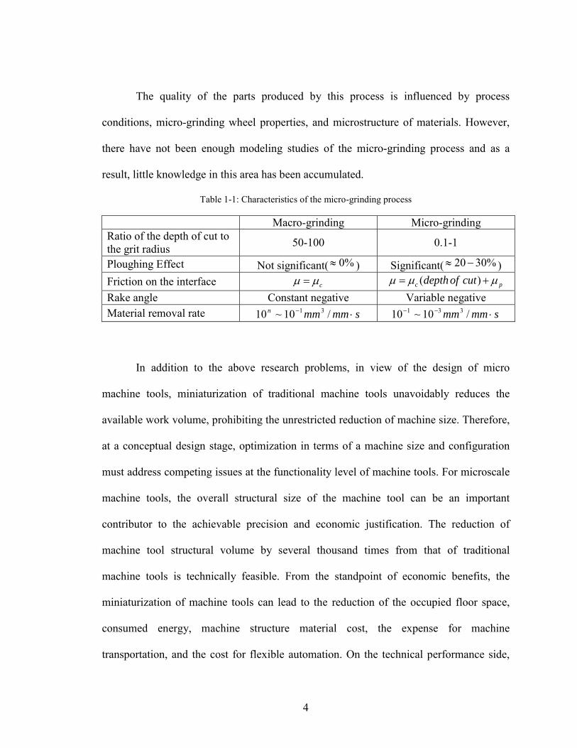
The quality of the parts produced by this process is influenced by process

conditions, micro-grinding wheel properties, and microstructure of materials. However,

there have not been enough modeling studies of the micro-grinding process and as a

result, little knowledge in this area has been accumulated

As the diameter of grinding wheels decrease, the negligible effects in the

conventional grinding process such as ploughing forces and grinding wheel deformation

becomes more important in micro-grinding. Although the boundary between micro and

conventional grinding is not clear, micro-grinding is not simply reduction of the

conventional grinding process, which is shown in Figure 1-3.

Figure 1-3: Variation trend of main parameter according to varying wheel dimensions

4

The quality of the parts produced by this process is influenced by process

conditions, micro-grinding wheel properties, and microstructure of materials. However,

there have not been enough modeling studies of the micro-grinding process and as a

result, little knowledge in this area has been accumulated.

Table 1-1: Characteristics of the micro-grinding process

Macro-grinding Micro-grinding Ratio of the depth of cut to the grit radius 50-100 0.1-1

Ploughing Effect Not significant( 0%≈ ) Significant( 20 30%≈ − ) Friction on the interface cµ µ= ( )c pdepth of cutµ µ µ= + Rake angle Constant negative Variable negative Material removal rate smmmmn ⋅− /10~10 31

smmmm ⋅−− /10~10 331

In addition to the above research problems, in view of the design of micro

machine tools, miniaturization of traditional machine tools unavoidably reduces the

available work volume, prohibiting the unrestricted reduction of machine size. Therefore,

at a conceptual design stage, optimization in terms of a machine size and configuration

must address competing issues at the functionality level of machine tools. For microscale

machine tools, the overall structural size of the machine tool can be an important

contributor to the achievable precision and economic justification. The reduction of

machine tool structural volume by several thousand times from that of traditional

machine tools is technically feasible. From the standpoint of economic benefits, the

miniaturization of machine tools can lead to the reduction of the occupied floor space,

consumed energy, machine structure material cost, the expense for machine

transportation, and the cost for flexible automation. On the technical performance side,

5

smaller manufacturing systems can provide higher static rigidity, thermal resistance, and

dynamic stiffness, thereby improving machining accuracy and precision. Recently, the

shapes of miniaturized machine tools have become more complex and precise. However,

there has not been enough discussion to provide a basic approach to the suitable

configuration for the design parameters of microscale manufacturing systems because the

previous design procedure of commercial manufacturing systems depends on designer

and company experience.

1.2 Research objective

Micro-grinding with miniaturized machine tools is an emerging area due to

possible impacts on the industrial field. Although there are many efforts to model the

conventional grinding process by experimental and analytical methods, these are limited

to grinding with a conventional grinding wheel.

In this research, after reviewing work relevant to micro-grinding with

miniaturized machine tools, in order to predict the micro-grinding force as a function of

the kinematics of the grinding process and wheel topography, the following tasks were

undertaken:

• Development of the single grit interaction between the workpiece and the

abrasive particle considering the size effects.

• Assessment and modeling of the thermal effects in micro-grinding.

• Calibration of the heat partition ratio in micro-grinding.

6

• Characterization of the micro-grinding wheel.

• Development of a material model incorporating crystallographic

effects

• Model validation with experimental data.

Micro-grinding is carried out using miniaturized machine tools. So optimization

of the structure of miniaturized machine tools has to be pursued. To optimize the size of

machine structure according to different machine configurations and sizes, in this

research, the following tasks are taken

• Development of mathematical models of key parameters such as

volumetric error, machine working space, and static, thermal, and dynamic

stiffness

• Optimization and sensitivity analysis of the weighing factors

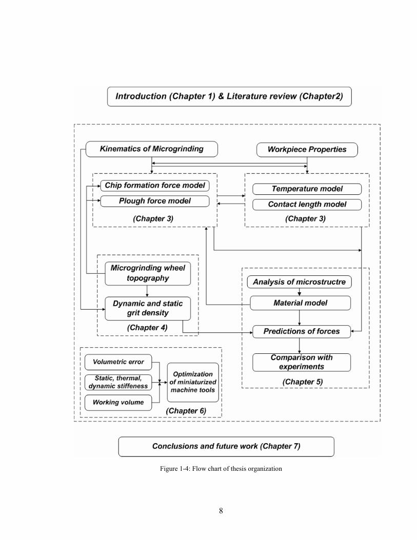
1.3 Dissertation organization

This dissertation is laid out as follows in Figure 1-4. Chapter 2 describes the

literature and relevant works in microscale machine tools, physical modeling of the

conventional grinding process, and mechanical micromachining. Modeling of the single

grit interaction for micro-grinding and modeling of thermal effects in micro-grinding

with calibration of the heat partition ratio to the workpiece is presented in Chapter 3.

7

Experimental and analytical studies of the micro-grinding wheel topography are

described in Chapter 4. Chapter 5 describes experiments of micro-grinding forces and

microstructure and comparison between experimental data and predictions. Optimization

of the size of machine tool structure is described in Chapter 6. Finally, Chapter 7

describes the conclusions and the recommendations for future research.

8

Figure 1-4: Flow chart of thesis organization

9

CHAPTER 2

LITERATURE REVIEW

This chapter presents a review of literature in relevant areas to the proposed

works. These works provide an overview of past and current research relating to

microscale machining which covers microscale machining using solid tools and

fabrication of microscale precision machines. A general synopsis of the literature review

is conveniently divided into three groups: (i) Microscale manufacturing systems, (ii)

Physical modeling of conventional grinding, (iii) Micromachining. The research on

microscale manufacturing systems will include reviews on the recent development of

prototypes such as micro lathes, micro turning, and design methodology of microscale

machine tools. Physical modeling of conventional grinding will include information on

mechanical interaction modeling, thermal effect modeling, and grinding wheel

topography. The literature review of the size effect will discuss experimental and

analytical studies of these effects.

2.1 Micro/meso-scale machine tools

Increasing demand for fabrication of microscale parts in electronic, computer, and

biomedical industrial sectors has created the need to minimize conventional machine

tools because the size of their target’s product is small compared to their size. In view of

this, the development of micro and meso scale machine tools has become an attractive

10

area to researchers. Many attempts to fabricate microscale prototype machine tools have

been conducted, primarily understand the underlying mechanisms of microscale machine

tools. Current research in microscale machine tools can be broadly classified into two

groups: (i) Construction and evaluation of various prototypes of microscale machine tools

and (ii) Design of microscale machine tools.

2.1.1 Current developments on microscale machine tools

Economic aspects such as cost savings of consumed power and used floor space

and technical advantages such as reduction of thermal deformation and enhancements of

static and dynamic stabilities[2, 3] have driven the development of smaller machine tools.

In the late 1980s, Japanese engineers started to develop prototypes of microscale machine

tools with the support of the Japanese government. Most researches at this early stage

sought to develop various prototypes of microscale machine tools [4-6]. In the earliest

attempt to develop a prototype of a microscale machine tool, a micro lathe was developed

by Kitahara et al.[4]. It has dimensions of 32mmx25mmx30.5mm. This machine consists

of an X-Y moving unit driven by a laminated piezo actuator and a small main shaft

driven by a micro motor. Its power consumption is 1/1000 that of a conventional lathe.

Lu and Yoneyama[5] summarized the growing issues of development of the microscale

machine tools and developed a new micro turning system which has a new point tool. It

is applied to a micro turning at an elevated rotation speed. Mishima et al.[6] developed a

micro factory consisting of three machine tools and two small manipulators. This factory

shows the capability to fabricate a ball bearing. Vogler et al.[7] developed a meso scale

11

machine tool with the dimensions of 25x25x25mm. In this research, two new major

concepts of driving were relative accuracy and volumetric utilization.

Some early successes in the development of microscale machine tools and some

recent advances in component technologies including the high speed spindle, positioning

table, handling system, and metrology system[8] provide a foundation for the

development of more accurate and better performance microscale machine tools. Based

on previous design experiences and prototypes, second generation microscale machine

tools have been developed at national laboratories and academic institutions around the

globe. Rahman et al.[9] developed a CNC micro turning machine tool. Its dimensions are

560x600x660 mm and each axis has an optical linear scale with resolution of 0.1µm.

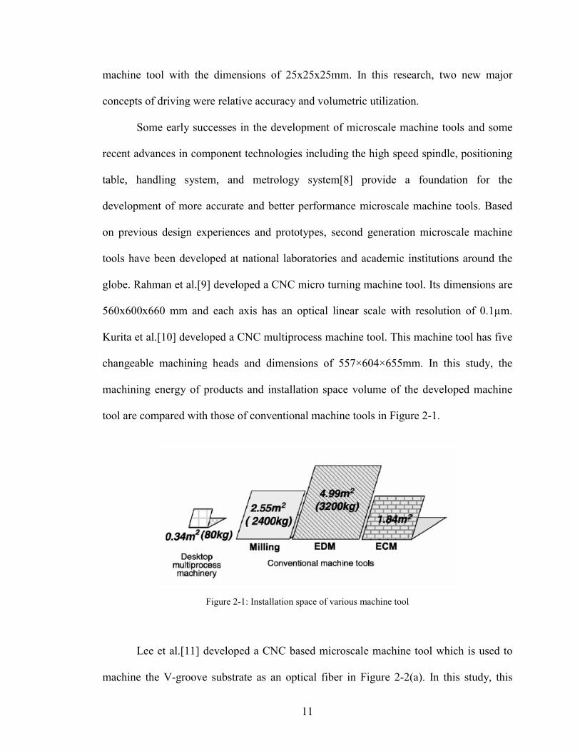
Kurita et al.[10] developed a CNC multiprocess machine tool. This machine tool has five

changeable machining heads and dimensions of 557×604×655mm. In this study, the

machining energy of products and installation space volume of the developed machine

tool are compared with those of conventional machine tools in Figure 2-1.

Figure 2-1: Installation space of various machine tool

Lee et al.[11] developed a CNC based microscale machine tool which is used to

machine the V-groove substrate as an optical fiber in Figure 2-2(a). In this study, this

12

developed machine shows the physical capability to machine an arbitrary 3D shape. It

indicates that the stiffness of a machine tool is closely related to the quality of the

products. The university of Illinois at Urbana-Champaign[8] developed a micro milling

machine. Its dimensions are 180×180×300mm and the movement travel range is

25×25×25mm. This machine is a three axis horizontal microscale machine tool with

voice coil motors, a 160k RPM air-turbine, air bearing spindle, and 0.1mm encoder

resolution as shown in Figure 2-2(b).

(a) (b)

Figure 2-2: (a) Machined grooves[11] and (b) 2nd generation UIUC Miniature Machine Tool[8]

Consequently, extensive researches involving the recent developments of

microscale machine tools like Chen et al.[12] ,Cox et al.[2], Okazaki et al.[13], and Lin

et al.[14] have been pursued. In order to provide further improvement of these microscale

machine tools, fundamental understanding of the issues in microscale machine tools is

needed.

13

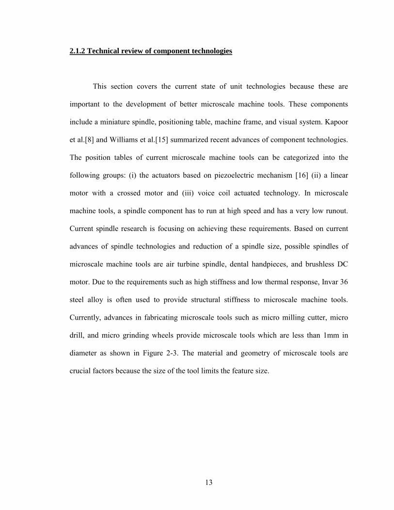
2.1.2 Technical review of component technologies

This section covers the current state of unit technologies because these are

important to the development of better microscale machine tools. These components

include a miniature spindle, positioning table, machine frame, and visual system. Kapoor

et al.[8] and Williams et al.[15] summarized recent advances of component technologies.

The position tables of current microscale machine tools can be categorized into the

following groups: (i) the actuators based on piezoelectric mechanism [16] (ii) a linear

motor with a crossed motor and (iii) voice coil actuated technology. In microscale

machine tools, a spindle component has to run at high speed and has a very low runout.

Current spindle research is focusing on achieving these requirements. Based on current

advances of spindle technologies and reduction of a spindle size, possible spindles of

microscale machine tools are air turbine spindle, dental handpieces, and brushless DC

motor. Due to the requirements such as high stiffness and low thermal response, Invar 36

steel alloy is often used to provide structural stiffness to microscale machine tools.

Currently, advances in fabricating microscale tools such as micro milling cutter, micro

drill, and micro grinding wheels provide microscale tools which are less than 1mm in

diameter as shown in Figure 2-3. The material and geometry of microscale tools are

crucial factors because the size of the tool limits the feature size.

14

(a) (b)

Figure 2-3: (a) 100 µm micro milling cutter and (b) 250µm micro grinding wheel

In microscale machine tools, although an inspection system doesn’t affect the

micromachining process, it is an important device to ensure good performance of

microscale machine tools. Due to the feature size of this process, observation of

micromachining processes using magnification is needed. Generally, optical

magnification cameras have been used in microscale machine tools because there is a

limitation of machine space.

2.1.3 Design methodology of microscale machine tools

In the case of traditional machine tools, the design methodology has matured

through experimental learning and methodological improvement[17]. However, there is

not enough accumulated knowledge for microscale machine tool design based on

experience and knowledge. There is no sufficient discussion devoted to the optimization

of individual miniaturized machine designs. As of yet, fairly little design experience and

knowledge base toward miniaturization of a manufacturing system have been

15

accumulated. Although several attempts have been made [12, 18, 19], the optimal size of

the miniaturized machine tool has not yet been systematically attained.

At the beginning of the research for miniaturized machine tools design, Mishima

et al.[20, 6, 19] presented a design evaluation method for miniaturized machine tools.

This method adopted a kinematic representation of machine structures with the Taguchi

method to estimate the contribution of each local error component, which serves as

proper background for this study. In this study, results showed that the spindle whirling

error and horizontal direction error of the feed unit have a considerable influence on

machining accuracy. Chen et al.[12] developed a novel virtual machine tool (VMT)

integrated design environment in which kinematic functionality was embedded in the

description of the sub-components. It was found that the results of the VMT

configuration analysis for miniaturized machine tools are similar with configuration

candidates of traditional machine tools. In these studies, volumetric error for various

machine configurations is used as a key criterion to estimate the proper configuration for

miniaturized machine tools. Recent work by Lee et al.[18] studies the dynamic behavior

characterization of a mesoscale machine tool (mMT). In this study, the size effect in the

dynamic behavior of the mMT was investigated experimentally and numerically. The

outcomes show that the characterization of the dynamic properties of the joints of mMTs

is an important factor in determining the dynamic behavior of mMTs. However, previous

works in Table 2-1 don’t provide information about the optimal dimensions per each

design configuration.

In design of traditional and miniaturized machine tools, a conceptual design stage

of all major elements is important. This step defines basic features and capabilities of

16

traditional and miniaturized machine tools. In the case of miniaturized machine tools, this

design stage acquires more importance because the ratio of the overall size of the

miniaturized machine tools to the target products significantly decreases compared to

traditional machine tools. The conceptual design for miniaturized machine tools has to be

accompanied with comprehensive analyses of possible effective factors such as static,

dynamic, and thermal stiffness, machine accuracy, and machine working volume.

Table 2-1: Category of previous works

Mishima et al.[20] Chen et al.[12] Lee et al.[18]

Geometrical error

Error transformation matrix and form shaping function

Multi-axis kinematic error module N/A

Dynamic stiffness N/A N/A

Structural dynamics of machine tools and scaling analysis

Thermal/static stiffness N/A N/A N/A

Others Effect of design parameters and error components

Development of a comprehensive integrated design environment

An equivalent lumped parameter model

2.2 Introduction of the micro-grinding process

Micro-grinding apparently resembles the conventional grinding process in terms

of its stochastic characteristics. It is distinctive in view of the size effect on the interaction

between a single grit and the workpiece. Analytical modeling of micro-grinding starts

from the individual grit interaction and then is commonly extrapolated into a whole

grinding wheel surface as in models of the conventional grinding process. In the micro-

grinding process, the deformation caused by a single grit during its interaction with the

17

workpiece is closely related with deformation modes, including micro-machining and

ploughing mechanisms. The following sections provide related past studies of (i) models

in grinding, (ii) modeling of thermal effects in grinding, and (iii) wheel characterization

of micro-grinding wheel.

2.2.1 Modeling in the grinding process

In micro and macro grinding, abrasive grits, which are hard particles with sharp

edges, are bonded to a wheel rotating at high speed to carry out the cutting process. The

orientation of individual grits on the grinding wheel surface is random. So conventional

grinding has historically been considered a complex manufacturing process. Due to this

complexity, most grinding models are based on empirical relations where the main

process variables like the cutting depth, velocity ratio and equivalent diameter are driven

to an exponent and multiplied by coefficients that are obtained experimentally by curve

fitting of experimental data.

Hahn and Linsay [21-24] experimentally addressed various aspects of the

grinding process and provided several quantitative relationships in material removal rate,

wheel wear, chatter, surface finish, and geometry. In this study, empirical equations were

obtained among process parameters. Malkin et al.[25] presented empirical observations

of the grinding process and established the equations for most grinding parameters. Shaw

[26] summarized the fundamental studies of grinding in his book. Tönshoff et al.[27]

reviewed most aspects of the grinding process including wheel topography, chip

thickness, grinding energy, temperature, and surface roughness. Most models in this

review are established based on experimental data except for the temperature model. In

18

industry, the empirical model has been extensively used to determine the setup

parameters of the machining. However, the exponents and coefficients in empirical

models must be adjusted for each different combination of workpiece material, wheel

topography, and kinematics of the grinding using time consuming and costly

experimental tests. This shows a constraint on the empirical model in predicting the

grinding process and drawing optimal solutions for the different grinding configurations.

Due to the random nature of the cutting edges and to poor understanding of the

behavior of a material subjected to extreme conditions, there has been motivation to

develop a physical model by first modeling the interaction of an individual grit with the

workpiece. After construction of the single grit interaction model, the single grit

interaction model can be extrapolated into the whole grinding wheel. Past works by Shaw

[28], Maan et al.[29], Komanduri [30], and Torrance [31] showed that the interaction

between a grit and the workpiece is dominated by high negative rake angle and high

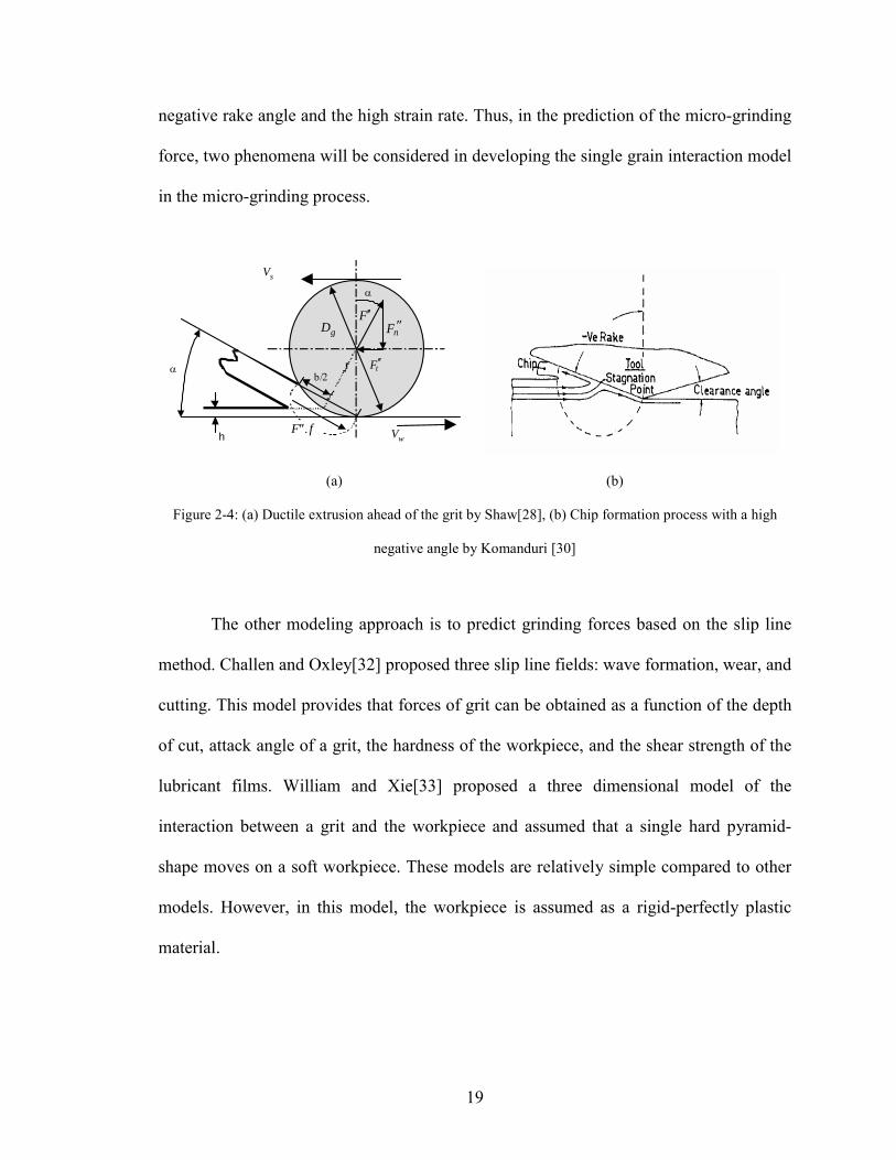
strain rate. Figure 2-4 shows two primary mechanisms between previous proposed works.

Shaw [28] assumed a spherical grit shape and presented the single grit model to predict

the force per grain based on a force equilibrium between the hardness of the material and

the indention force acting on a grit. However, this model doesn’t cover the effects of

process conditions. On the other hand, Komanduri [30] proposed that the single grit

interaction is similar to machining with a high negative rake angle. This research showed

that there is a stagnation point which is referred as to a minimum chip thickness. While

these two mechanisms are practically plausible, they cannot be used in the single grit

model for the micro-grinding process because, in the micro-grinding, the single grit

undergoes two phenomena: (i) micro-scale indentation, (ii) micro-cutting with the high

19

negative rake angle and the high strain rate. Thus, in the prediction of the micro-grinding

force, two phenomena will be considered in developing the single grain interaction model

in the micro-grinding process.

(a) (b)

Figure 2-4: (a) Ductile extrusion ahead of the grit by Shaw[28], (b) Chip formation process with a high

negative angle by Komanduri [30]

The other modeling approach is to predict grinding forces based on the slip line

method. Challen and Oxley[32] proposed three slip line fields: wave formation, wear, and

cutting. This model provides that forces of grit can be obtained as a function of the depth

of cut, attack angle of a grit, the hardness of the workpiece, and the shear strength of the

lubricant films. William and Xie[33] proposed a three dimensional model of the

interaction between a grit and the workpiece and assumed that a single hard pyramid-

shape moves on a soft workpiece. These models are relatively simple compared to other

models. However, in this model, the workpiece is assumed as a rigid-perfectly plastic

material.

α b/2

F′′nF ′′

h

tF ′′

α

.F f′′

gD

wV

sV

20

2.2.2 Modeling of thermal effects in grinding

In the grinding process, since the energy density in the grinding zone is high

compared to traditional machining processes such as turning, milling, planning, and

broaching, the thermally induced stress to the workpiece is an important parameter on the

workpiece property. There are many efforts devoted to modeling the thermal effects in

the grinding process using various techniques such as analytical and experimental

methods. These works seek to understand the heat partition in grinding and to predict the

temperature as well as its influence on surface integrity.

In most theoretical modeling of thermal effects, a moving heating source analysis

by Jaeger[34] was used to predict the temperature in grinding. In that model, the grinding

zone is assumed as a band source of heat that moves along the surface of the workpiece at

the workpiece feedrate, and the temperature rise was driven in direction of movement of

the heat source and the depth into the workpiece.

At the early stage, Outwater and Shaw[35] suggested that the possible sources of

heat generation are as follows:(i) heat, (ii) kinetic energy of the chips, (iii) surface energy

needed to form new surfaces, and (iv) potential energy residing in the workpiece and the

chips. They indicated that most grinding energy is transformed into heat and other

energies can be negligible. They presented a model of heat transfer to the workpiece

based on a sliding heat source at the shear plane; this is the shear plane partitioning model.

Hahn [36] proposed a sliding model for the heat partition ratio between the workpiece

and the wheel in grinding, in which the primary heat source is the grit and workpiece

rubbing surfaces. This study more accurately described heat generation by considering

21

the forces at the contact between the grit and the workpiece and ignoring the forces in the

shear plane. Makin[37] summarized the results of earlier researches and Makin and

Anderson [38, 39] proposed a model of the grinding zone temperature and the

temperature at the surface as a sum of a local temperature generated by grinding of an

individual grit and considered the frictional heating at the wear flat and shear deformation

on the shear plane. Ramanath and Shaw[40] showed that the fraction of heat conducted in

the workpiece depends on the thermal properties of workpiece and grits. They pointed out

that a small portion of the heat generated in grinding is conducted into the workpiece and

the grits carry away most of the heat. Tönshoff et al.[27] suggested that the locations of

heat generation in grinding are shearing zone, rake face friction, cutting edge, flank

friction, and bond and coolant frictions, and they indicated that the flank friction is a

important heat source in grinding because most energy generated in grinding is consumed

on sliding and plowing. In grinding, their works showed that the frictional energy is very

important to model thermal effects and the principal source of heat generation. Therefore,

the frictional heat model is suitable to represent the temperature in grinding.

The other approach is to use the finite element method (FEM) to find the surface

temperature. Werner et al.[41] adapted finite element analysis(FEA) to model

temperature in grinding and showed that the temperature at the workpiece surface

decreases with increasing depth of cut. One of their earlier attempts was to model the

effect of all four heat sinks. The FEM approach is a very useful way to assess thermal

damage in grinding. But it requires considerable computing time and power.

Measuring temperatures in grinding is a challenging problem because in a short

time period, there are multiple contacts between grits and the workpiece through the

22

grinding zone. Experimental techniques used in grinding experiments can be classified

into three: (i) an embedded thermocouple and (ii) an embedded infrared detector using a

fiber optic linked to a two color pyrometer. A thermocouple was first used to measure the

temperature in grinding and is still used at this time. The other technique is an infrared

method to measure the flash temperature. Although this method shows good capability to

measure the grain temperature, this method can be applicable when the fluid exists in

grinding. So, the thermocouple method is more suitable in micro-grinding experiments

and to improve the response time of this thermocouple, a smaller size for the

thermocouple is desired.

Xu and Malkin[42] compared three different methods such as the thermocouple

method and the infrared method by measuring the temperature of grinding AISI 1010

steel using a Cubic Boron Nitride (CBN) abrasive particle. All three methods provided

comparable temperature responses, which were consistent with analytical predictions

from a moving heat source analysis.

In thermal modeling, the heat partition ratio that is the fraction of the heat flux

that is transferred into the workpiece is an important factor[36, 43]. The estimation of the

heat partition is still the challenging problem. Experiments to determine the heat partition

ratio to the workpiece are generally based on the above techniques and temperature

matching by Kohil et al.[44]or inverse heat transfer techniques are used to find the heat

partition ratio. Generally, since the inverse heat transfer technique is not plausible,

temperature matching method is used in calibrating thermal models.

23

In the temperature matching method, data input to the workpiece were obtained

by measuring the temperature profile in the workpiece using an embedded thermocouple

technique and matching the results with analytically computed values.

2.2.3 Characterization of grinding wheel topography

The complexity of the grinding process comes from the grinding wheel, which

contains various abrasive particles. These grits are randomly distributed on the grinding

wheel surface. So there is significant variation of the process due to this randomness. But

information regarding the density, size, and shape of these grits is not given by the wheel

specifications. Identification of the topography of a grinding wheel provides a good

reliability to predict the overall grinding forces because the total grinding forces highly

depend on the total number of the grits engaged in grinding. The number of active grits

depends not only on the static density of the cutting edges but also on the kinematics of

grinding.

König et al.[45] combined the number of active cutting edges with the dynamic

chip thickness as well as the shape and angle of the cutting edges. They showed that all

static cutting edges within a contact zone are not engaged in grinding.

Verkerk et al.[46] reviewed different methods to measure the static and dynamic

density of grits such as the taper print, piezoelectric sensors, and stylus method. Their

studies proposed the common ground of two different parameters in grinding such as the

static and dynamic density of cutting edges. It was found that the experiments of

measuring the dynamic density of grits are complicated because the distinction between

24

cutting and plowing mechanisms is not clear. Generally, the static density of cutting

edges is obtained from direct measurements. But, the dynamic density of cutting edges is

determined from experimental data with the analytical approach considering the

kinematics of cutting edges.

Younis et al. [47] showed that the percentage of the dynamic cutting edges to the

static cutting edges is 2% to 12%.

Characterization of the grinding wheel is a crucial factor to allow better prediction

of a grinding process. Various techniques have been developed to get better information

about grinding wheel topography. The main techniques for grinding wheel topography

are

• Stylus methods

• Replication methods

• Microscopic methods

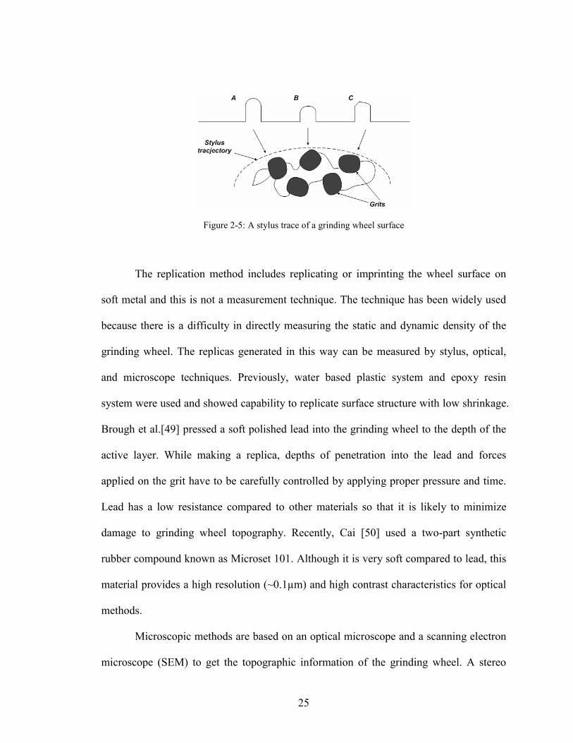
The principle of the stylus method is similar to that used for the surface roughness

measurement. A stylus with the small spherical tip is dragged over the wheel surface to

measure the profile of the grinding wheel surface. A two-dimensional profile of the

grinding wheel surface is obtained from this method. The experimental results can be

used as an input to predict the grinding process.

But there are drawbacks to this method. First, the accuracy of the method really

depends on the shape and size of the stylus tip. There is also the wear of the stylus due to

a continued contact between hard abrasive particles and the stylus tip. König et al.[48]

presented new techniques to obtain a three-dimensional image of a grinding wheel

surface by scanning the wheel in the transversal and circumferential directions.

25

Figure 2-5: A stylus trace of a grinding wheel surface

The replication method includes replicating or imprinting the wheel surface on

soft metal and this is not a measurement technique. The technique has been widely used

because there is a difficulty in directly measuring the static and dynamic density of the

grinding wheel. The replicas generated in this way can be measured by stylus, optical,

and microscope techniques. Previously, water based plastic system and epoxy resin

system were used and showed capability to replicate surface structure with low shrinkage.

Brough et al.[49] pressed a soft polished lead into the grinding wheel to the depth of the

active layer. While making a replica, depths of penetration into the lead and forces

applied on the grit have to be carefully controlled by applying proper pressure and time.

Lead has a low resistance compared to other materials so that it is likely to minimize

damage to grinding wheel topography. Recently, Cai [50] used a two-part synthetic

rubber compound known as Microset 101. Although it is very soft compared to lead, this

material provides a high resolution (~0.1µm) and high contrast characteristics for optical

methods.

Microscopic methods are based on an optical microscope and a scanning electron

microscope (SEM) to get the topographic information of the grinding wheel. A stereo

26

microscope using a built-in vertical illuminator is relatively inexpensive and invaluable.

This microscope provides fine details of the surface using a large magnification. But at

low magnifications, sometimes, it is hard to distinguish between grits and bonds.

SEM provides detailed and clear information about the grinding wheel surface

with high magnifications. The problems of this microscope are that sections of a wheel

have to be small enough to fit to the observation area and the size of SEM chamber and

that the replication materials tend to melt during experiments.

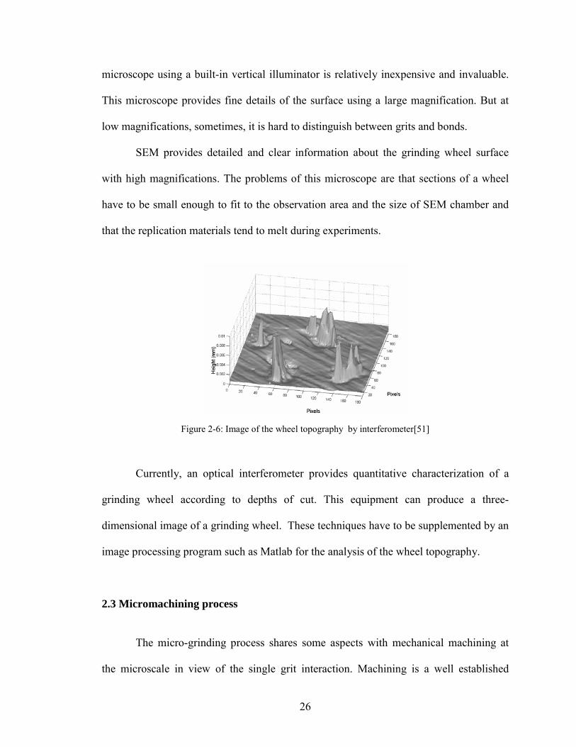
Figure 2-6: Image of the wheel topography by interferometer[51]

Currently, an optical interferometer provides quantitative characterization of a

grinding wheel according to depths of cut. This equipment can produce a three-

dimensional image of a grinding wheel. These techniques have to be supplemented by an

image processing program such as Matlab for the analysis of the wheel topography.

2.3 Micromachining process

The micro-grinding process shares some aspects with mechanical machining at

the microscale in view of the single grit interaction. Machining is a well established

27

material removal process for fabricating three dimensional macroscale components. As

the demand for fabrication of microscale components increases, mechanical machining at

the microscale, more commonly referred to as micromachining, is an emerging

technology because it can produce intricate three dimensional features which satisfy

stringent dimensional tolerance and high surface finish requirements. However, there are

still numerous challenges to address in order for micro-cutting to be economically viable

and reliable for fabricating microscale components.

Currently, there have been numerous studies of tool life, edge radius effect,

surface generation, size-effect in the specific cutting energy, minimum chip thickness,

micro-structural effects as well as finite element modeling and molecular dynamics

simulation of microscale cutting. However, there is no fundamental understanding and

general consensus on the mechanism that dominates mechanical machining at the

microscale. Specifically, there is no basic understanding of the size effect in specific

cutting energy in micromachining and there is no knowledge of how these process

responses differ from those in macro-scale cutting.

2.3.1 Size effect in micromachining

In these studies of micro-cutting forces, the specific energy in machining, which

is required to remove a unit volume of metal, is typically found to increase at small

values of the undeformed chip thickness. This increase is associated with an increase in

the specific cutting force with decreasing chip thickness, which phenomenon has been

termed the size effect. On the basis of previous findings, Subbiah and Melkote[52]

summarized possible contributors for the size effect. These contributors are tool edge

28

radius effects, sub-surface plastic deformation, material strengthening effects, and

material separation effects.

Shaw[53] and Backer et al.[54] attributed the size effect in shear energy per unit

volume to strain hardening and the short range inhomogeneity in metals, which is related

with a dislocation theory. Based on this theory, material strength in plastic deformation of

metals is determined by the motion of dislocation and their interactions. Nakayama[55]

attributed the size effect to the decrease of the shear angle due to the finite edge radius of

the tool and to greater energy dissipation which is related with sub-surface plastic

deformation of the workpiece. Atkins[56] attributed the size effect to the material

separation effect which is related with the energy required to create new surfaces via

ductile fracture.

Beside the above explanations, Masuko et al.[57] attributed the size effect to an

extra force required to penetrate the workpiece, which is related to an indentation force

due to ploughing before chip formation. Albrecht[58] suggested that the plough force is a

contributor to the size effect. The reason is that at small depths of cut, the ploughing force

contributes a greater proportion of the total cutting force.

Recent works by Dinesh et al.[59] and Joshi and Melkote[60] have suggested the

likelihood of strain gradient plasticity effects at the shear plane leading to the size effect

in machining. This phenomenon refers to an increase in yield stress of a material with

increasing strain gradient. Kai and Melkote[61] developed the FE model of orthogonal

cutting incorporating strain gradient effects. There is still no general consensus and

definitive explanation established for the size effect phenomenon. In this study, among

29

the described effects, the effects of the ploughing force and the tool edge radius are

implemented in the model developed.

2.3.2 Crystallographic effects

In micromachining, the cutting depth and feed rate are smaller with respect to

conventional machining. So the depth of cut can be smaller at machining polycrystalline

materials than the average grain size. During micromachining, the tool works intra-

crystalline and it cuts through grain boundaries, which is related with the grain size of

materials. In both cases, the crystallographic orientation and size have important effects

on the micromachining processes.

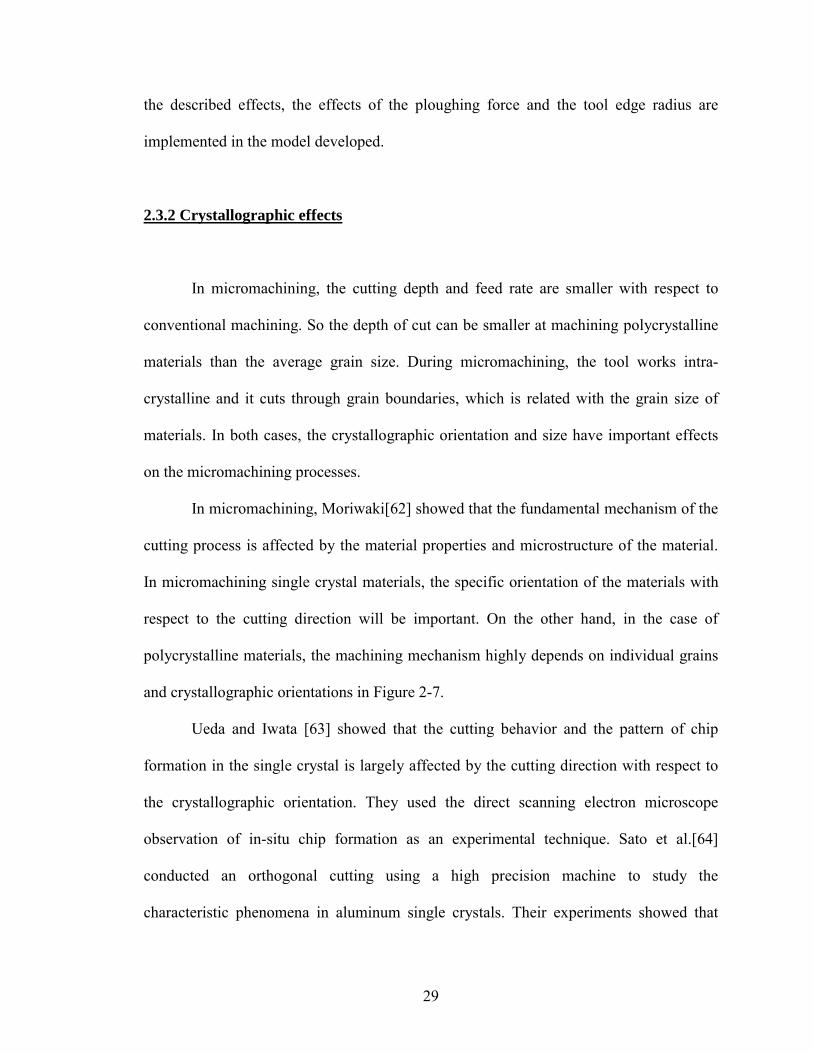
In micromachining, Moriwaki[62] showed that the fundamental mechanism of the

cutting process is affected by the material properties and microstructure of the material.

In micromachining single crystal materials, the specific orientation of the materials with

respect to the cutting direction will be important. On the other hand, in the case of

polycrystalline materials, the machining mechanism highly depends on individual grains

and crystallographic orientations in Figure 2-7.

Ueda and Iwata [63] showed that the cutting behavior and the pattern of chip

formation in the single crystal is largely affected by the cutting direction with respect to

the crystallographic orientation. They used the direct scanning electron microscope

observation of in-situ chip formation as an experimental technique. Sato et al.[64]

conducted an orthogonal cutting using a high precision machine to study the

characteristic phenomena in aluminum single crystals. Their experiments showed that

30

surface finish, chip topology, and cutting force significantly vary during micromachining

of single crystal aluminum.

In the case of polycrystalline materials, Turkovich et al.[65] found that the

principal shear action becomes dominant in the case in which the lamellae align to the

cutting direction; they found further that the thickness of the chip depends on the

crystallographic orientation.

Figure 2-7: Comparison between conventional and micromachining processes[62]

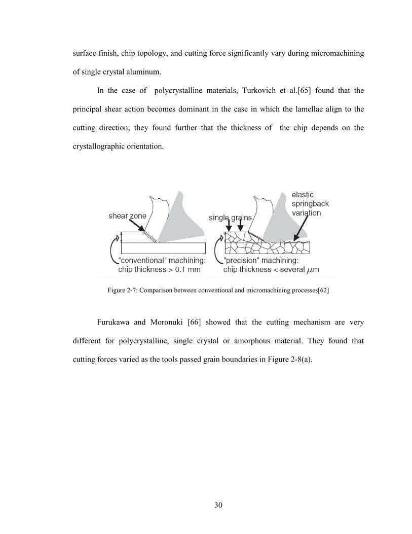
Furukawa and Moronuki [66] showed that the cutting mechanism are very

different for polycrystalline, single crystal or amorphous material. They found that

cutting forces varied as the tools passed grain boundaries in Figure 2-8(a).

31

(a) (b)

Figure 2-8: (a) Variation of cutting forces corresponding with the grain boundary of Al alloy [66]and (b)

FE model of heterogeneous materials[67]

Recent works by Chuzhoy[67, 68] studied the influence of microstructure effects

in micromachining. They developed a finite element (FE) model for simulation of

heterogeneous materials. They found that the variation of simulated forced in

micromachining the multiphase materials is larger than that in micromachining a single

phase material in Figure 2-8(b)

2.4 Summary

Based on literature reviews relating to micro-grinding and micro-machine tools, a

little knowledge of micro-grinding and design of microscale machine tools has been

accumulated in this emerging field. So, there is a need to develop an analytical model of

micro-grinding including the kinematics of micro-grinding, and workpiece properties.

Specially, development of the single grit interaction model including the size effect has to

32

be performed. On the other hand, as the shapes of miniaturized machine tools have

become more complex, optimization of the structure of microscale machine tools is

needed on the basis of mathematical models of key parameters such as volumetric error,

machine working space, and static, thermal, and dynamic stiffness.

These research directions are to fill these gaps outlined in this review of prior

works.

33

CHAPTER 3

MODELING OF MICRO-GRINDING FORCES AND THERMAL EFFECTS

3.1 Introduction

Grinding has been widely used to produce high quality parts. But, due to the

approximate size of conventional grinding wheels, conventional grinding is limited to

machining simple parts. So, grinding with the microscale grinding wheel, which is

referred to as micro-grinding in this dissertation, is a good candidate for producing high

quality parts at the micro domain by Feng et al.[69]. In micro-grinding, the single

interaction between the grit and a workpiece is more important because the micro-

grinding process is the cumulative outputs of numerous single grit interactions. So

modeling the single grit interaction is important for the predictions of process variables.

This chapter describes in detail the single grit interaction model for micro-

grinding. There are two major interactions in the grinding process: mechanical and

thermal interactions. The model for mechanical interaction between the workpiece and an

individual grit on the micro-grinding wheel is discussed in this chapter, considering both

micro-cutting and ploughing mechanisms along with associated friction effects at the

contact interface. Next, in order to estimate thermal effects in a micro-grinding process, a

thermal model is presented, which considers a moving heat source on the micro-grinding

zone under given machining conditions.

In addition, the ratio of heat partition into the workpiece in micro-grinding is

calculated by matching experimental data using embedded thermocouple measurement to

34

analytical calculations. The following sections described the models developed and used

to calculate forces per grit.

3.2 Modeling the single grit interaction in micro-grinding

In this section, the micro-grinding process is defined as grinding with the ratio of

the depth of cut to the grit radius smaller than 1. Further, in micro-grinding, the ratio of a

grit size to the grinding wheel increases compared to the conventional grinding process.

So, the analytical model of the individual grit interaction is the critical factor to use in

predictions about the micro-grinding process. This single grit interaction can be

characterized by micro-cutting with a high negative angle at a high strain rate. The size

effect is applied through the coupling of micro-cutting and ploughing mechanisms with

associated friction effects within the single grit interaction for the micro-grinding process.

In this study, the deformation of a workpiece subjected to micro-grinding is assumed as

pseudo orthogonal machining by considering microchips as a series of elements of

infinitesimal width and assuming no heat loss along primary and secondary heat zones. In

the following sections, the physical models for the microchip formation and the

ploughing mechanisms are independently presented.

3.2.1 Modeling of Chip Formation Forces in individual grits

Since the geometry of grits is random with other aspects in grinding, the grit

shape has to be approximated by a specific geometry to simplify the mathematical

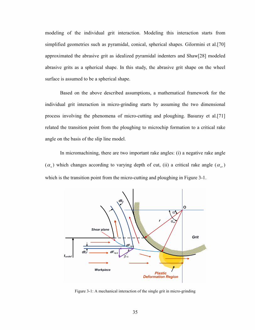
35

modeling of the individual grit interaction. Modeling this interaction starts from

simplified geometries such as pyramidal, conical, spherical shapes. Gilormini et al.[70]

approximated the abrasive grit as idealized pyramidal indenters and Shaw[28] modeled

abrasive grits as a spherical shape. In this study, the abrasive grit shape on the wheel

surface is assumed to be a spherical shape.

Based on the above described assumptions, a mathematical framework for the

individual grit interaction in micro-grinding starts by assuming the two dimensional

process involving the phenomena of micro-cutting and ploughing. Basuray et al.[71]

related the transition point from the ploughing to microchip formation to a critical rake

angle on the basis of the slip line model.

In micromachining, there are two important rake angles: (i) a negative rake angle

( sα ) which changes according to varying depth of cut, (ii) a critical rake angle ( crα )

which is the transition point from the micro-cutting and ploughing in Figure 3-1.

Figure 3-1: A mechanical interaction of the single grit in micro-grinding

36

The critical rake angle is the rake angle below which a workpiece material is

deformed by the ploughing effect. On the basis of the geometry relationship, the critical

rake angle can be determined by the minimum undeformed chip thickness and the cutting

edge radius according to the following:

1sin mcr

r tr

α − −⎛ ⎞= ⎜ ⎟⎝ ⎠

(3.1)

where r is the cutting edge radius, mt is the minimum undeformed chip thickness, and

crα is the critical rake angle

In the case of previous findings[71, 72], Ikawa et al.[72] showed that the

minimum undeformed chip thickness strongly depends on the sharpness of the cutting

edges. They suggested that the minimum undeformed chip thickness may be at the order

of 1/10 of the cutting edge radius. Based on the slip line analysis, Basuray et al.[71]

predicted that a stagnation point is constant and equal to 37.6˚ which is close to 2/10 of

the cutting edge radius. These results provide the approximate location of the stagnation

point. In this study, the minimum undeformed chip thickness is assumed to be between

0.1-0.2 of the cutting edge radius.

In the micromachining regime, the micro-cutting mechanism above the minimum

uncut chip thickness can be represented by applying the Merchant model to each of the

infinitesimal elements; this model is adapted from Liu[73] and Son et al.[74].

Considering an element of undeformed chip thickness, dt1, being cut at a position

corresponding to the associated local rake angle, a pair of chip formation and thrust

37

forces can be related with the friction and rake angles. The relationship between these can

be given as:

, , tan( )cg y cg x i idF dF β α= − (3.2)

Hence, the incremental cutting and thrust forces per unit width in the two dimensional

simplified configuration can be expressed as follows:

, 1cos( )

sin cos( )s i i

cg xi i i i

dF dtτ β αφ φ β α

−= −

+ − (3.3)

, 1sin( )

sin cos( )s i i

cg yi i i i

dF dtτ β αφ φ β α

−= −

+ − (3.4)

where τ is shear strength of the material, iβ is the instantaneous friction angle, iα is the

instantaneous rake angle, and iφ is the shear angle.

In micro-grinding, the effective rake angle ( sα ) is negative in the case in which

the undeformed chip thickness is below the cutting edge radius. The instantaneous rake

angle is obtained from a geometrical relationship like the following:

1 0( )sinsr t

rα − −

= (3.5)

where r is the cutting radius and 0t is the undeformed chip thickness

In micro-grinding, as the spherically shaped grit moves horizontally, the front half

of the hemisphere is involved in the material removal process. The chip formation forces

in micro-cutting can be obtained by multiplying the projected area of the contacting

surface as shown in Figure 3-2.

38

.

Figure 3-2: Illustration of the geometric configuration on the spherical shape grit

The cross section area of an ideal spherical shape grit between the increment of

the depth of cut and rake angle is

2 22 cosi i idA r dα α= (3.6)

The total cutting and thrust forces per each grit are obtained by integrating the

Equations (3.3)and(3.4). Finally, the expressions of the overall normal ( ,cg yF ) and

tangential forces ( ,cg xF ) per each grit are

1 0( )sin

2 2,

cos( ) 2 cossin cos( )

cr

r tr

s i icg x i

i i i i

F r dα

τ β α α αφ φ β α

− −

−=

+ −∫ (3.7)

1 0( )sin

2 2,

sin( ) 2 cossin cos( )

cr

r tr

s i icg y i

i i i i

F r dα

τ β α α αφ φ β α

− −

−=

+ −∫ (3.8)

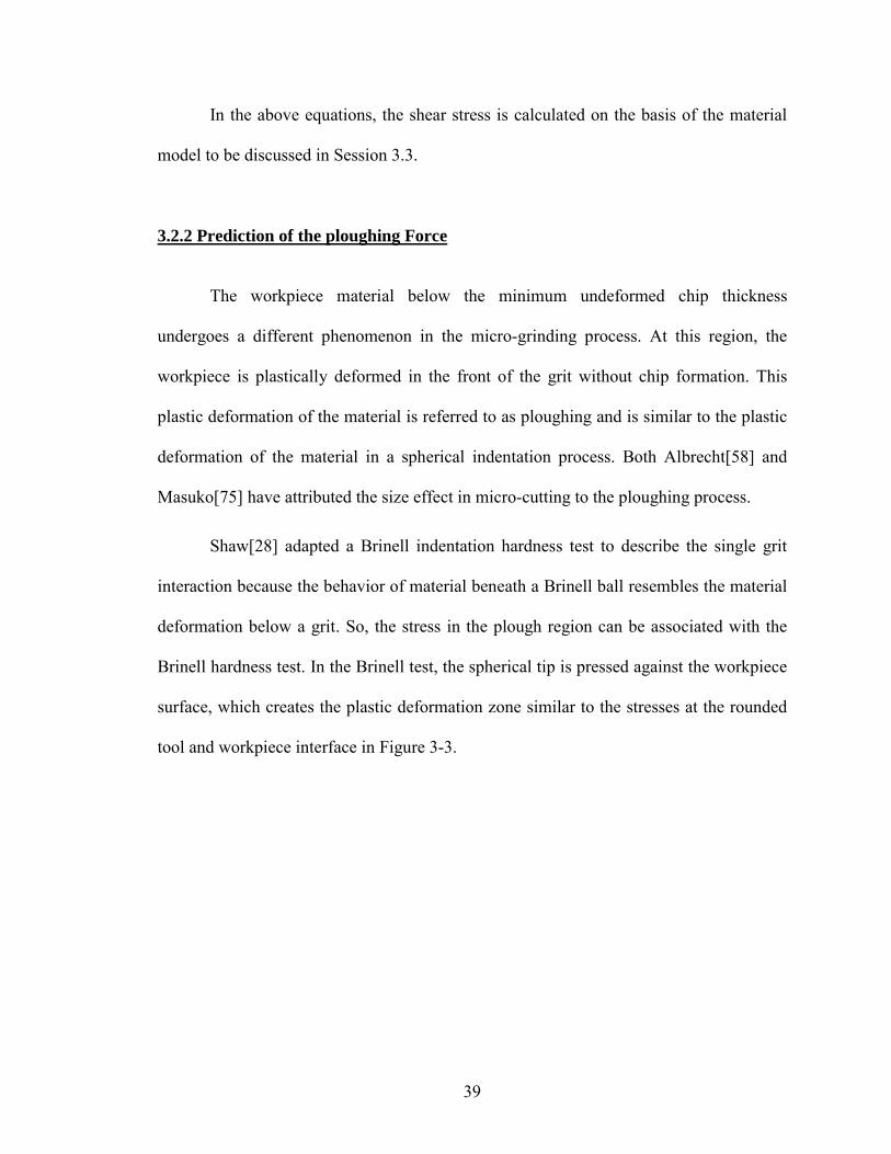
39

In the above equations, the shear stress is calculated on the basis of the material

model to be discussed in Session 3.3.

3.2.2 Prediction of the ploughing Force

The workpiece material below the minimum undeformed chip thickness

undergoes a different phenomenon in the micro-grinding process. At this region, the

workpiece is plastically deformed in the front of the grit without chip formation. This

plastic deformation of the material is referred to as ploughing and is similar to the plastic

deformation of the material in a spherical indentation process. Both Albrecht[58] and

Masuko[75] have attributed the size effect in micro-cutting to the ploughing process.

Shaw[28] adapted a Brinell indentation hardness test to describe the single grit

interaction because the behavior of material beneath a Brinell ball resembles the material

deformation below a grit. So, the stress in the plough region can be associated with the

Brinell hardness test. In the Brinell test, the spherical tip is pressed against the workpiece

surface, which creates the plastic deformation zone similar to the stresses at the rounded

tool and workpiece interface in Figure 3-3.

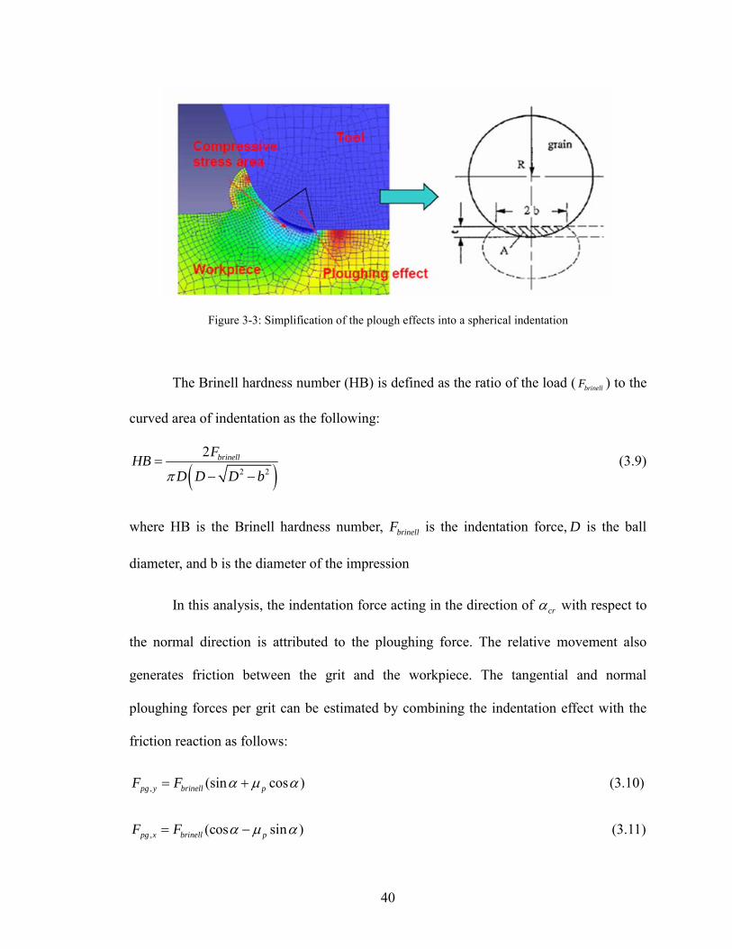
40

Figure 3-3: Simplification of the plough effects into a spherical indentation

The Brinell hardness number (HB) is defined as the ratio of the load ( brinellF ) to the

curved area of indentation as the following:

( )2 2

2 brinellFHBD D D bπ

=− −

(3.9)

where HB is the Brinell hardness number, brinellF is the indentation force, D is the ball

diameter, and b is the diameter of the impression

In this analysis, the indentation force acting in the direction of crα with respect to

the normal direction is attributed to the ploughing force. The relative movement also

generates friction between the grit and the workpiece. The tangential and normal

ploughing forces per grit can be estimated by combining the indentation effect with the

friction reaction as follows:

, (sin cos )pg y brinell pF F α µ α= + (3.10)

, (cos sin )pg x brinell pF F α µ α= − (3.11)

41

where pµ is the ploughing friction coefficient

At very low depths of cut, the coefficient of friction is highly influenced by the

ratio of the depth of indentation to the tool nose radius. Sin and Suh [76] extended the

predictive model of Goddard and Wilman [77] to estimate adhesion and ploughing

friction coefficients in a simple groove experiment under given conditions.

Assuming that the adhesion effect is negligible in the small depth of cut, the

ploughing mechanism in the individual grit interaction resembles the simple groove

experiment. Hence, in the ploughing region of a sliding spherical hard particle in Figure

3-4, the friction coefficient can be estimated by the following equation:

12 2 2

12 sin 12 2 2pw w wr r r

µπ

− −−

⎡ ⎤⎧ ⎫⎪ ⎪⎛ ⎞ ⎛ ⎞ ⎛ ⎞⎢ ⎥= − −⎨ ⎬⎜ ⎟ ⎜ ⎟ ⎜ ⎟⎢ ⎥⎝ ⎠ ⎝ ⎠ ⎝ ⎠⎪ ⎪⎩ ⎭⎢ ⎥⎣ ⎦

(3.12)

where w is the width of indentation and r is the spherical grit radius.

Bhushan [78] proposed the ploughing friction model in sliding cylinder. The model is

1/ 2

0

12( / ) 1p r t

µ⎡ ⎤

= ⎢ ⎥−⎣ ⎦ (3.13)

where r is the cylinder radius and 0t is the depth of cut

In both models, the ratio of the depth of cut of the radius has influenced a

coefficient of ploughing friction, which is shown in Figure 3-4(b). But, the effect of pile-

up of material ahead of the sliding sphere and cylinder is not involved in both cases.

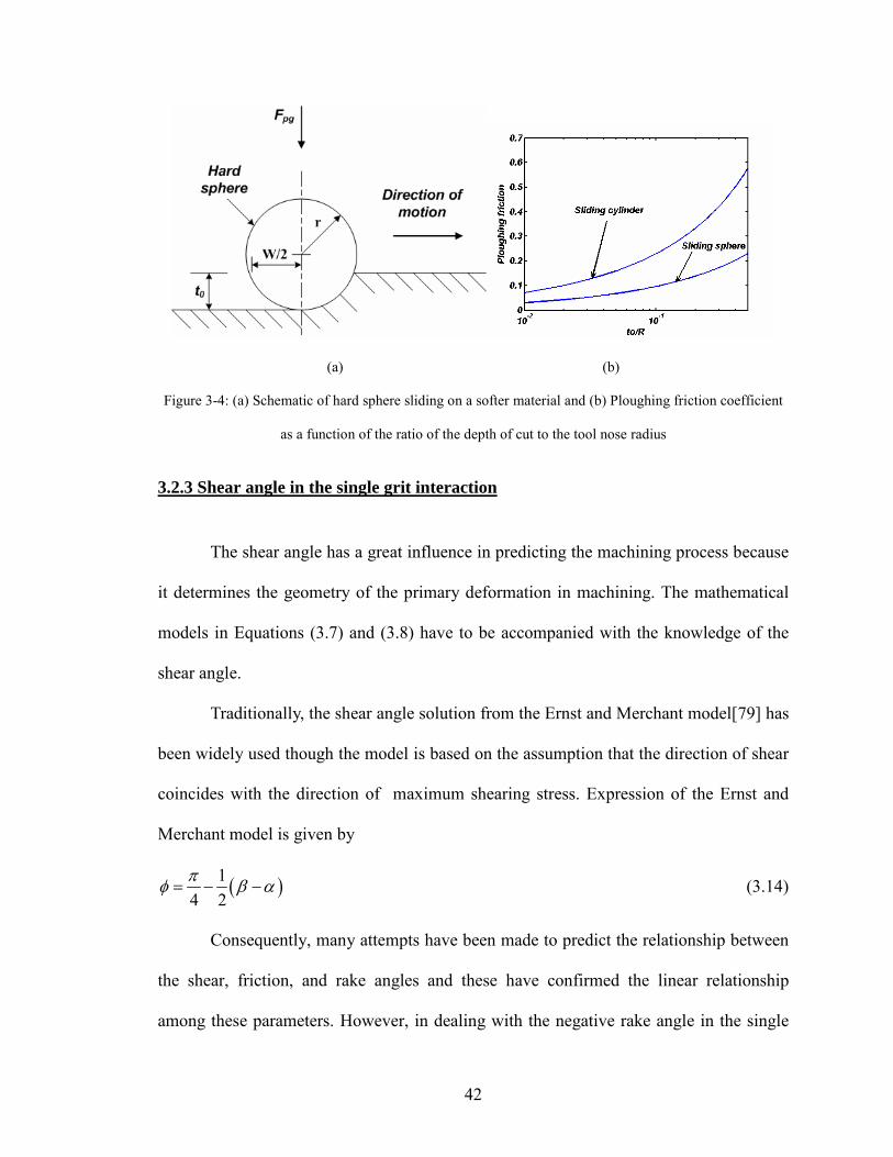
42

(a) (b)

Figure 3-4: (a) Schematic of hard sphere sliding on a softer material and (b) Ploughing friction coefficient

as a function of the ratio of the depth of cut to the tool nose radius

3.2.3 Shear angle in the single grit interaction

The shear angle has a great influence in predicting the machining process because

it determines the geometry of the primary deformation in machining. The mathematical

models in Equations (3.7) and (3.8) have to be accompanied with the knowledge of the

shear angle.

Traditionally, the shear angle solution from the Ernst and Merchant model[79] has

been widely used though the model is based on the assumption that the direction of shear

coincides with the direction of maximum shearing stress. Expression of the Ernst and

Merchant model is given by

( )14 2πφ β α= − − (3.14)

Consequently, many attempts have been made to predict the relationship between

the shear, friction, and rake angles and these have confirmed the linear relationship

among these parameters. However, in dealing with the negative rake angle in the single

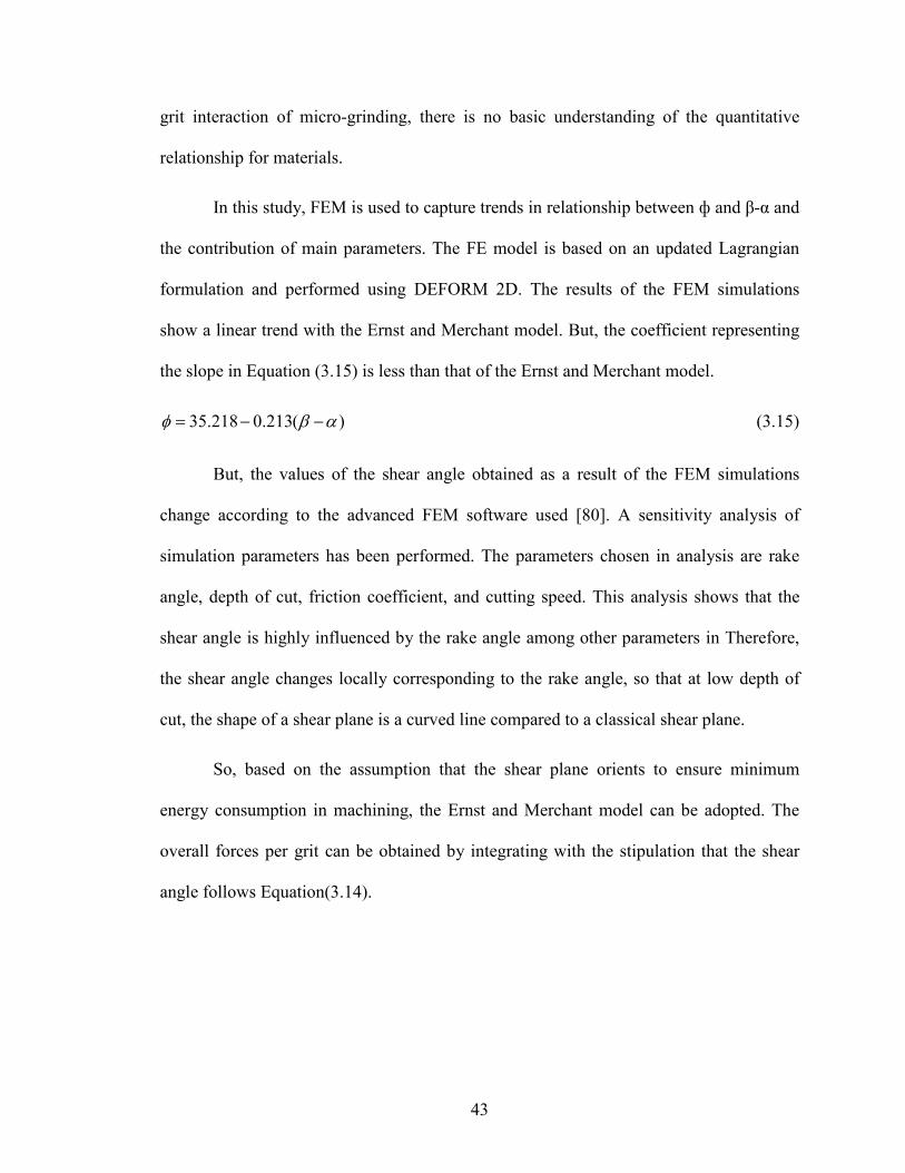
43

grit interaction of micro-grinding, there is no basic understanding of the quantitative

relationship for materials.

In this study, FEM is used to capture trends in relationship between ф and β-α and

the contribution of main parameters. The FE model is based on an updated Lagrangian

formulation and performed using DEFORM 2D. The results of the FEM simulations

show a linear trend with the Ernst and Merchant model. But, the coefficient representing

the slope in Equation (3.15) is less than that of the Ernst and Merchant model.

35.218 0.213( )φ β α= − − (3.15)

But, the values of the shear angle obtained as a result of the FEM simulations

change according to the advanced FEM software used [80]. A sensitivity analysis of

simulation parameters has been performed. The parameters chosen in analysis are rake

angle, depth of cut, friction coefficient, and cutting speed. This analysis shows that the

shear angle is highly influenced by the rake angle among other parameters in Therefore,

the shear angle changes locally corresponding to the rake angle, so that at low depth of

cut, the shape of a shear plane is a curved line compared to a classical shear plane.

So, based on the assumption that the shear plane orients to ensure minimum

energy consumption in machining, the Ernst and Merchant model can be adopted. The

overall forces per grit can be obtained by integrating with the stipulation that the shear

angle follows Equation(3.14).

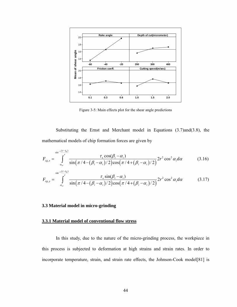
44

Mea

n of

she

ar a

ngle

-20-40-60

20

18

16

14

400300200

0.60.30.1

20

18

16

14

2.01.51.0

Rake angle Depth of cut(micrometer)

Friction coeff. Cutting speed(m/sec)

Figure 3-5: Main effects plot for the shear angle predictions

Substituting the Ernst and Merchant model in Equations (3.7)and(3.8), the

mathematical models of chip formation forces are given by

( )( ) ( )( )

1 0( )sin

2 2,

cos( ) 2 cossin / 4 / 2 cos / 4 / 2

cr

r tr

s i icg x i

i i i i

F r dα

τ β α α απ β α π β α

− −

−=

− − + −∫ (3.16)

( )( ) ( )( )

1 0( )sin

2 2,

sin( ) 2 cossin / 4 / 2 cos / 4 / 2

cr

r tr

s i icg y i

i i i i

F r dα

τ β α α απ β α π β α

− −

−=

− − + −∫ (3.17)

3.3 Material model in micro-grinding

3.3.1 Material model of conventional flow stress

In this study, due to the nature of the micro-grinding process, the workpiece in

this process is subjected to deformation at high strains and strain rates. In order to

incorporate temperature, strain, and strain rate effects, the Johnson-Cook model[81] is

45

adopted to represent the material deformation behavior on the shear plane, which is given

by

( )⎟⎟

⎠

⎞

⎜⎜

⎝

⎛⎟⎟⎠

⎞⎜⎜⎝

⎛−−

−⎟⎟⎠

⎞⎜⎜⎝

⎛++=

m

m

n

TTTT

CBA0

0

0

1ln1εεεσ (3.18)

where σ is the material flow stress, ε is equivalent strain, mT is the melting temperature,

0T is the environment temperature, A,B,C, m, and n are material constants.

Based on the above equation, the shear stress in Equations (3.16) and (3.17) can be

obtained as

( )⎟⎟

⎠

⎞

⎜⎜

⎝

⎛⎟⎟⎠

⎞⎜⎜⎝

⎛−−

−⎟⎟⎠

⎞⎜⎜⎝

⎛++=

m

m

ns TT

TTCBA

0

0

0

1ln13

1εεετ (3.19)

In the calculation of strain and strain rate, there are two possible methods: (1) the

Oxley’s model[82] with the assumption that the tool is perfectly sharp and (2) the

Manjunathaiah and Endres model[83]. In the Oxley’s model, the strain along a shear

plane is given by

cos1cos( )sin2 3

n

n n n

αεφ α φ

=−

(3.20)

where nφ is the nominal shear angle and nα is the nominal rake angle

The strain rate along a shear plane is given by

3oxley sh

s

C Vl

ε = (3.21)

where oxleyC is constant, shV is the shear velocity, and sl the length of a shear plane.

In Equation(3.21), the shear velocity of a shear plane is given by

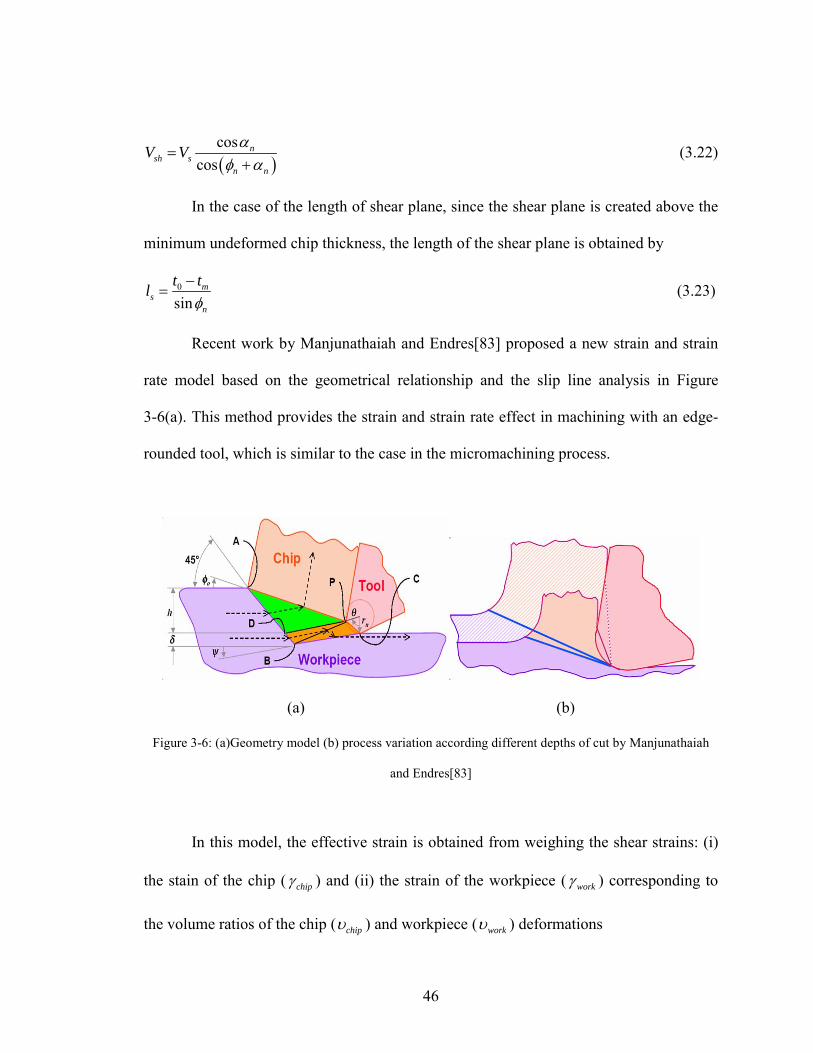
46

( )cos

cosn

sh sn n

V V αφ α

=+

(3.22)

In the case of the length of shear plane, since the shear plane is created above the

minimum undeformed chip thickness, the length of the shear plane is obtained by

0

sinm

sn

t tlφ−

= (3.23)

Recent work by Manjunathaiah and Endres[83] proposed a new strain and strain

rate model based on the geometrical relationship and the slip line analysis in Figure

3-6(a). This method provides the strain and strain rate effect in machining with an edge-

rounded tool, which is similar to the case in the micromachining process.

(a) (b)

Figure 3-6: (a)Geometry model (b) process variation according different depths of cut by Manjunathaiah

and Endres[83]

In this model, the effective strain is obtained from weighing the shear strains: (i)

the stain of the chip ( chipγ ) and (ii) the strain of the workpiece ( workγ ) corresponding to

the volume ratios of the chip ( chipυ ) and workpiece ( workυ ) deformations

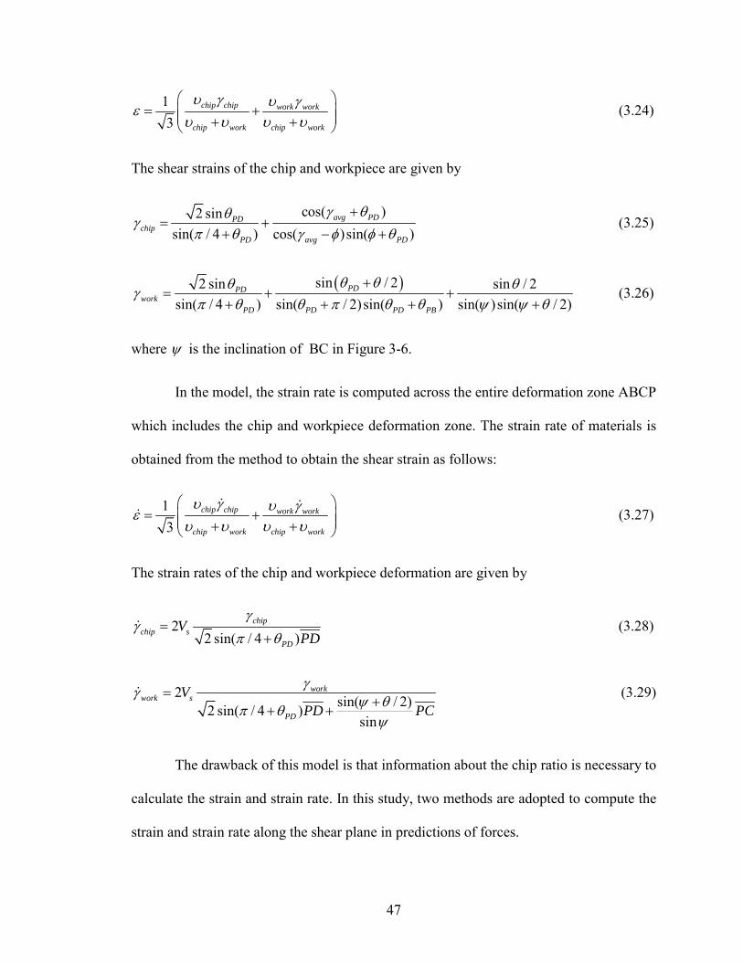
47

13

chip chip work work

chip work chip work

υ γ υ γευ υ υ υ⎛ ⎞

= +⎜ ⎟⎜ ⎟+ +⎝ ⎠ (3.24)

The shear strains of the chip and workpiece are given by

cos( )2 sinsin( / 4 ) cos( )sin( )

avg PDPDchip

PD avg PD

γ θθγπ θ γ φ φ θ

+= +

+ − + (3.25)

( )sin / 22 sin sin / 2sin( / 4 ) sin( / 2)sin( ) sin( )sin( / 2)

PDPDwork

PD PD PD PB

θ θθ θγπ θ θ π θ θ ψ ψ θ

+= + +

+ + + + (3.26)

where ψ is the inclination of BC in Figure 3-6.

In the model, the strain rate is computed across the entire deformation zone ABCP

which includes the chip and workpiece deformation zone. The strain rate of materials is

obtained from the method to obtain the shear strain as follows:

13

chip chip work work

chip work chip work

υ γ υ γευ υ υ υ⎛ ⎞

= +⎜ ⎟⎜ ⎟+ +⎝ ⎠ (3.27)

The strain rates of the chip and workpiece deformation are given by

22 sin( / 4 )

chipchip s

PD

VPD

γγ

π θ=

+ (3.28)

2 sin( / 2)2 sin( / 4 )sin

workwork s

PD

VPD PC

γγ ψ θπ θψ

=+

+ + (3.29)

The drawback of this model is that information about the chip ratio is necessary to

calculate the strain and strain rate. In this study, two methods are adopted to compute the

strain and strain rate along the shear plane in predictions of forces.

48

3.3.2 Material model considering the crystallographic effects

The depth of cut in micro-grinding is less than the size of a grain in the material.

So the crystallographic effects have to be considered in a material model for prediction.

The effects include grain size and orientation effects. The frame on this research work is

to analytically represent these microstructure effects by assuming a linear additive

contribution of incidental dislocation boundaries and geometrical dislocation boundaries.

Huges et al.[84] proposed a material model to represent the effect of dislocations

influencing the macroscopic flow stress. The dislocation boundaries can be divided into

two types: geometrically necessary boundaries (GNB) and incident dislocation

boundaries (IDB). The flow model proposed consists of three parts:(i) conventional flow

stress (ii) the flow stress by IDB (iii) the flow stress by GNB

This model incorporates the strength contribution of the IDB which can be

expressed as

IDB cont bg tM Gbσ α ρ= (3.30)

where M is the Taylor factor, contα is the material constant, G is the shear modulus of

material, bgb is the burger vector of dislocations, and tρ is the total density of dislocation

The total density of dislocation consists of the dislocation density in the volumes

between boundaries ( 0ρ ) and the dislocation in the boundary area per unit area ( bρ ),

which is

0t bρ ρ ρ= + (3.31)

49

Based on the assumption that the average grain boundary spacing is equal to the

grain size, the total dislocation density can be represented incorporating a microstructure

parameter as the following term.

avt

d bg

kD bθρ = (3.32)

So, the flow stress for dislocations in IDB can be given by

avIDB cont bg

d bg

kM GbD bθσ α= (3.33)

Generally, as a strain and stress increase, the misorientation angle in the GNBs

increases and becomes a high angle boundary. So recent work by Huges et al.[84]

introduced a Hall-Petch equation for high angle boundaries; the flow stress for

dislocations in the GNBs can be represented as described in (3.34)

HPGNB

d

KD

σ = (3.34)

The overall flow stress can be described as the sum of these three components of

the above equations and can represent the crystallographic effects such as grain

orientation and grain size. In this research, the modified material model of micro-grinding

is proposed as the following:

( , , ) avHPi cont

dd

kbKT M GDDθσ σ ε ε α= + + (3.35)

The distribution of a grain size and misorientation used in this model is obtained

and discussed in Chapter 5.

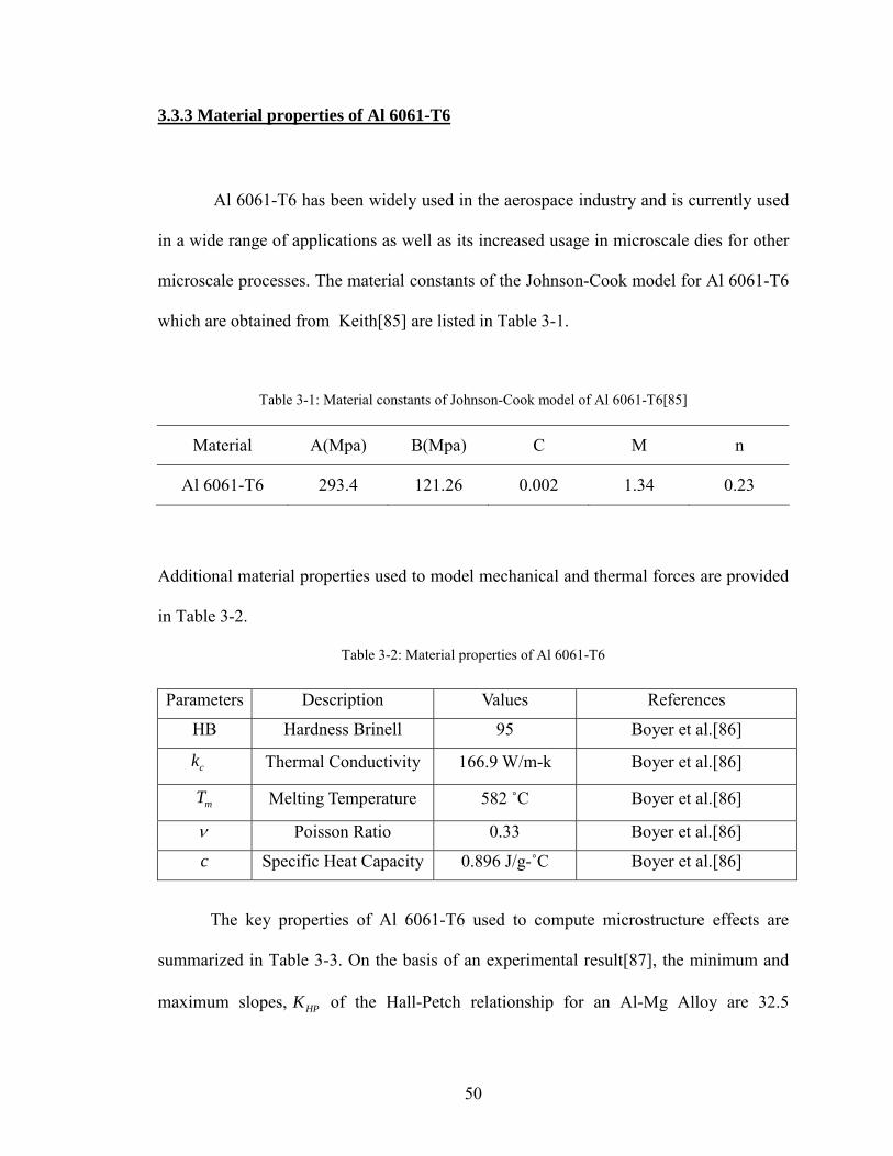
50

3.3.3 Material properties of Al 6061-T6

Al 6061-T6 has been widely used in the aerospace industry and is currently used

in a wide range of applications as well as its increased usage in microscale dies for other

microscale processes. The material constants of the Johnson-Cook model for Al 6061-T6

which are obtained from Keith[85] are listed in Table 3-1.

Table 3-1: Material constants of Johnson-Cook model of Al 6061-T6[85]

Material A(Mpa) B(Mpa) C M n

Al 6061-T6 293.4 121.26 0.002 1.34 0.23

Additional material properties used to model mechanical and thermal forces are provided

in Table 3-2.

Table 3-2: Material properties of Al 6061-T6

Parameters Description Values References

HB Hardness Brinell 95 Boyer et al.[86]

ck Thermal Conductivity 166.9 W/m-k Boyer et al.[86]

mT Melting Temperature 582 ˚C Boyer et al.[86]

ν Poisson Ratio 0.33 Boyer et al.[86]

c Specific Heat Capacity 0.896 J/g-˚C Boyer et al.[86]

The key properties of Al 6061-T6 used to compute microstructure effects are

summarized in Table 3-3. On the basis of an experimental result[87], the minimum and

maximum slopes, HPK of the Hall-Petch relationship for an Al-Mg Alloy are 32.5

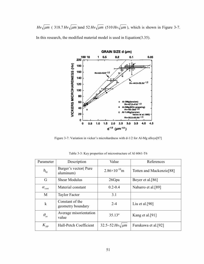
51

mHv µ ( 318.7 mHv µ )and 52 mHv µ (510 mHv µ ), which is shown in Figure 3-7.

In this research, the modified material model is used in Equation(3.35).

Figure 3-7: Variation in vicker’s microhardness with d-1/2 for Al-Mg alloys[87]

Table 3-3: Key properties of microstructure of Al 6061-T6

Parameter Description Value References

bgb Burger’s vector( Pure aluminum) 2.86×10-10m Totten and Mackenzie[88]

G Shear Modulus 26Gpa Boyer et al.[86]

contα Material constant 0.2-0.4 Nabarro et al.[89]

M Taylor Factor 3.1

k Constant of the geometry boundary 2-4 Liu et al.[90]

avθ Average misorientation value 35.13º Kang et al.[91]

HPK Hall-Petch Coefficient 32.5~52 mHv µ Furukawa et al.[92]

52

3.4 Analysis of the single grit force model behavior

Machining with a single grit is similar to the grooving process. The force model

described above is used to predict the overall single grit forces based on the conventional

material model in section 3.3. A breakdown of the predictions of the single grit forces is

shown in Figure 3-8 and Figure 3-9.

Contribution of forces in Tangential Direction

0%

20%

40%

60%

80%

100%

5µm 10µm 15µm 20µm 25µmDepth of Cut

ChipformationforcePloughing force

Figure 3-8: Breakdown of single grit force in normal direction for Grit size= 43µm, Vw=1mm/sec, and

spindle RPM=60000

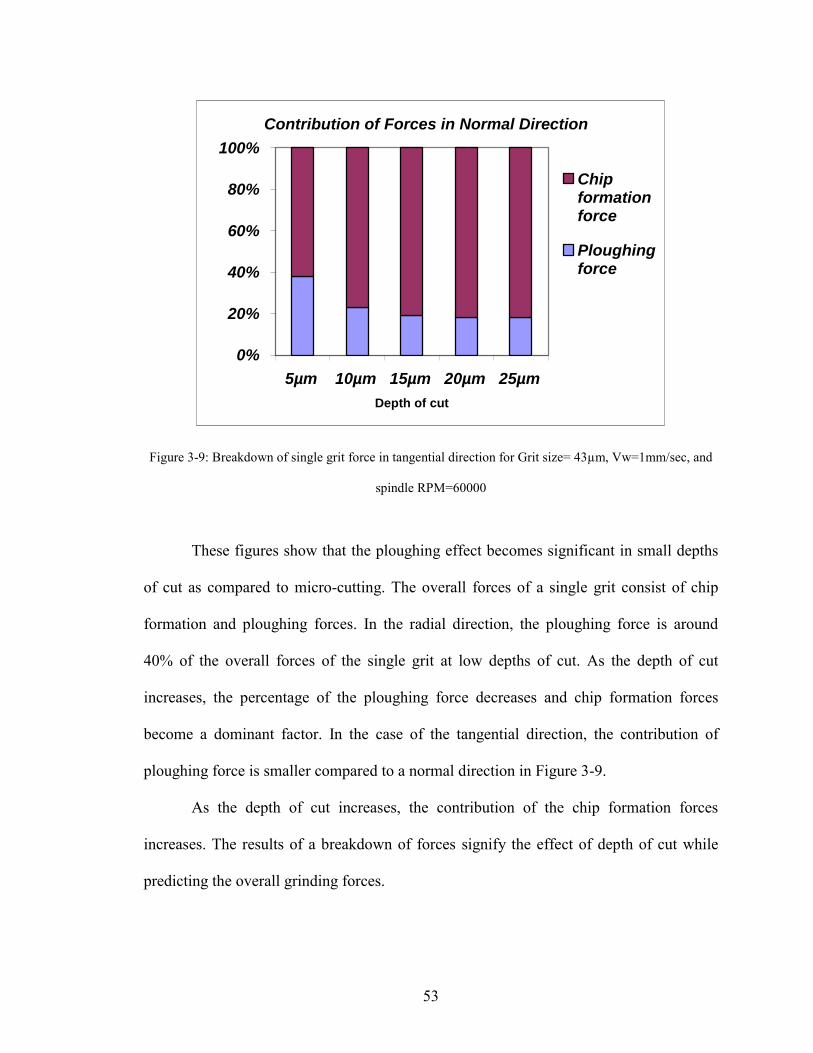
53

Contribution of Forces in Normal Direction

0%

20%

40%

60%

80%

100%

5µm 10µm 15µm 20µm 25µmDepth of cut

Chipformationforce

Ploughingforce

Figure 3-9: Breakdown of single grit force in tangential direction for Grit size= 43µm, Vw=1mm/sec, and

spindle RPM=60000

These figures show that the ploughing effect becomes significant in small depths

of cut as compared to micro-cutting. The overall forces of a single grit consist of chip

formation and ploughing forces. In the radial direction, the ploughing force is around

40% of the overall forces of the single grit at low depths of cut. As the depth of cut

increases, the percentage of the ploughing force decreases and chip formation forces

become a dominant factor. In the case of the tangential direction, the contribution of

ploughing force is smaller compared to a normal direction in Figure 3-9.

As the depth of cut increases, the contribution of the chip formation forces

increases. The results of a breakdown of forces signify the effect of depth of cut while

predicting the overall grinding forces.

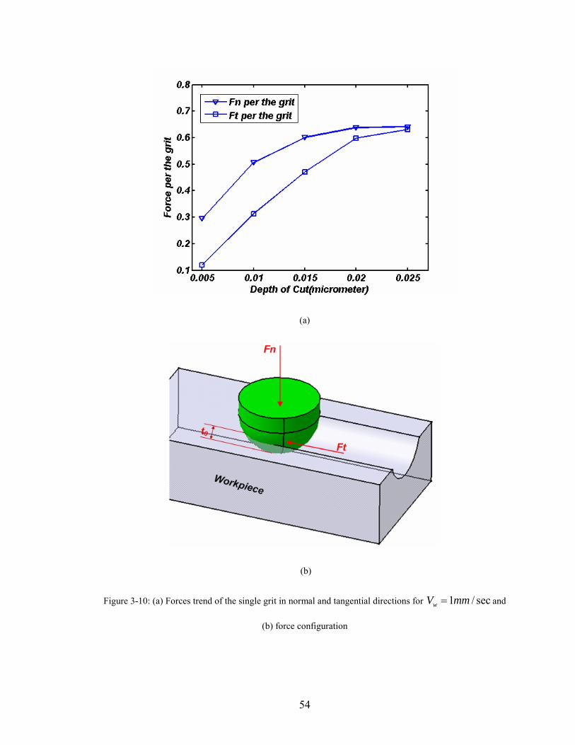
54

(a)

(b)

Figure 3-10: (a) Forces trend of the single grit in normal and tangential directions for 1 / secwV mm= and

(b) force configuration

55

In the case of the single grit forces, the normal forces are larger than the tangential

forces. But the amount of the difference between them decreases as depth of cut increases.

3.5 Modeling of thermal effects in micro-grinding

Thermally induced stress to the workpiece during micro-grinding affects material

behavior. During grinding, the duration of the heat pulse due to an individual grit is much

shorter than that of the heat pulse on the workpiece contact zone. There are some

examples of heat flux distribution such as a uniform and triangular law flux. A uniform

flux in which pressure is uniform is used for polishing and honing processes. A triangular

flux is approximate where the volume of chips is proportional to the depth of cut for

grinding. The experiments of measuring grinding temperatures by Rowe et al.[93]

supported this triangular flux approximation.

In this analysis, the heat generated during micro-grinding is approximated as a

triangular heat source moving along the direction of the x-axis with the angle, φ, in

Equation (3.37) between the line of motion and the plane of the band source as shown in

Figure 3-11.

1 0sine

td

ϕ −= (3.36)

where ϕ is the inclination angle of the micro-grinding zone, 0t is the depth of cut, and

ed is the micro-grinding wheel diameter

This band of heat on the contact zone between the workpiece and the grinding

wheel is considered as a series of moving heat source elements. The solution for moving

56

heat source elements can be represented by Bessel functions and obtained by summing

over the length of the micro-grinding contact surface.

Figure 3-11: Schematic of the micro-grinding thermal model

Based on the Jaeger moving heat source model[34], the summation for the

moving inclined triangular band source can be performed as the following:

( cos ) 2 2 1/ 222

( , ) 0

2

[( cos ) ( sin ) ]2

c

w

c

lV x a

wx z

l

qR v x a z aT e K dak

ϕα ϕ ϕ

π α

+−

−

⎧ ⎫+ + −= ⎨ ⎬

⎩ ⎭∫ (3.37)

where 0K is the second kind modified Bessel function, wR is the heat partition ratio to the

workpiece, q is the heat flux, ϕ is the inclined angle, wV is the workpiece speed, k is the

thermal conductivity, cl is the contact zone, and diffα is the thermal diffusivity.

57

For the triangular heat flux on the contact zone, the flux distribution can be

expressed in the following form:

021

c

aq ql

⎛ ⎞= +⎜ ⎟

⎝ ⎠ (3.38)

where 0( )x s w

c

F V Vql b+

= and 2 2c cl la− ≤ ≤

Based on the geometric relationship among parameters, the coordinate value of the shear

plane corresponding to Figure 3-11 can be represented by

tan cos sin2 sin 2 sinc m c m

i n il t l tz xφ ϕ ϕ

ϕ ϕ⎛ ⎞⎛ ⎞ ⎛ ⎞

= − + − + −⎜ ⎟⎜ ⎟ ⎜ ⎟⎝ ⎠ ⎝ ⎠⎝ ⎠

(3.39)

The contact length model and its relation to the depth of cut is important to

estimate the thermal effect in micro-grinding. Since elastic deflections between the tool

and the contact surface can produce a change in the contact length, the geometric contact

length model is not sufficient to describe the real contact length. Additionally, the surface

of the workpiece in the microscopic view is not smooth. In order to account for these

factors, the real contact length is calculated as Rowe et al.[94]

( )1

' 20 8 ( )c e r y e s wl t d R F d K K= + + (3.40)

where 0t is the depth of cut, ed is the effective diameter, rR is the roughness factor, 'yF is

the normal force per unit length, and iK is the wheel (i=w)and workpiece(i=s) elasticity

The estimation of the real contact length based on this model will be more

accurate as compared to the model that ignores the deflection effect. Within the model,

58

the roughness factor ( rR ) is the ratio of the rough and smooth contact lengths. In the case

of the rough surface, Rowe et al.[94] showed that a value of 5rR = provides a reasonable

agreement between predicted and experimental contact lengths.

3.6 Calibration of heat partition ratio to the workpiece

To assess thermal effects in micro-grinding, it is important to understand heat

transfer in micro-grinding. There are two different scales of heat transfer in grinding: (i)

the heat transfer between the grit and workpiece and (ii) the heat transfer between the

grinding wheel and workpiece. Heat transfers on two different scales interact with each

other.

In dry micro-grinding, the total heat in the contact zone flows into three heat

sinks: the workpiece, the micro-grinding wheel, and microchips because there is no heat

loss due to fluid. So, partition ratios can be defined as the proportions of these fluxes to

the total flux. Considering the energy convected by the microchips in the heat partition

ratio to the workpiece is expressed as

1 ccw ws

c

eR Re

⎛ ⎞= −⎜ ⎟

⎝ ⎠ (3.41)

where ce is the process specific energy and cce is the energy to melt the workpiece

material

In the micro-grinding process, the process specific energy is high and therefore

the value of /cc ce e is negligible. The relationship of partition ratios is

59

1w sR R+ = (3.42)

Figure 3-12: Microchips at 20µm depth of cut in micro-grinding

In this study, the heat partition ratio to the workpiece was calibrated by matching

between experimental data using an embedded thermocouple and the analytically

calculated temperature response in Figure 3-13.

Figure 3-13: Temperature matching technique

The experimental setup to calibrate the heat partition ratio is illustrated in Figure

3-14. The surface micro-grinding experiment was conducted using an electroplated

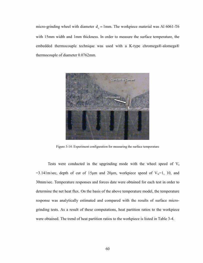
60

micro-grinding wheel with diameter ed = 1mm. The workpiece material was Al 6061-T6

with 15mm width and 1mm thickness. In order to measure the surface temperature, the

embedded thermocouple technique was used with a K-type chromega®-alomega®

thermocouple of diameter 0.0762mm.

Figure 3-14: Experiment configuration for measuring the surface temperature

Tests were conducted in the upgrinding mode with the wheel speed of Vs

=3.141m/sec, depth of cut of 15µm and 20µm, workpiece speed of Vw=1, 10, and

30mm/sec. Temperature responses and forces date were obtained for each test in order to

determine the net heat flux. On the basis of the above temperature model, the temperature

response was analytically estimated and compared with the results of surface micro-

grinding tests. As a result of these computations, heat partition ratios to the workpiece

were obtained. The trend of heat partition ratios to the workpiece is listed in Table 3-4.

61

Table 3-4: Estimated heat partition ratios to the workpiece

Depth of cut RPM Workpiece Speed Rw (Heat Partition)

15µm 60000 1mm/sec 0.398905 15µm 60000 10mm/sec 0.419129 15µm 60000 30mm/sec 0.379072 15µm 60000 1mm/sec 0.440004 15µm 60000 10mm/sec 0.440103 15µm 60000 30mm/sec 0.374008 15µm 60000 30mm/sec 0.340414 20µm 60000 1mm/sec 0.415059 20µm 60000 10mm/sec 0.460162 20µm 60000 30mm/sec 0.415059

The results of computations are compared with the predictions of the Hahn

model[36]:

1

1( )

gwws

w s s c w

kRRR R rV k cρ

−⎛ ⎞

= = +⎜ ⎟⎜ ⎟+ ⎝ ⎠ (3.43)

where gk is the grit thermal conductivity, ck is the thermal conductivity, ρ is density,

and c is the specific heat

The approximated values of thermal properties for CBN obtained by Rowe et

al.[43] are summarized in Table 3-5.

Table 3-5: Thermal properties of CBN

Conductivity Density heat Specific heat k cβ ρ=

CBN 240W/mk 3480(kg/m3 506(J/kgK) 20,600(J/m2sK

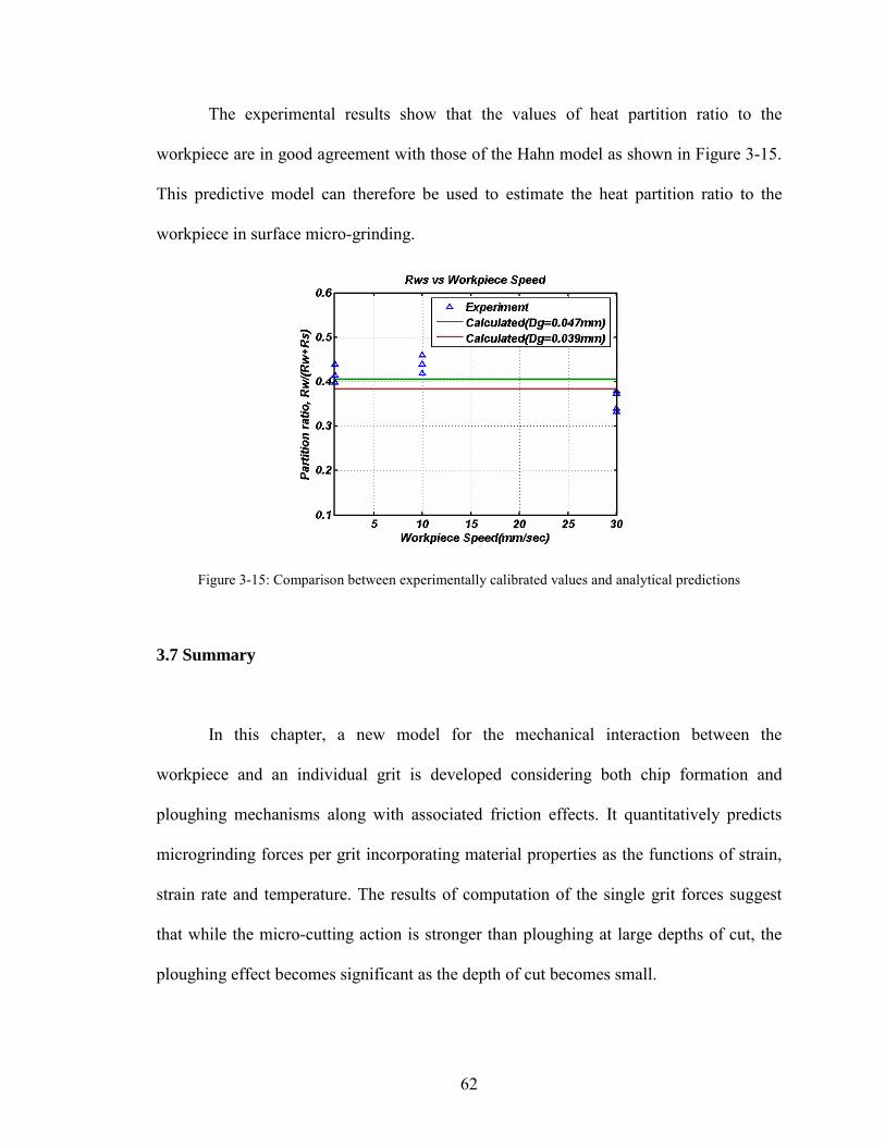
62

The experimental results show that the values of heat partition ratio to the

workpiece are in good agreement with those of the Hahn model as shown in Figure 3-15.

This predictive model can therefore be used to estimate the heat partition ratio to the

workpiece in surface micro-grinding.

Figure 3-15: Comparison between experimentally calibrated values and analytical predictions

3.7 Summary

In this chapter, a new model for the mechanical interaction between the

workpiece and an individual grit is developed considering both chip formation and

ploughing mechanisms along with associated friction effects. It quantitatively predicts

microgrinding forces per grit incorporating material properties as the functions of strain,

strain rate and temperature. The results of computation of the single grit forces suggest

that while the micro-cutting action is stronger than ploughing at large depths of cut, the

ploughing effect becomes significant as the depth of cut becomes small.

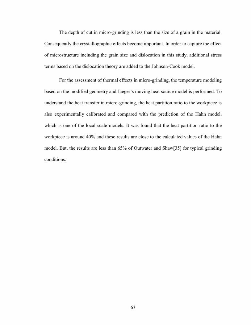
63

The depth of cut in micro-grinding is less than the size of a grain in the material.

Consequently the crystallographic effects become important. In order to capture the effect

of microstructure including the grain size and dislocation in this study, additional stress

terms based on the dislocation theory are added to the Johnson-Cook model.

For the assessment of thermal effects in micro-grinding, the temperature modeling

based on the modified geometry and Jaeger’s moving heat source model is performed. To

understand the heat transfer in micro-grinding, the heat partition ratio to the workpiece is

also experimentally calibrated and compared with the prediction of the Hahn model,

which is one of the local scale models. It was found that the heat partition ratio to the

workpiece is around 40% and these results are close to the calculated values of the Hahn

model. But, the results are less than 65% of Outwater and Shaw[35] for typical grinding

conditions.

64

CHAPTER 4

CHARACTERIZING THE TOPOGRAPHY OF A MICRO-GRINDING WHEEL

4.1 Introduction

The complexity in modeling the phenomena in micro and macro-grinding comes

from the randomness of the shape and distribution of grit on the grinding wheel. The

overall magnitude of micro-grinding forces depends on the topography of a micro-

grinding wheel and the overall shape of its cutting edges. Understanding of micro-

grinding wheel topography is crucial to modeling the micro-grinding process with high

reliability. Various techniques such as profilometry, imprint method, scratch method, and

microscopy have been developed to drive the topography of a grinding wheel. These

techniques have their advantages and limitations. Verkerk et al.[46] provided the

common distinction between static and dynamic cutting edge density. But, since

measuring the dynamic cutting edge density is complicated, the dynamic cutting edge

density is approximated from experimental data of the static cutting edge density

incorporating the kinematics of cutting edges.

In this chapter, two methods that were adopted to derive the static cutting edge

density corresponding to varying depths of cut are discussed. One is the optical method

with replication and microscopic methods based on Hacker’s approach [51]. The other

one is the direct method based on the polishing method, which is proposed in this study.

The static cutting edge densities using both methods are obtained with the assumption

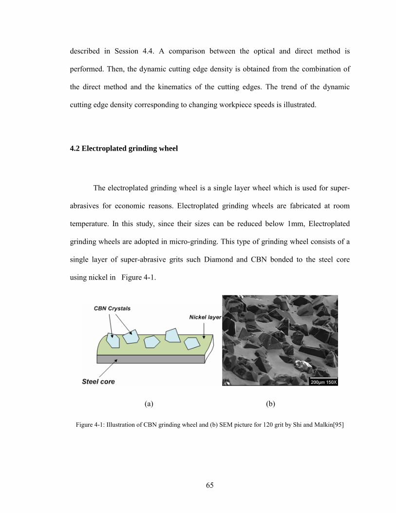
65

described in Session 4.4. A comparison between the optical and direct method is

performed. Then, the dynamic cutting edge density is obtained from the combination of

the direct method and the kinematics of the cutting edges. The trend of the dynamic

cutting edge density corresponding to changing workpiece speeds is illustrated.

4.2 Electroplated grinding wheel

The electroplated grinding wheel is a single layer wheel which is used for super-

abrasives for economic reasons. Electroplated grinding wheels are fabricated at room

temperature. In this study, since their sizes can be reduced below 1mm, Electroplated

grinding wheels are adopted in micro-grinding. This type of grinding wheel consists of a

single layer of super-abrasive grits such Diamond and CBN bonded to the steel core

using nickel in Figure 4-1.

(a) (b)

Figure 4-1: Illustration of CBN grinding wheel and (b) SEM picture for 120 grit by Shi and Malkin[95]

66

4.3 Characterizing micro-grinding topography

In the following sections, the wheel topography of an electroplated CBN wheel

specified as 85002-BM and with 240~270 grit number was experimentally analyzed. The

size of this grinding is around 1mm based on the wheel specifications. Due to its size and

curvature, it is very hard to directly extract information from the grinding wheel, which is

shown in Figure 4-2.

Figure 4-2: Illustration of 85002-BM electroplated CBN wheel

Due to resolution and the size of application, microscope method was adopted in

this study. The direct method based on the polishing method is also proposed to

characterize the micro-grinding wheel topography.

4.3.1 Optical method for the micro-grinding wheel topography

The ZYGO microscope offer a popular way to optically characterize the micro-

grinding wheel topography because this method can provide a three dimensional profile

of grinding wheel topography. Due to the difficulty of directly extracting the wheel

topography, imprinting or replicating the wheel surface on a second body is necessary.

For a second body for imprinting, lead plate is widely used due to its proper strength. But,

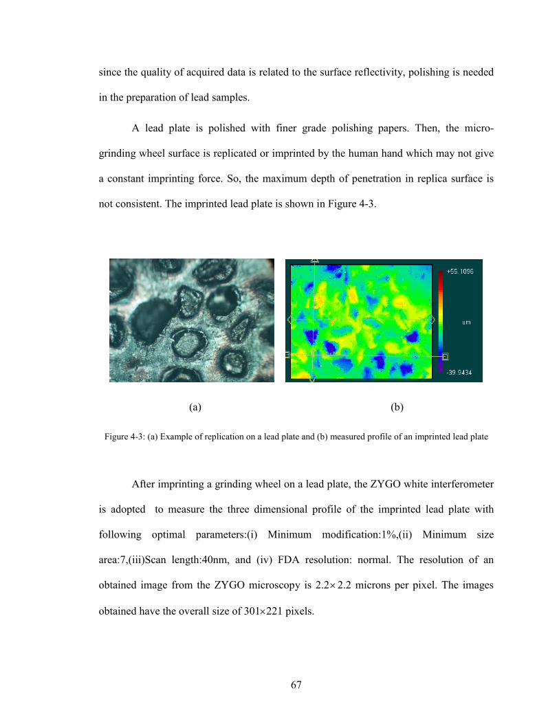
67

since the quality of acquired data is related to the surface reflectivity, polishing is needed

in the preparation of lead samples.

A lead plate is polished with finer grade polishing papers. Then, the micro-

grinding wheel surface is replicated or imprinted by the human hand which may not give

a constant imprinting force. So, the maximum depth of penetration in replica surface is

not consistent. The imprinted lead plate is shown in Figure 4-3.

(a) (b)

Figure 4-3: (a) Example of replication on a lead plate and (b) measured profile of an imprinted lead plate

After imprinting a grinding wheel on a lead plate, the ZYGO white interferometer

is adopted to measure the three dimensional profile of the imprinted lead plate with

following optimal parameters:(i) Minimum modification:1%,(ii) Minimum size

area:7,(iii)Scan length:40nm, and (iv) FDA resolution: normal. The resolution of an

obtained image from the ZYGO microscopy is 2.2×2.2 microns per pixel. The images

obtained have the overall size of 301×221 pixels.

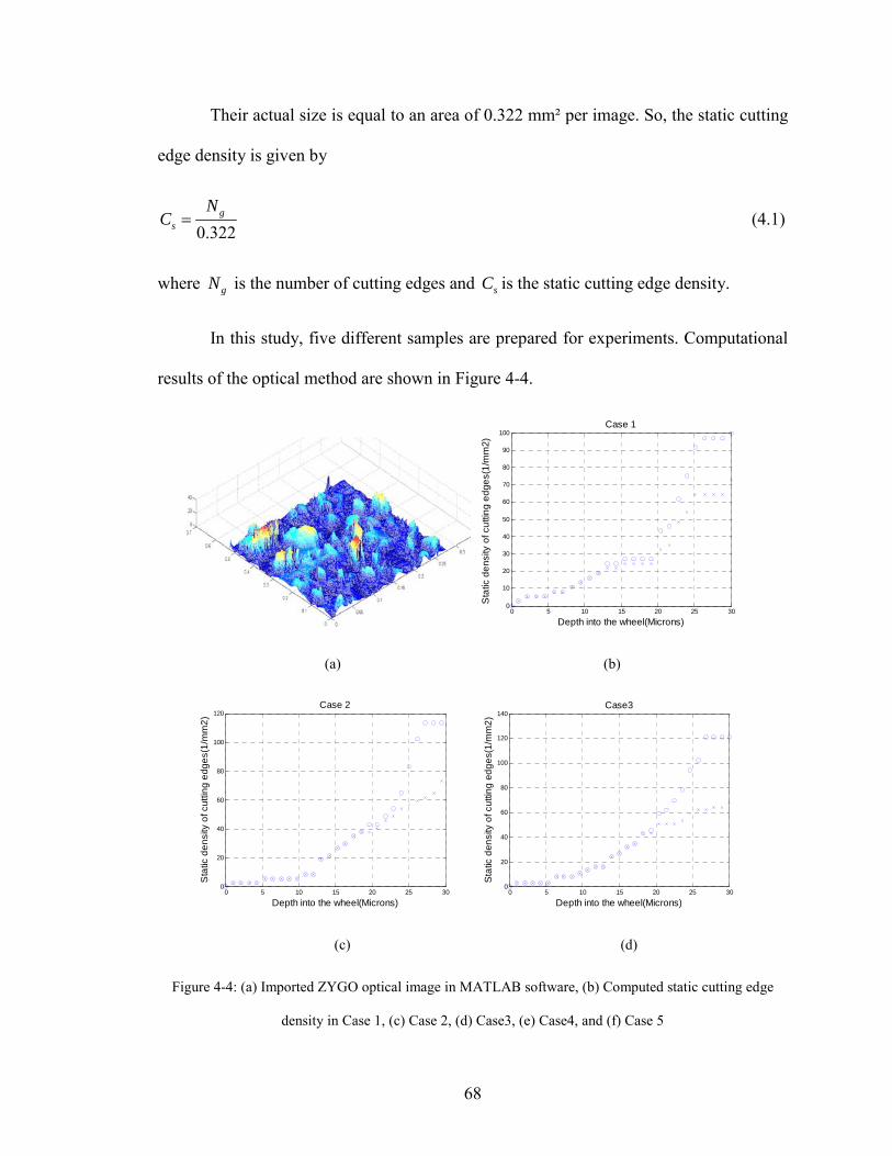
68

Their actual size is equal to an area of 0.322 mm² per image. So, the static cutting

edge density is given by

0.322g

s

NC = (4.1)

where gN is the number of cutting edges and sC is the static cutting edge density.

In this study, five different samples are prepared for experiments. Computational

results of the optical method are shown in Figure 4-4.

0 5 10 15 20 25 30

0

10

20

30

40

50

60

70

80

90

100

Depth into the wheel(Microns)

Sta

tic d

ensi

ty o

f cut

ting

edge

s(1/

mm

2)

Case 1

(a) (b)

0 5 10 15 20 25 300

20

40

60

80

100

120

Depth into the wheel(Microns)

Sta

tic d

ensi

ty o

f cut

ting

edge

s(1/

mm

2)

Case 2

0 5 10 15 20 25 300

20

40

60

80

100

120

140

Depth into the wheel(Microns)

Sta

tic d

ensi

ty o

f cut

ting

edge

s(1/

mm

2)

Case3

(c) (d)

Figure 4-4: (a) Imported ZYGO optical image in MATLAB software, (b) Computed static cutting edge

density in Case 1, (c) Case 2, (d) Case3, (e) Case4, and (f) Case 5

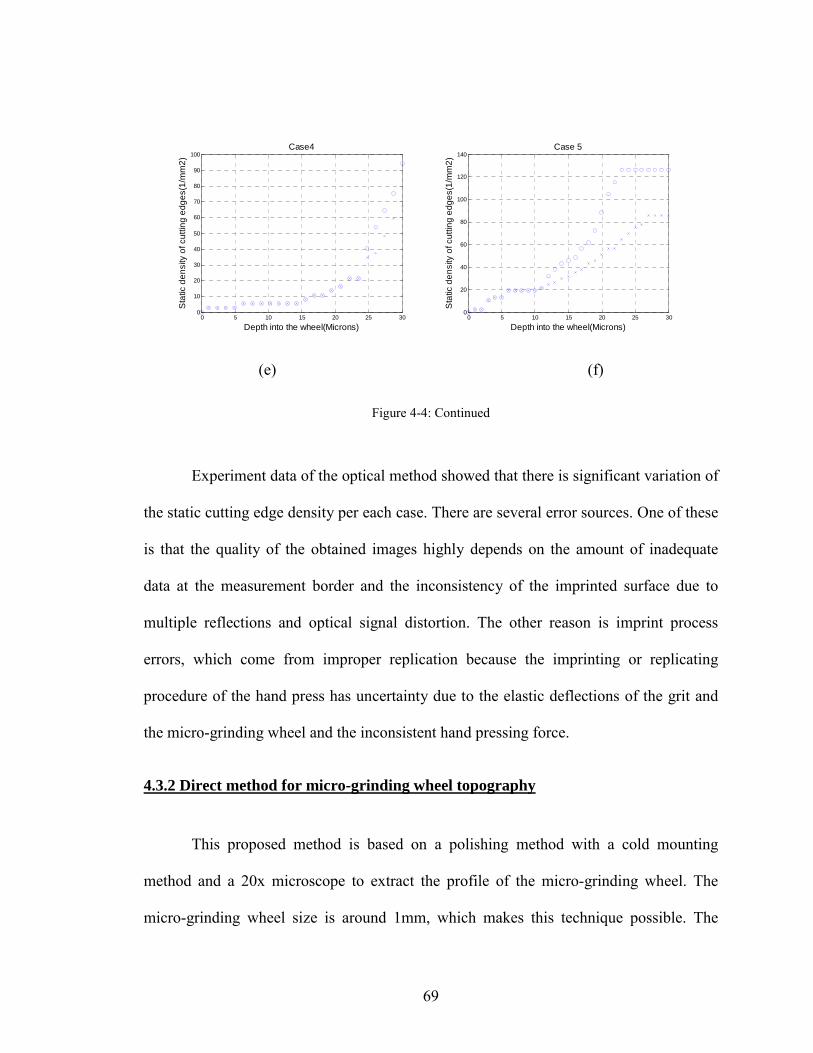
69

0 5 10 15 20 25 300

10

20

30

40

50

60

70

80

90

100

Depth into the wheel(Microns)

Sta

tic d

ensi

ty o

f cut

ting

edge

s(1/

mm

2)

Case4

0 5 10 15 20 25 30

0

20

40

60

80

100

120

140

Depth into the wheel(Microns)

Sta

tic d

ensi

ty o

f cut

ting

edge

s(1/

mm

2)

Case 5

(e) (f)

Figure 4-4: Continued

Experiment data of the optical method showed that there is significant variation of

the static cutting edge density per each case. There are several error sources. One of these

is that the quality of the obtained images highly depends on the amount of inadequate

data at the measurement border and the inconsistency of the imprinted surface due to

multiple reflections and optical signal distortion. The other reason is imprint process

errors, which come from improper replication because the imprinting or replicating

procedure of the hand press has uncertainty due to the elastic deflections of the grit and

the micro-grinding wheel and the inconsistent hand pressing force.

4.3.2 Direct method for micro-grinding wheel topography

This proposed method is based on a polishing method with a cold mounting

method and a 20x microscope to extract the profile of the micro-grinding wheel. The

micro-grinding wheel size is around 1mm, which makes this technique possible. The

70

specimen samples for this proposed method are prepared using a castable mounting

method because a castable mounting provides more accurate mounting. These specimens

are polished with different size diamond suspensions in Figure 4-5(a).

(a) (b)

Figure 4-5: (a) Illustration of a prepared sample and (b) Flowchart of the proposed direct method

In order to improve the quality of pictures, for one section profile, four pictures

are taken and are assembled into one image, which is shown in Figure 4-6. There are two

different experiments for fresh and worn micro-grinding wheels. Experimental data

obtained from this method showed that in the case of worn tools. The nickel layer rapidly

wears out and some grits are taken off from a base material.

71

(a) (b)

Figure 4-6: Section profiles of (a) fresh and (b) worn micro-grinding wheels

On the basis of these constructed images, the profile is extracted using

mathematical computation in MATLAB software. Profile data extracted from section

cuts are used to compute the diameters of the micro-grinding wheels and the size of CBN

grits.

In both cases, the least square nonlinear regression method is adopted because this

method has been widely used to solve sets of nonlinear equations given extracted data

points. The optimality criterion of this method is to minimize the sum of residual squares

between observed data and the values of the approximate numerical model. In the case of

two coordinate variables (x and y), a mathematical representation for the circle estimation

is given by

2 2( , ) 0f x y x y ax by c= + + + = (4.2)

To determine the mathematical representation model parameters (a, b, and c), a

least square error regression analysis will be pursued. Briefly, for a measured data

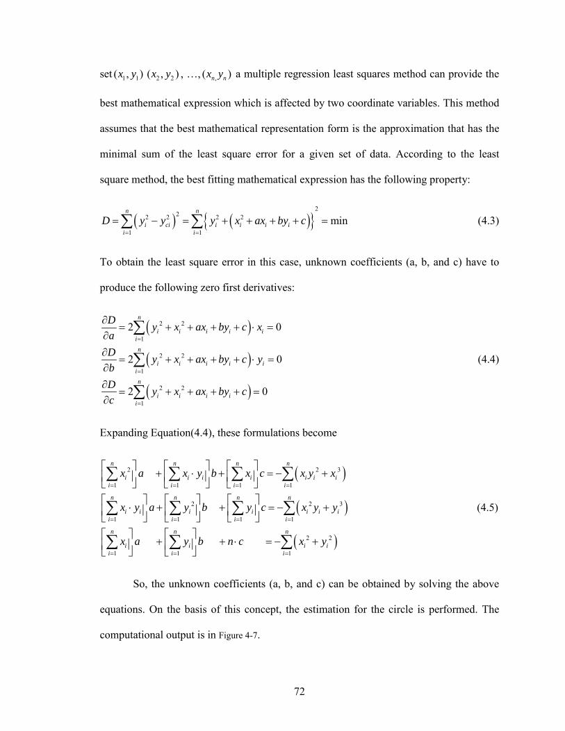
72

set 1 1( , )x y 2 2( , )x y , …, ,( )n nx y a multiple regression least squares method can provide the

best mathematical expression which is affected by two coordinate variables. This method

assumes that the best mathematical representation form is the approximation that has the

minimal sum of the least square error for a given set of data. According to the least

square method, the best fitting mathematical expression has the following property:

( ) ( ){ }2

22 2 2 2

1 1

minn n

i ci i i i ii i

D y y y x ax by c= =

= − = + + + + =∑ ∑ (4.3)

To obtain the least square error in this case, unknown coefficients (a, b, and c) have to

produce the following zero first derivatives:

( )

( )

( )

2 2

1

2 2

1

2 2

1

2 0

2 0

2 0

n

i i i i ii

n

i i i i iin

i i i ii

D y x ax by c xaD y x ax by c ybD y x ax by cc

=

=

=

∂= + + + + ⋅ =

∂∂

= + + + + ⋅ =∂∂

= + + + + =∂

∑

∑

∑

(4.4)

Expanding Equation(4.4), these formulations become

( )

( )

( )

2 2 3

1 1 1 1

2 2 3

1 1 1 1

2 2

1 1 1

n n n n

i i i i i i ii i i i

n n n n

i i i i i i ii i i i

n n n

i i i ii i i

x a x y b x c x y x

x y a y b y c x y y

x a y b n c x y

= = = =

= = = =

= = =

⎡ ⎤ ⎡ ⎤ ⎡ ⎤+ ⋅ + = − +⎢ ⎥ ⎢ ⎥ ⎢ ⎥⎣ ⎦ ⎣ ⎦ ⎣ ⎦⎡ ⎤ ⎡ ⎤ ⎡ ⎤

⋅ + + = − +⎢ ⎥ ⎢ ⎥ ⎢ ⎥⎣ ⎦ ⎣ ⎦ ⎣ ⎦⎡ ⎤ ⎡ ⎤+ + ⋅ = − +⎢ ⎥ ⎢ ⎥⎣ ⎦ ⎣ ⎦

∑ ∑ ∑ ∑

∑ ∑ ∑ ∑

∑ ∑ ∑

(4.5)

So, the unknown coefficients (a, b, and c) can be obtained by solving the above

equations. On the basis of this concept, the estimation for the circle is performed. The

computational output is in Figure 4-7.

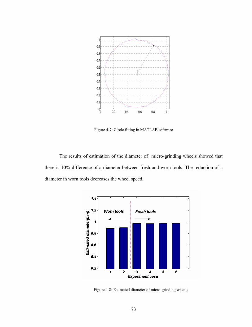
73

0 0.2 0.4 0.6 0.8 10

0.1

0.2

0.3

0.4

0.5

0.6

0.7

0.8

0.9

1

Figure 4-7: Circle fitting in MATLAB software

The results of estimation of the diameter of micro-grinding wheels showed that

there is 10% difference of a diameter between fresh and worn tools. The reduction of a

diameter in worn tools decreases the wheel speed.

Figure 4-8: Estimated diameter of micro-grinding wheels

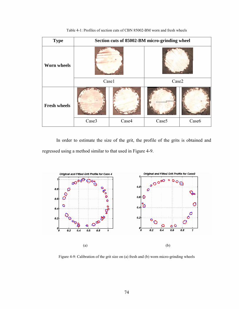
74

Table 4-1: Profiles of section cuts of CBN 85002-BM worn and fresh wheels

Type Section cuts of 85002-BM micro-grinding wheel

Worn wheels

Case1 Case2

Fresh wheels

Case3 Case4 Case5 Case6

In order to estimate the size of the grit, the profile of the grits is obtained and

regressed using a method similar to that used in Figure 4-9.

(a) (b)

Figure 4-9: Calibration of the grit size on (a) fresh and (b) worn micro-grinding wheels

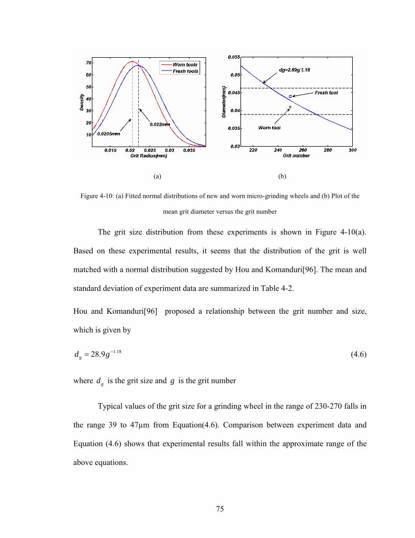
75

(a) (b)

Figure 4-10: (a) Fitted normal distributions of new and worn micro-grinding wheels and (b) Plot of the

mean grit diameter versus the grit number

The grit size distribution from these experiments is shown in Figure 4-10(a).

Based on these experimental results, it seems that the distribution of the grit is well

matched with a normal distribution suggested by Hou and Komanduri[96]. The mean and

standard deviation of experiment data are summarized in Table 4-2.

Hou and Komanduri[96] proposed a relationship between the grit number and size,

which is given by

1.1828.9gd g −= (4.6)

where gd is the grit size and g is the grit number

Typical values of the grit size for a grinding wheel in the range of 230-270 falls in

the range 39 to 47µm from Equation(4.6). Comparison between experiment data and

Equation (4.6) shows that experimental results fall within the approximate range of the

above equations.

76

Table 4-2: Estimation of the size of grits for fresh and worn tools

Fresh tool Worn tool

Mean (radius) 0.022mm 0.0205mm

Standard Deviation 0.0056mm 0.0059mm

4.4 Comparison between optical and direct methods

The type of experimental data obtained from the direct method is different from

those obtained in the optical method. Two-dimensional data of the direct method have to

be transformed to make possible a comparison between two methods.

To transform the experiment data of a direct method, the width of two

dimensional profiles has to be decided. So, based on the assumption that the grit is

spherical in shape, the width can be approximated to be equal to the maximum size of

grits in the profile cross section line because the extracted grit profile in the images is the

cross section of the spherical grits.

Figure 4-11: Schematic illustration of extension for the extracted profile data

On the basis of this concept, the static cutting edge density, which is the number

of active grits per unit area of the micro-grinding wheel surface, can be determined using

the direct method. In the case of the optical method, their experiment data are already

77

three dimensional profiles having a specific area. In MATLAB software, the static cutting

density can be obtained.

For both methods, since the experimental data is very widely scattered, the

process smoothing experiment data obtained is necessary prior to the regression analysis.

A moving averaging method is used to smooth the experimental data, which is equivalent

to low pass filtering. This method smoothes raw experiment data by replacing these data

with the average value of the neighboring data points with the defined span. Equation

(4.7) by Hacker[51] can be adopted to represent the static cutting edge density

sks sC A Z= (4.7)

On the basis of these smoothed data, a non-linear regression analysis is performed

within the range of the grit radius. The computation results are summarized in Table 4-3.

Table 4-3: Summary of computations for static cutting density

Cases sA sk aR

Fresh tool 2.355 0.922 0.984 Direct method

Worn tool 2.211 0.8527 0.961

Optical method for fresh tool 1.609 0.9019 0.887

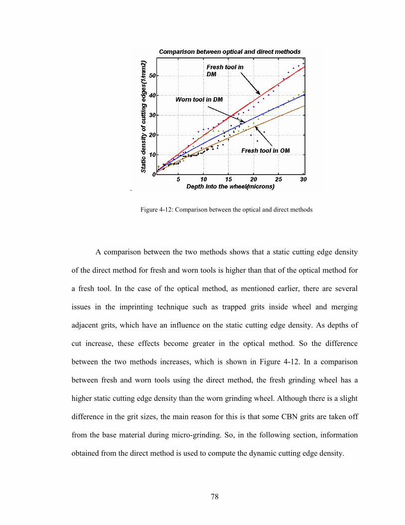
78

.

Figure 4-12: Comparison between the optical and direct methods

A comparison between the two methods shows that a static cutting edge density

of the direct method for fresh and worn tools is higher than that of the optical method for

a fresh tool. In the case of the optical method, as mentioned earlier, there are several

issues in the imprinting technique such as trapped grits inside wheel and merging

adjacent grits, which have an influence on the static cutting edge density. As depths of

cut increase, these effects become greater in the optical method. So the difference

between the two methods increases, which is shown in Figure 4-12. In a comparison

between fresh and worn tools using the direct method, the fresh grinding wheel has a

higher static cutting edge density than the worn grinding wheel. Although there is a slight

difference in the grit sizes, the main reason for this is that some CBN grits are taken off

from the base material during micro-grinding. So, in the following section, information

obtained from the direct method is used to compute the dynamic cutting edge density.

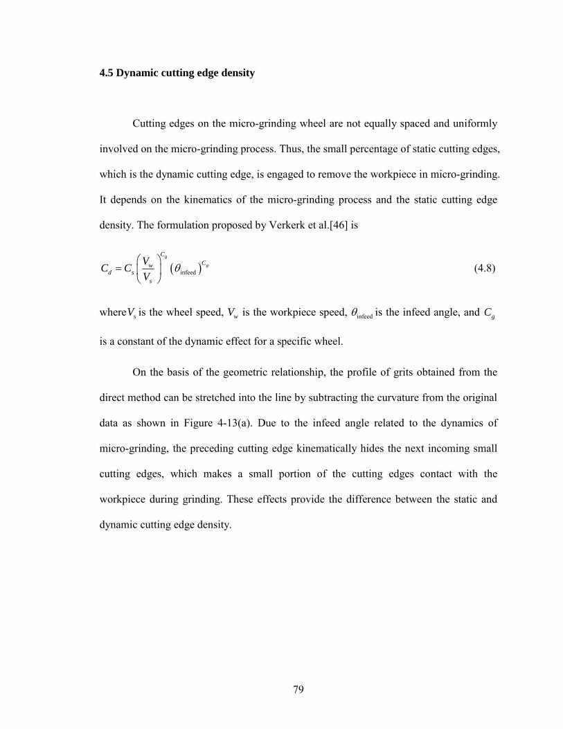
79

4.5 Dynamic cutting edge density

Cutting edges on the micro-grinding wheel are not equally spaced and uniformly

involved on the micro-grinding process. Thus, the small percentage of static cutting edges,

which is the dynamic cutting edge, is engaged to remove the workpiece in micro-grinding.

It depends on the kinematics of the micro-grinding process and the static cutting edge

density. The formulation proposed by Verkerk et al.[46] is

( )infeed

g

g

CCw

d ss

VC CV

θ⎛ ⎞

= ⎜ ⎟⎝ ⎠

(4.8)

where sV is the wheel speed, wV is the workpiece speed, infeedθ is the infeed angle, and gC

is a constant of the dynamic effect for a specific wheel.

On the basis of the geometric relationship, the profile of grits obtained from the

direct method can be stretched into the line by subtracting the curvature from the original

data as shown in Figure 4-13(a). Due to the infeed angle related to the dynamics of

micro-grinding, the preceding cutting edge kinematically hides the next incoming small

cutting edges, which makes a small portion of the cutting edges contact with the

workpiece during grinding. These effects provide the difference between the static and

dynamic cutting edge density.

80

-0.05

0

0.05

0.1

0 0.5 1 1.5 2 2.5 3

(a) (b)

Figure 4-13: (a) Tracing and (b) illustration of dynamic cutting edges

This infeed angle is represented from the geometrical and kinematical relationship

according to the following equation:

1 0infeed tan w

s e

V tV d

θ − ⎛ ⎞= ⎜ ⎟⎜ ⎟

⎝ ⎠ (4.9)

where 0t is the depth of cut and ed is the diameter of the micro-grinding wheel.

The above equation shows that as the workpiece speed and the depth of cut

increase, the infeed angle increases so that the number of engaged grits in micro-grinding

increases. From the experimental data of the direct method, the dynamic effect can be

estimated according to varying workpiece speeds, and the constant of dynamic effect for

this micro-grinding wheel is obtained from the mathematical computation on the basis of

the above equation.

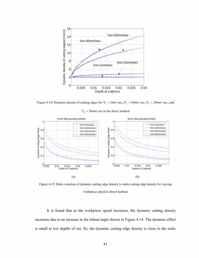
81

0.005 0.01 0.015 0.02 0.025 0.03

2

4

6

8

10

12

14

16

Depth of cut(mm)

Dyn

amic

den

sity

of c

uttin

g ed

ges(

1/m

m2)

Vw=30mm/sec

Vw=20mm/sec

Vw=10mm/secVw=1mm/sec

Figure 4-14: Dynamic density of cutting edges for 1 / secwV mm= , 10 / secwV mm= , 20 / secwV mm= , and

30 / secwV mm= in the direct method

0.005 0.01 0.015 0.02 0.0250

0.2

0.4

0.6

0.8

1

Depth of Cut(mm)

Dyn

amic

Cut

ting

Edg

e R

atio

Fresh Microgrinding Wheel

Vw=1mm/secVw=10mm/secVw=20mm/secVw=30mm/sec

0.005 0.01 0.015 0.02 0.0250

0.2

0.4

0.6

0.8

1

Depth of Cut(mm)

Dyn

amic

Cut

ting

Edg

e R

atio

Worn Microgrinding Wheel

Vw=1mm/secVw=10mm/secVw=20mm/secVw=30mm/sec

(a) (b)

Figure 4-15: Ratio variation of dynamic cutting edge density to static cutting edge density for varying

workpiece speed in direct method

It is found that as the workpiece speed increases, the dynamic cutting density

increases due to an increase in the infeed angle shown in Figure 4-14. The dynamic effect

is small at low depths of cut. So, the dynamic cutting edge density is close to the static

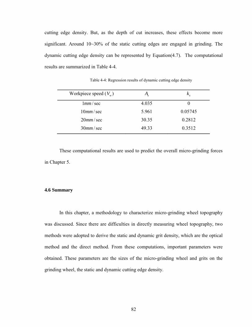
82

cutting edge density. But, as the depth of cut increases, these effects become more

significant. Around 10~30% of the static cutting edges are engaged in grinding. The

dynamic cutting edge density can be represented by Equation(4.7). The computational

results are summarized in Table 4-4.

Table 4-4: Regression results of dynamic cutting edge density

Workpiece speed ( wV ) sA sk

1 / secmm 4.035 0

10 / secmm 5.961 0.05745

20 / secmm 30.35 0.2812

30 / secmm 49.33 0.3512

These computational results are used to predict the overall micro-grinding forces

in Chapter 5.

4.6 Summary

In this chapter, a methodology to characterize micro-grinding wheel topography

was discussed. Since there are difficulties in directly measuring wheel topography, two

methods were adopted to derive the static and dynamic grit density, which are the optical

method and the direct method. From these computations, important parameters were

obtained. These parameters are the sizes of the micro-grinding wheel and grits on the

grinding wheel, the static and dynamic cutting edge density.

83

In the case of the size of the micro-grinding wheel, it is found that there is 10%

difference between a fresh and a worn grinding wheel. Experiments to determine the size

of grit also show 2µm difference of mean value between them, and the distribution of the

grit size is close to the normal distribution as was the case in the assumption proposed by

Hou and Komanduri[96].

The computational results based on two methods for static cutting edge show that

the static cutting edge density obtained from the direct method is higher than that of the

optical method. As the depth of cut increases, the differences between both methods

increase around 12.5% for worn wheels and 36% for fresh CBN electroplated grinding

wheels.

Computations of the dynamic cutting edge showed that 10~30% of the static

cutting edges are engaged in grinding at high depths of cut. In the case of micro-grinding

wheels, their diameters are smaller than those of conventional grinding wheels, which is

related to an increase in the infeed angle. Due to this increase of the infeed angle, the

results computed are higher than 2%~12% of Younis et al.[47].

84

CHAPTER 5

COMPARISON BETWEEN THEORETICAL AND EXPERIMENTAL

COMPUTATIONS

5.1 Introduction

Micro-grinding is a process which can be used to produce a good quality product.

In considering the characteristics of the micro-grinding process, prediction of micro-

grinding forces is a prerequisite to estimation of other factors such as tool life prediction,

process planning of micro-grinding and chatter analysis.

In this chapter, a model to predict micro-grinding forces is discussed and

compared with experimental data for micro-grinding an aluminum alloy (Al 6061-T6).

Based on modeling techniques of thermal and mechanical deformation on the micro-

grinding zone that were presented in Chapter 3, a model was developed to predict micro-

grinding forces, incorporating material properties as functions of strain, strain rate, and

temperature, characterization of micro-grinding wheel topography that were obtained in

Chapter 4, and the kinematics of the micro-grinding process.

Consequently, the experimental determination of the grain size of the micro-

structure is discussed in this chapter. Side micro-grinding tests over a wide range of

grinding speeds and depths of cut were conducted to validate the proposed micro-

grinding model. The effects of rising temperature on a micro-grinding zone were

estimated using the model in Chapter 3. A comparison between experimental data and

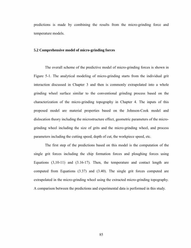
85

predictions is made by combining the results from the micro-grinding force and

temperature models.

5.2 Comprehensive model of micro-grinding forces

The overall scheme of the predictive model of micro-grinding forces is shown in

Figure 5-1. The analytical modeling of micro-grinding starts from the individual grit

interaction discussed in Chapter 3 and then is commonly extrapolated into a whole

grinding wheel surface similar to the conventional grinding process based on the

characterization of the micro-grinding topography in Chapter 4. The inputs of this

proposed model are material properties based on the Johnson-Cook model and

dislocation theory including the microstructure effect, geometric parameters of the micro-

grinding wheel including the size of grits and the micro-grinding wheel, and process

parameters including the cutting speed, depth of cut, the workpiece speed, etc.

The first step of the predictions based on this model is the computation of the

single grit forces including the chip formation forces and ploughing forces using

Equations (3,10-11) and (3.16-17). Then, the temperature and contact length are

computed from Equations (3.37) and (3.40). The single grit forces computed are

extrapolated in the micro-grinding wheel using the extracted micro-grinding topography.

A comparison between the predictions and experimental data is performed in this study.

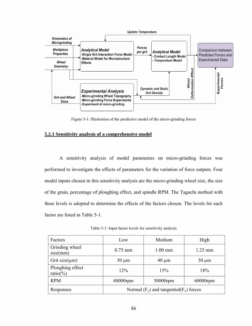
86

Figure 5-1: Illustration of the predictive model of the micro-grinding forces

5.2.1 Sensitivity analysis of a comprehensive model

A sensitivity analysis of model parameters on micro-grinding forces was

performed to investigate the effects of parameters for the variation of force outputs. Four

model inputs chosen in this sensitivity analysis are the micro-grinding wheel size, the size

of the grain, percentage of ploughing effect, and spindle RPM. The Taguchi method with

three levels is adopted to determine the effects of the factors chosen. The levels for each

factor are listed in Table 5-1.

Table 5-1: Input factor levels for sensitivity analysis

Factors Low Medium High Grinding wheel size(mm) 0.75 mm 1.00 mm 1.25 mm

Grit size(µm) 30 µm 40 µm 50 µm Ploughing effect ratio(%) 12% 15% 18%

RPM 40000rpm 50000rpm 60000rpm

Responses Normal (Fy) and tangential(Fx) forces

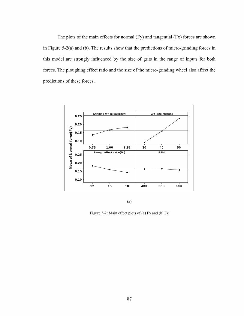
87

The plots of the main effects for normal (Fy) and tangential (Fx) forces are shown

in Figure 5-2(a) and (b). The results show that the predictions of micro-grinding forces in

this model are strongly influenced by the size of grits in the range of inputs for both

forces. The ploughing effect ratio and the size of the micro-grinding wheel also affect the

predictions of these forces.

Mea

n of

Nor

mal

for

ce(F

y)

1.251.000.75

0.25

0.20

0.15

0.10

504030

181512

0.25

0.20

0.15

0.10

60K50K40K

Grinding wheel size(mm) Grit size(micron)

Plough effect ratio(%) RPM

(a)

Figure 5-2: Main effect plots of (a) Fy and (b) Fx

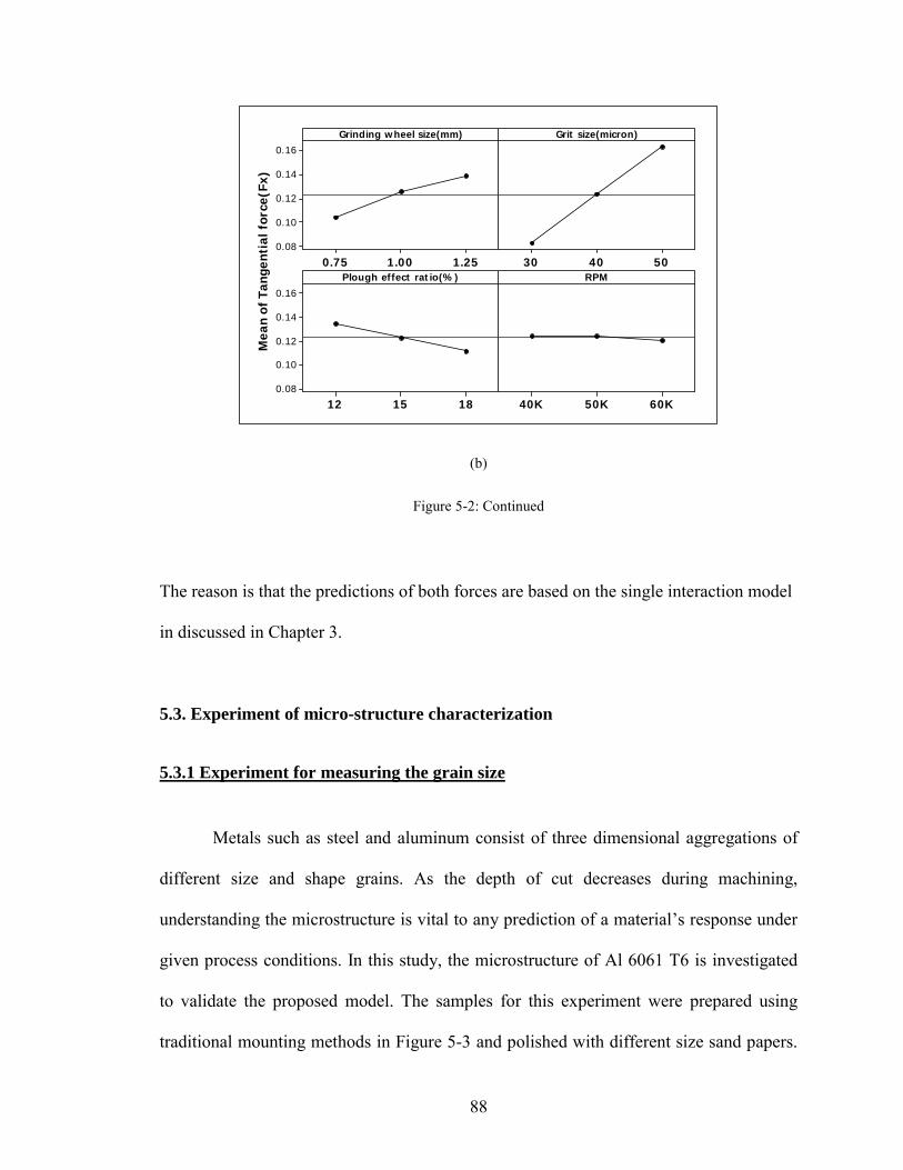
88

Mea

n of

Tan

gent

ial f

orce

(Fx)

1.251.000.75

0.16

0.14

0.12

0.10

0.08

504030

181512

0.16

0.14

0.12

0.10

0.08

60K50K40K

Grinding wheel size(mm) Grit size(micron)

Plough effect ratio(%) RPM

(b)

Figure 5-2: Continued

The reason is that the predictions of both forces are based on the single interaction model

in discussed in Chapter 3.

5.3. Experiment of micro-structure characterization

5.3.1 Experiment for measuring the grain size

Metals such as steel and aluminum consist of three dimensional aggregations of

different size and shape grains. As the depth of cut decreases during machining,

understanding the microstructure is vital to any prediction of a material’s response under

given process conditions. In this study, the microstructure of Al 6061 T6 is investigated

to validate the proposed model. The samples for this experiment were prepared using

traditional mounting methods in Figure 5-3 and polished with different size sand papers.

89

These samples are finally polished using NANOCLOTH paper and 0.05µm alumina.

Based on the literature survey[97], these samples are electrolytically etched using the

modified barker’s reagent: 108 ml of distilled OH 2 , 3.75 4HBF , and 37.5 of 22OH to

remove the grain boundaries of the samples.

Figure 5-3: Scheme of the prepared Al 6061-T6 sample

The images of the etched sample were taken using an optical microscope with a

polarized light in Figure 5-4(a) and (b). Based on the obtained images, the shape of grains

is analyzed using the optical software.

(a) (b)

Figure 5-4: Processed images in (a) sample position 1, (b) sample position 2, (c) sample position 3, and (d)

sample position 4

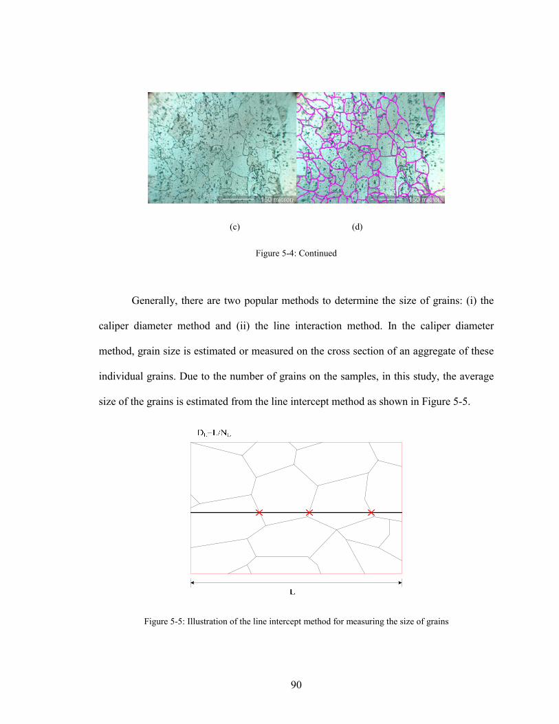
90

(c) (d)

Figure 5-4: Continued

Generally, there are two popular methods to determine the size of grains: (i) the

caliper diameter method and (ii) the line interaction method. In the caliper diameter

method, grain size is estimated or measured on the cross section of an aggregate of these

individual grains. Due to the number of grains on the samples, in this study, the average

size of the grains is estimated from the line intercept method as shown in Figure 5-5.

Figure 5-5: Illustration of the line intercept method for measuring the size of grains

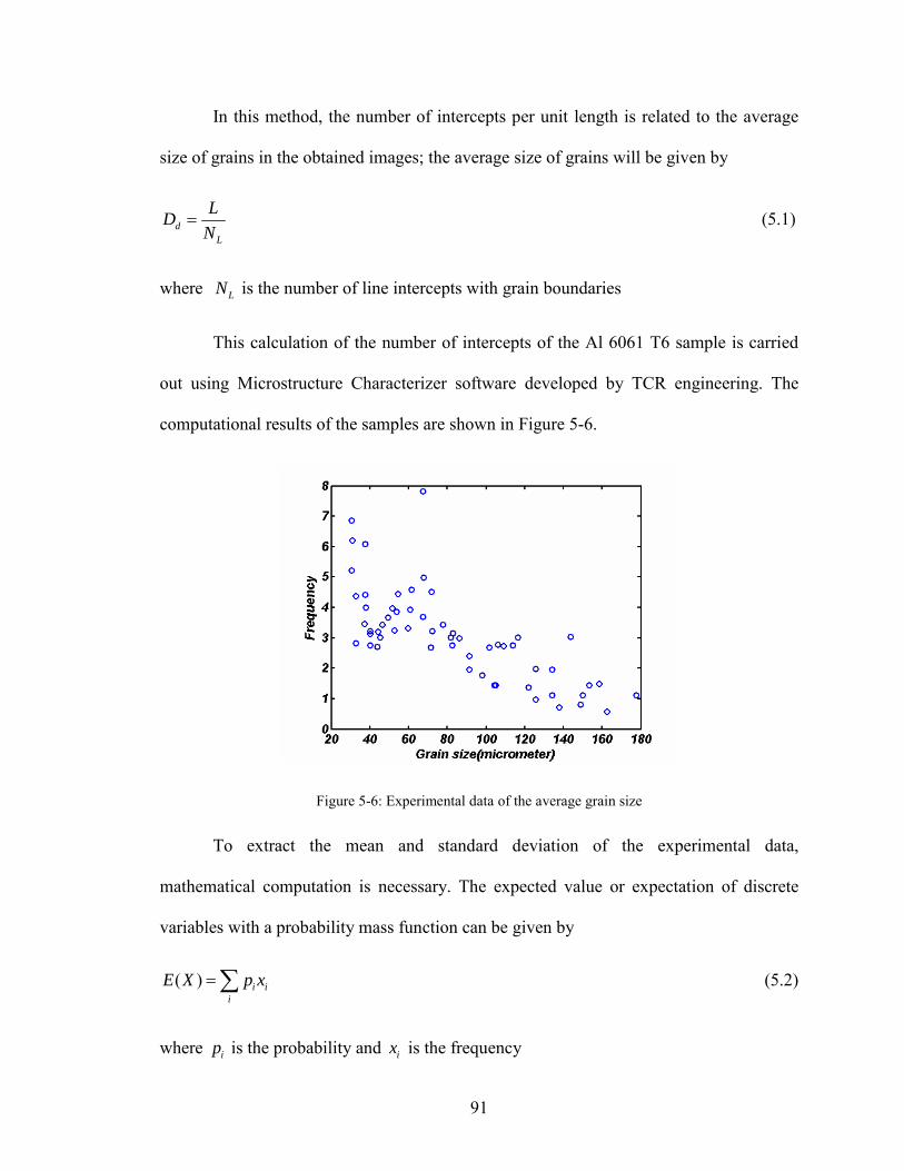
91

In this method, the number of intercepts per unit length is related to the average

size of grains in the obtained images; the average size of grains will be given by

dL

LDN

= (5.1)

where LN is the number of line intercepts with grain boundaries

This calculation of the number of intercepts of the Al 6061 T6 sample is carried

out using Microstructure Characterizer software developed by TCR engineering. The

computational results of the samples are shown in Figure 5-6.

Figure 5-6: Experimental data of the average grain size

To extract the mean and standard deviation of the experimental data,

mathematical computation is necessary. The expected value or expectation of discrete

variables with a probability mass function can be given by

( ) i ii

E X p x=∑ (5.2)

where ip is the probability and ix is the frequency

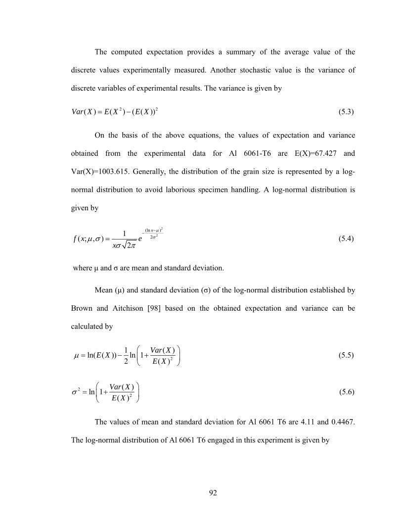
92

The computed expectation provides a summary of the average value of the

discrete values experimentally measured. Another stochastic value is the variance of

discrete variables of experimental results. The variance is given by

2 2( ) ( ) ( ( ))Var X E X E X= − (5.3)

On the basis of the above equations, the values of expectation and variance

obtained from the experimental data for Al 6061-T6 are E(X)=67.427 and

Var(X)=1003.615. Generally, the distribution of the grain size is represented by a log-

normal distribution to avoid laborious specimen handling. A log-normal distribution is

given by

2

2(ln )

21( ; , )2

x

f x ex

µσµ σ

σ π

−−

= (5.4)

where µ and σ are mean and standard deviation.

Mean (µ) and standard deviation (σ) of the log-normal distribution established by

Brown and Aitchison [98] based on the obtained expectation and variance can be

calculated by

2

1 ( )ln( ( )) ln 12 ( )

Var XE XE X

µ⎛ ⎞

= − +⎜ ⎟⎝ ⎠

(5.5)

22

( )ln 1( )

Var XE X

σ⎛ ⎞

= +⎜ ⎟⎝ ⎠

(5.6)

The values of mean and standard deviation for Al 6061 T6 are 4.11 and 0.4467.

The log-normal distribution of Al 6061 T6 engaged in this experiment is given by

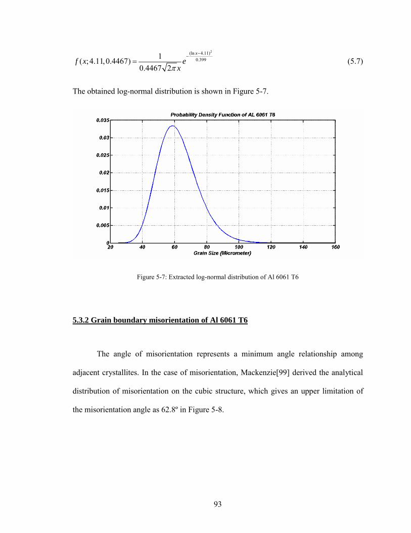
93

2(ln 4.11)0.3991( ;4.11,0.4467)

0.4467 2

x

f x exπ

−−

= (5.7)

The obtained log-normal distribution is shown in Figure 5-7.

Figure 5-7: Extracted log-normal distribution of Al 6061 T6

5.3.2 Grain boundary misorientation of Al 6061 T6

The angle of misorientation represents a minimum angle relationship among

adjacent crystallites. In the case of misorientation, Mackenzie[99] derived the analytical

distribution of misorientation on the cubic structure, which gives an upper limitation of

the misorientation angle as 62.8º in Figure 5-8.

94

Figure 5-8: The density function for the angle of misorientation

Generally, an EBSD-inspired method has been used to capture the misorientation

between the two crystals. Kang et al.[91] extracted the distribution of misorientation for

Al 6061 T6 using EBSD. The values of misorientations are plotted as absolute values in

Figure 5-9.

0 10 20 30 40 50 600

0.5

1

1.5

2

Misorientation(Degree)

Frac

tion[

%]

Figure 5-9: Grain boundary misorientation of AL 6061-T6 by Kang et al.[91]

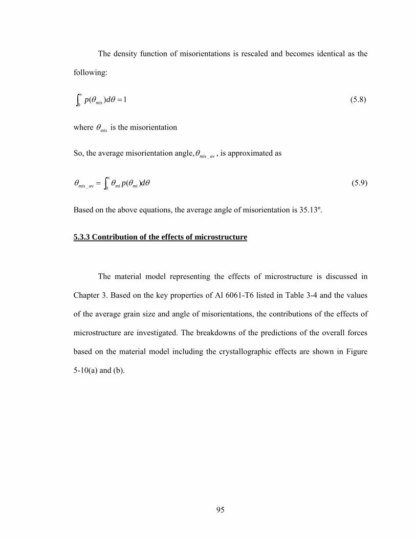
95

The density function of misorientations is rescaled and becomes identical as the

following:

0( ) 1misp dθ θ

∞=∫ (5.8)

where misθ is the misorientation

So, the average misorientation angle, _mis avθ , is approximated as

_ 0( )mis av mi mip dθ θ θ θ

∞= ∫ (5.9)

Based on the above equations, the average angle of misorientation is 35.13º.

5.3.3 Contribution of the effects of microstructure

The material model representing the effects of microstructure is discussed in

Chapter 3. Based on the key properties of Al 6061-T6 listed in Table 3-4 and the values

of the average grain size and angle of misorientations, the contributions of the effects of

microstructure are investigated. The breakdowns of the predictions of the overall forces

based on the material model including the crystallographic effects are shown in Figure

5-10(a) and (b).

96

Contribution of stress parameters

0%

20%

40%

60%

80%

100%

5µm 10µm 15µm 20µm 25µmDepth of cut

Misorientation

Grain size

Con. Flow

488

490

492

494

496

498

500

502

5µm 10µm 15µm 20µm 25µmDepth of cut

Shea

r str

ess(

MPA

)

(a) (b)

Figure 5-10: (a) The breakdowns of shear stresses computed and (b) shear stress along depths of cut for

1wV mm= , grit size=43µm, and 60000RPM rpm=

The values of constants used to compute the shear stresses are 2mk = , 0.2α = ,

3.0M = , and 32.5hk H mν µ= which are listed in Table 3-3. The computed results

show that the computed-variation of the shear stress is around 15% of the overall shear

stresses along depths of cut. The trend of the model behavior corresponding to the grain

size is shown in Figure 5-11.

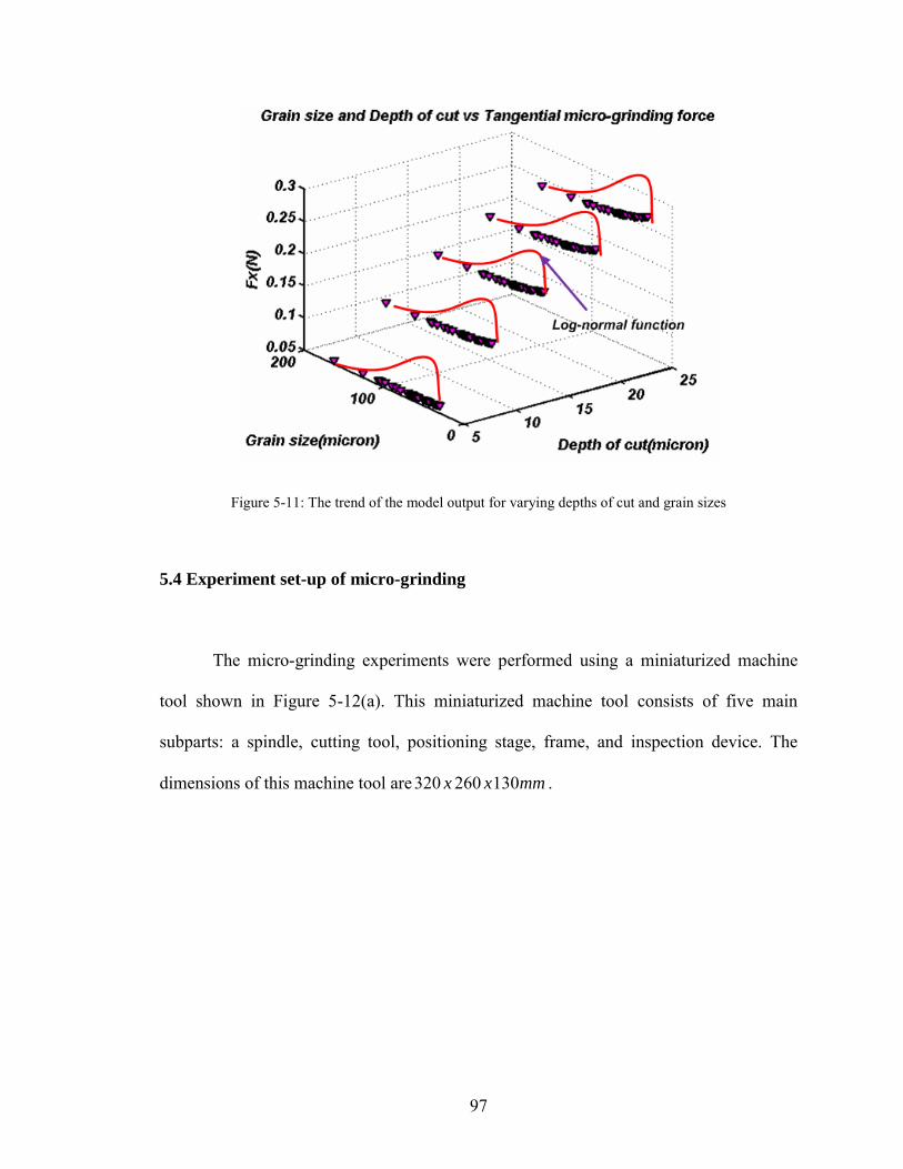
97

Figure 5-11: The trend of the model output for varying depths of cut and grain sizes

5.4 Experiment set-up of micro-grinding

The micro-grinding experiments were performed using a miniaturized machine

tool shown in Figure 5-12(a). This miniaturized machine tool consists of five main

subparts: a spindle, cutting tool, positioning stage, frame, and inspection device. The

dimensions of this machine tool are mmxx 130260320 .

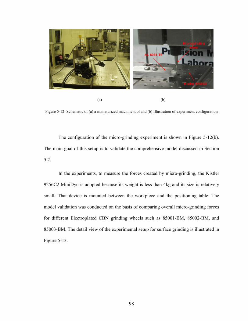
98

(a) (b)

Figure 5-12: Schematic of (a) a miniaturized machine tool and (b) Illustration of experiment configuration

The configuration of the micro-grinding experiment is shown in Figure 5-12(b).

The main goal of this setup is to validate the comprehensive model discussed in Section

5.2.

In the experiments, to measure the forces created by micro-grinding, the Kistler

9256C2 MiniDyn is adopted because its weight is less than 4kg and its size is relatively

small. That device is mounted between the workpiece and the positioning table. The

model validation was conducted on the basis of comparing overall micro-grinding forces

for different Electroplated CBN grinding wheels such as 85001-BM, 85002-BM, and

85003-BM. The detail view of the experimental setup for surface grinding is illustrated in

Figure 5-13.

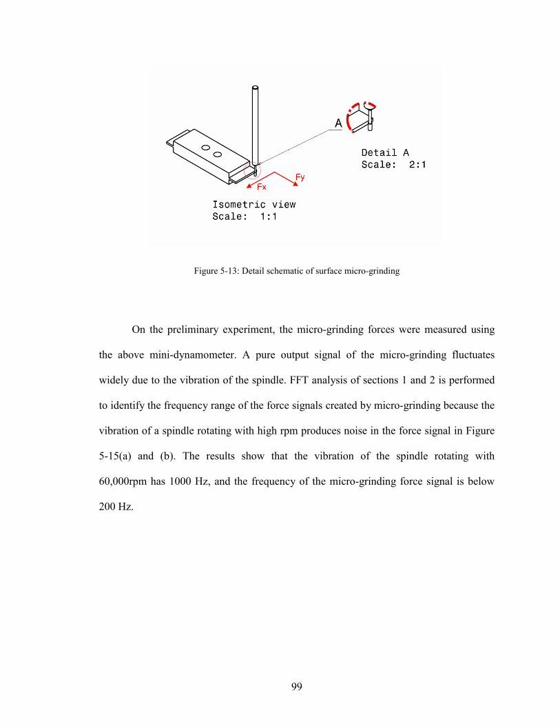
99

Figure 5-13: Detail schematic of surface micro-grinding

On the preliminary experiment, the micro-grinding forces were measured using

the above mini-dynamometer. A pure output signal of the micro-grinding fluctuates

widely due to the vibration of the spindle. FFT analysis of sections 1 and 2 is performed

to identify the frequency range of the force signals created by micro-grinding because the

vibration of a spindle rotating with high rpm produces noise in the force signal in Figure

5-15(a) and (b). The results show that the vibration of the spindle rotating with

60,000rpm has 1000 Hz, and the frequency of the micro-grinding force signal is below

200 Hz.

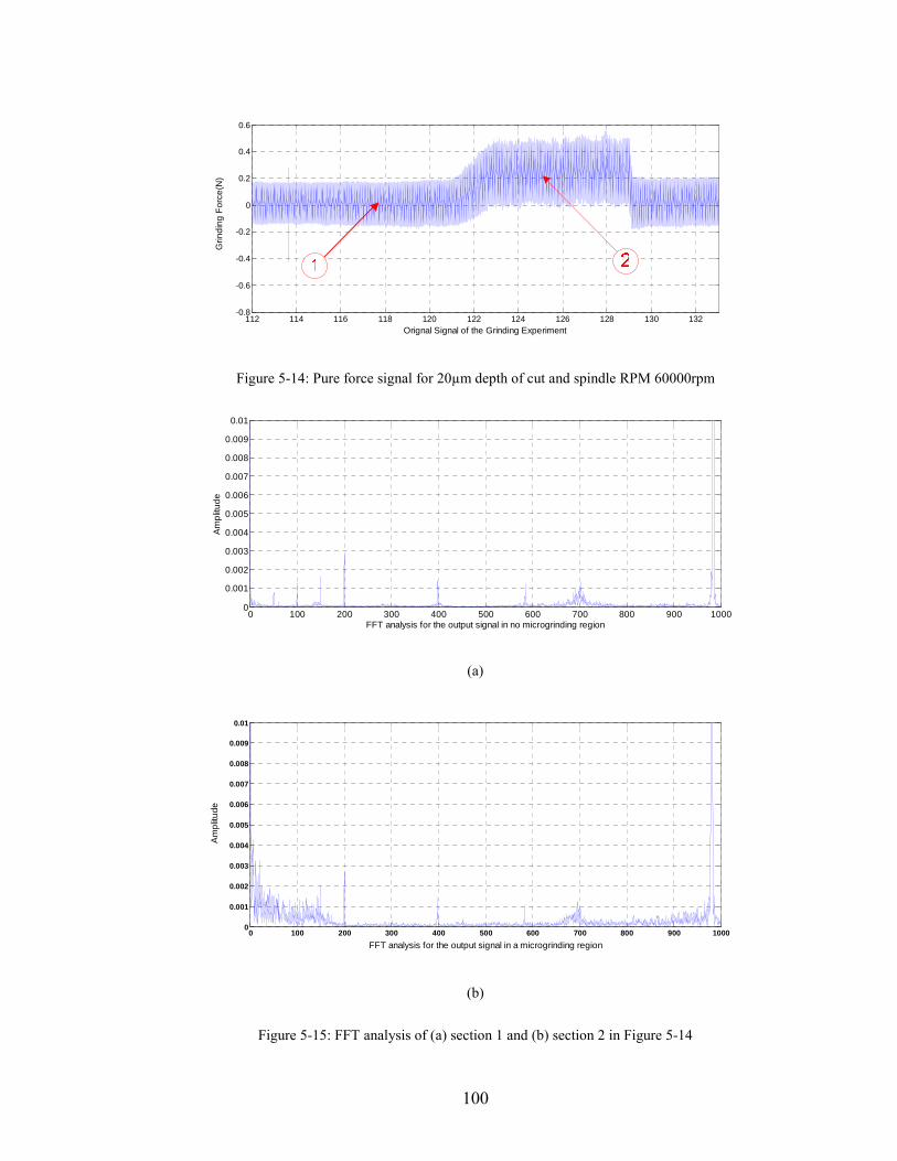
100

112 114 116 118 120 122 124 126 128 130 132-0.8

-0.6

-0.4

-0.2

0

0.2

0.4

0.6

Orignal Signal of the Grinding Experiment

Grin

ding

For

ce(N

)

Figure 5-14: Pure force signal for 20µm depth of cut and spindle RPM 60000rpm

0 100 200 300 400 500 600 700 800 900 10000

0.001

0.002

0.003

0.004

0.005

0.006

0.007

0.008

0.009

0.01

FFT analysis for the output signal in no microgrinding region

Am

plitu

de

(a)

0 100 200 300 400 500 600 700 800 900 10000

0.001

0.002

0.003

0.004

0.005

0.006

0.007

0.008

0.009

0.01

FFT analysis for the output signal in a microgrinding region

Am

plitu

de

(b)

Figure 5-15: FFT analysis of (a) section 1 and (b) section 2 in Figure 5-14

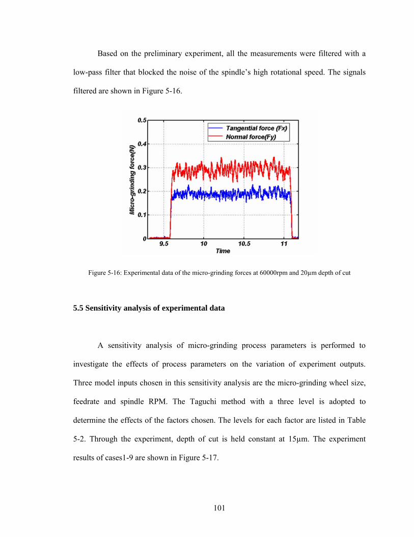
101

Based on the preliminary experiment, all the measurements were filtered with a

low-pass filter that blocked the noise of the spindle’s high rotational speed. The signals

filtered are shown in Figure 5-16.

Figure 5-16: Experimental data of the micro-grinding forces at 60000rpm and 20µm depth of cut

5.5 Sensitivity analysis of experimental data

A sensitivity analysis of micro-grinding process parameters is performed to

investigate the effects of process parameters on the variation of experiment outputs.

Three model inputs chosen in this sensitivity analysis are the micro-grinding wheel size,

feedrate and spindle RPM. The Taguchi method with a three level is adopted to

determine the effects of the factors chosen. The levels for each factor are listed in Table

5-2. Through the experiment, depth of cut is held constant at 15µm. The experiment

results of cases1-9 are shown in Figure 5-17.

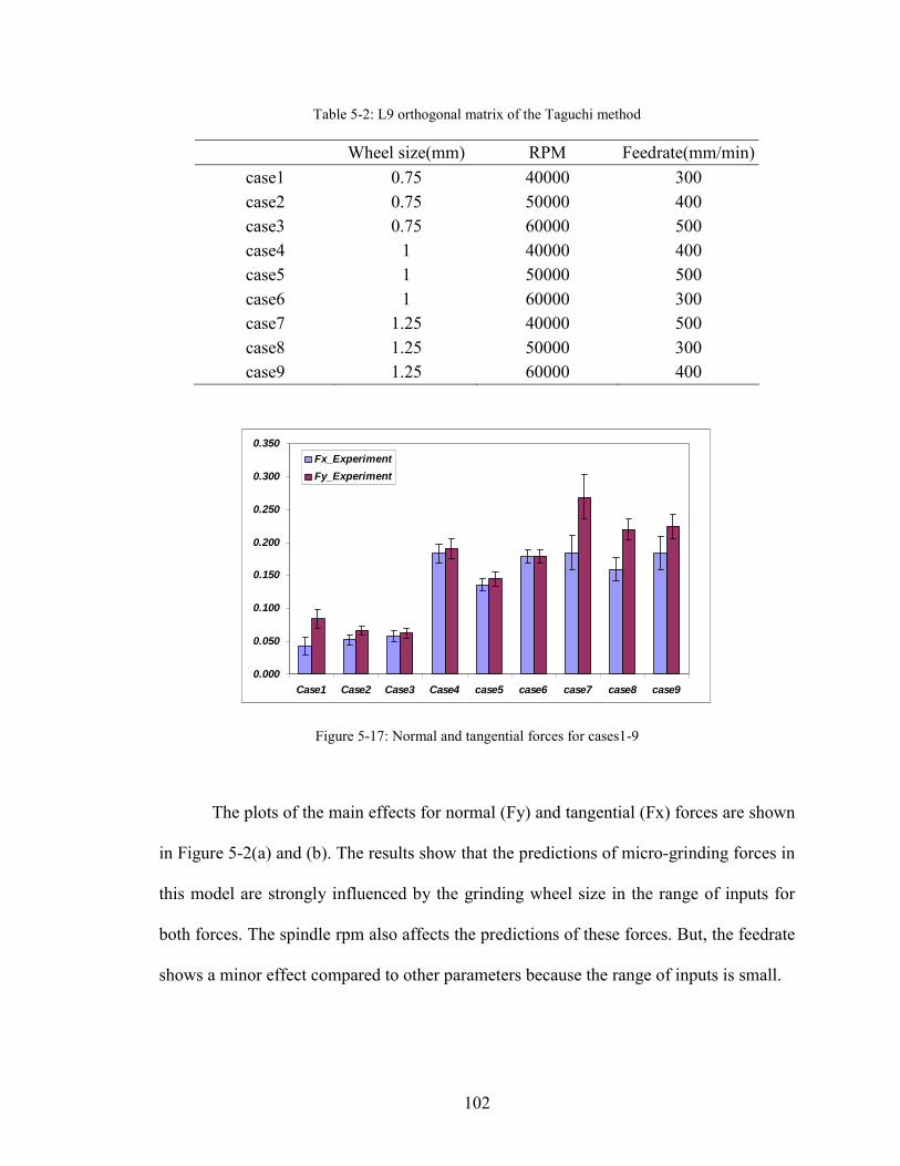
102

Table 5-2: L9 orthogonal matrix of the Taguchi method

Wheel size(mm) RPM Feedrate(mm/min)case1 0.75 40000 300 case2 0.75 50000 400 case3 0.75 60000 500 case4 1 40000 400 case5 1 50000 500 case6 1 60000 300 case7 1.25 40000 500 case8 1.25 50000 300 case9 1.25 60000 400

0.000

0.050

0.100

0.150

0.200

0.250

0.300

0.350

Case1 Case2 Case3 Case4 case5 case6 case7 case8 case9

Fx_ExperimentFy_Experiment

Figure 5-17: Normal and tangential forces for cases1-9

The plots of the main effects for normal (Fy) and tangential (Fx) forces are shown

in Figure 5-2(a) and (b). The results show that the predictions of micro-grinding forces in

this model are strongly influenced by the grinding wheel size in the range of inputs for

both forces. The spindle rpm also affects the predictions of these forces. But, the feedrate

shows a minor effect compared to other parameters because the range of inputs is small.

103

Mea

n of

Mea

ns

1.251.000.75

0.25

0.20

0.15

0.10

0.05600005000040000 500400300

Grinding wheel size RPM Feedrate

Main Effects Plot for Normal Force(Fy)

(a)

Mea

n o

f M

ean

s

1.251.000.75

0.175

0.150

0.125

0.100

0.075

0.050

600005000040000 500400300

Grinding wheel size RPM Feedrate

Main Effects Plot for Tangential Force(Fx)

(b)

Figure 5-18: Main effect plot of (a) normal forces and (b) tangential forces

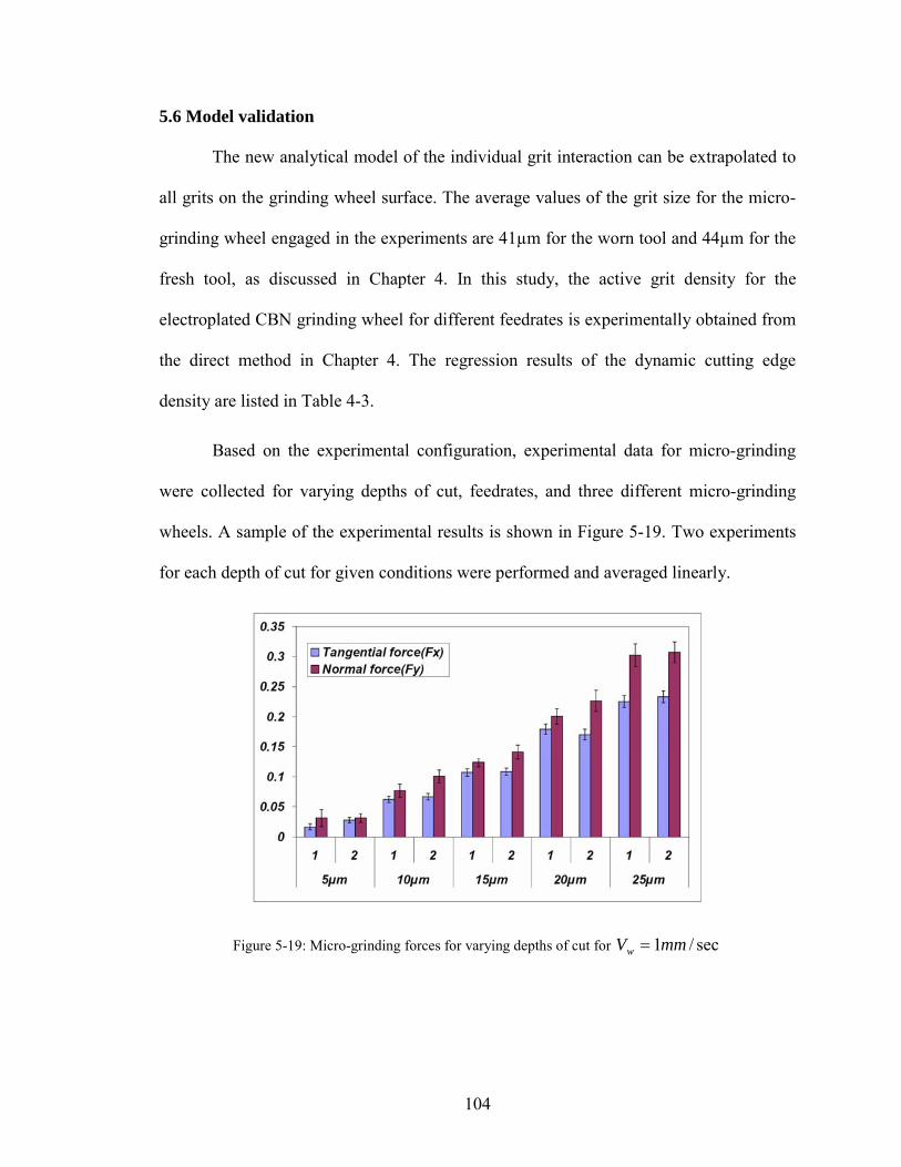
104

5.6 Model validation

The new analytical model of the individual grit interaction can be extrapolated to

all grits on the grinding wheel surface. The average values of the grit size for the micro-

grinding wheel engaged in the experiments are 41µm for the worn tool and 44µm for the

fresh tool, as discussed in Chapter 4. In this study, the active grit density for the

electroplated CBN grinding wheel for different feedrates is experimentally obtained from

the direct method in Chapter 4. The regression results of the dynamic cutting edge

density are listed in Table 4-3.

Based on the experimental configuration, experimental data for micro-grinding

were collected for varying depths of cut, feedrates, and three different micro-grinding

wheels. A sample of the experimental results is shown in Figure 5-19. Two experiments

for each depth of cut for given conditions were performed and averaged linearly.

Figure 5-19: Micro-grinding forces for varying depths of cut for sec/1mmVw =

105

5.6.1 Identification of parameter effects

The comparisons of normal and tangential forces for varying feedrates are shown

in Figure 5-20(a) and (b). The results show that the magnitudes of the forces in

10 /sec wV mm= and 30 /sec wV mm= are higher than those seen in Vw=1 mm/sec. The

differences between the results obtained at these speeds are around 50% for tangential

forces and 50~80% for normal forces. The gap between the results obtained at these

speeds increases at high depths of cut. But, deviation between results obtained at higher

feedrates such as 10 /sec wV mm= and 30 /sec wV mm= is around 2-3% at low depths of

cut. As the depth of cut increase, that gap increases to around 12%.

Tangential Force vs Depth of cut for varying feedrates

0

0.05

0.1

0.15

0.2

0.25

0.3

0.35

0.4

0.45

5µm 10µm 15µm 20µm 25µm

Depth of cut

Forc

e(N

)

Vw=1mm/secVw=10mm/secVw=30mm/sec

(a)

Figure 5-20: Comparisons of (a) tangential and (b) normal forces for varying feedrates

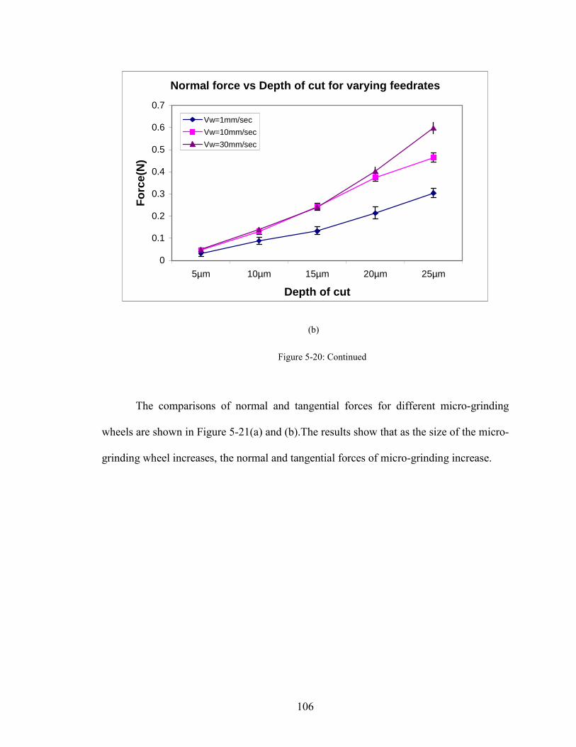
106

Normal force vs Depth of cut for varying feedrates

0

0.1

0.2

0.3

0.4

0.5

0.6

0.7

5µm 10µm 15µm 20µm 25µm

Depth of cut

Forc

e(N

)

Vw=1mm/secVw=10mm/secVw=30mm/sec

(b)

Figure 5-20: Continued

The comparisons of normal and tangential forces for different micro-grinding

wheels are shown in Figure 5-21(a) and (b).The results show that as the size of the micro-

grinding wheel increases, the normal and tangential forces of micro-grinding increase.

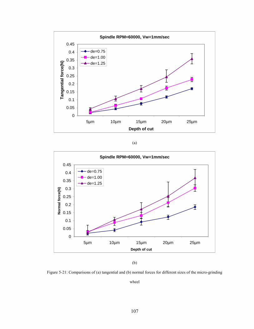
107

Spindle RPM=60000, Vw=1mm/sec

0

0.05

0.1

0.15

0.2

0.25

0.3

0.35

0.4

0.45

5µm 10µm 15µm 20µm 25µm

Depth of cut

Tang

entia

l for

ce(N

)

de=0.75de=1.00de=1.25

(a)

Spindle RPM=60000, Vw=1mm/sec

0

0.05

0.1

0.15

0.2

0.25

0.3

0.35

0.4

0.45

5µm 10µm 15µm 20µm 25µmDepth of cut

Nor

mal

forc

e(N

)

de=0.75de=1.00de=1.25

(b)

Figure 5-21: Comparisons of (a) tangential and (b) normal forces for different sizes of the micro-grinding

wheel

108

The increase of normal and tangential forces is more pronounced at higher depths

of cut. It seems that the increase of the size of the micro-grinding wheel leads to increases

in the geometry contact length and cutting speed as well as the static stiffness of the

micro-grinding wheel. It is also observed that the increasing trend of force components is

changed. For example, in the case of 1.00ed mm= , the normal and tangential forces

increase by15~30% and 30~50% with respect to 0.75ed mm= . For 1.25ed mm= , the

normal and tangential forces increase by30~50% and 16-24% with respect

to 1.00ed mm= .

5.6.2 Comparisons between experiment data and predictions

The predictions of the micro-grinding forces were performed on the basis of the

comprehensive model described in section 5.2. The parameters used in these predictions

are obtained in Chapters 4 and 5 and listed in Chapter 3. In these computations, two

methods:(1)the Oxley’s model[82] and (2)Manjunathaiah and Endres model[83] are used

to compute strains and strain rates of the proposed material model in Chapter 3 and

compared with experimental data.

The comparisons of normal and tangential forces obtained using different size

micro-grinding wheel are shown in Figure 5-20 and Figure 5-21.

109

Grit size:41micron, Ploughing effect: 12.5%

0

0.05

0.1

0.15

0.2

0.25

5µm 10µm 15µm 20µm 25µmDepth of cut

Tang

entia

l for

ce(N

)

Fx_experimentUsing_Manjunathaiah & EndresUsing_Oxley

(a)

Grit size:41micron, Ploughing effect: 12.5%

0

0.05

0.1

0.15

0.2

0.25

5µm 10µm 15µm 20µm 25µm

Depth of cut

Nor

mal

forc

e(N

)

Fy_experimentUsing_Manjunathaiah & EndresUsing_Oxley

(b)

Figure 5-22: Comparison between experimental data and predictions for (a) tangential (Fx) and (b) normal

forces (Fy) of 85001-BM ( 0.75ed mm≈ ) for 1 /secwV mm=

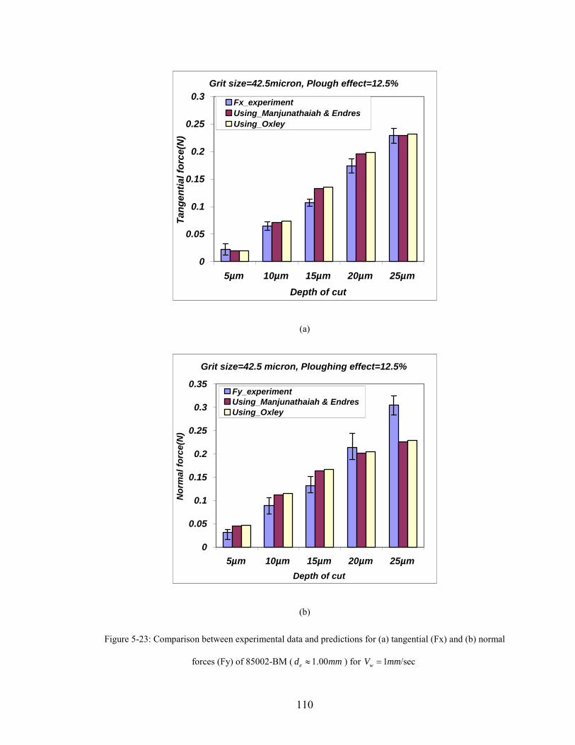
110

Grit size=42.5micron, Plough effect=12.5%

0

0.05

0.1

0.15

0.2

0.25

0.3

5µm 10µm 15µm 20µm 25µmDepth of cut

Tang

entia

l for

ce(N

)

Fx_experimentUsing_Manjunathaiah & EndresUsing_Oxley

(a)

Grit size=42.5 micron, Ploughing effect=12.5%

0

0.05

0.1

0.15

0.2

0.25

0.3

0.35

5µm 10µm 15µm 20µm 25µmDepth of cut

Nor

mal

forc

e(N

)

Fy_experimentUsing_Manjunathaiah & EndresUsing_Oxley

(b)

Figure 5-23: Comparison between experimental data and predictions for (a) tangential (Fx) and (b) normal

forces (Fy) of 85002-BM ( 1.00ed mm≈ ) for 1 /secwV mm=

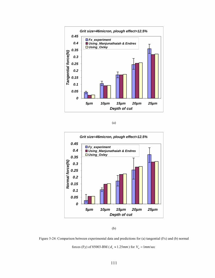
111

Grit size=46micron, plough effect=12.5%

0

0.05

0.1

0.15

0.2

0.25

0.3

0.35

0.4

0.45

5µm 10µm 15µm 20µm 25µmDepth of cut

Tang

entia

l for

ce(N

)

Fx_experimentUsing_Manjunathaiah & EndresUsing_Oxley

(a)

Grit size=46micron, plough effect=12.5%

0

0.05

0.1

0.15

0.2

0.25

0.3

0.35

0.4

0.45

5µm 10µm 15µm 20µm 25µmDepth of cut

Nor

mal

forc

e(N

)

Fy_experimentUsing_Manjunathaiah & EndresUsing_Oxley

(b)

Figure 5-24: Comparison between experimental data and predictions for (a) tangential (Fx) and (b) normal

forces (Fy) of 85003-BM ( 1.25ed mm≈ ) for 1 /secwV mm=

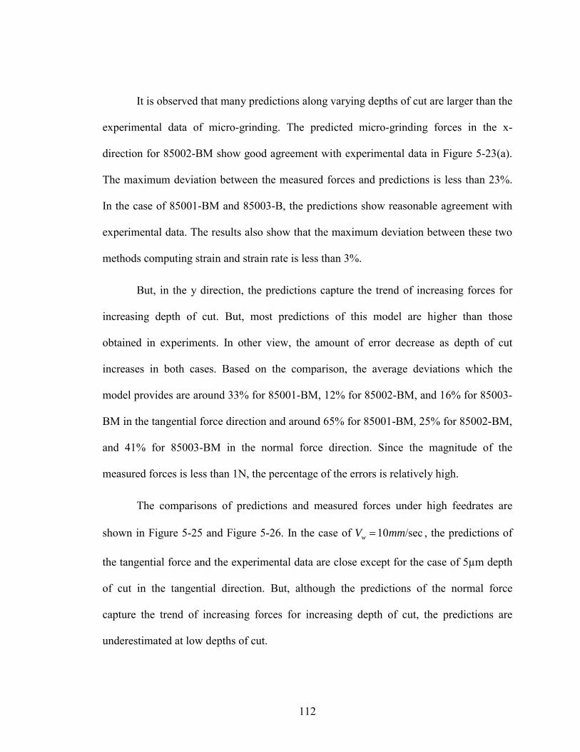
112

It is observed that many predictions along varying depths of cut are larger than the

experimental data of micro-grinding. The predicted micro-grinding forces in the x-

direction for 85002-BM show good agreement with experimental data in Figure 5-23(a).

The maximum deviation between the measured forces and predictions is less than 23%.

In the case of 85001-BM and 85003-B, the predictions show reasonable agreement with

experimental data. The results also show that the maximum deviation between these two

methods computing strain and strain rate is less than 3%.

But, in the y direction, the predictions capture the trend of increasing forces for

increasing depth of cut. But, most predictions of this model are higher than those

obtained in experiments. In other view, the amount of error decrease as depth of cut

increases in both cases. Based on the comparison, the average deviations which the

model provides are around 33% for 85001-BM, 12% for 85002-BM, and 16% for 85003-

BM in the tangential force direction and around 65% for 85001-BM, 25% for 85002-BM,

and 41% for 85003-BM in the normal force direction. Since the magnitude of the

measured forces is less than 1N, the percentage of the errors is relatively high.

The comparisons of predictions and measured forces under high feedrates are

shown in Figure 5-25 and Figure 5-26. In the case of 10 /secwV mm= , the predictions of

the tangential force and the experimental data are close except for the case of 5µm depth

of cut in the tangential direction. But, although the predictions of the normal force

capture the trend of increasing forces for increasing depth of cut, the predictions are

underestimated at low depths of cut.

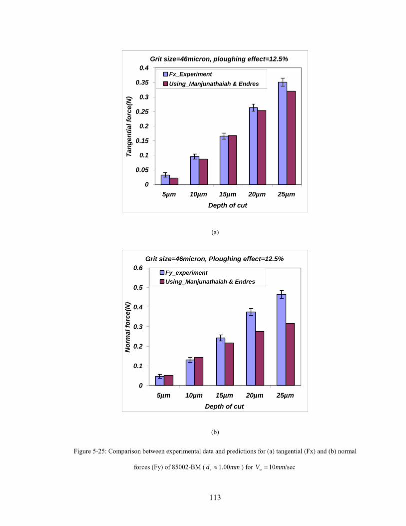
113

Grit size=46micron, ploughing effect=12.5%

0

0.05

0.1

0.15

0.2

0.25

0.3

0.35

0.4

5µm 10µm 15µm 20µm 25µmDepth of cut

Tang

entia

l for

ce(N

)

Fx_ExperimentUsing_Manjunathaiah & Endres

(a)

Grit size=46micron, Ploughing effect=12.5%

0

0.1

0.2

0.3

0.4

0.5

0.6

5µm 10µm 15µm 20µm 25µmDepth of cut

Nor

mal

forc

e(N

)

Fy_experimentUsing_Manjunathaiah & Endres

(b)

Figure 5-25: Comparison between experimental data and predictions for (a) tangential (Fx) and (b) normal

forces (Fy) of 85002-BM ( 1.00ed mm≈ ) for 10 /secwV mm=

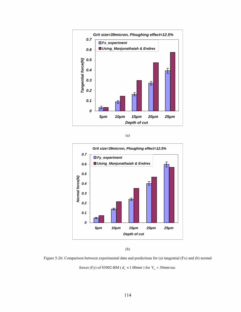
114

Grit size=39micron, Ploughing effect=12.5%

0

0.1

0.2

0.3

0.4

0.5

0.6

0.7

5µm 10µm 15µm 20µm 25µmDepth of cut

Tang

entia

l for

ce(N

)

Fx_experimentUsing_Manjunathaiah & Endres

(a)

Grit size=39micron, Ploughing effect=12.5%

0

0.1

0.2

0.3

0.4

0.5

0.6

0.7

5µm 10µm 15µm 20µm 25µm

Depth of cut

Nor

mal

forc

e(N

)

Fy_experimentUsing_Manjunathaiah & Endres

(b)

Figure 5-26: Comparison between experimental data and predictions for (a) tangential (Fx) and (b) normal

forces (Fy) of 85002-BM ( 1.00ed mm≈ ) for 30 /secwV mm=

115

The experimental results of 30 /secwV mm= show the opposite trend compared to

10 /secwV mm= in Figure 5-26. It is found that experimental data and predictions in the

normal direction are close at higher depth of cut. But, the overall predictions in both

directions are overestimated compared to the values obtained for low feedrates.

The errors in these comparisons may come from the following: (i) the effect of the

trapped chips and (ii) the rigidity of the micro-grinding wheel. During micro-grinding,

some chips created are trapped within the space between grits. These trapped chips can

prevent the engagement of other grits in micro-grinding. Otherwise, these chips can be

involved in micro-grinding. So, the dynamic cutting edge density may be different from

the results obtained in Chapter 4. The other source of the errors is the stiffness of the

micro-grinding wheel. Since the size of the micro-grinding tool is small, there is elastic

deflection during micro-grinding. Due to this deflection, vertical grinding may not be

ensured during the experiments.

5.6.3 Assessment of the effects of temperature

Figure 5-27 shows the temperature rise with respect to the depth of cut. This

temperature rise on the shear band is estimated from the predicted micro-grinding forces.

It is observed that the temperature rise is not significantly greater than that observed

during the conventional grinding process. In micro-grinding, the magnitude of forces is

generally below 1N so that the generated heat source is small. Besides this effect, the

workpiece (Al 6061-T6) has a large heat conductivity compared to other materials. So,

these phenomena are attributed to the lower temperature rise. But, for hard materials, the

temperature rise becomes more significant.

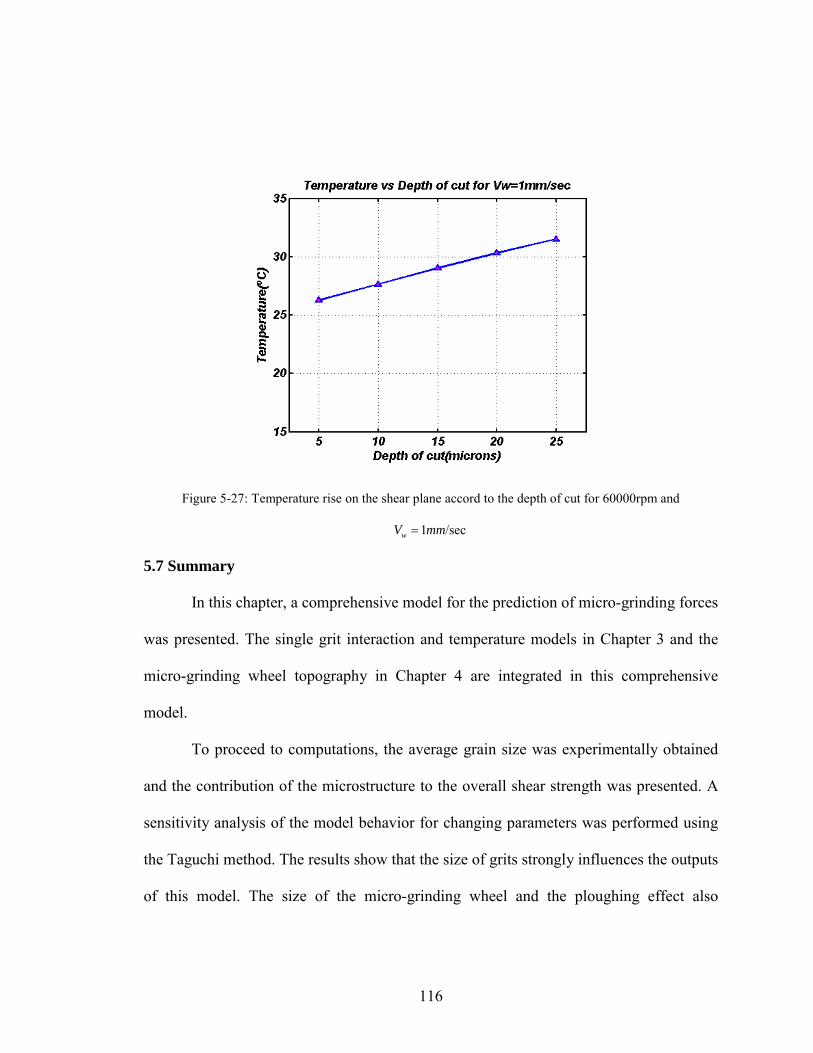
116

Figure 5-27: Temperature rise on the shear plane accord to the depth of cut for 60000rpm and

1 /secwV mm=

5.7 Summary

In this chapter, a comprehensive model for the prediction of micro-grinding forces

was presented. The single grit interaction and temperature models in Chapter 3 and the

micro-grinding wheel topography in Chapter 4 are integrated in this comprehensive

model.

To proceed to computations, the average grain size was experimentally obtained

and the contribution of the microstructure to the overall shear strength was presented. A

sensitivity analysis of the model behavior for changing parameters was performed using

the Taguchi method. The results show that the size of grits strongly influences the outputs

of this model. The size of the micro-grinding wheel and the ploughing effect also

117

influence the results. A sensitivity analysis of experimental outputs shows that the size of

the micro-grinding highly influences the variation of outputs

This model was validated by comparing the predictions of the micro-grinding

forces with the experimental data for different micro-grinding conditions. The

comparisons between them show that the predictions driven by this model capture the

trend of the experimental data. For 1 /secwV mm= and 85002-BM, the model provides

good agreement with the experiments, as it has a maximum deviation of 25%. In addition,

the temperatures predicted in this model were reasonable for input conditions used in this

analysis.

118

CHAPTER 6

MULTI-OBJECTIVE OPTIMIZATION OF MICROSCALE MACHINE TOOLS

6.1 Introduction

The inherent technical and economical advantages of the above research have

motivated the development of various prototypes of miniaturized machine tools[4, 5, 9,

100, 101, 102]. These tool prototypes’ ability is successfully to fabricate microscale parts.

However, there have not been enough studies for design of miniaturized machine tools

and as a result, little design knowledge and experience base concerning miniaturization of

these systems has been accumulated. Several attempts to optimize systematically

miniaturized machine tools have been unsuccessful. In order to provide guidance for

further development, studies of a systematic design of these systems are necessary.

In design of traditional and miniaturized machine tools, a conceptual design stage

for all major elements is important. This step defines the basic features and capabilities of

traditional and miniaturized machine tools. In the case of miniaturized machine tools, this

design stage acquires more importance because the ratio of the overall size of a

miniaturized machine tool to its target products is significantly smaller than that of

traditional machine tools. The conceptual design for miniaturized machine tools has to be

accompanied with comprehensive analyses of possible effective factors such as static,

dynamic, and thermal stiffness, machine accuracy, and machine working volume.

This chapter presents the work for optimization of a machine structure size

according to varying sizes of the miniaturized machine tool. In this study, theoretical and

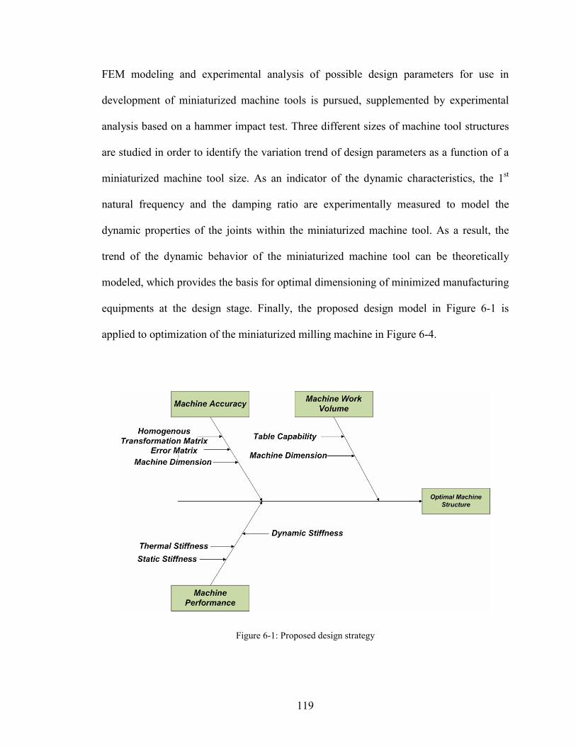
119

FEM modeling and experimental analysis of possible design parameters for use in

development of miniaturized machine tools is pursued, supplemented by experimental

analysis based on a hammer impact test. Three different sizes of machine tool structures

are studied in order to identify the variation trend of design parameters as a function of a

miniaturized machine tool size. As an indicator of the dynamic characteristics, the 1st

natural frequency and the damping ratio are experimentally measured to model the

dynamic properties of the joints within the miniaturized machine tool. As a result, the

trend of the dynamic behavior of the miniaturized machine tool can be theoretically

modeled, which provides the basis for optimal dimensioning of minimized manufacturing

equipments at the design stage. Finally, the proposed design model in Figure 6-1 is

applied to optimization of the miniaturized milling machine in Figure 6-4.

Figure 6-1: Proposed design strategy

120

The following sections provide the theoretical and FEM evaluation of the

miniaturized machine tool’s structural performance in terms of static, thermal, and

dynamic stiffness. This is followed by computations of volumetric error and machine

work volume according to different machine sizes. Finally, optimization for the

developed miniaturized milling machine is carried out and a comparison between

analytical and FEM computation is performed.

6.2 Structural performance evaluation

Machine tool’s structure consists of stationary and moving parts. The design of a

machine structure is an important decision step; it requires consideration of many aspects

of various products because the structure provides the means by which all components

such as spindles and positioning table are brought together. It is challenging because

existing sources of uncertainty, such as errors due to geometric configuration, thermal

deformation errors, and errors induced by load, affect a machine’s final performance. In

order to provide more reliable machine performance and better product quality, some key

factors such as static, thermal, and dynamic stiffness, machine accuracy, and machine

working volume have to be considered at a conceptual design stage.

6.2.1 Static stiffness evaluation

The structure of a miniaturized machine tool experiences external force during

machine operation and these forces can create the deflection of the machine structure.

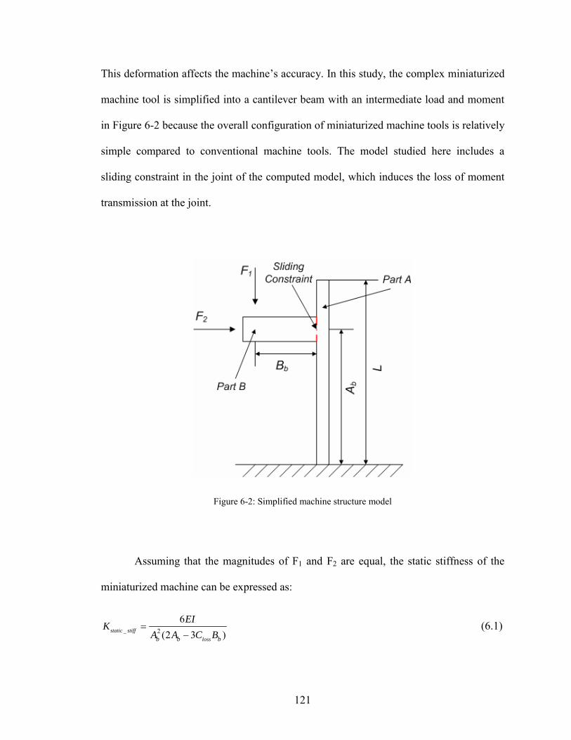
121

This deformation affects the machine’s accuracy. In this study, the complex miniaturized

machine tool is simplified into a cantilever beam with an intermediate load and moment

in Figure 6-2 because the overall configuration of miniaturized machine tools is relatively

simple compared to conventional machine tools. The model studied here includes a

sliding constraint in the joint of the computed model, which induces the loss of moment

transmission at the joint.

Figure 6-2: Simplified machine structure model

Assuming that the magnitudes of F1 and F2 are equal, the static stiffness of the

miniaturized machine can be expressed as:

_ 2

6(2 3 )static stiff

lossb b b

EIK

A A C B=

− (6.1)

122

where bA and bB are machine dimensions, lossC the moment loss, E the modulus of

elasticity, and I the moment of inertia.

The computed results of static stiffness for this miniaturized machine tool are

shown in Figure 6-3(a).

6.2.2 Thermal stiffness evaluation

In miniaturized machine tools, if the ambient temperature is stable, the main heat

source is the operating spindle with a high RPM. The temperature variation of the

miniaturized milling machine is observed to be around 12º during machine operation

using thermal couple data collected at different locations. The spindle is assembled at part

B in Figure 6-2. So, with the assumption that the temperature rise is equally distributed,

thermal stiffness that is related to the change in a machine linear dimension can be

obtained as:

1thermal

t b

KBα

= (6.2)

where tα is the thermal expansion coefficient.

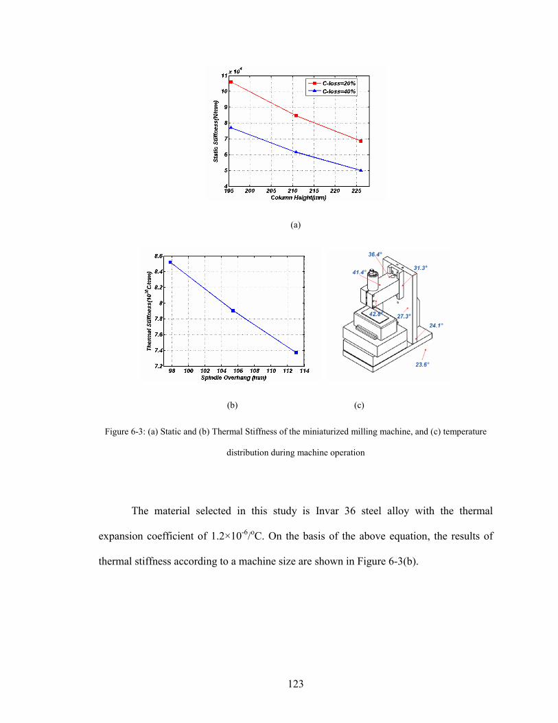
123

(a)

(b) (c)

Figure 6-3: (a) Static and (b) Thermal Stiffness of the miniaturized milling machine, and (c) temperature

distribution during machine operation

The material selected in this study is Invar 36 steel alloy with the thermal

expansion coefficient of 1.2×10-6/oC. On the basis of the above equation, the results of

thermal stiffness according to a machine size are shown in Figure 6-3(b).

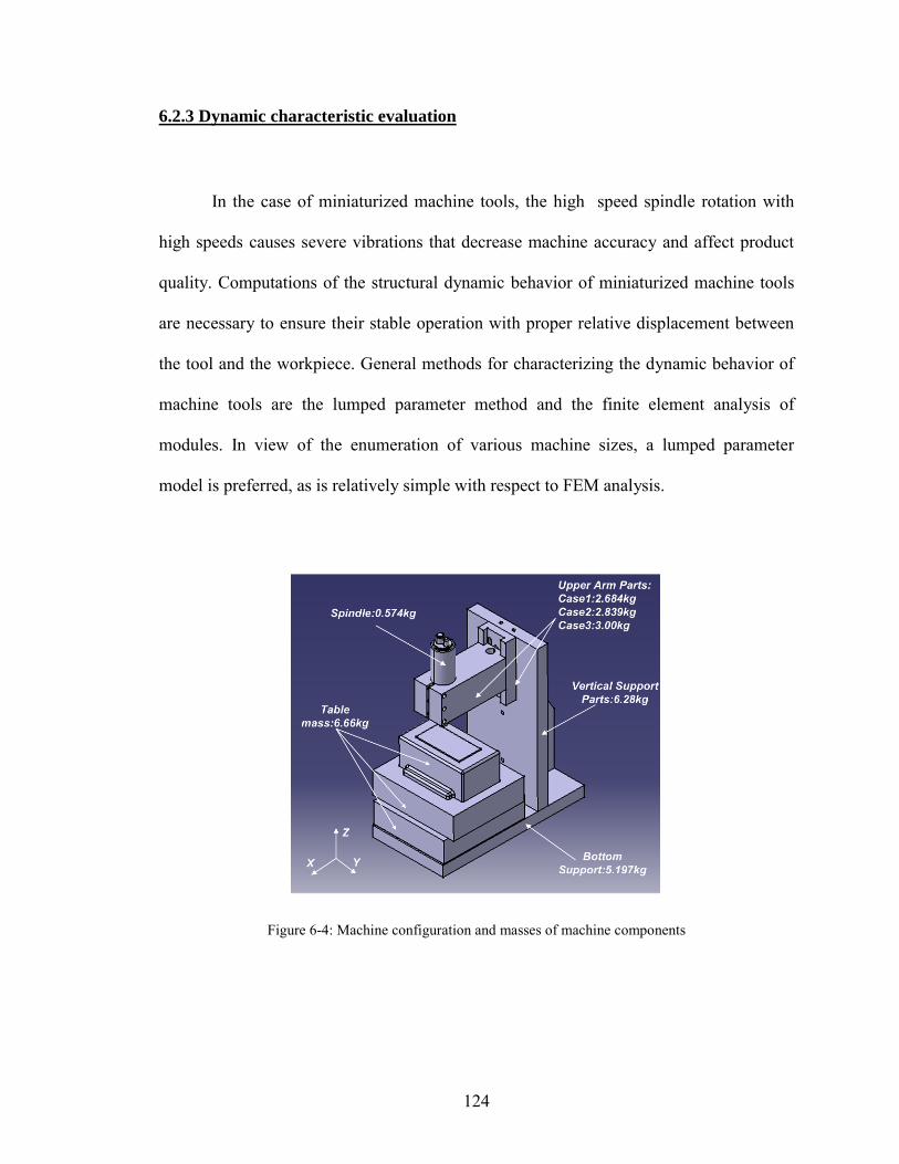
124

6.2.3 Dynamic characteristic evaluation

In the case of miniaturized machine tools, the high speed spindle rotation with

high speeds causes severe vibrations that decrease machine accuracy and affect product

quality. Computations of the structural dynamic behavior of miniaturized machine tools

are necessary to ensure their stable operation with proper relative displacement between

the tool and the workpiece. General methods for characterizing the dynamic behavior of

machine tools are the lumped parameter method and the finite element analysis of

modules. In view of the enumeration of various machine sizes, a lumped parameter

model is preferred, as is relatively simple with respect to FEM analysis.

Figure 6-4: Machine configuration and masses of machine components

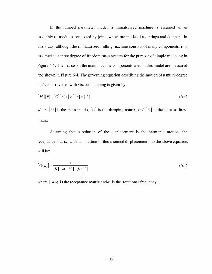
125

In the lumped parameter model, a miniaturized machine is assumed as an

assembly of modules connected by joints which are modeled as springs and dampers. In

this study, although the miniaturized milling machine consists of many components, it is

assumed as a three degree of freedom mass system for the purpose of simple modeling in

Figure 6-5. The masses of the main machine components used in this model are measured

and shown in Figure 6-4. The governing equation describing the motion of a multi-degree

of freedom system with viscous damping is given by:

[ ]{ } [ ]{ } [ ]{ } { }M x C x K x f+ + = (6.3)

where [ ]M is the mass matrix, [ ]C is the damping matrix, and [ ]K is the joint stiffness

matrix.

Assuming that a solution of the displacement is the harmonic motion, the

receptance matrix, with substitution of this assumed displacement into the above equation,

will be:

[ ][ ] [ ] [ ]2

1( )G w

K M j Cω ω=

− − (6.4)

where [ ]( )G w is the receptance matrix andω is the rotational frequency.

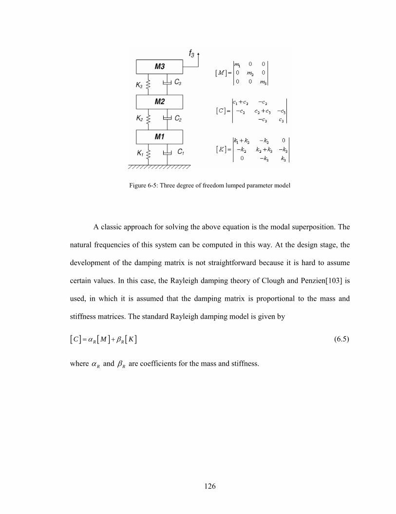
126

Figure 6-5: Three degree of freedom lumped parameter model

A classic approach for solving the above equation is the modal superposition. The

natural frequencies of this system can be computed in this way. At the design stage, the

development of the damping matrix is not straightforward because it is hard to assume

certain values. In this case, the Rayleigh damping theory of Clough and Penzien[103] is

used, in which it is assumed that the damping matrix is proportional to the mass and

stiffness matrices. The standard Rayleigh damping model is given by

[ ] [ ] [ ]R RC M Kα β= + (6.5)

where Rα and Rβ are coefficients for the mass and stiffness.

127

Figure 6-6: Contribution of Rayleigh damping parameters

Based on this theory, the damping coefficient in mode i can be expressed as:

2 2ni

ini

RR β ωαξ

ω= + (6.6)

where iξ is the damping ratio and niω is the rotational frequency in mode i.

However, the parameters of the springs and the coefficients of this damping

model need to be identified. Therefore, the analytical computation of a lumped parameter

model has to be supplemented by experimental analysis such as a hammer impact test.

6.3 Experimental analysis

The machine configuration studied here is the knee and column type vertical

milling machine shown in Figure 6-7 where Ab is the column height, Bb the spindle

overhang, Cb the spindle protrusion. In order to identify the above described parameters

of this machine configuration, a classic hammer impact test is engaged to investigate the

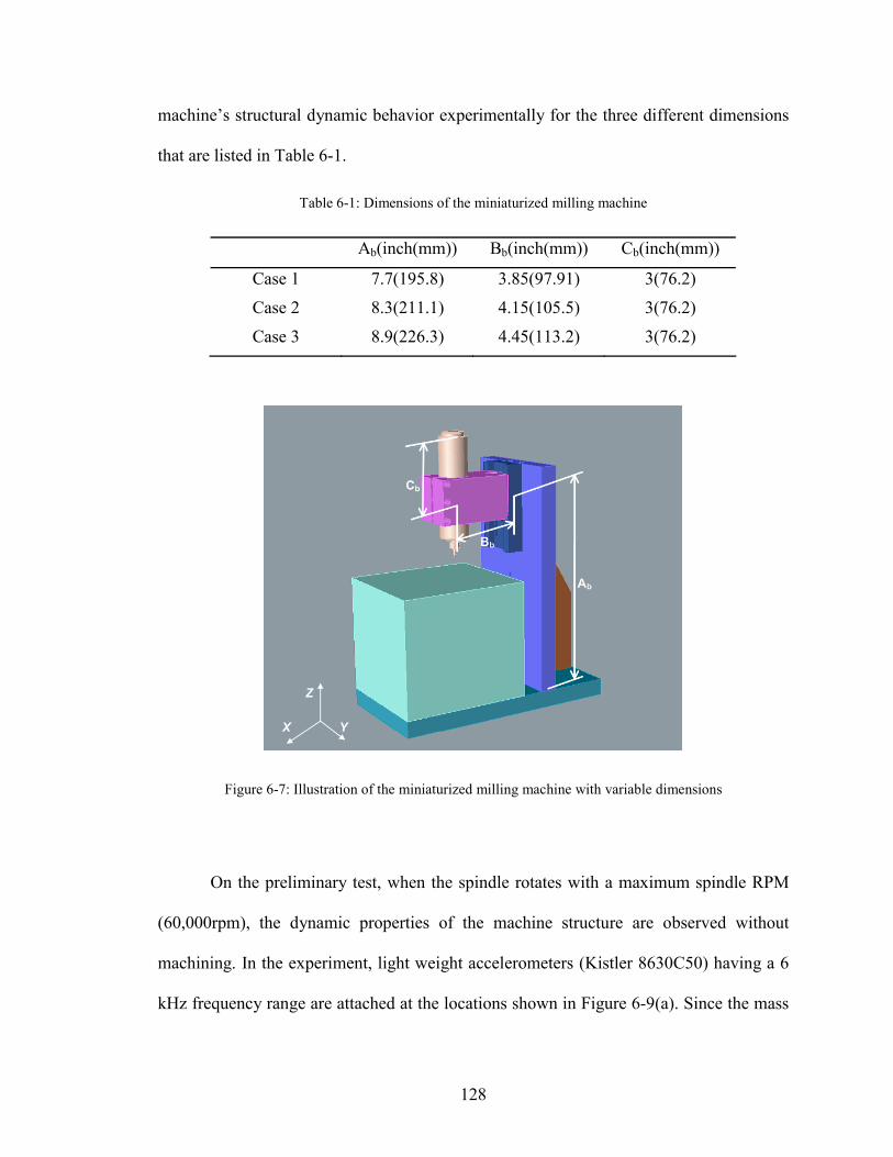
128

machine’s structural dynamic behavior experimentally for the three different dimensions

that are listed in Table 6-1.

Table 6-1: Dimensions of the miniaturized milling machine

Ab(inch(mm)) Bb(inch(mm)) Cb(inch(mm))

Case 1 7.7(195.8) 3.85(97.91) 3(76.2)

Case 2 8.3(211.1) 4.15(105.5) 3(76.2)

Case 3 8.9(226.3) 4.45(113.2) 3(76.2)

Figure 6-7: Illustration of the miniaturized milling machine with variable dimensions

On the preliminary test, when the spindle rotates with a maximum spindle RPM

(60,000rpm), the dynamic properties of the machine structure are observed without

machining. In the experiment, light weight accelerometers (Kistler 8630C50) having a 6

kHz frequency range are attached at the locations shown in Figure 6-9(a). Since the mass

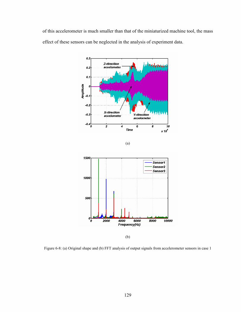
129

of this accelerometer is much smaller than that of the miniaturized machine tool, the mass

effect of these sensors can be neglected in the analysis of experiment data.

(a)

(b)

Figure 6-8: (a) Original shape and (b) FFT analysis of output signals from accelerometer sensors in case 1

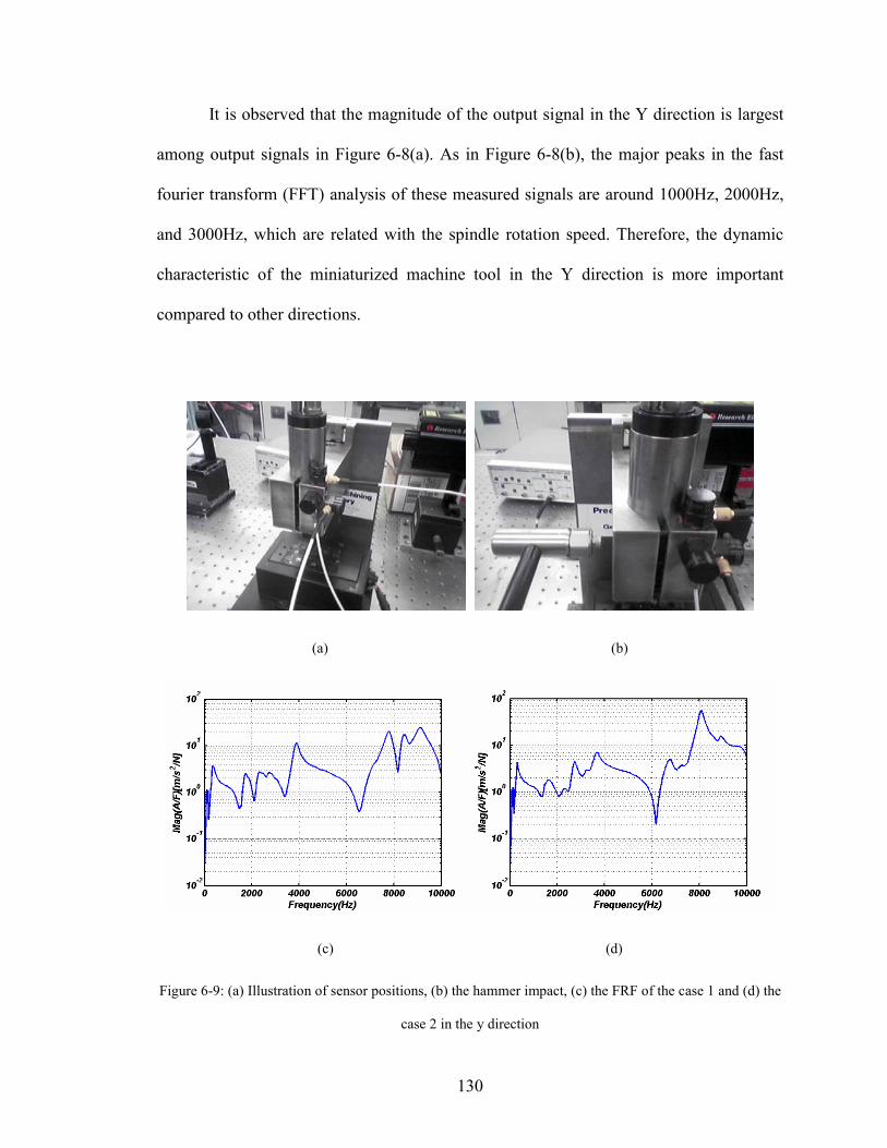
130

It is observed that the magnitude of the output signal in the Y direction is largest

among output signals in Figure 6-8(a). As in Figure 6-8(b), the major peaks in the fast

fourier transform (FFT) analysis of these measured signals are around 1000Hz, 2000Hz,

and 3000Hz, which are related with the spindle rotation speed. Therefore, the dynamic

characteristic of the miniaturized machine tool in the Y direction is more important

compared to other directions.

(a) (b)

(c) (d)

Figure 6-9: (a) Illustration of sensor positions, (b) the hammer impact, (c) the FRF of the case 1 and (d) the

case 2 in the y direction

131

In this experiment, a hammer impact test is adopted as a tool for inspection of the

dynamic behavior of miniaturized machine tools. Basically, the vibration of a machine

tool is excited by an impulse force, referred to as a hammer impact, and a response of

excited vibration is recorded by accelerometers. From the time histories recorded during

these tests, frequency response functions (FRFs) can be obtained as shown in Figure

6-9(c) and (d).

The impact hammer used in this study is a medium impact hammer with a metal

tip (Kistler type 9722A), and 20 impacts were recorded and averaged linearly. The

obtained results for three different sizes are listed in Table 6-3.

6.3.1 Identification of dynamic parameters

Based on these experimental results, the objective functions must be optimized in

order to identify the values of springs and damping coefficients at joints. The objective

functions for computations of joint stiffness and damping coefficients are obtained from

comparisons between experimental and computed results. The forms used in this work

are:

( )3

1 2 3 exp,1

min , ,ni nii

f abs k k kω ω=

= −⎛ ⎞⎛ ⎞

⎜ ⎟⎜ ⎟⎝ ⎠⎝ ⎠∑ (6.7)

and

( )3

exp,1

min ,i ii

R Rf abs ξ α β ξ=

= −⎛ ⎞⎛ ⎞⎡ ⎤⎜ ⎟⎜ ⎟⎣ ⎦⎝ ⎠⎝ ⎠

∑ (6.8)

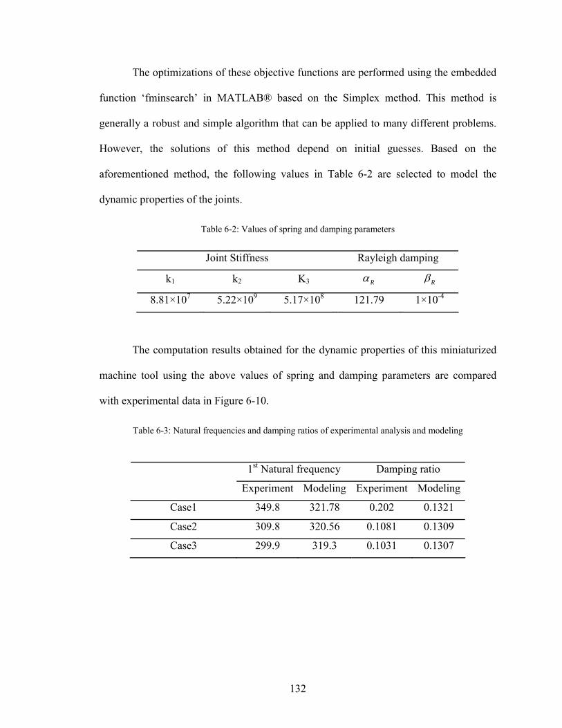
132

The optimizations of these objective functions are performed using the embedded

function ‘fminsearch’ in MATLAB® based on the Simplex method. This method is

generally a robust and simple algorithm that can be applied to many different problems.

However, the solutions of this method depend on initial guesses. Based on the

aforementioned method, the following values in Table 6-2 are selected to model the

dynamic properties of the joints.

Table 6-2: Values of spring and damping parameters

Joint Stiffness Rayleigh damping

k1 k2 K3 Rα Rβ

8.81×107 5.22×109 5.17×108 121.79 1×10-4

The computation results obtained for the dynamic properties of this miniaturized

machine tool using the above values of spring and damping parameters are compared

with experimental data in Figure 6-10.

Table 6-3: Natural frequencies and damping ratios of experimental analysis and modeling

1st Natural frequency Damping ratio

Experiment Modeling Experiment Modeling

Case1 349.8 321.78 0.202 0.1321

Case2 309.8 320.56 0.1081 0.1309

Case3 299.9 319.3 0.1031 0.1307

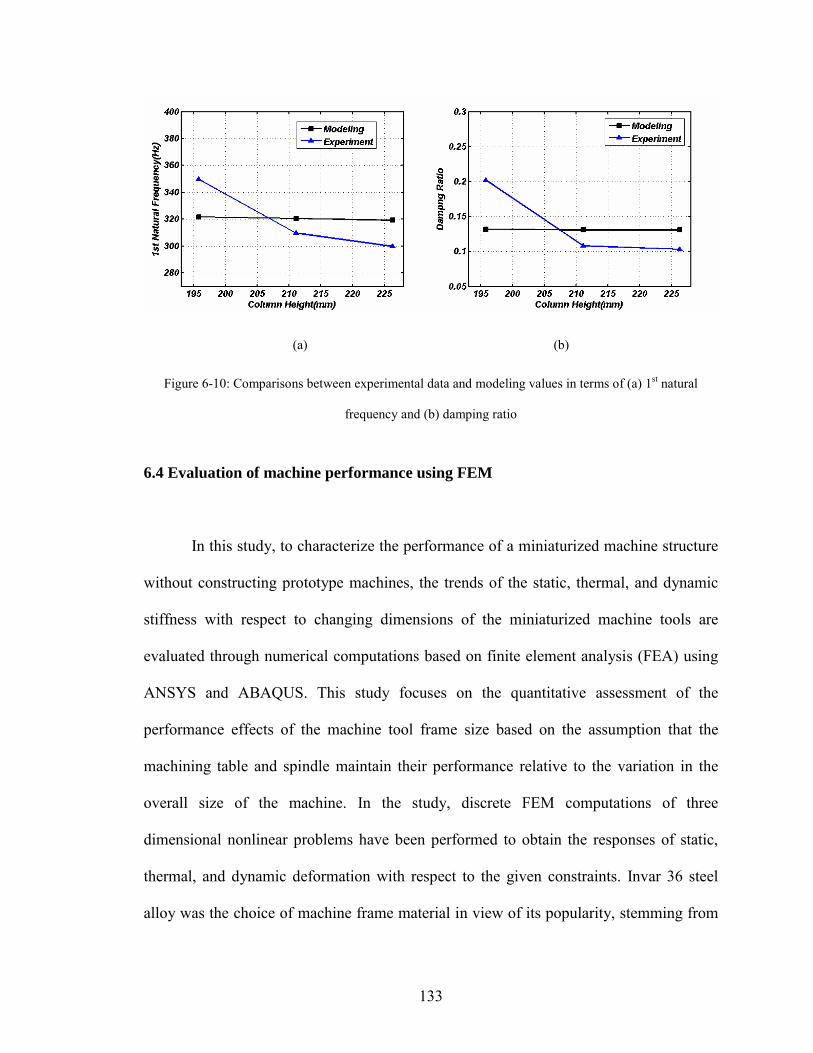
133

(a) (b)

Figure 6-10: Comparisons between experimental data and modeling values in terms of (a) 1st natural

frequency and (b) damping ratio

6.4 Evaluation of machine performance using FEM

In this study, to characterize the performance of a miniaturized machine structure

without constructing prototype machines, the trends of the static, thermal, and dynamic

stiffness with respect to changing dimensions of the miniaturized machine tools are

evaluated through numerical computations based on finite element analysis (FEA) using

ANSYS and ABAQUS. This study focuses on the quantitative assessment of the

performance effects of the machine tool frame size based on the assumption that the

machining table and spindle maintain their performance relative to the variation in the

overall size of the machine. In the study, discrete FEM computations of three

dimensional nonlinear problems have been performed to obtain the responses of static,

thermal, and dynamic deformation with respect to the given constraints. Invar 36 steel

alloy was the choice of machine frame material in view of its popularity, stemming from

134

low thermal expansion and reasonable modulus. It has elastic modulus of 141 GPa,

density of 8050 kg/m3, and thermal expansion coefficient of 1.2×10-6/oC. In the finite

element simulations, tetrahedron-type elements defined by twenty nodes, suitable for

irregular geometry meshing, are used to mesh a virtual microscale machine structure.

During these computations, the bottom surface of the three dimensional structure is

constrained.

The results of FEM computations of static and thermal deformation are shown in

Figure 6-11(a) and (b).

(a) (b)

Figure 6-11: FEM analysis of (a) static and (b) thermal deformation

A comparison between analytical and FEM models shows that the static stiffness

of analytical computation is 20%~50% higher than the FEM results in Figure 6-12(a).

The reason for this discrepancy is that the deformation caused by a mechanical load isn’t

evenly distributed on the overhang of the structure. But, in the case of the thermal

stiffness, the FEM results are 40% higher than the analytical computational results

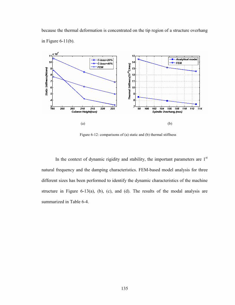
135

because the thermal deformation is concentrated on the tip region of a structure overhang

in Figure 6-11(b).

(a) (b)

Figure 6-12: comparisons of (a) static and (b) thermal stiffness

In the context of dynamic rigidity and stability, the important parameters are 1st

natural frequency and the damping characteristics. FEM-based model analysis for three

different sizes has been performed to identify the dynamic characteristics of the machine

structure in Figure 6-13(a), (b), (c), and (d). The results of the modal analysis are

summarized in Table 6-4.

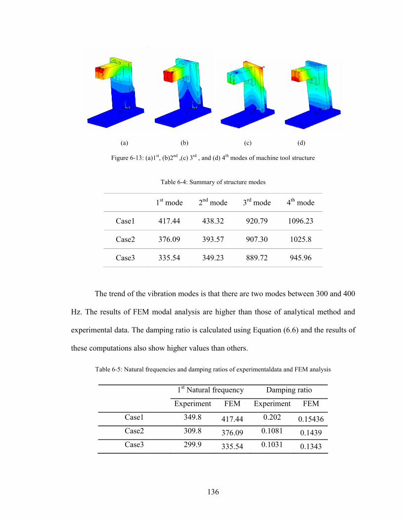
136

(a) (b) (c) (d)

Figure 6-13: (a)1st, (b)2nd ,(c) 3rd , and (d) 4th modes of machine tool structure

Table 6-4: Summary of structure modes

1st mode 2nd mode 3rd mode 4th mode

Case1 417.44 438.32 920.79 1096.23

Case2 376.09 393.57 907.30 1025.8

Case3 335.54 349.23 889.72 945.96

The trend of the vibration modes is that there are two modes between 300 and 400

Hz. The results of FEM modal analysis are higher than those of analytical method and

experimental data. The damping ratio is calculated using Equation (6.6) and the results of

these computations also show higher values than others.

Table 6-5: Natural frequencies and damping ratios of experimentaldata and FEM analysis

1st Natural frequency Damping ratio

Experiment FEM Experiment FEM

Case1 349.8 417.44 0.202 0.15436 Case2 309.8 376.09 0.1081 0.1439 Case3 299.9 335.54 0.1031 0.1343

137

Finite element analysis on static rigidity, thermal resistance, and dynamic stiffness

shows that miniaturization of machine tools increases the machine’s precision. In terms

of static stiffness, as the machine’s linear dimension decreases, its static stiffness

increases. This increase of the static stiffness is a result of the reduction of the frame

cantilever lengths in their absolute scales. It is shown that the size reduction of a machine

tool decreases its thermal expansion in response to environmental temperature variation

since the total volume involved in the expansion is reduced. The dynamic stiffness shows

the same trend with other stiffness.

6.5 Volumetric error evaluation

In this study, a kinematic chain representation model, referred to as the form

shaping theory [104], is used to estimate the volumetric error of a miniaturized machine

tool according to its size. In this method, coordinate transformation, which uses

homogenous transform matrix (HTM), is applied to represent the relative displacement

between a workpiece and a machine tool as a chain of directly linked rigid components.

The mathematical form for computing the result of transformation matrices between a

workpiece and a tool is:

[ ] [ ] [ ] [ ]z y t

ideal p p B Lr HTM HTM HTM HTM= × × (6.9)

138

(a) (b)

Figure 6-14: Schematic diagram of (a) the miniaturized machine tool and (b) chain representation

There are many error sources such as alignment errors and geometric errors in

actual machine tools. These errors can be considered as errors in transformations between

components with an error HTM. The basic form of this matrix is:

[ ]

11

10 0 0 1

i

ei ei xei

ei ei yei

errorei ei zei

HTM

γ β δ

γ α δ

β α δ

−

−= (6.10)

where eiα , eiβ , and eiγ are rotation errors and xeiδ , yeiδ , and zeiδ are translational errors.

Estimation of the resultant assembly volumetric error, which includes the errors

between moving components, can be obtained by implementing error HTMs between two

ideal HTMs. In this study, the assumptions used to simplify the numerical calculation in

miniaturized machine tool accuracy are the following: (i) rigid body motion and (ii) small

139

errors approximation. With these assumptions, the second, third, and forth orders error

terms can be cancelled during the matrix multiplications. After this computation, the

relative error between a tool and a workpiece can be obtained as the following:

error idealr r r∆ = − (6.11)

On the basis of the miniaturized milling machine structural drawing in Figure

6-14, the amount of error in each direction, including error terms and machine’s

dimensions can be obtained as the following:

1 2 3 4 1 2 2 1 1 2

1 2 3 4 1 2 3 4 1

1 2 3 4 1 2 3 1 2 3

1 2 1 2 1 2 3 4 1

1

( ) ( )( ) ( )

( ) ( )

( ) ( ) ( )

x x x x b y x

e e e e b e e e e t e

ye ye ye y e e e d e e e b

e e e e x e e e e t e y

ze

A P PB L W

x L Ay

V P L Pz

δ δ δ δ β β β β β β

γ γ γ γ β β β β γδ δ δ δ γ γ γ α α α

γ γ α α α α α α α

δ δ

=

+ + + + + + − − +

+ + + + + + + + −∆

+ + + + + + − + +∆

+ + + + + + + + +∆

+ 2 3 4 1 2 3 4 1 2

1 2 3 1

( ) ( )( )

ze ze ze e e e e b e e

e e e d e

B VL W

δ δ α α α α β ββ β β α

+ + − + + + − +

− + + +

(6.12)

where V and W are workpiece sizes.

On the basis of Equation(6.12), the amount of error for each direction can be

estimated as x∆ , y∆ , and z∆ . For the purpose of a simple modeling, error terms which are

used to compute machine accuracy are assumed to have the amplitude of unity (1µm) for

the sake of analysis. The variance of the error amounts has been used to estimate the error

magnitude according to a machine size because there are different signs within the

computation of error amounts in each axis, which is shown in Equation (6.13)

, ,x ref y ref z refx x y y z z∆ = ∆ −∆ ∆ = ∆ −∆ ∆ = ∆ −∆ (6.13)

Then, the mathematical function to compute machine accuracy of the

miniaturized milling machine can be expressed as:

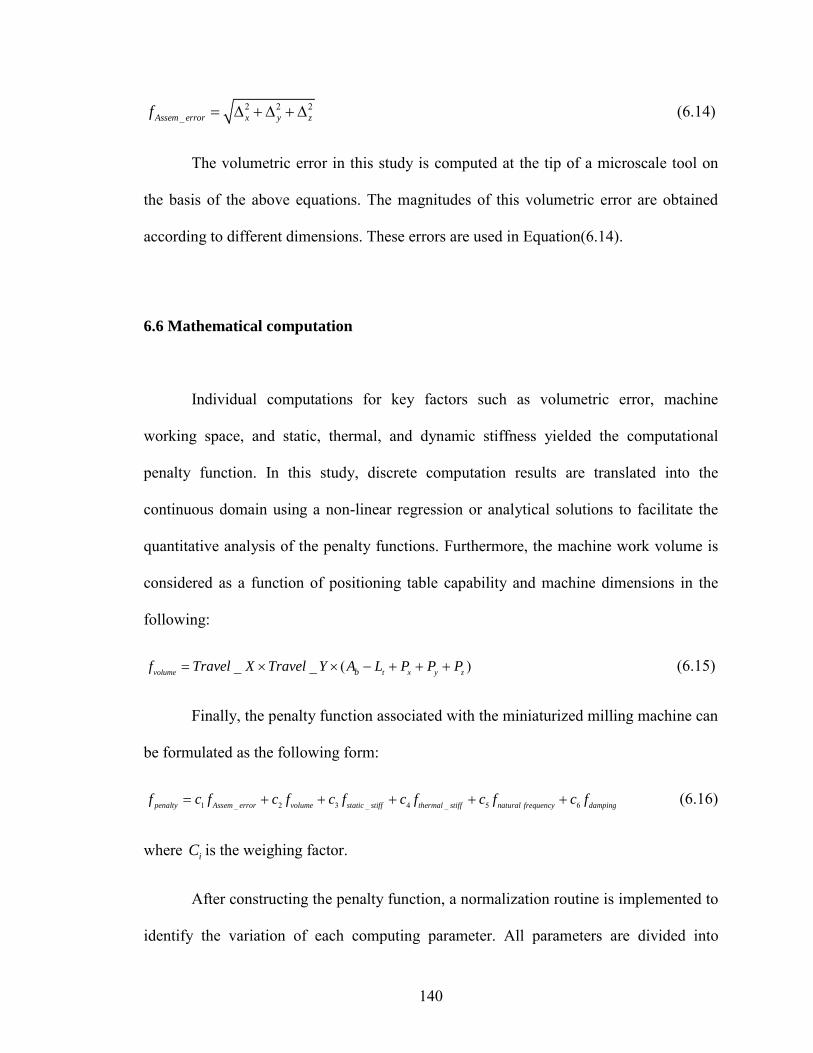
140

2 2 2_Assem error x y zf = ∆ + ∆ + ∆ (6.14)

The volumetric error in this study is computed at the tip of a microscale tool on

the basis of the above equations. The magnitudes of this volumetric error are obtained

according to different dimensions. These errors are used in Equation(6.14).

6.6 Mathematical computation

Individual computations for key factors such as volumetric error, machine

working space, and static, thermal, and dynamic stiffness yielded the computational

penalty function. In this study, discrete computation results are translated into the

continuous domain using a non-linear regression or analytical solutions to facilitate the

quantitative analysis of the penalty functions. Furthermore, the machine work volume is

considered as a function of positioning table capability and machine dimensions in the

following:

_ _ ( )volume t x y zbf Travel X Travel Y A L P P P= × × − + + + (6.15)

Finally, the penalty function associated with the miniaturized milling machine can

be formulated as the following form:

1 _ 2 3 _ 4 _ 5 6penalty Assem error volume static stiff thermal stiff natural frequency dampingf c f c f c f c f c f c f= + + + + + (6.16)

where iC is the weighing factor.

After constructing the penalty function, a normalization routine is implemented to

identify the variation of each computing parameter. All parameters are divided into

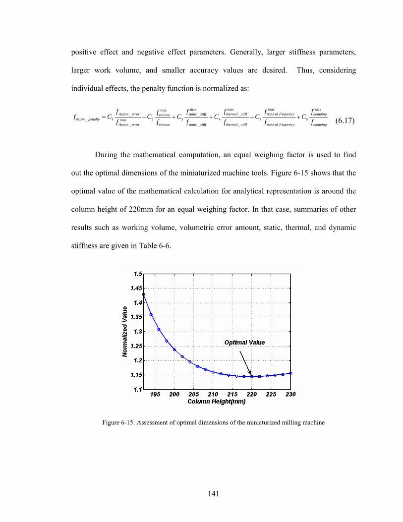
141

positive effect and negative effect parameters. Generally, larger stiffness parameters,

larger work volume, and smaller accuracy values are desired. Thus, considering

individual effects, the penalty function is normalized as:

maxmax max maxmax_ _ _

_ 1 2 3 4 5 6max_ __

natural frequencyAssem error static stiff thermal stiff dampingvolumeNorm penalty

volume static stiff thermal stiff natural frequency dampingAssem error

ff f f fff C C C C C C

f f f f ff= + + + + + (6.17)

During the mathematical computation, an equal weighing factor is used to find

out the optimal dimensions of the miniaturized machine tools. Figure 6-15 shows that the

optimal value of the mathematical calculation for analytical representation is around the

column height of 220mm for an equal weighing factor. In that case, summaries of other

results such as working volume, volumetric error amount, static, thermal, and dynamic

stiffness are given in Table 6-6.

Figure 6-15: Assessment of optimal dimensions of the miniaturized milling machine

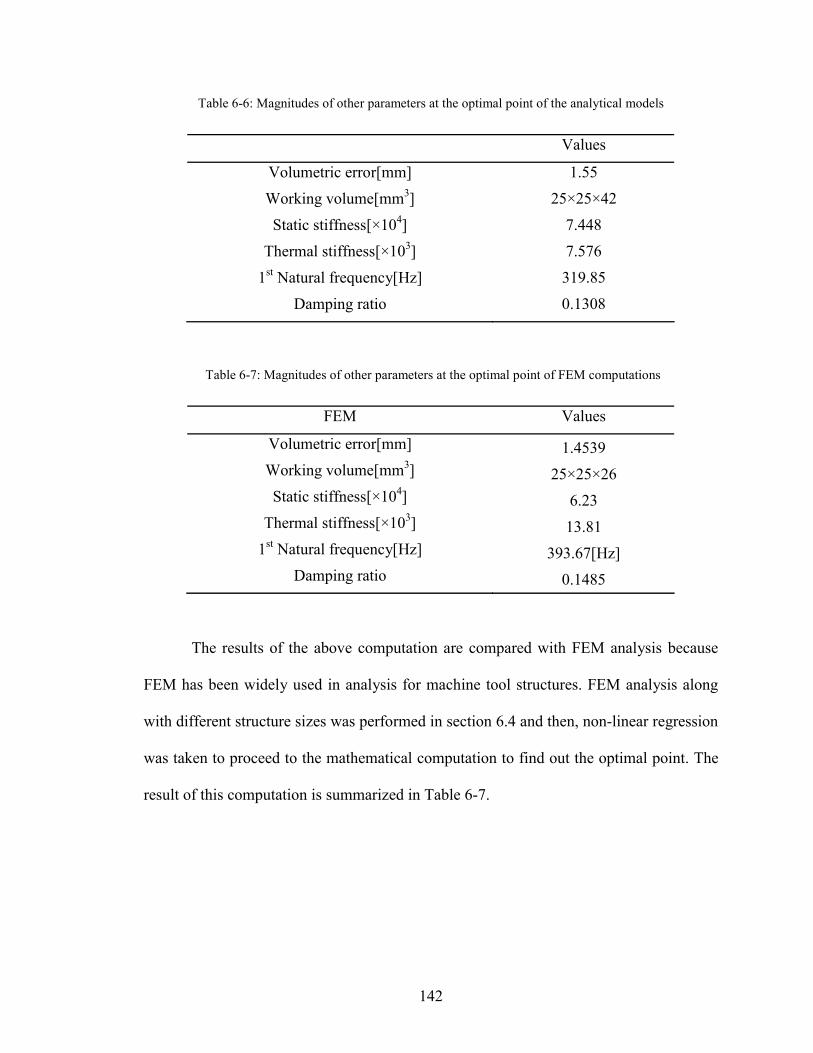
142

Table 6-6: Magnitudes of other parameters at the optimal point of the analytical models

Values

Volumetric error[mm] 1.55

Working volume[mm3] 25×25×42

Static stiffness[×104] 7.448

Thermal stiffness[×103] 7.576

1st Natural frequency[Hz] 319.85

Damping ratio 0.1308

Table 6-7: Magnitudes of other parameters at the optimal point of FEM computations

FEM Values

Volumetric error[mm] 1.4539 Working volume[mm3] 25×25×26 Static stiffness[×104] 6.23

Thermal stiffness[×103] 13.81 1st Natural frequency[Hz] 393.67[Hz]

Damping ratio 0.1485

The results of the above computation are compared with FEM analysis because

FEM has been widely used in analysis for machine tool structures. FEM analysis along

with different structure sizes was performed in section 6.4 and then, non-linear regression

was taken to proceed to the mathematical computation to find out the optimal point. The

result of this computation is summarized in Table 6-7.

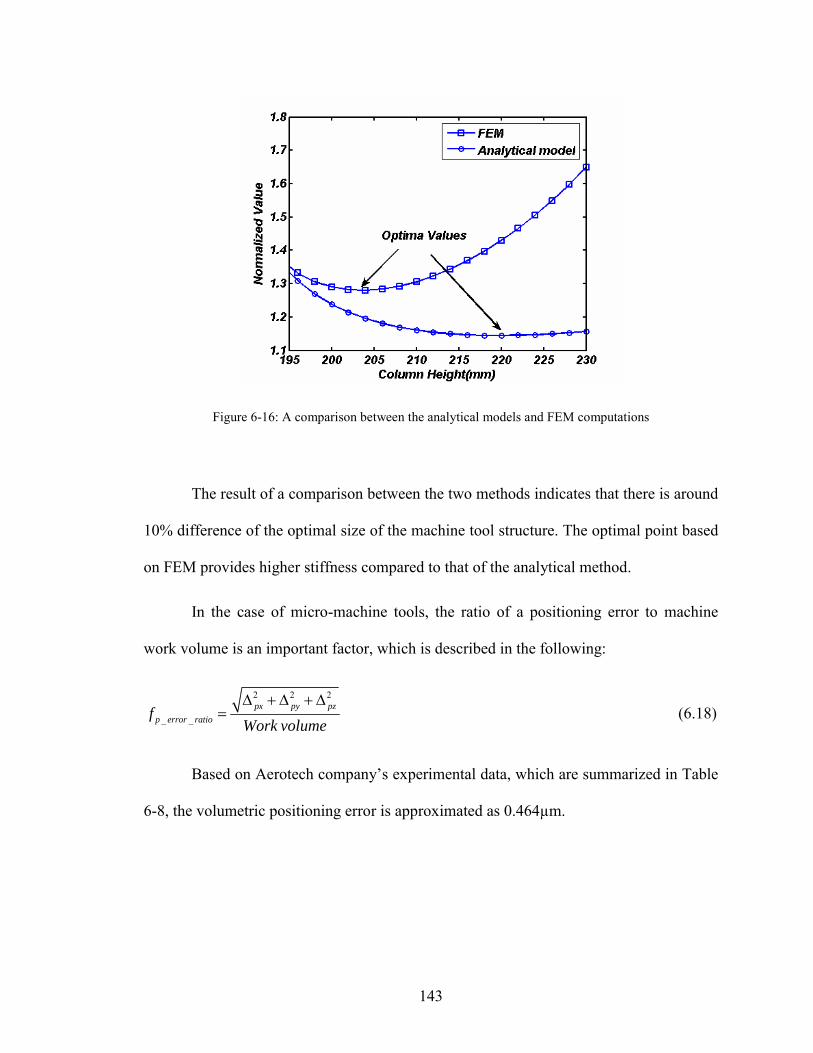
143

Figure 6-16: A comparison between the analytical models and FEM computations

The result of a comparison between the two methods indicates that there is around

10% difference of the optimal size of the machine tool structure. The optimal point based

on FEM provides higher stiffness compared to that of the analytical method.

In the case of micro-machine tools, the ratio of a positioning error to machine

work volume is an important factor, which is described in the following:

2 2 2

_ _px py pz

p error ratiofWork volume∆ + ∆ + ∆

= (6.18)

Based on Aerotech company’s experimental data, which are summarized in Table

6-8, the volumetric positioning error is approximated as 0.464µm.

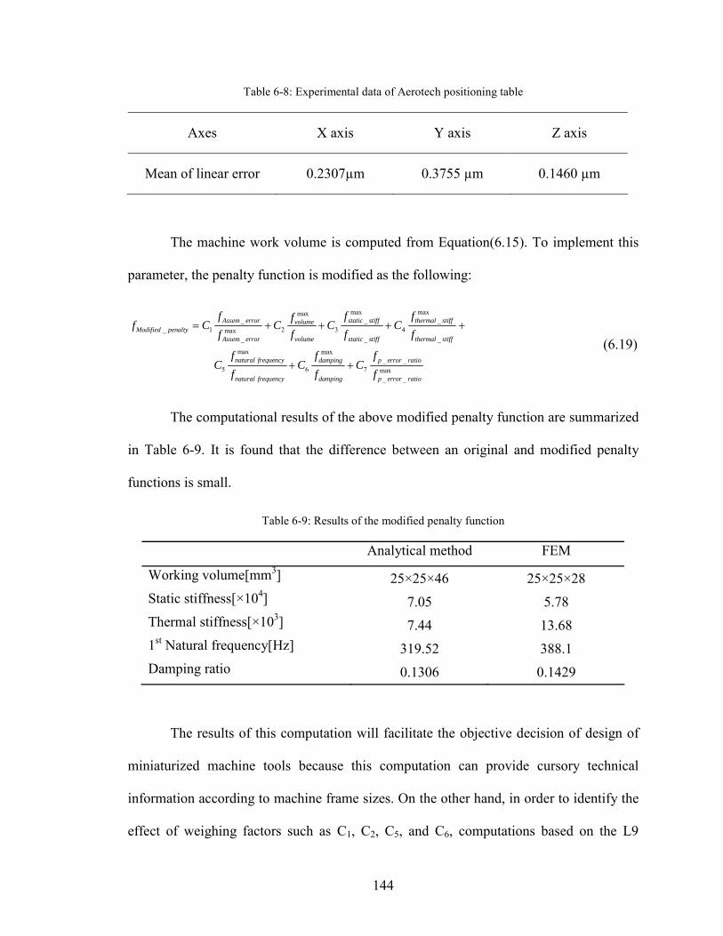
144

Table 6-8: Experimental data of Aerotech positioning table

Axes X axis Y axis Z axis

Mean of linear error 0.2307µm 0.3755 µm 0.1460 µm

The machine work volume is computed from Equation(6.15). To implement this

parameter, the penalty function is modified as the following:

max maxmax_ _ _

_ 1 2 3 4max_ __

max max

5 6 7

Assem error static stiff thermal stiffvolumeModified penalty

volume static stiff thermal stiffAssem error

natural frequency damping p

natural frequency damping

f f fff C C C C

f f ff

f f fC C C

f f

= + + + +

+ + _ _max_ _

error ratio

p error ratiof

(6.19)

The computational results of the above modified penalty function are summarized

in Table 6-9. It is found that the difference between an original and modified penalty

functions is small.

Table 6-9: Results of the modified penalty function

Analytical method FEM

Working volume[mm3] 25×25×46 25×25×28 Static stiffness[×104] 7.05 5.78 Thermal stiffness[×103] 7.44 13.68 1st Natural frequency[Hz] 319.52 388.1 Damping ratio 0.1306 0.1429

The results of this computation will facilitate the objective decision of design of

miniaturized machine tools because this computation can provide cursory technical

information according to machine frame sizes. On the other hand, in order to identify the

effect of weighing factors such as C1, C2, C5, and C6, computations based on the L9

145

matrix of the Taguchi method are carried out. In these computations, C3 and C4 are held

as constants. The results of this sensitivity analysis of weighing factors in Figure 6-17

show that the working volume weighing factor, C2, has the dominant effect on the

optimal solution of the penalty function.

Factor Effect Plot

Ov Mean

-47.05

-47.00

-46.95

-46.90

-46.85

-46.80

-46.75

-46.70

-46.65

-46.60

-46.55

-46.50E1 E2 E3 W1

W2

W3 N1

N2

N3

D1

D2

D3

Ov-

Mea

nControl Factor Levels

S/N

Rat

io in

dB

Figure 6-17: The sensitivity analysis of weighing factors

6.7 Summary

In this chapter, an effective design strategy for ensuring the good microscale

machine performance and to provide the proper dimensions of the miniaturized

manufacturing systems without resorting to physical prototyping was discussed. Then,

the optimization of the miniaturized machine tool was performed on the basis of the

C1 C2 C5 C6

146

proposed design strategy. Individual mathematical modeling of key parameters such as

volumetric error, machine working space, and static, thermal, and dynamic stiffness was

conducted and supplemented with experimental analysis using a hammer impact test to

find out the dynamic characteristics of the joints of the miniaturized machine tools. FEM

simulations were carried out as well.

These computations yield the optimal size of the miniaturized machine tool with

the technical information of other parameters. A comparison between the analytical

method and FEM was carried out. The result of the comparison shows that there is a 10%

difference in the optimal size of the machine tool structure.

In addition to this, the sensitivity of optimal machine size with respect to

weighing factor of the penalty function was also discussed on the basis of the Taguchi

method. It is observed that the working volume weighing factor plays an important role

in determining an optimal size for a miniaturized machine tool.

147

CHAPTER 7

CONCLUSIONS AND RECOMMENDATIONS

7.1 Summary

This dissertation presents a methodology for predicting the micro-grinding forces

under given process conditions and a method for optimal dimensioning of a machine

structure size according to varying size of the miniaturized machine tools. The model for

predicting the micro-grinding forces is as a function of the kinematics of the process,

workpiece material properties, and micro-grinding wheel topography. This model starts

from the single grit interaction model described in Chapter 3. The new model for the

single grit interaction between the workpiece and an individual grit was presented. This

single grit interaction model includes both chip formation and ploughing mechanisms.

The model can qualitatively predict the single grit forces. To capture the effect of

microstructure, the additional stress terms related to the dislocation method were

presented. For the assessment of thermal effects in micro-grinding, temperate modeling

was also presented. The heat partition ratio to the workpiece was calibrated by the

experiment.

In Chapter 4, two methods, the optical and direct methods, to characterize micro-

grinding wheel topography were presented. A comparison between them was performed.

The computational results for the static cutting edge density show that the result of the

direct method is higher than that of the optical method. The distribution of the grit size

148

was experimentally obtained. Also, the dynamic cutting edge density was obtained as

well.

Chapter 5 presents a comprehensive model for predicting micro-grinding forces

by integrating the single grit interaction and temperature models discussed in Chapter 3

and the micro-grinding wheel topography discussed in Chapter 4. A sensitivity analysis

of this comprehensive model behavior was performed to identify the effects of these

parameters. This comprehensive model for predicting the micro-grinding force was

compared to experimental data for different process conditions. The computational

results show that the predictions driven by this model can capture the trend of the

experimental data.

The experiments discussed in Chapter 5 were performed using the miniaturized

machine tool. Chapter 6 presents a method for optimization of the machine structure size.

This method consists of individual mathematical modeling of key properties of the

miniaturized machine tools using the analytical and FEM methods. To identify the

kinematics of joints, hammer impact tests were performed. This design method can

provide a rough estimation of the performance of the miniaturized machine tools. A

sensitivity analysis of the weighing factors was also performed.

7.2 Contributions and Conclusions

The contribution of this dissertation is to establish a comprehensive model for

predicting the micro-grinding forces by consolidating mechanical and thermal effects

within the single grit interaction model. The size effect of micro-machining and the

149

crystallographic effect are also included in this model. Additional contributions include

characterizing micro-grinding wheel topography and optimal dimensioning of a

miniaturized machine structure. Without resorting to expensive and time consuming

experiments and physical prototypes, the magnitude of the micro-grinding forces and the

performance of the miniaturized machine tools can be quantitatively estimated.

The following conclusions and contributions from Chapter 3 can be drawn

o Developed a model to describe the single grit interaction between the

workpiece and the individual grit including the chip formation and

ploughing mechanisms. This model is also a function of the kinematics of

the process

o Developed a model for assessing the thermal effects of micro-grinding

based on the Jaeger’s moving heat model

o Calibrated the heat partition ratio to the workpiece in micro-grinding

based on the temperature matching and embedded thermocouple

techniques. The computation result shows that the heat transfer to the

workpiece is around 40%.

o Developed a material model by incorporating crystallographic effects.

These effects are implemented as the additional stress term based on the

dislocation theory

The following conclusions and contributions from Chapter 4 can be drawn

150

o Performed the characterization of micro-grinding wheel topography using

the optical and direct methods. The static cutting edge density obtained

from the direct method is higher than that obtained by using the optical

method.

o Extracted the size of grit, the static and dynamic cutting edge density

using the direct method. The average sizes of grits are 41µm for worn

tools and 44µm for fresh tools. The number of grits of worn tools is less

than that of fresh tools. Computations of the dynamic cutting edge shows

that 10~30% of the static cutting edges are engaged in micro-grinding at

high depths of cut.

The following conclusions and contributions from Chapter 5 can be drawn

o Validate the model for predicting micro-grinding forces based on side

micro-grinding setup. These experiments were performed using the

miniaturized machine tool. The results show that the model captures the

trend of the experiments

o Performed a sensitivity analysis of the model behavior and experimental

outputs. The parameters that highly influence outputs in these analysis are

the size of grit for the model behavior and the size of the micro-grinding

wheel for experimental outputs

151

o Assessed the thermal effect in micro-grinding. The temperature rise is

small within the input range

The following conclusions and contributions from Chapter 6 can be drawn

o Proposed a design method based on mathematical models of key

parameters such as volumetric error, machine working space, and static,

thermal, and dynamic stiffness using the analytical and FEM methods.

o Performed hammer impact tests to identify the dynamic characteristics of

joints

o Estimated the optimal size of a machine tool structure with assessment of

the machine performance.

o Performed a sensitivity analysis of the weighing factors

7.3 Recommendations

The current research provides a physical foundation to predict the micro-grinding

forces and optimize the dimensions of a miniaturized machine structure. Since these

research fields are relatively new areas, there are opportunities for improvement. The

recommendations for future work are described.

152

7.3.1 Modeling of the micro-grinding wheel wear

Micro-grinding wheel topography is a critical factor to predict the micro-grinding

process and changes due to the wear mechanism. The difference of the grit size between

worn tools and fresh tools was investigated in this study. There is a need to develop a

wear model representing the wear mechanism of the micro-grinding wheel because

experimental techniques using SEM and white interferometer require costly and time

consuming experiments. The other aspect is that the micro-grinding process can be

interrupted during the wear tests. The wear model for the micro-grinding wheel can be

developed from the single grit interaction model described in this thesis.

7.3.2 Analysis of the space between grit behavior

Some chips created by micro-grinding are trapped within the space between

neighboring grits. These trapped chips influence the micro-grinding process by

preventing the engagement of other grits and polishing the workpiece. The

characterization of the grit space behavior can provide better predictions of the micro-

grinding process. The model has to correlate the process condition inputs with the surface

roughness and micro-grinding forces.

7.3.3 Predictive modeling of surface roughness

The surface roughness is important to the value of products. For micro-grinding,

the comprehensive model has to be established. Modeling of surface roughness could

start from the comprehensive force model described in this thesis. But, other aspects such

153

as the elastic recovery and the interfacial strength have to be implemented in that

comprehensive model for predicting the surface roughness.

7.3.4 Optimization of the micro-grinding process

Based on the models described and recommended in this thesis, the process

conditions of micro-grinding can be optimized using numerical techniques such as multi-

criteria optimization. This optimization provides improvement of the micro-grinding

process capability.

7.3.5 Performance evaluation techniques of miniaturized machine tools

Due to advantages of the miniaturized machine tool, many prototypes have been

developed and have shown the good capability. But, there are no test standards to

evaluate their performance. Development and standardization of performance evaluation

techniques for miniaturized machine tools provides a good foundation for the design of

advanced miniaturized machine tools.

154

REFERENCES

1. Liang, S. Y., 2004, "Machining and Metrology at Micro/Nano Scale," 1st International Coference on Positioning Technology,Act-city, Hamamatsu,Japan, pp 23-28.

2. Cox, D., Newby, G., Park, H. W., Liang, S. Y., 2004, "Performance evaluation

of a miniaturized machining center for precision manufacturing," 2004 ASME International Mechanical Engineering Congress and Exposotion,Anaheim, California USA.

3. Kussul, E. M., Rachkovskij, D. A., Baidyk, Y. N., Talayev, S. A., 1998,

"Micromechanical Engineering: a Basis for the Low-cost Manufacturing of Mechanical Microdevices using Microequipment," Journal of Micromech. Microeng, 6, pp 410-425.

4. Kitahara, T., Ishikawa, Y., Terada, T., Nakajima, N., Furuta, K., 1996,

"Development of Micro-lathe," Mechanical Lab. Report, pp 50(55):117-123. 5. Lu, Z., Yoneyama, 1999, "Micro Cutting in the Micro Lathe Turning System,"

International Journal of Machine Tools and Manufacture, 39(7), pp 1171-1183. 6. Mishima, N., Asida, K., Tanikawa, T., Maekawa, H., Kaneko, K., M.Tanaka,

2000, "Microfactory and a design evalution method for miniature machine tools," Proceedings for ASPE 15th Annual Meeting,Phoenix,AZ.

7. Vogler, M. P., Liu, X., Kapoor, S. G., DeVor, R. E., Ehmann, K. F., 2002,

"Development of Meso-Scale Machine Tool (mMT) Systems," Trans of North American Manufacturing Research Instituti, pp 653-661.

8. Kapoor, S. G., DeVor, R. E., Ehmann, K. F., 2004, "Current State of Micro-Scale

Machine Tool Systems and Machining Research," Presentation at the WTEC U.S. Review Workshop on MIcro-Manufacturing,Arlington, VA.

9. Rahman, M. A., Rahman, M., Kumar, A. S., Lim, H. S., 2005, "CNC

microturning : an application to miniaturization," International Journal of Machine Tools and Manufacture, 45, pp 631-639.

10. Kurita, T., Hattori, M., 2005, "Development of new-concept desk top size

machine tool," International Journal of Machine Tools and Manufacture, 45, pp 959-965.

11. Lee, J. H., Park, S. R., Yang, S. H., 2006, "Machining a micro/meso scale

structure using a minaturized machine tool by using a conventional cutting

155

process," Journal of Manufacturing Science and Engineering, Transactions of the ASME, 128(3), pp 820-825.

12. Chen, H., Mayer, T., Ni, J., 2004, "A virtual machine tool(vmt) integrated design

environment and its application to meso-scale machine tool development," Transactions of NAMRI/SME, 32, pp 327-334.

13. Okazaki, Y., Mori, T., Morita, N., 2001, "Desk-top NC milling Machine with 200

krpm Spindle," In Proc. ASPE Annual Meeting, pp 192-195. 14. Lin, W., Ohmori, H., Uehara, Y., Asami, M., Ohmori, M., 2004, "Development

and Characteristic on the Desk-top 4-Axes Machine "TRIDER-X" for Micro-fabrication," 4th International Workshop on Microfactories (IWMF2004),Shanghai, China.

15. Williams, R. E., Melkote, S., Sun, W., Huang, Y., Kinsey, B., Yao, D., 2005,

"Recent advances in micro/meso-scale manufacturing processes," Orlando, FL, United States 16-2, pp 863-884.

16. Phsik Instrumente (PI) GMBH & Co., 2004, "PZT Flexure NanoPositioners and

Scanner," Physik Instrumente Nanopositioners Catalogue. 17. Slocum, A. H., 1994, Precision Machine Design. 18. Lee, S. W., Mayor, R., Li, J., 2006, "Dynamic Analysis of a Mesoscale Machine

Tool," Journal of Manufacturing Science and Engineering, 128, pp 194-203. 19. Mishima, N., Ishii, K., 1999, "Robustness Evaluation of a Miniaturized Machine

Tool," 25th Design Automation Conference,Las Vegas, Nevada. 20. Mishima, N., 2003, "Design of a miniature manufacturing system for micro-

fabrication," 10th ISPE International Conference on Concurrent Engineering,Swets & Zeitlinger, Lisse, pp 1129-1135.

21. Hahn, R. S., Lindsay, L. P., 1982D, "Principles of Grinding Part4.Surface

Finish,Geometry, and Integrity," Grinding: theory, techniques and trouble shooting,SME, pp 25-35.

22. Hahn, R. S., Lindsay, R. P., 1982A, "Principles of Grinding Part1.The Metal

Removal Parameter," Grinding: theory, techniques and trouble shooting,SME, pp 3-10.

23. Hahn, R. S., Lindsay, R. P., 1982B, "Principles of Grinding Part2.The Metal

Removal Parameter," Grinding: theory, techniques and trouble shooting,SME, pp 11-17.

156

24. Hahn, R. S., Lindsay, R. P., 1982C, "Principles of Grinding Part3.The Wheel Removal Parameter," Grinding: theory, techniques and trouble shooting,SME, pp 18-24.

25. Malkin, S., 1989, Grinding Technology: Theory and Application of Machining

with Abrasives, Ellis Horwood Limited, New York. 26. Shaw, M., 1996, Principles of Abrasive Processing, Oxford University Press,

New York. 27. Tönshoff, H., Peters, J., Inasaki, I., Paul, T., 1992, "Modeling and Simulation of

Grinding Processes," Annals of CIRP, 42/2, pp 677-688. 28. Shaw, M., 1972, "Fundamentals of Grinding," Proceeding of the International

Grinding Conference: New Developments in Grinding, Pittsburgh, Pennsylvania, pp 221-258.

29. Maan, N., Groenou, A. B. V., 1977, "Low Speed Scratch Experiments on Steels,"

Wear, 42, pp 365-390. 30. Komanduri, R., 1971, "Some aspects of machining with negative rake tools

simulating grinding," Int.J.Mach. Tool Des., 11, pp 223-233. 31. Torrance, A., 1981, "A New Approach to the Mechanics of Abrasion," Wear, 67,

pp 233-257. 32. Challen, J. M., Oxley, P. L. B., 1978, "An explanation of the different regimes of

friction and wear using asperity deformation models," Wear, 53, pp 229-243. 33. Williams, J. A., Xie, Y., 1992, "The generation of worn surfaces by the repeated

interaction of parallel grooves," Wear, 164, pp 864-872. 34. Jaeger, J. C., 1942, "Moving sources of heat and temperature at sliding contacts,"

Royal Society of New South Wales -- Journal and Proceedings, 76(Part 3), pp 203-224.

35. Outwater, J. O., Shaw, M. C., 1952, "Surface temperatures in grinding,"

American Society of Mechanical Engineers -- Transactions, 74(1), pp 73-81. 36. Hahn, R. S., 1962, "On the Nature of the Grinding Process," Proceeding of the

3rd MTDR Conference, pp 129-154. 37. Malkin, S., 1973, "Review of materials processing literature em dash 1969-1972

em dash 2. grinding," Journal of Engineering for Industry, Transactions of the ASME, 95 Ser B(1), pp 299-306.

157

38. Malkin, S., 1974, "Thermal aspects of grinding em dash 2. surface temperatures and workpiece burn," Journal of Engineering for Industry, Transactions of the ASME, 96 Ser B(4), pp 1184-1191.

39. Malkin, S., Anderson, R. B., 1974, "Thermal aspects of grinding em dash 1.

energy partition," Journal of Engineering for Industry, Transactions of the ASME, 96 Ser B(4), pp 1177-1183.

40. Ramanath, S., Shaw, M. C., 1988, "Abrasive grain temperature at the beginning

of a cut in fine griding," ASME Journal of Engineering for Industry 110, pp 15-18. 41. Werner, P. G., Younis, M. A., Schlingensiepen, R., 1980, "Creep feed em dash

an effective method to reduce work surface temperatures in high-efficiency grinding processes," Manufacturing Engineering Transactions, pp 312-331.

42. Xu, X., Malkin, S., 2001, "Comparison of Methods to Measure Grinding

Temperatures," Journal of Manufacturing Science and Engineering, 123, pp 191-195.

43. Rowe, W. B., Black, S. C. E., Mills, B., Qi, H. S., Morgan, M. N., 1995,

"Experimental investigation of heat transfer in grinding," CIRP Annals - Manufacturing Technology, 44(1), pp 329-332.

44. Kohli, S., Guo, C., Malkin, S., 1995, "Energy partition to the workpiece for

grinding with aluminum oxide and CBN abrasive wheels," Journal of Engineering for Industry, Transactions of the ASME, 117(2), pp 160-168.

45. König, W., 1975, "Properties of cutting edges related to chip formation in

grinding," Annals of the CIRP, 24/1, pp 231-236. 46. Verkerk, J., Peters, J., 1977, "Final report concerning cirp cooperative work on

the characterization of grinding wheel topography," Annals of the CIRP, 26(2), pp 385-395.

47. Younis, M. A., Alawi, H., 1984, "Probabilistic analysis of the surface grinding

process," Transactions of the Canadian Society for Mechanical Engineers, 8(4), pp 208-213.

48. König, W., Lortz, w., 1974, "Three dimensional measurement of the griding

wheel surface-Evaluation and Effect of Cutting Behavior," Annals of the CIRP, 23/1, p 231.

49. Brough, D., Bell, W. F., Rowe, W. B., 1981, "Achieving and monitoring high-

rate centreless grinding," Swansea, Wales, pp 313-322.

158

50. Cai, R., 2002, "Assessment of Virtrified CBN Grinding Wheels for Precision Grinding," Ph.D, Liverpool John Moores University

51. Hacker, R. L., 2002, "Part surface roughness modeling and process optimal

control of cylindrical grinding," Ph.D, Mechanical engineering, Georgia Institute of Technology

52. Subbiah, S., Melkote, S. N., 2004, "On the size effect in micro-cutting at low and

high rake angles," Anaheim, CA, United States 15, pp 485-493. 53. Shaw, M. C., 1950, "A quantitized theory of strain hardening applied to the

cutting metals," Journal of Applied Physics, 21(6), p 599. 54. Backer, W. R., Marshall, E. R., M.C.Shaw, 1952, "The size effect in metal

cutting," Trans. of ASME, pp 61-74. 55. Nakayama, 1968, "Size effect in metal cutting force," J.of engg. for ind., p P119. 56. Atkins, A. G., 2003, "Modelling metal cutting using modern ductile fracture

mechanics: Quantitative explanations for some longstanding problems," International Journal of Mechanical Sciences, 45(2), pp 373-396.

57. Makino, Suto, Fokushima, 1966, "An Experimental Investigation of the Grinding

Process," Journal of Mech. Laboratory of Japan, 12(1), p 17. 58. Albrecht, P., 1960, "New developments in the theory of the metal-cutting

process," Transaction of the ASME, p P348. 59. Dinesh, D., Swanminathan, S., Chandrasekar, S., Farris, T. N., 2001, ""An

intrinsic size-effect in machining due to the strain gradient"," Symposium in Fundamental Issues in Machining, Proceedings of ASME IMECE, pp pp. 197-204.

60. Joshi, S. S., Melkote, S. N., 2004, "An explanation for the size-effect in

machining using strain gradient plasticity," Journal of Manufacturing Science and Engineering, Transactions of the ASME, 126(4), pp 679-684.

61. Liu, K., Melkote, S. N., 2004, "A strain gradient based finite element model for

micro/meso-scale orthogonal cutting process," Proceedings of 2004 Japan-USA Symposium on Flexible Automation

62. Moriwaki, T., 1995, "Experimental analysis of ultra-precision machining," Int. J.

Japan Soc. Precision Engng, 29(4), pp 287-290. 63. Ueda, K., Iwata, K., 1980, "Chip formation mechanism in single crystal cutting of

beta -brass," Annals of the CIRP, 29(1), pp 41-46.

159

64. Sato, M., Yamazaki, T., Shimizu, Y., Takabayashi, T., 1991, "Study on the microcutting of aluminum single crystals," JSME International Journal, Series 3: Vibration, Control Engineering, Engineering for Industry, 34(4), pp 540-545.

65. Von Turkovich, B. F., Black, J. T., 1970, "Micro-machining of copper and

aluminum crystals," 92 Ser B(1), pp 130-134. 66. Furukawa, Y., Moronuki, N., 1988, "Effect of Material Properties on Ultra

Precise Cutting Processes," CIRP Annals, 37, pp 113-116. 67. Chuzhoy, L., DeVor, R. E., 2003, "Machining simulation of ductile iron and its

constituents, Part 2: Numerical simulation and experimental validation of machining," Journal of Manufacturing Science and Engineering, Transactions of the ASME, 125(2), pp 192-201.

68. Chuzhoy, L., DeVor, R. E., Kapoor, S. G., Beaudoin, A. J., Bammann, D. J.,

2003, "Machining simulation of ductile iron and its constituents, Part 1: Estimation of material model parameters and their validation," Journal of Manufacturing Science and Engineering, Transactions of the ASME, 125(2), pp 181-191.

69. Feng, J., Kim, G. Y., Shih, A. J., Ni, J., 2007, "Investigation of Tool Wear in

Microgrinding of Ceramic Materials with Sintered Metal_bonded Wheel," 2nd international conference in micromanufacturing,Greenville, SC.

70. Gilormini, P., Felder, E., 1983, "Theoretical and experimental study of the

ploughing of a rigid-plastic semi-infinite body by a rigid pyramidal indenter," Wear, 88(2), pp 195-206.

71. Basuray, P. K., Misra, B. K., Lal, G. K., 1977, "Transition from ploughing to

cutting during machining with blunt tools," Wear, 43(3), pp 341-349. 72. Ikawa, N., Shimada, S., Tanaka, H., Ohmori, G., 1991, "Atomistic analysis of

nanometric chip removal as affected by tool-work interaction in diamond turning," Palo Alto, CA, USA 40, pp 551-554.

73. Liu, K., Li, X., 2001, "Modeling of ductile cutting of tungsten carbide,"

transaction of NAMRI/SME, pp 251-258. 74. Son, S. M., Lim, H. S., Ahn, J. H., 2005, "Effects of the friction coefficient on

the minimum cutting thickness in micro cutting," International Journal of Machine Tools & Manufacture, 45, pp 529-535.

75. Masuko, M., 1956, "Fundamental research on the metal cutting-second report,"

Bull. of Japan soc. of mech. engg., 22(118), p p371.

160

76. Sin, H., Saka, N., Suh, N. P., 1979, "Abrasive wear mechanisms and the grit size effect," Wear, 55(1), pp 163-190.

77. Goddard, J., Wilman, H., 1965, "A theory of friction and wear during the abrasion

of metals," Wear, 5, pp 114-135. 78. Bhushan, B., 1999, Tribology and Mechanics of Magnetic Storage Devices,

Springer-Verlag, New york. 79. Merchant, M. E., 1945, "Mechanics of metal cutting process, and type 2 chip,"

Journal of Applied Physics, 16(6), pp 318-324. 80. Bil, H., Kilic, S. E., Tekkaya, A. E., 2004, "A comparison of orthogonal cutting

data from experiments with three different finite element models," International Journal of Machine Tools and Manufacture, 44(9), pp 933-944.

81. Johnson, G. R., Cook, W. H., 1985, "Fracture Characteristics of Three Metals

Subjected to Various Strains, Strain Rates, Temperatures and Pressures," Engineering Fracture Mechanics 21(1), pp 31-48.

82. Oxley, P. L. B., 1989, The Mechanics of Machinin: An Analytical Approach to

Assessing Machinability, E. Horwood, New York. 83. Manjunathaiah, J., Endres, W. J., 2000, "A New Model and Analysis of

Orthogonal Machining With an Edge-Radiused Tool," Journal of Manufacturing Science and Engineering, 122, pp 384-390.

84. Hughes, D. A., Liu, Q., Chrzan, D. C., Hansen, N., 1997, "Scaling of

microstructural parameters: misorientations of deformation induced boundaries," Acta mater, 45(1), pp 105-112.

85. Keith, R. W., 1997, "Numerical scheme for extracting strength model coefficients

from Taylor test data," International Journal of Impact Engineering, 19(9-10), pp 797-810.

86. Boyer, H. E., Gall, T. L., 1985, Metals Handbook, American Society for Metals,

Materials Park, OH. 87. Furukawa, M., Horita, Z., Nemoto, M., Valiev, R. Z., Langdon, T. G., 1996,

"Microhardness measurements and the Hall-Petch relationship in an Al-Mg alloy with submicrometer grain size," Acta Materialia, 44(11), pp 4619-4629.

88. Totten, G. E., Mackenzie, D. S., 2003, Handbook of Aluminum, CRC Press, New

York.

161

89. Nabarro, F. R. N., Basinski, Z. S., Holt, D. B., 1964, "Plasticity of pure single crystals," Advances in Physics, 13(50), pp 193-323.

90. Liu, Q., Jensen, D. J., Hansen, N., 1998, "Effect of grain orientation on

deformation structure in cold-rolled polycrystalline aluminium," Acta mater, 46(16), pp 5819-5838.

91. Kang, S. H., Bang, W. H., Cho, J. H., Han, H. N., Oh, K. H., Lee, C. G., Kim,

S.-J., 2005, "Microtexture Analysis of Friction Stir Welded Al 6061-T651 Plates," Materials Science Forum, 495-497, pp 901-906.

92. Furukawa, M., Iwahashi, Y., Horita, Z., Nemoto, M., Tsenev, N. K., Valiev, R.

Z., Langdon, T. G., 1997, "Structural evolution and the Hall-Petch relationship in an Al-Mg-Li-Zr alloy with ultra-fine grain size," Acta Materialia, 45(11), pp 4751-4757.

93. Rowe, W. B., Black, S. C. E., Morgan, M. N., Qi, H. S., 1997, "Grinding

Temperature and Energy Partitioning," Proceeding Royal Society, Part A,453, pp 1083-1104.

94. Rowe, W. B., Morgan, M. N., Qi, H. S., Zheng, H. W., 1993, "Effect of

deformation on the contact area in grinding," CIRP Annals, 42(1), pp 409-412. 95. Shi, Z., Malkin, S., 2006, "Wear of electroplated CBN grinding wheels," Journal

of Manufacturing Science and Engineering, Transactions of the ASME, 128(1), pp 110-118.

96. Hou, Z. B., Komanduri, R., 2003, "On the mechanics of the grinding process -

Part I. Stochastic nature of the grinding process," International Journal of Machine Tools and Manufacture, 43(15), pp 1579-1593.

97. Geertruyden, W. H. V., Misiolek, W. Z., Wang, P. T., 2006, "Grain structure

evolution in a 6061 aluminum alloy during hot torsion," Materials Science and Engineering A, 419(1-2), pp 105-114.

98. Brown, J. A. C., Aitchison, J., 1957, The Lognormal Distribution, Cambridge

University Press, Cambridge (UK). 99. Mackenzie, J. K., 1958, "Second Paper on Statistics Associated with the Random

Disorientation of Cubes," Biometrika, 45(1/2), pp 229-240. 100. Mishima, N., Asida, K., Tanikawa, T.,Maekawa, H.,Kaneko, K. and Tanaka, M. ,

2000, "Microfactory and a design evalution method for miniature machine tools," Proceedings for ASPE 15th Annual Meeting,Phoenix,AZ.

162

101. T.Kurita, M. H., 2005, "Development of new-concept desk top size machine tool," International Journal of Machine Tools and Manufacture, 45, pp 959-965.

102. Vogler., M. P., Liu, X., Kapoor, S. G., DeVor, R. E., Ehmann, K. F., 2002,

"Development of Meso-Scale Machine Tool (mMT) Systems," In Trans of North American Manufacturing Research Institution, pp 653-661.

103. Clough, R. W., Penzien, J., 1993, Dynamics of Structures, McGraw-Hill, New

York. 104. Reshtov, D. N., Portman, V. T., 1988, Accuracy of Machine Tools, ASME press,

New York.

163

VITA

Hyung Wook Park was born in Hwan-Do island on Nov. 11, 1975 and grew in

Gwang-ju City. He received a Bachelor of Science degree in Mechanical Engineering in

January, 2000 from Seoul National University, Korea. After graduation, he attended the

graduate school of Seoul National University completing his Master of Science degree in

Mechanical Engineering in January, 2002. Then, he joined the Hyundai Motor Company

R&D team as a research engineer where he was responsible for design and development

of passenger cars for a period of two years.

He had a chance to pursue a Doctor of Philosophy degree in Mechanical

Engineering at Georgia Institute of Technology in August, 2003. He performed research

on micro-manufacturing and the development of miniaturized manufacturing systems

under the supervision of Dr. Steven Liang.