Development of Mercury Modeling Schemes Within

CMAQ-Hg: Science and Model Implementation Issues

Che-Jen Lin, Pruek Pongprueksa,

Thomas Ho, Hsing-wei Chu & Carey Jang

2004 CMAS Models-3 ConferenceOctober 19, 2004

• A potent neural toxin (LD50 = 10-60 mg/kg, RfD = 0.0003 mg/kg/day for methyl mercury)

• An EPA priority air pollutant• Persistent – long range transport possible• Established contamination episodes globally• Sequestration not likely• Bioaccumulative – enter the food chain• Cycling in the environment

Mercury as a Global Pollutant

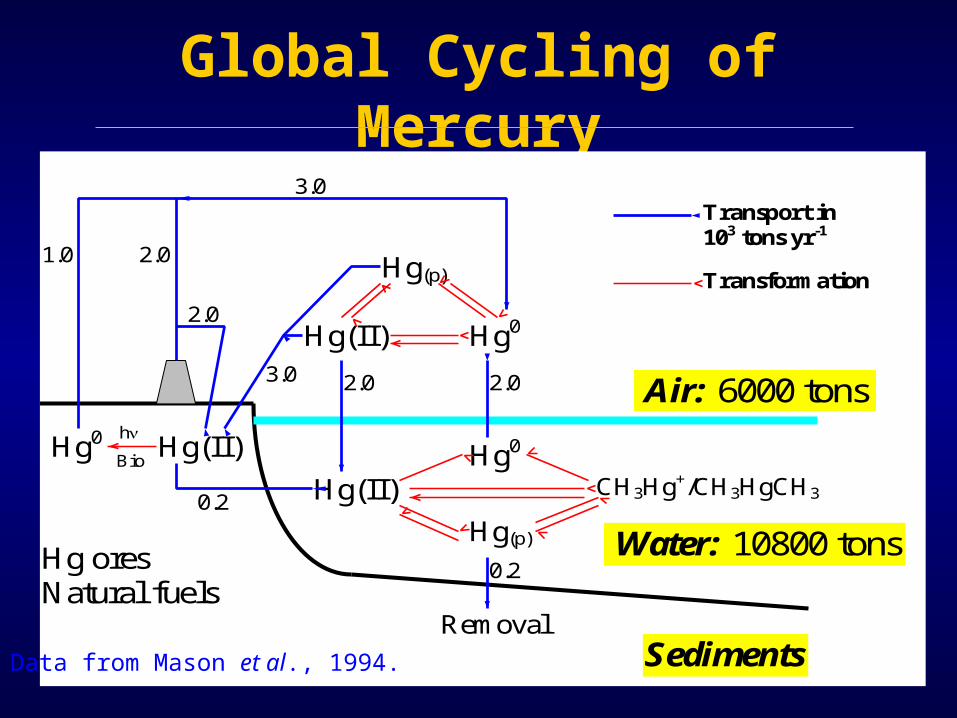
Global Cycling of Mercury

Air: 6000 tons

Hg(II) Hg0

Hg(p)

Hg0

Hg(II)

Hg(p)

CH3Hg+/CH3HgCH3

Hg(II) Hg0

Removal

1.0 2.0

2.0

3.0 2.0 2.0

3.0

Water: 10800 tons

Sediments

0.2

0.2

Transport in 103 tons yr-1

Transformation

h

Hg ores Natural fuels

Bio

Data from Mason et al., 1994.

Emission Sources• Anthropogenic sources

– Fuel combustion: air emission– Waste incineration: air emission– Chloralkali process: water/air emission

• Natural sources– Volcano eruption, weathering, etc.– Vegetation, open water, soil emissions

• Re-emission– Caused by past mercury emission and

deposition – Biotic and abiotic processes cause reduction of

deposited Hg(II) back to volatile – Re-emit into the atmosphere

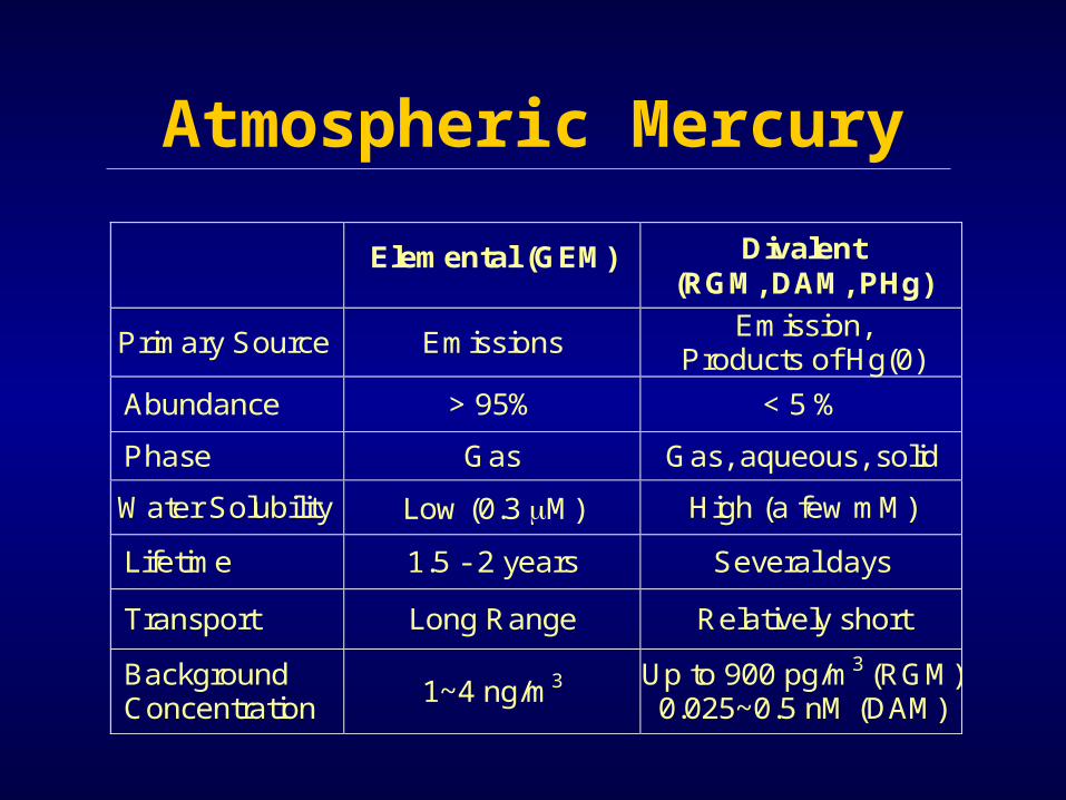
Atmospheric Mercury

Elemental (GEM) Divalent (RGM, DAM, PHg)

Primary Source Emissions Emission,

Products of Hg(0)

Abundance > 95% < 5 %

Phase Gas Gas, aqueous, solid

Water Solubility Low (0.3 M) High (a few mM)

Lifetime 1.5 - 2 years Several days

Transport Long Range Relatively short

Background Concentration

1~4 ng/m3 Up to 900 pg/m3 (RGM) 0.025~0.5 nM (DAM)

“One-Atmosphere” Modeling - Hg

• Mercury exists at very low concentrations and has “its

own” chemistry cycle in the atmosphere

• Concurrent atmospheric chemical processes involving

multiple pollutants affect mercury transport and deposition

• Coupling of mercury with other atmospheric processes is

complex and usually generates non-linear responses

• Chemical transport modeling of mercury needs to be

considered an integral part of the modeling of other

atmospheric pollutants and processes (e.g., ozone, PM,

acid deposition, etc.)

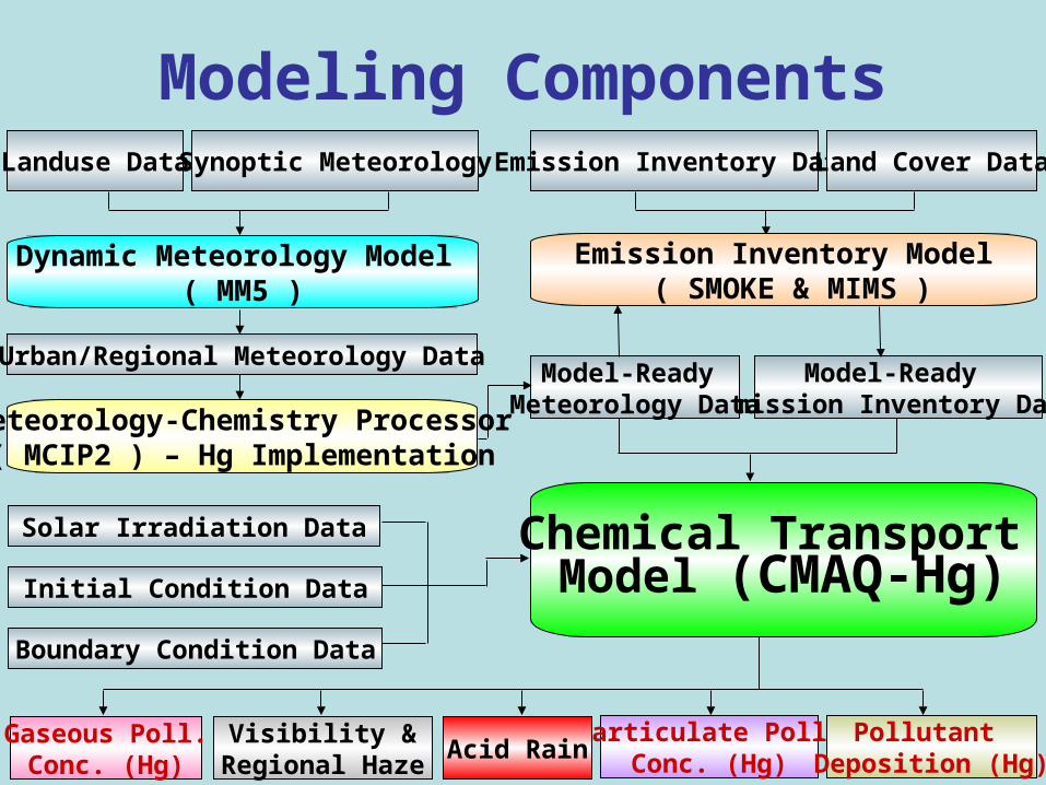
Modeling ComponentsLanduse Data Synoptic Meteorology

Urban/Regional Meteorology Data

Dynamic Meteorology Model ( MM5 )

Meteorology-Chemistry Processor( MCIP2 ) – Hg Implementation

Emission Inventory Model ( SMOKE & MIMS )

Model-Ready Emission Inventory Data

Model-Ready Meteorology Data

Chemical Transport Model (CMAQ-Hg)

Emission Inventory Data Land Cover Data

Solar Irradiation Data

Initial Condition Data

Boundary Condition Data

Gaseous Poll.Conc. (Hg)

Particulate Poll.Conc. (Hg)

Visibility &Regional Haze

Acid RainPollutant

Deposition (Hg)

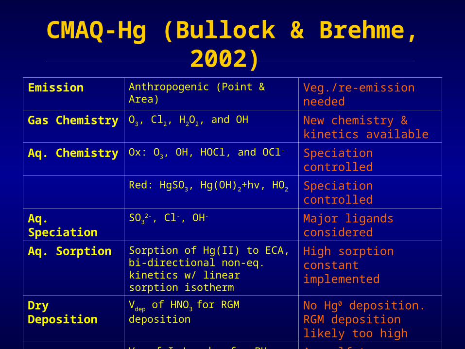
CMAQ-Hg (Bullock & Brehme, 2002)

Emission Anthropogenic (Point & Area) Veg./re-emission needed

Gas Chemistry O3, Cl2, H2O2, and OH New chemistry & kinetics available

Aq. Chemistry Ox: O3, OH, HOCl, and OCl- Speciation controlled

  Red: HgSO3, Hg(OH)2+hv, HO2 Speciation controlled

Aq. Speciation SO32-, Cl-, OH- Major ligands considered

Aq. Sorption Sorption of Hg(II) to ECA, bi-directional non-eq. kinetics w/ linear sorption isotherm

High sorption constant implemented

Dry Deposition Vdep of HNO3 for RGM deposition No Hg0 deposition. RGM deposition likely too high

  Vdep of I,J modes for PHg deposition As sulfate deposition

Wet Deposition Dissolved and Sorbed Hg(II)aq By precipitation & aqueous concentration

Proposed CMAQ-Hg Implementations

BCON

JPROC

ICON

PDM

HorizontalAdvection

VerticalAdvection

HorizontalDiffusion

VerticalDiffusion

Concentration

Gaseous-Phase

Chemistry

Couple&

Decouple

CMAQDriver

Outout Files

PhotolysisRate

AerosolAqueous Chemistry

&Cloud

PlumeIn

Grid

Init

BoundaryConditions

Meteorology

EmissionsSMOKE

InitialConditions

Plume Dynamics

MCIP

Dry deposition velocities of Hg0 and RGM

EI of veg. Hg emission; sea-salt aerosol gen.

Photolysis rates of reactive halogens

New gaseous phase chemistry and kinetic constants

Halogen activation chemistry; Hg

sorption in clouds

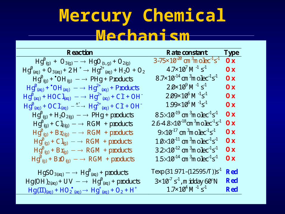
Mercury Chemical Mechanism

Reaction Rate constant Type Hg0

(g) + O3(g)

HgO(s, g) + O2(g) 3-75×10-20 cm3molec-1s-1 Ox Hg0

(aq) + O3(aq) + 2 H + Hg2+

(aq) + H2O + O2 4.7×107 M-1 s-1 Ox Hg0

(g) + OH(g) PHg + Products 8.7×10-14 cm3molec-1s-1 Ox Hg0

(aq) + OH(aq) Hg2+(aq) + Products 2.0×109 M-1 s-1 Ox

Hg0(aq) + HOCl(aq) Hg2+

(aq) + Cl- + OH- 2.09×106 M-1s-1 Ox

Hg0(aq) + OCl-

(aq) H

Hg2+(aq) + Cl- + OH- 1.99×106 M-1s-1 Ox

Hg0(g) + H2O2(g)

PHg + products 8.510-19 cm3molec-1s-1 Ox Hg0

(g) + Cl2(g) RGM + products 2.6-4.810-18cm3molec-1s-1 Ox

Hg0(g) + Br2(g)

RGM + products 910-17 cm3molec-1s-1 Ox Hg0

(g) + Cl(g) RGM + products 1.010-11 cm3molec-1s-1 Ox

Hg0(g) + Br(g)

RGM + products 3.210-12 cm3molec-1s-1 Ox Hg0

(g) + BrO(g) RGM + products 1.510-14 cm3molec-1s-1 Ox

HgSO3(aq) Hg0(aq) + products Texp(31.971-(12595/T))s-1 Red

Hg(OH)2(aq) + UV Hg0

(aq) + products 3×10-7 s-1, midday 60N Red Hg(II)(aq) + HO2

(aq) Hg+

(aq) + O2 + H+ 1.7×104 M-1 s-1 Red

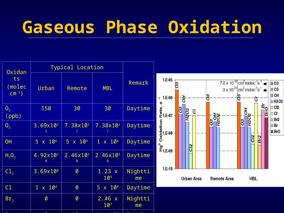
Gaseous Phase Oxidation

Oxidants

(molec cm-3)

Typical Location

RemarkUrban Remote MBL

O3 (ppb) 150 30 30 Daytime

O3 3.69x1012 7.38x1011 7.38x1011 Daytime

OH 5 x 106 5 x 105 1 x 106 Daytime

H2O2 4.92x1010 2.46x1010 2.46x1010 Daytime

Cl2 3.69x108 0 1.23 x 109 Nighttime

Cl 1 x 104 0 5 x 104 Daytime

Br2 0 0 2.46 x 107 Nighttime

Br 0 0 1 x 105 Daytime

BrO 0 0 5 x 106 Daytime

Sea-Salt Aerosol Inventory

• Sea-salt aerosol as the primary sources of reactive halogen species

• Affect the chemistry in coastal areas & in Marine Boundary Layers

• Sea-salt aerosol generation algorithm

• Implementation in SMOKE modeling system

})]log88.1(18.2[exp{)05.2exp(1045.6

10)057.01(373.1

1986) al.,et (Monahan ;

23

41

])65.0

log38.0exp[(19.1

3

05.141.30

10

2

rr

U

dr

dF

r

rU

dr

dF

dr

dF

dr

dF

dr

dF

r

Halogen Activation and Chemistry

• Activation of reactive halogens from sea salt aerosols (Vogt et al., 1996; Glasaw et al., 2002; Knipping and Dabdub, 2002)

• Acid replacement reactions• Oxidation of halides • Autocatalytic generation• Reaction from ClONO2 with sea salts• Photolysis of reactive halogen species• Implementation in CMAQ to provide halogen

oxidants for Hg0

Mercury Emission Inventory

0

2

4

6

8

10

12

14

Hg

Em

issi

on

(T

on

s)

Vegetation Point Source Area Source

Incorporation of vegetation emission in EI processingneeded!

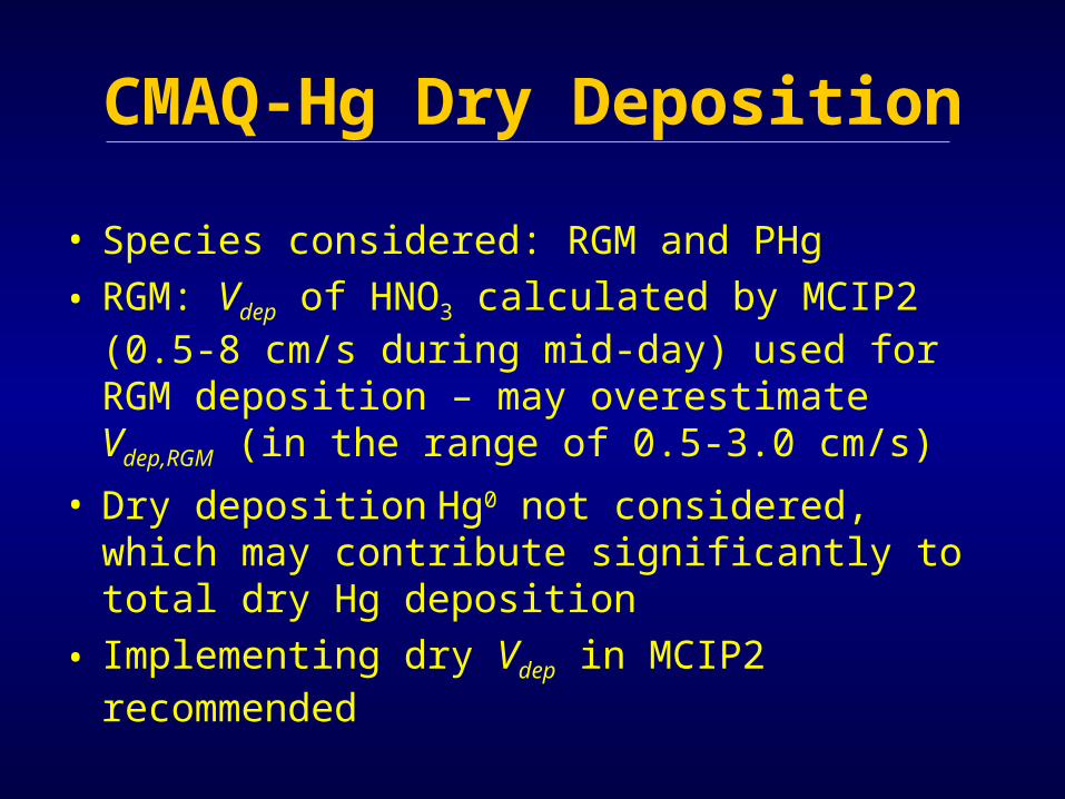
CMAQ-Hg Dry Deposition

• Species considered: RGM and PHg

• RGM: Vdep of HNO3 calculated by MCIP2 (0.5-8 cm/s during mid-day) used for RGM deposition – may overestimate Vdep,RGM (in the range of 0.5-3.0 cm/s)

• Dry deposition Hg0 not considered, which may contribute significantly to total dry Hg deposition

• Implementing dry Vdep in MCIP2 recommended

Estimating Mercury Vdep

• MCIP2 supports two dry deposition schemes– RADM by Wesely (1989)– M3DRY by Pleim (1999)

Vdep = (Ra + Rb + Rc)-1

Ra is the aerodynamic resistance

Rb is the quasi-laminar boundary

layer resistanceRc is the canopy (surface) resistanceEstimating Rc is the key to accurately represent mercury Vdep

RADM vs. M3DRYRADM

• Rc = [(rsx + rmx)-1 + (rlux)-1 + (rdc + rclx)-1 + (rac + rgsx)-1]-1

• Requires trace gas properties, horizontal winds, temperature, RH and 2-D met fields for Vdep estimate

M3DRY• Rs = {fv / rstb + LAI * [fv (1 –

fw) / rcut + fvfw / rcw] + (1 – fv) / rg + fv / (rlc + rg)} –1

• Uses common components as in MM5 land-surface model to estimate Vdep, corrected for landuse and soil moisture

Hg Vdep Implementation - Rc

Terms Formulation Description Remarks

rdc100[1 + 1000(G + 10)-1](1 + 1000)-1

- Buoyant convection resistance

 

 

rsxrsDH2O/Dx, where

rs = ri{1 + [200(G + 0.1)-1]2}

{400[Ts(40 - Ts)]-1}

- Stomatal resistance for substance x

HNO3: DH2O/DHNO3 = 1.9

RGM : DRGM = 0.086 cm2/s;DH2O/DRGM = 2.53

GEM : DGEM = 0.1194 cm2/s;DH2O/DGEM = 1.82

rclx [kH/(105rclS) + f0/rclO]-1 - Lower canopy resistance HNO3: kH = 1 x 10 14 M atm -1;f0(HNO3) = 0.0

rgsx [kH/(105rgsS) + f0/rgsO]-1 - Ground surf. resistance RGM : kH = 2.75x10 6 M atm–1;f0(RGM) = 0.1 or 1.0

rmx (kH/3000 + 100 f0)-1 - Mesophyll resistance

rlux

 

rlu (10-5 kH + f0)-1 - Leaf cuticular resist. GEM : kH = 0.139 M atm -1,

f0(GEM) = 0.0[1/(3rlu) + 10-7 kH + f0/rluO]-1 - Dew or rain correction

rluS

 

100 - Leaf cuticular, SO2 (Dew)  

[1/5000 + 1/(3rlu)]-1 - Rain correction  

rluO

 

[1/3000 + 1/(3rlu)]-1 - Leaf cuticular, O3 (Dew)  

[1/1000 + 1/(3rlu)]-1 - Rain correction  

Note: ri, rlu, rclS, rclO, rac, rgsS, rgsO are parameters depending on land uses and seasons

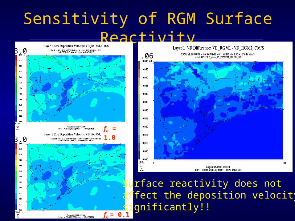
Sensitivity of RGM Surface Reactivity

f0 = 1.0

f0 = 0.1

Surface reactivity does not affect the deposition velocity significantly!!

3.0

3.0

.06

Dry Deposition Velocity: Hg vs. HNO3

HNO3

GEM HNO3 - RGM

RGM

3.0 3.0

3.0.005

Hg(II) Sorption in Aq. Phase

• Current version of CMAQ-Hg treats Hg(II) sorption as bi-directional sorption kinetics:

• Distribution of [HgS2+] and [HgD

2+] estimated from a linear sorption isotherm using a scaled-up sorption constant for EC based on the sorption constant of APM.

)][]([

][ ;

)][]([

][

][][ ;][][

][

22*

2

22*

2

2222

2

aqDaqS

aqDD

aqDaqS

aqSS

aqSaqDaqSDaqDs

aqS

HgHgt

Hgk

HgHgt

Hgk

dt

Hgd

dt

HgdHgkHgk

dt

Hgd

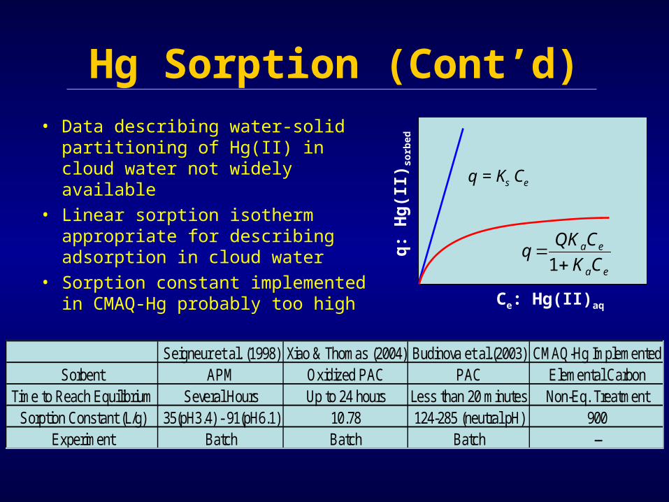
Hg Sorption (Cont’d)• Data describing water-solid

partitioning of Hg(II) in cloud water not widely available

• Linear sorption isotherm appropriate for describing adsorption in cloud water

• Sorption constant implemented in CMAQ-Hg probably too high

Ce: Hg(II)aq

q:

Hg

(II)

sorb

ed

q = Ks Ce

ea

ea

CK

CQKq

1

Seigneur et al. (1998) Xiao & Thomas (2004) Budinova et al.(2003) CMAQ-Hg ImplementedSorbent APM Oxidized PAC PAC Elemental Carbon

Time to Reach Equilibrium Several Hours Up to 24 hours Less than 20 minutes Non-Eq. TreatmentSorption Constant (L/g) 35(pH3.4) - 91(pH6.1) 10.78 124-285 (neutral pH) 900

Experiment Batch Batch Batch --

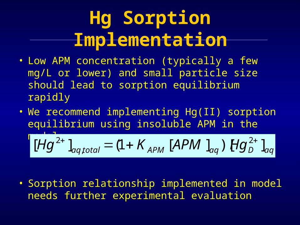
Hg Sorption Implementation

• Low APM concentration (typically a few mg/L or lower) and small particle size should lead to sorption equilibrium rapidly

• We recommend implementing Hg(II) sorption equilibrium using insoluble APM in the model:

• Sorption relationship implemented in model needs further experimental evaluation

aqDaqAPMtotalaq HgAPMKHg ])[][1(][ 2,

2

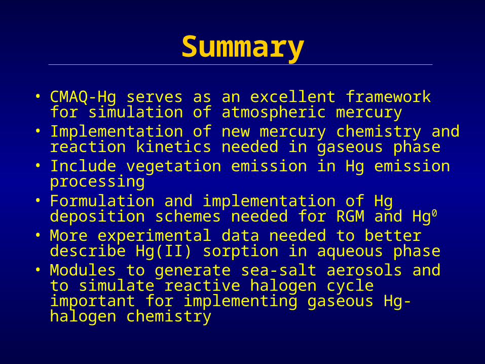
Summary

• CMAQ-Hg serves as an excellent framework for simulation of atmospheric mercury

• Implementation of new mercury chemistry and reaction kinetics needed in gaseous phase

• Include vegetation emission in Hg emission processing

• Formulation and implementation of Hg deposition schemes needed for RGM and Hg0

• More experimental data needed to better describe Hg(II) sorption in aqueous phase

• Modules to generate sea-salt aerosols and to simulate reactive halogen cycle important for implementing gaseous Hg-halogen chemistry

Acknowledgements

• Texas Commission on Environmental Quality

• EPA-Gulf Coast Hazardous Substance

Research Center

• Steve Lindberg, Oak Ridge National Laboratory

• Daewon Byun, University of Houston