DEVELOPMENT OF IN SILICO MODELS

FOR THE PREDICTION OF TOXICITY

INCORPORATING ADME INFORMATION

PRZEMYSLAW PIECHOTA

A thesis submitted in partial fulfilment of the requirements of Liverpool John

Moores University for the degree of Doctor of Philosophy

June 2015

i

LJMU RD10 Decl (1992/V1)

LIVERPOOL JOHN MOORES UNIVERSITY

Candidate’s declaration form (This form must be typed)

Note: This form must be submitted to the University with the candidate’s thesis.

Name of candidate: Przemyslaw Piechota School: Pharmacy & Biomolecular Sciences Degree for which thesis is submitted: Doctor of Philosophy (PhD)

1. Statement of related studies undertaken in connection with the programme of research

(see Regulations G4.1 and 4.4) I have attended lectures, workshops and conferences relevant to QSAR, cheminformatics, programming and predictive toxicology. In addition, I have attended faculty research seminars.

2. Concurrent registration for two or more academic awards (see Regulation G4.7) I declare that while registered as a candidate for the University’s research degree, I have not been a registered candidate or enrolled student for another award of the LJMU or other academic or professional institution

3. Material submitted for another award I declare that no material contained in the thesis has been used in any other submission for an academic award

Signed Przemyslaw Piechota Date 25th June 2015 (Candidate)

ii

Acknowledgments

First of all, I would like to thank my directors of studies Dr Judy Madden and Prof. Mark Cronin for

the chance they gave me to complete a research degree in a very interesting area of computational

toxicology. Your guidance on both academic and personal level has been hugely appreciated. I would

not be where I am now without your constant support and believing in me.

I would also like to thank my colleagues at Liverpool John Moores University (LJMU) for their support

and friendly advice. In particular, specials thanks go to Dr Katarzyna Przybylak, Dr Steve Enoch, Dr

Mark Hewitt, Dr Richard Marchese Robinson, Dr Philip Rowe, and Prof. John Dearden for their

willingness to advise me on many subjects and answer my numerous questions.

I also gratefully acknowledge the financial support provided by the eTOX project.

Finally, I would like to express my gratitude to my wife Dominika and my daughter Gabriela. Thank

you for your support and being patient with me during the time when I was writing up my thesis.

iii

Abstract

Drug discovery is a process that requires a significant investment in both time and resources.

Although recent developments have reduced the number of drugs failing at the later stages of

development due to poor pharmacokinetic and/or toxicokinetic profiles, late stage attrition of drug

candidates remains a problem. Additionally, there is a need to reduce animal testing for toxicological

risk assessment for ethical and financial reasons. In silico methods offer an alternative that can

address these challenges.

A variety of computational approaches have been developed in the last two decades, these must be

evaluated to ensure confidence in their use. The research presented in this thesis has assessed a

range of existing tools for the prediction of toxicity and absorption, distribution, metabolism and

elimination (ADME) parameters with an emphasis on absorption and xenobiotic metabolism. These

two ADME properties largely determine bioavailability of a drug and, in turn, also influence toxicity.

In vitro (Caco-2 cells and the parallel artificial membrane permeation assay) and in silico approaches,

such as various druglikeness filters, can be used to estimate human intestinal absorption; a

comparison between different methods was performed to identify relative strengths and

weaknesses of the approaches. In terms of xenobiotic metabolism it is not only important to predict

metabolites correctly, but it is also crucial to identify those compounds that can be biotransformed

into species that can covalently bind to biomolecules. Structural alerts are routinely used to screen

for such potential reactive metabolites. The balance between sensitivity and specificity of such

reactive metabolite alerts has been discussed in the context of correctly predicting reactive

metabolites of pharmaceuticals (using data available from DrugBank). Off-target toxicity, exemplified

by human Ether-à-go-go-Related Gene (hERG) channel inhibition, was also explored. A number of

novel structural alerts for hERG toxicity were developed based on groups of structurally similar

compounds. Finally, the importance of predicting potential ecotoxicological effects of drugs was also

considered. The utility of zebrafish embryos to distinguish between baseline and excess toxicity was

investigated. In evaluating this selection of existing tools, improvements to the methods have been

proposed where possible.

The funding form the European Community’s 7th Framework Programme Innovative Medicines

Initiative Joint Undertaking (IMI-JU) eTox Project (grant agreement n° 115002) is gratefully

acknowledged.

iv

Table of Contents

Chapter 1. Introduction

1.1. Introduction .................................................................................................................... 1

1.2. In silico methods in drug discovery................................................................................. 7

1.3. Toxicity and its assessment ............................................................................................ 9

1.4. ADME properties and their optimisation ....................................................................... 11

1.5. QSAR models .................................................................................................................. 14

1.5.1. Data ................................................................................................................... 14

1.5.2. Molecular descriptors........................................................................................ 14

1.5.3. Statistical modelling .......................................................................................... 16

1.5.4. QSAR validation ................................................................................................. 17

1.6. Zebrafish embryos as a screening tool ........................................................................... 18

1.7. The overall aims of the project ....................................................................................... 19

1.7.1. Summary of aims and key findings for each chapter ........................................ 19

Chapter 2. Predicting Drug Absorption and Bioavailability

2.1. Introduction .................................................................................................................... 22

2.1.1. Absorption ......................................................................................................... 22

2.1.2. Prediction of HIA ............................................................................................... 23

2.1.3. Bioavailability .................................................................................................... 24

2.2. Methods .......................................................................................................................... 25

2.2.1. Datasets ............................................................................................................. 25

2.2.2. Generation of molecular descriptors ................................................................ 26

2.2.3. Prediction of sites of metabolism and enzymes involved ................................. 27

2.2.4. Statistical analysis .............................................................................................. 27

v

2.3. Results and discussion .................................................................................................... 28

2.3.1. Dataset A: Applying druglikeness rules for prediction of HIA ........................... 28

2.3.1.1. Comparative analysis ........................................................................... 28

2.3.1.2. Investigation of the influence of TPSA and log D ................................. 34

2.3.2. Relationship between in vivo, in vitro and in silico methods ............................ 36

2.3.2.1. Comparison of Caco-2 and % HIA data ................................................ 36

2.3.2.2. Comparison of PAMPA and % HIA data ............................................... 40

2.3.2.3. Comparison of HIA, Caco-2 and PAMPA .............................................. 46

2.3.3. Metabolic contribution to bioavailability .......................................................... 47

2.3.3.1. Effect of clearance on bioavailability ................................................... 48

2.3.3.2. Prediction of metabolic clearance ....................................................... 49

2.3.3.3. Other considerations............................................................................ 51

Chapter 3. Pragmatic Approaches to Using Computational Methods to

Predict Metabolites

3.1. Introduction .................................................................................................................... 53

3.2. Methods .......................................................................................................................... 59

3.2.1. Datasets ............................................................................................................. 59

3.2.2. Collecting and storing metabolism data ............................................................ 59

3.2.3. Use of software ................................................................................................. 63

3.2.4. Statistical analysis .............................................................................................. 66

3.3. Results and discussion .................................................................................................... 67

3.3.1. General performance of the algorithms............................................................ 67

3.3.2. Pragmatic approach to using Meteor ................................................................ 68

3.3.3. Combining SMARTCyp and MetaPrint2D-React ................................................ 74

vi

Chapter 4. Development of Models to Predict hERG Channel Inhibition

4.1. Introduction .................................................................................................................... 79

4.1.1. Data sources ...................................................................................................... 79

4.1.2. QSAR approaches to modelling hERG inhibition ............................................... 80

4.1.3. hERG channel structure ..................................................................................... 81

4.1.4. hERG pharmacophore models........................................................................... 83

4.2. Methods .......................................................................................................................... 84

4.2.1. Dataset .............................................................................................................. 84

4.2.2. Generation of molecular descriptors ................................................................ 85

4.2.3. Similarity search ................................................................................................ 86

4.2.4. Field points analysis ........................................................................................... 86

4.2.5. Statistical analysis .............................................................................................. 86

4.2.6. Structural alerts development .......................................................................... 86

4.3. Results and discussion .................................................................................................... 87

4.3.1. Global models for predicting hERG inhibition ................................................... 87

4.3.1.1. Evaluation of the model of Aptula and Cronin (2004) using Log D and

Dmax descriptors to predict hERG inhibition ....................................... 87

4.3.1.2. Testing maximum diameter and log D rules for H_244 ....................... 89

4.3.1.3. Global regression model ...................................................................... 91

4.3.1.4. Binary classification models ................................................................. 91

4.3.2. Groups based on 2-D similarity ......................................................................... 93

4.3.2.1. Relationship between 2-D similarity and pIC50 ................................... 96

4.3.2.2. Local multi-linear regression models for individual categories ........... 97

4.3.2.3. Quantitative analysis of seven categories of compounds ................... 98

4.3.3. Development of structural alerts for hERG toxicity .......................................... 112

vii

Chapter 5. Structural Alerts for Reactive Metabolites

5.1. Introduction .................................................................................................................... 120

5.2. Methods .......................................................................................................................... 121

5.2.1. Datasets ............................................................................................................. 121

5.2.2. Structural alerts ................................................................................................. 122

5.2.3. Detection of alerts ............................................................................................. 123

5.3. Results and discussion .................................................................................................... 124

5.3.1. The distribution of alerts ................................................................................... 124

5.3.2. Structural alerts – an issue of sensitivity and specificity ................................... 127

Chapter 6. Assessing the Suitability of Zebrafish Embryos for Predicting

Acute Aquatic Toxicity

6.1. Introduction .................................................................................................................... 131

6.1.1. Use of Zebrafish embryos in toxicity testing ..................................................... 132

6.1.2. Modes of acute aquatic toxicity ........................................................................ 133

6.1.3. QSAR modelling of narcosis ............................................................................... 134

6.1.4. The Verhaar scheme .......................................................................................... 134

6.2. Methods .......................................................................................................................... 136

6.2.1. Datasets ............................................................................................................. 136

6.2.2. Calculating molecular descriptors ..................................................................... 138

6.2.3. Classifying compounds according to the Verhaar scheme ................................ 138

6.2.4. Statistical analysis .............................................................................................. 138

6.3. QSAR models for Verhaar classes ................................................................................... 138

6.3.1. Preliminary analysis ........................................................................................... 138

6.3.2. Verhaar class 1 compounds ............................................................................... 140

6.3.3. Verhaar class 2 compounds ............................................................................... 142

6.4. Refinement of models .................................................................................................... 143

viii

6.4.1. Refined baseline model ..................................................................................... 145

6.4.2. Refinement of model for polar narcotics (phenols and anilines) ...................... 146

6.4.3. Aliphatic amines models ................................................................................... 148

6.5. Other Verhaar classes ..................................................................................................... 152

6.6. Validation of baseline non polar narcosis and polar narcosis models ........................... 155

6.6.1. Performance of baseline models ....................................................................... 156

6.6.2. Testing the polar narcosis model ...................................................................... 159

Chapter 7. Discussion ............................................................................................................ 161

Future Work .................................................................................................................................. 168

References ..................................................................................................................................... 170

Appendices ......................................................................................................................... 193

ix

Abbreviations

% F Bioavailability

% FA Fraction of drug absorbed

3Rs Reduction, refinement and replacement

5HT4 5-Hydroxytryptamine

ABL Aqueous Boundary Layer

ADME(T) Absorption, Distribution, Metabolism, Excretion, (Toxicity)

ADR Adverse Drug Reactions

AM1 Austin Model 1

AP Applicability Domain

APIs Active pharmaceutical ingredients

ATP Adenosine triphosphate

Caco-2 Cells derived from colorectal carcinoma cells

CADD Computer-Aided Drug Design

CAS RN Chemical Abstracts Service Registration Number

CHO Chinese Hamster Ovary cells

Cl(h) (Hepatic) clearance

Clint Intrinsic clearance

cLog P Calculated partition coefficient

CNS Central Nervous System

CoMFA Comparative Molecular Field Analysis

CoMSiA Molecular Similarity Indices in a Comparative Analysis

COS Fibroblast-like cells

CSV Comma Separated Values file

CYP450 Cytochrome P450

D Dose of a drug

dG Deoxyguanosine

DILI Drug-Induced Liver Injury

x

Dmax Maximum diameter

DOS Diversity-Oriented Synthesis

DNA Deoxyribonucleic Acid

E Embryo

EC50 Half maximal effective concentration

EFPIA European Federation of Pharmaceutical Industries and Associations

EHOMO Energy of the Highest Occupied Molecular Orbital

ELE Eleutheroembryo

ELUMO Energy of the Lowest Unoccupied Molecular Orbital

EQU Equivocal

EU European Union

f Fraction of free drug

FATS Fish Acute Toxicity Syndrome

FBS Fragment-Based Screening

FDA Food and Drug Administration

FET Fish Embryo Test

FN False Negative

FP False Positive

FRB Freely Rotated Bonds

GI Gastro-Intestinal

GIT Gastro-Intestinal Tract

GRIND GRid-INdependent Descriptors

GSH Glutathione

HAS Human Serum Albumin

HBA Hydrogen Bond Acceptor

HBD Hydrogen Bond Donor

HCS High-Content Screening

HEK 293 Human Embryonic Kidney cells

Hep G2 Human hepatic carcinoma cell line

hERG human Ether-à-go-go-Related Gene

xi

HIA Human intestinal absorption

HMG CoA 3-Hydroxy-3-MethylGlutaryl-COenzyme A

HOMO Highest Occupied Molecular Orbital

HTD High-Throughput Docking

HTS High-Throughput Screening

IC50 Half maximal inhibitory concentration

IGC50 50% inhibitory growth concentration

IK Delayed rectifier current

IMI Innovative Medicines Initiative

InChIKey IUPAC International Chemical Identifier

IUPAC International Union of Pure and Applied Chemistry

IVIVE In Vitro-In Vivo Extrapolations

KCS Potassium cyanide

kNN k-nearest neighbours

KOW Octanol-water partition coefficient

LBVS Ligand-Based Virtual Screening

LC50 Concentration resulting in 50% lethality

LLE Lipophilic Ligand Efficiency

Log D Distribution coefficient

Log P Partition coefficient

Log Papparent Permeability coefficient

Log S Logarithm of aqueous solubility

LUMO Lowest Unoccupied Molecular Orbital

Mabs Total mass absorbed

MCTs Monocarboxylate Transporters

MDCK Madin-Darby Canine Kidney cell lines

MIST Metabolites In Safety Testing

MLP Multilayer Perceptron

MLR Multiple Linear Regression

MOE Molecular Operating Environment

xii

MR Molar Refractivity

MSE Mean swuared error

MW Molecular weight

NA Number of Atoms

NAPQI N-acetyl-p-benzoquinone imine

NAS New Active Substance

NBR Number of Rotational Bonds

NME New Molecular Entity

NMR Nuclear Magnetic Resonance

NRC National Research Council

NSAID Non-Steroidal Anti-inflammatory Drug

OECD Organization for Economic Cooperation and Development

PAMPA Parallel artificial membrane permeability assay

PBPK Physiologically-based pharmacokinetics

PLA Plausible

PRO Probable

PCA Principal Component Analysis

pIC50 Negative logarithm of IC50

pKa Ionisation constant

PLS Partial Least Squares

Q Hepatic blood flow

Q2 Cross-validated correlation coefficient

QED Quantitative Estimate of Drug-Likeness

(Q)SAR (Quantitative) Structure-Activity Relationship

QSPR Quantitative structure-Property Relationship

R Correlation coefficient

R2 Coefficient of determination

R2adj Adjusted determination coefficient

RBD Radioligand Binding Assay

REACH Registration, Evaluation, Authorisation and restriction of Chemical substances

xiii

RF Random Forest

RNA Ribonucleic Acid

ROC Receiver Operating Characteristic

SCA Semicarbazide

Sdf Structure-Data File

SLC Solute carrier

SMARTS SMiles ARbitrary Target Specification

SMILES Simplified Molecular-Input Line-Entry System

SMOreg Support vector machine for regression

SOM Site Of Metabolism

SVM Support Vector Machine

T1/2 Half-life

Te Toxic ratio

TdP Torsade de Pointes

TN True Negative

TP True Positive

TPSA Total polar surface area

UDP Uridine Diphosphate Glucose

UGT UDP Glucuronosyl-Transferase

US United States

UWL Unstirred Water Layer

VS Virtual Screening

vsurf Volume and surface descriptors

zERG Zebrafish orthologue of HERG

ZFET Zebrafish embryo acute toxicity tests

1

1. Introduction

1.1. Drug discovery

Drug discovery is a process driven by the need for suitable pharmaceutical products that can be

used, successfully, to treat a wide range of existing medical conditions (Hughes et al, 2011). A drug

discovery project is a huge undertaking that is both time-consuming and requires substantial

financial resources. The development of a novel drug can take up to 15 years - from the original

concept to introducing the drug to the market. A systematic review of drug development costs

showed that the figures may vary significantly but have been estimated to be in the range of USD$92

million to USD$883.2 before capitalisation (Morgan et al., 2011). However, drug development is a

business that involves a high risk of failure. The probability of success for a drug development

project may be as low as 7% (Lou & de Rond, 2006) although the rates vary. It is difficult to give

accurate estimates of time and cost due to the number of variables involved and the applied

methodology (Pronker et al., 2011), however the need for more rapid, cost-effective means of drug

development is evident. This need has been recognised within the Innovative Medicines Initiative

(IMI), a joint undertaking between the European Union and the association of pharmaceutical

companies (EFPIA), which currently funds approximately 50 projects aimed at improving the drug

discovery process. eTOX is one such project representing the combined effort of 25 participants

from both industry (e.g. Novartis, Pfizer, Bayer) and academia (e.g. Liverpool John Moores

University, University of Vienna, VU University Amsterdam) with the aim of speeding up the process

of introducing safer and more effective medicines, by developing strategies and tools to predict

safety and side-effects of drug candidates. The idea of the project grew from the realisation that the

pharmaceutical industry is in possession of large amounts of unpublished data that were acquired

during the drug development process. However, these data were not made available publicly due to

their confidentiality. The main objectives of the eTOX project include: building a large database that

would contain both public and private data, the implementation of methods that would allow access

to this proprietary information, whilst protecting the intellectual property, and using the compiled

database to develop or enhance toxicity prediction models (Briggs et al. 2012).

The aim of drug discovery is the development of new molecular entities (NME). NME refers to a drug

that contains an active ingredient that has not been approved in any form by the United States Food

and Drug Administration (US FDA). This term is very broad (in Europe the term new active substance

(NAS) is used) and includes both new chemical entities (small molecules) and also new biological

2

entities (Paul et al., 2010). The drug discovery process can be divided into four distinct stages, which

are characterised by different methodological approaches, each of which is discussed below.

I. Target discovery

The first stage of the drug discovery process involves target identification and validation. A broad

spectrum of targets has been recognised such as: genes, proteins, RNA, disease biomarkers or

elements of biological pathways that could be associated with a specific clinical condition (Yang,

Adelstein & Kassis, 2012). Two different strategies are employed to target discovery, namely,

systems approaches and molecular approaches. Systems approaches represent a more traditional

way of identifying a target by using whole organisms to study the disease. Data are obtained from

patients or in vivo animal models that focus on the relevant areas of physiology or pathology. The

majority of drugs available on the market have been discovered through systems approaches and

this methodology is still important in target discovery in the context of diseases for which specific

phenotypes are detected at the whole organism level, e.g. obesity, hypertension, stroke,

neurodegenerative conditions (Lindsay, 2003). However, recent advances in omics technology has

led to a shift towards molecular approaches (e.g. in oncology) although phenotypic screening is still a

major contributor in drug discovery when measured by number of new first-in-class small molecule

drugs introduced to the market (Swinney & Anthony, 2009). In molecular approaches the emphasis

is put on molecular mechanisms that are relevant to a specific pathological condition. In other

words, molecular approaches are geared towards discovering targets at the cellular level through

the study of molecular events. In this context, bioinformatics approaches are utilised to identify a

target (Chen & Chen, 2008). These include data mining methods such as searching large databases of

literature relevant to biomedical sciences (e.g. PubMed) and analysis of microarray data through

supervised classification or unsupervised clustering. This can be enhanced by the analysis of data

provided by proteomics and chemogenomics. Furthermore, target discovery can benefit from

integrative approaches (Kim et al., 2007). A combination of different data mining approaches gives a

more complete understanding of cellular mechanisms and, consequently, leads to selection of an

appropriate target. Such a target should be characterised by a high druggability, i.e. it should be

amenable to modulation when interacting with small molecules or proteins. The idea of a ‘druggable

genome’ was introduced by Hopkins & Groom, (2002). They emphasised that a limited number of

biological targets are available for drug discovery as not all genes are disease-modifying and some of

them are not druggable, i.e. they are not capable of binding drug-like molecules (e.g. orally

bioavailable compounds). In the case of the most common targets – proteins – one of the

determinants of druggability is binding affinity at levels below 10 µM (Keller, Pichota & Yin, 2006).

3

There are several different methods to assess or predict druggability; these include high-throughput

approaches for identifying drug binding sites (Schmidtke & Barril, 2010), calculating druggability

indices from data obtained in nuclear magnetic resonance (NMR) screening (Hajduk et al., 2005) or

structure-based methods for assessing maximum binding affinity (Cheng et al. 2007). The properties

of ideal druggable targets in drug discovery have been summarised by Gashaw et al., (2012).

II. Hit discovery

Once the target has been determined and validated the next step involves the identification of “hit”

compounds. In the context of drug discovery, hits can be defined as small molecules (low molecular

weight) that can display an adequate activity in relevant target assays (Bleicher et al., 2003). These

assays can determine appropriate binding affinities (usually in micromolar range) to such

therapeutic target classes as receptors, enzymes or ion channels. The identification of hits involves

screening large libraries of compounds. These libraries may contain thousands or millions of

compounds. High-throughput screening (HTS) of large libraries is a traditional approach to hit

identification. However, the development and maintenance of large libraries is costly and despite

the sheer size of the collection of compounds only a fraction of chemical space is represented.

Libraries may also include compounds that are not druglike. Consequently, the potential to discover

hits is limited and even if the hits are identified they may not be considered for further development

due to unsuitable physico-chemical properties. Hence, HTS libraries may not be an optimal starting

point for discovery of hit or lead compounds (Scott et al, 2012). In response to these challenges new

methodologies were developed for the design of chemical libraries that addressed the balance of

library size and molecular diversity. In the last two decades, two different strategies for library

design have emerged: fragment-based screening (FBS) and diversity-oriented synthesis (DOS). Both

FBS and DOS resulted from two different approaches to the concept of drug discovery. FBS libraries

contain small molecular fragments that are screened for binding affinities to the target. Fragments

that are found to bind target at micromolar concentrations are further utilised for identification of a

lead compound in a processes of fragment evolution, linking, self-assembly and optimisation (Rees

et. al, 2004). In comparison to HTS, this method offers a number of advantages: it is less resource-

intensive, it identifies more efficient binders (although less potent), it may provide better

understanding of binding interactions and it usually generates compounds with lead-like properties

(Rees et al., 2004). Similarly to FBS, DOS libraries consist of hundreds to thousands of compounds.

However, DOS libraries are composed of more druglike compounds with higher molecular weights or

log P (partition coefficient) values. Such structurally diverse compounds are usually synthesised from

common intermediates in a modular manner and then screened for lead-like molecules that

4

generally possess higher affinity for the target than do small fragments. DOS libraries are typically

built without prior knowledge of activity of the members toward the biological targets. Both FBS and

DOS libraries have been successfully used for drug discovery processes and each type of library can

have certain advantages. For instance, the FBS approach has been characterised to provide a more

structurally diverse library (Hajduk, 2011). However, this diversity may not necessarily be observed

in actual FBS libraries due to the medicinal chemistry bias in selection of fragments. In consequence,

FBS libraries tend to contain a large proportion of fragments based on aromatic rings, which leads to

obtaining structurally flat leads as opposed to producing more 3-D-like scaffolds from the DOS

approach, which could be more relevant in the biological context (Galloway & Spring, 2011).

A variety of screening strategies have been developed. HTS provides a means to test complete

libraries either directly against a drug target or, increasingly, by using cell-based assays with

application of high-content screening (HCS) (Fox et al., 2006). The advances in automation and

robotics, miniaturisation of the microtiter plate wells, replacement of radioactive reagents with

fluorescent labels and the development of new fluorescence methods resulted in HTS procedures

that required smaller amounts of reagents and were more time-efficient (Phatak, Stephan,

Cavasotto, 2009). Fragment screening, often accompanied by NMR used for structure

determination, represents another strategy for hit discovery although, in contrast to HTS, it relies on

the presence of the target crystal structure. Focused screens provide a cheaper alternative to HTS.

This strategy involves screening compounds that are already known to bind to certain classes of

targets, e.g. kinases. However, it may not be useful for discovery of novel pharmaceuticals. Lower

throughput screening is also used, for instance, in physiological screens. In this case, the effects of

selected potential drugs are studied at tissue level rather than by utilising cells or cellular

components (Hughes et al., 2011).

The final stage of hit discovery is establishing a hit series. The screening generates a number of hits

and their suitability for drug discovery has to be assessed. This is achieved by taking dose-response

curves to establish half maximal inhibitory concentrations, which can be used to compare the

potencies of the hits and also identify compounds that bind to the target in a reversible manner. This

process can be supported by secondary in vitro bioassays to confirm that a specific hit not only

interacts with an isolated target (e.g. a receptor) but can also induce functional change at the

cellular or tissue level. The selected hits can be then clustered into groups based on structure-

activity relationships (SARs). Compounds in each cluster usually have a common substructure that is

responsible for the activity however, their potencies differ as a result of differences between

chemical groups attached to the motif they share. At this stage, a further refinement process is

5

carried out. It involves the initial in vitro assessment of absorption, distribution, metabolism and

elimination (ADME) properties and also gathering more information about potential selectivity

issues. These processes allow for the definition of a number of hit series with each hit having activity

in the range of 100 nM to 5 µM (Hughes et al., 2011).

III. Hit to lead

The hit discovery process concentrates on identifying compounds with promising pharmacodynamic

properties, i.e. the major role of the screening process is to search for molecular entities that can

produce a desired biological activity. The hit to lead stage focuses on suitable pharmacokinetic

properties of potential NMEs, whilst attempting to further increase the potency and selectivity of

the hits. This stage encompasses consideration of the in vivo situation where the drug has to pass

through biological barriers, e.g. permeability barriers such as the wall of the gastrointestinal tract or

blood-brain barrier (Pardridge, 2001) before it can reach its target, i.e. it has to be bioavailable. The

rates of xenobiotic metabolism (biotransformation) and excretion may significantly reduce

bioavailability. Hence, ADME properties have to be carefully examined and modified where

necessary in order to make a compound more bioavailable.

The output of the hit to lead stage comprises a series of leads. A lead can be defined as a ligand that

has a suboptimal binding affinity towards a target. Characteristics of a lead, according to Oprea et al

(2001), may include: i) the lack of complex molecular features so that the structure is more

amenable to potential optimisation; ii) its presence in a clearly defined SAR series; iii) not being

subject to a patent and iv) possessing good ADME properties. In the context of ADME, certain rules

were defined to describe what constitutes a good lead molecule. These included Lipinski’s “rule of

five” defined for oral absorption or permeability (Lipinski et al., 2001) and Veber’s rules for oral

bioavailability (Veber et al., 2002). These druglikeness rules utilise simple molecular properties such

as log P, molecular weight, the number of hydrogen bond donors and acceptors, polar surface area

or the number of rotational bonds. The development of fragment based discovery led to the

introduction of the concept of “lead-likeness”. It was established that lead compounds usually have

lower molecular complexity, are less lipophilic and less druglike (Oprea et al., 2001). Consequently,

the rule of three was proposed to address the concept of lead-like ‘hits’ in fragment-based screening

(Congreve et al., 2003).

A number of assays are used both during hit discovery and the hit to lead phase. Aqueous solubility

and permeability across lipid membranes are key parameters that are measured. Permeability is

often determined in in vitro studies using Caco-2 cells (representing the intestinal epithelium) or

6

Madin-Derby Canine Kidney (MDCK) cells transfected with the MDR1 gene to quantify the effect of

efflux – a process which may limit gastro-intestinal uptake of molecules. Additionally, artificial

membranes that mimic biological structures (for example PAMPA membranes) can be used for this

purpose. Metabolism can be assessed using microsomal stability assays that measure compound

clearance and may identify metabolites. Finally, cytotoxicity assays, including CYP450 inhibition and

Hep G2 hepatotoxicity, may also be performed (Hughes et al., 2011).

IV. Lead optimisation

The final phase of drug discovery aims at obtaining a drug candidate that would be suitable for

preclinical studies. This is achieved by further improvements in both pharmacodynamic and

pharmacokinetic properties of a number of lead compounds so that only one or two structures

belonging to different lead series are selected for further development. Optimisation of candidates

is performed in terms of their potency, selectivity and ADME-Tox profile (encompassing oral

absorption, bioavailability, metabolic clearance and off-target toxicity - such as cardiotoxicity related

to hERG channel inhibition or adverse drug reactions resulting from the formation of reactive

metabolites (Kalgutkar et al., 2005)). Various metrics have been introduced to assess the suitability

of a lead. For instance, a number of ligand efficiency indices can be used to estimate the balance

between modulation of physico-chemical properties and increasing target affinity during lead

optimisation. This can include lipophilic ligand efficiency (LLE) which can be used to guide a

medicinal chemist as a measure of lipophilicity and in vitro potency (Hopkins et al., 2014).

Lipophilicity is an important property that affects both ADME and binding affinity. Reducing LLE has

been shown to improve ADME properties and safety profiles as a result of lowered lipophilicity

(Tarcsay, Nyiri & Keseru, 2013). Nevertheless, less than 10% of leads selected for development are

eventually launched to the market (Peck, 2006). Bias towards the potency may be indicated as one

of the reasons for drug candidates’ attrition during the development stage. The bias may be a result

of typically well-defined metrics during, such as binding affinity, while assessment of ADME

properties seems to be a more complex task and more difficult to estimate. However, molecular

properties that are important for binding to the target may be inversely correlated to ADME.

Gleeson et al., (2011) showed that no strong correlation between in vitro potency and the

therapeutic dose existed and that oral drugs seldom possess nanomolar activity. Moreover, off-

target activities for many orally delivered drugs are considerable which is related to their

promiscuity, i.e. binding to many targets despite drug discovery being focussed on a single target. In

an attempt to quantify the role of ADME in lead optimisation strategies the concept of drug

efficiency was introduced (Braggio et al., 2010). It was defined as a fraction of the dose that is

7

available at the site of action or, in other words, it is a ratio of the biophase concentration and the

dose. This single parameter takes into account all factors (ADME properties) that can affect the

concentration of a lead at the target site. The drug efficiency can be used to guide the medicinal

chemist during the selection of drug candidates with the aim of increasing the biophase

concentration and potentially reduce the attrition rate at the development stage.

The drug discovery process is complex and it is crucial that the output of this phase is represented by

very carefully selected drug candidates for which the balance of both potency and ADME properties

has been appropriately weighed. Such NMEs can then be subject to preclinical studies as

investigational drugs and if approved they can enter clinical phases. Due to the high costs of clinical

studies (Morgan et al., 2011) the necessity for high quality output from early drug discovery should

be emphasised.

Research within this thesis is most applicable to stages III and IV of drug discovery i.e. hit-to-lead and

lead optimisation processes. This thesis describes the development of in silico models that can be

used to predict ADME-Tox properties of a range of molecules based solely on molecular structure,

hence these models can be used to inform design and selection of the most promising drug

candidates.

1.2. In silico methods in drug discovery

The process of drug discovery, as described above, uses various computational approaches at each

stage. Such in silico methods not only allow the design of more potent drugs with better ADME

profiles (computer-aided drug design, CADD) but also they do it in a less time-consuming manner

and utilise less financial resources in comparison to in vitro and in vivo assays.

Virtual screening (VS) is a major application of CADD that has been utilised in the drug discovery

process. VS can be applied to virtual libraries that usually contain 105 – 107 compounds stored in a

digital format. The aim of VS is to significantly reduce this initial number of potential candidates

according to specific criteria, such as interaction with a biological target or desired physico-chemical

properties. The output of VS could be one molecule, or it could be hundreds of compounds,

depending on the purpose (Tanrikulu, Kruger & Proschak, 2013). VS can utilise either structure-

based or ligand-based in silico methods (Sliwoski et al, 2013).

Structure-based methods rely on the knowledge of the 3D target structure. Ideally, the three-

dimensional structure of a macromolecule should be based on experimental studies (X-ray

8

crystallography, NMR); if it is not readily available, homology models can be used as a substitute.

The assumption of the structure-based approach is that, for a given molecule, more favourable

interactions with a binding site on a biological molecule, e.g. a protein will result in more favourable

biological activity. The structure-based methods are also referred to as high-throughput docking

(HTD) methods. Firstly, HTD requires the potential binding sites and the druggability of the target to

be predicted. Secondly, a suitable virtual chemical library is selected. Such a library may be subject

to a filtering process, e.g. according to druglikeness rules. The remaining compounds are used in

molecular docking studies, i.e. each molecule is placed into a binding site of a macromolecule and

energetically favourable conformations of the protein and ligand pair are searched (e.g. by using

molecular dynamics, genetic algorithms) which are in turn assessed by a scoring function. The scores

represent the likelihood of favourable binding interactions and are used to rank the compounds of

interest (Phatak, Stephan & Cavasotto, 2009). In essence, HTD can be regarded as a virtual

equivalent of HTS and the increase in computational power, combined with more efficient

calculations of ligand poses/protein flexibility led to a number of successful applications of HTD in

drug discovery (McInnes, 2006).

Ligand-based virtual screening (LBVS) does not require the 3D structure of the target but instead, it

utilises the existing research on ligands that are known to be active towards a specific target (Phatak,

Stephan & Cavasotto, 2009). The assumption is made that similar molecules can exert similar

biological activity. LBVS often utilises a variety of similarity searching methods such as 2D

fingerprints, to filter compounds that are most similar to the active ligand(s). It can also use

quantitative structure-activity relationship (QSAR) studies to determine physico-chemical properties

important for binding of a particular ligand from which a predictive model can be generated. 3D

pharmacophore screening can also be performed. A pharmacophore is a structural abstraction that

describes steric and electronic features, such as hydrophobic regions, hydrogen bonding, number of

aromatic rings etc, that are important for ligand – receptor interactions (Sliwoski, 2013). A

pharmacophore model can be used to identify molecules that possess similar structural features that

are also similarly distributed spatially.

In silico ADMET modelling offers another useful computational approach that is applied to drug

discovery campaigns. QSAR, SAR and read-across methods are applied to ADMET data to prioritise

hits and leads. Hits prioritisation involves obtaining virtual hits profiles that predict such

characteristics as bioavailability, clearance, CYP450 metabolism, hERG or central nervous system

(CNS) liabilities, presence of structural alerts for genotoxicity or reactive metabolite formation

(Gleeson & Montanar, 2012). ADMET models are also useful in the process of lead optimisation,

9

especially in cases where pharmacokinetics and toxicity profiles are to be improved (Jorgensen,

2008). For instance, SAR information can be used to understand which structural changes could be

introduced to obtain an optimal ADMET profile without sacrificing the potency of the lead. The

incorporation of a variety of in silico filters, relating to ADME properties, in drug discovery has been

indicated as one of the reasons for the recent reduction in clinical failures amongst drugs due to

poor pharmacokinetics (Khanna, 2012).

1.3. Toxicity and its assessment

Toxicology is a scientific discipline that studies adverse effects of chemicals on living organisms.

Depending on the methods used, three main approaches to toxicology can be distinguished: in vivo,

in vitro and in silico approaches. In vivo toxicology is used to establish the relationship between a

chemical agent and the toxic effects it elicits by testing on living animals. In vitro (literally translated

to “within glass”) approaches apply a different methodology: cultured cells are exposed to

potentially harmful substances and then the toxicity towards these cells (either of human or animal

origin) is measured. In vitro testing is not limited to cells but can also involve assays on biological

macromolecules. Finally, in silico toxicology uses computational techniques in an attempt to produce

valid predictions so that the toxic effects of a chemical can be assessed without the necessity to

conduct laboratory-based experiments.

In silico toxicology can be characterised as a multidisciplinary science, utilising the findings from

areas such as chemistry, statistics, biological disciplines, computer studies and quantum mechanics.

One of the central themes of computational toxicology is building predictive models using existing

data. It is based on the assumption that compounds that are similar in terms of structural features

may be associated with similar effects, e.g. possess a similar toxicity profiles. This is the basis for

structure-activity relationship (SAR) analysis.

There are many benefits of applying computational techniques to toxicology. These include

providing an alternative to animal testing or reducing the number of required experiments, thus

saving both time and money which is especially important in the area of drug development.

However, the methods also have broader applicability. There has been an increased interest in

developing in silico tools to predict toxicity to address regulatory issues. For example, the EU

legislative scheme REACH (Registration, Evaluation, Authorisation & Restriction of Chemicals) has

been introduced to assess risks related to chemicals imported or manufactured in the EU in amounts

larger than 1 tonne per year (REACH in Brief, 2007). REACH promotes alternatives to animal testing

10

by advocating the implementation of the 3Rs principles (reduction, refinement or replacement of

animal use).

Toxicity of chemicals can be observed and studied at different levels in the context of pathological

effects. Toxicity can manifest as cell death or tissue damage as the result of apoptosis or necrosis. In

cases where the toxic effects are not lethal an alteration of the cell phenotype or function can be

observed. For instance, small molecules may modulate the output of a specific signalling pathway

which could in turn cause changes in hormone production and thus affect functioning of other cells.

Immunological hypersensitivity is yet another type of toxicity. It is frequently related to the presence

of hapten adducts which are formed when low molecular weight electrophilic compounds react with

nucleophilic moieties on proteins, i.e. protein binding (Chipinda, Hettick, Siegel, 2011). Haptens can

be responsible for downregulation of the immune system or can even induce auto-immune

responses. Cancer is a pathological state that may be associated with genotoxic or non-genotoxic

mechanisms (Liebler & Guengerich, 2005).

The assessment of toxicity of NMEs is an important challenge that is faced by drug discovery.

Adverse effects of drugs can be classified into five different categories: on-target toxicity,

hypersensitivity and immune response, off-target toxicity, toxicity related to bioactivation and

finally, idiosyncratic reactions (Guengerich, 2011). On-target toxicity is related to the modulation of

the primary target. In this case the drug binds to an appropriate target (providing the target has

been well-chosen) but either the concentration is too high or the target is present in a tissue not

intended for pharmacological intervention. The higher concentration may be a result of altered

pharmacokinetics, e.g. due to liver or kidney disease or it may be related to pharmacodynamic

interactions such as the increase in the number of target molecules (e.g. increased expression of

specific receptors). An example of action at a non-target tissue is provided by statins for which the

liver is the intended tissue - here they act to block cholesterol synthesis by the inhibition of HMG

CoA reductase. However, statins can also bind to the same enzyme in muscles disrupting post-

translational modifications of proteins, which can result in myopathy (Johnson et al., 2004).

Hypersensitivity and immune response are associated with hapten formation via covalent protein

binding. Four types of hypersensitivity reactions have been defined: immediate-hypersensitivity

reactions (type I); antibody-dependent cytotoxic reactions (type II); immune complex disease (type

III); and delayed-type hypersensitivity (type IV) (Bugelski, 2005). Off-target toxicity is related to the

specificity of a drug. Although a drug is typically designed to bind to a specific target it can also

interact with other targets. For instance, it may bind to other members of a protein family (e.g.

kinases) or it can be involved in interactions with proteins that can bind structurally-diverse

11

compounds. The hERG channel represents an example of such a promiscuous target (Babcok & Li,

2013). The nonspecific binding of small molecules to the hERG channel can cause arrhythmias. The

prediction of hERG channel inhibition is still a major challenge in pharmacological research. Another

type of toxicity is associated with drug metabolism. Xenobiotics can be metabolised to reactive

species, i.e. bioactivated. Reactive metabolites can either bind covalently to native proteins,

modifying their biological functions, or they can act as haptens leading to an immune-mediated

adverse drug effect. Acetaminophen is an example of drug that is metabolised to a hepatotoxic

reactive species. The prediction of xenobiotic metabolism, with an emphasis on the identification of

potentially reactive metabolites is another important challenge in drug-related research (Stepan et

al, 2011). Idiosyncratic drug reactions are least understood and least amenable to prediction

because they occur infrequently and animal models offer little predictivity. There are several

theories postulated to explain the occurrence of idiosyncratic drug reactions: polymorphism of

metabolising enzymes, hapten formation, inflammagen model, danger hypothesis and

pharmacological intervention models (Guengerich et al, 2011), however predicting such toxicities is a

significant challenge.

Within this thesis the areas of toxicity that have been investigated were toxicity due to inhibition of

the hERG channel, formation of reactive metabolites and ecotoxicity.

1.4. ADME properties and their optimisation

The pharmaceutical industry is one of the areas where alternative approaches such as in vitro-in vivo

extrapolations (IVIVE) and in silico modelling have gained much interest (Rostami-Hodjegan &

Tucker, 2007). It has been recognised that desirable properties of a drug include not only its efficacy

but also adequate pharmacokinetic characteristics. The toxicity of a drug is a function not only of its

inherent pharmacological properties but also of its absorption, distribution, metabolism, and

excretion (ADME) parameters. Poor ADME properties (for example, formation of toxic metabolites)

have been linked to high drug attrition rates in late stages of drug development. Adverse drug

reactions (ADRs) have led to the withdrawal of a number of drugs from the market due to high

toxicity that was a result of bioactivation. Examples of such drugs include: alclofenac

(antiinflammatory), tienilic acid (a diuretic) and amineptine (antidepressant) (Stepan et al., 2011).

Hence, the pharmaceutical industry has implemented the assessment of ADME properties of drugs

earlier in the drug design process (Kerns, 2008).

12

Within this thesis research has also been focussed on two ADME properties, namely absorption and

metabolism, these are arguably the most important of the ADME properties and are discussed in

more detail below. Distribution is also important as it describes the tendency of a compound to

move out of blood and enter other tissues to reach a target. It is usually reported as a volume of

distribution, i.e. the ratio of the amount of drug in body to the concentration of drug in blood.

Distribution depends on the ability of compounds to cross biological compartments and on factors

such as plasma protein binding – only unbound drug traverses biological membranes to reach a

target. Excretion refers to removing xenobiotics from the body completely, predominantly via the

renal route but also via bile, sweat or expired air. Renal excretion of unchanged drug, along with

xenobiotic metabolism (mostly hepatic), are the two main factors that determine the elimination of

a compound. The rate of elimination of a drug can be quantified by clearance (Cl; the volume of

blood completely cleared of drug in a given time) or half-life (t1/2; time for the concentration in the

body to decrease by one half).

I. Absorption

The uptake of a xenobiotic depends on its route of exposure. A compound may enter the body via

lungs, skin or can be absorbed via the gastrointestinal tract. Oral absorption is the most common

method of delivery of drugs. Absorption can be measured as a percentage of the amount of

compound take up via the gastrointestinal tract. A compound can cross the intestinal epithelium via

a number of mechanisms, these include transcellular and paracellular transport. The paracellular

mechanism, or passing between the cells, is a typical mechanism for small, hydrophilic molecules.

Molecules with higher molecular weight and greater lipophilicity usually pass through the epithelial

cells. The transcellular mechanism can be passive (a diffusion driven process) or it can be a carrier-

mediated transport (facilitated or active) process that requires transporter proteins (Sugano et al.,

2010). The logarithm of the aqueous solubility (log S) and logarithm of the octanol:water partition

coefficient (log P) are two important properties that influence the uptake of a drug. (Log D –

partition coefficient corrected for ionisation may be used as an alternative to log P). In vitro methods

(e.g. Caco-2 or MDCK cells) and artificial membrane systems such as PAMPA are used to estimate

absorption. Absorption alone does not determine the systemic availability of a compound (i.e. its

bioavailability); this is in part determined by (avoidance of) first-pass metabolism and active efflux

processes (Madden, 2010).

Various computational approaches have been used to predict absorption and bioavailability. These

include QSAR methods, which typically utilise “medicinal-chemistry” types of descriptors (e.g. log P,

molecular weight, hydrogen bonding ability) or classification methods based on machine learning

13

algorithms. Rules that use certain thresholds for selected descriptors (log P, hydrogen bonds or total

polar surface area) such as Lipinski’s rules (Lipinski et al, 1997) or Veber’s rules (Veber et al., 2002)

offer simple but widely accepted methods used in drug discovery for early identification of

compounds with potentially druglike characteristics. Further details on the processes of absorption

and existing models will be given in Chapter 2, where existing models for absorption have been

evaluated and modifications to improve prediction are proposed.

II. Metabolism

In the context of pharmaceuticals, metabolism can be described as a process of chemical

modification of xenobiotics whereby they become more polar and, therefore, more readily partition

into the aqueous urine or bile to be eventually removed from the body. This process can only occur

if other ADME parameters such as absorption and distribution, also known as Phase 0, allow access

to the site(s) of metabolism. Only then, can xenobiotics undergo biotransformation(s) (Phases I and

II) into more soluble and usually less toxic chemical species that are more readily eliminated from

the cells (Phase III). Phase I metabolism involves oxidation, hydroxylation, de-amination and de-

alkylation reactions which are catalysed mostly by the cytochrome P450 superfamily of enzymes

with CYP3A4, CYP2D6 and CYP2C9 isoforms being responsible for the majority of transformations of

drugs (Madden, 2009). Phase II reactions yield hydrophilic conjugates, e.g. glucuronides via the

action of glucuronyl transferases, and this step may either follow, or be independent of, phase I

reactions. Although the majority of metabolites tend to be chemically inert, on some occasions drugs

can be converted into species that exert non-desirable pharmacological activity or are chemically

reactive. Reactive metabolites formed by bioactivation can bind covalently to biological

macromolecules such as proteins leading to idiosyncratic drug toxicity also termed as type B ADRs

(adverse drug reactions) (Kalgutkar et al., 2005). Thus, it is important to take into account ADME

properties in order to build reliable models to predict activity/toxicity in the body. Otherwise, two

problematic scenarios may occur: i) models are built using data for parent drugs only, without

including any information on metabolites – in this case any metabolite-related toxicity will be

missed; ii) models are based relating to inherent toxicity of molecules with no adjustment for

absorption and distribution parameters. This can result in misleading models as apparent lack of

activity/toxicity may in fact be the result of lack of ability to reach the target site.

Confidence in predictions for metabolism can be increased by the incorporation of in vitro data.

However, in vitro predictions based on hepatocytes, human microsomes or recombinantly expressed

microsomal systems may not give a complete picture. Moreover, the results of in vitro studies need

to be validated in mammalian systems which can be both time-consuming and very costly (Eimon &

14

Rubinstein, 2009). Another important aspect is the compliance with recent animal testing policies.

Further details on metabolism, methods to predict metabolism and potential refinements to existing

methods are presented in Chapter 3.

1.5. QSAR models

Developing a QSAR model is a process that involves a number of steps. First of all, a high quality

dataset comprising relevant (biological) activity data, associated with a given chemical structure,

needs to be identified. Molecular descriptors for these chemicals can then be generated – those

most relevant to the activity should be considered. Finally, a function describing the relationship

between the activity and the selected descriptors is established and validated.

1.5.1. Data

A typical dataset used in QSAR modelling consists of a list of compounds with corresponding

experimental measurements obtained for a specific endpoint. A variety of experimental values can

be used in QSAR. For instance, data may be of biological origin and obtained from in vitro or in vivo

studies. Usually, a biological activity constitutes a fixed response related to a concentration. A

response that is halfway between the baseline and maximum effect is commonly used to quantify

biological potency. For instance, the effect of an agonist on a receptor would be reported as an EC50

value (dose producing 50% of maximal effect) whilst IC50 values would be obtained for the inhibition

of a receptor by an antagonist. ADME properties such as permeability in the form of fraction

absorbed can also be used for QSAR modelling. It is important to appreciate the inherent variability

of biological data as the large variation may influence the modelling process and can lead to

unreliable models. The variability of data obtained from in vivo systems is usually higher than for

activities measured in less complex in vitro systems (Dearden & Cronin, 2006).

1.5.2. Molecular descriptors

Molecular descriptors are obtained through the process of converting molecular structures into a set

of continuous numerical or binary values describing specific molecular properties (Dudek, Arodz,

Galvez, 2006). Two families of descriptors can be distinguished:

I. 2D QSAR descriptors

This family of descriptors is calculated without information relating to the 3D spatial arrangement of

the molecule. 2D descriptors can be further classified as: i) constitutional descriptors – these

describe simple properties related to the presence of elements that constitute a molecular

15

structure. Typical examples of such descriptors include the number of specific atoms, the number of

single, double and triple bonds or the number of aromatic rings. ii) topological descriptors – these

are the result of the application of graph theory to describe the way the atoms are connected.

Atoms are represented by vertices and bonds are represented by edges. Wiener index, Balaban’s J

index (both calculated from the distance and adjacency matrices), Kier and Hall indices (consider the

electrotopological state of the atoms withing the molecule) (Hall & Kier, 1995) belong to this group

of descriptors related to molecular connectivity. iii) electronic descriptors – these are related to

electronic properties of molecules. Polarisability and hydrogen bonding are among such descriptors

with the latter especially important in ligand-receptor interactions. This category also encompasses

quantum mechanical descriptors such as the energy of the highest occupied molecular orbital

(EHOMO) and the energy of the lowest unoccupied molecular orbital (ELUMO). These two descriptors are

especially useful for studying chemical reactivity. iv) steric descriptors – these describe size and

shape of a molecule. Molecular volume (a sum of the van der Waals volumes), molecular surface

area or molar refractivity, as a measure of the size of a molecule, are commonly used in QSAR

studies. v) hydrophobicity descriptors – this is an important group of descriptors that are widely

used in drug design and discovery as they can be applied to modelling both pharmacodynamic

(receptor binding) and pharmacokinetic properties (e.g. the uptake and distribution of a xenobiotic

relying on partitioning through biological membranes). Partition coefficient (log P), distribution

coefficient (log D) and aqueous solubility (log S) are important hydrophobicity/hydrophilicity

descriptors. vi) molecular fingerprints and fragment-based descriptors – these are very useful for

screening purposes and can also be used in QSAR modelling. A molecular fingerprint is a string of bits

representing the presence or lack of specific molecular features and as such it can be used to

quantify the similarity between molecules. In cases where only a specific substructure is to be

sought within a molecule SMARTS strings can offer an efficient method for the identification of such

motifs (Willet, Barnard & Downs, 1998). Structural alerts, i.e. functional groups or substructures

associated with a particular endpoint such as protein or DNA binding can be coded as SMARTS

patterns that can be then used to screen compounds represented as SMILES strings.

II. 3D QSAR descriptors

These descriptors are more computationally expensive than 2D features. To obtain 3D descriptors

the conformation of the structures has to be established either experimentally or by molecular

mechanics calculations. Alignment-dependent and alignment-independent 3D descriptors exist. The

former rely on aligning structures in space and therefore depends on knowledge of ligand-receptor

complexes. Comparative molecular field analysis (CoMFA) is a common method. It samples

16

compounds, which are represented by their steric and electrostatic fields, in a three-dimensional

lattice and then it analyses the data using the partial least square (PLS) technique to determine

which parts of the molecule are important for the biological activity (Cramer, Patterson & Bunce,

1988). For alignment-independent 3D descriptors the superposition of structures is not a pre-

requisite as the calculations are not affected by rotational and translational movements of

molecules in space. VolSurf and Grid-independent descriptors (GRIND) represent two common

approaches (Dudek, Arodz & Galvez, 2006).

1.5.3. Statistical modelling

The relationship between the biological activity (toxicity) or property of a molecule and its chemical

structure can be subject to statistical analysis: for instance, a linear regression can be obtained that

shows a relationship between toxicity and a particular property of the chemicals, such as log P. In

this case, the relationship is no longer qualitative analysis but also allows the measurement of the

strength of the link between the structure and function, hence it is referred to as quantitative

structure-activity relationship (QSAR) analysis (Cronin & Madden, 2010). Classification QSAR

modelling represents another popular group of methods for obtaining toxicity predictions. In this

case compounds are placed into a specific category (e.g. active or inactive) rather than a numerical

value being determined as in the case of regression models.

Advances in artificial intelligence methods have increased the application of machine learning to

QSAR modelling in an attempt to provide more accurate predictions. Machine learning provides

sophisticated algorithms that can learn from data and then use this knowledge to build both linear

and non-linear models. A variety of machine learning techniques are available. These include both

supervised learning methods: multiple linear regression (MLR), partial least squares (PLS), decision

trees, k-nearest neighbours (kNN), random forest (RF), multilayer perceptron (MLP) and support

vector machines (SVM) and also unsupervised learning techniques such as: self-organising maps and

principal component analysis (PCA). Supervised learning uses labelled data (e.g. inhibitor/non-

inhibitor) to build a model that can predict a value or class for new data points (compounds). In

other words, the training examples are provided with the output so that a function that describes

the relationship between chemical descriptors and the target variable can be learnt. On the other

hand, in unsupervised learning no labels are given to samples and an algorithm has to discover

patterns in data without “the teacher”. The integration of machine learning to biological data

modelling has been growing. For instance, in the context of ADME-tox property prediction, a 2.7-fold

increase was observed in the number of articles published on this topic between 2001 and 2013 with

SVM being the most popular and promising technique (Maltarollo et al, 2015).

17

Several methods for (Q)SAR development have been employed throughout this thesis and each is

described in more detail within the relevant chapters.

1.5.4. QSAR validation

In order to be acceptable for regulatory purposes, QSAR or QSPR (quantitative structure-property

relationship) models need to be scientifically valid. In 2004, the Organisation for Economic Co-

operation and Development (OECD) introduced a set of guidelines known as the OECD principles for

the validation of (Q)SARs (OECD, 2007). The following general rules were introduced to guide the

development of QSAR models but are applicable to a broader range of in silico methods. A QSAR

model should be associated with:

i. A defined endpoint – to ensure that the modelled data were obtained using suitable

experimental protocols and conditions. (Such an endpoint should also be of relevance to

regulatory purposes.)

ii. An unambiguous algorithm – methods used for building a QSAR model should be

transparent, i.e. details should be known to the potential users to ensure the reproducibility

of predictions. The lack of transparency has been recognised as an issue, particularly in

relation to commercial software packages and this may be an obstacle for regulatory

acceptance.

iii. A defined domain of applicability – models are based on specific subsets of chemical space.

Unreliable predictions may be obtained for compounds that do not belong to this subset of

chemical space in terms of their molecular structure, physico-chemical properties or

mechanism of action.

iv. Appropriate measures of goodness-of–fit, robustness and predictivity – the quality of

models should be assessed by both internal and external validation. Coefficient of

determination (R2), adjusted determination coefficient (R2adj), standard error of estimate (s),

F-statistics and t-values were indicated to represent statistical parameters describing the

goodness-of-fit for multilinear regression models. Explained variance of prediction (Q2) and

mean squared error (MSE) are amongst parameters that can be used to measure the

predictive power of QSAR models. The use of external datasets is the most appropriate

procedure to assess predictivity. However, in practical terms, the availability of external

datasets may be limited. Therefore, it is common to use internal validation by following such

18

simulation procedures as: cross validation (leave-one-out and leave-many-out),

bootstrapping, Y-scrambling or training/test set splitting.

v. A mechanistic interpretation, if possible – the explanation of the QSAR in terms of chemistry

or toxicology should be provided. However, such an interpretation is not always readily

available. This may be a consequence of the fact that many models evolve as a result of

refinement by the inclusion of more data and/or using different descriptors. Therefore,

inferring mechanistic information from models at early stages of development may not be

possible. Nevertheless, statistical models of good quality may still be used for regulatory

purposes provided they meet the relevant criteria.

Despite guidelines being available for the development and validation of QSARs these rules are not

always followed. Dearden, Cronin & Kaiser, (2009) provided a list of potential errors that may made

when building or using QSAR/QSPR models. Such errors include incorrect endpoint data, use of

collinear and/or incomprehensible descriptors, use beyond the domain of applicability,

unaccountable omission of data points, presence of duplicates within the dataset, data overfitting,

lack, or misuse, of statistics or failure to correctly validate the model. Such errors may be a result of

model developers or users not being fully aware of flaws or shortcoming in QSAR methods. Scior et

al, (2009) suggested how to recognise such pitfalls and avoid them.

1.6. Zebrafish embryos as a screening tool

Additional research has been undertaken within this thesis to determine the applicability of

zebrafish embryos as a means of screening compounds for activity/toxicity. Zebrafish

embryos/larvae can be considered as a bridge between in vitro and in vivo studies as they provide

experimental results in a broader physiological context and can be subject to high-throughput

screening (Deo & MacRae, 2011). Zebrafish in vivo screens have been utilised in various stages of the

drug discovery process such as target confirmation and lead discovery (Delvecchio, Tiefenbach &

Krause, 2012).

There are many reasons why using zebrafish embryos is considered to be a useful solution to

questions posed by toxicologists, for example: i) a great number of embryos can be obtained in short

time intervals; ii) their maintenance is easy and relatively cheap; iii) zebrafish embryos can be

cultured in microwell plates due to their small size and consequently only small amounts of tested

compounds are required - this leads to high amenability to large-scale automated screens; iv) the

zebrafish genome has been sequenced and it can be subject to genetic manipulations; v) the

19

embryos are transparent and phenotypic changes can be observed under the light microscope; vi)

embryogenesis is rapid and most of the internal organs are fully developed 96 hours post

fertilisation (Parng et al., 2002). This is also important in the regulatory context as it has been

suggested that zebrafish larvae should be protected from 120 hours after fertilisation i.e. when they

are capable of independent feeding (Strähle et al., 2011); vii) certain genes important in xenobiotic

metabolism are very similar to those found in mammals, e.g. cytochromes CYP1A1, CYP2B6, CYP3A5

and also UDP glucuronosyl-transferase (UGT) 1A1 (Jones, 2010). This homology means that

metabolic profiles comparable to those found in human can be identified. Additionally, zebrafish

larvae were shown to be capable of both Phase I and Phase II metabolic reactions (Alderton et al.,

2010). Such advantages may be very useful for drug toxicity screening as ADME properties can be

studied (Sukardi et al., 2011). Therefore, zebrafish embryos are considered a potentially useful tool

for safety assessment in mammalian toxicity. In addition, as part of the drug development process,

an assessment of the environmental impact of the drug must be undertaken. As traditional

ecotoxicity studies involve adult fish species, the use of zebrafish embryos may offer a refinement to

this form of animal testing if they can be shown to respond to toxicants in a similar manner to adult

fish. Chapter 6 of this thesis investigates the suitability of using zebrafish embryos in place of adult

fish to determine environmental toxicity of compounds, including drugs.

1.7. The overall aims of the project

The overall aim of this thesis is to evaluate existing models for selected ADME-tox endpoints and

develop improvements to these models where possible. These models should be of benefit not only

to the drug discovery process within the pharmaceutical industry but have wider application to other

areas where ADME-tox prediction is required (for example in the cosmetics, industrial chemical and

pesticide industries).

1.7.1 Summary of aims and key findings for each chapter

A summary of the aims and key findings for each chapter of this thesis is presented below:

Chapter 2 investigates the prediction of human intestinal absorption, in the context of

bioavailability, using druglikeness filters as well as data from in vitro Caco-2 and PAMPA

assays. The main aim was to compare the performance of in vitro (Caco-2 and PAMPA

assays) and in silico methods for the prediction of HIA. Additional aims included the

development of QSPRs in relation to HIA and bioavailability and the analysis of the role of

20

metabolism in the prediction of bioavailability. It was found that simple in sillico druglikeness

rules such as Lipinski’s rule of five or a combination of medicinal chemist-type of descriptors

such as log D and total polar surface area (TPSA) at certain cut-off values have comparable

performance to existing in vitro methods (Caco-2 and PAMPA assays). This confirms the

usefulness of simple rules in the early stages of the drug discovery. Nevertheless, such rules

could not distinguish between high and low bioavailability. To account for the influence of

xenobiotic metabolism on bioavailability, a QSPR model for the prediction of hepatic

clearance was built, however, its predictions were not of sufficient accuracy to be resolve

this issue.

The aim of Chapter 3 was to investigate the performance of three well-known,

representative, software packages for the prediction of metabolism (Meteor, SMARTCyp,

and MetaPrint2D-React). Performance was compared between two different datasets of

drugs and the results showed that both Meteor and MetaPrint2d-React performed well.

Further analysis of Meteor predictions was performed in order to address the tendency of

this package to over-predict metabolites. This analysis showed that using permissive

settings, but incorporating cut-offs for the number of metabolites investigated, can lead to

good precision with much reduced computational effort and simplification of output.

Interestingly, the combination of the empirically-based SMARTCyp program, for the

prediction of SOM, with software for predicting metabolites (MetaPrint2D-React) also offers

a pragmatic approach to directing the results of metabolite prediction to those metabolites

that are most likely to be formed. Chapter 4 describes the development of structural alerts and other in silico models for

predicting toxicity associated with hERG channel inhibition. Other aims included an

evaluation of an existing regression model, using a larger dataset, and development of new

QSAR models for hERG inhibition using a range of machine learning methods. It was found

that the existing regression model could not provide accurate predictions for the larger

hERG dataset. Due to a limited success with both global and local models for hERG inhibition

another approach was used. Seven categories of compounds based on their 2-D similarity

were analysed in an attempt to define structural features that could be important in hERG

binding. These were coded as SMARTS patterns and offer the potential to be implemented

as a screening tool for identification of putative hERG channed inhibitors. The main aim of Chapter 5 was to analyse the distribution of publically available structural

alerts for reactive metabolites for a large dataset of drug molecules from the DrugBank

database. Additionally, the importance of refining alerts was considered using the alert for a

21

carboxyl group as an example. The rationale was to consider sensitivity and specificity of

structural alerts for reactive metabolites. The main finding was that the development of

more specific structural alerts can reduce significantly the number of false positives in

screening. The structural alert for carboxylic acids was refined and coded as a SMARTS

pattern. Interestingly, the structural alerts were no more abundant in drugs that have been

withdrawn from the market compared to drugs in use or experimental pharmaceuticals. In Chapter 6 the use of zebrafish embryos to model acute aquatic toxicity was investigated.

The main aim was to build robust baseline QSAR models using zebrafish embryo toxicity data

in order to investigate whether such models can distinguish between baseline and excess

toxicity. Additionally, the Verhaar scheme was investigated, in the context of toxicity to

zebrafish embryos, to determine whether improvements to the rules could be proposed for

specific chemical classes. The Verhaar scheme is widely used for classification of compounds

according to four modes of action and is one of the tools that can potentially be used in

screening compounds in development for their potential impact on aquatic species.

Although it was originally developed in the context of industrial chemicals there has been

recent interest in assessing its suitability for application to pharmaceuticals. The

environmental fate of active pharmaceutical ingredients (APIs) is of great importance,

indeed pharmaceutical companies are required to produce an Environmental Risk

Assessment when submitting a marketing authorisation for new pharmaceuticals. The main

finding here was that zebrafish embryos can distinguish between compounds exhibiting

baseline and excess toxicity. These results add weight to the evidence of the suitability of

early developmental stages of zebrafish being used as an alternative to adult fish toxicity

tests in the environmental assessment of new and existing chemicals (including drugs).

Additionally, the analysis of aliphatic amines in the context of the Verhaar scheme, identified

where improvements could be made to the scheme in terms of correctly classifying

secondary and tertiary aliphatic amines.

22

2. Predicting Drug Absorption and Bioavailability

2.1. Introduction

Development of new drug candidates is a very time-consuming and costly undertaking. This process

requires both pharmacodynamic and pharmacokinetic properties of molecules to be taken into

account. Pharmacodynamics is related to the effect that a drug candidate could exert on a biological

activity of interest, for instance, binding to a receptor. However, efficacy of a lead should be

considered along with its ADME properties (absorption, distribution, metabolism and elimination).

These properties describe the effects that the organism has on the drug molecule. Poor

pharmacokinetics had previously been identified as the main reason for attrition in drug

development (Waterbeemd & Gifford, 2003). The shift towards earlier assessment of ADME

properties during drug discovery has contributed to the reduction in attrition rates from circa 40% in

1991 to circa 10% in 2000 (Wang & Hou, 2009). Advances in drug formulation also played an

important role in this improvement (Basaravaj & Betageri, 2014). The development and

incorporation of in silico methods for the prediction of ADME properties has become an important

tool in assessing the potential pharmacokinetic profile of drug candidates in the early stages of drug

discovery.

2.1.1 Absorption

Absorption is related to the capability of a compound to permeate biological membranes. Orally

administered drugs are absorbed from the gastro-intestinal tract (GIT). The intestine, due to its large

surface area, is the main site of absorption, although the stomach can also contribute significantly,

especially for acidic drugs. Human intestinal absorption (HIA) is experimentally determined as

fraction absorbed (% FA) and is defined, according to Hou et al (2007a) as follows:

% FA = Mabs /D (Eq 2.1)

% FA = fraction of drug absorbed; Mabs = total mass absorbed; D = the given dose of drug

Drugs can cross intestinal epithelium either passively or by active transport. Active transport involves

various transport proteins that, through energy-driven or facilitated processes, enable the

movement of molecules across the membrane. This process is also termed carrier-mediated

transport. It should be noted that this transport can be bi-directional, i.e. a compound can be

pumped into the epithelium cell (influx) or it can be effluxed from cells into the intestinal lumen.

23

Two large families of transporters can be distinguished: the solute carrier family (SLC) and the ATP-

binding cassette transporters, of which P-glycoprotein is a notable example because of its role in the

efflux of drugs (Sugano et al, 2010) and the implications for drug resistance. Another important form

of drug transport is via passive diffusion. This can occur either across the membrane of the

epithelium cells (transcellular route) or via tight junctions (paracellular route). The paracellular route

is known to be relevant for hydrophilic molecules with MW < 200 Da (Salama, Eddington, Fasano,

(2006). The transcellular route is arguably the most important route for drug molecules but active

transport and paracellular processes should be also considered when determining HIA. Efflux

transporters can significantly reduce HIA so knowledge as to whether or not a drug is a substrate for

such transporters is important for building predictive models. In the passive, transcellular mode of

transport the molecules permeate the lipid membrane following the concentration gradient and it is

dependent mostly on the fraction of the uncharged drug, which in turn is a function of the pKa of the

drug and the local pH (pH varies in the different regions of the intestine, but is generally lower than

the physiological pH of 7.4); this is known as pH-partition theory (Hogben et al, 1959). Hence, the

lipophilicity of a drug, corrected for pH at the site of interest, can be considered as a crucial

determinant of permeability across the lipid bilayer. Therefore, modelling intestinal absorption via

the transcellular route will be heavily dependent on the partition coefficient (commonly represented

as the logarithm of the octanol:water partition coefficient (log P)) corrected for pH; referred to as log

D. Solubility, molecular weight, H-bond formation capability or polar surface area are among other

molecular descriptors that can potentially correlate with HIA (Hou et al, 2006).

2.1.2. Prediction of HIA

Human intestinal absorption can be modelled via experiments on animals (in vivo) or using in vitro

and in silico techniques. The utilisation of in vitro and especially in silico methods is advantageous in

terms of reducing time and costs of drug discovery with the additional benefit of reduction of animal

testing.

In vitro methods for prediction

Caco-2 cells derived from colorectal carcinoma cells or Madin-Darby Canine Kidney (MDCK) cell lines

are commonly used as in vitro intestinal barrier models (Sugano et al, 2010). The parallel artificial

membrane permeation assay (PAMPA) is another in vitro method, especially suitable for high-

throughput screening (Akamatsu et al, 2009). PAMPA experiments are faster and cheaper but they

can only model passive diffusion kinetics due to the lack of transport proteins that could simulate

carrier-mediated transport. In contrast, Caco-2 cells express transport proteins and as such can more

24

comprehensively mimic in vivo conditions. Both these in vitro methods have been successfully used

to model HIA (Artursson & Karlsson, 1991; Yee, 1997; Sugano et al, 2003).

In silico methods for prediction

In silico techniques include quantitative structure-property relationship (QSPR) modelling or rule-

based filters. In QSPR, simple multi-linear regression (MLR) or more complex (but also less

transparent) machine learning methods have been applied in order to classify compounds according

to their potential permeability. The rule-based filters are, in practical terms, rules of thumb derived

from the analysis of the type of molecular descriptors commonly employed by medicinal chemists. A

variety of druglikeness filters have been defined with the Lipinski rule of five (Lipinski et al, 2001)

and Veber’s rules (Veber et al., 2002) being the most common. Other such filters were also devised

(Rishton, 2003; Ghose, Viswanadhan, Wendoloski, 1999; Oprea et al., 2000a/b; Walters & Murcko,

2002). All these filters define thresholds and/or ranges of values for descriptors that have been

selected as being determinants of HIA.

2.1.3. Bioavailability

Bioavailability (F) can be defined as the fraction of the administered dose of a drug that reaches the

systemic circulation in an unchanged form. Bioavailability depends mostly on two factors: oral

absorption and hepatic clearance (Berellini, Waters, Lombardo, 2012). These two variables have

opposing effects on bioavailability and therefore, a high % HIA may not necessarily lead to high % F

in cases where the rate of hepatic clearance is also high. First pass-metabolism occurring in the liver

is one of the main contributors that determine human plasma clearance. Different models exist for

describing hepatic elimination such as the “well-stirred” and the “parallel tubes” models (Liu & Pang,

2006). According to the well-stirred model, hepatic clearance can be described by equation 2.2.

Cl(h) = Q [(f x Clint) / (Q+ f x Clint)] (Eq. 2.2)

Cl(h) = hepatic clearance; Q = hepatic blood flow; f = fraction of free drug; Clint = intrinsic clearance

According to equation 2.2 there are three factors that determine what happens to the drug

following absorption from the GIT before it reaches the systemic circulation: (i) the rate of hepatic

blood flow, (ii) the fraction of the drug that is not bound to plasma proteins and (iii) the capacity of

hepatic enzymes to metabolise the drug (intrinsic clearance). Hence, in the context of intrinsic

clearance, the capability to predict the nature and extent of xenobiotic metabolism for a compound

could be useful for determining hepatic clearance, and in turn bioavailability.

25

The liver is host to many metabolising enzymes, with the CYP450 family of enzymes, notably

CYP3A4, CYP2D6 and CYP2C9, being responsible for the Phase I metabolism (addition or exposure of

a functional group) of the majority of drugs. Conjugation reactions of a parent drug, or its phase I

metabolite, with a water soluble functionality, leads to Phase II metabolites that are more

hydrophilic in comparison to the parent drug and as such are more readily excreted in urine. It

should be noted that local metabolism occurring in the gut wall can also contribute to reduced

bioavailability along with active efflux.

Application of druglikeness rules, such as Lipinski’s rule of five or Veber’s rules can provide an

estimate of ADME properties and as such can be used for filtering out compounds that do not fulfil

criteria for being a drug-like molecule. Predicting bioavailability is of high importance; not all

compounds that are drug-like will be highly bioavailable due to the aforementioned factors such as

xenobiotic metabolism.

The aims of the study described in this chapter are to: (i) compare the performance of in vitro (Caco-

2 and PAMPA assays) and in silico methods for the prediction of HIA; (ii) develop QSPRs in relation to

HIA and bioavailability and; (iii) analyse the role of metabolism in the prediction of bioavailability.

2.2. Methods

2.2.1. Datasets

Dataset A (HIA data):

This dataset comprised of Human Intestinal Absorption (HIA) data, expressed as % absorption, for

550 compounds. The data were obtained from Hou et al, (2007b) and were reported by the authors

to be compounds that were known to be entirely absorbed by passive diffusion. For the analysis

carried out here compounds with >30 % HIA were classified as “high” intestinal absorption and

compounds with ≤ 30% HIA were classified as low intestinal absorption (according to the criteria of

Kansy et al (1998)). Hou et al, (2007b) used three main sources for their data: previous compilations

of % HIA, reference books and bioavailability data. The structures and names of the compounds

were available in an sdf file provided by the authors.

Dataset B (Caco-2 data):

This dataset comprised absorption values for 250 compounds, these were obtained using Caco-2

cells and were recorded as permeability coefficients (log Papparent (cm/s)). These were obtained from

26

Paixãoa, Gouveiaa, Morais, (2010) who collected the data from various published studies. To reduce

interlaboratory variability the authors normalised the data with respect to one of the publications in

their compilation i.e. the publication of Yazdanian et al., 1998.

Dataset C (PAMPA data):

This dataset comprised absorption values for 105 compounds, measured using the PAMPA assay and

recorded as permeability coefficients (log Papparent (cm/s); measurements were taken at pH values of

5.5 (56 compounds) and/or 7.4 (64 compounds). For 51 compounds log Papparent was measured at

both pH values. The data were taken from Verma, Hansch, & Selassie (2007) and Kerns et al., (2004),

the measurements originated from two laboratories.

Dataset D (Bioavailability data):

This dataset was a subset of 80 compounds from Dataset A for which % bioavailability (% F) values

were also available. For these compounds, hepatic clearance values (recorded as ml/min/kg) were

obtained from Thummel et al, (2005).

Each dataset was stored as a spreadsheet (Microsoft Office 2013 Excel) which contained the

following information: id number, SMILES string, chemical name, InChIKey and the relevant endpoint

value (e.g. % HIA). SMILES strings were either generated by an automatic conversion (using

OpenBabel, ver. 2.3.1) of an available sdf file (datasets A and D) or were obtained from Chemspider

online chemical database (www.chemspider.com). InChIKeys were generated in OpenBabel.

Datasets A, B, C and D are presented in appendices I, II, III and IV.

2.2.2. Generation of molecular descriptors

The structures for the chemicals in each dataset were “washed” (i.e. salts removed) and neutralised

in Chemaxon Standardizer (v. 14.11.24.0). A number of software packages were used to calculate

molecular descriptors:

- MOE 2010.10 was used to generate 334 descriptors (both 2D and 3D – for details see

appendix IX); structures were optimised using the AM1 Hamiltonian.

- ACDLabs (9.0) was used to calculate log D values at five different pHs (2, 5.5, 6.5, 7.4 and

10).

27

- MOSES.Descriptors Community Edition (Web Service by Molecular Networks) provided a

total of 200 descriptors, including XlogP. The 3D structures were generated by an integrated

CORINA library

- Vcclab (online tool) was used to obtain the logarithm of the aqueous solubility (log S;

http://www.vcclab.org/web/alogps/)

- JoeLib Descriptors (accessed via ChemMine Tools) was used to obtain molar refractivity

(http://chemmine.ucr.edu/)

The descriptors required for the evaluation of druglikeness filters were mostly derived from a subset

of descriptors generated using MOSES.Descriptors Community Edition. The exceptions being log D

values (obtained from ACDLabs (9.0), log S (obtained from Vcclab) and molar refractivity (JoeLib

Descriptors).

2.2.3. Prediction of sites of metabolism and enzymes involved

Two online tools were used to obtain data concerning metabolism of the compounds present in

dataset D:

- WhichCyp Web Service (ver. 1.2) (http://drug.ku.dk/whichcyp/) – predicts the P450 isoform

that will be involved in metabolism. The input was provided in the form of an sdf file. The

output contained predictions for the potential CYPs isoforms (1A2, 2C9, 2C19, 2D6 or 3A4) in

a tabulated form (csv file).

- SMARTCyp Web Service (ver. 2.4.2) (http://www.farma.ku.dk/smartcyp/) – predicts sites of

metabolism (SOM). The software considers only CYP3A4, CYP2D6 and CYP2C9 isoforms. The

sdf file for dataset D constituted the input; the predictions of SOM for each compound were

outputted to a csv file and contained atoms ranked by score. An atom with the lowest score

had also the lowest rank and, in consequence, was most likely to be a site of metabolism.

2.2.4. Statistical analysis

Two software packages were used for the development of models relating to absorption and

bioavailability:

- Minitab (v.17.1) was used for performing (multiple) linear regression analysis and calculating

relevant statistics (R2 and S). Two and three-dimensional plots were also produced using

Minitab.

- Weka (v.3.6.11) was used for descriptor selection (using CfsSubsetEval evaluator and

BestFirst or GreedyStepwise search methods) and applying classification methods such as

28

logistic regression (SimpleLogistic classifier) or support vector machine (SMO classifier) or

MLR (LinearRegression). Molecular descriptors that were identified by Weka to be

statistically significant were further assessed manually in terms of their

relevance/interpretability and either selected or deselected for use in subsequent analyses.

It should be noted that the process of descriptor selection in Weka took into account

potential redundancy between descriptors resulting from their intercorrelation.

Analysis of the performance of in silico models (in terms of their sensitivity, specificity and accuracy)

was performed using Microsoft Excel 2013. Here, sensitivity, specificity and accuracy are defined as

follows:

SENSITIVITY = TP/(TP + FN) (Eq.3.3)

SPECIFICITY = TN/(FP + TN) (Eq.3.4)

ACCURACY = (TP + TN)/(P + N) (Eq.3.5)

TP (true positive) = correctly predicted to be highly absorbed or drug-like; TN (true negative) = correctly predicted

to be poorly absorbed or not drug-like; FP (false positive) = incorrectly predicted to be highly absorbed or drug-

like; FN (false negative) = incorrectly predicted to be poorly absorbed or not drug-like; P = highly absorbed or

drug-like compounds (experimental), N = poorly absorbed or not drug-like compounds (experimental).

2.3. Results and discussion

2.3.1. Dataset A: Applying druglikeness rules for prediction of HIA

2.3.1.1. Comparative analysis

Six different in silico filters, each containing a number of rules describing druglikeness, were applied

(using an in-house procedure) to predict % HIA for the 550 compounds in dataset A. The following

filters were utilised based on: Lipinski’s (Lipinski et al, 2001), Veber’s (Veber et al, 2002), Rishton’s

(Rishton, 2003), Ghose’s (Ghose, Viswanadhan & Wendoloski, 1999), Oprea’s (Oprea et al, 2000a/b)

and Walters’ (Walters & Murcko, 2002) rules. All of these filters utilise general physico-chemical

properties to identify potential drug candidates and can be applied in drug development as broad

screening tools. A range of filters was employed to determine which performed best alone, whether

a combination of filters improved predictivity and if any improvements could be made to (use of)

29

these existing filters. Table 2.1 shows the molecular descriptors used by each of the filters, which

account for the following properties of the molecules: (i) hydrophobicity (indicated by clog P); (ii)

number of hydrogen bond donors or acceptors (HBD or HBA respectively); (iii) molecular rigidity

(indicated by the number of freely rotatable bonds (NRB)); (iv) molecular weight (MW); (v) polarity

(indicated by the topological polar surface are (TPSA)) and; (vi) the count of atoms/substructures.

Note that the rules for each filter should be interpreted in the following way: if a rule is true then a

compound is potentially drug-like. Usually, all criteria of a given filter have to be fulfilled to

determine whether or not a compound is drug-like, although on some occasions certain rules can be

broken, depending on the how the filter is applied. There are many overlaps between the different

filters when it comes to the type of used descriptors. For instance, MW, log P and number of H-bond

donors and acceptors are used by five of the six filters. On the other hand, TPSA or molar refractivity

are less frequently used. Despite similar features being used in several filters, the threshold values

(cut-off values or ranges of values) applied by the filters do differ. Hence a comparison was made as

to the performance of the individual filters.

Table 2.1. Selected filters for druglikeness.

Filter No of descriptors Rules for drug likeness*

Lipinski 4 HBD ≤ 5

HBA ≤ 10

MW ≤ 500

cLogP ≤ 5

Veber 2 NRB ≤ 10

TPSA ≤140 Å2 or HBA+HBD ≤12

Rishton 6 HBD < 5

HBA(N+O) < 10

MW < 500

cLogP < 5

NRB ≤ 10

TPSA ≤140

Ghose 4 (A)logP range (-0.4 : 5.6)

MW range (160 : 480)

NA range (20 : 70)

MR range (40 : 130)

Oprea 6 HBD ≤ 5

HBA(N+O) range (1 : 8)

30

*HBD = number of hydrogen bond donors; HBA = number of hydrogen bond acceptors; MW = molecular weight; clogP =

calculated log P, NRB = number of rotational bonds; TPSA = total polar surface area; NA = number of atoms; MR = molar refractivity; Nrings = number of rings.

Figure 2.1 shows the results of applying the six filters in terms of their sensitivity, specificity and

accuracy. As can be seen in Figure 2.1, filters based on Lipinski’s rules and Veber’s rules were found

to have the greatest sensitivity (91% and 94%, respectively). True negative rates for these filters

were considerably lower than for the other filters (63% and 67%, respectively). For this dataset the

filters based on the rules of Walters and Oprea gave the least reliable predictions. Interestingly, the

results obtained using the filter based on Veber’s rules was the most successful in correctly

classifying high and low absorption compounds despite the rules originally being defined to

differentiate high from low bioavailability. Bioavailability is a composite parameter dependent on

both absorption and metabolism. However, the results obtained here indicate that despite a more

complex relationship between oral absorption and bioavailability, Veber’s rules can be used to

distinguish between high and low absorption.

MW range (200 :450)

clogP range (-2 : 4.5)

NRB range (1 : 9)

Nrings ≤ 5

Walters 6 HBD ≤ 5

HBA(N+O) < =10

MW range (200 : 500)

logP range (-5 : 5)

NRB ≤ 8

Formal charge range (-2 : 2)

31

Figure 2.1. Performance of the six different filters for druglikeness in distinguishing high (>30 % HIA) from low

(≤ 30 % HIA) absorption compounds

One of the key aims of this thesis is not only to investigate the performance of existing models, but

also to determine if the performance of the models can be improved by a more flexible

interpretation (or application) of the rules or by using a combination of different approaches. The

idea of using the six druglikeness filters in combination was explored in an attempt to obtain a

consensus classification for each compound. However, this approach did not improve the results

(data not shown). The next step was to use a more flexible approach to applying each filter. The

above six filters were again applied (individually) but in this case one violation of the rules for each

filter was permitted without the compound being classified as poorly absorbed. Figure 2.2 shows the

results of this more flexible application on the filters.

83

85

78

76

58

67

3

3

3

2

2

3

6

6

7

7

7

7

8

5

12

15

32

24

LIPINSKI

VEBER

RISHTON

GHOSE

OPREA

WALTERS

Percentage of compounds (%)

Filt

er

Filters performance A

TP FP TN FN

0%

10%

20%

30%

40%

50%

60%

70%

80%

90%

100%

Lipinski Veber Rishton Ghose Oprea Walters

sens spec acc

32

Figure 2.2. Performance of the six different filters for druglikeness in distinguishing high from low absorption

compounds where one violation of the rules is permitted

The results show that the number of compounds that were highly absorbed but were not classified

as such (false negatives) was reduced. For instance, only two compounds were classified by Veber’s

rules as false negatives. Oprea’s and Walter’s filters had significantly higher sensitivity values. In

general, sensitivity was even further improved but at a cost of reduced specificity and precision. The

increased number of false positives and a lower number of true negatives indicated that running

these filters in a more tolerant way could result in a reduced capability to discriminate between two

classes of absorption. It could be argued further whether it would be reasonable to run, for

instance, Veber’s filter in such a mode. The TPSA rule appears to be a more significant criterion for

distinguishing between compounds with good or poor absorption; only two compounds with low

absorption values had also a number of freely rotated bonds (FRB) > 10. In consequence, such a use

of Veber’s filter made it even more difficult to identify true negatives. On the other hand, Lipinski’s

89

90

88

83

82

88

5

9

3

5

3

4

4

1

6

4

6

5

1

0

3

7

9

3

LIPINSKI

VEBER

RISHTON

GHOSE

OPREA

WALTERS

Percentage of compounds (%)

Filt

er

Filters performance B

TP FP TN FN

0%

10%

20%

30%

40%

50%

60%

70%

80%

90%

100%

Lipinski Veber Rishton Ghose Oprea Walters

sens spec acc

33

filter is known to predict poorly absorbed compounds when two or more rules are broken. It should

also be noted that for an unbalanced dataset, which is the case here, a product of sensitivity and

specificity (Sen x Spec) may be a more adequate measure of predictive power of a model (Newby,

Freitas, Ghafourian, 2013). The balance between sensitivity and specificity should be considered in

relation to the practical application of screening tools within drug discovery: i.e. if it is better not to

screen out a potentially good drug candidate early in the process, then the reduction of false

negatives would be the priority. On the other hand, low accuracy of predictions may render the

whole filtering process as too unreliable and taking this into account it was decided to consider

predictions where no rules were violated.

It is apparent from these results that of the six filters for druglikeness studied here, only Lipinski’s

rules and Veber’s rules could provide good predictions for highly absorbed compounds. However,

other filters gave a lower number of false positives and a greater number of compounds correctly

classified as poorly absorbed. Hence, the different descriptors (and/or cut-off value for these

descriptors) as applied in the other four filters were investigated in more detail to see if

improvements could be made to in silico screens for absorption.

Selection criteria unique to the other filters were identified to be: molar refractivity and number of

atoms (used in the Ghose’s rules), number of rings (Oprea’s rules) and formal charge (Walters’

rules). The formal charge descriptor values were found to be the same for all compounds (value = 0),

as this feature was clearly non-discriminatory it was discarded from further analysis. The molar

refractivity descriptor is an indicator of general bulkiness of a molecule and it is related to the molar

volume and London dispersion forces (Padron, Carrasco, Pellon, 2002). The number of atoms is also

related to the size of molecules. The number of rings can be considered both as an indicator of the

bulk of a molecule and also its hydrophobic properties. Two additional descriptors, that were not

included in the original six filters but are nonetheless considered relevant in terms of drug

absorption, were also considered. These were the logarithm of the aqueous solubility (log S) and the

distribution coefficient (log D) at pH values of 5.5, 6.5 and 7.4 (representing different pH values

found throughout the intestine).

It was noted that a level of redundancy exists between some of these additional descriptors e.g

molar refractivity (MR) and MW were highly correlated (r = 0.93, p = 0.000). Additionally, MR

showed poor discriminatory power when used as a sole descriptor to distinguish between high and

low absorption (specificity = 27%) and was therefore not considered further. Similarly, the number

of atoms was highly correlated with MW (r = 0.86, p = 0.000) and MR (r = 0.93, p = 0.000). Further

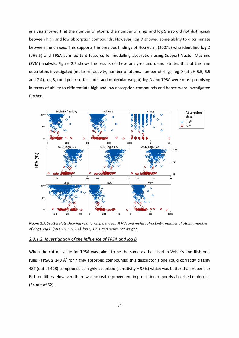
34

analysis showed that the number of atoms, the number of rings and log S also did not distinguish

between high and low absorption compounds. However, log D showed some ability to discriminate

between the classes. This supports the previous findings of Hou et al, (2007b) who identified log D

(pH6.5) and TPSA as important features for modelling absorption using Support Vector Machine

(SVM) analysis. Figure 2.3 shows the results of these analyses and demonstrates that of the nine

descriptors investigated (molar refractivity, number of atoms, number of rings, log D (at pH 5.5, 6.5

and 7.4), log S, total polar surface area and molecular weight) log D and TPSA were most promising

in terms of ability to differentiate high and low absorption compounds and hence were investigated

further.

Figure 2.3. Scatterplots showing relationship between % HIA and molar refractivity, number of atoms, number

of rings, log D (pHs 5.5, 6.5, 7.4), log S, TPSA and molecular weight.

2.3.1.2. Investigation of the influence of TPSA and log D

When the cut-off value for TPSA was taken to be the same as that used in Veber’s and Rishton’s

rules (TPSA ≤ 140 Å2 for highly absorbed compounds) this descriptor alone could correctly classify

487 (out of 498) compounds as highly absorbed (sensitivity = 98%) which was better than Veber’s or

Rishton filters. However, there was no real improvement in prediction of poorly absorbed molecules

(34 out of 52).

4002000

100

50

0

2001000 1050

100-10 100-10 100-10

100

50

0

0.0-2.5-5.0

100

50

0

4002000 16008000

MolarRefractivity

HIA

(%

)

NAtoms Nrings

ACD_LogD_5.5 ACD_LogD_6.5 ACD_LogD_7.4

LogS TPSA MW

high

low

class

Absorption

35

According to Hou et al., (2007b) log D values at pH 6.5 gave the best correlation with % HIA. They

suggested an approximate threshold value for log D6.5 of -3.2 log units (i.e. compounds with log D6.5

above -3.2 are well-absorbed and below -3.2 log units are poorly absorbed). The result of using log D

alone as a descriptor gave very similar results to using TPSA alone (sensitivity = 98% and specificity =

63%).

A combination of both TPSA and log D6.5 was considered to investigate whether the predictions for

the low absorption class could be improved; the results are shown in Figure 2.4. The threshold

values were kept at 140 Å2 for TPSA and -3.2 log units for log D6.5. Using this combination of TPSA

and log D descriptors improved specificity (80%), whilst the true positive rate remained at a high

level (96%). Applying a product of sensitivity and specificity as a statistical measure of performance

revealed that a filter based on TPSA and log D (pH 6.5) descriptors may give the most promising

results in terms of distinguishing between highly and poorly absorbed compounds (see Table 2.2). All

compounds (except for ceftizoxime) that had TPSA > 140 Å2 and log D6.5 ≤ -3.2 (i.e. 42 compounds in

total) were correctly predicted to be poorly absorbed (as shown in Figure 2.4). Ceftizoxime is a beta-

lactam and as such it may be absorbed by paracellular transport or be a substrate for the PepT1

transporter, as has been shown for ampicillin - another beta-lactam (Lafforque et al, 2008).

Table 2.2. Performance of selected filters for druglikeness as measured by a product of sensitivity and

specificity. Note: Filters based on Lipinski’s, Veber’s, Rishton’s, Ghose’s, Oprea’s and Walters’ rules were used

without allowing any rule violations.

Filter sensitivity specificity sens X spec

Lipinski 92% 63% 58%

Veber 94% 67% 63%

Rishton 87% 73% 63%

Ghose 84% 79% 66%

Oprea 64% 77% 50%

Walters 74% 71% 53%

TPSA 98% 65% 64%

logD 6_5 98% 63% 62%

TPSA_logD 6_5 96% 81% 78%

36

Figure 2.4. A scatterplot of log D 6.5 and TPSA for 550 compounds. Reference lines represent the cut-off values

used for log D and TPSA.

The results here indicate that the descriptors TPSA and logD6.5 may be useful for providing good

predictions for high versus low absorption, however, these preliminary findings should be validated

using an external dataset. Ideally, such a dataset should cover a wide range of values for both

descriptors, contain a large number of diverse structures and have an appropriate number of both

high and low absorption compounds. One of the problems in investigating HIA data is that is tends to

be skewed towards high absorption compounds, making modelling more problematic, as discussed

by Newby, Freitas, Ghafourian, (2013).

2.3.2. Relationship between in vivo, in vitro and in silico methods

2.3.2.1. Comparison of Caco-2 and % HIA data

Dataset B comprised measurements of permeability, assessed using Caco-2 cells, for 250

compounds. For 105 of these compounds HIA data were also available within Dataset A (taken from

Hou et al (2007b)). This enabled investigation into the extent to which Caco-2 data were predictive

of HIA data. Figure 2.5 illustrates the relationship between observed log Papparent values from Caco-2

assays and % HIA.

37

Figure 2.5. A scatterplot of % HIA versus Log Papparent (cm/s). N = 105. Compounds are classified as high

absorption (> 30% HIA; blue circles) or low absorption (≤ 30% HIA; red squares). Reference lines for 50% HIA

and log Papp -6 are also displayed.

The relationship between log Papp and HIA has previously been reported to be sigmoidal in

character (Artursson & Karlsson, 1991) although Hou et al (2007b) did not find a sigmoidal

relationship in their analysis. The vast majority of the compounds in this study belonged to the

category of highly absorbed molecules (HIA > 30%), which complicated the analysis of classification;

log Papparent spanned nearly 3.5 log units. Different threshold values for log Papp have previously

been suggested to be a criterion for good or poor absorption. Yee (1997) analysed 35 structurally

diverse compounds with % HIA ranging from 0% to 100%. He found a good correlation between in

vivo (oral) and in vitro (Caco-2) absorption and proposed a guideline for classifying compounds

according to their absorption, i.e. compounds with poor oral absorption have log Papparent < -6,

moderately absorbed compounds have a log Papp range of -6 ≤ log Papparent ≤ -5 and high oral

absorption compounds have log Papparent > -5. In that study HIA values of < 20% were classed as ‘low’

absorption, values above 70% HIA were high absorption and values between 20 and 70 were

considered as moderate. Other suggested threshold values, to differentiate between high and low

absorption, include: log Papparent = -5.69 (Gres et al, 1998), log Papparent = -6.15 (Rubas et al, 1993), log

Papparent = -4.69 (Stewart et al, 1995) and log Papparent = -5.25 (Hou et al, 2007b). Other authors (Ren &

Lien, 2000) indicated that log Papparent values below -5.3 may not form the basis for reliable

38

predictions of human gastro-intestinal (GI) absorption although above this threshold the absorption

is usually in a range of 50 – 100%. They also stated that experimental and inter-laboratory variability

may be responsible for a poor correlation between Caco-2 permeability and GI absorption especially

for compounds that are not very well absorbed.

It may be challenging to establish a Caco-2 permeability threshold value for this group of 105

compounds. One of the reasons is the previously mentioned lack of poorly absorbed chemicals. If

compounds with < 30% HIA are classed as low absorption, only four chemicals would fall into this

low absorption class. One way to overcome this issue was to redefine the classes. If the cut-off value

for poorly absorbed compounds is set at 50% HIA an additional eight compounds fall into this newly

defined ‘low’ absorption class. However, visual inspection of Figure 2.5 shows that for these

additional compounds no clear trend is distinguishable between log Papparent and % HIA.

Figure 2.5 shows a wide spread of HIA values for compounds with similar log Papp values, this serves

as an example of reliability issues in using log Papparent to predict % HIA for low absorption

compounds. Despite these reliability issues, some general trends could be observed. Compounds

with very high HIA tended to have a higher Caco-2 permeability. On the other hand, compounds with

HIA close to 0% also had low log Papparent values (refer to Figure 2.5). It was not possible to establish

conclusively the nature of the relationship between HIA and Caco-2 for this dataset or to define

threshold values to discriminate between high and low absorption. The plateau region in the top

right corner of Figure 2.

Although Figure 2.5 suggests that the relationship may have a sigmoidal character, this cannot be

verified as the bottom plateau cannot be determined due to the underrepresentation of poorly

absorbed compounds in this dataset. This shape may be expected when a rate variable (log Papparent)

is plotted against a fraction absorbed. In other words, highly absorbed compounds (approaching or

equal to 100%) may be absorbed at different rates but will still achieve 100% absorption provided

the rate is sufficiently rapid to allow for complete absorption.

The number of false negatives (defined as compounds with high log Papparent but low % HIA)

appearing in the top left corner of the Figure 2.5 suggests this particular Caco-2 model fails to

reliably distinguish between compounds of high and low HIA. However, to examine this hypothesis

fully, the dataset needs to be extended to consider a greater number of poorly absorbed

compounds.

39

The potential for in silico rules to give more accurate predictions for the compounds from this

dataset was investigated. As performed for the analysis of Dataset A, six druglikeness filters were

applied to the 105 compounds from Dataset B that had both % HIA and Caco-2 data associated with

them. Additionally, simple filters based on log D6.5 and TPSA (or combinations thereof) were used.

Finally, two filters based on different log Papparent threshold values were also utilised to enable a

comparison between purely in silico methods and those based on a hybrid of both in vitro and in

silico data. The results are presented in Table 2.3.

Table 2.3. Statistics for predictions of HIA class using selected filters. Filters I – VI are the same as applied for

Dataset A. Filters VII and VIII are: TPSA ≤140; logD6.5 ≥-3.2 respectively and filter IX is a combination of both

filters VII and VIII. The last two filters (X and XI) are based on in vitro Caco-2 permeability (log Papparent) with the

threshold values of -6 (Caco2_1) and -6.5 (Caco-2_2). TP = true positive; FP = false positive; TN = true negative;

FN = false negative; sens = sensitivity; spec = specificity; acc = accuracy.

Id Filter TP FP TN FN Sens(%) Spec(%) Acc(%) Sens x

spec(%)

I Lipinski 95 1 3 6 94.06 75.00 93.33 70.54

II Veber 96 1 3 5 95.05 75.00 94.29 71.29

III Rishton 91 1 3 10 90.10 75.00 89.52 67.57

IV Ghose 87 0 4 14 86.14 100.00 86.67 86.14

V Oprea 70 1 3 31 69.31 75.00 69.52 51.98

VI Walters 78 1 3 23 77.23 75.00 77.14 57.92

VII TPSA 97 1 3 4 96.04 75.00 95.24 72.03

VIII logD6.5 100 2 2 1 99.01 50.00 97.14 49.50

IX TPSA_logD6.5 96 1 3 5 95.05 75.00 94.29 71.29

X Caco2_1 85 0 4 16 84.16 100.00 84.76 84.16

XI Caco2_2 97 0 4 4 96.04 100.00 96.19 96.04

It is clear that some in silico methods show similar performance to filters based on Caco-2

permeability coefficients. This includes both Lipinski’s and Veber’s rules. Again, TPSA and logD6.5

descriptors appeared to be important, in a similar manner as that found for Dataset A. The rule

based on TPSA, where compounds with TPSA > 140 Å2 were considered to be poorly absorbed, could

predict the same number of true positives as a threshold of -6.5 for Caco-2 permeability coefficient.

TPSA was also able to predict 3 out of 4 compounds with low HIA values. The Caco-2 filter was

capable of identifying all poorly absorbed values – but it should be noted that both thresholds were

selected arbitrarily to obtain 100% specificity. The only true negative that was not identified by the

40

majority of in silico methods (with the exception of the Ghose filter) was Netivudine. However, this

antiviral drug had a HIA of 28% and therefore is on the borderline of the chosen threshold of 30%.

2.3.2.2. Comparison of PAMPA and % HIA data

Of the 105 compounds in Dataset C with log Papp data measured in PAMPA assays, 64 of these were

also present in Dataset A and therefore had % HIA data associated with them (taken from Hou et al

(2007b)). In the majority of cases, PAMPA permeability (PAMPA log Papparent) was measured at two

different pHs: 7.4 and 5.5. The relationship between PAMPA Log Papparent and % HIA was investigated

for all compounds where data for both were available. The analysis was performed using PAMPA

data measured at both pH 7.4 and pH 5.5 where possible.

Comparison of % HIA with PAMPA data obtained at pH7.4

Figure 2.6 shows the relationship between % HIA and PAMPA Log Papp (at pH7.4) for 64 compounds.

Only one compound known to have a poor oral absorption was present (Mitoxantrone). The

underrepresentation of poorly absorbed compounds did not allow a statistical analysis of predictions

of HIA based on PAMPA permeability.

Figure 2.6. A scatterplot of % HIA versus PAMPA log Papparent (at pH=7.4). HIA classes are defined as low

absorption (≤30% HIA; red square) and high absorption (> 30% HIA; blue circle)

-4.5-5.0-5.5-6.0-6.5-7.0-7.5-8.0

100

80

60

40

20

0

logPapp(cm/s)

HIA

(%

)

high

low

class

Absorption

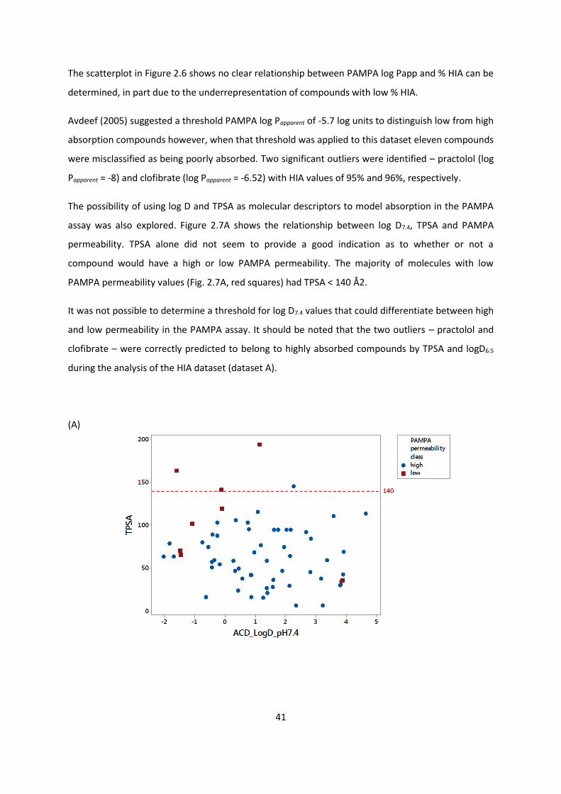
41

The scatterplot in Figure 2.6 shows no clear relationship between PAMPA log Papp and % HIA can be

determined, in part due to the underrepresentation of compounds with low % HIA.

Avdeef (2005) suggested a threshold PAMPA log Papparent of -5.7 log units to distinguish low from high

absorption compounds however, when that threshold was applied to this dataset eleven compounds

were misclassified as being poorly absorbed. Two significant outliers were identified – practolol (log

Papparent = -8) and clofibrate (log Papparent = -6.52) with HIA values of 95% and 96%, respectively.

The possibility of using log D and TPSA as molecular descriptors to model absorption in the PAMPA

assay was also explored. Figure 2.7A shows the relationship between log D7.4, TPSA and PAMPA

permeability. TPSA alone did not seem to provide a good indication as to whether or not a

compound would have a high or low PAMPA permeability. The majority of molecules with low

PAMPA permeability values (Fig. 2.7A, red squares) had TPSA < 140 Å2.

It was not possible to determine a threshold for log D7.4 values that could differentiate between high

and low permeability in the PAMPA assay. It should be noted that the two outliers – practolol and

clofibrate – were correctly predicted to belong to highly absorbed compounds by TPSA and logD6.5

during the analysis of the HIA dataset (dataset A).

(A)

42

(B)

Figure 2.7. Scatterplot of TPSA vs logD (pH 7.4) for 64 compounds found both in PAMPA and HIA datasets. (A)

Categories distinguished according to an arbitrary PAMPA log Papparent threshold (where low < -6). (B)

Categories according to HIA percentage thresholds (high >70%, 70% ≤ medium >30%, low ≤30%). It should be

noted that an additional class of medium HIA was distinguished for comparison purposes.

Comparison of %HIA with PAMPA data obtained at pH5.5

56 compounds with PAMPA log Papparent (pH = 5.5) were analysed. A similar general trend was

observed as for the PAMPA pH 7.4 dataset, namely higher log Papparent seemed to indicate a better

oral absorption. There was only one compound with a poor oral absorption, however, four other

compounds had the same log Papparent (= -7), yet they were either moderately or highly absorbed (see

Figure 2.8). Again, it was difficult to establish a threshold that would separate compounds into two

classes of absorption for the reasons stated previously. For the purpose of the analysis, a threshold

of PAMPA log Papparent = -6 was chosen where compounds were considered to have low absorption if

log Papparent < -6.

Similarly to the pH 7.4 PAMPA dataset, a TPSA cut-off of 140 Å2 could not distinguish high and low

PAMPA classes at the threshold of log Papparent = -6 (see Figure 2.9A). In this case applying the log D

cut-off of -3.2 was also not able to separate high from low absorption compounds.

The analysis of both PAMPA datasets (pH 5.5 and pH 7.4) seemed to suggest that artificial

membranes may be useful for identifying highly absorbed compounds; i.e. compounds that show

good absorption via PAMPA have high % HIA. However, compounds that are poorly absorbed via

PAMPA may be associated with either high or low % HIA. This result is not unexpected as PAMPA

permeability relates only to passive transport; drugs that undergo passive transport and are highly

43

absorbed are well predicted. However, it has previously been suggested that many drugs could rely

on a combination of active and passive transport mechanisms (Avdeef, 2005). These active transport

mechanisms cannot be replicated in the PAMPA assay, hence actively transported drugs may be

predicted to have low absorption although in reality % HIA is high.

Nevertheless, passive transport is an important way for drugs to enter the systemic circulation and

PAMPA may be a valuable tool for estimating oral absorption via this process.

Figure 2.8. A scatterplot of HIA (%) vs PAMPA log Papparent pH5.5 (cm/s). The HIA classes (high and low) were

colour coded (threshold = 30%).

(A)

44

(B)

Figure 2.9. Scatterplots of TPSA versus logD (pH 5.5) for 56 compounds found both in Datasets A and C.

(A) Categories according to arbitrary PAMPA log Papparent threshold (low < -6). (B) Categories according to HIA

percentage thresholds (high >70%, 70% ≤ medium >30%, low ≤30%). It should be noted that the medium HIA

class was distinguished for comparison purposes.

As PAMPA log Papp values were measured at two discrete pH values (for the majority of the

compounds in Dataset C) the question arose as to how the pH used in the PAMPA experiments could

influence the predictions of absorption. As the pH of the GIT varies, spanning a range of pHs from 2

to 8, using PAMPA log Papparent values taken at only one pH may be not sufficient to reliably predict

oral absorption. It has previously been suggested that log of a sum of PAMPA effective permeability

values, taken at three different pHs (5.0, 6.2 and 7.4) could be useful for discriminating high and low

absorption compounds in a “binning strategy” (Avdeef, 2005).

To investigate this further, the difference between log Papparent (at pH 7.4) and log Papparent (at pH 5.5)

for each compound containing both PAMPA permeability values was analysed; 51 compounds in

total (all having medium to high HIA). For 11 of these compounds the difference was > 0.5 log units.

In some cases, the correct predictions depended on pH-conditions under which the measurements

were taken. For instance, seven compounds were predicted to have low oral absorption based on a

threshold of PAMPA log Papparent = -6 at a pH of 5.5. However, for three of these compounds the

corresponding log Papparent at pH 7.4 correctly predicted high HIA. Five misclassified cases were

present when the predictions were made on PAMPA permeability values taken at pH 7.4 and, in

fact,one of these compounds was correctly predicted when a PAMPA log Papparent measured at pH 5.5

was used (see Table 2.4) .

45

Table 2.4. Misclassified compounds from dataset C.

Name HIA (%) HIA class log

Papparent

pH5.5

PAMPA

5.5

class

log Papparent

pH7.4

PAMPA

pH7.4

class

LogD

pH5.5

LogD

pH6.5

LogD

pH7.4

XlogP TPSA

Sulpiride 40 med -6.7 low -7 low -2.24 -1.83 -1.07 0.62 101.73

Acebutolol 85 high -6.7 low -5.48 high -1.27 -0.94 -0.24 1.68 87.66

Clofibrate 96 high -6.4 low -6.52 low 3.88 3.88 3.88 3.32 35.53

Sulfasalazine 62 med -6.52 low -7 low 0.02 -0.09 -0.10 4.51 141.31

Progesterone 96 high -6.1 low -5.4 high 3.83 3.83 3.83 3.47 34.14

Labetalol 95 high -7 low -5.35 high -0.30 0.11 0.80 2.52 95.58

Erythromycin 35 med -7 low -7 low -0.54 0.35 1.16 1.23 193.91

Bumetanide 96 high -5.34 high -6.52 low 1.32 0.44 -0.08 2.59 118.72

The PAMPA classes were based on a log Papparent threshold = -6. The HIA classes were: high >70%, 70% ≤ medium >30%, low ≤30%. TPSA,

XlogP and logD values predicted for three different pH conditions are also present. Green colour indicates compounds that were correctly

predicted by PAMPA log Papparent (at pH 7.4 or 5.5) to have a high % HIA.

Selected compounds present in Table 2.4 were further analysed in terms of their chemical

properties. Bumetanide was correctly predicted to have a high oral absorption by log Papparent at a pH

of 5.5. This compound could be categorised as an organic acid and as such it can be present in a

solution in an ionised or unionised form, depending on the pH. Analysis of the major microspecies

(Chemicalize, Chemaxon) showed that the unionised form (COOH) was prevalent at pH 4 but as pH

increased the deprotonated species (COO-) became more prevalent. These changes were reflected

in both log D values and PAMPA permeability. The neutral form was expected to be more lipophilic

(greater log D value at pH 5.5) and, therefore, more easily cross the PAMPA membrane. It shows

that a pH gradient needs to be considered when carrying out the PAMPA experiments so that

permeability coefficients are established for microspecies relevant to the GIT pH range. This also

supports the previous report that recommended using a combination of permeability coefficients as

a binning strategy (Avdeef, 2005). In addition, it should be mentioned that bumetanide can be

actively transported by proteins belonging to the class of monocarboxylate transporters (MCTs)

(Morris & Felmlee, 2008). This could account for the low value of PAMPA log Papparent despite high

bumetanide HIA (96%). Acebutolol and labetalol (beta-andrenergic antagonists) were correctly

predicted by PAMPA log Papparent 7.4 to be highly absorbed. Acebutolol is a base and a charged form

(with a protonated nitrogen) would be the prevalent species under GIT conditions where pH values

range from 1.7 in the stomach through ≈6.5 in jejunum and ileum to 8 in the colon (Avdeef, 2001).

Labetalol is an example of a zwitterionic ampholyte and at GIT pH it is present as a mixture of a

protonated and zwitterionic form. It is difficult to precisely calculate log D for zwitterions. The

contributions of such species to overall absorption could be negligible in comparison to the non-

charged form however such a contribution may be noticeable depending on the relative fraction

46

present among other microspecies (Mazak & Noszal, 2012). Nevertheless, log D accounts for a

mixture of species present at a given pH and for both acebutolol and labetalol the log D7.4 increased

by about one log unit when compared to log D5.5. An even more prominent increase was observed

for PAMPA log Papparent. Again, taking into account only one pH may not be sufficient to predict HIA.

Interestingly, progesterone had different permeability at pHs 5.5 and 7.4 despite the fact that it had

the same log D value, which suggested it was present in the unionised state. In this case, log D, log P

and TPSA would indicate that progesterone is a highly absorbed compound while PAMPA

experimental differences could lead to less reliable predictions.

It should be noted that when it comes more lipophilic compounds PAMPA permeability may depend

on log D in a bilinear fashion (Akamatsu et al, 2009). This is related to the presence of the unstirred

water layer (UWL) on both sides of the artificial membrane, which in turn may affect the rate and

extent of the absorption. Retention of compounds in the membrane could be also a factor

influencing oral absorption, i.e. compounds of medium to high lipophilicity (log D > 2) could partition

into a membrane but a lower fraction would then permeate into the cell. These factors are also

relevant to HIA. For instance, the aqueous boundary layer (ABL) present in the intestine can affect

the absorption significantly and the ABL effect should be identified and then its influence accounted

for when building an appropriate QSPR (Sugano, 2010). Factors such as the ABL effect are beyond

the scope of this study and will not be discussed further.

2.3.2.3. Comparison of HIA, Caco-2 and PAMPA

47 compounds that were common to Datasets A, B and C i.e. those for which HIA, Caco-2 and

PAMPA (pH = 7.4) data were all available were further investigated and used for comparative

analysis. Figure 2.10 shows the general trend that as log Papparent as measured in both PAMPA and

Caco-2 assays increases, % HIA also increases although outliers may introduce distortion to this

image. However, as previously discussed, data for compounds with lower HIA values are needed to

fully explore these trends and establish reliable thresholds as none of the 47 common compounds

studied here had a HIA value of < 30%.

Despite the obvious difficulties in modelling such data, an overall trend can be seen - both PAMPA

and Caco-2 are useful in identifying compounds that are highly absorbed. Compounds identified by

the assays as poorly absorbed may in fact demonstrate high % HIA because of processes such as

active transport which are not modelled by PAMPA and only modelled to a limited extent by Caco-2.

47

Figure 2.10. A contour plot of HIA (%), Caco-2 and PAMPA permeability.

The purpose of this study was to determine whether simple rules such as druglikeness filters or

combinations of “medicinal chemist”-type descriptors could classify compounds in terms of their

oral absorption (high or low) and investigate the usefulness of in vitro screening. Whilst Caco-2 and

PAMPA assays may provide useful screens, they still have the disadvantage of requiring

experimental measurements. Reliable in silico tools are more beneficial as screens because they can

be performed on virtual datasets. The results of the above analysis indicate that the in silico

methods used performed reasonably well in predicting the correct class for HIA (high or low); results

were comparable with, or in some cases superior to, results obtained from in vitro methods (Caco-2

and PAMPA) .

2.3.3. Metabolic contribution to bioavailability

For an orally administered drug to be useful, it is desirable that not only is absorption suitable but

also that the drug is not metabolised too extensively by first pass metabolism. Bioavailability is a

composite parameter, based on both absorption and avoidance of first pass metabolism. The final

part of this study was to investigate the influence of metabolism on overall bioavailability. For this

analysis a subset of 80 compounds from Dataset A was used, for which hepatic clearance values

were available from Thummel et al. (2005).

PAMPA logPapparent (cm/s) at pH7.4

Caco

-2 L

og

Pap

p (

cm

/s)

-5.0-5.5-6.0-6.5-7.0-7.5-8.0

-4.5

-5.0

-5.5

-6.0

-6.5

–

–

–

–

–

–

< 40

40 50

50 60

60 70

70 80

80 90

90 100

HIA (%)

48

2.3.3.1. Effect of clearance on bioavailability

The relationship between human oral bioavailability and % HIA taking into account the relative

hepatic clearance rate for the compounds is depicted in Figure 2.11. Bioavailability and % HIA data

are skewed towards highly bioavailable/highly absorbed compounds. However, the hepatic

clearance classes contained a similar number of compounds (high = 34 and low = 46). The

relationship between bioavailability and oral absorption is demonstrably influenced by the rate of

clearance. Compounds with high absorption and low clearance show high bioavailability, however

for compounds with extensive clearance bioavailability is reduced.

Figure 2.11. A scatterplot of bioavailability (% F) versus % HIA. Each compound was classified according to its

clearance: high clearance ≥ 7.5 ml/min/kg and low clearance is < 7.5 ml/min/kg. N= 80. For the description of

three compounds (high clearance class) circled in blue refer to the text below.

When only compounds with low clearance values, i.e. <7.5 ml/min/kg were analysed, a high

correlation coefficient (r = 0.7, p < 0.001) was obtained, which indicated that there was a strong

positive relationship between % F and % HIA. This indicates that, for compounds which are not

subject to extensive first-pass effect, bioavailability depends mostly on the extent of intestinal

absorption. On the other hand, no correlation between % F and % HIA was observed for compounds

with high clearance; although a few exceptions to this rule were noted. The position of three

compounds, belonging to the high clearance class (Figure 2.11, blue circles), shows that their

100806040200

100

80

60

40

20

0

HIA (%)

Hu

man

Ora

l F (

%)

low

high

class

Clearance

49

bioavailability correlated with their HIA. The clearance values for these compounds were either on

the borderline of the threshold of 7.5 ml/min/kg, or relatively close to this cut-off, for instance 9.9

(ml/min/kg) for nitrofurantoin. Also, nine compounds with low clearance values were found to have

large differences (> 20%) between % F and % HIA. Four of these compounds had very low clearance

values (< 1.3 ml/min/kg); clofibrate was of particular interest being an extreme example where HIA

was high (96%) and bioavailability was low (5%), however this large discrepancy could not be

accounted for by clearance as this was also low.

Of special interest were compounds with significant differences between % HIA and % F. As reported

by Hou et al (2007b) this difference may indicate a considerable effect of metabolism. Despite the

mentioned outliers, the majority of compounds (75% of the compounds for which the difference

between % HIA and % F was > 20%) belonged to the high clearance class. It is evident that the first-

pass effect contributed significantly to the reduced bioavailability for the studied compounds. Whilst

this result is predictable, given the nature of the bioavailability parameter, it was useful to

demonstrate that it applied to the data studied here so that the possibility of modelling

bioavailability by consideration of both absorption and clearance could be investigated.

2.3.3.2. Prediction of metabolic clearance

In this section of work two in silico methods were employed in an attempt to predict hepatic

metabolism, so that the effect of metabolism could be accounted for in overall prediction of

bioavailability.

Prediction of CYP isoform / SOM

Firstly, all 80 compounds from dataset D were grouped according to which cytochrome they were

most likely to bind to; this was carried out using the WhichCyp software. Only three enzymes were

considered: CYP3A4, CYP2D6 and CYP2C9. These enzymes are the most important in terms of drug

development as over 90% of drugs are metabolised by these three enzymes. These are the three

enzymes for which the SMARTCyp software could predict the probability of xenobiotic metabolism

occurring at a particular atom (site of metabolism; SOM). SMARTCyp calculates ranking scores by

considering such variables as energy of activation or accessibility. The top ranking atoms (highest

chances of being a SOM) are those with the lowest scores. Due to this interpretation it was

speculated that compounds with lower scores (for the top ranking atom) would have higher

clearance. 14 compounds were predicted to bind to 3A4 and there was a high negative correlation

between clearance and scores (Pearson coefficient = -0.75, p = 0.02). A similar analysis for

50

compounds predicted to be metabolised by CYP2D6 was also performed (n = 33). However, this time

a poor correlation (positive) between clearance values and ranking scores was observed. The same

analysis was also performed for CYP2C9, which resulted in obtaining a moderate negative

correlation (R = - 0.55, p = 0.052). It was apparent that this approach could not lead to identification

of compounds with high clearance.

There are several reasons why no reasonable correlation could be obtained. In many cases more

than one cytochrome may be involved in the metabolism of a given drug, so a given score for one

enzyme may not be representative of the complete metabolic profile. Additionally, only metabolism

related to the CYP family of enzymes was considered; these are involved in Phase I metabolism.

While cytochromes are known to be heavily involved in xenobiotic metabolism other enzymes can

also play a role, for instance those that facilitate the formation of conjugates in phase II metabolism.

Development of a QSAR model for clearance

A QSAR approach was also used to predict hepatic clearance. Li et al, (2009) built a successful

quantitative structure-hepatic clearance model for a dataset of 50 compounds. This regression

model was solely based on molecular descriptors (obtained using the TSAR software package, ver.

3.3). H-bond acceptor ability, energies of the highest occupied and lowest unoccupied molecular

orbitals (EHOMO and ELUMO) and torsional energy were identified as important features.

This section reports an attempt to build a similar model for the 80 compounds in this study using

descriptors calculated by MOE. Unfortunately, this attempt did not prove successful. All models that

were built using MLR or support vector machine for regression (SMOreg), did not compare

favourably with the model of Li et al. All R2 values obtained here were in the region of 50 % (specific

values were dependent on the Weka feature selection and classification method) whereas Li et al

obtained a value of 85% for their training set. In the study here, features that were found to be

correlated with clearance included LUMO energy (AM1 ELUMO) and various surface area/volume

(vsurf) and adjacency and distance matrix descriptors (for example petitjean), however, none of the

models were considered adequate to predict clearance

The reasons for the failure to obtain a model of similar predictive performance to that of Li et al are

possibly due to the differences between the datasets (only 18 compounds were common to both

studies) and the differences in software packages used for calculation of the molecular features. It

should be noted that MOE descriptors used here were of a similar type to those from TSAR (used by

Li et al) and the calculations were based on the same structure optimisation method (Hamiltonian,

51

AM1). Nevertheless, although the LUMO energy was found to be important in both models, HOMO

was not present in the model developed here. This suggests that building a robust model capable of

predicting hepatic clearance may be a challenging task and the applicability domain of such models

needs careful consideration.

Other efforts were made to establish in silico rules that could account for the differences between

HIA and bioavailability. Compounds were classified according to the difference () between % F and

% HIA ( >20% indicated metabolism has a significant influence on F; indicates metabolism

has little influence on F). The logistic regression model obtained included, similar to the clearance

QSAR, features related to surface, volume and shape of molecules (seven vsurf MOE descriptors) or

molecular density. The model correctly classified 72.5% of compounds. However, kappa statistics

(0.45) did not indicate strong predictive capability.

2.3.3.3. Other considerations

Other reasons for the difference between % F and % HIA were investigated. Metabolic capacity is an

important factor that influences clearance, which in turn affects bioavailability. However, clearance

can also be affected by plasma protein binding and the kinetics of this process (Baker & Parton,

2007). The degree to which this binding occurs is different for acids and bases, with acids showing

relatively higher binding than bases to human serum albumin (HSA) (Ghafourian & Amin, 2013). -1

acid glycoprotein is more important in binding neutral and basic drugs. The ability to enter

hepatocytes, and therefore be available for metabolism, is another factor to consider. The difference

between plasma pH (approximately 7.4) and the pH in the GIT can affect log D of a compound and

therefore alter the rate at which it crosses the hepatocyte membrane (assuming a passive

transport); this will affect rate and extent of metabolism.

The role of medicinal chemistry-type descriptors for prediction of bioavailability was also considered.

As previously shown, molecular features such as TPSA or log D could be considered very useful for

the prediction of druglikeness of compounds and implicitly HIA. Using simple threshold values can

provide rapid (not computationally intensive) and effective ways to screen for compounds that could

be potential drug candidates. This might be especially important when exploring a vast chemical

space. When it comes to prediction of human oral bioavailability these simple criteria may still hold

valid. In this dataset of 80 compounds, seven drugs had a bioavailability of < 20%; two of these

compounds had very low absorption (1% and 0%) and this was predicted by both TPSA and log D

descriptors. Five compounds had either high % HIA (over 90%) or medium % HIA (67%). All of these

compounds, except for clofibrate, had high clearance and TPSA and log D values within acceptable

52

boundaries. In two cases a greater value of log D at pH 7.4 might have contributed to better passive

permeability across hepatocyte membranes (potentially higher clearance). On the other hand, such

an increase in lipophilicity could also facilitate binding to plasma proteins and in turn affect the

metabolic rate (only unbound fraction can enter hepatocytes and be subject to metabolism).

However, for three other compounds log D values were not affected by pH yet, these three drugs

had poor % F to % FA ratios (the highest was 21%).

It is evident that prediction of bioavailability is a complex task; estimation of first-pass metabolic

effects is crucial to making accurate predictions. However, prediction of metabolism includes

predicting which CYP450 isoform(s) are involved, which are the potential SOM on the xenobiotic and

the kinetics of the reaction (dictating intrinsic clearance). One of the ways to approach this issue

could be the identification of structural features that are associated with high clearance/fast

metabolism. However, the CYP450 system is capable of binding a very broad range of structurally

diverse compounds. Such a lack of structural specificity may constitute a challenge for determination

of structural information important for high or low clearance. Building a large database of

compounds with known hepatic/intrinsic clearance values and then performing a similarity search

for an unknown compound could be useful.

***

In conclusion, the in silico methods studied here showed reasonable predictive performance in

determining which compounds belonged to the high or low class for HIA. The results were

comparable with (and in some cases better than) existing in vitro methods (i.e. Caco-2 and PAMPA

assays) but the in silico methods have the advantage of being much faster and more cost-effective.

In silico screens can be performed on virtual datasets early in the drug discovery process.

Attempts to build models to predict bioavailability were less successful. It was not possible to build a

model that could identify those compounds where % HIA was high but % F was low (which was

assumed to be related to metabolic effects). The simple rules for druglikeness (such as a

combination of TPSA and log D) although useful for the prediction of HIA, could not distinguish high

and low bioavailability.

Whilst the prediction of rate and extent of metabolism is of key importance to predicting

bioavailability, prediction of potential metabolites is also an important issue that will be investigated

in Chapter 3.

53

3. Pragmatic Approaches to Using Computational Methods

to Predict Metabolites

The results of this analysis have been published in Journal of Chemical Information and Modeling

(Piechota et al., 2013).1

3.1. Introduction

Prediction of xenobiotic metabolism is a research priority not only in drug development but also in

many other areas including cosmetic and food safety assessment and environmental studies. The

prediction of metabolism is important in the context of drugs’ efficacy. For example certain

pharmaceutical compounds require conversion from an inactive parent to an active metabolite.

However, the predominant reason for predicting metabolism is concern for consumer or

environmental safety as xenobiotics may be biotransformed to compounds that cause adverse

effects. Poor absorption, distribution, metabolism, excretion and toxicity (ADMET) properties of drug

candidates have resulted in high drug attrition rates in late stages of drug development and

withdrawal of drugs from the market due to adverse drug reactions (ADRs), resulting in great

financial and societal cost. Reactive metabolites formed by bioactivation may bind covalently to

biological macromolecules such as proteins leading to idiosyncratic drug toxicity, otherwise known

as type B ADRs (Kalgutkar et al., 2005). Hence, the pharmaceutical industry has implemented the

assessment of ADMET properties earlier in the drug development process which has already resulted

in significantly reduced attrition rates (Kerns & Li, 2008; Kruhlak et al., 2012).Other relevant factors

for the prediction of metabolism include identifying which enzymes may be involved in the

metabolism of specific drugs. For instance, one of the problems of an aging population is

polypharmacy and the potential for drug-drug interactions where the presence of one drug affects

the metabolism, and hence the in vivo concentration, of another. Drug-food or drug-herbal

interactions can similarly alter in vivo concentrations and knowledge of metabolic routes can help

predict such interactions. Therefore, there is a great deal of interest in predicting potential

metabolites and routes of metabolism for xenobiotics. This has resulted in a plethora of software

and techniques available to predict metabolism. Different methods provide alternative solutions to

1 Adapted with permission from: Piechota P, Cronin MT, Hewitt M, Madden JC. Pragmatic approaches to using computational methods to predict xenobiotic metabolism. J Chem Inf Model. 2013 Jun 24; 53(6):1282-93. doi: 10.1021/ci400050v. Copyright © 2013 American Chemical Society.

54

the problem and each is associated with advantages and disadvantages. Some methods are highly

computationally expensive, others may result in vast numbers of potential metabolites being

produced, where the true metabolites become obscured by too many data or other packages where

fewer of the true metabolites are predicted. Kirchmair et al., (2012) provide an excellent review of

the computational approaches to predicting metabolites and sites of metabolism. Table 3.1 lists

some of the methods available. There are many other methods available particularly with respect to

quantum chemical and docking approaches to predict likely sites of metabolism.

Table 3.1. In Silico Methods for the Prediction of Metabolites and Sites of Metabolism for Xenobiotics (adapted

from Kirchmair et al., 2012).

Prediction of

metabolites

Summary of method Website or key citation

META Uses a dictionary of biotransformations

to predict the structure of likely

metabolites. Analyses metabolite

stability.

Klopman, Dimayuga & Talafous, (1994)

Metabolexpert Uses rule-based knowledge to predict

likely metabolites in humans, animals or

plants.

http://www.compudrug.com/ ?q=node/

36

Metabolizer, (ChemAxon,

Budapest)

Includes libraries of biotransformation -

enumerates all possible metabolites,

predicts major metabolites, estimates

metabolic stability and supports species-

specific predictions of likely metabolites.

http://www.chemaxon.com/products/o

nline-tryouts/metabolizer/

Metaprint2D-React Predicts structures of metabolites based

on data-mining and statistical analysis –

refer to Metaprint2D below

http://www-

metaprint2d.ch.cam.ac.uk/metaprint2d-

react

MetaSite Considers enzyme-substrate recognition

and predicts metabolic transformations

for cytochrome-mediated reactions in

phase I metabolism. Provides the

structure of metabolites and provides a

ranking derived from estimated likelihood

of metabolic reaction at a given position.

http://www.moldiscovery.com/soft_me

tasite.php

Meteor Uses expert knowledge rules for

metabolism to predict metabolites which

https://www.lhasalimited.org/meteor/

55

are presented in metabolic trees

OECD QSAR Toolbox Contains both rat liver and skin

metabolism simulators in addition to

database of known biotransformations

https://www.qsartoolbox.org

SyGMa Predicts structures and probability of

metabolites based on rules derived from

Accelrys Metabolite Database

Ridder & Wagener, (2008)

TIMES (TIssue MEtabolism

Simulator)

A heuristic algorithm to generate

plausible metabolic maps from a

comprehensive library of

biotransformations and abiotic reactions

http://oasis-

lmc.org/?section=software&swid=4

Prediction of Sites of

Metabolism

Summary of method Website or key citation

ADMET Predictor –

Metabolite Module

Derives likelihood of metabolic reactions

occurring at specific atom positions;

identifies substrates for five CYP isoforms

http://www.simulations-

plus.com/Products.aspx?pID=13&mID=1

5

Metaprint2D Predicts sites of phase I xenobiotic

metabolism in dog, human and / or rat

through data-mining and statistical

analysis of known metabolic

transformations reported in literature.

http://www-

metaprint2d.ch.cam.ac.uk/metaprint2d

MetaSite See above - also predicts metabolites http://www.moldiscovery.com/soft_me

tasite.php

SMARTCYP Uses pre-calculated density functional

theory activation energies with

topological accessibility descriptors to

sites liable to cytochrome P450

metabolism.

http://www.farma.ku.dk/smartcyp/inde

x.php

StarDrop Combines quantum chemical analysis and

ligand-based model of CYP substrates to

estimate potential sites of metabolism

http://www.optibrium.com/stardrop/st

ardrop-p450-models.php

RS-WebPredictor Uses topological and quantum chemical

atom-specific predictors to identify sites

of metabolism. Regioselectivity models

http://reccr.chem.rpi.edu/Software/RS-

WebPredictor/

56

for substrates have been developed for

nine key CYP isozymes

Kirchmair et al., (2012) also listed many methods for the prediction of enzyme interactions, such as

binding affinity, inhibition and induction of cytochromes incorporating docking studies and binding

energy calculations. Such methods tend to be computationally expensive and were not considered in

the present study which focusses only on software to predict metabolites or sites of metabolism.

In general, metabolism results in chemical modification of xenobiotics so that they become more

polar and, therefore, more readily excreted via urine or bile. Phase I metabolism involves oxidation,

hydroxylation, de-amination and de-alkylation reactions which are catalysed by the cytochrome

P450 superfamily of enzymes with CYP3A4, CYP2D6 and CYP2C9 isoforms being responsible for the

majority of transformations for drugs. Phase II reactions yield hydrophilic conjugates, for example

glucuronides may be formed via the action of glucuronyl transferases. Phase II metabolism may

follow or be independent of phase I reactions. Hydrolysis and reduction reactions are also significant

in terms of metabolism. Metabolism is a highly complex process involving a multitude of

biotransformations that may occur consecutively, concurrently or in competition with each other.

Genetic and environmental factors can also affect the nature and abundance of metabolites making

prediction a difficult task. Nevertheless, software packages for prediction of metabolism are widely

used, particularly by the pharmaceutical industry, and especially during the screening phase of the

drug development process. Predictions made by the software may aid the development of drugs

with improved pharmacokinetic profiles and highlight potential metabolite induced toxicity (Sun &

Scott, 2010).

In 2002, the Metabolites in Safety Testing (MIST) committee defined how to approach metabolic

data when assessing the toxicity of drug candidates (Baillie et al., 2002); these guidelines were

subsequently modified (Smith & Obach, 2005). Because it is essential that the products of metabolic

pathways are considered for their potential toxicity, in silico methods to predict metabolism are

becoming increasingly important. Such methods need to be used with confidence, hence

performance and best practice in using the methods needs to be assessed.

To assess any software used for metabolism prediction, specific criteria should be established so that

the design of a particular package is taken into account. Due to differences between programs it is

not always possible to apply the same criteria to each program when assessing performance. Some

software (e.g. SMARTCYP Web Service) only provides sites of metabolism (SOM) rather than

metabolite structures. However, predicting SOM is not equivalent to identifying the correct

57

biotransformation that would take place at the particular atom. Prediction of SOM has been

successful with studies indicating up to 90% correct identification of the three most likely SOM.

However, prediction of the absolute likelihood of the formation of a certain metabolite is less

accurate (Kirchmair et al., 2012).

Where predicted metabolite structures are provided in the output of an algorithm, direct

comparison between different algorithms still may not be feasible. For example, some software may

only predict the outcome of Phase I, and not Phase II, metabolism or models may only consider

specific cytochrome P450 enzymes. Other issues affecting direct comparison of software packages

include selection of user-defined constraints such as species, probability level for a particular

metabolite being formed etc. Statistical analysis of predictions may provide a general indication of

algorithm performance, but comparisons between packages must be assessed with caution. The

underlying design and limitations of the software should be taken into consideration. Another

important consideration is the training set on which the software was developed; this information

may or may not be available. Output for a given package may reflect overall performance in

identifying metabolites but not give a true indication of predictive power of the model when faced

with unknown compounds. Therefore, a combination of the quantitative and qualitative assessment

of performance may be more informative. For example, investigating not only statistical values for

percentage metabolites correctly predicted, but also considering which metabolites are not

predicted e.g. if there are specific metabolic routes that are not identified in the software; this gives

scope for further improvements of algorithms. Clearly there are too many software routines of

diverse functionality and output to evaluate in a fully consistent manner.

The aim of the present study was to investigate the performance of three well-known,

representative, software packages for the prediction of metabolism. Performance was compared

between two different datasets. The first dataset (DS1) comprised 28 non-steroidal anti-

inflammatory drugs (NSAIDs) plus paracetamol, representing a homogenous chemical space. The

second dataset (DS2) comprised the first 30 drugs listed in the Top 200 Drugs for 2010 by Sales in the

United States, excluding drugs containing more than one active ingredient or peptides (Drugs.com,

2010). DS2 represented a more diverse chemical space than DS1 with a wider range of potential

metabolic biotransformations.

Investigation into the influence of modifying user-defined constraints was also carried out, for

appropriate packages, to enable recommendations to be made as to the most pragmatic software

settings for a given query.

58

The three software packages selected from those listed in Table 3.1 were:

(I) Meteor

This is an industry-standard, knowledge-based expert system developed by the not-for-profit

organisation Lhasa Limited, Leeds, England. Meteor (currently marketed by Lhasa Limited as Meteor

Nexus) predicts metabolites from the structure of the parent compound, based on an extensive set

of biotransformation rules which have been extracted from the literature or informed by

confidential data from the pharmaceutical industry. It uses two types of reasoning: absolute

reasoning describes the probability of a biotransformation taking place (in terms of probable,

plausible, equivocal, doubted and improbable) and relative reasoning that allows further ordering of

all possible metabolic outcomes in cases when there are competing biotransformations at a given

SOM (Marchant, Briggs & Long, 2008).

(II) Metaprint2D / Metaprint2D-React

Metaprint2D is a freely available algorithm that predicts the likelihood of a metabolic reaction

occurring at a given position in the molecule, using a circular fingerprints technique. Circular

fingerprints are used to represent the chemical environment of an atom. They are generated by

using concentric layers that radiate out from a central atom and then store information about the

number and types of atoms in each layer. The first layer contains only a central atom, the second

layer includes the direct neighbours of the central atom and the consecutive layer contains atoms

that are directly bonded to the atoms in the second layer. Circular fingerprints used by

MetaPrint2D can be based on up to six layers. To predict sites of metabolism, MetaPrint2D utilises

data found in the Symyx® Metabolite database, which is a collection of 80,000 xenobiotic

transformations (predominantly for pharmaceuticals) collated from the literature. The predictions

are obtained by generating fingerprints for the query compound and then comparing these using a

similarity search against two databases of fingerprints. The first of the two databases contains

fingerprints calculated for all the substrate atoms present in transformations found in the Symyx®

Metabolite database, whilst the second database contains fingerprints for only those atoms from

the Symyx® database that are known to be sites of metabolism (reaction centres). The results of

the similarity search for each atom of the query compound are reported as the occurrence ratio

which measures how often a similar chemical environment was found at a reaction centre relative

to all occurrences of similar environment in the Symyx® Metabolite database. Metaprint2D-React

59

is an extension of Metaprint2D that can provide structures of potential metabolites associated

with reaction at the identified positions (Carlsson et al., 2010; Adams, 2010).

(III) SMARTCyp

This software determines the sites in a molecule liable to metabolism using the 2D structure of the

compound and calculations of energies required for oxidation. These are matched against pre-

calculated activation energies for fragments represented as SMARTS patterns (Rydberg et al., 2010).

SMARTCyp uses two descriptors to predict a site of metabolism: reactivity (E) and accessibility (A).

The reactivity descriptor is based on transition state energies calculated for fragments using density

functional theory. The calculations are grouped by fragments and then average activation energies

are obtained and defined as SMARTS rules for each group. The accessibility is described as the

distance of the atom from the centre of the molecule. Both reactivity and accessibility descriptors

are used to obtain a score for each atom; an atom with the lowest score is ranked as the most likely

site of metabolism (Rydberg et al., 2010). Currently, CYP3A4, CYP2C9 and CYP2D6 are the only

models available in SMARTCyp.

3.2. Methods

3.2.1. Datasets

Dataset 1 (DS1) and dataset 2 (DS2) were chosen to represent homogenous and diverse drugs

respectively, in terms of action, structure and metabolic transformation. DS1 comprised 28

commonly used NSAIDs and paracetamol; DS2 comprised 30 drugs taken from the Top 200 drugs in

2010 by sales in the United States. The top 30 drugs in the list (excluding peptides) were considered;

if a drug comprised more than one active ingredient each of them were included providing they

were subject to CYP450 metabolism.

3.2.2. Collecting and storing metabolism data

A thorough literature search was performed to obtain the known in vivo metabolites, in humans, for

the 59 drugs considered in this study. Sources of information (see Appendix V) included original

research papers, reviews and online databases such as: Martindale: The Complete Drug Reference

60

and Clarke’s Analysis of Drugs and Poisons. As some of the predictive software investigated here

(such as SMARTCyp) was not designed to predict Phase II metabolites, data collection focused on

Phase I metabolism only.

The complete list of known metabolites found in the literature are available as supplementary

information (see Appendices VI and VII).

The structures of all parent drugs and metabolites were drawn in MarvinSketch, version 5.0.3

(Chemaxon) and stored in mol format. Information concerning the specific CYP450 isoform(s)

involved in biotransformations for DS2 was also recorded and is also available as supplementary

data.

In total, 78 known metabolites for DS1 and 101 known metabolites for DS2 were obtained from the

literature.

Table 3.2 lists the common names for the drugs used in this study along with their Chemical

Abstracts Service Registration Number (CAS RN), International Union of Pure and Applied Chemistry

(IUPAC) name and the number of phase I metabolites retrieved from the literature for each drug.

The Supporting Information Available also gives the SMILES strings for the parent drugs and their

known phase I metabolites.

Table 3.2. Common names, CAS registry numbers, IUPAC names and number of phase I metabolites obtained

from the literature for drugs used in datasets 1 and 2 in this study.

Dataset 1

Common Name CAS RN IUPAC Name No. of

metabolites

Alclofenac 22131-79-9 [4-(Allyloxy)-3-chlorophenyl]acetic acid 3

Aspirin 50-78-2 2-Acetoxybenzoic acid 3

Azapropazone 13539-59-8 5-(Dimethylamino)-9-methyl-2-propyl-1H-pyrazolo[1,2-

a][1,2,4]benzotriazine-1,3(2H)-dione

2

Bromfenac 91714-94-2 [2-Amino-3-(4-bromobenzoyl)phenyl]acetic acid 3

Carprofen 52263-47-5 2-(6-Chloro-9H-carbazol-2-yl)propanoic acid 3

Diclofenac 15307-86-5 {2-[(2,6-Dichlorophenyl)amino]phenyl}acetic acid 6

Diflunisal 22494-42-4 2',4'-Difluoro-4-hydroxy-3-biphenylcarboxylic acid 1

Fenbufen 36330-85-5 4-(4-Biphenylyl)-4-oxobutanoic acid 4

Fenclofenac 34645-84-6 [2-(2,4-Dichlorophenoxy)phenyl]acetic acid 1

61

Fenoprofen 31879-05-7 2-(3-Phenoxyphenyl)propanoic acid 1

Feprazone 30748-29-9 4-(3-Methyl-2-buten-1-yl)-1,2-diphenyl-3,5-

pyrazolidinedione

1

Flufenamic acid 530-78-9 2-{[3-(Trifluoromethyl)phenyl]amino}benzoic acid 3

Flurbiprofen 5104-49-4 2-(2-Fluoro-4-biphenylyl)propanoic acid 3

Ibuprofen 15687-27-1 2-(4-Isobutylphenyl)propanoic acid 4

Indomethacin 53-86-1 [1-(4-Chlorobenzoyl)-5-methoxy-2-methyl-1H-indol-3-

yl]acetic acid

3

Ketoprofen 22071-15-4 2-(3-Benzoylphenyl)propanoic acid 3

Ketorolac 66635-83-4 5-Benzoyl-2,3-dihydro-1H-pyrrolizine-1-carboxylic acid 1

Mefenamic acid 61-68-7 2-[(2,3-Dimethylphenyl)amino]benzoic acid 2

Nabumetone 42924-53-8 4-(6-Methoxy-2-naphthyl)-2-butanone 5

Naproxen 22204-53-1 (2S)-2-(6-Methoxy-2-naphthyl)propanoic acid 1

Paracetamol 103-90-2 N-(4-Hydroxyphenyl)acetamide 3

Phenylbutazone 50-33-9 4-Butyl-1,2-diphenyl-3,5-pyrazolidinedione 3

Piroxicam 36322-90-4 4-Hydroxy-2-methyl-N-(2-pyridinyl)-2H-1,2-benzothiazine-

3-carboxamide 1,1-dioxide

1

Pirprofen 31793-07-4 2-[3-Chloro-4-(2,5-dihydro-1H-pyrrol-1-

yl)phenyl]propanoic acid

5

Sulindac 38194-50-2 {(1Z)-5-Fluoro-2-methyl-1-[4-(methylsulfinyl)benzylidene]-

1H-inden-3-yl}acetic acid

2

Suprofen 40828-46-4 2-[4-(2-Thienylcarbonyl)phenyl]propanoic acid 5

Tiaprofenic acid 33005-95-7 2-(5-Benzoyl-2-thienyl)propanoic acid 2

Tolmetin 26171-23-3 [1-Methyl-5-(4-methylbenzoyl)-1H-pyrrol-2-yl]acetic acid 2

Zomepirac 33369-31-2 [5-(4-Chlorobenzoyl)-1,4-dimethyl-1H-pyrrol-2-yl]acetic

acid

2

Dataset 2

Aripiprazole 129722-12-9 7-{4-[4-(2,3-Dichlorophenyl)-1-piperazinyl]butoxy}-3,4-

dihydro-2(1H)-quinolinone

5

Atorvastatin 110862-48-1 (3R,5R)-7-[2-(4-Fluorophenyl)-5-isopropyl-3-phenyl-4-

(phenylcarbamoyl)-1H-pyrrol-1-yl]-3,5-

dihydroxyheptanoic acid

5

Buprenorphine 52485-79-7 (5α,6β,14β,18R)-17-(Cyclopropylmethyl)-18-[(2S)-2-

hydroxy-3,3-dimethyl-2-butanyl]-6-methoxy-18,19-

dihydro-4,5-epoxy-6,14-ethenomorphinan-3-ol

1

62

Celecoxib 169590-42-5 4-[5-(4-Methylphenyl)-3-(trifluoromethyl)-1H-pyrazol-1-

yl]benzenesulfonamide

2

Clopidogrel 90055-48-4 Methyl (2S)-(2-chlorophenyl)(6,7-dihydrothieno[3,2-

c]pyridin-5(4H)-yl)acetate

3

Donepezil 120011-70-3 Methyl (2S)-(2-chlorophenyl)(6,7-dihydrothieno[3,2-

c]pyridin-5(4H)-yl)acetate

4

Duloxetine 116539-58-3 (3S)-N-Methyl-3-(1-naphthyloxy)-3-(2-thienyl)-1-

propanamine

11

Efavirenz 154635-17-3 (4S)-6-Chloro-4-(cyclopropylethynyl)-4-(trifluoromethyl)-

1,4-dihydro-2H-3,1-benzoxazin-2-one

3

Emtricitabine 143491-57-0 4-Amino-5-fluoro-1-[(2R,5S)-2-(hydroxymethyl)-1,3-

oxathiolan-5-yl]-2(1H)-pyrimidinone

1

Escitalopram 59729-33-8 (1S)-1-[3-(Dimethylamino)propyl]-1-(4-fluorophenyl)-1,3-

dihydro-2-benzofuran-5-carbonitrile

5

Esomeprazole 73590-58-6 6-Methoxy-2-{(S)-[(4-methoxy-3,5-dimethyl-2-

pyridinyl)methyl]sulfinyl}-1H-benzimidazole

5

Ezetimibe 163222-33-1 (3R,4S)-1-(4-Fluorophenyl)-3-[(3S)-3-(4-fluorophenyl)-3-

hydroxypropyl]-4-(4-hydroxyphenyl)-2-azetidinone

1

Fenofibrate 49562-28-9 Isopropyl 2-[4-(4-chlorobenzoyl)phenoxy]-2-

methylpropanoate

2

Fluticasone

propionate

80474-14-2 (6α,11β,16α,17α)-6,9-Difluoro-17-

{[(fluoromethyl)sulfanyl]carbonyl}-11-hydroxy-16-methyl-

3-oxoandrosta-1,4-dien-17-yl propionate

1

Levofloxacin 100986-85-4 (3S)-9-Fluoro-3-methyl-10-(4-methyl-1-piperazinyl)-7-oxo-

2,3-dihydro-7H-[1,4]oxazino[2,3,4-ij]quinoline-6-carboxylic

acid

2

Methylphenidate 113-45-1 Methyl phenyl(2-piperidinyl)acetate 6

Modafinil 68693-11-8 2-[(Diphenylmethyl)sulfinyl]acetamide 2

Montelukast 158966-92-8 {1-[({(1R)-1-{3-[(E)-2-(7-Chloro-2-quinolinyl)vinyl]phenyl}-

3-[2-(2-hydroxy-2-

propanyl)phenyl]propyl}sulfanyl)methyl]cyclopropyl}acetic

acid

5

Naloxone 465-65-6 (5α)-17-Allyl-3,14-dihydroxy-4,5-epoxymorphinan-6-one 2

Olanzapine 132539-06-1 (5α)-17-Allyl-3,14-dihydroxy-4,5-epoxymorphinan-6-one 6

Oxycodone 76-42-6 (5α)-14-Hydroxy-3-methoxy-17-methyl-4,5-

epoxymorphinan-6-one

3

63

Pioglitazone 111025-46-8 5-{4-[2-(5-Ethyl-2-pyridinyl)ethoxy]benzyl}-1,3-

thiazolidine-2,4-dione

6

Pregabalin 148553-50-8 (3S)-3-(Aminomethyl)-5-methylhexanoic acid 1

Quetiapine 111974-69-7 2-{2-[4-(Dibenzo[b,f][1,4]thiazepin-11-yl)-1-

piperazinyl]ethoxy}ethanol

5

Rosuvastatin 287714-41-4 (3R,5S,6E)-7-{4-(4-Fluorophenyl)-6-isopropyl-2-

[methyl(methylsulfonyl)amino]-5-pyrimidinyl}-3,5-

dihydroxy-6-heptenoic acid

2

Salmeterol 89365-50-4 2-(Hydroxymethyl)-4-(1-hydroxy-2-{[6-(4-

phenylbutoxy)hexyl]amino}ethyl)phenol

2

Sildenafil 139755-83-2 5-{2-Ethoxy-5-[(4-methyl-1-piperazinyl)sulfonyl]phenyl}-1-

methyl-3-propyl-1,4-dihydro-7H-pyrazolo[4,3-d]pyrimidin-

7-one

4

Sitagliptin 486460-32-6 (3R)-3-Amino-1-[3-(trifluoromethyl)-5,6-

dihydro[1,2,4]triazolo[4,3-a]pyrazin-7(8H)-yl]-4-(2,4,5-

trifluorophenyl)-1-butanone

1

Valsartan 137862-53-4 N-Pentanoyl-N-{[2'-(2H-tetrazol-5-yl)-4-

biphenylyl]methyl}-L-valine

1

Venlafaxine 93413-69-5 1-[2-(Dimethylamino)-1-(4-

methoxyphenyl)ethyl]cyclohexanol

4

3.2.3. Use of software

(I) Meteor

Meteor, version 13, Lhasa Limited, Leeds, England was used to predict metabolites for both datasets.

The parent structures were submitted as mol format and the resulting metabolites were stored as

Meteor generic files (mtr). As stated previously, Meteor employs two types of reasoning - absolute

and relative.

With regard to absolute reasoning, three levels were selected in this analysis: probable, plausible

and equivocal (doubted and improbable were not considered). For each of these three levels of

absolute reasoning, three levels of relative reasoning were considered: levels 1, 2 and 3.

Table 3.3 shows the nine combinations of reasoning employed and the abbreviations for these that

will be used throughout this paper.

64

Table 3.3. Combinations of reasoning used in Meteor and abbreviations utilised in this paper

Absolute Reasoning Relative Reasoning 1 Relative Reasoning 2 Relative Reasoning 3

Probable PRO1 PRO2 PRO3

Plausible PLA1 PLA2 PLA3

Equivocal EQU1 EQU2 EQU3

All the other parameters selected from the option “Processing Constraints” were kept constant for

all combinations of reasoning. Processing constraints were: phase option = phase I only; species =

human; enzyme = not specified; max number of metabolites = 400; max number of steps in a

pathway = 4.

The presence of known metabolites for DS1 and DS2 was identified by means of the Meteor

functionality that allows direct searching for structures in a metabolic tree (mol format). All the true

positives (i.e. known metabolites from the literature that were correctly predicted by the software)

along with their positions in the Meteor metabolic tree were recorded and saved in a Microsoft

Excel spreadsheet. In the first part of the analysis described here, the percentage of known

metabolites that were correctly predicted within each metabolic tree (of up to 400 metabolites) for

each compound in DS1 and DS2 was calculated using reasoning level EQU3.

Further analysis was subsequently undertaken to establish the sensitivity for each of the nine

reasoning settings given in Table 3.2 by taking into account the number of metabolites correctly

predicted at different cut-off points. The cut-off points were 5, 10, 15, 20, 25, 30, 35, 40 and 400 and

refer to the number of predicted metabolites appearing sequentially in the metabolic tree that were

subsequently checked against structures of known metabolites. For example, using a cut-off value of

20 means that only the first 20 metabolites appearing in the Meteor tree of predicted metabolites

were considered; a cut-off value of 400 means that all 400 predicted metabolites were checked

against known metabolites to determine if the known metabolite had been predicted. The purpose

of this was to investigate the most pragmatic use of the Meteor software. Whilst it is possible to

generate 400 metabolites, investigation into the structure of each of these (as may be performed for

subsequent estimation of metabolite toxicity) is a very time-consuming process. It was considered

useful to determine whether or not it was possible to identify the majority of known metabolites

within the first 5, 10 or 20 etc. metabolites that appear in the highest positions of the metabolic

tree(s), to increase the efficiency of using the program.

65

(II) MetaPrint2D-React

The structures of the parent drugs were entered as SMILES strings into the MetaPrint2D-React web-

service software at the following URL: http://www-metaprint2d.ch.cam.ac.uk/metaprint2d-react/.

Fingerprint matching was set to a default value and the human model was selected. The resulting

predictions for metabolite structures were compared to known metabolites.

(III) Combination of SMARTCyp and MetaPrint2D-React

A subset of metabolites from DS2 that are known to be products of CYP3A4 or CYP2D6 metabolism

were identified from the literature. 39 of the metabolites from DS2 are known to be products of

CYP3A4 and 11 of the metabolites are known to be products of CYP2D6.

For each parent drug contained in this subset of data the following steps were followed. The parent

structure was submitted as a SMILES string to the SMARTCyp Web Service version 2.0; URL:

http://www.farma.ku.dk/smartcyp/. SMARTCyp was used to identify the top five ranking atoms (in

terms of most likely site of metabolism) for both CYP3A4 and CYP2D6. The parent structure of the

drug was then submitted as a SMILES string into the MetaPrint2D-React program. (URL: http://www-

metaprint2d.ch.cam.ac.uk/metaprint2d-react/); fingerprint matching was set to the default value

and the human model was selected. The output was analysed in terms of biotransformations

occurring at the atoms corresponding to the SOM previously predicted as being in the top five

ranked sites by SMARTCyp. The metabolites predicted from biotransformations at these sites were

compared to known metabolites. The procedure was repeated using only the top three ranked SOM

from SMARTCyp. This process is outlined in Figure 3.1.

66

Figure 3.1. Flow diagram showing the method to predict metabolites using a combination of SMARTCyp

(models for CYP3A4 and CYP2D6) and Metaprint2D-React.

3.2.4. Statistical analysis

The performance of Meteor and MetaPrint2D-React was assessed in terms of the number of

correctly predicted metabolites (sensitivity) and was calculated according to the following formula:

Sensitivity (%) = ([TP] / TOTAL invivo) *100%

Precision in the context used here was calculated as:

Precision (%) = [TP] / ([TP] + [FP]) * 100%

TOTAL invivo = total number of known metabolites observed (from in vivo literature data)

TP = No. of correct predictions (predicted metabolites that are also observed in vivo)

FP = No. of incorrect predictions (predicted metabolites that are not observed in vivo)

67

3.3. Results and discussion

3.3.1. General performance of the algorithms

Two datasets were used to analyse performance of different software in predicting metabolites and

sites of metabolism and to investigate pragmatic approaches to using the software. Dataset 1 (DS1)

was a more chemically homogenous set of 28 NSAIDs and paracetamol for which a total of 78 known

metabolites had been identified from a literature search. Dataset 2 (DS2) was a more diverse set of

30 drugs for which 101 metabolites had been identified in the literature. Figure 3.2 shows an

example of results for aripiprazole (and its five known metabolites) for illustrative purposes, along

with the predictions from Meteor and MetaPrint2D. Note that M1, M4 and M5 were not predicted

by Meteor when the probable (PRO) absolute reasoning engine was used.

Figure 3.2. Known metabolites of aripiprazole and the predictions obtained by Meteor and MetaPrint2D-React.

Table 3.4 shows the overall performance of the software packages in predicting the known

metabolites (as obtained from the literature) for DS1 and DS2.

68

Table 3.4. Performance of Meteor and Metaprint2D-React in Predicting Metabolites of datasets 1 and 2.

Software No. metabolites correctly

predicted for DS1

No. metabolites correctly

predicted for DS2

Meteor (setting EQU3) 57 (73%) 86 (85%)

Metaprint2D-React 62 (80%) 90 (89%)

Note that this analysis was carried out in order to obtain a general indication of performance and

compare the number of correct predictions that are obtained when using two different datasets

(one homogenous, one diverse). The results are not a true measure of overall predictivity of the

software used as it is likely that the drugs analysed are present to a greater or lesser extent in the

information used to develop the individual software packages.

Meteor and Metaprint2D-React both show good performance in predicting metabolites for datasets

DS1 and DS2. What is interesting to note is that in all cases predictions were marginally better for

the diverse dataset (DS2) than for the more homogenous dataset (DS1). This suggests that areas of

chemical space more predominant in one set of compounds may not be as well represented in the

training sets for the software than other areas. For example, none of the software packages

predicted the metabolites of the NSAID bromfenac. The metabolites of bromfenac are dependent on

the formation of a cyclic amide metabolite which was not predicted by the software tested.

Similarly, two metabolites of nabumetone and one metabolite of suprofen were not predicted by

any of the software indicating a possible knowledge gap in metabolite prediction. Such information

can be used to direct future improvements in software development. Aside from these examples, for

DS1 72 of the metabolites (i.e. 92%) were predicted by at least one of the software packages (or

combination of packages).

Cases where specific metabolites were not found by any of the packages studied also occurred for

DS2. They include: three metabolites of clopidogrel, two metabolites of pioglitazone and one

metabolite of sitagliptin which gave a total of 6 out of 101. Thus, 96 metabolites (95%) were

predicted by at least one of the packages used in the study.

3.3.2. Pragmatic approach to using Meteor

Table 3.5 shows the results of the predictions for the Meteor software where nine different

reasoning levels were investigated for the prediction of metabolites of DS1. The cut-off values in row

1 show the number of metabolites that were checked against known metabolites e.g. a cut-off value

69

of five indicates the first five metabolites only in the metabolic tree for each compound were

checked; for DS1 78 metabolites had been identified from the literature.

Table 3.5. Predictions from Meteor for dataset 1 using nine settings for reasoning (as defined in Table 3.3) and

nine cut-off values.

Cut-off

values 5 10 15 20 25 30 35 40 400

N % N % N % N % N % N % N % N % N %

PRO1 6 8 7 9 7 9 7 9 7 9 7 9 7 9 7 9 7 9

PRO2 7 9 8 10 8 10 8 10 8 10 8 10 8 10 8 10 8 10

PRO3 7 9 8 10 8 10 8 10 8 10 8 10 8 10 8 10 8 10

PLA1 33 42 39 50 39 50 39 50 39 50 39 50 39 50 39 50 39 50

PLA2 37 47 45 58 46 59 46 59 46 59 46 59 46 59 46 59 46 59

PLA3 37 47 45 58 46 59 46 59 46 59 46 59 46 59 46 59 46 59

EQU1 37 47 46 59 47 60 48 62 48 62 48 62 48 62 48 62 48 62

EQU2 41 53 49 63 52 67 54 69 55 71 55 71 55 71 55 71 55 71

EQU3 41 53 48 62 51 65 54 69 56 72 57 73 57 73 57 73 57 73

N = number of correctly predicted metabolites; % = percentage of correctly predicted metabolites.

Trends in the data shown in Table 3.5 can be more clearly visualised graphically as shown in Figure

3.3

Figure 3.3. Meteor predictions for DS1 showing the variation in number of metabolites correctly predicted as a

function of cut-off values and reasoning levels selected.

0%

10%

20%

30%

40%

50%

60%

70%

80%

5 10 15 20 25 30 35 40 400

% o

f co

rre

ctly

pre

dic

ted

me

tab

olit

es

Cut-off values for number of metabolites

PR1

PR2

PR3

PL1

PL2

PL3

EQ1

EQ2

EQ3

70

Table 3.6 shows the results of the Meteor predictions for DS2 using nine reasoning settings and nine

cut-off values; for DS2 101 metabolites had been identified from the literature.

Table 3.6. Predictions from Meteor for dataset 2 using nine settings for reasoning (as defined in Table 3.3) and

nine cut-off values.

Cut-off

values 5 10 15 20 25 30 35 40 400

N % N % N % N % N % N % N % N % N %

PRO1 27 27 28 28 29 29 29 29 29 29 29 29 29 29 29 29 29 29

PRO2 27 27 30 30 32 32 32 32 32 32 32 32 32 32 32 32 32 32

PRO3 27 27 30 30 32 32 32 32 32 32 32 32 32 32 32 32 32 32

PLA1 37 37 52 51 57 56 60 59 60 59 61 60 61 60 62 61 62 61

PLA2 37 37 58 57 67 66 69 68 71 70 73 72 74 73 74 73 75 74

PLA3 37 37 57 56 68 67 70 69 71 70 74 73 75 74 75 74 76 75

EQU1 39 39 58 57 64 63 67 66 68 67 69 68 69 68 70 69 70 69

EQU2 42 42 57 56 71 70 74 73 76 75 77 76 79 78 80 79 84 83

EQU3 42 42 56 55 67 66 73 72 78 77 80 79 81 80 82 81 86 85

N = number of correctly predicted metabolites; % = a percentage of correctly predicted metabolites.

Similarly to dataset 1 the results for the analysis can be visualised graphically as shown in Figure 3.4.

Figure 3.4. Meteor predictions for DS2 showing the variation in number of metabolites correctly predicted as a

function of cut-off values and reasoning levels selected.

0%

10%

20%

30%

40%

50%

60%

70%

80%

90%

5 10 15 20 25 30 35 40 400

% o

f co

rre

ctly

pre

dic

ted

me

tab

olit

es

Cut-off values for number of metabolites

PR1

PR2

PR3

PL1

PL2

PL3

EQ1

EQ2

EQ3

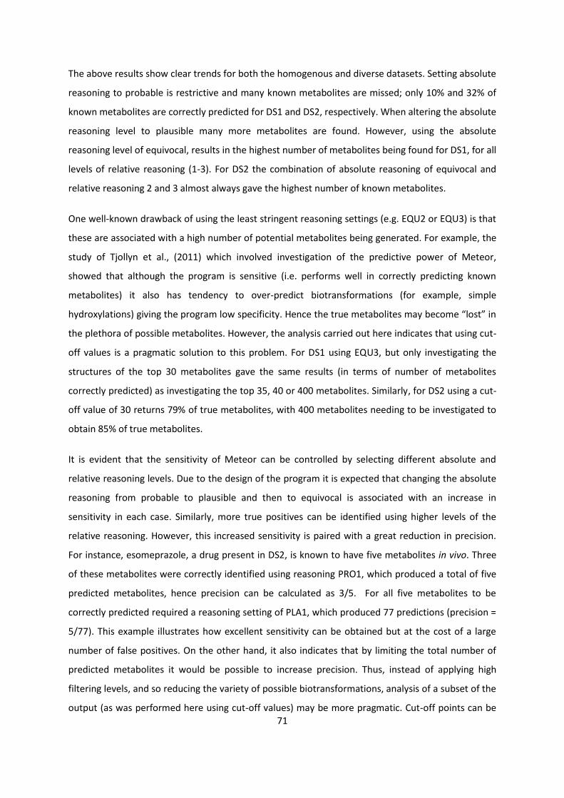
71

The above results show clear trends for both the homogenous and diverse datasets. Setting absolute

reasoning to probable is restrictive and many known metabolites are missed; only 10% and 32% of

known metabolites are correctly predicted for DS1 and DS2, respectively. When altering the absolute

reasoning level to plausible many more metabolites are found. However, using the absolute

reasoning level of equivocal, results in the highest number of metabolites being found for DS1, for all

levels of relative reasoning (1-3). For DS2 the combination of absolute reasoning of equivocal and

relative reasoning 2 and 3 almost always gave the highest number of known metabolites.

One well-known drawback of using the least stringent reasoning settings (e.g. EQU2 or EQU3) is that

these are associated with a high number of potential metabolites being generated. For example, the

study of Tjollyn et al., (2011) which involved investigation of the predictive power of Meteor,

showed that although the program is sensitive (i.e. performs well in correctly predicting known

metabolites) it also has tendency to over-predict biotransformations (for example, simple

hydroxylations) giving the program low specificity. Hence the true metabolites may become “lost” in

the plethora of possible metabolites. However, the analysis carried out here indicates that using cut-

off values is a pragmatic solution to this problem. For DS1 using EQU3, but only investigating the

structures of the top 30 metabolites gave the same results (in terms of number of metabolites

correctly predicted) as investigating the top 35, 40 or 400 metabolites. Similarly, for DS2 using a cut-

off value of 30 returns 79% of true metabolites, with 400 metabolites needing to be investigated to

obtain 85% of true metabolites.

It is evident that the sensitivity of Meteor can be controlled by selecting different absolute and

relative reasoning levels. Due to the design of the program it is expected that changing the absolute

reasoning from probable to plausible and then to equivocal is associated with an increase in

sensitivity in each case. Similarly, more true positives can be identified using higher levels of the

relative reasoning. However, this increased sensitivity is paired with a great reduction in precision.

For instance, esomeprazole, a drug present in DS2, is known to have five metabolites in vivo. Three

of these metabolites were correctly identified using reasoning PRO1, which produced a total of five

predicted metabolites, hence precision can be calculated as 3/5. For all five metabolites to be

correctly predicted required a reasoning setting of PLA1, which produced 77 predictions (precision =

5/77). This example illustrates how excellent sensitivity can be obtained but at the cost of a large

number of false positives. On the other hand, it also indicates that by limiting the total number of

predicted metabolites it would be possible to increase precision. Thus, instead of applying high

filtering levels, and so reducing the variety of possible biotransformations, analysis of a subset of the

output (as was performed here using cut-off values) may be more pragmatic. Cut-off points can be

72

selected according to the level of sensitivity required by the user. The results here indicate that in

terms of drug development a more pragmatic approach to predicting metabolites using Meteor may

be to use EQU3 but to limit the number of predicted metabolites investigated to the top 25 or 30.

This would offer significant savings in time and effort in predicting likely metabolites that can then

be processed as necessary for toxicity assessment.

It should be stressed that the known metabolites, collated from the literature for both datasets,

contained not only major metabolites, but also those that were present in plasma or urine in trace

amounts. Advances in analytical methods allow identification of less abundant metabolites so that

the total number of metabolites can be relatively high. For almost 50% of the drugs in DS2, four or

more metabolites have been identified in vivo (e.g. 11 known metabolites have been identified for

duloxetine). Thresholds for identification of metabolites in vivo may vary from 5% to 10% (relative to

the administered drug dose) according to different regulatory guidelines (OECD, 2008; FDA. U.S.

Food and Drug Administration, 2008; European Medicines Agency, 2009). The software studied here

was assessed for its ability to predict metabolites that had been identified in vivo irrespective of

their relative abundance i.e. it was tested without any quantitative assumptions. Meteor assesses

probabilities of metabolite formation according to its absolute and relative reasoning engines rules;

it does not provide explicit information concerning the relative abundance of these metabolites in

plasma or urine. Additionally, the method that Meteor uses to categorise metabolites in a tree may

not always reflect an actual in vivo abundance.

It should be noted that the precision values were calculated relative to cut-off points. For instance,

using the PRO1 setting gave 11 predicted metabolites for donepezil and three of these (at positions

1, 2 and 3) were true positives; as the correct predictions were within the threshold of the cut-off

point of 5 the precision was calculated as 3 out 5 (not 3 out of 11) this gives a more favourable value

for prediction. However, on some occasions, if the total number of predictions was lower than 5 and

true positives were found, the value for precision appears lower. Limiting the number of metabolites

in the output allows more permissive settings to be used (such as EQU2 or EQU3) where even

hundreds of predictions can be provided. As most true positives concentrate within the first 15 or 20

predicted metabolites for the compounds considered here, it is reasonable to include equivocal

reasoning as it improves sensitivity. For instance, when Meteor is used at EQU3 with the number of

metabolites set at default value of 400, the sensitivity is 85.2% whilst the precision equals 3.4%. If a

cut-off point of 25 is selected using the same reasoning engine, the sensitivity drops to 78.2% but

the precision increases threefold to 10.7%. Although the obtained precision values are not very high

in absolute terms, their significant increase with only a slight drop in sensitivity can still be valuable

73

when computational time is considered. For example where identified metabolites are subsequently

assessed for toxicity (e.g. using Derek Nexus (Lhasa Limited), or other predictive software); the

significant reduction in metabolite numbers is beneficial not only in the time to generate the

metabolite information but also in their subsequent processing. Figures 3.5 and 3.6 show the

improvement in precision where lower cut-off values are used.

Figure 3.5. Percentage precision for DS1 as a function of cut-off values.

Figure 3.6. Percentage precision for DS2 as a function of cut-off values.

0%

5%

10%

15%

20%

25%

30%

5 10 15 20 25 30 35 40 400

Pre

cisi

on

Cut-off values for number of metabolites

PR1

PR2

PR3

PL1

PL2

PL3

EQ1

EQ2

EQ3

0%

5%

10%

15%

20%

25%

30%

5 10 15 20 25 30 35 40 400

Pre

cisi

on

Cut-off values for number of metabolites

PR1

PR2

PR3

PL1

PL2

PL3

EQ1

EQ2

EQ3

74

The results from this study show that, pragmatically, cut-off values in the region of 20 – 30 give a

reasonable balance between sensitivity and specificity. The use of low filter settings with relatively

low cut-off values is further supported by the fact that Meteor absolute reasoning categories are not

directly correlated with the abundance of metabolites observed in vivo (Tjollyn et al., 2011). Meteor

does not indicate which prediction is ‘more important’ therefore the selection of settings to enhance

predictive power and adjustment of threshold points to levels that best suit the user is warranted.

3.3.3. Combining SMARTCyp and MetaPrint2D-React

SMARTCyp and MetaPrint2D can both be used to indicate SOM (site of metabolism) however, in this

study SMARTCyp (not MetaPrint2D) was combined with MetaPrint2DReact for the prediction of

metabolites. The rationale behind selecting a combination of these two approaches is that the

SMARTCyp method, in contrast to MetaPrint2D, does not depend on historical reaction data.

SMARTCyp utilises pre-calculated energies for a number of sub-fragments and as such can be

described as an empirical approach. One of the benefits of such a method is that it could be applied

with greater confidence to predict SOM for molecules that do not share substantial structural

similarity with compounds found in historical databases. Therefore, such predictions would be less

biased (towards already existing data) providing that the array of sub-fragments is large enough to

cover a variety of structures. On the other hand, SMARTCyp does not provide structures of

metabolites, which can be required by some users. Hence, MetaPrint2D-React was used to fill this

gap. It should be noted that although accurate prediction of SOM presents a greater challenge than

providing putative structures of the metabolites associated with a reaction at a given site, producing

definitive structures is advantageous for further processing, e.g. predicting toxicity of identified

metabolites. A combination of SMARTCyp and MetaPrint2D-React could be implemented to produce

a metabolic tree, i.e. MetaPrint2D-React could be used to obtain structures of metabolites for SOM

predicted by SMARTCyp. An example of such a tree for Aripiprazole is presented in Figure 3.7.

Investigation of the literature had revealed that 39 of the primary metabolites for 17 drugs from DS2

were known to be a product of CYP3A4 metabolism. Similarly, CYP2D6 was responsible for the

formation of 11 of the primary metabolites for six of the drugs in DS2. SMARTCyp was used to

determine the top three and top five sites of metabolism for these drugs. These drugs were then

entered into MetaPrint2D-React and metabolites corresponding to the SOM identified using

SMARTCyp were determined, according to the scheme shown in Figure 3.1, using the models for

CYP3A4 and CYP2D6.

75

(A)

(B)

Figure 3.7 (A) A simulation of a metabolic tree using a combination of SMARTCyp CYP3A4 and (B) CYP2D6

models and MetaPrint2D-React. The circles (present here in SMARTCyp output screenshots) indicate the top

ranked SOM (colour code: yellow = rank 1, brown = rank 2, green = rank 3). One SOM for each model was

selected to obtain possible structures from MetaPrint2D-React. The metabolites (shown in the boxes with

dotted lines) are those that correspond to known in vivo metabolites. Please note that the parent structure with

circled SOM as well as the structures of metabolites are screenshots of the original outputs from SMARTCyp

and MetaPrint2D-React, respectively.

76

For aripiprazole and quetiapine, both CYP3A4 and CYP2D6 were involved in metabolism; in these

cases the corresponding models were explored in SMARTCyp. Analysis of the predictions obtained

using this combination of methods indicates that the CYP2D6 model performed better than the

CYP3A4 model. The CYP2D6 model predicted 91% of metabolites correctly when the top five ranking

SOM were considered and predicted 73% of metabolites when only the top three SOM were taken

into account. For CYP3A4 the model predicted 56% of metabolites correctly when the top five SOM

were selected and 44% correctly when the top three SOM were considered as shown in Figure 3.8.

Figure 3.8. The percentage of known metabolites that were correctly predicted using a combination of

SMARTCyp and MetaPrint2D-React using three (3 SOM) or five (5 SOM) sites of metabolism associated with

CYP3A4 and CYP2D6. Note: The number of known metabolites in DS2 that were identified to be products of

cytochrome CYP3A4 and CYP2D6 were 39 and 11 respectively.

It should be noted that these percentages were calculated by taking into account all of the

experimentally observed metabolites. Rydberg et al., (2010) used a different approach wherein they

calculated the percentage of compounds for which SMARTCyp was able to correctly predict at least

one metabolic site among the top-ranked atoms. They found that for a dataset of 394 compounds,

81% of these had a correct SOM among the top three ranked SOM. Applying the method of Rydberg

et al. (2010) to the dataset of 17 drugs, known to produce 39 metabolites via CYP3A4, resulted in

correct predictions for 76% of the compounds i.e. for 13 of the 17 parent drugs SMARTCyp identified

a correct SOM within the top three ranked SOM. In a similar analysis Rydberg and Olsen (2012)

showed that for a dataset of 45 compounds, known to be metabolised by CYP2D6, 91% of the

structures were found to have a metabolic site among the top-three atoms. In the dataset studied

here, six drugs are known to be metabolised by CYP2D6 and of these the metabolites associated

44%

73%

56%

91%

0%

10%

20%

30%

40%

50%

60%

70%

80%

90%

100%

CYP3A4 CYP2D6

Pe

rce

nta

ge o

f co

rre

ctly

pre

dic

ted

m

eta

bo

lite

s

3 SOM

5 SOM

77

with the top three ranked SOM were correctly identified in 83% of cases. Although smaller datasets

were analysed here than those studied by Rydberg et al. (2010) and Rydberg and Olsen (2012) the

results support the usefulness of the SMARTCyp tool.

SMARTCyp’s use of pre-calculated energies for sub-fragments allows very fast processing in the

prediction of SOM which is of great value when applied to large scale screening in drug discovery.

Furthermore, the program has recently been enriched by including three additional cytochrome

models: CYP2C9, CYP2C19 and CYP1A2 so that predictions can be made for five major cytochromes

involved in drug metabolism. An evaluation of the latest three models (Liu et al., 2012) confirmed

that the accuracy of SMARTCyp in terms of identifying metabolic hot spots is comparable or even

better than that of the state-of-the-art software based on 3D structure-based methods such

Metasite and StarDrop. The benefits of using SMARTCyp in conjunction with other programs to

predict metabolism, as a filter to identify most likely SOM, and therefore reduce number of false

positives is another pragmatic approach that warrants further research. Development of a method

that allows discrimination between different models is in progress in collaboration with Lhasa Ltd

(Lhasa Limited, 2012); this directs a user in terms of identification of major contributors to

metabolism for a query compound.

***

In conclusion, within this study the overall performance of selected computational methods

(Meteor, SMARTCyp, MetaPrint2D and MetaPrint2-React) in predicting metabolites or sites of

metabolism has been assessed. The results indicate relative performance and highlight areas where

improvements may be made in the software (or in use of the software); the results do not indicate

true predictive performance as in many cases the compounds studied here may have been included

within the training set for the programs.

The results show that both Meteor and MetaPrint2D-React performed well in predicting metabolites

for both homogenous (DS1) and heterogenous (DS2) datasets. Of particular interest is that all

packages performed better in predicting metabolites of DS2 rather than DS1. This suggests that

there may be specific areas of chemical space that are less populated within the data used to train

the models. This study has identified structural types for which predictions could be improved if

metabolite data for these compounds (such as bromfenac) were incorporated.

78

The combination of the empirically-based SMARTCyp program, for the prediction of SOM, with

software for predicting metabolites also offers a pragmatic approach to directing the results of

metabolite prediction to those metabolites that are most likely to be formed.

A significant part of the research undertaken here was to determine a pragmatic approach to using

the Meteor software. One problem identified with this package is its tendency to over-predict

metabolites. The approach used here, i.e. using permissive settings such as EQU3, but incorporating

cut-offs for the number of metabolites investigated shows that good precision can be attained with

much reduced computational effort and simplification of output. As the importance of metabolites

and their potential to elicit toxicity is becoming increasingly recognised, tools that can aid the

rational prediction of such metabolites, such as the methods proposed here, will be of benefit.

The endpoints considered in this thesis thus far (absorption/bioavailability and metabolism) relate to

only one aspect of drug development i.e. investigation of internal exposure of drug candidates.

Another important aspect to consider is the potential toxicity elicited by drug candidates, hence the

subsequent chapters relate to prediction of toxicity. Clearly prediction of toxicity is a very broad

topic, therefore only a few specific examples, of particular relevance to drug design, have been

selected for investigation.

79

4. Development of Models to Predict hERG Channel

Inhibition

4.1. Introduction

An important challenge in drug design is to predict potential off-target adverse reactions. Efficacy

cannot be the only criterion for a lead compound; toxic effects must also be considered, including

those that are not related to the original activity. The hERG (human Ether-à-go-go-Related Gene)

potassium channel is known to be involved in off-target adverse reactions related to cardiotoxicity.

Inhibition of the hERG channel has been linked to life-threatening arrhythmias (Sanquinetti, Tristani-

Firouzi, 2006). The potassium channel is responsible for producing the delayed rectifier current (IK).

This outward current is responsible for the process of membrane repolarisation. Efflux of potassium

ions (positive current) causes the loss of positive charge from the cell which allows the membrane to

return to the resting state (around -80mV). A decreased function of the hERG channel can manifest

as QT interval prolongation (observable on electrocardiograms) which is the result of reduced

repolarisation. Lengthening of the QT interval is a risk factor for the occurrence of Torsade de

Pointes (TdP), a polymorphic ventricular tachycardia. Different drug classes such as antiarrhythmics,

microbial agents or antihistamines have been shown to bind to, and inhibit, the hERG channel.

Consequently, many previously approved drugs have either been withdrawn from the market (e.g.

cisapride or grepafloxacin) or their use has been limited (e.g. sertindole, pimozide). This has led to

obligatory drug screening for hERG1 inhibition by both the United States Food and Drug

Administration and the European Medicines Agency (Durgardi, 2014).

4.1.1. Data sources

Many data used in in silico modelling are obtained from in vitro experiments. The voltage clamp

electrophysiological assay is a technique commonly applied to mammalian cells (chinese hamster

ovary (CHO) cells, fibroblast-like cells (COS) or human embryonic kidney (HEK) 293 cells) transfected

with a gene coding for the hERG channel (Aronov, 2005). Non-mammalian cells such as Xenopus

laevis oocytes are also used to study hERG inhibition. However, using these cells may lead to

underestimation of IC50 (half maximal inhibitory concentration) as a result of reduced accessibility

of the hERG channel due to the highly lipophilic environment in Xenopus laevis oocytes (Netzer et al,

2002). Therefore, data used for modelling hERG channel inhibition should originate preferably from

80

mammalian cell lines or, if pIC50 values from non-mammalian sources are used, these should be

modelled separately. Other in vitro methods include the rubidium efflux assay, radioligand binding

assays (RBD) and fluorescence-based assays (Polak, Wisniowska & Brandys, 2008). In recent years,

advances in cell preparation techniques and automation of patch clamp assays has enabled higher

throughput hERG screening (Danker & Moller, 2014). In vivo tests are usually carried out on rodents

and, less frequently, on dogs.

The advances in experimental in vitro methods have contributed to the accumulation of larger

datasets of hERG inhibition values. Doddareddy et al., (2010) published a hERG dataset for 2644

compounds from more than 250 publications. However, this collection may require further curation

due to issues such as the presence of duplicates. Other large datasets are also available (Wang et al.

(2012) reports 806 compounds; Broccatelli et al. (2012) reports 1173 compounds). These collections

were also mostly compiled from scientific publications or publically available databases such as

WOMBAT-PK (http://www.sunsetmolecular.com), ChEMBL (https://www.ebi.ac.uk/chembl/) and

Tox-Portal (http://www.tox-portal.net/index.html).

4.1.2. QSAR approaches to modelling hERG inhibition

HERG channel inhibition has been modelled by various regression or classification techniques.

Regression models aim to predict absolute values of activity/inhibition. Multiple linear regression

(MLR) is one of the traditional methods used in developing quantitative structure-activity

relationships (QSARs). MLR was used by Aptula & Cronin, (2004) to model hERG inhibition for a set

of 19 compounds. The model obtained showed that molecular size and lipophilicity may influence

hERG inhibition. Keseru, (2003) developed a stepwise linear regression analysis model which

included five descriptors: calculated logarithm of the octanol:water partition coefficient (cLogP),

molar refractivity, partial negative surface area and two Volsurf-type descriptors (training set, n =

55). Coi et al, (2006) used a set of CODESSA descriptors to perform regression analysis. Another

regression model was built by Yoshida & Niwa, (2006; n = 104). They utilised easily interpretable

descriptors (calculated using the Molecular Operating Environment (MOE) software) such as log P,

topological polar surface area (TPSA), diameter and sum of the van der Waals surface area of atoms.

The correlation coefficients (R2) for the different models generated ranged from 0.71 to 0.94.

Classification methods attempt to predict a class (for instance, active/inactive) for data points rather

than indicate an absolute activity value. Many classification models have been developed for hERG

inhibition. In 2002, Roche et al., used a variety of machine learning techniques such as: self-

organising maps, principal component analysis (PCA), partial least squares (PLS) and supervised

81

neural networks (training set n = 244; validation set n = 72). Their best model (neural network) had

an accuracy of 71% and 93% for blockers and non-blockers, respectively. Other approaches used

include applying genetic programming to fragment-based descriptors (Bains, Basman & White, 2004)

and using genetic algorithm classifiers based on molecular similarity using topomers (Nisius & Goller,

2009). Atom-type descriptors, calculated for a dataset of 977 compounds, enabled a good classifier

to be developed using support vector machine (SVM) (accuracy = 94%, test set n=66) (Jia & Sun,

2008). Molecular fingerprint-based descriptors were successfully used for modelling large datasets.

For instance, Doddareddy et al. (2010) constructed SVM and linear discriminant analysis models

using extended-connectivity fingerprints (training set n = 2389). One of their SVM models achieved

an accuracy of 88% for the test set of 255 compounds. Wang et al., (2012) utilised molecular

fingerprints to obtain a binary hERG classification model using a naïve Bayesian classifier and

recursive partitioning (training set n = 620). They obtained 85% accuracy for their test set (n = 120),

in addition to 89.4% accuracy for an external test set from WOMBAT-PK (n = 66) and 87.3% accuracy

for another external test set derived from the PubChem database (n = 1953).

In addition to the ligand-based approaches there are also binding studies such as molecular docking.

However, as the crystal structure of hERG is not available these techniques have to rely on homology

models. Unfortunately, the sequence similarity of the hERG channel and available templates is low

which limits the potential to provide accurate predictions (Wang, et al., 2013).

4.1.3. hERG channel structure

The hERG channel is a membrane protein, many of which have proven to be challenging subjects for

crystallography, mainly due to issues related to their solubility, purity and stability (Carpenter et al,

2008). Although a crystal structure of the hERG channel has not yet been established, some studies

on mammalian Shaker (Kv1.1,) or bacterial (KcsA, TthK and KvAPThe hERG) potassium channels have

provided considerable structural information about the hERG channel. The hERG channel comprises

four identical subunits (homotetramer). Each of the subunits is composed of six-transmembrane

segments (S1-S6) that are helices. Domains S1-S4 form a voltage sensing functional subunit while S5

and S6 helices (linked by a selectivity filter and a smaller helix) constitute the pore domain

(Sanguinetti & Tristani-Firouzi, 2006) (see Figure 4.1A). The promiscuity of hERG binding may be

related to two factors. Firstly, it possesses a large central cavity in the pore domain where drug

binding occurs. Drugs enter the pore domain from the intracellular side and bind to the cavity, hence

the channel has to be in an open (or inactivated) conformation so that a drug can have access to the

cavity (see Figure 4.1.B).

82

Figure 4.1. a) schematic representation of the hERG channel. Blue colour represents S1-S4 alpha-helices while

yellow is for the S-5 and S-6 domains (also alpha-helices); b) shows the three conformations of the hERG

channel. c) shows a schematic representation of regions of the pore that are important for drug binding

Another factor is the presence of specific amino acids in the pore region. Mutagenesis studies have

identified a number of amino acids that may play an important role in stabilisation of drug binding to

the hERG channel. The potentially important residues are: Phe 656 (hydrophobic interactions), Tyr

83

652 (cation-π interactions) or Thr 623 and Ser 624 (which may be involved in hydrogen bonding). The

concentric rings that are formed by the side chains of these specific amino acids may constitute a

characteristic topology of the channel pore and partially explain why structurally diverse compounds

can bind to the channel (see Figure 4.1C).

4.1.4. hERG pharmacophore models

A number of pharmacophore models for hERG inhibition have also been developed. Ekins et al,

(2002) proposed a five-point pharmacophore model developed using a set of 15 compounds. This

model included four hydrophobic features and one positive ionisable centre. A similar model was

developed by Cavalli et al, (2002). The CoMFA analysis of 31 hERG channel blockers led to

identification of four features: three aromatic moieties (hydrophobic) and a tertiary amine that

possesses a nitrogen atom that is protonated at physiological conditions (pH7.4). Du et al, (2004)

developed a pharmacophore (for 34 Class III antiarrhythmic agents) that consisted of a positive

ionisable feature, two aromatic rings and a hydrophobic moiety. The pharmacophore model

developed by Aronov & Goldman (2004) indicated the presence of a hydrogen bond acceptor,

separated from a protonated nitrogen and an aromatic ring. A pharmacophore model for neutral

hERG blockers (n = 194), i.e. those that do not contain a basic nitrogen, has also been reported

(Aronov, 2006). This six-point model included three hydrogen bond acceptors and three

hydrophobes/aromatic moieties. Tan et al. (2012) have suggested that a single rigid pharmacophore

model may not be sufficient due to the flexible nature of the homotetramer. They developed an

ensemble 3D-QSAR model that could account for a number of interaction modes. Despite

differences between pharmacophore models, four elements appear to be important: i) between two

and four hydrophobic/aromatic features that take part in hydrophobic and/or π-π stacking

interactions with Phe 656 and Tyr 652 residues in the hERG binding pocket. ii) a basic centre

(protonated nitrogen) that can be involved in π-stacking interactions with Tyr 652. iii) hydrogen bond

acceptors - in case of neutral molecules and iv) ligand flexibility (Wang et al., 2013).

The aim of this study was to develop models for the prediction of hERG inhibition for a dataset of

244 compounds with known pIC50 values. In particular, the research included:

i. An evaluation of an existing regression model (Aptula & Cronin, 2004) using a larger dataset.

This was to determine whether simple medicinal-chemistry type descriptors, such as log D

or molecular diameter, could be used to predict hERG inhibition for a larger and more

chemically-diverse dataset.

84

ii. Development of new QSAR models for hERG inhibition using different approaches such as,

multiple linear regression and binary classification, using a range of machine learning

methods (logistic regression, naïve Bayes, k-nearest neighbour, support vector machine and

random forest).

iii. Development of structural alerts for hERG blockers using categories of compounds grouped

according to 2-D similarity. Such alerts can be coded as SMARTS patterns enabling rapid

screening of large datasets in drug discovery.

4.2 Methods

4.2.1. Dataset

The dataset used in this analysis was taken from (Nisius & Goller, 2009) and is subsequently referred

to as H_244. The authors compiled their dataset from scientific publications (32 references in total).

The following information was available from their supporting material:

i) A table containing 681 hERG patch-clamp measurements on mammalian cell lines (HEK,

CHO, COS) expressed as pIC50 values. Duplicate compounds with corresponding pIC50

values were present.

ii) An sdf file containing structures of 275 compounds. Additionally, this file also included

information about pIC50 classes to which the 275 compounds belonged; the classes were

used by the authors to distinguish between active and inactive: compounds with pIC50 ≤ 5

were considered as inactive, compounds with pIC50 > 6 were considered as active, and

compounds with 5 < pIC50 and ≤ 6 were considered as medium active.

The dataset was subjected to a “cleaning” process. First of all, in cases where there were multiple

pIC50 values for a compound the mean values were calculated. This procedure was performed only

when the difference between the highest and lowest values was not > 1.5 log units. This threshold

value was chosen arbitrarily to account for such factors as experimental errors. On occasions where

one of the multiple measurements was a clear outlier such a value was removed and the mean

pIC50 value was calculated from the remaining measurements.

Overall, after applying the above procedures, 244 compounds were present in the final dataset

(H_244) (see also Appendix VIII); these were stored in a Microsoft Office 2013 Excel file along with

the following information: identification number, SMILES string, chemical name, InChIKey, an

85

endpoint value (pIC50) and toxicity class (active, medium-active, inactive). SMILES strings and

InChIKeys were generated by an automatic conversion (using OpenBabel, ver. 2.3.1) of the available

sdf file.

The H_244 dataset was also stored in the following formats: sdf, SMILES (in OpenBabel, ver. 2.3.1)

and xyz (using Chemaxon Marvin View, ver. 14.11.23) for prospective processing by software

packages.

4.2.2. Generation of molecular descriptors

A number of software packages were used to calculate molecular descriptors:

- Molecular Operating Environment (MOE; version 2010.10, Chemical Computing Group)

software was used to generate 334 descriptors (both 2 and 3- dimensional); structures were

optimised using the AM1 Hamiltonian.

- ACDLabs (version 9.0, Advanced Chemistry Development) software was used to calculate log

D values at five different pHs (2, 5.5, 6.5, 7.4 and 10).

- HYBOT software (Molecular Properties Optimisation Project) was used to generate

descriptors related to H-bond thermodynamics

- MOPAC2012 (Molecular Orbital Package) software (applying AM1) was used to obtain the

maximum diameter (Dmax) descriptor. The maximum diameter values had to be extracted

from the MOPAC output and to facilitate this process a perl script was written to

automatically identify the maximum value present in the matrix of interatomic distances

(from the MOPAC results table). Another perl script was also written to separate the

previously obtained batch xyz file into separate files to fulfil MOPAC input requirements.

Calculations were performed for one compound at a time.

A total of 458 descriptors was obtained from the software packages and recorded in the form of a

spreadsheet (Microsoft Excel 2013). The data were subject to further processing to enable

subsequent analyses in the statistical software packages (Minitab and Weka). Columns containing

empty cells (missing descriptor calculations), or strings / descriptors for which a limited range of

values was present were removed. Consequently, the number of descriptors constituting the dataset

was reduced to 365. The full dataset of compound names, identifiers and descriptor values are given

in Appendix IX.

86

4.2.3. Similarity search

2-D similarity searching was perfomed using the Tanimoto distance similarity method in the

ToxMatch software (v. 1.07). Scripts in R and perl were written to extract automatically groups of

similar compounds according to pre-determined cut-off values (these were selected as similarity

scores of 0.6, 0.7, 0.8 and 0.9).

4.2.4. Field points analysis

Five compounds that were determined during this investigation to belong to category I (refer to

section 4.3.2; Table 4.2) were analysed using Activity Miner present in the Torch software (ver. 10.3,

Cresset) to determine the influence of 3-D features on their molecular fields. SMILES strings and

pIC50 values for the five compounds were provided in spreadsheet format (csv).

4.2.5. Statistical analysis

Two software packages were used for the development of hERG inhibition models:

- Minitab (ver. 17.0) was used to perform MLR analysis and to build QSAR models for hERG

inhibition.

- Weka (ver. 3.6) machine learning and data mining software was used to obtain classification

modes for the H_244 dataset. Logistic regression, naïve Bayes, k-nearest neighbour (IBk

classifier), support vector classifier (SMO – sequential minimal optimization) and random

forest were among the algorithms applied. The input for Weka was provided in a csv format

and it contained pIC50 values, toxicity classes and previously calculated descriptors. 10-fold

cross-validation was used to test the obtained models. The process of cross-validation was

performed automatically by Weka. The dataset was divided into 10 parts (folds) and then

each fold was used as test set (exactly once) whilst the rest of the data (none folds) was used

to train a particular model. Finally, the performance of the models was averaged and the

estimate of accuracy of each classifier was reported.

4.2.6. Structural alerts development

- Structural features and fragments associated with hERG channel inhibition were captured

using SMARTS (SMiles ARbitrary Target Specification) strings. SMARTSEditor (ver. 0.9.0.) was

used to develop SMARTS (Schomburg, Wetzer, Rarey, 2013) and SMARTSviewer (ver. 0.9.0.)

was utilised for visualisation of SMARTS (Schomburg et al, 2010). Both these software

87

packages were developed by the Center for Bioinformatics Hamburg (www.zbh.uni-

hamburg.de).

- OpenBabel (ver.2.3.1.) was used to identify the fragments described by the SMARTS strings

in the H_244 dataset.

4.3. Results and discussion

4.3.1. Global models for predicting hERG inhibition

Different strategies can be utilised to build models for hERG inhibition. The dataset in this study

comprised hERG channel inhibition values (pIC50) so it was possible to use regression techniques in

order to establish any potential relationship between pIC50 values and the calculated descriptors.

hERG inhibition values can also be categorised into three different classes with respect to their

biological activity. Classes associated with (in)activity have previously been reported by Nisius &

Geller, 2009) who allocated compounds to classes based on the following criteria: pIC50 ≤ 5 =

inactive; 5 < pIC50 ≤ 6 = medium active and; pIC50 > 6 = active. Presence of nominal activity class

(e.g. active/inactive) can be used to apply machine learning techniques, for instance, those that can

perform binary classification.

4.3.1.1. Evaluation of the model of Aptula and Cronin (2004) using Log D and Dmax

descriptors to predict hERG inhibition

Initially, an attempt was made to build a simple model based on log D (pH = 7.4) and Dmax. These

descriptors were used previously to model successfully a set of 19 compounds (Aptula & Cronin,

2004). The dataset studied here (H_244) is much larger and more chemically-diverse and therefore

provided the opportunity to test whether the existing model was broadly applicable to a wide range

of compounds. 17 of the 19 compounds from the Aptula and Cronin dataset were also present in

H_244. Figure 4.2 shows the predictions for the H_244 dataset based on Aptula and Cronin’s model

(Eq. 4.1).

88

Figure 4.2. A plot of observed pIC50 values versus those predicted using Aptula and Cronin’s model. Data points

that were present in both H_244 and Aptula and Cronin’s dataset are depicted as red squares. Eq.4.1. was used

to obtain predictions.

pIC50 = 0.58 log D + 0.3 Dmax – 0.36 (Eq. 4.1)

n = 19, R2 = 0.87, S = 0.73

The poor correlation between predicted and observed values in this study indicates that log D and

Dmax descriptors are not sufficient to model activity within the H_244 dataset. One reason for using

these descriptors is their transparency, hence interpretability of the model; such descriptors are

more easily rationalised. Log D describes hydrophobic properties (in a holistic way) at a specified

value of pH, for instance at physiological pH, and as such it can be useful for the prediction of a

compound’s fate in the organism, including whether it can reach the target and potentially bind to it.

As hydrophobic interactions play an important role in ligand-binding to the hERG channel pocket

(e.g. π-stacking interactions) it would be expected that hydrophobicity descriptors would be useful in

modelling. Dmax could also be potentially important in determining whether a compound can fit

into the binding pocket and then be positioned relative to crucial side chains of amino acids so that

the binding is strong enough to reduce activity of the hERG channel. However, the good correlation

obtained by Aptula’s model (R2 = 0.87) was not replicated in this larger H_244 dataset; this may be

due to many of these compounds falling outside of the applicability domain of the original model

and it could also be a result of using different versions of software (e.g. MOPAC2012 was used in this

study to calculate the maximum diameter descriptor). Other issues could also be important such as

the complexity of the interactions at the hERG channel. Ligands can bind to various conformations of

9876543210

9

8

7

6

5

4

3

2

predicted pIC50

ob

serv

ed

pIC

50

89

the hERG channel and some of these states (inactivated) can even promote high affinity binding

(Perrin et al, 2008). A broad spectrum of compounds can potentially inhibit the hERG channel and

this indicates a lack of binding specificity, hence finite predictions of binding affinity are difficult.

4.3.1.2. Testing maximum diameter and log D rules for H_244

In addition to the regression model, Aptula & Cronin (2004) identified broad rules regarding

maximum diameter and log D in the context of hERG inhibition. The authors proposed that: i) a log

D > 3.5 could be an indicator of strong hERG channel binding and ii) compounds with maximum

diameter (Dmax) > 18 Aͦ (not applicable to antipsychotics) and log D7.4 > 2.5 may prolong the QT

interval. Figures 4.3A and 4.3B show the distribution of active, medium-active and inactive

compounds in relation to these cut-off values for Dmax and log D. For this analysis compounds from

H_244 that were also present in the original Aptula and Cronin dataset were omitted.

It is clear from the below plots that the second of the above rules cannot be extrapolated to the

dataset studied here as many inactive and medium-active compounds had log D > 3.5. Similarly,

using the criterion of maximum diameter > 18 did not seem to discriminate between active and

inactive compounds. However, utilising the second rule that combined both maximum diameter and

log D, resulted in identification of 19 compounds that were mostly active or medium active (data not

shown). Five compounds were inactive with the lowest pIC50 value being around 4 log units. On the

other hand, less than a quarter of most active blockers (pIC50 > 6) were not identified using this rule,

which puts in question its practical application.

90

(A)

(B)

Figure 4.3. (A) a scatterplot of maximum diameter vs pIC50 values. (B) a scatterplot of log D vs pIC50 values.

91

4.3.1.3. Global regression model

As modelling the hERG inhibition using log D and Dmax descriptors did not yield a good correlation

an attempt was made to identify the most relevant descriptors, for modelling H_244 data, from a

large pool of descriptors that had been calculated previously (i.e. 364 descriptors generated as

detailed in section 4.2.2). Initially, all descriptors were employed in an attempt to obtain a linear

regression model for the 244 compounds. It was difficult to obtain a model with a correlation

coefficient greater than 0.5 without an unrealistically high number of terms in the equation.

Although Weka software eliminates collinear descriptors it was possible that some descriptors that

were more meaningful in terms of interpretability were removed and more “obscure” ones were

included in the model. An additional issue is that linear regression methods may not be the best

choice for modelling datasets where number of instances is lower than the number of descriptors.

Therefore, it was decided to select only a small subset of descriptors (from those that were

calculated by ACD) that were expected to be most relevant in the context of binding ligands to the

hERG S5 and S6 subunits. Selected descriptors were related to hydrophobicity (log P), H-bond

formation capability (potentially important in stabilising interactions between a ligand and side

chains of amino acids within the binding pocket) and constitutional descriptors, for instance the

number of aromatic rings (potentially important -stacking interactions with aromatic side chains of

amino acids). From this subset, three descriptors were automatically selected by Weka as most

relevant for further processing. Selecting these descriptors resulted in the following global model

being generated using MLR (as shown in Eq. 4.2).

pIC50 = 0.21 logP + 0.43 No_arom + 0.23 No_rings_6 + 3.15 (Eq. 4.2)

n = 244, R2 = 0.52, S = 1.14

Where No_arom = number of aromatic rings; No_rings_6 = number of six-membered rings

The above equation indicates limited correlation between the selected descriptors and hERG

inhibition, however as a good correlation was not obtained using the MLR approach alternative

methods were investigated.

4.3.1.4. Binary classification models

The possibility of building models to enable binary classification of active versus inactive compounds

was investigated. Compounds from the H_244 dataset, as previously mentioned, had been classified

as active, inactive or medium-active. This classification (as shown in Figure 4.4) was simplified for

92

machine learning techniques purposes so that only two classes were present: inactive and active.

Compounds in the “medium-active” category were placed into the “active” category. This resulted in

143 compounds now being classed as “active” and 101 compounds being classed as “inactive”.

Figure 4.4. Three classes of compounds from the hERG_244 dataset according to their potency to block the

hERG channel. No. actives = 62; no. inactives = 101; no. medium-actives = 81.

A number of classification techniques were then applied to attempt to distinguish between the

active and inactive classes. The results of these analyses are shown in Table 5.1. All models were

tested using 10-fold cross-validation. Note that within the table the following calculations have been

applied:

Recall = TP/(TP+FN) (Eq. 4.3)

Precision = TP/(TP+FP) (Eq. 4.4)

FP Rate = FP/(FP + TN) (Eq. 4.5)

F-Measure = 2(precision*recall)/(Precision+Recall) (Eq. 4.6)

Where TP = true positive; FP = false positive, TN = true negative, FN = false negative.

MediumInactiveActive

100

80

60

40

20

0

Classes

Co

un

t

93

Kappa statistics (a scalar value) are used to indicate the agreement of predicted class with the true

class or in other words it assesses the accuracy of the model (Othman & Yau, 2007). The Receiver

Operating Characteristic (ROC) curve is used as another performance measure for binary

classification. ROC curve is a two-dimensional graph where true positives are a function of false

positives. Kappa and ROC curves take into account randomness in estimating accuracy and both

these measures have been shown to be closely related concepts (Ben-David, 2008). Kappa and ROC

area are expressed as values in the range between 0 and 1. There is no standardised interpretation

of kappa and ROC area, however, higher values (approaching 1) are an indication of greater accuracy

of a model. On the other hand, a kappa value of 0 and ROC area value of 0.5 suggest that the

classification accuracy is comparable to that obtained by chance.

Table 4.1. A summary of the statistics obtained using a selection of hERG binary classification models. The

statistical approaches are described in the text.

Classifier Correctly

Classified

Instances

Incorrectly

Classified

Instances

Kappa

statistic

Precision FP Rate F-Measure ROC Area

Logistic Regression 61.1% 38.9% 0.16 0.60 0.46 0.59 0.65

Naïve Bayes 71.3% 28.7% 0.38 0.72 0.35 0.70 0.75

k-nearest neighbour

(IBk) 67.2% 32.8% 0.32 0.67 0.35 0.67 0.67

SMO 68.6% 31.2% 0.37 0.70 0.31 0.69 0.73

Random forest 78.3% 21.7% 0.53 0.80 0.28 0.77 0.84

The results presented in Table 4.1 show that the random forest model performed best out of all

models tested in terms of accuracy as it was able to correctly classify 78% of instances, with a

moderate kappa statistic and relatively high ROC area value. For the analyses presented here, only

the performance of the random forest classifier could be considered as acceptable, the other

machine learning methods applied to the dataset H_244 showed worse performance with logistic

regression the least successful of the methods applied.

4.3.2. Groups based on 2-D similarity

The ToxMatch software (v 1.07) was used to perform a 2-D similarity search on dataset H_244, using

the Tanimoto distance similarity method. This analysis revealed that some compounds could be

classified into groups on the basis of their structural similarities. Various cut-off values for similarity

94

for grouping were initially trialled; the value of 0.6 was selected empirically as this enabled

categories of suitable chemical diversity to be formed. Seven categories containing five or more

chemicals were identified (as shown in Table 4.2). 64 out of 244 compounds were classified into one

of the categories. Subsequently, each of these groups was subjected to further modelling.

Table 4.2. The seven categories containing similar compounds identified from the H_244 dataset using 2-D

similarity searching

Category Id. Name pIC50 Class

I 11 2-Amino-N-pyrimidin-4-ylacetamide-1 6.02 Active

12 2-Amino-N-pyrimidin-4-ylacetamide-2 6.55 Active

13 2-Amino-N-pyrimidin-4-ylacetamide-3 5.78 Medium

14 2-Amino-N-pyrimidin-4-ylacetamide-4 5.38 Medium

15 2-Amino-N-pyrimidin-4-ylacetamide-5 6.19 Active

II 25 AF_3013_(NM-394) 3 Inactive

95 Ciprofloxacin 3.02 Inactive

138 Gatifloxacin 3.89 Inactive

140 Grepafloxacin 4.23 Inactive

155 Levofloxacin 3.06 Inactive

158 Lomefloxacin 2.62 Inactive

182 Moxifloxacin 3.98 Inactive

214 Prulifloxacin 3.46 Inactive

228 Sparfloxacin 4.67 Inactive

III 29 Aminomethyl-tetrahydronaphthalene-ketopiperazine_1 5.09 Medium

30 Aminomethyl-tetrahydronaphthalene-ketopiperazine_2a 5.48 Medium

31 Aminomethyl-tetrahydronaphthalene-ketopiperazine_2b 5.77 Medium

32 Aminomethyl-tetrahydronaphthalene-ketopiperazine_2c 5.48 Medium

33 Aminomethyl-tetrahydronaphthalene-ketopiperazine_2d 5.92 Medium

34 Aminomethyl-tetrahydronaphthalene-ketopiperazine_4a 5.7 Medium

35 Aminomethyl-tetrahydronaphthalene-ketopiperazine_4b 5.4 Medium

36 Aminomethyl-tetrahydronaphthalene-ketopiperazine_4e 4.96 Inactive

37 Aminomethyl-tetrahydronaphthalene-ketopiperazine_4f 4.89 Inactive

38 Aminomethyl-tetrahydronaphthalene-ketopiperazine_4g 4.62 Inactive

39 Aminomethyl-tetrahydronaphthalene-ketopiperazine_4h 4.6 Inactive

95

40 Aminomethyl-tetrahydronaphthalene-ketopiperazine_4i 4.6 Inactive

IV 51 Benperidol 8.47 Active

117 Domperidone 6.79 Active

121 Droperidol 7.49 Active

200 Oxatomide 6.45 Active

207 Pimozide 7.59 Active

V 57 BMCL_03_13_1829-1835_1 7.06 Active

58 BMCL_03_13_1829-1835_10 8.21 Active

60 BMCL_03_13_1829-1835_14 6.69 Active

61 BMCL_03_13_1829-1835_15 7.96 Active

62 BMCL_03_13_1829-1835_16 4.59 Inactive

63 BMCL_03_13_1829-1835_17 5.83 Medium

64 BMCL_03_13_1829-1835_18 5.34 Medium

65 BMCL_03_13_1829-1835_19 5.71 Medium

66 BMCL_03_13_1829-1835_2 8 Active

67 BMCL_03_13_1829-1835_20 4.8 Inactive

68 BMCL_03_13_1829-1835_21 5.66 Medium

69 BMCL_03_13_1829-1835_22 5.46 Medium

70 BMCL_03_13_1829-1835_23 4 Inactive

71 BMCL_03_13_1829-1835_3 8.15 Active

72 BMCL_03_13_1829-1835_4 6.24 Active

73 BMCL_03_13_1829-1835_5 4.12 Inactive

74 BMCL_03_13_1829-1835_7 6.88 Active

75 BMCL_03_13_1829-1835_8 7.44 Active

76 BMCL_03_13_1829-1835_9 4 Inactive

80 BMCL131829-16 4.59 Inactive

81 BMCL131829-17 5.83 Medium

224 Sertindole 8.07 Active

VI 98 Clarithromycin 4.26 Inactive

129 Erythromycin 3.95 Inactive

130 Erythromycylamine 3.52 Inactive

150 Josamycin 3.99 Inactive

96

185 N-Demethylerythromycin 3.83 Inactive

221 Roxithromycin 4.44 Inactive

VII 99 Clebopride 6.21 Active

173 Metoclopramide 5.27 Medium

181 Mosapride 5.32 Medium

213 Prucalopride 5.31 Medium

218 Renzapride 5.7 Medium

4.3.2.1. Relationship between 2-D similarity and pIC50

Each of the categories was investigated in the context of the relationship between their similarity

and their pIC50 values. This was to identify whether or not a decreased similarity to a reference

molecule (the most potent hERG blocker in each group) was correlated with a decrease in pIC50

value. The rationale being that compounds less similar to the reference compound, should have

lower activities.

Figure 4.5. A scatterplot of 2-D similarity values versus hERG pIC50 values for compounds belonging to category

V. Compounds inside grey ellipses form clusters of similar compounds; outliers are depicted as crosses. Note

that similarity values are relative to the most active compound in the group.

97

However, no such qualitative trends were observed for most categories; the data were randomly

scattered when pIC50 values were plotted against similarity to the most potent compound. The only

exception was observed for compounds from category V which appeared to have greater hERG

channel inhibition potency with increasing 2-D similarity values (refer to Figure 4.5), where the

dotted regression line indicates a potential linear relationship between similarity and pIC50.

Moreover, three clusters of similar compounds were identified. These clusters were then analysed in

terms of whether the compounds present in them were acidic, basic or neutral. The smallest cluster

contained two bases that both had high pIC50 values. The cluster of compounds with the similarity

value around 0.7 was composed of was a mixture of bases, neutrals and a compound that contained

both acidic and basic groups. Finally, only neutral substances were found in the cluster of least

similar compounds. Interestingly, all basic compounds had an increased potency to inhibit the hERG

channel in comparison to neutral compounds. This trend coud also be observed within a cluster that

contained all classes of compounds; all bases had also higher pIC50 values. Three outliers, each

belonging to a different class, were identified. The difference in pIC50 values between the most

potent, basic outlier (compound no.61; red cross) and compounds no. 80 (neutral; green cross) and

73 (containing both acidic and basic groups; blue cross) was approximately 3.5 log units. It is also

apparent that the presence of an acidic group reduces the potency of hERG channel binding despite

the presence of a basic group. This analysis demonstrates the important role of the protonated

nitrogen in hERG binding. 2-D similarity, although useful for identifying categories, was of rather

limited application to SAR analysis for hERG toxicity. The promiscuity of interactions between the

hERG channel and potential ligands may even further complicate the analysis. Hence, it was decided

to place more emphasis on the investigation of the chemistry of the compounds in each group and

to try to establish a correlation between the molecular descriptors and the pIC50 values.

4.3.2.2. Local multi-linear regression models for individual categories

To build QSAR models for the individual categories identified in section 4.3.2, it was decided to use a

small subset of descriptors selected from the large number of descriptors previously calculated. The

criteria for selecting these descriptors were their interpretability and relevance to binding to the

hERG channel. The descriptors included: maximum diameter (Dmax), Log D (at pH 7.4), MW,

topological polar surface area, counts of H bond donors and acceptors, number of aromatic rings

and number of rotatable bonds. These descriptors could be categorised as being medicinal

chemistry-type and were similar to those used in attempts to develop a global model for the

complete H_244 dataset, including the descriptors used in the model of Aptula and Cronin (2004).

98

The models for the individual categories (where it was possible to generate a model) are presented

in Table 4.3.

Table 4.3. A summary of MLR models for the seven categories of compounds.

Category Model R2 R2(adj) S R2(pred) pIC50 range

I (n=5) No model could be developed 5.38-6.55

II (n=9) No model could be developed 2.62-4.67

III (n=12) pIC50 = 10.28- 0.2296 MOP_DMAX 43.56% 37.92% 0.38 29.75% 4.6-5.92

IV (n=5) No model could be developed 6.45-8.47

V (n=22) pIC50 = 3.364 + 0.1891 MOP_DMAX 34.38% 31.10% 1.20 20.22% 4.0-8.21

VI (n=6) pIC50 = 2.294 + 0.0905 MOP_DMAX 87.70% 84.63% 0.13 73.73% 3.52-4.44

VII (n=5) No model could be developed 5.27-6.21

It is clear that it was not possible to build good models based on the manually preselected features.

In four cases it was not possible to obtain any linear regressions as the terms would not fulfil the

condition of alpha < 0.05. Maximum diameter was the only feature that was included in cases where

models were obtained. The coefficients of correlation were rather poor as less than 50% of

variability in pIC50 values was explained by the independent variable (Dmax) - except for the model

for category VI. Interestingly, no model was obtained for category II compounds although five out of

nine compounds were also drugs were found in the training set of Aptula and Cronin (2004).

Moreover, running regression analysis for the overlapping (common to H_244 and Aptula and Cronin

datasets) compounds from category II enabled a high R2 to be obtained although log D was the only

descriptor present in the equation.

The model for compounds from category VI suggested that pIC50 values correlate positively with a

maximum diameter of the drug. A predicted R2 of 74% (determined using 10-fold cross-validation)

indicated that the model had reasonably good predictive power, however the limited number of

compounds present in each category made quantitative analysis problematic.

4.3.2.3. Qualitative analysis of seven categories of compounds

As little success was achieved with developing quantitative models for hERG channel inhibition for

each category of compounds, the next step was to investigate key chemical features common to the

compounds within each category. Analysis of the size and hydrophobic properties of compounds

99

within each category was also undertaken. The main focus was to identify, qualitatively, factors that

may play a role differentiating binding affinity for the hERG channel.

Category I.

Category I comprised five compounds as shown in Figure 4.6.

Figure 4.6. Compounds that belong to category I. The compounds are (left to right): 2-amino-N-pyrimidin-4-

ylacetamide-1, 2-amino-N-pyrimidin-4-ylacetamide-2, 2-amino-N-pyrimidin-4-ylacetamide-3, 2-amino-N-

pyrimidin-4-ylacetamide-4, 2-amino-N-pyrimidin-4-ylacetamide-5.

This group contains a series of analogous compounds. All of them contain a pyrimidine ring attached

to furan (containing a methyl group), pyrazole (also with a methyl group present) and acetylamide

(see Figure 4.7A). The differences between molecules are a consequence of various substitutions on

the acetylamide. These substituents include: heterocyclic amines (piperidine, piperazine,

homopiperazine) or aliphatic tertiary amines (see Figure 4.7B).

Of the five compounds in category I, three were active and two were medium active. It was assumed

that the common substructure was important for binding these molecules to the hERG channel. The

presence of rings could play a role in stabilising the molecule inside a pocket by hydrophobic or

stacking interactions with side chains of Phe or Tyr. The unique subfragments seemed to contribute

to changes in activity. It should be noted that all of them contained nitrogen atom(s) that had

potential to contribute a positive charge and as such was capable of interacting with π electrons of

Phe or Tyr. The activities range spanned over one log unit although all the five molecules were very

similar in terms of their 2D structures. This was an interesting case of studying potential activity

cliffs. The biggest difference in pIC50 values for compounds in this category was between a

compound containing the substructure 2 (pIC50 = 6.55) and a molecule with the fragment 4 (pIC50 =

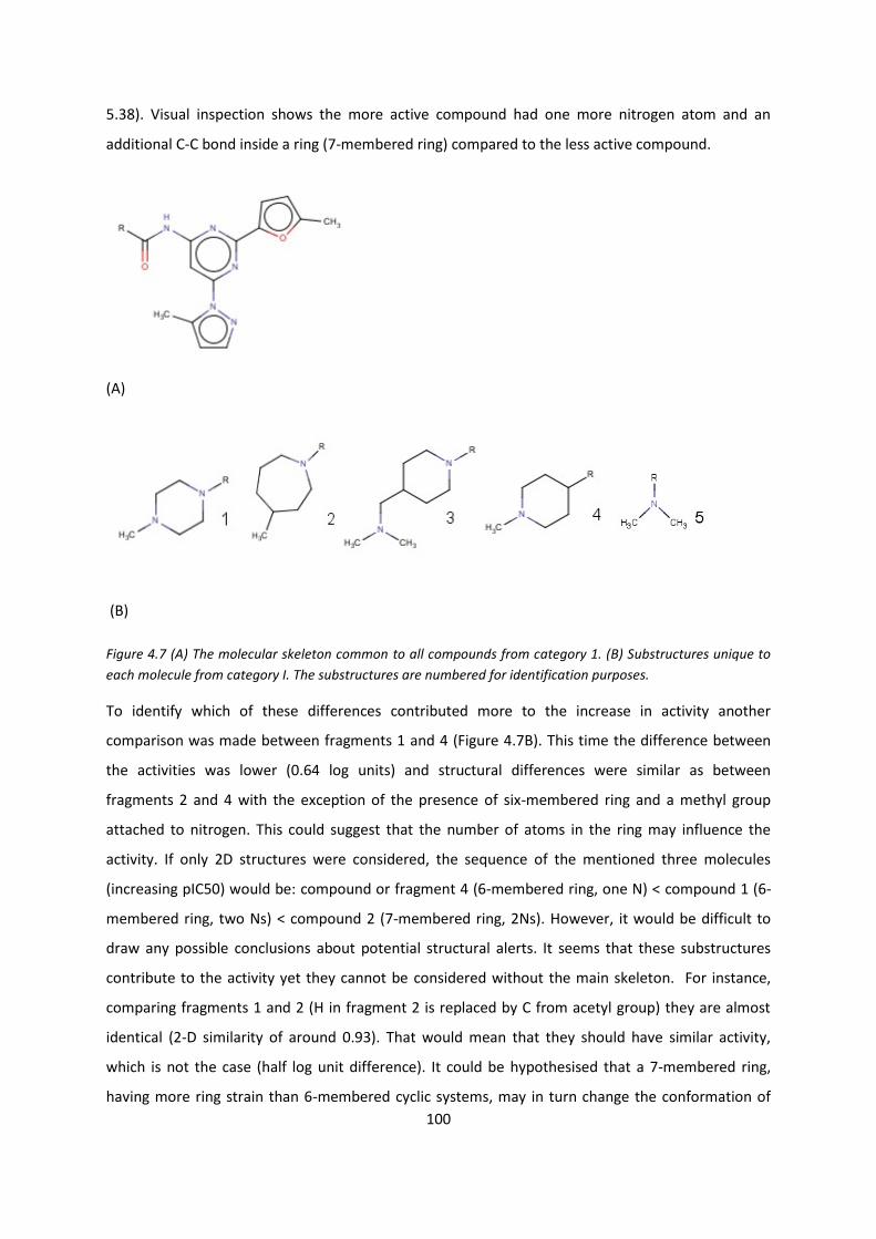
100

5.38). Visual inspection shows the more active compound had one more nitrogen atom and an

additional C-C bond inside a ring (7-membered ring) compared to the less active compound.

(A)

(B)

Figure 4.7 (A) The molecular skeleton common to all compounds from category 1. (B) Substructures unique to

each molecule from category I. The substructures are numbered for identification purposes.

To identify which of these differences contributed more to the increase in activity another

comparison was made between fragments 1 and 4 (Figure 4.7B). This time the difference between

the activities was lower (0.64 log units) and structural differences were similar as between

fragments 2 and 4 with the exception of the presence of six-membered ring and a methyl group

attached to nitrogen. This could suggest that the number of atoms in the ring may influence the

activity. If only 2D structures were considered, the sequence of the mentioned three molecules

(increasing pIC50) would be: compound or fragment 4 (6-membered ring, one N) < compound 1 (6-

membered ring, two Ns) < compound 2 (7-membered ring, 2Ns). However, it would be difficult to

draw any possible conclusions about potential structural alerts. It seems that these substructures

contribute to the activity yet they cannot be considered without the main skeleton. For instance,

comparing fragments 1 and 2 (H in fragment 2 is replaced by C from acetyl group) they are almost

identical (2-D similarity of around 0.93). That would mean that they should have similar activity,

which is not the case (half log unit difference). It could be hypothesised that a 7-membered ring,

having more ring strain than 6-membered cyclic systems, may in turn change the conformation of

101

the whole molecule (if rotatable bonds are present). On the other hand, the difference of half log

units may also be a result of experimental variability so that effectively, for compounds containing

fragments 1 and 2 there would be little difference in activities. Although, as was already mentioned,

it would be difficult to develop a clear structural alert it may be reasonable to indicate that a

presence of nitrogen atom(s) with a positive charge may play an important role in binding to the

hERG channel; this is in agreement with previous studies on hERG channel binding.

As investigation of structures at the 2-D level was of limited success, further work was carried out

that considered the influence of the 3-D features of the molecules in the context of molecular fields.

The Torch software package allows alignment of molecules against a reference molecule and then

calculates disparity values in a pairwise manner. Disparity is obtained by the following formula:

Disparity ≈ ∆Activity/(1-Similarity) (Eq. 4.7)

It follows that high disparity values indicate potential activity cliffs, in other words, high disparity

indicates molecules which are similar (in terms of 3-D molecular fields) but have significant

differences in activity. Similarity can be calculated for 2D-structures (fingerprints) or for molecular

fields. Figure 4.8 shows a visualisation of fields for two pairs of molecules. The first pair (Figure 4.8A)

has approximately 50% field similarity which is significantly different from the value obtained when

considering 2-D similarity. In this context, the changes in the activity could be potentially related to

the changes in molecular field. On the other hand, molecules with relatively different subfragments:

i.e. compounds 1 and 5 have higher field similarity (0.77) in comparison to values obtained from 2-D

method (both compounds have similar pIC50 values). This shows how potential SAR information

could be lost if steric and electronic conditions were not taken into account and only 2D structures

were examined. Here, the highest disparity value (3.0) was obtained for molecules with subfragment

2 and 4 which may indicate that introducing another heteroatom and much greater ring strain does

lead to a more favourable conformation when it comes to binding to the hERG pocket.

102

(A) (B)

Figure 4.8. Comparison of molecular fields for selected two pairs of molecules from category 1. (A) compounds

1 and 2; (B) compounds 1 and 5.

Category II.

Nine compounds were placed into category II, the structures of which are shown in Figure 4.9. The

compounds are all antimicrobial agents and chemically they are classified as fluoroquinolones. All of

the nine compounds were categorised as inactive with pIC50 values ranging from 2.62 (lomefloxacin)

to 4.67 (sparfloxacin). Although the compounds from category II are classed as inactive according to

their pIC50 values many fluoroquinolones are known to possess potential to cause arrhythmias.

Sparfloxacin and grepafloxacin have already been removed from the market due to cardiotoxicity;

others, such as: ciprofloxacin, gatifloxacin, levofloxacin, moxifloxacin have also been indicated as

being associated with TdP (Minotti, 2010). Although incidents of TdP caused by fluoroquinolones are

rare and depend on other factors such as sex, age, co-administration of drugs or xenobiotic

metabolism, they can still result in serious consequences, including sudden death. The case of

fluoroquinolones also illustrates that the conventional classification of chemicals according to their

hERG blockage potency may be, on occasions, misleading and some “borderline” pIC50 values can

also be responsible for substantial cardiotoxicity through inhibition of the hERG channel.

103

Figure 4.9. Category II compounds: (left to right) AF_3013_(NM-394), Ciprofloxacin, Gatifloxacin, Grepafloxacin, Levofloxacin,

Lomefloxacin, Moxifloxacin, Prulifloxacin, Sparfloxacin.

It is also important to realise that the adverse effects depend not only on absolute inhibition values

but they also should be considered in relation to therapeutic plasma concentrations of a drug. For

instance, sparfloxacin had a ratio of IC50/[plasma] = 10 whilst the same ratio for ciprofloxacin was

ten times greater (Kang et al, 2001). Nevertheless, there are great differences in absolute pIC50

values for fluoroquinolones from group II. This may indicate that the fluoroquinolone skeleton alone

is not sufficient to explain these differences and that focus should be rather put on substituents.

Substituent analysis may reveal some SAR trends. For instance, ciprofloxacin, grepafloxacin and

sparfloxacin differ by a substituent at position 5 (a hydrogen, a methyl and aminogroup,

respectively) but they also have a different number of methyl groups on the piperazine ring (zero,

one and two respectively). The toxicity exerted to hERG could possibly depend on an atom/group

attached at position 5 (hydrogen < methyl < amino). The increasing number of methyl groups on the

piperazine group may have a lower significance for blockage of the hERG channel. The least potent

104

compound has a hydrogen at position 5 and additionally differs from sparfloxacin (most potent) by

one less methyl group on the piperazine ring and the lack of the propyl group attached to N1 (only

methyl group present). The importance of the position 5 of the fluoroquinolone skeleton was

previously indicated. For the compounds from category II position 5 could be a candidate for forming

a potential structural alert where the presence of methyl or amino group would be an indicator of

increased hERG inhibition.

The presence of hydrogen was associated with QTc prolongation relatively lower in comparison to

the presence of other groups (< 2ms for ciprofloxacin, 3 ms for gatifloxacin, and 5-6 ms for

moxifloxacin and levofloxacin). In contrast, QTc prolongation time for grepafloxacin (methyl group at

position 5) was 11 ms whilst 15 ms was the prolongation of the QTc interval for sparfloxacin

containing NH2 group (Rubinstein & Camm, 2002).

Category III.

The twelve compounds in category III are a group of analogues of MCH-R1 (melanin-concentrating

hormone receptor 1) antagonists. Structurally, the molecules shared four common moieties: tetralin,

ketopiperazine, a tertiary amine linked to tetralin via a methyl group and finally, a hydrophobic

residue N-linked to ketopiperazine (see Figure 4.10).

105

Figure 4.10. Compounds from category III.

Meyers et al (2007) analysed the role of different substituents for hERG binding for these

compounds. They indicated that a hydrophobic residue does not need to be aromatic and hence the

binding of this part of a molecule is governed by hydrophobic interactions with Phe 565. They also

concluded that adding a polar group in the proximity of the tertiary amine residue decreased the

inhibition of the hERG channel. It should be noted that the analogues contained two “cation

centres” in the form of protonated nitrogen atoms (on tertiary amine residue and ketopiperazine)

106

and as such they could be involved in cation-π interactions with Tyr 652. However, considering the

disruptive role of incorporating polar groups, hydrophobic interactions may be important for

stabilisation of binding of this terminus of a molecule in addition to cation-π interactions.

Category IV.

Figure 4.11. Category IV compounds.

All compounds from this category (Figure 4.11) were very active with the lowest pIC50 value of 6.45.

Benperidol, droperidol (butyrophenones) and pimozide (diphenylbutylpiperidine) are antipsychotic

drugs and dopamine antagonists. Domperidone is an antiemetic and also a dopamine antagonist.

Oxatimide is a histamine H1 antagonist and as such can be categorised as an anti-allergic agent. All

molecules contain a bicyclic benzimidazole residue (with a carbonyl group at position 2). They also

contain a six-membered N-heterocyclic ring, an alkyl linker and hydrophobic residues such as phenyl

rings. N-heterocyclic ring contains a basic nitrogen that is protonated at physiological pH. Despite

107

sharing common structural features the range of pIC50 values spanned two log units. Three

antipsychotics were most potent hERG inhibitors.

Category V.

Figure 4.12. Two examples of category V compounds.

Compounds that belong to this category (Figure 4.12) include sertindole (antipsychotic drug) and its

21 analogues. Pearlstein et al (2003) used these compounds (among others) to study hERG channel

inhibition utilising CoMSiA and homology modelling. All these compounds contain a basic scaffold

consisting of indole with an attached phenyl group and a large proportion of the analogues also

contain a piperidyl substituent. This skeleton possesses a great deal of structural rigidity which to

some extent simplifies the analysis of the analogues. As sertindole is a potent hERG channel inhibitor

(the drug has already been withdrawn from the market due to cardiotoxicity) the analogues were

expected to exhibit similar properties and bind to the channel pocket. Indeed, the majority of the

compounds were either active (ten) or medium-active (six compounds). The remaining six

compounds were inactive and the lowest pIC50 value was four.

The pIC50 values spanned over four log units hence it was interesting to analyse some features of 2-

D structures that may influence the inhibition of the hERG channel. The five most potent inhibitors

from this group had pIC50 values around 8. Two analogues were only slightly stronger inhibitors

than sertindole although structurally they were very similar – apart from a missing chlorine

substituent on the indole ring and additionally in one chemical (no. 58) with the highest pIC50 value

108

the oxygen on the imidazolidine end was substituted by sulphur. Introducing a double bond to a

piperidyl group of the sertindole did not seem to change inhibition values (no. 66). The only

compound that was structurally least similar to sertindole (no. 61) had neither the imidazolidine nor

piperidyl rings. The piperidyl ring was replaced by a tertiary amine. Although such a structural

change reduced the diameter and molecular weight by nearly one third, the properties of this

molecule in terms of binding to the hERG channel remained nearly the same as those of the original

drug. However, it should be noted that nitrogen from the amine group is protonated under

physiological conditions and it may be an equivalent of the charged nitrogen from piperidyl group.

As previously mentioned, such protonated nitrogen may form interactions with π-electrons of Tyr

652. To further investigate this matter, other compounds were also analysed. Figure 4.13 illustrates

the fact that all compounds from category V form two distinctive groups when it comes to their size

(diameter). The chemicals with a greater diameter are associated with greater pIC50 values. On the

other hand, the analogues that are “truncated” versions of sertindole tend to have a reduced affinity

towards the hERG channel. However, three compounds do not follow these rules. Two compounds

represented by red triangles in Figure 4.13 were the only ones from the group of smaller analogues

that had a protonated nitrogen either present in a piperidyl ring (bottom triangle) or represented by

tertiary amine (top triangle). On the other hand, a compound represented by a red square had a low

pIC50 value although it possessed a protonated nitrogen. This could be explained by the presence of

negative charge introduced by a carboxyl group. This might suggest that the hydrophobic part of the

molecule may be important for interacting with Phe 656 and hindrance of this hydrophobic area by a

negative charge (in this case) could prevent such hydrophobic attraction between the side chains of

phenylanilines of the hERG channel and a molecule. This could be further supported by the fact that

replacing hydroxyl group with a methoxy substituent increased the pIC50 values by nearly 3.5 log

units (compare compounds no. 73 and 75). However, it should be noted that when a carboxyl group

was attached to the phenyl substituent via a methyl link (compound no. 72) the activity was much

higher (pIC50 = 6.24). This may suggest that adding another C-C bond allowed more access to the

hydrophobic phenyl ring. Nevertheless, it is clear that a presence of both a positive charge

(protonated nitrogen) and an accessible hydrophobic group (in this case, a phenyl ring) might be

important structural features that would indicate a potential hERG binder channel binder. The

spatial arrangement of crucial groups seems to play a role as well and a certain degree of spatial

separation may be required to accommodate for the distances between crucial side chains of amino

acids.

109

Figure 4.13. Scatterplot of pIC50 vs maximum diameter for compounds belonging to category V. Red colour

indicates unusual observations and the shape of the red data points refers to whether a compound is in the

group with larger diameter (triangle) or is a “truncated” analogue (square).

Category VI.

Category VI comprised six compounds (Figure 4.14) all of which are macrolide antibiotics (or, in the

case of N-demethylerythromycin) an active metabolite of a macrolide antibiotic). Structurally, they

share a macrocyclic lactone ring to which deoxy sugar moieties can be attached (such as cladinose or

desosamine in erythromacin) or other side chains such as N-oxime as in the case of roxithromycin.

Similarly to the antimicrobial agents from category II, the pIC50 values for macrolides were below

the cut-off value of 5 log units, nevertheless they are known to cause hERG channel blockage

(Volberg et al, 2002).

262422201816141210

8

7

6

5

4

Dmax

pIC

50

110

Figure 4.14. Compounds from category VI. (left to right) Clarithromycin, Erythromycin, Erythromycylamine, Josamycin, N-

Demethylerythromycin, Roxithromycin.

All macrolides from category VI contain amines which can be protonated in physiological conditions.

Again, the protonated nitrogen from the amine group could be important for taking part in cation-π

interactions with Tyr 652 hydroxyphenyl group. The rather large size and specific shape of these

111

molecules confirms the hERG channel binding pocket can accommodate a variety chemical entities.

The lactone ring may enable hydrophobic interactions with Phe 656 residues. However, the

relatively large number of polar groups may decrease the hydrophobicity of this region and, thus, it

should reduce the strength of the hydrophobic interactions. The analysis of log D values (pH = 7.4)

showed that compounds with the lowest pIC50 values (no. 130 and 185) also had considerably lower

log D values. Interestingly, the N-demethylated form of erythromycin (active metabolite) showed

insignificant reduction of the potency to block the hERG channel although the log D values differed

by approximately two log units. This may suggest that the change in lipohilicity was not prohibitive

neither for transmembrane transport nor access to the channel pocket. However, it may be noticed

that the metabolism site on erythromycin was the amine group and thus possibly involved in cation-

π interactions. Furthermore, the removal of the methyl group may potentially positively influence

the strength of the cation-π bond by removing steric hindrance and increasing charge density.

Nevertheless, the structural changes due to metabolism do not occur in that part of the molecule

that possibly took part in hydrophobic interactions. Hence, considering differences in log D values

may be misleading if the analysis of the corresponding structural changes is not present and it does

not take into account pharmacophorically important regions of the molecules.

Category VII.

The five compounds from category VII (Figure 4.15) are drugs with gastroprokinetic and/or

antiemetic properties. Clebopride and metoclopramide are dopamine antagonists while mosapride,

prucalopride and renzapride are serotonin receptors (5HT4) agonists. Chemically, all these molecules

are either substituted benzamides or (in case of prucalopride) carboxamides. All these drugs were

either active or medium active towards the hERG channel. All have a nitrogen that can be

protonated in physiological conditions (this N was always found on a substituent attached to an

amide nitrogen). Again, the positive charge had the potential to interact with tyrosine side chains in

the hERG channel pocket. Benzamide and carboxamide (with benzofuran) cores of the molecules are

planar structures and as such they could be considered as approximately constant in terms of

conformational geometries. Thus, the differences in potency to block the hERG channel could result

from differences in substituents that have more flexibility to adopt a greater number of

conformations. For instance, clebopride was about one log unit more active than metoclopramide.

They both share an identical benzamide structure. However, the clebopride molecule has both a

larger diameter and greater log D (by two log units). This could suggest that the presence of a phenyl

group (as piperidyl group is assumed to be involved in cation- π interactions through a protonated

nitrogen) may be important for stacking interactions. On the other hand, mosapride has pIC50

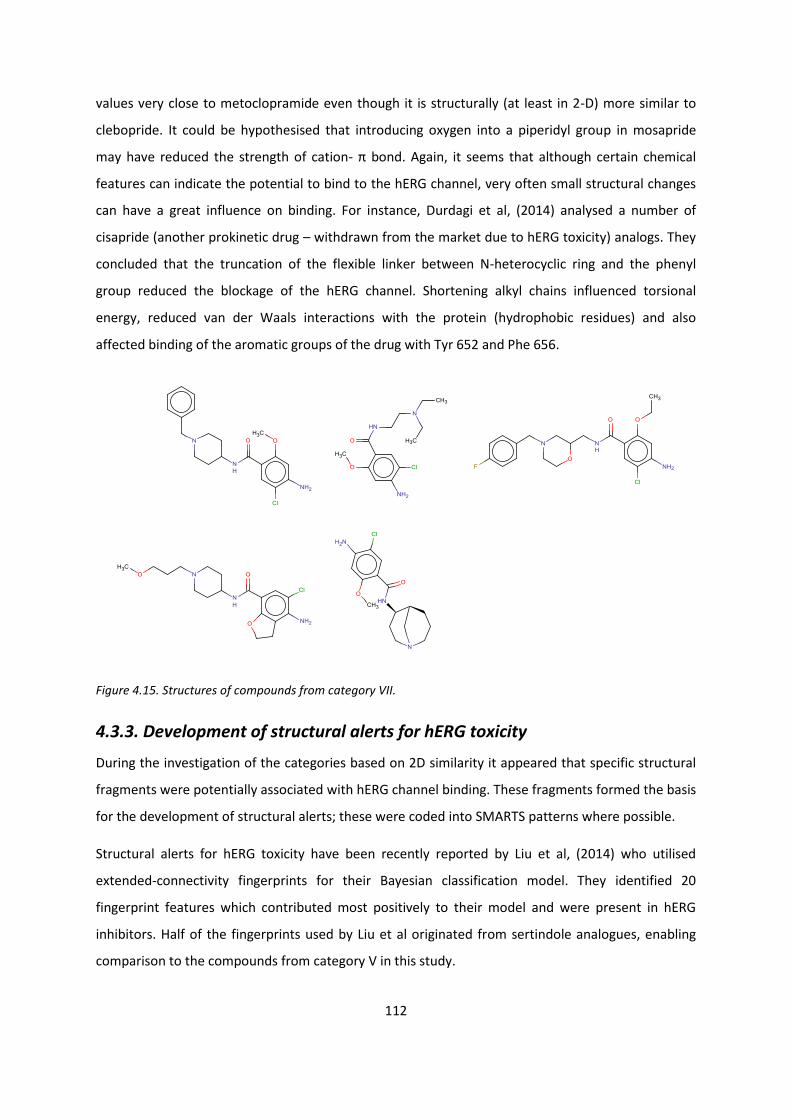
112

values very close to metoclopramide even though it is structurally (at least in 2-D) more similar to

clebopride. It could be hypothesised that introducing oxygen into a piperidyl group in mosapride

may have reduced the strength of cation- π bond. Again, it seems that although certain chemical

features can indicate the potential to bind to the hERG channel, very often small structural changes

can have a great influence on binding. For instance, Durdagi et al, (2014) analysed a number of

cisapride (another prokinetic drug – withdrawn from the market due to hERG toxicity) analogs. They

concluded that the truncation of the flexible linker between N-heterocyclic ring and the phenyl

group reduced the blockage of the hERG channel. Shortening alkyl chains influenced torsional

energy, reduced van der Waals interactions with the protein (hydrophobic residues) and also

affected binding of the aromatic groups of the drug with Tyr 652 and Phe 656.

Figure 4.15. Structures of compounds from category VII.

4.3.3. Development of structural alerts for hERG toxicity

During the investigation of the categories based on 2D similarity it appeared that specific structural

fragments were potentially associated with hERG channel binding. These fragments formed the basis

for the development of structural alerts; these were coded into SMARTS patterns where possible.

Structural alerts for hERG toxicity have been recently reported by Liu et al, (2014) who utilised

extended-connectivity fingerprints for their Bayesian classification model. They identified 20

fingerprint features which contributed most positively to their model and were present in hERG

inhibitors. Half of the fingerprints used by Liu et al originated from sertindole analogues, enabling

comparison to the compounds from category V in this study.

113

The proposed structural alerts for each of the seven categories are summarised in Figures 4.16 -

4.21. It should be noted that some categories were formed solely by compounds with pIC50 < 5

(categories II and VI). Nonetheless, structural alerts were still developed as some compounds from

these categories were known to cause blockage of the hERG channel. The alerts were visualised

using SMARTSviewer (ver. 0.9.0.) (Schomburg et al, 2010).

Category I

The structural alert developed for category I was based on the common skeleton for each molecule

(as shown in Figure 4.7A). The SMARTS pattern for this alert is:

[CX4H2]([CX3](=[OX1])[NX3H1]c1cc(nc(n1)c2ccc(o2)[CX4H3])n3nccc3[CX4H3])[CX4H1,CX4H2,NX3][*

$([NX3]),*$([CX4H2][CX4H2][NX3]),$([CX4H2][CX4H2][CX4H1][CX4H2][NX3])]

The differences between pIC50 values of the subfragments from Figure 4.7B were insufficient to

allow further consideration of these subfragments. A log unit range of potencies could be

considered, at least partially, as a result of experimental error that could range from 0.5 to 1 log unit.

However, the nitrogen atom present in each of the five subfragments was included in the structural

alert. At physiological pH (7.4) these nitrogen atoms would be protonated and as such they would

potentially stabilise interactions with the hERG channel.

Figure 4.16. Structural alert for category I compounds.

Category II

Fluoroquinolones can prolong the heart’s QT interval. Consequently, despite all compounds from

category II being classified as inactive a structural alert was developed. The main skeleton of

fluoroquinolones was included. The previously discussed potency differences potentially resulting

114

from a different substituent on position 5 (ciprofloxacin, grepafloxacin and sparfloxacin) were not

taken into account. This means that the least potent ciprofloxacin is also captured by the SMARTS

pattern. Matsuo et al, (2013) showed that ciprofloxacin can change the electrocardiographic

characteristic when used at supra-therapeutic dosage (10mg/kg rather than 3mg/kg) to prevent

bacterial resistance. Moreover, ciprofloxaxin was also shown to inhibit other cardiac channels (Na+,

Ca2+). The piperazine ring was not included in the alert even though it was present in eight

compounds. Possibly, the basic nitrogen, present in piperazine ring and in the N heterocyclic

subfragment of moxifloxacin, may play a role in hERG binding although this was not reflected in the

final SMARTS. This was an arbitrary choice in order to develop an alert that is less specific so that it

can match a broader category of compounds. However, this was compensated by adding a nitrogen

at the 7-position. The presence of a fluorine atom may be arguable, however, it was present in all

nine compounds.

SMARTS:

c21c(cc(c(c1)[NR1])F)c(=[OX1])c([CX3](=[OX1])[OX2H1])cn2[#6]

Figure 4.17. Structural alert for category II compounds.

Category III

All common substructures for compounds from category III were included in the structural alerts for

this group. The following four moieties were included: tetralin, ketopiperazine, a tertiary amine

linked to tetralin via a methyl group and finally, a hydrophobic residue N-linked to ketopiperazine.

The hydrophobic residue was coded as a carbon atom (aliphatic or aromatic).

This category was formed by a mixture of active and inactive compounds according to the pIC50

based classification. However, the pIC50 values for the inactive compounds were close to the cut-off

115

value of 5 log units. Again, such differences could be within the range of an experimental error,

which supports the argument that a structural alert could be a better indicator of activity than pIC50

values alone.

SMARTS:

c12cc([CX4H2][#7]([#6])[#6])ccc1[CX4H2][C@@X4H1]([NX3]3[CX3](=[OX1])[CX4H2][NX3]([CX4H2][#6

])[CX4H2][CX4H2]3)[CX4H2][CX4H2]2

Figure 4.18. Structural alert for category III compounds.

Category IV

All five compounds were very potent hERG blockers. The structural alert was based on

benzimidazole moiety. However, N-heterocyclic residue linked to benzimidazole via an aliphatic

linkage could also be potentially included in the SMARTS, especially in the context of including basic

nitrogen.

SMARTS:

c12ccccc1n([CX4,CX3])c(=[OX1])[nH]2

Figure 4.19. Structural alert for category IV compounds.

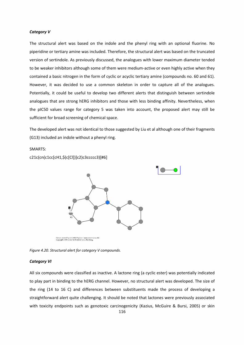
116

Category V

The structural alert was based on the indole and the phenyl ring with an optional fluorine. No

piperidine or tertiary amine was included. Therefore, the structural alert was based on the truncated

version of sertindole. As previously discussed, the analogues with lower maximum diameter tended

to be weaker inhibitors although some of them were medium-active or even highly active when they

contained a basic nitrogen in the form of cyclic or acyclic tertiary amine (compounds no. 60 and 61).

However, it was decided to use a common skeleton in order to capture all of the analogues.

Potentially, it could be useful to develop two different alerts that distinguish between sertindole

analogues that are strong hERG inhibitors and those with less binding affinity. Nevertheless, when

the pIC50 values range for category 5 was taken into account, the proposed alert may still be

sufficient for broad screening of chemical space.

The developed alert was not identical to those suggested by Liu et al although one of their fragments

(G13) included an indole without a phenyl ring.

SMARTS:

c21c(cn(c1cc[cH1,$(c[Cl])]c2)c3ccccc3)[#6]

Figure 4.20. Structural alert for category V compounds.

Category VI

All six compounds were classified as inactive. A lactone ring (a cyclic ester) was potentially indicated

to play part in binding to the hERG channel. However, no structural alert was developed. The size of

the ring (14 to 16 C) and differences between substituents made the process of developing a

straightforward alert quite challenging. It should be noted that lactones were previously associated

with toxicity endpoints such as genotoxic carcinogenicity (Kazius, McGuire & Bursi, 2005) or skin

117

sensitisation (Enoch, Madden & Cronin, 2008). However, it could be assumed that in the case of the

antibiotics from this category the size of the macrocyclic ring was much more important from a hERG

binding perspective than any involved reactivity.

Category VII

Benzamide was a common substructure for all the compounds from category 7 and as such it was

used to develop a structural alert for this group. Again, the role of other substructures, was not

specified in SMARTS even though some of them, especially those that contain basic nitrogen, may be

important for hERG binding.

SMARTS:

[NH2]c1c([Cl])cc(C(=[OX1])[NH][CX4])cc1

Figure 4.21. Structural alert for category VII compounds.

To ensure that the SMARTS captured all the compounds in the categories the developed alerts were

tested against the H_244 dataset. The re-screening process was successful. Further validation on an

external dataset would be required and is intended to be included in future work.

One of the challenges during development of structural alerts is to make a decision about how

specific the rule should be. This dilemma was present when writing SMARTS for the described

categories. For instance, in some cases the basic nitrogen was not included in the SMARTS pattern as

this would require writing a rule so specific to compounds from a given category that its use for

screening purposes would be questionable. The only exception was made for the structural alert for

category I that was more amenable to the inclusion of the ionisable nitrogen. On the other hand,

according to various pharmacophore models, a protonated nitrogen seemed to be an important

118

feature and as such it should be included in SMARTS (if applicable). Possibly, a better solution could

be provided by coding structural fragments that represent good features contributing to a model

such as those present in study by Liu et al, or Wang et al., (2012) – another naïve Bayesian classifier.

Additional work could be done on developing SMARTS for strong hERG inhibitors. Tobita, Nishikawa

& Nagashima, (2005) proposed features for strong hERG blockers and these included non-aromatic

nitrogen, hydrophobic fragments and also a ring connected through a nitrogen atom (see Figure

4.22). Such rules could be used for general screening of chemical space.

Developing structural alerts for inhibition of the hERG channel is a difficult task due to the

promiscuity of this channel. However, this approach offers some advantages such as being less

prone to experimental errors and less dependent on pIC50 threshold values. In this work, 1 µM

(pIC50 = 6) was used as this was used to distinguish between actives and inactive in other studies

(Nisius & Goller, (2009), Keseru, (2003). However, other thresholds have also been used. For

instance, Aronov & Goldman, (2004) used 40 µM cut-off which corresponds to pIC50 of 4.4.

Another possibility for future work could involve combining structural alerts for hERG channel

inhibitors with a set of rules based on molecular descriptors such as log P, TPSA or molar refractivity

(Buyck et al., 2003). This may provide a useful filter to be used by medicinal chemists in terms of

screening for hERG blockers.

Figure 4.22. Structural features for strong hERG inhibitors. Adapted from Tobita, Nishikawa & Nagashima,

(2005).

119

***

Development of predictive models for hERG channel inhibition is challenging. In the work carried out

here, a previously reported model, that used hydrophobicity and molecular size descriptors, was

evaluated to determine if it had broad applicability. Aptula and Cronin’s model did not provide

accurate predictions for the much larger H_244 dataset studies here. This shows that models

developed for smaller datasets have a more limited applicability domain. In this work, both global

and local regression models developed were not of sufficient quality to offer improvement to

existing models. It could be argued that the regression methods may not be the optimal choice for

hERG modelling possibly due to the promiscuity of the hERG channel that can bind structurally

diverse compounds. However, binary classification modelling was more successful with the best

performing random forest classifier that achieved a recall of 78%.

Due to limited success with modelling hERG binding a new approach was used in an attempt to

overcome poor accuracy of hERG models. Seven categories of compounds were identified through a

2-D similarity search. Each group was discussed in terms of potential structural features that could

play a role in hERG binding. This analysis resulted in the development of structural alerts for 6 out of

7 categories formed from the H_244 dataset. The author is not aware of any SMARTS rules for hERG

described in scientific literature and therefore, the developed SMARTS patterns may offer a

potential to be implemented as a screening tool for identification of putative hERG blockers. Future

work could include a further development of structural alerts both in terms of their number and

quality. Incorporation of such rules into decision trees that utilise medicinal chemistry-type

descriptors would constitute a further extension of this work.

Some analysis of structural alerts in the context of screening will be provided in the next chapter

where the specificity of alerts related to reactive metabolism will be discussed, particularly with

respect to the balance between the specificity and sensitivity.

120

5. Structural Alerts for Reactive Metabolites

5.1. Introduction

The formation of reactive metabolites in the process of bioactivation has been known to be

responsible for adverse drug effects, especially idiosyncratic toxicities (Kalgutkar et al., 2005; Stepan

et al., 2011). The prediction of bioactivation is not a trivial task as it depends not only on the

structure of the compound but also on factors that are characteristic to an individual - such as

genetic makeup, age or health. Moreover, the formation of reactive metabolites does not always

lead to toxic effects due to detoxification processes, such as reaction with glutathione that can bind

electrophilic species.

Reactive metabolites are either electrophiles, which are electron-deficient species, or free radicals

that contain unpaired electrons. Electrophiles can be further categorised as soft electrophiles (low

positive charge density) and hard electrophiles (high positive charge density). Soft electrophiles tend

to react with soft nucleophiles (e.g. quinone methides can bind covalently to lysine or histidine

residues on proteins) while hard electrophiles generally bind to hard nucleophiles (e.g. benzyl

carbonium ions can react with bases in DNA) (Stachulski et al., 2012). Reactive species can bind

covalently to proteins and disrupt their biological function, e.g. inhibiting a specific enzyme or

receptor activity or modulating a signalling pathway. Furthermore, a reactive metabolite bound to a

protein becomes a hapten and as such it forms an antigen and can potentially elicit an immune

response. Reactive metabolites can also induce oxidative stress. Finally, reactive species can form

DNA adducts (Byrns et al., 2006) that can introduce mutations which could further lead to

carcinogenic effects. Any of the described scenarios can result in cell death in either a controlled or

uncontrolled manner (apoptosis and necrosis). Reactive metabolites are formed from a structurally

heterogeneous spectrum of chemicals that includes a diverse group of small molecule drugs.

Moreover, there exists numerous potential targets for reactive metabolites. Hence, the association

between reactive metabolites formation and toxicity is not always clear (with the exception of

genotoxicity (Stachulski et al., 2012)). This means that the development of a screening tool that

could determine potential toxicity, via reactive metabolite formation, is an extremely challenging

task. It has been recognised that early and reliable detection and identification of reactive

metabolites can be a bottleneck in drug discovery and integrated approaches have been proposed

(Stepan et al., 2011; Reese et al., 2011; Thompson et al., 2012; Pelkonen et al., 2014).

121

A number of in vitro methods are employed to detect reactive metabolites; for instance, small-

molecular trapping agents. Among the trapping agents glutathione (GSH) is used to detect soft

electrophiles while hard electrophiles are detected using potassium cyanide (KCS) or semicarbazide

(SCA). Other trapping agents may include peptides and oligonucleotides, such as deoxyguanosine

(dG), the latter being utilised for detection of species that target DNA. Ideally, these tests for adduct

formation should be performed in combination with tests for biomarkers of toxicity (Pelkonen et al.,

2014).

In silico methods used for prediction of reactive metabolites include screening compounds against a

set of structural alerts. Such a preliminary screening process represents a strategy of avoidance, i.e.

not incorporating certain functional groups into a drug structure. The development of structural

alerts for reactive metabolites is based on the identification of molecular fragments/functional

groups that are known be subject to bioactivation. However, structural alerts also have limitations.

First of all, they are knowledge-based, which means that they only represent what is currently

known and available in the published literature. Secondly, the binary categorisation of structural

alerts being present or absent within a molecule can be ambiguous (Stachulski et al., 2012) as it may

not be entirely clear what constitutes an alert. Recently, it has been argued that structural alerts

may be applied too stringently so reducing the chemical diversity required in drug discovery (Liu, Yu

& Wallqvist, 2015). These authors also argued that a structural alert should be only developed if it

occurs more significantly in compounds that exert toxicity rather than in those chemicals that are

negative for the toxicity.

The main aim of this chapter was to analyse the distribution of publically available structural alerts

for reactive metabolites for a large dataset of drug molecules (DrugBank). Additionally, the

importance of refining alerts has been considered using the alert for a carboxyl group as an example.

5.2 Methods

5.2.1. Datasets

Structures of 6858 drug molecules were downloaded from DrugBank (http://www.drugbank.ca) in

sdf format. The DrugBank dataset included the following types of drugs: (i) approved (n = 1543), (ii)

experimental (n = 5023), (iii) nutraceutical (n = 84), (iv) illicit (n = 169), (v) withdrawn (n = 149) and

(v) investigational (n = 522).

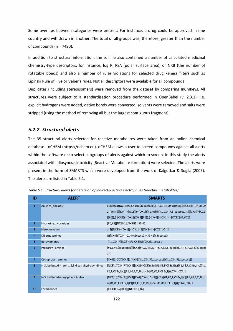
122

Some overlaps between categories were present. For instance, a drug could be approved in one

country and withdrawn in another. The total of all groups was, therefore, greater than the number

of compounds (n = 7490).

In addition to structural information, the sdf file also contained a number of calculated medicinal

chemistry-type descriptors, for instance, log P, PSA (polar surface area), or NRB (the number of

rotatable bonds) and also a number of rules violations for selected druglikeness filters such as

Lipinski Rule of Five or Veber’s rules. Not all descriptors were available for all compounds

Duplicates (including stereoisomers) were removed from the dataset by comparing InChIKeys. All

structures were subject to a standardisation procedure performed in OpenBabel (v. 2.3.1), i.e.

explicit hydrogens were added, dative bonds were converted, solvents were removed and salts were

stripped (using the method of removing all but the largest contiguous fragment).

5.2.2. Structural alerts

The 35 structural alerts selected for reactive metabolites were taken from an online chemical

database - oCHEM (https://ochem.eu). oCHEM allows a user to screen compounds against all alerts

within the software or to select subgroups of alerts against which to screen. In this study the alerts

associated with idiosyncratic toxicity (Reactive Metabolite formation) were selected. The alerts were

present in the form of SMARTS which were developed from the work of Kalgutkar & Soglia (2005).

The alerts are listed in Table 5.1.

Table 5.1. Structural alerts for detection of indirectly acting electrophiles (reactive metabolites).

ID ALERT SMARTS

1 Anilines_anilides c1ccccc1[NX3]([#1,CX4!R,$(c1ccccc1),$([CX3](=[OX1])[#6]),$([CX3](=[OX1])[OX

2][#6]),$([SX4](=[OX1])(=[OX1])[#1,#6])])[#1,CX4!R,$(c1ccccc1),$([CX3](=[OX1]

)[#6]),$([CX3](=[OX1])[OX2][#6]),$([SX4](=[OX1])(=[OX1])[#1,#6])]

2 Hydrazine_hydrazides [#6,#1][NX3H1][NX3H1][#6,#1]

3 Nitrobenzenes a[$([NX3](=[OX1])=[OX1]),$([NX3+](=[OX1])[O-])]

4 Dibenzazepines N([CX4])([CX4])C1=Nc2ccccc2[NX3H1]c3c1cccc3

5 Benzylamines [#1,CX4!R][NX3]([#1,CX4!R])[CH2]c1ccccc1

6 Propargyl_amines [#1,CX4,$(c1ccccc1)][CX2]#[CX2][NX3]([#1,CX4,$(c1ccccc1)])[#1,CX4,$(c1ccccc

1)]

7 Cyclopropyl_amines [CX4]1[CX4][CX4]1[NX3]([#1,CX4,$(c1ccccc1)])[#1,CX4,$(c1ccccc1)]

8 N-Substituted-4-aryl-1,2,3,6-tetrahydropyridines [NX3]1([CX4!R])[CX4][CX3]=[CX3](c2c([#1,#6,F,Cl,Br,I])c([#1,#6,F,Cl,Br,I])c([#1,

#6,F,Cl,Br,I])c([#1,#6,F,Cl,Br,I])c2([#1,#6,F,Cl,Br,I]))[CX4][CX4]1

9 N-Substituted-4-arylpiperidin-4-ol [NX3]1([CX4!R])[CX4][CX4][CX4]([OH1])(c2c([#1,#6,F,Cl,Br,I])c([#1,#6,F,Cl,Br,I])

c([#1,#6,F,Cl,Br,I])c([#1,#6,F,Cl,Br,I])c2([#1,#6,F,Cl,Br,I]))[CX4][CX4]1

10 Formamides [CX3H1](=[OX1])[NX3H1][#6]

123

11 Hydantoins_(glycolylurea) [NX3H1]1[CX3](=[OX1])[CX4]([#1,#6])([#1,#6])[NX3H1][CX3]1(=[OX1])

12 Thioamides [#1,#6][CX3](=[SX1])[NX3]([#1,#6])[#1,#6]

13 Thioureas [#1,#6][NX3]([#1,#6])[CX3](=[SX1])[#7]

14 Sylfonylureas [#6][Sv6X4](=[OX1])(=[OX1])[NX3H1][CX3](=[OX1])[NX3H1][#6]

15 Thiols [SX2!H0][#1,#6&!$([CX3]([SH1])=[OX1,SX1,NX2])]

16 Disulfides [#6,#1][SX2][SX2][#6,#1])

17 Ortho-_or_parahydroquinones [$(c1([OH1])c([OH1])cccc1),$(c1([OH1])ccc([OH1])cc1)]

18 Ortho- _or_paraquinones [$([#6]1(=[OX1])-,:[#6]=,:[#6]-,:[#6](=[OX1])-,:[#6]=,:[#6]1),$([#6]1(=[OX1])-

,:[#6](=[OX1])-,:[#6]=,:[#6]-,:[#6]=,:[#6]1)]

19 Ortho-_or_paraalkylphenols [$(c1([OH1])c([CX4]([#1,#6])[#1,#6])cccc1),$(c1([OH1])ccc([CX4]([#1,#6])[#1,#

6])cc1)]

20 Quinone_methide [$([OX1]=[#6X3]1-,:[#6X3]=,:[#6X3]-,:[#6X3]=,:[#6X3]-

,:[#6X3]1=[CX3]([#1,#6])[#1,#6]),$([OX1]=[#6]1-,:[#6]=,:[#6]-

,:[#6](=[CX3]([#1,#6])[#1,#6])-,:[#6]=,:[#6]1)]

21 Benzo-dioxolanes c1ccc([OX2]2)c([OX2][CX4H1]2[OH1])c1

22 3-Methylene_indoles c1ccc([nX3]2([#1,#6]))c(c([CH2][#1,#6])c2)c1

23 Furans c1ccc[oX2]1

24 Thiophenes c1ccc[sX2]1

25 Thiazoles_and_2-amino_derivatives [$(c1([#1,CX4!R])c([#1,CX4!R])[nX2]c([#1,CX4!R])[sX2]1),$(c1([#1,CX4!R])c([#1,

CX4!R])[nX2]c([NX3]([#1,CX4!R])[#1,CX4!R])[sX2]1)]

26 Thiazolidinediones [SX2]1[CX3](=[OX1])[NX3H1][CX3](=[OX1])[CX4]1[#6]

27 Arenes NOT [!#6!#1] AND c1ccccc1

28 Bromoarenes NOT [!#6!#1!Br] AND c1ccccc1Br

29 2- _or_4-Halopyridines [$(n1c([Cl,Br,I,F])cccc1),$(n1cccc([Cl,Br,I,F])cc1)]

30 Heterocycles_with_C-2_LG nc[$([OX2][Sv6X4](=[OX1])(=[OX1])[OH]),$([OX2][Sv6X4](=[OX1])(=[OX1])[OX2

][CH3]),$([OX2][Sv6X4](=[OX1])(=[OX1])[CH3]),$([OX2][Sv6X4](=[OX1])(=[OX1]

)[CF3]),$([OX2][Sv6X4](=[OX1])(=[OX1])c1ccc([CH3])cc1),$([I,Br,Cl])]

31 Alkynes [#6][CX2]#[CX2][#1,#6]

32 Michael_acceptors [$([CX3]=[CX3][$([$([NX3](=[OX1])=[OX1]),$([NX3+](=[OX1])[O-

])]),$([CX3](=[OX1])[OX2][#1,#6]),$([Sv6X4](=[OX1])(=[OX1])[OH]),$([CX3](=[O

X1])[#1,F,Cl,Br,I]),$([CX2]#[NX1]),$([CX4]([F,Cl])([F,Cl])[F,Cl]),$([CH2][OH]),$([C

H2][$([NX3](=[OX1])=[OX1]),$([NX3+](=[OX1])[O-

])]),$([CH2][F,Cl])]),$([CX3]=[CX3][CX3](=[OX1])[#1,#6])]

33 Alkylhalides [$([CX4]([F,Cl,Br,I])([H,!F!Cl!Br!I])([H,!F!Cl!Br!I])[H,!F!Cl!Br!I]),$([CX4]([#6])([F,

Cl,Br,I])([F,Cl,Br,I])[H,!F!Cl!Br!I])]

34 Carboxylic_acids [#6][CX3](=[OX1])[OH1]

35 Fluoroethyl_ethers_and_amines [$([F][CX4][$([CH2]),$([CH]),$(C[OH1])][OX2][#1,#6]),$([F][CX4][$([CH2]),$([C

H]),$(C[OH1])][NX3][#6])]

5.2.3. Detection of alerts

The presence of structural alerts for all compounds from the DrugBank dataset was evaluated using

OpenBabel. Structures in the sdf file were screened against each of the 34 SMARTS patterns. For a

given structural alert, when a hit was identified the given structure from the sdf file was converted

124

to SMILES format which was then appended to a text file. The results of the screening (34 runs in

total) were saved in a csv file for further analysis.

5.3. Results and discussion

5.3.1. The distribution of alerts

Out of the 35 structural alerts for idiosyncratic toxicity, related to reactive metabolite formation,

available in oCHEM the vast majority (i.e. 32) were matched against at least one compound from the

DrugBank dataset. The remaining alerts for which no matches were found were: disulfides, benzo-

dioxolanes and bromoarenes. The distribution of the individual alerts is shown in Figures 5.1A.

Figure 5.1 A. The histogram of reactive metabolism (RM) alerts found in the DrugBank dataset.

The total number of hits was 4342. Carboxylic acids (alert 34) and anilines/anilides (alert 1) were the

most frequently matched alert (1587 and 645, respectively). Alkyl phenols (ortho and para) as well

as Michael acceptors were also relatively frequent hits. For 52% of compounds from the DrugBank

dataset no alerts were matched.

The high number of structural alerts for carboxylic acids in the dataset was relatively surprising.

Although the –COOH moiety is known to be crucial for the mechanism of action of some drugs, for

instance non-steroidal anti-inflammatory drugs (NSAIDs), retinoids, cannabinoids, fibrate

hypolipidaemic agents, diuretics, anticonvulsants, antitumour agents and antibiotics (Regan et al,

125

2010), it is also an acidic functional group that can influence an ionisation state of a drug, which in

turn may affect solubility and lipophilicity, i.e. properties that contribute to the ADME profile. Acidic

drugs are most likely to be completely ionised in pH values greater than 7 (Charifson & Walters,

2014). In the DrugBank dataset, the carboxylic group was present in 23% of all drugs considered

(17% of approved drugs and 15% of withdrawn drugs).

It is possible for a compound to hit multiple alerts. As can be seen in Figure 5.1B, the total number of

identified alerts for any compound was never > 4 and in a majority of cases one or two alerts were

found (see Figure 5B).

Figure 5.1B. The counts of compounds for each of the hits categories. The categories were formed on the basis

of total number of hits for each compounds. ‘Hit’ is defined here as a presence of a structural alert.

One question that was considered was whether there was any correlation between the number of

identified alerts and the class of a drug. The assumption was that the higher number of detected

alerts may be associated with higher chances of idiosyncratic toxicity, simply because of the greater

number of sites in a molecule that could potentially lead to the formation of reactive metabolites.

None of the four compounds with the highest occurrence of alerts were found in the withdrawn

class; one of them was an approved drug (fluticasone furoate), the remaining three molecules were

experimental. Four compounds containing three structural alerts were found in the withdrawn or

withdrawn/approved class: cefadroxil, fluprednidene acetate, bentiromide and bunamiodyl.

Nevertheless, approved and experimental drugs constituted a much larger proportion of compounds

containing three structural alerts. Out of 130 compounds with three alerts there were 48 drugs from

the ‘approved’ category and 77 from the ‘experimental’ drug category. However, the absolute values

could not give the correct picture, as the number of compounds in each class was different. Hence,

43210

4000

3000

2000

1000

0

Hits

No

. co

mp

ou

nd

s

4134

767

2390

3564

126

values relative to the number of compounds in each drug group were obtained. Figure 5.2 presents

the frequencies of occurrence of structural alerts for the three different categories of drugs

(approved, experimental and withdrawn).

Figure 5.2. Distribution of numbers of alerts identified for three categories of compounds (approved,

experimental, and withdrawn) from DrugBank dataset.

There is no significant difference in the number of alerts identified for each of the three categories

of drugs (approved, withdrawn or experimental). Approximately 50% of compounds from each of

these three classes contained no structural alerts. The fraction of compounds with one, two, three

or four structural alerts was also similar across all three categories. Hence, it can be concluded that

there was no correlation between the number of hits and the class to which the drug belonged, i.e. a

higher number of hits was not associated with the ‘withdrawn’ class. It should be noted that

idiosyncratic toxicity is only one of the many reasons due to which drugs may be removed from the

market. Other reasons may be off-target toxicity such as hERG-channel inhibition. Similarly, some

compounds may be approved and not withdrawn and yet they are known to be associated with

adverse drug reactions. A famous example of such a drug is acetaminophen that can form a reactive

metabolite (NAPQI - quinone-imine intermediate, which can lead to liver necrosis (Mitchell et al,

1973). Nevertheless, it is interesting that the distribution of alerts was similar for approved,

withdrawn and experimental drugs. Additionally, the presence of relatively large number of hits for

approved drugs was also an indication that identifying structural alerts can have a limited use as a

predictive tool for determination of toxicity. Kalgutkar & Didiuk (2009) suggested that in silico

methods, including the toxicophore approach, are not extensively applied to prediction of

bioactivation in the context of drug discovery, because of limited validation studies.

0%

10%

20%

30%

40%

50%

60%

None Hits 1 alert 2 alerts 3 alerts 4 alerts

approved experimental withdrawn

127

5.3.2. Structural alerts – an issue of sensitivity and specificity

The rather poor specificity of the structural alerts in terms of prediction of toxicity may be related to

the way in which the alerts are defined. The alerts describe structural features that can potentially

be bioactivated, however, they do not contain any information on whether or not the process of

bioactivation will actually occur. Other sites of metabolism (SOM) on a molecule may be favoured by

a specific metabolising enzyme and in consequence, either no reactive metabolites are formed, or if

they are formed they are only present as minor species at concentrations that do not reach the

thresholds for toxicity. Furthermore, even the presence of reactive metabolites at higher

concentrations may not necessarily result in adverse effects, due to elimination mechanisms such as

glutathione (GSH) detoxification system that is capable of binding reactive species. All these factors

have to be considered when assessing toxic effects. As discussed in section 5.3.1 the alert for a

carboxyl group was found to be the most frequent alert for the DrugBank dataset. This moiety is

known to be involved in the formation of reactive acyl glucuronide by conjugation of a parent drug

with glucuronic acid (refer to Figure 5.3).

Figure 5.3. Mechanim of acyl glucuronide-mediated protein adduction. UDPGT is UDP glucuronosyltransferase.

Acyl migration

1-O-β-glucuronide Carboxylic acid

UDPGT Protein-XH

(Transacylation)

3-O-β-glucuronide

Protein-NH2

(Glycation)

X = S, O, NH

128

The electrophilic acyl glucuronides can form protein adducts through transacylation or glycation

reactions and as such they can lead to haptenisation of proteins, and in turn to evoke immunological

responses. Such covalent protein binding has been shown to occur in vitro. However, in vivo toxicity

of acyl glucuronides may depend on pharmacokinetic properties for instance, rapid elimination

ensure that toxic concentrations are not reached. The intrinsic reactivity of acyl glucuronides has

been shown to be dependent on the structure of a parent drug. Wang et al, (2004) indicated the

following order of reactivity - acetic acid > propionic acid > benzoic acid as a result of differences in

electronic and steric properties. Apart from structural features, physico-chemical properties may

influence elimination. Moreover, the presence of a carboxylic acid group does not guarantee that

glucuronidation will be the major metabolic process. For instance, the glucuronidation fractions for

zomepirac and lumiracoxib (both NSAIDs) are 90% and 2.5%, respectively. Although 17% (263/1521)

of all approved drugs contained a COOH group only a fraction of these will be implicated in

idiosyncratic toxicity despite the fact that the formation of acyl glucuronides is the most important

metabolism route for carboxylic acids (Skonberg et al., 2008). It is clear that the path from the

presence of a structural alert to the occurrence of toxicity is not simple even without considering

individual differences, such as age, health, specific genes expression level, etc..

The example of the carboxylic acid group exemplifies a typical challenge related to utilisation of

structural alerts that is the possibility of a large number of false positives. This is a recurring theme

for software packages that use structural information to define predictive rules. An example of such

an in silico tool is Meteor Nexus, which was previously shown to have a tendency to “overpredict”

potential metabolites (Piechota et al, 2013).

How can such a specificity issue be addressed, in relation to structural alerts? One thing that could

be considered is to refine a structural alert so that it can be used as a more restrictive filter by taking

into account additional structure-activity information. For instance, regarding the carboxylic acid

group – instead of using a SMARTS pattern for a very general form of a carboxylic acid group (R-

COOH), some SAR information could be incorporated to redefine the alert. As mentioned, acyl

glucuronides reactivity is related to the aglycone structure. In practical terms, one SMARTS rule

could be transformed into a number of more detailed rules. In the case of a carboxylic acid, a

number of NSAIDS drugs withdrawn from the market contained aryl-alkyl acid (Kalgutkar et al.,

2005) and this could form the basis for writing a refined version of the SMARTS pattern for the alert.

This idea was explored for the carboxylic acid alert. The general SMARTS pattern was rewritten so

that it could match aryl-alkyl acid, where the alkyl chain contained up to three carbon atoms and any

129

aryl group was present. This pattern could also be written in pseudoSMARTS as aryl-alkyl(C or CC or

CCC)-COOH (see Figure 5.4.).

Figure 5.4. The orgininal oCHEM structural alert for carboxylic acids (A) and its refined version (B).

The re-written SMARTS for carboxylic acids was used to test the full DrugBank dataset. The number

of hits was reduced to 99 drugs. However, the new SMARTS rule missed a few drugs that contain

carboxylic group and are known to cause idiosyncratic toxicities, such as valproic acid or amineptine.

However, these drugs exert their toxicity through a different mechanism. They do not form acyl

glucuronides but instead they can be oxidised by CYP450 to form reactive α,β-unsaturated carbonyl

species, which can cause hepatotoxicity through inhibition of mitochondrial β-oxidation (Kalgutkar et

al, 2005). Therefore, a refinement of SMARTS rules could be based on the mechanism of toxic action.

This approach may be more useful than simply identifying a functional group as it carries more

information relevant to drug discovery. Depending on the mechanism of action, the potential

toxicity of a lead compound could be assessed by selecting a specific assay relevant to the structural

alert and thus, possibly reduce the amount of experimental work required. However, it could also be

argued that the more specific SMARTS rules can decrease the sensitivity and therefore, a

cost/benefit scenario has to be considered when developing structural alerts. Alerts/toxicophores

can only be as good as the results and the extent of in vivo/in vitro studies they are based on. In

some cases, arbitrary decisions have to be included when defining the rule. For instance, a cut-off of

up to three C atoms in the alkyl group was arbitrarily chosen for the refined SMARTS pattern for

carboxylic aglycons.

SMARTS:

[#6][CX3](=[OX1])[OH1]

SMARTS: [#6][CX3](=[OX1])[OH1]

A B

130

Another factor to be considered when refining alerts is the amount of SAR information that can be

translated into SMARTS rules. Benet et al, (1993) reported that for a series of NSAIDs the lower the

number of substituents on the α-carbon (to the carboxyl group) was greater the capacity for

covalent protein binding. The question arises as to whether such mitigating factors should be

included directly into an alert or if separate rules should be written and their influence on toxicity

indicated by a classification scheme. This could be developed in a similar manner to the relative

reasoning engine developed within the software Meteor or Derek Nexus.

***

In conclusion, structural alerts for reactive metabolites are relatively common in drug molecules.

These structural alerts were no more abundant in drugs that have been withdrawn from the market

compared to drugs in use or experimental drugs. Although structural alerts may be useful for general

screening purposes other factors, such as dosage or pharmacokinetic properties, must also be

considered in a holistic approach to drug development. The development of more specific structural

alerts would be beneficial in reducing the potential for false positives in screening. This has been

demonstrated here, in the refinement of the carboxylic acid alert and indicates the future potential

of this approach in drug development. Identification of additional alerts and validation of all alerts

are also important but were beyond the scope of this thesis

131

6. Assessing the Suitability of Zebrafish Embryos for

Predicting Acute Aquatic Toxicity

6.1. Introduction

Acute toxicity testing on fish is a requirement for hazard and risk assessment of chemicals (OECD,

1992a). It is also mandatory for obtaining toxicological data for the purpose of registering new

chemicals. However, the REACH regulation (OECD/REACH, 2006) and the 3Rs philosophy to reduce,

replace and refine animal tests, where possible, has led to greater interest in alternatives to animal

testing for these purposes. Fish embryos are of interest as a potential alternative to testing on

juvenile or adult fish and have already been introduced as an alternative in certain ecotoxicological

scenarios. For instance, Germany introduced legislation in 2005 regarding mandatory testing of

sewage effluent on fish embryos (Braunbeck & Lammer, 2006).

In terms of drug development there are also regulations concerning the assessment of the potential

impact of drugs on environmental species (CDER, 1998; EMA, 2006; WHO, 2011). Active

pharmaceutical ingredients (APIs) are usually released into surface waters via the sewage systems.

Although the concentrations are low, the APIs are reported to remain in the environment for

months or even years (Monteiro & Boxall, 2009). As drugs are designed with high safety margins

they usually have low acute toxicity in mammals; this is also to some extent applicable to aquatic

species. It has been estimated that acute toxicity to fish at levels below 1mg/L characterises less

than 6% of all pharmaceuticals (Berninger & Brooks, 2009). However, environmentally persistent

APIs can cause chronic effects, where longer duration of exposure is observed (Brooks et al., 2012).

Despite low occurence of acute toxicity in fish caused by APIs it is still important to predict such

effects. The Verhaar scheme is a well-established predictive model used to categorise industrial

chemicals by their mode of acute toxicity to aquatic organisms. Although historically, the Verhaar

scheme has not been used to assess APIs, there has been a recent upsurge in interest in application

of the scheme to pharmaceuticals (Vestel et al., 2015).

Currently, environmental assessment is generally performed towards the end of the drug

development process. More rapid screens that could be used earlier in the process would be

beneficial and the methods could also be applied to priority setting for assessing the environmental

impact for existing drugs for which little data are available. Zebrafish embryos may provide a

132

solution to these testing requirements, however, there exists a need for assessment and validation

of the suitability of fish embryos for predicting acute aquatic toxicity.

6.1.1. Use of Zebrafish embryos in toxicity testing

Zebrafish embryos/eleutheroembryos have been recognised as a potential replacement for fish

acute toxicity testing. Lammer et al., (2009) have shown that fish embryo toxicity (FET) tests are

equivalent to tests conducted on fully developed fish. Moreover, embryos can be also used to

measure genotoxicity or possibly replace fish chronic toxicity test. The Gene-DarT project (gene

expression Zebrafish embryo test) has attempted to establish gene markers that correlate with

chronic toxicity (Scholz et al., 2008). Cardiotoxicity is another area where zebrafish embryo tests

have been applied. Dario rerio expresses a hERG ortholog (zERG) that shares high similarity in the

binding pocket region with the human version of the gene. It was shown that zebrafish embryos

could be used to study hERG inhibition (Mittelstadt et al., 2008) or to observe QT prolongation

effects (Langheinrich, Vacun & Wagner, 2003). Hepatotoxicity, for instance drug-induced liver injury

(DILI), may be modelled in zebrafish early developmental stages such as the embryonic or larval

stages (Jones et al, 2009; He et al., 2013). The transparency of the organism enables visual

assessment of phenotypic characteristic for this particular endpoint. Zebrafish embryos have also

been proposed for high-throughput screens for identification of small molecules that target common

phenotypes associated with cancer (Terriente & Pujades, 2013).

Zebrafish embryonic development includes embryo and eleutheroembryo stages. The embryonated

egg is enclosed in an acellular structure called chorion. The enzymatic breakage of inner chorion

layer leads to a rupture of the chorion envelope, which is observed as the process of hatching. This

occurs around 72h after fertilisation. The eleutheroembryo formed (sac fry) is still an autotroph and

feeds on the yolk that is present in yolk sac. The difference between hatched and unhatched

embryonic stages should be taken into account in the context of replacement of acute fish toxicity

tests with fish embryo tests (FET). The chorion forms a permeability barrier and therefore the

eleutheroembryo, lacking the chorion, would be more sensitive to tests (Embry et al., 2010). The

question of the effectiveness of the chorion barrier is still open. Lipophilic substances have been

shown to pass through chorion and accumulate in yolk (Wiegand et al., 2000). This accumulation is

possibly due to the presence of the very lipophilic environment (phospholipids, triglycerides) of the

yolk. This fact may also explain why older embryonic stages, which continue to consume yolk, may

become more sensitive to chemicals. On the other hand, a set of highly lipophilic pesticides were

shown to be more toxic to adult fish and larvae than to the embryo (Lammer et al., 2009; Wendler,

2006), which indicates that the chorion can prevent, at least to some extent, the intake of lipophilic

133

substances. In an attempt to avoid false negatives when using the non-protected stages of the

embryo rather than fully developed organisms, the use of dechorionation procedures at 24 h post-

fertilisation has been proposed (Henn & Braunbeck, 2011). Nevertheless, the work of Lammer et al.,

(2009) showed a very good correlation between the toxicity to the embryo and the toxicity to the

eleutheroembryo.

The standard apical endpoints for assessing lethality to zebrafish embryos (LC50) include: i)

coagulation of the embryo, ii) lack of somite formation, iii) non-detachment of the tail bud from the

yolk sac and iv) lack of heart-beat. Exposure times typically used for toxicity assessment are 48h- 96h

(OECD, 1992). A recent validation study that considered these endpoints and exposure times showed

that zebrafish embryo acute toxicity tests (ZFET) have good inter- and intra- laboratory

reproducibility. These authors also concluded that taking into consideration the good predictivity of

the ZFET in relation to acute fish toxicity (Belanger et al, 2013) the ZFET could be considered as a

valid alternative method of toxicity testing (Busquet et al. 2014).

6.1.2. Modes of acute aquatic toxicity

Acute aquatic toxicity can be characterised by two modes, namely general and specific toxicity.

General toxicity, or narcosis, is a process that can lead to anaesthesia or stupor in organisms living in

the aquatic environment. Narcosis is a non-specific and reversible mechanism that leads to the

disruption of the functioning of the biological membrane which is caused by the accumulation of

organic compounds in the lipid bilayer. Several categories of narcosis can be distinguished: non-

polar, polar, ester and amine narcosis (Ren, 2002). Narcosis can be modelled solely with log P – a

variable that describes the hydrophobicity of a compound. Using this descriptor it is possible to

obtain a baseline toxicity model that will describe compounds exhibiting minimum toxicity, i.e. non-

polar narcotics. Specific (excess) toxicity is closely related to the reactivity of chemicals. In this case,

reactive compounds possess such electronic and steric properties that allow them to interact with

specific biological entities (e.g. receptors) or to bind covalently to proteins, in both cases causing

disruption of the cell function. Similar to narcosis, different mechanisms are involved in reactive

toxicity: electrophilic interactions, oxidative phosphorylation uncoupling, central nervous system

seizure or acetycholinesterase inhibition (Gunatilleka & Poole, 1999). Compounds that act via such

mechanisms are usually associated with toxicity higher than baseline. For instance, the excess

toxicity of electrophiles is related to the fact that, in a biological context, they are capable of reacting

with nucleophilic groups found in proteins. Such groups are present in nitrogen and sulphur

containing side chains of amino acids and include: thiol (cysteine), sulphur atom (methionine), and

134

primary amino moiety (lysine), (Schwöbel et al, 2011). Typical reactions include: aliphatic and

aromatic nucleophilic substitution, Michael addition or Schiff base formation (Enoch et al, 2011).

6.1.3 QSAR modelling of narcosis

Many QSAR models exist for prediction of non-polar and polar narcosis. Pimephales promelas

(fathead minnow), P. reticulate (rainbow trout), Danio rerio (zebrafish), Daphnia magna (water flea)

or Tetrahymena pyriformis (protozoa) are among common aquatic organisms used for testing

purposes. The majority of reported QSAR models use regression techniques such as (multi-)linear

regression or Partial Least Squares analysis; log P has been shown to the most important descriptor.

For instance, Verhaar, Mulder & Hermens, (1995) obtained high quality models for non-polar (n = 58,

R2 = 0.94, Q2 = 0.93) and polar narcosis (n = 86, R2 = 0.90, Q2 = 0.90) for fathead minnow. Another

study (von der Ohe et al, 2005) obtained a baseline toxicity model for Daphnia magna using a set of

36 compounds (R2 = 0.90, Q2 = 0.94); they also built a regression model for polar narcosis for a group

of 33 chemicals these had been classed as Verhaar class 2 (see section 6.1.4), however anilines were

excluded. Ellison et al, (2008) obtained a regression model for non-polar narcosis (Tetrahymena

pyriformis) using a training set of 87 classic non-polar narcotics (alcohols, ketones) with R = 0.97.

Recently, Zhang et al, (2013) reported regression models for non-polar and polar narcosis for

Tetrahymena pyriformis and Daphnia magna. They also analysed interspecies correlation of toxicity

values and concluded that there exists a poor relationship between the toxicity to T. pyriformis and

the toxicity to D. magna with significant differences observed for anilines and their derivatives.

QSAR studies have also been carried out on data obtained from zebrafish embryos. Van Leeuwen,

Adema, Hermens, (1990) showed excellent correlation of the toxicity to zebrafish embryo and the

hydrophobicity descriptor (log P) both for inert compounds (chlorobenzenes, n = 6) and polar

narcotics (anilines, n = 6). Kammann, Vobash & Wosniok, (2006) studied the effect of brominated

phenols and indoles. They concluded that bromophenols are not associated with excess toxicity in

zebrafish embryos but rather act as non-polar narcotics. Ding et al, (2013) identified that

hydrophobicity (indicated by a calculated value for log P), the energy of the lowest unoccupied

molecular orbital (Elumo) and shape descriptors (e.g. molecular shape factor) correlated with the

toxicity of triazole fungicides (n = 17) to zebrafish embryos.

6.1.4. The Verhaar scheme

The well-established Verhaar scheme (Verhaar, Leeuwen & Hermens, 1992) offers a way of

categorising chemicals according to different mechanisms of aquatic toxicity. The Verhaar scheme

originated from previous works of McKim et al., (1987) and Bradbury et al., (1990) who studied the

135

physiological response of immobilised rainbow trout exposed to a range of industrial chemicals that

were known to be present in the aquatic environment. The analysis of the data allowed the

characterisation of six distinct fish acute toxicity syndromes (FATS): non-polar narcosis, polar

narcosis, uncoupling of oxidative phosphorylation, acetylcholinesterase inhibition, central nervous

system seizure, and respiratory membrane irritation. Veith & Broderius, (1990) showed that two

types of narcosis could be distinguished, namely, narcosis I syndrome (baseline) and narcosis II

syndrome. Their conclusion was based on an observation that chemicals such as anilines and

phenols did not produce a strictly additive toxicity when combined with octanol (a reference

baseline chemical). This indicated that phenols, anilines and their derivatives, exert greater toxicity

than predicted by the baseline model, i.e. they act via a different mechanism of action. Hermens,

(1989) analysed a number of aquatic toxicity models for various groups of compounds and

concluded that whilst octanol-water partition coefficient (Kow) is the most important descriptor for

modelling aquatic toxicity of less reactive compounds, it needs to be combined with descriptors

related to electronic and steric features in order to model more reactive chemicals. Verhaar et al.,

(1992) further developed the work by Hermens and defined four classes of compounds on the basis

of physicochemical properties (e.g., Kow or MW ranges) and by consideration of structural

characteristics for each class. The following four classes of compounds were distinguished:

i. Non-polar narcotics or inert chemicals – this includes compounds that are not reactive

and also do not exert any specific mode of action, for instance by acting on molecular

receptors. Toxicity of non-polar narcotics can be modelled by taking into account only

their hydrophobicity. These inert compounds determine baseline toxicity (e.g. aliphatic

alcohols, ketones).

ii. Polar narcotics or less inert chemicals – this class encompasses compounds that are not

reactive but exert higher than baseline toxicity. The term “polar” refers to a relatively

common characteristic of such compounds, namely they possess functional groups that

can act as hydrogen bond donors (e.g. anilines, phenols).

iii. Reactive chemicals - a very diverse category of compounds which are reactive and can

covalently bind to side chains of amino acids (e.g. α,β-unsaturated carbonyl compounds,

imines) .

iv. Specifically acting chemicals – this group comprises compounds that bind non-covalently

to biological receptors (e.g. phosphate esters acting as actycholinesterase inhibitors).

Verhaar et al., (1992) rationalised their scheme by the analysis of calculated toxic ratios for a dataset

of 166 compounds. The toxic ratio (TR) was defined as a ratio between the baseline LC50, and the

136

experimental LC50. The analysis of log TR distributions showed that polar narcotics had, on average,

nearly 1 log unit higher toxic ratios in comparison to the baseline model. Similarly, the mean log TR

values for compounds from classes 3 and 4 were almost 2 log units higher. It was also found that

non-polar narcotics and polar narcotics formed two distinct classes while no significant difference

for classes 3 and 4 chemicals was observed, which in turn suggested that classes iii and iv are not

composed of homogenous data. Verhaar et al., (2000) successfully validated their aquatic toxicity

classification scheme on a dataset of 176 compounds. In addition, they also reclassified some groups

of compounds (e.g. phthalate esters were reassigned from class iii to class i. It should be noted that

the Verhaar scheme was developed in the context of organic compounds of industrial origin and as

such it may not be directly applicable to pharmaceuticals despite the aforementioned interest in the

environmental fate of APIs.

The Verhaar classes have been implemented in the Toxtree software (Toxtree 2.6.0,

http://toxtree.sourceforge.net). This open source application uses a decision tree approach to

estimate toxic hazard. The method organises the query compounds into five categories; four of them

represent the aforementioned types of aquatic toxicity whilst the fifth category is reserved for

compounds that could not be classified into any of the Verhaar classes. The initial implementation of

the Verhaar scheme rules was updated following the work of Enoch et al, (2008) who evaluated the

performance of this method and suggested a number of improvements to avoid misclassification.

The aim of this chapter was to build robust baseline QSAR models using zebrafish embryo toxicity

data, in order to investigate whether such models can distinguish between baseline and excess

toxicity. The results should add to the discussion whether the early developmental stages of this

species can be used as an alternative to fish toxicity tests in environmental assessment of new and

existing chemicals (including drugs). Additionally, the Verhaar scheme was investigated, in the

context of toxicity to zebrafish embryos, to determine whether improvements to the rules could be

proposed for specific chemical classes i.e. aliphatic amines.

6.2. Methods

6.2.1. Datasets

Two datasets were used for the analysis of acute toxicity to zebrafish embryo: DS1 (training set) and

DS2 (test set).

137

DS1 (training set):

This dataset was extracted from Lammer et al., (2009). The authors collected fish embryo (E) and

eleutheroembryo (ELE) toxicity data from various sources. 203 toxicity values (EC50, expressed in

µg/L) were present for a wide range of compounds. Zebrafish (Danio rerio) was the main species

considered. Others included: fathead minnow (Pimephales promelas), medaka (Oryzias latipes) and

Clarias gariepinus. Experiment duration times varied from 24h to 120h. The effects measured

included lethal and sublethal apical endpoints, mostly developmental anomalies.

In order to build QSAR models a subset of the data was selected. It included only zebrafish species,

both E and ELE (i.e. hatched but not yet free feeding embryos) developmental stages. The whole

range of exposure times (24h – 120h) was present. Highly volatile compounds (e.g. acetone) and

metals or their salts (e.g. cadmium or cadmium chloride) were excluded. Measurements obtained

for compounds with high volatility (high vapour pressure at room temperature) may be a subject to

large experimental differences. Many software packages do not calculate molecular descriptors for

inorganic substances due to the lack of defined molecular graphs for such compounds (Toropova et

al., 2010). Similarly, substances with ambiguous names (e.g. high solubility alkyl sulphate) were also

removed as it was not possible to generate SMILES strings for such compounds. EC50 values were

converted to µM units and then log (1/EC50) values were obtained. When multiple toxicity data

were present for a compound, mean values were calculated. The final dataset consisted of 117

compounds.

DS2 (test set):

The dataset was derived from Belanger et al., (2013). This publication contained fish embryo

(zebrafish, fathead minnow, medaka and Clarias gariepinus) toxicity values (LC50 (µg/L) extracted

from scientific literature for 228 compounds. All compounds that were duplicates of structures

present in DS1 were excluded. Additionally, where compounds could not be identified by their CAS

numbers (13 compounds in total) these were removed from the analysis. With regard to selecting

species, experimental variables, removing certain classes of compounds and calculating mean

toxicity values, the same criteria were used as for DS1. This resulted in 76 compounds remaining for

investigation. Those compounds that were assigned to Verhaar classes 1 and 2 and had log P values

within the range of those from the models obtained for the Lammer dataset were used to assess the

utility of the regression equations developed using the Lammer data (DS1). The remaining

compounds were used to investigate excess toxicity.

138

For both DS1 and DS2, the structures in SMILES format were obtained from ChemSpider

(http://www.chemspider.com/) by manual search using CAS numbers. Finally, both datasets were

stored in Microsoft Excel format for further analysis (see also Appendix X).

6.2.2. Calculating molecular descriptors

All compounds (from both DS1 and DS2; 193 in total) were ‘washed’ (i.e. inorganic counterions

removed) and energy minimised by MOE (Molecular Operating Environment) software (ver. 2011.10,

Chemical Computing Group).

- KOWWIN version 1.67a (a program that can estimate the log octanol-water partition coefficient

of chemicals using an atom/fragment contribution method) was used to extract experimental

log P values providing these were available; otherwise values that were predicted using

KOWWIN were used. Overall, experimental log P values were present for 141 compounds out of

193 substances from both training and test datasets.

6.2.3. Classifying compounds according to the Verhaar scheme

The Verhaar scheme (modified) as implemented in Toxtree 2.6.0 was used for grouping compounds

into categories for aquatic toxicity. Subsequently, these groups were refined manually by subdividing

these Verhaar classes into smaller groups that were considered potentially relevant to aquatic

toxicity (such as primary amines or phenols and anilines).

6.2.4. Statistical analysis

- Minitab (version 17.1) was used to perform statistical analysis and to generate plots. Linear

regression equations and their associated statistical parameters e.g. the standard error (S), the

square of the correlation coefficient (R2) and R2 adjusted for degrees of freedom were recorded;

outliers were removed, where applicable, as discussed below.

6.3. QSAR models for Verhaar classes

6.3.1. Preliminary analysis

The initial step in the analysis of the relationship between the hydrophobicity descriptor (log P) and

toxicity to zebrafish embryos was to inspect visually the distribution of Verhaar classes for all

compounds in DS1. No attempt was made to build a global model in the true sense of this term due

139

to the fact that not all the compounds in DS1 exhibited the same mode of toxic action. It would not

be appropriate to include aliphatic alcohols (known non-polar narcotics) and aromatic alcohols

(known polar narcotics) in the same model. Instead, all the compounds from DS1 were classified

according to the Verhaar scheme (Table 6.1) and then plotted as colour-coded groups (Figure 6.1).

Table 6.1. The results of Verhaar classification for DS1.

Initially, plotting all Verhaar classes (Figure 6.1) shows that the non-polar narcotics (class 1) define a

level of baseline toxicity, as expected. Similarly, a regression line for class 2 compounds, shows that

polar narcotics have higher toxicity, in comparison to the less inert, polar narcotics. Class 2

compounds show correlation with log P but fall on a separate line. Compounds that belong to classes

3, 4 are scattered reflecting a lack of correlation with log P; this again is as expected as these

compounds act via diverse modes of action (e.g. specific receptor interactions or covalent binding to

proteins).

Verhaar class No. of compounds (Toxtree)

1 (non-polar narcotics) 27

2 (polar narcotics) 32

3 (reactive) 7

4 (specifically-acting) 5

5 (non-classified) 46

140

Figure 6.1. Scatterplot of toxicity vs log P for all Verhaar classes for compounds from DS1 (n = 117). Regression

lines shown are for compounds from class 1 (blue line) and class 2 (dashed red line); refer to text.

Table 6.1 shows that for a significant number of compounds (39%), no decision could be made as to

class allocation, therefore they are found in class 5. Class 5 compounds do not show any particular

trend; however, many compounds from this category show toxicity lower than baseline which may

indicate experimental errors in determining their toxicity. It is possible that some of these

compounds should in fact be classified as non-polar narcotics and this possibility will be considered

later in this chapter.

6.3.2. Verhaar class 1 compounds

27 compounds from Verhaar class 1 were used to obtain a baseline toxicity model. The initial

regression analysis is presented in Figure 6.2.

The determination coefficient for the Verhaar class 1 model was not very high when toxicity was

plotted against log P (R2adj = 60.7%; s = 0.83). However, visual inspection of the scatterplot indicated

the presence of at least three “obvious” outliers: methoxyacetic acid, tributylamine and triclosan (an

aromatic ether). These compounds had large residuals: 1.9, -1.8 and 1.2, respectively. If the

maximum residual permissible was set to +/- 1, and only those compounds that were found within

these boundaries were included in the model, methanol could also be considered an outlier (residual

141

= -1.1). It was decided not to remove methanol from this model, as it is a classic example of a non-

polar narcotic. The reasons for the presence of the outliers were investigated. First of all, the toxicity

and log P values were investigated. For methoxyacetic acid and tributylamine only estimated log P

values could be used and toxicity values originated from a single measurement, respectively. These

factors could influence the quality of the data points for modelling however, they are not conclusive;

in the case of triclosan, two relatively close experimental values for toxicity were present along with

a measured log P but this compound also appears to be an outlier. None of the outliers are

considerably volatile (low vapour pressures) a factor known to influence bioavailability. It may be the

case that methoxyacetic acid has been misclassified. In Figure 6.2 it appears to be a polar narcotic,

which can be supported by the presence of a polar, carboxylic group. Tributylamine and triclosan are

relatively insoluble, potentially reducing their bioavailability, in addition their log P values are high

(4.46 and 4.76, respectively), hence their toxicity may not show a linear dependence on log P. The

toxicity of triclosan is underpredicted whilst tributylamine is over-predicted. Triclosan is a

pharmaceutical and may exert greater toxicity than that predicted by baseline narcosis. In order to

develop a more robust baseline QSAR model these three outliers were removed due to the

significant leverage effect they exert. This resulted in the following regression equation (Eq. 6.1):

Figure 6.2. Regression model for compounds from Verhaar class 1 (n = 27).

Methoxyacetic acid

Triclosan

Tributylamine

142

Log(1/EC50) = -4.44 + 0.77 Log P (Eq. 6.1)

N = 24, S = 0.61, R2 = 75.1%, R2adj = 74.0%

The removal of the three outliers significantly increased the correlation coefficient as well as

reduced the standard error of the previous model (previously R2adj = 60.7%; s= 0.83).

6.3.3. Verhaar class 2 compounds

Similarly, an attempt was made to build a model for Verhaar class 2 compounds. The previous

analysis of all compounds in DS1 (refer to figure 6.1) showed that compounds from Verhaar class 2

showed greater toxicity in comparison to class 1 compounds.

In this case visual inspection did not indicate significant outliers. Closer analysis of the residuals

(based on Eq. 6.2) also did not reveal any outliers. The largest residuals were found to be 0.96 for

3,4-dichloroaniline and -0.61 for isopropylamine; however, removing these data points would not be

justified considering the previous assumptions about the residuals range. Therefore, all 32

compounds were used to build the final model for Verhaar class 2 (Figure 6.3, Eq. 6.2). The statistics

(both R2 and S) of the model for Verhaar class 2 compounds indicated a good relationship between

Log P and toxicity.

log(1/EC50) = - 3.73 + 0.63 Log P (Eq. 6.2)

N = 32, S = 0.36, R2 = 80.2%, R2adj = 79.6%

143

Figure 6.3. Regression model for Verhaar class 2 compounds (n = 32) where different chemical groups have

been identified.

6.4. Refinement of models

The two models built so far for Verhaar classes 1 and 2 showed that zebrafish embryos could be

used to model the relationship between the hydrophobicity descriptor and toxicity. However, the

question whether they could be used to distinguish between non-polar and polar narcosis may be

more difficult to answer. The preliminary analysis showed that zebrafish embryos can distinguish

between non-polar and polar narcotics (or at least between Verhaar class 1 and class 2 compounds).

On the other hand, a closer examination of these two Verhaar classes (Figure 6.4) revealed that for

compounds with log P values within a range of about 0.5 to 2.0 log units the distinction between the

non-polar and polar narcotics was less clear. An additional issue may be related to the fact that a lot

of compounds from class 1 had toxicities lower than that predicted by the baseline model (Eq. 6.1,

Figure 6.4) and this included classic non-polar chemicals such as aliphatic alcohols. This may indicate

that the baseline was not defined correctly which in turn may render the discussion about different

types of toxicity irrelevant.

43210

-1.0

-1.5

-2.0

-2.5

-3.0

-3.5

-4.0

-4.5

logP

log

(1

/EC

50

) (µ

M)

primary amine

aniline

phenol

chem. class

144

So far, the models were solely based on the Verhaar classification without a detailed analysis of

compounds that belonged to each particular class. However, these models may need further

refinement in order to provide more robust regression equations, if possible. One of the ways to

approach this issue is to divide the Verhaar classes 1 and 2 into smaller groups of compounds. A

similar approach is utilised by ECOSAR software (the US EPA). This program is used to estimate the

aquatic toxicity of industrial chemicals. It distinguishes between three major classes of compounds:

i) neutral organics, ii) organics with excess toxicity and iii) surfactant organic chemicals. These

general categories are further subdivided into distinct chemical classes for which individual, more

accurate, SAR models have been built. For instance, neutral organics class includes such subclasses

as: alcohols, aliphatic hydrocarbons, alkyl halides, aromatic hydrocarbons, arylhalides, cyanates,

disulfides, ethers, ketones, and sulphides (EPA, 2012).

Figure 6.4 shows this attempt to group the chemicals from Verhaar classes 1 and 2 into smaller

chemical categories. Grouping compounds was based on the possible mechanism of action. Plotting

Verhaar class 1 and 2 subcategories on the same graph was intended to provide some insight into

the question about poor segregation of non-polar and polar narcotics within the mentioned log P

range. The distribution of compounds in both Verhaar classes is summarised in Table 6.2. The most

numerous group of compounds were aliphatic amines as they comprised nearly half of the

chemicals. The primary aliphatic amines comprised 40% of all compounds from class 2 while

secondary and tertiary aliphatic amines constituted 54% of chemicals belonging to class 1. The rest

of the compounds from class 1 were mostly aliphatic alcohols. The group “other” contained

otherwise unclassified compounds and was composed of an ether, a ketone and an acid and as such

this group is excluded from further analysis. In addition to aliphatic amines, Verhaar class 2 also

included anilines and phenols. The subgroups defined here are relatively homogenous with the

exception of “other” class. The presence of a large number of amines in both Verhaar classes affords

the opportunity to build a separate model(s) for this group. The Toxtree implementation of Verhaar

scheme classifies amines as either belonging to Verhaar class 1 (secondary, tertiary) or to Verhaar

class 2 (primary). Nonetheless, it is worth exploring the idea of separate model(s) for amines to see

whether zebrafish embryos could distinguish this type of narcosis. Another reason to consider

amines separately is to determine whether this would lead to an improved model for baseline

toxicity.

145

Figure 6.4. Chemical subcategories for Verhaar classes 1 and 2. Groups are depicted by different shapes and

classes differentiated by a colour scheme (blue = class 1, red = class 2). Note: primary aliphatic amines are in

Verhaar class 2 while secondary and tertiary aliphatic amines are in Verhaar class 1. All amines are represented

as empty squares.

Table 6.2. The distribution of compounds for different chemical subgroups from Verhaar classes 1 and 2 for

DS1.

Chemical group Verhaar class 1 Verhaar class 2

Anilines 0 8

Phenols 0 11

Primary aliphatic amines 0 13

Secondary and tertiary aliphatic amines 13 0

Aliphatic alcohols 8 0

Other 3 0

Total 24 32

6.4.1. Refined baseline model

The first step to improve the baseline model was to exclude aliphatic amines from Verhaar class 1

compounds. The refined baseline model was based on eight aliphatic alcohols and three compounds

from “other” category. Standard error (S) was significantly decreased while a coefficient of

43210-1

-1

-2

-3

-4

-5

-6

logP

log

(1

/EC

50

) (µ

M)

phenol Class_2

aliph. alcohol Class_1

aliph. amine (III, II) Class_1

aliph. amine (I) Class_2

aniline Class_2

other Class_1

chem. class Verhar class

146

determination increased to 92%; the largest residual had a value of 0.46. The refined baseline model

is described by Eq. 6.3 (see also Figure 6.5).

Log(1/EC50) = -4.80 + 0.98 Log P (Eq. 6.3)

N = 11, S = 0.37, R2 = 92.7%, R2adj = 91.9%

Figure 6.5. A refined baseline toxicity model for zebrafish embryos. The compounds included are aliphatic

alcohols and three compounds from “other” subgroup (n = 11).

6.4.2. Refinement of model for polar narcotics (phenols and anilines)

This model was based on compounds from Verhaar class 2. The possibility of improving the model

was explored by removing aliphatic primary amines so that only anilines and phenols were subject to

modelling.

After removing the aliphatic primary amines from Verhaar class 2, the initial model (regression

equation not shown) for phenols and anilines had R2adj = 64.8% so it was reduced in relation to R2

obtained for Eq. 6.2. Phenols and anilines are usually associated with the polar narcosis mechanism

and, therefore, a better model was expected in this case. One of the ways to improve the model was

to identify statistical outliers. The analysis of residuals plot showed that 3,4-dichloroaniline was the

compound most significantly under-predicted whilst 2,6-dibromophenol was the most over-

predicted (see Table 6.3). However, the residual values were still within the previously considered

range of +/- 1.0, therefore, removal of these compounds would not be justified.

3210-1

-2

-3

-4

-5

-6

logP

log

(1

/EC

50

) (µ

M)

aliph. alcohol

other

chem. class

147

A further step in an attempt to refine the polar narcotics model was to perform the analysis of

chemical structures. This revealed the presence of two pairs of homologous compounds and within

each pair relatively high differences between toxicity values were present despite log P being similar.

3,4-dichloroaniline and 2,4-dichloroaniline had toxicities that differed by more than 1 log unit.

Similarly, 2,4-dibromophenol is fivefold (µM units) more toxic than 2,6-dibromophenol (Table 6.3).

The chemical differences between the compounds in each of these two pairs (relative halogen

positions) could not sufficiently explain such large differences between toxicity values. Most likely,

experimental errors may account for these discrepancies.

Table 6.3. Four halogenated compounds from the model for polar narcosis. The residuals values were based on

the model for phenols and anilines (data not shown).

Compound name Structure Log(1/EC50)(µM) Log P

(experimental)

Comments

2,4-

Dibromophenol

-1.50

3.22

residual = 0.18

2,6-

Dibromophenol

-2.22

3.36

overpredicted

(residual = - 0.63)

potential outlier

2,4-

Dichloroaniline

-2.12

2.78

residual = -0.16

3,4-

Dichloroaniline

-1.09

2.69

underpredicted

(residual = 0.93)

potential outlier

An attempt to build a new model after removing the two compounds with highest residuals (3,4-

dichloroaniline and 2,6-dibromophenol) resulted in a regression equation (for phenols and anilines)

with improved statistics. The determination coefficient was very close to that obtained for initial

148

Verhaar class 2 that included primary aliphatic amines (Eq. 6.2) while standard error was reduced

even further. Despite this improvement it was eventually decided not to remove these two

compounds from the QSAR model for phenols and anilines, mainly due to being consistent with the

chosen residuals range. Nevertheless, it was suspected that 3,4-dichloroanline was an outlier in both

Eq. 6.2 and a model for phenols and anilines.

Another question arose whether the first step of the refinement process for polar narcosis model,

i.e., removing primary aliphatic amines from Verhaar class 2, was justified? It seems that the answer

should be negative in this case. First of all, a high R2adj ≈ 80% achieved for Verhaar class 2 model

(Eq.6.2) was obtained for a larger number of compounds and the quality of predictions based on

QSAR models was shown to correlate positively with the dataset size (Gedeck, Rohde, Bartels, 2006).

Secondly, the intermediate model for phenols and anilines had to be improved by a more detailed

analysis of potential chemical outliers. This indicates that the model represented by Eq.6.2 is more

robust and – to apply Occam’s razor - the described refinement steps are not required. Therefore, it

could be concluded that for zebrafish embryos primary aliphatic amines should be modelled along

with anilines and phenols as polar narcotics.

Reliable assignment of compounds into their respective classes within the Verhaar scheme is

important as each class is associated with different modes of action and this, in turn, may be

reflected in toxicity values. The obtained QSAR model for Verhaar class 2 (Eq.6.2) did not benefit

from removing a group of primary aliphatic amines. On the other hand, the model for non-polar

narcotics was improved by removing aliphatic amines (both secondary and tertiary) although at an

expense of significant reduction in the size of the modelled data (by more than 50%) and also a

possibility of model overfitting. This could potentially compromise the robustness of the baseline

model and this will be addressed later during the validation of the models using an external test set.

6.4.3 Aliphatic amines models

The previous analysis showed that primary amines modelled well together with other compounds

from Verhaar class 2, i.e. phenols and anilines. However, secondary and tertiary aliphatic amines

were removed from Verhaar class 1 to improve the baseline model. This may indicate that secondary

and tertiary aliphatic amines exert excess toxicity and as such they could potentially be modelled

with other aliphatic amines (primary). If this is the case, tertiary and secondary amines could be

potentially categorised as Verhaar class 2 compounds, i.e. polar narcotics. This may add to a

discussion about the usage of such tools as Verhaar scheme for regulatory and risk assessment

purposes in the context of the REACH legislation (Enoch et al., 2008).

149

Figure 6.6 Regression model for primary, secondary and tertiary aliphatic amines (n = 26).

Aliphatic amines have been successfully modelled as a separate category of compounds in the

context of acute aquatic toxicity to fish. Newsome et al., (1991) developed a QSAR model (R2 = 84%,

S = 0.56) for a dataset of 41 aliphatic amines using solely log P. This model was validated for a larger

dataset of aliphatic amines (n = 61) and a very similar model was obtained in terms of goodness-of-

fit (Newsome, Johnson & Nabholz, 1993). Later studies indicated that amine narcosis might be a

separate mechanism of toxic action (Schultz, Jaworska & Hunter, 1995b). Sinks, Carver & Schultz,

(1998) studied 22 aliphatic amines in Tetrahymena pyriformis and they found that difference in

intercept between the previous model for aliphatic alcohols (non-polar narcosis) and their

regression equation was 0.6 log units, which again indicated that amines might exert excess toxicity.

Their model for IGC50 (50% inhibitory growth concentration) used log P to explain the differences in

toxicity and although it was developed for primary aliphatic amines the authors found it applicable

to prediction of toxicity for other aliphatic amines in their dataset (four compounds). Further

evidence that indicated the enhanced toxic effect of aliphatic amines in aquatic organisms was

provided by Dimitrov at al., (2003). They also identified hydrophobicity (log Kow) to be the only

significant variable that could explain the changes in LC50 values.

A model was developed for all 26 aliphatic amines present in DS1 (Figure 6.6, Eq. 6.4). The goodness-

of-fit was worse than in case of models for non-polar and polar narcosis. The lower R2adj (68%) could

be a result of the presence of possible outliers with large residuals. Isopropylamine and

43210

-1.0

-1.5

-2.0

-2.5

-3.0

-3.5

-4.0

-4.5

logP

log

(1

/EC

50

) (µ

M)

primary

secondary

tertiary

amine_type

150

tripropylamine were potential candidates with the largest absolute residuals (-0.8 and -0.7,

respectively). Interestingly, isopropylamine was also indicated to be a potential outlier in the model

for Verhaar class 2 compounds (Eq. 6.2). The removal of these outliers would result in R2adj = 77%.

Nevertheless, no compounds were removed from the global aliphatic amines model as they fulfilled

the residual range criteria (±1).

The developed models for subclasses of aliphatic amines (Eq. 6.5, Eq. 6.6 and Eq. 6.7 – see Table 6.4)

were of different quality with primary aliphatic amines showing the best correlation between log P

and toxicity whilst a very poor model (Eq. 6.7) was obtained for tertiary aliphatic amines. The

challenges of modelling aliphatic tertiary amines using lipophilicity was previously reported

(Newsome et al., 1991). For tertiary amines from DS1 that had log P values higher than 2.0 it was

observed that with an increase in hydrophobicity the toxicity was reduced. The analysis of water

solubility (log S) showed that for aliphatic amines, with solubility below 0.5, the toxicity decreased as

solubility decreased (Figure 6.7). The same pattern was not observed for primary and secondary

aliphatic amines. Primary and secondary aliphatic amines have structures that are similar to

phospholipids present in the biological membranes and as such their partitioning may be governed

by energetically favourable interactions with the membrane (Sinks, Carver & Schultz, 1998) - the

positively charged nitrogen can interact with phosphate polar head group and the lipophilic alkyl

chains are involved in hydrophobic interactions with the phospholipid tails. The interaction of

protonated nitrogen with phosphate is less favourable in case of tertiary aliphatic amines (Austin,

Davis & Mannes, 1998). In this context it could be reasonable to reconsider the classification of

tertiary amines as non-polar narcotics. Possibly, they could be classified as exerting baseline toxicity

only if their log P or log S values are above certain cut-offs. Otherwise, tertiary aliphatic amines

could be classified as polar narcotics.

An attempt to include seven secondary aliphatic amines along with other Verhaar class 2 chemicals

(primary aliphatic amines, phenols and anilines) reduced the determination coefficient (compare Eq.

6.2 and Eq. 6.10) however, the intercept difference was minimal, which could indicate that

secondary amines could be classified as Verhaar class 2 compounds.

Consequently, the global aliphatic amines model was not further developed. It was previously

suggested that measurements of partition coefficient based on 1-octanol system may not

completely reflect actual partitioning taking place in the biological membranes where protonated

amine species may be inserted. This could explain the excess of toxicity exerted by aliphatic amines

(Dimitrov et al., 2003). Additionally no specific FATS (fish acute toxicity syndrome) was identified for

151

amine narcosis although such FATS are known to exist for non-polar and polar narcotics (lethargy

and hyperactivity respectively) (Netzeva, Pavan & Worth, 2007).

Figure 6.7. A plot showing the relationship between log S (calculated) and log(1/EC50) for primary, secondary

and tertiary aliphatic amines. Note that tributylamine (an outlier removed from the baseline model) was

included

Table 6.4. Models for aliphatic amines from Verhaar classes 1 and 2.

Equation Id. Group Equation N R2 (%) R2adj (%) Q2 (%) S

Eq.6.4 IA, IIA, IIIA log(1/EC50 ) = -3.57 + 0.45 logP 26 69.6 68.3 62.0 0.36

Eq.6.5 IA log(1/EC50 ) = -3.72 + 0.59 logP 13 86.3 85.0 80.6 0.32

Eq.6.6 IIA log(1/EC50 ) = -3.47+ 0.34 logP 7 78.8 74.6 40.6 0.28

Eq.6.7 IIIA log(1/EC50 ) = -2.85 - 0.04 logP 6 3.70 0.00 0.00 0.17

Eq.6.8 IIA, IIIA log(1/EC50 ) = -3.34 + 0.26 logP 13 55.2 51.1 25.3 0.28

Eq.6.9 IA, IIA log(1/EC50 ) = -3.62 + 0.49 logP 20 78.9 77.7 71.8 0.34

Eq.6.10 IA, IIA,

Anil., Phen.

log(1/EC50 ) = -3.66 + 0.57 logP 39 76 75.3 73.0 0.38

IA = primary aliphatic amines, IIA = secondary aliphatic amines, IIIA = tertiary aliphatic amines, Anil. = anilines, Phen. = phenols.

Tributylamine

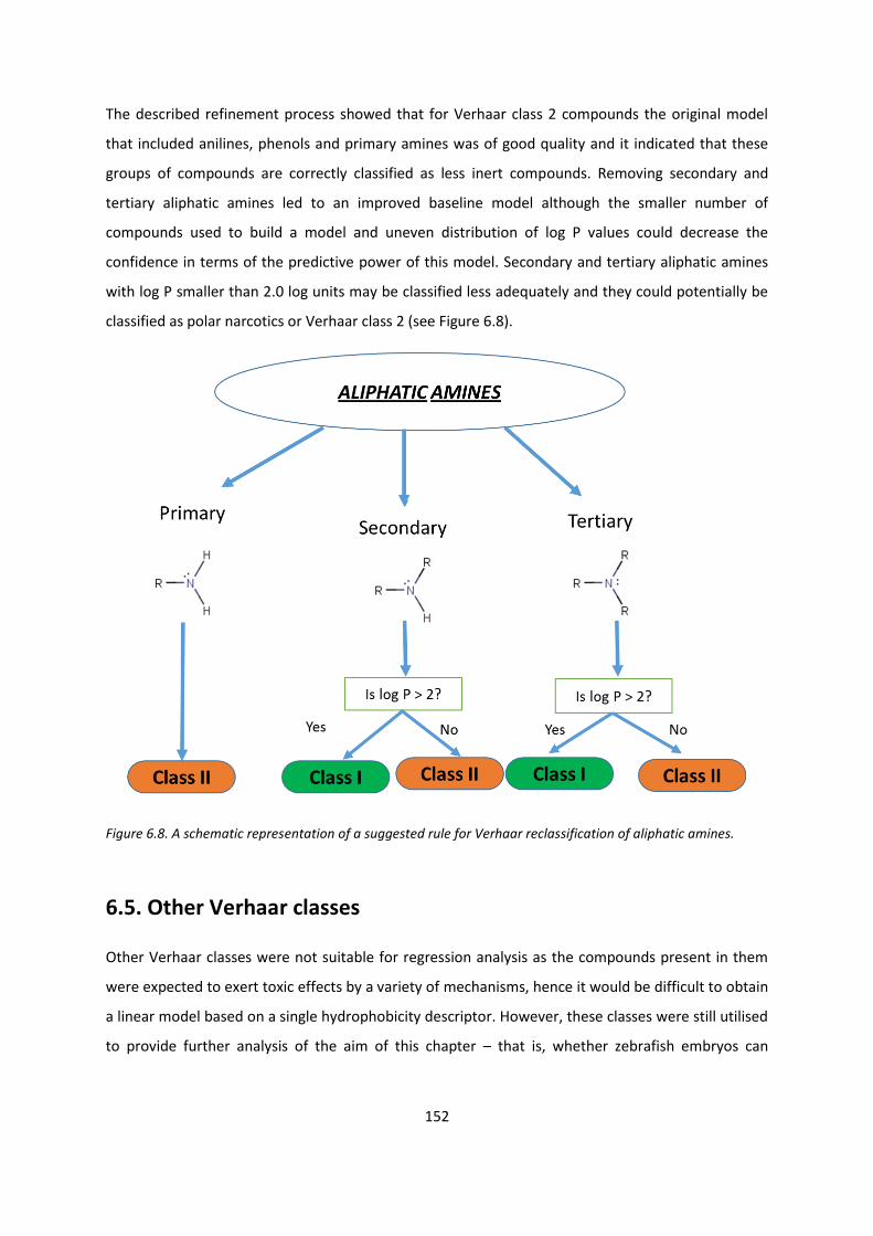
152

The described refinement process showed that for Verhaar class 2 compounds the original model

that included anilines, phenols and primary amines was of good quality and it indicated that these

groups of compounds are correctly classified as less inert compounds. Removing secondary and

tertiary aliphatic amines led to an improved baseline model although the smaller number of

compounds used to build a model and uneven distribution of log P values could decrease the

confidence in terms of the predictive power of this model. Secondary and tertiary aliphatic amines

with log P smaller than 2.0 log units may be classified less adequately and they could potentially be

classified as polar narcotics or Verhaar class 2 (see Figure 6.8).

Figure 6.8. A schematic representation of a suggested rule for Verhaar reclassification of aliphatic amines.

6.5. Other Verhaar classes

Other Verhaar classes were not suitable for regression analysis as the compounds present in them

were expected to exert toxic effects by a variety of mechanisms, hence it would be difficult to obtain

a linear model based on a single hydrophobicity descriptor. However, these classes were still utilised

to provide further analysis of the aim of this chapter – that is, whether zebrafish embryos can

153

distinguish between baseline and excess toxicity. The compounds from Verhaar classes 3, 4 and 5

were compared against the refined baseline model (Eq. 6.3) (Figure 6.9).

It is clear that the majority of compounds from Verhaar classes 3, 4 and 5 have toxicity greater than

predicted by the developed baseline. It should be noted that the range of log P values for Verhaar

classes 3, 4 and 5 is considerably greater than in baseline models; this indicates that the baseline

models should not be used for the prediction of toxicity for these compounds. This is particularly

important in the cases of extreme values for partition coefficient. These compounds could be either

very insoluble (not bioavailable) or so hydrophilic that their interactions with the biological

membrane would be thermodynamically unfavourable.

Interestingly, for a number of compounds from Verhaar class 5 the actual toxicities were lower than

was predicted according to the baseline models. This should not occur by the definition of the

baseline toxicity although some margin of error should be taken into account. These compounds are

shown in Table 6.5 and it appears that they are diverse in terms of chemical structure.

Figure 6.9. A scatterplot of log P toxicity to zebrafish embryos for Verhaar classes 3, 4 and 5. The added

regression line corresponds to a refined baseline model (Eq. 6.3). Compounds from class 5 (for which toxicity is

over-predicted) are depicted as crosses – these are presented in Table 6.5

9876543210-1-2-3-4-5

1

0

-1

-2

-3

-4

-5

-6

logP

log

(1

/EC

50

) (µ

M)

Class_3

Class_4

Class_5

VERHAAR

154

Table 6.5. Selected compounds from Verhaar class 5. All of these had lower actual toxicity values than

predicted by the developed baseline models.

Compound name Structure Comments

Saccharin

N,S heterocyclic, a common

sweetener

Ethyl acetate

ester; can be hydrolysed in vivo

Cyclohexanol

cyclic alcohol

Penicillin

pharmaceutical

Valpromide

pharmaceutical; possible

metabolism to valproic acid

Some of the compounds identified are heterocyclic compounds while others are structurally less

complex, for instance ethyl acetate (ester). Interestingly, a high quality separate model for ester

narcosis was previously obtained (Jaworska, Hunter, Schultz, 1995). However, although esters

seemed to exert excess toxicity in fish, this was not observed for ciliates (e.g. Tetrahymena

pyriformis). This was rationalised by indicating higher activity of esterases in fish. Hydrolysis of ester

by these enzymes was hypothesised to lead to changes in concentration gradient between fish and

water, which in turn would increase the uptake of a chemical by shifting the thermodynamic

equilibrium. On the other hand, no specific FATS were identified for monoesters. Additionally, the

presence of additivity of octanol and monoesters indicated that esters may act as non-polar

narcotics. Ethyl acetate present in the DS1 is a monoester and although it could not be classified

according to Verhaar rules (class 5) its low toxicity value (below a baseline) could indicate that it is a

non-polar narcotic.

Two pharmaceuticals (penicillin and valpromide) were among compounds with low toxicity that

were found in Verhaar class 5. Both these compounds can be a subject to xenobiotic metabolism. In

humans, valpromide is rapidly metabolised to valproic acid (a compound present in baseline models)

while penicillin is biotransformed to either 6-aminopenicillanic acid or penicilloic acid. Zebrafish

155

embryo expresses various CYP isoforms and is capable of oxidative and conjugative xenobiotic

metabolism (Jones et al., 2010). However, it is not known to what extent (if at all) the

biotransformations occur in the case of valpromide and penicillin in zebrafish embryos.

Visual inspection of Figure 6.9 reveals that a fraction (20 compounds) of Verhaar class 5 chemicals

had baseline level toxicity values. Some examples include: cyclohexylamine or piperidines

(heterocyclic amines). This might suggest that such categories of compounds could be reclassified as

non-polar narcotics. On the other hand, it may be the case that the slope of the regression line is too

high and such compounds exert excess toxicity. Nevertheless, it seems that some of the Verhaar

class 5 compounds could be incorporated into non-polar or polar models and therefore, reclassified

as Verhaar class 1 or 2. However, chemical diversity of these chemicals should be carefully examined

before drawing conclusions about creating new toxicophores.

6.6. Validation of baseline non polar narcosis and polar narcosis

models

The quality of selected narcosis models for zebrafish embryos was tested using compounds from

DS2. The test set presented more heterogeneous chemical space than DS1. All compounds from DS2

were grouped according to the Verhaar scheme as implemented in Toxtree. For 43% of compounds

from DS2 the mode of aquatic toxicity was not identified (see Figure 6.10).

Figure 6.10. Distribution of compounds for DS1 and DS2 according to Verhaar classes. The number of chemicals

in each class is presented in absolute values.

To ensure the correct usage of the models an attempt was made to define the applicability domain,

i.e. to determine a space for which the model can produce reliable predictions (Ellison et al., 2011).

Such a domain can be described in terms of x-space of the model that consists of independent

2732

7 5

46

17

8 7 11

33

CLASS 1 CLASS 2 CLASS 3 CLASS 4 CLASS 5

DS1 DS2

156

variables and also in y-space that constitutes a predictions space (Jaworska, Nikolova-Jeliazkova &

Aldenberg, 2005). One of the methods to define x-space is to determine descriptor ranges. All of the

obtained models for DS1 modelled toxicity using only a single variable, log P. Hence, the range of log

P values was described for each of the tested models (Eq. 6.1, 6.2 and 6.3) as well as the prediction

domain (see Table 6.6).

Table 6.6. Ranges of independent (log P) and dependent (toxicity) variables for selected subsets of DS1 or DS2.

Red colour indicates minimum and maximum values that are outside of the domain.

Model/subset log P Toxicity (log (1/EC50) (µM))

min. max. span min. max. span

Eq.6.1 -0.77 3.76 4.53 -5.84 -2.08 3.76

Eq.6.2 -0.57 4.13 4.70 -4.36 -1.06 3.30

Eq.6.3 -0.77 3.00 3.77 -5.84 -2.08 3.76

test set (Verhaar class 1) -0.49 4.60 5.09 -4.47 0.70 5.16

test set (Verhaar class 2) 0.60 5.76 5.16 -2.79 -0.23 2.56

Apart from determining the range of utilised physicochemical descriptors another important step

involves defining structural domain. For instance, Ellison et al., (2008), defined structural domain for

non-polar narcosis for Tetrahymena pyriformis by identifying structural fragments associated with

excess toxicity. The structural domains of the three tested models inherently originated from the

Verhaar rules. It is important to appreciate that the test set compounds should belong to the

training set structural domain to enhance reliability of predictions. The presence of some structural

features may determine the mode of action and constitute the differences in toxicity between

compounds with similar values of physicochemical descriptors, such as log P.

6.6.1. Performance of baseline models

The initial step was to observe (visual inspection of Figure 6.10) whether the refined baseline model

(Eq. 6.3) could distinguish between baseline and excess toxicity for compounds from DS2. The

rationale was that no compounds should have toxicity lower than the baseline, hence the diversity

of the test set would not greatly influence the classification of a compound exerting an excess

toxicity considering that the baseline model (Eq. 6.3) was developed from non-polar narcotics.

The observation of the scatterplot present in Figure 6.11 showed that at least within (or close to) a

range of Log P values in which the baseline models were developed only one compound

(cyclohexane/Verhaar class 1) had a toxicity value much lower than predicted by Eq. 6.3.

Interestingly, two chemicals from Verhaar class 1 were significantly underpredicted. Nevertheless, it

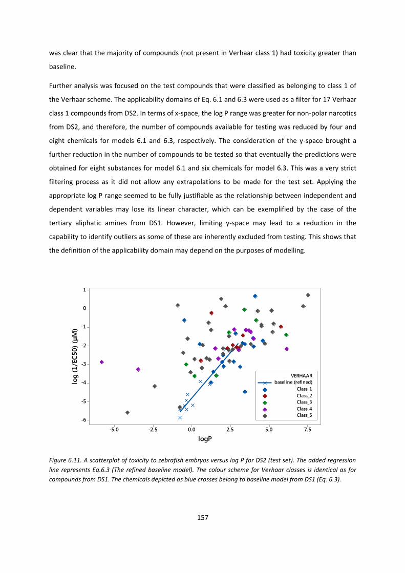
157

was clear that the majority of compounds (not present in Verhaar class 1) had toxicity greater than

baseline.

Further analysis was focused on the test compounds that were classified as belonging to class 1 of

the Verhaar scheme. The applicability domains of Eq. 6.1 and 6.3 were used as a filter for 17 Verhaar

class 1 compounds from DS2. In terms of x-space, the log P range was greater for non-polar narcotics

from DS2, and therefore, the number of compounds available for testing was reduced by four and

eight chemicals for models 6.1 and 6.3, respectively. The consideration of the y-space brought a

further reduction in the number of compounds to be tested so that eventually the predictions were

obtained for eight substances for model 6.1 and six chemicals for model 6.3. This was a very strict

filtering process as it did not allow any extrapolations to be made for the test set. Applying the

appropriate log P range seemed to be fully justifiable as the relationship between independent and

dependent variables may lose its linear character, which can be exemplified by the case of the

tertiary aliphatic amines from DS1. However, limiting y-space may lead to a reduction in the

capability to identify outliers as some of these are inherently excluded from testing. This shows that

the definition of the applicability domain may depend on the purposes of modelling.

Figure 6.11. A scatterplot of toxicity to zebrafish embryos versus log P for DS2 (test set). The added regression

line represents Eq.6.3 (The refined baseline model). The colour scheme for Verhaar classes is identical as for

compounds from DS1. The chemicals depicted as blue crosses belong to baseline model from DS1 (Eq. 6.3).

7.55.02.50.0-2.5-5.0

1

0

-1

-2

-3

-4

-5

-6

logP

log

(1

/EC

50

) (µ

M)

baseline (refined)

Class_1

Class_2

Class_3

Class_4

Class_5

VERHAAR

158

In terms of the structural domain, some compounds such as aromatic hydrocarbons (e.g. toluene)

were not used to build the baseline models. However, they were not excluded from testing as it was

decided to use a broader definition of structural domain for less inert chemicals that was equivalent

to Verhaar class 1 structural domain. Dataset 2 did not contain any aliphatic amines in the class 1 or

class 2 compounds therefore, no information was provided to add to the discussion about

classification of aliphatic amines. Nevertheless, both baseline models (Eq. 6.1 and Eq. 6.3) were

tested to see whether the refinement process led to obtaining a better model for non-polar

narcotics.

Predictions were classified as correct when predicted values did not deviate from experimental

values by more than 0.5 toxicity units (Ellison et al., 2008). The performance of both baseline models

is summarised in Table 6.7.

Table 6.7. Performance of the non-polar (Eq. 6.1 and Eq. 6.2) and polar (Eq. 6.2) narcosis models. The tested

compounds belonged to DS2.

Narcosis type Model No. of tested compounds Correct predictions (%)

Non-polar Eq.6.1 8 75

Eq.6.3 6 83

Polar Eq.6.2 7 71

The majority of compounds from Verhaar class 1 were predicted to be non-polar narcotics. Model

6.1 could not correctly predict two compounds: 2,3-dimethyl-1,3-butadiene and cyclohexane. These

chemicals were not included in model 6.3 as their log P values were not inside the applicability

domain. Additionally, the refined model overpredicted toluene. All three compounds, which were

not correctly predicted, were either aliphatic or aromatic hydrocarbons and as such did not contain

polar moieties that are required for solvation in water; this is also reflected in their low log P values.

Moreover, cyclohexane is immiscible in water. Volatility of toluene and dimethylbutadiene may also

affect measurements (overestimation of concentration). All these compounds could be treated as

outliers in the developed QSAR baseline models. A similar deviation from a positive correlation

between hydrophobicity descriptor and toxicity was observed when discussing tertiary aliphatic

amines at higher log P values (> 2). However, from the classification point of view, these chemicals

were correctly classified as inert substances (Verhaar class 1) and, therefore, their acute toxic effects

would be assessed appropriately. However, from the regression model perspective, the applicability

domain should be extended by additional rules, either related to structural information or regarding

other physicochemical properties, such as vapour pressure or water solubility. Such rules, for

159

instance only compounds with MW < 600 Da can be a subject to Verhaar classification, were indeed

included in the original Verhaar scheme (Verhaar, Leeuwen & Hermens, 1992).

The refined baseline model (Eq. 6.3) provided more correct predictions than the initial baseline

model (Eq. 6.1). However, to have a better understanding of the performance of the models some

additional aspects needed to be considered. First of all, only a limited number of test compounds

was available and it was even further reduced by the defined applicability domain. Structural domain

differences between the training set and test set were also present (e.g. hydrocarbons were only

present in DS2). The distribution of chemical groups within Verhaar class 1 differed with only a single

aliphatic alcohol and, more prominently, no aliphatic amines were present in the test set. In this

context the good performance of model 6.1 might support the classification of secondary and

tertiary amines as inert compounds and as such they could be used to build a baseline narcosis

model.

6.6.2. Testing the polar narcosis model

Similar analysis as for class 1 was carried out with regard to test compounds classified as Verhaar

class 2. Initially, this subset contained 8 chemicals however, one compound (nonylphenol) was later

removed due to the log P being outside of the applicability domain for polar narcosis model (Eq. 6.2).

In terms of the chemical classes, the final test set for polar narcosis was composed of four phenols,

one aniline and two nitropyridines. The model provided correct predictions for five out of seven

compounds (see Table 6.7). 3-nitropyridine (residue = -0.57) and 2-chloro-5-nitropyridine (residue = -

2.7) were the two compounds for which the toxicity values were underpredicted. The training set did

not contain pyridines and therefore, this class of compounds did not define the structural domain.

However, these compounds were categorised as Verhaar class 2 although their toxicity values were

higher than for classical polar compounds. In Tetrahymena pyriformis, nitropyridines were previously

shown to have high toxic ratio (Te) value that discriminated between polar narcosis and reactivity

related to covalent binding (Seward, Cronin & Schultz, 2000). It is possible that nitropyridines should

not be allocated to Verhaar class 2 and, consequently they should not be modelled with polar

narcotics. Instead, nitropyridines could be classified as Verhaar class 3 compounds.

Possible future work on this subject could include investigation of the usefulness of zebrafish

embryo for prediction of the ADME properties. For instance, it would be interesting to compare the

uptake of compounds by the zebrafish embryos to human intestinal absorption. Berghmans et al,

(2008) investigated nine drugs and observed that the amount of drug that penetrated the zebrafish

was related to the hydrophobicity of the drug (cLogP) and compounds with high cLogP values (> 3.8)

160

had a better ability to penetrate the zebrafish larvae. The author of the thesis identified six of these

compounds in the Hou et al., (2007b) HIA dataset (see Chapter 2 of the thesis) to compare how the

fish penetration was related to HIA. It appeared that 50% of these drugs were high absorption

despite their poor uptake by zebrafish embryos. More data are needed to derive any rules about the

relationship of zebrafish embryo and HIA.

***

In summary, zebrafish embryos appear to distinguish between baseline and excess toxicity. The

developed regression models for non-polar narcosis (Eq. 6.1 and Eq. 6.3) and polar narcosis (Eq. 6.2)

were validated using an external dataset. The applicability domains of the models were determined

by the ranges of independent and dependent variables. The models could predict the toxicity for the

majority of test compounds that belonged to the applicability domain. However, the validation

process could benefit from the availability of a greater number of compounds. The analysis of

aliphatic amines and the context of Verhaar scheme suggested that secondary and tertiary aliphatic

amines with log P smaller than 2.0 log units could potentially be reclassified as Verhaar class 2.

Interestingly, a number of Verhaar class 5 compounds appeared to exert baseline type of toxicity

which might suggest that further rules could be introduced. Additional rules may also reduce the

number of compounds for which, in terms of Verhaar scheme, no decisions can be made.

161

7. Discussion

The area of in silico toxicology has developed rapidly over the past few decades. There are many

factors that have driven the advances in non-testing methods (Raunio, 2013). The reduction

refinement and replacement philosophy (the 3Rs framework) has led to an appreciation of the need

to approach animal testing, and the search for alternatives, in a different way. Furthermore,

legislation and regulation have also played an important role. For example, the REACH regulation

promotes the use of non-testing methods and provides guidelines on the application of

computational methods, such as QSARs or read-across, in risk assessment (ECHA, 2008). In addition

the 7th amendment to the EU Cosmetics Directive effectively bans the use of animals for studying

toxicity of cosmetic ingredients. The US National Research Council has proposed a strategy for the

assessment of environmental toxicity (of industrial chemicals and pesticides) using in vitro and in

silico approaches to identify human toxicity pathways. This strategy involves the incorporation of

systems biology and “omics” methods (NRC, 2007). The pharmaceutical industry has also been a

significant contributor to the development of alternative methods by progressing the development

of in silico methods for drug discovery and assessment of ADME-tox profiles. The IMI project eTOX is

an example of a collaborative effort of pharmaceutical companies to develop novel approaches to

assessing drug-related toxicity. Despite the progress in computational approaches for the prediction

of toxicity, these methods still find limited application in the area of regulatory toxicology. For

instance, there is no “list” of in silico methods that have been approved formally for use complying

with REACH requirements. The limitations of applying in silico methods within REACH are in part due

to the lack of experimental data available for model development and also the lack of experience of

using such models for regulatory purposes (Benfenati et al., 2013). In the context of

pharmaceuticals, neither the US FDA nor the European Medicines Agency require in silico data to be

submitted (Valerio, 2009).

The wider acceptance of computational models for risk assessment could be achieved through the

development of high quality, validated models for clearly defined endpoints (OECD, 2007). In the

context of risk assessment such models should also be transparent, i.e. have a clear chemical and

biological interpretation. It is also important to critically evaluate existing in silico tools to determine

their suitability for purpose, both in terms of overall predictivity and their domain of applicability.

Assessment and evaluation of existing software for ADME-tox prediction can enhance the

understanding of these tools and provide guidelines of how they can be applied, most effectively, in

practice. This is particularly important for non-expert users. This was one of the themes that was

explored within this thesis.

162

For example, in Chapter 3, selected software for metabolism prediction was evaluated. It was noted

that, especially in the case of the Meteor software, there was the tendency for overprediction of

metabolites. Although Meteor provides a number of settings that may be selected by the user

(absolute and relative reasoning engines; number of metabolites in the output etc) it is not obvious

which settings are the most appropriate to select in order to identify correct metabolites without

producing a large number of false positives. Within this work it was demonstrated that using

relatively permissive reasoning engine settings (equivocal) and reducing the number of metabolites

to be predicted improved the precision of the results. Menikarachchi et al., (2013) suggested that a

certain number of false positives does not need to be disadvantageous providing that these can be

filtered out in an efficient way. In the case of Meteor, this software may be used in combination with

Derek Nexus (Lhasa Limited, Leeds) to determine the toxicological liability of the metabolites

predicted by Meteor. It may be argued that this combination represents a safer option in terms of

toxicity prediction i.e. toxicity of both parent drug and metabolites can be predicted. On the other

hand, obtaining Meteor predictions is computationally expensive and time consuming; this may

present a significant limitation when applying this combination approach to screening a large library

of compounds, as may be necessary in a pharmaceutical industry setting. Other freely available

software that was investigated here (SMARTCyp and MetaPrint2D-React) also proved to be very

useful tools for prediction of xenobiotic metabolism. Another outcome of the studies within this

thesis was the proposal to combine SMARTCyp and MetaPrint2D-React, whereby SMARTCyp could

be used to predict potential sites of metabolism (SOM) and MetaPrint2D-React could then provide

the structures of the metabolites generated at the given SOM. Although MetaPrint2D can also

provide SOM it relies solely on a historical database and hence, it may fail to correctly predict

metabolite structures for compounds representing a different chemical space, as may be the case in

specific drug development programs. SMARTCyp is based on quantum mechanical calculations and

therefore it is less dependent on historical data. (This advantage was realised by Lhasa Limited,

during the time in which these PhD studies were undertaken, and SMARTCyp has now been

incorporated into Meteor Nexus). The assessment of Meteor and MetaPrint2D-React also showed

that despite good overall performance, some metabolites were not correctly predicted, for example

in the case of bromfenac. This illustrates that each in silico tool is associated with certain limitations.

For bromfenac a particular biotransformation was not adequately represented within the expert

system (Meteor) nor was it present in the historical database utilised by the data mining approach

(MetaPrint2D-React). This is not the only limitation of concern. For instance, for SMARTCyp,

potential limitations relate to the number of fragments for which the energy calculations have been

performed and also by the number of CYP450 models (3A4, 2D6, etc.) that are currently available. In

163

each case, the limitations have to be recognised by the users. This also means understanding the

applicability domain of a model and having realistic interpretation of the output. Again, in the case

of the in silico tools for xenobiotic metabolism it should be appreciated that the predictions are

purely qualitative as they do not estimate the relative amounts of each metabolite likely to be

formed. These limitations add to the lack of confidence in decisions concerning the safety of a

chemical. This is especially important in a regulatory context where computational methods are not

widely accepted and carry relatively little weight in risk assessment (Modi et al., 2011).

Xenobiotic metabolism is a key component of ADME-Tox profiles. However, it cannot be considered

in isolation from absorption. If a compound is poorly absorbed it will not enter the systemic

circulation and therefore, it will not reach the CYP450 system in the liver where the majority of

metabolism occurs. Hence, the prediction of human intestinal absorption was another important

pharmacokinetic aspect that was considered (Chapter 2). In silico approaches may offer a fast and

cost-effective method for assessing the absorption of compounds especially at the early stages of

drug discovery when performing virtual screens on large number of compounds. Druglikeness filters,

such as Lipinski’s rule of five or Veber’s rules, are of special interest due to their simplicity relating to

the use of transparent, and therefore more easily-interpretable, medicinal-chemist type descriptors.

The accuracy of the predictions obtained from applying druglikeness filters were comparable (and in

some cases better) than those that resulted from in vitro approaches to predicting absorption (Caco-

2 and PAMPA). Interestingly, a combination of TPSA (≤ 140 Å2) and log D6.5 (Hou et al., 2007b) gave

the most promising results in terms of distinguishing between high and low human intestinal

absorption. This indicates that in the case of pharmaceuticals the distribution coefficient (log D),

especially at pH values similar to those encountered in the GIT, may be a better predictor of oral

drug absorption than log P as log D takes into account the ionisation of a compound. However,

druglikeness filters should be used with caution even though they are widely applied in the

pharmaceutical industry. One of the factors to consider is the binary nature of the predictions

obtained by application of druglikeness rules. This means that “hard” cut-offs may be applied in too

rigorous a manner and result in some useful compounds being discarded during screening. In

response to this potential pitfall, more sophisticated druglikeness measures have been introduced

recently, such as quantitative estimate of druglikeness (QED) (Bickerton et al., 2012). QED combines

eight characteristics (medicinal chemist-type descriptors) into a single metric that describes how

similar a compound is to known orally administered drugs. It would be interesting to examine

whether the QED could successfully be applied to the absorption dataset studied herein. Another

issue identified with the generic “druglikeness” rules is the poor distinction between human

intestinal absorption and bioavailability (in humans), for example Veber’s rules were developed for

164

oral bioavailability in rats. Nonetheless, a druglike molecule should be expected to be absorbed, at

least to some extent. Finally, druglikeness rules cannot provide a quantitative prediction for

absorption or bioavailability which might be useful, especially at later stages of drug discovery, e.g.

during the optimisation process. This is an area where in vitro techniques may be more

advantageous.

Within the work conducted here, application of rules such as the combination of TPSA and log D6.5

was not useful for the prediction of bioavailability. This may be expected due to the metabolic

clearance as these properties do not adequately account for the contribution of first pass hepatic

clearance. An attempt to build a model that could predict hepatic clearance was not successful;

hepatic clearance is a complex process and therefore is difficult to model. Similarly, in vitro

techniques (liver microsomes, human hepatocytes) have been shown to underpredict in vivo

metabolic clearance (Chiba, Ishii & Sugiyama, 2009). The extent to which a compound will be

metabolised was recently shown to be related to in vitro permeability rate measurements and also

to in silico permeability rate predictions. However, knowledge of metabolic rate is often limited

(Kirchmair et al., 2015) making it difficult to develop models to predict rate and extent of

metabolism and the contribution of these to bioavailability.

During analysis of oral absorption and bioavailability all the datasets (except that for hepatic

clearance) were significantly skewed towards high absorption/bioavailability values. More evenly

distributed datasets would be required to increase confidence in the models developed.

Xenobiotic metabolism is also linked to toxicity; as a result of bioactivation, reactive metabolites can

be formed. These tend to be electrophilic species that can readily attack nucleophilic centres on

biomolecules. This process may lead to a disruption of biological functions and may lead to toxic

effects such as type B adverse drug reactions. Elements of electrophilic chemistry, relevant to

protein binding, have been captured and described in terms of electrophilic reaction domains (Enoch

et al., 2011). The structural alerts associated with protein binding have been incorporated in a

number of software packages, such as the OECD (Q)SAR Toolbox or Toxtree or they can be accessed

via web services such as the ToxAlerts platform (Sushko et al., 2012).

Structural alerts offer a promising tool for screening purposes, for instance in drug discovery. Work

carried out here included analysis of the DrugBank dataset in relation to the distribution of structural

alerts for reactive metabolism. Interestingly, nearly half of the compounds from DrugBank contained

at least one structural alert. There were no significant differences in distribution of structural alerts

among different drug classes (approved, experimental, and withdrawn). There was also no

correlation between the number of identified alerts and the class of the drug. This shows that the

presence of a structural alert is not sufficient to predict the adverse outcome. A more holistic

165

approach is required that takes into account such factors as: dosage, route of clearance or the

existence of alternative sites on a molecule that are more liable to metabolism. Pharmacokinetic

properties, such as absorption need to be considered as well. A compound that is poorly absorbed

will not be subject to extensive xenobiotic metabolism as it will not reach the liver in large

quantities. This is where the aforementioned rule-based filters such as Lipinski’s rule of five can be

utilised to obtain more complete profiles for screened compounds. Despite the complexity of the

problem some non-expert users may not appreciate that structural alerts cannot be the only basis of

decision-making about the future of a compound. There may be a temptation to take advantage of

the binary nature of the result i.e. if an alert is present - reject the compound, otherwise take it

forward in development.

The structural alerts within oCHEM were initially used without refinement, leading to a high number

of compounds being associated with “hits”. As it is possible many of these “hits” could relate to false

positives in terms of toxicity prediction, refinement of the structural alerts was investigated. This

was exemplified by re-writing the SMARTS pattern for the carboxylic acid alert in order to reduce the

number of false positives. However, this approach may also carry a risk of missing potentially

reactive structures. The balance between sensitivity and specificity requires careful consideration of

mitigating factors and may be challenging to validate due to the lack of data.

Toxicity related to poor pharmacokinetic properties compounds is only one of the challenges for the

pharmaceutical industry. Off-target toxicity represents another challenging area in drug discovery

and development. Within this thesis, aspects of off-target toxicity related to hERG channel inhibition,

were also investigated. A previously reported QSAR model for hERG toxicity (Aptula & Cronin, 2004)

was evaluated. This model offered a transparent interpretation due to using simple medicinal

chemistry-type descriptors related to hydrophobicity (log D) or molecular size (maximum diameter).

Despite this advantage, the model could not provide accurate predictions for the larger dataset

(H_244) studied here. A limited applicability domain of the model developed by Aptula & Cronin,

(2004) was indicated to be an important factor that influenced the predictions. Building global linear

regression and classification models did not offer improvements to existing models. The best model

(78% correct predictions) was obtained using a random forest classifier. Local models, based on 2D-

similarity, were also developed for seven defined categories of compounds identified within the

dataset. The multiple linear regression models obtained for the categories investigated were not

satisfactory, except for compounds from category VI. The limited success with global modelling can

be explained by the fact that the hERG channel can bind very structurally diverse compounds.

However, better models were expected for local categories. The results suggest that multiple linear

regression methods are not suitable for hERG modelling. On the other hand, good regression models

166

were obtained by Yoshida & Niwa, (2006) although for a smaller dataset. The quality of models can

be affected by interlaboratory variability. The differences in IC50 values obtained from different

laboratories can be greater than 10-fold (Ekins, 2007). Additionally, the inhibition values may

originate from different cell lines increasing variability in results; this was noted to be the case for

the dataset studied here.

Due to the difficulties in building quantitative predictive models a more qualitative approach was

taken. The alerts developed for six (out of the seven) defined categories could be utilised as a

potential screening tool. However, these alerts require further validation. One of the limitations of

the structural alerts for hERG may be their specificity for the group of compounds on which they

were based. This is the opposite situation to that encountered during the analysis of structural alerts

for carboxylic acid in the context of reactive metabolites. Whilst the structural alert for carboxylic

acids was refined to be more specific, the alerts for hERG would benefit from greater generalisation

so that they capture more compounds. However, it should be appreciated that the hERG channel

inhibition is a result of weak interactions between a drug and a channel pocket rather than being

related to specific reactivity. As a result it may be more beneficial to develop SMARTS for fragments

based on pharmacophore models and then combine them with filters based on physico-chemical

properties, similar to those developed by Aptula & Cronin, (2004). This could be captured in the form

of a decision tree. Such fragments could be more useful for screening purposes as they could

capture broader chemical space, but they would have to be considered in conjunction with a filter

based, for instance, on molecular size that prohibits larger molecules entering the channel pocket.

This could narrow down the results of the screen and give a more pragmatic approach to prediction

of hERG-related off-target toxicity.

The trend to reduce animal testing stimulates the development of new approaches. One such

approach in the context of aquatic toxicity is using fish embryos, rather than adult organisms. It has

been established that the zebrafish embryo toxicity (ZFET) test is a valid alternative method of

determining aquatic toxicity (Belanger et al., 2013; Busquet et al., 2014). Research undertaken here

investigated whether zebrafish embryos could distinguish between baseline and excess toxicity. The

analysis was performed by utilisation of the Verhaar scheme. The implementation of the Verhaar

scheme was also of interest in terms of its performance. Whilst the scheme has been well

established there is a need to update and/or add new rules. This statement is based on the fact that

within both the training and test sets analysed here many compounds could not be placed into one

of the Verhaar categories (i.e. the software place many compounds into category V). Moreover,

some of these compounds exerted baseline toxicity. Zebrafish embryos were shown to distinguish

between non-polar and polar narcosis. The analysis of amines showed that secondary and tertiary

167

aliphatic amines, with log P smaller than 2.0 log units, may potentially be classified as polar

narcotics. However, more data points are required for this statement to be conclusive.

The applicability domain of the QSAR models developed for the prediction of aquatic toxicity was

also considered. This is a specific recommendation of the OECD guidelines for building valid QSAR

models and as such should be considered during model development and testing. The importance of

applicability domain may not be fully appreciated by naive users of toxicity prediction software and

therefore can have significant consequences for the reliability of predictions obtained.

Zebrafish embryos can also be useful for the assessment of ecotoxicity of pharmaceuticals that

constitute a class of environmental pollutants. Active pharmaceutical ingredients (APIs) that

originate from drug production for both medicinal and veterinary use can reach drinking water

through various pathways (Santos et al., 2013). Moreover, APIs can be subject to biotransformations

with the possibility of formation of reactive metabolites. The significance of the biotransformation of

the parent and the environmental risks of the metabolites have not yet been fully investigated

(Kummerer, 2010). The regulatory bodies have recognised the issue of APIs and in consequence, the

environmental risks and impact of medicinal products are required to be evaluated and assessed

(European Directive 2001/83/EC). Zebrafish embryos have been successfully used in the context of

toxicity testing of APIs. A recent study showed that pharmaceutical pollutants can have detrimental

effects on zebrafish embryos development (Pruvot et al., 2012). In another study, zebrafish embryos

were utilised to assess the toxicity of 15 veterinary pharmaceuticals and their metabolites (Carlsson

et al., 2013). As zebrafish embryos can distinguish between baseline and excess toxicity they appear

to be a promising organism for studying the effects of reactive metabolites.

***

The work undertaken within this thesis covered several aspects of ADME-tox prediction. Emphasis

was placed on topics related to drug discovery and development with a particular focus on

prediction of pharmacokinetic properties such as absorption and metabolism. A discussion of

screening tools such as structural alerts was also presented. Off-target toxicity and the use of

alternative fish developmental stages for the assessment of aquatic toxicity have been explored. A

number of existing software packages have been evaluated and recommendations made as to how

the packages, or the methods of their application, may be improved.

168

Future work

The studies conducted for this thesis have explored various aspects of computational toxicology

ranging from modelling ecotoxicity to prediction of ADME properties and off-target effects of drugs.

A variety of tools were evaluated, different modelling techniques were applied and improvements to

existing methods suggested where appropriate. It has been appreciated that in silico approaches to

prediction of toxicity may be useful, although they are not free from limitations. One of the most

important limitations is related to the availability of high quality, diverse, datasets that can be used

to train models. It is obvious that the quality of a model depends on the quality of data used for its

construction; size and diversity are also of importance. Nevertheless, large, well-curated and

balanced datasets are rather difficult to find in the public domain. The pharmaceutical industry may

be privileged in this respect as they own large collections of data. This cornucopia has been explored

by the eTOX project for building models without compromising the confidentiality of the data.

However, this can present another issue related to the applicability domain of such models. It relates

to the question whether a model built, for instance, on a dataset of leadlike/druglike molecules can

also give reliable predictions for toxicity of compounds belonging to alternative regions of chemical

space, such as that applicable to cosmetic ingredients, industrial chemicals etc. Detailed analysis and

accurate definition of the applicability domain of models is a key area for future development. In

particular how can the structural similarity between compounds be defined and what are the

consequences in terms of the similarity of training and test sets.

Structural alerts comprise another interesting area. For example the work on structural alerts for

hERG inhibition, as carried out in this thesis, might serve as a starting point for future work in this

area. Data mining approaches that allow the discovery of chemical fragments related to specific

endpoints in a more automated manner may enable results to be obtained more rapidly in future.

This may be more relevant to such an endpoint as hERG channel inhibition where there is no

definitive mechanistic interpretation of the channel inhibition due to the nature of the drug-channel

interactions of such a diverse range of drugs. Such an approach could also be applied to the

identification of potentially reactive metabolites which could add a new perspective to the existing

alerts, especially in the context of their specificity.

Finally, further work could also be carried out in relation to the prediction of ADME properties

possibly in combination with physiologically-based pharmacokinetic modelling (PBPK). The

prediction of pharmacokinetic profiles requires knowledge of some basic physico-chemical

properties such as solubility or permeability. The accurate and reliable prediction of medicinal

169

chemistry-type descriptors is a sine qua non for simulation of pharmacokinetics and, therefore, a

crucial area for future investigation in terms of improving the existing models.

170

References

Adams, S. E. (2010). Molecular similiarity and xenobiotic metabolism. Dissertation. University of

Cambridge, United Kingdom, pp 251.

Akamatsu, M., Fujikawa, M., Nakao, K., & Shimizu, R. (2009). In silico prediction of human oral

absorption based on QSAR analyses of PAMPA permeability. Chemistry and Biodiversity, 6(11), 1845-

1866.

Alderton, W., Berghmans, S., Butler, P., Chassaing, H., Fleming, A., Golder, Z., . . . Gardner, I. (2010).

Accumulation and metabolism of drugs and CYP probe substrates in zebrafish

larvae. Xenobiotica, 40(8), 547-557.

Aptula, A. O., & Cronin, M. T. D. (2004). Prediction of hERG K+ blocking potency: Application of

structural knowledge. SAR and QSAR in Environmental Research, 15(5-6), 399-411.

Aronov, A. M. (2005). Predictive in silico modeling for hERG channel blockers. Drug Discovery

Today, 10(2), 149-155.

Aronov, A. M. (2006). Common pharmacophores for uncharged human ether-a-go-go-related gene

(hERG) blockers. Journal of Medicinal Chemistry, 49(23), 6917-6921.

Aronov, A. M., & Goldman, B. B. (2004). A model for identifying HERG K+ channel

blockers. Bioorganic and Medicinal Chemistry, 12(9), 2307-2315.

Artursson, P., & Karlsson, J. (1991). Correlation between oral drug absorption in humans and

apparent drug permeability coefficients in human intestinal epithelial (caco-2) cells. Biochemical and

Biophysical Research Communications, 175(3), 880-885.

Austin, R. P., Davis, A. M., & Manners, C. N. (1995). Partitioning of ionizing molecules between

aqueous buffers and phospholipid vesicles. Journal of Pharmaceutical Sciences, 84(10), 1180-1183.

Avdeef, A. (2001). Physicochemical profiling (solubility, permeability and charge state). Current

Topics in Medicinal Chemistry, 1(4), 277-351.

Avdeef, A. (2005). The rise of PAMPA. Expert Opinion on Drug Metabolism and Toxicology, 1(2), 325-

342.

Babcock, J. J., & Li, M. (2013). HERG channel function: Beyond long QT. Acta PhB1:B76armacologica

Sinica, 34(3), 329-335.

171

Baillie, T. A., Cayen, M. N., Fouda, H., Gerson, R. J., Green, J. D., Grossman, S. J., . . . Shipley, L. A.

(2002). Contemporary issues in toxicology: Drug metabolites in safety testing. Toxicology and

Applied Pharmacology, 182(3), 188-196.

Bains, W., Basman, A., & White, C. (2004). HERG binding specificity and binding site structure:

Evidence from a fragment-based evolutionary computing SAR study. Progress in Biophysics and

Molecular Biology, 86(2), 205-233.

Baker, M., & Parton, T. (2007). Kinetic determinants of hepatic clearance: Plasma protein binding

and hepatic uptake. Xenobiotica, 37(10-11), 1110-1134.

Basavaraj, S., & Betageri, G. V. (2014). Can formulation and drug delivery reduce attrition during

drug discovery and development—review of feasibility, benefits and challenges, Acta Pharmaceutica

Sinica B, 4(1), 3-17.

Belanger, S. E., Rawlings, J. M., & Carr, G. J. (2013). Use of fish embryo toxicity tests for the

prediction of acute fish toxicity to chemicals. Environmental Toxicology and Chemistry, 32(8), 1768-

1783.

Ben-David, A. (2008). About the relationship between ROC curves and Cohen's kappa. Engineering

Applications of Artificial Intelligence, 21(6), 874-882.

Benet, L. Z., Spahn-Langguth, H., Iwakawa, S., Volland, C., Mizuma, T., Mayer, S., . . . Lin, E. T. (1993).

Predictability of the covalent binding of acidic drugs in man. Life Sciences, 53(8), PL141-PL146.

Benfenati, E., Diaza, R. G., Cassano, A., Pardoe, S., Gini, G., Mays, C., . . . Benighaus, L. (2011). The

acceptance of in silico models for REACH: Requirements, barriers, and perspectives. Chemistry

Central Journal, 5(58). Available from: http://journal.chemistrycentral.com/content/5/1/58

[Accessed: March 12th, 2015]

Berellini, G., Waters, N. J., & Lombardo, F. (2012). In silico prediction of total human plasma

clearance. Journal of Chemical Information and Modeling, 52(8), 2069-2078.

Berghmans, S., Butler, P., Goldsmith, P., Waldron, G., Gardner, I., Golder, Z., . . . Fleming, A. (2008).

Zebrafish based assays for the assessment of cardiac, visual and gut function - potential safety

screens for early drug discovery. Journal of Pharmacological and Toxicological Methods, 58(1), 59-

68.

172

Berninger, J. P., & Brooks, B. W. (2010). Leveraging mammalian pharmaceutical toxicology and

pharmacology data to predict chronic fish responses to pharmaceuticals. Toxicology

Letters, 193(1), 69-78.

Bickerton, G. R., Paolini, G. V., Besnard, J., Muresan, S., & Hopkins, A. L. (2012). Quantifying the

chemical beauty of drugs. Nature Chemistry, 4(2), 90-98.

Bleicher, K. H., Böhm, H. Müller, K., & Alanine, A. I. (2003). Hit and lead generation: Beyond high-

throughput screening. Nature Reviews Drug Discovery, 2(5), 369-378.

Bradbury, S. P., Henry, T. R., & Carlson, R. W. (1990). Fish acute toxicity syndromes in the

development of mechanism-specific QSARs. In W. Karcher, & L. Devillers, (Eds.), Practical

applications of quantitative structure-activity relationships (QSAR) in environmental chemistry and

toxicology, (Eds.), Chemical and Environmental Science. Volume 1, 295-315.

Braggio, S., Montanari, D., Rossi, T., & Ratti, E. (2010). Drug efficiency: A new concept to guide lead

optimization programs towards the selection of better clinical candidates.Expert Opinion on Drug

Discovery, 5(7), 609-618.

Braunbeck, T., & Lammer, E. (2006). Background Paper on Fish Embryo Toxicity Assays. Prepared for

German Federal Environment Agency,” UBA Contract No. 203 85 422. Available from:

http://is.muni.cz/el/1431/podzim2012/Bi5580/um/36667252/FishEmbryoToxicity.pdf [Accessed:

September 8th, 2014).

Briggs, K., Cases, M., Heard, D. J., Pastor, M., Pognan, F., Sanz, F., . . . Wichard, J. D. (2012). Inroads to

predict in vivo toxicology-an introduction to the eTOX project. International Journal of Molecular

Sciences, 13(3), 3820-3846.

Broccatelli, F., Mannhold, R., Moriconi, A., Giuli, S., & Carosati, E. (2012). QSAR modeling and data

mining link torsades de pointes risk to the interplay of extent of metabolism, active transport, and

hERG liability. Molecular Pharmaceutics, 9(8), 2290-2301.

Brooks, B. W, Berninger, J. P., Ramirez, A. J., & Huggett, D.B. (2012). Perspectives on Human

Pharmaceuticals in the Environment. In L. R. Shugart, (Ed.), Emerging Topics in Ecotoxicology.

Principles, Approaches and Perspectives. Volume 4, 1-16.

Bugelski, P. J. (2005). Genetic aspects of immune-mediated adverse drug effects. Nature Reviews

Drug Discovery, 4(1), 59-69.

173

Busquet, F., Strecker, R., Rawlings, J. M., Belanger, S. E., Braunbeck, T., Carr, G. J., . . . Halder, M.

(2014). OECD validation study to assess intra- and inter-laboratory reproducibility of the zebrafish

embryo toxicity test for acute aquatic toxicity testing. Regulatory Toxicology and

Pharmacology, 69(3), 496-511.

Buyck, C. (2003). An in silico model for detecting potential HERG blocking. In M. Ford, (Ed.),

EuroQSAR 2002. Designing Drugs and Crop Protectants: Processes, Problems, and Solutions.

Byrns, M. C., Vu, C. C., Neidigh, J. W., Abad, J. –L., Jones, R. A., & Peterson, L. A. (2006). Detection of

DNA adducts derived from the reactive metabolite of furan, cis-2-butene-1,4-dial. Chemical Research

in Toxicology, 19(3), 414-420.

Carlsson, G., Patring, J., Kreuger, J., Norrgren, L., & Oskarsson, A. (2013). Toxicity of 15 veterinary

pharmaceuticals in zebrafish (danio rerio) embryos. Aquatic Toxicology, 126, 30-41.

Carlsson, L., Spjuth, O., Adams, S., Glen, R. C., & Boyer, S. (2010). Use of historic metabolic

biotransformation data as a means of anticipating metabolic sites using MetaPrint2D and

bioclipse. BMC Bioinformatics, 11

Carpenter, E. P., Beis, K., Cameron, A. D., & Iwata, S. (2008). Overcoming the challenges of

membrane protein crystallography. Current Opinion in Structural Biology, 18(5), 581-586.

Cavalli, A., Poluzzi, E., De Ponti, F., & Recanatini, M. (2002). Toward a pharmacophore for drugs

inducing the long QT syndrome: Insights from a CoMFA study of HERG K+ channel blockers. Journal

of Medicinal Chemistry, 45(18), 3844-3853.

Charifson, P. S., & Walters, W. P. (2014). Acidic and basic drugs in medicinal chemistry: A

perspective. Journal of Medicinal Chemistry, 57(23), 9701-9717.

Chen, Y. -. P., & Chen, F. (2008). Identifying targets for drug discovery using bioinformatics. Expert

Opinion on Therapeutic Targets, 12(4), 383-389.

Cheng, A. C., Coleman, R. G., Smyth, K. T., Cao, Q., Soulard, P., Caffrey, D. R., . . . Huang, E. S. (2007).

Structure-based maximal affinity model predicts small-molecule druggability. Nature

Biotechnology, 25(1), 71-75.

Chiba, M., Ishii, Y., & Sugiyama, Y. (2009). Prediction of hepatic clearance in human from in vitro data

for successful drug development. AAPS Journal, 11(2), 262-276.

174

Chipinda I, Hettick JM, & Siegel PD. (2011) Haptenation: chemical reactivity and protein binding.

Journal of Allergy (Cairo). [Online] 2011, Article ID 839682. Available from:

http://www.ncbi.nlm.nih.gov/pmc/articles/PMC3138048/ [Accessed: 12th February 2015].

Coi, A., Massarelli, I., Murgia, L., Saraceno, M., Calderone, V., & Bianucci, A. M. (2006). Prediction of

hERG potassium channel affinity by the CODESSA approach. Bioorganic and Medicinal

Chemistry, 14(9), 3153-3159.

Congreve, M., Carr, R., Murray, C., & Jhoti, H. (2003). A 'rule of three' for fragment-based lead

discovery? Drug Discovery Today, 8(19), 876-877.

Cramer III, R. D., Patterson, D. E., & Bunce, J. D. (1988). Comparative molecular field analysis

(CoMFA). 1. Effect of shape on binding of steroids to carrier proteins. Journal of the American

Chemical Society, 110(18), 5959-5967.

Cronin, M. T. D. & Madden, J. C. (2010). In silico Toxicology – An Introduction. In Cronin, M. T. D., & J.

C., Madden (Ed.), In Silico Toxicology. Principles and Applications (pp. 1 – 10), Cambridge: RSC

Publishing.

Danker, T., & Möller, C. (2014). Early identification of hERG liability in drug discovery programs by

automated patch clamp. Frontiers in Pharmacology, 5 AUG Retrieved from www.scopus.com

Dearden, J. C., Cronin, M. T. D., & Kaiser, K. L. E. (2009). How not to develop a quantitative structure-

activity or structure-property relationship (QSAR/QSPR). SAR and QSAR in Environmental

Research, 20(3-4), 241-266.

Delvecchio, C., Tiefenbach, J., & Krause, H. M. (2011). The zebrafish: A powerful platform for in vivo,

HTS drug discovery. Assay and Drug Development Technologies, 9(4), 354-361.

Deo, R. C., & MacRae, C. A. (2011). The zebrafish: Scalable in vivo modeling for systems

biology. Wiley Interdisciplinary Reviews: Systems Biology and Medicine, 3(3), 335-346.

Dimitrov, S. D., Mekenyana, O. G., Sinks, G. D., & Schultz, T. W. (2003). Global modeling of narcotic

chemicals: Ciliate and fish toxicity. Journal of Molecular Structure: THEOCHEM, 622(1-2), 63-70.

Ding, F., Guo, J., Song, W., Hub, W., & Li, Z. (2011). Comparative quantitative structure-activity

relationship (QSAR) study on acute toxicity of triazole fungicides to zebrafish. Chemistry and

Ecology, 27(4), 359-368.

175

Doddareddy, M. R., Klaasse, E. C., Shagufta, Ijzerman, A. P., & Bender, A. (2010). Prospective

validation of a comprehensive in silico hERG model and its applications to commercial compound

and drug databases. ChemMedChem, 5(5), 716-729.

Drugs.com, (2012). Available from: http://www.drugs.com/top200.html [Accessed April 20th 2012).

Du, L. –P., Tsai, K. –Ch., Li, M. –Y., You, Q. –D., & Xia, L. (2004). The pharmacophore hypotheses of I

kr potassium channel blockers: Novel class III antiarrhythmic agents.Bioorganic and Medicinal

Chemistry Letters, 14(18), 4771-4777.

Dudek, A. Z., Arodz, T., & Gálvez, J. (2006). Computational methods in developing quantitative

structure-activity relationships (QSAR): A review. Combinatorial Chemistry and High Throughput

Screening, 9(3), 213-228.

Durdagi, S., Randall, T., Duff, H. J., Chamberlin, A., & Noskov, S. Y. (2014). Rehabilitating drug-

induced long-QT promoters: In-silico design of hERG-neutral cisapride analogues with retained

pharmacological activity. BMC Pharmacology & Toxicology, 15(1), 14.

ECHA. (2008). Guidance on information requirements and chemical safety assessment Chapter R.6:

QSARs and grouping of chemicals. Available from:

https://echa.europa.eu/documents/10162/13632/information_requirements_r6_en.pdf [Accessed:

June 2nd, 2015]

Eimon, P. M., & Rubinstein, A. L. (2009). The use of in vivo zebrafish assays in drug toxicity

screening. Expert Opinion on Drug Metabolism and Toxicology, 5(4), 393-401.

Ekins, S., Crumb, W. J., Dustan Sarazan, R., Wikel, J. H., & Wrighton, S. A. (2002). Three-dimensional

quantitative structure-activity relationship for inhibition of human ether-a-go-go-related gene

potassium channel. Journal of Pharmacology and Experimental Therapeutics, 301(2), 427-434.

Ellison, C. M., Cronin, M. T. D., Madden, J. C., & Schultz, T. W. (2008). Definition of the structural

domain of the baseline non-polar narcosis model for tetrahymena pyriformis. SAR and QSAR in

Environmental Research, 19(7-8), 751-783.

Ellison, C. M., Sherhod, R., Cronin, M. T. D., Enoch, S. J., Madden, J. C., & Judson, P. N. (2011).

Assessment of methods to define the applicability domain of structural alert models. Journal of

Chemical Information and Modeling, 51(5), 975-985.

176

Embry, M. R., Belanger, S. E., Braunbeck, T. A., Galay-Burgos, M., Halder, M., Hinton, D. E., . . .

Whale, G. (2010). The fish embryo toxicity test as an animal alternative method in hazard and risk

assessment and scientific research. Aquatic Toxicology, 97(2), 79-87.

Enoch, S. J., Ellison, C. M., Schultz, T. W., & Cronin, M. T. D. (2011). A review of the electrophilic

reaction chemistry involved in covalent protein binding relevant to toxicity.Critical Reviews in

Toxicology, 41(9), 783-802.

Enoch, S. J., Hewitt, M., Cronin, M. T. D., Azam, S., & Madden, J. C. (2008). Classification of chemicals

according to mechanism of aquatic toxicity: An evaluation of the implementation of the Verhaar

scheme in toxtree. Chemosphere, 73(3), 243-248.

Enoch, S. J., Madden, J. C., & Cronin, M. T. D. (2008). Identification of mechanisms of toxic action for

skin sensitisation using a SMARTS pattern based approach. SAR and QSAR in Environmental

Research, 19(5-6), 555-578.

European Commission. (2007). REACH in brief. Available from:

http://www.hse.gov.uk/reach/resources/inbrief.pdf [Accessed on: January 12th 2013].

European Medicines Agency. (2009). Note for Guidance on Non-Clinical Safety Studies for the

Conduct of Human Clinical Trials and Marketing Authorization for Pharmaceuticals

(CPMP/ICH/286/95). Available from: http://www.ema.europa.eu/docs/en_GB/document_library/

Scientific_guideline/2009/09/WC500002720.pdf [Accessed: 21st July 2012].

FDA. U.S. Food and Drug Administration. (2008). Guidance for Industry Safety Testing of Drug

Metabolites. Available from: http://www.fda.gov/downloads/Drugs/

GuidanceComplianceRegulatoryInformation/Guidances/ucm079266.pdf [Accessed: 18th July 2012].

Fox, S., Farr-Jones, S., Sopchak, L., Boggs, A., Nicely, H. W., Khoury, R., & Biros, M. (2006). High-

throughput screening: Update on practices and success. Journal of Biomolecular Screening, 11(7),

864-869.

Gashaw, I., Ellinghaus, P., Sommer, A., & Asadullah, K. (2012). What makes a good drug target? Drug

Discovery Today, 17(SUPPL.), S24-S30.

Gedeck, P., Rohde, B., & Bartels, C. (2006). QSAR - how good is it in practice? Comparison of

descriptor sets on an unbiased cross section of corporate data sets. Journal of Chemical Information

and Modeling, 46(5), 1924-1936.

177

Ghafourian, T., & Amin, Z. (2013). QSAR models for the prediction of plasma protein

binding. BioImpacts, 3(1), 21-27.

Ghose, A. K., Viswanadhan, V. N., & Wendoloski, J. J. (1999). A knowledge-based approach in

designing combinatorial or medicinal chemistry libraries for drug discovery. 1. A qualitative and

quantitative characterization of known drug databases. Journal of Combinatorial Chemistry, 1(1), 55-

68.

Gleeson, M. P., & Montanari, D. (2012). Strategies for the generation, validation and application of in

silico ADMET models in lead generation and optimization. Expert Opinion on Drug Metabolism and

Toxicology, 8(11), 1435-1446.

Gleeson, M. P., Hersey, A., Montanari, D., & Overington, J. (2011). Probing the links between in vitro

potency, ADMET and physicochemical parameters. Nature Reviews Drug Discovery, 10(3), 197-208.

Grès, M. -C, Julian, B., Bourrié, M., Meunier, V., Roques, C., Berger, M. . . . Fabre, G. (1998).

Correlation between oral drug absorption in humans, and apparent drug permeability in TC-7 cells, a

human epithelial intestinal cell line: comparison with the parental caco-2 cell line. Pharmaceutical

Research, 15(5), 726-733.

Guengerich, F. (2011). Mechanisms of drug toxicity and relevance to pharmaceutical

development. Drug Metabolism and Pharmacokinetics, 26(1), 3-14.

Gunatilleka, A. D., & Poole, C. F. (1999). Models for estimating the non-specific aquatic toxicity of

organic compounds. Analytical Communications, 36(6), 235-242.

Hajduk, P. J., Galloway, W. R., & Spring, D. R. (2011). Drug discovery: A question of library

design. Nature, 470(7332), 42-43.

Hajduk, P. J., Huth, J. R., & Fesik, S. W. (2005). Druggability indices for protein targets derived from

NMR-based screening data. Journal of Medicinal Chemistry, 48(7), 2518-2525.

He, J. -H., Guo, S. -Y., Zhu, F., Zhu, J. -J., Chen, Y. -X., Huang, C. -J., . . . Li, C. -Q. (2013). A zebrafish

phenotypic assay for assessing drug-induced hepatotoxicity. Journal of Pharmacological and

Toxicological Methods, 67(1), 25-32.

Henn, K., & Braunbeck, T. (2011). Dechorionation as a tool to improve the fish embryo toxicity test

(FET) with the zebrafish (danio rerio). Comparative Biochemistry and Physiology - C Toxicology and

Pharmacology, 153(1), 91-98.

178

Hermens, J. L. M. (1987). Quantitative structure-activity relationships of environmental pollutants.

In O. Hutzinger, (Ed.), The Handbook of Environmental Chemistry. Reactions and Processes.

Volume 2, Part E, 111-162.

Hogben, C. A.M., Tocco, D. J., Brodie, B. B., & Schanker, L. S (1959). On the mechanism of intestinal

absorption of drugs. Journal of Pharmacology and Experimental Therapeutics, 125, 275-282.

Hopkins, A. L., & Groom, C. R. (2002). The druggable genome. Nature Reviews Drug Discovery, 1(9),

727-730.

Hopkins, A. L., Keserü, G. M., Leeson, P. D., Rees, D. C., & Reynolds, C. H. (2014). The role of ligand

efficiency metrics in drug discovery. Nature Reviews Drug Discovery, 13(2), 105-121.

Hou, T. J., Zhang, W., Xia, K., Qiao, X. B., & Xu, X. J. (2004). ADME evaluation in drug discovery. 5.

Correlation of caco-2 permeation with simple molecular properties. Journal of Chemical Information

and Computer Sciences, 44(5), 1585-1600.

Hou, T., Wang, J., & Li, Y. (2007a). ADME evaluation in drug discovery. 8. The prediction of human

intestinal absorption by a support vector machine. Journal of Chemical Information and

Modeling, 47(6), 2408-2415.

Hou, T., Wang, J., Zhang, W., & Xu, X. (2007b). ADME evaluation in drug discovery. 7. Prediction of

oral absorption by correlation and classification. Journal of Chemical Information and

Modeling, 47(1), 208-218.

Hou, T., Wang, J., Zhang, W., Wang, W., & Xu, X. (2006). Recent advances in computational

prediction of drug absorption and permeability in drug discovery. Current Medicinal

Chemistry, 13(22), 2653-2667.

Hughes, J.P., Rees, S., Kalindjian, S. B., Philpott, K. L. (2011) Principles of early drug discovery. British

Journal of Pharmacology, 162, 1239–49.

Jaworska, J. S., Hunter, R. S., & Schultz, T. W. (1995). Quantitative structure-toxicity relationships and

volume fraction analyses for selected esters. Archives of Environmental Contamination and

Toxicology, 29(1), 86-93.

Jaworska, J., Nikolova-Jeliazkova, N., & Aldenberg, T. (2005). QSAR applicability domain estimation

by projection of the training set in descriptor space: A review. ATLA Alternatives to Laboratory

Animals, 33(5), 445-459.

179

Jia, L., & Sun, H. (2008). Support vector machines classification of hERG liabilities based on atom

types. Bioorganic and Medicinal Chemistry, 16(11), 6252-6260.

Johnson, T. E., Zhang, X., Bleicher, K. B., Dysart, G., Loughlin, A. F., Schaefer, W. H., & Umbenhauer,

D. R. (2004). Statins induce apoptosis in rat and human myotube cultures by inhibiting protein

geranylgeranylation but not ubiquinone. Toxicology and Applied Pharmacology, 200(3), 237-250.

Jones, H. S., Panter, G. H., Hutchinson, T. H., & Chipman, J. K. (2010). Oxidative and conjugative

xenobiotic metabolism in zebrafish larvae in vivo. Zebrafish, 7(1), 23-30.

Jorgensen, W. L. (2009). Efficient drug lead discovery and optimization. Accounts of Chemical

Research, 42(6), 724-733.

Kalgutkar, A. S., & Didiuk, M. T. (2009). Structural alerts, reactive metabolites, and protein covalent

binding: How reliable are these attributes as predictors of drug toxicity? Chemistry and

Biodiversity, 6(11), 2115-2137.

Kalgutkar, A. S., & Soglia, J. R. (2005). Minimising the potential for metabolic activation in drug

discovery. Expert Opinion on Drug Metabolism and Toxicology, 1(1), 91-142.

Kalgutkar, A. S., Gardner, I., Obach, R. S., Shaffer, C. L., Callegari, E., Henne, K. R., . . . Harriman, S. P.

(2005). A comprehensive listing of bioactivation pathways of organic functional groups. Current Drug

Metabolism, 6(3), 161-225.

Kammann, U., Vobach, M., & Wosniok, W. (2006). Toxic effects of brominated indoles and phenols

on zebrafish embryos. Archives of Environmental Contamination and Toxicology, 51(1), 97-102.

Kang, J., Wang, L., Chen, X. –L., Triggle, D. J., & Rampe, D. (2001). Interactions of a series of

fluoroquinolone antibacterial drugs with the human cardiac K+ channel HERG. Molecular

Pharmacology, 59(1), 122-126.

Kansy, M., Senner, F., & Gubernator, K. (1998). Physicochemical high throughput screening: Parallel

artificial membrane permeation assay in the description of passive absorption processes. Journal of

Medicinal Chemistry, 41(7), 1007-1010.

Kazius, J., McGuire, R., & Bursi, R. (2005). Derivation and validation of toxicophores for mutagenicity

prediction. Journal of Medicinal Chemistry, 48(1), 312-320.

Keller, T. H., Pichota, A., & Yin, Z. (2006). A practical view of 'druggability'. Current Opinion in

Chemical Biology, 10(4), 357-361.

180

Kerns, E. H., & Di, L. (2008). Drug-like properties: Concepts, structure design and methods

Kerns, E. H., Di, L., Petusky, S., Farris, M., Ley, R., & Jupp, P. (2004). Combined application of parallel

artificial membrane permeability assay and caco-2 permeability assays in drug discovery. Journal of

Pharmaceutical Sciences, 93(6), 1440-1453.

Keserü, G. M. (2003). Prediction of hERG potassium channel affinity by traditional and hologram

QSAR methods. Bioorganic and Medicinal Chemistry Letters, 13(16), 2773-2775.

Khanna, I. (2012). Drug discovery in pharmaceutical industry: Productivity challenges and

trends. Drug Discovery Today, 17(19-20), 1088-1102.

Kim, B., Hyun, J. L., Hye, Y. C., Shin, Y., Nam, S., Seo, G., . . . Lee, S. (2007). Clinical validity of the lung

cancer biomarkers identified by bioinformatics analysis of public expression data. Cancer

Research, 67(15), 7431-7438.

Kirchmair, J., Göller, A. H., Lang, D., Kunze, J., Testa, B., Wilson, I. D., . . . Schneider, G. (2015).

Predicting drug metabolism: Experiment and/or computation? Nature Reviews Drug

Discovery, 14(6), 387-404.

Kirchmair, J., Williamson, M. J., Tyzack, J. D., Tan, L., Bond, P. J., Bender, A., & Glen, R. C. (2012).

Computational prediction of metabolism: Sites, products, SAR, P450 enzyme dynamics, and

mechanisms. Journal of Chemical Information and Modeling, 52(3), 617-648.

Klopman, G., Dimayuga, M., & Talafous, J. (1994). META. 1. A program for the evaluation of

metabolic transformation of chemicals. Journal of Chemical Information and Computer

Sciences, 34(6), 1320-1325.

Kruhlak, N. L., Benz, R. D., Zhou, H., & Colatsky, T. J. (2012). (Q)SAR modeling and safety assessment

in regulatory review. Clinical Pharmacology and Therapeutics, 91(3), 529-534.

Kümmerer, K. (2010). Pharmaceuticals in the environment. Annual Review of Environment and

Resources, 35, 57-75.

Lafforgue, G., Arellano, C., Vachoux, C., Woodley, J., Philibert, C., Dupouy, V. . . . Houin, G. (2008).

Oral absorption of ampicillin: Role of paracellular route vs. PepT1 transporter. Fundamental and

Clinical Pharmacology, 22(2), 189-201.

Lammer, E., Carr, G. J., Wendler, K., Rawlings, J. M., Belanger, S. E., & Braunbeck, T. (2009). Is the fish

embryo toxicity test (FET) with the zebrafish (danio rerio) a potential alternative for the fish acute

181

toxicity test? Comparative Biochemistry and Physiology - C Toxicology and Pharmacology, 149(2),

196-209.

Langheinrich, U., Vacun, G., & Wagner, T. (2003). Zebrafish embryos express an orthologue of HERG

and are sensitive toward a range of QT-prolonging drugs inducing severe arrhythmia. Toxicology and

Applied Pharmacology, 193(3), 370-382.

Lhasa Limited, (2012). Available from: https://www.lhasalimited.org/events/item/2012_vicgm7/

[Accessed: Novemeber 12th 2012).

Li, H., Sun, J., Sui, X., Liu, J., Yan, Z., Liu, X., . . . He, Z. (2009). First-principle, structure-based

prediction of hepatic metabolic clearance values in human. European Journal of Medicinal

Chemistry, 44(4), 1600-1606.

Liebler, D. C., & Guengerich, F. P. (2005). Elucidating mechanisms of drug-induced toxicity. Nature

Reviews Drug Discovery, 4(5), 410-420.

Lindsay, M. A. (2003). Target discovery. Nature Reviews Drug Discovery, 2, 831–838.

Lipinski, C. A., Lombardo, F., Dominy, B. W., & Feeney, P. J. (2000). Experimental and computational

approaches to estimate solubility and permeability in drug discovery and development

settings. Advanced Drug Delivery Reviews, 46(1-3), 3-26.

Liu, L. L., Lu, J., Lu, Y., Zheng, M. –Y., Luo, X. –M., Zhu, W. –L., . . . Chen, K. –X. (2014). Novel bayesian

classification models for predicting compounds blocking hERG potassium channels. Acta

Pharmacologica Sinica, 35(8), 1093-1102.

Liu, L., & Pang, K. S. (2006). An integrated approach to model hepatic drug clearance. European

Journal of Pharmaceutical Sciences, 29(3-4 SPEC. ISS.), 215-230.

Liu, R., Liu, J., Tawa, G., & Wallqvist, A. (2012). 2D SMARTCyp reactivity-based site of metabolism

prediction for major drug-metabolizing cytochrome P450 enzymes.Journal of Chemical Information

and Modeling, 52(6), 1698-1712.

Liu, R., Yu, X., & Wallqvist, A. (2015). Data-driven identification of structural alerts for mitigating the

risk of drug-induced human liver injuries. Journal of Cheminformatics, 7(4). Available from:

http://www.jcheminf.com/content/7/1/4 [Accessed: March 7th 2015].

Lou, K., & de Rond, M. (2006). The 'not invented here' myth. Nature Reviews Drug Discovery, 5(6),

451-452.

182

Madden, J. C. In silico Approaches for Predicting ADME Properties. (2009). In T. Puzyn, & J.

Leszczynski, & M. T. D. Cronin (Ed.), Recent Advances in QSAR Studies. Methods and Applications (pp.

283 – 304), Dordrecht: Springer.

Maltarollo, V. G., Gertrudes, J. C., Oliveira, P. R., & Honorio, K. M. (2015). Applying machine learning

techniques for ADME-tox prediction: A review. Expert Opinion on Drug Metabolism and

Toxicology, 11(2), 259-271.

Marchant, C. A., Briggs, K. A., & Long, A. (2008). In silico tools for sharing data and knowledge on

toxicity and metabolism: Derek for windows, Meteor, and Vitic. Toxicology Mechanisms and

Methods, 18(2-3), 177-187.

Matsuo, K., Fujiwara, K., Omuro, N., Kimura, I., Kobayashi, K., Yoshio, T., & Takahara, A. (2013).

Effects of the fluoroquinolone antibacterial drug ciprofloxacin on ventricular repolarization in the

halothane-anesthetized guinea pig. Journal of Pharmacological Sciences, 122(3), 205-212.

Mazák, K., & Noszál, B. (2012). Lipophilicity of morphine microspecies and their contribution to the

lipophilicity profile. European Journal of Pharmaceutical Sciences, 45(1-2), 205-210.

McInnes, C. (2006). Virtual screening strategies in drug discovery. Current Opinion in Chemical

Biology, 11, 494-502.

McKim, J. M., Bradbury, S. P., & Niemi, G. J. (1987). Fish acute toxicity syndromes and their use

in the QSAR approach to hazard assessment. Environmental Health Perspectives, Vol. 71, 171-

186.

Menikarachchi, L. C., Hill, D. W., Hamdalla, M. A., Mandoiu, I. I., & Grant, D. F. (2013). In silico

enzymatic synthesis of a 400 000 compound biochemical database for nontargeted

metabolomics. Journal of Chemical Information and Modeling, 53(9), 2483-2492.

Meyers, K. M., Méndez-Andino, J. L., Colson, A. –O., Warshakoon, N. C., Wos, J. A., Mitchell, M. C., . .

. Hu, X. E. (2007). Aminomethyl tetrahydronaphthalene ketopiperazine MCH-R1 antagonists-

increasing selectivity over hERG. Bioorganic and Medicinal Chemistry Letters, 17(3), 819-822.

Minotti, G. (2010). Cardiotoxicity of non-cardiovascular drugs.

Mitchell, J. R., Jollow, D. J., Potter, W. Z., Gillette, J. R., & Brodie, B. B. (1973). Acetaminophen

induced hepatic necrosis. IV. Protective role of glutathione. Journal of Pharmacology and

Experimental Therapeutics, 187(1), 211-217.

183

Mittelstadt, S. W., Hemenway, C. L., Craig, M. P., & Hove, J. R. (2008). Evaluation of zebrafish

embryos as a model for assessing inhibition of hERG. Journal of Pharmacological and Toxicological

Methods, 57(2), 100-105.

Modi, S., Hughes, M., Garrow, A., & White, A. (2012). The value of in silico chemistry in the safety

assessment of chemicals in the consumer goods and pharmaceutical industries. Drug Discovery

Today, 17(3-4), 135-142.

Monteiro, S. C., & Boxall, A. B. A. (2009). Factors affecting the degradation of pharmaceuticals in

agricultural soils. Environmental Toxicology and Chemistry, 28(12), 2546-2554.

Morgan, S., Grootendorst, P., Lexchin, J., Cunningham, C., & Greyson, D. (2011). The cost of drug

development: A systematic review. Health Policy, 100(1), 4-17.

Morris, M. E., & Felmlee, M. A. (2008). Overview of the proton-coupled MCT (SLC16A) family of

transporters: Characterization, function and role in the transport of the drug of abuse γ-

hydroxybutyric acid. AAPS Journal, 10(2), 311-321.

Netzer, R., Ebneth, A., Bischoff, U., & Pongs, O. (2001). Screening lead compounds for QT interval

prolongation. Drug Discovery Today, 6(2), 78-84.

Netzeva, T. I., Pavan, M., & Worth, A. P. (2008). Review of (quantitative) structure - activity

relationships for acute aquatic toxicity. QSAR and Combinatorial Science, 27(1), 77-90.

Newby, D., Freitas, A.A., & Ghafourian T. (2013). Coping with unbalanced class data sets in oral

absorption models. Journal of Chemical Information and Modeling, 53(2), 461-74.

Newsome, L. D., Johnson, D. E., & Nabholz, J. V. (1993). Validation and upgrade of a QSAR study of

the toxicity of amines to freshwater fish. Paper presented at the ASTM Special Technical

Publication, (1179) 413-426.

Newsome, L. D., Johnson, D. E., Lipnick, R. L., Broderius, S. J., & Russom, C. L. (1991). A QSAR study of

the toxicity of amines to the fathead minnow. Science of the Total Environment, the, 109-110(C),

537-551.

Nisius, B., & Göller, A. H. (2009). Similarity-based classifier using topomers to provide a knowledge

base for hERG channel inhibition. Journal of Chemical Information and Modeling, 49(2), 247-256.

NRC (National Research Council). (2007). Toxicity testing in the 21st century: a vision and strategy.

Available from: http://coeh.berkeley.edu/greenchemistry/cbcrpdocs/ToxTesting21st.pdf [Accessed:

June 1st, 2015]

184

OECD. 2007. OECD principles for the validation, for regulatory purposes, of (quantitative) structure-

activity relationship models. Available from: http://www.oecd.org/chemicalsafety/risk-

assessment/37849783.pdf [Accessed: 12th January 2015].

OECD. (1992). OECD Guidelines for the Testing of Chemicals. Section 2: Effects on Biotic Systems Test

No. 203: Acute Toxicity for Fish. Available from: http://www.oecd-ilibrary.org/environment/oecd-

guidelines-for-the-testing-of-chemicals-section-2-effects-on-biotic-systems_20745761 [Accessed:

November 13th, 2013]

OECD. (2008). OECD Guideline for the Testing of Chemicals. Available from:

http://www.oecd.org/chemicalsafety/testingofchemicals/41690691.pdf [Acessed: 17th July 2012].

OECD. 2007. Guidance document on the validation of (quantitative) structure-activity relationships

[(Q)SAR] models. ENV/JM/MONO(2007)2. Available from:

http://www.oecd.org/officialdocuments/publicdisplaydocumentpdf/?doclanguage=en&cote=env/jm

/mono%282007%292 [Accessed: 4th February 2015].

OECD/REACH. (2006). Regulation (EC) No 1907/2006 of the European Parliament and the Council of

18 December 2006 concerning the Registration, Evaluation, Authorisation and Restriction of

Chemicals (REACH), establishing a European Chemicals Agency, amending Directive 1999/45/EC and

repealing Council Regulation (EEC) No 793/93 and Commission Regulation (EC) No 1488/94 as well as

Council Directive 76/769/EEC and Commission Directives 91/155/EEC, 93/67/EEC, 93/105/EC and

2000/21/EC. Official Journal of the European Union, 396, 1-849. Available from: http://eur-

lex.europa.eu/legal-content/EN/TXT/PDF/?uri=CELEX:02006R1907-20140410&from=EN [Accessed:

December 12th, 2013]

Oprea, T. I. (2000a). Property distribution of drug-related chemical databases. Journal of Computer-

Aided Molecular Design, 14(3), 251-264.

Oprea, T. I., Davis, A. M., Teague, S. J., & Leeson, P. D. (2001). Is there a difference between leads

and drugs? A historical perspective. Journal of Chemical Information and Computer Sciences, 41(3-6),

1308-1315.

Oprea, T. I., Gottfries, J., Sherbukhin, V., Svensson, P., & Kühler, T. C. (2000b). Chemical information

management in drug discovery: Optimizing the computational and combinatorial chemistry

interfaces. Journal of Molecular Graphics and Modelling, 18(4-5), 512-524.

Othman, M. F. B., & Yau, T. M. S. (2007). Comparison of different classification techniques using

WEKA for breast cancer. Paper presented at the IFMBE Proceedings. 15, 520-523.

185

Padrón, J. A., Carrasco, R., & Pellón, R. F. (2002). Molecular descriptor based on a molar refractivity

partition using randictype graph-theoretical invariant. Journal of Pharmacy and Pharmaceutical

Sciences,5(3), 258-265.

Paixão, P., Gouveia, L. F., & Morais, J. A. G. (2010). Prediction of the in vitro permeability determined

in caco-2 cells by using artificial neural networks. European Journal of Pharmaceutical

Sciences, 41(1), 107-117.

Pardridge, M. (2012). Drug transport across the blood-brain barrier. Journal of Cerebral Blood Flow &

Metabolism, 32, 1959-1972.

Parng, C., Seng, W. L., Semino, C., & McGrath, P. (2002). Zebrafish: A preclinical model for drug

screening. Assay Drug Dev Technol, 1(1 Pt 1), 41-48.

Paul, S. M., Mytelka, D. S., Dunwiddie, C. T., Persinger, C. C., Munos, B. H., Lindborg, S. R., & Schacht,

A. L. (2014). How to improve the R&D productivity: The pharmaceutical industry's grand

challenge. Nat Rev Drug Discov, 9(9), 203-214.

Pearlstein, R. A., Vaz, R. J., Kang, J., Chen, X. –L., Preobrazhenskaya, M., Shchekotikhin, A. E., . . .

Rampe, D. (2003). Characterization of HERG potassium channel inhibition using CoMSiA 3D QSAR

and homology modeling approaches. Bioorganic and Medicinal Chemistry Letters, 13(10), 1829-

1835.

Peck, R. W. (2007). Driving earlier clinical attrition: If you want to find the needle, burn down the

haystack. Considerations for biomarker development. Drug Discovery Today, 12(7-8), 289-294.

Pelkonen, O., Pasanen, M., Tolonen, A., Koskinen, M., Hakkola, J., Abass, K., . . . Rahikkala M. (2015).

Reactive metabolites in early drug development: predictive in vitro tools. Current Medicinal

Chemistry, 22(4), 538-50.

Perrin, M. J., Kuchel, P. W., Campbell, T. J., & Vandenberg, J. I. (2008). Drug binding to the

inactivated state is necessary but not sufficient for high-affinity binding to human ether-à-go-go-

related gene channels. Molecular Pharmacology, 74(5), 1443-1452.

Phatak, S. S., Stephan, C. C., & Cavasotto, C. N. (2009). High-throughput and in silico screenings in

drug discovery. Expert Opinion on Drug Discovery, 4(9), 947-959.

Piechota, P., Cronin, M. T. D., Hewitt, M., & Madden, J. C. (2013). Pragmatic approaches to using

computational methods to predict xenobiotic metabolism. Journal of Chemical Information and

Modeling, 53(6), 1282-1293.

186

Polak, S., Wiśniowska, B., & Brandys, J. (2009). Collation, assessment and analysis of literature in

vitro data on hERG receptor blocking potency for subsequent modeling of drugs' cardiotoxic

properties. Journal of Applied Toxicology, 29(3), 183-206.

Pronker, E. S., Weenen, T. C., Commandeur, H. R., Osterhaus, A. D. M. E., & Claassen, H. J. H. M.

(2011). The gold industry standard for risk and cost of drug and vaccine development

revisited. Vaccine, 29(35), 5846-5849.

Pruvot, B., Quiroz, Y., Voncken, A., Jeanray, N., Piot, A., Martial, J. A., & Muller, M. (2012). A panel of

biological tests reveals developmental effects of pharmaceutical pollutants on late stage zebrafish

embryos. Reproductive Toxicology, 34(4), 568-583.

Raunio, H. (2011). In silico toxicology non-testing methods. Frontiers in Pharmacology, 2, (33).

Available from: http://www.ncbi.nlm.nih.gov/pmc/articles/PMC3129017/ [Accessed on: May 27th,

2015]

Reese, M., Sakatis, M., Ambroso, J., Harrell, A., Yang, E., Chen, L. . . . Clarke, S. (2011). An integrated

reactive metabolite evaluation approach to assess and reduce safety risk during drug discovery and

development. Chemico-Biological Interactions, 192(1-2), 60-64.

Ren, S. (2002). Predicting three narcosis mechanisms of aquatic toxicity. Toxicology Letters, 133(2-3),

127-139.

Ren, S., & Lien, E. J. (2000). Caco-2 cell permeability vs human gastrointestinal absorption: QSPR

analysis. Progress in Drug Research, 54, 1-23.

Ress, D. C., Congreve, M., Murray, C. W., & Carr, R. (2004). Fragment-based lead discovery. Nature

Reviews Drug Discovery, 3(8), 660-672.

Ridder, L., & Wagener, M. (2008). SyGMa: Combining expert knowledge and empirical scoring in the

prediction of metabolites. ChemMedChem, 3(5), 821-832.

Rishton, G. M. (2003). Nonleadlikeness and leadlikeness in biochemical screening. Drug Discovery

Today, 8(2), 86-96.

Roche, O., Trube, G., Zuegge, J., Pflimlin, P., Alanine, A., & Schneider, G. (2002). A virtual screening

method for prediction of the hERG potassium channel liability of compound

libraries. ChemBioChem, 3(5), 455-459.

187

Rostami-Hodjegan, A., & Tucker, G. T. (2007). Simulation and prediction of in vivo drug metabolism

in human populations from in vitro data. Nature Reviews Drug Discovery, 6(2), 140-148.

Rubas, W., Jezyk, N., & Grass, G. M. (1993). Comparison of the permeability characteristics of a

human colonic epithelial (caco-2) cell line to colon of rabbit, monkey, and dog intestine and human

drug absorption. Pharmaceutical Research, 10(1), 113-118.

Rubinstein, E., & Camm, J. (2002). Cardiotoxicity of fluoroquinolones. Journal of Antimicrobial

Chemotherapy, 49(4), 593-596.

Rydberg, P., & Olsen, L. (2012). Predicting drug metabolism by cytochrome P450 2C9: Comparison

with the 2D6 and 3A4 isoforms. ChemMedChem, 7(7), 1202-1209.

Rydberg, P., Gloriam, D. E., Zaretzki, J., Breneman, C., & Olsen, L. (2010). SMARTCyp: A 2D method

for prediction of cytochrome P450-mediated drug metabolism. ACS Medicinal Chemistry

Letters, 1(3), 96-100.

Salama, N. N., Eddington, N. D., & Fasano, A. (2006). Tight junction modulation and its relationship

to drug delivery. Advanced Drug Delivery Reviews, 58(1), 15-28.

Sanguinetti, M. C., & Tristani-Firouzi, M. (2006). hERG potassium channels and cardiac

arrhythmia. Nature, 440(7083), 463-469.

Santos, L. H. M. L. M., Gros, M., Rodriguez-Mozaz, S., Delerue-Matos, C., Pena, A., Barceló, D., &

Montenegro, M. C. B. S. M. (2013). Contribution of hospital effluents to the load of pharmaceuticals

in urban wastewaters: Identification of ecologically relevant pharmaceuticals. Science of the Total

Environment, 461-462, 302-316.

Schmidtke, P., & Barril, X. (2010). Understanding and predicting druggability. A high-throughput

method for detection of drug binding sites. Journal of Medicinal Chemistry,53(15), 5858-5867.

Scholz, S., Fischer, S., Gündel, U., Küster, E., Luckenbach, T., & Voelker, D. (2008). The zebrafish

embryo model in environmental risk assessment - applications beyond acute toxicity

testing. Environmental Science and Pollution Research, 15(5), 394-404.

Schomburg, K. T., Wetzer, L., & Rarey, M. (2013). Interactive design of generic chemical

patterns. Drug Discovery Today, 18(13-14), 651-658.

188

Schultz, T. W., Jaworska, J. S., & Hunter, R. S. (1995). Volume fraction analyses for selected

mechanisms of toxic action. Paper presented at the ASTM Special Technical Publication, (1218) 172-

184.

Schwöbel, J. A. H., Koleva, Y. K., Enoch, S. J., Bajot, F., Hewitt, M., Madden, J. C., . . . Cronin, M. T. D.

(2011). Measurement and estimation of electrophilic reactivity for predictive toxicology. Chemical

Reviews, 111(4), 2562-2596.

Scior, T., Medina-Franco, J. L., Do, Q. -., Martínez-Mayorga, K., Yunes Rojas, J. A., & Bernard, P.

(2009). How to recognize and workaround pitfalls in QSAR studies: A critical review. Current

Medicinal Chemistry, 16(32), 4297-4313.

Scott, D. E., Coyne, A. G., Hudson, S. A., & Abell, C. (2012). Fragment-based approaches in drug

discovery and chemical biology. Biochemistry, 51(25), 4990-5003.

Seward, J. R., Cronin, M. T., & Schultz, T. W. (2001). Structure-toxicity analyses of Tetrahymena

pyriformis exposed to pyridines - an examination into extension of surface-response domains. SAR

and QSAR in Environmental Research, 11(5-6), 489-512.

Sinks, G. D., Carver, T. A., & Schultz, T. W. (1998). Structure-toxicity relationships for aminoalkanols:

A comparison with alkanols and alkanamines. SAR and QSAR in Environmental Research, 9(3-4), 217-

228.

Skonberg, C., Olsen, J., Madsen, K. G., Hansen, S. H., & Grillo, M. P. (2008). Metabolic activation of

carboxylic acids. Expert Opinion on Drug Metabolism and Toxicology, 4(4), 425-438.

Sliwowski, G., Kothiwale, S., Meiler, J., & Lowe, Jr., E.W. (2013). Computational Methods in Drug

Discovery. Pharmacological Reviews, 66, 334-395.

Smith, D. A., & Obach, R. S. (2005). Seeing through the MIST: Abundance versus percentage.

Commentary on metabolites in safety testing. Drug Metabolism and Disposition, 33(10), 1409-1417.

Stachulski, A. V., Baillie, T. A., Kevin Park, B., Scott Obach, R., Dalvie, D. K., Williams, D. P., . . .

Lennard, M. S. (2013). The generation, detection, and effects of reactive drug metabolites. Medicinal

Research Reviews, 33(5), 985-1080.

Stepan, A. F., Walker, D. P., Bauman, J., Price, D. A., Baillie, T. A., Kalgutkar, A. S., & Aleo, M. D.

(2011). Structural alert/reactive metabolite concept as applied in medicinal chemistry to mitigate

189

the risk of idiosyncratic drug toxicity: A perspective based on the critical examination of trends in the

top 200 drugs marketed in the United States. Chemical Research in Toxicology, 24(9), 1345-1410.

Stewart, B. H., Chan, O. H., Lu, R. H., Reyner, E. L., Schmid, H. L., Hamilton, H. W., . . . Taylor, M. D.

(1995). Comparison of intestinal permeabilities determined in multiple in vitro and in situ models:

Relationship to absorption in humans. Pharmaceutical Research, 12(5), 693-699.

Strähle, U., Scholz, S., Geisler, R., Greiner, P., Hollert, H., Rastegar, S., . . . Braunbeck, T. (2012).

Zebrafish embryos as an alternative to animal experiments-A commentary on the definition of the

onset of protected life stages in animal welfare regulations. Reproductive Toxicology, 33(2), 128-132.

Sugano, K. (2010). Aqueous boundary layers related to oral absorption of a drug: From dissolution of

a drug to carrier mediated transport and intestinal wall metabolism. Molecular Pharmaceutics, 7(5),

1362-1373.

Sugano, K., Kansy, M., Artursson, P., Avdeef, A., Bendels, S., Di, L., . . . Senner, F. (2010). Coexistence

of passive and carrier-mediated processes in drug transport. Nature Reviews Drug Discovery, 9(8),

597-614.

Sugano, K., Nabuchi, Y., Machida, M., & Aso, Y. (2003). Prediction of human intestinal permeability

using artificial membrane permeability. International Journal of Pharmaceutics, 257(1-2), 245-251.

Sukardi, H., Chng, H. T., Chan, E. C. Y., Gong, Z., & Lam, S. H. (2011). Zebrafish for drug toxicity

screening: Bridging the in vitro cell-based models and in vivo mammalian models. Expert Opinion on

Drug Metabolism and Toxicology, 7(5), 579-589.

Sun, H., & Scott, D. O. (2010). Structure-based drug metabolism predictions for drug

design. Chemical Biology and Drug Design, 75(1), 3-17.

Sushko, I., Salmina, E., Potemkin, V. A., Poda, G., & Tetko, I. V. (2012). ToxAlerts: A web server of

structural alerts for toxic chemicals and compounds with potential adverse reactions. Journal of

Chemical Information and Modeling, 52(8), 2310-2316.

Swinney, D. C., & Anthony, J. (2011). How were new medicines discovered? Nature Reviews Drug

Discovery, 10(7), 507-519.

Tan, Y., Chen, Y., You, Q., Sun, H., & Li, M. (2012). Predicting the potency of hERG K + channel

inhibition by combining 3D-QSAR pharmacophore and 2D-QSAR models.Journal of Molecular

Modeling, 18(3), 1023-1036.

190

Taniguchi, C. M., Armstrong, S. R., Green, L. C., Golan, D. E., & Tashjian, A. H. (2008). Drug toxicity. In

D. E. Golan, (Ed.), Principles of Pharmacology: The Pathophysiologic Basis of Drug Therapy (pp. 63–

74). Second Edition. Baltimore, MD: Lippincott Williams & Wilkins.

Tanrikulu, Y., Krüger, B., & Proschak, E. (2013). The holistic integration of virtual screening in drug

discovery. Drug Discovery Today, 18(7-8), 358-364.

Tarcsay, A., Nyíri, K., & Keserú, G. M. (2012). Impact of lipophilic efficiency on compound

quality. Journal of Medicinal Chemistry, 55(3), 1252-1260.

Terriente, J., & Pujades, C. (2013). Use of zebrafish embryos for small molecule screening related to

cancer. Developmental Dynamics, 242(2), 97-107.

Thompson, R. A., Isin, E. M., Li, Y., Weidolf, L., Page, K., Wilson, I., . . . Kenna, J. G. (2012). In vitro

approach to assess the potential for risk of idiosyncratic adverse reactions caused by candidate

drugs. Chemical Research in Toxicology, 25(8), 1616-1632.

Thummel, K. E, Shen, D. D., Isoherranen, N., & Smith, H. E. (2005). Design and Optimization of

Dosage Regimens; Pharmacokinetic Data. In L. L. Brunton, J. S. Lazo, &, K. L. Parker (Ed.), Goodman &

Gilman’s The Pharmacological Basis of Therapeutics (pp. 1787 – 1888), Eleventh Edition, Appendix II.

New York: McGraw-Hill.

T'Jollyn, H., Boussery, K., Mortishire-Smith, R. J., Coe, K., De Boeck, B., Van Bocxlaer, J. F., &

Mannens, G. (2011). Evaluation of three state-of-the-art metabolite prediction software packages

(meteor, MetaSite, and StarDrop) through independent and synergistic use. Drug Metabolism and

Disposition, 39(11), 2066-2075.

Tobita, M., Nishikawa, T., & Nagashima, R. (2005). A discriminant model constructed by the support

vector machine method for HERG potassium channel inhibitors. Bioorganic and Medicinal Chemistry

Letters, 15(11), 2886-2890.

Toropova, A. P., Toropov, A. A., Benfenati, E., & Gini, G. (2011). QSAR modelling toxicity toward rats

of inorganic substances by means of CORAL. Central European Journal of Chemistry, 9(1), 75-85.

Valerio Jr., L. G. (2009). In silico toxicology for the pharmaceutical sciences. Toxicology and Applied

Pharmacology, 241(3), 356-370.

van de Waterbeemd, H., & Gifford, E. (2003). ADMET in silico modelling: Towards prediction

paradise? Nature Reviews Drug Discovery, 2(3), 192-204.

191

Van Leeuwen, C. J., Adema, D. M. M., & Hermens, J. (1990). Quantitative structure-activity

relationships for fish early life stage toxicity. Aquatic Toxicology, 16(4), 321-334.

Veber, D. F., Johnson, S. R., Cheng, H. -Y., Smith, B. R., Ward, K. W., & Kopple, K. D. (2002). Molecular

properties that influence the oral bioavailability of drug candidates. Journal of Medicinal Chemistry,

45(12), 2615-2623.

Veith, G. D., & Broderius, S. J. (1990). Rules for distinguishing toxicants that cause type I and

type II narcosis syndromes. Environmental Health Perspectives, 87, 207-211.

Verhaar, H. J. M., Mulder, W., Hermens, J. L. M. (1995). Overview of structure-activity relationships

for environmental endpoints, Part 1: General outline and procedure, in: J. L. M. Hermens (Ed.),

QSARs for Ecotoxicity. Report prepared within the framework of the project “QSAR for Prediction of

Fate and Effects of Chemicals in the Environment”, an international project of the Environmental;

Technologies RTD Programme (DGXII/D-1) of the European Commission under contract number

EV5V-CT92-0211.

Verhaar, H. J. M., van Leeuwen, C. J., & Hermens, J. L. M. (1992). Classifying environmental

pollutants. Chemosphere, 25(4), 471-491.

Verma, R. P., Hansch, C., & Selassie, C. D. (2007). Comparative QSAR studies on PAMPA/modified

PAMPA for high throughput profiling of drug absorption potential with respect to caco-2 cells and

human intestinal absorption. Journal of Computer-Aided Molecular Design, 21(1-3), 3-22.

Vestel, J., Caldwell, D. J., Constantine, L., D'Aco, V. J., Davidson, T., Dolan, D. G., ... Wilson P. (2015).

Use of acute and chronic ecotoxicity data in environmental risk assessment of pharmaceuticals.

Environ Toxicol Chem. [Epub ahead of print]

Volberg, W. A., Koci, B. J., Su, W., Lin, J., & Zhou, J. (2002). Blockade of human cardiac potassium

channel human ether-a-go-go- related gene (HERG) by macrolide antibiotics. Journal of

Pharmacology and Experimental Therapeutics, 302(1), 320-327.

Von Der Ohe, P. C., Kühne, R., Ebert, R. -U., Altenburger, R., Liess, M., & Schüürmann, G. (2005).

Structural alerts - A new classification model to discriminate excess toxicity from narcotic effect

levels of organic compounds in the acute daphnid assay. Chemical Research in Toxicology, 18(3),

536-555.

Walters, W. P., & Murcko, M. A. (2002). Prediction of 'drug-likeness'. Advanced Drug Delivery

Reviews, 54(3), 255-271.

192

Wang, J., & Hou, T. (2009). Chapter 5 Recent Advances on in silico ADME Modeling, In: R. A.

Wheeler, (Ed.), Annual Reports in Computational Chemistry (Volume 5, pp. 101-127). Elsevier.

Wang, J., Davis, M., Li, F., Azam, F., Scatina, J., & Talaat, R. (2004). A novel approach for predicting

acyl glucuronide reactivity via schiff base formation: Development of rapidly formed peptide adducts

for LC/MS/MS measurements. Chemical Research in Toxicology, 17(9), 1206-1216.

Wang, S., Li, Y., Wang, J., Chen, L., Zhang, L., Yu, H., & Hou, T. (2012). ADMET evaluation in drug

discovery. 12. Development of binary classification models for prediction of hERG potassium channel

blockage. Molecular Pharmaceutics, 9(4), 996-1010.

Wang, S., Li, Y., Xu, L., Li, D., & Hou, T. (2013). Recent developments in computational prediction of

hERG blockage. Current Topics in Medicinal Chemistry, 13(11), 1317-1326.

Wendler, K. (2006). Toxicity of lipophilic substances in the fish embryo assay with the zebrafish

Danio rerio. Diploma thesis. Ruprecht-Karls-University Heidelberg, Germany, pp 110.

Wiegand, C., Pflugmacher, S., Giese, M., Frank, H., & Steinberg, C. (2000) Uptake, Toxicity, and

Effects on Detoxication Enzymes of Atrazine and Trifluoroacetate in Embryos of Zebrafish.

Ecotoxicology and Environmental Safety, 45, 122-131.

Willett, P., Barnard, J. M., & Downs, G. M. (1998). Chemical similarity searching. Journal of Chemical

Information and Computer Sciences, 38(6), 983-996.

Yang, Y., Adelstein, S. J., & Kassis, A. I. (2012). Target discovery from data mining approaches. Drug

Discovery Today, 17(SUPPL.), S16-S23.

Yazdanian, M., Glynn, S. L., Wright, J. L., & Hawi, A. (1998). Correlating partitioning and caco-2 cell

permeability of structurally diverse small molecular weight compounds.Pharmaceutical

Research, 15(9), 1490-1494.

Yee, S. (1997). In vitro permeability across caco-2 cells (colonic) can predict in vivo (small intestinal)

absorption in man - fact or myth. Pharmaceutical Research, 14(6), 763-766.

Yoshida, K., & Niwa, T. (2006). Quantitative structure - activity relationship studies on inhibition of

HERG potassium channels. Journal of Chemical Information and Modeling, 46(3), 1371-1378.

Zhang, X., Qin, W., He, J., Wen, Y., Su, L., Sheng, L., & Zhao, Y. (2013). Discrimination of excess

toxicity from narcotic effect: Comparison of toxicity of class-based organic chemicals to daphnia

magna and tetrahymena pyriformis. Chemosphere, 93(2), 397-407.

193

Appendices

The list of appendices includes:

1. Appendix I. Dataset A (HIA data) used in Chapter 2.

2. Appendix II. Dataset B (Caco-2 data) used in Chapter 2.

3. Appendix III. Dataset C (PAMPA data) used in Chapter 2.

4. Appendix IV. Dataset D (bioavailability and hepatic clearance data) used in Chapter 2.

5. Appendix V. List of references that were used to obtain in vivo metabolites for the 59 drugs

considered in Chapter 3.

6. Appendix VI. List of known metabolites for 29 NSAIDs discussed in Chapter 3.

7. Appendix VII. List of known metabolites for 30 top selling drugs discussed in Chapter 3.

8. Appendix VIII. H_244 dataset used in Chapter 4.

9. Appendix IX. Descriptors used for modelling compounds from H_244 dataset (Chapter 4).

10. Appendix X. DS1 (training) and DS2 (test) discussed in Chapter 6.

The data listed in each appendix can be found in an enclosed CD at the back of this thesis.