development of design rules for steel structures subjected
TRANSCRIPT
S C I E N C E RESEARCH D E V E L O P M E N T
E U R O P E A N
COMMISSION
technical steel research
Properties and in-service performance
Development of design rules for steel structures subjected to natural fires in large compartments
Report
EUR 18868 EN
h STEEL RESEARCH
EUROPEAN COMMISSION
Edith CRESSON, Member of the Commission responsible for research, innovation, education, training and youth
DG Xll/C.l — Competitive and sustainable growth 1 — Materials
Contact: ECSC Steel publications Address: European Commission, me de la Loi/Wetstraat 200 (MO 75 1/16), B-1049 Brussels — Fax (32-2) 29-65987; e-mail: [email protected]
European Commission
technical steel research Properties and in-service performance
Development of design rules for steel structures subjected to natural fires
in large compartments J.-B. Schleich, L.-G. Cajot, M. Pierre, M. Brasseur
ProfilARBED L-4009 Esch-sur-Alzette
J.-M. Franssen Université de Liège
Service Ponts et Sharpentes Institut Génie Civil Quai Banning 6 B-4000 Liège
J. Kruppa, D. Joyeux CTICM
Domaine de Satit Paul BP64
F-78470 Saint-Rémy-lès-Chevreuse
L Twilt, J. Van Oerle TNO
Lange Kleiweg 5 Rijswijk
2600 AA Delft Netherlands
G. Aurtenetxe Labein
Cuesta de Olabeaga, 16 Apartado 1234 E-48013 Bilbao
Contract No 7210-SA/210/317/517/619/932 1 July 1993 to 30 June 1996
Final report
Directorate-General Science, Research and Development
1999 EUR 18868 EN

LEGAL NOTICE
Neither the European Commission nor any person acting on behalf of the Commission is responsible for the use which might be made of the following information.
A great deal of additional information on the European Union is available on the Internet. It can be accessed through the Europa server (http://europa.eu.int).
Cataloguing data can be found at the end of this publication.
Luxembourg: Office for Official Publications of the European Communities, 1999
ISBN 92-828-7168-1
© European Communities, 1999
Reproduction is authorised provided the source is acknowledged.
Printed in Luxembourg
PRINTED ON WHITE CHLORINE-FREE PAPER
DEVELOPMENT OF DESIGN RULES FOR STEEL STRUCTURES SUBJECTED TO NATURAL FIRES IN LARGE COMPARTMENTS
C.E.C. AgreementN° 7210-SA/210,317,517,619,932
FINAL REPORT RPS Report n° 26
SUMMARY
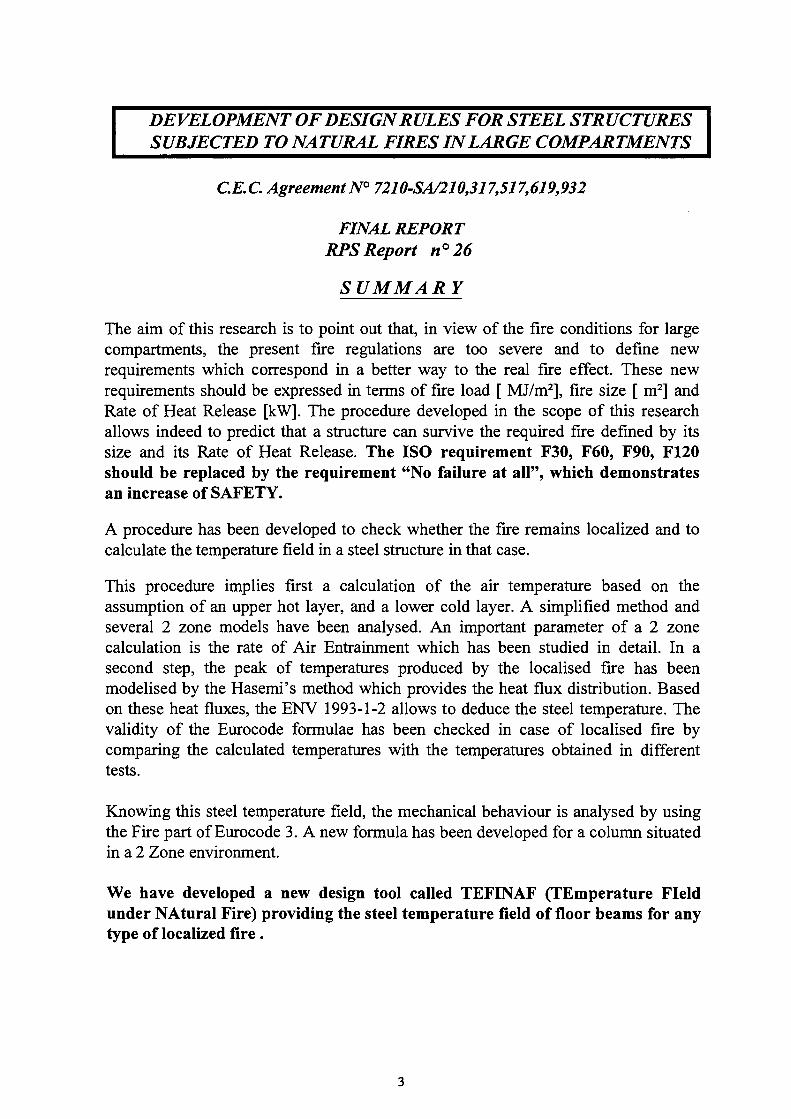
The aim of this research is to point out that, in view of the fire conditions for large compartments, the present fire regulations are too severe and to define new requirements which correspond in a better way to the real fire effect. These new requirements should be expressed in terms of fire load [ MJ/m2], fire size [ m2] and Rate of Heat Release [kW]. The procedure developed in the scope of this research allows indeed to predict that a structure can survive the required fire defined by its size and its Rate of Heat Release. The ISO requirement F30, F60, F90, F120 should be replaced by the requirement "No failure at all", which demonstrates an increase of SAFETY.
A procedure has been developed to check whether the fire remains localized and to calculate the temperature field in a steel structure in that case.
This procedure implies first a calculation of the air temperature based on the assumption of an upper hot layer, and a lower cold layer. A simplified method and several 2 zone models have been analysed. An important parameter of a 2 zone calculation is the rate of Air Entrainment which has been studied in detail. In a second step, the peak of temperatures produced by the localised fire has been modelised by the Hasemi's method which provides the heat flux distribution. Based on these heat fluxes, the ENV 1993-1-2 allows to deduce the steel temperature. The validity of the Eurocode formulae has been checked in case of localised fire by comparing the calculated temperatures with the temperatures obtained in different tests.
Knowing this steel temperature field, the mechanical behaviour is analysed by using the Fire part of Eurocode 3. A new formula has been developed for a column situated in a 2 Zone environment.
We have developed a new design tool called TEFINAF (TEmperature Field under NAtural Fire) providing the steel temperature field of floor beams for any type of localized fire .
DEVELOPPEMENT DE REGLES DE DIMENSIONNEMENT POUR LES STRUCTURES EN ACIER SOUMISES
A DES FEUX NATURELS DANS LES GRANDS COMPARTIMENTS
Agrément C.C.E. N° 7210-SA/210,317,517,619,932
RAPPORT FINAL Rapport RPS n° 26
RESUME
Le but de cette recherche est de montrer que, vu les conditions réelles d'incendie dans les grands compartiments, les réglementations actuellement en vigueur en matière de résistance au feu sont trop sévères et de définir de nouvelles exigences qui correspondent mieux à la réalité. Ces nouvelles exigences devraient être exprimées en termes de charge au feu [MJ/m2], de taille du feu [m2] et de Taux de Chaleur Dégagée [kW]. La procédure développée dans le cadre de cette recherche permet précisément d'étudier la stabilité d'une structure soumise à un feu défini par sa taille et son Taux de Chaleur Dégagée. L'exigence au feu ISO F30, F60, F90, F120 est à remplacer par l'exigence "Pas de Ruine lors de l'Incendie", ce qui implique un accroissement de SECURITE.
Une procédure a été développée pour vérifier si le feu reste localisé et pour calculer le champ de températures dans la structure en acier dans ce cas.
Cette procédure implique tout d'abord un calcul de la température de l'air basé sur l'hypothèse d'une stratification des gaz en une zone chaude supérieure et froide inférieure. Une méthode simplifiée et des modèles 2 Zones ont été analysés. Un paramètre important de cette approche à 2 zones est le taux d'Air Entraîné qui a été étudié en détail. Ensuite les pics de température provoqués par le feu localisé ont été modélisés par la méthode d'Hasemi qui fournit la distribution des flux de chaleur. A partir de ces flux de chaleur, la méthode comprise dans la ENV 1993-1-2 permet de déduire la température de l'acier. La validité des formules de l'Eurocode 3 a été vérifiée en cas de feu localisé, en comparant les températures calculées à celles obtenues lors de différents essais.
Connaissant le champ de températures dans l'acier, le comportement mécanique est analysé en utilisant la Partie Feu de l'Eurocode 3. Une nouvelle formule a été développée pour des colonnes situées dans un environnement à 2 Zones.
Nous avons développé un nouvel outil de dimensionnement appelé TEFINAF (TEmperature Field under NAtural Fire) donnant le champ des températures dans l'acier des poutrelles de plancher pour tout type de feu localisé !
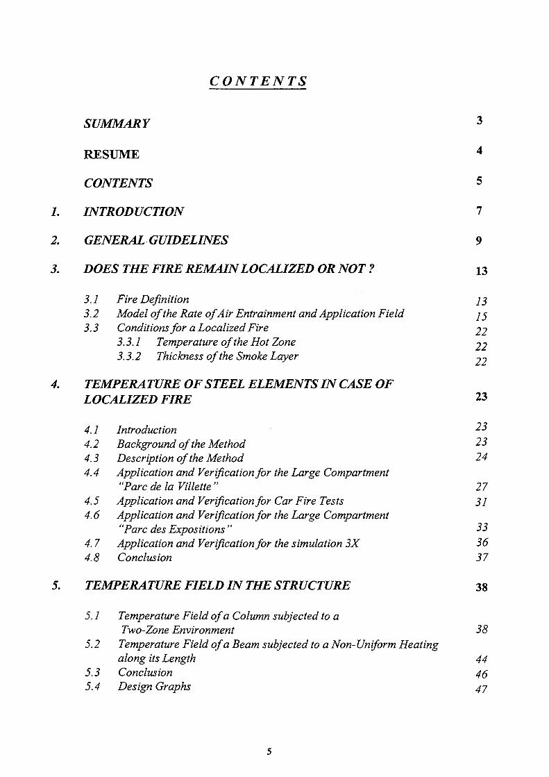
CONTENTS
SUMMARY 3
RESUME 4
CONTENTS 5
1. INTRODUCTION 7
2. GENERAL GUIDELINES 9
3. DOES THE FIRE REMAIN LOCALIZED OR NOT ? 13
3.1 Fire Definition 75 3.2 Model of the Rate of Air Entrainment and Application Field 75 3.3 Conditions for a Localized Fire 22
3.3.1 Temperature of the Hot Zone 22 3.3.2 Thickness of the Smoke Layer 2?
4. TEMPERATURE OF STEEL ELEMENTS IN CASE OF LOCALIZED FIRE 2 3
4.1 Introduction ¿3 4.2 Background of the Method 23 4.3 Description of the Method 24 4.4 Application and Verification for the Large Compartment
"Pare de la Villette" 27 4.5 Application and Verification for Car Fire Tests 31 4.6 Application and Verification for the Large Compartment
"Parc des Expositions " 33 4.7 Application and Verification for the simulation 3X 36 4.8 Conclusion 37
5. TEMPERATURE FIELD IN THE STRUCTURE 38
5.1 Temperature Field of a Column subjected to a Two-Zone Environment 38
5.2 Temperature Field of a Beam subjected to a Non- Uniform Heating along its Length 44
5.3 Conclusion 46 5.4 Design Graphs 47
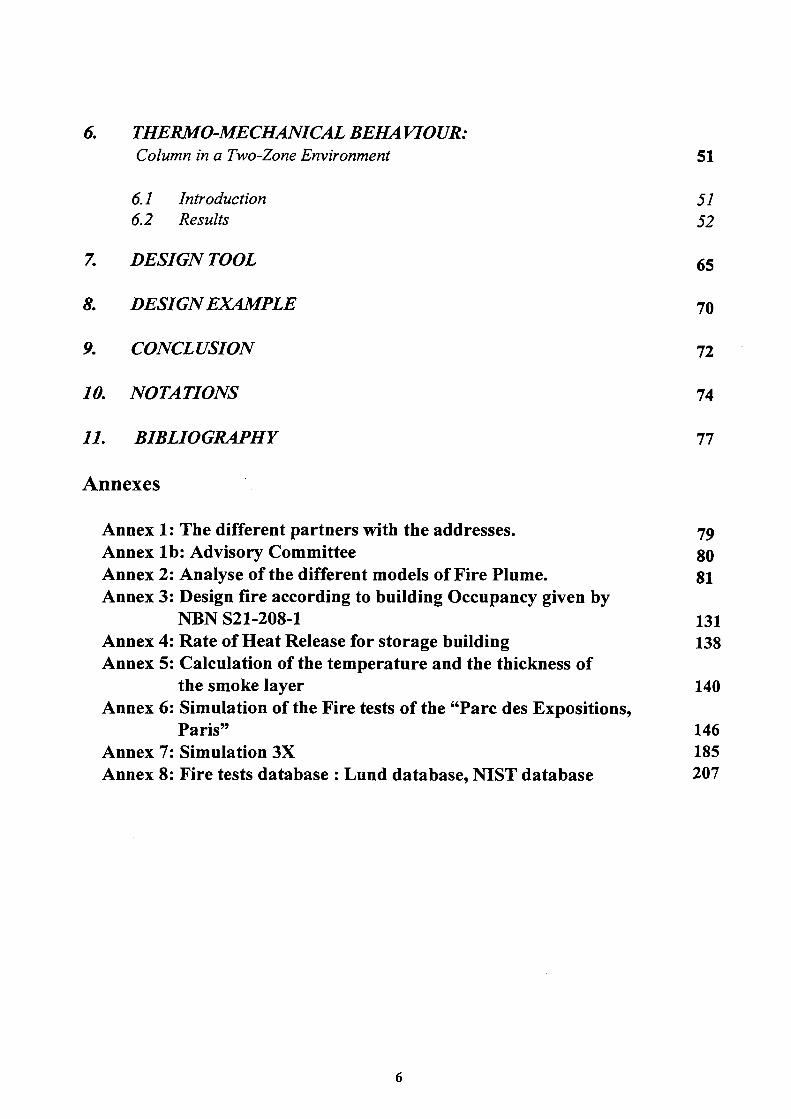
6. THERMO-MECHANICAL BEHA VIOUR: Column in a Two-Zone Environment 51
f5.7 Introduction 51 6.2 Results 52
7. DESIGN TOOL 6 5
8. DESIGN EXAMPLE 70
9. CONCLUSION 72
10. NOTATIONS 74
11. BIBLIOGRAPHY 11
Annexes
Annex 1 : The different partners with the addresses. 79 Annex lb : Advisory Committee 80 Annex 2: Analyse of the different models of Fire Plume. 81 Annex 3: Design fire according to building Occupancy given by
NBN S21-208-1 131 Annex 4: Rate of Heat Release for storage building 138 Annex 5: Calculation of the temperature and the thickness of
the smoke layer 140 Annex 6: Simulation of the Fire tests of the "Parc des Expositions,
Paris" 146 Annex 7: Simulation 3X 185 Annex 8: Fire tests database : Lund database, NIST database 207
1. INTRODUCTION
The present standards concerning the fire resistance are always based on an uniform fire temperature in the considered compartment given by the ISO curve. R30, 60, 90, 120 or 180 can be required and mean that the structure submitted to the ISO curve shouldn't fail before respectively 30, 60, 90, 120 or 180 minutes of ISO fire.
The following assumptions are thus adopted by the standards:
1) The temperature of the hot gases produced by the fire rises continuously up to the ISO curve up to required fire resistance time.
2) This temperature is uniform in the considered fire compartment of the building.
However both assumptions are quite unrealistic and uneconomical in the case of buildings containing very large volumes.
Indeed, on one hand, the fire loads of this type of construction (station hall, atrium of office building, shopping gallery, sport hall, multi-use hall, ...) are generally rather small so that it is not possible to reach the high temperatures of the ISO curve. Moreover a large amount of air is available, which is a second factor reducing the temperature.
On the other hand it is obvious that the temperature of the air in a large compartment in fire differs from one point to another. For instance a 10 m high column in a station hall in fire is not subjected to a same temperature field at its top and at its bottom part.
It is expected to be possible to define for the large volumes much less severe and much more economical fire conditions by considering real natural fire curves and real non-uniform temperature field in the considered compartment.
The following partners have participated in the research:
- ProfilARBED, Luxembourg, leader of the research - University of Liège, Belgium - CTICM, France - TNO, The Netherlands - LABEIN and ENSIDESA, Spain.
The complete address of the partners are given in Annex 1.
The technical coordination is handled by ProfilARBED Department "Recherches et Promotion technique Structure (RPS)".
A first meeting was held in Esch/Alzette the 8 of September 1993; the second one in Paris the 20th of January 1994; the third one in Esch/Alzette the 5th and 6th of July 1994; the fourth one in Maizières-les-Metz the 19th and 20th of January 1995; the fifth one in Delft the 4th and 5th of May 1995; the sixth one in Maizières-les-Metz the 21st and 22nd of September 1995; the seventh one in Esch/Alzette the 16th and 17th of November 1995; the eight one in Bilbao the 28th and 29th of February 1996; the nineth one in Delft the 20th and 21st of June 1996; the tenth one in Paris the 14th and 15th of November 96; the last meeting in Esch/Alzette the 27th and 28th of February 1997.
Amongst these meetings, five meetings (written in Bold hereabove) have involved the Advisory Committee which was composed of
BELGIUM: Major HERREMAN Service d'Incendie de l'Agglomération de Bruxelles
Mr. P. HOURLAY Ministère de l'Intérieur
FRANCE. Mr. H. TEPHANY Ministère de l'Intérieur
THE NETHERLANDS: Mr. G. BIJLSMA Brandweer Amsterdam
Mr. H.C. DE BEER Brandweer Utrecht
Mr. A. Van SCHAGEN Brandweer Amersfoort
SPAIN: Mr. José POSADA ESCOBAR Dir. Gral. Arquitectura y Vivienda M.O.P.T.
Thanks to these meetings, the experts were able to give their comments and to guide the research in a satisfactory way for their point of view.
Only one ECSC report including the work description of all partners has been written by ProfilARBED. Contributions were provided by Mr Franssen of the University of Liège, Mr Twilt and Mr Van Oerle of TNO, Mr Kruppa and Mr Joyeux of CTICM and Mr Aurtenetxe of LABEIN.

2. GENERAL GUIDELINES
This research is focused on the Structural behaviour in case of a natural fire in a Large Compartment. Natural fire means realistic fire instead of the Standard ISO-fire.
The aim of this research is to define a "Large Compartment" and the procedure to prove that a building fulfills the conditions to be a large compartment.
The general conditions of a large compartment are that:
• No uniform temperature field in the air and presence of a cold layer near the floor. • The fire is localised, thus no Flashover will occur. This implies that the fire load is
not uniformly distributed (localised fire) and the average temperature of the hot zone is less than 500°C (no Flashover).
ceiling
Fig. 2.1
The general procedure consists of 7 steps described in figures 2.2 and 2.3.
1) The first step in determining whether or not the compartment is a large compartment (or whether or not the fire remains localised) is to define the fire: Rate of Heat Release (RHR), Fire Area, Fire Perimeter, Fire Position. Different fire scenari implying different locations of a design fire should be analysed in order to cover the most critical situation for the structure.

2) The second step is to determine the height of the zone without smoke and also the average temperature of the upper layer. The temperature of the upper layer needs to be less than 500°C to ensure that the fire remains localised and that no Flashover occurs. The height of the layer without smoke needs to be known so that we can check that there is no danger of ignition of combustible material in the hot zone (see figure 2.1) and that we are dealing with a two zone phenomenom. Both these values (temperature and thickness of the hot zone) can be extracted by hand by the simple solution of several equations (see Annex 5) or from more sophisticated programs (Two-Zone model)
When we are sure that the fire is localised (step3), the fire definition is used together with the dimensions of the compartment to find the temperature in the air by using zone models. The calculations used in order to obtain the distribution of the heat flux to steel structure may be obtained by the Hasemi's method adapted by the University of Liège. It is the fourth step. In the following steps (5 and 6), the structure temperature field and the structural behaviour are calculated by applying ENV 1993-1-2 (Simplified method or advanced calculation model). In the last step (7), the compartment itself has to be checked.
10
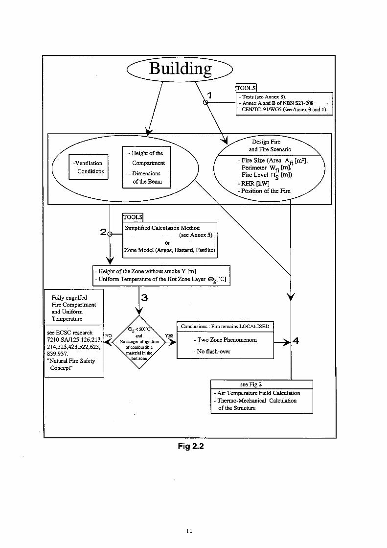
- Tests (see Annex 8). - Annex A and Β of NBNS21-208 CEN/TC191/WG5 (see Annex 3 and 4).
-Height of the
Compartment
- Dimensions of the Beam
TOOLS
Simplified Calculation Method (see Annex 5)
or Zone Model (Argos, Hazard, Fastlite)
• Height of the Zone without smoke Y [m] • Uniform Temperature of the Hot Zone Layer Og[°C]
Fully engulfed Fire Compartment and Uniform Temperature
see ECSC research 7210 SA/125,126,213, 214,323,423,522,623, 839,937. "Natural Fire Safety
Concept"
Conclusions : Fire remains LOCALISED
- Two Zone Phenomenom
- No flash-over
see Fig 2 • Air Temperature Field Calculation • Thermo-Mechanical Calculation
of the Structure
Fig 2.2
n

Return to Fig 1
o-
TOOLS
- Hasemi's Method -CFD
Gas Temperature Field © g (x,y,z,t) (or Heat Flux q" Field)
¿h TOOLS
ENV1993-1-2
Temperature Field in the Structure Oa (x,y,z,t)
TOOLS
ENV1993-1-2
Thermo-mechanical Calculation of the Structure - For simple structure like isostatic
structure, simplified method Oa(x,y,z,t=0—-x) ^ Gfc, c. (x,y,z)
see 4.2.4 (2) of ENV 1993-1-2:1995
if x minutes is required <=>raX(Xy,z) ^ Oa.crCx^Z)
see 4.2.4 (2) of ENV 1993-1-2:1995
if "No failure" is required or Complete analysis of the Structure
subjected to the Temperature Field O a (x,y,z,t)
N o
Fig 2.3
12
3. DOES THE FIRE REMAIN LOCALIZED OR NOT ?
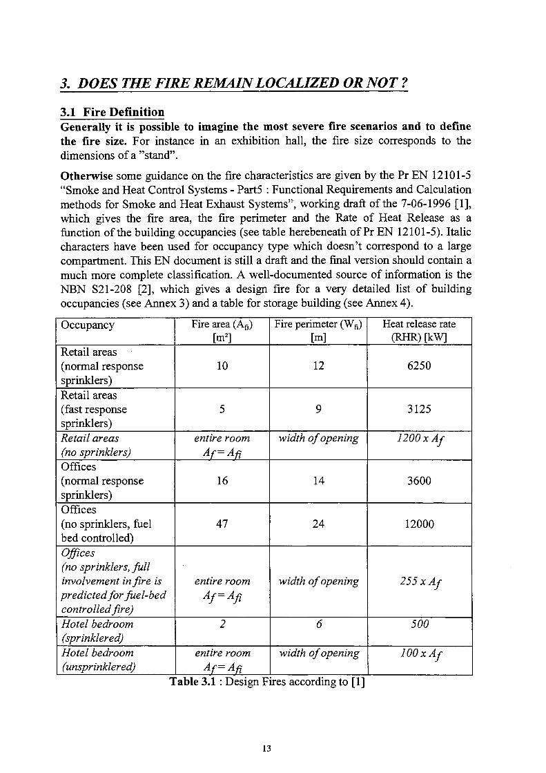
3.1 Fire Definition Generally it is possible to imagine the most severe fire scenarios and to define the fire size. For instance in an exhibition hall, the fire size corresponds to the dimensions of a "stand".
Otherwise some guidance on the fire characteristics are given by the Pr EN 12101-5 "Smoke and Heat Control Systems - Part5 : Functional Requirements and Calculation methods for Smoke and Heat Exhaust Systems", working draft of the 7-06-1996 [1], which gives the fire area, the fire perimeter and the Rate of Heat Release as a function of the building occupancies (see table herebeneath of Pr EN 12101-5). Italic characters have been used for occupancy type which doesn't correspond to a large compartment. This EN document is still a draft and the final version should contain a much more complete classification. A well-documented source of information is the NBN S21-208 [2], which gives a design fire for a very detailed list of building occupancies (see Annex 3) and a table for storage building (see Annex 4).
Occupancy
Retail areas (normal response sprinklers) Retail areas (fast response sprinklers) Retail areas (no sprinklers) Offices (normal response sprinklers) Offices (no sprinklers, fuel bed controlled) Offices (no sprinklers, full involvement in fire is predicted for fuel-bed controlled fire) Hotel bedroom (sprinklered) Hotel bedroom (unsprinklered)
Fire area (Afl) [m2]
10
5
entire room Af=Afl
16
47
entire room Af=Afl
2
entire room Af=Afi
Fire perimeter (Wfl) [m]
12
9
width of opening
14
24
width of opening
6
width of opening
Heat release rate (RHR) [kW]
6250
3125
1200 χ Af
3600
12000
255 xAf
500
lOOxAf
Table 3.1 : Design Fires according to [1]
13
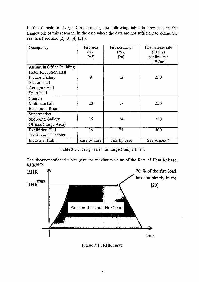
In the domain of Large Compartment, the following table is proposed in the framework of this research, in the case where the data are not sufficient to define the real fire ( see also [2] [3] [4] [5] ).
Occupancy
Atrium in Office Building Hotel Reception Hall Picture Gallery Station Hall Aerogare Hall Sport Hall Church Multi-use hall Restaurant Room Supermarket Shopping Gallery Offices (Large Area) Exhibition Hall "Do it yourself" center Industrial Hall
Fire area (Afi) [m2]
9
20
36
36
case by case
Fire perimeter (Wfi) [mj
12
18
24
24
case by case
Heat release rate (RHRfi)
per fire area [kW/m2]
250
250
250
500
See Annex 4
Table 3.2 : Design Fires for Large Compartment
The above-mentioned tables give the maximum value of the Rate of Heat Release, RHRmax.
A 70 % of the fire load RHR
RHR max has completely burnt
[20]
time
Figure 3.1 : RHR curve
14
In order to define the whole RHR curve, the growth phase and the decay phase have to be specified.
The growth phase can be simulated by the equation from [3]:
RHR [kW] = 1000 (t/ta)2 with t the time in seconds and t a deduced from the following table :
Building use
Picture Gallery Dwelling, Office, Hotel
Shop Industrial Storage
Fire growth rate
Slow Medium
Fast Ultra-fast
Time t a for RHR = lOOOkW [s]
600 300 150 75
Knowing the Rate of Heat Release curve, the fire load ([MJ/m2] or kg of wood Im2) enables us to define the duration of the fire. The Swiss document SIA 81 [4] and the CIB W14 document "Design Guide Structural Fire Safety" [5] are the most completed papers dealing with a fire load classication according to the building occupancy. The decay phase can be assumed to be linear and starts when 70% of the fire load has burnt.
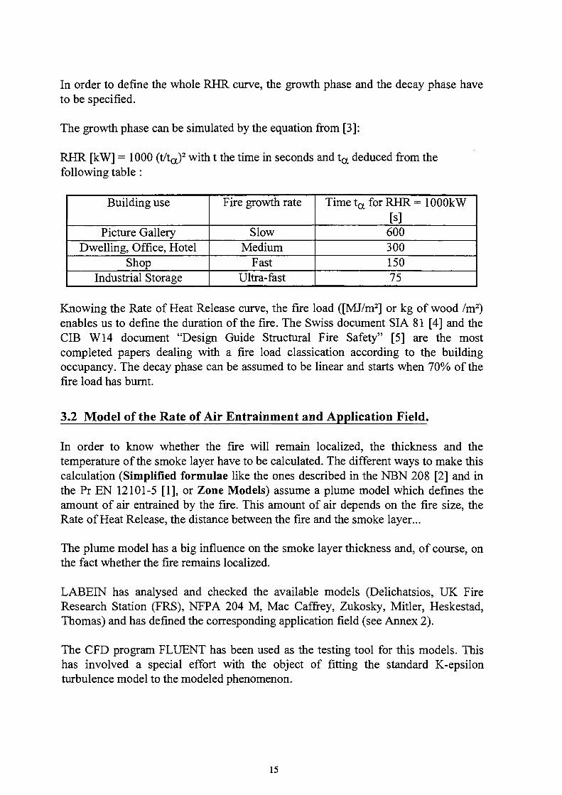
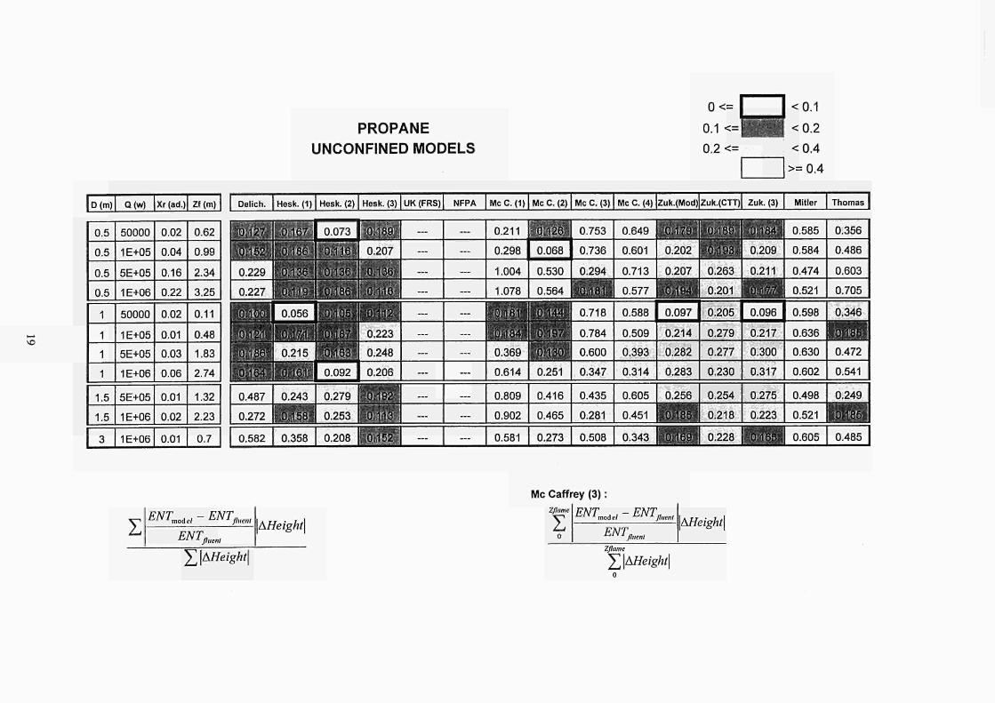
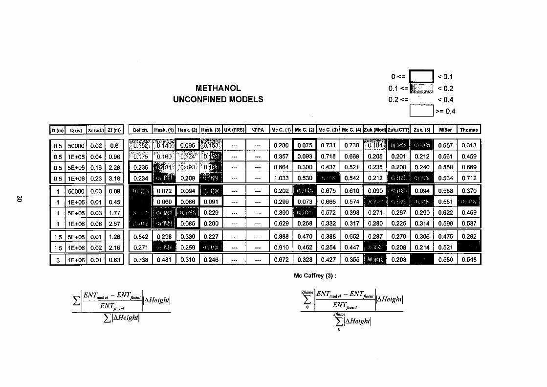
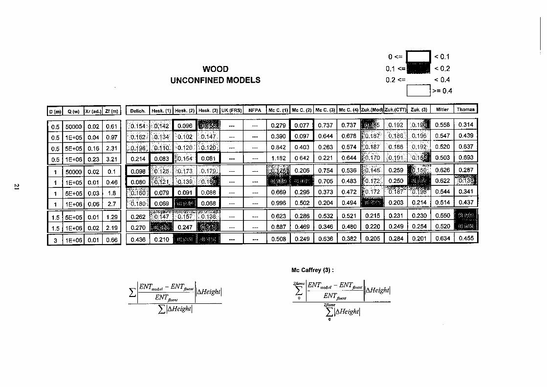
3.2 Model of the Rate of Air Entrainment and Application Field.
In order to know whether the fire will remain localized, the thickness and the temperature of the smoke layer have to be calculated. The different ways to make this calculation (Simplified formulae like the ones described in the NBN 208 [2] and in the Pr EN 12101-5 [1], or Zone Models) assume a plume model which defines the amount of air entrained by the fire. This amount of air depends on the fire size, the Rate of Heat Release, the distance between the fire and the smoke layer...
The plume model has a big influence on the smoke layer thickness and, of course, on the fact whether the fire remains localized.
LABEIN has analysed and checked the available models (Delichatsios, UK Fire Research Station (FRS), NFPA 204 M, Mac Caffrey, Zukosky, Mitler, Heskestad, Thomas) and has defined the corresponding application field (see Annex 2).
The CFD program FLUENT has been used as the testing tool for this models. This has involved a special effort with the object of fitting the standard K-epsilon turbulence model to the modeled phenomenon.
15

LABEIN has created some table advising which of the model to use in different situations. In order to achieve this goal, FLUENT has been used to model different fires with different characteristics ( RHR, Diameter, Confined : presence of a ceiling or Unconfined : no ceiling ...) and compare the obtained entrainment rates to those provided by each of empirical correlations.
Confinement has an important influence on the models agreement. Most expressions studied here apply for unconfined fires. Their application for confined situations implies a lost of accuracy.
F.R.S. and N.F.P.A. are specially defined for confined fires. These expressions show the best agreement and the widest range of application in confined fires.
Heskestad presents the best approximation for unconfined cases in the considered range. In confined cases accuracy decreases but it remains close to FRS and NFPA accuracy.
Delichatsios presents good approximation but its accuracy decreases for large diameters.
Although Zukoski models give more regular approximation in the considered range than Dalichatsios model, its accuracy is worse, particularly for confined fires. Further more, its use requires an intensive effort due to its difficult application.
Mc Caffrey (1) and (2) give good approximation for cases with low heat release rate, but they don't fit large heat release rate fires.
Mc Caffrey (3) is valid up to the flame tip. The lower the flame is, the worse accuracy Mc Caffrey (3) arises. The accuracy of Mc Caffrey (3) and Mc Caffrey (4) models is not good enough but for the largest heat release rates.
Mitler expression is similar to Zukoski (CTT) model. Nevertheless, Mitler presents worse results even than Zukoski (CTT) model. So, it could be discarded.
Finally, Thomas expression has application on some specific cases in unconfined fires. So, it must be discarded as a general expression.
The Comité Européen de Normalisation (C.E.N.) proposes two different models to be applied depending on the geometric characteristics : Heskestad model for small fires (Y>10A*'2) and Thomas expression for large fires (Y<10A^2).
16

All unconfined cases carried out here are defined as small fires under C.E.N, definition. For these cases, Heskestad model has been chosen as the best model in agreement with C.E.N, (see fig. 3.2.1).
For confined fires, only four cases satisfies the C.E.N, restrictions for large fires (Thomas expression). In these four cases, the present study suggests that FRS, NFPA and Heskestad models are better than Thomas expression.
In short, we suggest to give in the future the preference to the Heskestad model. For simplified method, the simple expression of Thomas may be used.
17

ENTRAINMENT COMPARISON : MODEL AND SIMULATION
o>
ε c co c
0.5 1.5
Height, m
2.5
o
1D (m) Q(w) Xr (ad.) Zf(m)
0.5
0.5
0.5
0.5
1
1
1
1
1.5
1.5
3
50000
1E+05
5E+05
1E+06
50000
1E+05
5E+05
1E+06
5E+05
1E+06
1E+06
0.02
0.04
0.16
0.22
0.02
0.01
0.03
0.06
0.01
0.02
0.01
0.62
0.99
2.34
3.25
0.11
0.48
1.83
2.74
1.32
2.23
0.7
PROPANE
UNCONFINED MODELS
0.1 < = |
0.2 <=
I <0.1
f <0.2
<0.4
>=0.4
Delich. Hesk. (1) Hesk. (2) Hesk. (3) UK(FRS) NFPA Mc C. (1) Mc C. (2) Mc C. (3) Mc C. (4) Zuk.(Mod) Zuk.(CTT) Zuk. (3) Mitler Thomas
ENTmoAel-ENTfluenl
ENT, fluent
\àHeight\
2Z\AHeight\
Mc Caffrey (3) :
Zflame
Σ o
ENTmoáel-ENTfll,enl
ENT, fluent
\AHeight\
Zflame
2Z\àHeight\
ë
1D (m) Q(w) Xr (ad.) Zf(m)
0.5
0.5
0.5
0.5
1
1
1
1
1.5
1.5
3
50000
1E+05
5E+05
1E+06
50000
1E+05
5E+05
1E+06
5E+05
1E+06
1E+06
0.02
0.04
0.16
0.23
0.03
0.01
0.03
0.06
0.01
0.02
0.01
0.6
0.96
2.28
3.18
0.09
0.45
1.77
2.67
1.26
2.16
0.63
0<=
METHANOL
UNCONFINED MODELS
<0.1
<0.2 0.1 <=■ Γ I ::-¡!.,vl
0.2 <= < 0.4
>=0.4
Delich. Hesk. (1) Hesk. (2) Hesk. (3) UK (FRS) NFPA Mc C. (1) Mc C. (2) Mc C. (3) Mc C. (4) Zuk.(Mod) Zuk.(CTT) Zuk. (3) Miller
Mc Caffrey (3)
Thomas
ENT model ENT, fluent
ENT, fluent
\AHeight\
ΣΙΔ^'Ή
Zflame
Σ o
ENTmoiel ENTßUeM
ENT, fluent
\AHeight\
Zflame
X|A*feigA/|
SJ
1 D (m) Q(w) Xr (ad.) Zf(m)
0.5
0.5
0.5
0.5
1
1
1
1
1.5
1.5
3
50000
1E+05
5E+05
1E+06
50000
1E+05
5E+05
1E+06
5E+05
1E+06
1E+06
0.02
0.04
0.16
0.23
0.02
0.01
0.03
0.06
0.01
0.02
0.01
0.61
0.97
2.31
3.21
0.1
0.46
1.8
2.7
1.29
2.19
0.66
WOOD
UNCONFINED MODELS
0<=
0.1 <=
0.2 <=
<0.1
<0.2
<0.4
>=0.4
Delich. Hesk. (1) Hesk. (2) Hesk. (3) UK(FRS) NFPA McC.ÇI) Mc C. (2) Mc C. (3) Mc C. (4) Zuk.(Mod) Zuk.(CTT) Zuk. (3) Mitler Thomas
ENT ENT, fluent
ENT, fluent
\AHeight\
J^hHeight]
Mc Caffrey (3)
Zflame
Σ o
ENT model ENT, fluent
ENT fluent
àHeightl
Zflame
Y,\AHeight\
3.3 Conditions for a localized fire
3.3.1 Temperature of the hot zone
The flash-over is assumed if the average temperature of the smoke layer reaches 500 °C. This average temperature can be calculated by simplified formulae (see Annex 5) (Pr EN 12101-5) [1] or Zone Models.
3.3.2 Thickness of the smoke layer
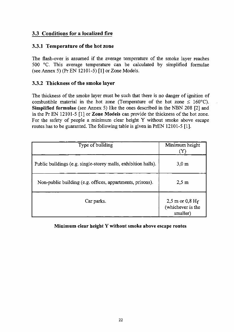
The thickness of the smoke layer must be such that there is no danger of ignition of combustible material in the hot zone (Temperature of the hot zone < 160°C). Simplified formulae (see Annex 5) like the ones described in the NBN 208 [2] and in the Pr EN 12101-5 [1] or Zone Models can provide the thickness of the hot zone. For the safety of people a minimum clear height Y without smoke above escape routes has to be guaranted. The following table is given in PrEN 12101-5 [1].
Type of building
Public buildings (e.g. single-storey malls, exhibition halls).
Non-public building (e.g. offices, appartments, prisons).
Car parks.
Minimum height (Y)
3,0 m
2,5 m
2,5 m or 0,8 Hf (whichever is the
smaller)
Minimum clear height Y without smoke above escape routes
22
4. TEMPERATURE OF STEEL ELEMENTS IN CASE OF LOCALIZED FIRE
4.1 Introduction
When a large compartment is submitted to a localised fire, the temperature distribution in the compartment may be estimated by a 2 layers zone model assuming that the gases are separated in 2 horizontal layers : 1 upper layer containing hot gases and 1 lower layer containing cold gases. This is also the case in a car park in which only 1 or a limited number of cars are engulfed in fire. In this model of the 2 layers separation, the temperature in each layer is calculated with the hypothesis that the temperature of the gases is uniform in each layer. The calculated temperature is therefore an average in each zone of the 3D temperature distribution that could be calculated by a more sophisticated model, like a CFD model for example. This average temperature in the hot zone is generally sufficiently accurate as far as global phenomenon are considered : quantity of smoke to be extracted from the compartment, likelihood of flash-over, total collapse of the roof or ceiling, etc. When it comes to estimating the local behaviour of a structural element located just above the fire, the hypothesis of a uniform temperature may be unsafe because this element is very close to the fire source and therefore much more subjected to the effect of the fire than the average of the hot zone. It is desirable to have a simple tool enabling to estimate and to quantify the local effect of the fire on adjacent elements. The method described hereafter and named as Hasemi's method is a simple tool for the evaluation of the localised effect of a fire on horizontal elements located above the fire.
4.2 Background of the method.
The background of the method is experimental and based on tests made by Hasemi at the Building Research Institute in Tsukuba, Japan [6]. A porous gas burner has been placed under an unconfined flat ceiling in the presence, or not, of an unprotected steel beam. The ceiling is a 1.82 m square consisting of 2 layers of 12 mm mineral fibre reinforced cement boards. Height of the ceiling was adjusted in each test to a value in the range 0.40 to 1.20 m. 0.30 m and 0.50 m diameter round propane burners were used as well as a 1.00 m square burner. The Rate of Heat Release of the burner was constant in each test, with a value in the range 100 to 700 kW. The heat flux to the ceiling surface and temperature in the steel beam were recorded. The size of the apparatus and the range of the heat release rate are smaller than real fires in a building. The results of the tests have been described in term of non dimensional parameters which should allow to use them for larger configuration.
23
4.3 Description of the method.
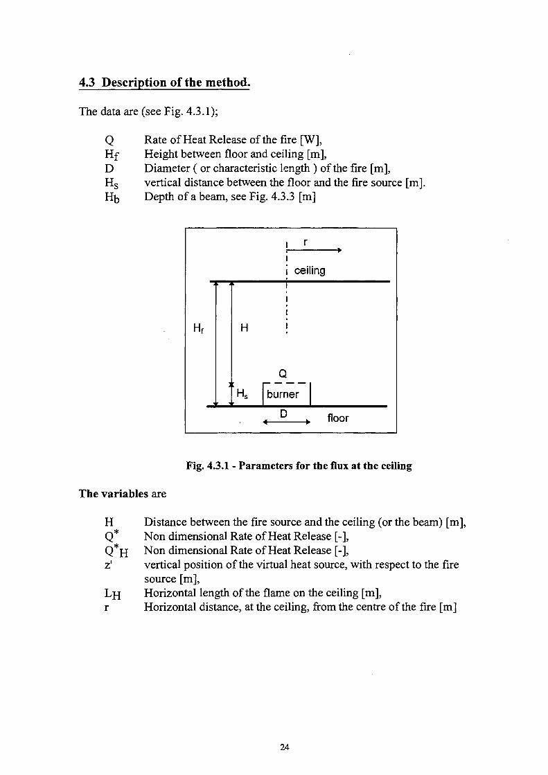
The data are (see Fig. 4.3.1);
Q Rate of Heat Release of the fire [W], Hf Height between floor and ceiling [m], D Diameter ( or characteristic length ) of the fire [m], H s vertical distance between the floor and the fire source [m]. HD Depth of a beam, see Fig. 4.3.3 [m]
Fig. 4.3.1 - Parameters for the flux at the ceiling
The variables are
H Distance between the fire source and the ceiling (or the beam) [m], Q Non dimensional Rate of Heat Release [-], Q*H Non dimensional Rate of Heat Release [-], z' vertical position of the virtual heat source, with respect to the fire
source [m], Lj-j Horizontal length of the flame on the ceiling [m], r Horizontal distance, at the ceiling, from the centre of the fire [m]
24
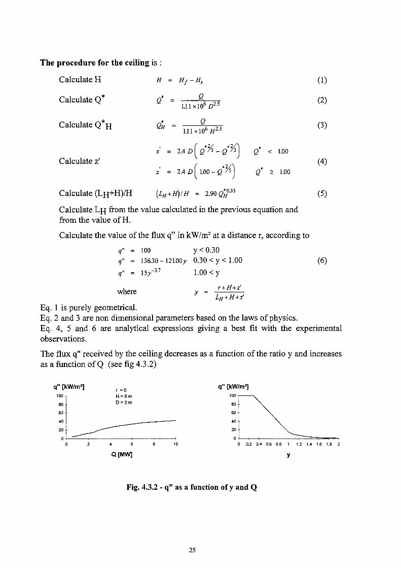
The procedure for the ceiling is :
Calculate H
Calculate Q
Calculate Q H
Calculate ζ'
Η =
ß' -
QH -
Hf-Hs
Q
1.11 xlO6 Ζ)2'5
Ô
1.11 χ ίο 6 ί^2·5
♦ 2 / »2/
ζ = 2.4 D β /5 - g /3
ζ' = 2.4 DΙ 1.00-g* ^
ρ < 1.00
ρ* > 1.00
Calculate ( L H + H ) / H (LH+H)/H = 2.90 β#( 0.33
d)
(2)
(3)
(4)
(5)
Calculate Lj j from the value calculated in the previous equation and
from the value of H.
Calculate the value of the flux q" in kW/m2 at a distance r, according to
q" = 100 y < 0.30
q" = 136.30 - ni.OOy 0.30 < y < 1.00 (6)
q" = \5y
where
-3.7 1.00 < y
r+H+z'
LH + H+z'
Eq. 1 is purely geometrical.
Eq. 2 and 3 are non dimensional parameters based on the laws of physics.
Eq. 4, 5 and 6 are analytical expressions giving a best fit with the experimental
observations.
The flux q" received by the ceiling decreases as a function of the ratio y and increases
as a function of Q (see fig 4.3.2)
q" [kW/m2]
80 -
6 0 -
4 0 -
20 -
0 -
( ) 2
r = 0
H = 5 m
D = 3 m
4 6
Q [MW]
s 10
q" [kW/m2]
80-
60 -
40-
20-
0
) 0.2 0.4 0.6 0.8 1
y
1.2 1.4 1.6 1.8 2
Fig. 4.3.2 - q" as a function of y and Q
25
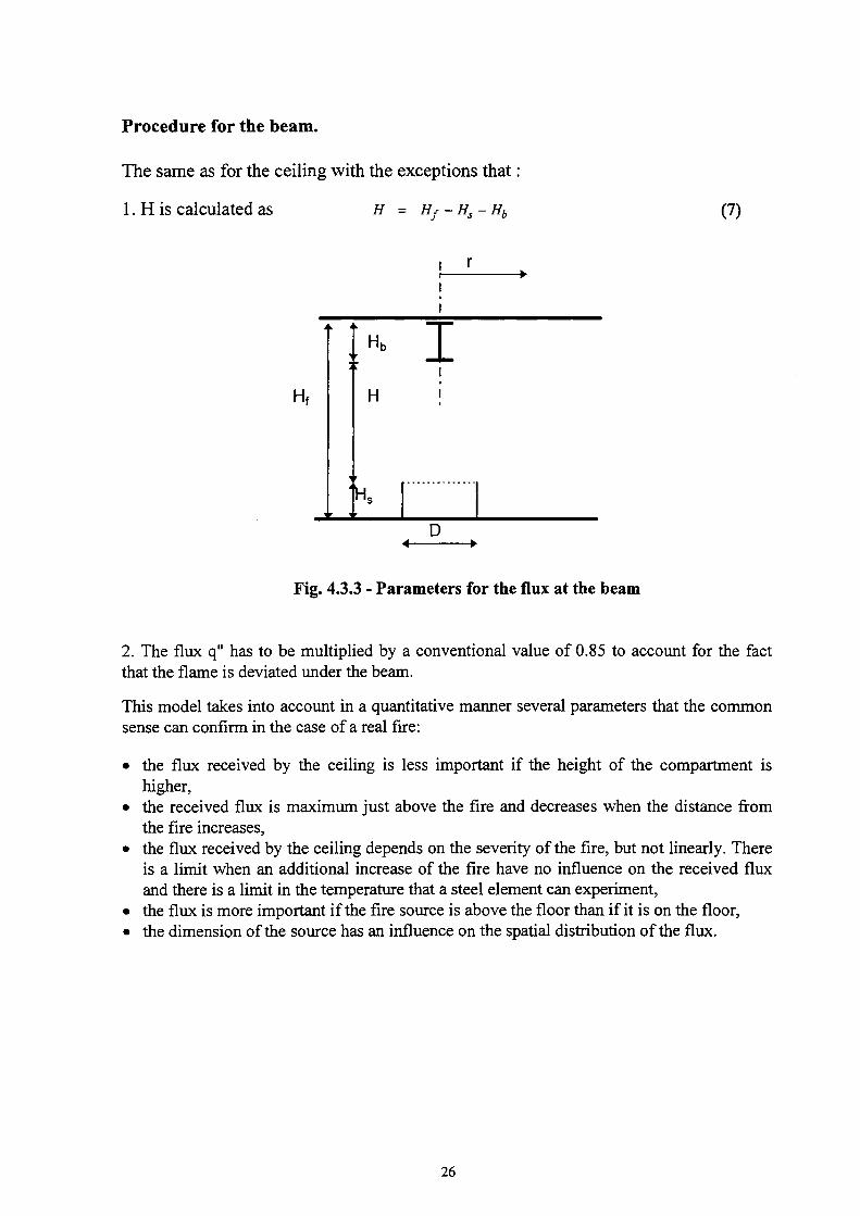
Procedure for the beam.
The same as for the ceiling with the exceptions that
1. H is calculated as H = Hf-Hs-Hb (7)
ι r
Hf
> I
t τ
Η
Ή. D
4 ►
Fig. 4.3.3 - Parameters for the flux at the beam
2. The flux q" has to be multiplied by a conventional value of 0.85 to account for the fact that the flame is deviated under the beam.
This model takes into account in a quantitative manner several parameters that the common sense can confirm in the case of a real fire:
• the flux received by the ceiling is less important if the height of the compartment is higher,
• the received flux is maximum just above the fire and decreases when the distance from the fire increases,
• the flux received by the ceiling depends on the severity of the fire, but not linearly. There is a limit when an additional increase of the fire have no influence on the received flux and there is a limit in the temperature that a steel element can experiment,
• the flux is more important if the fire source is above the floor than if it is on the floor, • the dimension of the source has an influence on the spatial distribution of the flux.
26
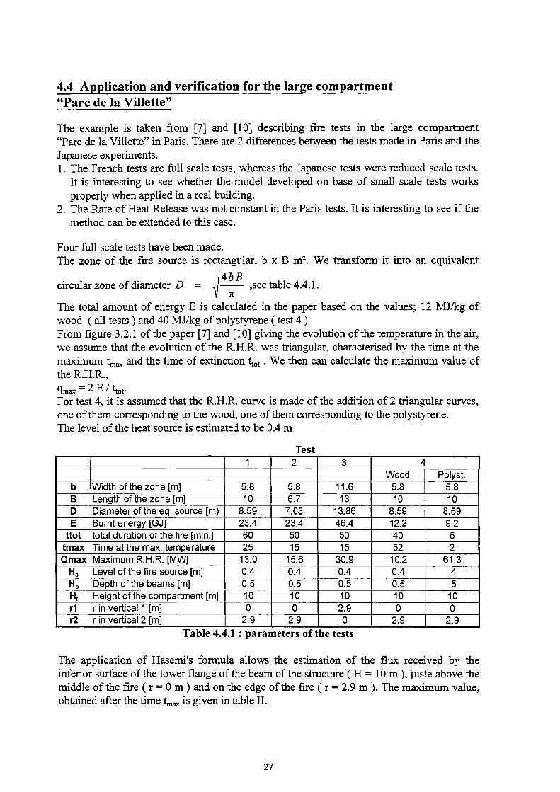
4.4 Application and verification for the large compartment
"Pare de la Villette"
The example is taken from [7] and [10] describing fire tests in the large compartment
"Pare de la Villette" in Paris. There are 2 differences between the tests made in Paris and the
Japanese experiments.
1. The French tests are full scale tests, whereas the Japanese tests were reduced scale tests.
It is interesting to see whether the model developed on base of small scale tests works
properly when applied in a real building.
2. The Rate of Heat Release was not constant in the Paris tests. It is interesting to see if the
method can be extended to this case.
Four full scale tests have been made.
The zone of the fire source is rectangular, b χ Β m2. We transform it into an equivalent
circular zone of diameter D = ÌAbB
π ,see table 4.4.1.
The total amount of energy E is calculated in the paper based on the values; 12 MJ/kg of
wood ( all tests ) and 40 MJ/kg of polystyrene ( test 4 ).
From figure 3.2.1 of the paper [7] and [10] giving the evolution of the temperature in the air,
we assume that the evolution of the R.H.R. was triangular, characterised by the time at the
maximum t , ^ and the time of extinction t ^ . We then can calculate the maximum value of
theR.H.R,
Ojnax = 2 L· / ttøf
For test 4, it is assumed that the R.H.R. curve is made of the addition of 2 triangular curves,
one of them corresponding to the wood, one of them corresponding to the polystyrene.
The level of the heat source is estimated to be 0.4 m
Test
b
B
D
E
ttot
tmax
Qmax
Hs
Hb
Hf
M
r2
Width of the zone [m]
Length of the zone [m]
Diameter of the eq. source [m)
Burnt energy [GJ]
total duration of the fire [min.]
Time at the max. temperature
Maximum R.H.R. [MW]
Level of the fire source [m]
Depth of the beams [m]
Height of the compartment [m]
r in vertical 1 [m]
r in vertical 2 [m]
Table 4.¿
1
5.8
10
8.59
23.4
60
25
13.0
0.4
0.5
10
0
2.9
r.l : parat
2
5.8
6.7
7.03
23.4
50
15
15.6
0.4
0.5
10
0
2.9
neters oft
3
11.6
13
13.86
46.4
50
15
30.9
0.4
0.5
10
2.9
0
he tests
4
Wood
5.8
10
8.59
12.2
40
52
10.2
0.4
0.5
10
0
2.9
Polyst.
5.8
10
8.59
9.2
5
2
61.3
.4
.5
10
0
2.9
The application of Hasemi's formula allows the estimation of the flux received by the
inferior surface of the lower flange of the beam of the structure ( H = 10 m) , juste above the
middle of the fire ( r = 0 m ) and on the edge of the fire ( r = 2.9 m ). The maximum value,
obtained after the time t ^ is given in table II.
27

Test
q"max(r=0) [kW/m2]
q"m„(r=2.9)[kW/ma]
1
17
7
2
21
8
3
34
17
4
50
35
Table 4.4.2 : maximum flux received by the flange.
The beam was an IPE 500. We assume that the lower surface and the lateral surfaces of the
lower flange receive q", whereas the upper surface receives 0.50 q". Given the geometrical
properties of the flange, Β = 200 mm and e = 16 mm, the average flux received by the lower
flange is given by;
1.00 (200+2x16)+ 050x200 ..
"»■ = 2*(200+16) q = ° J 7 q (8)
We assume that the heat flux received by the beam is proportional to the R.H.R. This is very
close to reality for test 1,2 and 4. This slightly underestimate the flux for test 3.
The net heat flux entering the flange is calculated according to
qne t = q ¡ v . - 2 5 ( 0 s - 2 9 3 ) - 0 . 5 0 σ ( θ ^ - 2 9 3 4 ) (9)
with 0S steel temperature.
N.B. Because the heat flux received by a surface is limited to 100 kW/m2, see Eq. (6),
Eq. (9) means that steel temperature cannot exceed 1 005 °C, see Fig. 4.4.1.
Heat flux [kW/m2]
100
90
80
70
60
50
40
30
20
10
I I
Flux lost by steel q = 25 (Ts-293) - 0.5 σ OV-2934) [kW/m
2]
^ ^ < ^
^f^
" t —
100 200 300 400 500 600
Steel temperature [°C]
700 800 900 1000
Fig. 4.4.1 : Heat flux lost by a surface as a function of its temperature.
28
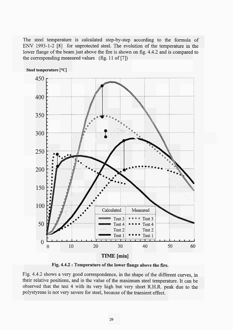
The steel temperature is calculated step-by-step according to the formula of ENV 1993-1-2 [8] for unprotected steel. The evolution of the temperature in the lower flange of the beam just above the fire is shown on fig. 4.4.2 and is compared to the corresponding measured values (fig. 11 of [7])
Steel temperature [°C]
450 r
400 -
TEME [min]
Fig. 4.4.2 : Temperature of the lower flange above the fire.
Fig. 4.4.2 shows a very good correspondence, in the shape of the different curves, in their relative positions, and in the value of the maximum steel temperature. It can be observed that the test 4 with its very high but very short R.H.R. peak due to the polystyrene is not very severe for steel, because of the transient effect.
29
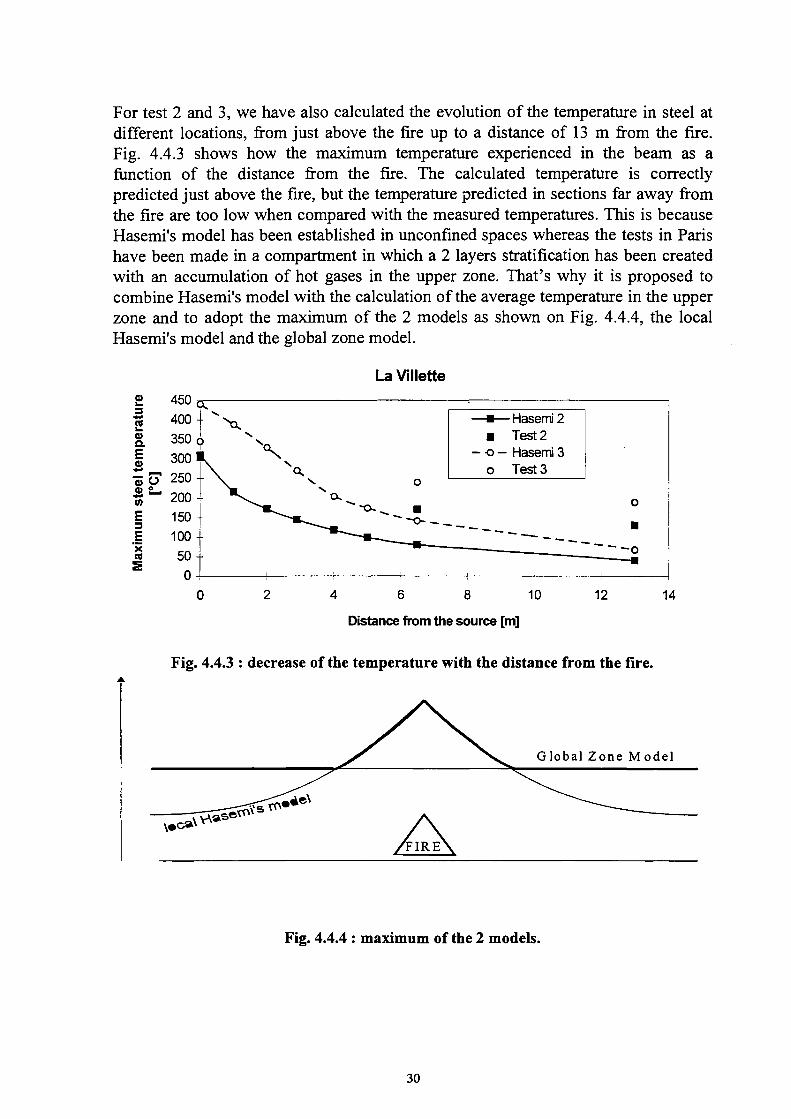
For test 2 and 3, we have also calculated the evolution of the temperature in steel at different locations, from just above the fire up to a distance of 13 m from the fire. Fig. 4.4.3 shows how the maximum temperature experienced in the beam as a function of the distance from the fire. The calculated temperature is correctly predicted just above the fire, but the temperature predicted in sections far away from the fire are too low when compared with the measured temperatures. This is because Hasemi's model has been established in unconfined spaces whereas the tests in Paris have been made in a compartment in which a 2 layers stratification has been created with an accumulation of hot gases in the upper zone. That's why it is proposed to combine Hasemi's model with the calculation of the average temperature in the upper zone and to adopt the maximum of the 2 models as shown on Fig. 4.4.4, the local Hasemi's model and the global zone model.
La Villette
6 8 10
Distance from the source [m]
12 14
Fig. 4.4.3 : decrease of the temperature with the distance from the fire.
Fig. 4.4.4 : maximum of the 2 models.
30
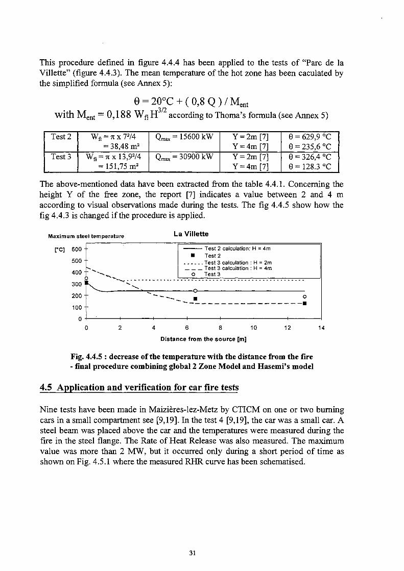
This procedure defined in figure 4.4.4 has been applied to the tests of "Parc de la
Villette" (figure 4.4.3). The mean temperature of the hot zone has been caculated by
the simplified formula (see Annex 5):
0 = 20°C + (0 ,8Q) /M, r3/2
ent with M e n t — 0,188 Wfi H according to Thoma's formula (see Annex 5)
Test 2
Test 3
Wfi = π χ 72/4
= 38,48 m2
Wfl = π χ 13,974
= 151,75 m2
Qmax= 15600 kW
Qmax = 30900 kW
Y = 2m [7]
Y = 4m [7]
Y = 2m [7]
Y = 4m [7]
θ = 629,9 °C
θ = 235,6 °C
θ = 326,4 °C
θ = 128.3 °C
The above-mentioned data have been extracted from the table 4.4.1. Concerning the
height Y of the free zone, the report [7] indicates a value between 2 and 4 m
according to visual observations made during the tests. The fig 4.4.5 show how the
fig 4.4.3 is changed if the procedure is applied.
Maximum steel temperature La Villette
4 6 8 10
Distance from the source [m]
12 14
Fig. 4.4.5 : decrease of the temperature with the distance from the fire - final procedure combining global 2 Zone Model and Hasemi's model
4.5 Application and verification for car fire tests
Nine tests have been made in Maizières-lez-Metz by CTICM on one or two burning
cars in a small compartment see [9,19]. In the test 4 [9,19], the car was a small car. A
steel beam was placed above the car and the temperatures were measured during the
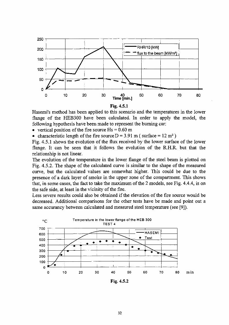
fire in the steel flange. The Rate of Heat Release was also measured. The maximum
value was more than 2 MW, but it occurred only during a short period of time as
shown on Fig. 4.5.1 where the measured RHR curve has been schematised.
31
250
200
150
100
50
0
/ ^
/ / — !
χ
\
I RHR/10[kW]
"~" — flux to the beam [kW/m2]
i "^"^ - ^ * - ^ .
10 20 30 40 Time [min.]
50 60 70 80
Fig. 4.5.1
Hasemi's method has been applied to this scenario and the temperatures in the lower
flange of the HEB300 have been calculated. In order to apply the model, the
following hypothesis have been made to represent the burning car:
• vertical position of the fire source Hs = 0.60 m
• characteristic length of the fire source D = 3.91 m ( surface = 12 m2 )
Fig. 4.5.1 shows the evolution of the flux received by the lower surface of the lower
flange. It can be seen that it follows the evolution of the R.H.R. but that the
relationship is not linear.
The evolution of the temperature in the lower flange of the steel beam is plotted on
Fig. 4.5.2. The shape of the calculated curve is similar to the shape of the measured
curve, but the calculated values are somewhat higher. This could be due to the
presence of a dark layer of smoke in the upper zone of the compartment. This shows
that, in some cases, the fact to take the maximum of the 2 models, see Fig. 4.4.4, is on
the safe side, at least in the vicinity of the fire.
Less severe results could also be obtained if the elevation of the fire source would be
decreased. Additional comparisons for the other tests have be made and point out a
same accurancy between calculated and measured steel temperature (see [9]).
°C Temperature in the lower flange of the HEB 300
TEST 4
700
600
500
400
300
200
100
/+
* - '/*
s * * ♦
y ^
, ♦ ♦ ►
♦ ♦ < * ♦
HASFMI
♦ Test
" \
* ♦ < ' ♦"%>
*"*. ♦
10 20 30 40 50 60 70 80
Fig. 4.5.2
min
32

4.6 Application and Verification for the Large Compartment "Parc des Expositions, Paris" [16,17]
4.6.1 Introduction
Two consecutive tests have been realised in a exposition hall, the "Parc des Expositions" (Paris) ; the first on May 18m 1994, and the second on May 20th 1994. The aim of these tests is to determinate the gas and structure temperatures in different zones, the gases composition and velocity in horizontal openings during fire.
The hall IB volume is the following : 144 χ 65 χ 28 m (L χ 1 χ h). Around this volume, the first 14 meters of height were not closed, and were adjacent with a volume extension, not exterior but sufficiently large to consider it as such.
The roof truss was separated from the hall by a horizontal screen situated at a height of 26 meters. The screen was composed with some plates without thermal isolation, and some roastings. Horizontal openings enables to evacuate smoke.
4.6.2 Burning load and fire conditions
The burning load consisted of wood pallets (Europ type, dimensions 1200 χ 800 χ 130 mm (L χ 1 χ h), about 30 kg/pallet).
A. Test i
The load mass was 3458 kg with 133 pallets and was distributed in 8 packs. These packs were grouped by 2, and the four groups were separated by partition walls. These partition walls made of wood, of the same type of those used in the separation of exposition stands (height of 2.5 m).
Two compartments were ignited firstly, and the fire has been propagated to the two other compartments in a natural way. The compartmentation wall failed 6 minutes after ignition.
B. Test 2
The load mass was 3562 kg with 120 pallets and was assessed in 10 packs, uniformly on burning surface. The load mass loss was measured by weighing. All packs were ignited at the same time.
33
4.6.3 Results
All results will not be shown in this report. During tests, temperatures were measured by thermocouples. About 50 thermocouples were placed in the hall, at 4 sections of the hall. These sections are shown in figure 1 of Annex 6. The position and numeration of thermocouples are indicated in figure 2 of Annex 6.
A. Testi
Some temperature results are shown in figures 3, 4 and 5 of Annex 6. We can notice the failure of the compartmentation wall, and the ignition of the two others packs (no ignited at the beginning) giving the second peak of temperature. Radiative fluxes were measured at a distance of 9.5 and 15 meters of the load centre. These fluxes are shown in figure 6 of Annex 6.
B. Test 2
Temperatures are shown in figures 7 to 21 of Annex 6. Radiative fluxes were measured at distances of 8 and 6.5 meters of the load centre. These fluxes are shown in figure 22 of Annex 6. Velocity at horizontal openings was measured with pitot anemometer, but results are not easily improvable. The load mass was measured by weighing. The temporal evolution of this mass is shown in figure 23 of Annex 6. The load mass evolution stopped 10 minutes after ignition, because a part of the load fell out of the weighing plateform.
In this test, it seems that the hot layer was homogeneous. The results of thermocouples show an homogeneity of temperatures at 22 meters height and in the plenum, despite a superiority in the plenum just above the fire and certain irregularities in temporal evolution. It seems that these irregularities proceeded from circulation zones and fresh air incomes for the fire development, especially during the maximum pyrolysis rate. The neutral surface height seemed to be equal to 20 or 21 meters. Indeed, the temperature at 22 meters was always close to the hot layer temperature. However, below (for example thermocouple n°13 at 18 meters), the temperature was much more lower. So the hot layer thickness was about 7 meters.
So, the test of the Parc des Expositions is a case which corresponds well to the use of the 2 Zone program FIRST [11].
The details and the measurements (Temperatures in the air and in the structure, mass lost, heat flux) for these two tests are given in Annex 6.
34

4.6.4 Test simulation
The second test has been analyzed by using the Hasemi's method with the following data :
• Rate of Heat Release (see Annex 6 figure 25).
6 0 -
5 0 -
40 -
30 -
2 0 -
1 0 -
RHR [MW] Γ 57,5 A
0 V ι ι 0 5 10
Time [min]
15 17 20
• Diameter of the fire : D = 4 m • Height of the fire : Hs = 0,84 m • Height of the compartment Hf = 26 m
The air temperature of the following figure is in fact the steel temperature of a profile with a very small section factor. In that way, the Hasemi's method gives a good approximation of the air temperature.
Temperature [*C] 120
Calculated temperature (= Hasemi) Measured temperature
Time [min]
Fig 4.6.1 : Calculated and measured air temperature at the ceiling just above the fire
35
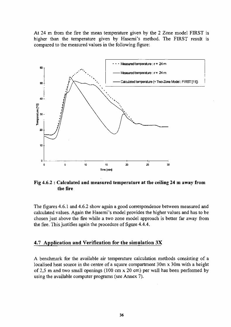
At 24 m from the fire the mean temperature given by the 2 Zone model FIRST is higher than the temperature given by Hasemi's method. The FIRST result is compared to the measured values in the following figure:
Measured temperature : r = 24 m
- Measured ternperature : r = 24m
- Calculated temperature (= Two-Zone Model : FIRST [11])
Fig 4.6.2 : Calculated and measured temperature at the ceiling 24 m away from the fire
The figures 4.6.1 and 4.6.2 show again a good correspondence between measured and calculated values. Again the Hasemi's model provides the higher values and has to be chosen just above the fire while a two zone model approach is better far away from the fire. This justifies again the procedure of figure 4.4.4.
4.7 Application and Verification for the simulation 3X
A benchmark for the available air temperature calculation methods consisting of a localised heat source in the centre of a square compartment 30m χ 30m with a height of 2,5 m and two small openings (100 cm χ 20 cm) per wall has been performed by using the available computer programs (see Annex 7).
36
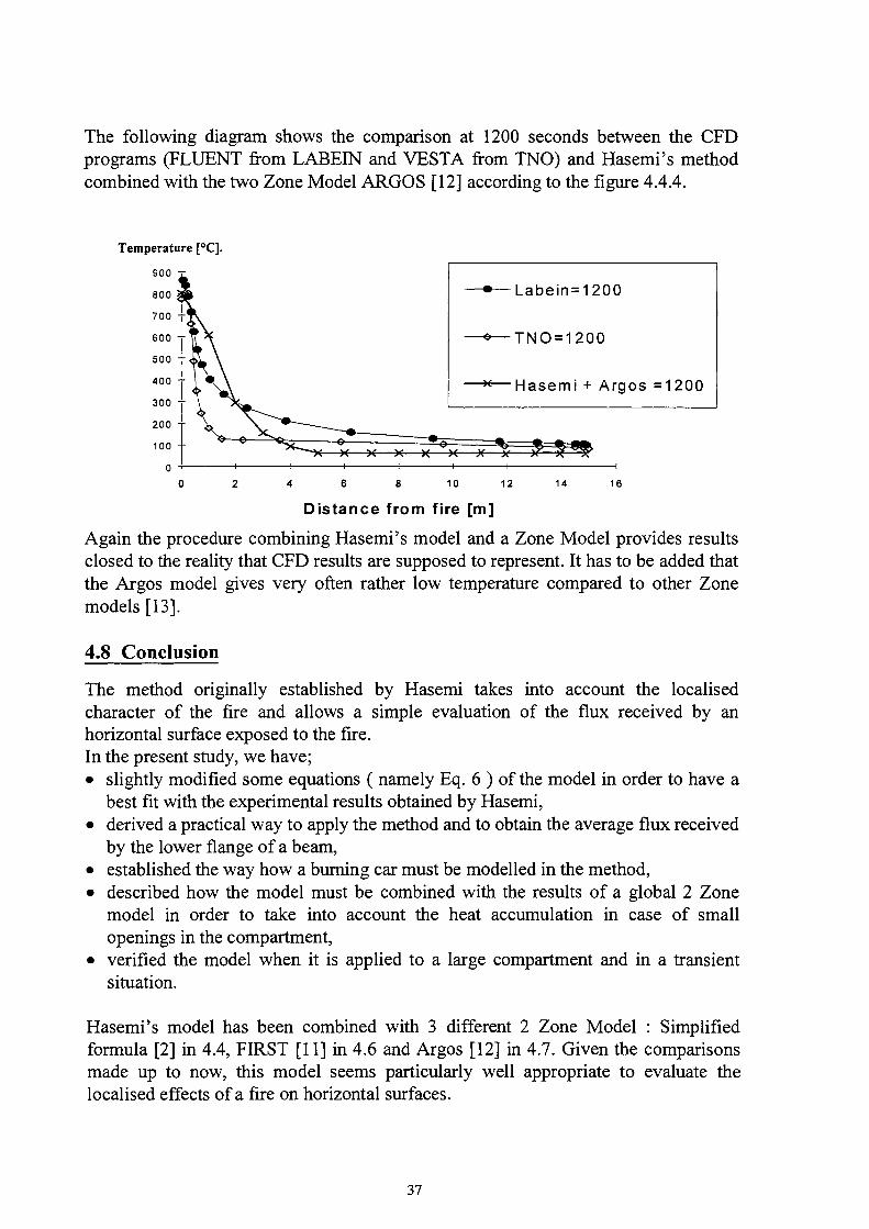
The following diagram shows the comparison at 1200 seconds between the CFD programs (FLUENT from LABEIN and VESTA from TNO) and Hasemi's method combined with the two Zone Model ARGOS [12] according to the figure 4.4.4.
Labein = 1200
-Θ—TNO = 1200
- *—Hasemi + Argos =1200
T V - H ^ 12 14 16
Distance from fire [m]
Again the procedure combining Hasemi's model and a Zone Model provides results closed to the reality that CFD results are supposed to represent. It has to be added that the Argos model gives very often rather low temperature compared to other Zone models [13].
4.8 Conclusion
The method originally established by Hasemi takes into account the localised character of the fire and allows a simple evaluation of the flux received by an horizontal surface exposed to the fire. In the present study, we have; • slightly modified some equations ( namely Eq. 6 ) of the model in order to have a
best fit with the experimental results obtained by Hasemi, • derived a practical way to apply the method and to obtain the average flux received
by the lower flange of a beam, • established the way how a burning car must be modelled in the method, • described how the model must be combined with the results of a global 2 Zone
model in order to take into account the heat accumulation in case of small openings in the compartment,
• verified the model when it is applied to a large compartment and in a transient situation.
Hasemi's model has been combined with 3 different 2 Zone Model : Simplified formula [2] in 4.4, FIRST [11] in 4.6 and Argos [12] in 4.7. Given the comparisons made up to now, this model seems particularly well appropriate to evaluate the localised effects of a fire on horizontal surfaces.
37
5. TEMPERATURE FIELD IN THE STRUCTURE
5.1 Temperature Field of a Column subjected to a Two-Zone
Environment
5.1.1 ID Modelling of a Column in a Two-Zone Model
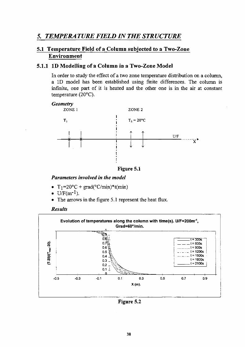
In order to study the effect of a two zone temperature distribution on a column,
a ID model has been established using finite differences. The column is
infinite, one part of it is heated and the other one is in the air at constant
temperature (20°C).
Geometry ZONE 1 ZONE 2
T,
> / \ V >
τ 2 = 20°C
Λ Λ
\ I
1 > ι ψ
U/F
Figure 5.1
Parameters involved in the model
• Ti=20°C + grad(°C/min)*t(min)
• LVF(m-l).
• The arrows in the figure 5.1 represent the heat flux.
Results
o
HE
Evolution of temperatures along the column with time(s).
Grad=60°/min. 1
" " " ^ a . om. o.it 0.6 ï
0.5 -
0.4 .
0.3 .
0.2 .
0.1 .
, Η 1 1 0
\
Jv\
\v\
U/F=200m"1,
t = son* t = 600s
t = 900s
. . t=1200s
t= 1500s
t=1800s t = 2100s
1 1 h
-0.5 -0.3 -0.1 0.1 0.3 0.5 0.7 0.9
X(m).
Figure 5.2
38
S" CM
it m
E
S" CM
Evolution of temperatures along the column with time(s). U/F=200m~1, Grad=30°/min.
1
0.6V
0.4 .
0.2 -
η
5
^ ί ^ ^
t = 300s t = 600s t = 900s
. . t=1200s t=1500s t=1800s t = 2100s
-0.5 -0.3 -0.1 0.1 0.3 0.5 0.7
X(m).
Figure 5.3
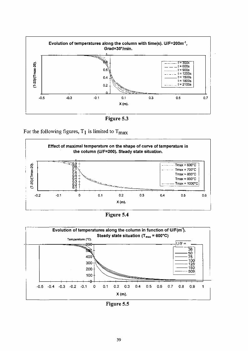
For the following figures, Tj is limited to T m a x
Effect of maximal temperature on the shape of curve of temperature in the column (U/F=200). Steady state situation.
ε o CM μ-
- Tmax = 600°C ¡
Tmax = 700°C
Tmax = 800°C
Tmax = 900°C
-Tmax=1000°C
-0.2 -0.1 0.1 0.2
X(m).
0.3 0.4 0.5 0.6
Figure 5.4
Evolution of temperatures along the column in function of U/F(m').
Steady state situation (Tmax = 600°C) Temperature (°C).
3ΘΘ- U/F:
36 ■50 •75 -100 -125 -150 -509
-0.5 -0.4 -0.3 -0.2 -0.1
Figure 5.5
0.1 0.2 0.3 0.4 0.5 0.6 0.7 0.8 0.9 1
X(m).
39

¿ςηπη -,
40000
35000
30000 -
J 25000 -
"ï" 20000 -
"■ 15000 -
10000 -
5000 -
Evolution of the flux crossing the separation between the zones.
/ ^ ^—"
/ /
! /
! 1 ■ / /
:' /
U/F-IOOmM
U/F-200m*-1
- / /
■ /
0 900 1800 2700
Time (s).
3600
Figure 5.6
Figures 5.2 and 5.3 show the influence of the external temperature gradient on
the temperature profile in the column. For a smaller gradient, the transient
zone in the column is greater. Nevertheless the length of the transient zone is
very small (<30cm).
Figure 5.4 shows the weak influence of the temperature of the hot zone when
the steady state situation is reached. The influence of U/F is shown in
figure 5.5.
The flux crossing the separation between the zones is not dependent of U/F of
the profile (figure 5.6) when the steady state situation is reached. The only
parameter is the temperature of the hot zone.
Conclusions
• The temperatures along an unprotected column in a two-zone model can be
assumed to be constant in the different zones.
• The flux crossing the separation between the two zones is weak and can be
neglected.
• In order to determine the temperature field in a cross section of a column
subjected to a 2 Zone Air temperature field, a 2 D temperature calculation is
sufficient.
40

5.1.2 3D MODELLING OF A COLUMN CROSSING A CONCRETE
PLATE
A column (HEA280) crossing a concrete slab (15cm of thickness) is modelled with
SAFIR finite elements code developed by the ULg. The influence of the column on
temperatures in the slab and of the slab on temperatures in the column are shown.
Geometry
COLUMN: HEA280.
CONCRETE: 150mm of thickness.
z ♦
HEA280
20 °C
15 cm
ISO fire
Figure 5.7
Modelling
• 3D modelling by SAFIR.
• Double symmetry (axis of the column).
• EC4 material models.
• ISO 834 fire.
• The origin of the co-ordinate axes is the centre of symetry of the HEA280
Results
Evolution of temperature at mid level in the concrete slab along
x-axis, y=0, z=0.
600
<ƒ 500 .
ir 4 0 ° -= 300 . I 200-| loo. £ o.
^ ~ | s ^ ν \
, —Vo-· ^ —
0 0.2 0.4 0.6 0
x (m) .
"IR min
λη min
45mJn
60 rrin
75 min
90 min
8
Figure 5.8
41

ISOTHERMS ON THE UPPER FACE OF THE CONCRETE SLAB AFTER 90 MIN
y 1
4^
o o
X
Figure 5.9
42
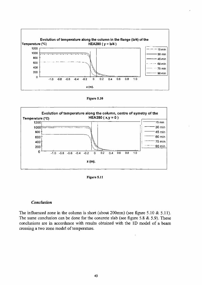
Evolution of temperature along the column in the flange (b/4) of the Temperature (°C) HEA280 ( y = b/4 )
0.6 0.8
z(m).
15 min
30 min
45 min
60 min
75 min
90 min
Figure 5.10
Evolution of temperature along the column, centre of symetry of the Temperature (°C) HEA280 ( x,y = 0 )
1200 1000 8001 600 400 200
0 -1.0 -0.8 -0.6 -0.4 -0.2 0.2 0.4 0.6 0.8 1.0
z (m).
"15 min
•30 min '45 min 60 min 75 min 90 min
Figure 5.11
Conclusion
The influenced zone in the column is short (about 200mm) (see figure 5.10 & 5.11). The same conclusion can be done for the concrete slab (see figure 5.8 & 5.9). These conclusions are in accordance with results obtained with the ID model of a beam crossing a two zone model of temperature.
43

5.2 Temperature Field of a Beam subjected
to a Non-Uniform Heating along its Length
5.2.1 3D Modelling of a Composite Beam
A comparison between calculated and tested temperatures in a composite beam is
given.
Tests
• The beam is defined at fig 5.12. Tests have been made at the university of Gent
for a REFAO research [14]. An IS0834 fire is put between points A & Β
(see figure 5.12). The cantilever part of the beam is at 20°C.
• Measurements : Sections 1 to 5 at points spot in the lower figure (Fig. 5.13)
Modelling
• 3D modelling by SAFIR.
• One plan of symmetry.
• EC4 material models.
' 3 0 0 x 2 9 6 x 2 0 ?<
9 ^ 3 5 0 x 2 4 0 x 2 0
?SQQ
2 » 2 5
ï « t o o
¿1 a teas
E «5ÍV β ο ο ο
éche l te 1 : 2 0
Section 1
I 9aooì
-f" 250-4-250-^-
2 1 5 0
2 5 0
Ξ Θ ΞΈΕΙ
J ι I αά 3SO * 3 0 0 * 2 0
Figure 5.13
44
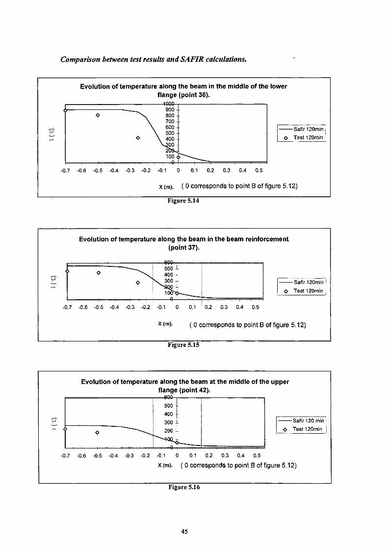
Comparison between test results and SAFIR calculations.
Evolution of temperature along the beam in the middle of the lower flange (point 36).
, 4βθθ-
O ^ \ 800 -\ 700 -\ 600 -\ 500 -
O \ 400 -V300-206^ 100 A^««^_
! 1 1 1 ! 1 1 i 1 i Λ 4 1 ^ T — , ι . i . ι .
Safir 120min O Test120min
-0.7 -0.6 -0.5 -0.4 -0.3 -0.2 -0.1 0 0.1 0.2 0.3 0.4 0.5
x (m). ( 0 corresponds to point Β of figure 5.12)
Figure 5.14
Evolution of temperature along the beam in the beam reinforcement (point 37).
600
-0.7 -0.6 -0.5 -0.4 -0.3 -0.2 -0.1
Safir 120min O Test 120min
0.1 0.2 0.3 0.4 0.5
x (m). ( o corresponds to point Β of figure 5.12)
Figure 5.15
Evolution of temperature along the beam at the middle of the upper flange (point 42).
O
— < o ~ ~ ^ \
500 -400 -300 -200 -
— 1 — Λ -
Safir 120 min O Test 120min
-0.7 -0.6 -0.5 -0.4 -0.3 -0.2 -0.1 0 0.1 0.2 0.3 0.4 0.5
x (m). ( 0 corresponds to point Β of figure 5.12)
Figure 5.16
45
"CT
<
-0
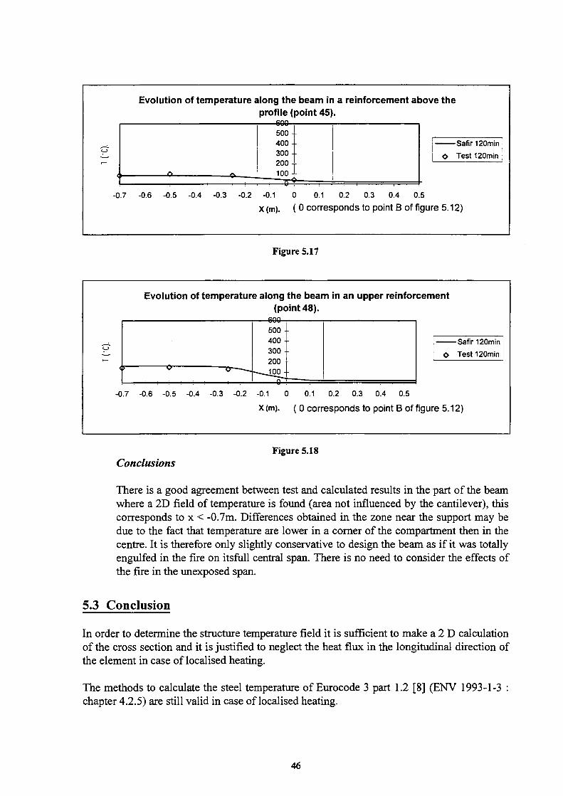
Evolution of temperature along the beam in a reinforcement above the
profile (point 45). cnn
> o 0
.7
500 -
4 0 0 -
3 0 0 -
2 0 0 -
100 -—A.
Safir 120min ι
O Test 120min
-0.6 -0.5 -0.4 -0.3 -0.2 -0.1 0 0.1 0.2 0.3 0.4 0.5
X(m). ( 0 corresponds to point Β of figure 5.12)
Figure 5.17
Evolution of temperature along the beam in an upper reinforcement
(point 48).
< > s/ O —
500 -
400 -
300 -
200 -
-—_J00-
—ι—Æ-
-Safir 120min
Test 120min
-0.7 -0.6 -0.5 -0.4 -0.3 -0.2 -0.1 0 0.1 0.2 0.3 0.4 0.5
x (m). ( 0 corresponds to point Β of figure 5.12)
Figure 5.18
Conclusions
There is a good agreement between test and calculated results in the part of the beam
where a 2D field of temperature is found (area not influenced by the cantilever), this
corresponds to χ < -0.7m. Differences obtained in the zone near the support may be
due to the fact that temperature are lower in a corner of the compartment then in the
centre. It is therefore only slightly conservative to design the beam as if it was totally
engulfed in the fire on itsfull central span. There is no need to consider the effects of
the fire in the unexposed span.
5.3 Conclusion
In order to determine the structure temperature field it is sufficient to make a 2 D calculation
of the cross section and it is justified to neglect the heat flux in the longitudinal direction of
the element in case of localised heating.
The methods to calculate the steel temperature of Eurocode 3 part 1.2 [8] (ENV 1993-1-3 :
chapter 4.2.5) are still valid in case of localised heating.
46

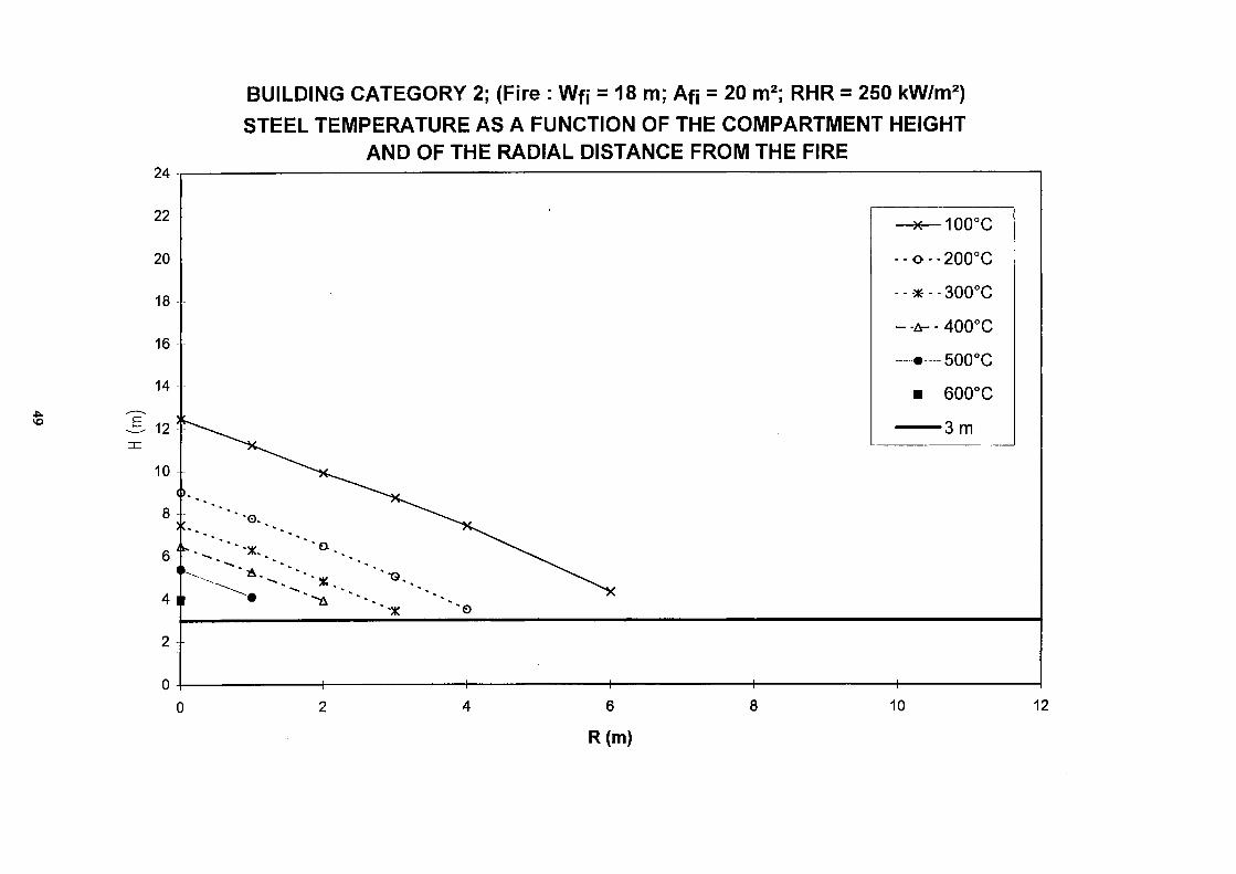
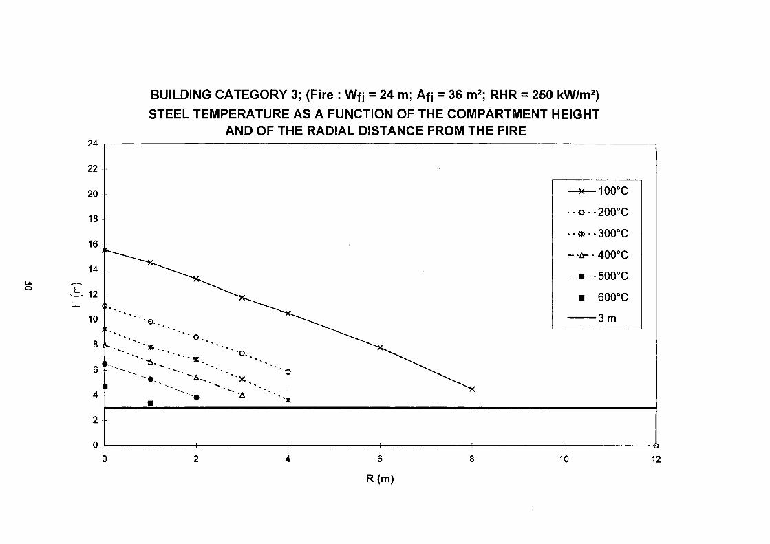
5.4 Design graphs
The whole procedure to obtain the steel temperature consist of 3 steps:
1) to define the fire characteristics : fire size and Rate of Heat Release Curve.
2) to calculate the air temperature around the steel element or the heat flux received by the steel element by using the Hasemi's method combined with a 2 Zone Model
3) to calculate the steel temperature by using the ENV 1993-1-2 [8].
By using this procedure, it is possible to produce design graphs showing the temperature field of a beam at the ceiling of the compartment.
When applying the procedure, the fire sizes and the constant values of Rate of Heat Release defined in table 3.2. have been considered. Building Category i refers to the i m line of the table 3.2. Graphs are given for the first three lines. The fire is supposed at ground level. As a steady state situation is considered (RHR = constant), the steel temperature doesn't depend on the profile. The following graphs show the steel temperature of the beam as a function of the Height of the building and the Radial distance R from the fire. These graphs based on a very conservative assumption (Steady State) enable us to determine very quickly the heating of a horizontal beam element at the ceiling level.
47

è
ΖΓ
BUILDING CATEGORY 1; (Fire : Wf¡ = 12 m; Af¡ = 9 m2; RHR = 250 kW/m
2)
STEEL TEMPERATURE AS A FUNCTION OF THE COMPARTMENT HEIGHT
AND OF THE RADIAL DISTANCE FROM THE FIRE
6
R(m)
10 12
VO
24
22
20
18
16
14
12
10
8
6
4
2
0
BUILDING CATEGORY 2; (Fire : Wf¡ = 18 m; Afj = 20 m2; RHR = 250 kW/m
2)
STEEL TEMPERATURE AS A FUNCTION OF THE COMPARTMENT HEIGHT
AND OF THE RADIAL DISTANCE FROM THE FIRE
6
R(m)
" ■ « * " - « ^ " " ^
II ^ · -Δ ■-. ' · . _
•χ o
ν mn°n Λ I UU W
--o--200°C
--*--300°C
- -Δ- - 400°C
- - · -500°C
■ 600°C
1 m
1 1 1 1 1
10 12
Ui O
BUILDING CATEGORY 3; (Fire : Wf¡ = 24 m; Af¡ = 36 m2; RHR = 250 kW/m2) STEEL TEMPERATURE AS A FUNCTION OF THE COMPARTMENT HEIGHT
AND OF THE RADIAL DISTANCE FROM THE FIRE
6
R(m) 10 12

6. THERMO-MECHANICAL BEHAVIOUR: COLUMN IN A
TWO-ZONE ENVIRONMENT
6.1 Introduction
As can be seen from the graphs found overleaf a study has been carried out
concerning the behaviour of columns in a two zone environment. Indeed, there are
methods to calculate columns at room temperature or at elevated temperature but no
simplified method exists for a column partially engulfed in a hot zone.
From the graphs it is possible to deduce the ultimate load of a certain column
exposed to two zone condition. The symbol alpha defines this two zone condition,
α = 0 means that there is no hot zone and that therefore the interface layer between
the lower cold layer and the upper hotter layer is at the ceiling, α = 1 indicates the
opposite, that there is no cold zone and that therefore the level of the interface is at
the floor, the whole of the column being heated to the specified maximum
temperature taken as 500 °C in this study (fig 6.1).
Hot Zone Conditions
Lh
NK
oc=0
ï /
θ =
m 500°C
!»
/Κ
oc=Lh
ψ
= 500°C
Fig 6.1
An HEB 300 has been analysed under different end fixing conditions and with
different lengths. The dimensions of the columns are identified by the non-
dimensional slenderness ratio, λ. λ = 0,4; 0,8 and 1,2 has been considered. The end
conditions that were analysed can be seen on the figure 6.2.2.
The results have been provided by the program SAFIR. An initial imperfection of the
column equal to L/1000 and a residual stresses distribution with a maximum residual
stress equal to 0,5 χ fy (20°C) have been assumed. Steel S 235 has been considered.
51
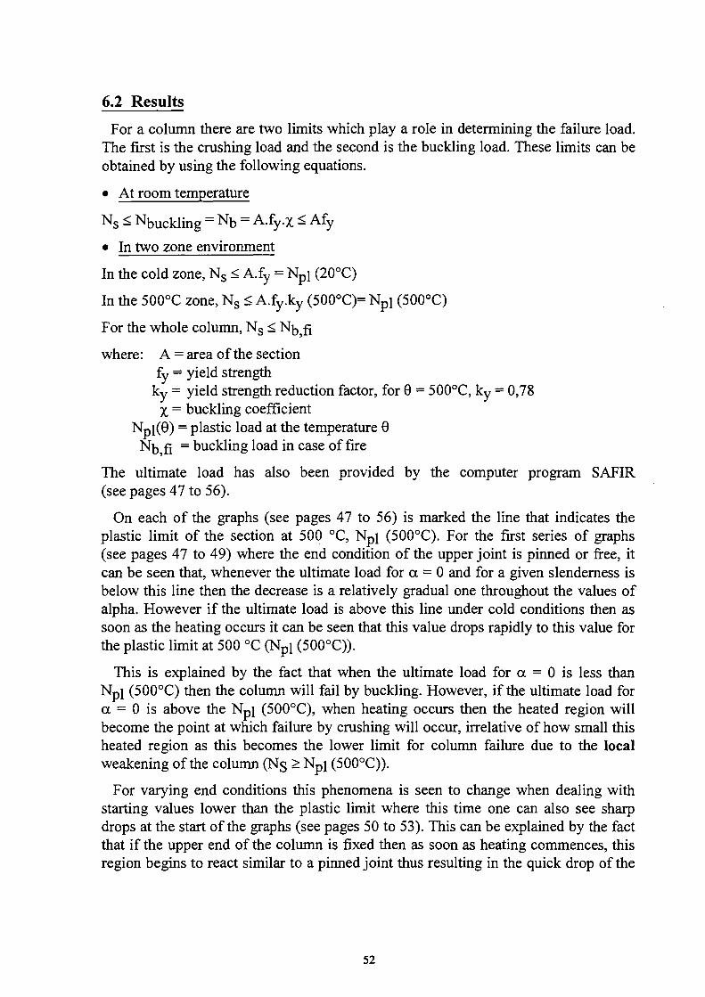
6.2 Results
For a column there are two limits which play a role in determining the failure load. The first is the crushing load and the second is the buckling load. These limits can be obtained by using the following equations.
• At room temperature
N s < Nbuckling = Nb = Α.%.χ < Afy
• In two zone environment
In the cold zone, N s < A.fy = Npi (20°C)
In the 500°C zone, N s < A.fy.ky (500°C)= Npj (500°C)
For the whole column, N s < N^fj
where: A = area of the section fy = yield strength
ky = yield strength reduction factor, for θ = 500°C, ky = 0,78 χ = buckling coefficient
Νρΐ(θ) = plastic load at the temperature θ Nb fi = buckling load in case of fire
The ultimate load has also been provided by the computer program SAFIR (see pages 47 to 56).
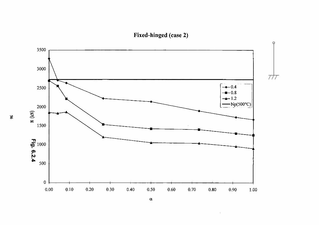
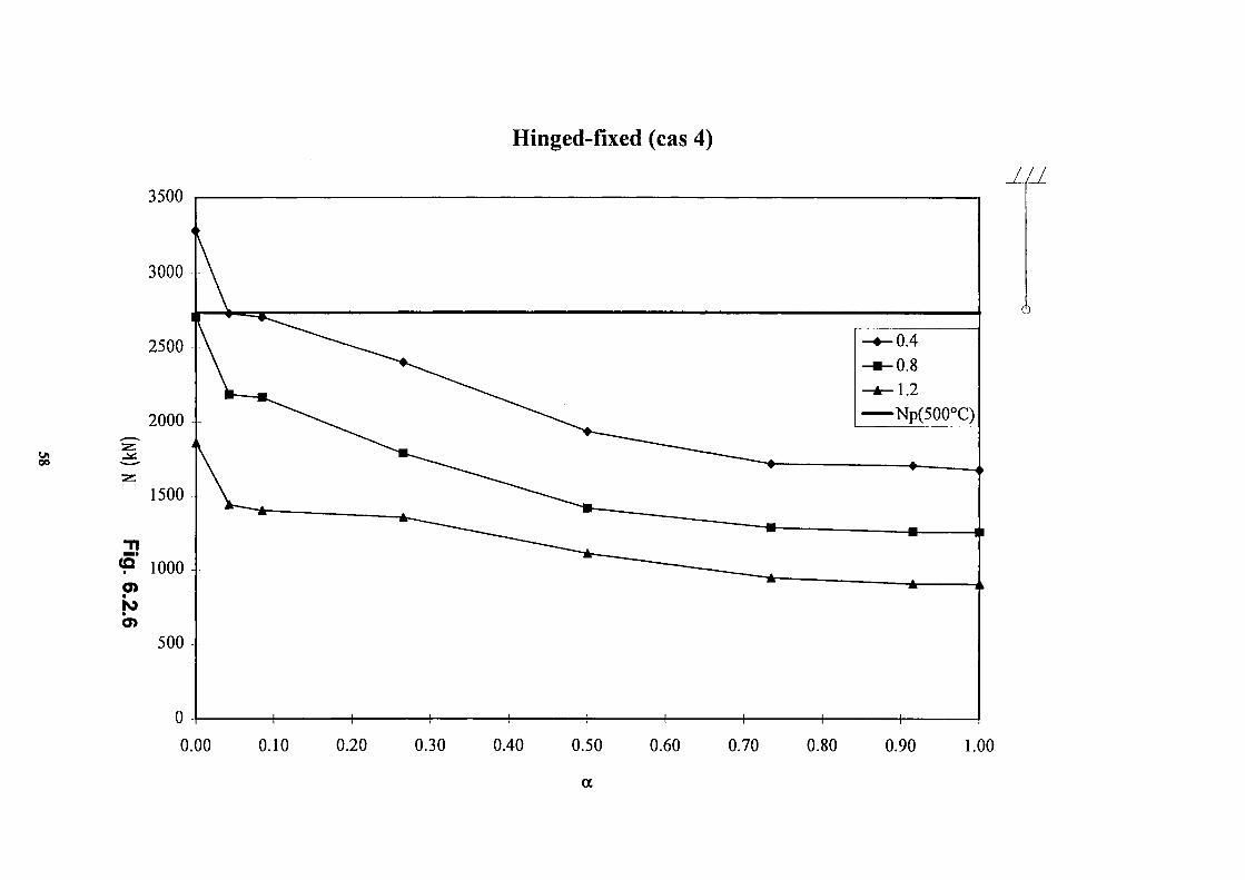
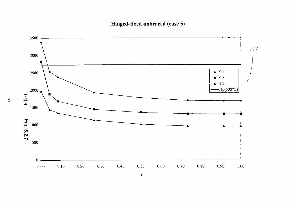
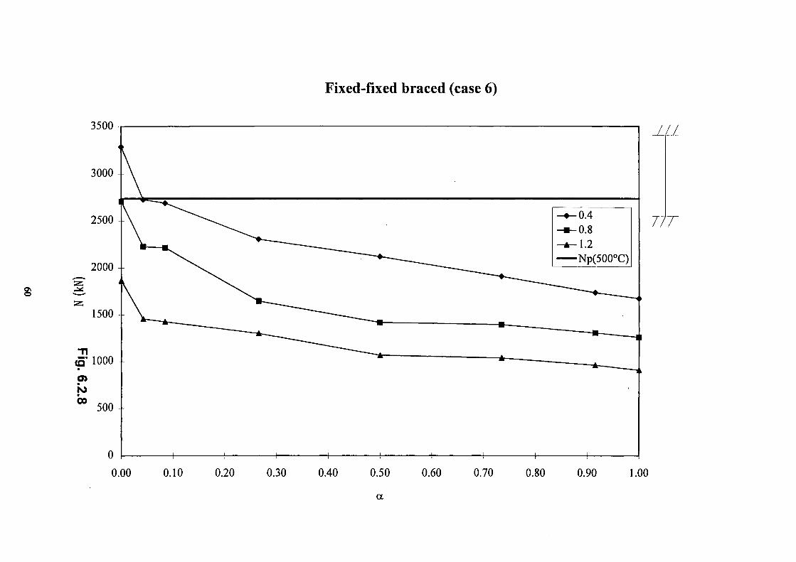
On each of the graphs (see pages 47 to 56) is marked the line that indicates the plastic limit of the section at 500 °C, Npi (500°C). For the first series of graphs (see pages 47 to 49) where the end condition of the upper joint is pinned or free, it can be seen that, whenever the ultimate load for α - 0 and for a given slenderness is below this line then the decrease is a relatively gradual one throughout the values of alpha. However if the ultimate load is above this line under cold conditions then as soon as the heating occurs it can be seen that this value drops rapidly to this value for the plastic limit at 500 °C (Npi (500°C)).
This is explained by the fact that when the ultimate load for α = 0 is less than Npi (500°C) then the column will fail by buckling. However, if the ultimate load for α = 0 is above the Npi (500°C), when heating occurs then the heated region will become the point at which failure by crushing will occur, irrelative of how small this heated region as this becomes the lower limit for column failure due to the local weakening of the column (N§ > Npj (500°C)).
For varying end conditions this phenomena is seen to change when dealing with starting values lower than the plastic limit where this time one can also see sharp drops at the start of the graphs (see pages 50 to 53). This can be explained by the fact that if the upper end of the column is fixed then as soon as heating commences, this region begins to react similar to a pinned joint thus resulting in the quick drop of the
52

ultimate load from the buckling load of a column with a upper fixed end condition to the ultimate load corresponding to a pinned one.
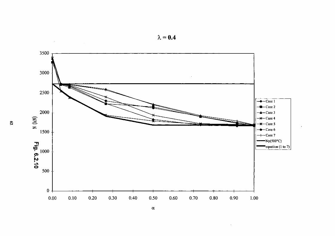
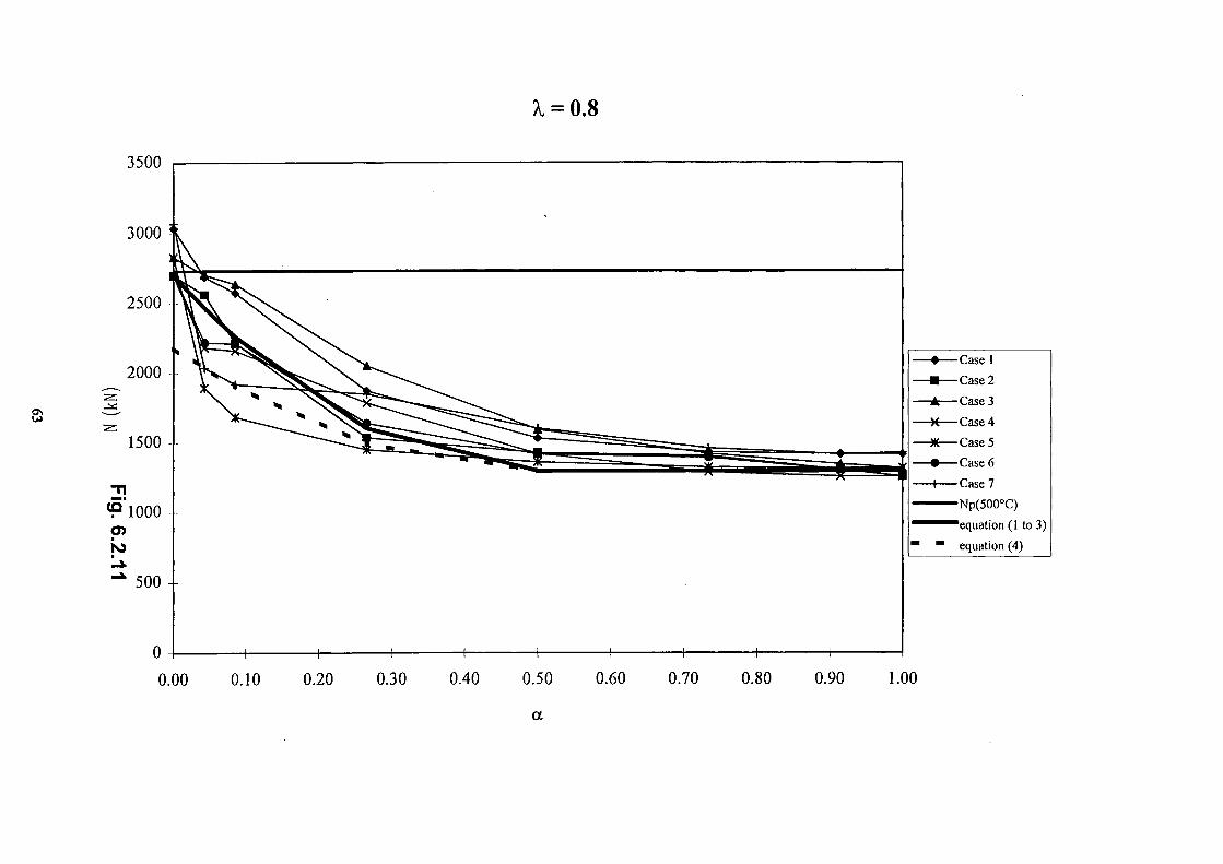
Over the final few pages of this chapter (see pages 54 to 56) there can be seen three graphs, each of which shows all the results gathered together for each slenderness ratios.
On these graphs it is also possible to see a line describing the path of an equation defined to represent the buckling load for columns in a two zone environment. The equation that has been defined is shown below:
N' = min [NU'(20°C); Npi (500°C)] > N u (500° C )
for 0 < α < 0,5 Ν = 4 (Ν'- Nu (500°C)) a?- - 4 α (N'-Nu (500°C)) + N'
for α > 0,5 N = NU(500°C)
with
NU'(20°C), the ultimate load at room temperature calculated with a hinge at the top.
N u (500°C), the ultimate load when the whole column is in a temperature of 500°C
This equation has been deduced from the following assumption :
• for α > 0,5 , there is no benefit of the two zone phenomenom. The ultimate load in two zone_environment is equal to the ultimate load assuming that the whole column is engulfed by the fire.
• For 0 < α < 0,5 , a parabolic curve between N' and N u (500°C) shows the influence of the two zone effect. The parabolic equation is defined by the three following conditions:
. ) i na = 0,N = N'
. ) i n a = 0,5,N = Nu(500°C)
.) in a = 0,5 , the slope of the parabole is equal to 0.
For any θ < 500°C
Ν
Ν'
Nu(500°C)
α=0 α=0.5 Fig 6.2.1
α=1
This procedure could be extended to other temperature θ < 500°C.
53
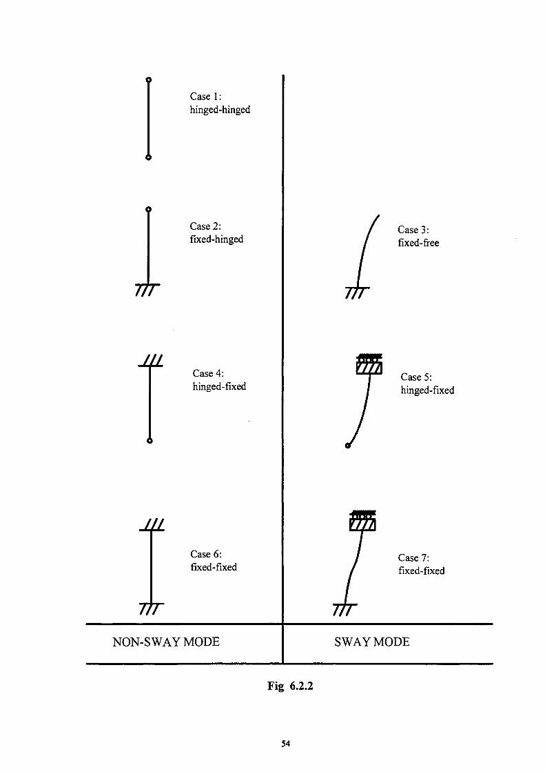
77Γ
Ml
Ml
77Γ
Case 1: hinged-hinged
Case 2: fixed-hinged
Case 4: hinged-fixed
Case 6: fixed-fixed
Case 3: fixed-free
Case 5: hinged-fixed
Case 7: fixed-fixed
NON-SWAY MODE SWAY MODE
Fig 6.2.2
54

Hinged-hinged (case 1)
Ui
3500
3000
2500
2000
1500
& loo«
O)
jo w 500
-^
0 4 —
0.00
-»-0.4
-*-0.6
-à-0.8
-χ-1.2
Np(500°C)
-*-
0.10 0.20 0.30 0.40 0.50
α
0.60 0.70 0.80 0.90 1.00
Fixed-hinged (case 2)
Φ
a ^
ζ
3500
3000
2500
2000
1500
"Π
to" ïooo
σ> io
500
0
TTT
0.00 0.10 0.20 0.30 0.40 0.50 0.60 0.70 0.80 0.90 1.00
α

Fixed-free (case 3)
3500
3000
2500
2000
1500
<α" σ> ro O l
ιυυυ
500
0.00 0.10 0.20 0.30 0.40 0.50 0.60 0.70 0.80 0.90 1.00
α
Hinged-fixed (cas 4)
Χ
οο
<
3000
2500
2000 -
ζ
1500
τι
<Ρ îooo
σ> ro ο>
500
0
\
\
ν ^ ^ ^ ^ ^ .
"~~ ■
-
1 1 1 1 i 1 1 1
-»-0.4
-»-0.8
Α1.2
Np(500°C)
■ ■ II
— Α 1 k
1
Ô
0.00 0.10 0.20 0.30 0.40 0.50 0.60 0.70 0.80 0.90 1.00
α
Hinged-fixed unbraced (case 5)
<
3000 I
2500 -
2000 , z?
ζ
1500 -
"Π <5" ίππο σ> ro ^1
500 -
0
•
Λ 1 \
\ V \ ^ * \ \ ^ ^
Λ ^—_______ ^^•±—. ■
A-
1 1 1 1 1 h -
■♦
g
A
1 1
-» -0 .4
-» -0 .8
- A - 1 . 2
Np(500°C)
♦ l>
■ II
A ík
1
0.00 0.10 0.20 0.30 0.40 0.50 0.60 0.70 0.80 0.90 1.00
α
Fixed-fixed braced (case 6)
g
3500
3000
2500
2000
1500
5'1000 σ> jo bo 500
TTT
o.oo o.io 0.20 0.30 0.40 0.50 0.60 0.70 0.80 0.90 1.00
α

Fixed-fixed unbraced (case 7)
σ\
3500
3000
2500
2000
1500
3Î 9 1 ooo σ> jo to
500
0
< >
1
— £
1 1 — 1 1
■ ■
1 1
-» -0 .4
-» -0 .8
-A-1.2
Np(500°C)
■ II
1
A * 1 k
1
0.00 0.10 0.20 0.30 0.40 0.50 0.60 0.70 0.80 0.90 1.00
α
λ = 0.4
3500
0.00 0.10 0.20 0.30 0.40 0.50 0.60 0.70 0.80 0.90 1.00
α
λ = 0.8
3500
Os
- · Case 1 -fl—Case 2 -A—Case 3 -X—Case 4 -X—Case 5 • Case 6
Η Case 7 Np(500°C)
"^"equa t ion (1 to 3) ™ equation (4)
0.00 0.10 0.20 0.30 0.40 0.50 0.60 0.70 0.80 0.90 1.00
α

λ =1.2
2
3000
2500
2000
<* 1500
1000 (Q
¡o
ro 500
-»—Case 1
-fl—Case 2
-A—Case 3
-X—Case 4
-X—Case 5
- · — C a s e 6
-I Case 7
Np(500°C)
^""equa t ion (1 to 3)
■ equation (4)
0.00 0.10 0.20 0.30 0.40 0.50 0.60 0.70 0.80 0.90 1.00
α
7. DESIGN TOOL
Introduction
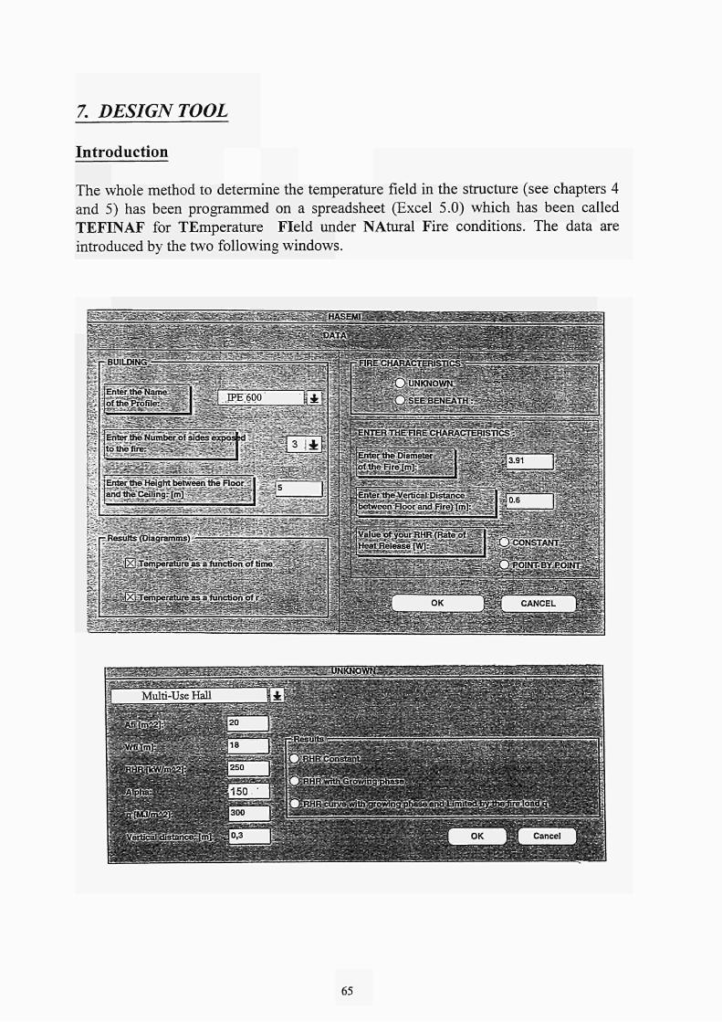
The whole method to determine the temperature field in the structure (see chapters 4 and 5) has been programmed on a spreadsheet (Excel 5.0) which has been called TEFINAF for TEmperature Field under N Aturai Fire conditions. The data are introduced by the two following windows.
KEH3CT1
65
On the first window you can introduce the name of the profile and the number of sides exposed to the fire thanks to a "pull down menu".
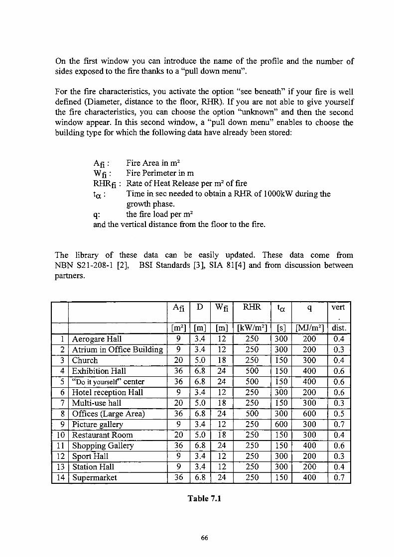
For the fire characteristics, you activate the option "see beneath" if your fire is well defined (Diameter, distance to the floor, RHR). If you are not able to give yourself the fire characteristics, you can choose the option "unknown" and then the second window appear. In this second window, a "pull down menu" enables to choose the building type for which the following data have already been stored:
Aß : Fire Area in m2
Wfi : Fire Perimeter in m RHRfi : Rate of Heat Release per m2 of fire t a : Time in sec needed to obtain a RHR of lOOOkW during the
growth phase, q: the fire load per m2
and the vertical distance from the floor to the fire.
The library of these data can be easily updated. These data come from NBN S21-208-1 [2], BSI Standards [3], SIA 81[4] and from discussion between partners.
1 2 3 4 5 6 7 8 9
10 11 12 13 14
Aerogare Hall Atrium in Office Building Church Exhibition Hall "Do it yourself" center Hotel reception Hall Multi-use hall Offices (Large Area) Picture gallery Restaurant Room Shopping Gallery Sport Hall Station Hall Supermarket
Afi
[m2] 9 9
20 36 36 9
20 36 9
20 36 9 9 36
D
[m] 3.4 3.4 5.0 6.8 6.8 3.4 5.0 6.8 3.4 5.0 6.8 3.4 3.4 6.8
Wfi
[m] 12 12 18 24 24 12 18 24 12 18 24 12 12 24
RHR
[kW/m2] 250 250 250 500 500 250 250 500 250 250 250 250 250 250
ta
[s] 300 300 150 150 150 300 150 300 600 150 150 300 300 150
q
[MJ/m2] 200 200 300 400 400 200 300 600 300 300 400 200 200 400
vert
dist. 0.4 0.3 0.4 0.6 0.6 0.6 0.3 0.5 0.7 0.4 0.6 0.3 0.4 0.7
Table 7.1
66
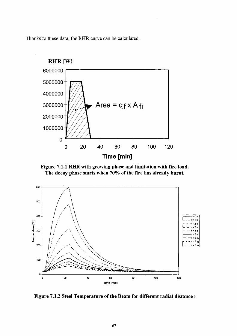
Thanks to these data, the RHR curve can be calculated.
RHR[W]
bUUUUUU"
5000000 -
4000000 -
3000000 -
2000000 -
1000000-
V//A
Area = qf χ Afj
0 20 40 60 80 100 120
Time [min]
Figure 7.1.1 RHR with growing phase and limitation with fire load. The decay phase starts when 70% of the fire has already burnt.
500
400
300
200-
10U -
0 -
/ Λ
\ / r
λ \
/ t 1 \
/ / 'Λ / / Λ / /
v \
/ ' * \ / ' * \ / '
v \
/ ' x
\ ■ / / \ \ \
Ι ι ; \ \ I I
v \
Ι ι : s
\
' ·· y ν
· ■ \ \
/' .· / y . >. \ ··. \ \
1 1 !
60
Time [min]
80 100
----
— - -—
—
--
■r = 0m
r= 1 m
•r = 2m
r = 3m
r = 4m
■r = 5m
•r = 6m
r = 7 m
r = 8m
Figure 7.1.2 Steel Temperature of the Beam for different radial distance r
67

o o s-, :
CO — OJ O-Β O)
600
500
400
300
200
100
V
4 6 r[m]
10
Figure 7.1.3: Steel Temperature of the Beam at different times as a function of the radial distance r
The final results are the temperature field in the beam at the ceiling depending on the time and on the radial distance r from the fire (see figures 7.1.2 and 7.1.3). Moreover a table provides the temperature and the thickness of the hot zone as a function of the forced ventilation or of the openings for the inlet and outlet in case of natural ventilation. This table enables to check the assumption of localized fire and to apply the procedure of chapter 4.4.
Height of the smoke
layer d
1 2 3 4
Temperature of the hot zone
[°C] 162,75 242,48 432,91 1197,03
Forced ventilation
[m3/h] 124518,53 95182,50 70409,52 51279,10
Natural ventilation, Openings area (AvCv) [m2]
AV*CV/AI*CI=1 13,58 5,76 2,46 0,86
0,8 12,57 5,38 2,33 0,83
0,6 11,73 5,06 2,22 0,81
0,4 11,08 4,82 2,14 0,80
0,2 10,68 4,67 2,09 0,79
Table 7.1.1
68
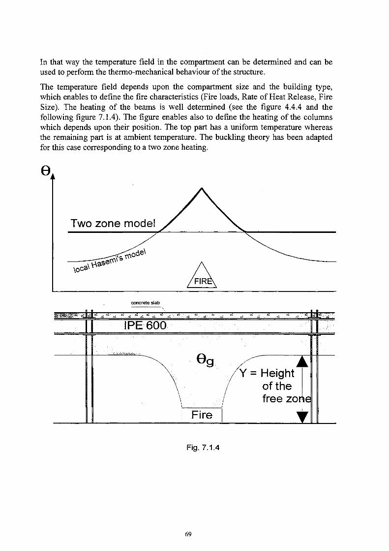
In that way the temperature field in the compartment can be determined and can be
used to perform the thermo-mechanical behaviour of the structure.
The temperature field depends upon the compartment size and the building type,
which enables to define the fire characteristics (Fire loads, Rate of Heat Release, Fire
Size). The heating of the beams is well determined (see the figure 4.4.4 and the
following figure 7.1.4). The figure enables also to define the heating of the columns
which depends upon their position. The top part has a uniform temperature whereas
the remaining part is at ambient temperature. The buckling theory has been adapted
for this case corresponding to a two zone heating.
θ
Two zone model
\0ca\ W&
concrete slab
,·. °·· ¿ °· ΛΜ .! J. . 6 . . . O. : . Ο» , · !■ O· .
I PE 600
θ g
Fire
A Height of the free zone
Fig. 7.1.4
69
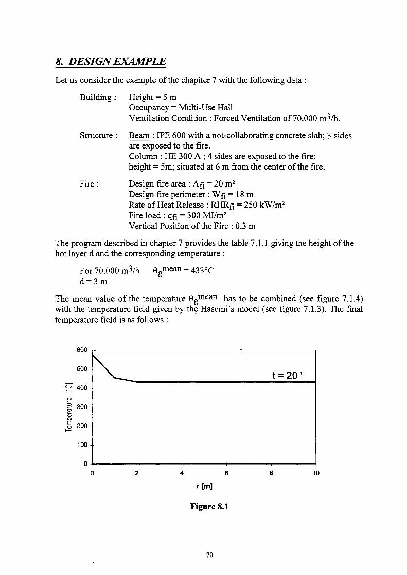
8. DESIGN EXAMPLE Let us consider the example of the chapiter 7 with the following data :
Building : Height = 5 m Occupancy = Multi-Use Hall Ventilation Condition : Forced Ventilation of 70.000 m^/h.
Structure : Beam : IPE 600 with a not-collaborating concrete slab; 3 sides are exposed to the fire. Column : HE 300 A ; 4 sides are exposed to the fire; height = 5m; situated at 6 m from the center of the fire.
Fire : Design fire area : Afi = 20 m2
Design fire perimeter : Wfi = 18 m Rate of Heat Release : RHRfi = 250 kW/m2
Fire load : qfi = 300 MJ/m2
Vertical Position of the Fire : 0,3 m
The program described in chapter 7 provides the table 7.1.1 giving the height of the hot layer d and the corresponding temperature :
For 70.000 m^/h 0gmean = 4 3 3°c d = 3m
The mean value of the temperature 0 g m e a n has to be combined (see figure 7.1.4) with the temperature field given by the Hasemi's model (see figure 7.1.3). The final temperature field is as follows :
Figure 8.1
70

Structural calculation of the Beam
Knowing the temperature evolution of the yield strength [8], the figure 8.2 can be
deduced from the figure 8.1.
1,00
8,00
Figure 8.2 Yield Strength reduction as a function of the radial distance r
for t = 20' corresponding to the maximal temperatures.
This yield strength fvø can be used to calculate the Bending Moment Resistance
Mj^ø [8] which has to be compared to the applied bending moment M¡§d fi.
Structural calculation of the Column
The figure 8.1 enables us to determine the temperature of the top of the column. This
temperature corresponds to the temperature of the column over a length equal to the
hot layer thickness d (d = 3 m). According to the method developed in chapter 6, the
column is heated on more than half of the length (a > 0,5) and the ultimate load is the
ultimate load N u (Θ = 433°C) calculated according to [8] which assumes a uniform
temperature along the length of the column.
71
9. CONCLUSIONS
The existing standards concerning the fire resistance are all based on an uniform fire temperature in the considered compartment given by the ISO curve. R30, 60, 90, 120 or 180 may be required and means that the structure submitted to the ISO curve shouldn't fail before respectively 30, 60, 90, 120 or 180 minutes of ISO fire.
The following assumptions are included in the standards:
1) The temperature of the hot gases produced by the fire rises continuously according to the ISO curve up to the required fire resistance time.
2) This temperature is uniform in the considered fire compartment of the building, which means that a Post-Flashover situation is always assumed.
However both assumptions are quite unrealistic and uneconomical in the case of buildings containing very free large volumes inside.
Indeed, on one hand, the fire loads of this type of construction (station hall, atrium of office building, shopping gallery, sport hall, multi-use hall, ...) are generally rather small so that it is not possible to reach the high temperatures of the ISO curve. Moreover a large amount of air is available, which is a second factor reducing the temperature.
On the other hand it is obvious that the temperature of the air in a large compartment in fire differs from one point to another. For instance a 10 m high column in a station hall under fire is not subjected to a same temperature field at its top and at its bottom part. In a large compartment the fire may remain localised and doesn't lead to a fully developed fire so that the regime corresponds to the Pre-Flashover conditions.
In order to determine whether or not the situation corresponds to a large compartment, it has to be checked that the fire will remain a localised fire.
This implies that :
• the fire load is such that a quick fire spread leading to a fully engulfment of the whole compartment and, as a consequence, of the whole fire load is not possible.
• no flashover occurs.
72
A procedure has been developed to check whether a building fulfills the conditions which ensure that the fire will remain localised. This procedure consists in defining the fire (Rate of Heat Release, fire area, fire load), calculating the mean temperature and the height of the smoke layer and in verifying that the spread of fire is limited and the flashover is not possible.
Consequently, the mean temperature of the hot gas is rather low (< 500°C). Nevertheless the peak values of the temperature in the immediate vicinity of the fire have to be quantified in order to ensure that they don't damage the structure.
The method to determine the peak values of the temperature field is based on the Hasemi's method [6] adapted by the University of Liège. By combining the Hasemi's method and the mean temperature of the hot gas layer, the thermal action on the structure is calculated and the fire part of Eurocode 3 is used to deduce the temperature of the structure itself and its structural behaviour. Concerning the heating of the element, the calculation method of EC3 can be used because the heat loss along the axis of the element may be neglected.
For a column, the fact that a part of it is not submitted to high temperature, has a quite small influence except if this cold zone extends to more than half of the column. In the later case, a proposal has been made to quantify this positive effect.
The whole procedure is described in chapter 2 "General Guidelines" and is available through the software TEFINAF. It enables to replace the ISO requirement F30, F60, F90, F120 by the following requirement: the structure shall survive the realistic fire defined by its size, its Rate of Heat Release and its fire load.
73

10. LIST OF NOTATIONS
Indices
a identifies data about steel c convective component of heat transfer cr critical value d design value f related to the floor area Af fi identifies values relevant for fire design i related to the element " i " k characteristic value r radiative component of heat transfer t related to the total area At w identifies data about windows
Latin case letters
A area of the section Af floor area [ m2 ] Afi fire area [ m2 ] b width of the fire zone [ m ] B length of the fire zone [ m ] Cp specific heat of air CM empirically derived constant of proportion d depth of layer of hot gases D diameter (or characteristic length) of the fire [ m ] E burnt energy [ GJ ] fy yield strength of the steel fy,0 yield strength of the steel at the temperature θ Fr Froude number g acceleration due to the gravity [ m/s^ ] H distance between the fire source and the ceiling or the beam [ m ] Hb depth of the beam [ m ] H c theoretical heat of combustion per fuel unit mass [ J/kg ] Hf height between floor and ceiling [ m ] Hs vertical distance between the floor and the fire source [ m ] I radiation intensity ky yield strength reduction factor Lh heated length of the column [ m ] Lj-j horizontal length of the flame on the ceiling [ m ]
74
m ent au" entrainment rate up to a height ζ [ kg/s ]
mf combustible mass flow rate [ kg/s ]
M R fi Resistance Bending Moment in case of fire
M s fi Applied Bending Moment in case of fire
Ntø fi buckling load in case of fire
Νρΐ(θ) plastic load at temperature θ NU(20°C) Ultimate load at room temperature calculated with a hinge at the top. q fire load per m2
q a v average flux received by the lower flange q" heat flux [kW/m2] Q Rate of Heat Release of the fire [W] Q* Non dimensional Rate of Heat Release [-] Qmax Maximum Rate of Heat Release [kW] r horizontal distance, at the ceiling, from the center of the fire [ m ] RHR Rate of Heat Release [kW] RHRfi Rate of Heat Release per m2 of fire [kW/m2] Sf thickness of layer I S the stoichiometric mass air to fuel ratio t m a x time corresponding to the max temperature [ min ] tfot t o t a l duration of the fire [ min ] Tj steel temperature in Zone 1 corresponding to the hot zone T2 steel temperature in Zone 2 corresponding to the cold zone Tg steel temperature Too ambient air absolute temperature u moisture content in % by weight v air velocity [ m/sec ] Wfi perimeter of the fire[ m ] w mjgas temperature dependent weighting functions for the component grey gases wm,soot temperature dependent weighting functions for the component grey gases X A efficiency of combustion Xr radiant fraction Y height of the zone without smoke [ m ] ζ distance to the pool surface [ m ] ζ' vertical position of the virtual heat source, with respect to the fire sourcef m ] Zf visible flame height [ m ] Z v virtual source origin based on entrainment rates [ m ] Zy virtual origin [ m ]
75
Greek upper case letters
Θ temperature [ °C] ; Θ [ °C] = Τ [ Κ ] - 273
0 a steel temperature
0 c r critical temperature [ °C], relevant for steel
Θ g uniform temperature of the hot layer [ °C]
Greek lower case letters
α convection coefficient am,gas absorption coefficient am,soot absorption coefficient
ßoo total buoyancy flow
ΔΤ temperature rise at the centerline
Γχ coefficient that take into account density decrease due to the fact that the
gases are hotter that the ambient
λ non dimensional slenderness ratio
λ} thermal conductivity of layer I [ W/mK ]
μι turbulent viscosity
Poo ambient air density [ kg/m^]
σ Stefan Boltzman constant
σ§ scattering coefficient
χ buckling coefficient
ω solid angle
76
11. BIBLIOGRAPHY
[I] Pr EN 12101-5 : Fixed Fire Fighting Systems, Smoke and Heat Control Systems. Part 5: Functional Requirements and Calculation Methods for Smoke and Heat Exhaust Systems; CENTC 191 SCI WG5.
[2] Norme NBN S 21-208 "Protection Incendie dans les Bâtiments - Conception et calcul des installations d'évacuation de fumées et de chaleur - Partie 1: grands espaces intérieurs non-cloisonnés s'étendant sur un niveau", Mai 1995.
[3] BSI Standards : DD 0000 "The Use of Fire Safety Engineering in Buildings". Draft for Approval for Publication; 27. March 96, Technical Committee FSH / 24. 96/540493.
[4] Document : SIA 81 "Brandrisikobewertung Berechnungsverfahren" "Evaluation du risque d'incendie", méthode de calcul.
[5] "Design Guide Structural Fire Safety", Workshop CIB W14, P.H. Thomas, February 1995.
[6] "Flame Geometry Effects on the Buoyant Plumes from Turbulent Diffusion Flames", Y. Hasemi and Tazo Tokunaga. Fire Science and Technology, Vol.4, N°l, 1984. "Numerical Analysis of Structures exposed to localized Fire", A. Ptchelintsev, Y Hasemi, M. Nikolaenko, ASIAFLAM's 95, Hong Kong, 1995. "Experimental Study on the Heating Mechanism of a Steel Beam under Ceiling exposed to a localized Fire", T. Wakamatsu, Y. Hasemi, Y. Yokobayashi, A. Ptchelintsev. "Fire Safety of Building Components Exposed to a Localized Fire - Scope and Experiments on Ceiling/Beam System Exposed to a Localized Fire-", Y. Hasemi, Y. Yokobayashi, T. Wakamatsu, A. Ptchelintsev, ASIAFLAM's 95, Hong Kong, 1995.
[7] Essais d'incendie dans un grand volume: "Parc de la Villette-Paris", numéro spécial de "L'ACIER POUR CONSTRUIRE" de l'Office Technique pour l'Utilisation de l'Acier.
[8] CEN; ENV 1993-1-2, Eurocode 3 - Design of steel structures, Part 1.2 - Structural Fire Design. CEN Central Secretariat, Brussels, Final Draft July 1995.
[9] CEC Agreements 7210-SA/211/318/518/620/933. Development of design rules for steel structures subjected to natural fires in Closed Car Parks. Final Report, February 97.
[10] Contribution à l'étude des incendies dans les bâtiments de grand volume réalisés en construction métallique, CTICM, J. Kruppa, G. Lamboley, Doc. N°l 016-5, septembre 1983.
[II] "User's guide to FIRST, a comprehensive single Room model", NSBIR 87-3595, National Bureau of Standards, Gaithersburg, MD, 1987.
[12] ARGOS Theory Manuel (draft 5) - Danish Institute of Fire Technology - 22nd July 1992.
[13] ULg, meeting in Düsseldorf the 29 and 30 June 95; Zone Models: Theoretical presentation; CTT model; Two applications.
[14] REFAO I - CAFIR, Computer assisted analysis of the fire resistance of steel and composite concrete-steel structures, Report EUR 10828 EN, PA-RE, J.B. SCHLEICH, 1987.
[15] HAZARD. Sprinkler fire suppression algorithm for HAZARD, NISTIR 5254. National Institute of Standards and Technology, Gaithersburg, MD, 1993; Evans D.D.
77
[16] "Simulation expérimentale d'incendies localisés dans un grand volume" : Halle IB, Parc des Expositions de la Porte de Versailles, Paris, rapport d'essai CTICM n° 94-R-242, Mai 1994.
[17] "Mesure de vitesse en sortie d'exutoire lors d'un incendie en temps réel", Porte de Versailles, rapport d'essais du CETIAT (Centre Technique des Industries Aérauliques et Thermiques), S. AREFI, V. DELLERBA, X. ATANGANA, juillet 1994.
[18] Simulation of tests in the "Parc des Expositions", Porte de Versailles - Paris, INC-95/34, D.Joyeux, February 1995.
[19] Car Fire tests: effect of smoke extraction on fire impact and rate of heat release: a Medium Car, INC-95/311-DJ, September 1995; CTICM, D. Joyeux.
[20] CEC Agreements 7210-SA/125,126,213,214,323,423,522,623,839,937. "Competitive Steel Buildings through Natural Fire Safety Concept", technical report n°4, semestrial report; February 96.
78
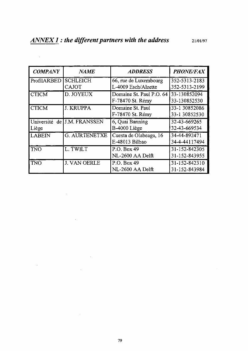
ANNEX 1 : the different partners with the address 21/01/97
COMPANY ProfilARBED
CTICM
CTICM
Université de Liège LABEIN
TNO
TNO
NAME SCHLEICH CAJOT D. JOYEUX
J. KRUPPA
J.M. FRANSSEN
G. AURTENETXE
L. TWILT
J. VAN OERLE
ADDRESS 66, rue de Luxembourg L-4009 Esch/Alzette Domaine St. Paul P.O. 64 F-78470 St. Rémy Domaine St. Paul F-78470 St. Rémy 6, Quai Banning B-4000 Liège Cuesta de Olabeaga, 16 E-48013 Bilbao P.O. Box 49 NL-2600 AA Delft P.O. Box 49 NL-2600 AA Delft
PHONE/FAX 352-5313-2183 352-5313-2199 33-130852094 33-130852530 33-1 30852086 33-1 30852530 32-43-669265 32-43-669534 34-44-892471 34-4-44117494 31-152-842305 31-152-843955 31-152-842310 31-152-843984
79
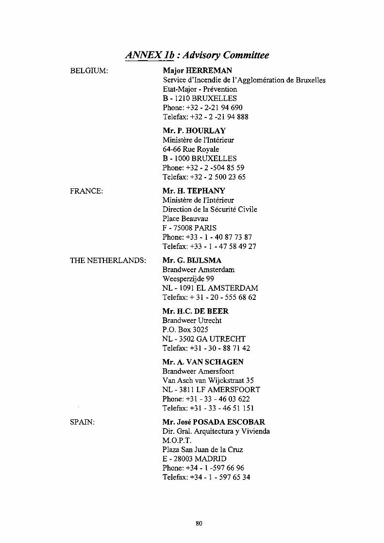
ANNEX lb : Advisory Committee BELGIUM: Major HERREMAN
Service d'Incendie de l'Agglomération de Bruxelles Etat-Major - Prévention B-1210 BRUXELLES Phone:+32-2-2194 690 Telefax:+32-2-21 94 888
Mr. P. HOURLAY Ministère de l'Intérieur 64-66 Rue Royale B-1000 BRUXELLES Phone: +32 - 2 -504 85 59 Telefax: +32 - 2 500 23 65
FRANCE: Mr. H. TEPHANY Ministère de l'Intérieur Direction de la Sécurité Civile Place Beauvau F - 75008 PARIS Phone: +33 -1 - 40 87 73 87 Telefax: +33 -1 - 47 58 49 27
THE NETHERLANDS:
SPAIN:
Mr. G. BIJLSMA Brandweer Amsterdam Weesperzijde 99 NL -1091 EL AMSTERDAM Telefax:+ 31-20-555 68 62
Mr. H.C. DE BEER Brandweer Utrecht P.O. Box 3025 NL - 3502 GA UTRECHT Telefax:+31-30-88 71 42
Mr. A. VAN SCHAGEN Brandweer Amersfoort Van Asch van Wijckstraat 35 NL - 3811 LF AMERSFOORT Phone:+31-33-46 03 622 Telefax:+31-33-46 51 151
Mr. José POSADA ESCOBAR Dir. Gral. Arquitectura y Vivienda M.O.P.T. Plaza San Juan de la Cruz E - 28003 MADRID Phone: +34 - 1 -597 66 96 Telefax: +34 -1 - 597 65 34
80
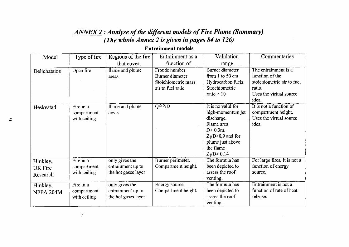
ANNEX 2 : Analyse of the different models of Fire Plume (Summary) (The whole Annex 2 is given in pages 84 to 126)
Entrainment models Model
Delichatsios
Heskestad
Hinkley, UK Fire Research
Hinkley, NFPA 204M
Type of fire
Open fire
Fire in a compartment with ceiling
Fire in a compartment with ceiling
Fire in a compartment with ceiling
Regions of the fire that covers
flame and plume areas
flame and plume areas
only gives the entrainment up to the hot gases layer
only gives the entrainment up to the hot gases layer
Entrainment as a function of
Froude number Burner diameter Stoichiometric mass air to fuel ratio
Q ^ / D
Burner perimeter. Compartment height.
Energy source. Compartment height.
Validation range
Burner diameter from 1 to 50 cm Hydrocarbon fuels. Stoichiometric r a t i o 10
It is no valid for high-momentum jet discharge. Flame area D> 0.3m. Zf/D>0,9 and for plume just above the flame Zf/D>0.14 The formula has been depicted to assess the roof venting. The formula has been depicted to assess the roof venting.
Commentaries
The entrainment is a function of the stoichiometric air to fuel ratio. Uses the virtual source idea. It is not a function of compartment height. Uses the virtual source idea.
For large fires, It is not a function of energy source.
Entrainment is not a function of rate of heat release.
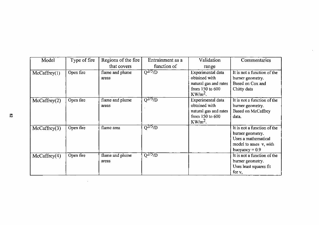
oo S)
Model
McCaffrey(l)
McCaffrey(2)
McCaffrey(3)
McCaffrey(4)
Type of fire
Open fire
Open fire
Open fire
Open fire
Regions of the fire that covers
flame and plume areas
flame and plume areas
flame area
flame and plume areas
Entrainment as a function of
QZ/:VD
Q2^/D
Qzo/D
Q^VD
Validation range
Experimental data obtained with natural gas and rates from 150 to 600 KW/m2. Experimental data obtained with natural gas and rates from 150 to 600 KW/m2.
Commentaries
It is not a function of the burner geometry. Based on Cox and Chitty data
It is not a function of the burner geometry. Based on McCaffrey data.
It is not a function of the burner geometry. Uses a mathematical model to asses v, with buoyancy = 0.9 It is not a function of the burner geometry. Uses least squares fit forv,

oo
Model
Zukoski CTT
Zukoski modified
Zukoski (3)
Mitler
Type of fire
Open fire
Open fire
Open fire
Open fire
Regions of the fire that covers
plume area
flame and plume area
flame and plume area
plume area
Entrainment as a function of
Energy source. Burner diameter Energy source. Burner diameter
Energy source. Burner diameter
Energy source.
Validation range
Burner from 10 up to 50 cm. Flame area D> 30 cm. Fires up to 100 KW. Burner from 10 up to 50 cm. Fires up to 100 KW.
Commentaries
Needs a model for Ζ virtual Needs a model for Ζ virtual, here Cetegen's model is used
Needs a model for two offsets. There is no available model for flame offset. Cetegen's model is used as plume offset. Needs a model for Ζ virtual


Annex 2
AIR ENTRAINMENT INTO BUOYANT PLUMES
MODELS AND THEIR APPLICATION
ENSIDESA / LABEIN

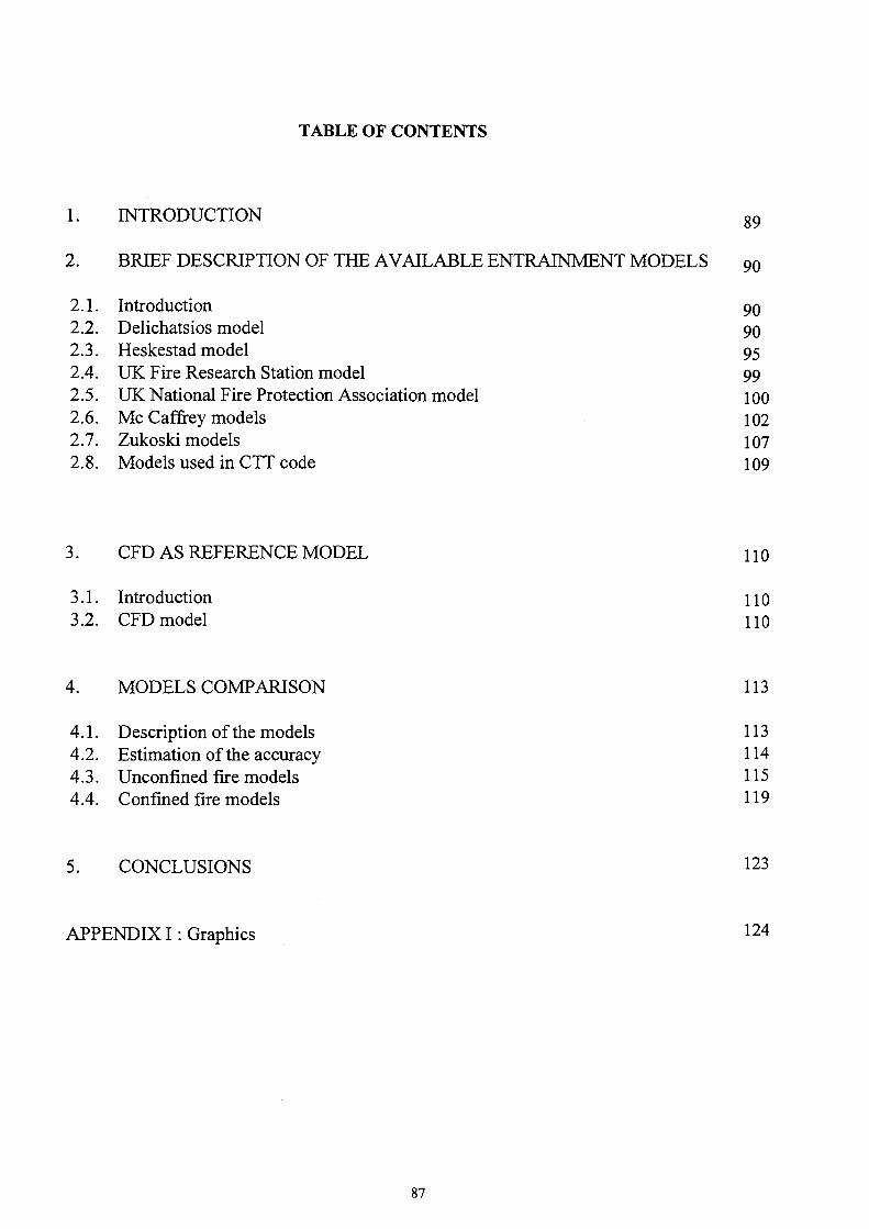
TABLE OF CONTENTS
1. INTRODUCTION 89
2. BRIEF DESCRIPTION OF THE AVAILABLE ENTRAINMENT MODELS 9 0
2.1. Introduction 90 2.2. Delichatsios model 90 2.3. Heskestad model 95 2.4. UK Fire Research Station model 99 2.5. UK National Fire Protection Association model 1 OO 2.6. Mc Caffrey models 102 2.7. Zukoski models 107 2.8. Models used in CTT code 109
3. CFD AS REFERENCE MODEL 110
3.1. Introduction 110 3.2. CFD model 110
4. MODELS COMPARISON 113
4.1. Description of the models 113 4.2. Estimation of the accuracy 114 4.3. Unconfined fire models 115 4.4. Confined fire models 119
5. CONCLUSIONS 123
APPENDIX I : Graphics 1 2 4
87

1. INTRODUCTION
The utility of the two zone models for modelling fire behaviour in closed compartments has a strong dependence on the correlations chosen for the different parameters that describe the fire dynamic. One of the most important parameters is the air entrained by the plume that gives the amount of air (kg/s) engulfed into the plume until it arises the layer of hot gases.
Several authors have investigated this parameter and different semi-empirical correlations are available. All of them are based on theoretical descriptions of the phenomenon. Nevertheless, the particular assumptions and the experimental data taken into account by each investigator have made it a difficult task to know clearly the range of application of each expression and their comparative accuracy for each specific case.
Actually, the Computational Fluid Dynamic represents a useful tool for describing the fluid movement for a large range of phenomenon. Although its application for combusting reactions is not enough validated, now a days, it is assumed that the development achieved by CFD is advanced enough for correctly describing the natural convection phenomenon and, as a consequence, fire plumes.
The contents of the present report deals with the study of the different air entrainment models and their comparison with C.F.D. models.
Aim of the present report can be summarised as :
Collecting the most important expressions for the air entrainment into buoyant plumes proposed by the different investigators . Setting CFD models and coefficients in order to achieve the most suitable results for a fire plume. Comparing the agreement of the different entrainment expressions with the results of the CFD models applied on specific cases. Quantifying the accuracy of each entrainment model and its best range of application.
In this Annex, the references are given at the end of each chapter.
89
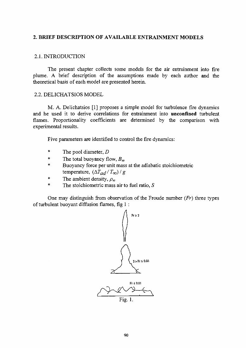
2. BRIEF DESCRIPTION OF AVAILABLE ENTRAINMENT MODELS
2.1. INTRODUCTION
The present chapter collects some models for the air entrainment into fire plume. A brief description of the assumptions made by each author and the theoretical basis of each model are presented herein.
2.2. DELICHATSIOS MODEL
M. A. Delichatsios [1] proposes a simple model for turbulence fire dynamics and he used it to derive correlations for entrainment into unconfined turbulent flames. Proportionality coefficients are determined by the comparison with experimental results.
Five parameters are identified to control the fire dynamics:
* The pool diameter, D * The total buoyancy flow, Bœ * Buoyancy force per unit mass at the adiabatic stoichiometric
temperature, (ATa^/Too) I g * The ambient density, pœ * The stoichiometric mass air to fuel ratio, S
One may distinguish from observation of the Froude number (Fr) three types of turbulent buoyant diffusion flames, fig 1 :
F r i 2
2>Fri0.01
Fr s 0.01 r N ^ -
Fig. 1.
90
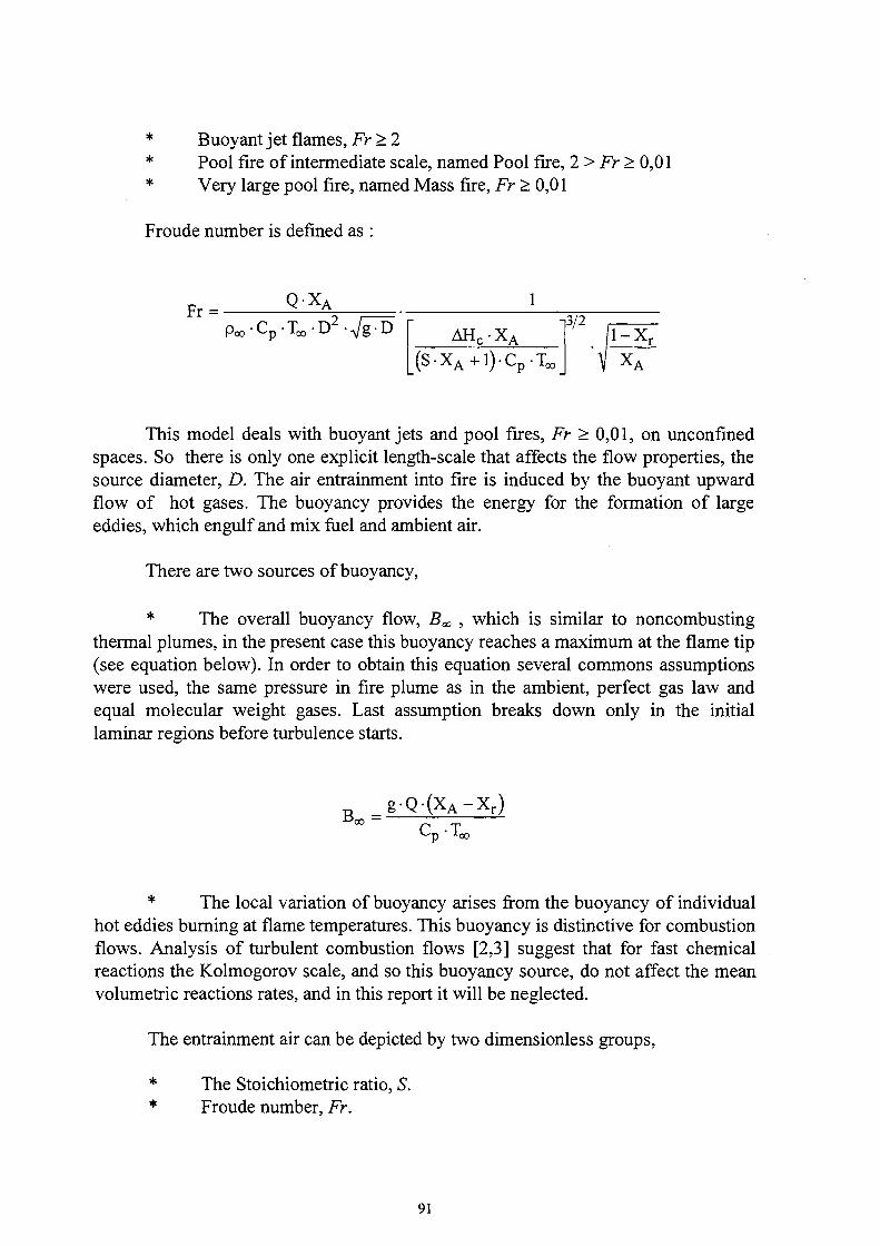
*
*
Buoyant jet flames, Fr>2
Pool fire of intermediate scale, named Pool fire, 2 > Fr > 0,01
Very large pool fire, named Mass fire, Fr > 0,01
Froude number is defined as
Fr = Q-Xy 1
Poo-Cp-Too-D^VFrJ ΔΗ0·ΧΑ
(S.XA+1)-Cp-Ta
5/2
1-Xr
X.
This model deals with buoyant jets and pool fires, Fr > 0,01, on unconfined
spaces. So there is only one explicit length-scale that affects the flow properties, the
source diameter, D. The air entrainment into fire is induced by the buoyant upward
flow of hot gases. The buoyancy provides the energy for the formation of large
eddies, which engulf and mix fuel and ambient air.
There are two sources of buoyancy,
* The overall buoyancy flow, Bœ , which is similar to noncombusting
thermal plumes, in the present case this buoyancy reaches a maximum at the flame tip
(see equation below). In order to obtain this equation several commons assumptions
were used, the same pressure in fire plume as in the ambient, perfect gas law and
equal molecular weight gases. Last assumption breaks down only in the initial
laminar regions before turbulence starts.
Bœ = _g-Q-(X A -X r )
Cn-T„
* The local variation of buoyancy arises from the buoyancy of individual
hot eddies burning at flame temperatures. This buoyancy is distinctive for combustion
flows. Analysis of turbulent combustion flows [2,3] suggest that for fast chemical
reactions the Kolmogorov scale, and so this buoyancy source, do not affect the mean
volumetric reactions rates, and in this report it will be neglected.
The entrainment air can be depicted by two dimensionless groups,
* The Stoichiometric ratio, S.
* Froude number, Fr.
91

For common fuel burning in air S is bigger than 10.Then the reaction rate is controlled principally by the supply of air to the diffusion flames, and S has a negligible influence on fire dynamics. So for hydrocarbon fuels and other fuels having large stoichiometric ratios, the fire Froude number is sufficient to characterize the overall flow field.
Using a theoretical model and experimental results Delichatsios proposes a model to define the entrainment air.
Air entrainment model [4]
There are two different zones : below the flame tip, and the buoyant plume above the flame tip. The air entrainment rate , ment , is the air that enters from the bottom of the pool fire to vertical distance z. There is a direct relationship between entrainment rates and flame height in turbulent diffusion flames. Delichatsios uses the following expressions for the flame height :
Zf =(l,35-104-Fr2)-D Fr<8,6-10-3
Zf = Í22,54-Fr2/3)-D 0'l<Fr<8,6-10 -3
Zf =(l2,52-Fr2/5)-D 0,1 < Fr
Recently, Cox and Chitty [7] reported flame heights for pool fires that correspond to the conditions of Fr < 8,6* 10~3, very large pool fires. They found a coefficient 6,66* 10^ instead of 1,35* 10^, a discrepancy that can probably be attributed to the fact that they tested square pool fires, while the data here apply to circular pool fires. In square pool fires, larger eddies are generated near the corners so that entrainment increases, burning speeds up, and, therefore flame heights become smaller. Note that differences between square and circular pool fires are larger for small flame heights.
The relationship between entrainment rates and flame height commented above becomes clear if one uses the experimental observation reported by various investigators [5,6] that, at the visible flame tip, the flow rate in the plume is about ten times the flow rate corresponding to the stoichiometric mass requirement for combustion.
92

Air entrainment into the Burning Region, below the flame tip, ζ < Ζ f.
( X A - S + I W ( zV / 2
m e n t = l _ A ¿—ï-· 0,086·— — <1 Fr ^ D J D
ζ
(XA-S + l)mf ΛΛΛ„ f z ì 3 / 2 ζ ment = V A - ; 0.093-l·- l í S ^ 5
Fr ID/ D
5<ί D
(XA-S + l)mf f zV / 2
ment = V A - ' -0,018- -Fr KOJ
Air entrainment in the buoyant plume, ζ > Ζ f.
(XA-S + l)mf fz + Zvf / 3
Z v = - Z f + 10,21-Fr2/5-D
The buoyant plume is entirely characterized by its constant buoyancy flow, Bœ , D, pœ and the initial conditions near the flame tip at the end of combustion. Buoyancy flow attains its maximum value at the end of combustion near the flame tip, and this is the constant value of, Bœ, at the plume, see equation above.
Virtual origin, Zv , is calculated assuming that at the flame tip the flow rate in the plume is about ten times the flow rate corresponding to the stoichiometric mass requirement for combustion. That is,
ment _ 1f)
(XA-S + l)-mf
Introducing this condition in the Buoyant plume model Zv may be obtained,
Z v = - Z f + 10^1-Fr2/5-D
93
Limitations
The entrainment model is only applicable for turbulent buoyant jet
flames and pool fires that do not represent a mass fire situation.
S> 10
The buoyant jet discharges to an unconfined space
Perfect gas law
At the flame tip the flow rate in the plume is about ten times the flow
rate corresponding to the stoichiometric mass requirement for
combustion.
The model is not adequate for the initial laminar regions before the
turbulence starts.
Nomenclature
Cp specific heat of air
D pool diameter
Fr fire Froude number
g gravitational acceleration ment entrainment rate up to a height ζ [kg/s]
mf combustible mass flow rate [kg/s]
Q theoretical heat release rate [w]
S stoichiometric mass air to fuel ratio
T ambient air absolute temperature
ζ distance to the pool surface
Zf visible flame height
Zv virtual source origin based on entrainment rates
He Theoretical heat of combustion per unit fuel mass
ambient air density
X¿ efficiency of combustion
Xr radiant fraction
All units are in S.I.
94
References
1. National fire Protection Engineering association, The SFPE Handbook of Fire Protection Engineering, Second Edition.
2. MA. Delichatsios, On the modelling of strong (Variable Density) Turbulent Buoyant Plumes and Ceiling jets, meeting, The Combustion Institute (1985).
3. P. Demotakis, J. Fluid Mech., 148, 349 (1984).
4. MA. Delichatsios, J. of fire Prot. Engr., 2(3), 1990 pp. 93-98.
5. B. M. Cetegen, E.E. Zukoski, and T. Kubota, Comb. Chi. and Tech., 39,305 (1984); see also E.E. Zukoski, E.E. Zukoski and B. M. Cetegen NABS CORR Grant GO-9014 Report, California institute of Technology, Pasadena, (1984). ref 2 delNFPA pag 2-31
6. MA. Delichatsios and L. Orloff, Entrainment Measurement in Turbulence Buoyant Jet Flames and Implications for Modelling, Twentieth Symp. (Int.) on Comb., Pittsburgh.
7. G. Cox and R. Chitty., Comb, and Flame, 60, p. 219 (1985)
2.3. HESKESTAD MODEL
Gunnar Heskestad [1] proposes a description for fires placed in rooms with floor and ceiling. The model assumes that the surrounding air is uniform in temperature and uncontaminated by the products of the combustion. The relations cease to be valid beyond the elevation where the plume enters the smoke layer.
The mass flow at a particular elevation in a fire plume is almost completely attributable to air entrainment by the plume at lower elevations. The mass flow contributed by the fire source itself is insignificant in comparison.
The plume theories assume :
1. A point source of buoyancy, 2. Variations of density in the field of motion are small compared to the
ambient density. 3. Air entrainment velocity at the edge of the plume is proportional to the
local vertical plume velocity. 4. Profiles of vertical velocity and buoyancy force in horizontal sections
are similar form at all heights.
95
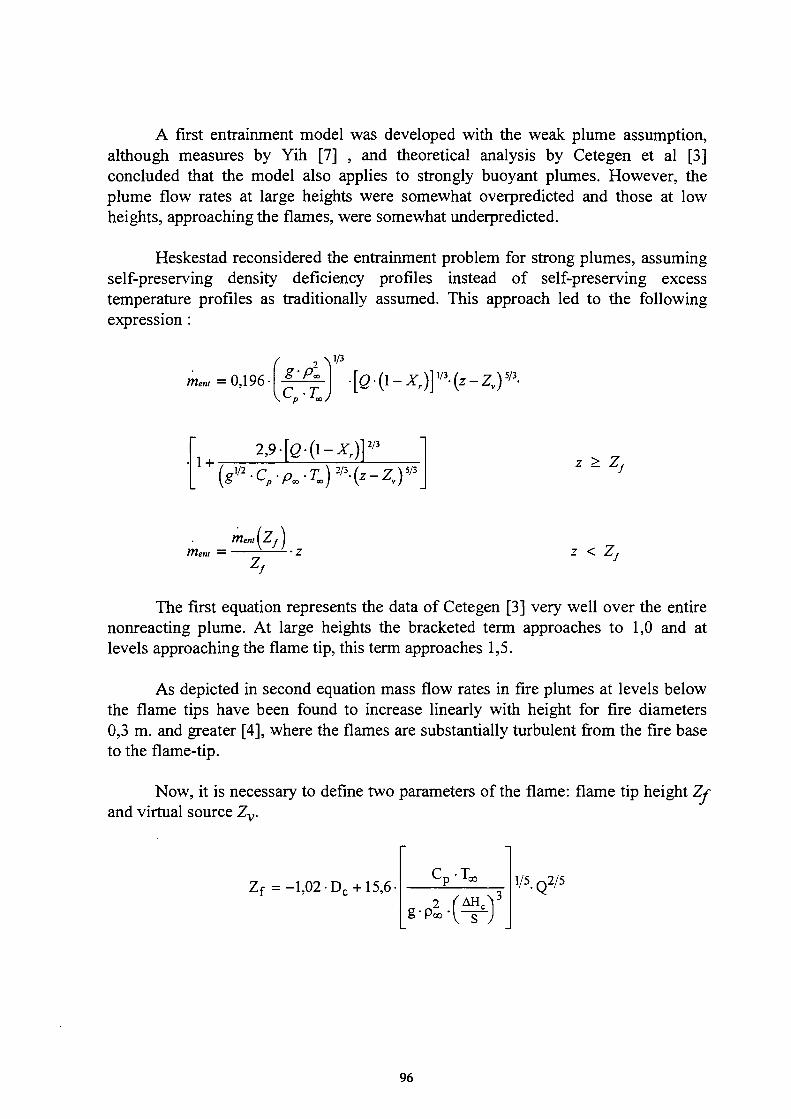
A first entrainment model was developed with the weak plume assumption,
although measures by Yih [7] , and theoretical analysis by Cetegen et al [3]
concluded that the model also applies to strongly buoyant plumes. However, the
plume flow rates at large heights were somewhat overpredicted and those at low
heights, approaching the flames, were somewhat underpredicted.
Heskestad reconsidered the entrainment problem for strong plumes, assuming
self-preserving density deficiency profiles instead of self-preserving excess
temperature profiles as traditionally assumed. This approach led to the following
expression :
me = 0,196-
f 2 V/ 3
g-Pl Cp-T„;
[ß.(i-jrr)]*.(,-zj 5/3.
1 + 2,9\Q-(\-Xr)} 2/3
{gV2-Cp-p„-T„)^(Z-Zv) 5/3
ζ > Z,
meni
ment = {h)
•ζ ζ < Zf
The first equation represents the data of Cetegen [3] very well over the entire
nonreacting plume. At large heights the bracketed term approaches to 1,0 and at
levels approaching the flame tip, this term approaches 1,5.
As depicted in second equation mass flow rates in fire plumes at levels below
the flame tips have been found to increase linearly with height for fire diameters
0,3 m. and greater [4], where the flames are substantially turbulent from the fire base
to the flame-tip.
Now, it is necessary to define two parameters of the flame: flame tip height Zƒ and virtual source Z,
Zf =-1,02-Dc +15,6 C ·Τ ^ p xoo 2 f ΔΗ,
V5.02/5
96

This equation is convenient and quite general. Although it does not fit
high-momentum jet discharge. This implies the following condition.
C Τ ^ p
x00
g - p » ΔΗ,
The virtual origin of a test fire is most conveniently determined from
temperature data above the flames along the plume axis. A plot of T0" versus ζ
should produce a straight line which intercepts the z-axis at Zv. Despite this apparent
simplicity of obtaining Zv the task is very difficult in practice. Slight inaccuracies in
the determination of centerline temperatures have large effects on the intercept, Zv.
Such inaccuracies may be associated with off axis placement of sensors, radiation-
induced errors in the temperature signal, or inadequate averaging of the signal.
Heskestad shows three models for Zv, although recommends the following
one, because of its simplicity, clear foundation in theory [5] , and central position
among the other correlations.
* Heskestad model, referred later as Heskestad (1). Experimental data have been
obtained with fire diameter varying from 1,16 to 2,4 m.
Zv =-1,02-Dc+0,083 1000
2/5
Hasemi and Togunaga [6] model, referred later as Heskestad (2). Experimental
data have been obtained with fire diameter varying from 0,2 to 0,5 m.
Zv = -2,4 -Dc+ 0,145 1000
2/5 2/5 1 ' Q γ°
NIOOOJ ! , > 16,5
Z v = 0,0224 ■
2/5 5/3
Ί000 Dc-0,145 U000
2/5 2/5 r_o_ UOOOJ D r
< 16,5
97

Cetegen et al [3], referred later as Heskestad (3). Experimental data have been obtained with fire diameter varying from 0,1 to 0,5 m.
Zv = -0,5 · Dc + 0,0659 v. 1000
2/5 Q ì 2 / 5 1 \000J ΌΓ
> 16,5
Zv =-0,5-Dc+0,01015
x2/5 Ί5/3
Ί000
Dr •D,
r Q ^ 5 1 UOOO; D,
< 16,5
Limitations
Fires with very low flame height-to-diameter Ζ f / Dc ratios have not been investigated extensively. It is no clear what Zf/ Dc limit the entrainment relation presented here apply up to the flame tip, but this limit is smaller than 0,9, the lowest ratio associated with Cetegen's data. Only fires with Zf / Dc > 0,9 have been extensively investigated.
For plume mass flows above the flame, there is no Zf/ Dc limit for prediction at higher elevations, but predictions of mass flows at levels just above the flames may begin to deteriorate before Zf/Dc = 0,14 is reached.
Nomenclature
»c g ment mf Q s τ ζ
Zf ζν
He Xr
specific heat of air diameter of a circle with the area of the fire source gravitational acceleration entrainment rate up to a height z, kg/s combustible mass flow rate, kg/s theoretical heat release rate, w stoichiometric mass air to fuel ratio ambient air absolute temperature distant to the pool surface visible flame height virtual source origin based on entrainment rates theoretical heat of combustion per unit fuel mass ambient air density radiant fraction
All units are in S.I.
98
References
1. National fire Protection Engineering association, The SFPE Handbook of Fire Protection Engineering, Second Edition.
2. C-S Yih, Proc, U.S. National Cong. App. Mech. (1952).
3. E.E. Zukoski, E.E. Zukoski and B. M. Cetegen NBS CFRR Grant G8-9014, California Institute of technology, Daniel and Florence Guggenheim Jet Propulsion Center, (1982). See also B. M. Cetegen, E.E. Zukoski, and T. Kubota, Comb. Csi. and Tech., 39,305 (1984);
4. G. Heskestad, 21th Symposium on Combustion, Comb Inst., Pittsburgh (1986).
5. G. Heskestad, F. Safety J., 5, 109 (1983).
6. Y. Hasemi and T. Tokunaga, Fire Sci. and Tech., 4,15 (1984).
2.4. UK FIRE RESEARCH STATION MODEL
The following expressions has been adopted for design of Smoke and Heat Roof Venting [1]. The rate of production of hot gases is primarily dependent on the rate of entrainment model. UK Fire Researches Station [2] provides some approximate engineering formulae. The formulae has been depicted to assess the roof venting, so it could be a limitation. UK FRS proposes two expressions: a first one for small fires and a second expression for large fires.
Small fires
Small fires are defined as those for which mean diameter, D, is less than (h-d)/2. The formulae includes the rate of heat release, and a virtual source below the floor.
ι \ ~|V3 iJ^P (h+zv-d)5/3
Pi" <-p · Too ment = 0,15 · pi
Poo · ment -Cp -T» Pl=
Q - ( l - X r ) + ment-Cp-Ta
99
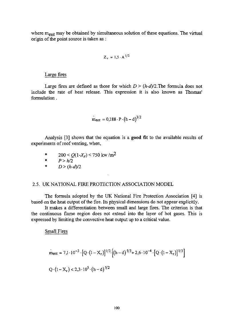
where m e n t may be obtained by simultaneous solution of these equations. The virtual origin of the point source is taken as :
Z v = 1,5-A 1/2
Large fires
Large fires are defined as those for which D > (h-d)/2.The formula does not include the rate of heat release. This expression it is also known as Thomas' formulation.
ment =0,188-P-(h-d)3 ' :
Analysis [3] shows that the equation is a good fit to the available results of experiments of roof venting, when,
* 200 < Q(l-Xr) < 750 kw /m2
* P>hl2 * D > (h-d)/2
2.5. UK NATIONAL FIRE PROTECTION ASSOCIATION MODEL
The formula adopted by the UK National Fire Protection Association [4] is based on the heat output of the fire. Its physical dimensions do not appear explicitly.
It makes a differentiation between small and large fires. The criterion is that the continuous flame region does not extend into the layer of hot gases. This is expressed by limiting the convective heat output up to a critical value.
Small Fires
ment=7,1.10-3.[Q-(l-X r)]1/3.[(h_d)5/3+256.io-4.[Q.(l-X r)]V3]
Q-(l-X r)<2,3-105-(h-d)5 /2
100

Large Fires
m e n t=5^-10-4-[Q-(l-X r)]3 / 5-(h-d)
Q-(l-X r)>2,3-105-(h-d)5 '2
This formula is not suitable for high heat output per unit area.
Nomenclature
A f fire area C ρ specific heat of air D fire diameter g gravitational acceleration h compartment height d depth of layer of hot gases ment entrainment rate up to a height z, kg/s Ρ fire perimeter Q theoretical heat release rate, w Too ambient air absolute temperature Zy virtual source origin based on entrainment rates AHc Theoretical heat of combustion per unit fuel mass j density of the layer of hot gases
ambient air density Xjl efficiency of combustion Xr radiant fraction
All units are in S.I.
References
1. National fire Protection Engineering association, The SFPE Handbook of Fire Protection Engineering, Second Edition.
2. P.H. Thomas et al." Investigations into the Flow of Hot Gases in Roof Venting" Fire Research Technical Paper No. 7, HMSO, London (1963).
3. P.L. Hinkley , "Rate of Production of Hot gases in Roof Venting Experiments" Fire Safety Journal 10 (1), pp. 57-65, (1986).
4. NFPA 204M, "Guide for Smoke and Heat Venting" Natural Fire Protection Association, Quincy, MA (1991).
101
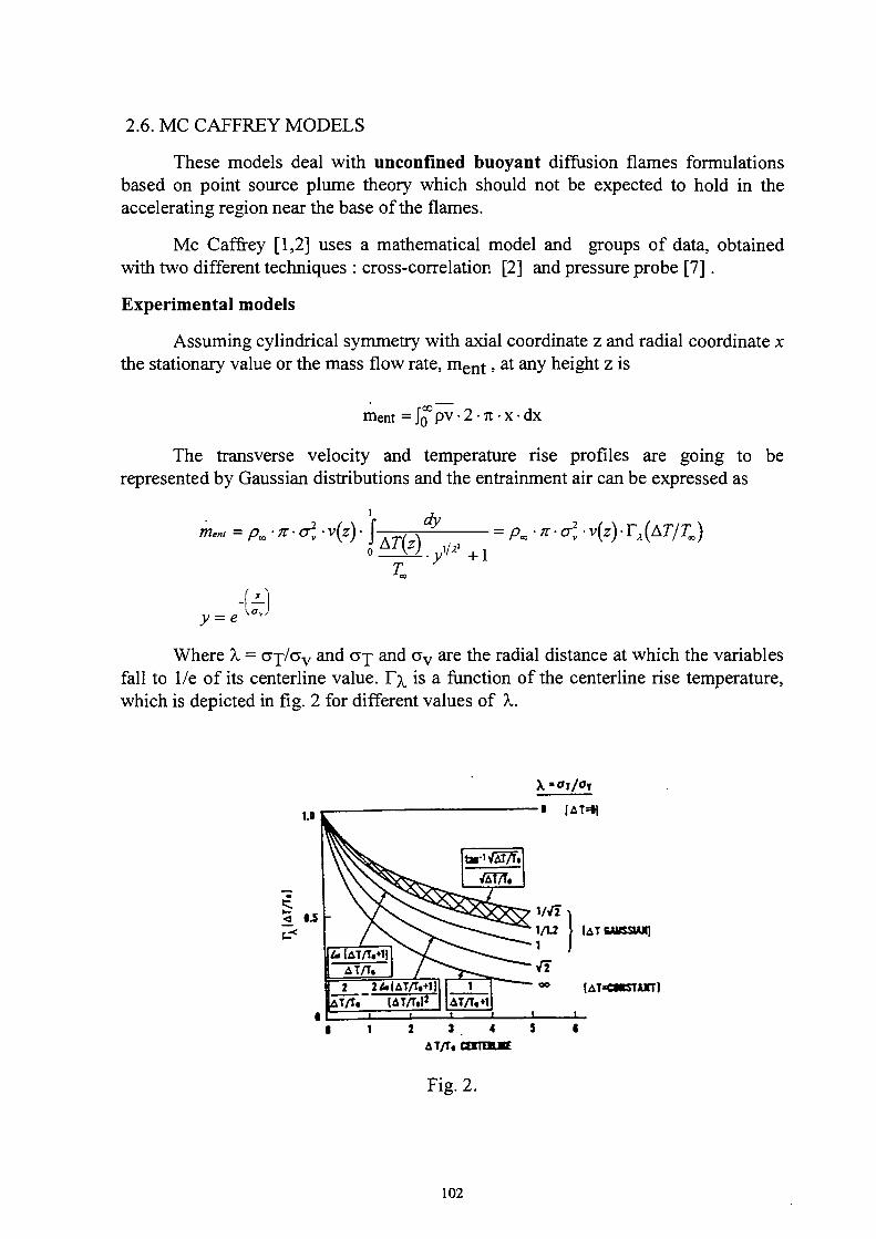
2.6. MC CAFFREY MODELS
These models deal with unconfined buoyant diffusion flames formulations
based on point source plume theory which should not be expected to hold in the
accelerating region near the base of the flames.
Mc Caffrey [1,2] uses a mathematical model and groups of data, obtained
with two different techniques : cross-correlation [2] and pressure probe [7] .
Experimental models
Assuming cylindrical symmetry with axial coordinate ζ and radial coordinate χ
the stationary value or the mass flow rate, m e n t , at any height ζ is
ment = ¡Q pv · 2 · π · χ · dx
The transverse velocity and temperature rise profiles are going to be
presented by Gaussian distributions and the entrainment air can be expressed as
i
mem = ρη-π-σ2
ν-ν(ζ)· j dy
Ä/+i = ρκ-π.σ2
ν-ν(ζ)-Γλ(ΑΤΧ)
y = e
Where λ = σ-τ;/σν and σ-ρ and σ ν are the radial distance at which the variables
fall to 1/e of its centerline value. Γχ is a function of the centerline rise temperature,
which is depicted in fig. 2 for different values of λ.
1.0
r -<
λ » Ol /Ol
|ΔΤ=*1
V/2
1/U } UTUiSSU]
u U V V l l
ΔΤ/Τ.
2 2ί·|ΔΤ/Τ,+1| AVT. ΙΔΤΛ.Ι1
1 ΔΤ/Μ1
π [ATcmsrun]
2 3 . 4 3
ΔΤ/Τ« COTBBJE
Fig. 2.
102

The above equation states that the air entrainment is equal to the ambient density times the centerline velocity times a representative area, πσ ν
2 , modified by Γχ which accounts for density decrease due to the fact that the gases are hotter than the ambient. At large z, high above the flame tip where ΔΤ —» 0, Γχ converges to 1 since the most of the gas consists of air entrainment. Near the burner ΔΤ/Τ can be as high as 3 or 4 leading to Γχ of the order to 0,5. This would produce large errors if the ambient density were used throughout.
The quantities in the right side of the equation above have been measured by two independent techniques, Cross correlation and Impact pressure probe using natural gas as the fuel and burning rates from 150 to 600 kw/m2.
The flame can be considered to be divided into three distinct regimes
* Continuous flame region, starting from the surface of the burning with velocity close to 0 at the surface of the burner and rising with the height above the burner, up to Zc.
* Higher up is an intermediate regime, with pulsating flame, up to Zf. * Still higher is the plume region which is, most of the times free of
flames.
The height of the continuous flame and the flame tip are respectively
Z c =0,08 f Q Λ2/5
UOOOJ
( η λ2/5
Zf =0,2 uooa/
Throughout the three regimes and indistinguishable among these is the consistency of a buoyancy relation, with a constant value, which involves that for this flames the buoyancy is due only to the temperature differences between flame and air.
ν V2-g-z-AT/Ta
0,9
So, the local variation of buoyancy arising from the buoyancy of individual hot eddies burning at flame temperatures is negligible.
Table 1 contains the experimental centerline and radial flame parameters required to assess the entrainment air into the fire. Profiles obtained with cross-correlation are named as Mc Caffrey (1), and those obtained with impact probe are named as Mc Caffrey (2).
103
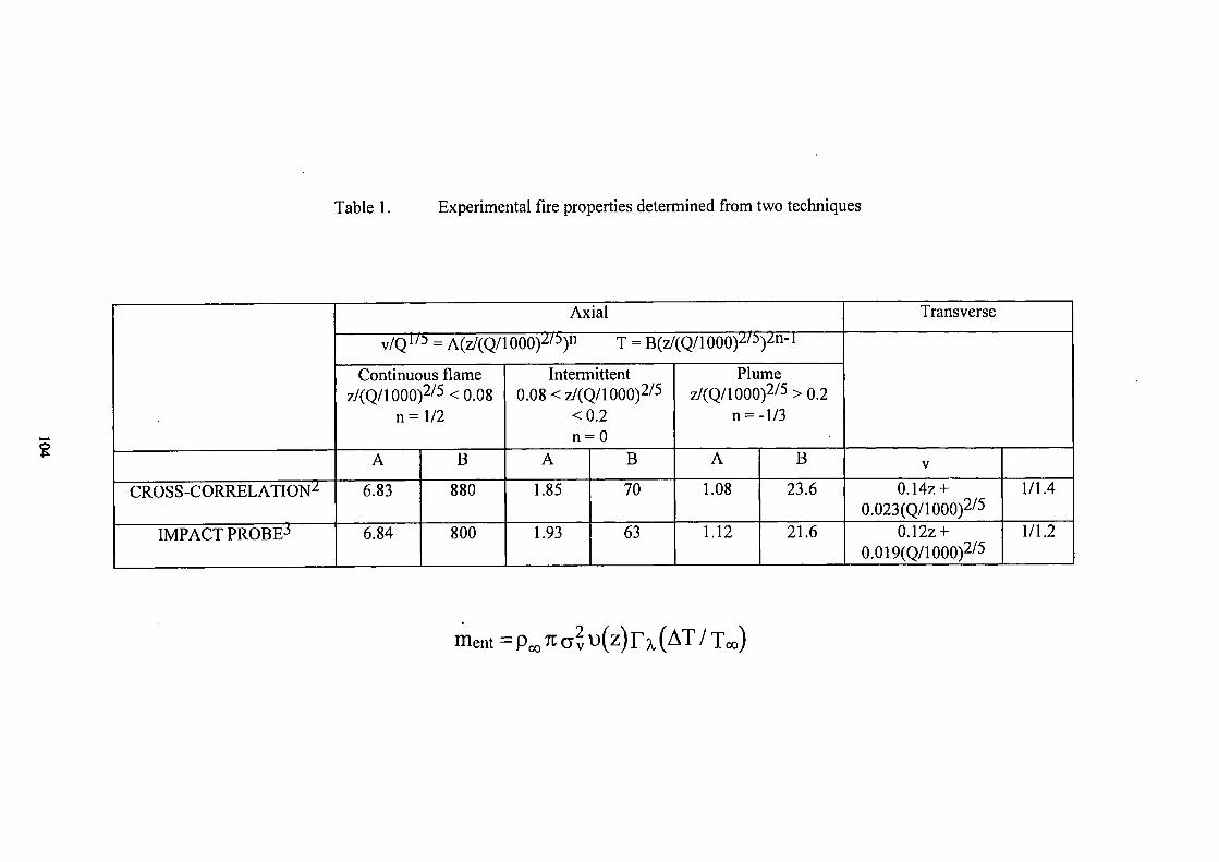
Table 1. Experimental fire properties determined from two techniques
?
CROSS-CORRELATIONz
IMPACT PROBER
Axial
V/QI/3 = A(z/(Q/1000)z/:>)n Τ = BCz/CQ/lOOOy^V11'1
Continuous flame z/(Q/1000)2/5<0.08
η =1/2
A
6.83
6.84
Β
880
800
Intermittent 0.08<z/(Q/1000)2/5
<0.2 n = 0
A
1.85
1.93
Β
70
63
Plume z/(Q/1000)2/5>0.2
η = -1/3
A
1.08
1.12
Β
23.6
21.6
Transverse
V
0.14Z + 0.023(Q/1000)2/5
0.12Z + 0.019(Q/1000)2/5
1/1.4
1/1.2
ηιεηί=ρ00πσ?υ(ζ)Γλ(ΔΤ/Τοο)
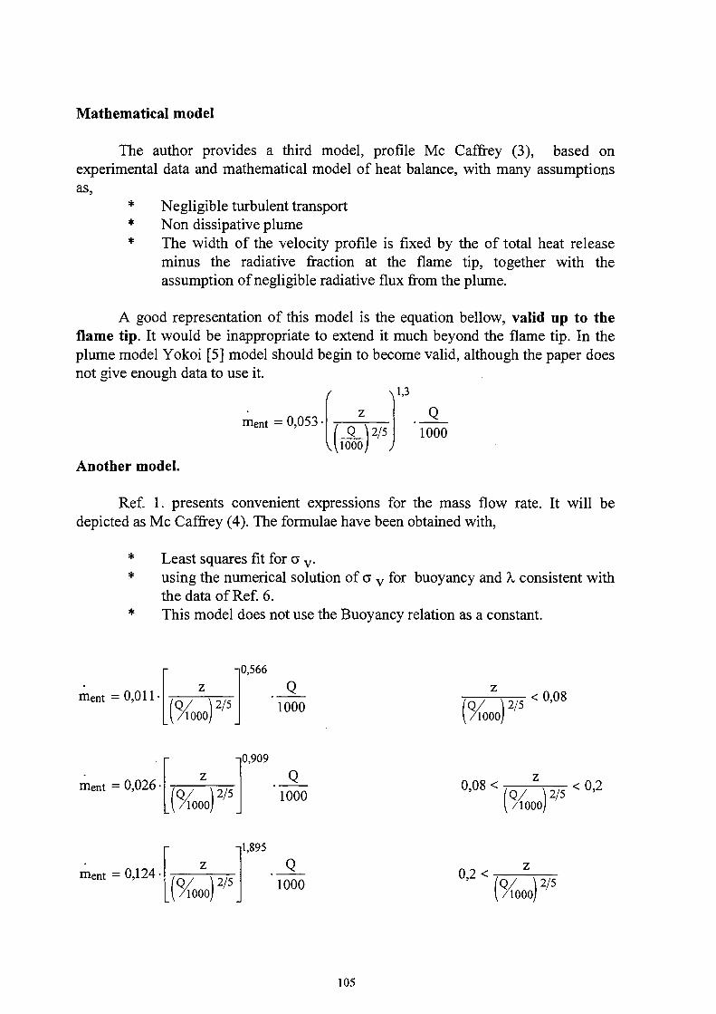
Mathematical model
The author provides a third model, profile Mc Caffrey (3), based on experimental data and mathematical model of heat balance, with many assumptions as,
* Negligible turbulent transport Non dissipative plume The width of the velocity profile is fixed by the of total heat release minus the radiative fraction at the flame tip, together with the assumption of negligible radiative flux from the plume.
A good representation of this model is the equation bellow, valid up to the flame tip. It would be inappropriate to extend it much beyond the flame tip. In the plume model Yokoi [5] model should begin to become valid, although the paper does not give enough data to use it.
f λ1 '3
Q ment =0,053-Aioooj
2/5 1000
Another model.
Ref. 1. presents convenient expressions for the mass flow rate. It will be depicted as Mc Caffrey (4). The formulae have been obtained with,
Least squares fit for σ v . using the numerical solution of σ v for buoyancy and λ consistent with the data of Ref. 6. This model does not use the Buoyancy relation as a constant.
ment =0,011
ment = 0,026
ment = 0,124
Ί0,566
1000
0,909
1000
-|1,895
1000
Q / 2/5 1000
<0,08
0,08 < Q / 2/5
1000 <0,2
0,2 < Q / 2/5
1000
105

Nomenclature
Cp specific heat of air g gravitational acceleration ment entrainment rate up to a height ζ Q rate of heat release To, ambient air absolute temperature v air velocity χ radial coordinate ζ distance to the pool surface Zc continuous flame height Zf visible flame height AT temperature rise at the centerline σι the radial distance at which the variable i fall to 1/e Poo ambient air density λ σγ/ σ ν Γχ coefficient that take into account density decrease due to the fact that the
gases are hotter than the ambient
All units are in S.I.
References
1. B. J. McCaffrey and G. Cox, Momentum Implications for Buoyant Diffusion, National Bureau of Standards Washington, D.C. 20234.
2. B. J. McCaffrey, Entrainment and Heat of Buoyant Diffusion Flames,Comb. and Flame: 52, 149(1983).
3. Cox, G and Chitty, R. A study of the deterministic properties of unbounded fire plumes. Comb, and Flame. 39: 191, (1980)
4. McCaffrey B. J. Purely Buoyant diffusion flames: some experimental results. Nat Bur. Stand. (U.S.) NBSIR 79-1910; 1979 October.
5. Yokoi, S. Study on the prevention of fire-spread caused by hot upward current. Report of the Building Research Institute; Ministry of Construction; Japan No 34; 1960 November.
6. B. J. McCaffrey, NBSIR 79-1910. National Bureau of Standards, October 1979.
106
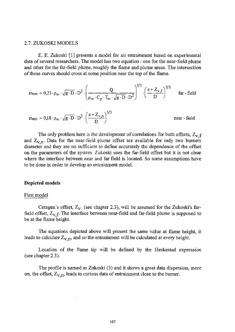
2.7. ZUKOSKI MODELS
E. E. Zukoski [1] presents a model for air entrainment based on experimental
data of several researchers. The model has two equation : one for the near-field plume
and other for the far-field plume, roughly the flame and plume areas. The intersection
of these curves should cross at some position near the top of the flame.
ment =0,21· ρ«-VgÕD-D' VHoo ■Cp-Too-ViU-D2
1/3
z + Z v,f Λ 5/3
v. D ; far - field
ment=0,18-Poo-Vg-D-D^ z + Z
v,n D
5/3
near - field
The only problem here is the development of correlations for both offsets, Zy f
and Zy n . Data for the near-field plume offset are available for only two burners
diameter and they are no sufficient to define accurately the dependence of the offset
on the parameters of the system. Zukoski uses the far-field offset but it is not clear
where the interface between near and far field is located. So some assumptions have
to be done in order to develop an entrainment model.
Depicted models
First model
Cetegen's offset, Zy (see chapter 2.3), will be assumed for the Zukoski's far-
field offset, Zv f. The interface between near-field and far-field plume is supposed to
be at the flame height.
The equations depicted above will present the same value at flame height, it
leads to calculate Zy n , and so the entrainment will be calculated at every height.
Location of the flame tip will be defined by the Heskestad expression
(see chapter 2.3).
The profile is named as Zukoski (3) and it shows a great data dispersion, more
on, the offset, Zy n , leads to curious data of entrainment close to the burner.
107
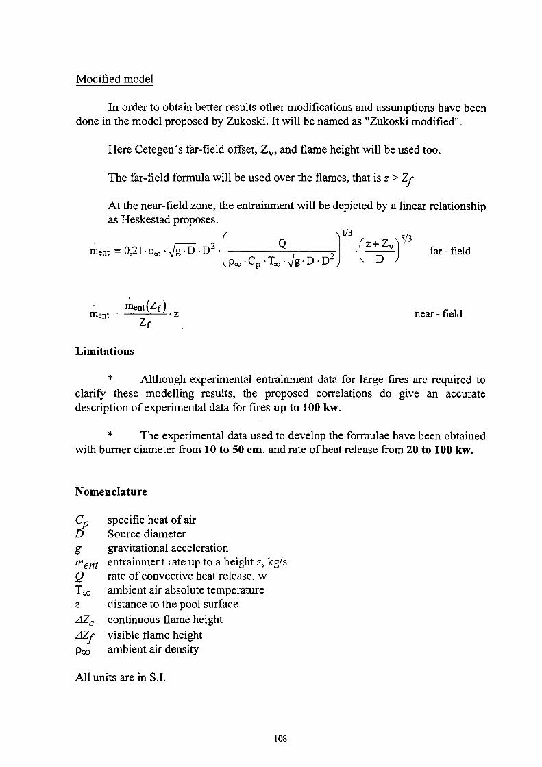
Modified model
In order to obtain better results other modifications and assumptions have been
done in the model proposed by Zukoski. It will be named as "Zukoski modified".
Here Cetegen's far-field offset, Zy, and flame height will be used too.
The far-field formula will be used over the flames, that is ζ > Zf
At the near-field zone, the entrainment will be depicted by a linear relationship
as Heskestad proposes.
f V/3
ment = 0,21-p«, · VgT) -D2 · IPco-Cp-Too-Vg^D-D
z + Z
D
5/3
far - field
ment(Zf) ment = —- ■ ζ near - field
z f
Limitations
* Although experimental entrainment data for large fires are required to
clarify these modelling results, the proposed correlations do give an accurate
description of experimental data for fires up to 100 kw.
* The experimental data used to develop the formulae have been obtained
with burner diameter from 10 to 50 cm. and rate of heat release from 20 to 100 kw.
Nomenclature
Cp specific heat of air
D Source diameter
g gravitational acceleration ment entrainment rate up to a height z, kg/s
Q rate of convective heat release, w
Too ambient air absolute temperature
ζ distance to the pool surface
AZC continuous flame height
AZf visible flame height
Poo ambient air density
All units are in S.I.
108
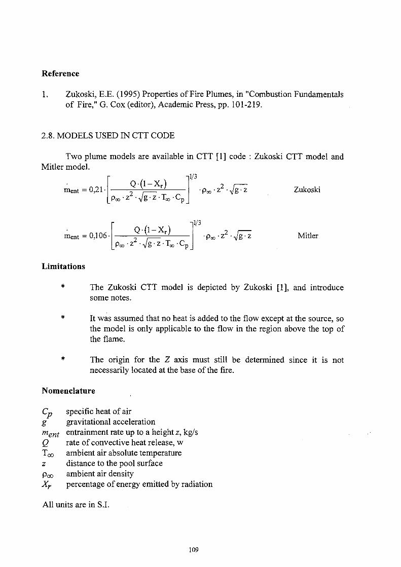
Reference
1. Zukoski, E.E. (1995) Properties of Fire Plumes, in "Combustion Fundamentals
of Fire," G. Cox (editor), Academic Press, pp. 101-219.
2.8. MODELS USED IN CTT CODE
Two plume models are available in CTT [1] code : Zukoski CTT model and
Mitler model.
ment = 0,21 Q - ( l - X r )
Ροο·ζ -Vg^z-Too-C,
1/3
•Poo-Z^Vg^Z Zukoski
ment = 0,106-Q - ( l - X r )
Ροο·ζ -Vg^z-Too-Cp
1/3
■ P o o " Ζ ■VÏ7■ Mitler
Limitations
* The Zukoski CTT model is depicted by Zukoski [1], and introduce
some notes.
* It was assumed that no heat is added to the flow except at the source, so
the model is only applicable to the flow in the region above the top of
the flame.
* The origin for the Ζ axis must still be determined since it is not
necessarily located at the base of the fire.
Nomenclature
C ρ specific heat of air
g gravitational acceleration
ment entrainment rate up to a height z, kg/s
Q rate of convective heat release, w
Too ambient air absolute temperature
ζ distance to the pool surface
Poo ambient air density
Xr percentage of energy emitted by radiation
All units are in S.I.
109
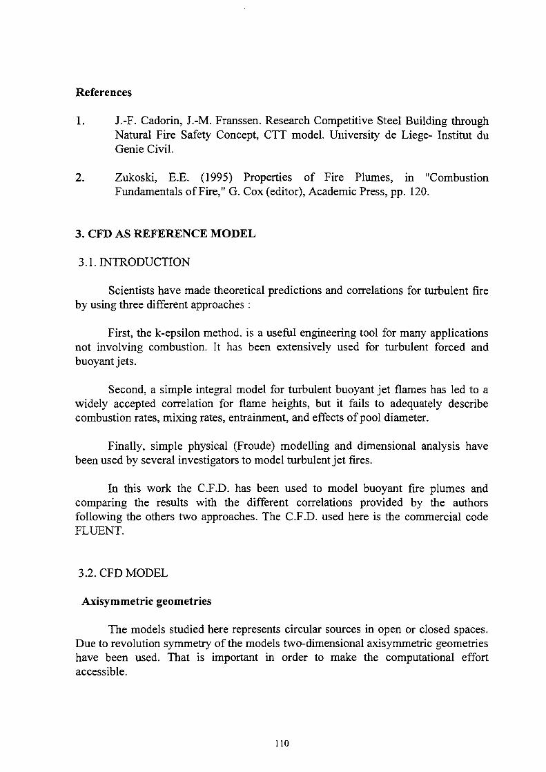
References
1. J.-F. Cadorin, J.-M. Franssen. Research Competitive Steel Building through Natural Fire Safety Concept, CTT model. University de Liege- Institut du Genie Civil.
2. Zukoski, E.E. (1995) Properties of Fire Plumes, in "Combustion Fundamentals of Fire," G. Cox (editor), Academic Press, pp. 120.
3. CFD AS REFERENCE MODEL 3.1. INTRODUCTION
Scientists have made theoretical predictions and correlations for turbulent fire by using three different approaches :
First, the k-epsilon method, is a useful engineering tool for many applications not involving combustion. It has been extensively used for turbulent forced and buoyant jets.
Second, a simple integral model for turbulent buoyant jet flames has led to a widely accepted correlation for flame heights, but it fails to adequately describe combustion rates, mixing rates, entrainment. and effects of pool diameter.
Finally, simple physical (Froude) modelling and dimensional analysis have been used by several investigators to model turbulent jet fires.
In this work the C.F.D. has been used to model buoyant fire plumes and comparing the results with the different correlations provided by the authors following the others two approaches. The C.F.D. used here is the commercial code FLUENT.
3.2. CFD MODEL
Axisymmetric geometries
The models studied here represents circular sources in open or closed spaces. Due to revolution symmetry of the models two-dimensional axisymmetric geometries have been used. That is important in order to make the computational effort accessible.
no
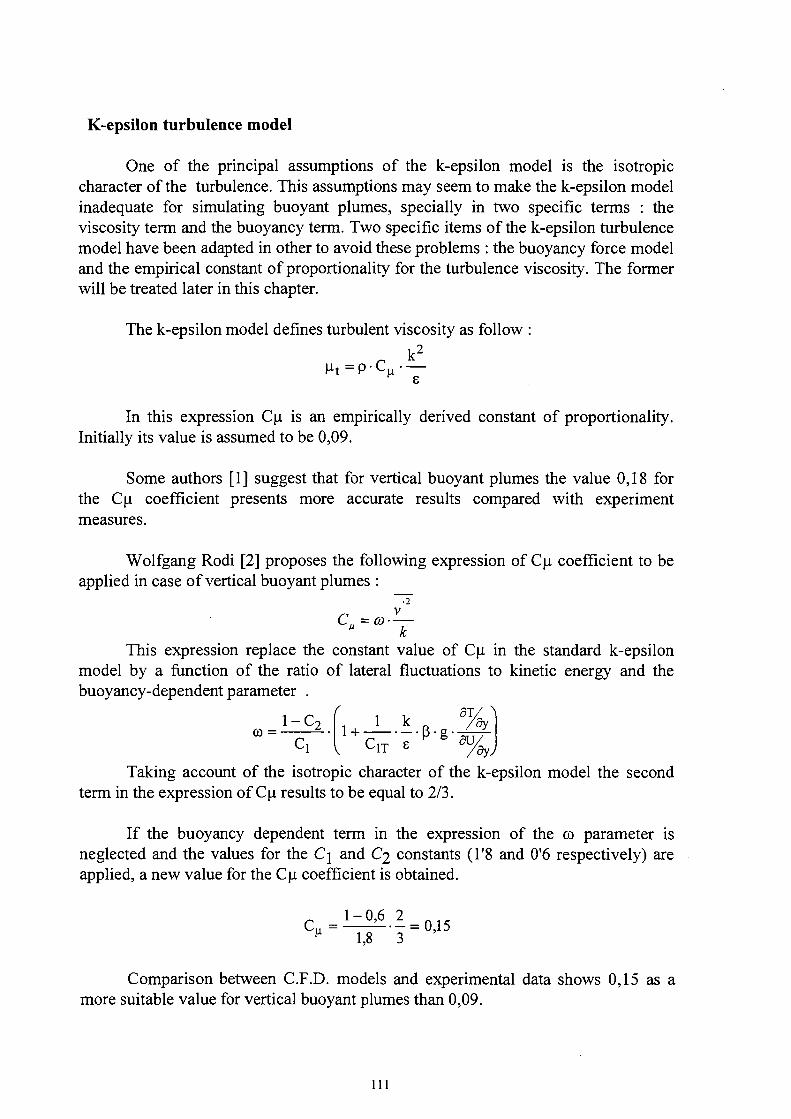
K-epsilon turbulence model
One of the principal assumptions of the k-epsilon model is the isotropic
character of the turbulence. This assumptions may seem to make the k-epsilon model
inadequate for simulating buoyant plumes, specially in two specific terms : the
viscosity term and the buoyancy term. Two specific items of the k-epsilon turbulence
model have been adapted in other to avoid these problems : the buoyancy force model
and the empirical constant of proportionality for the turbulence viscosity. The former
will be treated later in this chapter.
The k-epsilon model defines turbulent viscosity as follow
μι = P - < V k
2
In this expression Cp is an empirically derived constant of proportionality.
Initially its value is assumed to be 0,09.
Some authors [1] suggest that for vertical buoyant plumes the value 0,18 for
the C μ coefficient presents more accurate results compared with experiment
measures.
Wolfgang Rodi [2] proposes the following expression of Cp coefficient to be
applied in case of vertical buoyant plumes : ~7 ν
C =ω· — k
This expression replace the constant value of Cp in the standard k-epsilon
model by a function of the ratio of lateral fluctuations to kinetic energy and the
buoyancy-dependent parameter .
1-C; ω
C, V C1T ε ß g % ,
Taking account of the isotropic character of the k-epsilon model the second
term in the expression of Cp results to be equal to 2/3.
If the buoyancy dependent term in the expression of the ω parameter is
neglected and the values for the C\ and C2 constants (Γ8 and 0'6 respectively) are
applied, a new value for the C μ coefficient is obtained.
cM =IzM.! = 0,i5 μ 1,8 3
Comparison between C.F.D. models and experimental data shows 0,15 as a
more suitable value for vertical buoyant plumes than 0,09.
111

Radiation
Usually, fire plume correlations include the effect of radiation heat losses as a
drop in the heat release rate of the source (Xr factor). Comparative models carried out
with FLUENT have shown that radiation modelling has a decisive effect on the
curvature of the air entrainment profile. So, a specific radiation model has been used
thought the important computational effort it implies.
The radiative transfer equation for an absorbing, emitting, and scattering
medium is evaluated as
— + (a + as) · I = a + —— |Q I(S,Ü)) · da>
ds π 4 · π
where a is the absorption coefficient, σ s is the scattering coefficient, σ is the Stefan-
Boltzman constant, and I is the radiation intensity which depends on position (s) and
solid angle ( ω ). (α + σ s) is the extinction coefficient in m"l. Scattering is assumed
to be isotropic.
The absorption coefficient of the air has been simulated dependent on the
temperature as a weighted sum of five grey gases : three of them to represent the
non-grey gases (CO2, water vapour and air) and two, to represent the soot. That
represents a good approximation to the effect of the smoke in the plume and hot gases
layer. The model employed is based on the Fusegi treatment and can be written as
follow :
<*mix(T~)= Σ Σ (Ρ - a m j g a s + a n s o o t ) · w m g a s ( T ) · w n s o o t ( T ) m = 0 n = 1
In this formula, OL-^aas and a n s o o t are absorption coefficient, Ρ is the partial
pressure of combustion products in mixture. Wrøgas and wn s o o t are temperature
dependent weighting functions for the component grey gases.
Buoyancy model
The buoyancy term in the k and epsilon equations has been included through
the following expression :
G b = - g i —
p - a h öXi
In case of the epsilon equation, this expression is applied only for positive
values of G¿. That corresponds to vertical plumes.
112
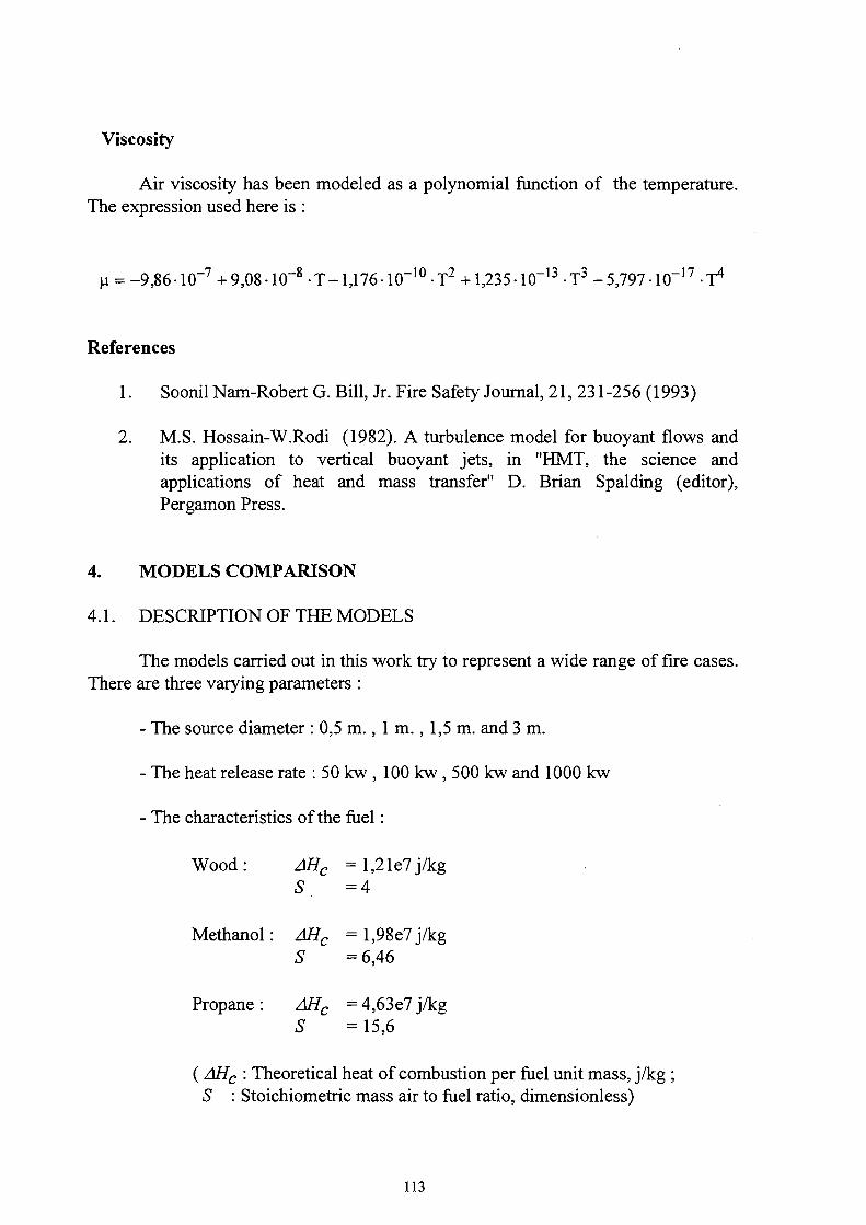
Viscosity
Air viscosity has been modeled as a polynomial function of the temperature. The expression used here is :
μ = -9,86-IO"7 +9,08-IO"8 -Τ-1,176-IO"10 ·Τ2 +1,235-ΙΟ"13 -Τ3 -5,797-10"17 -Τ4
References
1. Soonil Nam-Robert G. Bill, Jr. Fire Safety Journal, 21, 231-256 (1993)
2. M.S. Hossain-W.Rodi (1982). A turbulence model for buoyant flows and its application to vertical buoyant jets, in "HMT, the science and applications of heat and mass transfer" D. Brian Spalding (editor), Pergamon Press.
4. MODELS COMPARISON
4.1. DESCRIPTION OF THE MODELS
The models carried out in this work try to represent a wide range of fire cases. There are three varying parameters :
- The source diameter : 0,5 m., 1 m., 1,5 m. and 3 m.
- The heat release rate : 50 kw , 100 kw , 500 kw and 1000 kw
- The characteristics of the fuel :
Wood: AHC = l,21e7 j/kg S =4
Methanol: AHC = l,98e7 j/kg S = 6,46
Propane: AHC =4,63e7j/kg S = 15,6
( AHC : Theoretical heat of combustion per fuel unit mass, j/kg ; S : Stoichiometric mass air to fuel ratio, dimensionless)
113
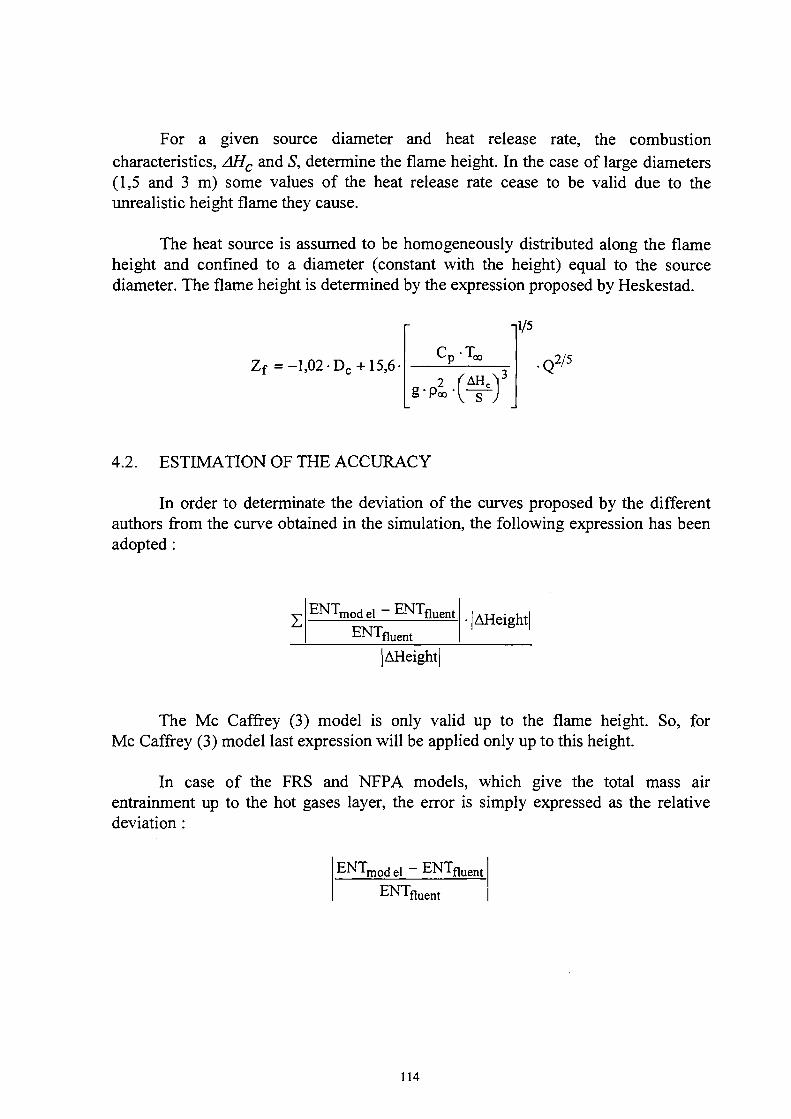
For a given source diameter and heat release rate, the combustion characteristics, AHC and S, determine the flame height. In the case of large diameters (1,5 and 3 m) some values of the heat release rate cease to be valid due to the unrealistic height flame they cause.
The heat source is assumed to be homogeneously distributed along the flame height and confined to a diameter (constant with the height) equal to the source diameter. The flame height is determined by the expression proposed by Heskestad.
Zf = -1,02- Dc+15,6 C Τ
g-p» ΔΗ.
-,1/5
,2/5
4.2. ESTIMATION OF THE ACCURACY
In order to determinate the deviation of the curves proposed by the different authors from the curve obtained in the simulation, the following expression has been adopted :
E N Tmodel ~ ENTfluent ENTfl uent
|AHeight|
|AHeight|
The Mc Caffrey (3) model is only valid up to the flame height. So, for Mc Caffrey (3) model last expression will be applied only up to this height.
In case of the FRS and NFPA models, which give the total mass air entrainment up to the hot gases layer, the error is simply expressed as the relative deviation :
E N Tmodel ~ ENTfluent
ENTfl uent
114
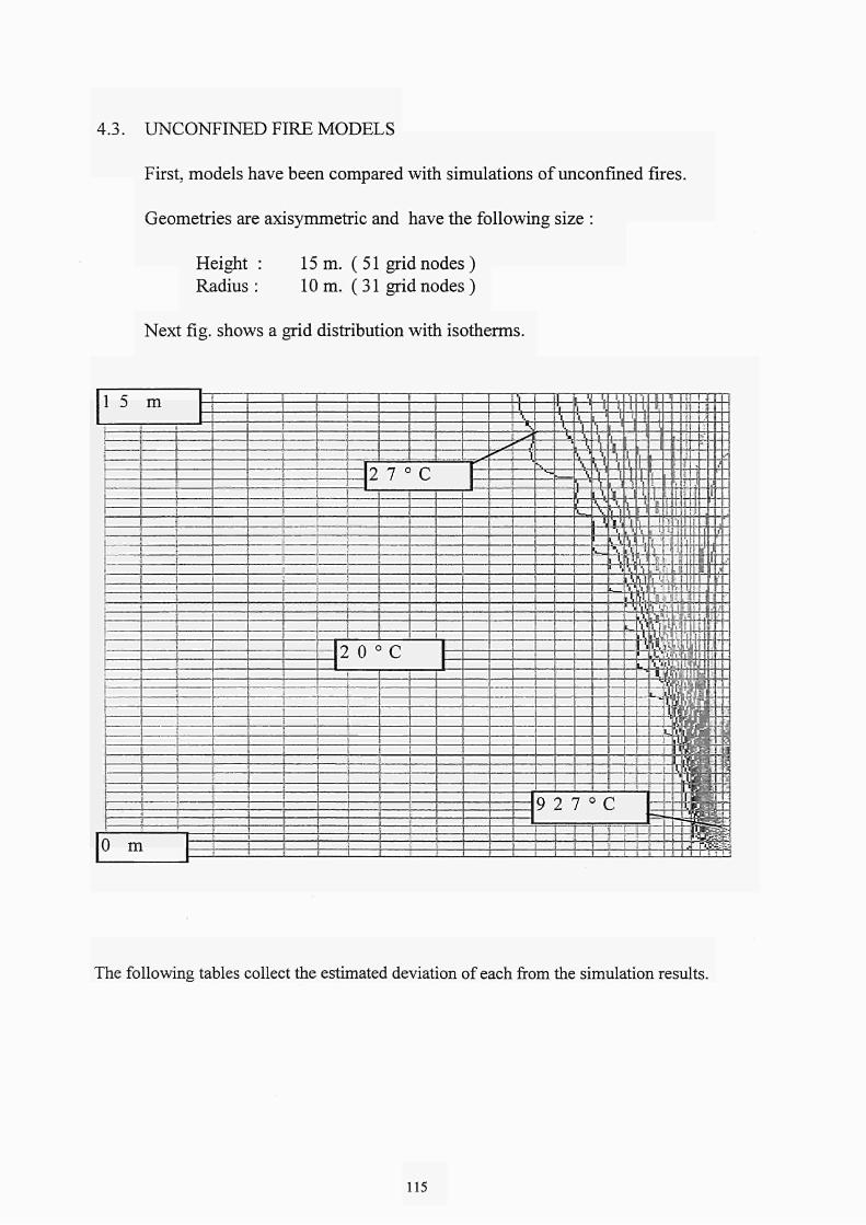
4.3. UNCONFINED FIRE MODELS
First, models have been compared with simulations of unconfined fires.
Geometries are axisymmetric and have the following size :
Height : 15 m. ( 51 grid nodes ) Radius : 10 m. ( 31 grid nodes )
Next fig. shows a grid distribution with isotherms.
ι ς i J i n
ι
I I I i I
t
1 J i i ; ! i
' i
0 ir J—
i
I
2vu t [
I ! I
;
1
| j : 1 I
i j I ! i Í
0 ι , 0 ° C
ί I Í
— ι — 1 1 1
. jj-J s
«·*
\ \ \
\ A
" / \
■s. ^ w
1 ', \ \ \
ι Ί '■ \ ' ■'
i \
. ". \ '
·■.
V 'l ·
I1
¡'
L,
ί
Ί Ί ì '■,
1 '
», \'-'s >,
■-
mj.j.JL'1 χ ■:: :
i o l i i l ] : : : z m . ι Τ... LJ I I i i . . . l i l i ï ι Γ μ :i:ì : : : JfCtu- IJII-Ií jLÏtzt.t: J : 11 l
! !
Ι Π Ί Γ Γ r1: : : ΓJAÜL t. . . Λ Γ Ί TÎ t-.--\ \ \ ] ', SdÌLjfiit :::ί Ί LÌ V
1' Ι
oEÌtt i : : saJtt i . t : : LÌQÌJÌLJ. X\.¿
<\\λν ■ Τ ? Λ ψ· ' Γ ' ν« ',; ·, ■ η -
asttt-1---X \Λϋ '
L VukVi i i l lUSli Μ I 1
lia"*Ui *L*Ti' 'iWt 1
^lö|l|.i.. ÎTÏTr ¡PB
ΠΙ?» A I '...:; ¡ Γ>Ή ì B I -!·ί
ί ιΊ Ι» : ! Ι'ύ ■ ■ ■ ■ ■ ■ Y . V . flir.
WLUX-'.-IBir: ■■■m·-π IE
§ ■ ■ ■ ■ ■ ■ L · if!£ HmW!^^^M^mm^mm\ l i t - ' 3,-31*1
y ζ ι \ ■ ¡ ■ ■ u J ■■ >n
\\\ \\ - : : : B g 1 1 i 1 1
J Π ! !
The following tables collect the estimated deviation of each from the simulation results.
115
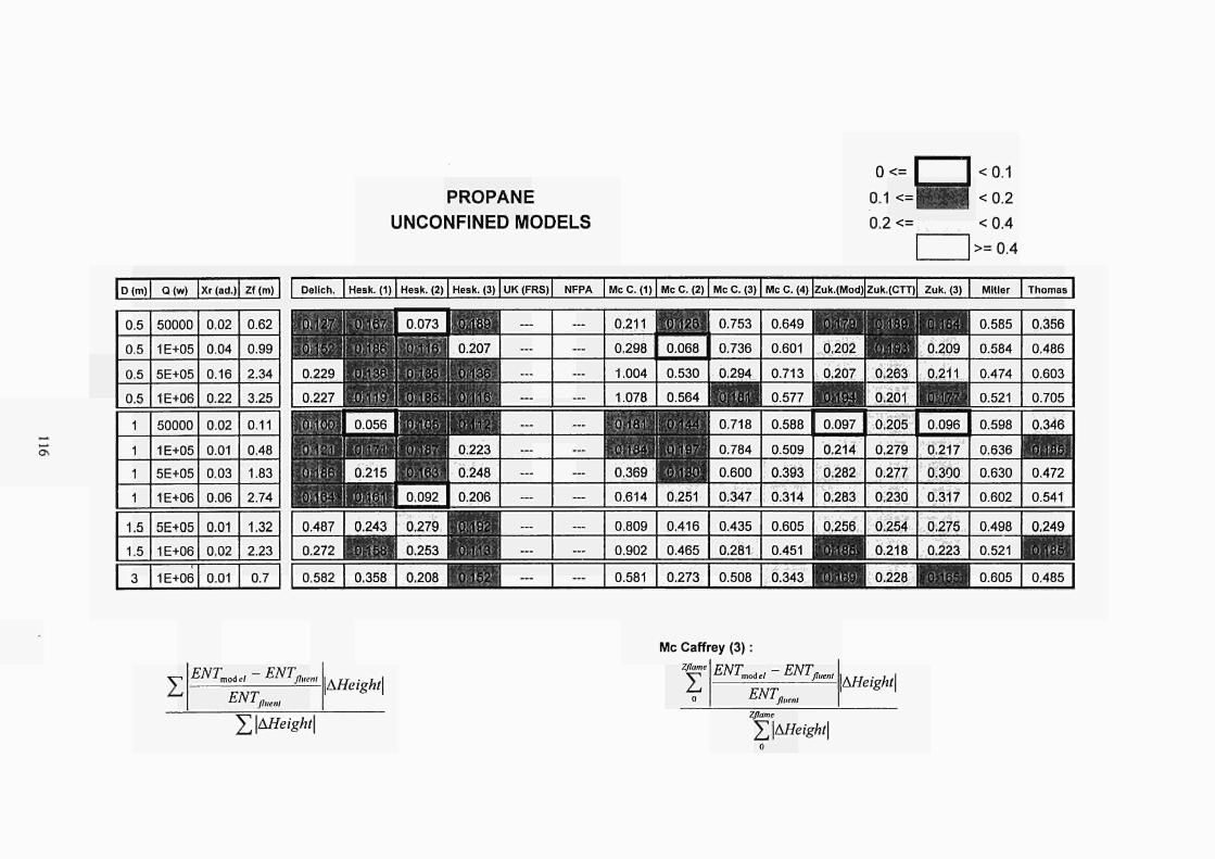
σ\
ΙD (m) Q(w) Xr (ad.) Zf(m)
0.5
0.5
0.5
0.5
1
1
1
1
1.5
1.5
3
50000
1E+05
5E+05
1E+06
50000
1E+05
5E+05
1E+06
5E+05
1E+06
1E+06
0.02
0.04
0.16
0.22
0.02
0.01
0.03
0.06
0.01
0.02
0.01
0.62
0.99
2.34
3.25
0.11
0.48
1.83
2.74
1.32
2.23
0.7
PROPANE
UNCONFINED MODELS
0<=
0.1 <=
0.2 <=
Β <0.1
<0.2
<0.4
>=0.4
Delicti. Hesk. (1)
0.127 .
J6.Ì52J
0.229
0.227
HUnluöl
W4$l
ÜM&.
|b';i36l
mvê 0.056
Hesk. (2)
0.073
;0.116:
to i l 36;
W(BB
S 0.215 J
0.487
0.272
0.582
0.243
Cotise?
0.092
0.279
0.253
0.358 I 0.208
Hesk. (3) UK (FRS) NFPA Mc C. (1) Mc C. (2) Mc C (3) Mc C. (4) Zuk.(Mod) Zuk.(CTT) Zuk. (3) Mitler Thomas |
íp89Í
0.207
;::B.Í36>
lolite
0.223
0.248
0.206
—
—
—
—
—
—
—
—
—
—
...
—
—
...
—
—
—
...
—
...
...
0.211
0.298
1.004
1.078
lötèël 0.068
0.530
0.564
mmm
0.369
0.614
0.809
0.902
0.581
0.251
0.416
0.465
0.273
0.753
0.736
0.294
'fl.181>
0.718
0.784
0.600
0.347
0.435
0.281
0.508
0.649 1
0.601
0.713
0.577
0.588
0.509
0.393
0.314
0.605
0.451
0.343
0.202
0.207
mm 0.097
0.214
0.282
0.283
0.256
;:.ò/:i85>·-
¿i0.1'69:í
0.263
0.201
0.205
0.279
0.277
0.230
0.254
0.218
0.228
0.209
0.211
'0.177^
0.096
0.217
0.300
0.317
0.275
0.223
0.585
0.584
0.474
0.521
0.598
0.636
0.630
0.602
0.498
0.521
0.605
0.356
0.486
0.603
0.705
0.346
0485-
0.472
0.541
0.249
EBã 0.485
ENT model ENT fluent
ENT, fluent
Mieightl
¿Z\àHeighí\
Mc Caffrey (3) :
Zflame
Σ 0
ENTmoiel-ENTfllienl
ENT, fluent
\AHeight\
Zflame
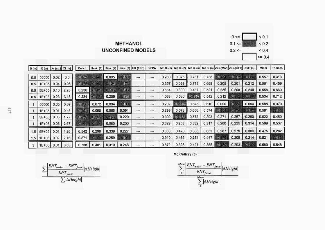
1D (m) Q(w) Xr (ad.) Zf(m)
0.5 0.5 0.5 0.5 1 1 1 1 1.5 1.5 3
50000 1E+05 5E+05 1E+06 50000 1E+05 5E+05 1E+06 5E+05 1E+06 1E+06
0.02 0.04 0.16 0.23 0.03 0.01 0.03 0.06 0.01 0.02 0.01
0.6 0.96 2.28 3.18 0.09 0.45 1.77 2.67 1.26 2.16 0.63
METHANOL UNCONFINED MODELS
0<=
0.1 <=
0.2 <= Β <0.1
<0.2
<0.4
>=0.4
Delich. Hesk. (1) Hesk. (2) Hesk. (3) UK (FRS) NFPA Mc C. (1) Mc C (2) Mc C (3) Mc C. (4) Zuk.(Mod) Zuk.(CTT) Zuk. (3) Mitler
ENZ moi el ENT, fluent
ENT, fluent
\AHeight\
^{AHeightl
Mc Caffrey (3) :
Zflame
Σ o
ENT model ENT. fluent
ENT, fluent
\AHeight\
Zflame
ΣΙΔ^*Ή
Thomas
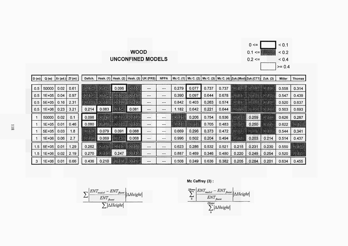
1D (m) Q(w) Xr (ad.) Zf(m)
0.5
0.5
0.5
0.5
1
1
1
1
1.5
1.5
3
50000
1E+05
5E+05
1E+06
50000
1E+05
5E+05
1E+06
5E+05
1E+06
1E+06
0.02
0.04
0.16
0.23
0.02
0.01
0.03
0.06
0.01
0.02
0.01
0.61
0.97
2.31
3.21
0.1
0.46
1.8
2.7
1.29
2.19
0.66
WOOD
UNCONFINED MODELS
0<=
0.1 <=
0.2 <=
H <0.1
<0.2
<0.4
>=0.4
Delich. Hesk. (1) Hesk. (2) Hesk. (3) UK (FRS) NFPA McC.(1) Mc C (2) McC(3) Mc C (4) Zuk.(Mod) Zuk.(CTT) Zuk. (3) Mitler Thomas
'^ΑΦ,
0.154.
0.162:
0.214
'Meì'M
άθ;ΐ34
)Miö :
0.098
0.080
0.16
0.096
Basa
ïm 20
0.083 0.154
;
zi μ§439>
0.079 I 0.091
0-069 I " [40
•omsi '0;l47v
01-120
0.081
P.17
:Mfà 0.088
0.068
0.279
0.390
0.842
1.182
0.996
0.623
0.887
0.508
0.077
0.097
0.403
0.642
0.206
0 m 0.296
0.502
0.286
0.469
0.249
0.737
0.644
0.263
0.221
0.754
0.705
0.373
0.204
0.532
0.346
0.636
0.737
0.678
0.574
0.644 1 1
0.536
0.483
0.472
0.494
0.521
0.480
0.382
ENT. model ENT, fluent
ENT, fluent
\AHeight\
%\¿iHeight\
Mc Caffrey (3)
Zflame
Σ o
ENTmoåel - ENTßuenl
ENT, fluent
\AHeight\
Zflame
X\AHeight\
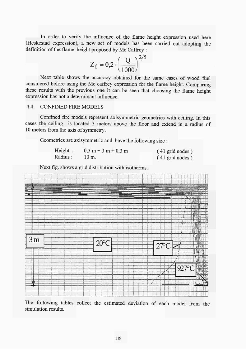
In order to verify the influence of the flame height expression used here
(Heskestad expression), a new set of models has been carried out adopting the
definition of the flame height proposed by Mc Caffrey :
2/5
0,2 1000,
Next table shows the accuracy obtained for the same cases of wood fuel
considered before using the Mc caffrey expression for the flame height. Comparing
these results with the previous one it can be seen that choosing the flame height
expression has not a determinant influence.
4.4. CONFINED FIRE MODELS
Confined fire models represent axisymmetric geometries with ceiling. In this
cases the ceiling is located 3 meters above the floor and extend in a radius of
10 meters from the axis of symmetry.
Geometries are axisymmetric and have the following size :
Height : 0,3 m - 3 m + 0,3 m
Radius : 10 m.
Next fig. shows a grid distribution with isotherms.
(41 grid nodes )
(41 grid nodes )
j
i
M I M I i ! ! I i Ι ι
^ g g g i ^ B 3 U ^ i M ü i i i » ^ ^ i » ü ü i ^ * i — ^ ^ ^ ^ ^ ^ — ■■■'- * . * ' * ' ■■■
— ; — — j — | — < — | —
; ;
- 3m -
f ;
j
' ! j
t i | l
. 1 . i
i
! ; ' : "r
~ ^ = 1 I I I
i , " 1 I ! '
1 : ι ! i
1 "'
20°C
1 i ¡
i
|
1 '
[
i ' i ! :
! i
! ' 1 I M I
1 ! I l ι
! i
i j
I 1
— ι
1
; ι
I
l i l t
= = = » — ■ — - V - 3 ;
¡ï
;
•m \
• ! /■
s \/ j
Ι ι !
1/ A ¿
!
ί I
ί ' ƒ ; ï ; : / 1 / :/ j'l 1 i
! I
1
Ί ; I -^JL *1
I i
/i r ■
¿ - 9 2 7
e
i i i i
1 1 1 !
i j I I
I i i
1 ί ! ι ί ι i Ι
^Q^pj
^å!tf -' Wim ' "■ f M II ■■,! t i 'Ρ M ' f , ¡lì i l in .M m mm m mm hi
i l ¡11! lui Il i IM IH Li H l ι m 'ι
i !
WW ^ : 'iiii 1 i 1 g : : vmÅ i «bflfri-i
ι lij """ ' , -.fa r^ Kiras ffiS l^l l iäS
Mg , .'Il IV-NI ί * ιι ρί τΒ
IMI Ί ! I M I Ι !
The following tables collect the estimated deviation of each model from the simulation results.
119

ë
1D (m) Q(w) Xr (ad.) Zf(m)
0.5
0.5
0.5
0.5
1
1
1
1
1.5
1.5
3
50000
1E+05
5E+05
1E+06
50000
1E+05
5E+05
1E+06
5E+05
1E+06
1E+06
0.02
0.03
0.1
0.17
0.02
0.01
0.02
0.04
0.01
0.02
0.01
0.62
0.99
2.34
3.25
0.11
0.48
1.83
2.74
1.32
2.23
0.7
PROPANE CONFINED MODELS
CEILING HEIGHT = 3 m.
0<=
0.1 <= 0.2 <=
g <0.1 <0.2 <0.4
>=0.4
Dollch. Hesk. (1) Hesk. (2) Hesk. (3) UK (FRS) .NFPA McC.<1) Mc C. (2) MC C; (3) Mc C. (4) Zuk.(Mod) Zlik.(CTT) Zuk. (3) Mltler Thomas |
0.370
0.401
0.591
0.698
0.401
0.313
0.432
0.691
0.212
0.348
0.338
0.440
0.440
0.320
0.266
0.395
0.451
0.461
0.626
0.385
0.406
:·0;ίΪ6:
0.213
0.287
0.341
0.358
0.501
0.478
0.365
0.567
0.342
0.307
0.268
0.482
0.479
0.341
0.262
0.514
0.537
0.507
0.660
0.468
0.465
0.330
0.252
0.268
0.331
0.495
0.352
0.351
0.364
0.594
0.279
0.328
■ 0.125
0.219
■i:>Ui?r7í3^
íf$¿2f
0.294
0.517
0.477
0.267
0.374
0.397
0.266
0.556
0.242
0.306
0.509
0.656
0.414
0.339
0.255
0.347
0.282
0.228
0.444
0.303
0.249
0.311
0.286
0.559
0.501
0.335
0.493
0.424
0.364
0.586
0.757
0.654
0.298
0.295
0.862
0.807
0.595
0.677
0.659
0.595
0.742
0.393
0.353 ι,.«, ι.-
0.341
0.615
0.594
0.396
0.493
0.485
0.353
0.562
0.540
0.570
0.535
0.487
0.568
0.601
0.640
0.748
0.596
0.610
0.495
0.584
0.577
0.535
0.566
0.740
0.734
0.711
0.800
0.756
0.755
0.842
0.573
0.624
0.557
0.424
0.575
0.633
0.755
0.859
0.701
0.778
0.553
0.790
0.786
0.765
0.781
0.869
0.866
0.854
0.899
0.877
0.876
0.920
0.587
0.664
0.778
0.829
0.482
0.581
0.733
0.854
0.663
0.731
0.652
ENTmodel - ENTfluenl
ENT, fluent
\AHeight\
Y\AHeight\
Mc CAFFREY (3) :
Zflame
Σ o
ENTmoiel-ENTßmn,
ENT, fluent
\AHeighí\
Zflame
ΣΙ^'Ή o
UK (FRS) & NFPA :
ENTmod el ~ ENTfluent ENTfluent
At height of hot gases layer
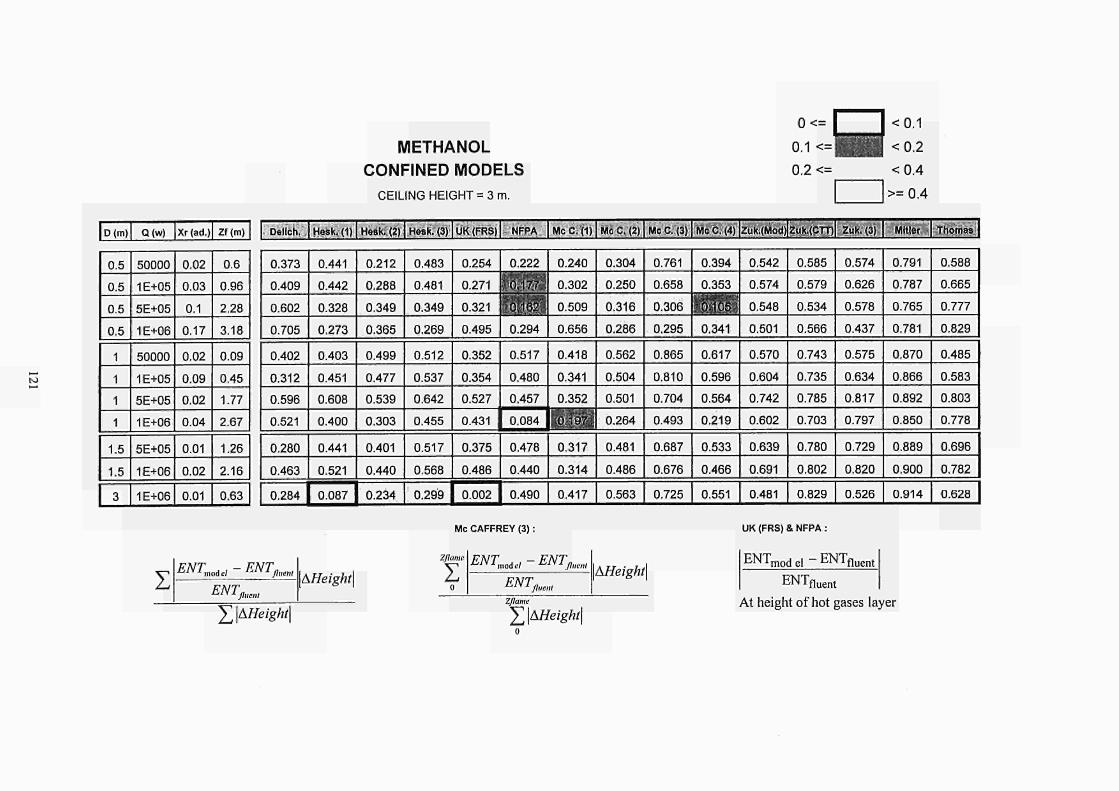
K)
1D (m) Q(w) Xr (ad.) Zf(m)
0.5
0.5
0.5
0.5
1
1
1
1
1.5
1.5
3
50000
1E+05
5E+05
1E+06
50000
1E+05
5E+05
1E+06
5E+05
1E+06
1E+06
0.02
0.03
0.1
0.17
0.02
0.09
0.02
0.04
0.01
0.02
0.01
0.6
0.96
2.28
3.18
0.09
0.45
1.77
2.67
1.26
2.16
0.63
Delicti.
0.373
0.409
0.602
0.705
0.402
0.312
0.596
0.521
0.280
0.463
0.284
ENTmaiel-ENTfluenl
ENT, fluent
METHANOL
CONFINED MODELS
CEILING HEIGHT = 3 m.
0<=
0.1 <=
0.2 <=
THSSBSEJ <0.1
<0.2
<0.4
>=0.4
Hesk.Q) Hesk: (2) Hesk. (3) UK (FRS) NFPA Mc'Ci'fQ McC,(2) McC(3) McC(4) Zuk.(Mod) ZÜk.(CTT) Zuk. (3) Mitler
0.441
0.442
0.328
0.273
0.403
0.451
0.608
0.400
0.441
0.521
0.087
0.212
0.288
0.349
0.365
0.499
0.477
0.539
0.303
0.401
0.440
0.234
0.483
0.481
0.349
0.269
0.512
0.537
0.642
0.455
0.517
0.568
0.299
0.254
0.271
0.321
0.495
0.352
0.354
0.527
0.431
0.375
0.486
0.002
0.222
0.177
0.294
0.517
0.480
0.457
0.084
0.478
0.440
0.490
0.240
0.302
0.509
0.656
0.418
0.341
0.352
0.317
0.314
0.417
0.304
0.250
0.316
0.286
0.562
0.504
0.501
0.264
0.481
0.486
0.563
0.761
0.658
0.306
0.295
0.865
0.810
0.704
0.493
0.687
0.676
0.725
0.394
0.353
0.341
0.617
0.596
0.564
0.219
0.533
0.466
0.551
0.542
0.574
0.548
0.501
0.570
0.604
0.742
0.602
0.639
0.691
0.481
0.585
0.579
0.534
0.566
0.743
0.735
0.785
0.703
0.780
0.802
0.829
0.574
0.626
0.578
0.437
0.575
0.634
0.817
0.797
0.729
0.820
0.526
0.791
0.787
0.765
0.781
0.870
0.866
0.892
0.850
0.889
0.900
0.914
Mc CAFFREY (3) :
AHeighil
Zflame
Σ o
ENTmoiel-ENTßuenl
ENT, fluent
AHeight\
UK (FRS) & NFPA :
E N Tmod el ~ ENTfluent
¿Z\AHeight\ Zflame
¿Z\&Height\
ENTfluent
At height of hot gases layer
Thomas
0.588
0.665
0.777
0.829
0.485
0.583
0.803
0.778
0.696
0.782
0.628
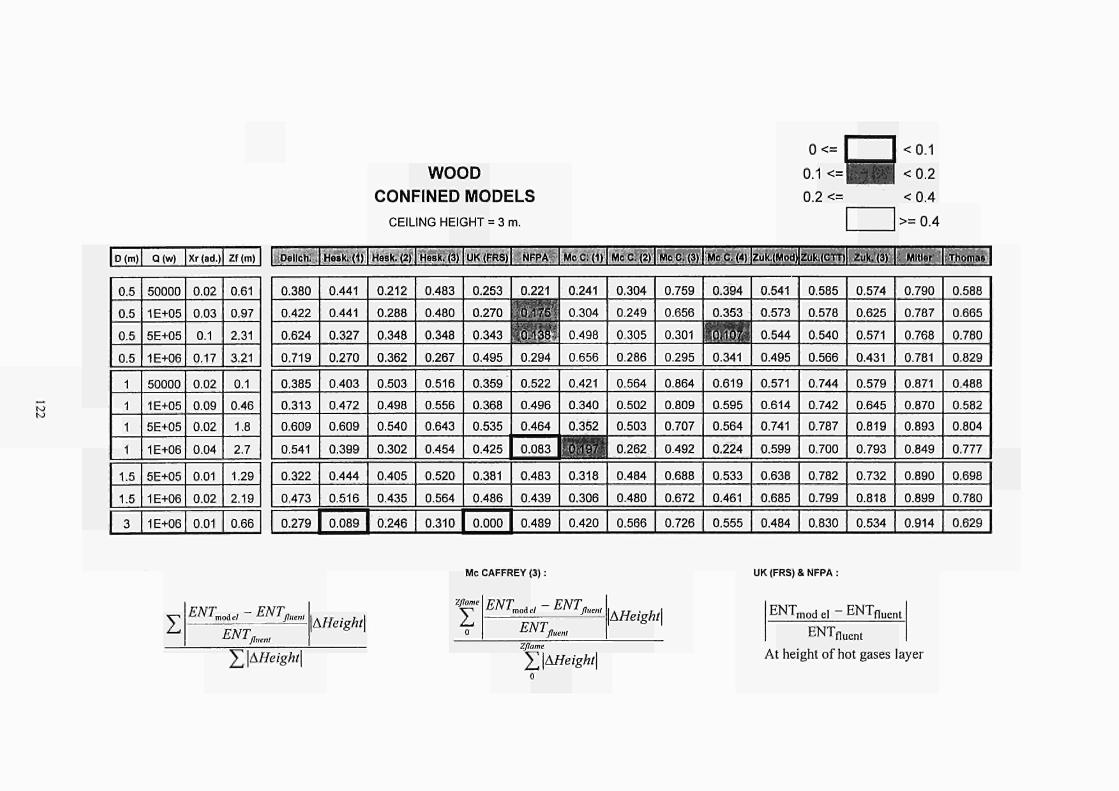
NI K)
WOOD
CONFINED MODELS
CEILING HEIGHT = 3 m.
0<=| <0.1
0.1 <=j [ < 0.2
0.2 <= <0.4
>=0.4
fo(m) Q(w) Xr (ad.) Zf(m)
0.5
0.5
0.5
0.5
1
1
1
1
1.5
1.5
3
50000
1E+05
5E+05
1E+06
50000
1E+05
5E+05
1E+06
5E+05
1E+06
1E+06
0.02
0.03
0.1
0.17
0.02
0.09
0.02
0.04
0.01
0.02
0.01
0.61
0.97
2.31
3.21
0.1
0.46
1.8
2.7
1.29
2.19
0.66
Dellch: Hosk.(1) Hesk. (2) Hesk. (3) UK (FRS) NFPA Mc c: (1) Mc C (2) Mc C (3) Mc C (4) Zuk-(Mod) Zuk.(CTT) Zuk.(3) .Mitler Thomas I
0.380
0.422
0.624
0.719
0.385
0.313
0.609
0.541
0.322
0.473
0.279
0.441
0.441
0.327
0.270
0.403
0.472
0.609
0.399
0.444
0.516
0.089
0.212
0.288
0.348
0.362
0.503
0.498
0.540
0.302
0.405
0.435
0.246
0.483
0.480
0.348
0.267
0.516
0.556
0.643
0.454
0.520
0.564
0.310
0.253
0.270
0.343
0.495
0.359
0.368
0.535
0.425
0.381
0.486
0.000
0.221
•0:175
0.138
0.294
0.522
0.496
0.464
0.083
0.483
0.439
0.489
0.241
0.304
0.498
0.656
0.421
0.340
0.352
i o « :
0.318
0.306
0.420
0.304
0.249
0.305
0.286
0.564
0.502
0.503
0.262
0.484
0.480
0.566
0.759
0.656
0.301
0.295
0.864
0.809
0.707
0.492
0.688
0.672
0.726
0.394
0.353
WBÈ 0.341
0.619
0.595
0.564
0.224
0.533
0.461
0.555
0.541
0.573
0.544
0.495
0.571
0.614
0.741
0.599
0.638
0.685
0.484
0.585
0.578
0.540
0.566
0.744
0.742
0.787
0.700
0.782
0.799
0.830
0.574
0.625
0.571
0.431
0.579
0.645
0.819
0.793
0.732
0.818
0.534
0.790
0.787
0.768
0.781
0.871
0.870
0.893
0.849
0.890
0.899
0.914
0.588
0.665
0.780
0.829
0.488
0.582
0.804
0.777
0.698
0.780
0.629
ENTmoáel-ENTftmnl
ENT, fluent
\AHeight\
Y^AHeigh^
Mc CAFFREY (3) :
Zflame
Σ o
ENTmoitl-ENTflum
ENT, fluent
\AHeight\
Zflame
Y\AHeight\ o
UK (FRS) & NFPA :
ENT, mod el ENT fluent ENTfluent
At height of hot gases layer
5. CONCLUSIONS
Confinement has an important influence on the models agreement. Most expressions studied here apply for unconfined fires. Their application for confined situations implies a lost of accuracy.
F.R.S. andN.F.P.A. are specially defined for confined fires. These expressions show the best agreement and the widest range of application in confined fires.
Heskestad presents the best approximation for unconfined cases in the considered range. In confined cases accuracy decreases but it remains close to FRS and NFPA accuracy.
Delichatsios presents good approximation but its accuracy decreases for large diameters.
Although Zukoski models give more regular approximation in the considered range than Delichatsios model, its accuracy is worse, particularly for confined fires. Furthermore, its use requires an intensive effort due to its difficult application.
Mc Caffrey (1) and (2) give good approximation for cases with low heat release rate, but they don't fit large heat release rate fires.
Mc Caffrey (3) is valid up to the flame tip. The lower the flame is, the worse accuracy Mc Caffrey (3) arises. The accuracy of Mc Caffrey (3) and Mc Caffrey (4) models is not good enough except for the largest heat release rates.
Mitler expression is similar to Zukoski (CTT) model. Nevertheless, Mitler presents worse results even than Zukoski (CTT) model. So, it could be discarded.
Finally, Thomas expression has application on some specific cases in unconfined fires. So, it must be discarded as a general expression.
123
C.E.N, application
The Comité Européen de Normalisation (C.E.N.) proposes two different models to be applied depending on the geometric characteristics : Heskestad model for small fires (Y>10A^'2) and Thomas expression for large fires (Y<10A^2).
All unconfined cases carried out here are defined as small fires under C.E.N, definition. For these cases, Heskestad model has been chosen as the best model in agreement with C.E.N..
For confined fires, only four cases satisfies the C.E.N, restrictions for large fires (Thomas expression). In these four cases, the present study suggests that FRS, NFPA and Heskestad models are better than Thomas expression.
APPENDIX I
GRAPHICS
Following pictures show the comparison between models and FLUENT simulation results. The case shown has the following characteristics :
* * * *
Confined fire : fuel: Source diameter : Heat release rate :
ceiling located 3 m. over the floor Methanol 3 m. 106w.
124
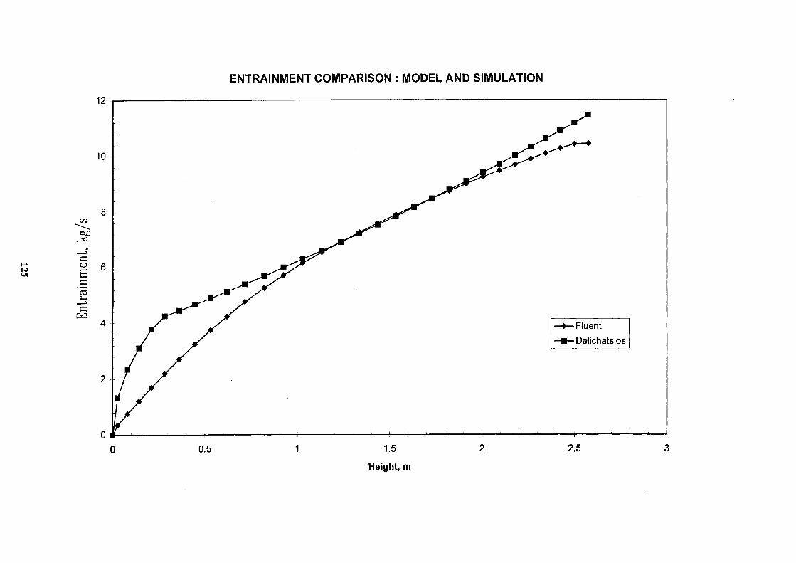
ENTRAINMENT COMPARISON : MODEL AND SIMULATION
S3 Ui
CO S-i
-4 -J
PO
0.5 1.5
Height, m
2.5
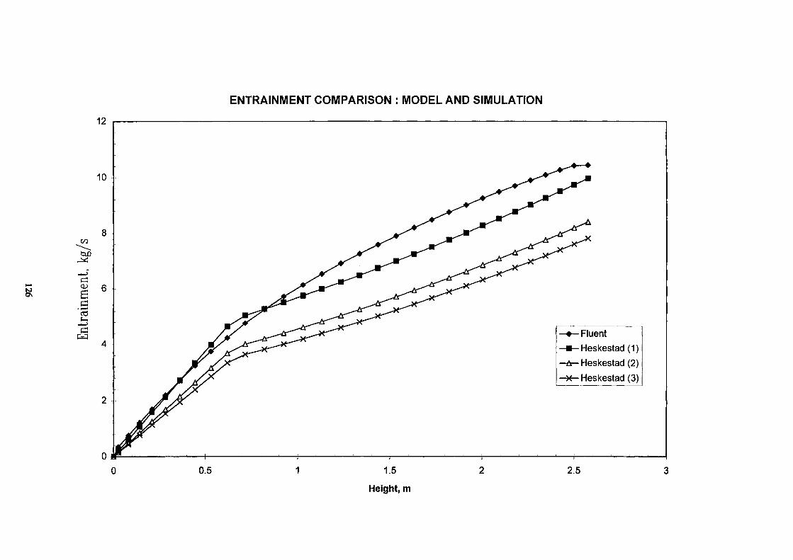
ENTRAINMENT COMPARISON : MODEL AND SIMULATION
S
00
Ο)
α3
tí DJ
0.5 1.5
Height, m
2.5
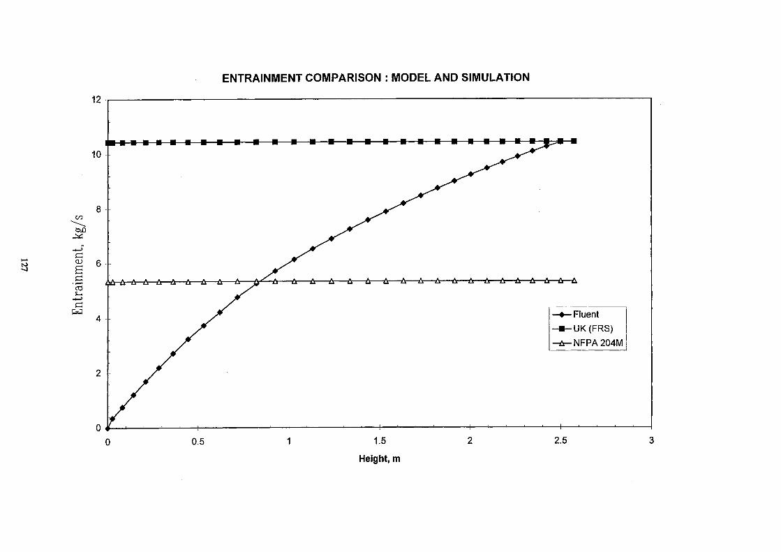
ENTRAINMENT COMPARISON : MODEL AND SIMULATION
tá
12
10
tí 2á 6
cö
I M
tí
ΛΛ-Λ Λ Λ A—Δ—Δ—Δ—Δ Δ -Δ"2—Δ Δ Δ Δ Δ Δ Δ Δ Δ Δ Δ — Δ — Δ — Δ — Δ
0.5 1.5
Height, m
•Fluent
•UK (FRS)
•NFPA204M
ί - ι 1 ι
2.5
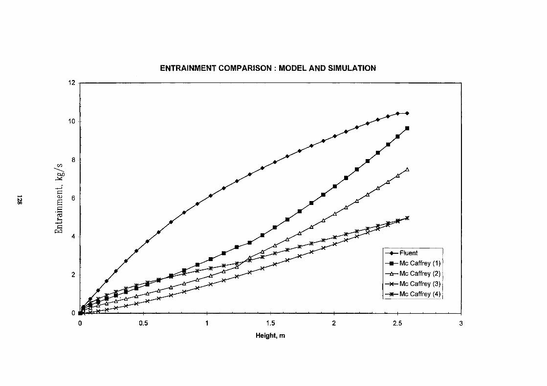
ENTRAINMENT COMPARISON : MODEL AND SIMULATION
12
»
co
tí OJ
S-Η - ♦ ->
tí
Fluent
Mc Caffrey (1)
Mc Caffrey (2)
Mc Caffrey (3)
Mc Caffrey (4)
0.5 1.5
Height, m
2.5
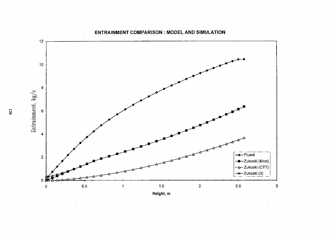
ENTRAINMENT COMPARISON : MODEL AND SIMULATION
IO
00
oo ¿a
tí
Β tí
'co S - .
tí
0.5 1.5
Height, m
2.5

ENTRAINMENT COMPARISON : MODEL AND SIMULATION
o
oo ¿4
c
ε 'cö t-,
"c
0.5 1.5
Height, m
2.5

ANNEX 3 : Design fire according to building Occupancy given by NBN S21-208-1 [2].
In the following pages of this annex, the buildings are divided into four categories. For each category a design fire has been defined :
Category
1 2 3 4
Class
L,N1,SC1 N2, SC2 N3, SC3
N4, Dl to D4, SC4
Fire Size
3,0 mx3,0 m 4,5 m χ 4,5 m 6,0 m χ 6.0 m 9,0 m \ 9.0 m
RHRfi [kW/m2] (see also Annex 4)
Forced Ventilation 500 500 500 500
Natural Ventilation 250 250 250 250
CI
C2
C3
Packings
incombustible packings, eventually put on wood pallet
paper, cardboard, corrugated paper, wood or plastic packings, plastic mosses excluded, eventually put on wood pallet all other packings
Storage Materials (Annex A)
SI
SCI
SC2
SC3
S2
SC2
SC2
SC3
S3
SC3
SC3
SC3
S4
SC4
SC4
SC4
Storage Categories
131

A N N E X 3 NBN S21-208-1
ANNEXE A : CLASSIFICATION DES ESPACES A PROTEGER (1)
La présente annexe reprend la classification des établissements à protéger donnée dans l'annexe à la norme belge NBN S21-028 "Installations d'extincteurs automatiques hydrauliques" (1982).
1 CONSIDERATIONS GENERALES
La quantité et le degré de réaction au feu des matériaux et marchandises dans les locaux protégés ainsi que les conditions de développement et de propagation d'un incendie sont les facteurs à la base de la classification des établissements à protéger.
2 CLASSIFICATION DES ETABLISSEMENTS
2.1 Classe des établissements à charge calorifique légère : L
Cette classe comprend uniquement les établissements ou parties d'établissements dont la quantité et le degré de réaction au feu du contenu sont peu importants.
Certains locaux de ces établissements sont, toutefois, en fonction de leur usage ou contenu, classés comme des locaux à charge calorifique légère aggravée.
- Asiles - Eglises - Bains publics - Homes - Bâtiments publics - Hôpitaux - Bibliothèques - Hôtels - Bureaux - Musées - Casernes - Pensions - Chapelles - Pensionnats - Châteaux - Prisons - Collèges - Stations de pompage d'eau - Couvents - Traitement des eaux - Crèches - Universités sauf laboratoires - Ecoles
Les locaux suivants de ces établissements : blanchisseries, chaufferies, cuisines, mansardes, restaurants avec cuisinesisines attenantes sont considérés comme des locaux à potentiel calorifique léger aggravé.
Les ateliers, les laboratoires et les entrepôts sont à classer dans le groupe qui leur est propre.
2.2 Classe des établissements à charge calorifique ordinaire : N
Cette classe contient les établissements industriels et commerciaux ou parties de ceux-ci comprenant la manutention, la fabrication et le stockage de produits divers avec limitation de hauteur suivant la nature des matériaux stockés.
Elle est subdivisée en quatre groupes caractérisés par la plus ou moins grande rapidité d'extension d'un feu naissant qui détermine l'ouverture d'un groupe plus ou moins grand de sprinklers pour éteindre ou contrôler ce feu
(1)La présente annexe sera remplacée par la classification en préparation au CENACI 91/WG5 (Sprinklers and water spray systems and components) dès que la norme correspondante sera publiée.
132

NBN S21-208-1
Ce sont les : - établissements à charoe calorifique ordinaire présentant un danger d'incendie faible : N1
Abattoirs Agglomérés de ciment
■ Béton ■ Bijouteries • Brasserie sans malterie • Broyage de minerais • Cabines de transformation ou de distribution (sauf les parties protégées spécialement)
• Cafés • Carrières ■ Centrales électriques (sauf les parties protégées spécialement)
• Champagnisation des vins - Chaufferie d'industrie - Chromage électrolytique - Cidreries - Ciment (industrie du ciment et fabrication
d'objets en ciment) - Eaux gazeuses, minérales, thermales et
boissons analogues - Entrepôts frigorifiques - Fromageries - Galvanoplastie - Glace artificielle
- Laiteries
- Lavoir publics - Meules abrasives (fabrique) - Nettoyage à sec sans usage de liquides
inflammables - Nickelage - Orfèvrerie - Poudres abrasives (fabrique) - Restaurants - Scierie de marbre, pierres de taille et analogue - Sel (raffinerie) - Stations d'accumulateurs (sauf les parties
protégées spécialement) - Tailleries de diamants - Vins de fruits à l'exclusion de la mise en bouteille qui est à classer comme un établissement à charge calorifique ordinaire présentant un danger d'incendie normal N2 et la mise en tonneaux effectuée dans des bâtiments de construction et couverture en matériaux incombustibles qui est à classer avec les établissements à charge calorifique ordinaire présentant un danger d'incendie élevé N3
établissements à charge calorifique ordinaire présentant un danaer d'incendie normal : N2
- Ammoniaque synthétique - Argile et terres diverses (fabrique d'objets) - Atelier de réparation de parties mécaniques
ou de carrosseries de véhicules automobiles
- Biscuiteries - Blanchisseries - Boulangeries - Briqueteries - Carbonisage de laines et déchets de peignage
(sans emploi de solvants inflammables)
- Céramique - Charbon de bois (fabrique) - Chimie minérale (industrie) - Confitureries - Conserves alimentaires (légumes, fruits, viande,
poisson, lait condensé, etc.)
- Construction de véhicules à moteurs - Dégraissage de laine et déchets de peignage
(sans emploi de solvants inflammables)
- Electrodes pour soudures (fabrique) - Engrais chimiques minéraux - Filatures de fibres de la classe A et de
laines peignées à l'exclusion de la laine cardée
- Frittage - uarages - Glycérine (fabrique)
- Gravure - Impressions sur tissus - Laboratoires divers à l'exception de ceux
classés en D - Laminoirs - Lampes électriques (fabrique) - Lavoirs - Métallurgie - Miroiteries - Montage de véhicules à moteur - Moulage de poudres métalliques - Optique (fabrique d'instruments)
- Papiers abrasifs - Parapluie (fabrique) - Parkings - Pâtes alimentaires
- Pâtisseries
- Photographie (accessoires) - Poteries - Siroperies - Stylos et porte-plumes - Sucreries (sans raffinerie) - Tabacs - Teinture - Torréfaction de café - Transport public (entreprise) - Travail mécanique des métaux à l'exclusion
des métaux et alliages légers - Tréfile ries - Tubes fluorescents - Verreries
133
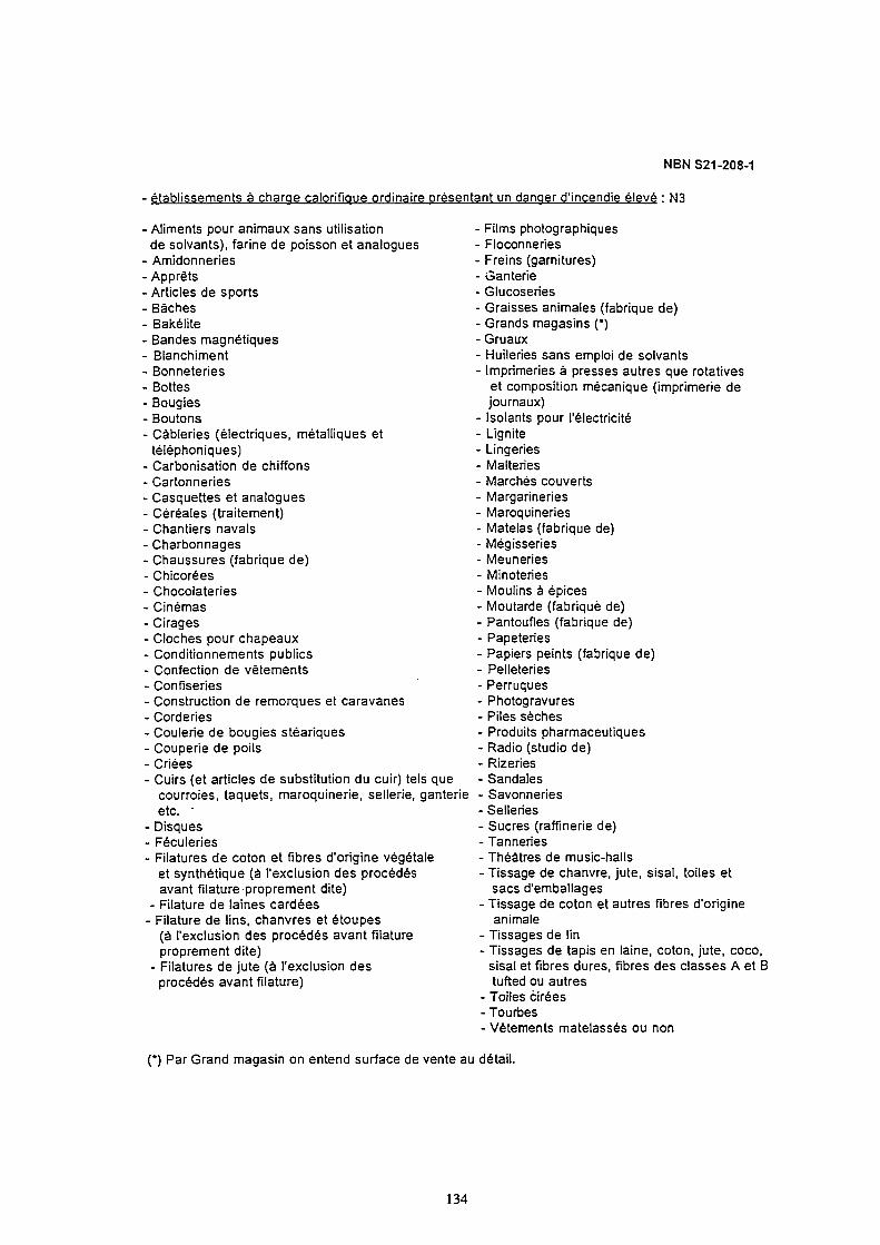
N BN S21 -208-1
établissements à charge calorifique ordinaire présentant un danaer d'incendie élevé : N3
• Aliments pour animaux sans utilisation
de solvants), farine de poisson et analogues
• Amidonneries
■ Apprêts
■ Articles de sports
■ Bâches
■ Bakélite
■ Bandes magnétiques
■ Blanchiment
• Bonneteries
• Bottes
■ Bougies
• Boutons
• Càbleries (électriques, métalliques et
téléphoniques)
■ Carbonisation de chiffons
■ Cartonneries
■ Casquettes et analogues
■ Céréales (traitement)
- Chantiers navals
■ Charbonnages
- Chaussures (fabrique de)
- Chicorées
- Chocolateries
- Cinémas
- Cirages
- Cloches pour chapeaux
- Conditionnements publics
- Confection de vêtements
- Confiseries
- Construction de remorques et caravanes
- Corderies
- Coulerie de bougies stéariques
- Couperie de poils
- Criées - Cuirs (et articles de substitution du cuir) tels que
courroies, taquets, maroquinerie, sellerie, ganterie
etc. ·
- Disques - Féculeries
- Filatures de coton et fibres d'origine végétale
et synthétique (à l'exclusion des procédés
avant filature proprement dite)
- Filature de laines cardées
- Filature de lins, chanvres et étoupes
(à l'exclusion des procédés avant filature
proprement dite)
- Filatures de jute (à l'exclusion des
procédés avant filature)
- Films photographiques
- Floconneries
- Freins (garnitures)
- Ganterie
- Glucoseries
- Graisses animales (fabrique de)
- Grands magasins (*)
- Gruaux
- Huileries sans emploi de solvants
- Imprimeries à presses autres que rotatives
et composition mécanique (imprimerie de
journaux)
- Isolants pour l'électricité
- Lignite
- Lingeries
- Malteries
- Marchés couverts
- Margarineries
- Maroquineries
- Matelas (fabrique de)
- Mégisseries
- Meuneries
- Minoteries
- Moulins à épices
- Moutarde (fabriqué de)
- Pantoufles (fabrique de)
- Papeteries
- Papiers peints (fabrique de)
- Pelleteries - Perruques
- Photogravures
- Piles sèches
- Produits pharmaceutiques
- Radio (studio de)
- Rizeries - Sandales
- Savonneries
- Selleries - Sucres (raffinerie de)
- Tanneries
- Théâtres de music-halls
- Tissage de chanvre, jute, sisal, toiles et
sacs d'emballages
- Tissage de coton et autres fibres d'origine
animale
- Tissages de lin
- Tissages de tapis en laine, coton, jute, coco,
sisal et fibres dures, fibres des classes A et B
tufted ou autres
- Toiles cirées
- Tourbes
- Vêtements matelassés ou non
(*) Par Grand magasin on entend surface de vente au détail.
134
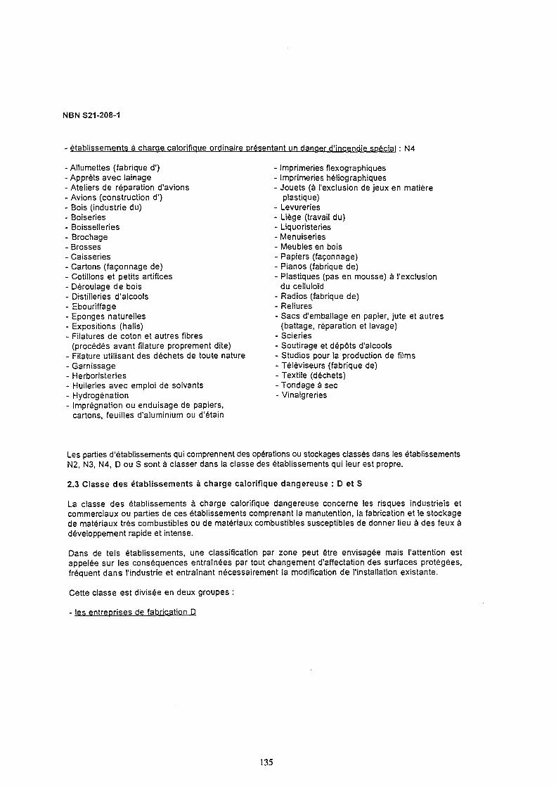
NBN S21-208-1
établissements à charge calorifique ordinaire présentant un danaer d'incendie spécial : N4
Allumettes (fabrique d')
Apprêts avec lainage
Ateliers de réparation d'avions
Avions (construction d')
■ Bois (industrie du)
■ Boiseries
■ Boisselleries
• Brochage
■ Brosses
• Caisseries
■ Cartons (façonnage de)
■ Cotillons et petits artifices
• Déroulage de bois
■ Distilleries d'alcools
■ Ebouriffage
■ Eponges naturelles
■ Expositions (halls)
- Filatures de coton et autres fibres
(procédés avant filature proprement dite)
- Filature utilisant des déchets de toute nature
- Garnissage
- Herboristeries
- Huileries avec emploi de solvants
- Hydrogénation
- Imprégnation ou enduisage de papiers,
cartons, feuilles d'aluminium ou d'étain
- Imprimeries flexographiques
- Imprimeries héliographiques - Jouets (à l'exclusion de jeux en matière
plastique)
- Levureries
- Liège (travail du)
- Liquoristeries
- Menuiseries - Meubles en bois
- Papiers (façonnage)
- Pianos (fabrique de)
- Plastiques (pas en mousse) à l'exclusion du celluloïd
- Radios (fabrique de)
- Reliures
- Sacs d'emballage en papier, jute et autres (battage, réparation et lavage)
- Scieries
- Soutirage et dépôts d'alcools
- Studios pour la production de films
- Téléviseurs (fabrique de)
- Textile (déchets)
- Tondage à sec
- Vinaigreries
Les parties d'établissements qui comprennent des opérations ou stockages classés dans les établissements
N2, N3, N4, D ou S sont à classer dans la classe des établissements qui leur est propre.
2.3 Classe des établissements à charge calorifique dangereuse : D et S
La classe des établissements à charge calorifique dangereuse concerne les risques industriels et
commerciaux ou parties de ces établissements comprenant la manutention, la fabrication et le stockage
de matériaux très combustibles ou de matériaux combustibles susceptibles de donner lieu à des feux à
développement rapide et intense.
Dans de tels établissements, une classification par zone peut être envisagée mais l'attention est
appelée sur les conséquences entraînées par tout changement d'affectation des surfaces protégées,
fréquent dans l'industrie et entraînant nécessairement la modification de l'installation existante.
Cette classe est divisée en deux groupes :
- les entreprises de fabrication D
135
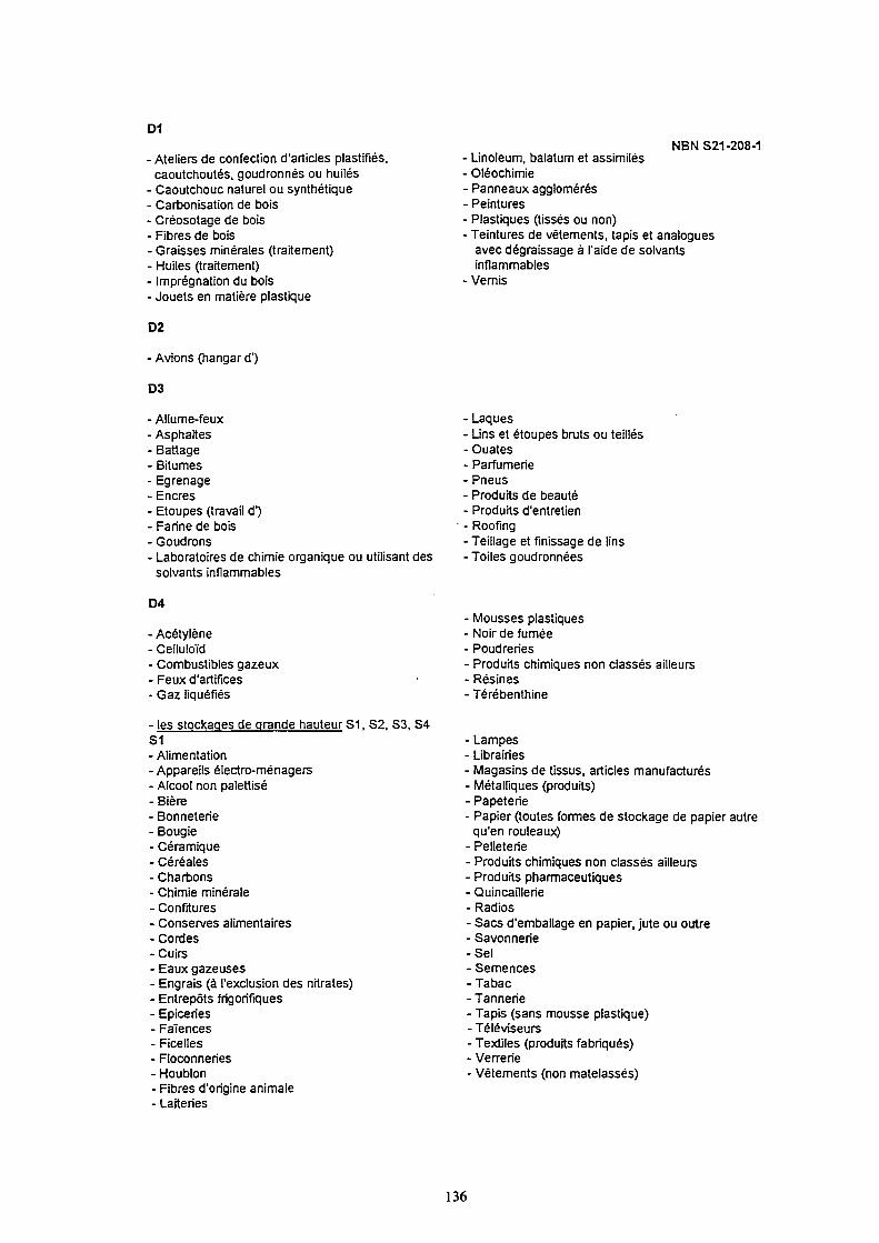
D1
- Ateliers de confection d'articles plastifiés, caoutchoutés, goudronnés ou huilés
- Caoutchouc naturel ou synthétique
- Carbonisation de bois
- Créosotage de bois - Fibres de bois - Graisses minérales (traitement) - Huiles (traitement) - Imprégnation du bois - Jouets en matière plastique
D2
- Avions (hangar d')
D3
NBN S21-208-1 Linoleum, balatum et assimilés
■ Oléochimie ■ Panneaux agglomérés ■ Peintures ■ Plastiques (tissés ou non) • Teintures de vêtements, tapis et analogues
avec dégraissage à l'aide de solvants inflammables
• Vernis
- Allume-feux - Asphaltes - Battage - Bitumes - Egrenage - Encres - Etoupes (travail d") - Farine de bois - Goudrons - Laboratoires de chimie organique ou utilisant des
solvants inflammables
• Laques ■ Lins et étoupes bruts ou teilles • Ouates • Parfumerie ■ Pneus Produits de beauté
■ Produits d'entretien ■ Roofing • Teillage et finissage de lins
• Toiles goudronnées
D4
- Acétylène - Celluloïd - Combustibles gazeux
- Feux d'artifices - Gaz liquéfiés
- les stockages de grande hauteur S1, S2, S3, S4 S1
- Alimentation - Appareils électro-ménagers
- Alcool non palettisé
- Bière - Bonneterie - Bougie - Céramique - Céréales - Charbons - Chimie minérale
- Confitures - Conserves alimentaires
- Cordes -Cuirs - Eaux gazeuses - Engrais (à l'exclusion des nitrates) - Entrepôts frigorifiques - Epiceries - Faïences - Ficelles - Floconneries - Houblon - Fibres d'origine animale - Laiteries
Mousses plastiques Noir de fumée Poudreries
• Produits chimiques non classés ailleurs ■ Résines Térébenthine
■ Lampes • Librairies • Magasins de tissus, articles manufacturés • Métalliques (produits) ■ Papeterie
• Papier (toutes formes de stockage de papier autre qu'en rouleaux)
- Pelleterie
• Produits chimiques non classés ailleurs • Produits pharmaceutiques ■ Quincaillerie ■ Radios
- Sacs d'emballage en papier, jute ou outre - Savonnerie -Sel - Semences - Tabac - Tannerie - Tapis (sans mousse plastique) - Téléviseurs - Textiles (produits fabriqués) - Verrerie - Vêtements (non matelassés)
136

NBN S21-208-1
Les listes des articles des catégories S2, S3 et S4 ne sont pas limitatives, c'est-à-dire que les articles de stockage qui ne sont pas mentionnés précisément ne sont pas automatiquement considérés comme entrant dans la catégorie S1. En général, les articles des catégories S2, S3 et S4 sont ceux pour lesquels l'expérience a montré que ces matières stockées produisent des feux exceptionnellement intenses. L'importance relative ou la nature de l'emballage peut modifier la classification du produit stocké.
S2 - Accumulateurs électriques - Alcool sur palettes - Bandes magnétiques - Barils vides (autres que métalliques) - Bitumes - Bois (industrie du) - Câbles électriques, téléphoniques et
télégraphiques - Cartons plats - Chiffons - Cirages - Cotillons (et petits artifices) - Couleurs - Décors - Décorateurs (articles pour) - Disques - Drogueries - Etoupes - Feuilles de bois sur plaquage - Fibres (en vrac ou en balles, à l'exclusion
de l'alfa) - Foins - Fûts vides (autres que métalliques) - Goudrons - Graisses minérales - Grands magasins (tous produits en réserve
autres que l'alimentation) - Huileries - Jouets - Laques - Lièges
S3 -Alfa - Allumettes - Bâches - Caoutchouc naturel ou synthétique - Cartons ondulés - Celluloïd - Encres - Farine de bois - Feutres - Fibres de bois
- Linoléum et assimilés - Lin, étoupes brutes ou teillées - Magasins à fibres textiles avant filature, à fils - Menuiseries - Meubles en bois - Modèles en bois - Moules en bois - Nitrates - Pailles - Papier (déchets) - Papier en rouleaux (stockage horizontal) - Parfumeries - Peintures - Piles électriques - Plastiques (pas en mousse à l'exclusion du
celluloïd) - Plomberie - Produits de beauté - Produits d'entretien - Scierie - Ship's chandler (articles marins) - Sucre - Tapis avec mousse plastique - Tapisserie (articles de garnisseurs) - Térébenthine - Tonneaux vides (autres que métalliques) - Vernis - Vêtements matelassés
- Mousse de caoutchouc (à l'exclusion des chutes : S4) - Noir de fumée - Papiers enduits - Papiers en rouleaux (stockage vertical) - Papiers asphaltés (stockage vertical) - Pneus - Résines - Textiles (déchets) - Toiles goudronnées ou non
S4 - Mousse de plastique - Mousse de caoutchouc (chutes) - Mousse de plastique (chutes)
- Mousse de caoutchouc en rouleaux - Mousse de plastique en rouleaux - Feux d'artifices
137
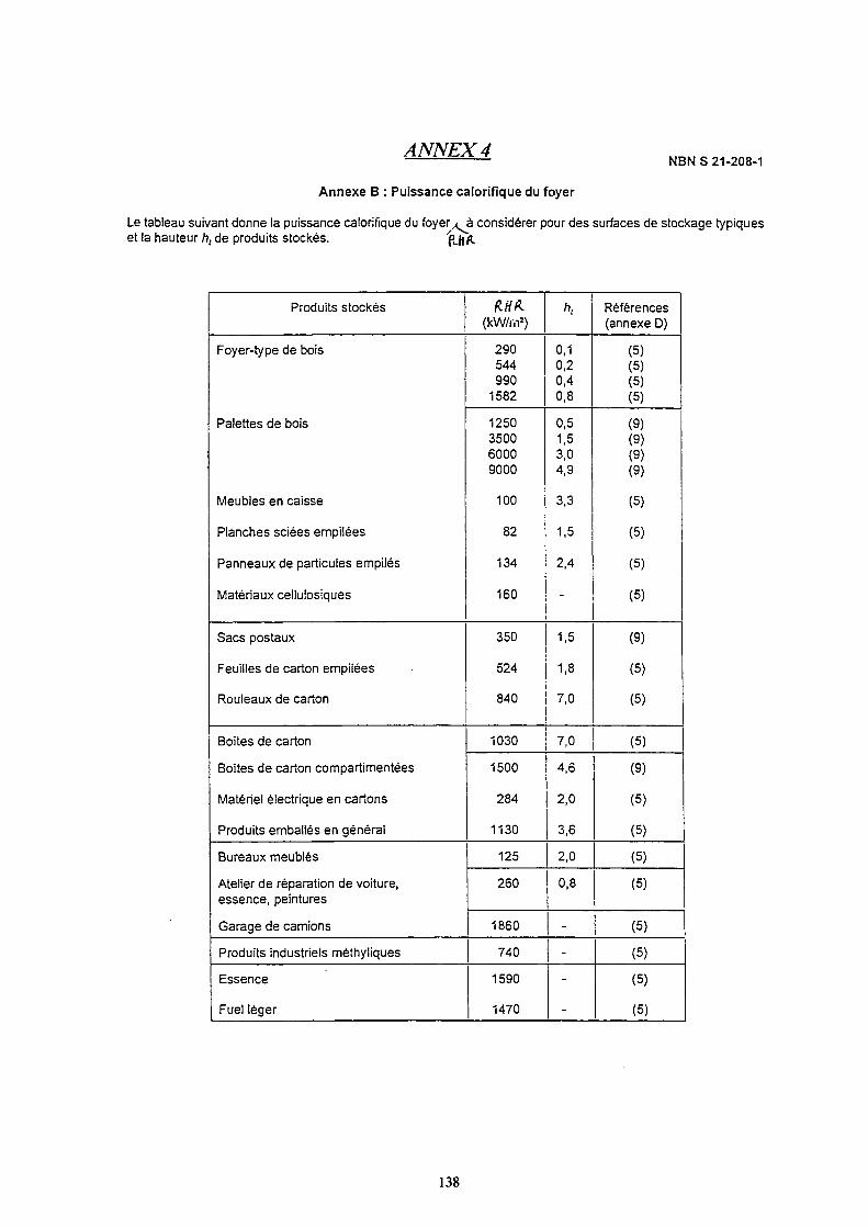
ANNEX 4 NBN S 21-208-1
Annexe Β : Puissance calorifique du foyer
Le tableau suivant donne la puissance calorifique du foyer ,<à considérer pour des surfaces de stockage typiques
et la hauteur h, de produits stockés. (LiiP~
Produits stockés
Foyer-type de bois
Palettes de bois
Meubles en caisse
Planches sciées empilées
Panneaux de particules empilés
Matériaux cellulosiques
Sacs postaux
Feuilles de carton empilées
Rouleaux de carton
Boîtes de carton
Boites de carton compartimentées
Matériel électrique en cartons
Produits emballés en général
Bureaux meublés
Atelier de réparation de voiture,
essence, peintures
Garage de camions
Produits industriels méthyliques
Essence
Fuel léger
RHU (kW/in
2)
290
544
990
1582
1250
3500
6000
9000
100
82
134
160
350
524
840
1030
1500
284
1130
125
260
1860
740
1590
1470
h,
0,1 0,2 0,4 0,8
0,5
1,5
3,0
4,9
3,3
1,5
2,4
1,5
1,8
7,0
7,0
4,6
2,0
3,6
2,0
0,8
-
-
-
-
Références (annexe D)
(5)
(5)
(5)
(5)
(9)
(9)
(9)
(9)
(5)
(5)
(5)
(5)
(9)
(5)
(5)
(5)
(9)
(5)
(5)
(5)
(5)
(5)
(5)
(5)
(5)
138
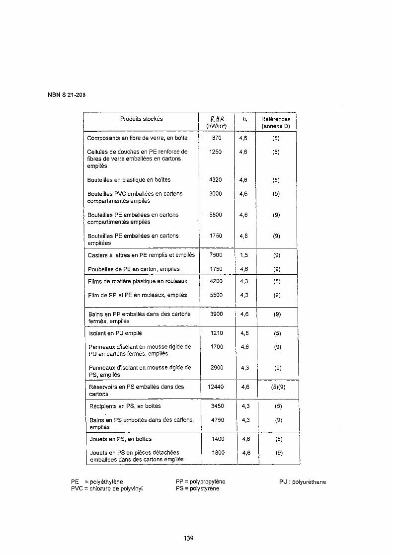
NBN S 21-208
Produits stockés
Composants en fibre de verre, en boîte
Cellules de douches en PE renforcé de
fibres de verre emballées en cartons
empilés
Bouteilles en plastique en boîtes
Bouteilles PVC emballées en cartons
compartimentés empilés
Bouteilles PE emballées en cartons
compartimentés empilés
Bouteilles PE emballées en cartons
empilées
Casiers à lettres en Ρ E remplis et empilés
Poubelles de PE en carton, empilés
Films de matière plastique en rouleaux
Film de PP et PE en rouleaux, empilés
Bains en PP emballés dans des cartons
fermés, empilés
Isolant en PU empilé
Panneaux d'isolant en mousse rigide de PU en cartons fermés, empilés
Panneaux d'isolant en mousse rigide de
PS, empilés
Réservoirs en PS emballés dans des
cartons
Récipients en PS, en boîtes
Bains en PS emboîtés dans des cartons,
empilés
Jouets en PS, en boîtes
Jouets en PS en pièces détachées emballées dans des cartons empilés
RtfA (kW/m
2)
870
1250
4320
3000
'5500
1750
7500
1750
4200
5500
3900
1210
1700
2900
12440
3450
4750
1400
1800
h,
4,6
4,6
4,6
4,6
4,6
4,6
1,5
4,6
4,3
4,3
4,6
4,6
4,6
4,3
4,6
4,3
4,3
4,6
4,6
Références (annexe D)
(5)
(5)
(5)
(9)
(9)
(9)
(9)
(9)
(5)
(9)
(9)
(5)
(9)
(9)
(5)(9)
(5)
(9)
(5)
(9)
PE = polyethylene PVC = chlorure de polyvinyl
PP = polypropylene PS = polystyrène
PU : polyuréthane
139
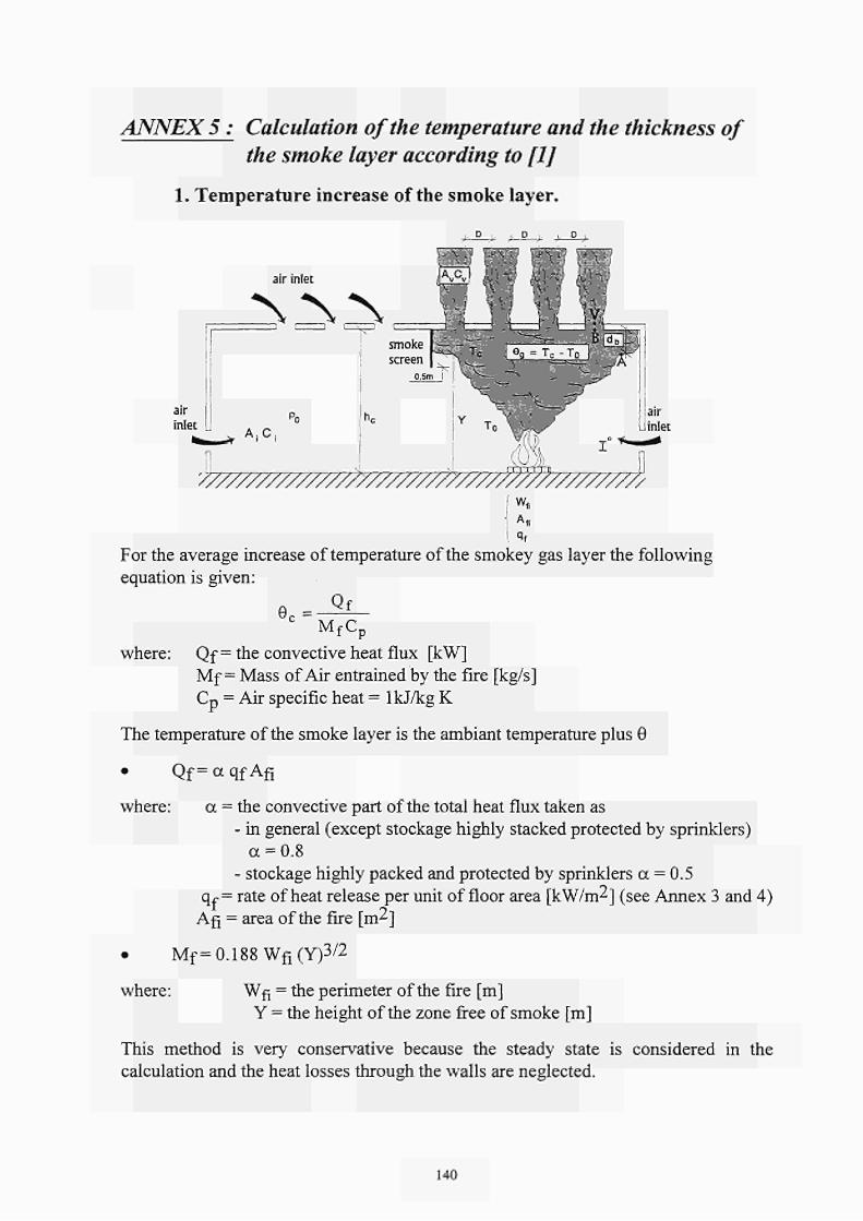
ANNEX 5 : Calculation of the temperature and the thickness of
the smoke layer according to flj
1. Temperature increase of the smoke layer.
■y y u
y y u
.ι-
air inlet
air inlet
N\\
A i C ;
'?//////////////fr/////////////J7ÏÏ9///77777, ν
I wfl
I «'t
For the average increase of temperature of the smokey gas layer the following
equation is given:
e c = ^ -M f C p
where: Qf = the convective heat flux [kW]
Mf = Mass of Air entrained by the fire [kg/s]
Cp = Air specific heat = lkJ/kg K
The temperature of the smoke layer is the ambiant temperature plus θ
• Qf = α qf Afi
where: α = the convective part of the total heat flux taken as
- in general (except stockage highly stacked protected by sprinklers)
α = 0.8
- stockage highly packed and protected by sprinklers α = 0.5
qr-= rate of heat release per unit of floor area [kW/m^] (see Annex 3 and 4)
Ag = area of the fire [m^]
• Mf= 0.188 Wfl (Y)3/2
where: Wfl = the perimeter of the fire [m]
Y = the height of the zone free of smoke [m]
This method is very conservative because the steady state is considered in the
calculation and the heat losses through the walls are neglected.
140
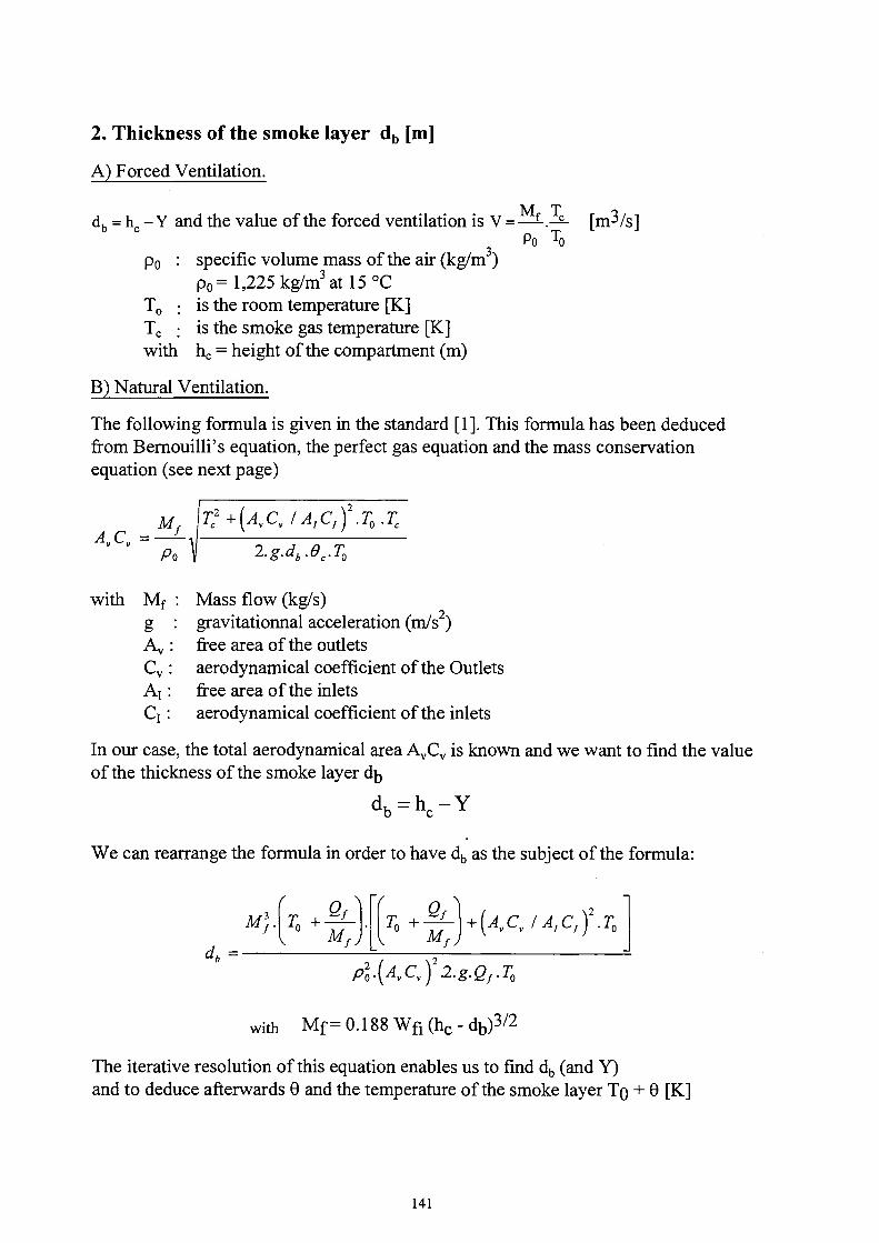
2. Thickness of the smoke layer db [m]
A) Forced Ventilation.
M, X. db = hc - Y and the value of the forced ventilation is V = —ΐ-.-ί- [mß/s] Po το
po : specific volume mass of the air (kg/m3)
Po= 1,225 kg/m3 at 15 °C
T0 : is the room temperature [K]
Tc : is the smoke gas temperature [K]
with hc = height of the compartment (m)
Β) Natural Ventilation.
The following formula is given in the standard [1]. This formula has been deduced
from Bernouilli's equation, the perfect gas equation and the mass conservation
equation (see next page)
A„ L·,,
¡Tc2
+(AVCV IAtCt) .T0.TC
2.g.db.0c.TQ
with Mf
g : Av :
Cv :
A j :
Q :
Mass flow (kg/s)
gravitationnal acceleration (m/s2)
free area of the outlets
aerodynamical coefficient of the Outlets
free area of the inlets
aerodynamical coefficient of the inlets
In our case, the total aerodynamical area AVCV is known and we want to find the value
of the thickness of the smoke layer dD
d b = h c - Y
We can rearrange the formula in order to have db as the subject of the formula:
M) Ά + M, d„ =■
T0 + Qf
M f J
+ (AVCV/A,CI)2.T0
P20.(AVCV) 2.g.Qf.TQ
with Mf= 0.188 Wfi (hc-db)3/2
The iterative resolution of this equation enables us to find db (and Y)
and to deduce afterwards θ and the temperature of the smoke layer TQ + θ [Κ]
141
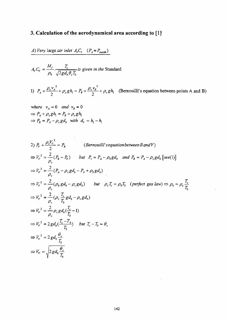
3. Calculation of the aerodynamical area according to [1]
A) Very large air inlet A,C, (PA = Pouside)
AyCy = ——. , c is given in the Standard Po yl2gd
B0cTo
2
1) PA + rc'A +pcghl = PB + °'B + pc ghj (Bernouilli' s equation between points A and B) PcVA , „ A t „ n , PcvB
where vA = 0 and vB = 0
PA+Pcg^ =PB+Pcgh2
PB = PA-Pcgdb with dy = h2-hl
2
2) Pv + C'V = PB (BernouillVsequationbetweenBandV) PYV
=> Vy2 =^(PB-Py) but PV = PA-p0gd„ and PB = PA- pcgdb [see{\)\ Pa
=> Vy2 = —(PA -pcgdb -PA+ p0gdb) Pc
2 Τ => Κ2 = — ( A ^ * -Pcgdb) but pcTc = p0T0 (perfect gas law) ^p0=pc^
Pc τ0
^Vy2=—(Pc^gdb-Pcgdb) Pc To
=>K2=—Pcgdbé-l) Pc το
^V2 =2gdb{^±) butTc-T0 = Øc
•Ό
=>Vy2=2gdb^
"-■Κ
142
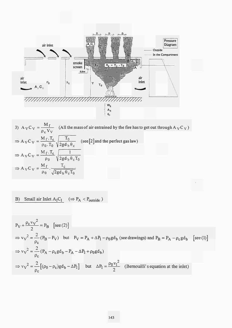
air inlet
\N\ •"XT? Í Ã 1 / í ñ 1 ? í 3 7 ^
Α Ί Γ Ι i-iioü .U.Y .1.) M-¿'
A fe te pι
.Ί Vi l V i íM
air inlet
A ¡ C ¡
v//////////////////////?/////ffifr/////////,
Pressure Diagram
Outside
In the Compartment
W,
I Mf
3) A V C V =
=> A V C V =
=> A V C V =
=> A V C V =
M. (All the mass of air entrained by the fire has to get out through A v C v )
(see [2] and the perfect gas law)
Pc V V
M f .T c
Ρθ·Τ0
Mf.Tc
Po
M f
Po -β
Ι τ 0 \ |2gd be c
1 1 \Í2gdbecT0
TC
g d b e c T 0
B) Small air Inlet ArCr (=> PA < P0utside )
Pv + Pc
vV = PB [see (2)]
2 2 v v = — (PB - Pv) but P v = PA + APj - p 0 gd b (see drawings) and PB = PA - p c gd b [see (1)]
Pc
? 2 v V = — (PA - P c E d b - p A - Δ Ρ ι + p 0 gd b )
Pc
2 2 v v = — [(Po - Pc)Ecib - ΔΡΤ ] but APj = ° (Bemouilli' s equation at the inlet)
Pc
143

air inlet
*\y Í TT? [ftf/ I j v7
W m if fe j Pressure ' Diagram
Χ Ν Ν V* ^ ^ ^] Outside
In the Compartment
v//////////////?///////////////ffi?//////////. [w,
ΔΡΤ
2 2 v„ = — (Po-Pc)gdi
_ 2TC
PoTo .
_ 2/?0rc
PoTo
2TC
_2TC
A>v
2
2"
ƒ
( P O - ^ S K - ^ 2
(i-f)^-^
[(^V.-f j^-\_
2 27c v / 27c 0
■»ο ^ -Ό ■'«
2 , TcVt
Vy +-£-
J
τ ■Ό
2
^0
w/ze« /JC = PoTo
but p0T0=PcTc =>£-& W ν / = 4 τ ^ ν -2o Α Λ Q Po
(All the mass of air which gets in, gets out)
Pc AICI Po T0
144
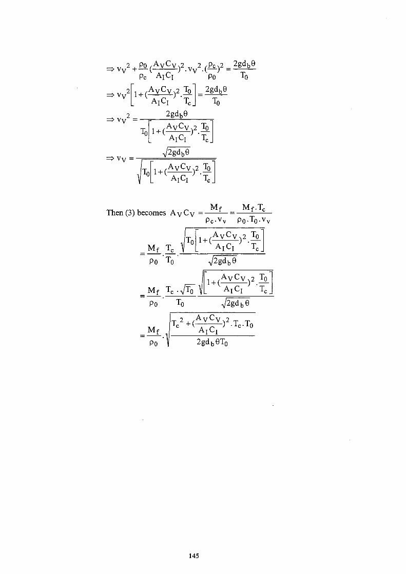
Λ7 2 , PO , A y C v , 2 „ 2 ,PCN2 _ 2gdbe vv + — (. ; ^ ) ·νν ·(.—; - — ~ —
V y
Pc A I C I
! , / A V C V N 2 Jo_ AT C
VV 2 =
(M V 2gdb9
Po 2gdb6
T0
l0
v v =
j | (AyCy 2 JO . ^ A j C r / X
V2gdbe
2 , /-AyCy 2 Jo . ^ A T C / X
Then (3) becomes Ay C y =
Mf Tc
M( Mf.T c
p c . v v po-T0 .vv
Po TO
M f Tc
V2gdbe
2gdb0T0
145
ANNEX 6 : Simulation of the Fire tests of the "Parc des Expositions, Paris"
1. Introduction
Two consecutive tests have been realised in a exposition hall, the "Parc des Expositions" (Paris) ; the first on May 18m 1994, and the second on May 20 m 1994. The aim of these tests is to determinate the gas and structure temperatures in different zones, the gases composition and velocity in horizontal openings during fire.
The hall IB volume is the following : 144 χ 65 χ 28 m (L χ 1 χ h). Around this volume, the first 14 meters of height were not closed, and were adjacent with a volume extension, not exterior but sufficiently large to consider it as such.
The roof truss was separated from the hall by a horizontal screen situated at a height of 26 meters. The screen was composed with some plates without thermal isolation, and some roastings. Horizontal openings enables to evacuate smoke.
1.1 Burning load and fire conditions
The burning load consisted of wood pallets (Europ type, dimensions 1200 χ 800 χ 130 mm (L χ 1 χ h), about 30 kg/pallet).
A. Test 1
The load mass was 3458 kg with 133 pallets and was distributed in 8 packs. These packs were grouped by 2, and the four groups were separated by partition walls. These partition walls made of wood, of the same type of those used in the separation of exposition stands (height of 2.5 m).
Two compartments were ignited firstly, and the fire has been propagated to the two other compartments in a natural way. The compartmentation wall failed 6 minutes after ignition.
B. Test 2
The load mass was 3562 kg with 120 pallets and was assessed in 10 packs, uniformly on burning surface. The load mass loss was measured by weighing. All packs were ignited at the same time.
146
1.2 Results
All results will not be shown in this report. During tests, temperatures were measured by thermocouples. About 50 thermocouples were placed in the hall, at 4 sections of the hall. These sections are shown in figure 1. The position and numeration of thermocouples are indicated in figure 2.
A. Test 1
Some temperature results are shown in figures 3, 4 and 5. We can notice the failure of the compartmentation wall, and the ignition of the two others packs (no ignited at the beginning ) giving the second peak of temperature. Radiative fluxes were measured at a distance of 9.5 and 15 meters of the load centre. These fluxes are shown in figure 6.
B. Test 2
Temperatures are shown in figures 7 to 21. Radiative fluxes were measured at distances of 8 and 6.5 meters of the load centre. These fluxes are shown in figure 22. Velocity at horizontal openings was measured with pitot anemometer, but results are not easily improvable. The load mass was measured by weighing. The temporal evolution of this mass is shown in figure 23. The load mass evolution stopped 10 minutes after ignition, because a part of the load fell out of the weighing plateform.
In this test, it seems that the hot layer was homogeneous. The results of thermocouples show an homogeneity of temperatures at 22 meters height and in the plenum, despite a superiority in the plenum just above the fire and certain irregularities in temporal evolution. It seems that these irregularities proceeded from circulation zones and fresh air incomes for the fire development, especially during the maximum pyrolysis rate. The neutral surface height seemed to be equal to 20 or 21 meters. Indeed, the temperature at 22 meters was always close to the hot layer temperature. However, below (for example thermocouple n°13 at 18 meters), the temperature was much more lower. So the hot layer thickness was about 7 meters.
We can remark that thermocouples situated above the woodshed gave temperatures around 800°C at 10 meters above the ground, 500°C at 14 meters, 300°C at 18 meters, 200°C at 22 meters, 100°C at 27 meters and 60°C at 28 meters. This shows that the hot layer was not exactly homogeneous as we said hereinabove, and its temperature was more greater just above the fire. However, these different locations were not numerous
147
and 100°C or 200°C are lower than flame temperatures (1000°C) which may introduce gradient much more problematic. This indicates that the height of hall IB of Parc des Expositions, Paris, was sufficient in order that it did not exist direct interaction between flames, hot layer and supporting structures.
So, the test of the Parc des Expositions is a case which corresponds well to the use of the program FIRST. This program is described in the next section.
Numerical Simulations
2.1 Pyrolysis Rate
In the test 2, the woodshed was composed with pallets dimensionalised 1200 χ 800 χ 130 mm. But the standard dimensions, which we find in literature, are 1220 χ 1220 χ 140 mm. We will consider that the woodshed was made with standard pallets. Various authors have worked on pyrolysis rate formed by such a load. In our case, we will refer to data of Babrauskas [7j8]5 and Krasner \s\ on woodsheds of pallets. Their data can be reduced in an empirical formula. This one is a correlation between the maximum heat release rate and the piling height of pallets
Qmax = 1450 (1 + 2.14 He) (1 - 0.027 M)
where He : the piling height, M the moisture constant, Qmax the maximum heat release rate.
In this equation, it was assumed that the heat of combustion of wood is 12 MJ/Kg. This is this value that we will use in our simulations. We will consider that wood is dry, so M = 0. In the test 2, the piling of 12 pallets gave a height of 1.68 m, and thus a heat release of 6.29 MW. The correspondent pyrolysis rate is 5.5 Kg/s.
A standard curve of temporal pyrolysis rate evolution has been deduced from numerous tests made by Krasner. This standard curve applied with the maximum pyrolysis rate calculated hereinabove can be compared with the experimental pyrolysis rate. Indeed, the measurements of the load mass loss allows the calculations of pyrolysis rate by a temporal derivation. This comparison is done in figure 24. We can remark in this figure that the ignition time is lower in the test than in the Krasner's evolution. This is due to the fact that in the test, it has been introduced an inflammable liquid which has reduced the ignition time.
148
In order to take into account this ignition time reduction, we have approximated the pyrolysis rate curve by analytical functions with a sooner growth. These functions are the following :
between 0 and 330 seconds q = 5.5 (t/330)°-5[exp(t*0.69/330)-l]
between 330 and 580 seconds q = 5.5
between 380 and 910 seconds q = 5.5 [(910-t)/330]°-5[exp((910-t)*0.69/330)-l]
This corresponding evolution is shown in figure 25 with the experimental shape.
2.2 The Zone Model : First
First is a program developed by Mitler et Rockett in 1987 of the National Bureau of Standards'^. FIRST (FIRe Simulations Technique) is a modified version of the Harvard Fire Code V of Emmons and Mitler!2,3'4!. It is based on a large number of physical parameters. It takes into account at a same time four objects in combustion and five openings. The modélisation of three types of object is possible :
- a pool fire, - a growing fire, - and a burner fire.
The last is the most classical fire. It represents an equipment fire. This one will be used in our simulation. The thermal transfers are done by the resolution of conservation equations. Thus, the program needs all physical and thermal properties of wall and gases. These various thermal transfers are done between different parts of the room. Each part is considered homogeneous. First considers only five zones where interactions (mass and energy exchanges) exist. These five zones are :
- wall (lateral wall, ceiling, floor), - outer gas, - the flame considered as a cone, - the inner gases near the floor (cold layer), - the inner gases near the ceiling (hot layer).
The contact surface between hot and cold layers is called neutral surface. The exchanges between these five zones are modelled. The temporal evolution of temperature of each zone is given. The flame and the plume is controlled by an apex angle and the object surface in combustion.
149
The convective exchanges between the flame and the others zones only depend on the pyrolysis rate which gives the heat release rate (convective and radiative heat release). This is again the pyrolysis rate that controls the system evolution. The hot (upper) and cold (lower) layers are separated by the neutral surface of which the height depends on the room openings (exit of burned gases and admission of cold air) and the pyrolysis of objects.
Both zones are considered homogeneous. This assumption reduces largely the application domain of First, but also its complexity. This induces the fact that it exits a correlation between the room volume and the burned gases formation (depending on the pyrolysis rate). A too large volume will give a temperature strongly attenuated between the fire impact location and the extremity of the room. A room with a low height will create a direct impact of flames on the ceiling, with a flame temperature higher than temperatures of burned gases distant of the flames. The resultant hot layer will not be homogeneous. Moreover, a too low level of the ceiling would give recirculation's zone disturbing the formation of a layer having a height spatially constant.
Thus, it is necessary to apply First with a volume having a correlation with the pyrolysis rate, but also correlated itself. The second test of the "Parc des Expositions" of Porte de Versailles in Paris in May 1994 is an application case of First. So we have simulated the second test and we have compared the experimental measurements of the test and the simulation results. The following section presents these comparisons.
The considered openings have to be studied attentively. They manage the numerical resolution of the problem (energy loss, height of hot layer and oxygen needs). First considers that the fire can not use the oxygen of the hot layer for its combustion process. Two important points of First have to be mentioned : firstly, the room must be rectangular; secondly, the thermal properties of walls, objects and gases are constant.
2.3 Results
The simulation with First has been done using the pyrolysis rate shape defined by the three mathematical formulations described hereinabove. The mass heat capacity is 12 MJ/Kg (value used by Krasner), and an opening corresponding to the half of lateral surface (L=144 m, inferior half).
The results of the simulation are compared to the test measurements (see § 1-3 .b).
150

A. The hot layer thickness
The figure 26 shows the temporal evolution of hot layer thickness.
B. The hot layer temperatures
The figures 27, 28 and 29 show the comparison between temporal evolution of hot layer temperature and thermocouple results at three different sections. In figure 27, is also indicated the temperature obtained with the pyrolysis rate close to the reality. This pyrolysis rate is shown in figure 25. This one has been taken with four segments (specified by black lozenges). This comparison can show the sensibility of First to the pyrolysis rate.
C. Radiative fluxes
The figure 30 shows the comparison between experimental radiative flux and the simulated radiative flux on a target located at 6.5 m from the pyrolysing object centre (flux n° 1). Numerically, are shown fluxes from flames, from walls and from hot layer (the two last fluxes may be neglected). It is also shown in this figure (thick dash) the radiative flux obtained in assuming 20 % radiative loss of heat release in an isotropic way. This value of 20% has been obtained by D. Joyeux in lab scale diffusion flames studies!^]. So this radiative flux on the target at distance d = 6.5 m is the following :
0.2 Q/(4 . π · d2) - Q is the rate of heat release.
2.4 Discussion
The neutral surface height is higher in our calculations than in the test; 25 meters in the simulations during the maximum of temperature and 21 meters in the test. But the mean temperature of the simulated hot layer is higher than the mean temperature in the test. It is clear that the numerical hot layer is more confined. Perhaps, the air quantity engulfed by the plume or entrained by turbulent mixing through the neutral surface in the hot layer is underestimated by First. But the comparison is not so bad. Some points must be notified.
Numerically, we have not taken into account the plenum existence which disturbs exchanges into the hot layer, and the roof horizontal openings which introduce an energy loss (this may compensate the fact that we don't take into account the plenum).
151

Moreover, the hall IB entrance has not been taken into account too. Its effect is also visible in experimental results. Temperatures at section C-C show a fall when the pyrolysis rate is maximum, so when fire needs a maximum air entrance. This air comes from the inferior lateral openings but also the entrance.
Nevertheless, the comparison for heat fluxes on a target are worse. Indeed, the radiation flux on a target has been measured during test by a radiation-meter located on a floor. First can simulate an inert object with unity of emissivity, receiving the flames radiation and located at 6.5 meters from the centre of the pyrolysing object (distance of the radiation-meter in test 2). Three fluxes reach the target : radiative flux from flames, radiative flux from hot layer, and radiative flux from walls. These three fluxes have been compared to experimental radiative flux (figure 30). It is clear that walls and hot layer radiative fluxes can be neglected. Only the flame flux interacts with the target but it is 6 times greater than experimental flux and it seems to be constant. The reason of this last observation is that First does not consider it exits a fire growth in the physical space. First considers that the flame temperature is constant and equals to 1260°C. The parameters which are able to change the radiative flux from flames, are the size of the pyrolysing objects and the variation of absorbent species in the gases. The size of the pyrolysing object does not vary in our case -we have considered the case of a burner fire (and not a growing fire) and experimentally the burner size did not vary - and the second parameter allows weak variations as it can be seen in figure 30. So radiative flux on the target is overestimated and might overestimate the target temperature. It is important to remark that the target can be a part of the supporting structure or object more sensitive to temperature.
3. First's limits and conclusion
As we can see in chapter 1, the test of the "Parc des Expositions de Paris" is an application case of the program First. Its volume seems to be in correlation with the woodshed fullness. This has permitted the hot layer homogenisation. A strong fire would have introduced the interaction between flames, hot layer and steel structures. A low fire should have given a response time to the hot layer extension too low to give homogeneousness. It would have been necessary to use a multicompartments model (multi-compartments with fictive partitions).
152
In the case of the use of First, the number of parameters taken into account is sufficient to give results satisfactorily. Of sure, the pyrolysis rate problem always exists, although it is reduced in our case. Indeed, wooden pallets fire are well surrounded by Babrauskas and Krasner works. The results of figure 28 show that First is sensitive to the pyrolysis rate, and that temperature evolution are totally relied to the temporal pyrolysis rate evolution.
These results must permit to calculate the temperature distribution more precisely in steel structures. However, temperature calculations in structure proof situated around the fire have not been done. Temperature of gases around structure proof is low and convection exchanges do not represent sufficient energy required to the temperature rise given in the test. Temperatures of 200°C have been measured. This rise is due to the flame radiation. But First overestimates this flux, so would overestimate the structure temperature. We think that it would be interesting to change these flame radiation calculations in First, in order to have a better estimation. For example, it would be interesting to introduce a flame growth, function of heat release rate. It exits empirical formulas which give the visible flame height from the heat release rate, for example by Heskestad (11) :
L f= -1.02 D + 0.235 Q 2 / 5
where L^ is the flame height (m) D, the burner diameter, or woodshed diameter (m)
and Q, the heat release rate versus the time (kW)
This formula may introduce a better approximation of the flame size and may permit a better estimation of the radiative flux on the target. It exits also formulas which give temperature and velocity in fires versus the heat release rate. These formulas may also be used for modelling the fire (it is important to know that First actually uses a constant temperature (1260°C) in the fire).
The use of wooden pallets for this test has permitted us to consider the works of Krasner in order to evaluate the pyrolysis rate. This rate has given a good correlation with experimental results. It may be interesting henceforth to use similar woodshed (wooden pallets), their pyrolysis rate having a good approximation.
153
REFERENCES
1/ H. Mitler and J. Rockett: "User's guide to First, a comprehensive single Room model" NSBIR 87-3595, National Bureau Of Standards, Gaithersburg, MD, 1987
2/ H. Mitler: "The havard Fire Model". Fire Safety Journal, 9 (1985) 7-16
3/ H. Mitler and H. Emmons: "Documentation for CFC V, The fifth Harvard Computer Fire Code" NBSGCR 81-344, National Bureau of Standards, Gaithersburg, MD, USA, 1981
4/ H. Mitler and J. Rockett: "How accurate is mathematical fire modeling?" NSBIR 86-3453, National Bureau of Standards, Gaithersburg, MD, USA, 1986
5/ M. Curtat et P. Fromy: "Prévisions par le calcul des sollicitations thermiques dans un local en feu" Cahier 2565 du CSTB, Mars 1992
6/ CTICM: Research Report n°94-R-242
7/ V. Babrauskas: "Heat release in fires" Elsevier applied science, 1992
8/ V. Babrauskas: "Burning rates" The SFPE handbook of fire protection engineering, 1988
9/ L.M. Krasner: "Burning Characteristics of wooden pallets as a test fuel" Serial 16437, factory mutual research corp, Norwood, 1968
10/ D. Joyeux: "simulation des essais du CES J. Perrin à l'aide du logiciel Nat" CTICM - INC - 95/33 - DJ/IM, Nov 1994
11/G. Heskestad: "Fire plumes" The SFPE handbook of fire protection engineering, 1988
12/ CTICM: Research Report n°94-R-187
13/ D. Joyeux: Thesis "Etudes expérimentales et numériques de la production des suies dans des flammes de diffusion turbulentes" - Rouen, Nov. 1993
154

exufoire 1 ι ι
__.νθ
Ι"0
t
τ
Ι Ο
CN
oi m CN
>o
3 !
ι—r
; ι-
ENTREE OU
BATIMENT
Ψ SECTION E-E
SECTION C-C
SECTION B-8
SECTION A-A vi ::v2 □ ::v3::v4
SECTION D-D
ι τ
Í . . 1 J2JL _32¿.
¿5
t
•A D O
E ■o CN
.
C
a
I
LI
in : BUCHER
ΓΤ
S:
NOTA : cotat ion en m
STATION ■ d'ESSAIS
wm C T I C M
v,„ DIMENSIONS DU BATIMENT ET IMPLANTATION DES SECTIONS DEMESURE
Utmonoe«· PAIC DES EXPOSITIONS DE PAIIS figure
155
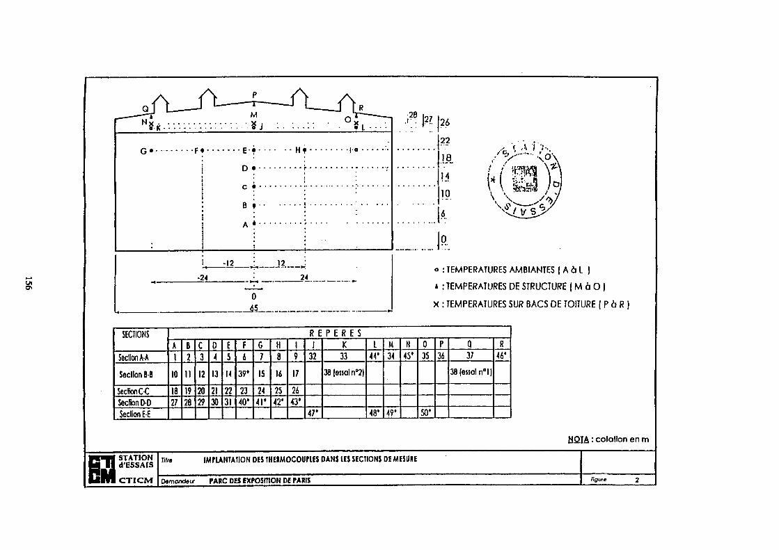
Ui
G ·
STATION d'ESSAIS
CTICM
F · · ■ E · ·
D ·
c ·
B f
A *
H · •|e
j * 127 26
22
il
tø
!9
ó
't Λ :;;·..
V ' 'fei
\ v
Jft -12
_».-*_.___ 12
-24 24 o : TEMPERATURES AMBIANTES | A à L )
* : TEMPERATURES DE STRUCTURE ( M à O )
X : TEMPERATURES SUR BACS D E TOITURE Ι Ρ à R
SECHONS
Section A-A
Section 6-8
Section C-C
Section DO
Section E-E
R E P E R E S
A
1
10
18
27
B
2
II
19
28
C
3
12
20
29
D
4
13
21
30
E
5
14
22
31
F
6
39'
23
40'
G
7
15
24
41·
H
8
16
25
42'
1
9
17
26
43*
J
32
47'
K
33
38 (essai n°2)
L
44*
48·
M
34
49'
N
45'
0
35
50'
Ρ
3«
Q
37
38 (essai nel )
R
46*
MOJA : cotation en m
mie IMPLANTATION DES THERMOCOUPLES DANS LES SECTIONS DE MESURE
Demander PARC DES EXPOSITION DE PARIS figure

Temperature (°C)
60
10 15 20 25 30 Time (min)
-KTC6 X:TC7 D:TC8 A :TC9
STATION d' ESSAIS CTICM
Title Ambient temperatures in section A-A TEST
Demandem Pore des Expositions de Paris Haute
157
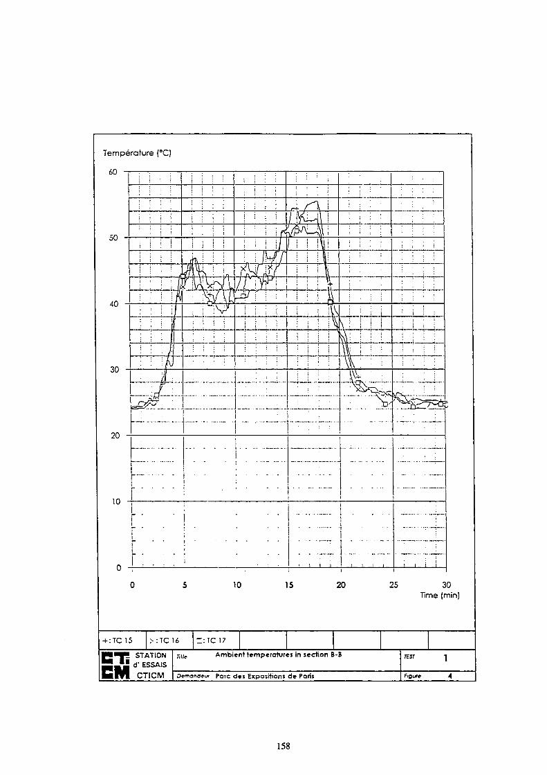
Température (°C)
60
10 15 20 25 30 Time (min)
+:TC 15 >:TC 16 Z:1C 17
STATION d' ESSAIS CTICM
Lile Ambient temperatures in section B-B TEST
Demandem Parc des Expositions de Paris figure
158
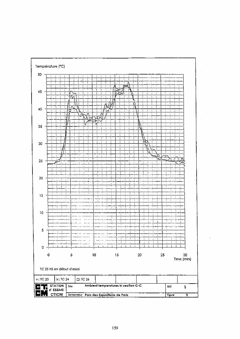
Température (°C)
50
10 15 20 25 30
Time (min)
TC 25 HS en début d'essai
+ -.TC23 X:TC24 D:TC26
■ STATION 1 d' ESSAIS
CTICM
Ambient temperatures in section C-C TEST
Demandeur Parc des Expositions de Paris figure
159
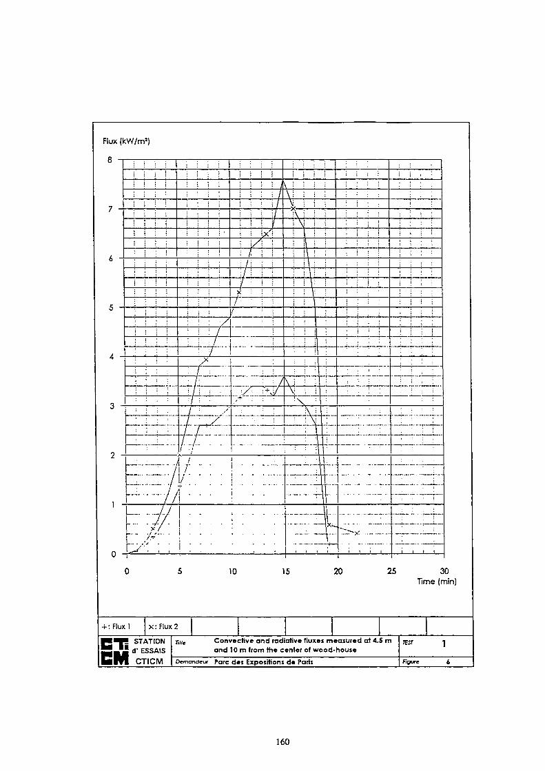
Flux (kW/m2
10 15 20 25 30
Time (min)
+ : Fluxl χ : Flux 2
■ STATION
2 d' ESSAIS
CTICM
Ti/le Convective and radiative fluxes measured at 4.5 m
and 10 m from the center of wood-house TEST
Qgmondgur Porc des Expositions de Paris figure
160

Temperature (°C)
900
800
700
10 15 20 25 30 Time (min)
-KTC2 X:TC3 D:TC4 A:TC5
STATION d' ESSAIS CTICM
Tille Ambient temperatures in section A-A Teif
Demandeur Porc des Expositions de Paris figure
161

Temperature (°C)
10 15 20 25 30
Time (min)
+ :TC6 X:TC7 D:TC8 A:TC9
■ STATION 1 d" ESSAIS
CTICM
ΤιΗΐ Ambient temperatures in section A-A TEST
Demandeur Parc des Expositions de Paris Figure S
162
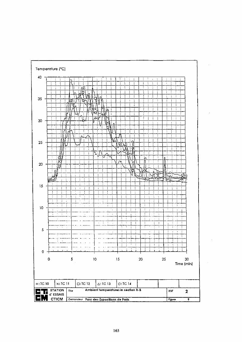
Temperature (°C)
10 15 20 25 30
Time (min)
+ :TC10 x : T C l l D:TC12 A : T C 1 3 0:TC14
■ STATION 1 d' ESSAIS
CTICM
Title Ambient temperatures in section B-B TEST
Demandeur Parc des Expositions de Paris figure
163
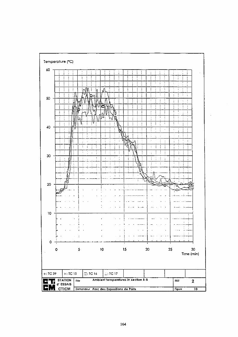
Temperature (°C)
10 15 20 25 30 Time (min)
+ : T C 3 9 >: :TC15 Z : T C 1 6 ¿.:TC 17
STATION d' ESSAIS
C T I C M
Tille Ambient temperatures in section B-B TEST
Demandeur Parc des Expositions de Paris figure 10
164

Temperature (°C)
40
10 15 20 25 30 Time (min)
+ :TC18 X-.TC19 Q:TC20 A : T C 2 1 0 :TC22
STATION d' ESSAIS
CTICM
Title Ambient temperatures in section C-C TEST
Demandeur Parc des Expositions de Paris figure ^ 1
165
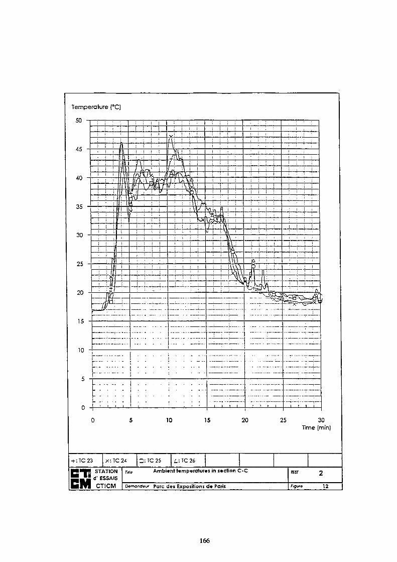
Temperature (°C)
50
10 15 20 25 30
Time (min)
+ -.TC23 X-.TC24 2j:TC25 ¿_:TC26
f i l " STATION
■ d' ESSAIS
CTICM
mie Ambient temperatures in section C-C TEST
Demandeur Parc des Expositions de Paris figure 12
166
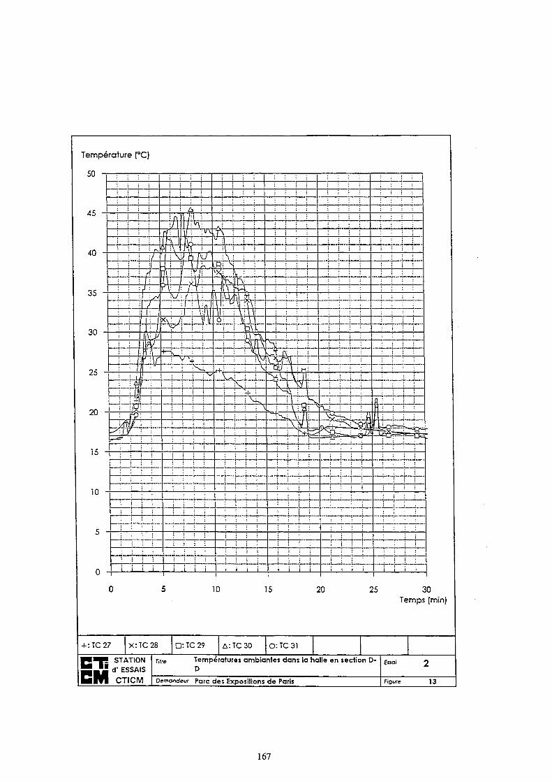
Température (°C)
50
10 15 20 25 30
Temps (min)
+:TC27 X-.TC28 D:TC29 A:TC30 0:TC31
f W " T P STATION
d' ESSAIS
CTICM
Températures ambiantes dans la halle en section Ο
υ Essai
Demandeur f OTC des Expositions de Paris Figure 13
167
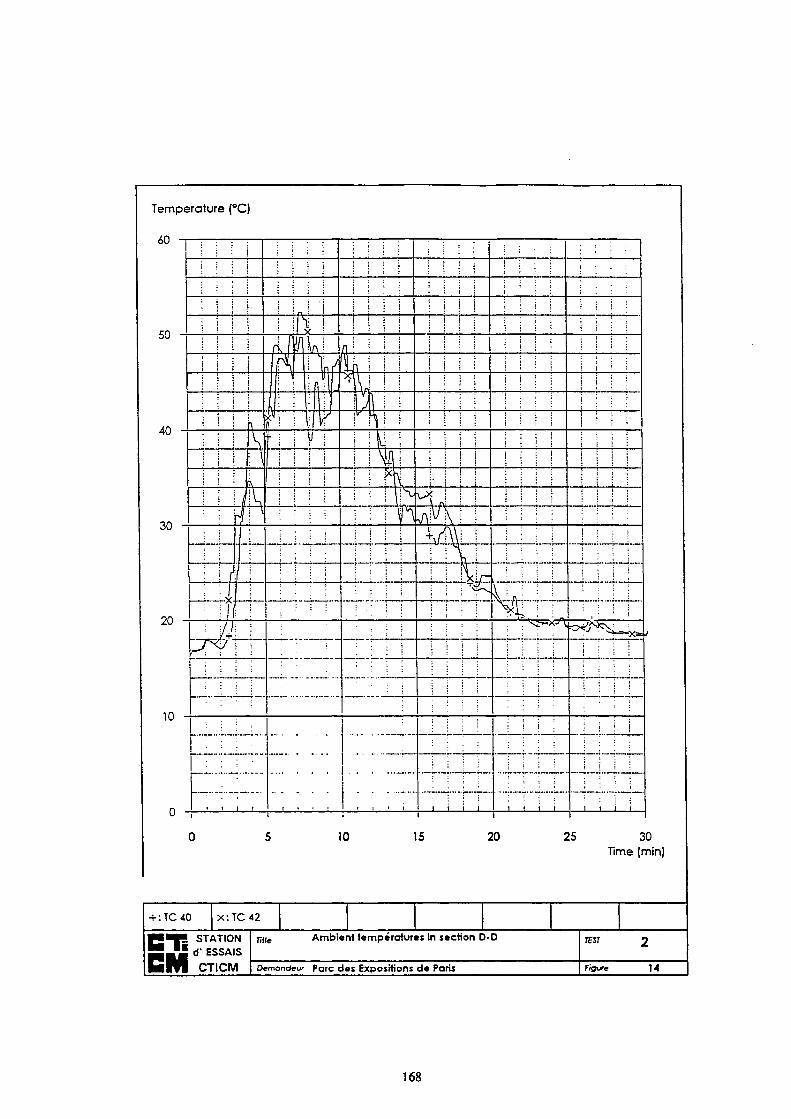
Temperature (°C)
60
IO 15 20 25 30 Time (min)
+:TC40 χ : TC 42
P I T I STATION
* J _ ^ d' ESSAIS
C M ci ■|CM
nue Ambient températures in section D-D
Demandeur Parc des Expositions de Paris
TEST
figure
2
14
168
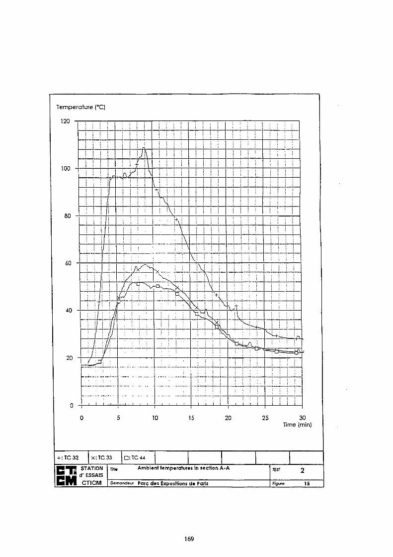
Temperature (°C)
120
10 15 20 25 30 Time (min)
+:TC32 x:TC33 D:TC44
STATION d' ESSAIS CTICM
mie Ambient temperatures in section A-A TEST
Demandeur Parc des Expositions de Paris figure 15
169
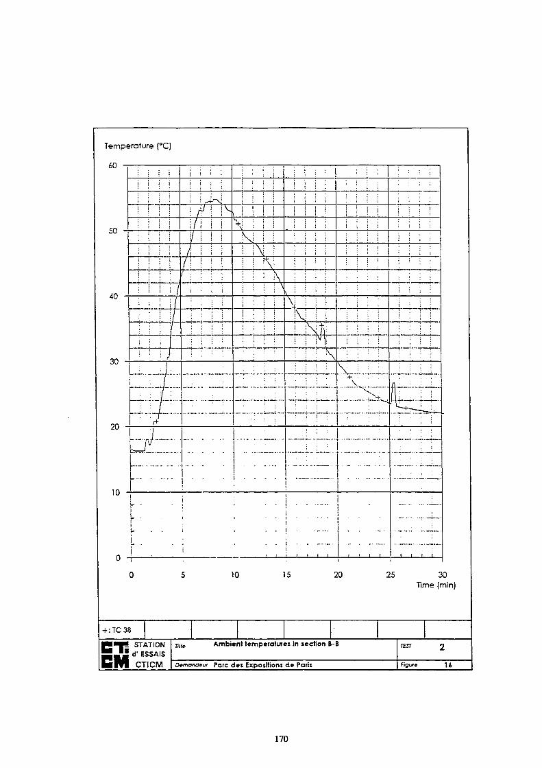
Temperature (°C)
Ò U
òu
4U
OU
Zv "
: ¡ ; ¡
: '· : ;
I M I 1 | j |
l i l i M M
1 i ί ι ; i ;
! i I i
I I I ! / Ι ι M /
\j f M M
i / ; I:
: ;/
>
MII
j i i
i r+-xi
l/l ! ! V | | |
J I M / M i l
: i ;
1 1 1 ! i i > :
_-..
— - - ■ - - *
ί ï ï !
L. ! M . S ¡ : : :
+! j ! i
KJ 1 i i !M i ι ¡ H- j
: ! Κ ! ! i M í Î t τ
I ! I I
" ■ " ' ■ - ■ ■ "
i i 1 t
I I I ! ¡ I l ; M M
i i i i
! ! ! ;
ν ι ι ì ;
V J M
M 1 ! ] N
i i:
11 ή i ¡ \ : \
: ; 1 ;
—;—i—ι—;—
;...__—
■ - ■ - - -
M M • !
; '
M l i 1 ! 1 !
• ; ; ! Ι | Ι 1
; ; ; I i i i
i i i !
V i i ; \.„
: ; ..
rr
_v...... 'S ,
- r
...... i........
; · - ■ ■
I 1 0
1 ' I
• ■ i :
■ ·
Γ j ί
i- · ■ i · · ■ ι — ! ·
Γ -i ■ ! Η 0 -i
: — . , , , , , , ι , , , ,
!
¡ i i i
I i i i
MM
i i
i l i ]
i i i i
i ! !
; ' '
; ■ ! ;
• f l — - - - ■
■Tffi-·
4 ~: -!—r—
■ r * ι
10 15 20 25 30
Time (min)
+ :TC38
W*m
ft STATION
■ d' ESSAIS
CTICM
Tille Ambient temperatures in section B-B
Demandeur Parc des Expositions de Paris
TEST
figure U
170
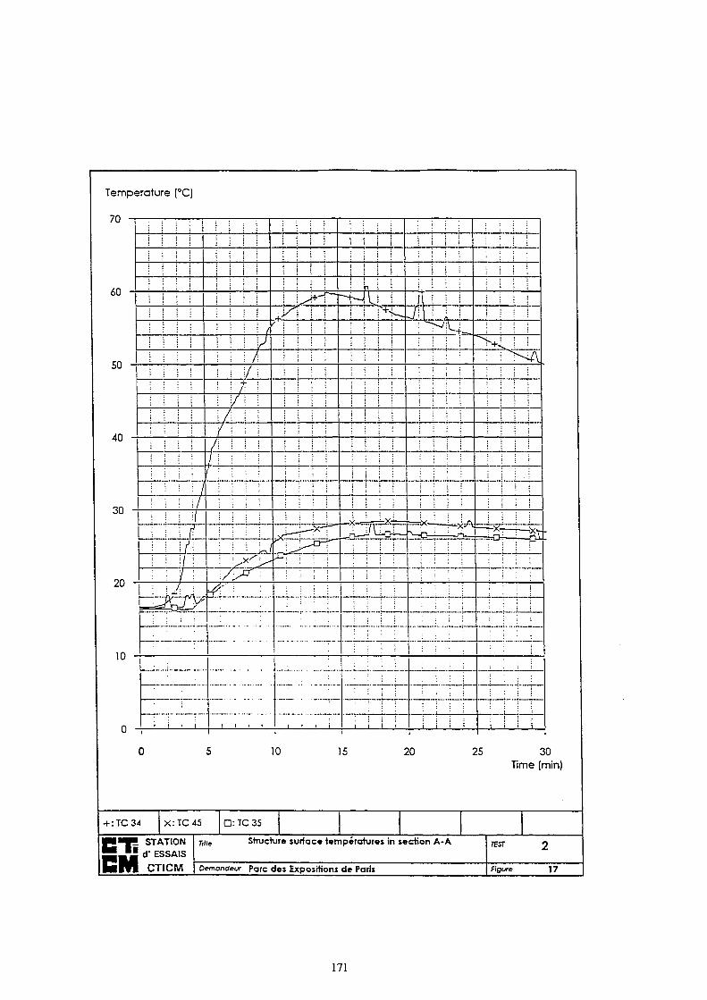
Temperature (°C)
70
10 15 20 25 30 Time (min)
+ :TC34 X:TC45 D:TC35
STATION d' ESSAIS CTICM
T¡ne Structure surface températures in section A-A TEST
Demandeur Porc des Expositions de Paris figure 17
171

Temperature (°C)
10 15 20 25 30 Time (min)
+ :TC49 x : T C 5 0
STATION d' ESSAIS CTICM
r¡ne Structure surface temperatures in section E-E TEST
Demandem Parc des Expositions de Paris figure 18
172
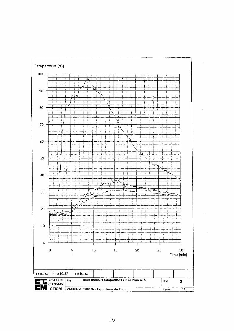
Temperature (°C)
100
90
80
70
60
50
40
30
20
10
M.
t Hi
TTtí*
5
Skl .Χ
S SU
A&=
y /•-H-r
V..~
prœ-
■-«AH,
t ι t I
rrX> V=T~X~
^ .
-r=X— S^g>
10 15 20 25 30
Time (min)
+ :TC36 X:TC37 0:TC46
■ STATION
m d' ESSAIS
CTICM
Title Roof structure temperatures in section A-A
Demandeur parc des Expositions de Paris
TEST
Figure 19
173
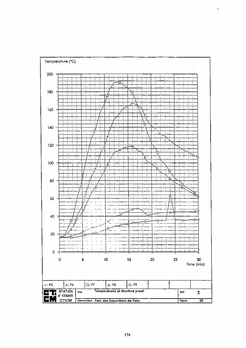
Temperature (°C)
200
10 15 20 25 30
Time (min)
+-.P5 x:P6 D : P 7 Δ : P8 Ο: P9
■ STATION 1 d" ESSAIS
CTICM
Tille Temperatures of structure proof TEST
Demondeur Porc des Expositions de Paris figure 20
174
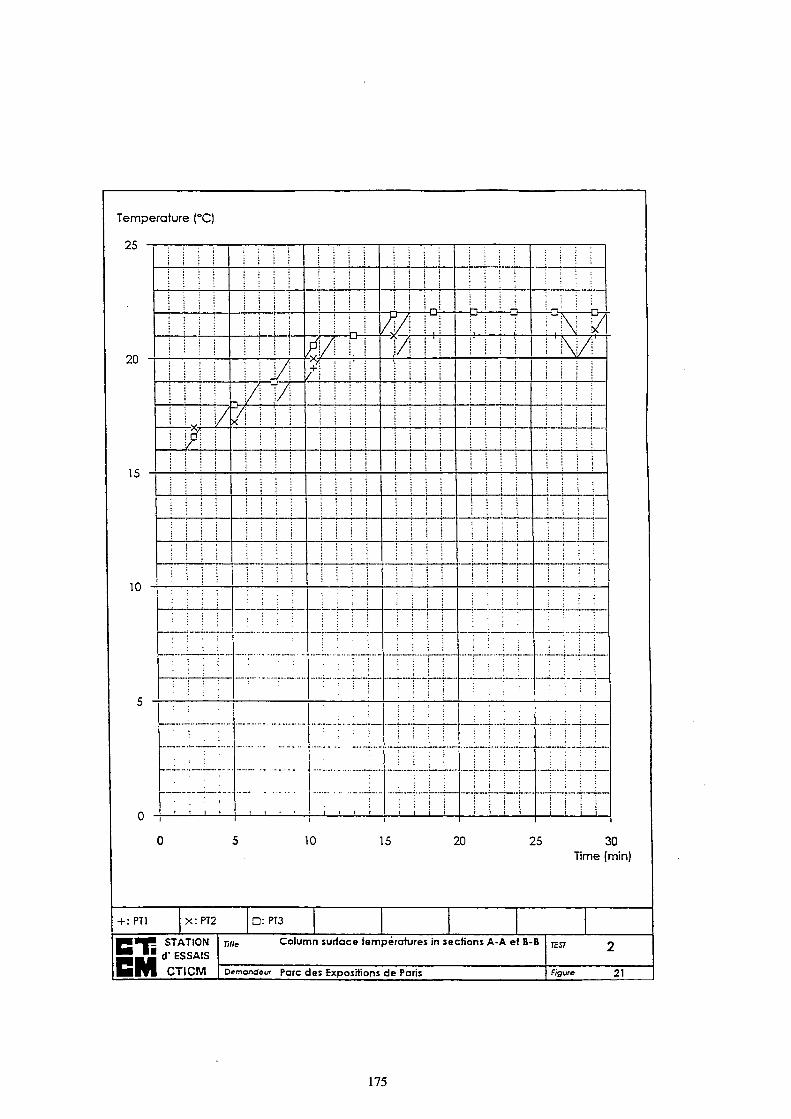
Temperature (°C)
κο —
zv
io
o ~
0 -
l i l i
ί ;
\ \ \ \
\ \ \ \
y '/ 1 di .
\ ; :
ι t ι ι ι
I j I ! M l i
M M
i ii/l ι/! V/l
yl i 1 i
ί
i ' ' · '
i i i ! l i l i 1 I j I ! 1 i - ¡ /
φΐ\ 'Y. : : ' : -H : !
/ I l i !
M M
; I ;
ί i ί
i ί ;
; - ι
h · ' ί I I
i i i i
l ì I I
4^ Γι VI i l
i ! i
! i i
1 1 1
i i i i
i i i !
l i l i
' ; : '
' i i i
:- - '
: \
¡ :
l i l i
1
' i i i
MM
:±:
I i i i
MM l i t i
M | i
MM ,
i : : ■
I I I I
Mil
; i i I
. , I :
■ i
j ! i
i i i i
i i i ;
¡ i i
!
MM
:
: ! : :
i i i i
10 15 20 25 30
Time (min)
PT1 x:PT2 □ : PT3
STATION
d' ESSAIS
CTICM
Column surface températures in sections A-A et B-B
Demandeur Pare des Expositions de Paris
TEST
figure 21
175
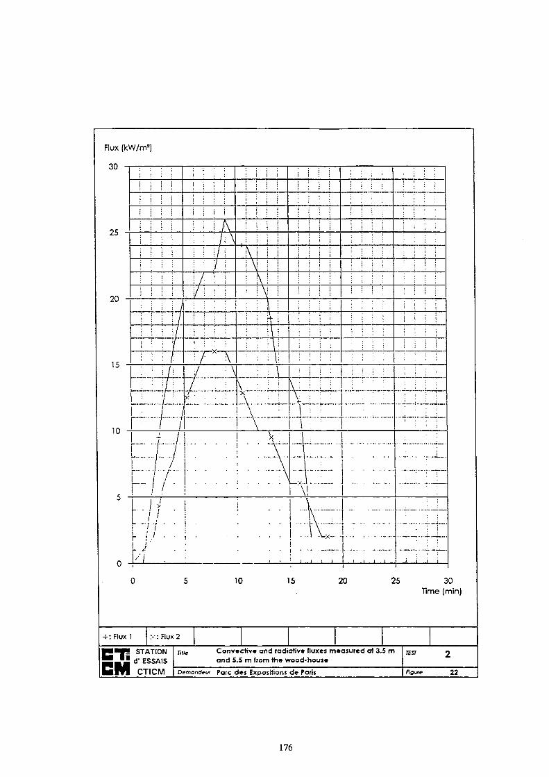
Flux (kW/m
30
25
20
15
10
i i i i
MM l i l i
; ; i 1
i i i i
i M ι / M M /
i i i i / I ! I if
I M /
i i i / !
; : ι/-M Li
r Η pf/ Γ / / '
! j ! 1
1 I ; !
i i i i
! M f\ ! i 1 /l \ i ;
i/| Μ i 1
! /s '
i i |
MX / ■ _ Λ
/ ^
i i i i
I M I
! i ! ¡ ' ; ί
' I I I
i \[ i i κ ! V :
M l i ! ix ; ! ! Π i ; ;
¡ j
: M
M \ j
L i-i \ \ : i !
X
• p m \__;
! \
':::.\\\ i \ 1
-. . / r . ι : I
--■/ ·■ M ' - i J ■ M
ι ;
M . . ' ; : :
1
; ·
| 1 | i
Mil i i i i
1 I ΐ i Ì I
■ i i ;
¡ i í i
i i i i
MM
: · :
V M : .. V i ! +
: ·
¥ ■ I I I I
! ! M : 1 i ;
l i i l
M i i
i i i i
• ί
I I I I
I M I i Ι Ι ί
i i i i
M M i i i i
M l ! M M M M
— ,.,—1_.
—--: ; --·--
* * ■ ;
10 15 20 25 30 Time (min)
+: Flux 1 χ : Flux 2
STATION
d ' ESSAIS
CTICM
Tille Convective and radiative fluxes measured at 3.5 m
and 5.5 m from the wood-house
Demandeur Parc des Expositions de Paris
TEST
figure 22
176

Mass (kg)
4UUU
ooUU
oUUU
Zbvv
ZVVV
lOUU
i i i i
— b j ! Λ
; : +: 1 i K i
i M k ! i i ι \ \ \ \ \
s
i i i :
i i i i
i i i i
i i i i
i i i i
i l l :
i i i :
i i i i
'· \ \ '
i i M
i i i i
i i i i
; ι j ;
i i i i
i i i i
i i i i ! :
■i i i i i
\ i M i
\ \ i \ : i
. \
1 I \i 1
! Ν i
M !\! i v
; ; i ;
i i :
i
¡ i i i
•— ----...
M~ :
i i i .
1
i i i ;
;
■ ;
; ¡
i i i i
I M I
I i i i
i : i i
i i i i
ι Ί ι i i i i i
i
i i ;
i 1 ! . i
-—-
1 1 1
■ í i !
l i l
i l í ;
i ! i ί
MM I i i i
; -
j ; j ;
i j ï i
M l i
;
: ¡ :
i i i i
I l i !
i l i !
i
I i i i
i i i i
■·· τ—M—
i t i i
i i ' ί
i i i i i i i i
i ; : i i i i
i i i i
i i i i i i i i
i i i i
; ■ ; i
1
: ί ! ¡
i i i
i i i i
i '■ i i
¡ i i
i i i 1
'i i i i
l ' i !
! i i
i i i
i i i i
i i i i
; :
M i l
i i i
i
i i i
i ;
ï : ¡ !
: :
i i :
!
i i i i
i ' ; !
i i i i
10 15 20 25 30
Time (min)
+ : Mass
STATION
d' ESSAIS
CTICM
mie Wood-house load mass loss
Demandeur Parc des Expositions de Paris
TEST
figure 23
177
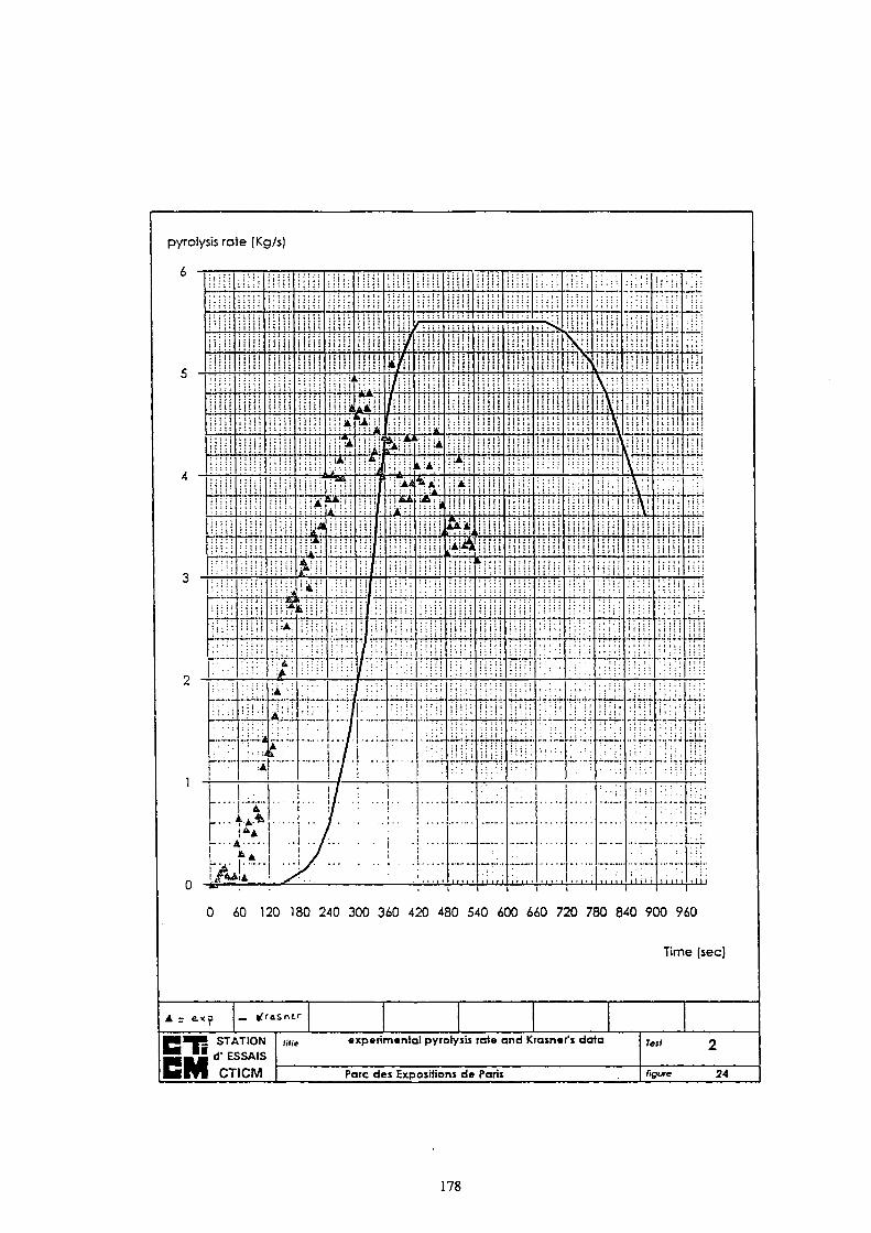
pyrolysis rate (Kg/s)
5 -
0 ~
4 -
o
Ζ -
0 -
i|!jl
i l i ¡I
i i i 11
ίίΙΠ
iiii!
I i i i : i i i i :
jiiil
Hill
. . . . . .
1 Γ" p::; 1
: ;.
i j i ' í
: iiil!
Mí
' : : ': '
i Ì ! I !
M : : j ί :
:;
M M ; ■
: M
■ ■ ' .
i i i i i
3
íjíjj
un! i i i i ;
Nili
¡ I i i i
! ! i i i
IM;
i 1 i i i
: ! i i i
iiili
Hil! M
i ; : ; i
ï ! | j 1
i l i l i
■ ! ! ί ! i j 1 !
¡ l i l i
I{|||
i:*
A
.LiÁli.
áí«i ΗΜΙΜΠ
IÜÍ*
i: A.
i.
A ;■:
Á; i
'
t
L
: ! ■ ■ j
:
iiii! ¡ i i i i
i i i ü
i μ
¡ i i i ¡II*
ittü :ili
*τ55-
KA::~
A ' .
Ini!
1
iilli
i i iv i
t i l i t
lilt! ïlii! ; i i i ;
i': j j ! j
A*il frrrr j ; j i U
liiÀI
: · ; li
i i i i !
Ill 11
i í /
*¿
/iiii
y f · i i i i /
i lili
!! l/l j ι
I
Ί
: / :
...I
I :
i ...
i-¡Ai
:;££'
A
! 11 i 1
':! !
M ;
i;
I
n±-:..¡ .
i i i i i
M ¡
r
i i i l i
¡üll | l¡||
jllj j
, r,'m
)m k'A'.i
* A Í M Í A !
m i 1 i 1 i. : 'i I Ι 1
jjijj ■ ■ :
: ,\
;
- ■ :í
i Ι ι i i
i
¡M !
S
M ;
! ï 1 ! I
¡ : l
j l lp
i í j i i • M i l
i i i ! !
i;¡) i
i i*: i
; i*j
%
$4 \{['\
1 ; i · i
i i i l i
* '\ '.
: :
i
; Ï : : ί
' . i i i :
m?; • i | { 1 i I ;
1
¡ . i i i ί i ί ι i i i i I i i i Híj
i i i l i
I i i ; ι
! ! ! i ! Liü
MH kj i
• : ; ; ;
:' M
i i i i i
i i i i '
i i i i i
i i i · ' .
M ¡ ;
! i i i ;
i i i i i : i ¡ ; ι
i t i t i
í ! i i i I ! i ! !
! | ï t t
) : .1
i i ! ' ;
! i ! ί í
.;
[ l i f t
' l ' I : j i i ; i
; M :
M :
t tTTÏ
ι
;.;.- ' :
• · ■ :
■: " S,
n m '. : : ·. : Mill
: : : : i
■ ■ ■ • ί ; M ; i
I : : i :
tilli
i i i i i i i l i
i i i . . ; ί : ; :
i i i i ' . i t i ' ;
-•M
•H-
1
i i i ! χ
ί ï t i i
! \J j
; M
■ M '
i u i i
: ;
: ':
! ï i ; i -
-M-4-S-Î
..iii.;
'ΠΙ'
i j I ί ί
¡¡Y : ! ! l\ Ι
: V-
i i '
; .
i i i i '
υ!
i: :
ü
'ni
.-.1 J_
■TT^T'-
— - - .
M ï ¡ :
M M
i;!!!
(ijij
' M '
iüiï l i n i ί i i l j
Λ j ! Λ ΐ
i ¡ j i j
•111
1 j î ! ' : ! ! ! f
: ; : :
i
1 ; i i i
"*" TT"
" " "TT
i l ι i i
; . i
l i i ! ;
i ! !
i ; ;| j
i t i t i i t : i :
Will
j f j 1 i
i i i i !
i i l l i : ! j ι I
ï M M
• ■ M
t i : i i
" * " " "
- · - - - -
' i í i
; ¡ i j
I ί I
hij 1 ί 1 t
ΐ i ί ί
, | j
■ M :
ι : : :
• I ! ·
M' "
' i1
;
; ί ; !
• ' ¡ j
;
:;
j j ;
TTT]
l i t t
0 60 120 180 240 300 360 420 480 540 600 660 720 780 840 900 960
Time (sec)
A - £*p — tfrosntr
STATION d" ESSAIS CTICM
experimental pyrolysis rate and Krasner1 s data
Parc des Expositions de Paris
Test
figure 24
178
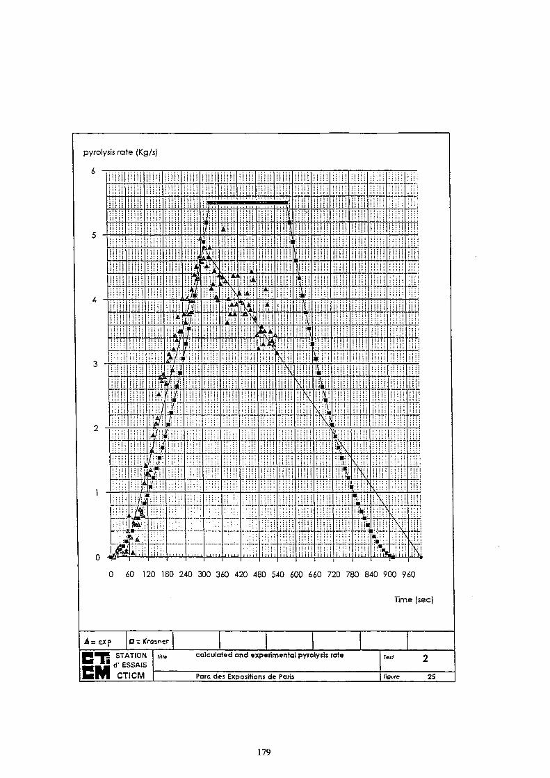
pyrolysis ra te (Kg/s)
0
0
4
3
ζ
ι -
0 -
ii
: i i i i
Mi i
■ Ml
i i i i ;
Hill
¡ M;
iiiii
Mi
i ; ! ; ;
i i i l i i ■ ; ■ ;
——;-
' ;
i ;'
-;-;-
,j¡ft
M i l
i i i ί i
i : i i i
l i l i !
ï i ! i i
iM: ί ί ί ί ί . i i ; i i i ; i i t i : : :
illll
i j i j i
i i i i i
" M
- f - : -—r
i
i , i , i i i i i ' : : ■ / ·
i i i / i
A ... B—..
f* Ί * ! 11
M
¡|!JÍ
i ! ' i i
IIHI
i i i i i
l i l i ! i i i i i
":;;i
: . : ;;
I ÍA
"il i" /
Ύ A/
ir 1 Í/Í
^ ■ i:
Β - j
i M i ¡
MI '
. M
i i i i i
M i
" l i l i
í t i l i
: ! 1 : i
A
i M
-Ai í .
Φ tiu/ : Π ' β is/ i' iLüí
F:
.w . " i ; :
ìli : i ; i ; ; ; ! ;
i i i i i
i i i i i
M I :
i i i i i
i i í i i
: i :'
~7~H
' 'Úit
á II' ffi f t. i i iL
i ■
i . , ; .
i i i l i
::'.:': _ ' '
-
1
' i , ; .
í k m «A— Nu * * i i: Π' ■ '
:'Å
4 ■, 1 1 *
i i i i i
M; Í
i i : i !
i M' i t i l i
i i i i i
: :,.
i ■ · ' I
.
! ι " : 1
: M
• ! 1 ! Τ
; i; :'
l i l i-ί 1 1 ί i
iiiii m
> i i ¡ΑΧ
" X A
A
: ■ ' : ;
ί ί ί ί ί i ! ! ! ;
HM
ii i i
-----
.i : ι i.i
ΙΠΠ ' M
'lili i ï ! ; i ·.··.<·. U]U
l i ; ; ;
i i i i
iiihf λ A
ty
* *
: i ii
; : I i
¡ i t i ! I ' l l ! , . ; ■ ;
-
i i i
:;
ι ι τ i '
Iiili i i i i i
UM
:;;::
- · ■;
ï i ! i i
,.,.
lini i i*:;
* :
i ; i i :
í k * • ¡Ufi M \\\\\
i i ■ i i
! ! ! ! ! i I ! ; I
! j 1 i !
i i i 1 :
: . :
: i :
i i · i i
i i i i i
ΙΠΙ
à ü i i ! I l í l f l t i l i l
. ' i l
" '"
Hin
i i i i i
i i 1 i i
! · ! '·
i í j i í
k' i
Mi!
\
1 ! ! ! !
i ! ί ! i
ï i ! ! !
f ; i i i
M ; Í :
• i i i ;
t i i l i
π υ
i . i
mu
M ;
i i j i
i i i i i
lii il
¡H;
[Ui
L! ih
ι-—
l i n «ui IS: S i
ili ■ ^
^ iiii* • : i t i \
. il
i i : ; ;
\ ■
i \ i 1 !
i i H¡
'■ ■ · i i
' i i i i
ί ί ί ί ί
; -
: i ·'
Γ 'i
I I I I
i i i i :
i i i i i ι ; · | :
ì ì ì I ì
hill
; M '
¡ l u i
i ' i : :
l i ! : i
\i : i ; i M'
* í | !
\ ■
M i i i
• Η · : í i j | i>
üiVi i :
i * .
M« ■■ NI
. . . . Λ
■ i :
! ; i | !
i i : : ;
I I 1 I I
: M
i
i i i i i
' ; i i i
i i i i i
; ; M
; ;;
: i | ; ;
i ; j ; ; ! i : : :
i i i i ;
: ¡ : ! i
iiiii
I
ft' t i ! i
> . . ¡v \ l '
; ;■ ; . ¡;¡\!:
11 i iv i i i ! " :::: . U u t ι : i j '
i ¡ ■ · "
l i l i
■ ■ · ; -
Mil
.:
i i i i i
i i i i i
i i i i i
i i i : i
i t ' t i
■ . i . .
i i ! : :
¡i ' i
¡ l i l i
iiiii
: :
·
' ■ i i ;
\ ¡ ·
1 i ' ■
m j ι Λ- i ■ t
m ; : ■
I I I I I
,
s i i l i
ί ί ί ί ί
.... i i i i i
¡ 1 :
: ί ¡ i i
: ! ■ ' ■ ■
: '. ' M
I i i i i
M
-
.. ij ι
í - i i -
m\
; i ; ·
■ ; m ■ '
i i · "
l'.f>
' : l'i
. i i! i
ί i 11 i
; ■
! i Ii !
: ! ! : i
; ; i ; ; • M : !
- ; :
i i i i i ' i ; Î !
' ' :.'
i
. : i
iiiii
i -
; ; i :
i i i i ' l ' I
Ι ί ί ί
i i i i
ili
i ! i i i i i i
' : ■
i i i i
'.'.'.' M
: ι
I
iiii
; : : i i
M';
1 0 60 120 180 240 300 360 420 480 540 600 660 720 780 840 900 960
Time (sec)
4 = ej;ρ Or Kramer
■ STATION ■ d' ESSAIS
CTICM
calculated and experimental pyrolysis rate
Parc des Expositions de Paris figure 25
179
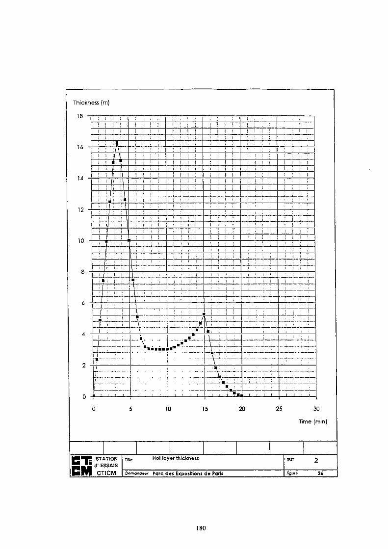
Th ickness (m)
IO
I 6
14 -
12 -
10
O
O
ζ -
0 -
i ;
i ■ ; ■ η ■
i i i/y ι ι A 1
7 Τ 1 I
IM i i i il Ι : ι Ι i i i i
i l i i ι τ ! i | i i j ; I l i i
MI M
i i i i '
i h i . i 7 i i 1 ; i i
i i i i
i i i i
• li M _ M ' !
191 i
!!
l i l !
il ! M 1 :
M M Ι ί
m ι i ; Γ ι
Γ ' i i
-■ -i
j Τ Γ" L. _ ..
II ι ■ ι ι ι
i i i i
i i i i
¡ i i i
' i i :
i Ι ί i i i i i i i i
i i i i
i i i i
i i j
i i i i
i i i i i
i i i i 1 i · :
I i i i i ■ ■■ ι ·
! ; i ;
i ! M T i i i
L L . .... M_......
: m \ \
■. . . . . \ ">■■■■
i i i i
i i i i
i i i !
¡ l i l
ί ί ί I i i i i i i i i
i i i i
ί ί i i ¡ : :
¡ i i i i i i
ί 1 : :
i ; i i
i
;il V ι m
•jA ■«■ 1
i I . , , ,
i
' i i !
i i i i
i i i i
i i i i
i i i i
i :
i i i i
1 i i i
i i i i
. . . .
I ; ί ί i i i i
ι I i i i i \ i i i i ■ i
\ i 1 1 1 V ■■ ■
\ ■
i - -: a ;
-*4-f~ i ■
I I i ~ ¥ «
i i i ■
i : i :
i i i i
! ! !
i i i i
i i i !
i i i i
i i i i
: ¡
i i 1
i i i i
i ; i ¡
I ' l l
¡ i i '
i i i
i i
' i
..._i :.._
■ ,
■ i i i i 1
i j l ;
' i ι :
i i i i
i i i i
ί ! i
i i i i i i i
■
j i i ! ■ i :
1
ί ; i
: i i i
¡ ;
¡ i
—-1—:—i —
. · : · i i i i
10 15 20 25 30
Time (min)
STATION d' ESSAIS CTICM
Tifie. Hot layer thickness
Demandeur Parc des Expositions de Paris
TEST
figure 2¿
180

Temperature (°C)
70
10 15 20 25 30 Time (min)
:TC6 x:TC7 D:TC8 A:TC9 4>5.'n,/Ut· ^ . m. >'*tulof '.» O
STATION d' ESSAIS CTICM
noe Ambient temperatures in section A-A TEST
Demandeur Parc des Expositions de Paris ligure 27
181
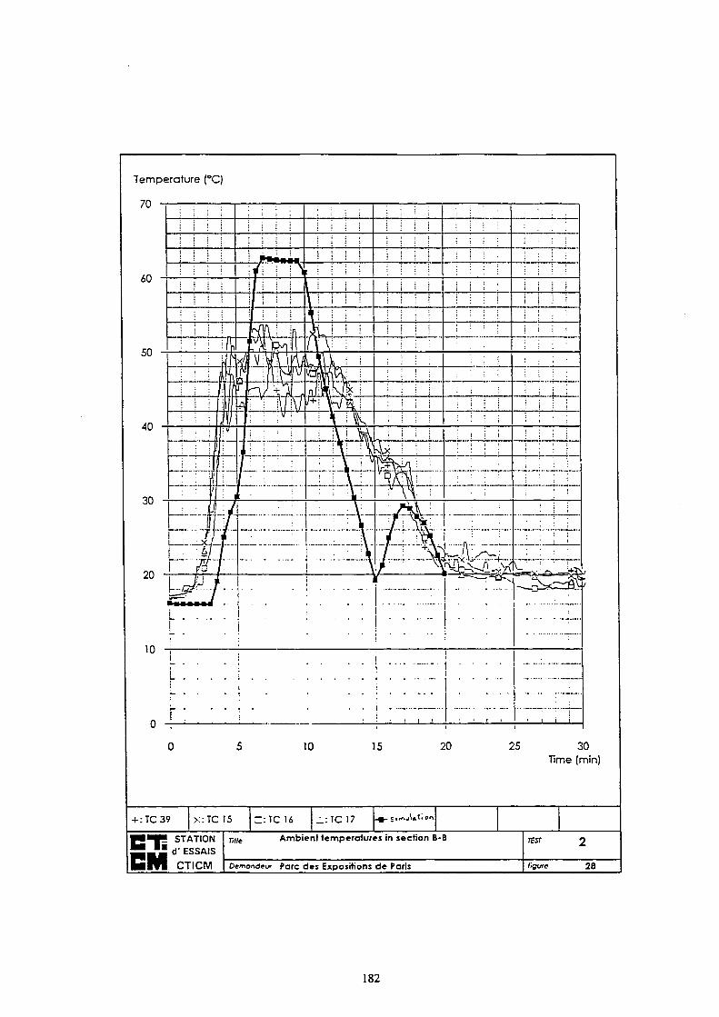
Temperature (°C)
70
10 15 20 25 30 Time (min)
+:TC39 x:TC 15 C:TC 16 . i :TC 17 J>!'«1
! STATION d ' ESSAIS
CTICM
mie Amb ien t temperatures in section B-B TEsr
Demandeur Parc des Expositions de Paris ligure 28
182
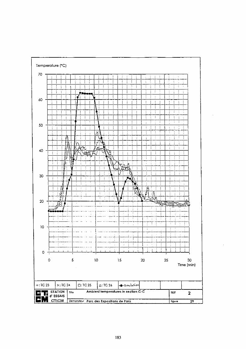
Temperature (°C)
70
10 15 20 25 30 Time (min)
:TC23 X-.TC24 O: TC 25 A:TC26 -SlNwWlOA
STATION S d' ESSAIS
CTICM
Title Ambient temperatures in section C-C
Demandeur Parc des Expositions de Paris figure 2?
183
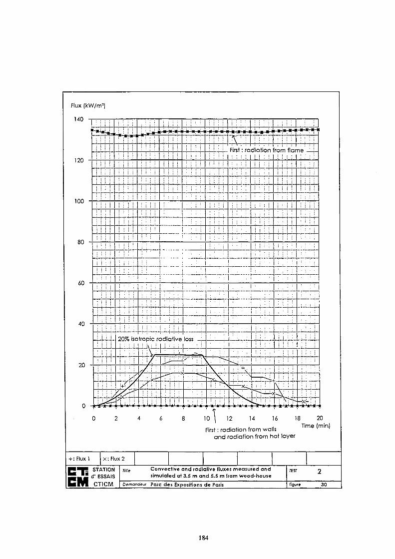
Flux (kW/m5)
140
120
100
80
60
40
20
■-■*-,
t i l l
l i l i
i i i '
; ■ ι
i i i i
I l i
: ■ :
M i i
i i i i
M M
' i .
•*-j*f»=i
: ;
, i
I I I I
j ι ί ;
: ; i
; : ; ;
i ■ i
■ i 1 ;
i : i
20% is c
M I :
: s, i + i / l
'^/O^f
M | : . ■
rjfrpfo^
i i i i
I I I I
i 1 i
: ; I :
ί - » ,» . » «
I i i i
I 1 i i i i i i
I M I
. : 1
i i i i
: i ; i
! : : :
'.'."'.'
! i ;
ι
: ! , ι ·
tropic radiative .}. i\M 1 H i i,
. :
i i i i : i i
l i l i
l i l i
: . | ; : ..
"Φ1 ■ i l l , ,
-a ■ ■ «
First : rar l in t inn f rnm f lnmp i
M i l
i i ! ;
; i
i i i i
l i i '
i
¡ Μ ι
| M | | i M ; | i i M
; | : l i i '
M ; ; í
: i t i
i ; i ;
: ; ; ;
i ! i ;
i i i i
i i i i
, '■ i
■1 M M M
1 i : i i
■ > ' :
•y ;
. \,x¿l
. V . :
\
I i i i i "
i i i i ;
i : 1 - ! M ■ 1 : ;
: . : ; | ; . : ¡ : ; : ; | j j | ;
. | 1 ; | ! . μ ' , : ; | ¡ ¡ ¡ I
■M! M M ; 1 : : i ; - - - ρ . . , i ; ; ; i ; ; ; ;
! 3 S ^ . -
i ; i ; 1 i i ; i - - : - Π , j ,
; ι ?
i :
i !
1 ' : ■ : i i i
L^i i * 1 ï | i > 1
S
Ms
r S ¿
; ι : : : — < l i i '
i M 1 |\[ i I !
"^—_>
H^¡ NIKL
i i i i
; ; ; !
1 Μ I
i i
\ : :
: ' '·
. ■
i i i i
i i i i
¡
M i i
—X-
10 12 14 16 18 20
,. χ- ι π Time (min) First : rad ia t ion f rom wails
a n d rad ia t ion f rom hot layer
+ :F lux l X: Flux 2
rine Convective and radiative fluxes measured and
simulated at 3.5 m and 5.5 m from wood-house STATION
d' ESSAIS
CTICM Demandeur Parc des Expositions de Paris
TEST
figure 30
184

Annex 7 : Simulation 3X
AIR TEMPERATURE CALCULATION
1. Introduction
The four following pages define the simulation 3X which has been performed by the different partners to check the results of calculations of temperatures in the air.
The results of the simulations 1, 2 and 3 had already been described in the previous semestrial reports. As it was appeared that the very small size of the openings constituted a problem for the FLUENT, a new simulation called 3X had been defined.
The chapter 2 presents the main results of LABEIN using FLUENT. In chapter 3, these results are compared with the results of TNO using VESTA and the results of PA-RE using the multi-compartment two zone model ARGOS. Only the main figures are given; the whole comparison has been described in the paper LC44.
185
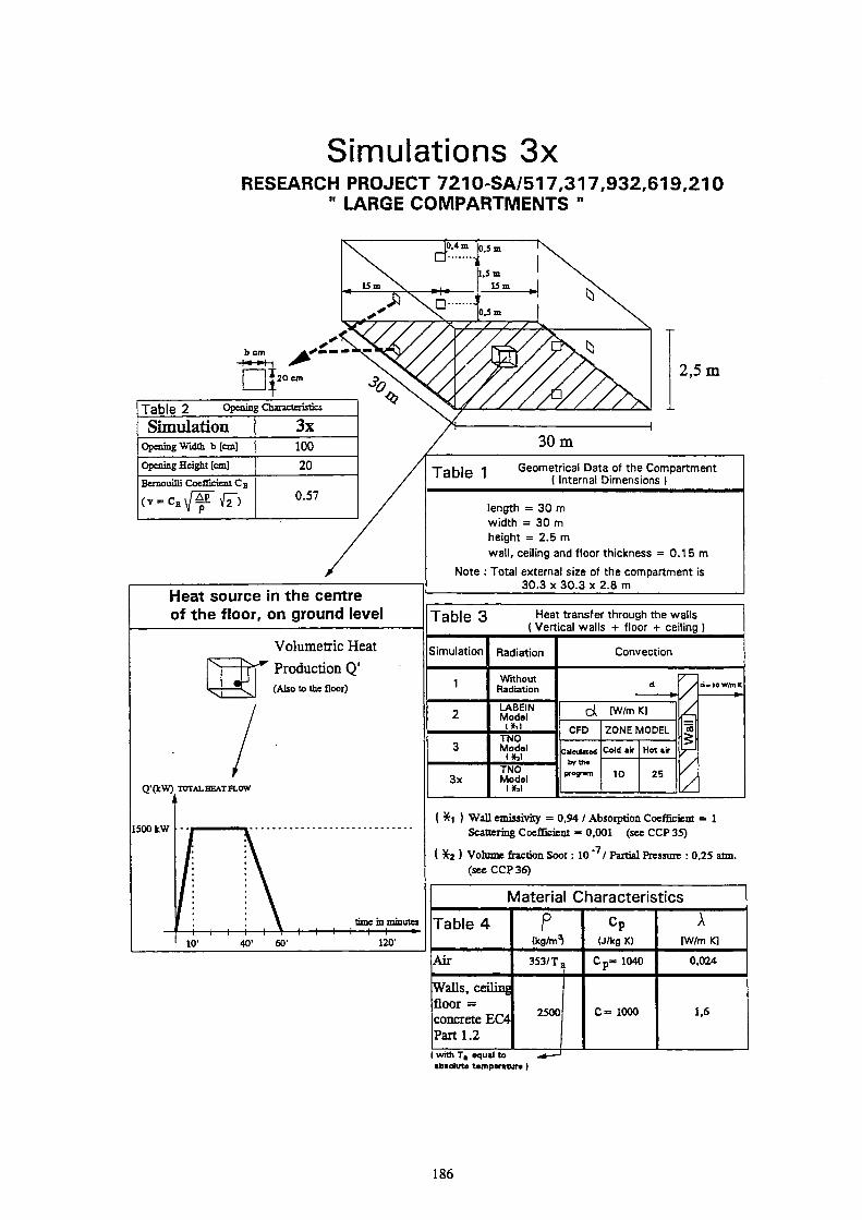
Simulations 3x RESEARCH PROJECT 7210-SA/517,317,932,619,210
" LARGE COMPARTMENTS "
b cm Λ
Π +20 cm
T a b l e 2 Opening Characteristics
Simulation Opening Width b [cm]
Opening Height [cm]
Bemouilli Coefficient C a
3x 100
20
0.57
Table 1
Table 3
Simulation
2,5 m
Geometrical Data of the Compartment ( Internal Dimensions )
length = 30 m
width = 30 m
height = 2.5 m
wall, ceiling and floor thickness = 0.15 m
Note : Total external size of the compartment is 30.3 χ 30.3 χ 2.8 m
Heat transfer through the walls ( Vertical walls + floor + ceiling )
Radiation
Without
Radiation
LABEIN Model
U M
TNO Model
I*,)
TNO Model
l* i l
Convection
d tW/m Kl
CFD
dictated
bytt»
program
ZONE MODEL
Cold air
10
Hot air
25
A ra
( XÏ ) Wall emissivity = 0,94 / Absorption Coefficient = 1
Scattering Coefficient = 0,001 (see CCP 35)
( #2 ) Volume fraction Soot : 10 / Partial Pressure : 0,25 atm.
(see CCP 36)
Material Characteristics
Table 4
Walls, ceiling floor = concrete EC4 Part 1.2
Ρ (kg/πΛ
3 S 3 / T ,
Cp
U/kg Κ)
Cp= 1040
C= 1000
λ IW/m Κ]
0,024
1.6
( with T a equal to
absolute temperature )
186
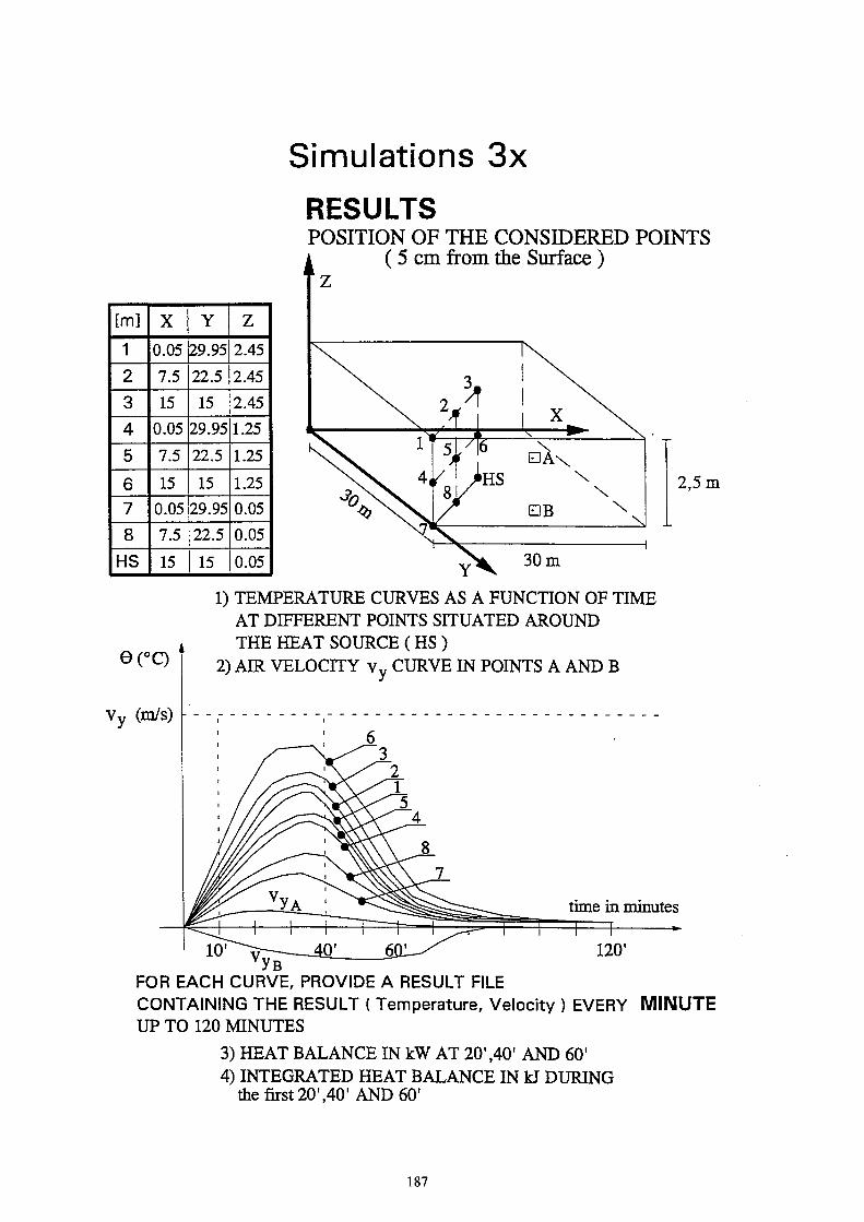
Simulations 3x RESULTS POSITION OF THE CONSIDERED POINTS
( 5 cm from the Surface ) z
[m]
1 2 3 4 5 6 7 8
HS
Χ 0.05 7.5 15
0.05 7.5 15
0.05 7.5 15
Y 29.95 22.5 15
29.95 22.5 15
29.95 22.5 15
Ζ 2.45 2.45 2.45 1.25 1.25 1.25 0.05 0.05 0.05
2,5 m
θ(°ο
Vy (m/s)
1) TEMPERATURE CURVES AS A FUNCTION OF TIME AT DIFFERENT POINTS SITUATED AROUND THE HEAT SOURCE ( HS )
2) AIR VELOCITY v y CURVE IN POINTS A AND B
time m minutes
FOR EACH CURVE, PROVIDE A RESULT FILE CONTAINING THE RESULT ( Temperature, Velocity ) EVERY MINUTE UP TO 120 MINUTES
3) HEAT BALANCE IN kW AT 20*,40' AND 60' 4) INTEGRATED HEAT BALANCE IN kJ DURING
the first 20',40' AND 60'
187

5) 1ΉΕ TEMPERATURE PROFILE ( temperature as a function of the height ) FOR THE TIMES 120", 300", 600", 1200", 2400", 3000", 3600" ) FOR X = 0.05 and Y = 29.95 (or 0.05 ) ( this profile includes the points 1, 4 and 7 ); FOR X = 7.5 and Y = 22.5 (or 7.5 ) ( this profile includes the points 2, 5 and 8 ); FOR X = 1 5 and Y = 1 5 ( this profile includes the points 3, 6 and HS )
Tcap. profil« {at X-Y- ^ £~ ») Simulation 3.x
3 600
1 1.5 Height [a] ■»>
6) ΤΉΕ MEAN TEMPERATURE PROFILE ( temperature as a function of the height ) FOR THE TIMES 120", 300", 600", 1200", 2400", 3000", 3600"
100
10
60
40
Mean teap. 1
T i M - 120 1 [a] - · — Tia« » 300 i [s] H — Tim« - 600 1 [a] -D·· Tia« - 1200! [3] -*-T i M " 2«00i (3] -a— T i M - 3000·: [3] -»-· Tia« - 3100: [s"¡ ·«■" ■
i
! i
,«--'
* ^ X Í .·■"
4L'.' ■<? * ' '
í'' ~J Τ'
Γ . .β.'
xt—t , ■ ■ * ■ ■ ■ — r — — o
profile in
i t
ΐ
XL·«*"
1-*-°"**
i---" Il ï fl
th« C C P
jr
,..--"'
Simulation 3
! M U' M
--
1" ..·
jr''
_.a'
..o
.X
1 :
"Π ..•-·8:ΐ;Βϊ 1 .--i· ar .*
TAC· eva (c) m s
1 l . S Height [a) ■—>
188
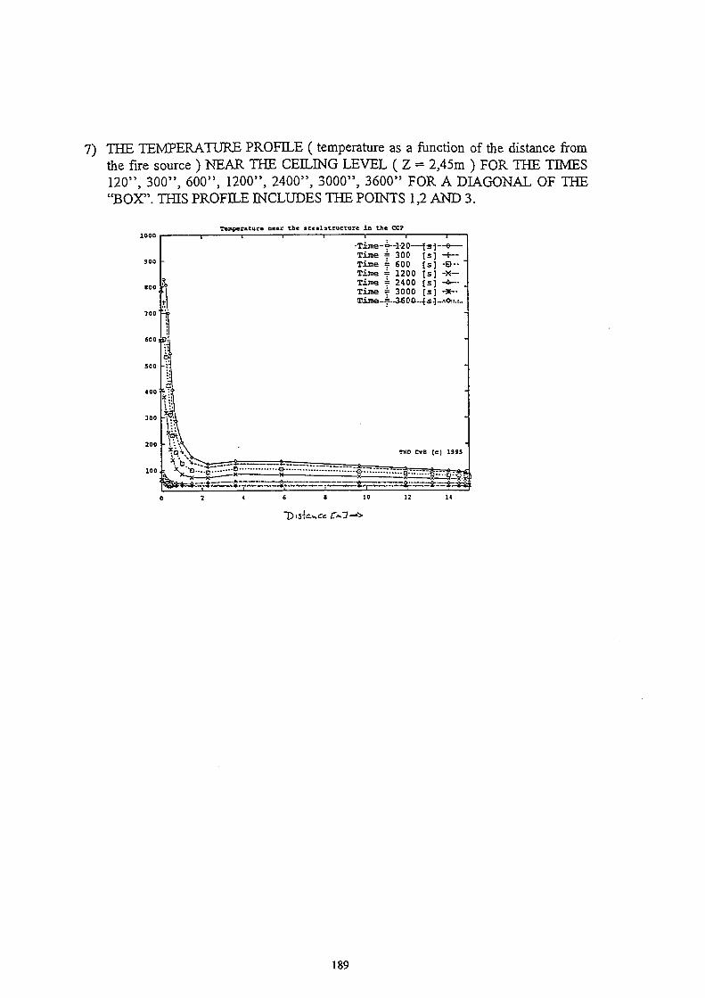
7) THE TEMPERATURE PROFILE ( temperature as a function of the distance from the fire source ) NEAR ΤΉΕ CEILING LEVEL ( Ζ = 2,45m ) FOR THE TIMES 120", 300", 600", 1200", 2400", 3000", 3600" FOR A DIAGONAL OF THE "BOX". THIS PROFILE INCLUDES THE POINTS 1,2 AND 3.
Temperature near the ateelstructure in the CCP
6 8 10
189

2. "FLUENT" results of the simulation 3X
Fire scenario known as simulation 3 (see semestrial report N° 3 Annex 2) has
been updated with a new window size 0.2 m high χ 1.0 m width. The
compartment consists on 30 χ 30 m floors and 2.5 m high. The geometry and the
heat source have two symmetrical planes, so only a quarter of the compartment
has been modeled with 15000 cells (25*24*25), see fig. 3.1 and 3.2. The
combustion itself has not been modeled, its thermal effect has been considered by
means of a reference curve of rate of heat release. The considered boundary
conditions can be seen in fig. 3.2. The walls have been modelized as concrete
with thermal conductivity = 1.6 J/smK and specific heat = 1000 J/kgK,
density = 2500 Kg/m^. While the convection coefficient from wall to the outside
is a data, 10 J/sm^K, in order to calculate the heat flux from the inner fluid to
wall Fluent solves a multi-dimensional conduction equation, which can be written
as:
FÎT
PwCw T7 = Δ* kwAT + q ot
p w = wall density
C w = wall heat capacity
k w = wall conduction coefficient
T = wall Temperature
q = internal heat generation rate
q = α * (Tw - Tf) [J/msK]
with: α = convection coefficient
T w = wall temperature
Tf = fluid temperature
This equation is solved with a special treatment at the wall/fluid interface where
the heat flux is computed via a harmonic mean "conductivity" that correctly
incorporates the thermal resistance change at the interface. This feature does not
use the convection coefficient which can be calculated in a post analysis in order
to assess the heat flux from air to the supporting structure with the classic
equation.
Pressure boundary conditions have been used to define the fluid pressure at flow
inlets and/or exits. The pressure boundary condition represents the plenum
pressure, this will be static pressure when flow exists the domain through the
plenum. If flow enters the domain through the plenum the pressure boundary
condition will be total pressure (stagnation pressure).
190
Simulation 3 X includes a radiant heat transfer model, the buoyancy effect on turbulence and an absorption coefficient model based on Fussegi's model. The implementation of the last two features has increased the convergence problems and the computational effort in great measure.
Results of temperature along the compartment has been obtained for 50 minutes, although the fire duration is 60 minutes, the last ten minutes represent the burnt out, and have few importance in order to assess the fire severity. This period will be obtained in next semester.
Fig. 3.3 shows the measurement points, points 1, 2, 3, 7, 8, HS are five centimetres from wall surface.
Fig. 3.4 shows temperatures from point 1 to 8. The most important profile is the number 6, this profile defines the higher temperature in the compartment. Points 7 and 8 show the same temperature profile, although point 7 is at a corner of the compartment and point 8 is closer to the fire place, this involves that a cold layer exists at the bottom of the compartment surrounding the fire place.
Fig. 3.5 shows the temperature distribution along a diagonal at the top of the compartment, the temperature distribution along the top is very important, because the beams will be exposed to this temperature distribution.
Fig. 3.6 shows the temperature distribution along height (measurement line passes through points 1, 4, 7) for several times 120", 300", 600", 1200", 2400", 3000". This figure shows the hot and cold layers with an interface between them, these layers remain during all the fire, although their thickness varies with time.
Fig. 3.7 shows the inlet velocity at windows, where the flow gets into the compartment, the fluid temperature is 20°C, thereby the mass flow is proportional to the velocity by means of the fluid density at 20°C. If the flow leaks the garage, the fluid temperature at outlets varies, and so mass flow must be obtained with the density at that point at the moment.
191
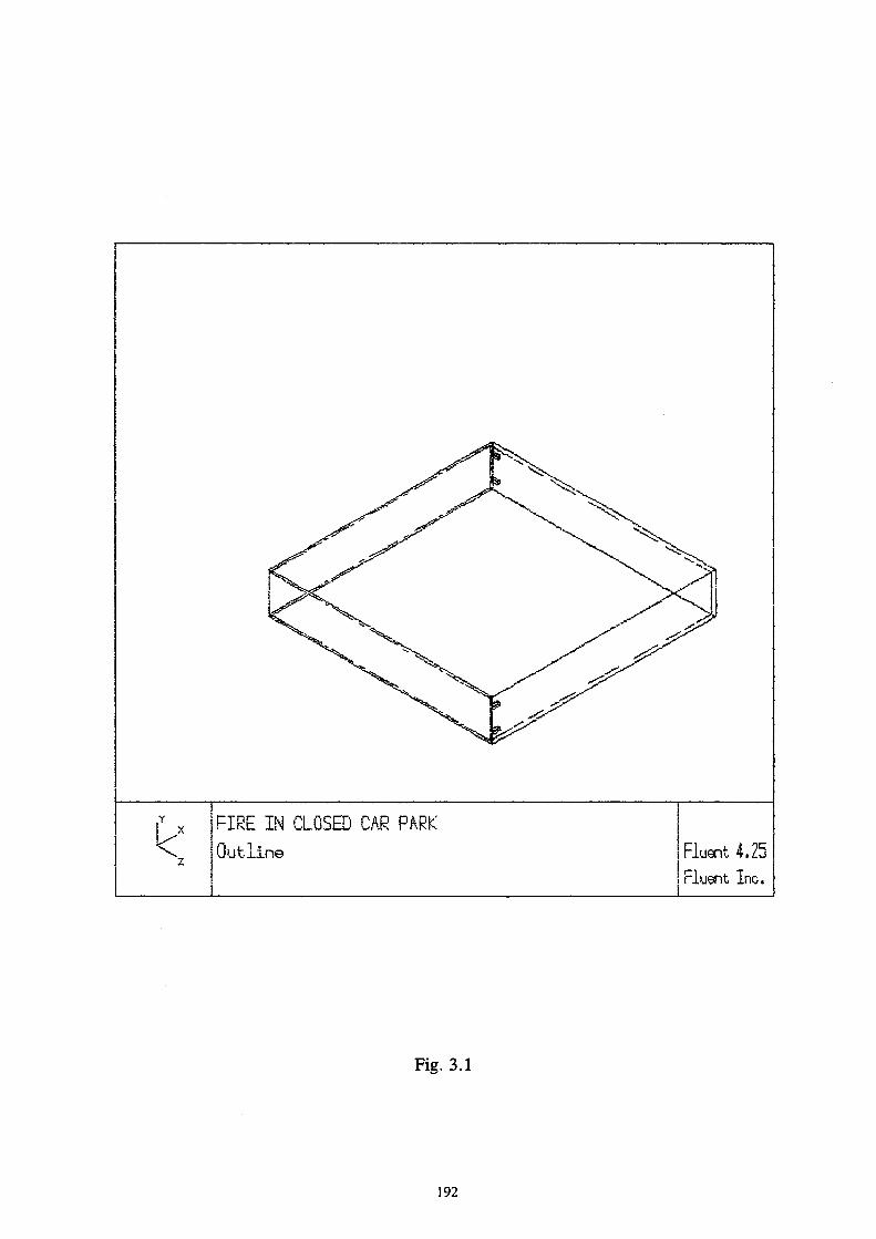
x ¡FIRE IN CLOSED CAR PARK s I Ou t l ine Fluent 4.25
Fluent Inc.
Fig. 3.1
192
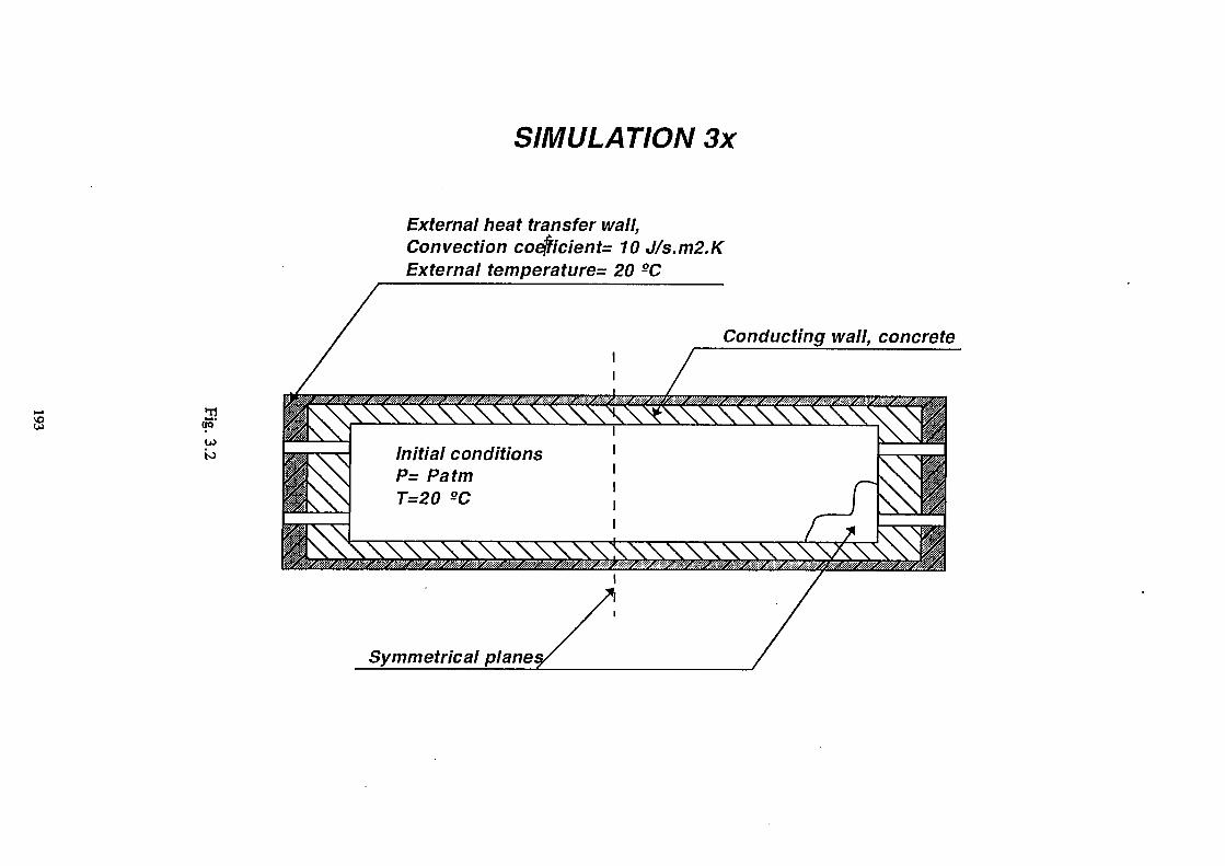
SIMULATION 3x
U> ►n
to
External heat transfer wall, Convection coeficient= 10 J/s.m2.K External temperature^ 20 -C
Conducting wall, concrete
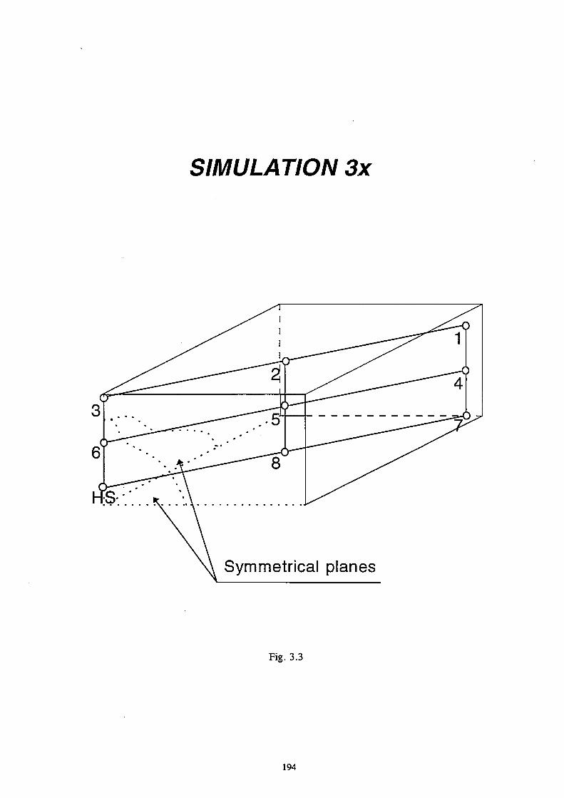
SIMULATION 3x
Fig. 3.3
194
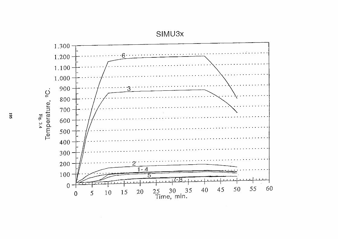
SIMU3X
VO
o oi
ω" 1 1 3 ·*—>
"ri CO rjq J— ω α.
E fi
w
5 10 15 20 25 30 35 40 45 50 55 60 u Time, min.
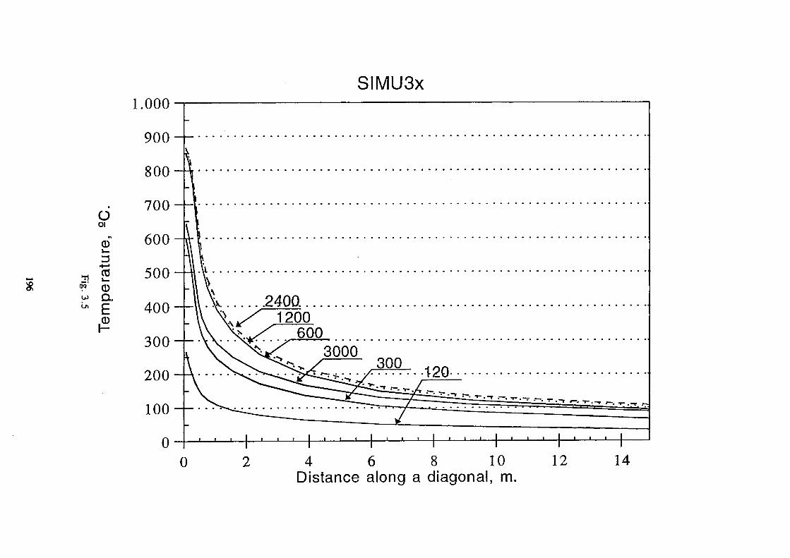
SIMU3X
rS
O Ol
<D
•4—<
HH Λ
<?' Q) w Q. U, £
.Φ
1.000
o 4 6 8 10 Distance along a diagonal, m.
12 14

VO
-J
ü
Ol
Φ
£ «o ω Φ cr, Q.
E |2
300
2 5 0 - r
2 0 0 - r
1 5 0 - r
1 0 0 - ï
0
0
SIMU3X, (Temp, profile at points 7,4,1)
_1 I L ' ■ I L _I I l_
0,5 1 1,5 Height, m.
2,5
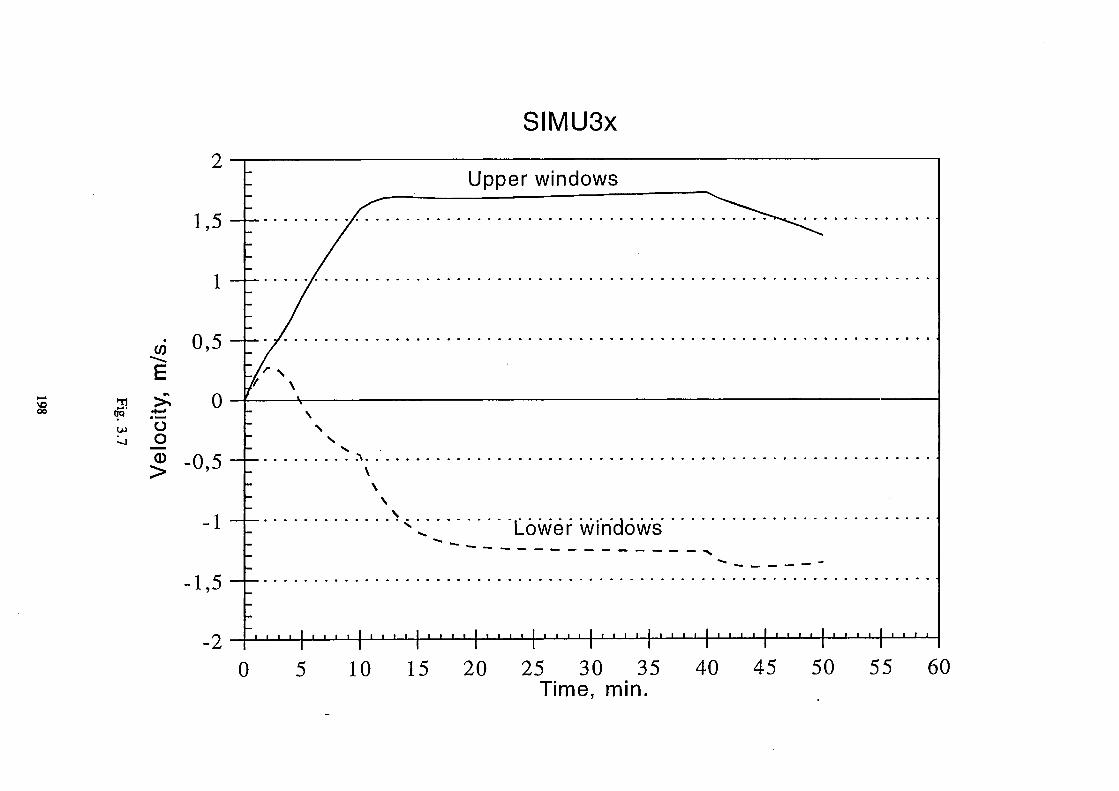
SIMU3X
VO oo
Upper windows
Lower 'window's
■ ■ ι I ■ ι ι ι Ι ι ι ι ι I I I I I I I I I ■ I I I I I I I I I I I
0 10 15 20 25 30 35 Time, min.
40 45 50 55 60

3. Comparison between results of the simulation 3X provided by FLUENT, VESTA and ARGOS
In the chapter 1 it can be noticed that 7 different types of results were asked.
The two following pages show the type number 2 which is the air velocity at the top and bottom openings. It must be noted that the FLUENT simulation was made with a Bernouilli coefficient equal to 1 because the user can not enter himself the value. However, if the FLUENT velocity curve is multiplied by the Bernouilli coefficient, it correspond rather well to the VESTA and ARGOS results. HAZ means results provided by HAZARD which is a multicompartment two Zone Model from the NIST (National Institute of Standards and Technology) of USA:
The other following pages correspond to the result type number 5, 6 and 7, i.e. different temperature profiles at different types.
All the results are available (see LC 44). In this report only the profiles corresponding to 40 minutes are given.
199

Air Velocity Vy curve in point A
Time6i°n min
-A-ARGOS Va s3x
-•-HAZ Va s3x
LABEIN Va s3x
o TNO Va s3x
100 120
vel s3xA.xls
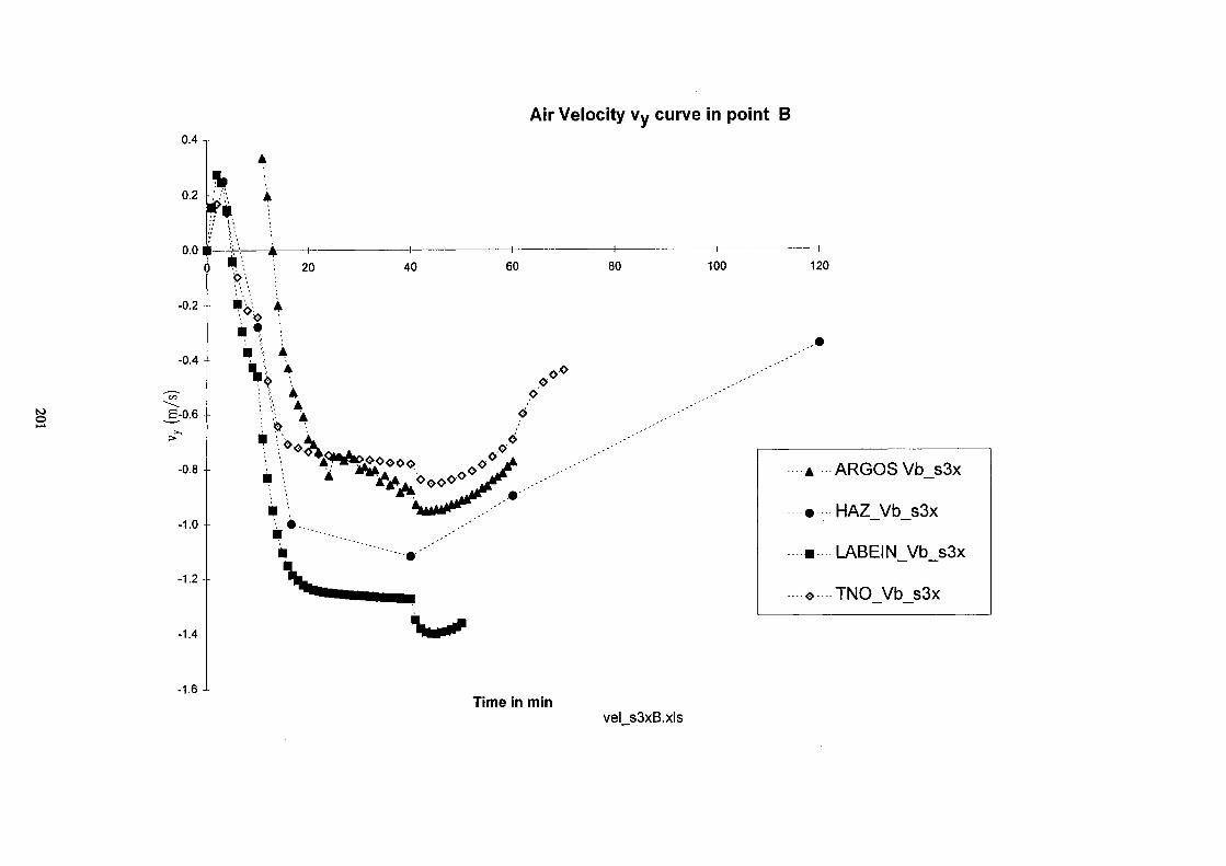
to
o
Air Velocity vy curve in point Β
0.4
0.2
m a v.
0.0 Ü
-0.2
-0.4
GO
J3-0.6
>
-0.8
-1.0
-1.2
-1.4
-1.6
■ 20 40 60
U \ A
o ·. 4
▲
ÎNk .o
Time in min
80 100 120
A--ARGOS Vb_s3x
■·--;■ HAZ_Vb_s3x
■ l_ABEIN_Vb_s3x
o TNO Vb s3x
vel s3xB.xls

N>
120
100
80
O
tu Ρ
"«α 6 0
s-,
C X
cu E—
40
20
SIMULATION 3x - Temperature Profile COMPARISON - ARGOS, FLUENT, VESTA (Points 1, 4, 7) 2400"
ο M
0.5
-^ -^ - —o— —o O O O- -o o
i Height [m] ΐ·« 2 Tprof1c.xls
2.5
A - Argos=2400
Labein=2400
TNO=2400
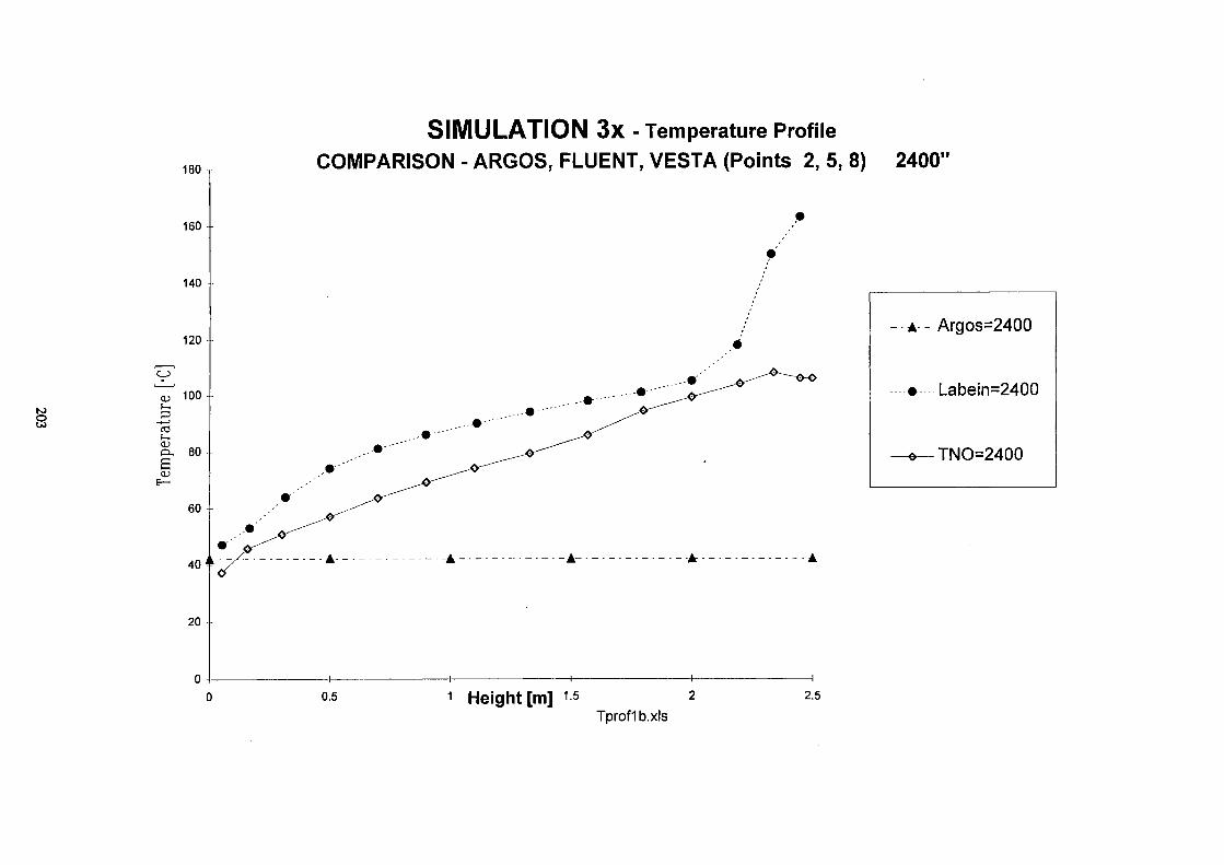
(O o
180
SIMULATION 3x - Temperature Profile COMPARISON - ARGOS, FLUENT, VESTA (Points 2, 5, 8) 2400"
0.5 ï Height [m] ΐ·β 2 Tprofl b.xls
A
- - - - · - ■
— 0 -
Argos=
Labein
=2400
=2400
TNO=2400
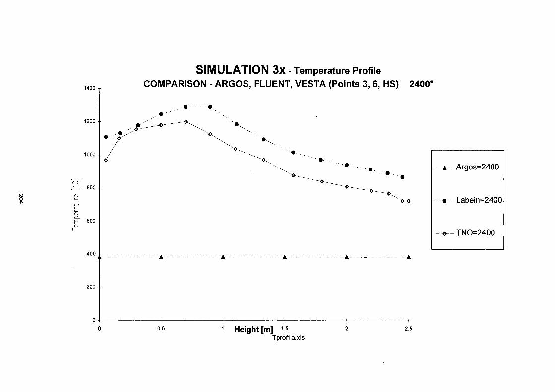
N) CJ>
1400
1200
1000
800
CD £ 600 cu
400
200
SIMULATION 3x - Temperature Profile COMPARISON - ARGOS, FLUENT, VESTA (Points 3, 6, HS) 2400"
.·· · .
0.5 ï Height [m] ΐ·β Tprof1a.xls
2.5
A - Argos=2400
• Labein=2400
o__ TNO=2400
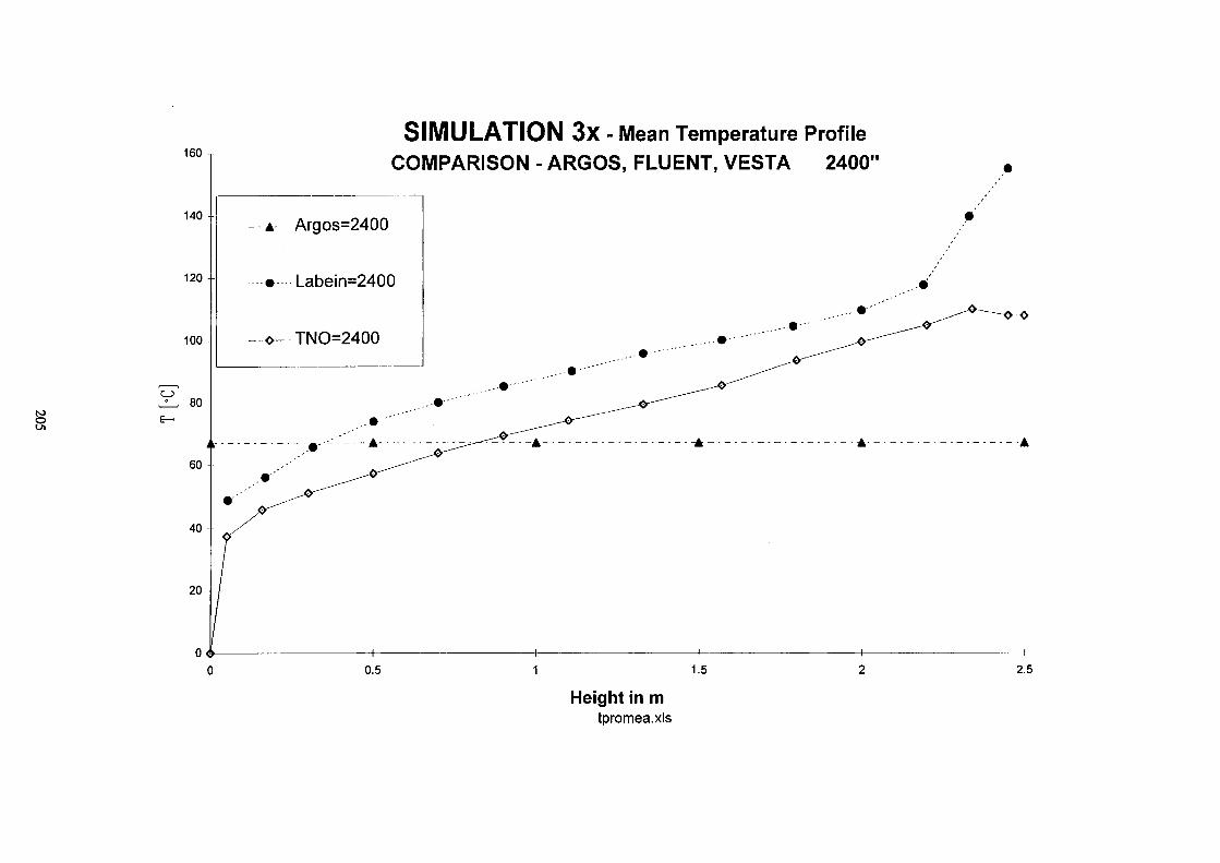
to o
SIMULATION 3x - Mean Temperature Profile COMPARISON - ARGOS, FLUENT, VESTA 2400"
Height in m tpromea.xls
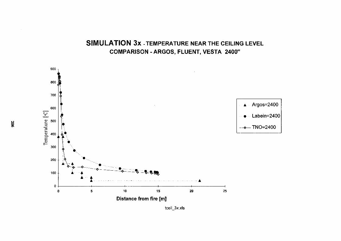
g
SIMULATION 3x -TEMPERATURE NEAR THE CEILING LEVEL COMPARISON - ARGOS, FLUENT, VESTA 2400"
900
A Argos=2400
• Labein=2400
_o_TNO=2400
^ ^ % %
— t —
10 —ι— 15
— ( — 20
—ι 25
Distance from fire [m]
tceil 3x.xls

Annex 8 : Fire tests database : Lund database, NIST database.
Another way to find an RHR curve is to make a test. Useful techniques for measuring heat release rates in the open were not available until a few years ago, when the principle of oxygen consumption calorimetry was developed. Earlier attempts required the direct measurement of sensible enthalpy, something which is very difficult to do correctly. The oxygen consumption technique, however, has enabled these measurememts to be made easily and with a good accurancy. The oxygen consumption principle states that, within a small uncertainty band, the heat released from the combustion of any common combustible is uniquely related to the mass of oxygen removed from the combustion flow stream. The measurement technique then requires that only the flow rate and the oxygen concentration be determined, along with the knowledge of the oxygen consumption constant, 3.1 10^ kJ heat released per kg of oxygen consumed. This technique has been used and has unabled to establish database oftest results.
The hazard [15] two zone simulation model within its framework, contains a database where various items are laid out and information on their RHR among other things is given. These items tend to be only items found in the home, for example, chairs, TV's, Christmas trees... . This obviouly leads to a limitation in the field of use. Although in its particular region of use it appears to be a very good source of information, as it includes every phase during an RHR curve.
Argos is another database found within the framework of a fire simulation programme. In Argos, different equations are given for solid material fire, melting material fire, liquid fire and smouldering fire. These equations define the RHR as a function of the fire spread velocity in the horizontal and vertical directions. The numerical values valid for different materials and objects are given in the Argos database.
Another source oftest result information is the "Initial Fires" document compiled by the University of Lund. This has the same format as the hazard database but contains more results which are also a little more diverse. In the document, one can find information not only on household objects but also objects such as various vehicle types. Although a little more diverse it is not overly so. There are even results in both of these databases which are the same.
207

European Commission
EUR 18868 — Properties and in-service performance Development of design rules for steel structures subjected to natural fires in large compartments
J.-B. Schleich, L-G. Cajot, M. Pierre, M. Brasseur J.-M. Franssen J. Kruppa, D. Joyeux L Twilt, J. Van Oerie G. Aurtenetxe
Luxembourg: Office for Official Publications of the European Communities
1999 — 207 pp. — 21 χ 29.7 cm
Technical steel research series
ISBN 92-828-7168-1
Price (excluding VAT) in Luxembourg: EUR 31
The aim of this research is to point out that, in view of the fire conditions for large compartments, the present fire regulations are too severe, and to define new requirements which better correspond to the real fire effect. These new requirements should be expressed in terms of fire load (MJ/m2), fire size (m2) and rate of heat release (kW). The procedure developed in the scope of this research allows the prediction that a structure can survive the required fire defined by its size and its rate of heat release. The ISO requirements F30, F60, F90 and F120 should be replaced by the requirement 'no failure at all', which demonstrates an increase in safety.
A procedure has been developed to check whether the fire remains localised and to calculate the temperature field in a steel structure in this case.
This procedure implies first a calculation of the air temperature based on the assumption of an upper hot layer and a lower cold layer. A simplified method and several two-zone models have been analysed. An important parameter of a two-zone calculation is the rate of air entrainment which has been studied in detail. In a second step, the peak of temperatures produced by the localised fire has been modelled by Hasemi's method which provides the heat flux distribution. Based on these heat fluxes, the ENV 1993-1-2 allows the steel temperature to be deduced. The validity of the Eurocode formulae has been checked in the case of localised fire by comparing the calculated temperatures with the temperatures obtained in different tests.
Knowing this steel temperature field, the mechanical behaviour is analysed by using the fire part of Eurocode 3. A new formula has been developed for a column situated in a two-zone environment.
We have developed a new design tool called Tefinaf (temperature field under natural fire) providing the steel temperature field of floor beams for any type of localised fire.


verna · saig · verKauT · ιιωλησεις · baies · venie · venerna · verKOop · venaa · myynti · i-orsaijnmg BELGIQUE/BELGIE
Jean De Lannoy Avenue du Roi 202, 'Koningslaan 202 B-1190 Bruxelles/Brussel Tél. (32-2) 538 43 08 Fax (32-2) 538 08 41 E-mail: [email protected] URL: http://www.jean-de-lannoy.be
La librairie européenne/ De Europese Boekhandel
Rue de la Loi 244/Wetstraat 244 B-1040 Bruxelles/Brussel Tél. (32-2) 295 26 39 Fax (32-2) 735 08 60 E-mail: [email protected] URL: http://www.libeurop.be
Moniteur beige/Belgisch Staatsblad
Rue de Louvain 40-42/Leuvenseweg 40-42 B-1000 Bruxelles/Brussel Tél. (32-2) 552 22 11 Fax (32-2) 511 01 84
DANMARK
J. H. Schultz Information A/S
Herstedvang 10-12 DK-2620 Albertslund Tlf. (45) 43 63 23 00 Fax (45) 43 63 19 69 E-mail: [email protected] URL: http://www.schultz.dk
DEUTSCHLAND
Bundesanzeiger Verlag GmbH
Vertriebsabteilung Amsterdamer Straße 192 D-50735 Köln Tel. (49-221)97 66 80 Fax (49-221) 97 66 82 78 E-Mail: [email protected] URL: http://www.bundesanzeiger.de
ΕΛΛΑΔΑ/GREECE
G. C. Eleftheroudakis SA
International Bookstore Panepistimiou 17 GR-10564 Athina Tel. (30-1) 331 41 80/1/2/3/4/5 Fax (30-1) 323 98 21 E-mail: [email protected]
ESPANA
Boletín Oficial del Estado
Trafalgar. 27 E-28071 Madrid Tel. (34) 915 38 21 11 (Libros).
913 84 17 15(Suscrip.) Fax (34) 915 38 21 21 (Libros),
913 84 17 14 (Suscrip.) E-mail: [email protected] URL: http://www.boe.es
Mundi Prensa Libros, SA
Castellò, 37 E-28001 Madrid Tel. (34)914 36 37 00 Fax (34) 915 75 39 98 E-mail: [email protected] URL: http://www.mundiprensa.com
FRANCE
Journal officiel
Service des publications des CE 26, rue Desaix F-75727 Paris Cedex 15 Tél. (33) 140 58 77 31 Fax (33) 140 58 77 00 URL: http://www.joumal-officiel.gouv.fr
IRELAND
Government Supplies Agency
Publications Section 4-5 Harcourt Road Dublin 2 Tel. (353-1)661 31 11 Fax (353-1) 475 27 60
ITALIA
Licosa SpA
Via Duca di Calabria, 1/1 Casella postale 552 1-50125 Firenze Tel. (39) 055 64 83 1 Fax (39) 055 64 12 57 E-mail: [email protected] URL: http://www.ftbcc.it/licosa
LUXEMBOURG
Messageries du livre SARL
5. rue Raiffeisen L-2411 Luxembourg Tél. (352)40 10 20 Fax (352) 49 06 61 E-mail: [email protected] URL: http://www.mdl.lu
NEDERLAND
SDU Servicecentrum Uitgevers
Christoffel Plantijnslraal 2 Postbus 20014 2500 EA Den Haag Tel. (31-70)378 98 80 Fax (31-70) 378 97 83 E-mail: [email protected] URL: http://www.sdu.nl
ÖSTERREICH
Manz'sche Verlags- und Universitätsbuchhandlung GmbH
Kohlmarkt 16 A-1014 Wien Tel. (43-1)53 16 11 00 Fax (43-1) 53 16 11 67 E-Mail: bestellen ©manz.co.at URL: http://www.manz.at/index.htm
PORTUGAL
Distribuidora de Livras Bertrand Ld. '
Grupo Bertrand, SA Rua das Terras dos Vales, 4-A Apartado 60037 P-2700 Amadora Tel. (351-1)495 90 50 Fax (351-1) 496 02 55
Imprensa Nacional-Casa da Moeda, EP
Rua Marqués Sá da Bandeira, 16-A Ρ-1050 Lisboa Codex Tel. (351-1)353 03 99 Fax (351-1) 353 02 94 E-mail: [email protected] URL: http://www.incm.pt
SUOMI/FINLAND
Akateeminen Kirjakauppa/ Akademiska Bokhandeln
Keskuskatu 1 /Centralgatan 1 PL/PB 128 FIN-00101 Helsinki/Helsingfors Ρ ./tfn (358-9) 121 44 18 F ./fax (358-9) 121 44 35 Sähköposti: [email protected] URL: http://www.akateeminen.com
SVERIGE
BTJAB
Traktorvägen 11 S-221 82 Lund Tfn (46-46) 18 00 00 Fax (46-46) 30 79 47 E-post: [email protected] URL: http://www.btj.se
UNITED KINGDOM
The Stationery Office Ltd
International Sales Agency 51 Nine Elms Lane London SW8 5DR Tel. (44-171)873 90 90 Fax (44-171) 873 84 63 E-mail: ipa.enquiries @ theso.co.uk URL: http://www.the-stationery-office.co.uk
ISLAND
Bokabud Larusar Blondel Skólavördustig, 2 IS-101 Reykjavik Tel. (354) 551 56 50 Fax (354) 552 55 60
NORGE
Swets Norge AS Østenjoveien 18 Boks 6512 Etterstad N-0606 Oslo Tel. (47-22) 97 45 00 Fax (47-22) 97 45 45
SCHWEIZ/SUISSE/SVIZZERA
Euro Info Center Schweiz
c/o OSEC Stampfenbachstraße 85 PF 492 CH-8035 Zürich Tel. (41-1)365 53 15 Fax (41-1) 365 54 11 E-mail: [email protected] URL: http://www.osec.ch/eics
BALGARIJA
Europress Euromedia Ltd 59, blvd Vitosha BG-1000 Sofia Tel. (359-2) 980 37 66 Fax (359-2) 980 42 30 E-mail: [email protected]
CESKÁ REPUBLIKA
USIS
NIS-prodejna Havelkova 22 CZ-130 00Praha3 Tel. (420-2)24 23 14 86 Fax (420-2) 24 23 11 14 E-mail: [email protected] URL: http://usiscr.cz
CYPRUS
Cyprus Chamber of Commerce and Industry
PO Box 1455 CY-1509 Nicosia Tel. (357-2) 66 95 00 Fax (357-2) 66 10 44 E-mail: [email protected]
EESTI
Eesti Kaubandus-Töö8tuskoda (Estonian Chamber of Commerce and Industry)
Toom-Kooli 17 EE-0001 Tallinn Tel. (372) 646 02 44 Fax (372) 646 02 45 E-mail: [email protected] URL: http://www.koda.ee
HRVATSKA
Mediatrade Ltd Pavia Hatza 1 HR-10000 Zagreb Tel. (385-1)481 94 11 Fax (385-1) 481 94 11
MAGYARORSZÄG
MALTA
Miller Distributors Ltd
Malta International Airport PO Box 25 Luqa LQA 05 Tel. (356) 66 44 88 Fax (356) 67 67 99 E-mail: [email protected]
POLSKA
ROMANIA
Euromedia
Str. G-ral Berthelot Nr 41 RO-70749 Bucuresti Tel. (40-1)315 44 03 Fax (40-1) 314 22 86
ROSSIYA
CCEC
60-letiya Oktyabrya Av. 9 117312 Moscow Tel. (7-095) 135 52 27 Fax (7-095) 135 52 27
SLOVAKIA
SLOVENIJA
Gospodarski Vestnik Dunajska cesta 5 SLO-1000 Ljubljana Tel.(386)613 09 16 40 Fax (386) 613 09 16 45 E-mail: [email protected] URL: http://www.gvestnik.si
TURKiYE
AUSTRALIA
CANADA
ISRAËL
Euro Info Service Europa Haz Margitsziget PO Box 475 H-1396 Budapest 62 Tel. (36-1 350 80 25 Fax (36-1) 350 90 32 E-mail: [email protected] URL: http://www.euroinfo.hu/index.htm
Ars Polona Krakowskie Przedmiescie 7 Skr. pocztowa 1001 PL-00-950 Warszawa Tel. (48-22) B26 12 01 Fax (48-22) 826 62 40 E-mail: [email protected]
ROY International
41, Mlshmar Hayarden Street PO Box 13056 61130 Tel Aviv Tel. (972-3) 649 94 69 Fax (972-3) 648 60 39 E-mail: [email protected] URL: http://www.royint.co.il
Sub-agent for the Palestinian Authority:
Index Information Services
PO Box 19502 Jerusalem Tel. (972-2)627 16 34 Fax (972-2) 627 12 19
JAPAN
PSI-Japan
Asahi Sanbancho Plaza #206 7-1 Sanbancho, Chiyoda-ku Tokyo 102 Tel. (81-3)32 34 69 21 Fax (81-3) 32 34 69 15 E-mail: [email protected] URL: http://www.psi-japan.com
EBIC Malaysia
Level 7. Wisma Hong Leong 18 Jalan Perak 50450 Kuala Lumpur Tel. (60-3) 262 62 98 Fax (60-3) 262 61 98 E-mail: [email protected]
MÉXICO
Centrum VTI SR
Nam. Slobody, 19 SK-81223 Bratislava Tel. (421-7)54 41 83 64 Fax (421-7) 54 41 83 64 E-mail: [email protected] URL: http://www.sltk.stuba.sk
Dunya Infotel AS
100, Yil Mahallessi 34440 TR-80050 Bagcilar-Istanbul Tel. (90-212)629 46 89 Fax (90-212) 629 46 27 E-mail: [email protected]
Hunter Publications
PO Box 404 3067 Abbotsford, Victoria Tel. (61-3)94 17 53 61 Fax (61-3) 94 19 71 54 E-mail: [email protected]
Les éditions La Libertó Inc.
3020, chemin Sainte-Foy G1X 3V Sainte-Foy, Québec Tel. (1-418)658 37 63 Fax (1-800) 567 54 49 E-mail: [email protected]
Renouf Publishing Co. Ltd
5369 Chemin Canotek Road Unit 1 K U 9J3 Ottawa. Ontario Tel. (1-613)745 26 65 Fax (1-613) 745 76 60 E-mail: [email protected] URL: http://www.renoufbooks.com
EGYPT
The Middle East Observer
41 Sherif Street Cairo Tel. (20-2)392 6919 Fax (20-2) 393 97 32 E-mail: [email protected] URL: http://www.meobserver.com.eg
INDIA
EBIC India
3rd Floor, Υ. B. Chavan Centre Gen. J. Bhosale Marg. 400 021 Mumbai Tel. (91-22)282 60 64 Fax (91-22) 285 45 64 E-mail: ebic@giasbm01 .vsnl.net.in URL: http://www.ebicindia.com
Mundi Prensa Mexico, SA de CV
Rio Panuco No 141 Colonia Cuauhtemoc MX-06500 Mexico, DF Tel. (52-5) 533 56 58 Fax (52-5) 514 67 99 E-mail: [email protected]
PHILIPPINES
EBIC Philippines
19th Floor, PS Bank Tower Sen. Gil J. Puyat Ave. cor. Tindalo St. Makati City Metro Manilla Tel. (63-2) 759 66 80 Fax (63-2) 759 66 90 E-mail: [email protected] URL: http://www.eccp.com
EBIC Sri Lanka
Trans Asia Hotel 115 Sir chittampalam A. Gardiner Mawatha Colombo 2 Tel. (94-1)074 71 50 78 Fax (94-1) 44 87 79 E-mail: [email protected]
THAILAND
EBIC Thailand
29 Vanissa Building, 8th Floor Soi Chidlom Ploenchit 10330 Bangkok Tel. (66-2) 655 06 27 Fax (66-2) 655 06 28 E-mail: [email protected] URL: http:/www.ebicbkk.org
UNITED STATES OF AMERICA
Beman Associates
4611-F Assembly Drive Lanham MD20706 Tel. (1-800) 274 44 47 (toll free telephone) Fax (1-800) 865 34 50 (toll free fax) E-mail: [email protected] URL: http://www.beman.com
ANDERE LANDER/OTHER COUNTRIES/ AUTRES PAYS
Bitte wenden Sie sich an ein Büro Ihrer Wahl/ Please contact the sales office of your choice/ Veuillez vous adresser au bureau de vente de votre choix
Office for Official Publications of the European Communities
2, rue Mercier L-2985 Luxembourg Tel. (352) 29 29-42455 Fax (352) 29 29-42758 E-mail: [email protected] URL: http://eur-op.eu.int
NOTICE TO THE READER
Information on European Commission publications in the areas of research and innovation can be obtained from:
♦ RTD info
The European Commission's free magazine on European research, focusing on project results and policy issues, published every three months in English, French and German. For more information and subscriptions, contact: DG XII — Communication Unit, rue de la Loi/Wetstraat 200, B-1049 Brussels Fax (32-2) 29-58220; e-mail: [email protected]
o o
00 αϊ en co
Price (excluding VAT) in Luxembourg: EUR 31 ISBN 1 S - f l E f l - 7 1 t i f l - l
* EUR +
• o p • OFFICE FOR OFFICIAL PUBLICATIONS OF THE EUROPEAN COMMUNITIES
9 789282"871683 > * ir * L-2985 Luxembourg