development of control in brain networks over temporal and
TRANSCRIPT
CompleSystems
Development of control in brain networks overtemporal and spatial scales using graph models
Regional Control of System State vs. System Mode
Summary
References & Acknowledgements
Lindsay Smith1, Harang Ju2, & Danielle S. Bassett1,3-6
1Department of Physics & Astronomy, University of Pennsylvania; 2Neuroscience Graduate Group, University of Pennsylvania;3Department of Bioengineering, University of Pennsylvania; 4Department of Electrical & Systems Engineering, University of Pennsylvania;
5Department of Neurology, University of Pennsylvania; 6Department of Psychiatry, University of Pennsylvania
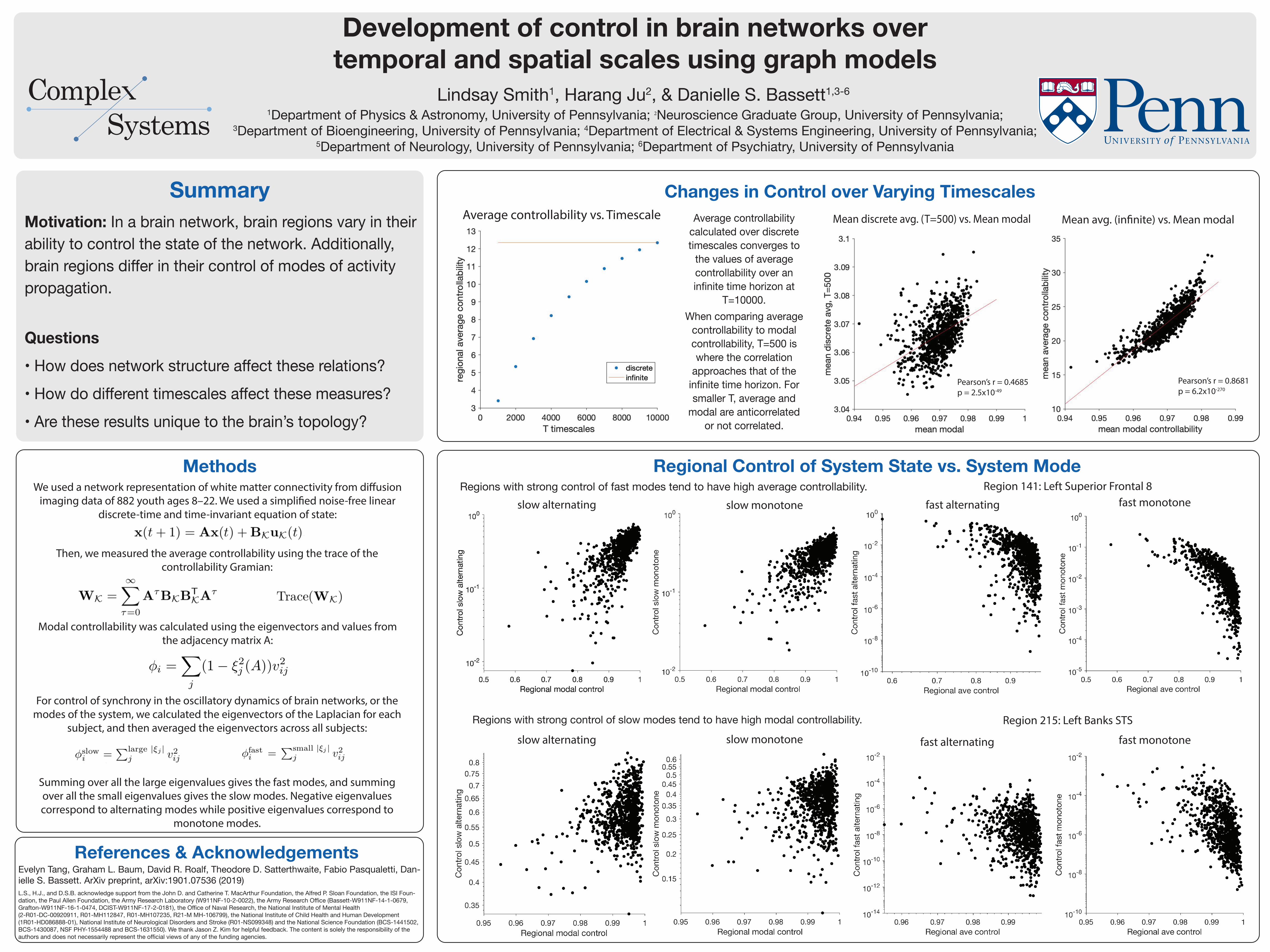
Changes in Control over Varying TimescalesMotivation: In a brain network, brain regions vary in their ability to control the state of the network. Additionally, brain regions differ in their control of modes of activity propagation.
Questions• How does network structure affect these relations?• How do different timescales affect these measures?• Are these results unique to the brain’s topology?
Average controllability calculated over discrete timescales converges to
the values of average controllability over an infinite time horizon at
T=10000.When comparing average
controllability to modal controllability, T=500 is where the correlation
approaches that of the infinite time horizon. For smaller T, average and
modal are anticorrelated or not correlated.
Evelyn Tang, Graham L. Baum, David R. Roalf, Theodore D. Satterthwaite, Fabio Pasqualetti, Dan-ielle S. Bassett. ArXiv preprint, arXiv:1901.07536 (2019)L.S., H.J., and D.S.B. acknowledge support from the John D. and Catherine T. MacArthur Foundation, the Alfred P. Sloan Foundation, the ISI Foun-dation, the Paul Allen Foundation, the Army Research Laboratory (W911NF-10-2-0022), the Army Research Office (Bassett-W911NF-14-1-0679, Grafton-W911NF-16-1-0474, DCIST-W911NF-17-2-0181), the Office of Naval Research, the National Institute of Mental Health (2-R01-DC-00920911, R01-MH112847, R01-MH107235, R21-M MH-106799), the National Institute of Child Health and Human Development (1R01-HD086888-01), National Institute of Neurological Disorders and Stroke (R01-NS099348) and the National Science Foundation (BCS-1441502, BCS-1430087, NSF PHY-1554488 and BCS-1631550). We thank Jason Z. Kim for helpful feedback. The content is solely the responsibility of the authors and does not necessarily represent the official views of any of the funding agencies.
Regions with strong control of fast modes tend to have high average controllability.
Regions with strong control of slow modes tend to have high modal controllability.
slow monotone
Average controllability vs. Timescale Mean discrete avg. (T=500) vs. Mean modal Mean avg. (in�nite) vs. Mean modal
MethodsWe used a network representation of white matter connectivity from di�usion
imaging data of 882 youth ages 8–22. We used a simpli�ed noise-free linear discrete-time and time-invariant equation of state:
Then, we measured the average controllability using the trace of the controllability Gramian:
Modal controllability was calculated using the eigenvectors and values from the adjacency matrix A:
For control of synchrony in the oscillatory dynamics of brain networks, or the modes of the system, we calculated the eigenvectors of the Laplacian for each
subject, and then averaged the eigenvectors across all subjects:
Summing over all the large eigenvalues gives the fast modes, and summing over all the small eigenvalues gives the slow modes. Negative eigenvalues correspond to alternating modes while positive eigenvalues correspond to
monotone modes.
Pearson’s r = 0.8681p = 6.2x10-270
Pearson’s r = 0.4685p = 2.5x10-49
fast alternating fast monotone
Region 141: Left Superior Frontal 8
Region 215: Left Banks STS
fast alternating fast monotoneslow monotoneslow alternating
slow alternating