development of an oct for small animal retinal imaging · técnicas úteis no diagnóstico e...
TRANSCRIPT

Faculdade de Ciências e Tecnologia
Universidade de Coimbra
DEVELOPMENT OF AN OPTICAL
COHERENCE TOMOGRAPHY FOR SMALL
ANIMAL RETINAL IMAGING
João Miguel Guedes de Oliveira
Coimbra, September 2012


Faculdade de Ciências e Tecnologia
Universidade de Coimbra
DEVELOPMENT OF AN OPTICAL
COHERENCE TOMOGRAPHY FOR SMALL
ANIMAL RETINAL IMAGING
Thesis submitted for the degree of Master in Biomedical Engineering
Supervisors: Prof. Dr. António Miguel Morgado (IBILI-UC)
Prof. Dr. José Paulo Domingues (IBILI-UC)
João Miguel Guedes de Oliveira
Coimbra, September 2012


Development of an OCT for small animal retinal imaging 2012
I
This copy of the thesis has been supplied on condition that anyone who consults it is
understood to recognize that its copyright rests with its author and that no quotation from the
thesis and no information derived from it may be published without proper acknowledgement.

Development of an OCT for small animal retinal imaging 2012
II

Development of an OCT for small animal retinal imaging 2012
III
Abstract
Currently, animal models represent an important tool in biomedical research.
Not only to understand the physiological processes involved in various diseases, but
also for developing new instrumentation and techniques helpful in the diagnostic and
treatment of those diseases.
The objective of the project is to develop an optical coherence tomography for
small animal retinal imaging. The development was based on the integration of different
optical and electronic components.
This report describes the equipment, tests and architecture of several optical
bench setups. An OCT computer simulation was also developed.
Although at the end of this work, it was already possible to acquired OCT
images, the system still requires a lot of improvement, namely the inclusion of the
galvanometer mirrors and the control of the acquired data by the DAQ board.

Development of an OCT for small animal retinal imaging 2012
IV

Development of an OCT for small animal retinal imaging 2012
V
Resumo
Actualmente, os modelos animais representam uma ferramenta importante na
investigação biomédica. Não só para compreender os processos fisiológicos envolvidos
em várias doenças, mas também para o desenvolvimento de novos instrumentos e
técnicas úteis no diagnóstico e tratamento dessas doenças.
O objetivo do projeto é desenvolver uma tomografia de coerência óptica para
imagens da retina de pequenos animais. O desenvolvimento baseou-se na integração de
diversos componentes ópticos e electrónicos.
Este relatório descreve os equipamentos, testes e arquitetura de várias
configurações ópticas. Também foi realizada uma simulação de OCT em computador.
Embora no final deste trabalho, já fosse possível adquirir imagens de OCT, o
sistema ainda requer uma série de melhorias, como a inclusão dos espelhos
galvanômetro e o controle dos dados adquiridos por placa DAQ.

Development of an OCT for small animal retinal imaging 2012
VI

Development of an OCT for small animal retinal imaging 2012
VII
Acknowledgements
First, I would like to thank my family, especially to my mother, who made
possible for me to be here and always encouraged my decisions.
To my supervisors, Prof. Dr. António Miguel Morgado, Prof. Dr. José Paulo
Domingues for their guidance, help and encouragement throughout this year. I also
would like to mention a particular acknowledgment to Prof. Dr. Custódio Loureiro, who
kindly helped us with some issues during the project, despite not being a team member.
Finally, a special thanks to all my friends for their unconditional support and
enjoying life together with me.
Thank you all.

Development of an OCT for small animal retinal imaging 2012
VIII

Development of an OCT for small animal retinal imaging 2012
IX
Index
Abstract ........................................................................................................................................ III
Resumo .......................................................................................................................................... V
Acknowledgements ..................................................................................................................... VII
List of Figures .............................................................................................................................. XI
List of Graphics .......................................................................................................................... XIII
List of Tables ............................................................................................................................... XV
Introduction ................................................................................................................................... 1
Chapter One .................................................................................................................................. 3
1.1 Optical Coherence Tomography.......................................................................................... 3
1.1.1 Time Domain OCT ......................................................................................................... 3
1.1.2 Resolution..................................................................................................................... 6
1.1.3 Fourier Domain OCT ..................................................................................................... 8
1.1.4 Sources for OCT .......................................................................................................... 10
1.1.5 Scanning Modes ......................................................................................................... 12
1.1.6 Image Distortions ....................................................................................................... 13
1.1.7 Time Domain versus Fourier Domain ......................................................................... 14
1.2 Other Techniques Based on OCT ....................................................................................... 18
1.2.1 Full-Field OCT ............................................................................................................. 18
1.2.2 Doppler OCT ............................................................................................................... 19
1.2.3 Polarization sensitive OCT .......................................................................................... 20
Chapter Two ................................................................................................................................ 23
2.1 State of the art .................................................................................................................. 23
Chapter Three .............................................................................................................................. 29
3.1 Simulation ......................................................................................................................... 29
Chapter Four ................................................................................................................................ 35
4.1 OCT Setup .......................................................................................................................... 35
4.1.1 Axsun Swept Source ................................................................................................... 37
4.1.2 Thorlabs Balanced Detector ....................................................................................... 38
4.1.3 Innovative Integration DAQ Board ............................................................................. 40
4.1.4 Thorlabs Interferometer............................................................................................. 41
4.1.5 Thorlabs OCT Lenses, Gold Mirror and Collimator ..................................................... 43

Development of an OCT for small animal retinal imaging 2012
X
4.2 Thorlabs Scanning System ................................................................................................. 44
Chapter Five ................................................................................................................................ 47
5.1 Results and Discussion ...................................................................................................... 47
5.1.1 Equipment tests and acquired signals........................................................................ 47
5.1.2 Galvo System tests ..................................................................................................... 55
Chapter Six .................................................................................................................................. 59
6.1 Future Work ...................................................................................................................... 59
6.1.1 Instrument Optimization ............................................................................................ 59
6.1.2 Acquisition board programming and data processing ............................................... 59
References ................................................................................................................................... 63
Appendix A ................................................................................................................................. 69
Appendix B ................................................................................................................................. 83
Appendix C ................................................................................................................................. 85

Development of an OCT for small animal retinal imaging 2012
XI
List of Figures
FIGURE 1 – MICHELSON INTERFEROMETER ..................................................................................... 5
FIGURE 2 – INTERFERENCE PATTERN FOR LONG AND SHORT COHERENCE LENGTH .......... 6
FIGURE 3 – RELATION BETWEEN INTERFERENCE PEAK AND COHERENT LENGTH .............. 6 FIGURE 4 – COMPARISON OF RESOLUTION AND PENETRATION DEPTH OF OCT AND
OTHER IMAGING TECHNIQUES ................................................................................................... 7
FIGURE 5 – FREQUENCY DOMAIN OCT SCHEMATICS .................................................................... 8 FIGURE 6 – RELATION BETWEEN WAVELENGTH AND ABSORPTION COEFFICIENT FOR
DIFFERENT BIOLOGICAL TISSUES ............................................................................................ 11
FIGURE 7 – DIAGRAM OF DIFFERENT OCT SCAN TYPES ............................................................. 13
FIGURE 8 – DIAGRAM OF FAN DISTORTION .................................................................................... 14
FIGURE 9 – SCHEMATICS OF WIDE FIELD OCT AND FULL FIELD OCT ..................................... 19
FIGURE 10 – DIAGRAM OF DOPPLER OCT SAMPLE ARM ............................................................. 20
FIGURE 11 – SCHEMATICS OF POLARIZATION SENSITIVE OCT ................................................. 21
FIGURE 12 – RETINAL LAYERS ........................................................................................................... 24
FIGURE 13 – BENCH CONFIGURATION OF OUR OCT SYSTEM .................................................... 35
FIGURE 14 – FINAL OCT DIAGRAM .................................................................................................... 36
FIGURE 15 – WARNING LABEL FOR CLASS 1M LASER ................................................................. 37
FIGURE 16 – AXSUN SWEPT SOURCE OCT BENCH VERSION ........................................................ 38
FIGURE 17 – FRONT AND REAR PANELS OF AXSUN SOURCE. ..................................................... 38
FIGURE 18 – THORLABS BALANCED DETECTOR ............................................................................. 39
FIGURE 19 – FUNCTIONAL BLOCK DIAGRAM OF BALANCED DETECTOR .............................. 40
FIGURE 20 – INNOVATIVE INTEGRATION DAQ BOARD ................................................................... 40
FIGURE 21 – X5-400M BLOCK DIAGRAM .......................................................................................... 41
FIGURE 22 – THORLABS INT-MZI INTERFEROMETER ..................................................................... 42
FIGURE 23 – FUNCTIONAL DIAGRAM OF THE MZI 1050 INTERFEROMETER ........................... 42
FIGURE 24 – THORLABS GALVO SYSTEM .......................................................................................... 45
FIGURE 25 – SERVO BOARD DIAGRAM ............................................................................................. 46
FIGURE 26 – J7- COMMAND INPUT CONNECTOR PIN- CONNECTION DIAGRAM .................... 46
FIGURE 27 – DIAGRAM OF REFERENCE AND SAMPLE ARMS ..................................................... 50
FIGURE 28 – AXSUN CLOCK SIGNAL AT THE END OF THE PERIOD ............................................ 52
FIGURE 29 – AXSUN CLOCK SIGNAL WHERE THE LASER IS TURNED ON ................................ 53
FIGURE 30 – AXSUN CLOCK SIGNAL WHERE THE LASER IS TURNED OFF ............................... 53
FIGURE 31 – DETAILED OF THE SCANNING LINE IN THE Y DIRECTION .................................. 55
FIGURE 32 – SCANNING LINE FOR AN AMPLITUDE OF 10 V ........................................................ 56
FIGURE 33 – SCANNING LINE FOR AN AMPLITUDE OF 5 V .......................................................... 56
FIGURE 34 – GALVO SYSTEM SCHEMATICS .................................................................................... 57
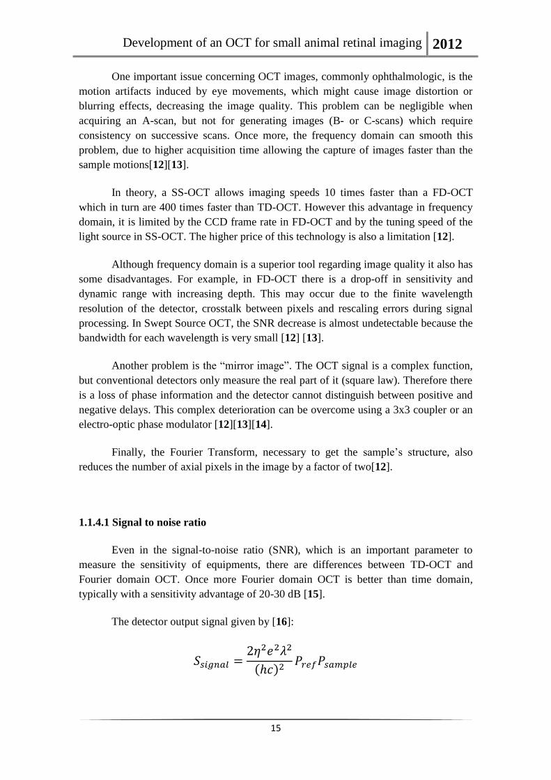
FIGURE 35 – ACQUISITION CYCLE OF DAQ BOARD ...................................................................... 60
FIGURE 36 – FINAL OCT CONFIGURATION ...................................................................................... 61
FIGURE 37 – SERVO BOARD ................................................................................................................. 73
FIGURE 38 – X5-400M MODULE ........................................................................................................... 78
FIGURE 39 – HOST BOARD ................................................................................................................... 78
FIGURE 40 – 2X2 COUPLER SCHEMATIC ........................................................................................... 79
FIGURE 41 – CABLE CONSTRUCTION AND CONNECTOR FINISH ............................................... 82

Development of an OCT for small animal retinal imaging 2012
XII

Development of an OCT for small animal retinal imaging 2012
XIII
List of Graphics
GRAPHIC 1 – RELATION BETWEEN LATERAL RESOLUTION AND DEPTH OF FIELD ............... 8 GRAPHIC 2 –THE SPECTRAL INTENSITY DETECTED IN FD-OCT AND THE CORRESPONDING
FFT. ..................................................................................................................................................... 9
GRAPHIC 3 – SIMULATED SPECTRUM OF GAUSSIAN SOURCE ................................................... 29
GRAPHIC 4 – SIMULATED TIME DOMAIN INTERFEROGRAM OF SAMPLE 1 ............................ 30
GRAPHIC 5 – SIMULATED SPECTRAL INTENSITY (FD-OCT) SIGNAL OF SAMPLE 1 ............... 31
GRAPHIC 6 – FOURIER TRANSFORM OF SPECTRAL INTENSITY................................................. 31 GRAPHIC 7 – SIMULATED TIME DOMAIN INTERFEROGRAM OF SAMPLE 2, USING A
SOURCE WITH CENTER WAVELENGTH AT 800 NM AND A LINEWIDTH OF 50 NM ....... 32 GRAPHIC 8 – SIMULATED TIME DOMAIN INTERFEROGRAM OF SAMPLE 2, USING A
SOURCE WITH CENTER WAVELENGTH AT 400 NM AND A LINEWIDTH OF 50 NM ....... 32 GRAPHIC 9 – SIMULATED TIME DOMAIN INTERFEROGRAM OF SAMPLE 2, USING A
SOURCE WITH CENTER WAVELENGTH AT 800 NM AND A LINEWIDTH OF 150 NM ..... 33
GRAPHIC 10 – MIRROR REFLECTANCE FOR DIFFERENT WAVELENGTHS ............................... 44
GRAPHIC 11 – ACQUIRED AXSUN CLOCK SIGNAL, USING DAQ BOARD ................................... 47
GRAPHIC 12 – ACQUIRED AXSUN TRIGGER SIGNAL, USING DAQ BOARD ............................... 48 GRAPHIC 13 – ACQUIRED POWER OUTPUT SIGNAL FROM MZI INTERFEROMETER, USING
DAQ BOARD .................................................................................................................................... 48
GRAPHIC 14 – ACQUIRED MZI OUTPUT SIGNAL, USING DAQ BOARD ...................................... 48 GRAPHIC 15 – ACQUIRED REFLECTANCE SIGNAL FROM REFERENCE ARM, USING DAQ
BOARD ............................................................................................................................................. 49 GRAPHIC 16 – ACQUIRED REFLECTANCE FROM REFERENCE ARM AND POWER OUTPUT
FROM MZI INTERFEROMETER SIGNALS, USING DAQ BOARD ........................................... 49 GRAPHIC 17 – ACQUIRED SIGNAL 1 FROM REFLECTANCE OF BOTH, REFERENCE AND
SAMPLE, MIRRORS, USING DAQ BOARD ................................................................................. 50 GRAPHIC 18 – ACQUIRED SIGNAL 2 FROM REFLECTANCE OF BOTH, REFERENCE AND
SAMPLE, MIRRORS, USING DAQ BOARD ................................................................................. 50 GRAPHIC 19 – ACQUIRED A-SCAN OF THE SPECTRALIS TARGET, USING DAQ BARD, AND
ITS CORRESPONDING DEPTH PROFILE .................................................................................... 51 GRAPHIC 20 - THREE INTERFEROGRAMS FOR DIFFERENT POSITION WITHIN THE TARGET
ACQUIRED USING DAQ BOARD. ................................................................................................ 51 GRAPHIC 21 – ACQUIRED AXSUN CLOCK SIGNAL AND INTERFERENCE SIGNAL, USING
DAQ BOARD .................................................................................................................................... 52
GRAPHIC 22 – B-SCAN OBTAINED USING THE SPECTRALIS TEST TARGET ............................ 54
GRAPHIC 23 – SINUSOIDAL AND SQUARE WAVES ........................................................................ 55
GRAPHIC 24 – POWER SPECTRUM OF THE ENGINE ....................................................................... 70
GRAPHIC 25 – CLOCK OUTPUT SIGNAL ............................................................................................ 70
GRAPHIC 26 - TRIGGER OUTPUT SIGNAL ......................................................................................... 70
GRAPHIC 27 – OPTICAL POWER SIGNAL .......................................................................................... 70
GRAPHIC 28 – DETECTOR RESPONSITIVITY .................................................................................... 72
GRAPHIC 29 – DETECTOR FREQUENCY RESPONSE ....................................................................... 72
GRAPHIC 30 – DETECTOR SPECTRAL NOISE ................................................................................... 72
GRAPHIC 31 – REFLECTANCE OF DISPERSION COMPENSATORS ............................................... 81

Development of an OCT for small animal retinal imaging 2012
XIV

Development of an OCT for small animal retinal imaging 2012
XV
List of Tables
TABLE 1 – CHARACTERISTICS OF OCT LOW COHERENCE LIGHT SOURCES .......................... 12
TABLE 2 – SAMPLE 1 PROPERTIES ..................................................................................................... 30
TABLE 3 – SAMPLE 2 PROPERTIES. .................................................................................................... 31
TABLE 4 – LENSES FEATURES ............................................................................................................ 43
TABLE 5 – COLLIMATOR FEATURES ................................................................................................. 44
TABLE 6 – SCANNING RANGE ............................................................................................................ 57
TABLE 7 - AXSUN ENGINE FEATURES: .............................................................................................. 69
TABLE 8 – PDB145C PARAMETERS .................................................................................................... 71
TABLE 9 – GVS002 SPECIFICATIONS .................................................................................................. 75
TABLE 10 – INTERFEROMETER SPECIFICATIONS .......................................................................... 76
TABLE 11 – A/D AND D/A CONVERTER FEATURES ........................................................................ 77
TABLE 12 – COUPLERS FEATURES ..................................................................................................... 79
TABLE 13 – MIRROR SPECIFICATIONS .............................................................................................. 80
TABLE 14 – DISPERSION COMPENSATORS FEATURES ................................................................. 81
TABLE 15 – FIBER OPTIC PATCH CORD PARAMETERS ................................................................. 82

Development of an OCT for small animal retinal imaging 2012
XVI

Development of an OCT for small animal retinal imaging 2012
1
Introduction
Optical Coherence Tomography (OCT) is a widely used imaging technique in
medicine, mostly in ophthalmology. In biomedical research small animals are often
used in order to develop, validate, or test new techniques. Imaging animals also offers
the means to understand physiology, pathology, and phenotypes in an intact living
system, similar to human beings.
The objective of our project is to develop a Swept Source OCT (SS-OCT) for
retinal imaging in small animals. This will be a fundamental tool for research on retinal
physiology and for the improvement of new instrumentation and methods for OCT
based morphological and functional retinal images.
It was decided to assemble the overall system from separate blocks, including
the electronics, a light source, several optical components, a detector and a data
acquisition board. Thereby, instead of spending a large amount of money acquiring an
available OCT system, we can save some resources and also get a better understanding
on the technologies and on the difficulties and limitations involved in developing a
complex system like this.
Axsun
AXP50125-3 1060 nm – Swept Source Engine in enclosure
Thorlabs
INT-MZI-1050 – Interferometer
PDB145C – Fixed Gain Balance Detector, InGaAs, 800-1700 nm
FC1064-50B-APC – 2x2 SM Coupler, 1064 nm, 50:50 Split, FC/APC
FC1064-90B-APC – 2x2 SM Coupler, 1064 nm, 90:10 Split, FC/APC
GVSM002/M - 2D – Galvo System
LSM02 BB and LSM03 BB – OCT Scan Lenses
LSM02 DC and LSM03 DC - Dispersion Compensators
PF10-03-M01 – Protected Gold Mirror
Innovative Integration
X5-400M – Acquisition Module
OZ Optics
SMJ-3A3A-1060 -3.6/125-3-2 – Fiber Optic

Development of an OCT for small animal retinal imaging 2012
2
Our project was developed in IBILI and the research team was composed by
João Miguel Guedes de Oliveira master degree student, Prof. Dr. António Miguel
Morgado and Prof. Dr. José Paulo Domingues, both supervisors and assistant professors
from Physics Department of University of Coimbra. Prof. Dr. Custódio Loureiro also
from Physics Department gave a great help in simulating the OCT signal, mostly on
Fourier Transforms.

Development of an OCT for small animal retinal imaging 2012
3
Chapter One
1.1 Optical Coherence Tomography
Nowadays, there are a great number of techniques for medical imaging. With
recent advances and research on new materials and signal processing, it is expected that
more, better and cheaper imaging systems will appear in the next years.
For each clinical situation, professionals have to choose between these
techniques, according to the desired information, either anatomical or functional. In
most cases, only with a combination of two or more techniques it is possible to assess
the required information. Indeed it has to be a wise decision, because each equipment as
its own risks and complications.
Optical Coherence Tomography (OCT) is a recent imaging method based on an
optical interferometer of low coherence, which produces images similar to ultrasound.
However it uses a light source, instead of mechanical waves. Due to the high value of
speed of the light it is impossible to measure directly, with an adequate resolution, the
time of flight. So, to obtain the depth information it is necessary to use an
interferometric technique.
Thereby, it uses non ionizing radiation, is non invasive and the acquisition time
is reduced comparing with other imaging techniques. Another advantage is the higher
resolution, sub micrometer, compared to other devices. It collects cross sectional
bidimensional or tridimensional images, as well as depth profile of heterogenic
materials, such as biological tissues.
Currently, OCT can be applied in a large variety of fields, like material analysis
for studying mechanical defects and properties; art conservation. In medicine it has been
used for diagnostic, mostly in ophthalmology, but in recent years some studies
demonstrate that it is also useful in dermatology, dentistry and cardiology.
1.1.1 Time Domain OCT
Electromagnetic radiation is a form of energy, which travels through waves, with
both electric and magnetic fields. Waves are characterized by their frequency,
amplitude, velocity and phase.

Development of an OCT for small animal retinal imaging 2012
4
The interference phenomenon occurs when two or more waves combine. The
interference pattern can be constructive, if the relative phase between superimposed
waves is multiple of 2π. Otherwise, if they are shifted by a factor of π, 3π, 5π, etc. the
interference is destructive. In case of phase differences within these extremes, the
emergent wave magnitude is a combination of the initial waves.
For example, two waves defined, in function of time and space, by:
with A the wave amplitude; waves’ angular frequency; the wavenumber;
and the phase in origin
If they have the same angular frequency and velocity, but different phase in
origin:
From trigonometry if
Otherwise, if
Therefore, combine the two waves for both situation, we get:

Development of an OCT for small animal retinal imaging 2012
5
There are different types of interferometers employed in OCT, such as
Michelson, Mach-Zehnder, Fizeau. Michelson is the one most frequently used. Figure 1
shows a simple diagram of the interferometer operation.
A light source (OS) illuminates a beam splitter (BS) and the new beams travel
along a reference and a sample arm. A mirror is placed at the end of the reference arm,
while the sample is located on the other one. After reflection, the two beams recombine
and interfere in the beam splitter. Thus the resulting output measured at a photodetector,
is given by [1]:
where α is the photodetector responsivity; P0 is the incident power on the object;
O and R are target and reference reflectance, respectively; λ is the central wavelength of
the source; d is the optical path difference between both arms; correlation degree
among the two waves. The first terms describe the noise component and are constants,
while the last one is responsible for the interference pattern.
The light source applied on interferometers performs an important role, mainly
through its coherence length (lc) which is the distance from the source to the point
where the wave maintains a certain degree of correlation. For example a monochromatic
light, like an ideal laser, has an infinite coherence length. Consequently, its interference
Figure 1 – Michelson Interferometer. Reproduced from [1]

Development of an OCT for small animal retinal imaging 2012
6
profile is a continuous sinusoidal (Figure 2-a), thus it is impractical to make any depth
measure using this method.
However if the source spectrum is not monochromatic, in other words if the
source has a large bandwidth, by controlling the optical path difference (OPD) to be
within the coherence length of source, interference will occur and has a shape similar to
Figure 2-b. Therefore, by scanning the mirror position we can obtain the interference
depth and reconstruct sample’s structure. In short, the path difference between both
arms and the light sources are the key to ensure a suitable interference [2][3].
1.1.2 Resolution
In Figure 3 it is clear that interference peaks’ width is strictly related to
coherence length, so the axial OCT resolution (ROCT) is half of coherence length,
because of the beams trajectory.
Figure 3 – Relation between interference peak and
coherent length. Reproduced from [3]
Figure 2 – Interference pattern for long (a) and short (b) coherence length, according to optical path difference.
Reproduced from [1]
a)
b)

Development of an OCT for small animal retinal imaging 2012
7
For this reason and because that in OCT applications it is important to measure
biological structures with micrometer dimensions, low coherence light sources are
commonly employed. Figure 4 shows spatial resolutions and penetration depth for
typical imaging techniques.
Furthermore, when comparing with other optic systems, like microscopy, axial
and lateral resolution are independent. While the axial resolution is associated to
coherence length, the lateral resolution only depends on the focusing properties of the
OCT objective lens. Therefore, high axial and transversal resolution can be achieved.
According to Abbé, Born and Wolf, as mention in [4], improving transversal
resolution compromises depth of field (Graphic 1), because both related to the
objectives’ numerical aperture (NA). Thus there is compromise between lateral
resolution (LOCT) and depth of field (DOF). An ideal OCT would have good lateral
resolution and depth of field, but since it is impossible the optical system has to be
optimized [4][5][6].
After some algebric manipulation:
Figure 4 – Comparison of resolution and penetration depth of OCT and other imaging techniques. Reproduced from
[54]

Development of an OCT for small animal retinal imaging 2012
8
1.1.3 Fourier Domain OCT
Frequency Domain Optical Coherence Tomography (FD-OCT),represented in
Figure 5, is based on the same interferometry principles, only differing in the depth
scanning process. Unlike Time Domain OCT, where the output beam is measured with
the help of a photodetector, in FD-OCT the detection system is replaced by a
spectrometer.
Graphic 1 – Relation between lateral resolution and depth of field, for different central wavelengths.
Reproduced from [4]
Figure 5 – Frequency Domain OCT schematics Reproduced from [4]

Development of an OCT for small animal retinal imaging 2012
9
After the beam splitter, the beam passes through a dispersive element, such as a
diffraction grating, and the light is decomposed on its fundamental wavelengths. The
detector comprises an array of photodiodes which measures the intensity at each
wavelength.
The general OCT signal is given by:
with Tr and Ts the transmission on beam splitter to the reference and sample arm;
S ( ) and H ( ) the source intensity spectrum and samples’ frequency response; and
the phase accumulation on moving the mirror [4].
In FD-OCT the mirror is stationary, thus the exponential term equals one
( ). Considering an ideal beam splitter (Tr=Ts=0.5), we get:
After analyzing this equation it becomes clear that the samples function can be
easily de-convolved dividing the output signal by the spectrum of the source The depth
profile of the sample is achieved after applying a Fourier Transform which transforms
signal from the frequency into the time domain and some scaling. Graphic 2 shows the
detected spectrum and the corresponding Fast Fourier transform (FFT), where it is
visible the interference within the sample [4].
Graphic 2 –The spectral intensity detected in FD-OCT (a) and the corresponding FFT (b), clearly shows the
interference peaks at sample’s layers. Reproduced from [4].

Development of an OCT for small animal retinal imaging 2012
10
The measured signal is composed by N discrete points corresponding to the
intensity detected by the N photodiodes of the detector array. Therefore, using the
Fourier Transform properties, the maximum possible depth on FD-OCT is [4]:
where is the average refractive index of sample; the center
wavelength and bandwidth of source, respectively. So it is clear that maximum depth
increases with the number of photodiodes.
In Fourier Domain it is also possible to use a single photodetector instead of a
spectrometer, but in this case it is necessary to scan independently the entire source
frequencies. This is called Swept Source OCT (SS-OCT). The sweep can be extremely
fast, and the output signal is equivalent to the FD-OCT
1.1.4 Sources for OCT
Light sources play an important role on OCT properties, such as axial resolution
and sensitivity, and therefore must be chosen carefully.
Undoubtedly, light power is the characteristic that most affects the signal.
However, high power sources increase noise levels without providing better sensitivity
and in most applications, like ophthalmology, the samples do not tolerate high beam
power [7].
The absorption on materials depends on the source wavelength. In Figure 6 are
represented the absorption coefficient of some biological molecules according to the
wavelength. Typically, using radiation between 600-1300nm, soft tissues have
absorption coefficients within 0,1-1 mm. Although biological tissues are heterogeneous,
typically the depth penetration increases with the wavelength. The red end of the visible
spectrum and the Near Infra-Red (NIR) represents the therapeutic window, in spite of
the increased light absorption by water on those longer wavelengths [7].
As already seen, the source bandwidth is the variable which most affects OCT
resolution. A laser source has a very small bandwidth, in the range of 0,01nm. On the
other side a tungsten bulb could reach a 300 nm bandwidth. We could consider that
tungsten bulbs are adequate for use in OCT applications, but it is extremely difficult to
confine the lamp emission into an optical fiber [1].

Development of an OCT for small animal retinal imaging 2012
11
For this reason, Light Emitting Diodes (LED) and Super Luminescent Diodes
(SLD) have been used as source devices. Modern OCT equipments already use Kerrlens
mode-locked lasers and photonics crystal fibers to achieve submicron coherence length.
Table 1 resumes some of the light sources used in OCT [1][7].
Figure 6 – Relation between wavelength and absorption coefficient for different biological tissues.
Reproduced from [55]

Development of an OCT for small animal retinal imaging 2012
12
Table 1 – Characteristics of OCT low coherence light sources. Reproduced from [7]
Light Sources (nm)* nm (µm) Coherent
Power (mW)*
SLD
675 10 20 40
820 20 15 50
820 50 6 6
930 70 6 30
1300 35 21 10
1550 70 15 5
Kerr Lens
Ti:Sapphite laser *0,81 µm 260 1,5 400
Cr:forsterite 1280 120 6 100
LED
1240 40 17 0,1
1300
ASE fiber sources
1300 40 19 60
1550 80 13 40
Superfluorescence
Yb-doped 1064 30 17 40
Er-doped 1550 80-100 16 100
Tm-doped 1800 80 18 7
Photonic crystal fiber
*1,3 µm 370 2,5 6
725 370 0,75
Thermal Tungsten Halogen
880 320 1,1 *0,2 µm
1.1.5 Scanning Modes
Depending on the direction and how the scanners handle the backreflected light,
different information is obtained.
A depth profile (A-scan) is performed by doing a single axial scan that detects
changes on the refractive index of structures. Since there is only information from one
direction, data is visualized in a plot (Amplitude vs Depth).
The common method of scanning is to simply acquire successive A-scans, by
shifting the laser beam incident position longitudinally on the sample (B-scan).

Development of an OCT for small animal retinal imaging 2012
13
However, transverse images could be useful for visualization or comparison of a
specific structure with other imaging techniques. Here the sample is scanned
perpendicularly to the optical axis for a specific depth (T-scan). T-scans could generate
either B-scan or C-scan (En-face OCT), by changing the depth after each scan or by
changing the y-scanner position after the scan for a fixed depth. Figure 7 clarifies the
scanning modes employed in OCT [1][8][9]
For both scanning architectures two-dimensional cross-sectional in grey or false
color scale images are obtained. Volume scans, which are composed by consecutive
images, can be obtained using any of the techniques described before [1][3].
1.1.6 Image Distortions
OCT has the potential to become vital for biometry and topography of ocular
surfaces, due to its significant advantages over conventional imaging techniques, such
as resolution and acquisition speed. However, there are issues regarding image
distortions which limit its applications.
Fan distortion, Figure 8, is related to the scanners architecture, which is
commonly implemented by two mirrors mounted in different axes. It generates field
distortion and astigmatism. If the main ray is not perfectly aligned with the mirror’s
optical axis, then the first surface it is not well reproduced and even a linear surface
Figure 7 – Diagram of different OCT scan types. A-scan is an axial scan, B-scan is an axial image, T-scan is a
transversal scan and C-scan is transversal image. Reproduced from [1]

Development of an OCT for small animal retinal imaging 2012
14
becomes curve. Other contributions result from the space between both mirrors and its
surface [9][10].
Optical distortion leads to significant degradation of geometrical parameters of
the sample under analysis, like curvature and thickness. It occurs when imaging in a
medium different from vacuum (air), due to the refractive indices of diverse layers [10].
Therefore, when imaging inner structures of the eye, both distortions are present
as each layer has its unique opical properties. These effects can be minimized by a
proper calibration of the scanning system and by processing the signal using numerical
models and algorithms based on ray propagation [10][11].
1.1.7 Time Domain versus Fourier Domain
Although both time and frequency domain OCTs are based in the same
interferometric principle, the distinct detection methods yield significant differences on
the detected signal.
In contrast to time domain, where it is necessary to perform a depth sweep in
order to obtain each axial scan, in frequency domain the reflectance from the entire
sample’s structure is obtained simultaneously with a single exposure. As there are no
moving parts, the acquisition speed and sensitivity of frequency domain are very high
compared to time domain OCT. The improvement on speed acquisition leads to a
superior image density which is a desired feature on OCT applications [12].
Figure 8 – Diagram of fan distortion produced by the scanning mirrors. and are the angle between the main
ray and the mirror’s optical axis. Reproduced from [57]
Development of an OCT for small animal retinal imaging 2012
15
One important issue concerning OCT images, commonly ophthalmologic, is the
motion artifacts induced by eye movements, which might cause image distortion or
blurring effects, decreasing the image quality. This problem can be negligible when
acquiring an A-scan, but not for generating images (B- or C-scans) which require
consistency on successive scans. Once more, the frequency domain can smooth this
problem, due to higher acquisition time allowing the capture of images faster than the
sample motions[12][13].
In theory, a SS-OCT allows imaging speeds 10 times faster than a FD-OCT
which in turn are 400 times faster than TD-OCT. However this advantage in frequency
domain, it is limited by the CCD frame rate in FD-OCT and by the tuning speed of the
light source in SS-OCT. The higher price of this technology is also a limitation [12].
Although frequency domain is a superior tool regarding image quality it also has
some disadvantages. For example, in FD-OCT there is a drop-off in sensitivity and
dynamic range with increasing depth. This may occur due to the finite wavelength
resolution of the detector, crosstalk between pixels and rescaling errors during signal
processing. In Swept Source OCT, the SNR decrease is almost undetectable because the
bandwidth for each wavelength is very small [12] [13].
Another problem is the “mirror image”. The OCT signal is a complex function,
but conventional detectors only measure the real part of it (square law). Therefore there
is a loss of phase information and the detector cannot distinguish between positive and
negative delays. This complex deterioration can be overcome using a 3x3 coupler or an
electro-optic phase modulator [12][13][14].
Finally, the Fourier Transform, necessary to get the sample’s structure, also
reduces the number of axial pixels in the image by a factor of two[12].
1.1.4.1 Signal to noise ratio
Even in the signal-to-noise ratio (SNR), which is an important parameter to
measure the sensitivity of equipments, there are differences between TD-OCT and
Fourier domain OCT. Once more Fourier domain OCT is better than time domain,
typically with a sensitivity advantage of 20-30 dB [15].
The detector output signal given by [16]:

Development of an OCT for small animal retinal imaging 2012
16
With being the detector quantum efficiency; is the electron charge; is
the photon energy, is Planck’s constant, photon’s wavelength and is the speed of
light. Considering that the reference spectral density is equal to source spectral density
(S ( )), while sample’s is attenuated by a factor of , the reference and sample radiant
power are given by:
Therefore the TD-OCT signal can be rewritten as:
In the OCT signal there are, mainly, three sources of noise. Below we find the
general equation for noise [4][16]:
corresponds to the dc current, from the reference arm power; and is the
source bandwidth; they are given by:

Development of an OCT for small animal retinal imaging 2012
17
The final noise equation is given by:
where is Boltzmann’s constant; is the temperature in Kelvin; is the
transimpedance amplifier feedback resistor; BW is the signal passband; and is the
source’s coherence time.
Assuming that shot noise is predominant over the other noise sources, the
relation between signal and noise becomes [17][16]:
If the detection components of an hypothetic system is composed by two
photodetectors, instead of a single one used in time domain, with each one receiving
half of the source spectrum, the SNR is given by [16]:
It is clearly visible that the hypothetic system with two detectors has an
improvement in sensitivity by a factor of two. If this relation is extrapolated to a system
with M detectors, the SNR obtain is:
Increasing the number of detectors leads to higher optical intensity noise In
order to overcome this problem a balanced detection is required [16].

Development of an OCT for small animal retinal imaging 2012
18
The sensitivity for a Fourier domain OCT can be achieved using the same
analysis, but is important to remember that according to Nyquist’s theorem the
bandwidth per detector becomes 1/2 . It is also important to refer that the phase
information is lost in the detection, so the final result is reduced by a factor of two.
Therefore the signal-to-noise ratio for a FD-OCT is [4][16]:
where represents the integration time of the detector’s array.
1.2 Other Techniques Based on OCT
1.2.1 Full-Field OCT
In order to get three-dimensional images, TD-OCT needs to scan across the
sample surface and combine every A-scan. The acquisition time required by
conventional OCT systems leads to a trade-off in image density. If the acquisition time
is too short, few axial scans will be detected and the final image has low detail. On the
other hand, for longer scan times the image density increases, but there will be also a
higher probability of eye motion artifacts [18][19].
Full-field OCT (FF-OCT) and Wide-Field OCT (WF-OCT), Figure 9, are two
OCT concepts which improve the acquisition speed. For this reason, they are very
helpful in biology applications, like subcellular real-time imaging [4].
By replacing the photodetctor in TD-OCT, by a CCD or a CMOS camera, it is
possible to get a two-dimensional en-face image with a single exposure, with no lateral
scans. While FF-OCT uses a microscope objective with a high numerical aperture, the
WF-OCT is based on optics imaging with a single lens. Although WF-OCT lights a
larger sample area, its lateral resolution is worse than other OCT systems [20].

Development of an OCT for small animal retinal imaging 2012
19
Besides the improvements in acquisition speed, the slow frame rates of available
cameras jeopardizes the depth scan acquisition speed [19].
1.2.2 Doppler OCT
Doppler Effect, proposed in 1842, allows determining the velocity of an object,
by analyzing the change in frequency of a reflected wave.
Doppler OCT (DOCT), also known as Optical Doppler Tomography (ODT),
provides in vivo flow velocity measurements. It is a combination of OCT with a Laser
Doppler Flowmetry (LDF). The most common applications are the study of vascular
pathologies, embryo cardiac dynamics and blood flow measurements under the skin
[21].
DOTC can use a time or a frequency domain schema, but requires the sample
arm to be angled relatively to the flow direction, as illustrated in Figure 10, and the
reference mirror to be adjusted to match the capillary depth. Then, it is necessary to
analyze the frequency of the detected signal to evaluate the scattering particle velocity.
The velocity resolution only depends on the detection electronics and the scanning
angle [4][21].
Figure 9 – Schematics of Wide Field OCT (a) and Full Field OCT (b). Reproduced from [19]

Development of an OCT for small animal retinal imaging 2012
20
The Doppler frequency shifted (fd) and object velocity ( ) can be written as [21]:
with and the source frequency and wavelength; the refractive index of the
tissue; and the angle between the sample arm and the sample.
1.2.3 Polarization sensitive OCT
Although TD and FD are the most applied OCT configurations, they treat
electromagnetic waves as scalar quantities without concern about polarization state and
birefringence within the sample. Anisotropic tissues, such as tendons, muscles, teeth,
bones, blood vessels, and skin, act as having different refractive indexes for the two
polarization states, resulting in an optical delay between those states, in the reflected
light in two polarization states with an optical delay between both states. Polarization
information can be very useful in retinal imaging particularly in the assessment of optic
nerve, an important feature when studying glaucoma. [4] [22].
Figure 10 – Diagram of Doppler OCT sample arm. The laser beam (blue) is angled relative to the blood vessel
(red). Reproduced from [21]

Development of an OCT for small animal retinal imaging 2012
21
For those birrefringent tissues, Polarization Sensitive OCT (PS-OCT),
schematized in Figure 11, enhances the image contrast and allows the analysis of both
structure and polarization properties of samples [22][23].
The configuration is similar to TD-OCT or FD-OCT, but between the source and
the interferometer, the light beam passes through a linear polarizer and at the end,
instead of a single phtodetector or a spectrometer, there is a polarizing beam splitter and
two photodetectors. The linear polarizer sets a reference polarization state before the
sample. Then, the polarizing beam splitter divides the reflected beam into two
orthogonal linearly polarized components (TM and TE), which are detected
independently by the two photodetectors. This way, it is possible to measure the beam
polarization state [4][24].
Figure 11 – Schematics of Polarization Sensitive OCT. Reproduced from [4]

Development of an OCT for small animal retinal imaging 2012
22

Development of an OCT for small animal retinal imaging 2012
23
Chapter Two
2.1 State of the art
Nowadays, OCT is well accepted as a fundamental tool for ophthalmology, but
this was not always the case. Only after roughly ten years since its invention (in 1991)
did it become established in clinical practice. The year of 1996 was marked for the
commercialization of the first OCT equipment (Zeiss OCT), with an axial resolution of
10 µm and an acquisition speed of 100 A-scans/s. However, it was not until 2004 that
OCT became usual among clinicians [12].
The new millennium brought an increasing worldwide interest on this field.
OCT improvements were only possible due to simultaneous advances of new broadband
light sources emitting at different wavelengths, new tunable light sources, as well as
new high-speed Fourier detection techniques. This progress is clearly visible by the
large number of publications from 2000 to the present day. The impact caused by OCT
is also notorious in clinical applications. After just twelve years since its first
commercialization, many companies have released a fourth generation of equipments.
This chapter lists some of the most important events about OCT, either in academic
studies as in clinical applications [12].
The whole theory behind OCT, including Fresnel’s laws and Michelson
interferometer, was already well studied since the end of 19th
Century. In the 1980’s
several research teams produced axial scans [25]. In 1991 Huang et al. obtained a cross-
sectional image; and in 1993 two groups, Fercher and Swason, perform the first in vivo
studies of the human retina, as mention in [12].
While many groups were trying to improve time domain systems, in 1995
Fercher [26] established the principles of spectral domain detectio. Due to its enormous
advantage in acquisition speed, it was adopted in 2004 and became largely used in
circumstances which require high speed or ultrahigh resolution, as well as in Doppler
OCT [12][27][28][29].

Development of an OCT for small animal retinal imaging 2012
24
In 2002 and 2003, Kowalevicz [30] and Unterhuber [31] revealed that an
ultrahigh resolution OCT (UH-OCT) could be achieved using a solid-state femtosecond
Ti:Sapphire laser. In the next two years, Dexter carried out different studies on high
resolution OCT images. In 2004, new cost efficient, wide bandwidth SLDs allows
resolutions close to the ones obtained with femtosecond lasers, but at center wavelength
(>900 nm) superimposed on the range of water absorption[12][32].
Although UH-OCT has a sub-cellular resolution of 2-3µm which allows the
visualization of individual retinal layers, it is only employed in research laboratories due
to its high cost. The standard axial resolution for commercial OCT with a SLD source is
10 µm and the newest systems available on the market have an axial resolution of 5-8
µm [12].
From 2003 until 2006 many studies demonstrated the visualization of the
proximal layers of the retina, including the photoreceptors layer, illustrated in Figure 12.
Unfortunately, it has not yet been possible to correlate OCT images of the distal
intraretinal layers with histological images. To date, the OCT reaches easily the retinal
pigment epithelium (RPE), but beyond that layer, the detected signal is not strong
enough to generate an image [12][33][34].
Using an OCT source within 800 nm center wavelength is adequate to image the
nearest layers of the retina, but higher wavelengths are necessary to achieve deeper
tissue penetration and acquire images from distal retina and choroid. It was already
known that melanin, a component of RPE, was an extremely scattering and absorbing
agent. During OCT studies, it was demonstrated that cataracts and corneal haze also
decrease the beam penetration in tissue [12].
Figure 12 – Retinal Layers. Reproduced from [56]

Development of an OCT for small animal retinal imaging 2012
25
In 2003 Povazˇay et al. [35] [36] proved that using a 1050 nm source, layers
beneath the RPE as well as choroidal structures could be visualized and delineated,
which may be important to an early diagnostic of eye disorders. In 2007, the same team
demonstrated the value of imaging at 1050 nm and acquired images with a 7 µm
resolution, from patients with cataracts and retinal diseases, as mention in [12].
Although 1050 nm allows the imaging of deeper structures it requires the use of
InGaAs detectors, because silicon based ones, employed in 800 nm systems, are not
sensitive to long wavelengths. This is a disadvantage since InGaAs detectors are more
expensive and both pixel density and acquisition speed are slower, which results in
images with less quality [12].
Another advantage of OCT is the possibility to perform three dimensional
images, which are very helpful for quantitative and qualitative measurements in
medicine enabling an early and specific diagnostic or the evaluation of disease progress
and therapy response. With advanced processing, such as image segmentation, it is also
possible to perform virtual biopsy using 3D-OCT images, which is helpful to analyze
and identify tissue boundaries and thicknesses. The imaging speed of OCT is essential
to acquire the high densities data sets required for 3D images. However, as already
stated, there is a trade-off between data rate and sensitivity [12].
The first 3D-OCT retinal images used time domain detection with an acquisition
time of 64 planes per second in depth, each of them composed by 256 128 pixels,
which corresponds to nearly 2 million of voxels per second. The en-faced image had
good resolution, but the axial density was limited resulting in poor cross-sectional
images [37].
Spectral domain OCT contributed significantly to the improvement of
acquisition speed, either with FD-OCT or SS-OCT. Although these technologies were
already known since 1995 [26], they were only implemented several years later, due to
limitations in CCD technology. The first clinical researches using an ultrahigh
resolution 3D OCT with spectral detection were performed by Schmidt [38] and
Monson [39] in 2005 and 2007, who had successfully got images from patients with
retinal pathologies. Currently Fourier domain OCT achieves imaging speeds of 25
million voxels per second which is much faster than time domain OCT [12].
From the beginning of spectral OCT, most investigation teams prefer FDOCT
rather than SS-OCT, maybe due to the fact that acquisition is limited by tuning speed of
laser or the excessive cost of available swept sources. The performance of SS-OCT is
related to the swept laser source used which implies some trade-offs between imaging
speed, bandwidth, and output power according to laser physics [12][40].

Development of an OCT for small animal retinal imaging 2012
26
In 1997, Chinn and Golubovic, as mention in [12], developed the first OCT with
swept sources of 800 nm and 1300 nm. Several years later, Yun team [27] set up a 1300
nm high speed SS-OCT with 14 µm of axial resolution which achieved 16000 A-
scans/second. Later, with external cavity tunable semiconductor laser, Srinivasan [41]
achieved a better resolution, of 7 µm, but worse imaging speed.
Hubert [40] discovered in 2006 a new laser technique, Fourier Domain
Modelocking (FDML), which overcomes the conventional swept laser limitations and
also increases the acquisition speed. Therefore, using their technology, the same team
achieved 370000 A-scans per second with an axial resolution of 10 µm, as mention
in[12].
Although SS-OCT could reach imaging speeds 10 times faster than FD-OCT, to
date it is impossible to obtain images with the same resolution. Another disadvantage of
FDML is the reduced performance when imaging at 800 nm, due to dispersion in fiber
cavity necessary in this process [12].
Shortly after the initial development of OCT, several teams investigated the
possibility of getting not only structural images but also functional images. Doppler and
Polarization Sensitive OCT were the most important developments for functional
imaging OCT [12].
The early studies about DOCT were performed in 1995 by Wang [42]. One
advantaged of frequency domain DOCT, demonstrated in 2003 by Leitgeb [43] and
White [28], is that the phase information is immediately obtained from the detected
spectrum. The available DOCT can easily achieve blood flow sensitivities of less than
some tens of micrometers per second. Since quantitative measurements of retinal
perfusion remains complicated, DOCT is used to enhance the image contrast in clinical
applications [12].
PS-OCT was also demonstrated early by two research groups, in 1997 by Hee et.
al. and in 1999 by Boer team [44]. In 1997 Zhou and Knighton, as mention in [12],
proved that by combining both information from thickness and birefringence it is
possible to make an accurate diagnostic of glaucoma. A variation of PS-OCT was
proposed by Hitzenberger [45] in 2001, which acquired reflectivity, retardation and
optic axis orientations parameters simultaneous. Although it advantages, it is necessary
to perform more studies until PS-OCT become used among clinicians[12].
OCT became even more powerful and helpful in research with the possibility to
perform studies in animal models, since rodents and monkeys play an important role to
better understand eye structure and diseases. As OCT is a non-invasive technique, one
animal can be subjected to repeated measures in order to evaluate disease progression or

Development of an OCT for small animal retinal imaging 2012
27
therapy response, in contrast to histology and other imaging methods where the animals
have to be sacrified [12].
For this reason, several animal studies were performed, in order to get a better
knowledge about eye structure. In 2003, Gloesmann’s team [46] obtained retinal images
from pigs, and in 2004 and 2005 Anger group [47] and Ahnelt and Drexler [48][49]
used monkeys. They proved that it is possible to visualize important structures and that
images could be correlated to the ones obtained through histological preparations.
Given that mice and rats eyes are much smaller than human, it is necessary to use high
resolution equipment. In 2006 Srinivasan et. al. [50], using a high speed frequency
domain OCT (24000 A-scans/s) with a resolution of 2,8µm, acquired a three
dimensional image composed of 256 B-scans with 512 axial scans each.
OCT will play a crucial role in monitoring and validating novel therapeutic
approaches, but it will not replace the ‘gold standard’ of biopsy and histology or the
already used imaging modalities. Its unique features will enable a large range of new
research and clinical applications that will complement the available imaging
technologies and enlarge the knowledge on retinal biology and function [12].

Development of an OCT for small animal retinal imaging 2012
28

Development of an OCT for small animal retinal imaging 2012
29
1.4 1.6 1.8 2 2.2 2.4 2.6 2.8 3 3.2
x 1015
0
0.1
0.2
0.3
0.4
0.5
0.6
0.7
0.8
0.9
1
Inte
nsity (
arb
.)
Angular Frequency (rad/s)
Chapter Three
3.1 Simulation
As stated in chapter one, there are key equations that govern and define the OCT
signal. We simulated them in MATLAB ®
, in order to get a comprehensive knowledge
and understanding on how different sources and samples influence the interferogram.
Our simulation was based on Tomlins and Wang study [4].
The time domain signal obeys the equation , similar to the one presented in
Chapter one, and is readily obtained from it. On the other hand, for frequency OCT we
need to perform a Fast Fourier Transform (FFT) on the density spectrum given by ,
so we can see the sample’s depth profile.
Initially, we define a Gaussian source spectrum, with center wavelength at 800
nm and a spectral linewidth of 50 nm (Graphic 3):
Graphic 3 – Simulated spectrum of Gaussian source

Development of an OCT for small animal retinal imaging 2012
30
0 10 20 30 40 50 60 70 80 90 100
0.44
0.46
0.48
0.5
0.52
0.54
0.56
0.58
0.6
0.62
Mirror Displacement (m)
Inte
nsity (
arb
.)
Secondly we had to identify, Table 2, our sample optical and structural features,
such as refractive index and thickness, in order to modulate its frequency response
function, given by:
where N is the number of sample’s layers; and are the refractive index
and thickness of the mth
layer; and is the reflectance of each layer given by:
Table 2 – Sample 1 properties
Layer Refractive index (n) Layer thickness (z)
1 1.00 5.00 µm
2 1.30 15.00 µm
3 1.50 30.00 µm
4 1.00 0.00 µm
Graphic 4 and Graphic 5 represent the detected signals for time and frequency
domains, respectively; Graphic 6 corresponds to the FFT from By analyzing these
graphics it is clear visible that both detection system achieved the same information
Graphic 4 – Simulated time domain interferogram of Sample 1,

Development of an OCT for small animal retinal imaging 2012
31
1.4 1.6 1.8 2 2.2 2.4 2.6 2.8 3 3.2
x 1015
0
0.1
0.2
0.3
0.4
0.5
0.6
0.7
0.8
0.9
1
Inte
nsity
(ar
b.)
Angular Frequency
10 20 30 40 50 60 70 800
0.1
0.2
0.3
0.4
0.5
0.6
0.7
0.8
0.9
Inte
nsity
(arb
.)
Depth (m)
In this simulation we not only identify the different OCT signals, but we also get
a better comprehension about how the signal behaves when changing the sample and/or
source parameters.
For example, maintaining the source and changing the sample to have one layer
with 3 µm of thickness (Table 3), it is not expected that our virtual system axial
resolution is enough to discriminate between different layers, as seen in Graphic 7.
Table 3 – Sample 2 properties.
Layer Refractive index (n) Layer thickness (z)
1 1.00 15.00 µm
2 1.30 3.00 µm
3 1.50 25.00 µm
4 1.00 0.00 µm
Graphic 5 – Simulated spectral intensity (FD-OCT) signal of Sample 1,
Graphic 6 – Fourier transform of spectral intensity, clearly shows interference at layer interfaces.

Development of an OCT for small animal retinal imaging 2012
32
0 10 20 30 40 50 60 70 80 90 100
0.44
0.46
0.48
0.5
0.52
0.54
0.56
0.58
0.6
0.62
Mirror Displacement (m)
Inte
nsity (
arb
.)
0 10 20 30 40 50 60 70 80 90 100
0.44
0.46
0.48
0.5
0.52
0.54
0.56
0.58
0.6
0.62
Mirror Displacement (m)
Inte
nsity (
arb
.)
Graphic 7 – Simulated time domain interferogram of Sample 2, using a source with center wavelength at 800 nm and
a linewidth of 50 nm. It is visible that layer 1 and layer 2 are superimposed.
Therefore, by lowering the center wavelength and/or increasing the bandwidth, it
is possible to improve the axial resolution and clearly differentiate the closest layers. In
a real system these features are linked to the light source available on the market.
Graphic 8 and Graphic 9 show the axial resolution enhancement for two
situations. The first one using a source with a center wavelength of 400 nm and a
linewidth of 50 nm, while for the second one we simulated a source with a center
wavelength of 800 nm and a linewidth of 150 nm.
Graphic 8 – Simulated time domain interferogram of sample 2, using a source with center wavelength at 400 nm and a
linewidth of 50 nm

Development of an OCT for small animal retinal imaging 2012
33
0 10 20 30 40 50 60 70 80 90 100
0.44
0.46
0.48
0.5
0.52
0.54
0.56
0.58
0.6
0.62
Mirror Displacement (m)
Inte
nsity (
arb
.)
Clearly for retinal imaging purposes, a light source with a wavelength centered
at 400 nm is not realistic; Graphic 8 merely illustrates how center wavelength influences
the signal.
Graphic 9 – Simulated time domain interferogram of sample 2, using a source with center wavelength at 800 nm and a
linewidth of 150 nm

Development of an OCT for small animal retinal imaging 2012
34

Development of an OCT for small animal retinal imaging 2012
35
Chapter Four
4.1 OCT Setup
After we installed and performed several tests and modifications on the
equipments’ set up, we were able to assemble an OCT bench system capable of
acquiring an interference signal.
Figure 13 is a photograph of the final bench system, and Figure 14 is a diagram
which illustrates how the different equipments are connected.
Figure 13 – Bench configuration of our OCT system. Above from left to right are: Axsun swept source, MZI
interferometer; and balanced detector. Below are the sample (left) and reference (right) arms

Development of an OCT for small animal retinal imaging 2012
36
1. Swept Source
2. 90:10 Coupler
3. 50:50 Coupler
4. Reference Arm:
a. Collimator
b. Lens
c. Gold Mirror
5. Sample Arm:
a. Collimator
d. Target
6. Balanced Detector
7. DAQ Board
In our bench system, the Axsun swept source generates the laser beam. Connected to
the source is a Mach-Zehnder interferometer, not represented in Figure 14 because
currently its only function is to attenuate the optical power by a factor of 5%. After
exiting the interferometer the beam passes through two couplers, which drive it to the
reference and sample arm. The reference arm is composed by a collimator to allow laser
alignment and a lens that focuses the beam on a gold mirror. The sample arm is
mounted in a moving platform and only has a collimator and a target. After reflection in
both arms, the beams interfere in the couplers. The first coupler is attached to the
positive monitor of a balanced detector and the second is linked to the negative one. The
detector is connected to a DAQ board which transfers the information to a host PC
enabling data visualization and processing.
Below, in this chapter, are listed the operation methods of the key components, as
well as their main features. In Appendix A, the data sheets from all the equipments are
specified. All the information is based on the user’s manual provided by manufacture.
Figure 14 – Final OCT diagram

Development of an OCT for small animal retinal imaging 2012
37
4.1.1 Axsun Swept Source
The Axsun OCT Swept Source Engine (AXSUN Technologies Inc., Billerica,
Massachusetts, USA) is classified, according to IEC 60825-1 standard, as a Class 1M
LASER Product. It is safe to use in all conditions and usually the Maximum Permissible
Exposure (MPE)1 cannot be exceeded (Figure 15). If the LASER beam passes through
optical instruments, such as microscopes and telescopes, the risk of causing injuries
increases and the product class may change. Typically, Class 1M lasers produce large-
diameter beams or divergent beams.
When working with the Axsun SS-OCT Engine, there are several procedures we
need to take into consideration:
The internal components are sensitive to electric discharges
The LASER should only be turned on with a cord attached. Otherwise there
is a risk of damaging the fiber end inside the unit.
The Axsun OCT Swept Source Engine, Model SSOCT-1060 (Figure 16), is
based on Axsun Technologies’ optical integration platform and patented MEMS tunable
optical filter. It produces a pulsed laser beam at every 10 µs, although the laser duty
cycle, the interval of time where the laser is turned on, is about only 5/6 µs. The laser
spectrum is in the Near Infrared (NIR) region, center at 1060 nm with a linewidth of
110 nm.
1 MPE - The maximum power or energy density of a light source which does not cause any damage. It is
measured at the cornea or skin for a given wavelength and exposure time.
Figure 15 – Warning Label for Class 1M LASER

Development of an OCT for small animal retinal imaging 2012
38
Figure 16 is a generic vision of Axsun swept source and Figure 17 are detailed
views of the frontal and rear panels.
4.1.2 Thorlabs Balanced Detector
Thorlabs PDB145C Balanced Amplified Photodetector (Thorlabs GmbH,
Munich, Germany), in Figure 18, consists of two well-matched photodiodes and an
ultra-low noise, high-speed transimpedance amplifier that generates an output voltage
proportional to the difference between the photocurrents in the two photodiodes, i.e. the
two optical input signals.
Figure 17 – Front and rear panels of Axsun source.
Figure 16 – Axsun Swept Source OCT bench version

Development of an OCT for small animal retinal imaging 2012
39
The fiber inputs are coupled to the photodiodes using two removable FC
adapters, which can accommodate either single-mode or multi-mode fiber with FC/PC
or FC/APC connectors. When using free-space beam applications the FC adapters
should be removed in order to get accurate measurements.
The detector can be used in balanced mode (both inputs are illuminated) as well
as in single detector mode. In single detector mode, the RF OUTPUT swing depends on
which input is used, it is positive for INPUT+ while it is negative for INPUT-.
The PDB145C has three SMA output connectors, carrying INPUT+/INPUT-
monitoring signals (MONITOR+ / MONITOR-) and the balanced output signal
(RFOUTPUT).
RF OUTPUT output voltage is proportional to the difference between the
photocurrents in the two photodiodes and its maximum output voltage swing is ±3.6 V
for high impedance or ±1.8 V for 50 Ω impedance loads
The signal monitor outputs allow observation of the input power levels and are
used as independent power meters for each channel. These outputs are low frequency
outputs and cannot be used to measure RF modulation on the signal. The maximum
output voltage swing of the MONITOR output is +10 V and saturation will occur at
optical input power greater than 100μW. The monitor outputs are designed to drive
high-impedance loads.
Figure 18 – Thorlabs balanced detector

Development of an OCT for small animal retinal imaging 2012
40
Figure 19 is a functional diagram of the balanced detector.
4.1.3 Innovative Integration DAQ Board
The X5-400M (Innovative Integration, Simi Valley, California, USA), in Figure
20, is an XMC IO module with a programmable microprocessor (Virtex5 FPGA) which
communicates to a host pc by PCI Express. The Virtex5 core has 512 MB DDR2 and
4MB QDR-II memories. The close connection between the analog IO, memory and host
interface allows real-time signal processing with high performance and rates.
The X5 an XMC module is attached to a host board with Innovative's powerful
Velocia architecture. It has a 8-lane PCI Express interface that provides over 1 GB/s
transfer rates.
Figure 19 – Functional block diagram of balanced detector
Figure 20 – Innovative Integration DAQ board

Development of an OCT for small animal retinal imaging 2012
41
Figure 21 represents a functional diagram of acquisition board.
The FPGA firmware could be developed or modified using Framework Logic.
FrameWork Logic tools are written in MATLAB and Register Transfer Language (RTL).
On one hand, the MathWork tools provide a graphical block diagram environment for
hardware-in-the-loop and support real-time data generation and analysis. One the other
hand, the RTL tools complement the MATLAB environment and offer the flexibility of a
high-level language.
Innovative Integration provides software tools for host development that include
C++ libraries and drivers for Windows and Linux. The software pack also includes
basic applications just to demonstrate the module features and applicability.
4.1.4 Thorlabs Interferometer
Due to its time non linearity, the swept source must be optically clocked or
calibrated to achieve equal spaced sampling in k-space (or frequency space). The
calibration trace is obtained resorting to an interferometer, either a Michelson or a
Mach-Zehnder [51].
Figure 21 – X5-400M block diagram

Development of an OCT for small animal retinal imaging 2012
42
The Thorlabs INT-MZI 1050 Interferometer (Thorlabs GmbH, Munich,
Germany), in Figure 22, is very useful in swept source OCT systems. It provides both
Power Monitor and k-Clock signals to check the output power and the swept source
wavelength.
Figure 23 shows the operation of the MZI interferometer. Nearly 5% of the input
light is captured to produce the Power Monitor and MZI output, while the remaining
light goes to the Output connector.
The Monitor Output signal is proportional to the optical input power. The input
light is transmitted and detected by a photodiode and amplified.
The k-clock signal is generated by a Mach-Zehnder interferometer, MZI Output.
The signal has the property to be periodic for every change in the source wavelength.
The signal maxima and minima are equally spaced in optical frequency domain. This
signal is very helpful, in swept source OCT imaging systems, to trigger the acquisition
and guarantee that data points are equidistant in frequency. The interferometer signals
are connected into two well-matched photodiodes.
Figure 23 – Functional diagram of the MZI 1050 Interferometer
Figure 22 – Thorlabs INT-MZI interferometer

Development of an OCT for small animal retinal imaging 2012
43
For both signals the maximum output voltage swing is +3,6 V and +1,8 V for
high impedance and 50 Ω loads. For this reason the output signal should be below this
maximum output voltage to avoid saturation.
4.1.5 Thorlabs OCT Lenses, Gold Mirror and Collimator
Thorlabs' scan lenses are objectives used in laser imaging systems since they
enable a flat imaging plane thus it is not necessary post processing to correct optical
aberrations. Another important advantage of these lenses is that the spot size in the
image plane is almost constant over the entire field of view. In table 4 are listed the
important features of both types of lenses, LSM02-BB and LSM03-BB (Thorlabs
GmbH, Munich, Germany).
Table 4 – Lenses features
LSM02-BB LSM03-BB
Magnification 10X 5X
Design Wavelength 1050 nm
Wavelength Range ±50 nm
Effective Focal Length 17,97 mm 35,88 mm
Lens Working Distance 7,5 mm 25,0 mm
Scanning Distance 16,1 mm 18,9 mm
Pupil Size (1/e2) 4 mm
Depth of View 0,12 mm 0,58 mm
Field of View 4,7 mm x 4,7 mm 9,4 mm x 9,4 mm
Parfocal Distance 30,7 mm 50,5 mm
Mean Spot Size 11 μm 21 μm
Scan Angle ±7,5º

Development of an OCT for small animal retinal imaging 2012
44
Gold is the most efficient reflective coating over the entire IR range. For this
reason we choose a gold mirror, for the reference arm. Graphic 10 shows the mirror’s
reflectance for different incidence angles, according to the wavelength.
The F260APC-C collimator (Thorlabs GmbH, Munich, Germany) is ideal for
systems that are sensitive to back reflections. The end face of the APC connector is
angled by 8 degrees, which leads to a return loss greater than 60 dB. Table 5 lists some
of the collimator’s properties.
Table 5 – Collimator features
Design Wavelength 1310 nm
Wavelength Range 1050 – 1620 nm
Output Waist Diameter 2,7 mm
Divergence 0,035°
Numerical Aperture 0,16 mm
Effective Focal Length 15,30 mm
4.2 Thorlabs Scanning System
In the final month of this year’s project, when we were already acquiring
interference signals, we received the Thorlabs scanning mirrors. Since our time was
limited we did not install the scanning system in the OCT bench system. We only
checked the equipment and performed the basic tests to understand its operation.
a) b)
Graphic 10 – Mirror reflectance for different wavelengths and two angles of incidence; a)0º and b)45º

Development of an OCT for small animal retinal imaging 2012
45
A galvanometer is an instrument which detects and measures small electric
currents. It uses a wire wound into a coil and a permanent magnet, when current flows
through the wire creates a magnetic field which interacts with the field from the magnet.
Due to the fact that Galvo Scanners are easily programmed to achieve different
scanning resolutions, frequencies or velocities, they are widely used from commercial to
medical applications, such as barcode reading, laser etching, laser measurements and
confocal microscopy. [52].
The GVS002 system (Thorlabs GmbH, Munich, Germany), represent in Figure
24, consists of two main components: a motor that moves the mirror and a detector that
feeds back mirror position information.
The laser beam enters the system and hits the mirror on the X scanner. After
reflection, the beam travels to the second mirror, on Y-axis. Thereby, the coordinates of
the outgoing ray are determined by the rotation angles of the mirrors [11].
The mirror assembly is attached to the end of an actuator, and moves according
to the angular range of the motor shaft. The motor has a limited range and its
acceleration is proportional to the current that flows through its coils. If there is no
current on the actuator, the mirror remains stationary and the laser beam remains at the
center of the target, whereas when positive current travels through the coil the motor
rotates and the beam is deflected to the right. Otherwise, if there are polarity changes,
the mirror moves to the other side [53].
The detector is composed of two pairs of photodiodes and a light source. The
current produced by the photodiodes changes according to the variations on detected
light from mirror movements.
Figure 24 – Thorlabs galvo system

Development of an OCT for small animal retinal imaging 2012
46
The servo board, represented in Figure 25, interprets the signals from the
position detector and the input current to generate an output which controls the actuator
position.
We connected one servo board, with the supplied cable, to the corresponding
mirror motor (Y-mirror) to control the scanning system only in one direction. Because
the Axsun source has a wavelength longer than visible light (NIR), we used a common
laser pointer to see the scanning line. To control the scanning range and velocity, by
changing wave amplitude, frequency and/or type, we used a signal generator. For this
purpose, we needed to wire the J7-command input connector pin (see Appendix A)-
from servo board to the function generator, according to Figure 26.
Figure 25 – Servo board diagram
Figure 26 – J7- command input connector pin- connection diagram

Development of an OCT for small animal retinal imaging 2012
47
Chapter Five
5.1 Results and Discussion
5.1.1 Equipment tests and acquired signals
During this year, we tested and installed the OCT system components. Several
instruments setups were tested before the final configuration.
First we installed, on a desktop PC computer, all the hardware and software
required to the suitable for data acquisition, namely the Innovative Integration DAQ
board.
Afterwards, we start acquiring signals using the swept source outputs, the
interferometer and the balanced detector. The signals from the laser source and from the
interferometer were consistent with the data sheets and behave as expected. However,
we could not perform any measurement with the detector, because it saturated when we
connected it directly to the fiber from Axsun source. Due to this difficulty, we ordered
two couplers, for reducing the optical power at the detector.
Below we present the first signals acquired using the DAQ board. Graphic 11
and Graphic 12 are from the Axsun source and represent its clock and trigger signals.
Graphic 11 – Acquired Axsun clock signal, using DAQ board

Development of an OCT for small animal retinal imaging 2012
48
Graphic 13 and Graphic 14 are obtained by monitoring the POWER MONITOR
and MZI OUTPUT outputs from the MZI interferometer. Graphic 13 corresponds to
2.5% of the laser optical power. Graphic 14 is the source’s autocorrelation.
Graphic 12 – Acquired Axsun trigger signal, using DAQ board
Graphic 13 – Acquired power output signal from MZI interferometer, using DAQ board
Graphic 14 – Acquired MZI output signal, using DAQ board

Development of an OCT for small animal retinal imaging 2012
49
Then we started to assemble the reference arm, using a collimator to allow the
beam alignment, an available lens and a common mirror. Since we only had one
collimator and without it the fiber alignment is impossible, we could not mount the
sample arm. Thus the first reflectance signal we acquired, represented in Graphic 15,
was not an interference signal.
In Graphic 16 are represented the signal from power output from MZI
interferometer (blue; also shown by Graphic 13) and the detected signal from reference
reflectance (red; also shown by Graphic 15). The signals do not have the same origin,
but they are strictly related. Although they have the same profile, the reflectance signal
is smoother because of the not ideal mirror’s characteristics. The amplitude difference
observed is because the power output from MZI only represents 2,5% of the total
optical power.
Graphic 15 – Acquired reflectance signal from reference arm, using DAQ board
Graphic 16 – Acquired reflectance from reference arm (red) and power output from MZI interferometer
(blue) signals, using DAQ board

Development of an OCT for small animal retinal imaging 2012
50
Afterwards, a gold mirror was bought to replace the mirror initially placed in the
reference arm and improve its performance. The sample arm was mounted using the
same components of the reference, except the mirror. In Figure 27 are illustrated the
optical components used in both arms: collimator (a); OCT scan lenses (b); and the
mirror (c).
Graphic 17 and Graphic 18 are two examples of the signal obtained with the
configuration described before. The difference in the amplitude of the detected signal is
results from changing the lenses working distance. It is clear that it was not the expected
interferogram.
Graphic 17 – Acquired signal 1 from reflectance of both, reference and sample, mirrors, using DAQ board
Figure 27 – Diagram of reference and sample arms
Graphic 18 – Acquired signal 2 from reflectance of both, reference and sample, mirrors, using DAQ board

Development of an OCT for small animal retinal imaging 2012
51
Finally, we modified the sample arm, replacing the mirror by a target used for
servicing the Spectralis ophthalmic imaging system (Heidelberg Engineering,
Heidelberg, Germany) in the OCT mode, allowing us to capture an interference signal.
After applying the necessary processing, including the Fourier transform and scaling,
we recovered the information from each interferogram (A-scan), represented in Graphic
19.
It is also essential to mention that the final sample arm was mounted on a
platform with three micrometer screws which are important to control the beam position
and perform a manual scan of the sample. Below in Graphic 20 are shown three A-scans
for different positions within the target.
Graphic 19 – Acquired A-scan of the Spectralis target, using DAQ bard, and its corresponding depth profile
Graphic 20 - Three interferograms for different position within the target acquired using DAQ board.

Development of an OCT for small animal retinal imaging 2012
52
In all the graphics presented above it is clearly visible that at every 10
microseconds the signal is repeated, which is consistent with the typical 100 KHz swept
frequency from Axsun engine.
Graphic 21 shows that the laser is turned on for more than 5 microseconds and
the clock signal is unstable. The frequency difference within the clock signal is not
noticeable, but the next figures are photographs taken from an oscilloscope which
clarify the frequency for both regions of the clock.
Figure 28 shows the region of the clock signal near the end of one period. It is
clear that the clock’s frequency during the cycle is not constant, mainly in the final
nanoseconds.
Graphic 21 – Acquired Axsun clock signal (blue) and interference signal (red), using DAQ Board
Figure 28 – Axsun clock signal at the end of the period

Development of an OCT for small animal retinal imaging 2012
53
The two figures above show two regions of the clock signal. The first one,
Figure 29, is a region of the duty cycle, where the clock reaches is maximum frequency,
near 350 MHz. Unlike, Figure 30 is not from duty cycle, but from the region where the
laser is turned off and the clock signal is constant with a frequency of 125 MHz.
Figure 29 – Axsun clock signal where the laser is turned on
Figure 30 – Axsun clock signal where the laser is turned off

Development of an OCT for small animal retinal imaging 2012
54
To generate a B-scan, we acquired several consecutive A-scans, changing the
beam incidence spot on the target along one direction, by using the corresponding
micrometer, and then conjugated them, using a simple script on Matlab. We tried to
rotate the micrometer screw only a few micrometers and to keep this value constant, but
it proved to be a difficult task to perform manually.
Graphic 22 represents a B-scan of Spectralis test target. It is a conjugation of 28
consecutive A-scans (see appendix C). The depth information is visible along the x-
axis. However the axes’ scales do not represent any physical information. We just built
this image in order to demonstrate the potential of our bench system to obtain a B-scan.
Graphic 22 – B-scan obtained using the Spectralis test target

Development of an OCT for small animal retinal imaging 2012
55
a) b)
5.1.2 Galvo System tests
We tested the position control of the galvo scanners using either square or
sinusoidal waves. We also measured the maximum scanning angle.
First, we studied the frequency influence of both wave types. To perform this
test we generated a wave with 10 V of amplitude and a frequency of 1 Hz. The scanning
range is equal for both waves. However, while the transition between the up and down
scanning limit using a sinusoidal wave is visible, for the square type we only see the
laser spot at the up end and one second later the spot appears on the down limit. This
phenomenon occurs because the form of the two wave types, represented in Graphic 23.
With the increase of wave frequency the transition between the extremes of the
scanning range is faster. For frequencies higher than 40 Hz the sweep is imperceptible
and we can only figure the scanning line (Y direction), clearly visible in Figure 31.
Figure 31 – Detailed of the scanning line in the Y direction
Graphic 23 – Sinusoidal (a) and square (b) waves

Development of an OCT for small animal retinal imaging 2012
56
Second, we saw how wave amplitude governs the scanning position. We
generated a wave with a constant frequency of 100 Hz and verified that the scanning
range changes proportionally to wave’s amplitude. It is wide for higher amplitudes,
maximum for 10 V and narrow for smaller amplitude. Figure 32 and Figure 33 show the
relation between the scanning range and wave’s amplitude.
Figure 32 – Scanning line for an amplitude of 10 V
Figure 33 – Scanning line for an amplitude of 5 V

Development of an OCT for small animal retinal imaging 2012
57
The scanning range is related to the scanning angle of the galvo system. We used
the diagram represented in Figure 34 to calculate the scanning angle. The distance I is
the laser projection after exiting the scanners (scanning range); d is the distance between
the mirrors and the projection screen; and is the scanning angle.
We tested the scanning angle for both waves’ amplitude, 10V (maximum) and
5V. In Table 6 are listed the measurements of laser spot size and distance I for an
amplitude of 10V and 5V.
Table 6 – Scanning range (I)
Laser spot size
(mm)
10 V (mm) 5 V (mm)
4,48 7,71 4,49
4,27 7,80 4,76
4,39 7,73 4,10
4,23 8,14 4,43
4,16 8,06 4,29
4,59 7,70 4,44
4,21 7,33 3,80
4,14 7,26 4,96
Mean
4,31 7,72 4,41
Figure 34 – Galvo system schematics

Development of an OCT for small animal retinal imaging 2012
58
Using basic trigonometry, the scanning angle is given by:
Since the laser spot is very large and it is difficult to measure the right dimension
of the scanning line, we assumed reasonable that the error associated corresponds to half
of the spot size. Thus the scanning line for an amplitude of 10V is 7,72 ± 2,16 mm and
4,41 ± 2,16 mm with 5V. Therefore the scanning angle is 13,6 ± 3,9 degrees and 7,90 ±
3,9 degrees for 10V and 5V respectively. Unfortunately, we could not perform more
rigorous measurements. Our results are confirmed by data sheet which indicates that the
scaling factor corresponds to 1 °/V (see Appendix A, JP7 jumper).

Development of an OCT for small animal retinal imaging 2012
59
Chapter Six
6.1 Future Work
At the end of the first year of the project, we had the main components, either
electronic or optical. We also made some initial tests of the equipment. However, there
is still much work to be done in order to obtain an operational OCT system useful in
biomedical investigation with small animals.
Since this project is to be continued, it is necessary to make some improvements
not only in instrumentation, but also on the DAQ board, mainly about its programming
and data processing.
6.1.1 Instrument Optimization
Since the project time was limited, we did not perform bench trials to evaluate
the system performance. So for future work it is crucial to test our bench system and
assess the main parameters in order to create a data sheet for the final OCT system.
Important details must be confirmed and specified, such as axial and lateral resolution,
axial scan rate, average output power and sensitivity.
Regarding the scanning mirrors, we only checked the received equipment and
made the early tests in order to get a better understand about its operation. So in the
future it will be necessary to modify the sample arm to include the galvo system.
The sample arm will have to suffer modifications, since we only performed tests
on an inanimate target and the project objective was to collect images from small
animals’ eyes. For this purpose, some kind of platform for small animals has to be
mounted on the system to support small animals during the exams. The beam alignment
should be also improved to get a better stability, in order to reduce the motion artifacts
and allow a better control of the focus system.
6.1.2 Acquisition board programming and data processing
Since Innovative Integration DAQ board has two digital to analog and two
analog to digital converters, it will play an important role in controlling the acquired
data and the scanning mirrors. Both scanning and acquisition rates are closely related to
the implemented programs on the acquisition board.
Development of an OCT for small animal retinal imaging 2012
60
To acquire the detected signal we used an example program from Innovative
Integration (Snap Example) which allows the acquisition of an A-scan at a time. Once it
is desired to obtain an OCT image, for future work the DAQ board program must be
modified. The program should allow the acquisition of an entire B-scan. To achieve
this, a cycle has to be implemented on the acquisition board, Figure 35:
In order to synchronize the acquisition rate, the trigger for start the data
acquisition comes from the swept source, so at each 10 µs (100 kHz swept rate) a new
A-scan is acquired.
When the scanning system is implemented in the sample arm, the servo board
from the galvo system will be controlled by the DAQ board also. To allow this
communication it will be necessary to expand the program capabilities to generate a
sine or a square wave. The resulting wave must have a specific form in order to move
the beam to the desired position within the sample. The wave frequency is a crucial
feature, because it will influence the scanning rate, which must be equal to the
acquisition rate and swept rate.
After acquiring all scans, a Fourier Transform has to be applied, since the
acquired signals are interferograms which need to be converted to space domain in
order to get the depth information. At the end of this year a simple MATLAB script was
developed to perform the post processing of data. For future work it is convenient to
improve it. If possible, it will be very helpful to make processing automatically, at real
time.
We admit that when in vivo studies begin more problems will appear. In order to
resolve them, new equipment will have to be bought or it will be necessary to modify
the actual system configuration. However, we expect that the final OCT configuration
will be similar to the one represented on Figure 36.
Figure 35 – Acquisition cycle of DAQ board

Development of an OCT for small animal retinal imaging 2012
61
1. Swept Source
2. 90:10 Coupler
3. 50:50 Coupler
4. Reference Arm:
a. Collimator
b. Lens
c. Gold Mirror
5. Sample Arm:
a. Collimator
b. Scanning System
c. Lens
d. Small animal’s eye
6. Balanced Detector
7. DAQ Board
8. Electrical Wire
Figure 36 – Final OCT configuration

Development of an OCT for small animal retinal imaging 2012
62

Development of an OCT for small animal retinal imaging 2012
63
References [1] A Gh Podoleanu, "Optical Coherence Tomography," The British Journal of Radiology, vol.
78, pp. 976–988, November 2005.
[2] C. Crosby Sean, "Optical Coherence Tomography," The University of Melbourne, Honours
Report for Bachelor of Science degree 2003.
[3] James G. Fujimoto, , E. Bouma Brett and J. Tearney Guillermo, Eds.: Marcel Dekker, Inc.,
2002, ch. one.
[4] Peter H. Tomlins and R. K. Wang, "Theory, developments and applications of optical
coherence tomography," Journal of Physics, vol. 38, pp. 2519–2535, 2005.
[5] Hising Wen Wang, Joseph A. Izatt, and Manish D. Kulkarni, , Brett E. Bouma and Guillermo
J. Tearney, Eds.: Marcel Dekker, Inc, 2002, ch. 10.
[6] Peter Van Osta. Basics of Microscopy. [Online]. http://www.vanosta.be/microscopy.htm
[7] A F Fercher, W Drexler, C K Hitzenberge, and T Lasser, "Optical coherence tomography—
principles and applications," Reports on Progress in Physics, vol. 66, pp. 239–303, 2003.
[8] D. Merino, A. Bradu, C. Daintya, and A. Podoleanub, "Improvement of in-vivo en-face OCT
retinal images using adaptive optics," in 5th International Workshop on Adaptive Optics
for Industry and Medicine, Beijing, China, 2005.
[9] Sergio Ortiz, Damian Siedlecki, Laura Remon, and Susana Marcos, "Optical coherence
tomography for quantitative surface topography," Appiled Optics, vol. 48, pp. 6708-6715,
December 2009.
[10] Sergio Ortiz et al., "Optical distortion correction in Optical Coherence Tomography for
quantitative ocular anterior segment by three-dimensional imaging," Optics Express, vol.
18, pp. 2782-2796, February 2010.
[11] Alkhazur Manakov, Hans Peter Seidel, and Ivo Ihrke, "A Mathematical Model and
Calibration Procedure for Galvanometric Laser Scanning Systems," in Proceedings of the
Vision, Modeling, and Visualization Workshop, Berlim, Germany, 2011.
[12] Wolfgang Drexler and James G. Fujimoto, "State-of-the-art retinal optical coherence
tomography," Progress in Retinal and Eye Research, vol. 27, pp. 45–88, 2008.
[13] Zahid Yaqoob, Jigang Wu, and Changhuei Yang, "Spectral domain optical coherence
tomography: a better OCT imaging strategy," BioTechniques, vol. 39, pp. 6-13, December
2005.
[14] Michael A. Choma, Changhuei Yang, and Joseph A. Izatt, "Instantaneous quadrature low-

Development of an OCT for small animal retinal imaging 2012
64
coherence interferometry with 3 x 3 fiber-optic couplers," Optics Express, vol. 28, pp.
2162-2164, November 2003.
[15] Michael A. Choma, Marinko V. Sarunic, Changhuei Yang, and Joseph A. Izatt, "Sensitivity
advantage of swept source and Fourier domain optical coherence tomography," Optics
Express, vol. 11, pp. 2183-2189, September 2003.
[16] Johannes F. de Boer et al., "Improved signal-to-noise ratio in spectral-domain compared
with time-domain optical coherence tomograohy," Optics Express, vol. 28, pp. 2067-2069,
November 2003.
[17] Peter H. Tomlins and R. K. Wang, "Theory, developments and applications of optical
coherence tomography," JOURNAL OF PHYSICS D: APPLIED PHYSICS, vol. 38, pp. 2519–
2535, 2005.
[18] Joel S. Schuman, "Spectral Domain Optical Coherence Tomography for Glaucoma,"
Transactions of the American Ophthalmological Society, vol. 106, pp. 426-458, December
2008.
[19] HrebeshMolly Subhash, "Full-Field and Single-Shot Full-Field Optical Coherence
Tomography: A Novel Technique for Biomedical Imaging Applications," Advances in
Optical Technologies, vol. 2012, pp. 1-26, December 2011.
[20] Yuuki Watanabe and Manabu Sato, "Three-dimensional wide-field optical coherence
tomography using an ultrahigh-speed CMOS camera," Optics Communications, vol. 281,
pp. 1889–1895, 2008.
[21] Victor XD Yang and I. Alex Vitkin, "Principles of Doppler OCT," in Optical Coherence
Tomography in Cardiovascular Research, Evelyn Regar, Ton Leeuwen, and Patrick Serruys,
Eds.: Taylor and Francis Medical, 2007, ch. 32.
[22] Thorlabs. Thorlabs - Polarization Sensitive OCT. [Online].
http://www.thorlabs.com/NewGroupPage9.cfm?ObjectGroup_ID=4406
[23] N. J. Kemp et al., "Polarization Sensitive OCT Imaging of the Primate Retinal Nerve Fiber
Layer," in Second Joint EMBSBMES Conference, Houston, TX, USA, 2002, pp. 1204-1205.
[24] Erich Götzinger et al., "Three-dimensional polarization sensitive OCT imaging and
interactive display of the human retina," Optics Express, vol. 17, pp. 4151-4165, March
2009.
[25] A.F Fercher, K. Mengedoht, and W. Werner, "Eye length measurement by interferometer
with partially coherent light," Optics Letters, vol. 13, pp. 186-188, March 1988.
[26] A.F. Fercher, C. K. Hitzenberger, G. Kamp, and S. Y. El-Zaiat, "Measurement of intraocular
distances by backscattering spectral interferometry," Optics Communications, vol. 117,
Development of an OCT for small animal retinal imaging 2012
65
pp. 43-48, May 1995.
[27] S. H. Yun, G. J. Tearney, J. F. de Boer, N. Iftimia, and B. E. Bouma, "High-speed optical
frequency-domain imaging," Optics Express, vol. 11, pp. 2953-2963, November 2003.
[28] Brian R. White et al., "In vivo dynamic human retinal blood flow imaging using ultra-high-
speed spectral domain optical Doppler tomography," Optics Express, vol. 11, pp. 3490-
3497, December 2003.
[29] Maciej Wojtkowski et al., "Ultrahigh-resolution, high-speed, Fourier domain optical
coherence tomography and methods for dispersion compensation," Optics Express, vol.
12, pp. 2404-2422, May 2004.
[30] A. M. Kowalevicz, T. R. Schibli, F X. Kärtner, and J. G. Fujimoto, "Ultralow-threshold Kerr-
lens mode-locked Ti:Al2O3 laser," Optics Letters, vol. 27, pp. 2037-2039, November 2002.
[31] A. Unterhuber et al., "Compact, low-cost Ti:Al2O3 laser for in vivo ultrahigh-resolution
optical coherence tomography," Optics Letters, vol. 28, pp. 905-907, June 2003.
[32] Philipp C. Wagenblast, Tony H. Ko, James G. Fujimoto, and Franz X. Kaertner, "Ultrahigh-
resolution optical coherence tomography with a diode-pumped broadband Cr3+:LiCAF
laser," Optics Express, vol. 12, pp. 3257-3263, July 2004.
[33] Erdem Ergun et al., "Assessment of central visual function in Stargardt’s disease/fundus
flavimaculatus with ultrahigh-resolution optical coherence tomography," Investigative
Ophthalmology & Visual Science, vol. 46, pp. 310-316, January 2005.
[34] Gadi Wollstein et al., "Ultrahigh-Resolution Optical Coherence Tomography in Glaucoma,"
Ophthalmology, vol. 112, pp. 229-237, February 2005.
[35] B. Považay et al., "Enhanced visualization of choroidal vessels using ultrahigh resolution
ophthalmic OCT at 1050 nm," Optics Express, vol. 11, pp. 1980-1986, August 2003.
[36] A. Unterhuber et al., "In vivo retinal optical coherence tomography at 1040 nm -
enhanced penetration into the choroid," Optics Express, vol. 13, pp. 3252-3258, May
2005.
[37] Christoph K. Hitzenberger, Peter Trost, Pak-Wai Lo, and Qienyuan Zhou, "Three-
dimensional imaging of the human retina by high-speed optical coherence tomography,"
Optics Express, vol. 11, pp. 2753-2761, October 2003.
[38] Ursula Schmidt-Erfurth et al., "Three-Dimensional Ultrahigh-Resolution Optical Coherence
Tomography of Macular Diseases," Investigative Ophthalmology & Visual Science, vol. 46,
pp. 3393-3402, September 2005.

Development of an OCT for small animal retinal imaging 2012
66
[39] B K Monson et al., "High-speed, ultra-high-resolution optical coherence tomography of
acute macular neuroretinopathy," British Journal of Ophthalmology, vol. 91, pp. 119-120,
January 2007.
[40] R. Huber, M. Wojtkowski, K. Taira, J. G. Fujimoto, and K. Hsu, "Amplified, frequency swept
lasers for frequency domain reflectometry and OCT imaging: design and scaling
principles," Optics Express, vol. 13, pp. 3513-3528, May 2005.
[41] V. J. Srinivasan et al., "High-speed, high-resolution optical coherence tomography retinal
imaging with a frequency-swept laser at 850 nm," Optics Letters, vol. 32, pp. 361-363,
February 2007.
[42] X. J. Wang, T. E. Milner, and J. S. Nelson, "Characterization of fluid flow velocity by optical
Doppler tomography," Optics Letters, vol. 20, pp. 1337-1339, June 1995.
[43] R. A. Leitgeb et al., "Real-time assessment of retinal blood flow with ultrafast acquisition
by color Doppler Fourier domain optical coherence tomography," Optics Express, vol. 11,
pp. 3116-3121, November 2003.
[44] J.F. de Boer et al., "Determination of the depth resolved Stokes parameters of light
backscattered from turbid media using tomography," in Lasers and Electro-Optics
Conference, vol. 24, May 1999.
[45] Christoph K. Hitzenberger, Erich Götzinger, Markus Sticker, Michael Pircher, and Adolf F.
Fercher, "Measurement and imaging of birefringence and optic axis orientation by phase
resolved polarization sensitive optical coherence tomography," Optics Express, vol. 9, pp.
780-790, December 2001.
[46] Martin Gloesmann et al., "Histologic Correlation of Pig Retina Radial Stratification with
Ultrahigh-Resolution Optical Coherence Tomography," Investigative Ophthalmology &
Visual Science, vol. 44, pp. 1696-1703, April 2003.
[47] Elisabeth M. Anger et al., "Ultrahigh resolution optical coherence tomography of the
monkey fovea. Identification of retinal sublayers by correlation with semithin histology
sections," Experimental Eye Research, vol. 78, pp. 117-1125, 2004.
[48] Peter K. Ahnelt and Wolfgang Drexler, "Comment on ‘Ultrahigh resolution optical
coherence tomography of the monkey fovea. Identification of retinal sublayers by
correlation with semithin histology sections’ by E.M. Anger et al. [Exp. Eye Res. 78 (2004)
1117–1125]," Experimental Eye Research, vol. 80, pp. 447-448, 2005.
[49] Peter K. Ahnelt and Wolfgang Drexler, "Reply to ‘Comment on: Ultrahigh resolution
optical coherence tomography of the monkey fovea. Identification of retinal sublayers by
correlation with semithin histology sections’ by E.M. Anger et al. [Exp. Eye Res. 78 (2004)
1117–1125] by Velthoven et.al.," Experimental Eye Research, vol. 80, pp. 449-450, 2005.

Development of an OCT for small animal retinal imaging 2012
67
[50] Vivek J. Srinivasan et al., "Noninvasive Volumetric Imaging and Morphometry of the
Rodent Retina with High-Speed, Ultrahigh-Resolution Optical Coherence Tomography,"
Investive Ophthalmology and Visual Science, vol. 47, pp. 5522-5528, December 2006.
[51] Benjamin Potsaid et al., "Ultrahigh speed 1050nm swept source /Fourier domain OCT
retinal and anterior segment imaging at 100,000 to 400,000 axial scans per second,"
Optics Express, vol. 18, pp. 20029-20048, September 2010.
[52] V. F. Duma and Gh. A. Podoleanub, "Theoretical approach on a galvanometric scanner
with an enhanced duty cycle," in 1st Canterbury Workshop on Optical Coherence
Tomography and Adaptive Optics, Canterbury, 2008.
[53] John Munro, Heroes of the Telegraph.: Project Gutenberg, 1997.
[54] OBEL Introduction to Optical Coherence Tomography (OCT). [Online].
http://obel.ee.uwa.edu.au/research/oct/intro/
[55] Welcome to Warren Group: Introduction to Tissue Imaging. [Online].
http://www.chem.duke.edu/~wwarren/tissueimaging.php
[56] Retina - Wikipedia, the free encyclopedia. [Online].
http://en.wikipedia.org/wiki/File:Gray881.png
[57] Thorlabs, GVS002 Scanning Glavo System User Guide.

Development of an OCT for small animal retinal imaging 2012
68

Development of an OCT for small animal retinal imaging 2012
69
Appendix A
This appendix lists all the equipment necessary to the development of our OCT
system. The information is adapted from user manuals from manufacturers.
Axsun Swept Source
Table 7 - Axsun Engine Features:
Wavelength Range(-10dB) 980 - 1100 nm
Wavelength Center 1040 - 1060 nm
Average Output Power Min 15mW
Sweep Rep Rate 10 - 100 kHz
Coherence Length Min 10 nm, Typical 12 nm
Output Connector FC/APC
Sweep Trigger Output
Clock Output
TTL(0 - 3,3 V) SMA connector
0,2 - 0,8 V SMA connector
Laser Drive Sine or Linear
Power Input 100 – 240 VAC, 50/60 Hz
Power Consumption (~25ºC)
12 W (Laser engine alone)
40 W (with Axsun supplied power supply)
Mechanical Dimensions
Weight
208 x 152 x 70 mm
0.6 Kg

Development of an OCT for small animal retinal imaging 2012
70
Signals
Graphic 25 - Clock output signal
Graphic 26 - Trigger output signal
Graphic 27 - Optical power signal
Graphic 24 – Power Spectrum of the Engine

Development of an OCT for small animal retinal imaging 2012
71
Thorlabs Balanced Detector
Table 8 – PDB145C parameters
Detector Material/Type InGaAs / PIN
Wavelength Range 800 nm - 1700 nm
Typical Max. Responsivity 1,0 A/W
Detector Diameter 0,3 mm
Bandwidth (3dB) DC - 15 MHz
Common Mode Rejection Ratio > 35 dB
Transimpedance Gain* 51 x 103 V/A
Conversion Gain RF-Output 51 x 103 V/W
Conversion Gain Monitor Outputs 100 V/mW @ 1550 nm
CW Saturation Power 70 μW @ 1550 nm
Optical Inputs FC (Removable)
Max. Input Power
(photodiode damage threshold))
20 mW
Electrical outputs SMA
RF-Output Impedance 50Ω
NEP (DC-10MHz) 3,2 pW/√Hz
DC-offset RF Output < ± 2 mV
Size 85x80x30mm
Power Supply ±12 V, 200 mA
* Transimpedance gain is reduced by factor 2 into 50 Ohm load.
(All accuracy data are given at 23 ± 5°C and 45 ±15% humidity)

Development of an OCT for small animal retinal imaging 2012
72
Graphic 28 – Detector responsitivity
Graphic 29 – Detector frequency response
Graphic 30 – Detector spectral noise

Development of an OCT for small animal retinal imaging 2012
73
Thorlabs Galvo System
Server Board Electric Connections
Connector J10 is used for power supply
J9 is to connect the servo board to the galvo motor. Each board has a
serial number which must correspond to the motor serial number
Figure 37 – Servo board

Development of an OCT for small animal retinal imaging 2012
74
J7 is the input connector
Connector J6 is used for diagnostic
JP7 is a jumper to set the scaling factor

Development of an OCT for small animal retinal imaging 2012
75
Table 9 – GVS002 Specifications
Mirror
Maximum Beam Diameter 5 mm
Finish Protected Silver Coated
Damage Threshold 3 J/cm2at 1064 nm, 10 ns
pulse
Motor and
Position Sensor
Linearity 99.9%, range ±20°
Scale Drift 40PPM/°C(Max)
Zero Drift 10 μRad/°C(Max)
Repeatability 15 μRad
Resolution with GPS011 Linear
PSU 0.0008° (15 μRad)
Average Current 1 A
Peak Current 5 A
Load Mirror Aperture 5 mm
Coil Resistance 2.2 Ω±10%
Coil Inductance 150μH ±10%
Rotor Inertia: 0.02gm per cm2
Maximum Scan Angle ±12.5° (with 0.8V/° scaling
factor)
Motor Weight 50 g
Optical Position Sensor Output
Range 40 to 80 μA
Drive
Electronics
Full Scale Bandwidth 100 Hz Square wave, 250
Hz Sinewave
Small Angle (±0.2°) Bandwidth 1kHz
Small Angle Step Response 300 μs
Power Supply +/-15V to +/-18V dc
Analog Signal Input Resistance 20K±1%
Position Signal Output
Resistance:
Analog Position Signal Input
Range ±10V
Mechanical Position Signal Input
Scale Factor 0.5V/°, 0.8V/° or 1.0V/°
Mechanical Position Signal
Output Scale Factor 0.5V/°
Servo Board Size (L x W x H) 85 mm × 74 mm × 44 mm
Operating Temperature Range 0 ~ 40° C

Development of an OCT for small animal retinal imaging 2012
76
Thorlabs Interferometer
Table 10 – Interferometer specifications
Wavelength Range 990 – 1100 nm
Free Spectral Range MZI
Output
103,3 GHz ±5%
Fiber Type 980 - HP
Optical Input, Output FC/APC pigtail, 50 cm
Insertion Loss* < 1,5 dB typical
3 dB max.
Detector Material/Type InGas/PIN
Power Monitor and MZI-
Output Bandwidth (3dB)
DC – 200 MHz (3 dB)
Electrical Outputs,
Impedance
SMA, 50Ω
Size 120x80x16 mm³
Power Supply 12V, 200 mA

Development of an OCT for small animal retinal imaging 2012
77
Innovative Integration DAQ Board
Table 11 – A/D and D/A converter features
Connectors
SMA Female
Calibration
Factory calibrated. Gain and offset errors are digitally corrected in logic. Non-volatile
EEPROM coefficient memory
A/D D/A
Inputs 2 Output 2
Input Range
+1V to – 1V single ended
for DC coupled version.
+0,55V to - 0,55V for AC
version
Output Range
+1V to -1V
terminated into 50
Ω
Input Coupling AC or DC Outpt type Single-ended DC
coupled
Input
Impedance 50 Ω
Output
Impedance 50 Ω
A/D Devices Texas Instruments
ADS5474 DAC Device
Texas Instruments
DAC5687
Sample Rate 20-400 MSPS DAC
Resolution 16 bit
Number of A/D
Devices 2 simultaneously sampling
DAC Sample
Rate
16MHz to
500MHz,
depending on mode
Output Format 2’s complement, 14 bit DAC
Interpolation Programmable 2-8x
Data Format 2’s complement, 16
bit integer

Development of an OCT for small animal retinal imaging 2012
78
Figure 38 – X5-400M module
Figure 39 – Host board. Innovative x8 Lane PCI Express – XMC.3 (8x lanes) adapter card (P/N 80173-0)

Development of an OCT for small animal retinal imaging 2012
79
Thorlabs Coupler
Fiber optic couplers are used to combine different light inputs. For example, the
coupler receives two light inputs and the output beams are composed of a defined ratio
of each input. A particularity of couplers is that they work in both directions.
Table 12 – Couplers features
Center Wavelength 1064 nm
Bandwidth ±15 nm
Coupling Ratio
50:50
9:10
Insertion Loss
(Coupling Ratio + Excess Loss)
3,1 – 3,5/3,1 – 3,5 dB (50:50)
9,5 – 10,5/0,4 – 0,7 dB (90:10)
Excess Loss (Typical) 0,12 dB
PDL <0,2 dB
Directivity >55 dB
Operating Temperature -40 to 85 °C
Figure 40 – 2x2 coupler schematic

Development of an OCT for small animal retinal imaging 2012
80
Thorlabs Gold Mirror
Table 13 – Mirror Specifications
Substrate Material Fused Silica
Clear Aperture >90% of Diameter
Front Surface Flatness /10 at 633 nm
Front Surface Quality 40-20 Scratch-Dig
Back Surface Fine Ground
Damage Threshold
2 J/cm2
(1064 nm, 10 ns Pulse, 10 Hz, Ø1,000 mm)
Diameter Tolerance +0/-0,1 mm
Thickness Tolerance ±0,2 mm
Parallelism ≤3 arcmin
Chamfers 0,50 mm x 45° (Both Sides)
Coating Protected Gold

Development of an OCT for small animal retinal imaging 2012
81
Thorlabs Dispersion Compensators
Thorlabs’ dispersion compensators are single glass compensation blocks whose
glass type and thickness were chosen to match the dispersion of the scan lenses
Table 14 – Dispersion compensators features
LSM02DC LSM03DC
Material N-SF8 N-SK4
Wavelength Range 800 – 1400 nm
Diameter 25,4 mm
Clear Aperture 22,8 mm
Surface Quality 40-20 Scratch-Dig
Wavefront Error /4
Thickness Tolerance ±0,1 mm
Diameter Tolerance +0/-0,2 mm
Graphic 31 – Reflectance of dispersion compensators

Development of an OCT for small animal retinal imaging 2012
82
OZ Optics fiber optics
We assemble fiber optic from OZ Optics but it was not used on our project. It
might be necessary for future work to adjust path lengths. The SMJ-3A3A-1060 -
3.6/125-3-2 single mode fiber features are shown next:
Table 15 – Fiber optic patch cord parameters
Operating Wavelength Range1 (nm) 980-1550
Cutoff Wavelength (nm) <970
Core Diameter (μm) 6.0
Cladding Diameter (μm) 125 ± 0.5
Mode Field Diameter (μm)
5.9 ± 0.3 @980 nm
6.2± 0.3 @1060 nm
Attenuation (dB/km)
2.1 @ 980 nm
1.5 @ 1060 nm
Numerical Aperture
(Manufacturer's Specs)
0.14
Effective Numerical Aperture (1/e2) 0.11 @1060 nm
Connector Type Angle PC (APC)
Jacket Diameter (mm) and Type 3mm PVC cable
Fiber Length 2 m
Figure 41 – Cable construction and connector finish

Development of an OCT for small animal retinal imaging 2012
83
Appendix B
In this appendix are other photographs of our bench systems. Two photographs
from OCT system and another two from galvo scanners.

Development of an OCT for small animal retinal imaging 2012
84

Development of an OCT for small animal retinal imaging 2012
85
Appendix C
This appendix has all the A-scan acquired (28) and the corresponding Fourier
transform in order to obtain the B-scan in Graphic 20, from chapter five.

Development of an OCT for small animal retinal imaging 2012
86

Development of an OCT for small animal retinal imaging 2012
87

Development of an OCT for small animal retinal imaging 2012
88

Development of an OCT for small animal retinal imaging 2012
89
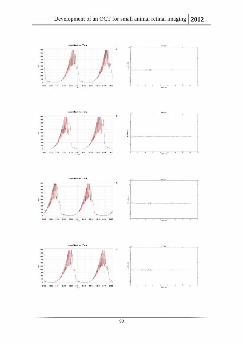
Development of an OCT for small animal retinal imaging 2012
90

Development of an OCT for small animal retinal imaging 2012
91