development of an electrically small vivaldi antenna…

DEVELOPMENT OF AN ELECTRICALLY SMALL VIVALDI ANTENNA:

THE CReSIS AERIAL VIVALDI (CAV-A)

BY

Ben Panzer

BSEE, University of Kansas 2004

Submitted to the graduate degree program in Electrical Engineering

And the Faculty of the Graduate School of the University of Kansas

In partial fulfillment of the requirements for the degree of

Master’s of Science

______________________

Dr. Chris Allen

Professor in Charge

Committee members ______________________

Dr. Shannon Blunt

______________________

Dr. Kenneth Demarest

______________________ Dr. James Stiles

Date defended: ______________

2

The Thesis Committee for Ben Panzer certifies

That this is the approved Version of the following thesis:

DEVELOPMENT OF AN ELECTRICALLY SMALL VIVALDI ANTENNA:

THE CReSIS AERIAL VIVALDI (CAV-A)

Committee:

______________________

Dr. Chris Allen

Professor in Charge

______________________

Dr. Shannon Blunt

______________________

Dr. Kenneth Demarest

______________________ Dr. James Stiles

Date approved: ______________

3

ABSTRACT

Radar operation from the CReSIS Meridian UAV requires a broadband antenna array

composed of lightweight, thin, end-fire antenna elements. Toward this goal four Vivaldi

antenna designs were simulated, fabricated, and characterized. The final design, dubbed the

CReSIS Aerial Vivaldi – Revision A (CAV-A) provides operation over a band extending

from 162 MHz to 1.121 GHz. The CAV-A measures 40 cm long, 51 cm wide, and 0.125

inch thick with a weight of 3.22 lbs., thus satisfying the requirements for UAV operation.

Due to size, weight, and bandwidth requirements, a simple frequency scaling of a previously

published design was unachievable. Most published single-element Vivaldi antenna designs

were constrained by traditional thought that says the antenna length should be multiple free-

space wavelengths and the antenna width should be a half free-space wavelength, both at the

lowest frequency of interest. Contrary to convention, the CAV-A is an electrically small

antenna, with an antenna width and length on the order of a quarter free-space wavelength at

the lowest frequency of operation.

4

TABLE OF CONTENTS

INTRODUCTION................................................................................................................... 9

1.1 AIRBORNE OPERATION AND MOTIVATION................................................. 9 1.2 ANTENNA REQUIREMENTS DRIVEN BY UAV............................................ 10

Size................................................................................................................................. 11 Weight ............................................................................................................................ 11

1.3 BANDWIDTH AND BEAMWIDTH REQUIREMENTS DRIVEN BY RADAR

SYSTEMS............................................................................................................. 12 Operation........................................................................................................................ 12 Array Configuration ....................................................................................................... 12 Planar Structure.............................................................................................................. 12

1.4 THESIS ORGANIZATION .................................................................................. 13

OVERVIEW OF TAPERED SLOT ANTENNAS............................................................. 14

2.1 BASIC GEOMETRIES ......................................................................................... 14 Individual Element ......................................................................................................... 14 Linear Tapered Slot Antenna ......................................................................................... 15 Vivaldi Antenna ............................................................................................................. 16 Arrays............................................................................................................................. 17

2.3 CLASSIFICATION............................................................................................... 17 2.4 RADIATION CHARACTERISTICS.................................................................... 18

Description ..................................................................................................................... 18 Gain................................................................................................................................ 18 Beamwidth ..................................................................................................................... 19

2.5 ANTENNA PARAMETER EFFECTS ON RADIATION ................................... 19 Substrate......................................................................................................................... 19 Taper Profile................................................................................................................... 20 Length and Aperture Height........................................................................................... 20 Phase Center................................................................................................................... 21

2.6 DESIGN ................................................................................................................ 21 2.7 CONCLUSIONS ON TAPERED SLOT ANTENNAS........................................ 22 2.8 LITERATURE SEARCH AND FREQUENCY SCALING OF PREVIOUS

DESIGNS .............................................................................................................. 22

RESULTS AND DESIGN PROCEDURE .......................................................................... 26

3.1 CReSIS AERIAL VIVALDI................................................................................. 26 Design summary............................................................................................................. 26 Percentage bandwidth summary..................................................................................... 29 Results ............................................................................................................................ 30

3.2 DESIGN PROCEDURE........................................................................................ 35 Substrate......................................................................................................................... 36 Stripline trace width ....................................................................................................... 38 Antenna length ............................................................................................................... 38 Mouth opening ............................................................................................................... 39 Throat Width .................................................................................................................. 40 Backwall offset............................................................................................................... 43

5

Edge offset ..................................................................................................................... 44 Radial stub stripline termination .................................................................................... 45 Circular cavity resonator diameter ................................................................................. 48 Taper profile................................................................................................................... 49 Summary of recommendations....................................................................................... 51

3.3 COMMON MISCONCEPTIONS ......................................................................... 52

CONCLUSIONS AND FUTURE WORK .......................................................................... 53

APPENDIX A SIMULATION SETUP............................................................................... 56

APPENDIX B MEASUREMENT SETUP ......................................................................... 60

APPENDIX C PRINCIPAL PLANE RADIATION PATTERNS.................................... 65

APPENDIX D ARRAY CHARACTERISTICS................................................................. 69

APPENDIX E SIGNAL LAUNCH...................................................................................... 74

REFERENCES...................................................................................................................... 76

6

LIST OF FIGURES

Figure 1.1 – Antenna dimensions for Meridian configuration ................................... 11

Figure 2.1 – Overview of TSA dimensions and fields................................................ 14

Figure 2.2 – Taper profiles.......................................................................................... 14

Figure 2.3 – Balanced antipodal Vivaldi layout [20].................................................. 15

Figure 2.4 – Linear tapered slot antenna [39] ............................................................. 16

Figure 2.5 – Exponentially tapered slot antenna [17] ................................................. 16

Figure 2.6 – Standard array configurations................................................................. 17

Figure 2.7 – Scaled length normalized to λ0 at lowest operating frequency versus

percentage bandwidth ......................................................................................... 24

Figure 2.8 – Scaled width normalized to λ0 at lowest operating frequency versus


Figure 3.1 – Vivaldi antenna geometry....................................................................... 27

Table 3.1 – Design summary; Figure 3.2 – Revision 1; Figure 3.3 – Revision 2;

Figure 3.4 – Revision 3; Figure 3.5 – Revision 4 ............................................... 28

Figure 3.6 – Return loss vs. frequency, all designs .................................................... 29

Figure 3.7 - Scaled length normalized to λ0 at lowest operating frequency versus


Figure 3.8 - Scaled width normalized to λ0 at lowest operating frequency versus


Figure 3.9 – Return loss vs. frequency for CAV-A .................................................... 31

Figure 3.10 – Orientation of the spherical coordinate system with antenna geometry32

Figure 3.11 - E-plane gain vs. θ, measured vs. simulated........................................... 33

Figure 3.12 –H-plane gain vs. θ, measured vs. simulated .......................................... 33

Figure 3.13 – Measured CAV-A peak gain vs. frequency.......................................... 34

Figure 3.14 – CAV-A effective aperture vs. frequency.............................................. 35

Figure 3.15 – Design methodology followed ............................................................. 36

Figure 3.16 – Return loss vs. frequency, +/- 5% substrate thickness variation from

CAV-A................................................................................................................ 37

Figure 3.17 – Return loss vs. frequency, +/- 10% antenna length variation from CAV-

A.......................................................................................................................... 39

Figure 3.18 – Return loss vs. frequency, +/- 25% mouth opening variation from

CAV-A................................................................................................................ 40

Figure 3.19 – Unilateral (left) slotline vs. Bilateral slotline (right) ............................ 42

Figure 3.20 – Return loss vs. frequency, +/- 25% throat width variation from CAV-A

............................................................................................................................. 43

Figure 3.21 – Gibson Vivaldi antenna [2, 17] ............................................................ 44

Figure 3.22 – Return loss vs. frequency, +/- 50% backwall offset variation from

CAV-A................................................................................................................ 45

Figure 3.23 – Return loss vs. frequency, +/- 25% edge offset variation from CAV-A

............................................................................................................................. 46

Figure 3.24 – Return loss vs. frequency, +/- 25% radial stub radius variation from

CAV-A................................................................................................................ 47

7

Figure 3.25 – Return loss vs. frequency, radial stub angle variation from CAV-A ... 48

Figure 3.27 – Return loss vs. frequency, +/- 10% taper rate variation from CAV-A. 50

Figure A.1 – CAV-A simulation layout...................................................................... 57

Figure A.2 - Wave port orientation............................................................................. 58

Figure B.1 – Positioner stackup and return loss measurement setup.......................... 60

Figure B.2 – Vivaldi under test, E-plane measurement .............................................. 61

Figure B.3 – Calibrated H-plane boresight measurement setup ................................. 62

Figure B.4 – E-plane measurement setup ................................................................... 63

Figure B.5 – H-plane measurement setup................................................................... 63

Figure C.1 – E-plane gain vs. θ, 160 MHz ................................................................. 65









Figure C.10 – H-plane gain vs. θ, 160 MHz............................................................... 67









Figure D.1 – Return loss vs. frequency, 4 element H-plane array with 75 cm center-

to-center spacing ................................................................................................. 69

Figure D.2 – Coupling between array elements.......................................................... 70

Figure D.3 – Array factor vs. theta at 200 MHz; 8 element H-plane array with 75 cm

element separation .............................................................................................. 72

Figure D.4 – Array gain vs. theta at 200 MHz; 8 element H-plane array with 75 cm

element separation .............................................................................................. 73

Figure E.1 – Revision 1 and 2 BNC connectors; left – Amphenol 112536 [4], right –

Amphenol 112515 [4] ......................................................................................... 74

Figure E.2 – Blind via before (left) and after (right) soldering BNC connector ........ 74

Figure E.3 – Revision 3 and 4 SMA connectors; left – Pasternack 4190 [38], right –

Amphenol 132134 [4] ......................................................................................... 75

8

LIST OF TABLES

Table 1.1 – Aircraft specifications.............................................................................. 10

Table 1.2 – Antenna requirements .............................................................................. 13

Table 2.1 – Summary of published designs scaled ..................................................... 25

Table 3.1 – Design summary ...................................................................................... 28

9

CHAPTER 1

INTRODUCTION

1.1 AIRBORNE OPERATION AND MOTIVATION

Airborne radar mapping missions over the polar regions provide glaciologists with detailed

ice characterization data over extensive areas. Current Center for Remote Sensing of Ice

Sheets (CReSIS) airborne science missions employ manned aircraft such as the Orion P-3 and

Twin Otter DHC-6. However, manned missions over polar regions are dangerous for pilots

and crews given the low altitude, indistinct horizon and remoteness of the missions. In

addition, manned flights are expensive and time consuming. Given the aircraft utilized and

the risks of polar airborne measurements, CReSIS plans to reduce the human element in

airborne science missions by constructing an unmanned aerial vehicle (UAV) capable of

flying smaller scale missions [3].

The Aerospace Engineering Department at the University of Kansas, in coordination with

CReSIS, is currently building two prototypes of the Meridian, a UAV. The Meridian will be

17 ft. in length with a 26.4 ft. wingspan [22]. Consequently, both UAVs, given their reduced

size, can be shipped together in a standard 20 ft. long shipping crate for delivery to polar

regions [22]. Presently, the payload weight budget for radar system design purposes is 120

lbs. for 13 hr. flight endurance [22]. Heavier payloads can be flown by reducing the fuel load

resulting in decreased endurance, with a worst-case payload of 165 lbs. The Meridian can

support wideband radar sensors, eliminating some of the electromagnetic interference (EMI)

issues associated with navigation and communications of crewed missions [3]. Table 1.1

below summarizes properties of the manned aircraft versus the Meridian.

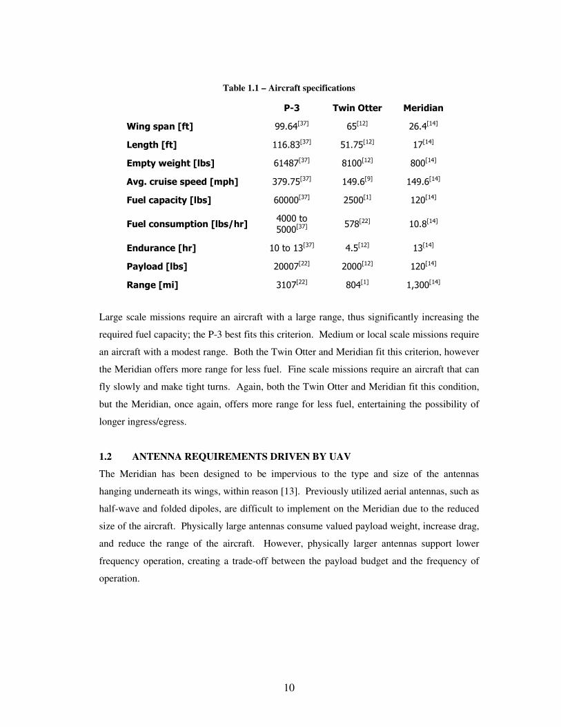
10

Table 1.1 – Aircraft specifications

P-3 Twin Otter Meridian

Wing span [ft] 99.64[37] 65[12] 26.4[14]

Length [ft] 116.83[37] 51.75[12] 17[14]

Empty weight [lbs] 61487[37] 8100[12] 800[14]

Avg. cruise speed [mph] 379.75[37] 149.6[9] 149.6[14]

Fuel capacity [lbs] 60000[37] 2500[1] 120[14]

Fuel consumption [lbs/hr] 4000 to

5000[37] 578[22] 10.8[14]

Endurance [hr] 10 to 13[37] 4.5[12] 13[14]

Payload [lbs] 20007[22] 2000[12] 120[14]

Range [mi] 3107[22] 804[1] 1,300[14]

Large scale missions require an aircraft with a large range, thus significantly increasing the

required fuel capacity; the P-3 best fits this criterion. Medium or local scale missions require

an aircraft with a modest range. Both the Twin Otter and Meridian fit this criterion, however

the Meridian offers more range for less fuel. Fine scale missions require an aircraft that can

fly slowly and make tight turns. Again, both the Twin Otter and Meridian fit this condition,

but the Meridian, once again, offers more range for less fuel, entertaining the possibility of

longer ingress/egress.

1.2 ANTENNA REQUIREMENTS DRIVEN BY UAV

The Meridian has been designed to be impervious to the type and size of the antennas

hanging underneath its wings, within reason [13]. Previously utilized aerial antennas, such as

half-wave and folded dipoles, are difficult to implement on the Meridian due to the reduced

size of the aircraft. Physically large antennas consume valued payload weight, increase drag,

and reduce the range of the aircraft. However, physically larger antennas support lower

frequency operation, creating a trade-off between the payload budget and the frequency of

operation.

11

Size

Real estate for the antenna is limited to 50 cm length × 50 cm width × 1 inch thickness.

Wing flutter and the wing-to-ground clearance are the limiting factors for the 50 cm length.

The antenna width requirement is rather soft; making the antenna wider than 50 cm

introduces center of gravity issues that can be resolved by shifting the element placement on

the wing or reshaping the element to have a smaller footprint connected to the wing compared

to the footprint in the wind, so to speak [14]. Antenna thicknesses greater than 1 in. introduce

a significantly larger aerodynamic footprint. All effects mentioned above are greatly

exaggerated as a result. Regardless of antenna dimensions, components to stiffen and support

the UAV-mounted antenna will be required.

Figure 1.1 – Antenna dimensions for Meridian configuration

Weight

Antenna elements should weigh between 2 and 3 lbs [13]. As discussed earlier, the

maximum payload weight for a 13-hr. flight endurance is 120 lbs. Antennas weighing greater

than 3 lbs. will cut into the already limited radar system payload weight budget. Again,

heavier payloads can be accommodated at the expense of endurance.

12

1.3 BANDWIDTH AND BEAMWIDTH REQUIREMENTS DRIVEN BY RADAR

SYSTEMS

Operation

Currently, missions flown on the P-3 or Twin Otter utilize narrowband antenna elements such

as half-wave or folded dipoles. Usage of a dipole-like aerial requires tuning the response to

behave properly in presence of a conducting backplane, or wing, in this instance. To operate

systems at significantly different frequencies requires switching antenna elements while on

the ground resulting in lost flight time. Furthermore, center-to-center separation of the

antenna elements is optimized for 150-MHz operation. This separation distance is fixed and

does not change, even though the frequency of operation might. Consequently, operation at

higher frequencies may involve grating lobes in the radiation pattern of the array; typical for

any frequency of operation whose wavelength is less than the element separation.

Ideally the antenna will operate over a continuous range of frequencies supporting a variety

of foreseeable radar deployments, introducing the possibility of carrying multiple radars

simultaneously, all utilizing the same antenna structure.

The antenna’s operational frequency range must extend from 150 MHz to 1 GHz, if not

higher. Acceptable performance is dictated by a -10-dB return loss benchmark. A maximum

worst-case return loss is set to -8 dB.

Array Configuration

Meridian was designed with the intention to carry three antenna elements beneath each wing.

The initial radar system configuration will have four antenna elements beneath each wing. A

dedicated transmit/receive module will be mounted on or near each antenna element. Hard

points, spaced every 25 cm, designed for antenna attachments are included in the wing

structure of the Meridian [13]. Consequently, the antenna element center-to-center spacing

should be designed to be a multiple of 25 cm.

Planar Structure

While initial designs considered integrating a broadside radiator into a carbon fiber wing

structure, the as yet unknown complexities of the wing structure coupled with the bandwidth

13

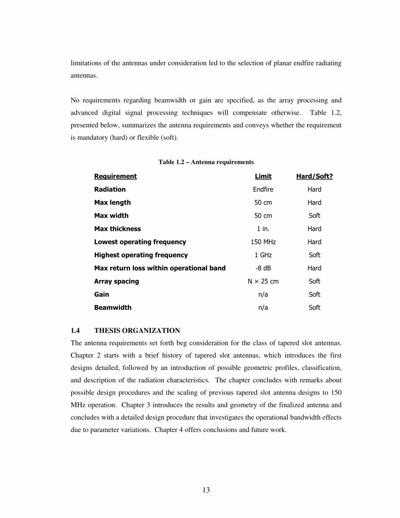
limitations of the antennas under consideration led to the selection of planar endfire radiating

antennas.

No requirements regarding beamwidth or gain are specified, as the array processing and

advanced digital signal processing techniques will compensate otherwise. Table 1.2,

presented below, summarizes the antenna requirements and conveys whether the requirement

is mandatory (hard) or flexible (soft).

Table 1.2 – Antenna requirements

Requirement Limit Hard/Soft?

Radiation Endfire Hard

Max length 50 cm Hard

Max width 50 cm Soft

Max thickness 1 in. Hard

Lowest operating frequency 150 MHz Hard

Highest operating frequency 1 GHz Soft

Max return loss within operational band -8 dB Hard

Array spacing N × 25 cm Soft

Gain n/a Soft

Beamwidth n/a Soft

1.4 THESIS ORGANIZATION

The antenna requirements set forth beg consideration for the class of tapered slot antennas.

Chapter 2 starts with a brief history of tapered slot antennas, which introduces the first

designs detailed, followed by an introduction of possible geometric profiles, classification,

and description of the radiation characteristics. The chapter concludes with remarks about

possible design procedures and the scaling of previous tapered slot antenna designs to 150

MHz operation. Chapter 3 introduces the results and geometry of the finalized antenna and

concludes with a detailed design procedure that investigates the operational bandwidth effects

due to parameter variations. Chapter 4 offers conclusions and future work.

14

CHAPTER 2

OVERVIEW OF TAPERED SLOT ANTENNAS

Tapered slot antennas (TSA) first appeared in 1979 when Prasad and Mahapatra introduced

the linear tapered slot antenna (LTSA) [39]. Gibson originated the exponentially tapered slot

antenna (ETSA or Vivaldi) shortly thereafter [17]. Tapered slot antennas offer qualities such

as efficiency, bandwidth, light weight, and geometric simplicity [48]. Utilizing

photolithography, low cost, reproducible, and repeatable designs result. Figure 2.1 specifies

dimensions and fields referred to throughout the chapter.

Figure 2.1 – Overview of TSA dimensions and fields

2.1 BASIC GEOMETRIES

Individual Element

The gradual widening of a slotline transmission line constitutes the radiating region, which

can take on three geometric profiles [31]. The three classes of taper profile include constant

width, linear, and non-linear, which includes Vivaldi and Fermi taper profiles. Figure 2.2

illustrates these taper profiles. Fermi tapering, compared to the other three profiles, provides

additional degrees of freedom, allowing more control over radiation characteristics [24].

Figure 2.2 – Taper profiles

The taper profiles illustrated in Figure 2.2 can be used in either a unilateral or bilateral

slotline configuration. Unilateral slotline refers to a spatially asymmetric geometry in which

there is only one tapered slotline backed by bare substrate. Bilateral slotline refers to a

15

spatially symmetric geometry in which there are two tapered slotlines, separated some

distance by a substrate. However, there exists an antipodal layout that cannot be described as

either. Figure 2.3 below illustrates a particular layout of a balanced antipodal Vivaldi

antenna presented in [20]. Mirrored metallization makes the antenna antipodal; the stripline

feed makes the antenna balanced.

Figure 2.3 – Balanced antipodal Vivaldi layout [20]

Various feeding methods have been utilized in previous work. The earliest tapered slot

antennas used a microstrip feed, taking advantage of half of the unilateral slotline flare as a

ground plane. More recently, stripline and coplanar waveguide feed lines have been

incorporated. Stripline feed lines are used for bilateral slotline designs, making the structure

spatially symmetric, unlike the first two designs. Another feed line seldom used is coaxial

cable.

Linear Tapered Slot Antenna

Figure 2.4 illustrates the geometry of the LTSA presented in [39]. As can be seen, the so-

called taper of the slotline transmission line can be described as a linear function, thus the

moniker, linear tapered slot antenna. The operational frequency range of the antenna extends

from 8.5 GHz to 9.45 GHz.

The overall length and aperture height of the antenna were on the order of a free-space

wavelength (λ0) and λ0/4, respectively, at 8.5 GHz. The theory of operation was based on

excessive widening of the slotline transmission line. The authors state that if the guide

wavelength, a function of slot width and frequency, exceeds 40% of the free space

wavelength, propagation ceases and radiation transpires.

16

Figure 2.4 – Linear tapered slot antenna [39]

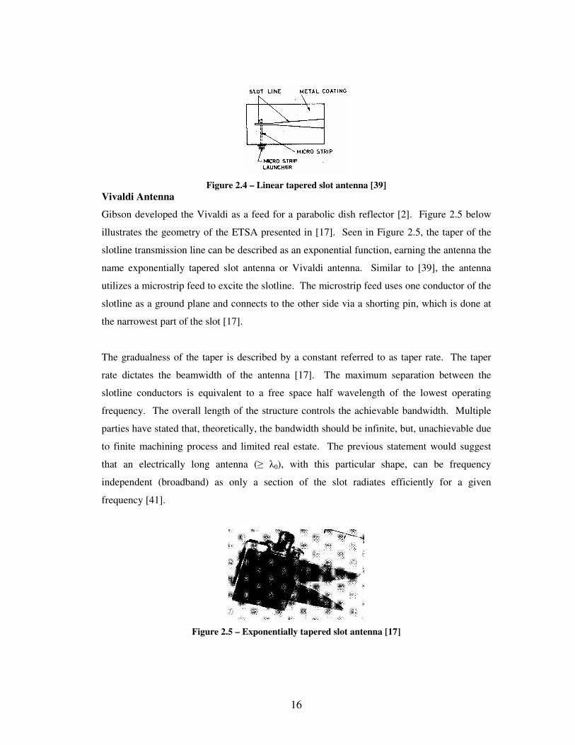
Vivaldi Antenna

Gibson developed the Vivaldi as a feed for a parabolic dish reflector [2]. Figure 2.5 below

illustrates the geometry of the ETSA presented in [17]. Seen in Figure 2.5, the taper of the

slotline transmission line can be described as an exponential function, earning the antenna the

name exponentially tapered slot antenna or Vivaldi antenna. Similar to [39], the antenna

utilizes a microstrip feed to excite the slotline. The microstrip feed uses one conductor of the

slotline as a ground plane and connects to the other side via a shorting pin, which is done at

the narrowest part of the slot [17].

The gradualness of the taper is described by a constant referred to as taper rate. The taper

rate dictates the beamwidth of the antenna [17]. The maximum separation between the

slotline conductors is equivalent to a free space half wavelength of the lowest operating

frequency. The overall length of the structure controls the achievable bandwidth. Multiple

parties have stated that, theoretically, the bandwidth should be infinite, but, unachievable due

to finite machining process and limited real estate. The previous statement would suggest

that an electrically long antenna (≥ λ0), with this particular shape, can be frequency

independent (broadband) as only a section of the slot radiates efficiently for a given

frequency [41].

Figure 2.5 – Exponentially tapered slot antenna [17]

17

Arrays

Figure 2.6 displays standard array configurations for tapered slot antennas. Dual-polarized

arrays utilize both standard configurations. For H-plane arrays, coupling between adjacent

elements hinders more than aids the return loss of each. Although a slight separation is

shown between adjacent elements in the E-plane array, this does not have to be the case.

Metallization and substrate from adjacent elements can be extended between the elements if

desired. Mutual coupling between adjacent elements, unlike the H-plane array configuration,

actually helps the individual return loss of each element. In either case, the separation of

elements will need to be optimized, as the impact of coupling varies with frequency. Given

limited wing span for center-to-center spacing, in addition to restricted antenna size and

frequencies of interest, a possible combination of E- and H-plane arrays is immediately ruled

out; a simple H-plane array configuration will be used.

Figure 2.6 – Standard array configurations

2.3 CLASSIFICATION

Tapered slot antennas belong to the class of endfire traveling wave antennas [48]. “All

antennas whose current and voltage distributions can be represented by one or more traveling

waves, usually in the same direction, are referred to as traveling wave antennas [5].” The

class of traveling wave antennas can be divided into leaky-wave and surface-wave [41].

Tapered slot antennas belong to the surface-wave class since the traveling wave propagates

with a phase velocity less than or equal to the speed of light, resulting in endfire radiation

[41]. “An antenna which radiates power flow from discontinuities in the structure that

interrupt a bound wave on the antenna surface” defines a surface-wave antenna [25].

18

Leaky-wave antennas propagate a traveling wave with a phase velocity greater than the speed

of light, resulting in a main beam direction other than endfire [41]. “An antenna that couples

power in small increments per unit length, either continuously or discretely, from a traveling

wave structure to free-space” defines a leaky-wave antenna [25]. “Leaky-wave antennas

continuously lose energy due to radiation…the fields decay along the structure in the

direction of wave travel and increase in others [5].”

A spatially symmetric endfire radiation pattern over large bandwidths with appreciable gain

and low sidelobes is inherent to the class of endfire traveling wave antennas [48]. Due to

their classification as a traveling wave structure, tapered slot antennas have moderately high

directivity (10-17 dB) for a given cross section, for electrically long antennas on the order of

3 to 8λ0 [41].

2.4 RADIATION CHARACTERISTICS

Description

The surface-wave nature of tapered slot antennas results in a radiation mechanism based on

incomplete or full conversion of incident power of the slotline propagation mode to radiating

power [23]. Conversion might occur at: the antenna end, the feeding area, or along the

slotline profile. Given its planar shape and surface wave nature, the radiated E-field is

parallel to the plane of the slot and linearly polarized, as seen in Figure 2.1 [26].

In general, the slotline radiates when the separation between the conductors is made markedly

wide [39]. “Energy in the traveling wave is tightly bound to the conductors when the

separation is small compared to a free space wavelength and becomes progressively weaker

and more coupled to the radiating field as the separation is increased [17].” The taper profile

can be divided into propagation and radiation regions [23]. When the slot widens to the order

of λ0/2, propagation ceases and radiation begins [23, 41].

Gain

As the electrical length of the antenna increases with frequency the gain increases [44].

Typical directivity for a tapered slot antenna with length, L, on the order of 3 to 8 free space

wavelengths, is (10L)/λ0 [41].

19

Beamwidth

Despite their planar geometry, tapered slot antennas can produce a symmetric beam, in both

E- and H-planes, over wide bandwidths [41]. However, judicious choice of antenna

parameters such as shape, total length, dielectric thickness, and dielectric constant must be

made [41]. Gibson obtained approximately constant beamwidth versus frequency in both the

E- and H-planes [17].

Beamwidth is dependent on the taper profile chosen. For a given substrate, length, and

aperture height, the constant width tapered slot antenna (CWSA) produces the narrowest

beamwidth, followed by the LTSA and Vivaldi [53]. In addition, sidelobe power levels are

greatest for the CWSA, followed by the LTSA and Vivaldi [53].

2.5 ANTENNA PARAMETER EFFECTS ON RADIATION

Substrate

Phase velocity of the propagating surface wave determines radiation performance [11].

Kotthaus and Vowinkel [30] stated that the H-plane pattern is dependent upon phase velocity.

Substrate thickness and dielectric constant control the phase velocity of the surface wave [11].

Therefore, radiation pattern and performance is dependent upon substrate thickness and

dielectric constant [28, 31].

The primary effect of the dielectric substrate is the narrowing of the main beam of the

antenna [31]. Increasing the substrate thickness increases the gain of the antenna, with the

consequence of higher sidelobes [30, 31] and asymmetric beam patterns [30]. Low dielectric

constant substrates maximize the antenna radiation by reducing the dielectric discontinuity at

the end of the TSA [8]. Large dielectric contrasts at the end of the TSA can cause scattering

of the surface wave traveling along the antenna, resulting in spurious radiation pattern effects

[35]. Tapered dielectric sections can be attached to the end of the antenna to ease the

transition to free space [35].

[53] introduced the substrate effective thickness normalized to a wavelength, which is

presented below as Equation 2.1, and should be in the range of 0.005 to 0.03 for optimal

endfire directivity. The variable, t, represents the physical substrate thickness.

20

( )00

1λ

ελ

ttr

eff −= Eq. 2.1 [53]

The substrate effective thickness, teff, was defined for antennas on the order of 4 to 10λ0.

How this applies to Vivaldi antennas with lengths on the order of λ0/4 has yet to be

determined. For values below the recommended range, decreased gain results [36, 53]. The

main beam of the antenna splits if above the recommended range [53]. Effective thickness

increases with frequency resulting in beamwidth reduction, sidelobe power level increase,

and pattern degradation [36]. For effective substrate thickness above the upper bound

“unwanted substrate modes develop that degrade performance [36].” As suggested in [33], a

photonic bandgap structure consisting of conducting strips, essentially a spatial filter, can be

incorporated to cutoff unwanted substrate modes at operating frequencies of interest.

Taper Profile

Radiation patterns for tapered slot antennas are dependent on the slot taper profile [28].

Taper profile significantly affects both the beamwidth and sidelobe power levels [17, 31].

Opening the flared slotline “quicker” narrows the beamwidth, consequently raising sidelobe

power levels [35]. Shifting the opening of the slotline toward the end of the antenna widens

the E-plane pattern while narrowing the H-plane pattern [24]. Furthermore, a taper profile

with a constant width toward the beginning of the antenna results in a narrower E-plane

pattern [24].

Length and Aperture Height

Beamwidths in the E- and H-plane are dependent on the length of the tapered slotline and the

spacing of the conductors composing the tapered slotline [30]. Increasing antenna length, L,

subsequently increases the gain and decreases the beamwidths in both the E- and H-planes

[31]. Two sources have reported a 1/√L relationship between antenna length and E- and H-

plane beamwidths [15, 31]. [31] reports that the relationship holds true for the H-plane

beamwidth, but the E-plane beamwidth is more dependent upon aperture height.

21

Phase Center

“Phase center is a reference point from which radiation is said to emanate” [5]. This

definition implies a three-dimensional phase center; regardless of observation point/plane, the

radiation from the antenna appears to originate at a single point. Contrasting opinions have

been published concerning the movement of the phase center with frequency for both

principal planes. Published results for the Vivaldi antenna [51] shows that the E-plane phase

center is stable compared to that of the H-plane which fluctuates as a function of frequency.

Results for the TSA [7] indicate a stable H-plane phase center, located in the vicinity of the

feed transition, compared to that of the E-plane which moves from the widest aperture height

toward the feed transition as frequency increases. Further clouding the issue, [52] states that

a TSA “can radiate a short pulse with a constant phase center.” Which principal plane(s) the

authors of [52] where referring to is unclear, but may be the 3-D phase center.

Disagreement seems to dominate this issue. Particularly confusing is the distinction between

principal plane phase centers and a 3-D phase center. If the E- and H-plane phase centers do

not coincide, discussion of a 3-D phase center seems rather meaningless.

2.6 DESIGN

Design methodologies for tapered slot antennas rely heavily on either theory or experiment

[18, 48]. General guidelines provided by [31] suggest an aperture height greater than a free-

space wavelength and an antenna length on the order of 2 to 12 free space wavelengths, both

at the lowest frequency of interest.

Methods for very large arrays are not directly applicable to the design of a single element. E-

plane mutual coupling between adjacent array elements significantly aids the antenna

designer in effectively reducing the size of a single element while expanding the bandwidth

of the entire array through alteration of each element’s input impedance characteristics.

Generally speaking, arrays of tapered slot antennas provide wideband operation, while the

individual elements, themselves, do not.

22

2.7 CONCLUSIONS ON TAPERED SLOT ANTENNAS

Below is a summary of conclusions gleaned from various statements on tapered-slot antennas

in the literature. Bear in mind these reflect a wide variety of experiences and largely

represent findings for electrically large antennas, i.e., length and width greater than λo at the

lowest operating frequency.

1. Light weight, wide bandwidth, geometrically simple, low cost and easily

reproducible.

2. Endfire, traveling wave antenna.

3. Gain and beamwidth are functions of antenna length, dielectric substrate, and taper

rate.

4. Symmetrical E- and H-plane beamwidths can be attained.

5. Addition of a dielectric substrate increases the gain and narrows the main beam, at

the consequence of higher sidelobes.

6. Antenna length affects the H-plane beamwidth, while the taper profile affects the E-

plane beamwidth.

7. Mixed opinions on the stability of the phase centers for both principal planes. (Not

much of a conclusion)

2.8 LITERATURE SEARCH AND FREQUENCY SCALING OF PREVIOUS

DESIGNS

With the absence of a proven methodology to follow for designing the UAV antenna, a

literature search was performed to gain an overview of previous designs. The goal of the

search was to compile as many detailed designs previously published. Of particular interest

are the overall antenna dimensions and the operational frequency range. Table 2.1

summarizes the results of the search. The table is not meant to be exhaustive; some designs

were not completely detailed and were therefore omitted. For those designs adequately

detailed, the dimensions and frequency range of the antenna were scaled for a lowest

operating frequency of 150 MHz. Figures 2.7 and 2.8 plot both scaled length and scaled

width of each design, normalized to free space wavelength versus percent bandwidth.

Percent bandwidth was calculated using Equation 2.2. Upper and lower cutoff frequencies

are represented by fu and fl, respectively.

23

2fwhere

%BW

c

lu

l

c

lu

fff

f

-ff

−+=

= Eq. 2.2

The boxes within the plot indicate the region of interest (~145% bandwidth, ~λ0/4

dimensionality), and clearly demonstrate the absence of suitable scaled designs. For

completeness, both single and array elements are included.

Most of the scaled designs violate either the length or width constraints or both. Those scaled

designs barely outside the dimension constraints fail to fulfill the bandwidth requirements.

However, in the absence of a proven design methodology, a good starting point for design

purposes would be the scaled version of [10], but one must account for the fact that the

element is part of a dual-polarized array.

Given the size constraints in Chapter 1, designing a tapered slot antenna for operation in the

meter wavelength region was not a trivial task. Previous single element designs fall into the

surface-wave regime. Surface-wave antennas are typically multiple wavelengths in length.

Essentially, for 150-MHz operation, the design “falls out” of the surface-wave regime due to

the fact that the length of the antenna is restricted to λ0/4. The Vivaldi antenna designed will

possibly straddle the distinction between traveling wave and non-traveling wave antennas.

24

Scaled electrical length vs. Percentage bandwidth

0

0.1

0.2

0.3

0.4

0.5

0.6

0.7

0.8

0.9

1

0 20 40 60 80 100 120 140 160 180 200

Percentage bandwidth

Scale

d e

lectr

ical

length

Single Element Array Element

Figure 2.7 – Scaled length normalized to λ0 at lowest operating frequency versus percentage

bandwidth

Scaled electrical width vs. Percentage bandwidth

0

0.1

0.2

0.3

0.4

0.5

0.6

0.7

0.8

0.9

1

0 20 40 60 80 100 120 140 160 180 200


Scale

d e

lectr

ical w

idth

Single Element Array Element

Figure 2.8 – Scaled width normalized to λ0 at lowest operating frequency versus percentage

bandwidth

25

Table 2.1 – Summary of published designs scaled

Ref

Specia

l C

odes

Low

er

Fre

qu

en

cy

Upper

Fre

qu

en

cy

Scale

d U

pper

Fre

q.*

Len

gth

Wid

thS

cale

d L

en

gth

*

Scale

d W

idth

*

[GH

z]

[GH

z]

[GH

z]

[cm

][c

m]

[cm

][c

m]

[45]

O2

26.5

1.99

2.8575

10.85

38

145

[47]

M3.1

4.85

0.23

2.3

2.975

48

61

[10]

S, A

14.5

0.68

7.35

249

13

[32]

CPW

3.1

8.3

0.40

33

62

62

[52]

M1.233

9.914

1.21

9.6

12

79

99

[20]

S, AP

1.3

20

2.31

10

7.4

87

64

[50]

O, A

0.15

1.75

1.75

92

88

92

88

[45]

M, AP

220

1.50

7.13

5.35

95

71

[54]

M2.8

11.09

0.59

5.5

5103

93

[40]

S, A

0.5

1.5

0.45

31.5

11.25

105

38

[9]

M, A

13.75

0.56

18

9.5

120

63

[16]

S6

18

0.45

3.159

2.5

126

100

[34]

M4.5

13.5

0.45

54.8

150

144

[46]

M1.6

12.4

1.16

15

12

160

128

[46]

M, A

1.8

15.2

1.27

15

10

180

120

[19]

S, AP

3.8

20

0.79

10.5

7.5

266

190

[24]

CPW

12

24

0.30

3.33

1.67

266

134

[39]

M8.55

9.45

0.17

5.08

2.54

290

145

[17]

M8

40

0.75

5.5

2.5

293

133

[29]

CPW

618

0.45

93

360

120

[30]

M7.5

90.18

11

7.5

550

375

[36]

O30

36

0.18

42.8

800

560

[49]

CPW, A

28

0.60

76

64

1013

853

AP

Antipodal

MMicrostrip feed

SStripline feed

CPW

Coplanar waveguide feed

CCoaxial feed

OOther feed (probe or diode)

AArray

*Lower frequency scaled to 150 MHz

Table

2.1

26

CHAPTER 3

RESULTS AND DESIGN PROCEDURE

3.1 CReSIS AERIAL VIVALDI

To satisfy the UAV antenna requirements, four different Vivaldi antenna designs were

developed and tested within a 9 month period of time. Table 3.1 summarizes the antenna

geometry for each, with associated parameters presented in Figure 3.1. Motivation for

development and the starting point for each design differ. The first design, which started as a

frequency scaled version of [10], was simply used as verification of the simulations

performed in Ansoft HFSS. The desire to decrease the antenna weight and lowest frequency

of operation prompted the second design. However, the frequency scaling technique

employed for the first design was abandoned given the results of [15, 29, 31, 41, 43, 53] that

the mouth opening (Figure 3.1) of the antenna controlled the lowest frequency of operation

and needed to be increased substantially to obtain 150-MHz operation. A design

methodology resulted from the second design which significantly accelerated design time of

the third and fourth designs. The third design was, yet, another attempt to decrease the

antenna weight, which was accomplished by decreasing the mouth opening, but the fourth

design originated as a request from the UAV group to widen the structure back to 50 cm for

mounting purposes.

All Vivaldi elements were fabricated using photolithography on inexpensive and readily

available FR-4 substrate by Hughes Circuits. The reader is referred to Appendix E for

discussion involving signal excitation.

Design summary

Figure 3.2 through 3.5 depict the four design revisions in their physical forms. Summarized

below are observations of the variations in design geometry.

1. Revision 1 is at least 2 times thicker than the other three.

2. Length and width of revision 1 are reversed compared to the other three.

3. Revision 1 has a taper rate 30% greater than the other three.

4. Edge offset, throat length, and backwall offset remain constant throughout.

5. Stripline trace width was designed for a 50-Ω impedance given the substrate

thickness.

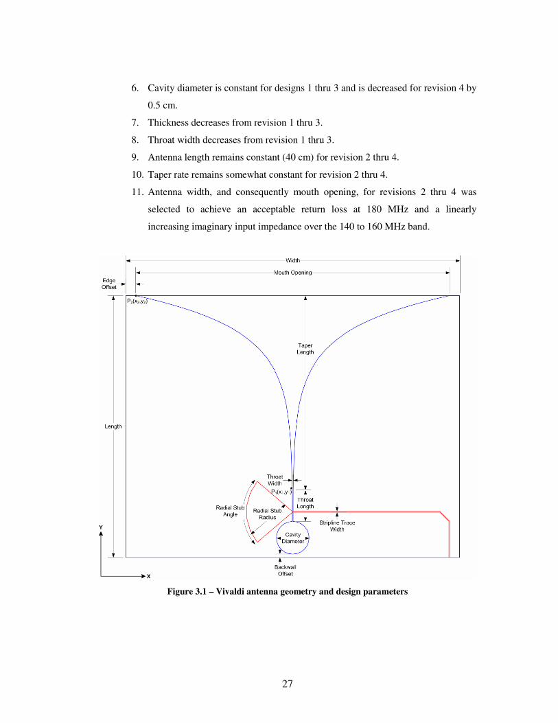
27

6. Cavity diameter is constant for designs 1 thru 3 and is decreased for revision 4 by

0.5 cm.

7. Thickness decreases from revision 1 thru 3.

8. Throat width decreases from revision 1 thru 3.

9. Antenna length remains constant (40 cm) for revision 2 thru 4.

10. Taper rate remains somewhat constant for revision 2 thru 4.

11. Antenna width, and consequently mouth opening, for revisions 2 thru 4 was

selected to achieve an acceptable return loss at 180 MHz and a linearly

increasing imaginary input impedance over the 140 to 160 MHz band.

Figure 3.1 – Vivaldi antenna geometry and design parameters

28

Table 3.1 – Design summary; Figure 3.2 – Revision 1; Figure 3.3 – Revision 2; Figure 3.4 –

Revision 3; Figure 3.5 – Revision 4

Fig

. 3

.2

Fig

. 3

.3

Fig

. 3

.4

Fig

. 3

.5

29

100 200 300 400 500 600 700 800 900 1000-50

-45

-40

-35

-30

-25

-20

-15

-10

-5

0

frequency [MHz]

S11 [

dB

]

Measured return loss vs. frequency, all designs

1

2

3

4

Figure 3.6 – Measured return loss vs. frequency for all four antenna designs

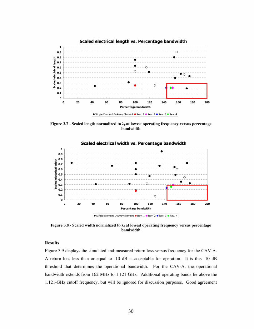
Percentage bandwidth summary

Shown below in Figures 3.7 and 3.8 are updated versions of Figures 2.7 and 2.8 that include

the four designs. Revision 4 was the only design to satisfy both the bandwidth and dimension

requirements. From this point forward only revision 4 will be discussed and will be referred

to as CAV-A (CReSIS Aerial Vivaldi – Revision A).

30

Scaled electrical length vs. Percentage bandwidth

0

0.1

0.2

0.3

0.4

0.5

0.6

0.7

0.8

0.9

1

0 20 40 60 80 100 120 140 160 180 200


Scale

d e

lectr

ical le

ngth

Single Element Array Element Rev. 1 Rev. 2 Rev. 3 Rev. 4

Figure 3.7 - Scaled length normalized to λ0 at lowest operating frequency versus percentage

bandwidth

Scaled electrical width vs. Percentage bandwidth

0

0.1

0.2

0.3

0.4

0.5

0.6

0.7

0.8

0.9

1

0 20 40 60 80 100 120 140 160 180 200


Scale

d e

lectr

ical w

idth

Single Element Array Element Rev. 1 Rev. 2 Rev. 3 Rev. 4

Figure 3.8 - Scaled width normalized to λ0 at lowest operating frequency versus percentage

bandwidth

Results

Figure 3.9 displays the simulated and measured return loss versus frequency for the CAV-A.

A return loss less than or equal to -10 dB is acceptable for operation. It is this -10 dB

threshold that determines the operational bandwidth. For the CAV-A, the operational

bandwidth extends from 162 MHz to 1.121 GHz. Additional operating bands lie above the

1.121-GHz cutoff frequency, but will be ignored for discussion purposes. Good agreement

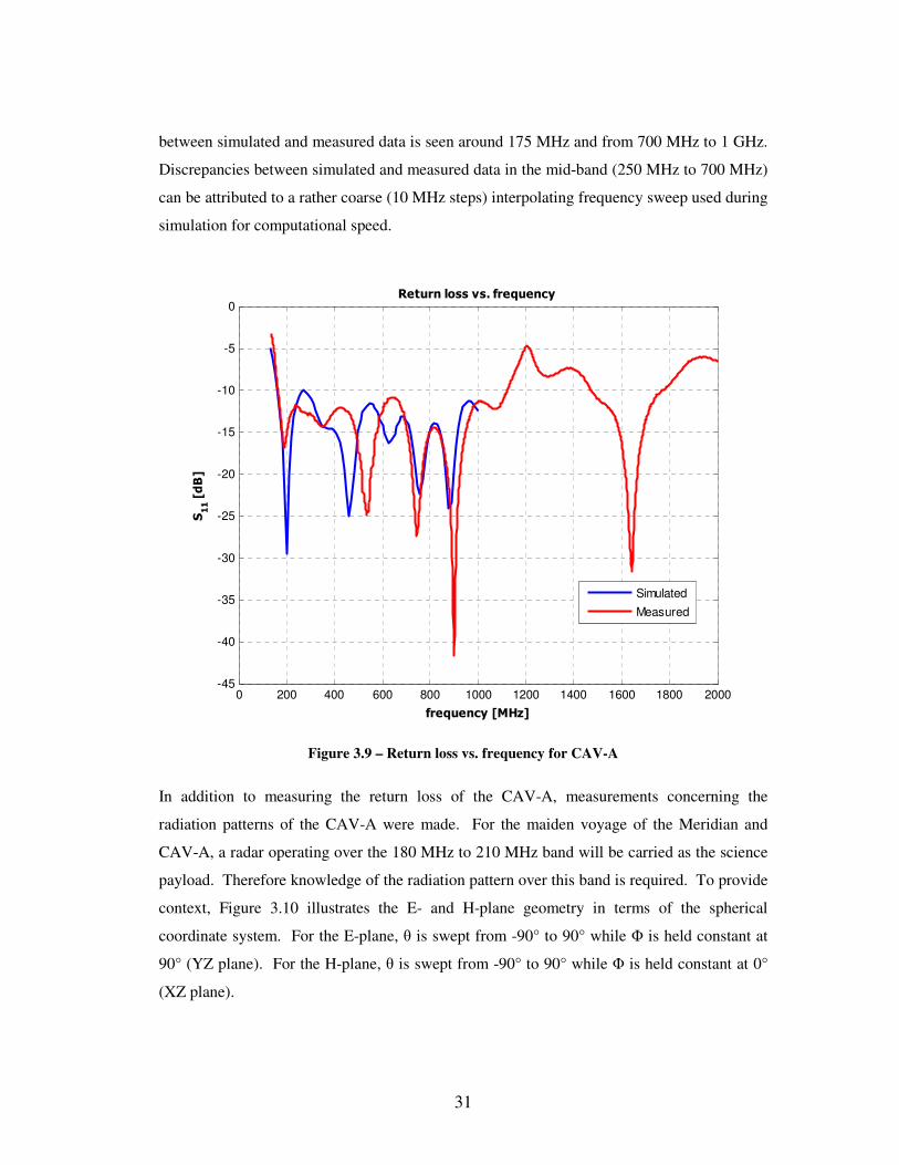
31

between simulated and measured data is seen around 175 MHz and from 700 MHz to 1 GHz.

Discrepancies between simulated and measured data in the mid-band (250 MHz to 700 MHz)

can be attributed to a rather coarse (10 MHz steps) interpolating frequency sweep used during

simulation for computational speed.

0 200 400 600 800 1000 1200 1400 1600 1800 2000-45

-40

-35

-30

-25

-20

-15

-10

-5

0

frequency [MHz]

S11 [

dB

]

Return loss vs. frequency

Simulated

Measured

Figure 3.9 – Return loss vs. frequency for CAV-A

In addition to measuring the return loss of the CAV-A, measurements concerning the

radiation patterns of the CAV-A were made. For the maiden voyage of the Meridian and

CAV-A, a radar operating over the 180 MHz to 210 MHz band will be carried as the science

payload. Therefore knowledge of the radiation pattern over this band is required. To provide

context, Figure 3.10 illustrates the E- and H-plane geometry in terms of the spherical

coordinate system. For the E-plane, θ is swept from -90° to 90° while Φ is held constant at

90° (YZ plane). For the H-plane, θ is swept from -90° to 90° while Φ is held constant at 0°

(XZ plane).

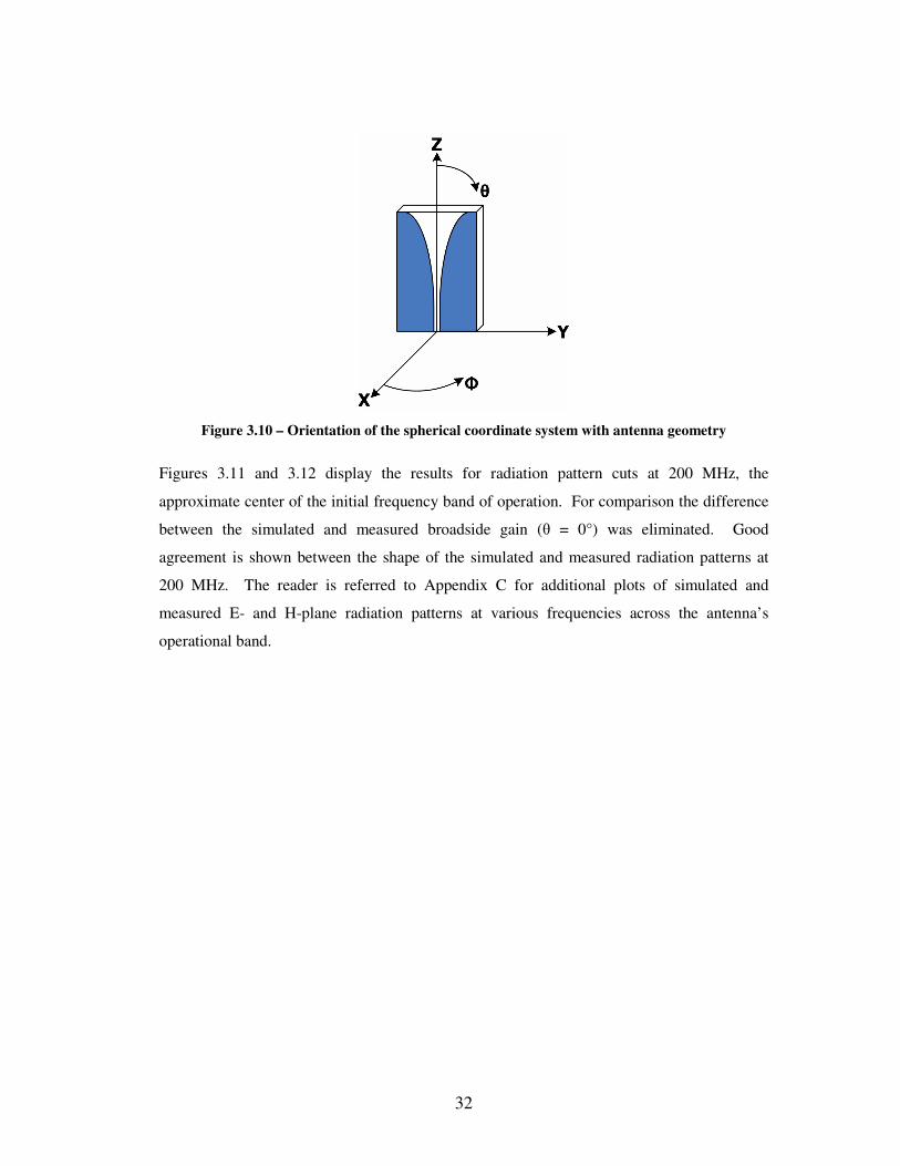
32

Figure 3.10 – Orientation of the spherical coordinate system with antenna geometry

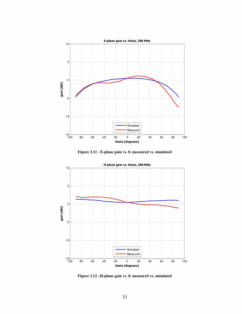
Figures 3.11 and 3.12 display the results for radiation pattern cuts at 200 MHz, the

approximate center of the initial frequency band of operation. For comparison the difference

between the simulated and measured broadside gain (θ = 0°) was eliminated. Good

agreement is shown between the shape of the simulated and measured radiation patterns at

200 MHz. The reader is referred to Appendix C for additional plots of simulated and

measured E- and H-plane radiation patterns at various frequencies across the antenna’s

operational band.

33

-100 -80 -60 -40 -20 0 20 40 60 80 100-15

-10

-5

0

5

10

theta [degrees]

ga

in [

dB

i]

E-plane gain vs. theta, 200 MHz

Simulated

Measured

Figure 3.11 - E-plane gain vs. θ, measured vs. simulated

-100 -80 -60 -40 -20 0 20 40 60 80 100-15

-10

-5

0

5

10

theta [degrees]

ga

in [

dB

i]

H-plane gain vs. theta, 200 MHz

Simulated

Measured

Figure 3.12 –H-plane gain vs. θ, measured vs. simulated

34

Using the result of measured gain versus frequency, the effective aperture as a function of

frequency, defined in Equation 3.1, can be obtained.

πλ

4

2⋅=

GainAe Eq. 3.1 [5]

Measured gain versus frequency and effective aperture versus frequency are presented in

Figures 3.13 and 3.14, respectively. Peak antenna gain monotonically increases as a function

of frequency up to 750 MHz; however, the effective aperture is a monotonically decreasing

function of frequency. If the effective aperture of the antenna were to remain constant, then

gain would continually increase with frequency, which happens to be true for the CAV-A up

to 750 MHz. Given that peak gain and effective aperture are directly proportional, a decrease

in gain corresponds to a decrease in effective aperture, leading to the conclusion that the

effective aperture is moving closer to the throat beyond 750 MHz. This conclusion supports

earlier publications stating that the aperture of efficient radiation moves closer to the feed as

frequency increases.

200 300 400 500 600 700 800 900 1000 1100 12000

1

2

3

4

5

6

7

8

9

10

frequency [MHz]

ga

in [

dB

i]

Peak antenna gain vs. frequency

Figure 3.13 – Measured CAV-A peak gain vs. frequency

35

200 300 400 500 600 700 800 900 1000 1100 12000

500

1000

1500

2000

2500

frequency [MHz]

Ae [

cm

2]

Effective aperture vs. frequency

Figure 3.14 – CAV-A effective aperture vs. frequency

3.2 DESIGN PROCEDURE

The lack of a proven design procedure and the multitude of adjustable antenna parameters led

to the development of the design methodology detailed below. The proposed design

methodology serves as a guide to establish a starting point, at which, the methodology

outlines antenna parameter adjustments that can be made to optimize Vivaldi performance.

Figure 3.15 presents the flow diagram for the proposed methodology. For each step of the

process, typical starting values will be given, using the CAV-A as an example. In addition,

the effects of varying each parameter on the operational bandwidth will be discussed. These

effects will be illustrated using perturbations in the CAV-A and comparing simulated results.

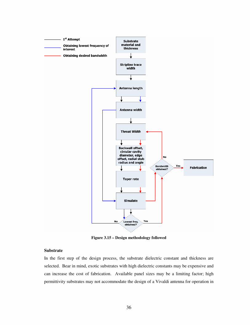
36

Figure 3.15 – Design methodology followed

Substrate

In the first step of the design process, the substrate dielectric constant and thickness are

selected. Bear in mind, exotic substrates with high dielectric constants may be expensive and

can increase the cost of fabrication. Available panel sizes may be a limiting factor; high

permittivity substrates may not accommodate the design of a Vivaldi antenna for operation in

37

the meter-wavelength region. One possible advantage is a decrease in the overall antenna

dimensions to obtain the same bandwidth performance.

As an example, the CAV-A is compared against two designs representing a +/- 5% variation

in substrate thickness. All other antenna parameters, sans stripline trace width, remain

constant. Stripline trace width is recalculated to maintain a 50-Ω characteristic impedance

for each design.

A small variation in substrate thickness does not produce any deleterious effects on

bandwidth, as seen in Figure 3.16. In fact, both variations might provide additional operation

above 1 GHz based on the 1-GHz response seen. Generally speaking, the thicker substrate

provides deeper nulls; examples can be seen at 200, 625, 750, and 900 MHz. Varying the

substrate thickness has little effect on the lowest frequency of operation, as the lower cutoff

frequency for each design is within 3 MHz of each other.

100 200 300 400 500 600 700 800 900 1000-45

-40

-35

-30

-25

-20

-15

-10

-5

0

frequency [MHz]

S1

1 [

dB

]

Return loss vs. frequency, +/- 5% substrate thickness

CAV-A

-5%

+5%

Figure 3.16 – Return loss vs. frequency, +/- 5% substrate thickness variation from CAV-A

38

A substrate material survey, noting available panel sizes, thicknesses, density, price per panel,

and dielectric constants, is recommended. Since it is the first step in the design process, a

prudent choice will be required. Changing the substrate material in the middle of the design

process would require completely starting over.

Stripline trace width

The characteristic impedance of the stripline should match the characteristic impedance of the

transmission line feeding the antenna, in this case, a coaxial cable. If the coaxial cable has a

50-Ω impedance, design the stripline for a 50-Ω characteristic impedance. For the substrate

thickness and dielectric constant selected, ADS LineCalc can be used to solve for the stripline

trace width needed.

Antenna length

Contradictory to the general consensus, an antenna length on the order of λ0/4 at the lowest

frequency of interest, combined with a sensible selection of mouth opening, determines the

lowest frequency of operation. The general consensus would suggest that for best

performance, the Vivaldi antenna length should be greater than λ0 [17, 26, 31, 43]. However,

the term performance is rather vague, and given the thrust of each paper, performance could

be quantified as gain and/or beamwidth. Most discussions concerning antenna length revolve

around beamwidth and gain effects, not bandwidth.

To demonstrate the effect of antenna length on bandwidth performance, the CAV-A is

compared against two models representing a 10% increase/decrease in antenna length. All

other antenna parameters remain constant, implying the increase/decrease in antenna length

results from an increase/decrease in taper length. Results of the simulation are captured in

Figure 3.17. As expected, an increase in antenna length results in a decrease of the lowest

frequency of operation. The converse, also expected, is also shown to be true. In addition,

based on the 1-GHz return loss, the longer antenna might provide additional bandwidth

compared to the CAV-A.

39

100 200 300 400 500 600 700 800 900 1000-40

-35

-30

-25

-20

-15

-10

-5

0

frequency [MHz]

S1

1 [

dB

]

Return loss vs. frequency, +/- 10% antenna length

CAV-A

-10%

+10%

Figure 3.17 – Return loss vs. frequency, +/- 10% antenna length variation from CAV-A

Mouth opening

An antenna mouth opening on the order of λ0/4 at the lowest frequency of interest, combined

with an antenna length, also on the order of λ0/4, determines the lowest frequency of

operation. This finding contradicts Gibson who established a lower cutoff frequency where

the mouth opening is λ0/2 [17]. Many authors have since agreed with Gibson [15, 29, 31, 41,

43, 53].

To illustrate the bandwidth effects of mouth opening, the mouth opening of the CAV-A, 48

cm, is compared against a 25% increase/decrease in mouth opening. All other antenna

parameters remain constant. Results of these simulations are shown in Figure 3.18. As

expected, a smaller/wider mouth opening results in an increase/decrease in the lowest

frequency of operation. Since the desired output is a Vivaldi with continuous bandwidth, the

smaller mouth opening is deemed unacceptable. The wider mouth opening gives comparable

performance to the CAV-A, with the exception of the deep nulls at 550 and 800 MHz. In

40

addition, the wider mouth opening might provide a greater upper cutoff frequency than the

CAV-A, extrapolating the return loss performance given at 1 GHz.

100 200 300 400 500 600 700 800 900 1000-40

-35

-30

-25

-20

-15

-10

-5

0

frequency [MHz]

S1

1 [

dB

]Return loss vs. frequency, +/- 25% mouth opening

CAV-A

36 cm

58 cm

Figure 3.18 – Return loss vs. frequency, +/- 25% mouth opening variation from CAV-A

Throat Width

Optimizing the separation between slotline conductors at the stripline-to-slotline transition is

of utmost importance. Regardless of the primary feed mechanism, be it stripline, microstrip,

or coplanar waveguide, the “slotline to feedline transition limits the bandwidth and requires

considerable ingenuity to give broadband performance” [15].

Throat width only begins to describe what is happening at the stripline-to-slotline transition.

Both transmission lines need to be properly terminated. These terminations, in combination

with the transition, compose the so-called balun section of the antenna [42]. For all four

designs, the balun structure described in [10] was scaled and subsequently optimized for the

frequencies of interest. The circular cavity resonator termination for the slotline and radial

stub termination for the stripline will be discussed shortly.

41

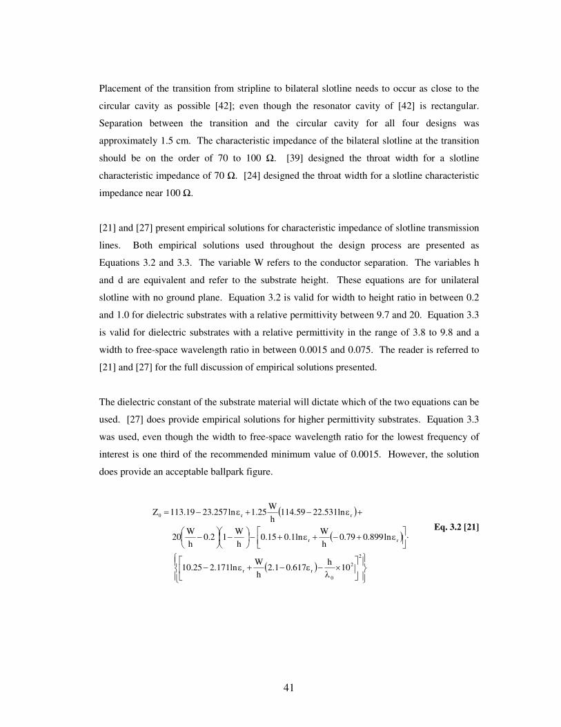
Placement of the transition from stripline to bilateral slotline needs to occur as close to the

circular cavity as possible [42]; even though the resonator cavity of [42] is rectangular.

Separation between the transition and the circular cavity for all four designs was

approximately 1.5 cm. The characteristic impedance of the bilateral slotline at the transition

should be on the order of 70 to 100 Ω. [39] designed the throat width for a slotline

characteristic impedance of 70 Ω. [24] designed the throat width for a slotline characteristic

impedance near 100 Ω.

[21] and [27] present empirical solutions for characteristic impedance of slotline transmission

lines. Both empirical solutions used throughout the design process are presented as

Equations 3.2 and 3.3. The variable W refers to the conductor separation. The variables h

and d are equivalent and refer to the substrate height. These equations are for unilateral

slotline with no ground plane. Equation 3.2 is valid for width to height ratio in between 0.2

and 1.0 for dielectric substrates with a relative permittivity between 9.7 and 20. Equation 3.3

is valid for dielectric substrates with a relative permittivity in the range of 3.8 to 9.8 and a

width to free-space wavelength ratio in between 0.0015 and 0.075. The reader is referred to

[21] and [27] for the full discussion of empirical solutions presented.

The dielectric constant of the substrate material will dictate which of the two equations can be

used. [27] does provide empirical solutions for higher permittivity substrates. Equation 3.3

was used, even though the width to free-space wavelength ratio for the lowest frequency of

interest is one third of the recommended minimum value of 0.0015. However, the solution

does provide an acceptable ballpark figure.

( )

( )

( )

×

λ−ε−+ε−

⋅

ε+−+ε+−

−

−

+ε−+ε−=

2

2

0

rr

rr

rr0

10h

617.01.2h

Wln171.225.10

ln899.079.0h

Wln1.015.0

h

W12.0

h

W20

ln531.2259.114h

W25.1ln257.2319.113Z

Eq. 3.2 [21]

42

( )

( )

( )( )0

0

r

0

r

r

2

r

6.0

0

rr0

/W

d753.0

d100lnd/W12.251.0

2876.0d/W

d/W2254123.36

W37.319.63815.26.73Z

λ

λε

−

λ+ε+

−ε+

−+ε+

λε−+ε−=

Eq. 3.3 [27]

Figure 3.19 displays the difference between unilateral and bilateral slotline, the latter of

which was used for all four designs.

Figure 3.19 – Unilateral (left) slotline vs. bilateral slotline (right)

The characteristic impedance of a bilateral slotline was assumed to be the result of two

unilateral slotlines combined in parallel. For example, two 100-Ω unilateral slotlines would

result in an approximate bilateral slotline characteristic impedance of 50 Ω. Using equation

3.3, the CAV-A throat width produces an approximate characteristic impedance average of

90 Ω over the frequency range of interest for a unilateral case, so 45 Ω for the bilateral case.

Slotline impedance for a constant separation increases as frequency increases, and decreases

as the substrate thickness increases. For constant frequency and thickness, characteristic

impedance is a monotonically increasing function of slot width.

43

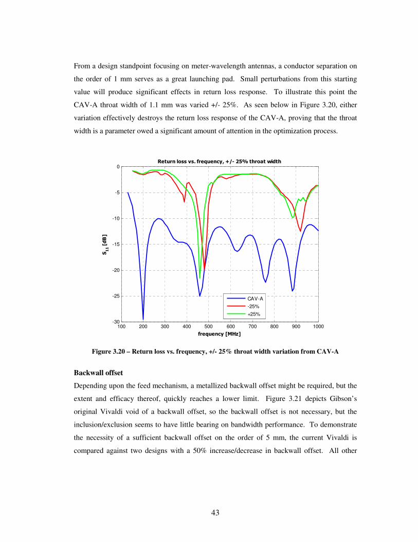
From a design standpoint focusing on meter-wavelength antennas, a conductor separation on

the order of 1 mm serves as a great launching pad. Small perturbations from this starting

value will produce significant effects in return loss response. To illustrate this point the

CAV-A throat width of 1.1 mm was varied +/- 25%. As seen below in Figure 3.20, either

variation effectively destroys the return loss response of the CAV-A, proving that the throat

width is a parameter owed a significant amount of attention in the optimization process.

100 200 300 400 500 600 700 800 900 1000-30

-25

-20

-15

-10

-5

0

frequency [MHz]

S1

1 [

dB

]

Return loss vs. frequency, +/- 25% throat width

CAV-A

-25%

+25%

Figure 3.20 – Return loss vs. frequency, +/- 25% throat width variation from CAV-A

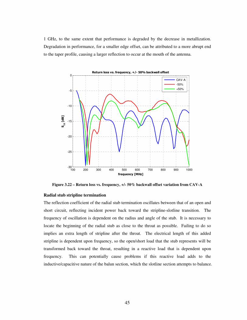
Backwall offset

Depending upon the feed mechanism, a metallized backwall offset might be required, but the

extent and efficacy thereof, quickly reaches a lower limit. Figure 3.21 depicts Gibson’s

original Vivaldi void of a backwall offset, so the backwall offset is not necessary, but the

inclusion/exclusion seems to have little bearing on bandwidth performance. To demonstrate

the necessity of a sufficient backwall offset on the order of 5 mm, the current Vivaldi is

compared against two designs with a 50% increase/decrease in backwall offset. All other

44

antenna parameters remain constant, therefore, for a smaller backwall offset the extra

“length” is lumped on to the taper length of the design.

Figure 3.21 – Gibson Vivaldi antenna [2, 17]

Figure 3.22 shows the simulated results. Either variation raises the lowest frequency of

operation, an indication that the backwall offset is a parameter to be optimized. However,

sufficient metallization must be present behind the circular cavity, as seen in the smaller

offset result. The only visual advantage to an increased backwall offset, is the -30-dB null

present at 1 GHz, almost ensuring operational bandwidth extending past that of the CAV-A,

with the consequence of non-operation in the 350 to 450 MHz and 775 to 850 MHz ranges.

A frequency scaled backwall offset is a recommended starting point.

Edge offset

The extent of the extra metallization present at the end of the taper profile has not been fully

discussed. Extra metallization is needed as the edge currents present on the slotline

conductor do not want to see an abrupt end. Exactly how much extra copper is needed is still

in question. The frequency scaled edge offset of [10] was used as a starting point, and did not

change through the four design iterations; the same is suggested as a starting point. To

exhibit the need for extra metallization, the CAV-A is compared against two designs with a

25% increase/decrease in edge offset. The mouth opening of both models remains constant;

hence an increase/decrease in edge offset implies an increase/decrease in overall antenna

width. Seen in Figure 3.23, additional metallization does not aid performance, except around

45

1 GHz, to the same extent that performance is degraded by the decrease in metallization.

Degradation in performance, for a smaller edge offset, can be attributed to a more abrupt end

to the taper profile, causing a larger reflection to occur at the mouth of the antenna.

100 200 300 400 500 600 700 800 900 1000-30

-25

-20

-15

-10

-5

0

frequency [MHz]

S1

1 [

dB

]

Return loss vs. frequency, +/- 50% backwall offset

CAV-A

-50%

+50%

Figure 3.22 – Return loss vs. frequency, +/- 50% backwall offset variation from CAV-A

Radial stub stripline termination

The reflection coefficient of the radial stub termination oscillates between that of an open and

short circuit, reflecting incident power back toward the stripline-slotline transition. The

frequency of oscillation is dependent on the radius and angle of the stub. It is necessary to

locate the beginning of the radial stub as close to the throat as possible. Failing to do so

implies an extra length of stripline after the throat. The electrical length of this added

stripline is dependent upon frequency, so the open/short load that the stub represents will be

transformed back toward the throat, resulting in a reactive load that is dependent upon

frequency. This can potentially cause problems if this reactive load adds to the

inductive/capacitive nature of the balun section, which the slotline section attempts to balance.

46

100 200 300 400 500 600 700 800 900 1000-45

-40

-35

-30

-25

-20

-15

-10

-5

0

frequency [MHz]

S1

1 [

dB

]

Return loss vs. frequency, +/- 25% edge offset

CAV-A

-25%

+25%

Figure 3.23 – Return loss vs. frequency, +/- 25% edge offset variation from CAV-A

“The stripline stub reactance varies from very large capacitive values in the lower frequencies,

through a wide frequency range of near zero reactance in the mid-band, to inductive values in

the upper band [43].” The reactance of the radial stub provides favorable compensation of

the slotline reactance, greatly contributing to wide-band performance [43]. Essentially, a

conjugate match between the balun section and the tapered slotline will provide ultra-

wideband (≥ 150% bandwidth) performance [42].

The extent, or angle, of the radial stub remained the same between all designs. Each design

used scaled values presented in [10]. Varying the radius and angle of the radial stub produces

noticeable effects on bandwidth performance, but are not as significant as variation of other

parameters (antenna length and width). Essentially, both parameters ensure a proper

termination of the stripline feed, therefore, for meter-wavelength operation both parameters

are rather large compared to the other geometry in the feed transition area of the antenna.

Small perturbations in radius and angle should not produce deleterious effects in bandwidth

response.

47

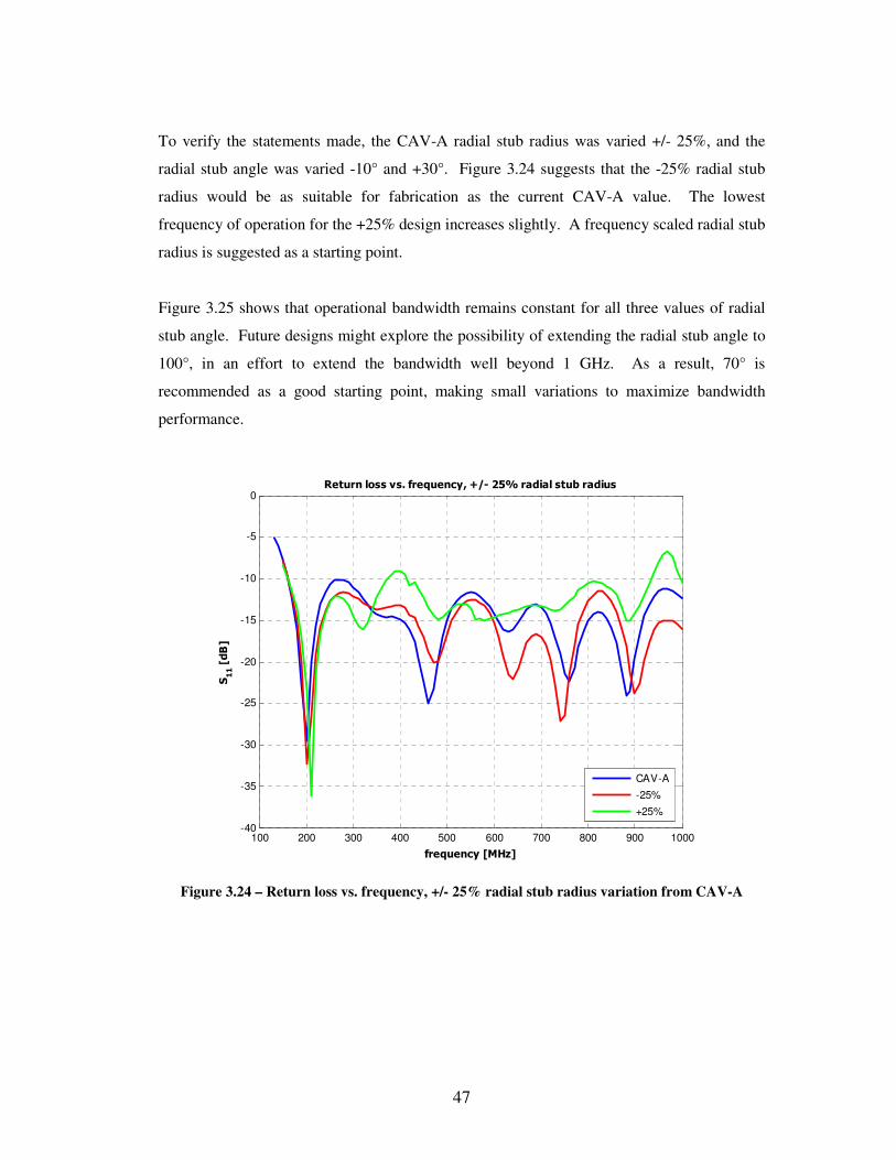
To verify the statements made, the CAV-A radial stub radius was varied +/- 25%, and the

radial stub angle was varied -10° and +30°. Figure 3.24 suggests that the -25% radial stub

radius would be as suitable for fabrication as the current CAV-A value. The lowest

frequency of operation for the +25% design increases slightly. A frequency scaled radial stub

radius is suggested as a starting point.

Figure 3.25 shows that operational bandwidth remains constant for all three values of radial

stub angle. Future designs might explore the possibility of extending the radial stub angle to

100°, in an effort to extend the bandwidth well beyond 1 GHz. As a result, 70° is

recommended as a good starting point, making small variations to maximize bandwidth

performance.

100 200 300 400 500 600 700 800 900 1000-40

-35

-30

-25

-20

-15

-10

-5

0

frequency [MHz]

S1

1 [

dB

]

Return loss vs. frequency, +/- 25% radial stub radius

CAV-A

-25%

+25%

Figure 3.24 – Return loss vs. frequency, +/- 25% radial stub radius variation from CAV-A

48

100 200 300 400 500 600 700 800 900 1000-35

-30

-25

-20

-15

-10

-5

0

frequency [MHz]

S1

1 [

dB

]

Return loss vs. frequency, radial stub angle variation

CAV-A

60 deg.

100 deg.

Figure 3.25 – Return loss vs. frequency, radial stub angle variation from CAV-A

Circular cavity resonator diameter

Given the experience of multiple designs, a larger circular cavity resonator diameter was

found to aid bandwidth to a limit. However, given the lack of real estate, better results would

be attained if the extra diameter was added to the existing taper length. All four designs

incorporated a circular cavity resonator for terminating the slotline. Motivation for the

inclusion of a circular resonator originated from remarks made in [10]. To demonstrate the

effect of the circular slot cavity diameter on bandwidth performance, the CAV-A is compared

against two designs with a 25% increase/decrease in circular cavity diameter. All other

antenna parameters remain constant; as a result, for the decrease in diameter, the extra

“length” will be added to the taper length. The initial design began with a frequency scaled

version of [10] and did not vary much from there, with acceptable results. Figure 3.26 below

shows that a reduced circular cavity diameter suffers from a 200 to 300 MHz in band region

of non-operation, while the lowest operating frequency for the increased circular cavity

diameter increases.

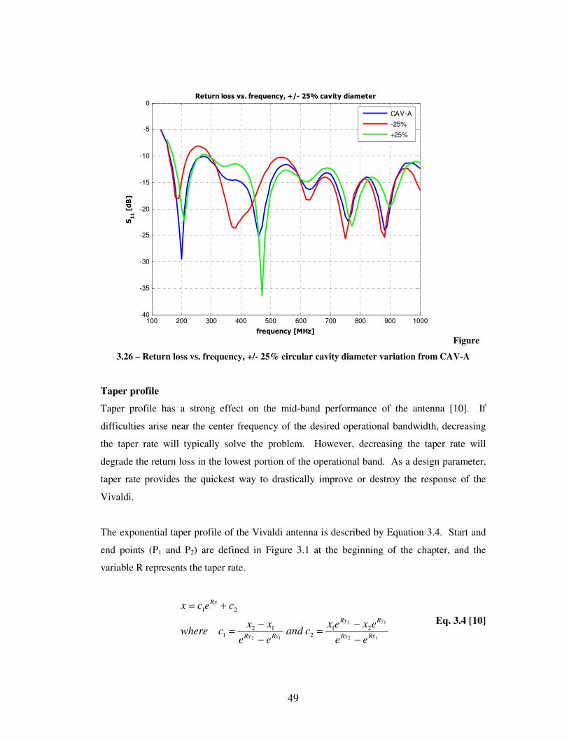
49

100 200 300 400 500 600 700 800 900 1000-40

-35

-30

-25

-20

-15

-10

-5

0

frequency [MHz]

S1

1 [

dB

]

Return loss vs. frequency, +/- 25% cavity diameter

CAV-A

-25%

+25%

Figure

3.26 – Return loss vs. frequency, +/- 25% circular cavity diameter variation from CAV-A

Taper profile

Taper profile has a strong effect on the mid-band performance of the antenna [10]. If

difficulties arise near the center frequency of the desired operational bandwidth, decreasing

the taper rate will typically solve the problem. However, decreasing the taper rate will

degrade the return loss in the lowest portion of the operational band. As a design parameter,

taper rate provides the quickest way to drastically improve or destroy the response of the

Vivaldi.

The exponential taper profile of the Vivaldi antenna is described by Equation 3.4. Start and

end points (P1 and P2) are defined in Figure 3.1 at the beginning of the chapter, and the

variable R represents the taper rate.

12

12

12

212

121

21

RyRy

RyRy

RyRy

Ry

ee

exexcand

ee

xxcwhere

cecx

−−

=−−

=

+= Eq. 3.4 [10]

50

To illustrate the earlier statements, the CAV-A was compared against two models

representing a 10% increase/decrease in taper rate. Figure 3.27 displays the simulation

results. As can be seen in the 500 to 600 MHz band, reducing the taper rate from the +10%

value to that of the CAV-A will suppress the hump extending from 500 to 550 MHz.

Lowering the taper rate to the -10% value will help suppress this hump even further.

Consequently, lowering the taper rate to the -10% value, degrades the return loss response in

the 200 to 450 MHz band. These results indicate the inherent trade-off present between low-

band and mid-band response.

100 200 300 400 500 600 700 800 900 1000-50

-45

-40

-35

-30

-25

-20

-15

-10

-5

0

frequency [MHz]

S1

1 [

dB

]

Return loss vs. frequency, +/- 10% taper rate

CAV-A

-10%

+10%

Figure 3.27 – Return loss vs. frequency, +/- 10% taper rate variation from CAV-A

For the first Vivaldi design, a modest taper rate such as 0.15 cm

-1 is a good starting point.

Typical values range from 0.10 to 0.25 cm-1

. To improve the mid-band response at the

expense of low-band, lowering the taper rate usually produces the desired result. Taper rate

is a parameter to be constantly pushed. Modest values must be used in the beginning of the

design process, else the lowest frequency of operation might be skewed upward leading to

reconsideration of the mouth opening value.

51

Summary of recommendations

Based on the experience gained from these designs, the following recommendations are

suggested for others interested in designing broad bandwidth Vivaldi antenna that may fall

into the electrically small category.

1. Selecting a substrate material is entirely dependent on operational bandwidth and

budget.

2. Design the stripline trace width for a characteristic impedance equal to that of the

feed line.

3. The antenna length should be on the order of λ0/4.

4. Mouth opening, hence antenna width, should be on the order of λ0/4.

5. Design the throat width to have a characteristic impedance in the range of 50 to

75 Ω.

6. Start with frequency scaled values for backwall offset, edge offset, radial stub

radius, and circular cavity diameter.

7. Start with a radial stub angle of 70°.

8. Start with a modest taper rate of 0.15 cm-1

.

52

3.3 COMMON MISCONCEPTIONS

Experience gained from the design of these four Vivaldi antennas has shown inconsistencies

with guidance found in the literature. Below are the misconceptions that have been identified.

1. The stripline characteristic impedance is an optimization parameter.

The stripline trace width is not meant to be optimized. Set it equal to the characteristic

impedance of the coaxial cable.

2. Antenna length should be greater than a free-space wavelength.

To preserve the traveling wave nature of the antenna, make the antenna as long as possible.

If designing the antenna for gain and beamwidth requirements, this will be necessary. If not,

the antenna length can be significantly reduced to the order of λ0/4.

3. Mouth opening of the antenna should be greater than a half free-space wavelength.

If a narrow main beam is desired, then widen the mouth as much as possible. If this is not the

case, the mouth opening can be significantly reduced. An antenna mouth opening on the

order of λ0/4 will determine the lowest operating frequency of the antenna. The throat width

determines the highest frequency of operation.

4. Vivaldi antennas are typically traveling wave antennas.

The CAV-A can be classified as a non-traveling wave antenna given the inverse parabolic-

like peak gain response of the element.

The lowest frequency of operation for Vivaldi antennas is determined by the

combination of antenna length and mouth opening, with both dimensions

approximating λ0/4.

53

CHAPTER 4

CONCLUSIONS AND FUTURE WORK

The CReSIS Aerial Vivaldi (CAV-A), with operation from 162 MHz to 1.121 GHz, was

designed, simulated, fabricated, and characterized. The required lowest frequency of

operation was changed during the design process from 150 MHz to 180 MHz, due to

electromagnetic interference issues in Greenland. The updated lowest frequency requirement

was satisfied, as was the desired bandwidth. The measured bandwidth was consistent with

Ansoft HFSS simulations, building confidence for future work.

Dimensions of the antenna are 51 cm wide by 40 cm long by 1/8” thick, for a total mass of

3.22 lbs. Size requirements were satisfied with room to spare. Given the reduced length of

the structure, the structure falls into the non-traveling wave antenna category, following in the

footsteps of Prasad and Mahapatra [39].

The overall shape of the radiation patterns measured for the CAV-A agrees well with

simulated results. However, the simulations did not provide a reliable absolute gain level to

compare with the measured gain level of the CAV-A. Discussion concerning this issue can

be found in Appendix A. Peak gain for the CAV-A was measured to be an increasing

function of frequency up to 750 MHz, beyond which, the gain steadily decreases as a function

of frequency.

A design methodology was developed as a result of the first two antenna designs. The next

two designs closely followed the methodology presented. The first design started with a

frequency scaled version of a published Vivaldi design [10] and quickly realized that the

structure had to grow considerably to facilitate 180-MHz radar operation. The proposed

design methodology was put forth in hopes of creating a “launch pad” for future designs.

Future work involving the CAV-A includes modifying the antenna for its UAV operation.

The modifications include integration of a transmit/receive (T/R) module at the back corner

of the structure as well as adding structural elements to stiffen the antenna. Exact placement

and orientation of the T/R module is dependent upon coordination with the Meridian design

group to make the structure flight ready. The purpose of stiffening of the antenna element is

54

to reduce flexure in a cross wind environment as well as avoiding damaging resonant

vibrations. Preliminarily, edge stiffeners made out of carbon fiber are to be used. Placement

of mounting holes and the construction of mounting brackets comes next. Integration of a

leading and trailing edge to the structure, forming a tear drop shape, with the round edge

pointing into the wind, rounds out flight preparation. Early measurements indicate that the

flight readiness measures and deploying the antennas in an H-plane array will deteriorate the

return loss response of each element. Full integration with the Meridian UAV for flight

testing and radar testing will verify field readiness.

CReSIS, in addition to aerial data measurements, also performs ground-based measurements

using antennas mounted on sleds pulled behind a variety of vehicles. Preliminary

measurements made in the sand box indicate that for ground-based measurements, the lowest

frequency of operation decreases for the CAV-A when placed in close proximity to dry sand

(εr ~ 3). This drop in the lowest operating frequency can be attributed to easing the dielectric

contrast from the antenna to the surrounding medium. Development and implementation of a

dual-polarized CAV array sled could provide both radar engineers and glaciologists new

information.

Necessary for the advanced signal processing techniques utilized at CReSIS is knowledge of

the phase center of the CAV-A. A technique borrowed from [7] was executed with no

success. Any future measurements should include determining the phase center of the CAV-

A using methods described in [5]. Mixed opinions concerning phase centers of tapered slot

antennas will be squelched another day.

Future improvements involve investigating the two dimensional space that is the stripline

radial stub termination. Given simulation results presented in Chapter 3, increasing the flare

angle from 80 to 100 degrees, could improve return loss around 1 GHz. The design process

only considered exponential tapers; perhaps, an unconventional flare profile would yield even

wider bandwidth performance. [42] is recommended as a good reference for designers

wishing to go this route. However, this route is highly dependent on accurately calculating

the characteristic impedance and complex propagation constant of bilateral slotline for a wide

range of conductor separation.

55

A possible blue sky is the substitution of a Rohacell© substrate for FR-4, whose dielectric

properties, for lower frequencies, resemble that of free space. Fabrication for said antenna

would be done by the Meridian UAV group. Incorporation of a Rohacell©

substrate would

significantly reduce weight; an antenna with the same footprint as the CAV-A would weigh

less than one-tenth of a pound. Possible difficulties are the inclusion of a stripline feed

mechanism and development of precision tooling methods for repeatable designs.

Absent of these difficulties, is the possibility of a so-called “all-metal Vivaldi”, whose basic

premise is the removal of the stripline feed and substrate and joining the front and back

copper flares. Such a structure could be made out of a sheet of copper or brass using a mill.

The feed mechanism would be similar to a TEM horn antenna in which the outer conductor

of a coaxial cable is soldered to one side of the throat while the inner conductor extends

across the throat and solders to the opposite side. Vivaldi antennas of this sort can actually

support TEM propagation and do not suffer from bandwidth limitations due to the onset of

higher order substrate modes [7].

Summarizing, the iterative process to produce the CAV-A was every bit a learning

experience, as it was a design process. There seems to be a mystique surrounding the

operation of tapered slot antennas, and hopefully the CAV-A design contributes a piece to the

puzzle.

56

APPENDIX A

SIMULATION SETUP

Simulations were performed in Ansoft HFSS, a finite element method electromagnetic solver.

Ansoft HFSS v10 runs on the Macaroni terminal at CReSIS, which consists of 4 dual core

Xeon 2.66 GHz processors hyper-threaded, with 24 GB of RAM [6]. By thoroughly abusing

the resources at hand, typical run times of the CAV-A simulations range from 1 to 3 hours.

Given the rather quick run times, simulations involving multiple parameter variations could

be ran daily.

Figure A.1 shows the simulation geometry for the CAV-A. All metal is modeled as perfect

electric conductors. As a result, run time decreases and simplicity is achieved. The grey box

surrounding the structure represents the air box, or solution boundary, which incorporates a

radiation boundary condition. At minimum, a quarter free-space wavelength separation

between the model and the air box is demanded by HFSS. Far field solution accuracy is

increased when a larger air box is employed, but the run time of the simulation increases

exponentially. Simulations were run from 150 MHz to 1 GHz, so a 50-cm separation was

used.

57

Figure A.1 – CAV-A simulation layout

Exciting the simulation model was accomplished using a wave port at the back of the

structure. Figure A.2 shows the wave port at the back of the model. HFSS requires the wave

port excitation to lie in one of the 6 planes of the air box. Since there is little backside

radiation for a Vivaldi antenna, it was safe to constrict the solution space on the back of the

antenna. Adequate dimensions of the wave port facilitate simulation of the lowest frequency

of interest. For all intents and purposes, it is safe to assume the wave port is an end view of

an infinitely long rectangular wave guide, whose cutoff frequencies are dictated by the

dimensionality. As a result, the wave port used for simulation purposes spans the entire

width of the structure and protrudes from the front and back copper flares, as seen in Figure

A.2.

58

Figure A.2 - Wave port orientation

Another possible method of exciting the simulation model would require designing and

drawing a 50-Ω coaxial cable in the model. On the antenna end of the coax, the center

conductor would be placed against the stripline trace, with the outer conductor making

contact with both copper flare planes. On the other end, a circular wave port with the same

diameter as the outer conductor will be placed at the termination, which would coincide with

one face of the air box. Simulating this model takes much longer than the model presented,

due to the length of coaxial cable. Implementation of this model would allow backing the air

box away from the back of the structure, which would aid accuracy in the far field toward the

back of the antenna, but run time increases as a result.

To illustrate the accuracy attained from larger radiation boundaries, prior experience

involving the simulation of simple, half-wavelength dipoles will be discussed. Any antenna

designer would be able to rattle off the peak gain of a half-wave dipole as 2.15 dB. It is a

known and accepted fact, however, using the quarter-wavelength separation between dipole

and air box, a value less than 2.15 dB is returned. To attain the correct value of 2.15 dB,

the air box needs to be over 3 free space wavelengths away from the dipole. The run time

59

of these simulations was on the order of days. Imagine incorporating an air box of this

immenseness to the CAV-A simulation model. It would be safe to bet that each simulation

would take a couple of days, at least.

The choice was made to sacrifice far-field accuracy for quicker run times. As a result,

simulated peak directivity is not correct at the lower frequencies, but the overall shape of the

pattern can be trusted. The separation between the element and air box becomes electrically

longer as frequency increases, so the peak directivity given at higher frequencies is more

accurate. However, the inaccuracies of the EM solver did not significantly affect the design

process.

60

APPENDIX B

MEASUREMENT SETUP

The measurement setup is centered primarily on the reconfiguration of a GTI Electronics

antenna positioner and controller, originally intended for tracking satellites, for ground-based

radiation measurements. Figure B.1 shows the system stackup. The positioner is securely

fastened to the plastic shipping pallet. The Styrofoam column is secured to a 2’ by 2’ piece

of polycarbonate that is joined to the PVC pipe by means of a PVC toilet flange. This entire

assembly is secured to the positioner using a machined steel plate.

Figure B.1 – Positioner stackup and return loss measurement setup

61

Figure B.1 shows the setup for return loss measurement. The Vivaldi is held in place by two

pieces of rope and pointed skyward to eliminate any possible multi-path effects.

E- and H-plane radiation pattern measurements incorporate a second Vivaldi and a calibrated

log periodic antenna, ETS 3148. Since the measurement routine for both principal planes is

the same, only the E-plane will be discussed. For E-plane radiation pattern measurements,

the Vivaldi lies flat on the Styrofoam column in a broadside arrangement, which is seen in

Figure B.2.

Figure B.2 – Vivaldi under test, E-plane measurement

First, the Vivaldi under test is pointed directly at the calibrated log periodic antenna. Figure

B.3 illustrates this situation for an H-plane measurement; for the E-plane setup, both antennas

are laid flat. S21 is recorded and stored as the calibrated boresight measurement.

62

Figure B.3 – Calibrated H-plane boresight measurement setup

Next, the calibrated log periodic antenna is substituted for a second Vivaldi. The E-plane

measurement setup can be seen in Figure B.4. Using the antenna positioner and controller,

the Vivaldi under test is swept from -90° (facing left) to +90° (facing right) in 5° increments.

S21 is recorded at every increment. For the H-plane measurement, both antennas are turned

on their sides as seen in Figure B.5.

63

Figure B.4 – E-plane measurement setup

Figure B.5 – H-plane measurement setup

64

Using the boresight measurement with the calibrated log periodic and the boresight

measurement between the two Vivaldis, the transmit gain of the Vivaldi under test can be

calculated as a ratio between the received power for the former and that of the latter. The

simplification results in Equation B.1, where the transmit gain of the log periodic (Gtlp) is

given and S21V and S21LP are the boresight measurements for two Vivaldis and one Vivaldi

and the log periodic, respectively. All values are functions of frequency.

LP

VLP

V S

SGG

t

t

21

21= Eq. B.1

Given the radiation pattern measurements in decibels, the difference between the measured

boresight value and the calculated transmit gain is added to each angular measurement to

produce the overall gain plot for each frequency. These results can be seen in Appendix C.

65

APPENDIX C

PRINCIPAL PLANE RADIATION PATTERNS

Figures C.1 through C.9 show the comparisons between simulated and measured radiation

patterns in the E-plane. Good agreement is shown between simulated and measured for the

frequencies considered. The only problem exists at 160 MHz, where a peak gain of nearly

5 dBi is exhibited. Rest assured, this is not the case. The log periodic antenna used for

measurement purposes was not calibrated below 200 MHz. Transmit gain for the log

periodic antenna at 160 MHz was assumed to be the same as 200 MHz, which probably is not

the case. Peak gain for 160 MHz is approximately 0.15 dBi. Figures C.10 through C.18

show the comparisons between simulated and measured radiation patterns in the H-plane.

Good agreement is shown once again between simulated and measured for the frequencies

considered. The 160-MHz H-plane radiation cut shows the same peak gain as the E-plane,

which has already been established as incorrect.

-100 -80 -60 -40 -20 0 20 40 60 80 100-15

-10

-5

0

5

10

theta [degrees]

gain

[d

Bi]


Simulated

Measured

Figure C.1 – E-plane gain vs. θ, 160 MHz

-100 -80 -60 -40 -20 0 20 40 60 80 100-15

-10

-5

0

5

10

theta [degrees]

gain

[d

Bi]


Simulated

Measured


66

-100 -80 -60 -40 -20 0 20 40 60 80 100-15

-10

-5

0

5

10

theta [degrees]

gain

[d

Bi]


Simulated

Measured


-100 -80 -60 -40 -20 0 20 40 60 80 100-15

-10

-5

0

5

10

theta [degrees]

gain

[d

Bi]


Simulated

Measured


-100 -80 -60 -40 -20 0 20 40 60 80 100-15

-10

-5

0

5

10

theta [degrees]

gain

[d

Bi]


Simulated

Measured


-100 -80 -60 -40 -20 0 20 40 60 80 100-15

-10

-5

0

5

10

theta [degrees]

gain

[d

Bi]


Simulated

Measured


-100 -80 -60 -40 -20 0 20 40 60 80 100-15

-10

-5

0

5

10

theta [degrees]

gain

[d

Bi]


Simulated

Measured


-100 -80 -60 -40 -20 0 20 40 60 80 100-15

-10

-5

0

5

10

theta [degrees]

gain

[d

Bi]


Simulated

Measured


67

-100 -80 -60 -40 -20 0 20 40 60 80 100-15

-10

-5

0

5

10

theta [degrees]

gain

[d

Bi]


Simulated

Measured


-100 -80 -60 -40 -20 0 20 40 60 80 100-15

-10

-5

0

5

10

theta [degrees]

gain

[d

Bi]


Simulated

Measured

Figure C.10 – H-plane gain vs. θ, 160 MHz

-100 -80 -60 -40 -20 0 20 40 60 80 100-15

-10

-5

0

5

10

theta [degrees]

gain

[d

Bi]


Simulated

Measured


-100 -80 -60 -40 -20 0 20 40 60 80 100-15

-10

-5

0

5

10

theta [degrees]

gain

[d

Bi]


Simulated

Measured


-100 -80 -60 -40 -20 0 20 40 60 80 100-15

-10

-5

0

5

10

theta [degrees]

gain

[d

Bi]


Simulated

Measured


-100 -80 -60 -40 -20 0 20 40 60 80 100-15

-10

-5

0

5

10

theta [degrees]

gain

[d

Bi]


Simulated

Measured


68

-100 -80 -60 -40 -20 0 20 40 60 80 100-15

-10

-5

0

5

10

theta [degrees]

gain

[d

Bi]


Simulated

Measured


-100 -80 -60 -40 -20 0 20 40 60 80 100-15

-10

-5

0

5

10

theta [degrees]

gain

[d

Bi]


Simulated

Measured


-100 -80 -60 -40 -20 0 20 40 60 80 100-15

-10

-5

0

5

10

theta [degrees]

gain

[d

Bi]


Simulated

Measured


-100 -80 -60 -40 -20 0 20 40 60 80 100-15

-10

-5

0

5

10

theta [degrees]

gain

[d

Bi]


Simulated

Measured


69

APPENDIX D

ARRAY CHARACTERISTICS

Simulated results for a four-element H-plane array with 75-cm center-to-center spacing will

be presented. Figure D.1 shows the return loss for each element. Elements 1 and 4 are the

outermost elements. Within an array, the return loss responses of the outermost elements (1

and 4) are expected to track one another. Likewise the return loss responses of the innermost

elements (2 and 3) are expected to track one another. Both of these statements are verified in

Figure D.1 below. Operation is preserved in the 180 to 210 MHz region, the initial operating

bandwidth of the science payload on the Meridian UAV. What is troubling is the response of

the outermost elements beyond 350 MHz. The underlying problem is the non-convergence of

the interpolating sweep. If one chooses to take these results with a grain of salt, that is their

prerogative, however, one can expect the return loss response of the outermost elements to

resemble that of the innermost, within 1 to 1.5 dB. These results are shown to simply

indicate that the CAV-A can be arrayed without too much degradation in performance.

100 200 300 400 500 600 700 800 900 1000-45

-40

-35

-30

-25

-20

-15

-10

-5

frequency [MHz]

retu

rn lo

ss [

dB

]

Return loss vs. frequency, 4 element H-plane array

1

2

3

4

Figure D.1 – Return loss vs. frequency, 4 element H-plane array with 75-cm center-to-center

spacing

70

The four-element H-plane array is but a sub-array of the overall eight element array.

Separation between the sub-arrays is approximately 1.5 meters. Filling the separation is the

fuselage of the Meridian UAV. Mutual coupling, albeit minimal, between the two sub-arrays

should not degrade the performance of the eight individual elements. Coupling between sub-

array elements is presented in Figure D.2. Maximum coupling, approximately -20 dB, is seen

in the 300 to 350 MHz band. Coupling responses between adjacent elements (1 and 2, 2 and

3, 3 and 4, and vice versa) are identical across the operational bandwidth. For the rest of the

appendix, any mention of an array will refer to the 8 element H-plane array with 75-cm

center-to-center spacing and 150-cm separation between two 4-element sub-arrays.

Figure D.2 – Coupling between array elements

71

Prepared with knowledge of the measured radiation pattern as a function of frequency,

finding the radiation pattern for the array requires “beating” the measured radiation pattern

with the array factor. Array factors are frequency dependent; the separation between all

elements remains constant, however, the electrical separation is becoming increasingly larger.

As a result, for an ultra wideband array, such as the 8-element CAV-A array, the main beam

of the array narrows as frequency increases. The array factor only narrows in the H-plane,

the plane that the axis of the array lies in, while the E-plane is isotropic. Equations D.1

through D.5 derive the H-plane array gain at 200 MHz.

( )ψ1

1

AF −

=∑= nj

N

n

nea Eq. D.1 [5]

Where

βγψ += coskd Eq. D.2 [5]

For a uniform array with no progressive phase shifts, the weights, an, all equal one and β = 0.

To obtain the correct result, the two 4 element sub-arrays, will be treated as a 9-element array

where the middle element is not excited, i.e. a5 = 0. Given 8 isotropic radiators along the X-

axis,

( )φθγ sinsincos 1−= Eq. D.3 [5]

Where θ and Φ are the angles associated with the spherical coordinate system. Since the H-

plane is the XZ plane (Φ = 0°, sweep θ), the H-plane array factor becomes

∑=

⋅−=9

1

sin)1(

n

nj

neaAF θπ Eq. D.4 [5]

To calculate the expected array gain in the H-plane,

( ) ( )0,G)(log200,G ACAV10ARRAY =+== − φθφθ AF Eq. D.5 [5]

The resulting array factor from equation D.4 is shown in Figure D.3. Mutual coupling would

slightly perturb the expected radiation pattern and peak gain for the array.

72

Figure D.3 – Array factor vs. theta at 200 MHz; 8-element H-plane array with 75-cm element

separation

Figure D.4 shows the resulting H-plane array gain for the array, calculated using equation D.5.

To facilitate accurately determining the 3 dB beamwidth of the array, the measured H-plane

data at 200 MHz was linearly interpolated to 0.1° increments. Expected peak array gain is

18.6 dB with a 3-dB beamwidth of 12.4°.

73

Figure D.4 – Array gain vs. theta at 200 MHz; 8-element H-plane array with 75-cm element

separation

74

APPENDIX E

SIGNAL LAUNCH

Finding suitable RF connectors for the first two iterations was challenging given the thickness

of the antenna. Run of the mill SMA connectors were simply not big enough for the

application. Revision 1 used the 112536 BNC straight PCB mount jack available online from

Amphenol Connex. Revision 2 used the 112515 BNC straight PCB mount jack also available

from Amphenol Connex. Both connectors are shown in Figure E.1.

Figure E.1 – Revision 1 and 2 BNC connectors; left – Amphenol 112536 [4], right – Amphenol

112515 [4]

For stripline excitation, half of a non-plated blind via was specified at the edge of the board;

see Figure E.2 left. Presence of the blind via allowed for edge excitation as opposed to a

surface mount excitation that would require plated through vias, whose mechanical stability

would be questioned, given the thickness of the design. Figure E.2 right shows the

orientation of the RF connector after soldering.

Figure E.2 – Blind via before (left) and after (right) soldering BNC connector

75

As a consequence of making the design thinner, a wider range of connector possibilities

emerged. Revision 3 utilized the Pasternack Enterprises 4190 SMA stripline end launch

connector, which was, hands down, a much better connector, regarding mechanical stability

in this configuration, than its two predecessors. Revision 4 uses the standard PCB mount

SMA, available from any vendor that offers RF connectors. Both connectors are shown in

Figure E.3. Use of the PCB mount SMA connector, was facilitated by the addition of five

plated through vias. As a result, the length of the stripline trace did not extend to the edge of

the board. Integration of a transmit/receive module (T/R) at the back corner of the antenna

will encompass the surface mount SMA connector feeding the antenna.

Figure E.3 – Revision 3 and 4 SMA connectors; left – Pasternack 4190 [38], right – Amphenol

132134 [4]

76

REFERENCES

[1] Aircraft Museum - DHC-6 Twin Otter, Aerospaceweb.org,

http://www.aerospaceweb.org/aircraft/commuter/dhc6/

[2] Allen, B., M. Dohler, E.E. Okon, W.Q. Malik, A.K. Brown, and D.J. Edwards,

“Ultra-wideband Antennas and Propagation,” John Wiley and Sons Ltd., England,

2007.

[3] Allen, C.T., Professor of Electrical Engineering, University of Kansas, personal

communication.

[4] Amphenol Connex, http://www.amphenolconnex.com.

[5] Balanis, C.A., “Antenna Theory: Analysis and Design,” John Wiley and Sons, Inc.,

New Jersey, 2005.

[6] Begole, K., Information Technology Support Staff, Center for Remote Sensing of Ice

Sheets, personal communication.

[7] Bowen, J.W., “Astigmatism in Tapered Slot Antennas,” International Journal of

Infrared and Millimeter Waves, Vol. 16, No. 10, 1995, pp. 1733-1756.

[8] Burrell, D.A., and J.T. Aberle, “Characterization of Vivaldi Antennas Utilizing a

Microstrip-to-Slotline Transition,” IEEE Antennas and Propagation Society

International Symposium, Vol.3, 28 Jun- 2 Jul 1993, pp. 1212-1215.

[9] Catedra, M.F., J.A. Alcaraz, and J.C. Arredondo, “Analysis of Arrays of Vivaldi and

LTSA Antennas,” IEEE Antennas and Propagation Society International Symposium,

Vol. 1, 26-30 Jun 1989, pp. 122-125.

77

[10] Chio, T.H., and D.H. Schaubert, “Parameter Study and Design of Wide-band

Widescan Dual-polarized Tapered Slot Antenna Arrays,” IEEE Transactions on

Antennas and Propagation, Vol. 48, No. 6, Jun 2000, pp. 879-886.

[11] Colburn, J.S., and Y. Rahmat-Samii, “Linear Taper Slot Antenna Directivity

Improvement via Substrate Perforation: A FDTD Evaluation,” IEEE Antennas and

Propagation Society International Symposium, Vol. 2, 21-26 Jun 1998, pp. 1176-

1179.

[12] DeHavilland Twin Otter (DHC-6), NOAA Aircraft Operations Center,

http://www.aoc.noaa.gov/aircraft_otter.htm

[13] Donovan, W., “CReSIS UAV Critical Design Review: The Meridian,” CReSIS-TR-

123, 2007, https://www.cresis.ku.edu/about/tech_reports/TechRpt123.pdf

[14] Donovan, W., Graduate Research Assistant, personal communication.

[15] Gazit, E., “Improved Design of the Vivaldi Antenna,” IEE Proceedings –

Microwaves, Antennas and Propagation, Vol. 135, No. 2, Apr 1988, pp. 89-92.

[16] Gentili, G.B., R. Braccini, and M. Leoncini, “Using the FDTD Method to Model the

Reflection Coefficient of a Vivaldi Tapered Slot Antenna fed through a Planar

Balun,” Applied Computational Electromagnetics Society Journal, Vol. 12, No. 3,

Nov 1997, pp. 26-30.

[17] Gibson, P.J., “The Vivaldi Aerial,” 9th European Microwave Conference, Brighton,

UK, Oct 1979, pp. 101-105.

[18] Greenberg, M.C., and K.L. Virga, “Characterization and Design Methodology for the

Dual Exponentially Tapered Slot Antenna,” IEEE Antennas and Propagation Society

International Symposium, Vol. 1, Aug 1999, pp. 88-91.

78

[19] Guangyou, F., “New Design of the Antipodal Vivaldi Antenna for a GPR System,”

Microwave and Optical Technology Letters, Vol. 44, No. 2, 7 Dec 2004, pp. 136-139.

[20] Guillanton, E., J.Y. Dauvignac, Ch. Pichot, and J. Cashman, “A New Design Tapered

Slot Antenna for Ultra-Wideband Applications,” Microwave and Optical Technology

Letters, Vol. 19, No. 4, Nov 1998, pp. 286-289.

[21] Gupta, K.C., R. Garg, and R. Chadha, “Computer-Aided Design of Microwave

Circuits,” Artech House, Inc., Massachusetts, 1981.

[22] Hale, R., and W. Donovan, “Mission Planning and Conceptual Design of Low

Altitude Unmanned Air Vehicles for Remote Sensing in the Cryosphere,” Feb 13,

2006, http://www.cresis.ku.edu/research/documents/CReSIS_NSF_Presentation.pdf

[23] Helier, M., P. Lartigue, and D. Lecointe, “Analysis of Planar Non-Uniform Slot-line

Antennas,” Proc. of the IEE 5th International Conference on Antennas and

Propagation, York, England, Part 1, 30 Mar- 2 Apr 1987, pp. 194-197.

[24] Hojjat, N., S. Yarasi, S. Safavi-Naeini, and T. Manku, “Design and Analysis of new

Fermi-like Tapered Slot Antennas,” IEEE Antennas and Propagation Society

International Symposium, Vol. 3, 2000, pp. 1616-1619.

[25] “IEEE Standard Definitions of Terms for Antennas,” IEEE Transactions on Antennas

and Propagation, Vol. 31, No. 6, Part 2, Nov 1983.

[26] Janaswamy, R., and D. Schaubert, “Analysis of the Tapered Slot Antenna,” IEEE

Transactions on Antennas and Propagation, Vol. 35, No. 9, Sep 1987, pp. 1058-1065.

[27] Janaswamy, R., and D.H. Schaubert, “Characteristic Impedance of a Wide Slotline on

Low-Permittivity Substrates,” IEEE Transactions on Microwave Theory and

Techniques, Vol. 34, No. 8, Aug 1986, pp. 900-902.

79

[28] Judaschke, R.H., and M.A. Palacios, “Millimeter-wave Corrugated Tapered-Slot

Antennas,” IEEE MTT-S International Microwave Symposium Digest, Vol. 1, 6-11

Jun 2004, pp. 357-360.

[29] Knott, P., and A. Bell, ”Coaxially-fed Tapered Slot Antenna,” Electronics Letters,

Vol. 37, No. 18, 30 Aug 2001, pp. 1103-1104.

[30] Kotthaus, U., and B. Vowinkel, “Investigation of Planar Antennas for Submillimeter

Receivers,” IEEE Transactions on Microwave Theory and Techniques, Vol. 37, No.

2, Feb 1989, pp. 375-380.

[31] Lee, R.Q., “Notch Antennas,” NASA Tech Memorandum NASA TM—2004-213057,

Glenn Research Center, Jul 2004.

[32] Lee, S.H., J.K. Park, and J.N. Lee, “A Novel CPW-fed Ultra-Wideband Antenna

Design,” Microwave and Optical Technology Letters, Vol. 44, No. 5, 20 Jan 2005, pp.

393-396.

[33] Lim, T.G., H.N. Ang, I.D. Robertson, and B.L. Weiss, “Tapered Slot Antenna using

Photonic Bandgap Structure to Reduce Substrate Effects,” Electronics Letters, Vol.

41, No. 7, Mar 2005, pp. 393-394.

[34] Matsui, A., “Experimental consideration on Tapered Slot Antenna Divided into

Radiator and Feeding Circuit,” IEEE Antennas and Propagation Society

International Symposium, Vol. 1, 20-25 Jun 2004, pp. 1010-1013.

[35] Mirshekar-Syahkal, D., and H.Y. Wang, “Single and Coupled Modified V-shaped

Tapered Slot Antennas,” IEEE Antennas and Propagation Society International

Symposium, Vol. 4, 21-26 Jun 1998, pp. 2324-2327.

80

[36] Muldavin, J.B., and G. M. Rebeiz, “MM-Wave Tapered Slot Antennas on

Synthesized Low Permittivity Substrates,” IEEE Transactions on Antennas and

Propagation, Vol. 47, No. 8, 1999, pp. 1276-1280.

[37] P-3 Orion, Federation of American Scientists,

http://www.fas.org/man/dod-101/sys/ac/p-3.htm.

[38] Pasternack Enterprises, http://www.pasternack.com.

[39] Prasad, S.N., and S. Mahapatra, “A New MIC Slotline Antenna for Short Range

Radar,” 17th International Electronics Convention and Exhibition, Univ. of New

South Wales, 27-31 Apr 1979, pp. 5-8.

[40] Schaubert, D.H., T.-H. Chio, and H. Holter, “TSA Element Design for 500-1500

MHz Array,” IEEE Antennas and Propagation Society International Symposium, Vol.

1, 2000, pp. 178-181.

[41] Schaubert, D., E. Kollberg, T. Korzeniowski, T. Thungren, J. Johansson, and K.

Yngvesson, “Endfire Tapered Slot Antennas on Dielectric Substrates,” IEEE

Transactions on Antennas and Propagation, Vol. 33, No. 12, Dec 1985, pp. 1392-

1400.

[42] Schuneman, N., J. Irion, and R. Hodges, “Decade Bandwidth Tapered Notch Antenna

Array Element,” Proc. 2001 Antenna Applications Symposium, Allerton Park,

Monticello, Illinois, 2001, pp. 280-294.

[43] Shin, J., and D.H. Schaubert, “A Parameter Study of Stripline-fed Vivaldi Notch-

Antenna Arrays,” IEEE Transactions on Antennas and Propagation, Vol. 47, No. 5,

May 1999, pp. 879-886.

81

[44] Simons, R.N., and R.Q. Lee, “Impedance Matching of Tapered Slot Antenna Using a

Dielectric Transformer,” Electronics Letters, Vol. 34, No. 24, 26 Nov 1998, pp.

2287-2289.

[45] Smith, E.C., Y.M.M. Antar, and G.A. Morin, “Compact Ultra Wideband Antipodal

Tapered Slot Antenna,” IEEE Antennas and Propagation Society International

Symposium, Vol. 2A, 3-8 Jul 2005, pp. 491-494.

[46] Tu, W.-H., S.-G. Kim, and K. Chang, “Wideband Microstrip-fed Tapered Slot

Antennas and Phased Array,” International Journal of RF and Microwave Computer-

Aided Engineering, Vol. 17, No. 2, 1 Mar 2007, pp. 233-242.

[47] Verbiest, J.R., and G.A.E. Vandenbosch, “Low-cost Small-size Tapered Slot Antenna

for Lower Band UWB Applications,” Electronics Letters, Vol. 42, No. 12, 8 Jun

2006, pp. 670-671.

[48] Wang, H.Y., D. Mirshekar-Syahkal, and I.J. Dilworth, "A Rigorous Analysis of

Tapered Slot Antennas on Dielectric Substrates,” 10th International Conference on

Antennas and Propagation, Edinburgh, U.K., 14-17 Apr 1997, pp. 1286-1289.

[49] Wu., F.T, N.C. Yuang, W. Zhang, and G.F. Zhang, “Research on a New Type of

UWB Tapered Slot Antenna for Receiving Arrays,” Microwave and Optical

Technology Letters, Vol. 48, No. 7, 27 Apr 2006, pp. 1230-1233.

[50] Wu. F.T., G.F. Zhang, X.L. Yuang, and N.C. Yuang, “Research on Ultra-wide Band

Planar Vivaldi Antenna Array,” Microwave and Optical Technology Letters, Vol. 48,

No. 10, 24 Jul 2006, pp. 2117-2120.

[51] Wu, Q., B. Jin, L. Bian, Y. Wu, and L. Li, “An Approach to the Determination of the

Phase Center of Vivaldi-based UWB Antenna,” IEEE Antennas and Propagation

Society International Symposium, 9-14 Jul 2006, pp. 563-566.

82

[52] Xiaoxing, Y., S. Ziguo, H. Wei, J. C. Tie, “An Ultra Wideband Tapered Slot

Antenna,” IEEE Antennas and Propagation Society International Symposium and

USNC/URSI Meeting Digest, Vol. 2A, 2005, pp. 516-519.

[53] Yngvesson, K.S., T.L. Korzeniowski, Y.-S. Kim, E.L. Kollberg, and J.F. Johansson,

“The Tapered Slot Antenna – A New Integrated Element for Millimeter-wave

Applications,” IEEE Transactions on Microwave Theory and Techniques, Vol. 37,

No. 2, Feb 1989, pp. 365-374.

[54] Yoon, I.-J., H. Kim, H.K. Yoon, Y.J. Yoon, and Y.-H. Kim, “Ultra-wideband

Tapered Slot Antenna with Band Cutoff Characteristic,” Electronics Letters, Vol. 41,

No. 11, 26 May 2005, pp. 629-630.

development of an electrically small vivaldi antenna…

Documents