development of a quantitative method for grain size ...570371/fulltext01.pdf · development of a...
TRANSCRIPT
Development of a quantitative method for grain size measurement using EBSD
- and Comparison of WC-Co materials produced with different production methods.
Fredrik Josefsson
Master of Science Thesis, Stockholm 2012
Department of Materials Science and Engineering
Royal Institute of Technology
Sponsored by Sandvik Machining Solutions

1 INTRODUCTION
ABSTRACT
High performance cutting tools are essential in many industry areas. Cemented carbides (WC-Co)
are common materials used for these applications due to the excellent mechanical properties. The
mechanical properties of the material are manly dependent on the WC grain size distribution.
To be able to tailor the material properties it is important to be able to characterize and
control the WC grain size.
In this study a quantitative method for WC grain size distribution measurements has been
developed using the automated electron backscatter diffraction (EBSD) technique. The EBSD
system was optimized for a fast and accurate measurement. Using the method approximately
2000-3000 WC grains can be measured in approximately 25 minutes. This will give reliable
statistics and information about the material.
The method was used to compare materials produced with three different milling methods;
traditional 30l ball mill, method A and B. Two WC raw materials with different initial particle
sizes, one coarser and one finer, was milled aiming for similar grain sizes in the sintered
structure. The results showed some tendency for a larger fraction of large grains in the materials
produced using the ball mill compared to the materials produced with method A and B. The
difference between the milling methods was larger using a raw material with a coarser initial
particle size.
The developed quantitative method was successfully used to compare grain size distributions
of different materials in a fast and quantitative way. The differences between the materials were
small and materials with similar grain size distribution and mechanical properties could be
produced using both the traditional ball mill method and method A and B.
SAMMANFATTNING
Högpresterande verktyg för skärande bearbetning är en nödvändighet för många industrier.
Hårdmetaller (WC-Co) är vanliga material för sådana tillämpningar på grund av dess utmärkta
mekaniska egenskaper. De mekaniska egenskaperna är i huvudsak beroende av WC
kornstorleksfördelningen. För att kunna styra materialegenskaperna är det viktigt att kunna
karakterisera och kontrollera WC kornstorleken.
I den här studien har en kvantitativ metod för att mäta WC kornstorleksfördelningen
utvecklats genom att använda automatisk bakåtspridd elektrondiffraktion (EBSD) teknik. EBSD
systemet optimerades för en snabb och noggrann mätning. Genom att använda metoden kan
mellan 2000-3000 WC korn mätas på ungefär 25 minuter. Det ger pålitlig statistik och
information om materialet.
Metoden användes till att jämföra material producerade med tre olika malmetoder: kulkvarn,
metod A och B. Två olika WC råmaterial med olika initiala partikelstorlekar, en grövre och en
finare, maldes med syfte att uppnå en liknande kornstorlek i den sintrade strukturen. Resultatet
visade en viss tendens till en större fraktion stora korn i materialet producerat med kulkvarnen
jämfört med metod A och B. Skillnaden mellan malmetoderna var större när en grövre WC
råvara användes.
Den utvecklade kvantitativa metoden användes framgångsrikt för att jämför
kornstorleksfördelningen mellan olika material på ett snabbt och kvantitativt sätt. Skillnaden
mellan materialen var liten och material med liknande kornstorleksfördelning och mekaniska
egenskaper kunde produceras med både kulkvarn och metod A och B.

2 INTRODUCTION
CONTENT
1 INTRODUCTION ...................................................................................................................... 4
1.1 Background .................................................................................................................................. 4
1.2 The current work.......................................................................................................................... 4
2 LITTERATURE REVIEW ....................................................................................................... 5
2.1 The EBSD Technique .................................................................................................................... 5
2.2 Acquisition parameters and accuracy .......................................................................................... 8
2.3 Area and step size ...................................................................................................................... 10
2.4 Noise reduction .......................................................................................................................... 11
2.5 Presentation of grains size distribution ..................................................................................... 12
2.6 Summary .................................................................................................................................... 13
3 METHOD DEVELOPMENT ................................................................................................ 14
3.1 Equipment .................................................................................................................................. 14
3.2 Camera performance ................................................................................................................. 14
3.3 Indexing settings ........................................................................................................................ 15
3.4 Effective spatial resolution ........................................................................................................ 15
3.5 Results and discussion ............................................................................................................... 16
3.6 Conclusion .................................................................................................................................. 21
4 EXPERIMENTAL PROCEDURE ......................................................................................... 23
4.1 Material and equipment ............................................................................................................ 23
4.2 Magnetic measurement ............................................................................................................. 24
4.3 Powder characterization ............................................................................................................ 25
4.4 Grain size measurement ............................................................................................................ 25
5 RESULTS................................................................................................................................. 28
5.1 Powder ....................................................................................................................................... 28
5.2 EBSD grain size measurements .................................................................................................. 29
6 DISCUSSION .......................................................................................................................... 36
6.1 Particle size distribution of the milled WC powder ................................................................... 36
6.2 EBSD measurement of sintered materials ................................................................................. 36
6.3 Final discussion .......................................................................................................................... 37
7 CONCLUSION ........................................................................................................................ 39
8 SUGGESTIONS FOR FUTURE WORK .............................................................................. 40
ACKNOWLEDGEMENTS .............................................................................................................. 41
REFERENCES .................................................................................................................................. 42
APPENDIX A ................................................................................................................................... 44

3 INTRODUCTION
APPENDIX B ................................................................................................................................... 46
APPENDIX C ................................................................................................................................... 47
APPENDIX D ................................................................................................................................... 49
APPENDIX E ................................................................................................................................... 51
4 INTRODUCTION
Chapter 1
This chapter contains the background of this thesis followed by the purpose and aim.
1 INTRODUCTION
1.1 Background
High performance cutting tools are essential in many industry areas such as automotive,
aerospace and mechanical industries. Common materials used for cutting tools are high-speed
steels, hardmetals, ceramics and diamond. However cemented carbides are probably the most
widely used material for machining metals due to its mechanical properties. Traditional cemented
carbides are composite materials with hard WC grains embedded in a tough binder phase of Co.
The hardness is closely correlated with the WC grain size and the amount of binder phase. To be
able to tailor the material properties to the e.g. customers need it is important to have quantitative
methods available for characterization of the WC grain size.
The grain size is mainly controlled by a milling process where the WC raw material is milled
into a fine powder. It is then pressed into the desired shape and sintered at high temperature. At
the elevated temperature there is a driving force for grain growth which alters the microstructure
and close pores.
Grain sizes can be measured using microscopy techniques such as light optical and electron
microscopy or with indirect measurement such as coercivity measurements. However traditional
microscopy techniques is often time consuming, require a lot of manual labor and can in many
cases be too subjective methods due to the problem of identifying grain boundaries. There is a
high demand for a fast and quantitative method for grain size measurements. Since the 1990s,
automated Electron Backscatter Diffraction (EBSD) techniques have developed rapidly. EBSD
has become an important tool for microstructure analysis and has in recent years been used for
grain size measurements. The advantage of using EBSD over LOM and SEM images for grain
size measurements is the ability to identify the grain boundaries since the image is constructed
based on crystallographic data such as orientation and phase. The measurement can be done
automatically and grain size distribution data can be achieved in a quantitative way.
1.2 The current work
The purpose this work is to develop a quantitative method for WC grain size distribution
measurements on sintered WC-Co samples using EBSD. Further the method should be used to
compare materials produced with two different milling processes from two different raw
materials. Chapter 2 is a literature review focusing on the EBSD technique and grain size
measurement.
In Chapter 3 the EBSD system has been evaluated and a method for WC grain size
measurement is proposed. In Chapter 4 the method has been used to compare sintered materials
produced with different milling processes.
5 LITTERATURE REVIEW
Chapter 2
This chapter contains a literature review focusing on the EBSD technique and grain size
measurement. It firstly consist of a brief explanation of the EBSD technique followed by a deeper
investigation on optimal conditions and parameters to achieve an accurate, fast and statistical
representative result from the EBSD measurement.
2 LITTERATURE REVIEW
2.1 The EBSD Technique
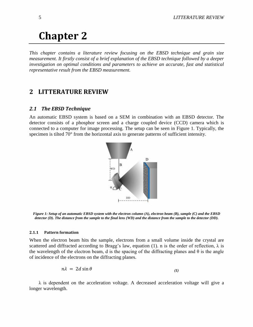
An automatic EBSD system is based on a SEM in combination with an EBSD detector. The
detector consists of a phosphor screen and a charge coupled device (CCD) camera which is
connected to a computer for image processing. The setup can be seen in Figure 1. Typically, the
specimen is tilted 70° from the horizontal axis to generate patterns of sufficient intensity.
Figure 1: Setup of an automatic EBSD system with the electron column (A), electron beam (B), sample (C) and the EBSD
detector (D). The distance from the sample to the final lens (WD) and the distance from the sample to the detector (DD).
2.1.1 Pattern formation
When the electron beam hits the sample, electrons from a small volume inside the crystal are
scattered and diffracted according to Bragg’s law, equation (1). n is the order of reflection, λ is
the wavelength of the electron beam, d is the spacing of the diffracting planes and θ is the angle
of incidence of the electrons on the diffracting planes.
(1)
λ is dependent on the acceleration voltage. A decreased acceleration voltage will give a
longer wavelength.
6 LITTERATURE REVIEW
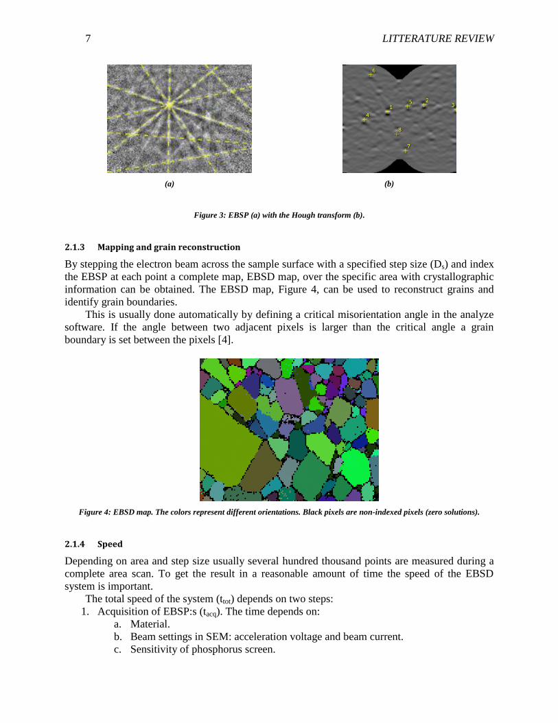
The phosphorus screen is fluoresced by the diffracted electrons and a Kikuchi pattern (BKP)
or Electron backscatter pattern (EBSP) is formed. A typical EBSP can be seen in Figure 3a. The
pattern consists of a number of bands, called Kikuchi bands and the band configuration is
dependent on different lattice properties. The band width is related to the interplanar spacing, d,
and the band geometry can be seen as a projection of the crystal lattice [1].
2.1.2 Band detection
When a pattern appears on the phosphorus screen a CCD camera takes an image of the EBSP.
The image is processed with a software on a computer. To be able to identify the bands
automatically, the image is transformed with Hough transformation.
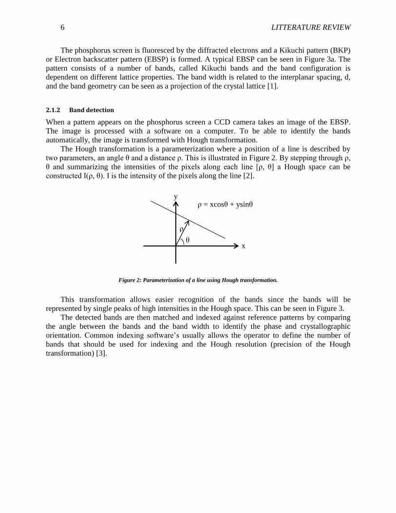
The Hough transformation is a parameterization where a position of a line is described by
two parameters, an angle θ and a distance ρ. This is illustrated in Figure 2. By stepping through ρ,
θ and summarizing the intensities of the pixels along each line [ρ, θ] a Hough space can be
constructed I(ρ, θ). I is the intensity of the pixels along the line [2].
Figure 2: Parameterization of a line using Hough transformation.
This transformation allows easier recognition of the bands since the bands will be
represented by single peaks of high intensities in the Hough space. This can be seen in Figure 3.
The detected bands are then matched and indexed against reference patterns by comparing
the angle between the bands and the band width to identify the phase and crystallographic
orientation. Common indexing software’s usually allows the operator to define the number of
bands that should be used for indexing and the Hough resolution (precision of the Hough
transformation) [3].
x
y
θ
ρ
ρ = xcosθ + ysinθ
7 LITTERATURE REVIEW
(a)
(b)
Figure 3: EBSP (a) with the Hough transform (b).
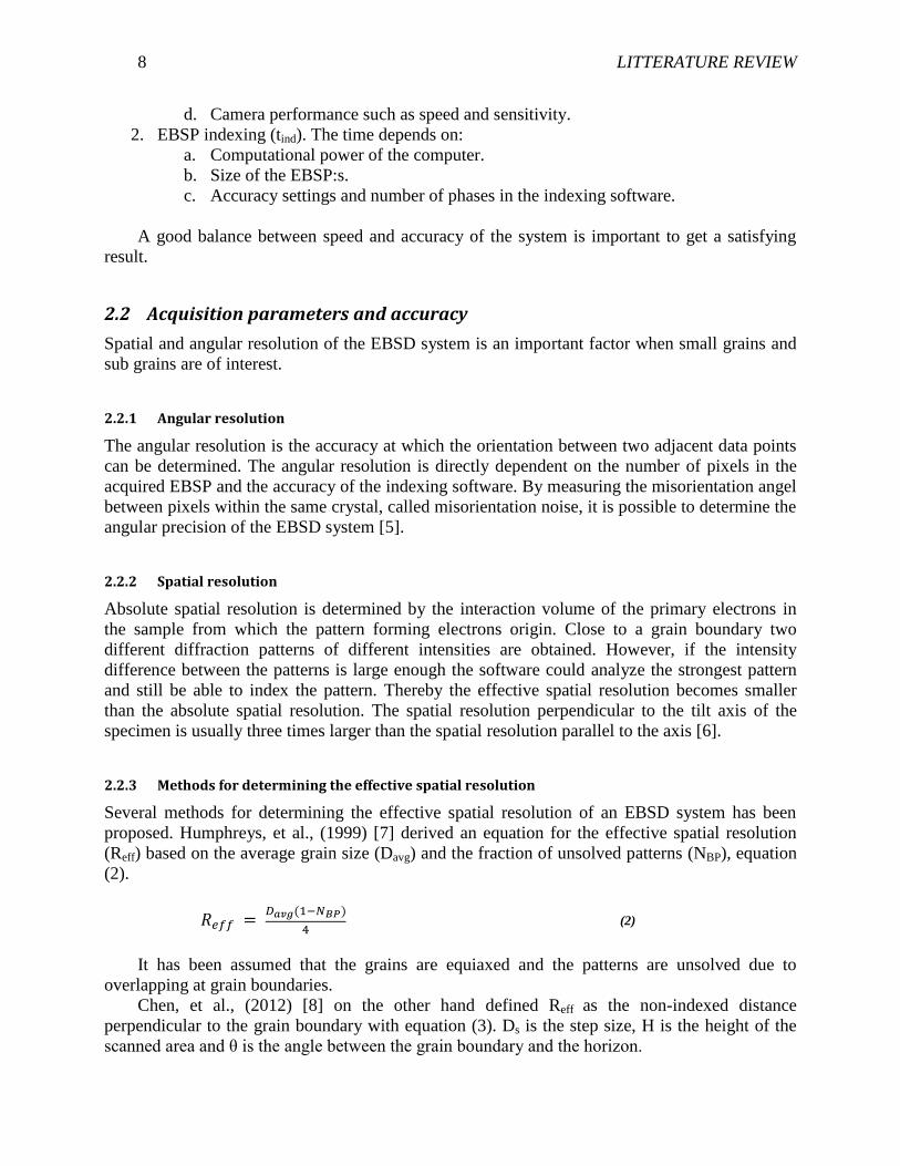
2.1.3 Mapping and grain reconstruction
By stepping the electron beam across the sample surface with a specified step size (Ds) and index
the EBSP at each point a complete map, EBSD map, over the specific area with crystallographic
information can be obtained. The EBSD map, Figure 4, can be used to reconstruct grains and
identify grain boundaries.
This is usually done automatically by defining a critical misorientation angle in the analyze
software. If the angle between two adjacent pixels is larger than the critical angle a grain
boundary is set between the pixels [4].
Figure 4: EBSD map. The colors represent different orientations. Black pixels are non-indexed pixels (zero solutions).
2.1.4 Speed
Depending on area and step size usually several hundred thousand points are measured during a
complete area scan. To get the result in a reasonable amount of time the speed of the EBSD
system is important.
The total speed of the system (ttot) depends on two steps:
1. Acquisition of EBSP:s (tacq). The time depends on:
a. Material.
b. Beam settings in SEM: acceleration voltage and beam current.
c. Sensitivity of phosphorus screen.
8 LITTERATURE REVIEW
d. Camera performance such as speed and sensitivity.
2. EBSP indexing (tind). The time depends on:
a. Computational power of the computer.
b. Size of the EBSP:s.
c. Accuracy settings and number of phases in the indexing software.
A good balance between speed and accuracy of the system is important to get a satisfying
result.
2.2 Acquisition parameters and accuracy
Spatial and angular resolution of the EBSD system is an important factor when small grains and
sub grains are of interest.
2.2.1 Angular resolution
The angular resolution is the accuracy at which the orientation between two adjacent data points
can be determined. The angular resolution is directly dependent on the number of pixels in the
acquired EBSP and the accuracy of the indexing software. By measuring the misorientation angel
between pixels within the same crystal, called misorientation noise, it is possible to determine the
angular precision of the EBSD system [5].
2.2.2 Spatial resolution
Absolute spatial resolution is determined by the interaction volume of the primary electrons in
the sample from which the pattern forming electrons origin. Close to a grain boundary two
different diffraction patterns of different intensities are obtained. However, if the intensity
difference between the patterns is large enough the software could analyze the strongest pattern
and still be able to index the pattern. Thereby the effective spatial resolution becomes smaller
than the absolute spatial resolution. The spatial resolution perpendicular to the tilt axis of the
specimen is usually three times larger than the spatial resolution parallel to the axis [6].
2.2.3 Methods for determining the effective spatial resolution
Several methods for determining the effective spatial resolution of an EBSD system has been
proposed. Humphreys, et al., (1999) [7] derived an equation for the effective spatial resolution
(Reff) based on the average grain size (Davg) and the fraction of unsolved patterns (NBP), equation
(2).
(2)
It has been assumed that the grains are equiaxed and the patterns are unsolved due to
overlapping at grain boundaries.
Chen, et al., (2012) [8] on the other hand defined Reff as the non-indexed distance
perpendicular to the grain boundary with equation (3). Ds is the step size, H is the height of the
scanned area and θ is the angle between the grain boundary and the horizon.
9 LITTERATURE REVIEW
(3)
Both of these methods use the non-indexed pixels at the grain boundaries to determine Reff.
However, when patterns inside grains fail to be indexed, which is often the case, Humphreys’ [7]
method will give an higher and false value of Reff compared to Chens [8]. The accuracy of the
methods is dependent on the step size since for instance a large step size give fewer pixels across
the grain boundary and the size of the pixels is the smallest length of which Reff can be
determined. Therefore it is important to use a small step size when measuring Reff.
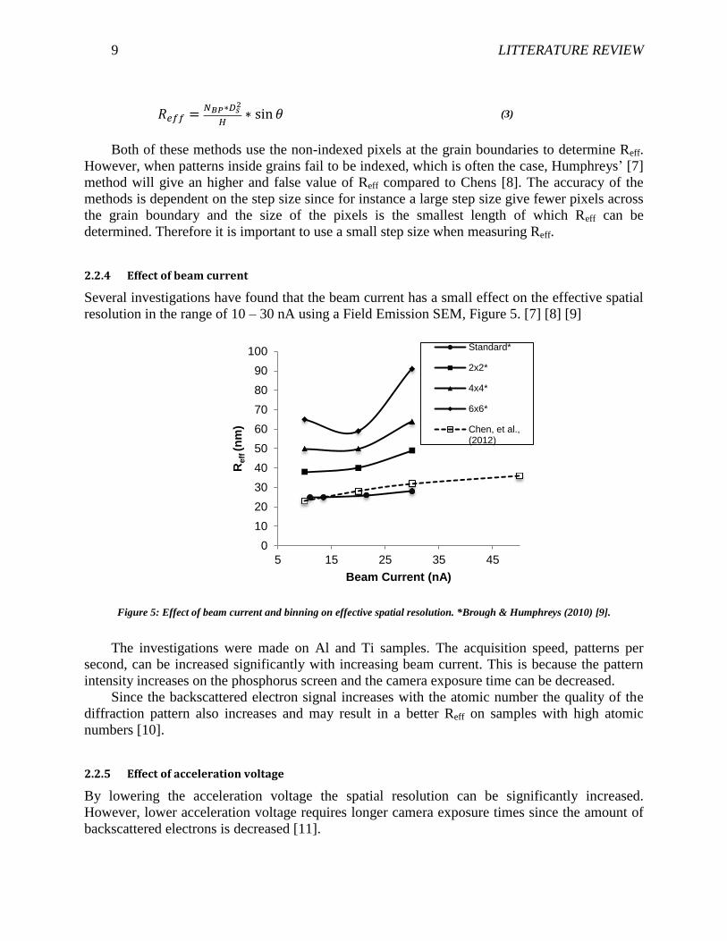
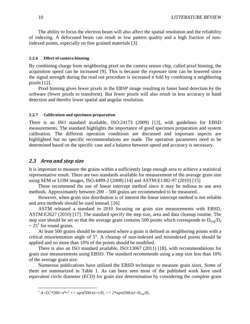
2.2.4 Effect of beam current
Several investigations have found that the beam current has a small effect on the effective spatial
resolution in the range of 10 – 30 nA using a Field Emission SEM, Figure 5. [7] [8] [9]
Figure 5: Effect of beam current and binning on effective spatial resolution. *Brough & Humphreys (2010) [9].
The investigations were made on Al and Ti samples. The acquisition speed, patterns per
second, can be increased significantly with increasing beam current. This is because the pattern
intensity increases on the phosphorus screen and the camera exposure time can be decreased.
Since the backscattered electron signal increases with the atomic number the quality of the
diffraction pattern also increases and may result in a better Reff on samples with high atomic
numbers [10].
2.2.5 Effect of acceleration voltage
By lowering the acceleration voltage the spatial resolution can be significantly increased.
However, lower acceleration voltage requires longer camera exposure times since the amount of
backscattered electrons is decreased [11].
0
10
20
30
40
50
60
70
80
90
100
5 15 25 35 45
Re
ff (n
m)
Beam Current (nA)
Standard*
2x2*
4x4*
6x6*
Chen, et al.,(2012)
10 LITTERATURE REVIEW
The ability to focus the electron beam will also affect the spatial resolution and the reliability
of indexing. A defocused beam can result in low pattern quality and a high fraction of non-
indexed points, especially on fine grained materials [3].
2.2.6 Effect of camera binning
By combining charge from neighboring pixel on the camera sensor chip, called pixel binning, the
acquisition speed can be increased [9]. This is because the exposure time can be lowered since
the signal strength during the read out procedure is increased n fold by combining n neighboring
pixels [12].
Pixel binning gives fewer pixels in the EBSP image resulting in faster band detection by the
software (fewer pixels to transform). But fewer pixels will also result in less accuracy in band
detection and thereby lower spatial and angular resolution.
2.2.7 Calibration and specimen preparation
There is an ISO standard available, ISO:24173 (2009) [13], with guidelines for EBSD
measurements. The standard highlights the importance of good specimen preparation and system
calibration. The different operation conditions are discussed and important aspects are
highlighted but no specific recommendations are made. The operation parameters need to be
determined based on the specific case and a balance between speed and accuracy is necessary.
2.3 Area and step size
It is important to measure the grains within a sufficiently large enough area to achieve a statistical
representative result. There are two standards available for measurement of the average grain size
using SEM or LOM images, ISO:4499-2 (2008) [14] and ASTM:E1382-97 (2010) [15]
These recommend the use of linear intercept method since it may be tedious to use area
methods. Approximately between 200 – 500 grains are recommended to be measured.
However, when grain size distribution is of interest the linear intercept method is not reliable
and area methods should be used instead. [16]
ASTM released a standard in 2010 focusing on grain size measurements with EBSD,
ASTM:E2627 (2010) [17]. The standard specify the step size, area and data cleanup routine. The
step size should be set so that the average grain contains 500 points which corresponds to Davg/Ds
~ 251 for round grains.
At least 500 grains should be measured where a grain is defined as neighboring points with a
critical misorientation angle of 5°. A cleanup of non-indexed and misindexed points should be
applied and no more than 10% of the points should be modified.
There is also an ISO standard available, ISO:13067 (2011) [18], with recommendations for
grain size measurements using EBSD. The standard recommends using a step size less than 10%
of the average grain size.
Numerous publications have utilized the EBSD technique to measure grain sizes. Some of
them are summarized in Table 1. As can been seen most of the published work have used
equivalent circle diameter (ECD) for grain size determination by considering the complete grain
1 A=Ds
2*500=π*r
2 => sqrt(500/π)=r/Ds => 2*sqrt(500/π)=Davg/Ds
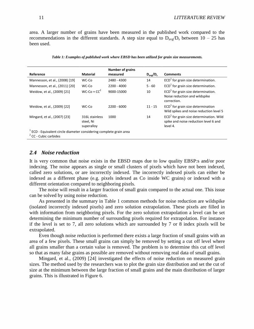
11 LITTERATURE REVIEW
area. A larger number of grains have been measured in the published work compared to the
recommendations in the different standards. A step size equal to Davg/Ds between 10 – 25 has
been used.
Table 1: Examples of published work where EBSD has been utilized for grain size measurements.
Reference Material Number of grains measured Davg/Ds Comments
Mannesson, et al., (2008) [19] WC-Co 2480 - 4300 14 ECD1 for grain size determination.
Mannesson, et al., (2011) [20] WC-Co 2200 - 4000 5 - 60 ECD1 for grain size determination.
Weidow, et al., (2009) [21] WC-Co + CC2
9000-15000 10 ECD1 for grain size determination.
Noise reduction and wildspike correction.
Weidow, et al., (2009) [22] WC-Co 2200 - 6000 11 - 15 ECD1 for grain size determination
Wild spikes and noise reduction level 5
Mingard, et al., (2007) [23] 316L stainless steel, Ni superalloy
1000 14 ECD1 for grain size determination. Wild
spike and noise reduction level 6 and level 4.
1 ECD - Equivalent circle diameter considering complete grain area
2 CC - Cubic carbides
2.4 Noise reduction
It is very common that noise exists in the EBSD maps due to low quality EBSP:s and/or poor
indexing. The noise appears as single or small clusters of pixels which have not been indexed,
called zero solutions, or are incorrectly indexed. The incorrectly indexed pixels can either be
indexed as a different phase (e.g. pixels indexed as Co inside WC grains) or indexed with a
different orientation compared to neighboring pixels.
The noise will result in a larger fraction of small grain compared to the actual one. This issue
can be solved by using noise reduction.
As presented in the summary in Table 1 common methods for noise reduction are wildspike
(isolated incorrectly indexed pixels) and zero solution extrapolation. These pixels are filled in
with information from neighboring pixels. For the zero solution extrapolation a level can be set
determining the minimum number of surrounding pixels required for extrapolation. For instance
if the level is set to 7, all zero solutions which are surrounded by 7 or 8 index pixels will be
extrapolated.
Even though noise reduction is performed there exists a large fraction of small grains with an
area of a few pixels. These small grains can simply be removed by setting a cut off level where
all grains smaller than a certain value is removed. The problem is to determine this cut off level
so that as many false grains as possible are removed without removing real data of small grains.
Mingard, et al., (2009) [24] investigated the effects of noise reduction on measured grain
sizes. The method used by the researchers was to plot the grain size distribution and set the cut of
size at the minimum between the large fraction of small grains and the main distribution of larger
grains. This is illustrated in Figure 6.

12 LITTERATURE REVIEW
Figure 6: Schematic illustration of grain size distribution with the cut off size (vertical line) between the large fraction of small
grains and main distribution.
The researchers found that a cut of size of 3 pixels was the most appropriate for their sample.
A cut off size of 12 pixels removed some real grains but the result was closer to results achieved
with image analysis from SEM images. But still a larger fraction of small grains are recorded
using EBSD compared with the SEM measurements.
2.5 Presentation of grains size distribution
It is important to consider the presentation of a grain size distribution so that the data are
highlighted and shown in a truthful way. A basic approach is to present the data using a
histogram where the data are grouped based on size in defined intervals called bins. Special care
need to be taken when selecting the width of the bins. Too large bins will over smooth the data
and important details in the distribution can be lost. On the other hand too small bins will result in
a noisy histogram which is hard to interpret. Scott, (1979) [25] proposed the following equation
to calculate the bin width. h is the bin width, σ is the standard deviation of the data set and n is
the number of data available.
⁄ (4)
Even though the bin width is optimized artifacts in the presentation using histograms can
occur. Jeppson, et al., (2011) [26] developed a method using a kernel density estimator and
transforming the grain sizes from 2D to 3D. This resulted in a smoother distribution function
compared with histograms.
It is also possible to present the data using a cumulative distribution plot based on number or
size fraction, equation (5) and (6). Ni is the cumulative number of grains up to the i:th grain, Ai is
the cumulative area up to the i:th grain. N is total number of grains and A is the total area for all
grains.
deqv
relN

13 LITTERATURE REVIEW
(5)
(6)
Some advantages and disadvantages using different plots are discussed by Roebuck, et al.,
(1999) [27]. A linear x-axis will highlight the large grains more clearly compared with a
logarithmic scale where the small grains are highlighted. Using area instead of number will give
more weight to the larger grains and highlight the difference more clearly.
Calculating average values based on area or volume instead of number will reduce the effect
of small grains and, in the same manner as for plotting, give more weight to the larger grains
[24].
2.6 Summary
The effective spatial resolution is an important property for an EBSD system. Chen, et al., (2012)
[8] developed a good method for determining the effective spatial resolution.
It has been shown that the beam current has little effect on the effective spatial resolution
and high beam currents can increase the acquisition rate. Increased camera binning and
acceleration voltage will deteriorate the effective spatial resolution but also increase acquisition
rate.
The step size used in the literature and specified in the standards is based on an estimate of
the average grain size and Davg/Ds is in the range of 10 – 25. The number of grains measured is in
the range of 500 – 6000.
A noise reduction and data filtering has to be performed to the EBSD map to get a realistic
result. Common ways are to extrapolate wildespikes and zero solutions and removing small
grains of only a few pixels.
Equivalent circle diameter calculated from area is a common way to describe the grain size.
Presentation of grain size distribution using a histogram is a common method however it is
sensitive to selection of the bin widths. Methods exist to optimize the bin width. Other methods
of presenting grain size distributions are with cumulative plots or with a kernel density estimator.
Using fraction based on area or volume instead of number can highlight the larger grains more
clearly.
14 METHOD DEVELOPMENT
Chapter 3
This chapter describes the methodology and results for the development of a quantitative method
for grain size measurement using EBSD. The first part will describe the method used to evaluate
the performance of the EBSD system followed by the results. In the last part a complete
quantitative method will be presented based on the results from the evaluation and the literature
review.
3 METHOD DEVELOPMENT
As described in section 2.1.4 the total speed of the EBSD system (ttot) depends both on the
acquisition speed of the EBSP:s (tacq) and indexing by the computer (tind). To be able to optimize
speed and accuracy the two processes have been investigated separately.
3.1 Equipment
The EBSD system used consists of a Zeiss Supra 55 VP FEG-SEM together with a Nordlys F
EBSD detector. The CPU in the indexing computer was an 8 core Intel i7-2600 processor at 3.4
GHz and 8GB RAM.
Oxford instruments Aztec 2.0 software was used as indexing software and Channel 5 –
Tango was used for data analysis. IBM SPSS Statistics 19 was used for regression analysis and
Matlab R2011a used for plotting the grain size distributions and statistical calculations.
3.2 Camera performance
The performance of the CCD camera in the EBSD detector was evaluated at different electron
beam and camera settings. The evaluation was made on a sample prepared according to section
4.4.1 with a working distance of 8.5 mm and a detector insertion distance of 176 mm. The beam
was swept across the sample surface in a fast rate and the exposure time set by the software using
“auto-exposure” was recorded. According to the software manual the exposure time are adjusted
so that the signal strength is between 85 – 95 and signal strength is defined as the end tail of the
pixel intensity histogram.
Camera binning, camera gain, acceleration voltage and aperture size were varied
systematically according to Table 2. The beam currents corresponding to the different aperture
sizes were measured using a faradays cup.

15 METHOD DEVELOPMENT
Table 2: Parameters used for EBSD camera evaluation.
Parameters Values
Acceleration voltage 15 kV, 20 kV
Camera binning 1x1, 2x2, 4x4, 6x6, 8x8
Camera gain 5, 10, 15
Apertures 60 µm, 120 µm, 240 µm
The correlation between the signal strength during readout of an image from the CCD
camera and the beam current, the camera binning and the camera gain can be seen in Equation
(7). PCCD is the signal strength, I is the beam current (nA), B is the camera binning (1x1, 2x2, 4x4
or 8x8 pixels binned), f(G) is the camera gain function (amplification of the signal) where G is
the gain value set in the software.
(7)
PCCD is proportional to 1/texp where texp is the required exposure time (ms). This results in the
following relationship for the exposure time, equation (8).
(8)
k1 is a constant which is dependent on the acceleration voltage, detector distance, working
distance, EBSD hardware and specimen composition.
Regression analysis was used to find k1. The calculation was made for 15 kV and 20 kV
acceleration voltages separately. During the regression analysis equation (8) was used in
logarithmic form to reduce the influence of the high exposure times on the fitting of k1.
3.3 Indexing settings
To evaluate the indexing speed on the computer, EBSP:s saved on the local hard drive were
reindexed using three different Hough resolutions: 60, 90 and 120. The number of bands was set
to 8 and the phases used are specified in Table 3.
Table 3: Phases used for indexing
Phase Reflectors
WC (HCP) 59
Co (FCC) 56
Co (HCP) 50
3.4 Effective spatial resolution
The method used in this work for calculating the effective spatial resolution was proposed by
Chen, et al., (2010) [8] as discussed in section 2.2.3.

16 METHOD DEVELOPMENT
In total 6 maps were acquired where the beam current and camera binning was varied (Table
4). An average of 4-5 grain boundaries on each map were analyzed using equation (9).
(9)
Reff is the effective spatial resolution, NBP is the fraction of unsolved patterns, Ds is the step
size and L is the length of the grain boundary.
Table 4: Acquisition parameters for maps used to calculate the effective spatial resolution.
Beam current (nA) Camera binning (EBSP resolution)
8.71 2x2 (320x240 pixels)
8.71 4x4 (160x120 pixels)
8.71 6x6 (104x80 pixels)
36.9 2x2 (320x240 pixels)
36.9 4x4 (160x120 pixels)
36.9 6x6 (104x80 pixels)
All maps were acquired using an acceleration voltage of 20 kV, working distance of 8.5 mm
and a detector insertion distance of 176 mm. The step size was set to 0.03 µm.
3.5 Results and discussion
3.5.1 Camera performance
The beam currents measured with a Faradays cup are shown in Table 5. The beam currents were
used as I in equation (8) for the regression analysis.
Table 5: Measured beam currents using a Faradays cup.
Aperture Beam current (at 15 kV) Beam current (at 20 kV)
60 µm 2.96 (nA) 3.23 (nA)
120 µm 8.27 (nA) 8.71 (nA)
240 µm 29.32 (nA) 36.9 (nA)
To identify the camera gain function, f(G), texp was plotted against the gain (G) used in the
software, see Figure 7.

17 METHOD DEVELOPMENT
Figure 7: texp plotted against the camera gain (red squares) with an exponential function fitted to the data (black line).
The red squares are texp for 4x4 binned camera with 20 kV acceleration voltage and 240 µm
aperture which corresponds to 36.9 nA beam current. The black line is an exponential function
fitted to the data. As can be seen the exponential function gives an R2 = 1 which indicates that the
camera gain function is an exponential function. Equation (10) was used as the camera gain
function in equation (8).
(10)
The complete data set used for the regression analysis can be seen in Appendix A.
The results from the regression analysis can be seen in Table 6. Observe that texp is in ms and
I is in nA. k2 is only dependent on the detector hardware and this results in the same value of the
constant for both 15 and 20 kV.
Table 6: Result from regression analysis. Values of k1 and k2 for 15kV and 20 kV acceleration voltage.
Parameter fit: k1, k2 .
15 kV 20 kV
k1 3288.5 2213.1
k2 0.049 0.049
R2 0.997 0.997
Measured exposure times are plotted versus the calculated exposure times in Figure 8. The
axes are logarithmic.

18 METHOD DEVELOPMENT
Figure 8: Measured exposure time vs. calculated exposure time.
The camera frame rate is the inverse of the exposure time, Hz = 1/texp. This is valid up to the
theoretical maximum frame rate for the camera and is dependent on the camera binning. If a
higher binning is used the individual images will become smaller and this results in a higher
maximum frame rate. The maximum frame rates at different camera binnings are shown in Table
7.
Table 7: Theoretical camera speed for different binnings.
Binning Theoretical limit (ms) Frame rate (Hz)
1x1 12.81 78
1
2x2 3.71 269
4x4 2.23 448
6x6 1.76 566
8x8 1.54 648 1The theoretical limit was not reached during the experiments. The specified
frame rates are the highest achieved frame rate and not the limit.
3.5.2 Indexing settings
The indexing time as function of the Hough resolution is plotted Figure 9 for different camera
binnings. Approximate CPU usage is also shown in the figure as percentage numbers. A higher
camera binning will result in a lower EBSP image resolution and thereby fewer pixels to
transform with the Hough resolution. As can be seen, the indexing time is generally longer for
2x2 binning compared to 4x4 and 6x6 binning. The indexing time is increased with increasing
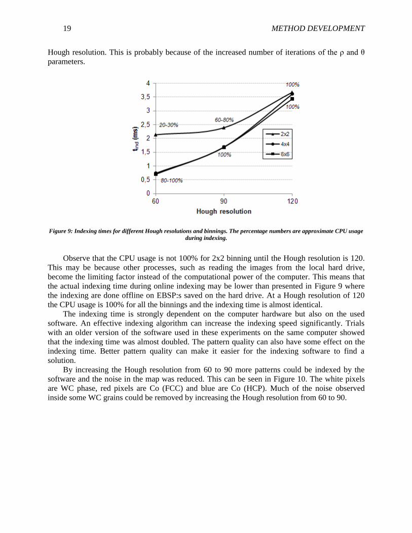
19 METHOD DEVELOPMENT
Hough resolution. This is probably because of the increased number of iterations of the ρ and θ
parameters.
Figure 9: Indexing times for different Hough resolutions and binnings. The percentage numbers are approximate CPU usage
during indexing.
Observe that the CPU usage is not 100% for 2x2 binning until the Hough resolution is 120.
This may be because other processes, such as reading the images from the local hard drive,
become the limiting factor instead of the computational power of the computer. This means that
the actual indexing time during online indexing may be lower than presented in Figure 9 where
the indexing are done offline on EBSP:s saved on the hard drive. At a Hough resolution of 120
the CPU usage is 100% for all the binnings and the indexing time is almost identical.
The indexing time is strongly dependent on the computer hardware but also on the used
software. An effective indexing algorithm can increase the indexing speed significantly. Trials
with an older version of the software used in these experiments on the same computer showed
that the indexing time was almost doubled. The pattern quality can also have some effect on the
indexing time. Better pattern quality can make it easier for the indexing software to find a
solution.
By increasing the Hough resolution from 60 to 90 more patterns could be indexed by the
software and the noise in the map was reduced. This can be seen in Figure 10. The white pixels
are WC phase, red pixels are Co (FCC) and blue are Co (HCP). Much of the noise observed
inside some WC grains could be removed by increasing the Hough resolution from 60 to 90.

20 METHOD DEVELOPMENT
(a) (b)
Figure 10: Map indexed with a Hough resolution of 60 (a) and map indexed a Hough resolution of 90 (b). White pixels are
WC phase, red pixels are Co (FCC) and blue are Co (HCP).
The number of bands set in the indexing software also affects the amount of noise in the
map, for instance using 8 instead 7 bands will reduce the amount of noise significantly.
3.5.3 Effective spatial resolution
In the Figure 11 the effective spatial resolution is plotted against the camera binning for two
beam currents. As can be seen the effective spatial resolution becomes lower with increased
binning which is in agreement with the other researchers that was discussed in the literature
review in section 2.2.4. The values are of the same order and follow the same trend. Both 2x2 and
4x4 binning for both beam currents have relatively similar Reff. However for 6x6 binning Reff is
significantly deteriorated.
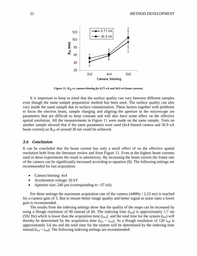
21 METHOD DEVELOPMENT
Figure 11: Reff vs. camera binning for 8,71 nA and 36,9 nA beam currents.
It is important to keep in mind that the surface quality can vary between different samples
even though the same sample preparation method has been used. The surface quality can also
vary inside the same sample due to surface contamination. These factors together with problems
to focus the electron beam, sample charging and aligning the aperture in the microscope are
parameters that are difficult to keep constant and will also have some effect on the effective
spatial resolution. All the measurements in Figure 11 were made on the same sample. Tests on
another sample showed that if the same parameters were used (4x4 binned camera and 36.9 nA
beam current) an Reff of around 30 nm could be achieved.
3.6 Conclusion
It can be concluded that the beam current has only a small effect of on the effective spatial
resolution both from the literature review and from Figure 11. Even at the highest beam currents
used in these experiments the result is satisfactory. By increasing the beam current the frame rate
of the camera can be significantly increased according to equation (8). The following settings are
recommended for fast acquisition:
Camera binning: 4x4
Acceleration voltage: 20 kV
Aperture size: 240 µm (corresponding to ~37 nA)
For these settings the maximum acquisition rate of the camera (448Hz / 2.23 ms) is reached
for a camera gain of 5. But to ensure better image quality and better signal to noise ratio a lower
gain is recommended.
The results from the indexing settings show that the quality of the maps can be increased by
using a Hough resolution of 90 instead of 60. The indexing time (tind) is approximately 1.7 ms
(592 Hz) which is lower than the acquisition time (tacq) and the total time for the system (ttot) will
thereby be determined by the acquisition time (ttot ~ tacq). At a Hough resolution of 120 tind is
approximately 3.6 ms and the total time for the system will be determined by the indexing time
instead (ttot ~ tind). The following indexing settings are recommended:
22 METHOD DEVELOPMENT
Number of bands: 8
Hough resolution: 90
These acquisition and indexing settings have been used successfully on materials with an
average grain sizes down to ~0.5 µm. For measurements on materials with smaller grain sizes it
might be necessary to adjust the acquisition parameters for higher spatial resolution, for instance
lowering the camera binning, beam current and/or acceleration voltage.
It is recommended that an approximate average grain size is used to determine the step size
and the area that needs to be measured to get enough grain statistics. From the literature a step
size of Davg/Ds ~ 15 seems enough. The following equations can be used to estimate the step size
and area:
(11)
√ (12)
In the literature it is recommended to measure more than 2000 grains.
The following parameters are recommended for grain reconstruction and noise reduction:
Critical misorientation angle: 5°
Exclude border grains
Wild spike extrapolation
Zero solution extrapolation: 5 neighbors
Cut of size: set between the peaks in the histogram (usually between 3 – 6 pixels)
A critical misorientation angle between 5 – 15 ° for grain reconstruction has been used in the
literature. However, there is a reduced risk that some grain boundaries are missed if the
misorientation angle is set to 5°. If the results are to be compared with grain size measurements
using image analysis from SEM or LOM pictures the ∑2 grain boundaries should be excluded.
The grains cut by an edge of the map should be excluded since the complete grain areas not have
been measured. Wildspike extrapolation will reduce the amount of noise in the map.
Extrapolation of zero solutions from 5 neighbors will remove some of the noise and make the
grain size closer to the actual size without introducing any artifacts in the map.
It is recommended that the grain size distribution is presented both using a number and area
fraction plots to highlight both small and large grains.

23 EXPERIMENTAL PROCEDURE
Chapter 4
This chapter covers the comparison between materials produced in a traditional ball mill versus
materials produced with milling method A and B. Both a comparison of the particle size
distribution after milling before sintering and WC grain size distribution on the sintered samples
has been made.
4 EXPERIMENTAL PROCEDURE
In this section, the method used to manufacture and compare the materials will be explained.
4.1 Material and equipment
The sintered samples used in this investigation were produced at Sandvik Machining Solutions.
4.1.1 Raw materials and Milling
Two different WC raw materials were used. The properties are specified in Table 8.
Table 8: Raw materials used for milling.
Raw material dfsss as supplied dfsss ASTM-milled
WC0B - 633 0.85 0.80
WC2B - 554 1.32 1.25
The raw materials were milled with a traditional 30l ball milling method (will be referred to
as 30l ball mill) and with method A and B. In a ball mill, Figure 12, the milling chamber is
rotated and the milling media falls down and collides with other milling media and the powder in
between is crushed.
Figure 12: Ball mill.
1. Milling chamber 2. Milling media 3. Milling suspension
1
2
3
24 EXPERIMENTAL PROCEDURE
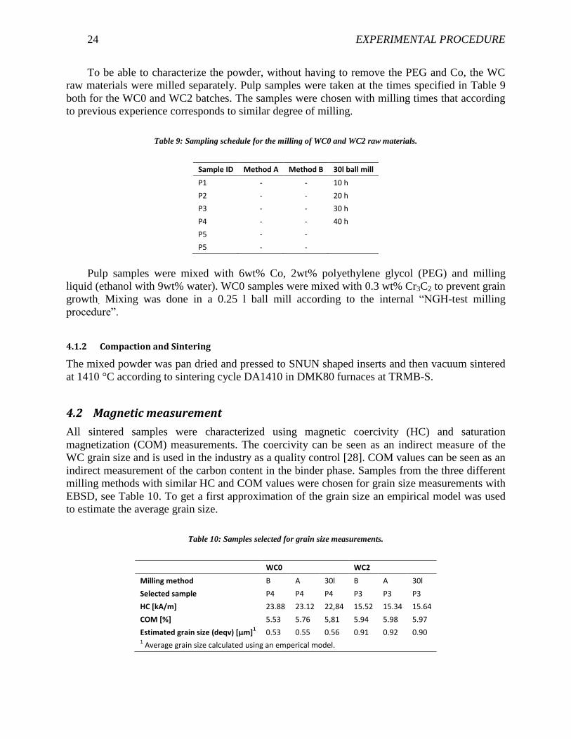
To be able to characterize the powder, without having to remove the PEG and Co, the WC
raw materials were milled separately. Pulp samples were taken at the times specified in Table 9
both for the WC0 and WC2 batches. The samples were chosen with milling times that according
to previous experience corresponds to similar degree of milling.
Table 9: Sampling schedule for the milling of WC0 and WC2 raw materials.
Sample ID Method A Method B 30l ball mill
P1 - - 10 h
P2 - - 20 h
P3 - - 30 h
P4 - - 40 h
P5 - -
P5 - -
Pulp samples were mixed with 6wt% Co, 2wt% polyethylene glycol (PEG) and milling
liquid (ethanol with 9wt% water). WC0 samples were mixed with 0.3 wt% Cr3C2 to prevent grain
growth. Mixing was done in a 0.25 l ball mill according to the internal “NGH-test milling
procedure”.
4.1.2 Compaction and Sintering
The mixed powder was pan dried and pressed to SNUN shaped inserts and then vacuum sintered
at 1410 °C according to sintering cycle DA1410 in DMK80 furnaces at TRMB-S.
4.2 Magnetic measurement
All sintered samples were characterized using magnetic coercivity (HC) and saturation
magnetization (COM) measurements. The coercivity can be seen as an indirect measure of the
WC grain size and is used in the industry as a quality control [28]. COM values can be seen as an
indirect measurement of the carbon content in the binder phase. Samples from the three different
milling methods with similar HC and COM values were chosen for grain size measurements with
EBSD, see Table 10. To get a first approximation of the grain size an empirical model was used
to estimate the average grain size.
Table 10: Samples selected for grain size measurements.
WC0 WC2
Milling method B A 30l B A 30l
Selected sample P4 P4 P4 P3 P3 P3
HC [kA/m] 23.88 23.12 22,84 15.52 15.34 15.64
COM [%] 5.53 5.76 5,81 5.94 5.98 5.97
Estimated grain size (deqv) [μm]1 0.53 0.55 0.56 0.91 0.92 0.90
1 Average grain size calculated using an emperical model.

25 EXPERIMENTAL PROCEDURE
4.3 Powder characterization
The milled and dried powder corresponding to the samples in Table 10 was first deagglomerated
using an ASTM-standard milling procedure. It was then mixed with deionized water and Extran
to form a dispersion and then characterized using a laser diffraction instrument (Microtrac), see
Figure 13. The particle size distribution is determined by a software which analyzes the intensity
and angle of the scattered light. Three measurements on each sample were made and the average
value was used.
Figure 13: Principle of particle size measurement using laser diffraction.2
4.4 Grain size measurement
4.4.1 Sample preparation for EBSD
Sintered samples were mechanically polished in two steps using Struers RotoForce-4. In the first
step a 9 µm diamond slurry and a pressure of 75N was used for 20 minutes. The samples were
cleaned before the second step where the samples were polished with 1 µm diamond slurry until
all visible scratches were removed, approximately 10 – 20 minutes.
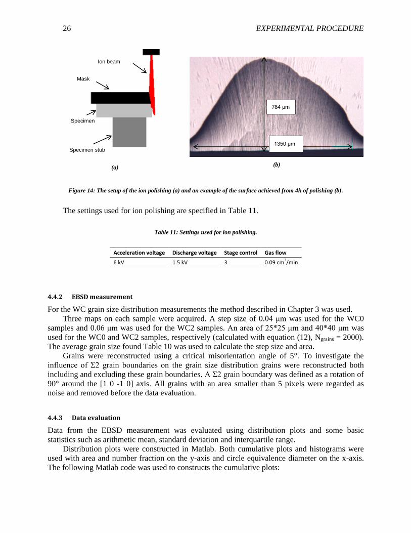
After the mechanical polishing the samples were mounted on stubs with carbon tape and ion
polished in a Hitachi E-3500 Ion Milling System Plus for 4 hours to get a deformation free
surface. The setup can be seen in Figure 14a and an example of the surface achieved after 4 h of
polishing in Figure 14b. The area is approximately 1 mm2.
2 Modified from: Björn Uhrenius, Powder metallurgy, Chapter 2.
1. Laser 2. Incident beam 3. Powder feeder 4. Sample cell 5. Scattered beam 6. Detector 7. Computer
1 2
3
4
5
6
7
26 EXPERIMENTAL PROCEDURE
(a)
(b)
Figure 14: The setup of the ion polishing (a) and an example of the surface achieved from 4h of polishing (b).
The settings used for ion polishing are specified in Table 11.
Table 11: Settings used for ion polishing.
Acceleration voltage Discharge voltage Stage control Gas flow
6 kV 1.5 kV 3 0.09 cm3/min
4.4.2 EBSD measurement
For the WC grain size distribution measurements the method described in Chapter 3 was used.
Three maps on each sample were acquired. A step size of 0.04 μm was used for the WC0
samples and 0.06 μm was used for the WC2 samples. An area of 25*25 μm and 40*40 μm was
used for the WC0 and WC2 samples, respectively (calculated with equation (12), Ngrains = 2000).
The average grain size found Table 10 was used to calculate the step size and area.
Grains were reconstructed using a critical misorientation angle of 5°. To investigate the
influence of Σ2 grain boundaries on the grain size distribution grains were reconstructed both
including and excluding these grain boundaries. A Σ2 grain boundary was defined as a rotation of
90° around the [1 0 -1 0] axis. All grains with an area smaller than 5 pixels were regarded as
noise and removed before the data evaluation.
4.4.3 Data evaluation
Data from the EBSD measurement was evaluated using distribution plots and some basic
statistics such as arithmetic mean, standard deviation and interquartile range.
Distribution plots were constructed in Matlab. Both cumulative plots and histograms were
used with area and number fraction on the y-axis and circle equivalence diameter on the x-axis.
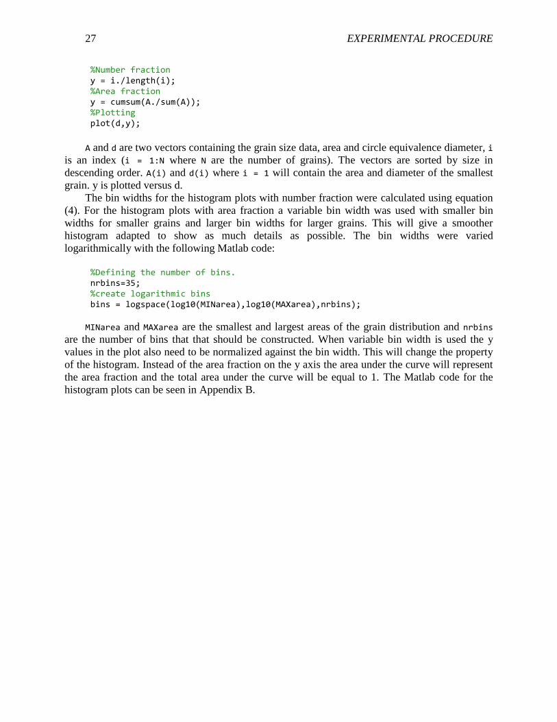
The following Matlab code was used to constructs the cumulative plots:
Ion beam
Mask
Specimen
Specimen stub
784 μm
1350 μm
27 EXPERIMENTAL PROCEDURE
%Number fraction y = i./length(i); %Area fraction y = cumsum(A./sum(A)); %Plotting plot(d,y);
A and d are two vectors containing the grain size data, area and circle equivalence diameter, i
is an index (i = 1:N where N are the number of grains). The vectors are sorted by size in
descending order. A(i) and d(i) where i = 1 will contain the area and diameter of the smallest
grain. y is plotted versus d.
The bin widths for the histogram plots with number fraction were calculated using equation
(4). For the histogram plots with area fraction a variable bin width was used with smaller bin
widths for smaller grains and larger bin widths for larger grains. This will give a smoother
histogram adapted to show as much details as possible. The bin widths were varied
logarithmically with the following Matlab code:
%Defining the number of bins. nrbins=35; %create logarithmic bins bins = logspace(log10(MINarea),log10(MAXarea),nrbins);
MINarea and MAXarea are the smallest and largest areas of the grain distribution and nrbins
are the number of bins that that should be constructed. When variable bin width is used the y
values in the plot also need to be normalized against the bin width. This will change the property
of the histogram. Instead of the area fraction on the y axis the area under the curve will represent
the area fraction and the total area under the curve will be equal to 1. The Matlab code for the
histogram plots can be seen in Appendix B.
28 RESULTS
5 RESULTS
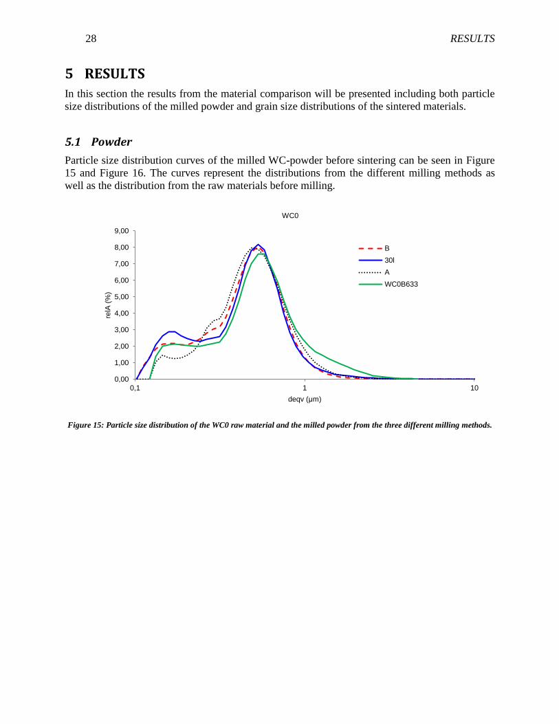
In this section the results from the material comparison will be presented including both particle
size distributions of the milled powder and grain size distributions of the sintered materials.
5.1 Powder
Particle size distribution curves of the milled WC-powder before sintering can be seen in Figure
15 and Figure 16. The curves represent the distributions from the different milling methods as
well as the distribution from the raw materials before milling.
Figure 15: Particle size distribution of the WC0 raw material and the milled powder from the three different milling methods.
0,00
1,00
2,00
3,00
4,00
5,00
6,00
7,00
8,00
9,00
0,1 1 10
relA
(%
)
deqv (μm)
WC0
B
30l
A
WC0B633
29 RESULTS
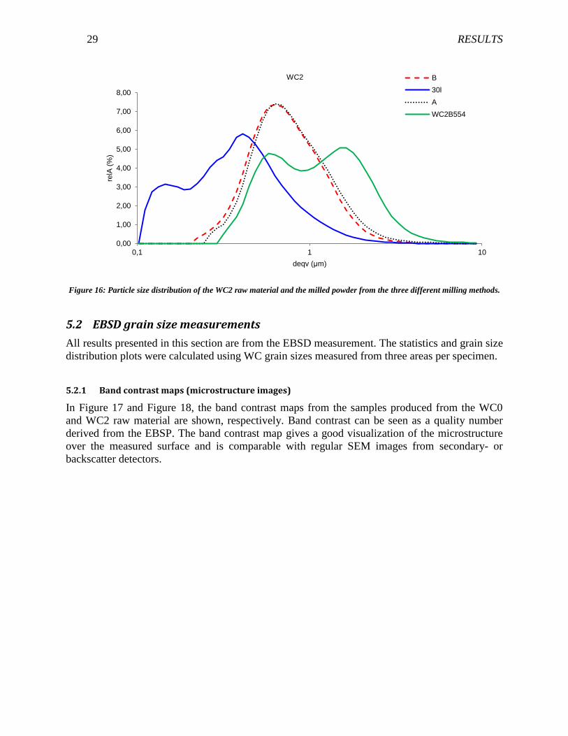
Figure 16: Particle size distribution of the WC2 raw material and the milled powder from the three different milling methods.
5.2 EBSD grain size measurements
All results presented in this section are from the EBSD measurement. The statistics and grain size
distribution plots were calculated using WC grain sizes measured from three areas per specimen.
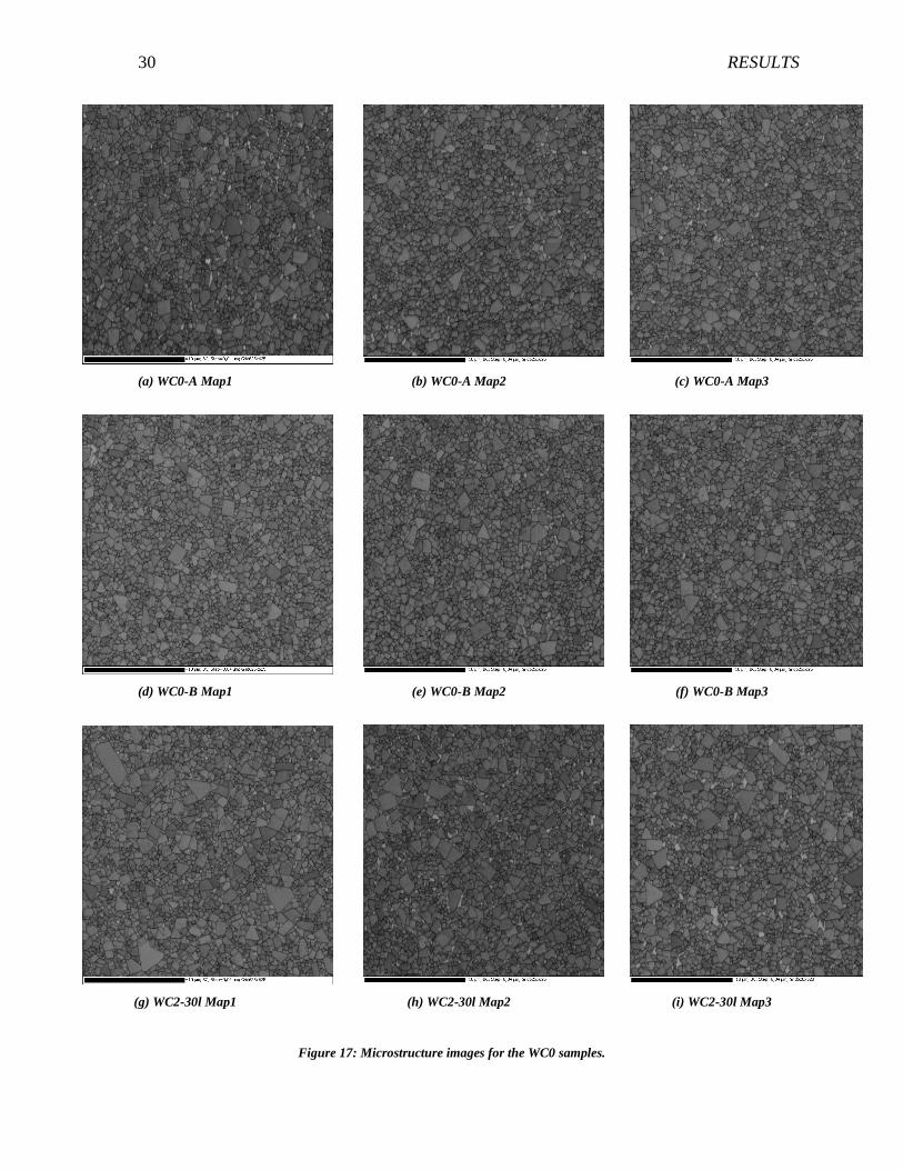
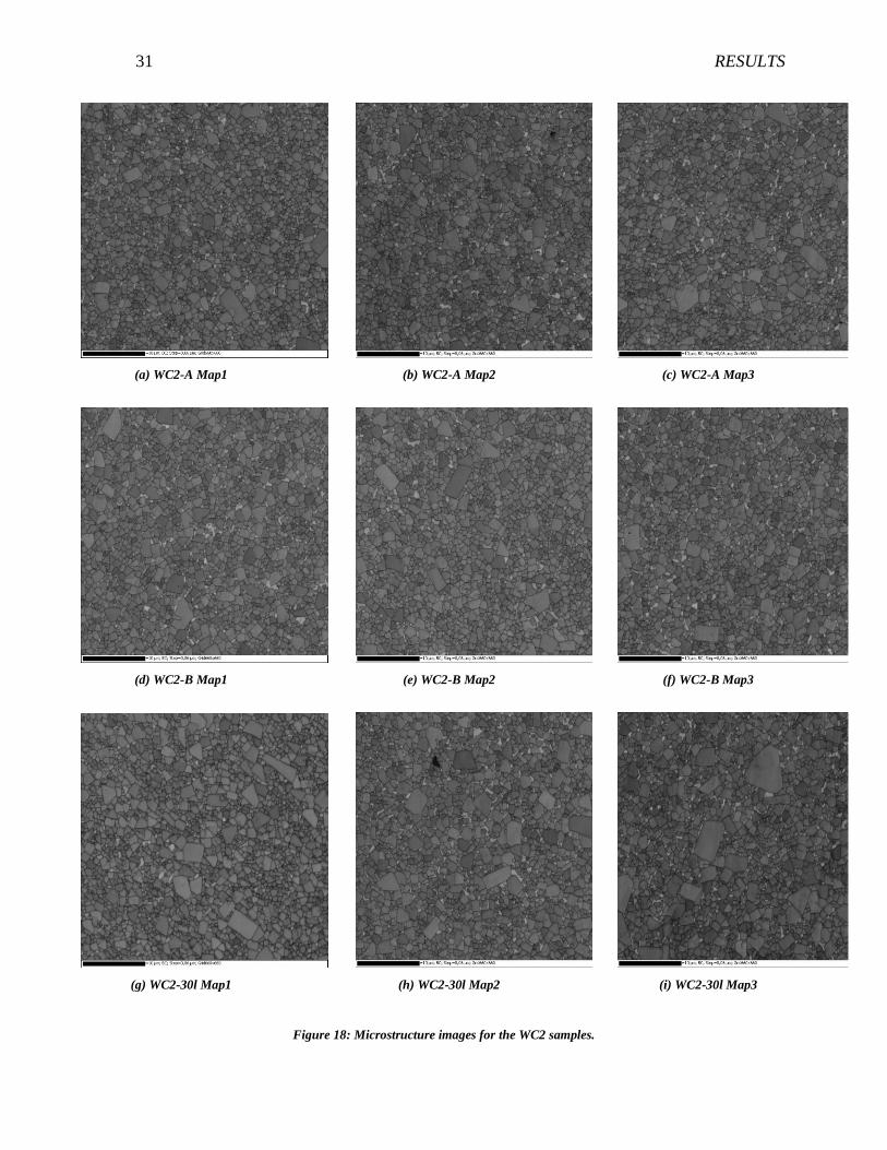
5.2.1 Band contrast maps (microstructure images)
In Figure 17 and Figure 18, the band contrast maps from the samples produced from the WC0
and WC2 raw material are shown, respectively. Band contrast can be seen as a quality number
derived from the EBSP. The band contrast map gives a good visualization of the microstructure
over the measured surface and is comparable with regular SEM images from secondary- or
backscatter detectors.
0,00
1,00
2,00
3,00
4,00
5,00
6,00
7,00
8,00
0,1 1 10
relA
(%
)
deqv (μm)
WC2 B
30l
A
WC2B554
30 RESULTS
(a) WC0-A Map1
(b) WC0-A Map2
(c) WC0-A Map3
(d) WC0-B Map1
(e) WC0-B Map2
(f) WC0-B Map3
(g) WC2-30l Map1
(h) WC2-30l Map2
(i) WC2-30l Map3
Figure 17: Microstructure images for the WC0 samples.
31 RESULTS
(a) WC2-A Map1
(b) WC2-A Map2
(c) WC2-A Map3
(d) WC2-B Map1
(e) WC2-B Map2
(f) WC2-B Map3
(g) WC2-30l Map1
(h) WC2-30l Map2
(i) WC2-30l Map3
Figure 18: Microstructure images for the WC2 samples.
32 RESULTS
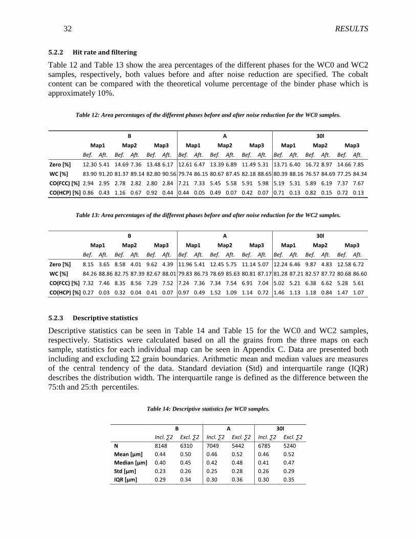
5.2.2 Hit rate and filtering
Table 12 and Table 13 show the area percentages of the different phases for the WC0 and WC2
samples, respectively, both values before and after noise reduction are specified. The cobalt
content can be compared with the theoretical volume percentage of the binder phase which is
approximately 10%.
Table 12: Area percentages of the different phases before and after noise reduction for the WC0 samples.
B A 30l
Map1 Map2 Map3 Map1 Map2 Map3 Map1 Map2 Map3
Bef. Aft. Bef. Aft. Bef. Aft. Bef. Aft. Bef. Aft. Bef. Aft. Bef. Aft. Bef. Aft. Bef. Aft.
Zero [%] 12.30 5.41 14.69 7.36 13.48 6.17 12.61 6.47 13.39 6.89 11.49 5.31 13.71 6.40 16.72 8.97 14.66 7.85
WC [%] 83.90 91.20 81.37 89.14 82.80 90.56 79.74 86.15 80.67 87.45 82.18 88.65 80.39 88.16 76.57 84.69 77.25 84.34
CO(FCC) [%] 2.94 2.95 2.78 2.82 2.80 2.84 7.21 7.33 5.45 5.58 5.91 5.98 5.19 5.31 5.89 6.19 7.37 7.67
CO(HCP) [%] 0.86 0.43 1.16 0.67 0.92 0.44 0.44 0.05 0.49 0.07 0.42 0.07 0.71 0.13 0.82 0.15 0.72 0.13
Table 13: Area percentages of the different phases before and after noise reduction for the WC2 samples.
B A 30l
Map1 Map2 Map3 Map1 Map2 Map3 Map1 Map2 Map3
Bef. Aft. Bef. Aft. Bef. Aft. Bef. Aft. Bef. Aft. Bef. Aft. Bef. Aft. Bef. Aft. Bef. Aft.
Zero [%] 8.15 3.65 8.58 4.01 9.62 4.39 11.96 5.41 12.45 5.75 11.14 5.07 12.24 6.46 9.87 4.83 12.58 6.72
WC [%] 84.26 88.86 82.75 87.39 82.67 88.01 79.83 86.73 78.69 85.63 80.81 87.17 81.28 87.21 82.57 87.72 80.68 86.60
CO(FCC) [%] 7.32 7.46 8.35 8.56 7.29 7.52 7.24 7.36 7.34 7.54 6.91 7.04 5.02 5.21 6.38 6.62 5.28 5.61
CO(HCP) [%] 0.27 0.03 0.32 0.04 0.41 0.07 0.97 0.49 1.52 1.09 1.14 0.72 1.46 1.13 1.18 0.84 1.47 1.07
5.2.3 Descriptive statistics
Descriptive statistics can be seen in Table 14 and Table 15 for the WC0 and WC2 samples,
respectively. Statistics were calculated based on all the grains from the three maps on each
sample, statistics for each individual map can be seen in Appendix C. Data are presented both
including and excluding Σ2 grain boundaries. Arithmetic mean and median values are measures
of the central tendency of the data. Standard deviation (Std) and interquartile range (IQR)
describes the distribution width. The interquartile range is defined as the difference between the
75:th and 25:th percentiles.
Table 14: Descriptive statistics for WC0 samples.
B A 30l
Incl. ∑2 Excl. ∑2 Incl. ∑2 Excl. ∑2 Incl. ∑2 Excl. ∑2
N 8148 6310 7049 5442 6785 5240
Mean [μm] 0.44 0.50 0.46 0.52 0.46 0.52
Median [μm] 0.40 0.45 0.42 0.48 0.41 0.47
Std [μm] 0.23 0.26 0.25 0.28 0.26 0.29
IQR [μm] 0.29 0.34 0.30 0.36 0.30 0.35

33 RESULTS
Table 15: Descriptive statistics for WC2 samples.
B A 30l
Incl. ∑2 Excl. ∑2 Incl. ∑2 Excl. ∑2 Incl. ∑2 Excl. ∑2
N 6186 4943 6972 5549 5951 4726
Mean [μm] 0.79 0.88 0.73 0.82 0.77 0.86
Median [μm] 0.73 0.82 0.66 0.74 0.68 0.76
Std [μm] 0.41 0.45 0.39 0.43 0.45 0.50
IQR[μm] 0.49 0.54 0.47 0.54 0.50 0.58
5.2.4 Grain size distributions
The grain size distributions for the WC0 and WC0 samples excluding the Σ2 grain boundaries are
shown in Figure 19 and Figure 20, respectively. Cumulative plots using both number and area
fraction are shown in (a) and (b). Histograms constructed using number and area are shown in (c)
and (d). Distributions of the individual maps on each sample can be seen in Appendix D and the
effect of including and excluding Σ2 grain boundaries are shown in Appendix E.

34 RESULTS
(a)
(b)
(c)
(d)
Figure 19: Grain size distributions for the WC0 samples.

35 RESULTS
(a)
(b)
(c)
(d)
Figure 20: Grain size distributions for the WC2 samples.
36 DISCUSSION
6 DISCUSSION
6.1 Particle size distribution of the milled WC powder
Comparing the particle size distributions of the WC powder milled from the WC0 raw material
(Figure 15) it can be seen that the distributions from method A and B are rather similar to the
distribution from the 30l ball mill. There is a small tendency for a larger fraction of small
particles for the powder milled in the 30l ball mill although it is difficult to determine if it is
significant. Comparing the distributions of milled powder with the distribution of the initial raw
material it seems like the larger particles have been decreased during the milling. The shape of
the initial distribution and the distributions of the milled powder are rather similar and there is
only a small difference before and after milling.
It is a significantly large difference of the particle size distributions between method A and B
and the 30l ball milled material from the WC2 raw material (Figure 16). The particle size
distribution from the 30l ball mill shows a larger fraction of small particles compared to the
distributions from method A and B. This is in agreement with previous studies conducted at
Sandvik Machining Solutions. There is no significant difference between the distributions from
method A and B. There is also a larger difference between the milled powder and the raw
material for the WC2 powders compared to the WC0 powders indicating that the milling effect is
larger when a coarser initial raw material are used.
6.2 EBSD measurement of sintered materials
Comparing the area fractions of the different phases from the EBSD measurements (Table 12 and
Table 13) it can be seen that the amount of binder phase is lower compared to the theoretical
which should be around 10 area percent. This indicates that there may be some difficulties to
index the Co phases. The reason for this may be because the resolution of the system and the used
step size can’t resolve some of the small areas of binder phase between WC grains. However, this
will not affect the WC grain size.
The amount of zero solutions is generally larger for the WC0 materials compared to the
WC2 materials. This may be because most of the zero solutions origin at the grain boundaries due
to pattern overlapping. Since the WC0 materials has a smaller grain size there will also be a
larger amount of grain boundaries compared to the WC2 materials.
When comparing the amount of zero solutions before and after noise reduction it can be seen
that approximately 4-8% of the zero solutions are extrapolated. This is within the
recommendations of a maximum of 10% made in the ASTM:E2627 (2010) [17] standard.
No significant differences between the WC0 samples can be identified from the statistics in
Table 14. As expected the mean, median, standard deviation and interquartile range are increased
when the the Σ2 grain boundaries are excluded. The grain size distributions in Appendix E
support this conclusion. The reason for this is because when Σ2 grain boundaries are included
they will cut some of the larger grains into two smaller grains and therby decreas the average
values and also narrowing the destribution width. The same tendancy can be seen for the WC2
samples (Table 15).
When comparing the standard deviation between the WC2 samples there are some
indications of a wider distribution for the material produced in the 30l ball mill where the
standard deviation is slighly larger compared to materials produced using method A and B.
37 DISCUSSION
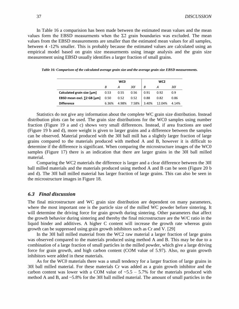
In Table 16 a comparision has been made between the estimated mean values and the mean
values form the EBSD measurments when the Σ2 grain boundaries was excluded. The mean
values from the EBSD measurements are smaller than the estimated mean values for all samples,
between 4 -12% smaller. This is probably because the estimated values are calculated using an
empirical model based on grain size measurments using image analysis and the grain size
measurement using EBSD usually identifies a larger fraction of small grains.
Table 16: Comparison of the calculated average grain size and the average grain size EBSD measurements.
WC0 WC2
B A 30l B A 30l
Calculated grain size [μm] 0.53 0.55 0.56 0.91 0.92 0.9
EBSD mean excl. ∑2 GB [μm] 0.50 0.52 0.52 0.88 0.82 0.86
Difference 6.36% 4.98% 7.58% 3.40% 12.04% 4.14%
Statistics do not give any information about the complete WC grain size distribution. Instead
distribution plots can be used. The grain size distributions for the WC0 samples using number
fraction (Figure 19 a and c) shows very small differences. Instead, if area fractions are used
(Figure 19 b and d), more weight is given to larger grains and a difference between the samples
can be observed. Material produced with the 30l ball mill has a slightly larger fraction of large
grains compared to the materials produced with method A and B, however it is difficult to
determine if the difference is significant. When comparing the microstructure images of the WC0
samples (Figure 17) there is an indication that there are larger grains in the 30l ball milled
material.
Comparing the WC2 materials the difference is larger and a clear difference between the 30l
ball milled materials and the materials produced using method A and B can be seen (Figure 20 b
and d). The 30l ball milled material has larger fraction of large grains. This can also be seen in
the microstructure images in Figure 18.
6.3 Final discussion
The final microstructure and WC grain size distribution are dependent on many parameters,
where the most important one is the particle size of the milled WC powder before sintering. It
will determine the driving force for grain growth during sintering. Other parameters that affect
the growth behavior during sintering and thereby the final microstructure are the W/C ratio in the
liquid binder and additives. A higher C content will increase the growth rate whereas grain
growth can be suppressed using grain growth inhibitors such as Cr and V. [29]
In the 30l ball milled material from the WC2 raw material a larger fraction of large grains
was observed compared to the materials produced using method A and B. This may be due to a
combination of a large fraction of small particles in the milled powder, which give a large driving
force for grain growth, and high carbon content (COM value of 5.97). Also, no grain growth
inhibitors were added in these materials.
As for the WC0 materials there was a small tendency for a larger fraction of large grains in
30l ball milled material. For these materials Cr was added as a grain growth inhibitor and the
carbon content was lower with a COM value of ~5.5 – 5.7% for the materials produced with
method A and B, and ~5.8% for the 30l ball milled material. The amount of small particles in the

38 DISCUSSION
WC0 milled powders was also smaller compared to the WC2 milled powders. This may have
resulted in less grain growth during sintering and thereby a more equal grain size distribution.
The tendency of a larger fraction of large grains in 30l ball milled material can be explained by
slightly higher carbon content and a slightly larger fraction of small particles in the milled
powder. The difference between the milling methods was found to be small and materials with
similar properties could be produced using both the traditional ball mill method and method A
and B.

39 CONCLUSION
7 CONCLUSION
The WC2 raw material milled in the 30l ball mill showed a larger fraction of small
particles compared to the materials produced using method A and B. The difference is
smaller when milling the WC0 raw material.
From the EBSD measurements the amount of indexed binder phases is lower than the
theoretical value but this will not affect the measured WC grain size.
The mean values from the EBSD measurements are 4-12% smaller than the estimated
mean values using the empirical model.
Excluding the Σ2 grain boundaries will increase the mean and standard deviation and
parallell shift the cumulative grain size distributions towards larger grains.
The WC2 sample produced with the 30l ball mill show a larger fraction of large grains
compared to materials produced with method A and B.
The WC0 sample produced with the 30l ball mill show some tendancy of a larger fraction
of large grains compared to the materials produced with method A and B. It is difficult to
determine if the difference is significant.
No significant differences in the milled powder or sintered structure could be seen
between method A and B.
By comparing the materials, using the quantitative method developed in chapter 3, some
differences between the materials could sucessfully be identified. The differences could
also be seen in the microstructure images. However the differences were small and
materials with similar grain size distribution and mechanical properties could be produced
using both the traditional ball mill method and method A and B.

40 SUGGESTIONS FOR FUTURE WORK
8 SUGGESTIONS FOR FUTURE WORK
The method used in this work has only been evaluated for grain sizes down to
approximately 0.5 μm in average grain diameter. It would be interesting to use the same
parameters for finer grade materials and investigate if the accuracy is enough and if the
same settings can be used.
The method has been optimized to measure WC grain sizes in WC-Co materials. Further
optimizations can be made to adapt the method for measurements of materials with γ-
phase. This will be more challenging since it can be difficult for the indexing software to
differentiate between Co(FCC) phase and other cubic carbide phases.
Even though the EBSD measurement is fast, sample preparation takes a significant
amount of time. An investigation of alternative sample preparation methods should be
made.

41 ACKNOWLEDGEMENTS
ACKNOWLEDGEMENTS
First of all I would like to give a special thanks to my supervisors Ernesto Coronel and Carl-
Johan Maderud at Sandvik Machining Solutions for all the help, guidance and support along the
way and for providing me with this opportunity. Without you this would not have been possible.
I would also like to thank Svend Fjordvald for help with the sample preparation and questions
regarding the SEM, Christer Fahlgren and Anders Nordgren for inputs and discussions regarding
grain size measurements, Anders Stenberg and Katalina Holmqvist for the help and questions
regarding milling processes and particle size measurements.
I am also thankful to my supervisor at KTH, Prof. John Ågren.
Finally I am very grateful to all the nice people that I have met along the way for their support,
nice lunches and coffee breaks.
42 REFERENCES
REFERENCES
[1] T. Maitland och S. Sitzman, ”Electron Backscatter Diffraction (EBSD) Technique and
Materials Characterization Examples,” i Scanning Microscopy for Nanotechnology,
Springer, 2007, pp. 41-75.
[2] N. C. Krieger Lassen, ”Automated Determination of Crystal Orientations from Electron
Backscattering Patterns,” Technical University of Denmark, Lyngby, 1994.
[3] R. A. Schwarzer, D. P. Field, B. L. Adams, A. Kumar och A. J. Schwartz, ”Present State of
Backscatter Diffraction and Prospective Developments,” i Electron Backscatter Diffraction
in Material Science 2nd Ed., Springer, 2009, pp. 1-19.
[4] F. J. Humphreys, ”Reconstruction of grains and subgrains from electron backscatter
diffraction maps,” Journal of Microscopy, vol. 213, nr 3, pp. 247-256, 2004.
[5] F. J. Humphreys, ”Quantitative metallography by electron backscattered diffraction,”
Journal of Microscopy, vol. 195, nr 3, pp. 170-185, 1999.
[6] F. J. Humphreys, ”Characterisation of fine-scale microstructures by electron backscatter
diffraction (EBSD),” Scripta Materialia, vol. 51, pp. 771-776, 2004.
[7] F. J. Humphreys, Y. Huang, I. Brough och C. Harris, ”Electron backscatter diffraction of
grain and subgrain structures - resolution consideration,” Journal of Microscopy, vol. 195, nr
3, pp. 212-216, 1999.
[8] Y. Chen, J. Hjelen, S. S. Gireesh och H. J. Roven, ”Optimization of EBSD parameters for
ultra-fast characterization,” Journal of Microscopy, vol. 245, nr 2, pp. 111-118, 2012.
[9] I. Brough och F. J. Humphreys, ”Evalution and application of a fast EBSD detector,”
Material Science and Technology, vol. 26, nr 6, pp. 636-639, 2010.
[10] F. J. Humphreys, ”Review - Grain and subgrain characterisation by electron backscatter
diffraction,” Journal of Material Science, vol. 36, pp. 3833-3854, 2001.
[11] D. R. Steinmetz och S. Zaefferer, ”Towards ultrahigh resolution EBSD by low accelerating
voltage,” Material Science and Technology, vol. 26, nr 6, pp. 640-645, 2010.
[12] R. A. Schwarzer och J. Hjelen, ”Orientation microscopy with fast EBSD,” Material Science
and Technology, vol. 26, nr 6, pp. 646-649, 2010.
[13] ISO:24173, ”Microbeam analysis - Guidelines for orientation measurement using electron
backscatter diffraction,” 2009.
[14] ISO:4499-2, ”Hard metals - Metallographic determination of microstructure - Part 2:
Measurement of WC grain size,” 2008.
[15] ASTM:E1382-97, ”Standard Test Methods for Determining Average Grain Size Using
Semiautomatic and Automatic Image Analysis,” 2010.
[16] K. Mannesson, ”Best practice methods for grain sisze measurements of cemented carbides
(M.Sc),” KTH, Stockholm, 2004.
[17] ASTM:E2627-10, ”Standard Practice for Determining Average Grain Size Using Electron
Backscatter Diffraction (EBSD) in Fully Recrystallized Polycrystalline Materials,” 2010.
[18] ISO:13067, ”Microbeam analysis - Electron backscatter diffraction - Measurement of
average grain size,” 2011.
[19] K. Mannesson, M. Elfwing, A. Kusoffsky, S. Nordgren och J. Ågren, ”Analysis of WC grain
43 REFERENCES
growth during sintering using electron backscatter diffraction and image analysis,”
International Journal of Refractory Metals & Hard Materials, vol. 26, pp. 449-455, 2008.
[20] K. Mannesson, I. Borgh, A. Borgenstam och J. Ågren, ”Abnormal grain growth in cemented
carbides - Experiments and simulations,” International Journal of Refractory Metals & Hard
Meterials, vol. 29, pp. 488-494, 2011.
[21] J. Weidow, J. Zackrisson, B. Jansson och H.-O. Andrén, ”Characterisation of WC-Co with
cubic carbide additions,” International Journal of Refractory Metals and Hard Materials,
vol. 27, pp. 244-248, 2009.
[22] J. Weidow, S. Norgren och H.-O. Andrén, ”Effect of V, Cr and Mn additions on the
microstructure of WC-Co,” International Journal of Refractory Metals and Hard Materials,
vol. 27, pp. 817-822, 2009.
[23] K. P. Mingard, B. Roebuck, E. G. Bennett, M. Thomas, B. P. Wynne och E. J. Palmiere,
”Grain size measurmen by EBSD in complex hot deformed metal alloy microstructures,”
Journal of Microscopy, vol. 227, nr 3, pp. 298-308, 2007.
[24] K. P. Mingard, B. Roebuck, E. G. Bennet, M. G. Gee, H. Nordenstrom, G. Sweetman och P.
Chan, ”Comparision of EBSD and conventional methods of grain size measurement of
hardmetals,” International Journal of Refractory & Hard Materials, vol. 27, pp. 213-223,
2009.
[25] D. W. Scott, ”On Optimal and Data-Based Histograms,” Biometrika, vol. 66, nr 3, pp. 605-
610, 1979.
[26] J. Jeppsson, K. Mannesson, A. Borgenstam och J. Ågren, ”Inverse Saltykov analysis for
particle-size distributions and their time evolution,” Acta Materialia, vol. 59, pp. 874-882,
2011.
[27] B. Roebuck, N. J. McCormick, A. Day och E. G. Bennett, ”Measurment of WC Grain Size
Distribution,” NPL, 1999.
[28] B. Roebuck, ”Magnetic Coercivity Measurements for WC/Co Hardmetals,” NPL, 1999.
[29] C. H. Allibert, ”Sintering features on cemented carbides WC-Co processed from fine
powders,” International Journal of Refractory Metals and Hard Materials, vol. 19, pp. 53-
61, 2001.
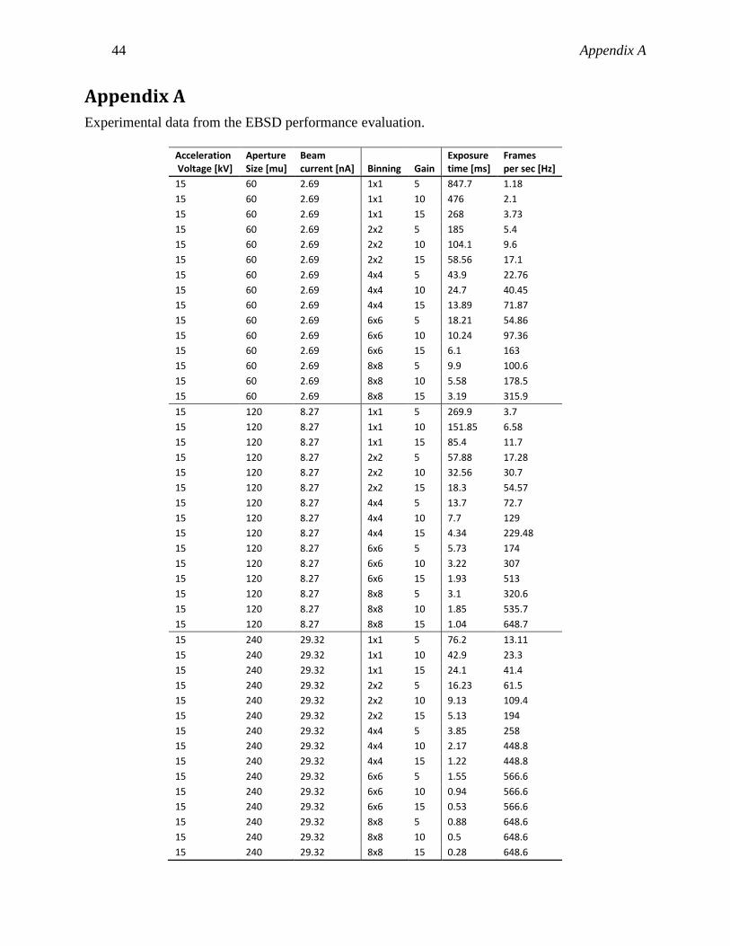
44 Appendix A
Appendix A
Experimental data from the EBSD performance evaluation.
Acceleration Voltage [kV]
Aperture Size [mu]
Beam current [nA] Binning Gain
Exposure time [ms]
Frames per sec [Hz]
15 60 2.69 1x1 5 847.7 1.18
15 60 2.69 1x1 10 476 2.1
15 60 2.69 1x1 15 268 3.73
15 60 2.69 2x2 5 185 5.4
15 60 2.69 2x2 10 104.1 9.6
15 60 2.69 2x2 15 58.56 17.1
15 60 2.69 4x4 5 43.9 22.76
15 60 2.69 4x4 10 24.7 40.45
15 60 2.69 4x4 15 13.89 71.87
15 60 2.69 6x6 5 18.21 54.86
15 60 2.69 6x6 10 10.24 97.36
15 60 2.69 6x6 15 6.1 163
15 60 2.69 8x8 5 9.9 100.6
15 60 2.69 8x8 10 5.58 178.5
15 60 2.69 8x8 15 3.19 315.9
15 120 8.27 1x1 5 269.9 3.7
15 120 8.27 1x1 10 151.85 6.58
15 120 8.27 1x1 15 85.4 11.7
15 120 8.27 2x2 5 57.88 17.28
15 120 8.27 2x2 10 32.56 30.7
15 120 8.27 2x2 15 18.3 54.57
15 120 8.27 4x4 5 13.7 72.7
15 120 8.27 4x4 10 7.7 129
15 120 8.27 4x4 15 4.34 229.48
15 120 8.27 6x6 5 5.73 174
15 120 8.27 6x6 10 3.22 307
15 120 8.27 6x6 15 1.93 513
15 120 8.27 8x8 5 3.1 320.6
15 120 8.27 8x8 10 1.85 535.7
15 120 8.27 8x8 15 1.04 648.7
15 240 29.32 1x1 5 76.2 13.11
15 240 29.32 1x1 10 42.9 23.3
15 240 29.32 1x1 15 24.1 41.4
15 240 29.32 2x2 5 16.23 61.5
15 240 29.32 2x2 10 9.13 109.4
15 240 29.32 2x2 15 5.13 194
15 240 29.32 4x4 5 3.85 258
15 240 29.32 4x4 10 2.17 448.8
15 240 29.32 4x4 15 1.22 448.8
15 240 29.32 6x6 5 1.55 566.6
15 240 29.32 6x6 10 0.94 566.6
15 240 29.32 6x6 15 0.53 566.6
15 240 29.32 8x8 5 0.88 648.6
15 240 29.32 8x8 10 0.5 648.6
15 240 29.32 8x8 15 0.28 648.6
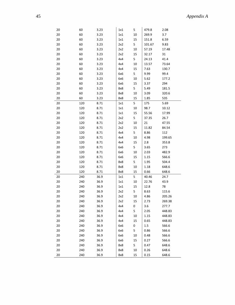
45 Appendix A
20 60 3.23 1x1 5 479.8 2.08
20 60 3.23 1x1 10 269.9 3.7
20 60 3.23 1x1 15 151.8 6.59
20 60 3.23 2x2 5 101.67 9.83
20 60 3.23 2x2 10 57.19 17.48
20 60 3.23 2x2 15 32.17 31
20 60 3.23 4x4 5 24.13 41.4
20 60 3.23 4x4 10 13.57 73.64
20 60 3.23 4x4 15 7.63 130.7
20 60 3.23 6x6 5 9.99 99.4
20 60 3.23 6x6 10 5.62 177.2
20 60 3.23 6x6 15 3.37 294
20 60 3.23 8x8 5 5.49 181.5
20 60 3.23 8x8 10 3.09 320.6
20 60 3.23 8x8 15 1.85 535
20 120 8.71 1x1 5 175 5.69
20 120 8.71 1x1 10 98.7 10.12
20 120 8.71 1x1 15 55.56 17.99
20 120 8.71 2x2 5 37.35 26.7
20 120 8.71 2x2 10 21 47.55
20 120 8.71 2x2 15 11.82 84.54
20 120 8.71 4x4 5 8.86 112
20 120 8.71 4x4 10 4.98 199.65
20 120 8.71 4x4 15 2.8 353.8
20 120 8.71 6x6 5 3.65 273
20 120 8.71 6x6 10 2.03 482.9
20 120 8.71 6x6 15 1.15 566.6
20 120 8.71 8x8 5 1.95 504.4
20 120 8.71 8x8 10 1.18 648.6
20 120 8.71 8x8 15 0.66 648.6
20 240 36.9 1x1 5 40.46 24.7
20 240 36.9 1x1 10 22.76 43.9
20 240 36.9 1x1 15 12.8 78
20 240 36.9 2x2 5 8.63 115.6
20 240 36.9 2x2 10 4.86 205.26
20 240 36.9 2x2 15 2.73 269.38
20 240 36.9 4x4 0 3.6 277.7
20 240 36.9 4x4 5 2.05 448.83
20 240 36.9 4x4 10 1.15 448.83
20 240 36.9 4x4 15 0.65 448.83
20 240 36.9 6x6 0 1.5 566.6
20 240 36.9 6x6 5 0.86 566.6
20 240 36.9 6x6 10 0.48 566.6
20 240 36.9 6x6 15 0.27 566.6
20 240 36.9 8x8 5 0.47 648.6
20 240 36.9 8x8 10 0.26 648.6
20 240 36.9 8x8 15 0.15 648.6

46 Appendix B
Appendix B
Matlab code for plotting the histograms.
%Stepping through the bin intervals %bins = upper bin limits in which the data will be grouped <= bins(i) for i = 1:length(bins) %searching for the indexes in the first bin and %calculating the sum within the bin range indexes = find(area<=bins(i)); Ni = length(indexes); Ai = sum(area(indexes)); %storing the values N = [N Ni]; A = [A Ai]; %removing the areas to the next loop area(indexes) = []; diameter(indexes) = []; end %Normalizing on the total area and number. N = N./sum(N); A = A./sum(A); %Calculating the bin centers. We don’t want to plot versus the upper binlimits %First we calculate the width of the bins. binwidths = [(bins(1)-0) bins(2:end)-bins(1:end-1)]; %then calculating the bincenters bincenters = [bins(1:end)-binwidths(1:end)./2];
N or A are then plotted versus the bincenters transformed from area to circle equivalence
diameter.

47 Appendix C
Appendix C
Statistics for the individual maps on the WC0 samples.
N Mean Median Std IQR
B
Map1 Incl. ∑2 2760 0.44 0.40 0.23 0.29
Excl. ∑2 2128 0.50 0.46 0.26 0.34
Map2 Incl. ∑2 2604 0.45 0.40 0.23 0.28
Excl. ∑2 2020 0.51 0.46 0.26 0.34
Map3 Incl. ∑2 2784 0.44 0.40 0.23 0.29
Excl. ∑2 2162 0.49 0.44 0.27 0.34
Tot Incl. ∑2 8148 0.44 0.40 0.23 0.29
Excl. ∑2 6310 0.50 0.45 0.26 0.34
A
Map1 Incl. ∑2 2057 0.49 0.44 0.26 0.31
Excl. ∑2 1576 0.55 0.50 0.30 0.38
Map2 Incl. ∑2 2492 0.45 0.41 0.24 0.29
Excl. ∑2 1915 0.51 0.46 0.27 0.36
Map3 Incl. ∑2 2500 0.45 0.41 0.24 0.31
Excl. ∑2 1951 0.51 0.47 0.26 0.35
Tot Incl. ∑2 7049 0.46 0.42 0.25 0.30
Excl. ∑2 5442 0.52 0.48 0.28 0.36
30l
Map1 Incl. ∑2 2249 0.47 0.42 0.26 0.29
Excl. ∑2 1755 0.52 0.47 0.30 0.35
Map2 Incl. ∑2 2369 0.45 0.40 0.25 0.30
Excl. ∑2 1834 0.51 0.46 0.29 0.35
Map3 Incl. ∑2 2167 0.46 0.41 0.26 0.30
Excl. ∑2 1651 0.53 0.48 0.30 0.36
Tot Incl. ∑2 6785 0.46 0.41 0.26 0.30
Excl. ∑2 5240 0.52 0.47 0.29 0.35
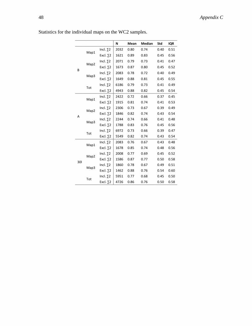
48 Appendix C
Statistics for the individual maps on the WC2 samples.
N Mean Median Std IQR
B
Map1 Incl. ∑2 2032 0.80 0.74 0.40 0.51
Excl. ∑2 1621 0.89 0.83 0.45 0.56
Map2 Incl. ∑2 2071 0.79 0.73 0.41 0.47
Excl. ∑2 1673 0.87 0.80 0.45 0.52
Map3 Incl. ∑2 2083 0.78 0.72 0.40 0.49
Excl. ∑2 1649 0.88 0.81 0.45 0.55
Tot Incl. ∑2 6186 0.79 0.73 0.41 0.49
Excl. ∑2 4943 0.88 0.82 0.45 0.54
A
Map1 Incl. ∑2 2422 0.72 0.66 0.37 0.45
Excl. ∑2 1915 0.81 0.74 0.41 0.53
Map2 Incl. ∑2 2306 0.73 0.67 0.39 0.49
Excl. ∑2 1846 0.82 0.74 0.43 0.54
Map3 Incl. ∑2 2244 0.74 0.66 0.41 0.48
Excl. ∑2 1788 0.83 0.76 0.45 0.56
Tot Incl. ∑2 6972 0.73 0.66 0.39 0.47
Excl. ∑2 5549 0.82 0.74 0.43 0.54
30l
Map1 Incl. ∑2 2083 0.76 0.67 0.43 0.48
Excl. ∑2 1678 0.85 0.74 0.48 0.56
Map2 Incl. ∑2 2008 0.77 0.69 0.45 0.52
Excl. ∑2 1586 0.87 0.77 0.50 0.58
Map3 Incl. ∑2 1860 0.78 0.67 0.49 0.51
Excl. ∑2 1462 0.88 0.76 0.54 0.60
Tot Incl. ∑2 5951 0.77 0.68 0.45 0.50
Excl. ∑2 4726 0.86 0.76 0.50 0.58
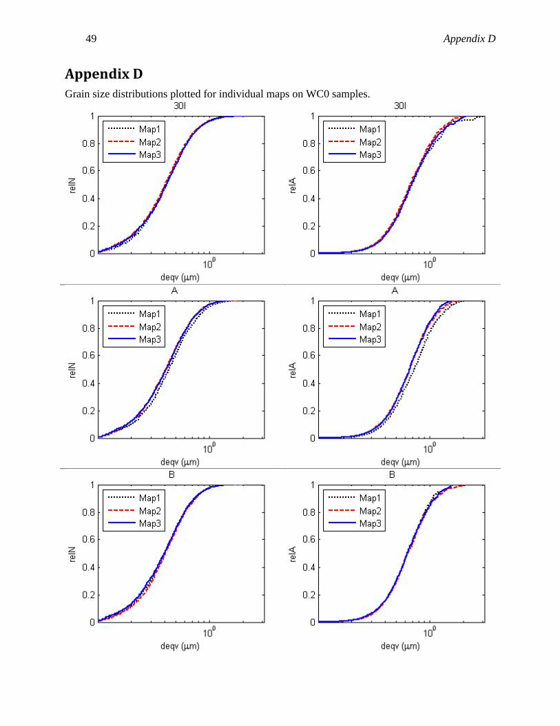
49 Appendix D
Appendix D
Grain size distributions plotted for individual maps on WC0 samples.

50 Appendix D
Grain size distributions plotted for individual maps on WC2 samples.
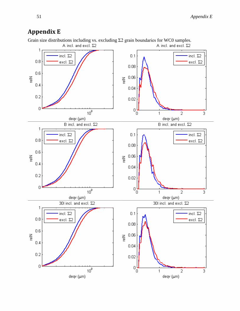
51 Appendix E
Appendix E
Grain size distributions including vs. excluding Σ2 grain boundaries for WC0 samples.
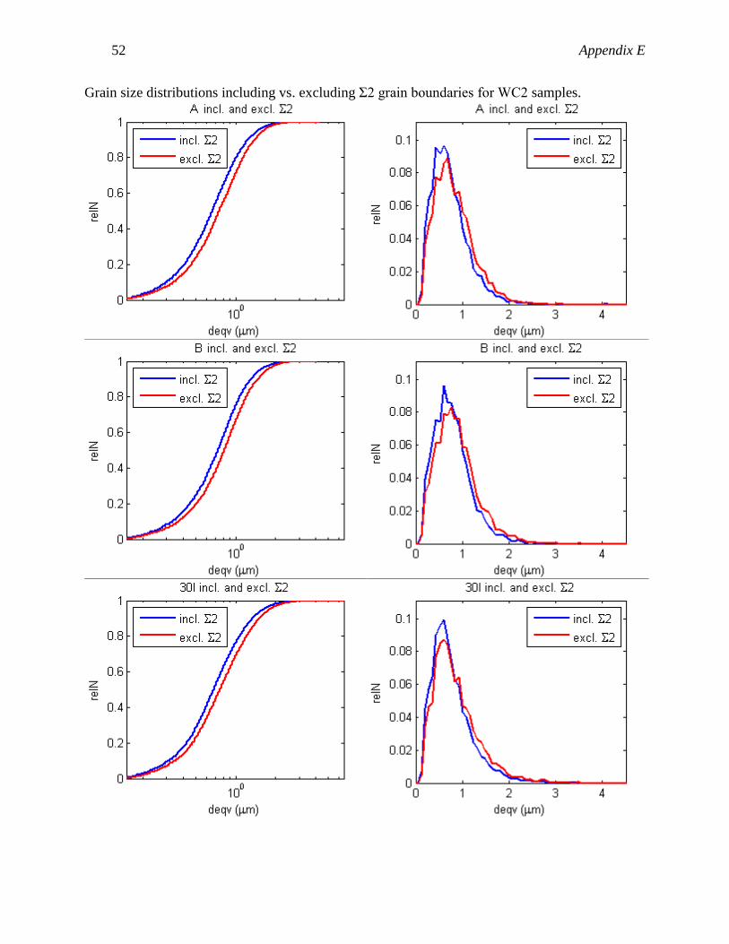
52 Appendix E
Grain size distributions including vs. excluding Σ2 grain boundaries for WC2 samples.