development of a novel invertebrate indexing tool …
TRANSCRIPT

Page i
DEVELOPMENT OF A NOVEL INVERTEBRATE INDEXING TOOL
FOR THE DETERMINATION OF SALINITY IN AQUATIC INLAND
DRAINAGE CHANNELS
Alexander G. G. Pickwell
A thesis submitted in partial fulfilment of the requirements of the University of Lincoln for
the degree of Master of Philosophy in Biology
This research programme was carried out in collaboration with the Environment Agency
August 2012

Page i
Certificate of Originality
This is to certify that I am responsible for the work submitted in this thesis, that the original
work is my own, except as specified in the acknowledgements and in references, and that
neither the thesis nor the original work contained therein has been previously submitted to
any institution for the award of a degree.
Signature:
Name: Alexander G. G. Pickwell
Date: 31st August 2012

Page ii
Abstract
Salinisation of freshwater habitats is an issue with global implications that can have serious
detrimental effects on the environment resulting in an overall loss in biodiversity. Whilst
increases in salinity can occur naturally, such anthropogenic actions as the disposal of
industrial and urban effluents and the disturbance of natural hydrological cycles can also
result in the salinisation of freshwater habitats.
The Water Framework Directive (WFD) requires Member States to restore all
freshwater habitats to “good ecological status” and to prevent any further deterioration.
Macro-invertebrates are widely used as indicators of river condition for a wide range of
reasons and have been designated a key biological element in the assessment of aquatic
habitats by the WFD. A review of the available literature, however, found no macro-
invertebrate-based biotic indices have been developed for the detection and determination
of salinity increases in freshwater habitats that are suitable for application in the United
Kingdom for the purposes of the WFD. To this end, a biotic index based on the aquatic
macro-invertebrate community response to changes in salinity, termed the Salinity
Association Group (SAG) index, was developed.
The potential of the SAG index for assessing water quality in terms of salinity in
freshwater systems was investigated using data collected from survey sites in Lincolnshire
and Norfolk, England, and the results compared to several published salinity indices. Whilst
the SAG index was found to show both geographic and seasonal dependence, as is common
among many biotic indices, the proposed metric exhibited a stronger relationship to salinity
than macro-invertebrate indices employed in Europe for the purposes of the WFD show to
their specific pressure. Furthermore, the SAG index was found to be highly selective to only
salinity concentration, was significantly related to salinity when used with less detailed
information and significantly discriminated between the salinity classes defined by the WFD.
It is also highlighted that application of the SAG index with such predictive models as the
River InVertebrate Prediction And Classification System (RIVPACS) can resolve the exhibited
geographical and seasonal dependence.

Page iii
In a comparison of the SAG index with the published indices, it was found that the
SAG index was the superior metric in terms of recognising abundance as required by the
WFD, reliably indicating changes in salinity, compatibility with sampling protocols employed
by England’s regulatory authority and producing a linear output. Consequently, it was
concluded that the SAG index surpasses other published metrics for the detection and
determination of salinity increases in freshwater habitats and is a viable biomonitoring tool
suitable for use in England for informing aquatic habitat management decisions, research
application and the purposes of the WFD. It is proposed, however, that more rigorous
sampling protocols for both macro-invertebrate and environmental data may result in more
accurate metric scores and reveal further issues or benefits associated with the SAG index
and could also be used to further refine the metric. It is also suggested that adaptation and
examination of the SAG index at a larger geographical scale would further demonstrate the
validity of the proposed metric and illustrate the potential of the SAG index for worldwide
application. Furthermore, intercalibration of the SAG index to harmonise WFD reference
conditions and class boundaries across Europe would allow the application of the SAG index
throughout Europe for the purpose of the WFD.

Page iv
Acknowledgements
The author wishes to acknowledge:
The project work, for which this thesis is a culmination, was part-funded by the Broads
Authority, a grant from the Alice McCosh Trust and a grant from the Environment Agency,
without which this project would not have proceeded. The author is immensely grateful to all
three parties. The author would also like to acknowledge the following for advice,
information or materials given:
The staff at the Spalding office of the Environment Agency, Dorothy Gennard and Ron Dixon
(University of Lincoln), Pam Taylor (British Dragonfly Society), Helen Booth and Jeremy Halls
(Halcrow Ltd), Mike Elliott (Institute of Estuarine & Coastal Studies), Clive Doarks and Rick
Southwood (Natural England), Roy Baker (Norfolk and Norwich Naturalists' Society), Nigel
Dunthorne (Rockland Wildfowlers Association), Tim Strudwick and Matt Wilkinson
(Strumpshaw Fen Nature Reserve), Charles Deeming, Paul Eady, Jamie Legge, Amanda Mylett
and Tom Pike (University of Lincoln), Joe Cullum, Derek Howlett and Chris Mutten.
The author wishes to thank:
Richard Chadd, Chris Extence and Helgi Gudmundsson (Environment Agency) for the advice,
support and assistance provided during the course of this work, Mike Dunbar (Environment
Agency) and Paul Corcoran (National Suicide Research Foundation) for statistical advice, and
the numerous members of staff at the University of Lincoln who offered their assistance and
encouragement. The author wishes to thank friends and family members for their
unrelenting support in all of my endeavours. Special mention must also be made for James
Coulter, Louise Hopkins and Rachel Farrow for their support and assistance, which were
always given without question.
The views expressed in this body of work are those of the author, and not necessarily those of
the Environment Agency.

Page v
Table of Contents
List of Figures ........................................................................................................................ ix
List of Tables ........................................................................................................................ xii
List of Plates ........................................................................................................................ xvi
List of Abbreviations and Symbols ..................................................................................... xvii
1 INTRODUCTION................................................................................................................ 1
1.1 Aims and Objectives ................................................................................................... 3
2 LITERATURE REVIEW ........................................................................................................ 4
2.1 Salinisation ................................................................................................................. 4
2.2 Measurement of Salinity ............................................................................................ 7
2.3 Classification of Surface Waters Based on Salinity ...................................................... 8
2.4 The Scale of Salinisation in Freshwater Habitats ....................................................... 10
2.5 The Impact of Salinisation on Freshwater Habitats ................................................... 11
2.6 Legislation and Water Quality .................................................................................. 13
2.6.1 The Water Framework Directive ......................................................................... 14
2.7 The Assessment of Water Quality............................................................................. 16
2.7.1 Biological Organisms Used for the Assessment of Water Quality ........................ 19
2.7.1.1 Fish ............................................................................................................... 20
2.7.1.2 Macrophytes ................................................................................................ 23
2.7.1.3 Phytoplankton and periphyton ..................................................................... 25
2.7.1.4 Macro-invertebrates ..................................................................................... 28
2.8 Approaches to Biological Monitoring........................................................................ 32
2.8.1 Functional Approach .......................................................................................... 32
2.8.2 Biotic Indices ...................................................................................................... 34
2.8.3 Multimetric Indices ............................................................................................ 36
2.8.4 Multivariate Approaches .................................................................................... 37
2.9 Salinity Indices ......................................................................................................... 38
2.9.1 Comparison of Salinity Indices ............................................................................ 45
2.10 Rationale for a New Salinity Index ............................................................................ 50
Page vi
3 DEVELOPMENT OF THE SALINITY ASSOCIATION GROUP INDEX..................................... 52
4 SURVEY SITES ................................................................................................................. 55
4.1 Study Areas: Lincolnshire ......................................................................................... 56
4.1.1 South Forty Foot Drain ....................................................................................... 57
4.1.2 South Holland Main Drain .................................................................................. 58
4.2 Study Area: Norfolk .................................................................................................. 59
4.2.1 Survey Sites of the Upper Thurne Catchment ..................................................... 60
4.2.2 Survey Sites of the River Yare Catchment ........................................................... 61
5 METHODS ...................................................................................................................... 63
5.1 Sampling Procedure ................................................................................................. 64
5.2 Environmental Data ................................................................................................. 64
5.3 Macro-invertebrate Community Samples ................................................................. 66
5.3.1 Macro-invertebrate Diversity and Water Quality Measures ................................ 67
5.4 Statistical Analysis .................................................................................................... 73
6 RESULTS ......................................................................................................................... 80
6.1 Environmental Data ................................................................................................. 81
6.1.1 Spatial and Temporal Trends in Environmental Data .......................................... 89
6.2 Macro-invertebrate Data.......................................................................................... 96
6.2.1 Spatial and Temporal Trends in Macro-invertebrate Data .................................104
6.2.2 Effect of Environmental Variables on Macro-invertebrate Fauna .......................114
6.3 Examination of the Salinity Association Group Index ...............................................119
6.3.1 The Influence of Season and Habitat on the Salinity Association Group Index ...122
6.3.2 The Discriminative Ability of the Salinity Association Group Index .....................124
6.3.3 The Selectivity of the Salinity Association Group Index ......................................126
6.3.4 The Effect of Data Resolution on the Salinity Association Group Index ..............127
6.4 Comparison of the Salinity Association Group Index to Published Salinity Indices ...130

Page vii
7 DISCUSSION ..................................................................................................................135
7.1 Differences Between Survey Sites in Lincolnshire and Survey Sites in Norfolk .........135
7.2 Differences Between Lincolnshire Water Bodies .....................................................136
7.3 Differences Between Seasons..................................................................................137
7.4 Influence of Environmental Variables on Macro-invertebrate Fauna .......................138
7.5 The Salinity Association Group Index .......................................................................140
7.5.1 Influence of Season on the Salinity Association Group Index .............................143
7.5.2 Discriminative Ability of the Salinity Association group Index ............................144
7.5.3 Effect of Data Resolution on the Salinity Association Group Index .....................145
7.5.4 Comparison of the Salinity Association Group Index to Published Salinity Indices
..........................................................................................................................147
8 CONCLUSIONS ...............................................................................................................150
8.1 The Salinity Association Group Index .......................................................................151
8.2 Comparison of the Salinity Association Group Index to Published Salinity Indices ...152
8.3 Limitations ..............................................................................................................153
9 FURTHER WORK ............................................................................................................155
10 REFERENCES ..................................................................................................................156
11 GLOSSARY OF TERMS ....................................................................................................227
12 APPENDIX .....................................................................................................................229
Appendix 1: List of Taxa Assignments to Salinity Association Groups ...............................229
Appendix 2: Justifications for Salinity Association Group (SAG) Assignment of Macro-
invertebrate Taxa ....................................................................................................243
Appendix 3: Salinity Association Group (SAG) Index Calculation Example ........................315
Appendix 4: Survey Dates for Lincolnshire and Norfolk Sites ...........................................316
Page viii
Appendix 5: Further detail for survey sites located in Lincolnshire ..................................317
South Forty Foot Drain survey sites .............................................................................317
South Holland Main Drain survey sites .........................................................................322
Appendix 6: Further detail for survey sites located in Norfolk .........................................329
Survey Sites of the Upper Thurne Catchment ..............................................................329
Survey Sites of the River Yare Catchment ....................................................................332
Appendix 7: Environmental Data Collected at Survey Sites in Lincolnshire ......................337
Appendix 8: Environmental Data Collected at Survey Sites in Norfolk .............................340
Appendix 9: Macro-invertebrate Data Collected at Survey Sites in Lincolnshire...............341
Appendix 10: Macro-invertebrate Data Collected at Survey Sites in Norfolk ....................347
Appendix 11: Results of Application of Salinity Indices to Data Collected at Survey Sites in
Lincolnshire .............................................................................................................351
Appendix 12: Results of Application of Salinity Indices to Data Collected at Survey Sites in
Norfolk ..................................................................................................................352

Page ix
List of Figures
Figure 4.1: Study locations and survey sites in Lincolnshire .................................................. 56
Figure 4.2: Diagrammatic sketch of the South Forty Foot Drain, Lincolnshire, illustrating the
sequence of the survey sites ............................................................................... 58
Figure 4.3: Diagrammatic sketch of the South Holland Main Drain, Lincolnshire, illustrating
the sequence of the survey sites ......................................................................... 58
Figure 4.4: Study locations and survey sites in Norfolk ......................................................... 60
Figure 4.5: The survey sites of the Upper Thurne catchment ................................................ 61
Figure 4.6: The survey sites of the River Yare Catchment ..................................................... 62
Figure 6.1: Matrix of scatter plots and Spearman’s rank order correlation coefficient (rs)
values ................................................................................................................. 83
Figure 6.2: Ordination plot resulting from principal component analysis of environmental
variables ............................................................................................................. 85
Figure 6.3: Temperature, dissolved oxygen, redox potential and salinity profiles of the South
Forty Foot Drain and South Holland Main Drain.................................................. 90
Figure 6.4: Phosphate and nitrate profiles of the South Forty Foot Drain and South Holland
Main Drain.......................................................................................................... 90
Figure 6.5: Temperature, phosphate, nitrate and salinity measurements collected from the
Norfolk survey sites ............................................................................................ 95
Figure 6.6: Dissolved oxygen and redox potential measurements collected from the Norfolk
survey sites. See Table 5.1 for site code definitions. ........................................... 95
Figure 6.7: Cluster analysis dendrogram of samples based on fourth-root transformed
macro-invertebrate data .................................................................................... 99
Figure 6.8: Non-metric multidimensional scaling ordination plot of samples based on fourth-
root transformed macro-invertebrate data....................................................... 100
Figure 6.9: Taxon richness, number of individuals, Margalef richness index, Shannon diversity
index, Berger-Parker dominance index, Simpson dominance index, evenness and
ASPTBMWP index profiles of the South Forty Foot Drain and South Holland Main
Drain ................................................................................................................ 105

Page x
Figure 6.10: Taxon richness, number of individuals, Margalef richness index, Shannon
diversity index, Berger-Parker dominance index, Simpson dominance index,
evenness and ASPTBMWP index results for the Norfolk survey sites.................. 111
Figure 6.11: Canonical Correspondence Analysis ordination diagram from macro-
invertebrate and environmental data collected during spring season............. 115
Figure 6.12: Canonical Correspondence Analysis ordination diagram from macro-
invertebrate and environmental data collected during summer season ......... 116
Figure 6.13: Canonical Correspondence Analysis ordination diagram from macro-
invertebrate and environmental data collected during autumn season .......... 117
Figure 6.14: Linear regression models of Salinity Association Group (SAG) index scores
calculated from spring, summer and autumn macro-invertebrate samples
collected at the survey sites in Lincolnshire and Norfolk correlated against
salinity concentration ..................................................................................... 120
Figure 6.15: Linear regression model of Salinity Association Group (SAG) index scores
calculated from macro-invertebrate samples collected at the survey sites
located in Norfolk correlated against salinity concentration ........................... 123
Figure 6.16: Box plots showing relationship between brackish water classes, defined by the
Venice System (Battaglia, 1959) and used by the Water Framework Directive
(WFD), and grouped Salinity Association Group index scores calculated all from
macro-invertebrate samples .......................................................................... 125
Figure 6.17: Salinity Association Group (SAG) index calculated using data of varying
resolution from Norfolk survey sites correlated against transformed salinity
concentration ................................................................................................. 128
Figure 6.18: Scores for the salinity index of Horrigan et al. (2005) calculated using data from
Norfolk survey sites correlated against transformed salinity concentration .... 131
Figure 6.19: Scores for the SPEARsalinity index of Schäfer et al. (2011) calculated using data
from Norfolk survey sites correlated against transformed salinity concentration
....................................................................................................................... 132
Figure 6.20: Ditch salinity index of Palmer et al. (2010) calculated using data from Norfolk
survey sites correlated against transformed salinity concentration ................ 133
Figure 12.1: The location of the SF1 (Casswell’s Bridge) survey site ................................... 317
Page xi
Figure 12.2: The location of the SF2 (Donington Bridge) survey site. ............................... 319
Figure 12.3: The Location of the SF3 (Swineshead Bridge) survey site.............................. 320
Figure 12.4: The location of the SF4 (Wyberton Chain Bridge) survey site. ...................... 322
Figure 12.5: The Location of the SH1 (Weston Fen) survey site ........................................ 323
Figure 12.6: The Location of the SH2 (Clifton’s Bridge) survey site ................................... 324
Figure 12.7: The location of the SH3 (A1101 Road Bridge) survey site. ............................ 326
Figure 12.8: The location of the SH4 (Nene Outfall Sluice) survey site. ............................ 327
Figure 12.9: The survey sites of the Upper Thurne catchment ......................................... 329
Figure 12.10: The survey sites of the River Yare Catchment ............................................... 332

Page xii
List of Tables
Table 2.1: Salinity ranges of the different zones proposed in the systems of Redeke,
Välikangas and the Venice System .......................................................................... 8
Table 2.2: Salinity ranges of the different zones proposed in the systems based on salinity
tolerances and preferences of aquatic organisms ................................................... 9
Table 2.3: Advantages and disadvantages of physico-chemical and biological assessments of
water quality ........................................................................................................ 17
Table 2.4: Summarised advantages and disadvantages of common biological organism types
used in the assessment of water quality ............................................................... 21
Table 2.5: Definitions developed by Palmer et al. (2010) to assign invertebrate taxa salinity
index scores .......................................................................................................... 42
Table 2.6: Biotic classes of the Salinity Classification System of Wolf et al. (2009) ................. 43
Table 2.7: Scoring system employed by the Salinity Classification System of Wolf et al. (2009)
............................................................................................................................. 44
Table 2.8: Advantages and disadvantages of five macro-invertebrate based salinity indices . 45
Table 2.9: Comparison of macro-invertebrate sample collection methods ............................ 47
Table 3.1: Definitions of the Salinity Association Groups ....................................................... 52
Table 3.2: Scoring matrix for determining Salinity Association Scores ................................... 54
Table 5.1: Prefixes and meanings used in sample coding system ........................................... 63
Table 5.2: Suffixes and meanings used in sample coding system ........................................... 63
Table 5.3: Scores allocated to macro-invertebrate families in the Biological Monitoring
Working Party score system .................................................................................. 72
Table 6.1: Shapiro-Wilk test results for untransformed environmental variables .................. 80
Table 6.2: Shapiro-Wilk test results for Log10(X+1) transformed environmental variables ..... 80
Table 6.3: Environmental data for the survey sites in Lincolnshire ........................................ 81
Table 6.4: Environmental data for the survey sites in Norfolk ............................................... 82
Table 6.5: Principal components, eigenvalues and percent variance explained from the
principal component analysis of environmental variables ..................................... 84
Table 6.6: Correlations of scores for component 1 and component 2 resulting from principal
component analysis with the environmental variables ......................................... 85
Page xiii
Table 6.7: Results of Mann-Whitney U tests on environmental data for differences between
spring and summer at Norfolk survey sites ......................................................... 87
Table 6.8: Results of Kruskal-Wallis tests on environmental data for differences between
spring, summer and autumn at Lincolnshire survey sites .................................... 88
Table 6.9: P-values of post-hoc pairwise Mann-Whitney U tests on water temperature,
dissolved oxygen and redox potential data for differences between spring,
summer and autumn at Lincolnshire survey sites ............................................... 88
Table 6.10: Results of Mann-Whitney U tests on environmental data for differences between
Lincolnshire survey sites and Norfolk survey sites ............................................... 89
Table 6.11: Summarised macro-invertebrate data for Lincolnshire survey sites .................... 97
Table 6.12: Summarised macro-invertebrate data for Norfolk survey sites ........................... 98
Table 6.13: Symbols and colours representing clusters in non-metric multidimensional scaling
ordination plot ................................................................................................... 99
Table 6.14: P-values of post-hoc pairwise ANOSIM tests between all pairs of clusters defined
by cluster analyses of macro-invertebrate data ................................................ 101
Table 6.15: Summary statistics of environmental variables for each cluster defined by
clustering analyses............................................................................................ 101
Table 6.16: Samples associated with each cluster defined by clustering analyses ............... 102
Table 6.17: Spearman’s rank order correlation coefficient (rs) and p-values resulting from
tests between macro-invertebrate diversity and water quality indices for data
collected at survey sites in Lincolnshire ............................................................ 106
Table 6.18: Results of Kruskal-Wallis and Mann-Whitney U tests on macro-invertebrate
diversity and water quality measures from Lincolnshire survey sites for
differences between seasons and the Lincolnshire water bodies ...................... 110
Table 6.19: Spearman’s rank order correlation coefficient (rs) and p-values resulting from
tests between macro-invertebrate diversity and water quality indices for data
collected at survey sites in Norfolk ................................................................... 112
Table 6.20: Results of Mann-Whitney U tests on macro-invertebrate diversity and water
quality measures from Norfolk survey sites for differences between seasons... 114
Table 6.21: Eigenvalues and variation of the taxon-environmental structure explained for the
derived axes of Canonical Correspondence Analysis ordination plots ............... 116
Page xiv
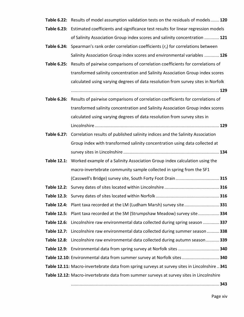
Table 6.22: Results of model assumption validation tests on the residuals of models ....... 120
Table 6.23: Estimated coefficients and significance test results for linear regression models
of Salinity Association Group index scores and salinity concentration ............ 121
Table 6.24: Spearman’s rank order correlation coefficients (rs) for correlations between
Salinity Association Group index scores and environmental variables ............ 126
Table 6.25: Results of pairwise comparisons of correlation coefficients for correlations of
transformed salinity concentration and Salinity Association Group index scores
calculated using varying degrees of data resolution from survey sites in Norfolk
....................................................................................................................... 129
Table 6.26: Results of pairwise comparisons of correlation coefficients for correlations of
transformed salinity concentration and Salinity Association Group index scores
calculated using varying degrees of data resolution from survey sites in
Lincolnshire .................................................................................................... 129
Table 6.27: Correlation results of published salinity indices and the Salinity Association
Group index with transformed salinity concentration using data collected at
survey sites in Lincolnshire ............................................................................. 134
Table 12.1: Worked example of a Salinity Association Group index calculation using the
macro-invertebrate community sample collected in spring from the SF1
(Casswell's Bridge) survey site, South Forty Foot Drain ................................... 315
Table 12.2: Survey dates of sites located within Lincolnshire ............................................ 316
Table 12.3: Survey dates of sites located within Norfolk ................................................... 316
Table 12.4: Plant taxa recorded at the LM (Ludham Marsh) survey site ............................ 331
Table 12.5: Plant taxa recorded at the SM (Strumpshaw Meadow) survey site ................. 334
Table 12.6: Lincolnshire raw environmental data collected during spring season ............. 337
Table 12.7: Lincolnshire raw environmental data collected during summer season .......... 338
Table 12.8: Lincolnshire raw environmental data collected during autumn season........... 339
Table 12.9: Environmental data from spring survey at Norfolk sites ................................. 340
Table 12.10: Environmental data from summer survey at Norfolk sites .............................. 340
Table 12.11: Macro-invertebrate data from spring surveys at survey sites in Lincolnshire .. 341
Table 12.12: Macro-invertebrate data from summer surveys at survey sites in Lincolnshire
....................................................................................................................... 343

Page xv
Table 12.13: Macro-invertebrate data from autumn surveys at survey sites in Lincolnshire
....................................................................................................................... 345
Table 12.14: Macro-invertebrate data from spring surveys at survey sites in Norfolk ......... 347
Table 12.15: Macro-invertebrate data from summer surveys at survey sites in Norfolk ...... 349
Table 12.16: Results following application of the Salinity Association Group Index, the salinity
index of Horrigan et al. (2005), the ditch salinity index of Palmer et al. (2010)
and SPEARsalinity (Schäfer et al., 2011) to Lincolnshire data .............................. 351
Table 12.17: Results following application of the Salinity Association Group Index, the salinity
index of Horrigan et al. (2005), the ditch salinity index of Palmer et al. (2010)
and SPEARsalinity (Schäfer et al., 2011) to Norfolk data ..................................... 352

Page xvi
List of Plates
Plate 12.1: The SF1 (Casswell’s Bridge) survey site ........................................................... 318
Plate 12.2: The SF2 (Donington Bridge) survey site .......................................................... 319
Plate 12.3: The SF3 (Swineshead Bridge) survey site ........................................................ 321
Plate 12.4: The SF4 (Wyberton Chain Bridge) survey site ................................................. 321
Plate 12.5: The SH1 (Weston Fen) survey site .................................................................. 323
Plate 12.6: The SH2 (Clifton’s Bridge) survey site ............................................................. 325
Plate 12.7: The SH3 (A1101 Road Bridge) survey site ....................................................... 326
Plate 12.8: The SH4 (Nene Outfall Sluice) survey site ....................................................... 328
Plate 12.9: The LD (Long Dyke) survey site ....................................................................... 330
Plate 12.10: The MM (Middle Marsh) survey site ............................................................... 330
Plate 12.11: The LM (Ludham Marsh) survey site ............................................................... 331
Plate 12.12: The SM (Strumpshaw Meadow) survey site .................................................... 333
Plate 12.13: The BM (Buckenham Marsh) survey site......................................................... 333
Plate 12.14: The RM (Rockland Marsh) survey site ............................................................. 334
Plate 12.15: The ND (Near Dry Dyke) survey site ................................................................ 335
Plate 12.16: The HM (Hatchet Marsh) survey site .............................................................. 336

Page xvii
List of Abbreviations and Symbols
1-D: Simpson’s dominance index
ANCOVA: ANalysis of COVAriance
ANNA: Assessment by Nearest Neighbor Analysis
ANOSIM: ANalysis Of SIMilarity
ANOVA: ANalysis Of VAriance
ASPTBMWP: Average Score Per Taxon derivation of the BMWP scoring system
AUSRIVAS: AUStralian RIVer Assessment Scheme
B: Berger-Parker dominance index
BEAST: BEnthic Assessment SedimenT
BMWP: Biological Monitoring Working Party
CC: Cophenetic correlation coefficients
CCA: Canonical Correspondence Analysis
CEN: European Committee for Standardisation
df: degrees of freedom
DMg: Margalef's richness index
E: Buzas & Gibson’s Evenness
EC: Electrical Conductivity
EPT: Ephemeroptera, Plecoptera and Trichoptera index
H: Kruskal-Wallis statistic
Hi: Shannon diversity index
IBI: Index of Biotic Integrity
ISO: International Organization for Standardization
LIFE: Lotic-invertebrate Index for Flow Evaluation
LOWESS: LOcally WEighted Scatterplot Smoothing
MEDPACS: MEDiterranean Prediction And Classification System
NMDS: Non-metric MultiDimensional Scaling
NO3: nitrate
NPMANOVA: Non-parametric Permutational Multivariate ANalysis Of VAriance
NTAXABMWP: Number of scoring taxa derivation of the BMWP scoring system
OSGR: Ordnance Survey Grid Reference

Page xviii
p: significance level
PAST: PAleontological STatistics software package
PCA: Principal Component Analysis
Pers. comm.: Personal communication
PO4: phosphate
PSU: Practical Salinity Units
RICT: River Invertebrate Classification Tool
RIVPACS: River InVertebrate Prediction And Classification System
r: Pearson product-moment correlation coefficient
rs: Spearman’s rank order correlation coefficient
SAG: Salinity Association Group
SAG.FA: SAG scores calculated using family level identification and abundance data
SAG.FnA: SAG scores calculated using family level identification and presence/absence data
SAG.MA: SAG scores calculated using mixed level identification and abundance data
SAG.MnA: SAG scores calculated using mixed level identification and presence/absence data
SAS: Salinity Association Score
SF: South Forty Foot Drain
SH: South Holland Main Drain
SIGNAL: Stream Invertebrate Grade Number – Average Level index
SPEARsalinity: SPEcies At Risk salinity index
SSS: Salinity Sensitivity Score
SWEPAC: SWEdish invertebrate Prediction and Classification predictive model
U: Mann-Whitney statistic
UKTAG: United Kingdom Technical Advisory Group
WFD: Water Framework Directive
Σ: the sum of
σ: standard deviation of a population
σ2: variance of a population
μ: mean of a population
z: standardised score of value x

Page 1
1 INTRODUCTION
Water is widely regarded as the world’s most essential natural resource (Vörösmarty et al.,
2010), providing a vital resource for humans and a unique habitat for a richly diverse,
sensitive and endemic collection of flora and fauna (Strayer & Dudgeon, 2010). Humans have
made use of fresh waters for a variety of reasons, such as fishing, irrigation, transportation,
farming of aquatic plants and animals, industrial purposes and power production (Strayer &
Dudgeon, 2010). In addition to the direct economic value of freshwater uses for humans, the
ecosystem services provided by the freshwater environment beneficial to human populations
have been conservatively estimated to have a global value greater than US$1.7 trillion per
year (Costanza et al., 1997). Fresh water, however, accounts for only 0.01% of the water in
the world covering approximately 0.8% of the world’s surface (Dudgeon et al., 2006) and is
facing a multitude of pressures (Carpenter et al., 2011).
The salinisation of freshwater habitats has reportedly affected an area of 950 million
hectares (Hart et al., 1990) and is considered to be is an issue with global implications
(Williams, 2001). Whilst the arid and semi-arid regions of the world are the areas most
commonly affected by increases in salinity (Williams, 1987, 1999, 2001; Brock et al., 2005),
temperate regions are also experiencing salinisation (Williams, 1987, 1999, 2001; Ghassemi
et al., 1995). Increases in salinity beyond a threshold level will result in the loss of a
freshwater supply for domestic, agricultural and industrial purposes (Williams, 1999)
incurring substantial economic costs (Williams, 1987, 1999, 2001) and, in the most severe
circumstances, affect human health (Williams, 1999, 2001). Furthermore salinisation of
freshwater habitats can have serious detrimental effects on the environment as salt sensitive
taxa are replaced by salt tolerant taxa resulting in an overall loss in biodiversity (Williams,
1999, 2001; Hart et al., 2003; James et al., 2003; Nielsen et al., 2003), which itself can result
in the loss of aquatic organisms for food and such recreational activities as fishing and eco-
tourism (Costanza et al., 1997).
In some cases natural processes have increased salinity concentrations in inland
waters, such as in terminal lakes where salts in the water basin collect and concentrate (Hart
et al., 1990; Williams, 1999). Furthermore, some rivers and streams have naturally high
salinities (Metzeling, 1993; Gallardo-Mayenco, 1994; Velasco et al., 2006; Dunlop et al.,
2008).

Page 2
The salinity of freshwater habitats, however, can also be increased as a result of the actions
of man such as the disposal of oilfield wastewater (Short et al., 1991), industrial and urban
effluents (Williams, 1987, 2001; Piscart et al., 2005a), mine waters (Kowalik & Obarska-
Pempkowiak, 1997; Echols et al., 2009; Wolf et al., 2009) and the application and subsequent
washing of road salts into nearby freshwater habitats (Williams et al., 1999; Blasius &
Merritt, 2002; Kaushal et al., 2005). The largest contribution to the salinisation of inland
waters, however, results from such disturbance of natural hydrological cycles as the
abstraction (Goetsch & Palmer, 1997) and diversion of water (Williams & Aladin, 1991;
Williams, 1999, 2001), and the agricultural practices of replacing deep rooted native
vegetation with shallow rooted crops and irrigation (Pillsbury, 1981; Hart et al., 1990;
Williams, 1999; Kay et al., 2001; Marshall & Bailey, 2004).
The use of bio-indication is central to the implementation of the Water Framework
Directive (WFD; European Commission, 2000), which was developed to safeguard and
improve the condition of the water bodies in Europe (Kallis & Butler, 2001; Blanchet et al.,
2008). Member States of the European Union are required by the WFD to classify the
ecological status of freshwater habitats on a scale from high to bad based on the biological
communities present (European Commission, 2000; UKTAG, 2007). Member States are then
required to restore all habitats to “good ecological status”, defined as where the biological
communities only slightly deviate from that which would be present in undisturbed
conditions (European Commission, 2000; UKTAG, 2007; Moss, 2008), and to prevent the
deterioration of those waters already classified as in good status (European Commission,
2000; Kallis & Butler, 2001; Griffiths, 2002; UKTAG, 2007). Furthermore, the Water
Framework Directive requires salinity, as well as a number of other environmental
parameters such as acidification and selected pollutants, to be monitored in freshwater
habitats as a supporting element of the biological data (European Commission, 2000).
Macro-invertebrates are favoured for use in bio-indication and many indices have
been developed based on macro-invertebrate community responses to a wide range of
environmental stressors (e.g. Chesters, 1980; Lenat, 1988; Extence et al., 1999; Williams et
al., 1999; Alvarez et al., 2001; Chadd & Extence, 2004; Davy-Bowker, 2005; Horrigan et al.,
2005; Palmer et al., 2010; Extence et al., 2011; Schäfer et al., 2011).

Page 3
Despite this, the potential environmental and economic impacts resulting from salinisation
and the legislative requirement, to date only the biotic index by Palmer et al. (2010) has been
developed for the assessment of salinity in freshwater habitats in the United Kingdom. The
index proposed by Palmer et al. (2010), however, was designed specifically for use in coastal
grazing marsh drainage channels and does not make use of abundance data, which is a
requirement of the Water Framework Directive in the biological assessment of European
water bodies (European Commission, 2000).
1.1 Aims and Objectives
The aim of this work is to develop and test an index to assess water quality in terms of
salinity pollution in freshwater systems. The following hypotheses are proposed for
examination to meet this aim:
i. A biotic index can be developed to detect and quantify the impact of salinity in
freshwater habitats.
ii. The proposed index will have a significant relationship with, and high selectivity to,
salinity concentration.
The objectives of this study are to:
i. Assess the need and requirements for an index assessing water quality in terms of
salinity in freshwater systems.
ii. Develop a new index to be compliant with the requirements of the Water Framework
Directive and compatible with the sampling protocol of the regulatory authority.
iii. Investigate the influence exerted by salinity and other environmental features on the
aquatic biota.
iv. Investigate the relationship between the new salinity index and salinity
concentration, as well as the other measured environmental features.
v. Compare the new salinity index with any other relevant published salinity indices.

Page 4
2 LITERATURE REVIEW
Salinity has been defined as the concentration of salts dissolved in a solvent (Williams, 1987;
Metzeling, 1993; Goetsch & Palmer, 1997; Hart et al., 2003). Dissolved salts are a natural
component of freshwater (Pillsbury, 1981), and some inland water systems have naturally
high salinities (Dunlop et al., 2008). Salts can enter freshwater systems through a number of
routes; incorporation by way of dissolution when water flows through soils and weathers
terrestrial material such as rocks (McCaull & Crossland, 1974; Pillsbury, 1981), seawater
intrusion into rivers through tidal influence (Williams et al., 1991; Greenwood & Wood, 2003;
Wolf et al., 2009), saline groundwater seepage into surface waters (Pillsbury, 1981; Williams,
1987; Kefford, 1998a), and through precipitation. Precipitation contains a small amount of
salts originating from the ocean (Nielsen et al., 2003), whilst additional salts may also
become associated with the precipitation as it travels through the atmosphere (McCaull &
Crossland, 1974).
Salts separate into their component ions upon dissolution (McCaull & Crossland,
1974), of which the most commonly encountered in surface waters are sodium and chloride
(McCaull & Crossland, 1974; Williams, 1987; Bunn & Davies, 1992). Other major ions
contributing to salinity include calcium and sulphate (Pillsbury, 1981; Williams, 1987; Bunn &
Davies, 1992), magnesium, potassium, carbonate and bicarbonate (Goetsch & Palmer, 1997;
Nielsen et al., 2003; Kefford et al., 2004a), whilst McCaull & Crossland (1974) also identified
bromide, iodide, phosphate and nitrate as component ions of salts in surface waters.
2.1 Salinisation
The process whereby salinity increases is termed salinisation (Hart et al., 1990; Williams et
al., 1991; Horrigan et al., 2005; Velasco et al., 2006). Furthermore, Piscart et al. (2005a) and
Williams (1987) both also define salinisation as the resulting condition of surface waters and
land caused by increasing salinity levels. Two types of salinisation have been distinguished:
primary salinisation, also termed natural salinisation (Williams, 2001), and secondary
salinisation, also designated anthropogenic salinisation (Williams, 1987, 1999).

Page 5
Primary, or natural, salinisation is the increase in salinity in inland waters due to
natural factors and occurring at rates unaffected by human activities (Williams, 2001).
Primary salinisation usually occurs in closed basins where rivers, or streams, flow into a
terminal lake (Hart et al., 1990; Williams, 1999), for example the Caspian Sea in central Asia
(Williams, 1987), Pyramid Lake in Nevada, USA (Williams, 1999) and the Aral Sea in Asia
between Kazakhstan and Uzbekistan (Williams & Aladin, 1991). Some rivers and streams,
frequent in the Mediterranean basin (Gallardo-Mayenco, 1994), also have naturally high
salinities (Dunlop et al., 2008). Examples of such rivers include Deep Creek, also known as
Saltwater Creek, in Australia (Metzeling, 1993) and the Rambla Salada stream in south-east
Spain studied by Velasco et al. (2006).
The increase in salinity in inland waters resulting from human activities is termed
secondary, or anthropogenic, salinisation (Williams, 1999; Marshall & Bailey, 2004).
Secondary salinisation may result from human actions directly, such as the disposal of saline
wastewater (Short et al., 1991; Piscart et al., 2005a). Secondary salinisation may also occur
indirectly as a consequence of obvious human activities affecting natural hydrological cycles
(Williams et al., 1991; Kay et al., 2001; Hart et al., 2003), such as abstraction (Goetsch &
Palmer, 1997) and diversion of water (Williams & Aladin, 1991; Williams, 1999, 2001) for
irrigation purposes (Pillsbury, 1981; Williams, 1987) and the cultivation of non-native plants
using intensive agricultural practices (Williams, 1987, Hart et al., 1990; Williams, 1999; Kay et
al., 2001; Marshall & Bailey, 2004).
Whilst human activities causing secondary salinisation may be as innocuous as the
application of salt to road, which can enter rivers and streams and increase the salinity of
these waters (Williams et al., 1999; Blasius & Merritt, 2002; Kaushal et al., 2005), secondary
salinisation may also occur from the input of mine waste waters (Kowalik & Obarska-
Pempkowiak, 1997; Echols et al., 2009; Wolf et al., 2009) or industrial (Short et al., 1991;
Piscart et al., 2005a) and urban effluents (Williams, 1987, 2001). Addition of salt to inland
waters from industry and urban activities, however, generally tends to be of local significance
(Williams, 1987).

Page 6
Disturbance of natural hydrological cycles as a result of human actions can cause the
mobilisation of naturally accumulated salts held in groundwater (Hart et al., 1990), soil (Kay
et al., 2001) and rocks (McCaull & Crossland, 1974; Pillsbury, 1981), and it is these
disturbances which make the largest contribution to the salinisation of inland waters
(Williams, 1987). Irrigation and the removal of native deep-rooted plants are the two
activities with the greatest effect on hydrological cycles resulting in the mobilisation of
naturally held salts (Williams, 1987). Clearing deep-rooted vegetation and replacing it with
shallow rooted crops results in decreased interception of precipitation and increased
groundwater recharge (Hart et al., 1990; Williams, 1999; Kay et al., 2001), resulting in a rise
in groundwater tables, which may be naturally saline (Hart et al., 1990; Marshall & Bailey,
2004), and mobilising salts held in soil (Hart et al., 1990; Williams, 1999; Kay et al., 2001).
This process has been implicated as the cause of increased salinity in Blackwood River and
Gleneg River in Australia (Williams et al., 1991).
Evapo-transpiration by crops and natural evaporation causes irrigation water to
become more saline (Pillsbury, 1981; Williams, 1987). Irrigation water may further increase
in salinity by leaching salts (McCaull & Crossland, 1974; Kay et al., 2001) as it filters through
the soil, eventually reaching groundwater or a nearby surface water body (Pillsbury, 1981;
Williams, 1987).
Abstraction of water also leads to salinity increases in inland waters as a result of
concentrating water-held salts (Goetsch & Palmer, 1997). Increases in the salinity of lakes
can result from the diversion of inflowing water. Lake volumes decrease as water is lost
through evaporation and not replaced as inflowing water has been diverted, whilst the salt
mass contained within the lake remains the same (Williams, 1999, 2001). As a consequence
of the decrease in water volume, the salinity of the lake increases as the salts concentrate
(Pillsbury, 1981; Goetsch & Palmer, 1997; Williams, 1999, 2001).
Despite the distinction between the two, salinisation cannot always be specifically
classified as either primary or secondary. For example, salinity in near coastal inland waters
elevated by tidal intrusion (e.g. Williams et al., 1991; Greenwood & Wood, 2003; Wolf et al.,
2009) may be classed as primary salinisation.

Page 7
Global warming causing sea levels to rise (Short & Neckles, 1999; Edwards & Winn, 2006)
will, however, result in increased seawater intrusion into rivers and saline penetration
further upstream in the future (Short & Neckles, 1999). Decreased freshwater flow, which
results from droughts or increased abstraction of freshwater, also results in increased
seawater penetration (Attrill et al., 1996). Hence, whilst seawater intrusion may be classed as
primary salinisation, it is also influenced, at least in part, by human activities.
2.2 Measurement of Salinity
The accurate determination of salinity requires comprehensive ionic analysis (Williams, 1987;
Rice et al., 2012). This method, however, is time-consuming and consequently salinity is
frequently determined by measuring a physical property (Rice et al., 2012) such as electrical
conductivity (Hart et al., 1990; Wood & Dykes, 2002; Kefford et al., 2004a; Horrigan et al.,
2005; Kefford et al., 2007). Electrical conductivity measures the ability of a water sample to
conduct an electrical current, and as such can be defined as a measure of the concentration
of ionic material present in the sample (Goetsch & Palmer, 1997). Electrical conductivity is
easily, rapidly and accurately measured (Kefford et al., 2003, 2004b) and is utilised by the
Environment Agency (Environment Agency, 2012a) in assessing water quality. Whilst Panter
et al. (2011) stated that using conductivity has a poor relationship with salinity for
conductivities less than 1000μScm-1, Williams (1987) reported that use of electrical
conductivity to measure salinity does not result in any significant error. Furthermore, Rice et
al. (2012) state that the use of electrical conductivity to determine salinity is recommended
for precise field and laboratory work due to its high precision and sensitivity.
Quantification of total dissolved solids can also be used to determine salinity
(Metzeling, 1993; Kefford et al., 2004b; Marshall & Bailey, 2004). Total dissolved solids is the
concentration of all dissolved material in a water sample (Goetsch & Palmer, 1997). Williams
(1987) stated the concentration of total dissolved solids is not significantly different from
salinity.

Page 8
2.3 Classification of Surface Waters Based on Salinity
Mixtures of fresh water and marine water resulting in a salinity concentration between 0.3
and 35PSU (Practical Salinity Units) are termed brackish (Williams, 1987). Transitional waters,
which are brackish, occur where rivers and other surface water systems are influenced in
terms of salinity by both coastal waters and freshwater flows (European Commission, 2000).
Several systems have been proposed to describe brackish waters, such as the classification
systems of Redeke (Den Hartog, 1974), Välikangas (Den Hartog, 1974), Bulger et al. (1993)
and Christensen et al. (1997). These systems were all developed based on observations of
changes in biotic communities in relation to salinity. Table 2.1 displays the salinity ranges
that characterise the various zones of brackish water according to the systems of Redeke
(Den Hartog, 1974), Välikangas (Den Hartog, 1974) and the Venice System (Battaglia, 1959).
Table 2.1: Salinity ranges of the different zones proposed in the systems of Redeke,
Välikangas and the Venice System
Salinity range of zones (PSU)
System Freshwater Oligohaline Mesohaline Polyhaline Euhaline (or marine)
Venice System1 < 0.5 0.5 - < 5.0 5.0 - < 18.0 18.0 - < 30.0 30.0 - < 40.0
Redeke2 < 0.1 0.1 - 1.0 1.0 - 10.0A 10.0 - 17.0 > 17.0
Välikangas2 < 0.3 0.3 - 1.6 1.6 - 10.0A 10.0 - 16.5 > 16.5
References: 1 = Battaglia, 1959;
2 = Den Hartog, 1974.
PSU = Practical Salinity Units.
A Välikangas separated the mesohaline zone into two distinct zones, with the salinity range (1.6-8.0PSU)
termed α-mesohaline and the salinity range (8.0-10.0PSU) termed β-mesohaline (Den Hartog, 1974).
Redeke first proposed his system in 1922 and sub-divided brackish water on the basis of the
biotic communities present, but also stressed the figures were approximate to be refined
when new data became available (Den Hartog, 1974). In contrast, in 1933 Välikangas
proposed a classification system of brackish water based only on the planktonic communities
present (Den Hartog, 1974). The Venice System was proposed at the International
Symposium for the Classification of Brackish Waters held in Venice in 1958 (Battaglia, 1959).
This system was designed for universal application and to clearly define terms such as
oligohaline, mesohaline, polyhaline and euhaline (Battaglia, 1959; Den Hartog, 1974).

Page 9
The Venice System is essentially a modified amalgamation of the Redeke and Välikangas
systems (Battaglia, 1959), and as such has been criticised by Den Hartog (1974) for being a
compromise and having no biological basis. The Venice System has since been used in the
Water Framework Directive as a tool to describe the zones of transitional waters in terms of
salinity (European Commission, 2000).
Alternative classification systems have been developed which are based on the
statistical analysis of the salinity tolerances and preferences of organisms present in
transitional waters (Bulger et al., 1993; Christensen et al., 1997). Table 2.2 displays the
salinity ranges that characterise the various zones of brackish water according to the systems
of Bulger et al. (1993) and Christensen et al. (1997).
Table 2.2: Salinity ranges of the different zones proposed in the systems based on salinity
tolerances and preferences of aquatic organisms
Salinity range of zones (PSU)
System Component
/Biozone 1
Component
/Biozone 2
Component
/Biozone 3
Component
/Biozone 4
Component
/Biozone 5
Bulger et al. (1993) Freshwater - 4 2 - 14 11 - 18 16 - 27 24 - marine
Christensen et al. (1997) < 0.5 > 0.5 – 8 8 – 15 15 – 25 25 – 35
PSU = Practical Salinity Units.
The different salinity zones were termed components by Bulger et al. (1993) and biozones by Christensen et
al. (1997).
Bulger et al. (1993) used a multivariate analysis to generate their classification system.
Principal component analysis was applied to known salinity ranges of fish and invertebrates
found in the Chesapeake and Delaware Bays, USA, to derive the salinity zones of the
classification system. Bulger et al. (1993) termed the salinity zones of their classification
system “components”, whereas Christensen et al. (1997) used the term “biozones”.
Christensen et al. (1997) used the same technique as Bulger et al. (1993) to develop the
boundaries, but used the salinity tolerances and preferences of species commonly found in
the estuaries of the northern Gulf of Mexico to derive the salinity “biozones”.

Page 10
The differences in salinity tolerances and preferences between the species present in the
estuaries of the northern Gulf of Mexico and those present in Chesapeake Bay and Delaware
Bay (Bulger et al., 1993; Christensen et al., 1997) may be the reason for the differences in the
salinity zone boundaries of the two systems.
2.4 The Scale of Salinisation in Freshwater Habitats
Salinisation is an important global issue (Williams, 2001) that has been reported to affect an
area of 950 million hectares (Hart et al., 1990). Although the threat and impact of salinisation
is well recognised at national levels (Hassell et al., 2006), its global extent and importance is
less well recognised (Williams, 1999). Semi-arid and arid regions of the world are the areas
most commonly affected (Williams, 1987, 1999, 2001; Brock et al., 2005) and represent
almost one third of total land area, a proportion likely to increase with global climatic change
(Williams, 1999, 2001).
Water supplies in countries from Pakistan in the east to Libya in the west are afflicted
by salinisation problems (Williams, 1987), as are Ethiopian and Egyptian lakes, central Asian
rivers and some American reservoirs (Williams, 2001). Salinisation issues have been reported
in the Prairie Provinces of Canada, large areas of North America (Williams, 1987; Kaushal et
al., 2005) and in North American rivers (Pillsbury, 1981). The southern part of the African
continent experiences issues with salinisation (Williams, 1987), whilst salinisation has also
been acknowledged as a major concern in South Africa (Goetsch & Palmer, 1997),
northeastern USA (Kaushal et al., 2005) and Australia (Williams, 1987; Bunn & Davies, 1992;
James et al., 2003). An estimated 5.7 million hectares of rural land in Australia is afflicted by
raised salinities (Marshall & Bailey, 2004; Hassell et al., 2006; Dunlop et al., 2008) and
increased salinities have been widely documented in Australian rivers (Williams, 1987;
Williams et al., 1991; Williams, 2001).
The issue of salinisation, however, is not limited to the arid and semi-arid regions
(Williams, 1987). Salinisation has been reported in countries with a Mediterranean climate
(Piscart et al., 2005a), as well as in countries in temperate regions (Williams, 1999, 2001).
Salinity problems are occurring in Thailand (Williams, 1987, 1999), China and Argentina
(Ghassemi et al., 1995).

Page 11
Saline groundwaters are polluting waters in former opencast coal mines in Germany
(Williams, 2001) and extraction of salt, which has occurred since before early Roman times to
later than Victorian times (Cooper, 2002), has also caused salinisation of several Cheshire
lakes (Williams, 1999, 2001).
2.5 The Impact of Salinisation on Freshwater Habitats
Significant economic, social and environmental costs can result from the impact of
salinisation on inland aquatic ecosystems (Williams, 2001). It has been suggested that the
demise of some ancient civilisations, such as the Sumerian civilisation of the Middle East
(Williams, 1987, 2001), was a direct consequence of land and water degradation by
salinisation (Pillsbury, 1981; Williams, 1987). The most important economic and
environmental effects upon water bodies, however, concern salinity increases over only a
small part of the total salinity range of inland waters (Williams, 1987) and can result in severe
costs being incurred (e.g. Williams 1987; 2001). For example, Williams (1999) suggested an
increase in salinity beyond approximately 1PSU renders water unsuitable for domestic,
agricultural and industrial purposes.
Salts are not regarded as traditional contaminants of freshwaters such as heavy
metals, oil, organic effluent and pesticides (Hynes, 1960). When present in excess, however,
salts can have adverse effects on aquatic biota (Hart et al., 1990). Salinisation impacts on
aquatic systems through direct toxic effects and through habitat loss in the water, riparian
zones and adjacent floodplains (James et al., 2003; Horrigan et al., 2005). Small increases in
salinity can be significant in fresh waters since the salinity tolerance of the freshwater biota is
much lower than that of saltwater biota (Williams, 2001). Biota unable to tolerate an
increase in salinity either perish, or disperse to re-colonise if salinity levels drop to a
favourable concentration (Hart et al., 2003; James et al., 2003; Nielsen et al., 2003). Even
small increases in salinity will result in the loss of sensitive species (James et al., 2003) and
can lead to the gain of salt tolerant biota (Nielsen et al., 2003). Examples of halo-sensitive
species loss and halo-tolerant species gain resulting from increasing salinity are provided by
Williams (1987), who reported that the brackish mussel Fluviolanatus subtortus (Dunker,
1857) replaced the freshwater mussel Westralunio carteri (Iredale, 1944) in the Avon river,
Western Australia.

Page 12
Williams (1987) also recorded halo-sensitive diatom taxa being replaced by a halo-tolerant
but less diverse group of diatom taxa in both the Fish River and the Sundays River in South
Africa.
The replacement of the halo-sensitive biota with halo-tolerant biota, along with a
decrease in biodiversity, is the general biological response to increased salinity (Williams,
1999, 2001; Hart et al., 2003; James et al., 2003; Nielsen et al., 2003). The addition and loss
of taxa can further affect biota as the taxa removed or gained due to a salinity increase may
modify refuge and food availability as well as predation pressure (Nielsen et al., 2003).
Furthermore, the addition or loss of taxa is likely to affect the flow of energy and material
through trophic webs as well as ecosystem processes such as primary productivity (Kaushal
et al., 2005), decomposition and nutrient recycling (James et al., 2003). Although many taxa
may be able to survive at elevated salt concentrations, chronic exposure to increased salinity
may significantly reduce the recruitment and growth of juveniles, as well as the reproductive
capability of the taxa, with severe consequences for subsequent generations (Hart et al.,
2003; Nielsen et al., 2003).
In summary, an increase in salinity is likely to have a detrimental effect on the
ecosystem processes of primary productivity (Kaushal et al., 2005), decomposition and
nutrient recycling (James et al., 2003), alterations in predator/prey relationships and
ecosystem resilience through the addition or loss of taxa (Williams, 1999, 2001; Hart et al.,
2003; James et al., 2003; Nielsen et al., 2003), which itself may result in the loss of aquatic
organisms for food and such recreational activities as fishing and eco-tourism (Costanza et
al., 1997). Furthermore, increases in salinity beyond a threshold level will result in the loss of
a freshwater supply for domestic, agricultural and industrial purposes (Williams, 1999). As
such, it can be seen that salinity increases in the freshwater environment can result in a
substantial decrease in the ecosystem services beneficial to human populations, which have
been conservatively estimated to have a global value greater than US$1.7 trillion per year
(Costanza et al., 1997).

Page 13
2.6 Legislation and Water Quality
In addition to environmental and economic reasons (see Section 2.5), there is also a
legislative requirement to monitor and manage salinity. Council Directive 79/409/EEC on the
Conservation of Wild Birds, known as the Birds Directive, and Council Directive 79/409/EEC
on the Conservation of Natural Habitats and of Wild Fauna and Flora, known as the Habitats
Directive, both legislate for the protection of habitats (European Community, 1979;
European Community, 1992).
The Birds Directive provides measures for the protection of wild birds and their
habitats within Europe (European Community, 1979). Article 3 of the Birds Directive requires
Member States of the European Union to take measures to preserve, maintain, and, if
required, restore habitats for the naturally occurring wild birds of Europe (European
Community, 1979).
The Habitats Directive is designed to ensure the biodiversity of the European Union
(European Community, 1992; Lund, 2002) through conservation of natural habitats and the
populations of species of wild fauna and flora (European Community, 1992; Domínguez
Lozano et al., 1996). Furthermore, the Habitats Directive requires, where necessary, Member
States of the European Union to maintain or restore habitats to a favourable status in areas
designated as Special Areas of Conservation (European Community, 1992). Given the effect
salinity has on habitats (see Section 2.5), it can be seen that salinity is a factor which must be
managed in order to maintain habitats as required by both the Birds Directive and the
Habitats Directive.
In addition to the Birds Directive and the Habitats Directive, Council Directive
78/569/EEC on the quality of fresh waters needing protection or improvement in order to
support fish life, updated in 2006 (European Community, 2006; Petrescu-Mag, 2008) and
commonly known as the Fresh Water Fish Directive (Davies et al., 2004; Petrescu-Mag, 2008)
requires Member States of the European Union to designate, protect and improve the quality
of surface fresh water bodies that are capable of supporting certain species of fish (Davies et
al., 2004; European Community, 2006; Petrescu-Mag, 2008). Consequently, very large
quantities of standing and flowing freshwater habitats in Britain are designated under the
Fresh Water Fish Directive (Ormerod, 2003).

Page 14
Member States are then required to ensure that the designated stretches of standing or
flowing surface waters meet physical and chemical quality standards listed in Annex I of the
Fresh Water Fish Directive (European Community, 2006; Petrescu-Mag, 2008). Despite the
aim of this Directive to protect and improve fresh surface waters for fish, salinity is not
among the standards listed in this Directive (European Community, 2006). Furthermore, the
Fresh Water Fish Directive is among six European directives due to be fully integrated into
Directive 2000/60/EC of the European Parliament and of the Council establishing a
framework for the Community action in the field of water policy, known as the Water
Framework Directive (Carter & Howe, 2006), and either phased out or repealed by 2013
(Mayes & Codling, 2009).
2.6.1 The Water Framework Directive
The Water Framework Directive (WFD) came into force in December 2000 (Kaika, 2003). The
WFD complements the many water directives that already exist (Mostert, 2003; Carter &
Howe, 2006) and brings together many legislative instruments in the context of water, as
well as some from other environmental aspects (Chave, 2001).
Member States of the European Union are required by the WFD to classify the
ecological status of aquatic habitats on a scale from high to bad by comparing the biological
communities present to that which would be expected to be present in undisturbed
conditions (European Commission, 2000; UKTAG, 2007). The chemical status of aquatic
habitats is also required to be classified and is undertaken by examining if the water contains
substances listed in Annex IX and Annex X of the WFD exceeding the concentration
established as the environmental quality standard for that specific substance (European
Commission, 2000; UKTAG, 2007). Chemical status is presented simply as either “good”
where no substance is present at concentrations its established environmental quality
standard or “failing to achieve good” where the concentration of one or more substance
exceeds its established quality standard (European Commission, 2000; UKTAG, 2007). The
overall “surface water status” of a water body is determined by the lower of the ecological
status and chemical status of that water body (European Commission, 2000; UKTAG, 2007).

Page 15
Member States are then required to restore all habitats to “good surface water status”
where good status is defined as slightly different from high status (European Commission,
2000; UKTAG, 2007; Moss, 2008) and to prevent the deterioration of those waters already
classified as in good status (European Commission, 2000; Kallis & Butler, 2001; Griffiths,
2002; UKTAG, 2007). Good ecological potential instead of good ecological status, however, is
the minimum target for water bodies that have been designated as either “artificial” or
“heavily modified” by Member States (European Commission, 2000; Griffiths, 2002). An
artificial water body is defined by the WFD as a body of water created by human activity
(European Commission, 2000), whilst a heavily modified water body is defined as a body of
water which has been substantially altered by human activity (European Commission, 2000).
Good surface water chemical status remains the target for such water bodies (European
Commission, 2000).
According to the WFD, the ecological assessment of a water body must be based on
the evaluation of biological elements and reinforced by the measurement of hydro-
morphological and physico-chemical elements (Chave, 2001; Kallis & Butler, 2001). The
reason for assessing biological elements is based on the concept of bio-indication, whereby
the fauna and flora indicate the status of environmental parameters such as organic
pollution (Wolf et al., 2009) and changes in the environment are evaluated by using the
response of the biota affected (Matthews et al., 1982; Lemke et al., 1997). The biological
elements to be monitored include benthic invertebrate fauna, fish fauna, macrophytes and
other biological entities such as diatoms (European Commission, 2000). Hydrological
conditions, river continuity and morphological regime are the hydro-morphological elements
required to be monitored by the WFD (European Commission, 2000). The physico-chemical
elements to be monitored include, among others, salinity, acidification and nitrification
status (European Commission, 2000; Kallis & Butler, 2001). Each element is given a rating of
high, good, moderate, poor or bad status according to how they correspond to the expected
undisturbed conditions (European Commission, 2000; Kallis & Butler, 2001).
Transitional and coastal waters are further classified in terms of annual mean salinity
(European Commission, 2000) and the concentrations of the salinity classes in the WFD
correspond with those in the Venice System (Wolf et al., 2009).

Page 16
The Venice System, however, has been strongly criticised by Den Hartog (1974) for being a
compromise and having no biological basis (see Section 2.3). The WFD is further criticised by
Wolf et al. (2009) for not specifying the depth, season or tide in which salinity measurements
in transitional waters should be taken. The WFD, however, does state that where relevant
CEN/ISO standards have been developed for monitoring and/or sampling procedures, these
should be used (European Commission, 2000).
2.7 The Assessment of Water Quality
Given the environmental and economic reasons and legislative requirements (see Sections
2.5 and 2.6) for monitoring and managing salinity, the efficiency of water quality assessment
methods need to be considered. The assessment of water quality can be performed through
physical and chemical analyses or by assessing the biota present in the water (Hynes, 1960;
Lancaster & Scudder, 1987; Williams et al., 1999; Iliopoulou-Georgudaki et al., 2003), though
both of these techniques have inherent advantages and disadvantages (Table 2.3). Thus, in
an ideal situation both techniques would be used in the assessment of water quality (Wright,
1994; Iliopoulou-Georgudaki et al., 2003).
Physico-chemical assessment is the conventional technique employed in the
determination of water quality (Wright, 1994). The main advantage of physico-chemical
assessments is that they provide the exact concentrations of pollutants, such as salinity, in a
water body (Lafferty, 1997). In comparison, biological assessments cannot reveal the precise
concentration of pollutant in the water (Hynes, 1960). There are, however, several major
disadvantages to the use of physico-chemical assessments of aquatic habitats. Firstly,
physico-chemical assessments do not indicate the impact of pollutants, such as salinity
(Wright, 1994; Clarke et al., 2003), on the resident ecology (Knoben et al., 1995; Lafferty,
1997) as required by the WFD (European Commission, 2000; UKTAG, 2007). Secondly,
chemical analysis of water quality provides only a snapshot of pollutant concentration, such
as salinity, at the time of sample collection (Hynes, 1960; Hellawell, 1986; Wright, 1994;
Knoben et al., 1995; Vrana et al., 2002). Consequently, short-term pollution events (Hynes,
1960; Wright, 1994; Clarke & Wharton, 2001; Vrana et al., 2002) and variations in pollutant
concentrations (Hynes, 1960; Wright, 1994; Clarke & Wharton, 2001; Vrana et al., 2002) may
be missed.

Page 17
Table 2.3: Advantages and disadvantages of physico-chemical and biological assessments
of water quality
Assessment
method Advantages Disadvantages
Ph
ysic
o-c
hem
ica
l
1. Cost effective
1. Does not indicate the impact of pollutant on the
resident ecology
2. Quick process
2. Only a snapshot of conditions at time of sampling;
short term or intermittent pollution can be missed
3. Precise determination of pollutant concentrations
such as salinity
3. Low levels and variation in concentration of salinity
may not be recorded
4. Can introduce automatic sampling, but this is an
expensive and impractical solution
Bio
log
ica
l
1. Public interest in biological communities such as fish 1. Dependent upon the organism-type being assessed
2. Cost effective; less equipment needed, quick
sampling process and large areas can be sampled
quickly
2. May result in a delay in preventing further damage
due to length of sample analysis time
3. Pollutants such as salinity can be detected at low
levels
3. Cannot give exact concentrations of a specific
pollutant
4. Facilitates the tracking of temporal changes
5. Knowledge can be taught to amateurs easily
6. Not as dependent on when samples are collected
7. Lower frequency of sampling required
See Section 2.7 for relevant references and greater detail.
Whilst high sampling frequency (Knoben et al., 1995; Vrana et al., 2002) or installation of
automatic sampling systems (Vrana et al., 2002) can resolve this issue, both solutions
increase costs and can be impractical as secure sites are required for sampling system
installations (Vrana et al., 2002). Thus, whilst the evaluation of biotic communities can be
time consuming and expensive (Lafferty, 1997; Koponen et al., 2002), physico-chemical
assessments can be less cost and time effective (Lafferty, 1997; Lemke et al., 1997;
Iliopoulou-Georgudaki et al., 2003) as it may require many series of samples to obtain the
same information that can be revealed by a single series of biological samples (Hynes, 1960).
Furthermore, when undertaken by trained personnel biological assessments can be rapid and
relatively cheap (Freidrich et al., 1996; Barbour et al., 1999).
A further issue with the use of physico-chemical assessments arises from the fact that
saline water sinks below fresh water due to the difference in density, a process termed halo-
stratification (Dyer, 1973; Davidson et al., 1991).

Page 18
For example, Muñoz & Prat (1994) noted that the salinity at the water’s surface of an
estuarine site was 0.7-1.1PSU, but 1.5m below the water’s surface salinity was 24.9-37.7PSU.
Thus to accurately determine the salinity of a section of a water body, chemical tests may
need to be made at a series of depths. The depth from which salinity data are recorded,
however, is not specified in the Water Framework Directive (European Commission, 2000;
Wolf et al., 2009), nor is a standard depth stated in the relevant ISO standard (International
Organization for Standardization, 1985). The only advice given regarding depth during the
collection of water samples for analysis, regardless of the constituent tested, is to collect a
sample from the water body surface (International Organization for Standardization, 1985;
Ritter, 2010; Rice et al., 2012). As such, a range of depths have been used to collect salinity
data. For example, depths of 10-20cm (Horrigan et al., 2005; Carlsson, 2006), 0.5m (Wolf et
al., 2009), and 1m below the surface (Lancaster & Scudder, 1987), as well as the middle
(Short et al., 1991; Joyce et al., 2005), base (Greenwood & Wood, 2003; Kazanci et al., 2003)
and top (Kazanci et al., 2003) of the water column have all been used in the collection of
salinity data from surface waters.
In contrast to physico-chemical analyses, the results from biological analyses are less
dependent upon the time of sampling (Clarke & Wharton, 2001). Aquatic biota integrate the
effect of continuous, episodic and fluctuating pollution events into a single response for a
given period of time (Hynes, 1960; Hellawell, 1986; Cuffney et al., 1993; Knoben et al., 1995;
Wright, 1995; Barbour et al., 1999; Williams et al., 1999; Vrana et al., 2002), which is
dependent on the organism-group used (Hellawell, 1986; Cuffney et al., 1993; Knoben et al.,
1995; Friedrich et al., 1996; Barbour et al., 1999; Melzer, 1999; Nurminen, 2003).
Consequently biological analyses require lower frequency of sampling in comparison to
chemical analyses (Knoben et al., 1995). Further advantages of biological assessments over
physico-chemical assessments include the requirement of less equipment, a large area can
be intensively surveyed in a short time (Freidrich et al., 1996), as well as the fact that there is
a high degree of public interest in the status of biological communities (Barbour et al., 1999)
and the protection of threatened and endangered species (Cuffney et al., 1993).
Furthermore, it has been shown that salinity at very low concentrations may not be revealed
by chemical assessments but can be detected by biological assessments (Wolf et al., 2009).

Page 19
As well as the fact that biological assessments do not reveal the concentrations of
pollutants (Hynes, 1960), using biological assessment in favour of chemical assessment may
result in delays in the prevention of further damage and the remediation of a salinised water
body as biological assessments are only responsive once a detectable effect has been elicited
from the organism, or organisms, under evaluation (Clarke & Wharton, 2001; Azrina et al.,
2006). There are also further disadvantages to using biological assessments that are
dependent upon the organism group used in to assess water quality and these are discussed
in greater detail in Sections 2.7.1.1, 2.7.1.2, 2.7.1.3 and 2.7.1.4.
2.7.1 Biological Organisms Used for the Assessment of Water Quality
Biological assessments of water quality can be performed using different types of organisms
such as micro-organisms, vegetation, invertebrates and fish (Hynes, 1960; Clarke & Wharton,
2001; Iliopoulou-Georgudaki et al., 2003). There is some debate about which type of
organism is best suited for use in the biological assessment of water bodies (Hynes, 1960).
The selection of organism type can be based on such factors as distribution, mobility, ease of
sampling and identification (Hynes, 1960; Hellawell, 1986; Johnson et al., 1993), sensitivity to
pollution (MacNeil et al., 2002; Azrina et al., 2006), abundance (Hynes, 1960; Johnson et al.,
1993) and length of life cycle (Johnson et al., 1993; Wright, 1994; Clarke et al., 2003).
The selected organism type should have a relatively large number of species with
known responses to disturbance (Niemi & McDonald, 2004) and should be both abundant
(Hynes, 1960; Johnson et al., 1993; Linton & Warner, 2003) and well distributed (Hellawell,
1986; Johnson et al., 1993; Linton & Warner, 2003). Furthermore, organism types exploited
by humans should be avoided as this would confound any trends shown through monitoring
of their presence and abundance (Phillips, 1980; Wenner, 1988).
Given that taxonomic uncertainties can confuse data interpretation (Hellawell, 1986),
the selected organism type should be easy to identify (Johnson et al., 1993; Niemi &
McDonald, 2004) and have a stable taxonomy that can easily be taught to amateurs (Linton
& Warner, 2003). The selected organism type should be easy and inexpensive to sample
(Dale & Beyeler, 2001; Niemi & McDonald, 2004) in a quantitative and objective manner
(Linton & Warner, 2003) without the need for expensive equipment or several operators
(Hellawell, 1986).

Page 20
Sedentary organisms reflect local water conditions more faithfully and accurately
than mobile organisms (Moore, 1977). Furthermore, sedentary organisms are also more
useful in detecting the precise location of pollutant sources than mobile organisms
(Hellawell, 1986). As such, a sedentary nature in the selected organism type is considered
advantageous (Hynes, 1960; Moore, 1977; Hellawell, 1986; Johnson et al., 1993). A long life
cycle in the selected organism type is also considered an advantage (Johnson et al., 1993).
Long life cycles allow temporal changes to be followed and integrate the effects of prolonged
exposure to variable concentrations or intermittent discharges of pollutant (Hellawell, 1986).
Furthermore, a long life cycle justifies the adoption of periodic sampling as such a procedure
would not be valid for organisms with short life cycles (Hellawell, 1986).
The selected organism type should have a high sensitivity to the particular stress in
question and respond to the stress in a predictable manner with a low variability in the
response exhibited (Dale & Beyeler, 2001). Furthermore, the selected organism type should
exhibit a graded response relative to the quantity of the particular stress (Linton & Warner,
2003). Ideally, the selected organism type should present measurable changes before a
substantial change in ecological system integrity occurs (Dale & Beyeler, 2001). The
advantages and disadvantages associated with each the organism group used in the
assessment of water quality are presented in Table 2.4 and discussed in greater detail in
Sections 2.7.1.1, 2.7.1.2, 2.7.1.3 and 2.7.1.4.
2.7.1.1 Fish
Fish are considered as a key biotic element in the assessment of aquatic habitats by the WFD
(European Commission, 2000) and they have long been used to undertake such assessments
(Karr, 1981; Fausch et al., 1990; Angermeier & Davideanu, 2004). The first fish-based multi-
metric index, the index of biotic integrity (IBI), was developed in 1981 (Karr, 1981) and has
since been modified for application in many countries (Hughes & Oberdorff, 1999).
Furthermore, a variety of fish-based biotic indices have been developed to assess water
quality with many based on the original IBI (Aparicio et al., 2011).

Page 21
Table 2.4: Summarised advantages and disadvantages of common biological organism
types used in the assessment of water quality
Advantages Disadvantages
Fish
1. Taxonomy of European species is simple 1. Less abundant than other organisms
2. Extensive knowledge regarding life-histories and
ecological requirements
2. Highly mobile; exhibit seasonal migrations and capable
of moving away from pollution
3. Bio-accumulating ability 3. Generally tolerant of increases in salinity
4. Reflect conditions over large spatial areas
4. Comparatively expensive and difficult to survey in fast-
flowing or deep habitats
5. Low number of species; approximately 60 in the UK
Aq
ua
tic
ma
cro
ph
ytes
1. Respond to a large number of environmental variables
including salinity
1. Hybridisation/lack of flowering bodies make
identification difficult
2. Easy to survey - little lab based ID and low manpower
demands
2. Seasonal variations in biomass and not visible for long
periods of time
3. Immobile & visible to the naked eye 3. Incapable of exhibiting a graded response to
environmental stress tolerant of intermittent pollutions
4. Long lived - long term indicator potential 4. Slow response time to environmental stress
5. Large number of species; over 350 in the UK 5. Few species in any one region
Ph
yto
pla
nkt
on
an
d p
erip
hyt
on
1. Large number of species; approximately 2400
freshwater algae and 2500 diatom species described
so far in the UK
1. Only reflect water quality for 1-2 weeks prior to sample
collection and recovery from pollution is rapid
2. Algae sensitive to some pollutants that only start to
affect other organisms at higher concentrations
2. Specialist equipment required for preparation and
analysis of algal, bacterial and protozoan samples
3. Diatom samples can be preserved indefinitely 3. Protozoa, algae and bacteria are taxonomically difficult
4. Diatoms less sensitive than macroinvertebrates to
salinity
5. Well defined seasonal variation in abundance
Ma
cro
-in
vert
ebra
tes
1. Greater than 3000 aquatic species in Britain 1. Issues with comparing samples collected in different
seasons
2. Wide variation in salinity tolerance of different macro-
invertebrate taxa
2. Flow rate - some species can drift being carried into
areas where they would not usually occur
3. Reliable indicators of local conditions at the site of
sampling and respond rapidly to environmental
changes
3. Not all water quality stresses illicit a detectable
response from macro-invertebrate communities
4. Sensitive life stages respond quickly to changes in
environmental conditions
4. Macro-invertebrate community structure influenced by
substrate type
5. Long-lived species exhibit a graded response to
changes in pollution load and type
5. Some groups are difficult to identify to species level,
e.g. chironomid fly larvae, oligochaete worms
6. Convenient size for field examination, storage,
transport and predicatably responds to changes in
water quality
7. Taxonomy of groups is well known
8. Comparatively easy and inexpensive to sample and
identify
9. Sedentary in nature with limited migration patterns
See Sections 2.7.1.1, 2.7.1.2, 2.7.1.3 and 2.7.1.4 for relevant references and greater detail.

Page 22
There are many reasons to use fish in the assessment of water quality. Due to their
position towards the apex of food pyramids (Maitland, 1974; Hellawell, 1986; Knoben et al.,
1995; Barbour et al., 1999), fish reflect the effects of pollutants on their prey organisms as
well as the direct effect on the fish themselves (Maitland, 1974; Hellawell, 1986; Friedrich et
al., 1996; Barbour et al., 1999; Resh, 2008). The taxonomy of European fish species is
relatively easy (Hellawell, 1986; Friedrich et al., 1996; Resh, 2008), allowing adult fish to be
identified in the field and returned alive to the water (Barbour et al., 1999; Maitland &
Linsell, 2009). Furthermore, fish are ideal organisms for tracking changes over time as they
have a long generation time and are long-term integrators that bio-accumulate toxins within
their tissues (Resh, 2008). Furthermore, fish reflect conditions over large spatial areas
resulting from their mobility and longevity (Plafkin et al., 1989; Cuffney et al., 1993; Knoben
et al., 1995). The recreational (Resh, 2008) and commercial value of fish (Hellawell, 1986;
Oberdorff et al., 2001) and the availability of pre-existing information (Barbour et al., 1999;
Oberdorff et al., 2001) are also considered advantages of using fish in water quality
assessments.
There are, however, disadvantages associated with using fish for assessing water
quality. Fish are very mobile organisms (Hynes, 1960; Hellawell, 1986; Knoben et al., 1995;
Friedrich et al., 1996; Iliopoulou-Georgudaki et al., 2003; Kefford et al., 2004b; Resh, 2008)
and many fish species exhibit seasonal migrations for spawning (Knoben et al., 1995). As
such, fish frequently occur far from their normal habitats (Hynes, 1960) and are capable of
avoiding polluting water to return if favourable conditions are restored (Hellawell, 1986;
Knoben et al., 1995; Friedrich et al., 1996). Furthermore, natural fish movements can be
disrupted by the presence of physical barriers such as dams (Fore & Graffe, 2002), thus
influencing the affected fish community composition. There are a relatively small number of
freshwater fish species present in the UK in comparison to other organism types; Davies et al.
(2004) included only 60 species in a checklist of freshwater fish species in Britain.
Furthermore, fish are also less abundant than other organisms (Hynes, 1960; Iliopoulou-
Georgudaki et al., 2003; Kefford et al., 2004b; Resh, 2008). Certain fish species are exploited
through angling and managed through such actions of fish farming as movement of fish
stocks between locations (Maitland, 1974; Wheeler, 1983; Maitland & Linsell, 2009).
Page 23
All of these actions are likely to confound any trends shown through the monitoring of the
presence and abundance these species (Phillips, 1980; Wenner, 1988). The requirement of
extensive manpower (Hellawell, 1986; Knoben et al., 1995) and the difficulty with surveying
the fish community in fast-flowing or deep aquatic habitats are also considered to be
disadvantages (Hellawell, 1986). It has also been noted that freshwater fish are generally
tolerant of increased salinities (James et al., 2003; Nielsen et al., 2003), up to a salinity of
10PSU according to Hart et al. (2003). Given that a high sensitivity to the particular stress is
considered advantageous (Dale & Beyeler, 2001) the general tolerance of freshwater fish to
increased salinities should also be viewed as a disadvantage.
2.7.1.2 Macrophytes
Macrophytes are widely used in the assessment of aquatic habitats as many species have
well-defined ecological ranges (Schneider, 2007). Furthermore, macrophytes are categorised
as a key biological element for the assessment of aquatic habitats by the WFD (European
Commission, 2000). Many macrophyte-based indices have been developed for assessing the
trophic status of aquatic habitats (e.g. Dawson et al., 1999; Holmes et al., 1999; Melzer,
1999; Schneider & Melzer, 2003; Haury et al., 2006). Aquatic macrophytes, however, are
known to respond to a large number of environmental factors other than nutrient
concentration, such as rate and variability of water flow (Soley et al., 2002; Lacoul &
Freedman, 2006), alkalinity and substrate (Pentecost et al., 2009), oxygen-concentration
(Barendregt & Bio, 2003), pollutants (Lacoul & Freedman, 2006), salinity (Barendregt & Bio,
2003; Lacoul & Freedman, 2006) and shading (Barendregt & Bio, 2003; Lacoul & Freedman,
2006; Pentecost et al., 2009). As such, macrophyte-based indices have been developed to
assess several of these features (e.g. Soley et al., 2002; Willby et al., 2009; Palmer et al.,
2010).
There are numerous advantages associated with using macrophytes in water quality
assessments. Macrophytes are not mobile (Hynes, 1960; Hellawell, 1986; Knoben et al.,
1995; Friedrich et al., 1996; Clarke & Wharton, 2001; Nurminen, 2003) and are visible to the
naked eye (Friedrich et al., 1996; Hellawell, 1986).

Page 24
Whilst many macrophyte species are easy to identify (Knoben et al., 1995; Friedrich et al.,
1996), hybridisation or the lack of flowering or fruiting bodies required to make accurate
determinations means certain species are difficult to identify (e.g. Lansdown, 2007, 2009).
For these reasons, macrophyte surveys are considered easy (Hynes, 1960), rapid with little or
no laboratory-based identification (Clarke & Wharton, 2001), and have low manpower
demands (Hellawell, 1986). Macrophytes are relatively long-living (Carbiener et al., 1990) and
as such can be used as long-term indicators (Melzer, 1999; Nurminen, 2003). In relation to
salinity, many aquatic macrophytes have been reported to be halo-sensitive (Hart et al.,
2003; Nielsen et al., 2003) and are reported to respond to increases in salinity at the
community level (Hart et al., 1990; Wollheim & Lovvorn, 1995), exhibiting a reduction in
species diversity as salinity increases (Hart et al., 2003). Furthermore, aquatic plants may
exhibit adverse effects such as loss of vigour (Hart et al., 2003), reduced growth rates and
reduced root and leaf development at salinities as low as 1PSU (Nielsen et al., 2003).
Iliopoulou-Georgudaki et al. (2003) reported, however, that these effects are slow to become
apparent.
There are further disadvantages to using aquatic macrophytes in the assessment of
water quality. Whilst there are over 350 species of macrophytes associated with one or more
of standing waters, canals, rivers and streams in the UK (Hill et al., 2004), it has been claimed
that there are relatively few species within any one region (Clarke & Wharton, 2001). Many
inland aquatic habitats have sparse macrophyte growth resulting from physical factors such
as high water velocity or limited light attenuation (Clarke & Wharton, 2001). Macrophytes
show substantial seasonal variations in biomass (Hellawell, 1986; Knoben et al., 1995) and
community composition resulting from the organism type dying back during winter (Clarke &
Wharton, 2001). Consequently, macrophytes are not readily visible for lengthy periods of
time (Hellawell, 1986; Friedrich et al., 1996). Macrophyte communities can be influenced by
channel management actions (Knoben et al., 1995) such as cutting (Hellawell, 1986; Clarke &
Wharton, 2001) or herbicide applications (Hellawell, 1986). Furthermore, macrophyte
communities show a slow response to changes in environmental conditions (Melzer, 1999;
Iliopoulou-Georgudaki et al., 2003; Nurminen, 2003) and consequently are frequently
tolerant of intermittent pollution events (Friedrich et al., 1996).

Page 25
It has also been reported that macrophytes are incapable of exhibiting a graded response to
varying degrees of environmental stress (Iliopoulou-Georgudaki et al., 2003).
2.7.1.3 Phytoplankton and periphyton
Phytoplankton has been designated as a key element in assessing the biological quality of
aquatic habitats by the Water Framework Directive (WFD; European Commission, 2000).
Certain phytoplankton groups have a long history of use in the biological monitoring of
aquatic habitats, namely bacteria (Lin et al., 1974; Hellawell, 1986; Lemke et al., 1997;
Skraber et al., 2004) and diatoms (Whitton & Kelly, 1995; Stevenson & Pan, 1999; Lavoie et
al., 2008). The use of bacteria, however, is largely limited to assessing the sanitary quality of
surface waters (Hellawell, 1986; Lemke et al. 1997; Fong & Lipp, 2005). In contrast, diatom
species are known to integrate water quality variations at a given site (Feio et al. 2009), are
sensitive to changes in many factors (Reid et al., 1995; Stevenson & Pan, 1999) and have well
defined ecological tolerances (Reid et al., 1995). As a result, a large range of indices the make
use of diatom data have been developed to assess water quality features such as organic
pollution (Descy & Coste, 1991; Kelly & Whitton, 1995), acidification (Eloranta, 1990), pH
(Renberg & Hellberg, 1982; Hakansson, 1993) and general pollution levels (Descy, 1979;
Watanbe et al., 1986). Furthermore, changes in the wider algae community assemblages
have also been linked with changes in water chemistry such as nitrogen, phosphorus and pH
(Fore & Graffe, 2002).
There are a number of further reasons for using microorganisms in water quality
assessments. There are a large number of species within this organism group. For example,
John et al. (2011) describe over 2400 species of freshwater algae (not including diatoms) and
state that many more are likely yet to be discovered, whilst Kelly et al. (2005) stated that
over 2500 species of diatoms have been recorded from Britain and Ireland. Microorganisms
are more abundant and much less mobile in comparison to fish (Hynes, 1960). Diatoms in
particular can be found in almost all aquatic habitats (Stevenson & Pan, 1999; Feio et al.
2009) and are abundant in most (Reid et al., 1995). Diatoms and algae, however, have well-
defined seasonal variations in abundance and high flows may scour and move algae from a
location (Barbour et al., 1999).

Page 26
Whilst quantitative sampling of algae and bacteria is difficult, this can be overcome by the
use of artificial substrates (Hellawell, 1986; Knoben et al., 1995). Artificial substrates have
several advantages, namely that they allow sampling of typically difficult sampling sites and
habitat differences are negated through provision of a standard micro-habitat (Barbour et al.,
1999). Consequently sampling variability is decreased through reduced micro-habitat
irregularities and subjective sampling techniques are eliminated (Barbour et al., 1999). Using
artificial substrates, however, are not without drawbacks such as requiring deploy and
collection trips, and that they are prone to vandalism, natural damage or loss (Barbour et al.,
1999). Artificial substrates also introduces an unnatural habitat and the collected samples are
not truly representative of the natural community present (Friedrich et al., 1996) as the
material of the substrate influences the composition of the community (Barbour et al., 1999).
Furthermore, the orientation and exposure length of the artificial substrate also influences
the periphyton community structure and composition (Barbour et al., 1999). Substrate type
also is known to influence diatom community composition (Reid et al., 1995). Different
diatoms communities are prevalent on different substrates such as, for example,
macrophytes, rocks, silt and sand (Reid et al., 1995). Regardless of this particular issue,
microorganisms in general are considered easy to sample (Hynes, 1960; Hellawell, 1986;
Friedrich et al., 1996; Barbour et al., 1999; Resh, 2008) and have low manpower demands
associated with sampling procedures (Hellawell, 1986; Barbour et al., 1999; Resh, 2008). In
addition, sampling of microorganisms is inexpensive and causes minimal impact to resident
biota (Barbour et al., 1999). Diatom samples in particular have relatively simple sampling and
preparation methods (Feio et al. 2009) and the cost of sampling and analysing diatoms are
relatively low when compared to other organisms (Stevenson & Pan, 1999). Furthermore,
prepared diatom samples can be preserved indefinitely (Feio et al. 2009). There are further
advantages associated with certain microorganism groups. As primary producers, algae are
most directly affected by physical and chemical factors due to being primary producers
(Barbour et al., 1999). Furthermore, algae communities are sensitive to some pollutants
which only affect other organism groups at higher concentrations, such as herbicides
(Rosenberg & Resh, 1993; Barbour et al., 1999).
Page 27
Protozoa exhibits high sensitivity to pollutants resulting from their small stature and large
relative surface area (Zhou et al., 2008). Furthermore, most Protozoan species have a global
distribution and are not influenced by seasonal variations (Zhou et al., 2008).
Rapid responses to changes in environmental conditions are advantages of protozoa
(Friedrich et al., 1996), bacteria (Hellawell, 1986; Friedrich et al., 1996; Lemke et al., 1997),
algae and diatoms (Knoben et al., 1995; Barbour et al., 1999; Stevenson & Pan, 1999; Lavoie
et al., 2008) that result from the short generation time of these organism types (Hellawell,
1986; Reid et al., 1995; Barbour et al., 1999; Stevenson & Pan, 1999; Lavoie et al., 2008). This
short generation time, however, means that microorganisms only reflect water quality for
approximately 1-2 weeks prior to sample collection (Friedrich et al., 1996; Barbour et al.,
1999) and that recovery from pollution events is rapid (Hellawell, 1986), both of which are
considered to be disadvantages. There are also further disadvantages associated with using
microorganisms in water quality assessments. Algae and diatoms may be sparse in heavily
shaded streams due to their light-dependence (Knoben et al., 1995; Barbour et al., 1999).
Whilst diatoms are relatively easy to identify based on morphological features (Stevenson &
Pan, 1999) and have a number of taxonomic guides to assist identification (Reid et al., 1995;
Feio et al. 2009), protozoa, bacteria and algae are all considered taxonomically difficult
(Hellawell, 1986; Friedrich et al., 1996; Resh, 2008) and accurate identification to species,
genus or family level requires specialist training (Hynes, 1960; Knoben et al., 1995). Analysis
of algal and bacterial samples can be further complicated by the difficulty in distinguishing
between living and dead cells (Hellawell, 1986; Knoben et al., 1995). Specialist equipment is
needed for the preparation and analysis of samples of algae, bacteria and protozoa (Friedrich
et al., 1996). With respect to bacteria, some species are known to be difficult or even
impossible to culture (Lemke et al., 1997). Furthermore, the culturing of bacterial samples
results in a delay, up to several days, in obtaining results (Hellawell, 1986). The results of
bacterial cultures are further complicated by not knowing if the cells which grow on the
culture media were active when the sample was collected (Hellawell, 1986). A further
disadvantage arises from the fact that the origin of bacterial and protozoan cells may not be
from the sampling location and is unknown (Hellawell, 1986; Friedrich et al., 1996). With
respect to salinity, the majority of freshwater micro-organism taxa do not appear to be
tolerant of increasing salinity (Nielsen et al., 2003).

Page 28
Diatoms, however, are known to be strongly influenced by salinity and concentrations of
major ions (Poyapova & Charles, 2003). Whilst diatoms exhibit a graded response to
pollution increases, they are less sensitive to these changes than macro-invertebrates
(Iliopoulou-Georgudaki et al., 2003).
2.7.1.4 Macro-invertebrates
Macro-invertebrates are considered to be sensitive indicators of water quality (Larimore,
1974; Goetsch & Palmer, 1997; Clarke et al., 2003) and their use as an indicator of water
quality has long been recognised as effective (Williams et al., 1991), the validity of which has
been repeatedly confirmed (Rutt et al., 1989). The use of macro-invertebrate assemblages is
considered one of the best understood, most convenient, and most economical water quality
monitoring systems (Olive et al., 1988). As such, macro-invertebrates have been designated a
key biological element in the assessment of aquatic habitats by the WFD (European
Commission, 2000). Macro-invertebrates are also widely used as indicators of river condition
in North America (Azrina et al., 2006) and many other parts of the world (Kay et al., 2001; Li
et al., 2010). Consequently there is more information on macro-invertebrates than many
other biotic groups (Wright, 1994; Hering et al., 2003; Nielsen et al., 2003; Bonada et al.,
2006). For example, the responses of many common species to different pollutant types have
been established (Rosenberg & Resh, 1993; Bonada et al., 2006). Many indices have been
developed to use macro-invertebrates (Chessman, 2003; Azrina et al., 2006) to assess many
features of the aquatic habitat, such as acidification (Davy-Bowker, 2005), conservation value
(Chadd & Extence, 2004), flow (Extence et al., 1999), organic pollution (Chesters, 1980;
Lenat, 1988; Alvarez et al., 2001), pesticide pollution (Schäfer et al., 2011), salinity (Williams
et al., 1999; Horrigan et al., 2005; Palmer et al., 2010; Schäfer et al., 2011) and sedimentation
(Extence et al., 2011).

Page 29
There are many reasons why macro-invertebrates are used in the biological
assessment of water. Many macro-invertebrate species have an essentially sedentary nature
(Hynes, 1960; Hellawell, 1986; Cuffney et al., 1993; Rosenberg & Resh, 1993; Wright, 1994;
Chessman, 1995; Clarke et al., 2003; Bonada et al., 2006; De Pauw et al., 2006) with limited
migration patterns (Barbour et al., 1999) and as such are reliable indicators of local
conditions at the site of sampling (Plafkin et al., 1989; Knoben et al., 1995; Friedrich et al.,
1996; Barbour et al., 1999; De Pauw et al., 2006). There are a large number of macro-
invertebrate species (Rosenberg & Resh, 1993; Bonada et al., 2006); for example Davies &
Edwards (2011) list over 3000 species of macro-invertebrates occurring in aquatic habitats in
Britain. Macro-invertebrates frequently exhibit greater taxonomic variety than other
organism types (Barbour et al., 1999; Lammert & Allan, 1999). They are also abundant
(Hynes, 1960; Barbour et al., 1999; Hering et al., 2003; Iliopoulou-Georgudaki et al., 2003)
and widespread (Wright, 1994; Clarke et al., 2003; Iliopoulou-Georgudaki et al., 2003;
Bonada et al., 2006). Macro-invertebrates can be found in all river types (Barbour et al.,
1999; Lammert & Allan, 1999; Hering et al., 2003) as well as aquatic environments ranging
from thermal springs to salt lakes (Grandjean et al., 2003).
Macro-invertebrates are relatively long-living organisms (Wright, 1994; Knoben et al.,
1995; Clarke et al., 2003; Bonada et al., 2006) that have life cycles that range from a few
weeks to a few years in length (Cuffney et al., 1993; Chessman, 1995; De Pauw et al., 2006).
Macro-invertebrates generally respond rapidly to environmental changes (Wright, 1994;
Iliopoulou-Georgudaki et al., 2003). Whilst sensitive life stages of macro-invertebrate species
will respond quickly to changes in environmental conditions, the overall community will
respond more slowly (Barbour et al., 1999). Long-lived species can indicate the integrated
effects of regular and intermittent discharges of pollutants that may vary in concentration
over time (Cook, 1976; Milbrink, 1983; Hellawell, 1986; Olive et al., 1988; Cuffney et al.,
1993; Rosenberg & Resh, 1993; Knoben et al., 1995; Friedrich et al., 1996; Barbour et al.,
1999). Macro-invertebrates are also capable of exhibiting a graded response to changes in
pollution load and type (Iliopoulou-Georgudaki et al., 2003) as communities are composed of
many taxa among which there is a wide range of tolerances to different pollutants (Friedrich
et al., 1996; Barbour et al., 1999; Li et al., 2010).

Page 30
Further advantages of macro-invertebrates include the facts that they are an important food
source for aquatic predators such as fish (Barbour et al., 1999; Grandjean et al., 2003), they
are of convenient size for field examination, storage and transport (Chessman, 1995) and
that macro-invertebrate assemblages respond to changes in water quality in a predictable
fashion (Grandjean et al., 2003).
The taxonomy of many groups is well known (Rosenberg & Resh, 1993; Bonada et al.,
2006) and good taxonomic keys to identification exist (Hellawell, 1986; Rosenberg & Resh,
1993; Friedrich et al., 1996). As a result, the identification of macro-invertebrate taxa is
relatively simple (Barbour et al., 1999; Clarke et al., 2003; Hering et al., 2003) and many taxa
can be identified to low taxonomic levels, i.e. genus or species, with ease (Barbour et al.,
1999), even after preservation (Hynes, 1960). There are, however, certain groups which are
taxonomically difficult (Hellawell, 1986; Rosenberg & Resh, 1993; Friedrich et al., 1996), e.g.
the larvae of Chironomid flies and oligochaete worms (Hellawell, 1986; Rosenberg & Resh,
1993), that require great expertise to identify to species level (Basset et al., 2004).
Qualitative sampling of macro-invertebrates is easy (Hynes, 1960; Hellawell, 1986;
Rosenberg & Resh, 1993; Friedrich et al., 1996; Barbour et al., 1999; Clarke et al., 2003;
Iliopoulou-Georgudaki et al., 2003) and uses inexpensive equipment (Hellawell, 1986;
Rosenberg & Resh, 1993; Friedrich et al., 1996; Barbour et al., 1999; Bonada et al., 2006).
Furthermore, sampling requires few people and has only a slight detrimental effect on the
biota (Barbour et al., 1999). Substrate type is important when sampling macro-invertebrates
(Friedrich et al., 1996; De Pauw et al., 2006) and quantitative sampling can be difficult
(Hellawell, 1986; Knoben et al., 1995; Friedrich et al., 1996; De Pauw et al., 2006) resulting
from the irregular distribution within the substrate (Hellawell, 1986; Knoben et al., 1995; De
Pauw et al., 2006). Consequently, quantitative sampling of macro-invertebrates may require
a large number of samples to be collected to account for this irregular distribution (Basset et
al., 2004).
There are further disadvantages to macro-invertebrates as well as issues with the
identification of certain macro-invertebrate groups and quantitative sampling. Factors other
than water quality, for example flow rate and substrate type, can influence macro-
invertebrate abundance and distribution (Rosenberg & Resh, 1993; De Pauw et al., 2006).

Page 31
Not all water quality stresses illicit a detectable response from macro-invertebrates
(Rosenberg & Resh, 1993). Furthermore, some macro-invertebrate species exhibit drift
behaviour (Rosenberg & Resh, 1993; Knoben et al., 1995; Friedrich et al., 1996) which in
flowing habitats can carry specimens into areas in which they would not usually occur
(Rosenberg & Resh, 1993). Macro-invertebrates and in particular the insect taxa present
well-defined seasonal variations in abundance and distribution (Rosenberg & Resh, 1993;
Knoben et al., 1995). Consequently, there may be difficulties with comparing samples
collected in different seasons (Rosenberg & Resh, 1993) and knowledge of the life cycles of
certain macro-invertebrates is required to interpret the absence of species from samples
(Friedrich et al., 1996).
Many studies have shown that there is a wide variation in the salinity tolerances of
different macro-invertebrate taxa (Lancaster & Scudder, 1987; Metzeling, 1993; Berezina,
2003; Greenwood & Wood, 2003; Kefford et al., 2004a, 2004b). The salinity tolerances of
individual macro-invertebrate species have been observed to be similar regardless of
geographic sampling location (Kefford et al., 2003; Dunlop et al., 2008). It has long been
established that salinity can influence the presence, and thus distribution, of macro-
invertebrate taxa within the aquatic habitat (Lancaster & Scudder, 1987; Bulger et al., 1993;
Attrill et al., 1996; Iliopoulou-Georgudaki et al., 2003). For example, Macan (1977) indicated
that salinity is an important environmental factor influencing the aquatic taxa of the order
Gastropoda by separating species on the basis of those found only in brackish water and
those found in freshwater habitats. Elliott & Mann (1979) reported that salinity was one of
eleven environmental factors influencing the distribution of leeches, but also stated that it is
most frequently the combination of all eleven environmental factors that ultimately
determines each leech species’ distribution. Savage (1989) showed that species of the
Heteropteran family Corixidae with lentic habitat preferences are each distributed within
defined ranges of electrical conductivity. Savage (1989) further stated that there is a
succession of changes in the species present within the lake-dwelling Corixidae community as
conductivity increases from 100µScm-1 to 30000µScm-1 (salinity equivalent is 0.05PSU to
18.56PSU). In coastal habitats Wolf et al. (2009) stated that salinity, along with tidal
influence, determines the distribution of benthic macro-invertebrates.

Page 32
As such, macro-invertebrates also respond to salinity increases at the wider community level
(Muñoz & Prat, 1994; Greenwood & Wood, 2003; Piscart et al., 2005a; Velasco et al., 2006;
Wolf et al., 2009). It has also been reported that macro-invertebrate community structure
and salinity concentration are related even when considered over narrow ranges of salinity
(Kefford et al., 2006a).
The ubiquitous nature, general ease and inexpensiveness of identification and
sampling, as well as the temporally-integrating ability of the macro-invertebrate community
and the rapid and graded response to increases in salinity, appears to make macro-
invertebrates the most suitable candidates for use in the detection of increasing salt
concentrations.
2.8 Approaches to Biological Monitoring
A variety of approaches have been developed use in the biological monitoring of aquatic
habitats, such as the functional approach, biotic indices, multimetric indices and the
multivariate approach (Bonada et al., 2006; Li et al., 2010). The nature and effectiveness of
each of these approaches to biological monitoring are discussed in greater detail in Sections
2.8.1, 2.8.2, 2.8.3 and 2.8.4.
2.8.1 Functional Approach
The functional approach depends on morphological and behavioural traits rather taxonomic
distinctions (Cummins et al., 2005). A trait is defined as an attribute that reflects an
adaptation by a species to its environment (Menezes et al., 2010). Such traits are usually
separated into two categories, namely ecological traits which are related to habitat
preferences, such as pollution, pH and temperature tolerance, and biological traits which
include behavioural and physiological characteristics among other traits (Menezes et al.,
2010). The use of the functional approach in monitoring programs is a relatively recent
development and may still be considered largely experimental (Dolédec et al., 1999; Charvet
et al., 2000; Statzner et al., 2001; Gayraud et al., 2003; Vandewalle et al., 2010).

Page 33
The functional approach has largely been used to examine and assess ecological
integrity and ecosystem health (Castela et al., 2008; Young & Collier, 2009). A number of
ecosystem processes have been suggested to meet this particular requirement, such as rates
of nutrient uptake (Sabater et al., 2000; Hall & Tank, 2003), organic matter decomposition
and ecosystem metabolism (Young & Collier, 2009), benthic microbial respiration (Niyogi et
al., 2001; Hill et al., 2002), denitrification (Bernhardt et al., 2002; Udy et al., 2006), fine
particulate organic matter export (Wallace et al., 1996), organic matter retention (Speaker et
al., 1984; Quinn et al., 2007), and invertebrate production (Woodcock & Huryn, 2007).
One advantage of the functional approach is its capability to reduce a large amount of
species-specific information into a small number of categories of attributes (Rader, 1997).
Given that the functional approach is based on easily recognisable behavioural and
morphological characteristics of the biotic group being utilised (Cummins et al., 2005), a
further advantage of the functional approach is the greatly reduced taxonomic effort
required for analysis compared to a taxonomic approach (Cummins et al., 2005).
Furthermore, the functional approach can allow comparisons across different eco-regions as
it does not rely on specific taxa (Statzner et al., 2001; Bonada et al., 2006; Vandewalle et al.,
2010). It has also been suggested that the functional approach may have the ability to
discriminate between low levels of impairment (Young & Collier, 2009). The disadvantage
with the functional approach is describing traits on the same scale consistently due to the
lack of information for many parts of the world (Bonada et al., 2006).
Cummins et al. (2005) stated that whilst the functional approach is rapid and
appropriate to characterise ecosystem condition, the taxonomic approach is the most useful
in the assessment of chemical contaminants. Despite this assessment, the functional
approach has been integrated into indices (e.g. Schäfer et al., 2007, 2011; Extence et al.,
2011) under the principle that certain environmental stressors only draw a response from
specific traits and as such these traits can be used to determine that environmental stressor
(Schäfer et al., 2007). Furthermore, given that ecological traits are one of the two major
aspects of the functional approach that are directly related to habitat preference (Menezes
et al., 2010), biotic indices may be considered products of the functional approach. The
functional approach has also been combined with both multimetric indices and multivariate
approaches (Li et al., 2010).

Page 34
2.8.2 Biotic Indices
Biotic indices are utilised in the assessment of the biological integrity of ecosystems (Pinto et
al., 2009), where biological integrity is defined as how closely the current biotic community
composition mirrors one which would be present in the habitat in its natural state (Karr &
Dudley, 1981). Biotic indices perform this task by reducing biotic community data into simple
measurements which can be used to assess alterations in the biotic community in relation to
environmental and physico-chemical parameters (Griffith et al., 2001).
Despite the advantages in utilising aquatic biota in the assessment of aquatic
habitats, biotic indices are not without their restrictions. Geographical, seasonal and diurnal
differences result in variation in the macro-invertebrate community that can influence the
scores of biotic indices (e.g. Hellawell, 1978; Murphy, 1978; Chesters, 1980; Armitage et al.,
1983; Washington, 1984; Leunda et al., 2009) and constitute the main arguments against the
use of biotic indices (Rosenberg & Resh, 1993). Biotic indices can also be confounded by
physical and chemical variables other than the factor being assessed. For example, the
physical characteristics of a river system, such as width, depth, velocity, sediment load and
particle size (Vannote et al., 1980), naturally alter from source to mouth and this results in
continual changes in the community composition along the river (Vannote et al., 1980;
Statzner & Higler, 1985; Montgomery, 1999) which can manifest in the scores resulting from
the application of biotic indices. Furthermore, the introduction of such invasive species as
the signal crayfish Pacifastacus leniusculus (Dana, 1852) and the shrimp Dikerogammarus
villosus (Sowinsky, 1894) can also influence the native macro-invertebrate community
composition (e.g. Nyström et al., 2001; Dick et al., 2002; Crawford et al., 2006) and thus
biotic index scores (e.g. MacNeil & Briffa, 2009), as can alterations in a water body’s adjacent
land use (Paul & Meyer, 2001; Walsh et al., 2005).
Biotic indices have been developed to assess many features of aquatic habitats. For
example, the Lotic-invertebrate Index for Flow Evaluation (LIFE) system was developed by
Extence et al. (1999) to evaluate river flow rate. The Biological Monitoring Working Party
(BMWP) system was devised for quick assessment of a location for organic pollution (Wright,
1994), whilst the Average Score Per taxon (ASPTBMWP) derivation of the BMWP system is
widely regarded as one of the most reliable indices for the detection of organic pollution
(MacNeil et al., 2002).

Page 35
The Ephemeroptera, Plecoptera and Trichoptera (EPT) index is widely used in the United
States to assess the water quality at a location (Leland & Fend, 1998; Compin & Céréghino,
2003), whilst indices for the detection of sewage effluent and trace metals have been
designed by Chessman & McEvoy (1998).
Biotic indices range in design from the simple to the complex. Some indices are
calculated purely by the number of taxa present in a sample belonging to certain orders. An
example of such an index is the EPT index (Wallace et al., 1996; Leland & Fend, 1998). Many
indices, such as the ASPTBMWP system (MacNeil et al., 2002) and the Stream Invertebrate
Grade Number – Average Level (SIGNAL) index (Chessman, 2003), have expanded on this
basis by introducing a scoring system (Wallace et al., 1996). Such indices assign numerical
values to individual taxa based on their ability to inhabit aquatic environments differing in
water quality and then average the values for all the taxa present in a sample (Chessman &
McEvoy, 1998). These types of indices are favoured as they accommodate variations in
sample size (Chessman & McEvoy, 1998), sampling effort and duration (MacNeil et al., 2002).
Furthermore, these indices can be continually reviewed and refined (Chessman & McEvoy,
1998). Some indices, such as the LIFE system (Extence et al., 1999), have further expanded on
scoring systems to incorporate abundance data. The recognition of abundance is a
requirement of the Water Framework Directive (WFD; European Commission, 2000) and it
has been reported that abundance data is as informative as occurrence of species (Hynes,
1960). It has also been suggested the use of abundance data can improve the accuracy and
precision of indices (Horrigan et al., 2005).
Whilst numerous indices have been produced for the assessment of many aquatic
habitat parameters, relatively few indices have been proposed for the detection and
determination of salinity increases in freshwater habitats. One such index is the chloride
contamination index proposed by Williams et al. (1999). Due to the fact that Australia has a
serious issue with salinisation of inland waters (Williams, 1987; Bunn & Davies, 1992; James
et al., 2003; Marshall & Bailey, 2004; Hassell et al., 2006; Dunlop et al., 2008), much of the
research into the ecological effects of salinity on freshwater communities has been
undertaken in Australia. The production of the salinity index by Horrigan et al. (2005) and the
Species At Risk salinity index (denoted by SPEARsalinity) developed by Schäfer et al. (2011) are
two results of this research.

Page 36
The introduction of the WFD (European Commission, 2000) has led to increased interest in
quantifying and monitoring the effects of salinity in Europe, two outcomes of which are the
salinity index proposed by Wolf et al. (2009) and the ditch salinity index developed by Palmer
et al. (2010).
2.8.3 Multimetric Indices
Multimetric indices combine several individual biological indices to assess and communicate
the biological condition (Davis et al., 1996; Hughes et al., 1998; Barbour et al., 1999; Emery et
al., 2003; Karr & Chu, 2006; Gabriels et al., 2010) of a water body (Blocksom, 2003).
Individual metrics designed to be a measure of such features as behavioural traits, functional
feeding guilds, pollution tolerance, taxonomic composition or richness, among others, may
be integrated into a multimetric index (Blocksom, 2003). As such, multimetric indices have
the capacity to consider multiple stressors (Hering et al., 2006).
The multimetric method was first developed to use fish for the assessment of stream
quality by Karr (1981). Since this initial development, numerous additional multimetric
indices have also been proposed (Plafkin et al., 1989; Hering et al., 2004). Multimetric
methods are commonly and widely used in the assessment of the biological condition of
water bodies in the USA (Davis et al., 1996; Hughes & Oberdorff, 1999) and the United States
Environmental Protection Agency has since developed rapid biological assessment protocols
specifically for use with multimetric indices (Plafkin et al., 1989). Multimetric indices have
also been, or are being, developed for use in Australia (Boulton, 1999), several European
countries (e.g. De Pauw & Vanhooren, 1983; Böhmer et al., 2004; Hering et al., 2004) and are
used on six continents in terrestrial, marine and freshwater environments (Karr & Chu, 2006).
The use of multimetric indices has been recommended for the overall assessment of
biological condition as they are considered to improve data interpretation and consequently
reduce the judgement errors caused by the use of individual biological measures (Davis et al.,
1996).
The flexibility of multimetric indices which results from adding or removing individual
metrics or adjusting the integration system of the multimetric index is an important
advantage (Gabriels et al., 2010). There are, however, disadvantages inherent with
multimetric indices.

Page 37
The major disadvantage is that whilst multimetric indices can distinguish between impacted
sites and sites with no or minimal impact, multimetric indices do not determine the cause of
the impact (Fore, 2003; Hering et al., 2006). The development of pressure-specific
multimetric indices, however, has been suggested (Hering et al., 2006). Given that
multimetric indices are composed from individual indices, the issues of geographical,
seasonal and diurnal differences (e.g. Hellawell, 1978; Murphy, 1978; Chesters, 1980;
Armitage et al., 1983; Washington, 1984; Leunda et al., 2009), the introduction of invasive
species (e.g. Nyström et al., 2001; Dick et al., 2002; Crawford et al., 2006) and alterations in a
water body’s adjacent land use (Paul & Meyer, 2001; Walsh et al., 2005) can also manifest in
the scores resulting from the application of multimetric indices. Furthermore, useful
individual indices do not always integrate successfully into a multimetric index (Boulton,
1999).
2.8.4 Multivariate Approaches
Multivariate approaches use statistical analyses to predict the aquatic site-specific faunal
composition which would be present at the site in the absence of any environmental stress
(Wright, 2000; Bonada et al., 2006; Li et al., 2010), referred to as expected fauna (Norris &
Hawkins, 2000; Li et al., 2010). Predictive models are constructed using reference sites in
pristine condition that are assigned to groups based on similarities in faunal community
composition and finally correlated with natural environmental variables (Bonada et al., 2006)
such as altitude, slope and alkalinity (Poquet et al., 2009), distance from source substratum,
river width and depth (Wright, 2000). Biological evaluations for the site are then undertaken
by comparing the observed faunal composition with the expected faunal composition (Norris
& Hawkins, 2000; Wright, 2000; Bonada et al., 2006). This method of using multivariate
approaches has proven to be an effective tool in biological monitoring (Li et al., 2010). For
example, the WFD (European Commission, 2000) requires Member States in Europe to assess
ecological status for all water bodies as deviation from the reference condition for biological
quality elements (see Section 2.6.1).

Page 38
Many Member States undertake these assessments using predictive models based on the
multivariate approach (Poquet et al., 2009), examples of which include the SWEdish
invertebrate Prediction and Classification predictive models (SWEPAC; Johnson & Sandin,
2001), the PERLA predictive model (named after the Plecoptera genus) of the Czech Republic
(Kokeš et al., 2006), the predictive model developed by Ferréol et al. (2008) for use in
Luxembourg and the MEDiterranean Prediction And Classification System (MEDPACS; Poquet
et al., 2009). Many of these multivariate approaches are based on the British River
InVertebrate Prediction And Classification System (RIVPACS; Wright et al., 1984; Moss et al.,
1987; Wright, 2000) and its Australian derivative AUStralian RIVer Assessment Scheme
(AUSRIVAS; Simpson & Norris, 2000). Further examples of multivariate predictive models
include the Canadian BEnthic Assessment SedimenT (BEAST; Reynoldson et al., 1995,
Rosenberg et al., 2000) and Assessment by Nearest Neighbor Analysis (ANNA; Linke et al.,
2005).
Generally, multivariate approaches predict faunal composition as taxon identity
(Bonada et al., 2006), although a key difference between the RIVPACS model II and the
RIVPACS model III was the addition in the latter model to predict log10 abundance categories
(Wright, 2000). Nonetheless, the multivariate approach is typically used in conjunction with
biotic indices or simple measures diversity such as taxon richness (Bonada et al., 2006).
Furthermore, multivariate approaches are designed to act as measures of change in overall
community composition resulting from environmental stresses and as tools to identify the
stress causing the impairment in the community composition (Bonada et al., 2006). It has
been stated, however, that the ability to identify the environmental stressor could be
conferred to multivariate approaches if they are used in conjunction with suitable biotic
indices (Wright, 2000). As such, it can be seen that the development of effective and suitable
biotic indices is a pre-requisite for the multivariate approach to be used in the identification
of environmental stressors.
2.9 Salinity Indices
The published salinity indices are essentially based on the fact that as salinity increases, halo-
sensitive macro-invertebrate species decrease in abundance until they disappear whilst halo-
tolerant species become increasingly abundant.

Page 39
This reaction in the macro-invertebrate community to increases in salinity has been
documented in many research papers (e.g. Lancaster & Scudder, 1987; Short et al., 1991;
Gallardo-Mayenco, 1994; Muñoz & Prat, 1994; Wollheim & Lovvorn, 1995; Piscart et al.,
2005a; Silberbush et al., 2005; Velasco et al., 2006).
Horrigan et al. (2005) utilised an artificial neural network in order to assess the
sensitivity of macro-invertebrate taxa to salinity. Artificial neural networks, in this context,
are non-linear mapping structures used to develop models that predict the response of a
macro-invertebrate taxon to changes in water quality variables such as flow rate, pH or
dissolved oxygen (Goethals et al., 2007). The network constructs a predictive model based on
data containing the information required to establish the relationship (Goethals et al., 2007).
In the case of Horrigan et al. (2005), the relationship for one predictive model was the
probability of a macro-invertebrate taxon being present relative to the salinity concentration.
The output of the predictive model was plotted against conductivity and the shape of the
resulting graph, along with the mean conductivity of the habitats where a taxon was
recorded, was used to assign taxa to one of three salinity sensitivity scores (Horrigan et al.,
2005). A score of 10 was attributed to sensitive taxa, 5 to generally tolerant taxa whilst a
score of 1 was ascribed to very tolerant taxa (Horrigan et al., 2005). The salinity index score
for a sample was calculated using the following formula (Horrigan et al., 2005):
𝑆𝑎𝑙𝑖𝑛𝑖𝑡𝑦 𝐼𝑛𝑑𝑒𝑥 𝑠𝑐𝑜𝑟𝑒 = 𝑋𝑖 × 𝑆𝑆𝑆𝑖
𝑛
where Σ = the sum of, Xi = 1 if taxon i present and 0 if absent, SSSi = salinity sensitivity score
of taxon i, and n = total number of taxa in the sample.
In simple terms, the index score is calculated by taking the average of the salinity sensitivity
scores of all the taxa present in a sample, and as such the salinity index can theoretically vary
between 1 for very high salinity sites and 10 for very low salinity sites.
Horrigan et al. (2005) applied the salinity index to samples taken where the water
quality, except salinity, was good in order to determine whether it reflected changes in the
macro-invertebrate communities. The results indicated that the salinity index values
decreased as salinity increased (Horrigan et al., 2005).

Page 40
This was also the case when the salinity index was applied to samples taken where water
quality was not good (Horrigan et al., 2005). These findings demonstrate the index could be
used to detect sites with high salinity. It appears, however, that Horrigan et al. (2005) used
the same data obtained from a Queensland (Australia) government agency to both test the
salinity index and develop the salinity sensitivity scores employed by the index. This may
have introduced a beneficial bias into the assessment of the salinity index.
The chloride contamination index was developed by Williams et al. (1999) in order to
assess the salinity concentration of freshwater springs, acting as a proxy of assessing the
groundwater itself. Freshwater springs in and around the Greater Toronto Area, Canada,
were sampled twice in a single month for macro-invertebrates and monthly for a year to
determine chloride concentrations (Williams et al., 1999). Due to the difficulty in identifying
some taxonomic groups to species level and the desire to keep the index simple enough to
be used by non-specialists, macro-invertebrates were identified to varying levels of
taxonomic resolution (Williams et al., 1999). The relationship between the sampled
invertebrates and chloride concentration was examined using Canonical Correspondence
Analysis (CCA) (Williams et al., 1999), a multivariate statistical method which directly relates
a set of taxa to a set of environmental factors (Ter Braak, 1986, 1987). Average Euclidean
Distance and Ward Linkage, a type of cluster analysis (Unal et al., 2003), was then applied to
the taxon scores obtained from the first CCA axis, which resulted in the identification of two
groups of invertebrates which differed in their association with chloride concentrations
(Williams et al., 1999). Each group was assigned a tolerance value according to their
association with chloride concentrations (Williams et al., 1999). The taxa in the group
associated with low chloride concentrations were attributed a score of 10, whilst the taxa in
the group associated with high chloride concentrations scored 5 and no other scores were
assigned (Williams et al., 1999). The final index score was calculated using the following
formula:
𝐶ℎ𝑙𝑜𝑟𝑖𝑑𝑒 𝐶𝑜𝑛𝑡𝑎𝑚𝑖𝑛𝑎𝑡𝑖𝑜𝑛 𝐼𝑛𝑑𝑒𝑥 𝑠𝑐𝑜𝑟𝑒 = 𝑋𝑖 × 𝑇𝑖
𝑛
where Σ = the sum of, Xi = 1 if taxon i present and 0 if absent, Ti = tolerance of taxon i, and
n = total number of taxa in the sample.

Page 41
Simply put, the chloride contamination index score for a sample is calculated by averaging
the tolerance values of all the taxa present in the sample. As no other scores were assigned,
the chloride contamination index can theoretically vary between 5 for high chloride locations
and 10 for low chloride locations.
Williams et al. (1999) plotted the chloride contamination index scores calculated for
macro-invertebrate samples collected during spring against the average chloride
concentration of the sampled sites for the entire season in order to establish the significance
of the relationship between the index scores and chloride concentration. The resulting graph
revealed a strong relationship between the index scores and chloride concentration,
indicating that the index could be used to discriminate between sites with high chloride
concentrations and those with low chloride concentrations (Williams et al., 1999). This
conclusion was validated by applying the chloride contamination index to three rural springs
with low chloride levels and three urban springs with much higher chloride levels (Williams et
al., 1999). The three rural springs demonstrated high index scores whilst the urban springs
achieved lower index scores, indicating the index is successful in predicting chloride
concentration levels (Williams et al., 1999).
The Water Framework Directive (WFD) requires good ecological status to be attained
for all inland and coastal waters (European Commission, 2000), not just rivers and lakes.
Grazing marsh ditch systems, though classified as artificial water bodies under the WFD, are
important for biodiversity as they can accommodate rich communities of both fauna and
flora (Buisson et al., 2008). In response to the requirements of the WFD, and with the general
biological response of a decrease in biodiversity as salinity increases (Williams, 1999, 2001;
Hart et al., 2003; James et al., 2003; Nielsen et al., 2003) to be accounted for, Palmer et al.
(2010) developed a methodology for the detailed evaluation of grazing marsh ditch
vegetation and invertebrate communities which included the ditch salinity index. Palmer et
al. (2010) defined three scores, displayed in Table 2.5, and classified invertebrate taxa
according to these definitions.
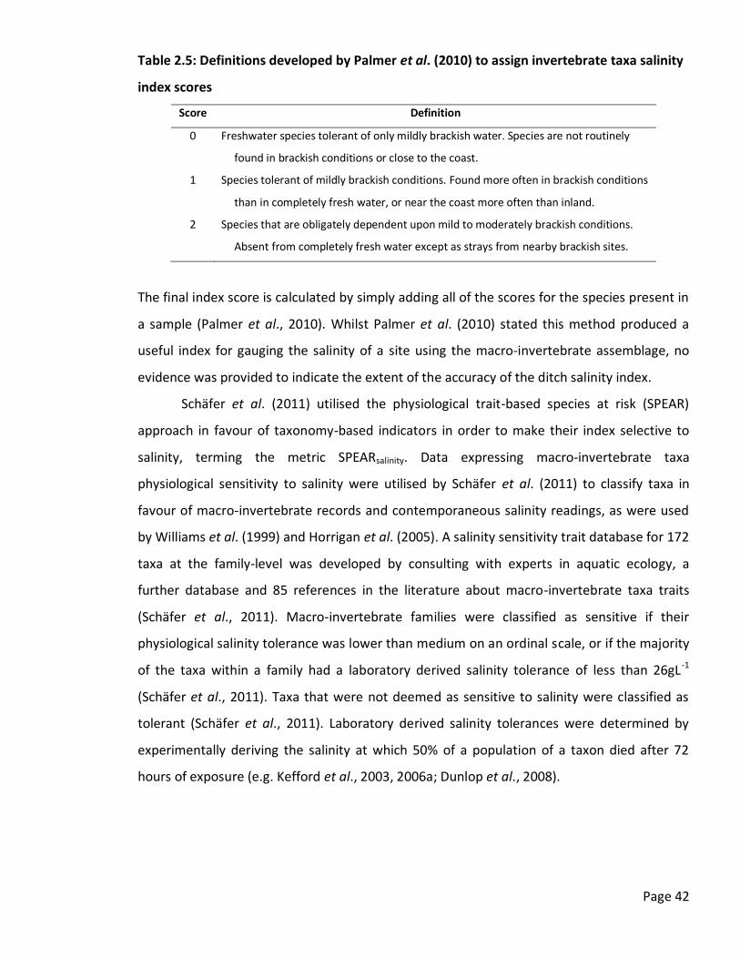
Page 42
Table 2.5: Definitions developed by Palmer et al. (2010) to assign invertebrate taxa salinity
index scores
Score Definition
0 Freshwater species tolerant of only mildly brackish water. Species are not routinely
found in brackish conditions or close to the coast.
1 Species tolerant of mildly brackish conditions. Found more often in brackish conditions
than in completely fresh water, or near the coast more often than inland.
2 Species that are obligately dependent upon mild to moderately brackish conditions.
Absent from completely fresh water except as strays from nearby brackish sites.
The final index score is calculated by simply adding all of the scores for the species present in
a sample (Palmer et al., 2010). Whilst Palmer et al. (2010) stated this method produced a
useful index for gauging the salinity of a site using the macro-invertebrate assemblage, no
evidence was provided to indicate the extent of the accuracy of the ditch salinity index.
Schäfer et al. (2011) utilised the physiological trait-based species at risk (SPEAR)
approach in favour of taxonomy-based indicators in order to make their index selective to
salinity, terming the metric SPEARsalinity. Data expressing macro-invertebrate taxa
physiological sensitivity to salinity were utilised by Schäfer et al. (2011) to classify taxa in
favour of macro-invertebrate records and contemporaneous salinity readings, as were used
by Williams et al. (1999) and Horrigan et al. (2005). A salinity sensitivity trait database for 172
taxa at the family-level was developed by consulting with experts in aquatic ecology, a
further database and 85 references in the literature about macro-invertebrate taxa traits
(Schäfer et al., 2011). Macro-invertebrate families were classified as sensitive if their
physiological salinity tolerance was lower than medium on an ordinal scale, or if the majority
of the taxa within a family had a laboratory derived salinity tolerance of less than 26gL-1
(Schäfer et al., 2011). Taxa that were not deemed as sensitive to salinity were classified as
tolerant (Schäfer et al., 2011). Laboratory derived salinity tolerances were determined by
experimentally deriving the salinity at which 50% of a population of a taxon died after 72
hours of exposure (e.g. Kefford et al., 2003, 2006a; Dunlop et al., 2008).

Page 43
Schäfer et al. (2011) used the following formula to calculate the final index score, termed
%SPEAR:
%𝑆𝑃𝐸𝐴𝑅 = 𝑥𝑖𝑦𝑖 𝑛𝑖
𝑥𝑖𝑛𝑖
where Σ = the sum of, n = the total number of species in the sample, xi = the logarithm of the
abundance +1 of species i, and y = 1 for a sensitive taxon and 0 for all other taxa.
Thus the calculation of the final index score is simply the percent of the sensitive individuals
of a community in a sample. Schäfer et al. (2011) used data collected from the Australian
states of Victoria and South Australia to determine the accuracy of the index. The results
indicated a linear relationship between %SPEAR and the common logarithm (log10) of
electrical conductivity, resulting in a Pearson’s product moment correlation of between 0.62
and 0.71 depending on the habitat type sampled (Schäfer et al., 2011). Schäfer et al. (2011)
also determined that the index did not respond to water quality variables other than salinity
and, as such, concluded that it is highly selective.
Wolf et al. (2009) developed an ordination technique to determine how the
composition of the salinity tolerances and preferences of the benthic macro-invertebrate
community changes in relation to salinity. Wolf et al. (2009) defined six biotic classes of
macro-invertebrate salinity preferences/tolerances (Table 2.6), to which macro-invertebrate
taxa were classified based on 137 references in the literature.
Table 2.6: Biotic classes of the Salinity Classification System of Wolf et al. (2009)
Biotic salinity preference/
tolerance class Description
Limnic Freshwater taxa; do not tolerate even low salinity
Limnic, tolerates salt Freshwater taxa; tolerate salinity below 5gL-1
Euryhaline-limnic Freshwater taxa; tolerate salinity up to 10gL-1 (even higher salinity for a short time)
Brackish water Brackish water taxa; permanently living and reproducing in brackish waters, tolerate
varying salinity between 0.5 and 30gL-1
Euryhaline marine Marine taxa with a wide affinity for salinity, tolerates salinity between 0.5 and 35gL-1
Holeuryhaline Taxa with a marine origin but tolerate the entire range of salinity from freshwater to
seawater

Page 44
Wolf et al. (2009) also developed a scoring system based on the combination of the five
abiotic salinity classes in the Water Framework Directive (European Commission, 2000) and
six classes of macro-invertebrate salinity preferences/tolerances (Table 2.7). The scores in
the scoring system were apportioned according to the main focus of species distribution with
respect to the salinity classes (Wolf et al., 2009).
Table 2.7: Scoring system employed by the Salinity Classification System of Wolf et al.
(2009)
Salinity
range
(gL-1
)
Biotic salinity
preference/
tolerance class
WFD salinity classification, salinity range in brackets
(<0.5gL-1
)
Freshwater
(0.5-<5gL-1
)
Oligohaline
(5-<18gL-1
)
Mesohaline
(18-<30gL-1
)
Polyhaline
(30-<40gL-1
)
Euhaline
<0.5 Limnic 10
0-5 Limnic, tolerates salt 7 3
0-10 Euryhaline-limnic 6 2 2
0.5-<30 Brackish water 2 5 3
0.5-35 Euryhaline marine 2 2 3 3
0-35 Holeuryhaline 2 2 2 2 2
The scoring system was used by Wolf et al. (2009) in conjunction with the following formula
to calculate the percentage tolerance of the community to a particular salinity class:
% 𝑡𝑜𝑙𝑒𝑟𝑎𝑛𝑐𝑒 𝑜𝑓 𝑐𝑜𝑚𝑚𝑢𝑛𝑖𝑡𝑦 𝑖𝑛 𝑐𝑙𝑎𝑠𝑠 𝑗 = 𝑆𝑐𝑜𝑟𝑒𝑖𝑗 × 𝐴𝐵𝑖
𝐴𝐵 × 10
where Σ = the sum of, Scoreij = tolerance score of taxon i and salinity class j,
ABi = abundance of taxon i, and AB = total abundance of all taxa.
The application of the salinity classification system developed by Wolf et al. (2009) to data
derived from two official surveys carried out in several brackish water systems in Germany
resulted in the system detecting salinity gradients that were not detected by chemical
assessment (Wolf et al., 2009). Salinity readings, however, were only taken at a depth of
0.5m below the surface (Wolf et al., 2009). Salinity can increase greatly with a small increase
in depth due to halo-stratification (Dyer, 1973; Davidson et al., 1991).

Page 45
Furthermore, periodic increases in salinity may not have been detected as salinity readings
were only collected once (Wolf et al., 2009). As such, a more thorough examination by taking
a series of chemical readings over a period of time and from a range of depths may well have
revealed the salinity gradients that Wolf et al. (2009) concluded were detected by the salinity
classification system.
2.9.1 Comparison of Salinity Indices
Each of the salinity indices presented in Section 2.9 have inherent advantages and
disadvantages (Table 2.8) associated with their respective applications which are further
discussed here.
Table 2.8: Advantages and disadvantages of five macro-invertebrate based salinity indices
Index Advantages Disadvantages
Horrigan et
al. (2005)
1. Produces a single output for each
sample data set
2. Uses qualitative data
1. Uses presence/absence data
2. Uses family-level identification
3. Uses qualitative data
Williams et
al. (1999)
1. Uses varying levels of taxonomic
identification
2. Uses qualitative data
3. Produces a single output for each
sample data set
1. Uses presence/absence data
2. Uses qualitative data
Palmer et
al. (2010)
1. Uses species-level identification
2. Uses qualitative data
3. Produces a single output for each
sample data set
1. Uses presence/absence data
2. Uses qualitative data
Wolf et al.
(2009)
1. Uses abundance data
2. Uses fully quantitative data
3. Uses species-level identification
1. Produces five outputs for each
sample data set
2. Uses fully quantitative data
Schäfer et
al. (2011)
1. Uses abundance data
2. Uses fully quantitative data
3. Produces a single output for each
sample data set
1. Uses family-level identification
2. Uses fully quantitative data

Page 46
It is evident that Williams et al. (1999), Horrigan et al. (2005) and Palmer et al. (2010) all
developed their respective indices to evaluate presence/absence data. As such, these indices
all essentially operate by applying a scoring system to a list of taxa present at a location. Any
change in the scores of the indices proposed by Williams et al. (1999), Horrigan et al. (2005)
and Palmer et al. (2010) would have to be facilitated by the loss or gain of a macro-
invertebrate taxon, whilst a rise in salinity that affects the abundance of a taxon without
affecting its presence would not be detected. Furthermore, changes in the number of
individuals of each taxon are considered to be more significant than changes in the lists of
taxa present at a location (Hynes, 1960). For example, Extence et al. (1999) found that scores
calculated by the LIFE system exhibited a stronger correlation with flow rate when relative
abundance data were utilised in favour of presence/absence data. Thus, the use of
abundance data allows the detection of the subtle changes in the macro-invertebrate
community which precede the loss or gain of taxa (Extence, 2012). The recognition of
abundance in water quality assessments using biological elements is also a requirement of
the WFD (European Commission, 2000). Horrigan et al. (2005) acknowledged the benefit of
abundance data by proposing its use in order to improve the accuracy and precision their
index. The incorporation of abundance data may also improve the indices of Williams et al.
(1999) and Palmer et al. (2010). In comparison to the indices proposed by Williams et al.
(1999), Horrigan et al. (2005) and Palmer et al. (2010), abundance data were incorporated
into the indices developed by Wolf et al. (2009) and Schäfer et al. (2011).
Due to the fact that both indices utilise abundance data, the salinity classification
system of Wolf et al. (2009) and the SPEARsalinity index of Schäfer et al. (2011) do not depend
on the loss or gain of taxa, but react to changes in the abundances of macro-invertebrate
taxa. These indices, however, require fully quantitative sampling and sample analysis
methods, the use of which are not without their criticisms. Fully quantitative sampling and
sample analysis methods are both time consuming and labour intensive in comparison to
qualitative and semi-quantitative sampling and sample analysis methods, such as those
described in Murray-Bligh et al. (1997) and utilised by the Environment Agency (Chadd,
2011). Surber samplers, cylinder or box corers, and Ekman bottom grabs can all be deployed
to obtain fully quantitative data (British Standards Institution, 2012).

Page 47
These methodologies, however, may not completely incorporate the different local habitat
types present at a sampling site (Chadd, 2010). For example, surber samplers, box samplers
and cylinder samplers can only be utilised in flowing water conditions and therefore are not
suitable for use in still or slowly-flowing water conditions (Chadd, 2010; British Standards
Institution, 2012). Table 2.9 illustrates further issues related with a variety of macro-
invertebrate sample collection methods that collect qualitative, semi-quantitative and fully
quantitative data.
Table 2.9: Comparison of macro-invertebrate sample collection methods
Conditions Hand
net
Surber
sampler
Box &
cylinder
samplers
Ekman-
Birge
grab
Ponar &
van Veen
grabs
Polyp
grab
Air-lift
sampler
Core and
tube
samplers
Colonisation
sampler
Suitable in still
water
Suitable in flowing
waters
Suitable in shallow
waters
Suitable in deep
waters
A
B
B
Suitable in soft
substrate
Suitable in hard
substrate
C
C
Suitable in boulders
and bedrock
Suitable in
macrophytes
Collect surface-
dwelling inverts
Types of data
produced QL, SQ
QL, SQ,
QN
QL, SQ,
QN
QL, SQ,
QN
QL, SQ,
QN
QL, SQ,
QN
QL, SQ,
QN
QL, SQ,
QN QL, SQ
A = limited to handle length,
B = Limited to sampler height,
C = where particle size is less than 16mm.
QL =Qualitative data, SQ = Semi-quantitative data, QN = Quantitative data.
Table 2.9 adapted from British Standards Institution (2012).
It can be seen that sampling by hand net is the only macro-invertebrate sample
collection method that successfully collects surface-dwelling invertebrates, such as the water
measurer Hydrometra stagnorum (Linnaeus, 1758) or Gyrinidae whirligig beetles (Table 2.9).

Page 48
Sampling by hand net can also be applied in any habitat type and on any type of substrate
(Table 2.9; British Standards Institution, 2012). In comparison, surface dwelling macro-
invertebrates are not collected by any of the methods used to collect fully quantitative data
(Table 2.9; British Standards Institution, 2012). Box and cylinder samplers are the only fully
quantitative sampling methods that are suitable for use in macrophytes, whilst the polyp
grab is the only one of these methods that can be used with a boulder substrate (Table 2.9;
British Standards Institution, 2012). Furthermore, all of the fully quantitative sampling
methods that make use of grabs may require a winch to collect samples (British Standards
Institution, 2012).
The chloride contamination index proposed by Williams et al. (1999) does not identify
to the species level, but instead uses varying levels of taxonomic resolution. This was due to
the difficulty in identifying some taxonomic groups and the desire to keep the index simple
enough to be used by non-specialists (Williams et al., 1999). In contrast, Horrigan et al.
(2005) and Schäfer et al. (2011) both developed their respective indices to be used in
conjunction with identification of macro-invertebrates made to family level. This was likely
due to the data used by Horrigan et al. (2005) to generate the salinity sensitivity scores also
being at family level identification, and this data could not be used to assign salinity
sensitivity scores to genus or species levels of identification. This was also the case with
Schäfer et al. (2011). Family level identification is both quicker and cheaper than
identification to species (Armitage et al., 1990). Furthermore, Kefford (1998b) reported that
similar results are obtained regardless of whether family level identification or species level
identification is used, whilst Chessman et al. (2007) found that an index using genus level
identification of invertebrates was slightly more sensitive than one which employed family
level identification. Chessman et al. (2007) concluded that a tiered approach, where only the
families with a wide variation in tolerance are identified with greater taxonomic resolution,
would likely be the most cost and time effective solution.
Armitage et al. (1990) stated, however, that identification to species level produces
the most detailed ecological data. For example, Extence et al. (1999) found that LIFE scores
obtained from family level data were more weakly correlated with flow rate than scores
obtained using species level data, whilst Chessman et al. (2007) stated that the use of greater
resolution is justified for the detection of subtle impacts.

Page 49
This indicates that the use of species level data results in the generation of the most accurate
scores. Furthermore, it has also been documented that some families contain species that
have different salinity tolerances (Dunlop et al., 2008). For example, Notonecta obliqua
(Gallén in Thunberg, 1787) is found at salinities less than 1.6gL-1 (Savage, 1989),
approximately 1.08PSU, whereas Notonecta viridis (Delcourt, 1909) has been recorded at
salinities ranging from 4gL-1 to 23gL-1 (Greenwood & Wood, 2003), approximately 2.85-
18.91PSU. Increased taxonomic resolution would resolve this potential source of error in an
index. This was a proposal made by Horrigan et al. (2005) to improve the accuracy and
precision of their index. The same proposal could also be applied to the chloride
contamination index of Williams et al. (1999) and the SPEARsalinity index of Schäfer et al.
(2011) to achieve the same improvements. Horrigan et al. (2005) noted that their salinity
index appeared to be unreliable when calculated for samples with less than fifteen families
present. Increased taxonomic resolution to species level may solve this issue simply by
increasing the number of taxa used in the index calculation.
In comparison to the indices of Williams et al. (1999), Horrigan et al. (2005) and
Schäfer et al. (2011), the salinity classification system proposed by Wolf et al. (2009) and the
ditch salinity index developed by Palmer et al. (2010) both require identification to species
level. The major criticism of the salinity classification system of Wolf et al. (2009) is that the
result following the application of the system is not a single figure which can be directly
related to the salinity of the sampling location. Instead the system produces a series of
numbers which can be used to produce graphs that describe the salinity
preference/tolerance of the macro-invertebrate community present at the site at the time of
sampling (Wolf et al., 2009). It is this which reflects the salinity of the location. Furthermore,
the salinity classification system requires several calculations to be performed for each
sample. In contrast the indices of Williams et al. (1999), Horrigan et al. (2005), Palmer et al.
(2010) and Schäfer et al. (2011) require only one calculation to be performed for each
sample, thus making these indices easier and quicker to use than the salinity classification
system of Wolf et al. (2009).

Page 50
2.10 Rationale for a New Salinity Index
Increases in salinity can have serious detrimental effects on both the economy and the
environment of the areas affected (see Section 2.5). Despite the existence of European
legislation which requires the use of fauna to monitor salinity as well as other physico-
chemical elements (European Commission, 2000), only the index of Palmer et al. (2010) was
developed in the UK. Palmer et al. (2010), however, specify that the ditch salinity index is
only for use in coastal and near-coastal flood plain grazing marsh drainage ditches.
Furthermore, the sampling and analysis protocol required to use an index should be
compatible for use with other existing biotic indices and surveys (Bonada et al., 2006). The
Environment Agency employs a semi-quantitative sampling and sample analysis
methodology (Murray-Bligh et al., 1997; Chadd, 2011) and as such meets the requirement of
the Water Framework Directive for recognition of abundance in the assessment of water
quality (European Commission, 2000). However, the indices developed by Williams et al.
(1999), Horrigan et al. (2005) and Palmer et al. (2010) use qualitative data and as such fail to
meet the aforementioned requirement of the WFD. Whilst the indices developed by Wolf et
al. (2009) and Schäfer et al. (2011) use fully quantitative data and thus meet the WFD
requirement for recognising abundance, neither of these indices are compatible with the
sampling and sample analysis protocol currently employed by the Environment Agency due
to the requirement for fully quantitative data. As such there is a lack of diagnostic indices for
the detection and determination of salinity increases in freshwater habitats that are suitable
for use, nor have been developed, in the UK.
Developing an index which incorporates a scoring system and the use of abundance
data, whilst keeping it simple enough to be used by both specialists and non-specialists,
would make the index much more sensitive and accessible (Hynes, 1960; Extence et al.,
1999; MacNeil et al., 2002; Horrigan et al., 2005). The literature also indicates that use of
mixed level identification where families with a wide variation in tolerance are identified with
greater taxonomic resolution, as opposed to general family level identification, would also
increase the sensitivity of the index (Extence et al., 1999; Horrigan et al., 2005; Chessman et
al., 2007) whilst retaining a level of accessibility for both specialists and non-specialists
(Williams et al., 1999).

Page 51
Whilst it is recognised that the indices developed by Williams et al. (1999), Horrigan
et al. (2005), Wolf et al. (2009) and Schäfer et al. (2011) may work in the UK, no known
studies have yet been undertaken to confirm or refute this. Furthermore, the index of
Williams et al. (1999) may be difficult to test due to the small number of taxa attributed
scores in the study.

Page 52
3 DEVELOPMENT OF THE SALINITY ASSOCIATION GROUP
INDEX
Following the principles adopted in devising the Lotic-invertebrate Index for Flow Evaluation
(LIFE) (Extence et al., 1999), Community Conservation Index (Chadd & Extence, 2004) and the
Proportion of Sediment-sensitive Invertebrates metric (Extence et al., 2011), taxa (species,
genera and families) of British benthic macro-invertebrates were classified into five groups,
defined in Table 3.1, termed Salinity Association Groups (SAGs).
Table 3.1: Definitions of the Salinity Association Groups
Salinity Association
Group (SAG) Group definition*
I Macro-invertebrate taxa which tolerate only salinities below 2.5gL-1, approximately
1.73PSU. Typically freshwater taxa; may be tolerant of slightly brackish conditions, or
completely intolerant.
II Macro-invertebrate taxa which can tolerate salinities over 2.5gL-1 (1.73PSU) up to a
salinity of 10gL-1 (7.63PSU). Taxa may be present at slightly higher salinities, but only in
small numbers. Freshwater taxa tolerant of mild brackish conditions.
III Macro-invertebrate taxa which are characterised by the largest abundance occurring in
the salinity range 8-20gL-1 (5.99-16.22PSU). Taxa are tolerant of the salinity range 4-
25gL-1 (2.85-20.73PSU), but may also be recorded at salinities greater, or less, than
those specified in this range. Characteristic brackish water taxa, tolerant of a wide
range of salinity conditions from long term brackish to near freshwater.
IV Macro-invertebrate taxa which tolerate salinities below 20gL-1 (16.22PSU) down to
14gL-1 (14.99PSU). Taxa may be present at slightly lower salinities, but only in small
numbers. Long-term brackish taxa tolerant of lower salinities, i.e. transition zones.
V Macro-invertebrate taxa which tolerate only salinities greater than 20gL-1
,
approximately 16.22PSU. Full coastal seawater taxa rarely moving into nominally
freshwater habitats.
*Definitions using salinity concentrations are in regular font style, whilst the descriptive definitions of the
groups are in italic font style.
Whilst it is recognised that species level identification gives the most detailed ecological data
(Armitage et al., 1990), a mixed level of identification was employed in order that the Salinity
Association Group (SAG) index could be utilised by both specialists and non-specialists.

Page 53
This approach is also considered to be the most cost and time effective with regards to the
identification of macro-invertebrates for use in biotic indices (Chessman et al., 2007).
Furthermore, this method has been successfully utilised by several published biotic indices
(e.g. Extence et al., 1999, 2011) which are employed by the regulatory bodies in the UK.
Classification of the taxa was accomplished by undertaking an extensive literature review to
determine the association of taxa with salinity (see Appendix 1 for list of taxa assignments to
Salinity Association Groups (SAGs), and Appendix 2 for justifications of assignments of macro-
invertebrate taxa).
It has been stated that changes in the abundance of each taxon are more informative
than changes in the lists of taxa present at a location (Hynes, 1960). Evidence of this is
provided by Extence et al. (1999), who found that utilisation of abundance data with the LIFE
system resulted in scores which exhibited a stronger correlation with flow rate than the
scores obtained using presence/absence data. The use of abundance data was a proposal by
Horrigan et al. (2005) to improve their salinity index, whilst the use abundance data was
incorporated into the indices developed by Wolf et al. (2009) and Schäfer et al. (2011).
Williams (1987) stated that the influence of salinity of the aquatic macro-invertebrate
community may be so subtle as to only be evident by gradual changes in the abundances of
the taxa present. Furthermore, recognition of abundance in the assessment of water quality
is a requirement of the Water Framework Directive (European Commission, 2000). Thus, the
use of abundance data was incorporated into the SAG index methodology in order to
improve the accuracy and precision of the metric. The abundance categories integrated into
the SAG index method (Table 3.2) are the same as those utilised as part of the operating
procedure of the Environment Agency for analysing macro-invertebrate samples (Murray-
Bligh et al., 1997).
A scoring matrix incorporating the Salinity Association Groups and the Environment
Agency abundance categories was developed by assigning the arbitrary scores 1 to 20,
termed Salinity Association Scores (SAS). The SAG index calculation is based upon the sum of
the individual salinity association scores for each scoring taxon in a sample. A taxon score is
determined by reference to the scoring matrix presented in Table 3.2.

Page 54
Table 3.2: Scoring matrix for determining Salinity Association Scores
Salinity Association
Group (SAG)
Abundance category (number of individuals)
A (1-9) B (10-99) C (100-999) D/E (1000+)
I 4 3 2 1
II 5 6 7 8
III 9 10 11 12
IV 13 14 15 16
V 17 18 19 20
Thus, for a theoretical sample which contains 300 individuals of a taxon (abundance category
C) that has been assigned to SAG III, based on the taxon’s association with salinity as
reported in the literature, a SAS of 11 would be awarded for that taxon. A taxon which has
been assigned to SAG V and had nine individuals present in the sample (abundance category
A) would be awarded a SAS of 17. To calculate the final SAG index score for a sample, the
following formula is applied.
SAG index = ΣSAS/n
where ΣSAS = the sum of individual taxon salinity association scores present in the sample
and n = the number of taxa used to calculate ΣSAS.
Hence, the final SAG index score for a sample is simply the arithmetic mean of all the scores
obtained for the taxa present in the sample (see Appendix 3 for a worked example of the
SAG index).

Page 55
4 SURVEY SITES
Surveys were undertaken at locations in both Lincolnshire and Norfolk in order to collect
environmental data, as well as macro-invertebrate community data over a range of salinity
concentrations.
Within Lincolnshire two separate study locations were chosen; namely the South
Forty Foot Drain and the South Holland Main Drain. The South Forty Foot Drain and South
Holland Main Drain were selected as study locations as both water bodies are believed to be
subject to increased salinity (Chadd, 2009). Furthermore, examination of macro-invertebrate
data collected by the Environment Agency (data collected from February 1987 to May 2009)
provided evidence of variable salinity in both drains. The data revealed that taxa indicative of
brackish conditions, such as Palaemontes varians (Leach, 1837), Gammarus zaddachi Sexton,
1912, Haliplus apicalis C.G. Thomson, 1868 and Enochrus bicolor (Fabricius, 1792), have been
recorded from both the South Forty Foot Drain and South Holland Main Drain.
The majority of the sites surveyed in Lincolnshire were large fen drains. In order to
assess the suitability of the Salinity Association Group (SAG) index in a different habitat type,
a total of eight sites located within the Norfolk Broads area were surveyed in order to obtain
macro-invertebrate community data over a range of salinity concentrations. All of the survey
sites were located on small, non-flowing drainage ditches. Much of the Norfolk Broads area is
flat (Gilvear et al., 1997) and only slightly higher than sea level (Wheeler & Giller, 1982). The
defining characteristic of the Broads area is an extensive river system inter-linked by a
number of shallow lakes termed Broads (Wheeler & Giller, 1982; Matless, 1994). The river
system is tidal up to 40-50km from the mouth of Breydon Water estuary (Baker & Howlett,
2010) as a result of very shallow gradients (Wheeler & Giller, 1982). For example, Birkett et
al. (2002) stated the River Yare has a bed gradient of approximately 3cm per km. The Broads
themselves are shallow lakes formed from the flooding of peat-diggings (Phillips, 1977;
Wheeler & Giller, 1982; Matless, 1994) undertaken in the 12th and 13th centuries (Gilvear et
al., 1997). All of the Broads are susceptible to flooding as they lie below the highest river
levels (Baker & Howlett, 2010).
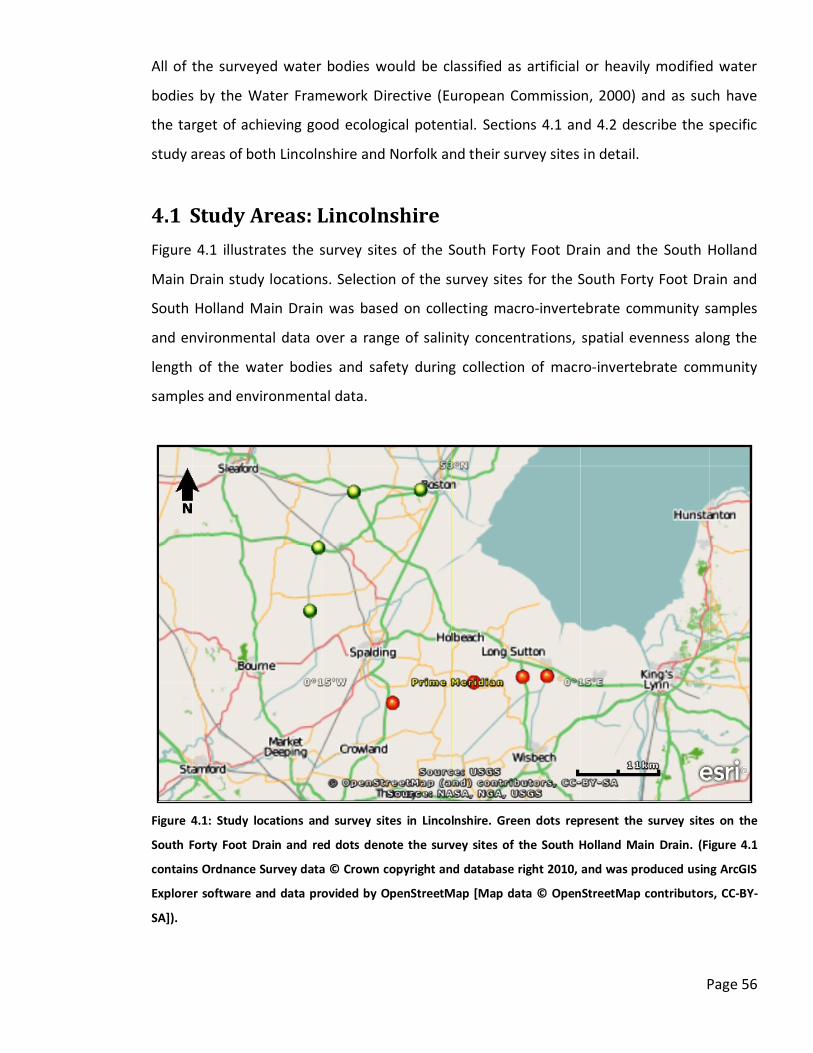
Page 56
All of the surveyed water bodies would be classified as artificial or heavily modified water
bodies by the Water Framework Directive (European Commission, 2000) and as such have
the target of achieving good ecological potential. Sections 4.1 and 4.2 describe the specific
study areas of both Lincolnshire and Norfolk and their survey sites in detail.
4.1 Study Areas: Lincolnshire
Figure 4.1 illustrates the survey sites of the South Forty Foot Drain and the South Holland
Main Drain study locations. Selection of the survey sites for the South Forty Foot Drain and
South Holland Main Drain was based on collecting macro-invertebrate community samples
and environmental data over a range of salinity concentrations, spatial evenness along the
length of the water bodies and safety during collection of macro-invertebrate community
samples and environmental data.
Figure 4.1: Study locations and survey sites in Lincolnshire. Green dots represent the survey sites on the
South Forty Foot Drain and red dots denote the survey sites of the South Holland Main Drain. (Figure 4.1
contains Ordnance Survey data © Crown copyright and database right 2010, and was produced using ArcGIS
Explorer software and data provided by OpenStreetMap [Map data © OpenStreetMap contributors, CC-BY-
SA]).

Page 57
Consideration was also given to rights of way for access and, consequently, the majority of
the sites had road bridges in close proximity. Each of the sites within Lincolnshire were
surveyed three times, once in spring, once in summer and again in autumn (see Appendix 4
for specific dates). Spring was defined as March April and May, summer as June, July and
August, and autumn as September, October and November, following the definitions
specified in Murray-Bligh et al. (1997) and utilised by the Environment Agency. Given that
seasonal variation is a major criticism of biotic indices (see Section 2.8.2), surveys were
undertaken in spring, summer and autumn in order that any seasonal differences in the
macro-invertebrate fauna may be detected and any resulting effect upon the SAG index
examined.
4.1.1 South Forty Foot Drain
The South Forty Foot Drain is located in the Lincolnshire Fens and is managed by Black Sluice
Internal Drainage Board. The South Forty Foot Drain is 33.3km long and currently drains a
total of 750km2 of land (Faulkner, 2009). The water body starts near to Guthram Gowt
(Ordnance Survey Grid Reference (OSGR): TF-17500-22500) and terminating in Boston
(OSGR: TF-33700-42600). The first section of the drain was constructed in the 1630s (Taylor,
1999). This was later extended and revised in the late eighteenth century, resulting in the
current course of the South Forty Foot Drain (Barnwell, 1998). Drainage water is pumped
directly into the channel by 21 pumping stations, whilst Black Sluice pumping station pumps
water out of the South Forty Foot Drain and into the tidal section of the River Witham,
known as The Haven, at Boston (Faulkner, 2009).
The four survey sites on the South Forty Foot Drain are all currently, or have been,
utilised as macro-invertebrate community sample collection points for routine monitoring of
water quality by the Environment Agency. The survey sites were, in order of upstream to
downstream, SF1 (Casswell’s Bridge; OSGR: TF-16500-27500), SF2 (Donington Bridge; OSGR:
TF-17300-35600), SF3 (Swineshead Bridge; OSGR: TF-21800-42900) and SF4 (Wyberton Chain
Bridge; OSGR: TF-30400-43400) (Figure 4.2). Further detail for each individual survey site of
the South Forty Foot Drain is available in Appendix 5.

Page 58
Figure 4.2: Diagrammatic sketch of the South Forty Foot Drain, Lincolnshire, illustrating the sequence of the
survey sites. CB = Casswell’s Bridge, DB = Donington Bridge, SB = Swineshead Bridge, and WCB = Wyberton
Chain Bridge.
4.1.2 South Holland Main Drain
The South Holland Main Drain is located between the River Welland and the River Nene
(Moriarty & French, 1975) and is managed by the South Holland Internal Drainage Board. The
drain is 22.5 kilometres long, running from Cowbit (OSGR: TF-26500-17900) to Sutton Bridge
(OSGR: TF-47500-21500) where it discharges into the tidal River Nene (South Holland Internal
Drainage Board, 1984). In contrast to the South Forty Foot Drain, where water levels are
maintained by a pumping station, the water level of the South Holland Main Drain is
controlled by a tidal sluice gate, Nene Outfall Sluice, at the confluence with the River Nene.
The South Holland Main Drain was constructed as a result of the South Holland Drainage Act
1793 and currently, with its subsidiaries, drains a total of 216km2 of land (South Holland
Internal Drainage Board, 1984).
The four survey sites on the South Holland Main Drain are all currently, or have been,
utilised by the Environment Agency as survey sites for routine monitoring of water quality. In
order of furthest upstream to furthest downstream, the survey sites located on the South
Holland Main Drain were SH1 (Weston Fen; OSGR: TF-27600-15900), SH2 (Clifton’s Bridge;
OSGR: TF-38000-18900), SH3 (A1101 Road Bridge; OSGR: TF-44300-19800) and SH4 (Nene
Outfall Sluice; OSGR: TF-47400-19900) (Figure 4.3).
Figure 4.3: Diagrammatic sketch of the South Holland Main Drain, Lincolnshire, illustrating the sequence of
the survey sites. WF = Weston Fen, CB = Clifton’s Bridge, ARB = A1101 Road Bridge, and NOS = Nene Outfall
Sluice.

Page 59
Further detail for each individual survey site of the South Holland Main Drain is available in
Appendix 5.
4.2 Study Area: Norfolk
The Norfolk Broads area is managed by the Broads Authority, a statutory body which was
established following the 1988 Norfolk and Suffolk Broads Act (Norfolk Wildlife Services Ltd.
& the Broads Authority, 2009). As well as rivers and Broads, the Broads Authority Executive
Area is comprised of a wide range of habitats (Norfolk Wildlife Services Ltd. & the Broads
Authority, 2009). Such habitats include grazing marsh and dykes originating from drainage
and reclamation of estuarine land, estuarine and coastal habitat (Norfolk Wildlife Services
Ltd. & the Broads Authority, 2009). Selection of the survey sites within Norfolk was based on
collecting macro-invertebrate community samples and environmental data over a range of
salinity concentrations and safety during collection of macro-invertebrate community
samples and environmental data. Consideration was also given to rights of way for access.
The sites located within Norfolk were each surveyed twice to obtain macro-invertebrate
community samples and environmental data; once in spring and again in summer as defined
by Murray-Bligh et al. (1997) (see Appendix 4 for specific dates).
The survey sites within Norfolk were separated into two broad geographic regions
based on their locations within river catchments; the River Yare catchment and the Upper
Thurne catchment (Figure 4.4).

Page 60
Figure 4.4: Study locations and survey sites in Norfolk. Survey sites are indicated by coloured dots, with green
dots representing the survey sites of the River Yare and the blue dots indicating the survey sites of the Upper
Thurne catchment. (Figure 4.4 contains Ordnance Survey data © Crown copyright and database right 2010,
and was produced using ArcGIS Explorer software and data provided by OpenStreetMap [Map data ©
OpenStreetMap contributors, CC-BY-SA]).
4.2.1 Survey Sites of the Upper Thurne Catchment
The Upper Thurne catchment was located in the north-east of Norfolk (Drake, 2011).
Examination of historical data has shown that electrical conductivity was one of the most
important variables in explaining differences in the macro-invertebrate communities of this
region through time (Drake, 2011). The survey sites within the Upper Thurne catchment are
illustrated in Figure 4.5 and were LD (Long Dyke; OSGR: TG-41300-27700), MM (Middle
Marsh; OSGR: TG-41300-20800) and LM (Ludham Marsh; TG-40900-17900). Whilst the LM
(Ludham Marsh) survey site was not strictly within the boundaries of the Upper Thurne
catchment, it was included here due to its proximity to the catchment. Further detail for
each of the survey sites located within Norfolk is available in Appendix 6.

Page 61
Figure 4.5: The survey sites of the Upper Thurne catchment. (Figure 4.5 contains Ordnance Survey data ©
Crown copyright and database right 2010, and was produced using ArcGIS Explorer software and data
provided by OpenStreetMap [Map data © OpenStreetMap contributors, CC-BY-SA]).
4.2.2 Survey Sites of the River Yare Catchment
The River Yare catchment was located to the south-east of Norwich (Figure 4.4). The River
Yare has been known to flood within this area, resulting in brackish waters intruding nearby
ditches (Strudwick, 2011). As such, the area appeared ideal for investigating the impacts of
salinity on macro-invertebrate ditch fauna. The survey sites located within the River Yare
catchment were SM (Strumpshaw Meadow; OSGR: TG-33800-06700), BM (Buckenham
Marsh; OSGR: TG-35300-05400), ND (Near Dry Dyke; TG-35900-05300), HM (Hatchet Marsh;
TG-36500-05100) and RM (Rockland Marsh; OSGR: TG-33500-04900) and the locations of
these survey sites are displayed in Figure 4.6. Further detail for each of the survey sites
located within Norfolk is available in Appendix 6.

Page 62
Figure 4.6: The survey sites of the River Yare Catchment. (Figure 4.6 contains Ordnance Survey data © Crown
copyright and database right 2010, and was produced using ArcGIS Explorer software and data provided by
OpenStreetMap [Map data © OpenStreetMap contributors, CC-BY-SA]).

Page 63
5 METHODS
The methods employed in the collection and analysis of macroinvertebrate community
samples, environmental data and sediment samples are detailed in the following sections.
The techniques utilised to analyse the resulting data are also described. The coding system
developed to label samples, and used hereinafter, is comprised of prefixes denoting the
specific survey site (Table 5.1) and suffixes denoting the specific season during which the
sample was collected (Table 5.2).
Table 5.1: Prefixes and meanings used in sample coding system
Prefix Site Name Location
SF1 Casswell's Bridge, South Forty Foot Drain
Lin
coln
shir
e
SF2 Donington Bridge, South Forty Foot Drain
SF3 Swineshead Bridge, South Forty Foot Drain
SF4 Wyberton Chain Bridge, South Forty Foot Drain
SH1 Weston Fen, South Holland Main Drain
SH2 Clifton's Bridge, South Holland Main Drain
SH3 A1101 Road Bridge, South Holland Main Drain
SH4 Nene Outfall Sluice, South Holland Main Drain
HM Hatchet Marsh
No
rfo
lk
ND Near Dry Dyke
SM Strumpshaw Meadow
LM Ludham Marsh
LD Long Dyke
BM Buckenham Marsh
MM Middle Marsh
RM Rockland Marsh
Table 5.2: Suffixes and meanings used in sample coding system
Suffix Season
SPR Spring
SUM Summer
AUT Autumn

Page 64
5.1 Sampling Procedure
Surveys of the selected sites consisted of collecting environmental data and macro-
invertebrate community samples, as well as surveying the vegetation taxa present during
each visit. Macro-invertebrate community sampling was undertaken after the collection of
environmental data. This order was chosen to negate the possibility of the macro-
invertebrate sampling procedure creating disturbances, which could result in the higher
freshwater water layer and the lower salinity layer to mix, resulting in the introduction of
error into the chemical data. It was recognised, however, that the collection of
environmental data may cause macro-invertebrates to enter drift prior to sampling due to
disturbances created by the collection of environmental data. To minimise this potential
source of error, the collection of environmental data was performed slightly downstream of
the areas to be sampled for macro-invertebrates. The survey sites of the South Forty Foot
Drain and South Holland Main Drain were visited starting at the furthest downstream site
and working upstream.
5.2 Environmental Data
Water body depth was measured at the centre of the channel using a length of cable marked
at measured intervals and weighted at one end. Water body width was measured as the
width of the water surface using a tape measure where possible, or otherwise estimated by
counting the number of steps required to walk from one bank to the other and measuring
the length of a step. The methods employed to measure watercourse width are the same as
those detailed in Murray-Bligh et al. (1997), which are standard techniques employed by the
Environment Agency.
There is not a standard depth from which to collect chemical data (see Section 2.7).
As such, it was decided to collect chemical data at each survey site from the surface, mid-
depth and base of the water column from the middle of the water bodies and the surface
and base at one bank of the water bodies where feasible. These positions were determined
following the measurement of the water body depth. Chemical data were only collected
from the surface and base of the water column from the middle of the water bodies during
the surveys of the sites located within Norfolk due to the lack of depth and width of these
water bodies.

Page 65
An YSI-556 multi-probe field meter, supplied by Van Walt Ltd., was used to measure
electrical conductivity (accuracy: the greater of 0.001mScm-1 or ±0.5% of reading), redox
potential (accuracy ±20 mV), dissolved oxygen (accuracy: the greater of ±0.2 mg/L or ±2% of
reading) and water temperature (accuracy ±0.15°C) at the Lincolnshire survey sites in all
survey seasons and the Norfolk survey sites in the spring surveys. A Hanna Instruments HI-
98312 Dist6 Conductivity & TDS and temperature meter was used to determine conductivity
(accuracy ±0.4 mS/cm) and water temperature (accuracy ±0.5°C) at the Norfolk survey sites
in the summer surveys. Conductivity was later transformed into Practical Salinity Units (PSU)
using the 6th-order polynomial equation described by Schemel (2001), which is based the
equation given in Lewis (1980) and developed for a single temperature (25°C) and
atmospheric pressure (760 mm):
𝑆𝑎𝑙𝑖𝑛𝑖𝑡𝑦 𝑃𝑆𝑈 = 0.012 + −0.2174
EC1000
53.087
0.5
+ 25.3283
EC1000
53.087
1
+ 13.7714
EC1000
53.087
1.5
+ −6.4788
EC1000
53.087
2
+ 2.5842
EC1000
53.087
2.5
where EC = specific conductivity compensated to 25°C in µScm-1.
Given that nitrates and phosphates can make significant contributions to conductivity
(Panter et al., 2011), both nitrate and phosphate concentration were determined during the
autumn surveys of the Lincolnshire sites and all surveys of the Norfolk sites. Phosphate and
nitrate concentrations were determined using a Palintest Photometer 5000 (accuracy: ±0.5%
transmittance) and water samples collected from the base at one bank of the survey sites.
Photometers operate by measuring the intensity of colour at a predetermined wavelength
when reagents are added to a sample solution to produce a coloured complex with a target
chemical (Palintest instruction sheet PHOT.1). The intensity of colour produced is
proportional to the concentration of the chemical being analysed (Palintest instruction sheet
PHOT.1). Phosphate concentration was determined as PO4, whilst nitrate was measured as N
and converted to NO3 by multiplying by 4.4 as stated in the Palintest instruction sheet
PHOT.23.

Page 66
5.3 Macro-invertebrate Community Samples
Macro-invertebrate community samples were collected in accordance with the procedure
defined within the UK Technical Advisory Group methodology for macro-invertebrate
sampling and analysis (Murray-Bligh et al., 1997). The same procedure is used by the
Environment Agency to collect invertebrate data for use with the River Invertebrate
Classification Tool (RICT) for classifying water bodies in accordance with the requirements of
the WFD (WFD-UKTAG, 2008) and is compliant with the international standard BS EN ISO
10870:2012 (British Standards Institution, 2012), which has superseded the European
standards EN 27828:1994 (European Committee for Standardization, 1994a) and EN
28265:1994 (European Committee for Standardization, 1994b). The procedure consisted of a
three minute pond net kick/sweep sampling and a one minute manual search which was split
into two parts; one undertaken prior to the kick/sweep sampling and the other performed
after. The first part of the manual search was to seek and collect water surface-dwelling
animals that would rapidly leave the sampling area or seek refuge if they are disturbed. The
second part of the manual search was to seek and collect animals from habitats that were
not sampled effectively by the kick/sweep sampling method. During the three minute pond
net kick/sweep sampling, each invertebrate micro-habitat within the sampling area was
sampled with effort in proportion to its cover. The aperture of the net used during the
collection of macro-invertebrate community samples was 670cm² and the mesh size was
1mm. The net was cleared of vegetation, sediment and other material periodically during
each three minute sampling run. This prevented blockages building up in the mesh of the net
and thus maintaining the effectiveness of the sampling. Material removed from the net was
retained as it constitutes part of the sample.
Once collected, samples were stored in a refrigerator at temperatures between 1 and
3°C until sorting and identification could be performed. Sorting was achieved by washing
samples through a bank of sieves with mesh sizes 2mm, 1mm and 710μm to remove debris
and plant matter. The material retained in each sieve was washed into a tray from which
macro-invertebrates were picked using forceps. Specimens of the classes Gastropoda and
Bivalvia were preserved in 70% ethanol, whilst all other macro-invertebrates were preserved
in Kahle’s solution.

Page 67
Macro-invertebrates were identified generally to species or genus-level, with the
exception of Diptera larvae and pupae which were identified to family-level. Identification of
specimens was determined with reference to Janus (1982), Macan (1977), Ellis (1978),
Reynoldson (1978), Elliott & Mann (1979), Lincoln (1979), Croft (1986), Fitter & Manuel
(1986), Elliott et al. (1988), Friday (1988), Unwin (1988), Savage (1989), Wallace et al. (1990),
Gledhill et al. (1993), Barnes (1994), Edington & Hildrew (1995), Miller (1995), Brooks &
Lewington (1997) and Cham (2007, 2009).
5.3.1 Macro-invertebrate Diversity and Water Quality Measures
A variety of diversity indices and water quality measures were used to summarise macro-
invertebrate community composition. Diversity indices are quantitative measures that
provide more information about community composition than taxa richness by taking into
account the relative abundances of the different taxa present (Okpiliya, 2012). Diversity
indices generally quantify either taxon richness or the proportional representation of the
taxa present (Derksen et al., 1995), also known as evenness or equitability (Peet, 1975). One
concept that is frequently considered is that diversity combines both taxon richness and
evenness (Peet, 1974, 1975), and diversity indices that combine measures of both these
features have also been developed (Peet, 1975; Derksen et al., 1995). Different features of
the relative abundances between taxa are measured by different indices (Hill, 1973) as each
index differs in their sensitivity to each aspect (Boyle et al., 1990). As a consequence, it has
been recommended that different types of diversity indices are used together (Boyle et al.,
1990). As such, the different aspects of diversity were measured using taxon richness
(relative number of taxa), total number of individuals (abundance), Margalef’s index (taxon
richness), Simpson’s index of dominance (dominance and evenness), Shannon index (taxon
richness and evenness), Buzas & Gibson’s evenness (also known as Sheldon’s evenness) and
Berger-Parker dominance index (dominance). In order to assess general water quality in
biological terms, the Average Score Per Taxon (ASPTBMWP) derivative of the Biological
Monitoring Working Party (BMWP) scoring system (BMWP, 1978; Chesters, 1980; Hawkes,
1997) was also applied to the macro-invertebrate data.

Page 68
Taxon richness is the simplest index of diversity (Pianka, 1966; Peet, 1974; Okpiliya,
2012). Species richness is one of the most widespread diversity indices (Gallardo et al., 2011)
and is still frequently used (Peet, 1974). Taxon richness, however, is not independent of
sample size and larger samples can be expected to yield a greater number of taxa (Peet,
1974; Okpiliya, 2012). Furthermore, taxon richness is strongly affected by rare taxa (Hill,
1973) and does not account for differing abundances of taxa (Pianka, 1966). As a
consequence, more complex diversity indices which account for relative abundance among
taxa have been developed (Pianka, 1966), such as the commonly used Margalef’s index,
Shannon index and Simpson’s index (Pullin, 2002), and are used in this study.
Margalef’s index (Margalef, 1958) is a well known (Magurran, 2004; Okpiliya, 2012)
index designed to simply measure taxon richness (Death & Winterbourn, 1995; Derksen et
al., 1995; Hamer et al., 2003; Magurran, 2004; Okpiliya, 2012). The index is simple to
interpret (Lexerød & Eid, 2006) as the Margalef index value increases as diversity in a sample
increases (Smale et al., 2003). Margalef’s richness index was calculated using the following
formula:
Margalef ′s richness index (DMg ) = 𝑛 − 1
ln𝐴
where n = taxon richness, and A = total number of individuals.
Whilst Margalef’s richness index is designed to compensate for sample size (Magurran,
2004), the metric is sensitive to sampling size (Magurran, 2004). Nonetheless, Margalef’s
index can be used in tandem with diversity indices designed to be sensitive to changes in
dominant taxa or evenness (Magurran, 2004), such as Simpson’s index (Hill, 1973; Peet,
1974; Krebs, 1985; Death & Winterbourn, 1995). Furthermore, Margalef’s index has
remained in use in relatively recent years (e.g. Fisher & Petrini, 1990; Ogbeibu & Oribhabor
2002; Cheng, 2004; Azrina et al., 2006; Velasco et al., 2006; Teixeira et al., 2009; Ren et al.,
2011).
Simpson’s index (Simpson, 1949) is commonly used (Pullin, 2002) and has long been
considered the principal diversity metric not from the subject field of communication
(McDonald & Dimmick, 2003).

Page 69
The index is sensitive to changes in abundant taxa (Peet, 1974; Hill, 1973; Magurran, 2004)
resulting from the relative weighting given to rare species and abundant species by the index
(Krebs, 1985; Magurran, 2004; Okpiliya, 2012). The addition of a rare species results in only a
small difference in the Simpson’s index value (Okpiliya, 2012). As such, Simpson’s index has
been described as an index of dominance (Hill, 1973; Krebs, 1985), although Death &
Winterbourn (1995) described the index as a measure of evenness. Simpson’s index was
calculated using the following formula:
Simpson′s index 1− D = 1 − 𝐴𝑖𝐴
2
where Ai = the number of individuals in taxon i, and A = total number of individuals.
The original formulation of Simpson’s index varied inversely with diversity, but subtracting
the calculated index value from its maximum possible value of 1 (as in the formula above), as
suggested by Greenberg (1956) and Berger & Parker (1970) avoids any difficulty in
interpretation. Simpson’s index is considered by Magurran (2004) to be among the most
robust and meaningful diversity metrics, which may explain the prolonged use of Simpson’s
index (e.g. Terman, 1997; Kaiser et al., 1998; Cheng, 2004; Azrina et al., 2006; Velasco et al.,
2006; Gómez-Anaya & Novelo-Gutiérrez, 2010; Naigaga et al., 2011).
The Shannon index (Shannon & Weaver, 1949) is a commonly used diversity measure
(Pullin, 2002; McDonald & Dimmick, 2003; Smale et al. 2003; Spellerberg & Fedor, 2003;
Magurran, 2004; Tataranni & Lardicci, 2010; Gallardo et al., 2011), despite being originally
developed within the subject field of communication (McDonald & Dimmick, 2003; Smale et
al. 2003; Spellerberg & Fedor, 2003; Okpiliya, 2012). The Shannon-Wiener index takes into
account taxon richness and the evenness of the abundances of the taxa (Krebs, 1985;
Magurran, 2004; Tataranni & Lardicci, 2010). The Shannon index was calculated using the
following formula:
Shannon index Hi = − 𝐴𝑖𝐴 ln
𝐴𝑖𝐴
where Ai = the number of individuals in taxon i, and A = total number of individuals.

Page 70
Whilst sample size does not significantly influence the Shannon index (Johnson et al., 2007),
error is introduced in the metric if not all taxa in a community are represented in a sample
collected from that community (Peet, 1974). Furthermore, the size of this error increases as
the proportion of the species missing from the sample increases (Magurran, 2004). Despite
this issue, the Shannon index is regarded as one of the best measures of community diversity
(Baker et al., 1987) and is still widely used (e.g. Clair & Paterson, 1976; Lancaster & Scudder,
1987; Naidu et al., 1990; Gallardo-Mayenco, 1994; Marmonier et al., 2000; Kirkman et al.,
2004; Leponce et al., 2004; Bonner et al., 2005; Richardson, 2006; Schouten et al., 2010;
Tataranni & Lardicci, 2010; Gallardo et al., 2011).
Evenness has been defined as the ratio between the number of abundant taxa and
total taxon richness (Alatalo, 1981; Smale et al., 2003). Evenness measures can be expected
to show a response to a change in community composition even when there is no change in
taxon richness (Johnston & Roberts, 2009). One such metric that is easy to both calculate and
interpret is Buzas & Gibson’s evenness (Webb & Leighton, 2011). Buzas & Gibson’s evenness
(Buzas & Gibson, 1969) quantifies the deviation from complete evenness between the
abundances of all taxa in a sample (Peet, 1974; Buzas et al., 2007a) by using the Shannon
index value and taxon richness of the sample (Webb & Leighton, 2011). Buzas & Gibson’s
evenness was calculated using the following formula:
Buzas & 𝐺𝑖𝑏𝑠𝑜n′ s Evenness E = 𝑒𝐻𝑖
𝑛
where n = taxon richness, and Hi = Shannon index value.
Buzas & Gibson’s evenness is designed as such that the calculated value should not change
when the number of individuals of each taxon present is multiplied with a constant, which is
a vital requirement for an evenness index according to Heip & Engels (1974). Buzas &
Gibson’s evenness is reported to not be sensitive to rare taxa in a sample (Kirkman et al.,
2004). This particular diversity measure has been employed in studies by the likes of Naidu et
al. (1990), Terman (1997), Leponce et al. (2004), Kirkman et al. (2004), Bonner et al. (2005),
Richardson (2006), Buzas et al. (2007a, 2007b), Webb et al. (2009) and Amini Yekta et al.
(2012).

Page 71
The Berger-Parker index is a simple dominance metric (Berger & Parker, 1970; May,
1975; Death & Winterbourn, 1995; Lexerød & Eid, 2006) that measures the proportional
abundance of the most abundant taxon (Colunga-Garcia et al., 1997; Smale et al., 2003;
Magurran, 2004). The Berger-Parker index was calculated using the following formula:
Berger− Parker dominance index B = 1 − 𝐴𝑚𝑎𝑥𝐴
where Amax = number of individuals in the dominant taxon, and A = total number of
individuals.
The Berger-Parker index is independent of taxon richness (Southwood, 1978; Lexerød & Eid,
2006) and is generally insensitive to sample size (Southwood, 1978). May (1975) concluded
the Berger-Parker index is among the most acceptable diversity metrics as a result of the
aforementioned advantages, the ecological significance and simplicity of the index. the
Berger-Parker index has been used by the likes of Colunga-Garcia et al. (1997), Sures et al.
(1999), Alyokhin & Sewell (2004), Wilsey et al. (2005) Wood et al. (2001) and Wood et al.
(2005).
The Biological Monitoring Working Party (BMWP) score system (BMWP, 1978;
Chesters, 1980; Hawkes, 1997) has formed the basis of the river invertebrate status
classification system used by the relevant authorities in the UK since 1980 and, as such, has
been extensively used for nationally reporting water quality in biological terms (Extence et
al., 1986; Extence & Ferguson, 1989). The BMWP scoring system has also been published as a
standard method by the International Organization of Standardization (ISO-BMWP, 1979).
The number of BMWP-scoring families (shown in Table 5.3) present in a sample (NTAXABMWP)
and the average score per taxon (ASPTBMWP) present, which is calculated by summing all of
the scores of all taxa present in a sample and dividing by NTAXABMWP (Mason, 1991; Friedrich
et al., 1996), is still currently used in the UK in the assessment of ecological status for the
WFD (Clarke, 2009).
Whilst the BMWP score system and it’s ASPTBMWP derivative were originally devised
for the detection of organic pollution (Wright, 1994; MacNeil et al., 2002), these indices can
also respond to inorganic pollutants and give an indication of water quality (Chadd, 2010).

Page 72
The ASPTBMWP derivative, however, is considered to be less sensitive to sample size (Armitage
et al., 1983; Mason, 1991; Demers & Reynolds, 2002), sampling effort and seasonal changes
than BMWP (Hawkes, 1997), which is calculated by simply summing the scores of all the
families present (Friedrich et al., 1996; Hawkes, 1997; Artemiadou & Lazaridou, 2005).
Table 5.3: Scores allocated to macro-invertebrate families in the Biological Monitoring
Working Party score system
Score Macro-invertebrate families
10 Siphlonuridae, Heptageniidae, Leptophlebiidae, Ephemerellidae, Potamanthidae, Ephemeridae
Taeniopterygidae Leuctridae, Capniidae, Perlodidae, Perlidae, Chloroperlidae, Aphelocheiridae,
Phryganeidae, Molannidae, Beraeidae, Odontoceridae, Leptoceridae, Goeridae,
Lepidostomatidae, Brachycentridae, Sericostomatidae
8 Astacidae, Lestidae, Agriidae, Gomphidae, Cordulegasteridae, Aeshnidae, Corduliidae,
Libellulidae, Philopotamidae, Psychomyiidae (Ecnomidae)
7 Caenidae, Nemouridae, Rhyacophilidae (Glossosomatidae), Polycentropodidae, Limnephilidae
6 Neritidae, Viviparidae, Ancylidae (Acroloxidae), Unionidae, Corophiidae, Gammaridae
(Crangonyctidae), Platycnemididae, Coenagriidae, Hydroptilidae
5 Planariidae (Dugesiidae), Dendrocoelidae, Mesovelidae, Hydrometridae, Gerridae, Nepidae,
Naucoridae, Notonectidae, Pleidae, Corixidae, Haliplidae, Hygrobiidae, Dytiscidae (Noteridae),
Gyrinidae, Hydrophilidae(Helophoridae, Hydraenidae), Clambidae, Scirtidae, Dryopidae,
Elmidae, Hydropsychidae, Tipulidae (Pediciidae, Limoniidae), Simuliidae
4 Pisicolidae, Baetidae, Sialidae
3 Valvatidae, Hydrobiidae (Bithyniidae), Lymnaeidae, Physidae, Planorbidae, Sphaeriidae,
Glossiphoniidae, Hiruadinidae, Erpobdellidae, Asellidae
2 Chironomidae
1 Oligochaeta
N.B. Families in brackets are new families that were previously contained in the preceding family in the list.
New families originate from developments in taxonomy since the Biological Monitoring Working Party
(BMWP) system was originally prepared.
Table 5.3 adapted from Friedrich et al. (1996).

Page 73
The success of the BMWP scoring system at indicating water quality has led to it being
adapted for use in Argentina (Capítulo et al., 2001), Brazil (Cota et al., 2003), Greece
(Artemiadou & Lazaridou, 2005) and Thailand (Mustow, 2002), whilst a version adapted for
the Iberian peninsula has become widely used in Spain (Zamora-Muñoz et al., 1995).
Furthermore, BMWP or the ASPTBMWP derivative have been used in scientific studies to assess
the effects of metal pollution (De Jonge et al., 2008) and drought (Attrill et al., 1996), as well
as organic pollution (MacNeil et al., 2002) and general water quality (Beavan et al., 2001;
Iliopoulou-Georgudaki et al., 2003; Azrina et al., 2006).
5.4 Statistical Analysis
Environmental data were tested for normality using the Shapiro-Wilk test as first described
by Shapiro & Wilk (1965). This normality test has been used in many studies such as Gray et
al. (1999), Echols et al. (2009), Kovalenko & Dibble (2011) and Sala et al. (2012), despite the
fact that for small datasets the power of preliminary normality tests is low and for large
datasets the tests for normality are sensitive to small deviations (Läärä, 2009). Furthermore,
the central limit theory implies approximate normality for large datasets and many statistical
techniques based on normality are also robust against violation of this assumption (Läärä,
2009). Where necessary, data were transformed by Log10(X+1), as has been used in many
studies (e.g. Kefford, 1998a; Griffith et al., 2001; Marshall & Bailey, 2004; Azrina et al., 2006;
Pinto et al., 2009; Maltchik et al., 2010), in order to improve the assumptions of normality
and homogeneity of variance (Kefford, 1998a, Kefford et al., 2006b). Transformed data were
back-transformed where required to display the original data (Lang & Murphy, 2012).
Scatter plots with a smoothing curve, computed using LOWESS (LOcally WEighted
Scatterplot Smoothing) algorithm (Cleveland, 1979), added to show the general trend of the
plotted data and the non-parametric Spearman’s rank order correlation coefficient (rs) was
used to examine the environmental data for covariance. Where there were missing values,
the paired value for the other environmental variable in the test was removed.

Page 74
Principal Component Analysis (PCA) using a correlation matrix was used to investigate
the environmental data in order to determine any differences between the samples based on
the environmental variables measured at the time of sampling, a process that has also been
used by Metzeling (1993), Marmonier et al. (2000), Piscart et al. (2005b), Chessman et al.
(2007), Sousa et al. (2007) and Dunlop et al. (2008) among others. PCA is one of the most
commonly used tools in the analysis of ecological data (Randerson, 1993; Peres-Neto et al.,
2003). The purpose of PCA is to explain as much of the total variation in a dataset (Kleinbaum
et al., 1988) by transforming the variables in the dataset to a new set of variables referred to
as principal components (Chatfield & Collins, 1980; Fowler et al., 1998), each of which is a
particular linear combination of the original variables (Chatfield & Collins, 1980; Everitt &
Dunn, 1991). The first principal component is derived to explain the maximum amount of the
variation in the original dataset (Chatfield & Collins, 1980; Fowler et al., 1998; Everitt &
Dunn, 1991), the second principal component is derived to be as different as possible from
the first and then to explain the maximum amount of the variation remaining in the original
dataset and so on (Fowler et al., 1998). Environmental data, transformed where necessary,
were standardised to z-scores prior to PCA using the following formula:
𝑧 = 𝑥 − 𝜇
𝜎
where z = standardised score of value x, μ = mean of the population, and σ = standard
deviation of the population.
Missing values were accommodated by iterative imputation, whereby an initial PCA run is
performed which is used to compute regression values for the missing data and the
procedure is iterated until convergence occurs (Ilin & Raiko, 2010).
Non-parametric Permutational Multivariate ANalysis Of VAriance (NPMANOVA;
Anderson, 2001; McArdle & Anderson, 2001) was used to test the hypotheses generated by
the PCA. NPMANOVA is a statistical technique based on a measure of distance or similarity
that compares the distance or similarity within a group of observations of potentially non-
independent variables, such as taxa in an assemblage, against those in different groups and
tests for a significant difference (Anderson, 2001; McArdle & Anderson, 2001).

Page 75
NPMANOVA allows comparisons between uneven sample sizes (Andrew et al., 2003) and has
been used by, for example, Andrew et al. (2003), Commito et al. (2008), Peck et al. (2008),
Carver et al. (2009) and Tataranni & Lardicci (2010). All tests using NPMANOVA employed the
Bray-Curtis similarity measure (Bray & Curtis, 1957) and were run using 10000 permutations.
Significant results were further explored by undertaking Kruskal-Wallis and Mann-Whitney U
tests, as appropriate, in order to determine which of the environmental variables were
contributing to the significant differences.
Cluster analysis using the Unweighted Pair-Group Method using arithmetic Averages
(UPGMA) alogorthim and the Bray-Curtis similarity measure (Bray & Curtis, 1957), as
employed by Kaiser et al. (1998), Kay et al. (2001), Carlsson (2006), Velasco et al. (2006),
Akbulut et al. (2009), Gómez-Anaya & Novelo-Gutiérrez (2010) and Rawson et al. (2010), was
initially undertaken to reveal similarity between samples (Kay et al., 2001; Carlsson, 2006;
Akbulut et al., 2009) in terms of the macro-invertebrate taxa present (Lancaster & Scudder,
1986; Kay et al., 2001; Velasco et al., 2006; Rawson et al., 2010). Cluster analysis is a
multivariate method for classifying data points into a set of groups (Chatfield & Collins, 1980;
Everitt & Dunn, 1991; Ennos, 2007) based on their differences or similarities (Bridge, 1993)
such that data points within a group are similar while those in different groups are dissimilar
(Chatfield & Collins, 1980). Macro-invertebrate data were fourth root transformed in order
to reduce the impact of highly abundant taxa (Attrill et al., 1996; Chessman, 2003) and this
approach has been used by Kaiser et al. (1998), Hampel et al. (2009) and Rawson et al. (2010)
among others. Cophenetic correlation coefficients (CC) are used to assess the quantity of
distortion associated with dendrograms, with a perfect correlation (CC = 1.00) indicating no
distortion on converting data into a dendrogram (Lancaster & Scudder, 1986). A cophenetic
correlation of 0.80 is considered the lowest acceptable limit (Lancaster & Scudder, 1986).
The similarity of the macro-invertebrate communities between samples were further
analysed using Non-metric MultiDimensional Scaling (NMDS) based on the Bray-Curtis
similarity measure (Bray & Curtis, 1957), as employed by Kaiser et al. (1998), Brock et al.
(2005), Joyce et al. (2005), Carlsson (2006), Sousa et al. (2007), Commito et al. (2008),
Rawson et al. (2010) and Tataranni & Lardicci (2010).

Page 76
Multidimensional scaling is a multivariate method for organising samples into a two-
dimensional ordination in which the proximity of any two items is representative of their
similarity (Chatfield & Collins, 1980; Everitt & Dunn, 1991; Everitt, 1993). Similar samples are
organised close together in a multidimensional scaling plot whilst very dissimilar samples are
placed far apart (Everitt & Dunn, 1991; Everitt, 1993). The plots produced by NMDS
represent the rank order of similarities using the Bray-Curtis similarity measure and the
accuracy of the plots is shown as a stress level (Joyce et al., 2005). Stress levels below 0.20 in
NMDS provide a useful ordination (Joyce et al., 2005), whilst stress levels higher than 0.20
indicate an unreliable ordination (Commito et al., 2008). Macro-invertebrate data were
fourth root transformed prior to analysis.
ANalysis Of SIMilarity (ANOSIM; Clarke & Green, 1988; Clarke, 1993) using the Bray-
Curtis similarity measure (Bray & Curtis, 1957) and run using 10000 permutations was used
on fourth root transformed macro-invertebrate data to test if clusters identified by the
cluster analysis and NMDS were significantly different. ANOSIM is a non-parametric,
multivariate statistical technique that uses a similarity measure to compare average
similarities within groups of samples against the average similarities of all pairs between
groups (Clarke & Warwick, 1994; Chapman & Underwood, 1999) in order to determine if
there is a significant difference between groups (Brock et al., 2005; Akbulut et al., 2009).
ANOSIM was also used to examine if the hypotheses generated by the PCA of the
environmental data were reflected in the macroinvertebrate data. Examinations of macro-
invertebrate data by ANOSIM has been undertaken by Kaiser et al. (1998), Moore et al.
(2004), Brock et al. (2005), Sousa et al. (2007), Akbulut et al. (2009) and Rawson et al. (2010),
among others. All tests using ANOSIM were carried out using the Bray-Curtis similarity
measure (Bray & Curtis, 1957) and run using 10000 permutations on fourth root transformed
macro-invertebrate data.
Canonical Correspondence Analysis (CCA; Ter Braak, 1986, 1987; Ter Braak &
Verdonschot, 1995) was undertaken to examine the influences of the measured
environmental variables on the macro-invertebrate assemblages at the survey sites. This
method has been used for the same purpose by the likes of Parr & Mason (2003), Williams et
al. (2003), Velasco et al. (2006), Akbulut et al. (2009), Gómez-Anaya & Novelo-Gutiérrez
(2010), Maltchik et al. (2010) and Rawson et al. (2010) among others.

Page 77
CCA is a multivariate direct gradient analysis (Ter Braak, 1986, 1987; Lelend & Fend, 1998;
Griffith et al., 2001; Sato & Riddiford, 2008) wherein both biotic and environmental data are
analysed (Ter Braak, 1986, 1987; Penczak et al., 2002) in order to detect patterns of variation
in the biotic data that can be best explained by the measured environmental data (Ter Braak,
1986, 1987; Griffith et al., 2001; Sato & Riddiford, 2008). The algorithm used in CCA is based
on reciprocal averaging (Lelend & Fend, 1998; Penczak et al., 2002) and results in an
ordination diagram where sample scores are positioned at the weighted averages of the
taxon scores present in the sample and taxon scores are positioned at the weighted averages
of the sample scores in which the taxon is present (Lelend & Fend, 1998). Environmental
variables are also represented in a CCA ordination diagram by vectors which point to the
maximum variation of the represented variable (Ter Braak & Verdonschot, 1995; César et al.,
2009). The length of the vectors is proportional to the importance of the represented
environmental variable in the ordination diagram (Ter Braak & Verdonschot, 1995; César et
al., 2009). Log10(X+1) transformed environmental data were used in the examination by CCA
as the algorithms for CCA standardise the environmental data to a mean of zero and
standard deviation of one to remove the effect of differences in measurement units among
these variables (Ter Braak, 1986; Griffith et al., 2001). Macro-invertebrate data were fourth
root transformed in order to reduce the impact of highly abundant taxa (Attrill et al., 1996;
Chessman, 2003).
Linear regression models, constructed during the examination of the Salinity
Association Group (SAG) index and other published salinity indices, were validated by
examination of the residuals produced by the models for normality and homogeneity of
variance, as recommended by Zuur et al. (2010). The residuals were tested for normality
using the Shapiro-Wilk test (Shapiro & Wilk, 1965), whilst the Breusch-Pagan test (Breusch &
Pagan, 1979) was used to examine the residuals for homogeneity of variance. The Breusch-
Pagan test is a test for heterogeneity of variance (Breusch & Pagan, 1979). As such, p-values
generated by the test that are greater than 0.05 show that the assumption of homogeneity
of variance in the residuals is satisfied. The Breusch-Pagan test has been used by Pandit &
Laband (2007), Pavelsky & Smith (2009), Paerl et al. (2010), Krumhansl & Scheibling (2011)
and Murphy et al. (2011), among others, for the same purpose.

Page 78
Furthermore, positive autocorrelation of the residuals was examined using the Durbin-
Watson test (Durbin & Watson, 1950, 1951) as used by, for example, Verschuren et al.
(2000), Hampton et al. (2008) and Murphy et al. (2011). An exact p-value for the Durbin-
Watson test was calculated using Pan’s algorithm (Farebrother, 1980, 1984).
Pearson product-moment correlation coefficient (r), Spearman's rank correlation
coefficient (rs) and partial correlations were used to further examine the relationship
between various published salinity indices, the SAG index and salinity. Partial correlation is a
technique wherein the relationship between two variables is examined whilst statistically
controlling the influence of a third variable (Heino et al., 2005) and has been used by Thorp
et al. (1979), Bell (1984), Rempel et al. (2000), Heino et al. (2005), McAbendroth et al. (2005)
and Nislow & Lowe (2006) among others.
Correlation coefficients for the SAG index calculated using data of varying degrees of
resolution and other published salinity indices were compared using Hotelling’s t-test for
correlated correlations, calculated by the following equation given in Field (2009):
𝑡𝐷𝑖𝑓𝑓𝑒𝑟𝑒𝑛𝑐𝑒 = 𝑟𝑥𝑦 − 𝑟𝑧𝑦 𝑛 − 3 1 + 𝑟𝑥𝑧
2 1 − 𝑟𝑥𝑦2 − 𝑟𝑥𝑧2 − 𝑟𝑧𝑦2 + 2𝑟𝑥𝑦 𝑟𝑥𝑧𝑟𝑧𝑦
where rxy = the correlation coefficient for first index and salinity, rzy = the correlation
coefficient for second index and salinity, rxz = the correlation coefficient for first index and
second index and n = sample size. Degrees of freedom for the test are given by n-3.
ANalysis of COVAriance (ANCOVA) was used to examine the influence of season of
the SAG index. ANCOVA is a statistical method that uses linear regression to evaluate the
influence of a potentially confounding scale-level variable (Hawkins, 2009) and has been used
by, for example, Gewurtz et al. (2000), Elliott (2003), Spooner & Vaughn (2006), Effenberger
et al. (2008), Yule et al. (2009), Mormul et al. (2011). The assumption of homogeneity of
variance for ANCOVA was examined using Levene's test for equality of error variances as
used by, for example, Tiemann et al. (2004), Hargeby et al. (2005), Liess & Ohe (2005),
Effenberger et al. (2008), and Beketov et al. (2009).

Page 79
The ability of the SAG index to discriminate between the brackish water zones
defined by the Water Framework Directive (European Commission, 2000) was statistically
examined using an ANalysis Of VAriance (ANOVA). ANOVA is a powerful statistical technique
in which groups of data are tested for a significant difference in the means of the groups
(Elliott, 1977). Post-hoc pairwise comparisons using Tukey’s Honestly Significant Difference
(HSD) test (Kramer, 1956) were undertaken where a significant difference was found by
ANOVA in order to determine which groups were significantly different (Hawkins, 2009). The
combination of ANOVA with post-hoc pairwise comparisons undertaken by Tukey’s HSD test
has been employed by the likes of Arocena (2007), Muturi et al. (2008), Gardner & Royer
(2010) and Waterkeyn et al. (2010), among others.
The Shaprio-Wilk test, PCA, NPMANOVA, Kruskal-Wallis test, Mann-Whitney U test,
cluster analysis, NMDS, ANOSIM, CCA, Breusch-Pagan test, Durbin-Watson test, Pearson
product-moment correlation coefficient (r), Spearman’s rank correlation coefficient (rs) and
partial correlations were all performed using the statistical software package PAleontological
STatistics (PAST) version 2.17 (Hammer et al., 2001). PAST has been used by, for example,
Heino et al. (2005), Effenberger et al. (2008), Kasangaki et al. (2008) and Akbulut et al.
(2009), among others. PCA, NMDS and CCA ordination diagrams were also produced using
PAST version 2.17, as were scatterplots with LOWESS smoothing curves, cluster analysis and
boxplot diagrams. Regression and trend graphs were produced in Microsoft® Excel® 2007,
which was also used to calculate the correlation coefficient difference test described in Field
(2009). ANCOVA, ANOVA and post-hoc Tukey’s HSD analyses were undertaken using IBM®
SPSS® Statistics version 21.

Page 80
6 RESULTS
The environmental data were tested for normality using the Shapiro-Wilk test (Shapiro &
Wilk, 1965). The results, displayed in Table 6.1, showed that none of the environmental data
were normally distributed.
Table 6.1: Shapiro-Wilk test results for untransformed environmental variables
Environmental
variable
Number of
observations
Shapiro-Wilk
statistic p-value
Water body width 40 0.85 <0.01
Water body depth 40 0.88 <0.01
Water temperature 40 0.93 <0.05
Salinity 40 0.75 <0.01
Dissolved oxygen 32 0.82 <0.01
Redox potential 32 0.91 <0.05
Phosphate 24 0.81 <0.01
Nitrate 24 0.76 <0.01
Transformation of environmental data by Log10(X+1) was performed to improve the
assumptions of normality and homogeneity of variance (Kefford, 1998a, Kefford et al.,
2006b) and resulted in salinity, dissolved oxygen and phosphate meeting the assumptions of
normality according to the Shapiro-Wilk test (Table 6.2).
Table 6.2: Shapiro-Wilk test results for Log10(X+1) transformed environmental variables
Environmental
variable
Number of
observations
Shapiro-Wilk
statistic p-value
Water body width 40 0.88 <0.01
Water body depth 40 0.83 <0.01
Water temperature 40 0.92 <0.05
Salinity 40 0.95 <0.10
Dissolved oxygen 32 0.98 <0.64
Redox potential 32 0.72 <0.01
Phosphate 24 0.93 <0.09
Nitrate 24 0.81 <0.01

Page 81
6.1 Environmental Data
The environmental data collected from the survey sites in Lincolnshire are summarised in
Table 6.3. The data presented are average figures for the measurements collected at the
range of depths and positions at that site (see Section 5.2 for positions of measurements and
Appendix 7 for raw data). Following investigations of the sites in Norfolk during which
phosphate and nitrate were determined to be possible important environmental variables,
phosphate and nitrate readings were additionally collected during the autumn 2011 survey.
Table 6.3: Environmental data for the survey sites in Lincolnshire
Seas
on
Survey Site Te
mp
era
ture
(°C
)
Salin
ity
(PSU
)
Dis
solv
ed
oxy
gen
(mgL
-1)
Re
do
x p
ote
nti
al
(mV
)
Ph
osp
hat
e
(mgL
-1)
Nit
rate
(mgL
-1)
Spri
ng
20
10
SF1 (Casswell's Bridge) 8.94 0.56 9.17 137.54 N/A N/A
SF2 (Donington Bridge) 9.24 0.86 12.12 139.76 N/A N/A
SF3 (Swineshead Bridge) 9.20 0.70 13.68 161.18 N/A N/A
SF4 (Wyberton Chain Bridge) 9.80 0.66 11.68 38.35 N/A N/A
SH1 (Weston Fen) 8.26 2.14 13.37 168.54 N/A N/A
SH2 (Clifton's Bridge) 10.10 3.10 10.12 111.86 N/A N/A
SH3 (A1101 Road Bridge) 9.96 3.81 13.95 185.04 N/A N/A
SH4 (Nene Outfall Sluice) 10.09 3.82 16.81 133.80 N/A N/A
Sum
me
r 2
01
0
SF1 (Casswell's Bridge) 21.21 0.69 9.29 52.12 N/A N/A
SF2 (Donington Bridge) 19.98 0.53 9.09 109.58 N/A N/A
SF3 (Swineshead Bridge) 20.50 4.45 9.48 94.80 N/A N/A
SF4 (Wyberton Chain Bridge) 21.27 4.84 10.72 121.58 N/A N/A
SH1 (Weston Fen) 19.33 1.13 5.84 12.64 N/A N/A
SH2 (Clifton's Bridge) 21.98 4.83 6.51 45.00 N/A N/A
SH3 (A1101 Road Bridge) 21.11 8.11 9.58 140.04 N/A N/A
SH4 (Nene Outfall Sluice) 24.14 6.17 10.70 158.10 N/A N/A
Au
tum
n 2
01
1
SF1 (Casswell's Bridge) 11.90 0.50 8.53 58.52 0.00 0.48
SF2 (Donington Bridge) 13.82 0.97 5.86 -6.98 1.23 0.44
SF3 (Swineshead Bridge) 13.33 9.76 7.30 -54.92 2.92 0.00
SF4 (Wyberton Chain Bridge) 13.65 10.90 9.59 8.94 3.35 1.23
SH1 (Weston Fen) 10.85 0.45 9.84 37.46 0.00 0.84
SH2 (Clifton's Bridge) 13.87 13.71 7.74 112.46 0.54 2.24
SH3 (A1101 Road Bridge) 13.55 13.36 25.19 97.40 0.34 0.48
SH4 (Nene Outfall Sluice) 13.00 9.27 6.28 98.75 0.86 1.41
SF = South Forty Foot Drain, SH = South Holland Main Drain, N/A = Not Available.
All figures in Table 6.3 are averages. See Appendix 7 for raw data.

Page 82
The environmental data collected from the survey sites in Norfolk are summarised in Table
6.4. The data presented are the average figures for the measurements collected at the range
of depths and positions at that site (see Section 5.2 for positions of measurements and
Appendix 8 for raw data).
Table 6.4: Environmental data for the survey sites in Norfolk Se
aso
n
Survey Site
Tem
pe
ratu
re (
°C)
Salin
ity
(PSU
)
Dis
solv
ed
oxy
gen
(mgL
-1)
Re
do
x p
ote
nti
al
(mV
)
Ph
osp
hat
e
(mgL
-1)
Nit
rate
(mgL
-1)
Spri
ng
20
11
BM (Buckenham Marsh) 16.95 0.33 31.70 -91.25 1.88 0.00
LM (Ludham Marsh) 13.56 0.39 4.58 -144.90 1.00 0.00
ND (Near Dry Dyke) 14.01 0.40 1.79 -219.90 0.34 0.00
HM (Hatchet Marsh) 11.52 0.43 3.25 -165.05 0.00 0.00
RM (Rockland Marsh) 16.10 0.46 5.71 -113.05 1.38 0.30
SM (Strumpshaw Meadow) 16.43 1.63 3.77 -107.30 0.42 0.00
MM (Middle Marsh) 13.82 3.40 4.50 -201.50 0.58 0.00
LM (Long Dyke) 13.90 19.88 4.83 -26.20 0.00 0.00
Sum
me
r 2
01
1
BM (Buckenham Marsh) 22.90 0.14 N/A N/A 1.06 1.10
LM (Ludham Marsh) 19.00 0.26 N/A N/A 0.36 0.00
ND (Near Dry Dyke) 18.60 0.20 N/A N/A 0.44 0.00
HM (Hatchet Marsh) 19.50 0.22 N/A N/A 0.28 3.34
RM (Rockland Marsh) 20.80 0.28 N/A N/A 1.09 1.58
SM (Strumpshaw Meadow) 20.70 0.98 N/A N/A 0.44 1.63
MM (Middle Marsh) 21.80 2.25 N/A N/A 0.75 0.00
LD (Long Dyke) 19.90 14.63 N/A N/A 0.67 0.00
N/A = Not Available.
All figures in Table 6.4 are averages. See Appendix 8 for raw data.
The environmental data were initially inspected for covariance between variables by
producing scatter plots. Significance of relationships between environmental variables were
tested using the non-parametric Spearman’s rank order correlation coefficient (rs) as the
majority of the environmental variables were not normally distributed, even after
transformation (Table 6.1). Scatter plots, degrees of freedom (df) and rs values are displayed
in Figure 6.1, with scatter plots in the lower triangle of the matrix and both degrees of
freedom (df) and rs values in the upper triangle.

Page 83
Water body
width
0.84**
df=38
-0.19
df=38
0.50**
df=38
0.63**
df=30
0.67**
df=30
0.43*
df=22
0.38
df=22
Water body
depth
-0.16
df=38
0.52**
df=38
0.46**
df=30
0.55**
df=30
0.11
df=22
0.58**
df=22
Water
temperature
-0.02
df=38
-0.30
df=30
-0.25
df=30
0.21
df=22
0.04
df=22
Salinity
0.15
df=30
0.34
df=30
0.03
df=22
-0.02
df=22
Dissolved
oxygen
0.70**
df=30
0.23
df=14
0.58*
df=14
Redox
potential
-0.06
df=14
0.85**
df=14
Phosphate
0.04
df=22
Nitrate
Wat
er b
ody
wid
th
Wat
er b
ody
dep
th
Wat
er
tem
per
atur
e
Salin
ity
Dis
solv
ed
oxy
gen
Red
ox
po
ten
tial
Ph
osp
hat
e
Nit
rate
Figure 6.1: Matrix of scatter plots and Spearman’s rank order correlation coefficient (rs) values. Significant
correlations indicated by * when p<0.05 and ** when p<0.01.
The results displayed in Figure 6.1 shows that there is a high degree of covariance
within the environmental data, as demonstrated by the significant correlations indicated. For
example, salinity is significantly correlated with both water body depth (rs=0.52, df=38,
p<0.01) and water body width (rs=0.50, df=38, p<0.01).
The environmental data were investigated by undertaking a Principal Component
Analysis (PCA) in order to determine any differences between the samples based on the
environmental variables measured at the time of sampling. It has been stated that principal
components with eigenvalues of 1 or greater are considered to be significant (Ho, 2006),
although it has also been suggested that only principal components with eigenvalues less
than 0.7 should be excluded from subsequent analyses (Joliffe, 1972). Application of PCA to
the environmental data resulted in only two components that had eigenvalues greater than
0.7.

Page 84
These components explained 79% of the variance, with component 1 accounting for 49.54%
and component 2 accounting for 29.95% of the total variance within the correlation matrix
(Table 6.5).
Table 6.5: Principal components, eigenvalues and percent variance explained from the
principal component analysis of environmental variables
Principal
component Eigenvalue
Variance
explained (%)
1 3.96 49.54
2 2.40 29.95
3 0.60 7.53
4 0.41 5.07
5 0.37 4.61
6 0.12 1.54
7 0.08 1.02
8 0.06 0.75
Plotting of the sample scores from components 1 and 2 (Figure 6.2) did not separate the
samples collected from the survey sites located on the South Forty Foot Drain from those
collected from the survey sites located on the South Holland Main Drain (samples labelled
with SFx- and SHx- prefixes respectively in Figure 6.2), but did result in the separation of the
samples collected at the Lincolnshire survey sites from the samples collected at the Norfolk
survey sites along component 1 (Lincolnshire samples indicated by blue asterisks and Norfolk
samples indicated by purple circles in Figure 6.2). Furthermore, Figure 6.2 also indicates a
separation of the samples based on season during which the data were collected along
component 2 (samples collected in spring season, summer season and autumn season
indicated by -SPR, -SUM and AUT suffixes respectively in Figure 6.2).
Correlations of scores for component 1 and component 2 with the environmental
variables (Table 6.6) shows that water body width, redox potential, water body depth,
dissolved oxygen and salinity contributed to the differences found in component 1, whilst
water temperature, phosphate and nitrate contributed to the differences found in
component 2.

Page 85
Figure 6.2: Ordination plot resulting from principal component analysis of environmental variables. Samples
collected at survey sites in Lincolnshire, indicated by blue asterisks and enclosed blue polygon, and samples
collected at survey sites in Norfolk, indicated by purple circles and enclosed by purple polygon. Component 1
explained 49.54% variance and component 2 explained 29.95% variance. See Table 5.1 and Table 5.2 for
sample code definitions.
Table 6.6: Correlations of scores for component 1 and component 2 resulting from principal
component analysis with the environmental variables
Environmental variable Component 1 Component 2
Water body width 0.95 -0.04
Redox potential 0.95 -0.03
Water body depth 0.91 0.03
Dissolved oxygen 0.80 -0.25
Salinity 0.70 0.03
Nitrate 0.41 0.87
Water temperature -0.20 0.89
Phosphate -0.04 -0.88
SF1-SPR
SF2-SPR
SF3-SPR
SF4-SPR
SH1-SPR
SH2-SPR SH3-SPR
SH4-SPR
SF1-SUM
SF2-SUM
SF3-SUM SF4-SUM
SH1-SUM
SH2-SUM SH3-SUM
SH4-SUM
SF1-AUT
SF2-AUT
SF3-AUT
SF4-AUT
SH1-AUT
SH2-AUT
SH3-AUT
SH4-AUT HM-SPR ND-SPR SM-SPR
LM-SPR
LD-SPR
BM-SPR
MM-SPR RM-SPR
HM-SUM
ND-SUM
SM-SUM
LM-SUM LD-SUM
BM-SUM
MM-SUM RM-SUM
-4.0 -3.2 -2.4 -1.6 -0.8 0.0 0.8 1.6 2.4 3.2 4.0
Component 1
-4.0
-3.2
-2.4
-1.6
-0.8
0.0
0.8
1.6
2.4
3.2
4.0
Co
mp
on
en
t 2

Page 86
As such, the results from the PCA suggest that the difference between the samples collected
at the Lincolnshire survey sites and those collected from the Norfolk survey sites, as
illustrated in Figure 6.2, results from either one, or a combination, of the physical structure
of the sites (i.e. water body width and depth) or water quality (redox potential, dissolved
oxygen, salinity). Furthermore, the results from the PCA suggest that the differences
between the samples collected in spring, summer and autumn samples results from either
one, or a combination of water temperature, nitrate or phosphate.
A two-way Non-parametric Permutational Multivariate ANalysis Of VAriance
(NPMANOVA; Anderson, 2001; McArdle & Anderson, 2001) was used to test the hypotheses
indicated by the PCA that there is not a significant difference in the environmental variables
between the samples collected at the survey sites of the South Forty Foot Drain and those of
the South Holland Main Drain and that there is a significant difference between the seasons
in which the samples were collected. A non-parametric test was used as the majority of the
environmental variables were not normally distributed after transformation (see Table 6.2).
Environmental variables with missing data values (phosphate and nitrate) were omitted from
the analysis. A one-way NPMANOVA was employed to test the hypothesis that there is a
significant difference in the environmental data between the samples collected in spring
season and those collected in the summer season at the Norfolk sites. Variables with missing
data values (dissolved oxygen and redox potential) were omitted from the analysis. These
data were tested separately from the Lincolnshire data as the PCA also indicated a difference
between the environmental data for the samples collected at the Lincolnshire sites and those
collected at the Norfolk sites, as well as the fact that no data were collected at the Norfolk
sites for the autumn season. The hypothesis generated by the PCA, that the Norfolk samples
are different from the Lincolnshire samples, was also tested by a one-way NPMANOVA.
Variables with missing data values (dissolved oxygen, redox potential, phosphate and nitrate)
were omitted from the analysis, as was the data collected from the survey sites in
Lincolnshire during autumn due to the lack of comparable data for the survey sites in Norfolk
in the same season.

Page 87
The results of the two-way NPMANOVA showed that there is not a significant
difference in the environmental variables between the samples collected at the survey sites
of the South Forty Foot Drain and those of the South Holland Main Drain (NPMANOVA,
F=2.18, p=0.15) and that there is a significant difference in the environmental variables
between the seasons in which the samples were collected (NPMANOVA, F=2.50, p<0.05).
Furthermore, a significant difference in the environmental variables between spring and
summer seasons was also found when data collected at the Norfolk sites were examined
(NPMANOVA, F=2.85, p<0.05). These results were further explored by undertaking Kruskal-
Wallis and Mann-Whitney U tests, as appropriate, in order to determine which of the
environmental variables were contributing to the significant differences between seasons.
Non-parametric tests were used as the majority of the environmental variables were found
to not be normally distributed after log10 transformation (Table 6.2). Variables with missing
data values were omitted from the analyses.
The results of the Mann-Whitney U tests show that water temperature was the only
measured environmental variable that was significantly different between spring season and
summer season for samples collected at the Norfolk survey sites (Table 6.7).
Table 6.7: Results of Mann-Whitney U tests on environmental data for differences between
spring and summer at Norfolk survey sites
Environmental
variable
Mann-Whitney
statistic (U) p-value
Water body width 32 1.00**
Water body depth 32 1.00**
Water temperature 0 <0.01**
Salinity 18 0.16**
Phosphate 29 0.78**
Nitrate 18 0.08**
** = Highly significant difference.
In comparison, the results of the Kruskal-Wallis tests for differences between seasons using
environmental data collected at the Lincolnshire survey sites show that dissolved oxygen and
redox potential were significantly different, as well as water temperature (Table 6.8).

Page 88
Table 6.8: Results of Kruskal-Wallis tests on environmental data for differences between
spring, summer and autumn at Lincolnshire survey sites
Environmental
variable
Kruskal-Wallis
statistic (H) p-value
Water body width 0.46 0.79**
Water body depth 4.75 0.09**
Water temperature 19.57 <0.01**
Salinity 1.94 0.38**
Dissolved oxygen 10.05 <0.01**
Redox potential 9.47 <0.01**
** = Highly significant difference.
The results of post-hoc pairwise Mann-Whitney U tests for these environmental variables are
presented in Table 6.9 and show that water temperature was found to significantly different
between every season, whilst redox potential was found to be significantly different between
only the spring and autumn seasons. Dissolved oxygen was significantly different between
the spring season and both summer and autumn seasons (Table 6.9).
Table 6.9: P-values of post-hoc pairwise Mann-Whitney U tests on water temperature,
dissolved oxygen and redox potential data for differences between spring, summer and
autumn at Lincolnshire survey sites
Water temperature Dissolved oxygen Redox potential
Spring Summer Spring Summer Spring Summer
Summer <0.01** <0.01** 0.10**
Autumn <0.01** <0.01** <0.05** 0.13** <0.05** 0.13**
* = Significant difference, ** = Highly significant difference.
The results shown in Table 6.7 and Table 6.9 are in agreement with the PCA exploration of
the environmental data in determining water temperature as the main variable driving the
differences between samples collected in different seasons when the environmental data are
considered.
The results of the one-way NPMANOVA showed a significant difference in the
environmental variables between the Norfolk samples and the Lincolnshire samples
(NPMANOVA, F=22.47, p<0.01).
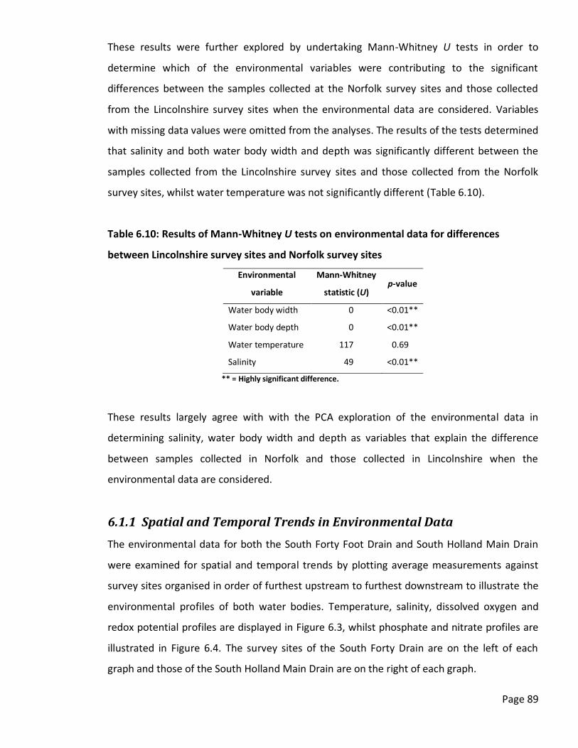
Page 89
These results were further explored by undertaking Mann-Whitney U tests in order to
determine which of the environmental variables were contributing to the significant
differences between the samples collected at the Norfolk survey sites and those collected
from the Lincolnshire survey sites when the environmental data are considered. Variables
with missing data values were omitted from the analyses. The results of the tests determined
that salinity and both water body width and depth was significantly different between the
samples collected from the Lincolnshire survey sites and those collected from the Norfolk
survey sites, whilst water temperature was not significantly different (Table 6.10).
Table 6.10: Results of Mann-Whitney U tests on environmental data for differences
between Lincolnshire survey sites and Norfolk survey sites
Environmental
variable
Mann-Whitney
statistic (U) p-value
Water body width 110 <0.01**
Water body depth 110 <0.01**
Water temperature 117 0.69**
Salinity 149 <0.01**
** = Highly significant difference.
These results largely agree with with the PCA exploration of the environmental data in
determining salinity, water body width and depth as variables that explain the difference
between samples collected in Norfolk and those collected in Lincolnshire when the
environmental data are considered.
6.1.1 Spatial and Temporal Trends in Environmental Data
The environmental data for both the South Forty Foot Drain and South Holland Main Drain
were examined for spatial and temporal trends by plotting average measurements against
survey sites organised in order of furthest upstream to furthest downstream to illustrate the
environmental profiles of both water bodies. Temperature, salinity, dissolved oxygen and
redox potential profiles are displayed in Figure 6.3, whilst phosphate and nitrate profiles are
illustrated in Figure 6.4. The survey sites of the South Forty Drain are on the left of each
graph and those of the South Holland Main Drain are on the right of each graph.

Page 90
Figure 6.3: Temperature (A), dissolved oxygen (B), redox potential (C) and salinity (D) profiles of the South
Forty Foot Drain (SF) and South Holland Main Drain (SH). Graphs are arranged with South Forty Foot Drain
survey sites (SFx) on the left and South Holland Main Drain survey sites (SHx) on the right, with survey sites
arranged in order of furthest upstream to furthest downstream. See Table 5.1 for site code definitions.
Figure 6.4: Phosphate (PO4) and nitrate (NO3) profiles of the South Forty Foot Drain and South Holland Main
Drain. Graph is arranged with South Forty Foot Drain survey sites (SFx) on the left and South Holland Main
Drain survey sites (SHx) on the right, with survey sites arranged in order of furthest upstream to furthest
downstream. See Table 5.1 for site code definitions.
5
10
15
20
25
30
SF1 SF2 SF3 SF4 SH1 SH2 SH3 SH4Te
mp
era
ture
(°C
)
Site code
A: Temperature profile of SF and SH
0
5
10
15
20
25
30
35
SF1 SF2 SF3 SF4 SH1 SH2 SH3 SH4
Dis
solv
ed
oxy
gen
(m
gL-1
)
Site code
B: Dissolved oxygen profile of SF and SH
-250
-200
-150
-100
-50
0
50
100
150
200
SF1 SF2 SF3 SF4 SH1 SH2 SH3 SH4
Re
do
x p
ote
nti
al (
mV
)
Site code
C: Redox potential profile of SF and SH
0
2
4
6
8
10
12
14
16
18
20
SF1 SF2 SF3 SF4 SH1 SH2 SH3 SH4
Salin
ity
(PSU
)
Site code
D: Salinity profile of SF and SH
0.0
0.5
1.0
1.5
2.0
2.5
3.0
3.5
4.0
0.0
0.5
1.0
1.5
2.0
2.5
3.0
3.5
4.0
SF1 SF2 SF3 SF4 SH1 SH2 SH3 SH4
Nit
rate
co
nce
ntr
atio
n (
mgL
-1)
Ph
osp
hat
e c
on
cen
trat
ion
(m
gL-1
)
Site code
Phosphate Nitrate

Page 91
Temperature remained relatively consistent along both the South Forty Foot Drain
and the South Holland Main Drain in all seasons (Figure 6.3A). The one exception was the
South Holland Main Drain in summer, where temperature increased between the SH1
(Weston Fen) and the SH4 (Nene Outfall Sluice) survey sites. Furthermore, there were
distinct differences shown in the temperature profiles of both drains between the different
seasons, with summer temperatures highest and spring temperatures lowest. The dissolved
oxygen profiles of the South Forty Foot Drain and South Holland Main Drain vary both
between the water bodies and seasonally (Figure 6.3B). The South Holland Main Drain
appeared to experience greater variation in dissolved oxygen concentration between the
seasons than the South Forty Foot Drain. The large peak in dissolved oxygen concentration at
SH3 (A1101 Road Bridge) in autumn may have resulted from the release of fresh water into
the South Holland Main Drain by the Environment Agency and South Holland Internal
Drainage Board in June 2011 in response to reports of dead fish (Environment Agency,
2012b). The redox potential profiles of the South Forty Foot Drain and South Holland Main
Drain show considerable differences both seasonally and between the two water bodies
(Figure 6.3C). The only increasing gradient in redox potential along either drain was recorded
in summer for the South Holland Main Drain.
A narrow range of salinity concentrations were recorded at the survey sites of the
South Forty Foot Drain in spring (Figure 6.3D), from 0.56PSU at the SF1 (Casswell’s Bridge)
survey site to 0.86PSU at the SF2 (Donington Bridge) site. The decrease in salinity between
the SF2 (Donington Bridge) survey site and the SF3 (Swineshead Bridge) site, from 0.86PSU to
0.70PSU, may be due to a diluting freshwater inflow from the North Beck watercourse
entering the South Forty Foot Drain between these two sites. Similarly, the decrease in
salinity concentration from 0.70PSU at the SF3 (Swineshead Bridge) site to 0.66PSU at the
SF4 (Wyberton Chain Bridge) survey site may also result from a diluting freshwater inflow,
originating from either or both of Skerth Drain or Clay Dike, entering the main watercourse
between these two sites. The salinity concentration of the South Forty Foot Drain in summer
ranged from 0.53PSU at the SF2 (Donington Bridge) site to 4.84PSU at the SF4 (Wyberton
Chain Bridge) site. A small decrease in salinity from 0.69PSU to 0.53PSU between the SF1
(Casswell’s Bridge) and the SF2 (Donington Bridge) survey sites was recorded in summer.

Page 92
This decrease may have resulted from an input of fresh water, originating from one or more
of the eight inflowing drains between the two survey sites, diluting the concentration of salts
held in the water of the South Forty foot Drain. In contrast to spring and summer, the South
Forty Foot Drain in autumn showed a consistent increase in salinity between each survey site
(Figure 6.3D), increasing from 0.50PSU at the SF1 (Casswell’s Bridge) site to 10.90PSU at the
SF4 (Wyberton Chain Bridge) site.
The South Holland Main Drain showed a consistent increase in salinity between each
survey site in spring (Figure 6.3D), increasing from 2.14PSU at the SH1 (Weston Fen) site to
3.82PSU at the SH4 (Nene Outfall Sluice) site. Figure 6.3D, however, indicates that the SH4
(Nene Outfall Sluice) survey site was less saline than the SH3 (A1101 Road Bridge) site in
summer (8.11PSU at SH3, 6.17PSU at SH4) and autumn (13.36PSU at SH3, 9.27PSU at SH4).
This is most likely a result of the fact that it was not possible to collect environmental
measurements from the centre of the channel at the SH4 (Nene Outfall Sluice) survey site
due to safety concerns. Salinity can be expected to be greatest at the base of the centre of
the channel due to halo-stratification (Dyer, 1973; Davidson et al., 1991).Thus it is believed
that the SH4 (Nene Outfall Sluice) survey site would have recorded a higher salinity
concentration than the SH3 (A1101 Road Bridge) site if environmental data could have been
collected from the centre of the channel. Alternatively, the decrease in salinity concentration
between the SH3 (A1101 Road Bridge and the SH4 (Nene Outfall Sluice) survey sites may
have resulted from an inflow of fresh water, decreasing the salinity at the latter site. The
Environment Agency implemented such an action to decrease salinity in the South Holland
Main Drain in June 2011 in response to reports of dead fish (Environment Agency, 2012b).
It can be seen from Figure 6.3D that salinity was affected by season and that,
generally, salinity concentration was greatest in autumn. This is to be expected as increased
air temperature and decreased rainfall during spring and summer results in a decrease in the
volume of water (Pillsbury, 1981; Goetsch & Palmer, 1997; Wolf et al., 2009) thereby
concentrating the salts present in the water. Figure 6.3D also shows that salinity remained at
a relatively similar concentration at the SF1 (Casswell’s Bridge) and SF2 (Donington Bridge)
survey sites between the three surveyed seasons. Salinity varied between 0.50PSU and
0.69PSU at the SF1 (Casswell’s Bridge) site across the three seasons, whilst the SF2
(Donington Bridge) site recorded salinity concentrations between 0.53PSU and 0.97PSU.

Page 93
In contrast, the SF3 (Swineshead Bridge) and SF4 (Wyberton Chain Bridge) survey sites both
recorded substantial increases in salinity concentration between spring and summer, as well
as between summer and autumn. The SF3 (Swineshead Bridge) site showed an increase in
salinity of 3.74PSU between the spring and summer surveys, and an increase of 5.31PSU
between the summer and autumn surveys. The SF4 (Wyberton Chain Bridge) site increased in
water salinity by 4.18PSU between spring and summer, whilst an increase in salinity of
6.07PSU was recorded between summer and autumn. In contrast, three of the four survey
sites of the South Holland Main Drain showed wide variations in salinity concentration
between the three seasons. Only the SH1 (Weston Fen) survey site showed a narrow range of
salinity concentrations, varying between 0.45PSU and 2.14PSU. The SH2 (Clifton’s Bridge) site
showed a small increase in salinity of 1.73PSU between spring and summer, followed by a
large increase of 8.88PSU between summer and autumn. Large increases in salinity were also
recorded at the SH3 (A1101 Road Bridge) survey site, which showed an increase of 4.30PSU
between spring and summer, as well as an increase of 5.25PSU between summer and
autumn. The SH4 (Nene Outfall Sluice) survey site experienced an increase in salinity of
2.34PSU between spring and summer, as well as an increase of 3.10PSU between summer
and autumn. Thus, a range of salinities was experienced by the macro-invertebrate
communities present at each of the surveyed sites.
Phosphate (PO4) and nitrate (NO3) measurements were only collected during the
autumn 2011 season. Both phosphate and nitrate showed variation along the South Forty
Foot Drain and the South Holland Main Drain (Figure 6.4). Despite both water bodies being
drainage channels, the South Forty Foot Drain and South Holland Main Drain appear to be
dissimilar in terms of nitrate and phosphate profiles. Figure 6.4 illustrates that phosphate
increased at a greater rate along the profile of the South Forty Foot Drain, whilst nitrate
varied much more along the South Holland Main Drain.
Overall, these data show that the Salinity Association Group index is being tested with
data collected from linearly-connected sites which provide a range of conditions within a
salinity concentration range from 0.50PSU to 13.71PSU with unrestricted aquatic movement
possible between the sites along the individual drains.

Page 94
As such, macro-invertebrate taxa were able to colonise in response to water conditions
within each season through such vectors as upstream and downstream migration (drift),
vertical movements from within the substrate and aerial sources such as oviposition by flying
adult life stages (Williams & Hynes, 1976). Further vectors of colonisation include accidental
or deliberate releases (Grigorovich et al., 2002) or via internal or external transport by birds
(Green & Figuerola, 2005).
The environmental data for the survey sites located in Norfolk were examined by
plotting average measurements for temperature, salinity, phosphate and nitrate in Figure
6.5, whilst the dissolved oxygen and redox potential measurements for the Norfolk survey
sites in summer are presented in Figure 6.6.
Figure 6.5 and Figure 6.6 show that the environmental condition of the water at the
survey sites varied both seasonally and between the sites, showing that the macro-
invertebrate community samples were collected from a wide range of environmental
conditions. For example, salinity concentration in spring varied between 0.33PSU at the
Buckenham Marsh survey site and 19.88PSU at the Long Dyke site. The same survey sites
recorded the lowest and highest salinity concentrations in summer (Figure 6.5D).
Nitrate was consistently low during the spring surveys at the Norfolk survey sites,
with the Rockland Marsh survey site recording a nitrate concentration of 0.30mgL-1 and no
other survey site recording a nitrate concentration. Whilst nitrate concentrations generally
increased during the summer surveys, four of the survey sites that did not record a nitrate
concentration during the spring surveys also did not record a nitrate concentration in
summer (the Long Dyke, Middle Marsh, Near Dry Dyke and Ludham Marsh survey sites). The
highest nitrate concentration recorded during the summer surveys was 3.34mgL-1 at the
Hatchet Marsh survey site.
A range of phosphate concentrations were recorded at the Norfolk survey sites. No
phosphates were detected at the Long Dyke and Hatchet Marsh survey sites in spring, whilst
the highest phosphate concentration recorded in spring was 1.88mgL-1 at the Buckenham
Marsh survey site. The highest phosphate concentration recorded in summer was 1.09mgL-1
at the Rockland Marsh site, whereas the lowest phosphate concentration was 0.28mgL-1 at
the Hatchet Marsh survey site.

Page 95
Figure 6.5: Temperature (A), phosphate (B), nitrate (C) and salinity (D) measurements collected from the
Norfolk survey sites. See Table 5.1 for site code definitions.
Figure 6.6: Dissolved oxygen and redox potential measurements collected from the Norfolk survey sites. See
Table 5.1 for site code definitions.
5
10
15
20
25
30
BM LM ND HM RM SM MM LD
Tem
pe
ratu
re (°
C)
SIite code
A: Temperature measurements
0.0
0.5
1.0
1.5
2.0
2.5
3.0
3.5
4.0
BM LM ND HM RM SM MM LDPh
osp
hat
e c
on
cen
trat
ion
(m
gL-1
)
Site code
B: Phosphate measurements
0.0
0.5
1.0
1.5
2.0
2.5
3.0
3.5
4.0
BM LM ND HM RM SM MM LD
Nit
rate
co
nce
ntr
atio
n (
mgL
-1)
Site code
C: Nitrate measurements
0
2
4
6
8
10
12
14
16
18
20
BM LM ND HM RM SM MM LD
Salin
ity
(PSU
)
Site code
D: Salinity measurements
-250
-200
-150
-100
-50
0
50
100
150
200
0.00
5.00
10.00
15.00
20.00
25.00
30.00
35.00
BM LM ND HM RM SM MM LD
Re
do
x p
ote
nti
al (
mV
)
Dis
solv
ed
oxy
gen
(m
gL-1
)
Site code
Dissolved oxygen Redox potential

Page 96
Thus, the potential influence of phosphate on the Salinity Association Group (SAG) index can
be fully explored using the range of phosphate concentrations recorded at the Norfolk survey
sites. Furthermore, the data collected from the Norfolk survey sites can be used to test the
SAG index in a significantly different habitat type and geographic region from the
Lincolnshire survey sites (see Section 6.1).
6.2 Macro-invertebrate Data
A total of 25901 specimens were identified to 162 taxa (136 species, eight genera and 18
families) during the analysis of the macro-invertebrate samples. Analysis of the macro-
invertebrate community samples collected at the survey sites in Lincolnshire yielded 18453
specimens identified to 112 taxa (94 species, six genera and 12 families). Analysis of the
samples collected from the survey sites in Norfolk resulted in the identification of 7448
specimens to 101 taxa (84 species, six genera and 11 families). The macro-invertebrate
community data for the survey sites in Lincolnshire are summarised by the application of
various diversity and water quality measures in Table 6.11 (see Appendix 9 for complete
table of macro-invertebrate data), whilst the macro-invertebrate community data for the
survey sites in Norfolk are summarised in Table 6.12 (see Appendix 10 for complete tables of
macro-invertebrate data).
Cluster analysis of fourth root transformed macro-invertebrate data, undertaken to
reveal similarity between samples (Kay et al., 2001; Carlsson, 2006; Akbulut et al., 2009) in
terms of the macro-invertebrate taxa present (Lancaster & Scudder, 1987; Kay et al., 2001;
Velasco et al., 2006; Rawson et al., 2010), revealed that few samples showed a similarity of
greater than 70% (Figure 6.7) and consequently indicating a relatively high degree of
variation in the macro-invertebrate samples. The samples collected at the LD (Long Dyke)
survey site in spring and summer showed a similarity greater than 85%, whilst the samples
collected during the summer surveys at the SH3 and SH4 survey sites showed a similarity
greater than 70%. A cut-off at 40% similarity resulted in six clusters of two or more samples
and two outlying samples not connected to a cluster (Figure 6.7).

Page 97
Table 6.11: Summarised macro-invertebrate data for Lincolnshire survey sites
Seas
on
Biological measure Survey site code
SF1 SF2 SF3 SF4 SH1 SH2 SH3 SH4
Spri
ng
(201
0)
Taxon richness 24 35 27 22 22 7 10 10
Number of individuals 320 240 741 68 269 199 67 54
Margalef richness index 3.99 6.20 3.94 4.98 3.75 1.13 2.14 2.26
Shannon diversity index 2.02 2.66 2.30 2.45 2.35 0.61 1.70 1.65
Berger-Parker dominance index 0.45 0.22 0.24 0.32 0.25 0.84 0.37 0.46
Simpson dominance index 0.76 0.89 0.86 0.85 0.86 0.28 0.76 0.72
Evenness 0.31 0.41 0.37 0.53 0.48 0.26 0.55 0.52
ASPTBMWP 4.35 4.42 4.07 4.31 4.29 3.50 3.50 4.00
Sum
mer
(20
10)
Taxon richness 32 35 38 25 29 10 8 10
Number of individuals 901 730 829 877 1306 206 218 389
Margalef richness index 4.56 5.16 5.51 3.54 3.90 1.69 1.30 1.51
Shannon diversity index 2.07 2.36 2.28 1.93 1.77 1.62 1.07 0.76
Berger-Parker dominance index 0.49 0.25 0.28 0.40 0.41 0.38 0.57 0.82
Simpson dominance index 0.74 0.86 0.84 0.75 0.74 0.75 0.56 0.32
Evenness 0.25 0.30 0.26 0.27 0.20 0.51 0.36 0.21
ASPTBMWP 4.53 4.73 4.63 4.46 4.50 3.33 3.67 3.67
Au
tum
n (2
011)
Taxon richness 24 29 9 8 29 6 7 8
Number of individuals 272 446 192 3367 606 559 3538 2059
Margalef richness index 4.10 4.59 1.52 0.86 4.37 0.79 0.73 0.92
Shannon diversity index 2.30 2.20 0.81 0.32 2.43 1.08 0.45 0.44
Berger-Parker dominance index 0.22 0.24 0.79 0.91 0.22 0.60 0.90 0.91
Simpson dominance index 0.86 0.84 0.36 0.16 0.88 0.57 0.19 0.18
Evenness 0.42 0.31 0.25 0.17 0.39 0.49 0.23 0.19
ASPTBMWP 4.59 4.82 5.00 3.80 4.39 3.67 3.67 4.00
See Table 5.1 for site code definitions.

Page 98
Table 6.12: Summarised macro-invertebrate data for Norfolk survey sites
Seas
on
Biological measure Survey site code
BM LM ND HM RM SM MM LD
Spri
ng
(201
1)
Taxon richness 25 26 22 23 34 30 20 4
Number of individuals 278 194 181 166 395 529 563 369
Margalef richness index 4.27 4.75 4.04 4.30 5.52 4.62 3.00 0.51
Shannon diversity index 2.69 2.71 2.26 2.42 2.54 2.18 1.67 0.98
Berger-Parker dominance index 0.14 0.17 0.31 0.24 0.24 0.38 0.38 0.60
Simpson dominance index 0.91 0.91 0.84 0.87 0.88 0.81 0.74 0.57
Evenness 0.59 0.58 0.44 0.49 0.37 0.30 0.27 0.67
ASPTBMWP 4.18 4.19 4.47 4.47 4.50 4.39 4.42 4.39
Sum
mer
(20
11)
Taxon richness 26 42 33 39 24 27 19 3
Number of individuals 693 919 543 388 530 311 820 569
Margalef richness index 3.82 6.01 5.08 6.38 3.67 4.53 2.68 0.32
Shannon diversity index 1.59 2.01 2.45 2.78 2.45 1.97 1.65 1.02
Berger-Parker dominance index 0.61 0.52 0.32 0.24 0.23 0.49 0.40 0.47
Simpson dominance index 0.61 0.71 0.85 0.89 0.88 0.73 0.74 0.62
Evenness 0.19 0.18 0.35 0.42 0.48 0.27 0.27 0.93
ASPTBMWP 4.06 4.90 4.53 5.10 3.67 4.87 4.45 4.08
See Table 5.1 for site code definitions.
The similarity of the macro-invertebrate communities between samples were further
analysed using Non-metric MultiDimensional Scaling (NMDS) based on the Bray-Curtis
similarity measure (Bray & Curtis, 1957). The clusters of the macro-invertebrate samples
defined by the cluster analysis at 40% similarity are highlighted in the ordination plot
resulting from the NMDS analysis of macro-invertebrate data (Figure 6.8) by differing
symbols and polygons of different colours, as summarised in Table 6.13.

Page 99
Figure 6.7: Cluster analysis dendrogram of samples based on fourth-root transformed macro-invertebrate
data (Unweighted Pair-Group Method using arithmetic Averages (UPGMA) algorithm, Bray-Curtis similarity
measure). Cophentic correlation coefficient (CC) of dendrogram = 0.89. See Table 5.1 and Table 5.2 in Section
5 for sample code definitions.
Table 6.13: Symbols and colours representing clusters in non-metric multidimensional
scaling ordination plot
Cluster Symbol Colour
1 Hollow Diamond () Green
2 Asterisk () Dark blue
3 Hollow circle () Violet
4 Diagonal cross (X) Orange
5 Hollow square () Pale blue
6 Upright cross () Red
Outlying samples Filled circle () Black
0.1
0.2
0.3
0.4
0.5
0.6
0.7
0.8
0.9
1.0
Similarity
SF1-SPRSF1-AUTSF2-SPRSF1-SUMSF2-SUMSF2-AUTSH1-SPRSH1-AUTSH1-SUMSF3-SPRSF3-SUMSF4-SUMND-SPRSM-SPRSM-SUMRM-SUMND-SUMLM-SUMRM-SPRHM-SUMLM-SPRBM-SPRBM-SUMHM-SPRMM-SPRMM-SUMSF3-AUTSF4-AUTSF4-SPRSH2-AUTSH3-AUTSH4-AUTLD-SPRLD-SUMSH2-SUMSH3-SUMSH4-SUMSH3-SPRSH2-SPRSH4-SPR
3
1
1
1
2
1
4
1
5
1
6
1

Page 100
Figure 6.8: Non-metric multidimensional scaling ordination plot of samples based on fourth-root transformed
macro-invertebrate data (Bray-Curtis similarity measure). Clusters of samples defined by the cluster analysis
at 40% similarity are highlighted by differing symbols and polygons of different colours. Stress level of
ordination plot = 0.14. See Table 5.1 and Table 5.2 in Section 5 for sample code definitions.
A one-way ANalysis Of SIMilarity (ANOSIM; Clarke & Green, 1988; Clarke, 1993) using the
Bray-Curtis similarity measure (Bray & Curtis, 1957) and run using 10000 permutations was
used on fourth root transformed macro-invertebrate data to test if the six clusters identified
by the cluster analysis and NMDS were significantly different. The results of the analysis
showed that there is a highly significant difference between the six clusters defined by the
cluster analysis and NMDS (ANOSIM, R=0.87, p<0.01). The results of post-hoc pairwise
ANOSIM tests between all pairs of clusters (Table 6.14) show that all clusters were
significantly different from each other, except when cluster 3 and cluster 4 were examined.
SH2-SPR SH3-SPR SH4-SPR
SH2-SUM
SH3-SUM
SH4-SUM
SH2-AUT SH3-AUT
SH4-AUT
LD-SPR
LD-SUM
SF4-SPR
SF3-AUT
SF4-AUT
MM-SPR MM-SUM
HM-SPR
SF1-SPR
SF1-AUT
SF2-SPR
SF1-SUM
SF2-SUM
SF2-AUT
SH1-SPR SH1-AUT
SH1-SUM
SF3-SPR SF3-SUM
SF4-SUM
ND-SPR
SM-SPR SM-SUM
RM-SUM
ND-SUM
LM-SUM RM-SPR
HM-SUM
LM-SPR
BM-SPR
BM-SUM
-0.30 -0.25 -0.20 -0.15 -0.10 -0.05 0.00 0.05 0.10 0.15 0.20
Coordinate 1
-0.20
-0.16
-0.12
-0.08
-0.04
0.00
0.04
0.08
0.12
0.16
0.20
Co
ord
inat
e 2

Page 101
Table 6.14: P-values of post-hoc pairwise ANOSIM tests between all pairs of clusters
defined by cluster analyses of macro-invertebrate data
Cluster number
1 2 3 4 5
Clu
ster
nu
mb
er
2 <0.01**
3 <0.01** <0.05**
4 <0.01** <0.05** 0.34**
5 <0.01** <0.01** <0.05** <0.05**
6 <0.01** <0.01** <0.05** <0.05** <0.01**
* = Significant difference, ** = Highly significant difference.
Summary statistics (mean average, standard deviation and range) for the environmental
variables associated with the samples of each cluster are shown in Table 6.15, whilst the
samples associated with each cluster are listed in Table 6.16.
Table 6.15: Summary statistics of environmental variables for each cluster defined by
clustering analyses
Environmental variable Cluster (number of samples in cluster)
1 (n =14) 2 (n = 9) 3 (n = 2) 4 (n = 2) 5 (n = 5) 6 (n = 6)
Water body width
(m)
Average (± 1 SD) 6.27 (±6.75) 10.00 (±1.73) 2.80 (±0.00) 19.00 (±1.41) 16.60 (±13.77) 26.00 (±6.20)
Range (min - max) 1.60 - 20.00 8.00 - 12.00 2.80 - 2.80 18.00 - 20.00 2.50 - 30.00 18.00 - 30.00
Water body depth
(m)
Average (± 1 SD) 1.00 (±0.83) 1.20 (±0.57) 0.28 (±0.00) 2.65 (±0.49) 1.70 (±1.31) 2.50 (±0.49)
Range (min - max) 0.30 - 2.50 0.50 - 1.80 0.28 - 0.28 2.30 - 3.00 0.30 - 3.10 1.80 - 3.10
Water temperature
(°C)
Average (± 1 SD) 17.82 (±3.72) 13.73 (±5.14) 17.81 (±5.64) 13.49 (±0.23) 14.84 (±2.85) 16.23 (±6.84)
Range (min - max) 9.20 - 22.90 8.26 - 21.21 13.82 - 21.80 13.33 - 13.65 13.00 - 19.90 9.96 - 24.14
Salinity
(PSU)
Average (± 1 SD) 1.09 (±1.56) 0.87 (±0.53) 2.82 (±0.81) 10.33 (±0.81) 14.17 (±3.80) 4.97 (±1.87)
Range (min - max) 0.14 - 4.84 0.45 - 2.14 2.25 - 3.40 9.76 - 10.90 9.27 - 19.88 3.10 - 8.11
Dissolved oxygen
(mgL-1
)
Average (± 1 SD) 10.18 (±9.55) 9.24 (±2.48) N/A 8.44 (±1.62) 11.01 (±9.53) 11.28 (±3.60)
Range (min - max) 1.79 - 31.70 5.84 - 13.37 N/A 7.30 - 9.59 4.83 - 25.19 6.51 - 16.81
Redox potential
(mV)
Average (± 1 SD) -37.36 (±141.70) 78.80 (±61.98) N/A -22.99 (±45.16) 70.60 (±64.89) 128.97 (±47.92)
Range (min - max) -219.90 - 161.18 -6.98 - 168.54 N/A -54.92 - 8.94 -26.20 - 112.46 45.00 - 185.04
Phosphate
(mgL-1
)
Average (± 1 SD) 0.79 (±0.53) 0.41 (±0.71) 0.67 (±0.12) 3.14 (±0.30) 0.48 (±0.33) N/A
Range (min - max) 0.28 - 1.88 0.00 - 1.23 0.58 - 0.75 2.92 - 3.35 0.00 - 0.86 N/A
Nitrate
(mgL-1
)
Average (± 1 SD) 0.72 (±1.09) 0.59 (±0.22) 0.00 (N/A) 0.62 (±0.87) 0.83 (±0.98) N/A
Range (min - max) 0.00 - 3.34 0.44 - 0.84 0.00 - 0.00 0.00 - 1.23 0.00 - 2.24 N/A
Individual samples not associated to a cluster were omitted.
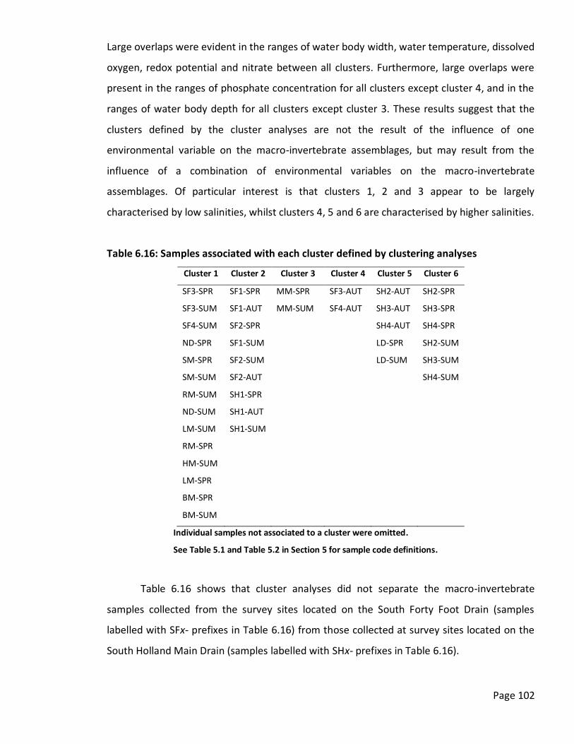
Page 102
Large overlaps were evident in the ranges of water body width, water temperature, dissolved
oxygen, redox potential and nitrate between all clusters. Furthermore, large overlaps were
present in the ranges of phosphate concentration for all clusters except cluster 4, and in the
ranges of water body depth for all clusters except cluster 3. These results suggest that the
clusters defined by the cluster analyses are not the result of the influence of one
environmental variable on the macro-invertebrate assemblages, but may result from the
influence of a combination of environmental variables on the macro-invertebrate
assemblages. Of particular interest is that clusters 1, 2 and 3 appear to be largely
characterised by low salinities, whilst clusters 4, 5 and 6 are characterised by higher salinities.
Table 6.16: Samples associated with each cluster defined by clustering analyses
Cluster 1 Cluster 2 Cluster 3 Cluster 4 Cluster 5 Cluster 6
SF3-SPR SF1-SPR MM-SPR SF3-AUT SH2-AUT SH2-SPR
SF3-SUM SF1-AUT MM-SUM SF4-AUT SH3-AUT SH3-SPR
SF4-SUM SF2-SPR
SH4-AUT SH4-SPR
ND-SPR SF1-SUM
LD-SPR SH2-SUM
SM-SPR SF2-SUM
LD-SUM SH3-SUM
SM-SUM SF2-AUT
SH4-SUM
RM-SUM SH1-SPR
ND-SUM SH1-AUT
LM-SUM SH1-SUM
RM-SPR
HM-SUM
LM-SPR
BM-SPR
BM-SUM
Individual samples not associated to a cluster were omitted.
See Table 5.1 and Table 5.2 in Section 5 for sample code definitions.
Table 6.16 shows that cluster analyses did not separate the macro-invertebrate
samples collected from the survey sites located on the South Forty Foot Drain (samples
labelled with SFx- prefixes in Table 6.16) from those collected at survey sites located on the
South Holland Main Drain (samples labelled with SHx- prefixes in Table 6.16).

Page 103
Furthermore, the cluster analysis also did not separate the macro-invertebrate samples
collected in different seasons (samples labelled with suffixes -SPR for spring, -SUM for
summer and -AUT for autumn in Table 6.16). A two-way ANOSIM, however, found a highly
significant difference between the macro-invertebrate samples collected from the survey
sites located on the South Forty Foot Drain and those collected at survey sites located on the
South Holland Main Drain (ANOSIM, R=0.44, p<0.01), but no significant difference resulting
from differences in seasonality when only macro-invertebrate data for the survey sites in
Lincolnshire were considered (ANOSIM, R=0.11, p=0.12). Macro-invertebrate samples
collected from the survey sites in Norfolk were omitted from the analysis as no data were
collected at these sites for the autumn season and the cluster analyses suggested a
difference between the macro-invertebrate data for the collected at the sites within
Lincolnshire and those collected at the sites located within Norfolk. A one-way ANOSIM
found no significant difference between the spring and summer seasons when only macro-
invertebrate data for the survey sites in Norfolk were considered (ANOSIM, R=-0.04, p=0.68).
The clusters defined by the cluster analyses are largely composed of samples
collected at either survey sites located within Lincolnshire or those located within Norfolk.
Only cluster 1 and cluster 5 are composed of samples collected from survey sites within both
Lincolnshire and Norfolk (Table 6.16). This suggests that the difference between the survey
sites in Lincolnshire and those in Norfolk, and thus the associated differences in habitat
structure and water quality found by PCA and subsequent tests by NPMANOVA of the
environmental variables (see Section 6.1), may be a major factor influencing the macro-
invertebrate assemblages of the survey sites. A one-way ANOSIM found a highly significant
difference between the macro-invertebrate assemblages for the survey sites in Lincolnshire
and those in Norfolk (ANOSIM, R=0.25, p<0.01). Data collected for the autumn season at
survey sites within Lincolnshire were omitted as no comparable data were collected for the
same season at the survey sites located within Norfolk.
The significant difference between the macro-invertebrate assemblages of the survey
sites located on the South Forty Foot Drain and those of the survey sites of the South Holland
Main Drain is unexpected given that no signficant difference was found when the associated
environmental data for these samples were similarly examined (see Section 6.1).

Page 104
As such, these results suggest that the difference between the macro-invertebrate
assemblages of the survey sites for these two water bodies may occur due to a difference in
one or more unmeasured environmental variables between the two water bodies. In
contrast, the significant difference between the macro-invertebrate assemblages of the
survey sites located within Lincolnshire and those of the survey sites located in Norfolk most
likely results from the significant differences found when the environmental variables when
the associated environmental data for these samples were similarly examined (see Section
6.1). As such, it appears that the data collected from the survey sites in Lincolnshire and
those in Norfolk form two distinct datasets differing in terms of habitat structure and water
quality with which to examine the proposed salinity index at sites.
6.2.1 Spatial and Temporal Trends in Macro-invertebrate Data
Spatial and temporal trends in the macro-invertebrate communities of the South Forty Foot
Drain and South Holland Main Drain were investigated by plotting untransformed diversity
and water quality measures (taxon richness, number of individuals, Margalef richness index,
Shannon diversity index, Berger-Parker and Simpson dominance indices, evenness and
ASPTBMWP index) against the survey sites for both the South Forty Foot Drain and South
Holland Main Drain. The survey sites were arranged in order of furthest upstream to furthest
downstream, with the survey sites of the South Forty Foot Drain on the left of each graph
and those of the South Holland Main Drain on the right of each graph (Figure 6.9).
Many of the macro-invertebrate diversity and water quality indices showed similar
profiles and were found to be significantly correlated with each other when examined using
Spearman’s rank order correlation coefficient (rs), as indicated in Table 6.17. For example,
taxon richness, the Margalef richness index and the ASPTBMWP index were all significantly
correlated with each other in each season (Table 6.17). The Margalef richness index was also
significantly correlated with both the Shannon diversity index and Simpson dominance index
when data for the spring and summer season were considered (Table 6.17). Furthermore, the
Shannon diversity index, Simpson dominance index and Berger-Parker dominance index were
also all significantly correlated with each other in each season (Table 6.17).

Page 105
Figure 6.9: Taxon richness (A), number of individuals (B), Margalef richness index (C), Shannon diversity index
(D), Berger-Parker dominance index (E), Simpson dominance index (F), evenness (G) and ASPTBMWP index (H)
profiles of the South Forty Foot Drain (SF) and South Holland Main Drain (SH). Graphs are arranged with
South Forty Foot Drain survey sites (SFx) on the left and South Holland Main Drain survey sites (SHx) on the
right, with survey sites arranged in order of furthest upstream to furthest downstream. See Table 5.1 in
Section 5 for site code definitions.
0
5
10
15
20
25
30
35
40
45
SF1 SF2 SF3 SF4 SH1 SH2 SH3 SH4
Taxo
n r
ich
ne
ss
Site code
A: Taxon richness profile of SF and SH
0
500
1000
1500
2000
2500
3000
3500
SF1 SF2 SF3 SF4 SH1 SH2 SH3 SH4
Nu
mb
er
of
ind
ivid
ual
s
Site code
B: Number of individuals profile of SF and SH
0.0
1.0
2.0
3.0
4.0
5.0
6.0
7.0
SF1 SF2 SF3 SF4 SH1 SH2 SH3 SH4
Mar
gale
f ri
chn
ess
ind
ex
Site code
C: Margalef richness index profile of SF and SH
0.0
0.5
1.0
1.5
2.0
2.5
3.0
SF1 SF2 SF3 SF4 SH1 SH2 SH3 SH4
Shan
no
n d
ive
rsit
y in
de
x
Site code
D: Shannon diversity index profile of SF and SH
0.0
0.1
0.2
0.3
0.4
0.5
0.6
0.7
0.8
0.9
1.0
SF1 SF2 SF3 SF4 SH1 SH2 SH3 SH4Be
rge
r-P
arke
r d
om
inan
ce in
de
x
Site code
E: Berger-Parker dominance index profile of SF and SH
0.0
0.1
0.2
0.3
0.4
0.5
0.6
0.7
0.8
0.9
1.0
SF1 SF2 SF3 SF4 SH1 SH2 SH3 SH4
Sim
pso
n d
om
inan
ce in
de
x
Site code
F: Simpson dominance index profile of SF and SH
0.0
0.1
0.2
0.3
0.4
0.5
0.6
0.7
0.8
0.9
1.0
SF1 SF2 SF3 SF4 SH1 SH2 SH3 SH4
Eve
nn
ess
Site code
G: Evenness profile of SF and SH
0.0
1.0
2.0
3.0
4.0
5.0
6.0
SF1 SF2 SF3 SF4 SH1 SH2 SH3 SH4
ASP
T BM
WP
ind
ex
Site code
H: ASPTBMWP index profile of SF and SH

Page 106
Table 6.17: Spearman’s rank order correlation coefficient (rs) and p-values resulting from
tests between macro-invertebrate diversity and water quality indices for data collected at
survey sites in Lincolnshire
Taxo
n
rich
nes
s
Nu
mb
er o
f
ind
ivid
ual
s
Shan
no
n d
iver
sity
ind
ex
Sim
pso
n
do
min
ance
ind
ex
Even
nes
s
Mar
gale
f ri
chn
ess
ind
ex
Ber
ger-
Par
ker
do
min
ance
ind
ex
ASP
T BM
WP
Taxon richness
-<0.08** -<0.05** -<0.05** -<0.69** -<0.01** -<0.05** -<0.05**
-<0.14** -<0.01** -<0.06** -<0.45** -<0.01** -<0.08** -<0.01**
-<0.25** -<0.10** -<0.10** -<0.69** -<0.01** -<0.10** -<0.05**
Number of
individuals
<-0.68**
-<0.39** -<0.17** -<0.08** -<0.36** -<0.22** -<0.26**
<-0.58** -<0.24** -<0.70** -<0.05** -<0.17** -<0.98** -<0.13**
<-0.47** -<0.17** -<0.17** -<0.13** -<0.13** -<0.17** -<0.05**
Shannon diversity
index
<-0.80** -<0.36**
-<0.01** -<0.58** -<0.01** -<0.01** -<0.05**
<-0.91** <-0.45** -<0.05** -<0.98** -<0.01** -<0.05** -<0.01**
<-0.64** <-0.55** -<0.01** -<0.05** -<0.07** -<0.01** -<0.32**
Simpson
dominance index
<-0.86** -<0.55** <-0.93**
-<0.84** -<0.05** -<0.01** -<0.05**
<-0.70** <-0.14** <-0.83** -<0.46** -<0.05** -<0.01** -<0.12**
<-0.64** <-0.55** <-1.00** -<0.05** -<0.07** -<0.01** -<0.32**
Evenness
<-0.17** <-0.64** <-0.21** <-0.07**
-<0.98** -<0.67** -<0.76**
<-0.31** <-0.74** <-0.02** <-0.31** -<0.54** -<0.36** -<0.47**
<-0.17** <-0.57** <-0.83** <-0.83** -<0.46** -<0.05** -<0.81**
Margalef richness
index
<-0.87** <-0.38** <-0.88** <-0.76** <-0.02**
-<0.06** -<0.01**
<-0.99** -<0.55** <-0.93** <-0.74** <-0.24** -<0.06** -<0.01**
<-0.96** <-0.60** <-0.67** <-0.67** -<0.29** -<0.07** -<0.05**
Berger-Parker
dominance index
<-0.83** <-0.48** <-0.88** <-0.95** -<0.17** <-0.69**
-<0.14**
<-0.66** <-0.02** <-0.79** <-0.98** <-0.38** <-0.71** -<0.18**
<-0.64** <-0.55** <-1.00** <-1.00** <-0.83** <-0.67** -<0.32**
ASPTBMWP
<-0.83** <-0.46** <-0.81** <-0.74** <-0.13** <-0.95** -<0.59**
<-0.92** -<0.59** <-0.90** <-0.61** <-0.30** <-0.90** -<0.54**
<-0.80** <-0.79** <-0.41** <-0.41** <-0.11** <-0.83** -<0.41**
Spearman’s rank correlation coefficient values shown in lower left triangle, p-values shown in upper right
triangle. Significant correlations indicated by * when p<0.05 and ** when p<0.01. In all cases df=6. Blue text
relates to data collected in spring season, red text to data collected in summer season and green text to data
collected in autumn season.
Page 107
The shape of the taxon richness profile of the South Forty Foot Drain is similar in
spring and autumn, although there were large differences in magnitude between the two
seasons at three of the four survey sites. Furthermore, taxon richness at the sites along the
South Forty Foot Drain in summer showed a different profile to that for spring and autumn
(Figure 6.9A). In contrast, the number of macro-invertebrate taxa profile along the South
Holland Main Drain appeared to be unaffected by changes in season (Figure 6.9A). The South
Holland Main Drain consistently showed a large decrease in the number of macro-
invertebrate taxa between the SH1 (Weston Fen) and SH2 (Clifton’s Bridge) survey sites
followed by a slight increase along the remaining survey sites.
The number of individuals profile along the South Forty Foot Drain (Figure 6.9B) in
spring showed a large increase at SF3 (Swineshead Bridge) followed by a decrease at SF4
(Wyberton Chain Bridge). This profile remained relatively constant along the South Forty
Foot Drain in summer but showed a large increase between SFFD-3 (Swineshead Bridge) and
SF4 (Wyberton Chain Bridge) in autumn (Figure 6.9B). In contrast the number of individuals
profile along the South Holland Main Drain (Figure 6.9B) showed a slight decrease along the
water body in spring. In summer, the number of individuals decreased between SH1 (Weston
Fen) and SH2 (Clifton’s Bridge) followed by a slight increase along the remaining survey sites.
The number of individuals profile along the South Holland Main Drain remained somewhat
constant between SH1 (Weston Fen) and SH2 (Clifton’s Bridge) in autumn, but showed a
large increase at SH3 (A1101 Road Bridge) followed by a decrease at SH4 (Nene Outfall
Sluice).
The profiles of the Margalef richness index, Shannon diversity index, Berger-Parker
and Simpson dominance indices for the South Forty Foot Drain showed differences between
the seasons (Figure 6.9C, Figure 6.9D, Figure 6.9E, and Figure 6.9F respectively), despite no
significant differences being found between different seasons in the macro-invertebrate data
for the South Forty Foot Drain and South Holland Main Drain. The Margalef richness and
Shannon diversity profiles both fluctuated along the South Forty Foot Drain in the spring
season, increasing between the SF1 (Caswell’s Bridge) and SF2 (Donington Bridge) survey
sites before decreasing to the SF3 (Swineshead Bridge) site and finally increasing at the SF4
(Wyberton Chain Bridge) site.

Page 108
In contrast, the Berger-Parker and Simpson dominance indices both showed higher values at
the SF2 (Donington Bridge) and SF3 (Swineshead Bridge) survey sites while the two terminal
survey sites attained lower scores in spring, with the SF1 (Caswell’s Bridge) site showing
lower values that the SF4 (Wyberton Chain Bridge) site for both indices. The profiles of the
Margalef richness index, Shannon diversity index, Berger-Parker and Simpson dominance
indices for the South Forty Foot Drain in summer all showed a peak at the SF2 (Donington
Bridge) and SF3 (Swineshead Bridge) survey sites, while the two terminal survey sites
attained lower scores. In autumn, the profile of the Shannon diversity index, Berger-Parker
and Simpson dominance indices of the South Forty Foot Drain consistently decreased
between each site, with the largest decrease occurring between the SF2 (Donington Bridge)
and SF3 (Swineshead Bridge) survey sites in all cases. The Margalef richness index showed a
slight increase between the SF1 (Caswell’s Bridge) and SF2 (Donington Bridge) survey sites,
but decreased between all other sites with the largest decrease occurring between the SF2
(Donington Bridge) and SF3 (Swineshead Bridge) survey sites as with Shannon diversity index,
Berger-Parker and Simpson dominance indices. The profiles of Margalef richness index,
Shannon diversity index, Berger-Parker and Simpson dominance indices along the South
Holland Main Drain (Figure 6.9C, Figure 6.9D, Figure 6.9E, and Figure 6.9F respectively) in
spring all showed a large decrease between the SH1 (Weston Fen) and SH2 (Clifton’s Bridge)
survey sites followed by an increase at the SH3 (A1101 Road Bridge) site. In contrast, the
profiles of these four indices all decreased consistently along the South Holland Main Drain in
both summer and autumn, with the exception of the Berger-Parker and Simpson dominance
indices which both exhibited a slight increase between the SH1 (Weston Fen) and SH2
(Clifton’s Bridge) survey sites in summer.
Evenness showed distinctly different profiles for each season along both drains
(Figure 6.9G). Evenness generally increased along the South forty foot Drain in spring,
remained relatively constant along the drain in summer and consistently decreased along the
drain in autumn. Evenness showed a large decrease between the SH1 (Weston Fen) and the
SH2 (Clifton’s Bridge) survey sites, exhibited a larger increase between the SH2 (Clifton’s
Bridge) and SH3 (A1101 Road Bridge) sites and a slight decrease to the SH4 (Nene Outfall
Sluice) site of the South Holland Main Drain in spring.

Page 109
The evenness profiles of the South Holland Main Drain in summer and autumn were
somewhat similar, with both exhibiting increases between the SH1 (Weston Fen) and the SH2
(Clifton’s Bridge) sites and decreases between all the remaining sites. There were, however,
differences in the magnitude of the increases and decreases for the evenness profiles of the
South Holland Main Drain in summer and autumn. The autumn profile showed a larger
decrease between the SH2 (Clifton’s Bridge) and SH3 (A1101 Road Bridge) sites and smaller
decreases between the SH1 (Weston Fen) and the SH2 (Clifton’s Bridge) sites and between
the SH3 (A1101 Road Bridge) and the SH4 (Nene Outfall Sluice) sites.
The ASPTBMWP index remained relatively constant along the South Forty Foot Drain in
both spring and summer (Figure 6.9H), attaining scores between 4.0 and 4.5 in spring and
between 4.4 and 4.8 in summer. The SF2 (Donington) Bridge survey site attained the highest
scores in both spring and summer (4.42 and 4.73 respectively). the ASPTBMWP index exhibited
a different profile along the South Forty Foot Drain in the autumn season, indicating a slight
increase between each of the first three upstream survey sites before showing a large
decrease at the SF4 (Wyberton Chain Bridge) survey site. In contrast, the ASPTBMWP index
showed distinctly similar profiles along the South Holland Main Drain in each season (Figure
6.9H). A large decrease between the SH1 (Weston Fen) and SH2 (Clifton’s Bridge) survey sites
followed by small increases or the same scores occurring between each of the remaining
sites of the South Holland Main drain was exhibited by the ASPTBMWP index in each season.
The macro-invertebrate diversity and water quality measures were examined using
Kruskal-Wallis and Mann-Whitney U tests, as appropriate, to determine if there is a
significant difference between summary macro-invertebrate data of the South Forty Foot
Drain and the South Holland Main Drain, as well as between different seasons. Non-
parametric methods were used in order to avoid making assumptions of normality and
homogeneity of variance, as stated by Kay et al. (2001). The results of these analyses are
presented in Table 6.18.

Page 110
Table 6.18: Results of Kruskal-Wallis and Mann-Whitney U tests on macro-invertebrate
diversity and water quality measures from Lincolnshire survey sites for differences
between seasons and the Lincolnshire water bodies
Test for difference: Between SF and SH Between seasons
Diversity/water quality
measure
Mann-Whitney
statistic (U) p-value
Kruskal-Wallis
statistic (H) p-value
Taxon richness 27 <0.01** 3.58 <0.16**
Number of individuals 60 <0.51** 7.31 <0.05**
Margalef richness index 22 <0.01** 2.75 <0.25**
Shannon index 35 <0.05** 2.77 <0.25**
Berger-Parker index 44 <0.11** 1.51 <0.47**
Simpson index 41 <0.08** 2.68 <0.26**
Evenness 63 <0.62** 6.64 <0.05**
ASPTBMWP 14 <0.01** 1.43 <0.49**
SF = South Forty Foot Drain, SH = South Holland Main Drain.
* = Significant difference, ** = Highly significant difference.
It is apparent from Table 6.18 that there are significant differences between the macro-
invertebrate communities of the South Forty Foot Drain and South Holland Main Drain for
four of the eight diversity and water quality measures considered. This difference was also
found when the macro-invertebrate data for the two drains were examined directly using
ANOSIM (see Section 6.2). Whilst no significant difference was found between different
seasons when the macro-invertebrate data were directly examined using ANOSIM (see
Section 6.2), Table 6.18 shows a significant difference between the number of individuals
recorded and the evenness of the macro-invertebrate communities between different
seasons.
The taxon richness, number of individuals, Margalef richness index, Shannon diversity
index, Berger-Parker dominance index, Simpson dominance index, evenness and ASPTBMWP
index results in both spring and summer for the survey sites located in Norfolk are presented
in Figure 6.10.

Page 111
Figure 6.10: Taxon richness (A), number of individuals (B), Margalef richness index (C), Shannon diversity
index (D), Berger-Parker dominance index (E), Simpson dominance index (F), evenness (G) and ASPTBMWP
index (H) results for the Norfolk survey sites. See Table 5.1 in Section 5 for site code definitions.
0
5
10
15
20
25
30
35
40
45
BM LM ND HM RM SM MM LD
Taxo
n r
ich
ne
ss
Site code
A: Taxon richness
0
500
1000
1500
2000
2500
3000
3500
BM LM ND HM RM SM MM LD
Nu
mb
er
of
ind
ivid
ual
s
Site code
B: Number of individuals
0.0
1.0
2.0
3.0
4.0
5.0
6.0
7.0
BM LM ND HM RM SM MM LD
Mar
gale
f ri
chn
ess
ind
ex
Site code
C: Margalef richness index
0.0
0.5
1.0
1.5
2.0
2.5
3.0
BM LM ND HM RM SM MM LD
Shan
no
n d
ive
rsit
y in
de
x
Site code
D: Shannon diversity index
0.0
0.1
0.2
0.3
0.4
0.5
0.6
0.7
0.8
0.9
1.0
BM LM ND HM RM SM MM LDBe
rge
r-P
arke
r d
om
inan
ce in
de
x
Site code
E: Berger-Parker dominance index
0.0
0.1
0.2
0.3
0.4
0.5
0.6
0.7
0.8
0.9
1.0
BM LM ND HM RM SM MM LD
Sim
pso
n d
om
inan
ce in
de
x
Site code
F: Simpson dominance index
0.0
0.1
0.2
0.3
0.4
0.5
0.6
0.7
0.8
0.9
1.0
BM LM ND HM RM SM MM LD
Eve
nn
ess
Site code
G: Evenness
0.0
1.0
2.0
3.0
4.0
5.0
6.0
BM LM ND HM RM SM MM LD
ASP
T BM
WP
ind
ex
Site code
H: ASPTBMWP index

Page 112
Several of the macro-invertebrate diversity and water quality indices were found to
be significantly correlated with each other when examined using Spearman’s rank order
correlation coefficient (rs), as shown in Table 6.19 and as was found when the Lincolnshire
data were examined (Table 6.17). For example, the Margalef richness index was significantly
correlated with taxon richness in both spring and summer, as well as the Shannon diversity
index in summer (Table 6.19). The Shannon diversity index was significantly correlated with
the Simpson dominance index in both seasons and the Berger-Parker dominance index in
spring (Table 6.19). Furthermore, the Berger-Parker dominance index was also significantly
correlated with the Simpson dominance index in both seasons and evenness when summer
data were considered (Table 6.19).
Table 6.19: Spearman’s rank order correlation coefficient (rs) and p-values resulting from
tests between macro-invertebrate diversity and water quality indices for data collected at
survey sites in Norfolk
Taxo
n
rich
nes
s
Nu
mb
er o
f
ind
ivid
ual
s
Shan
no
n d
iver
sity
ind
ex
Sim
pso
n
do
min
ance
ind
ex
Even
nes
s
Mar
gale
f ri
chn
ess
ind
ex
Ber
ger-
Par
ker
do
min
ance
ind
ex
ASP
T BM
WP
Taxon richness
-<0.84** -<0.08** -<0.11** -<0.54** -<0.01** -<0.33** -<0.83**
-<0.84** -<0.06** -<0.54** -<0.20** -<0.01** -<0.84** -<0.13**
Number of individuals <-0.10**
-<0.24** -<0.27** -<0.17** -<0.84** -<0.20** -<0.16**
<-0.07** -<0.27** -<0.20** -<0.27** -<0.58** -<0.22** -<0.33**
Shannon diversity
index
<-0.64** <-0.45**
-<0.01** -<0.54** -<0.06** -<0.01** -<0.42**
<-0.69** <-0.43** -<0.05** -<0.84** -<0.05** -<0.08** -<0.70**
Simpson dominance
index
<-0.62** <-0.43** <-0.98**
-<0.54** -<0.08** -<0.01** -<0.32**
<-0.26** <-0.52** <-0.86** -<0.27** -<0.36** -<0.01** -<0.54**
Evenness <-0.26** <-0.55** <-0.24** <-0.26**
-<0.58** -<0.46** -<0.69**
<-0.52** <-0.43** <-0.10** <-0.43** -<0.33** -<0.05** -<0.05**
Margalef richness
index
<-0.95** <-0.07** <-0.71** <-0.64** <-0.21**
-<0.22** -<0.72**
<-0.98** <-0.21** <-0.76** <-0.38** <-0.41** -<0.98** -<0.24**
Berger-Parker
dominance index
<-0.41** <-0.52** <-0.93** <-0.95** <-0.29** -<0.48**
-<0.20**
<-0.10** <-0.48** <-0.64** <-0.91** <-0.74** -<0.02** -<0.22**
ASPTBMWP <-0.10** <-0.55** <-0.34** <-0.41** <-0.17** <-0.16** <-0.51**
<-0.60** <-0.41** <-0.14** <-0.26** <-0.83** <-0.45** <-0.50**
Spearman’s rank correlation coefficient (rs) values shown in lower left triangle, p-values shown in upper right
triangle. Significant correlations indicated by * when p<0.05 and ** when p<0.01. In all cases df=6. Blue text
relates to data collected in spring season and red text to data collected in summer season.

Page 113
The macro-invertebrate communities showed substantial variation between the
survey sites located in Norfolk in both spring and summer (Figure 6.10). Furthermore,
seasonal differences in the macro-invertebrate diversity and water quality measures of the
sites are suggested in Figure 6.10, despite no significant difference being found in the macro-
invertebrate communities when examined directly by ANOSIM (see Section 6.2). Taxon
richness, the Margalef richness index and the Shannon diversity index all showed increases at
the RM (Rockland Marsh), SM (Strumpshaw Meadow), MM (Middle Marsh) and LD (Long
Dyke) survey sites between spring and summer. The Margalef richness index and Shannon
diversity index both also increased at the BM (Buckenham Marsh), with the Shannon
diversity index also increasing at the LM (Ludham Marsh) survey sites between spring and
summer. The number of individuals increased at all survey sites except for the SM
(Strumpshaw Meadow) site between spring and summer. The Berger-Parker and Simpson
dominance indices both showed decreases at the BM (Buckenham Marsh), LM (Ludham
Marsh), SM (Strumpshaw Marsh) and MM (Middle Marsh) survey sites between spring and
summer, with the Berger-Parker dominance index also decreasing at the ND (Near Dry Dyke)
survey site. Evenness decreased at the BM (Buckenham Marsh), LM (Ludham Marsh) ND
(Near Dry Dyke), HM (Hatchet Marsh) and SM (Strumpshaw Marsh) survey sites between
spring and summer, whilst the ASPTBMWP water quality index only showed relatively small
decreases at the BM (Buckenham Marsh), RM (Rockland Marsh) and the LD (Long Dyke)
survey sites between spring and summer.
The macro-invertebrate diversity and water quality measures were examined using
Mann-Whitney U tests to determine if there is a significant difference between the spring
season and the summer season. Non-parametric methods were used in order to avoid
making assumptions of normality and homogeneity of variance, as stated by Kay et al.
(2001). The results of these analyses are presented in Table 6.20 and largely agree with the
direct analysis of the macro-invertebrate communities using ANOSIM (see Section 6.2) in not
showing a significant difference between spring and summer. The sole exception is the
number of individuals recorded, which was found to be significantly different between the
spring and summer seasons (Table 6.20). The same macro-invertebrate community measure
was also found to be significantly different between seasons when the Lincolnshire data
were examined (Table 6.18).

Page 114
Table 6.20: Results of Mann-Whitney U tests on macro-invertebrate diversity and water
quality measures from Norfolk survey sites for differences between seasons
Diversity/water quality
measure
Mann-Whitney
statistic (U) p-value
Taxon richness 25 <0.46**
Number of individuals 09 <0.05**
Margalef richness index 31 <0.96**
Shannon index 25 <0.49**
Berger-Parker index 19 <0.19**
Simpson index 21 <0.27**
Evenness 19 <0.19**
ASPTBMWP 27 <0.64**
* = Significant difference.
Overall, the differences in the number of individuals shown in Table 6.18 and Table
6.20 may result from the significant differences in the environmental variables between the
different seasons (see Section 6.1) as well as the change in season.
6.2.2 Effect of Environmental Variables on Macro-invertebrate Fauna
Significant differences were found between the macro-invertebrate communities of the
survey sites located within Lincolnshire and those of the survey sites located in Norfolk (see
Section 6.2) that may result from the significant differences between the environmental
variables (see Section 6.1) or from the general difference in the geographical location and
habitat structure of the two sets of survey sites. Furthermore, subtle differences were also
found the macro-invertebrate diversity and water quality measures between different
seasons (see Section 6.2.1) that may also result from the significant differences in the
environmental variables between the different seasons (see Section 6.1) as well as the
change in season. Thus Canonical Correspondence Analysis (CCA; Ter Braak, 1986, 1987; Ter
Braak & Verdonschot, 1995) was undertaken to examine the influences of the measured
environmental variables on the macro-invertebrate assemblages at the survey sites.

Page 115
Application of CCA results in an ordination diagram in which sample scores are positioned at
the weighted averages of the taxon scores present in the sample and taxon scores are
positioned at the weighted averages of the sample scores in which the taxon is present
(Lelend & Fend, 1998). Environmental variables are represented in a CCA ordination diagram
by vectors which point to the maximum variation of the represented variable (Ter Braak &
Verdonschot, 1995; César et al., 2009) and the length of which is proportional to the
importance of the represented environmental variable in the ordination diagram (Ter Braak
& Verdonschot, 1995; César et al., 2009). Environmental variables with missing values were
omitted from the analysis. The data for each season was examined separately by CCA and the
resulting ordination diagrams are presented in Figure 6.11 for the spring season, Figure 6.12
for the summer season and Figure 6.13 for the autumn season. In addition, the eigenvalues
and percentage of the variation of the taxon-environmental structure explained for the
derived axes of each CCA ordination plot are presented in Table 6.21.
Figure 6.11: Canonical Correspondence Analysis ordination diagram from macro-invertebrate and
environmental data collected during spring season. Environmental vectors are amplified by a factor of 2. Axis
1 explained 31.75% of the variation in the taxon-environmental structure, axis 2 explained 24.48% of the
variation. See Table 5.1 and Table 5.2 in Section 5 for sample code definitions.
Width Depth
Temperature
Salinity
Dissolved oxygen
Redox potential
SF1-SPR
SF2-SPR
SF3-SPR
SF4-SPR
SH1-SPR
SH2-SPR SH3-SPR
SH4-SPR
HM-SPR
ND-SPR
SM-SPR
LM-SPR
BM-SPR
MM-SPR
RM-SPR
LD-SPR
-3.0 -2.5 -2.0 -1.5 -1.0 -0.5 0.0 0.5 1.0 1.5 2.0
Axis 1
-2.0
-1.6
-1.2
-0.8
-0.4
0.0
0.4
0.8
1.2
1.6
2.0
Axi
s 2

Page 116
Figure 6.12: Canonical Correspondence Analysis ordination diagram from macro-invertebrate and
environmental data collected during summer season. Environmental vectors are amplified by a factor of 2.
Axis 1 explained 51.57% of the variation in the taxon-environmental structure, axis 2 explained 26.04% of the
variation. See Table 5.1 and Table 5.2 in Section 5 for sample code definitions.
Table 6.21: Eigenvalues and variation of the taxon-environmental structure explained for
the derived axes of Canonical Correspondence Analysis ordination plots
Axis
Spring Summer Autumn
Eigenvalue Variation
explained (%) Eigenvalue
Variation
explained (%) Eigenvalue
Variation
explained (%)
1 0.45 31.75 0.39 51.57 0.80 31.74
2 0.34 24.48 0.20 26.04 0.48 18.99
3 0.27 19.49 0.17 22.39 0.35 13.80
4 0.22 15.40 2.91x10⁻⁶
3.86x10⁻⁴
0.29 11.72
5 0.13 88.88 N/A N/A 0.29 11.42
6 8.81x10⁻⁶ 6.26x10⁻⁴ N/A N/A 0.21 88.56
7 N/A N/A N/A N/A 0.09 73.77
Width
Depth
Temperature
Salinity
SF1-SUM
SF2-SUM
SF3-SUM SF4-SUM
SH1-SUM
SH2-SUM
SH3-SUM
SH4-SUM HM-SUM
ND-SUM
SM-SUM
LM-SUM
BM-SUM
MM-SUM
RM-SUM
LD-SUM
-3.0 -2.5 -2.0 -1.5 -1.0 -0.5 0.0 0.5 1.0 1.5 2.0
Axis 1
-2.0
-1.6
-1.2
-0.8
-0.4
0.0
0.4
0.8
1.2
1.6
2.0
Axi
s 2

Page 117
Figure 6.13: Canonical Correspondence Analysis ordination diagram from macro-invertebrate and
environmental data collected during autumn season. Environmental vectors are amplified by a factor of 2.
Axis 1 explained 31.74% of the variation in the taxon-environmental structure, axis 2 explained 18.99% of the
variation. See Table 5.1 and Table 5.2 in Section 5 for sample code definitions.
The results displayed in Table 6.21 show that greater than 50% of the variation in taxon-
environmental structure was explained by the first two axes in each of the CCA ordination
diagrams. As such, the CCA diagrams provide a useful ordination of the biotic and
environmental data and the patterns of variation contained therein for each season.
The CCA ordination diagrams of the biotic and environmental data collected during
the spring season (Figure 6.11) and the summer season (Figure 6.12) both showed a broad
continuum between the macro-invertebrate assemblages collected at the survey sites
located within Lincolnshire and Norfolk along a water body width and depth gradient. Given
that salinity was found to be highly significantly correlated with both variables (Figure 6.1),
the macro-invertebrate assemblages may also be responding to a gradient in salinity.
Furthermore, the ordination diagram for the data collected during the spring season (Figure
6.11) also indicates that redox potential and water temperature are both important variables
in explaining the variation in the macro-invertebrate assemblages.
Width
Depth
Temperature
Salinity
Dissolved oxygen
Redox potential
Phosphate
Nitrate
SF1-AUT
SF2-AUT
SF3-AUT
SF4-AUT
SH1-AUT SH2-AUT
SH3-AUT
SH4-AUT
-3.0 -2.5 -2.0 -1.5 -1.0 -0.5 0.0 0.5 1.0 1.5 2.0
Axis 1
-2.0
-1.6
-1.2
-0.8
-0.4
0.0
0.4
0.8
1.2
1.6
2.0
Axi
s 2

Page 118
In contrast, the ordination diagram for the data collected during the summer season (Figure
6.12) indicates that salinity, as well as water body width and depth, is an important
environmental variable in explaining the variation in the biotic data.
The CCA ordination diagram for the biotic and environmental data collected during
the spring season (Figure 6.11) showed that macro-invertebrate samples collected at survey
sites located within Lincolnshire were distinct from those collected at the survey sites located
within Norfolk, as was also found by investigation of the environmental data by PCA and
subsequent tests by NPMANOVA (see Section 6.1) and examination of the macro-invertebrate
data by cluster analyses and subsequent tests by ANOSIM (see Section 6.1.1). This was also
the case when data collected during the summer season was examined by CCA (Figure 6.12).
The relatively close grouping of the samples collected at the survey sites in Norfolk during
the spring season evident in the CCA diagram (Figure 6.11) indicate that macro-invertebrate
assemblages and environmental data were relatively similar across these samples. In
contrast, samples collected from the survey sites in Lincolnshire during the same season
showed a relatively high degree of dispersion and as such suggests a greater degree of
variation in the macro-invertebrate assemblages and environmental data for these samples.
This pattern was reversed when biotic and environmental data collected during the summer
season were examined by CCA (Figure 6.12), with samples collected from survey sites located
within Lincolnshire showing a close grouping and the samples collected from survey sites
located within Norfolk showing a relatively high degree of dispersion. The CCA diagrams for
both the spring season (Figure 6.11) and summer season (Figure 6.12) indicate that water
body width was the environmental variable that had the largest correlation with Axis 1 of the
CCA, along which the samples collected from the survey sites located within Lincolnshire and
those collected from the survey sites at Norfolk largely separate. It is noticeable, however,
that water body depth also had a substantial correlation with Axis 1 in both CCA diagrams. As
such, these results suggests that the differences in these two groups of samples largely
results from differences in the habitat structure of the survey sites located within
Lincolnshire, which were all large fenland drains, and those located in Norfolk which were
small drainage ditches.

Page 119
The CCA ordination diagram for the biotic and environmental data collected during
the autumn season (Figure 6.13) showed a broad continuum between the macro-
invertebrate assemblages collected at the survey sites located within Lincolnshire along a
redox potential and phosphate gradient. Salinity and water body width, however, are also
shown to be important variables in explaining the variation in the macro-invertebrate
assemblages during the autumn season, as was also found when data for both the spring
season and summer season were examined by CCA.
6.3 Examination of the Salinity Association Group Index
The Salinity Association Group (SAG) index (see Section 3) was applied to the macro-
invertebrate data obtained from the survey sites and the resulting index scores were plotted
against the transformed average salinity concentration recorded at the time of sampling in
order to determine the accuracy of the index. Statistical differences in the environmental
data were found between the survey sites in Lincolnshire and those in Norfolk (see Section
6.1). As such, the SAG index scores and associated environmental data for these two groups
of survey sites were considered separately. Furthermore, due to the statistical differences
that were also found between the environmental data collected in different seasons (see
Section 6.1) and to determine if the SAG index is influenced by seasonality, the SAG index
scores and environmental data for different seasons were also initially considered separately.
Graphs of the linear regression models resulting from plotting the SAG index scores against
the transformed average salinity concentration recorded at the time of sampling in order to
determine the accuracy of the index are presented in Figure 6.14. The model assumptions of
all linear regression models were validated by the results of the Shapiro-Wilk test for
normality, Durbin-Watson test for autocorrelation and Breusch-Pagan test for homogeneity
of variance on the residuals of the models (Table 6.22).
Figure 6.14 shows that the SAG index scores calculated for the macro-invertebrate
samples collected at the survey sites in Lincolnshire (Figure 6.14A) and those in Norfolk
(Figure 6.14B) increased linearly as the transformed salinity concentration increased in each
season.

Page 120
Figure 6.14: Linear regression models of Salinity Association Group (SAG) index scores calculated from spring,
summer and autumn macro-invertebrate samples collected at the survey sites in Lincolnshire (A) and Norfolk
(B) correlated against salinity concentration for each season. Correlation of determination (r2) and F values
for each model are shown in the top left of each graph. Significant results indicated by * when p<0.05 and **
when p<0.01. See Table 6.22 for results of model assumption validation tests on residuals.
Table 6.22: Results of model assumption validation tests on the residuals of models
Model Number of
observations
Shapiro-Wilk
statistic (p-value)
Durbin-Watson
statistic (p-value)
Breusch-Pagan
statistic (p-value)
Lincolnshire, spring season 8 0.87 (0.15) 1.49(0.22) 0.22 (0.64)
Lincolnshire, summer season 8 0.97 (0.87) 1.30(1.20) 1.51 (0.22)
Lincolnshire, autumn season 8 0.96 (0.76) 1.05(0.06) 0.38 (0.54)
Norfolk, spring season 8 0.89 (0.23) 2.65(0.96) 0.57 (0.45)
Norfolk, summer season 8 0.91 (0.37) 1.00(0.13) 0.28 (0.60)
The relationship between the SAG index scores and transformed salinity when data collected
from the survey sites in Lincolnshire were considered was found to be significant in summer
(Pearson’s product-moment correlation (r)=0.83, df=6, p<0.05) and highly significant in
autumn (r=0.92, df=6, p<0.01). Furthermore, the relationship between the SAG index scores
and transformed salinity when data collected from the survey sites in Lincolnshire during the
spring season were considered was found to be approaching significance (r=0.70, df=6,
p=0.06). Consideration of the SAG index scores and transformed salinity concentration for
the survey sites in Norfolk shows a highly significant correlation in both the spring season
(r=0.92, df=6, p<0.01) the summer season (r=0.92, df=6, p<0.01).
Spring: r2=0.48; F=(1,6)=5.61Summer: r2=0.69; F(1,6)=13.49**Autumn: r2=0.85; F(1,6)=35.52**
0.00
1.00
2.00
3.00
4.00
5.00
6.00
7.00
8.00
9.00
10.00
-1.00 -0.80 -0.60 -0.40 -0.20 0.00 0.20 0.40 0.60 0.80 1.00 1.20 1.40
SAG
ind
ex
sco
re
Log10(Salinity (PSU) +1)
A: Linear regression models from data collected at survey sites in Lincolnshire
Spring: r2=0.85; F(1,6)=35.00**Summer: r2=0.84; F(1,6)=30.76**
0.00
1.00
2.00
3.00
4.00
5.00
6.00
7.00
8.00
9.00
10.00
-1.00 -0.80 -0.60 -0.40 -0.20 0.00 0.20 0.40 0.60 0.80 1.00 1.20 1.40
SAG
ind
ex
sco
re
Log10(Salinity (PSU) +1)
B: Linear regression models from data collected at survey sites in Norfolk

Page 121
The intercept, slope and the results of significance tests on these coefficients for each linear
regression model are displayed in Table 6.23.
Table 6.23: Estimated coefficients and significance test results for linear regression models
of Salinity Association Group index scores and salinity concentration
Model Intercept (t-statistic,
p-value)
Slope (t-statistic,
p-value)
Lincolnshire, spring season 3.65 (5.25, p<0.01)** 3.51 (2.37, p=0.06)**
Lincolnshire, summer season 2.90 (3.51, p<0.05)** 4.55 (3.67, p<0.05)**
Lincolnshire, autumn season 4.88 (10.73, p<0.01)** 3.16 (5.88, p<0.01)**
Norfolk, spring season 4.62 (30.30, p<0.01)** 1.52 (5.92, p<0.01)**
Norfolk, summer season 4.92 (29.81, p<0.01)** 1.33 (5.55, p<0.01)**
Significant results indicated by * when p<0.05 and ** when p<0.01.
Salinity was found to significantly co-vary with both water body depth (rs=0.52, df=38,
p<0.01; see Section 6.1) and water body width (rs=0.50, df=38, p<0.01; see Section 6.1). As
such, partial correlations were undertaken in order to determine if salinity, and not water
body depth or width, is significantly correlated with the SAG index. Given that water body
depth and water body width were found to be significantly correlated (rs=0.84, df=38,
p<0.01; see Section 6.1) and salinity had a stronger relationship (1.3% higher) with water
body depth than water body width, the partial correlations were undertaken whilst
statistically controlling water body depth. The results of the partial correlation analyses on
the data collected at the survey sites in Lincolnshire showed a significant correlation
between the SAG index scores and transformed salinity when controlling for water body
depth in both spring (r(SAGI)(Salinity).Depth=0.83, df=5, p<0.05) and autumn (r(SAGI)(Salinity).Depth=0.87,
df=5, p<0.05), whilst the partial correlation was approaching significance when data collected
at the survey sites in Lincolnshire during the summer season were considered
(r(SAGI)(Salinity).Depth=0.73, df=5, p=0.06). Examination of the data collected at the survey sites in
Norfolk with partial correlation controlling for water body depth showed a highly significant
correlation between the SAG index scores and transformed salinity in both spring
(r(SAGI)(Salinity).Depth=0.97, df=5, p<0.01) and summer (r(SAGI)(Salinity).Depth=0.92, df=5, p<0.01).

Page 122
6.3.1 The Influence of Season and Habitat on the Salinity Association
Group Index
Figure 6.14 suggests that the Salinity Association Group (SAG) index scores showed a similar
response to salinity regardless of season when data collected from the survey sites in
Lincolnshire (Figure 6.14A) and those in Norfolk (Figure 6.14B) were considered separately.
The homogeneity of the regression slopes and the effect of seasonality on the relationship
between the SAG index and salinity were statistically examined using a one-way ANalysis of
COVAriance (ANCOVA) with transformed salinity as the covariate and season as the fixed
factor. Data collected from the survey sites in Lincolnshire were considered separately from
the data collected at the survey sites in Norfolk due to the statistical differences in the
environmental data between these two groups of survey sites (see Section 6.1).
Examination of the data collected at the survey sites in Lincolnshire showed that
assumption of homogeneity of variance for ANCOVA was not violated (Levene’s test,
F(2,21)=0.03, p=0.97) and that the slopes of the three regression lines in Figure 6.14A do not
differ significantly (ANCOVA, F(2,18)=0.61, p=0.56). The results of the ANCOVA showed that
whilst season has a significant effect on the SAG index (ANCOVA, F(2,20)=3.92, p<0.05),
transformed salinity showed a highly significant correlation to the SAG index (ANCOVA,
F(1,20)=52.94, p<0.01). Similar results were found when the data collected at the survey sites
in Norfolk were examined; the assumption of homogeneity of variance for ANCOVA was not
violated (Levene’s test, F(1,14)=0.02, p=0.89), the slopes of the two regression lines in Figure
6.14B do not differ significantly (ANCOVA, F(2,13)=0.30, p=0.60) and transformed salinity
showed a highly significant correlation to the SAG index (ANCOVA, F(1,13)=69.12, p<0.01).
Furthermore, the results of the ANCOVA on the data collected at the survey sites in Norfolk
also showed that season does not have a significant effect on the SAG index (ANCOVA,
F(1,13)=2.11, p=0.17), the sole case which contrasts with the results of the examination of
the data collected at the survey sites in Lincolnshire.
The results of the ANCOVA analyses and the fact that the SAG index scores are
significantly correlated with salinity in each season when the data for the survey sites in
Lincolnshire and the data for the survey sites in Norfolk are considered separately (see
Section 6.3) justified combining the data collected during different seasons from the survey
sites in Norfolk, but not the data collected in Lincolnshire.

Page 123
The linear regression model of the pooled data for the survey sites in Norfolk, the
assumptions of which were validated by tests on residuals for normality (Shapiro-Wilk=0.96,
n=32, p=0.31), autocorrelation (Durbin-Watson=1.51, n=16, p=0.24) and homogeneity of
variance (Breusch-Pagan=2.21, n=32, p=0.14), is presented in Figure 6.15.
Figure 6.15: Linear regression model of Salinity Association Group (SAG) index scores calculated from macro-
invertebrate samples collected at the survey sites located in Norfolk correlated against salinity concentration.
Correlation of determination (r2) and F value the model are shown in the top left of the graph. Significant
results indicated by * when p<0.05 and ** when p<0.01. Assumptions of model validated by tests on
residuals for normality (Shapiro-Wilk=0.96, n=16, p=0.31), autocorrelation (Durbin-Watson=1.51, n=16,
p=0.24) and homogeneity of variance (Breusch-Pagan=2.21, n=16, p=0.14).
The coefficients of the regression model using data collected at the survey sites in Norfolk
were found to be significant for both the intercept (4.78; t=42.74, p<0.01) and the slope
(1.37; t=7.88, p<0.01). Furthermore, the model using data collected at the survey sites in
Norfolk showed a highly significant relationship between the SAG index scores and
transformed salinity (r=0.90, df=14, p<0.01) that remained significant when analysed using
partial correlation controlling for water body depth (r(SAGI)(Salinity).Depth=0.92, df=13, p<0.01).
Significant differences were found in the environmental data between the survey
sites in Lincolnshire and those in Norfolk (see Section 6.1). As such, the effect of these
differences, summed up as habitat type, on the relationship between the SAG index and
salinity were statistically examined using a one-way ANCOVA with transformed salinity as the
covariate and habitat type as the fixed factor.
r² = 0.82; F(1,14)=62.12**
0.001.002.003.004.005.006.007.008.009.00
10.00
-1.00 -0.80 -0.60 -0.40 -0.20 0.00 0.20 0.40 0.60 0.80 1.00 1.20 1.40
SAG
ind
ex
sco
re
Log10(Salinity (PSU)+1)
Page 124
Data collected in autumn season at the survey sites in Lincolnshire were excluded from the
analysis due to the lack of comparable data for the survey sites in Norfolk in the same season
and to retain a balanced design in the analysis. Furthermore, data collected in spring were
analysed separately from yhose collected in the summer season to avoid any potential
influence due to seasonality.The results of the analysis showed that the assumption of
homogeneity of variance for ANCOVA was not violated when using the data collected in the
spring season (Levene’s test, F(1,14)=2.63, p=0.13) or when using the data collected in
summer (Levene’s test, F(1,14)=2.46, p=0.14). The results of the analyses, however, showed
that the slopes of the regression lines were significantly different when data collected in the
spring season were considered (ANCOVA, F(2,13)=10.23, p<0.01) and when the summer data
were considered (ANCOVA, F(2,13)=10.03, p<0.01). As such, these results show that the SAG
index shows a significantly different response when applied to data collected in a different
habitat and in a different geographic location.
6.3.2 The Discriminative Ability of the Salinity Association Group Index
The discriminative ability of the Salinity Association Group (SAG) index was examined using
all the data collected from the survey sites in both Lincolnshire and Norfolk. The SAG index
scores calculated from macro-invertebrate samples were assigned to bins based on the
untransformed average salinity concentration recorded at the time of the sample collection.
Bin sizes were based on the brackish water classes defined by the Venice System (Battaglia,
1959) and used by the Water Framework Directive (WFD) to describe the zones of
transitional waters in terms of salinity (European Commission, 2000). No data were assigned
to the euhaline class (18.0- <30.0PSU), whilst only one datum was assigned to the polyhaline
class (30.0- <40.0PSU). As such, both of these classes, and the one associated datum, were
omitted from the analysis. The distributions of the data for the bins are presented as box
plots in Figure 6.16 and show that the analysis did not detect any outliers in any of the
groups of data.

Page 125
The ability of the SAG index to discriminate between the brackish water zones shown
in Figure 6.16 was statistically examined using a one-way ANalysis Of VAriance (ANOVA) after
log10 transformation of the SAG index scores to meet the assumption of homogeneity of
variance (Levene’s test, F(2,36)=2.64, p=0.09). Furthermore, examination of the residuals for
normality (Shapiro-Wilk=0.98, n=39, p=0.82) validated the use of ANOVA.
Figure 6.16: Box plots showing relationship between brackish water classes, defined by the Venice System
(Battaglia, 1959) and used by the Water Framework Directive (WFD), and grouped Salinity Association Group
index scores calculated all from macro-invertebrate samples. No outliers were identified.
The results of the analysis showed a highly significant difference between the SAG index
scores, grouped by the brackish water zones of the Venice System (ANOVA, F(2,36)=48.9,
p<0.01). Post-hoc pairwise comparisons using Tukey’s Honestly Significant Difference (HSD)
test (Kramer, 1956) showed a significant difference between the freshwater and oligohaline
groups (p<0.05) and a highly significant difference between the oligohaline and mesohaline
groups (p<0.01) based on the mean transformed SAG index scores of the groups.
Fres
hw
ater
(<
0.5
PSU
)
Olig
oh
alin
e
(0.5
- <5
.0P
SU)
Mes
oh
alin
e
(5.0
- <1
8.0
PSU
) 3.2
4.0
4.8
5.6
6.4
7.2
8.0
8.8
9.6
SAG
ind
ex s
core
Brackish water class

Page 126
A highly significant difference was also found between the freshwater and mesohaline
groups (p<0.01).
6.3.3 The Selectivity of the Salinity Association Group Index
The selectivity of the Salinity Association Group (SAG) index was examined by performing
correlations between SAG index scores and environmental variables other than salinity.
Spearman’s rank order correlation coefficient (rs) was used as many of the environmental
variables were not normally distributed after log10 (x+1) transformation (Table 6.1). Data
from different survey sites and seasons were considered separately to avoid the confounding
factors of season, geography and habitat type (see Section 6.1 and Section 6.3.1). The results
of the analysis are displayed in Table 6.24.
Table 6.24: Spearman’s rank order correlation coefficients (rs) for correlations between
Salinity Association Group index scores and environmental variables
Log10(x+1) transformed
environmental variable
Lincolnshire data Norfolk data
Spring Summer Autumn Spring Summer
Water body width -0.96** -0.82** -0.93** -0.05** -0.22**
Water body Depth -0.80** -0.76** -0.83** -0.67** -0.25**
Water temperature -0.74** -0.64** -0.40** -0.24** -0.26**
Dissolved oxygen -0.64** -0.43** -0.10** -0.10** N/A
Redox potential -0.17** -0.48** -0.55** -0.00** N/A
Phosphate N/A N/A -0.32** -0.16** -0.30**
Nitrate N/A N/A -0.44** -0.08** -0.29**
Significant results indicated by * when p<0.05 and ** when p<0.01.
The results shown in Table 6.24 indicate that the SAG index was significantly correlated with
both water body width and depth in all seasons when data collected at the survey sites in
Lincolnshire were considered. This is unsurprising given that salinity was found to
significantly co-vary with both water body depth (rs=0.52, df=38, p<0.01; see Section 6.1) and
water body width (rs=0.50, df=38, p<0.01; see Section 6.1). In contrast, the SAG index was
not significantly correlated with either width or depth when data collected at the survey sites
in Norfolk were considered.

Page 127
This may be explained by the fact that width and depth both varied considerably less
between the survey sites in Norfolk (width, σ2=0.39; depth, σ2=0.16) in comparison to the
survey sites in Lincolnshire (width, σ2=70.21; depth, σ2=0.71). The SAG index was also found
to be significantly correlated with water temperature only when data collected in the spring
season at the Lincolnshire survey sites were examined. Given that no other significant
correlations were found between water temperature and the SAG index scores (Table 6.24),
this would suggest that the significant result for water temperature and SAG index scores
appears to be incidental. No other significant correlations were found by the analysis.
Overall, these results indicate that the SAG index has a high selectivity towards salinity.
6.3.4 The Effect of Data Resolution on the Salinity Association Group
Index
In order to assess the potential of the Salinity Association Group (SAG) index for use with
data of varying degrees of resolution, SAG index scores were calculated using all the data
collected at all of the survey sites located in Norfolk at mixed level taxonomic resolution both
with abundance data (indicated by SAG.MA) and without abundance data (indicated by
SAG.MnA). SAG index scores were also calculated at family level identification, again both
with abundance data (indicated by SAG.FA) and without abundance data (indicated by
SAG.FnA). Where abundance scores were not used, taxon scores were determined using the
first column of the scoring matrix (Table 3.2). Families were assigned to Salinity Association
Groups by calculating the average Salinity Association Group value for all the taxa assigned
within a family and rounding to the nearest integer. The resulting SAG index scores were
plotted against transformed salinity concentration (Figure 6.17). Spearman’s rank order
correlation coefficient (rs) was calculated in each case as the assumption of homogeneity of
variances of the residuals was violated for correlations using SAG index scores calculated
with family level data both with abundance data (SAG.FA; Breusch-Pagan=7.82, n=16,
p<0.01) and without abundance data (SAG.FnA; Breusch-Pagan=9.22, n=16, p<0.01).
The rs values displayed in Figure 6.17 show that the SAG index scores are significantly
correlated to the transformed salinity concentration (p<0.05) regardless of the resolution of
the data utilised in the index calculation.

Page 128
Significance tests of the correlation coefficients of the SAG index calculated using data of
varying degrees of resolution showed that there was not a significant difference between the
correlation coefficients in any of the pairwise comparisons (Table 6.25). Furthermore, the
same results were found when the data collected from survey sites in Lincolnshire were
examined in the same manner (Table 6.26).
Figure 6.17: Salinity Association Group (SAG) index calculated using data of varying resolution from Norfolk
survey sites correlated against transformed salinity concentration. Index scores calculated using mixed level
identification and abundance data indicated by SAG.MA (A), mixed level identification and presence/absence
data indicated by SAG.MnA (B), family level identification and abundance data indicated by SAG.FA (C), and
family level identification and presence/absence data indicated by SAG.FnA (D). Spearman’s rank order
correlation coefficient (rs) for each correlation are shown in the top left of each graph, in all cases df=14.
Significant results indicated by * when p<0.05 and ** when p<0.01.
rs= 0.71**
0.00
1.00
2.00
3.00
4.00
5.00
6.00
7.00
8.00
9.00
10.00
-1.00 -0.80 -0.60 -0.40 -0.20 0.00 0.20 0.40 0.60 0.80 1.00 1.20 1.40
SAG
.MA
ind
ex
sco
re
Log10(Salinity (PSU) +1)
A: SAG index calculated using mixed level identification and abundance data
rs= 0.63**
0.00
1.00
2.00
3.00
4.00
5.00
6.00
7.00
8.00
9.00
10.00
-1.00 -0.80 -0.60 -0.40 -0.20 0.00 0.20 0.40 0.60 0.80 1.00 1.20 1.40
SAG
.Mn
A in
de
x sc
ore
Log10(Salinity (PSU) +1)
B: SAG index calculated using mixed level identification and presence/absence data
rs= 0.62*
0.00
1.00
2.00
3.00
4.00
5.00
6.00
7.00
8.00
9.00
10.00
-1.00 -0.80 -0.60 -0.40 -0.20 0.00 0.20 0.40 0.60 0.80 1.00 1.20 1.40
SAG
.FA
ind
ex
sco
re
Log10(Salinity (PSU) +1)
C: SAG index calculated using family level identification and abundance data
rs=0.65**
0.00
1.00
2.00
3.00
4.00
5.00
6.00
7.00
8.00
9.00
10.00
-1.00 -0.80 -0.60 -0.40 -0.20 0.00 0.20 0.40 0.60 0.80 1.00 1.20 1.40
SAG
.Fn
A in
de
x sc
ore
Log10(Salinity (PSU) +1)
D: SAG index calculated using family level identification and presence/absence data

Page 129
Table 6.25: Results of pairwise comparisons of correlation coefficients for correlations of
transformed salinity concentration and Salinity Association Group index scores calculated
using varying degrees of data resolution from survey sites in Norfolk
SAG
.MA
SAG
.Mn
A
SAG
.FA
SAG.MnA 1.17
SAG.FA 0.87 0.12
SAG.FnA 0.64 0.10 0.79
SAG.MA indicates SAG index calculated using mixed level identification with abundance data.
SAG.MnA indicates SAG index calculated using mixed level identification without abundance data.
SAG.FA indicates SAG index calculated using family level identification with abundance data.
SAG.FnA indicates SAG index calculated using family level identification without abundance data.
Significant differences indicated by * when p<0.05 and ** when p<0.01, df=13 in all cases.
Table 6.26: Results of pairwise comparisons of correlation coefficients for correlations of
transformed salinity concentration and Salinity Association Group index scores calculated
using varying degrees of data resolution from survey sites in Lincolnshire
Data collected in
spring season
Data collected in
summer season
Data collected in
autumn season
SAG
.MA
SAG
.Mn
A
SAG
.FA
SAG
.MA
SAG
.Mn
A
SAG
.FA
SAG
.MA
SAG
.Mn
A
SAG
.FA
SAG.MnA 2.23 1.18 0.59
SAG.FA 1.25 1.86 0.00 1.18 0.17 0.29
SAG.FnA 1.63 2.33 0.25 0.80 0.42 0.80 0.35 0.19 1.17
SAG.MA indicates SAG index calculated using mixed level identification with abundance data.
SAG.MnA indicates SAG index calculated using mixed level identification without abundance data.
SAG.FA indicates SAG index calculated using family level identification with abundance data.
SAG.FnA indicates SAG index calculated using family level identification without abundance data.
Significant differences indicated by * when p<0.05 and ** when p<0.01, df=5 in all cases.

Page 130
Given that the results displayed in Figure 6.17 show that show that the SAG index scores are
significantly correlated to the transformed salinity concentration (p<0.05) regardless of the
resolution of the data and Table 6.25 and Table 6.26 indicate that there are no significant
differences in the correlation coefficients when data of different resolution are used to
calculate the SAG index, it is apparent that the SAG index can be used with less detailed
information without resulting in a significant loss of accuracy.
6.4 Comparison of the Salinity Association Group Index to
Published Salinity Indices
Several diagnostic indices have been proposed for the detection and determination of
salinity increases in freshwater habitats. The salinity index of Horrigan et al. (2005), the
SPEARsalinity index of Schäfer et al. (2011) and the ditch salinity index of Palmer et al. (2010)
were applied to the macro-invertebrate data obtained from the survey sites located in
Norfolk and the resulting index scores were plotted against the transformed average salinity
concentration recorded at the time of sampling in order to determine the accuracy of the
indices. The salinity classification system of Wolf et al. (2009) was not examined as this
metric was developed for application in transitional waters, defined as surface waters which
are characterised by salinity tidal influences (European Commission, 2000), rather than for
detection and determination of saline intrusion in freshwater habitats. The chloride
contamination index proposed by Williams et al. (1999) was not applied to the data as to the
low number of taxa attributed scores made examination of this index unfeasible. The
accuracy of the examined indices was compared against that of the Salinity Association
Group (SAG) index, calculated using mixed level identification and abundance data, proposed
in this work.
Scores resulting from the application of the salinity index of Horrigan et al. (2005)
were plotted against the transformed salinity concentration recorded at the survey sites at
the time of sampling to determine the accuracy of the index (Figure 6.18; see Appendix 12
for table of index results). Two data points were omitted from the analysis as application of
the salinity index of Horrigan et al. (2005) to the macro-invertebrate samples for these data
points did not results in an index score due to the lack of any scoring taxa.

Page 131
Figure 6.18: Scores for the salinity index of Horrigan et al. (2005) calculated using data from Norfolk survey
sites correlated against transformed salinity concentration. Correlation of determination (r2) and F values for
the model are shown in the top left of the graph. Significant results indicated by * when p<0.05 and ** when
p<0.01. Assumptions of model validated by tests on residuals for normality (Shapiro-Wilk=0.95, n=16,
p=0.51), autocorrelation (Durbin-Watson=1.59, n=16, p=0.28) and homogeneity of variance (Breusch-
Pagan=0.16, n=16, p=0.69).
The coefficients of the regression model for the salinity index of Horrigan et al. (2005) using
data collected at the survey sites in Norfolk were found to be significant for the intercept
(3.09; t=-13.34, p<0.01) but not for the slope (-0.351; t=-4.64, p=0.46). Furthermore, the
model for the salinity index of Horrigan et al. (2005) showed a weak, non-significant
relationship between index scores and transformed salinity concentration (r=-0.22, df=12,
p=0.46). In comparison, application of the SAG index to the same data resulted in a highly
significant relationship between SAG index scores and transformed salinity concentration
(r=0.71, df=12, p<0.01). A comparison of the correlation coefficients for the salinity index of
Horrigan et al. (2005), which was made positive for the analysis, and the correlation
coefficient for the SAG index applied to the same data did not reveal a significant difference
(tDifference=1.77, df=11, p>0.05).
Scores resulting from the application of the SPEARsalinity metric of Schäfer et al. (2011)
were plotted against the transformed salinity concentration recorded at the survey sites at
the time of sampling to determine the accuracy of the index (Figure 6.19; see Appendix 12
for table of index results).
r² = 0.05; F(1,12)=5.88
0.000.501.001.502.002.503.003.504.004.505.00
-1.00 -0.80 -0.60 -0.40 -0.20 0.00 0.20 0.40 0.60 0.80 1.00 1.20 1.40
Salin
ity
ind
ex
sco
re
Log10(Salinity (PSU)+1)

Page 132
Figure 6.19: Scores for the SPEARsalinity index of Schäfer et al. (2011) calculated using data from Norfolk survey
sites correlated against transformed salinity concentration. Correlation of determination (r2) and F values for
the model are shown in the top left of the graph. Significant results indicated by * when p<0.05 and ** when
p<0.01. Assumptions of model validated by tests on residuals for normality (Shapiro-Wilk=0.93, n=16,
p=0.29), autocorrelation (Durbin-Watson=1.93, n=16, p=0.57) and homogeneity of variance (Breusch-
Pagan=0.08, n=16, p=0.77).
The coefficients of the regression model for the SPEARsalinity metric using data collected at the
survey sites in Norfolk were found to be significant for both the intercept (0.65; t=45.08,
p<0.01) and the slope (-0.11; t=-4.64, p<0.01). Furthermore, the model showed a highly
significant relationship between the SPEARsalinity index scores and transformed salinity
concentration (r=-0.78, df=14, p<0.01). The same result was also found when the SAG index
was applied to the same data (r=0.90, df=14, p<0.01). Whilst the calculated correlation
coefficient for the SPEARsalinity index is lower than that for the SAG index, this difference was
not found to be significant (tDifference=1.56, df=13, p>0.05).
Scores resulting from the application of the ditch salinity index of Palmer et al. (2010)
were plotted against the transformed salinity concentration recorded at the survey sites at
the time of sampling to determine the accuracy of the index (Figure 6.20; see Appendix 12
for table of index results).
r² = 0.61; F(1,14)=21.56**
0.000.100.200.300.400.500.600.700.800.901.00
-1.00 -0.80 -0.60 -0.40 -0.20 0.00 0.20 0.40 0.60 0.80 1.00 1.20 1.40
SPEA
Rsa
linit
y sc
ore
Log10(Salinity (PSU)+1)

Page 133
Figure 6.20: Ditch salinity index of Palmer et al. (2010) calculated using data from Norfolk survey sites
correlated against transformed salinity concentration. Spearman’s rank order correlation coefficient (rs) is
shown in the top left of the graph, df=14. Significant result indicated by * when p<0.05 and ** when p<0.01.
Spearman’s rank order correlation coefficient (rs) was calculated as the correlation between
transformed salinity concentration and the ditch salinity index of Palmer et al. (2010) showed
a non-linear relationship. Figure 6.20 shows a highly significant relationship between the
ditch salinity index of Palmer et al. (2010) and transformed salinity concentration (rs=0.76,
df=14, p<0.01). In order to compare the SAG index with the ditch salinity index of Palmer et
al. (2010), rs values were calculated following application of the SAG index to the same data
and also showed a highly significant relationship (rs=0.71, df=14, p<0.01). Whilst the
calculated correlation coefficient for the SAG index with salinity is less than that for the ditch
salinity index of Palmer et al. (2010) with salinity, this difference was not found to be
significant (tDifference=0.40, df=13, p>0.05).
The salinity index of Horrigan et al. (2005), the SPEARsalinity index of Schäfer et al.
(2011) and the ditch salinity index of Palmer et al. (2010) were examined using the data
collected from the survey sites in Lincolnshire. Data collected in different seasons were
considered separately to avoid the confounding influence of seasonality (see Section 6.3.1).
The results of the analysis showed that the salinity index of Horrigan et al. (2005), SPEARsalinity
index and the ditch salinity index of Palmer et al. (2010) all had weak, non-significant
relationships with transformed salinity concentration in each season (Table 6.27).
rs=0.76**
0
0.5
1
1.5
2
2.5
-1.00 -0.80 -0.60 -0.40 -0.20 0.00 0.20 0.40 0.60 0.80 1.00 1.20 1.40
Dis
tch
sal
init
y in
de
x sc
ore
Log10(Salinity (PSU)+1)

Page 134
Table 6.27: Correlation results of published salinity indices and the Salinity Association
Group index with transformed salinity concentration using data collected at survey sites in
Lincolnshire
Season Salinity index of
Horrigan et al. (2005)
SPEARsalinity index of
Schäfer et al. (2011)
Ditch salinity index of
Palmer et al. (2010)
Salinity Association
Group index
Spring r=-0.37, df=6, p=0.37 r=0.35, df=6, p=0.39 rs=0.23, df=6, p=0.59 r=0.70, df=6, p=0.06**
Summer r=-0.32, df=5, p=0.48 r=-0.37, df=6, p=0.37 rs=0.62, df=6, p=0.11 r=0.83, df=6, p<0.05**
Autumn r=-0.25, df=3, p=0.69 r=-0.29, df=6, p=0.49 rs=0.60, df=6, p=0.14 r=0.92, df=6, p<0.01**
Significant result indicated by * when p<0.05 and ** when p<0.01.
See Appendix 11 for table of index results.
In comparison, the SAG index was significantly correlated with transformed salinity
concentration in both summer and autumn (Table 6.27). Furthermore, the correlation
between the SAG index and salinity concentration was approaching significance in spring
(Table 6.27).
Page 135
7 DISCUSSION
The results of the current study have shown a number of significant differences between the
groupings of the survey sites. Statistical differences were found between the survey sites
located in Lincolnshire and those in Norfolk in both the macro-invertebrate (see Section 6.2)
and environmental data (see Section 6.1). Furthermore, a significant difference between the
survey sites of the South Forty Foot Drain and the South Holland Main Drain, both
Lincolnshire, was found in the macro-invertebrate data (see Section 6.2) despite the lack of a
corresponding difference in the environmental data between the two water bodies (see
Section 6.1). Whilst a statistical difference was found between the environmental data
collected in different seasons (see Section 6.1), a corresponding difference was not
discovered in the macro-invertebrate data (see Section 6.2). Finally, analysis of both the
environmental and macro-invertebrate data indicated that water body width and depth,
redox potential, temperature, phosphate and salinity were the most important
environmental variables influencing the macro-invertebrate community composition (see
Section 6.2.2).
7.1 Differences Between Survey Sites in Lincolnshire and
Survey Sites in Norfolk
The observed significant difference in the macro-invertebrate data between the survey sites
in Lincolnshire and those in Norfolk is unsurprising given that differences in macro-
invertebrate community structure resulting from geographic differences have been reported
(e.g. Sponseller et al., 2001; Townsend et al., 2003) even over small spatial scales (Bunn et
al., 1986; Downes et al., 1993). As such, the difference observed in the macro-invertebrate
data between the two regions in the current study may result from geographic range
restrictions of macro-invertebrate taxa (Hellawell, 1978; Chesters, 1980; Washington, 1984;
Ode et al., 2008) such as those reported in, for example, Hammond (1985), Friday (1988),
Savage (1989), Brooks & Lewington (1997) and Cham (2007, 2009).

Page 136
Habitat structure is also known to influence the spatial distribution of freshwater
invertebrate populations (Downing, 1991) and both Briers & Biggs (2005) and Zimmer et al.
(2000) found that environmental conditions contributed to the spatial difference in macro-
invertebrate community structures. Given that a significant difference between the survey
sites in Lincolnshire and those in Norfolk was observed in the environmental variables,
specifically water body depth, water body width and salinity, the same argument may also be
applied to explain the results of the current study. The importance of salinity concentration
to macro-invertebrate community structure has been highlighted in many other studies (e.g.
Lancaster & Scudder, 1987; Williams, 1987; Hart et al., 1990, 2003; Short et al., 1991;
Gallardo-Mayenco, 1994; Muñoz & Prat, 1994; Wollheim & Lovvorn, 1995; Williams, 2001;
James et al., 2003; Nielsen et al., 2003; Piscart et al., 2005a; Silberbush et al., 2005; Velasco
et al., 2006). Furthermore, both water body depth (e.g. Zimmer et al., 2000; Williams et al.,
2003) and width (e.g. Tate & Heiny, 1995; Carter et al., 1996) are also known to influence
macro-invertebrate community composition (Furse et al., 1984; Wright et al., 1984, 1989;
Moss et al., 1987).
7.2 Differences Between Lincolnshire Water Bodies
Whilst no significant difference was found in the environmental data between the survey
sites of the South Forty Foot Drain and the South Holland Main Drain in the current study, a
significant difference was observed in the macro-invertebrate data of the two water bodies.
This result corroborates the reports of differences in macro-invertebrate community
composition over small spatial scales (Bunn et al., 1986; Downes et al., 1993) and there are
several possible reasons for the observed difference.
Environmental conditions have been reported to influence macro-invertebrate
community composition (e.g. Zimmer et al., 2000; Briers & Biggs, 2005). This is unlikely to
explain the lack of similarity between the macro-invertebrate communities of the South
Forty Foot Drain and South Holland Main Drain as no difference was observed in the
environmental data collected from the two water bodies. It is recognised, however, that a
difference may exist in an environmental variable that was not measured in the current
study, such as the aquatic macrophyte community composition.

Page 137
Macrophyte community structure is known to influence macro-invertebrate community
composition (Gregg & Rose, 1985; Strayer et al., 2003; Warfe & Barmuta, 2006).
Furthermore, the influence of such catchment scale variables as land use (Helms et al., 2009),
surface geology (Richards et al., 1997; Death & Joy, 2004) anthropogenic developments
adjacent to water bodies (Sponseller et al., 2001; Townsend et al., 2003) are well reported
and may also explain the lack of similarity between the macro-invertebrate communities of
the two water bodies. Alternatively, the observed difference between the macro-
invertebrate communities of the South Forty Foot Drain and South Holland Main Drain may
result from the observed geographic range restrictions of macro-invertebrate taxa (e.g.
Hammond, 1985; Friday, 1988; Savage, 1989; Brooks & Lewington, 1997; Cham, 2007, 2009).
7.3 Differences Between Seasons
The absence of an observed significant difference in the macro-invertebrate between
different seasons in the current study is surprising given that many insect taxa have seasonal
life cycles which affect aquatic macro-invertebrate community composition (Gaufin &
Tarzwell, 1952; Hynes, 1970; Furse et al., 1984; Wright et al., 1984; Soulsby et al., 2001). For
example, Odonata species leave freshwater habitats in spring and summer to emerge as
adults (Brooks & Lewington, 1997). Trichoptera larvae generally emerge as adults at varying
times of spring, summer and autumn depending on the species (Wallace et al., 1990;
Edington & Hildrew, 1995), whereas the majority of Hemiptera species overwinter as adults
(Savage, 1989). Non-insect macro-invertebrate taxa have also been reported to present
seasonal variations in abundance and distribution that influence community composition
(Elliott & Mann, 1979; Gledhill et al., 1993; Rosenberg & Resh, 1993; Knoben et al., 1995; De
Jonge et al., 2008). Furthermore, seasonal differences in macro-invertebrate community
composition have been well reported (e.g. Bunn & Davies, 1992; Metzeling, 1993;
Greenwood & Wood, 2003; Velasco et al., 2006; Gómez-Anaya & Novelo-Gutiérrez, 2010).
The lack of a significant seasonal difference in the macro-invertebrate data collected from
the survey sites in Norfolk may result from the proximity of the spring season sampling date
(16th-18th May 2011) to the summer season sampling date (15th-21st June 2011).

Page 138
The same rationalisation, however, cannot be used to explain the lack of a seasonal
difference in the macro-invertebrate data collected from the survey sites located in
Lincolnshire, where survey dates were substantially separated for the spring (29th-30th March
2010), summer (26th-28th June 2010) and autumn (8th-9th October 2011) seasons.
In contrast to the macro-invertebrate data, a significant seasonal difference was
observed in the environmental variables as has been reported in many studies (e.g. Lancaster
& Scudder, 1987; Bunn & Davies, 1992; Metzeling, 1993; Leland & Fend, 1998; Greenwood &
Wood, 2003; Azrina et al., 2006; Velasco et al., 2006; Akbulut et al., 2009; Gómez-Anaya &
Novelo-Gutiérrez, 2010). Specifically in the current study, seasonal differences were
observed in water temperature, dissolved oxygen concentration and redox potential (see
Section 6.1). The seasonal difference in water temperature is to be expected and is well
reported (e.g. Lancaster & Scudder, 1987; Metzeling, 1993; Akbulut et al., 2009; Gómez-
Anaya & Novelo-Gutiérrez, 2010). It is well known that water temperature and dissolved
oxygen concentration are related (Chapman & Kimstach, 1996; Horrigan et al., 2005; Kefford,
1998b; Williams, 1998), despite the results of the current study which did not find such a
relationship (see Section 6.1). Dissolved oxygen, along with organic compounds such as
nitrates and nitrites, are among the most influential chemical species in determining the
redox potential (Chapman & Kimstach, 1996; Delaune & Reddy, 2005) and as such it is little
surprise that redox potential was found to co-vary with dissolved oxygen (see Section 6.1).
Furthermore, these findings explain the observed significant seasonal differences in the
environmental variables.
7.4 Influence of Environmental Variables on Macro-
invertebrate Fauna
The results of the current study suggested that water body width and depth, redox potential,
temperature, phosphate and salinity were the most important environmental variables
influencing the macro-invertebrate community composition (see Section 6.2.2). Temperature
is reported to influence macro-invertebrate communities (Jacobsen et al., 1997; Stone &
Wallace, 1998; Vinson & Hawkins, 1998; Daufresne et al., 2004) and as such, corroborates
this result from the current study.

Page 139
In comparison, no studies appear to have reported redox potential as a prominent
environmental influencer of macro-invertebrate community composition. Water
temperature and dissolved oxygen concentration are known to be related (Chapman &
Kimstach, 1996; Horrigan et al., 2005; Kefford, 1998b; Williams, 1998), whilst dissolved
oxygen is one of the major influencers of redox potential (Chapman & Kimstach, 1996;
Delaune & Reddy, 2005) and these two environmental variables were found to significantly
co-vary in the current study (see Section 6.1). Furthermore, redox potential was also found to
have a highly significant relationship with both water body depth and width (see Section 6.1),
both of which were also found to be important in determining macro-invertebrate
community composition. As such, the finding of redox potential as a prominent
environmental influencer of macro-invertebrate community composition may result from
covariance between redox potential and other environmental variables found to be
important in determining macro-invertebrate community composition.
Increases in phosphate concentration and other nutrients have been well reported to
modify macro-invertebrate assemblages (e.g. Richardson & Qian, 1999; Smith et al., 1999;
Parr & Mason, 2003; Steinman et al., 2003), as well as the wider biological community
including fish and macrophytes (Carpenter et al., 1998), substantiating the results of the
current study. Given the macro-invertebrate community composition may also be influenced
by the aquatic macrophyte community structure (Gregg & Rose, 1985; Strayer et al., 2003;
Warfe & Barmuta, 2006) and the influence of nutrient enrichment over macrophytes
communities (e.g. Dawson et al., 1999; Holmes et al., 1999; Melzer, 1999; Schneider &
Melzer, 2003; Haury et al., 2006), it is evident that macro-invertebrate communities can be
influenced by phosphate concentration both directly and indirectly.
The influence of salinity on macro-invertebrate community composition was been
extensively reported (e.g. Lancaster & Scudder, 1987; Williams, 1987; Hart et al., 1990, 2003;
Short et al., 1991; Gallardo-Mayenco, 1994; Muñoz & Prat, 1994; Wollheim & Lovvorn, 1995;
Williams, 2001; James et al., 2003; Nielsen et al., 2003; Piscart et al., 2005a; Silberbush et al.,
2005; Velasco et al., 2006) and, in brief, increases in salinity result in halo-sensitive macro-
invertebrate species decreasing in abundance until they disappear whilst halo-tolerant
species become increasingly abundant (for a full account see Section 2.5).

Page 140
Furthermore, both water body depth (e.g. Zimmer et al., 2000; Williams et al., 2003) and
width (e.g. Tate & Heiny, 1995; Carter et al., 1996) are known to be important influencers of
macro-invertebrate community composition to the extent the both variables are required
data for the River InVertebrate Prediction And Classification System (RIVPACS) to make site-
specific predictions of the expected macro-invertebrate community in the absence of
stressors (Furse et al., 1984; Wright et al., 1984, 1989; Moss et al., 1987). As such, the
findings that salinity, water body depth and width corroborates the results presented in
other published studies.
7.5 The Salinity Association Group Index
The results of the current study show that the Salinity Association Group (SAG) index is
significantly correlated with salinity in all cases examined except one (see Section 6.3). Only
the correlation coefficient between the SAG index and salinity using data collected from the
survey sites in Lincolnshire in spring was not significant, but was approaching significance.
The correlation coefficients between SAG index scores and salinity using data collected at
survey sites located in Norfolk were generally greater in comparison with the correlation
coefficients resulting from application of the SAG index to the data collected at the survey
sites in Lincolnshire. This may result from the fact that the environmental variables, other
than salinity, varied considerably less at the survey sites in Norfolk. In comparison the survey
sites in Lincolnshire showed considerably greater variation in the environmental variables,
such as water body width and depth, and consequently the macro-invertebrate communities
of these sites could also be responding to these changes (Ormerod et al., 2010) which are
confounding the relationship between the macro-invertebrate community and salinity. The
correlation coefficients between the SAG index and salinity in this study ranged from 0.70 to
0.92, with a median value also of 0.92. In comparison, Birk et al. (2012) examined 33 macro-
invertebrate assessment techniques employed in Europe for the delivery of the Water
Framework Directive in response to their respective pressure and found that 0.64 was the
median correlation coefficient. As such, these results show that the SAG index is more robust
than indices that are used to deliver the Water Framework Directive (WFD).

Page 141
It has been stated that a good biomonitoring tool should reliably indicate changes in
its respective pressure and respond only to its specific pressure(s) (Dolédec et al., 1999; Birk
et al., 2012), be compatible with a sampling protocol employed by other biomonitoring tools
and surveys and that a linear output is desirable to aid interpretation of results (Bonada et
al., 2006). It is apparent that the SAG index is compatible with the sampling protocol used by
the regulatory authority (see Section 3), the Environment Agency, and is compliant with the
international standard BS EN ISO 10870:2012 (British Standards Institution, 2012). The same
protocol is used by the Environment Agency to report water quality in biological terms by
calculating number of BMWP-scoring families present in a sample (NTAXABMWP) and the
average score per taxon (ASPTBMWP). These indices are further employed to assess water
bodies in accordance with the requirements of the WFD (WFD-UKTAG, 2008). Furthermore,
the results of this study show that the SAG index has a linear relationship with log10(X+1)
transformed salinity, as such meeting this recommendation of Bonada et al. (2006). The
results of this study have also shown that the SAG index is highly selective to salinity (see
Section 6.3.3). Although significant correlations between SAG index scores and both water
body width and depth were also found when data collected from survey sites in Lincolnshire
were examined, these correlations could be explained by significant covariance between
these two variables and salinity. Furthermore, examination of the data collected in Norfolk,
where both water body depth and width showed substantially less variation, found that SAG
index scores were significantly correlated only with salinity.
A broad geographic application has been defined as a requirement of a good
biomonitoring tool (Dolédec et al., 1999; Bonada et al., 2006). The results of the current
study show that the SAG index is highly correlated to salinity when applied to data collected
in Lincolnshire and when applied to data collected in Norfolk, demonstrating the applicability
of the SAG index across this geographic region. It was, however, found that the SAG index
showed a different response to salinity when applied to data collected in Lincolnshire in
comparison to when applied to data collected in Norfolk (see Section 6.3.1). Schäfer et al.
(2011) found similar results during the examination of the SPEARsalinity index, producing
different regression models for application in Victoria, Australia and South Australia.
Furthermore, geographic dependence is a common criticism of biotic indices (Rosenberg &
Resh, 1993).

Page 142
Whilst it is possible that the difference shown by the SAG index when applied in different
geographic regions results from the resident macro-invertebrate fauna showing local
adaptations to salinity, this is unlikely as it has been shown that salinity tolerances of macro-
invertebrate taxa are similar regardless of geographic sampling location (Kefford et al., 2003;
Dunlop et al., 2008). The observed difference in the response of the SAG index to salinity
when applied to data collected in Lincolnshire in comparison to when applied to data
collected in Norfolk may result from the greater variability in other environmental variables
observed at the survey sites in Lincolnshire confounding the response of the SAG index, or
may result from the difference in the macro-invertebrate communities between the survey
sites in Lincolnshire and those in Norfolk. Variation in the macro-invertebrate community
resulting from geographical differences has been shown to influence the scores of biotic
indices (e.g. Hellawell, 1978; Chesters, 1980; Washington, 1984; Ode et al., 2008).
Alternatively, the observed difference may result from the observed significant difference in
habitat structure between the survey sites in Lincolnshire and those in Norfolk (see Section
7.1). This is supported by the fact that comparable results were also obtained by Horrigan et
al. (2005) and Schäfer et al. (2011) in examinations of their respective indices. Horrigan et al.
(2005) produced separate regression models for samples collected from edge habitats and
riffle habitats. Similarly, Schäfer et al. (2011) developed models to examine the SPEARsalinity
metric with samples collected from riffle habitats and pool habitats separately.
The issue of geographical dependence shown by the SAG index could potentially be
resolved through the use of predictive multivariate approaches such as River InVertebrate
Prediction And Classification System (RIVPACS; Wright et al., 1984; Moss et al., 1987; Wright,
2000). Such approaches are able to derive site and season-specific predictions of the macro-
invertebrate fauna that would be present in the absence of environmental and physical
stressors which can be used to calculate observed/expected index score ratios that are
standardised across both site and season (Wright et al., 1998; Wright, 2000; Clarke et al.,
2003), thus negating both geographical and seasonal influences.

Page 143
7.5.1 Influence of Season on the Salinity Association Group Index
Seasonal dependence is one of the main issues related to the use of biotic indices (Rosenberg
& Resh, 1993; Zamora-Muñoz et al., 1995; Šporka et al., 2006) and it has been shown that
many biological metrics are susceptible to seasonal differences (e.g. Zamora-Muñoz et al.,
1995; Leunda et al., 2009; Álvarez-Cabria et al., 2010; Johnson et al., 2012). To quantify this,
Šporka et al. (2006) examined 76 biotic indices and found that 31 of the metrics exhibited
statistically significant seasonal variations. It has been shown in the current study that the
Salinity Association Group (SAG) index also exhibited significant seasonal variation when
examined using the data collected in Lincolnshire. When examined using the data collected
in Norfolk, however, the SAG index showed no significant difference between the spring and
summer seasons. It is recognised that the lack of significant difference in this case may result
from the proximity of the spring season sampling date (16th-18th May 2011) to the summer
season sampling date (15th-21st June 2011) for the survey sites in Norfolk. Nonetheless, use
of such predictive multivariate approaches as River InVertebrate Prediction And Classification
System (RIVPACS; Wright et al., 1984; Moss et al., 1987; Wright, 2000) to produce site- and
season-standardised observed/expected index score ratios could potentially resolve the issue
of the seasonal dependence shown by the SAG index.
The life histories of the macro-invertebrate taxa have been related to the seasonal
variations in biotic indices (Soulsby et al., 2001; Šporka et al., 2006; Johnson et al., 2012). It
has long been recognised that many insect taxa have seasonal life cycles which influence
aquatic macro-invertebrate community composition throughout the year (Hynes, 1970;
Furse et al., 1984; Wright et al., 1984; Soulsby et al., 2001). It has also been recognised that
non-insect macro-invertebrate taxa also present well-defined seasonal variations in
abundance and distribution (Rosenberg & Resh, 1993; Knoben et al., 1995). Whilst seasonal
differences in the macro-invertebrate communities were evident in the current study these
differences were not found to be significant (see Section 6.2.1). The seasonal variation in
macro-invertebrate community composition may also result from seasonal changes in
physical and environmental variables (Marchant, 1982) such as hydrological regime, light
levels, temperature and water chemistry (Šporka et al., 2006). Significant seasonal
differences were found in the environmental variables measured in this study (see Section
6.1).

Page 144
7.5.2 Discriminative Ability of the Salinity Association group Index
Statzner et al. (2005) stated that a viable biotic monitoring tool should be able to assign
samples to groups correctly in around 70% of instances. The results of the ANOVA and post-
hoc Tukey Honestly Significant Difference tests in this study (see Section 6.3.2) showed that
the Salinity Association Group (SAG) index successfully and significantly discriminates
between all of the examined brackish water classes defined by the Venice System (Battaglia,
1959) and used by the Water Framework Directive (WFD; European Commission, 2000). It is
apparent, however, that there are overlaps in the SAG index scores between the brackish
water classes. The overlaps between the brackish water classes may result from the
examined macro-invertebrate communities responding to multiple pressures (Ormerod et
al., 2010). Further potential sources of error in the SAG index include the lack of accounting
of the integrating ability of long-lived macro-invertebrate species, as well as the inability of
the sampling protocol to fully collect a sample representative of the maximum diversity of a
location.
Whilst sensitive macro-invertebrate species respond rapidly to environmental
changes (Wright, 1994; Barbour et al., 1999; Iliopoulou-Georgudaki et al., 2003), the overall
community responds more slowly and long-lived species indicate the integrated effects of
environmental changes over a period of time (Cook, 1976; Milbrink, 1983; Hellawell, 1986;
Olive et al., 1988; Cuffney et al., 1993; Rosenberg & Resh, 1993; Knoben et al., 1995;
Friedrich et al., 1996; Barbour et al., 1999). The sampling protocol employed to attain
environmental data, however, only provided a snapshot of the environmental conditions at
the time of sample collection (Hynes, 1960; Hellawell, 1986; Wright, 1994; Knoben et al.,
1995; Vrana et al., 2002) and, as such, does not represent conditions of the same period of
time as the integrated picture provided by the macro-invertebrate data.
The macro-invertebrate sampling protocol employed in the current study was the
procedure defined within the UK Technical Advisory Group methodology for macro-
invertebrate sampling and analysis (Murray-Bligh et al., 1997). It has been stated, however,
that this procedure collects around 70% of the macro-invertebrate families present at a site
(Chadd, 2010), whilst a separate study found that the same procedure collected
approximately 62% of families and 50% of species in comparison to the collection of six
replicate samples at the same site (Furse et al., 1981).

Page 145
As such, it is likely the employment of a more rigorous sampling protocol which collects data
indicating close to the maximum diversity of a site would, in turn, result in more accurate
metric scores. The sampling procedure, however, is used by the regulatory authority, the
Environment Agency, to collect invertebrate data to assess water bodies in accordance with
the requirements of the WFD (WFD-UKTAG, 2008) and is compliant with the international
standard BS EN ISO 10870:2012 (British Standards Institution, 2012).
7.5.3 Effect of Data Resolution on the Salinity Association Group Index
The advantages and disadvantages of taxonomic resolution have been examined in
numerous studies. Family level identification has been recognised to be both quicker and less
expensive than identification to species level (Armitage et al., 1990), is likely to result in less
identification errors and does not require extensive taxonomic expertise (Furse et al., 1984;
Bailey et al., 2001). Furthermore, several studies have reported similar results when
comparing family-level data with species- or genus-level data (e.g. Kefford, 1998b; Clements
et al., 2000; Chessman et al., 2007). Salinity Association Group (SAG) index scores calculated
using family level and mixed (species, genus and family) level identification in this study were
all significantly correlated to the transformed salinity concentration (p<0.05) there were no
significant differences in the correlation coefficients between the SAG index scores
calculated at family level and mixed level identification (see Section 6.3.4). As such, these
results indicate that the SAG index can be used with less detailed information without
resulting in a significant loss of accuracy. Armitage et al. (1990) stated, however, that
identification to species level produces the most detailed ecological data. Both Melo (2005)
and Chessman et al. (2007) stated that the use of greater resolution is justified for the
detection of subtle impacts, whilst Jones (2008) concluded in a review that species level
identification should be the default for bioassessment purposes. Furthermore, increased
taxonomic resolution was a proposal made by Horrigan et al. (2005) to improve the accuracy
and precision of their index.
Page 146
For example, Pond et al. (2008) found that correlations between a genus-level multimetric
index and water-quality variables were stronger than correlations between the family-level
multimetric index and those variables in an investigation of mining disturbance on West
Virginia streams, whilst Hawkins et al. (2000) found that predictive models based on species-
level data gave better predictions of watershed alterations by logging than models based on
family-level data. Furthermore, Extence et al. (1999) found that Lotic-invertebrate Index for
Flow Evaluation (LIFE) scores obtained from family level data were more weakly correlated
with flow rate than scores obtained using species level data. The decreases in the rs values in
the relationship between SAG index scores and salinity as data resolution decreases, albeit
non-significant, suggest that where saline effects are subtle, the use of the best taxonomic
resolution with the SAG index is justified and support the findings of Extence et al. (1999),
Melo (2005) and Chessman et al. (2007).
It has also been stated that changes in the number of individuals of each taxon are
considered to be more significant than changes in the lists of taxa present at a location
(Hynes, 1960). Furthermore, recognition of abundance in the assessment of water quality is
also a requirement of the Water Framework Directive (WFD; European Commission, 2000).
Extence et al. (1999) examined the effect of using presence/absence data instead of relative
abundance data in the calculation of LIFE scores and found that the resulting LIFE scores
exhibited weaker correlations with flow rate. In a study comparing the use of numeric and
presence/absence resolutions, Melo (2005) also concluded that using simplified data in local
datasets results in a significant loss of information. SAG index scores calculated with and
without abundance data in this study showed no significant differences in correlation
coefficients were all significantly correlated to the transformed salinity concentration
(p<0.05; see Section 6.3.4). It was apparent, however, that there is a substantial, although
non-significant, difference between the correlation coefficients of SAG index scores
calculated at mixed-level identification with and without abundance data. These results
indicate that the use of abundance data with the SAG index is recommended to detect subtle
saline effects, and as such tend to support the conclusions of Extence et al. (1999) and Melo
(2005).

Page 147
7.5.4 Comparison of the Salinity Association Group Index to Published
Salinity Indices
The current study has shown that the salinity index of Horrigan et al. (2005) had a weak, non-
significant relationship between index scores and transformed salinity concentration when
examined with both data collected at survey sites in Norfolk and data collected in
Lincolnshire (see Section 6.4). Both the ditch salinity index of Palmer et al. (2010) and the
SPEARsalinity index of Schäfer et al. (2011) were found to be significantly correlated with
transformed salinity concentration when examined using the data collected in Norfolk (see
Section 6.4). Neither of these indices, however, were found to be significantly correlated to
transformed salinity concentration when examined using the data collected in separate
seasons at the survey sites located in Lincolnshire (see Section 6.4). In comparison, the
Salinity Association Group (SAG) index proposed in the current study was found to be
significantly correlated with salinity in all cases examined except one (see Section 7.5).
Despite this, no significant difference was found in the correlation coefficients of index
scores and salinity for any of the published metrics and the SAG index.
Palmer et al. (2010) specifically developed the ditch salinity index for use with the
macro-invertebrate assemblages present in the ditches of coastal and flood plain grazing
marshes. Given that the survey sites in Norfolk were all drainage ditches located on grazing
marshes whilst the survey sites in Lincolnshire were all large fenland drains, thus not suitable
habitats for application of this index, the results shown in this study related to the
examination of the index of Palmer et al. (2010) are not unexpected. There are also several
possible explanations for the lack of a significant correlation between salinity concentration
and both the index of Horrigan et al. (2005) and the SPEARsalinity metric. The index scores
attributed to the taxa in the development of both indices were derived from macro-
invertebrate data collected in Australia where the metrics were both originally developed
and assessed. Whilst many macro-invertebrate families found in Australia are also present in
the United Kingdom, few species are common to both countries. For example, Abell et al.
(2008) attributed areas of the United Kingdom and Australia to distinctly different regions
whilst delineating global freshwater ecoregions based on the distinctness of the freshwater
communities and species present in the freshwater systems within each region.

Page 148
Consequently, the scoring taxa of the both the index of Horrigan et al. (2005) and the
SPEARsalinity metric will most likely have different index values when considered in the United
Kingdom. Biotic index scores are known to be influenced by variation in macro-invertebrate
communities resulting from geographical differences (e.g. Hellawell, 1978; Chesters, 1980;
Washington, 1984; Ode et al., 2008). Reassignment of index values to macro-invertebrate
taxa based on locally collected data may improve the performance of both the SPEARsalinity
index and the salinity index of Horrigan et al. (2005) in the United Kingdom. Horrigan et al.
(2005) also proposed increased taxonomic resolution to improve accuracy and precision of
the salinity index, the use of which has been shown to improve the performance of metrics in
several studies (Extence et al., 1999; Hawkins et al., 2000; Pond et al., 2008). The same
proposal may also improve the accuracy of the SPEARsalinity index of Schäfer et al. (2011).
Integration of abundance data, which has also been shown to improve the accuracy of index
scores (e.g. Extence et al., 1999; Melo, 2005), may also improve the index of Horrigan et al.
(2005).
Further issues are also related to the salinity index of Horrigan et al. (2005) It appears
that during the initial examination of the index, Horrigan et al. (2005) used the same data to
both derive the salinity sensitivity scores for taxa and to examine the validity of the index
(see Section 2.9) thus introducing bias into the assessment of the metric. As such, it is
possible that the initial examination of the salinity index of Horrigan et al. (2005) produced a
false positive result and the lack of functionality of the index has been shown in the current
study. Alternatively, the taxa could have been assigned the erroneous Salinity Sensitivity
Scores and the examination of the index undertaken by Horrigan et al. (2005) may not have
detected this fault. Horrigan et al. (2005) also reported that the index produces odd values
when fewer than 15 macro-invertebrate families are present in a sample. No sample
collected during this study possessed more than 13 families. The use of increased taxonomic
resolution would likely increase the number of scoring taxa used in the index calculation and
thus also resolve this issue. Any one, or a combination, of these reasons may explain the
failure of the salinity index of Horrigan et al. (2005) to function as designed when applied to
the data collected in this study.

Page 149
The Water Framework Directive (WFD) requires the recognition of abundance in the
assessment of water quality (European Commission, 2000), whilst compatibility with the
sampling protocol used by other biomonitoring tools and surveys (Bonada et al., 2006),
reliable indication of change in the targeted pressure (Dolédec et al., 1999; Birk et al., 2012)
and a linear output (Bonada et al., 2006) have all been also defined as requirements or
desirable benefits of good biomonitoring tools. The results of the current study have shown
that whilst the salinity index of Horrigan et al. (2005) has a linear output and can potentially
be used with the sampling protocol employed by the regulatory authority in England, the
metric does not reliably indicate changes in salinity concentration (see Section 6.4) and also
does not recognise abundance data. The ditch salinity index of Palmer et al. (2010) does not
produce a linear output and whilst the metric was significantly correlated with transformed
salinity concentration when examined using the data collected in Norfolk, it was not found to
reliably indicate changes in salinity when examined using the data collected in separate
seasons at the survey sites located in Lincolnshire (see Section 6.4). The ditch salinity index of
Palmer et al. (2010) shows potential for use with the sampling protocol employed by the
regulatory authority but, as with the salinity index of Horrigan et al. (2005), does not
recognise abundance data. The SPEARsalinity index of Schäfer et al. (2011) has been shown in
the current study to have a linear output and, as with the ditch salinity index of Palmer et al.
(2010), was also found to reliably indicate changes in salinity concentration when examined
using data in Norfolk but not when examined using data collected in Lincolnshire (see Section
6.4). Furthermore, the SPEARsalinity index of Schäfer et al. (2011) requires the use of fully
quantitative abundance data which, whilst meeting this particular requirement of the WFD,
is currently incompatible with the sampling and sorting protocols used by England’s
regulatory authority. Whilst it is recognised that further development of the SPEARsalinity
index of Schäfer et al. (2011), the ditch salinity index of Palmer et al. (2010) and the salinity
index of Horrigan et al. (2005) may remedy their respective deficiencies, none of the
published salinity indices would be considered to be suitable for use in England for the
purposes of the WFD in their current state. In comparison, the current study shows that the
Salinity Association group (SAG) index reliably indicates changes in salinity concentration and
has a linear output, recognises abundance data and is compatible with the sampling and
sorting protocols of the regulatory authority in England (see Section 7.5).

Page 150
8 CONCLUSIONS
Water is widely regarded as the world’s most essential natural resource (Vörösmarty et al.,
2010) and, in addition to the direct economic value of such services as fishing, irrigation,
transportation, farming of aquatic plants and animals, industrial purposes and power
production (Strayer & Dudgeon, 2010) provided by freshwater bodies, the ecosystem
services provided by the freshwater environment beneficial to human populations have been
conservatively estimated to have a global value greater than US$1.7 trillion per year
(Costanza et al., 1997). Salinisation of freshwater habitats has reportedly affected an area of
950 million hectares (Hart et al., 1990) and is considered to be is an issue with global
implications (Williams, 2001), with increases in salinity occurring in temperate, arid and semi-
arid regions around the globe (Williams, 1987, 1999, 2001; Ghassemi et al., 1995; Brock et
al., 2005). Increased salinities can be a natural feature of inland waters (Hart et al., 1990;
Metzeling, 1993; Gallardo-Mayenco, 1994; Williams, 1999; Velasco et al., 2006; Dunlop et al.,
2008), but may also result from anthropogenic actions such as the disposal of industrial
(Short et al., 1991; Kowalik & Obarska-Pempkowiak, 1997; Piscart et al., 2005a; Echols et al.,
2009; Wolf et al., 2009) and urban effluents (Williams, 1987, 2001), application and
subsequent washing of road salts into nearby freshwater habitats (Williams et al., 1999;
Blasius & Merritt, 2002; Kaushal et al., 2005) and the disturbance of natural hydrological
cycles (Pillsbury, 1981; Hart et al., 1990; Williams & Aladin, 1991; Goetsch & Palmer, 1997;
Williams, 1999, 2001; Kay et al., 2001; Marshall & Bailey, 2004).
Salinisation of freshwater habitats can have serious detrimental effects on the
environment as salt sensitive taxa are replaced by salt tolerant taxa, resulting in an overall
loss in biodiversity (Williams, 1999, 2001; Hart et al., 2003; James et al., 2003; Nielsen et al.,
2003). The Water Framework Directive (WFD) requires Member States to restore all
freshwater habitats to “good ecological status” where the biological communities are only
slightly different from that which would be present in undisturbed conditions (European
Commission, 2000; UKTAG, 2007; Moss, 2008) and to prevent the deterioration of those
waters already classified as in good status (European Commission, 2000; Kallis & Butler,
2001; Griffiths, 2002; UKTAG, 2007).

Page 151
Macro-invertebrates are widely used as indicators of river condition (Kay et al., 2001; Azrina
et al., 2006; Li et al., 2010) for a variety of reasons (see Section 2.7.1.4) and have been
designated a key biological element in the assessment of aquatic habitats by the WFD
(European Commission, 2000). A review of the available literature, however, found that few
macro-invertebrate-based biotic indices have been developed for the detection and
determination of salinity increases in freshwater habitats (see Section 2.9). Furthermore,
none of these indices appeared to be suitable for application in the United Kingdom for the
purposes of the WFD. To this end, a biotic index based on the aquatic macro-invertebrate
community response to changes in salinity, termed the Salinity Association Group (SAG)
index, was developed.
The potential of the SAG index for assessing water quality in terms of salinity in
freshwater systems was investigated using data collected from survey sites in Lincolnshire
and Norfolk, England. The influence exerted by salinity and other environmental features on
the aquatic macro-invertebrate communities at these survey sites were investigated. Salinity
indices proposed by Horrigan et al. (2005), Palmer et al. (2010) and Schäfer et al. (2011) were
also examined using the same data and the results of these published indices were compared
against that of the SAG index.
8.1 The Salinity Association Group Index
The Salinity Association Group (SAG) scores resulting from application of the index to the
macro-invertebrate data were significantly related to salinity in all cases examined except
one (see Section 6.3), exhibiting a stronger relationship than macro-invertebrate indices
employed for the purposes of the Water Framework Directive (WFD) in Europe (see Section
7.5). Furthermore, the SAG index was found to significantly discriminate between the salinity
classes defined by the WFD (see Section 6.3.2). Despite the results showing that water
temperature, phosphate water body depth and width, as well as salinity, were the major
influencers of macro-invertebrate community structure in the current study (see Section
6.2.2), the SAG index was found to be highly selective to only salinity concentration (see
Section 7.5).
Page 152
The result finding the SAG index showed geographic (see Section 7.5) and seasonal
dependence (see Section 7.5.1) corroborates the current knowledge regarding macro-
invertebrate index dependence on geographical location (e.g. Hellawell, 1978; Chesters,
1980; Washington, 1984; Ode et al., 2008) and season (e.g. Zamora-Muñoz et al., 1995;
Leunda et al., 2009; Álvarez-Cabria et al., 2010; Johnson et al., 2012). Whilst undesirable,
both of these potential issues could be resolved by application of the SAG index with such
predictive models as the River InVertebrate Prediction And Classification System (RIVPACS;
Wright et al., 1984; Moss et al., 1987; Wright, 2000). Given the aforementioned findings, it
was concluded that the SAG index is a viable biomonitoring tool suitable for use in England
for the purposes of the WFD, application to research and for informing aquatic habitat
management decisions.
It was determined that the SAG index scores remain significantly related to salinity
even when the index is applied without abundance data and using family level identification
instead of greater taxonomic resolution (see Section 6.3.4). As such, it was concluded that
the SAG index can be used with less detailed information without resulting in a severe loss of
accuracy, illustrating the potential for the SAG index to be used by non-experts in macro-
invertebrate identification. Furthermore, this finding adds further weight to the conclusion
that the SAG index is suitable for application for the WFD. Although the decreases in the
correlation coefficients as less detailed information was used to calculate SAG scores were
non-significant, it was concluded that the use of abundance data and the best taxonomic
resolution is justified where saline effects are subtle.
8.2 Comparison of the Salinity Association Group Index to
Published Salinity Indices
The current study found that the salinity index of Horrigan et al. (2005), the ditch salinity
index of Palmer et al. (2010) and the SPEARsalinity index of Schäfer et al. (2011) were not
significantly related to salinity concentration when examined using the data collected in
separate seasons at the survey sites located in Lincolnshire (see Section 6.4), although both
the ditch salinity index of Palmer et al. (2010) and the SPEARsalinity index of Schäfer et al.
(2011) showed a significant relationship with salinity when examined using the data collected
in Norfolk (see Section 6.4).

Page 153
It was concluded that the findings relating to the index proposed by Palmer et al. (2010)
results from the fact that the metric was designed for use in a specific habitat, namely
coastal and flood plain grazing marsh ditches. It was also concluded that the respective
findings relating to the metrics proposed by Horrigan et al. (2005) and Schäfer et al. (2011) is
largely due to the difference in macro-invertebrate species present in Australia and the
United Kingdom.
A comparison of the SAG index with the published indices found that the SAG index
surpasses the other metrics in terms of recognising abundance as required by the Water
Framework Directive (WFD), reliably indicating changes in salinity, compatibility with
sampling protocols employed by England’s regulatory authority and producing a linear
output. As such, it was concluded that the SAG index is the superior metric for the detection
and determination of salinity increases in freshwater habitats.
8.3 Limitations
The macro-invertebrate sampling protocol employed in the current study was the same as
that defined within the UK Technical Advisory Group methodology for macro-invertebrate
sampling and analysis (Murray-Bligh et al., 1997) and employed by the regulatory authority,
the Environment Agency, in the assessment of water bodies for the Water Framework
Directive (WFD; WFD-UKTAG, 2008). It has been reported that the protocol collects
approximately 60-70% of the macro-invertebrate families (Furse et al., 1981; Chadd, 2010)
and 50% of species (Furse et al., 1981) present at a site. The employment of a more rigorous
sampling protocol which collects data indicating close to the maximum diversity of a site may
result in more accurate metric scores. Nonetheless, the procedure recommended by the UK
Technical Advisory Group and employed by the Environment Agency for WFD purposes is
compliant with the international standard BS EN ISO 10870:2012 (British Standards
Institution, 2012).
It is well reported that the macro-invertebrate community reflects the integrated
environmental condition over a period of time (Cook, 1976; Milbrink, 1983; Hellawell, 1986;
Olive et al., 1988; Cuffney et al., 1993; Rosenberg & Resh, 1993; Knoben et al., 1995;
Friedrich et al., 1996; Barbour et al., 1999). The sampling protocol employed in the current
study, however, comprised of only one visit to collect environmental data.

Page 154
As such, these data only provided a snapshot of the environmental conditions at the time of
sample collection (Hynes, 1960; Hellawell, 1986; Wright, 1994; Knoben et al., 1995; Vrana et
al., 2002) and does not reflect the environmental conditions of the same period of time as
provided by the macro-invertebrate data. A more temporally encompassing method of
environmental data collection may reveal further issues or benefits associated with the SAG
index and could also be used to further refine the metric.

Page 155
9 FURTHER WORK
Macroinvertebrate taxa were assigned to the Salinity Association Groups (SAGs) following an
extensive literature review (see Section 3). Assignment of taxa using primary data, such as
testing the salinity tolerances of macro-invertebrate taxa or using field records of taxa and
associated salinity records taken at the same time as macro-invertebrate community
samples, may enhance the legitimacy and accuracy of the Salinity Association Group (SAG)
index. As such, a comparison between the index scores obtained following application of the
SAG index based on the literature taxa assignments and the SAG index based on the field
data taxa assignments is also recommended.
The collection of a greater quantity of macro-invertebrate data with associated
salinity measurements recorded simultaneously, followed by a detailed examination of the
data, would allow the identification of the macro-invertebrate taxa with wide salinity
tolerances. These taxa appear to detract accuracy from the SAG index by only generating
noise when used within the index. Thus identification of these taxa and their removal from
the SAG index may improve the accuracy of index.
The SAG index has so far only been tested in the east of England. Thus testing of the
SAG index on a much larger geographical scale, such as in Wales and Scotland, would provide
a much more rigorous examination of the index’s validity. Adaptation of the SAG index for
application in another country, such as Spain or Australia, followed by an examination of the
validity of the adapted index would also illustrate the potential of the SAG index for
worldwide adaptation and application. Furthermore, intercalibration of the SAG index to
harmonise WFD reference conditions and class boundaries across Europe would allow the
application of the SAG index throughout Europe for the purpose of the WFD.
Page 156
10 REFERENCES
Abell, R., Thieme, M.L., Revenga, C., Bryer, M., Kottelat, M., Bogutskaya, N., Coad, B.,
Mandrak, N., Contreras Balderas, S., Bussing, W., Stiassny, M.L.J., Skelton, P., Allen,
G.R., Unmack, P., Naseka, A., Ng, R., Sindorf, N., Robertson, J., Armijo, E., Higgins, J.V.,
Heibel, T.J., Wikramanayake, E., Olson, D., López, H.L., Reis, R.E., Lundberg, J.G., Sabaj
Pérez, M.H. and Petry, P. (2008) Freshwater ecoregions of the world: a new map of
biogeographic units for freshwater biodiversity conservation. BioScience, 58 (5), 403-
414.
Akbulut, M., Odabasi, D.A., Kaya, H., Celik, E.S., Yildirim, M.Z., Odabasi, S. and Selvi, K. (2009)
Changing of Mollusca fauna in comparison with water quality: Saricay Creek and
Atikhisar Reservior models (Canakkale-Turkey). Journal of Animal and Veterinary
Advances, 8 (12), 2699-2707.
Alatalo, R.V. (1981) Problems in the measurement of evenness in ecology. Oikos, 37, 199-
204.
Alvarez, M., Pardo, I., Moyá, G., Ramόn, G. and Martínez-Taberner, A. (2001) Invertebrate
communities in temporary streams of the island of Majorca: a comparison of
catchments with different land use. Limnética, 20 (2), 255-266.
Álvarez-Cabria, M., Barquín, J. and Antonio Juanes, J. (2010) Spatial and seasonal variability
of macroinvertebrate metrics: do macroinvertebrate communities track river
health?. Ecological Indicators, 10 (2), 370-379.
Alyokhin, A. and Sewell, G. (2004) Changes in a lady beetle community following the
establishment of three alien species. Biological Invasions, 6 (4), 463-471.
Amini Yekta, F., Kiabi, B., Shokri, M. and Ashja Ardalan, A. (2012) Abundance and species
richness of intertidal Gastropods in Qeshm Island, the Persian Gulf, before and after
cyclone Gonu (2007-2008). Journal of the Persian Gulf, 3 (9), 25-31.

Page 157
Anderson, M.J. (2001) A new method for non‐parametric multivariate analysis of
variance. Austral Ecology, 26 (1), 32-46.
Andrew, N.R., Rodgerson, L. and Dunlop, M. (2003) Variation in invertebrate–bryophyte
community structure at different spatial scales along altitudinal gradients. Journal of
Biogeography, 30 (5), 731-746.
Angermeier, P.L. and Davideanu, G. (2004) Using fish communities to assess streams in
Romania: initial development of an index of biotic integrity. Hydrobiologia, 511 (1-3),
65–78.
Aparicio, E., Carmona-catot, G., Moyle, P.B. and García-berthou, E. (2011) Development and
evaluation of a fish‐based index to assess biological integrity of Mediterranean
streams. Aquatic Conservation: Marine and Freshwater Ecosystems, 21 (4), 324–337.
Armitage, P.D., Moss, D., Wright, J.F. and Furse, M.T. (1983) The performance of a new
biological water-quality score system based on macroinvertebrates over a wide-range
of unpolluted running-water sites. Water Research, 17 (3), 333-347.
Armitage, P.D., Pardo, I., Furse, M.T. and Wright, J.F. (1990) Assessment and prediction of
biological quality. A demonstration of a British macroinvertebrate-based method in two
Spanish rivers. Limnética, 6, 147-156.
Arocena, R. (2007) Effects of submerged aquatic vegetation on macrozoobenthos in a coastal
lagoon of the Southwestern Atlantic. International Review of Hydrobiology, 92 (1), 33-
47.
Artemiadou, V. and Lazaridou, M. (2005) Evaluation score and interpretation index for the
ecological quality of running waters in central and northern Hellas. Environmental
Monitoring and Assessment, 110 (1-3), 1-40.

Page 158
Attrill, M.J., Rundle, S.D. and Thomas, R.M. (1996) The influence of drought-induced low
freshwater flow on an upper-estuarine macroinvertebrate community. Water
Research, 30 (2), 261-268.
Attrill, M.J. and Thomas, R.M. (1996) Long-term distribution patterns of mobile estuarine
invertebrates (Ctenophora, Cnidaria, Crustacea: Decapoda) in relation to hydrological
parameters. Marine Ecology Progress Series, 143 (1-3), 25-36.
Azrina, M.Z., Yap, C.K., Ismail, A.R., Ismail, A. and Tan, S.G. (2006) Anthropogenic impacts on
the distribution and biodiversity of benthic macroinvertebrates and water quality of
the Langat River, Peninsular Malaysia. Ecotoxicology and Environmental Safety, 64 (3),
337-347.
Bailey, R.C., Norris, R.H. and Reynoldson, T.B. (2011) Taxonomic resolution of benthic
macroinvertebrate communities in bioassessments. Journal of the North American
Benthological Society, 20, 280-286.
Baker, J.M., Hartley J.P. and Dicks, B. (1987) Planning biological surveys. In: J.M. Baker and
W.J. Wolff (eds). Biological surveys of estuaries and coasts. Cambridge: Cambridge
University Press, 1-26.
Baker, R. and Howlett, D. (2010) An historical study of the freshwater snails, mussels and
clams of Wheatfen and Rockland Broads and their associated marshes. Unpublished
report for the Broads Authority.
Bamber, R.N. (1993) Changes in the infauna of a sandy beach. Journal of Experimental Marine
Biology and Ecology, 172 (1-2), 93-107.
Bamber, R.N., Gilliland, P.M. and Shardlow, M.E.A. (2001) Saline lagoons: a guide to their
management and creation. Peterborough: English Nature.

Page 159
Barbour, M.T., Gerritsen, J., Snyder, B.D. and Stribling, J.B. (1999) Rapid bioassessment
protocols for use in streams and wadeable rivers: periphyton, benthic
macroinvertebrates and fish. EPA 841-B-99-002. 2nd edition. Washington D.C.: U.S.
Environmental Protection Agency.
Barendregt, A. and Bio, A.M.F. (2003) Relevant variables to predict macrophyte communities
in running waters. Ecological Modelling, 160 (3), 205-217.
Barnes, R.S.K., Dorey, A.E. and Little, C. (1971) An ecological study of a pool subject to varying
salinity (Swanpool, Falmouth) – introductory account of topography, fauna and flora.
Journal of Animal Ecology, 40 (3), 709-734.
Barnes, R.S.K. (1994) The brackish-water fauna of Northwestern Europe. Cambridge:
Cambridge University Press.
Barnwell, P.S. (1998) An extra dimension? Lincolnshire farm buildings as historical evidence.
The Agricultural History Review, 46 (1), 35-46.
Basset, A., Sangiorgio, F. and Pinna, M. (2004) Monitoring with benthic macroinvertebrates:
advantages and disadvantages of body size descriptors. Aquatic Conservation: Marine
and Freshwater Ecosystems, 14 (S1), S43-S58.
Battaglia, B. (1959) The final resolution of the symposium on the classification of brackish
waters. Archo Oceanography Limnology, 11 (suppl.), 243-248.
Batty, L.C., Atkin, L. and Manning, D.A.C. (2005) Assessment of the ecological potential of
mine-water treatment wetlands using a baseline survey of macroinvertebrate
communities. Environmental Pollution, 138 (3), 412-419.
Beavan, L., Sadler, J. and Pinder, C. (2001) The invertebrate fauna of a physically modified
urban river. Hydrobiologia, 445 (1-3), 97-108.

Page 160
Beketov, M.A., Foit, K., Schäfer, R.B., Schriever, C.A., Sacchi, A., Capri, E., Biggs, J., Wells, C.
and Liess, M. (2009) SPEAR indicates pesticide effects in streams–comparative use of
species-and family-level biomonitoring data. Environmental Pollution, 157 (6), 1841-
1848.
Bell, G. (1984) Measuring the cost of reproduction. II. The correlation structure of the life
tables of five freshwater invertebrates. Evolution, 38 (2), 314-326.
Berezina, N.A. (2003) Tolerance of freshwater invertebrates to changes in water salinity.
Russian Journal of Ecology, 34 (4), 261-266.
Berger, W.H. and Parker, F.L. (1970) Diversity of planktonic Forminifera in deep-sea
sediments. Science, 168 (3937), 1345-1347.
Bernhardt, E.S., Hall Jr, R.O. and Likens, G.E. (2002) Whole-system estimates of nitrification
and nitrate uptake in streams of the Hubbard Brook Experimental Forest. Ecosystems, 5
(5), 419-430.
Beschovski, V. and Marinov, M. (2007) Fauna, Ecology, and Zoogeography of Dragonflies
(Insecta: Odonata) of Bulgaria. In: V. Fet and A. Popov (eds). Biogeography and Ecology
of Bulgaria. Dordrecht: Springer, 199-232.
Bingham, C. (2006) Factors influencing the abundance of emerging Norfolk Hawker
dragonflies at RSPB Mid-Yare reserves, Norfolk. Unpublished MSc thesis. University of
Aberdeen.
Birk, S., Bonne, W., Borja, A., Brucet, S., Courrat, A., Poikane, S., Solimini, A., van de Bund, W.,
Zampoukas, N. and Hering, D. (2012) Three hundred ways to assess Europe's surface
waters: an almost complete overview of biological methods to implement the Water
Framework Directive. Ecological Indicators, 18, 31-41.

Page 161
Birkett, J.W., Noreng, J.M.K. and Lester, J.N. (2002) Spatial distribution of mercury in the
sediments and riparian environment of the River Yare, Norfolk, UK. Environmental
Pollution, 116 (1), 65-74.
Blanchet, H., Lavesque, N., Ruellet, T., Dauvin, J.C., Sauriau, P.G., Desroy, N., Desclaux, C.,
Leconte, M., Bachelet, G., Janson, A.-L., Bessineton, C., Duhamel, S., Jourde, J., Mayot,
S., Simon, S. and de Montaudouin, X. (2008) Use of biotic indices in semi-enclosed
coastal ecosystems and transitional waters habitats-implications for the
implementation of the European Water Framework Directive. Ecological Indicators, 8
(4), 360-372.
Blasius, B.J. and Merritt, R.W. (2002) Field and laboratory investigations on the effects of
road salt (NaCl) on stream macroinvertebrate communities. Environmental Pollution,
120 (2), 219-231.
Blocksom, K.A. (2003) A performance comparison of metric scoring methods for a
multimetric index for Mid-Atlantic Highlands streams. Environmental Management, 31
(5), 670-682.
Blunden, J. and Curry, N. (1996) 2 Analysing amenity and scientific problems: The Broadlands,
England. Environmental Policy in an International Context, 2, 37-66.
BMWP (1978) Final report: assessment and presentation of the biological quality of rivers in
Great Britain. Unpublished Report. Department of the Environment, Water Data Unit.
Böhmer, J., Rawer-Jost, C., Zenker, A., Meier, C., Feld, C.K., Biss, R. and Hering, D. (2004)
Assessing streams in Germany with benthic invertebrates: development of a
multimetric invertebrate based assessment system. Limnologica-Ecology and
Management of Inland Waters, 34 (4), 416-432.

Page 162
Bonada, N., Prat, N., Resh, V.H. and Statzner, B. (2006) Developments in aquatic insect
biomonitoring: a comparative analysis of recent approaches. Annual
Review of Entomology, 51, 495-523.
Bonner, T.H., Thomas, C., Williams, C.S. and Karges, J.P. (2005) Temporal assessment of a
west Texas stream fish assemblage. The Southwestern Naturalist, 50 (1), 74-78.
Boulton, A.J. (1999) An overview of river health assessment: philosophies, practice, problems
and prognosis. Freshwater Biology, 41 (2), 469-479.
Boyle, T.P., Smillie, G.M., Anderson, J.C., and Beeson, D.R. (1990) A sensitivity analysis of nine
diversity and seven similarity indices. Research Journal of the Water Pollution Control
Federation, 62 (6), 749-762.
Brady, F. (1943) The distribution of the fauna of some intertidal sands and muds on the
Northumberland coast. Journal of Animal Ecology, 12 (1), 27-41.
Bray, J.R. and Curtis, J.T. (1957) An ordination of the upland forest communities of southern
Wisconsin. Ecological Monographs, 27 (4), 325-349.
Breusch, T.S. and Pagan, A.R. (1979) A simple test for heteroscedasticity and random
coefficient variation. Econometrica: Journal of the Econometric Society, 47 (5), 1287-
1294.
Bridge, P.D. (1993) Classification. In: J.C. Fry (ed.) Biological data analysis: a practical
approach. Oxford: IRL Press Ltd, 219-242.
Briers, R.A. and Biggs, J. (2005) Spatial patterns in pond invertebrate communities: separating
environmental and distance effects. Aquatic Conservation: Marine and Freshwater
Ecosystems, 15 (6), 549-557.

Page 163
British Standards Institution (2012) BS EN ISO 10870:2012: Water quality - guidelines for the
selection of sampling methods and devices for benthic macroinvertebrates in fresh
waters. London: British Standards Institution.
Brock, M.A., Nielsen, D.L. and Crosslé, K. (2005) Changes in biotic communities developing
from freshwater wetland sediments under experimental salinity and water regimes.
Freshwater Biology, 50 (8), 1376-1390.
Brooks, S. and Lewington, R. (1997) Field guide to the dragonflies and damselflies of Great
Britain and Ireland. Dorset: British Wildlife Publishing.
Buisson, R.S.K., Wade, P.M., Cathcart, R.L., Hemmings, S.M., Manning, C.J. and Mayer, L.
(2008) The drainage channel biodiversity manual: integrating wildlife and flood risk
management. Peterborough: Association of Drainage Authorities and Natural England.
Bulger, A.J., Hayden, B.P., Monaco, M.E., Nelson, D.M. and McCormick-Ray, M.G. (1993)
Biologically-based estuarine salinity zones derived from a multivariate analysis.
Estuaries, 16 (2), 311-322.
Bunn, S.E., Edward, D.H. and Loneragan, N.R. (1986) Spatial and temporal variation in the
macroinvertebrate fauna of streams of the northern jarrah forest, Western Australia:
community structure. Freshwater Biology, 16 (1), 67-91.
Bunn, S.E. and Davies, P.M. (1992) Community structure of the macroinvertebrate fauna and
water quality of a saline river system in the south-western Australia. Hydrobiologia,
248 (2), 143-160.
Burbank, W.D. (1959) The distribution of the estuarine Isopod Cyathura sp. along the eastern
coast of the United States. Ecological Society of America, 40 (3), 507-511.

Page 164
Buzas, M.A. and Gibson, T.G. (1969) Species diversity: benthonic foraminifera in western
North Atlantic. Science, 163 (3862), 72–75.
Buzas, M.A., Hayek, L.A.C. and Culver, S.J. (2007a) Community structure of benthic
Foraminifera in the Gulf of Mexico. Marine Micropaleontology, 65 (1), 43-53.
Buzas, M.A., Hayek, L.A.C., Hayward, B.W., Grenfell, H.R. and Sabaa, A.T. (2007b) Biodiversity
and community structure of deep-sea foraminifera around New Zealand. Deep Sea
Research Part I: Oceanographic Research Papers, 54 (9), 1641-1654.
Camusso, M., Martinotti, W., Balestrini, R. and Guzzi, L. (1998) C and N stable isotopes and
trace metals in selected organisms from the River Po delta. Chemosphere, 37 (14-15),
2911-2920.
Capítulo A.R., Tangorra M. and Ocón C. (2001) Use of macroinvertebrates to assess the
biological status of Pampean streams in Argentina. Aquatic Ecology, 35 (2), 109-119.
Carbiener, R., Trémolières, M., Mercier, J.L. and Ortscheit, A. (1990) Aquatic macrophyte
communities as bioindicators of eutrophication in calcareous oligosaprobe stream
waters (upper Rhine plain, Alsace). Vegetatio, 86 (1), 71-88.
Carlsson, R. (2006) Freshwater snail assemblages of semi-isolated brackish water bays on the
Åland Islands, SW Finland. Boreal Environment Research, 11 (5), 371-382.
Carpenter, S.R., Caraco, N.F., Correll, D.L., Howarth, R.W., Sharpley, A.N. and Smith, V.H.
(1998) Nonpoint pollution of surface waters with phosphorus and nitrogen. Ecological
Applications, 8 (3), 559-568.
Carpenter, S.R., Stanley, E.H. and Vander Zanden, M.J. (2011) State of the world's freshwater
ecosystems: physical, chemical, and biological changes. Annual Review of Environment
and Resources, 36, 75-99.

Page 165
Carter, J.L., Fend, S.V. and Kennelly, S.S. (1996) The relationships among three habitat scales
and stream benthic invertebrate community structure. Freshwater Biology, 35 (1), 109-
124.
Carter, J. and Howe, J. (2006) The Water Framework Directive and the Strategic
Environmental Assessment Directive: exploring the linkages. Environmental Impact
Assessment Review, 26 (3), 287-300.
Carver, S., Storey, A., Spafford, H., Lynas, J., Chandler, L. and Weinstein, P. (2009) Salinity as a
driver of aquatic invertebrate colonisation behaviour and distribution in the wheatbelt
of Western Australia. Hydrobiologia, 617 (1), 75-90.
Castela, J., Ferreira, V. and Graça, M.A. (2008) Evaluation of stream ecological integrity using
litter decomposition and benthic invertebrates. Environmental Pollution, 153 (2), 440-
449.
César, I.I., Martín, S.M., Gullo, B.S. and Liberto, R. (2009) Biodiversity and ecology of
Hirudinea (Annelida) from the Natural Reserve of Isla Martín García, Río de la Plata,
Argentina. Brazilian Journal of Biology, 69 (4), 1107-1113.
Chadd, R. and Extence, C. (2004) The conservation of freshwater macroinvertebrate
populations: a community-based classification scheme. Aquatic Conservation: Marine
and Freshwater Ecosystems, 14 (6), 597-624.
Chadd, R. (2009) Historic data. Email to: A. Pickwell. 27 October.
Chadd, R. (2010) Assessment of aquatic invertebrates. In: C. Hurford, M. Schneider and I.
Cowx (eds). Conservation monitoring in freshwater habitats: a practical guide and case
studies. Dordrecht: Springer, 63-72.
Chadd, R. (2011) Sampling methods. Email to: A. Pickwell. 19 September.

Page 166
Cham, S. (2007) Field guide to the larvae and exuviae of British dragonflies, volume 1:
Dragonflies (Anisoptera). Whittlesey: The British Dragonfly Society.
Cham, S. (2009) Field guide to the larvae and exuviae of British dragonflies, volume 2:
Dragonflies (Zygoptera). Whittlesey: The British Dragonfly Society.
Chapman, D. and Kimstach, V. (1996) Selection of water quality variables. In: D. Chapman
(ed). Water quality assessments - a guide to the use of biota, sediments and water in
environmental monitoring. 2nd edition. Cambridge: E & FN Spon, 59-126.
Chapman, M.G. and Underwood, A.J. (1999) Ecological patterns in multivariate assemblages:
information and interpretation of negative values in ANOSIM tests. Marine Ecology
Progress Series, 180, 257-265.
Charvet, S., Statzner, B., Usseglio‐Polatera, P. and Dumont, B. (2000) Traits of benthic
macroinvertebrates in semi‐natural French streams: an initial application to
biomonitoring in Europe. Freshwater Biology, 43 (2), 277-296.
Chatfield, C. and Collins, A.J. (1980) Introduction to multivariate analysis. London: CRC Press.
Chave, P. (2001) The EU Water Framework Directive: an introduction. London: IWA
Publishing.
Cheng, C.C. (2004) Statistical approaches on discriminating spatial variation of species
diversity. Botanical Bulletin of Academia Sinica, 45, 339-345.
Chessman, B.C. (1995) Rapid assessment of rivers using macroinvertebrates: a procedure
based on habitat-specific sampling, family level identification and a biotic index.
Australian Journal of Ecology, 20 (1), 122-129.

Page 167
Chessman, B.C. and McEvoy, P.K. (1998) Towards diagnostic indices for river
macroinvertebrates. Hydrobiologia, 364 (2), 169-182.
Chessman, B.C. (2003) New sensitivity grades for Australian river macroinvertebrates. Marine
and Freshwater Research, 54 (2), 95-103.
Chessman, B.C., Williams, S. and Besley, C. (2007) Bioassessment of streams with
macroinvertebrates: effect of sampled habitat and taxonomic resolution. Journal of
North American Benthological Society, 26 (3), 546-565.
Chesters, R.K. (1980) Biological Monitoring Working Party. The 1978 national testing exercise.
Department of the Environment, Water Data Unit, Technical Memorandum 19.
Chinery, M. (1986) Collins guide to the insects of Britain and Western Europe. London: Harper
Collins.
Christensen, J.D., Monaco, M.E. and Lowery, T.A. (1997) An index to assess the sensitivity of
Gulf of Mexico species to changes in estuarine salinity regimes. Gulf Research Reports,
9 (4), 219-229.
Clair, T. and Paterson, C.G. (1976) Effect of a salt water intrusion on a freshwater
Chironomidae community: a paleolimnological study. Hydrobiologia, 48 (2), 131-135.
Clark, R.B., Alder, J.R. and McIntyre, A.D. (1962) The distribution of Nephtys on the Scottish
coast. Journal of Animal Ecology, 31 (2), 359-372.
Clarke, K.R. and Green, R.H. (1988) Statistical design and analysis for a" biological effects"
study. Marine Ecology Progress Series, 46 (1), 213-226.
Clarke, K.R. (1993) Non‐parametric multivariate analyses of changes in community
structure. Australian Journal of Ecology, 18 (1), 117-143.

Page 168
Clarke, K.R. and Warwick, R.M. (1994) Change in marine communities: an approach to
statistical analysis and interpretation. Plymouth: Natural Environment Research
Council.
Clarke, S.J. and Wharton, G. (2001) Using macrophytes for the environmental assessment of
rivers: the role of sediment nutrients. R&D technical report E1-S01/TR. Bristol:
Environment Agency.
Clarke, R.T., Wright, J.F. and Furse, M.T. (2003) RIVPACS models for predicting the expected
macroinvertebrate fauna and assessing the ecological quality of rivers. Ecological
Modelling, 160 (3), 219-233.
Clarke, R. (2009) Uncertainty in WFD assessments for rivers based on macroinvertebrates and
RIVPACS. Science report: SC060044/SR4. Bristol: Environment Agency.
Clements, W.H., Carlisle, D.M., Lazorchak, J.M. and Johnson, P.C. (2000) Heavy metals
structure benthic communities in Colorado mountain streams. Ecological
Applications, 10 (2), 626-638.
Cleveland, W.S. (1979) Robust locally weighted regression and smoothing
scatterplots. Journal of the American Statistical Association, 74 (368), 829-836.
Cogan, B. (1978) Sand dunes. In: A. Stubbs and P. Chandler (eds). A Dipterist’s Handbook.
Middlesex: The Amateur Entomologist’s Society, 125-128.
Colunga-Garcia, M., Gage, S.H. and Landis, D.A. (1997) Response of an assemblage of
Coccinellidae (Coleoptera) to a diverse agricultural landscape. Environmental
Entomology, 26 (4), 797-804.

Page 169
Commito, J.A., Como, S., Grupe, B.M. and Dow, W.E. (2008) Species diversity in the soft-
bottom intertidal zone: Biogenic structure, sediment, and macrofauna across mussel
bed spatial scales. Journal of Experimental Marine Biology and Ecology, 366 (1-2), 70-
81.
Compin, A. and Céréghino, R. (2003) Sensitivity of aquatic insect species richness to
disturbance in the Adour-Garonne stream system (France). Ecological Indicators, 3 (2),
135-142.
Cook, S.E. (1976) Quest for an index of community structure sensitive to water
pollution. Environmental Pollution, 11 (4), 269-288.
Cooper, H.A. (2002) Halite karst geohazards (natural and man-made) in the United Kingdom.
Environmental Geology, 42 (5), 505-512.
Copp, G.H., Tarkan, A.S., Godard, M.J., Edmonds, N.J. and Wesley, K.J. (2010) Preliminary
assessment of feral goldfish impacts on ponds, with particular reference to native
crucian carp. Aquatic Invasions, 5 (4), 413-422 [Online]. Available at:
http://www.aquaticinvasions.net/2010/AI_2010_5_4_Copp_etal.pdf
[Accessed 10th August 2010].
Corbet, P.S. (1999) Dragonflies: behaviour and ecology of Odonata. New York: Comstock
Publishing Associates of Cornell University Press.
Correia, A.D. and Costa, M.H. (2000) Effects of sediment geochemical properties on the
toxicity of copper-spiked sediments to the marine amphipod Gammarus locusta. The
Science of the Total Environment, 247 (2-3), 99-106.

Page 170
Costanza, R., d'Arge, R., De Groot, R., Farber, S., Grasso, M., Hannon, B., Limburg, K., Naeem,
S., O’Neill, R.V., Paruelo, J., Raskin, R.G., Sutton, P. and Van den Belt, M. (1997) The
value of the world's ecosystem services and natural capital. Nature, 387 (6630), 253-
260.
Cota, L., Goulart, M., Moreno, P. and Callisto, M. (2003) Rapid assessment of river water
quality using an adapted BMWP index: a practical tool to evaluate ecosystem
health. Internationale Vereinigung fur Theoretische und Angewandte Limnologie
Verhandlungen, 28 (4), 1713-1716.
Cranston, P.S., Ramsdale, C.D., Snow, K.R. and White, G.B. (1987) Keys to the adults, male
hypopygia, fourth instar larvae and pupae of the British mosquitoes (Culcidae) with
notes on their ecology and medical importance. Ambleside: Freshwater Biological
Association.
Crawford, L., Yeomans, W.E. and Adams, C.E. (2006) The impact of introduced signal crayfish
Pacifastacus leniusculus on stream invertebrate communities. Aquatic Conservation:
Marine and Freshwater Ecosystems, 16 (6), 611–621.
Crisp, D.J. (1964) The effects of the severe winter of 1962-63 on marine life in Britain. Journal
of Animal Ecology, 33 (1), 165-210.
Croft, P.S. (1986) A key to the major groups of British freshwater invertebrates. Field studies,
6 (3), 531-580.
Croston, N.J., Bubb, J.M. and Lester, J.N. (1996) Spatial distribution and seasonal changes in
methylmercury concentrations in shallow lakes. Hydrobiologia, 321 (1), 35-45.
Crothers, J. (1997) A key to the major groups of British marine invertebrates. Field Studies, 9
(1), 1-177.
Page 171
Cuffney, T.F., Gurtz, M.E. and Meador, M.R. (1993) Methods for collecting benthic
invertebrate samples as part of the National Water-Quality Assessment Program.
Raleigh, North Carolina: US Geological Survey.
Cummins, K.W., Merritt, R.W. and Andrade, P.C. (2005) The use of invertebrate functional
groups to characterize ecosystem attributes in selected streams and rivers in south
Brazil. Studies on Neotropical Fauna and Environment, 40 (1), 69-89.
Cunha, M.R., Moreira, M.H. and Sorbe, J.C. (2000) The amphipod Corophium multisetosum
(Corophiidae) in Ria de Aveiro (NW Portugal). II. Abundance, biomass and production.
Marine Biology, 137 (4), 651-660.
Dale, V.H. and Beyeler, S.C. (2001) Challenges in the development and use of ecological
indicators. Ecological Indicators, 1 (1), 3–10.
Dauer, D.M., Mahon, H.K. and Sardá, R. (2003) Functional morphology and feeding behaviour
of Streblospio benedicti and S. shrubsolii (Polychaeta: Spionidae). Hydrobiologia, 496 (1-
3), 207-213.
Daufresne, M., Roger, M.C., Capra, H. and Lamouroux, N. (2004) Long‐term changes within
the invertebrate and fish communities of the Upper Rhône River: effects of climatic
factors. Global Change Biology, 10 (1), 124-140.
Dauvin, J.-C., Ruellet, T., Thiebaut, E., Desroy, N., Janson, A.L., Duhamel, S., Jourde, J. and
Simon, S. (2007) The presence of Melinna palmata (Annelida: Polychaeta) and Ensis
directus (Mollusca: Bivalvia) related to sedimentary changes in the Bay of Seine (English
Channel, France). Cahiers de Biologie Marine, 48 (4), 391-401.
Davidson, N.C., Laffoley, D.d’A., Doody, J.P., Way, L.S., Gordon, J., Key, R., Pienkowski, M.W.,
Mitchell, R. and Duff, K.L. (1991) Nature conservation and estuaries. Peterborough:
Nature Conservancy Council.

Page 172
Davies, C.E., Shelley, J., Harding, P.T., McLean, I.F.G., Gardiner, R. and Peirson, G. (2004)
Freshwater fishes in Britain: the species and their distribution. Colchester: Harley Books.
Davies, C. and Edwards, F. (2011) CEH code list for recording the macroinvertebrates in fresh
water in the British Isles. Wallingford: Centre for Ecology & Hydrology.
Davis, W.S., Snyder, B.D., Stribling, J.B. and Stoughton, C. (1996) Summary of state biological
assessment programs for streams and wadeable rivers. EPA 230-R-96-007. Washington
D.C.: U.S. Environmental Protection Agency.
Davy-Bowker, J., Murphy, J.F., Rutt, G.P., Steel, J.E. and Furse, M.T. (2005) The development
and testing of a macroinvertebrate biotic index for detecting the impact of acidity on
streams. Archiv für Hydrobiologie, 163 (3), 383-403.
Dawson, F.H., Newman, J.R., Gravelle, M.J., Rouene, K.J. and Henville, P. (1999) Assessment
of the trophic status of rivers using macrophytes. Evaluation of the mean trophic rank.
R&D technical report E39. Bristol: Environment Agency.
De Jonge, M., Van de Vijver, B., Blust, R. and Bervoets, L. (2008) Responses of aquatic
organisms to metal pollution in a lowland river in Flanders: a comparison of diatoms
and macroinvertebrates. Science of the total Environment, 407 (1), 615-629.
De Pauw, N. and Vanhooren, G. (1983) Method for biological quality assessment of
watercourses in Belgium. Hydrobiologia, 100 (1), 153–168.
De Pauw, N., Gabriels, W. and Goethals, P.L. (2006) River monitoring and assessment
methods based on macroinvertebrates. In: G. Ziglio, M. Siligardi and G. Flaim (eds.)
Biological monitoring of rivers. Chichester: John Wiley & Sons Ltd, 113-134.
Death, R.G., and Winterbourn, M.J. (1995) Diversity patterns in stream benthic invertebrate
communities: the influence of habitat stability. Ecology, 76 (5), 1446-1460.

Page 173
Death, R.G. and Joy, M.K. (2004) Invertebrate community structure in streams of the
Manawatu–Wanganui region, New Zealand: the roles of catchment versus reach scale
influences. Freshwater Biology, 49 (8), 982-997.
Dekker, R. and Beukema, J.J. (1999) Relations of summer and winter temperatures with
dynamics and growth of two bivalves, Tellina tenuis and Abra tenuis, on the northern
edge of their intertidal distribution. Journal of Sea Research, 42 (3), 207-220.
Delaune, R.D. and Reddy, K.R. (2005) Redox potential. In: D. Hillel, J.H. Hatfield, D.S. Powlson,
C. Rosenzweig, K.M. Scow, M.J. Singer and D.L. Sparks (eds.) Encyclopedia of soils in the
environment. Amsterdam: Academic Press, 366-371.
Demers, A. and Reynolds, J.D. (2002) A survey of the white-clawed crayfish,
Austropotamobius pallipes (Lereboullet), and of water quality in two catchments of
eastern Ireland. Bulletin Français de la Pêche et de la Pisciculture, 367, 729-740.
Den Hartog, C. (1974) Brackish water classification, its development and problems. Aquatic
Ecology, 8 (1/2), 15-28.
Derksen, D.A., Thomas, A.G., Lafond, G.P., Loeppky, H.A., and Swanton, C.J. (1995) Impact of
post‐emergence herbicides on weed community diversity within conservation‐tillage
systems. Weed Research, 35 (4), 311-320.
Descy, J.P., (1979) A new approach to water quality estimation using diatoms. Nova
Hedwigia, 64, 305-323.
Descy, J.P. and Coste, M. (1991) A test of methods for assessing water quality based on
diatoms. Verhandlungen des Internationalen Verein Limnologie, 24 (4), 2112-2116.

Page 174
Dick, J.T.A., Platvoet, D. and Kelly, D.W. (2002) Predatory impact of the freshwater invader
Dikerogammarus villosus (Crustacea: Amphipoda). Canadian Journal of Fisheries and
Aquatic Sciences, 59 (6), 1078-1084.
Dolédec, S., Statzner, B. and Bournard, M. (1999) Species traits for future biomonitoring
across ecoregions: patterns along a human‐impacted river. Freshwater Biology, 42 (4),
737-758.
Dominguez Lozano, F., Galicia Herbada, D., Moreno Rivero, L., Moreno Saiz, J.C. and Sainz
Ollero, H. (1996) Threatened plants in the peninsular and Balearic Spain: a report based
on the EU Habitats Directive. Biological Conservation, 76 (2), 123-133.
Downes, B.J., Lake, P.S. and Schreiber, E.S.G. (1993) Spatial variation in the distribution of
stream invertebrates: implications of patchiness for models of community
organization. Freshwater Biology, 30 (1), 119-132.
Downing, J.A. (1991) The effect of habitat structure on the spatial distribution of freshwater
invertebrate populations. In: S.S. Bell, E.D. McCoy and H.R. Mushinsky (eds.) Habitat
structure. London: Chapman & Hall, 87-106.
Drake, C.M. (2011) Upper Thurne grazing marsh ditches: An analysis of data on aquatic flora
and fauna, 1973 to 2009. Peterborough: Buglife - The Invertebrate Conservation Trust.
Dudgeon, D., Arthington, A.H., Gessner, M.O., Kawabata, Z.I., Knowler, D.J., Lévêque, C.,
Naiman, R.J., Prieur-Richard, A.-H., Soto, D., Stiassny, M.L.J. and Sullivan, C.A. (2006)
Freshwater biodiversity: importance, threats, status and conservation
challenges. Biological Reviews, 81 (2), 163-182.

Page 175
Dunlop, J.E., Horrigan, N., McGregor, G., Kefford, B.J., Choy, S. and Prasad, R. (2008) Effect of
spatial variation on salinity tolerance of macroinvertebrates in Eastern Australia and
implications for ecosystem protection trigger values. Environmental Pollution, 151 (3),
621-630.
Durbin, J. and Watson, G.S. (1950) Testing for serial correlation in least squares regression:
I. Biometrika, 37 (3-4), 409-428.
Durbin, J. and Watson, G.S. (1951) Testing for serial correlation in least squares regression.
II. Biometrika, 38 (1-2), 159-177.
Dyer, K.R. (1973) Estuaries: a physical introduction. London: John Wiley & Sons Ltd.
Echols, B.S., Currie, R.J. and Cherry, D.S. (2009) Influence of conductivity on benthic
macroinvertebrates in the North Fork Holston River, Virginia downstream of a point
source brine discharge during severe low-flow conditions. Human and Ecological Risk
Assessment, 15 (1), 170-184.
Edington, J.M. and Hildrew, A.G. (1995) A revised key to the caseless caddis larvae of the
British Isles with notes on their ecology. Ambleside: Freshwater Biological Association.
Edwards, A.M.C. and Winn, P.S.J. (2006) The Humber Estuary, Eastern England: strategic
planning of flood defences and habitats. Marine Pollution Bulletin, 53 (1-4), 165–174.
Effenberger, M., Engel, J., Diehl, S. and Matthaei, C.D. (2008) Disturbance history influences
the distribution of stream invertebrates by altering microhabitat parameters: a field
experiment. Freshwater Biology, 53 (5), 996-1011.
Elliott, J.M. (1977) Some methods for the statistical analysis of samples of benthic
invertebrates. 2nd edition. Ambleside: Freshwater Biological Association.

Page 176
Elliott, J.M. and Mann, K.H. (1979) A key to the British freshwater leeches with notes on their
life cycles and ecology. Ambleside: Freshwater Biological Association.
Elliott, J.M. and Humpesch, U.H. (1983) A key to the adults of the British Ephemeroptera with
notes on their ecology. Ambleside: Freshwater Biological Association.
Elliott, J.M., Humpesch, U.H. and Macan, T.T. (1988) Larvae of the British Ephemeroptera: a
key with ecological notes. Ambleside: Freshwater Biological Association.
Elliott, J.M. (2003) A comparative study of the dispersal of 10 species of stream
invertebrates. Freshwater Biology, 48 (9), 1652-1668.
Ellis, A.E. (1978) British freshwater bivalve Mollusca. London: The Linnean Society of London.
Eloranta, P. (1990) Periphytic diatoms in the acidification project lakes. In: P. Kauppi, P.
Antilla and K. Kenttamies (eds.) Acidification in Finland. Berlin: Springer-Verlag, 985-
994.
Emery, E.B., Simon, T.P., McCormick, F.H., Angermeier, P.L., Deshon, J.E., Yoder, C.O.,
Sanders, R.E., Pearson, W.D., Hickman, G.D., Reash, R.J. and Thomas, J.A. (2003).
Development of a multimetric index for assessing the biological condition of the Ohio
River. Transactions of the American Fisheries Society, 132 (4), 791-808.
Ennos, A.R. (2007) Statistical and data handling skills in biology. 2nd edition. Harlow: Pearson
Education.
Environment Agency (2012a) 1a. Routine environmental monitoring in rivers supporting
information for chemistry, Operational Instruction 034_08. Unpublished.

Page 177
Environment Agency (2012b) Water transferred between rivers to save fish. Available at:
http://www.environment-agency.gov.uk/news/131019.aspx
[Accessed on 12 April 2012].
European Commission (2000) Directive 2000/60/EC of the European Parliament and of the
Council of 23 October 2000 establishing a framework for Community action in the field
of water policy. Official Journal of the European Communities, L327, 1-72.
European Committee for Standardization (1994a) EN 27828:1994: Water quality - methods
for biological testing - methods of biological sampling: guidance on handnet sampling
of aquatic benthic macro-invertebrates. Brussels: CEN.
European Committee for Standardization (1994b) EN 28265:1994: Water quality - design and
use of quantitative samplers for benthic macro-invertebrates on stony substrata in
shallow freshwaters. Brussels: CEN.
European Community (1979) Directive 79/409/EEC of 2 April 1979 on the conservation of
wild birds. Official Journal of the European Communities, L103, 1-26.
European Community (1992) Directive 92/43/EEC of 21 May 1992 on the conservation of
natural habitats and of wild fauna and flora. Official Journal of the European
Communities, L206, 7-66.
European Community (2006) Directive 2006/44/EC of the European Parliament and of the
Council of 6 September 2006 on the quality of fresh waters needing protection or
improvement in order to support fish life. Official Journal of the European Union, L264,
20-31.
Everitt, B.S. and Dunn, G. (1991) Applied multivariate data analysis. London: Edward Arnold.
Everitt, B.S. (1993) Cluster analysis. 3rd edition. London: Edward Arnold.

Page 178
Extence, C.A., Bates, A.J., Forbes, W.J. and Barham, P.J. (1987) Biologically based water
quality management. Environmental Pollution, 45 (3), 221-236.
Extence, C.A. and Ferguson, A.J.D. (1989) Aquatic invertebrate surveys as a water quality
management tool in the Anglian Water region. Regulated Rivers: Research and
Management, 4 (2), 139-146.
Extence, C.A., Balbi, D.M. and Chadd, R.P. (1999) River flow indexing using British benthic
macroinvertebrates: a framework for setting hydroecological objectives. Regulated
Rivers: Research and Management, 15 (6), 543-574.
Extence, C.A., Chadd, R.P., England, J., Dunbar, M.J., Wood, P.J. and Taylor, E.D. (2011) The
assessment of fine sediment accumulation in rivers using macro-invertebrate
community response. River Research and Applications. doi: 10.1002/rra.1569.
Extence, C. (2012) Index methods and techniques. Email to: A. Pickwell. 23 August.
Ezhova, E., Żmudzioski, L. and Maciejewska, K. (2005) Long-term trends in the
macrozoobenthos of the Vistula Lagoon, southeastern Baltic Sea, species composition
and biomass distribution. Bulletin of the Sea Fisheries Institute, 1 (164), 55-73.
Farebrother, R.W. (1980) Algorithm AS 153: Pan's procedure for the tail probabilities of the
Durbin-Watson statistic. Journal of the Royal Statistical Society. Series C (Applied
Statistics), 29 (2), 224-227.
Farebrother, R.W. (1984) Remark AS R53: A Remark on Algorithms AS 106, AS 153 and AS
155: The Distribution of a Linear Combination of χ2 Random Variables. Journal of the
Royal Statistical Society. Series C (Applied Statistics), 33 (3), 366-369.
Faulkner, A.H. (2009) The new Black Sluice lock opens at Boston. The Easterling, Journal of
the East Anglian Waterways Association, 8, 1-4.

Page 179
Fausch K.D., Lyons J., Karr J.R. and Angermeier P.L. (1990) Fish communities as indicators of
environmental degradation. American Fisheries Society Symposium, 8, 123–144.
Feio, M.J., Almeida, S.F.P., Craveiro, S.C. and Calado, A.J. (2009) A comparison between biotic
indices and predictive models in stream water quality assessment based on benthic
diatom communities. Ecological Indicators, 9 (3), 497-507.
Ferreira, S.M., Pardal, M.A., Lillebø, A.I., Cardoso, P.G. and Marques, J.C. (2004) Population
dynamics of Cyathura carinata (Isopoda) in a eutrophic temperate estuary. Estuarine,
Coastal and Shelf Science, 61 (4), 669-677.
Ferréol, M., Dohet, A., Cauchie, H.M. and Hoffmann, L. (2008) An environmental typology of
freshwater sites in Luxembourg as a tool for predicting macroinvertebrate fauna under
non-polluted conditions. Ecological Modelling, 212 (1), 99-108.
Field, A. (2009) Discovering statistics using SPSS. 3rd edition. London: SAGE Publications Ltd.
Fish, J.D. and Fish, S. (1996) A student’s guide to the seashore. 2nd edition. Cambridge:
Cambridge University Press.
Fisher, P.J. and Petrini, O. (1990) A comparative study of fungal endophytes in xylem and
bark of Alnus species in England and Switzerland. Mycological Research, 94 (3), 313-
319.
Fitter, R. and Manuel, R. (1986) Field guide to the freshwater life of Britain and North-West
Europe. London: Collins.
Fong, T. and Lipp, E.K. (2005) Enteric viruses of humans and animals in aquatic environments:
health risks, detection and potential water quality assessment tools. Microbiology and
Molecular Biology Reviews, 69 (2), 357-368.

Page 180
Fore, L.S. and Graffe, C. (2002) Using diatoms to assess the biological condition of large rivers
in Idaho (U.S.A.). Freshwater Biology, 47 (10), 2015–2037.
Fore, L.S. (2003) Developing biological indicators: lessons learned from mid-Atlantic streams.
EPA/903/R-03/003. Fort Meade, Maryland: US Environmental Protection Agency.
Fowler, J., Cohen, L. and Jarvis, P. (1998) Practical statistics for field biology. 2nd edition.
Chichester: John Wiley & Sons Ltd.
Frid, C. and James, R. (1989) The marine invertebrate fauna of a British coastal salt marsh.
Holartic Ecology, 12 (1), 9-15.
Friday, L.E. (1988) A key to the adults of British water beetles. Field Studies, 7 (1), 1-151.
Friedrich, G., Chapman, D. and Beim, A. (1996) The use of biological material. In: D. Chapman
(ed.) Water quality assessments – a guide to use of biota, sediments and water in
environmental monitoring. 2nd edition. London: E & Fn Spon, 175-234.
Furse, M.T., Wright, J.F., Armitage, P.D. and Moss, D. (1981) An appraisal of pond-net
samples for biological monitoring of lotic macro-invertebrates. Water Research, 15 (6),
679-689.
Furse, M.T., Moss, D., Wright, J.F. and Armitage, P.D. (1984) The influence of seasonal and
taxonomic factors on the ordination and classification of running‐water sites in Great
Britain and on the prediction of their macro‐invertebrate communities. Freshwater
Biology, 14 (3), 257-280.
Gabriels, W., Lock, K., De Pauw, N. and Goethals, P.L. (2010) Multimetric Macroinvertebrate
Index Flanders (MMIF) for biological assessment of rivers and lakes in Flanders
(Belgium). Limnologica-Ecology and Management of Inland Waters, 40 (3), 199-207.

Page 181
Gallardo-Mayenco, A. (1994) Freshwater macroinvertebrate distribution in two basins with
different salinity gradients (Guadalete and Guadaira river basins, south-western Spain).
International Journal of Salt Lake Research, 3 (1), 75-91.
Gallardo, B., Gascón, S., Quintana, X. and Comín, F.A. (2011) How to choose a biodiversity
indicator–redundancy and complementarity of biodiversity metrics in a freshwater
ecosystem. Ecological Indicators, 11 (5), 1177-1184.
Garbutt, R.A., Reading, C.J., Wolters, M., Gray, A.J. and Rothery, P. (2006) Monitoring the
development of intertidal habitats on former agricultural land after the managed
realignment of coastal defences at Tollesbury, Essex, UK. Marine Pollution Bulletin, 53
(1-4), 155-164.
Gardner, K.M. and Royer, T.V. (2010) Effect of road salt application on seasonal chloride
concentrations and toxicity in south-central Indiana streams. Journal of Environmental
Quality, 39 (3), 1036-1042.
Gaufin, A.R. and Tarzwell, C.M. (1952) Aquatic invertebrates as indicators of stream
pollution. Public Health Reports, 67 (1), 57-64.
Gayraud, S., Statzner, B., Bady, P., Haybachp, A., Schöll, F., Usseglio‐Polatera, P. and Bacchi,
M. (2003) Invertebrate traits for the biomonitoring of large European rivers: an initial
assessment of alternative metrics. Freshwater Biology, 48 (11), 2045-2064.
Gennard, D.E. (2007) Forensic entomology: an introduction. Chichester: John Wiley & Sons
Ltd.
Gerend, R. and Callot, H. (2001) Helophorus discrepans Rey, 1885 recently discovered in
Luxembourg and in north-eastern France. Bulletin de la Société des Naturalistes
Luxembourgeois, 102, 83-86.

Page 182
Gewurtz, S.B., Lazar, R. and Haffner, G.D. (2000) Comparison of polycyclic aromatic
hydrocarbon and polychlorinated biphenyl dynamics in benthic invertebrates of Lake
Erie, USA. Environmental Toxicology and Chemistry, 19 (12), 2943-2950.
Ghassemi, F., Jakeman, A.J. and Nix, H.A. (1995) Salinisation of land and water resources:
human causes, extent, management and case studies. Wallingford: CAB International.
Gibbs, P.E., Langston, W.J., Burt, G.R. and Pascoe, P.L. (1983) Tharyx marioni (Polychaeta): a
remarkable accumulator of arsenic. Journal of the Marine Biological Association of the
United Kingdom, 63 (2), 313-325.
Gilvear, D.J., Sadler, P.J.K., Tellam, J.H. and Lloyd, J.W. (1997) Surface water processes and
groundwater flow within a hydrologically complex floodplain wetland, Norfolk Broads,
UK. Hydrology and Earth System Sciences, 1 (1), 115-135.
Gledhill, T., Sutcliffe, D.W. and Williams, W.D. (1993) British freshwater Crustacea
Malacostraca: a key with ecological notes. Ambleside: Freshwater Biological
Association.
Goethals, P.L.M., Dedecker, A.P., Gabriels, W., Lek, S. and De Pauw, N. (2007) Applications of
artificial neural networks predicting macroinvertebrates in freshwaters. Aquatic
Ecology, 41 (3), 491-508.
Goetsch, P.-A. and Palmer, C.G. (1997) Salinity tolerances of selected macroinvertebrates of
the Sabie River, Kruger National Park, South Africa. Archives of Environmental
Contamination and Toxicology, 32 (1), 32-41.
Gómez-Anaya, J.A. and Novelo-Gutiérrez, R. (2010) Richness and structure of an Odonata
larval assemblage from Río Pinolapa, Tepalcatepec, Michoacán, Mexico in relation to
their habitat characteristics. Odonatologica, 39 (4), 287.

Page 183
Grandjean, F., Momon, J. and Bramard, M. (2003) Biological water quality assessment of the
white-clawed crayfish habitat based on macroinvertebrate communities: usefulness for
its conservation. Bulletin Français de la Pêche et de la Pisciculture, 370/371, 115-125.
Gray, M.J., Kaminski, R.M., Weerakkody, G., Leopold, B.D. and Jensen, K.C. (1999) Aquatic
invertebrate and plant responses following mechanical manipulations of moist-soil
habitat. Wildlife Society Bulletin, 27 (3), 770-779.
Green, A.J. and Figuerola, J. (2005) Recent advances in the study of long-distance dispersal of
aquatic invertebrates via birds. Diversity and Distributions, 11 (2), 149-156.
Greenberg, J.H. (1956) The measurement of linguistic diversity. Language, 32, 109-115.
Greenwood, M.T. and Wood, P.J. (2003) Effects of seasonal variation in salinity on a
population of Enochrus bicolor Fabricius 1792 (Coleoptera: Hydrophilidae) and
implications for other beetles of conservation interest. Aquatic Conservation: Marine
and Freshwater Ecosystems, 13 (1), 21-34.
Gregg, W.W. and Rose, F.L. (1985) Influences of aquatic macrophytes on invertebrate
community structure, guild structure, and microdistribution in
streams. Hydrobiologia, 128 (1), 45-56.
Griffith, M.B., Kaufmann, P.R., Herlihy, A.T. and Hill, B.H. (2001) Analysis of
macroinvertebrate assemblages in relation to environmental gradients in rocky
mountain streams. Ecological Applications, 11 (2), 489-505.
Griffiths, M. (2002) The European Water Framework Directive: an approach to integrated
river basin management. European Water Management Online, 2002/05, 1-14.

Page 184
Grigorovich, I.A., Macsaac, H.J., Shadrin, N.V. and Mills, E.L. (2002) Patterns and mechanisms
of aquatic invertebrate introductions in the Ponto-Caspian region. Canadian Journal of
Fisheries and Aquatic Sciences, 59 (7), 1189-1208.
Hakansson, S. (1993) Numerical methods for the inference of pH variations in mesotrophic
and eutrophic lakes in southern Sweden ― a progress report. Diatom Research, 8 (2),
349-370.
Hall Jr, R.O. and Tank, J.L. (2003) Ecosystem metabolism controls nitrogen uptake in streams
in Grand Teton National Park, Wyoming. Limnology and Oceanography, 48 (3), 1120-
1128.
Hamer, K.C., Hill, J.K., Benedick, S., Mustaffa, N., Sherratt, T.N. and Maryati, M. (2003)
Ecology of butterflies in natural and selectively logged forests of northern Borneo: the
importance of habitat heterogeneity. Journal of Applied Ecology, 40 (1), 150-162.
Hammer, Ø., Harper, D.A.T. and Ryan, P.D. (2001) PAST: Paleontological statistics software
package for education and data analysis. Palaeontologia Electronica, 4 [Online].
Available at: http://palaeoelectronica.org/2001_1/past/issue1_01.htm
[Accessed on 13 August, 2010].
Hammond, C.O. (1985) The dragonflies of Great Britain and Ireland. 2nd edition. Colchester:
Harley Books.
Hampel, H., Elliott, M. and Cattrijsse, A. (2009) Macrofaunal communities in the habitats of
intertidal marshes along the salinity gradient of the Schelde estuary. Estuarine, Coastal
and Shelf Science, 84 (1), 45-53.
Hampton, S.E., Izmest’eva, L.R., Moore, M.V., Katz, S.L., Dennis, B. and Silow, E.A. (2008) Sixty
years of environmental change in the world's largest freshwater lake–Lake Baikal,
Siberia. Global Change Biology, 14 (8), 1947-1958.

Page 185
Hargeby, A., Stoltz, J. and Johansson, J. (2005) Locally differentiated cryptic pigmentation in
the freshwater isopod Asellus aquaticus. Journal of Evolutionary Biology, 18 (3), 713-
721.
Hart, B.T., Bailey, P., Edwards, R., Hortle, K., James, K., McMahon, A., Meredith, C. and
Swadling, K. (1990) Effects of salinity on river, stream and wetland ecosystems in
Victoria, Australia. Water Research, 24 (9), 1103-1117.
Hart, B.T., Lake, P.S., Webb, J.A. and Grace, M.R. (2003) Ecological risk to aquatic systems
from salinity increases. Australian Journal of Botany, 51 (6), 689-702.
Hassell, K.L., Kefford, B.J. and Nugegoda, D. (2006) Sub-lethal and chronic salinity tolerances
of three freshwater insects: Cloeon sp. and Centroptilum sp. (Ephemeroptera: Baetidae)
and Chironomus sp. (Diptera: Chironomidae). The Journal of Experimental Biology, 209
(20), 4024-4032.
Haury, J., Peltre, M.-C., Trémolières, M., Barbe, J., Thiébaut, G., Bernez, I., Daniel, H.,
Chatenet, P., Haan-Archipof, G., Muller, S., Dutartre, A., Laplace-Treyture, C.,
Cazaubon, A. and Lambert-Servien, E. (2006) A new method to assess water trophy and
organic pollution – The Macrophyte biological index for rivers (IBMR): its application to
different types of river and pollution. Hydrobiologia, 570, 153–158.
Hawkes, H.A. (1998) Origin and development of the biological monitoring working party
score system. Water Research, 32 (3), 964-968.
Hawkins, C.P., Norris, R.H., Hogue, J.N. and Feminella, J.W. (2000) Development and
evaluation of predictive models for measuring the biological integrity of
streams. Ecological Applications, 10 (5), 1456-1477.
Hawkins, D. (2009) Biomeasurement: a student's guide to biological statistics. 2nd edition.
Oxford: Oxford University Press.

Page 186
Heino, J., Soininen, J., Lappalainen, J. and Virtanen, R. (2005) The relationship between
species richness and taxonomic distinctness in freshwater organisms. Limnology and
Oceanography, 50 (3), 978-986.
Heip, C. and Engels, P. (1974) Comparing species diversity and evenness indices. Journal of
the Marine Biological Association of the United Kingdom, 54 (3), 559-563.
Hellawell, J.M. (1978) Biological surveillance of rivers: a biological monitoring manual.
Stevenage: Water Research Centre.
Hellawell, J.M. (1986) Biological indicators of freshwater pollution and environmental
management. London: Elsevier Applied Science Publishers.
Helms, B.S., Schoonover, J.E. and Feminella, J.W. (2009) Seasonal variability of landuse
impacts on macroinvertebrate assemblages in streams of western Georgia,
USA. Journal of the North American Benthological Society, 28 (4), 991-1006.
Hering, D., Buffagni, A., Moog, O., Sandin, L., Sommerhäuser, M., Stubauer, I., Feld, C.,
Johnson, R. Pinto, P., Skoulikidis, N., Verdonschot, P. and Zahrádková, S. (2003) The
development of a system to assess the ecological quality of streams based on
macroinvertebrates–design of the sampling programme within the AQEM
project. International Review of Hydrobiology, 88 (3‐4), 345-361.
Hering, D., Moog, O., Sandin, L. and Verdonschot, P.F.M. (2004) Overview and application of
the AQEM assessment system. Hydrobiologia, 516 (1-3), 1–20.
Hering, D., Feld, C.K., Moog, O. and Ofenböck, T. (2006) Cook book for the development of a
Multimetric Index for biological condition of aquatic ecosystems: experiences from the
European AQEM and STAR projects and related initiatives. Hydrobiologia, 566 (1), 311-
324.

Page 187
Herkül, K. and Kotta, J. (2007) New records of the amphipods Chelicorophium curvispinum,
Gammarus tigrinus, G. duebeni, and G. lacustris in the Estonian coastal sea.
Proceedings of the Estonian Academy of Sciences, Biology and Ecology, 56 (4), 290-296.
Hill, M.O. (1973) Diversity and evenness: a unifying notation and its
consequences. Ecology, 54 (2), 427-432.
Hill, B.H., Herlihy, A.T. and Kaufmann, P.R. (2002) Benthic microbial respiration in
Appalachian Mountain, Piedmont, and Coastal Plains streams of the eastern
USA. Freshwater Biology, 47 (2), 185-194.
Hill, M.O., Preston, C.D. and Roy, D.B. (2004) PLANTATT Attributes of British and Irish plants:
status, size, life history, geography and habitats. Huntingdon: Centre for Ecology &
Hydrology.
Ho, R. (2006) Handbook of univariate and multivariate data analysis and interpretation with
SPSS. Boca Raton: Chapman & Hall/CRC Press.
Hohenstein, K. and Shain, D. (2006) Divergence of the F1-ATP synthase complex in the ice
worm, Mesenchytraeus solifugus (Annelida, Clitellata, Enchytraeidae), Hydrobiologia,
564 (1), 51-58.
Holman, I.P. (1994) Controls on saline intrusion in the crag aquifer of North-East Norfolk.
Unpublished PhD Thesis. University of East Anglia.
Holmes, N.T.H., Newman, J.R., Chadd, S., Rouen, K.J., Saint, L. and Dawson, F.H. (1999) Mean
Trophic Rank: a user's manual. R&D technical report E38. Bristol: Environment Agency.
Horrigan, N., Choy, S., Marshall, J. and Recknagel, F. (2005) Response of stream
macroinvertebrates to changes in salinity and the development of a salinity index.
Marine and Freshwater Research, 56 (6), 825-833.

Page 188
Hughes, R.M., Kaufmann, P.R., Herlihy, A.T., Kincaid, T.M., Reynolds, L. and Larsen, D.P.
(1998) A process for developing and evaluating indices of fish assemblage integrity.
Canadian Journal of Fisheries and Aquatic Sciences, 55 (7), 1618–1631.
Hughes, R.M. and Oberdorff, T. (1999) Applications of IBI concepts and metrics to waters
outside the United States and Canada. In: T.P. Simon (ed.) Assessing the sustainability
and biological integrity of water resources using fish communities. Boca Raton: CRC
Press, 79–96.
Hynes, H.B.N. (1960) The biology of polluted waters. Liverpool: Liverpool University Press.
Hynes, H.B.N. (1970) The ecology of running waters. Toronto: University of Toronto Press.
Hynes, H.B.N. (1977) Adults and nymphs of British stoneflies (Plecoptera) with notes on their
ecology and distribution. 3rd edition. Ambleside: Freshwater Biological Association.
Ilin, A. and Raiko, T. (2010) Practical approaches to principal component analysis in the
presence of missing values. The Journal of Machine Learning Research, 11, 1957-2000.
Iliopoulou-Georgudaki, J., Kantzaris, V., Katharios, P., Kaspiris, P., Georigiadis, Th. and
Montesantou, B. (2003) An application of different bioindicators for assessing water
quality: a case study in the rivers Alfeios and Pineios (Peloponnisos, Greece). Ecological
Indicators, 2 (4), 345-360.
İncekara, Ü. (2009) Records of aquatic beetles (Helophoridae, Hydrophilidae, Hydrochidae,
Dytiscidae) and physico-chemical parameters in a natural lake (Artvin, Turkey). Turkish
Journal of Zoology, 33 (1), 89-92.
International Organization for Standardization (1985) ISO 7888:1985: water quality - method
for the determination of electrical conductivity. Geneva: International Organization for
Standardization.

Page 189
Irvine, K., Moss, B., Bales, M. and Snook, D. (1993) The changing ecosystem of a shallow,
brackish lake, Hickling Broad, Norfolk, U.K. I. Trophic relationships with special
reference to the role of Neomysis integer. Freshwater Biology, 29 (1), 119-139.
ISO-BMWP (1979) Assessment of the biological quality of rivers by a macroinvertebrate score.
ISO/TC147/SC5/WG6/N5. Geneva: International Organization for Standardization.
Jacobsen, D., Schultz, R. and Encalada, A. (1997) Structure and diversity of stream
invertebrate assemblages: the influence of temperature with altitude and
latitude. Freshwater Biology, 38 (2), 247-261.
James, K.R., Cant, B. and Ryan, T. (2003) Responses of freshwater biota to rising salinity levels
and implications for saline water management: a review. Australian Journal of Botany,
51 (6), 703-713.
Janus, H. (1982) The illustrated guide to molluscs. London: Harold Starke Ltd.
Jażdżewski, K., Konopacka, A. and Grabowski M. (2005) Native and alien malacostracan
Crustacea along the Polish Baltic Sea coast in the 20th century. Oceanological and
Hydrobiological Studies, 34 (Suppl. 1), 175-193.
John, D.M., Whitton, B.A. and Brook, A.J. (eds.) (2011) The freshwater algal flora of the
British Isles: an identification guide to freshwater and terrestrial algae. 2nd edition.
Cambridge: Cambridge University Press.
Johnson, D.E., Bartlett, J. and Nash, L.A. (2007) Coastal lagoon habitat re-creation potential in
Hampshire, England. Marine Policy, 31 (5), 599-606.

Page 190
Johnson, R.K., Wiederholm, T. and Rosenberg, D.M. (1993) Freshwater biomonitoring using
individual organisms, populations, and species assemblages of benthic
macroinvertebrates. In: D.M. Rosenberg and V.H. Resh (eds.) Freshwater biomonitoring
and benthic macroinvertebrates. London: Chapman & Hall, 40-158.
Johnson, R.K. and Sandin, L. (2001) Development of a prediction and classification system for
lake (littoral, SWEPACLLI) and stream (riffle SWEPACSRI) macroinvertebrate
communities. Rapport, 23. Uppsala: Department of Environmental Assessment,
Swedish University of Agricultural Sciences.
Johnson, R.C., Carreiro, M.M., Jin, H.S. and Jack, J.D. (2012) Within-year temporal variation
and life-cycle seasonality affect stream macroinvertebrate community structure and
biotic metrics. Ecological Indicators, 13 (1), 206-214.
Johnston, E.L. and Roberts, D.A. (2009) Contaminants reduce the richness and evenness of
marine communities: a review and meta-analysis. Environmental Pollution, 157 (6),
1745-1752.
Jolliffe, I.T. (1972) Discarding variables in a principal component analysis. I: Artificial
data. Applied Statistics, 21 (2), 160-173.
Jolly, M.T., Rogers, A.D. and Sheader, M. (2003) Microgeographic genetic variation of
populations of Idotea chelipes (Crustacea: Isopoda) in lagoons of the southern English
coast. Cahiers de Biologie Marine, 44 (4), 319-327.
Jones, M.B. (1974) Breeding biology and seasonal population changes of Jaera nordmanni
nordica Lemercier (Isopoda, Asellota). Journal of the Marine Biological Association of
the United Kingdom, 54 (3), 727-736.

Page 191
Jones, F.C. (2008) Taxonomic sufficiency: the influence of taxonomic resolution on
freshwater bioassessments using benthic macroinvertebrates. Environmental
Reviews, 16, 45-69.
Jones, P.J.S. and Carpenter, A. (2009) Crossing the divide: the challenges of designing an
ecologically coherent and representative network of MPAs for the UK. Marine Policy,
33 (5), 737-743.
Joyce, C.B., Vina-Herbon, C. and Metcalfe, D.J. (2005) Biotic variation in coastal water bodies
in Sussex, England: Implications for saline lagoons. Estuarine, Coastal and Shelf Science,
65 (4), 633-644.
Kaika, M. (2003) The Water Framework Directive: a new Directive for a changing social,
political and economic European framework. European Planning Studies, 11 (3), 299-
316.
Kaiser, M.J., Edwards, D.B., Armstrong, P.J., Radford, K., Lough, N.E.L., Flatt, R.P. and Jones,
H.D. (1998) Changes in megafaunal benthic communities in different habitats after
trawling disturbances. ICES Journal of Marine Science, 55 (3), 353-361.
Kallis, G. and Butler, D. (2001) The EU Water Framework Directive: measures and
implications. Water Policy, 3 (2), 125-142.
Karr, J.R. (1981) Assessment of biotic integrity using fish communities. Fisheries, 6 (6), 21–27.
Karr, J.R. and Dudley, D.R. (1981) Ecological perspective on water quality goals.
Environmental Management, 5 (1), 55-68.
Karr, J.R. and Chu, E.W. (2006) Seven foundations of biological monitoring and
assessment. Biologia Ambientale, 20 (2), 7-18.
Page 192
Kasangaki, A., Chapman, L.J. and Balirwa, J. (2008) Land use and the ecology of benthic
macroinvertebrate assemblages of high‐altitude rainforest streams in
Uganda. Freshwater Biology, 53 (4), 681-697.
Kaushal, S.S., Groffman, P.M., Likens, G.E., Belt, K.T., Stack, W.P., Kelly, V.R., Band, L.E. and
Fisher, G.T. (2005) Increased salinization of fresh water in the northeastern United
States. Proceedings of the National Academy of Sciences of the United States of
America, 102 (38), 13517-13520.
Kay, W.R., Halse, S.A., Scanlon, M.D. and Smith, M.J. (2001) Distribution and environmental
tolerances of aquatic macroinvertebrate families in the agricultural zone of
southwestern Australia. Journal of the North American Benthological Society, 20 (2),
182-199.
Kazanci, N., Oğuzkurt, D., Girgin, S. and Dügel, M. (2003) Distribution of benthic
macroinvertebrates in relation to physico-chemical properties in the Köyceğiz-Dalyan
estuarine channel system (Mediterranean Sea, Turkey). Indian Journal of Marine
Sciences, 32 (2), 141-146.
Kefford, B.J. (1998a) Is salinity the only water quality parameter affected when saline water is
disposed in rivers? International Journal of Salt Lake Research, 7 (4), 285-299.
Kefford, B.J. (1998b) The relationship between electrical conductivity and selected
macroinvertebrate communities in four river systems of south-west Victoria, Australia.
International Journal of Salt Lake Research, 7 (2), 153-170.
Kefford, B.J., Papas, P.J. and Nugegoda, D. (2003) Relative salinity tolerance of
macroinvertebrates from the Barwon River, Victoria, Australia. Marine and Freshwater
Research, 54 (6), 755-765.

Page 193
Kefford, B.J., Palmer, C.G., Pakhomova, L. and Nugegoda, D. (2004a) Comparing test systems
to measure the salinity tolerance of freshwater invertebrates. Water SA, 30 (4), 499-
505.
Kefford, B.J., Papas, P.J., Metzeling, L. and Nugegoda, D. (2004b) Do laboratory salinity
tolerances of freshwater animals correspond with their field salinity? Environmental
Pollution, 129 (3), 335-362.
Kefford, B.J., Nugegoda, D., Metzeling, L. and Fields, E.J. (2006a) Validating species sensitivity
distributions using salinity tolerance of riverine macroinvertebrates in the southern
Murray-Darling Basin (Victoria, Australia). Canadian Journal of Fisheries and Aquatic
Sciences, 63 (8), 1865-1877.
Kefford, B.J., Zalizniak, L. and Nugegoda, D. (2006b) Growth of the damselfly Ischnura
heterosticta is better in saline water than freshwater. Environmental Pollution, 141 (3),
409-419.
Kelly, M.G. and Whitton, B.A. (1995) The trophic diatom index: a new index for monitoring
eutrophication in rivers. Journal of Applied Phycology, 7 (4), 433-444.
Kelly, M.G., Bennion, H., Cox, E.J., Goldsmith, B., Jamieson, J., Juggins, S., Mann, D.G. and
Telford, R.J. (2005) Common freshwater diatoms of Britain and Ireland: an interactive
key. Bristol: Environment Agency.
Kirkman, L.K., Goebel, P.C., Palik, B.J. and West, L.T. (2004) Predicting plant species diversity
in a longleaf pine landscape. Ecoscience, 11 (1), 80-93.
Kleinbaum, D.G., Kupper, L.L. and Muller, K.E. (1988). Applied regression analysis and
multivariable methods. Boston: PWS-KENT Publishing Company.

Page 194
Knoben, R.A.E., Roos, C. and van Oirschot, M.C.M. (1995) Biological assessment methods for
watercourses. Lelystad, Netherlands: RIZA, Institute for Inland Water Management and
Waste Water Treatment.
Kokeš, J., Zahrádková, S., Němejcová, D., Hodovský, J., Jarkovský, J. and Soldán, T. (2006) The
PERLA system in the Czech Republic: a multivariate approach for assessing the
ecological status of running waters. Hydrobiologia, 566, 343-354.
Koponen, S., Pulliainen, J., Kallio, K. and Hallikainen, M. (2002) Lake water quality
classification with airborne hyperspectral spectrometer and simulated MERIS data.
Remote Sensing of Environment, 79 (1), 51-59.
Kovalenko, K.E. and Dibble, E.D. (2011) Effects of invasive macrophyte on trophic diversity
and position of secondary consumers. Hydrobiologia, 663 (1), 167-173.
Kowalik, P.J. and Obarska-Pempkowiak, H. (1997) The influence of industrial and municipal
waste on the quality of the environment in Poland, taking Gdansk region as an
example. In: G. Best, T. Bogacka and E. Niemirycz (eds). International river water
quality: pollution and restoration. London: E & FN Spon, 111-120.
Kowalik, W. and Bucyoski, P. (2003) Beetles (Coleoptera) of saline waters from “Bogdanka”
stone coal mine (South-Eastern Poland). Acta Agrophysica, 1 (1), 115-121.
Kramer, C.Y. (1956) Extension of multiple range tests to group means with unequal numbers
of replications. Biometrics, 12 (3), 307-310.
Krebs, C.J. (1985) Ecology: the experimental analysis of distribution and abundance. 3rd
edition. New York: Harper & Row Publishers Inc.

Page 195
Krumhansl, K.A., and Scheibling, R.E. (2011) Spatial and temporal variation in grazing damage
by the gastropod Lacuna vincta in Nova Scotian kelp beds. Aquatic Biology, 13 (2), 163-
173.
Läärä, E. (2009) Statistics: reasoning on uncertainty, and the insignificance of testing null.
Annales Zoologici Fennici, 46 (2), 138-157.
Lacoul, P. and Freedman, B. (2006) Environmental influences on aquatic plants in freshwater
ecosystems. Environmental Reviews, 14 (2), 89-136.
Lafferty, K.D. (1997) Environmental parasitology: what can parasites tell us about human
impacts on the environment?. Parasitology Today, 13 (7), 251-255.
Lambert, J.M. (1946) The distribution and status of Glyceria maxima (Hartm.) Holmb. in the
region of Surlingham and Rockland Broads, Norfolk. Journal of Ecology, 33 (2), 230-267.
Lammert, M. and Allan, J.D. (1999) Assessing biotic integrity of streams: effects of scale in
measuring the influence of land use/cover and habitat structure on fish and
macroinvertebrates. Environmental Management, 23 (2), 257-270.
Lancaster, J. and Scudder, G.G.E. (1987) Aquatic Coleoptera and Hemiptera in some Canadian
saline lakes: patterns in community structure. Canadian Journal of Zoology, 65 (6),
1383-1390.
Lance, J. (1964) The salinity tolerances of some estuarine planktonic crustaceans. Biological
Bulletin, 127 (1), 108-118.
Lang, P. and Murphy, K.J. (2012) Environmental drivers, life strategies and bioindicator
capacity of bryophyte communities in high-latitude headwater
streams. Hydrobiologia, 679 (1), 1-17.

Page 196
Lansdown, R.V. (2007) The identity of Ranunculus subgenus batrachium in the River Itchen.
Stroud: Ardeola Environmental Services.
Lansdown, R.V. (2009) A field guide to the riverine plants of Britain and Ireland. Including
selected vascular plants, bryophytes, lichens and algae. Stroud: Ardeola Environmental
Services.
Larimore, R.W. (1974) Stream drift as an indication of water quality. Transactions of the
American Fisheries Society, 103 (3), 507-517.
Lavoie, I., Campeau, S., Darchambeau, F., Cabana, G. and Dillon, P.J. (2008) Are diatoms good
integrators of temporal variability in stream water quality?. Freshwater Biology, 53 (4),
827–841.
Leland, H.V. and Fend, S.V. (1998) Benthic invertebrate distributions in the San Joaquin River,
California, in relation to physical and chemical factors. Canadian Journal of Fisheries
and Aquatic Sciences, 55 (5), 1051-1067.
Lemke, M.J., Brown, B.J. and Leff, L.G. (1997) The response of three bacterial populations to
pollution in a stream. Microbial Ecology, 34 (3), 224-231.
Lenat, D.R. (1988) Water quality assessment using a qualitative collection method for benthic
macroinvertebrates. Journal of the North American Benthological Society, 7 (3), 222-
233.
Leponce, M., Theunis, L., Delabie, J.H. and Roisin, Y. (2004) Scale dependence of diversity
measures in a leaf‐litter ant assemblage. Ecography, 27 (2), 253-267.
Leunda, P.M., Oscoz, J., Miranda, R. and Ariño, A.H. (2009) Longitudinal and seasonal
variation of the benthic macroinvertebrate community and biotic indices in an
undisturbed Pyrenean river. Ecologocial Indicators, 9 (1) 52-63.

Page 197
Lewis, E.L. (1980) The Practical Salinity Scale 1978 and its antecedents. IEEE Journal of
Oceanic Engineering, OE-5 (1), 3-8.
Lexerød, N.L. and Eid, T. (2006) An evaluation of different diameter diversity indices based on
criteria related to forest management planning. Forest Ecology and Management, 222
(1), 17-28.
Li, L., Zheng, B. and Liu, B. (2010) Biomonitoring and bioindicators used for river ecosystems:
definitions, approaches and trends. Procedia Environmental Sciences, 2, 1510-1524.
Liess, M. and Ohe, P.C.V.D. (2005) Analyzing effects of pesticides on invertebrate
communities in streams. Environmental Toxicology and Chemistry, 24 (4), 954-965.
Lin, S., Evans, R.L. and Beuscher, D.B. (1974) Bacteriological assessment of Spoon River water
quality. Applied Microbiology, 28 (2), 288-297.
Lincoln, R.J. (1979) British marine Amphipoda: Gammaridea. London: British Museum
(Natural History).
Lingdell, P.E. and Müller, K. (1981) The influence of reactor cooling water on the life cycle of
Caenis horaria L. (Ins.: Ephemeroptera). Fauna Norrlandica, 8, 1-10.
Linke, S., Norris, R.H., Faith, D.P. and Stockwell, D. (2005) ANNA: a new prediction method for
bioassessment programs. Freshwater Biology, 50 (1), 147-158.
Linton, D.M. and Warner, G.F. (2003) Biological indicators in the Caribbean coastal zone and
their role in integrated coastal management. Ocean and Coastal Management, 46 (3),
261–276.

Page 198
Lund, M.P. (2002) Performance of the species listed in the European Community ‘Habitats’
Directive as indicators of species richness in Denmark. Environmental Science and
Policy, 5 (2), 105-112.
Macan, T.T. (1965) A revised key to the British water bugs (Hemiptera-Heteroptera) with
notes on their ecology. 2nd edition. Ambleside: Freshwater Biological Association.
Macan, T.T. (1977) A key to the British fresh- and brackish- water gastropods with notes on
their ecology. 4th edition. Ambleside: Freshwater Biological Association.
Macan, T.T. (1979) A key to the nymphs of British Ephemeroptera with notes on their ecology.
3rd edition. Ambleside: Freshwater Biological Association.
MacNeil, C., Dick, J.T.A., Bigsby, E., Elwood, R.W., Montgomery, W.I., Gibbins, C.N. and Kelly,
D.W. (2002) The validity of the Gammarus: Asellus ratio as an index of organic
pollution: abiotic and biotic influences. Water Research, 36 (1), 75-84.
MacNeil, C. and Briffa, M. (2009) Replacement of a native freshwater macroinvertebrate
species by an invader: implications for biological water quality monitoring.
Hydrobiologia, 635 (1), 321-327.
Magurran, A.E. (2004) Measuring biological diversity. Oxford: Blackwell Science Ltd.
Maitland, P.S. (1974) The conservation of freshwater fishes in the British Isles. Biological
Conservation, 6 (1), 7-14.
Maitland, P.S. and Linsell, K. (2009) The Hamlyn guide to freshwater fish of Britain and
Europe. London: Bounty Books.

Page 199
Maltchik, L., Stenert, C., Kotzian, C.B. and Pires, M.M. (2010) Responses of Odonate
communities to environmental factors in Southern Brazil wetlands. Journal of the
Kansas Entomological Society, 8 (3), 208-220.
Marchant, R. (1982) Seasonal variations in the macroinvertebrate fauna of billabongs along
Magela Creek, Northern Territory. Marine and Freshwater Research, 33 (2), 329-342.
Margalef, R. (1958) Information theory in ecology. General Systematics, 3, 36-71.
Marmonier, P., Claret, C. and Dole-Olivier, M. J. (2000) Interstitial fauna in newly-created
floodplain canals of a large regulated river. Regulated Rivers Research and
Management, 16 (1), 23-36.
Marshall, N.A. and Bailey, P.C.E. (2004) Impact of secondary salinisation on freshwater
ecosystems: effects of contrasting, experimental, short-term releases of saline
wastewater on macroinvertebrates in a lowland stream. Marine and Freshwater
Research, 55 (5), 509-523.
Martinoy, M., Boix, D., Sala, J., Gascón, S., Gifre, J., Argerich, A., de la Barrera, R., Brucet, S.,
Badosa, A., López-Flores, R., M´endez, M., Utgé, J.M. and Quintana, X.D. (2006)
Crustacean and aquatic insect assemblages in the Mediterranean coastal ecosystems of
Empordà wetlands (NE Iberian peninsula). Limnética, 25 (3), 665-682.
Mason, C.F. (1991) Biology of freshwater pollution. 2nd edition. Harlow: Longman Scientific &
Technical.
Mason, C.F., Heath, D.J. and Gibbs, D.J. (1991) Invertebrate assemblages of Essex salt
marshes and their conservation importance. Aquatic Conservation: Marine and
Freshwater Ecosystems, 1 (2), 123-137.
Matless, D. (1994) Moral geography in Broadland. Ecumene, 1 (2), 127-155.

Page 200
Matthews, R.A., Buikema, A.L., Cairns, J. and Rodgers, J.H. (1982) Biological monitoring: Part
IIA—receiving system functional methods, relationships and indices. Water
Research, 16 (2), 129-139.
May, R.M. (1975) Patterns of species abundance and diversity. In: M.L. Cody and J.M.
Diamond (eds) Ecology and evolution of communities. Cambridge: Harvard University
Press, 81-120.
Mayes, E. and Codling, I. (2009) Water Framework Directive and related monitoring
programmes. Biology and Environment: Proceedings of the Royal Irish Academy, 109B
(3), 321–344.
McAbendroth, L., Foggo, A., Rundle, S.D. and Bilton, D.T. (2005) Unravelling nestedness and
spatial pattern in pond assemblages. Journal of Animal Ecology, 74 (1), 41-49.
McArdle, B.H. and Anderson, M.J. (2001) Fitting multivariate models to community data: a
comment on distance-based redundancy analysis. Ecology, 82 (1), 290-297.
McCaull, J. and Crossland, J. (1974) Water pollution. New York: Harcourt Brace Jovanovich.
McCorry, M.J. and Otte, M.L. (2001) Ecological effects of Spartina anglica on the macro-
invertebrate infauna of the mud flats at Bull Islands, Dublin Bay, Ireland. Web Ecology,
2, 71-73.
McDonald, D.G. and Dimmick, J. (2003) The conceptualization and measurement of
diversity. Communication Research, 30 (1), 60-79.
Meijera, T. and Cleveringab, P. (2009) Aminostratigraphy of Middle and Late Pleistocene
deposits in the Netherlands and the southern part of the North Sea Basin. Global and
Planetary Change, 68 (4), 326-345.

Page 201
Melo, A.S. (2005) Effects of taxonomic and numeric resolution on the ability to detect
ecological patterns at a local scale using stream macroinvertebrates. Archiv für
Hydrobiologie, 164 (3), 309-323.
Melzer, A. (1999) Aquatic macrophytes as tools for lake management. Hydrobiologia,
395/396, 181–190.
Menezes, S., Baird, D.J. and Soares, A.M. (2010) Beyond taxonomy: a review of
macroinvertebrate trait‐based community descriptors as tools for freshwater
biomonitoring. Journal of Applied Ecology, 47 (4), 711-719.
Metzeling, L. (1993) Benthic macroinvertebrate community structure in streams of different
salinities. Australian Journal of Marine and Freshwater Research, 44 (2), 335-351.
Milbrink, G. (1983) An improved environmental index based on the relative abundance of
oligochaete species. Hydrobiologia, 102 (2), 89-97.
Miller, P.L. (1995) Dragonflies. 2nd edition. Slough: The Richmond Publishing Co. Ltd.
Montgomery, D.R. (1999) Process domains and the river continuum. Journal of the American
Resources Association, 35 (2), 397-410.
Moore, P.G. (1977) Marine pollution. Co. Durham: Meadowfield Press Ltd.
Moore, J.W., Schindler, D.E. and Scheuerell, M.D. (2004) Disturbance of freshwater habitats
by anadromous salmon in Alaska. Oecologia, 139 (2), 298-308.
Moriarty, F. and French, M.C. (1975) Mercury in waterways that drain into the Wash, in
eastern England. Water Research, 11 (4), 367-372.

Page 202
Mormul, R.P., Thomaz, S.M., Takeda, A.M. and Behrend, R.D. (2011) Structural complexity
and distance from source habitat determine invertebrate abundance and
diversity. Biotropica, 43 (6), 738-745.
Morton, B. and Tong, K.Y. (1985) The salinity tolerance of Corbicula fluminea (Bivalvia:
Corbiculoidea) from Hong Kong. Malacological Review, 18 (1-2), 91-95.
Moss, D., Furse, M.T., Wright, J.F. and Armitage, P.D. (1987) The prediction of the
macro‐invertebrate fauna of unpolluted running‐water sites in Great Britain using
environmental data. Freshwater Biology, 17 (1), 41-52.
Moss, B. (2008) The Water Framework Directive: total environment or political compromise?.
Science of the Total Environment, 400 (1), 32-41.
Mostert, E. (2003) The European Water Framework Directive and water management
research. Physics and Chemistry of the Earth, 28 (12-13), 523-527.
Muñoz, I. and Prat, N. (1994) Macroinvertebrate community in the lower Ebro river (NE
Spain). Hydrobiologia, 286 (2), 65-78.
Murphy, P.M. (1978) The temporal variability in biotic indices. Environmental Pollution, 17
(3), 227-236.
Murphy, R.R., Kemp, W.M. and Ball, W.P. (2011) Long-term trends in Chesapeake Bay
seasonal hypoxia, stratification, and nutrient loading. Estuaries and Coasts, 34 (6),
1293-1309.
Murray-Bligh, J.A.D., Furse, M.T., Jones, F.H., Gunn, R.J.M., Dines, R.A. and Wright, J.F. (1997)
Procedure for collecting and analysing macroinvertebrate samples for RIVPACS. Bristol:
Environment Agency.

Page 203
Mustow, S.E. (2002) Biological monitoring in rivers of Thailand: use and adaptation of the
BMWP score. Hydrobiologia, 479 (1-3), 191-229.
Muturi, E.J., Mwangangi, J., Shililu, J., Jacob, B.G., Mbogo, C., Githure, J. and Novak, R.J.
(2008) Environmental factors associated with the distribution of Anopheles arabiensis
and Culex quinquefasciatus in a rice agro-ecosystem in Mwea, Kenya. Journal of Vector
Ecology, 33 (1), 56-63.
Naidu, T.Y., Kamalakaram, S., Rao, V.B. and Kaladhar, R. (1990) Living foraminiferal diversity
in marginal water bodies, east coast of India. Journal of the Palaeontological Society of
India, 35, 33-39.
Naigaga, I., Kaiser, H., Muller, W.J., Ojok, L., Mbabazi, D., Magezi, G. and Muhumuza, E.
(2011) Fish as bioindicators in aquatic environmental pollution assessment: a case
study in Lake Victoria wetlands, Uganda. Physics and Chemistry of the Earth, Parts
A/B/C, 36 (14), 918-928.
Naylor, E. and Slinn, D.J. (1958) Observations of some brackish water organisms in pools at
Scarlett Point, Isle of Man. Journal of Animal Ecology, 27 (1), 15-25.
Naylor, E. (1972) British marine isopods: keys and notes for the identification of the species.
London: Academic Press for the Linnean Society of London.
Nickell, T.D., Cromey, C.J., Borja, Á. and Black, K.D. (2009) The benthic impacts of a large cod
farm – are there indicators for environmental sustainability? Aquaculture, 295 (3-4),
226-237.
Nielsen, D.L., Brock, M.A., Rees, G.N. and Baldwin, D.S. (2003) Effects of increasing salinity on
freshwater ecosystems in Australia. Australian Journal of Botany, 51 (6), 655-665.

Page 204
Niemi, G.J. and McDonald, M.E. (2004) Application of ecological indicators. Annual Review of
Ecology, Evolution, and Systematics, 35, 89–111.
Nislow, K.H. and Lowe, W.H. (2006) Influences of logging history and riparian forest
characteristics on macroinvertebrates and brook trout (Salvelinus fontinalis) in
headwater streams (New Hampshire, USA). Freshwater Biology, 51 (2), 388-397.
Niyogi, D.K., Lewis Jr, W.M. and McKnight, D.M. (2001) Litter breakdown in mountain
streams affected by mine drainage: biotic mediation of abiotic controls. Ecological
Applications, 11 (2), 506-516.
Norfolk Wildlife Services Ltd and the Broads Authority. (2009) Broads Authority Biodiversity
Action Plan framework document. Broads Authority. [Online] Available at:
http://www.broads-authority.gov.uk/broads/live/managing/broads-biodiversity-
action-plan/BiodiversityActionPlanframeworkdocument.pdf
[Accessed 7 January 2011].
Normant, M. and Lamprecht, I. (2006) Does scope for growth change as a result of salinity
stress in the amphipod Gammarus oceanicus? Journal of Experimental Marine Biology
and Ecology, 334 (1), 158-163.
Normant, M., Feike, M., Szaniawska, A. and Graf, G. (2007) Adaptation of Gammarus tigrinus
Sexton, 1939 to new environments - some metabolic investigations. Thermochimica
Acta, 458 (1-2), 107-111.
Norris, R.H. and Hawkins, C.P. (2000) Monitoring river health. Hydrobiologia, 435 (1-3), 5-17.
Nurminen, L. (2003) Macrophyte species composition reflecting water quality changes in
adjacent water bodies of lake Hiidenvesi, SW Finland. Annales Botanici Fennici, 40 (3),
199-208.

Page 205
Nyström, P., Svensson, O., Lardner, B., Brönmark, C. and Granéli, W. (2001) The influence of
multiple introduced predators on a littoral pond community. Ecology, 82 (4), 1023-
1039.
Oberdorff, T., Pont, D., Hugueny, B. and Chessel, D. (2001) A probabilistic model
characterizing fish assemblages of French rivers: a framework for environmental
assessment. Freshwater Biology, 46 (3), 399-415.
Ode, P.R., Hawkins, C.P. and Mazor, R.D. (2008) Comparability of biological assessments
derived from predictive models and multimetric indices of increasing geographic
scope. Journal of the North American Benthological Society, 27 (4), 967-985.
Ogbeibu, A.E. and Oribhabor, B.J. (2002) Ecological impact of river impoundment using
benthic macro-invertebrates as indicators. Water Research, 36 (10), 2427-2436.
Okpiliya, F.I. (2012) Ecological diversity indices: any hope for one again?. Journal of
Environment and Earth Science, 2 (10), 45-52.
Olive, J.H., Jackson, J.L., Bass, J., Holland, L. and Savisky, T. (1988) Benthic macroinvertebrates
as indexes of water quality in the upper Cuyahoga River. The Ohio Journal of Science, 88
(3), 91-98.
Ormerod, S.J. (2003) Current issues with fish and fisheries: editor's overview and
introduction. Journal of Applied Ecology, 40 (2), 204–213.
Ormerod, S.J., Dobson, M., Hildrew, A.G. and Townsend, C.R. (2010) Multiple stressors in
freshwater ecosystems. Freshwater Biology, 55 (Supplementary 1), 1-4.

Page 206
Paerl, H.W., Rossignol, K.L., Hall, S.N., Peierls, B.L. and Wetz, M.S. (2010) Phytoplankton
community indicators of short-and long-term ecological change in the
anthropogenically and climatically impacted Neuse River Estuary, North Carolina,
USA. Estuaries and Coasts, 33 (2), 485-497.
Palmer, M., Drake, M. and Stewart, N. (2010) A manual for the survey and evaluation of the
aquatic plant and invertebrate assemblages of grazing marsh ditch systems version 4.
Peterborough: Buglife - The Invertebrate Conservation Trust.
Pandit, R. and Laband, D.N. (2007) Spatial autocorrelation in country-level models of species
imperilment. Ecological Economics, 60 (3), 526-532.
Panter, C., Mossman, H. and Dolman, P.M. (2011) Biodiversity audit and tolerance sensitivity
mapping for the Broads. Norwich: University of East Anglia.
Parr, L.B. and Mason, C.F. (2003) Long-term trends in water quality and their impact on
macroinvertebrate assemblages in eutrophic lowland rivers. Water Research, 37 (12),
2969-2979.
Paul, M.J. and Meyer, J.L. (2001) Streams in the urban landscape. Annual Review of Ecology,
Evolution, and Systematics, 32 (1), 333-365.
Pavelsky, T.M. and Smith, L.C. (2009) Remote sensing of suspended sediment concentration,
flow velocity, and lake recharge in the Peace‐Athabasca Delta, Canada. Water
Resources Research, 45 (11), W11417, doi:10.1029/2008WR007424.
Peck, G.W. and Walton, W.E. (2008) Effect of mosquitofish (Gambusia affinis) and sestonic
food abundance on the invertebrate community within a constructed treatment
wetland. Freshwater Biology, 53 (11), 2220-2233.

Page 207
Peet, R.K. (1974) The measurement of species diversity. Annual Review of Ecology and
Systematics, 5, 285-307.
Peet, R.K. (1975) Relative diversity indices. Ecology, 56 (2), 496-498.
Penczak, T., Godinho, F. and Agostinho, A.A. (2002) Verification of the dualism ordering
method by the canonical correspondence analysis: fish community
samples. Limnologica-Ecology and Management of Inland Waters, 32 (1), 14-20.
Pentecost, A., willby, N. and Pitt, J.-A. (2009) River macrophyte sampling: methodologies and
variability. Report: SC070051/R1. Bristol: Environment Agency.
Peres-Neto, P.R., Jackson, D.A. and Somers, K.M. (2003) Giving meaningful interpretation to
ordination axes: assessing loading significance in principal component
analysis. Ecology, 84 (9), 2347-2363.
Petrescu-Mag R.M. (2008) Water legal provisions with special focus on the quality of fresh
waters needing protection or improvement in order to support fish life. Considerations
on Romania’s progress. Aquaculture, Aquarium, Conservation and Legislation:
International Journal of the Bioflux Society, 1, 11-20.
Phillips, G.L. (1977) The mineral nutrient levels in three Norfolk Broads differing in trophic
status, and an annual mineral content budget for one of them. Journal of Ecology, 65
(2), 447-474.
Phillips, D.J.H. (1980) Quantitative aquatic biological indicators. London: Applied Science
Publishers Ltd.
Pianka, E.R. (1966) Latitudinal gradients in species diversity: a review of concepts. American
Naturalist, 100 (910), 33-46.

Page 208
Pickess, B.P. (1995) Management of RSPB Nature Reserves and their benefit to dragonflies.
Journal of the British Dragonfly Society, 11 (1), 16-19.
Pillsbury, A.F. (1981) The salinity of rivers. Scientific American, 245 (1), 54-65.
Pinto, R., Patrício, J., Baeta, A., Fath, B.D., Neto, J.M. and Marques, J.C. (2009) Review and
evaluation of estuarine biotic indices to assess benthic condition. Ecological Indicators,
9 (1), 1-25.
Piscart, C., Moreteau, J.-C. and Beisel, J.-N. (2005a) Biodiversity and structure of
macroinvertebrate communities along a small permanent gradient (Meurthe River,
France). Hydrobiologia, 551 (1), 227-236.
Piscart, C., Lecerf, A., Usseglio-Polatera, P., Moreteau, J.-C. and Beisel, J.-N. (2005b)
Biodiversity patterns along a salinity gradient: the case of net-spinning
caddisflies. Biodiversity and Conservation, 14 (9), 2235-2249.
Plafkin, J.L., Barbour, M.T., Porter, K.D., Gross, S.K. and Hughes, R.M. (1989) Rapid
bioassessment protocols for use in stream and rivers: benthic macroinvertebrates and
fish. EPA/444/4-89-011. Washington D.C.: US Environmental Protection Agency.
Pond, G.J., Passmore, M.E., Borsuk, F.A., Reynolds, L. and Rose, C.J. (2009) Downstream
effects of mountaintop coal mining: comparing biological conditions using family-and
genus-level macroinvertebrate bioassessment tools. Journal of the North American
Benthological Society, 27 (3), 717–737.

Page 209
Poquet, J.M., Alba-Tercedor, J., Puntí, T., del Mar Sánchez-Montoya, M., Robles, S., Álvarez,
M., Zamora-Muñoz, C., Sáinz-Cantero, C.E., Vidal-Abarca, M.R., Suárez, M.L., Toro, M.,
Pujante, A.M., Rieradevall, M. and Prat, N. (2009) The MEDiterranean Prediction And
Classification System (MEDPACS): an implementation of the RIVPACS/AUSRIVAS
predictive approach for assessing Mediterranean aquatic macroinvertebrate
communities. Hydrobiologia, 623 (1), 153-171.
Potapova, M. and Charles, D.F. (2003) Distribution of benthic diatoms in US rivers in relation
to conductivity and ionic composition. Freshwater Biology, 48 (8), 1311-1328.
Pullin, A.S. (2002) Conservation biology. Cambridge: Cambridge University Press.
Quinn, J.M., Phillips, N.R. and Parkyn, S.M. (2007) Factors influencing retention of coarse
particulate organic matter in streams. Earth Surface Processes and Landforms, 32 (8),
1186-1203.
Rader, R.B. (1997) A functional classification of the drift: traits that influence invertebrate
availability to salmonids. Canadian Journal of Fisheries and Aquatic Sciences, 54 (6),
1211-1234.
Randerson, P.F. (1993) Ordination. In: J.C. Fry (ed.) Biological data analysis: a practical
approach. Oxford: IRL Press Ltd, 219-242.
Ranta, E. (1982) Animal communities in rock pools. Annales Zoologici Fennici, 19 (4), 337-347.
Rawson, C.A., Lim, R.P., Tremblay, L.A., Warne, M.S.J., Ying, G.G., Laginestra, E. and
Chapman, J.C. (2010) Benthic macroinvertebrate assemblages in remediated wetlands
around Sydney, Australia. Ecotoxicology, 19 (8), 1589-1600.

Page 210
Rees, H.L., Pendle, M.A., Waldock, R., Limpenny, D.S. and Boyd, S.E. (1999) A comparison of
benthic biodiversity in the North Sea, English Channel and Celtic Seas. ICES Journal of
Marine Science, 56 (2), 228-246.
Reid, M.A., Tibby, J.C., Penny, D. and Gell, P.A. (1995) The use of diatoms to assess past and
present water quality. Australian Journal of Ecology, 20 (1), 57-64.
Rempel, L.L., Richardson, J.S. and Healey, M.C. (2000) Macroinvertebrate community
structure along gradients of hydraulic and sedimentary conditions in a large gravel‐bed
river. Freshwater Biology, 45 (1), 57-73.
Ren, L., Zhang, Z., Zeng, X., Ma, Y., Zeng, Y. and Zhou, C. (2011) Community structure of
zooplankton and water quality assessment of Jialing River in Nan Chong. Procedia
Environmental Sciences, 10, 1321-1326.
Renberg, I. and Hellberg, T. (1982) The pH history of lakes in south-western Sweden, as
calculated from the subfossil diatom flora of the sediments. Ambio, 11, 30–33.
Resh, V.H. (2008) Which group is best? Attributes of different biological assemblages used in
freshwater biomonitoring programs. Environmental Monitoring and Assessment, 138
(1-3), 131-138.
Reynoldson, T.B. (1978) A key to the British species of freshwater triclads. Ambleside:
Freshwater Biological Association.
Reynoldson, T.B., Bailey, R.C., Day, K.E. and Norris, R.H. (1995) Biological guidelines for
freshwater sediment based on BEnthic Assessment of SedimenT (the BEAST) using a
multivariate approach for predicting biological state. Australian Journal of Ecology, 20
(1), 198-219.

Page 211
Rice, E.W., Baird, R.B., Eaton, A.D. and Clesceri, L.S. (eds.) (2012) Standard methods for the
examination of water and wastewater. 22nd edition. Washington D.C.: American Public
Health Association, American water Works Association, Water Environment
Federation.
Richards, C., Haro, R., Johnson, L. and Host, G. (1997). Catchment and reach‐scale properties
as indicators of macroinvertebrate species traits. Freshwater Biology, 37 (1), 219-230.
Richardson, C.J. and Qian, S.S. (1999) Long-term phosphorus assimilative capacity in
freshwater wetlands: a new paradigm for sustaining ecosystem structure and
function. Environmental Science and Technology, 33 (10), 1545-1551.
Richardson, S.L. (2006) Response of epiphytic foraminiferal communities to natural
eutrophication in seagrass habitats off Man O'War Cay, Belize. Marine Ecology, 27 (4),
404-416.
Ritter, J. (2010) Water quality. 4th edition. Denver: American Water Works Association.
Rosenberg, D.M. and Resh, V.H. (1993) Introduction to freshwater biomonitoring and benthic
macroinvertebrates. In: D.M. Rosenberg and V.H. Resh (eds.) Freshwater biomonitoring
and benthic macroinvertebrates. London: Chapman & Hall, 1-9.
Rosenberg, D.M., Reynoldson, T.B. and Resh, V.H. (2000) Establishing reference conditions in
the Fraser River catchment, British Columbia, Canada, using the BEAST (BEnthic
Assessment of SedimenT) predictive model. In: J.F. Wright, D.W. Sutcliffe and M.T.
Furse (eds.) Assessing the biological quality of fresh waters: RIVPACS and other
techniques. Ambleside: Freshwater Biological Association, 181-194.
Rutt, G.P., Weatherley, N.S. and Ormerod, S.J. (1989) Microhabitat availability in Welsh
moorland and forest streams as a determinant of macroinvertebrate
distribution. Freshwater Biology, 22 (2), 247-261.

Page 212
Sabater, F., Butturini, A., Marti, E., Munoz, I., Romani, A., Wray, J. and Sabater, S. (2000)
Effects of riparian vegetation removal on nutrient retention in a Mediterranean stream.
Journal of the North American Benthological Society, 19 (4), 609-620.
Sala, S., Migliorati, S., Monti, G.S. and Vighi, M. (2012) SSD-based rating system for the
classification of pesticide risk on biodiversity. Ecotoxicology, 21 (4), 1050-1062.
Sato, M. and Riddiford, N. (2008) A preliminary study of the Odonata of S’Albufera Natural
Park, Mallorca: status, conservation priorities and bio-indicator potential. Journal of
Insect Conservation, 12 (5), 539-548.
Savage, A.A. (1989) Adults of the British aquatic hemiptera heteroptera: a key with ecological
notes. Ambleside: Freshwater Biological Association.
Schäfer, R.B., Caquet, T., Siimes, K., Mueller, R., Lagadic, L. and Liess, M. (2007) Effects of
pesticides on community structure and ecosystem functions in agricultural streams of
three biogeographical regions in Europe. Science of the Total Environment, 382 (2),
272-285.
Schäfer, R.B., Kefford, B.J., Metzeling, L., Liess, M., Burgert, S., Marchant, R., Pettigrove, V.,
Goonan, P. and Nugegoda, D. (2011) A trait database of stream invertebrates for the
ecological risk assessment of single and combined effects of salinity and pesticides in
South-East Australia. Science of the Total Environment, 409 (11), 2055-2063.
Schemel, L.E. (2001) Simplified conversions between specific conductance and salinity units
for use with data from monitoring studies. Interagency Ecological Program Newsletter,
14 (1), 17–18.
Schmid-Araya, J.M., Hildrew, A.G., Robertson, A., Schmid, P.E. and Winterbottom, J. (2002)
The importance of meiofauna in food webs: evidence from an acid stream. Ecology, 83
(5), 1271-1285.

Page 213
Schneider, S. and Melzer, A. (2003) The trophic index of macrophytes (TIM) – a new tool for
indicating the Trophic state of running waters. International Review of Hydrobiology, 88
(1), 49–67.
Schneider, S. (2007) Macrophyte trophic indicator values from a European perspective.
Limnologica - Ecology and Management of Inland Waters, 37 (4), 281-289.
Schouten, M.A., Barendregt, A., Verweij, P.A., Kalkman, V.J., Kleukers, R.M.J.C., Lenders,
H.J.R. and Siebel, H.N. (2010) Defining hotspots of characteristic species for multiple
taxonomic groups in the Netherlands. Biodiversity and Conservation, 19 (9), 2517-2536.
Shannon, C.E. and Weaver, W. (1949) The mathematical theory of communication. Illinois:
University of Illinois Press.
Shapiro, S.S. and Wilk, M.B. (1965) An analysis of variance test for normality (complete
samples). Biometrika, 52 (3-4), 591-611.
Shillabeer, N. and Tapp., J.F. (1990) Long-term studies of the benthic biology of Tees bay and
the Tees estuary. Hydrobiologia, 195 (1), 63-78.
Short, T.M., Black, J.A. and Birge, W.J. (1991) Ecology of a saline stream: community
responses to spatial gradients of environmental conditions. Hydrobiologia, 226 (3),
167-178.
Short, F.T. and Neckles, H.A. (1999) The effects of global climate change on seagrasses.
Aquatic Botany, 63 (3-4), 169-196.
Silberbush, A., Blaustein, L. and Margalith, Y. (2005) Influence of salinity concentration on
aquatic insect community structure: a mesocosm experiment in the Dead Sea Basin
Region. Hydrobiologia, 548 (1), 1-10.

Page 214
Simpson, E.H. (1949) Measurement of diversity. Nature, 163, 688.
Simpson, J.C. and Norris, R.H. (2000) Biological assessment of river quality: development of
AUSRIVAS models and outputs. In: J.F. Wright, D.W. Sutcliffe and M.T. Furse (eds.)
Assessing the biological quality of fresh waters: RIVPACS and other techniques.
Ambleside: Freshwater Biological Association, 125-142.
Simpson, T.B. (2007) Understanding the groundwater system of a heavily drained coastal
catchment and the implications for salinity management. Unpublished PhD Thesis.
Cranfield University.
Skraber, S., Gassilloud, B. and Gantzer, C. (2004) Comparison of coliforms and coliphages as
tools for assessment of viral contamination in river water. Applied and Environmental
Microbiology, 70 (6), 3644-3649.
Smale, M., Meng, E., Brennan, J.P. and Hu, R. (2003) Determinants of spatial diversity in
modern wheat: examples from Australia and China. Agricultural Economics, 28 (1), 13-
26.
Smart, M. and Coutts, K. (2004) Footdrain management to enhance habitat for breeding
waders on lowland wet grassland at Buckenham and Cantley Marshes, Mid-Yare RSPB
Reserve, Norfolk, England. Conservation Evidence, 1, 16-19.
Smith, V.H., Tilman, G.D. and Nekola, J.C. (1999) Eutrophication: impacts of excess nutrient
inputs on freshwater, marine, and terrestrial ecosystems. Environmental Pollution, 100
(1), 179-196.
Soley, R., Akande, K., Quinn, S., Holmes, N. and Solomon, D. (2002) Resource assessment and
management framework report and user manual (version 3). R&D technical manual
W6-066M. Bristol: Environment Agency.

Page 215
Soulsby, P.G., Lowthion, D. and Houston, M. (1982) Effects of macroalgal mats on the ecology
of intertidal mudflats. Marine Pollution Bulletin, 13 (5), 162-166.
Soulsby, C., Malcolm, R., Gibbins, C. and Dilks, C. (2001) Seasonality, water quality trends and
biological responses in four streams in the Cairngorm Mountains, Scotland. Hydrology
and Earth System Sciences Discussions, 5 (3), 433-450.
Sousa, R., Antunes, C. and Guilhermino, L. (2007) Species composition and monthly variation
of the Molluscan fauna in the freshwater subtidal area of the River Minho estuary.
Estuarine, Coastal and Shelf Science, 75 (1-2), 90-100.
South Holland Internal Drainage Board (1984) History [Online] Available at:
http://www.wlma.org.uk/uploads/SHIDB_History.pdf
[Accessed 17th June 2010].
Southwood, T.R.E. (1978) Ecological methods. London: Chapman & Hall.
Speaker, R., Moore, K. and Gregory, S. (1984) Analysis of the process of retention of organic
matter in stream ecosystems. Verhandlungen der Internationalen Vereinigung für
theoretische und angewandte Limnologie, 22, 1835-1841.
Spellerberg, I.F. and Fedor, P.J. (2003) A tribute to Claude Shannon (1916–2001) and a plea
for more rigorous use of species richness, species diversity and the ‘Shannon–Wiener’
Index. Global Ecology and Biogeography, 12 (3), 177-179.
Sponseller, R.A., Benfield, E.F. and Valett, H.M. (2001) Relationships between land use,
spatial scale and stream macroinvertebrate communities. Freshwater Biology, 46 (10),
1409-1424.
Spooner, D.E. and Vaughn, C.C. (2006) Context‐dependent effects of freshwater mussels on
stream benthic communities. Freshwater Biology, 51 (6), 1016-1024.
Page 216
Šporka, F., Vlek, H.E., Bulánková, E. and Krno, I.J. (2006) Influence of seasonal variation on
bioassessment of streams using macroinvertebrates. Hydrobiologia, 566 (1), 543-555.
Stace, C.A. (1991) New flora of the British Isles. Cambridge: Cambridge University Press.
Statzner, B. and Higler, B. (1985) Questions and comments on the river continuum concept.
Canadian Journal of Fisheries and Aquatic Sciences, 42 (5), 1038-1044.
Statzner, B., Bis, B., Dolédec, S. and Usseglio-Polatera, P. (2001) Perspectives for
biomonitoring at large spatial scales: a unified measure for the functional composition
of invertebrate communities in European running waters. Basic and Applied Ecology, 2
(1), 73-85.
Statzner, B., Bady, P., Doledec, S. and Schöll, F. (2005) Invertebrate traits for the
biomonitoring of large European rivers: an initial assessment of trait patterns in least
impacted river reaches. Freshwater Biology, 50 (12), 2136-2161.
Steinman, A.D., Conklin, J., Bohlen, P.J. and Uzarski, D.G. (2003) Influence of cattle grazing
and pasture land use on macroinvertebrate communities in freshwater
wetlands. Wetlands, 23 (4), 877-889.
Stevenson, R.J. and Pan, Y. (1999) Assessing environmental conditions in rivers and streams
with diatoms. In: E.F. Stoermer and J.P. Smol (eds.) The diatoms: applications for the
environmental and earth sciences. Cambridge: Cambridge University Press, 11-40.
Stillman, R.A., West, A.D., Goss-Custard, J.D., McGrorty, S., Frost, N.J., Morrisey, D.J., Kenny,
A.J. and Drewitt, A.L. (2005) Predicting site quality for shorebird communities: a case
study on the Humber estuary, UK. Marine Ecology Progress Series, 305, 203-217.

Page 217
Stone, M.K. and Wallace, J.B. (1998) Long‐term recovery of a mountain stream from clear‐cut
logging: the effects of forest succession on benthic invertebrate community
structure. Freshwater Biology, 39 (1), 151-169.
Strayer, D.L., Lutz, C., Malcom, H.M., Munger, K. and Shaw, W.H. (2003) Invertebrate
communities associated with a native (Vallisneria americana) and an alien (Trapa
natans) macrophyte in a large river. Freshwater Biology, 48 (11), 1938-1949.
Strayer, D.L. and Dudgeon, D. (2010) Freshwater biodiversity conservation: recent progress
and future challenges. Journal of the North American Benthological Society, 29 (1), 344-
358.
Strudwick, T. (2011) Saline intrusion at Strumpshaw Fen. Email to: A. Pickwell. 11 February.
Stubbs, A.E. (1978) The sea shore and cliffs. In: A. Stubbs and P. Chandler (eds). A dipterist’s
handbook. Middlesex: The Amateur Entomologist’s Society, 129-131.
Sures, B., Knopf, K., Würtz, J. and Hirt, J. (1999) Richness and diversity of parasite
communities in European eels Anguilla anguilla of the River Rhine, Germany, with
special reference to helminth parasites. Parasitology, 119 (03), 323-330.
Tataranni, M. and Lardicci, C. (2010) Performance of some biotic indices in the real variable
world: a case study at different spatial scales in North-Western Mediterranean Sea.
Environmental Pollution, 158, 26-34.
Tate, C.M. and Heiny, J.S. (1995) The ordination of benthic invertebrate communities in the
South Platte River Basin in relation to environmental factors. Freshwater Biology, 33
(3), 439-454.
Page 218
Teixeira, H., Neto, J.M., Patrício, J., Veríssimo, H., Pinto, R., Salas, F. and Marques, J.C. (2009)
Quality assessment of benthic macroinvertebrates under the scope of WFD using BAT,
the Benthic Assessment Tool. Marine Pollution Bulletin, 58 (10), 1477-1486.
Ter Braak, C.J.F. (1986) Canonical correspondence analysis: a new eigenvector technique for
multivariate direct gradient analysis. Ecology, 67 (5), 1167-1179.
Ter Braak, C.J.F. (1987) The analysis of vegetation-environment relationships by canonical
correspondence analysis. Plant Ecology, 69 (1-3), 69-77.
Ter Braak, C.J.F. and Verdonschot, P.F.M. (1995) Canonical correspondence analysis and
related multivariate methods in aquatic ecology. Aquatic Ecology, 57 (3), 255-289.
Terman, M.R. (1997) Natural links: naturalistic golf courses as wildlife habitat. Landscape and
Urban Planning, 38 (3), 183-197.
Thorp, J.H., Giesy, J.P. and Wineriter, S.A. (1979) Effects of chronic cadmium exposure on
crayfish survival, growth, and tolerance to elevated temperatures. Archives of
Environmental Contamination and Toxicology, 8 (4), 449-456.
Tiemann, J.S., Gillette, D.P., Wildhaber, M.L. and Edds, D.R. (2004) Effects of lowhead dams
on riffle-dwelling fishes and macroinvertebrates in a midwestern river. Transactions of
the American Fisheries Society, 133 (3), 705-717.
Tooley, M.J. and Smith, D.E. (2005) Relative sea-level change and evidence for the Holocene
Storegga Slide tsunami from a high-energy coastal environment: Cocklemill Burn, Fife,
Scotland, UK. Quaternary International, 133-134, 107-119.
Townsend, C.R., Dolédec, S., Norris, R., Peacock, K. and Arbuckle, C. (2003) The influence of
scale and geography on relationships between stream community composition and
landscape variables: description and prediction. Freshwater Biology, 48 (5), 768-785.

Page 219
Udy, J.W., Fellows, C.S., Bartkow, M.E., Bunn, S.E., Clapcott, J.E. and Harch, B.D. (2006)
Measures of nutrient processes as indicators of stream ecosystem
health. Hydrobiologia, 572 (1), 89-102.
UKTAG (2007) Recommendations on surfacewWater classification schemes for the purposes
of the Water Framework Directive. Bristol: Environment Agency.
Unal, Y., Kindap, T. and Karaca, M. (2003) Redefining the climate zones of Turkey using
cluster analysis. International Journal of Climatology, 23 (9), 1045-1055.
Unwin, D.M. (1988) A key to the families of British Coleoptera (and Strepsiptera). Field
Studies, 6 (1), 149-197.
Van Hoey, G., Vincx, M. and Degraer, S. (2005) Small- to large-scale geographical patterns
within the macrobenthic Abra alba community. Estuarine, Coastal and Shelf Science, 64
(4), 751-763.
Vandewalle, M., De Bello, F., Berg, M.P., Bolger, T., Dolédec, S., Dubs, F., Feld, C.K.,
Harrington, R., Harrison, P.A., Lavorel, S., da Silva, P.M., Moretti, M., Niemela, J.,
Santos, P., Sattler, T., Sousa, J.P., Sykes, M.T., Vanbergen, A.J. and Woodcock, B.A.
(2010) Functional traits as indicators of biodiversity response to land use changes
across ecosystems and organisms. Biodiversity and Conservation, 19 (10), 2921-2947.
Vannote, R.L., Minshall, G.W., Cummins, K.W., Sedell, J.R. and Cushing, C.E. (1980) The river
continuum concept. Canadian Journal of Fisheries and Aquatic Sciences, 37 (1), 130-
137.
Velasco, J., Millán, A., Hernández, J., Gutiérrez, C., Abellán, P., Sánchez, D. and Ruiz, M.
(2006) Response of biotic communities to salinity changes in a Mediterranean
hypersaline stream. Saline Systems, 2 (12), 1-15.

Page 220
Verschuren, D., Tibby, J., Sabbe, K. and Roberts, N. (2000) Effects of depth, salinity, and
substrate on the invertebrate community of a fluctuating tropical lake. Ecology, 81 (1),
164-182.
Verween, A., Vincx, M. and Degraer, S. (2007) The effect of temperature and salinity on the
survival of Mytilopsis leucophaeata larvae (Mollusca, Bivalvia): the search for
environmental limits. Journal of Experimental Marine Biology and Ecology, 348 (1-2),
111-120.
Vinson, M.R. and Hawkins, C.P. (1998) Biodiversity of stream insects: variation at local, basin,
and regional Scales 1. Annual Review of Entomology, 43 (1), 271-293.
Vörösmarty, C.J., McIntyre, P.B., Gessner, M.O., Dudgeon, D., Prusevich, A., Green, P.,
Glidden, S., Bunn, S.E., Sullivan, C.A., Liermann, C.R. and Davies, P.M. (2010) Global
threats to human water security and river biodiversity. Nature, 467 (7315), 555-561.
Vrana, B., Mills, G.A., Allan, I.J., Dominiak, E. Svensson, K., Knutsson, J., Morrison, G. and
Greenwood, R. (2005) Passive sampling techniques for monitoring pollutants in water.
Trends in Analytical Chemistry, 24 (10), 845-868.
Vuori, K.-M., Luotonen, H. and Liljaniemi, P. (1999) Benthic macroinvertebrates and aquatic
mosses in pristine streams of the Tolvajärvi region, Russian Karelia. Boreal Environment
Research, 4 (2), 187-200.
Wallace, I.D., Wallace, B. and Philipson, G.N. (1990) A key to the case-bearing caddis larvae of
Britain and Ireland. Ambleside: Freshwater Biological Association.
Wallace, J.B., Grubaugh, J.W. and Whiles, M.R. (1996) Biotic indices and stream ecosystem
processes: results from an experimental study. Ecological Applications, 6 (1), 140-151.

Page 221
Walsh, C.J., Roy, A.H., Feminella, J.W., Cottingham, P.D., Groffman, P.M. and Morgan II, R.P.
(2005) The urban stream syndrome: current knowledge and the search for a cure.
Journal of the North American Benthological Society, 24 (3), 706-723.
Warfe, D.M. and Barmuta, L.A. (2006) Habitat structural complexity mediates food web
dynamics in a freshwater macrophyte community. Oecologia, 150 (1), 141-154.
Washington, H.G. (1984) Diversity, biotic and similarity indices – A review with special
relevance to aquatic ecosystems. Water Research, 18 (6), 653-694.
Watanabe, T., Asai, K. and Houki, A. (1986) Numerical estimation to organic pollution of
flowing water by using the epilithic diatom assemblage - diatom assemblage index
(DAIpo). Science of the Total Environment, 55, 209–218.
Waterkeyn, A., Vanschoenwinkel, B., Grillas, P. and Brendonck, L. (2010) Effect of salinity on
seasonal community patterns of Mediterranean temporary wetland crustaceans: a
mesocosm study. Limnology and Oceanography, 55 (4), 1712-1722.
Webb, A.E., Leighton, L.R., Schellenberg, S.A., Landau, E.A. and Thomas, E. (2009) Impact of
the Paleocene-Eocene thermal maximum on deep-ocean microbenthic community
structure: Using rank-abundance curves to quantify paleoecological
response. Geology, 37 (9), 783-786.
Webb, A.E. and Leighton, L.R. (2011) Exploring the ecological dynamics of extinction. In:
M.Laflamme, J.D. Schiffbauer and S.Q. Dornbos (eds.) Quantifying the evolution of early
life: numerical approaches to the evaluation of fossils and ancient ecosystems. London:
Springer, 185-222.
Wenner, A.M. (1988) Crustaceans and other invertebrates as indicators of beach pollution.
In: D.F. Soule and G.S. Kleppel (eds). Marine organisms as indicators. New York:
Springer, 199–229.

Page 222
WFD-UKTAG (2008) UKTAG River assessment methods - benthic invertebrate fauna: River
Invertebrate Classification Tool (RICT). Edinburgh: Water Framework Directive - United
Kingdom Advisory Group (WFD-UKTAG).
Wheeler, B.D. and Giller, K.E. (1982) Species richness of herbaceous fen vegetation in
Broadland, Norfolk in relation to the quantity of above-ground plant material. Journal
of Ecology, 70 (1), 179-200.
Wheeler, A. (1983) Kingfisher guide to freshwater fishes of Britain and Europe. London:
Kingfisher Books Limited.
Whitton, B.A. and Kelly, M.G. (1995) Use of algae and other plants for monitoring
rivers. Australian Journal of Ecology, 20 (1), 45-56.
Willby, N., Pitt, J.-A. and Phillips, G. (2009) The ecological classification of UK rivers using
aquatic macrophytes. Project SC010080⁄SR1. Bristol: Environmental Agency.
Williams, D.D. and Hynes, H.B.N. (1976) The recolonization mechanisms of stream
benthos. Oikos, 27, 265-272.
Williams, W.D. (1987) Salinization of rivers and streams: an important environmental hazard.
Ambio, 16 (4), 180-185.
Williams, W.D. and Aladin, N.V. (1991) The Aral Sea: recent limnological changes and their
conservation significance. Aquatic Conservation: Marine and Freshwater Ecosystems, 1
(1), 3-23.
Williams, W.D., Taaffe, R.G. and Boulton, A.J. (1991) Longitudinal distribution of
macroinvertebrates in two rivers subject to salinisation. Hydrobiologia, 210 (1-2), 151-
160.

Page 223
Williams, W.D. (1998) Salinity as a determinant of the structure of biological communities in
salt lakes. Hydrobiologia, 381 (1-3), 191-201.
Williams, D.D. and Williams, N.E. (1998a) Aquatic insects in an estuarine environment:
densities, distribution and salinity tolerance. Freshwater Biology, 39 (3), 411-421.
Williams, D.D. and Williams, N.E. (1998b) Seasonal variation, export dynamics and
consumption of freshwater invertebrates in an estuarine environment. Estuarine,
Coastal and Shelf Science, 46 (3), 393-410.
Williams, D.D., Williams, N.E. and Cao, Y. (1999) Road salt contamination of groundwater in a
major metropolitan area and development of a biological index to monitor its impact.
Water Research, 34 (1), 127-138.
Williams, W.D. (1999) Salinisation: a major threat to water resources in the arid and semi-
arid regions of the world. Lakes and Reservoirs: Research and Management 4 (3-4), 85-
91.
Williams, W.D. (2001) Anthropogenic salinisation of inland waters. Hydrobiologia, 466 (1-3),
329-337.
Williams, P., Whitfield, M., Biggs, J., Bray, S., Fox, G., Nicolet, P. and Sear, D. (2003)
Comparative biodiversity of rivers, streams, ditches and ponds in an agricultural
landscape in Southern England. Biological Conservation, 115 (2), 329-341.
Wilsey, B.J., Chalcraft, D.R., Bowles, C.M. and Willig, M.R. (2005) Relationships among indices
suggest that richness is an incomplete surrogate for grassland biodiversity. Ecology, 86
(5), 1178-1184.

Page 224
Wolf, B., Kiel, E., Hagge, A., Krieg, H.-J. and Feld, C.K. (2009) Using the salinity preferences of
benthic macroinvertebrates to classify running waters in brackish marshes in Germany.
Ecological Indicators, 9 (5), 837-847.
Wollheim, W.M. and Lovvorn, J.R. (1995) Salinity effects on macroinvertebrate assemblages
and waterbird food webs in shallow lakes of the Wyoming High Plains. Hydrobiologia,
310 (3), 207-223.
Wood, P.J., Greenwood, M.T., Barker, S.A. and Gunn, J. (2001) The effects of amenity
management for angling on the conservation value of aquatic invertebrate
communities in old industrial ponds. Biological Conservation, 102 (1), 17-29.
Wood, P.J. and Dykes, A.P. (2002) The use of salt dilution gauging techniques: ecological
considerations and insights. Water Research, 36 (12), 3054-3062.
Wood, P.J., Gunn, J., Smith, H. and Abas-Kutty, A. (2005) Flow permanence and
macroinvertebrate community diversity within groundwater dominated headwater
streams and springs. Hydrobiologia, 545 (1), 55-64.
Woodcock, T.S. and Huryn, A.D. (2007) The response of macroinvertebrate production to a
pollution gradient in a headwater stream. Freshwater Biology, 52 (1), 177-196.
Wright, J.F., Moss, D., Armitage, P.D. and Furse, M.T. (1984) A preliminary classification of
running‐water sites in Great Britain based on macro‐invertebrate species and the
prediction of community type using environmental data. Freshwater Biology, 14 (3),
221-256.
Wright, J.F., Armitage, P.D., Furse, M.T. and Moss, D. (1989) Prediction of invertebrate
communities using stream measurements. Regulated Rivers: Research and
Management, 4 (2), 147-155.

Page 225
Wright, J.F. (1994) Development of RIVPACS in the UK and the value of the underlying
database. Limnética, 10 (1), 15-31.
Wright, J.F. (1995) Development and use of a system for predicting the macroinvertebrate
fauna in flowing waters. Australian Journal of Ecology, 20, 181-197.
Wright, J.F., Furse, M.T. and Moss, D. (1998) River classification using invertebrates: RIVPACS
applications. Aquatic Conservation: Marine and Freshwater Ecosystems, 8 (4), 617-631.
Wright, J.F. (2000) An introduction to RIVPACS. In: J.F. Wright, D.W. Sutcliffe and M.T. Furse
(eds.) Assessing the biological quality of fresh waters: RIVPACS and other techniques.
Ambleside: Freshwater Biological Association, 1-24.
Young, R.G. and Collier, K.J. (2009) Contrasting responses to catchment modification among a
range of functional and structural indicators of river ecosystem health. Freshwater
Biology, 54 (10), 2155-2170.
Ysebaert, T., Herman, P.M.J., Meire, P., Craeymeersch, J., Verbeek, H. and Heip, C.H.R. (2003)
Large-scale spatial patterns in estuaries: estuarine macrobenthic communities in the
Schelde estuary, NW Europe. Estuarine, Coastal and Shelf Science, 57 (1-2), 335-355.
Yule, C.M., Leong, M.Y., Liew, K.C., Ratnarajah, L., Schmidt, K., Wong, H.M. Pearson, R.G. and
Boyero, L. (2009) Shredders in Malaysia: abundance and richness are higher in cool
upland tropical streams. Journal of the North American Benthological Society, 28 (2),
404-415.
Zamora-Muñoz, C., Sáinz-Cantero, C.E., Sánchez-Ortega, A. and Alba-Tercedor, J. (1995) Are
biological indices BMPW' and ASPT' and their significance regarding water quality
seasonally dependent? Factors explaining their variations. Water Research, 29 (1), 285-
290.

Page 226
Zettler, M.L. and Daunys, D. (2007) Long-term macrozoobenthos changes in a shallow boreal
lagoon: Comparison of a recent biodiversity inventory with historical data. Limnologica,
37 (2), 170-185.
Zettler, M.L., Schiedek, D. and Bobertz, B. (2007) Benthic diversity indices versus salinity
gradient in the southern Baltic Sea. Marine Pollution Bulletin, 55 (1-6), 258-270.
Zhou, Q., Zhang, J., Fu, J., Shi, J. and Jiang, G. (2008) Biomonitoring: an appealing tool for
assessment of metal pollution in the aquatic ecosystem. Analytica Chimica Acta, 606
(2), 135-150.
Zimmer, K.D., Hanson, M.A. and Butler, M.G. (2000) Factors influencing invertebrate
communities in prairie wetlands: a multivariate approach. Canadian Journal of Fisheries
and Aquatic Sciences, 57 (1), 76-85.
Zuur, A.F., Ieno, E.N. and Elphick, C.S. (2010) A protocol for data exploration to avoid
common statistical problems. Methods in Ecology and Evolution, 1 (1), 3-14.

Page 227
11 GLOSSARY OF TERMS
Anthropogenic (secondary) salinisation: The increase in salinity in water resulting from
human activities (Williams, 1999; Marshall & Bailey, 2004).
Benthic macro-invertebrate: Macro-invertebrate that dwells on the bottom of an aquatic
habitat (Velasco et al., 2006).
Bio-indication: A concept whereby the fauna and flora indicate the status of environmental
parameters such as organic pollution (Wolf et al., 2009).
Biota: ogranisms (Velasco et al., 2006).
Euhaline: Water with mean annual salinity in the range 30PSU to <40PSU (European
Commission, 2000).
Euryhaline: The ability to tolerate a wide range of salinities (Wolf et al., 2009).
Freshwater: Water with mean annual salinity less than 0.5PSU (European Commission,
2000).
Groundwater: Water that is below the surface of the ground and in direct contact with the
ground or subsoil (European Commission, 2000).
Halo-sensitive: Sensitive to increases in salt concentration (Hart et al., 2003; James et al.,
2003; Nielsen et al., 2003).
Halo-stratification: The process whereby saline water sinks below fresh water due to the
difference in density (Dyer, 1973; Davidson et al., 1991).
Halo-tolerant: Tolerant of high salt concentrations (Hart et al., 2003; James et al., 2003;
Nielsen et al., 2003).
Hypersaline: Term to describe salinities greater than 100PSU (Velasco et al., 2006).
Kahle’s solution: A solution for the preservation of larvae and adult macro-invertebrates,
composed of 1 part glacial acetic acid, 4 parts formaldehyde, 7.5 parts 95% ethyl alcohol
and 15 parts water (Gennard, 2007).
Mesohaline: Water with mean annual salinity in the range 5PSU to 18PSU (European
Commission, 2000).
Oligohaline: Water with mean annual salinity in the range 0.5PSU to 5PSU (European
Commission, 2000).
Polyhaline: Water with mean annual salinity less than 18PSU to 30PSU (European
Commission, 2000).
Page 228
Primary (natural) salinisation: The increase in salinity in water due to natural factors and
occurring at rates unaffected by human activities (Williams, 2001)
Salinisation: The process whereby the salinity of water increases (Hart et al., 1990; Williams
et al., 1991; Horrigan et al., 2005; Velasco et al., 2006).
Total dissolved solids: The concentration of all dissolved material in a water sample (Goetsch
& Palmer, 1997).
Transitional waters: Bodies of surface water which are partly saline as a result of their
proximity to coastal waters, but which are substantially influenced by freshwater flows
(European Commission, 2000).

Page 229
12 APPENDIX
Appendix 1: List of Taxa Assignments to Salinity Association
Groups
The following is a list of macro-invertebrate taxa and the Salinity Association Group (SAG) to
which they were assigned.
Tricladida
Planariidae II
Crenobia alpina II
Planaria torva III
Polycelis nigra I
Polycelis tenuis I
Dugesiidae II
Dugesia lugubris II
Dugesia polychroa II
Dugesia tigrina I
Dendrocoelidae II
Dendrocoelum lacteum II
Nemertea
Tetrastemmatidae III
Tetrastemma melanocephalum IV
Prostoma sp. II
Lineidae V
Lineus longissimus V
Lineus ruber III
Lineus viridis V
Ramphogordius sanguineus V
Amphiporidae V
Amphiporus lactifloreus V
Gastropoda
Trochidae V
Patellidae V
Cerithiidae IV
Gibbula cineraria V
Patella vulgata V
Bittium reticulatum IV
Littorinidae IV
Lacuna pallidula IV
Lacuna vincta IV
Littorina littorea V
Littorina saxatilis III
Nassariidae IV
Neritidae II
Nassarius reticulatus IV
Theodoxus fluviatilis II
Viviparidae I
Viviparus contectus I
Viviparus viviparus I
Valvatidae I
Valvata cristata I
Valvata piscinalis I

Page 230
Hydrobiidae III
Hydrobia acuta IV
Peringia ulvae IV
Potamopyrgus antipodarum II
Ventrosia ventrosa III
Bithyniidae II
Bithynia leachii I
Bithynia tentaculata II
Assimineidae III
Muricidae V
Buccinidae IV
Assiminea grayana III
Nucella lapillus V
Buccinum undatum IV
Ellobiidae IV
Auriculinella bidentata IV
Ovatella myosotis IV
Physidae II
Physa fontinalis II
Lymnaeidae II
Galba truncatula II
Lymnaea stagnalis II
Radix auricularia II
Radix balthica II
Stagnicola palustris II
Planorbidae II
Anisus spirorbis V
Anisus vortex II
Bathyomphalus contortus I
Gyraulus albus II
Gyraulus crista II
Gyraulus laevis I
Hippeutis complanatus I
Planorbarius corneus I
Planorbis carinatus I
Planorbis planorbis II
Ancylidae I
Acroloxidae I
Ancylus fluviatilis I
Acroloxus lacustris I
Bivalvia
Mytilidae IV
Ostreidae V
Mytilus edulis IV
Ostrea edulis V
Cardiidae IV
Cerastoderma edule IV
Cerastoderma glaucum III
Parvicardium exiguum IV
Parvicardium ovale V
Veneridae V
Mactridae V
Scrobiculariidae III
Venerupis senegalensis V
Spisula subtruncata V
Scrobicularia plana III
Semelidae IV
Abra alba IV
Abra tenuis III
Corbulidae IV
Tellinidae III
Corbula gibba IV
Macoma balthica III
Myidae IV
Mya arenaria III
Mya truncata IV

Page 231
Pholadidae V
Barnea candida V
Unionidae I
Anodonta anatina I
Anodonta cygnea II
Pseudanodonta complanata I
Unio pictorum I
Sphaeriidae II
Pisidium amnicum II
Pisidium casertanum II
Pisidium subtruncatum I
All other Pisidium sp. I
Dreissenidae III
Dreissena polymorpha II
Mytilopsis leucophaeata III
Corbiculidae II
Corbicula fluminea II
Sessilia
Balanidae IV
Balanus improvisus II
Semibalanus balanoides V
Elminiidae IV
Elminius modestus IV
Polychaeta
Aphroditidae IV
Aphrodita aculeata IV
Polynoidae V
Gattyana cirrhosa V
Harmothoe extenuata V
Harmothoe imbricata IV
Harmothoe impar V
Lepidonotus squamatus IV
Sigalionidae V
Sthenelais boa V
Phyllodocidae IV
Eteone longa IV
Eulalia viridis IV
Mysta picta V
Glyceridae V
Glycera tridactyla V
Hesionidae V
Kefersteinia cirrata V
Magelona mirabilis V
Syllidae V
Eusyllis blomstrandi V
Nereidae IV
Neanthes (Attila) virens IV
Nereis (Hediste) diversicolor III
Nereis pelagica V
Perinereis cultrifera V
Platynereis dumerilii V

Page 232
Nephtyidae V
Nephtys caeca IV
Nephtys cirrosa V
Nephtys hombergii IV
Nephtys longosetosa V
Cirratulidae V
Cirratulus cirratus V
Cirriformia tentaculata V
Tharyx marioni IV
Orbiniidae IV
Scoloplos (Scoloplos) armiger IV
Spionidae IV
Malacoceros fuliginosus V
Polydora ciliata IV
Pygospio elegans III
Scolelepis foliosa V
Scolelepis squamata IV
Spiophanes bombyx V
Streblospio shrubsoli III
Capitellidae IV
Capitella capitata IV
Heteromastus filiformis IV
Arenicolidae IV
Opheliidae IV
Oweniidae V
Arenicola marina IV
Ophelia rathkei IV
Owenia fusiformis V
Pectinariidae V
Lagis koreni V
Sabellariidae V
Sabellaria alveolata V
Sabellaria spinulosa V
Ampharetidae V
Alkmaria romijni IV
Melinna palmata V
Terebellidae V
Eupolymnia nebulosa V
Lanice conchilega V
Neoamphitrite figulus V
Sabellidae IV
Manayunkia aestuarina III
Myxicola infundibulum IV
Sabella pavonina V
Serpulidae V
Hydroides norvegicus V
Pomatoceros triqueter V
Protula tubularia V
Hirudinea
Piscicolidae II
Piscicola geometra II
Glossiphoniidae II
Glossiphonia sp. I
Helobdella stagnalis II
Hemiclepsis marginata II
Theromyzon tessulatum II
Erpobdellidae I
Erpobdella octoculata II
Erpobdella testacea I
Trocheta bykowskii I
Trocheta subviridis I

Page 233
Araneae
Cybaeidae II
Argyroneta aquatica II
Decapoda
Palaemonidae III
Palaemon elegans IV
Palaemon longirostris III
Palaemonetes varians III
Crangonidae III
Portunidae IV
Astacidae I
Crangon crangon III
Carcinus maenas IV
Austropotamobius pallipes I
Cambaridae I
Orconectes limosus I
Procambarus clarkii I
Mysidacea
Mysidae IV
Gastrosaccus spinifer V
Mesopodopsis slabberi III
Neomysis integer III
Praunus flexuosus V
Praunus inermis V
Schistomysis ornata V
Schistomysis spiritus V
Isopoda
Gnathiidae IV
Paragnathia formica IV
Asellidae II
Asellus aquaticus II
Proasellus meridanus I
Anthuridae III
Cirolanidae IV
Janiridae III
Cyathura carinata III
Eurydice pulchra IV
Jaera nordmanni III
Sphaeromatidae IV
Lekanesphaera monodi IV
Lekanosphaera hookeri III
Lekanosphaera rugicauda III
Sphaeroma serratum IV
Idoteidae IV
Idotea balthica IV
Idotea chelipes III
Idotea granulosa IV
Amphipoda
Corophiidae III
Corophium arenarium III
Corophium curvispinum III
Corophium insidiosum IV
Corophium multisetosum III
Corophium volutator III
Talitridae IV
Orchestia cavimana IV
Orchestia gammarellus IV
Crangonyctidae II
Haustoriidae III
Crangonyx pseudogracilis II
Haustorius arenarius III

Page 234
Gammaridae II
Gammarus chevreuxi II
Gammarus duebeni III
Gammarus lacustris I
Gammarus locusta IV
Gammarus oceanicus IV
Gammarus pulex I
Gammarus salinus III
Gammarus tigrinus II
Gammarus zaddachi II
Melitidae III
Hyalidae V
Melita palmata III
Hyale prevostii V
Pontoporeiidae III
Bathyporeia pelagica III
Bathyporeia pilosa III
Bathyporeia sarsi III
Chilopoda
Geophilidae II
Strigamia maritima II
Ephemeroptera
Baetidae I
Alainites muticus I
Baetis fuscatus I
Baetis rhodani I
Baetis scambus I
All other Baetis sp. I
Centroptilum luteolum I
Cloeon dipterum II
Cloeon simile I
Heptageniidae I
Heptagenia sulphurea I
Rhithrogena semicolorata I
Leptophlebiidae I
Ephemeridae I
Ephemerellidae I
Paraleptophlebia submarginata I
Ephemera danica I
Serratella ignita I
Caenidae I
Caenis horaria II
Caenis luctosa I
Caenis pseudorivulorum I
Caenis pusilla I
All other Caenis sp. I
Plecoptera
Nemouridae I
Nemoura cinerea I
Nemoura erratica II
Protonemura sp. I
Leuctridae I
Leuctra fusca I
Leuctra geniculata I
Perlodidae I
Isoperla grammatica II
Perlidae II
Dinocras cephalotes II
Perla bipunctata II
Odonata
Platycnemididae II
Platycnemis pennipes II

Page 235
Coenagrionidae II
Coenagrion puella II
Enallagma cyathigerum II
Ischnura elegans II
Ischnura pumilio II
Lestidae II
Lestes dryas II
Lestes sponsa II
Calopterygidae I
Calopteryx splendens I
Calopteryx virgo I
Gomphidae I
Cordulegastridae I
Gomphus sp. I
Cordulegaster boltonii I
Aeshnidae II
Aeshna grandis II
Aeshna juncea I
Aeshna mixta III
Hemianax ephippiger II
Libellulidae III
Libellula depressa II
Libellula quadrimaculata II
Orthetrum cancellatum II
Pantala flavescens IV
Sympetrum danae II
Sympetrum nigrescens II
Sympetrum sanguineum II
Sympetrum striolatum II
Hemiptera
Hebridae I
Hydrometridae I
Hebrus ruficeps I
Hydrometra stagnorum I
Veliidae I
Microvelia pygmaea I
Microvelia reticulata II
Velia (Plesiovelia) caprai I
Velia (Plesiovelia) saulii I
Gerridae I
Aquarius najas I
Gerris argentatus I
Gerris costae I
Gerris gibbifer I
Gerris lacustris I
Gerris odontogaster I
Gerris thoracicus II
Nepidae II
Nepa cinerea II
Naucoridae II
Ilyocoris cimicoides II
Naucoris maculatus I
Aphelocheiridae I
Aphelocheirus aestivalis I
Notonectidae II
Notonecta glauca II
Notonecta maculata I
Notonecta obliqua I
Notonecta viridis III
Page 236
Corixidae I
Arctocorisa carinata I
Arctocorisa germari I
Callicorixa praeusta I
Callicorixa wollastoni I
Corixa affinis II
Corixa dentipes I
Corixa panzeri II
Corixa punctata II
Cymatia bonsdorffii I
Cymatia coleoptrata I
Glaenocorisa propinqua I
Hesperocorixa castanea I
Hesperocorixa linnaei II
Hesperocorixa moesta I
Hesperocorixa sahlbergi II
Micronecta poweri I
Paracorixa concinna II
Sigara distincta I
Sigara dorsalis II
Sigara falleni II
Sigara fossarum I
Sigara iactans I
Sigara lateralis II
Sigara limitata I
Sigara nigrolineata I
Sigara scotti I
Sigara selecta III
Sigara semistriata II
Sigara stagnalis III
Sigara venusta I
Coleoptera
Haliplidae II
Haliplus apicalis II
Haliplus confinis II
Haliplus lineatocollis II
All other Haliplus sp. II
Noteridae III
Noterus clavicornis III
Dytiscidae II
Agabus conspersus III
Agabus didymus I
Colymbetes fuscus III
Dytiscus circumflexus II
Graptodytes pictus I
Hydroporus palustris II
Hydroporus pubescens II
Hydroporus tessellatus II
Hygrotus impressopunctatus I
Hygrotus parallellogrammus III
Ilybius subaeneus II
Laccophilus hyalinus II
Rhantus frontalis III
Rhantus suturalis III
Gyrinidae II
Gyrinus caspius II
Gyrinus marinus II
Gyrinus substriatus II
Orectochilus villosus I
Helophoridae II
Helophorus alternans II
Helophorus brevipalpis I
Helophorus fulgidicollis III
Helophorus granularis II
Helophorus minutus III
Hydrophilidae II
Anacaena limbata II
Berosus affinis III
Cercyon depressus III
Cercyon littoralis III
Enochrus bicolor III
Enochrus melanocephalus II
Hydrobius fuscipes II
Laccobius atratus II
Laccobius bipunctatus II
Hydraenidae III
Hydraena testacea I
Ochthebius auriculatus III
Ochthebius dilatatus III
Ochthebius marinus III
Ochthebius punctatus III
Ochthebius viridis III
Scirtidae I
Dryopidae I
Hydrocyphon deflexicollis I
Dryops sp. I

Page 237
Elmidae I
Elmis aenea I
Esolus parallelepipedus I
Limnius sp. I
Oulimnius sp. I
Riolus subviolaceus I
Heteroceridae III
Augyles maritimus III
Megaloptera
Sialidae I
Sialis fuliginosa I
Sialis lutaria I
Sialis nigripes I
Trichoptera
Rhyacophilidae I
Rhyacophila dorsalis I
Rhyacophila munda I
Glossosomatidae II
Agapetus delicatulus I
Agapetus fuscipes I
Glossosoma boltoni II
Glossosoma conformis II
Hydroptilidae I
Hydroptila sp. I
Ithyrichia lamellaris I
Philopotamidae II
Chimarra sp. I
Philopotamus montanus II
Psychomyiidae I
Lype reducta I
Psychomyia pusilla I
Tinodes waeneri I
Ecnomidae II
Ecnomus tenellus II
Polycentropodidae I
Cyrnus trimaculatus I
Neurecilpsis bimaculata I
Plectrocnemia geniculata II
Polycentropus flavomaculatus II
All other Polycentropus sp. I
Hydropsychidae II
Cheumatopsyche lepida II
Hydropsyche contubernalis I
Hydropsyche instabilis II
Hydropsyche pellucidula I
Hydropsyche siltalai II
Phryganeidae I
Brachycentridae II
Lepidostomatidae I
Oligotricha striata I
Brachycentrus subnilus II
Lepidostoma sp. I
Limnephilidae I
Halesus radiatus I
Limnephilus affinis III
Limnephilus decipiens I
Limnephilus flavicornis I
Limnephilus rhombicus I
Potamophylax cingulatus I
Goeridae II
Goera pilosa I
Silo pallipes II

Page 238
Sericostomatidae II
Odontoceridae II
Molannidae I
Sericostoma personatum II
Odontocerum albicorne II
Molanna sp. I
Leptoceridae I
Adicella reducta I
Athripsodes aterrimus I
Athripsodes cinerus I
Ceraclea annulicornis I
Ceraclea sp. I
Leptocerus tineiformis I
Mystacides azurea I
Mystacides longicornis II
Oecetis ochracea II
Lepidoptera
Pyralidae II
Elophila nymphaeata II
Diptera
Athericidae I
Ceratopogonidae II
Culicidae II
Dixidae I
Dolichopodidae III
Limoniidae II
Psychodidae II
Simuliidae II
Stratiomyidae II
Tabanidae II

Page 239
In order to show the connections between macro-invertebrate taxa relating to the Salinity
Association Group (SAG) assignments, the taxa are also presented below according to their
SAG assignment.
Salinity Association Group I (Species/Genera)
Acroloxus lacustris Cordulegaster boltonii Hydrometra stagnorum Polycelis tenuis
Adicella reducta Corixa dentipes Hydropsyche contubernalis Potamophylax cingulatus
Aeshna juncea Cymatia bonsdorffii Hydropsyche pellucidula Proasellus meridanus
Agabus didymus Cymatia coleoptrata Hydroptila sp. Procambarus clarkii
Agapetus delicatulus Cyrnus trimaculatus Hygrotus impressopunctatus Protonemura sp.
Agapetus fuscipes Dryops sp. Ithyrichia lamellaris Pseudanodonta complanata
Alainites muticus Dugesia tigrina Lepidostoma sp. Psychomyia pusilla
Ancylus fluviatilis Elmis aenea Leptocerus tineiformis Rhithrogena semicolorata
Anodonta anatina Ephemera danica Leuctra fusca Rhyacophila dorsalis
Aphelocheirus aestivalis Erpobdella testacea Leuctra geniculata Rhyacophila munda
Aquarius najas Esolus parallelepipedus Limnephilus decipiens Riolus subviolaceus
Arctocorisa carinata Gammarus lacustris Limnephilus flavicornis Serratella ignita
Arctocorisa germari Gammarus pulex Limnephilus rhombicus Sialis fuliginosa
Athripsodes aterrimus Gerris argentatus Limnius sp. Sialis lutaria
Athripsodes cinerus Gerris costae Lype reducta Sialis nigripes
Austropotamobius pallipes Gerris gibbifer Micronecta poweri Sigara distincta
Baetis fuscatus Gerris lacustris Microvelia pygmaea Sigara fossarum
Baetis rhodani Gerris odontogaster Molanna sp. Sigara iactans
Baetis scambus Glaenocorisa propinqua Mystacides azurea Sigara limitata
Bathyomphalus contortus Glossiphonia sp. Naucoris maculatus Sigara nigrolineata
Bithynia leachii Goera pilosa Nemoura cinerea Sigara scotti
Caenis luctosa Gomphus sp. Neurecilpsis bimaculata Sigara venusta
Caenis pseudorivulorum Graptodytes pictus Notonecta maculata Tinodes waeneri
Caenis pusilla Gyraulus laevis Notonecta obliqua Trocheta bykowskii
Callicorixa praeusta Halesus radiatus Oligotricha striata Trocheta subviridis
Callicorixa wollastoni Hebrus ruficeps Orconectes limosus Unio pictorum
Calopteryx splendens Helophorus brevipalpis Orectochilus villosus Valvata cristata
Calopteryx virgo Heptagenia sulphurea Oulimnius sp. Valvata piscinalis
Centroptilum luteolum Hesperocorixa castanea Paraleptophlebia submarginata Velia (Plesiovelia) caprai
Ceraclea annulicornis Hesperocorixa moesta Pisidium subtruncatum Velia (Plesiovelia) saulii
Ceraclea sp. Hippeutis complanatus Planorbarius corneus Viviparus contectus
Chimarra sp. Hydraena testacea Planorbis carinatus Viviparus viviparus
Cloeon simile Hydrocyphon deflexicollis Polycelis nigra
Salinity Association Group I (Families)
Acroloxidae Dixidae Hydrometridae Phryganeidae
Ancylidae Dryopidae Hydroptilidae Polycentropodidae
Aphelocheiridae Elmidae Lepidostomatidae Psychomyiidae
Astacidae Ephemerellidae Leptoceridae Rhyacophilidae
Athericidae Ephemeridae Leptophlebiidae Scirtidae
Baetidae Erpobdellidae Leuctridae Sialidae
Caenidae Gerridae Limnephilidae Unionidae
Calopterygidae Gomphidae Molannidae Valvatidae
Cambaridae Hebridae Nemouridae Veliidae
Cordulegastridae Heptageniidae Perlodidae Viviparidae
Corixidae

Page 240
Salinity Association Group II (Species/Genera)
Aeshna grandis Enallagma cyathigerum Hydroporus pubescens Philopotamus montanus
Anacaena limbata Enochrus melanocephalus Hydroporus tessellatus Physa fontinalis
Anisus vortex Erpobdella octoculata Hydropsyche instabilis Piscicola geometra
Anodonta cygnea Galba truncatula Hydropsyche siltalai Pisidium amnicum
Argyroneta aquatica Gammarus chevreuxi Ilybius subaeneus Pisidium casertanum
Asellus aquaticus Gammarus tigrinus Ilyocoris cimicoides Planorbis planorbis
Balanus improvisus Gammarus zaddachi Ischnura elegans Platycnemis pennipes
Bithynia tentaculata Gerris thoracicus Ischnura pumilio Plectrocnemia geniculata
Brachycentrus subnilus Glossosoma boltoni Isoperla grammatica Polycentropus flavomaculatus
Caenis horaria Glossosoma conformis Laccobius atratus Potamopyrgus antipodarum
Cheumatopsyche lepida Gyraulus albus Laccobius bipunctatus Prostoma sp.
Cloeon dipterum Gyraulus crista Laccophilus hyalinus Radix auricularia
Coenagrion puella Gyrinus caspius Lestes dryas Radix balthica
Corbicula fluminea Gyrinus marinus Lestes sponsa Sericostoma personatum
Corixa affinis Gyrinus substriatus Libellula depressa Sigara dorsalis
Corixa panzeri Haliplus apicalis Libellula quadrimaculata Sigara falleni
Corixa punctata Haliplus confinis Lymnaea stagnalis Sigara lateralis
Crangonyx pseudogracilis Haliplus lineatocollis Microvelia reticulata Sigara semistriata
Crenobia alpina Helobdella stagnalis Mystacides longicornis Silo pallipes
Dendrocoelum lacteum Helophorus alternans Nemoura erratica Stagnicola palustris
Dinocras cephalotes Helophorus granularis Nepa cinerea Strigamia maritima
Dreissena polymorpha Hemianax ephippiger Notonecta glauca Sympetrum danae
Dugesia lugubris Hemiclepsis marginata Odontocerum albicorne Sympetrum nigrescens
Dugesia polychroa Hesperocorixa linnaei Oecetis ochracea Sympetrum sanguineum
Dytiscus circumflexus Hesperocorixa sahlbergi Orthetrum cancellatum Sympetrum striolatum
Ecnomus tenellus Hydrobius fuscipes Paracorixa concinna Theodoxus fluviatilis
Elophila nymphaeata Hydroporus palustris Perla bipunctata Theromyzon tessulatum
Salinity Association Group II (Families)
Aeshnidae Dytiscidae Lestidae Piscicolidae
Asellidae Ecnomidae Limoniidae Planariidae
Bithyniidae Gammaridae Lymnaeidae Planorbidae
Brachycentridae Geophilidae Naucoridae Platycnemididae
Ceratopogonidae Glossiphoniidae Nepidae Psychodidae
Coenagrionidae Glossosomatidae Neritidae Pyralidae
Corbiculidae Goeridae Notonectidae Sericostomatidae
Crangonyctidae Gyrinidae Odontoceridae Simuliidae
Culicidae Haliplidae Perlidae Sphaeriidae
Cybaeidae Helophoridae Philopotamidae Stratiomyidae
Dendrocoelidae Hydrophilidae Physidae Tabanidae
Dugesiidae Hydropsychidae
Salinity Association Group III (Species/Genera)

Page 241
Abra tenuis Corophium multisetosum Limnephilus affinis Ochthebius marinus
Aeshna mixta Corophium volutator Lineus ruber Ochthebius punctatus
Agabus conspersus Crangon crangon Littorina saxatilis Ochthebius viridis
Assiminea grayana Cyathura carinata Macoma balthica Palaemon longirostris
Augyles maritimus Enochrus bicolor Manayunkia aestuarina Palaemonetes varians
Bathyporeia pelagica Gammarus duebeni Melita palmata Planaria torva
Bathyporeia pilosa Gammarus salinus Mesopodopsis slabberi Pygospio elegans
Bathyporeia sarsi Haustorius arenarius Mya arenaria Rhantus frontalis
Berosus affinis Helophorus fulgidicollis Mytilopsis leucophaeata Rhantus suturalis
Cerastoderma glaucum Helophorus minutus Neomysis integer Scrobicularia plana
Cercyon depressus Hygrotus parallellogrammus Nereis (Hediste) diversicolor Sigara selecta
Cercyon littoralis Idotea chelipes Noterus clavicornis Sigara stagnalis
Colymbetes fuscus Jaera nordmanni Notonecta viridis Streblospio shrubsoli
Corophium arenarium Lekanosphaera hookeri Ochthebius auriculatus Ventrosia ventrosa
Corophium curvispinum Lekanosphaera rugicauda Ochthebius dilatatus
Salinity Association Group III (Families)
Anthuridae Dreissenidae Janiridae Pontoporeiidae
Assimineidae Haustoriidae Libellulidae Scrobiculariidae
Corophiidae Heteroceridae Melitidae Tellinidae
Crangonidae Hydraenidae Noteridae Tetrastemmatidae
Dolichopodidae Hydrobiidae Palaemonidae
Salinity Association Group IV (Species/Genera)
Abra alba Eteone longa Lekanesphaera monodi Ovatella myosotis
Alkmaria romijni Eulalia viridis Lepidonotus squamatus Palaemon elegans
Aphrodita aculeata Eurydice pulchra Mya truncata Pantala flavescens
Arenicola marina Gammarus locusta Mytilus edulis Paragnathia formica
Auriculinella bidentata Gammarus oceanicus Myxicola infundibulum Parvicardium exiguum
Bittium reticulatum Harmothoe imbricata Nassarius reticulatus Peringia ulvae
Buccinum undatum Heteromastus filiformis Neanthes (Attila) virens Polydora ciliata
Capitella capitata Hydrobia acuta Nephtys caeca Scolelepis squamata
Carcinus maenas Idotea balthica Nephtys hombergii Scoloplos (Scoloplos) armiger
Cerastoderma edule Idotea granulosa Ophelia rathkei Sphaeroma serratum
Corbula gibba Lacuna pallidula Orchestia cavimana Tetrastemma melanocephalum
Corophium insidiosum Lacuna vincta Orchestia gammarellus Tharyx marioni
Elminius modestus
Salinity Association Group IV (Families)
Aphroditidae Cirolanidae Myidae Phyllodocidae
Arenicolidae Corbulidae Mysidae Portunidae
Balanidae Ellobiidae Mytilidae Sabellidae
Buccinidae Elminiidae Nassariidae Semelidae
Capitellidae Gnathiidae Nereidae Sphaeromatidae
Cardiidae Idoteidae Opheliidae Spionidae
Cerithiidae Littorinidae Orbiniidae Talitridae
Salinity Association Group V (Species/Genera)
Amphiporus lactifloreus Hyale prevostii Nephtys cirrosa Protula tubularia

Page 242
Anisus spirorbis Hydroides norvegicus Nephtys longosetosa Ramphogordius sanguineus
Barnea candida Kefersteinia cirrata Nereis pelagica Sabella pavonina
Cirratulus cirratus Lagis koreni Nucella lapillus Sabellaria alveolata
Cirriformia tentaculata Lanice conchilega Ostrea edulis Sabellaria spinulosa
Eupolymnia nebulosa Lineus longissimus Owenia fusiformis Schistomysis ornata
Eusyllis blomstrandi Lineus viridis Parvicardium ovale Schistomysis spiritus
Gastrosaccus spinifer Littorina littorea Patella vulgata Scolelepis foliosa
Gattyana cirrhosa Magelona mirabilis Perinereis cultrifera Semibalanus balanoides
Gibbula cineraria Malacoceros fuliginosus Platynereis dumerilii Spiophanes bombyx
Glycera tridactyla Melinna palmata Pomatoceros triqueter Spisula subtruncata
Harmothoe extenuata Mysta picta Praunus flexuosus Sthenelais boa
Harmothoe impar Neoamphitrite figulus Praunus inermis Venerupis senegalensis
Salinity Association Group V (Families)
Ampharetidae Lineidae Patellidae Sigalionidae
Amphiporidae Mactridae Pectinariidae Syllidae
Cirratulidae Muricidae Pholadidae Terebellidae
Glyceridae Nephtyidae Polynoidae Trochidae
Hesionidae Ostreidae Sabellariidae Veneridae
Hyalidae Oweniidae Serpulidae

Page 243
Appendix 2: Justifications for Salinity Association Group
(SAG) Assignment of Macro-invertebrate Taxa
The macro-invertebrate taxa were assigned to specific Salinity Association Groups (SAGs) for
the following reasons.
Tricladida
Tricladida have been reported to be among the most salt-sensitive invertebrates (Kefford et
al., 2003).
Planariidae
Planaria torva (Müller, 1774) is common in coastal areas such as ports and connecting
canals (Reynoldson, 1978). As such, P. torva was assigned to Salinity Association Group
(SAG) III.
Polycelis nigra (Müller, 1774) is found in lowland streams and lakes (Reynoldson, 1978)
and has been recorded in a lake with a salinity of 1gL-1 (Johnson et al., 2007),
approximately 0.66PSU. Consequently, P. nigra was assigned to SAG I.
Polycelis tenuis Ijima, 1884 competes with P. nigra for food (Reynoldson, 1978), and thus
occupies similar habitats. Therefore it can be assumed that P. tenuis has a similar salinity
tolerance to P. nigra, thus it was also assigned to SAG I.
Crenobia alpina (Dana, 1766) is found in underground water, streams and at sea-level
where a suitable habitat for C. alpina exists (Reynoldson, 1978), indicating that the
species has some tolerance to salinity. As such, C. alpina was assigned to SAG II.
Dugesiidae
Species of the genus Dugesia are distributed in salinities less than 1.6gL-1 (approximately
1.08PSU) according to Gallardo-Mayenco (1994). Dugesia tigrina (Girard, 1850) has a
salinity tolerance range of 0.1-2.2gL-1 (Berezina, 2003), approximately 0.07-1.51PSU, and
so it was assigned to SAG I.
Page 244
Barnes (1994) reported that whilst Dugesia lugubris (Schmidt, 1861) and Dugesia
polychroa (Schmidt, 1861) are essentially freshwater invertebrates, both species may
penetrate dilute brackish waters with salinities below 8gL-1 (Barnes, 1994), approximately
5.99PSU. Furthermore, Piscart et al. (2005a) found that species of the genus Dugesia to
be relatively insensitive to increases in salinity. Thus D. lugubris and D. polychroa are
assigned to SAG II.
Dendrocoelidae
Dendrocoelum lacteum (O.F. Müller, 1774) is found in lakes containing greater than
10mgL-1 of calcium (Reynoldson, 1978) and has been found to be tolerant of increases in
salinity (Piscart et al., 2005a). As such, D. lacteum was assigned to SAG II.
Nemertea
Species of Nemertea are most often marine in nature (Fitter & Manuel, 1986). A few genera
of Nemertea, however, are freshwater inhabitants and the genus Prostoma is the only
freshwater genus of Nemertea encountered in north-west Europe (Fitter & Manuel, 1986).
Tetrastemmatidae
Leland & Fend (1998) reported that the genus Prostoma tolerates salinities within the
range 2-5gL-1, approximately 1.37-3.62PSU. Hence the genus Prostoma was assigned to
Salinity Association Group (SAG) II.
Tetrastemma melanocephalum (Johnston, 1837) was added to the list as the species is
widely distributed around Britain, inhabiting sand flats, mud flats and salt marshes (Fish
& Fish, 1996). Barnes (1994) stated that the species also occurs in the mouths of
estuaries. It has been reported that T. melanocephalum feeds on Corophium species
(Barnes, 1994; Fish & Fish, 1996) and as such it can be assumed that Tetrastemma
melanocephalum tolerates similar salinities. Thus, T. melanocephalum was assigned to
SAG IV.
Lineidae
Lineus ruber (Müller, 1774) was added to the list as the species is common in estuarine
sands and mud, as well as on salt marshes (Fish & Fish, 1996). Lineus ruber tolerates
brackish waters with salinities as low as 8gL-1 (Barnes, 1994; Fish & Fish, 1996),
approximately 5.99PSU, and as such the species was assigned to SAG III.

Page 245
Lineus longissimus (Gunnerus, 1770) was added to the list as the species is common
around Britain (Fish & Fish, 1996) and may be recorded in brackish waters (Barnes, 1994).
Barnes (1994) stated that whilst L. longissimus is recorded in the brackish Baltic Sea, it is
not otherwise often recorded in brackish waters. Hence, L. longissimus was assigned to
SAG V.
Lineus viridis (Müller, 1774) was added to the list as the species is commonly found
around Britain (Fish & Fish, 1996), distributed in muddy estuarine sediments and brackish
waters (Barnes, 1994). Commito et al. (2008) found that L. viridis was among the most
abundant invertebrates at a location with a salinity of 30gL-1, approximately 25.36PSU.
Thus, L. viridis was assigned to SAG V.
Ramphogordius sanguineus (Rathke, 1799) was added to the list as the species is
common around Britain (Fish & Fish, 1996) and may be recorded in brackish waters and
estuarine mud (Barnes, 1994). Barnes (1994) stated that R. sanguineus is the least
euryhaline species when compared to L. ruber and L. viridis. As such, R. sanguineus was
assigned to SAG V.
Amphiporidae
Amphiporus lactifloreus (Johnston, 1828) was added to the list as the species is widely
distributed around Britain (Fish & Fish, 1996). According to Barnes (1994), Amphiporus
lactifloreus is distributed where salinities are greater than 20gL-1, approximately
16.22PSU. Thus, A. lactifloreus was assigned to SAG V.
Gastropoda
It has been suggested that Gastropoda are among the more halo-sensitive taxa (Hart et al.,
1990; Kefford, 1998a; Kefford et al., 2003; Hassell et al., 2006). This proposal has been
verified by the research of Wollheim & Lovvorn (1995) and Piscart et al. (2005a). Wollheim &
Lovvorn (1995) found that Gastropoda were rare in mesohaline lakes but were major
components in oligohaline lakes, whilst Piscart et al. (2005a) concluded that pulmonate
Gastropoda are not tolerant of increases in salinity. Furthermore, Dunlop et al. (2008)
compared the salinity tolerances of taxa at the order and sub-order levels and concluded
that Gastropoda are more sensitive to salinity increases than Hemiptera and Odonata but are
less sensitive than Ephemeroptera.

Page 246
Trochidae
Gibbula cineraria (Linnaeus, 1758) was added to the list as the species is widely
distributed around Britain (Fish & Fish, 1996) and has long been recorded (Crisp, 1964).
The species tolerates only salinities above 20gL-1 (Barnes, 1994), approximately
16.22PSU. As such, G. cineraria was assigned to Salinity Association Group (SAG) V.
Patellidae
Patella vulgata Linnaeus, 1758 was added to the list as the species is widely distributed in
north-western Europe (Barnes, 1994; Fish & Fish, 1996), as well as in Britain (Fish & Fish,
1996). Patella vulgata is found in habitats where salinity does not go below 20gL-1
(Barnes, 1994; Fish & Fish, 1996), approximately 16.22PSU. Hence P. vulgata was
assigned to SAG V.
Cerithiidae
Bittium reticulatum (da Costa, 1778) was added to the list as the species has been
recorded in the south and west of Britain (Fish & Fish, 1996) and is expected to spread
quickly (Jones & Carpenter, 2009). Kazanci et al. (2003) recorded that the largest
abundance of B. reticulatum occurred at a salinity of 24gL-1 (approximately 19.81PSU)
and that the species also occurred at higher salinities. Akbulut et al. (2009), however, also
recorded B. reticulatum in the salinity range 10-18gL-1 (7.63-14.45PSU). Consequently the
species was assigned to SAG IV.
Littorinidae
Lacuna pallidula (da Costa, 1778) was added to the list as the species is frequently
encountered around Britain (Fish & Fish, 1996). Barnes (1994) stated that L. pallidula is
found only in habitats with salinities greater than 15gL-1 (approximately 11.84PSU). As
such L. pallidula was assigned to SAG IV.
Lacuna vincta (Monatgu, 1803) was added to the list as the species is common around
Britain (Fish & Fish, 1996). Barnes (1994) reported that L. vincta tolerates only salinities
greater than 15gL-1 (approximately 11.84PSU). Hence L. vincta was assigned to SAG IV.

Page 247
Littorina littorea (Linnaeus, 1758) was added to the list as the species is common in
Britain (Fish & Fish, 1996) and frequently occurs in estuaries and on mud flats (Fish &
Fish, 1996; Joyce et al., 2005). Littorina littorea has been recorded from a salt marsh
where salinity ranged from 17gL-1 to 37gL-1 (Frid & James, 1989), approximately 13.57-
32.04PSU. Barnes (1994) reported that L. littorea is associated with high salinities as the
eggs of the species require a salinity of 20gL-1 (16.22PSU) to develop. As such, L. littorea
was assigned to SAG V.
Littorina saxatilis (Olivi, 1792) was added to the list as the species is common in Britain
(Fish & Fish, 1996), frequently occurring in estuaries and mud flats (Fish & Fish, 1996;
McCorry & Otte, 2001) as well as salt marshes (Mason et al., 1991). Littorina saxatilis
tolerates salinities as low as 8gL-1 (Barnes, 1994; Fish & Fish, 1996), approximately
5.99PSU, and as such the species was assigned to SAG III.
Nassariidae
Nassarius reticulatus (Linnaeus, 1758) was added to the list as the species is frequently
encountered around Britain and tolerates salinities down to 16gL-1 (Barnes, 1994; Fish &
Fish, 1996), approximately 12.71PSU. Thus N. reticulatus was assigned to SAG IV.
Neritidae
Theodoxus fluviatilis (Linnaeus, 1758) is a common, hard water species (Macan, 1977)
that has been found to be absent from estuarine locations by Muñoz & Prat (1994).
However, Carlsson (2006) recorded T. fluviatilis in salinities in the range 0.7-7.4gL-1
(approximately 0.46-5.51PSU). Furthermore, Kazanci et al. (2003) documented the largest
abundance of the species occurred at a salinity of 8gL-1 (5.99PSU) and was present in
salinities up to 15gL-1 (11.84PSU), but only in very small numbers. Hence T. fluviatilis was
assigned to SAG II.
Viviparidae
Viviparus contectus (Millet, 1813) was assigned to SAG I as Crothers (1997) described the
species as freshwater.
Viviparus viviparus (Linnaeus, 1758) is a common hard water species according to Macan
(1977). Ezhova et al. (2005) described V. viviparus as a freshwater species and presented
records that indicated the species has a low tolerance to salinities above 1.5-2.9gL-1
(approximately 1.01-2.03PSU). Thus V. viviparus was assigned to SAG I.

Page 248
Valvatidae
Valvata cristata O.F. Müller, 1774 has been recorded at a salinity of 0.7gL-1
(approximately 0.46PSU) by Carlsson (2006), whilst Akbulut et al. (2009) recorded the
species in the salinity range 0.1-0.2gL-1 (0.07-0.13PSU). As such, V. cristata was assigned
to SAG I.
Valvata piscinalis (O.F. Müller, 1774) is common in all kinds of running water (Macan,
1977) and has been recorded at salinity less than 1gL-1 (Sousa et al., 2007), approximately
0.66PSU. Akbulut et al. (2009) recorded the largest abundance of V. piscinalis in the
salinity range 0.1-0.2gL-1 (0.07-0.13PSU), whilst Carlsson (2006) recorded the species in a
lake with a salinity of 0.7gL-1 (0.46PSU). Thus V. piscinalis was assigned to SAG I.
Hydrobiidae
It has been reported that Hydrobia acuta (Draparnaud, 1805) tolerates salinities in the
range 10-50gL-1 (Bamber et al., 2001), approximately 7.63-45.03PSU. Thus, H. acuta was
assigned to SAG IV.
Potamopyrgus antipodarum (J.E. Gray, 1843) is found in running waters of all types and is
recorded in brackish waters (Macan, 1977; Velasco et al., 2006). The species is relatively
insensitive to salinity according to Piscart et al. (2005a), whilst Wolf et al. (2009)
indicated that P. antipodarum can tolerate salinities up to 10gL-1 (approximately 7.63PSU)
and higher for a short time. Carlsson (2006) recorded the presence of P. antipodarum in
the salinity range 0.7-7.4gL-1 (0.46-5.51PSU). Furthermore, Barnes (1994) stated that
whilst the species mostly occupies freshwater habitats, the species can tolerate salinities
up to 20gL-1 (16.22PSU). As such P. antipodarum was assigned to SAG II.
Ventrosia ventrosa (Montagu, 1803) is found in brackish water and is relatively common
in estuaries, ditches, and brackish lagoons (Macan, 1977; Joyce et al., 2005). Bamber et
al. (2001) reported V. ventrosa tolerates salinities in the range 4-40gL-1 (approximately
2.85-34.97PSU), whilst Fish & Fish (1996) stated that the species is most commonly found
in the salinity range 6-20gL-1 (4.40-16.22PSU). Ventrosia ventrosa has also been recorded
at salinities as low as 5gL-1 (Carlsson, 2006), approximately 3.62PSU. Thus V. ventrosa was
assigned to SAG III.

Page 249
Peringia ulvae (Pennant, 1777) is found in brackish water (Joyce et al., 2005), and is
commonly found on mud flats (McCorry & Otte, 2001), salt marshes (Mason et al., 1991)
and in estuaries (Macan, 1977). Frid & James (1989) recorded P. ulvae on a salt marsh
where salinity ranged from 17gL-1 to 37gL-1 (approximately 13.57-32.04PSU) The species
tolerates salinities as low as 1.5gL-1 (1.01PSU) but has a preference for salinities in the
range 10-33gL-1 (7.63-28.20PSU) according to Fish & Fish (1996). Kazanci et al. (2003)
recorded that the largest abundance of P. ulvae occurred at a salinity of 25gL-1
(20.73PSU), whilst Ysebaert et al. (2003) noted large numbers of the species at a salinity
of 20gL-1 (16.22PSU). Kazanci et al. (2003) also reported that the species was present at
salinities as low as 8gL-1 (5.99PSU), whereas Barnes (1994) stated P. ulvae tolerates
salinities as low as 4gL-1 (2.85PSU). Hence the species was assigned to SAG IV.
Bithyniidae
Bithynia tentaculata (Linnaeus, 1758) is a common hard water species (Macan, 1977) that
has been found to be relatively insensitive to salinity increases (Piscart et al., 2005a),
tolerating salinities up to 10gL-1 (approximately 7.63PSU) and possibly higher for a short
time (Wolf et al., 2009). Berezina (2003) reported that the salinity tolerance range of the
species is within the range 45-6300mgL-1 (0.03-4.64PSU), whilst Carlsson (2006) recorded
the species in lakes varying in salinity between 0.7gL-1 and 7.4gL-1 (0.46-5.51PSU). As
such, B. tentaculata was assigned to SAG II.
Ezhova et al. (2005) described Bithynia leachii (Sheppard, 1823) as a freshwater species
and presented records indicating the species tolerates only salinities below 2.9gL-1,
approximately 2.03PSU. Hence B. leachii was assigned to SAG I.
Assimineidae
Assiminea grayana Fleming, 1828 is found in brackish water and is common in the
Thames estuary and north of the Wash (Macan, 1977). Assiminea grayana has been
recorded on salt marshes (Mason et al., 1991; Barnes, 1994) and is common in brackish
water habitats but can survive fresh water for several days (Barnes, 1994). Consequently,
A. grayana was assigned to SAG III.

Page 250
Muricidae
Nucella lapillus (Linnaeus, 1758) was added to the list as the species is commonly
encountered in Britain (Fish & Fish, 1996). Nucella lapillus penetrates the more saline
parts of estuaries (Barnes, 1994) and as such the species was assigned to SAG V.
Buccinidae
Buccinum undatum Linnaeus, 1758 was included as the species is widely distributed in
Britain (Fish & Fish, 1996). Buccinum undatum penetrates estuaries down to salinities of
15gL-1 (Barnes, 1994), approximately 11.84PSU. Thus B. undatum was assigned to SAG IV.
Ellobiidae
Auriculinella bidentata (Montagu, 1808) was added to the list as the species is relatively
common on British salt marshes (Mason et al., 1991; Crothers, 1997) and in estuaries
(Barnes, 1994; Fish & Fish, 1996). Hence A. bidentata was assigned to SAG IV.
Ovatella myosotis (Draparnaud, 1801) was added to the list as the species is frequently
recorded from estuaries (Fish & Fish, 1996) and salt marshes (Mason et al., 1991;
Crothers, 1997). Barnes (1994) reported that O. myosotis survives the entire brackish
water salinity range, whilst Kazanci et al. (2003) recorded the species at a salinity
concentration of 15gL-1 (approximately 11.84PSU). As such O. myosotis was assigned to
SAG IV.
Physidae
Physa fontinalis (Linnaeus, 1758) is commonly found in clean running water and
occasionally lakes (Macan, 1977). Wolf et al. (2009) indicated that P. fontinalis only
tolerates salinity below 5gL-1 (approximately 3.62PSU), whilst Carlsson (2006) recorded
the species in lakes varying in salinity between 0.7gL-1 and 5.3gL-1 (0.46-3.85PSU).
Consequently, P. fontinalis was assigned to SAG II.
Lymnaeidae
Lymnaea stagnalis (Linnaeus, 1758) is a common hard water species (Macan, 1977) which
Wollheim & Lovvorn (1995) reported was restricted to lakes with salinity less than 5gL-1
(approximately 3.62PSU). Carlsson (2006), however, recorded L. stagnalis in lakes varying
in salinity from 0.7gL-1 to 7.4gL-1 (0.46-5.51PSU). Thus L. stagnalis was assigned to SAG II.
Page 251
Galba truncatula (O.F. Müller, 1774) is commonly found at the edges of ditches, streams
and rivers (Macan, 1977). Piscart et al. (2005a) found G. truncatula to be greatly affected
by increases in salinity, whilst Gallardo-Mayenco (1994) reported the largest abundance
of the species occurred where salinity was 3.7gL-1 (approximately 2.63PSU). Akbulut et al.
(2009) recorded that the largest abundance of G. truncatula occurred in the salinity range
0.2-3.5gL-1 (0.13-2.47PSU) and the presence of the species at higher salinities.
Consequently G. truncatula was assigned to SAG II.
Stagnicola palustris (O.F. Müller, 1774) has been recorded in lakes with salinities ranging
from 0.7gL-1 to 7.4gL-1 (approximately 0.46-5.51PSU) by Carlsson (2006), whilst Akbulut et
al. (2009) recorded the species in the salinity range 0.2-3.5gL-1 (0.13-2.47PSU).
Consequently S. palustris was assigned to SAG II.
Radix auricularia (Linnaeus, 1758) is a common hard water species according to Macan
(1977). Akbulut et al. (2009) recorded the largest abundance of R. auricularia occurred in
the salinity range 0.2-3.5gL-1 (approximately 0.13-2.47PSU) and also noted the presence
of the species at higher salinities. As such, R. auricularia was assigned to SAG II.
Radix balthica (Linnaeus, 1758) is a freshwater to brackish species (Joyce et al., 2005)
which tolerates salinities below 5gL-1 (Wolf et al., 2009), approximately 3.62PSU. Akbulut
et al. (2009) recorded the largest abundance of R. balthica in the salinity range 0.1-3.5gL-1
(0.07-2.47PSU) and also noted the presence of the species at higher salinities. Kazanci et
al. (2003) recorded R. balthica at salinities up to 8.4gL-1 (6.32PSU) and noted the largest
abundance of the species occurred at 8gL-1 (5.99PSU). Hence R. balthica was assigned to
SAG II.
Planorbidae
Planorbis carinatus (O. F. Müller, 1774) has been recorded at salinities within the range
0.1-0.2gL-1 (approximately 0.07-0.13PSU) by Akbulut et al. (2009). Hence P. carinatus was
assigned to SAG I.
Anisus spirorbis (Linnaeus, 1758) was described as a marine species by Joyce et al. (2005)
and as such A. spirorbis was assigned to SAG V.

Page 252
Planorbis planorbis (Linnaeus, 1758) is a common hard water species (Macan, 1977),
which Berezina (2003) documented had a salinity tolerance range of 20-4200mgL-1,
approximately 0.02-3.01PSU. Akbulut et al. (2009) recorded P. planorbis in the salinity
range 0.1-0.3gL-1 (0.07-0.19PSU), whereas Carlsson (2006) recorded the species in lakes
with salinities from 0.7gL-1 to 3.8gL-1 (0.46-2.70PSU). As such, P. planorbis was assigned to
SAG II.
It has been reported that Anisus vortex (Linnaeus, 1758) is a common hard water species
(Macan, 1977). Carlsson (2006) recorded the presence of A. vortex in lakes with salinities
in the range 2.1-7.4gL-1, approximately 1.44-5.51PSU. Consequently, A. vortex was
assigned to SAG II.
Macan (1977) stated that Bathyomphalus contortus (Linnaeus, 1758) is widespread and
occupies a wide range of habitats. Carlsson (2006) recorded B. contortus in a lake with a
salinity of 0.7gL-1 (approximately 0.46PSU). Hence B. contortus was assigned to SAG I.
Macan (1977) reported Gyraulus albus (O.F. Müller, 1774) inhabits all types of
freshwater, regardless of flow regime and Wolf et al. (2009) described the species as a
purely freshwater inhabitant. Gyraulus albus, however, has been recorded in lakes with
salinities in the range 2.1-5.3gL-1 (Carlsson, 2006), approximately 1.44-3.85PSU. As such,
G. albus was assigned to SAG II.
Macan (1977) stated the common habitats of Gyraulus laevis (Alder, 1838) are lakes and
ponds. Gyraulus laevis has been recorded at a salinity of less than 1gL-1 (approximately
0.66PSU) by Sousa et al. (2007). Thus G. laevis was assigned to SAG I.
Gyraulus crista (Linnaeus, 1758) occurs in a variety of habitats (Macan, 1977). Carlsson
(2006) recorded the species in lakes ranging in salinity from 0.7-4.7gL-1, approximately
0.46-3.39PSU. Hence G. crista was assigned to SAG II.
Hippeutis complanatus (Linnaeus, 1758) has been recorded in freshwater lakes by
Carlsson (2006), who also noted the absence of the species from lakes with salinities
greater than 0.7gL-1 (approximately 0.46PSU). As such H. complanatus was assigned to
SAG I.

Page 253
Planorbarius corneus (Linnaeus, 1758) has been found to be highly tolerant of salinity by
Piscart et al. (2005a), whereas Gallardo-Mayenco (1994) stated that the largest
abundance of the species is found at a salinity of 1.1gL-1 (approximately 0.73PSU).
Consequently P. corneus was assigned to SAG I.
Ancylus fluviatilis (O.F. Müller, 1774) has been reported to be tolerant of salinities up to
2.45gL-1 (Muñoz & Prat, 1994), approximately 1.70PSU, but is greatly affected by further
increases in salinity (Piscart et al., 2005a). Furthermore, Gallardo-Mayenco (1994) found
that the largest abundance of A. fluviatilis occurred where salinity was 1.4gL-1 (0.94PSU).
Hence A. fluviatilis was assigned to SAG I.
Acroloxidae
It has been reported that Acroloxus lacustris (Linnaeus, 1758) is a common hard water
species (Macan, 1977). Carlsson (2006) recorded A. lacustris in a lake with a salinity of
0.7gL-1 (approximately 0.46PSU). As such, A. lacustris was assigned to SAG I.
Bivalvia
Bivalvia species are frequently encountered in a wide range of surface habitats and are often
abundant in canals and slow-flowing rivers (Fitter & Manuel, 1986).
Mytilidae
Mytilus edulis Linnaeus, 1758 was added to the list as the species is common in coastal
and estuarine waters tolerating salinities down to 4-5gL-1 (Fish & Fish, 1996),
approximately 2.85-3.62PSU. Barnes (1994) also reported M. edulis survives salinities as
low as 4gL-1 (2.85PSU) but Barnes (1994) noted that growth rates of M. edulis are
reduced in salinities below 15-20gL-1 (11.84-16.22PSU). Verween et al. (2007) reported
that the species is commonly found in the salinity range 15-40gL-1 (11.84-34.97PSU). Thus
M. edulis was assigned to Salinity Association Group (SAG) IV.

Page 254
Ostreidae
Ostrea edulis (Linnaeus, 1758) was added to the list as the species is common in Britain
(Crothers, 1997). Ostrea edulis tolerates salinities down to 23gL-1 (approximately
18.91PSU) and extends into estuaries (Fish & Fish, 1996). Verween et al. (2007) stated
that the species inhabits the salinity range 28-32gL-1 (23.49-27.25PSU), whereas Barnes
(1994) reported that O. edulis survives in salinities down to 20gL-1 (16.22PSU).
Consequently O. edulis was assigned to SAG V.
Cardiidae
Cerastoderma edule (Linnaeus, 1758) was added to the list as the species is often
abundant in UK estuaries living in salinities between 15-35gL-1 (Fish & Fish, 1996),
approximately 11.84-30.11PSU. Ysebaert et al. (2003) described C. edule as a polyhaline
species, whilst Verween et al. (2007) stated that the species survives in the salinity range
18-40gL-1 (14.45-34.97PSU). Furthermore, Brady (1943) recorded C. edule in salinities in
the range 32-38gL-1 (27.25-33.01PSU), whereas Barnes (1994) reported that C. edule
occurs in salinities as low as 15gL-1 (11.84PSU). Hence C. edule was assigned to SAG IV.
Cerastoderma glaucum (Poiret, 1789) was added to the list as the species is common in
Britain in the salinity range of 5-38gL-1 (Fish & Fish, 1996), approximately 3.62-33.01PSU.
Joyce et al. (2005) stated that C. glaucum is a brackish water species, whilst Barnes (1994)
reported that the species occurs in salinities down to 4gL-1 (2.85PSU). Bamber et al.
(2001) stated that whilst C. glaucum tolerates salinities in the range 5-40gL-1 (3.62-
34.97PSU), the species prefers salinities of 10-35gL-1 (7.63-30.11PSU). Thus C. glaucum
was assigned to SAG III.
Parvicardium exiguum (Gmelin, 1791) was added to the list as the species is commonly
extends into estuaries where it tolerates salinities as low as 17gL-1 (Fish & Fish, 1996),
approximately 13.57PSU. Barnes (1994) stated that P. exiguum tolerates salinities down
to 20gL-1 (16.22PSU), whereas Kazanci et al. (2003) recorded the presence of P. exiguum
in the salinity range 8-24gL-1 (5.99-19.81PSU). The species, however, was only recorded in
very small numbers at the lower salinity. Thus P. exiguum was assigned to SAG IV.

Page 255
Parvicardium ovale (G.B. Sowerby, 1840) was added to the list as the species has been
recorded in British waters (Tooley & Smith, 2005; Nickell et al., 2009). Kazanci et al.
(2003) noted that the largest abundance of P. ovale occurred at a salinity of 25gL-1
(approximately 20.73PSU) and that the species was present at a salinity of 8gL-1
(5.99PSU), though it was only recorded in very small numbers at this low salinity. Hence
P. ovale was assigned to SAG V.
Veneridae
Venerupis senegalensis (Gmelin, 1791) was added to the list as the species is widely
distributed around Britain (Fish & Fish, 1996). Venerupis senegalensis tolerates salinities
down to 20gL-1 (Barnes, 1994), approximately 16.22PSU. Thus V. senegalensis was
assigned to SAG V.
Mactridae
Spisula subtruncata (da Costa, 1778) was added to the list as the species is frequently
found around Britain (Fish & Fish, 1996). Spisula subtruncata is tolerant of salinities as
low as 15gL-1 (approximately 11.84PSU) according to Barnes (1994), whereas Meijera &
Cleveringab (2009) considered the species to be fully marine. Camusso et al. (1998) found
that the species is the dominant filter-feeder of the marine section of the River Po delta
in Italy. Consequently S. subtruncata was assigned to SAG V.
Scrobiculariidae
Scrobicularia plana (da Costa, 1778) was added to the list as the species is common in
estuarine and intertidal habitats where it survives salinities down to 10gL-1 (Fish & Fish,
1996), approximately 7.63PSU. Hence S. plana was assigned to SAG III.
Semelidae
Abra tenuis (Montagu, 1803) was added to the list as the species is frequently
encountered in northern Britain (Barnes, 1994; Dekker & Beukema, 1999). Barnes (1994)
stated that A. tenuis tolerates salinities as low as 10gL-1, approximately 7.63PSU.
Consequently A. tenuis was assigned to SAG III.

Page 256
Abra alba (Wood W., 1802) was added to the list as the species is widely distributed
around Britain (Rees et al., 1999; Van Hoey et al., 2005). Barnes (1994) documented that
A. alba tolerates only salinities greater than 20gL-1 (approximately 16.22PSU), whilst
Akbulut et al. (2009) recorded the species in the salinity range 10-18gL-1 (7.63-14.45PSU).
As such A. alba was assigned to SAG IV.
Corbulidae
Corbula gibba (Olivi, 1792) was added to the list as the species is frequently encountered
around Britain (Crothers, 1997). Barnes (1994) reported that C. gibba tolerates salinities
as low as 15gL-1 (approximately 11.84PSU). Hence C. gibba was assigned to Salinity
Association Group (SAG) IV.
Tellinidae
Macoma balthica (Linnaeus, 1758) was added to the list as the species is often abundant
in estuaries tolerating salinities as low as 5gL-1 (Fish & Fish, 1996), approximately
3.62PSU. Macoma balthica has been recorded in Essex salt marshes (Mason et al., 1991),
the southern Baltic Sea (Zettler et al., 2007), an euhaline marsh (Hampel et al., 2009) and
mud flats (McCorry & Otte, 2001). Brady (1943) recorded M. balthica in the salinity range
27-39gL-1 (22.57-33.99PSU) from the River Tyne. Furthermore, Frid & James (1989) also
recorded M. balthica from a salt marsh with a salinity range of 17-37gL-1 (13.57-
32.05PSU), whilst Ysebaert et al. (2003) reported large numbers of the species in the
salinity range 14-20gL-1 (10.99-16.22PSU). Thus M. balthica was assigned to SAG III.
Myidae
Mya arenaria Linnaeus, 1758 was added to the list as the species is common in estuaries
and mud flats (Fish & Fish, 1996). Fish & Fish (1996) stated M. arenaria is known to feed
in salinities of 15gL-1 (approximately 11.84PSU) and survive in salinities of 4gL-1 (2.85PSU)
for some time. Barnes (1994) also reported that M. arenaria survives salinities of 4gL-1
(2.85PSU) but requires salinities of 10-15gL-1 (7.63-11.84PSU) for active life functions such
as movement and feeding. Mya arenaria has been described as a mesohaline species by
Ysebaert et al. (2003), who also recorded large numbers of the species at a salinity of
20gL-1, (16.22PSU). As such M. arenaria was assigned to SAG III.

Page 257
Mya truncata Linnaeus, 1758 was added to the list as the species is widely distributed
throughout Britain (Fish & Fish, 1996). Barnes (1994) reported that M. truncata only
tolerates salinities down to 10gL-1 (7.63PSU). Hence M. truncata was assigned to SAG IV.
Pholadidae
Barnea candida (Linnaeus, 1758) was added to the list as the species is common around
Britain and extends into estuaries down to salinities 20gL-1 (Fish & Fish, 1996), 16.22PSU.
Barnes (1994) also reported that the species tolerates salinities down to 20gL-1
(16.22PSU). Thus B. candida was assigned to SAG V.
Unionidae
Unio pictorum (Linnaeus, 1758) has been recorded at salinities less than 1gL-1,
approximately 0.66PSU, by Sousa et al. (2007). As such U. pictorum was assigned to SAG I.
Anodonta anatina (Linnaeus, 1758) has been recorded at salinities less than 1gL-1,
approximately 0.66PSU, by Sousa et al. (2007). Hence A. anatina was assigned to SAG I.
Anodonta cygnea (Linnaeus, 1758) has been found at salinities less than 1gL-1,
approximately 0.66PSU, by Sousa et al. (2007) and in the salinity range 0.1-3.5gL-1 (0.07-
2.47PSU) by Akbulut et al. (2009). Attrill et al. (1996) suggested that this species of
Unionidae is more tolerant of increases in salinity than other members of Unionidae.
Thus A. cygnea was assigned to SAG II.
Attrill et al. (1996) reported that Pseudanodonta complanata (Rossmässler, 1835) were
not recorded from the Thames when salinity increased above 1.5gL-1, approximately
1.01PSU. As such the species was assigned to SAG I.
Species of the family Unionidae appear intolerant of salinities above 2gL-1, approximately
1.37PSU, according to Attrill et al. (1996). Furthermore, Sousa et al. (2007) stated that
species of the family Unionidae are usually present in limnetic estuarine zones. Thus the
remaining members of the family not yet assigned to a Salinity Aassociation Group were
assigned to SAG I.
Sphaeriidae
Pisidium amnicum (Müller, 1774) has been recorded at a salinity of less than 1gL-1 (Sousa
et al., 2007), approximately 0.66PSU, whilst Berezina (2003) reported that the salinity
tolerance of P. amnicum is 45-4200mgL-1 (0.03-3.01PSU). Hence P. amnicum was assigned
to SAG II.

Page 258
Pisidium casertanum (Poli, 1791) has been recorded at a salinity of less than 1gL-1,
approximately 0.66PSU, by Sousa et al. (2007), whilst Akbulut et al. (2009) recorded that
the largest abundance of Pisidium casertanum occurred in the salinity range 0.2-3.5gL-1
(0.13-2.47PSU). As such, P. casertanum was assigned to SAG II.
Pisidium subtruncatum Malm, 1855 has been found at a salinity of less than 1gL-1 (Sousa
et al., 2007), approximately 0.66PSU. Thus P. subtruncatum was assigned to SAG I.
Whilst Sphaeriidae appear to be tolerant of changes in salinity over the range 0-6gL-1
(Attrill et al., 1996), approximately 0-4.40PSU, species of the genus Pisidium are greatly
affected by increases in salinity (Piscart et al., 2005a). Gallardo-Mayenco (1994) stated
that the genus Pisidium is distributed where salinity is less than 1.6gL-1 (1.08PSU) whilst
species of the genus have been recorded in the salinity range 24-170mgL-1 (Short et al.,
1991) and 0-600mgL-1 (Williams et al., 1999), approximately 0.02-0.11PSU and 0-0.39PSU.
Thus species of the genus Pisidium not yet assigned to a Salinity Association Group were
assigned to SAG I.
Dreissenidae
Akbulut et al. (2009) recorded Dreissena polymorpha (Pallas, 1771) in the salinity range
0.1-0.3gL-1, approximately 0.07-0.19PSU. The presence of D. polymorpha, however, was
first found in the Meurthe River, France, at a salinity of 2.6gL-1 (Piscart et al., 2005a),
approximately 1.81PSU, and a large population of the species inhabits the Aral Sea
(Williams & Aladin, 1991). Wolf et al. (2009) indicated that D. polymorpha tolerates
salinities up to 5gL-1 (3.62PSU), whilst Berezina (2003) reported that the species has a
salinity tolerance range of 45mgL-1 to 8100mgL-1 (0.03-6.08PSU). Hence D. polymorpha
was assigned to SAG II.
Mytilopsis leucophaeata (Conrad, 1831) has been reported to have a salinity tolerance
range of 0.1-31gL-1, approximately 0.07-26.30PSU, by Verween et al. (2007).
Consequently M. leucophaeata was assigned to SAG III.

Page 259
Corbiculidae
Corbicula fluminea (Müller, 1774) is commonly found in estuaries (Williams & Williams,
1998b) and is reported to be insensitive to salinity increases (Piscart et al., 2005a). Sousa
et al. (2007) recorded C. fluminea at a salinity concentration less than 1gL-1,
approximately 0.03PSU, whilst Wolf et al. (2009) indicated that the species tolerates
salinities up to 5gL-1 (3.62PSU). Furthermore, Morton & Tong (1985) found that the
species can tolerate salinities up to 13gL-1 (10.13PSU) for several days. Thus C. fluminea
was assigned to SAG II.
Sessilia
Balanidae
Balanus improvisus Darwin, 1854 was added to the list as the species is common in large
British estuaries where it tolerates salinities down to 15gL-1 (Fish & Fish, 1996),
approximately 11.84PSU. Barnes (1994) reported that B. improvisus is characteristic of
brackish waters and that the species is capable of surviving salinities close to that of
freshwater. As such, Balanus improvisus was assigned to Salinity Association Group (SAG)
II.
Semibalanus balanoides (Linnaeus, 1758) was added to the list as the species is
widespread in Britain (Fish & Fish, 1996). The species tolerates salinities as low as 20gL-1
(Barnes, 1994; Fish & Fish, 1996), approximately 16.22PSU. Hence S. balanoides was
assigned to SAG V.
Elminiidae
Elminius modestus Darwin 1854 was added to the list as this Australasian species has
become well established around Britain (Fish & Fish, 1996). Elminius modestus displaces
Balanus improvisus where the two species compete (Barnes, 1994). The lower limit of the
salinity range that E. modestus can tolerate and survive appears to be 12gL-1 (Lance,
1964), approximately 9.29PSU. Thus E. modestus was assigned to SAG IV.

Page 260
Polychaeta
According to Crothers (1997), all the British species of Polychaeta are only found in marine
habitats. Fitter & Manuel (1986), however, stated that whilst Polychaeta are mostly marine
in nature, some species may also be found in brackish water. Furthermore, several authors
such as Fish & Fish (1996), Ysebaert et al. (2003), Johnson et al. (2007) and Zettler et al.
(2007) have reported that some species of Polychaeta are also tolerant of salinities lower
than that of seawater.
Aphroditidae
Aphrodita aculeata Linnaeus, 1758 was added to the list as the species is common in
coastal and marine waters (Fish & Fish, 1996). The species may occur in salinities as low
as 18gL-1 (Barnes, 1994), approximately 14.45PSU. Thus A. aculeata was assigned to
Salinity Association Group (SAG) IV.
Polynoidae
Gattyana cirrhosa (Pallas, 1766) was added to the list as the species has been recorded in
Britain (Kaiser et al., 1998) and is common in north-western Europe (Barnes, 1994).
Barnes (1994) reported that G. cirrhosa inhabits the mouths of estuaries, tolerating
salinities as low as 22gL-1 (approximately 18.00PSU). As such G. cirrhosa was assigned to
SAG V.
Harmothoe extenuata (Grube, 1840) was added to the list as the species is common in
coastal and marine waters around Britain (Fish & Fish, 1996). Thus H. extenuata was
assigned to SAG V.
Harmothoe imbricata (Linnaeus, 1767) was added to the list as the species is common in
coastal and marine waters (Fish & Fish, 1996). Barnes (1994) reported that H. imbricata
frequently inhabits locations with salinities as low as 16gL-1 (approximately 12.71PSU)
and very occasionally occupies habitats with salinities down to 5gL-1 (3.62PSU), although
Barnes (1994) noted that this is a rare occurrence. Hence H. imbricata was assigned to
SAG IV.
Harmothoe impar (Johnston, 1839) was added to the list as the species is common in
coastal and marine waters around Britain (Fish & Fish, 1996) and as such H. impar was
assigned to SAG V.
Page 261
Lepidonotus squamatus (Linnaeus, 1758) was added to the list as the species is common
in coastal and marine waters around Britain (Fish & Fish, 1996). Barnes (1994) noted that
L. squamatus can occur in habitats with a salinity as low as 18gL-1, approximately
14.45PSU. Thus L. squamatus was assigned to SAG IV.
Sigalionidae
Sthenelais boa (Johnston, 1833) was added to the list as the species is common in coastal
and marine waters around Britain (Fish & Fish, 1996). Thus S. boa was assigned to SAG V.
Phyllodocidae
Eteone longa (Fabricius, 1780) was added to the list as the species has been recorded in
the Humber estuary, North Yorkshire (Stillman et al., 2005) and is common in north-
western Europe (Barnes, 1994). Barnes (1994) reported E. longa occupies habitats with
salinities as low as 18gL-1, approximately 14.45PSU. Consequently, E. longa was assigned
to SAG IV.
Eulalia viridis (Johnston, 1829) was added to the list as the species is common in coastal
and marine waters around Britain (Fish & Fish, 1996), inhabiting waters with a salinity as
low as 18gL-1 (Barnes, 1994), approximately 14.45PSU. As such, E. viridis was assigned to
SAG IV.
Mysta picta (Quatrefagues, 1865) was added to the list as the species may occasionally
be found in brackish waters (Barnes, 1994) and has long been recorded in Britain (Brady,
1943). Mysta picta has been recorded in the salinity range 31-35gL-1 by Brady (1943),
approximately 26.30-30.11PSU. Hence M. picta was assigned to SAG V.
Glyceridae
Glycera tridactyla Schmarda, 1861 was added to the list as the species is common in
coastal and marine waters (Fish & Fish, 1996). Thus G. tridactyla was assigned to SAG V.
Hesionidae
Kefersteinia cirrata (Keferstein, 1862) was added to the list as the species is common in
coastal and marine waters (Fish & Fish, 1996). Hence K. cirrata was assigned to SAG V.
Magelona mirabilis (Johnston, 1865) was added to the list as the species is common in
north-western Europe (Barnes, 1994) and has been recorded in large numbers in County
Durham. According to Barnes (1994), M. mirabilis tolerates only salinities above 22gL-1,
approximately 18.00PSU. Thus M. mirabilis was assigned to SAG V.

Page 262
Syllidae
Eusyllis blomstrandi Malmgren, 1867 was added to the list as the species is common in
coastal and marine waters around Britain (Fish & Fish, 1996). Thus E. blomstrandi was
assigned to SAG V.
Nereidae
Nereis (Hediste) diversicolor (O.F. Müller, 1776) was added to the list as the species is
common coastal and estuarine waters (Fish & Fish, 1996; Crothers, 1997). The species has
been recorded in the Essex salt marshes by Mason et al. (1991) and in a lake with a
salinity of 2gL-1, approximately 1.37PSU, by Johnson et al. (2007). Kazanci et al. (2003)
recorded the largest abundance of the species occurred at a salinity of 8gL-1 (5.99PSU),
whilst Ysebaert et al. (2003) noted large abundances of N. diversicolor in the salinity
range 10-14gL-1 (7.63-10.99PSU). Frid & James (1989) recorded the species on a salt
marsh with a salinity range of 17-37gL-1 (13.57-32.04PSU), whilst Brady (1943) recorded
N. diversicolor from the River Tyne at a salinity of 31gL-1 (26.30PSU). Wolf et al. (2009)
attributed a salinity tolerance range of 0.5-35gL-1 (0.32-30.11PSU) to N. diversicolor,
whilst Fish & Fish (1996) stated that the species tolerates salinities as low as 1gL-1
(0.66PSU). Barnes (1994) reported that N. diversicolor can tolerate salinities lower than
5gL-1 (3.62PSU). Consequently, N. diversicolor was assigned to Salinity Association Group
(SAG) III.
Nereis pelagica Linnaeus, 1758 was added to the list as the species is common in coastal
waters (Fish & Fish, 1996). Brady (1943) recorded the presence of the species in the
salinity range 32-34gL-1, approximately 27.25-29.15PSU. Thus N. pelagica was assigned to
SAG V.
Neanthes (Attila) virens (M. Sars, 1835) was added to the list as the species is distributed
around Britain and can be abundant locally (Fish & Fish, 1996). Brady (1943) recorded the
species from the River Tyne in the salinity range 31-34gL-1, approximately 26.30-
29.15PSU. Barnes (1994) documented that N. virens occupies habitats with salinities
greater than 17gL-1 (13.57PSU). Hence N. virens was assigned to SAG IV.
Platynereis dumerilii (Audouin & Milne Edwards, 1833) was added to the list as the
species is common in coastal and marine waters (Fish & Fish, 1996). Thus P. dumerilii was
assigned to SAG V.

Page 263
Perinereis cultrifera (Grube, 1840) was added to the list as the species is widely
distributed around Britain (Fish & Fish, 1996). Perinereis cultrifera tends to replace Nereis
diversicolor in habitats where salinities are over 20gL-1 (Barnes, 1994), approximately
16.22PSU. Thus, P. cultrifera was assigned to SAG V.
Nephtyidae
Nephtys caeca (Fabricius, 1780) was added to the list as the species is common in coastal
and marine waters (Fish & Fish, 1996). The species can tolerate salinities as low as 20gL-1,
approximately 16.22PSU, and occasionally penetrates habitats with salinities down to
18gL-1 (Barnes, 1994), equivalent to 14.45PSU. Hence N. caeca was assigned to SAG IV.
Nephtys cirrosa (Ehlers, 1868) was added to the list as the species is frequently
encountered in north-western Europe (Barnes, 1994) and has long been recorded in the
UK (Clark et al., 1962; Bamber, 1993). Barnes (1994) reported that N. cirrosa tolerates
salinities down to 20gL-1, approximately 16.22PSU. Thus N. cirrosa was assigned to SAG V.
Nephtys hombergii Savigny in Lamarck, 1818 was added to the list as the species is
common in coastal waters (Fish & Fish, 1996). Nephtys hombergii has been recorded on a
salt marsh with a salinity range of 17-37gL-1 (approximately 13.57-32.04PSU) by Frid &
James (1989), whilst Brady (1943) recorded the species from the River Tyne in a salinity
range of 30-34gL-1 (25.36-29.15PSU). Barnes (1994) reported that N. hombergii tolerates
salinities down to 20gL-1 (16.22PSU) and occasionally occupies habitats with salinities
down to 18gL-1 (14.45PSU). As such, N. hombergii was assigned to SAG IV.
Nephtys longosetosa Örsted, 1843 was added to the list as the species is widely
distributed in north-western Europe (Barnes, 1994) and has long been recorded in Britain
(Clark et al., 1962). Barnes (1994) documented that the species tolerates salinities down
to 20gL-1, approximately 16.22PSU. Hence N. longosetosa was assigned to SAG V.
Cirratulidae
Cirratulus cirratus (O. F. Müller, 1776) was added to the list as the species is common in
coastal and marine waters (Fish & Fish, 1996). Barnes (1994) stated that C. cirratus
tolerates only salinities above 20gL-1, approximately 16.22PSU. As such, the species was
assigned to SAG V.

Page 264
Cirriformia tentaculata (Montagu, 1808) was added to the list as the species is common
in coastal and marine waters (Fish & Fish, 1996). Barnes (1994) reported that the species
is only recorded from the mouths of estuaries. Consequently C. tentaculata was assigned
to SAG V.
Tharyx marioni (Saint-Joseph, 1894) was added to the list as the species has long been
recorded in British estuarine waters (Gibbs et al., 1983). Barnes (1994) noted that the
species is recorded in salinities as low as to 12gL-1 (approximately 9.29PSU), whilst
Ysebaert et al. (2003) found that T. marioni was dominant, in terms of numbers, in the
invertebrate community at a salinity of 28gL-1 (23.49PSU). Thus T. marioni was assigned
to SAG IV.
Orbiniidae
Scoloplos (Scoloplos) armiger (Müller, 1776) was added to the list as the species is
common in coastal waters (Fish & Fish, 1996). The species has been recorded on mudflats
(McCorry & Otte, 2001), and is also found in the southern Baltic Sea (Zettler et al., 2007),
indicating it is tolerant of reduced salinities. Brady (1943) recorded S. armiger from
habitats with salinities in the range 29-35gL-1, approximately 24.42-30.11PSU. Ysebaert et
al. (2003) described S. armiger as characteristic of polyhaline waters, whilst Barnes (1994)
reported that the species frequently inhabits locations with salinities as low as 15gL-1
(11.84PSU). As such, S. armiger was assigned to SAG IV.
Spionidae
Polydora ciliata (Johnston, 1838) was added to the list as the species is common in
coastal and marine waters (Fish & Fish, 1996). Barnes (1994) stated that P. ciliata inhabits
waters with salinities as low as 18gL-1, approximately 14.45PSU. Thus P. ciliata was
assigned to SAG IV.
Malacoceros fuliginosus (Claparède, 1869) was added to the list as the species is common
in coastal waters (Fish & Fish, 1996). Barnes (1994) documented that M. fuliginosus is
most frequently recorded where salinity is above 20gL-1, approximately 16.22PSU. As
such, the species was assigned to SAG V.

Page 265
Pygospio elegans Claparède, 1863 was added to the list as the species is common in
coastal and estuarine waters (Fish & Fish, 1996; Crothers, 1997). The species has also
been recorded in the southern Baltic Sea (Zettler et al., 2007), whilst Barnes (1994)
reported that P. elegans is found in lagoonal and estuarine habitats with salinities as low
as 4gL-1 (approximately 2.85PSU). Barnes (1994) further stated that the species may
tolerate a salinity of 2gL-1 (1.37PSU) for a short period of time. Johnson et al. (2007)
recorded P. elegans in a lake with salinity of 2gL-1 (1.37PSU) and also stated that this
species is characteristic of salinities above 4gL-1 (2.85PSU). Furthermore, P. elegans has
been recorded in large abundances in the salinity range 14-28gL-1 (Ysebaert et al., 2003),
approximately 10.99-23.49PSU. Hence P. elegans was assigned to SAG III.
Scolelepis foliosa (Audouin & Milne Edwards, 1833) was added to the list as the species is
common in coastal and marine waters (Fish & Fish, 1996). Barnes (1994) noted that the
species is generally found in the mouths of estuaries with salinities as low as 23gL-1,
approximately 18.91PSU. As such, S. foliosa was assigned to SAG V.
Scolelepis squamata (O.F. Muller, 1806) was added to the list as the species is common in
coastal and marine waters (Fish & Fish, 1996). Scolelepis squamata has been recorded
from the Northumberland coast in the salinity range of 28-35gL-1 (Brady, 1943),
approximately 23.49-30.11PSU. Barnes (1994) reported that S. squamata is recorded in
estuaries at salinities as low as 18gL-1 (14.45PSU). Consequently S. squamata was
assigned to SAG IV.
Streblospio shrubsoli (Buchanan, 1890) was added to the list as the species has been
recorded in England (Soulsby et al., 1982; Dauer, 2003). Barnes (1994) reported that
Streblospio shrubsoli inhabits locations in both estuaries and lagoons with salinities down
to 4gL-1, approximately 2.85PSU. Hence S. shrubsoli was assigned to SAG III.
Spiophanes bombyx (Claparède, 1870) was added to the list as the species is common in
brackish north-western European waters (Barnes, 1994) and has been recorded in large
numbers in English north-eastern estuaries (Shillabeer & Tapp, 1990). Barnes (1994)
reported that S. bombyx is only tolerant of salinities down to 22gL-1, approximately
18.00PSU. As a result S. bombyx was assigned to SAG V.

Page 266
Capitellidae
Capitella capitata (Fabricius, 1780) was added to the list as the species is common in
coastal and marine waters (Fish & Fish, 1996). The species has been recorded from a salt
marsh with salinities ranging from 17gL-1 to 37gL-1 (Frid & James, 1989), approximately
13.57-32.04PSU. Barnes (1994) stated the species occurs in salinities as low as 18gL-1
(14.45PSU). Hence C. capitata was assigned to SAG IV.
Heteromastus filiformis (Claparède, 1864) was added to the list as the species is common
in coastal and marine waters (Fish & Fish, 1996; Crothers, 1997). The species has also
been recorded in freshwater, mesohaline, polyhaline and euhaline marshes by Hampel et
al. (2009). Ysebaert et al. (2003) noted large abundances of the species in the salinity
range 10-28gL-1, approximately 7.63-23.49PSU. Barnes (1994) noted that H. filiformis
survives salinities down to 5gL-1 (3.62PSU) but also reported that the species is rarely
recorded below 18gL-1 (14.45PSU). Consequently H. filiformis was assigned to SAG IV.
Arenicolidae
Arenicola marina Lamarck, 1801 was added to the list as species is frequently found on
mud flats (McCorry & Otte, 2001; Joyce et al., 2005) as well as in coastal and estuarine
waters, tolerating salinities as low as 12gL-1 (Fish & Fish, 1996), approximately 9.29PSU. In
contrast, Barnes (1994) stated that A. marina is only abundant in salinities above 18gL-1
(14.45PSU). Brady (1943) recorded the species from the River Tyne in salinities which
ranged from 28gL-1 to 38 gL-1 (23.49-33.01PSU). Frid & James (1989) recorded A. marina
from a salt marsh where salinity varied from 17 gL-1 to 37gL-1 (13.57-32.04PSU), whilst
Ysebaert et al. (2003) noted that large numbers of the species at a salinity concentration
of 20gL-1 (16.22PSU). As such, A. marina was assigned to SAG IV.
Opheliidae
Ophelia rathkei McIntosh, 1908 was added to the list as Barnes (1994) reported that the
species occurs around Britain tolerating salinities down to 18gL-1, approximately
14.45PSU. Hence O. rathkei was assigned to SAG IV.
Oweniidae
Owenia fusiformis Delle Chiaje, 1844 was added to the list as the species is common in
coastal and marine waters around Britain (Fish & Fish, 1996). Thus O. fusiformis was
assigned to SAG V.

Page 267
Pectinariidae
Lagis koreni Malmgren, 1866 was added to the list as the species is common in coastal
and marine waters around Britain (Fish & Fish, 1996). Hence L. koreni was assigned to
SAG V.
Sabellariidae
Sabellaria alveolata (Linnaeus, 1767) was added to the list as the species is common in
coastal and marine waters (Fish & Fish, 1996). Sabellaria alveolata only occurs in salinities
over 22gL-1, approximately 18.00PSU, according to Barnes (1994). Thus S. alveolata was
assigned to Salinity Association Group (SAG) V.
Sabellaria spinulosa Leuckart, 1849 was added to the list as the species is common in
coastal and marine waters (Fish & Fish, 1996). The lowest salinity S. spinulosa is
distributed at appears to be 22gL-1 (Barnes, 1994), approximately 18.00PSU.
Consequently S. spinulosa was assigned to SAG V.
Ampharetidae
Alkmaria romijni Horst, 1919 was added to the list as the species is distributed along the
eastern coast of Britain (Barnes, 1994). It has been reported A. romijni is rarely recorded
out of the salinity range 4-25gL-1 (Barnes, 1994), approximately 2.85-20.83PSU. As such,
A. romijni was assigned to SAG III.
Ampharete grubei Malmgren, 1865 was added to the list as the species is frequently
encountered in north-western Europe (Barnes, 1994) and has been recorded in the
Humber estuary, North Yorkshire (Stillman et al., 2005), and Blackwater estuary, Essex
(Garbutt et al., 2006). Barnes (1994) reported that A. grubei is most frequently recorded
where salinity is greater than 18gL-1, approximately 14.45PSU. Hence, A. grubei was
assigned to SAG IV.
Melinna palmata Grube, 1870 was added to the list as the species is well distributed and
frequently encountered around Britain (Dauvin et al., 2007). Barnes (1994) noted that the
species is present only in the marine sections of estuaries. Thus, M. palmata was
assigned to SAG V.
Terebellidae
Eupolymnia nebulosa (Monatgu, 1818) was added to the list as the species is common in
coastal and marine waters (Fish & Fish, 1996). Hence E. nebulosa was assigned to SAG V.

Page 268
Lanice conchilega Pallas, 1766 was added to the list as the species is common in coastal
and marine waters (Fish & Fish, 1996). Barnes (1994) reported that L. conchilega inhabits
only waters with salinities greater than 22gL-1, approximately 18.00PSU. As such, the
species was assigned to SAG V.
Neoamphitrite figulus (Dalyell, 1853) was added to the list as Fish & Fish (1996) described
the species as common in estuarine waters and tolerant of low salinities. Barnes (1994)
documented that N. figulus does not occur in salinities below 22gL-1, approximately
18.00PSU. Thus N. figulus was assigned to SAG V.
Sabellidae
Manayunkia aestuarina (Bourne, 1883) was added to the list as the species is common in
coastal and estuarine waters (Fish & Fish, 1996; Crothers, 1997). The species has been
recorded in a lake with salinity of 2gL-1 (Johnson et al., 2007), whilst Wolf et al. (2009)
indicated that it is a brackish water species tolerating salinities of 0.5-30gL-1,
approximately 0.32-25.36PSU. Furthermore, Barnes (1994) noted that M. aestuarina
occurs throughout the brackish water range down to salinities of less than 1gL-1
(0.66PSU). Hence M. aestuarina was assigned to SAG III.
Myxicola infundibulum (Montagu, 1808) was added to the list as the species is common
in coastal and marine waters (Fish & Fish, 1996). Barnes (1994) noted that the species can
be found in salinities as low as 18gL-1 (approximately 14.45PSU). As such M. infundibulum
was assigned to SAG IV.
Sabella pavonina Savigny in Sars, 1835 was added to the list as the species is common in
coastal and marine waters (Fish & Fish, 1996). Barnes (1994) reported that S. pavonina is
found where salinities are greater than 20gL-1, approximately 16.22PSU. Thus S. pavonina
was assigned to SAG V.
Serpulidae
Hydroides norvegicus Gunnerus, 1768 was added to the list as the species is common in
coastal and marine waters (Fish & Fish, 1996). Hence H. norvegicus was assigned to SAG
V.
Pomatoceros triqueter (Linnaeus, 1758) was added to the list as the species is common in
coastal and marine waters (Fish & Fish, 1996). As such, P. triqueter was assigned to SAG
V.
Page 269
Protula tubularia (Montagu, 1803) was added to the list as the species is common in
coastal and marine waters (Fish & Fish, 1996). Thus P. tubularia was assigned to SAG V.
Serpula vermicularis (Linnaeus, 1767) was added to the list as the species is common in
coastal and marine waters (Fish & Fish, 1996). Hence S. vermicularis was assigned to SAG
V.
Hirudinea
In a survey of Backwood River and Gleneg River, Australia, Williams et al. (1991) found that
Hirudinea were rare or absent in these salinised rivers, indicating a lack of tolerance to
increases in salinity in this particular taxon. Kefford et al. (2003) reported that Hirudinea are
among the least halo-tolerant taxa, whilst Fitter & Manuel (1986) stated that Hirudinea are
frequently encountered in freshwater habitats.
Piscicolidae
Piscicola geometra (Linnaeus, 1761) has been found to be relatively insensitive to salinity
increases by Piscart et al. (2005a) and Wolf et al. (2009) indicated that the species is
tolerant of salinities up to 5gL-1, approximately 3.62PSU. Elliott & Mann (1979), however,
stated that P. geometra has been recorded at salinities up to 8gL-1 (5.99PSU).
Consequently P. geometra was assigned to Salinity Association Group (SAG) II.
Glossiphoniidae
Theromyzon tessulatum (O.F. Müller, 1774) has been recorded in numbers in freshwater
habitats by De Jonge et al. (2008) and in small numbers in fresh to slightly brackish water
by Zettler & Daunys (2007). Hohenstein & Shain (2006) maintained populations of the
species at a salinity of 3gL-1 (approximately 2.10PSU), indicating that T. tessulatum
tolerates some salinity in water. Hence T. tessulatum was assigned to SAG II.
Zettler & Daunys (2007) recorded Hemiclepsis marginata (O.F. Müller, 1774) from sites
where salinity varied between 0-8gL-1, approximately 0-5.99PSU. As such, H. marginata
was assigned to SAG II.
Piscart et al. (2005a) reported that the genus Glossiphonia is greatly affected by increases
in salinity. Coupled with the knowledge that British species of Glossiphonia occupy
freshwater habitats (Elliott & Mann, 1979), Glossiphonia complanata (Linnaeus, 1758)
and Alboglossiphonia heteroclita (Linnaeus, 1758) were both assigned to SAG I.

Page 270
Helobdella stagnalis (Linnaeus, 1758) is found in all types of freshwater, regardless of the
type of flow (Elliott & Mann, 1979) and has been found to be greatly affected by salinity
increases (Piscart et al., 2005a). Wolf et al. (2009) indicated that H. stagnalis is tolerant of
salinities up to 5gL-1 (approximately 3.62PSU), whereas Berezina (2003) found that the
species has a salinity tolerance range of 0.1-6.3gL-1 (0.07-4.64PSU). Furthermore, Barnes
(1994) noted that the species may be recorded in dilute brackish water with a salinity less
than 8gL-1 (5.99PSU). Hence H. stagnalis was assigned to SAG II.
Erpobdellidae
Erpobdella octoculata (Linnaeus, 1758) is found in freshwater according to Elliott & Mann
(1979). Wolf et al. (2009) implied that the species is tolerant of salinities up to 5gL-1
(approximately 3.62PSU), whilst Berezina (2003) reported that E. octoculata has a salinity
tolerance within the range 45-6300mgL-1 (0.03-4.64PSU). As such E. octoculata was
assigned to SAG II.
Erpobdella testacea (Savigny, 1812) is found in lakes, rivers, ditches and eutrophic ponds
(Elliott & Mann, 1979). Erpobdella testacea has been recorded in a lake with a salinity of
1gL-1, approximately 0.66PSU, by Johnson et al. (2007). Thus E. testacea was assigned to
SAG I.
Attrill et al. (1996) recorded that Erpobdellidae disappeared when salinity increased
above 1.5gL-1, approximately 1.01PSU. As such all other species of the family, namrly Dina
lineata (O.F. Müller, 1774), Trocheta bykowskii (Gedroyc, 1913) and Trocheta subviridis
(Dutrochet, 1817), were assigned to SAG I.
Araneae
Cybaeidae
Argyroneta aquatica (Clerck, 1758) has been recorded at a salinity of 4.4gL-1
(approximately 3.16PSU) by Batty et al. (2005), hence the species was assigned to SAG II.
Decapoda
Kefford (1998a) stated that Decapoda are suspected to be affected by changes in salinity. In
contrast, Dunlop et al. (2008) found that Decapoda are among the most salt tolerant
freshwater taxa with only Isopoda more tolerant of salinity increases.

Page 271
Palaemonidae
Palaemonetes varians (Leach, 1837) is found in brackish waters and estuaries with salinity
as low as 1gL-1 (Barnes, 1994; Fish & Fish, 1996), approximately 0.66PSU. Palaemonetes
varians has also been recorded in the salinity range 4-8gL-1 (2.85-5.99PSU) by Johnson et
al. (2007). Hence P. varians was assigned to Salinity Association Group (SAG) III.
Palaemon elegans Rathke, 1837 was added to the list as the species is common around
Britain and reported to tolerate salinities down to 6gL-1 (Fish & Fish, 1996), approximately
4.40PSU. Palaemon elegans was successfully introduced into the Aral Sea (Williams &
Aladin, 1991) and as such is capable of surviving at higher salinities. Barnes (1994)
reported that P. elegans has a mostly marine distribution, but added the species can
occur in salinities as low as 4gL-1, approximately 2.85PSU. Palaemon elegans has been
recorded from a salt marsh with a salinity range of 17-37gL-1 (Frid & James, 1989),
approximately 13.57-32.04PSU. Thus P. elegans was assigned to SAG IV.
Palaemon longirostris H. Milne Edwards, 1837 is a brackish water species according to
Wolf et al. (2009), who also indicated that it inhabits the salinity range 0.5-30gL-1,
approximately 0.32-25.36PSU. Barnes (1994) noted that P. longirostris adults can
penetrate freshwater habitats. As such, the species was assigned to SAG III.
Crangonidae
Crangon crangon (Linnaeus, 1758) is found in coastal and estuarine waters (Fish & Fish,
1996). Crangon crangon has been recorded in the salinity range 4-35gL-1 (approximately
2.85-30.11PSU) by Attrill & Thomas (1996), whilst Wolf et al. (2009) implied that the
species is tolerant of salinities in the range 0.5-35gL-1 (0.32-30.11PSU). Barnes (1994)
reported that C. crangon tolerates salinities down to 6gL-1 (4.40PSU). Hence C. crangon
was assigned to SAG III.

Page 272
Portunidae
Carcinus maenas (Linnaeus, 1758) was added to the list as the species has been recorded
in the Essex salt marshes by Mason et al. (1991). Carcinus maenas has also been recorded
from a salt marsh with a salinity range of 17-37gL-1 (approximately 13.57-32.04PSU) by
Frid & James (1989). Both Barnes (1994) and Fish & Fish (1996) stated that the adults of
C. maenas can survive salinities down to 4gL-1 (2.85PSU), whilst Barnes (1994) further
reported that the eggs of C. maenas are killed by salinities lower than 20gL-1 (16.22PSU).
Thus C. maenas was assigned to SAG IV.
Astacidae
Austropotamobius pallipes (Lereboullet, 1858) is commonly found in clean standing and
running water according to Gledhill et al. (1993), who added that the species is sensitive
to both organic and inorganic pollution. As such, A. pallipes was assigned to SAG I.
Cambaridae
Gallardo-Mayenco (1994) found the largest abundance of Procambarus clarkii (Girard,
1852) at a salinity of 2.1gL-1, approximately 1.44PSU. Hence P. clarkia was assigned to
SAG I.
Piscart et al. (2005a) stated that Orconectes limosus (Rafinesque, 1817) is greatly affected
by increases in salinity. Thus O. limosus was assigned to SAG I.
Mysidacea
Mysidae
Gastrosaccus spinifer (Goës, 1864) was added to the list as the species is commonly
found in brackish waters (Crothers, 1997) at salinities as low as 20gL-1 (Fish & Fish, 1996),
approximately 16.22PSU. Gastrosaccus spinifer has been described by Ysebaert et al.
(2003) as a polyhaline species. As such, G. spinifer was assigned to Salinity Association
Group (SAG) V.
Mesopodopsis slabberi (van Beneden, 1861) was added to the list as the species is
common in estuarine waters with salinities as low as to 0.5gL-1 (Fish & Fish, 1996),
approximately 0.32PSU. Barnes (1994) reported that M. slabberi tolerates salinities down
to 0.5gL-1 (0.32PSU) and further stated that the species can tolerate fresh water for short
periods of time. Hence M. slabberi was assigned to SAG III.

Page 273
Neomysis integer (Leach, 1814) is commonly found in estuarine waters and salt marsh
pools (Crothers, 1997), tolerating salinities as low as 1gL-1 (Fish & Fish, 1996),
approximately 0.66PSU. Wolf et al. (2009) implied that N. integer is tolerant of salinities
ranging from 0.5-30gL-1 (0.32-25.36PSU), a tolerance range that Barnes (1994) agreed the
species possessed. Thus N. integer was assigned to SAG III.
Praunus flexuosus (Müller, 1776) was added to the list as the species is common in
coastal waters where it tolerates salinities down to 5gL-1 (Fish & Fish, 1996),
approximately 3.62PSU. Barnes (1994) reported that whilst P. flexuosus can tolerate
salinities as low as 6gL-1 (4.40PSU), it is most frequently encountered in the salinity range
20-35gL-1 (16.22-30.11PSU) where it replaces Neomysis integer. As such, P. flexuosus was
assigned to SAG V.
Praunus inermis (Rathke, 1843) was added to the list as the species is common in Britain
and extends into estuaries (Fish & Fish, 1996). However, it has been reported the species
is most frequently recorded from the mouths of estuaries (Barnes, 1994). Consequently
P. inermis was assigned to SAG V.
Schistomysis ornata (G.O. Sars, 1864) was added to the list as Barnes (1994) reported that
even though the species has a mainly marine distribution, it has been recorded in some
estuaries in salinities down to 20gL-1 (approximately 16.22PSU). Thus S. ornata was
assigned to SAG V.
Schistomysis spiritus (Norman, 1860) was added to the list as the species is common in
marine and coastal waters and extends into estuaries (Fish & Fish, 1996). Barnes (1994)
reported that S. spiritus just extends into the mouths of estuaries. As such the species
was assigned to SAG V.

Page 274
Isopoda
It has been reported by Dunlop et al. (2008) that Isopoda are the most halo-tolerant
freshwater taxa.
Gnathiidae
Paragnathia formica (Hesse, 1864) was added to the list as the species is distributed in
Britain and tolerates salinities down to 18gL-1 (Fish & Fish, 1996), approximately
14.45PSU. Barnes (1994) described P. formica as characteristic of estuarine habitats and
also stated that the species tolerates salinities as low as to 18gL-1 (14.45PSU).
Consequently P. formica was assigned to Salinity Association Group (SAG) IV.
Asellidae
It has been stated that Asellus aquaticus (Linnaeus, 1758) is tolerant of high salinities
(Gledhill et al., 1993). Piscart et al. (2005a) found that A. aquaticus is insensitive to
increases in salinity, whilst Attrill et al. (1996) found that the species is not tolerant of
increased salinities. However, Johnson et al. (2007) reported that A. aquaticus is most
frequently found in the salinity range of 1-2gL-1 (approximately 0.66-1.37PSU), whilst
Wolf et al. (2009) indicated that the species tolerates salinities up to 5gL-1 (3.62PSU).
Furthermore, Berezina (2003) reported that the salinity tolerance range of A. aquaticus is
20mgL-1 to 8100mgL-1 (0.02-6.08PSU). Thus the species was assigned to SAG II.
Gledhill et al. (1993) stated that Proasellus meridanus (Racovitza, 1919) is less tolerant of
high salinities than A. aquaticus. As such P. meridanus was assigned to SAG I.
Anthuridae
Cyathura carinata (Krøyer, 1847) inhabits sites where freshwater and salt water mix
(Burbank, 1959) and has been recorded from sites which range in salinity from 15gL-1 to
30gL-1 (approximately 11.84-25.36PSU) by Ferreira et al. (2004). Hampel et al. (2009)
reported that C. carinata occurs in large numbers in oligohaline environments, whilst
Barnes (1994) stated that C. carinata can occur sporadically in salinities as low as 1gL-1
9.066PSU0. As such, the species was assigned to SAG III.

Page 275
Cirolanidae
Eurydice pulchra Leach, 1815 was added to the list as the species is common in British
marine and estuarine waters (Fish & Fish, 1996). Ysebaert et al. (2003) reported that the
species is most often found in mesohaline waters and that E. pulchra can also be found in
polyhaline and oligohaline waters. Brady (1943) recorded E. pulchra in salinities of 35gL-1
(approximately 30.11PSU), whilst Barnes (1994) stated that the species tolerates salinities
as low as 18gL-1 (14.45PSU). Consequently E. pulchra was assigned to SAG IV.
Janiridae
Jaera nordmanni Rathke, 1837 is usually found in salinities less than 5gL-1 (approximately
3.62PSU) according to Barnes (1994). However, Jones (1974) observed J. nordmanni
tolerating salinities fluctuating from 10gL-1 to 30gL-1 (7.63-25.36PSU), whilst Naylor &
Slinn (1958) recorded the species in salinities ranging from 2gL-1 to 34gL-1 (1.37-
29.15PSU). Jones (1974) further stated that the species can also be found in freshwater
sites, brackish waters and estuaries. Thus J. nordmanni was assigned to SAG III.
Sphaeromatidae
Lekanesphaera monodi (Arcangeli, 1934) was added to the list as the species is common
on salt marshes and in estuaries where it tolerates salinities down to 14gL-1 (Barnes,
1994; Fish & Fish, 1996), approximately 10.99PSU. Naylor (1972) described L. monodi as a
brackish water species. Hence L. monodi was assigned to SAG IV.
Lekanesphaera hookeri Leach, 1814 is most commonly found in habitats where salinity is
within the range of 1-10gL-1 (approximately 0.66-7.63PSU) and higher (Fish & Fish, 1996).
Naylor (1972) stated that the species can be found in brackish ditches as well as at the
head of sheltered estuaries. Bamber et al. (2001) stated that the species is tolerant of
salinities in the range 2-40gL-1 (1.37-34.97PSU), whereas Barnes (1994) reported that L.
hookeri may be found in salinities ranging from 1gL-1 to 10gL-1 (0.66-7.63PSU) and
occasionally up to 35gL-1 (30.11PSU). As such, L. hookeri was assigned to SAG III.
Lekanesphaera rugicauda Leach, 1814 is found in estuaries and on salt marshes (Fish &
Fish, 1996). Barnes (1994) reported that L. rugicauda is frequently found where salinity is
over 8gL-1 (approximately 5.99PSU) and that rarely in salinities as low as 4gL-1 (2.85PSU).
Consequently L. rugicauda was assigned to SAG III.

Page 276
Sphaeroma serratum (Fabricius, 1787) was added to the list as the species is common in
marine and estuarine waters (Fish & Fish, 1996). Naylor (1972) reported that Sphaeroma
serratum generally inhabits the mouths of estuaries. Kazanci et al. (2003) recorded that
the largest abundance of S. serratum occurred at a salinity of 15gL-1 (approximately
11.84PSU) and also noted that the species occurred at salinities as low as 8gL-1 (5.99PSU).
The species, however, was only present in very small numbers at this salinity.
Consequently S. serratum was assigned to SAG IV.
Idoteidae
Idotea chelipes (Pallas, 1766) was added to the list as the species has been recorded in
large numbers in Britain (Jolly et al., 2003) and has been found in estuaries (Fish & Fish,
1996). Naylor & Slinn (1958) recorded I. chelipes in salinities ranging from 2gL-1 to 34gL-1,
approximately 1.37-29.15PSU. Barnes (1994) stated that I. chelipes has been recorded in
salinities as low as 4gL-1 (2.85PSU), whilst Bamber et al. (2001) reported that the species
tolerates salinities in the range 5-40gL-1 (3.62-34.97PSU) but prefers salinities in the range
15-40gL-1 (11.84-34.97PSU). Hence I. chelipes was assigned to SAG III.
Idotea balthica (Pallas, 1772) was added to the list as the species is commonly found in
Britain (Fish & Fish, 1996). The species can tolerate salinities as low as 18gL-1
(approximately 14.45PSU) according to Barnes (1994). Thus I. balthica was assigned to
SAG IV.
Idotea granulosa Rathke, 1843 was added to the list as it has been suggested that tha
animal is the most common species of the genus Idotea in Britain (Fish & Fish, 1996).
Barnes (1994) stated that I. granulosa inhabits waters with salinities greater than 18gL-1,
approximately 14.45PSU. As such, I. granulosa was assigned to SAG IV.
Amphipoda
Kefford (1998a) stated that Amphipoda are suspected to be affected by changes in salinity, a
view which is supported by Wollheim & Lovvorn (1995). Wollheim & Lovvorn (1995) found
Amphipoda were present in much smaller numbers in mesohaline lakes than in oligohaline
lakes, indicating a low tolerance to high salinity.

Page 277
Corophiidae
Corophium volutator (Pallas, 1766) survives salinities down to 2gL-1 (approximately
1.37PSU) in estuaries according to Fish & Fish (1996), whereas Wolf et al. (2009)
indicated that the species tolerates salinities in the range 0.5-35gL-1 (0.32-30.11PSU).
Barnes (1994) reported that C. volutator may occur in habitats with salinities as low as
1gL-1 (0.66PSU). Hampel et al. (2009) stated that the species is also found in oligohaline,
mesohaline and polyhaline marshes. The species has also been recorded from salt
marshes (Mason et al., 1991). Brady (1943) recorded the presence of C. volutator in the
salinity range 32-34gL-1 (27.25-29.15PSU), whilst Ysebaert et al. (2003) reported large
abundances of the species in the salinity range 10-14gL-1 (7.63-10.99PSU). Consequently
C. volutator was assigned to Salinity Association Group (SAG) III.
Corophium arenarium Crawford, 1937 was added to the list as the species is common in
British estuaries and has a slightly narrower salinity range than C. volutator (Fish & Fish,
1996). Barnes (1994) reported that the preferred salinity range of C. arenarium is
between 6gL-1 and 35gL-1 (approximately 4.40-30.11PSU). Thus C. arenarium was
assigned to SAG III.
Chelicorophium curvispinum Sars, 1895 occurs in both fresh and brackish water (Barnes,
1994). The species was first found in a river with a permanent salinity gradient at a
salinity of 2.6gL-1 (Piscart et al., 2005a), approximately 1.81PSU, whilst C. curvispinum has
also been recorded at a salinity of 4.5gL-1 (Herkül & Kotta, 2007), equivalent to 3.23PSU.
As such, C. curvispinum was assigned to SAG III.
Monocorophium insidiosum Crawford, 1937 has been described by Ysebaert et al. (2003)
as a mesohaline to oligohaline species. Bamber et al. (2001) stated that M. insidiosum
tolerates salinities in the range 15-40gL-1, approximately 11.84-34.97PSU. Barnes (1994)
reported that the species occurs in the salinity range 12-35gL-1 (9.29-30.11PSU). Hence
M. insidiosum was assigned to SAG IV.

Page 278
Corophium multisetosum Stock, 1952 has been described as a brackish water species by
Wolf et al. (2009), who further indicated that the species can inhabit the salinity range
0.5-30gL-1, approximately 0.32-25.36PSU. Cunha et al. (2000) stated that C. multisetosum
tolerates salinities up to 20gL-1 (16.22PSU), whereas Barnes (1994) reported that the
species occurs in fresh and brackish water up to a salinity of 16gL-1 (12.71PSU).
Consequently C. multisetosum was assigned to salinity SAG III.
Talitridae
Orchestia cavimana Heller, 1865 is commonly found in estuarine and brackish waters
(Gledhill et al., 1993) and as such O. cavimana was assigned to SAG IV.
Orchestia gammarellus (Pallas, 1766) was added to the list as the species is common in
coastal and estuarine waters (Fish & Fish, 1996). The species has been recorded from salt
marshes in Essex (Mason et al., 1991). Hence O. gammarellus was assigned to SAG IV.
Crangonyctidae
Crangonyx pseudogracilis Bousfield, 1958 inhabits most types of water courses and is
tolerant of saline water (Gledhill et al., 1993). Thus C. pseudogracilis was assigned to SAG
II.
Haustoriidae
Haustorius arenarius (Slabber, 1767) is the only British species of the family and was
added to the list as it is frequently recorded in coastal waters and estuary mouths (Fish &
Fish, 1996). Brady (1943) recorded H. arenarius at a salinity of 35gL-1, approximately
30.11PSU, whereas Barnes (1994) stated that the species can tolerate salinities as low as
10gL-1 (7.63PSU). Ysebaert et al. (2003) reported that H. arenarius is mainly found in
mesohaline water, but can also be found in polyhaline and oligohaline waters.
Consequently H. arenarius was assigned to SAG III.
Gammaridae
According to Bamber et al. (2001), Gammarus chevreuxi Sexton, 1913 tolerates salinities
in the range 1-15gL-1, approximately 0.66-11.84PSU, whilst Barnes (1994) reported that
the species has been recorded in the salinity range 1-10gL-1 (0.66-7.63PSU). Subsequently
G. chevreuxi was assigned to SAG II.

Page 279
Gammarus duebeni Liljeborg, 1852 primarily occurs in brackish water such as estuaries
and salt marsh pools according to Gledhill et al. (1993). Jażdżewski et al. (2005) described
G. duebeni as a brackish water species and stated that it has been recorded in salinities of
0.5-1.5gL-1, approximately 0.32-1.01PSU, whilst Naylor & Slinn (1958) recorded the
species in salinities ranging from 2gL-1 to 34gL-1 (1.37-29.15PSU). Thus G. duebeni was
assigned to SAG III.
Gammarus lacustris Sars, 1863 is tolerant only of slightly brackish water according to
Gledhill et al. (1993). Wollheim & Lovvorn (1995) noted that G. lacustris was frequently
found in oligohaline lakes, but rare in mesohaline lakes. Thus G. lacustris was assigned to
SAG I.
Gammarus locusta Linnaeus, 1758 is common in coastal and estuarine waters where it
tolerates salinities down to 4gL-1 (Fish & Fish, 1996), approximately 2.85PSU. Brady
(1943) recorded G. locusta from the River Tyne at a salinity of 31gL-1 (26.30PSU), whilst
Correia & Costa (2000) described the species as marine and held specimens at a salinity
of 33gL-1 (28.20PSU) prior to performing experiments investigating metal toxicity. Barnes
(1994) stated that G. locusta is most frequently found in salinities over 12gL-1 (9.29PSU)
and added that the species can tolerate salinities down to 8gL-1 (5.99PSU). Consequently
G. locusta was assigned to SAG IV.
Gammarus oceanicus Segerstrale, 1947 is found in the open sea, brackish waters and
some fresh waters, surviving in salinities as low as 5gL-1 (Normant & Lamprecht, 2006),
approximately 3.62PSU. Barnes (1994), however, reported that G. oceanicus is only found
where salinity is over 18gL-1 (14.45PSU). Thus G. oceanicus was assigned to SAG IV.
Gammarus pulex (Linnaeus, 1758) is frequently found in flowing and standing freshwater
(Gledhill et al., 1993) in salinities of 1-2gL-1 (Johnson et al., 2007), approximately 0.66-
1.37PSU. Barnes (1994) noted that G. pulex may occasionally be washed into dilute
brackish waters. Piscart et al. (2005a) reported that G. pulex is greatly affected by salinity
increases, a conclusion which is supported by Wood & Dykes (2002). Wood & Dykes
(2002) recorded that G. pulex entered drift when a salt solution was added to a river as
part of the dilution gauging technique to measure stream velocity and flow discharge. As
such, G. pulex was assigned to SAG I.

Page 280
Gammarus salinus Spooner, 1942 is reported to be confined to brackish and marine
habitats (Gledhill et al., 1993). Johnson et al. (2007) found G. salinus in a lake with salinity
ranging from 2gL-1 to 8gL-1 (approximately 1.37-5.99PSU) and also stated that G. salinus is
replaced by Gammarus locusta at higher salinities. Barnes (1994) stated that G. salinus
tolerates salinities in the range 3-25gL-1 (2.10-20.73PSU). Hence G. salinus was assigned
to SAG III.
Gammarus tigrinus Sexton, 1939 inhabits brackish water from slightly saline waters to
coastal estuarine habitats (Gledhill et al., 1993) and was first recorded in the Meurthe
River, France, when salinity rose to 2.6gL-1 (Piscart et al., 2005a), approximately 1.81PSU.
Gammarus tigrinus has also been recorded in large numbers at salinities ranging from
0.5-10gL-1 (Normant et al., 2007), 0.32-7.63PSU. Thus G. tigrinus was assigned to SAG II.
Gammarus zaddachi Sexton, 1912 is a brackish water species which is tolerant of
freshwater (Gledhill et al., 1993). Gammarus zaddachi is most active in the middle
reaches of estuaries (Attrill et al., 1996) and is found in the salinity range 1-8gL-1 (Williams
& Williams, 1998b), approximately 0.66-5.99PSU. Barnes (1994) stated that G. zaddachi is
only found where salinity is less than 10gL-1 (7.63PSU), whilst Johnson et al. (2007) also
stated that the species is replaced by G. salinus at higher salinities. As such, G. zaddachi
was assigned to SAG II.
Melitidae
Melita palmata (Montagu, 1804) was added to the list as the species is widely distributed
in Britain (Fish & Fish, 1996). Barnes (1994) reported that M. palmata tolerates salinities
down to 5gL-1, approximately 3.62PSU. Hence M. palmata was assigned to SAG III.
Hyalidae
Hyale prevostii (Milne-Edwards, 1830) was added to the list as the species is common in
coastal and estuarine waters (Fish & Fish, 1996). Thus H. prevostii was assigned to SAG V.
Pontoporeiidae
Bathyporeia pelagica (Bate, 1856) was added to the list as the species is common in
coastal waters and estuary mouths (Fish & Fish, 1996). Ysebaert et al. (2003) described
the species as an inhabitant of mesohaline conditions which may also be found in
polyhaline and oligohaline waters. As such, B. pelagica was assigned to SAG III.

Page 281
Bathyporeia pilosa Lindström, 1855 was added to the list as the species is commonly
found in coastal and estuarine waters tolerating salinities down to 5gL-1 (Fish & Fish,
1996), approximately 3.62PSU. Barnes (1994) stated that B. pilosa can tolerate salinities
as low as 4gL-1 (2.85PSU), whilst Ysebaert et al. (2003) described the species as
mesohaline which can also be found in oligohaline and polyhaline waters. Hence B. pilosa
was assigned to SAG III.
Bathyporeia sarsi Watkin, 1938 was added to the list as the species is frequently found in
coastal waters and estuary mouths (Fish & Fish, 1996). As with B. pelagica and B. pilosa,
Ysebaert et al. (2003) described B. sarsi as a mesohaline species which may also be found
in polyhaline and oligohaline waters. Thus B. sarsi was assigned to SAG III.
Chilopoda
Geophilidae
Strigamia maritima (Leach, 1817) is frequently found around the high-water mark on
beaches and estuaries where it hides in crevices and under seaweed (Crothers, 1997). As
such, S. maritima was assigned to SAG II.
Ephemeroptera
James et al. (2003), Kefford et al. (2004a) and Hassell et al. (2006) all stated that mayflies are
salt sensitive species, whilst Dunlop et al. (2008) reported Ephemeroptera are the most salt
sensitive species. These views are supported by the findings of Short et al. (1991), Bunn &
Davies (1992) and Piscart et al. (2005a). Short et al. (1991) studied the effect that the
disposal of saline waste water had on the macro-invertebrate community of a river system in
Kentucky, USA, and found that Ephemeroptera were the most severely affected taxon.
During an investigation of a salinised river system in Australia, Bunn & Davies (1992) found
no mayflies were present. In a study along a permanent salinity gradient in the Meurthe
River, France, Piscart et al. (2005a) reported that abundances of Ephemeroptera decreased
as salinity increased.

Page 282
Baetidae
Baetis fuscatus (Linnaeus, 1761) is found in running water and may have a preference for
calcareous waters (Elliott & Humpesch, 1983; Elliott et al., 1988). Gallardo-Mayenco
(1994) noted larger abundances of B. fuscatus occurring at low salinities, with the largest
abundance occurring at 1.7gL-1, approximately 1.15PSU. Hence B. fuscatus was assigned
to Salinity Association Group (SAG) I.
Baetis rhodani (Pictet, 1843-1845) is found in running water, mostly in riffles in streams
and rivers (Elliott & Humpesch, 1983; Elliott et al., 1988). Gallardo-Mayenco (1994)
reported that larger abundances of B. rhodani occur at lower salinities and the largest
abundance occurred at a salinity of 1.3gL-1, approximately 0.87PSU. Thus B. rhodani was
assigned to SAG I.
Baetis scambus Eaton, 1870 is found in running water (Elliott & Humpesch, 1983; Elliott
et al., 1988). Gallardo-Mayenco (1994) documented larger abundances of B. scambus
occurring at lower salinities and also noted that the largest abundance occurred at
0.97gL-1, approximately 0.64PSU. As such, B. scambus was assigned to SAG I.
Short et al. (1991) recorded the genus Baetis in the salinity range 48-88mgL-1,
approximately 0.04-0.06PSU, whilst Piscart et al. (2005a) found that the genus Baetis is
greatly affected by increases in salinity. Hence the remaining species of the genus not yet
assigned to a Salinity Association Group were assigned to SAG I.
Centroptilum luteolum (Müller, 1776) is frequently found in slow-flowing water and on
the wave-washed shores of lakes (Elliott & Humpesch, 1983; Elliott et al., 1988). Wolf et
al. (2009) described the species as purely freshwater, whilst Gallardo-Mayenco (1994)
observed that C. luteolum is distributed where salinity is below 1.63gL-1, approximately
1.10PSU, and noted that the largest abundance of the species occurred at a salinity of
1.22gL-1 (0.81PSU). Thus C. luteolum was assigned to SAG I.
Cloeon dipterum (Linnaeus, 1761) inhabits ponds, shallow lakes and slow flowing water
(Elliott & Humpesch, 1983; Elliott et al., 1988). Silberbush et al. (2005) found that the
species tolerates salinities from freshwater to a concentration of 30gL-1, approximately
25.36PSU, with no preference, whereas Wolf et al. (2009) indicated that C. dipterum
tolerates salinities up to 5gL-1 (3.62PSU). Barnes (1994) reported that C. dipterum is
occasionally recorded from low salinity sites. As such, the species was assigned to SAG II.

Page 283
Cloeon simile (Eaton, 1870) inhabits slow flowing and standing waters (Elliott &
Humpesch, 1983; Elliott et al., 1988). Wolf et al. (2009) described C. simile as a
freshwater species. Furthermore, Gallardo-Mayenco (1994) noted that larger abundances
of the species occur at lower salinities and that the largest abundance occurred at a
salinity of 1.5gL-1, approximately 1.01PSU. Hence C. simile was assigned to SAG I.
Alainites muticus (Linnaeus, 1758) is found in small stony streams and rivers (Elliott &
Humpesch, 1983; Elliott et al., 1988). Gallardo-Mayenco (1994) recorded that the largest
abundance of A. muticus occurred at a salinity of 1.22gL-1, approximately 0.81PSU. Thus
A. muticus was assigned to SAG I.
Heptageniidae
Rhithrogena semicolorata (Curtis, 1834) is chiefly found in riffles in running water and in
stony streams and rivers (Macan, 1979; Elliott & Humpesch, 1983; Elliott et al., 1988).
Williams & Williams (1998a) reported that R. semicolorata was confined to the upper
sections of the Aber Estuary, Wales. Williams & Williams (1998a) also found that the
species only survived one hour immersion in undiluted seawater. Hence R. semicolorata
was assigned to SAG I.
Heptagenia sulphurea (Müller, 1776) inhabits riffles in large rivers and may also be found
on the wave-washed shores of calcareous rivers (Macan, 1979; Elliott & Humpesch, 1983;
Elliott et al., 1988). Wolf et al. (2009) described the species as purely freshwater. As such
H. sulphurea was assigned to SAG I.
Leptophlebiidae
Paraleptophlebia submarginata (Stephens, 1835) is found in stony streams and rivers
(Elliott & Humpesch, 1983; Elliott et al., 1988). Gallardo-Mayenco (1994) recorded that
the species is distributed at salinities below 1.63gL-1, approximately 1.10PSU, and that the
largest abundance occurred where salinity was 1.5gL-1 (1.01PSU). Wolf et al. (2009)
classified P. submarginata as a purely freshwater species. Thus the species was assigned
to SAG I.
Page 284
Ephemeridae
Ephemera danica Müller, 1764 is distributed in lakes, as well as in the sand and gravel of
fast-flowing rivers and streams (Macan, 1979; Elliott & Humpesch, 1983; Elliott et al.,
1988). Gallardo-Mayenco (1994) noted that the largest abundance of E. danica occurred
where salinity was 1.47gL-1 (approximately 0.99PSU) and that the species is distributed
where salinity is below 1.63gL-1 (1.10PSU). As such, E. danica was assigned to SAG I.
Ephemerellidae
Serratella ignita (Poda, 1761) inhabits fast-flowing rivers and streams (Macan, 1979;
Elliott & Humpesch, 1983; Elliott et al., 1988). It has been documented that S. ignita is
distributed at salinities below 1.63gL-1 (approximately 1.10PSU) with the largest
abundance occurring at a salinity of 1.47gL-1 (Gallardo-Mayenco, 1994), approximately
0.99PSU. Hence S. ignita was assigned to SAG I.
Caenidae
Caenis horaria (Linnaeus, 1758) is found in the mud and silt of lakes, canals and large
rivers (Macan, 1979; Elliott & Humpesch, 1983; Elliott et al., 1988). Wolf et al. (2009)
stated that C. horaria is tolerant of salinities up to 5gL-1, approximately 3.62PSU, whilst
Lingdell & Müller (1981) reported that the species occurs in the salinity range 2.5-5.5gL-1
(1.73-4.01PSU). Thus C. horaria was assigned to SAG II.
Caenis luctosa (Burmeister, 1839) is distributed in the silt of standing and flowing water
(Macan, 1979; Elliott & Humpesch, 1983; Elliott et al., 1988). Muñoz & Prat (1994) found
that the mean density of C. luctosa decreases severely when salinity reaches 2.45gL-1,
approximately 1.70PSU, whilst Gallardo-Mayenco (1994) noted that the largest
abundance of the species occurred at a salinity of 1.1gL-1 (0.73PSU). As such, C. luctosa
was assigned to SAG I.
Caenis pseudorivulorum Keffermüller, 1960 has been described by Wolf et al. (2009) as a
purely freshwater species. Hence C. pseudorivulorum was assigned to SAG I.
Caenis pusilla Navás, 1913 inhabits the pools and margins of stony streams and rivers
(Elliott et al., 1988). Muñoz & Prat (1994) recorded that the mean density of C. pusilla
decreased severely at estuarine sites. Thus C. pusilla was assigned to SAG I.

Page 285
Piscart et al. (2005a) reported that species of the genus Caenis are relatively insensitive
to increases in salinity. However, Leland & Fend (1998) recorded the presence of the
genus in the salinity range 0-2gL-1, approximately 0-1.37PSU, whilst Short et al. (1991)
found species of the genus Caenis in the salinity range 860-1350mgL-1 (0.56-0.90PSU).
Hence species of the genus Caenis not yet assigned to a Salinity Association Group were
assigned to SAG I.
Plecoptera
It has been proposed that stoneflies are among the most salt sensitive invertebrates (Hart et
al., 1990; Kefford, 1998a; James et al., 2003) and the findings of both Williams et al. (1991)
and Bunn & Davies (1992) support this suggestion. In a survey of Backwood River and Gleneg
River, Australia, Williams et al. (1991) found that Plecoptera were rare or absent in these
salinised rivers. Whilst surveying Thirty-four Mile Brook and Hotham River in Australia, where
salinity ranged from 0.2gL-1 to 2.4gL-1 (0.13-1.66PSU), Bunn & Davies (1992) only recorded
one specimen of stonefly from conditions.
Nemouridae
It has been reported that the genus Protonemura is distributed at salinities less than
1.6gL-1 (Gallardo-Mayenco, 1994), approximately 1.08PSU. As such, the genus
Protonemura was assigned to Salinity Association Group (SAG) I.
Nemoura cinerea (Retzius, 1783) inhabits still or slow-flowing water with emergent
vegetation (Hynes, 1977). Wood & Dykes (2002) studied the effects on macro-
invertebrates of using a salt solution in implementing the gulp injection technique and
found that N. cinerea was one of the species which entered drift as a result. This indicates
that N. cinerea has a low tolerance to even small increases in salinity. Hence N. cinerea
was assigned to SAG I.
Nemoura erratica Claassen, 1936 is typically found in small stony streams (Hynes, 1977).
Gallardo-Mayenco (1994) recorded the species in a stream with a salinity ranging from
5.5 gL-1 to 8.8gL-1 (approximately 4.01-6.64PSU). Thus N. erratica was assigned to SAG II.

Page 286
Leuctridae
Leuctra fusca (Linnaeus, 1758) can be found in all types of water courses with a stony
substratum (Hynes, 1977). Leuctra fusca is distributed at salinities less than 1.6gL-1,
approximately 1.08PSU, according to Gallardo-Mayenco (1994), who also found that the
largest abundance of the species occurred at a salinity of 1.3gL-1 (0.87PSU) in the
Guadalete and Guadaira rivers, Spain. As such, L. fusca was assigned to SAG I.
Leuctra geniculata (Stephens, 1836) inhabits the stony beds of rivers and large streams
(Hynes, 1977). Gallardo-Mayenco (1994) reported that the species is distributed in
salinities less than 1.6gL-1, approximately 1.08PSU. Hence L. geniculata was assigned to
SAG I.
Perlodidae
Isoperla grammatica (Poda, 1761) is found in rivers and streams with a stony substratum
(Hynes, 1977). The species has been recorded from locations in Guadalete and Guadaira
rivers, Spain, with salinity ranging from 5.5 gL-1 to 8.8gL-1 by Gallardo-Mayenco (1994),
approximately 4.01-6.64PSU. Thus I. grammatica was assigned to SAG II.
Perlidae
Dinocras cephalotes (Curtis, 1827) can be found in rivers, and occasionally in streams,
with a stony substratum (Hynes, 1977; Chinery, 1986). Williams & Williams (1998a) noted
that D. cephalotes was confined to only freshwater sites in the Aber Estuary, Wales.
Williams & Williams (1998a) also reported that the species survived a four hour
immersion in undiluted seawater. As such, D. cephalotes was assigned to SAG II.
Perla bipunctata Pictet, 1833 inhabits rivers and streams with a stony substratum (Hynes,
1977). Following a study of the Aber Estuary, Wales, Williams & Williams (1998a)
reported that P. bipunctata was confined to the upper parts of the estuary. Williams &
Williams (1998a) also found that the species survived a four hour immersion in undiluted
seawater. Consequently P. bipunctata was assigned to SAG II.

Page 287
Odonata
Hart et al. (1990) stated that larvae of Odonata are salt sensitive, whereas Kefford et al.
(2003) reported that Odonata are, in general, more salt tolerant than other insect orders
such as Ephemeroptera, Trichoptera and Hemiptera. Whilst Berezina (2003) found that the
larvae of Odonata were among some of the insect larvae least tolerant to salinity increases,
thus agreeing with the view of Hart et al. (1990), Piscart et al. (2005a) noted that Odonata
contains both salt tolerant and salt sensitive species and, as such, is in contrast with both
suggestions.
Platycnemididae
Platycnemis pennipes (Pallas, 1771) occupies slow-flowing water habitats (Chinery, 1986)
in weedy streams and rivers (Hammond, 1985). Piscart et al. (2005a) found P. pennipes to
be relatively insensitive to increases in salinity. Thus P. pennipes was assigned to Salinity
Association Group (SAG) II.
Coenagrionidae
Ischnura elegans (Vander Linden, 1820) can be found in slow-flowing and still water
habitats, including brackish and polluted water (Hammond, 1985; Chinery, 1986; Miller,
1995). Greenwood & Wood (2003) reported that I. elegans has been recorded in the
salinity range 4-23gL-1, approximately 2.85-18.91PSU, whilst Barnes (1994) documented
that the nymphs of I. elegans can develop in habitats with salinities up to, and very
occasionally over, 18gL-1 (14.45PSU). Beschovski & Marinov (2007) stated that I. elegans
prefers salinities below 5gL-1 (3.62PSU), but can also tolerate salinities up to 13gL-1
(10.13PSU). As such I. elegans was assigned to SAG II.
Ischnura pumilio (Charpentier, 1825) tolerates brackish conditions according to Miller
(1995). Thus, I. pumilio was assigned to SAG II.
Enallagma cyathigerum (Charpentier, 1840) inhabits slow-flowing water and tolerates
brackish conditions (Hammond, 1985; Chinery, 1986). Wollheim & Lovvorn (1995) noted
that higher salinities corresponded with an increased biomass of Enallagma cyathigerum,
whilst Corbet (1999) reported that the species is tolerant of all salinities below 7.4gL-1,
approximately 5.51PSU. Hence E. cyathigerum was assigned to SAG II.

Page 288
Coenagrion puella (Linnaeus, 1758) is found in weedy ponds, lakes, dykes and canals
(Hammond, 1985; Chinery, 1986). Johnson et al. (2007) reported that C. puella tolerates
salinities in the range 1-8gL-1, approximately 0.66-5.99PSU. Thus C. puella was assigned to
SAG II.
Lestidae
Lestes dryas Kirby, 1890 is tolerant of brackish water conditions (Miller, 1995). Hence the
species was assigned to SAG II.
Lestes sponsa (Hansemann, 1823) tolerates brackish conditions (Miller, 1995).
Consequently L. sponsa was assigned to SAG II.
Calopterygidae
Calopteryx splendens (Harris, 1782) inhabits sluggish streams and occasionally ponds with
a muddy substratum (Hammond, 1985). The species is greatly affected by salinity
increases (Piscart et al., 2005a). As such, C. splendens was assigned to SAG I.
The genus Calopteryx is distributed at salinities less than 1.6gL-1, approximately 1.08PSU,
according to Gallardo-Mayenco (1994). Thus Calopteryx virgo (Linnaeus, 1758) was
assigned to SAG I.
Gomphidae
Short et al. (1991) recorded the genus Gomphus in the salinity range 860-1350mgL-1
(approximately 0.56-0.90PSU), whilst Piscart et al. (2005a) reported that the genus is
greatly affected by increases in salinity. Hence the genus Gomphus was assigned to SAG I.
Cordulegastridae
Cordulegaster boltonii (Donovan, 1807) inhabits moorland streams and occasionally
boggy pools (Hammond, 1985). Gallardo-Mayenco (1994) noted that the species is
distributed at salinities less than 1.6gL-1, approximately 1.08PSU. Thus C. boltonii was
assigned to SAG I.
Aeshnidae
Aeshna grandis (Linnaeus, 1758) has been recorded at a site with a salinity of 3.8gL-1
(approximately 2.70PSU) by Vuori et al. (1999). Thus A. grandis was assigned to SAG II.
Aeshna juncea (Linnaeus, 1758) can be found in weedy ponds, lakes and peat pools
(Hammond, 1985). Corbet (1999) reported that A. juncea only tolerates salinities up to
1.8gL-1, approximately 1.22PSU. As such, A. juncea was assigned to SAG I.

Page 289
Aeshna mixta Lattreille, 1805 is found mainly in still waters such as ponds and lakes
(Chinery, 1986), but can breed in brackish water conditions (Miller, 1995). The species
has been recorded in the salinity range 4-23gL-1 (Greenwood & Wood, 2003),
approximately 2.85-18.91PSU. Consequently A. mixta was assigned to SAG III.
Hemianax ephippiger (Burmeister, 1839) is reportedly tolerant of salinity (Corbet, 1999).
Thus H. ephippiger was assigned to SAG II.
Libellulidae
Orthetrum cancellatum (Linnaeus, 1758) occupies a wide range of habitats (Hammond,
1985; Chinery, 1986). Barnes (1994) reported that O. cancellatum has been recorded
from salinities up to 13gL-1, approximately 10.13PSU. As such, O. cancellatum was
assigned to SAG II.
Libellula depressa Linnaeus, 1758 inhabits ponds, lakes and canals (Hammond, 1985;
Chinery, 1986). Berezina (2003) reported that the salinity tolerance range of the species
is 20-6300mgL-1, approximately 0.02-4.64PSU. Hence L. depressa was assigned to SAG II.
Libellula quadrimaculata Linnaeus, 1758 is frequently found in brackish water in ponds,
lakes and canals and often occupies waters close to the sea (Hammond, 1985; Chinery,
1986). Corbet (1999) stated that the species tolerates salinities up to 9gL-1, approximately
6.81PSU. Consequently L. quadrimaculata was assigned to SAG II.
Sympetrum nigrescens Lucas, 1912 favours waters close to the coast (Hammond, 1985)
and thus must have some tolerance to increased salinity. As such S. nigresens was
assigned to SAG II.
Sympetrum sanguineum Müller, 1764 can be found in a wide range of habitats
(Hammond, 1985). The species has been recorded from habitats with salinities of up to
8gL-1 (Barnes, 1994), approximately 5.99PSU. Thus S. sanguineum was assigned to SAG II.
Sympetrum danae (Sulzer, 1776) inhabits moorland bog-holes and rush-filled pools
(Hammond, 1985). It has been reported that S. danae tolerates salinities up to 5gL-1
(Corbet, 1999), approximately 3.62PSU. Hence S. danae was assigned to SAG II.
Sympetrum striolatum (Charpentier, 1840) occurs in brackish water conditions according
to Miller (1995). Thus S. Striolatum was assigned to SAG II.
It has been stated that Pantala flavescens (Fabricius, 1798) occasionally inhabits brackish
intertidal pools (Corbet, 1999). As such, P. flavescens was assigned to SAG IV.
Page 290
Hemiptera
Hart et al. (1990) proposed that certain genera of Hemiptera are halo-sensitive. James et al.
(2003) agreed with this proposal, stating that certain Hemiptera appear to be tolerant of
salinity increases whereas other Hemiptera are sensitive to even slight increases in salinity.
Dunlop et al. (2008) found that Hemiptera are more tolerant of salinity increases than
Gastropoda and Ephemeroptera, but less halo-tolerant than Odonata. Kefford et al. (2003)
also found that Hemiptera are more halo-tolerant than Ephemeroptera and also reported
that Hemiptera are less halo-tolerant than Coleoptera and Odonata.
Hebridae
It has been documented that Hebrus ruficeps Thomson, 1871 is only found where
salinities are less than 0.9gL-1 (Savage, 1989), approximately 0.59PSU. Hence H. ruficeps
was assigned to Salinity Association Group (SAG) I.
Hydrometridae
Hydrometra stagnorum (Linnaeus, 1758) occupies the vegetation at the edge of still or
slow moving water (Macan, 1965). Savage (1989) stated that H. stagnorum is found at
salinities less than 1.6gL-1 (approximately 1.08PSU), whilst Gallardo-Mayenco (1994)
recorded the largest abundance of the species at a salinity of 1.1gL-1 (0.73PSU).
Consequently H. stagnorum was assigned to SAG I.
Veliidae
Velia (Plesiovelia) caprai (Tamanini, 1947) is found in running water and ponds (Macan,
1965). It has been noted that V. caprai is found where salinity is less than 1.6gL-1 (Savage,
1989), approximately 1.08PSU. As such, V. caprai was assigned to SAG I.
Velia (Plesiovelia) saulii (Tamanini, 1947) inhabits large, open water bodies according to
Macan (1965). Savage (1989) reported that V. saulii only occurs where salinity is not
greater than 1.6gL-1, approximately 1.08PSU. Hence V. saulii was assigned to SAG I.
Microvelia pygmaea (Dufour, 1833) is only found where salinity is below 1.6gL-1 (Savage,
1989), approximately 1.08PSU. Thus M. pygmaea was assigned to SAG I.
It has been documented by Savage (1989) that Microvelia reticulata (Burmeister, 1835)
tolerates salinities up to 9gL-1, approximately 6.81PSU. As such, M. reticulata was
assigned to SAG II.

Page 291
Gerridae
Savage (1989) stated that Gerris argentatus Schummel, 1832 only inhabits waters where
salinity is not greater than 1.6gL-1, approximately 1.08PSU. Hence G. argentatus was
assigned to SAG I.
Gerris costae (Herrich-Schäffer, 1850) is found where salinity is below 0.9gL-1 (Savage,
1989), approximately 0.59PSU. Thus G. costae was assigned to SAG I.
Gerris gibbifer Schummel, 1832 inhabits waters where salinity is below 0.9gL-1,
approximately 0.59PSU, and may also occur in salinities up to 1.6gL-1 (Savage, 1989),
approximately 1.08PSU. As such, G. gibbifer was assigned to SAG I.
Gerris lacustris (Linnaeus, 1758) is commonly found where salinity is below 1.6gL-1,
approximately 1.08PSU, according to Savage (1989). Gallardo-Mayenco (1994) recorded
that the largest abundance of the species occurred at a salinity of 1.1gL-1 (0.73PSU).
Hence G. lacustris was assigned to SAG I.
Gerris odontogaster (Zetterstedt, 1828) inhabits the salinity range 0.9-1.6gL-1 according to
Savage (1989), approximately 0.59-1.08PSU, who further stated that the species may also
occur at slightly higher salinities. Thus G. odontogaster was assigned to SAG I.
Macan (1965) described Gerris thoracicus Schummel, 1832 as an inhabitant of brackish
water. Savage (1989) stated that the species may be found in the salinity range 0.9-9gL-1,
approximately 0.59-6.81PSU, whereas Gallardo-Mayenco (1994) recorded that the largest
abundance of G. thoracicus occurred at a salinity of 1.3gL-1 (0.87PSU). Consequently the
species was assigned to SAG II.
Aquarius najas (DeGeer, 1773) is found in large bodies of still water as well as in running
water (Macan, 1965). It has been noted that A. najas occurs most frequently where
salinity is not more than 0.9gL-1 (Savage 1989), approximately 0.59PSU. Savage (1989)
also stated that the species may occasionally be present in salinities up to 1.6gL-1
(1.08PSU). Hence A. najas was assigned to SAG I.
Nepidae
Macan (1965) stated that Nepa cinerea (Linnaeus, 1758) inhabits the mud or thick
undergrowth of shallow water. The species is frequently found in where salinity ranges
from 0.9gL-1 to 1.6gL-1 (approximately 0.59-1.08PSU) and also tolerates up to 9gL-1
(Savage, 1989), approximately 6.81PSU. Thus N. cinerea was assigned to SAG II.

Page 292
Naucoridae
Ilyocoris cimicoides (Linnaeus, 1758) inhabits still water according to Macan (1965). It is
most commonly found in the salinity range 0.9-1.6gL-1 (approximately 0.59-1.08PSU) and
may also be found at salinities up to 9gL-1 (Savage, 1989), approximately 6.81PSU. As
such, I. cimicoides was assigned to SAG II.
Gallardo-Mayenco (1994) recorded that the largest abundance of Naucoris maculatus
(Fabricius, 1758) occurred at a salinity of 1.3gL-1, approximately 0.87PSU. Consequently
N. maculatus was assigned to SAG I.
Aphelocheiridae
Aphelocheirus aestivalis (Fabricius, 1794) inhabits waters with a salinity of 0.9-1.6gL-1
(Savage, 1989), approximately 0.59-1.08PSU, and is greatly affected by increases in
salinity (Piscart et al., 2005a). Consequently A. aestivalis was assigned to SAG I.
Notonectidae
It has been reported that Notonecta glauca (Linnaeus, 1758) is found in the salinity range
0.9-9gL-1 (Savage, 1989), approximately 0.59-6.81PSU. Barnes (1994) stated that the
species can occupy habitats with relatively low salinities. As such, N. glauca was assigned
to SAG II.
According to Savage (1989), Notonecta maculata Fabricius, 1794 is found in the salinity
range 0.9-1.6gL-1, approximately 0.59-1.08PSU. Gallardo-Mayenco (1994) recorded that
the largest abundance of the species occurred at a salinity of 1.1gL-1 (0.73PSU). Hence N.
maculata was assigned to SAG I.
Notonecta obliqua Gallén in Thunberg, 1787 is frequently found where salinity is less
than 0.9gL-1 (approximately 0.59PSU) and can be found in salinities up to 1.6gL-1 (Savage,
1989), approximately 1.08PSU. Thus N. obliqua was assigned to SAG I.
Macan (1965) stated that Notonecta viridis Delcourt, 1909 is found mostly in brackish
water but has also been recorded in freshwater. Greenwood & Wood (2003) reported
that N. viridis has been recorded in the salinity range 4-23gL-1, approximately 2.85-
18.91PSU, whilst Barnes (1994) stated that the species can occupy habitats with relatively
low salinities. As such Notonecta viridis was assigned to SAG III.

Page 293
Corixidae
Micronecta poweri (Douglas & Scott, 1869) inhabits lakes and rivers (Macan, 1965) with
salinities less than 1.6gL-1 (Savage, 1989), approximately 1.08PSU. Hence M. poweri was
assigned to SAG I.
Cymatia bonsdorffii (C.R. Sahlberg, 1819) is found in heath and moorland ponds, lakes
and rivers (Macan, 1965) where salinity is below 1.6gL-1 (Savage, 1989), approximately
1.08PSU. Thus the species was assigned to SAG I.
Cymatia coleoptrata (Fabricius, 1777) is an inhabitant of heath and moorland ponds,
lakes and rivers (Macan, 1965) where salinity is in the range of 0.9-1.6gL-1 (Savage, 1989),
approximately 0.59-1.08PSU. As such, C. coleoptrata was assigned to SAG I.
Glaenocorisa propinqua (Fieber, 1860) is frequently found where salinity is less than
0.9gL-1, approximately 0.59PSU, but may also be present in habitats with salinities up to
1.6gL-1 (Savage, 1989), approximately 1.08PSU. Consequently G. propinqua was assigned
to SAG I.
Callicorixa praeusta (Fieber, 1848) inhabits rivers and small lakes (Macan, 1965),
generally in the salinity range 0.9-1.6gL-1 (Savage, 1989), approximately 0.59-1.08PSU.
Thus C. praeusta was assigned to SAG I.
Callicorixa wollastoni (Douglas & Scott, 1865) is found primarily in peat pools (Macan,
1965) and at salinities less than 0.9gL-1 (Savage, 1989), approximately 0.59PSU. As such,
C. wollastoni was assigned to SAG I.
Macan (1965) stated that Corixa affinis Leach, 1817 inhabits ponds which are often close
to the sea. Savage (1989) noted that C. affinis usually occupies habitats with water
salinity in the range 0.9-1.6gL-1 (approximately 0.59-1.08PSU). Savage (1989), however,
also stated that the species may occur in salinities up to 9gL-1 (6.81PSU). Hence C. affinis
was assigned to SAG II.
It has been documented that Corixa dentipes (Thomson, 1869) only occurs at salinities
less than 1.6gL-1 (Savage, 1989), approsimately 1.08PSU. Thus C. dentipes was assigned to
SAG I.
Corixa panzeri (Fieber, 1848) typically occurs in lakes, rivers and ponds (Macan, 1965) at
salinities up to 9gL-1 (Savage, 1989), approximately 6.81PSU. As such, C. panzeri was
assigned to SAG II.

Page 294
Macan (1965) noted that Corixa punctata (Illiger, 1807) usually occurs in ponds. Savage
(1989) stated that the species typically inhabits waters in the salinity range 0.9-1.6gL-1,
approximately 0.59-1.08PSU, and is also tolerant of salinities up to 9gL-1 (6.81PSU). Hence
C. punctata was assigned to SAG II.
Hesperocorixa castanea (Thomson, 1869) is typically found in waters with salinity less
than 0.9gL-1, approximately 0.59PSU, but may also be present in salinities up to 1.6gL-1
(Savage, 1989), approximately 1.08PSU. Consequently H. castanea was assigned to SAG I.
Hespercorixa linnaei (Fieber, 1848) usually inhabits lakes and ponds (Macan, 1965). It has
been reported that H. linnaei tolerates salinities up to 9gL-1 (approximately 6.81PSU) but
usually occurs in the salinity range 0.9-1.6gL-1 (Savage, 1989), approximately 0.59-
1.08PSU. As such, H. linnaei was assigned to SAG II.
Hesperocorixa moesta (Fieber, 1848) usually inhabits ponds (Macan, 1965). Savage (1989)
reported that H. moesta occupies habitats with a salinity range of 0.9-1.6gL-1,
approximately 0.59-1.08PSU. Consequently H. moesta was assigned to SAG I.
Hesperocorixa sahlbergi (Fieber, 1848) is an inhabitant of small bodies of water (Macan,
1965). Savage (1989) stated that H. sahlbergi tolerates salinities up to 9gL-1,
approximately 6.81PSU, but is more frequently found in the salinity range 0.9-1.6gL-1
(0.59-1.08PSU). Thus H. sahlbergi was assigned to SAG II.
Arctocorisa carinata (C.R. Sahlberg, 1819) is usually found in peat pools (Macan, 1965)
and at a salinity less than 0.9gL-1 (Savage, 1989), approximately 0.59PSU. Consequently,
A. carinata was assigned to SAG I.
Arctocorisa germari (Fieber, 1848) is frequently found in calcareous lakes and peat pools
(Macan, 1965) where salinity is less than 1.6gL-1 (Savage, 1989), approximately 1.08PSU.
Hence A. germari was assigned to SAG I.
Lakes and rivers are the usual habitats of Sigara dorsalis (Leach, 1817) according to
Macan (1965). Savage (1989) noted that S. dorsalis inhabits waters with a salinity less
than 1.6gL-1, approximately 1.08PSU, but also stated that the species may occasionally be
found in salinities up to 9gL-1 (6.81PSU). Thus S. dorsalis was assigned to SAG II.
Sigara distincta (Fieber, 1848) is an inhabitant of lakes and ponds (Macan, 1965) where
salinities are not greater than 1.6gL-1 (Savage, 1989), approximately 1.08PSU.
Consequently S. distincta was assigned to SAG I.
Page 295
Sigara falleni (Fieber, 1848) is found in lakes and ponds (Macan, 1965). Wolf et al. (2009)
indicated that S. falleni tolerates salinities up to 5gL-1, approximately 3.62PSU. Savage
(1989) reported that the species occurs in the salinity range 0.9-1.6gL-1 (0.59-1.08PSU)
and may occur in habitats with salinities as high as 9gL-1 (6.81PSU). Thus S. falleni was
assigned to SAG II.
Sigara fossarum (Leach, 1817) inhabits lakes, ponds and rivers (Macan, 1965) with
salinities less than 1.6gL-1 (Savage, 1989), approximately 1.08PSU. As such, S. fossarum
was assigned to SAG I.
Macan (1965) noted that ponds and pools are the usual habitats of Sigara scotti (Douglas
& Scott, 1868). Savage (1989) stated that the species only occurs where salinity is below
1.6gL-1, approximately 1.08PSU. Hence S. scotti was assigned to SAG I.
Sigara iactans Jansson, 1983 has been described by Wolf et al. (2009) as a purely
freshwater species. Hence S. iactans was assigned to SAG I.
Savage (1989) stated that Sigara lateralis (Leach, 1817) is usually found in the salinity
range 0.9-9gL-1, approximately 0.59-6.81PSU, and occasionally at higher salinities. Wolf et
al. (2009) indicated that the species tolerates salinities up to 10gL-1 (7.63PSU) and can
also tolerate higher salinities for a short time. Thus S. lateralis was assigned to SAG II.
Sigara nigrolineata (Fieber, 1848) usually inhabits ponds and pools of all types (Macan,
1965). Savage (1989) stated that S. nigrolineata only tolerates salinities less than 1.6gL-1,
approximately 1.08PSU. As such, S. nigrolineata was assigned to SAG I.
Sigara limitata (Fieber, 1848) is usually found in ponds (Macan, 1965) and where salinity
is in the range 0.9-1.6gL-1 (Savage, 1989), approximately 0.59-1.08PSU. Hence S. limitata
was assigned to SAG I.
Sigara semistriata (Fieber, 1848) is found where salinity is below 1.6gL-1 (approximately
1.08PSU) according to Savage (1989). Wolf et al. (2009), however, stated that the species
tolerates salinities up to 10gL-1 (7.63PSU) and can survive higher salinities for a short
time. Thus S. semistriata was assigned to SAG II.
Macan (1965) stated that streams, peat pools and lake shores are usual the habitats of
Sigara venusta (Douglas & Scott, 1869). Savage (1989) reported that the species is only
present at these habitats if salinity is less than 0.9gL-1, approximately 0.59PSU.
Consequently, S. venusta was assigned to SAG I.

Page 296
Sigara selecta (Fieber, 1848) is described as a brackish water species by Macan (1965),
whilst Velasco et al. (2006) recorded that the species was present in a hypersaline stream
at salinity as high as 75gL-1, approximately 72.17PSU. Savage (1989) stated that S. selecta
is distributed in salinities greater than 9gL-1 (6.81PSU), which is supported by the findings
of Gallardo-Mayenco (1994). Gallardo-Mayenco (1994) recorded that the largest
abundance of S. selecta occurred at a salinity of 9.1gL-1 (6.89PSU), whilst Greenwood &
Wood (2003) noted that the species has been recorded in the salinity range 18-65gL-1
(14.45-60.96PSU). Hence S. selecta was assigned to SAG III.
Macan (1965) described Sigara stagnalis (Leach, 1817) as a brackish water species.
Greenwood & Wood (2003) stated that S. stagnalis has been recorded in the salinity
range 4-23gL-1 (approximately 2.85-18.91PSU), whilst Savage (1989) reported that the
species is distributed at salinities greater than 9gL-1 (6.81PSU). Thus S. stagnalis was
assigned to SAG III.
Paracorixa concinna (Fieber, 1848) inhabits lakes and rivers with slightly brackish waters
(Macan, 1965). The species tolerates salinities in the range 1.6-9gL-1 (approximately 1.08-
6.81PSU) and occasionally occurs in salinities as low as 0.9gL-1 (Savage, 1989),
approximately 0.59PSU. As such, P. concinna was assigned to SAG II.
Coleoptera
Coleoptera appear to be relatively tolerant to salinity increases (James et al., 2003; Kefford et
al., 2003). In contrast to this view, both Kefford (1998a) and Piscart et al. (2005a) found that
Coleoptera appear to be sensitive to increases in salinity. Piscart et al. (2005a), however, also
noted that Coleoptera contains both halo-sensitive and halo-tolerant species. For example,
Velasco et al. (2006) noted that the Hydraenidae, Dytiscidae and Hydrophilidae families of
Coleoptera contain species which survive in a broad range of salinity. After comparing the
salinity tolerances of taxa at the order and sub-order level, Dunlop et al. (2008) concluded
that Coleoptera are not sensitive to salinity increases and that Coleoptera are more halo-
tolerant than Hemiptera, Odonata, Gastropoda and Ephemeroptera.

Page 297
Haliplidae
Friday (1988) described Haliplus apicalis C.G. Thomson, 1868 as a brackish water species.
Greenwood & Wood (2003) stated that H. apicalis has been recorded in the salinity range
1-16gL-1, approximately 0.66-12.71PSU. Hence H. apicalis was assigned to Salinity
Association Group (SAG) II.
Haliplus confinis Stephens, 1828 is commonly found in fen ditches and dykes (Friday,
1988). Haliplus confinis has been recorded in the salinity range 2-6gL-1 (1.37-4.40PSU) by
Johnson et al. (2007). Thus H. confinis was assigned to SAG II.
Haliplus lineatocollis (Marsham, 1802) inhabits mainly slow running waters according to
Friday (1988). Gallardo-Mayenco (1994) reported that larger abundances of the species
occurred at higher salinities and also noted that the largest abundance occurred at a
salinity of 9.1gL-1, approximately 6.89PSU. As such, H. lineatocollis was assigned to SAG II.
Species of the genus Haliplus can occur in habitats with salinities up to 10gL-1 (Barnes,
1994), approximately 7.63PSU. Hence the remaining members of the genus are all
assigned to SAG II.
Noteridae
Noterus clavicornis (DeGeer, 1774) is found in still water (Friday, 1988), and has been
recorded at a salinity of 18.4gL-1 (approximately 14.80PSU) by Greenwood & Wood
(2003). Barnes (1994) noted that N. clavicornis has been recorded from low salinity
habitats. Thus N. clavicornis was assigned to SAG III.
Dytiscidae
Laccophilus hyalinus (DeGeer, 1774) inhabits mainly slow running waters according to
Friday (1988). Gallardo-Mayenco (1994) noted larger abundances of the species occurring
at higher salinities and that the largest abundance of L. hyalinus occurred at a salinity of
7.7gL-1, approximately 5.75PSU. As such L. hyalinus was assigned to SAG II.
Hygrotus impressopunctatus (Schaller, 1783) is found in the vegetation of ponds and
drains (Friday, 1988). Lancaster & Scudder (1987) recorded the species in a Canadian lake
with an average salinity of 2gL-1, approximately 1.37PSU. Hence H. impressopunctatus
was assigned to SAG I.

Page 298
It has been stated that Hygrotus parallellogrammus (Ahrens, 1812) is found in brackish
water (Friday, 1988). Greenwood & Wood (2003) reported that the species has been
recorded at salinities in the range 9-22gL-1, approximately 6.81-18.00PSU. Consequently
H. parallellogrammus was assigned to SAG III.
Barnes et al. (1971) reported that Hydroporus palustris (Linnaeus, 1761) is known from
sites with salinities up to 8gL-1 (approximately 5.99PSU) and as such the species was
assigned to SAG II.
Friday (1988) documented that Hydroporus pubescens (Gyllenhal, 1808) can be found in
peaty, fresh or brackish water (Friday, 1988). As such, H. pubescens was assigned to SAG
II.
Hydroporus tessellatus (Drapiez, 1819) is frequently found in running water, pools and on
salt marshes (Friday, 1988). Hence H. tessellatus was assigned to SAG II.
Graptodytes pictus (Fabricius, 1787) has been recorded from sites ranging in salinity from
0.2gL-1 to 1.55gL-1 (Kowalik & Bucyoski, 2003), approximately 0.13-1.05PSU. Consequently
G. pictus was assigned to SAG I.
Agabus conspersus (Marsham, 1802) inhabits brackish pools and drains (Friday, 1988).
The species has been recorded in the salinity range 8.4-21gL-1 (approximately 6.32-
17.11PSU) according to Greenwood & Wood (2003). Thus A. conspersus was assigned to
SAG III.
Agabus didymus (Olivier, 1795) has been recorded from a site with a salinity in the range
0.2-0.26gL-1 (approximately 0.13-0.17PSU) by Kowalik & Bucyoski (2003), but was not
recorded from sites with higher salinities. Hence A. didymus was assigned to SAG I.
Friday (1988) noted that Ilybius subaeneus Erichson, 1837 is an inhabitant of detritus
ponds. Lancaster & Scudder (1987) have recorded the species in lakes ranging in salinity
from 0.86gL-1 to 4.5gL-1 (approximately 0.56-3.23PSU). As such, I. subaeneus was assigned
to SAG II.
Rhantus frontalis (Marsham, 1820) is found in sandy pools and subsidence ponds on peat
according to Friday (1988). Lancaster & Scudder (1987) recorded R. frontalis in lakes
ranging in salinity from 1.6gL-1 to 4.5gL-1 (approximately 1.08-3.23PSU), whereas
Greenwood & Wood (2003) reported that the species has been recorded in the salinity
range 3-27gL-1 (2.10-22.57PSU). Hence R. frontalis was assigned to SAG III.

Page 299
Rhantus suturalis (Macleay, 1825) can be found in silt and detritus pools (Friday, 1988)
and has been recorded at a salinity of 18.4gL-1 (Greenwood & Wood, 2003),
approximately 14.80PSU. Consequently R. suturalis was assigned to SAG III.
Colymbetes fuscus (Linnaeus, 1758) inhabits ponds and ditches (Friday, 1988). Barnes
(1994) stated that C. fuscus can occupy habitats with salinities up to 20gL-1,
approximately 16.22PSU. Consequently C. fuscus was assigned to SAG III.
Friday (1988) stated that Dytiscus circumflexus Fabricius, 1801 inhabits brackish inland
pools. Hence D. circumflexus was assigned to SAG II.
Gyrinidae
Gyrinus caspius Ménétriés, 1832 is found in fen drains and pools usually in coastal
locations (Friday, 1988). Thus G. caspius was assigned to SAG II.
Friday (1988) stated that Gyrinus marinus Gyllenhal, 1808 survives in fresh, peaty and
brackish water. As such, G. marinus was assigned to SAG II.
It has been reported that Gyrinus substriatus Stephens, 1828 inhabits fresh, peaty and
occasionally brackish waters (Friday, 1988). Hence G. substriatus was assigned to SAG II.
Orectochilus villosus (O.F. Müller, 1776) is an inhabitant of running waters and the wave-
washed shores of lakes (Friday, 1988). Gallardo-Mayenco (1994) reported that O. villosus
is distributed where salinity is below 1.6gL-1 (approximately 1.08PSU) and also recorded
that the largest abundance of O. villosus occurred at a salinity of 1.4gL-1 (0.94PSU), Piscart
et al. (2005a) found that the species is greatly affected by increases in salinity.
Consequently O. villosus was assigned to SAG I.
Helophoridae
Friday (1988) documented that Helophorus alternans Gené, 1836 occupies weedy ponds
usually in coastal areas. As such, H. alternans was assigned to SAG II.
Helophorus brevipalpis Bedel, 1881 was recorded from freshwater habitats by Martinoy
et al. (2006), who also noted that the species was absent from brackish water sites. Copp
et al. (2010) also recorded H. brevipalpis from freshwater sites. Thus H. brevipalpis was
assigned to SAG I.
Helophorus fulgidicollis Motschulsky, 1860 inhabits salt marshes according to Friday
(1988). Hence H. fulgidicollis was assigned to SAG III.

Page 300
Helophorus granularis (Linnaeus, 1760) can be found in grassy ponds according Friday
(1988). Wolf et al. (2009) stated that the species tolerates salinities up to 10gL-1,
approximately 7.63PSU, and can survive higher salinities for a short period of time. Thus
H. granularis was assigned to SAG II.
Helophorus minutus Fabricius, 1775 inhabits grassy ponds (Friday, 1988). Wolf et al.
(2009) indicated that the species tolerates salinities up to 5gL-1, approximately 3.62PSU.
Greenwood & Wood (2003) reported that H. minutus has been recorded in the salinity
range 4-23gL-1 (2.85-18.91PSU). As such, H. minutus was assigned SAG III.
Hydrophilidae
Friday (1988) noted that Hydrobius fuscipes (Linnaeus, 1758) is usually found in detritus
pools. Johnson et al. (2007) recorded the species at a salinity of 6gL-1, approximately
4.40PSU. Hence H. fuscipes was assigned to SAG II.
Anacaena limbata (Fabricius, 1792) has been recorded from a freshwater location by
Gerend & Callot (2001) and from several freshwater sites by Copp et al. (2010). Ranta
(1982), however, reported A. limbata tolerates salinities up to 6.1gL-1 (approximately
4.48PSU) and as such the species was assigned to SAG II.
Gallardo-Mayenco (1994) recorded that the largest abundance of Laccobius atratus
(Rottenburg, 1874) occurred at a salinity of 7.7gL-1, approximately 5.75PSU. Consequently
L. atratus was assigned to SAG II.
İncekara (2009) recorded Laccobius bipunctatus (Fabricius, 1775) from a lake only when
salinity dropped to 10.2gL-1, approximately 7.79PSU, indicating that the species is not
tolerant of salinities greater than this concentration. The species has also been recorded
from sites with salinities of 2.5gL-1 (1.73PSU) and 2.0gL-1 (1.37PSU) by Kowalik & Bucyoski
(2003). Hence L. bipunctatus was assigned to SAG II.
Friday (1988) described Enochrus bicolor (Fabricius, 1792) as an inhabitant of brackish
water. Greenwood & Wood (2003) reported that E. bicolor tolerates salinities in the
range 4.7-62.6gL-1, approximately 3.39-58.34PSU, whilst Velasco et al. (2006) stated that
the species has been recorded from salinities as high as 76.4gL-1 (73.77PSU).
Consequently E. bicolor was assigned to SAG III.
Enochrus melanocephalus (Olivier, 1792) occupies brackish water according to Friday
(1988). Hence E. melanocephalus was assigned to SAG II.
Page 301
Berosus affinis Brullé, 1835 is found in silt ponds and drains which may be brackish
(Friday, 1988). Greenwood & Wood (2003) stated that B. affinis has been recorded in the
salinity range 12-23gL-1, approximately 9.29-18.91PSU. Thus B. affinis was assigned to
SAG III.
Cercyon depressus Stephens, 1830 can be found under decaying seaweed (Friday, 1988)
and thus must survive in a wide range of salinities. As such, C. depressus was assigned to
SAG III.
Cercyon littoralis (Glyllenhal, 1808) can be found under decaying seaweed (Friday, 1988)
and as such must be able to tolerate a wide range of salinities. Hence C. littoralis was
assigned to SAG III.
Hydraenidae
Ochthebius auriculatus Rey, 1886 inhabits brackish water according to Friday (1988). Thus
O. auriculatus was assigned to SAG III.
Ochthebius dilatatus Stephens, 1829 is found in muddy water (Friday, 1988). Gallardo-
Mayenco (1994) recorded that the largest abundance of O. dilatus occurred at a salinity
of 12.7gL-1, approximately 9.88PSU. As such, O. dilatatus was assigned to SAG III.
Ochthebius marinus (Paykull, 1798) occupies brackish pools (Friday, 1988) and has been
recorded in the salinity range 7-34gL-1 (Greenwood & Wood, 2003), approximately 5.19-
29.15PSU. Hence O. marinus was assigned to SAG III.
Friday (1988) stated that Ochthebius punctatus Stephens, 1829 tolerates brackish water,
whilst Greenwood & Wood (2003) reported that O. punctatus has recorded at a salinity
of 18gL-1 (approximately 14.45PSU). Thus O. punctatus was assigned to SAG III.
Ochthebius viridis Peyron, 1858 inhabits brackish and heath pools (Friday, 1988) and has
been recorded in salinities ranging from 8.4gL-1 to 34.1gL-1 (Greenwood & Wood, 2003),
approximately 6.32-29.25PSU. As such, O. viridis was assigned to SAG III.
Hydraena testacea Curtis, 1831 is an inhabitant of stagnant water and muddy streams
according to Friday (1988). Wolf et al. (2009) described H. testacea as a purely freshwater
species. Hence H. testacea was assigned to SAG I.
Page 302
Scirtidae
The genus Hydrocyphon is distributed at salinities less than 1.6gL-1 (approximately
1.08PSU) according to Gallardo-Mayenco (1994). Thus Hydrocyphon deflexicollis (Müller,
1821), the only British member of the genus, was assigned to SAG I.
Dryopidae
Despite the fact that Piscart et al. (2005a) found the genus Dryops to be greatly tolerant
of increases in salinity, Muñoz & Prat (1994) only recorded the genus in the salinity range
1.5-2.0gL-1 (approximately 1.01-1.37PSU). Thus the genus Dryops was assigned to SAG I.
Elmidae
Elmis aenea (Müller, 1806) is found in riffles in running water (Friday, 1988). In a study of
the Aber Estuary, Wales, Williams & Williams (1998a) only recorded low numbers of the
species at sites located at the upper estuary, indicating a low tolerance to increased
salinity. This conclusion is supported by Wood & Dykes (2002), who found that E. aenea
entered drift due to the addition of saline solution to a stream. Hence E. aenea was
assigned to SAG I.
Esolus parallelepipedus (Müller, 1806) occupies running water (Friday, 1988), and was
only found in low numbers at upper estuary sites by Williams & Williams (1998a).
Consequently E. parallelepipedus was assigned to SAG I.
Gallardo-Mayenco (1994) reported that species of the genus Limnius are distributed at
salinities less than 1.6gL-1 (approximately 1.08PSU), whilst Piscart et al. (2005a)
determined that the genus is greatly affected by increases in salinity. As such, the genus
Limnius was assigned to SAG I.
Muñoz & Prat (1994) recorded the genus Oulimnius from salinities within the range of
1.5-2.0gL-1 (approximately 1.01-1.37PSU), whilst Short et al. (1991) reported the presence
the genus in the salinity range 48-88mgL-1 (0.04-0.06PSU). Furthermore, Piscart et al.
(2005a) found that the genus Oulimnius is greatly affected by increases in salinity. Hence
the genus Oulimnius was assigned to SAG I.
Page 303
Friday (1988) noted that Riolus subviolaceus (Müller, 1817) is generally found in running
water. Gallardo-Mayenco (1994) reported that R. subviolaceus is distributed where
salinity is below 1.6gL-1 (approximately 1.08PSU) and that the largest abundance of the
species occurred at a salinity of 1.1gL-1 (0.73PSU). Thus R. subviolaceus was assigned to
SAG I.
Heteroceridae
Augyles maritimus Guerin-Meneville, 1844 has been recorded on the Essex salt marshes
by Mason et al. (1991). As such, A. maritimus was assigned to SAG III.
Megaloptera
Megaloptera were rare or absent from the survey of salinised rivers Blackwood River and
Gleneg River, Australia (Williams et al., 1991), indicating that this order of insects generally
have a low salinity tolerance.
Sialidae
Sialis fuliginosa F. Pictet, 1836 has been recorded in a stream with an average salinity of
0.8gL-1 (Schmid-Araya et al., 2002), approximately 0.52PSU. As such, S. fuliginosa was
assigned to Salinity Association Group (SAG) I.
Johnson et al. (2007) recorded Sialis lutaria (Linnaeus, 1758) at a salinity of 1gL-1
(approximately 0.66PSU), whilst Piscart et al. (2005a) determined that the species is
greatly affected by increases in salinity. Thus S. lutaria was assigned to SAG I.
Gallardo-Mayenco (1994) reported that Sialis nigripes (Pictet, 1865) is distributed in
waters where salinity is not greater than 1.6gL-1, approximately 1.08PSU. Consequently,
S. nigripes was assigned to SAG I.

Page 304
Trichoptera
Hart et al. (1990) stated that Trichoptera appear to be among the more salt sensitive
invertebrates. This appears to be supported by the findings of Bunn & Davies (1992), who
noted during a study of a salinised river system that most species of Trichoptera found were
represented by single specimens. This indicates a lack of tolerance to high concentrations of
salinity in this order. Furthermore, James et al. (2003) reported that some species of
Trichoptera are sensitive to even slight increases in salinity. Kefford et al. (2003), however,
reported that Trichoptera are more halo-tolerant than Ephemeroptera, but less halo-tolerant
than Coleoptera and Odonata. In contrast, Piscart et al. (2005a) documented that
Trichoptera are more tolerant of salinity than other major invertebrate groups such as
Ephemeroptera, Coleoptera and Heteroptera, but also stated that Trichoptera contains both
halo-tolerant and halo-sensitive species.
Rhyacophilidae
Williams & Williams (1998a) found Rhyacophila dorsalis (Curtis, 1834) only in the upper
parts of the Aber Estuary, Wales, and also discovered that the species survived only two
hours immersion in undiluted seawater. Piscart et al. (2005a) reported that R. dorsalis is
greatly affected by increases in salinity. Hence R. dorsalis was assigned to Salinity
Association Group (SAG) I.
Rhyacophila munda McLachlan, 1862 is found in small streams and rivers (Edington &
Hildrew, 1995). Gallardo-Mayenco (1994) noted that the largest abundance of R. munda
occurred at a salinity of 0.97gL-1, approximately 0.64PSU. Thus R. munda was assigned to
SAG I.
Glossosomatidae
Glossosoma boltoni Curtis, 1834 inhabits the stony substrata in rivers and large streams
(Wallace et al., 1990). Williams & Williams (1998a) recorded G. boltoni at all the sampling
stations on the Aber Estuary, Wales, and also discovered that the species survived a four
hour immersion in undiluted seawater. As such, G. boltoni was assigned to SAG II.

Page 305
Glossosoma conformis Neboiss, 1963 is an inhabitant of the stony substrata of streams
and rivers (Wallace et al., 1990). Williams & Williams (1998a) recorded G. conformis at all
parts of the Aber Estuary, Wales, and also found that the species survived a four hour
immersion in undiluted seawater. Hence G. conformis was assigned to SAG II.
Agapetus delicatulus McLachlan, 1884 is found in rivers and large streams with a stony
substratum according to Wallace et al. (1990). Williams & Williams (1998a) documented
the presence of A. delicatulus from only the upper sampling stations of the Aber Estuary,
Wales, and also noted that the species only survived one and a half hours of immersion in
undiluted seawater. Thus A. delicatulus was assigned to SAG I.
Agapetus fuscipes Curtis, 1834 can be found on lake shores and in the stony substratum
of permanent streams and rivers (Wallace et al., 1990). Wood & Dykes (2002) noted that
A. fuscipes entered drift due to the addition of a salt solution to a stream, indicating a low
tolerance to small increases in salinity. Consequently A. fuscipes was assigned to SAG I.
Hydroptilidae
The genus Hydroptila has been recorded in the salinity range 1.5-2.0gL-1 (approximately
1.01-1.37PSU) by Muñoz & Prat (1994). Piscart et al. (2005a) reported that the genus is
relatively insensitive to increases in salinity, whereas Wolf et al. (2009) classified the
genus Hydroptila as tolerant of only freshwater. Thus the genus Hydroptila was assigned
to SAG I.
According to Piscart et al. (2005a), Ithyrichia lamellaris (Eaton, 1873) is greatly affected
by increases in salinity. Hence I. lamellaris was assigned to SAG I.
Philopotamidae
Philopotamus montanus (Donovan, 1813) is found in the rapids of headwaters and
tributaries and other swiftly flowing waters (Chinery, 1986; Edington & Hildrew, 1995).
The species has been recorded by Williams & Williams (1998a) at the upper sampling
stations of the Aber Estuary, Wales, and extending into the middle reaches of the
estuary. Williams & Williams (1998a) also documented that P. montanus survived four
hours of immersion in undiluted seawater. As such, P. montanus was assigned to SAG II.

Page 306
The genus Chimarra have been recorded in the salinity range 24-3850mgL-1
(approximately 0.02-2.74PSU) by Short et al. (1991), who also noted that the largest
abundance of the genus occurred in the salinity range 48-88mgL-1 (0.04-0.06PSU). Hence
the genus Chimarra was assigned to SAG I.
Psychomyiidae
Lype reducta (Hagen, 1868) inhabits streams, rivers, ponds and lakes according to
Edington & Hildrew (1995). Piscart et al. (2005a) found that L. reducta is greatly affected
by increases in salinity. Thus L. reducta was assigned to SAG I.
Psychomyia pusilla (Fabricius, 1781) can be found in rivers and large streams (Edington &
Hildrew, 1995). Piscart et al. (2005a) concluded that P. pusilla is insensitive to increases in
salinity. Gallardo-Mayenco (1994), however, reported that the species is distributed at
salinities below 1.6gL-1 (approximately 1.08PSU) and also noted that the largest
abundance of P. pusilla occurred at a salinity of 1.2gL-1 (0.80PSU). Furthermore, Muñoz &
Prat (1994) noted that P. pusilla was absent from estuarine locations, indicating a lack of
tolerance to salinity. As such, P. pusilla was assigned to SAG I.
It has been reported that Tinodes waeneri (Linnaeus, 1758) is found in streams and rivers
as well as on the wave-washed stony shores of lakes and (Edington & Hildrew, 1995).
Tinodes waeneri is greatly affected by increases in salinity (Piscart et al., 2005a).
Consequently T. waeneri was assigned to SAG I.
Ecnomidae
Wolf et al. (2009) stated that Ecnomus tenellus (Rambur, 1842) is a purely freshwater
species, whilst Piscart et al. (2005a) concluded that E. tenellus is highly tolerant of salinity
increases. In contrast, Muñoz & Prat (1994) found that the mean density of the species
decreased only slightly as salinity increased. Thus E. tenellus was assigned to SAG II.
Polycentropodidae
Cyrnus trimaculatus (Curtis, 1834) inhabits ponds, lakes and the slow flowing sections of
rivers according to Edington & Hildrew (1995). Piscart et al. (2005a) reported that Cyrnus
trimaculatus is greatly affected by increases in salinity. As such, C. trimaculatus was
assigned to SAG I.

Page 307
Neurecilpsis bimaculata (Linnaeus, 1758) inhabits streams draining from lakes (Edington
& Hildrew, 1995). Piscart et al. (2005a) found N. bimaculata to be greatly affected by
increases in salinity. Hence N. bimaculata was assigned to SAG I.
Plectrocnemia geniculata McLachlan, 1871 is generally found in small headwater streams
(Edington & Hildrew, 1995). Williams & Williams (1998a) recorded P. geniculata at
sampling stations located on the upper parts of the Aber Estuary, Wales. Williams &
Williams (1998a) also reported that the species survived four hours of immersion in
undiluted seawater. Thus P. geniculata was assigned to SAG II.
Edington & Hildrew (1995) stated Polycentropus flavomaculatus (Pictet, 1934) can be
found on stony lake shores and in the lower reaches of rivers and streams. The species
has been recorded at all the sampling stations of the Aber Estuary, Wales, except the
most seaward station by Williams & Williams (1998a). Williams & Williams (1998a) also
reported that P. flavomaculatus survived a four hour immersion in undiluted seawater.
Furthermore, Wolf et al. (2009) described the species as tolerant of salinities up to 5gL-1,
approximately 3.62PSU. Thus P. flavomaculatus was assigned to SAG II.
The genus Polycentropus is distributed at salinities less than 1.6gL-1 (approximately
1.08PSU) according to Gallardo-Mayenco (1994). As such, all other species of the genus
Polycentropus were assigned to SAG I.
Hydropsychidae
Edington & Hildrew (1995) stated that Cheumatopsyche lepida (Pictet, 1834) inhabits the
lower reaches of rivers and the outflows from lakes. Gallardo-Mayenco (1994) recorded
the largest abundance of C. lepida at a salinity of 3.4gL-1, approximately 2.40PSU. Hence
C. lepida was assigned to SAG II.
Hydropsyche contubernalis McLachlan, 1865 can be found in the lower reaches of large
rivers according to Edington & Hildrew (1995). Piscart et al. (2005a) determined that the
species is affected substantially by increases in salinity, whilst Wolf et al. (2009) described
H. contubernalis as a purely freshwater species. Thus H. contubernalis was assigned to
SAG I.

Page 308
Gallardo-Mayenco (1994) documented that Hydropsyche instabilis (Curtis, 1834) is
distributed at salinities less than 1.6gL-1 (approximately 1.08PSU) and also recorded that
the largest abundance of the species occurred at 1.5gL-1 (1.01PSU). Williams & Williams
(1998a), however, recorded the species in all parts of the Aber Estuary, Wales, and also
found that H. instabilis survived six hours of immersion in undiluted sea water. As such,
H. instabilis was assigned to SAG II.
Still and slow flowing water is the preferred habitat of Hydropsyche pellucidula (Curtis,
1834) according to Chinery (1986). Piscart et al. (2005a) found that the species is greatly
affected by increases in salinity. Hence H. pellucidula was assigned to SAG I.
Hydropsyche siltalai Döhler, 1963 is found in fast flowing rivers and streams (Edington &
Hildrew, 1995). Piscart et al. (2005a) concluded that the species is greatly affected by
increases in salinity. Williams & Williams (1998a), however, recorded H. siltalai in the
upper and middle reaches of the Aber Estuary, Wales. Furthermore, Williams & Williams
(1998a) also found that the species survived four hours of immersion in undiluted
seawater. Thus H. siltalai was assigned to SAG II.
Phryganeidae
Oligotricha striata (Linnaeus, 1758) inhabits deep pools and ditches (Wallace et al., 1990).
Berezina (2003) reported that the salinity tolerance range of O. striata is 20-2200mgL-1,
approximately 0.02-1.51PSU. As such, O. striata was assigned to SAG I.
Brachycentridae
Brachycentrus subnubilus Curtis, 1834 can be found in slow flowing sections of streams
and rivers (Chinery, 1986; Wallace et al., 1990). Piscart et al. (2005a) reported that the
species is relatively insensitive to increases in salinity. Hence B. subnubilus was assigned
to SAG II.
Lepidostomatidae
The genus Lepidostoma has been recorded in salinities below 250mgL-1 (approximately
0.16PSU) by Williams et al. (1999). Thus the genus Lepidostoma was assigned to SAG I.
Limnephilidae
Halesus radiatus (Curtis, 1834) is found in streams, rivers and lake shores according to
Wallace et al. (1990). Piscart et al. (2005a) found H. radiatus to be greatly affected by
increases in salinity. As such, H. radiatus was assigned to SAG I.

Page 309
Potamophylax cingulatus (Stephens, 1837) inhabits streams and rivers with a stony
substratum (Wallace et al., 1990). Williams & Williams (1998a) reported that the species
is confined to the extreme upper reaches of the Aber Estuary in Wales, indicating a low
tolerance to increased salinity. Hence P. cingulatus was assigned to SAG I.
Limnephilus affinis Curtis, 1834 is an inhabitant of lakes and slow flowing ditches (Wallace
et al., 1990). Crothers (1997) stated that L. affinis can tolerate salinities up to 24gL-1
(approximately 19.81PSU), whilst Williams & Williams (1998a) documented that the
species can survive several months at a salinity of 26gL-1 (21.64PSU). Furthermore, Barnes
(1994) reported that L. affinis can develop in habitats with salinities up to almost 20gL-1
(16.22PSU) and that the species can survive salinities over 25gL-1 (20.73PSU).
Consequently L. affinis was assigned to SAG III.
Wallace et al. (1990) reported that Limnephilus decipiens (Kolenati, 1848) can be found in
lakes, canals and dykes. Wolf et al. (2009) described L. decipiens as a purely freshwater
species. As such, L. decipiens was assigned to SAG I.
Wood & Dykes (2002) noted that Limnephilus flavicornis (Fabricius, 1787) entered drift
when a salt solution was added to a stream as part of the dilution gauging technique to
measure stream velocity and flow discharge. This indicates L. flavicornis has a very low
tolerance to salinity increases. Hence L .flavicornis was assigned to SAG I.
According to Piscart et al. (2005a), Limnephilus rhombicus (Linnaeus, 1758) is greatly
affected by increases in salinity. Thus L. rhombicus was assigned to SAG I.
Goeridae
Goera pilosa (Fabricius, 1775) usually inhabits gravelly lake shores and the fast flowing
sections of streams and rivers (Chinery, 1986; Wallace et al., 1990). Piscart et al. (2005a)
reported that G. pilosa is greatly affected by increases in salinity. As such, G. pilosa was
assigned to SAG I.
Silo pallipes (Fabricius, 1781) inhabits streams and rivers (Wallace et al., 1990). Williams
& Williams (1998a) recorded S. pallipes in the upper sections of the Aber Estuary, Wales,
and also discovered that the species survived six hours immersion in undiluted seawater.
Hence S. pallipes was assigned to SAG II.

Page 310
Sericostomatidae
Sericostoma personatum (Spence in Kirby & Spence, 1826) is found in streams, rivers and
lakes with a stony substratum (Chinery, 1986; Wallace et al., 1990). Williams & Williams
(1998a) recorded S. personatum at all the sampling stations on the Aber Estuary, Wales,
and also noted that the species survived eight hours immersion in undiluted seawater.
Thus S. personatum was assigned to SAG II.
Odontoceridae
Odontocerum albicorne (Scopoli, 1763) is an inhabitant of streams and rivers with a stony
substratum (Chinery, 1986; Wallace et al., 1990). Williams & Williams (1998a) recorded
O. albicorne from the upper reaches of the Aber Estuary, Wales, but also discovered that
the species survived sixteen hours immersion in undiluted seawater. As such, O. albicorne
was assigned to SAG II.
Molannidae
Williams et al. (1999) only recorded the genus Molanna in salinities below 25mgL-1,
approximately 0.02PSU. Hence the genus Molanna was assigned to SAG I.
Leptoceridae
Athripsodes aterrimus (Stephens, 1836) can be found in ponds, lakes and slow flowing
sections of rivers and streams according to Wallace et al. (1990). Berezina (2003)
discovered that the salinity tolerance range of A. aterrimus is 45-2200mgL-1,
approximately 0.03-1.51PSU. Consequently A. aterrimus was assigned to SAG I.
Athripsodes cinerus (Curtis, 1834) inhabits rivers, streams, lakes and canals with a stony
or sandy substratum (Wallace et al., 1990). Piscart et al. (2005a) discovered that
Athripsodes cinerus is greatly affected by increases in salinity. Thus, A. cinerus was
assigned to SAG I.
Ceraclea annulicornis (Stephens, 1836) is found in rivers and occasionally on lake shores
(Wallace et al., 1990). The species is greatly affected by increases in salinity according to
Piscart et al. (2005a). Hence C. annulicornis was assigned to SAG I.
The greatest density of the genus Ceraclea was recorded in the salinity range 1.5-2.5gL-1
(approximately 1.01-1.37PSU) by Muñoz & Prat (1994), who also noted only a very low
density of the genus at salinities over 2.5gL-1 (1.73PSU). Thus all other species of the
genus Ceraclea were assigned to SAG I.

Page 311
Piscart et al. (2005a) found that Leptocerus tineiformis Curtis, 1834, an inhabitant of lakes
and large weedy ponds (Wallace et al., 1990), is greatly affected by increases in salinity.
As such, L. tineiformis was assigned to SAG I.
Mystacides azurea (Linnaeus, 1761) can be found in lakes, canals and the still and slow
flowing sections of rivers and streams (Wallace et al, 1990). Wolf et al. (2009) described
M. azurea as a purely freshwater species, whilst Piscart et al. (2005a) concluded that the
species is greatly affected by increases in salinity. Hence M. azurea was assigned to SAG I.
Piscart et al. (2005a) found Mystacides longicornis (Linnaeus, 1758), an inhabitant of
large ponds, lakes, canals and very slowly flowing rivers (Wallace et al., 1990), to be
greatly affected by increases in salinity. Barnes (1994), however, reported that
Mystacides longicornis has occasionally been recorded from habitats with salinities as
high as 10gL-1 (approximately 7.63PSU). Thus M. longicornis was assigned to SAG II.
Adicella reducta (McLachlan, 1865) inhabits rivers, canals, streams and flowing marshes
(Wallace et al., 1990). Williams & Williams (1998a) found that A. reducta was restricted
to the freshwater sampling station above the Aber Estuary, Wales, indicating a very low
tolerance to increasing salinities. As such, A. reducta was assigned to SAG I.
Oecetis ochracea (Curtis, 1825) can be found in lakes, large ponds and canals (Wallace et
al., 1990). Piscart et al. (2005a) found this species to be intolerant of increases in salinity,
whilst Barnes (1994) reported that O. ochracea has occasionally been recorded from
habitats with salinities up to 10gL-1 (approximately 7.63PSU). Hence O. ochracea was
assigned to SAG II.
Lepidoptera
Pyralidae
Elophila nymphaeata (Linnaeus, 1758) has been recorded from a low salinity habitat
(Barnes, 1994). Thus E. nymphaeata was assigned to SAG II.

Page 312
Diptera
Aquatic Diptera larvae are difficult to identify to species and it has been reported that salinity
tolerances within families tend to vary less than the salinity tolerances between families as a
whole (Dunlop et al., 2008). Consequently it was decided to only score the families of Diptera
instead of species, thus negating the requirement to identify to species level.
The scores obtained from these families during the application of the index should be
used with caution due to the lack of literature relating to the salinity tolerances of aquatic
Dipteran larvae and the fact that species within the same families may vary widely in salinity
tolerances.
Limoniidae
The larvae of Limoniidae species can be found in a range of salinities. For example, Short
et al. (1991) recorded Hexatoma and Antocha species in the salinity range 24-3850mgL-1
(approximately 0.02-2.74PSU), and further noted the largest abundance of these species
occurred in the salinity range 48-1350mgL-1 (0.04-0.90PSU). In contrast, Dicranomyia sera
(Walker, 1848), Dicranomyia ventralis (Schummel, 1829) and Geranomyia unicolor
(Haliday 1833) are all tolerant of brackish water and can be found in habitats where a
concentration of salinity greater than 2.5gL-1 (1.37PSU) can be expected (Stubbs, 1978).
Thus the family Limoniidae was assigned to Salinity Association Group (SAG) II.
Psychodidae
It has been reported that two genera of the family Psychodidae have wide distributions
across the brackish water range (Short et al., 1991; Gallardo-Mayenco, 1994). Gallardo-
Mayenco (1994) found that whilst the genus Pericoma is distributed across a wide range
of salinities, the genus was present in larger abundances at lower salinities. Short et al.
(1991) recorded the genus Psychoda across the salinity range 2.7-22.7gL-1 (approximately
1.88-18.64PSU) and also noted that the largest abundance of the genus occurred in the
range 12.1-22.7gL-1 (9.38-18.64PSU). As such, the family Psychodidae was assigned to
SAG II.

Page 313
Dixidae
Dixa and Dixella are the only genera of Dixidae found in Britain. Gallardo-Mayenco (1994)
found that the genus Dixa is distributed at salinities less than 1.6gL-1 (approximately
1.08PSU), whilst the genus Dixella has been recorded from locations in the salinity range
0-175mgL-1 (0-0.11PSU) by Williams et al. (1999). Hence the family Dixidae was assigned
to SAG I.
Culicidae
It has been stated that species of the family Culicidae are generally found in freshwater
to low salinity brackish water habitats (Cogan, 1978; Cranston et al., 1987; Silberbush et
al., 2005). For example, Silberbush et al. (2005) found that during a mesocosm
experiment in the Dead Sea, Ochlerotatus caspius (Pallas, 1771) was most abundant in
pools with a salinity of 10gL-1 (approximately 7.63PSU) and least abundant in pools with a
salinity of 30gL-1 (25.36PSU). Cranston et al. (1987) stated that Anopheles claviger
(Meigen, 1804) tolerates freshwater and brackish water up to a salinity of 13gL-1
(10.13PSU), and that Culiseta annulata (Schrank, 1776), Culiseta litorea (Shute, 1928),
Culiseta morsitans (Theobald, 1901), Culex pipiens (Linnaeus, 1758) and Culex territans
(Walker, 1856) can all inhabit freshwater and brackish water habitats with salinities up to
up to 5gL-1 (3.62PSU). Thus, the family Culicidae was assigned to SAG II.
Ceratopogonidae
Some of the species of Ceratopogonidae are reported to tolerate salinities from
freshwater up to 6.3gL-1 (Berezina, 2003), approximately 4.64PSU. Furthermore, the
genus Culicoides has been recorded in the salinity range 0.9-22.7gL-1 (0.59-18.64PSU)
with the largest abundance occurring in the range 2.7-8.9gL-1 (Short et al., 1991),
approximately 1.88-6.72PSU. As such, the family Ceratopogonidae was assigned to SAG II.
Simuliidae
It has been reported that some of the species of Simuliidae are tolerant of salinities up to
4.7gL-1 (Gallardo-Mayenco, 1994), approximately 3.39PSU, and can occur in the upper,
and occasionally middle, reaches of estuaries (Williams & Williams, 1998a). Hence the
family Simuliidae was assigned to SAG II.

Page 314
Stratiomyidae
Gallardo-Mayenco (1994) reported that the species of the genus Odontomyia are
distributed where salinity is less than 1.6gL-1 (approximately 1.08PSU) and also stated
that the genus Stratiomys is distributed at salinities greater than 3.6gL-1 (2.55PSU), whilst
Williams et al. (1999) recorded species of the genus Stratiomys at sites with salinities in
the range 350-500mgL-1 (0.22-0.32PSU). Furthermore, it has been reported that several
species of Nemotelus can be found on salt marshes, indicating a tolerance to increased
salinities (Stubbs, 1978; Mason et al., 1991). Thus the family Stratiomyidae was assigned
to SAG II.
Tabanidae
It has been reported that some species of Tabanidae, such as Chrysops relictus Meigen,
1820 and Haematopota bigoti Gobert, 1880, can be found on salt marshes (Stubbs,
1978). Other species of the family, for example Chrysops caecutiens (Linnaeus, 1758),
Tabanus bromius Linnaeus, 1758 and Tabanus cordiger Meigen, 1820, can be found in
large abundances in the salinity range 7-10gL-1 (Gallardo-Mayenco, 1994), approximately
5.19-7.63PSU. As such, the family Tabanidae was assigned to SAG II.
Athericidae
Two of the three species of Athricidae which occur in Britain, namely Atrichops crassipes
(Meigen, 1820) and Ibisia marginata (Fabricius, 1791), are reported to only be distributed
in habitats where salinity is less than 1.6gL-1 (Gallardo-Mayenco, 1994), approximately
1.08PSU. Hence the family Athericidae was assigned to SAG I.
Dolichopodidae
Many species of the family Dolichopodidae, such as Hydrophorus oceanus (Macquart,
1838), Dolichopus plumipes (Scopoli, 1763), and Rhaphium consobrinum Zetterstedt,
1843, have been recorded in salt marshes (Mason et al., 1991) as this is their natural
habitat (Stubbs, 1978). Thus the family Dolichopodidae was assigned to SAG III.

Page 315
Appendix 3: Salinity Association Group (SAG) Index
Calculation Example
A worked example of the calculation performed to obtain the SAG index score for a sample is
shown in Table 12.1. The spring macro-invertebrate sample collected from the SF1
(Casswell’s Bridge) survey site on the South Forty Foot Drain is used in the example.
Table 12.1: Worked example of a Salinity Association Group index calculation using the
macro-invertebrate community sample collected in spring from the SF1 (Casswell's Bridge)
survey site, South Forty Foot Drain
Taxon Salinity Association
Group (SAG)
Recorded
abundance
Abundance
category
Salinity Association
Score (SAS)
Bithynia tentaculata II 111 B 6
Bithynia leachii II 116 B 3
Physa fontanilis II 113 B 6
Anisus vortex II 118 A 5
Hippeutis complanatus II 111 A 4
Sphaeriidae II 111 A 5
Piscicola geometra II 111 A 5
Glossiphonia complanata II 111 A 4
Abloglossiphonia heteroclita II 111 A 4
Erpobdella octoculata II 111 A 5
Erpobdella testacea II 111 A 4
Asellus aquaticus II 134 B 6
Crangonyx pseudogracilis II 144 C 7
Gammarus pulex II 111 A 4
Centroptilum luteolum II 111 A 4
Coenagrion puella II 112 A 5
Haliplus laminatus II 111 A 5
Nebrioporus elegans N/A 111 A N/A
Sialis lutaria II 112 A 4
Limnephilus lunatus N/A 133 B N/A
Athripsodes aterrimus II 114 A 4
Triaenodes bicolor N/A 115 A N/A
Chrysomelidae N/A 111 A N/A
Chironomidae N/A 126 B N/A
SAG index score for sample (Arithmetic mean of SAS) = 4.74

Page 316
Appendix 4: Survey Dates for Lincolnshire and Norfolk Sites
The dates when surveys were undertaken at the Lincolnshire sites are displayed in Table
12.2. The dates when surveys were undertaken at the Norfolk sites are displayed in Table
12.3.
Table 12.2: Survey dates of sites located within Lincolnshire
Survey site Water body Survey date and season
Spring Summer Autumn
SF1 (Casswell's Bridge)
South Forty
Foot Drain
30-Mar-10 26-Jun-10 08-Oct-11
SF2 (Donington Bridge) 30-Mar-10 26-Jun-10 08-Oct-11
SF3 (Swineshead Bridge) 29-Mar-10 26-Jun-10 09-Oct-11
SF4 (Wyberton Chain Bridge) 29-Mar-10 26-Jun-10 09-Oct-11
SH1 (Weston Fen)
South Holland
Main Drain
29-Mar-10 28-Jun-10 08-Oct-11
SH2 (Clifton's Bridge) 29-Mar-10 28-Jun-10 08-Oct-11
SH3 (A1101 Road Bridge) 29-Mar-10 28-Jun-10 08-Oct-11
SH4 (Nene Outfall Sluice) 29-Mar-10 28-Jun-10 08-Oct-11
Table 12.3: Survey dates of sites located within Norfolk
Survey site Survey date and season
Spring Summer
HM (Hatchet Marsh) 17-May-11 21-Jun-11
ND (Near Dry Dyke) 17-May-11 21-Jun-11
SM (Strumpshaw Meadow) 17-May-11 21-Jun-11
LM (Ludham Marsh) 16-May-11 15-Jun-11
LD (Long Dyke) 18-May-11 15-Jun-11
BM (Buckenham Marsh) 17-May-11 21-Jun-11
MM (Middle Marsh) 16-May-11 15-Jun-11
RM (Rockland Marsh) 18-May-11 21-Jun-11

Page 317
Appendix 5: Further detail for survey sites located in
Lincolnshire
South Forty Foot Drain survey sites
SF1 (Casswell’s Bridge) survey site
The SF1 (Casswell’s Bridge) survey site (OSGR: TF-16500-27500; Figure 12.1) was located east
of Dunsby Fen Farm on the boundaries of Pinchbeck North Fen and Dunsby Fen,
approximately five kilometres below the start of the South Forty Foot Drain. The water body
was determined to be 1.3m deep at its centre and eight metres wide at the SF1 (Casswell’s
Bridge) survey site.
Figure 12.1: The location of the SF1 (Casswell’s Bridge) survey site (OSGR: TF-16500-27500), indicated by the
green dot. (Figure 12.1 contains Ordnance Survey data © Crown copyright and database right 2010, and was
produced using ArcGIS Explorer software and data provided by OpenStreetMap [Map data © OpenStreetMap
contributors, CC-BY-SA]).
The dominant species of vegetation at the SF1 (Casswell’s Bridge) survey site was Phragmites
australis (Cav.) Trin. ex Steud. (Plate 12.1), commonly known as Common Reed (Lambert et
al., 2007).

Page 318
Plate 12.1: The SF1 (Casswell’s Bridge) survey site (OSGR: TF-16500-27500) was sampled directly beneath the
bridge, where a large abundance of Phragmites australis (Cav.) Trin. ex Steud. can be seen. (Photograph
taken 30th March, 2010)
Sagittaria sagittifolia Linnaeus (Arrowhead) was also recorded during all the visits to the SF1
(Casswell’s Bridge) survey site. Lemna trisulca Linnaeus (Ivy-leaved Duckweed) and other
Lemna species were present during the autumn survey of the site.
SF2 (Donington Bridge) survey site
The SF2 (Donington Bridge) survey site (OSGR: TF-17300-35600; Figure 12.2) was located
where the A52 road crosses the South Forty Foot Drain, approximately 8.3km downstream
from the SF1 (Casswell’s Bridge) survey site. The South Forty Foot Drain was 12m wide and
1.8m deep at its centre at the SF2 (Donington Bridge) survey site (Plate 12.2)
Glyceria maxima (Hartm.) Holmberg, commonly known as Reed Sweet-grass (Stace,
1991), was the dominant species of vegetation present at the SF2 (Donington Bridge) survey
site, whilst Nymphoides peltata Kuntze (Fringed Water-lily), Sparganium (Bur-reed) and
Myriophyllum (Water Milfoil) were also recorded during the spring and summer surveys.
Gutweed (Enteromorpha) was also present at the SF2 (Donington Bridge) site when sample
and data collection was undertaken during the summer survey. Sparganium, Myriophyllum
and N. peltata were not recorded during the autumn survey, although several new taxa of
vegetation were recorded; namely Lemna, Azolla filiculoides Lam. (Water Fern),
Ceratophyllum demersum L. (Rigid Hornwort) and Elodea nuttallii (Planch.) H. St. John
(Nuttall’s Waterweed).

Page 319
Figure 12.2: The location of the SF2 (Donington Bridge) survey site (OSGR: TF-17300-35600), represented by
the green dot. (Figure 12.2 contains Ordnance Survey data © Crown copyright and database right 2010, and
was produced using ArcGIS Explorer software and data provided by OpenStreetMap [Map data ©
OpenStreetMap contributors, CC-BY-SA]).
Plate 12.2: The SF2 (Donington Bridge) survey site (OSGR: TF-17300-35600). Glyceria maxima (Hartm.)
Holmberg was the dominant vegetation at the SF2 (Donington Bridge) survey site. (Photograph taken 30th
March, 2010)

Page 320
SF3 (Swineshead Bridge) survey site
The SF3 (Swineshead Bridge) survey site (OSGR: TF-21800-42900; Figure 12.3) was located
where the A17 road crosses the South Forty Foot Drain, 8.9km downstream from the SF2
(Donington Bridge) survey site. The South Forty Foot Drain was determined to be 18m wide
and 2.3m deep at its centre at the SF3 (Swineshead Bridge) survey site (Plate 12.3).
Figure 12.3: The Location of the SF3 (Swineshead Bridge) survey site (OSGR: TF-21800-42900), denoted by the
green dot. (Figure 12.3 contains Ordnance Survey data © Crown copyright and database right 2010, and was
produced using ArcGIS Explorer software and data provided by OpenStreetMap [Map data © OpenStreetMap
contributors, CC-BY-SA]).
Glyceria maxima was the dominant vegetation at the survey site, whilst N. peltata was also
present during both the spring and summer surveys. Enteromorpha was present in the
margins of the channel during the summer survey but absent during autumn. The presence
of A. filiculoides and Myriophyllum spicatum L., commonly known as Spiked Water Milfoil
(Stace, 1991), was noted during the autumn survey.

Page 321
Plate 12.3: The SF3 (Swineshead Bridge) survey site (OSGR: TF-21800-42900), looking downstream from the
bridge. The site was sampled just before the bridge, in the bottom right corner of the photograph.
(Photograph taken 29th March, 2010)
SF4 (Wyberton Chain Bridge) survey site
The SF4 (Wyberton Chain Bridge) survey site (OSGR: TF-30400-43400; Figure 12.4) was
located where the A52 crosses over the South Forty Foot Drain, on the outskirts of Boston.
The site was 8.8km downstream from the SF3 (Swineshead Bridge) survey site. At the SF4
(Wyberton Chain Bridge) survey site, the South Forty Foot Drain was measured as 20m wide
and had a depth of greater than three metres at its centre (Plate 12.4).
Plate 12.4: The SF4 (Wyberton Chain Bridge) survey site (OSGR: TF-30400-43400). The site was sampled
before the bridge, in the foreground of the photograph. The presence of Phragmites australis (Cav.) Trin. ex
Steud. can also be observed in the photograph in the bottom left corner. (Photograph taken 29th March,
2010)

Page 322
Figure 12.4: The location of the SF4 (Wyberton Chain Bridge) survey site (OSGR: TF-30400-43400), indicated
by the green dot. (Figure 12.4 contains Ordnance Survey data © Crown copyright and database right 2010,
and was produced using ArcGIS Explorer software and data provided by OpenStreetMap [Map data ©
OpenStreetMap contributors, CC-BY-SA]).
Large rocks and an abundance of P. australis were noted at the side of the channel, though
no submerged vegetation was apparent during the spring and summer surveys.
Enteromorpha was recorded at the margins of the SF4 (Wyberton Chain Bridge) survey site
when sample and data collection was undertaken during the summer survey, whilst
Myriophyllum spicatum was additionally recorded in autumn.
South Holland Main Drain survey sites
SH1 (Weston Fen) survey site
The SH1 (Weston Fen) survey site (OSGR: TF-27600-15900; Figure 12.5) was located in
Weston Fen, approximately 3.2km downstream from the source of the South Holland Main
Drain. At the SH1 (Weston Fen) survey site (Plate 12.5), the South Holland Main Drain was
determined to be 10m wide and 0.5m deep at its centre.

Page 323
Figure 12.5: The Location of the SH1 (Weston Fen) survey site (OSGR: TF-27600-15900), represented by the
red dot. (Figure 12.5 contains Ordnance Survey data © Crown copyright and database right 2010, and was
produced using ArcGIS Explorer software and data provided by OpenStreetMap [Map data © OpenStreetMap
contributors, CC-BY-SA]).
Plate 12.5: The SH1 (Weston Fen) survey site (OSGR: TF-27600-15900). The sparseness of margins of the
channel during the spring survey is evident in the photograph. (Photograph taken 29th March, 2010)
During the spring survey at the SH1 (Weston Fen) survey site, it was noted that the channel
had recently been dredged. Whilst G. maxima was present at the site, the marginal
vegetation was sparse as a result of this action.

Page 324
It was noted during the summer survey at the SH1 (Weston Fen) survey site that the
vegetation had increased in both diversity and abundance. Whilst G. maxima was apparently
absent, Phragmites australis, E. canadensis (Canadian Pondweed), M. spicatum, Rumex
hydrolapathum Hudson (Water Dock) and Enteromorpha were all recorded at the survey site.
During the autumn survey of the SH1 (Weston Fen) survey site both E. nuttallii and Lemna
were recorded, although M. spicatum, E. canadensis and Rumex hydrolapathum were all
found to be absent.
SH2 (Clifton’s Bridge) survey site
The SH2 (Clifton’s Bridge) survey site (OSGR: TF-38000-18900; Figure 12.6) was located
where the B1165 road crosses the South Holland Main Drain on the outskirts of Sutton St
James. The site was 9.5km downstream from the SH1 (Weston Fen) survey site. The South
Holland Main Drain was measured as being 18m wide and 2.3m deep at its centre at the site.
Figure 12.6: The Location of the SH2 (Clifton’s Bridge) survey site (OSGR: TF-38000-18900), denoted by the red
dot. (Figure 12.6 contains Ordnance Survey data © Crown copyright and database right 2010, and was
produced using ArcGIS Explorer software and data provided by OpenStreetMap [Map data © OpenStreetMap
contributors, CC-BY-SA]).

Page 325
Whilst no submerged vegetation was evident during the spring and summer surveys of the
SH2 (Clifton’s Bridge) survey site, P. australis was present at the margins at this point along
the drain. The presence of M. spicatum was additionally recorded during the autumn survey.
There was a lack of vegetation under the bridge, where it was moderately dark (Plate 12.6).
Plate 12.6: The SH2 (Clifton’s Bridge) survey site (OSGR: TF-38000-18900). The site was surveyed before the
bridge, in the bottom centre of the photograph. The presence of Phragmites australis (Cav.) Trin. ex Steud.
can be seen in the photograph. (Photograph taken 29th March, 2010)
SH3 (A1101 Road Bridge) survey site
The SH3 (A1101 Road Bridge) survey site (OSGR: TF-44300-19800; Figure 12.7) was located
where the A1101 road crosses the South Holland Main Drain, on the outskirts of Tydd St
Mary. The site was 6.4km downstream from the SH2 (Clifton’s Bridge) survey site. The South
Holland Main Drain was determined to be 30m wide and the depth was greater than three
metres at its centre at the SH3 (A1101 Road Bridge) survey site. Phragmites australis was the
dominant species of vegetation (Plate 12.7), whilst Myriophyllum spicatum and Equisetum
fluviatile L. (Water Horsetail) were also recorded during both the spring and summer surveys.
Equisetum fluviatile, however, was absent during the autumn survey.

Page 326
Figure 12.7: The location of the SH3 (A1101 Road Bridge) survey site (OSGR: TF-44300-19800), indicated by
the red dot. (Figure 12.7 contains Ordnance Survey data © Crown copyright and database right 2010, and was
produced using ArcGIS Explorer software and data provided by OpenStreetMap [Map data © OpenStreetMap
contributors, CC-BY-SA]).
Plate 12.7: The SH3 (A1101 Road Bridge) survey site (OSGR: TF-44300-19800). The presence of Phragmites
australis (Cav.) Trin. ex Steud. can be seen in the photograph. (Photograph taken 29th March, 2010)

Page 327
SH4 (Nene Outfall Sluice) survey site
The SH4 (Nene Outfall Sluice) survey site (OSGR: TF-47400-19900; Figure 12.8) was located
where the South Holland Main Drain meets the River Nene, on the outskirts of Sutton Bridge.
The site was 3.2km downstream from the SH3 (A1101 Road Bridge) survey site.
Figure 12.8: The location of the SH4 (Nene Outfall Sluice) survey site (OSGR: TF-47400-19900), represented by
the red dot. (Figure 12.8 contains Ordnance Survey data © Crown copyright and database right 2010, and was
produced using ArcGIS Explorer software and data provided by OpenStreetMap [Map data © OpenStreetMap
contributors, CC-BY-SA]).
The South Holland Main Drain was measured at 30m wide at the SH4 (Nene Outfall Sluice)
survey site. Phragmites australis formed the majority of the vegetation along the length of
the drain at the survey site (Plate 12.8) during all the surveys. Both Enteromorpha and M.
spicatum were additionally recorded during the autumn survey of the SH4 (Nene Outfall
Sluice) site.

Page 328
Plate 12.8: The SH4 (Nene Outfall Sluice) survey site (OSGR: TF-47400-19900). The sluice can be seen in the
background, as can a power station. Phragmites australis (Cav.) Trin. ex Steud. can be seen extending along
the banks of the South Holland Main Drain. (Photograph taken 29th March, 2010)

Page 329
Appendix 6: Further detail for survey sites located in Norfolk
Survey Sites of the Upper Thurne Catchment
The locations of the survey sites of the Upper Thurne catchment in Norfolk are displayed in
Figure 12.9.
Figure 12.9: The survey sites of the Upper Thurne catchment. (Figure 12.9 contains Ordnance Survey data ©
Crown copyright and database right 2010, and was produced using ArcGIS Explorer software and data
provided by OpenStreetMap [Map data © OpenStreetMap contributors, CC-BY-SA]).
The LD (Long Dyke) survey site (OSGR: TG-41300-27700; Plate 12.9) was located on the
Brograve Level, close to the north-east coast of Norfolk and between the villages of
Hempstead and Sea Palling. It has been stated that the water bodies of the Brograve Level
are influenced by coastal saline groundwater inflow (Simpson, 2007), which has resulted in
elevated salinity readings being recorded in drain surface waters (e.g. Holman, 1994;
Simpson, 2007). The LD (Long Dyke) survey site was determined to be 300mm deep and 2.5m
wide. The only vegetation recorded at the site in both spring and summer was Phragmites
australis.

Page 330
Plate 12.9: The LD (Long Dyke) survey site (OSGR: TG-41300-27700). Phragmites australis (Cav.) Trin. ex
Steud. was the only plant species recorded at the site. (Photograph taken 18th May, 2011)
The MM (Middle Marsh) survey site (OSGR: TG-41300-20800; Plate 12.10) was
located near Hickling Broad. It was considered that the site may be influenced in terms of
salinity given the proximity to Hickling Broad, which itself is brackish (Irvine et al., 1993). The
water depth at the MM (Middle Marsh) site was measured at 275mm and the width at 2.8m.
The dominant vegetation in both spring and summer was P. australis. Two species of Carex,
namely Carex acutiformis Ehrh. (Lesser Pond-sedge) and C. riparia Curtis (Greater Pond-
sedge), were also both recorded at a substantially lower percentage cover of the water body
at this site.
Plate 12.10: The MM (Middle Marsh) survey site (OSGR: TG-41300-20800). Phragmites australis (Cav.) Trin. ex
Steud. was the dominant plant species recorded at the site. (Photograph taken 16th May, 2011)

Page 331
LM (Ludham Marsh) was declared a National Nature Reserve in 1987 (Blunden &
Curry, 1996) and was located on the north bank of the River Thurne (Figure 12.9), between
Potter Heigham (OSGR: TG-41500-19300) and Ludham (OSGR: TG-38900-18300).
Plate 12.11: The LM (Ludham Marsh) survey site (OSGR: TG-40900-17900). A wide range of aquatic plant taxa
were recorded at the site. (Photograph taken 16th May, 2011)
The LM (Ludham Marsh) site (TG-40900-17900; Plate 12.11) was surveyed in both spring and
summer, during which water depth was determined to be 300mm and width was found to be
2.8m. It was noted that a wide range of aquatic plant taxa were present at the survey site
(Table 12.4), of which Stratiotes aloides L. was the dominant member.
Table 12.4: Plant taxa recorded at the LM (Ludham Marsh) survey site
Plant taxon Common name
Epilobium hirsutum (L.) Great Willowherb
Equisetum sp. Horsetail
Glyceria maxima (Hartm.) Holmb. Reed Sweet-grass
Hydrocharis morsus-ranae L. Frogbit
Juncus sp. Rushes
Lemna trisulca L. Ivy-leaved Duckweed
Mentha aquatica L. Water Mint
Rorippa sp. Water-cresses
Stratiotes aloides L. Water Soldier
Typha latifolia L. Bulrush
Veronica anagallis-aquatica/catenata Water-Speedwells

Page 332
Survey Sites of the River Yare Catchment
The locations of the survey sites of the River Yare catchment in Norfolk are displayed in
Figure 12.10.
Figure 12.10: The survey sites of the River Yare Catchment. (Figure 12.10 contains Ordnance Survey data ©
Crown copyright and database right 2010, and was produced using ArcGIS Explorer software and data
provided by OpenStreetMap [Map data © OpenStreetMap contributors, CC-BY-SA]).
The SM (Strumpshaw Meadow) survey site (OSGR: TG-33800-06700; Plate 12.12) and the BM
(Buckenham Marsh) survey site (OSGR: TG-35300-05400; Plate 12.13) are both managed by
the Royal Society for the Protection of Birds (RSPB) and form part of the Mid-Yare Reserve
(Smart & Coutts, 2004; Bingham, 2006) located on the north side of the River Yare (Figure
12.10). Isolation of the reserve from the River Yare and the major mechanical management
undertaken since 1978 has resulted in a large improvement in the water quality of the
formerly eutrophic fen and Broad (Pickess, 1995). SM (Strumpshaw Meadow), however, has
suffered two saline intrusion events in recent years, once in December 2006 and again in
December 2007 (Strudwick, 2011). The BM (Buckenham Marsh) and SM (Strumpshaw
Meadow) survey sites were both surveyed in spring and summer.

Page 333
Plate 12.12: The SM (Strumpshaw Meadow) survey site (OSGR: TG-34000-06200). A diverse aquatic plant
community was recorded at the site. (Photograph taken 17th May, 2011)
Plate 12.13: The BM (Buckenham Marsh) survey site (OSGR: TG-35200-05400). Ceratophyllum demersum L.
was the dominant aquatic plant at the site in both spring and summer. (Photograph taken 17th May, 2011)
The BM (Buckenham Marsh) survey site had a water depth of 300mm and a width of
3.8m. Whilst Eleocharis palustris (L.) Roemer & Schultes (Common Spike-rush), G. maxima,
Juncus effusus L. (Soft-rush), Lemna, L. trisulca, Mentha aquatica L. (Water Mint) and Rorippa
were all recorded at the site, C. demersum was noted to be the dominant aquatic plant. The
SM (Strumpshaw Meadow) survey site also supported a wide range of aquatic plants (Table
12.5). Water depth at the SM (Strumpshaw Meadow) site was 1400mm, whilst the width was
2.6m.

Page 334
Table 12.5: Plant taxa recorded at the SM (Strumpshaw Meadow) survey site
Plant taxon Common name
Carex acutiformis Ehrh. Lesser Pond-sedge
Carex riparia Curtis Greater Pond-sedge
Ceratophyllum demersum L. Rigid Hornwort
Hydrocharis morsus-ranae L. Frogbit
Iris pseudacorus L. Yellow Iris
Lemna trisulca L. Ivy-leaved Duckweed
Phragmites australis (Cav.) Trin. ex Steud. Common Reed
Rorippa sp. Water-cresses
Stratiotes aloides L. Water Soldier
Typha latifolia L. Bulrush
Vaucheria sp. Mole-Pelt Algae
The RM (Rockland Marsh) survey site (OSGR: TG-33500-04900; Plate 12.14) was
located to the south of Rockland Broad (Figure 12.10) and to the east of the village Rockland
St Mary. Rockland Broad itself is connected to the River Yare by a dyke and may be subjected
to increased levels of salinity due to the influence of tidal waters (Lambert, 1946; Croston et
al., 1996).
Plate 12.14: The RM (Rockland Marsh) survey site (OSGR: TG-33500-04900). A diverse aquatic plant
community was present at the site. (Photograph taken 18th May 2011)

Page 335
The RM (Rockland Marsh) site was surveyed in both spring and summer. Agrostis stolonifera
L. (Creeping Bent), Carex rostrata Stokes (Bottle Sedge), Myriophyllum spicatum L., L. trisulca,
Hydrocharis morsus-ranae and S. aloides were all recorded at the RM (Rockland Marsh) site.
Stratiotes aloides was the dominant plant species. Water depth was determined to be
740mm at the RM (Rockland Marsh) survey site, whilst width was 3.2m.
The ND (Near Dry Dyke) survey site (TG-35900-05300; Plate 12.15) and the HM
(Hatchet Marsh) survey site (TG-36500-05100; Plate 12.16) were both located within Cantley
Marshes on the north bank of the River Yare (Figure 12.10), located between the villages of
Cantley, Hassingham and Buckenham.
Plate 12.15: The ND (Near Dry Dyke) survey site (TG-35900-05300). Ceratophyllum demersum L. was the
dominant member of the aquatic plant community. (Photograph taken 17th May 2011)
Cantley Marshes occurs on the floodplain of the River Yare (Smart & Coutts, 2004) and thus
the surface water bodies of the area may be subject to brackish floodwater originating the
river. The HM (Hatchet Marsh) and ND (Near Dry Dyke) survey sites were both surveyed in
spring and summer. The HM (Hatchet Marsh) survey site was found to have a water depth of
810mm and a water width of 1.6m. The aquatic vegetation community of the HM (Hatchet
Marsh) site was composed of Carex rostrata, H. morsus-ranae, M. spicatum, P. australis,
Lemna and dominated by S. aloides (Plate 12.16). The water depth at the ND (Near Dry Dyke)
survey site was determined to be 300mm and width was 2.8m. The aquatic plant community
of the ND (Near Dry Dyke) survey site was composed of Carex riparia, Lemna, L. trisulca,
Juncus, P. australis, S. aloides, T. latifolia and the dominant member was C. demersum.

Page 336
Plate 12.16: The HM (Hatchet Marsh) survey site (TG-36500-05100). Stratiotes aloides L. was the dominant
member of the aquatic plant community. (Photograph taken 17th May 2011)

Page 337
Appendix 7: Environmental Data Collected at Survey Sites in
Lincolnshire
Table 12.6: Lincolnshire raw environmental data collected during spring season
South Forty Foot Drain South Holland Main Drain
Po
siti
on
Parameter
SF1
(C
assw
ell'
s
Bri
dge
)
SF2
(D
on
ingt
on
Bri
dge
)
SF3
(Sw
ine
she
ad
Bri
dge
)
SF4
(W
ybe
rto
n
Ch
ain
Bri
dge
)
SH1
(W
est
on
Fen
)
SH2
(C
lift
on
's
Bri
dge
)
SH3
(A1
10
1 R
oad
Bri
dge
)
SH4
(N
en
e O
utf
all
Slu
ice
)
N/A Width (m) 8.00 12.00 18.00 20.00 10.00 17.50 30.00 30.00
N/A Depth, at centre (m) 1.30 1.80 2.30 3.00 0.50 2.30 2.70 3.00
Sid
e, s
urf
ace
Temperature (°C) 8.78 9.25 9.24 9.90 8.23 9.79 9.89 10.10
Conductivity (mS/cm³) 0.92 1.71 1.41 1.31 4.04 4.84 6.10 6.74
Dissolved oxygen (mgL-1
) 9.44 12.08 13.79 12.17 13.46 10.81 14.80 17.33
Redox potential (mV) 162.00 164.10 232.30 25.50 166.10 106.70 169.70 139.30
Sid
e, b
ase
Temperature (°C) 8.89 9.25 9.22 9.84 8.36 10.27 9.90 10.08
Conductivity (mS/cm³) 1.00 1.71 1.41 1.31 4.05 6.21 6.14 7.22
Dissolved oxygen (mgL-1
) 8.79 11.68 12.65 11.43 11.81 9.45 14.25 16.28
Redox potential (mV) 144.10 164.80 193.60 31.60 160.40 108.10 164.90 128.30
Mid
dle
, su
rfac
e Temperature (°C) 8.76 9.24 9.21 9.85 8.24 9.79 9.93 N/A
Conductivity (mS/cm³) 0.88 1.71 1.40 1.31 4.04 4.81 6.13 N/A
Dissolved oxygen (mgL-1
) 9.60 12.60 14.41 12.09 14.48 11.10 15.47 N/A
Redox potential (mV) 135.60 118.60 104.90 36.90 177.70 118.30 205.90 N/A
Mid
dle
, mid
dle
Temperature (°C) 8.83 9.24 9.16 9.61 8.24 10.28 9.97 N/A
Conductivity (mS/cm³) 0.95 1.71 1.40 1.33 4.05 6.20 6.20 N/A
Dissolved oxygen (mgL-1
) 9.06 12.03 13.56 11.03 13.79 9.94 14.29 N/A
Redox potential (mV) 114.90 133.10 159.80 59.40 170.50 116.80 186.60 N/A
Mid
dle
, bas
e Temperature (°C) 9.42 9.24 9.18 N/A 8.25 10.35 10.12 N/A
Conductivity (mS/cm³) 1.89 1.72 1.41 N/A 4.05 6.59 10.25 N/A
Dissolved oxygen (mgL-1
) 8.97 12.22 13.99 N/A 13.30 9.31 10.92 N/A
Redox potential (mV) 131.10 118.20 115.30 N/A 168.00 109.40 198.10 N/A
Ave
rage
Temperature (°C) 8.94 9.24 9.20 9.80 8.26 10.10 9.96 10.09
Conductivity (mS/cm³) 1.13 1.71 1.41 1.32 4.04 5.73 6.96 6.98
Salinity (PSU) 0.56 0.86 0.70 0.66 2.14 3.10 3.81 3.82
Dissolved oxygen (mgL-1
) 9.17 12.12 13.68 11.68 13.37 10.12 13.95 16.81
Redox potential (mV) 137.54 139.76 161.18 38.35 168.54 111.86 185.04 133.80

Page 338
Table 12.7: Lincolnshire raw environmental data collected during summer season
South Forty Foot Drain South Holland Main Drain
Ch
ann
el p
osi
tio
n
Parameter
SF1
(C
assw
ell'
s
Bri
dge
)
SF2
(D
on
ingt
on
Bri
dge
)
SF3
(Sw
ine
she
ad
Bri
dge
)
SF4
(W
ybe
rto
n
Ch
ain
Bri
dge
)
SH1
(W
est
on
Fen
)
SH2
(C
lift
on
's
Bri
dge
)
SH3
(A1
10
1 R
oad
Bri
dge
)
SH4
(N
en
e O
utf
all
Slu
ice
)
N/A Width (m) 8.00 12.00 18.00 20.00 10.00 17.50 30.00 30.00
N/A Depth, at centre (m) 1.30 1.80 2.30 3.00 0.50 2.30 2.70 3.00
Sid
e, s
urf
ace
Temperature (°C) 21.66 20.45 21.82 22.08 19.08 23.66 22.82 24.17
Conductivity (mS/cm³) 1.39 1.08 2.44 3.74 2.23 7.08 9.97 10.86
Dissolved oxygen (mgL-1
) 8.80 10.58 10.81 12.41 7.33 10.17 10.11 10.58
Redox potential (mV) 68.50 136.60 159.80 133.80 27.60 19.20 159.20 160.90
Sid
e, b
ase
Temperature (°C) 21.01 20.31 19.86 21.90 18.59 21.19 22.78 24.10
Conductivity (mS/cm³) 1.35 1.07 14.11 3.73 2.23 9.37 9.99 10.92
Dissolved oxygen (mgL-1
) 7.10 10.45 13.44 11.49 3.16 5.08 10.08 10.82
Redox potential (mV) 16.30 134.10 143.50 118.60 10.90 15.20 153.50 155.30
Mid
dle
, su
rfac
e Temperature (°C) 21.61 20.03 21.82 22.32 20.61 23.93 23.00 N/A
Conductivity (mS/cm³) 1.41 1.07 2.46 3.81 2.17 7.12 10.06 N/A
Dissolved oxygen (mgL-1
) 9.70 10.71 11.10 12.54 8.74 9.46 10.57 N/A
Redox potential (mV) 53.70 127.80 121.30 119.50 14.00 23.30 141.40 N/A
Mid
dle
, mid
dle
Temperature (°C) 21.24 20.28 20.73 22.05 19.86 21.22 21.47 N/A
Conductivity (mS/cm³) 1.39 1.07 5.13 3.87 2.20 9.44 13.23 N/A
Dissolved oxygen (mgL-1
) 10.32 9.85 9.05 10.69 7.22 4.14 12.45 N/A
Redox potential (mV) 63.60 14.90 44.40 91.00 5.30 52.80 65.00 N/A
Mid
dle
, bas
e Temperature (°C) 20.55 18.83 18.27 18.00 18.52 19.91 15.48 N/A
Conductivity (mS/cm³) 1.34 1.13 16.04 28.30 2.24 10.38 26.93 N/A
Dissolved oxygen (mgL-1
) 10.54 3.84 3.00 6.48 2.73 3.71 4.67 N/A
Redox potential (mV) 58.50 134.50 5.00 145.00 5.40 114.50 181.10 N/A
Ave
rage
Temperature (°C) 21.21 19.98 20.50 21.27 19.33 21.98 21.11 24.14
Conductivity (mS/cm³) 1.38 1.08 8.04 8.69 2.21 8.68 14.04 10.89
Salinity (PSU) 0.69 0.53 4.45 4.84 1.13 4.83 8.11 6.17
Dissolved oxygen (mgL-1
) 9.29 9.09 9.48 10.72 5.84 6.51 9.58 10.70
Redox potential (mV) 52.12 109.58 94.80 121.58 12.64 45.00 140.04 158.10

Page 339
Table 12.8: Lincolnshire raw environmental data collected during autumn season
South Forty Foot Drain South Holland Main Drain
Ch
ann
el p
osi
tio
n
Parameter
SF1
(C
assw
ell'
s
Bri
dge
)
SF2
(D
on
ingt
on
Bri
dge
)
SF3
(Sw
ine
she
ad
Bri
dge
)
SF4
(W
ybe
rto
n
Ch
ain
Bri
dge
)
SH1
(W
est
on
Fen
)
SH2
(C
lift
on
's
Bri
dge
)
SH3
(A1
10
1 R
oad
Bri
dge
)
SH4
(N
en
e O
utf
all
Slu
ice
)
N/A Width (m) 8.00 12.00 18.00 20.00 10.00 17.50 30.00 30.00
N/A Depth, at centre (m) 1.30 1.80 2.30 3.00 0.50 2.30 2.70 3.00
Sid
e, s
urf
ace
Temperature (°C) 11.92 13.79 12.93 13.23 10.83 11.42 12.93 12.99
Conductivity (mS/cm³) 1.01 1.30 15.04 14.74 0.91 13.46 18.47 15.67
Dissolved oxygen (mgL-1
) 8.73 7.03 9.58 11.61 9.93 9.57 8.22 5.86
Redox potential (mV) 85.40 24.20 14.80 22.90 40.80 104.50 93.00 101.90
Sid
e, b
ase
Temperature (°C) 11.90 13.80 13.24 13.24 10.86 15.06 12.94 13.00
Conductivity (mS/cm³) 1.01 1.37 16.39 15.73 0.91 28.76 18.46 16.09
Dissolved oxygen (mgL-1
) 7.40 6.50 6.19 10.22 9.75 6.84 8.07 6.70
Redox potential (mV) 46.00 -140.00 -227.20 27.10 46.20 110.10 95.60 95.60
Phosphate (PO4, mg/L) 0.00 1.23 2.92 3.35 0.00 0.54 0.34 0.86
Nitrate (N, mg/L) 0.11 0.10 0.00 0.28 0.19 0.51 0.11 0.32
Nitrate NO3 (mgL-1
) 0.48 0.44 0.00 1.23 0.84 2.24 0.48 1.41
Mid
dle
, su
rfac
e Temperature (°C) 11.92 13.80 12.91 13.26 10.83 11.38 12.96 N/A
Conductivity (mS/cm³) 1.01 1.31 14.50 13.98 0.92 12.67 17.87 N/A
Dissolved oxygen (mgL-1
) 9.84 8.17 10.92 12.37 10.45 11.54 99.39 N/A
Redox potential (mV) 70.90 97.50 106.00 166.80 69.70 116.10 110.90 N/A
Mid
dle
, mid
dle
Temperature (°C) 11.89 13.81 12.91 13.19 10.84 15.95 12.99 N/A
Conductivity (mS/cm³) 1.01 1.33 15.22 15.77 0.91 28.89 18.58 N/A
Dissolved oxygen (mgL-1
) 8.56 6.41 8.78 12.26 9.74 4.38 7.80 N/A
Redox potential (mV) 82.60 9.20 3.20 13.20 32.50 112.80 90.30 N/A
Mid
dle
, bas
e Temperature (°C) 11.88 13.88 14.66 15.33 10.91 15.56 15.95 N/A
Conductivity (mS/cm³) 1.01 4.31 22.10 31.99 0.91 29.96 37.70 N/A
Dissolved oxygen (mgL-1
) 8.14 1.21 1.01 1.47 9.34 6.37 2.46 N/A
Redox potential (mV) 7.71 -25.80 -171.40 -185.30 -1.90 118.80 97.20 N/A
Ave
rage
Temperature (°C) 11.90 13.82 13.33 13.65 10.85 13.87 13.55 13.00
Conductivity (mS/cm³) 1.01 1.92 16.65 18.44 0.91 22.75 22.22 15.88
Salinity (PSU) 0.50 0.97 9.76 10.90 0.45 13.71 13.36 9.27
Dissolved oxygen (mgL-1
) 8.53 5.86 7.30 9.59 9.84 7.74 25.19 6.28
Redox potential (mV) 58.52 -6.98 -54.92 8.94 37.46 112.46 97.40 98.75
Phosphate (PO4, mg/L) 0.00 1.23 2.92 3.35 0.00 0.54 0.34 0.86
Nitrate (N, mg/L) 0.11 0.10 0.00 0.28 0.19 0.51 0.11 0.32
Nitrate NO3 (mgL-1
) 0.48 0.44 0.00 1.23 0.84 2.24 0.48 1.41

Page 340
Appendix 8: Environmental Data Collected at Survey Sites in
Norfolk
Table 12.9: Environmental data from spring survey at Norfolk sites
Survey Site
Wid
th (
m)
De
pth
(m
m) Water
column
position
Co
nd
uct
ivit
y
(mSc
m-1
)
Salin
ity
(PSU
)
Tem
pe
ratu
re
(°C
)
Dis
solv
ed
oxy
gen
(mgL
-1)
pH
Re
do
x p
ote
nti
al
(mV
)
Ph
osp
hat
e P
O4
(mgL
-1)
Nit
rate
NO
3 (
mgL
-1)
LD (Long
Dyke) 2.5 300
Top 31.92 19.88 13.90 4.83 6.88 -26.20 0.00 0.00
Bottom N/A N/A N/A N/A N/A N/A N/A N/A
MM (Middle
Marsh) 2.8 275
Top 6.25 3.40 13.82 4.50 6.84 -201.50 0.58 0.00
Bottom N/A N/A N/A N/A N/A N/A N/A N/A
SM (Strumpshaw
Meadow) 2.6 1400
Top 3.14 1.63 16.69 5.42 7.45 -80.40 0.42 0.00
Bottom 3.13 1.63 16.16 2.12 7.34 -134.20 N/A N/A
HM (Hatchet
Marsh) 1.6 810
Top 0.84 0.41 11.73 2.80 6.91 -155.70 0.00 0.00
Bottom 0.92 0.45 11.30 3.70 6.85 -174.40 N/A N/A
LM (Ludham
Marsh) 2.7 300
Top 0.80 0.39 13.56 4.58 7.03 -144.90 1.00 0.00
Bottom N/A N/A N/A N/A N/A N/A N/A N/A
RM (Rockland
Marsh) 3.2 740
Top 0.90 0.44 17.75 9.06 7.60 -77.10 1.38 0.30
Bottom 0.99 0.49 14.45 2.35 6.97 -149.00 N/A N/A
BM (Buckenham
Marsh) 3.8 300
Top 0.66 0.32 17.60 13.34 8.47 -48.90 1.88 0.00
Bottom 0.68 0.33 16.30 50.06 7.34 -133.60 N/A N/A
ND (Near Dry
Dyke) 2.8 300
Top 0.81 0.40 14.01 1.79 7.09 -219.90 0.34 0.00
Bottom N/A N/A N/A N/A N/A N/A N/A N/A
Table 12.10: Environmental data from summer survey at Norfolk sites
Survey Site
De
pth
(mm
)
Wid
th
(m)
Co
nd
uct
ivit
y
(mSc
m-1
)
Salin
ity
(PSU
)
Tem
pe
ratu
re
(°C
)
pH
Ph
osp
hat
e P
O4
(mgL
-1)
Nit
rate
NO
3
(mgL
-1)
LD (Long Dyke) 300 2.5 24.14 14.63 19.90 7.06 0.67 0.00
MM (Middle Marsh) 275 2.8 4.24 2.25 21.80 7.20 0.75 0.00
SM (Strumpshaw Meadow) 1400 2.6 1.94 0.98 20.70 7.77 0.44 1.63
HM (Hatchet Marsh) 810 1.6 0.45 0.22 19.50 7.64 0.28 3.34
LM (Ludham Marsh) 300 2.7 0.54 0.26 19.00 7.31 0.36 0.00
RM (Rockland Marsh) 740 3.2 0.58 0.28 20.80 7.79 1.09 1.58
BM (Buckenham Marsh) 300 3.8 0.29 0.14 22.90 9.75 1.06 1.10
ND (Near Dry Dyke) 300 2.8 0.41 0.20 18.60 7.85 0.44 0.00

Page 341
Appendix 9: Macro-invertebrate Data Collected at Survey
Sites in Lincolnshire
Table 12.11: Macro-invertebrate data from spring surveys at survey sites in Lincolnshire
Taxon Site
SF1
(C
assw
ell'
s
Bri
dge
)
SF2
(D
on
ingt
on
Bri
dge
)
SF3
(Sw
ines
he
ad
Bri
dge
)
SF4
(W
ybe
rto
n
Ch
ain
Bri
dge
)
SH1
(W
est
on
Fen
)
SH2
(C
lifto
n's
Bri
dge
)
SH3
(A1
10
1 R
oad
Bri
dge
)
SH4
(N
en
e O
utf
all
Slu
ice
)
Dugesia lugubris/polychroa - - 1 - - - - -
Valvata piscinalis - 5 - - 12 - - -
Potamopyrgus antipodarum - 2 13 1 66 1 3 -
Peringia ulvae - - - - - - - 1
Bithynia tentaculata 11 6 105 3 9 1 - -
Bithynia leachii 16 6 21 - - - - -
Assiminea grayana - - - - - - - -
Physa fontanilis 13 1 19 - 13 - - -
Physella sp. - - 3 - - - - -
Lymnaea stagnalis - - 4 1 - - - -
Galba truncatula - 2 - - 1 - - -
Stagnicola palustris - - 4 - - - - -
Radix balthica - 1 32 5 9 3 2 -
Planorbis carinatus - - 1 - - - - -
Planorbis planorbis - 3 47 - 6 - 1 -
Anisus vortex 8 52 50 1 - - - -
Bathyomphalus contortus - 2 1 - - - - -
Gyraulus albus - 2 - - - - - -
Hippeutis complanatus 1 3 - - - - - -
Sphaerium sp. - 4 - - - - - -
Pisidium sp. 1 13 - - 29 - - -
Dreissena polymorpha - - 7 2 - 168 5 10
Piscicola geometra 1 - - - - - 1 -
Hemiclepsis marginata - 2 - - - - - -
Glossiphonia complanata 1 - - - - - - -
Helobdella stagnalis - - 1 - - - - -
Alboglossiphonia heteroclita 1 - - - - - - -
Erpobdella octoculata 1 - - - - - - -
Erpobdella testacea 1 1 - - - - - -
Argyroneta aquatica - - - 1 - - - -
Neomysis integer - - - - 17 - - -
Asellus aquaticus 34 29 69 1 17 - - -
Cyathura carinata - - - - - - - 1
Lekanesphaera rugicauda - - - - - - - 1
Corophium multisetosum - - - 2 - - 11 7
Crangonyx pseudogracilis 144 42 153 - 10 1 - -
Gammarus pulex 1 1 10 - - - - 5
Gammarus tigrinus - - 2 1 - 5 17 -
Gammarus zaddachi - - 1 - - - - 2
Isotomurus palustris - 2 - - - - 1 1

Page 342
Table 12.11: continued
Taxon Site
SF1
(C
assw
ell'
s
Bri
dge
)
SF2
(D
on
ingt
on
Bri
dge
)
SF3
(Sw
ines
he
ad
Bri
dge
)
SF4
(W
ybe
rto
n
Ch
ain
Bri
dge
)
SH1
(W
est
on
Fen
)
SH2
(C
lifto
n's
Bri
dge
)
SH3
(A1
10
1 R
oad
Bri
dge
)
SH4
(N
en
e O
utf
all
Slu
ice
)
Centroptilum luteolum 1 - - - - - - -
Caenis horaria - 1 - - - - - -
Caenis robusta - 2 - - - - - -
Coenagrion puella 2 - 7 1 - - - -
Notonecta glauca - 1 4 - - - - -
Notonecta viridis - - - 1 - - - -
Sigara dorsalis - - 1 1 - - - 1
Haliplus larvae - - - 1 - - - -
Haliplus confinis - - 1 - - - - -
Haliplus lineatocollis - 2 - 6 5 - - -
Haliplus laminatus 1 1 - - - - - -
Haliplus "ruficollis group" - 4 2 2 - - - -
Noterus clavicornis - 2 3 - - - - -
Laccophilus hyalinus - - - - 1 - - -
Hydroporus palustris - - - - 3 - - -
Graptodytes pictus - - - - 2 - - -
Nebrioporus elegans 1 - - 10 1 - - -
Stictotarsus duodecimpustulatus - - - 3 - - - -
Agabus didymus - - - - 1 - - -
Gyrinus caspius - - - 1 - - - -
Anacaena limbata - 1 - - - - - -
Laccobius colon - - - 1 - - - -
Laccobius bipunctatus - 1 - - - - - -
Sialis lutaria 2 - - - 1 - - -
Cyrnus flavidus - 1 - - - - - -
Limnephilus lunatus 33 - - - 3 - - -
Athripsodes aterrimus 4 - - - - - - -
Mystacides longicornis - - - - 1 - - -
Triaenodes bicolor 5 1 - - - - - -
Tipulidae - 3 - - - - - -
Chrysomelidae 1 17 - 1 - - - -
Chironomidae 26 23 179 22 61 20 25 25
Stratiomyidae - 1 - - - - - -
Tabanidae - - - - 1 - 1 -
Number of taxa 24 35 27 22 22 7 10 10
Number of individuals 320 240 741 68 269 199 67 54

Page 343
Table 12.12: Macro-invertebrate data from summer surveys at survey sites in Lincolnshire
Taxon Site
SF1
(C
assw
ell'
s
Bri
dge
)
SF2
(D
on
ingt
on
Bri
dge
)
SF3
(Sw
ines
he
ad
Bri
dge
)
SF4
(W
ybe
rto
n
Ch
ain
Bri
dge
)
SH1
(W
est
on
Fen
)
SH2
(C
lifto
n's
Bri
dge
)
SH3
(A1
10
1 R
oad
Bri
dge
)
SH4
(N
en
e O
utf
all
Slu
ice
)
Polycelis nigra/tenuis - 1 - - - - - -
Dendrocoelum lacteum - - - 2 4 - - -
Viviparus contectus - 1 - - - - - -
Valvata piscinalis 3 6 - - - - - -
Potamopyrgus antipodarum 4 117 1 14 531 55 2 -
Peringia ulvae - - - - - - 5 6
Bithynia tentaculata 29 6 147 41 14 - - -
Bithynia leachii 36 3 16 5 46 - - -
Assiminea grayana - - - - - - - -
Physa fontanilis 21 - 15 - 18 1 - -
Lymnaea stagnalis 2 5 1 - - - - -
Galba truncatula - - 36 - - 2 - -
Stagnicola palustris 7 - 5 25 - - - -
Radix balthica 9 14 45 238 344 15 - -
Planorbis carinatus 7 - - - - - - -
Planorbis planorbis 23 9 19 26 107 - - -
Anisus vortex 77 114 152 29 - - - -
Bathyomphalus contortus - 1 1 - - - - -
Gyraulus albus 9 - - - - - - -
Gyraulus crista - - 1 - - 2 - -
Hippeutis complanatus 4 5 - - - - - -
Planorbarius corneus - - 6 - - - - -
Sphaerium sp. 19 11 - - 12 - - -
Pisidium sp. 3 46 1 - 10 - - -
Dreissena polymorpha - - - - - 12 4 1
Piscicola geometra - 1 - - - - - -
Theromyzon tessulatum - 1 - - - - - -
Hemiclepsis marginata 1 - - - - - - -
Glossiphonia complanata 1 - 1 - - - - -
Helobdella stagnalis - 1 - - - - - -
Alboglossiphonia heteroclita 1 3 - - - - - -
Argyroneta aquatica 3 - 9 - - - - -
Palaemonetes varians - - - - - - - 1
Crangon crangon - - - - - - 1 2
Carcinus maenas - - - - - - - -
Neomysis integer - - - - - 1 - 1
Asellus aquaticus 441 181 71 45 156 - - -
Lekanesphaera rugicauda - - - - - - - 1
Corophium multisetosum - - - - - - 2 28
Crangonyx pseudogracilis 56 69 28 13 11 - - -
Gammarus pulex 81 4 3 - - - - -
Gammarus tigrinus - - - - 6 32 124 20
Gammarus zaddachi - - 1 - 1 7 7 11
Caenis horaria - 3 - - - - - -
Coenagrion puella 1 - 1 - - - - -
Lestes sponsa - - 1 - - - - -

Page 344
Table 12.12: continued
Taxon Site
SF1
(C
assw
ell'
s
Bri
dge
)
SF2
(D
on
ingt
on
Bri
dge
)
SF3
(Sw
ines
he
ad
Bri
dge
)
SF4
(W
ybe
rto
n
Ch
ain
Bri
dge
)
SH1
(W
est
on
Fen
)
SH2
(C
lifto
n's
Bri
dge
)
SH3
(A1
10
1 R
oad
Bri
dge
)
SH4
(N
en
e O
utf
all
Slu
ice
)
Aeshna grandis 1 - - - - - - -
Aeshna mixta - - 3 1 - - - -
Microvelia reticulata - - 2 - - - - -
Gerridae nymphs - 3 2 - - - - -
Ilyocoris cimicoides - - 1 - - - - -
Notonecta nymphs 13 1 2 8 3 - - -
Haliplus larvae - 4 4 25 1 - - -
Haliplus lineatocollis - - - 1 3 - - -
Haliplus mucronatus - - - 2 - - - -
Haliplus "ruficollis group" 1 1 3 - - - - -
Noterus larvae - - 2 2 - - - -
Noterus clavicornis - - 1 2 - - - -
Laccophilus hyalinus - - - - 1 - - -
Hygrotus versicolor - - - - 2 - - -
Hydroporinae larvae - - - 26 - - - -
Hydroporus marginatus - - - - 1 - - -
Hydroporus pubescens - - - - 1 - - -
Graptodytes pictus - 1 - - 7 - - -
Nebrioporus elegans - - 2 6 2 - - -
Stictotarsus duodecimpustulatus - - - 2 - - - -
Agabus conspersus - - - - 1 - - -
Agabus didymus - - - - 1 - - -
Gyrinus caspius - 5 - - - - - -
Hydrophilidae larvae - - 3 3 - - - -
Helophorus brevipalpis - - - - 1 - - -
Laccobius colon - - - 2 - - - -
Dryopidae larvae - - 7 - - - - -
Sialis lutaria 2 23 - - 16 - - -
Cyrnus flavidus - 2 - - - - - -
Phryganea bipunctata - 1 1 - 2 - - -
Limnephilus lunatus 21 1 - - 1 - - -
Athripsodes aterrimus 3 - - - - - - -
Mystacides longicornis 2 - - - - - - -
Tipulidae - - - 4 - - - -
Ceratopogonidae - - 1 1 - - - -
Chironomidae 19 79 232 354 3 79 73 318
Stratiomyidae - - 2 - - - - -
Tabanidae 1 1 - - - - - -
Ephydridae - 6 - - - - - -
Number of taxa 30 31 37 23 27 9 6 9
Number of individuals 894 605 828 861 771 151 211 383

Page 345
Table 12.13: Macro-invertebrate data from autumn surveys at survey sites in Lincolnshire
Taxon Site
SF1
(C
assw
ell'
s
Bri
dge
)
SF2
(D
on
ingt
on
Bri
dge
)
SF3
(Sw
ines
he
ad
Bri
dge
)
SF4
(W
ybe
rto
n
Ch
ain
Bri
dge
)
SH1
(W
est
on
Fen
)
SH2
(C
lifto
n's
Bri
dge
)
SH3
(A1
10
1 R
oad
Bri
dge
)
SH4
(N
en
e O
utf
all
Slu
ice
)
Polycelis nigra/tenuis - 1 - - - - - -
Dugesia lugubris/polychroa - 1 - - - - - -
Valvata piscinalis - - - - 2 - - -
Potamopyrgus antipodarum - - - 3074 135 1 40 -
Peringia ulvae - - - - - - - -
Bithynia tentaculata 52 12 - - 21 - - -
Bithynia leachii - 1 - - - - - -
Physa fontanilis 3 - - - 26 - - -
Physella sp. - 2 1 - 36 - - -
Radix balthica - - - - 103 - - -
Planorbis planorbis 5 - - - 8 - - -
Anisus vortex 3 2 - - - - - -
Gyraulus albus 3 - - - - - - -
Sphaerium sp. 2 61 - - 4 - - -
Pisidium sp. 61 4 - - 89 - - -
Dreissena polymorpha - - - - - - - 2
Mytilopsis leucophaeta - - 3 2 - 335 52 -
Hediste diversicolor - - - - - - - -
Piscicola geometra - 1 - - - - - -
Glossiphonia complanata - - - - 1 - - -
Helobdella stagnalis 1 1 - - - - - -
Erpobdella octoculata 1 1 - - - - - -
Erpobdella testacea 3 - - - - - - -
Palaemonetes varians - - - - - - - 1
Palaemon longirostris - - - - - - - -
Crangon crangon - - - - - - - -
Carcinus maenas - - - - - - - 2
Neomysis integer - - - 1 - - 241 1864
Asellus aquaticus 46 105 - 2 51 - - -
Lekanesphaera rugicauda - - - - - - 2 10
Corophium multisetosum - - - 3 - 133 20 49
Crangonyx pseudogracilis 36 78 - - 29 - - -
Gammarus pulex 12 - - - - - - -
Gammarus tigrinus - - 151 277 - - - -
Gammarus zaddachi - - - - - 43 3167 86
Cloeon dipterum - 19 - - - - - -
Caenis horaria 1 6 - - - - - -
caenis luctosa - - - - 1 - - -
Coenagrion puella 1 6 1 - 11 - - -
Brachytron pratense - - 1 - - - - -
Notonecta glauca - 1 - - 5 - - -
Plea minutissima 1 - - - - - - -
Sigara dorsalis - 5 - - 2 - - -
Sigara falleni - 6 - - - - - -
Haliplus larvae 3 - - - 1 - - -
Haliplus lineatocollis - 1 - - 1 - - -

Page 346
Table 12.13: continued
Taxon Site
SF1
(C
assw
ell'
s
Bri
dge
)
SF2
(D
on
ingt
on
Bri
dge
)
SF3
(Sw
ines
he
ad
Bri
dge
)
SF4
(W
ybe
rto
n
Ch
ain
Bri
dge
)
SH1
(W
est
on
Fen
)
SH2
(C
lifto
n's
Bri
dge
)
SH3
(A1
10
1 R
oad
Bri
dge
)
SH4
(N
en
e O
utf
all
Slu
ice
)
Haliplus "ruficollis group" 8 3 3 2 1 - - -
Hyphydrus ovatus 1 - - - - - - -
Hygrotus versicolor - - - - 1 - - -
Graptodytes pictus - - - - 4 - - -
Nebrioporus elegans 1 - 2 - 1 - - -
Dytiscus marginalis - - - - 1 - - -
Gyrinus substriatus - 12 - - - - - -
Laccobius colon - - 5 - - - - -
Sialis lutaria 17 3 - - 7 - - -
Cyrnus flavidus 1 1 - - - - - -
Phryganea bipunctata - 2 - - - - - -
Athripsodes aterrimus - - - - 7 - - -
Mystacides longicornis - 1 - - 2 - - -
Triaenodes bicolor 3 2 - - - - - -
Ceratopogonidae - 4 - - 1 - - -
Chironomidae 7 104 25 6 50 45 16 45
Tabanidae - - - - 5 - - -
Empididae - - - - - 2 - -
Number of taxa 24 29 9 8 29 6 7 8
Number of individuals 272 446 192 3367 606 559 3538 2059

Page 347
Appendix 10: Macro-invertebrate Data Collected at Survey
Sites in Norfolk
Table 12.14: Macro-invertebrate data from spring surveys at survey sites in Norfolk
Taxon Site
LD (
Lon
g D
yke
)
MM
(M
idd
le
Mar
sh)
SM (
Stru
mp
shaw
Me
ado
w)
HM
(H
atch
et
Mar
sh)
LM (
Lud
ham
Mar
sh)
RM
(R
ock
lan
d
Mar
sh)
BM
(B
uck
en
ham
Mar
sh)
ND
(N
ear
Dry
Dyk
e)
Polycelis nigra/tenuis - - - - - 1 - -
Dugesia polychroa - - - - - 1 - -
Viviparus viviparus - - 5 - - - - -
Valvata cristata - - - 7 - 1 - 4
Valvata piscinalis - - - - - - 1 -
Potamopyrgus antipodarum 76 27 - - - - - -
Bithynia tentaculata - - 53 10 - 94 34 11
Bithynia leachii - - 25 - 33 32 - 7
Physa fontinalis - - 1 - 11 - 4 1
Lymnaea stagnalis - 1 2 - 3 5 - 2
Stagnicola palustris - - - 1 - - - -
Radix balthica - 2 21 1 3 27 16 -
Planorbis planorbis - 12 - 2 - 2 35 1
Anisus vortex - - - - 7 54 39 1
Bathyomphalus contortus - - - - - 3 - -
Hippeutis complanatus - - 1 5 - 7 5 14
Planorbarius corneus - - 1 2 1 1 - -
Acroloxus lacustris - - 2 15 - - - 5
Sphaerium sp. - - 12 - - 3 18 1
Pisidium sp. - - 9 - 17 - - -
Theromyzon tessulatum - - - - - - 1 -
Hemiclepsis marginata - - - - - - - 1
Glossiphonia complanata - - - - 2 - - -
Glossiphonia heteroclita - - - 2 - 1 1 1
Helobdella stagnalis - - - - 2 - - -
Erpobdella octoculata - - - 1 2 1 2 -
Argyroneta aquatica - - - - - 3 - -
Asellus aquaticus - 212 63 - 17 24 8 -
Proasellus meridianus - 124 - - 1 - 15 -
Crangonyx pseudogracilis - - 64 39 13 66 1 36
Gammarus zaddachi 71 12 - - - - - -
Caenis robusta - - - - - - 15 -
Coenagrion puella - - 12 3 10 5 4 18
Coenagrion pulchellum - - 1 - 4 3 - -
Aeshna cyanea - - - - - 3 - -
Aeshna isosceles - - - - - 2 - -
Sympetrum sanguineum - 2 - - - - - -
Nepa cinerea - 1 - - - - - -
Ilyocoris cimicoides - - - - - - - 1
Notonecta nymphs - 5 14 - 13 1 3 -

Page 348
Table 12.14: continued
Taxon Site
LD (
Lon
g D
yke
)
MM
(M
idd
le
Mar
sh)
SM (
Stru
mp
shaw
Me
ado
w)
HM
(H
atch
et
Mar
sh)
LM (
Lud
ham
Mar
sh)
RM
(R
ock
lan
d
Mar
sh)
BM
(B
uck
en
ham
Mar
sh)
ND
(N
ear
Dry
Dyk
e)
Notonecta viridis - 1 - - - - - 1
Corixidae nymphs - 3 - - 1 - 2 -
Callicorixa praeusta - 1 - - - - - -
Peltodytes caesus - - - - - - 1 -
Haliplus fluviatilis - - - 1 - - - -
Haliplus "ruficollis group" - 1 1 - 1 - 13 3
Hygrobia hermanni - - - - - - 4 -
Noterus clavicornis - - - - 1 1 - -
Noterus crassicornis - 1 5 - - 10 - -
Dytiscidae larvae - 4 1 - - - 4 1
Hyphydrus ovatus - - 1 - 1 1 - -
Hygrotus inaequalis - 4 2 8 - - - -
Hydroporus pubescens - 7 - - - - - -
Porhydrus lineatus - - 1 - - - - -
Copelatus haemorrhoidalis - - - 1 - - - -
Rhantus grapii - 1 1 - - - - -
Hydaticus seminger - - - 1 - - - -
Hydaticus transversalis - - 1 - - - - -
Dytiscus marginalis - - - 1 - - - -
Suphrodytes dorsalis - - - 1 - - - -
Enochrus testaceus - - - - - 1 - -
Holocentropus picicornis - - 3 11 7 7 - -
Limnephilus affinis 2 - - - - - - -
Limnephilus flavicornis - - - - 3 - - -
Limnephilus lunatus - - - - - 1 - 9
Limnephilus marmoratus - - 2 - 3 - - -
Leptocerus tineiformis - - - - - - 9 -
Triaenodes bicolor - - - - 3 - - -
Tipulidae - - - - - 3 5 1
Chaoboridae - - 20 37 - - - 6
Culicidae - - - 4 - 4 - -
Ceratopogonidae - - 1 - - - - -
Chironomidae 220 142 203 12 32 18 38 56
Stratiomyidae - - 1 1 - 8 - -
Sciomyzidae - - - - 3 1 - -
Number of taxa 4 20 30 23 26 34 25 22
Number of individuals 369 563 529 166 194 395 278 181

Page 349
Table 12.15: Macro-invertebrate data from summer surveys at survey sites in Norfolk
Taxon Site
LD (
Lon
g D
yke
)
MM
(M
idd
le
Mar
sh)
SM (
Stru
mp
shaw
Me
ado
w)
HM
(H
atch
et
Mar
sh)
LM (
Lud
ham
Mar
sh)
RM
(R
ock
lan
d
Mar
sh)
BM
(B
uck
en
ham
Mar
sh)
ND
(N
ear
Dry
Dyk
e)
Planaria torva - 1 - - - - - -
Polycelis nigra/tenuis - - - - - 1 - -
Dugesia lugubris - - - 1 - - 1 -
Viviparus viviparus - - - - - - - -
Valvata cristata - - 2 3 - - - 8
Valvata piscinalis - - - - - - 2 3
Potamopyrgus antipodarum 265 147 - - - - - -
Bithynia tentaculata - - 26 12 - 77 49 19
Bithynia leachii - - 5 7 9 26 - 9
Physa fontinalis - - 1 1 77 51 - 12
Physella sp. - 1 - - - - - -
Lymnaea stagnalis - - - 1 9 - - 2
Stagnicola palustris - - 1 6 1 3 1 -
Radix balthica - 29 8 - 26 48 34 37
Planorbis carinatus - - - 4 1 - 1 -
Planorbis planorbis - 39 1 4 17 35 49 31
Anisus vortex - - - 34 473 58 29 19
Bathyomphalus contortus - - - 6 - - - -
Gyraulus albus - - - - - - 1 -
Hippeutis complanatus - - 2 25 2 15 1 37
Segmentina nitida - - - 1 - - - -
Planorbarius corneus - - 3 - 49 14 - 4
Acroloxus lacustris - - - 13 - - - 2
Sphaerium sp. - - 8 2 - 4 9 2
Pisidium sp. - - 2 2 - 13 - -
Theromyzon tessulatum - - - - - - 423 -
Glossiphonia complanata - - - - 1 - - -
Glossiphonia heteroclita - - - - 1 - 3 2
Helobdella stagnalis - - - - 1 - - 2
Erpobdella octoculata - - - 6 5 - - -
Erpobdella testacea - - - 1 3 - - -
Argyroneta aquatica - - - 2 3 1 - -
Palaemonetes varians - - - - - - - -
Asellus aquaticus - 212 27 14 33 123 1 -
Proasellus meridianus - 25 - 19 2 - 5 2
Crangonyx pseudogracilis - - 41 68 83 28 31 59
Gammarus zaddachi 96 - - - - - - -
Caenis robusta - - - - 1 - 7 2
Pyrrhosoma nymphula - - - 10 - - - -
Ischnura elegans - - 2 - 3 - - -
Coenagrion puella - - 2 1 7 2 1 9
Coenagrion pulchellum - - - - 2 - - -
Lestes sponsa - - 2 - 3 1 - -
Brachytron pratense - - - - 1 - - -
Aeshna sp. - - 2 - - - - -
Aeshna mixta - - - - 2 - - -

Page 350
Table 12.15: continued
Taxon Site
LD (
Lon
g D
yke
)
MM
(M
idd
le
Mar
sh)
SM (
Stru
mp
shaw
Me
ado
w)
HM
(H
atch
et
Mar
sh)
LM (
Lud
ham
Mar
sh)
RM
(R
ock
lan
d
Mar
sh)
BM
(B
uck
en
ham
Mar
sh)
ND
(N
ear
Dry
Dyk
e)
Sympetrum sanguineum - 1 - - 2 - - 2
Nepa cinerea - - - - 2 - - -
Ilyocoris cimicoides - - 1 - 2 1 1 -
Notonecta nymphs - 8 7 6 6 - - 11
Plea minutissima - - 1 - - - - -
Corixidae nymphs - 5 1 - - - 1 1
Corixa punctata - - - - - - 1 -
Haliplidae larvae - - - - - - - 1
Haliplus "ruficollis group" - 3 1 - 2 - 3 -
Hygrobia hermanni larvae - - - - - - - 1
Noterus clavicornis - - - - 5 - - -
Noterus crassicornis - - - 2 3 - - -
Dytiscidae larvae - 1 2 - 1 - - 4
Hyphydrus ovatus - - - 1 3 - - 2
Hydroglyphus geminus - 2 - - - - - -
Hygrotus inaequalis - 10 - 1 - - - 3
Hydroporus angustatus - - - 10 - - - -
Ilybius ater - 1 - - - - - -
Hydrophilidae larvae - - 2 2 1 3 - 1
Hydrobius fuscipes - 2 - 4 - - -
Anacaena limbata - - - 2 - 1 - -
Helochares punctatus - - - 1 - - - -
Enochrus coarctatus - - - 9 - - - -
Enochrus halophilus - 1 - - - - - -
Holocentropus picicornis - - - 4 - - - -
Agrypnia pagetana - - - - - 6 1 1
Limnephilus lunatus - - - - 2 - - -
Limnephilus marmoratus - - - - 5 - - -
Leptocerus tineiformis - - - - - - 5 4
Triaenodes bicolor - - - - 1 - - 5
Chaoboridae - 4 7 1 6 7 - 73
Ceratopogonidae - - - - - - 1 -
Chironomidae 208 328 151 91 53 11 32 173
Stratiomyidae - - 3 10 10 1 - -
Tabanidae - - - 1 - - - -
Number of taxa 3 19 27 39 42 24 26 33
Number of individuals 569 820 311 388 919 530 693 543

Page 351
Appendix 11: Results of Application of Salinity Indices to Data
Collected at Survey Sites in Lincolnshire
Table 12.16: Results following application of the Salinity Association Group Index, the
salinity index of Horrigan et al. (2005), the ditch salinity index of Palmer et al. (2010) and
SPEARsalinity (Schäfer et al., 2011) to Lincolnshire data
Seas
on
Survey site
Salinity Association Group Index
Salin
ity
ind
ex
(Ho
rrig
an e
t a
l., 2
00
5)
SPEA
Rsa
linit
y
(Sch
äfe
r e
t a
l., 2
01
1)
D
itch
Sal
init
y In
de
x
(P
alm
er
et
al.
, 20
10
)
Mix
ed
-lev
el
iden
tifi
cati
on
wit
h
abu
nd
ance
dat
a
Mix
ed
leve
l
iden
tifi
cati
on
wit
ho
ut
abu
nd
ance
dat
a
Fam
ily-l
evel
iden
tifi
cati
on
wit
h
abu
nd
ance
dat
a
Fam
ily-l
evel
iden
tifi
cati
on
wit
ho
ut
abu
nd
ance
dat
a
Spri
ng
(20
10
)
SF1 (Casswell's Bridge) 3.42 3.11 4.19 3.75 3.00 0.96 0
SF2 (Donington Bridge) 4.26 4.11 4.65 4.40 4.63 0.77 0
SF3 (Swineshead Bridge) 5.00 4.50 5.88 5.50 3.83 0.93 2
SF4 (Wyberton Chain Bridge) 5.53 5.53 5.56 5.50 3.00 0.57 1
SH1 (Weston Fen) 4.74 4.37 5.25 4.75 1.80 0.54 2
SH2 (Clifton's Bridge) 5.33 5.00 6.67 6.33 1.00 0.96 0
SH3 (A1101 Road Bridge) 5.75 5.50 6.75 6.50 1.00 0.91 0
SH4 (Nene Outfall Sluice) 7.13 7.00 8.00 7.86 5.00 0.94 6
Sum
mer
(2
01
0)
SF1 (Casswell's Bridge) 4.04 3.67 5.00 4.40 2.71 0.97 0
SF2 (Donington Bridge) 3.69 3.31 4.08 3.83 3.00 0.68 1
SF3 (Swineshead Bridge) 4.70 4.20 5.16 4.84 3.00 0.96 2
SF4 (Wyberton Chain Bridge) 5.87 5.27 6.21 5.57 4.13 0.87 0
SH1 (Weston Fen) 4.90 4.20 5.35 4.53 2.00 0.47 3
SH2 (Clifton's Bridge) 5.89 5.44 7.86 7.29 1.00 0.64 4
SH3 (A1101 Road Bridge) 7.57 7.29 8.60 8.20 N/A 0.91 6
SH4 (Nene Outfall Sluice) 8.44 8.11 9.75 9.50 5.00 0.98 12
Au
tum
n (
20
11
)
SF1 (Casswell's Bridge) 4.60 4.20 4.25 3.75 3.00 0.78 0
SF2 (Donington Bridge) 4.77 4.45 3.96 3.61 4.70 0.92 0
SF3 (Swineshead Bridge) 7.00 6.33 5.75 5.50 3.00 0.71 0
SF4 (Wyberton Chain Bridge) 7.83 7.00 8.57 7.86 N/A 0.00 2
SH1 (Weston Fen) 4.33 3.86 4.70 4.20 3.00 0.60 0
SH2 (Clifton's Bridge) 8.25 7.00 9.25 8.00 N/A 0.99 2
SH3 (A1101 Road Bridge) 9.00 7.67 11.00 9.67 N/A 0.46 6
SH4 (Nene Outfall Sluice) 9.29 8.43 10.86 10.14 5.00 0.90 10

Page 352
Appendix 12: Results of Application of Salinity Indices to Data
Collected at Survey Sites in Norfolk
Table 12.17: Results following application of the Salinity Association Group Index, the
salinity index of Horrigan et al. (2005), the ditch salinity index of Palmer et al. (2010) and
SPEARsalinity (Schäfer et al., 2011) to Norfolk data
Seas
on
Survey site
Salinity Association Group Index
Salin
ity
ind
ex
(Ho
rrig
an e
t a
l., 2
00
5)
SPEA
Rsa
linit
y
(Sch
äfe
r e
t a
l., 2
01
1)
Dit
ch S
alin
ity
Ind
ex
(P
alm
er
et
al.
, 20
10
)
Mix
ed
-lev
el
iden
tifi
cati
on
wit
h
abu
nd
ance
dat
a
Mix
ed
leve
l
iden
tifi
cati
on
wit
ho
ut
abu
nd
ance
dat
a
Fam
ily-l
evel
iden
tifi
cati
on
wit
h
abu
nd
ance
dat
a
Fam
ily-l
evel
iden
tifi
cati
on
wit
ho
ut
abu
nd
ance
dat
a
Spri
ng
(20
11
)
BM (Buckenham Marsh) 4.82 4.65 5.19 4.94 4.13 0.70 0
LM (Ludham Marsh) 5.19 4.94 5.56 5.17 2.71 0.77 0
ND (Near Dry Dyke) 5.06 4.94 5.33 5.07 2.86 0.75 0
HM (Hatchet Marsh) 4.73 4.67 5.15 5.00 1.80 0.70 0
RM (Rockland Marsh) 5.05 4.86 5.45 5.18 4.09 0.66 0
SM (Strumpshaw Meadow) 5.00 4.67 5.56 5.22 2.71 0.64 0
MM (Middle Marsh) 5.50 5.17 6.33 5.92 2.71 0.56 2
LD (Long Dyke) 7.00 6.33 6.67 6.00 N/A 0.60 2
Sum
mer
(2
01
1)
BM (Buckenham Marsh) 5.00 4.68 5.25 4.38 4.13 0.80 0
ND (Near Dry Dyke) 4.76 4.52 5.30 5.10 3.40 0.79 0
HM (Hatchet Marsh) 4.76 4.68 5.55 5.20 3.33 0.60 0
LM (Ludham Marsh) 5.21 4.97 5.63 5.33 3.15 0.69 0
RM (Rockland Marsh) 5.11 4.79 5.86 5.21 2.60 0.68 0
SM (Strumpshaw Meadow) 5.00 4.76 5.35 5.12 3.40 0.64 0
MM (Middle Marsh) 5.75 5.38 6.00 5.40 3.67 0.57 1
LD (Long Dyke) 6.50 5.00 8.50 7.00 N/A 0.49 2