Roel Mangelschots

Cognitive Wireless Network PlanningDevelopment of a Mobile Application for Real-Time

Academic year 2013-2014Faculty of Engineering and ArchitectureChairman: Prof. dr. ir. Daniël De ZutterDepartment of Information Technology

Master of Science in de ingenieurswetenschappen: computerwetenschappen Master's dissertation submitted in order to obtain the academic degree of

Counsellors: Dr. ir. David Plets, Dr. ir. Toon De Pessemier, Kris VanheckeSupervisors: Prof. dr. ir. Wout Joseph, Prof. dr. ir. Luc Martens

Roel Mangelschots

Cognitive Wireless Network PlanningDevelopment of a Mobile Application for Real-Time

Academic year 2013-2014Faculty of Engineering and ArchitectureChairman: Prof. dr. ir. Daniël De ZutterDepartment of Information Technology

Master of Science in de ingenieurswetenschappen: computerwetenschappen Master's dissertation submitted in order to obtain the academic degree of

Counsellors: Dr. ir. David Plets, Dr. ir. Toon De Pessemier, Kris VanheckeSupervisors: Prof. dr. ir. Wout Joseph, Prof. dr. ir. Luc Martens

Word of Thanks

First of all, I would like to thank David Plets, Kris Vanhecke and Quentin Braet fortheir support and supervision of this research. They gave me the freedom to find myown course, and their extensive knowledge about the subject made it possible for me toget insight to the network planning technologies. The continuous advice they offered memade it possible to keep thinking with the right objective in mind, and certainly helpedthe progression of this dissertation.

Secondly, I very much like to thank the WiCa research group for the feedback andgiving me the opportunity to do a PhD in their department in the coming years.

Finally, I thank everyone around me that has supported my academic trajectory. Aspecial thanks is in order for my parents and sister, for their ongoing support, and allowingme to make measurements in their homes for this research.

Roel Mangelschots, May 2014 Roel Mangelschots, May 2014

i

Usage Permission

The author gives permission to make this master dissertation available for consultationand to copy parts of this master dissertation for personal use. In the case of any otheruse, the limitations of the copyright have to be respected, in particular with regard to theobligation to state expressly the source when quoting results from this master dissertation.

Roel Mangelschots, May 2014

ii

Development of a Mobile Application for Real-Time CognitiveWireless Network Planning

byRoel Mangelschots

Dissertation submitted for obtaining the degree ofMaster of Science in Computer Science Engineering

Academic year 2013-2014

Ghent UniversityFaculty of Engineering and ArchitectureDepartment Wireless & CableHead of the Department: prof. dr. ir. Luc Martens

Supervisors: prof. dr. ir. Wout Joseph, prof. dr. ir. Luc MartensAssociate supervisors: dr. ir. David Plets, dr. ir. Toon De Pessemier, Kris Vanhecke,Quentin Braet

Summary

In this article, a mobile application is presented which lets users plan wireless networksusing various path loss models and can improve the results returned by these models byperforming measurements with the device. To evaluate to what extent one can improvethe path loss results and how many measurements are required to efficiently improve them,tests have been performed. Very promising results were obtained for the three differentmonitored environments when fitting the model results by a single shift and fitting themodels themselves by fitting multiple variables.

Samenvatting

Dit artikel behandelt een mobiele applicatie die gebruikers in staat stelt om draad-loze netwerken te plannen, gebruikmakend van verschillende padverliesmodellen waarvande resultaten verbeterd kunnen worden door metingen te doen met het mobiele toestel.Om te bepalen tot in hoeverre deze padverlies resultaten kunnen verbeteren en hoeveelmetingen nodig zijn om deze efficient te verbeteren, zijn verschillende tests uitgevoerd.Veelbelovende resultaten werden behaald voor de drie testomgevingen wanneer de mod-elresultaten gefit worden met een shift alsook wanneer de modellen zelf gefit werden doormeerdere variabelen aan te passen.

Keywords: mobile application, path loss, network planning

Trefwoorden: mobiele applicatie, padverlies, netwerkplanning

iii

Development of a Mobile Application forReal-Time Cognitive Wireless Network Planning

Roel Mangelschots

Supervisor(s): Prof. dr. ir. Wout Joseph, Prof. dr. ir. Luc Martens

Abstract— In this article, a mobile application is presented which letsusers plan wireless networks using various path loss models and can im-prove the results returned by these models by performing measurementswith the device. To evaluate to what extent one can improve the path lossresults and how many measurements are required to efficiently improvethem, tests have been performed. Very promising results were obtained forthe three different monitored environments when fitting the model resultsby a single shift and fitting the models themselves by fitting multiple vari-ables.

Keywords—mobile application, path loss, network planning

I. INTRODUCTION

AS we advance further in the digital era, more and more elec-tronics become mobile. These mobile devices often need

a way to communicate with other devices. Due to an immenseamount of types of mobile applications, wireless connectionsare everywhere in our daily lives.

Wireless networks often require a stable connection for con-tinuous transmission, a certain throughput to support largeramounts of traffic and maximum delay for fast responsiveness.Trying to satisfy these constraints in an environment, often leadsto a sub-optimal usage of available network resources (e.g. ca-pacity).

In this study, a mobile application serving as a portable net-work planning tool is developed. It strives to return the bestpossible results on a floor plan of an environment using severaltypes of algorithms and real-time measurements by the device.The main goal was to determine to what extent it is possible toimprove existing network planning algorithms using measure-ments performed on a mobile device. This optimized networkplanning will be performed on the mobile device itself, thereforean Android app is developed in which floor plans can be drawn,on which a network planning model is performed. These modelswill be improved by the application using the device’s measure-ments. This app can be of use for firms or private individualsthat install wireless networks.

II. SYSTEM DESCRIPTION

A. WHIPP Tool

The WiCa (Wireless & Cable) research group of Ghent uni-versity developed the WHIPP (WiCa Heuristic Indoor Propaga-tion Prediction) tool to calculate path loss, optimize exposureand to predict and optimize coverage of indoor wireless net-works. This tool is however not fit for mobile devices. It makesuse of a web service (described in WSDL1) which was devel-oped by WiCa and applies five different path loss models to floorplans.

1http://wicaweb2.intec.ugent.be/DeusService/Deus?wsdl

The first is the free-space model [1] which makes use of theFriis transmission equation [2] and assumes there are no obsta-cles in the direct path from transmitter to receiver. The secondmodel is the TGn IEEE indoor model [3] and consists of twoformulas. One for distances smaller than and one for distancesgreater than a certain break-point distance. The one-slope model[1] is an extension on the free-space model and can adjusted toaccount for obstacles in the environment. The multiwall model[1] extends this one-slope model and includes the penetrationloss of the traversed types of walls. The last model is the SIDP(simple indoor dominant path) model [4] which not only con-siders the direct ray, but also many other possible signal pathsleading to the receiver.

B. Typical User Scenario

A typical user scenario for the application is as follows. Firstthe user draws a floor plan. Then, parameters like the path lossmodel to use and the receiver specifications are set. Subse-quently, the desired prediction tool is selected (e.g. coverageprediction, optimal access point placement, etc.). As a fourthstep, the results which can be graphically displayed are checked.As a last step, the user can attempt to improve the results by per-forming signal strength measurements with the mobile device asthe web service results are adjusted to those measurements.

C. General Design

The Android platform provides a range of build-in design pat-terns making apps behave in a consistent, predictable fashion[5]. These patterns are applied as it was deemed necessary andappropriate. As major design pattern of the application, MVC(model-view-controller [6]) was chosen. Models contain whatto render, views determine how to render and the controllers re-act on user input or events. In Android, the Activity instancesdeliver both view and controller functionality and are thus im-plemented for both purposes. The components of which the ap-plication exists are POJOs (which contain actual data), models(performing actions on the POJOs) and the views and controllers(taking care of the communication with the user).

D. Libraries

Two external libraries are used. This first one is aFileDialog,which is an Android library for browsing files. File browsing isa must when the user should be able to manage (load and save)data of the application, like floor plans and results. The sec-ond library is a SOAP parser, specifically designed for Android,called ksoap2-android. It is lightweight, efficient and is used tocommunicate with the WiCa web service.

III. APPLICATION DESIGN

When designing the application, issues and trade-off consid-erations appeared. Some are specific for the mobile applicationand others are in common with the WHIPP tool.

A. Requirement differences compared to WHIPP Tool

A first consideration which does not appear for the WHIPPtool is the way the user can draw a floor plan. This includeszooming, dragging and the actual drawing of the floor plan. Forzooming and dragging, two fingers are used, and in the caseof single-touch devices, buttons and scroll bars are provided.Drawing is performed by using only one finger. As long as theuser has his finger on the screen, the object is not yet placed, buta preview at a small distance left above the finger is shown so itis clear where the object will be placed once the finger is lifted.

Horizontal and vertical scrolling (or dragging) at the sametime is not supported by default in Android. This required acustom view implementation.

As there is no graphical interface foreseen in the AndroidSDK for file browsing purposes, the external library aFileDi-alog was used.

As the application is required to use and produce floor planfiles with the same structure that is used in other WiCa software,the data structures represented in the files are not the same asthe self-created ones. Therefore it is not possible to have easilyautomated conversions from and to the desired XML structure.For conversion, separate methods are implemented for each filetype.

Performance issues appeared when the GUI (graphical userinterface) was developed. The cause was a very hierarchic struc-ture of the layout. This was detected by the Android HierarchyViewer. The problem was solved by flattening the hierarchy andmaking the views more independent of scaling updates.

A minimal supported Android version had to be set. To sup-port as many devices as possible, Android API level 8 waspicked.

B. Similar requirements to WHIPP Tool

There is a need for the walls (and windows and doors) to con-nect precisely in order for the web service to detect the distinctrooms. We do not want to burden the user with exact drawing,thus a complex system was engineered to simplify the drawingof usable floor plans.

In a drawing application, functionality to undo and redo ac-tions is indispensable. The choice was made to save the com-plete floor plan states in an undo and redo stack.

In software with a GUI, issues with multithreading ofter arise.In Android, the UI thread is the main thread. Different threadsneed to be used for CPU intensive operations since a non-responsive GUI needs to be avoided. ASyncTask objects werechosen to be used as they are specifically developed to solvethese kind of issues.

Depending on how large the floor plan is, many location spe-cific results can be returned by the algorithms of the web service.When drawing them separately, high CPU usage and lag was ob-served. The solution was to store the results as a bitmap where

one pixel for each ten square centimeter is provided. Whendrawing the results, a scaled up version of this bitmap is used.

IV. TESTING

For testing the network planning model improvement possi-bilities for Android devices, signal strength measurements weretaken in three different indoor environments. The same measur-ing procedure was used for each measurement. First, The loca-tion on the floor plan where the measurement takes place is se-lected on the device. Then, the amount of measurement samplesto be take is set to five. The device is held at the same locationand height during the measurements. Subsequently, the averageresult at each location is stored. Finally, the results are saved inXML (Extensible Markup Language) format, to be parsed andprocessed by Excel for statistics.

The first environment is a detached residential house in Turn-hout. The second is an old townhouse in Bruges. The thirdand last is the third floor of Complex Zuiderpoort in Ghent. Anexample of a drawn floor plan in the application is shown inFigure 1 for Turnhout. The black dots are the locations wheremeasurements were done. At the first two environments, thecomplete floor was used for measurements, and at the third en-vironment, the hallway and toilets were used.

Fig. 1. Monitored floor plan of the house in Turnhout

A. Result Improvement Based on Fitted Shift

Firstly, the maximum improvement of the results returnedeach algorithm in each test environment is investigated. Wedefine improvement as decrease in MSE (mean squared error)[7]. The maximum improvement is defined as the MSE whenshifting is done based on all measurements. The shift is equalto the average deviation. The error reductions (or result im-provements) of the four used path loss models for each environ-ment are shown in Table I. Except for two results (Ghent TGnand Ghent multiwall) very large improvements can be achieved.Ghent TGn already has accurate results without the shift andGhent multiwall should not be used for this type of floor plan asit performs badly at specific locations unreachable by direct ray.

Next, we test how many locations should be measured to ef-ficiently improve results. Random generated subsets of the totalset of measurements are used. The accumulated improvementsfor different subset sizes, which are the MSE decrease percent-ages towards the above obtained minimal MSE, are set out inTable II. If the two previously described situations (Ghent TGn

TABLE ITHE OBTAINED ERROR REDUCTIONS (ER) FOR TURNHOUT (T), BRUGES

(B) AND GHENT (G).

sidp tgn free-space multiwallER T (%) 47.60 72.58 72.16 63.66ER B (%) 91.41 93.92 92.03 82.23ER G (%) 62.59 17.12 74.69 17.81

TABLE IITHE ACCUMULATED IMPROVEMENTS OBTAINED FOR TURNHOUT (T),

BRUGES (B) AND GHENT (G) FOR DIFFERENT AMOUNTS OF

MEASUREMENTS.

amount of measurements2 3 4 5

T SIDP (%) 52.18 66.98 66.89 77.07T TGn (%) 80.87 87.86 90.15 92.38

T Free-space (%) 82.84 87.92 90.54 92.14T Multiwall (%) 53.86 69.41 71.41 75.68

B SIDP (%) 95.85 97.05 97.44 97.93B TGn (%) 96.98 97.45 99.26 99.38

B Free-space (%) 96.37 97.79 98.25 99.09B Multiwall (%) 96.09 97.17 99.15 99.09

G SIDP (%) 74.81 81.94 86.02 87.00G TGn (%) -140.82 -66.99 -17.91 3.85

G Free-space (%) 83.18 87.88 89.85 92.69G Multiwall (%) -117.27 -43.63 -18.16 13.99

and Ghent multiwall) can be detected, three measurements pro-duce an average accumulated improvement of 87.14 percent forthe other situations. When five measurement were done, even inthe two less performing cases an improvement is achieved.

Instead of adding random measurements to the subsets, thesubsets will consist of measurements done in separate rooms. InGhent, the hallway spans 90 percent of the area, so it is excludedfrom this test. When comparing these two methods, no patternwas found. Therefore, we can assume random measurements(but fairly spread) are as good as measuring in different rooms.

B. Result Improvement Based on Multiple Parameters

We also can adjust multiple variables of the path loss mod-els to try and decrease the MSE even more. Table III con-tains the resulting MSE, taking into account all measurements.When comparing MSE results, we notice the free-space modelis only improving slightly. This means there is not a lot of differ-ence in using average error to shift compared to minimizing theMSE. By adding the slope as variable in the One-slope model,a big improvement is obtained. An even bigger improvement isachieved by the multiwall model as the MSE values often morethan halve compared to the two other models. It also has a largeimprovement when comparing to the shifted multiwall modelwith default values.

TABLE IIIMSE OF RESULTS WITH FITTED VARIABLES FOR TURNHOUT (T), BRUGES

(B) AND GHENT (G)

Free-space One-slope MultiwallT shift 35.57 - 20.37T multivar 35.44 24.48 13.14B shift 24.11 - 34.26B multivar 22.70 15.46 7.70G shift 34.16 - 9033.45G multivar 33.94 28.37 19.83

V. CONCLUSION AND FUTURE WORK

A. Conclusion

In this dissertation, a mobile Android application for real-timecognitive wireless network planning is developed to study thepossible impact of the usage of a mobile device to improve pathloss models. To enable future improvement and expansion ofthis application, attention was given to modifiability and usabil-ity.

Possible result improvements of up to 94 percent with an av-erage of 70 percent were observed when shifting model resultsbased on average deviation of measurements.

The impact of the amount of measurements on the improve-ment of the results was investigated. When omitting two cases,the average improvement is 87.14 percent at three measure-ments. If such situations can be detected, three measurementsare sufficient to significantly improve path loss model results.If not, five measurements or more can be required for boostmodel results. No significant increase or decrease in model per-formance was observed when adding measurements room perroom.

When fitting multiple variables of models, a significant pos-itive impact was observed. This gives an incentive for furtherresearch.

VI. FUTURE WORK

It can be interesting to study the performance relations be-tween network planning models. For instance, in case a certainalgorithm performs badly or well in a given situation, other al-gorithms can be advised or avoided.

The floor plan can also be analyzed to detect which path lossmodels will perform. A further study is required to find the re-lations between floor plan properties and model performance.This way, advise can be given even before a model is applied.

As shown in this article, model result fitting for multiple vari-ables can give big opportunities. To determine if multivariablefitting is also viable for a small amount of measurements, furtherresearch needs to be done. This type of fitting is a more complexoptimization problem that needs an advanced algorithm (likeGRG2 in Excel) for solving.

Data of the resulting fit, like model parameters, model resultaccuracy, access point product details and mobile device, canbe stored locally or sent to the web service to improve futuremodel predictions. and to gain useful statistics. If this function-ality would be implemented, useful statistics could be gained

and other possible future work can be dis- covered.

REFERENCES

[1] Saunders SR., Antennas and Propagation for Wireless Communication Sys-tems, John Wiley & Sons Ltd, 1999.

[2] Harald Trap Friis, “Friis transmission equation,” http://en.wikipedia.org/wiki/Friis_transmission_equation,2014, [Online; accessed 24-May-2014].

[3] Vinko Erceg, Laurent Schumacher, et al., “Ieee p802.11 wireless lans. tgnchannel models,” doc.: IEEE 802.11-03/940r4, 2004.

[4] David Plets et al., “Coverage prediction and optimization algorithms forindoor environments,” EURASIP Journal on Wireless Communications andNetworking, vol. 2012, no. 123, 2012.

[5] Open Handset Alliance, “Android design patterns,” https://developer.android.com/design/patterns/index.html,2014, [Online; accessed 24-May-2014].

[6] Robert Eckstein, “Java se application design with mvc,”http://www.oracle.com/technetwork/articles/javase/index-142890.html, 2007, [Online; accessed 24-May-2014].

[7] “Mean squared error,” http://en.wikipedia.org/wiki/Mean_squared_error, [Online; accessed 24-May-2014].

Ontwikkeling van een Mobiele Applicatie voorReal-Time Cognitieve Draadloze Netwerkplanning

Roel Mangelschots

Supervisor(s): Prof. dr. ir. Wout Joseph, Prof. dr. ir. Luc Martens

Abstract— Dit artikel behandelt een mobiele applicatie die gebruikersin staat stelt om draadloze netwerken te plannen, gebruikmakend vanverschillende padverliesmodellen waarvan de resultaten verbeterd kunnenworden door metingen te doen met het mobiele toestel. Om te bepalen totin hoeverre deze padverlies resultaten kunnen verbeteren en hoeveel metin-gen nodig zijn om deze efficient te verbeteren, zijn verschillende tests uitge-voerd. Veelbelovende resultaten werden behaald voor de drie testomgevin-gen wanneer de modelresultaten gefit worden met een shift alsook wanneerde modellen zelf gefit werden door meerdere variabelen aan te passen.

Trefwoorden—mobiele applicatie, padverlies, netwerkplanning

I. INTRODUCTIE

ELEKTRONISCHE apparaten worden steeds meer mobiel.Deze mobiele toestellen hebben vaak een manier nodig om

met de buitenwereld te communiceren. Door een immens aan-tal verschillende types van mobiele toepassingen, verschijnendraadloze verbindingen overal in ons dagelijks leven.

Draadloze netwerken vereisen vaak een stabiele verbindingvoor continue transmissie, een bepaalde doorvoersnelheid omgrotere hoeveelheden verkeer te ondersteunen en een maximalevertraging voor snelle reacties. Wanneer men tracht te beant-woorden aan deze vereisten, resulteert dit vaak in een sub-optimaal gebruik van netwerk resources (bv. capaciteit).

In deze studie wordt een mobiele applicatie, die dient alsdraagbare netwerk planning tool, ontwikkeld. Het tracht de bestmogelijke resultaten weer te geven op een grondplan gebruik-makend van verschillende types algoritmen en real-time metin-gen van het toestel. De voornaamste doelstelling is om te bepa-len tot in hoeverre het mogelijk is om bestaande netwerkplan-ning modellen te verbeteren door gebruik te maken van werke-lijke metingen. Dit optimaliserend proces zal uitgevoerd wor-den op het toestel zelf. Hiervoor is een Android app ontwik-keld waarin een grondplan getekend kan worden waarop eennetwerkplanning model toegepast wordt. Deze modellen zul-len verbeterd worden door de resultaten die teruggegeven wor-den door de modellen aan te passen aan de metingen. Deze ap-plicatie kan interessant zijn voor bedrijven en particulieren diedraadloze netwerken installeren.

II. SYSTEM BESCHRIJVING

A. WHIPP Tool

De WiCa (Wireless & Cable) onderzoeksgroep van iMindsUGent heeft de WHIPP (WiCa Heuristic Indoor PropagationPrediction) tool gemaakt op pathloss the berekenen, blootstel-ling te optimaliseren en om de coverage van indoor draadlozenetwerken te optimaliseren. Deze tool is echter niet geschiktvoor mobiele toestellen. Het maakt gebruik van een web service

(beschreven in WSDL1) die ook ontwikkeld is door WiCa enpast vijf verschillende netwerkplanning modellen toe op grond-plannen.

Het eerste model is het free-space model [1] welke gebruikmaakt van de Friis transmission equation [2] en er vanuit gaatdat er geen obstakels zijn in het directe pad van zender naar ont-vanger. Het tweede model is het TGn IEEE indoor model [3] enbestaat uit twee formules. De eerste voor afstanden kleiner daneen zekere break-point afstand en de tweede voor grotere afstan-den dan deze. Het one-slope model [1] is een uitbreiding vanhet free-space model en kan aangepast worden om rekening tehouden met mogelijke obstakels in de omgeving. Het multiwallmodel [1] breidt dan weer het one-slope model uit. Het maaktgebruik van het penetratieverlies van de muren welke doorkruistworden door het direct signaal. Het laaste model is het SIDP(simple indoor dominant path) model [4]. Deze betrekt niet en-kel het directe pad, maar overweegt ook vele andere mogelijkesignaal paden die naar de ontvanger leiden.

B. Typisch gebruikersscenario

Een typische gebruikersscenario gaat als volgt. Eerst tekentde gebruiker een grondplan in de applicatie. Vervolgens wor-den parameters ingesteld zoals het te gebruiken padverlies mo-del. Daarna wordt de gewenste prediction tool geselecteerd (bv.pathloss berekenen, berekenen coverage, etc.). Als vierde stapkan de gebruiker de verschillende resultaten grafisch weergeven.In de laatste stap kan de gebruiker de geretourneerde resultatenproberen te verbeteren door signaalsterktes te meten met het mo-biele toestel waarbij de resultaten zich automatisch aanpassen.

C. Algemeen Design

Het Android platform voorziet een reeks van ingebouwde de-sign patterns [5] zodat apps zich gedragen op een consistente,voorspelbare manier. Deze patterns zijn toegepast waar het no-dig leek. Als voornaamste design pattern van de applicatie isMVC (model-view-controller [6]) gekozen. Modellen bevattenwat er weergeven moet worden, views bepalen hoe er weer-gegeven moet worden en de controllers reageren op user in-put of gebeurtenissen. In Android zorgen de Activity instan-ties zowel voor view als controller functionaliteit en zijn dusgeımplementeerd voor beide doelen. De componenten waaruitde applicatie bestaat zijn POJO’s (bevatten de data), modellen(doen bewerkingen op de POJO’s) en de views en controllers(zorgen voor communicatie met de gebruiker).

1http://wicaweb2.intec.ugent.be/DeusService/Deus?wsdl

D. Libraries

Twee externe libraries zijn gebruikt. De eerste is aFileDi-alog, een Android library om te browsen naar bestanden. Demogelijkheid om te browsen is een vereiste aangezien de gebrui-ker de data uit de applicatie, zoals grondplannen en resultaten,moet kunnen opslaan en inladen. De tweede library is een SOAPparser genaamd ksoap2-android, specifiek ontworpen voor An-droid. De library is lightweight en efficient. Deze zal gebruiktworden om met de WiCa web service te communiceren.

III. APPLICATION ONTWERP

Wanneer een applicatie werd ontworpen doken verschillendeoverwegingen op. Sommige zijn specifiek voor de mobiele ap-plicatie terwijl andere gelijkaardig zijn aan deze van de WHIPPtool.

A. Verschil in vereisten WHIPP Tool

Een eerste overweging is de manier waarop gebruikers eengrondplan moeten tekenen. Dit houdt in- en uitzoomen, ver-slepen en het werkelijke tekenen van het grondplan in. Voorhet zoomen en verslepen worden twee vingers gebruikt, en inhet geval van single-touch toestellen zijn knoppen en scrollbarsvoorzien. Het tekenen gebeurt met een enkele vinger. Zolangde gebruiker deze vinger op het scherm heeft staan is het objectnog niet getekend, maar een preview zal afgebeeld worden linksboven de vinger zodat het duidelijk is waar het object werkelijkgeplaatst zal worden eens de vinger wordt opgeheven.

Horizontaal en verticiaal scrollen (of slepen) tegelijkertijd isstandaard niet ondersteund in Android. Bijgevolg moest er voordeze funcitonaliteit een custom view gemaakt worden.

Aangezien er geen grafische interface is voorzien in de An-droid SDK om te browsen voor files, was de externe library aFi-leDialog gebruikt.

Aangezien de applicatie grondplan bestanden met dezelfdestructuur moet kunnen gebruiken en maken, komen de data-structuren van de applicatie niet overeen met deze van de be-standen. Daarom is het niet mogelijk om gemakkelijk geauto-matiseerde conversies te doen van en naar de gewenste XMLstructuur. Voor elk bestandstype is er een verschillende functieontwikkeld.

Performantie problemen doken op wanneer de GUI (graphi-cal user interface) werd ontwikkeld. De oorzaak was een erghierarchische structuur van de layout. Dit was gedetecteerd doorde Android Hierachy Viewer. Het probleem werd volledig op-gelost door de hierarchie in te krimpen en de views meer onaf-hankelijk te maken van schalingen.

Een minimaal ondersteunde Android versie moest bepaaldworden. Om zoveel mogelijk toestellen te ondersteunen is ervoor Android API level 8 gekozen.

B. Gelijkaardige vereisten WHIPP Tool

Muren, ramen en deuren moeten correct aansluiten zodat deweb service de individuele kamers kan detecteren. We willen degebruiker niet lastigvallen om dit exact te tekenen. Hiervoor iseen complex systeem ontworpen dat het tekenproces van bruik-bare grondplannen simpel maakt op touchscreen.

In een tekenapplicatie is er ook undo en redo functionaliteitnodig. De keuze is gemaakt om volledige grondplantoestandenop te slaan in een undo en redo stack.

Bij software met een GUI duiken vaak problemen op met mul-tithreading. In Android is de UI thread de main thread. Anderethreads moeten gebruikt worden voor CPU intensieve operatiesaangezien een niet-reagerende GUI vermeden dient te worden.ASyncTask objecten werden gekozen om hiervoor een oplossingte bieden aangezien deze specifiek gemaakt zijn om dergelijkeproblemen op te lossen.

Wanneer het grondplan groot is zal de web service erg veellocatiespecifieke resultaten teruggeven. Wanneer ze apart gete-kend werden, deed zich een hoog CPU gebruik en lag voor. Deoplossing was om de resultaten als bitmap op te slaan waarbijeen enkele pixel voor elke tien vierkante centimeter voorzienwordt. Wanneer de resultaten nu getekend worden, wordt eenopgeschaalde versie van deze bitmap gebruikt.

IV. TESTS

Om te testen tot in hoeverre het mogelijk is de resultaten vande netwerkplanning modellen te verbeteren, werden metingengedaan in drie verschillende indoor omgevingen. Dezelfde pro-cedure werd steeds gevolgd. Eerst wordt de locatie op het grond-plan waar de meting zich plaats vindt aangeduid. Vervolgenswordt het aantal samples dat genomen moet worden ingesteldop vijf. Het toestel wordt op dezelfde plaats gehouden tijdensde metingen. Daarna wordt de gemiddelde signaalsterkte op dielocatie opgeslagen. Tenslotte worden de resultaten opgeslagenin een XML formaat waarna het verwerkt wordt door Excel voorstatistieken.

De eerste omgeving is een alleenstaand huis in Turnhout. Hettweede is een oud rijhuis in Brugge. De derde en laatste om-geving is de derde verdieping van het Zuiderpoort Complex inGent. Een voorbeeld van een in de applicatie getekend grond-plan wordt getoond in Figure 1 voor Turnhout. De zwarte cirkelszijn de locaties waar metingen plaatsvonden. Bij de eerste tweeomgevingen werd de hele verdieping gebruikt voor metingen,en bij de derde omgeving werden enkel metingen gedaan in degang en de toiletten.

Fig. 1. Grondplan met metingen van het huis in Turnhout

A. Resultaatverbetering gebaseerd op fitted shift

Als eerste test werd de maximale verbetering van resultatendie gegenereerd werden door de modellen onderzocht. We de-finieren verbetering als vermindering van MSE (mean squared

TABLE IDE VERKREGEN FOUTVERMINDERINGEN (FV) VOOR TURNHOUT (T),

BRUGGE (B) AND GENT (G).

sidp tgn free-space multiwallFV T (%) 47.60 72.58 72.16 63.66FV B (%) 91.41 93.92 92.03 82.23FV G (%) 62.59 17.12 74.69 17.81

TABLE IIDE GEACCUMULEERDE VERBETERINGEN VERKREGEN VOOR TURNHOUT

(T), BRUGGE (B) EN GENT (G) VOOR VERSCHILLENDE AANTALLEN

METINGEN.

aantal metingen2 3 4 5

T SIDP (%) 52.18 66.98 66.89 77.07T TGn (%) 80.87 87.86 90.15 92.38

T Free-space (%) 82.84 87.92 90.54 92.14T Multiwall (%) 53.86 69.41 71.41 75.68

B SIDP (%) 95.85 97.05 97.44 97.93B TGn (%) 96.98 97.45 99.26 99.38

B Free-space (%) 96.37 97.79 98.25 99.09B Multiwall (%) 96.09 97.17 99.15 99.09

G SIDP (%) 74.81 81.94 86.02 87.00G TGn (%) -140.82 -66.99 -17.91 3.85

G Free-space (%) 83.18 87.88 89.85 92.69G Multiwall (%) -117.27 -43.63 -18.16 13.99

error) [7]. We definieren maximale verbetering als de MSE wan-neer shifting is gedaan gebruikmakend van alle metingen. Deshift is hier gelijk aan de gemiddelde afwijking. De foutvermin-deringen (of resultaatverbeteringen) zijn gegeven in Table I. Uit-gezonderd twee resultaten (Gent TGn en Gent multiwall), zijn ererg grote verbeteringen mogelijk. Bij Gent TGn is dit te wijtenaan dat het al accurate resultaten gaf zonder de shift. Gent mul-tiwall zou voor dit type grondplan niet gebruikt mogen wordenomdat het slechte resultaten geeft op specifieke plaatsen welkeonbereikbaar zijn als men enkel het directe pad volgt.

Vervolgens testen we hoeveel meetlocaties nodig zijn om deresultaten efficient te verbeteren. Random gegenereerde subsetsvan de totale set van metingen worden gebruikt voor statistieken.De geaccumuleerde verbeteringen voor de verschillende subsetgroottes, welke de MSE verminderingspercentages is met be-trekking tot de in het hierboven verkregen minimale MSE, zijnuitgesteld in Table II. Indien de in de zopas omschreven situa-ties (Gent TGn en Gent multiwall) kunnen gedetecteerd worden,leveren drie metingen een gemiddelde geaccumuleerde verbete-ring van 87.14 percent voor de overige gevallen. Wanneer vijfmetingen gedaan werden, krijgen we zelfs in de minder preste-rende gevallen een verbetering.

In plaats van random metingen in de subsets te steken, be-kijken we nu de impact wanneer er steeds metingen van an-dere kamers toegevoegd worden. Aangezien in Gent de gang90 percent van de totale meetoppervlakte overspant, zal dezeomgeving niet gebruikt worden voor deze test. Wanneer dezetwee methodes vergeleken werden, werd er geen patroon ont-

TABLE IIIMSE VAN DE RESULTATEN MET GEFITTE VARIABELEN VOOR TURNHOUT

(T), BRUGGE (B) AND GENT (G)

Free-space One-slope MultiwallT shift 35.57 - 20.37T multivar 35.44 24.48 13.14B shift 24.11 - 34.26B multivar 22.70 15.46 7.70G shift 34.16 - 9033.45G multivar 33.94 28.37 19.83

dekt. Hierdoor kunnen we aannemen dat random metingen evengoede resultaten opleveren dan metingen in aparte kamers.

B. Resultaatverbetering gebaseerd op meerdere parameters

We kunnen ook verschillende variabelen van de padverlies-modellen gaan aanpassen om de MSE nog meer proberen te ver-beteren. De resulterende MSE’s waarbij alle metingen gebruiktwerden staan in Table III. We zien maar een kleine verbete-ring bij het free-space. Dit betekent dat er niet veel verschil istussen een shift gebruiken gebaseerd op gemiddelde afwijkingen gebaseerd op de minimalisatie van de MSE. Door de slopeals variabele in het one-slope model toe te voegen is een groteverbetering verkregen. Een nog grotere verbetering is verkregendoor het multiwall model aangezien de MSE waardes vaak meerdan halveren in vergelijking met de andere modellen. Ook wan-neer men vergelijkt met het shifted multiwall model vinden zichgrote verbeteringen plaats.

V. CONCLUSIE

Een mobiele Android applicatie voor real-time cognitieve wi-reless netwerkplanning is ontwikkeld om de impact te onderzoe-ken van het gebruik van een mobiel toestel om padverliesmodel-len te verbeteren. Om toekomstige verbeteringen en uitbreidin-gen van de applicatie te ondersteunen, is er aandacht besteed aanmodifiability en usability.

Mogelijke resultaatverbetering tot 94 percent met een gemid-delde van 70 percent zijn vastgesteld wanneer de modelresulta-ten worden geshift op basis van de gemiddelde afwijking vanmetingen.

De impact van het aantal metingen op de verbetering vande resultaten was onderzocht. Wanneer twee speciale gevallenworden weggelaten, is de gemiddelde verbetering 87.14 percentvoor slechts drie metingen. Indien zulke speciale gevallen ge-detecteerd kunnen worden voldoen drie metingen dus om de re-sultaten significant te verbeteren. Indien niet, leverden vijf me-tingen zelfs in de slechtste gevallen een verbetering op. Geensignificante stijging of daling van verbetering werd vastgesteldwanneer metingen gelijkmatig per kamer geselecteerd werden.

Wanneer we meerdere variabelen van modellen gaan fitten ende MSE minimaliseren, is er een significant positieve impactopgemerkt. Dit geeft een aanzet naar verder onderzoek.

VI. TOEKOMSTIG WERK

Het kan interessant zijn om de performantie relatie tussen ver-schillende netwerkplanning modellen te onderzoeken. Zo kun-

nen, indien een bepaald model goed of slecht presteert, anderemodellen geadviseerd of vermeden worden.

Het grondplan kan ook geanalyseerd worden om te detecterenwelk padverlies model het beste resultaat zal teruggeven. Eenverdere studie is nodig om deze relatie tussen grondplan eigen-schappen en model performantie te vinden. Op deze manier zouadvies zelfs al gegeven kunnen worden alvorens een model toete passen.

Zoals aangetoond in deze studie, heeft het fitten van meer-dere modelvariabelen veel potentieel. Om te bepalen of mul-tivariable fitting ook goede resultaten oplevert voor een kleinaantal metingen, is verder onderzoek nodig. Dit type van fittingis een complexer optimalisatieprobleem dat een geavanceerdealgoritme (zoals GRG2 in Excel) nodig heeft.

Data van de resulterende fit zoals model parameters, nauw-keurigheid van modelresultaten en eigenschappen van accesspoints en mobiele toestellen, kunnen lokaal opgeslagen wor-den of naar de webservice gestuurd worden om toekomstigemodelvoorspellingen te verbeteren. Indien deze functionaliteitgeımplementeerd wordt, zou dit kunnen resulteren in nuttige sta-tistieken zodat meer toekomstig werk wordt ontdekt.

REFERENTIES

[1] Saunders SR., Antennas and Propagation for Wireless Communication Sys-tems, John Wiley & Sons Ltd, 1999.

[2] Harald Trap Friis, “Friis transmission equation,” http://en.wikipedia.org/wiki/Friis_transmission_equation,2014, [Online; accessed 24-May-2014].

[3] Vinko Erceg, Laurent Schumacher, et al., “Ieee p802.11 wireless lans. tgnchannel models,” doc.: IEEE 802.11-03/940r4, 2004.

[4] David Plets et al., “Coverage prediction and optimization algorithms forindoor environments,” EURASIP Journal on Wireless Communications andNetworking, vol. 2012, no. 123, 2012.

[5] Open Handset Alliance, “Android design patterns,” https://developer.android.com/design/patterns/index.html,2014, [Online; accessed 24-May-2014].

[6] Robert Eckstein, “Java se application design with mvc,”http://www.oracle.com/technetwork/articles/javase/index-142890.html, 2007, [Online; accessed 24-May-2014].

[7] “Mean squared error,” http://en.wikipedia.org/wiki/Mean_squared_error, [Online; accessed 24-May-2014].

Contents

1 Introduction 1

1.1 Problem statement . . . . . . . . . . . . . . . . . . . . . . . . . . . . . . . 1

1.2 Outline . . . . . . . . . . . . . . . . . . . . . . . . . . . . . . . . . . . . . . 1

2 Extensive system description 3

2.1 WHIPP Tool . . . . . . . . . . . . . . . . . . . . . . . . . . . . . . . . . . 3

2.1.1 Web service . . . . . . . . . . . . . . . . . . . . . . . . . . . . . . . 4

2.2 Typical User Scenario . . . . . . . . . . . . . . . . . . . . . . . . . . . . . . 6

2.3 General Design . . . . . . . . . . . . . . . . . . . . . . . . . . . . . . . . . 7

2.4 Components . . . . . . . . . . . . . . . . . . . . . . . . . . . . . . . . . . . 10

2.4.1 POJOs . . . . . . . . . . . . . . . . . . . . . . . . . . . . . . . . . . 10

2.4.2 Models . . . . . . . . . . . . . . . . . . . . . . . . . . . . . . . . . . 12

2.4.3 Views and controllers . . . . . . . . . . . . . . . . . . . . . . . . . . 13

2.5 Libraries . . . . . . . . . . . . . . . . . . . . . . . . . . . . . . . . . . . . . 15

2.5.1 aFileDialog . . . . . . . . . . . . . . . . . . . . . . . . . . . . . . . 15

2.5.2 KSoap2Parser . . . . . . . . . . . . . . . . . . . . . . . . . . . . . . 15

3 Application Design 18

3.1 Requirement Differences Compared to WHIPP Tool . . . . . . . . . . . . . 18

3.1.1 Mobile Device Drawing Operations . . . . . . . . . . . . . . . . . . 18

3.1.2 Horizontal and Vertical Scrolling . . . . . . . . . . . . . . . . . . . 19

3.1.3 File Browsing . . . . . . . . . . . . . . . . . . . . . . . . . . . . . . 19

3.1.4 XML Structure . . . . . . . . . . . . . . . . . . . . . . . . . . . . . 21

3.1.5 Performance Issues . . . . . . . . . . . . . . . . . . . . . . . . . . . 21

3.1.6 Android Version . . . . . . . . . . . . . . . . . . . . . . . . . . . . . 22

3.2 Complex Wall Drawing . . . . . . . . . . . . . . . . . . . . . . . . . . . . . 22

3.3 Undo and Redo . . . . . . . . . . . . . . . . . . . . . . . . . . . . . . . . . 24

3.4 Multithreading . . . . . . . . . . . . . . . . . . . . . . . . . . . . . . . . . 24

3.5 Draw Results . . . . . . . . . . . . . . . . . . . . . . . . . . . . . . . . . . 25

xii

4 Testing 26

4.1 Test Environments . . . . . . . . . . . . . . . . . . . . . . . . . . . . . . . 26

4.1.1 Turnhout . . . . . . . . . . . . . . . . . . . . . . . . . . . . . . . . 26

4.1.2 Bruges . . . . . . . . . . . . . . . . . . . . . . . . . . . . . . . . . . 27

4.1.3 Ghent . . . . . . . . . . . . . . . . . . . . . . . . . . . . . . . . . . 28

4.2 Measurements and Deductions . . . . . . . . . . . . . . . . . . . . . . . . . 30

4.2.1 Result Improvement Based on Fitted Shift . . . . . . . . . . . . . . 30

4.2.2 Result Improvement Based on Multiple Parameters . . . . . . . . . 37

5 Conclusion and Future Work 39

5.1 Conclusion . . . . . . . . . . . . . . . . . . . . . . . . . . . . . . . . . . . . 39

5.2 Future Work . . . . . . . . . . . . . . . . . . . . . . . . . . . . . . . . . . . 40

5.2.1 Model Advise . . . . . . . . . . . . . . . . . . . . . . . . . . . . . . 40

5.2.2 Multivariable Fitting . . . . . . . . . . . . . . . . . . . . . . . . . . 40

5.2.3 Store Data . . . . . . . . . . . . . . . . . . . . . . . . . . . . . . . . 40

A DVD 42

A.1 Contents . . . . . . . . . . . . . . . . . . . . . . . . . . . . . . . . . . . . . 42

Bibliografie 44

xiii

List of Figures

2.1 Drawing a floor plan . . . . . . . . . . . . . . . . . . . . . . . . . . . . . . 7

2.2 Setting the parameters . . . . . . . . . . . . . . . . . . . . . . . . . . . . . 8

2.3 Selecting and running a prediction tool . . . . . . . . . . . . . . . . . . . . 8

2.4 Viewing the results . . . . . . . . . . . . . . . . . . . . . . . . . . . . . . . 9

2.5 Improving the results by measurements . . . . . . . . . . . . . . . . . . . . 9

2.6 The Back button in Android . . . . . . . . . . . . . . . . . . . . . . . . . . 10

2.7 Possible display styles of the view for a door . . . . . . . . . . . . . . . . . 14

2.8 Import background . . . . . . . . . . . . . . . . . . . . . . . . . . . . . . . 16

2.9 The aFileDialog library GUI . . . . . . . . . . . . . . . . . . . . . . . . . . 17

3.1 Zoom buttons in the application . . . . . . . . . . . . . . . . . . . . . . . . 19

3.2 Illustration drag and zoom . . . . . . . . . . . . . . . . . . . . . . . . . . . 20

3.3 Illustration of drawing overlapping walls . . . . . . . . . . . . . . . . . . . 23

3.4 Illustration of drawing a wall near an edge of another wall. . . . . . . . . . 23

4.1 Indoor picture of the environment in Turnhout . . . . . . . . . . . . . . . . 27

4.2 Monitored floor plan in Turnhout . . . . . . . . . . . . . . . . . . . . . . . 28

4.3 Indoor picture of the environment in Bruges . . . . . . . . . . . . . . . . . 29

4.4 Monitored floor plan in Bruges . . . . . . . . . . . . . . . . . . . . . . . . 29

4.5 Indoor picture of the environment in Ghent . . . . . . . . . . . . . . . . . 30

4.6 Monitored floor plan in Ghent . . . . . . . . . . . . . . . . . . . . . . . . . 31

4.7 Improvement by automatic shift based on all measurements . . . . . . . . 32

4.8 Comparison between random and room measurement addition . . . . . . . 36

xiv

Abbreviations

API Application Programming InterfaceBSSID Basic service set identificationCPU Central Processing UnitDOM Document Object ModelGUI Graphical User InterfaceGRG2 Generalized Reduced GradientIEEE Institute of Electrical and Electronics EngineersINTEC Department of Information Technology of UGentMSE mean squared errorPOJO Plain Old Java ObjectRX ReceiveSOAP Simple Object Access ProtocolSIDP Simple Indoor Dominant PathTGn Task Group NUI User InterfaceUTP Unshielded twisted pairW3C World Wide Web ConsortiumWHIPP WiCa Heuristic Indoor Propagation PredictionWiCa Wireless & CableWSDL Web Service Definition LanguageXML Extensible Markup Language

xv

Chapter 1

Introduction

1.1 Problem statement

As we advance further in the digital era, more and more electronics become mobile.

These mobile devices often need a way to communicate with other devices. Not only

mobile phones, laptops, airplay speakers and other sort of consumer electronics, but also

industrial tools, various sort, etc. Wireless connections are everywhere in our daily lives.

Wireless networks often require a stable connection for continuous transmission, a

certain throughput to support larger amounts of traffic and maximum delay for fast

responsiveness. Trying to satisfy these constraints in an environment, often leads to a

sub-optimal usage of available network resources (e.g. capacity).

In this dissertation, a mobile application serving as a portable network planning tool

is developed. It strives to return the best possible results on a floor plan of an environ-

ment using several types of algorithms and real-time measurements by the device. The

main goal of this thesis is to determine to what extent it is possible to improve existing

network planning algorithms using measurements performed on a mobile device. This

optimized network planning will be performed on the mobile device itself, therefore an

Android app is developed in which floor plans can be drawn, on which a network planning

model is performed. These models will be improved by the application using the device’s

measurements. This app can be of use for firms or private individuals that install wireless

networks.

1.2 Outline

The outline of this thesis is as follows. In Chapter 2 an extensive description of the

Android application is given. Design considerations are stated alongside their elaborated

1

solutions in Chapter 3. Chapter 4 presents the measurement setup and results of various

environments. Conclusions are drawn and possible future work is proposed in Chapter 5.

2

Chapter 2

Extensive system description

In this chapter, an extensive description of the mobile application is elaborated. Usability

as well as modifiability are prioritized as quality attributes for the developed software.

This ensures the ability to expand the functionality of the tool with little effort. Since no

similar tool exists thus far, there are opportunities to market the application.

First of all, the WHIPP tool of the WiCa research group of INTEC will be addressed

in Section 2.1. Section 2.2 describes a typical user scenario to show what this application

should be capable of and to clarify how and where this tool can be useful in practice. Next,

the general design will be presented in Section 2.3. In Section 2.4, the most important

components of the code structure will be explained. In the last section of this chapter,

Section 2.5, the two used Android libraries are discussed.

2.1 WHIPP Tool

The WiCa research group of Ghent university developed a tool to calculate path loss,

optimize exposure and to predict and optimize coverage of indoor wireless networks. It is

available by web browser and is developed in Adobe Flash.

As Apple’s iOS does not support Adobe Flash and Adobe has cut support for Flash

in Android Jelly Bean (API level 16) and beyond, the tool is not fit for mobile devices.

Even if the Flash is available on the mobile device, the GUI of the WHIPP tool has

not been developed with the mindset of possible mobile usage, resulting in inconvenient

touchscreen actions.

In case the user wants to use both the mobile applications and the WHIPP tool, it

would be smart for their layouts to be similar. Hence, the appearance of the WHIPP tool

was used as a model for the mobile app. The same icons and navigation type was used.

This will significantly decrease the learning curve for the second application if one of both

is already mastered.

3

2.1.1 Web service

The WHIPP tool makes use of a web service, also developed by WiCa, which applies net-

work planning algorithms on inputted indoor environments. It makes use of five different

prediction algorithms (Free-space, TGn IEEE Indoor, One-slope, Multiwall, SIDP) which

will be explained further on in this chapter. The web service is described in WSDL1 with

its associated XML Schemas2,3. It can return multiple results:

• Data at locations:

– Download speed

– Upload speed

– Path loss

– Electric field

– Absorption

– Receive power

– Transmit power

• Benchmarks

• Diffuse power

• Optimized plan

• . . .

Requests and responses are communicated by the SOAP protocol. This web service will

be used in the mobile application.

Free-space

The free-space path loss model [7] presumes there are no obstacles in the line-of-sight

path from transmitter to receiver and makes use of the Friis transmission equation [5]

to get a specific formula for 2.4 GHz WiFi access points. Equation 2.1 contains the

resulting formula where PL0 is the path loss at distance d0 and d is the distance between

transmitter and receiver. As default values, the web service uses 40 as PL0 for a distance

of one meter.

PL = PL0 + 20 log10

(d

d0

)(2.1)

1http://wicaweb2.intec.ugent.be/DeusService/Deus?wsdl2http://wicaweb2.intec.ugent.be/DeusService/Deus?xsd=13http://wicaweb2.intec.ugent.be/DeusService/Deus?xsd=2

4

TGn IEEE Indoor

The TGn IEEE indoor model [4] consists of the free-space path loss model up a certain

distance and a slope of 3.5 for distances larger than that break-point distance. This gives

Equation 2.2. The default values in the web service for PL0 and d0 are the same as for

free-space. PLFS in the equation is the path loss when applying the free space model.

PL =

PLFS = PL0 + 20 log10

(dd0

)for d ≤ d0

PLFS + 35 log10

(dd0

)for d > d0

(2.2)

One-slope

The one-slope model [7] is an extension on the free-space model where the slope of the

distance part of the formula is variable. This different slope can be useful to account

for objects and other obstacles in the environment. Equation 2.3 is the used one-slope

formula where n is the path loss exponent. The default values the web service uses are

2.85 for n, 27 for PL0 and 1 for d0, which are based on measurements performed by WiCa

at Complex Zuiderpoort.

PL = PL0 + 10n log10

(d

d0

)(2.3)

Multiwall

An extension on the one-slope model is the multiwall model [7]. It takes the walls that

are passed by the signal from transmitter to receiver into account. The penetration losses

of the types of walls supported by the application are given in Table 2.1. The formula

of this model is given in equation 2.4. LWistands for penetration loss (L) of all walls

traversed along the signal’s path, i = 1, ...,WT , where WT is the total amount of passed

walls and i is the index.

Table 2.1: Wall penetration loss values for different types of walls (in dB)

Material Thin ThickBrick 8.5 20Layered drywall 10 10Concrete 10 30Glass 2 4Wood 6 10Metal 100 100

5

PL = PL0 + 10n log10

(d

d0

)+∑i

LWi(2.4)

SIDP

The simple indoor dominant path model [6] combines semi-empirical models that only

consider the direct ray between transmitter and receiver and ray-tracing models that

investigate many possible signal paths leading to the receiver. The path loss of each

signal is calculated by the formula in equation 2.5 which takes into account the distance

along the ray’s path (distance loss), the corresponding wall losses, and the propagation

direction changes along the dominant path (interaction loss). This interaction loss is an

additional part compared to the multiwall model’s formula, where LBjis the loss caused

by propagation direction change j with j = 1, ..., BT where BT is the total number of

times the propagation path changes its direction. The same wall penetration losses are

used as in the multiwall model (see Table 2.1).

PL = PL0 + 10n log10

(d

d0

)︸ ︷︷ ︸

distance loss

+∑i

LWi︸ ︷︷ ︸cumulated wall loss

+∑j

LBj︸ ︷︷ ︸interaction loss

(2.5)

2.2 Typical User Scenario

1. Draw floorplan (Figure 2.1)

The different types of objects to draw and other drawing functions are on the right

side of the screen. The user draws a floor plan on the design area on the left.

2. Set parameters (Figure 2.2)

In the second tab, several types of parameters are set. The configured parameters

of the receivers are shown at the right.

3. Select prediction tool (Figure 2.3)

The required prediction tool is selected and initiated. The web service will be

invoked.

4. Check results (Figure 2.4)

Results will be displayed graphically. At the right side of the screen, a legend is

shown to clarify all visual data. Different types of results (like pathloss, download

speed, etc.) can be chosen to be displayed.

5. Improve results (Figure 2.5)

By doing actual measurements with the device, the results that are returned by the

6

web service can be improved. The shown results on the floor plan are updated with

the adjusted values.

Figure 2.1: Drawing a floor plan

2.3 General Design

The Android platform provides a range of build-in design patterns making apps behave

in a consistent, predictable fashion[2].

As this app is mainly developed for tablet usage, much data and functionality is

displayed at the same time while still being very accessible to the user. To have all

components of the layout well-arranged, a multi-pane layout4 was used which contains

the navigation hierarchy. All levels of the hierarchy are displayed at the same time. Such

hierarchical structure is typical for Android applications5. The top level views of this

hierarchy are the numbered buttons describing the first four steps of the typical user

scenario of Section 2.2. The second level of views are the buttons located at the right side

of the screen, under the top hierarchy level buttons. These contain specific information on

what action can be done with them. The deepest level contains the details of the action

which often can be edited.

4https://developer.android.com/design/patterns/multi-pane-layouts.html5https://developer.android.com/design/patterns/app-structure.html

7

Figure 2.2: Setting the parameters

Figure 2.3: Selecting and running a prediction tool

8

Figure 2.4: Viewing the results

Figure 2.5: Improving the results by measurements

9

The system Back button (see Figure 2.6) is used to close pop-up windows, and thus

functions as a cancel button. When being in the main application and no pop-up dialogs

are shown, the Back button exits the application. This is a typical navigation element of

an Android app6.

Figure 2.6: The Back button in Android

As major design pattern of the app, MVC[3] was chosen. Models contain what to

render, views determine how to render and the controllers react on user input or events.

There are two models implemented which are located in the model package. The classes

representing the models extend the Observable class as they need to be observed by the

views. Activities and their Views act as both view and controller and therefore implement

the Observer interface. These classes are located in the layout package.

2.4.2 2.4.3

2.4 Components

Basic Android coding knowledge is required to understand this section.

2.4.1 POJOs

Floor plan

A FloorPlan object contains all data contained in the floor plan. There are several types of

objects that can be placed on a floor plan. There are walls, access points, data activities,

connection points, and access point measurements. The java classes representing these

object types will need to extend the abstract class which is called FloorPlanObject.

The FloorPlanObject has a Point variable which represents the location of the ob-

ject on the floor plan. It also contains an enum which depicts the type of object and

should be set in the constructor of extending classes. It has an abstract method, called

getPartialDeepCopy(), which should return a deep copy of the object with only the static

characteristics of it (i.e. without location data), mainly used to get a fresh similar in-

stance after adding it to the floor plan. It also has two methods for acquiring its state

and usually overridden by extending classes. The method isComplete() returns whether

6https://developer.android.com/design/patterns/navigation.html

10

the object is ready to be added to the floor plan, and thus misses no required data. The

method canDraw() returns whether the instance has sufficient data to be drawn on the

floor plan. Its usage will become clear with an example. A wall can be partially drawn

when one of its two locations is set (the position of a wall is defined by two locations), but

it needs two locations to be complete. An abstract method, called drawOnCanvas(), is

provided to make the object draw itself on a Canvas that belongs to the DrawingView dis-

cussed in Section 2.4.2. To know where should be drawn exactly, location transformation

is performed by the DrawingModel (see Section 2.4.2) instance, passed as an argument

for the method.

The FloorPlan object itself contains four lists. The first list contains instances of Wall

objects. The Wall class extends FloorPlanObject and is representing any type of object

that has a start and end point, including windows, doors and actual walls. The type of

Wall is defined by the WallType enum. The wall also has a thickness and is made from

a certain material, both stored in variables. Connection points are located in the second

list. The ConnectionPoint class can represent locations for access to both data, such as

UTP wall outlets, and electricity. The third list holds access points (AccessPoint class).

An access point has various properties, e.g. what network it is on, frequency, height, ...

It also has an optional RealAccessPoint variable, so it can be linked with an actual access

point to compare measurements with algorithm results (see Section 2.4.1). The last list

contains data activities, required at certain locations. Certain rooms may need to have

a connection strong enough to play HD video while others should not have any coverage

for security reasons.

Deus objects

Deus objects are used for communication between the web service, which is explained in

section 2.1.1, and the application. Firstly, there is the DeusRequest class, containing the

input for the web service. Any type of request to the web service can be represented by

it. DeusResult on the other hand, represents whatever is returned by the service. As

results need to be displayed on the floor plan, a drawResult() method is implemented and

has a result type as parameter to indicate which one of the returned results needs to be

drawn. When there are location-specific results, they are stored in CSVResult objects.

One CSVResult instance is required for each location.

Measurements

The ApMeasurement class is provided for measurement storage. It extends FloorPlanOb-

ject because measurements must be able to be rendered on the floor plan. It holds the

signal strength and the amount of samples it is based on. In order to measure, one must

11

first link the appropriate access points of the floor plan with actual access points detected

by the device. This ensures that correct signals are sampled. Real access points are stored

in the RealAccessPoint class and are uniquely identified by their BSSID.

The class WifiManager of the Android’s android.net.wifi package is used for the mea-

surements. First, a BroadcastReceiver is registered with the current Context, which will

be notified when the device finished a scan for WiFi signals. When this notification takes

place, the getScanResults() method of the WifiManager will be called and returns a list

of ScanResults. Each ScanResult instance represents a signal. Out of these ScanResult

instances, the concerning signal is retrieved and the signal strength contained in the level

variable is stored. Calling the WifiManager ’s startScan() method makes the device start

a scan for WiFi connections.

2.4.2 Models

Floor plan model

The first model (FloorPlanModel class) is the one holding the floor plan, its change history

(for undo and redo functionality) and any info displayable on it. This other info includes

measurements and the result of the web service. Because no more than one instance needs

to be used, it is implemented as a singleton. The model has the following functionality:

• Get and set the data it holds.

• Add FloorPlanObject instances (see Section 3.2 for adding Wall objects in particu-

lar).

• Remove FloorPlanObject instances.

• Get closest FloorPlanObject to location for selection and removal.

• Get closest Wall object to location for snapping.

• Undo and redo logic, also discussed in Section 3.3.

Drawing model

The DrawingModel class is responsible for what actually should be displayed and where.

Several sorts of data are managed by this model:

• Dimensions of the drawing area.

• Properties of the grid.

12

• Which part of the total drawing area is shown.

• The state of the drawing area (idle, place, selection, edit, remove).

• Which FloorPlanObject is currently being addressed.

• The last touched location.

• Background image and its scale.

One of its key functionalities is transforming locations on the floor plan to coordinates on

screen and vice versa. The drawing model uses the floor plan model to get FloorPlanObject

objects dependent on the touch location and can add completed FloorPlanObject instances

to it.

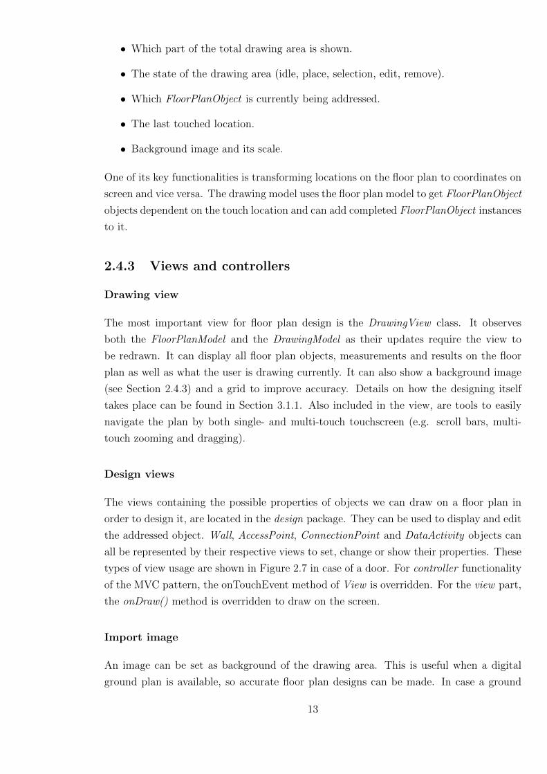
2.4.3 Views and controllers

Drawing view

The most important view for floor plan design is the DrawingView class. It observes

both the FloorPlanModel and the DrawingModel as their updates require the view to

be redrawn. It can display all floor plan objects, measurements and results on the floor

plan as well as what the user is drawing currently. It can also show a background image

(see Section 2.4.3) and a grid to improve accuracy. Details on how the designing itself

takes place can be found in Section 3.1.1. Also included in the view, are tools to easily

navigate the plan by both single- and multi-touch touchscreen (e.g. scroll bars, multi-

touch zooming and dragging).

Design views

The views containing the possible properties of objects we can draw on a floor plan in

order to design it, are located in the design package. They can be used to display and edit

the addressed object. Wall, AccessPoint, ConnectionPoint and DataActivity objects can

all be represented by their respective views to set, change or show their properties. These

types of view usage are shown in Figure 2.7 in case of a door. For controller functionality

of the MVC pattern, the onTouchEvent method of View is overridden. For the view part,

the onDraw() method is overridden to draw on the screen.

Import image

An image can be set as background of the drawing area. This is useful when a digital

ground plan is available, so accurate floor plan designs can be made. In case a ground

13

(a) Menu to adjustproperties of thedoor to be drawn

(b) Menu to edit properties of a door

(c) Menu displaying properties of a door

Figure 2.7: Possible display styles of the view for a door

14

plan is hung up against a wall or a paper version is available, it is easy to take a picture

of it with the device itself and import it to the application. In Figure 2.8, a ground plan

of the third floor of Complex Zuiderpoort is being imported. In (a), a line was drawn

and we set the length of the line to be five meters in real life. The application shows the

scaling that will be done. The scale represents the amount of pixels per centimeter. The

result of the import is shown in (b) where a few walls are drawn on top of it already.

2.5 Libraries

2.5.1 aFileDialog

To be able to browse for files in Android, the open source library aFileDialog was used.

As there are little libraries available with this functionality, aFileDialog seemed the best

documented and most mature. It is licensed under LGPL 3 and is compatible with

Android 2.2+. It is easy to use and to extend. It can be used as an Activity or a Dialog.

The latter was picked for the application as it appears more integrated into the application

and reduces complexity. Displayed files and folders can be filtered which is useful in our

application for only displaying appropriate file types (i.e. images and XML files). It also

has a GUI to let the user create a new file. It does not actually create the new file,

but returns the file name to the application so it can be handled manually in a different

thread. This feature is used whenever applicable.

The library has a user guide in English, French and Spanish. Developer guides are

available in English and Spanish. The code of the library is structured using the design

patterns embedded in the Android API and can easily be internationalized by making

use of the internationalization mechanisms provided by the Android SDK. Figure 2.9 is

a screenshot of aFileDialog in action in the application.

2.5.2 KSoap2Parser

In order to read the data returned by the web service and send messages to it, a SOAP

parser is required. The ksoap2-android library seemed to be the ideal client library for

this purpose. It is lightweight, efficient and specifically made for usage on the Android

platform. The library is open source and licensed under MIT. Being actively maintained,

any bugs that might show up in the future are very likely to be fixed. There are many

tutorials and helpful resources to be found on their wiki page hosted by Google.

15

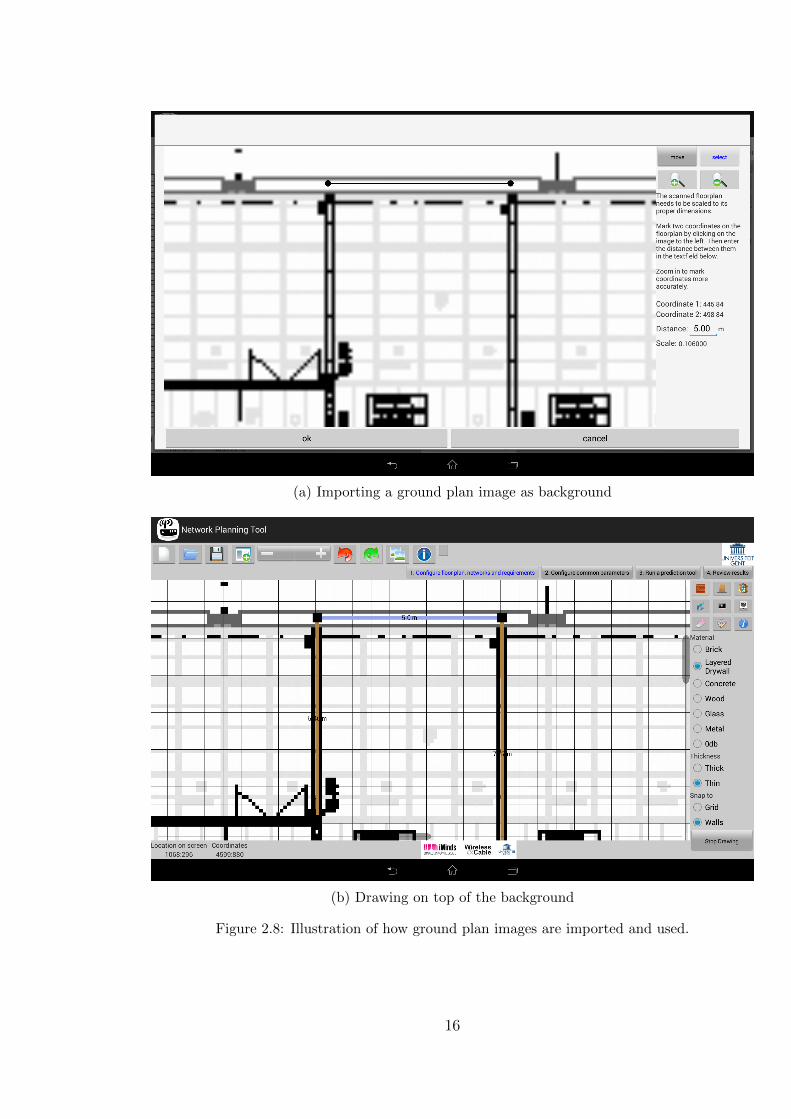
(a) Importing a ground plan image as background

(b) Drawing on top of the background

Figure 2.8: Illustration of how ground plan images are imported and used.

16

Figure 2.9: The aFileDialog library GUI.

17

Chapter 3

Application Design

When designing the application, issues and trade-off considerations appeared. This in-

cludes code-specific as well as general development issues. Some are specific for the mobile

application and others are in common with the WHIPP tool.

3.1 Requirement Differences Compared to WHIPP

Tool

3.1.1 Mobile Device Drawing Operations

As the Android application should allow the user to draw a floor plan, a user-friendly

drawing functionality is required. Because mobile devices almost never have other input

possibilities than a touchscreen (i.e. there is no mouse), it should be straight-forward to

draw the floor plan as well as moving its view (i.e. zooming and shifting). An additional

issue would be to make it as easy as possible both for single- as multi-touch devices.

For the drawing part, objects need to be divided into two categories. The first cat-

egory has two location points to define its position on the floor plan (e.g. walls, doors,

windows). The second category only has one such location point (e.g. access points, data

activities, connection points, measurements). All objects will be drawn with single touch

functionality. When the user touches the screen, a location left above the touch location

will be marked as the current position to draw. As long as the user keeps touching the

screen, this current draw position can be changed by moving on the touchscreen. When

the screen is no longer touched (i.e. finger or pen is lifted), the object will be drawn at

the last touched location. If the object is of the second category, this is all what needs

to be done to draw it. In case the object is of the first category, the user has follow the

same procedure again. When the user is touching the screen to draw the second location

point, the connection line in between the two points will be drawn as well.

18

As for the zooming and shifting functionality, a difference was made between single

and multi-touch devices. For zooming, single-touch users can use the zoom buttons at

the top menu bar (Figure 3.1). This will zoom in/out with the focus on the center of

the drawing part of the screen. For shifting purposes, scroll bars have been implemented.

These scroll bars needed to be custom made as the scrolling functionality also needed

to be custom made (see Section 3.1.2). Multi-touch devices have the extra functionality

to zoom and shift by using 2 fingers on the drawing canvas. When two fingers start

touching, all drawing activities (caused by touching with one finger first) are canceled.

When moving the 2 fingers on the touchscreen, the zooming degree will be linear with the

difference in distance between fingers. Shifting is based on the smallest x and y coordinate

the fingers are located at. Figure 3.2 contains an example of dragging and zooming.

Figure 3.1: Zoom buttons in the application

3.1.2 Horizontal and Vertical Scrolling

In the part of the application where the floor plan is drawn on the screen by the user, both

horizontal and vertical scrolling should be possible at the same time. This is required in

order to significantly simplify drawing with multi-touch. This is however not available as a

GUI component in Android by default. Therefore, it was necessary to implement a custom

view which allowed this behavior. The result is contained in the DrawingView class which

processes the touches on the screen and displays the changes in visible elements.

3.1.3 File Browsing

In the application, different types of files need to be opened and saved. Examples of types

of files to be opened are images of floor plans and the floor plans themselves. Files that

are to be saved are floor plans, screenshots, measurements, and all kinds of results that

are generated by the algorithms.

As there currently are no standard features in Android to browse for files, four possible

solutions were considered:

1. No file browsing; only let user select and save files in a dedicated application folder.

2. Develop a custom file browser.

3. Let the browsing be handled by third-party apps.

19

Figure 3.2: Illustration of how to do dragging and zooming. The green arrows depict where thefingers of the user are touching the screen.

20

4. Use a file browsing library.

The first option implies that users always has to move external files to the correct

folder in order to open it with the application. It can also cause confusion about the

exact location of the files when they are required for usage in other software.

The second option would be a very user-friendly solution as it can modified exactly

to any needs. However, there are certain risks that go hand in hand with this choice. It

is very work-intensive to implement the GUI as well as the functionality and to handle

everything that can go wrong in an appropriate manner.

Option number three means that the device needs to have file browsing software in-

stalled to select files for our application to open or save. This requirement is rather

undesirable.

The last option is chosen as the best option. A reliable externally developed library

is preferred over option two. The Android library aFileDialog is chosen to be the file

browser of the application. See Section 2.5.1 for detailed information about aFileDialog.

3.1.4 XML Structure

As the application is required to use and produce floor plan files with the same structure

that is used in other WiCa software, the data structures represented in the files are not

the same as the self-created ones. Therefore it is not possible to have easily automated

conversions from and to the desired XML structure.

All data classes that need to be able to transform to XML implement the XMLTrans-

formable interface and require implementing its toXML() method in which the required

data is formatted and returned in an Element object of the W3C DOM package. To

transform XML to the data objects, seperate methods are implemented for each file type

and are located in the XMLIO class.

3.1.5 Performance Issues

The GUI of the application is rather big and contains a lot of functionality on a single

screen. This is to limit the amount of actions needed to be performed by the user. As

the user interface kept expanding, slow responsiveness of the screen occurred. The cause

was found using Android Hierarchy Viewer. The quite hierarchic structure of the layout

resulted in slow loading and updating of several views. The solution of this problem was

flattening the hierarchy and making the views more independent of scaling updates. After

the restructuring, no lag or delay of any kind was perceived anymore.

21

3.1.6 Android Version

Because we want to maximize the amount of devices compatible with the application, we

want to pick an Android version with the lowest possible version as the newer version

are backward compatible. The used library aFileDialog (see Section 2.5.1) requires a

minimum API level of 8 (Android 2.2 Froyo). Devices starting from API level 8 have access

to Google Play, formerly Android Market. This means all possible users are reachable by

solely publishing it on Google Play.

3.2 Complex Wall Drawing

There is a need for the walls (and windows and doors) to connect precisely in order for

the web service to detect the distinct rooms. We do not want to burden the user with

exact drawing, thus a system was engineered to simplify the drawing of usable floor plans.

To select the locations where the edges of a new wall have to be, two ways of drawing

are made possible. The first is the option Snap to grid. The background of the floor plan

is a grid with spacing of 50 centimeters. Enabling this options will the currently drawing

edge to snap to the closest grid, or to a wall if it is even closer. The other possible option

is Snap to walls. In this mode, only snapping to walls will occur if drawing close enough

to it.

The snapping itself is not sufficient to provide an acceptable level of user-friendliness.

In case walls are overlapping, they should be split in two at the intersection point (e.g.

Figure 3.3). Also, if a wall is near the edge of another wall, this edge should be used

for the wall (e.g. Figure 3.4). For this functionality, an algorithm for adding new walls

(Algorithm 1) is elaborated.

For each already existing wall (line 2), save the wall’s edge locations (line 6) if they

can be perpendicularly projected on the new wall (line 5) and are 40cm or less away from

it (line 5). If no edges of the current wall are added and it gets intersected by the new

wall (line 9), split the current wall in two separate walls (line 10) and save the intersection

location (line 11). After iterating all walls, sort the list of saved locations by distance to

the first edge of the new wall (line 14). Next, add new walls with the same properties of

the new wall using the sorted locations (line 15). Finally, remove duplicate walls, if any

(line 16).

22

Figure 3.3: Illustration of drawing overlapping walls.

Figure 3.4: Illustration of drawing a wall near an edge of another wall. The brown colored wallis drawn after the red colored wall.

23

Algorithm 1 Add wall algorithm

1: procedure AddWall(newWall, wallList)2: for all wall ∈ wallList do3: for all location ∈ wall do4: if isPerpendicularlyProjectable(location, newWall)5: && distance(location, newWall) < 40 then6: locations← location7: end if8: end for9: if noLocationsAdded && isIntersectedByWall(wall, newWall) then

10: splitWall(wall)11: locations← intersectionLocation12: end if13: end for14: locations.sortByDistance(newWall)15: addWalls(locations, newWall)16: removeDuplicateWalls17: end procedure

3.3 Undo and Redo

In a drawing application, functionality to undo and redo actions is indispensable. Cer-

tainly needed components are an undo stack, containing the data to return to past state,

and a redo stack, containing data to return to a previously undone state. When invoking

an undo, the undo stack is popped, and the element is pushed to the redo stack. Vice

versa when invoking a redo. Of course, the redo stack is cleared when a new action is

taken.

There are two possible manners to actually implement this. The first possibility is

storing the actions themselves in the stacks. When undoing, the inverse action should be

performed. This would make undoing the placement of a wall (see Section 3.2) extremely

complicated since it involves merging walls. The second manner is saving the complete

states in the stacks. A state contains all elements of the floor plan. This solution requires

more storage since much duplicate data is stored. Performance on the other hand is

expected to be much better than the complex inversions proposed in the first possibility.

Considering the data overhead is not large enough to be worried about, and the low

complexity, the second option is implemented.

3.4 Multithreading

In software with a GUI, issues with multithreading often arise. In Android, the UI thread

is the main thread. Different threads need to be used for CPU intensive operations since

24

a non responsive GUI needs to be avoided.

Because ASyncTasks operate in a thread separate from the UI thread, they are used

in the application to perform background operations. The only tasks that can take a

long time are the ones involving I/O. We use two types of I/O operations. The first is

file reading and writing. The application can read and write plain text, xml and images.

The other type is communication with the web service described in Section 2.1.1. The

duration of both the operations depend on the amount of data that needs to be processed

and to what extent this data needs to be transformed. All ASyncTask instances are

managed by the ASyncIOTaskManager which can provide a progress dialog to the UI.

An implementation of the OnAsyncTaskCompleteListener〈T 〉 interface will be notified

when the task is complete, and it will be passed the result of the task.

3.5 Draw Results

Depending on how large the floor plan is, many location specific results can be returned

by the algorithms of the web service. When drawing them separately, high CPU usage

and lag was observed. For this reason, a different approach was vital. Now, one pixel

for each ten square centimeter is provided. The results for the complete ground plan are

provided by small bitmaps whereas each bitmap represents one result type (i.e. download

speed, RX power, . . . ). No lag presented itself after this adjustment.

25

Chapter 4

Testing

For testing the network planning model improvement possibilities for Android devices,

signal strength measurements were taken in three different indoor environments. All

measurements were done using the same Android device (Sony Xperia Tablet Z) with the

application described in Chapter 2 (see Section 2.4.1 for the measurement implementa-

tion). During each measurement, the tablet was held horizontally, facing the access point

at a height of approximately one meter. The measurement procedure was as follows:

1. Select the location on the floor plan where the measurement needs to be taken.

2. Set amount of measurements to be taken at the location to 5.

3. Hold the device at the same location and height during the measurements.

4. Store the average result at each location.

5. Save the results in XML format, to be parsed and processed by Excel for statistics.

4.1 Test Environments

4.1.1 Turnhout

The first set of measurements was taken in a detached residential house in Turnhout

(Figure 4.1). It has three floors including the attic. All measurements took place on the

first floor. The walls of this residence are brick and all doors are made of wood. As can

be seen in Figure 4.2, every single room was used and measurement locations are fairly

spread out. The residence is little furnished and the access point was placed in the bottom

right location on the floor plan. The used access point was a DLink dir-615 (hardware

version H2, firmware version 8.02) which has two antennas and a transmit power of 13

26

dBm. The TX power of the router is an estimation based on online searching as the

actual value could not be found in any documentation nor settings. The surface on which

the monitoring took place is 89.25 square meters. Since 112 locations were measured,

the number of measurements per square meters is 1.255. Data per room can be found in

Table 4.1. All rooms have at least 1.2 measurements per square meter.

Figure 4.1: Indoor picture of the environment in Turnhout

Table 4.1: Properties of the monitored rooms in Turnhout.

surface(m2) #measurements #measurements/m2

Room 0 5 8 1.6Room 1 14 17 1.214285714Room 2 30 36 1.2Room 3 20.25 26 1.283950617Room 4 20 25 1.25Total 49 61 1.244897959

4.1.2 Bruges

The second set of measurements was taken in an old townhouse in Bruges (Figure 4.3).

It has a total of four floors including the basement. The measurements were taken on the

ground floor. All rooms were included in the measurements except for the stairs leading

to the basement as can be seen in the top center of Figure 4.4. It has brick walls and

the doors are from glass or wood. The residence is averagely furnished, meaning it has

27

Figure 4.2: Monitored floor plan of the house in Turnhout

several objects that can possibly block signals (e.g. piano, metal music stand, high filled

bookcases). A DLink dir-600 access point (firmware DD-WRT v24-sp2) was placed on

top of a sofa at a height of one meter. It has one antenna and a transmit power of 8 dBm.

The surface of this floor is 77.75 square meters where 96 measurements were done. This

results in 1.235 measurements per meter. As in Turnhout, the rooms also have at least

1.2 measurements per square meter. More detailed information can be found in Table 4.2.

Table 4.2: Properties of the monitored rooms in Bruges.

surface(m2) #measurements #measurements/m2

Room 0 11 14 1.272727273Room 1 30 36 1.2Room 2 23.25 29 1.247311828Room 3 1.5 2 1.333333333Room 4 12 15 1.25Total 77.75 96 1.234726688

4.1.3 Ghent

The third and final set of measurements was taken in Complex Zuiderpoort in Ghent

(Figure 4.5). As can be seen in Figure 4.6, most walls are layered drywall and concrete

except for some metal in the center and glass at the sides of the floor plan. The metal

walls represent the elevators. The third floor was used for the measurements. As students

and employees are working in all of the rooms, only the hallways and toilets were used for

measurements. The rooms were slightly furnished while the hallway is as good as clear

of objects. The same access point as in Bruges was set up here. The two rooms and the

28

Figure 4.3: Indoor picture of the environment in Bruges

Figure 4.4: Monitored floor plan of the house in Bruges

29

hallway have a surface of 243.5 square meters and have 272 measured locations in total.

This makes a measurement density of 1.117 measurements per square meter. The details

per room are located in Table 4.3.

Figure 4.5: Indoor picture of the environment in Ghent

Table 4.3: Properties of the monitored rooms in Ghent.

surface(m2) #measurements #measurements/m2

Room 6 219 244 1.114155251Room 11 9.5 12 1.263157895Room 22 15 16 1.066666667Total 243.5 272 1.117043121

4.2 Measurements and Deductions

In this section, two different methods with the purpose of improving the results of the

algorithms will be tested.

4.2.1 Result Improvement Based on Fitted Shift

Maximum Improvement

Firstly, the maximum improvement of the results returned each algorithm in each test

environment is investigated. We define improvement as decrease in MSE (mean squared

30

Figure 4.6: Monitored floor plan of Complex Zuiderpoort in Ghent

error[1]). The MSE when shifting is done based on all measurements will be called the

maximum improvement.

We add the average deviation of the difference between result and measurement to the

result. This will make the average deviation between the new results and the measure-

ments zero. The impact of adjusting the results will be evaluated by the change in MSE

because it incorporates both variance and bias. Since only a shift is applied, the standard

deviation will always be the same before and after the shift. At every monitored environ-

ment and for each algorithm using default values statistics are calculated. This includes

the average error, the average deviation, the standard deviation, the average error after

shift and the error reduction. The results for Turnhout are displayed in Table 4.4, for

Bruges in Table 4.5 and for Ghent in Table 4.6. Figure 4.7 shows how the results of the

SIDP model are shifted for the house in Turnhout.

Table 4.4: Algorithm comparison statistics of Turnhout.

sidp tgn free-space multiwallMSE (dBm) 40.94 101.21 127.77 56.06

avg. dev. (dBm) -4.41 -8.57 -9.60 -5.97std. dev. (dBm) 4.65 5.29 5.99 4.53

MSE shift (dBm) 21.45 27.75 35.57 20.37error reduction (%) 47.60 72.58 72.16 63.66

We notice large error reductions (and thus result improvements) for almost every algo-

rithm at every environment. The observed improvement rates in Turnhout vary between

47 and 73 percent. In Bruges, this is between 82 and 94 percent. The environment in

Ghent produces good results for the SIDP and Free-space algorithms as their improve-

ments are over 62 percent. The TGn algorithm in Ghent shows almost no improvement

31

Figure 4.7: Improvement by automatic shift based on all measurements for Turnhout shownin the application. The top image shows the received power predictions of SIDP. The bottomimage shows the shifted results.

32

Table 4.5: Algorithm comparison statistics of Bruges.

sidp tgn free-space multiwallMSE (dBm) 287.19 261.52 302.36 192.83

avg. dev. (dBm) -16.20 -15.67 -16.68 -12.59std. dev. (dBm) 4.99 4.01 4.94 5.88

MSE shift (dBm) 24.67 15.91 24.11 34.26error reduction (%) 91.41 93.92 92.03 82.23

Table 4.6: Algorithm comparison statistics of Ghent.

sidp tgn free-space multiwallavg. error (dBm) 63.31 43.50 134.95 10991.26avg. dev. (dBm) -6.29 -2.73 -10.04 44.25std. dev. (dBm) 4.88 6.02 5.86 95.22

avg. error after shift (dBm) 23.68 36.06 34.16 9033.45error reduction (%) 62.59 17.12 74.69 17.81

using the shift. This can be explained by the fact that it already had good results without

the shift and the shift itself is very small compared to those used by the other algorithms.

The multiwall algorithm in Ghent gave a very large MSE and standard deviation. This is

caused by the algorithm only taking into account the signal path straight to the receiver.

The metal elevators in the middle of the environment block all signals passing through.

However, locations behind the elevators can have a good connection by signals advancing

through the hallway. The shift appears unable to improve very inaccurate results. With-

out accounting for the exceptional situation for the Multiwall model in Ghent, an average

error reduction of 70 percent is obtained.

Impact Amount of Measurements

Now we know the improvement we can achieve given the algorithm and environment

by using all the measurements, it is interesting to know how many locations should be

measured to efficiently improve results. This information can be used as advise for the user

in the mobile app. If all the possible subsets of measurements are taken into account,

this would result in too much data to be coped with. As for the combinations of k

measurements, there are(nk

)possibilities, with n the total amount of measurement. For

this reason, random subsets were generated where the generated amount of each subset

size is equal to the total amount of measurement. Now, we can observe the improvement

every time we add a measurement. The shift is computed on each subset making the

average deviation zero. The new average error when comparing to all measurements is

stored in Excel for observation (see Appendix A). This way, the improvement when adding

measurements can be calculated and evaluated.

The improvement for i measurements is given by Equation 4.1 where Ei is the MSE for

33

i measurements and max is the total amount of measurements taken at the environment,

given in Section 4.1. This improvement statistic represents the percentage of how much

closer the current MSE is to the MSE when using all measurements compared to the MSE

for one less measurement.

Improvement(i) =(Ei−1 − Emax)− (Ei − Emax)

E0 − Emax

=Ei−1 − Ei

E0 − Emax

(4.1)

Table 4.7 contains the improvement statistics of all models in all three environments.

In three cases (Turnhout SIDP, Ghent TGn and Ghent Multiwall), the first measurement

increases the MSE. This is not surprising as only accounting for one measurement is very

biased. We notice for the majority of cases, that the improvement is very small starting

from three measurements. When not taking into account Ghent TGn and Ghent multi-

wall, the average accumulated improvement is 87.14 percent for three measurements. TGn

and multiwall in Ghent deliver worse results than without measurements at that point.

If a way to detect such cases is implemented (e.g. floor plan analyzation for multiwall or

detection of very small shifts for already accurate results), three measurements can be a

good performing minimum. If such detection functionality would not be sufficient, five

measurements could be an alternative minimum as MSE values at that point are smaller

on average than when no measurements were done.

Now the influence of adding a certain amount of measurements is known, it is interest-

ing to look at the impact of measurement addition when all measurements are done in a

different room instead of random locations. This might result in more improvement with

less measurements and could therefore be beneficial for user-friendliness. The Complex

Zuiderpoort environment was not included in this test as it only has three rooms, one of

which (the hallway) spans 90 percent of the monitored area. Again, the subsets are ran-

dom generated, but this time only subsets whereas measurements are in different rooms.

The maximum subset size is therefore equal to the amount of rooms. As both Bruges

as Turnhout have 5 rooms, the subsets are not larger than 5. The amount of random

generated subsets for each subset size will be equal to the total number of measurements

at that environment. The resulting statistics are shown in Table 4.8 and the comparison

between random measurement addition and per room are displayed in Figure 4.8. When

comparing these two methods, no pattern was found. Therefore, we can assume random

measurements (but fairly spread) are as good as measuring in different rooms.

34

Tab

le4.

7:M

easu

rem

ent

qu

anti

ty-b

ase

dm

od

elco

mp

aris

onst

atis

tics

inal

lth

ree

envir

onm

ents

.Set

sou

th

owm

uch

per

cent

the

MS

Eh

asim

pro

ved

(or

dec

reas

edin

case

of

an

egat

ive

nu

mb

er)

com

par

edto

the

situ

atio

ns

wh

ere

no

mea

sure

men

tsar

ed

one

and

all

mea

sure

men

tsar

ed

one.

amou

nt

ofm

easu

rem

ents

12

34

56

78

910

Impro

vem

ent

(%)

Bru

ges

SID

P90

.60

5.24

1.20

0.39

0.49

0.60

0.48

-0.1

50.

35-0

.01

TG

n94

.49

2.49

0.47

1.81

0.12

0.22

0.15

0.18

-0.0

70.

02F

ree-

spac

e92

.18

4.19

1.41

0.46

0.84

0.20

-0.1

80.

490.

20-0

.12

Mult

iwal

l84

.15

11.9

41.

081.

98-0

.06

0.71

0.69

0.40

0.17

0.14

Turn

hou

t

SID

P-1

0.07

62.2

514

.81

-0.0

910

.18

5.83

1.99

1.81

1.39

-1.6

8T

Gn

62.2

218

.65

6.99

2.30

2.22

2.46

-0.1

20.

691.

300.

12F

ree-

spac

e61

.43

21.4

15.

092.

611.

602.

82-0

.81

0.89

1.61

-1.0

2M

ult

iwal

l22

.37

31.5

015

.55

2.00

4.27

3.66

2.47

0.62

0.78

1.18

Ghen

t

SID

P40

.23

34.5

77.

134.

080.

983.

661.

87-0

.33

1.14

1.04

TG

n-3

84.0

624

3.24

73.8

349

.08

21.7

622

.51

6.18

6.64

5.47

11.3

3F

ree-

spac

e66

.11

17.0

64.

701.

982.

841.

400.

790.

041.

800.

06M

ult

iwal

l-3

61.4

124

4.13

73.6

425

.47

32.1

520

.73

-2.5

612

.48

9.43

2.36

Acc

um

ula

ted

Impro

vem

ent

(%)

Bru

ges

SID

P90

.60

95.8

597

.05

97.4

497

.93

98.5

399

.01

98.8

699

.21

99.2

0T

Gn

94.4

996

.98

97.4

599

.26

99.3

899

.60

99.7

599

.94

99.8

799

.88

Fre

e-sp

ace

92.1

896

.37

97.7

998

.25

99.0

999

.29

99.1

199

.60

99.8

099

.68

Mult

iwal

l84

.15

96.0

997

.17

99.1

599

.09

99.8

010

0.48

100.

8810

1.05

101.

19

Turn

hou

t

SID

P-1

0.07

52.1

866

.98

66.8

977

.07

82.9

084

.88

86.6

988

.08

86.4

0T

Gn

62.2

280

.87

87.8

690

.15

92.3

894

.84

94.7

295

.40

96.7

096

.82

Fre

e-sp

ace

61.4

382

.84

87.9

290

.54

92.1

494

.95

94.1

595

.04

96.6

595

.63

Mult

iwal

l22

.37

53.8

669

.41

71.4

175

.68

79.3

481

.81

82.4

283

.21

84.3

8

Ghen

t

SID

P40

.23

74.8

181

.94

86.0

287

.00

90.6

692

.53

92.2

193

.35

94.3

9T

Gn

-384

.06

-140

.82

-66.

99-1

7.91

3.85

26.3

632

.53

39.1

744

.65

55.9

7F

ree-

spac

e66

.11

83.1

887

.88

89.8

592

.69

94.1

094

.89

94.9

496

.73

96.7

9M

ult

iwal

l-3

61.4

1-1

17.2

7-4

3.63

-18.

1613

.99

34.7

232

.16

44.6

454

.07

56.4

3

35

90,00

91,00

92,00

93,00

94,00

95,00

96,00

97,00

98,00

99,00

100,00

2 3 4 5

Acc

um

ula

ted

imp

rove

men

t (%

)

# measurements

Bruges SIDP

Bruges SIDP(room)

Bruges TGn

Bruges TGn(room)

Bruges Freespace

Bruges Freespace(room)

Bruges Multiwall

Bruges Multiwall(room)

(a) Comparison between random and room measurement addition for Bruges

-20,00

0,00

10,00

20,00

30,00

40,00

50,00

60,00

70,00

80,00

90,00

100,00

2 3 4 5

Acc

um

ula

ted

imp

rove

men

t (%

)

# measurements

Turnhout SIDP

Turnhout SIDP(room)

Turnhout TGn

Turnhout TGn(room)

Turnhout Freespace

Turnhout Freespace(room)

Turnhout Multiwall

Turnhout Multiwall(room)

(b) Comparison between random and room measurement addition for Turnhout

Figure 4.8: Comparison between random and room measurement addition

36

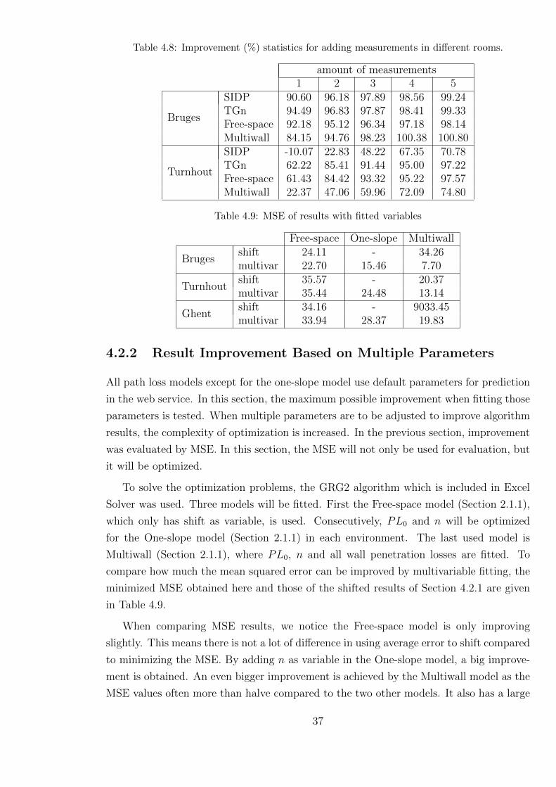
Table 4.8: Improvement (%) statistics for adding measurements in different rooms.

amount of measurements1 2 3 4 5

Bruges

SIDP 90.60 96.18 97.89 98.56 99.24TGn 94.49 96.83 97.87 98.41 99.33Free-space 92.18 95.12 96.34 97.18 98.14Multiwall 84.15 94.76 98.23 100.38 100.80

Turnhout

SIDP -10.07 22.83 48.22 67.35 70.78TGn 62.22 85.41 91.44 95.00 97.22Free-space 61.43 84.42 93.32 95.22 97.57Multiwall 22.37 47.06 59.96 72.09 74.80

Table 4.9: MSE of results with fitted variables

Free-space One-slope Multiwall

Brugesshift 24.11 - 34.26multivar 22.70 15.46 7.70

Turnhoutshift 35.57 - 20.37multivar 35.44 24.48 13.14

Ghentshift 34.16 - 9033.45multivar 33.94 28.37 19.83

4.2.2 Result Improvement Based on Multiple Parameters

All path loss models except for the one-slope model use default parameters for prediction

in the web service. In this section, the maximum possible improvement when fitting those

parameters is tested. When multiple parameters are to be adjusted to improve algorithm

results, the complexity of optimization is increased. In the previous section, improvement

was evaluated by MSE. In this section, the MSE will not only be used for evaluation, but

it will be optimized.

To solve the optimization problems, the GRG2 algorithm which is included in Excel

Solver was used. Three models will be fitted. First the Free-space model (Section 2.1.1),

which only has shift as variable, is used. Consecutively, PL0 and n will be optimized

for the One-slope model (Section 2.1.1) in each environment. The last used model is

Multiwall (Section 2.1.1), where PL0, n and all wall penetration losses are fitted. To

compare how much the mean squared error can be improved by multivariable fitting, the

minimized MSE obtained here and those of the shifted results of Section 4.2.1 are given

in Table 4.9.

When comparing MSE results, we notice the Free-space model is only improving

slightly. This means there is not a lot of difference in using average error to shift compared

to minimizing the MSE. By adding n as variable in the One-slope model, a big improve-

ment is obtained. An even bigger improvement is achieved by the Multiwall model as the

MSE values often more than halve compared to the two other models. It also has a large

37

improvement when comparing to the shifted Multiwall model with default values.

38

Chapter 5

Conclusion and Future Work

5.1 Conclusion

In this dissertation, the possible impact of the usage of a mobile device to improve path loss

models is studied. For this purpose a mobile Android application for real-time cognitive

wireless network planning is developed. To enable future improvement and expansion

of this application, attention was given to modifiability and usability. Therefore, the

application is extensively described on different levels. The what, why and how of the

general design and the actual implementation are discussed to get a better understanding

of the tool and to inform other software developers of points of concern when expanding

this tool or developing similar software.

In order to obtain better results, the app automatically applies a fitted shift to the

model results based on actual measurements taken with the device. This fit is based on

the minimization of the average error. To determine the possible impact of this method,

three test environments were used. First, the maximum improvement (when shifting is

done based on all measurements) was determined for all models at the test environments.

Result improvements of up to 94 percent with an average of 70 percent were observed.

Consecutively, the impact of the amount of measurements on the improvement of the re-

sults was tested. We find that on average, 87.14 percent of the total possible improvement

is reached with only three random measurements (omitting two cases). At 5 measure-

ments done, all model-environment combinations showed improved MSE results. When

restricting measurements to a maximum of one per room, no relational pattern was found

as the results are similar. This indicates that measuring in separate rooms does not sig-

nificantly improve results over random measurements. As a result of these tests, a hint is

displayed in the application telling the user it is advised to take at least five measurements

at random locations to improve results.

As a last test, not only a shift is used for fitting, but multiple variables of models. The

39

even smaller resulting MSE values tell us that more variables can have a significant positive

impact over a single shift. This gives an incentive for further research (see Section 5.2.2).

5.2 Future Work

5.2.1 Model Advise

Measurement-Based

When measurements are done on the device and the standard deviation of the difference

between these measurements and the fitted model results exceeds a certain threshold,

other models can be advised. It can be interesting to study the performance relations

between network planning models. For instance, in case a certain algorithm performs

badly or well in a given situation, other algorithms can be advised or avoided.

Floor plan-based

In the tests, it was immediately clear that the Multiwall model can perform terrible for

locations that cannot be reached by rays going in a straight line from access point to

device (because of walls with very high penetration loss, like metal), but can be reached

by rays having a different path. When such an issue appears, the model’s results cannot

and should not be improved, but another model should be used instead. Other such

specific environment properties can be investigated for impact on results to automatically

advise certain models.

5.2.2 Multivariable Fitting

Model result fitting for multiple variables can give big opportunities, as shown in Sec-

tion 4.2.2. To determine if multivariable fitting is also viable for a small amount of

measurements, further research needs to be done. Issues with overfitting are expected to

arise, which cause a higher required amount of measurements. With the results of that

research, it would be interesting for the application to support automatic fitting for mul-

tiple variables. This type of fitting is a more complex optimization problem that needs

an advanced algorithm (like GRG2 in Excel) for solving.

5.2.3 Store Data

Data of the resulting fit, like model parameters, model result accuracy, access point prod-

uct details and mobile device, can be stored locally or sent to the web service to improve

40

future model predictions. and to gain useful statistics. If this functionality would be

implemented, useful statistics could be gained and other possible future work can be dis-

covered. In order to get these statistics, the application should be marketed so data of

many different users and hardware can be gathered and compared.

41

Appendix A

DVD

A.1 Contents

The enclosed DVD includes the following items:

• An electronic version of this document.

• The source code and executable of the Android application, including:

– The Android Studio project files

– The ksoap2-android library

– The aFileDialog library source code

– The actual source code

– The Javadoc documentation

• An Excel file (statistics.xlsx), with the following contents:

– The shifted results

(worksheets called Shift Environment)

– The results when adding random measurements to fit

(worksheets called Environment model random)

– The results when adding measurements of different rooms to fit

(worksheets called Environment model rooms)

– The fitted results based on multiple model variables

(worksheets called MultiVar Environment)

– A worksheet comparing MSE results

(called compare MSE)

42

– A worksheet comparing standard deviations of the results

(called compare std dev)

43

Bibliography

[1] Mean squared error. http://en.wikipedia.org/wiki/Mean_squared_error. [On-

line; accessed 24-May-2014].

[2] Open Handset Alliance. Android design patterns. https://developer.android.

com/design/patterns/index.html, 2014. [Online; accessed 24-May-2014].

[3] Robert Eckstein. Java se application design with mvc. http://www.oracle.com/

technetwork/articles/javase/index-142890.html, 2007. [Online; accessed 24-

May-2014].

[4] Vinko Erceg, Laurent Schumacher, et al. Ieee p802.11 wireless lans. tgn channel

models. doc.: IEEE 802.11-03/940r4, 2004.

[5] Harald Trap Friis. Friis transmission equation. http://en.wikipedia.org/wiki/

Friis_transmission_equation, 2014. [Online; accessed 24-May-2014].

[6] David Plets et al. Coverage prediction and optimization algorithms for indoor environ-

ments. EURASIP Journal on Wireless Communications and Networking, 2012(123),

2012.

[7] Saunders SR. Antennas and Propagation for Wireless Communication Systems. John

Wiley & Sons Ltd, 1999.

44