development of a mixed-flow compressor impeller for micro ... · micro gas turbine application ....

Development of a Mixed-Flow Compressor

Impeller for Micro Gas Turbine Application

by

Olaf Herbert Ferdinand Diener

Thesis presented in partial fulfilment of the requirements for the degree

of Master of Engineering (Mechanical) in the Faculty of Engineering at

Stellenbosch University

Supervisor: Dr. S.J. van der Spuy

Co-supervisor: Dr. T. Hildebrandt

Co-supervisor: Prof. T.W. von Backström

March 2016

i

DECLARATION

By submitting this thesis electronically, I declare that the entirety of the work

contained therein is my own, original work, that I am the sole author thereof (save

to the extent explicitly otherwise stated), that reproduction and publication thereof

by Stellenbosch University will not infringe any third party rights and that I have

not previously in its entirety or in part submitted it for obtaining any qualification.

March 2016

Copyright © 2016 Stellenbosch University

All rights reserved

Stellenbosch University https://scholar.sun.ac.za

ii

ABSTRACT

Development of a Mixed-Flow Compressor Impeller for

Micro Gas Turbine Application

O.H.F. Diener

Department of Mechanical and Mechatronic Engineering, Stellenbosch

University,

Private Bag X1, Matieland 7602, South Africa

Thesis: M. Eng. (Mech)

March 2016

This thesis details the development of a mixed-flow compressor impeller to be

used in a micro gas turbine (MGT) delivering 600 N thrust. Today‟s unmanned

aerial vehicles (UAVs) demand high thrust-to-weight ratios and low engine

frontal area. This combination may be achieved using mixed-flow

compressors. The initial mixed-flow compressor impeller design was obtained

using a 1-dimensional turbomachinery layout tool. A multi-point optimization

of the impeller aerodynamic performance was completed. Thereafter a

mechanical optimization was conducted to reduce mechanical stresses in the

impeller. A coupled aero-mechanical (multi-disciplinary) optimization was

concluded with the purpose of increasing the choke limit and reducing stresses

while conserving aero-performance. Finally, a modal analysis was conducted

and the rotor Campbell diagram was analysed to identify potential resonant

conditions. The optimization process was set up and controlled in an integrated

environment that includes a 3-dimensional Navier-Stokes flow solver and a 3-

dimensional finite element (FE) structural solver. An artificial neural network

(ANN) was used to generate a response surface based on a database of

performance and geometric information. A genetic algorithm (GA) was applied

to the response surface for optimization. The overall optimization process

achieved an increase in total-to-total pressure ratio of 30.6% compared to the

initial design while the isentropic total-to-total efficiency was increased by 5%

at design conditions. The choke limit of the initial design was improved

meaningfully. These values were obtained while also decreasing the peak von

Mises stress to 30% below the material yield limit. Recommendations were

made regarding the structural surroundings of the compressor and the operating

speeds based on the Campbell diagram.

Keywords: micro gas turbine, mixed-flow compressor, multi-disciplinary

optimization, Campbell diagram


iii

UITTREKSEL

Ontwerp van ‘n Gemengde-Vloei Mikrogasturbine Kompressorrotor

(“Development of a Mixed-Flow Compressor Impeller for

Micro Gas Turbine Application”)

O.H.F. Diener

Departement Meganiese en Megatroniese Ingenieurswese,

Universiteit van Stellenbosch,

Privaatsak X1, Matieland 7602, Suid-Afrika

Tesis: M. Eng. (Meg)

Maart 2016

Hierdie tesis beskryf die ontwikkeling van „n gemengde-vloei kompressorrotor vir

„n mikrogasturbine wat 600 N dryfkrag lewer. Hedendaagse onbemande vliegtuie

vereis „n hoë dryfkrag-tot-gewig verhouding en „n lae enjin frontale area. Hierdie

kombinasie kan bereik word met behulp van gemengde-vloei kompressors. Die

aanvanklike gemengde-vloei kompressorrotor-ontwerp is verkry deur „n 1-

dimensionale ontwerpskode. „n Multi-punt optimering van die rotor se

aerodinamiese vermoë is voltooi. Daarna is „n meganiese optimering uitgevoer

om spanning in die rotor te verminder. „n Aero-meganiese (multidissiplinêre)

optimering van die rotor is gedoen met die doel om die smoorperk te verhoog en

die spanning te verminder, terwyl die aerodinamiese vermoë behoue bly. Laastens

is „n modale analise uitgevoer en die rotor se Campbell diagram geanaliseer om

potensiële resonante toestande te identifiseer. Die optimeringsproses is opgestel

en beheer in „n geïntegreerde omgewing wat 3-dimensionale berekenings

vloeidinamika en 3-dimensionale eindige element strukturele berekeninge uitvoer.

„n Kunsmatige neurale netwerk is gebruik om „n reaksieoppervlakte te skep,

gebaseer op „n databasis van rotor vermoë en geometriese inligting. „n Genetiese

algoritme is toegepas op die reaksieoppervlakte vir die optimering. Die algehele

optimeringsproses het „n toename in die totaal-tot-totale drukverhouding van

30.6% in vergelyking met die aanvanklike ontwerp bereik, terwyl die isentropiese

totaal-tot-totale benuttingsgraad verhoog was met 5%. Die smoorperk van die

aanvanklike ontwerp is noemenswaardig verhoog. Hierdie waardes is behaal

gesamentlik met die vermindering van die piek von Mises spanning tot 30% laer

as die materiaal swiglimiet. Aanbevelings is gemaak ten opsigte van die

strukturele omgewing van die kompressor en die bedryfspoed gebaseer op die

resultate van die modale analise.

Sleutelwoorde: mikrogasturbine, gemengde-vloei compressor, multidissiplinêre

optimering, Campbell diagram


iv

ACKNOWLEDGEMENTS

First and foremost, I would like to thank my supervisor, Dr van der Spuy, for his

support and guidance I received during the course of this study. Additionally, I

would like to thank him for providing me with the opportunity to travel to

Germany as part of the thesis.

I gratefully acknowledge the experienced and insightful opinions, comments and

tips I received from my co-supervisors, Prof. von Backström and Dr Hildebrandt,

that allowed this thesis to be successful. Special thanks go to Dr Hildebrandt, for

not only allowing me to complete part of the research at his company office in

Germany, but also for welcoming me and inviting me to experience German

hospitality. Furthermore, I thank him for making it possible for me to obtain a

unique view of the CFD industry and also to gain some insight into the world of

professional engineering.

Mr Sven Albert contributed a great deal to this research through his advice and

insight, which is highly appreciated. I would also like thank the entire NIB team,

who welcomed me in their ranks and made the research period in Germany such a

great experience.

I would like to express my appreciation to CFturbo for allowing me to use their

software for this research.

My thanks go to the CSIR; more specifically to Mr Radeshen Moodley, for his

time and advice regarding the design of micro gas turbines and compressors.

Thank you to my friends in “die Lasraam” for the laughs and great discussions we

had during tea time and any other random time.

This research would not have been possible without the funding I received. Many

thanks go to the University Centre for Studies in Namibia (TUCSIN), who, in co-

operation with the German Academic Exchange Service (DAAD), chose to

support me and my research.

Finally, to my parents, my sincere appreciation, for their support provided during

my time at Stellenbosch, and proof-reading the thesis.


v

TABLE OF CONTENTS

Page

DECLARATION ................................................................................................... I

ABSTRACT ........................................................................................................... II

UITTREKSEL .................................................................................................... III

ACKNOWLEDGEMENTS ............................................................................... IV

LIST OF FIGURES ............................................................................................ IX

LIST OF TABLES ............................................................................................. XII

NOMENCLATURE ......................................................................................... XIV

1. INTRODUCTION ....................................................................................... 1

1.1. BACKGROUND ............................................................................................. 1

1.2. OBJECTIVES ................................................................................................. 1

1.3. MOTIVATION ............................................................................................... 2

1.4. THESIS OUTLINE .......................................................................................... 2

2. THEORY ...................................................................................................... 3

2.1. MICRO GAS TURBINES ................................................................................ 3

2.2. MIXED-FLOW COMPRESSORS ....................................................................... 4

2.2.1. Pressure Ratio and Efficiency ............................................................... 10

2.2.2. Surge and Choke ................................................................................... 11

3. THE COMPRESSOR DESIGN PROCESS ............................................ 12

4. LITERATURE OVERVIEW ................................................................... 14

4.1. MIXED-FLOW COMPRESSORS ..................................................................... 14

4.2. COMPRESSOR ANALYSIS AND DESIGN ....................................................... 15

4.2.1. Mean-Line Performance Analysis ..................................................... 15

4.2.2. 3-dimensional Aerodynamic, Structural and Multi-disciplinary

Analysis .............................................................................................. 15


Optimization ....................................................................................... 16

4.2.4. 3-dimensional Modal Analysis ........................................................... 17

4.3. PREVIOUS WORK AT STELLENBOSCH UNIVERSITY (SU) ........................... 17

5. REFERENCE MIXED-FLOW COMPRESSOR ANALYSIS .............. 18

5.1. GEOMETRY ................................................................................................ 18

5.2. COMPUTATIONAL DOMAIN AND DISCRETIZATION ..................................... 19

5.3. CFD MODEL .............................................................................................. 21

5.3.1. Fluid and Flow Model ....................................................................... 22


vi

5.3.2. Boundary Conditions ......................................................................... 22

5.3.3. Numerical Model ............................................................................... 23

5.3.4. Initial Solution, Output and Convergence Criteria ........................... 24

5.3.5. Post-processing .................................................................................. 25

5.4. RESULTS .................................................................................................... 25

6. INITIAL IMPELLER DESIGN ............................................................... 26

6.1. PERFORMANCE AND SIZE SPECIFICATIONS ................................................ 26

6.2. MEAN-LINE DESIGN .................................................................................. 27

6.2.1. Approach ............................................................................................ 28

6.2.2. Computational Domain and Discretization ....................................... 29

6.2.3. Impeller Performance Evaluation ..................................................... 31

6.2.4. CFD Model ........................................................................................ 31

6.2.5. Results ................................................................................................ 32

6.3. CONCLUSION ............................................................................................. 34

7. AERODYNAMIC OPTIMIZATION ...................................................... 35

7.1. THE OPTIMIZATION PROCESS .................................................................... 35

7.2. PARAMETERIZATION .................................................................................. 37

7.2.1. Endwalls ............................................................................................. 38

7.2.2. Stream Surfaces ................................................................................. 38

7.2.3. Stacking Laws .................................................................................... 38

7.2.4. Main Blade Camber Curve and Side Curves ..................................... 39

7.3. FITTING ..................................................................................................... 40

7.4. PARAMETER VALUE BOUNDS .................................................................... 41

7.5. OPERATING POINTS ................................................................................... 42

7.6. POST-PROCESSING ..................................................................................... 44

7.7. DATABASE GENERATION ........................................................................... 44

7.7.1. Grid Toughness and Quality .............................................................. 44

7.7.2. Numerical Model ............................................................................... 46

7.7.3. Results ................................................................................................ 46

7.8. OPTIMIZATION ........................................................................................... 48

7.8.1. Optimization Settings and Objective Function Definition ................. 48

7.8.2. Numerical Model ............................................................................... 50

7.8.3. Results ................................................................................................ 50

7.9. CONCLUSION ............................................................................................. 53

8. MECHANICAL OPTIMIZATION ......................................................... 54

8.1. PARAMETERIZATION .................................................................................. 55

8.2. DISCRETIZATION ....................................................................................... 56


vii

8.3. FE MODEL ................................................................................................. 57

8.4. IMPELLER BACKFACE AND BORE ............................................................... 57

8.4.1. Database Generation ......................................................................... 58

8.4.2. Results ................................................................................................ 58

8.5. IMPELLER BLADE ...................................................................................... 59

8.5.1. Database Generation ......................................................................... 59

8.5.2. Optimization Settings and Objective Function Definition ................. 59

8.5.3. Optimization and Results ................................................................... 60

8.6. CONCLUSION ............................................................................................. 62

9. COUPLED AERO-MECHANICAL OPTIMIZATION ........................ 63

9.1. DATABASE GENERATION ........................................................................... 63

9.2. OPTIMIZATION SETTINGS AND OBJECTIVE FUNCTION DEFINITION ............ 64

9.3. RESULTS .................................................................................................... 65

9.4. ERRORS AND UNCERTAINTY ...................................................................... 70

9.5. CONCLUSION ............................................................................................. 71

10. ROTOR DYNAMIC ANALYSIS ............................................................. 72

10.1. LINEAR STATIC FEA VALIDATION ......................................................... 72

10.1.1. SimXpert FE Model and Simulation Procedure ............................. 72

10.1.2. Results ............................................................................................. 73

10.2. MODAL ANALYSIS ................................................................................. 75

10.2.1. FE Model ........................................................................................ 75

10.2.2. Results ............................................................................................. 75

11. CONCLUSION AND RECOMMENDATIONS ..................................... 79

11.1. RECOMMENDATIONS .............................................................................. 80

11.2. FUTURE WORK ....................................................................................... 81

REFERENCES ..................................................................................................... 82

APPENDIX A: THEORY AND SOFTWARE .................................................. 87

A.1 COMPUTATIONAL FLUID DYNAMICS (CFD) ................................................. 87

A.1.1 Reynolds-Averaged Navier-Stokes (RANS) Equations .......................... 87

A.1.2 Turbulence Modelling ............................................................................ 87

A.2 FINITE ELEMENT ANALYSIS (FEA) ............................................................... 88

A.2.1 Linear Static Analysis ............................................................................ 88

A.2.2 Rotor Dynamics and Modal Analysis .................................................... 88

A.3 SOFTWARE .................................................................................................... 91

A.3.1 CFturbo ................................................................................................. 91

A.3.2 NUMECA ............................................................................................... 91


viii

A.3.3 MSC SimXpert and Nastran................................................................... 94

APPENDIX B: MATLAB IN-HOUSE CODE FLOWCHART ...................... 95

APPENDIX C: CFTURBO SETTINGS ............................................................ 96

APPENDIX D: COMPRESSOR IMPELLER PERFORMANCE

EVALUATION ........................................................................ 98

APPENDIX E: CFD AND FEA GRID DETAILS AND DEPENDENCY ... 100

E.1 REFERENCE COMPRESSOR STAGE GRID ...................................................... 100

E.2 GRID USED FOR THE INITIAL CFTURBO DESIGN AS WELL AS DB01 AND DB02

................................................................................................................... 101

E.3 DB03, AERODYNAMIC OPTIMIZATION AND COUPLED OPTIMIZATION CFD

GRID ........................................................................................................... 103

E.4 HEXPRESSTM

/HYBRID FEA GRID SETTINGS ............................................ 104

APPENDIX F: Y-PLUS VALUES ................................................................... 106

APPENDIX G: NUMECA AUTOBLADE DESIGN SPACE ........................ 107

APPENDIX H: DOE IMPELLER PARAMETERS ...................................... 108

H.1 PARAMETRIC MODEL OVERVIEW ............................................................... 108

H.2 AERODYNAMIC OPTIMIZATION: FREE PARAMETERS ................................... 108

H.3 AERODYNAMIC OPTIMIZATION: FROZEN PARAMETERS .............................. 109

APPENDIX I: OBJECTIVE FUNCTIONS .................................................... 111

APPENDIX J: SHAFT STRESS CALCULATIONS ..................................... 112

APPENDIX K: MERIDIONAL VELOCITIES AND B2B RELATIVE

MACH NUMBERS IN COMPARISON .............................. 113

APPENDIX L: PROCESSOR MANAGEMENT AND CPU TIME............. 115

L.1 CFD DATABASE AND OPTIMIZATION .......................................................... 115

L.1.1 Database .............................................................................................. 115

L.1.2 Optimization ......................................................................................... 115

L.2 OOFELIE FEA ........................................................................................... 116

L.3 COUPLED OPTIMIZATION ............................................................................. 116

APPENDIX M: BLADE CAMBER ANGLE COMPARISON ..................... 117

APPENDIX N: FINAL IMPELLER PERFORMANCE MAP ..................... 118

APPENDIX O: INITIAL AND FINAL IMPELLER RENDER ................... 119


ix

LIST OF FIGURES

Page

Figure 1: Micro gas turbine components (Pichlmeier, 2010) .................................. 3

Figure 2: Mollier diagram of a typical centrifugal compressor stage (adapted from

Dixon, 1998) ............................................................................................ 5

Figure 3: Different compressor rotor types (CFturbo, 2015) ................................... 7

Figure 4: Compressor components in the meridional plane .................................... 8

Figure 5: Velocity triangles of a mixed-flow compressor impeller ......................... 9

Figure 6: Typical compressor map (Dixon, 1998) ................................................. 11

Figure 7: Compressor impeller design procedure .................................................. 13

Figure 8: Reference compressor stage meridional contours and traces ................. 18

Figure 9: 3D grid lines on hub and blades of the reference stage (2nd

multigrid

level) ...................................................................................................... 21

Figure 10: Boundary patches of the reference compressor stage .......................... 23

Figure 11: Reference stage performance curves in contrast .................................. 25

Figure 12: Mean-line calculations according to Aungier (2000) compared with

CFD results of a mixed-flow impeller design obtained from the in-

house MATLAB code .......................................................................... 28

Figure 13: Meridional view of a CFturbo design with hub nose and diffuser

passage .................................................................................................. 30

Figure 14: Computational domain enclosed by hub, shroud, inlet and outlet ....... 30

Figure 15: 3-dimensional grid projections on the 2nd

multi-grid level of a CFturbo

design .................................................................................................... 31

Figure 16: Results of designs generated using CFturbo ........................................ 33

Figure 17: The optimization process in FINETM

/Design3D .................................. 37

Figure 18: Parameterization of the hub and shroud contours (endwalls) .............. 39

Figure 19: Section 1 and 2 camber Bézier points and associated freedom ............ 40

Figure 20: Meridional contours and traces of randomly generated geometries .... 42

Figure 21: B2B views of possible blade shapes at section 1 (hub) ........................ 42

Figure 22: CFturbo compressor performance curves and chosen operating points

for optimization (evaluation at r = 55.5 mm) ....................................... 43

Figure 23: Comparison of mass-averaged total pressures at different radii with

different TE topology ........................................................................... 45


x

Figure 24: Results of the designs from the final CFD database ............................ 47

Figure 25: ANN convergence of the CFD optimization ........................................ 51

Figure 26: Initial fitted and optimized blade geometry at section 1 and 2 ............ 51

Figure 27: Comparison of initial and optimized meridional contours and locations

.............................................................................................................. 52

Figure 28: Initial and optimized design performance curves at design speed ....... 53

Figure 29: Parameterization of the impeller solid sector in the meridional plane . 55

Figure 30: Various geometries obtained in the impeller backface database .......... 58

Figure 31: Initial backface design (left) and best database result .......................... 59

Figure 32: Hub and shroud blade thickness of the aero-optimized and

mechanically optimized designs ........................................................... 61

Figure 33: VM stresses of the aero-optimized design (left) and the mechanically

optimized design with = 1.85 mm ................................................ 61

Figure 34: Relative Mach number distribution in the meridional plane at choke . 65

Figure 35: Final design vs. CFturbo and aero-optimized designs at 95 krpm ....... 67

Figure 36: The mechanically optimized design with = 1.85 mm (left)

compared to the design resulting from the shroud camber and backface

optimization .......................................................................................... 67

Figure 37: Blade profiles of the aero-optimized design and the aero-mechanically

optimized design ................................................................................... 69

Figure 38: Relative Mach number contours of the CFturbo design (left) and the

final optimized design at 90% span and design conditions .................. 69

Figure 39: Comparison of OOFELIE (left) and SimXpert equivalent stress results

.............................................................................................................. 74

Figure 40: Different mode shape groups: main blade (left), splitter blade (middle)

and combined ........................................................................................ 76

Figure 41: Compressor rotor Campbell diagram (SimXpert 2) ............................. 77

Figure 42: Campbell diagram and associated damped vibration amplitude (Boyce,

2002) ..................................................................................................... 90

Figure 43: Construction of the dm/r-θ plane (Verstraete et al., 2010) .................. 93

Figure 44: Flow chart of the in-house mean-line compressor design code (van der

Merwe, 2012) ....................................................................................... 95

Figure 45: Inlet bulb mesh topology of the reference stage ................................ 100

Figure 46: Main blade (top) and splitter blade grid points of reference impeller 101

Figure 47: Grid point distribution of reference diffuser ...................................... 101


xi

Figure 48: Main blade (top) and splitter blade grid points of initial design,

database and optimization grid ........................................................... 102

Figure 49: CFturbo (initial) impeller design grid independence study results .... 103

Figure 50: Grid independence study results of the grid used for DB03, OPT14 and

all subsequent CFD simulations ......................................................... 104

Figure 51: NUMECA AutoBladeTM

design space ............................................... 107

Figure 52: Meridional velocity contours of the CFturbo (left) and final design . 113

Figure 53: Relative Mach number contours at design conditions and 10% span of

the CFturbo design (left) and the final design .................................... 113


the CFturbo design (left) and the final optimized design ................... 114

Figure 55: Blade camber angles of the initial, aero-optimized and aero-

mechanically optimized design .......................................................... 117

Figure 56: Compressor map of the final compressor impeller design ................. 118

Figure 57: Side view of the baseline (left) and final impeller design (not to scale)

............................................................................................................ 119

Figure 58: Isometric view of the baseline (left) and final impeller designs ........ 119


xii

LIST OF TABLES

Page

Table 1: Important grid defining dimensions of the reference stage ..................... 19

Table 2: Reference compressor stage mesh quality ............................................... 20

Table 3: Ideal (perfect) gas properties of air .......................................................... 22

Table 4: Boundary conditions of the reference compressor stage ......................... 23

Table 5: Reference stage numerical model details ................................................ 24

Table 6: Compressor stage specifications and anticipated impeller specifications

............................................................................................................... 26

Table 7: Machine type according to specific speed (CFturbo, 2014) .................... 29

Table 8: Boundary conditions used for the CFturbo designs ................................. 32

Table 9: Comparison of various mixed-flow compressor impellers ...................... 34

Table 10: Operating points chosen for the CFD database and optimization ......... 44

Table 11: Final CFD database grid quality ............................................................ 45

Table 12: Numerical model for databases DB01, DB02 and DB03 ...................... 46

Table 13: Imposed quantity values for the CFD optimization objective function . 49

Table 14: CFturbo, best database design and optimized design performance

comparison at HEP ................................................................................ 52

Table 15: Various potential impeller materials and their properties ..................... 57

Table 16: Summary of design steps and effects on performance .......................... 62

Table 17: Imposed quantity values for the coupled optimization objective function

............................................................................................................... 64

Table 18: Summary of important design parameters ............................................. 68

Table 19: SimXpert linear static FEA mesh independence study results .............. 73

Table 20: Linear static simulation result comparison ............................................ 73

Table 21: Pre-stressed modal analysis results at 95 krpm ..................................... 76

Table 22: Possible resonant conditions obtained from the Campbell diagram ...... 78

Table 23: Specified and obtained impeller performance quantities ...................... 80

Table 24: Important grid defining dimensions of the initial design .................... 102

Table 25: Final CFturbo design mesh quality ...................................................... 103

Table 26: Automatic grid generation settings in FINETM

/Design3D .................. 105

Table 27: Maximum wall- values for important impeller designs at HEP ..... 106


xiii

Table 28: Parametric model overview ................................................................. 108

Table 29: Objective function definition of the aerodynamic optimization with

balanced penalty values according to the given quantity value .......... 111

Table 30: Objective function definition of the coupled optimization with penalty

values according to the given quantity value ...................................... 111

Table 31: CFD database and optimization computational time ........................... 116


xiv

NOMENCLATURE

Symbols

Area perpendicular to the flow (m2)

Hub-to-shroud height (m)

Absolute fluid velocity (m/s)

c Speed of sound (m/s)

Specific heat at constant pressure (J/kg.K)

dm Meridional length along meridional co-ordinate m (-)

Surface vector differential (m2)

Objective function value (-)

Frequency (Hz)

Head (m)

Specific enthalpy (J/kg)

I Rothalpy (J/kg)

Penalty term exponent (-)

Ma Mach number (-)

Meridional co-ordinate, mass flow rate (-), (kg/s)

N Rotational speed (rpm)

Station or state, engine order (-), (-)

Pressure (Pa)

Volumetric flow rate (m3/s)

Quantity value ()

Specific gas constant (J/kg.K)

Re Reynolds number (-)

Radius, radial co-ordinate (m), (-)

Entropy (J/kg.K)

Temperature (K)

Blade velocity (m/s)

Velocity (m/s)

Relative fluid velocity (m/s)


xv

Work done (W)

Weight factor (-)

Weight vector (-)

Dimensionless wall distance (-)

z Axial co-ordinate (-)

x-y-z Cartesian co-ordinates (-)

Greek symbols

Impeller meridional exit angle (°)

Blade camber angle (°)

Specific heat ratio (-)

Isentropic efficiency (-)

Tangential co-ordinate (°)

Kinematic viscosity (m2/s)

Turbulent kinematic viscosity (m2/s)

Pressure ratio (-)

Density (kg/m3)

Maximum von Mises stress (MPa)

Torque around an axis A-A (N.m)

Rotational speed (rad/s)

Subscripts

Compressor inlet

Stagnation condition

Impeller inlet

Impeller outlet

Diffuser outlet

Choke conditions

Specified design condition

Fillet

Highest efficiency point

h Hub


xvi

Impeller, imposed value

Mean-line

Highest efficiency point on operating line

Domain outlet

Domain inlet

Reference quantity

Total-to-total

s Shroud, isentropic process, stall condition

Quantity evaluated across the compressor stage

r, θ, z Cylindrical co-ordinates

Abbreviations

ANN Artificial neural network

ASME American Society of Mechanical Engineers

B2B Blade-to-blade

BC Boundary condition

CAD Computer aided design

CFD Computational fluid dynamics

CFL Courant-Friedrichs-Lewi

CP Choke point

CPU Central processing unit

CSIR Council for Scientific and Industrial Research

DoE Design of experiments

DP Design point

EO Engine order

FE Finite element

FEA Finite element analysis

FEM Finite element method

FV Finite volume

GA Genetic algorithm

GUI Graphical user interface

HEP Highest efficiency point


xvii

LE Leading edge

MB Main blade

SB Splitter blade

SP Surge point

SST Shear stress transport

MDO Multi-disciplinary optimization

MGT Micro gas turbine

MSC MacNeil-Schwendler Corporation

NACA National Advisory Committee for Aeronautics

NASA National Aeronautics and Space Administration

NIB NUMECA Ingenieurbüro

NINT NUMECA International

RAM Random access memory

RANS Reynolds-averaged Navier-Stokes

SA Spalart-Allmaras

SM Surge margin

TE Trailing edge

UAV Unmanned aerial vehicle

VM Von Mises


1

1. INTRODUCTION

Micro gas turbines (MGTs) find increased interest in application for the

propulsion of unmanned aerial vehicles (UAVs) due to their high thrust-to-

weight-ratio (Benini and Giacometti, 2007). Especially in the United States (US) a

large demand exists for economical MGTs designed to power UAVs, according to

the US National Research Council (2010), citing an investment of US$50 billion

to US$100 billion in gas turbine research and investment over the past five

decades. The application of MGTs in portable and backup power generation is

also becoming attractive (Vick et al., 2010).

This thesis aimed to develop a mixed-flow compressor impeller (rotor) to be used

in a MGT providing 600 N thrust. Mixed-flow compressors share the advantages

of axial and centrifugal compressors: a relatively high mass flow rate per unit

frontal area may be achieved along with a high pressure ratio in a single stage

(Eisenlohr and Benfer, 1993). These characteristics may be exploited for use in

MGTs powering UAVs, where size and weight play an important role along with

performance.

The initial impeller design is obtained using a 1-dimensional turbomachinery

layout tool. An optimization of the impeller aerodynamic performance using

computational fluid dynamics (CFD) follows. Finite element methods (FEM) are

consequently applied to optimize the mechanical stresses in the impeller. A

coupled aero-mechanical optimization is completed to ensure that an increase in

aero-performance does not lead to higher mechanical stresses and aero-

performance is not sacrificed when stresses are reduced. Finally, a modal analysis

of the rotor is conducted and a Campbell diagram of the rotor is analysed to

identify potential resonant conditions.

1.1. Background

The LEDGER university research program was introduced by the South African

Department of Defence to revive defence-related research at tertiary institutions.

The aeronautics branch of LEDGER is made up of two projects. One project,

called BALLAST, aims to attend to the advancement of skills in gas turbine

technology (LEDGER University Research Program, 2014). This thesis falls

under the BALLAST project. The project is managed by the Council for Scientific

and Industrial Research (CSIR). The research presented herein was funded by the

German Academic Exchange Service (DAAD) in partnership with the University

Centre for Studies in Namibia (TUCSIN).

1.2. Objectives

The main objectives of the project are the following:


2

Complete an extensive literature study on the design of mixed-flow

compressors.

Formulate a design approach.

Optimise a mixed-flow compressor impeller design obtained from a 1-

dimensional mean-line design code using CFD.

Verify the structural integrity of the impeller using FEA.

1.3. Motivation

An increased interest in the application of MGTs to the military and civil sectors

makes the development of such an engine and its components a viable project.

The success experienced by the Hamilton Sundstrand TJ-50 MGT (Harris et al.,

2003) with its mixed-flow compressor stage adds to the motivation for the

development of such a machine.

The development of small turbomachines has a distinct academic advantage:

students have the possibility to be involved with the manufacture and testing of

the parts, giving them exposure to the full product development cycle.

1.4. Thesis Outline

The thesis is divided into seven major parts:

Theory

Design process

Literature

Reference impeller analysis

Initial design

Optimization

Rotor dynamic analysis

The applicable theory related to the activities in this thesis is illustrated in the first

part. A general understanding of the function and theory of mixed-flow

compressors is conveyed. An overview of the design process is presented next.

Thereafter, the literature on the relevant themes is discussed. The performance of

a reference mixed-flow compressor stage is consequently analysed using the CFD

analysis tools chosen for the design presented in this thesis. This step proves the

author‟s capability to operate the numerical analysis software.

Following the CFD analysis of the reference compressor stage, the initial impeller

design is presented. It was generated using a 1-dimensional mean-line

turbomachinery layout tool. Part 6 of the thesis is split into three design steps

involving a 3-dimensional optimization: an aerodynamic, mechanical and a

coupled aero-mechanical optimization are conducted. An investigation into the

rotor dynamics using the results of a modal analysis concludes the thesis.


3

2. THEORY

A theoretical background regarding the operation of MGTs and the associated

compressor stages is provided in this chapter. Different compressor impeller types

and their associated differences are explained. Important geometric features of a

mixed-flow compressor impeller are clarified. The physical laws governing the

operation of the compressor are indicated. Theoretical analysis relations help to

explain the operation of a compressor impeller.

2.1. Micro Gas Turbines

The compressor forms part of a micro gas turbine, which is a compact form of a

jet engine. The fundamental mechanism of a jet engine can be explained using

Newton‟s 2nd

and 3rd

law: conservation of momentum yields a net reactive force

(thrust) acting on the given geometry due to combustion gases accelerating in the

opposite direction (Hill and Peterson, 1992).

A compressor is responsible for increasing the pressure of air entering the

machine and thereby making combustion more effective. Fuel is added to the air

after exiting the compressor stage and the air-fuel mixture is ignited in the

combustion chamber. The combustion gases enter a turbine which drives the

compressor. A major part of the thrust is generated as the gases exit the turbine

and accelerate through a nozzle, forming a jet. The aforementioned components

are shown in Figure 1. In modern jet engines for airliners a large amount of air (by

mass), circumvents the gas generator core. These engines are called by-pass

engines in which the majority of thrust is generated through bypass air.

Figure 1: Micro gas turbine components (Pichlmeier, 2010)


4

2.2. Mixed-flow Compressors

The flow in a compressor rotor is governed by the following four physical laws:

continuity (conservation of mass)

Newton‟s 2nd

law (conservation of momentum)

the 1st law of thermodynamics (conservation of energy)

the 2nd

law of thermodynamics

The following summary of the governing equations was taken from Dixon (1998).

In a 1-dimensional steady flow analysis the mass flow rate is constant in the

general flow direction from point 1 to point 2:

(2.1)

where and are the fluid velocities at point 1 and 2 respectively. In a control

volume angular momentum around an arbitrary axis A-A is conserved:

∑ ( ) (2.2)

and represent the tangential velocity at point 1 and 2 respectively. The

right-hand side of Equation 2.2 is a result of having assumed steady flow and

uniform velocity at point 1 and 2. The work done on the fluid by a pump or

compressor is then

( ) (2.3)

where is the blade speed at radius r. Equation 2.3 is referred to as Euler‟s

pump equation.

Under typical operating conditions the rothalpy, I, is conserved from entry to exit

in a compressor:

(2.4)

For adiabatic flows (no heat transfer from or to the surroundings), in which a

change in elevation is negligibly small, the steady flow energy equation boils

down to:


5

( ) (2.5)

The 2nd

law of thermodynamics states that, for a fluid undergoing a state change

from state 1 to state 2 with the flow being steady and 1-dimensional, the process is

reversible if the entropy stays constant:

(2.6)

A process behaving according to Equation 2.6 is called an isentropic process. In a

real process some energy is always lost as energy not available to do any work,

meaning there is an increase in entropy during the process. Figure 2 shows the

changes in heat content (enthalpy) with entropy of a gas in a typical centrifugal

compressor stage. This chart is commonly called a Mollier diagram. The bold, red

line follows the static enthalpy states of the gas.

Figure 2: Mollier diagram of a typical centrifugal compressor stage (adapted from

Dixon, 1998)


6

A stagnation condition is denoted by a subscript 0 which appears before the

subscript number representing the state (or station). If only one subscript is

present, it implies a static condition. It should be noted that in this study any

differences in elevation can be ignored and thus the stagnation conditions equal

the total (static, dynamic and hydrostatic part) conditions.

Stagnation enthalpy is defined at any state, n, as the sum of the static and dynamic

of enthalpy components:

(2.7)

The gas is accelerated in the inlet casing from state 0 to state 1, where the

stagnation enthalpy stays constant. Next, the impeller imparts energy on the gas

from state 1 to state 2, increasing static and stagnation enthalpy. Thereafter the

diffuser recovers static pressure from state 2 to state 3 the while stagnation

enthalpy does not change. The stagnation enthalpy stays constant from states 0 to

1 and 2 to 3 as no shaft work has been done and steady, adiabatic flow is assumed.

For constant specific heats and a perfect gas behaving according to the ideal gas

law

(2.8)

the following is true

( ) (2.9)

and the following equation relates the pressures at two different states (pressure

ratio) to the temperatures at the same states if the process undergone from state 1

to state 2 was isentropic (Dixon, 1998:18):

(

)

(2.10)

where γ is the specific heat ratio which can usually be safely taken as constant

(White, 1998).

In a centrifugal compressor the pressure of a gas is raised significantly by

increasing the radius of the mean flow-path (Eisenlohr and Benfer, 1993). The

increased radius results in a higher blade speed compared to along the flow-


7

path, which leads to an increased circumferential speed of the gas. Referring

back to the Euler pump equation (Equation 2.3), would be significantly

larger than , which leads to high work input and thus a high potential

pressure ratio. This is not the case in an axial compressor rotor, where the radius

of the mean flow-path does not change and therefore and stay constant

along the flow path.

In an axial compressor the circumferential velocity of the gas is increased

only by turning the flow along a flow path. For an axial compressor to achieve an

equivalent pressure ratio of a centrifugal compressor for the same frontal area,

several compressor stages are necessary, where each stage comprises of a rotor

and a stator. The axial length of an axial compressor is thus much larger than that

of a centrifugal compressor with an equivalent pressure ratio. However, the radial

space of a centrifugal machine required is larger due to the need for a diffuser

downstream of the impeller. A diffuser decelerates the gas and has an increasing

cross-sectional area along the flow path in order to obtain the maximum possible

pressure rise before the gas enters the combustion chamber.

A compromise between the pressure ratio, radial and axial space and therefore the

mass flow capabilities per unit frontal area can be found in a mixed-flow

compressor impeller. A mixed-flow compressor directs the flow partly into the

radial direction and partly into the axial direction, as shown in the meridional (z-r)

plane in Figure 3.

Figure 3: Different compressor rotor types (CFturbo, 2015)

The main entities of the geometry of a turbomachine are defined in the z-r plane,

which is also called the meridional plane. By revolving the curves defined in the

z-r plane around the axis of rotation (z-axis) the 3-dimensional shape of the

turbomachine is formed. In the meridional plane the hub, shroud, main- and

splitter blade leading edge (LE) and trailing edge (TE) shapes are defined. The

blades are attached to the hub and span from the hub to the tip gap. The tip gap

prevents the moving blades from coming into contact with the casing. The casing

above the tip of the blades is called the shroud. Important features of a compressor

impeller are shown in the meridional plane in Figure 4. Symbols defined are the


8

impeller tip hub-to-shroud height , the meridional exit angle and the hub

(subscript h) and shroud (subscript s) radii at impeller inlet (subscript 1) and outlet

(subscript 2).

Figure 4: Compressor components in the meridional plane

The inlet section of the impeller is called the impeller eye or inducer. Here the

leading edge of the main blade “scoops up” the atmospheric air at a relative fluid

velocity , an absolute velocity and a blade tip velocity and directs it

towards the blade passage. The air may approach the inducer with a pure axial

velocity ( ) or with an added tangential component (whirl). After the flow

has been aligned with the blades it is accelerated and moves along the blade

passage. The pressure and temperature experience an increase from inlet to outlet

through the work imparted by the impeller.

At the impeller outlet the air leaves the TE blade surface and proceeds towards the

diffusing section of the machine. In case of a mixed-flow compressor impeller, the

absolute impeller exit velocity has a radial ( ), axial ( ) and tangential

( ) component. The flow does not leave the blades exactly at the blade angle due to a phenomenon called slip. Slip is responsible for decreasing the ideal

by . The blade loading, which in a centrifugal impeller is mostly due to

Coriolis acceleration, is required to shrink towards the TE. As a consequence

there is no means to ensure that the flow is perfectly guided (Cumpsty, 1989). The

velocity triangles of a mixed-flow impeller are shown in Figure 5.


9

Figure 5: Velocity triangles of a mixed-flow compressor impeller

By changing the outlet angle from a radial direction (centrifugal impeller) to a

mixed-flow scenario, the Coriolis force is relaxed, reducing slip. The degree to

which the Coriolis force is relaxed depends on the change in radius of the mean

flow path as well as the meridional exit angle . In literature meridional exit

angles of mixed-flow compressors range from 22° to 65° (Mönig et al., 1993),

(Kano et al., 1984) (Harris et al., 2003) (Cevic and Uzol, 2011) (Rajakumar et al.,

2013). The lean towards the axial direction means a lower frontal area may be

achieved compared to centrifugal compressors, since it facilitates the transition of

the flow channel towards the axial. The axial length of the mixed-flow impeller is,

however, usually higher than that of a centrifugal impeller (Niculescu et al.,

2007).

Centrifugal impellers frequently feature main blades as well as splitter blades.

Splitter blades are usually a truncated section of the main blade. They help reduce

the blade loading on the individual blades towards the impeller outlet while

potentially increasing the mass flow capabilities at the throat of the inducer

(Cumpsty, 1989) (Japikse, 1996) (Aungier, 2000). The blade geometry cannot be

fully defined in the meridional plane. At a specified span, the blade profile may be

described by either using the pressure and suction side definitions in space or the

camber line and a corresponding thickness distribution. In a NUMECA

*.geomTurbo file, which contains all the geometric data necessary for meshing,

the blade pressure and suction sides are defined as points in x-y-z or r-θ-z space.

The camber line is usually defined in the dm/r-θ plane beforehand and mapped to

x-y-z space. More information on the dm/r-θ plane, also called the blade-to-blade

(B2B) plane, is given in Appendix A.


10

The blade profiles have to adhere to certain prerequisites of an acceptable flow

field, for example gradual changes in camber curvature, which facilitate boundary

layer attachment. Blade sweep is an important geometric feature of an impeller

blade. The blade sweep angle is the blade angle at the TE in the r-θ (and dm/r-

θ) plane at a specific span-wise location. It may be constant along the span, which

is assumed in mean-line calculations, or differ along the span. Backsweep,

meaning a sweep angle opposite to the direction of rotation, is likely to reduce

impeller exit Mach number (Eisenlohr and Benfer, 1993) and ensure a higher

efficiency and less work input necessary for the same mass flow rate (Cumpsty,

1989). Another geometric blade feature is the blade-lean. The blade-lean is

defined by the angle of the blade cross-section to the tangential if viewed in the z-

θ plane.

2.2.1. Pressure Ratio and Efficiency

Considering that radial and mixed-flow compressors are used to increase the static

and dynamic properties of the fluid, it is useful to define the total-to-total pressure

ratio as an indicator of performance. A total-to-total measure implies a

comparison of total conditions at station (or state) 1 to total conditions at station 2

as in Equation 2.11.

( )

(2.11)

Total-to-total measures are critical if the kinetic energy is exploited in the next

part of the stage, as is the case in this study. Total-to-static measures are useful if

the exit kinetic energy is wasted (Dixon, 1998).

The impeller tip speed, U2, has a big influence on the pressure ratio that can be

achieved. The higher the speed, the higher the pressure ratio. However, material

stresses limit the tip speed, since the stresses increase approximately proportional

to the tip speed squared (Eisenlohr and Benfer, 1993).

Gases inherently gain in temperature when undergoing a compression process.

The compression process is not reversible, which is why more heat is generated

than ideally predicted. A measure of efficiency of a compressor impeller is the

isentropic efficiency. It is defined by the ratio of useful energy imparted to the

fluid to the power supplied to the rotor (Dixon, 1998) which may be written as

( )

( )

( )

(2.12)


11

2.2.2. Surge and Choke

Surge and choke are the two extremes on the impeller performance curve. Stable

operation of the compressor is achieved between these two extremes. When

considering internal flow, the flow area exhibits a minimum at some point along a

streamline. The location of this area is called the throat. If the Mach number

reaches unity at the throat the mass flow rate is at its highest possible value and

the flow is said to choke: (Dixon, 1998). Surge, on the other hand,

represents the condition of unstable operation of the compressor at low flow rates.

The instability is characterised by flow reversal connected with audible sounds

and major mechanical vibration; the primary cause being aerodynamic stall

(Boyce, 2002). Aerodynamic or blade stall occurs when the angle of attack

exceeds its critical value such that the separation point moves far away from the

TE, which causes the pressure drag to dominate and the lift to decrease

drastically. In order to define the operating range of a compressor, Tamaki et al.

(2009) describe a surge margin (SM) by

(2.13)

where the subscript s denotes the point on the surge line and o the design point on

the same operating line. Figure 6 depicts a typical compressor map of mass flow

parameter √

against pressure ratio showing the surge line, operating line and

different corrected speed lines.

Figure 6: Typical compressor map (Dixon, 1998)


12

3. THE COMPRESSOR DESIGN PROCESS

In order to achieve the MGT thrust specification, it is necessary that the

compressor stage design be integrated into the MGT layout and match the engine

thermodynamic cycle. It is critical for an efficient engine design to consider all

MGT components and their interaction with each other. Important factors to

consider include the engine size, engine performance, global temperatures, engine

and component layout, the materials, fitting and assembly of the components as

well as the dynamic and thermodynamic behaviour and interaction of the different

components. Additionally, it is important to consider off-design conditions such

as operating points of mass flows and/or rotational speeds that differ from design

conditions.

As the engine is in an early phase of development it was not possible to deliberate

all factors. It would also have exceeded the scope of the thesis. The focus

therefore lied in

adhering to the given engine size specifications

meeting the compressor performance requirements (aerodynamic and

structural)

considering off-design conditions and behaviour

In order to design a compressor, the performance and size specifications are

needed. The engine size and compressor stage specifications were defined by the

CSIR with help of an engine thermodynamic cycle analysis code. The design

operational conditions as well as the thermodynamic conditions at the boundaries

are transferred to a 1-dimensional mean-line compressor design code. This code

generates the impeller geometry based on the performance predicted by

turbomachinery theory and empirical methods applied to a mean flow path. The

engine cycle analysis (ECA) and 1-dimensional performance prediction might

have to be repeated based on the results of the 1-dimensional code.

Once a design has been found using 1-dimensional methods, the performance of

the design needs to be confirmed using 3-dimensional flow simulation tools

(CFD). If flow-related problems arise which were not predicted by the 1-

dimensional mean-line analysis, the designer must go back to the ECA and mean-

line design. If the performance of the mean-line design is satisfactory, the design

may be optimized in three dimensions, as done in this thesis. The optimization

may entail a CFD-chain coupled with an FEA (finite element analysis)-chain

(aero-mechanical optimization) or the aerodynamic (CFD) and mechanical (FEA)

optimization may be done independently.

In this thesis the original objective was to obtain a compressor impeller design

using 1-dimensional methods and aerodynamically optimize this design using

CFD. The optimized design was to be counter-checked for its structural integrity


13

thereafter, with small manual changes to be made, if necessary. However, initial

FEA showed the structural performance was worse than anticipated and thus it

was decided to look at the mechanical optimization routine as well. The resources

were made available by the NUMECA Ingenieurbüro (NIB) (engineering office)

to complete a mechanical optimization using FEA, which meant a coupled CFD-

FEA optimization could also be completed.

The FEA chain implemented in the optimization only accommodates the

application of radial acceleration loads. Aerodynamic loads are not included. A

modal analysis is also not integrated in the software. The time and resources were

available to complete a modal analysis using a different FEA package.

The ECA was conducted using GasTurb12. Initially it was planned to use the in-

house 1-dimensional compressor performance prediction code to obtain an

impeller design. For reasons that will be explained in the following chapters, it

was decided to use the commercial layout-tool CFturbo instead. The subsequent

CFD-, FEA- and coupled optimization were completed using NUMECA

FINETM

/Design3D. MSC SimXpert was implemented for the subsequent linear

static FEA to validate FINETM

/Design3D‟s FEA results and to complete a modal

analysis of the rotor. A detailed explanation of the numerical methods and the

software packages used to apply them can be found in Appendix A, along with the

CFturbo layout methodology. The theory regarding linear static and modal

analyses is also explained in Appendix A.

The design procedure conferred above is outlined in Figure 7. A solid line

represents the path followed in this thesis and dotted lines represent possible

alternatives. Shaded boxes denote the different software packages indicated in

italics.

Figure 7: Compressor impeller design procedure


14

4. LITERATURE OVERVIEW

In this chapter the relevant literature concerning mixed-flow compressors is

reviewed. This includes the design, analysis and optimization of this

turbomachine.

4.1. Mixed-flow Compressors

Work on mixed-flow compressors began in the early 1940s at the National

Advisory Committee for Aeronautics (NACA), the predecessor of the NASA.

NACA mainly sought to apply the mixed-flow compressors in turbochargers for

aircraft engines. Results by King and Glodeck (1942) revealed high impeller

efficiency (0.92) and large losses in the diffuser.

Hindering the work on mixed-flow compressor stages in the „50s and „60s were

the structural limitations, lack of an experimental database, restricted

computational capability and difficulties with the development of the diffuser.

Once compressor designers had produced a means of designing the compressor

using computational tools, successful mixed-flow compressor designs started

emerging (Musgrave and Plehn, 1987). In the „80s interest in mixed-flow

impellers was revived, starting with Whitfield and Roberts (1981). Their testing of

three mixed-flow impellers demonstrated that “overall flow stability between low

and high rotational speeds is improved by using a mixed flow impeller whose

vane tips are cut off horizontally”. Musgrave and Plehn (1987) successfully

designed a mixed-flow compressor stage with a pressure ratio of 3:1 and a rotor

efficiency of 91%.

Mönig et al. (1987) discussed the possible application of mixed-flow compressors

in small gas turbines due to the high mass flow and pressure ratio obtained in a

single stage, which meant that a high power-to-weight ratio could be obtained. Six

years later Mönig et al. (1993) had designed and experimentally tested a 5:1

mixed-flow supersonic compressor, focussing on shock-wave stabilization in the

impeller. Eisenlohr and Benfer (1994) outlined the aerodynamic design and

investigation of a 5.5:1 mixed-flow compressor stage to be used in a turbojet. The

diffuser was responsible for a significant reduction in stage efficiency.

A two-stage mixed-flow/centrifugal compressor combination for a turbojet engine

was patented by Youssef and Weir (2002). The authors noted that there was no

production jet engine with a mixed-flow compressor to that date, although

experimental results were well documented. The authors focused their design on

subsonic flow. Hamilton and Sundstrand have successfully developed MGTs of

mixed-flow design for thrusts between 200 and 450 N and revealed some details

of their designs (Harris et al., 2003). The Hamilton and Sundstrand TJ-50

demonstrated performance capabilities surpassing any other engine of its size in


15

the late „90s. Notable was that the engine had to operate amid two of the shaft

critical modes and, at full power, it had to be kept stable near the 2nd

eigenmode.

4.2. Compressor Analysis and Design

4.2.1. Mean-Line Performance Analysis

Mean-line theory as well as loss models and deviation angles provided by Aungier

(2000) were successfully implemented by Benini and Giacometti (2007) to design

a centrifugal impeller with radial blades. The compressor stage design was part of

a MGT development for research purposes. The engine was tested and achieved

the objective of 200 N thrust.

Fischer et al. (2014) designed a centrifugal compressor stage for a turbocharger

using the layout tool CFturbo. The specified total stage pressure ratio was 4:1.

CFD analyses were completed on different stages where the variation in targeted

geometric features was performed. A design of the compressor stage was obtained

which conformed to the specifications. Experimental results showed discrepancies

in the mass flows predicted by the CFD analysis and the test data, which was

attributed to the testing method and experimental ambient conditions.

4.2.2. 3-dimensional Aerodynamic, Structural and Multi-disciplinary Analysis

Numerical analyses and theoretical evaluations of mixed-flow compressor rotors

were done by Niculescu et al. (2007) to try to diminish secondary flows.

Niculescu et al. (2007) showed that swirl induced by inlet guide vanes reduce

secondary flows in areas of axial to radial flow transition. Two years later

Ramamurthy and Srharsha (2009) published their numerical work on a 60o-cone-

angle compressor impeller to be used for a micro jet engine and confirmed that

constant tip clearance compares favourably to varying tip clearance and also that

the flow at impeller exit is uniform without the jet-wake flow pattern common in

radial impellers.

Chen et al. (2011) successfully improved the performance of an existing 80 mm

diameter transonic mixed-flow compressor via modifications to the splitter blades.

CFD was used to help improve the design. The impeller is used in a micro jet

engine producing 180 N thrust. In the same year Cevic and Uzol (2011) presented

an optimized mixed-flow impeller design for a 220 N MGT. The optimization was

applied to a neural network, which was trained using a database of two-

dimensional performance prediction results. The constraints were specific thrust

and thrust specific fuel consumption of the MGT. Initial CFD results of the

optimized design illustrated shock structures potentially reducing the performance

of the impeller.


16

Zheng et al. (2012) studied the effects of disk geometry on the strength of a

centrifugal compressor impeller used for a high pressure turbocharger using FEA.

Only centrifugal loads were considered. It was found that reduced disk tip

thickness decreases bore and fillet stresses. With increase of the height of the hub

step the fillet stresses were reduced, but the bore stresses passed a minimum and

then increased. Increasing the bore radius also increased the bore stresses.

Ramesh Rajakumar et al. (2013a) detailed a CFD analysis done on the flow

through a mixed-flow compressor under various operating conditions. The jet-

wake pattern found in radial compressors was not observed in this analysis of the

mixed-flow rotor. Ramesh Rajakumar et al. (2013b) investigated the effects of

different tip clearances on the performance of a mixed-flow compressor impeller.

CFD results showed that the performance deteriorates with increased tip

clearance. In a very recent paper, Xuanyu et al. (2015) published their design and

analysis results of three different mixed-flow compressor impellers using

NUMECA CFD software in order to determine the effect of load distribution on

the impeller performance. It was concluded that higher loading of the blade

should occur near the “posterior area” (trailing edge) at the hub and, in case of the

shroud, near the front of the blade (leading edge). The authors predicted an

increased application of mixed-flow compressors in the future due to the demand

for higher mass flow and performance.


Optimization

The approach of constructing an approximate model (“response surface”) by using

an artificial neural network (ANN) applied to a database with Navier-Stokes

solutions, which is utilized by a genetic algorithm (GA) to optimize blade shapes,

was proposed by Pierret et al. (2000). Demeulenaere et al. (2004) presented a 3-

dimensional multipoint optimization process proposed by NUMECA

International. A turbine rotor and a transonic compressor rotor blade were

optimized.

Valakos et al. (2007) structurally optimized the backface geometry of a

centrifugal compressor impeller using a differential evolution (DE) algorithm. The

optimization was completed in the CATIA environment. A 68% improvement in

stresses was obtained compared to the planar reference geometry. The DE

algorithm produced better results than the simulated annealing algorithm.

A radial compressor stage for turbocharger application was optimized by

Hildebrandt et al. (2009) using only CFD. The optimization was conducted at

three operating points simultaneously. An increase of 20% in total pressure was

achieved while conserving surge margin and choke limit. Numerics were

validated via experiment. Verstraete et al. (2010) conducted a multi-disciplinary

optimization of a radial compressor for MGT applications. A GA was

implemented together with an ANN while combining CFD and FEA results. The

authors report on the main parameters that allow the stresses to be reduced as:


17

Blade thickness at hub

Blade leading edge lean and height

Trailing edge blade height

Blade curvature

Similarly, Hildebrandt et al. (2011) completed a coupled aero-mechanical

optimization of a centrifugal compressor impeller at multiple operating points.

The performance map of the compressor was successfully widened. The diffuser

geometry was kept constant. Numerical outcomes were confirmed by

experimental results. In a comparable fashion Demeulenaere et al. (2015)

redesigned a centrifugal compressor impeller utilizing a multi-point aero-

mechanical optimization approach. Aerodynamic performance as well as the

operating margin was improved while the peak stresses were reduced

considerably. FINETM

/Design3D and the integrated OOFELIE kernel were used.

4.2.4. 3-dimensional Modal Analysis

Kammerer (2009) analysed the vibrational characteristics of high-speed radial

compressor blades. He investigated four forced-response scenarios: inlet flow

distortion, unsteady blade excitation, damping and resonant response. The

behaviour corresponding to the first two resonant blade modes were examined.

FEA was used for the numerical analysis of the solid sector and was validated via

experiment. Aerodynamic and material damping properties were found and it was

concluded that aerodynamic damping is dominant.

4.3. Previous Work at Stellenbosch University (SU)

Research into the design of a centrifugal compressor (van der Merwe, 2012) as

well as a radial diffuser (Krige, 2014) for MGT application was successfully

completed at SU. Van der Merwe (2012) aero-optimized a mean-line compressor

design obtained using an in-house 1-dimensional code adapted from de Wet

(2011). He also analysed the structural integrity of the radial impeller design

subject to centrifugal loads. By adding a curved back plate contour with a hub

step to the impeller he reduced the bore stresses.

De Villiers (2014) designed a radial compressor stage focusing on impeller-

diffuser matching. Basson (2014) presented a design methodology for axial flow

turbine stages for MGT application. He conducted CFD analyses as well as linear

static and modal FEA on different turbine designs. The design of a single blade-

row radial-to-axial curved diffuser was completed but not yet published by

Burger.


18

5. REFERENCE MIXED-FLOW COMPRESSOR ANALYSIS

In order to prove proficiency in using the CFD software, a reference mixed-flow

impeller-diffuser stage was analysed. The geometry was made available by the

NUMECA Ingenieurbüro (engineering office) (NIB), Germany, and the meshing,

solving and post-processing was completed using NUMECA software. Numerical

results for pressure ratio and efficiency were compared to those previously

obtained by NIB. Experimental values from the DLR (Deutsches Zentrum für Luft

und Raumfahrt) of the stage pressure ratio and efficiency at design speed were

available.

5.1. Geometry

The geometry of the reference stage was obtained from NIB in the form of a

*.geomTurbo file. A meridional view of the geometry analysed is shown in Figure

8. The stage is designated SRV4-D104 by NIB.

Figure 8: Reference compressor stage meridional contours and traces


19

The stage consists of an inlet bulb, an impeller with splitter blades and a vaned

diffuser section, which is followed by a vaneless diffusing passage. The bladed

sections are shaded to differentiate from the vaneless space. The stage has a

meridional exit angle of = 86.6°.

5.2. Computational Domain and Discretization

AutoGrid5TM

was used to generate the CFD-mesh. The following steps were

followed to generate the grid:

The *.geomTurbo geometry file was imported.

The row wizard was run to obtain an initial grid.

Grid quality was improved by manually changing the B2B grid

properties.

The 3-dimensional grid was generated and the 3-dimensional

properties were changed thereafter, if necessary.

The computational domain encompasses the surface of the hub, shroud and blades

as well as the through-flow volume from inlet to outlet. Since the computation by

NIB was completed without fillets, the computation in this project was run

without fillets as well.

Grid defining parameters which are critical to the solution are given in Table 1.

These include the cell width at the wall and TE, the number of flow paths from

hub to shroud and the size of the tip gap, which was constant from leading to

trailing edge and was specified by NIB.

Table 1: Important grid defining dimensions of the reference stage

The cell width at the wall is a parameter used to calculate the dimensionless wall-

distance . The dimensionless wall-distance needs to have a value below 10 at

the wall (NUMECA International, 2014b) for the model to accurately resolve the

boundary layer when implementing the Spalart-Allmaras (SA) turbulence model

(Appendix A). The wall- values can only be confirmed after a simulation has

been run, but a first guess of 5 μm was shown by experience to yield wall-

close to the required range. However, after investigating preliminary results, the

wall- values were too high and the cell width at the wall was halved, which

resulted in acceptable wall- values. The maximum wall- values of the

reference stage are given in Appendix F.

The B2B grid is formed by combining mesh blocks of (typically) H- and O-

topology. Different combinations are suitable for different geometries. For

Cell width at wall and TE (μm) # of flow paths Tip gap (mm)

2.5 73 (17 in tip gap) 0.5


20

impellers with splitter blades the H&I-topology ensures better mesh quality

(Numeca International, 2014a). This topology consists of three H-blocks and one

skin O-block for each blade, where the O-block and two H-blocks are optional.

The H&I topology was used for all impeller CFD grids in this thesis. The

distribution of the grid points of the reference impeller is shown in Appendix E.

The H-topology at inlet and outlet was disabled. High Staggered Blade

Optimization was enabled for main blade and splitter, where the main blade inlet

type was set to high angle and the outlet type to low angle. Splitter blade inlet

type was normal and outlet type low angle. The diffuser was meshed using the

default O4H-topology and a butterfly-topology was selected for the inlet bulb,

which extended to a radius of 0 mm (Appendix E). In the 3-D mesh control tab,

the inlet and outlet were not untwisted. The cell width at the blade wall was

enforced. A Span interpolation of 5% yielded acceptable grid quality. This means

the mesh optimization was done on 20 layers or flow paths (0%, 5%, 10%, etc…)

and was interpolated in-between the layers.

A grid must be of a certain quality in order to ensure solver stability and a

converged solution. Major quality criteria are skewness (orthogonality), expansion

ratio, aspect ratio and angular deviation. They can be applied to surface or

volumetric cells.

Orthogonality is a 2-dimensional measure of the minimum angle between

cell edges. It is in the range of 0° to 90°.

Comparing the size of two adjacent cells produces the expansion ratio of a

range between 1 and 100.

Aspect ratio is defined by the ratio of height to width of the same cell and

is in the range of 1-50,000.

A contrast of the deviation in angle between two adjacent cells produces

the 3-dimensional angular deviation. It is in the range of 0° to 90°.

The quality of the final grid used for the reference stage is summarized in Table 2.

The suggested range is based on values obtained from NIB by van der Merwe

(2012). The values are a guideline, but should be enforced if solver instabilities

and solution inaccuracies are to be prevented. Depending on the blade geometry,

this might be difficult to realize; a maximum expansion ratio of less than 2.5 is

especially difficult to achieve without compromising the angular skewness.

Table 2: Reference compressor stage mesh quality

Criterion Critical value Suggested range % bad cells

Angular skewness (deg) 21.7 >20 0

Aspect ratio 1 705 <10 000 0

Expansion ratio 2.78 <2.5 0.02

Angular deviation (deg) 35.5 <45 0


21

The AutoGridTM

5 grid optimizer aims to optimize the grid quality and generates

the B2B mesh. If the grid quality is not acceptable when comparing values to the

suggested limits in Table 2, the user has to look for ways of improving the quality

manually, like changing the number of grid points along a block or the number of

grid optimization steps. In this case 200 optimization steps along with 100 gap

optimization steps produced the best grid quality.

The entire final mesh consisted of 4.9 million cells. The inlet bulb consisted of

230,000, the impeller of 3.7 million and the diffuser of 1 million cells. A

comparison of final results with those of NIB showed that a grid independence

study was unnecessary. The grid at the 2nd

grid level (1-1-1) is presented in Figure

9. A close-up of the TE is also shown. The structured grid shows minimal cell

clustering and a uniform cell distribution. Refinements at the walls of the blade

can also be seen.

Figure 9: 3D grid lines on hub and blades of the reference stage (2nd

multigrid

level)

5.3. CFD Model

Modelling of the flow of gas through a compressor stage comprises the definition

of a gas model reflecting the behaviour of the gas, the turbulence model, the

rotor/stator (R/S) interface, boundary conditions of the flow domain and the


22

details of the numerical method and solver. An initial solution from 1-dimensional

methods is commonly used when running the first computation of the

performance curve. These tasks were completed using FINETM

/Turbo v. 9-1.3.

5.3.1. Fluid and Flow Model

Air was modelled as a perfect gas, which improves CPU time compared to the

real gas model (NUMECA International, 2014b). This meant the air behaved

according to Equation 2.8 with its property values as given in Table 3. The

specific heat cp and specific heat ratio γ were constants, which is an adequate

assumption for the relatively small temperature changes in the compressor (White,

1998).

Table 3: Ideal (perfect) gas properties of air

The RANS equations were selected to govern the steady-flow physics. To model

the effects of turbulence the SA model was implemented (Xuanyu et al., 2015).

Gravity forces and preconditioning for low-speed flows was disabled. The R/S

interface chosen for the computation was the non-reflecting 1-D R/S interface

with the expert parameter LOCCOR enabled to improve mass conservation.

LOCCOR “applies corrections for the entropy and the stagnation enthalpy in case

of using a non-reflecting R/S interface” (NUMECA International, 2014b).

5.3.2. Boundary Conditions

In Figure 10 the boundary patches of the CFD model are depicted. Different

colours represent different boundary types. Only the periodic boundaries have not

been shaded. Periodic boundaries are present at the left and right confines of the

domain, where the pressures on the one surface are aligned with those of the other

periodic surface to model periodicity.

The boundary conditions (BCs) applied at the different patches are shown in

Table 4. At the inlet total conditions were imposed and the inlet velocity was

assumed purely axial (in the z-direction). For a complete performance curve in the

stable operating region the outlet static pressures varied from 390 kPa (choke) to

600 kPa (surge). The blades were set to rotate at 50 krpm while the shroud was

fixed. An area was defined, which enclosed the rotating part of the hub, by

entering a lower and upper bound for the z and r-values. The rectangular area

covered the hub curve from inlet bulb to the TE of the blades. This ensured a

fixed hub upstream of the impeller.

cp (J/kg.K) γ ν @T = 293.11K (m2/s) Viscosity law

1,006 1.4 1.716*10-5

Sutherland


23

Figure 10: Boundary patches of the reference compressor stage

Table 4: Boundary conditions of the reference compressor stage

5.3.3. Numerical Model

The so-called CPU booster, a convergence acceleration algorithm, was enabled. It

reduces computational time significantly while increasing the risk of

computational instability. The NUMECA flow solver EURANUS makes use of a

Inlet

Total

Quantities

Imposed

Angle

from axial

direction (kPa) (K)

Turbulent

viscosity,

(m2/s)

103.25 288.15 0.0001

Outlet

Pressure

Imposed

Averaged Static Pressure

(kPa)

390…610

Hub,

shroud,

blades

Solid (no-slip

condition) Shroud Blades

Hub: area defined

rotation speed

0 rpm 50,000 rpm 50,000 rpm


24

multi-grid technique allowing the solution to converge faster by first running on

coarse grids and subsequently transferring the data to a finer grid. The current grid

level was set to be the finest (0-0-0) and the number of grid levels was 3. Table 5

contains the details of the numerical model.

Table 5: Reference stage numerical model details

5.3.4. Initial Solution, Output and Convergence Criteria

A mean-line analysis is performed by the code prior to the first iteration. The 1-

dimensional results are then extrapolated on the 3-dimensional mesh, applying

radial equilibrium. For the solver to calculate the initial solution for

turbomachinery, the inlet static pressure was defined to be of constant distribution

with a value of 90 kPa. Similarly, at the R/S interface a value of 300 kPa was

defined.

The quantities to be written to the solution file (*.cgns) can be selected in the

Output window. The pressure, temperature, velocity, Mach number, density,

entropy and wall- values were selected to be recorded. Circumferentially-

averaged solutions were set to be calculated for the meridional view.

While monitoring the simulation status, the convergence of the global residual,

total pressure ratio, isentropic efficiency as well as inlet and outlet mass flow rates

may be observed. The mass-averaged weighted integral as described in Appendix

D is used at inlet and outlet of the domain to calculate these quantities.

Convergence is said to be satisfactory when the following criteria have been met

(NUMECA International, 2014b):

the residuals have decreased by at least three orders of magnitude

the global performance has completely stabilized

the mass flow in and out have converged to a difference of less than 1%

Sweeps Scheme definition

# of sweeps on

successive grid levels

Increase on higher level 1 2 16

Spatial discretization scheme Time stepping

technique

Central Local

Full multigrid

parameters

Max. # of cycles per grid level Convergence criteria

on each grid level

25 -3


25

The convergence criteria were set to be a decrease of seven orders of magnitude

such that the solver does not exit prematurely.

5.3.5. Post-processing

To evaluate the results the NUMECA result file (*.mf) was used. The relevant

performance parameters as well as the mass flow at the inlet and outlet of the flow

domain are listed here. This was convenient, as the stage performance was to be

compared and not the impeller performance only. Hence no post-processing

macro needed to be written and the evaluation was consistent with the results

evaluation procedure by NIB.

5.4. Results

The pressure ratio, efficiency and mass flow rate were normalized using the

design point value of the stage pressure ratio and efficiency obtained by NIB.

Hence the normalized value is the operating value divided by the value at design

point. The performance curves are given in Figure 11. The curves obtained by this

investigation as well as the curves obtained by NIB are shown in addition to the

experimental results.

Figure 11: Reference stage performance curves in contrast

The CFD results compare very well with those obtained by NIB, a relative

indication already given in the figure due to the normalization. Experimental

values show a deviation of around 7% in pressure ratio at design point.

Proficiency in the use of the NUMECA CFD software has now been proven and a

mixed-flow compressor impeller may now be analysed using the software.

0.5

0.6

0.7

0.8

0.9

1

1.1

0.6

0.7

0.8

0.9

1

1.1

1.2

0.8 0.85 0.9 0.95 1 1.05

No

rmal

ized

ise

ntr

op

ic e

ffic

ien

cy

No

rmal

ized

pre

ssu

re r

atio

Normalized reduced mass flow rate

PR NIBPR DienerPR MeasuredEfficiency DienerEfficiency NIBEfficiency Measured


26

6. INITIAL IMPELLER DESIGN

This chapter details the initial 1-dimensional mean-line design of the impeller, the

strategy followed to obtain a well-performing design and the CFD analysis of

some of the designs that were generated using 1-dimensional methods.

6.1. Performance and Size Specifications

The size and performance specifications of the MGT and compressor were

obtained from the CSIR. The engine diameter was limited to 180 mm, and the

engine length to 400 mm. A thrust of 600 N at design conditions was the target.

This target was to be met at an actual design mass flow rate of

= 0.85 kg/s and a rotational speed of = 95,000 rpm. The total

inlet conditions were specified as = 300 K and = 100 kPa.

The gas turbine cycle results performed in GasTurb12 by the CSIR yielded the

following performance specifications for the compressor stage: a compressor

stage pressure ratio of ( ) = 3.83 and a compressor stage efficiency of

( ) = 0.85. The target efficiency was 85% and it was not allowed to drop

below 70%. The targets were to be reached at the point of highest efficiency.

These values were calculated using a turbine inlet temperature of 1150 K. Using

this temperature equates to 520 N thrust only. The thrust is meant to be improved

by increasing the burner exit temperature which should be possible when using a

ceramic turbine. The temperature increase may be achieved by raising the fuel

mass flow rate.

The impeller performance has to surpass that of the stage, as no more energy is

delivered to the system in the diffusing passage while the total quantities will only

incur losses in the diffuser. Therefore the impeller pressure ratio was estimated by

transferring the total pressure loss in percent from the reference stage. This loss

was approximately 8%, meaning with a stage pressure ratio of 3.83 the impeller

pressure ratio should be at least 4.15. The target efficiency a designer strives for is

as close to unity as possible. Given a stage target of 85%, the impeller had to

demonstrate an even higher value. Table 6 summarizes the performance

specifications.

Table 6: Compressor stage specifications and anticipated impeller specifications

Given the criteria, a first estimate of the necessary impeller tip radius along a

mean-line ( ) was calculated using the theory described in Chapter 2. The

Quantity ( ) ( ) ( ) ( )

Specification 3.83 >4.15 85% >85%


27

calculation was completed using an estimated impeller efficiency of

( ) = 85%, an impeller pressure ratio of ( ) = 4.15, the assumption

of axial entry ( ) and radial discharge ( ), neglecting slip and

assuming no backsweep ( ). This yielded ( ) = 42.4 mm.

6.2. Mean-Line Design

Performance of compressors may be roughly estimated by implementation of

turbomachinery theory along a mean-line through the machine. The physical

properties are assumed constant perpendicular to the direction of motion and

change only in the direction of motion (Whitfield and Baines, 1990:43). The flow

along the mean-line is modelled using continuity, Euler‟s turbomachinery

equation, the 1st law of thermodynamics and the 2

nd law of thermodynamics.

Losses incurred in the machine that cannot be predicted using these equations are

defined through analytically and empirically determined relations.

Students from SU have previously developed a 1-dimensional mean-line

compressor design code for centrifugal compressors in MATLAB (de Wet, 2009)

(van der Merwe, 2012). The method of performance prediction is based on the

theory described by Aungier (2000). A flow-chart of this code is given in

Appendix B. An attempt was made to adapt this code to support the performance

prediction of mixed-flow compressors. This was done by changing the mean-line

to be at an angle of at the impeller outlet and including the resulting axial

velocity component in all calculations. It was, however, not possible to obtain a

performance curve of a mixed- flow compressor based on only the geometric

relations and optimization that are integrated in the code.

An indication of the range of certain geometric parameters was needed for the

mean-line code to work. The CSIR was also conducting a 1-dimensional analysis

of a mixed-flow compressor impeller at the time. Using preliminary general

dimensions obtained from the CSIR, the MATLAB code was able to generate an

impeller performance curve. A CFD analysis of the design generated by the in-

house code was completed thereafter. The results were evaluated at the impeller

tip and are shown in Figure 12. The potential of the MATLAB code is evident: the

highest efficiency point (HEP) is at the specified mass flow rate and the efficiency

value at the HEP also compares very well with CFD results. There is, however, a

significant difference (22%) between the mean-line and the CFD pressure ratio

results. Surge and choke are seen to be predicted very conservatively, with a

smaller stable region of operation.

It is clear that the pressure ratio, with a value of 2.63 at HEP, was well below the

specified value of 4.15 (-36%). This was a problem with all the attempts at a

mean-line design in MATLAB. Given that a well-performing design could not be

obtained from the 1-dimensional in-house code, time constraints forced the use of

a different 1-dimensional layout tool. CFturbo was selected for this purpose.


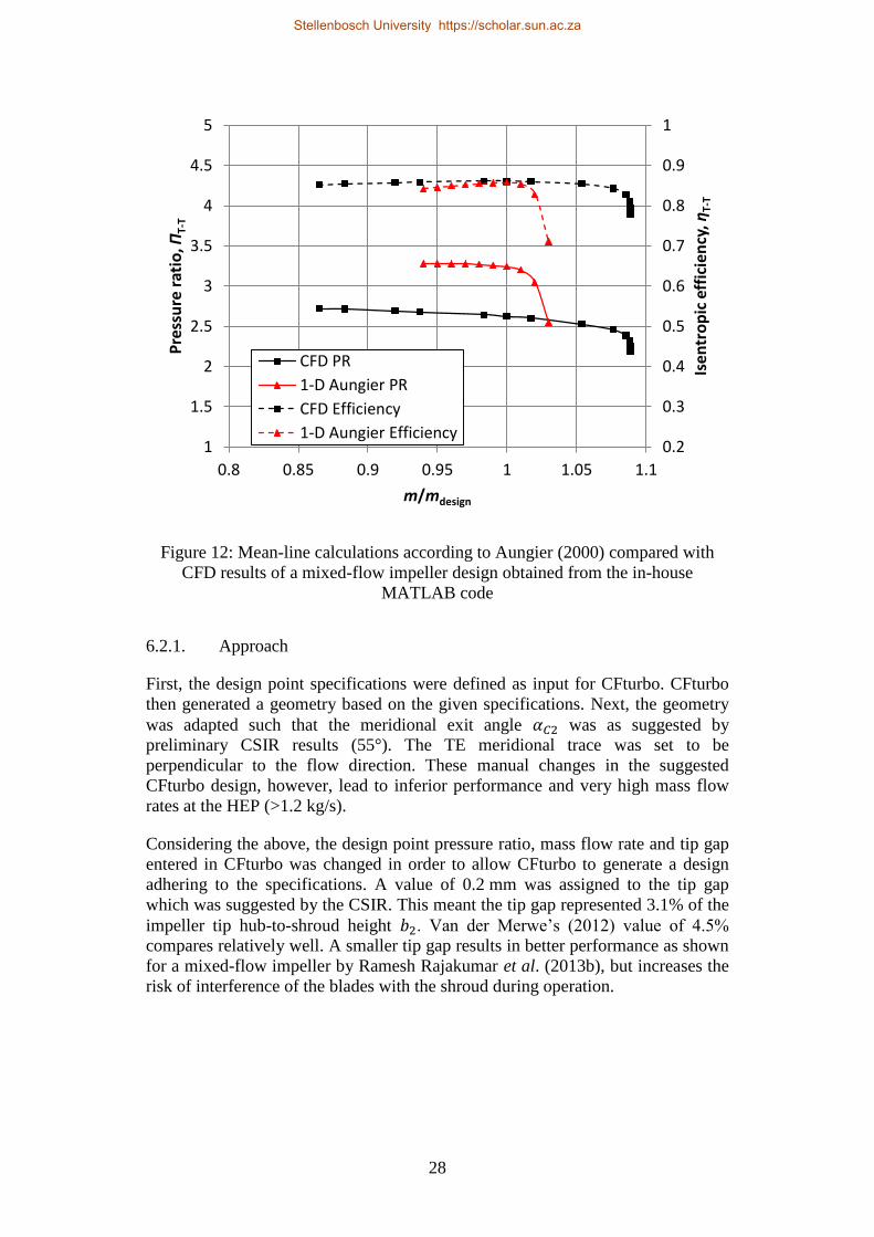
28

Figure 12: Mean-line calculations according to Aungier (2000) compared with

CFD results of a mixed-flow impeller design obtained from the in-house

MATLAB code

6.2.1. Approach

First, the design point specifications were defined as input for CFturbo. CFturbo

then generated a geometry based on the given specifications. Next, the geometry

was adapted such that the meridional exit angle was as suggested by

preliminary CSIR results (55°). The TE meridional trace was set to be

perpendicular to the flow direction. These manual changes in the suggested

CFturbo design, however, lead to inferior performance and very high mass flow

rates at the HEP (>1.2 kg/s).

Considering the above, the design point pressure ratio, mass flow rate and tip gap

entered in CFturbo was changed in order to allow CFturbo to generate a design

adhering to the specifications. A value of 0.2 mm was assigned to the tip gap

which was suggested by the CSIR. This meant the tip gap represented 3.1% of the

impeller tip hub-to-shroud height . Van der Merwe‟s (2012) value of 4.5%

compares relatively well. A smaller tip gap results in better performance as shown

for a mixed-flow impeller by Ramesh Rajakumar et al. (2013b), but increases the

risk of interference of the blades with the shroud during operation.

0.2

0.3

0.4

0.5

0.6

0.7

0.8

0.9

1

1

1.5

2

2.5

3

3.5

4

4.5

5

0.8 0.85 0.9 0.95 1 1.05 1.1

Ise

ntr

op

ic e

ffic

ien

cy, η

T-T

Pre

ssu

re r

atio

, ПT-

T

m/mdesign

CFD PR

1-D Aungier PR

CFD Efficiency

1-D Aungier Efficiency


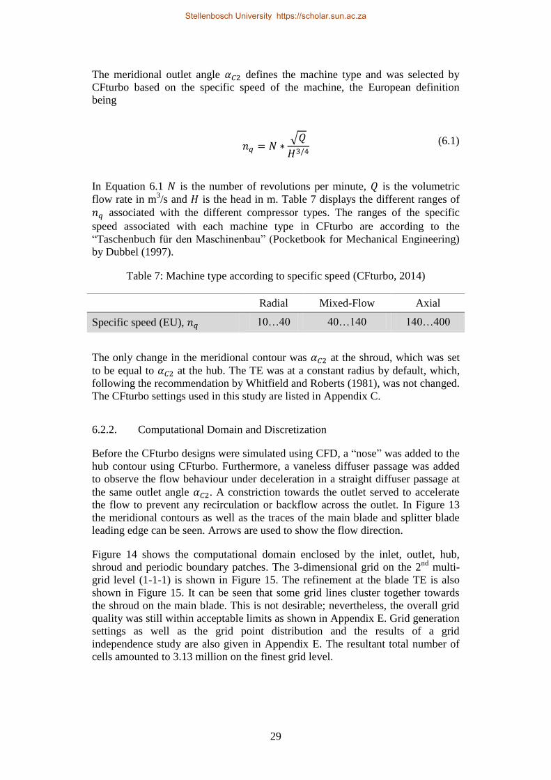
29

The meridional outlet angle defines the machine type and was selected by

CFturbo based on the specific speed of the machine, the European definition

being

√

(6.1)

In Equation 6.1 is the number of revolutions per minute, is the volumetric

flow rate in m3/s and is the head in m. Table 7 displays the different ranges of

associated with the different compressor types. The ranges of the specific

speed associated with each machine type in CFturbo are according to the

“Taschenbuch für den Maschinenbau” (Pocketbook for Mechanical Engineering)

by Dubbel (1997).

Table 7: Machine type according to specific speed (CFturbo, 2014)

The only change in the meridional contour was at the shroud, which was set

to be equal to at the hub. The TE was at a constant radius by default, which,

following the recommendation by Whitfield and Roberts (1981), was not changed.

The CFturbo settings used in this study are listed in Appendix C.

6.2.2. Computational Domain and Discretization

Before the CFturbo designs were simulated using CFD, a “nose” was added to the

hub contour using CFturbo. Furthermore, a vaneless diffuser passage was added

to observe the flow behaviour under deceleration in a straight diffuser passage at

the same outlet angle . A constriction towards the outlet served to accelerate

the flow to prevent any recirculation or backflow across the outlet. In Figure 13

the meridional contours as well as the traces of the main blade and splitter blade

leading edge can be seen. Arrows are used to show the flow direction.

Figure 14 shows the computational domain enclosed by the inlet, outlet, hub,

shroud and periodic boundary patches. The 3-dimensional grid on the 2nd

multi-

grid level (1-1-1) is shown in Figure 15. The refinement at the blade TE is also

shown in Figure 15. It can be seen that some grid lines cluster together towards

the shroud on the main blade. This is not desirable; nevertheless, the overall grid

quality was still within acceptable limits as shown in Appendix E. Grid generation

settings as well as the grid point distribution and the results of a grid

independence study are also given in Appendix E. The resultant total number of

cells amounted to 3.13 million on the finest grid level.

Radial Mixed-Flow Axial

Specific speed (EU), 10…40 40…140 140…400


30

Figure 13: Meridional view of a CFturbo design with hub nose and diffuser

passage

Figure 14: Computational domain enclosed by hub, shroud, inlet and outlet


31

Figure 15: 3-dimensional grid projections on the 2nd

multi-grid level of a CFturbo

design

6.2.3. Impeller Performance Evaluation

In the mean-line approach the performance of the impeller is estimated by

calculating the theoretical pressure ratio and temperature ratio between inlet of the

impeller and the impeller tip. Evaluation of the CFD results was therefore initially

also performed at the impeller tip, along the meridional TE position. This was the

case for the MATLAB and CFturbo designs. At a later stage in the design

(Chapter 7), the evaluation plane had to be shifted 2.5 mm downstream of the

impeller tip. To prevent confusion, a quantity evaluated on a plane of constant r is

designated by a subscript which includes r in brackets, for example the total

pressure ratio at r = 58 mm would be ( ). A detailed explanation on the

post-processing realized in CFViewTM

is given in Appendix D.

6.2.4. CFD Model

Fluid and flow model settings were carried over from the CFD analysis of the

reference stage. No R/S interface was necessary since the impeller was modelled

with a vaneless diffuser passage only. These settings also applied to the CFD

simulations completed for the optimization routines discussed in the subsequent

Chapters.


32

The BCs in the CFD model (Table 8) of the mean-line designs were similar to the

BCs in the reference stage. The air was to enter axially and the specified total inlet

conditions were entered. Discrete values between 150 kPa (choke) and 330 kPa

(surge) were assigned to the outlet static pressure to calculate the performance

curve.

Table 8: Boundary conditions used for the CFturbo designs

The same numerical model was used as in the CFD analysis of the reference

stage. The initial solution for the first computation at lowest backpressure was the

calculated solution for turbomachinery. The subsequent computations were given

the initial solution from the previous computation. For the 1-dimensional solution

the inlet initial condition was set to a constant static pressure distribution with a

value of 90 kPa. Again the rotating part of the hub was enclosed by a pre-defined

area.

6.2.5. Results

It was found that the HEP of the original CFturbo design (“design_5”) features a

mass flow at HEP ( ) around 30% above design specification, as shown in

Figure 16. Thus an iterative approach was formulated for the impeller

characteristic to reach the required mass flow rate at HEP. The options were to

directly scale the model in FINETM

/Turbo or to change the design point parameter

values entered in CFturbo. Design “d_5_scaled_0925” was obtained by directly

scaling “design_5” in FINETM

/Turbo by a factor of 0.925. This design displayed

an acceptable but a substantial reduction in pressure ratio. The decision

then lay between the two designs in which the CFturbo input parameters were

changed. The “d_5_065” design had a design mass flow defined as 0.65 kg/s

instead of 0.85 kg/s. Two inputs were changed to generate the

“d_5_p4_063_mod2” design: The pressure ratio was changed from 4.15 to 4 and

the mass flow rate to 0.63 kg/s.

Inlet

Total

Quantities

Imposed

Velocity

direction

| |

| |

| |

(kPa) (K)

Turbulent

viscosity,

(m2/s)

0 0 1 100 300 0.0001

Outlet

Pressure

Imposed

Averaged

Static Pressure

(kPa)

150…330

Hub,

shroud,

blades

Solid (no-

slip) shroud blades

Hub: area defined rotation

speed

0 rpm 95,000 rpm 95,000 rpm


33

Figure 16: Results of designs generated using CFturbo

The design “d_5_p4_063_mod2” was chosen over the design “d_5_056” because

of its higher efficiency. Efficiency was weighted higher than better pressure ratio,

since the pressure ratio was close to the specified minimum value of 4.15. In

hindsight it can be said that the “d_5_065” design was, in fact, the stronger

favourite, given that the efficiency of “d_5_065” was only 1% higher than that of

“d_5_p4_063_mod2”, but the pressure ratio was 6% lower. The scale on the

efficiency axis was misleading. The choke margin was, unfortunately, not a factor

considered in this decision.

The chosen design features a pressure ratio of 4.13 and an efficiency of 83.3% at a

mass flow rate of 0.83 kg/s and a constant-radius trailing edge of = 55.5 mm,

which reflects a 30% larger radius than estimated in Section 6.1 for a similar

pressure ratio and efficiency. The resulting specific speed (EU) was = 52 and

the meridional exit angle was = 74.5°. Table 9 compares mixed-flow

compressor designs from literature for perspective.

It can be seen that, given the tip speed of the CFturbo design, potential exists

for an increase in pressure ratio. Also, 15° larger than a typical angle angle for

mixed-flow compressor designs mentioned in recent literature (Ramesh

Rajakumar et al. (2013a). The designation of “mixed-flow” may thus be

debatable, but is still 17% smaller than for a radial machine, adding a

significant axial component to the velocity.

The FEA of this design was side-lined at the time due to time constraints. Wall-

values of the chosen CFturbo design HEP computation can be found in

Appendix D.

3

3.5

4

4.5

5

5.5

6

0.6 0.8 1 1.2 1.4

Pre

ssu

re r

atio

, ПT-

T (5

5.5

)

m/mdesign

design_5d_5_065d_5_scaled_0925d_5_063_p4_mod2

0.75

0.8

0.85

0.9

0.6 0.8 1 1.2 1.4

Ise

ntr

op

ic e

ffic

ien

cy, η

T-T

(55

.5)

m/mdesign

design_5d_5_065d_5_scaled_0925d_5_063_p4_mod2


34

Table 9: Comparison of various mixed-flow compressor impellers

(m/s) ( ) ( )

Harris et al. (2004) 45 - - -

Cevic and Uzol (2011) 50 540 4.34 72%

Ramesh Rajakumar et al. (2013a) 60 528 4.5 90%

Chosen CFturbo 74.5 552 4.13 83%

6.3. Conclusion

A mixed-flow impeller design with performance values close to the design

specifications was obtained using the commercial 1-dimensional turbomachinery

layout tool CFturbo. CFturbo was chosen as the designated layout tool, because

designs generated by the in-house mean-line code did not produce designs that

performed well enough to be considered for optimization.

CFD analyses showed that the of the original CFturbo design exceeded the

specified value by 30%. Different approaches were implemented in order to

reduce the HEP mass flow rate of the design. A change in CFturbo input

parameter values resulted in a design with its within 3% of the specified

mass flow rate and with an acceptable performance. The meridional exit angle

= 74.5° was chosen by CFturbo according to the specific speed of the

machine, based on values from the Pocketbook for Mechanical Engineering by

Dubbel (1997). With the pressure ratio close to the specified value and an

efficiency value above 80%, the design is suitable to be aerodynamically

optimized.


35

7. AERODYNAMIC OPTIMIZATION

After an acceptable impeller design was obtained from CFturbo, the design‟s

performance was optimized using FINETM

/Design3D v 10.05a. This chapter

describes how the impeller geometry was defined using lines and Bézier curves

linked by control points and their parameters. The fitting of the parametric

geometry to the original geometry is outlined. The procedure for determining

reasonable parameter bounds is explained before reporting on the database

generation, which was based on the design of experiments (DoE) approach.

Finally the optimization procedure, which involves teaching of an artificial neural

network (ANN) and the implementation of a genetic algorithm (GA), is outlined

and results are shown.

7.1. The Optimization Process

Optimization is the process of minimizing or maximizing a given function. In the

field of turbomachinery the design space is very large and any small change in

geometry can have a big impact. In order to search the design space for the best

design that adheres to the given requirements, a design may be optimized in three

dimensions using CFD. Optimizing in three dimensions ensures an accurate

representation of the actual flow conditions if done correctly.

It would be very time-consuming to evaluate the design space using only CFD

computations, because thousands of computations would be necessary to define

the design space accurately enough to be optimized. FINETM

/Design3D thus

makes use of an ANN to generate a “response surface”, which is used to predict

the performance of different designs and approximate a design space represented

by CFD simulations. A database of performance values corresponding to different

geometries is used as an input to the ANN. According to Hildebrandt et al.

(2009), the minimum number of database samples needed for an ANN to be

effective is three times the amount of free parameters.

The database is generated following the DoE approach. This approach expands

the extent of information included in the database, for a restricted amount of

geometries (Montgomery, 2001). During the database generation a parameter

value was allowed to take any value in the given continuous range. Each step in

the database generation as well as the optimization comprises of smaller steps

associated with the CFD-chain as follows:

Automatic grid generation using a grid-template file (*.trb)

Adaptation of BCs and flow solver settings via an associated computation

which was defined in FINETM

/Turbo

Solving

Automatic post-processing using a user-defined CFViewTM

macro linked

to FINETM

/Design3D


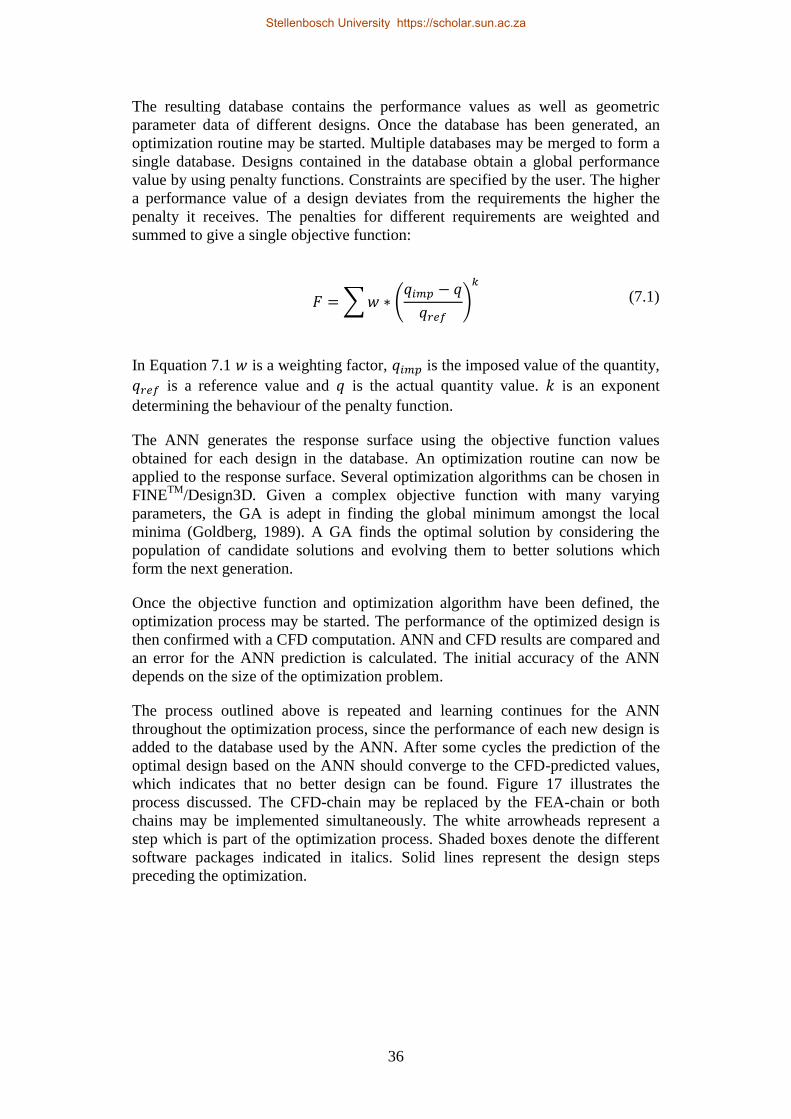
36

The resulting database contains the performance values as well as geometric

parameter data of different designs. Once the database has been generated, an

optimization routine may be started. Multiple databases may be merged to form a

single database. Designs contained in the database obtain a global performance

value by using penalty functions. Constraints are specified by the user. The higher

a performance value of a design deviates from the requirements the higher the

penalty it receives. The penalties for different requirements are weighted and

summed to give a single objective function:

∑ (

)

(7.1)

In Equation 7.1 is a weighting factor, is the imposed value of the quantity,

is a reference value and is the actual quantity value. is an exponent

determining the behaviour of the penalty function.

The ANN generates the response surface using the objective function values

obtained for each design in the database. An optimization routine can now be

applied to the response surface. Several optimization algorithms can be chosen in

FINETM

/Design3D. Given a complex objective function with many varying

parameters, the GA is adept in finding the global minimum amongst the local

minima (Goldberg, 1989). A GA finds the optimal solution by considering the

population of candidate solutions and evolving them to better solutions which

form the next generation.

Once the objective function and optimization algorithm have been defined, the

optimization process may be started. The performance of the optimized design is

then confirmed with a CFD computation. ANN and CFD results are compared and

an error for the ANN prediction is calculated. The initial accuracy of the ANN

depends on the size of the optimization problem.

The process outlined above is repeated and learning continues for the ANN

throughout the optimization process, since the performance of each new design is

added to the database used by the ANN. After some cycles the prediction of the

optimal design based on the ANN should converge to the CFD-predicted values,

which indicates that no better design can be found. Figure 17 illustrates the

process discussed. The CFD-chain may be replaced by the FEA-chain or both

chains may be implemented simultaneously. The white arrowheads represent a

step which is part of the optimization process. Shaded boxes denote the different

software packages indicated in italics. Solid lines represent the design steps

preceding the optimization.


37

Figure 17: The optimization process in FINETM

/Design3D

7.2. Parameterization

Parameterization is an important step preceding optimization, since it determines

the way the model may be varied (topology), the degree of freedom in the model

and the possible design variables. The geometry should be parameterized such

that it reflects the target design geometry and accommodates the envisaged

freedom. Ideally the parametric model should have as few free parameters (design

variables) as possible in order to simplify the optimization problem and reduce

optimization time and cost.

For parameterization of the geometry AutoBladeTM

was used. The CFturbo design

was parameterized by importing the *.geomTurbo file of the geometry as the

target geometry into the AutoBladeTM

design space (Appendix G) and generating

an initial parametric model via a turbomachine-type specific template and an

initialization. An initialization via the Adapt model tab estimates parameter values

and bounds of the model. Subsequently, necessary changes were made to the

parametric model topology. For example, C-splines were changed to Bézier

curves to define the camber. The model was adapted after the changes were made

using the Improve option. The following four definition sets construct the major

part of the parametric model of the impeller:

Endwalls

Stream surfaces

Stacking laws

Main blade camber curves and side curves

These definition sets are discussed in the following subsections.


38

7.2.1. Endwalls

The endwalls define the impeller meridional contours in the z-r-plane. In this

project the endwalls are symmetric about the axis of rotation. The hub nose

contour was defined by a C-spline. A Bézier curve with five control points was

utilized to define the impeller hub contour. Bézier curves exhibit more gradual

changes in gradients compared to C-splines. This makes them ideal for parametric

contour and camber definitions.

At the shroud the endwall definition begins with a line. The impeller contour was

again defined using a five-point Bézier curve. The diffusing part downstream of

the TE and the constriction was defined using straight lines. The endwall control

points are shown in Figure 18. Red dots connected by red, dashed lines represent

the Bézier control points. The control points were free to move in the directions

indicated by the arrows. The endwall control points totalled 18, which adds up to

36 endwall parameters.

No change in discharge angle was allowed in the optimization due to the

resulting increase in free parameters and potential negative effects this change

would have on the grid quality. Relaxing would, however, be a potential

factor for future investigation. was held constant at the impeller tip at hub and

shroud by enabling slope continuity at the end of the Bézier curve.

7.2.2. Stream Surfaces

Figure 18 shows black, dashed curves below the hub curve and above the shroud

curve. These curves represent the stream surfaces. The stream surfaces are the

segments at which the blade sections are defined. Linear interpolation surfaces

are typically used for radial turbomachinery and allow blade definition in the

dm/r-θ plane. To parameterize the geometry, two primary sections were made:

one at the hub at -2% span-wise location and one at the shroud at +102%. The

Rulings were activated. Ruled surfaces allow flank milling of the impeller. A

ruled surface is a surface which can be generated entirely by straight lines.

7.2.3. Stacking Laws

The stacking point defines the reference point to which the hub and shroud are

positioned. It was chosen to be the blade LE. The LE position in the dm/r-θ plane

can only be changed using the LE meridional position and tangential lean

parameters if the endwalls stay constant.


39

Figure 18: Parameterization of the hub and shroud contours (endwalls)

The main blade LE meridional location was relaxed (free to vary). Additionally,

the tangential location parameter LEAN_BETA was free, which controls the

overall blade lean.

7.2.4. Main Blade Camber Curve and Side Curves

The construction plane for the camber curves was the dm/r-θ plane. To define the

main blade camber curve on the hub and shroud section, a Bézier -curve with six

control points was used. The inner points were moved away from the centre and

thus toward the edges to improve fitting using the twice-geometric distribution

with the first and second common ratio equalling 1.5. Blade camber curvature and

blade lean are influenced by changes in these parameters. The splitter was set to

be a truncated section of the main blade.


40

No dependencies were established between the hub and shroud Bézier points. This

implies that the blade angles were free to differ from LE to TE throughout the

blade span. The CFturbo design features the same sweep angle at the TE

throughout the blade span. Neighbouring Bézier-points could have been

constrained in order to acquire the same blade angle at hub and shroud, but the

blade angles were not constrained since that would restrict the design space. Ten

camber parameters were relaxed as displayed in Figure 19, with the LE control

point being the reference point.

Blade thickness was defined in AutoBladeTM

by parameterizing the blade side

curves. Symmetric thickness addition was chosen with the camber as reference. A

Bézier spline with three uniformly distributed parameters for main and splitter

blade thickness was selected. A rounded LE and a blunt TE were enforced, where

the TE radius in the meridional plane was set to be constant. No thickness

parameters were relaxed, as the aerodynamic optimization is usually commenced

with the blade thickness frozen (Hildebrandt et al., 2009) (Demeulenaere et al.,

2015).

Figure 19: Section 1 and 2 camber Bézier points and associated freedom

The parameters of the final parametric model used in the optimization may be

split into seven major groups as listed in Appendix H. A detailed list of the free

and frozen parameters is shown in Appendix H.

7.3. Fitting

Obtaining a parametric geometry that is closer to the target geometry than it was

after initialization is achieved through the fitting process. Topology and parameter

bounds were checked to see if they didn‟t inhibit the fitting process from


41

achieving a better fit. A GA was used for the fitting. The model was fitted using

the medium option, as any more optimization steps did not improve the fitting

significantly. For the fitting the ruled surfaces had to be de-activated.

The blade camber angle at the TE at the hub was not attempted to match

perfectly with the target geometry. A better fit could have been achieved using

very high values for the geometric common ratios, but the camber curve was

rather set to experience gradual changes in gradient to improve flow conditions.

When comparing the fitted design with the original design it was observed that the

pressure ratio increased by 1.5%, the efficiency decreased by 0.2% and the choke

limit was reduced by 2.4%.

7.4. Parameter Value Bounds

The parameter value limits were defined according to visual impression.

Parameter values were varied in AutoBladeTM

to observe the effect on the

geometry. Not all possible geometric variations could be identified, but the

procedure gave a good first impression of the possible geometries.

To have a closer look at the geometric possibilities with the specified bounds the

parametric modeller was run to randomly generate geometries, as would be done

in the database generation process. These geometries could then be analysed and

compared by loading the *.par files into the Compare Geometries window in

FINETM

/Design3D, which makes 2-dimensional comparisons possible.

Geometries were also compared in three dimensional space by importing the *.par

files into the AutoBladeTM

design environment (Appendix G) and adding

overlays. This conveyed a better impression of the blade geometry.

Based on the meridional contours and traces no unrealistic geometries were

produced. This is confirmed by looking at some geometries shown in Figure 20,

which were generated with the parametric modeller.

An inspection of the B2B sections showed that many different camber shapes

could be produced, but once again no unrealistic shapes were generated. The shift

in the horizontal axis shown in Figure 21 is due to the change in radius of the hub

contour and/or the change in LE meridional position.

A 3-dimensional investigation showed that the blade lean was allowed to be very

aggressive at the TE – both towards and against the direction of rotation – as a

result of the different possible θ positions of the camber Bézier points at hub and

shroud. This was left unchanged to enlarge the design space.


42

Figure 20: Meridional contours and traces of randomly generated geometries

Figure 21: B2B views of possible blade shapes at section 1 (hub)

7.5. Operating Points

The operating points to be investigated during the optimization had to be chosen

before creation of the database. Only investigating the design point is not a

guarantee for a working design, the behaviour at off-design conditions is also

critical. Three operating points were chosen to be included (multi-point

optimization):


43

one point at design conditions (DP)

one point towards surge at a lower mass flow rate (SP)

one point at choking conditions at a low backpressure (CP)

By looking at these three operating points, an indication would be obtained of the

design and off-design performance at the design rotational speed. A 3D

Associated Computation was selected, which makes it possible to link the CFD

model inputs defined in FINETM

/Turbo projects to FINETM

/Design3D. The SP

was run at 95% of the DP mass flow rate which was imposed at the outlet. Placing

the SP too close to actual surge might result in unstable computations. Locating

the SP closer to the DP ensures stable simulations and allows for a better

indication of the highest efficiency mass flow rate . The DP was run with

0.83 kg/s mass flow imposed at the outlet as this is the highest efficiency mass

flow of the CFturbo design ( ).

If a mass flow BC is selected, FINETM

/Turbo reads the total mass flow input

while imposing the mass flow divided by the periodicity. For both mass flow

imposed operating points the velocity scaling technique for imposing mass flow

was used as better convergence was observed compared to the pressure

adaptation technique. The FINETM

/Turbo Manual (NUMECA International,

2014b) notes that velocity scaling is not valid for significant backflows at the

outlet. Any substantial backflow was prevented by adding a constriction at the

outlet. The CP was run with a value of 200 kPa averaged static pressure imposed

at the outlet. Backflow control was enabled for all operating points. Figure 22

shows the three operating points on the performance curve of the CFturbo design.

Figure 22: CFturbo compressor performance curves and chosen operating points

for optimization (evaluation at r = 55.5 mm)

0.4

0.5

0.6

0.7

0.8

0.9

2

3

4

5

6

7

0.55 0.6 0.65 0.7 0.75 0.8 0.85 0.9

Ise

ntr

op

ic e

ffic

ien

cy, η

T-T

(55

.5)

Pre

ssu

re r

atio

, ПT-

T (5

5.5

)

Mass flow rate, m (kg/s)

D5_063_p4_mod2_PRD5_063_p4_mod2_EffDesign PointStall PointChoke Point


44

Table 10 summarizes the three operating conditions.

Table 10: Operating points chosen for the CFD database and optimization

7.6. Post-processing

In FINETM

Design/3D it is possible to implement a user-defined post-processing-

macro which will automatically be executed in CFViewTM

. The required

quantities are then added to the results file and can be accessed in the

FINETM

/Design3D GUI.

A macro was written in Python which finds the necessary quantities at a specified

location to calculate efficiency and pressure ratio. The efficiency and pressure

ratio were calculated using mass-averaged total quantities at constant radius near

the trailing edge of the impeller. The same macros were used for database

generation and optimization.

7.7. Database Generation

After the visual investigation of the different possible designs, the database

generation process was started. The database was generated according to the DoE

approach. Parameters were chosen to vary randomly between the upper and lower

bounds (Continuous).

7.7.1. Grid Toughness and Quality

The final optimization made use of the results from three database runs: DB01,

DB02 and DB03. For DB01 and DB02 the mesh template utilized for the CFturbo

design was used. After checking the mesh quality of the two databases, it was

found that the grid quality was poor for many geometries. Hence DB03 was

started with a new mesh template. The major difference to the grid used for DB01

and DB02 was in the main blade outlet topology type which was set from low

angle to normal. The H-topology at the outlet was also enabled. These changes

meant that acceptable grids were created with large and small backsweep angles.

The results of the first database run were compared to those of DB01 and major

differences were observed. After an investigation it was found that with the new

TE topology the results were not reasonable if the impeller performance was

evaluated directly at the TE (r = 55.5 mm). However, the results of three different

meshes converged at around 57 mm radius. Thus the evaluation plane was shifted

to r = 58 mm. Figure 23 displays the mesh inconsistency at highest efficiency

SP DP CP

Outlet BC 0.79 kg/s 0.83 kg/s 200 kPa


45

point of the CFturbo design. It also shows results of the evaluation using the real

velocity values used for the mass-weighted average as opposed to the absolute

values. The mesh template that replaced the old template was designated

“new_TE_topology_1”.

In order to obtain an indication of the robustness of the new grid template, the grid

quality of the designs in the three databases is tabulated in Table 11. The quality

criteria were relaxed due to the original criteria being too conservative to be

enforced in an optimization with geometric freedom of this scale. DB01 and

DB02 used the old topology and DB03 the new topology.

Figure 23: Comparison of mass-averaged total pressures at different radii with

different TE topology

Table 11: Final CFD database grid quality

370

380

390

400

410

420

430

440

450

460

55 60 65 70 75

Tota

l pre

ssu

re (

kPa)

Radius of the evaluation plane (mm)

original_mesh

new_TE_topology_1

new_TE_topology_2

original_no_absolute_values

Number of designs DB01, DB02 cleaned DB03

in the database 67 77

with maximum aspect ratio >1,000 0% 0%

with maximum expansion ratio >4 5 (7%) 0%

with minimum angular skewness <18° 30 (45%) 4 (5%)

with maximum angular deviation >40° 10 (15%) 2 (3%)


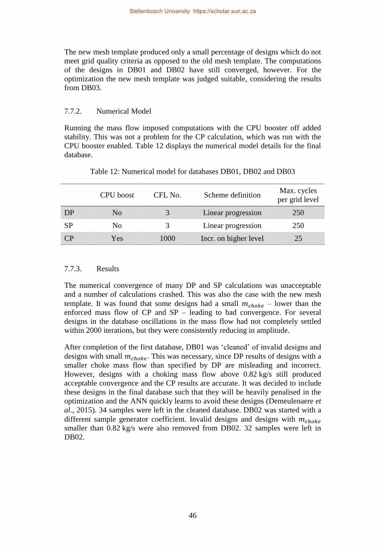
46

The new mesh template produced only a small percentage of designs which do not

meet grid quality criteria as opposed to the old mesh template. The computations

of the designs in DB01 and DB02 have still converged, however. For the

optimization the new mesh template was judged suitable, considering the results

from DB03.


Running the mass flow imposed computations with the CPU booster off added

stability. This was not a problem for the CP calculation, which was run with the

CPU booster enabled. Table 12 displays the numerical model details for the final

database.

Table 12: Numerical model for databases DB01, DB02 and DB03

7.7.3. Results

The numerical convergence of many DP and SP calculations was unacceptable

and a number of calculations crashed. This was also the case with the new mesh

template. It was found that some designs had a small – lower than the

enforced mass flow of CP and SP – leading to bad convergence. For several

designs in the database oscillations in the mass flow had not completely settled

within 2000 iterations, but they were consistently reducing in amplitude.

After completion of the first database, DB01 was „cleaned‟ of invalid designs and

designs with small . This was necessary, since DP results of designs with a

smaller choke mass flow than specified by DP are misleading and incorrect.

However, designs with a choking mass flow above 0.82 kg/s still produced

acceptable convergence and the CP results are accurate. It was decided to include

these designs in the final database such that they will be heavily penalised in the

optimization and the ANN quickly learns to avoid these designs (Demeulenaere et

al., 2015). 34 samples were left in the cleaned database. DB02 was started with a

different sample generator coefficient. Invalid designs and designs with smaller than 0.82 kg/s were also removed from DB02. 32 samples were left in

DB02.

CPU boost CFL No. Scheme definition Max. cycles

per grid level

DP No 3 Linear progression 250

SP No 3 Linear progression 250

CP Yes 1000 Incr. on higher level 25


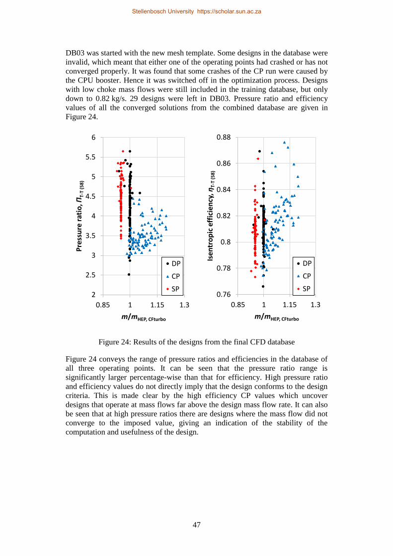
47

DB03 was started with the new mesh template. Some designs in the database were

invalid, which meant that either one of the operating points had crashed or has not

converged properly. It was found that some crashes of the CP run were caused by

the CPU booster. Hence it was switched off in the optimization process. Designs

with low choke mass flows were still included in the training database, but only

down to 0.82 kg/s. 29 designs were left in DB03. Pressure ratio and efficiency

values of all the converged solutions from the combined database are given in

Figure 24.

Figure 24: Results of the designs from the final CFD database

Figure 24 conveys the range of pressure ratios and efficiencies in the database of

all three operating points. It can be seen that the pressure ratio range is

significantly larger percentage-wise than that for efficiency. High pressure ratio

and efficiency values do not directly imply that the design conforms to the design

criteria. This is made clear by the high efficiency CP values which uncover

designs that operate at mass flows far above the design mass flow rate. It can also

be seen that at high pressure ratios there are designs where the mass flow did not

converge to the imposed value, giving an indication of the stability of the

computation and usefulness of the design.

2

2.5

3

3.5

4

4.5

5

5.5

6

0.85 1 1.15 1.3

Pre

ssu

re r

atio

, ПT-

T (5

8)

m/mHEP, CFturbo

DP

CP

SP0.76

0.78

0.8

0.82

0.84

0.86

0.88

0.85 1 1.15 1.3

Ise

ntr

op

ic e

ffic

ien

cy, η

T-T

(58

)

m/mHEP, CFturbo

DP

CP

SP


48

7.8. Optimization

After the three databases were cleaned and combined, the optimization was

prepared. Preparation included the definition of the objective function, setting the

appropriate weightings for the penalty terms, configuring the ANN, and choosing

the optimization algorithm and number of design iterations.

7.8.1. Optimization Settings and Objective Function Definition

A GA was implemented for the optimization step. Fifty optimizer steps were

enabled. This ensured optimizer convergence without a significant sacrifice in

time. In FINETM

/Design3D the objective function to be minimized is defined as in

Equation 7.1. In the final aerodynamic optimization penalty terms were based on

the following arguments:

Design Point

At DP the efficiency needed to be as close to unity as possible. An

equality constraint was used. The minimum pressure ratio at DP was

determined to be 4.2 to allow a pressure ratio loss across the diffuser of

15% (as observed with the reference stage). A maximum deviation of the

mass flow at the inlet of 2% from the mean in the last 500 iterations

was allowed at DP.

Choke Point

Designs that choke below the design mass flow of the CFturbo design had

to be penalised: A minimum mass flow rate of 0.84 kg/s at CP was

enforced. Additionally, designs with a higher mass flow than 0.9 kg/s had

to be penalised. This limited the highest efficiency point mass flow rate.

The value is based on the database results.

Stall Point

A maximum deviation of of 5% from the mean in the last 500

iterations was allowed.

DP-CP relative efficiency

After inspecting the database results, it was determined that many designs

had a higher CP efficiency than DP efficiency. To ensure that the HEP

exhibits a smaller mass flow than the CP, it was decided to not allow the

CP efficiency to be higher than DP efficiency. The database results show a

trend towards higher mass flows at highest efficiency point. The SP

efficiency was always lower than the DP efficiency.

SP-DP relative pressure ratio


49

A negative slope of the pressure ratio towards surge had to be guaranteed.

A positive slope is generally associated with dynamic instability (Hill and

Peterson, 1992). Therefore the SP pressure ratio had to be equal or larger

than the DP pressure ratio.

Penalties were assigned if design performance did not adhere to the constraints

shown in Table 13. Evaluation of performance was done at a constant radius of

58 mm.

Table 13: Imposed quantity values for the CFD optimization objective function

The final setting of the weightings and reference values evolved during the

optimization by suspending, manual checking, adapting and re-starting. Several

optimization runs were started in order to investigate where the optimizer is

heading and the following questions were asked:

Have the computations converged properly?

Is the optimizer producing better designs according to the objective

function? If yes, have the designs improved? If not, does the

optimizer penalise improved designs?

Do the improved designs adhere to all geometric and performance

constraints?

Do the improved designs produce reasonable performance curves,

judging from the three calculated operating points?

Are any parameter bounds reached? If yes, would it make sense to

increase the given range of the respective parameter?

Based on the above, does the objective function need to be

adapted?

In the final optimization the aim was a penalty value of 0.2 for a highly

undesirable quantity value, subject to designer estimate of importance. A table of

the weightings is given in Appendix I.

Imposed Values

Quantity Stall Point

(SP)

Design Point

(DP)

Choke Point

(CP)

DP -

CP

SP -

DP

( ) 1 EQUAL 0 MIN

( ) 4.2 MIN 0 MIN

m (kg/s) 0.84 MIN

0.9 MAX

deviation

0.05 MAX 0.02 MAX


50

The grid quality of the designs generated during the final optimization was within

the margins given in Table 11 for more than 98% of the designs. This again

proved the robustness of the grid which was changed during the database

generation.


The CPU booster was turned off for the CP calculation due to problems

encountered while generating the database. For mass-flow imposed outlet

boundaries (DP and SP) faster convergence was observed with the Increase on

higher level sweep scheme definition. Hence the option was enforced for DP and

SP during optimization. It was also enforced for the CP during optimization, with

no noticeable negative effects.

7.8.3. Results

The ANN converged after ca. 75 iterations. ANN convergence is displayed in

Figure 25. Due to the large amount of parameters, the parameter value ranges and

the relatively complex objective function, the necessary optimization steps for

convergence were more than the expected 40 (NUMECA International, 2014e).

Some critical parameter value bounds were reached during the optimization and

the bounds of S1_CAMBER_H2, S2_CAMBER_H2 and Z_LE_SHROUD were

adapted. Meridional lengths changed accordingly.

Figure 26 compares the B2B sections at the hub and shroud in the dm/r-θ plane of

the CFturbo and aero-optimized designs. Important to note is that the aero-

optimized curves were shifted in the horizontal axis for better comparison. It can

be seen that the LE blade angle has increased relative to the horizontal at hub

and shroud. The meridional length of the blade has also decreased.

Due to the parameter bounds set for the optimization, the shroud radius of the

impeller was allowed to decrease somewhat with increasing z. This was observed

while analysing the database geometries, but the implications were only realized

after the optimized design was found: If the decrease in radius was more than the

tip gap, the housing could not slide over the impeller. Therefore the shroud radius

at the inlet was manually reduced from 43.2 mm to the lowest value on the shroud

curve (42.934 mm (-0.6%)) while ensuring the rest of the contour remained

unchanged. The effect of the change in radius on the performance was

insignificant (<0.2%). Figure 27 contrasts the CFturbo design meridional contour

and the final adjusted optimized meridional contour.

Evident in Figure 27 is the shift in meridional location of the main blade LE and

splitter blade LE, both shifting towards the positive z-direction and thus reducing

the meridional length of the blades. The hub curve radius also increased notably

towards the location of the splitter.


51

Figure 25: ANN convergence of the CFD optimization

Figure 26: Initial fitted and optimized blade geometry at section 1 and 2


52

Figure 27: Comparison of initial and optimized meridional contours and locations

A comparison of the initial CFturbo and the final aero-optimized design is shown

in Figure 28. The design point is achieved well in the optimized design.

Additionally, an increase in pressure ratio of 15% compared to the initial design

along with an increase in efficiency of 4.6% was achieved. The actual

optimization process achieved an increase in pressure ratio from 4.21 to 4.62

(+9.7%) and an efficiency increase from the best value in the database of 82.8% to

85.6%. Table 14 compares the performance of the best database design and aero-

optimized design with the CFturbo design. The percentage increase relative to the

CFturbo design is given in brackets. The surge margin (Equation 2.16), which was

not a constraint in the optimization, was reduced from 30% (CFturbo) to 16%

(aero-optimized). This is still more than acceptable if compared to van der

Merwe‟s (2012) value of 10.9%.

Table 14: CFturbo, best database design and optimized design performance

comparison at HEP

CFturbo Database best Aero-optimized

Pressure ratio, ( ) 4.02 4.21 (+4.7%) 4.62 (+14.9%)

Efficiency, ( ) 81.0% 82.8% 85.6%


53

Figure 28: Initial and optimized design performance curves at design speed

7.9. Conclusion

A multi-point aerodynamic optimization of the CFturbo design was completed

using FINETM

/Design3D. The CFturbo design was successfully parameterized and

fitted. Parameter value bounds were carefully selected. Database geometries were

investigated visually before commencement of the CFD-chain. The initial mesh

was found to be weak in terms of quality for different geometries. A new, robust

mesh template was generated. The evaluation plane radius was changed due to

inconsistencies experienced when evaluating directly at the TE radius.

Convergence problems were encountered in the database even with the robust

mesh. This was attributed to the fact that was smaller than the imposed

for some database samples. Through the optimization process a gain of 15%

in pressure ratio was acquired at HEP and the efficiency was increased by 4.6%.

The next step in the development process was to confirm the structural integrity of

the aero-optimized design and, if necessary, complete a mechanical optimization.

0.4

0.5

0.6

0.7

0.8

0.9

2

3

4

5

6

7

0.7 0.75 0.8 0.85 0.9 0.95 1 1.05

Ise

ntr

op

ic e

ffic

ien

cy, η

T-T

(58

)

Pre

ssu

re r

atio

, ПT-

T (5

8)

m/mdesign

PR (aero-optimized)

PR (CFTurbo)

Efficiency (aero-optimized)

Efficiency (CFturbo)


54

8. MECHANICAL OPTIMIZATION

In order to ensure the impeller‟s structural integrity, the finite element (FE) kernel

integrated in FINETM

/Design3D v. 9-1.3, called OOFELIE, was applied for the

structural simulation under radial acceleration loads. It was found that the von

Mises (VM) stresses of the aerodynamically optimized design exceed the

acceptable limit in the main blade as well as in the impeller disk. The aim of the

structural optimization was to reduce the maximum VM stress to below 300 MPa

while preserving aerodynamic performance.

The VM stress is an equivalent value for the complete overall state of stress. It can

be compared to the material yield strength to indicate if yielding would occur for

the given stress state. The VM stress is derived from the distortion-energy theory

for ductile materials (Budynas and Nisbett, 2011).

The material stresses are influenced by the centrifugal load, the aerodynamic load

and also thermal effects. However, in this analysis only the centrifugal load was

considered. As mentioned by van der Merwe (2012), aerodynamic loads are

typically used for fatigue analyses, which are beyond the scope of this project.

Based on the work of Demeulenaere et al. (2015) a maximum VM stress target of

= 300 MPa, which was also recommended by NIB, was set. This being a

very conservative value, the peak VM stress was allowed to reach 380 MPa if

300 MPa could not be achieved. This value was based on the successful testing of

van der Merwe‟s (2012) aluminium impeller with a predicted of

380 MPa.

An approach was devised to obtain a well-performing, structurally sound design.

This approach is based on current literature by Demeulenaere et al. (2015). The

following steps were envisaged:

Disable the ruled-surfaces enforcement (software limitations).

Reduce disk stresses using only a database of different impeller backface

designs.

Optimize the blade stresses to ideally reduce to disk stress levels.

Confirm the aerodynamic performance of the optimized design.

If necessary, commence a coupled CFD-FEA optimization.

The constraint in the optimization was the global maximum VM stress. It was not

possible to define a stress location which could be included in the objective

function. Hence the optimization was split into two steps, which form task 2 and 3

in the list above: The disk stresses were to be reduced using a database, such that

the blade stresses may be reduced as far as possible in the optimization process,

before the maximum stress relocates to the disk.


55

8.1. Parameterization

The impeller disk contour was defined using eight control points and thus a total

of 16 parameters, shown in Figure 29 in the meridional view. The disk was

defined by four lines and one Bézier curve with four control points in red.

Dependent parameters are linked via a dashed line. The z next to the dashed line

indicates that the z-direction-parameter of the control point was the dependent

parameter.

Figure 29: Parameterization of the impeller solid sector in the meridional plane

A fillet was added to the blade roots by activating the blend parameters and

enabling the constant radius setting. An initial fillet radius, , of 0.5 mm lead to

a large number of cells required to mesh the fillet. The fillet radius was therefore

provisionally increased to 1 mm.

In Appendix J a shaft-stress calculation is given which was completed to

determine a provisional value for the bore diameter. The torque obtained from the


56

aero-optimized design‟s CFD results was utilized. With the material selected as

mild steel, a shaft diameter of 10 mm was calculated with a safety factor of two.

The blade thickness parameters were uniformly distributed along the camber.

Bézier splines formed the blade side curves (pressure and suction side), which

consisted of the following three parameters:

radius at the leading edge

half-thickness in the middle of the blade and

half-thickness at the trailing edge

Thickness addition was selected as symmetric. The splitter blade thickness values

were aligned with the main blade thickness in order to keep the number of free

parameters to a minimum. All other parameters were frozen at the aero-optimized

designs‟ values.

8.2. Discretization

HEXPRESSTM

/Hybrid automatically generates 3-dimensional elements of mixed

nature: tetrahedrals, hexahedrals, prisms and pyramids. According to the file

containing the mesh and element details (*.fea.mesh.e) all elements are linear:

The tets have four nodes, the pyramids have five nodes and so on. This was

deduced from the Propoelem definition, which declares the elements in the mesh

file.

When running an FEA in FINETM

/Design3D, the solid model is exported as

ParaSolid (*.xmt_txt) and then automatically meshed using

HEXPRESSTM

/Hybrid. Only a periodic section of the impeller is modelled, which

provides good correlation with the full model results (linear static analysis) but

decreases the computational prowess necessary and time expended significantly

(Valakos et al., 2007).

A cell count of around 380,000 to 400,000 was obtained in the database.

Refinements at the fillets, blade pressure and suction side as well as the blade tip

were enabled. No negative jacobians, concave, twisted or negative cells were

obtained. The maximum equiangular skewness was around 0.9 and the maximum

expansion ratio 12.

The automatic projection check had to be switched off. General face accuracy as

well as periodic face accuracy were set to 2. These values are in the same unit as

the AutoBladeTM

geometry, which is in millimeters. Maximum equiangular

skewness was set to unity in order for the software to accept the grid quality.

Geometry units had to be set to millimetres. The mesh is however scaled to meters

before it is transferred to OOFELIE (NUMECA International, 2014e).


57

8.3. FE Model

To create the solid model, the rulings, which enable flank milling of the impeller,

were initially switched off.

A number of materials eligible for the impeller are compared in Table 15. Inconel

was suggested by the CSIR. Al 7075 (in bold, also called Ergal) is the material

used by van der Merwe (2012). Ergal is readily available and relatively cheap,

and was also the material of choice in this thesis. A particularly strong aluminium

alloy and a common titanium alloy are included for comparison. Some fatigue

strengths are also shown, but depend on the number of cycles and therefore values

have many different ranges.

Table 15: Various potential impeller materials and their properties

Material Density

(kg/m3)

Modulus of

Elasticity

(GPa)

Poisson‟s

ratio

0.2 % yield

strength

(MPa)

Fatigue

Stength

(MPa)

Inconel 718SPF 8200 205 0.284 829-1293 -

Al 7075-T6 2810 71.7 0.33 500 159

RSA-7034 T6 2890 71 - 730 425

Ti-6Al-4V (G5) 4430 113.8 0.342 880 240-600

Material Property Data. [Online]. Available: www.matweb.com. [2015, July 5]

The material was modelled as isotropic and homogeneous. A rotational speed of

95,000 rpm was defined, resulting in a tip speed of 552 m/s. Boundary conditions

for symmetry and rotational load were applied automatically by

FINETM

/Design3D. Thereafter OOFELIE solved the matrices for the unknowns.

Cyclic symmetry implies the displacements and stresses on one periodic surface

are the same as on the other periodic surface, which was implemented by

OOFELIE. For OOFELIE to support non-matching grids on the periodic faces, an

integration scheme is used (NUMECA International, 2014e).

8.4. Impeller Backface and Bore

Disregarding the impeller blades, the highest stresses in the solid sector occurred

at the bore. A curved backface has shown to significantly reduce bore stresses

compared to a straight radial backface (Valakos et al., 2007). An improvised

curve was thus initially defined to describe the backface. To further reduce the

bore stresses, a database was created with only the backface parameters relaxed

(impeller disk control points 3 to 7).

Zheng et al. (2012) make it clear that the parameters relaxed in the database

generation play an important role in relation to the bore stress. The bore diameter


http://www.matweb.com/

58

had to be kept fixed, however, which according to Zheng et al. (2012) has a

significant influence on the bore stress.

8.4.1. Database Generation

The final backface design was a result of the investigation of several databases,

each database having undergone some changes in parameter value ranges based

on the results from the previous database. In Figure 30 some of the resulting

database geometries are shown.

Figure 30: Various geometries obtained in the impeller backface database

8.4.2. Results

Bore stresses were not reduced to 300 MPa in the database and thus an undercut

was considered. Investigating the results made it clear, however, that an undercut

increases blade stresses towards the TE as well as stresses on the impeller


59

backface. Additionally, van der Merwe (2012) reported on unacceptable impeller

tip deformations as a result of an undercut. With this in mind it was decided to

continue without an undercut.

The best database design without undercut had a peak bore stress of 362 MPa

(Figure 31, right) compared to the initial 425 MPa (left). This represents a 15%

decrease in bore stress. The backface stresses were below 300 MPa.

Figure 31: Initial backface design (left) and best database result

8.5. Impeller Blade

The main blade stresses exceeded the acceptable limit by a large margin.

Consequently the blade stresses were to be optimized while preserving

aerodynamic performance.

8.5.1. Database Generation

A database was generated with fixed backface parameters. All six main blade

thickness parameters as well as the shroud camber parameters H2 and H3 (as

shown in Figure 19) were relaxed. The other three shroud camber parameters were

left frozen, since they were further away from the high stress location. The

influence of blade inlet and outlet angle on aerodynamic performance was

expected to be large, which did not encourage the relaxation of these parameters.

The inducer shroud radius, , was also relaxed.

8.5.2. Optimization Settings and Objective Function Definition

A GA was implemented for optimization. The only penalty term was that of the

maximum VM stress, which was given an equality constraint of 300 MPa with a

weight of 2 for a quadratic penalty function and a reference value set equal to the


60

constraining value. The small number of free parameters and the simple objective

function meant the number of optimizer steps for each iteration could be set to

coarse (25 steps), since optimizer convergence was fast.

8.5.3. Optimization and Results

Two optimization runs were completed. In the first optimization the blade

thickness was reduced to below 0.5 mm at the LE. This was unacceptable from a

manufacturing point of view, and therefore the second optimization was started

with a 0.5 mm thickness lower bound. In the first optimization the optimizer also

decreased due to its influence on . As a result and were

reduced, as confirmed by a CFD computation, which is why was changed back

to its original value and was frozen in the second optimization.

In order to force the optimizer to produce better results, the stress objective was

set to 250 MPa. The optimized design showed peak VM stress of 430 MPa at the

tip and root of the main blade. ANN convergence was almost instant due to the

small number of design variables and constraints. The blade thickness distribution

is compared in Figure 32. Due to the side curves consisting only of three

parameters, the optimizer reduced the stresses at the peak stress location by

raising the TE thickness, resulting in a continuous increase in blade tip thickness

from leading to trailing edge.

Investigating the FEA results showed that the peak stress was situated at the tip as

well as the root of the main blade. The optimizer was not able to reduce these

stresses any more by only varying the shroud thickness parameters. Therefore

other parameters needed to be considered.

The hub blade thickness was previously limited to 2 mm, because it was known to

reduce the mass flow capabilities (due to a reduced throat area). Hence the hub

blade thickness limit of 2 mm was not increased.

Another option to reduce the stresses was to increase the fillet radius . The

effect of the fillet with a radius = 1.85 mm on the pressure ratio is documented

by van der Merwe (2012): a maximum deviation of only 2.5% was obtained

between numerical and experimental results. No efficiency data was available.

Hence was changed to 1.85 mm.


61

Figure 32: Hub and shroud blade thickness of the aero-optimized and

mechanically optimized designs

Using a fillet radius of = 1.85 mm reduced the stresses significantly. The

blade root stress and also the blade tip stress values dropped. As a result, the bore

stress peaked at 377 MPa and the blade tip and root stresses were somewhat lower

(370 MPa). The results of the blade thickness optimization are shown in Figure

33, where the aero-optimized design and the structurally optimized design are

compared.

Figure 33: VM stresses of the aero-optimized design (left) and the mechanically

optimized design with = 1.85 mm


62

The effect of the shroud camber was investigated next, since its influence on the

stresses could not yet be separated from the effects of the change in thickness

distribution. Original values from the aero-optimized design were used first, with

the results showing a lower mass flow rate as well as worse performance

(aerodynamically and structurally) compared to the mechanically optimized

design. Since this change resulted in lower mass flow, the camber values were

subsequently decreased, resulting in higher mass flow and better performance. As

a result of the manual shroud camber changes, the blade tip and root stresses were

reduced from 370 MPa to 300 MPa and 340 MPa respectively. Efficiency and

pressure ratio were higher than for the aero-optimized design. The aerodynamic

optimization did not achieve this performance since any changes in camber would

have had a negative effect on .

Table 16 summarizes the important design criteria values for the different designs

obtained. No significant differences in efficiency were observed among these

designs. Maximum VM stresses are given in MPa.

Table 16: Summary of design steps and effects on performance

8.6. Conclusion

A solid model of the aero-optimized design was successfully generated in

FINETM

Design3D. Only centrifugal loads were considered while commencing the

linear static FEAs. A hand calculation based on the torque obtained from the CFD

results indicated a bore diameter of 10 mm when using a safety factor of 2. The

initial database of varying backface parameters was able to reduce the impeller

disk stresses by 15%. The blade stress optimization using only FEA lead to new

blade thickness distributions at hub and shroud as well as a different fillet radius

and shroud camber curve. Blade tip maximum stresses were reduced from above

500 MPa to 300 MPa, while the blade root stresses were reduced to a maximum of

340 MPa. As a result, was located at the bore with a value of 377 MPa.

These values were obtained without a decrease in aerodynamic performance but

with a small sacrifice in highest efficiency mass flow and choking mass

flow . Attention could now be turned to improving the HEP and choking

mass flow rates and reducing through an aero-mechanical optimization.

[bore]

[root]

[tip]

( ) (kg/s)

Aero-optimized 362 >500 >500 4.62 0.851

Mech.-optimized 377 420 431 4.7 0.823

= 1.85 mm 377 370 370 4.7 0.823

Decreased 2 shroud

camber values

377 340 300 4.88 0.835


63

9. COUPLED AERO-MECHANICAL OPTIMIZATION

The resources were available to complete a coupled optimization in

FINETM

/Design3D v. 9-1.3, where each optimization step comprises a CFD

simulation and FEA of a different rotor geometry. Performance results of both

simulations were included in the objective function as constraints.

The primary objective of this optimization was to recover the CP mass flow rate

. Judging from previous calculations, there was a chance that the highest

efficiency point would also gain in mass flow if increases. Obtaining a

larger was found to have a bigger effect on thrust compared to an increase

in pressure ratio of the same percentage of the respective design value. This was

concluded by analysing different operating points using the ECA code

GasTurb12.

As a secondary objective, the maximum VM stress, , was to be reduced.

The objectives were to be reached while conserving aerodynamic performance. It

was established in the previous chapter that changes in blade camber of the aero-

optimized design affect the blade root stresses, amongst others. Thus another

objective was to ensure that any changes in camber did not lead to high VM

stresses at the blade root.

The free parameters were:

Section 2 (shroud) camber parameters H2 and H3

Impeller backface control points 3, 4, 5 and 6

S2_CAMBER_H2 and S2_CAMBER_H3 were relaxed due to the previously

observed influence on blade tip and root stresses, aerodynamic performance and

the choke limit.

9.1. Database Generation

The following steps were followed during the database generation:

Generate the geometries

Generate the CFD meshes and confirm mesh quality

Run the CFD simulation on the CP

Run the FEA

To be consistent and to prevent previously experienced problems, the same

numerical model settings were used as in the aerodynamic optimization. The

mechanical optimization showed that relaxing the inducer radius has a

negative effect on mass flow and thus the parameter was not relaxed.


64

9.2. Optimization Settings and Objective Function Definition

The numerical modelling settings from the database generation were carried over

to the coupled optimization. Given that the choke limit was of primary importance

regarding the CFD in this optimization, only the CP was chosen as an operating

point evaluated in the optimization. The performance of the CP and the HEP were

found to be closely related; the pressure ratio and efficiency differing by a

constant value. This was deduced from results of four different designs where

only the two shroud camber values H2 and H3 were varied. A comparison

between the difference in and of the four different designs was also

made. These values did not exhibit the same degree of similarity. The highest

difference was 0.017 kg/s, which was rounded down to 0.015 for definition of the

minimum choking mass flow constraint. For the objective function the following

constraints were defined:

Choke point

A choking mass flow of = 0.865 kg/s was expected to be

achievable by only varying the shroud camber values. This was based on

previous computations with different shroud camber values. CP pressure

ratio and efficiency incurred penalties if their values were below four and

one respectively. Based on previous calculations the CP performance

directly relates to the highest efficiency point performance.

Maximum VM Stress

The maximum VM stress constraint was set to a very optimistic minimum

of = 250 MPa in an attempt to stretch the optimizer.

In Table 17 the final objective function constraints are given.

Table 17: Imposed quantity values for the coupled optimization objective function

In the coupled optimization the mass flow rate criterion was of primary

importance, because it related to the aim of the optimization. Maximum VM

stresses and pressure ratio were of higher importance than efficiency, because the

database results showed that much more potential existed for an increase in

pressure ratio and decrease in than for an increase in efficiency.

The reference penalty value was taken to be the largest penalty for that

was assigned to the database designs according to the objective function while the

default weight factor and exponent were used. The highest penalty for was

set to be double that. The other maximum penalties were set to be half the

( ) ( ) (kg/s) (MPa)

Imposed values 1 EQUAL 4 MIN 0.865 MIN 250 MIN


65

reference penalty value. This lead to the best sample in the database being the one

which had the following characteristics: largest with low , high

pressure ratio and high efficiency.

Of the 20 database designs and 50 designs in the optimization only 4 grids (6%)

had a minimum skewness below 18° and 5 grids (7%) had a maximum angular

skewness above 40°.

9.3. Results

After some optimization attempts, the parameter ranges were adapted to provide

the optimizer with enough freedom in the direction of optimization. It was

important to limit the impeller disk tip thickness to a minimum of 0.5 mm as

suggested by Mr David Krige of Cape Aerospace Technologies.

The optimization was not able to increase of the best database design.

However, the optimizer was able to increase the pressure ratio meaningfully from

3.79 to 3.97 (at CP) until the changes started affecting negatively. No

substantial increase in efficiency was obtained. These results meant had to

be increased using parameters other than H2 and H3 at the shroud. Looking at the

circumferentially averaged relative Mach number plot of the aero-mechanically

optimized design, the choke location can be seen as marked in Figure 34.

Figure 34: Relative Mach number distribution in the meridional plane at choke


66

To enable a larger mass flow passing through the marked location, the flow area

had to be increased. Knowing that some room existed for the main blade root

stress to be increased to the level of the bore stress, the following options were

considered:

Increase the inducer radius, (shift shroud up)

Increase the impeller tip hub-to-shroud height, (shift shroud left)

As a result of a 0.5 mm increase in (1.16%), was shifted to .

This was achieved with the disadvantage of having a smaller pressure gradient of

the impeller performance curve towards surge. experienced no change.

Through an increase in by 0.5 mm (7.7%), stayed equal to but

the choke margin improved from 2.3% to 5%. This was achieved with a small

penalty in efficiency.

To evaluate the influence of the 1.85 mm fillet radius on the choke limit, a CFD

analysis was completed with the fillets included. The results showed a 1.2%

decrease in . This meant the aero-mechanically optimized design with

increased and features a choke margin of 3.8% if the fillets are considered.

As for the influence of the fillets on the remainder of the performance curve, van

der Merwe (2012) noted a maximum difference in CFD and experimental results

in pressure ratio and in the unchoked region of 2.5%. He attributed this to

omitting the fillet in the CFD.

In Figure 35 the aerodynamic performance of the CFturbo and aero-optimized

designs are compared with the aero-mechanically optimized design with manual

changes to and . This design is the final design. No further changes have

been made to this design in this study. A compressor map of the final design can

be found in Appendix N.

Due to being located at the bore with blade root stresses lying well below

the bore stress before the optimization was started, and not shifting to the

blades during the optimization process, the backface could be optimized. The

resulting backface contour together with the VM stress plot is shown in Figure 36.

has been reduced from 377 MPa to 342 MPa as a result of the optimized

backface contour and the lower blade root stress is due to the optimized camber.

This reflects a safety factor of 1.5 based on the material‟s yield strength. The best

database value of was 346.7 MPa.


67

Figure 35: Final design vs. CFturbo and aero-optimized designs at 95 krpm

Figure 36: The mechanically optimized design with = 1.85 mm (left) compared

to the design resulting from the shroud camber and backface optimization

Table 18 summarizes the important design parameter values of the different

optimized designs and the results of the manual changes on the aero-mechanically

optimized design. The increase in reflects the final step and the performance of

the final design. The pressure ratio increased steadily, while no efficiency penalty

0.4

0.5

0.6

0.7

0.8

0.9

2

3

4

5

6

7

0.7 0.75 0.8 0.85 0.9 0.95 1 1.05

Ise

ntr

op

ic e

ffic

ien

cy, η

T-T

(58

)

Pre

ssu

re r

atio

, ПT-

T (5

8)

m/mdesign

PR (aero-optimized)PR (final_design)PR (CFturbo)Efficiency (aero-optimized)Efficiency (final_design)Efficiency (CFturbo)


68

was incurred. Stresses can be seen to have improved meaningfully and have not

been affected by the manual changes in the aero-mechanically optimized design,

which are responsible for the improvement in mass flows.

Table 18: Summary of important design parameters

In order to obtain an impression of the changes in camber and thickness from the

aero-optimized design to the resultant design of the coupled optimization, the

blade profiles in the B2B-view (dm/r-θ plane) are shown in Figure 37. The change

in shroud camber angle as well as blade thickness is evident. The camber metallic

angle distributions of the initial, aero-optimized and final design are compared in

Appendix M.

To understand how the geometric changes improved the aerodynamic

performance of the CFturbo design, the relative Mach number distributions in the

B2B plane were analysed and compared. If the flow in a compressor is transonic,

meaning Mach numbers exceed unity, shock structures may form. Shocks

typically occur in compressors with pressure ratios larger than 3.5 (Tamaki,

2012). Shocks have a negative effect on performance due to the irreversibilities

associated with shocks and the potential boundary layer separation induced by

shocks. Relative Mach number distributions were thus analysed at design

conditions at the HEP of the CFturbo and final designs at 10, 50 and 90% of the

blade span.

At 10% span the results showed no shocks, but a very low Mach number region at

the pressure side of the main blade of both designs. This region is somewhat

smaller in the optimized design (Appendix K). At 50% span the CFturbo design

experiences a shock at the suction side of the main blade close to the LE. This

shock structure is not present in the optimized design as can be seen in Appendix

K.

(MPa)

( ) ( ) (kg/s)

(kg/s)

Aero-optimized >500 4.622 85.5% 0.851 0.865

Mech.-optimized

(manually changed)

377 4.88 86.2% 0.835 0.852

Aero-mech. opt. 342 5.20 86.6% 0.830 0.856

increase 342 5.165 86.8% 0.85 0.869

increase

(final design)

342 5.25 86.0% 0.844 0.891


69

Figure 37: Blade profiles of the aero-optimized design and the aero-mechanically

optimized design

Shocks are prone to appear near the shroud as shown by van der Merwe (2012).

That is also the case with the CFturbo and optimised designs when analysing the

B2B views at 90% span, as seen in Figure 38.

Figure 38: Relative Mach number contours of the CFturbo design (left) and the

final optimized design at 90% span and design conditions

Both designs show normal shocks occurring upstream of the main blade LE. Once

the air reaches the main blade LE, it accelerates to a relative Mach number of 1.8


70

at the suction surface before another shock occurs. In the CFturbo design, this

shock causes the boundary layer to separate from the main blade suction surface,

which might be the reason for the large region of very low relative Mach number

downstream of the shock. In this region the flow is reversed and does not stream

towards the splitter. The final design also experiences a shock at the main blade

suction surface, although this shock occurs further downstream of the main blade

LE and the low relative Mach number region downstream of the shock is

significantly smaller, contributing to the better performance. The flow separation

on the main blade suction surface is not present anymore.

The meridional view was inspected for the presence of any significant

recirculation which contributes to a decrease in performance. Comparing the

meridional velocity of the CFturbo and the final optimized design (Appendix K),

a small recirculation zone near the LE at the shroud is evident in the CFturbo

design, but completely diminished in the final design. Meridional velocities close

to the TE of the CFturbo design have been reduced and show a smoother

transition to higher velocities. A large recirculation zone is present in both designs

downstream of the impeller due to flow separation at the shroud. This has a

negative effect on stage performance and must be addressed in the future.

9.4. Errors and Uncertainty

When numerically modelling fluid flow, many possible reasons for discrepancies

between the predicted results and the actual flow behaviour exist. These reasons

are split into two categories: error and uncertainty. Errors in a CFD model are

defined by “any deficiency that is not caused by lack of knowledge” (Versteeg

and Malalasekera, 2007). Major errors are:

numerical errors due to rounding, iterative methods and discretization

coding errors that occurred during development of the software

user error due to incorrect use of the software

Significant numerical errors were prevented by ensuring a reduction in the global

residual by at least three orders of magnitude and by proving grid independence.

Coding errors are unlikely, since the commercial software implemented has been

used and validated before many times. User error was prevented by proving the

author‟s proficiency in the use of the software via simulation of a reference

compressor stage (Chapter 4).

Uncertainty is associated with the deficiencies in a CFD model due to lack of

knowledge. These include:

input uncertainty: domain geometry, BCs and fluid properties

physical model uncertainty: semi-empirical sub-models and simplifying

assumptions


71

The domain geometry could be optimized for CFD modelling by placing the inlet

and outlet boundaries relatively far away from the areas of interest. Pressure and

temperature at the inlet were specified and an axial velocity direction could be

assumed as the compressor impeller is the first component of the MGT. Using the

perfect gas air model to define fluid properties reduces computational time and

was deemed appropriate for compressors by MacIsaac and Langton (2011:288).

Its validity for the pressure and temperature ratios achieved in this thesis was

proven by computing the performance curve of the final design using the real gas

model and observing a difference in performance values of less than 1%.

Turbulence models are a main contributor to physical model uncertainty.

Choosing an appropriate turbulence model is essential to reducing physical model

uncertainty. The Spalart-Allmaras (SA) one-equation model is often used in

turbomachinery applications (van der Merwe, 2012) (Xuanyu et al., 2015)

(Tamaki, 2012). More information on turbulence modelling and the SA model is

given in Appendix A. The validity of the SA model was confirmed by computing

the performance curve of the final design using the commonly implemented k-ω

SST (shear stress transport) two-equation turbulence model. The SST-model

results reveal efficiency values almost 3% higher than predicted by the SA model

and a significantly larger surge margin of 40%. This leads to the conclusion that

the SA model results are conservative. This will be confirmed by experimental

results in the future.

9.5. Conclusion

A coupled aero-mechanical optimization was successfully completed using

FINETM

/Design3D. The starting design was taken as the best design from the

mechanical optimization. A choke mass flow rate of = 0.891 kg/s was

achieved while was reduced from 377 MPa in the mechanical

optimization to 343 MPa (-9%). The highest efficiency mass flow rate was shifted

from = 0.83 kg/s to = 0.844 kg/s with a choke margin of 5%

disregarding the effects of the fillet. The final choke margin was increased to

3.8% based on a CFD calculation including fillets. Compared to the aero-

optimized design, the pressure ratio was increased by 11% and highest efficiency

by 1.3%. These values were achieved through changes in camber, shroud radius

and hub-to-shroud height at the impeller tip . A surge margin of 12% was

calculated for the final design. Relative Mach number distributions in the B2B

plane showed diminished areas of low relative Mach number and less flow

separation in the final design compared to the CFturbo design. Now that the

aerodynamic and mechanical performances of the impeller have been optimised, a

study on the vibrational characteristics of the design could be completed.


72

10. ROTOR DYNAMIC ANALYSIS

In this chapter the dynamics of the compressor rotor are analysed, which entails

the determination of its natural frequencies and their potential excitations

associated with the shaft rotational speed. FE-methods were employed to compute

the natural frequencies and mode shapes of the rotor. The procedure and results of

the rotor dynamic analysis are presented in this chapter.

10.1. Linear Static FEA Validation

A linear static FEA was conducted in MSC‟s SimXpert in preparation for the

subsequent modal analysis. Given that a model for a linear static analysis had to

be created for the modal analysis discussed in the next chapter, it was convenient

to contrast and confirm the OOFELIE results.

10.1.1. SimXpert FE Model and Simulation Procedure

The following procedure was undergone to complete one linear static analysis of

the compressor rotor.

CAD export and import: The scaled solid sector geometry was exported

from AutoBladeTM

as a Parasolid *.xmt_txt file and imported in MSC

SimXpert. Care had to be taken that the correct units were selected. The

periodic section as well as the full impeller model was exported.

Mesh: Quadratic tetrahedral elements were generated by SimXpert‟s

automatic solid mesher. Quadratic behaviour of displacements and stresses

in between nodes was assumed such as implemented by van der Merwe

(2012) and Verstraete et al. (2010).

Material and co-ordinate system: Ergal was assigned to the solid property

NASTRAN card as an isotropic, homogeneous material. A cylindrical co-

ordinate system was created with its origin at (0, 0, 0) to which the nodal

displacements were assigned.

Cyclic symmetry: Multi-point constraints would accurately model the

cyclic symmetry condition by equalling the stress states on the periodic

surfaces, but for simplicity an investigation was done using only zero-

displacement constraints in the tangential (θ) direction on the periodic

surfaces as also done by van der Merwe (2012). Some problems with this

modelling technique were identified to be the fact that the blades are

curved and some of the periodic surfaces were not exactly orthogonal to

the θ-direction. Validity of the BC could be proven by modelling the full

impeller. With the tangential constraint implemented no radial constraint

was necessary.


73

Axial constraint: The OOFELIE results suggest a large part of the flat

impeller backface surface was axially constrained. Thus the whole flat

surface was axially constrained in SimXpert. Zheng et al. (2012) use the

same axial constraint for the linear static analysis.

Loading: A centrifugal force was assigned to all nodes with the center of

rotation at the origin and the z-axis being the axis of rotation.

Solving: The model is written to a Nastran analysis file, which is sent to

the solver.

Post-processing: Result averaging across surfaces was switched off. This

meant the values at the integration points were shown for the specified

integration area, and not averaged for a smoother visual.

10.1.2. Results

A mesh independence study was conducted. The results of the study are shown in

Table 19. It can be seen that from Mesh 2 to Mesh 3, a cell number increase of

63% resulted in a change in of only 0.3% and no noticeable change in

displacement.

Table 19: SimXpert linear static FEA mesh independence study results

Table 20 lists the locations and values of the maximum VM stresses as well as the

largest displacement magnitudes predicted by the different FEA packages.

Table 20: Linear static simulation result comparison

Mesh # of

elements

# of

nodes (MPa)

[location]

Max. displ. mag. (mm)

[location]

1 58k 93k 361.5 [blade root] 0.367 [LE tip]

2 110k 174k 345.5 [bore] 0.365 [LE tip]

3 180k 281k 344.4 [bore] 0.366 [LE tip]

# of

elements

# of nodes (MPa)

[location]

Max. displ. mag.

(mm) [location]

OOFELIE 400k 284k 344.2 [bore] 0.277 [TE tip]

SimXpert 110k 174k 345.5 [bore] 0.365 [LE tip]

ANSYS 92k 254k 340.1 [bore] 0.366 [LE tip]

ANSYS (full) 320k 527k 340.4 [bore] 0.365 [LE tip]


74

The stresses of the SimXpert and OOFELIE models do not only compare very

well in values, but also in the distribution as can be seen in Figure 39. However,

the displacement magnitude predicted by the SimXpert model is 30% higher than

predicted by OOFELIE. Another inconsistency in terms of displacements in the

OOFELIE model is that the displacement magnitude decreases with increasing

mesh density as opposed to what is observed with the SimXpert model.

Additionally, the location of maximum displacement is predicted to be at the

trailing edge. Due to the better solidity at the trailing edge, this result does not

seem realistic.

Figure 39: Comparison of OOFELIE (left) and SimXpert equivalent stress results

The periodic CAD model as well as the full impeller model were imported into

ANSYS Mechanical. This served the following two purposes:

Validate the cyclic symmetry BC implemented in SimXpert

Confirm the displacement magnitude as obtained from the SimXpert

model

The bore surface nodes were constrained in the θ-direction and the full back plate

planar surface in the z-direction. The SimXpert displacement values and

distribution were confirmed by both ANSYS models, as shown in Table 20 which

increases the reliability of the SimXpert results. These were thus used in

determining whether the displacements are acceptable.

The tip gap is 0.2 mm wide and therefore the displacement normal to the blade

tips must be below 0.2 mm to avoid the blades making contact with the casing. A

safe 0.12 mm peak radial displacement located at the TE was calculated. The

maximum displacement in the negative axial direction is 0.24 mm, but is located

at the tip of the LE and is therefore acceptable.

Possible reasons for the discrepancy in displacement magnitude from OOFELIE

could include the use of linear elements (especially tets) instead of quadratic


75

elements (over which the user has no control) or a discrepancy in the way the

displacement magnitude is derived. Although time constraints prevented the

investigation, a possible approach to finding the cause would be to analyse

simpler shapes in OOFELIE in small steps, starting with a solid disk followed by

a disk with straight vanes and so on.

10.2. Modal Analysis

Using the model described in Chapter 10 as a foundation, an undamped modal

analysis was conducted. The objective was to obtain possible natural frequencies

of the impeller and draw up a Campbell diagram (see Appendix A) to assess and,

if necessary, change the vibration characteristics of the impeller. As discussed in

Chapter 2, the stiffness of the impeller blades changes due to the centrifugal

forces. This results in a shift in modal frequency at high rotational speeds.

10.2.1. FE Model

The important changes made to the linear static SimXpert model were:

the change in analysis type from linear static to modal analysis with

preload

the axially constrained surface area

A rotational preload had to be added to the load cases due to centrifugal effects.

The load case had to be selected as a preload in the LoadCaseControl under the

DefaultLoadCase of the SOL103 (modal analysis). Important rotational speeds for

the preload are the design speed, 10% overspeed to consider overshoot, 10%

below design speed (potential testing speed), and idling speed at around 50 krpm.

The impeller back plate was assumed to be located at a shaft shoulder of 2 mm

radius larger than the impeller bore. Axial displacements were therefore

constrained for all nodes at a radius up to 7 mm.

10.2.2. Results

Different modal frequencies correspond to different mode shapes. In the case of

the impeller, the shapes may be split into three groups:

main blade flapping mode

splitter blade flapping mode

combined mode (main blade, splitter blade and disk)

Examples from each group are shown in Figure 40.


76

Figure 40: Different mode shape groups: main blade (left), splitter blade (middle)

and combined

The resulting modal frequencies are shown in Table 21. Results from a periodic

SimXpert and a periodic ANSYS model are given. In both models the whole flat

backside surface of the impeller was axially constrained. This represents

modelling condition 1. Condition 2 represents the smaller axially constrained

surface with a radius of 7 mm. Each fill colour corresponds to a different mode

shape. The natural frequencies are marginally higher than the measured values

obtained by Kammerer (2009) of an aluminium radial compressor with

= 200 mm, whose first four modes are in the range of 1,400 to 5,000 Hz.

Table 21: Pre-stressed modal analysis results at 95 krpm

The effect of the change in axial constraint is the change in modal frequency of a

combined mode from 14,277 Hz (condition 1) to 8,160 Hz (condition 2). Also, the

effect of the cyclic symmetry BC is evident, as the ANSYS results show an

additional combined mode at 5,600 Hz which the SimXpert model did not pick up

due to its tangential constraint on the periodic surfaces.

Potential resonant conditions can be found by investigating the Campbell diagram

in Figure 41. Modelling condition 2 was implemented to obtain the modal

frequencies. Dashed lines represent engine order (EO) lines and the vertical line

shows the design rotational speed. Triangles represent main blade flapping mode

frequencies, squares represent splitter flapping modes and circles a combined

blade-disk mode. The diamond signifies the ANSYS combined mode not obtained

in SimXpert.

Mode #

Model 1 2 3 4 5 6

Frequency

(Hz)

SimXpert 2 4,114 8,160 8,981 9,822 11,259 15,917

SimXpert 1 4,117 8,977 9,820 11,258 14,277 15,917

ANSYS 1 3,970 5,595 9,008 9,800 11,307 14,405


77

Figure 41: Compressor rotor Campbell diagram (SimXpert 2)

When analysing the Campbell diagram, it was decided to ignore self-excited

stimuli as they do not need any perturbation of fixed amplitude to evoke them

(Cumpsty, 1989). Only flow-field related forced vibration stimuli were

considered. Unbalance and other mechanical forced vibration stimuli are more

likely to be occurring at EO 1 and 2, which don‟t coincide with the natural

frequencies. Other stimuli must, however, not be dismissed altogether. The

identified potential regions of resonance are summarized in Table 22, not all listed

critical speeds have the same weight, though.

The incidence of the low natural frequencies with the very low EOs are

considered serious, as explained by Cumpsty (1989). Regarding the higher EOs,

any critical number of struts or stator vanes near the inducer or impeller outlet as

indicated in Table 22 should not be present once the MGT has been constructed.

Considering the above, it can be said that the MGT should not have any 3, 6 or 9

struts or stator vanes located near the inducer. Additionally, there should be no 6,

9 or 18 stator vanes in close proximity to the impeller tip.

Speeds of 75 to 90 krpm should not be used for prolonged testing or idling speeds

due to the possible excitation of the 1st main blade flapping mode at EO 3. The

other main blade flapping mode critical speeds should not be serious if no 6 or 9

struts or stator vanes are located close to the inducer. The same can be said about

the combined modes.

0

5 000

10 000

15 000

20 000

25 000

30 000

35 000

0 25 000 50 000 75 000 100 000

Freq

uen

cy (

Hz)

Rotational speed (RPM)

design speed

main blade

combined

splitter blade

ANSYS

1 2 3

6

9

18

EO


78

Table 22: Possible resonant conditions obtained from the Campbell diagram

Changes in blade design would not be helpful, in the sense that even though

higher frequency modes would be shifted, the first main blade flapping mode

would be moved to coincide with low EOs at design speed.

In summary, the compressor impeller features many potential resonant conditions,

of which most could be prevented by considering the structural surroundings of

the compressor in the MGT layout. Speeds between 70 and 90 krpm should be

avoided given that a low EO coincides with the 1st main blade flapping mode. No

problems are expected when running at the design speed of 95 krpm.

Mode Excited by Critical speed (krpm)

[EO]

1st MB flap 3 struts/stator vanes near inducer,

inlet distortion

~75-90 [3]

1st combined 6 stator vanes near impeller outlet ~75-90 [6]

2nd

MB flap 9 & 6 struts/stator vanes near inducer ~55-65 [9], ~85-95 [6]

3rd

MB flap 9 & 6 struts/stator vanes near inducer ~60-70 [9], ~95-105 [6]

1st SB flap 9 struts/stator vanes near inducer or

impeller outlet

~70-80 [9]

2nd

combined 18 & 9 stator vanes near impeller

outlet

~50[18], 105 [9]


79

11. CONCLUSION AND RECOMMENDATIONS

Due to the increased interest in the application of MGTs for the propulsion of

UAVs, a design of a mixed-flow compressor for an MGT was proposed. The

design procedure and modelling results were presented in this report. Relevant

theory and the function of a mixed-flow impeller was explained. An overview of

the design process which was followed in this thesis was given. Literature

concerning the history of mixed-flow compressors as well as the 1-dimensional

and 3-dimensional analysis and development of mixed-flow compressors was

detailed.

A reference compressor stage was analysed using CFD, proving the author‟s

proficiency in the use of the software. An initial compressor impeller design was

obtained using CFturbo. The initial design was optimized aerodynamically using

CFD. Through the aerodynamic optimization process a gain in pressure ratio of

15% at design conditions was acquired and the efficiency was increased by 4.6%

compared to the initial CFturbo design. Following the aero-optimization, a

mechanical optimization was completed using FEA. The mechanical optimization

process achieved a reduction in the peak VM stress from far above 500 MPa

(material yield strength) in the aero-optimized design to below 400 MPa. A

subsequent aero-mechanical optimization helped increase the pressure ratio of the

aero-optimized design by 11% without sacrificing efficiency. The global peak

VM stress was furthermore reduced to below 350 MPa (safety factor of 1.5) while

the choke margin was increased by 3% as a result of manual changes to the

shroud contour. The surge margin suffered a decrease from 30% in the initial

design to 12% in the final design, which, according to literature, is still an

acceptable surge margin. Errors and uncertainties in the CFD model were

discussed. Possible resonant conditions were identified on the Campbell diagram

of the rotor and relevant recommendations regarding the surrounding structure of

the compressor were made.

The final mixed-flow compressor impeller design achieves a total-to-total

pressure ratio of 5.2 at design conditions. This leaves a large margin for the

diffuser to reach the specified stage pressure ratio of 3.83. An isentropic total-to-

total efficiency of 86% was obtained for the impeller. These quantities were

evaluated at a constant radius 2.5 mm downstream of the impeller tip. The

maximum VM stress equals 344 MPa, which is 30% below the yield limit of the

chosen material. The impeller features a surge margin of 12% as well as a choke

margin of 3%, which includes the effects of the fillets. Thus the performance

specifications have been met without neglecting the off-design characteristics. A

summary of the impeller specifications and achieved values is given in Table 23.

Potential resonant conditions close to design speed have been identified, which

should not be neglected. Critical resonant conditions exist between 75 and

90 krpm. No problems are expected when running at the design speed of 95 krpm.


80

Any structural members causing 3, 6 or 9 excitations per revolution should not

exist near the inducer. Stator vanes near the impeller tip should be prevented to

cause 6, 9 or 18 excitations per revolution. This is the result of the modal analysis

that was conducted.

Table 23: Specified and obtained impeller performance quantities

The numerical analyses and optimization processes presented in this thesis

required considerable computational time. The CPU time was, however,

significantly reduced by making use of computer clusters and parallel processing.

A summary of the processor management and CPU time of the major

computations is given in Appendix L. A 3-dimensional render of the initial and

final designs are shown in Appendix O for comparison.

11.1. Recommendations

Regarding the aerodynamic optimization, it was learnt that it is advisable to

complete an optimization initially with small parameter bounds. This leads to a

greater chance of obtaining good quality meshes as well as a smaller chance of

being lower than . It is much more efficient to reduce the chance of

crashed or badly converged designs before optimization, because the database

requires significant computational time. If the optimizer reaches any bounds, these

may be increased (but should not be reduced). Should it then be necessary to

create a better mesh template, it can be done.

It might also be advisable to run only the CP calculations first to check whether

designs are generated where is smaller than . The CP computations

have a greater chance of being stable and have a higher guarantee of convergence

if the parameter value ranges are high.

Consistency in the aero-optimization should have been guaranteed by an earlier

prognosis of the robustness of the CFD grid and running all database and

optimization samples using the same grid template. This did not, however, prevent

the optimizer from improving the initial design.

Looking back critically, the number of free parameters on the hub and shroud in

the parametric model could have been reduced by assigning four instead of five

Bézier points to the impeller endwalls. Also, one parameter on the impeller shroud

Quantity Specified Final design

(kg/s) 0.85 0.844

( ) >4.15 5.25

( ) >85% 86%

(MPa) <300 (or <380) 344


81

curve was “free” in the parametric model, but was in fact fixed by the slope

continuity constraint.

11.2. Future Work

The following areas have potential for future investigation:

It would be interesting to observe the effect of a change in meridional exit

angle on the performance of the impeller. An optimization with

relaxed could be achieved by firstly enforcing a trailing edge trace

orthogonal to the flow direction in the meridional plane. This could be

done by relating the hub control point co-ordinates to the shroud contour

co-ordinates using . The vaneless diffuser passage parameters would

have to be related to the trailing edge parameters. The Bezier control point

adjacent to the trailing edge control point should have slope continuity

enforced, such that it will automatically adjust to conserve the outlet angle.

This change will have an effect on the grid using the current grid template.

The template should, however, be able to accommodate small changes in

without a major sacrifice in grid quality.

The manufacturing and experimental testing of the impeller is an

important step necessary to validate the numerical results presented in this

thesis and should be completed in the future. Testing of the impeller could

be completed in a blow-down facility as done by van der Merwe (2012) or

on an MGT test rig along with all other engine components assembled.

The diffuser is a critical component still to be designed. A single-row

vaned cross-over diffuser is currently under consideration to be matched to

the impeller at SU. This kind of diffuser would be ideal in terms of

geometric constraints, as it would complete the tasks of directing the flow

in the axial direction and recovering of the pressure in a single row. A big

task for the diffuser would be to eliminate, if possible, the separation

occurring at the shroud near the impeller outlet. Curving the shroud

contour towards the axial direction as soon as possible is thought help

reduce the separation by pushing the fluid back against the wall. The fact

that the air is decelerated in that region does not assist in keeping the

boundary layer attached. Therefore it might be beneficial to accelerate the

fluid to prevent separation before diffusing. If this is not possible, minor

changes to the impeller design could be made in order to shift the

separation point or reduce the recirculation region.


82

REFERENCES

Aungier, R.H. 2000. Centrifugal Compressors: A Strategy for Aerodynamic

Design and Analysis. ASME press, New York.

Basson, J.G.T. 2014. Design Methodology of an Axial-flow Turbine for a Micro

Jet Engine. Master Thesis. Stellenbosch University. Stellenbosch.

Benini, E. and Giacometti, S. 2007. Design, Manufacturing and Operation of a

Small Turbojet-engine for Research Purposes. Applied Energy 84: 1102–1116.

Budynas, R.G. and Nisbett, J.K. 2011. Shigley’s Mechanical Engineering Design.

9th

ed. McGraw-Hill, New York.

Boyce, M.P. 2002. Gas Turbine Engineering Handbook. Gulf Professional

Publishing. Houston, Texas.

Cevic, M. and Uzol, O. 2011. Design Optimization of a Mixed-flow Compressor

Impeller for a Small Turbojet Engine. Aircraft Engineering and Aerospace

Technology: An International Journal. 83(3): 127–137

Cloud, C.H. 2009. Design Audits of Turbomachinery: Rotor Dynamics.

Proceedings of the 21st Ethylene Producers’ conference. Tampa, Florida,

USA.

CFturbo. 2014. CFturbo 9.2. User‟s Manual.

Cumpsty, N.A. 1989. Compressor Aerodynamics. Longman Group UK Limited.

Singapore.

Chen, J., Huang, G., Xia, C., Zhu, J. 2011. Flow Analysis and Improvement of a

micro Transonic Compressor Impeller. 47th AIAA/ASME/SAE/ASEE Joint

Propulsion Conference & Exhibit. AIAA 2011-5750.

Demeulenaere, A. and Hirsch, C. 2004. Application of Multipoint Optimisation to

the Design of Turbomachinery Blades. ASME Paper GT-2004-53110.

Demeulenaere, A., Jonnacorsi, J.C., Gutzwiller, D., Hu, L., and Sun, H. 2015.

Multi-disciplinary multi-point optimization of a turbocharger compressor

wheel. Proceedings of ASME Turbo Expo 2015. Montreal, Canada.

De Wet, A.L. 2011. Performance Investigation of a Turbocharger Compressor.

Master Thesis. Stellenbosch University. Stellenbosch.

De Villiers, L.C.B. 2014. Design of a Centrifugal Compressor for Application in

Micro Gas Turbines. Master Thesis. Stellenbosch University. Stellenbosch.


83

Dixon, S.L. 1998. Fluid Mechanics and Thermodynamics of Turbomachinery. 5th

ed. Elsevier Butterworth-Heinemann. Oxford.

Dubbel, H. 1997. DUBBEL: Taschenbuch für den Maschinenbau. 19th ed. W.

Beitz, & K. H. Küttner (Editors). Springer.

Eisenlohr, G. and Benfer, F.W. 1994. Aerodynamic Design and Investigation of a

Mixed-Flow Compressor Stage. AGARD Conference Proceedings 537:

Technology Requirements for Small Gas Turbines.

Fischer, A., Korfanty, M., Müller, R., Strobel, J. 2014. Auslegung, Entwurf,

Nachrechnung und Optimierung einer Hochdruck-Turboverdichterstufe.

ANSYS Conference and 32nd

CADFEM User’s Meeting. Nuremberg,

Germany. [Online]. Available:

http://en.cfturbo.com/fileadmin/content/down/papers/ACUM_2014_CFturbo.p

df [2015, November 2]

Goldberg, D.E. 1989. Genetic Algorithm. Addison Wesley Publishing.

Harris, M., Jones, A. and Alexander, E. 2003. Miniature Turbojet Development at

Hamilton Sundstrand: The TJ-50, TJ-120 and TJ-30 Turbojets. Paper

presented at the 2nd AIAA Unmanned Unlimited Systems, Technologies and

Operations–Aerospace Conference, Sand Diego, CA, USA.

Hildebrandt, T., Thiel, P. and Lehmann, I. 2009. Entwicklung eines

leistungsgesteigerten Radialverdichters für Ab-gasturbolader: Von der CFD

basierten Optimierung mit FINE™/Turbo bis zum serienreifen Prototyp im

Hause KBB. Proceedings of the 14th

Aufladetechnische Konferenz, Dresden.

Hildebrandt, T., Gressera, L. and Sievert, M. 2011. Kennfeldverbreiterung eines

Radialverdichters für Ab-gasturbolader durch multi-disziplinäre CFD-FEM-

Optimierung mit FINETM

/Turbo. Aufladetechnische Konferenz Dresden.

Hill, G.H. and Peterson, C.R. 1992. Mechanics and Thermodynamics of

Propulsion. Addison-Wesley. USA.

Japikse, D. 1996. Centrifugal Compressor Design and Performance. Concepts

ETI. USA.

Japikse, D., and Baines, N.C. 1997. Introduction to Turbomachinery. Oxford

University Press.

Kammerer, A. 2009. Experimental Research into Resonant Vibration of

Centrifugal Compressor Blades. PhD dissertation. Zürich: Swiss Federal

Institute of Technology (ETH Zürich). Diss. ETH No. 18587.


84

Kano, F., Fukao, Y. and Shirakami, T. 1984. Development of High Specific Speed

Mixed Flow Compressors. Proceedings of the 13th

Turbomachinery

Symposium. Texas A&M University. Texas, USA. pp. 139-147.

Krige, D.S. 2013. Performance Evaluation of a Micro Gas Turbine Centrifugal

Compressor Diffuser. Master Thesis. Stellenbosch University. Stellenbosch.

King, J.A. and Glodeck, E. 1942. Performance Characteristics of Mixed-Flow

Impeller and Vaned Diffuser with several Modifications. NACA Wartime

Report E-197.

LEDGER University Research Program. [Online]. Available:

http://ledger.wikispaces.com/ [2014, July 18]

MacIsaac, B. and Langton, R. 2011. Gas Turbine Propulsion Systems. 1st ed.

Wiley-Blackwell.

Mönig, R., Broichhausen, K. and Gallus, H. 1987. Application of Highly Loaded

Single-Stage Mixed-Flow Compressors in Small Jet-Engines. AGARD

Conference Proceedings No. 42.

Mönig, R., Elmendorf, W. and Gallus, H. 1993. Design and Rotor Performance of

a 5:1 Mixed-Flow Supersonic Compressor. Journal of Turbomachinery,

115(3): 565-72.

Montgomery, D. 2001. Design and Analysis of Experiments. 5th

ed. John Wiley &

Sons Inc. New York, USA.

MSC Software. 2015. [Online]. Available:

http://www.mscsoftware.com/product/simxpert [2015, October 31]

Müller, R.P. and Kreuzfeld, G. 2011. CFturbo – Modern turbomachinery design

software. Compressor Tech Magazine.

Musgrave, D. and Plehn, N. 1987. Mixed-Flow Compressor Stage Design and

Test Results with a Pressure Ratio of 3: 1. Journal of Turbomachinery, 109(4):

513-9.

National Research Council. 2000. Uninhabited Air Vehicles: Enabling Science for

Military Systems. National Academy Press, Washington, D.C. pp. 59–61.

Niculescu, M.L., Silivestru, V., Vizitiu, G., Danaila, S. and Berbente, C. 2007.

Theoretical and Numerical Investigation of Centrifugal and Mixed

Compressor Impellers. Paper presented at the 8th International Symposium on

Experimental and Computational Aerothermodynamics of Internal Flows.

NUMECA International. 2014a. AutoGrid5TM

User Manual.


85

NUMECA International. 2014b. FINETM

/Turbo 9.1 User Manual.

NUMECA International. 2014c. CFView 9.1 User Manual.

NUMECA International. 2014d. AutoBladeTM

User Manual.

NUMECA International. 2014e. FINETM

/Design3D 9.1 User Manual.

Patankar, S.V. 1980. Numerical Heat Transfer and Fluid Flow. USA: McGraw-

Hill.

Pichlmeier, D. 2010. [Online]. Available: http://www.dapi-

tech.de/EN/turbine_cad_en.html [2015, November 1]

Pierret, S., Demeulenaere, A., Gouverneur, B. and Hirsch, C. 2000. Designing

Turbomachinery Blades with the Function Approximation Concept and the

Navier-Stokes Equations. 8th AIAA/NASA/USAF/ISSMO Symposium on MDO,

Long Beach, CA.

Ramamurthy, S. and Srharsha, A.M. 2009. Theoretical Evaluation of Flow

through a Mixed Flow Compressor Stage. 19th

International Symposium on

Air Breathing Engines.

Ramesh Rajakumar, D., Ramamurthy, S. and Govardhan, M. 2013a. CFD

Analysis of Flow through Mixed Flow Compressor Under various Operating

Conditions. International Journal of Scientific & Engineering Research, 4(2).

Ramesh Rajakumar, D., Ramamurthy, S. and Govardhan, M. 2013b. Study on the

Performance Deterioration of Mixed Flow Impeller due to Change in Tip

Clearance. Journal of Thermal Sciences, 22(6): 532-538.

Schenk, O. and Gärtner, K. 2004. Solving unsymmetric sparse systems of linear

equations with PARDISO. Journal of Future Generation Computer Systems.

20(3): 475-487.

Tamaki, H. 2012. Effect of Recirculation Device with Counter Swirl Vane on

Performance of High Pressure Ratio Centrifugal Compressor. ASME Journal

of Turbomachinery. 134(5). 051036.

Tamaki, H., Unno, M., Kawakubo, T. and Hirata, Y., 2009. Aerodynamic Design

to Increase Pressure Ratio of Centrifugal Compressors for Turbochargers.

Proceedings of the ASME Turbo Expo 2009: Power for Land, Sea and Air.

ASME, Orlando, Florida, pp. 1171–1184.

Valakos, I.M., Ntipteni, I.S. and Nikolos, I.K. 2007. Structural Optimization of a

Centrifugal Impeller using Differential Evolution Algorithm in CATIA

Environment. Operational Research. 7(2): 185 – 212.


86

Van der Merwe, B.B. 2012. Design of a Centrifugal Compressor Impeller for

Micro Gas Turbine Application. Master Thesis. Stellenbosch University.

Velde, O., Kreuzfeld, G., Lehmann, I., and Buchmann, K. 2012. Schneller

Designprozess für Radialverdichterlaufräder durch Beurteilung der

Meridianströmung und der Schaufeldruckverteilung während des Entwurfs.

Aufladetechnische Konferenz Dresden.

Versteeg, H.K. and Malalasekera,W. 2007. An Introduction to Computational

Fluid Dynamics: The Finite Volume Method, 2nd

ed. Harlow: Pearson

Education Limited.

Verstraete, T, Alsahili, Z and Van den Braembussche, R.A. 2010.

Multidisciplinary optimization of a radial compressor for micro gas turbine

application. ASME Journal of Turbomachinery. 132(3) 0.31004.

Vick, M.J., Heyes, A. and Pullen, K. 2010. Design Overview of a 3 Kilowatt

Recuperated Cermaic Turboshaft Engine. ASME Journal of Engineering for

Gas Turbines and Power. 132(9) 092301.

Visser, G. 2014. Modal Analysis: What it is and is not. [Online] Available:

https://esteq.co.za/2014/11/25/modal/ [2015, November 7]

White, F.M. 1998. Fluid Mechanics. 4th

ed. McGraw-Hill.

Whitfield, A. and Baines, N.C. 1990. Design of Radial Turbomachinery.

Longman Scientific & Technical, Essex, England

Whitfield, A. and Roberts, D. 1981. The Effect of Impeller Tip Design on the

Performance of a Mixed Flow Turbocharger Compressor. Paper presented at

the ASME Gas Turbine Conference and Products Show, Houston, Texas.

Youssef, N. and Weir, G. 2002. Mixed Flow and Centrifugal Compressor for Gas

Turbine Engine. US Patent Number 6488469 B1

Xuanyu,C., Xiangwei, M., Xingmin, G., and Donghai, J. 2015. The Aerodynamic

Design and Investigation of Loading Distribution of a Mixed Flow

Compressor. Procedia Engineering 99 484 – 490

Zheng, X., Jin, L., Zhang, Y., Qian, H. and Liu, F. 2012. Effects of Disk

Geometry on Strength of a Centrifugal Compressor Impeller for a High

Pressure Ratio Turbo Charger. Proceedings of ASME 2012 Gas Turbine India

Conference, Mumbai, India.


87

APPENDIX A: THEORY AND SOFTWARE

A.1 Computational Fluid Dynamics (CFD)

Computational fluid dynamics is the numerical analysis of fluid behaviour under

given boundary conditions. Partial differential equations (PDEs) defining the flow

field are converted to algebraic relations (White, 1998). The algebraic equations

are applied on a discretized space. This means there are a discrete number of

“cells” inside the space of interest, which is termed the flow domain.

In CFD-terminology the word cell is used, since in CFD the finite volume (FV)

discretization approach is predominantly implemented. The FV-method splits the

flow field into control volumes with cell-centred nodes, over which the PDEs are

integrated by assuming appropriate interpolation schemes for the behaviour of the

property in-between nodes (Patankar, 1980).

A.1.1 Reynolds-Averaged Navier-Stokes (RANS) Equations

One of the governing physical laws of fluid flow is the conservation of

momentum. For a Newtonian fluid the Navier-Stokes (NS) equations embody this

law. The nature of flows encountered in practice is predominantly turbulent,

which means highly three-dimensional and time-dependent. However, in steady

flow, the fluctuations of a flow variable revolve around a steady average value. To

simplify flow modelling, the Reynolds-averaged NS (RANS) equations were thus

developed, defining a flow variable by its time average plus an average deviation.

This leads to additional terms in the underlying equations called Reynolds

stresses. The basic NS equations do not provide enough information to solve these

additional terms; a so-called closure problem arises, leading to turbulence

modelling.

A.1.2 Turbulence Modelling

In order to close the system of equations generated by the additional Reynolds

stresses, turbulence models were developed. Commonly used turbulence models

are based on the Boussinesque approximation, which relates Reynolds stresses to

mean rates of deformation using the so-called eddy viscosity . A very successful

model for aerofoil applications is the Spalart-Allmaras (SA) turbulence model,

with only one additional transport equation to close the system of equations: the

transport equation for the “eddy viscosity parameter”, which is a parameter used

to define (Versteeg and Malalasekera, 2007). A transport equation relates the

rate of change of a quantity to the convection, diffusion, production and

dissipation of the quantity. It is a low-Re model and is suitable for aerofoil

applications due to its stall-predicting ability (Versteeg and Malalasekera, 2007).


88

The SA model has proven its capabilities in aerofoil applications and has been

implemented in this project.

A.2 Finite Element Analysis (FEA)

Much like the dynamic behaviour of fluids is simulated in CFD, the stresses and

deformations of a solid body can be simulated as well. In this field, called CSM

(Computational Structural Mechanics), finite element methods (FEM) are usually

applied. A computational structural (mechanical) analysis using FEM is called a

finite element analysis (FEA). A solid is divided into small elements of finite size

which share nodes at the element boundaries. The nodal displacements (and

rotations) are linked through the force-displacement relations and material

behaviour. Given the boundary conditions, the unknown displacements may be

obtained through iterative or direct (matrix inversion) approaches. From the

displacements the stresses in the material may be derived and failure predicted

using appropriate failure theories.

A.2.1 Linear Static Analysis

A linear static analysis assumes deformation in the linear-elastic region of the

material. The analysis looks at the deformation of a fully constrained static body

resulting from a specified load.

A.2.2 Rotor Dynamics and Modal Analysis

Any structure experiences an unusual degree of displacement if excited at its

natural frequency. This is due to the structure absorbing all of the energy supplied

by the excitation (Visser, 2014). Each natural frequency has an associated mode

shape, which are properties of the structure. The natural frequencies and mode

shapes of a structure are dependent on the stiffness, mass and damping of the

structure. However, the un-damped modes may be used to describe the motion,

because the mechanical and aerodynamic damping is typically adequately small

(Cumpsty, 1989). The purpose of a modal analysis is to determine these natural

frequencies and associated mode shapes.

In the case of a rotating structure (rotor) many different kinds of vibration stimuli

may occur during operation and lead to resonance. If, for example, the rotational

speed of the rotor aligns with a natural frequency, any rotor imbalance will cause

resonance due to the resulting excitation frequency. This will result in excessive

vibratory motion (Cloud, 2009). The speed coinciding with the natural frequency

speed is called the critical speed. According to Boyce (2002) an excitation may be

a

forced instability dependent on outside stimuli or a

self-excited instability independent of outside stimuli such as flutter.


89

Typical forced vibration stimuli are:

Mechanical stimuli such as:

o Unbalance

o Asymmetric flexibility (sag in the rotor shaft)

o Shaft misalignment

o Bearings

Flow field stimuli including:

o wake or potential field of an upstream stator or strut

o inlet distortion (Cumpsty, 1989)

Japikse and Baines (1997) cite struts in the inlet, diffuser vanes and harmonics of

the rotational speed as excitation sources. Judging from a Campbell diagram, the

authors show possible excitations in a radial impeller due to subsynchronous whirl

of the bearings (2 per rev). Excitation was avoided by making blade thickness

modifications.

The Campbell diagram gives an indication of operational areas that could

encounter resonance (Boyce, 2002). Engine order (EO) lines (Equation A.1),

which represent harmonics of the rotational speed, are shown as well as the

natural frequencies measured or simulated. If an important EO line coincides with

a natural frequency, resonance can be expected at that excitation frequency and

corresponding rotational speed.

(A.1)

The critical EO lines depend on the excitations that may be caused per revolution

of the rotor. If the rotor has 18 blades, any integer divider of 18 may excite a

natural frequency linked to the main and splitter blade, or the whole impeller disk.

Hence the EO lines to be considered would be 1, 2, 3, 6, 9 and 18 excitations per

revolution. These EO lines are likely to coincide with multiple natural frequencies

and it would be an impossible task to prevent all intersections. Cumpsty (1989)

explains that the intersection of the low order natural frequencies with the very

low order EOs are more serious than the others, and thus the focus should be to

preventing these occurrences. High EO excitations of rotor blades are dangerous if

stator rows or struts are located near the rotor blades. Increased axial spacing

between adjacent blade rows leads to faster dissipation of the excitation strength.

A dominant excitation frequency is the design rotational speed. Other important

speeds are the idling speed and potential testing speeds. Once a vaned diffuser is

added to the design the stator blade passing frequency would also play a critical

role. Figure 42 depicts a typical Campbell diagram showing three EO lines and

one natural frequency. Hatched regions are drawn close to the intersections,


90

emphasizing the risk of resonance being within a frequency/speed region which is

to be avoided while operating the machine.

Figure 42: Campbell diagram and associated damped vibration amplitude (Boyce,

2002)

The flexural natural frequencies (flapping modes) of the rotor tend to increase

with rotational speed due to the stiffening of the blade at high rotational speeds

Cumpsty (1989). Thus not only do the natural frequencies and modes of the

impeller have to be found, they have to be found as a function of rotational speed

as shown by Basson (2014).

Another factor affecting the natural frequencies is the change in temperature. An

increase in temperature causes the modulus of elasticity to decrease, which leads

to a reduction in natural frequency. Thermal effects do, however, not form a part

of this study. FEA or experimental methods may be used to find the natural

frequencies and associated mode shapes of a structure.


91

A.3 Software

This thesis has a strong focus on numerical modelling. Numerical modelling

allows the designer to obtain relatively accurate performance predictions and

insight into the behaviour of materials such that modifications can be made to

improve the design before it is manufactured. This section refers to the major

software packages that were used - for numerical modelling purposes and others -

and explains their role in the design of compressors.

A.3.1 CFturbo

CFturbo is a commercial turbomachinery layout tool designed for radial and

mixed-flow turbomachinery (CFturbo, 2014). The first design step requires the

definition of the design point and the fluid properties. Thereafter the machine type

and general meridional shape is defined based on the specific speed. Next the

main dimensions (suction diameter, impeller diameter and outlet width) are

generated based on conservation of mass, energy and momentum.

Efficiencies and empirical parameters (such as work coefficient, total flow

coefficient, outlet width ratio, etc…) are predicted using the software. The

prediction is based on empirical approximation functions that are dependent on

specific speed or flow rate. Velocity triangles are generated next and meridional

contours (Hub, shroud, LE and TE of blades) are defined. The “leading edge blade

angles are calculated for shock-less inflow considering blade blockade. Trailing

edge blade angles are calculated using the Euler equation and a slip model”

(Mueller and Kreuzfeld, 2011). Blade thickness is also used for blade angle

calculations. Initial blade thickness is determined by empirical functions

(dependent on impeller diameter).

Using the Euler equation and the determined velocity triangles, the blade angles

are placed on several span-wise cuts (Velde et al., 2012). The blade angle

distribution between LE and TE forms the blade mean lines and together the mean

lines form the blade surface. Blade mean lines are formed in conformal mapped

space using Bézier splines. The 3-dimensional form of the blade is generated.

Until now the user always has the option to confirm the aerodynamic quality via

empirical methods such as the Cordier diagram and manual geometric analysis.

The performance prediction is purely empirically based and to be used with

extreme caution. “The Cordier diagram is based on intensive empirical analysis of

proved turbomachinery using extensive experimental data” (CFturbo, 2014).

A.3.2 NUMECA

NUMECA develops commercial software for the 3-dimensional simulation of

fluid flow and multi-physics scenarios. In this thesis six different NUMECA

packages are used. AutoGrid5TM

is used to generate structured CFD meshes,

FINETM

/Turbo for definition of boundary conditions and solving, CFViewTM

for


92

post-processing and visualization, AutoBladeTM

for parametric modelling,

FINETM

/Design3D for multi-disciplinary optimization and HEXPRESS/HybridTM

for the generation of unstructured FEA grids. The FE-kernel that was utilized in

the optimization is developed by Open Engineering S.A. (www.open-

engineering.com) and is integrated in FINETM

/Design3D. More detailed

information on the six software packages from NUMECA is highlighted as

follows:

AutoGrid5TM

AutoGrid5TM

(Automated Grid Generator for Turbomachinery) is a software

package developed to automatically generate high-quality structured grids for

complex turbomachinery geometries. Structured grids are favoured in

turbomachinery applications due to the higher accuracy obtained.

In AutoGrid5TM

cylindrical blade surfaces are mapped from 3-dimensional

Cartesian (x-y-z) space to 2-dimensional blade-to-blade (B2B) space (dm/r-θ

plane) in a process called conformal mapping. Four main steps make up the grid

generation process:

Geometry definition (blades, hub and shroud curves, splitters, etc…).

Creation of the meridional flow paths. The 3-dimensional grid is

constructed on the surfaces of revolution defined by the meridional traces

of the flow paths.

Building and regulation of the 2-dimensional meshes on span-wise cuts.

This process includes

o Blade & layer intersection

o Conformal mapping

o B2B mesh initialization

o B2B topology optimization

Construction of the 3-dimensional mesh by joining the 2-dimensional

meshes defined on the flow paths along the span.

The surfaces of revolution created via the flow path definition are called layers.

They intersect the 3-dimensional blade geometry and the resulting surfaces of

intersection are projected onto the dm/r-θ plane. Through conformal mapping

angles are preserved during projection, which means the mesh quality is also

conserved. Each B2B grid is linked to a flow path. The curvilinear co-ordinate of

a flow path is equal to the meridional co-ordinate in the dm/r-θ plane (NUMECA

International, 2014a) shown in Figure 43.


93

Figure 43: Construction of the dm/r-θ plane (Verstraete et al., 2010)

FINETM

/Turbo

FINETM

(Flow Integrated Environment)/Turbo is the software package to which

an AutoGridTM

5 mesh is imported. The boundary conditions are applied to the

grid and the numerical method and flow solver settings are defined using

FINETM

/Turbo. Subsequently the computation is run using the FINETM

/Turbo

solver, EURANUS. EURANUS is a 3-dimensional multi-block solver capable of

solving Euler or Navier-Stokes (laminar and turbulent) flows (NUMECA

International, 2014b).

CFViewTM

CFViewTM

is a post-processing tool which can be used to represent relevant scalar

or vector quantities obtained through a FINETM

/Turbo simulation in two and three

dimensions. It is possible to display in cylindrical and Cartesian co-ordinates as

well as B2B views. Circumferential averaging can be applied and surface integrals

can be evaluated among others. New quantities can be defined and computed. The

integrated macro capabilities are useful for automating the post-processing step.

Macros can be recorded while working in CFViewTM

and are written in the

Python programming language which makes writing, reading and handling of data

simple (NUMECA International, 2014c).

AutoBladeTM

AutoBladeTM

is a parametric geometry modeller for 3-dimensional

turbomachinery blades. In AutoBladeTM

it is possible to model the blades and also


94

to fit a modelled geometry to a given target geometry by automatically varying

the previously defined model parameters (NUMECA International, 2014d).

FINE/Design3D

FINE™/Design3D integrates the AutoGrid5TM

, CFViewTM

, FINETM

/Turbo and

AutoBladeTM

package to form an environment for 3-dimensional optimization of

turbomachinery. This is achieved by an optimization feature linked to the

AutoBladeTM

parametric model and creating a coupling between the optimization

and the CFD-chain in FINETM

/Turbo. FINE™/Design3D is also coupled to

HEXPRESSTM

/Hybrid and OOFELIE, which represent the FEA-chain. It is

therefore possible to run a multi-disciplinary optimization in FINE™/Design3D

(NUMECA International, 2014e).

HEXPRESSTM

/Hybrid and OOFELIE

HEXPRESSTM

/Hybrid generates unstructured hex-dominant meshes for all kinds

of applications. It can mesh inner and outer geometries of any complexity in

parallel.

OOFELIE (Object Oriented Finite Elements led by an Interactive Executor) is a

numerical modelling toolkit that includes a finite-element (FE) kernel. OOFELIE

was designed for multi-disciplinary interactions as well as couplings between

other professional numerical modelling tools (Open Engineering, 2015). The

parallel direct sparse linear solver (PARDISO) (Schenk and Gärtner, 2004) for

linear systems of equations is the default solver used by OOFELIE in

FINE™/Design3D.

A.3.3 MSC SimXpert and Nastran

MSC (MacNeal-Schwendler Corporation) SimXpert is a commercial multi-

disciplinary computer-aided engineering (CAE) tool. It supports simulation of

structural (FEA), multi-body dynamic, crash and thermal problems, among others.

The simulation chain from pre- to post-processing is completed in a unified

environment. SimXpert prepares models to be solved by MSC Nastran. MSC

Nastran (NASA structural analysis) is a version of the Nastran FE solver

developed by MSC (MSC Software, 2015).


95

APPENDIX B: MATLAB IN-HOUSE CODE FLOWCHART

Figure 44: Flow chart of the in-house mean-line compressor design code (van der

Merwe, 2012)


96

APPENDIX C: CFTURBO SETTINGS

Global Setup

Mass flow: 0.63 kg/s

Total pressure ratio: 4

Revolutions per minute: 95,000

Gas: Air, perfect

Casing efficiency (stator & volute): 85 %

Inlet conditions: = 0.987 bar, = 26 degC

Swirl number: Hub: 1, Shroud: 1

Meridional Contour

Changed shroud meridional exit angle to be the same as hub angle: 74.5°

Main Dimensions

Setup

o Splitter blades selected

o Unshrouded selected

o Tip clearance 0.2 mm

Parameters

o Diameter coefficient: 3.084

o Outlet width ratio: 0.058

o Meridional deceleration: 1

o Total-to-total efficiency: 89.1

Dimensions

o Shaft allowable stress: 15 MPa, factor of safety: 1.15

o Min shaft diameter: 16.9 mm

o Hub diameter: 17.2 mm

o Suction diameter: 86.4 mm

o Impeller diameter: 111 mm

o Outlet width: 6.44 mm

o Cordier diagram

Blade Properties

Blade setup

o Number of blades: 9/9

o Blade shape: ruled surface 3D

o Splitter blade linked to main blade selected

o Blade average thickness: hub, shroud, main, splitter: 0.6 mm

o Incidence: flow ratio shockless/design selected. hub 100%, shroud

100%


97

o Deviation flow Model: Wiesner slip coefficient selected

Blade angles

o Automatic selected

o number of blade profiles: 5

o Main blade incidence angle: Hub: 53.5, Shroud: 15.3

o Main blade sweep: Hub: 38, Shroud: 38

Blade edges:

Leading edge: design mode ellipse, axis ratio: 3

Trailing edge: blunt

Blade Profiles:

Main blade: design mode: linear. SS-PS coupling: symmetric. global point

count: 4


98

APPENDIX D: COMPRESSOR IMPELLER PERFORMANCE

EVALUATION

In the mean-line approach the performance of the impeller is estimated by

calculating the theoretical pressure ratio and temperature ratio between inlet of the

impeller and the impeller tip (blade TE). Evaluation of the CFD results was

therefore initially also at the impeller tip, in line with the meridional trailing edge

position. This was the case for the MATLAB and CFturbo designs.

Studies were conducted on the influence of the position of the evaluation plane.

They showed that, with the grid topology as set for the CSIR and CFturbo

designs, there is a major drop in efficiency when evaluating a small distance

downstream of the trailing edge, but no big variation in total pressure. This may,

however, depend on the design.

To generate an evaluation plane in CFViewTM

, a new quantity may be defined, of

which an Isosurface generates the evaluation plane at a specific quantity value.

The radius r was defined by:

√ (D.1)

This forms a cylindrical evaluation plane at any given radius r. A quantity

evaluated on a plane of constant r is designated by a subscript which includes r in

brackets, for example the total pressure ratio at r = 58 mm would be ( ). For

the designs with the TE orthogonal to the channel curves the following quantity

was defined:

( ) (D.2)

which forms a conical evaluation plane at a given value for c. Equation D.2 was

used to evaluate the design obtained from the in-house 1-dimensional code shown

in Figure 12.

Cell-values of the quantity of interest were averaged on the cylindrical or conical

evaluation plane by using a mass-weighted surface integral. The weighting factor

was set to be the product of density and the absolute velocity vector (mass flux).

As recommended by the CFViewTM

Manual (NUMECA International, 2014c), the

absolute values of the absolute velocity components were taken to prevent the

results not reflecting the max/min range of the quantity which might be caused by

backflow. The weighted integral is defined by:


99

∫ ( )

∫( ) (D.3)

where q is the quantity value, is the weight vector and is the surface vector

differential. The dot represents the dot-product. For a mass-averaged weighted

integral . The mass-weighted integral is commonly used for total

quantities in compressible flow due to influence of the mass flux on the quantity.

The mass flow rate was evaluated at the domain outlet. This value had to be

treated with care, as backflow at the outlet would lead to different mass flow rates

if the absolute value velocity was used to compute the mass flow as compared to

the real velocity. Backflow was, however, minimized at the outlet through the use

of a constriction.


100

APPENDIX E: CFD AND FEA GRID DETAILS AND DEPENDENCY

E.1 Reference Compressor Stage Grid

The impeller inlet bulb topology was selected to be a “butterfly” rounded

topology with the grid points and smoothing steps as indicated in Figure 45.

Figure 45: Inlet bulb mesh topology of the reference stage

Figure 46 shows the number of grid points of the impeller grid along the different

block boundaries and also, in case of the splitter blade, the distribution between

inlet and skin block. The skin block is the block closest to the blades and has been

enabled for both blades. In Figure 47 the diffuser O4H topology and the grid point

distribution is shown.


101

Figure 46: Main blade (top) and splitter blade grid points of reference impeller

Figure 47: Grid point distribution of reference diffuser

E.2 Grid used for the Initial CFturbo Design as well as DB01 and DB02

In Table 24 the important grid defining parameters for the grid generated for the

initial CFturbo design are given. The *.trb grid template file generated in the

process was implemented for databases DB01 and DB02, which were part of the

final database used for the aerodynamic optimization.


102

Table 24: Important grid defining dimensions of the initial design

600 B2B optimization steps along with 500 gap optimization steps produced the

best grid quality while skewness control in gaps was set to medium. No fillets

were implemented in the CFD. No optional H-topology for inlet and outlet was

selected in the topology tab. High staggered blade optimization was enabled with

both, the main and splitter blade being of low angle outlet type, where the main

blade was of inlet type high angle and the splitter of inlet type normal.

The outlet was selected to be untwisted from a stream-wise starting point 13%

downstream of the control line closest to the TE. This improved the span-wise

grid quality. An improvement in span-wise grid quality was also obtained by

placing a few z-constant lines uniformly spaced between inlet and LE. Prior to

this change, the hub curvature created low angles in the span-wise direction. No

shroud gap interpolation was enabled. Span interpolation was 7%.

Figure 48: Main blade (top) and splitter blade grid points of initial design,

database and optimization grid

Cell width at wall and TE (μm) # of flow paths Tip gap (mm)

5 73 (17 in tip gap) 0.2


103

A grid independence study was completed and results are shown in Figure 49. The

quality of the grid on the CFturbo design is given in Table 25.

Figure 49: CFturbo (initial) impeller design grid independence study results

Table 25: Final CFturbo design mesh quality

Criterion Critical value Suggested range % bad cells

Angular skewness (deg) 21.7 >20 0

Aspect ratio 410 <10 000 0

Expansion ratio 2.53 <2.5 0.002

Angular deviation (deg) 23.9 <45 0

E.3 DB03, Aerodynamic Optimization and Coupled Optimization CFD Grid

As mentioned in the main body of the text, the major difference to the grid used

for DB01 and DB02 was in the main blade outlet topology type which was set

from low angle to normal and the fact that the H-topology at the outlet was

enabled. A mesh independence study was also conducted for this grid, evaluating

performance 2.5 mm downstream of the trailing edge. Results are shown in Figure

50.

0.5

0.6

0.7

0.8

0.9

2

3

4

5

6

0.55 0.6 0.65 0.7 0.75 0.8 0.85 0.9

Ise

ntr

op

ic e

ffic

ien

cy, η

T-T

(55

.5)

Pre

ssu

re r

atio

, ПT-

T (5

5.5

)


Efficiency (3.1 mio)



PR (3.1 mio)

PR (2.5 mio)

PR (1.4 mio)


104

Figure 50: Grid independence study results of the grid used for DB03, OPT14 and

all subsequent CFD simulations

E.4 HEXPRESSTM

/Hybrid FEA Grid Settings

Grid generation settings that were applied in FINETM

/Design3D for the FEA are

given in Table 26. A grid independence study of the HEXPRESSTM

/Hybrid grid

was not conducted due to computational limits. The linear static FEA stress

results of the final impeller design were, however, confirmed by grid independent

SimXpert results as well as ANSYS results using a periodic section and also a full

impeller model.

0.5

0.6

0.7

0.8

0.9

2

3

4

5

6

0.5 0.6 0.7 0.8 0.9

Ise

ntr

op

ic e

ffic

ien

cy, η

T-T

(58

)

Pre

ssu

re r

atio

, ПT-

T (5

8)


PR (2.8 mio)PR (2 mio)PR (1.5 mio)Efficiency (2.8 mio)Efficiency (2 mio)Efficiency (1.5 mio)


105

Table 26: Automatic grid generation settings in FINETM

/Design3D

Parameter Value

Global Element Size 2.4

Refinement Diffusion 0

Curved Face Max NB Divisions 4

Blend Refinements 3, 3

Blade PS/SS Refinements (min, max) 3, 3

Blade Blunt/Tip Refinements (min, max) 3, 3

General Refinements (min, max) 2, 2


106

APPENDIX F: Y-PLUS VALUES

In Table 27 the maximum values of the -values at the wall boundaries at HEP

of grids for the following geometries are given:

the reference compressor stage

the CFturbo design chosen as base design for the optimization

the final design, which was aero-mechanically optimized

The values correspond to the fine grids used to generate the results presented in

this thesis (~3 million cells). They had to be kept below 10.

Table 27: Maximum wall- values for important impeller designs at HEP

Geometry of computational grid Maximum wall- value

Reference compressor stage 6.3

CFturbo design 7.5

Final optimized impeller 8.4


107

APPENDIX G: NUMECA AUTOBLADE DESIGN SPACE

Figure 51: NUMECA AutoBladeTM

design space


108

APPENDIX H: DOE IMPELLER PARAMETERS

H.1 Parametric Model Overview

Table 28 lists the different parametric groups and the associated parameters of the

parametric model used in the aerodynamic optimization. Main blade and splitter

blade are abbreviated MB and SB respectively.

Table 28: Parametric model overview

Parametric group Amount of parameters

Sum Free

1) Endwalls 16 + 20 = 36 12

2) Stream surfaces: sectional locations 2 0

3) Section 1 & 2: camber (MB) 2 x 5 = 10 10

Section 1 & 2: thickness distributions (MB &SB) 2 x 6 = 12 0

Section 1 & 2: SB meridional position 2 x 3 = 6 2

4) Meridional location: MB LE & TE 2 + 2 = 4 2

Meridional length: section 1 & 2 2 0

5) Tangential location: lean 1 1

6) Number of blades 1 0

7) Rotational speed 1 0

Total 75 27

H.2 Aerodynamic Optimization: Free Parameters

NAME MINIMUN VALUE MAXIMUM REFERENCE

---- ------- ----- ------- ---------

HUB_Z5 4.9936 6.993583 8.9936 1

HUB_R5 10.1085 10.10853 11.1085 1

HUB_Z6 21.4255 23.4255 25.4255 1

HUB_R6 9.8652 14.8652 19.8652 1

HUB_Z7 28.0993 30.0993 32.0993 1

HUB_R7 33.4401 35.4401 37.4401 1

SHROUD_Z3 7.890094 10.89009 13.89009 1

SHROUD_R3 43.202 43.20203 46.202 1


109

SHROUD_Z4 20.7399 23.79349 26.7399 1

SHROUD_R4 41.2806 43.28161 46.2806 1

SHROUD_Z5 22.396 26.41798 30.396 1

SHROUD_R5 41.3544 45.43364 49.3544 1

S1_CAMBER_H1 -0.461 -0.261 -0.161 0.05

S1_CAMBER_H2 -0.653 -0.503 -0.403 0.05

S1_CAMBER_H3 -0.669 -0.569 -0.469 0.05

S1_CAMBER_H4 -0.58 -0.48 -0.38 0.05

S1_CAMBER_H5 -0.795 -0.695 -0.595 0.05

S1_SPLIT1_MLE 0.5325 0.57 0.6075 0.0375

S2_CAMBER_H1 -0.392 -0.242 -0.192 0.05

S2_CAMBER_H2 -0.361 -0.261 -0.211 0.05

S2_CAMBER_H3 -0.527 -0.477 -0.427 0.05

S2_CAMBER_H4 -0.612 -0.562 -0.512 0.05

S2_CAMBER_H5 -0.748 -0.698 -0.648 0.05

S2_SPLIT1_MLE 0.278 0.353 0.428 0.0375

Z_LE_HUB 1.551 3.551 5.551 2

Z_LE_SHROUD 1.538 3.538 5.538 2

LEAN_BETA 0 0.145455 3.145 3

H.3 Aerodynamic Optimization: Frozen Parameters

NAME MINIMUN VALUE MAXIMUM REFERENCE

---- ------- ----- ------- ---------

HUB_Z1 -39.2000 -39.2000 -39.2000 0

HUB_R1 0.8000 0.8000 0.8000 0

HUB_Z2 30.5308 30.5308 30.5308 0

HUB_R2 1.7846 1.7846 1.7846 0

HUB_Z3 6.4475 6.4475 6.4475 0

HUB_R3 8.2264 8.2264 8.2264 0

HUB_Z4 3.5752 3.5752 3.5752 0

HUB_R4 9.0499 9.0499 9.0499 0

HUB_Z8 35.6431 35.6431 35.6431 0

HUB_R8 55.4855 55.4855 55.4855 0

HUB_Z9 46.5273 46.5273 46.5273 0

HUB_R9 94.8409 94.8409 94.8409 0

HUB_Z10 47.3367 47.3367 47.3367 0

HUB_R10 103.2490 103.2490 103.2490 0

SHROUD_Z1 -39.2000 -39.2000 -39.2000 0

SHROUD_R1 43.2 43.2 43.2 0

SHROUD_Z2 3.5308 3.5308 3.5308 0


110

SHROUD_R2 43.2017 43.2017 43.2017 0

SHROUD_Z6 29.2084 29.2084 29.2084 0

SHROUD_R6 55.4993 55.4993 55.4993 0

SHROUD_Z7 40.5590 40.5590 40.5590 0

SHROUD_R7 96.4435 96.4435 96.4435 0

SHROUD_Z8 44.2338 44.2338 44.2338 0

SHROUD_R8 104.1095 104.1095 104.1095 0

S1_SPAN -0.02 -0.02 -0.02 0

S2_SPAN 1.02 1.02 1.02 0

S1_LE_RADIUS 0.373007 0.373007 0.373007 0

S1_HALF_THICKNESS_P1 0.278889 0.278889 0.278889 0


S1_SPLIT1_MTE 0 0 0 0

S1_SPLIT1_DELTA_THETA 0.001062 0.001062 0.001062 0

S1_SPLIT1_LE_RADIUS 0.387632 0.387632 0.387632 0

S1_SPLIT1_HALF_THICKNESS_P1 0.225941 0.225941 0.225941 0


S2_LE_RADIUS 0.366348 0.366348 0.366348 0



S2_SPLIT1_MTE 0 0 0 0

S2_SPLIT1_DELTA_THETA 0.007272 0.007272 0.007272 0

S2_SPLIT1_LE_RADIUS 0.319261 0.319261 0.319261 0



R_TE_HUB 55.5 55.5 55.5 0

R_TE_SHROUD 55.5 55.5 55.5 0

S1_MERID_LENGTH 2.791985 2.791985 2.791985 0.001

S2_MERID_LENGTH 0.676490 0.676490 0.676490 0.001

NB 9 9 9 0

BLADE_ROTATION 39.83848 39.83848 39.83848 0


111

APPENDIX I: OBJECTIVE FUNCTIONS

The imposed value, constraint type, relevant actual value, weight factor, exponent,

reference value and the resultant penalty value of the relevant quantities for the

aero-optimization objective function is given in Table 29. Values for the aero-

mechanical optimization objective function are given in Table 30.

Table 29: Objective function definition of the aerodynamic optimization with

balanced penalty values according to the given quantity value

Quantity Type w k Penalty

DP-CP ( ) 0 MIN -0.003 200 2 0.1 0.18

SP-DP ( ) 0 MIN -0.01 20 2 0.1 0.2

CP m 0.9 MAX 0.91 16 2 0.09 0.198

CP m 0.84 MIN 0.835 55 2 0.084 0.195

SP conv. 0.05 MAX 0.06 5 2 0.05 0.2

DP conv. 0.02 MAX 0.03 80 2 0.2 0.2

DP ( ) 4.2 MIN 4.1 350 2 4.2 0.198

DP ( ) 1 EQUAL 0.78 4 2 1 0.194

Coupled optimization:

Table 30: Objective function definition of the coupled optimization with penalty

values according to the given quantity value

Quantity Type w k Penalty

CP ( ) 1 EQUAL 0.855 12 2 1 0.252

CP ( ) 4 MIN 3.35 20 2 4 0.528

CP m 0.865 MIN 0.853 2 2 0.017 0.996

FEA 250e06 MAX 380e06 2 2 250e06 0.541


112

APPENDIX J: SHAFT STRESS CALCULATIONS

The maximum von Mises stress of a shaft in terms of shaft stresses is given by

Budynas and Nisbett (2011:370):

√ ( ( )

)

(J.1)

where is the fatigue stress-concentration factor for torsion and is the

midrange torque. Equation J.1 is a shortened version of the original equation,

where the midrange and alternating bending moments have been ignored, since

the available information was not sufficient to obtain these. The same applied to

the alternating torque.

Rearranging Equation J.1 yields

(

( )

√(

))

(J.2)

The midrange torque acting on the shaft was obtained from the CFD calculation

of the aero-optimized design at design conditions and yielded = 16.7 N.m. was taken to be 1, assuming low notch-sensitivity. The material was selected to be

mild steel as suggested by the CSIR. The cold-drawn low carbon steel designated

AISI 1018 is a common mild steel with a yield strength of 370 MPa (Budynas and

Nisbett, 2011). The safety factor is defined as

(J.3)

where is the yield strength. The CSIR suggested a safety factor of 2, which

leads to a maximum VM stress of 185 MPa, which was rounded down to a

conservative 150 MPa, given that bending stresses were ignored and low notch

sensitivity was assumed. Substituting this value in Equation J.2 yields a minimum

shaft diameter of 10 mm.


113

APPENDIX K: MERIDIONAL VELOCITIES AND B2B RELATIVE

MACH NUMBERS IN COMPARISON

In Figure 52 the circumferentially averaged meridional velocity distribution in the

meridional plane of the CFturbo design and the final design are shown. A

diminished high-velocity region can be seen in the final design. The recirculation

zone at the shroud of the vaneless diffusing passage is evident.

Figure 52: Meridional velocity contours of the CFturbo (left) and final design

Figure 53 compares the relative Mach number distribution of the CFturbo design

and the final design in the B2B plane at 10% span. Similarly, the relative Mach

number distribution is compared at 50% span in Figure 54.


the CFturbo design (left) and the final design


114


the CFturbo design (left) and the final optimized design


115

APPENDIX L: PROCESSOR MANAGEMENT AND CPU TIME

L.1 CFD Database and Optimization

L.1.1 Database

During the database generation one mesh took 25 minutes to generate.

AutoGrid5TM

can only be run sequentially, according to the AutoGrid5TM

User‟s

manual (NUMECA International, 2014d), hence assigning more cores did not

help with the speed of meshing. The ruled surfaces were deemed responsible for

the large amount of time taken for meshing. Completion of the three EURANUS

jobs using parallel partitioning on each node (11 cores per node) on a LINUX

cluster and the mesh consisting of 3-million cells took 94 minutes for the SP and

DP (2400 iterations). The CP took 80 minutes (600 iterations, CPU boost).

Parallel partitioning was necessary, since the number of cores exceeded the

number of blocks in the mesh, making the parallel mode inefficient.

For DB03, with the new mesh template defining a 2.8 million cells mesh, the DP

and SP took 71 minutes (2400 iterations). The CP took 35 minutes (300 iterations,

CPU boost). The processors used were Intel XEON 5650 2.67 GHz with 6

physical cores (two processors on one mainboard makes 12 cores per node).

Generating all three databases took 12.2 days.

L.1.2 Optimization

Completion of one optimization cycle using parallel partitioning on 3 nodes with

11 cores assigned to each job on a LINUX cluster took 3 hours. This includes

mesh generation, ANN teaching and optimization with 50 GA optimizer steps.

2500 iterations plus the coarse grid initialization steps (total of 2800 iterations) of

one DP and SP job on one node took 100 minutes. The CP took 80 minutes (2200

iterations). The new_TE_topology_1 grid template was used, which consists of

2.8 million cells. The final optimization took 13.8 days.


116

Table 31: CFD database and optimization computational time

CP DP & SP Database Optimization

Old mesh 80 min 94 min 292 h (12.2 d)

-

New mesh 35 min 71 min 330 h (13.8 d)

L.2 OOFELIE FEA

All FEA computations were run on a 4-core i7 (2.4 GHz) machine with 16 GB of

RAM. According to the FINETM

/Design3D User‟s manual (NUMECA

International, 2014e) the grid generation process is parallelizable. It was

confirmed that assigning more cores to the grid generation task improved the

speed of the grid generation. The available 4 cores were thus assigned to the grid

generation process. Generating one grid with the given settings took 12 minutes.

PARDISO is a direct solver and thus has high memory demands. 10 GB of RAM

were used for solving with a mesh size of 380k cells. It took 4 minutes to solve

one FE geometry.

L.3 Coupled Optimization

The same machine and processor settings as used for the mechanical optimization

were utilized for the FEA in the coupled optimization. The CFD task was split

into 4 parts, one for each processor core. The CP calculation took 72 minutes for

1000 iterations including multi-grid initialization.


117

APPENDIX M: BLADE CAMBER ANGLE COMPARISON

The camber metallic angles of the initial, aero-optimized and final design are

graphed in Figure 55. The angles are measured from the dm/r axis in the dm/r-θ

plane; a clock-wise measurement being negative.

Figure 55: Blade camber angles of the initial, aero-optimized and aero-

mechanically optimized design

-80

-70

-60

-50

-40

-30

-20

-10

0

0 0.2 0.4 0.6 0.8 1

Cam

be

r m

eta

l an

gle

(d

eg)

Blade length fraction

initial_parametric (hub)

initial_parametric(shroud)aero_optimized (hub)

aero_optimized(shroud)final (hub)

final (shroud)


118

APPENDIX N: FINAL IMPELLER PERFORMANCE MAP

CFD simulations of the final impeller design were completed at design speed of

95 krpm and three lower speeds in increments of 10 krpm. Results are shown in

Figure 56.

Figure 56: Compressor map of the final compressor impeller design

0.3

0.4

0.5

0.6

0.7

0.8

0.9

1

0

1

2

3

4

5

6

7

0 0.1 0.2 0.3 0.4 0.5 0.6 0.7 0.8 0.9

Ise

ntr

op

ic e

ffic

ien

cy, η

T-T

(58

)

Pre

ssu

re r

atio

, ПT-

T (5

8)


65 krpm

75 krpm

85 krpm

95 krpm


119

APPENDIX O: INITIAL AND FINAL IMPELLER RENDER

Figure 57 and Figure 58 show 3-dimensional renderings of the baseline and final

impeller design obtained in Autodesk Inventor.

Figure 57: Side view of the baseline (left) and final impeller design (not to scale)

Figure 58: Isometric view of the baseline (left) and final impeller designs


development of a mixed-flow compressor impeller for micro ... · micro gas turbine application ....

Documents