development and validation of a c++ object...

ASME-JSME 2007Thermal Engineering and Summer Heat Transfer Conference

July, 08-12, 2007 - Vancouver, Canada

AJ-1266

DEVELOPMENT AND VALIDATION OF A C++ OBJECT ORIENTED CFD CODE FORHEAT TRANSFER ANALYSIS

L. Mangani, C. Bianchini, A. Andreini, B. FacchiniDepartment of Energy Engineering ”Sergio Stecco”

University of Florence - ItalyVia Santa Marta, 3 - 50139 Florence - Italy

[email protected]

ABSTRACT

This paper describes the development and validation steps ofcomputational sub-models for gas turbine heat transfer applica-tions, within an open source CFD code based on the Field Opera-tion and Manipulation C++ class library for continuum mechan-ics (OpenFOAM, http://www.opencfd.co.uk). OpenFOAM is based on a polyhedral finite-volume approach with aco-located variables arrangement. In order to set up OpenFOAMtoolbox to analyze heat transfer problems with RANS approach,it was necessary to add and implement some additional sub-models. First of all a SIMPLE like algorithm was specificallydeveloped to solve the fully three dimensional, steady state formof compressible Navier Stokes equations. Moreover several eddyviscosity models such as the standard, the Two Layer version andthe realizable k − ε model and the k − ω SST model have beenimplemented. The accuracy of the implementations was vali-dated comparing results with experimental data available bothfrom standard literature test cases and from in house performedexperiments. The geometries considered as validation tests coverthe typical heat transfer problems in gas turbine design . On thewhole, during the tests, OpenFOAM code has shown a good ac-curacy and robustness. The purpose of this work is to show theability of an innovative CFD tool as support for gas turbine de-signers and to verify its role as an effective substitute for standardcommercial CFD packages.

INTRODUCTIONOne of the most demanding problem in gas turbine design

is the proper evaluation of heat transfer phenomena which in-volve all hot components of the engine. Furthermore, all topicaldesign criteria make heat transfer problems more and more diffi-cult. An improvement in gas turbine performance, for example,can be produced by increasing turbine inlet temperature, whichis usually well above the metal critical temperature. In addition,new design concepts adopted for combustors, based on lean pre-mixed flames, reduce the amount of air available for wall cooling.These are only two typical examples that justify the increasinginterest in developing more and more advanced cooling systems.The complexity of geometries usually adopted in such designsand the high costs required for accurate heat transfer measure-ments justify the increasing use of CFD analysis in each phaseof the design process. Nevertheless, CFD simulations for eval-uation of thermal loads and effectiveness of the cooling devicesin gas turbine engines are demanding both in terms of physicalmodeling and geometrical mesh handling. Actual cooling ge-ometries are characterized, for example, by intricate shapes, withnon aerodynamic turbulators such as pins and ribs that must beproperly discretized, or they involve complex flows such as im-pinging jets that make turbulence modelling a key point. Suchissues usually require CFD codes to satisfy some essential fea-tures: a quite large set of turbulence models, in order to haveaccurate predictions with all possible flows and the capabilityin handling hybrid unstructured meshes. The consequence ofsuch strict requirements is that a very reduced set of CFD codesis available worldwide, and the choice is usually limited to few

1 Copyright c© 2007 - by ASME

well known commercial codes. Commercial software have dom-inated, in the last decade, CFD analysis of heat transfer problemsfor turbomachinery applications both in industrial and academicfield. Besides their numerous advantages, such as the simplic-ity of use via practical graphical interfaces, they present somecommon drawbacks: for example the waste of system resourceswith a large part of packages not used in standard simulations,which is one of the source of their poor performances in termsof calculation times. However, according to experts, we thinkthat the main drawback of commercial CFD codes is their natureof “black box solution maker”. Advanced users in heat trans-fer applications need to understand the physics and sometimesthe use of “ad hoc” models or modifications suitable for specificcases. User subroutine features provided by commercial pack-ages become quickly inadequate as the complexity of modifica-tions grows. Furthermore R&D department of big companiesusually need to tune built-in models in order to feed calculationstools with their design practice frequently based on detailed andexpensive experimental tests.

The objective of the work presented in this paper is toshow the capabilities of a new open-source software environmentwhere it is possible to implement new models, renew the exist-ing ones and experiment with model combinations. The Open-FOAM package (Field Operation And Manipulation) [1, 2] is anobject-oriented numerical simulation toolkit written in C++ lan-guage [3, 4, 5]. Besides its advanced basic native CFD features,which will be described in the next parts, its essential charac-teristic is the opportunity to build new models and solvers withhigh simplicity and in less time than with standard Fortran basedcodes. Object-oriented programming of C++ drastically reducesthe probability of bugs introduction with a consequent saving indebugging time. This paper describes the attempt to build a CFDpackage suitable for typical steady state heat transfer analysiswhich could be able to assist gas turbine design process. As willbe described later, to reach such goal it was necessary to intro-duce specific modules to the standard release in order to over-come the limitations of built-in approaches: first of all a com-pressible steady state solver capable at handling transonic flows,then a set of turbulence two-equations closures with particularreference to a detailed near wall treatment. Additional featuressuch as temperature dependent thermo-physical properties andgeneric grid interfacing have also been developed. It’s impor-tant t remark that such features are not available in the releasedversion of the toolkit, as built models are mainly focused on un-steady weakly compressible flows. As a consequence it’s notpossible to draw out specific comparisons between default anddeveloped models.

As confirmation of the work done a set of validation test-cases were performed. In particular, in this paper, we will fo-cus our attention on the validation of the code with some com-plex configurations typical of heat transfer problems such as filmcooling and impingement cooling. Both film and impingement

cases were analyzed with single and multi-hole configurations.In particular the well known Sinha experiment was consideredfor single hole film cooling test [6], while for multi-hole case anexperiment performed in our Department was chosen [7]. Filmcooling geometries here considered belong to full-coverage filmcooling case also known as effusion cooling, a promising tech-nique used in combustor wall and turbine end-wall cooling. Forsingle hole impingement tests, we referred to the classical ER-COFTAC C.25 test [8] while for multi-hole case again an exper-iment performed in our Department was considered [9]. Com-parison with experimental data are reported in terms of adiabaticeffectiveness for film cooling tests and wall heat transfer coeffi-cient for impingement runs. Furthermore, in order to verify theaccurate implementation of selected turbulence models, a simpleflat plate tests was considered, while to show the robustness ofthe steady state solver developed results of classical validationtests are briefly commented.

NOMENCLATUREU Vector velocity [m s−1]D Hole diameter [m]h Heat transfer coefficient [W m−2 K−1]

k Turbulent kinetic energy [m2 s−2]L Height of the jet [m]p Pressure [N m−2]

p′ Pressure corrector [N m−2]

q̇ Heat flux [W m−2]Re Reynolds numberT Temperature [K]Ts Turbulent time scale [s]Pk Turbulence production term

= µt

“∂Ui∂xj

+∂Uj∂xi

− 23 δij

∂Uk∂xk

”∂Ui∂xj

− 23 ρk

∂Uj∂xj

[kg m−1 s−3]

S Tensor strain = 0.5“

∂Ui∂xj

+∂Uj∂xi

”[s−1]

X Streamwise direction [m]Y Spanwise direction [m]Cρ Compressibility term 1

RT [kg J−1]

H Diffusive discretization term [kg−1 s m3]Greeksα Angle between hole and crossflowη Adiabatic effectiveness (T∞−Taw)

(T∞−Tc)

< η > Spanwise averaged effectivenessP

n(T∞−Taw)(T∞−Tc)

ω Turbulence frequency [s−1]

ε Turbulence dissipation [m2 s−3]

µt,eff Eddy viscosity [kg m−1 s−1]ρ Density [kg m−3]Subscripts0 Uncooled plateaw Adiabatic wall∞ Crossflowc Coolantw Wall

OpenFOAMThe OpenFOAM (Field Operation And Manipulation) code

[10, 11, 12] is an object-oriented numerical simulation toolkitwritten in C++ language. The toolkit implements operator-basedimplicit and explicit second and fourth-order Finite Volume (FV)discretization in three dimensional space. Efficiency of executionis achieved by the use of preconditioned Conjugate Gradient [13]


and Algebraic Multigrid solvers and the use of massively parallelcomputers in the domain decomposition mode.

Being primarily a C++ library ready to create executables,OpenFOAM uses object based programming language. It meansprogrammers can use OpenFOAM native classes both to definetheir own classes or to build new applications, such as solversor utilities, with ease of development. Object oriented program-ming allows data abstraction, object orientation, operator over-loading and generic programming. It means that it enables theconstruction of new types of data specific for the problem tobe solved, the bundling of data and operations into hierarchi-cal classes preventing accidental corruptions, a natural syntaxfor user defined classes and it easily permits the code re-use forequivalent operations on different types.

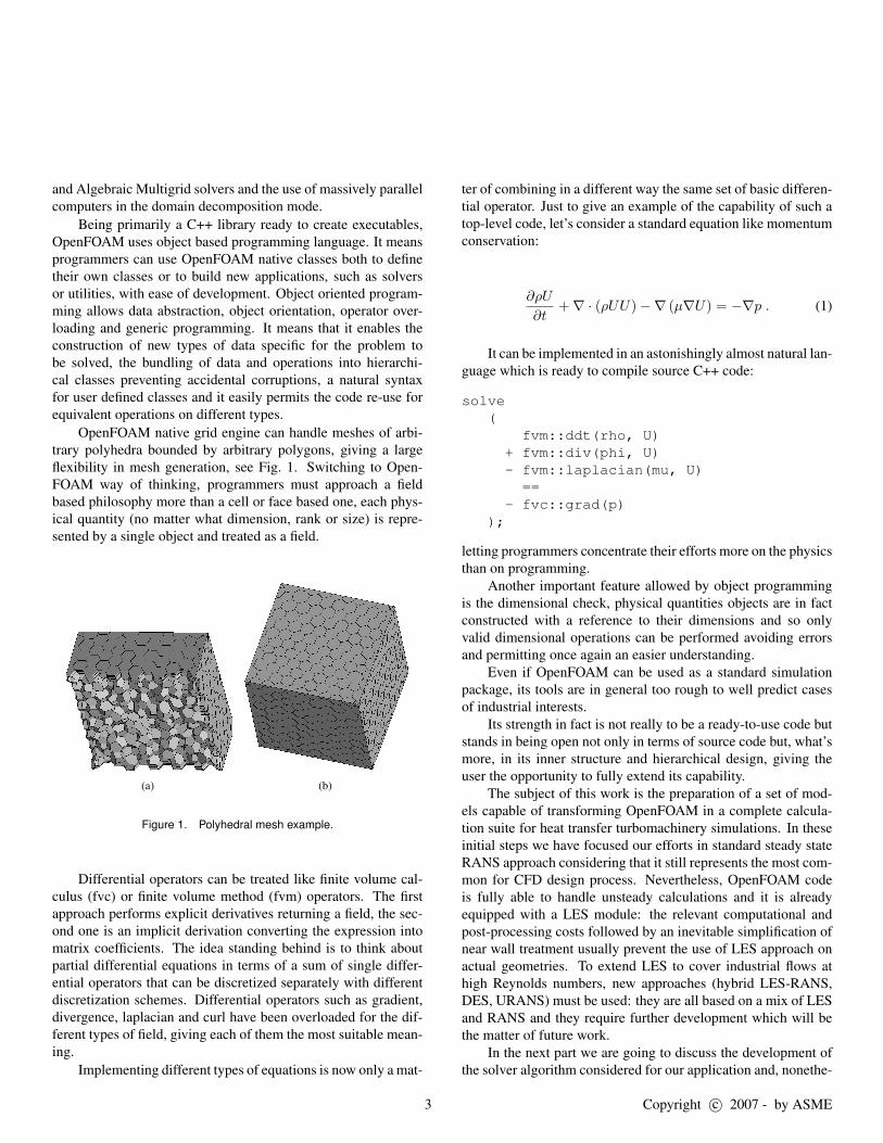
OpenFOAM native grid engine can handle meshes of arbi-trary polyhedra bounded by arbitrary polygons, giving a largeflexibility in mesh generation, see Fig. 1. Switching to Open-FOAM way of thinking, programmers must approach a fieldbased philosophy more than a cell or face based one, each phys-ical quantity (no matter what dimension, rank or size) is repre-sented by a single object and treated as a field.

(a) (b)

Figure 1. Polyhedral mesh example.

Differential operators can be treated like finite volume cal-culus (fvc) or finite volume method (fvm) operators. The firstapproach performs explicit derivatives returning a field, the sec-ond one is an implicit derivation converting the expression intomatrix coefficients. The idea standing behind is to think aboutpartial differential equations in terms of a sum of single differ-ential operators that can be discretized separately with differentdiscretization schemes. Differential operators such as gradient,divergence, laplacian and curl have been overloaded for the dif-ferent types of field, giving each of them the most suitable mean-ing.

Implementing different types of equations is now only a mat-

ter of combining in a different way the same set of basic differen-tial operator. Just to give an example of the capability of such atop-level code, let’s consider a standard equation like momentumconservation:

∂ρU

∂t+∇ · (ρUU)−∇ (µ∇U) = −∇p . (1)

It can be implemented in an astonishingly almost natural lan-guage which is ready to compile source C++ code:

solve(

fvm::ddt(rho, U)+ fvm::div(phi, U)- fvm::laplacian(mu, U)==

- fvc::grad(p));

letting programmers concentrate their efforts more on the physicsthan on programming.

Another important feature allowed by object programmingis the dimensional check, physical quantities objects are in factconstructed with a reference to their dimensions and so onlyvalid dimensional operations can be performed avoiding errorsand permitting once again an easier understanding.

Even if OpenFOAM can be used as a standard simulationpackage, its tools are in general too rough to well predict casesof industrial interests.

Its strength in fact is not really to be a ready-to-use code butstands in being open not only in terms of source code but, what’smore, in its inner structure and hierarchical design, giving theuser the opportunity to fully extend its capability.

The subject of this work is the preparation of a set of mod-els capable of transforming OpenFOAM in a complete calcula-tion suite for heat transfer turbomachinery simulations. In theseinitial steps we have focused our efforts in standard steady stateRANS approach considering that it still represents the most com-mon for CFD design process. Nevertheless, OpenFOAM codeis fully able to handle unsteady calculations and it is alreadyequipped with a LES module: the relevant computational andpost-processing costs followed by an inevitable simplification ofnear wall treatment usually prevent the use of LES approach onactual geometries. To extend LES to cover industrial flows athigh Reynolds numbers, new approaches (hybrid LES-RANS,DES, URANS) must be used: they are all based on a mix of LESand RANS and they require further development which will bethe matter of future work.

In the next part we are going to discuss the development ofthe solver algorithm considered for our application and, nonethe-


less, the implementation of specific turbulence models for Low-Reynolds and High-Reynolds simulations.

SOLVERIn turbomachinery and heat transfer applications, involved

fluid flows may usually cover a wide range of Mach regimes. Inparticular, it usually happens that different Mach conditions si-multaneously arise in the same domain. Such situation makes theaccurate solution of viscous flows governing equations a com-plex task.

Most widely used algorithms for compressible flows cal-culation use density as one of the main independent variablesand pressure is determined via an equation of state. As thereis very little or no change in density for low subsonic or nearlyincompressible flows, these density-based methods fail in suchregimes. Their application in cases of incompressible or lowMach number flows is questionable, since in that situation thedensity changes are so small that the pressure-density couplingbecomes very weak.

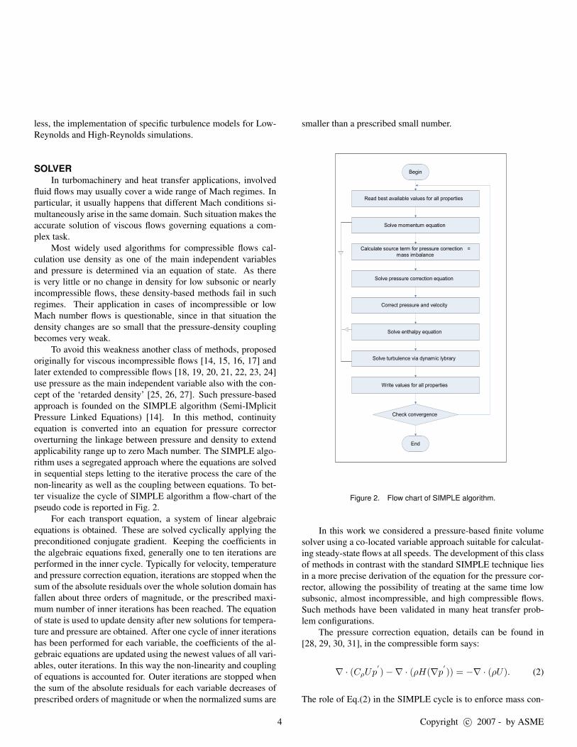
To avoid this weakness another class of methods, proposedoriginally for viscous incompressible flows [14, 15, 16, 17] andlater extended to compressible flows [18, 19, 20, 21, 22, 23, 24]use pressure as the main independent variable also with the con-cept of the ‘retarded density’ [25, 26, 27]. Such pressure-basedapproach is founded on the SIMPLE algorithm (Semi-IMplicitPressure Linked Equations) [14]. In this method, continuityequation is converted into an equation for pressure correctoroverturning the linkage between pressure and density to extendapplicability range up to zero Mach number. The SIMPLE algo-rithm uses a segregated approach where the equations are solvedin sequential steps letting to the iterative process the care of thenon-linearity as well as the coupling between equations. To bet-ter visualize the cycle of SIMPLE algorithm a flow-chart of thepseudo code is reported in Fig. 2.

For each transport equation, a system of linear algebraicequations is obtained. These are solved cyclically applying thepreconditioned conjugate gradient. Keeping the coefficients inthe algebraic equations fixed, generally one to ten iterations areperformed in the inner cycle. Typically for velocity, temperatureand pressure correction equation, iterations are stopped when thesum of the absolute residuals over the whole solution domain hasfallen about three orders of magnitude, or the prescribed maxi-mum number of inner iterations has been reached. The equationof state is used to update density after new solutions for tempera-ture and pressure are obtained. After one cycle of inner iterationshas been performed for each variable, the coefficients of the al-gebraic equations are updated using the newest values of all vari-ables, outer iterations. In this way the non-linearity and couplingof equations is accounted for. Outer iterations are stopped whenthe sum of the absolute residuals for each variable decreases ofprescribed orders of magnitude or when the normalized sums are

smaller than a prescribed small number.

Figure 2. Flow chart of SIMPLE algorithm.

In this work we considered a pressure-based finite volumesolver using a co-located variable approach suitable for calculat-ing steady-state flows at all speeds. The development of this classof methods in contrast with the standard SIMPLE technique liesin a more precise derivation of the equation for the pressure cor-rector, allowing the possibility of treating at the same time lowsubsonic, almost incompressible, and high compressible flows.Such methods have been validated in many heat transfer prob-lem configurations.

The pressure correction equation, details can be found in[28, 29, 30, 31], in the compressible form says:

∇ · (CρUp′)−∇ · (ρH(∇p

′)) = −∇ · (ρU). (2)

The role of Eq.(2) in the SIMPLE cycle is to enforce mass con-


servation, it is in fact derived from a combination of momentumconservation and continuity equation. In order to solve Eq.(2),attention should be posed on the fact that the pressure correc-tion equation now assumes a convective-diffusive form instead ofa purely diffusive behavior like the original incompressible for-mulation. While the other steady-state form transport equationshave to be relaxed in order to characterize the inertial physicslost by the elimination of the time derivative, for the pressurecorrection equation this cannot be done. Usage of usual implicitrelaxation techniques on pressure corrector, in fact, corrupt massconservation on single iteration steps breaking the concept stand-ing behind SIMPLE algorithm. In subsonic cases, standard Neu-mann conditions at inlet velocity boundary, like in incompress-ible tests, determine ill-defined problems for Eq.(2). Care mustbe taken in handling pressure correction boundary condition inorder to solve in a well-posed manner such an equation [32]. Acombination of Dirichlet and Neumann type condition for the in-let has been tested.

TURBULENCE MODELSThe correct modeling of turbulent quantities is fundamental

in conducting heat transfer simulations, because of the simulta-neous importance of well predicting both the near wall behaviorand the complex structures of the main flow [33, 34]. Correctpredictions of thermal quantities and gradients inside boundarylayers are necessary to establish whether or not the cooling sys-tem is efficient. At the same time wall properties are very depen-dent on the development of the free stream flow.

Usage of wall function approach has to be avoided becauseof the unpredictability of boundary thermal gradient and the fail-ure in predicting transitional, Low Reynolds as well as adversepressure gradient flows.

First step in modeling flows close to solid walls has been theimplementation of several so called Low Reynolds k− ε models[35]. The idea standing behind such models is to damp turbulentviscosity near the wall through a damping function fµ going to-wards zero as the distance from the wall is reducing. Constantsmultiplying source terms in the turbulent dissipation equation arein some cases also damped. The basic structure of the modelsis the same for all of them differing in the tuning of the damp-ing functions and some extra sources in dissipation equation, asshown below:

∂ρk

∂t+∇ · (ρUk)−∇ · (µeff∇k) = Pk − ρε , (3)

∂ρε

∂t+∇ · (ρUε)−∇ · (µeff∇ε) = f1Pk

ε

k− f2ρ

ε2

k. (4)

Of the many Low Reynolds k− ε models proposed in litera-ture in the course of years, the models by Lien and Leschziner

[25], Lien [36], Abe et al [37], Chien [38], Chen et al [39],Hwang and Lin [40] and Lam and Bremhorst [41] have been im-plemented.

It is known from literature that in high strain rate regionseddy viscosity models overpredict turbulent kinetic energy: thisproblem is sometimes referred to as “stagnation point anomaly”[42]. These higher values of k are due to an overestimate ofproduction term Pk. To avoid such overprediction linear depen-dence between Pk and |S|2 should be bounded in regions where|S| grows. This is achieved with a time scale bound, derivedfrom a “realizability” constraint for Reynolds stress tensor to bedefinite positive:

Ts =µt

Cµρk= min

(k

ε,

α√6Cµ|S|

)(5)

This limiter proposed by Durbin [43] has been inserted inall Low Reynolds models above presented as an option to beswitched on or off by the user.

Then, in order to match good near wall predictions with suit-able modeling of flow structures far from the wall, Two Layerk − ε models have been implemented. Such methods consist inpatching together a one equation model in the near wall layerand a two equation High Reynolds model in the outer layer[44]. Both Wolfestein and Norris&Reynolds closure formulas[36] have been tried without significant discrepancies in the re-sults.

Last model to be mentioned is the k−ω SST: it includes themodification of the standard k − ω to avoid sensitivity to quitearbitrary freestream values of ω [45, 46]. The basic idea is sim-ilar to Two Layer models: two different approaches are mergedtogether to model the two different flow regions. The sublayerand logaritmic model is the standard k − ω, chosen because ofits robustness, the absence of damping function and Dirichlettype boundary conditions. From the wake region and outside theboundary layer the standard k−ε, written in terms of ω, has beenpreferred due to its good compromise in predicting different kindof flows.

RESULTS

GeneralitiesAll the cases to be presented, apart from the flat plate one,

have been chosen because already tested and analyzed with com-mercial solvers by the authors, with some results already pub-lished, see for example [9, 47]. Grid sensitivity analysis havebeen performed when those runs were set up and it’s not repeatedin this case, the various meshes however guarantee a first node


y+ ≤ 1. All fluid domains are discretized via hexahedral ele-ments except Goldman test, total number of elements for eachtest is reported in Tab. 1.

Table 1. Grid sizes (thousands of elements)GAMM test 1 10.0

GAMM test 2 13.5

Goldman test 7.2

Flat plate 17.6

ERCOFTAC C25 Axial-symmetric Impingement Jet 69

1-Hole Impingement Jet 387.0

5-Holes Impingement Jet 1705.0

Sinha test 177.0

6-Holes Effusion 2000.0

Due to the great number of implemented turbulence models,a shortcut has been used to name most of them: the acronymspresented in Tab. 2 will be widely used in substitution of authors’full name.

Table 2. Acronyms for the various turbulence models.k − ε Low Reynolds by Abe et al. AKN

k − ε Low Reynolds by Yoder and Georgiadis CH

k − ε Low Reynolds by Lien et al. CLL

k − ε Low Reynolds by Hwang and Lin HW

k − ε Low Reynolds by Lam and Bremhorst LB

k − ε Low Reynolds by Lien and Leschziner LW

k − ε Low Reynolds by Lien LNR

Realizability constraint correction Real

Two Layer TL

k − ω SST SST

The convective spatial discretization used is based on theNormal Variable Approach (NVA), and named in literature asSelf Filtered Central Differencing (SFCD) scheme [10].

To check convergence the arrest criterium has been definedas single scalar normalized residual lower than 10−6. Normal-ization factor, Norm, was not changed from the released versionand is defined as:

Φref = Φ ,

S = A · Φ ,

Sref = A · Φref ,

Norm =∑

(|S − Sref |+ |Q− Sref |) .

If this condition was satisfied for all scalar but pressure cor-rector calculations were stopped. Due to its nature, pressure cor-rection residual is of no interest and, moreover, its initial valueis set to zero at every iteration. To verify whether or not pres-sure field is still varying, the maximum module of the pressurecorrector, at convergence exactly null, is imposed to be less than10 [Pa], remember an averaged relaxation factor for the pressurecorrector is of the order of 10−2.

Solver Validation Tests

GAMM testsThe developed calculation procedure has been used to solve

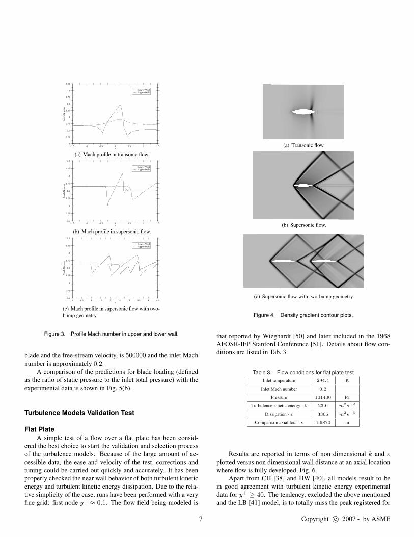
a variety of problems in heat transfer applications. Here the em-phasis is on the high compressible flows. The capability of thepresent method is demonstrated by computing inviscid flow in achannel with a bump on the lower wall named GAMM test. Thistest case has been used by various researchers to test their algo-rithms [18, 48]. Application of the method to two different typesof inviscid flow, transonic and supersonic, are presented below.

The width of the channel is equal to the length of the bump,and the channel length is equal to three lengths of the jump. Fortransonic calculation, the thickness-to-chord ratio is 10% whilefor supersonic flow calculations it is 4%. In transonic and super-sonic regime at inlet is assumed that flow has uniform proper-ties and the upstream far field variable values (except pressure intransonic case) are specified while at the outlet all variable (ex-cept pressure in transonic case) are extrapolated. At the upperand the lower boundaries wall slip condition is prescribed.

First case with imposed inlet Mach number Main = 0.675,gives the Mach number distributions along the walls and densitygradient magnitude contour plot shown in Fig. 3(a) and Fig. 4(a).In the supersonic case, Main = 1.65, the flow results super-sonic all along the bump: Mach number distributions and den-sity gradient magnitude contour plots are shown in Fig. 3(b) andFig. 4(b). These results correspond to reference solutions fromliterature [18, 48].

Fig. 3(c) and Fig. 4(c) show the Mach number distributionand density gradient magnitude contour plot under the same con-dition of supersonic case but with two bumps. As can be seen bycomparing Fig. 3(b), Fig. 3(c) and Fig. 4 the second bump doesnot influence the flow upstream indicating that the solution algo-rithm correctly reproduces the hyperbolic behavior of the flow.

Goldman testAs example of highly compressible subsonic, we have re-

ported the simulation of a test based on the work of Goldmanet al.[49]. It is a 2-D turbulent analysis of a stator blade at themid-span; the details of the geometry and the mesh are shown inFig. 5(a). The Reynolds number, based on the chord length of the


-1.5 -1 -0.5 0 0.5 1 1.5x

0

0.25

0.5

0.75

1

1.25

1.5

1.75

2

2.25

Mac

h N

umbe

r

Lower-WallUpper-Wall

(a) Mach profile in transonic flow.

-1.5 -1 -0.5 0 0.5 1 1.5x

0.5

0.75

1

1.25

1.5

1.75

2

2.25

2.5

Mac

h N

umbe

r


(b) Mach profile in supersonic flow.

0 0.5 1 1.5 2 2.5 3 3.5 4 4.5x

0.5

0.75

1

1.25

1.5

1.75

2

2.25

2.5

Mac

h N

umbe

r


(c) Mach profile in supersonic flow with two-bump geometry.

Figure 3. Profile Mach number in upper and lower wall.

blade and the free-stream velocity, is 500000 and the inlet Machnumber is approximately 0.2.

A comparison of the predictions for blade loading (definedas the ratio of static pressure to the inlet total pressure) with theexperimental data is shown in Fig. 5(b).

Turbulence Models Validation Test

Flat PlateA simple test of a flow over a flat plate has been consid-

ered the best choice to start the validation and selection processof the turbulence models. Because of the large amount of ac-cessible data, the ease and velocity of the test, corrections andtuning could be carried out quickly and accurately. It has beenproperly checked the near wall behavior of both turbulent kineticenergy and turbulent kinetic energy dissipation. Due to the rela-tive simplicity of the case, runs have been performed with a veryfine grid: first node y+ ≈ 0.1. The flow field being modeled is

(a) Transonic flow.

(b) Supersonic flow.

(c) Supersonic flow with two-bump geometry.

Figure 4. Density gradient contour plots.

that reported by Wieghardt [50] and later included in the 1968AFOSR-IFP Stanford Conference [51]. Details about flow con-ditions are listed in Tab. 3.

Table 3. Flow conditions for flat plate testInlet temperature 294.4 K

Inlet Mach number 0.2

Pressure 101400 Pa

Turbulence kinetic energy - k 23.6 m2s−2

Dissipation - ε 3365 m2s−3

Comparison axial loc. - x 4.6870 m

Results are reported in terms of non dimensional k and εplotted versus non dimensional wall distance at an axial locationwhere flow is fully developed, Fig. 6.

Apart from CH [38] and HW [40], all models result to bein good agreement with turbulent kinetic energy experimentaldata for y+ ≥ 40. The tendency, excluded the above mentionedand the LB [41] model, is to totally miss the peak registered for


(a) Geometry mesh.

0 0.005 0.01 0.01 0.02 0.03 0.03 0.04 0.04x(m)

0.55

0.6

0.65

0.7

0.75

0.8

0.85

0.9

0.95

1

1.05

Padi

m

FOAMexp

(b) Pressure ratio over experimental data.

Figure 5. Stator Blade analysis.

y+ ' 10. LB estimation viceversa is higher than experimen-tal registration. Level of approximation results in being quiteuniform for the different models with CLL[39] and AKN [37]slightly better in overlapping free stream values for k+.

Also for turbulent dissipation, models well predict outerlayer behavior: all models apart from LNR [36] basically coin-cide for y+ ≥ 40. The major disagreements are registered insidethe viscous layer. There is no agreement in fact in predicting thepeak both in terms of positioning and values. Due to the dif-ferent boundary conditions imposed to the dissipation, near wallbehavior is quite different for each model: LB fails in predictingthe peak, AKN and HW results in having pretty high wall valuesfor ε. The models that best suit experimental data reported byPatel [35] are LNR and CLL.

Of all the tested Low Reynolds models the CLL has beenchosen as the most reliable one and used as the example for LowReynolds models in the following cases.

Heat Transfer tests

Impingement CoolingAmong various possible techniques to enhance heat transfer

rate, impingement cooling certainly presents very high coolingefficency, thus it’s commonly found both in typical blade and

0 20 40 60 80 1000

1

2

3

4

5

6

7

8

k+

y+

exp Patel AKN CH CLL HW LB LW LNR

(a) k+ profile

0 20 40 60 80 1000,00

0,05

0,10

0,15

0,20

0,25

0,30

+

y+

1/xy+ exp Patel AKN CH CLL HW LB LW LNR

(b) ε+ profile

Figure 6. Turbulence quantities profiles.

combustor cooling systems, operating in a wide range of designconditions. From a numerical point of view, impinging jet flowspresent several interesting aspects allowing deep evaluation ofturbulence models.

The problem of a 2-D normal impinging jet of air has beenperformed following a test case by ERCOFTAC. Then, the firstrow of an array of holes was simulated, with a comparison ofthe experimental results obtained during the European projectLOPOCOTEP, with different turbulence models. Further simula-tions of the complete array were done with the selected models.To obtain the desired heat transfer results, runs simulation withan imposed heat flux on the impact wall has been performed.


ERCOFTAC C25 Axial-symmetric ImpingementAn incompressible flow of a turbulent air jet impinging onto aflat plate was modeled [8]. The impact surface is heated and keptat constant heat flux. From the experiment, the Nusselt numberdistribution for various jet Reynolds numbers is known. Fig. 7shows the geometry of the test case. The diameter of the pipeis D = 0.004 m. The inflow velocity and turbulence conditionswere obtained from the development of a 50 D upstream extrudedinlet hole. For validation purpose, a Reynolds number of 23.000and a distance of L/D = 2 were chosen. The heated surface wasmodeled as a wall at constant heat flux q̇ = 200 W/m2 . Allother walls were treated as adiabatic walls. The far-field bound-aries are modeled as mixed inflow/outflow pressure boundaries.

(a) total (b) particular

Figure 7. Entire geometry and particular of the grid around the stagna-tion point.

0 1 2 3 4 50

50

100

150

200

250

300

350

400

450

Nu D

r/D

Exp CLL AKN CLLReal SST TL

Figure 8. Nusselt number distribution along radius.

Fig. 8 compares the predicted Nusselt number distributionsof 5 turbulence models, namely AKN, SST, CLL, CLLReal andTwo Layer , with the experimental profile.

The predictions of all two-equation models used in this val-idation case are in good agreement with the experimental datafar from the stagnation point. As known in literature [42] in thearea around the stagnation point Low Reynolds models withoutrealizability constraint fail and dramatically overpredict the peakin the heat transfer coefficient (error of almost 200%).

At the same time Two Layer SST and realizable mod-els show about the same peak value. The local maximum atr/D ≈ 2 is not seen by the Two Layer and is slightly predictedby the SST. On the contrary, the CLLReal is well predicting suchpeak only shifting a bit towards higher values of the radius.

1-Hole Impingement cooling Both this and the fol-lowing case, simulating typical design conditions for impinge-ment cooling of a gas turbine, has been performed on the set up ofan experiment done at the Energy Engineering Department of theUniversity of Florence for the European project LOPOCOTEP(LOw POllutant COmbustor TEchnical Programme). Coolant isinjected from a plenum through a perforated plate and impactsover a flat plate at uniform heat flux. The holes on the plenumcompose an array of 10 − 11 spanwise rows per 9 streamwiseholes. This test is simulating the behavior of the first row whilein the following one 3− 2 rows (the array of holes is staggered)for a total of 5 jets are impinging. For further details refer to [52].

Main flow parameters and grid are reported in Tab. 4 andFig. 9.

Table 4. Flow conditions for 1-hole impingement testInlet Temperature 308.2 K

Outlet Pressure 85101 Pa

Inlet Turbulence level - Tu ≤ 0.5% %

Rej 7600

Inlet Velocity 0.28956 m/s

Wall Heat flux 3000 W/m2

Simulations have been validated in terms of heat transfer co-efficient calculated with respect to inlet static temperature almostcoincident for such low Mach number with inlet total tempera-ture. Adiabatic simulations have been done too, in order to checkwhether this approximation could be done or not.

First thing to notice from Fig. 10 is that, contrarily to ER-COFTAC test, CLLReal model fails in well predicting heat trans-fer coefficient around the stagnation point. Moreover, due to thepotential core that is not extinguished at the wall, two unphysicalspurious peaks are predicted at X/D ≈ 1.


Figure 9. Impingement single hole grid.

-3 -2 -1 0 1 2 3 4 5

0

100

200

300

400

500

600

700

HTC

[Wm

-2K

-1]

X / D

Exp TL kOmega SST ChenLienReal

Figure 10. Heat transfer coefficient on impinged wall along symmetryline.

Two Layer and SST result in being almost equivalent bothfor the peak level and the far from the stagnation point values,with the Two Layer predictions slightly lower everywhere on theimpinged surface.

5-Holes Impingement cooling This case refer to thesame set of experiments of the previous test. For this multi-holesimulation the plenum as been schematized with a big plenumwhere the inlet mass flow is imposed. Computational boundaryconditions follow exactly the previous 1-hole test.

For this geometry only the Two Layer and k−ω SST modelshave been tested against experimental results in terms of heattransfer coefficient, see Fig. 11 and Fig. 12.

Both experimental and numerical data are sampled onto thetwo different lines connecting symmetry planes and then mergedtogether in the zone where a relative minimum is localized.

0 10 20 30 400

100

200

300

400

500

HTC

[Wm

-2K

-1]

X / D

experimental TL path1 TL path2 SST path1 SST path2

Figure 11. Heat transfer coefficient along center lines.

(a) Experimental

(b) Two Layer

(c) k-ω SST

Figure 12. Heat transfer coefficient [W m−2 K−1] distribution on im-pinged wall.

Even if obtained results are in good agreement with exper-imental data far from the stagnation point, it should be noticedthat predictions for the peak value are quite different from mea-sured data. Higher discrepancies on the even peaks are probablydue to errors in the experimental measurements [52]. Comparingthe two models, Two Layer predicts peak values a 10% better ofthe SST giving basically identical results outside the stagnationpoints area. In any case, it should be considered that tempera-ture gradients are quite small. A better agreement is expected forhigher values of wall heat flux.


Film and effusion coolingAmong the different techniques used in the cooling of hot

parts in a gas turbine engine, the injection of cooling air in themain flow, producing a thin film of air that isolates the walls fromthe hot gases, is one of the most used. Because of the complexinteraction between air and hot gases during mixing, many dif-ferent injection hole shapes and distribution have been studiedand a great amount of research work is still on going [7]. Inparticular, most recent developments in drilling capabilities al-low the manufacturing of wide arrays of micro-holes (diametersbelow 1 mm), currently referred to as effusion cooling. Even ifthis technique does not produce a film wall protection as in stan-dard film cooling, its most important feature is the heat removedby the passage of coolant inside the holes (heat sink effect): thegreat number of holes and their high length/diameter ratio (withangles below 30◦) allows to heavily increase the overall coolingeffectiveness [53]. Effusion cooling represents the base in thethermal design of modern aero-engine combustors and its use inthe cooling of turbine endwalls is also investigated [7].

Even if film wall protection may not represent the main cool-ing effect in effusion technique, the prediction of mixing betweencoolant and cross flow and the corresponding assessment of adi-abatic effectiveness, still represent some of the most difficult taskin CFD analysis [47]. Despite the well known deficiency of stan-dard eddy viscosity turbulence models in the accurate predictionof jet mixing in cross flow, essentially due to the isotropy as-sumption for turbulent stresses [54, 55, 56], both k−ε and k−ωmodels are still widely used in industrial CFD computations.

Therefore we will analyze in this part the accuracy of Open-FOAM code in the prediction of adiabatic effectiveness in ef-fusion cooling geometries, using the set of turbulence modelsselected for heat transfer analysis of this work. As introducedabove, two test-cases will be studied: the well known single holeexperiment by Sinha [6] and an experimental multi-hole geome-try aimed at turbine endwalls cooling [7].

Sinha test Experimental data and geometries are basedon tests made by Sinha et al.[6]; local and spanwise averagedeffectiveness is compared with calculated values. The geometryis a flat plate with a single row of holes, while flow conditionsare listed in table 5.

In the chosen geometry, hot gas flows over a flat plate, whilecoolant is injected through one row of holes; upstream of theinjection channel there is a plenum. Fig. 13 shows the fluid do-main and the different boundary conditions imposed; in partic-ular, symmetry planes pass through hole axis and half spanwisepitch. On all inlet surfaces mass flow rate and static tempera-ture are imposed, symmetry conditions ensure zero gradient overboundaries in span direction.

Single row configuration was mainly considered in order tohave a reference geometry to compare results for different turbu-

Table 5. Flow conditions for Sinha testCross flow temperature 300 K

Coolant temperature 153 K

Pressure 105 Pa

Density ratio - DR 2.0

Blowing-rate - M 0.5

Momentum ratio - I 0.125

Turbulence level - Tu ≤ 0.2 %

Cross flow velocity 20 m/s

Rec 15700

Figure 13. Calculation domain and boundary conditions (Sinha etal.[6]).

lence models and calculation meshes. The performances of thesame five turbulence models as single hole impingement casewere analyzed, namely AKN, CLL, CLLReal, SST, TL. The gridused is a structured grid, see Fig. 14 in which it is also reporteda magnification of the zone around the hole.

Figure 14. Mesh details near walls.

In Fig. 16, laterally averaged effectiveness downstream ofthe hole is shown. Local lateral effectiveness at 1, 10 and 15diameters downstream, is also shown in Fig. 15. A map of wall


0,0 0,2 0,4 0,6 0,8 1,0 1,2 1,40,0

0,1

0,2

0,3

0,4

0,5

0,6

0,7

0,8

0,9

1,0

Y / D

exp CLL AKN TL SST CLLReal

(a) 1D

0,0 0,2 0,4 0,6 0,8 1,0 1,2 1,40,0

0,1

0,2

0,3

0,4

0,5

0,6

0,7

0,8

0,9

1,0


Y / D

(b) 10D

0,0 0,2 0,4 0,6 0,8 1,0 1,2 1,40,0

0,1

0,2

0,3

0,4

0,5

0,6

0,7

0,8

0,9

1,0

Y / D


(c) 15D

Figure 15. Spanwise distribution of film cooling effectiveness at varioussections.

effectiveness as well as distribution over the symmetry plane isreported in Fig. 17 and Fig. 18. There is a fairly good agreement

between numerical and experimental results for all models used.

0 5 10 15 20 250,00

0,05

0,10

0,15

0,20

0,25

0,30

0,35

0,40

0,45

0,50

X / D

Exp CLL AKN TL SST CLLReal

(a) Laterally averaged

0 5 10 15 20 250,0

0,1

0,2

0,3

0,4

0,5

0,6

0,7

0,8

0,9

1,0

X / D

Exp CLL AKN TL SST CLLReal

(b) Center line

Figure 16. Comparison between laterally averaged and local center linefilm cooling effectiveness.

Attention must be paid on the results at one diameter testsection for the CLLReal model. The baffle underlined at the endof the spanwise direction is a consequence of a poor develop-ing of the boundary layer predicted by the model. Low valuesof turbulent viscosity do not dissipate the horse-shoe vortex up-stream of the hole. A low pressure zone drives coolant gas com-ing from the plenum around the jet. As a consequence there ismore spreading of the film in spanwise direction and the evidenceis a local maximum for the effectiveness at X/D ≈ 1.2. On theother hand, centreline values show that SST model has a deeperpenetration of the jet, see also Fig. 18, showing a local minimumin the effectiveness profile just downstream the hole.

It’s clear that numerical simulations predict a coherent jetFig. 17, thus severally underestimating coolant lateral diffusion.


(a) CLLReal

(b) CLL

(c) SST

(d) Two Layer

(e) Colormap

Figure 17. Effectiveness distribution over the wall.

(a) CLLReal (b) CLL

(c) SST (d) TL

Figure 18. Sinha - Temperature distribution on symmetry plane [K].

This is not evident at 1 D downstream, but the effect grows pro-ceeding in cross flow direction. This behavior is mostly due toan isotropic modeling of turbulence near the wall, see Simon,Jubran, Azzi and Lakehal [57, 54, 55, 56]. Similar results can befound also in Andreini et al. [47] with commercial solvers.

6-Holes effusion cooling The geometry of this case isa six holes flat plate interposed in between a plenum and a chan-nel at lower pressure. To enhance numerical stability, the plenumhas been gridded as six different smaller plena each one with thesame inlet mass flow imposed to respect total experimental cool-ing air mass flow Fig. 19. A summary of flow conditions can befound in Tab. 6.

Table 6. Flow conditions for 6-holes effusion testCross flow temperature 323 K

Coolant temperature 298 K

Pressure 7.0 · 104 Pa

Density ratio - DR 1.103

Blowing-rate - M 0.2

Figure 19. 6-holr effusion cooling case mesh.

Results are reported in terms of spanwise averaged adiabaticeffectiveness, see Fig. 20. Together with experimental data, cor-relative approach predictions using L’Ecuyer and Soechting cor-relation with Sellers superposition criterion have been reported[7]. First of all it can be noticed that Two Layer model strongly

0 10 20 30 40 50 600.00

0.05

0.10

0.15

0.20

0.25

0.30

0.35

0.40

0.45

0.50

X / D

Experimental OF-TL OF-SST Ecuyer-Soechting

Figure 20. Spanwise averaged adiabatic effectiveness.

improves matching of both experimental and correlative data incomparison to k− ω SST. Two Layer is still in slightly over pre-diction for the peak values especially for even peaks, for the oddones in fact peak values result in being on the same level of the


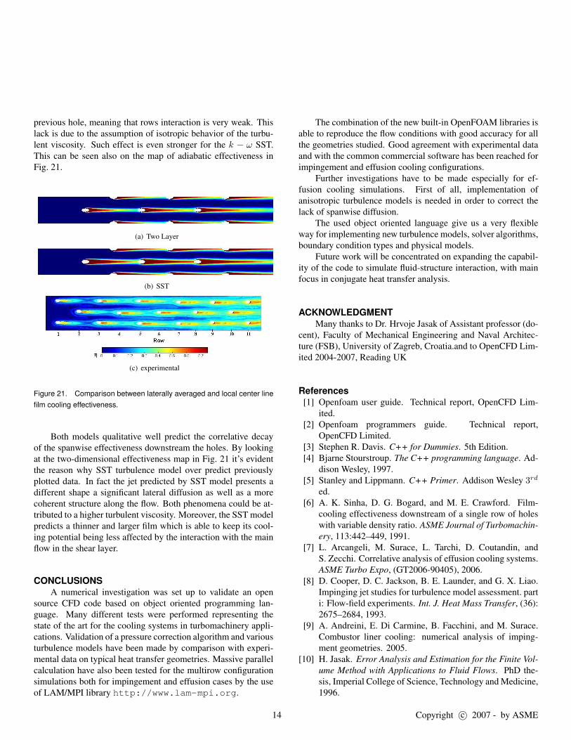
previous hole, meaning that rows interaction is very weak. Thislack is due to the assumption of isotropic behavior of the turbu-lent viscosity. Such effect is even stronger for the k − ω SST.This can be seen also on the map of adiabatic effectiveness inFig. 21.

(a) Two Layer

(b) SST

(c) experimental

Figure 21. Comparison between laterally averaged and local center linefilm cooling effectiveness.

Both models qualitative well predict the correlative decayof the spanwise effectiveness downstream the holes. By lookingat the two-dimensional effectiveness map in Fig. 21 it’s evidentthe reason why SST turbulence model over predict previouslyplotted data. In fact the jet predicted by SST model presents adifferent shape a significant lateral diffusion as well as a morecoherent structure along the flow. Both phenomena could be at-tributed to a higher turbulent viscosity. Moreover, the SST modelpredicts a thinner and larger film which is able to keep its cool-ing potential being less affected by the interaction with the mainflow in the shear layer.

CONCLUSIONSA numerical investigation was set up to validate an open

source CFD code based on object oriented programming lan-guage. Many different tests were performed representing thestate of the art for the cooling systems in turbomachinery appli-cations. Validation of a pressure correction algorithm and variousturbulence models have been made by comparison with experi-mental data on typical heat transfer geometries. Massive parallelcalculation have also been tested for the multirow configurationsimulations both for impingement and effusion cases by the useof LAM/MPI library http://www.lam-mpi.org.

The combination of the new built-in OpenFOAM libraries isable to reproduce the flow conditions with good accuracy for allthe geometries studied. Good agreement with experimental dataand with the common commercial software has been reached forimpingement and effusion cooling configurations.

Further investigations have to be made especially for ef-fusion cooling simulations. First of all, implementation ofanisotropic turbulence models is needed in order to correct thelack of spanwise diffusion.

The used object oriented language give us a very flexibleway for implementing new turbulence models, solver algorithms,boundary condition types and physical models.

Future work will be concentrated on expanding the capabil-ity of the code to simulate fluid-structure interaction, with mainfocus in conjugate heat transfer analysis.

ACKNOWLEDGMENTMany thanks to Dr. Hrvoje Jasak of Assistant professor (do-

cent), Faculty of Mechanical Engineering and Naval Architec-ture (FSB), University of Zagreb, Croatia.and to OpenCFD Lim-ited 2004-2007, Reading UK

References[1] Openfoam user guide. Technical report, OpenCFD Lim-

ited.[2] Openfoam programmers guide. Technical report,

OpenCFD Limited.[3] Stephen R. Davis. C++ for Dummies. 5th Edition.[4] Bjarne Stourstroup. The C++ programming language. Ad-

dison Wesley, 1997.[5] Stanley and Lippmann. C++ Primer. Addison Wesley 3rd

ed.[6] A. K. Sinha, D. G. Bogard, and M. E. Crawford. Film-

cooling effectiveness downstream of a single row of holeswith variable density ratio. ASME Journal of Turbomachin-ery, 113:442–449, 1991.

[7] L. Arcangeli, M. Surace, L. Tarchi, D. Coutandin, andS. Zecchi. Correlative analysis of effusion cooling systems.ASME Turbo Expo, (GT2006-90405), 2006.

[8] D. Cooper, D. C. Jackson, B. E. Launder, and G. X. Liao.Impinging jet studies for turbulence model assessment. parti: Flow-field experiments. Int. J. Heat Mass Transfer, (36):2675–2684, 1993.

[9] A. Andreini, E. Di Carmine, B. Facchini, and M. Surace.Combustor liner cooling: numerical analysis of imping-ment geometries. 2005.

[10] H. Jasak. Error Analysis and Estimation for the Finite Vol-ume Method with Applications to Fluid Flows. PhD the-sis, Imperial College of Science, Technology and Medicine,1996.


[11] H. Jasak, H.G. Weller, and N. Nordin. In cylinder cfd sim-ulation using a c++ object-oriented toolkit. SAE Technicalpapers, (2004-01-0110).

[12] F. Juretic. Error Analysis in Finite Volume. PhD thesis, Im-perial College of Science, Technology and Medicine, 2004.

[13] J. R. Shewchuk. An introduction to the conjugate gradi-ent method without the agonizing pain. Technical report,School of Computer Science, Carnegie Mellon University -Pittsburgh, PA 15213, 1994.

[14] S. V. Patankar. Numerical Heat Transfer and Fluid Flow.Taylor & Francis, USA, 1980.

[15] W. Malasakera and H. K. Versteeg. Computational FluidDynamics. Longman Scientific, England, 1995.

[16] M. Peric. Numerical methods for computing turbulentflows. Technical Report VKI LS 2004-06.

[17] J. H. Ferziger and M. Peric. Computational Methods forFluid Dynamics. Springer, Germany, 2002.

[18] M. Peric, Z. Lilek, and L. Demirdzic. A collocated finitevolume method for predicting flows at all speed. Journal ofNumerical Methods in Fluids, 16:1029–1050, 1993.

[19] M. Darbandi and G. E. Schneider. Application of an all-speed flow algorithm to heat transfer problems. Numericalheat transfer, 35:695–715, 1999.

[20] C. M. Rhie. Pressure based navier-stokes solver using themultigrid method. AIAA Journal, 27(8):1017–1018, 1989.

[21] W. Shyy and M. E. Braaten. Applications of a general-ized pressure correction algorith for flows in complicatedgeometries. Advances and Applications in ComputationalFluid Dynamics - ASME Winter Annual Meeting, pages109–119, 1988.

[22] W. Shyy and M. E. Braaten. Adaptive grid computationfor inviscid compressible flows using a pressure correctionmethod. AIAA, ASME, SIAM, and APS, National Fluid Dy-namics Congress, pages 112–120, 1988.

[23] K. C. Karki and S. V. Patankar. Pressure based calculationprocedure for viscous flows at all speeds in arbitrary con-figurations. AIAA Journal, 27(9).

[24] J. Rincon and R. Elder. A high resolution pressure basedmethod for compressible flow. Journal of Computation andPhysics, 3:217–231, 1997.

[25] F. S. Lien and M. A. Leschziner. A pressure-velocity so-lution strategy for compressible flow and its applicationto shock/boundary-layer interaction using second-momentturbulence closure. Journal of fluids engineering, 115:717–725, 1993.

[26] E. S. Politis and K. C. Giannakoglou. A pressure-basedalgorithm for high speed turbomachinery flows. Interna-tional journal for numerical methods in fluids, 25:63–80,1996.

[27] J. J. McGuirk and G. Page. Shock capturing using apressure-correction method. AIAA Journal, 28(10):1751–1757, 1990.

[28] F. Moukalled and M. Darwish. Tvd schemes for unstruc-tured grids. International Journal of heat and mass trans-fer, 46:599–611, 2003.

[29] F. Moukalled and M. Darwish. Normalized variableand space formulation methodology for high-resolutionschemes. Numerical heat transfer. Part B, fundamentals,26:79–96, 1994.

[30] F. Moukalled and M. Darwish. A unified formulation of thesegregated class of algorithms for fluid flow at all speeds.Numerical heat transfer. Part B, fundamentals, 37:103–139, 2000.

[31] F. Moukalled and M. Darwish. A robust pressure basedalgorithm for multiphase flow. International journal fornumerical methods in fluids, 41:1221–1251, 2003.

[32] I. Senocak and W. Shyy. A pressure based method fot turbu-lent cavitating flow computations. Journal of Computationand Physics, 176:363–383, 2001.

[33] L. Davidson. An introduction to turbulence models. Tech-nical Report Publication 97/2, Chalmers University ofTechnology, 2003.

[34] J. Bredberg. On two equation eddy-viscosity models. Tech-nical Report Internal report 01/8, Chalmers University ofTechnology, 2001.

[35] V. C. Patel, W. Rodi, and G. Sheuerer. Turbulence mod-els for near wall and low reynolds number flows: a review.AIAA Journal, 26:1308–1319, 1993.

[36] F. S. Lien. Computational modeling of 3-D flow in complexducts and passages. PhD thesis, University of Manchester,Institute of science and technology, 1992.

[37] K. Abe, T. Kondoh, and Y. Nagano. A new turbulence mod-els for predicting fluid flow and heat transfer in separatingand reattaching flows-i. flow field calculations. Interna-tional Journal of Heat Mass Transfer, 37:139–151, 1994.

[38] D. A. Yoder and N. J. Georgiadis. Implementation andvalidation of the chien k − ε turbulence model in thewind navier-stokes code. Technical Report 209080, NASA,Glenn Research Center, Cleveland Ohio, 1999.

[39] F. S. Lien, W. L. Chen, and M. A. Leshziner. Low-reynolds-number eddy-viscosity modelling based on non-linear stress-strain/vorticity relations. Engineering turbu-lence modelling and experiments, 3:91–100, 1996.

[40] C. B. Hwang and C. A. Lin. Improved low-reynolds-number k − ε model based on direct numerical simulationdata. AIAA Journal, 36(1):38–43, 1998.

[41] C. K. G. Lam and K. Bremhorst. A modified form of thek−ε model for predicting wall turbulence. Journal of fluidsengineering, 103:456–460, 1981.

[42] P. A. Durbin. On the k− ε stagnation point anomaly. Inter-national journal of heat and fluid flow, 17(1):89–90, 1996.

[43] G. Medic and P. A. Durbin. Towards improved prediction ofheat transfer on turbine blades. Journal of turbomachinery,124:187–192, 2002.


[44] D. Lakehal, G. S. Theodoris, and W. Rodi. Three-dimensional flow and heat tranfer calculations of film cool-ing at the leading edge of a symmetrical turbine blademodel. International journal of heat and fluid flow, 22:113–122, 2001.

[45] F. R. Menter. Two equation eddy viscosity turbulencemodel for engineering applications. AIAA Journal, 32:1598–1604, 1994.

[46] F. R. Menter. Zonal two equation k − ω turbulence modelsfor aerodynamic flows. AIAA Paper, (93-2906), 1993.

[47] A. Andreini, C. Carcasci, S. Gori, and M. Surace. Filmcooling system numerical design: adiabatic and conjugateanalysis. ASME paper, (HT2005-72042), 2005.

[48] K.C. Karki. A calculation procedure for viscous flows atall speeds in complex geometries. PhD thesis, Universityof Minnesota, 1986.

[49] L. G. Goldman, , and K. L. McLallin. Cold-air annu-lar cascade investigation of aerodynamic performance ofcore-engine-cooled turbine vanes: I solid vane performanceand facility description. Technical report, NASA TechnicalMemorandum, 1977.

[50] K. Wieghardt and W. Tillman. On the turbulent fric-tion layer for rising pressure. Technical Report TM-1314,NACA, 1951.

[51] D. E. Coles and E. A. Hirst. Computation of turbulentboundary layers. In AFOSRIFP Stanford Conference, vol-ume 2. Stanford University, 1969.

[52] B. Facchini and M. Surace. Impingement cooling for mod-ern combustors: experimental analysis of heat transfer andeffectiveness. Experiments in Fluids, (40):601–611, 2006.

[53] K. M. B. Gustafsson. Experimental studies of effusion cool-ing. PhD thesis, Chalmers University of technology, De-partment of Thermo and Fluid Dynamics, 2001.

[54] A. Azzi and D. Lakehal. Perspectives in modeling filmcooling of turbine blades by transcending conventionaltwo-equation turbulence models. Journal of turbomachin-ery, (124):472–484, 2002.

[55] A. Azzi and B. A. Jubran. Numerical modeling of filmcooling from short length steam-wise injection holes. Heatand mass transfer, (39):345–353, 2003.

[56] D. Lakehal. Near-wall modeling of turbulent convectiveheat transport in film cooling of turbine blades with the aidof direct numerical simulation data. Journal of turboma-chinery, (124):485–498, 2002.

[57] T. Simon. Film-cooling lateral diffusion and hole entry ef-fects. NASA Lewis, (1996 Coolant flow management work-shop), 1996.


development and validation of a c++ object...

Documents