development and performance prediction of idaho superpave ... · compaction (masad et al....
TRANSCRIPT

Development and Performance Prediction of
Idaho Superpave Mixes
FINAL REPORT July 2004
Revised April 2006
NIATT Project No. KLK 464 ITD Project No. SPR-0003(014) 148
FC #00-212 4304
Prepared for
Idaho Transportation Department Mr. Robert (Bob) Smith, PE
Mr. Michael Santi, PE Assistant Material Engineer
Prepared by
National Institute for Advanced Transportation Technology University of Idaho
Fouad Bayomy, Ph.D., P.E. (PI) Eyad Masad, Ph.D., P.E. (Co-PI)
Samer Dessoukey, Graduate Assistant Marhaba Omer, Graduate Assistant


ii
TABLE OF CONTENTS
TABLE OF CONTENTS ...................................................................................... II
LIST OF TABLES ..................................................................................................V
LIST OF FIGURES .............................................................................................. VI
1. INTRODUCTION............................................................................................1
1.1 BACKGROUND .......................................................................................1 1.2 PROJECT OBJECTIVES..................................................................................2 1.3 RESEARCH METHODOLOGY.........................................................................3 1.4 PROJECT TASKS...........................................................................................3 1.5 MODIFICATIONS TO THE ORIGINAL WORK PLAN.........................................4 1.6 ORGANIZATION OF THE REPORT .................................................................5
2. LITERATURE REVIEW ...............................................................................7
2.1 INTRODUCTION............................................................................................7 2.2 DEFINITION OF ASPHALT MIX .....................................................................8 2.3 DEVELOPMENT OF GYRATORY COMPACTORS .............................................8
2.3.1 Texas Gyratory Compactor ...................................................................9 2.3.2 Corps of Engineers Gyratory Compactor............................................10 2.3.3 French Gyratory Compactor (LCPC Compactor) ..............................11 2.3.4 Superpave Gyratory Compactor..........................................................11 2.3.5 Servopac Gyratory Compactor............................................................12
2.4 SHEAR STRESS PARAMETERS ....................................................................13 2.4.1 Compaction Curve Characteristics .....................................................13 2.4.2 Shear Stress Measurements .................................................................15
2.5 ANALYSIS OF THE INTERNAL STRUCTURE .................................................28 2.6 SUMMARY.................................................................................................32
3. ANALYSIS OF HMA STABILITY USING THE SGC.............................34
3.1 INTRODUCTION..........................................................................................34 3.2 SERVOPAC GYRATORY COMPACTION METHODOLOGY AND ANALYSIS.....34
3.2.1 Compaction Mechanism ......................................................................34 3.2.2 Analysis of Shear Stress During Compaction......................................37 3.2.3 Derivation of Shear Compaction Energy for Stability Analysis..........43
3.3 EXPERIMENTS AND RESULTS.....................................................................45 3.3.1 The Effect of Mix Constituents on Energy Indices ..............................46 3.3.2 The Effect of Compaction Variables on Energy Indices......................62

iii
3.4 COMPARISON OF CONTACT ENERGY INDEX WITH MIX MECHANICAL PROPERTIES...........................................................................................................69 3.5 COMPARISON WITH PERFORMANCE AND MECHANICAL PROPERTIES.........69 3.6 SUMMARY.................................................................................................74
4. THE FINITE ELEMENT ANALYSIS (FEA) IN DETERMINING THE SHEAR STRESS....................................................................................................75
4.1 INTRODUCTION..........................................................................................75 4.2 FINITE ELEMENT ANALYSIS METHODOLOGY ............................................76 4.3 DESCRIPTION OF THE FINITE ELEMENT PROGRAM: (ADINA 2000) ...........76 4.4 2-DIMENSIONAL FINITE ELEMENT MODEL................................................77
4.4.1 Material Modeling ...............................................................................80 4.4.2 Boundary Conditions ...........................................................................81 4.4.3 Analysis and Results ............................................................................82
4.5 3-DIMENSIONAL FINITE ELEMENT MODEL................................................93 4.5.1 Material Modeling Properties .............................................................99 4.5.2 Boundary Conditions ...........................................................................99 4.5.3 Analysis and Results ......................................................................... 100
4.6 SUMMARY.............................................................................................. 103
5. THE ROLE OF INTERNAL STRUCTURE IN ASPHALT MIX STABILITY......................................................................................................... 105
5.1 INTRODUCTION....................................................................................... 105 5.2 IMAGE ANALYSIS METHODOLOGY......................................................... 105
5.2.1 Image Analysis System...................................................................... 105 5.2.2 Image Analysis Techniques............................................................... 106
5.3 INTERNAL STRUCTURE PARAMETERS..................................................... 109 5.3.1 Aggregate Orientation ...................................................................... 109 5.3.2 Aggregate Contacts........................................................................... 110
5.4 ANALYSIS AND RESULTS........................................................................ 110 5.5 SUMMARY.............................................................................................. 121
6. DEVELOPMENT AND EVALUATION OF ITD MIXES .................... 122
6.1 DESCRIPTION OF SELECTED ITD MIXES................................................. 122 6.2 ITD MIXES EVALUATION USING SUPERPAVE GYRATORY COMPACTOR 122
6.2.1 Effect of percent of binder content on Total and Contact Energy Indices 124 6.2.2 Effect of Aggregate Type................................................................... 126 6.2.3 Effect of Aggregate Gradation.......................................................... 127 6.2.4 Summary of Effect of Mix Constituents on Energy Indices .............. 129

iv
6.3 ITD MIXES EVALUATION USING ASPAHLT PAVEMENT ANALYZER (APA) 129 6.4 ITD MIXES EVALUATION USING IMAGE ANALYSIS ............................... 130
7. SUMMARY, CONCLUSIONS AND RECOMMENDATIONS............ 134
7.1 SUMMARY AND CONCLUSIONS............................................................... 134 7.2 RECOMMENDATIONS .............................................................................. 136
REFERENCES.................................................................................................... 138
LIST OF APPENDICES .................................................................................... 145
Appendix A: MIX PROPERTIES AND GRADATIONS – Mixes Obtained
from the NCHRP 9-16 Project
Appendix B: Worksheet for Calculating Shear Stress and Contact Energy Index, CEI.
Appendix C: Job Mix Formula for ITD Mixes (D1, D2 and D3)
Appendix D: Data for ITD Mixes Gradation, Volumetric Analysis and Calculation of Energy Indices (CEI and TEI)
Appendix E: APA Test Results for ITD Mixes
Appendix F: Image Analysis Test Results for ITD Mixes
Appendix G: e-Files Included on CD-ROM

v
LIST OF TABLES Table 2.1 Maximum Shear Resistance at Different Angles and Binder Type (Butcher 1998) .... 21
Table 3.1 The Experimental Matrix of Asphalt Mixes with Different Constituents .................... 47
Table 3.2 The Average Difference in Percent Air Voids among Replicates ................................ 49
Table 3.3 Energy Indices of Mixes with Different Asphalt Content. ........................................... 51
Table 3.4 Energy Indices of Mixes with Different Aggregate Type ............................................ 53
Table 3.5 Energy Indices of Mixes with Different NMAS........................................................... 55
Table 3.6 Energy Indices of Mixes with Different Aggregate Gradation Shape.......................... 57
Table 3.7. Energy Indices of Mixes with Different Percent of Natural Sand. .............................. 59
Table 3.8 Energy Indices at Different Angle of Gyrations. .......................................................... 67
Table 3.9 Energy Indices at Different Angles and Pressures........................................................ 67
Table 3.10 Comparison between the Viscoelastic Properties and Contact Energy Index ............ 69
Table 3.11 Summary of the 1992 SPS-9 mixtures........................................................................ 70
Table 3.12 Performance and Experimental Data Presented by Anderson .................................... 71
Table 4.1 The Tolerance in Determining the Shear Stress Mathematically Versus the Finite
Element................................................................................................................................ 91
Table 4.2 Energy Indices Values Derived From the Mathematical............................................ 103
Table 5.1 The Values of the Quantifying Parameters of Aggregate Structure and Energy Indices.
........................................................................................................................................... 110
Table 5.2 The Values of the Contact Density at Different Compaction Gyrations. .................. 121
Table 6.1 Energy Indices of Mixes with different asphalt content
Table 6.2 Energy Indices of Mixes with different aggregate type
Table 6.3 Energy Indices of Mixes with different aggregate gradations
Table 6.4 Comparisons between the Rut Depth and Contact Energy Index
Table 6.5 Values of the Quantifying Parameters of Aggregate Structure and Energy Indices.

vi
LIST OF FIGURES
Figure 2.1 Parameters used for Calculating the Shear Stress ( McRea 1965). ............................. 16
Figure 2.2 Typical GTM Densification Results, (Ruth et al. 1991) ............................................. 18
Figure 2.3 Parameters for the Calculation of Shear Stress (De Sombre et al.1998)..................... 19
Figure 2.4 Shear Stress Measurements at Different Compaction Levels; (a) AC14 (soft asphalt)
(b) AC 20 (stiff asphalt) (Butcher 1998). ............................................................................ 21
Figure 2.5 The Change in Percent Air Voids at Maximum Shear Stress (Butcher 1998). ........... 22
Figure 2.6 French maximum shear stress by Moutier (1997) ....................................................... 23
Figure 2.7 Plot of Gyratory Shear (Sg) Versus Number of Gyrations (Mallick 1999) ................ 24
Figure 2.8 Plot of Rutting Versus Gyratory Ratio (Mallick 1999) ............................................... 24
Figure 2.9 Gyratory Load Cell Plate Assembly (Guler et al. 2000)............................................. 26
Figure 2.10 Gyratory Load Cell Plate Assembly Placed on the Mold During Gyration Process
(Guler et al. 2000) ............................................................................................................... 27
Figure 2.11 Applied External Forces and The Stress Distributions Used in Energy Relations
(Guler et al. 2000) ............................................................................................................... 27
Figure 2.12 Variation of Vector Magnitude, Angle of Inclination, and Percent Air Voids with
Compaction (Masad et al. 1999) .......................................................................................... 30
Figure 2.13 Distribution of Air Voids in Gyratory Specimens at Different Number of Gyrations
(Masad et al. 1999)............................................................................................................... 31
Figure 2.14 Accuracy of Calculating Aggregate Gradation Using............................................... 32
Figure 3.1 Test Specimen Motion Diagram (IPC Operating and Maintenance Manual 1996)... 35
Figure 3.2 Actuator Forces Acting by Sine Wave with 120° out of Phase................................... 36
Figure 3.3 A Schematic Diagram of the Compactor Components. .............................................. 36
Figure 3.4 Plan View of the Forces Acting on the Specimen and the Mold................................. 38
Figure 3.5 Plan View of the Forces Acting on the Specimen and the Mold................................. 39
Figure 3.6 Illustration of the Location of the Resultant Vertical Force........................................ 40
Figure 3.7 The Forces Acting on the Mold at Angle � and the Change in the ............................ 41
Figure 3.8 A Schematic Diagram Shows the Two Zones of the Compaction Curve ................... 46
Figure 3.9 Aggregate Gradation for Mixes with 19.0 mm & 9.5 mm NMAS Raised to the Power
of 0.45.................................................................................................................................. 49
vii
Figure 3.10 The Changing in the Compaction Curve with Two Replicate Samples. ................... 49
Figure 3.11 Examples of Shear Stress Curves for Asphalt Mixes During Compaction. .............. 50
Figure 3.12 Comparison among Mixes with Different Asphalt Content in Terms of Total &
Contact Energy Index. ......................................................................................................... 52
Figure 3.13 Comparison among Mixes with Different Aggregate Type in terms of Total &
Contact Energy Indices........................................................................................................ 54
Figure 3.14 Comparison among Mixes with Different Aggregate NMAS in terms of Total &
Contact Energy Indices........................................................................................................ 56
Figure 3.15 Comparison among Mixes with Different Aggregate Gradation Shape in terms of
Total & Contact Energy Indices. ......................................................................................... 58
Figure 3.16 Comparison among Mixes with Different Percent Natural Sand in terms of Total &
Contact Energy Indices........................................................................................................ 60
Figure 3.17 Compaction Curves and Their Slopes for Mixes with Different Percent Natural Sand.
............................................................................................................................................. 61
Figure 3.18 Shear Stress Curves at Different Angles of Gyrations (3.00, 2.25, 1.5 and 0.75°) ... 64
Figure 3.19 Maximum Shear Stress at Different Angles of Gyrations......................................... 65
Figure 3.20 The Total & Contact Energy Indices at Different Angles of Gyrations.................... 66
Figure 3.21 The Total & Contact Energy Indices at Different Pressures and Angles of Gyrations.
............................................................................................................................................. 68
Figure 3.22 Relationships between the CEI and the mechanical properties................................. 73
Figure 4.1 A Schematic Diagram of the Gyratory Compactor. .................................................... 75
Figure 4.2 Element Type Used in 2-Dimensional Model ............................................................. 78
Figure 4.3 Normal and Tangential Vectors of a Contactor Segment in 2-D Analysis. (ADINA
Modeling Guide 2000)......................................................................................................... 80
Figure 4.4 2-Dimensional Model with Boundary Conditions ...................................................... 83
Figure 4.5(a, b & c): Shear Stress Distribution for a Deformation of 1.97 mm & Layout of the
Vertical Displacement and Contact Force Distribution....................................................... 86
Figure 4.6(a-h): Shear Stresses Derived at Compaction with different combinations of contact
pressure and angle of Gyrations .......................................................................................... 90
Figure 4.7 (a, b): Determination of the Total and Contact Energy Indicies in the Finite Element92
Figure 4.8 4-node Tetrahedral Element. (ADINA Modeling Guide 2000).................................... 93

viii
Figure 4.9 The Mold Carrier with the Attaching Spheres (Actuator Positions). .......................... 94
Figure 4.10 The Sphere Surrounding by the Fixed Ring (Actuator Assembly). .......................... 94
Figure 4.11 3-Dimensional Model with the Loading and Boundary Conditions ......................... 95
Figure 4.12 3-Dimensional Model in Cross Sectional View Describes the Boundary Conditions.
............................................................................................................................................. 96
Figure 4.13 3-Dimensional Model in Plan and SideView. ........................................................... 97
Figure 4.14 Calculation of Average Normal and Two Tangential Tractions for a Contactor
Segment. (ADINA Modeling Guide 2000)........................................................................... 99
Figure 4.15 Shear Stress Calculating Area in the 3-D Model..................................................... 101
Figure 4.16 (a-c): Mixes “C” and “D’ under different pressures and Angle of Gyration........... 103
Figure 4.17(a& b): Determination of the Total & Contact Energy Indices in the Finite Element
........................................................................................................................................... 104
Figure 5.1 An Asphalt Specimen After Cutting in Two Vertical Sections................................. 107
Figure 5.2 Bilevel Image Obtained by Thresholding Gray Scale 8 Image................................. 108
Figure 5.3 Illustration of the Image Analysis Procedure for Measuring Aggregate Contacts.
(Tashman 2001) ................................................................................................................. 111
Figure 5.4(a-d): Typical Images of Mixes C, D, K & L ............................................................. 114
Figure 5.5(a &b) The Relation and Statistical Correlation Between Contact Energy Index and the
Vector Magnitude for Different Mixes.............................................................................. 115
Figure 5.6(a &b) The Relation and Statistical Correlation Between Total Energy Index and the
Vector Magnitude for Different Mixes.............................................................................. 116
Figure 5.7 (a &b) The Relation and Statistical Correlation Between Contact Energy Index and
the number of contacts for Different Mixes. ..................................................................... 117
Figure 5.8(a &b) The Relation and Statistical Correlation Between Total Energy Index and the
number of contacts for Different Mixes. ........................................................................... 118
Figure 5.9 The Effect of Binder Content on Vector Magnitude. ................................................ 119
Figure 5.10 The Influence of Aggregate Type and Percent Natural Sand on Aggregate
Orientation. ........................................................................................................................ 119
Figure 5.11 The Influence of Aggregate Type and Percent Natural Sand on Aggregate Contact.
........................................................................................................................................... 120
Figure 6.1 Schematic Diagram Shows the Two Zones of the Compaction Curve

ix
Figure 6.2a Comparisons among Mixes with Different Asphalt Content in Terms of the Total
Energy Index
Figure 6.2b Comparisons among Mixes with Different Asphalt Content in Terms of the Contact
Energy Index
Figure 6.3a Comparisons among Mixes with Different Aggregate Type in Terms of the Total
Energy Index
Figure 6.3b Comparisons among Mixes with Different Aggregate Type in Terms of the Contact
Energy Index
Figure 6.4a Comparisons among Mixes with Different Aggregate Gradation Shape in Terms of
the Total Energy Index
Figure 6.4b Comparisons among Mixes with Different Aggregate Gradation Shape in Terms of
the Contact Energy Index
Figure 6.5 Variation of Rut Depth with CEI for ITD Mixes
Figure 6.6a Variation of the Vector Magnitude with TEI
Figure 6.6b Variation of the Vector Magnitude with CEI
Figure 6.7a Variation of the Number of Contacts with TEI
Figure 6.7b Variation of the Number of Contacts with CEI

1
1. INTRODUCTION
1.1 BACKGROUND
The original proposal for this research project dates back to August 98, in which the research
problem statement emphasized that there are many on-going research efforts to address various
challenges with asphalt mixes designed by the SHRP Superpave mix design system (AASHTO
MP2). The WesTrack test road built in Reno, Nevada is the FHWA largest Superpave field
implementation study. The main focus of WesTrack project was to develop a performance-based
specification for Superpave mix construction. The state of Idaho faced, like many other states,
several issues that are related to the construction and performance of these mixes.
As Idaho is preparing to implement the Superpave mix design system, the proposal identified
several issues that need to be resolved, some of which are:
Selecting the appropriate gradation for different mix types,
Binder selection for various climatic regions in the state,
Mix design criteria for different layers and road class,
Incorporation of performance-based criteria for mix design optimization, and
Filed compaction specifications to achieve designated Superpave densities.
There are several on-going national projects to address one or more of these main issues that face
not only Idaho, but all agencies that are moving towards Superpave system. For example, a five-
year international project sponsored by FHWA is being conducted to develop a “simple”
performance test that can be coupled with the Superpave mix design system. NCHRP project 9-
16, which is currently being done at the Asphalt Institute, is focusing on prediction of
performance by analyzing performance of actually built pavements. NCHRP 9-10 at the

2
University of Wisconsin, Madison focused on developing new specifications that work with
polymer modified binders. NCHRP Report 459 has been recently released which summarized the
results of the NCHRP 9-10 project.
The Superpave system was created to replace the long time used Hveem and Marshall methods,
and this will not be in place until extensive experience has been established so that agencies can
implement it with level of comfort that justify the spending on these superior mixes.
Researchers from the University of Idaho NIATT Centre for Transportation Infrastructure (CTI)
have teamed with ITD engineers to execute a plan that ensures a successful implementation of
the Superpave mix design system. Such a plan involves developing mix design specifications
that are relevant to traffic and environment in Idaho, build trial sections to validate developed
specifications, and develop a mix design manual with specific data that are relevant to materials
and environmental conditions in Idaho.
1.2 PROJECT OBJECTIVES
The plan mentioned above is a long-term and needs to be executed in a stepwise approach. ITD
main need was to find out a measurable and objective mix design indicator that can be
augmented to the volumetric-based Superpave mix design. Thus, for this project, the main
objective was to target the first step in the plan mentioned above. Two main objectives are
sought of this project:
Develop a mix design indicator from the gyratory compaction parameters that can be related to
pavement performance, especially rutting potential, and
Develop relationship(s) between these parameters and pavement performance.

3
1.3 RESEARCH METHODOLOGY
This research relates to the fundamentals of the development of the Superpave mix design
system as represented by the strategic highway research program (SHRP). Based on research
done under SHRP, it is concluded that the gyratory compactor reasonably simulates field
compaction. One of the unique features of the Superpave volumetric mixture design procedure
(AASHTO MP2) is the use of the gyratory densification curves to account for two phenomena:
compaction during construction and densification under traffic during pavement service life.
Hence, the methodology adopted was to develop gyratory compaction curve indices that relate to
performance. This can be achieved through investigating the mix compaction characteristics and
its field performance for pavements built with Superpave mixes. For this purpose, various mixes
that are being investigated by the Asphalt Institute under the NCHRP project 9-16 were
investigated in this study. It is to be noted that, the original plan was to get mixes from the
WesTrack test road in Nevada, but this was not possible at the time of conducting the research.
Instead mixes from NCHRP 9-16 were procured. For mixes developed for Idaho, performance
can be predicted based on the developed relations from the gyratory compaction. If, at or near the
end of this phase, a performance test has been recommended by the FHWA project, it can then
be used to verify the developed recommendations.
1.4 PROJECT TASKS
Task 1: Development of project trial mixes: The original work plan for this project called for
developing Superpave trial mixes, which have potential to be used in the state of Idaho. An
experiment design was proposed to select two binder grades representing the northern and
southern regions of the state and two gradations representing coarse and fine mixes. However,
shortly after the initiation of the project, the research team determined that the best way to

4
implement this development is to use actual mixes that are being used for state projects. Those
mixes are discussed in Chapter 6 of this report.
Task 2: Study the relationship between the gyratory compaction curve characteristics and
permanent deformation (rutting) in pavements from WesTrack and other states. Develop
compaction parameters that can be related to performance. During the execution of this project,
WesTrack mixes were found to hard to get. Instead, mixes from NCHRP 9-16 project were
obtained from the Asphalt Institute.
Task 3: Assess the sensitivity of the proposed compaction parameters to asphalt mixtures.
Task 4: Conduct gyratory compaction on Idaho mixes and measure the parameters, which are to
be developed from tasks 2 and 3.
Task 5: Perform image analysis as well as energy calculations on obtained mix samples to
identify regions in the densification curves that correspond to construction and traffic loading.
This will assist in linking compaction parameters and aggregate structure to pavement
performance.
Task 6: Establish performance criteria based on the developed compaction-performance
relationship to be developed in task 5.
Task 7: Prepare a report to document research findings and recommendations for Superpave mix
design and construction in the state of Idaho.
1.5 MODIFICATIONS TO THE ORIGINAL WORK PLAN
There are two modifications to the original research plan that emerged in order to
facilitate the mix preparations and execution of the research plan. These are:
1. In task 1, three mixes were selected from three ITD projects in Districts 1, 2 and 3
instead of developing trail Superpave mixes. The research team felt this was more

5
realistic approach to implement the research results. In addition, these mixes were
also verified whether they fit Superpave criteria or not. And, if not, they were
modified to satisfy the Superpave volumetric criteria.
2. Mixes from the asphalt Institute project, NCHRP 9-16, were procured instead of
the WesTrack project (Task 2). This modification was needed because the
WesTrack samples were not available and there was wide variety of mixes that
can be used from the NCHRP 9-16 project, which in fact was a better approach to
the overall project objective.
1.6 ORGANIZATION OF THE REPORT
This report documents the developed experimental and analytical procedures for assessing the
mix shear strength and stability during compaction in the Superpave Gyratory Compactor, SGC.
In addition, it briefly describes the work being done on the development of evaluation of Idaho
Superpave mixes. The report is organized as follows:
The first chapter gives an overview of the problem statement, objectives, tasks, and report
organization.
Chapter two presents a detailed review of the development of the gyratory compactor and its
ability to produce specimen similar to field pavement. It also discusses different formulas that
have been developed to express the shear stress in an asphalt mix during Superpave gyratory
compaction. A review of internal structure analysis using imaging technology is also offered in
this chapter.
Chapter three presents detailed analysis of the asphalt mix compaction using the SGC.
Equations for the shear stress and stability index “Contact Energy Index (CEI)” based on energy
calculations are developed in this chapter. The relationships between the CEI and mix

6
constituents, internal compaction variables, and mechanical properties are also discussed in
chapter 3.
Chapter four presents two and three-dimensional finite element models of the compaction
process in the SGC. The shear stress and CEI are calculated using these models and related to
experimental measurements.
Chapter five presents the use of image analysis techniques to quantify the internal structure of
asphalt mixes. The relationship between the internal structure analysis results and the CEI is
investigated in this chapter.
Chapter six addresses the ITD mixes’ selection and evaluation.
Chapter seven summarizes the main conclusions and recommendations of this study.

7
2. LITERATURE REVIEW
2.1 INTRODUCTION
Permanent deformation is one of the main distresses in asphalt pavements. It occurs due to the
shear failure in asphalt mixes and/or underneath supporting layers. The shear strength of an
asphalt mix is a result of the aggregate interlock and adhesion provided by the asphalt binder.
Several mechanical tests have been developed to evaluate the resistance of an asphalt mix to
permanent deformation. Some of these tests are intended to measure material properties that can
be used in constitutive models for predicting permanent deformation. Others can only be used to
rank asphalt mixes based on their resistance to shear failure under different loading conditions.
These tests are conducted on asphalt mix specimens compacted using one of the available
devices such as the roller compactor, California kneading compactor, Marshall hammer, and
gyratory compactor.
Several attempts have been directed at extracting information about the mix shear strength and
resistance to permanent deformation during specimen preparation, and especially in the gyratory
compactor. These attempts have been motivated mainly by the need of a rapid method to assess
the mix shear strength or stability. Specimens are prepared in the gyratory compactor under a
combination of shear and normal forces, and the reaction of the mix to these forces can be
analyzed and used as a predictor of its stability.
During the Strategic Highway Research Program (SHRP), the Superpave gyratory compactor
(SGC) was developed to prepare specimens and as a tool for quality control in the field.
This chapter summarizes the literature review related to the development and operational
characteristics of the gyratory compactors. It discusses some of the features of the gyratory

8
compactors developed prior to SHRP. Then, the chapter offers discussion on the development of
the Superpave gyratory compactor during SHRP. The emphasis is on the characteristics of the
Australian Servopac gyratory compactor used in this study.
In addition, the chapter presents a review of previous studies targeted at extracting
information on the mix stability during gyratory compaction. These studies focused on analyzing
the compaction curves, or measuring the shear strength of the mix as compaction progresses. The
experimental results from these studies are discussed, and the limitations of the analysis methods
are presented. Finally, the application of image analysis techniques in qualifying the internal
structure of gyratory compacted specimens is presented.
2.2 DEFINITION OF ASPHALT MIX
Asphalt concrete mix, often referred to as Hot Mix Asphalt (HMA), is a paving material
that consists of asphalt binder and mineral aggregate. The asphalt binder, either an asphalt
cement or modified asphalt cement, acts as the binding agent that glues aggregate particles into a
dense mass and to waterproof the mixture. When bound together, the mineral aggregates act as a
stone framework to import strength and toughness to the system. The performance of the mixture
is affected by both the properties of the individual components and their combined reaction in
the system.
2.3 DEVELOPMENT OF GYRATORY COMPACTORS
The researchers of the Strategic Highway Research Program (SHRP) had several goals in
developing a laboratory compaction method. Most importantly they wanted to realistically
compact mix specimens to densities achieved under actual pavement climate and loading
condition. The compaction device was needed to be capable of measuring compactability so that
9
potential tender mix behavior and compaction problem could be identified. In addition, a high
priority of SHRP was a device portable enough for use in mixing facility and quality control
operation. Since no existing compactor achieved all these goals, the Superpave Gyratory
Compactor (SGC) was developed. The basis for the SGC was some of the operational
characteristics of the Texas gyratory compactor, the Corps of Engineering gyratory compactor,
and French gyratory compactor. The development and characteristics of these compactors are
discussed in the following subsections.
2.3.1 Texas Gyratory Compactor
Gyratory compaction has been used in asphalt mixture design since the 1930's when a
procedure was developed by Texas Department of Transportation. The original gyratory
compaction procedure was done manually. A mold, constructed from a section of 4-inch inside
diameter pipe, was placed between two parallel plates. The plates were spaced one half inch
further apart than the mold height, which allowed the mold to be, tilted approximately 6 degree
until the diagonal corners contacted the upper and lower plate, (Huber 1996).
A study by Consuegra et al. (1989) evaluated different compactors and ranked the Texas
gyratory first in terms of its ability to produce compacted mixtures with engineering properties
similar to those of field cores, because of its operational simplicity, and the potential to use the
large gyratory models capable of fabricating large-size aggregate.
A similar study conducted by Button et al. (1994) found the Texas gyratory to have the
advantage over other laboratory compaction mechanism in producing specimens similar to
pavement cores in their mechanical properties. A study by Sousa at al. (1991) showed that the
mechanical properties of field cores lied between those of the Texas gyratory compacted
specimens, and the California kneading compacted specimens.

10
2.3.2 Corps of Engineers Gyratory Compactor
During the post World War II the Corps of Engineers began developing a testing machine
based on the gyratory compaction process. The Gyratory Testing Machine (GTM) was designed
to measure forces during the compaction process, as shown later these forces were used to
calculate the shear strength of the mix. It was postulated that the change in angle during
compaction could be related to permanent deformation performance. The GTM was used to
design asphalt mixes for heavy-duty airfield pavements, (Huber 1996).
The Corps of Engineering GTM has been recognized as a research tool for years by many
agencies around the world and for mix design and quality control of asphalt pavement
construction. The GTM process has been adopted in ASTM D 3387 standard. According to Mc
Rea (1962) the kneading compaction used in the GTM produces a specimen that has stress-strain
properties that are more representatives of the actual compacted asphalt pavement structure than
an impact hummer compaction. This conclusion was reached based on previous studies that
compared the mechanical properties of GTM specimens with field cores (Ruth and Schaub
1966). Murfee and Manzione (1992) indicated that the GTM is still preferable to the Marshall
method of mix design for pavement subjected to heavy loads
As reported by Crawley (1993), the research conducted by the Mississippi Department of
Transportation (MDOT) indicated that the GTM shear strength properties were more sensitive to
variations in the mixture proportions than was Marshall stability. Ruth et al. (1992) reported that
the GTM provides rapid assessment of a mixture’s shear resistance as related to changes in
asphalt content, aggregate gradation, and density.

11
2.3.3 French Gyratory Compactor (LCPC Compactor)
During the 1960's and early 1970's, the development of the French gyratory compactor
protocol occurred. In the early 1970's LCPC replaced the Marshall method of mix design with a
new method using the French compactor. Extensive studies investigated the shape of the
gyratory densification curves and the effects of aggregate gradation, mineral filler content, and
asphalt properties on the position and slope of the curve. During the same time, studies were
done to investigate the compaction characteristics of mixture under rollers and relate the results
to densification properties of the mixture in the compactor, (Huber 1996). As a result, the current
LCPC mix design standardizes the relationship between the compaction effort on the road based
on the number of gyrations in the laboratory to the number of roller passes in the field. This
relationship was established based on investigating the compaction characteristics under rollers
and related the results to densification properties of the mixture in the compactor, (Moutier
1997). As opposed to the GTM, the French compactor operates under a preset gyration angle,
and the mold is heated during the compaction.
2.3.4 Superpave Gyratory Compactor
The decision to develop the Superpave gyratory compactor was based on NCHRP 9-5
Study. This study focused on compaction methods and developed a preliminary mix design and
analysis system using pre-SHRP performance related tests, (Huber 1996).
The Superpave Gyratory Compactor (SGC) is a transportable device whose primary
function is to fabricate test specimens by simulating the effect of traffic on an asphalt pavement,
produce large specimens to accommodate large size aggregates, and allow monitoring the
densification during compaction. According to a study by Consuegra et al. (1989) the Superpave
gyratory compactor provides specimens that are much more representative of actual in-service
pavements. The level or amount of compaction is dependent on the environmental conditions and
traffic levels expected at the job site.
12
Studies conducted at the Asphalt Institute during SHRP investigated the effect of angle of
gyration, speed of gyration and vertical pressure on mix densification, (SHRP 1994). Density
was most influenced by the angle of gyration. Speed of gyration showed little effect on density,
while vertical pressure had a small effect on the density achieved.
As mentioned earlier the ability to evaluate the rate of densification was selected as a
desirable characteristic during SHRP research. The constant angle and constant vertical pressure
of the Texas gyratory compactor allowed the densification curves to be developed. Early testing
showed that a high angle, five degrees, produced a very rapid rate of compaction and produced
densification curves, which were difficult to measure. An angle of one degree was then selected
which matched the LCPC protocol. Subsequent work indicated that the rate of densification was
not sufficient; hence, the final angle selected for Superpave was 1.25 degrees, (SHRP 1994).
The current Superpave gyratory compactor operates at a constant pressure of 600 kPa.
The mixture is compacted by a gyratory kneading action using a compaction angle of 1.25
degrees and operating at 30 rpm. By knowing the mass of the specimen being compacted and the
height of the specimen, specimen density can be estimated during the compaction process. This
is accomplished by dividing the specimen mass by the specimen volume. The current mix design
requires that percent air voids in the gyratory specimens meet certain criteria at different number
of gyrations in order for the aggregate blend and optimum asphalt binder to be acceptable.
2.3.5 Servopac Gyratory Compactor
Australia in 1992 adopted the gyratory compactor as a standard method for preparing
asphalt mix specimen. The first Australian gyratory compactor, the Gyropac, was produced in
1992. Following a period of investigation and development, Australian Standard AS1289.2.2
(1995), for preparing asphalt specimens by gyratory compaction. Subsequently, a number of
State Road Authorities have replaced the Marshall compaction method in their standard asphalt
specification documents with gyratory compaction, (Butcher 1998).

13
The Australian gyratory compactor meets the standards of the Superpave gyratory
compactor in terms of angle, pressure and monitoring of specimen height during compaction. It
is discussed here in a separate section in order to highlight its additional features that make it an
attractive machine for measuring the shear stress at the mix during compaction.
The second generation Australian gyratory compactor, the Servopac, is a servo-controlled
gyratory compactor, designed to apply a static compressive vertical force to an asphalt specimen,
whilst simultaneously applying a gyratory motion to a cylindrical mold containing the asphalt,
(Butcher 1998). The Servopac was designed to maintain the gyratory angle constant during
compaction, and to provide a means to simply and quickly adjust the critical compaction
variables (pressure, angle). It is Discussed in the following chapter, the forces applied to a
specimen during compaction. These forces recorded by the machine can be used to calculate the
shear stress of the mix, and predict its stability, (Butcher 1998).
2.4 SHEAR STRESS PARAMETERS
The gyratory compactor actuators exert forces on the specimen during compaction in order to
apply the vertical pressure and angle of gyration. The response of the mix to these forces can be
monitored and used to evaluate the mix stability. Two main approaches can be identified in the
literature in order to achieve this objective. The first approach is analyzing the compaction curve
characteristics, and relating them to mix stability. The second approach relies on developing
experimental tools and analysis methods to measure the shear stress during compaction and
relating them to stability. The following sections discuss these two approaches.
2.4.1 Compaction Curve Characteristics
An experiment conducted under SHRP contract A-001 evaluated the ability of the SGC
to discern changes in key mix properties, (SHRP 1994). Results of height measurements taken

14
during the compaction process were used to calculate changes in specimen density expressed as a
percent of the maximum specific gravity Gmm %. A plot was made of the percent maximum
specific gravity versus the log of the number of gyrations. This compaction or densification
curve is characterized by three parameters. C10 is the percent maximum specific gravity after 10
gyrations, and C230 is the percent maximum specific gravity after 230 gyrations. The slope of the
densification curve, K, is calculated from the best-fit line for all data points assuming that the
curve is approximately linear.
A comparison of C10, C230, and K found that they were sensitive to changes in asphalt
content, gradation or aggregate type. Based on the results of this experiment, it was found that
the slope of the compaction curve, K, was affected by asphalt content and the aggregate percent
passing the 75 μm sieve. The position of the curve however, varied as the experiment variables
changed. Other studies have also related K to mix performance; Rand (1997) for example,
showed that K is strongly related to the amount of asphalt and coarse aggregates in the mix. A
study in France compared the K values for two mixes with known permanent deformation in the
field, (Moutier 1997). This study illustrated that higher K values were associated with better
performance in the field.
It is noted that most of the studies on the SGC used the average slope of the compaction
curve. However, one of the unique features of the Superpave volumetric mixture design
procedure developed by SHRP (AASHTO MP2 1996) is the use of the gyratory densification
curves to account for the two phases of compaction in situ:
(a) Compaction during construction using rollers at high temperatures, and
(b) Densification under traffic at ambient temperatures.

15
It is well recognized that a good mixture should be easy to compact during construction,
but should show adequate resistance to permanent deformation under traffic. Therefore, in order
to be able to effectively evaluate permanent deformation potential, compaction properties should
be evaluated relative to these distinct phases. The compaction curve characteristics should be
analyzed to identify mixes that:
(a) can be successfully compacted during construction, but
(b) can resist traffic induced densification and alternate plastic flow.
2.4.2 Shear Stress Measurements
Other measurements that might be derived from the gyratory compaction are based on the
resistance to deformation and the amount of energy required to compact the mix. Compaction in
the gyratory compactor occurs due to two mechanisms; vertical pressure at the top of the
specimen and shear displacement induced by the gyratory movement.
McRea (1965) proposed a formula to determine the shear stress in the asphalt mixture
during compaction in the GTM, the formula is based on a simplicity equilibrium analysis of the
mix and the mold by taking the moment about the lower center of the mix (0). (Figure 2.1)

16
Figure 2.1 Parameters used for Calculating the Shear Stress ( McRea 1965).
h*A)b*N()d*FL*W(2S +−
= (2.1)
Where, S is the shear stress, F is the friction force between the aggregate particles, d is
the distance of the resultant friction from the center, N is the applied vertical pressure, A and h
are the sectional area and the height respectively, W is the applied forced to proceed the angle,
and L is the moment arm to point (0). Mc Rea (1965) neglected the distance b -arguing that it is
too small- and the friction force F, then he obtained the following equation:
h*A
L*W*2S = (2.2)
It is noted that the free body diagram in Figure 2.1, includes external and internal forces
which is incorrect. Also, the derivation neglects the friction between the mold and the mix. These
assumptions are believed to affect the validity of equation (2.2), and limit its applicability.

17
A study by Kumar and Goetz (1974) was performed to evaluate:
1) the GTM design method, and
2) the relationship between densification and the mixture properties, and
3) the job mix formula tolerance limits.
They noted that the gyratory shear results (i.e. equation 2.2) on gravel mixtures indicated in
general that coarse gradation and low percent asphalt combinations were different as compared
with fine gradation and high percent asphalt combinations. Kumar and Goetz (1974) showed that
the difference in gyratory shear values was insignificant with respect to variations in percent
asphalt content. They also indicated that the GTM was sensitive to study the changes in mixture
properties caused by small variations in gradation and asphalt content.
Sigurjonsson and Ruth (1990) conducted a study to evaluate the sensitivity of the GTM to
minor changes in asphalt content and aggregate gradation. They showed that the combined effect
of aggregate particle shape, surface texture, and gradation of the aggregate blend could be
evaluated for level of attainable shear strength (equation 2.2) and for sensitivity to slight changes
in mix proportions. Also, a minimum S value of 54 psi (372 kPa) should be required for any
mixture densified for 200 revolutions. They estimated that a dense-grade structural mix should
have a minimum shear stress value of 56 psi (386 kPa) when the pavement lift thickness is
greater than 50 mm. They also showed that the GTM densification testing procedure provides
information on the shear resistance of the mix regardless of the factors influencing its behavior
(e.g., air void content, aggregate characteristics, asphalt content, and VMA).
A study by Ruth et al. (1991) used the GTM air roller testing procedure to evaluate
asphalt mixtures and to identify undesirable mixtures which would be susceptible to excess
permanent deformation. Regression analyses were used to show the relationships between the

18
gyratory shear (S) value and physical properties of the mixture. Ruth et al. (1991) used two
different sources of aggregate, different aggregate blends, and asphalt AC-30. These mixes
conformed to Florida DOT specifications. They concluded that the GTM compaction and
densification testing procedure provided rapid assessment of a mixture’s shear resistance as
related to change in asphalt content, aggregate gradation, percent of natural sand and density.
Figure 2.2 shows the influence of binder content sensitivity on gyratory shear measurements in
the GTM, while S of 372 kPa at 200 gyrations was thought by them to be applicable for light to
medium traffic conditions.
Figure 2.2 Typical GTM Densification Results, (Ruth et al. 1991)
19
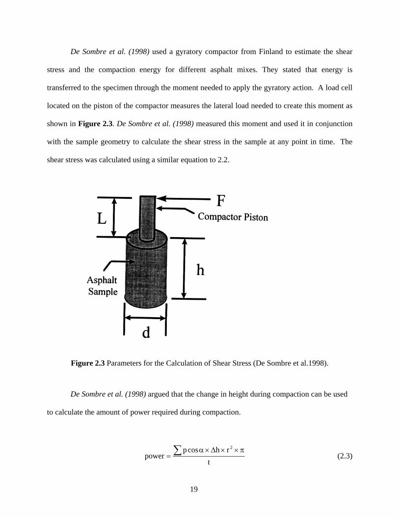
De Sombre et al. (1998) used a gyratory compactor from Finland to estimate the shear
stress and the compaction energy for different asphalt mixes. They stated that energy is
transferred to the specimen through the moment needed to apply the gyratory action. A load cell
located on the piston of the compactor measures the lateral load needed to create this moment as
shown in Figure 2.3. De Sombre et al. (1998) measured this moment and used it in conjunction
with the sample geometry to calculate the shear stress in the sample at any point in time. The
shear stress was calculated using a similar equation to 2.2.
Figure 2.3 Parameters for the Calculation of Shear Stress (De Sombre et al.1998).
De Sombre et al. (1998) argued that the change in height during compaction can be used
to calculate the amount of power required during compaction.
trhcosp
power2∑ π××Δ×α
= (2.3)

20
where:
p = pressure in cylinder,
α = gyratory angle,
Δh = change in height per cycle,
r = radius of cylinder and
t = time.
A study conducted at the Department of Transport in Australia had shown that the shear stress
evolution calculated using equation (2.2) was a function of the applied angle and mix
components, (Butcher 1998). At an angle of gyration greater than or equal to 1.00o, the shear stress
increased with compaction until a maximum value is reached when it began to decrease with further
increase in the compaction level as shown in Figure 2.4. In general, the reduction of shear stress
was shown to be more significant in mixes with softer asphalt (AC14) that were more susceptible
to permanent deformation as shown in Table 2.1. This study also used the change in voids at
maximum shear stress as a parameter to distinguish among mixes. Figure 2.5 shows that mixes
with different asphalt grades experienced distinct changes in percent air voids at maximum shear
stress. Other studies have also illustrated the relationship between the change of shear stress with
compaction and the change in mix design components (Gauer 1996, Moutier 1996).

21
(a) (b)
Figure 2.4 Shear Stress Measurements at Different Compaction Levels; (a) AC14 (soft asphalt) (b) AC 20 (stiff asphalt) (Butcher 1998).
Table 2.1 Maximum Shear Resistance at Different Angles and Binder Type (Butcher 1998)
AC14 AC20 Angle (Deg.) Vertical
Stress (kPa)
Max. Shear Stress (kPa)
Voids (%) Max. Shear Stress (kPa)
Voids (%)
0.05 0.50 1.00 1.25 1.50 2.00 3.00
600
175 (est.*) 405 (est.*)
467 481
- 515 571
- -
5.1 4.4 -
4.4 4.1
225 (est.*) 450 (est.*)
502 529 534 561 601
- -
4.3 4.0 4.5 4.9 4.3
2.00 2.00
400 240
365 231
5.6 5.6
398 250
5.7 4.6
* Maximum shear resistance not achieved and values estimated.
Gyrations Gyrations
22
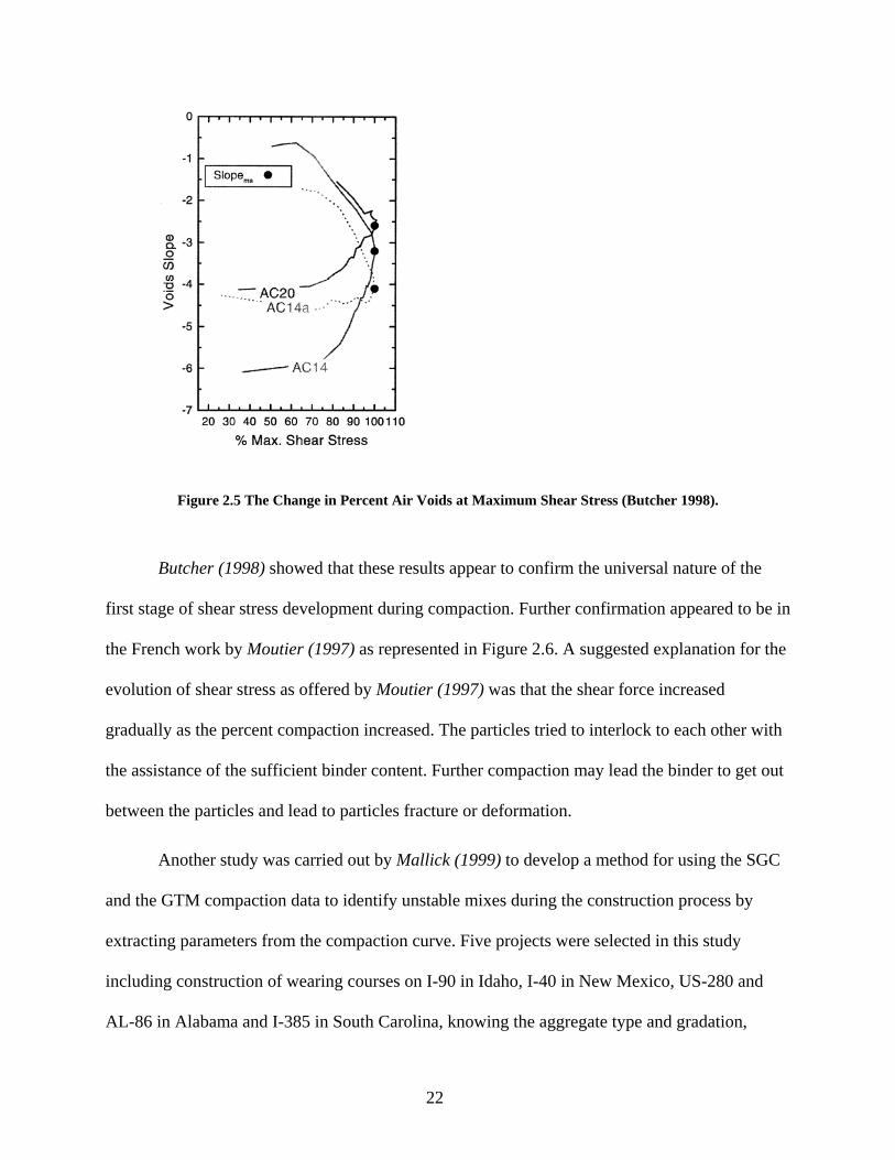
Figure 2.5 The Change in Percent Air Voids at Maximum Shear Stress (Butcher 1998).
Butcher (1998) showed that these results appear to confirm the universal nature of the
first stage of shear stress development during compaction. Further confirmation appeared to be in
the French work by Moutier (1997) as represented in Figure 2.6. A suggested explanation for the
evolution of shear stress as offered by Moutier (1997) was that the shear force increased
gradually as the percent compaction increased. The particles tried to interlock to each other with
the assistance of the sufficient binder content. Further compaction may lead the binder to get out
between the particles and lead to particles fracture or deformation.
Another study was carried out by Mallick (1999) to develop a method for using the SGC
and the GTM compaction data to identify unstable mixes during the construction process by
extracting parameters from the compaction curve. Five projects were selected in this study
including construction of wearing courses on I-90 in Idaho, I-40 in New Mexico, US-280 and
AL-86 in Alabama and I-385 in South Carolina, knowing the aggregate type and gradation,

23
Figure 2.6 French maximum shear stress by Moutier (1997)
asphalt binder type and content, and traffic levels of these projects. All of these mixes were
compacted with the SGC operated at 600 kPa and a 1.25-degree angle, and all mixes except the
I-385 were compacted with the GTM operated at 800 kPa and a 1-degree angle.
The shear stress measurements in the GTM are shown in Figure 2.7. The results show
that the I-90 mix is inferior to the other mixes. In the SGC, Mallick (1991) identified inferior
mixes during compaction process by calculating the gyratory ratio between the number of
gyrations required by the Superpave gyratory compactor to compact a mix to 98 and 95 percent
of theoretical maximum specific gravity. He presented the results in Figure 2.8 to show the
relationship between rutting in the field and the gyratory ratio.
A method for using the Superpave Gyratory Compactor (SGC) results to select optimum
mixture design introduced by Bahia et al. (1998). The method divided the measured
densification curve into two zones. The first zone represents the compaction characteristics
related to the construction stage; the second zone represents the densification under traffic.

24
Figure 2.7 Plot of Gyratory Shear (Sg) Versus Number of Gyrations (Mallick 1999)
Figure 2.8 Plot of Rutting Versus Gyratory Ratio (Mallick 1999)

25
Bahia et al. (1998) found that the densification curve measured by the SGC could be used
to calculate densification indices that represent the performance of mixture during construction
and during in-service. They also introduced the Compaction Energy Index (CEI) and the Traffic
Densification Index (TDI) to evaluate the potential performance of mixture during construction
and in-service. The values of CEI and TDI for different gradations tested showed that finer
gradations, above or passing through the restricted zone, require significantly less energy to
compact to 8% air voids, also these mixtures offered more resistance to densification between
8% and both of 4% and 2% air voids. This indicated that finer blends could be more favorable
for construction and can perform better under traffic densification. They showed the importance
of fine aggregate angularity for some mixture and also suggested that blends with high content of
rounded sand may offer reasonable performance.
Guler et al. (2000) conducted a study for the purpose of developing a device that can be
used in the SGC and allow shear measurements. The device consists of three load cells placed
120o apart on the top plate of the SGC called the Gyratory Load Cell Plate Assembly (GLPA).
Illustration of the GLPA and its components are shown in Figure 2.9 and Figure 2.10.
They reported that the energy balance for the mixture sample at any gyration cycle could be
written using the following equation:
W=U (2.4)
where W= work of external forces; U= total strain energy of sample. The above equation was
written in the following form:
VSM γθ = (2.5)

26
where M = applied moment during gyration; θ = gyration angle (radians); γ = shear strain; S =
frictional resistance; and V = sample volume at any cycle. The forces measured by the GLPA
and the top vertical actuator, were used to calculate the resultant force (R) and force eccentricity
(e), as shown in (Figure 2.11).
Figure 2.9 Gyratory Load Cell Plate Assembly (Guler et al. 2000)

27
Figure 2.10 Gyratory Load Cell Plate Assembly Placed on the Mold During Gyration Process
(Guler et al. 2000)
Figure 2.11 Applied External Forces and The Stress Distributions Used in Energy Relations
(Guler et al. 2000)
They suggested that two-dimensional distribution of the eccentricity of the resultant load
could be used to calculate the effective moment required to overcome the shear resistance of
mixture and tilt the mold to the 1.25 degrees. Guler et al. (2000) stated that this effective
moment is a direct measure of the resistance of asphalt mixtures to distortion and densification.

28
As shown in Figure 2.9 the moment M needed to apply the angle can be calculated by
multiplying the resultant ram force R, by the average eccentricity, e, for a given gyration cycle.
Guler et al. (2000) stated that θ and γ in equation (2.5) are equal, and the shear stress can be
calculated as follows:
hAeRS
⋅⋅
= (2.6)
where A = sample cross section area; and h = sample height at any gyration cycle. They
presented experimental results showing that the derived frictional resistance is sensitive to the
asphalt content, aggregate gradation, and fine aggregate angularity. Careful analysis of the
derivation provided by Guler et al. (2000) reveals that the shear stress in Equation (2.6) is
actually the frictional stress between the mold and the mix. This equation does not represent the
mix shear strength. Also U and W in equations 2.4 and 2.5 are both calculated from external
forces and U does not represent the energy dissipated.
2.5 ANALYSIS OF THE INTERNAL STRUCTURE
Digital image analysis provides the capacity of rapid measurement of particle distribution
and characteristics. Several studies established the effect of aggregate contacts on the shear
strength properties Oda (1972, 1977). It is also well documented that aggregate orientation is an
important factor that controls the shear strength and the stiffness of granular materials. For
example, Tobita (1989) showed that the yielding behavior of unbound granular materials is
controlled by aggregate distribution. Also, Masad et al. (2001) showed that the asphalt mix
stiffness could be expressed in terms of parameters that describe aggregate orientation.

29
Image analysis techniques usually treat particles as two-dimensional objects because only
the two dimensional projection of the particles is captured and measured. The principle of the
technique is that an image is digitizing into picture elements (usually 512x512 pixels). Each
pixel has an intensity value (gray level) that is scaled from 0-255 (black - white). Features of
interest are measured by their corresponding gray level. For example, after proper contrast has
been achieved so that the gray levels of all the phases can be distinguished from one another. It is
a simple matter to count all the pixels that fall within a certain range of intensities. This provides
a measure of area fraction of each phase. For particle analysis, when proper contrast is achieved
so that particles can be distinguished from the background, numerous measurements for each
particle can be made in near real time
Yue et al. (1995) work showed that internal structure characteristics such as gradation,
shape, and orientation of coarse aggregates in asphalt mixes could be accurately measured using
the digital image processing technique. The main objective of the Yue et al. (1995) work was to
quantitatively, capture the difference in the internal structure of asphalt mixtures compacted
using different methods of compaction, and to relate the internal structure to the performance of
the mix. Eriksen and Wegan (1993) conducted microscopic analysis of air voids in AC mixtures
at the Danish Road Institute. However efforts were directed at specimen preparation technique
instead of digital image analysis.
Masad et al. (1998, 1999a, 1999b) focused on developing image analysis techniques to
quantify the internal structure of asphalt concrete based on aggregate orientation, aggregate
gradation, aggregates contacts, aggregate segregation, and air voids distribution. These
measurements were used to quantify the internal structure of asphalt concrete specimens
prepared by the Superpave gyratory compactor at different levels of compaction and test its

30
ability to duplicate field conditions. Twelve specimens were compacted in the gyratory at
different number of gyrations (8, 50, 100, 109, 150, and 174 gyrations) where two specimens
were prepared at each level of compaction; these specimens were then cut vertically. In addition,
five field cores were recovered from pavement directly after construction and prior to trafficking.
Comparison of the internal structure of gyratory compacted specimens with field cores
showed that gyratory specimens reached the initial aggregate orientation of field cores at higher
number of gyrations (100 gyrations). Whereas they reached the average percent air voids in the
field cores at a much lower number of gyrations (20 gyrations), Figure 2.12.
Figure 2.12 Variation of Vector Magnitude, Angle of Inclination, and Percent Air Voids with
Compaction (Masad et al. 1999)
Masad et al. (1998) also showed that in the mix evaluation, there was a tendency in the
aggregate orientation to increase up to a certain level of compaction (100 gyrations), after which,

31
aggregate structure tended to have more random orientation. Air voids distribution was found to
be non-uniform, more voids were noticed at the top and bottom of the specimens, whereas the
specimens compacted more in the middle portion, Figure 2.13.
0
20
40
60
80
100
120
0 5 10 15
Percent voids %
Dep
th, m
m...
174 gyrations150 gyrations109 gyrations100 gyrations50 gyrations8 gyrations
Figure 2.13 Distribution of Air Voids in Gyratory Specimens at Different Number of Gyrations (Masad et al. 1999)
Masad et al. (1998) work emphasized that the new image analysis techniques were
useful tools to describe and compare asphalt materials produced using different laboratory
equipment and mix designs. In addition, these procedures would improve mechanical modeling
by providing consistent and accurate quantifying parameters of internal structure to be included
in constitutive relationships. Coarse aggregate gradation of gyratory compacted specimens was

32
well captured using the image analysis techniques and there was no change in aggregate
gradation during compaction, Figure 2.14.
Figure 2.14 Accuracy of Calculating Aggregate Gradation Using
Image Analysis (Masad et al. 1999)
Tashman et al. (2001) evaluated the ability of the Superpave gyratory compactor to
simulate the internal structure of HMA in the field, and the influence of different field
compaction patterns on the produced internal structure. They concluded that the compaction
variables in the compactor (angle, pressure, height, and temperature) influenced the internal
structure in laboratory specimens. They recommended a set of variables to improve the
simulation of the gyratory compactor to field conditions.
2.6 SUMMARY
The literature review shows that the Superpave gyratory compactor has been developed
during SHRP to compact HMA specimens with relatively large aggregate size, and to achieve
compaction under the influence of shear and normal stresses, which is believed to be similar to

33
field conditions. Several studies have used different types of gyratory compactors in order to
evaluate the mix shear strength during compaction. This shear strength was related the mix
resistance to permanent deformation. A critical review of these studies has revealed their
limitations especially in the derivation of the shear stress formula, and accounting of all forces
acting on HMA during compaction. There is a need to develop a new procedure to evaluate the
mix stability and shear strength based on the response of the mix to the forces applied during
compaction.
The review above indicated that image analysis techniques are powerful methods to
quantify the internal structure of asphalt mixes. These methods have already been used to
measure aggregate orientation, contacts, segregation, and air void distribution. In this study,
image analysis techniques will be used to relate the aggregate structure parameters to HMA
stability and shear strength.

This is a blank Page

34
3. ANALYSIS OF HMA STABILITY USING THE SGC
3.1 INTRODUCTION
This chapter presents detailed analysis of the HMA compaction using the Servopac
Gyratory Compactor (SGC). The compaction forces are analyzed in order to derive a
mathematical expression of the shear stress inside the mix. The shear stress value is used to
calculate the compaction energy, which is divided into two regions according to the type of
dominating strain. The volumetric strain dominates the first region, while the shear strain
dominates the second region. Analytical procedure is developed to identify these two regions.
An index termed the “Contact Energy Index” is developed to measure the stability of mixes. The
contact energy index is used to analyze mixes with different constituents such as percent of
binder, percent of natural sand, type of aggregate, gradation, and nominal maximum aggregate
size. The effect of the gyratory compaction variables such as the angle of gyration, and vertical
pressure on the contact energy index is investigated in order to determine the variables that
would best discern among mixes with different constituents. The contact energy indices are
compared to mechanical properties and permanent deformation of HMA.
3.2 SERVOPAC GYRATORY COMPACTION METHODOLOGY AND ANALYSIS
3.2.1 Compaction Mechanism
The compaction device used in this study is the Servopac gyratory compactor produced
by Industrial Process Controls (IPC) in Australia, which is a Servo-controlled multi-axis
pneumatic loading system designed for the laboratory production of asphalt specimens. The
compaction is achieved by the simultaneous action of static compression and shearing resulting

35
from the motion of the centerline of the upper boundary test specimen. Thus, the line connecting
the middle of the lower and upper boundaries generates a conical surface of revolution, while the
ends of the specimen remain perpendicular to the axis of the conical surface, (Figure 3.1).
Figure 3.1 Test Specimen Motion Diagram (IPC Operating and Maintenance Manual 1996).
The vertical compressive force is applied using a digital servo controlled, pneumatic
actuator, where a load cells is used to measure the vertical force. The vertical actuator is
connected to an intermediate plate via the load cell. This mechanism allows the top platen to
move freely in the horizontal plane.
In addition, there are three actuators located 120 degrees apart around the perimeter of
the mold carrier ring. The electronic control system sends a sine wave via a servo valve to each
of these actuators. The three sine waves are 120 degrees out of phase from each other as shown
in Figure 3.2. The amplitude of the sine wave controls the angle magnitude, and its frequency
controls the gyration rate. The feedback signal comes from the displacement transducer, which
bears directly on the bearing that connects the actuator rod to the mold carrier ring. All forces

36
acting on the specimen and the mold during compaction are shown in Figure 3.3. (IPC PTY LTD
1996)
Figure 3.2 Actuator Forces Acting by Sine Wave with 120° out of Phase
Figure 3.3 A Schematic Diagram of the Compactor Components.

37
3.2.2 Analysis of Shear Stress During Compaction
Several equations have been used to calculate the shear stresses in a mix during
compaction. These equations have essentially similar forms as they all rely on the force or
momentum needed to apply the gyration angle as a measure of shear stress (McRea 1965, De
Sombre et al. 1998, Butcher 1998, Guler et al. 2000). As demonstrated in the previous chapter,
the shear stress equation used in the GTM and the Servopac gyratory compactor was derived
using a free body diagram. This section presents a derivation of the shear stress in a gyratory
specimen during compaction in the Servopac machine. Consider a specimen inclined at a certain
angle of gyration, where the actuator P1 is applied at its maximum value (the amplitude of the
sinusoidal force). Points of application of the forces on the bottom plate are shown in Figure 3.4.
The force “A” is the result of the constant pressure “a” applied by the upper actuator on the
specimen during the compaction process. As it can be seen in Figure 3.4, the mix weight “Wm”
and the force “A” are at different offsets from the specimen centeroid due to the applied gyration
angle. By taking the summation of moment around the P3-R line to be equal to zero, the
following equation is derived P2:
2
43112 d
dWAddPP m++
= (3.1)
where:
=3d δ sin π/3
θ=δ tanh
θ : the angle of gyration,
h: the specimen height, and
34 d21d =

38
Because of symmetry as shown in Figure 3.2, P2 is equal to P3 when P1 is at the
amplitude. P1 is measured using a load cell in the Servopac; therefore P2 and P3 can be
calculated using Equ. (3.1).
δ
Figure 3.4 Plan View of the Forces Acting on the Specimen and the Mold.
The shear stress varies within the specimen depth. For the purpose of comparing the
shear stress in different mixes, the location at which the shear stress is calculated should be
specified. In this study, the average shear stress at the middle of the specimen is calculated.
This location is selected in order to avoid the high change in the shear stress along the
boundaries due to friction with upper and lower plates. Consider the free body for the top half of
a specimen shown in Figure 3.5, where the shear force Sθ can be expressed by taking the
summation of forces in the horizontal direction
θθθ sin)FF(cos)NN(S 2112 ++−= (3.2)

39
where N1, N2 are the normal forces acting on half the specimen surface, and F1, F2 are the
resultant frictional force acting on half the specimen surface. It is assumed here that these
normal and frictional forces are uniformly distributed and the friction factor between the
specimen and the mold is constant during compaction. Due to the dynamic motion of the
specimen with the mold, Eq. (3.2) is valid only when the angle is fully applied (when one of the
actuators reaches its maximum height). The normal and frictional forces can then be calculated
as follows:
⎪⎪⎭
⎪⎪⎬
⎫
==
==
2211
2211
2,
2
2,
2
fhrFfhrF
nhrNnhrN
ππ
ππ (3.3)
where n1, n2 represent the average normal stresses, and f1, f2 are the average frictional
stresses. r* refers to the vertical pressure acts at bottom of the specimen. Generally, small letter
refers to acting stress, and capital letter refers to acting force.
Figure 3.5 Plan View of the Forces Acting on the Specimen and the Mold.

40
Similarly, taking the summation of forces in the vertical direction results in the following
equilibrium equation:
θθ sin)(cos)()2
(* 1221 NNFFWAR m −++−+= (3.4)
where R* is force acting on the bottom of the top half of a specimen, A is the applied
vertical force which is kept constant during compaction, and Wm is the weight of the specimen.
Assuming that the specimen is subjected to vertical compressive stress along its horizontal cross
section. This assumption is motivated by the high vertical stress 600 kPa, and the small-applied
angle of gyrations θ. It is noted that 2
WAR m* +≠ because of the presence of the frictional and
normal forces acting on the mold. Also, R* is not located exactly at the center of the specimen
because of the applied angle, (Figure 3.6). Calculating the moment around the center “o” gives
another formula for determining R* as follows:
⎥⎦⎤
⎢⎣⎡ ++−++−−= θθθ
θθ
tan2
)2
(cos)(sin)(cos4
)(1* 121212hwArFFrNNhNN
xR m (3.5)
θ
θ
Figure 3.6 Illustration of the Location of the Resultant Vertical Force
at the Bottom of the Top Half of the Specimen.

41
where xθ is the distance from the center to the point where the force R* is acting. The
value of xθ increases with an increase in the applied angle. The maximum value for xθ is one
third of the specimen radius (r/3), which occurs when the applied angle causes triangular stress
distribution at the bottom of the specimen. The minimum value of xθ is zero at which the angle
of gyration is zero.
Consider the free body diagram of the mold shown in Figure 3.7. The summation of
forces in the vertical direction gives the following expression:
Figure 3.7 The Forces Acting on the Mold at Angle θ and the Change in the
Direction of P2 and P3 is to Satisfy the Equilibrium.
θθ cos)FF(2sin)NN(2WP 2121d ++−=−∑ (3.6)
where ∑P is the summation of the forces applied to the mold from the actuators and Wd is
the weight of the mold. As mentioned earlier, P2 and P3 are 120 degrees out of phase from P1,

42
and consequently, they have different sign than P1 when it is at the maximum value. Therefore,
the summation of the actuator forces is expressed as follows:
321 PPPP −−=∑ (3.7)
Mathematical manipulations of Eqs. (3.4), (3.5) and (3.6) give the following expressions:
[ ]
θμθθμ
θ
θμ
θ θθ
cossinrcosr
cos4h
tanrxWP21tan
2hx
2W
ANN 2
dm
12
−+
⎟⎟⎠
⎞⎜⎜⎝
⎛−−∑−⎟
⎠⎞
⎜⎝⎛ −⎥⎦
⎤⎢⎣
⎡ +=− (3.8)
μθ
θμtan)NN(
cos2WP
NN 12d
21 −+−∑
=+ (3.9)
The normal and frictional forces are assumed to be related through a constant frictional
factor μ ( 11 FN μ= , 22 FN μ= ) in the derivation of Eqs. (3.8) and (3.9). The friction factor was
taken a value of 0.28 based on a study by Abou-Chakra and Tuzun (1999) to determine the
coefficient of friction between coarse and fine granular materials and a smooth wall. Substituting
Eq. (3.9) in Eq. (3.2) results in the following equation for the shear force:
( ) ( )θ
θθθθ cossintan
21cos)(
212
12NNWPNNS d
−+−∑+−= (3.10)
The term θθ
cossin 2
can be neglected because it is too small relative to the other
components. Therefore, the shear force has the following expression:
( ) θθθ tanWP21cos)NN(S d12 −∑+−= (3.11)

43
where (N2-N1) is calculated using Eq. (3.8). The above equation indicates the shear forces
increases with an increase in the applied angle, and an increase in the applied actuator forces.
The expression in Eq. (3.11) can be used to calculate the shear stress by dividing over the cross-
section area at all gyrations during compaction.
3.2.3 Derivation of Shear Compaction Energy for Stability Analysis
The conservation of energy principle states that the total rate of work done to the system
by all external sources must equal the rate of increase of the total energy of the system. This
principle is also called the first law of thermodynamics. The conservation of energy can be
written in the following form:
i,ijiij qrDdtdu
−ρ+σ=ρ (3.12)
where ρ is the material density, dtdu is the rate of change of the internal energy per unit
volume, ijσ is the stress tensor, Dji is the deformation rate, ρr is the heat supplied by internally
distributed sources, and qi,i is the heat provided by the flow of thermal energy through the
boundary into the system or continuous body. If the deformation is assumed to occur under
isothermal conditions, the equation of energy conservation becomes:
jiijDdtdu
σ=ρ (3.13)
The term jiijDσ represents the mechanical work done by the external forces not
converted into kinetic energy. The applications of the conservation of energy to the gyratory
compaction are discussed here. The time increment used in Eq. (3.13) represents the time

44
needed to complete one gyration. If the deformation induced within each gyration is considered
to be all plastic deformation, then the change in the internal energy in each gyration (du) is
equivalent to the dissipated energy due to volumetric and shear strain as follows:
dsdvdu += (3.14)
where dv is the change in the internal energy due volumetric deformation, and ds is the change in
the internal energy due to shear deformation. A typical compaction curve from the gyratory
compaction is shown in Figure 3.8. It can be divided into two parts; the first one has a steep
change in percent air voids with an increase in number of gyrations. In this part (part A), most of
the applied energy is used in inducing volumetric permanent deformation (reduction in percent
air voids). Also, in the first part, the aggregates do not experience significant amount of shearing
force. In the second part (part B), however, most of the energy applied by the induced angle
does not cause significant volumetric change (small change in percent air voids). However, most
of this energy is consumed in overcoming the shear resistance between the particles. Therefore,
the energy calculations for assessing the mix stability under shear loading should focus on the
second part of the compaction curve.
In a discrete time domain where each gyration is considered a time increment, a measure of
energy can be calculated as follows:
dSindexEnergyTG
G
N
N⋅= ∑
2
1
otal θ (3.15)
where Sθ is the shear force at N number of gyrations derived from equation (3.11) and
angle θ and d is the vertical deformation (Specimen Diameter × tanθ). The summation is
conducted over the “Part B” of the compaction curve. It should be noted that the quantity in Eq.

45
(3.15) does not represent the actual compaction energy, as it does not account for all the forces
acting on a specimen multiplied by the deformations in the directions of these forces. The
complexity of the applied stresses and induced deformations makes it difficult if not impossible
to account for all forces and their associated deformations. However, since the shear force in Eq.
(3.11) is a result of all the applied forces, and the deformation d is also the resultant of all
deformations, equation (3.15) is a reasonable index of the compaction energy.
The applied energy in “Part B” is either used in developing more contacts among the
aggregates and cause reduction in percent air voids, or is dissipated by aggregate sliding as the
aggregate structure fails to develop more contacts. In order to capture this phenomenon in
evaluating the mix stability, another index is introduced that captures the energy used in reducing
the percent air voids or developing contacts:
∑ ⋅=2
1
index Energy ontact G
G
N
NedSC θ (3.16)
where de is the change in height at each consecutive gyrations in Part B of Figure 3.8. For
consistency, units were taken N.mm, because the vertical deformations are too small.
3.3 EXPERIMENTS AND RESULTS
Two experiments have been conducted to evaluate the ability of the developed shear
stress and energy indices to discern among different mixes. The first experiment evaluated the
influence of changes in the mix constituents including asphalt binder content, percent of natural
sand, nominal maximum aggregate size, aggregate source, and type of gradation on the energy
indices. The second experiment was targeted at evaluating the influence of changes in
compaction variables on the energy indices to determine the variables that have the best ability in

46
discerning among the mixes. Mixes were prepared at WCAT (Washington Center of Asphalt
Technology) and the compaction process using the Servopac was done at University of Idaho.
0
5
10
15
20
25
0 50 100 150 200Number of Gyrations
% A
ir Vo
ids
Part A Part B
Figure 3.8 A Schematic Diagram Shows the Two Zones of the Compaction Curve
3.3.1 The Effect of Mix Constituents on Energy Indices
The first experiment consists of 16 mixes as shown in
Table 3.1. The aggregate gradations are shown in Figure 3.9. The optimum asphalt
content was selected to achieve a target of 4% air void at Ndes gyrations. The actual percent air
voids varied between 3.5% and 4.5%. In order to study the effect of excess asphalt content, all
mixes were prepared at the optimum asphalt content and 0.8% more than the optimum value. All
the mixes were prepared at a temperature of 325° F, and compacted at a temperature of 300° F.
All specimens were compacted to a maximum number of gyrations (Nmax) of 160. This level of
compaction corresponds to a Superpave traffic level of 3 to 10 million equivalent single axle
loads (AASHTO 2001). A summary of mix properties is shown in
NG1 NG2

47
Table 3.1. In this Table, the coarse gradation indicates that the gradation curve passes
below the restricted zone, while the fine gradation passes above the restricted zone. More details
on aggregate gradations and properties are provided in Appendix A.
Table 3.1 The Experimental Matrix of Asphalt Mixes with Different Constituents
Aggregate Gradation Size, mm % Fine Aggregate
Design AC, %
Mix label
0 5.3 A 9.5 40 5.7 B 0 4.4 C
Co
arse 19 40 4.7 D 0 6.2 E 9.5
40 6.3 F 0 4.7 G
Li
mestone Fin
e 19 40 5.2 H 0 6.3 I 9.5
40 5.9 J 0 5.4 K
Co
arse 19 40 4.8 L 0 6.7 M 9.5
40 6.3 N 0 5.0 O
Gr
avel Fin
e 19 40 5.4 P
Prior to the analysis of the compaction energy, the repeatability of the compaction
procedure should be evaluated in order to determine the number of specimens needed to
represent each mix. Two specimens from each of the C, D, K, and L mixes were compacted
using the same vertical pressure (600 kPa), angle of gyration (1.5o), rate of gyration (30
gyrations/minute). The compaction curve results are shown in Figure 3.10. The two replicates
from each mix followed almost the same compaction curve. Also, as shown in Table 3.2, the
maximum difference in percent air voids was about 0.5%, which is within the experimental error

48
that is usually experienced in the laboratory. Consequently, it was decided to use only one
specimen to represent each mix at a given set of compaction variables.
37.525.419.012.59.54.752.361.180.075 0.60
10
20
30
40
50
60
70
80
90
100
Sieve Size mm
% P
assi
ng
Mix L Mix K Mix C Mix D Mix P Mix H Mix G Mix O
A: Mixes with 19.0 mm NMAS Raised to the Power of 0.45.
37.525.419.012.59.54.752.361.180.075 0.60
10
20
30
40
50
60
70
80
90
100
Sieve Size mm
% P
assi
ng
Mix A Mix B Mix E Mix F Mix I Mix J Mix M Mix N
B. Mixes with 9.5 mm NMAS Raised to the Power of 0.45.

49
Figure 3.9 Aggregate Gradation for Mixes with 19.0 mm & 9.5 mm NMAS Raised to the Power of 0.45.
0
5
10
15
20
25
30
0 20 40 60 80 100 120 140 160N
Air V
oids
%
Mix D Mix K Mix C Mix L
Figure 3.10 The Changing in the Compaction Curve with Two Replicate Samples.
Table 3.2 The Average Difference in Percent Air Voids among Replicates
Mix # Average Diff. %C 0.26D 0.17K 0.59L 0.26
As mentioned earlier, the compaction energy is calculated in the shear deformation part
(Part B of the compaction curve shown in Figure 3.8). Therefore, a criterion is needed to
establish the start and the end of part B. The number of gyrations (NG1) that indicates the
beginning of part B is defined by fitting a polynomial of the sixth degree to the compaction curve
and determines the slope at each gyration. Then, NG1 is taken as the point at which the change in
the slope of two consecutive gyrations is less or equal to 0.001%. The approach followed here to

50
determine the number of gyrations that defines the end of Part B (NG2) was first to determine the
mix with the lowest “160- NG1” value, and then to add this value to NG1 of each mix. This
approach ensures that the same and maximum number of gyrations possible (NG2- NG1) is used in
calculating the energy indices for all mixes. The maximum number of gyrations is needed in
order to capture the shear stress behavior along a large number of gyrations. For example,
Figure 3.11 shows the difference of shear stress behavior for two specimens with different binder
content. The beginning of the shear compaction region (NG1) occurs at about 80 gyrations. The
difference between the energy indices of these two mixes is best captured by taking the
maximum NG2 value possible which is 160 gyrations in this case. However, NG2 of 160 gyrations
cannot be applied for all mixes since they do not all have the same NG1.
An example of data required for the calculation of the shear stress and the energy indices
is shown in Appendix B.
135
140
145
150
155
160
0 20 40 60 80 100 120 140 160N
She
ar s
tress
(kP
a)
mix G opt.+ mix G opt.
Figure 3.11 Examples of Shear Stress Curves for Asphalt Mixes During Compaction.

51
Effect of percent of binder content
Two different binder contents were used to investigate the effect of the binder content on
the energy indices. The first one was the optimum value determined from the Superpave mix
design procedure. The second one was 0.8% higher than the optimum value, which is referred to
hereinafter as optimum plus. It was noticed that most of the optimum plus mixes reached a peak
value at which it started to decrease with further compaction. The rate of reduction was a function
of the aggregate gradation. However, most of the mixes with optimum asphalt content reached a
maximum shear stress and stabilized at that value with further compaction. An example of this
phenomenon is shown in Figure 3.11. A comparison between the shear indices is presented in
Figure 3.12 and Table 3.3. It is evident that the total energy index did not show a certain pattern
in comparing the optimum and optimum plus mixes. However, the contact energy index was
always higher for mixes with optimum asphalt content. This indicates that the applied energy
was used to develop contacts in the optimum mixes, while it was dissipated in aggregate sliding
in the optimum plus mixes.
Table 3.3 Energy Indices of Mixes with Different Asphalt Content. ratio ratio
Mix # opt. opt.+ opt/opt+ opt. opt. + opt/opt+mix a 1402.89 1397.47 1.004 25.80 22.43 1.150mix b 1289.80 1322.17 0.976 11.15 8.82 1.264mix c 1315.44 1336.67 0.984 24.20 20.16 1.200mix d 1306.94 1292.29 1.011 9.82 8.57 1.146mix e 1400.21 1383.36 1.012 23.12 23.24 0.995mix f 1293.79 1303.36 0.993 10.62 9.97 1.065mix g 1238.65 1251.00 0.990 28.20 8.88 3.177mix h 1344.64 1287.33 1.045 9.27 8.63 1.074mix I 1348.73 1403.00 0.961 24.49 22.49 1.089mix j 1274.62 1249.19 1.020 10.17 7.95 1.279mix k 1432.65 1419.30 1.009 29.03 25.33 1.146mix L 1283.52 1356.96 0.946 10.45 8.82 1.185mix m 1245.30 1249.52 0.997 21.59 9.12 2.368mix n 1446.35 1427.85 1.013 20.41 17.89 1.141mix o 1428.27 1400.26 1.020 20.58 20.54 1.002mix p 1319.32 1357.94 0.972 9.62 8.95 1.075
Total E.I. Contact E.I.

52
0
5
10
15
20
25
30
mix
a
mix
b
mix
c
mix
d
mix
e
mix
f
mix
g
mix
h
mix
I
mix
j
mix
k
mix
L
mix
m
mix
n
mix
o
mix
p
Con
tact
Ene
rgy
Inde
x
Mixes with opt. binder Mixes with opt.+ binder
1150
1200
1250
1300
1350
1400
1450
mix
a
mix
b
mix
c
mix
d
mix
e
mix
f
mix
g
mix
h
mix
I
mix
j
mix
k
mix
L
mix
m
mix
n
mix
o
mix
p
Tota
l Ene
rgy
Inde
x
Mixes with optimum % binder Mixes with optimum+ % binder
A: The Total Energy Index.
B: Contact Energy Index.
Figure 3.12 Comparison among Mixes with Different Asphalt Content in Terms of Total & Contact Energy Index.

53
Effect of the aggregate type
Two types of aggregates were used in this evaluation; limestone and gravel. A
comparison between the energy indices of the gravel and limestone mixes is shown in Figure
3.13 (a, b) and Table 3.4. It is evident that both the total and contact energy indices were higher
for the limestone than for the gravel mixes. This indicates that more energy was needed to
compact the limestone mixes, and the part of this energy that was transferred to developing more
aggregate contacts was higher for the limestone mixes as well. It is well known that limestone
has more texture and angularity than gravel, which explains the higher stability of the limestone
mixes as indicated by the energy indices.
Table 3.4 Energy Indices of Mixes with Different Aggregate Type Limestone Total Contact Gravel Total Contact Total Contact
Mix # E.I. E.I. Mix # E.I. E.I. % E.I. Ratio E.I. Ratiomix a 1382.50 21.39 mix I 1358.75 24.59 1.017 0.870mix b 1291.82 8.16 mix j 1249.19 7.95 1.034 1.026mix c 1336.67 24.59 mix k 1318.68 23.02 1.014 1.068mix d 1337.76 10.01 mix L 1293.46 9.39 1.034 1.066mix e 1360.86 14.35 mix m 1352.85 9.12 1.006 1.574mix f 1303.36 10.72 mix n 1282.01 12.11 1.017 0.885mix g 1399.87 21.92 mix o 1428.27 20.58 0.980 1.065mix h 1375.81 8.63 mix p 1319.32 8.33 1.043 1.036

54
1150
1200
1250
1300
1350
1400
1450
mix
a
mix
I
mix
b
mix
j
mix
c
mix
k
mix
d
mix
L
mix
e
mix
m
mix
f
mix
n
mix
g
mix
o
mix
h
mix
p
Tota
l Ene
rgy
Inde
x
Mixes with Gravel type Mixes with Limestone type
0
5
10
15
20
25
30
mix
a
mix
I
mix
b
mix
j
mix
c
mix
k
mix
d
mix
L
mix
e
mix
m
mix
f
mix
n
mix
g
mix
o
mix
h
mix
p
Con
tact
Ene
rgy
Inde
x
Mixes with Gravel type Mixes with Limestone type
A: Total Energy Index.
B: Contact Energy Index.
Figure 3.13 Comparison among Mixes with Different Aggregate Type in terms of Total & Contact Energy Indices.

55
Effect of the Nominal Maximum Aggregate Size (NMAS)
The nominal maximum aggregate size (NMAS) is defined as the sieve size larger than the
first sieve to retain more than 10 percent of the material. The analysis results in Figure 3.14a
indicate that the majority of the mixes with 19.0 mm NMAS required higher energy to compact.
However, the contact energy index results in Figure 3.14b show no trend in favoring one NMAS
over the other in developing contacts and strong aggregate structure. A comparison between the
mixes is shown in Table 3.5.
Table 3.5 Energy Indices of Mixes with Different NMAS. 9.50 mm Total Contact 19 mm agg. Total Contact Total Contact
agg. Mix # E.I. E.I. Mix # E.I. E.I. E.I. Ratio E.I. Ratiomix a 1402.89 22.28 mix c 1385.83 20.16 0.99 0.91mix b 1289.80 8.74 mix d 1337.76 8.57 1.04 0.98mix e 1400.21 22.66 mix g 1420.07 8.88 1.01 0.39mix f 1293.79 9.89 mix h 1375.81 8.63 1.06 0.87mix I 1358.75 22.59 mix k 1381.66 25.20 1.02 1.12mix j 1314.75 7.95 mix L 1303.40 8.77 0.99 1.10
mix m 1352.85 9.12 mix o 1407.98 23.47 1.04 2.57mix n 1318.12 17.49 mix p 1339.28 8.95 1.02 0.51

56
1150
1200
1250
1300
1350
1400
1450
mix
a
mix
c
mix
b
mix
d
mix
e
mix
g
mix
f
mix
h
mix
I
mix
k
mix
j
mix
L
mix
m
mix
o
mix
n
mix
p
Tota
l Ene
rgy
Inde
x
Mixes with 19mm size Mixes with 9.5mm size
0
5
10
15
20
25
30
mix
a
mix
c
mix
b
mix
d
mix
e
mix
g
mix
f
mix
h
mix
I
mix
k
mix
j
mix
L
mix
m
mix
o
mix
n
mix
p
Con
tact
Ene
rgy
Inde
x
Mixes with 19 mm size Mixes with 9.5 mm size
A: Total Energy Index.
B: Contact Energy Index.
Figure 3.14 Comparison among Mixes with Different Aggregate NMAS in terms of Total & Contact Energy Indices.

57
Effect of the Aggregate Gradation Shape
Two different gradations were used in this study, below the restricted zone (BRZ) and
above the restricted zone (ARZ). The BRZ gradation is usually referred to as coarse gradation,
while the ARZ gradation is referred to as fine gradation. There have been several studies to
evaluate the influence of the location of the aggregate gradation curve with respect to the
restricted zone on mix stability and performance (Chowdry et al. 2001, Hand and Epps 2001).
These studies came to the conclusion that there is no trend between the mix stability and location
of the gradation curve below or above the restricted zone. The energy indices results shown in
Figure 3.15 and Table 3.6 are in agreement with these findings as no relationship was found
between the energy indices and gradation shape.
Table 3.6 Energy Indices of Mixes with Different Aggregate Gradation Shape. B.R.Z Total Contact A.R.Z Total Contact Total Contact
(Coarse) Mix # E.I. E.I. % (Fine) Mix # E.I. E.I. % E.I. Ratio E.I. Ratiomix a 1433.35 22.43 mix e 1400.21 23.11 1.024 0.970mix b 1339.31 8.82 mix f 1323.18 9.89 1.012 0.892mix c 1385.83 19.75 mix g 1389.80 8.88 0.997 2.225mix d 1337.76 8.57 mix h 1375.81 8.60 0.972 0.996mix I 1358.75 22.36 mix m 1343.10 9.12 1.012 2.452mix j 1314.75 7.95 mix n 1288.45 17.29 1.020 0.460mix k 1412.24 25.33 mix o 1428.27 23.83 0.989 1.063mix L 1333.34 8.82 mix p 1339.28 8.82 0.996 1.000

58
1150
1200
1250
1300
1350
1400
1450
mix
a
mix
e
mix
b
mix
f
mix
c
mix
g
mix
d
mix
h
mix
I
mix
m
mix
j
mix
n
mix
k
mix
o
mix
L
mix
p
Tot
al E
nerg
y In
dex
Mixes with gradation above the Restricted ZoneMixes with gradation below the Restricted Zone
A: Total Energy Index.
0
5
10
15
20
25
30
mix
a
mix
e
mix
b
mix
f
mix
c
mix
g
mix
d
mix
h
mix
I
mix
m
mix
j
mix
n
mix
k
mix
o
mix
L
mix
p
Con
tact
Ene
rgy
Inde
x
Mixes with gradation above the Restricted ZoneMixes with gradation below the Restricted Zone
B: Contact Energy Index.
Figure 3.15 Comparison among Mixes with Different Aggregate Gradation Shape in terms of Total & Contact Energy Indices.

59
Effect of Percent Natural Sand
Mixes with 0% and 40% natural sand were tested in this study. Figure 3.16 and Table
3.7 show that the total energy index did not distinguish between mixes with and without natural
sand. However, the results show that the contact energy index was higher for all mixes without
natural sand compared with those included 40% natural sand. It is evident that the contact energy
index captures the influence of natural sand on mix stability. Most natural sands and especially
the one used in this study have rounded shape with very small texture, therefore, mixes with
natural sand are expected to be less stable than the mixes that do not include natural sand.
Table 3.7. Energy Indices of Mixes with Different Percent of Natural Sand.
0% Natural Total Contact 40% Natural Total Contact Total ContactSand Mix # E.I. E.I. % Sand Mix # E.I. E.I. E.I. Ratio E.I. Ratio
mix a 1392.69 25.80 mix b 1369.03 11.35 1.017 2.274mix c 1295.35 24.05 mix d 1337.76 10.01 0.968 2.403mix e 1331.37 22.91 mix f 1323.18 10.72 1.006 2.138mix g 1319.21 28.63 mix h 1375.81 9.35 0.959 3.064mix I 1301.86 24.20 mix j 1249.19 10.27 1.042 2.357mix k 1361.27 28.61 mix L 1343.27 10.70 1.013 2.673mix m 1352.85 21.91 mix n 1367.43 20.05 0.989 1.093mix o 1367.34 20.35 mix p 1339.28 9.62 1.021 2.114
The effect of natural sand can also be seen in compaction curves. Figure 3.17a shows
that mixes with natural sand started at smaller percent air voids. The slopes of the compaction
curves are plotted in Figure 3.17b, in which the slope is calculated for each 10 gyrations. It is
clear that mixes with 0% natural sand had higher slopes than mixes with 40% natural sand. This
observation is especially true in the shear compaction range (Part B in Figure 3.17), which starts
between 30 to 50 gyrations. As mentioned earlier, an increase in the slope in Part B indicates an
increase in the portion of the applied energy transferred into developing contacts among
aggregates.

60
1150
1200
1250
1300
1350
1400
1450
mix
a
mix
b
mix
c
mix
d
mix
e
mix
f
mix
g
mix
h
mix
I
mix
j
mix
k
mix
L
mix
m
mix
n
mix
o
mix
p
Tota
l Ene
rgy
Inde
x
Mixes with 40% sand Mixes with 0% sand
0
5
10
15
20
25
30
mix
a
mix
b
mix
c
mix
d
mix
e
mix
f
mix
g
mix
h
mix
I
mix
j
mix
k
mix
L
mix
m
mix
n
mix
o
mix
p
Con
tact
Ene
rgy
Inde
x
Mixes with 40% sand Mixes with 0% sand
A: Total Energy Index.
B: Contact Energy Index.
Figure 3.16 Comparison TEI and CEI among Mixes with Different % Natural Sand.
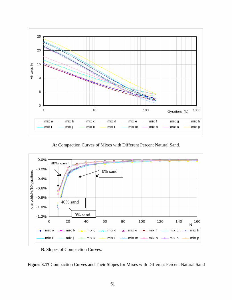
61
0
5
10
15
20
25
1 10 100 1000Gyrations (N)
Air
void
s %
mix a mix b mix c mix d mix e mix f mix g mix h
mix I mix j mix k mix L mix m mix n mix o mix p
-1.2%
-1.0%
-0.8%
-0.6%
-0.4%
-0.2%
0.0%
0 20 40 60 80 100 120 140 160N
Δ a
irvoi
ds%
/10
gyra
tions
mix a mix b mix c mix d mix e mix f mix g mix h
mix I mix j mix k mix L mix m mix n mix o mix p
A: Compaction Curves of Mixes with Different Percent Natural Sand.
B. Slopes of Compaction Curves.
Figure 3.17 Compaction Curves and Their Slopes for Mixes with Different Percent Natural Sand
0% sand
40% sand
0% sand
40% sand

62
3.3.2 The Effect of Compaction Variables on Energy Indices
The previous section evaluated the influence of mix constituents on the energy indices.
This evaluation was conducted using the same set of compaction variable (Angle = 1.5o,
Pressure = 600 kPa). However, Butcher et al. (1998) showed that the shear stress in a mix
changes as a function of the angle of gyration. As shown in Figure 2.4, the shear stress at small
angles (θ < 1.0) increases with the number of gyrations until reaches a constant value, indicating
that the material reaches a stable state at low angles of gyrations. However, the shear stress
curve has different characteristics at higher angle values as it increases up to a maximum value
beyond which the shear stress tends to decrease with further compaction. It can be seen in
Figure 2.4, that two different mixes (a and b) might behave similarly at low angle but different
at high angle such as 3o. Mix “a” takes almost 50 gyrations to start showing unstable behavior,
while instability in mix b is triggered at 100 gyrations.
In this section, the influence of changes in compaction pressure and angle of gyration on
the energy indices is investigated using four mixes (C, D, K, and L). This is necessary to
determine if there exists a set of compaction variables that have the best ability to differentiate
among mixes with different constituents. Five specimens of each of the four mixes were
compacted at 0, 0.75, 1.5, 2.25, 3.0°. Mixes compacted at 0° angle collapsed right after taking
them from the mold, which emphasized the influence of shear action induced by the angle of
gyration on developing aggregate contacts, as shown in Figure 3.18. The difference in shear
stress among the mixes increased with an increase in the angle of gyration. It is also noticed that
the shape of the compaction curve for mix k changed with an increase of angle of gyration from
0.75 to 3.00. Figure 3.19 shows that the shear stress increased remarkably with an increase in
angle of gyration.

63
220
222
224
226
228
230
232
234
236
238
240
0 20 40 60 80 100 120 140 160N
Shea
r Stre
ss (k
Pa)
C300 L300 K300 D300
Figure 3.18a. Shear Stress Curves at an Angle of 3.00°
160
162
164
166
168
170
172
174
176
178
180
0 20 40 60 80 100 120 140 160N
Shea
r Stre
ss (k
Pa)
C225 L225 K225 D225
Figure 3.18b. Shear Stress Curves at an Angle of 2.25°
Average difference =4.62 kPa
Average difference =3.92 kPa

64
40
42
44
46
48
50
52
54
56
58
60
0 20 40 60 80 100 120 140 160N
Shea
r Stre
ss (k
Pa)
C075 L075 D075 K075
100
102
104
106
108
110
112
114
116
118
120
0 20 40 60 80 100 120 140 160
N
Shea
r Stre
ss (k
Pa)
C150 L150 K150 D150
Figure 3.18c. Shear Stress Curves at an Angle of 1.50°
Figure 3.18d. Shear Stress Curves at an Angle of 0.75°
Figure 3.18 Shear Stress Curves at Different Angles of Gyrations (3.00, 2.25, 1.5 and 0.75°)
Average difference =3.01 kPa
Average difference =2.95 kPa

65
0
50
100
150
200
250S
hear
stre
ss (k
Pa)
3 2.25 1.5 0.75 0
angle of gyrations (θ)
C D K L
Figure 3.19 Maximum Shear Stress at Different Angles of Gyrations.
Both the total and contact energy indices were calculated at all angles for the four mixes
(Figure 3.20 and Table 3.8). As can be seen the total energy index was almost the same for all
mixes at a given angle of gyration. The contact energy indices for the four mixes had the same
order at all angles, in spite of the increase in their values with an increase in angle. The ratio of
contact energy index of mix C to that of D and of mix K to that of L remained almost the same at
different angles. This result suggests that the angle of gyration affects the shear stress but does
not change the order of the mixes in terms of stability.

66
0
5
10
15
20
25
30
Con
tact
Ene
rgy
Inde
x
C00
C07
5
C15
0
C22
5
C30
0
D00
D07
5
D15
0
D22
5
D30
0
K00
K075
K150
K225
K300 L00
L075
L150
L225
L300
Mix C Mix D Mix K Mix L
0
500
1000
1500
2000
2500
3000
3500
4000
4500
Tota
l Ene
rgy
Inde
x
C00
C07
5
C15
0
C22
5
C30
0
D00
D07
5
D15
0
D22
5
D30
0
K00
K075
K150
K225
K300 L00
L075
L150
L225
L300
Mix C Mix D Mix K Mix L
A: The Total Energy Index.
B: The Contact Energy Index
Figure 3.20 The Total & Contact Energy Indices at Different Angles of Gyrations.

67
.
Table 3.8 Energy Indices at Different Angle of Gyrations.
E.I. @ angle Mix C Mix D Mix K Mix L Mix C Mix D Mix K Mix L0.00 0.01 0.01 0.00 0.00 0.00 0.00 0.00 0.000.75 207.54 261.31 214.32 212.61 8.67 6.14 8.06 5.891.50 825.87 1035.72 825.88 843.01 17.84 7.53 18.24 7.052.25 1982.38 2428.39 1960.31 1972.71 25.24 12.08 19.62 11.733.00 3524.14 4220.72 3500.16 3470.16 25.43 15.01 32.73 14.69
Total E.I. Contact E.I.
The vertical pressure is another factor that influences the compaction process. An
increase in pressure leads to an increase in confinement during compaction. Specimens from the
C, D, K, and L mixes were compacted at pressures of 450 kPa, 600 kPa, and 750 kPa at 1.5 and
2.25 angles. The results in Figure 3.21a show that the total energy index was almost the same
for all mixes at given pressure and angle values, while the contact energy index decreased with a
decrease in the pressure and angle values as shown in Figure 3.21b. The rank of the contact
energy index remained almost the same at the different combinations of pressure and angle. The
mixes without natural sand C and K showed higher stability than their counterpart mixes with
natural sand D and L. These results suggest any combination of the pressure and angle would be
suitable to characterize the mixes.
Table 3.9 Energy Indices at Different Angles and Pressures.
AnglePressure 450 600 750 450 600 750
C 982.83 1361.72 1606.75 2108.16 2907.77 3664.91D 1035.72 1414.39 1658.11 2189.90 3133.69 3784.86K 978.96 1354.86 1657.57 2099.51 3122.75 3605.88L 1003.82 1370.49 1716.48 2108.05 2909.42 3718.85
AnglePressure 450 600 750 450 600 750
C 12.76 20.51 18.75 14.01 28.17 28.49D 7.37 10.58 11.48 8.88 13.63 17.44K 13.53 19.08 17.71 14.27 27.86 25.57L 7.05 9.95 11.90 8.66 13.58 17.12
1.50 2.25Contact E.I.
Total E.I.1.50 2.25

68
0
5
10
15
20
25
30
450 600 750 450 600 750
1.5 (deg.) 2.25 (deg.)
Vertical Pressure (kPa)
Con
tact
Ene
rgy
Inde
x
C D K L
0
500
1000
1500
2000
2500
3000
3500
4000
450 600 750 450 600 750
1.5 (deg.) 2.25 (deg.)
Vertical Pressure (kPa)
Tota
l Ene
rgy
Inde
x
C D K L
A: The Total Energy Index
B: The Contact Energy Index
Figure 3.21 The Total & Contact Energy Indices at Different Pressures and Angles of Gyrations.

69
3.4 COMPARISON OF CONTACT ENERGY INDEX WITH MIX MECHANICAL PROPERTIES
The Superpave shear test was used to measure the viscoelastic properties; namely the
dynamic shear modulus G* and phase angle δ of four mixes (C, D, K, and L) of two
temperatures (40C, and 52C). All measurements were conducted on mixes with optimum
asphalt content. The viscoelastic properties and contact energy indices at an angle of 1.5o and a
pressure of 600 kPa are shown in Table 3.10. Each of the viscoelastic properties is an average of
three measurements. The comparison focuses on G*/sinδ since it has been recommended as a
parameter to evaluate the mix resistance to permanent deformation (Romero and Mogawer
1998a, and b). It can be seen that both G*/sinδ and the contact energy index were higher for
mixes without natural sand (C and K), compared with their counterpart mixes that included 40%
natural sand (D and L). The contact energy index was higher for mixes with limestone
compared with those that included gravel. In general, this limited data show that good correlation
exists between the contact energy index predictions and G*/sinδ.
Table 3.10 Comparison between the Viscoelastic Properties and Contact Energy Index Mix # G* δ G*/sinδ Contact
40C 52C 40C 52C 40C 52C E.I. C 545031.8 206360.3 39.6 44.3 854618.8 295539.5 17.84 D 532877.0 188875.1 43.1 46.7 780314.9 259696.2 7.53 K 653159.4 273335.5 37.1 45.3 1083127.9 384240.5 18.24 L 506535.1 192294.6 43.3 50.6 738910.7 248672.1 7.05
3.5 COMPARISON WITH PERFORMANCE AND MECHANICAL PROPERTIES
Three compacted mixtures specimens from each of three SPS-9 projects from 1992 were
received. These mixes were analyzed and tested using different experiments by Michael
Anderson et al. (2000). The energy indices were calculated to all mixes and averaged for each

70
project then compared to the findings and results presented by Anderson et al. (2000). The
following table presents the mixes description:
Table 3.11 Summary of the 1992 SPS-9 mixtures
Project Mix LabelS-4 (2)S-4 (5)S-4 (7)S-3 (84)S-3 (89)S-3 (90)S-3 (2)S-3 (4)S-3 (5)
Wisconsin IH-94
Wisconsin IH-43
Indiana IH-65
These mixes were tested with the Static Shear Creep Testing (SSCH), and Shear
Frequency Sweep Testing (FSCH) at two different temperatures. SSCH determined the average
maximum shear strain (γmax) and the FSCH determined the average shear stiffness (G*) and
phase angle (δ). In addition, field rutting measurements were obtained after six years of service.
These measurements were presented by Anderson et al. (2000) in terms of the rutting rate
parameter expressed in mm/ESAL1/2, Table 3.12. As reported by Anderson et al. (2000) all
mixes would be considered to have minimal rutting since they all had a rutting rate less than
0.00584 mm/ESAL1/2.
The relationships between the CEI and the mechanical properties are shown in Figure
3.22. In general, the results show that the CEI increases with an increase in G* and G*/sinδ, and
a decrease in maximum shear strain. This shows the potential of the CEI in reflecting the mix
stability and shear strength. The CEI index is also the highest for the mixes from IH-43, which
has the lowest rutting rate, Table 3.12. However, the CEI is almost the same for IH-94 and IH-
65 although these two sections have different rutting rates. It should be noticed that the three

71
sections did not experience significant rutting that would allow complete verification of the
ability of the CEI to predict the field permanent deformation.
Table 3.12 Performance and Experimental Data Presented by Anderson et al. (2000) on SPS-9 Sections.
Project IH-43 IH-94 IH-65Rut Depth (mm) 2 2 5ESAL 3.58E+06 7.39E+06 1.65E+07Ruttin rate
(mm/ESAL1/2) 1.06E-03 7.36E-04 1.23E-03Total energy index 1052.76 1077.18 1051.24Contact energy index 28.47 25.91 25.59
Temperature T1 ( C) 38 38 39Temperature T2 ( C) 22 21 23
SSCH (γmax)T1 ( C) 1246.00 932.00 2060.00T2 ( C) 370.00 453.00 1187.00
FSCH (G* kPa)T1 ( C) 863176 656499 370655T2 ( C) 3422942 2344772 1811702
FSCH (δ degree)T1 ( C) 33.90 35.70 43.70T2 ( C) 8.90 16.40 25.40
G*/sinδ 1547.62 1125.03 536.50

72
25.00
26.00
27.00
28.00
29.00
I-43 I-94 I-65
Con
tact
Ene
rgy
Inde
x
0.000E+00
4.000E-04
8.000E-04
1.200E-03
1.600E-03
Rut
Rat
e
C. E.I. Rutting Rate
Figure 3.22a. Rutting Rate Versus Contact Energy Index
25.00
26.00
27.00
28.00
29.00
I-43 I-94 I-65
Con
tact
Ene
rgy
Inde
x
0
500
1000
1500
2000
2500
She
ar S
train
C. E.I. Maximum Shear Strain (SSCH @ T1)
Figure 3.22b. Maximum Shear Strain at T1 Versus Contact Energy Index
25.00
26.00
27.00
28.00
29.00
I-43 I-94 I-65
Con
tact
Ene
rgy
Inde
x
0
200
400
600800
1000
1200
1400
She
ar S
train
C. E.I. Maximum Shear Strain (SSCH @ T2 )
Figure 3.22c. Maximum Shear Strain at T2 Versus Contact Energy Index

73
25.000
26.000
27.000
28.000
29.000
I-43 I-94 I-65
Con
tact
Ene
rgy
Inde
x
0
200000
400000
600000
800000
1000000
G*
(kP
a)
C. E.I. G* (FSCH @ T1)
Figure 3.22d. Stiffness Modulus G* at T1 Versus Contact Energy Index
25.000
26.000
27.000
28.000
29.000
I-43 I-94 I-65
Con
tact
Ene
rgy
Inde
x
0
1000000
2000000
3000000
4000000
G*
(kP
a)C. E.I. G* (FSCH @ T2)
Figure 3.22e. Stiffness Modulus G* at T2 Versus Contact Energy Index
25.000
26.000
27.000
28.000
29.000
I-43 I-94 I-65
Con
tact
Ene
rgy
Inde
x
0
400000
800000
1200000
1600000
2000000
G*/
sin
C. E.I. G*/sind (FSCH @ T1)
Figure 3.22f. Stiffness Parameter G*/Sinδ at T1 Versus Contact Energy Index
Figure 3.22 Relationships between the CEI and the mechanical properties

74
3.6 SUMMARY
The compaction process in Servopac has been analyzed and a new equation for
calculating the shear stress in the mix is developed. The shear stress is used to develop energy
indices that account for the total energy needed to compact a specimen (Total Energy Index), and
the energy used to develop contacts among the aggregates (Contact Energy Index). The energy
indices were determined for mixes with different asphalt content, percent natural sand, aggregate
gradation, nominal maximum aggregate size, and aggregate type. The contact energy index was
found to capture the influence of binder content, percent of natural sand, and aggregate type on
mix stability. The value of the contact energy index was less for mixes with natural sand, excess
binder content, and smooth surface aggregates.
The influence of the compaction pressure and angle of gyration on the energy indices was
investigated in order to determine the best combination that would capture the difference among
mixes with different constituents. It was found that an increase in pressure or angle would
increase the value of the energy indices. However, the order of mixes in terms of their contact
energy index value was not affected by changing the pressure or angle values. Therefore, the
values recommended in the current Superpave procedure (angle = 1.25, pressure = 600 kPa)
would be effective in capturing the influence of mix constituents on the value of the contact
energy index.
The Superpave shear test was used to measure G*, G*/sinδ and maximum shear strain of
three mixes at two different temperatures. In general, the CEI was in agreement with the values
of the mechanical properties. The results show that the CEI increases with an increase in G* and
G*/sinδ, and a decrease in maximum shear strain. The CEI was able to distinguish between the
mix that had the lowest rutting rate and the other two mixes.

This is a blank Page

75
4. THE FINITE ELEMENT ANALYSIS (FEA) IN DETERMINING THE SHEAR STRESS
4.1 INTRODUCTION
This chapter presents two-dimensional (2-D) and three-dimensional (3-D) models of the
Superpave gyratory compactor. The general geometry and loading conditions that are converted
to finite element models are illustrated in Figure 4.1. The HMA material properties are selected
such that the specimen vertical deformation in the model is similar to the laboratory
measurements. The shear stress and contact energy index are calculated using the finite element
models and the results are compared with values obtained using the experiments and analysis
procedures given in Chapter 3 of this report. The 3-D finite element model is shown to be able
to simulate the gyration action, and give results similar to laboratory measurements.
Figure 4.1 A Schematic Diagram of the Gyratory Compactor.

76
4.2 FINITE ELEMENT ANALYSIS METHODOLOGY
FEA uses a complex system of points called nodes, which make a grid called a mesh. This mesh
is programmed to contain the material and structural properties, which define how the structure
will react to certain loading conditions. Nodes are assigned at a certain density throughout the
material depending on the anticipated stress levels of a particular area. Regions, which will
receive large amounts of stress usually, have a higher node density than those, which experience
little or no stress. Points of interest may consist of: fracture point of previously tested material,
fillets, corners, complex detail, and high stress areas. The mesh acts like a spider web in that
from each node, there extends a mesh element to each of the adjacent nodes. This web of vectors
is what carries the material properties to the object, creating many elements.
4.3 DESCRIPTION OF THE FINITE ELEMENT PROGRAM: (ADINA 2000)
The finite element program ADINA was used to develop a model of an asphalt mix specimen
during the compaction process in the Servopac gyratory compactor. ADINA (Automatic
Dynamic Incremental Nonlinear Analysis) is a commercial finite element program. It has been
developed by ADINA R & D, Inc founded in 1986 by K. J. Bathe and associates. The exclusive
mission is the development of the ADINA System for the analysis of solids; structures, fluids
and fluid flow with structural interactions. Numerous types of elements, constitutive material
definition and loading procedures are included within the program. The ADINA (version 7.4) is
capable of solving dynamic and static analyses for a variety of material behavioral properties,
from simple (elastic) to complex (plastic, visco-elastic, etc), in either two or three dimensions
with the capability of linear and nonlinear analyses. For the engineering problems developed in
this section, the following capabilities of ADINA were used in this analysis. For material
property definition, the elastic modulus and poisson ratio is defined based on the incremental

77
deformation of a specimen at a certain gyration. The model was loaded by a constant uniform
pressure at the top while subjected to confining pressure and friction along the both sides. The
boundary conditions are maintained at the base to prevent any vertical movement.
4.4 2-DIMENSIONAL FINITE ELEMENT MODEL
Two-dimensional solid element with plane strain type was used to model the specimen,
the model consists of a quadratic quadrilateral (iso-parametric) element contains 8-nodes
distributed along the corners and the mid spans of the sides is used to model an asphalt specimen,
the nodal variable is displacement and each node has two degrees of freedom (uy, uz) as shown
in Figure 4.2. The reason for choosing the rectangle quadrilateral element is the geometrically
isotropic characteristic, better than triangle elements in terms of the linear variation over the
entire element, appropriate for bending behavior, and the compatibility along boundaries among
the rectangular elements is guaranteed. The term quadratic refers to two types of numerical
integration methods, full and reduced integration. For full integration, the number of integration
points should be sufficient to integrate the virtual work expression exactly at least for linear
material behavior, use of full integration is the only sure way to avoid mesh instability. For
reduced integration the number of integration points should be sufficient to exactly integrate the
contributions of the strain field that are one order less than the order of interpolation. The
advantage of the reduced integration elements is the accuracy to find the stresses and strains at
specific locations, and maintain the simplicity and save on computational time.

78
η = −
1
ξ = −1
η =
0
η =1
ξ = 0
ξ = 1
ξ
η
η ξ
Quadratic plane element with straight sides and mid-sides nodes in the parent coordinate system
The quadratic element defined in global coordinate with deformed sides
Figure 4.2 Element Type Used in 2-Dimensional Model
The steel mold accepts no lateral deformation, and rotates as a rigid body with fixity at
one end, so it works as a cantilever. Therefore, the most appropriate model is a beam element
with constant cross section in rectangle shape with width 0.01m and unit height. The element
consists of 2-nodes composed together to form segment. The interaction between the specimen
and the steel mold was modeled by defining contact surface along the boundaries, with the
characteristic of not tied element to allow the relative movement of specimen with no
penetration. In order to define the frictional plane, which is represented by a line in 2-D
modeling, two types of surfaces has to be defined in “contact pair” menu i.e., two contact-
surfaces, which are either initially in contact or are anticipated to come into contact during
analysis. One contact-surface is termed the “contactor” contact-surface and must be deformable,
i.e., has contact segments associated with the boundary surfaces of deformable finite elements
(i.e., with nodes with free displacement degrees of freedom) within the model, which is the
specimen in this case. The other contact-surface, which makes up the contact pair, is termed the
“target” contact-surface. The target contact-surface may be deformable or have prescribed
displacement, which is taken as the mold in this case. The nodes given on the frictional plane are

79
constrained not to penetrate into the target surface. Generally, the target surface is chosen as the
surface with coarser mesh, while the boundaries of the specimen are the contactor surface,
(ADINA Modeling Guide 2000).
When surfaces are in contact, they usually transmit shear stress as well as normal pressure. These
tractions are considered in a local basis system defined by the normal to the contacting surface n
and shear component nr Figure 4.3. The friction factor defines the relation between the normal
pressure and shear stress. The Coulomb friction coefficient μ introduced by ADINA, maintain
that the surfaces do not slide over each other as long as the shear stress magnitude is less than the
friction coefficient μ multiplied by the normal stress. The coefficient of friction was set to 0.28
to extract consistent results with previous analysis in chapter (3). The two-dimensional contact
surfaces are planar and lying in the global YZ plane, with all X coordinates equal to zero.
Two-dimensional contact surfaces are formed of a series of linear contact segments and each
segment is bounded by two nodes. Two successive nodes along a two-dimensional contact
surface define a contact segment. A two-dimensional contact surface is an open surface while the
segments do not form a closed path. The contact surface can be defined over only a part of a two-
dimensional solid boundary if the remaining portion of the boundary does not take part in any
contact interactions. Each two-dimensional contact surface must be formed by at least two nodes
(i.e., one segment) so that the surface segment normal and tangential vectors n and nr can be
calculated.

80
Figure 4.3 Normal and Tangential Vectors of a Contactor Segment in 2-D Analysis. (ADINA Modeling Guide 2000)
4.4.1 Material Modeling
Different types of materials are available through ADINA material library such as elastic, plastic,
viscoelastic, creep and concrete. Two different material types are defined in this analysis, the
specimen and the mold. The mold is defined as an elastic isotropic material with high young’s
modulus (2x10¹¹ N/m2) to prevent any lateral deformation developed from the confining
pressure. The Poisson ratio is taken 0.3 as a typical value for metal. For asphalt specimen, since
the infinitesimal deformation at each gyration occurs during the compaction, the behavior of the
specimen can be practically assumed to be quasi-elastic behavior at each gyration. The specimen
subject to constant vertical stress induced a decrease in the strain as the gyrations increased. The
elastic properties were set to values such that the vertical deformation in the model is very close
to the measured deformation value.

81
4.4.2 Boundary Conditions
In order to model the asphalt specimen as effectively as possible and simulate the effect of
vertical pressure and lateral displacement, appropriate boundary conditions were applied to the
model; all the nodes at the bottom of the specimen were restrained in the Y and Z-directions. As
well as the lower node of each beam elements at the lower left and lower right edges. The top
fiber of the specimen is set free to move in the Y-Z plane, to allow both vertical deformation and
horizontal displacement from the actuators movement. The fixity at the bottom of the beam
element occurs due to the attachment to the mold carrier, which prevents lateral displacement
and vertical movement. (Figure 4.4)
Two different types of loading were applied to the model, first a uniform constant pressure at the
top of the specimen with magnitude 6x10⁵ N/m2. The load was applied directly in a period of one
second. A lateral displacement was also applied at the top of the mold to simulate the motion in
the gyratory compactor. The lateral deformation was determined such that the vertical inclination
angle is equal to the angle of gyration. A detailed model with the element types, boundary
conditions, and loading is presented in Figure 4.4. In this figure the solid line between the
specimen and the mold indicates the position of friction line while the direction of the arrows is
perpendicular to the relative movement of the friction direction. The character “B” indicates the
boundary condition at the bottom fiber, which prevents the displacement u2, u3, while u2 is the
displacement in the Y-direction, and u3 is the displacement in the Z-direction. The specimen is
represented by 10X10 2-D solid elements. The prescribed lateral displacement is acting at the top
of the beam elements, which is responsible for applying the angle of gyration. Another vertical
pressure uniformly distributed along the top fiber is also presented.

82
Figure 4.5 show the distribution of the shear stress τyz along the all height at two different
deformation values. The average of the shear stress is taken at the middle height and middle
width far from the effect of boundary contact. This value is compared next with the shear stress
calculated in chapter three. Figure 4.5c shows the distributions of the Z-displacement and the
contact force along the boundary with the beam elements.
4.4.3 Analysis and Results
The 2-Dimensional model is used to determine the shear stress at the middle height of a
specimen under the same loading and boundary conditions that exist in the gyratory compactor.
A parametric study is conducted in order to calculate the shear stress at different pressure and
angle values and compare with the numerical results to those calculated in chapter three. The
parametric study includes changing the pressure (450, 600 and 750 kPa) and angle values (0.75,
1.50, 2.25 and 3.00°). The elastic properties are determined such that the vertical deformation in
the model is equal to the measured value. The vertical deformation is averaged for each four
gyrations. Figure 4.6 (a-h) show the relationship between the shear stress derived
mathematically using equation (3-11) and the finite element results.
The results as shown in Table 4.1 indicate that measurement are matching with a tolerance not
exceeding than ±10%, for all cases at small number of gyrations (less than 19 gyrations),
However the 2-D finite element model represents higher shear stresses than measurements at a
number of gyrations higher than 19.

Figu
re 4
.4 2
-Dim
ensi
onal
Mod
el w
ith B
ound
ary
Con
ditio
ns

Figu
re 4
.5a.
She
ar S
tress
Dis
tribu
tion
for a
Def
orm
atio
n of
1.9
7 m
m

Figu
re 4
.5b.
She
ar S
tress
Dis
tribu
tion
for a
Def
orm
atio
n of
1.7
4 m
m

Figu
re 4
.5c.
Lay
out o
f the
Ver
tical
Dis
plac
emen
t and
Con
tact
For
ce D
istri
butio
n
Figu
re 4
.5(a
, b &
c):
Shea
r Stre
ss D
istri
butio
n fo
r a D
efor
mat
ion
of 1
.97
mm
& L
ayou
t of t
he V
ertic
al D
ispl
acem
ent a
nd C
onta
ct
Forc
e D
istri
butio
n

87
0
50
100
150
200
250
300
350
400
3--7 7--11 11--15 15--19 19--23
5.94 3.07 1.97 1.74 1.01
range of gyration & deformation (mm)
She
ar s
tress
(kP
a)
Finite ElementMath. Equ.
0
50
100
150
200
250
300
3--7 7--11 11--15 15--19 19--23
3.33 3.11 2.58 2.13 1.11
range of gyration & deformation (mm)
She
ar s
tress
(kP
a)
Finite ElementMath. Equ.
Figure 4.6a. Shear Stress Derived at Compaction with Pressure= 600 kPa and angle θ=1.50°
Figure 4.6b. Shear Stress Derived at Compaction with Pressure= 600 kPa and angle θ=2.25°

88
0
50
100
150
200
250
300
3--7 7--11 11--15 15--19 19--23
3.11 2.68 2.38 1.59 1.24
range of gyration & deformation (mm)
She
ar s
tress
(kP
a)
Finite ElementMath. Equ.
0
20
40
60
80
100
120
140
160
180
200
3--7 7--11 11--15 15--19 19--23
3.11 3.00 2.55 1.70 1.27
range of gyration & deformation (mm)
Shea
r stre
ss (k
Pa)
Finite ElementMath. Equ.
Figure 4.6c. Shear Stress derived at Compaction with Pressure= 450 kPa and angle θ=1.50°
Figure 4.6d. Shear Stress Derived at Compaction with Pressure= 450 kPa and angle θ=2.25°
89
0
50
100
150
200
250
3--7 7--11 11--15 15--19 19--23
4.30 3.77 2.92 2.12 1.73
range of gyration & deformation (mm)
She
ar s
tress
(kP
a)
Finite ElementMath. Equ.
Figure 4.6e. Shear Stress Derived at Compaction with Pressure= 750 kPa and angle θ=1.50°
0
50
100
150
200
250
300
350
3--7 7--11 11--15 15--19 19--23
3.38 3.77 2.92 2.31 1.85
range of gyration & deformation (mm)
Shea
r stre
ss (k
Pa)
Finite ElementMath. Equ.
Figure 4.6f. Shear Stress Derived at Compaction with Pressure= 750 kPa and angle θ=2.25°

90
0
20
40
60
80
100
3--7 7--11 11--15 15--19 19--23
2.68 2.64 2.36 2.08 1.74
range of gyration & deformation (mm)
She
ar s
tress
(kP
a)
Finite ElementMath. Equ.
0
50
100
150
200
250
300
350
3--7 7--11 11--15 15--19 19--23
3.23 2.80 2.54 2.20 1.73
range of gyration & deformation (mm)
She
ar s
tress
(kP
a)
Finite ElementMath. Equ.
Figure 4.6g. Shear Stress Derived at Compaction with Pressure= 450 kPa and angle θ=0.75°
Figure 4.6h. Shear Stress Derived at Compaction with Pressure= 600 kPa and angle θ=3.00°
Figure 4.6(a-h): Shear Stresses Derived at Compaction with different combinations of contact
pressure and angle of Gyrations

91
Table 4.1 The Tolerance in Determining the Shear Stress Mathematically Versus the Finite Element
Vl. deformation (mm) gyration range Finite Element Math. Equ. % error
5.94 3--7 120.00 130.71 -8.193.07 7--11 120.00 134.68 -10.901.97 11--15 147.60 136.86 7.851.74 15--19 154.72 138.59 11.641.01 19--23 330.00 139.68 136.25
3.33 3--7 182.5 194.24 -6.043.11 7--11 198 198 0.002.58 11--15 200 203 -1.482.13 15--19 225 205 9.761.11 19--23 266 206 29.13
3.11 3--7 85 94 -9.573.00 7--11 90 97 -7.222.55 11--15 100 98.51 1.511.70 15--19 133 99.62 33.511.27 19--23 171 100.43 70.27
3.11 3--7 113 145.2 -22.182.68 7--11 135 149 -9.402.38 11--15 150 151.5 -0.991.59 15--19 200 153 30.721.24 19--23 293 154 90.26
3.38 3--7 220 242 -9.093.77 7--11 220 246.87 -10.882.92 11--15 247.5 252 -1.792.31 15--19 266 257 3.501.85 19--23 300 260 15.38
4.30 3--7 120 156 -23.083.77 7--11 145 162.54 -10.792.92 11--15 150 166 -9.642.12 15--19 160 169 -5.331.73 19--23 202.5 171 18.42
2.68 3--7 45 44.81 0.422.64 7--11 45 45.7 -1.532.36 11--15 48 46.4 3.452.08 15--19 56 47.2 18.641.74 19--23 63 47.6 32.35
3.23 3--7 225 275 -18.182.80 7--11 270 284.5 -5.102.54 11--15 275 285 -3.512.20 15--19 293 289.07 1.36
Compaction @ pressure= 600 kPa and angle θ=1.50
Compaction @ pressure= 750 kPa and angle θ=1.50
Compaction @ pressure= 450 kPa and angle θ=0.75
Compaction @ pressure= 600 kPa and angle θ=3.00
Compaction @ pressure= 600 kPa and angle θ=2.25
Compaction @ pressure= 450 kPa and angle θ=1.50
Compaction @ pressure= 450 kPa and angle θ=2.25
Compaction @ pressure= 750 kPa and angle θ=2.25

92
0
10
20
30
40
50
60
70
80
90
C150-600 D225-600 C225-450
Mix Type
Con
tact
Ene
rgy
Inde
x
Math. Equ. Finite Element
0
2000
4000
6000
8000
10000
12000
14000
16000
C150-600 D225-600 C225-450
Mix Type
Tota
l Ene
rgy
Inde
x
Math. Equ. Finite Element
Figure 4.7a. Determination of the Total Energy Index in the Finite Element
Figure 4.7b. Determination of the Contact Energy Index in the Finite Element
Figure 4.7 (a, b): Determination of the Total and Contact Energy Indicies in the Finite Element

93
4.5 3-DIMENSIONAL FINITE ELEMENT MODEL
This section discusses the development of a 3-D finite element model. The model in this case
was similar to the real shape of the mold with the attachment components including actuators
and hinges, which are responsible of the gyratory motion. A three-solid that has 4-nodes was
used in this model. Figure 4.8.
Figure 4.8 4-node Tetrahedral Element. (ADINA Modeling Guide
2000)
Figure 4.8 4-node Tetrahedral Element. (ADINA Modeling Guide 2000)
The mold was modeled as a hollow cylinder with thickness of 1 cm, height of 25 cm and internal
diameter of 15 cm, attached by a mold carrier consists of another hollow cylinder (ring) of
internal diameter of 16 cm and height of 5 cm. The mold carrier is connected to three spheres
120° apart with diameter of 1 cm as represented in Figure 4.9. All these parts are attached
together to construct one body. Also, rings that surround the spheres similar to the gyratory
actuators are modeled. These rings are responsible for applying the force on the spheres as
shown graphically in Figure 4.10. The specimen was modeled as a disc element (solid cylinder)
of diameter 15 cm, placed inside the hollow cylinder which the lower face is 2 cm apart form the
cylinder bottom face, the 2 cm is reserved for the lower plate. The model including all the
elements and the attached parts is shown in Figure 4.11.

94
Notice that the rigidity of the top platen that transfers the vertical pressure to the specimen is
responsible for the uniform and constant displacement at the top of the specimen at each
gyration. This is considered in the model by using the constraint equation option available in
ADINA. This equation ensures that all points in the plate move the same value in Z-direction as
shown in Figure 4.12.
120.00°
Rear ActuatorAttach Point
Front LeftFront Right
Mold Carrier Ring
Figure 4.9. The Mold Carrier with the Attaching Spheres (Actuator Positions).
(IPC PTY LTD 1996)
Figure 4.10. The Sphere Surrounding by the Fixed Ring (Actuator Assembly).
(IPC PTY LTD 1996)

Figu
re 4
.11.
3-D
imen
sion
al M
odel
with
the
Load
ing
and
Bou
ndar
y C
ondi
tions

Figu
re 4
.12.
3-D
imen
sion
al M
odel
in C
ross
Sec
tiona
l Vie
w D
escr
ibes
the
Bou
ndar
y C
ondi
tions
.

97
A:. 3-Dimensional Model in Plan View.
B: 3-Dimensional Model in Side View
Figure 4.13: 3-Dimensional Model in Plan and SideView.

98
Figure 4.13 show the model in different views to describe the element connectivity. The
interaction between the specimen and the steel mold was modeled by defining contact surface
along the boundaries, with the characteristic of not tied element to allow the relative movement
of specimen with no penetration. The frictional plane was defined here between the specimen
boundary and the internal surface of the mold. Each two faces attached together composed
“contact pair”, the contactor in this case is the specimen (deformable) and the target is the mold.
The nodes given on the frictional plane were constrained not to penetrate into the target surface.
Another frictional plan was defined between the spheres and the surrounding rings. The friction
factor μ at the spheres was taken 0.80 for stability purpose, and around the specimen was 0.28.
The contact between the surfaces causes the development of shear stress and normal pressure.
These tractions are considered in a local basis system defined by the normal to the contacting
surfaces, n and two shear components r and s. (
Figure 4.14)

99
Figure 4.14 Calculation of Average Normal and Two Tangential Tractions for a Contactor
Segment. (ADINA Modeling Guide 2000)
4.5.1 Material Modeling Properties
The model is defined similar to the 2-D in which the mold is an elastic isotropic material with
modulus of elasticity (2x10¹¹ N/m2) to prevent any lateral deformation developed from the
confining pressure, with the poisson ratio defined for metal (0.3). The elastic properties are
determined such that the vertical deformation in the model is equal to experimental
measurement. The Poisson’s ratio is set to be constant with a value of 0.35.
4.5.2 Boundary Conditions
The displacement field consists of six components u1, u2, u3, θ1, θ2 and θ3 defined for each
element in the model instead of two components only in the 2-D u1, u2. Two types of fixity are
defined in the 3-D model; the first one at the lower face of the specimen, which has only two
displacement components in the X-Y plane u1 and u2 while the other components are zero as
indicated by the character “B” in Figure 4.11. The second fixity was defined at the rings, which
holds the whole body. The fixity was defined only at two rings and the third kept free in order to
apply the angle of gyration as indicated by the character “C”.
Two different types of loading were applied on the model. The first was a uniform constant
pressure at the top face of the 3-D solid element (specimen) with magnitude 6x10⁵ N/m2, and
direction downward. At the meantime, a vertical displacement acting upward was applied at one
of the rings with no fixity to induce the angle.

100
4.5.3 Analysis and Results
The average shear stress measurement was taken around the specimen centeroid away from the
edges. Typical shear stress distribution at the middle height is shown in Figure 4.15. The
rectangle shape illustrates the calculated area of stresses. The variability in stresses around the
edges can be seen in Figure 4.15. The analysis was carried out using different angles and
pressures, angles of 1.50°, 2.25°, and pressures 450, 600 kPa for two different mixes. The shear
stress results are shown on Figure 4.16 and examples of the comparison between the 3-D FE
results and experimental measurement for mixes at different angles, pressures are shown in
Figure 4.17.
The results from ADINA show the same trend of shear stress with the mathematical formula, at a
wide range of gyrations. In addition, the energy indices determined by the Finite element are
much closed to the mathematical formula. Figure 4.17.

10
1
Figu
re 4
.15.
She
ar S
tress
Cal
cula
ting
Are
a in
the
3-D
Mod
el

102 102
0
40
80
120
160
200
0 20 40 60 80 100 120 140 160
Number of gyration
She
ar s
tress
(kP
a)
Mathematical Equation Finite Element "ADINA"
Figure 4.16a. Mix “C” under 600 kPa and 1.50° Angle of Gyration
0
50
100
150
200
250
0 20 40 60 80 100 120 140 160
Number of Gyrations
Shea
r Stre
ss (k
Pa)
Mathematical Equation Finite Element "ADINA"
Figure 4.16b. Mix “D” under 600 kPa and 2.25° Angle of Gyration

103
0
50
100
150
200
250
0 20 40 60 80 100 120 140 160
Number of Gyrations
She
ar S
tress
(kP
a)
Mathematical Equation Finite Element "ADINA"
Figure 4.16c. Mix “C” under 450 kPa and 2.25° Angle of Gyration
Figure 4.16 (a-c): Mixes “C” and “D’ under different pressures and Angle of Gyration
Table 4.2 Energy Indices Values Derived From the Mathematical
Equation and the Finite Element
Math. Equ. Finite Element Math. Equ. Finite ElementTEI TEI CEI CEI
C150-600 1458.568 1481.533 24.588 25.657D225-600 2943.882 3021.562 12.798 13.064C225-450 2495.676 2353.072 31.073 27.54
4.6 SUMMARY
A finite element model was introduced to model an asphalt specimen under compaction process
in the gyratory compaction. Two and three-dimensional models were developed to express the
shear stress distribution and compare it with the mathematical formula. The 2-D model showed
close results with the shear stress equation only at the early gyrations. However, the 3-D model

104
0
500
1000
1500
2000
2500
3000
3500
C150-600 D225-600 C225-450
Mix Type
Tota
l Ene
rgy
Inde
x
Math. Equ. Finite Element
0
5
10
15
20
25
30
35
C150-600 D225-600 C225-450
Mix Type
Con
tact
Ene
rgy
Inde
x
Math. Equ. Finite Element
showed better correlations with measurements of the shear stress and energy indices at all
gyration.
Figure 4.17a. Determination of the Total Energy Index in the Finite Element
Figure 4.17b. Determination of the Contact Energy Index in the Finite Element
Figure 4.17(a& b): Determination of the Total & Contact Energy Indices in the Finite Element

105
5. THE ROLE OF INTERNAL STRUCTURE IN ASPHALT MIX STABILITY
5.1 INTRODUCTION
This chapter presents the results of analyzing the internal structure of asphalt mixes using image
analysis techniques. The main objective is to demonstrate the influence of the aggregate
orientation and contacts on the mix stability and shear strength. The mixes are similar to the ones
analyzed in chapters 3 and 4. The image analysis results are compared with the shear stress
measurements and energy indices developed in chapter 3.
5.2 IMAGE ANALYSIS METHODOLOGY
5.2.1 Image Analysis System
The image analysis system used in this study to characterize the internal structure of asphalt
concrete consisted of the following devices and software: (1) An image processing and analysis
program (Image Pro Plus 4.1, 1998), developed by Media Cybernetics founded in 1981. Image
Pro Plus software was used to develop automated procedures for quantifying the internal
structure of asphalt concrete. “Image Pro Plus has a built in language, IPBasic, which is a sub-
programming language of Visual Basic, IPBasic language facilitates writing macros to automate
the procedures and make it user friendly” noted by Tashman (2001). (2) Pixera Visual
Communication Suite, which consists of a digital camera and a program which displays a live
image of the camera’s field of view (Pixera, 1997). The program controls the camera with
resolution selection, image manipulation, and capture capability. (3) A Windows NT based
computer system with 128 MB RAM.

106
5.2.2 Image Analysis Techniques
Image analysis technique is the process of converting an image into a digital form and applying
various mathematical procedures to extract significant information from the image. Recently
Masad et al. (1998, 1999a and b, Tashman 2001) have developed computer automated image
analysis techniques to analyze the internal structure of asphalt concrete. The techniques were
successfully implemented to evaluate different laboratory compaction procedures. Image
analysis technique involves three major steps: image acquisition, image processing, and image
analysis illustrated as following. (Tashman 2001):
1- Image acquisition: All the mixes were cut vertically with a diamond saw. A specimen was
fastened between two clamps as it was advanced toward a rotating saw. The cutting speed was
kept at a slow rate to improve the smoothness of the surface to acquire quality images. Each
specimen was cut into two vertical sections as shown in Figure 5.1. Then two images were
captured from the two faces of each cut- that is a total of four images per specimen. This is the
most important step. A good image will produce accurate results with limited image processing
and enhancement techniques.
2- Image processing: Each vertical section was placed under a live digital camera from which
the image was captured by the computer. The live image appearing in the computer screen was
used to visually aid in positioning and focusing the image and optimizing the light conditions to
produce quality image. The camera lens was adjusted for focus and sensitivity before the final
image was retained for analysis. Image processing is used for two different reasons, improving
the visual appearance of images to human viewer, and preparing images for measurements of the
features and structures present. Good Image processing does not reduce the amount of data

107
Figure 5.1 An Asphalt Specimen After Cutting in Two Vertical Sections
presented but simply rearranges it. Some arrangements may be more appealing to the senses,
while others may preserve more quantitative information. (Russ, 1999)
3- Image analysis: this step involves analyzing the processed image to get the required
measurements. The measurement of images generally requires that features be well defined.
Defining the features to be measured frequently requires image processing to correct acquisition
defects, enhance the visibility of particular structures, threshold them from the background, and
perform further steps to separate touching objects or select those to be measures. The types of
measurements that will be performed on entire scenes or individual features are important in
determining the appropriate processing steps. An image of a gyratory cut section was first
captured under the digital camera (Pixera, 1997). The digital image was then saved in TIF
format. The saved digital image is a true color image that has “RGB 24” class. RGB 24 class
stands for Red Green Blue image with 24-bits size of each pixel. The true color RGB 24 image
was converted to a “Gray Scale 8” image. Gray Scale 8 image is the most common for two

108
reasons: 1) its 1-byte-per pixel size (1 byte=8bits) makes it easy to manipulate with a computer
which speeds up the processing, 2) it can faithfully represent any gray scale image because it
provides 256 distinct levels of gray (the human eye can distinguish less than 200 gray levels).
Gray Scale pixel values represent a level of grayness or brightness, ranging from completely
black to completely white. In an 8-bit Gray Scale image, a pixel with a value of 0 is completely
black, and a pixel with a value of 255 is completely white. After the image has been converted to
a “Gray Scale 8”, the intensities were equalized using the “Best Fit” equalizer. This will optimize
the values of the image by stretching the intensity histogram to achieve the best possible contrast
distribution of pixels values in the image. Best Fit assigns the bottom 3% of values to the shadow
point (0), and the top 3% of the values to the highlight point (255). The rest of the values are
distributed evenly across the scale. This makes the objects (aggregates) more distinguishable and
easier to capture. “Watershed” filter was applied to separate the aggregates. The Watershed filter
erodes the aggregates until they disappear, then dilates them again, but will not allow them to
touch. At this point, the aggregates in the image were separated and ready to be analyzed. Figure
5.2.
Figure 5.2: Bilevel Image Obtained by Thresholding Gray Scale 8 Image

109
5.3 INTERNAL STRUCTURE PARAMETERS
The effects of aggregate contacts and orientation on their shear strength properties have
been established by many studies in the past (e.g. Oda 1972 and 1977, Tashman 2001).
Consequently, it would be of interest to measure aggregate orientation and contacts using image
analysis techniques. This section discusses the parameters used in this study to represent the
internal structure of gyratory compacted specimens and their relationship with the shear strength.
More details about these parameters are given by Tashman (2001).
5.3.1 Aggregate Orientation
The orientation of an aggregate is measured by the angle between its major axis and a
horizontal line on the scanned image. The major axis length is defined by the greatest distance
between two pixels of the boundary contour. Using the orientation of individual aggregates, the
vector magnitude, Δ can be calculated to quantify the directional distribution of aggregates:
( ) ( ) (%)2cos2sinN
100)(MagnitudeVector 2k
2k θ∑+θ∑=Δ (5.1)
where θk is the orientation of an individual aggregate on an image from -90o to +90o
measured from the horizontal direction, the positive sign indicates that the angle is measured
counterclockwise from the horizontal direction. N is the number of aggregates on that image.
The value of Δ varies from zero percent to 100 percent. Complete random distribution of the
orientation will give a vector magnitude of zero percent. On the other hand, 100 percent of vector
magnitude value means that all observed orientations have exactly the same direction.

110
5.3.2 Aggregate Contacts
To obtain the number of contacts, the image is first converted to a bi-level image, i.e.
black and white image using an automatic threshold value (T). The second step is separating the
aggregates in contact using a “Watershed Filter”. The Watershed filter erodes the aggregates
until they disappear then dilates them again. The image is then inverted and a “Thinning Filter”
is applied to the inverted image, which reduces the image to its skeleton. The resultant image
consists of segments of lines representing the regions of contacts of aggregates. These lines are
counted as the number of contacts. (Figure 5.3)
5.4 ANALYSIS AND RESULTS
Specimens from nine mixes A, C, D, E, G, I, K, L and O were compacted to 160 gyrations using
an angle 1.5o and a pressure of 600 kPa. The vector magnitude and number of contacts were
measured on these specimens and recorded in Table 5.1.
Table 5.1 The Values of the Quantifying Parameters of Aggregate Structure and Energy Indices.
Mix Vector
Magnitude
Contacts/m2 TEI CEI
C 28.20 48782.35 1315.44 24.2
D 25.83 20373.76 1306.94 9.82
K 22.88 78746.01 1432.65 29.03
L 24.14 32180.49 1283.52 10.45
A 29.50 72429.41 1402.89 25.8
G 32.11 73383.30 1238.65 28.2
I 27.55 75322.26 1348.73 24.49
O 29.30 76300.46 1428.27 20.58

111
(a) Original Bilevel image (b) Separating the aggregates by “Watershed Filter”.
(c) Applying “Thinning Filter” (d) Lines of contacts. reduces the image to its skeleton.
ContactDirectionNormal to Contact
Normal to Contact
Contact Direction
Figure 5.3: Illustration of the Image Analysis Procedure for Measuring Aggregate Contacts.
(Tashman 2001)
Examples of images from some of these mixes are shown in
Figure 5.4. These values are compared with the contact energy index and total energy index as
shown in Figure 5.5 –5.8. The relationship between the contact energy index and vector

112
magnitude is shown in Figure 5.5. Except for mix K, there is a very good relationship between
the vector magnitude and the contact energy index. Figure 5.5b shows that the correlation
improved from R2 of 0.17 to 0.77 when mix K is excluded from the analysis. Figure 5.6 shows
that very small correlation, if any, exists between the vector magnitude and the total energy
index. These results are consistent with the findings in chapter 3 that the contact energy index is
better than the total energy index in capturing the performance of asphalt mixes. The
relationship in Figure 5.7 shows very good correlation between the number of contacts and the
contact energy index. However, poor correlation exists between the total energy index and
number of contacts as shown in Figure 5.8.
The influence of binder content was studies using mixes A, C, G, L and I. The results are shown
in Figure 5.9. As it can be seen that all mixes except mix G, an increase in the binder content
caused an increase in the vector magnitude. This is can be attributed to the fact that the excess
binder content works as a lubricant that facilitates aggregate orientation and yields higher vector
magnitude. The influence of the aggregate type on the internal structure is investigated using
specimens from mixes C, D, K, and L. Some specimens were compacted up to the maximum
shear stress, while the others were compacted to 160 gyrations. Examples of images captured
from these specimens are shown in
Figure 5.4. The vector magnitudes at the two levels of compactions are shown in Figure 5.10. It
is evident from this figure that the mixes with limestone had higher vector magnitude at 160
gyrations compared with the gravel mixes (C vs. K, and D vs. L). Also, the difference in vector
magnitude between the maximum shear stress and 160 gyrations dropped more for the gravel
mixes than for the limestone mixes. In addition,

113
Figure 5.4a. A Typical Image of Mix C.
Figure 5.4b. A Typical Image of Mix D.

114
Figure 5.4c. A Typical Image of Mix K.
Figure 5.4d. A Typical Image of Mix L.
Figure 5.4(a-d): Typical Images of Mixes C, D, K & L

115
0
5
10
15
20
25
30
35
A C D E G I K L O
Vec
tor m
agni
tude
0
5
10
15
20
25
30
Con
tact
Ene
rgy
Inde
x
Vector magnitude Contact Energy Index
A: The Relation Between Contact Energy Index and the Vector Magnitude for Different Mixes.
R2 = 0.17
R2 = 0.77
0
5
10
15
20
25
30
35
0 5 10 15 20 25 30 35
Vector Magnitude
Con
tact
Ene
rgy
Inde
x…. Mix K
B:. Statistical Correlation Between the Contact Energy Index And the Vector Magnitude.
Figure 5.5(a &b) The Relation and Statistical Correlation Between Contact Energy Index and
the Vector Magnitude for Different Mixes.

116
0
5
10
15
20
25
30
35
A C D E G I K L O
Vec
tor m
agni
tude
1250
1260
1270
1280
1290
1300
1310
1320
1330
1340
Tota
l Ene
rgy
Inde
x
Vector magnitude Total Energy Index
A: The Relation Between the Total Energy Index and the Vector Magnitude
R2 = 0.013
1280
1300
1320
1340
1360
1380
1400
0 5 10 15 20 25 30 35
Vector Magnitude
Tota
l Ene
rgy
Inde
x….
B:. Statistical Correlation
Figure 5.6(a &b) The Relation and Statistical Correlation Between Total Energy Index and the
Vector Magnitude for Different Mixes.

117
0
10000
20000
30000
40000
50000
60000
70000
80000
90000
A C D E G I K L O
Con
tact
s/ m
2
0
20
40
60
80
100
120
140
160
180
Con
tact
Ene
rgy
Inde
x
Contacts/ m2 Contact Energy Index
A. The Relation Between Contact Energy Index and Number of Contacts for Different Mixes.
R2 = 0.7701
0
5
10
15
20
25
30
35
0 10000 20000 30000 40000 50000 60000 70000 80000 90000
Contact/m2
Con
tact
Ene
rgy
Inde
x….
B. Statistical Correlation Between the Contact Energy Index and Number of Contacts.
Figure 5.7 (a &b) The Relation and Statistical Correlation Between Contact Energy Index and
the number of contacts for Different Mixes.
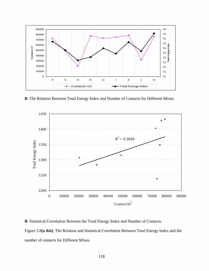
118
0
10000
20000
30000
40000
50000
60000
70000
80000
90000
A C D E G I K L O
Con
tact
s/ m
2
71
71
72
72
73
73
74
74
75
75
76
Tota
l Ene
rgy
Inde
x
Contacts/ m2 Total Energy Index
B. The Relation Between Total Energy Index and Number of Contacts for Different Mixes.
R2 = 0.2694
1200
1250
1300
1350
1400
1450
0 10000 20000 30000 40000 50000 60000 70000 80000 90000
Contact/m2
Tota
l Ene
rgy
Inde
x….
B. Statistical Correlation Between the Total Energy Index and Number of Contacts.
Figure 5.8(a &b): The Relation and Statistical Correlation Between Total Energy Index and the
number of contacts for Different Mixes.

119
-5
0
5
10
15
20
25
30
35
A C G I L
Vec
tor m
agni
tude
Opt. Opt. Plus differences
Figure 5.9: The Effect of Binder Content on Vector Magnitude.
0
5
10
15
20
25
30
35
C K D L
Vec
tor m
agni
tude
N@ max shear N@160 gyrations differnces
Figure 5.10: The Influence of Aggregate Type and Percent Natural Sand on Aggregate Orientation.

120
the effect of the natural sand is clear on the vector magnitude. An increase in the natural sand
causes a decrease in the vector magnitude at 160 gyrations and an increase in the difference in
the vector magnitude between the point at which the maximum shear stress is achieved and the
end of compaction (C vs. D and K vs. L).
As shown in Figure 5.11 the number of contacts for mixes C and K was higher than for mixes D
and L, respectively. The loss in number of contacts was higher for mixes D and L compared with
mixes C and K, respectively as presented in Table 5.2. This loss was caused by the weak
aggregate structure which caused aggregate reorientation and sliding.
0
10000
20000
30000
40000
50000
60000
70000
C D K L
Con
tact
/m2
N@max shear N@160 gyrations Differences
Figure 5.11: The Influence of Aggregate Type and Percent Natural Sand on Aggregate Contact.

121
Table 5.2 The Values of the Contact Density at Different Compaction Gyrations.
N@max shear N@160 gyrations DifferencesC 44981.33 41363.91 3617.42D 32070.17 14417.68 17652.49K 63570.29 60282.78 3287.51L 37518.59 31723.02 5795.57
Contact/m2
5.5 SUMMARY
The internal structure was analyzed in terms of the vector magnitude (aggregate orientation) and
aggregate contacts. In general, both the vector magnitude and number of contacts were found to
increase with an increase in the contact energy index. In addition, the total energy index had no
correlation with the internal structure parameters. The binder content, aggregate type and percent
of natural sand were also found to influence the aggregate orientation. Limestone mixes and
those without natural sand had higher vector magnitude and number of contacts. They also
resisted the change in orientation and contacts beyond the point of maximum shear stresses more
than the other mixes.

This is a blank Page

122
6. DEVELOPMENT AND EVALUATION OF ITD MIXES
6.1 DESCRIPTION OF SELECTED ITD MIXES
There are three mixes that have been identified by ITD research team from the three districts,
D1, D2 and D3. The three mixes were developed using the Hveem design method, which was
still adopted by ITD. The three mixes represented three different PG binder grades and three
different gradations. Mix D1 with PG 58-28, Mix D2 with PG 64-34, and Mix D3 with PG 76-
28. The mixes were evaluated to determine their acceptance in accordance to the Superpave mix
design criteria. It was found that, the asphalt mix from district 1 that was designed using Hveem
method (designated as D1-H), satisfies the Superpave criteria. Thus, the Superpave design of
district 1 mix (designated as D1-S) is the same as D1-H, with no changes needed. Mix D2-H was
slightly modified by changing the asphalt content. However, mix D3-H did not satisfy the
Superpave criteria. Both changes in binder content and gradation are needed. The work is still in
progress to optimize the D3 mix to satisfy the Superpave design criteria. Details of the mix
design of these mixes are presented in Appendix C.
6.2 ITD MIXES EVALUATION USING SUPERPAVE GYRATORY COMPACTOR
Two experiments have been conducted to evaluate the ability of the developed shear stress and
energy index to discern among different mixes. The experiment evaluated the influence of
changes in the mix constituents including asphalt binder content, aggregate source, and type of
gradation on the energy indices. Mixes were prepared and compacted using the Servopac
compactor at University of Idaho.
Based on the discussions in the previous chapters, a typical compaction curve from the gyratory
compaction is shown in Figure 6.1. The compaction curve is divided into two parts; the first one

123
has a steep change in percent air voids with an increase in number of gyrations. In part A, most
of the applied energy is used in inducing volumetric permanent deformation (reduction in
percent air voids), where the aggregates do not experience significant amount of shearing force.
In part B, however, most of the energy applied by the induced angle does not cause significant
volumetric change (small change in percent air voids). The energy is consumed in overcoming
the shear resistance among the mix particles. Therefore, the energy calculations for assessing the
mix stability under shear loading should focus on the second part of the compaction curve. The
applied energy in "Part B" is either used in developing more contacts among the aggregates and
cause reduction in percent air voids, or is dissipated by aggregate sliding as the aggregate
structure fails to develop more contacts.
The details of calculation of the Contact energy index (CEI) and the Total energy index (TEI)
are presented in Appendix D.
0
5
10
15
20
25
0 50 100 150 200Number of Gyrations
% A
ir Vo
ids
Part A Part B
Figure 6.1 Schematic Diagram Shows the Two Zones of the Compaction Curve

124
Prior to the analysis of the compaction energy, the repeatability of the compaction procedure
should be evaluated in order to determine the number of specimens needed to represent each
mix. Two specimens from each of the D1, D2, and D3 mixes were compacted using the same
vertical pressure (600 kPa), angle (1.25°), and the rate of gyration (30 gyrations/minute). The
compaction result shows that the maximum difference in percent air voids was about 0.4%,
which is within the experimental error that is usually experienced in the laboratory.
Consequently, it was decided to use only one specimen to represent each mix at a given set of
variables.
6.2.1 Effect of percent of binder content on Total and Contact Energy Indices
Three different binder contents were used in each group from mix D1, D2 and D3 to investigate
the effect of the binder content on the energy index. The first one was the optimum value
determined from the Superpave mix design procedure. The second one was 1% higher than the
optimum value, which is referred to herein as optimum plus. The third one was 1% lower than
the optimum value, which is referred to herein as optimum minus. It was noticed that both the
optimum plus and the optimum minus mixes reached a peak value at which it started to decrease
with further compaction. However, most of the mixes with optimum asphalt content reached a
maximum shear stress and stabilized at that value with further compaction. A comparison among
the shear indices is presented in Figure 6.2a - 6.2b and Table 6.1. It is clear that the total energy
index did not show a certain pattern in comparing the optimum, optimum plus, and optimum
minus mixes. However, the contact energy index was always higher for mixes with optimum
asphalt content. This indicates that the applied energy was used to develop contacts in the
optimum mixes, while it was dissipated in aggregate sliding in the optimum plus and optimum
minus mixes.

125
0
200
400
600
800
1000
1200
D1S1 D1H14 D1H15 D2S2 D2H11 D2S15 D3S2 D3H5 D3S6
Tota
l Ene
rgy
Inde
x
Series1 Opt.- Opt.+ Opt.
Figure 6.2a Comparisons among Mixes with Different Asphalt Content in Terms of the Total Energy Index
0
5
10
15
20
25
D1S1 D1H14 D1H15 D2S2 D2H11 D2S15 D3S2 D3H5 D3S6
Con
tact
Ene
rgy
Inde
x
Series1 Opt.- Opt.+ Opt.
Figure 6.2b Comparisons among Mixes with Different Asphalt Content in Terms of the Contact Energy Index

126
Table 6.1 Energy Indices of Mixes with different asphalt content Mix Pb content Total E.I Contact E.I
D1S1 Opt. 901 22.053
D1H14 Opt.+ 931.882 18.586
D1H15 Opt.- 810.527 18.441
D2S2 Opt. 989.84 22.783
D2H11 Opt.+ 916.017 19.322
D2H15 Opt.- 907.030 19.677
D3S2 Opt. 824.894 22.788
D3H5 Opt.+ 835.289 19.463
D3S6 Opt.- 840.14 18.872
6.2.2 Effect of Aggregate Type
Three types of aggregates were used in this evaluation: D1, D2, and D3. A comparison among
the energy indices of the three mixes is shown in Figures 6.3a - 6.3b and Table 6.2. It is evident
that contact energy indices were highest for the D1 mix than for the D3 and D2 mixes. This
indicates that the energy was used to developing more aggregate contacts was highest for the D1
mixes, and was lowest for the D2 mixes. It is known that D1 aggregate has more texture and
angularity than D3 and D2, which shows the highest stability as indicated by the energy indices.
Table 6.2 Energy Indices of Mixes with different aggregate type
Mix Total E.I Contact E.I Mix Total E.I Contact E.I
D1S1 901 22.053 D2H2 924.27 17.815
D1H2 970.54 21.839 D3S2 824.894 22.788
D2S2 989.84 22.783 D3H5 834.918 12.41

127
700750800850900950
10001050
D1S1 D1H2 D2S2 D2H2 D3S2 D3H5
Tota
l Ene
rgy
Inde
x
D1S1 D1H2 D2S2 D2H2 D3S2 D3H5
Figure 6.3a Comparisons among Mixes with Different Aggregate
Type in Terms of the Total Energy Index
0
5
10
15
20
25
D1S1 D1H2 D2S2 D2H2 D3S2 D3H5
Con
tact
Ene
rgy
Inde
x
D1S1 D1H2 D2S2 D2H2 D3S2 D3H5
Figure 6.3b Comparisons among Mixes with Different Aggregate
Type in Terms of the Contact Energy Index
6.2.3 Effect of Aggregate Gradation
Two different gradations were used in this study from each group mix D1, D2 and D3. below the
restricted zone (BRZ) and above the restricted zone (ARZ). The BRZ gradation is usually
referred to as coarse gradation, while the ARZ gradation is referred to as fine aggregate. The
energy indices result shown in Figure 6.4a - 6.4b and Table 6.3 are indicated that there are no

128
trend between the mix stability and location of the gradation shape, which is below or above the
restricted zone.
0
200
400
600
800
1000
1200
D1S1 D1S6 D2S2 D2S10 D3S2 D3H5
Tota
l Ene
rgy
Inde
x
Series1 ARZ BRZ
Figure 6.4a Comparisons among Mixes with Different Aggregate
Gradation Shape in Terms of the Total Energy Index
0
5
10
15
20
25
D1S1 D1S6 D2S2 D2S10 D3S2 D3H5
Con
tact
Ene
rgy
Inde
x
Series1 ARZ BRZ
Figure 6.4b Comparisons among Mixes with Different Aggregate
Gradation Shape in Terms of the Contact Energy Index Table 6.3 Energy Indices of Mixes with different aggregate gradations
Mix Total E.I Contact E.I Mix Total E.I Contact E.I
D1S1 901 22.053 D2S10 913.743 20.038
D1S6 918.387 20.875 D3S2 824.894 22.788
D2S2 989.84 22.783 D3H5 834.918 12.41

129
6.2.4 Summary of Effect of Mix Constituents on Energy Indices
Results of ITD Mixes revealed that the Total Energy Index did not correlate well with various
mix design parameters. On the hand, the Contact Energy Index (CEI) was found to capture the
influence of binder content, aggregate type on mix stability. However, there are no clear
correlation found between CEI and aggregate the gradation.
6.3 ITD MIXES EVALUATION USING ASPAHLT PAVEMENT ANALYZER (APA)
Two compacted specimens from each of D1, D2, and D3 mix groups were sent to ITD for
evaluation permanent deformation (rutting) used Asphalt Pavement Analyzer, APA rut test. The
specimens were prepared at air voids of 7% percent and height of 150mm. The details of the
APA rut test are shown in Appendix E. The relationship between the rut depth and the energy
indices are shown in Figure 6.5a, 6.5b and Table 6.4. In general, the result shows that there is a
trend between the mix stability as represented by the Contact Energy Index (CEI) and the rut
depth measured at the APA test. In general, CEI index increased with a decrease in rut depth.
Thus, mixes with high CEI values tend to resist rutting more than those with low CEI values.

130
0
2
4
6
8
10
12
14
16
18
D1S4 D1H12 D2S6 D2H13 D3H8 D3H9
CEI
, kN
.m
0
0.5
1
1.5
2
2.5
3
Rut
Dep
th, m
m
Contact E.I
Rut Depth
Figure 6.5 Variation of Rut Depth with CEI for ITD Mixes
Table 6.4 Comparisons between the Rut Depth and Contact Energy Index
Mix Rut
Depth
Total E.I Contact E.I Mix Rut
Depth
Total E.I Contact
E.I
D1S4 2.744 130.575 10.279 D2H13 1.898 254.430 13.412
D1H12 1.965 137.434 10.061 D3H8 2.324 147.44 10.755
D2S6 1.756 234.528 16.432 D3H9 2.208 128.612 9.215
6.4 ITD MIXES EVALUATION USING IMAGE ANALYSIS
The objective of using imaging analysis is to capture the influence of the aggregate orientation
and contacts on the mix stability and shear strength. The mixes used in this study are selected
from total mixes from three different districts developed using Hveem and Superpave mix design
method. Total mixes used in image analysis is 30. Twenty two specimens from each mix group
were compacted to 160 gyration using an angle 1.25 and pressure of 600 kPa. The vector

131
magnitude and number of contacts were measured on these specimens and recorded in Table 6.5.
These values are compared with the contact energy index CEI and total energy index TEI as
shown in Figure 6.6 and 6.7 Results show that there is a good correlation between number of
contacts and the contact energy index (CEI).
These results are consistent with those obtained from the NCHRP 9-16 mixes.
They are also consistent with APA results presented earlier.
Table 6.5 Values of the Quantifying Parameters of
Aggregate Structure and Energy Indices.
Mix
Vector
Magnitude
Contacts/m2 TEI CEI
D1H4 27.90 72568.05 946.99 21.31
D1S1 28.53 72685.12 901 22.05
D2H2 27.94 48673.54 937.61 17.82
D2S2 23.59 72935.81 920.56 22.87
D3H4 22.84 38974.33 837.87 10.05
D3S2 22.33 78736.06 824.89 22.79
In summary, the internal structure was analyzed in terms of the vector magnitude (aggregate
orientation) and aggregate contacts. In general, both the vector magnitude and number of
contacts were found to increase with an increase in the contact energy index. The total energy
index did not show to correlate well with the internal structure parameters as measured by the
number of contacts or vector magnitude.

132
800
850
900
950
1000
D1H4 D1S1 D2H2 D2S2 D3H4 D3S2
Tota
l Ene
rgy
Inde
x, T
EI
20
25
30
Vect
or M
agni
tude
TEI
Vector Magnitude
Figure 6.6a Variation of the Vector Magnitude with TEI
5
10
15
20
25
D1H4 D1S1 D2H2 D2S2 D3H4 D3S2
Con
tact
Ene
rgy
Inde
x, C
EI
20
25
30
Vect
or M
agni
tude
CEIVector Magnitude
Figure 6.6b Variation of the Vector Magnitude with CEI

133
800
850
900
950
1000
D1H4 D1S1 D2H2 D2S2 D3H4 D3S2
Tota
l Ene
rgy
Inde
x, T
EI
30000
40000
50000
60000
70000
80000
Con
tact
s / m
2
TEI
Contacts/m2
Figure 6.7a Variation of the Number of Contacts with TEI
10D1H4 D1S1 D2H2 D2S2 D3H4 D3S2
Con
tat E
nerg
y In
dex,
CE
I
30000
40000
50000
60000
70000
80000
Con
tact
s / m
2
CEI
Contacts/m2
Figure 6.7b Variation of the Number of Contacts with CEI

134
7. SUMMARY, CONCLUSIONS AND RECOMMENDATIONS
7.1 SUMMARY AND CONCLUSIONS
The new Superpave™ asphalt mix design system developed by the Strategic Highway Research
Program (SHRP), considers the mix volumetrics in the design of hot-mix asphalt (HMA). The
absence of a performance test in the Superpave volumetric mix design procedure led many
agencies to delay its implementation. Therefore, there is a need to develop methods for the
assessment of HMA performance. This report presents a new method to evaluate the mix shear
strength during the design stage. The shear strength is considered a measure of the mix
resistance to permanent deformation. The new method relies on the analysis of the mix response
to the shear and normal forces applied on the mix during compaction in the Superpave Gyratory
Compactor (SGC).
The report presents detailed analysis of the HMA compaction in the Servopac gyratory
compactor. The compaction forces are analyzed and a mathematical expression of the shear
stress inside the mix is derived. The shear stress value is used to calculate the compaction
energy, which is divided into two regions according to the type of dominating strain. The
volumetric strain dominates the first region, while the shear strain dominates the second region.
Analytical procedure is developed to identify these two regions. An index termed as the “contact
energy index, CEI” that reflects the compaction energy in the second region has been developed.
The CEI showed to be an objective indicator of the mix stability as represented by its shear
strength. In this study, the contact energy index was used to analyze mixes with different
constituents such as percent of binder, percent of natural sand, type of aggregate, gradation, and
nominal maximum aggregate size. The effect of the gyratory compaction variables such as the

135
angle of gyration, and vertical pressure on the contact energy index have also been investigated
in order to determine the variables that would best discern among mixes with different
constituents.
Based on the results of this research study, the contact energy index was lower for mixes
with higher asphalt content over its optimum. Results also showed lower CEI values for mixes
with high content of natural sand as compared to mixes without natural sand. Mixes made with
gravel materials showed lower CEI values as compared to those with crushed limestone
aggregates.
The Superpave shear test was used to measure G*, G*/sinδ and maximum shear strain of
three mixes at two different temperatures. In general, the contact energy index has good
correlation with these mechanical properties. The results show that the contact energy index
increases with an increase in G* and G*/sinδ, and a decrease in maximum shear strain. This
shows the potential of the CEI in reflecting the mix stability and shear strength.
These results coincide with the intuitive expected performance of these mixes, which
confirm that the CEI can be used as objective indicator of mix stability.
In order to make sure that the CEI trends were independent of mix compaction parameters (e.g.
angle of gyration and compaction pressure), several comparison were made at varied angle of
gyrations and varied compaction pressures. The results conformed same trends. This concludes
that the CEI can still work as a stability indicator to discern mixes for any given compaction
specifications.
Two and three dimensional finite element models are developed to simulate the compaction in
the Servopac gyratory compactor. The two dimensional model is able to predict the measured
shear stresses at small number of gyrations, and fails to predict shear stresses at number of

136
gyrations more than 19. However, the results from the three dimensional model compares very
well with the shear stress and contact energy index calculated from experimental data. The three
dimensional model includes the friction between the mix and the mold, and simulates most of the
details of the loading mechanisms used in the Servopac gyratory compactor. The three
dimensional model along with vertical deformation during compaction can be used to calculate
the contact energy index and predict mix stability.
Analysis of the internal structure using imaging techniques is utilized in order to demonstrate the
influence of the aggregate orientation and contacts on the mix stability and shear strength. In
general, both the vector magnitude and number of contacts are found to increase with an increase
in the contact energy index. In addition, the total energy index has no correlation with the
internal structure parameters. The aggregate type and percent of natural sand are also found to
influence the aggregate orientation. Limestone mixes and those without natural sand have higher
vector magnitude and resist the change in orientation beyond the point of maximum shear
stresses more than the other mixes.
7.2 RECOMMENDATIONS
Most of the available gyratory compactors are not equipped with a mechanism to measure the
reaction forces such as P1, P2, and P3 as done in the Servopac gyratory compactor. Therefore, it
is recommended to develop an experimental setup to measure the reaction forces in order for the
analysis methods developed in this study to be used in the evaluation of mixes compacted using
gyratory compactors different than Servopac.
This report shows the potential of the contact energy index in differentiating mixes with different
constituents. In addition, it shows that the contact energy index correlates with some of the mix
mechanical properties. Consequently, the second recommendation is to use the developed

137
analysis methods to evaluate the stability of mixes with known resistance to rutting in the field.
This would allow developing specifications for mix stability based on the results of the value of
the contact energy index.
The third recommendation is related to the 3-D finite element model. Currently, the material
properties are selected such that the vertical deformation in the model is similar to experimental
measurements at different compaction levels. It is recommended to use a constitutive model to
represent the change in the HMA properties during compaction.

138
REFERENCES
1. AASHTO (1996). “Standard Specifications for Transportation Materials and Methods of
Sampling and Testing.” AASHTO Provisional Standards, MP2-95. Specifications for
Superpave Volumetric Mix Design.
2. AASHTO. (2001). “Specifications for Superpave Volumetric Mix Design.” Standard
Specifications for Transportation Materials and Methods of Sampling and Testing, AASHTO
Provisional Standards, Washington, D. C.
3. Abou-Chakra, H., Tuzun, U., (1999). “Coefficient of friction of binary granular mixtures in
contact with a smooth wall. Part I: Direct shear box measurements of the effects of particle
size ratio and particle surface roughness” Chemical Engineering Science, Vol. 54, Issue 24.
pp. 5901-5912
4. ADINA, “Theory and Modeling Guide” Report ARD 00-7, August 2000, Volume I.
5. ADINA version 7.4 (2000). “ADINA R & D, Inc” Watertown, MA
6. Anderson, R, M, Huber, G, A, Walker D, E, and Zhang X. (2000). “Mixture Testing,
Analysis and Field Performance of the Pilot Superpave Projects: The 1992 SPS-9 Mixtures”
Journal of the Association of Asphalt Paving Technologists. Vol. 69.
7. Australian Standards (1995) - AS/NZS 2891.2.2 “Methods of Sampling and Testing Asphalt.
Method 2.2 Sample Preparation” - Compaction of Asphalt Test Specimens Using a Gyratory
Compactor.
8. Bahia, H, Friemel, T, Peterson, P, and Russell, J. (1998). “Optimization of Constructability
and Resistance to Traffic: A New Design Approach for HMA Using the Superpave
Compactor.” Journal of the Association of Asphalt Paving Technologists V.67-98, p.189.

139
9. Butcher, M, (1998) “Determining Gyratory Compaction Characteristics Using Servopac
Gyratory Compactor” Transportation Research Record, 1630
10. Chowdry, A., Gray, J., Button, J., and Little, D. (2001). “Effect of Aggregate Gradation on
Permanent Deformation of Superpave HMA.” A Paper Presented at the 80th Annual Meeting
of the Transportation Research Board, Washington DC.
11. Cominsky, R, Harrigan, E, Leahy, R., (1994) “Level One Mix Design: Materials Selection,
Compaction, and Conditioning” SHRP-A-408, 121.
12. Consugera, A., Little, D. N., Quintus, H.V., and Burati, J. (1989). “Comparative evaluation
of laboratory compaction devices based on their ability to produce mixtures with engineering
properties similar to those produced in the field.” TRR 1228, Transportation Research Board,
National Research Council, Washington D.C., 80-87
13. Crawley, A. B. (1993) “Gyratory Testing Machine Usage in Monitoring HMA Quality”
United State Federal Highway Administration, Pupl. By ASCE, New York, USA, p 270-276
14. DeSombre, R, Chadbourn, B, Newcomb, DE, Voller, V, (1998) “Parameters to Define The
Laboratory Compaction Temperature Range of Hot-Mix Asphalt” Journal of the Association
of Asphalt Paving Technologists 67.
15. Eriksen, K. and V. Wegan. (1993). “Optical Methods for evaluation of Asphalt Concrete and
Polymer-Modified Bituminous Binders.” Danish Road Institute, Note 244.
16. Gauer, M. (1996). “Compaction of Asphalt in the Darmstadt Gyratory Compactor.”
International Workshop on the Use of the Gyratory Shear Compactor, LCPC, Nantes, France.
17. Guler, M., Bahia, H. U., Bosscher, P. J., Plesha, M. E. (2000). “Device for Measuring Shear
Resistance of Hot-Mix Asphalt in the Gyratory Compactor.” Transportation Research
Record, Journal of the Transportation Research Board 1723, pp. 116-124.

140
18. Hand, A., and Epps, A. (2001). “Impact of Gradation Relative to the Superpave Restricted
Zone on HMA Performance.” A Paper Presented at the 80th Annual Meeting of the
Transportation Research Board, Washington DC.
19. Huber G A, (1996) “Development of the Superpave Gyratory Compactor” The Superpave
Asphalt Research Program, The University of Texas at Austin, web site
(http://www.utexas.edu/research/superpave/articles/gyr_hist.html)
20. Image- Pro Plus Version 4.1. (1998). Media Cybernetics, L.P, Georgia, MD
21. IPC PTY LTD (1996) - Servopac (Servo-Controlled Gyratory Compactor) Operating and
Maintenance Manual.
22. Kumar, A, Goetz W, (1974) “The Gyratory Testing Machine as a Design Tool and
Instrument for Bituminous Mixture Evaluation” Asphalt Paving Technology, 43, 351-371.
23. Mallick, RB. (1999). “Use Of Superpave Gyratory Compactor To Characterize Hot-Mix
Asphalt.” Transportation Research Record - Journal of the Transportation Research Board
1681
24. Masad, E, Harman, T, Muhunthan, B, Shashidhar, N, (1998) “Aggregate Orientation and
Segregation in Asphalt Concrete, Application of Geotechnical Principles In Pavement
Engineering” Proceedings of Sessions of Geo-Congress 98, 69-80.
25. Masad, E., Muhunthan, B., Shashidhar, N., and Harman T. (1998). “Quantifying Labora-tory
Compaction Effects on the Internal Structure of Asphalt Concrete.” Paper submitted for
Publication in Transportation Research Board.
26. Masad, E, Muhunthan, B, Shashidhar, N, Harman, T, (1999a). “Internal Structure
Characterization of Asphalt Concrete Using Image Analysis.” Journal of Computing in Civil
Engineering, 13(2), 88-95.

141
27. Masad, E, Muhunthan, B, Shashidhar, N, Harman, T, (1999b). “Effect of Compaction
Procedure on the Aggregate Structure in Asphalt Concrete.” Transportation Research Board,
No. 1681, 179-185
28. Masad, E. A., Tashman, L.S., Niranjanan, S., Little, D. (2001). “Micromechanics Based
Analysis of Stiffness Anisotropy in Asphalt Mixes” Paper Number 01-2052 Submitted for
publication in Transportation Research Board, 80th annual Meeting, January 9-13, 2001,
Washington, D.C.
29. McRea J. L., (1962). “Gyratory Compaction Method for Determining Density Requirements
For Subgrade and Base of Flexible Pavements.” Miscellaneous paper No. 4-494, U.S. Army
Engineering Waterways Experiment Station, Corps of Engineering, Vicksburg, MS, 2.
30. McRea, J. L., (1965). “Gyratory Testing Machine Technical Manual” Engineering
Developments Company, Inc. Vicksburg, MS, 2.
31. Monismith, C. L. (1992). “Analytically based asphalt pavement design and rehabilita-tion.”
Transportation Research Record 1354, TRB, National Research Council, Washington, D. C.,
5 – 26.
32. Moutier, F. (1996). "G.S.P. Result Modeling - Comments on the Compaction Ultimate
Threshold, Eurasphalt & Eurobitume Congress. Strasbourg.
33. Moutier, F. (1997). “Gyratory Compactor (GC or PCG) Justification of its Use in the French
Mix Design.” Paper presented in the Superpave Asphalt Mixture Expert Task Group.
34. Moutier, F, Bonnot, J, Corte, JF, (1997) “Comparison of The Use of The Gyratory
Compactor in The French Mix Design Method and in Superpave Level 1” Proceedings of the
Conference: Road Safety in Europe and Strategic Highway Research Program (SHRP).
35. Murfee, J; Manzione, CW., (1992).”Construction Of Rut-Resistant Asphalt Mixtures“
Transportation Research Record 1337

142
36. Oda, M, (1972a) “Initial Fabric and Their Relations to Mechanical Properties of Granular
Material.” Soils and foundations, 12(1), 17-36.
37. Oda, M, (1972b) “The Mechanism of Fabric Changes During Compressional Deformation
of Sands” Soils and foundations, 12(2), 1-8.
38. Oda, M, (1977) “Co-Ordination Number and its Relation to Shear Strength of Granular
Material” Soils and Foundations, 17(2), 29-42
39. Pixera. (1997). “Pixera visual Communication Suite for Windows 95” Pixera Corporation,
California
40. Rand, D. A. (1997). "Comparative Analysis of Superpave Gyratory Compactors and TxDOT
Gyratory Compactors." Master Thesis, University of Texas, Austin, TX.
41. Robert Cook, David Malkus, Michael Plesha (1989) “Concepts and Applications of Finite
Element Analysis” Third Edition
Roberts, F L, Kandhal, P S, Brown, E R. Lee D, Kennedy, T W, (1996) “Hot Mix Asphalt
Materials Mixture Design and Construction” NAPA Education Foundation Lanham, Maryland,
Second Edition.
42. Romero, P. and Mogawer, W. (1998a). "Evaluation of the Superpave Shear Tester using 19-
mm Mixtures from the Federal Highway Administration’s Accelerated Loading Facility."
Journal of the Association of Asphalt Paving Technologist, 67, 573-601.
43. Romero, P. and Mogawer, W. (1998b). “Evaluation of the Superpave Shear Tester’s Ability
to Discern Two Mixtures with Different Size Aggregates Using the FHWA’s Accelerated
Loading Facility.” In Transportation Research Record 1630, TRB, National Research
Council, Washington D.C., 69-76.
44. Russ, J., C. (1999). “The image Processing Handbook” third edition, CRC, Boca Raton, Fla.

143
45. Ruth, B. E., Shen, X. and Wang, L. H. (1991). “Gyratory Evaluation of Aggregate Blends to
Determine Their Effects on Shear Resistance and Sensitivity to Asphalt Content.” STP 1147,
American Society for Testing Materials.
46. Ruth, B. E., and Schaub J.H. (1996). “Gyratory Testing Machine Simulation of Field
Compaction of Asphalt Concrete.” Proceedings, Association of Asphalt Paving
Technologists, 35.
47. Ruth, B.E, (1996) “Evaluation of Pavement Materials for Design, Compaction, and Quality
Control by Gyratory Testing Methods” International Workshop on the Use of the Gyratory
Shear Compactor, LCPC, Nantes, France.
48. Servopac Monitor version 1.24 (2000). Australia
49. SHRP (1994), “Level One Mix Design: Material Selection, Compaction, and Conditioning”
SHRP-A-408, Strategic Highway Research Program, National Research Council, DC.
50. Sigurjonsson, S, Ruth, BE (1990). “Use Of Gyratory Testing Machine To Evaluate Shear
Resistance Of Asphalt Paving Mixture” Transportation Research Record 1259
51. Standard Test Method for Theoretical Maximum Specific Gravity and Density of Bituminous
Paving Mixtures, (1999). Annual Book of ASTM Standards, Designation: D2041-95, Vol.
04.03, American Society for Testing and Material
52. Sousa, J. B., Harvey, J., Painter, L., Deacon, J. A. and Monismith, C.L. (1991). “Evaluation
of Laboratory Procedures for Compacting Asphalt-Aggregate Mixtures” Report No. SHRP-
A-UWP=91-523, Strategic Highway Research Program, National Research Council,
Washington D.C.

144
53. Stuart, K, Davis, F, Parobeck, S, Sylor, T M, (1996) "Evaluation of the U.S. Corps of
Engineers Gyratory Testing Machine Model 8A-6B-4C" U.S. Department of Transporta-
tion, Federal Highway Administration, FHWA-RD-95-205.
54. Tashman L., Masad E., Peterson B., and Saleh H. (2001). “Internal Structure Analysis of
Asphalt Mixes to Improve The Simulation of Superpave Gyratory Compaction to Field
Conditions” Journal of the Association of Asphalt Paving Technologist.
55. Tobita, Y. (1998) “Fabric Tensors in Constitutive Equations for Granular Materials.” Soils
and Foundations, Vol. 29(4), pp. 99-104
56. Yue, Z. Q., Bekking, and I. Morin. (1995). “Application of Digital Image Processing to
quantitative study of Asphalt Concrete Microstructure.” Transp. Res. Rec. 1492,
Transportation Research Board, National Research Council, Washington D.C., 53-60

This is a blank Page

145
List of Appendices
Appendix A: MIX PROPERTIES AND GRADATIONS – Mixes
Obtained from the NCHRP 9-16 Project
Appendix B: Worksheet for Calculating Shear Stress and Contact Energy Index, CEI.
Appendix C: Job Mix Formula for ITD Mixes (D1, D2 and D3)
Appendix D: Data for ITD Mixes Gradation, Volumetric Analysis and Calculation of Energy Indices (CEI and TEI)
Appendix E: APA Test Results for ITD Mixes
Appendix F: Image Analysis Test Results for ITD Mixes
Appendix G: e-Files Included on CD-ROM

This is a blank Page

APPENDIX A
MIX PROPERTIES AND GRADATIONS –
MIXES OBTAINED FROM THE NCHRP 9-16 PROJECT

Mix A Mix B9.5mm Limestone Coarse, 0% Sand 9.5mm Limestone Coarse, 40% SandLimestone 8's 43% Limestone 8's 40%Limestone Sand 13% Washed LSS 10%Washed LSS 44% Limestone Sand 10%
Natural Sand 40%Sieve Mass, g Sieve Mass, g1 - 3/4 (25 - 19 mm) 0 1 - 3/4 (25 - 19 mm) 03/4 - 1/2 (19 - 12.5 mm) 0 3/4 - 1/2 (19 - 12.5 mm) 01/2 - 3/8 (12.5 - 9.5 mm) 441 1/2 - 3/8 (12.5 - 9.5 mm) 4103/8 - #4 (9.5 - 4.75 mm) 1652 3/8 - #4 (9.5 - 4.75 mm) 1431#4 - #8 (4.75 - 2.36 mm) 774 #4 - #8 (4.75 - 2.36 mm) 436#8 - #16 (2.36 - 1.18 mm) 612 #8 - #16 (2.36 - 1.18 mm) 410#16 - #30 (1.18 - 0.6 mm) 437 #16 - #30 (1.18 - 0.6 mm) 594#30 - #50 (0.6 - 0.3 mm) 266 #30 - #50 (0.6 - 0.3 mm) 886#50 - #100 (0.3 - 0.15 mm) 122 #50 - #100 (0.3 - 0.15 mm) 189#100 - #200 (0.15 - 0.075 mm) 50 #100 - #200 (0.15 - 0.075 mm) 31 - #200 ( - 0.075 mm) 149 - #200 ( - 0.075 mm) 113TOTAL 4500 TOTAL 4500PG 64-22 5.30% PG 76-22 6.50%
Mix C Mix D19mm Limestone Coarse, 0% Sand 19mm Limestone Coarse, 40% SandLimestone 57's 42% Limestone 57's 48%Limestone 8's 26% Limestone 8's 12%Limestone Sand 20% Natural Sand 40%Washed LSS 12% Sieve Mass, g Sieve Mass, g1 - 3/4 (25 - 19 mm) 360 1 - 3/4 (25 - 19 mm) 4103/4 - 1/2 (19 - 12.5 mm) 756 3/4 - 1/2 (19 - 12.5 mm) 8641/2 - 3/8 (12.5 - 9.5 mm) 626 1/2 - 3/8 (12.5 - 9.5 mm) 5363/8 - #4 (9.5 - 4.75 mm) 1305 3/8 - #4 (9.5 - 4.75 mm) 824#4 - #8 (4.75 - 2.36 mm) 410 #4 - #8 (4.75 - 2.36 mm) 194#8 - #16 (2.36 - 1.18 mm) 351 #8 - #16 (2.36 - 1.18 mm) 221#16 - #30 (1.18 - 0.6 mm) 243 #16 - #30 (1.18 - 0.6 mm) 441#30 - #50 (0.6 - 0.3 mm) 162 #30 - #50 (0.6 - 0.3 mm) 792#50 - #100 (0.3 - 0.15 mm) 81 #50 - #100 (0.3 - 0.15 mm) 140#100 - #200 (0.15 - 0.075 mm) 36 #100 - #200 (0.15 - 0.075 mm) 9 - #200 ( - 0.075 mm) 171 - #200 ( - 0.075 mm) 72TOTAL 4500 TOTAL 4500PG 76-22 5.20% PG 64-22 4.70%
A - 1
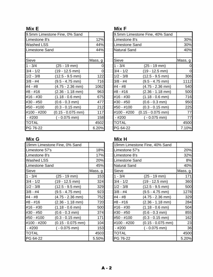
Mix E Mix F9.5mm Limestone Fine, 0% Sand 9.5mm Limestone Fine, 40% SandLimestone 8's 12% Limestone 8's 30%Washed LSS 44% Limestone Sand 30%Limestone Sand 44% Natural Sand 40%
Sieve Mass, g Sieve Mass, g1 - 3/4 (25 - 19 mm) 0 1 - 3/4 (25 - 19 mm) 03/4 - 1/2 (19 - 12.5 mm) 0 3/4 - 1/2 (19 - 12.5 mm) 01/2 - 3/8 (12.5 - 9.5 mm) 122 1/2 - 3/8 (12.5 - 9.5 mm) 3063/8 - #4 (9.5 - 4.75 mm) 716 3/8 - #4 (9.5 - 4.75 mm) 1112#4 - #8 (4.75 - 2.36 mm) 1062 #4 - #8 (4.75 - 2.36 mm) 540#8 - #16 (2.36 - 1.18 mm) 963 #8 - #16 (2.36 - 1.18 mm) 500#16 - #30 (1.18 - 0.6 mm) 675 #16 - #30 (1.18 - 0.6 mm) 716#30 - #50 (0.6 - 0.3 mm) 477 #30 - #50 (0.6 - 0.3 mm) 950#50 - #100 (0.3 - 0.15 mm) 212 #50 - #100 (0.3 - 0.15 mm) 225#100 - #200 (0.15 - 0.075 mm) 117 #100 - #200 (0.15 - 0.075 mm) 77 - #200 ( - 0.075 mm) 158 - #200 ( - 0.075 mm) 77TOTAL 4502 TOTAL 4500PG 76-22 6.20% PG 64-22 7.10%
Mix G Mix H19mm Limestone Fine, 0% Sand 19mm Limestone Fine, 40% SandLimestone 57's 18% Limestone 57's 20%Limestone 8's 17% Limestone 8's 32%Washed LSS 20% Limestone Sand 8%Limestone Sand 45% Natural Sand 40%Sieve Mass, g Sieve Mass, g1 - 3/4 (25 - 19 mm) 153 1 - 3/4 (25 - 19 mm) 1713/4 - 1/2 (19 - 12.5 mm) 324 3/4 - 1/2 (19 - 12.5 mm) 3601/2 - 3/8 (12.5 - 9.5 mm) 329 1/2 - 3/8 (12.5 - 9.5 mm) 5003/8 - #4 (9.5 - 4.75 mm) 923 3/8 - #4 (9.5 - 4.75 mm) 1278#4 - #8 (4.75 - 2.36 mm) 752 #4 - #8 (4.75 - 2.36 mm) 329#8 - #16 (2.36 - 1.18 mm) 720 #8 - #16 (2.36 - 1.18 mm) 284#16 - #30 (1.18 - 0.6 mm) 500 #16 - #30 (1.18 - 0.6 mm) 504#30 - #50 (0.6 - 0.3 mm) 374 #30 - #50 (0.6 - 0.3 mm) 855#50 - #100 (0.3 - 0.15 mm) 171 #50 - #100 (0.3 - 0.15 mm) 162#100 - #200 (0.15 - 0.075 mm) 104 #100 - #200 (0.15 - 0.075 mm) 23 - #200 ( - 0.075 mm) 153 - #200 ( - 0.075 mm) 36TOTAL 4503 TOTAL 4500PG 64-22 5.50% PG 76-22 5.20%
A - 2

Mix I Mix J9.5mm Gravel Coarse, 0% Sand 9.5mm Gravel Coarse, 40% Sand Gravel 8's 50%Gravel 8's 50% Limestone Sand 10%Washed LSS 25% Natural Sand 40%Limestone Sand 25% Sieve Mass, g Sieve Mass, g1 - 3/4 (25 - 19 mm) 0 1 - 3/4 (25 - 19 mm) 03/4 - 1/2 (19 - 12.5 mm) 0 3/4 - 1/2 (19 - 12.5 mm) 01/2 - 3/8 (12.5 - 9.5 mm) 297 1/2 - 3/8 (12.5 - 9.5 mm) 2973/8 - #4 (9.5 - 4.75 mm) 1787 3/8 - #4 (9.5 - 4.75 mm) 1670#4 - #8 (4.75 - 2.36 mm) 923 #4 - #8 (4.75 - 2.36 mm) 594#8 - #16 (2.36 - 1.18 mm) 567 #8 - #16 (2.36 - 1.18 mm) 342#16 - #30 (1.18 - 0.6 mm) 383 #16 - #30 (1.18 - 0.6 mm) 518#30 - #50 (0.6 - 0.3 mm) 248 #30 - #50 (0.6 - 0.3 mm) 842#50 - #100 (0.3 - 0.15 mm) 117 #50 - #100 (0.3 - 0.15 mm) 171#100 - #200 (0.15 - 0.075 mm) 77 #100 - #200 (0.15 - 0.075 mm) 23 - #200 ( - 0.075 mm) 104 - #200 ( - 0.075 mm) 45TOTAL 4503 TOTAL 4500PG 64-22 7.10% PG 76-22 5.90%
Mix K Mix L19mm Gravel Coarse, 0% Sand 19mm Gravel Coarse, 40% SandGravel 57's 30% Gravel 57's 35%Gravel 8's 25% Gravel 8's 25%Washed LSS 25% Limestone Sand 0%Limestone Sand 20% Natural Sand 40%Sieve Mass, g Sieve Mass, g1 - 3/4 (25 - 19 mm) 270 1 - 3/4 (25 - 19 mm) 3153/4 - 1/2 (19 - 12.5 mm) 500 3/4 - 1/2 (19 - 12.5 mm) 5811/2 - 3/8 (12.5 - 9.5 mm) 405 1/2 - 3/8 (12.5 - 9.5 mm) 4503/8 - #4 (9.5 - 4.75 mm) 1238 3/8 - #4 (9.5 - 4.75 mm) 1157#4 - #8 (4.75 - 2.36 mm) 752 #4 - #8 (4.75 - 2.36 mm) 374#8 - #16 (2.36 - 1.18 mm) 518 #8 - #16 (2.36 - 1.18 mm) 243#16 - #30 (1.18 - 0.6 mm) 347 #16 - #30 (1.18 - 0.6 mm) 441#30 - #50 (0.6 - 0.3 mm) 216 #30 - #50 (0.6 - 0.3 mm) 792#50 - #100 (0.3 - 0.15 mm) 131 #50 - #100 (0.3 - 0.15 mm) 95#100 - #200 (0.15 - 0.075 mm) 68 #100 - #200 (0.15 - 0.075 mm) 9 - #200 ( - 0.075 mm) 59 - #200 ( - 0.075 mm) 45TOTAL 4504 TOTAL 4500PG 76-22 5.40% PG 64-22 5.60%
A - 3

Mix M Mix N9.5mm Gravel Fine, 0% Sand 9.5mm Gravel Fine, 40% SandGravel 8's 5% Gravel 8's 16%Limestone Sand 65% Limestone Sand 44%Washed LSS 30% Natural Sand 40% Sieve Mass, g Sieve Mass, g1 - 3/4 (25 - 19 mm) 0 1 - 3/4 (25 - 19 mm) 03/4 - 1/2 (19 - 12.5 mm) 0 3/4 - 1/2 (19 - 12.5 mm) 01/2 - 3/8 (12.5 - 9.5 mm) 32 1/2 - 3/8 (12.5 - 9.5 mm) 943/8 - #4 (9.5 - 4.75 mm) 473 3/8 - #4 (9.5 - 4.75 mm) 675#4 - #8 (4.75 - 2.36 mm) 1152 #4 - #8 (4.75 - 2.36 mm) 716#8 - #16 (2.36 - 1.18 mm) 1017 #8 - #16 (2.36 - 1.18 mm) 635#16 - #30 (1.18 - 0.6 mm) 729 #16 - #30 (1.18 - 0.6 mm) 779#30 - #50 (0.6 - 0.3 mm) 504 #30 - #50 (0.6 - 0.3 mm) 1022#50 - #100 (0.3 - 0.15 mm) 266 #50 - #100 (0.3 - 0.15 mm) 270#100 - #200 (0.15 - 0.075 mm) 144 #100 - #200 (0.15 - 0.075 mm) 77 - #200 ( - 0.075 mm) 185 - #200 ( - 0.075 mm) 234TOTAL 4500 TOTAL 4500PG 76-22 7.50% PG 64-22 6.30%
Mix O Mix P19mm Gravel Fine, 0% Sand 19mm Gravel Fine, 40% SandGravel 57's 18% Gravel 57's 29%Gravel 8's 17% Gravel 8's 13%Limestone Sand 50% Limestone Sand 18%Washed LSS 15% Natural Sand 40%Sieve Mass, g Sieve Mass, g1 - 3/4 (25 - 19 mm) 162 1 - 3/4 (25 - 19 mm) 2613/4 - 1/2 (19 - 12.5 mm) 302 3/4 - 1/2 (19 - 12.5 mm) 4811/2 - 3/8 (12.5 - 9.5 mm) 252 1/2 - 3/8 (12.5 - 9.5 mm) 3293/8 - #4 (9.5 - 4.75 mm) 914 3/8 - #4 (9.5 - 4.75 mm) 765#4 - #8 (4.75 - 2.36 mm) 896 #4 - #8 (4.75 - 2.36 mm) 473#8 - #16 (2.36 - 1.18 mm) 662 #8 - #16 (2.36 - 1.18 mm) 374#16 - #30 (1.18 - 0.6 mm) 522 #16 - #30 (1.18 - 0.6 mm) 580#30 - #50 (0.6 - 0.3 mm) 351 #30 - #50 (0.6 - 0.3 mm) 886#50 - #100 (0.3 - 0.15 mm) 176 #50 - #100 (0.3 - 0.15 mm) 194#100 - #200 (0.15 - 0.075 mm) 131 #100 - #200 (0.15 - 0.075 mm) 36 - #200 ( - 0.075 mm) 135 - #200 ( - 0.075 mm) 121TOTAL 4500 TOTAL 4500PG 64-22 5.00% PG 76-22 6.20%
A - 4

This is a blank Page

APPENDIX B
WORKSHEET FOR CALCULATING SHEAR STRESS AND
CONTACT ENERGY INDEX, CEI

Recommended Procedure for Calculating the Shear Force and Contact Energy Index (CEI)
1. Prepare gyratory specimens and compact them up to 200 gyrations 2. Fit a polynomial function to the compaction curve (Air voids, %
versus Number of Gyrations, N) 3. Use the polynomial function to determine the number of gyration
(NG1) at which the change in the slope is equal to 0.001%. 4. Use the equation:
h*A
L*W*2S =
with S, A, and h values to calculate W (the actuator force value P1) at every gyration, where: S: is the shear stress, A and h: are the sectional area and the height respectively, W: is the applied forced to proceed the angle, and L: is the moment arm (165 mm)
5. Use the equation (3.11, Chapter 3) to determine the shear force, Sθ ( ) θθθ tanWP
21cos)NN(S d12 −∑+−=
where: N2-N1 is derived from equation (3.8), (the parameters in this equation can be found in the next table, ΣP: is calculated from equations (3.7), and (3.1), Wd : is the weight of the mold (For Servopac Gyratory at UI, 15960 gm) and θ: is the angle of gyration
6. Use equation (3.16) to calculate the contact energy index
∑ ⋅=2
1
index Energy ontact G
G
N
NedSC θ
where : Sθ is the shear force derived from step 5 de is the change in height at each consecutive gyrations NG1: is derived from step 3 NG2 : is the termination number of gyration ( i.e. 200)
B - 1

Measurements and Data required for Mix A at Pressure of 600 kPa and Angle of 1.5°
B - 2
mix ID Adiameter (D) 150 mmvertical stress (A) 600 kPaangle (θ) 1.5 degreemix weight (W m) 4.69 kgmax specific gravity (Gmm) 2506 kg/m3max No. of gyrations 160mold weight (W d) 15.96 kgmoment arm (L) 165 mmfriction factor (μ) 0.28xθ 12.5 mmNG1 14d1 (=d2) 142.89 mm

S θC
onta
ct
Tota
lN
Pre
s.he
ight
angl
esh
ear
P1
(N)
P2,
P3
(N)
% A
vsl
ope
Δ
B -
3
3460
111
4.56
1.5
437
2680
.85
2874
.36
7.54
5-9
.487
-0.0
5225
46.0
34-5
521.
795
141.
740.
409.
84
slo
peN
2-N
1N
1+N
2(k
Pa)
E.I.
E.I.
158
013
7.72
1.39
162
1194
.73
1402
.78
23.0
89-8
.618
0.92
021
08.3
96-2
974.
281
118.
137.
602
599
133.
021.
5427
819
80.2
522
10.1
720
.372
-9.5
390.
635
2229
.016
-442
4.54
612
4.21
9.81
8.85
360
013
0.17
1.52
319
2223
.62
2446
.06
18.6
35-1
0.17
40.
364
2288
.11
-482
9.69
712
7.41
6.26
8.96
460
012
8.14
1.5
342
2346
.76
2562
.85
17.3
41-1
0.53
70.
206
2328
.024
-502
6.05
912
9.61
4.57
9.00
560
012
6.57
1.5
357
2419
.68
2633
.12
16.3
09-1
0.74
30.
111
2353
.146
-514
4.49
913
0.98
3.60
9.09
660
012
5.29
1.49
368
2469
.01
2678
.88
15.4
53-1
0.85
50.
052
2376
.714
-521
9.12
913
2.30
2.96
9.12
760
012
4.23
1.49
378
2514
.65
2722
.74
14.7
25-1
0.90
70.
014
2393
.926
-529
2.70
813
3.24
2.48
9.19
860
012
3.3
1.49
386
2548
.64
2755
.18
14.0
92-1
0.92
1-0
.011
2408
.849
-534
6.48
513
4.06
2.19
9.24
960
012
2.51
1.49
393
2578
.24
2783
.45
13.5
33-1
0.91
0-0
.029
2421
.67
-539
3.42
913
4.77
1.87
9.29
1060
012
1.8
1.49
398
2595
.91
2799
.93
13.0
35-1
0.88
1-0
.040
2432
.795
-541
9.71
135.
391.
699.
3311
600
121.
161.
4940
326
14.7
128
17.6
612
.585
-10.
841
-0.0
4924
43.0
45-5
448.
511
135.
961.
539.
3712
600
120.
591.
4940
726
28.2
328
30.2
412
.176
-10.
792
-0.0
5424
52.0
54-5
468.
431
136.
461.
379.
4113
600
120.
091.
4941
026
36.6
328
37.7
911
.802
-10.
738
-0.0
5824
59.8
09-5
479.
714
136.
891.
219.
4414
600
119.
631.
4941
326
45.7
528
46.1
411
.457
-10.
680
-0.0
6124
67.0
53-5
492.
578
137.
301.
119.
4715
600
119.
191.
4941
626
55.1
728
54.8
211
.138
-10.
619
-0.0
6224
74.0
52-5
506.
116
137.
691.
079.
4916
601
118.
781.
4941
926
65.1
128
64.4
110
.841
-10.
557
-0.0
6324
84.5
33-5
521.
642
138.
271.
009.
5317
601
118.
441.
4942
126
70.1
728
68.9
010
.564
-10.
493
-0.0
6424
89.8
7-5
528.
1413
8.57
0.83
9.55
1860
111
8.1
1.49
422
2668
.83
2866
.99
10.3
05-1
0.43
0-0
.064
2494
.873
-552
3.24
213
8.86
0.83
9.57
1960
111
7.76
1.5
424
2673
.76
2872
.67
10.0
60-1
0.36
6-0
.064
2496
.824
-553
3.03
513
8.95
0.83
9.64
2060
111
7.45
1.5
426
2679
.30
2877
.69
9.83
0-1
0.30
2-0
.063
2501
.788
-554
0.59
713
9.23
0.76
9.66
2160
111
7.18
1.5
427
2679
.41
2877
.35
9.61
3-1
0.23
9-0
.063
2505
.866
-553
8.79
313
9.46
0.66
9.68
2260
111
6.91
1.5
429
2685
.76
2883
.24
9.40
6-1
0.17
6-0
.062
2510
.297
-554
8.08
713
9.70
0.67
9.70
2360
111
6.66
1.5
430
2686
.27
2883
.32
9.21
0-1
0.11
4-0
.061
2514
.115
-554
7.12
213
9.92
0.62
9.71
2460
111
6.44
1.5
431
2687
.43
2884
.12
9.02
4-1
0.05
3-0
.060
2517
.523
-554
7.56
514
0.11
0.54
9.73
2560
111
6.2
1.49
431
2681
.90
2876
.87
8.84
6-9
.993
-0.0
6025
24.2
89-5
532.
4614
0.52
0.59
9.69
2660
111
5.98
1.49
433
2689
.24
2883
.84
8.67
7-9
.933
-0.0
5925
28.0
55-5
543.
9114
0.73
0.55
9.70
2760
111
5.78
1.5
434
2690
.80
2886
.37
8.51
4-9
.874
-0.0
5825
27.7
84-5
548.
637
140.
690.
509.
7728
601
115.
591.
543
426
86.3
928
81.6
48.
359
-9.8
16-0
.057
2530
.453
-553
9.35
314
0.85
0.47
9.78
2960
111
5.39
1.5
435
2687
.92
2882
.83
8.21
0-9
.759
-0.0
5625
33.6
1-5
540.
585
141.
030.
509.
7930
601
115.
221.
4943
526
83.9
628
77.2
88.
066
-9.7
03-0
.055
2539
.42
-552
8.86
214
1.38
0.42
9.75
3160
111
5.06
1.5
436
2686
.39
2880
.75
7.92
9-9
.648
-0.0
5425
38.6
08-5
535.
401
141.
310.
409.
8132
601
114.
861.
4943
726
87.8
728
80.6
07.
796
-9.5
93-0
.054
2545
.193
-553
3.16
314
1.70
0.50
9.77
3360
111
4.72
1.49
437
2684
.60
2877
.08
7.66
8-9
.540
-0.0
5325
47.1
75-5
526.
287
141.
820.
359.
78
Serv
opac
out
put
Det
erm
inat
ion
of N
G1

S θC
onta
ct
Tota
lN
Pre
s.he
ight
angl
esh
ear
P1
(N)
P2,
P3
(N)
% A
vsl
ope
Δ s
lope
N2-
N1
N1+
N2
(kP
a)E
.I.E
.I.35
601
114.
411.
4943
826
83.4
728
75.4
47.
426
-9.4
35-0
.051
2551
.917
-552
1.97
414
2.09
0.38
9.80
3660
111
4.28
1.5
439
2686
.54
2879
.58
7.31
1-9
.384
-0.0
5025
50.6
98-5
529.
828
142.
000.
339.
8637
601
114.
141.
543
926
83.2
528
76.0
57.
199
-9.3
33-0
.050
2552
.693
-552
2.91
714
2.11
0.35
9.86
3860
111
4.03
1.49
439
2680
.66
2871
.99
7.09
1-9
.283
-0.0
4925
57.6
71-5
514.
148
142.
410.
289.
8239
601
113.
881.
543
926
77.1
428
69.5
06.
987
-9.2
34-0
.048
2556
.407
-551
0.08
214
2.33
0.38
9.88
4060
111
3.77
1.49
439
2674
.55
2865
.44
6.88
6-9
.186
-0.0
4825
61.3
85-5
501.
326
142.
630.
289.
8341
601
113.
651.
544
026
77.8
228
69.7
96.
787
-9.1
38-0
.047
2560
.039
-550
9.56
814
2.53
0.30
9.89
4260
111
3.53
1.49
439
2668
.91
2859
.40
6.69
2-9
.091
-0.0
4625
64.8
22-5
489.
489
142.
830.
309.
8543
601
113.
411.
544
126
78.2
328
69.8
06.
599
-9.0
45-0
.046
2563
.822
-550
8.51
214
2.75
0.30
9.91
4460
111
3.31
1.49
441
2675
.87
2865
.99
6.50
9-8
.999
-0.0
4525
68.6
63-5
500.
253
143.
040.
259.
8645
601
113.
21.
544
126
73.2
728
64.4
96.
422
-8.9
54-0
.045
2566
.843
-549
8.10
414
2.92
0.28
9.92
4660
111
3.1
1.49
441
2670
.91
2860
.68
6.33
6-8
.909
-0.0
4425
71.6
84-5
489.
855
143.
220.
259.
8747
602
113.
021.
544
126
69.0
228
60.2
56.
253
-8.8
65-0
.044
2573
.441
-548
9.94
143.
300.
209.
9548
602
112.
911.
4944
126
66.4
328
56.1
96.
173
-8.8
21-0
.043
2578
.433
-548
1.19
814
3.60
0.28
9.90
4960
211
2.83
1.5
441
2664
.54
2855
.44
6.09
4-8
.778
-0.0
4325
76.1
89-5
480.
519
143.
460.
209.
9650
601
112.
711.
4944
126
61.7
028
50.8
26.
017
-8.7
36-0
.042
2577
.311
-547
0.54
214
3.54
0.30
9.90
5160
111
2.62
1.5
441
2659
.58
2849
.81
5.94
2-8
.694
-0.0
4225
75.2
19-5
469.
353
143.
410.
239.
9552
602
112.
541.
4944
126
57.6
928
46.8
35.
869
-8.6
52-0
.041
2583
.79
-546
2.87
143.
910.
209.
9253
602
112.
421.
544
226
60.8
728
51.0
85.
797
-8.6
11-0
.041
2582
.475
-547
0.91
114
3.82
0.31
9.98
5460
211
2.34
1.5
442
2658
.98
2849
.06
5.72
8-8
.570
-0.0
4025
83.6
38-5
466.
936
143.
890.
209.
9955
602
112.
251.
4944
226
56.8
528
45.5
15.
660
-8.5
30-0
.040
2588
.343
-545
9.20
914
4.17
0.23
9.94
5660
211
2.17
1.5
443
2660
.96
2850
.75
5.59
3-8
.490
-0.0
4025
86.4
51-5
469.
187
144.
040.
2010
.00
5760
211
2.12
1.5
442
2653
.77
2843
.48
5.52
8-8
.450
-0.0
3925
86.8
43-5
456.
005
144.
070.
1310
.00
5860
211
2.03
1.49
443
2657
.64
2845
.93
5.46
4-8
.411
-0.0
3925
91.8
87-5
458.
974
144.
370.
239.
9559
602
111.
971.
4944
326
56.2
228
44.4
05.
402
-8.3
72-0
.038
2592
.762
-545
5.99
144.
420.
159.
9660
602
111.
881.
4944
326
54.0
828
42.1
25.
341
-8.3
34-0
.038
2594
.076
-545
1.51
414
4.50
0.23
9.96
6160
211
1.82
1.5
442
2646
.67
2835
.87
5.28
1-8
.296
-0.0
3825
91.2
24-5
441.
097
144.
330.
1510
.02
6260
211
1.75
1.5
443
2651
.00
2840
.08
5.22
3-8
.258
-0.0
3725
92.5
85-5
448.
277
144.
400.
1810
.02
6360
211
1.68
1.49
443
2649
.34
2837
.04
5.16
6-8
.221
-0.0
3725
97-5
441.
566
144.
670.
189.
9764
602
111.
611.
544
326
47.6
828
36.5
25.
109
-8.1
84-0
.037
2594
.635
-544
1.30
614
4.52
0.18
10.0
365
602
111.
551.
4944
326
46.2
628
33.7
45.
054
-8.1
47-0
.036
2598
.903
-543
5.1
144.
780.
159.
9866
602
111.
511.
544
326
45.3
128
33.9
85.
001
-8.1
11-0
.036
2596
.102
-543
6.32
714
4.60
0.10
10.0
467
602
111.
411.
4944
326
42.9
328
30.1
84.
948
-8.0
75-0
.036
2600
.956
-542
8.13
614
4.90
0.26
9.99
Serv
opac
out
put
Det
erm
inat
ion
of N
G1
6860
211
1.38
1.49
443
2642
.22
2829
.42
4.89
6-8
.039
-0.0
3626
01.3
96-5
426.
643
144.
920.
089.
99
B -
4

S θC
onta
ct
Tota
lN
Pre
s.he
ight
angl
esh
ear
P1
(N)
P2,P
3 (N
)%
Av
slop
e Δ
slo
peN
2-N
1N
1+N
2(k
Pa)
E.I.
E.I.
6960
211
1.32
1.49
443
2640
.80
2827
.89
4.84
5-8
.003
-0.0
3526
02.2
77-5
423.
659
144.
970.
1510
.00
7060
211
1.25
1.5
443
2639
.14
2827
.37
4.79
5-7
.968
-0.0
3525
99.9
22-5
423.
3814
4.83
0.18
10.0
571
602
111.
21.
544
326
37.9
528
26.1
04.
746
-7.9
33-0
.035
2600
.657
-542
0.89
144.
870.
1310
.06
7260
211
1.13
1.49
443
2636
.29
2823
.07
4.69
8-7
.898
-0.0
3526
05.0
7-5
414.
207
145.
140.
1810
.01
7360
211
1.1
1.49
443
2635
.58
2822
.30
4.65
1-7
.864
-0.0
3426
05.5
12-5
412.
714
145.
160.
0810
.01
7460
211
1.02
1.5
443
2633
.68
2821
.52
4.60
4-7
.829
-0.0
3426
03.3
09-5
411.
926
145.
020.
2110
.07
7560
211
0.98
1.5
443
2632
.73
2820
.51
4.55
9-7
.795
-0.0
3426
03.8
99-5
409.
934
145.
060.
1010
.07
7660
211
0.91
1.5
443
2631
.07
2818
.73
4.51
4-7
.761
-0.0
3426
04.9
32-5
406.
448
145.
120.
1810
.07
7760
211
0.86
1.5
443
2629
.89
2817
.46
4.47
0-7
.728
-0.0
3326
05.6
71-5
403.
958
145.
160.
1310
.08
7860
211
0.82
1.49
443
2628
.94
2815
.19
4.42
7-7
.694
-0.0
3326
09.6
39-5
398.
784
145.
400.
1010
.03
7960
211
0.78
1.49
443
2627
.99
2814
.17
4.38
5-7
.661
-0.0
3326
10.2
3-5
396.
794
145.
440.
1010
.03
8060
211
0.73
1.5
443
2626
.80
2814
.15
4.34
3-7
.628
-0.0
3326
07.5
92-5
397.
484
145.
270.
1310
.08
8160
211
0.72
1.5
443
2626
.57
2813
.90
4.30
2-7
.595
-0.0
3326
07.7
4-5
396.
986
145.
280.
0310
.08
8260
211
0.64
1.5
443
2624
.67
2811
.87
4.26
1-7
.563
-0.0
3226
08.9
24-5
393.
001
145.
350.
2110
.09
8360
211
0.58
1.5
443
2623
.24
2810
.34
4.22
2-7
.530
-0.0
3226
09.8
12-5
390.
013
145.
400.
1510
.09
8460
211
0.55
1.49
442
2616
.61
2802
.41
4.18
3-7
.498
-0.0
3226
13.2
93-5
374.
807
145.
620.
0810
.04
8560
211
0.5
1.49
443
2621
.35
2807
.06
4.14
4-7
.466
-0.0
3226
14.3
71-5
382.
863
145.
680.
1310
.04
8660
211
0.45
1.5
442
2614
.25
2801
.12
4.10
6-7
.434
-0.0
3226
11.4
05-5
373.
004
145.
500.
1310
.10
8760
211
0.41
1.5
442
2613
.30
2800
.11
4.06
9-7
.403
-0.0
3226
11.9
98-5
371.
016
145.
530.
1010
.10
8860
211
0.39
1.49
441
2606
.91
2792
.44
4.03
2-7
.371
-0.0
3126
15.3
26-5
356.
333
145.
740.
0510
.05
8960
211
0.32
1.5
441
2605
.26
2791
.92
3.99
6-7
.340
-0.0
3126
13-5
356.
0214
5.59
0.18
10.1
190
602
110.
281.
4944
126
04.3
227
89.6
63.
961
-7.3
08-0
.031
2616
.958
-535
0.88
114
5.83
0.10
10.0
691
602
110.
251.
544
126
03.6
127
90.1
53.
926
-7.2
77-0
.031
2614
.04
-535
2.54
614
5.65
0.08
10.1
192
602
110.
211.
4944
126
02.6
627
87.8
93.
891
-7.2
46-0
.031
2617
.998
-534
7.41
114
5.90
0.10
10.0
693
602
110.
181.
544
126
01.9
627
88.3
83.
857
-7.2
16-0
.031
2615
.081
-534
9.07
314
5.71
0.08
10.1
194
602
110.
121.
4944
126
00.5
427
85.6
13.
824
-7.1
85-0
.031
2619
.336
-534
2.95
145.
970.
1510
.06
9560
211
0.1
1.5
441
2600
.07
2786
.35
3.79
1-7
.154
-0.0
3026
16.2
72-5
345.
103
145.
780.
0510
.12
9660
211
0.05
1.49
441
2598
.89
2783
.84
3.75
8-7
.124
-0.0
3026
20.3
77-5
339.
4814
6.03
0.13
10.0
797
602
110.
021.
544
125
98.1
827
84.3
33.
726
-7.0
94-0
.030
2617
.463
-534
1.13
314
5.85
0.08
10.1
298
602
109.
981.
544
025
91.3
427
77.4
23.
695
-7.0
64-0
.030
2617
.725
-532
8.65
914
5.87
0.10
10.1
399
602
109.
951.
544
025
90.6
427
76.6
73.
664
-7.0
34-0
.030
2618
.172
-532
7.17
314
5.90
0.08
10.1
310
060
210
9.91
1.49
440
2589
.69
2774
.42
3.63
3-7
.004
-0.0
3026
22.1
25-5
322.
057
146.
140.
1010
.08
101
602
109.
881.
4943
925
83.1
027
67.7
83.
603
-6.9
74-0
.030
2622
.235
-531
0.09
314
6.15
0.08
10.0
8
Serv
opac
out
put
Det
erm
inat
ion
of N
G1
102
602
109.
841.
543
925
82.1
627
68.0
13.
573
-6.9
44-0
.030
2619
.48
-531
1.24
914
5.98
0.10
10.1
3
B -
5

Sθ
Con
tact
To
tal
NP
res.
heig
htan
gle
shea
rP
1 (N
)P
2,P
3 (N
)%
Av
slop
e Δ
slo
peN
2-N
1N
1+N
2(k
Pa)
E.I.
E.I.
103
602
109.
821.
543
925
81.6
927
67.5
03.
544
-6.9
15-0
.029
2619
.778
-531
0.26
114
6.00
0.05
10.1
310
460
210
9.78
1.5
439
2580
.75
2766
.50
3.51
5-6
.886
-0.0
2926
20.3
76-5
308.
283
146.
030.
1010
.14
105
602
109.
771.
4943
925
80.5
227
65.0
03.
486
-6.8
56-0
.029
2623
.876
-530
4.66
114
6.25
0.03
10.0
810
660
210
9.71
1.49
439
2579
.11
2763
.49
3.45
8-6
.827
-0.0
2926
24.7
72-5
301.
698
146.
300.
1610
.09
107
602
109.
671.
4943
925
78.1
727
62.4
93.
430
-6.7
98-0
.029
2625
.37
-529
9.72
314
6.33
0.10
10.0
910
860
210
9.65
1.5
438
2571
.82
2757
.35
3.40
3-6
.769
-0.0
2926
21.9
86-5
291.
399
146.
130.
0510
.14
109
602
109.
621.
4943
825
71.1
227
55.3
63.
376
-6.7
40-0
.029
2625
.781
-528
6.79
914
6.36
0.08
10.0
911
060
210
9.6
1.49
438
2570
.65
2754
.85
3.34
9-6
.711
-0.0
2926
26.0
8-5
285.
813
146.
380.
0510
.09
111
602
109.
561.
4943
825
69.7
127
53.8
53.
323
-6.6
83-0
.029
2626
.678
-528
3.84
114
6.41
0.10
10.0
911
260
210
9.53
1.49
438
2569
.01
2753
.09
3.29
7-6
.654
-0.0
2926
27.1
27-5
282.
362
146.
440.
0810
.10
113
602
109.
521.
543
725
62.9
127
48.2
13.
271
-6.6
26-0
.028
2623
.598
-527
4.53
914
6.23
0.03
10.1
511
460
210
9.48
1.49
437
2561
.97
2745
.97
3.24
6-6
.597
-0.0
2826
27.5
39-5
269.
456
146.
470.
1010
.10
115
602
109.
451.
4943
625
55.4
127
39.3
63.
221
-6.5
69-0
.028
2627
.652
-525
7.54
214
6.48
0.08
10.1
011
660
210
9.43
1.5
436
2554
.94
2740
.10
3.19
6-6
.541
-0.0
2826
24.6
14-5
259.
6714
6.29
0.05
10.1
511
760
210
9.39
1.49
436
2554
.01
2737
.86
3.17
2-6
.512
-0.0
2826
28.5
51-5
254.
596
146.
530.
1010
.10
118
602
109.
371.
543
725
59.4
027
44.4
53.
148
-6.4
84-0
.028
2625
.848
-526
7.15
114
6.36
0.05
10.1
611
960
210
9.33
1.5
435
2546
.75
2731
.74
3.12
4-6
.456
-0.0
2826
25.7
81-5
244.
327
146.
360.
1010
.16
120
602
109.
311.
4943
525
46.2
927
30.0
03.
101
-6.4
28-0
.028
2629
.415
-524
0.24
214
6.59
0.05
10.1
112
160
210
9.3
1.49
435
2546
.06
2729
.75
3.07
8-6
.401
-0.0
2826
29.5
65-5
239.
752
146.
590.
0310
.11
122
602
109.
251.
4943
525
44.8
927
28.5
13.
055
-6.3
73-0
.028
2630
.315
-523
7.30
214
6.64
0.13
10.1
112
360
210
9.23
1.5
434
2538
.58
2723
.39
3.03
2-6
.345
-0.0
2826
26.9
5-5
229.
004
146.
440.
0510
.16
124
602
109.
21.
4943
325
32.0
327
15.5
63.
010
-6.3
17-0
.028
2630
.394
-521
4.02
214
6.65
0.08
10.1
112
560
210
9.18
1.5
433
2531
.57
2716
.30
2.98
8-6
.290
-0.0
2726
27.3
69-5
216.
143
146.
460.
0510
.17
126
602
109.
161.
543
325
31.1
027
15.8
02.
966
-6.2
62-0
.027
2627
.67
-521
5.16
514
6.48
0.05
10.1
712
760
210
9.13
1.5
433
2530
.41
2715
.05
2.94
5-6
.235
-0.0
2726
28.1
21-5
213.
699
146.
510.
0810
.17
128
602
109.
111.
543
325
29.9
427
14.5
52.
924
-6.2
08-0
.027
2628
.422
-521
2.72
214
6.53
0.05
10.1
712
960
210
9.09
1.49
433
2529
.48
2712
.83
2.90
3-6
.180
-0.0
2726
32.0
48-5
208.
652
146.
750.
0510
.12
130
602
109.
081.
543
325
29.2
527
13.8
12.
882
-6.1
53-0
.027
2628
.874
-521
1.25
514
6.55
0.03
10.1
713
160
210
9.05
1.5
433
2528
.55
2713
.06
2.86
2-6
.126
-0.0
2726
29.3
26-5
209.
789
146.
580.
0810
.17
132
602
109.
031.
543
125
16.4
127
00.8
92.
842
-6.0
99-0
.027
2628
.961
-518
8.01
514
6.57
0.05
10.1
713
360
210
9.01
1.49
431
2515
.95
2699
.16
2.82
2-6
.072
-0.0
2726
32.5
8-5
183.
954
146.
790.
0510
.12
134
602
108.
981.
543
125
15.2
626
99.6
52.
802
-6.0
45-0
.027
2629
.715
-518
5.58
114
6.61
0.08
10.1
8
Ser
vopa
c ou
tput
Det
erm
inat
ion
of N
G1
135
602
108.
951.
4943
125
14.5
726
97.6
82.
782
-6.0
18-0
.027
2633
.484
-518
1.03
614
6.84
0.08
10.1
213
660
210
8.94
1.5
431
2514
.33
2698
.66
2.76
3-5
.991
-0.0
2726
30.3
18-5
183.
634
146.
640.
0310
.18
B -
6

This is a blank Page

APPENDIX C
JOB MIX FORMULA FOR ITD MIXES (D1, D2 and D3)

C - 2

C - 3

C - 4

C - 5

C - 6
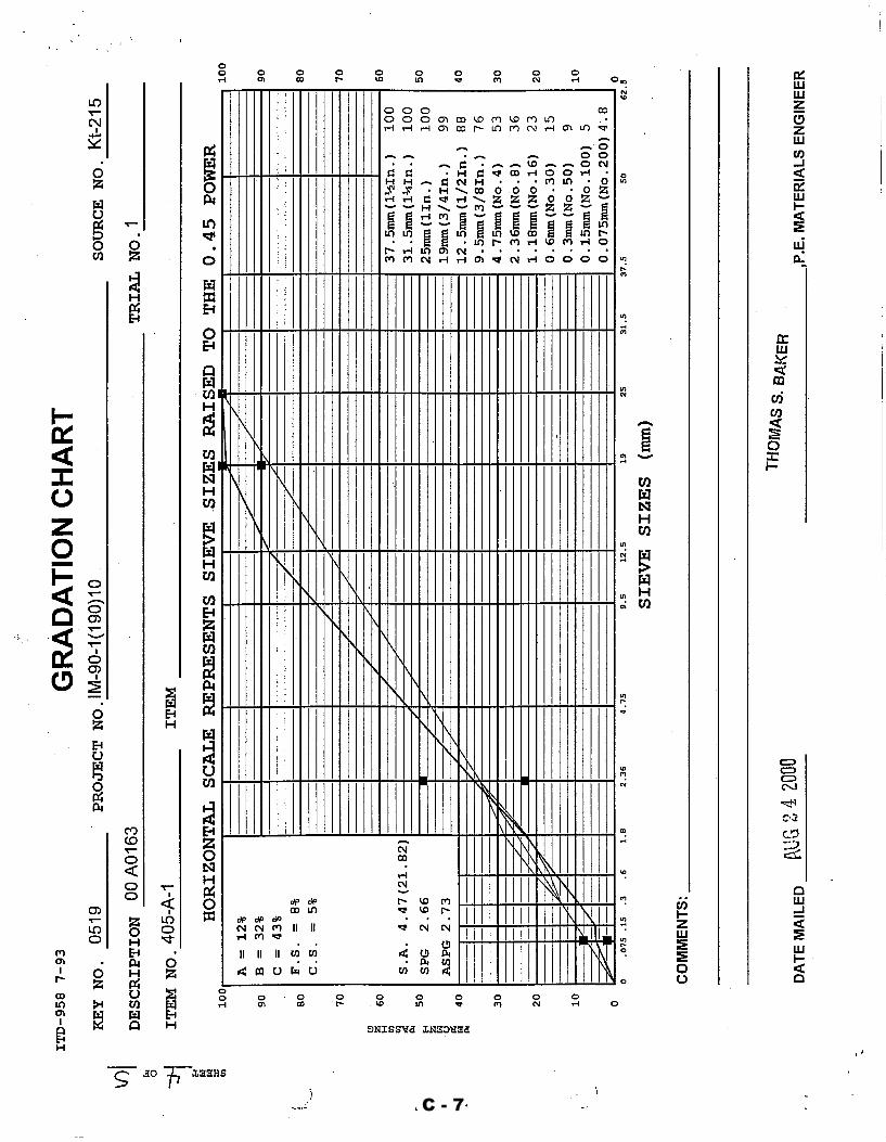
C - 7

C - 8

C - 9

C - 10

C - 11

C - 12

C - 13

C - 14

C - 15

C - 16

C - 17

C - 18

C - 19

C - 20

C - 21

C - 22

C - 23

C - 24

C - 25

C - 26

APPENDIX D
Data for ITD Mixes
Gradation, Volumetric Analysis and Calculation of
Energy Indices (CEI and TEI)

Gradation Analysis of ITD Mixes (Hveem and Superpave)
Mix D1Mix D1 Gradation and wt.of aggr.(Hveem and SP)
Sieve Sizes Trial passing Wt of agg. Wt of agg. Wt of agg.(4500g) (5500g) (5799g) hight 150
25mm (1In) 100%19mm (3/4 In) 99% 45 55 58
12.5mm (1/2 In) 88% 495 605 6389.5mm (3/8 In) 76% 540 660 6964.75mm (N0.4) 53% 1035 1265 13342.36mm (No.8) 36% 765 935 9861.18mm (No.30) 23% 585 715 754600um (No.50) 15% 360 440 464300um (No.16) 9% 270 330 348150um (No.100) 5% 180 220 23275um (No.200) 4.8% 9 11 12
-200 216 264 278Total wt.of agg. 4500 5500 5799Pb by wt.of agg. Hv. 5.3%
SP. 5.3%Wt.of asphalt Hv. 239 292 307
SP. 239 292 307
Mix D1 - Changed Gradation of SP and wt.of aggr.
Sieve Sizes Trial passing Wt of agg. Wt of agg. Wt of agg.(4500g) (5500g) (5799g) hight 150
25mm (1In) 100%19mm (3/4 In) 93% 315 385 406
12.5mm (1/2 In) 71% 990 1210 12769.5mm (3/8 In) 53% 810 990 10444.75mm (N0.4) 34% 855 1045 11022.36mm (No.8) 26% 360 440 4641.18mm (No.30) 20% 270 330 348600um (No.50) 13% 315 385 406300um (No.16) 8% 225 275 290150um (No.100) 4% 180 220 23275um (No.200) 3.0% 45 55 58
-200 135 165 174Total wt.of agg. 4500 5500 5799Pb by wt.of agg.
SP. 5.3%Wt.of asphalt
SP. 239 292 307
D - 1

Gradation Analysis of ITD Mixes (Hveem and Superpave)
Mix D2Mix D2 - Gradation and wt.of aggr.(Hveem and SP)
Sieve Sizes Trial passing Wt of agg. Wt of agg. Wt of agg.for Hv. Wt of agg.for SP.(4500g) (5500g) (5961g) hight 150 (5917g) hight 150
25mm (1In) 100%19mm (3/4 In) 99% 45 55 60 59
12.5mm (1/2 In) 80% 855 1045 1133 11249.5mm (3/8 In) 69% 495 605 656 6514.75mm (N0.4) 51% 810 990 1073 10652.36mm (No.8) 33% 810 990 1073 10651.18mm (No.30) 22% 495 605 656 651600um (No.50) 14% 360 440 477 473300um (No.16) 10% 180 220 238 237150um (No.100) 7% 135 165 179 17875um (No.200) 5.7% 58.5 71.5 77 77
-200 256.5 313.5 340 337Total wt.of agg. 4500 5500 5961 5917Pb by wt.of agg. Hv. 6.1%
SP. 6.6%Wt.of asphalt Hv. 275 336 364 361
SP. 298 364 395 392
Mix D2 - Changed Gradation of SP and wt.of aggr
Sieve Sizes Trial passing Wt of agg. Wt of agg. Wt of agg.for Hv. Wt of agg.for SP.(4500g) (5500g) (5961g) hight 150 (5917g) hight 150
25mm (1In) 100%19mm (3/4 In) 93% 315 385 417 414
12.5mm (1/2 In) 70% 1035 1265 1371 13619.5mm (3/8 In) 51% 855 1045 1133 11244.75mm (N0.4) 34% 765 935 1013 10062.36mm (No.8) 24% 450 550 596 5921.18mm (No.30) 20% 180 220 238 237600um (No.50) 13% 315 385 417 414300um (No.16) 9% 180 220 238 237150um (No.100) 7% 90 110 119 11875um (No.200) 4.5% 112.5 137.5 149 148
-200 202.5 247.5 268 266Total wt.of agg. 4500 5500 5961 5917Pb by wt.of agg.
SP. 6.62%Wt.of asphalt
SP. 298 364 395 392
D - 2

Gradation Analysis of ITD Mixes (Hveem and Superpave)
Mix D3Mix D3 - Gradation and wt.of aggr.(Hveem)
Sieve Sizes Trial passing Wt of agg. Wt of agg. Wt of agg.for Hv.(4500g) (5500g) (5683g) hight 150
37.5mm (11/2 In) 100%25mm (1In) 97% 135 165 170.4919mm (3/4 In) 88% 405 495 511.47
12.5mm (1/2 In) 60% 1260 1540 1591.249.5mm (3/8 In) 53% 315 385 397.81
4.75mm (N0.4) 47% 270 330 340.982.36mm (No.8) 32% 675 825 852.451.18mm (No.30) 22% 450 550 568.3600um (No.50) 15% 315 385 397.81300um (No.16) 10% 225 275 284.15150um (No.100) 6% 180 220 227.3275um (No.200) 4.0% 90 110 113.66
-200 180 220 227.32Total wt.of agg. 4500 5500 5683
Pb by wt.of agg. Hv. 5.0%Wt.of asphalt Hv. 225 275 284
Mix D3 - Changed Gradation and wt.of aggr.
Sieve Sizes Trial passing Wt of agg. Wt of agg. Wt of agg.for Hv.(4500g) (5500g) (5683g) hight 150
37.5mm (11/2 In) 100%25mm (1In) 97% 135 165 170.4919mm (3/4 In) 88% 405 495 511.47
12.5mm (1/2 In) 60% 1260 1540 1591.249.5mm (3/8 In) 53% 315 385 397.81
4.75mm (N0.4) 47% 270 330 340.982.36mm (No.8) 32% 675 825 852.451.18mm (No.30) 22% 450 550 568.3600um (No.50) 15% 315 385 397.81300um (No.16) 10% 225 275 284.15150um (No.100) 6% 180 220 227.3275um (No.200) 4.0% 90 110 113.66
-200 180 220 227.32Total wt.of agg. 4500 5500 5683
Pb by wt.of agg. Hv. 5.0%Wt.of asphalt Hv. 225 275 284
D - 3

Vol
umet
ric A
naly
sis
of S
ampl
es fo
r ITD
Mix
es a
t N-in
itial
Sam
ples
for M
ix D
1 at
Ni
Sam
ples
for D
1D
1S3
at N
40D
1S4
at N
40D
1H6
at N
100
D1H
7 at
N85
D1H
8 at
N85
D1h
9 at
N85
D1H
10 a
t N50
D1H
12 a
t N40
Asp
halt
cont
ent P
b by
agg
r.WT
5.25
%5.
25%
5.30
%5.
3%5.
30%
5.30
%5.
3%5.
3%A
spha
lt co
nten
t Pb
by m
ix W
T5.
0%5.
0%5.
00%
5.0%
5.0%
5.0%
5.0%
5.0%
Wdr
y:59
8960
86.5
5772
5773
5777
5773
5765
5830
Wsu
b:34
33.3
3494
.233
6933
4533
7833
6833
2533
80W
ssd:
6023
6123
.757
9458
22.2
5796
.457
94.3
5808
5896
.2G
mm
:2.
478
2.47
82.
478
2.47
82.
478
2.47
82.
478
2.47
8G
sb:
2.66
2.66
2.66
2.66
2.66
2.66
2.66
2.66
Ps:
95.0
%95
.0%
95.0
%95
.0%
95.0
%95
.0%
95.0
%95
.0%
H14
8.61
151.
1513
9.5
140.
4213
8.84
139.
1614
1.23
141.
83
Gm
b=W
dry/
Wss
d-W
sub
Gm
b(m
easu
red)
2.31
32.
315
2.38
02.
330
2.38
92.
379
2.32
22.
317
Gm
b(es
timat
ed)
2.28
22.
280
2.34
32.
328
2.35
62.
349
2.31
12.
327
CF
1.01
41.
015
1.01
61.
001
1.01
41.
013
1.00
50.
996
Gm
b(es
timat
ed)@
Nm
ax:
2.28
22.
280
2.34
32.
328
2.35
62.
349
2.31
12.
327
Gm
b(co
rrec
ted)
@N
max
:2.
313
2.31
52.
380
2.33
02.
389
2.37
92.
322
2.31
7%
Va=
1-G
mb/
Gm
m%
Va6.
7%6.
6%3.
9%6.
0%3.
6%4.
0%6.
3%6.
5%%
VM
A=1
00-G
mb*
Ps/
Gsb
%VM
A17
.4%
17.3
%15
.0%
16.8
%14
.7%
15.0
%17
.1%
17.3
%%
VFA
=100
*(V
MA
-Va)
/VM
A%
VFA
61.7
%62
.0%
73.7
%64
.5%
75.5
%73
.5%
63.1
%62
.3%
D -
4
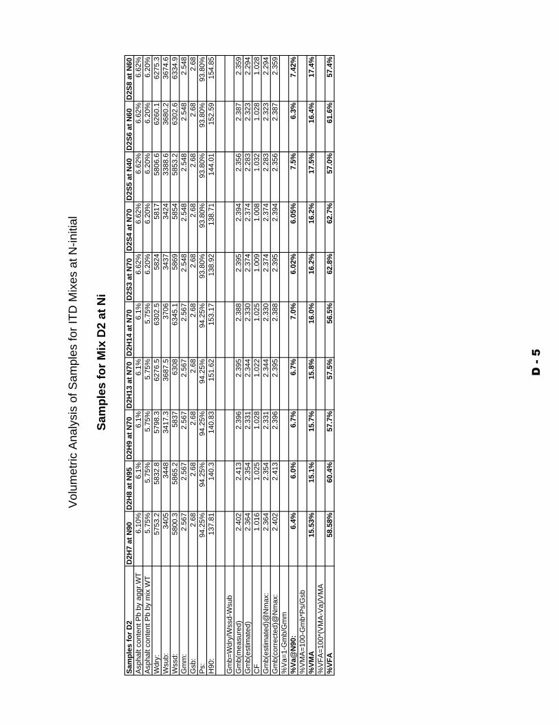
Vol
umet
ric A
naly
sis
of S
ampl
es fo
r ITD
Mix
es a
t N-in
itial
Sam
ples
for M
ix D
2 at
Ni
Sam
ples
for D
2D
2H7
at N
90D
2H8
at N
95D
2H9
at N
70D
2H13
at N
70D
2H14
at N
70D
2S3
at N
70D
2S4
at N
70D
2S5
at N
40D
2S6
at N
60D
2S8
at N
60A
spha
lt co
nten
t Pb
by a
ggr.W
T6.
10%
6.1%
6.1%
6.1%
6.1%
6.62
%6.
62%
6.62
%6.
62%
6.62
%A
spha
lt co
nten
t Pb
by m
ix W
T5.
75%
5.75
%5.
75%
5.75
%5.
75%
6.20
%6.
20%
6.20
%6.
20%
6.20
%W
dry:
5753
.258
32.8
5798
.362
76.5
6302
.558
2458
1758
06.6
6260
.162
75.3
Wsu
b:34
0534
4834
17.3
3687
.537
0634
3734
2433
88.6
3680
.236
74.6
Wss
d:58
00.3
5865
.258
3763
0863
45.1
5869
5854
5853
.263
02.6
6334
.9G
mm
:2.
567
2.56
72.
567
2.56
72.
567
2.54
82.
548
2.54
82.
548
2.54
8G
sb:
2.68
2.68
2.68
2.68
2.68
2.68
2.68
2.68
2.68
2.68
Ps:
94.2
5%94
.25%
94.2
5%94
.25%
94.2
5%93
.80%
93.8
0%93
.80%
93.8
0%93
.80%
H90
:13
7.81
140.
314
0.83
151.
6215
3.17
138.
9213
8.71
144.
0115
2.59
154.
85
Gm
b=W
dry/
Wss
d-W
sub
Gm
b(m
easu
red)
2.40
22.
413
2.39
62.
395
2.38
82.
395
2.39
42.
356
2.38
72.
359
Gm
b(es
timat
ed)
2.36
42.
354
2.33
12.
344
2.33
02.
374
2.37
42.
283
2.32
32.
294
CF
1.01
61.
025
1.02
81.
022
1.02
51.
009
1.00
81.
032
1.02
81.
028
Gm
b(es
timat
ed)@
Nm
ax:
2.36
42.
354
2.33
12.
344
2.33
02.
374
2.37
42.
283
2.32
32.
294
Gm
b(co
rrec
ted)
@N
max
:2.
402
2.41
32.
396
2.39
52.
388
2.39
52.
394
2.35
62.
387
2.35
9%
Va=
1-G
mb/
Gm
m%
Va@
N90
:6.
4%6.
0%6.
7%6.
7%7.
0%6.
02%
6.05
%7.
5%6.
3%7.
42%
%V
MA
=100
-Gm
b*P
s/G
sb%
VMA
15.5
3%15
.1%
15.7
%15
.8%
16.0
%16
.2%
16.2
%17
.5%
16.4
%17
.4%
%V
FA=1
00*(
VM
A-V
a)/V
MA
%VF
A58
.58%
60.4
%57
.7%
57.5
%56
.5%
62.8
%62
.7%
57.0
%61
.6%
57.4
%
D -
5

Vol
umet
ric A
naly
sis
of S
ampl
es fo
r ITD
Mix
es a
t N-in
itial
Sam
ple
for M
ix D
3 at
Ni
Sam
ples
for D
3D
3H6
at N
40D
3H7
at N
40D
3H8
at N
40D
3H9
at N
50A
spha
lt co
nten
t Pb
by a
ggr.W
5.0%
5.0%
5.0%
5.0%
Asp
halt
cont
ent P
b by
mix
WT
4.8%
4.8%
4.8%
4.8%
Wdr
y:57
58.2
5757
.559
29.7
5937
.1W
sub:
3290
3302
3384
3394
.1W
ssd:
5850
5844
5996
.860
18.6
Gm
m:
2.42
22.
422
2.42
22.
422
Gsb
:2.
547
2.54
72.
547
2.54
7P
s:95
.24%
95.2
4%95
.24%
95.2
4%H
147.
0714
3.81
151.
0415
3.04
Gm
b=W
dry/
Wss
d-W
sub
Gm
b(m
easu
red)
2.24
92.
265
2.26
92.
262
Gm
b(es
timat
ed)
2.21
72.
267
2.22
32.
196
CF
1.01
50.
999
1.02
11.
030
Gm
b(es
timat
ed)@
Nm
ax:
2.21
72.
267
2.22
32.
196
Gm
b(co
rrec
ted)
@N
max
:2.
249
2.26
52.
269
2.26
2%
Va=
1-G
mb/
Gm
m%
Va7.
1%6.
5%6.
3%6.
6%%
VM
A=1
00-G
mb*
Ps/
Gsb
%VM
A15
.9%
15.3
%15
.1%
15.4
%%
VFA
=100
*(V
MA
-Va)
/VM
A%
VFA
55.1
%57
.6%
58.4
%57
.2%
D -
6

Volu
met
ric A
naly
sis
and
CEI
Cal
cula
tions
for S
ampl
es o
f Mix
D1
Sam
ples
Com
pact
ed to
N m
ax =
160
D -
7

Volu
met
ric A
naly
sis
and
CEI
Cal
cula
tions
for S
ampl
es o
f Mix
D2
Sam
ples
Com
pact
ed to
N m
ax =
160
D -
8
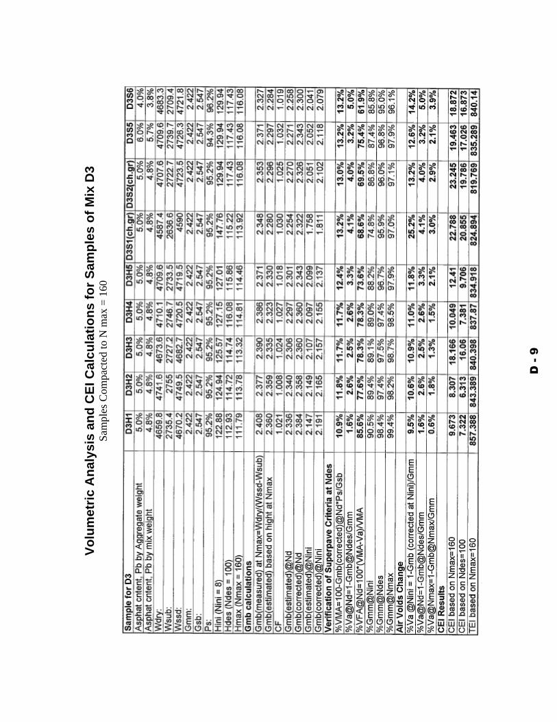
Volu
met
ric A
naly
sis
and
CEI
Cal
cula
tions
for S
ampl
es o
f Mix
D3
Sam
ples
Com
pact
ed to
N m
ax =
160
D -
9

APPENDIX E
APA Test Results for ITD Mixes

E - 1
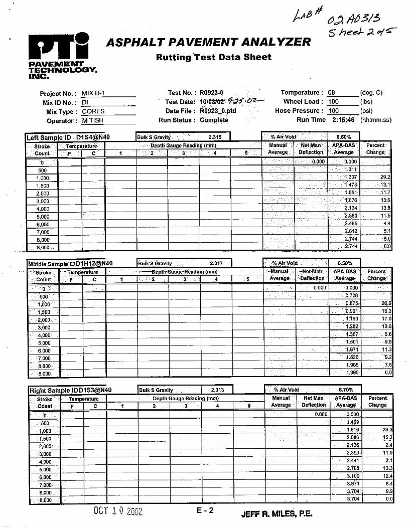
E - 2

E - 3

E - 4

E - 5
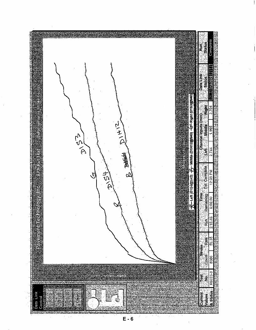
E - 6

E - 7
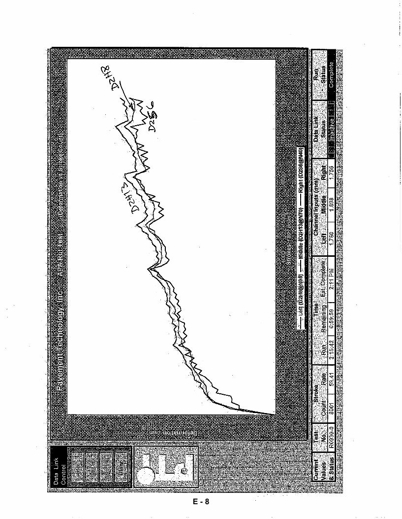
E - 8

E - 9
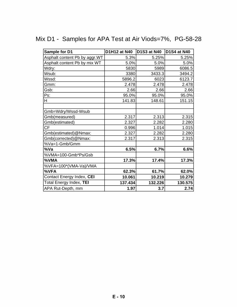
Mix D1 - Samples for APA Test at Air Viods=7%, PG-58-28
Sample for D1 D1H12 at N40 D1S3 at N40 D1S4 at N40Asphalt content Pb by aggr.WT 5.3% 5.25% 5.25%Asphalt content Pb by mix WT 5.0% 5.0% 5.0%Wdry: 5830 5989 6086.5Wsub: 3380 3433.3 3494.2Wssd: 5896.2 6023 6123.7Gmm: 2.478 2.478 2.478Gsb: 2.66 2.66 2.66Ps: 95.0% 95.0% 95.0%H 141.83 148.61 151.15
Gmb=Wdry/Wssd-WsubGmb(measured) 2.317 2.313 2.315Gmb(estimated) 2.327 2.282 2.280CF 0.996 1.014 1.015Gmb(estimated)@Nmax: 2.327 2.282 2.280Gmb(corrected)@Nmax: 2.317 2.313 2.315%Va=1-Gmb/Gmm%Va 6.5% 6.7% 6.6%%VMA=100-Gmb*Ps/Gsb%VMA 17.3% 17.4% 17.3%%VFA=100*(VMA-Va)/VMA%VFA 62.3% 61.7% 62.0%Contact Energy Index, CEI 10.061 10.219 10.279Total Energy Index, TEI 137.434 132.226 130.575APA Rut-Depth, mm 1.97 3.7 2.74
E - 10

Mix D2 - Samples for APA Test at Air Voids=7%, PG-64-34
Sample for D2 D2H8 at N95 D2H13 at N70 D2H14 at N70 D2S6 at N60 D2S8 at N60Asphalt content Pb by aggr.WT 6.1% 6.1% 6.1% 6.62% 6.62%Asphalt content Pb by mix WT 5.75% 5.75% 5.75% 6.20% 6.20%Wdry: 5832.8 6276.5 6302.5 6260.1 6275.3Wsub: 3448 3687.5 3706 3680.2 3674.6Wssd: 5865.2 6308 6345.1 6302.6 6334.9Gmm: 2.567 2.567 2.567 2.548 2.548Gsb: 2.68 2.68 2.68 2.68 2.68Ps: 94.25% 94.25% 94.25% 93.80% 93.80%H90: 140.3 151.62 153.17 152.59 154.85
Gmb=Wdry/Wssd-WsubGmb(measured) 2.413 2.395 2.388 2.387 2.359Gmb(estimated) 2.354 2.344 2.330 2.323 2.294CF 1.025 1.022 1.025 1.028 1.028Gmb(estimated)@Nmax: 2.354 2.344 2.330 2.323 2.294Gmb(corrected)@Nmax: 2.413 2.395 2.388 2.387 2.359%Va=1-Gmb/Gmm%Va@N90: 6.0% 6.7% 7.0% 6.3% 7.42%%VMA=100-Gmb*Ps/Gsb%VMA 15.1% 15.8% 16.0% 16.4% 17.4%%VFA=100*(VMA-Va)/VMA%VFA 60.4% 57.5% 56.5% 61.6% 57.4%Contact Energy Index, CEI 20.746 13.412 13.658 16.432 15.817Total Energy Index, TEI 447.572 254.43 263.025 234.528 233.667APA Rut-Depth, mm 1.76 1.9 1.73 1.76 1.86
E - 11

Mix D3 - Samples for APA Test at Air Voids=7%, PG-76-28
Sample for D3 D3H6 at N40 D3H8 at N40 D3H9 at N50Asphalt content Pb by aggr.WT 5.0% 5.0% 5.0%Asphalt content Pb by mix WT 4.8% 4.8% 4.8%Wdry: 5758.2 5929.7 5937.1Wsub: 3290 3384 3394.1Wssd: 5850 5996.8 6018.6Gmm: 2.422 2.422 2.422Gsb: 2.547 2.547 2.547Ps: 95.24% 95.24% 95.24%H 147.07 151.04 153.04
Gmb=Wdry/Wssd-WsubGmb(measured) 2.249 2.269 2.262Gmb(estimated) 2.217 2.223 2.196CF 1.015 1.021 1.030Gmb(estimated)@Nmax: 2.217 2.223 2.196Gmb(corrected)@Nmax: 2.249 2.269 2.262%Va=1-Gmb/Gmm%Va 7.1% 6.3% 6.6%%VMA=100-Gmb*Ps/Gsb%VMA 15.9% 15.1% 15.4%%VFA=100*(VMA-Va)/VMA%VFA 55.1% 58.4% 57.2%Contact Energy Index, CEI 11.156 10.755 9.215Total Energy Index, TEI 150.391 147.44 128.612APA Rut-Depth, mm 4.57 2.32 2.21
E - 12

This is a blank Page

APPENDIX F
Image Analysis Test Results for ITD Mixes

Mix
D1
- Sam
ples
for I
mag
e Te
st
Sam
ple
for D
1D
1H1
D1H
4D
1H13
D1H
14D
1H11
5D
1H11
6D
1S1
D1S
2A
spha
lt co
nten
t, P
b by
agg
rega
te w
eigh
t 5.
3%5.
3%6.
3%6.
3%4.
3%4.
3%5.
3%5.
3%A
spha
lt co
nten
t, P
b by
mix
wei
ght
5.0%
5.0%
5.93
%5.
93%
4.1%
4.1%
5.0%
5.0%
Wdr
y:47
27.2
4756
.147
62.7
4765
.558
01.7
5800
4709
4688
Wsu
b:27
7228
01.5
2814
.128
14.2
3429
.334
30.5
2774
2753
Wss
d:47
3847
67.7
4770
.847
7458
21.8
5818
.347
3047
02G
mm
:2.
478
2.47
82.
444
2.44
42.
511
2.51
12.
478
2.47
8G
sb:
2.66
2.66
2.66
2.66
2.66
2.66
2.66
2.66
Ps:
95.0
%95
.0%
94.1
%94
.1%
95.9
%95
.9%
95.0
%95
.0%
Hin
i:12
6.09
128.
1912
6.95
126.
7115
3.96
153.
9312
9.91
127.
77H
des:
113.
0511
4.65
113.
8111
3.82
138.
2113
8.13
116.
5111
5.03
Hm
ax:
111.
6511
3.14
112.
3811
2.36
136.
4913
6.36
115.
0711
3.67
Gm
b ca
lcul
atio
nG
mb(
mea
sure
d) a
t Nm
ax=W
dry/
(Wss
d-W
sub)
2.40
42.
419
2.43
42.
432
2.42
52.
429
2.40
72.
405
Gm
b(es
timat
ed)
2.39
72.
380
2.39
92.
401
2.40
72.
408
2.31
72.
335
CF
1.00
31.
016
1.01
41.
013
1.00
81.
009
1.03
91.
030
Gm
b(es
timat
ed)@
Nd:
2.36
72.
349
2.36
92.
370
2.37
72.
377
2.28
82.
307
Gm
b(co
rrec
ted)
@N
d:2.
375
2.38
72.
403
2.40
02.
395
2.39
82.
378
2.37
7G
mb(
estim
ated
)@N
ini:
2.12
32.
101
2.12
42.
129
2.13
42.
133
2.05
22.
077
Gm
b(co
rrec
ted)
@N
ini:
2.12
92.
135
2.15
52.
156
2.15
02.
152
2.13
22.
140
Verif
icat
ion
of S
uper
pave
Crit
eria
at N
des
%V
MA
=100
-Gm
b(co
rrec
ted)
@N
d*P
s/G
sb15
.19%
14.7
5%15
.00%
15.1
1%13
.68%
13.5
7%15
.08%
15.1
1%%
Va@
Nd=
1-G
mb@
Nde
s/G
mm
4.17
%3.
67%
1.66
%1.
78%
4.63
%4.
50%
4.05
%4.
08%
%V
FA@
Nd=
100*
(VM
A-V
a)/V
MA
72.6
%75
.1%
88.9
%88
.2%
66.2
%66
.8%
73.2
%73
.0%
%G
mm
@N
ini
85.9
%86
.2%
88.2
%88
.2%
85.6
%85
.7%
86.1
%86
.4%
%G
mm
@N
des
95.8
%96
.3%
98.3
%98
.2%
95.4
%95
.5%
96.0
%95
.9%
%G
mm
@N
max
97.0
%97
.6%
99.6
%99
.5%
96.6
%96
.7%
97.2
%97
.1%
Air
Void
s C
hang
e%
Va
@N
ini =
1-G
mb
(cor
rect
ed a
t Nin
i)/G
mm
14.1
%13
.8%
11.8
%11
.8%
14.4
%14
.3%
13.9
%13
.6%
%V
a@N
d=1-
Gm
b@N
des/
Gm
m4.
2%3.
7%1.
7%1.
8%4.
6%4.
5%4.
0%4.
1%%
Va@
Nm
ax=1
-Gm
b@N
max
/Gm
m3.
0%2.
4%0.
4%0.
5%3.
4%3.
3%2.
8%2.
9%C
EI R
esul
tsC
EI b
ased
on
Nm
ax=1
6020
.043
21.3
0817
.27
18.5
8618
.441
19.5
8522
.054
21.0
83C
EI b
ased
on
Nde
s=10
017
.086
18.2
8314
.275
15.6
5815
.343
16.6
3219
.44
18.6
14TE
I bas
ed o
n N
max
=160
966.
3994
6.99
932.
5593
1.88
810.
5378
0.63
901
914.
95
F - 1

Mix
D2
- Sam
ples
for I
mag
e Te
st
Sam
ple
for D
2D
2H2
D2H
6D
2S1
D2S
2D
2H10
D2H
11D
2H14
D2H
15A
spha
lt co
nten
t, P
b by
agg
rega
te w
eigh
t 6.
1%6.
1%6.
62%
6.62
%7.
6%7.
6%5.
6%5.
6%A
spha
lt co
nten
t, P
b by
mix
wei
ght
5.75
%5.
75%
6.20
%6.
20%
7.08
%7.
08%
5.32
%5.
32%
Wdr
y:47
38.2
4758
4751
.747
4247
9547
91.1
4664
4665
Wsu
b:28
21.3
2842
2838
.428
35.4
2867
.228
58.1
2787
.527
79.8
Wss
d:47
42.4
4776
4758
4751
4804
.747
95.5
4720
.547
12.4
Gm
m:
2.56
72.
567
2.54
82.
548
2.51
42.
514
2.58
52.
585
Gsb
:2.
682.
682.
682.
682.
682.
682.
682.
68P
s:94
.25%
94.2
5%93
.8%
93.8
%92
.92%
92.9
2%94
.68%
94.6
8%H
ini:
127.
3612
5.66
125.
6612
5.66
127.
8212
7.83
129.
5113
0.08
Hde
s:11
2.99
111.
8111
1.81
111.
8111
2.99
113.
6211
5.54
116.
08H
max
:11
1.52
110.
4311
0.43
110.
4311
1.45
112.
1111
3.99
114.
52G
mb
calc
ulat
ion
Gm
b(m
easu
red)
at N
max
=Wdr
y/(W
ssd-
Wsu
b)2.
466
2.46
02.
475
2.47
52.
475
2.47
32.
413
2.41
4G
mb(
estim
ated
)2.
406
2.43
92.
436
2.43
12.
436
2.42
02.
317
2.30
6C
F1.
025
1.00
91.
016
1.01
81.
016
1.02
21.
042
1.04
7G
mb(
estim
ated
)@N
d:2.
374
2.40
92.
406
2.40
12.
403
2.38
72.
285
2.27
5G
mb(
corr
ecte
d)@
Nd:
2.43
42.
430
2.44
52.
445
2.44
12.
440
2.38
02.
381
Gm
b(es
timat
ed)@
Nin
i:2.
106
2.14
42.
141
2.13
72.
124
2.12
22.
039
2.03
0G
mb(
corr
ecte
d)@
Nin
i:2.
160
2.16
22.
175
2.17
52.
158
2.16
92.
124
2.12
5Ve
rific
atio
n of
Sup
erpa
ve C
riter
ia a
t Nde
s%
VM
A=1
00-G
mb(
corr
ecte
d)@
Nd*
Ps/
Gsb
14.3
9%14
.55%
14.4
3%14
.43%
15.3
6%15
.40%
15.9
0%15
.87%
%V
a@N
d=1-
Gm
b@N
des/
Gm
m5.
17%
5.34
%4.
05%
4.05
%2.
90%
2.94
%7.
91%
7.88
%%
VFA
@N
d=10
0*(V
MA
-Va)
/VM
A64
.1%
63.3
%71
.9%
72.0
%81
.1%
80.9
%50
.2%
50.4
%%
Gm
m@
Nin
i84
.1%
84.2
%85
.4%
85.4
%85
.8%
86.3
%82
.2%
82.2
%%
Gm
m@
Nde
s94
.8%
94.7
%96
.0%
96.0
%97
.1%
97.1
%92
.1%
92.1
%%
Gm
m@
Nm
ax96
.1%
95.8
%97
.1%
97.2
%98
.4%
98.4
%93
.3%
93.4
%A
ir Vo
ids
Cha
nge
%V
a @
Nin
i = 1
-Gm
b (c
orre
cted
at N
ini)/
Gm
m15
.87%
15.7
8%14
.63%
14.6
2%14
.17%
13.7
3%17
.85%
17.7
9%%
Va@
Nd=
1-G
mb@
Nde
s/G
mm
5.17
%5.
34%
4.05
%4.
05%
2.90
%2.
94%
7.91
%7.
88%
%V
a@N
max
=1-G
mb@
Nm
ax/G
mm
3.92
%4.
16%
2.85
%2.
85%
1.56
%1.
63%
6.66
%6.
62%
CEI
Res
ults
CE
I bas
ed o
n N
max
=160
17.8
1519
.98
22.8
7222
.783
18.4
3119
.322
21.6
5119
.677
CE
I bas
ed o
n N
des=
100
15.3
5817
.169
20.0
7419
.81
15.2
4516
.29
18.6
6316
.587
TEI b
ased
on
Nm
ax=1
6093
7.61
924.
5992
0.56
989.
8491
9.24
916.
0290
7.36
907.
03
F - 2

Mix
D3
- S
ampl
es fo
r Im
age
Test
Sam
ple
for D
3D
3H2
D3H
4D
3S1(
ch.g
r)D
3S2(
ch.g
r)A
spha
lt co
nten
t, P
b by
agg
rega
te w
eigh
t 5.
0%5.
0%5.
0%5.
0%A
spha
lt co
nten
t, P
b by
mix
wei
ght
4.8%
4.8%
4.8%
4.8%
Wdr
y:47
41.6
4710
.145
87.4
4707
.6W
sub:
2755
2746
.726
36.6
2722
.7W
ssd:
4749
.547
20.5
4590
4723
.5G
mm
:2.
422
2.42
22.
422
2.42
2G
sb:
2.54
72.
547
2.54
72.
547
Ps:
95.2
%95
.2%
95.2
%95
.2%
Hin
i:12
4.94
127.
1514
7.76
129.
94H
des:
114.
7211
6.08
115.
2211
7.43
Hm
ax:
113.
7811
4.81
113.
9211
6.08
Gm
b ca
lcul
atio
nG
mb(
mea
sure
d) a
t Nm
ax=W
dry/
(Wss
d-W
sub)
2.37
72.
386
2.34
82.
353
Gm
b(es
timat
ed)
2.35
92.
323
2.28
02.
296
CF
1.00
81.
027
1.03
01.
025
Gm
b(es
timat
ed)@
Nd:
2.34
02.
297
2.25
42.
270
Gm
b(co
rrec
ted)
@N
d:2.
358
2.36
02.
322
2.32
6G
mb(
estim
ated
)@N
ini:
2.14
92.
097
1.75
82.
051
Gm
b(co
rrec
ted)
@N
ini:
2.16
52.
155
1.81
12.
102
Verif
icat
ion
of S
uper
pave
Crit
eria
at N
des
%V
MA
=100
-Gm
b(co
rrec
ted)
@N
d*P
s/G
sb11
.8%
11.7
%13
.2%
13.0
%%
Va@
Nd=
1-G
mb@
Nde
s/G
mm
2.6%
2.6%
4.1%
4.0%
%V
FA@
Nd=
100*
(VM
A-V
a)/V
MA
77.6
%78
.3%
68.6
%69
.5%
%G
mm
@N
ini
89.4
%89
.0%
74.8
%86
.8%
%G
mm
@N
des
97.4
%97
.4%
95.9
%96
.0%
%G
mm
@N
max
98.2
%98
.5%
97.0
%97
.1%
Air
Void
s C
hang
e%
Va
@N
ini =
1-G
mb
(cor
rect
ed a
t Nin
i)/G
mm
10.6
%11
.0%
25.2
%13
.2%
%V
a@N
d=1-
Gm
b@N
des/
Gm
m2.
6%2.
6%4.
1%4.
0%%
Va@
Nm
ax=1
-Gm
b@N
max
/Gm
m1.
8%1.
5%3.
0%2.
9%C
EI R
esul
tsC
EI b
ased
on
Nm
ax=1
608.
307
10.0
4922
.788
23.2
45C
EI b
ased
on
Nde
s=10
06.
313
7.38
120
.855
19.7
86TE
I bas
ed o
n N
max
=160
843.
389
837.
873
824.
894
819.
769
F - 3

APPENDIX G
e-Files Included on CD-ROM
The CD ROM includes files for:
• Servopac Gyratory Files for All Samples • Excel files for CEI calculations for all samples • Template for CEI Calculation Excel Sheet • Various Excel files for raw data for volumetric analysis