development and evaluation of a robust algorithm for computer-assisted detection of sentinel lymph...

Development and evaluation of a robust algorithm forcomputer-assisted detection of sentinel lymph nodemicrometastases

Gina M Clarke,1 Chris Peressotti,1 Claire M B Holloway,2,3 Judit T Zubovits,4,5 Kela Liu1 &

Martin J Yaffe1,6,7

1Imaging Research, Sunnybrook Health Sciences Centre, 2Department of Surgical Oncology, Sunnybrook Health Sciences

Centre, 3Department of Surgery, University of Toronto, 4Department of Anatomic Pathology, Sunnybrook Health Sciences

Centre, 5Department of Laboratory Medicine and Pathobiology, University of Toronto, 6Departments of Medical Biophysics,

and 7Medical Imaging, University of Toronto, Toronto, ON, Canada

Date of submission 3 September 2010Accepted for publication 23 November 2010

Clarke G M, Peressotti C, Holloway C M B, Zubovits J T, Liu K & Yaffe M J

(2011) Histopathology 59, 116–128

Development and evaluation of a robust algorithm for computer-assisted detection ofsentinel lymph node micrometastases

Aims: Increasing the sectioning rate for breast sentinellymph nodes can increase the likelihood of detectingmicrometastases. To make serial sectioning feasible, wehave developed an algorithm for computer-assisteddetection (CAD) with digitized lymph node sections.Methods and results: K-means clustering assigned im-age pixels to one of four areas in a colourspace(representing tumour, unstained background, counter-stained background and microtomy artefacts). Fourfilters then removed ‘false-positive’ pixels from thetumour cluster. A set of 43 sections containing tumour(a total of 259 foci) and 59 sections negative formalignancy was defined by two pathologists, usinglight microscopy, and CAD was applied. For the

clinically relevant task of identifying the largest focusin each section (micrometastasis in 22 ⁄ 43 sections),the sensitivity and specificity were 100%. Isolatedtumour cells (ITCs) were identified in one slide initiallyconsidered to be negative. Identification of all 259 fociyielded sensitivities of 57.5% for ITCs (<0.200 mm),89.5% for micrometastases, and 100% for largermetastases, with one false-positive. Reduced sensitivitywas ascribed to variable staining. Nine additionalmetastases (<0.01–0.3 mm) that were not initiallyidentified were detected by CAD.Conclusions: This algorithm is well suited to the task ofsentinel lymph node evaluation and may enhance thedetection of occult micrometastases.

Keywords: anti-cytokeratin immunohistochemistry, breast cancer, computer-assisted detection, sentinel lymphnode micrometastases, serial sectioning

Abbreviations: AEC, aminoethyl carbazole; ALND, axillary node dissection; CAD, computer-assisted detection; CD,colour distance; FP, false-positive; HSV, hue-saturation value; IHC, immunohistochemistry; ITCs, isolated tumourcells; LM, light microscopy; RGB, red–green–blue; SLN, sentinel lymph node; SLNB, sentinel lymph node biopsy

Introduction

Disease status in the axillary lymph nodes is themost important prognostic factor for breast cancer

patients.1,2 Nodal status is incorporated into tumourstage in the Tumour Node Metastasis (TNM) classifica-tion.3,4 Nodal status assessment has been traditionallybased on axillary lymph node dissection (ALND) and,more recently, sentinel lymph node (SLN) biopsy(SLNB).5–8 SLNB is a less invasive alternative to ALND,9

based on the concept that there is an obligatory pathwayfor metastatic deposits through a limited number (1–4)

Address for correspondence: G M Clarke, Sunnybrook Health Sciences

Centre, 2075 Bayview Avenue, Room S6-32, Toronto, ON M4N

3M5, Canada. e-mail: [email protected]

� 2011 Blackwell Publishing Limited.

Histopathology 2011, 59, 116–128. DOI: 10.1111/j.1365-2559.2011.03896.x

of SLNs.10,11 SLNB has been shown to predict axillarystatus in 95% of cases.12 Recent results from a large,randomized prospective multicentre trial (NationalSurgical Adjuvant Breast and Bowel Project-B32) haveshown equivalent regional recurrence, disease-freesurvival and overall survival with SLNB compared toALND after a mean follow-up of 95 months.13

Histological sampling can be concentrated on a smallnumber of key nodes in SLNB11 compared to ALND,and this is a likely reason why SLNB identifiesmetastases in approximately 15% of cases that wouldbe considered to be node-negative according toALND.14 There is no universal consensus on theoptimal scheme for pathological evaluation of theSLN, and there is considerable variability in thisregard.15,16 A Consensus Statement from the Collegeof American Pathologists recommends the evaluationof one section per node, stained with haematoxylin andeosin.17 This limited sampling strategy favours detec-tion of relatively large (i.e. >2 mm) metastases. Theprognostic significance of metastases in this size rangehas been well established.1,18

However, micrometastases, defined as the largestmetastatic deposit having a dimension in the range of0.2–2 mm,19 have been associated with an increasedrisk of distant recurrence and a decrease in overallsurvival in some retrospective studies.20,21 The clinicalsignificance of isolated tumour cells (ITCs)(<0.2 mm19) is less clear. Some studies have associatedITCs with poor prognosis.20,22 The vast majority ofITCs are detected with immunohistochemistry (IHC)alone, as they are usually occult with the use ofhaematoxylin and eosin. However, a recent report fromthe American College of Surgeons Oncology Group-Z0010 trial, a prospective study to determine theprognostic significance of SLN metastases that aredetectable only by IHC, showed no reduction in 5-yearsurvival among women with such metastases com-pared to those who were SLN-negative.23 It may be thecase that ITCs are prognostically significant as markersof more extensive disease occurring elsewhere in theaxilla. According to one systematic review, disease ispresent in additional nodes in 12.3% of patients whenITCs are detected in the SLNs.24 If a sparse samplingstrategy for the SLN is utilized, the detection ofmicrometastases and ITCs is largely a matter of chance.

There are ample data to support the idea that thelikelihood of detecting metastases, especially smallerones, increases as the sampling or sectioning rate of theSLN increases,25–27 and also with the use of IHC (i.e.pan-cytokeratin or low molecular weight keratin).28,29

Several studies have estimated that in 7–33% of casesoccult micrometastases are detected by use of the

additional information obtained from haematoxylinand eosin serial sectioning and ⁄ or IHC.29–35 With theuse of serial sectioning and IHC, the rate at whichtumours are ‘upstaged’ on the basis of detection ofoccult micrometastastes increases with the rate ofexhaustive step sectioning. For example, Cserni36 hasshown that the rate of upstaging increases from 19%for IHC sections 250 lm apart to 28% for sections 50–100 lm apart. A scheme for routine IHC and moreexhaustive serial sectioning to reliably detect microm-etastases,37 and thus to increase the likelihood of ITCdetection, might therefore have the potential toimprove patient outcomes.

Exhaustive sectioning of lymph nodes is not feasiblein clinical laboratories, because of workload and cost.Computer-assisted detection (CAD) of SLN metastasesfrom an automatically acquired, digital image of thewhole scanned slide could render systematic identifi-cation of SLN metastases feasible and practical. CADmay also improve the accuracy of detecting smaller focicompared to conventional interpretation. Althoughonly a few studies have been performed to evaluateCAD performance in detecting breast SLN metastases,they have all shown that CAD outperforms conven-tional microscopy for smaller tumour deposits, detect-ing additional micrometastases or ITCs (0.01–0.1 mmin diameter) in 3–15% of the cases initially deemedto be negative by a pathologist reader using themicroscope.38–40

In addition to increasing the accuracy relative toconventional slide inspection, CAD can overcomeissues related to diagnostic reproducibility. Inter-ratervariation in the classification of tumour deposits asmicrometastases versus ITCs can be high. However,accurate classification is essential to determine whetheror not further treatment is indicated. This is especiallyproblematic for metastases that involve a lymph nodein a diffuse tumour pattern, as is the tendency inlobular carcinoma. In such cases, typical pathologistinter-rater agreement is only 71.5%.41–44 Even for amore typical representation of diagnostic cases includ-ing metastases >2 mm, inter-rater variation of 2.6%(conversion from negative to positive) has beenreported.11 Finally, CAD in the context of lymph nodesections is a useful research tool that enables outcome-based study of potential new biomarkers throughquantitative analysis using measures such as area45,46

or volume.We have developed a CAD algorithm for analysing

IHC sections in breast SLNs. Here, we describe thealgorithm, and evaluate its performance in terms ofsensitivity and specificity for the task of identifyingtumour status (positive ⁄ negative) in nodal sections.

CAD for breast sentinel lymph nodes 117

� 2011 Blackwell Publishing Ltd, Histopathology, 59, 116–128.

This was performed for a variety of pathologicalsubtypes in the context of a per-section detection task.We also evaluate performance in the detection of alltumour foci present in each section, i.e. a per-focusdetection task, as each section frequently containsmultiple metastatic deposits. Although clinical diagno-sis is based on the per-section detection task, testingalgorithm performance with the per-focus task providesan opportunity to enlarge the sample set and increasestatistical power as well as to obtain a better under-standing of how well the algorithm performs. Theanalysis is performed for three size categories ofmetastases (<0.2, 0.2–2, and >2 mm).

Materials and methods

case selection and slide preparation

This study was performed on breast cancer casesobtained retrospectively from the Department ofAnatomic Pathology at Sunnybrook Health SciencesCentre, with the approval of the institutional ResearchEthics Board.

To develop the algorithm, a training set of 36 slideswas created. The set consisted of 18 pairs of contiguousserial sections, one pair being cut from the top of eachof 18 paraffin blocks. These training slides weregenerated from SLNs in nine cases of invasive breastcancer, four with and five without SLN involvement,documented in the pathology evaluation for routinepatient care. The negative slides included examples ofbenign cells that are known to react with theanti-cytokeratin antibody (e.g. dendritic cells).

The study dataset was constructed from 103 sectionsfrom 14 cases as selected by a board-certified pathol-ogist who specializes in breast cancer (J.Z.). A querywas performed in CoPath (Sunquest InformationSystems, Tucson, AZ, USA), the Department of Pathol-ogy specimen database, for cases of breast carcinoma(lumpectomy or mastectomy) with lymph node metas-tases. The first 14 consecutive cases, in reversechronological order starting from November 2008,excluding those cases in which the entire node wasreplaced by tumour, were included in the study. Noother selection criteria were applied to limit metastasissize, tumour type, or other parameters, in order toachieve a selection that models the distribution of thetypical diagnostic presentation.

Each case was typically composed of multiple nodes;multiple paraffin blocks were created for larger nodes,which were bisected or trisected. In some of the caseswhere there was lymph node involvement in somenodes, others were free of metastases. Of the 103

selected sections, 102 comprised the test set of slidesand the remaining section was used as a ‘calibration’slide for developing the CAD algorithm. A slide that hada wide variety of diagnostic and artefactual features(e.g. isolated tumour cells, air bubbles, preprintedmarkings on the slide, or folds in the tissue) wasselected as the calibration slide to best define a completeset of features to challenge the algorithm. Thesesections were cut from the top of each block, aftertrimming, at the rate of one per block.

For all of the study test slides as well as the trainingslides, IHC was performed with anti-cytokeratin-8monoclonal antibody CAM 5.2 (Becton Dickinson, SanJose, CA, USA) at 1:100 dilution following enzymatic(pepsin) antigen retrieval. Red chromogen [aminoethylcarbazole (AEC) with horseradish peroxidase-linkingenzyme] was used with the test slides, as well as withone section from each pair of training slides. Brownchromogen (3,3¢-diaminobenzidine and horseradishperoxidase) was used with the other section in eachpair of training slides. All of the slides were counter-stained with haematoxylin. A positive and a negativecontrol slide were included in all staining batches.

All slides were digitized by use of an automatedMirax slide scanner (Zeiss, Jena, Germany), with anacquisition pixel size of 0.33 lm, and the images werethen downsampled to 1.33 lm ⁄ pixel for computa-tional efficiency.

diagnosis by light microscopy ( lm )

A pathologist (K.L.) reviewed all 102 test sections, inaddition to the calibration slide, using LM, and iden-tified individual tumour foci to define the detection taskfor CAD. On the corresponding digitized image, thelargest dimension of each focus was measured, andthe outline of the focus was drawn as an overlay to theimage.

In those cases where, because of a diffuse tumourpattern, a tumour could not be readily classified ashaving distinct foci versus a single focus, a decision wasbased on the minimum distance between cells in thetwo areas. If the distance was <200 lm, the metastasiswas defined as a single focus, and if it was >200 lm, itwas classified as having separate foci. The slides werereviewed by a second pathologist (J.Z.) to estimatereliability, and where there was disagreement, the finalLM diagnosis was arrived at subsequently by consen-sus. Of the 102 test sections, 43 contained at least onefocus of tumour, and these were defined as LM-positivefor the per-slide detection task. The remaining 59 weredeemed to be negative on LM. Within the 43 positivesections, a total of 259 tumour foci were identified.

118 G M Clarke et al.


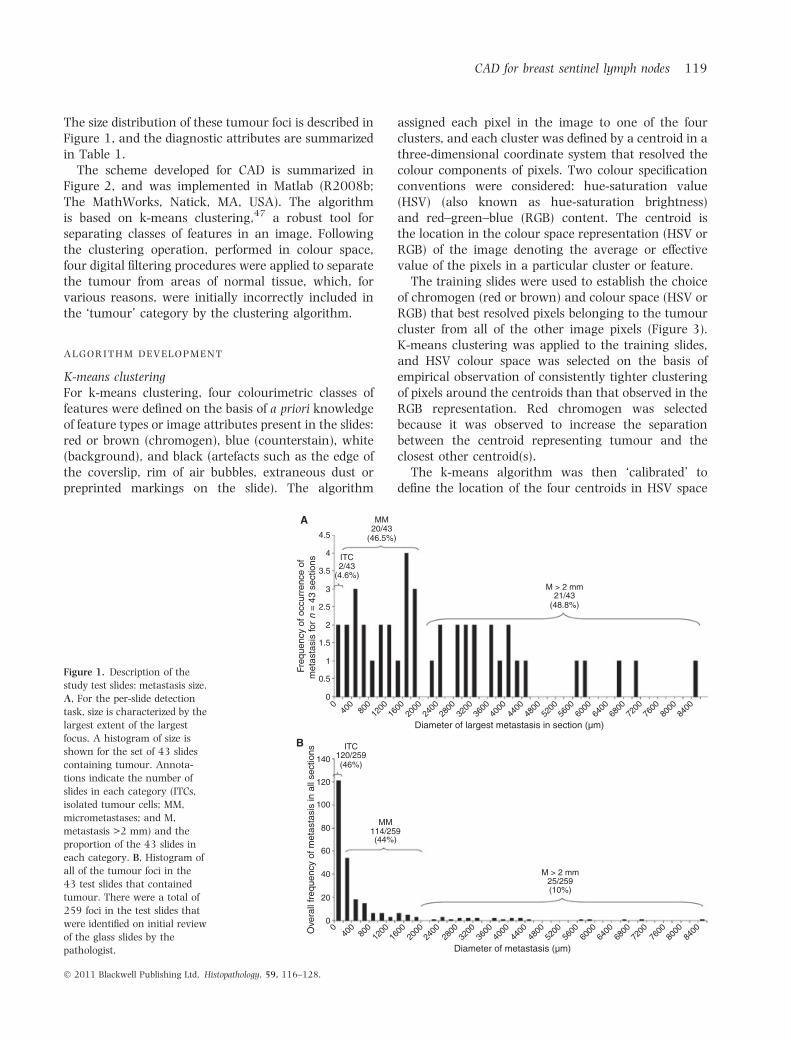
The size distribution of these tumour foci is described inFigure 1, and the diagnostic attributes are summarizedin Table 1.

The scheme developed for CAD is summarized inFigure 2, and was implemented in Matlab (R2008b;The MathWorks, Natick, MA, USA). The algorithmis based on k-means clustering,47 a robust tool forseparating classes of features in an image. Followingthe clustering operation, performed in colour space,four digital filtering procedures were applied to separatethe tumour from areas of normal tissue, which, forvarious reasons, were initially incorrectly included inthe ‘tumour’ category by the clustering algorithm.

algorithm development

K-means clusteringFor k-means clustering, four colourimetric classes offeatures were defined on the basis of a priori knowledgeof feature types or image attributes present in the slides:red or brown (chromogen), blue (counterstain), white(background), and black (artefacts such as the edge ofthe coverslip, rim of air bubbles, extraneous dust orpreprinted markings on the slide). The algorithm

assigned each pixel in the image to one of the fourclusters, and each cluster was defined by a centroid in athree-dimensional coordinate system that resolved thecolour components of pixels. Two colour specificationconventions were considered: hue-saturation value(HSV) (also known as hue-saturation brightness)and red–green–blue (RGB) content. The centroid isthe location in the colour space representation (HSV orRGB) of the image denoting the average or effectivevalue of the pixels in a particular cluster or feature.

The training slides were used to establish the choiceof chromogen (red or brown) and colour space (HSV orRGB) that best resolved pixels belonging to the tumourcluster from all of the other image pixels (Figure 3).K-means clustering was applied to the training slides,and HSV colour space was selected on the basis ofempirical observation of consistently tighter clusteringof pixels around the centroids than that observed in theRGB representation. Red chromogen was selectedbecause it was observed to increase the separationbetween the centroid representing tumour and theclosest other centroid(s).

The k-means algorithm was then ‘calibrated’ todefine the location of the four centroids in HSV space

4.5

4

3.5

2.5

1.5

0.5

00

400

800

1200

1600

2000

2400

2800

3200

3600

4000

4400

4800

5200

5600

6000

6400

6800

7200

7600

8000

8400

040

080

012

0016

0020

0024

0028

0032

0036

0040

0044

0048

0052

0056

0060

0064

0068

0072

0076

0080

0084

00

1

2

3

Freq

uenc

y of

occ

urre

nce

ofm

etas

tasi

s fo

r n

= 4

3 se

ctio

ns

Diameter of largest metastasis in section (µm)

ITC

ITC

2/43(4.6%)

MM

MM

20/43(46.5%)

M > 2 mm

M > 2 mm

21/43(48.8%)

120/259(46%)

114/259(44%)

25/259(10%)

Ove

rall

freq

uenc

y of

met

asta

sis

in a

ll se

ctio

ns

140

120

100

80

60

40

20

0

Diameter of metastasis (µm)

A

B

Figure 1. Description of the

study test slides: metastasis size.

A, For the per-slide detection

task, size is characterized by the

largest extent of the largest

focus. A histogram of size is

shown for the set of 43 slides

containing tumour. Annota-

tions indicate the number of

slides in each category (ITCs,

isolated tumour cells; MM,

micrometastases; and M,

metastasis >2 mm) and the

proportion of the 43 slides in

each category. B, Histogram of

all of the tumour foci in the

43 test slides that contained

tumour. There were a total of

259 foci in the test slides that

were identified on initial review

of the glass slides by the

pathologist.



and, most importantly, to define the one that corre-sponded to red or brown, i.e. metastases. This wasperformed with the calibration slide that was preparedin the same batch as the test slides. Areas were selectedin this slide, by the operator, on the basis of theirrepresentation of a sample of each of the followingimage attributes: chromogen (tumour cells, lympho-cytes and dendritic cells), counterstained background(blue), blank slide (white), and black areas (air bubbles,edge of the coverslip and preprinted markings). Thealgorithm calculated the centroid for each feature.

FiltersFour filters were defined, also using the calibrationslide, to reduce the number of false-positive (FP)findings or non-tumour cells that were incorrectlyassigned by k-means to the centroid representingtumour cells. These were: a colour distance (CD) filter,an area filter, a neighbourhood filter and a hue filter(Figure 4).

CD filter. The CD filter was implemented as follows.A measure, CD, of distance in HSV space between eachpixel in the tumour cluster and the tumour centroidwas calculated. A threshold was applied to thehistogram of the CD in an attempt to distinguishbetween two peaks, one representing true-positivepixels (i.e. tumour pixels that were clustered closer tothe centroid) and the other representing FP pixels. TheFP pixels were located at greater CDs from the tumour

centroid. The CD that occurred least often, i.e. the‘valley’ or local minimum in the histogram betweenthe two peaks, was selected by inspection and used asthe threshold or cut-off CD between tumour pixels andFP pixels to be discarded (Figure 4D).

The pixels identified as falsely positive that wereremoved by this filter frequently occurred because ofextraneous dust, dirt, preprinted markings on the slideor air bubbles. The edges of these features, whichthemselves physically appeared grey (‘transition’region between the black feature edge and whitebackground), contained individual red pixels that couldbe resolved in the image, and this was most likely anartefact or chromatic aberration arising in the detectorused in the slide scanner.

Area filter. The area filter was defined to eliminatefeatures assigned by k-means to the tumour cluster,that passed through the CD filter, but that were toosmall to be considered as ITCs (e.g. lymphocytes,dendritic cells and proteinaceous debris). Pixels thatdid not actually represent tumour may also have failedto be removed by the CD filter, because of uncertaintyin defining the threshold value for the filter. Thisoccurred when the local minimum between the twopeaks in the CD histogram was not well resolvedbecause the peaks overlapped. The area filter wasdefined simply by a size threshold, and worked bydiscarding those features whose area was <45 pixels(corresponding to a circular cell of diameter 10 lm).

An important feature of this filter was that itpreserved pixel sets that were four-connected, meaningthat the pixels were connected horizontally or verti-cally, touching along the edges only.48 On the otherhand, several of the features that were falsely identifiedas tumour contained eight-connected pixel sets; that is,pixels may also touch at the corners, being connectedhorizontally, vertically, or diagonally, so it was desir-able to remove pixel sets with this attribute. Frequently,eight-connectivity was observed to occur in air bubbles,which contained a circular rim of red (transition)pixels. Some of the pixel sets in an air bubble were four-connected; however, they usually comprised fewerthan 45 pixels, and were therefore removed by thearea filter. Similarly, debris was often encircled byjagged edges, resulting in the formation of eight-connected pixel sets. Again, if there were four-connected pixel sets in the interior, they were alsousually dispersed, and were therefore small enough tobe removed by the area filter. The staining in an ITC,on the other hand, was more compact, increasing thelikelihood of the occurrence of a (four-connected)horizontally or vertically adjacent set of more than45 red pixels.

Table 1. Description of the study test slides: diagnosis

DiagnosisNo. ofcases

No. ofsections

IDC with prominent lymphoidstroma

1 1

IDC NOS (includes IDCgrowing in small nests, withextensive DCIS)

10 24

IDC with lobular features 1 7

ILC pleomorphic type 2 11

ILC classic type 1 1

Total 15 44

DCIS, Ductal carcinoma in situ; IDC, infiltrating duct carci-noma; ILC, infiltrating lobular carcinoma; NOS, not otherwisespecified.

Note that 14 different cases comprising 43 test slides wereselected for this study; however, in one case the tumour wasmultifocal, and both ductal and lobular carcinoma compo-nents metastasized to the lymph nodes.



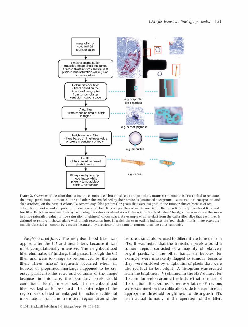
Neighbourhood filter. The neighbourhood filter wasapplied after the CD and area filters, because it wasmost computationally intensive. The neighbourhoodfilter eliminated FP findings that passed through the CDfilter and were too large to be removed by the areafilter. These ‘misses’ frequently occurred when airbubbles or preprinted markings happened to be ori-ented parallel to the rows and columns of the imagebecause, in this case, the boundary pixels wouldcomprise a four-connected set. The neighbourhoodfilter worked as follows: first, the outer edge of theregion was dilated or enlarged to include additionalinformation from the transition region around the

feature that could be used to differentiate tumour fromFPs. It was noted that the transition pixels around atumour region consisted of a majority of relativelybright pixels. On the other hand, air bubbles, forexample, were mistakenly flagged as tumour, becausethey were enclosed by a tight rim of pixels that werealso red (but far less bright). A histogram was createdfrom the brightness (V) channel in the HSV dataset forthe annular region around the feature that consisted ofthe dilation. Histograms of representative FP regionswere examined on the calibration slide to determine anappropriate threshold brightness to distinguish FPsfrom actual tumour. In the operation of the filter,

Image of lymphnode in RGB

representation

k-means segmentation- classifies image pixels into tumouror other clusters from scatterplot ofpixels in hue-saturation-value (HSV)

representation

Colour distance filter- filters based on the

distance of image pixelfrom tumour cluster

centroid in colour space

Area filter- filters based on area of pixels

in region

e.g. preprintedslide marking

e.g. carbon pigment

e.g. air bubble

e.g. debris

Neighbourhood filter- filters based on brightness value

for pixels in periphery of region

Hue filter- filters based on hue of

pixels in region

Binary overlay to lymphnode image: white

pixels = tumour, blackpixels = not tumour

Figure 2. Overview of the algorithm, using the composite calibration slide as an example: k-means segmentation is first applied to separate

the image pixels into a tumour cluster and other clusters defined by their centroids (unstained background, counterstained background and

slide artefacts) on the basis of colour. To remove any ‘false-positives’ or pixels that were assigned to the tumour cluster because of red

colour but do not actually represent tumour, there are four filter stages: the colour distance (CD) filter, area filter, neighbourhood filter and

hue filter. Each filter removes pixels by comparing the value calculated at each step with a threshold value. The algorithm operates on the image

in a hue-saturation value (or hue-saturation brightness) colour space. An example of an artefact from the calibration slide that each filter is

designed to remove is shown along with a high-resolution inset in which the cyan outline indicates the ‘red’ pixels (that is, these pixels are

initially classified as tumour by k-means because they are closer to the tumour centroid than the other centroids).



features with neighbouring regions containing enoughneighbourhood pixels having values below the bright-ness threshold were discarded as FPs (Figure 4E).

Hue filter. Finally, the hue filter was applied toremove image signals from any debris that took upchromogen and acquired a brown appearance. Ahistogram was generated from the hue (‘H’ in HSVspace) channel data from areas in the calibration slidethat were representative of tumour, and from the FPsthat failed to be filtered in the prior steps. Again, thelocal minimum (valley) in the bimodal distribution wasused to identify a threshold, chosen as the mean valuebetween the two peaks. True-positives were representedby the lower hue level (red), and FP pixels by the higherhue level (brown) (Figure 4F). The separation betweenthese peaks was unambiguous.

evaluation of cad: comparison with

lm-identif ied tumour

Once fully configured, the CAD algorithm was appliedto the test slides. Comparison of CAD output with LMidentification of tumour foci was automated by afunction written in Matlab to compare the CADfindings with the tumour foci identified under LM bythe pathologist. The digitized section, with annotations

(closed curves outlining each focus of metastasis asidentified on LM), was displayed on a monitor. TheCAD results after application of k-means clustering andthe four filtering steps were represented as a binaryimage (white pixels, tumour; black pixels, not tumour)overlaid on this image. The resulting image for onesection is shown in Figure 4G. For the per-sectionanalysis, sensitivity was calculated as the proportion ofthe 43 sections that contained any white pixels in theCAD representation of the metastases identified underLM. Specificity was calculated as the proportion of the59 tumour-free slides that contained no white pixels.For the per-focus task, sensitivity was calculated as thefraction of the number of LM-identified foci that werealso detected by CAD. This was calculated for fourgroupings of the data: (i) the entire set of 259 foci;(ii) ITCs; (iii) micrometastases in the size range0.2–2 mm; and (iv) metastases >2 mm. In addition,the total number of FP foci ‘detected’ on each slide bythe algorithm was enumerated, as specificity is unde-fined for this per-focus detection.

Results

The pathologists compared initial digitization of slidesat 0.33 lm with the downsampled resolution of

200 µm

1

0.5

Val

ue

Blu

e0

200

A B

C D

100

00

100200 0

100200

Green

Red

10.5

0Hue

1

0.5

Saturation0

1

0.5

Val

ue

01

0.50

Hue1

0.5Saturatio

n0

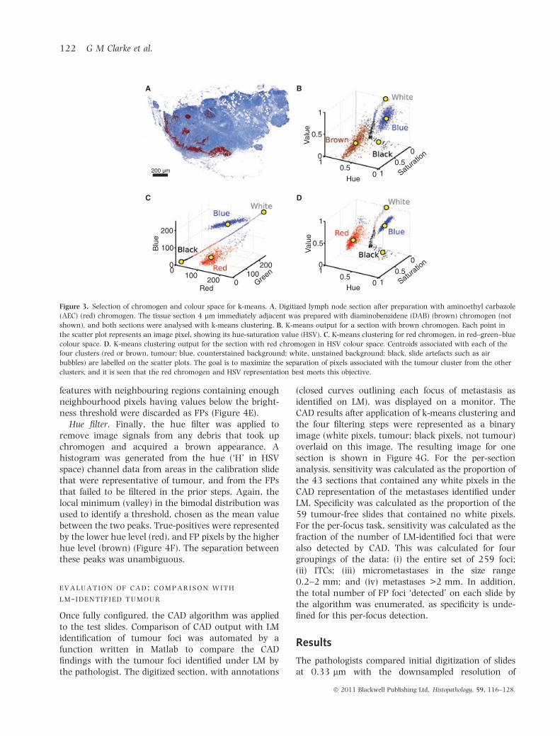
Figure 3. Selection of chromogen and colour space for k-means. A, Digitized lymph node section after preparation with aminoethyl carbazole

(AEC) (red) chromogen. The tissue section 4 lm immediately adjacent was prepared with diaminobenzidene (DAB) (brown) chromogen (not

shown), and both sections were analysed with k-means clustering. B, K-means output for a section with brown chromogen. Each point in

the scatter plot represents an image pixel, showing its hue-saturation value (HSV). C, K-means clustering for red chromogen, in red–green–blue

colour space. D, K-means clustering output for the section with red chromogen in HSV colour space. Centroids associated with each of the

four clusters (red or brown, tumour; blue, counterstained background; white, unstained background; black, slide artefacts such as air

bubbles) are labelled on the scatter plots. The goal is to maximize the separation of pixels associated with the tumour cluster from the other

clusters, and it is seen that the red chromogen and HSV representation best meets this objective.



1.33 lm, and determined that there was no lossof diagnostic information in the task of detectingmetastases.

determination of lm diagnosis

The agreement between the two pathologist readers inthe task of identifying and defining the extent of thelargest focus in each section under light microscopywas 100%. In the per-focus analysis, disagreementoccurred for approximately 30% of the sections that

contained tumour (13 ⁄ 43). All disagreement wasdiagnostically insignificant (e.g. related to incompleteinspection of the slide and identification of all of thefoci). Of the sections for which there was disagreement,approximately half demonstrated a diffuse tumourpattern.

algorithm development: f ilter thresholds

The histogram of CD was found to be bimodal, and onthe basis of identification of its local minimum, pixels

1

A

C D

G

E F

B

0.5

Val

ue

01

0.50 0 0 50 100 0.4 0.6 0.8

Hue HueColour distance % of neighbourhoodpixels with value > T

10.5

Red-blue

Black-white

Black-white

“TP”

“TP”

“TP”“FP”

“FP”

“FP”Brown

0.5Satu

ratio

n0

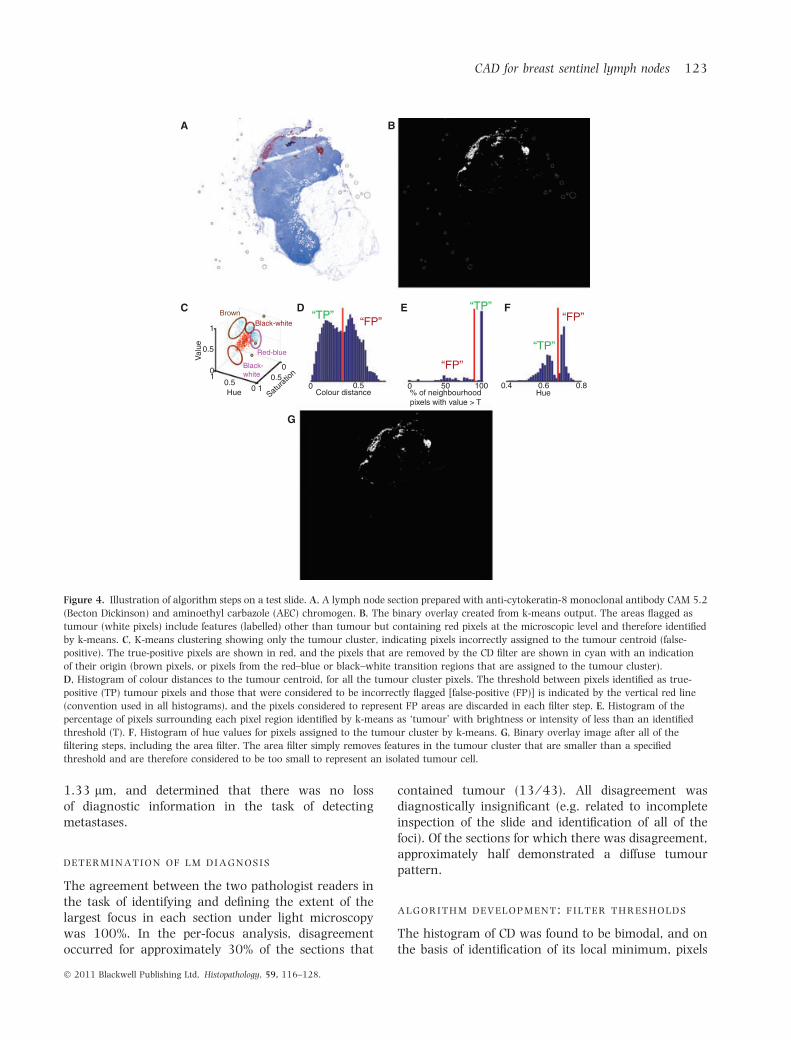
Figure 4. Illustration of algorithm steps on a test slide. A, A lymph node section prepared with anti-cytokeratin-8 monoclonal antibody CAM 5.2

(Becton Dickinson) and aminoethyl carbazole (AEC) chromogen. B, The binary overlay created from k-means output. The areas flagged as

tumour (white pixels) include features (labelled) other than tumour but containing red pixels at the microscopic level and therefore identified

by k-means. C, K-means clustering showing only the tumour cluster, indicating pixels incorrectly assigned to the tumour centroid (false-

positive). The true-positive pixels are shown in red, and the pixels that are removed by the CD filter are shown in cyan with an indication

of their origin (brown pixels, or pixels from the red–blue or black–white transition regions that are assigned to the tumour cluster).

D, Histogram of colour distances to the tumour centroid, for all the tumour cluster pixels. The threshold between pixels identified as true-

positive (TP) tumour pixels and those that were considered to be incorrectly flagged [false-positive (FP)] is indicated by the vertical red line

(convention used in all histograms), and the pixels considered to represent FP areas are discarded in each filter step. E, Histogram of the

percentage of pixels surrounding each pixel region identified by k-means as ‘tumour’ with brightness or intensity of less than an identified

threshold (T). F, Histogram of hue values for pixels assigned to the tumour cluster by k-means. G, Binary overlay image after all of the

filtering steps, including the area filter. The area filter simply removes features in the tumour cluster that are smaller than a specified

threshold and are therefore considered to be too small to represent an isolated tumour cell.



with CD from the tumour centroid of <0.342 (dimen-sionless distance measured in HSV space) were retainedas being representative of tumour, and those above thisthreshold were treated as FPs. For the neighbourhoodvalue filter, the appropriate threshold determined fromthe brightness histogram of neighbouring pixels was0.3, to separate regions surrounding tumour (bright-ness >0.3) from regions surrounding FPs (brightness<0.3). It was also necessary to impose the requirementthat more than 90% of the border pixels in the regionhave brightness >0.3 for accurate classification astumour. Finally, also on the basis of the identification ofa local minimum, the hue filter was defined bydiscarding those pixels with a hue above 0.679, whichbest separates tumour (red, hue <0.679) from FPs(brown, hue >0.679). When the histograms werecalculated for 5–10 different areas on the calibrationslide representing each feature (tumour, counterstain,unstained background, air bubble, debris and preprint-ed markings on the slide), all thresholds were found tobe reproducible.

evaluation of cad: comparison with

lm-identif ied tumour

The performance of CAD is summarized in Table 2.False-negatives occurred only in the per-focus task, and

all of these, as well as the single FP, were re-reviewedby the pathologist (J.Z.).

For both detection tasks, CAD identified additionalfoci that were not identified in the LM evaluation. Uponreview by the pathologist, these were confirmed to bemetastases. On one slide, CAD identified an ITC thatwas categorised as ‘Negative for malignancy’ by LM inthe per-slide detection task. In the per-focus task, CADidentified an additional nine foci that were not identi-fied by LM. These are characterized in Figure 5 in termsof their diameter and distance from the nearest focus.

Table 2. Summary of computer-assisted detection performance

Sensitivity Specificity False positives

Per-slide 100%[91.8–100%](n = 43)

100%[93.8–100%](n = 59)

0

Per-focusAll 75.7%

[70.0–80.8%](n = 259)

NA (undefined) 0

Metastases >2 mm 100%[86.3–100%](n = 25)

NA 0

Micrometastases 89.5%[82.3–94.4%](n = 114)

NA 0

Isolated tumour cells 57.5%[48.2–66.5%](n = 120)

NA 1

NA, not applicable.

The 95% exact binomial confidence interval for each quantity is shown in square brackets, and the sample size for the categoryin parentheses.49

0 50 100 150 200 250 300 350Diameter of focus not identified using LM (µm)

350030002500200015001000500

0

Dis

tanc

e to

nea

rest

focu

sid

entif

ied

usin

g LM

(µm

)

Figure 5. Characterization of additional findings in computer-assisted

detection that were not made by light microscopy. For each of the

nine additional findings, the size of the focus, as established by

pathologist on re-review, and the distance of the focus to its nearest

neighbour are shown. Note that the points in the lower left and upper

left of the figure each contain two foci that overlap.



Discussion

This algorithm has several desirable features for theidentification of IHC-positive SLN metastases. Because itis automated, it can allow more intensive samplingwithout overtaxing human resources. The morphologyof the metastasis is preserved, and in our tests there was100% sensitivity and 100% specificity for the per-slidedetection task. Although sensitivity was <100% for theper-focus task, no slide on which there were metastaseswas called negative by the algorithm. In approximatelyhalf of the 43 slides with metastases, the largest focus oftumour was classified as a micrometastasis (44%) orITC (7%) (Figure 1), so our results support the sugges-tion that the algorithm would reliably detect smalltumour deposits to assist a pathologist in clinical work.

Considering published rates of conversion fromnegative to positive diagnosis on re-review in LM,11

we deemed the acceptable target sensitivity for CAD tobe 97%. We also set the target specificity at 97%. Weconsider that performance at this level would fulfil thegoal of CAD to effectively minimize reader involvementin analysing the large datasets generated from seriallysectioned nodes. Our algorithm more than fulfilled thisgoal on the per-slide detection task. With the use of a95% confidence interval, sensitivity and specificity withexact binomial confidence limits were 91.8–100% and93.8–100%, respectively.49 For the more challengingper-focus detection task, a lower sensitivity would beacceptable, and currently the algorithm has achieved asensitivity of 75.7%, with a 95% confidence limit of70.0–80.8%. The algorithm as tested probably outper-forms what would be required in a practical diagnosticsetting. In clinical practice, there would be multiplesections taken from a single node or patient to cross-reference, so that even if a metastasis were to be missedon one section, it would probably be detected in asubsequent section.

In the per-focus detection task, we encountered onlya single instance in which a feature was falselyidentified as a metastasis. We note, however, that ourtest does not model the way in which a diagnosis isactually made, but rather was performed to allow us toevaluate the algorithm more thoroughly with a largernumber of foci and a wider variety of features. Aftervery careful scrutiny by a pathologist, this FP CADfinding was confirmed to be caused by out-of-planeproteinaceous debris. This material included a largeenough area of four-connected pixels to satisfy theconditions of the area filter, was sufficiently distantfrom any very dark areas to escape the neighbourhoodfilter, and had appropriate colour characteristics suchthat it was not removed by either the CD or hue filter.

The vast majority of benign cells in a lymph nodethat would react with the anti-cytokeratin antibodytook up the stain sufficiently lightly that their locationin HSV space was closer to the centroid associatedwith unstained background than to the centroid thatidentified metastasis. Those outliers that were closer tothe tumour centroid were removed by the CD filter and,in the cases where that failed, the area threshold of 45pixels (10 lm) prevented these isolated cells (e.g.dendritic cells, stained red) from being falsely identifiedas metastases. The algorithm is robust, and did not failwhen it encountered a variety of artefacts or otherstructures such as haemosiderin (which can have a redappearance) and carbon pigment.

Significant failures did occur, however, in the per-focus detection task for increasingly smaller tumourdeposits. This resulted in part from variability in thequality of staining. False-negatives occurred only forITCs and micrometastases, which were detected withsensitivities of 57.5% and 89.5%, respectively. WhereCAD missed these lesions, the staining quality wastypically very poor (e.g. lack of staining in the interiorof the focus and incomplete staining around the entiremembrane). In one case that was initially consideredfor inclusion in the study, a complete lack of stainingfor low molecular weight keratin in the metastasis wasobserved. In this scenario, CAD is guaranteed to fail.The choice of antibody in this study (low molecularweight keratin, CAM 5.2) detects only cytokeratins 7and 8, whereas there are 20 different types of cytoker-atin. Although incomplete staining attributable to lackof expression of these specific cytokeratins may beovercome by a pathologist reader, who makes adiagnosis on the basis of morphological information,a more appropriate antibody for use with CAD might bepan-keratin, for example, which can bind a muchwider range of cytokeratins.

Poor staining was especially problematic in thisstudy for tumours presenting a diffuse pattern withsmall and scattered cells that were not crisply outlinedby the stain. Such a pattern is more typical of thelobular subtype. Compared with tumours with a morelocalized pattern, the algorithm was about twice aslikely to miss a focus in these types of image. Of the 43slides that contained tumour, about 25% (11 ⁄ 43)represented lobular cancers but, conversely, the lobularsubtype occurred in about half of the images in which afalse-negative occurred (6 ⁄ 14). Similarly, about half ofthe ‘lobular’ images (6 ⁄ 11) contained a false-negativefocus, as opposed to about 20% (6 ⁄ 32) of the imagesdemonstrating ductal carcinoma. Mesker et al.38

reported one false-negative in their CAD assessment,and this was attributable to a 24-lm ITC of infiltrating



lobular carcinoma pleomorphic type. It has been notedthat diffuse tumour patterns present a significantchallenge in lymph node diagnosis, even for experi-enced readers.41–44

In this study, the sections were mounted in a mannerthat attempted to reduce artefacts in the CAD algo-rithm. This may have exacerbated problems associatedwith inadequate quality of staining. AEC was selectedas the chromogen to facilitate segmentation of metas-tasis on the basis of colour (red). However, as AEC isnot compatible with traditional alcohol-based mount-ing media, no glass coverslip was used initially; instead,an aqueous mounting medium was employed. This is avery poor choice for imaging, as the air bubbles, whichwould normally be ruptured by the application of thecover glass, remained. In the black–white transitionregion around the bubbles, these occasionally createdFP pixels. This necessitated additional processing timefor the filters, and significantly confounded the detec-tion of underlying true-positive pixels.

These problems were subsequently mitigated byusing ImmuMount� (Shandon Thermo Electron Cor-poration, Pittsburgh, PA, USA), an aqueous mountingmedium that is compatible with AEC and glass cover-slipping. Although this improved image quality andCAD performance dramatically, it is possible that thewashing of the original mounting medium removedsome chromogen. Furthermore, the manufacturerspecifications suggest that the stain may fade after1 year from the application of ImmuMount and, in fact,at 1.5 years, noticeable or, in some cases, considerable,fading was observed in the majority of the slides. This,of course, did not affect the performance of the CADalgorithm, as the slides were digitized shortly afterpreparation.

Another technical modification in the slide prepara-tion that could be adopted in a follow-up study toimprove sensitivity is the replacement of a red chro-mogen with a pink one (e.g. Fast Red). Theoretically,this would achieve increased separation of the tumourclusters (pink) from the others (blue, white, and black)in the colour space.

In this study, there were 10 instances of additionalCAD findings that were not initially detected by eitherpathologist on LM review. One of these additionalfindings (a 25-lm ITC) occurred in the per-slideanalysis (that is, the slide was initially called negativefor any malignancy under LM). The other nineadditional findings occurred in the per-focus analysis,and were therefore additional foci found by CAD inslides where the pathologist had already identified atleast one focus under LM. Overall, 1.7% of the slidesinitially categorised as negative were converted to

positive, and 3.3% of the total 259 tumour foci wereinitially identified by CAD alone.

Our results are in line with other reports of CADdetecting small (0.01–0.3 mm) metastases that weremissed in review by a trained pathologist under LM,citing a 3–12% rate of diagnostic conversion (subse-quently confirmed by the pathologist) after applicationof CAD.37,38 The additional CAD findings in our studyfrom the per-focus analysis, as characterized in Fig-ure 5, can probably be attributed to factors such ashuman fatigue (e.g. upper left quadrant of the figure,small metastasis far from other foci), incomplete visualsearch of sections (e.g. upper right quadrant, largemetastases far from other foci), or inconsistent appli-cation of the instructions, i.e. the ‘200-lm rule’ usedto distinguish separate foci (e.g. lower quadrants, fociclose to another focus that was identified by thepathologist).

We found that the amount of user interventionrequired in application of the CAD algorithm wasminimal, and that the processing was performedefficiently. However, user intervention is essential tocontrol for batch-to-batch variations in staining andachieve accurate calibration. This requires about 5–10 min per batch (each batch consists of about 30–50slides for typical automatic immunostainers). In addi-tion, about 5 min is required to set up each run of 50slides, which is the capacity of the automatic slidescanner currently in use. Slides are then scannedautomatically at a rate of approximately six slidesper hour.

Depending on the size of the section to be digitized,the amount of data per image ranges from 7 to365 MB, plus an additional 5–6 MB of temporaryspace for interim files (e.g. binary masks). For thisresearch, the per-slide processing time of 6–8 min wasachieved by running Matlab on a 64-bit platform,using a two-quad-core Intel Xeon X5365, 3-GHzprocessor with 32 GB of RAM.

This computational capacity generally exceeds whatis available in most clinical laboratories, but digitalprocessing speed can be increased enormously throughthe use of more efficient programming languages thanMatlab, which is optimized for flexibility during algo-rithm development, not for speed. Therefore, processingtime should not be a barrier in the long term. Theprocessing time that we report compares favourablywith the 30–40 min reported by Weaver in 200337

and the <20 min per slide in 2004.38

The choice of the k-means tumour clustering algo-rithm also provides increased computational efficiencyas compared with iterative algorithms, which wouldrequire considerably greater processing time on these



large datasets. Besides efficiency, the choice of algo-rithm and filters confers robustness. K-means offers theflexibility of redefining the centroids or classifying thepixels to account for variations in the stain intensity.Once the centroids have been obtained, the pixelscan be classified relatively quickly, as only a distancemeasure needs to be performed for each pixel. This is incontrast to ‘fuzzy’ algorithms, which classify on thebasis of distance and probability. Specificity wasincreased by application of the filters, which effectivelyremoved FPs. The filter that most dramaticallyimproved specificity was the CD filter. Even in caseswhere the CD filter alone failed to eliminate an FP, itfacilitated identification of the FP by the neighbour-hood value filter, because it accomplished a reductionin the black–white transition regions.

We have shown that automated detection of SLNmetastases in histological sections can be achieved withvery high sensitivity on a per-slide basis and very highspecificity. The per-focus sensitivity for metastases>2 mm in extent was 100%. For micrometastasesand ITCs, the sensitivities were 89.5% and 57.5%,respectively, and can be improved by more rigid qualitycontrol in IHC staining. This technique maymake intensive sampling of SLNs more practical, toimprove the accuracy of detection of small lymph nodemetastases.

Acknowledgements

We are grateful for the contributions of Lisa Dang,Marko Katic, Kevin Kwok and Laibao Sun to this work.This work was supported financially by a ProgramProject Grant, ‘Medical Imaging for Cancer (#17005),from The Terry Fox Foundation.

References

1. Fisher ER, Palekar A, Rockette H et al. Pathologic findings from

the National Surgical Adjuvant Breast Project (Protocol No. 4).

V. Significance of axillary nodal micro- and macrometastases.

Cancer 1978; 42; 2032–2038.

2. Fisher ER, Anderson S, Redmond C et al. Pathologic findings from

the National Surgical Adjuvant Breast Project protocol B-06. 10-

year pathologic and clinical prognostic discriminants. Cancer

1993; 71; 2507–2514.

3. Sobin L, Wittekind C eds. UICC TNM: classification of malignant

tumours, 6th edn. New York: Wiley-Liss, 2002.

4. Edge SB, Byrd DR, Compton CC et al. eds. AJCC cancer staging

manual, 7th edn. New York: Springer-Verlag, 2010.

5. Kuerer HM, Newman LA. Lymphatic mapping and sentinel

lymph node biopsy for breast cancer: developments and resolving

controversies. J. Clin. Oncol. 2005; 23; 1698–1705.

6. Veronesi U, Paganelli G, Viale G et al. Sentinel lymph node biopsy

and axillary dissection in breast cancer: results in a large series.

J. Natl Cancer Inst. 1999; 91; 368–373.

7. Derossis AM, Fey J, Yeung H et al. A trend analysis of the relative

value of blue dye and isotope localization in 2,000 consecutive

cases of sentinel node biopsy for breast cancer. J. Am. Coll. Surg.

2001; 193; 473–478.

8. Giuliano AE, Jones RC, Brennan M et al. Sentinel lymphadenec-

tomy in breast cancer. J. Clin. Oncol. 1997; 15; 2345–2350.

9. Baron RH, Fey JV, Borgen PI et al. Eighteen sensations after

breast cancer surgery: a 5-year comparison of sentinel lymph

node biopsy and axillary lymph node dissection. Ann. Surg. Oncol.

2007; 14; 1653–1661.

10. Treseler PA, Tauchi PS. Pathologic analysis of the sentinel lymph

node. Surg. Clin. North Am. 2000; 80; 1695–1719.

11. Weaver DL, Krag DN, Ashikaga T et al. Pathologic analysis of

sentinel and nonsentinel lymph nodes in breast carcinoma: a

multicenter study. Cancer 2000; 88; 1099–1107.

12. Lyman GH, Giuliano AE, Somerfield MR et al. American Society

of Clinical Oncology guideline recommendations for sentinel

lymph node biopsy in early-stage breast cancer. J. Clin. Oncol.

2005; 23; 7703–7720.

13. Krag DN, Anderson SJ, Julian TB et al. Primary outcome results

of NSABP B-32, a randomized phase III clinical trial to compare

sentinel node resection (SNR) to conventional axillary dissection

(AD) in clinically node-negative breast cancer patients. J. Clin.

Oncol. 2010; 28(18 Suppl.); LBA505.

14. Giuliano AE, Dale PS, Turner RR et al. Improved axillary staging

of breast cancer with sentinel lymphadenectomy. Ann. Surg.

1995; 222; 394–399; discussion 9–401.

15. Rampaul RS, Miremadi A, Pinder SE et al. Pathological valida-

tion and significance of micrometastasis in sentinel nodes in

primary breast cancer. Breast Cancer Res. 2001; 3; 113–116.

16. Treseler P. Pathologic examination of the sentinel lymph node:

whatisthebestmethod? BreastJ.2006;12(5Suppl.2);S143–S151.

17. Fitzgibbons PL, Page DL, Weaver D et al. Prognostic factors in

breast cancer. College of American Pathologists Consensus

Statement 1999. Arch. Pathol. Lab. Med. 2000; 124; 966–978.

18. Huvos AG, Hutter RV, Berg JW. Significance of axillary

macrometastases and micrometastases in mammary cancer.

Ann. Surg. 1971; 173; 44–46.

19. Singletary SE, Allred C, Ashley P et al. Staging system for breast

cancer: revisions for the 6th edition of the AJCC Cancer Staging

Manual. Surg. Clin. North Am. 2003; 83; 803–819.

20. de Boer M, van Deurzen CH, van Dijck JA et al. Micrometastases

or isolated tumor cells and the outcome of breast cancer. N. Engl.

J. Med. 2009; 361; 653–663.

21. Sakorafas GH, Geraghty J, Pavlakis G. The clinical significance of

axillary lymph node micrometastases in breast cancer. Eur. J.

Surg. Oncol. 2004; 30; 807–816.

22. Colleoni M, Rotmensz N, Peruzzotti G et al. Size of breast cancer

metastases in axillary lymph nodes: clinical relevance of minimal

lymph node involvement. J. Clin. Oncol. 2005; 23; 1379–1389.

23. Cote R, Giuliano AE, Hawes D et al. ACOSOG Z0010: a

multicenter prognostic study of sentinel node (SN) and bone

marrow (BM) micrometastases in women with clinical

T1 ⁄ T2 N0 M0 breast cancer. J. Clin. Oncol. 2010; 28(18 Suppl.);

CRA504.

24. van Deurzen CH, de Boer M, Monninkhof EM et al. Non-sentinel

lymph node metastases associated with isolated breast cancer

cells in the sentinel node. J. Natl Cancer Inst. 2008; 100; 1574–

1580.

25. Pickren JW. Significance of occult metastases. A study of breast

cancer. Cancer 1961; 14; 1266–1271.

26. Saphir O, Amromin G. Obscure axillary lymph node metastasis in

carcinoma of the breast. Cancer 1948; 1; 238–241.



27. Rushing L, Joste N. The surgical pathology report: standardizing

the ‘gold standard’. J. Surg. Oncol. 1997; 65; 1–2.

28. Galea MH, Athanassiou E, Bell J et al. Occult regional lymph node

metastases from breast carcinoma: immunohistological detection

with antibodies CAM 5.2 and NCRC-11. J. Pathol. 1991; 165;

221–227.

29. Trojani M, de Mascarel I, Bonichon F et al. Micrometastases to

axillary lymph nodes from carcinoma of breast: detection by

immunohistochemistry and prognostic significance. Br. J. Cancer

1987; 55; 303–306.

30. Cote RJ, Peterson HF, Chaiwun B et al. Role of immunohisto-

chemical detection of lymph-node metastases in management of

breast cancer. International Breast Cancer Study Group. Lancet

1999; 354; 896–900.

31. Dowlatshahi K, Fan M, Snider HC et al. Lymph node microme-

tastases from breast carcinoma: reviewing the dilemma. Cancer

1997; 80; 1188–1197.

32. Cummings MC, Walsh MD, Hohn BG et al. Occult axillary

lymph node metastases in breast cancer do matter: results of

10-year survival analysis. Am. J. Surg. Pathol. 2002; 26; 1286–

1295.

33. Weaver DL, Le UP, Dupuis SL et al. Metastasis detection in

sentinel lymph nodes: comparison of a limited widely spaced

(NSABP protocol B-32) and a comprehensive narrowly spaced

paraffin block sectioning strategy. Am. J. Surg. Pathol. 2009; 33;

1583–1589.

34. Apostolikas N, Petraki C, Agnantis NJ. The reliability of histo-

logically negative axillary lymph nodes in breast cancer.

Preliminary report. Pathol. Res. Pract. 1988; 184; 35–38.

35. International (Ludwig) Breast Cancer Study Group. Prognostic

importance of occult axillary lymph node micrometastases from

breast cancers. Lancet 1990; 335; 1565–1568.

36. Cserni G. Complete sectioning of axillary sentinel nodes in

patients with breast cancer. Analysis of two different step

sectioning and immunohistochemistry protocols in 246 patients.

J. Clin. Pathol. 2002; 55; 926–931.

37. Weaver DL. Occult ‘micrometastases’ in ductal carcinoma

in situ: investigative implications for sentinel lymph node biopsy.

Cancer 2003; 98; 2083–2087.

38. Mesker WE, Torrenga H, Sloos WC et al. Supervised automated

microscopy increases sensitivity and efficiency of detection of

sentinel node micrometastases in patients with breast cancer.

J. Clin. Pathol. 2004; 57; 960–964.

39. Weaver DL, Krag DN, Manna EA et al. Comparison of patholo-

gist-detected and automated computer-assisted image analysis

detected sentinel lymph node micrometastases in breast cancer.

Mod. Pathol. 2003; 16; 1159–1163.

40. Weaver DL, Krag DN, Manna EA et al. Detection of occult

sentinel lymph node micrometastases by immunohistochemistry

in breast cancer. An NSABP protocol B-32 quality assurance

study. Cancer 2006; 107; 661–667.

41. Apple SK, Moatamed NA, Finck RH et al. Accurate classification

of sentinel lymph node metastases in patients with lobular breast

carcinoma. Breast 2010; 19; 360–364.

42. Cserni G, Sapino A, Decker T. Discriminating between microm-

etastases and isolated tumor cells in a regional and institutional

setting. Breast 2006; 15; 347–354.

43. Roberts CA, Beitsch PD, Litz CE et al. Interpretive disparity

among pathologists in breast sentinel lymph node evaluation.

Am. J. Surg. 2003; 186; 324–329.

44. Turner RR, Weaver DL, Cserni G et al. Nodal stage classification

for breast carcinoma: improving interobserver reproducibility

through standardized histologic criteria and image-based train-

ing. J. Clin. Oncol. 2008; 26; 258–263.

45. Kohrt HE, Nouri N, Nowels K et al. Profile of immune cells in

axillary lymph nodes predicts disease-free survival in breast

cancer. PLoS Med. 2005; 2; e284.

46. Holmes S, Kapelner A, Lee PP. An interactive Java statistical

image segmentation system: GemIdent. J. Stat. Softw. 2009; 30;

1–20.

47. Jain K, Dubes R. Algorithms for clustering data. Englewood Cliffs,

NJ: Prentice Hall, 1988.

48. Rosenfeld A, Avinash CK. Digital picture processing, 2nd edn. New

York: Academic Press, 1982.

49. Rosner B. Fundamentals of biostatistics, 6th edn. Belmont, CA:

Thomson-Brooks ⁄ Cole, 2006.



development and evaluation of a robust algorithm for computer-assisted detection of sentinel lymph...

Documents