development and design space exploration of deep

DEVELOPMENT AND DESIGN SPACE EXPLORATION OF DEEP

CONVOLUTION NEURAL NETWORK FOR IMAGE RECOGNITION

A Thesis Submitted to the Department of

Computer Science

African University of Science and Technology

In Partial Fulfilment of the Requirements for the Degree of

MASTER of Computer Science

By

Aboki Nasiru Aliu

Abuja, Nigeria

November, 2017

ii

CERTIFICATION

This is to certify that the thesis titled “Development and Design Space Exploration of Deep

Convolution Neural Network for Image Recognition” submitted to the school of postgraduate

studies, African University of Science and Technology (AUST), Abuja, Nigeria for the award

of the Master's degree is a record of original research carried out by Aboki Nasiru Aliu in the

Department of Computer Science.

iii

DEVELOPMENT AND DESIGN SPACE EXPLORATION OF DEEP

CONVOLUTION NEURAL NETWORK FOR IMAGE RECOGNITION

By

ABOKI Nasiru Aliu

A THESIS APPROVED BY THE COMPUTER SCIENCE

DEPARTMENT

RECOMMENDED:

Supervisor, Prof. Ben Abdallah

Co-supervisor

Head, Department of Computer Science

APPROVED:

Chief Academic Officer

Date

iv

COPYRIGHT

© 2017

Aboki Nasiru Aliu

ALL RIGHTS RESERVED

v

ABSTRACT

Deep Neural Networks are now deployed for many modern artificial Intelligence applications

including computer vision, speech recognition, self-driving cars, cancer detection, gaming and

robotics.

Inspired by the mammalian visual cortex, Convolutional Neural Networks (CNNs) have been

shown to achieve impressive results on a number of computer vision challenges, but often

with large amounts of processing power and no timing restrictions. Software simulations of

CNNs are an efficient way to evaluate and explore the performance of the system.

In this thesis, I present a software implementation and study of a Deep CNN for image

recognition. The parameterization of our design offers the flexibility to adjust the design in

order to balance performance and flexibility, particularly for resource-constrained systems. I

also present a design space exploration for obtaining the implementation with the highest

performance on a given platform.

vi

ACKNOWLEDGEMENTS

Success is said to be achieved when preparation coincides with opportunity. I want to

acknowledge the enormous sacrifice of my dearest treasure and darling wife, Mrs. Fajemi

Comfort Aboki, for showing me the biggest support throughout the course of this masters’

program and for adding to my joy by giving me a lovely son, Jaden Zebada Aboki, during the

course of the masters’ program. Much gratitude goes to all the Faculty that have contributed

a wealth of knowledge that has given me the confidence to carry out this research. I really

want to appreciate my supervisor, Prof. Ben Abdallah for generously taking his time to guide

me through this project to produce the best in my thesis work and I am thankful for his words

of encouragement which reminded me that I can achieve anything I put my mind to

accomplish. I also want to thank AUST for providing me with such an opportunity and platform

to advance my knowledge in my current academic discipline. I am also grateful to all my class

and set mates for their encouragements and contributions that have enabled me to be

successful during our stay in AUST. The race has not been easy but God has been faithful.

Much gratitude goes to Mr. Isah Charles Saidu, once again you have proved yourself a good

friend and helper. I want to acknowledge the efforts and contributions of my Father and Mother

In-law and the rest of their Family. You are all a gift to me and God sent and I cherish you all

for you have been with my wife and I through thick and thin. To my Elder Brother, Dr.

Nuruddeen and Family, we are really grateful for your love, support and encouragement as

well. I am also grateful to my fellow residents of Red Roof Mini-Estate for all their help, love

and support as well. To the rest of my grand Family, I want to say a big thank you for all the

roles you have played in my life that has made me come this far. May God continue to crown

all your efforts with success. Amen!!!

vii

DEDICATION

I dedicate this thesis to God Almighty, for giving me the strength, enablement, vision and

purpose to go thus far in my academic pursuits. I also dedicate this thesis to the memory of

the loved ones I lost too soon, My darling Mother, Mrs. Betty Aisha A. Lukolm, My dearest

Dad, Mr. Aliu Ango Aboki and my sweetest and most enduring sister, Hadiza Ladi Aboki.

viii

TABLE OF CONTENTS

CERTIFICATION ...................................................................................................................ii

ABSTRACT ........................................................................................................................... v

ACKNOWLEDGEMENTS ..................................................................................................... vi

DEDICATION ....................................................................................................................... vii

LIST OF TABLES .................................................................................................................. x

LIST OF FIGURES ............................................................................................................... x

LIST OF ABBREVIATIONS .................................................................................................. xii

CHAPTER ONE Introduction ........................................................................................... 1

1.1 Introduction to Neuro-Inspired Systems ................................................................ 1

1.2 Statement of the Problem ..................................................................................... 2

1.3 Motivation ............................................................................................................. 3

1.4 Research Objective ............................................................................................... 4

1.5 Significance of Study ............................................................................................ 5

1.6 Thesis Outline ....................................................................................................... 5

1.6.1 Chapter 1 – Introduction to Neuro-inspired Systems ......................................... 5

1.6.2 Chapter 2 – Literature Review (Related work about Image Recognition) .......... 5

1.6.3 Chapter 3 – Study of Image Recognition Algorithm Using Supervised Learning Algorithms 5

1.6.4 Chapter 4 – Evaluation and Discussion ............................................................ 5

1.6.5 Chapter 5 – Conclusion and Future Work ......................................................... 6

CHAPTER TWO Literature Review .................................................................................. 7

2.1 Introduction ........................................................................................................... 7

2.2 Computer Vision Supervised Machine Learning Classifiers .................................. 7

2.2.1 Pairwise Support Vector Machine ..................................................................... 7

2.2.2 K-Nearest-Neighbour (K-NN with Euclidean Distance) ..................................... 9

2.2.3 Deep Convolutional Neural Networks ............................................................. 10

2.3 Machine Learning Algorithms .............................................................................. 11

2.3.1 Unsupervised Machine Learning Algorithm ..................................................... 11

2.3.2 Reinforcement Machine Learning Algorithm ................................................... 12

2.3.3 Supervised Machine Learning Algorithm ........................................................ 13

2.3.4 Backpropagation Learning Algorithm .............................................................. 13

2.4 Conclusion .......................................................................................................... 23

CHAPTER THREE Methodology ....................................................................................... 24

3.1 Introduction of Deep Convolutional Neural Networks .......................................... 24

ix

3.2 Topology of Deep Convolutional Neural Networks .............................................. 25

3.3 Layers of Deep Convolutional Neural Networks .................................................. 25

3.3.1 Convolutional Layer ........................................................................................ 25

3.3.2 Activation Layer .............................................................................................. 26

3.3.3 Down-Sampling or Pooling Layer ................................................................... 27

3.3.4 Fully Connected Layer .................................................................................... 28

3.4 Learning Algorithm of Deep Convolutional Neural Networks ............................... 29

CHAPTER FOUR Implementation.................................................................................... 32

4.1 Introduction to the Implementation ...................................................................... 32

4.2 Model Implementation of the Deep Convolutional Neural Networks .................... 32

4.3 Test Results of the Convolutional Neural Network Model .................................... 34

4.4 Test Observation and Discussion ........................................................................ 38

CHAPTER FIVE Evaluation and Conclusion .................................................................. 39

5.1 Introduction ......................................................................................................... 39

5.2 Evaluation of various Deep Convolutional Neural Network Models ..................... 39

5.2.1 Training Time Against Filter Size Evaluation ................................................... 40

5.2.2 Training Time Against Activation Function Evaluation .................................... 41

5.2.3 Accuracy Against Activation Function Evaluation............................................ 42

5.2.4 Accuracy Against Filter Size Evaluation .......................................................... 43

5.3 Future Work ........................................................................................................ 43

5.3.1 Data Augmentation ......................................................................................... 44

5.3.2 Transfer Learning ........................................................................................... 44

5.3.3 Object Localization, Detection and Segmentation ........................................... 45

5.4 Discussion and Conclusion ................................................................................. 46

5.4.1 Contribution to Deep Performance CNN Modelling ......................................... 46

5.4.2 Conclusion...................................................................................................... 47

REFERENCES ................................................................................................................... 48

x

LIST OF TABLES

Table 2.1: Probabilistic Table for Rainfall Occurrence ................................................. 14

Table 2.2: Normalized Probabilistic Table for Rainfall Occurrence .............................. 15

Table 2.3: Normalized Probabilistic Table for Rainfall Occurrence with Output Errors(Ȳ) .................................................................................................................. 19

Table 2.4: Final Normalized Probabilistic Table for Rainfall Occurrence ..................... 22

Table 2.5: Final Probabilistic Table for Rainfall Occurrence ........................................ 22

Table 5.1: Training & Test Accuracy Table for the Convolutional Neural Network Models ....................................................................................................... 40

LIST OF FIGURES

Figure 1.1: Object Recognition in Machines and Humans .............................................. 3

Figure 2.1: Pairwise SVM Image Classification .............................................................. 8

Figure 2.2: K-NN Image Classification ........................................................................... 9

Figure 2.3: A Deep Convolutional Neural Network ....................................................... 11

Figure 2.4: A Neural Network for Rainfall Predictions ................................................... 15

Figure 2.5: Sigmoid Activation Function ....................................................................... 16

Figure 2.6: A Rectified Linear Unit Activation Function ................................................. 17

Figure 2.7: A Tanh Activation Function ........................................................................ 18

Figure 2.8: Forward Propagation.................................................................................. 18

Figure 2.9: A Neural Network for Rainfall Predictions with Random Weight Values ..... 19

Figure 2.10: Backward Pass .......................................................................................... 20

Figure 2.11: Weights Updates ........................................................................................ 20

Figure 2.12: Final Optimal Weights ................................................................................ 20

Figure 2.13: A Neural Network for Rainfall Predictions with Optimal Weight Values ...... 21

Figure 3.1: Structure of A Convolutional Neural Network ............................................. 24

Figure 3.2: Element-Wise Multiplication and Summation Convolution .......................... 26

Figure 3.3: A Rectified Feature Map Transformation .................................................... 27

Figure 3.4: A Max-Pooling Transformation ................................................................... 28

Figure 3.5: A Fully Connected Layer Transformation ................................................... 28

Figure 3.6: A Gradient Descent Slope .......................................................................... 29

Figure 4.1: Class Label and Test Image ....................................................................... 35




xi







Figure 5.1: Training Time Against Filter Size ............................................................... 40

Figure 5.2: Training Time Against Activation Function ................................................. 41

Figure 5.3: Accuracy Against Activation Function ........................................................ 42

Figure 5.4: Accuracy Against Filter Size ....................................................................... 43

Figure 5.5: Image Classification, Object Localization and Object Detection ................. 45

Figure 5.6: Image Classification and Object Segmentation .......................................... 46

xii

LIST OF ABBREVIATIONS

Adadelta Adaptive Delta

Adagrad Adaptive Gradient Algorithm

Adam Adaptive Moment Estimation

AI Artificial Intelligence

ANN Artificial Neural Network

API Application Programming Interface

Backprop Backpropagation

BDG Batch Gradient Descent

CNN Deep Convolution Neural Network

ConvNet Convolutional Neural Network

CPU Central Processing Unit

CV Computer Vision

DCNN Deep Convolutional Neural Network

DCNN Deep Convolution Neural Network

DL Deep Learning

DNN Neural Network

FC Fully Connected

GD Gradient Descent

GPU Graphics Processing Unit

HOG Histogram of Gradients

ILSVRC ImageNet Large Scale Visual Recognition Competition

ML Machine Learning

MSE Mean Square Error

NAG Nesterov Accelerated Gradient

NN Neural Network

OpenCV Open Computer Vision

RELU Rectified Linear Unit

xiii

RL Reinforcement Learning

RMSProp Root Mean Square Propagation

RNN Recurrent Neural Network

SML Supervised Machine Learning Algorithms

SGD Stochastic Gradient Descent

SVM Support Vector Machine

USML Unsupervised Machine Learning Algorithms

1

CHAPTER ONE

Introduction

1.1 Introduction to Neuro-Inspired Systems

Neuro-Inspired systems are computing systems which are modelled after biological neuro-

processes in the brain of animals, especially higher animals like humans. Such processes

have cognitive abilities which make the animal intelligent, in the sense that they are able to

make decisions having processed data they receive from their environment or with changes

involved in their body system. Biological beings are not born with the ability to make decisions

after perceiving stimuli but they attentively perform an activity when they continually process

such novel stimulus; and such neurological cognition is the ability that neuro-inspired systems

want to leverage on and mimic, if not surpass.

Artificial intelligence (AI) is a branch of computer science that emphasizes the creation of

intelligent agents that work and perceive as humans do (Techopedia, 2017). Machine learning

(ML) algorithms are learning algorithms for AI and have to do with the mathematical models

used to build software that progressively modifies its algorithms so as to improve future results,

that is software with the ability to learn. These algorithms are different from the conventional

sequential algorithms mostly used in computing in the fact that they are not deterministic

algorithms. Examples of machine learning algorithms are supervised learning, unsupervised

learning, reinforcement learning, transduction, learning to learn, semi-supervised learning

algorithms.

Artificial neuro-science deals with artificial neural networks (ANNs) which are an ML method

with the goal of building cognitive algorithms which are closely modelled after neural networks

in the human brain (a connectionist network). Deep learning has to do with perceiving many

levels of abstraction and representation that help a person to make sense of datasets such as

2

images, sound, and text (Ng et al., 2015). It is composed of more complex algorithms because

it is an advanced form of an ANN.

Computer vision is the science of endowing computing machines with visual perception, that

is, the ability to see (Henrique & Pinheiro, 2017). A convolutional neural network (CNN) is a

variant of ANN that possesses a deep learning architecture which is a neural network

architecture with a stack of more than two or more non-linear layers (Ian, 2016). The eyes are

described as being the light of the body or the window of the soul, the soul being an

embodiment of thought or perception. In computer vision, the processing elements emulate

the activity of neuronal cells in the visual cortex of the human eye and their deep complex

architecture, where some neurons activate when low-level features are seen, while other

neurons which have a wider receptive field activate when more abstract or high-level features

are being viewed. Computer vision – an image recognition system with the aid of convolutional

neural networks – is the focus of this thesis due to this deep neuro-inspired architecture.

1.2 Statement of the Problem

Most computing algorithms are deterministic or sequential in nature. A sequential algorithm is

an algorithm that follows a specific set of rules to accomplish a task. But not all computing

problems can be solved with deterministic algorithms. Deterministic algorithms do not have

cognitive abilities, meaning that they cannot learn from examples provided and use the

information gained to identify patterns.

The Von Neumann architecture of computing does not possess true parallelism due to the

processing latency it experiences between the memory and the central processing unit, but a

neural networking system eliminates the use of such an architecture and it is regarded as

possessing true parallelism.

An ANN can be a software or hardware implementation. A software implementation of an ANN

suffers the bottlenecks of bandwidth and use of too much memory. Consequently, the

3

hardware implementation is a massively parallel system which overcomes such bottlenecks.

A software or hardware implementation of a neural network can still have cognitive abilities

and can solve problems that sequential algorithms cannot.

1.3 Motivation

Deep learning became a sensation in its use for classification of objects using deep CNNs

(DCNNs) in the year 2012 when Krizhevsky achieved impressive results in the yearly

ImageNet image classification contest (Krizhevsky, Sutskever, & Hinton, 2012). The

computational power using parallel processing computational units and graphical processing

units have further advanced research using deep learning methods. DCNNs are able to learn

feature representations for novel datasets, they behave well when they are trained using many

datasets and have adhered to state of the art performance compared to other computer vision

approaches. Computer vision can be applied in industry and find various applications in our

daily lives, like the production of driverless cars, autonomous aerial vehicles and can be used

in medicine to identify pathogens and ailments like cancer with very high success (Davy et al.,

2013). Figure 1.1 depicts the vision of a CNN system and that of a human eye.

Figure 1.1: Object Recognition in Machines and Humans

4

1.4 Research Objective

ANNs are of various kinds and can be applied in various aspect of life. One of the objectives

of this thesis is to gain a deep understanding of neuro-inspired computing systems and their

various applications such as in weather predictions, in building recommender systems, in

predicting stock exchange markets, and building autonomous systems.

The main objective of this thesis to gain a deep understanding of DCNNs that are used for

image recognition and build an efficient algorithm that can be used for object recognition and

classification and perform deep space explorations by implementing software emulations to

determine the best CNN model that can be used for an image classification based the

performance of its image classification accuracy. The deep space exploration is achievable

because the design of the algorithm for our CNN model provides us with the flexibility to adjust

some of its parameters so as to observe the results of its performance in image classification.

The optimized classifier system should be used for software emulations that exhibit neuronal

processing in the visual cortex for object recognition of static and real-time images just as it is

possible in humans, with little room for errors caused by objects in an image exhibiting

variations such as pose, view pose, illumination, appearance and occlusion. Visual recognition

is a difficult computational problem and it will be significantly involved in making intelligent

systems (Pinheiro & Henrique, 2017). A DCNN (Yann, Haffner, Bottou, & Yoshua, 2012) has

an architecture that has surpassed others when it comes to the use of image-based

applications for computer vision. It is able to reliably identify objects in an image irrespective

if its position and pose within the image dataset.

5

1.5 Significance of Study

Object recognition using DCNN machine learning models is of importance as a study because

of the diversity it can cut across in its application. Before a cognitive agent is able to make

decisions in a live environment, its first point of call is an observation of its surroundings, which

is possible with computer vision. DCNNs can be applied in building autonomous machines,

speech recognition and natural language processing. DCNN models are cheap to implement.

The only downside is the time taken to train the network models, but once they are

implemented, they can be made available on the internet for use by millions of people that

require their features.

1.6 Thesis Outline

1.6.1 Chapter 1 – Introduction to Neuro-inspired Systems

This chapter introduces the definition of neuro-inspired systems, using neuro-inspired systems

for image recognition, its objects and goals.

1.6.2 Chapter 2 – Literature Review (Related work about Image Recognition)

Related work about Image recognition agents is discussed in this chapter.

1.6.3 Chapter 3 – Study of Image Recognition Algorithm Using Supervised Learning

Algorithms

Supervised machine learning algorithms such as backpropagation will be discussed in this

chapter and results from software emulations of the CNN models tested will be documented

as well.

1.6.4 Chapter 4 – Evaluation and Discussion

In this chapter, the software model being developed is evaluated against the objectives set in

Chapter one of this project, to see if it meets up with the requirements and goals that were

initially set.

6

1.6.5 Chapter 5 – Conclusion and Future Work

The purpose of this chapter is to see if the project has added more knowledge and functionality

to similar previous works being carried out to evaluate the effects of using other activation

functions such as Sigmoid, Tanh in the activation layer in a chosen CNN model and also the

effect of using different kernel sizes in the convolution layer of a chosen CNN. Future work

regarding the software model is also discussed.

7

CHAPTER TWO

Literature Review

2.1 Introduction

This chapter reviews literature associated with this thesis. Section 2.1 discusses different

computer learning classifiers used for computer vision with emphasis on their image

classification accuracy and how deep learning methods using a CNN have proven to

outperform other traditional computer vision learning methods with much better accuracy in

image classification. Section 2.2 discusses the various machine learning (ML) algorithms and

the ML algorithm used for a CNN.

2.2 Computer Vision Supervised Machine Learning Classifiers

2.2.1 Pairwise Support Vector Machine

A Support Vector Machine (SVM) is a traditional computer vision classifier and it uses a

supervised learning algorithm. Pairwise classification is the task to predict whether a binary

pair belongs to the same class or different classes (Brunner, 2012). Image classification

problems can be treated in this manner. The order of the binary pair in pairwise classification

should not affect the classification result (Brunner, 2012). The learning algorithm that would

be required for this classification is done using an SVM. SVM uses a histogram of gradients

(HOG) descriptor in its algorithm for classification. SVM uses the best demarcation line to

distinguish features extracted from other unwanted features as seen in Figure 2.1.

An HOG is a feature extractor algorithm that converts an image of fixed size to a feature vector

of fixed size and is called the HOG feature descriptor of that image (Mallick, 2016).

An HOG is based on the idea that local object appearance can be efficiently described by the

distribution (histogram) of edge directions also known as oriented gradients (Mallick, 2016).

During training, we provide the SVM with symmetric datasets or examples from separate

classes which it uses to distinguish their features using the provided HOG descriptor

8

vector(Brunner, 2012). SVM is a well-known and widely adopted binary classification algorithm

still in use in industry today. The demerits of a HOG are that it is a hand-crafted feature

extractor, in the sense that it is already proven that two simple features that can be extracted

from images are curves and edges; therefore, a HOG materializes on that information for its

feature extraction; thus, its accuracy on classification is not very precise. The learning

algorithm therefore, is already fixed in the sense that it cannot check for more complex high-

level features than what is already defined (it does not learn to detect features automatically).

Applying an SVM learning method with Gaussian kernels in a data training and classification

exercise performed, produced poor test error performance results on given test images

compared to its counterpart, the CNN image classifier (LeCun, Huang, & Bottou, 2004). The

advantage of SVM is that it performs exceptionally well on datasets that have many features,

even when the training datasets size is limited. The disadvantage of SVM though is that it has

limitations in speed and size during the testing and training phase of its algorithm and also a

selection of its kernel function is another hassle (Kim, Kim, Savarese, & Arbor, 2012). Figure

2.1 depicts the working principle of an SVM classifier.

Figure 2.1: Pairwise SVM Image Classification

(Image adapted from https://docs.opencv.org)

9

2.2.2 K-Nearest-Neighbour (K-NN with Euclidean Distance)

K-NN is another traditional computer vision classifier which uses a supervised learning

algorithm for classification problems. The K-NN algorithm is a learning object classification

based on closest training examples in a particular feature space (Kim et al., 2012). The K-NN

classifier has one of the simplest machine learning algorithms. During training, the algorithm

stores only feature vectors and labels of the training images (Kim et al., 2012). During the

testing/classification phase of the K-NN model, the test image is assigned to the label of its K-

NN based on a majority vote and the value of K-NN must have a value of k=1 (Kim et al.,

2012). The K-NN classifier uses the Euclidean distance function to determine its k-neighbours

(Muralidharan, 2014). A K-NN algorithm has good accuracy performance with multi-modal

classes, but its disadvantage is that it uses all the features equally during testing to determine

a class for an object, which can lead to classification errors, especially when there are just a

few features extracted for a classification(Kim et al., 2012). Figure 2.2 depicts the working

principle of a K-NN classifier.

Figure 2.2: K-NN Image Classification

(Image adapted from https://static.squarespace.com)

10

2.2.3 Deep Convolutional Neural Networks

Neural Networks also use a supervised machine learning algorithm called backpropagation

learning networks. A DCNN uses deep learning during its training phase for object recognition

(‘Deep’ in the sense that it has many hidden layers with kernels that will need to be trained for

optimal feature extraction). A CNNs which is a DNN is a state-of-the-art means of image

classification and object recognition. A CNN uses a backpropagation machine learning

algorithm during training of the network to enable it to perform image classification (Yoshua,

Yann, Bottou, & Haffner, 1998). A CNN was first proposed by Prof. Yann LeCun when he

carried out experiments using images of hand written digits and their labels using a

Modified National Institute of Standards and Technology database. He trained the datasets

using a supervised learning algorithm called a backpropagation learning algorithm which he

engineered and from which he got outstanding results (Yoshua et al., 1998).

A CNN has the advantage of training using datasets of labelled images that are very large

compared to other computer vision classifiers (Krizhevsky et al., 2012). CNNs actually gained

popularity during the ImageNet Large Scale Visual Recognition Competition (ILSVRC) in 2012

when Alex Krizhevsky achieved outstanding performance results and the least error rate

observed during the image recognition exercise (Krizhevsky et al., 2012). CNNs have better

image classification accuracy that its other object recognition classifier counterparts due to the

fact that they are not easily affected by variations and transformations such as pose, lighting,

noise, occlusions, clutter and so on during the training of the network(LeCun et al., 2004). A

CNN does not also use hand-crafted feature extractions created by experts but the classifier

model is able to detect and learn features automatically during training using its

backpropagation machine learning algorithm (Yann et al., 2012). A CNN combines three

architectural concepts so as to ensure an appropriate degree of shift, scale and distortion

invariance such as local receptive fields, shared weights (weight replication across the layers)

and spatial or temporal sub-sampling (Yoshua et al., 1998). Figure 2.3 depicts the working

principle of a CNN Classifier.

https://en.wikipedia.org/wiki/National_Institute_of_Standards_and_Technology

11

Figure 2.3: A Deep Convolutional Neural Network

2.3 Machine Learning Algorithms

2.3.1 Unsupervised Machine Learning Algorithm

An Unsupervised Machine Learning Algorithm (USML) is a machine learning algorithm that

involves training a classifier model, but the datasets used during the training phase of the

model are not labelled (Emer, 2017). It is much harder than a supervised learning approach

because we tell a computer to complete a task without telling it the means of accomplishing it

(Ayodele, 2010). There are two approaches to USML algorithms. The first approach is to teach

the agent by handing it explicit categories but using a reward system to indicate failure or

success (Ayodele, 2010).

This is a decision/problem approach and not a classification exercise. The goal is to make

decisions that would yield maximal trends of success until a goal is attained and a punishment

will occur for making wrong decisions (Ayodele, 2010). Reinforcement learning (RL) can be

used for USML, where the agents base their next actions based on past rewards or

punishment. The advantage of this approach is that the agent knows what to expect before

any processing (a reward or punishment) so does not need to take every step for making

decisions (Ayodele, 2010). Still, there are many trial and error attempts before success occurs

(Ayodele, 2010). An example of the success of this approach was found when a USML

program beat the champion of the backgammon game. The other USML approach is called

clustering, the assumption being that clusters that are discovered will have an intuitive

classification (Ayodele, 2010). The goal here is to find similarity between training datasets.

12

The USML algorithm produces clusters based on similarity of training data and uses the

clusters to create new examples, as in the case where social information filtering algorithms

are used to create clusters of groups and users are assigned to such clusters, and

recommendations are made to them based on the type of books they usually purchase on the

web (Ayodele, 2010). Clustering algorithms are only possible if there is sufficient data during

training.

2.3.2 Reinforcement Machine Learning Algorithm

In reinforcement learning, the algorithm learns of a policy of how to act after observing its

environment (Ayodele, 2010). Every action has some predominant impact in the surrounding

world and the environment provides feedback (memory of a success or failure) that helps to

guide the learning algorithm. Therefore, the subsequent outputs are assessed based on a

reward or punishment after an action is taken (Emer, 2017).

Reinforcement learning is learning what to do and how to map situations to actions, thus

maximizing the reward (Shaikh, 2017). The agent is not told which action to take but instead

must discover which action will yield the maximum reward (Shaikh, 2017).

In a problem statement, an agent is trying to manipulate his environment by taking actions

from one state to another (Shaikh, 2017). The agent receives a reward for accomplishing a

task or punishment if the task is not accomplished. Reinforcement learning has a mapping

between an input and output but unlike supervised learning where an external supervisor helps

its agent to complete a task based on its knowledge of the environment (Shaikh, 2017). The

reinforcement agent learns by receiving a reward function after a trial and error which acts as

a feedback to the agent based on its next actions (Shaikh, 2017). Thus, RL algorithms build a

knowledge graph base on maximal rewards.

13

2.3.3 Supervised Machine Learning Algorithm

Supervised learning is used for logical regression and classification problems, but it is mostly

used for classification (Ayodele, 2010). Its training examples are labelled datasets and it

consists of an external supervisor which has prior knowledge of the problem to be solved.

Therefore it guides it agent on the actions it should take in an environment so as to receive a

reward (Shaikh, 2017). Various supervised learning classifiers exist, such as Support-Vector-

Machines, K Nearest Neighbour, neural networks, Bayesian Networks and so on. Our point of

interest though has to do with the neural network classifier and its supervised learning

algorithm which is the backpropagation learning algorithm that can be applied to DNNs such

as a CNN.

2.3.4 Backpropagation Learning Algorithm

Backpropagation (backprop) is a gradient-based learning technique (Yann et al., 2012).

Gradient-Based learning algorithms can be used to synthesize complex decisions that can

classify high dimensional patterns with minimal computational processing (Yoshua et al.,

1998). A CNN which is specifically designed to deal with two-dimensional datasets has been

shown to outperform their counterparts during image classification by applying gradient-based

learning.

The synaptic weights that are obtained for producing optimal outputs in a neural network are

derived using backpropagation. CNNs use backpropagation during their training phase to

update the values of their parameters or weights on each of their filters so as to be able to

detect the feature abstractions used for classification. Backpropagation has four phases,

namely forward pass, loss function, backward pass and weight update.

These four phases are known as a single epoch. Many epochs need to be performed before

optimal parameter values can be obtained during the training of a neural network. Care should

be taken not to put the system in a state of over-generalization (overfitting). The loss function

14

is minimized using gradient descent and is used to update the values of the weights

accordingly so as to enable the CNN to predict better classifications or outputs.

Gradient descent (GD) is an optimization technique used to find the values of weights of a

function that minimizes the loss function during backpropagation. GD is best used when

optimal parameters in a neural network cannot be found analytically and must be obtained

using optimization algorithms.

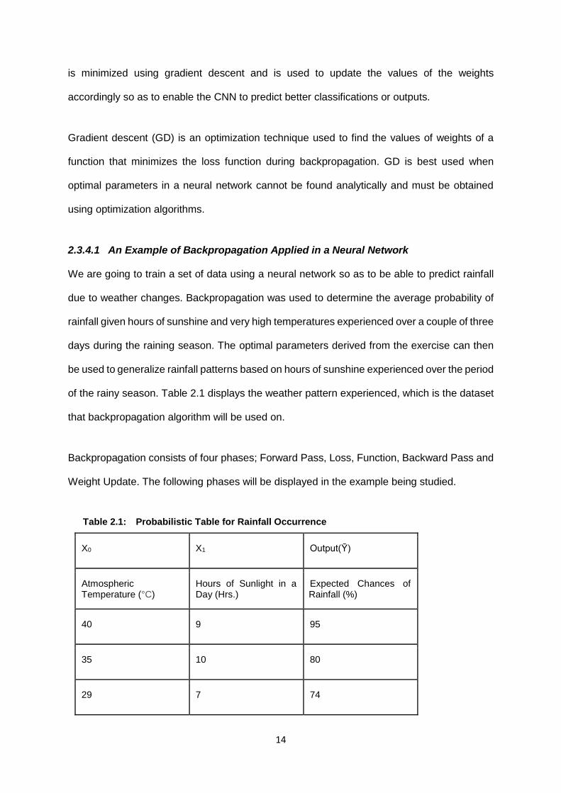
2.3.4.1 An Example of Backpropagation Applied in a Neural Network

We are going to train a set of data using a neural network so as to be able to predict rainfall

due to weather changes. Backpropagation was used to determine the average probability of

rainfall given hours of sunshine and very high temperatures experienced over a couple of three

days during the raining season. The optimal parameters derived from the exercise can then

be used to generalize rainfall patterns based on hours of sunshine experienced over the period

of the rainy season. Table 2.1 displays the weather pattern experienced, which is the dataset

that backpropagation algorithm will be used on.

Backpropagation consists of four phases; Forward Pass, Loss, Function, Backward Pass and

Weight Update. The following phases will be displayed in the example being studied.

Table 2.1: Probabilistic Table for Rainfall Occurrence

X0 X1 Output(Ȳ)

Atmospheric Temperature (°C)

Hours of Sunlight in a Day (Hrs.)

Expected Chances of Rainfall (%)

40 9 95

35 10 80

29 7 74

15

Table 2.2: Normalized Probabilistic Table for Rainfall Occurrence

X0 X1 Output(Ȳ)

Atmospheric Temperature(°C)

Hours of Sunlight in a Day(Hrs.)


1.0 0.9 0.95

0.875 1.0 0.80

0.725 0.7 0.74

The neural network representation diagram is also needed for visual stimulation and

understanding and it is displayed in Figure 2.4.

Figure 2.4: A Neural Network for Rainfall Predictions

Symbols used in the network are: X – A tensor or Array of input elements(Datasets) Y- An Array output from Network W – The Weights on the Synapses Z – The Sum of the product of Inputs and Weights in the Neurons a – The activation on ‘Z’ across the Neurons which is a “Sigmoid Function” in this case

16

𝑆𝑖𝑔𝑚𝑜𝑖𝑑(𝑍) = 𝑓(𝑍) =1

(1 + 𝑒−𝑧), 𝑆𝑖𝑔𝑚𝑜𝑖𝑑𝑃𝑟𝑖𝑚𝑒(𝑍) = 𝑓′(𝑍) =

𝑒−𝑧

(1 + 𝑒−𝑧)

Various activation functions can be applied to the model apart from a sigmoidal activation

function Such as a Tanh activation function or a RELU activation function. These activation

functions are necessary so as to find non-linear patterns that are necessary for the prediction

process. The activation functions can also be applied in a CNN. The activation layer of a CNN

uses either a Tanh or RELU Activation function and Sigmoid Activation function can be used

as a binary classifier as well in the fully connected layer of a CNN.

2.3.4.2 Sigmoidal Activation Function

𝑆𝑖𝑔𝑚𝑜𝑖𝑑(𝑧) =1

(1 + 𝑒−𝑧)

The range of values of z are -9.0 to 9.0, with a step size of 0.01.

Figure 2.5: Sigmoid Activation Function

17

2.3.4.3 RECTIFIED LINEAR UNIT ACTIVATION FUNCTION

RELU(z) = Max(z,0)


Figure 2.6: A Rectified Linear Unit Activation Function

2.3.4.4 Tanh Activation Function

Tanh(z) =(e𝑧 − e−𝑧)

(e𝑧 + e−𝑧)


18

Figure 2.7: A Tanh Activation Function

During the Training Phase of the Neural Network, the Forward Pass exhibited a couple of

outputs which were captured in Table 2.2 and Fig 2.7. Note that the network is initiated with

random weights and the random weights are gradually updated via backpropagation.

The Forward Propagation:

Figure 2.8: Forward Propagation

The initial weights are randomly generated

The output, Ȳ = f (f (X * W (1)

) * W (2)

The Loss Function, J = ∑ ½ (Y – f (f (X * W (1)

) * W (2)

)2

19

Table 2.3: Normalized Probabilistic Table for Rainfall Occurrence with Output Errors(Ȳ)

X0 X1 Output(Ȳ) Output(Y)

Atmospheric Temperature(°C)

Hours of Sunlight in a Day(Hrs.)

Network Predicted Chances of Rainfall (%)


1.0 0.9 0.2199 0.95

0.875 1.0 0.2161 0.80

0.725 0.7 0.2351 0.74

Figure 2.9: A Neural Network for Rainfall Predictions with Random Weight Values

20

The Backward Pass is shown in Figure 2.10.

Figure 2.10: Backward Pass

The Weight updates are shown in Figure 2.11 for every synapse in the NN

Figure 2.11: Weights Updates

Figure 2.12: Final Optimal Weights

The Back-Propagation Begins:

gradient descent for Weights W (2),

𝑑𝐽 𝑑𝑊(2)⁄ =−(Y−Ȳ) * f′ (Z (3)

) * dZ (3)

/dW (2)

gradient descent for Weights W (1)

𝑑𝐽 𝑑𝑊(1)⁄ =(X)T * δ (3) * (W

(2))

T* f′ (Z

(2)), Where δ

(3) = −(Y−Ȳ) * f′ (Z

(3))

Weights update for W (2)

W

(2) ±𝑑𝐽 𝑑𝑊(2)⁄

Weights update for W (1)

W

(1) ±𝑑𝐽 𝑑𝑊(1)⁄

The Final optimal weights are obtained after training the network using Back-Propagation.

The output, Ȳ = f (f (X * W (1)

) * W (2)

The output result ‘Y’ is now very good

The Loss Function, J = ∑ ½ (Y – f (f (X * W (1)

) * W (2)

)2:

The Loss function(Error) in the network is now minimal

21

After backprop occurrence, the neural network model can now predict rainfall occurrence even

when new data is presented to the model because the optimal values for the weights have

been found across each synapse after the network learning process. The final results of the

Network can be seen in Table 2.4, Table 2.5 and Figure 2.13.

Figure 2.13: A Neural Network for Rainfall Predictions with Optimal Weight Values

22

Table 2.4: Final Normalized Probabilistic Table for Rainfall Occurrence






1.0 0.9 0.947 0.95

0.875 1.0 0.799 0.80

0.725 0.7 0.741 0.74

Table 2.5: Final Probabilistic Table for Rainfall Occurrence






40 9 94.7 95

35 10 79.9 80

29 7 74.1 74

23

2.4 Conclusion

CNNs require a supervised learning backpropagation algorithm during training so as to be

able to learn feature abstractions that are necessary for accurate image classification. It should

be noted though that a CNN possesses various parameterizations that need to be correctly

chosen in order learn the feature abstractions such as filter size used for convolutions,

activation function in the activation layer of the CNN, the learning rate of the CNN model,

momentum, number of strides, padding and so on. Design space exploration is carried out

during the course of this thesis where different metrics are altered for some parameterizations

so as to determine the CNN implementation model with the highest performance on a given

platform. The metrics of that model can then be used to build an optimized hardware CNN

implementation. Hardware CNN implementation is better for real-time usage because it offers

true parallelism, does not consume much power and is not memory intensive.

24

CHAPTER THREE

Methodology

3.1 Introduction of Deep Convolutional Neural Networks

A deep convolutional neural network is an example of a DNN. It is called a deep network due

to its possession of multiple hidden layers. It is used in the large-scale classification of objects

in an image or images. The DCNN model was built by a New York University professor named

Yann LeCun and his associates (Yoshua et al., 1998), but it gained its popularity when Alex

Krizhevsky used it to win the ImageNet computer vision classification competition in 2012

(Krizhevsky et al., 2012). The DCNN model is the image recognition system that is used in

this thesis because of its depth of accuracy in predicting objects in images. It has a neuro-

inspired architecture because it was modelled after the neuronal processing of the human

visual cortex. A CNN goes through a network training phase where it learns to identify various

patterns that give distinguishable characteristics that are necessary for object classification

and a CNN model is built and saved after training. The CNN’s inputs during a training phase

are image datasets with their corresponding dataset labels. During the training phase, the

CNN can adjust values of its filters through a process called backpropagation. The durability

of the CNN model is checked during the testing phase so as to measure how accurate it

performs in image classification exercises. Figure 3.1 depicts the schema of a Convolutional

Neural Network.

Figure 3.1: Structure of A Convolutional Neural Network

25

3.2 Topology of Deep Convolutional Neural Networks

The topology of a DCNN consists of a hierarchical order of layers which are the Convolution

layer, the activation layer, the down-sampling layer and fully connected layer. Each layer is

responsible for some sort of feature extraction. The convolution, activation and sub-sampling

layers can be replicated multiple times before being connected to the fully connected layer(s).

A DCNN is usually a repetition of a number of layers as mentioned, but the abstract features

obtained are more complex the deeper they are within the neural network. The network layers

will be discussed in detail in the next section. Inputs to the DCNN consist of image datasets

which are convolved by the convolutional layer and the outputs from the DCNN are obtained

after exiting from the fully connected layers.

3.3 Layers of Deep Convolutional Neural Networks

The DCNN consists of the following hierarchical layers:

3.3.1 Convolutional Layer

The convolutional layer is the building block of a CNN. The aim of the CNN is to be able to

look for specific features that distinguish between objects in an image, and the Convolutional

layer is the first step to this computation. It uses filters (an array of numbers or weights or

parameters) which slide and move across an input image dataset (an array of pixel values)

from the top left corner (the receptive field), to produce feature/activation maps. Filters look

for simple colours and geometries such as edges or curves that are required for low-level

feature extraction. The convolutional layer is not an entirely connected layer. The filter size,

padding and strides used in convolution are a number of hyper-parameters that need to be

carefully chosen in order to obtain optimal results in feature extractions. Subsequent

convolutional layers in the DCNN have filters that look for a higher level of feature abstractions

that will be needed in making decisions for object classifications.

26

A convolution is an element-wise matrix multiplication and summation between the input

image and the filter in the convolution layer which produces activation maps. An example of a

substantial filter size is 3 by 3 with an RGB colour channel (3*3*3). The input image can also

be normalized to have uniform width and height of 32 by 32 with an RGB colour channel as

well (32*32*3).

Figure 3.2 shows an illustration of what happens in the Convolution layer.

Figure 3.2: Element-Wise Multiplication and Summation Convolution

3.3.2 Activation Layer

The activation layer introduces non-linearity to the system because the computations of the

previous convolutional layers have been linear, while still maintaining that the determined

desired features in an input exist (during training in the network). Various non-linear functions

exist that can be applied in the activation layer such as Tanh, Sigmoid or RELU activation

functions, but the most acceptable is the RELU activation function because it allows the

network to train faster than the other activation functions, and it helps to alleviate the vanishing

gradient problem experienced in gradient descent during the network training (Deshpande,

2016). We are normalizing our model so as to enable it check for complex patterns, in other

words increasing the model’s non-linear properties.

An Input Image A Feature Map

A Filter

27

The RELU activation function f(x) = max(x,0) is applied on all the input values to the activation

layer and it basically changes all the negative values to 0 or maintains the values greater than

0. This in turn, increases the non-linear properties of the input feature map. The example in

Figure 3.3 shows an input feature map and a rectified feature map when the RELU function is

applied to it.

Figure 3.3: A Rectified Feature Map Transformation

3.3.3 Down-Sampling or Pooling Layer

Different pooling functions can be applied to this layer but the most popular and efficient based

on research is the max-pooling function. Max-pooling is when a filter of size 2 by 2 with a stride

of 2 is applied to an input feature map to convolve over it. The maximum number in every

convolved region is the resultant output of the Convolution and the remaining values are

disregarded. The result obtained is that the spatial dimensions of the input feature map are

reduced, that is the width and height are reduced but features obtained in the feature map do

not change. Reducing the spatial dimensions help to reduce the number of parameters, thus

reducing computational cost and also it controlling overfitting. Overfitting is a term used when

the network model is fine-tuned to predicting the training datasets very well but is not able to

predict objects on novel datasets during the testing phase. Figure 3.4 depicts an example of

max-pooling.

RELU FUNCTION

F(x) = max(x,0)

28

Figure 3.4: A Max-Pooling Transformation

3.3.4 Fully Connected Layer

The convolutional, RELU and pooling layers discover a host of complex patterns but cannot

understand them. Thus, the fully connected layers look at the output of the previous layers

which are high values in the activation maps that represent high-level features from the input

image and predict what the input image is based on probabilities (data sample classification).

The output can be a single class or a probability of classes that best describe the image.

Outputs are usually expressed using labels. The feature maps are stacked onto a vector in

the FC and are connected to one of the predictions to be voted for during the testing phase.

This vector stacking occurs during training. Figure 3.5 depicts a transformation from feature

maps to a vector (1-dimensional array) which is then tied to a prediction during training.

Figure 3.5: A Fully Connected Layer Transformation

A Rectified Feature Map A Max-Pooled Feature Map

Final Rectified

+ Max-

Pool

Feature Maps

A vector

Predicted

class

linked to

the vector

29

3.4 Learning Algorithm of Deep Convolutional Neural Networks

CNNs make use of a learning algorithm called backpropagation. Backpropagation is a

supervised learning algorithm for neural networks. The synapse weights that are obtained for

producing optimal outputs in a neural network are derived using backpropagation. CNNs use

backpropagation during their training phase to update the values of their parameters or

weights on each of their filters so as to be able to detect the feature abstractions used for

classification.

Backpropagation has four phases, namely the forward pass, loss function, backward pass and

weight update. The loss function is minimized using gradient descent and is used to update

the values of the weights accordingly so as to enable the CNN to predict better classifications

or outputs. Gradient descent is a ratio of the change in a loss or cost function to change in

weight of the synapses on the neurons and it is a partial derivative. It is used to train the

network until we can obtain the least cost function. The gradient is best when it is at the

minimum as it descends down a slope as seen in Figure 3.6.

Figure 3.6: A Gradient Descent Slope

As mentioned earlier, CNNs make use of a supervised learning algorithm called

backpropagation, where training sample datasets are propagated through the network in its

training phase and the outputs obtained are compared against an anticipated set of test

datasets. The computed difference between them is known as the error or loss function. Our

30

goal is to keep the error between the computed output from the network and the actual outputs

we are expecting to a minimum, and that is possible when the weights on the neurons in the

network are iteratively updated during backpropagation, till the optimal weight values are

obtained.

There are various mathematical functions for calculating the loss function such as mean

square error (MSE) and cross-entropy loss function. The latter is a better means of calculating

loss function because it solves the learning slowdown experienced using an MSE quadratic

cost function when any learning rate value is chosen (Nielsen, 2017).

An optimization algorithm in neural network learning is used to produce better results by

updating weight and bias values in a neural network accordingly. Gradient descent or batch

gradient descent (BGD) is an optimization algorithm used to minimize the loss function using

its gradient values with respect to the weight parameters on synapses. BGD, also known as

an offline gradient descent, calculates the gradient of a batch of data samples but makes just

one update at a time, thus converging slowly to a minimum on the slope. Other faster

optimizations are stochastic gradient descent (an online gradient descent) which updates the

parameters after every training sample iteration. Mini-batch gradient descent is an

improvement on the SGD because it performs updates after iterating through a batch of

training samples and it overcomes the high variance experience in parameter updates when

trying to determine the local minima of a slope.

Other optimizations algorithms which can be used to further improve convergence and find

the optimal direction in which parameter updates should occur include momentum, Nesterov

accelerated gradient (NAG), adaptive gradient algorithm (Adagrad), adaptive delta (Adadelta),

adaptive moment estimation (Adam) and root mean square propagation (RMSProp). These

optimization algorithms all help to determine the fastest convergence but the algorithms that

31

support an adaptive learning algorithm for each parameter update amongst them such as

Adagrad, Adadelta and Adam converge very fast.

32

CHAPTER FOUR

Implementation

4.1 Introduction to the Implementation

The DCNN is implemented using the Python programming language and its machine learning

APIs such as Keras, PyQt, Numpy, OpenCV, TensorFlow, SciPy etc. The CNN model itself is

built using the Keras deep learning library. Keras is an open-source high-level neural network

API which has a capability of working on top of TensorFlow, MXNet, Deeplearning4j, CNTK

or Theano Python APIs (Chollet, 2015). It was built by François Chollet who is an engineer at

Google. It has a set of abstractions but its usage is made to be modular, simple and highly

extensible regardless of the backend computing library. Keras data structure is a linear stack

of layers, the most popular model being the sequential model. The sequential model can be

used to build various types of abstractions of neural networks such as a CNN and recurrent

neural network. The advantages of its use make it a preference for research and

experimentation with DNNs; therefore, it has become the choice that was made for building,

training and testing the CNN model used in this research. Keras also has the compatibility of

running on a CPU or GPU.

4.2 Model Implementation of the Deep Convolutional Neural Networks

The model of the CNN will have a sequential stack of layers comprising modules that are

stacked together to obtain a deep structure of the neural network to be obtained. All the hyper-

parameters can easily be configured into the model because the neural layers, activation

functions, optimizers and regularization schemes are individual modules that are combined to

build the system and give it its ‘deep’ structure.

The model of the CNN is simple and extensible and a sample of its structure is displayed using

the following algorithm:

33

# dimensions of our images.

img_width, img_height = 150, 150

input_shape = (img_width, img_height, 3)

model = Sequential ()

model.add (Conv2D (32, (3, 3), input_shape=input_shape))

model.add(Activation('relu'))

model.add (MaxPooling2D (pool_size= (2,2)))

model.add (Conv2D (32, (3, 3)))









model.add (Flatten ())

model.add (Dense (128))


model.add (Dropout (0.5))

model.add (Dense (1))

model.add(Activation('sigmoid'))

model. compile (loss='binary_crossentropy',

optimizer='rmsprop',

metrics=['accuracy'])

model.fit_generator (train_generator,

steps_per_epoch=2048,

epochs=30,

validation_data=validation_generator,

validation_steps=nb_validation_samples)

model.save_weights('models/simple_CNNLinux.h5')

model.save('models/simple_CNNLinuxModel30epochs.h5')

The saved model after training is the structure of the CNN and it can be used to test against

a set of novel images for object classification exercises. The model can be called for object

prediction testing using the algorithm below.

34

basedir = "test1/test1/"

predict (basedir, test_model)

model = load_model('models/simple_CNNLinuxModel30epochs.h5')

def predict (basedir, model):

for i in range (12490,12501): #24 to 29

path = basedir + str(i) + '.jpg' #path = basedir + str(i) + '.jpg'

orig = cv2.imread(path)

orig = cv2.cvtColor(orig, cv2.COLOR_BGR2RGB)

max_dim = max (orig. shape)

scale = 480/max_dim

orig = cv2.resize(orig, None, fx= scale, fy = scale)

orig = cv2.cvtColor(orig, cv2.COLOR_RGB2BGR)

print("[INFO] loading and preprocessing image...")

names = ['cat', 'dog']

img = load_img (path, False, target_size= (img_width, img_height))

x = img_to_array(img)

x = np.expand_dims (x, axis=0)

print("[INFO] classifying image...")

preds = model.predict_classes(x)

if (preds== [[0]]):

label = names [0]

else:

label = names [1]

# Display the predictions

print ("Label: {}”. format(label))

cv2.putText(orig, "Label: {}”. format(label), (10, 30),

cv2.FONT_HERSHEY_SIMPLEX, 0.9, (255, 0, 255), 2)

cv2.imshow("Classification", orig)

cv2.waitKey(0) predict (basedir, test_model)

print ('Prediction Ended')

4.3 Test Results of the Convolutional Neural Network Model

The model is being trained with dog and cat datasets and their respective labels. The dataset

of cats and dogs was downloaded from Kaggle.com website. Kaggle is a machine learning

organization which provides free datasets that can be used for training diverse neural

networks. The training phase had a dataset of 2048 images, 1024 each for both cats and dogs,

35

and a validation dataset of 832 images, 416 each for both cats and dogs. It is a binary

classification model. The training simulation was run over 30 epochs and it took about 10

hours. On testing of the CNN model, the classifier should display a prediction of a 0 or 1 (binary

classification), depending on the test input image, to be able to identify if the image contains

either a cat or a dog (0 or 1). A CNN model can also be trained to classify more than two

objects depending on what the model is built to perform. A binary classifier uses a sigmoid

function for its classification, while a categorical classifier uses a SoftMax function.

A test simulation was performed on the obtained model of the CNN which showed

considerable ability in distinguishing objects in novel images to obtain predictions for cats and

dogs. The test evaluations for 10 images were captured on screen and the results are

displayed later in this report. The simulation was performed to test the accuracy and

robustness of the classifier. Figures 4.1 to 4.10 depict the results of the test results carried

out. Using a visual aid as seen in Figure 4.1–4.10 to demonstrate the classification and its

label to check for accuracy is efficient.

Figure 4.1: Class Label and Test Image


36





37





38

4.4 Test Observation and Discussion

The predictions from the test simulations demonstrated a high success rate in the image

classification exercise. On the other hand, it was observed that not all the objects were

predicted correctly. The trained CNN model has an average prediction accuracy of about 70%

whenever it is run against a random set of test images. It classified eight out of 10 images

correctly in Figure 4.0 – 4.10 captured above. Figure 4.9 and 4.10 were not classified correctly.

Visual Recognition is a very difficult computational issue. Here are various reasons why a

classifiers’ accuracy may vary;

• A CNN needs many training datasets for better feature abstractions in its feature maps.

• A CNN needs a long training iteration period (epochs) over the datasets provided which

could run for hours or days.

• Each of the objects to be identified in the training and test images have a lot of

variations across them such as pose, appearance, viewpoint, background, the position

of objects in the image, illumination and occlusion (Pinheiro & Henrique, 2017).

• A DCNN is a black box with thousands or millions of free parameters that need to be

well trained for better feature abstractions and learning the optimal parameters with a

few thousand training images may be insufficient (Oquab, Bottou, Laptev, & Sivic,

2014).

• Overfitting (where the classifier has a 95% chance identifying the objects properly, but

during testing, it may have a 50% chance) may occur during training and it may affect

the generalization ability of the classifier during testing.

• The size of the filters that are used for feature extraction during training of the CNN

can also affect its ability to classify objects. A large filter size can overlook the basic

features needed for extraction and could skip the essential details in the images,

whereas a small filter size could provide too much information that can lead to

computational complexity. Thus, there is a need to determine the most suitable filter

size used for feature extraction.

39

CHAPTER FIVE

Evaluation and Conclusion

5.1 Introduction

Benchmarking is performed to set a point of reference for something that can be measured. It

is also a set of standards used as a point of reference for evaluating performance metrics or

quality (BusinessDictionary, 2017). This benchmarking evaluation was performed to

determine which was the best CNN model for solving the classification task required, and the

metrics that were varied in each of the models were the activation function used in the

activation layer of the CNN Model as well as the filter/kernel size that was used in the

convolutional layer of the CNN model as well. The size of the dataset that was used during

the training phase of each CNN Model obtained had 2048 Images (1024 images of cats and

1024 images of dogs). Each CNN model was trained using the following computing system

specification:

• A 64-bit Ubuntu 16.04 LTS Linux Operating System

• An Intel Core i5-6500 CPU @ 3.20GHz (4 CPU cores)

• 8 GB of System Memory.

5.2 Evaluation of various Deep Convolutional Neural Network Models

Table 5.1 contains all the metrics and hyper-parameters that were used to build the chart

evaluations of the various CNN models that were trained and observations that were noticed

have been recorded with possible reasons why they occurred during the testing of each model

for accuracy of object classifications. All the models were tested against the same size of the

dataset. A dataset can definitely affect the accuracy of object classification. A CNN needs a

lot of training datasets, possible millions for better object classification. Figures 5.1–5.4 are

charts that depict various evaluations.

40

Table 5.1: Training & Test Accuracy Table for the Convolutional Neural Network Models

S/N Activation Function

Filter Size

Training Time (hrs.)

Test Accuracy (%) using 10 test sample images

Training Data Set

(images)

Validation Data Set

(images)

No. of Epochs

1 RELU 3 9.7 70 2048 832 30

2 Sigmoid 3 15.2 10 2048 832 30

3 Tanh 3 15.4 40 2048 832 30

4 RELU 7 19.5 10 2048 832 30

5 Sigmoid 7 21.7 10 2048 832 30

6 Tanh 7 21.3 50 2048 832 30

5.2.1 Training Time Against Filter Size Evaluation

Figure 5.1: Training Time Against Filter Size

From observations in Figure 5.1, it can be deduced that there would be fewer computations at

a given time for each convolution with smaller filter sizes during the linear element-wise

41

computations between the filters and their relative reception fields on every input image during

each epoch so that the training time will be less.

5.2.2 Training Time Against Activation Function Evaluation

Figure 5.2: Training Time Against Activation Function

From observations in Figure 5.1, it can be deduced that the CNN models that were trained

using the RELU Activation function had faster training time compared to the rest. This is due

to the fact that RELU Activation function converges quicker during training to update the

parameters on their neurons to optimal values that would be used during object classification.

42

5.2.3 Accuracy Against Activation Function Evaluation

Figure 5.3: Accuracy Against Activation Function

From observations in Figure 5.3, it can be deduced that RELU activation does not suffer the

vanishing gradient problem during backpropagation like Tanh and sigmoid activation

functions. While using a sigmoid activation function during the backward pass in a

backpropagation, the weights are not updated, so the loss function remains unchanged and

the network does not learn. While using a RELU the network converges faster and the

parameters (weights on each synapse) are optimized with the required values necessary for

quicker feature extraction. There might not also be a guarantee for the network to learn while

using a RELU because an appropriate filter size was not chosen during training; therefore, the

low-level features that are necessary to capture interesting properties are unforeseen. It

should be noted that the probability on each properly classified object using the RELU with a

filter size 3 had 100% probability of prediction, but the Tanh activations had between 40% and

50% probability of a prediction guess, despite having accurate classifications.

43

5.2.4 Accuracy Against Filter Size Evaluation

Figure 5.4: Accuracy Against Filter Size

From observations in Figure 5.4, it can be deduced that the size of the filters plays an important

role in finding the key features used for classification of objects. A larger kernel size can

overlook the necessary features during training of the network and could skip the essential

low-level details in the training dataset images.

5.3 Future Work

Various means of improving the object classification of the CNN model such as data

augmentation and transfer learning (using a pre-built model) will be discussed, as well as

better means of representing the classified objects in the data by visual means such as object

localization, object detection, object segmentation and such visual means are possible

through the use of Python programming languages’ OpenCV library. The models created are

able to identify just one object at a time.

44

A better model can be built to identify the binary objects that need to be classified at the same

time and display their labels.

5.3.1 Data Augmentation

The size of the dataset used during the training phase of a ConvNet can affect its classification

accuracy properties. If the size is small, the CNN model will not be able to properly effect best

object classification (Krizhevsky et al., 2012). Data augmentation can be used to remedy such

a case because it is an artificial means of making your existing dataset larger through a couple

of needful transformations (Deshpande, 2014). Data augmentation is also a means of

preventing overfitting in generalization (Krizhevsky et al., 2012). The input image dataset is

an array of pixel values or numbers and transformations can be made by altering a few of the

values but still maintaining the label and classification of the object in the image and therefore

new datasets samples can be created by such means. Various dataset augmentation

techniques used for applying transformations to sample training datasets include grayscales,

vertical flips, colour jitters, translations, rotations, random crops, horizontal flips and much

more (Deshpande, 2014). The size of the training examples can be increased significantly

through such artificial means.

5.3.2 Transfer Learning

Transfer learning involves using a pre-built or pre-trained model has been done by someone

else, where the weights on the synapses of the model have been highly optimized by training

them using a very large dataset that and using it to train your own model (Deshpande, 2014).

The pre-built model will act as your feature extractor. Transfer learning (using a pre-built CNN

model) helps to train your network faster and you get better object classification results from

input images. A pre-built model has already been trained with millions of images, so the

parameters on the synapses of the neurons are already optimized. You only need to replace

the fully connected layer on the pre-built model so it can classify your images. Using a pre-

built model also minimizes the time required to train your network. Rather than training your

45

CNN model with initial random weights, you use the weights on the layers of the pre-built

model during gradient descent and train the higher layers for classification (Deshpande, 2014).

5.3.3 Object Localization, Detection and Segmentation

Image classification is not enough (predicting that an object exists in an image, e.g. a cat or a

dog). It is a better exercise to determine and show visually the precise region in with the

classified objects exist in a receptive field. It would be necessary especially when an

autonomous vehicle needs to make appropriate decisions upon viewing its receptive field such

what to do upon viewing the colour of a traffic light or to avoid coming in contact with other

vehicles, pedestrians and so on.

Object localization involves putting a bounding box to describe where an object exists in an

image alongside its label (Deshpande, 2014). Image detection is an image localization process

which involves putting a bounding box on every object in an image alongside their relative

labels as well (Deshpande, 2014). Figure 5.5 shows an image with object localization.

Figure 5.5: Image Classification, Object Localization and Object Detection

(Image courtesy http://images.google.com)

46

Image segmentation involves displaying the exact region where each classified object exists

in a test input image by displaying the outlined region over the object and the label for the

object as well (Pinheiro & Henrique, 2017); therefore we are assigning an object class to every

pixel. Figure 5.6 shows an image with object segmentation.

Figure 5.6: Image Classification and Object Segmentation

(Image courtesy www.petsworld.in)

5.4 Discussion and Conclusion

5.4.1 Contribution to Deep Performance CNN Modelling

Based on the evaluation of the performance of the deep learning models built, it was possible

to determine the hyper-parameters that are necessary for the best performance of a CNN

model that can be used for image classification. I was also able to use OpenCV library for the

visualization of the Classification images and display their corresponding labels as well. The

classification of objects were binary representations. I was able to collect the data during

testing and transform them to string representations as well (cat or dog).

47

5.4.2 Conclusion

The computer vision Implementation carried out in this thesis was done via software

simulations, and it was necessary to be able to find out the optimal parametrizations that can

be used on a CNN model so as to satisfy the design space explorations objective of this thesis.

The optimized CNN model obtained also proved to serve as a better image classifier

compared to other machine learning implementations mentioned in the related works section

of this thesis, because of its high accuracy of performance and low error rate experienced

during the object recognition testing phase. The limitations of using software simulations

though is that it is memory intensive, it does not offer real parallelization, and it requires long

computational hours for training the network even though it is still very fast for usage.

Hardware CNN models are a better option for real-time usage and the results obtained using

software simulations can be adapted to build the hardware convolutional network system.

Hardware CNN offers true parallelism computing, it has low power consumption and it does

not suffer the computation and bandwidth bottlenecks suffered due to limitations of memory

usage during CNN Software Simulations (Projects, 2017). Computer vision applications using

a DCNN by far have proven to mimic the human visual cortex with very slight variations and

are outstanding in their usage as well.

48

REFERENCES

Ayodele, T. O. (2010). Types of Machine Learning Algorithms. New Advances in

Machine Learning, 19–49. https://doi.org/10.5772/56672

Brunner, C. (2012). Pairwise Support VectorMachines and their Application to Large

Scale Problems. Journal of Machine Learning Research, 13(1), 2279–2292.

BusinessDictionary. (2017). What is a benchmark? definition and meaning -

BusinessDictionary.com. Retrieved October 26, 2017, from

http://www.businessdictionary.com/definition/benchmark.html

Chollet, F. (2015). Keras Documentation. Keras.io. Retrieved from

https://keras.io/#why-this-name-keras

Davy, A., Havaei, M., Warde-farley, D., Biard, A., Tran, L., Jodoin, M., … Bengio, Y.

(2013). Brain Tumor Segmentation With Deep Neural Networks, 2013.

Deshpande, A. (2014). Understanding CNNs The 9 Deep Learning Papers You Need

to Know About Part 3. https://adeshpande3.github.io/adeshpande3.github.io/The-

9-Deep-Learning-Papers-You-Need-To-Know-About.html, 1–31.

Deshpande, A. (2016). A Beginner's Guide To Understanding Convolutional Neural

Networks, 1–17.

Emer, J. (2017). Hardware Architectures for Deep Neural Networks CICS / MTL

Tutorial Speakers and Contributors.

Henrique, P., & Pinheiro, O. (2017). Large-Scale Image Segmentation with

Convolutional Networks, 7571, 1–70.

Ian, G. (2016). Deep Learning. https://doi.org/10.1007/s00287-016-1013-2

Kim, J., Kim, B., Savarese, S., & Arbor, A. (2012). Comparing Image Classification

Methods : K-Nearest-Neighbor and Support-Vector-Machines, 133–138.

Krizhevsky, A., Sutskever, I., & Hinton, G. E. (2012). ImageNet Classification with

Deep Convolutional Neural Networks. Advances In Neural Information

Processing Systems, 1–9.

https://doi.org/http://dx.doi.org/10.1016/j.protcy.2014.09.007

LeCun, Y., Huang, F. J., & Bottou, L. (2004). Learning Methods for Generic Object

49

Recognition with Invariance to Pose and Lighting. Computer Vision and Pattern

Recognition, 2004. CVPR 2004. Proceedings of the 2004 IEEE Computer Society

Conference on, 2, II-97-104. https://doi.org/10.1109/CVPR.2004.1315150

Mallick, S. (2016). Image Recognition and Object Detection : Part 1 | Learn OpenCV.

Retrieved November 14, 2017, from https://www.learnopencv.com/image-

recognition-and-object-detection-part1/

Muralidharan, R. (2014). Object Recognition Using K-Nearest Neighbor Supported By

Eigen Value Generated From the Features of an Image, 5521–5528.

Ng, A., Ngiam, J., Foo, C. Y., Mai, Y., Suen, C., Coates, A., … Sameep Tandon.

(2015). Deep Learning Tutorial. University of Stanford. Retrieved from

http://ufldl.stanford.edu/tutorial/supervised/ConvolutionalNeuralNetwork/

Nielsen, M. a. (2017). Improving the way neural networks learn. Neural Networks and

Deep Learning. Determination Press. Retrieved from

http://neuralnetworksanddeeplearning.com/chap3.html

Oquab, M., Bottou, L., Laptev, I., & Sivic, J. (2014). Learning and transferring mid-

level image representations using convolutional neural networks. Computer

Vision and Pattern Recognition, 1717–1724.

Pinheiro, O., & Henrique, P. (2017). Large-Scale Image Segmentation with

Convolutional Networks, 7571.

Projects, C. (2017). Research and Projects Learning Theory , Learning Algorithms, 1–

9.

Shaikh, F. (2017). Beginner’s guide to Reinforcement Learning & its implementation

in Python. Retrieved November 15, 2017, from

https://www.analyticsvidhya.com/blog/2017/01/introduction-to-reinforcement-

learning-implementation/

Techopedia. (2017). What is Artificial Intelligence (AI)? - Definition from Techopedia.

Retrieved September 12, 2017, from

https://www.techopedia.com/definition/190/artificial-intelligence-ai

Yann, L., Haffner, P., Bottou, L., & Yoshua, B. (2012). Object Recognition with

Gradient-Based Learning. AT&T Shannon Labs, XXXIII(2), 81–87.

https://doi.org/10.1007/s13398-014-0173-7.2

50

Yoshua, B., Yann, L., Bottou, L., & Haffner, P. (1998). Gradient-Based Learning

Applied to Document Recognition. Proceeding of the IEEE , November 1998, 46.

https://doi.org/10.1109/5.726791

Brunner, C. (2012). Pairwise Support Vector Machines and their Application to Large

Scale Problems. Journal of Machine Learning Research, 13(1), 2279–2292.

BusinessDictionary. (2017). What is a benchmark? definition and meaning -

BusinessDictionary.com. Retrieved October 26, 2017, from

http://www.businessdictionary.com/definition/benchmark.html

Chollet, F. (2015). Keras Documentation. Keras.io. Retrieved from

https://keras.io/#why-this-name-keras

Current Projects. (n.d.). Retrieved November 16, 2017, from http://adaptive.u-

aizu.ac.jp/?page_id=5

Davy, A., Havaei, M., Warde-farley, D., Biard, A., Tran, L., Jodoin, M., … Bengio, Y.

(2013). Brain Tumor Segmentation with Deep Neural Networks, 2013.

Deshpande, A. (2014). Understanding CNNs: The 9 Deep Learning Papers You Need

to Know About Part 3. https://adeshpande3.github.io/adeshpande3.github.io/The-

9-Deep-Learning-Papers-You-Need-To-Know-About.html, 1–31.

Deshpande, A. (2016). A Beginner’s Guide to Understanding Convolutional Neural

Networks, 1–17.

Emer, J. (2017). Hardware Architectures for Deep Neural Networks CICS / MTL

Tutorial Speakers and Contributors.

Henrique, P., & Pinheiro, O. (2017). Large-Scale Image Segmentation with

Convolutional Networks, 7571, 1–70.

Ian, G. (2016). Deep Learning. https://doi.org/10.1007/s00287-016-1013-2

Kim, J., Kim, B., Savarese, S., & Arbor, A. (2012). Comparing Image Classification

Methods: K-Nearest-Neighbor and Support-Vector-Machines, 133–138.

Krizhevsky, A., Sutskever, I., & Hinton, G. E. (2012). ImageNet Classification with

Deep Convolutional Neural Networks. Advances in Neural Information Processing

Systems, 1–9. https://doi.org/http://dx.doi.org/10.1016/j.protcy.2014.09.007

51

LeCun, Y., Fu Jie Huang, & Bottou, L. (2004). Learning methods for generic object

recognition with invariance to pose and lighting. Proceedings of the 2004 IEEE

Computer Society Conference on Computer Vision and Pattern Recognition,

2004. CVPR 2004., 2, 97–104. https://doi.org/10.1109/CVPR.2004.1315150

LeCun, Y., Huang, F. J. H. F. J., & Bottou, L. (2004). Learning Methods for Generic

Object Recognition with Invariance to Pose and Lighting. Computer Vision and

Pattern Recognition, 2004. CVPR 2004. Proceedings of the 2004 IEEE Computer

Society Conference on, 2, II-97-104.

https://doi.org/10.1109/CVPR.2004.1315150

Mallick, S. (2016). Image Recognition and Object Detection: Part 1 | Learn OpenCV.

Retrieved November 14, 2017, from https://www.learnopencv.com/image-

recognition-and-object-detection-part1/

Muralidharan, R. (2014). Object Recognition Using K-Nearest Neighbor Supported by

Eigen Value Generated from the Features of an Image, 5521–5528.

Ng, A., Ngiam, J., Foo, C. Y., Mai, Y., Suen, C., Coates, A., … Sameep Tandon.

(2015). Deep Learning Tutorial. University of Stanford. Retrieved from

http://ufldl.stanford.edu/tutorial/supervised/ConvolutionalNeuralNetwork/

Nielsen, M. a. (2017). Improving the way neural networks learn. Neural Networks and

Deep Learning. Determination Press. Retrieved from

http://neuralnetworksanddeeplearning.com/chap3.html

Oquab, M., Bottou, L., Laptev, I., & Sivic, J. (2014). Learning and transferring mid-

level image representations using convolutional neural networks. Computer

Vision and Pattern Recognition, 1717–1724.

Pinheiro, O., & Henrique, P. (2017). Large-Scale Image Segmentation with

Convolutional Networks, 7571.

Shaikh, F. (2017). Beginner’s guide to Reinforcement Learning & its implementation

in Python. Retrieved November 15, 2017, from

https://www.analyticsvidhya.com/blog/2017/01/introduction-to-reinforcement-

learning-implementation/

Techopedia. (2017). What is Artificial Intelligence (AI)? - Definition from Techopedia.

Retrieved September 12, 2017, from

52

https://www.techopedia.com/definition/190/artificial-intelligence-ai

Yann, L., Haffner, P., Bottou, L., & Yoshua, B. (2012). Object Recognition with

Gradient-Based Learning. AT&T Shannon Labs, XXXIII (2), 81–87.

https://doi.org/10.1007/s13398-014-0173-7.2

Yoshua, B., Yann, L., Bottou, L., & Haffner, P. (1998). Gradient-Based Learning

Applied to Document Recognition. Proceeding of the IEEE, November 1998, 46.

https://doi.org/10.1109/5.726791

development and design space exploration of deep

Documents