development and application of foraminiferal carbonate

University of South CarolinaScholar Commons

Theses and Dissertations

2016

Development And Application Of ForaminiferalCarbonate System Proxies To Quantify OceanAcidification In The California CurrentEmily B. OsborneUniversity of South Carolina

Follow this and additional works at: https://scholarcommons.sc.edu/etd

Part of the Marine Biology Commons

This Open Access Dissertation is brought to you by Scholar Commons. It has been accepted for inclusion in Theses and Dissertations by an authorizedadministrator of Scholar Commons. For more information, please contact [email protected].

Recommended CitationOsborne, E. B.(2016). Development And Application Of Foraminiferal Carbonate System Proxies To Quantify Ocean Acidification In TheCalifornia Current. (Doctoral dissertation). Retrieved from https://scholarcommons.sc.edu/etd/3973

https://scholarcommons.sc.edu?utm_source=scholarcommons.sc.edu%2Fetd%2F3973&utm_medium=PDF&utm_campaign=PDFCoverPages

https://scholarcommons.sc.edu/etd?utm_source=scholarcommons.sc.edu%2Fetd%2F3973&utm_medium=PDF&utm_campaign=PDFCoverPages

https://scholarcommons.sc.edu/etd?utm_source=scholarcommons.sc.edu%2Fetd%2F3973&utm_medium=PDF&utm_campaign=PDFCoverPages

http://network.bepress.com/hgg/discipline/1126?utm_source=scholarcommons.sc.edu%2Fetd%2F3973&utm_medium=PDF&utm_campaign=PDFCoverPages

https://scholarcommons.sc.edu/etd/3973?utm_source=scholarcommons.sc.edu%2Fetd%2F3973&utm_medium=PDF&utm_campaign=PDFCoverPages

mailto:[email protected]

DEVELOPMENT AND APPLICATION OF FORAMINIFERAL CARBONATE SYSTEM

PROXIES TO QUANTIFY OCEAN ACIDIFICATION IN THE CALIFORNIA CURRENT

by

Emily B. Osborne

Bachelor of Science

College of Charleston, 2012

Submitted in Partial Fulfillment of the Requirements

For the Degree of Doctor of Philosophy in

Marine Science

College of Arts and Sciences

University of South Carolina

2016

Accepted by:

Robert C. Thunell, Major Professor

Claudia Benitez-Nelson, Committee Member

Michael Bizimis, Committee Member

Howie D. Scher, Committee Member

Leslie R. Sautter, Committee Member

Cheryl L. Addy, Vice Provost and Dean of the Graduate School

ii

© Copyright by Emily B. Osborne, 2016

All Rights Reserved.

iii

DEDICATION

I dedicate my dissertation to a group of people who have unconditionally loved and

supported me throughout this process and throughout my life. Tim for being so loving

and patient while making me feel like the coolest gal in the universe. I’m so glad you

found me in that introductory geology lab at CofC. My dad, for being my first teacher

and inspiring my scientific curiosity at a young age. Let’s make the world a better place

in which to live, together! My mom for being the most patient listener and for always

being eager to learn more about my scientific world. Your love for me is unparalleled and

keeps me in constant awe of you. My big sister, Whitney, for always making me laugh

and living in an alternate Osborne sister universe with me. Without each of you, this

work would not have been possible.

iv

ACKNOWLEDGEMENTS

First and foremost, I have to acknowledge my fantastic advisor, Bob Thunell. It has been

such an honor and pleasure being your student. You have helped me grow so much as a

scientist, writer and individual. I am so lucky that you chose me to be part of your lab.

Also, thank you for trying to teach me the English language and usually making me

laugh/cry in the process. Accordingly, I have to also thank my amazing undergraduate

advisor who gently guided me into the world of forams and encouraged me to follow in

her footsteps at USC, Leslie “Doc” Sautter. A HUGE thanks to my amazing officemates

who have become close friends, Natalie Umling, Brittney Marshall and Dominika

Wojcieszek (and Jessica Holm as an honorary officemate) for making the last 4.5 years

so much fun. Having you gals in the office and traveling all over the world with you guys

has made for some amazing and lasting memories. I love you girls! An extra special

shout out to Gnat, aka. my school wife, I could not have maintained sanity without you.

Also thank you to all of the many, amazing graduate school friends who have come and

gone during my time and USC you all made this process so much more fun! A special

thank you to Wayne Buckley for spending many chilly hours with me in the CEMS lab,

teaching me to be an analytical chemist. Of course, the chemistry would not have been

possible without the huge help from Michael Bizimis. And last but not least, thank you to

Eric Tappa, the omniscient one of the MSRL lab. I don’t know what the lab (or I) would

do without you.

v

ABSTRACT

The oceanic uptake of anthropogenic carbon has mitigated climate change, but has also

resulted in a global average 0.1 decline in surface ocean pH over 20th century known as

ocean acidification. The parallel reduction in carbonate ion concentration ([CO32-]) and

the saturation state of seawater (Ω) has caused many major calcium carbonate-secreting

organisms such as planktonic foraminifera to exhibit impaired calcification. We develop

proxy calibrations and down core records that use calcification and geochemical

characteristics of planktonic foraminifera as proxies for the marine carbonate system.

This study focuses specifically on the surface ocean chemistry of the California Current

Ecosystem (CCE), which has been identified as a region of rapidly progressing ocean

acidification due to natural upwelling processes and the low buffering capacity of these

waters. The calibration portion of this study uses marine sediments collected by the Santa

Barbara Basin (SBB), California sediment-trapping program located in the central region

of the CCE. We calibrate the relationships of Globigerina bulloides calcification intensity

to [CO32-] and the B/Ca ratios of G. bulloides, Neogloboquadrina dutertrei and

Neogloboquadrina incompta shells to Ω calcite using in situ measurements and model

simulations of these independent variables. By applying these proxy methods to down

core, our records from the SBB indicate a 20% reduction in foraminiferal calcification

since ~1900, translating to a 35% decline in [CO32-] in the CCE over this period. Our

high-resolution calcification record also reveals a substantial interannual to decadal

modulation of ocean acidification in the CCE related to the sign of Pacific Decadal

vi

Oscillation and El Niño Southern Oscillation. In the future we can expect these climatic

modes to both enhance and moderate anthropogenic ocean acidification. Based on our

historic record, we predict that if atmospheric CO2 reaches 540 ppm by the year 2100 as

predicted by a conservative CO3 pathway, [CO32-] will experience a net reduction of

55%, resulting in at least a 30% reduction in calcification of planktonic foraminifera that

will likely be mirrored by other adversely affected marine calcifiers.

vii

TABLE OF CONTENTS

DEDICATION ....................................................................................................................... iii

ACKNOWLEDGEMENTS ........................................................................................................ iv

ABSTRACT ............................................................................................................................v

LIST OF TABLES .................................................................................................................. ix

LIST OF FIGURES ...................................................................................................................x

CHAPTER 1: CALCIFICATION OF THE PLANKTONIC FORAMINIFERA GLOBIGERINA BULLOIDES

AND CARBONATE ION CONCENTRATION: RESULTS FROM THE SANTA BARBARA

BASIN ..........................................................................................................................1

1.1 ABSTRACT .............................................................................................................2

1.2 INTRODUCTION ......................................................................................................3

1.3 REGIONAL SETTING: THE SANTA BARBARA BASIN ...............................................9

1.4 MATERIALS AND METHODS .................................................................................10

1.5 RESULTS AND DISCUSSION ..................................................................................16

1.6 CONCLUSIONS .....................................................................................................35

CHAPTER 2: NATURAL AND ANTHROPOGENIC OCEAN ACIDIFICATION IN THE CALIFORNIA

CURRENT AND CONSEQUENCES FOR MARINE CALCIFIERS .........................................51

2.1 ABSTRACT ...........................................................................................................52

2.2 INTRODUCTION ....................................................................................................52

2.3 METHODS ............................................................................................................57

2.4 RESULTS AND DISCUSSION ..................................................................................61

viii

2.5 CONCLUSIONS .....................................................................................................68

CHAPTER 3: BORON CONCENTRATION OF NON-DINOFLAGELLATE HOSTING PLANKTONIC

FORAMINIFERA CALCITE AND SEAWATER CARBONATE CHEMISTRY .........................87

3.1 ABSTRACT ...........................................................................................................88

3.2 INTRODUCTION ....................................................................................................89

3.3 MATERIALS AND METHODS .................................................................................93

3.4 RESULTS AND DISCUSSION ................................................................................100

3.5 CONCLUSIONS ...................................................................................................111

REFERENCES .....................................................................................................................135

APPENDIX A – SUPPORTING INFORMATION FOR CHAPTER 1 .............................................151

APPENDIX B–COPYRIGHT PERMISSIONS FOR CHAPTER 1 ..................................................170

ix

LIST OF TABLES

Table 1.1 Sediment trap sample information and morphometric measurements...............36

Table 1.2 Stable isotope results, calcification depths and hydrographic data ...................37

Table 1.3 Down core calculations of marine carbonate system variables .........................38

Table 1.4 Final calibration equations .................................................................................40

Table 2.1 Down core ages and morphometric measurements ...........................................70

Table 2.2 Down core carbonate system calculations .........................................................72

Table 2.3 Projected carbonate system calculations ............................................................74

Table 2.4 Relative changes in historic and projected carbonate variables ........................76

Table 3.1 N. dutertrei B/Ca and Mg/Ca data ...................................................................113

Table 3.1 N. incompta B/Ca and Mg/Ca data ..................................................................114

Table 3.1 SLR of independent variables ..........................................................................115

x

LIST OF FIGURES

Figure 1.1 Bathymetric map of the Santa Barbara Basin ...................................................41

Figure 1.2 Sediment trap area density data 2007-2011 ......................................................42

Figure 1.3 Area density versus SNSW for normal and encrusted G. bulloides .................43

Figure 1.4 SEM images of normal and encrusted G. bulloides .........................................44

Figure 1.5 Temperature and calcification depths of G. bulloides ......................................45

Figure 1.6 Area density time-series November 2010-December 2011 ..............................46

Figure 1.7 Historic hydrographic time-series and down core morphometric data ............47

Figure 1.8 Comparison of calculated and area density-estimated [CO32-] .........................48

Figure 1.9 Final calibration relationships for normal and encrusted G. bulloides .............49

Figure 1.10 Comparison of G. bulloides morphotypes to Cariaco regressions .................50

Figure 2.1 Schematic diagram showing ocean acidification carbonate chemistry ............77

Figure 2.2 Historic changes in temperature and shell size .................................................78

Figure 2.3 Proxy [CO32-] compared to model and in situ datasets .....................................79

Figure 2.4 Pacific decadal oscillation, [CO32-] and upwelling strength ............................80

Figure 2.5 Upwelling strength and carbon isotopes of G. bulloides ..................................81

Figure 2.6 The Suess Effect recorded in planktic foraminifera .......................................82

Figure 2.7 Offset in N. incompta and G. bulloides depth habitats and upwelling ............83

Figure 2.8 Anomalous acidification events and strong El Niño events .............................84

Figure 2.9 Anomalous acidification events in proxy and model data................................85

xi

Figure 2.10 Projection, hindcast and proxy estimates of [CO32-] from 1850-2100 ...........86

Figure 3.1 Comparison of model and in situ measurements of [CO32-] ...........................116

Figure 3.2 Comparison of model and in situ measurements of Ω calcite ........................117

Figure 3.3 Replicate B/Ca and Mg/Ca measurements of the foraminiferal standard ......118

Figure 3.4 Boron intensity of acid leachates from cleaning borate treated samples........119

Figure 3.5 B/Ca of borate treated samples for each cleaning step ...................................120

Figure 3.6 B/Ca values of samples stored long-term in borate buffer .............................121

Figure 3.7 Time-series of N. dutertrei B/Ca and size-fraction replicates ........................122

Figure 3.8 Time-series of N. incompta B/Ca and size-fraction replicates .......................123

Figure 3.9 Comparison of Mg/Ca calcification depth to temperature profiles ................124

Figure 3.10 Comparison of N. dutertrei B/Ca to modeled 30 m Ω calcite ......................125

Figure 3.11 Comparison of N. incompta B/Ca to modeled 40 m Ω calcite .....................126

Figure 3.12 Matrix of linear regressions of independent variables and B/Ca .................127

Figure 3.13 Correlations between Neogloboquadrina B/Ca and Mg/Ca .........................128

Figure 3.14 Compilation of Neogloboquadrina B/Ca versus Ω calcite calibration data .129

Figure 3.15 Time-series of G. bulloides B/Ca and size-fraction replicates .....................130

Figure 3.15 Time-series of G. bulloides B/Ca and size-fraction replicates .....................130

Figure 3.16 Morphometric data used to identify encrusted G. bulloides.........................131

Figure 3.17 Comparison of G. bulloides B/Ca to modeled 40 m Ω calcite .....................132

Figure 3.18 Down core Fe/Ca and Al/Ca indicate as clay contaminant indicators .........133

Figure 3.19 Down core N. incompta B/Ca estimated Ω calcite .......................................134

Figure A.1 Hydrographic contour plots for the calibration sampling period ..................157

xii

Figure A.2 Radioisotope activities used to derive age model ..........................................158

Figure A.3 Modeled area density percent error as a function of n ..................................159

Figure A.4 Calcite saturation with depth in the SBB.......................................................160

Figure A.5 Individual morphometric data used to identify morphospecies .....................161

Figure A.6 Histograms of morphospecies morphometric data ........................................162

Figure A.7 SLR of independent variables in the SBB .....................................................163

Figure A.8 Comparison of δ18O temperatures to in situ temperatures .............................164

Figure A.9 Comparison of Mauna Loa measured pCO2 and calculated pCO2 ................165

1

CHAPTER 1

CALCIFICATION OF THE PLANKTONIC FORAMINIFERA GLOBIGERINA BULLOIDES

AND CARBONATE ION CONCENTRATION: RESULTS FROM THE SANTA BARBARA

BASIN1

1 Osborne, E.B., Thunell, R.C., Marshall, B.J., Holm, J.A., Tappa, E.J., Benitez-Nelson,

C., Cai, W-J. and Chen, B. (2016), Paleoceanography 31, doi:10.1002/2016PA002933.

Reprinted with permission of publisher.

2

1.1 ABSTRACT

Planktonic foraminiferal calcification intensity, reflected by shell wall thickness,

has been hypothesized to covary with the carbonate chemistry of seawater. Here we use

both sediment trap and box core samples from the Santa Barbara Basin to evaluate the

relationship between the calcification intensity of the planktonic foraminifera species

Globigerina bulloides, measured by area density (µg/µm2), and the carbonate ion

concentration of seawater ([CO32-]). We also evaluate the influence of both temperature

and nutrient concentration ([PO43-]) on foraminiferal calcification and growth. The

presence of two G. bulloides morphospecies with systematically different calcification

properties and offset stable isotopic compositions were identified within sampling

populations using distinguishing morphometric characteristics. The calcification

temperature and by extension calcification depth of the more abundant “normal” G.

bulloides morphospecies was determined using δ18O temperature estimates. Calcification

depths vary seasonally with upwelling and were used to select the appropriate [CO32-],

temperature and [PO43-] depth measurements for comparison with area density. Seasonal

upwelling in the study region also results in collinearity between independent variables

complicating a straightforward statistical analysis. To address this issue, we use

additional statistical diagnostics and a down core record to disentangle the respective

roles of each parameter on G. bulloides calcification. Our results indicate that [CO32-] is

the primary variable controlling calcification intensity while temperature influences shell

size. We report a modern calibration for the normal G. bulloides morphospecies that can

be used in down core studies of well preserved sediments to estimate past [CO32-].

3

1.2 INTRODUCTION

Planktonic foraminifera are ubiquitous microzooplankton that secrete calcium

carbonate (CaCO3) shells that comprise up to 80% of the calcite preserved in seafloor

sediments [Schiebel, 2002]. Fossil shells of foraminifera preserved in marine sediments

have been used for a wide variety of paleoclimate applications that have greatly enhanced

our understanding of past oceanic and climatic conditions. Due to the relatively short life

span of planktonic foraminifera (~ 1 month), their shells represent a brief snapshot of

surface ocean conditions during their time of calcification [Bé, 1977]. It is generally

accepted that surface ocean carbonate ion concentration ([CO32-]) plays a key role in the

calcification of planktonic foraminifera with the level of response varying among species

[e.g., Spero et al., 1997; Bijma et al., 1999, 2002; Barker and Elderfield, 2002; Mekik

and Raterink, 2008; Moy et al., 2009; Marshall et al., 2013]. The calcification intensity

of planktonic foraminifera, or the amount of calcite deposited relative to shell size,

reflects both the efficiency (effort to precipitate calcite under varying environmental

conditions) and rate (how much calcite is added over time) of calcification during an

individual’s lifespan [Weinkauf et al., 2016]. Calcification intensity of fossil

foraminiferal shells can be estimated using morphometric characteristics such as weight,

size and area.

Initial morphometric observations of shells grown in culture and their relationship

to carbonate chemistry indicate that the species Orbulina universa produced a 37%

higher shell mass at elevated [CO32-] (600 μmol kg-1) relative to that of individuals grown

in ambient seawater [CO32-] (170 μmol kg-1) [Spero et al. 1997; Bijima et al., 1999,

2002]. Subsequently, Barker and Elderfield [2002] found that the size-normalized shell

4

weights (SNSW), which are more reflective of shell thickness rather than size, from a

series of core-top samples varied systematically with latitude. The authors found that

SNSW decreased with increasing latitude due increased CO2 solubility and declining

[CO32-] associated with decreasing temperature [Barker and Elderfield, 2002]. A down

core study in the Southern Ocean observed that SNSW of post-industrial-age

foraminiferal shells from surface sediments were 35% lower than Holocene-age shells

and attributed this difference to increasing anthropogenic CO2 and declining [CO32-]

during the last two centuries [Moy et al., 2009]. A recent sediment trap study highlighted

the importance of the shell weight size-normalization technique and described a new size-

normalization method, area density, which resulted in a highly significant relationship

with [CO32-] for two species of tropical planktonic foraminifera [Marshall et al., 2013].

While considerable effort has gone into developing foraminiferal geochemical

proxies for carbonate system variables [e.g., Sanyal et al., 1996; Yu et al., 2007; Foster et

al., 2008; Henehan et al., 2013; Rae et al., 2011; Allen et al., 2011, 2012], relatively less

emphasis has been placed on developing morphometric-based techniques [e.g., Spero et

al., 1997; Bijma et al., 1999, 2002; Barker and Elderfield, 2002; Marshall et al., 2013].

In this regard, SNSW estimates of foraminiferal calcification intensity have great

potential for serving as a quantitative measure for past [CO32-]. SNSW analyses also

require minimal analytical instrumentation and therefore can easily be measured in many

laboratories. Because SNSW measurements are non-destructive, foraminifera used for

this purpose can be used for geochemical analyses, thus providing tandem proxy records

on a single sample population.

5

The development of proxy methods for estimating carbonate system parameters is

needed since observational records are limited to the last 20-30 years [e.g. Takahashi et

al., 1982; Bates et al., 2014]. Such methods could provide an indirect means for

estimating how marine calcifiers and the marine carbonate system have responded to

carbon perturbations on both short (decadal to century) and long time-scales (millennial).

These records would be instrumental in understanding how the marine carbonate system

will respond to future increases in ocean acidification associated with various projected

CO2 scenarios. This study establishes a means to reconstruct past [CO32-] by providing an

empirical relationship between Globigerina bulloides calcification intensity and ambient

[CO32-] that can be applied to well-preserved marine sediments.

1.2.1 VARIABLES INFLUENCING GROWTH AND CALCIFICATION

The calcification and growth of planktonic foraminifera have been linked not

only to seawater [CO32-], but also to variables such as temperature and nutrient

concentration [e.g. Bé et al., 1973; Spero et al., 1997; Aldridge et al., 2012]. It has been

suggested that a unique combination of these factors comprises a species-specific set of

“optimal growth” conditions that result in a stress-induced, reduced calcification response

when these environmental conditions are not satisfied [de Villers et al., 2004]. However,

several tests of the optimal growth hypothesis failed to find a link between either the

absolute abundance of a given species, which would hypothetically occur under that

species’ optimal growth conditions, or the calcification intensity of those individuals

[Beer et al., 2010; Weinkauf et al., 2013; Weinkauf et al., 2016]. Rather, a study using

Mediterranean sediment samples indicated that the calcification of four species of

planktonic foraminifera responded passively to changes in seawater properties, such as

6

[CO32-], as opposed to a physiologic response brought about by stress from unfavorable

conditions [Weinkauf et al., 2013]. Despite being unable to identify the specific

environmental factors that controlled calcification response for each of these species, the

results of this work were consistent with carbonate chemistry being the primary control

on calcification [Weinkauf et al., 2013]. Furthermore, another study evaluated

foraminiferal calcification change over a deglaciation (Marine Isotope Stages 6-7) and

noted that Globigerinoides ruber and G. bulloides showed very similar calcification

responses despite having very different ecological requirements and therefore optimal

growth conditions. Rather, these changes were linked to pCO2 and the carbonate

saturation of seawater [Gonzalez-Mora et al., 2008].

Temperature has been cited as a control of foraminiferal shell size, with larger

shells growing in warmer waters [Bé et al., 1973; Hecht, 1976; Schmidt et al., 2004;

Lombard et al., 2009], where [CO32-] is also generally high. In order to differentiate the

influence of these variables, a culture study by Lombard et al. [2010] maintained constant

temperature and varied [CO32-], and observed that foraminifera (Orbulina universa and

Globigerinoides sacculifer) had a significant increase in shell weight with no significant

change in shell size in response to elevated [CO32-]. This result corroborated earlier

observations of lower SNSW associated with the Holocene relative to SNSW during the

Last Glacial Maximum when temperatures were colder and [CO32-] was higher [Barker

and Elderfield, 2002]. While previous results indicate that [CO32-] is the predominant

factor controlling calcification intensity, some research has suggested that temperature

does perhaps play an important role in calcification rate, which is inherently related to

calcification intensity. A study of eight modern planktonic foraminifera species found

7

that increased temperature resulted in an increase in calcification rate across all species

[Lombard et al., 2009]. de Villers [2004] also concluded that optimum temperatures were

an important factor in foraminiferal calcification rates measured by SNSW. Contrary

results from a culturing study by Manno et al. [2012] indicated that increased temperature

resulted in no net change in Neogloboquadrina pachyderma (sinistral) calcification rate.

Rather, this study found that a decline in pH, and by extension [CO32-], resulted in a

significant decline in calcification rate even in cultures where temperature was elevated

simultaneously.

Due to the fact that previous results indicate that shell size is influenced by

temperature, size-normalization of shell weights is essential for creating a metric that best

constrains calcification intensity [e.g. Barker and Elderfield, 2002; Lombard et al., 2010;

Beer et al., 2010]. Sieve-based weights (SBW), measurement-based weights (MBW) and

area density (AD) are examples of such methods. SBW measurements are made on a

narrow size-range (~50 µm) by sieving and measuring the mean weight of a pool of

individuals to calculate an average weight for the sample population [Broecker and

Clark, 2001]. MBW more effectively accounts for shell size by normalizing sieve-based

weights with a mean diameter or silhouette area parameter [Barker and Elderfield, 2002].

However, both of these size-normalizing methods are confined to examination of a

narrow size-fraction of sediments, thereby potentially limiting the number of individuals

available for analysis [see Marshall et al., 2013 for a review]. Area density overcomes

this limitation by using an individual rather than a population approach, allowing for a

broad size-fraction to be used and maximizing the number of individuals available per

sample [Marshall et al., 2013]. The area density method uses an individual weight and

8

silhouette area measured for each shell and normalizes individual weights prior to taking

the population mean. Although time consuming, the area density method effectively

captures the intrinsic natural variability of biological samples, particularly at the

individual level that would otherwise be lost when measuring bulk weights. Furthermore,

since there is no size-fraction restriction for the AD method, a larger number of

individuals is typically available for analysis, thus generating a more robust estimate of

the sample population. Importantly, the area density method has also proven to be the

most effective size-normalization technique, which is important in calcification intensity

studies such as this one [Beer et al., 2010b; Marshall et al., 2013].

While temperature and [CO32-] have been the primary variables considered in

foraminiferal calcification studies, some research indicates that nutrient concentration

may also influence foraminiferal calcification. A North Atlantic study of the species G.

bulloides suggests that high concentrations of nitrate (NO3-) and phosphate (PO4

3-) have

adverse effects on calcification of this species [Aldridge et al., 2012]. Previous research

on corals and coccolithophores has observed a decline in calcification as a result of high

nutrient concentrations, which is attributed to adsorption of calcium hydrogen phosphate

(CaHPO4) onto the calcite surface blocking growth cites for crystallization [Kinsey and

Davies, 1979; Paasche and Brubank, 1994; Lin and Singer, 2006]. Conversely, the

results of a sediment trap study in the Cariaco Basin (Venezuela) indicate that nutrients

are not a key factor controlling calcification intensity of two planktonic foraminiferal

species (G. ruber and G. sacculifer) and that covariation between [CO32-] and nutrient

concentrations can result in spurious correlations between foraminiferal calcification

intensity and nutrient concentration [Marshall et al., 2013].

9

1.3 REGIONAL SETTING: THE SANTA BARBARA BASIN

This study utilizes G. bulloides shells preserved in marine sediments (both

sediment trap and sediment core) and hydrographic data collected off the California

Margin in the Santa Barbara Basin (SBB). Globigerina bulloides is a species that often

dominates the foraminiferal flux in the SBB [Kincaid et al., 2000] and has been used

commonly in down-core paleoceanographic reconstructions for this basin [e.g. Hendy

and Kennett, 1999; Friddell et al., 2003; Pak et al., 2004; Pak et al., 2012]. It is a

symbiont-barren spinose foraminifera found in transitional to subpolar waters and is

frequently found in association with upwelling regimes [Bé et al., 1977; Hemleben et al.,

1989].

The SBB is an approximately 100 km long, ~600 m deep east-west trending basin

extending from Point Conception to the greater Los Angeles area (Figure 1). There are

north and south bounding continental shelves, with the Channel Islands forming the

southern bound of the basin. Sills at the eastern and western mouths of the basin (200

meters and 400 meters, respectively) restrict water exchange between the basin and the

open ocean. Limited influx of oxygenated water coupled with high productivity rates

result in anoxic conditions in the deepest part of the basin producing ideal conditions for

the preservation of annually laminated or varved sediments [Reimers et al., 1990; Thunell

et al., 1995]. Prevailing southward winds result in Ekman-induced upwelling in the basin

that typically peaks during the spring to early summer months and relaxes during the fall

and winter [Hendershot and Wiant, 1996]. Seasonal upwelling produces a wide range of

[CO32-], temperature and nutrient values, making this an ideal setting for examining the

influence of each of these variables on calcification (Supporting information Figure S1).

10

1.4 MATERIALS AND METHODS

1.4.1 SEDIMENT TRAP AND SEDIMENT CORE SAMPLES

The University of South Carolina has maintained a sediment trap time-series in

the deepest portion of the SBB (34˚14’N, 120˚02’W, ~580 m water depth; Figure 1) from

1993-present [Thunell; et al., 1995, 2007; Thunell, 1998]. McLean Mark VII-W

automated sediment traps equipped with 0.5 m2 funnel openings are deployed for 6-

month periods and samples are collected continuously on a bi-weekly basis. Sample

bottles are buffered and poisoned with a sodium azide solution prior to deployment.

Sediment samples are split using a McLean four-head rotary splitter and usually

refrigerated in sodium borate buffered deionized water to prevent dissolution of

carbonates prior to sample use. This study utilizes sediment trap material collected from

2007-2010, a period when water column carbonate system variables were measured on

water samples collected near the SBB sediment trap mooring by the Plumes and Blooms

Program.

Additionally, a 0.5 meter box-core collected in 2012 near the sediment trap

mooring (34˚13’N, 119˚58’W, 580 m water depth; Figure 1) was used to supplement our

sediment trap observations. Radiogenic isotopes of lead (210Pb) and cesium (137Cs) were

used to develop an age model for the box-core (Supporting information Text 1) using a

high purity germanium well detector [Moore, 1984]. Radioisotope activities indicate an

average sedimentation rate of 0.43 cm yr-1; and an average mass accumulation rate of

5.84 g cm2 yr-1 (Supporting information Figure S2). Using these age constrains we

11

estimate that the 0.5 meter core extends back to ~1895 and the uppermost sediments

contained in the core represent the year ~2006.

A 1/16 split of each sediment trap sample and roughly 3 grams of box-core

sediment were used for foraminiferal analyses; if insufficient material was available from

the sediment trap sample an additional 1/16 split was used. Despite the high organic

matter content typically found in sediment trap samples, previous tests demonstrated that

an oxidative treatment of the samples (buffered 30% H2O2 for 45 min) yielded

statistically identical area density values to that of untreated samples [Marshall et al.

2013]. Therefore it was deemed unnecessary to oxidatively clean sediment trap samples

prior to area density analysis. Both trap and core sediments were washed using borate

buffered deionized water through a 125 µm sieve and dried in a 40˚C oven prior to

analyses.

1.4.2 HYDROGRAPHIC MEASUREMENTS

Monthly hydrographic measurements are made along a transect in the SBB by the

Plumes and Blooms Program (http://www.icess.ucsb.edu/PnB/PnB.html), with one of the

sampling stations (Station 4; 34˚15’N, 119˚54’W) located adjacent to the sediment trap

mooring (Figure 1). From 2007-2010 total alkalinity (TA) and total dissolved inorganic

carbon (DIC) measurements were also made at Station 4 on 25 monthly cruises that took

place over a 40 month period (Supporting Information Text S2). Water samples used for

TA and DIC analyses were collected at depths of 0, 5, 10, 20, 30, 50, 75, 100, 150, and

200 meters.

The CO2Sys program (Version 2.1) originally by Lewis and Wallace [1998]

12

(CO2SYS.BAS) and modified by Pierrot et al. [2006] was used to estimate unknown

seawater marine carbonate system variables. This program uses two “master” carbonate

system variables (TA, DIC, pH and pCO2) to estimate the remaining unknown variables

at a set of given input conditions (e.g. temperature, salinity and pressure). For the time

period associated with the sediment trap samples (2007-2010), [CO32-] is estimated using

in situ measurements of TA and DIC from the SBB. Supplementary CTD and bottle data

from Plumes & Blooms Station 4 including salinity, temperature, pressure, phosphate

concentration ([PO4]) and silicate concentration ([SiO4]) are used as input conditions for

these calculations. For the sediment core portion of the study, pCO2 and TA are used as

mater variables. We assume a constant TA of 2250 µmol kg-1 based on the mean

measured surface TA measured in the SBB from 2007-2010. Seawater pCO2 is derived

according to Henry’s Law using atmospheric CO2 measurements from the Mauna Loa

Time-Series [1960-present; http://www.esrl.noaa.gov/gmd/ccgg/trends/]/] and

temperature, salinity and pressure dependent solubility coefficients (K0) following the

formulation of Weiss [1974]. Measured sea surface temperature from the SBB (1955-

present; 34° 24.2' N, 119° 41.6' W") and salinity from the Scripps Pier (1916-present; 32°

52.0′ N, 117° 15.5′ W) measured as a part of the Shore Stations Program

(http://shorestations.ucsd.edu/shore-stations-data/) were used to determine time-specific

K0 values and as input conditions for our down core calculations. The dissociation

constants (K1 and K2) determined by Mehrbach et al. [1973] and refit to the seawater

scale by Dickson and Millero [1987] were used as constants for our CO2Sys carbonate

system calculations. The HSO4 and B(OH)3 dissociation constant (KSO4 and KB,

respectively) according to Dickson et al. [1990] and the boron concentration and

13

chlorinity relationship determined by Lee et al. [2010] were used for our calculations

1.4.3 AREA-NORMALIZED SHELLS WEIGHTS: THE AREA DENSITY METHOD

A total of 82 sediment samples (39 sediment trap and 43 sediment core) are

included in our area density analysis. We use a combination of upper and lower sediment

trap samples (n=32) that coincide with the 25 TA and DIC sampling periods (2007-2010)

for our modern area density sediment trap calibration (Table 1.1). Lower trap samples

(~450 m depth) were available for 22 of the 25 carbonate chemistry sampling periods,

while upper trap samples (~150 m depth) were available for ten of these periods. The

upper sediment trap was added to the SBB sediment trap mooring in 2009 allowing for

both upper and lower sediment trap samples to be analyzed for eight of the TA and DIC

sampling periods. An additional 7 sediment trap samples from months when no water

column carbonate chemistry data is available were analyzed to produce a full annual-

cycle of area density measurements from December 2009-December 2010.

Globigerina bulloides shells were systematically picked from the >125 µm size

fraction of each sediment sample using a gridded tray. The >125 µm size fraction was

chosen because G. bulloides smaller than this range likely represent individuals that have

not reached the adult stage [Berger, 1971; Peeters et al., 1999]. On average shell

diameters from sediment trap and core samples range from 200-400 µm in size. Atypical

G. bulloides shells with abnormally large and thin final chambers or individuals with

over-sized apertures where the final chamber is not fully sutured to the test were excluded

from our analyses due to the effect these morphologic features have on shell area. Careful

14

attention was paid to selecting individuals that were free of visible clay particles or

organic matter that could potentially bias shell weights.

SNSW was measured using the area density method described in detail by

Marshall et al. [2013]. Following this method, individual shells were weighed in a copper

weigh boat using a high precision microbalance (Mettler Toledo XP2U; ±0.43 µg) in an

environmentally controlled weigh room and then photographed umbilical side up using a

binocular microscope (Zeiss Stemi 2000-C) fitted with a camera (Point Grey Research

Flea3 1394b). Photos were uploaded to a microscopic imaging program (Orbicule

Macnification 2.0) to measure the length of the longest shell diameter (Feret diameter)

and the 2-D surface area or silhouette area of each shell. This program uses RGB images

to calculate a region of interest by outlining the imaged shell to estimate a pixel 2-D area.

Pixel measurements are converted to lengths (µm) and areas (µm2) by calibrating an

image of a 1 mm microscale taken at the same magnification and working distance as

shell photos. Individual weights were then divided by their corresponding areas and the

mean area density value was calculated for each sample population (equation 1). Mean

area density values are most representative of the population calcification intensity and

by extension ambient calcification conditions, and were the focus of our calibration and

statistical analyses. Ideally 40 individuals were included in each sample population in

order to minimize measurement standard error (SE = σ/√ n). Due to the asymptotic nature

of area density standard error, we would argue that a sample size of 30-40 individuals

represents a high level of confidence (Supporting information Figure S3).

Area Density (µg/µm2) = Individual Weight (µg)/Individual Area (µm2) (1)

15

1.4.4 STABLE ISOTOPE ANALYSIS

Approximately 70µg (15-30 individuals) of G. bulloides from each sample used

for area density analyses were pooled to measure δ18O (Table 1.2). The foraminifera were

cleaned for 30 minutes in 3% H2O2 followed by a brief sonication and acetone rinse.

Isotopic analyses were carried out on an Isoprime isotope ratio mass spectrometer

equipped with a carbonate preparation system. The long-term standard reproducibility is

0.07‰ for δ18O. Results are reported relative to Vienna Pee Dee Belemnite (V-PDB).

Because the δ18O of foraminifera reflects both seawater temperature and the δ18O of

seawater (δ18Ow), accounting for any variations in δ18Ow is essential to properly

estimating temperature. The δ18Ow varies as a function of salinity and therefore a

δ18O:salinity relationship typically is used to determine δ18Ow; here we use a δ18O:salinity

relationship that was determined specifically for the Southern California Bight (equation

2). Measured sea surface salinity from Plumes and Blooms (Station 4) and the SIO Pier

time-series (1916-Present) are used, respectively, for sediment trap and sediment core

estimates of δ18Ow. The use of measured surface salinity as opposed to assuming constant

salinity for the down core record was particularly important in calculating δ18Ow and the

resulting temperature estimates. Scaling to V-PDB from Standard Mean Ocean Water

(SMOW) of estimated δ18Ow was done by subtracting 0.27‰ [Hut, 1987]. δ18O

calcification temperatures were calculated using a culture-derived temperature

relationship (equation 3) developed within the Southern California Bight region for G.

bulloides (12-chambered shells) [Bemis et al.,1998].

16

δ18Owater = 0.39 * (Salinity) – 13.23 (2)

T(˚C) = 13.2 – 4.89 * (δ18Ocalcite - δ18Owater) (3)

1.5 RESULTS AND DISCUSSION

1.5.1 COMPARISON OF SEDIMENT TRAP AND SEDIMENT CORE AREA DENSITY

MEASUREMENTS

Assessing the potential for dissolution of foraminiferal shells within the water

column and on the seafloor is of utmost importance when using foraminiferal shell

weights as a water column proxy. For a total of eight sampling periods from 2009-2010,

samples from both trap depths were available for area density analysis and are used to

assess similarities and differences of area density and morphometric measurements

recorded at each sampling depth. A comparison of measurements from each depth was

used to determine if dissolution impacts foraminiferal shells as they settle through the

water column and a comparison of sediment trap and sediment core measurements is

used to assess the potential for seafloor dissolution.

Observations by Milliman et al. [1999] suggest that 60-80% of CaCO3 particles

dissolve in the upper 500-1,000 m of the water column despite being well above the

lysocline. The mechanism driving water column dissolution is not well understood and

has not been replicated by either in situ [Thunell et al., 1981] or modeling studies [Jansen

et al., 2002]. Estimates for the Pacific Ocean north of 20˚N indicate that the depth of the

calcite saturation horizon can range from 200 to 1000 meters with a mean of 600 meters

water depth (Feely et al., 2004). Water column measurements of TA and DIC from 2007-

2010 in the SBB were used to assess calcite saturation. Although water column

measurements are limited to 0-400 meters, these data indicate supersaturated values

17

(1.25) at 400 meters and suggest that supersaturation also exists at the basin bottom (600

meters water depth; Supporting information Figure S4). The preservation of

unfragmented assemblages of foraminifera and the occasional presence of aragonite

thecosome pteropods that are highly susceptible to dissolution are physical evidence that

preservation of calcite in the SBB is not an issue. Shell features that are typically used as

indicators of dissolution, such as reduced spine bases and formation of cracks [Dittert

and Henrich, 2000], are not observed in trap or core sediments.

For the eight sampling periods where both upper and lower trap samples were

measured, the mean area density values determined for each depth are within two

standard errors of each other (Figure 2). Independent t-tests indicate that there is no

significant difference in the area density population means for six of eight sampling

periods (p 2-tail >0.05), while there is a moderately different sample mean recorded for a

single sampling period (p 2-tail= 0.02; 9/25/09) and a significant different sample mean

for one sampling period (p 2-tail <0.001; 10/8/10). These results indicate that generally

there is no difference in area density between the two sampling depths suggesting that

there is no significant dissolution occurring within the SBB water column.

We also compare shell weights, diameters and area densities between the

sediment trap and the seafloor sediments to assess post-depositional dissolution. If

significant dissolution is occurring on the seafloor in SBB we would expect to see

differences in shell morphometric characteristics in the sediment trap samples versus the

seafloor samples. While the lack of temporal overlap between sediment trap (2007 to

2010) and down core measurements (1985-2005) is not ideal for such a comparison,

measurements from each of these populations indicate a similar range in weight and size.

18

Independent t-tests were conducted to statistically determine if the weight, diameter and

area density of shells collected by the trap and in the core are significantly different.

These results indicate there is no significant difference in shell size preserved in trap and

seafloor sediments (p >0.05). However, there is a moderately significant difference in

shell weight (p >0.01) and highly significant difference in area density (p <0.001). The

results of this comparison indicate that overall higher weights and area density values are

observed in core sediments relative to trap sediments. We attribute these offsets to higher

[CO32-] and increased calcification intensity over the 100-year down core sampling

period relative to the more recent sediment trap sampling period (See section 4.6 for

discussion on [CO32-] change over this interval).

1.5.2 GLOBIGERINA BULLOIDES MORPHOSPECIES

Studies of G. bulloides small subunit ribosomal RNA (SSU rRNA) indicate high

cryptic diversity with a total of seven distinct genotypes [Darling et al., 2008]. Genetic

studies of G. bulloides from the SBB and the greater Southern California Bight have

identified the presence of two of these genotypes that represent two distinct

morphospecies [Darling et al., 2000]. The most dominant genotype, IId, is found in

abundance throughout the year, while a rare genotype, IIa, that is found commonly at

high latitudes, is present during cool periods in the SBB [Darling et al., 1999; Darling et

al., 2000; Darling et al., 2003]. It was speculated that the IIa individuals were a heavily

calcified G. bulloides morphotype that has previously been observed in the Southern

California Bight [Darling et al., 2003]. Sautter and Thunell [1991] first identified a

heavily calcified “encrusted” morphotype of G. bulloides that is enriched in 18O during

peak upwelling (April) in the San Pedro Basin, located just south of the SBB. Hendy and

19

Kennett [2000] also identified an abundant small and thickly calcified G. bulloides

morphotype in glacial sediments from the SBB. Bemis et al. [2002] applied a δ18O

temperature relationship derived for normal G. bulloides to these encrusted glacial

specimens and found that they yielded unreasonably cold temperature estimates.

Due to the fact that species- and morphospecies-specific calcification responses

have been documented in foraminifera, it is important to determine if more than one G.

bulloides morphospecies exists in our sample populations and if these morphospecies

calcify differently. Since both genetic observations and isotopic analyses of G. bulloides

morphospecies within the SBB indicate two distinct forms, it is likely that these

morphospecies also calcify differently [Bemis et al., 2002; Darling et al., 2003]. To

assess if calcification varies between “encrusted” (IIa) and “normal” G. bulloides (IId),

we examined weight-area and area density-diameter relationships of individuals included

in our study. Marshall et al. [2015] demonstrated that cryptic species of Orbulina

universa can be identified using this technique and highlighted significant differences in

calcification between morphospecies in the Cariaco Basin, Venezuela.

If the calcification differs between morphospecies we would expect the slopes and

intercepts of their weight-area regressions to be different. We would also expect to see a

distinct grouping of morphotype populations when area density is regressed against shell

diameter with the encrusted individuals likely plotting in the higher area density range.

This assessment indicates that the encrusted G. bulloides morphotype is present in our

samples and does in fact calcify differently from the normal morphotype. The weight-

area relationship of the less abundant encrusted morphotype has a slightly higher

intercept and a steeper slope (Supporting information Figure S5). Encrusted individuals

20

identified by our weight-area analyses were also identified using area density-diameter

relationships, with the encrusted individuals plotting in the upper area density range.

Accordingly, these morphometric relationships were used to identify encrusted

individuals and we exclude them from our normal sample populations.

The normal G. bulloides morphospecies dominates all sample populations with

typically fewer than two encrusted individuals in each sample. However, during winter

and peak upwelling periods the abundances of encrusted individuals increase and

comprise as much as 15-25% of the G. bulloides population. The association of the

encrusted G. bulloides with cooler conditions is not surprising due to the fact that this

genotype is found typically in polar regions [Darling et al., 2003]. For a limited number

of samples there were enough individuals of the encrusted form to compare mean area

densities between the two morphospecies. The difference between normal and encrusted

populations is illustrated by plotting mean area density versus mean size-normalized shell

weight (mean sample weight/mean sample diameter) (Figure 3). The encrusted

morphospecies consistently have a higher weight and area density range due to the more

heavily calcified nature of their shells.

It is important to note that not all encrusted individuals identified by our weight-

area analyses were visually distinct using a light microscope. A closer evaluation of

surface texture and pore density of the two morphotypes using a scanning electron

microscope (SEM) reveals a decreased pore density and more rigid surface structure of

encrusted compared to normal G. bulloides (Figure 4). While previous studies have

suggested that encrusted G. bulloides are rare in the Southern California Bight, possibly

due to the difficulty of visual distinction between the morphospecies, our results indicate

21

that this morphospecies is more abundant than previously thought. Frequency

distributions of individual morphometric measurements (shell diameter, weight, 2-D area

and area density) from the entire sediment trap dataset for normal (n = 1,108) and

encrusted (n = 77) G. bulloides were used to identify characteristic features of each

morphospecies (Supporting information Figure S6). These data indicate that the

morphospecies are similarly sized, although encrusted individuals are slightly smaller in

terms of diameter and 2-D area and are typically heavier although the ranges in weights

between morphospecies overlap making this a non-diagnostic characteristic. The

difference in area density distributions between morphospecies is the most diagnostic

feature for differentiating the normal and encrusted morphospecies. Based on this

assessment, the combination of a weight and size measurement is the best morphological

means to confidently differentiate between normal and encrusted G. bulloides. This

method, as opposed to SEM analyses that require sample coating, is particularly useful if

individuals will be used later for geochemical analyses.

1.5.3 δ18-O DERIVED CALCIFICATION DEPTHS

Previous sediment trap and plankton tow studies have verified that the δ18O of G.

bulloides is a reliable indicator of the seawater temperature at which individuals calcified

[Curry and Matthews, 1981; Ganssen and Sarnthein, 1983; Kroon and Ganssen, 1988;

Sautter and Thunell, 1991b; Thunell et al., 1999]. While we assume that the δ18O value

for multiple shells represents the mean temperature and depth at which each population

of individuals calcified, there are limitations to this assumption. Single-specimen δ18O

results have shown that a considerable range of δ18O can exist within a single sample

population and this variability has been attributed to differences in depth habitats,

22

bioturbation of sedimentary sequences, and possibly vital effects [Killingley et al., 1981;

Ganssen et al., 2011]. A statistical assessment by Schiffelbein and Hills [1984] examined

the relationship between the number of specimens used in a δ18O analysis and

measurement precision, and recommended 20+ individuals for high confidence in bulk

δ18O measurements [Schiffelbein and Hills, 1984]. We used on average 20 individuals per

δ18O analysis in order to maximize confidence in our δ18O values while preserving

enough material to duplicate measurements. Another important consideration when using

δ18O to estimate calcification depth is that the δ18O signature of foraminiferal calcite is a

composite representation of various depth/calcification habitats throughout the life cycle

of that individual. Although the exact depth habitats and timing of ontogenic stages are

not well constrained, it is generally thought that juvenile planktonic foraminifera calcify

in shallower water depths and that the majority of foraminiferal calcite is formed at

greater depths within the water column during the final adult and terminal life stages [e.g.

Hemleben et al., 1989]. Lastly and perhaps most importantly for our study, bulk isotopic

analyses may also include cryptic morphospecies. In our case the inclusion of encrusted

G. bulloides that have a documented offset in their stable isotopic composition from the

normal morphospecies can result in a δ18O measurement that is a mixture of significantly

different δ18O end member values.

The oxygen isotopic composition of 15-30 individuals of G. bulloides was used to

determine a mean calcification temperature (Table 1.2; Equation 3) and by extension a

mean calcification depth for each sediment trap sample. The depth of calcification was

determined by comparing each population mean δ18O calcification temperature to a time

equivalent CTD temperature profile to determine the depth of that temperature.

23

Anomalously high δ18O (>0.80‰) from several winter and peak upwelling sampling

periods were the first indication that 18O-enriched encrusted individuals were included in

some samples. A subsequent examination of weight-area relationships of the G. bulloides

populations included in our initial stable isotope analyses supported this hypothesis.

Duplicate measurements were made on sample populations that excluded encrusted

individuals that were identified by morphometric analyses. For example, a stable isotope

measurement on a sample from an upwelling period that included encrusted individuals

had a δ18O value of 0.66‰, equating to a calcification temperature of 8.2˚C and an

unreasonable calcification depth of greater than 200 meters. A duplicate measurement

made on a strictly normal population from the same sample yielded a δ18O of -0.58‰,

equating to a 14.3˚C calcification temperature and a 20 meter calcification depth.

Morphometric analyses were used to identify and exclude initial δ18O results from

samples that included encrusted individuals. Duplicate δ18O measurements where then

made on strictly normal populations of G. bulloides from these samples. The stable

isotope results indicate that normal G. bulloides calcifies over a range of temperatures

and depths over the course of the three-year time-series (n = 45). δ18O values range from

0.4 to -0.9‰, with a mean of -0.20‰.

Normal G. bulloides δ18O temperatures estimated using Equation 2 indicate a

mean calcification temperature for G. bulloides of 12.5˚C, with a range of 10-16˚C. This

range is in good agreement with the previously established preferred temperature range

(11-16˚C) for G. bulloides in this region [Sautter and Thunell, 1991a]. These results

indicate that G. bulloides calcifies over a broad range of water depths (0-75 m), with a

mean calcification depth of 40 meters during the study period that loosely follows the

24

12.5 ˚C isotherm. The range in calcification temperatures and depths is not surprising due

to the fact that G. bulloides is a surface-mixed layer species whose depth habitat is

influenced by seasonal upwelling and vertical migration of the thermocline and

chlorophyll maximum [Prell and Curry, 1981; Hemleben et al., 1989; Sautter and

Thunell, 1991a and 1991b]. Previous studies in upwelling regions have found G.

bulloides at depths ranging from near the sea surface [Thiede, 1983; Kroon and Ganssen,

1988] to below the thermocline [Fairbanks et al., 1982]. Low δ18O during upwelling

suggests shoaling of the G. bulloides depth habitat during these periods. Generally, depth

habitats and calcification temperatures tend to be deeper and cooler, respectively, prior to

upwelling with a shift to shallower depths and warmer temperatures at the onset of

upwelling (Figure 5).

Due to the range of δ18O-determined calcification depths and the large surface to

depth change in [CO32-], temperature and [PO4

3-], the water column measurements were

carefully selected to best reflect in situ calcification conditions before pairing with area

density measurements. We use the δ18O-derived calcification depth to select the

applicable water depth measurement (0, 5, 10, 20, 30, 50, 75 m). For three samples from

an unusually strong upwelling period in early 2008, the very small sample sizes (smaller

shells and lower abundances) did not allow for duplicate measurements to exclude

encrusted individuals. Original δ18O values indicate calcification temperatures less than

9˚C and calcification depths well over 100 meters. Encrusted individuals were identified

using morphometric analyses and removed from the mean area density value for each of

these samples and the depth of the 12.5˚C isotherm (mean calcification temperature) was

instead used to assign a calcification depth.

25

1.5.4 AREA DENSITY ANNUAL CYCLE

Due to the discontinuous nature of the available carbonate chemistry data and the

sediment trap samples selected for the area density:[CO32-] calibration, seven additional

sediment trap samples were measured to complete one full annual cycle of area density

measurements from December 2009 to December 2010. Fourteen sediment trap samples

were used to generate this continuous annual cycle of normal G. bulloides area density.

Nine out of fourteen samples had more than one encrusted individual, these individuals

were removed from the normal population and are examined separately in our time-series

analysis. The Pacific Fisheries Upwelling Index (PFEL;

http://www.pfeg.noaa.gov/products/PFEL; 33˚ N, 119˚ W), which is based on sea surface

windstress, is used as an indicator of upwelling strength in SBB.

The highest area density values for both the normal and encrusted G. bulloides

occur during winter months, when upwelling is weakest, and the lowest area density

values generally occur during spring through early summer, when upwelling is strongest

(Figure 6). We attribute the inverse relationship observed between G. bulloides area

density and upwelling strength to the introduction of low [CO32-] deep-waters to the sea

surface during periods of increased upwelling. The exact timing of changes in upwelling

recorded by the PFEL index are reflective of sea surface conditions, while G. bulloides is

responding to changes in upwelling that occur at varying depths within the water column.

Generally, the δ18O-derived calcification depth of normal G. bulloides remains around

40-50 meters with the exception of upwelling. During peak upwelling in March the

calcification depth shoals to the surface mixed layer and when upwelling weakens in

April the calcification depth deepens to 25 meters. Because TA and DIC measurements

26

were not made continuously over this interval, we use measured temperature and oxygen

concentration from the Plumes and Blooms and CalCOFI datasets to estimate [CO32-]

using an empirical relationship relating these two variables [Alin et al., 2012]. Changes in

[CO32-] agree well with the seasonal trends observed in both normal and encrusted area

densities (Figure 6). SEM images of final chamber shell wall cross sections taken of

similarly sized individuals from a peak upwelling and non-upwelling period clearly

illustrate differences in shell wall thickness associated with low and high [CO32-]

conditions, respectively (Figure 6 A, B).

We also evaluated how abundances of encrusted and normal G. bulloides vary in

relation to seasonal hydrographic changes in the SBB. The number of encrusted and

normal individuals was determined for a 1/16th split of each sample, with the maximum

number of individuals picked from any sample being 40 (Figure 6). Four consecutive

sediment trap samples extending from late April to late June had fewer than 40 normal G.

bulloides in a split, with the lowest number of individuals (13) occurring in April,

coinciding with the lowest temperatures and strongest upwelling (Figure 6). Interestingly,

the timing of the lowest normal G. bulloides abundances do not coincide with the lowest

area densities. Several other studies have also indicated that calcification intensity and

abundance of G. bulloides are not always linked, weakening the optimal growth

hypothesis proposed by de Villers [2004; Beer et al., 2010; Weinkauf et al., 2013]. The

lack of synchroneity between lowest abundance, which would hypothetically coincide

with the species’ non-optimal growth conditions and lowest calcification intensity instead

suggests that G. bulloides calcification is responding abiotically to changes in its

27

calcification environment as proposed by Weinkauf et al. [2013], while abundance is

responding to favorable ecological conditions.

While G. bulloides has generally been identified as an “upwelling indicator”, peak

abundances of the normal morphospecies in the SBB are inversely related to upwelling

strength. These observations suggest that normal G. bulloides thrive when the mixed

layer is deep, the water column is well stratified and there is a well-defined chlorophyll

maximum. Such conditions exist during the non-upwelling periods in the fall and winter

months in the SBB. Like normal G. bulloides, the encrusted form was also found in

highest abundance during winter months but also reappears briefly during peak upwelling

in late May. Peak abundances of the encrusted morphospecies also occur during non-

upwelling periods, but there is also a considerable secondary pulse of encrusted

individuals that coincides with peak upwelling, indicating that this morphospecies thrives

in low temperature conditions.

There were enough encrusted individuals to evaluate the stable oxygen and

carbon isotopic composition of this morphospecies from four samples used in the area

density time-series. Encrusted samples are consistently enriched in both 13C and 18O

relative to values determined for time-equivalent normal individuals. Our analyses

indicate that on average there is a 0.5‰ and a 1.0‰ offset between the δ18O and δ13C,

respectively. However, there is considerable variability in offsets, particularly for δ18O.

Therefore, due to the limited number of observations (n=4) these average offsets should

be considered with caution. When the normal δ18O-temperature calibration is applied to

encrusted samples, the resulting temperature estimates are up to 2˚C colder than those for

28

the normal individuals, resulting in calcification depth estimates that differ by nearly 100

meters.

1.5.5 REGRESSION ANALYSES

A series of regression analyses (simple, multiple and hierarchical) were conducted

using SPSS statistical software (IBM) to test the correlations between water column

variables (in situ [CO32-], temperature and [PO4

3-]) and normal G. bulloides mean shell

area density (Appendix A; Text S3). Statistical analyses were also used to evaluate

covariance among the independent variables themselves and to weigh the influence of

each predictor variable on calcification intensity. Values for each independent variable

were determined using the δ18O-derived calcification depths for each sample (described

in section 4.3).

Simple linear regressions (SLR) indicate that G. bulloides area density correlates

significantly with all three of the predictor variables ([CO32-] R2= 0.80, Temperature R2=

0.70 and [PO43-] R2= 0.54); with the highest correlation coefficients observed between

area density and [CO32-] and temperature (Supporting Information Table S1). SLR

between the independent variables themselves also indicate that significant correlations

exist between the variables; temperature is positively correlated with [CO32-] and [PO4

3-]

is negatively correlated with [CO32-] and temperature (Supporting information Figure

S7). Because the SBB is influenced by seasonal upwelling, it is not surprising that the

predictor variables co-vary, thus complicating a straightforward SLR approach. During

early spring and summer months upwelling results in low temperature waters depleted in

[CO32-] and enriched in nutrients being brought to the surface, resulting in collinearity

29

amongst these environmental variables (Supporting information Table S2). In fact,

Multiple linear regression (MLR) statistics were used to quantify further the redundancy

between the collinear independent variables using a stepwise multiple regression. By

using a variable that is unrelated to the dependent variable, in this case mean shell area,

the shared variance between two independent variables can be estimated. Using this

method, we estimate that temperature and [CO32-] are 86% redundant, while [PO4

3-] and

[CO32-] are 65% redundant in our dataset (Supporting information Table S3).

Due to the strong collinearity that exists between the independent variables used

in this study, a number of statistical tests were conducted in attempt to disentangle these

relationships. The issue of collinearity can be resolved by replacing measured values with

calculated residual values. This approach was used in a series of stepwise hierarchal

regressions analyses to model the influence of each predictor variable (Supporting

information Table S4). The results of the four models indicate that [PO43-] is not an

important predictor variable while temperature and [CO32-] are excellent predictors of

area density. Although the results of our tests consistently suggest that [CO32-] is more

significantly related to area density than temperature, the tight collinearity that exists

between these two independent variables (86% shared variance) resulted in very similar

outcomes of our statistical tests. The covarying nature of temperature and [CO32-] during

our study period makes it nearly impossible to confidently distinguish their respective

influences using only statistical tests. This highlights the need for an alternative approach

to decouple the respective roles of these variables on G. bulloides calcification intensity.

30

1.5.6 DECOUPLING TEMPERATURE AND [CO32-]

We chose to further evaluate the influence of temperature and [CO32-] on G.

bulloides calcification intensity using a down core sediment record. As a result of

increasing atmospheric CO2 during the last 100 years, surface water [CO32-] has been

declining as a result of ocean acidification [e.g., Gruber et al., 2012], while temperature

has been increasing as a result of the greenhouse effect [e.g., Field et al., 2006]. Thus,

long-term trends in temperature and [CO32-] are effectively decoupled during the last

century as opposed to being tightly positively correlated as in our sediment trap study

period. We use sea surface temperature data from the SBB (1955-present; 34° 24.2′ N,

119° 41.6′ W), sea surface salinity data from the Scripps Pier (1916-present; 32° 52.0′ N,

117° 15.5′ W), measured atmospheric CO2 (1958-present; Mauna Loa), and assume a

constant total alkalinity (2250 µmol kg-1) to quantitatively estimate how [CO32-] has

changed over the last century in our study region (Table 1.3; Appendix A; Text S4). The

inverse trends between temperature and [CO32-] over this interval in our study region

provide an opportunity to independently evaluate the influences of these variables on the

calcification of G. bulloides (Figure 7).

Area density, shell diameter and δ18O measured on normal G. bulloides from the

SBB box core are compared to the hydrographic time-series of temperature and [CO32-]

(Figure 7). Globigerina bulloides δ18O decreases over the sediment core and indicates

roughly a 2˚C warming, which is in good agreement with in situ measurements of

temperature from the SBB (Supporting information Figure S8). Shell diameter increases

while area density decreases over the 100 year down core dataset. There is a significant

and positive correlation between δ18O-derived temperature and mean shell diameter (R2=

31

0.40, p <0.001). More importantly, there is an insignificant and negative correlation

between temperature and area density (R2= 0.11, p= 0.03). The correlation between

temperature and diameter supports previous observations that shell size is predominantly

controlled by ambient temperature [e.g. Schmidt et al., 2004; Lombard et al., 2010]. The

anticorrelation between temperature and area density indicates that correlations in our

sediment trap observations are due simply to the collinearity between temperature and

[CO32-] during that study interval.

We use the linear regression between area density and [CO32-] from our sediment

trap observations (Figure 9) to estimate [CO32-] from the down core area density values.

A comparison of area density-[CO32-] estimates to calculated surface [CO3

2-] (1960-2005)

indicates considerable agreement between these records (Figure 8). Overall both datasets

indicate a similar long term declining trend although the [CO32-] estimated from area

density measurements are generally lower, which is likely due to the fact that G.

bulloides is not recording sea surface conditions. The increased variability observed in

the proxy record is likely a product of calculated [CO32-] values not appropriately

accounting for shifts in upwelling (Supporting information Figure S9). The proxy [CO32-]

error represents the standard error of the estimate associated with our regression

relationship and is typically within error of the calculated [CO32-].

1.5.7 FINAL RESULTS AND COMPARISON TO PREVIOUS WORK

While both temperature and [PO43-] could play some mediating role in

calcification intensity, our hierarchical regression models and down core results indicate

that these variables are secondary to [CO32-]. In particular, the down core data indicate

32

that calcification temperature affects shell size while [CO32-] is the dominant control on

calcification intensity of G. bulloides. Based on our sediment trap observations, the

relationships that exists between area density and [CO32-] for the normal and encrusted G.

bulloides morphospecies are best described by linear relationships (Table 1.4; Figure 9).

The regression for encrusted G. bulloides is based on a limited number of observations

and therefore has a low level of certainty. Due to the significant offset observed between

G. bulloides morphospecies calcification intensity observed in this study, these

calibration equations should be applied with caution to other G. bulloides morphospecies.

While the normal G. bulloides (genotype IIb) occurs over a range of sea surface

temperatures (10-19 ˚C) during both upwelling and non upwelling periods it has not yet

been observed in the Atlantic Ocean [Darling et al., 2003]. Therefore our normal G.

bulloides area density calibration may not be suitable for Atlantic morphotypes [Stewart,

2000; Kucera and Darling, 2002].

The results of our work agree well with several previous studies that have cited

[CO32-] as the dominant factor influencing G. bulloides calcification [Barker and

Elderfield, 2002; Gonzalez-Mora et al., 2008; Moy et al., 2009]. The commonality

amongst these previous studies is that they were all conducted using sediment core-top

and down core records, making this the first sediment trap study to directly assess the

relationship between in situ [CO32-] and G. bulloides calcification. Another recent

sediment trap study in the North Atlantic (Madeira Basin), where there are negligible

changes in [CO32-], evaluated the response of G. bulloides calcification intensity to

temperature and productivity and also observed no significant response of SNSW to these

variables [Weinkauf et al., 2016]. A laboratory culture that exposed G. bulloides to

33

varying [CO32-] found no conclusive influence on shell weight but this is likely due to the

fact that these weight measurements were not size-normalized and that calcite added

during culturing cannot be separated from pre-cultured calcite [Spero et al., 1997].

While our results agree with much of the previous work on G. bulloides

calcification, they also contrast with two studies that link G. bulloides calcification to

nutrient concentration. Results from an Arabian Sea plankton tow (0-60 m) study

suggested that the relationship observed between G. bulloides MBW and [CO32-] (R2=

0.4) was not the product of a causal relationship and recommended investigating the

influence of other environmental variables on calcification [Beer et al., 2010a]. In a

follow up study, both SBW and MBW of G. bulloides (150-200 µm and 200-250 µm)

from a North Atlantic plankton tow indicated a significant negative correlation with

nutrient concentration leading the authors to suggest that increased nutrient content of

seawater inhibits G. bulloides calcification [Aldridge et al., 2012]. As in the SBB,

nutrient concentration ([PO43- and [NO3

-]) and [CO32-] are closely linked in the North

Atlantic (R2= 0.72 and 0.82, respectively; Aldridge et al., 2012) making it difficult to

determine the extent to which each variable affects calcification intensity. It is also

important to note that surface plankton tows (0-60 m) were used to collect the individuals

used in both of these studies and therefore possibly contain a range of pre-adult ontogenic

stages that would complicate shell weight analysis. Specifically, the authors indicate that

some individuals from this study had not completed calcification of their final chamber

[Aldridge et al., 2012]. Further, our work highlights the importance of pairing SNSW

with ambient calcification conditions rather than simply surface conditions. This is

34

particularly important for G. bulloides as its depth of calcification appears to be strongly

related to the depth of the thermocline, which can vary significantly seasonally.

Several species-specific area density calibrations have been developed for tropical

species using sediment trap samples from the Cariaco Basin [Marshall et al., 2013]

providing a direct comparison to our area density results. Despite the differences in

[CO32-] ranges between studies, this comparison clearly indicates that strong inter-species

differences exist and highlights the considerable offset even between G. bulloides

morphospecies (Figure 10). The slopes of the symbiont-bearing species (G. sacculifer

and G. ruber) are notably steeper than those recorded for symbiont-barren G. bulloides

morphospecies. Some studies have suggested that the calcification in symbiont and non-

symbiont bearing species may respond differently to changes in carbonate chemistry.

Species that harbor photosynthetic symbionts such as G. ruber and G. sacculifer have the

ability to convert HCO3- to CO3

2- via pH regulation thereby increasing ambient [CO32-]

and enhancing a microenvironment for calcification [Jørgensen et al., 1985; Rink et al.,

1998]. For this reason Aldridge et al. [2012] suggested that due to a lack of symbionts G.

bulloides exhibit a larger change in shell weights [Barker and Elderfield, 2002] as

compared to G. ruber [de Moel et al., 2009] since the Last Glacial Maximum. The inter-

species comparison of area density calibrations suggests the opposite; symbiont-bearing

species respond more dramatically to changes in [CO32-] relative to the non-symbiont

bearing species. In order to fully assess the differences between the calcification intensity

of symbiont-bearing and -barren foraminifera and [CO32-], calibrations should be

developed for additional foraminifera species.

35

1.6 CONCLUSIONS

Our results indicate that the calcification intensity of the planktonic foraminifera

G. bulloides is significantly related to the ambient [CO32-] making it an ideal species for

reconstructions of surface ocean [CO32-] from well-preserved sediments. The non-

destructive nature of the area density method allows for [CO32-] estimates to be directly

coupled with geochemical measurements from a single sample population, which is an

exciting prospect for developing multi-proxy climate records. We also identify two

cryptic morphospecies of G. bulloides that have been previously found in our study

region using a combination of morphometric measurements. Due to the significant

difference in calcification and offset in the stable isotopes observed between these

morphospecies, we suggest using this morphometric technique as a means to identify

cryptic species when generating paleo reconstructions using G. bulloides.

36

Table 1.1 Sediment trap sample information and morphometric measurements.

Trap ID Sampling

Date n

Mean

Area

Density

(µg/µm2)

Area

Density

1-sigma

Area

Density 2

Standard

Errors

Mean

Sample

Mass

(µg)

Mean

Sample

Diameter

(µm)

Mean

Sample

Area

(µm2)

SBB28 Cup 12 9/14/07 40 5.95E-05 9.27E-06 2.93E-06 4.00 320.70 69120.88

SBB29 Cup 1 10/9/07 32 6.88E-05 7.65E-06 2.70E-06 3.33 282.08 47705.31

SBB29 Cup 3 11/13/07 35 6.61E-05 8.94E-06 3.02E-06 3.40 289.54 51971.62

SBB29 Cup 8 2/11/08 29 5.82E-05 1.35E-05 5.02E-06 2.79 264.86 43132.23

SBB29 Cup 10 3/18/08 35 5.20E-05 1.17E-05 3.96E-06 3.14 295.07 51484.82

SBB29 Cup 12 4/22/08 24 6.05E-05 9.13E-06 3.73E-06 3.26 292.55 52535.93

SBB30 Cup 1 5/30/08 33 6.20E-05 1.29E-05 4.48E-06 3.03 276.09 48913.89

SBB30 Cup 5 6/16/08 29 7.15E-05 1.05E-05 3.90E-06 2.97 253.85 41558.00

SBB30 Cup 8 7/21/08 26 6.06E-05 1.70E-05 6.67E-06 2.22 240.94 44619.51

SBB31 Cup 2 4/21/09 26 5.30E-05 1.86E-05 7.31E-06 1.31 191.72 28133.93

SBB31Cup 5 5/27/09 23 5.44E-05 2.06E-05 8.61E-06 1.40 217.70 30139.98

SBB31Cup 7 6/26/09 33 7.64E-05 1.08E-05 3.74E-06 4.05 287.50 53222.53

SBB31Cup 10 7/28/09 33 7.52E-05 1.24E-05 4.30E-06 3.91 269.86 48355.76

SBB31 Cup 12 8/27/09 39 7.20E-05 9.18E-06 2.94E-06 4.08 292.92 56752.28

SBB32T Cup 1 9/25/09 40 6.45E-05 6.27E-06 1.98E-06 5.64 384.31 88165.28

SBB32T Cup 3 10/30/09 40 5.90E-05 7.76E-06 2.45E-06 5.32 389.32 90705.17

SBB32T Cup 5 11/20/09 32 6.27E-05 1.03E-05 3.63E-06 4.59 347.33 73448.54

SBB32T Cup 10 2/26/10 27 7.07E-05 6.70E-06 2.58E-06 5.43 358.30 76028.01

SBB32B Cup 1 9/25/09 39 6.70E-05 7.19E-06 2.30E-06 6.06 383.52 253489.77

SBB32B Cup 3 10/30/09 37 6.16E-05 9.07E-06 2.98E-06 5.22 372.26 85349.99

SBB32B Cup 5 11/20/09 30 6.74E-05 8.57E-06 3.13E-06 4.84 345.53 73089.22

SBB32B Cup 10 2/26/10 31 7.01E-05 1.08E-05 3.89E-06 4.51 325.64 67841.72

SBB33T Cup 9 7/21/10 35 5.99E-05 9.97E-06 3.37E-06 4.37 334.40 70165.72

SBB33T Cup 12 8/20/10 30 6.21E-05 7.58E-06 2.77E-06 5.10 367.47 82217.40

SBB34T Cup 1 9/21/10 39 5.83E-05 5.41E-06 1.73E-06 5.60 392.26 96486.26

SBB34T Cup 3 10/28/10 31 5.81E-05 4.69E-06 1.68E-06 5.83 392.82 96902.16

SBB34T Cup 5 11/19/10 38 5.71E-05 1.15E-05 3.72E-06 4.40 352.46 77019.80

SBB34T Cup 7 12/16/10 38 5.67E-05 7.88E-06 2.56E-06 4.47 355.33 77579.35

SBB34B Cup 1 9/21/10 31 5.29E-05 7.47E-06 2.68E-06 4.22 363.65 79928.89

SBB34B Cup 3 10/28/10 35 5.57E-05 7.28E-06 2.46E-06 5.14 385.49 89122.85

SBB34B Cup 5 11/19/10 37 5.79E-05 9.30E-06 3.06E-06 4.38 348.90 74751.42

SBB34B Cup 7 12/16/10 30 6.10E-05 9.45E-06 3.45E-06 4.69 357.72 78415.93

37

Table 1.2 Stable isotope results, calcification depths and hydrographic data.

Trap ID Samplin

g Date n

δ18O

(‰)

δ18O-

Tempera

ture (˚C)

δ18O-

Calcific

ation

Depth

(m)

Depth

Specific

Carbonat

e (µmol

kg-1)

Depth

Specific

Tempera

ture (˚C)

Depth

Specific

Phosphat

e (µmol

kg-1)

SBB28 Cup 12 9/14/07 40 -0.19 12.37 26 118.49 11.70 1.22

SBB29 Cup 1 10/9/07 32 -0.09 11.69 55 141.78 12.00 1.13

SBB29 Cup 3 11/13/07 35 -0.03 11.40 57 135.66 13.00 0.82

SBB29 Cup 8 2/11/08 29 0.02 N/A N/A 86.78 10.90 1.52

SBB29 Cup 10 3/18/08 35 N/A N/A N/A 74.21 10.10 1.68

SBB29 Cup 12 4/22/08 24 0.37 N/A N/A 123.65 13.10 1.06

SBB30 Cup 1 5/30/08 33 0.08 11.87 13 83.38 10.00 1.84

SBB30 Cup 5 6/16/08 29 0.05 14.22 37 131.82 11.79 1.19

SBB30 Cup 8 7/21/08 26 -0.59 14.32 20 82.36 10.30 1.75

SBB31 Cup 2 4/21/09 26 -0.06 11.92 8 66.53 9.60 2.07

SBB31Cup 5 5/27/09 23 -0.14 12.04 15 70.02 11.03 1.70

SBB31Cup 7 6/26/09 33 -0.53 13.97 12 154.64 14.06 0.72

SBB31Cup 10 7/28/09 33 -0.38 13.12 26 158.35 14.54 0.48

SBB31 Cup 12 8/27/09 39 -0.55 13.83 31 150.00 13.29 0.93

SBB32T Cup 1 9/25/09 40 -0.28 12.55 50 140.93 12.60 0.95

SBB32T Cup 3 10/30/09 40 -0.01 11.14 65 111.40 12.19 1.11

SBB32T Cup 5 11/20/09 32 -0.25 12.17 53 120.43 12.46 0.61

SBB32T Cup

10 2/26/10 27 -0.27 12.08 74 141.12 13.45 0.43

SBB32B Cup 1 9/25/09 39 -0.91 15.62 23 127.29 12.60 0.95

SBB32B Cup 3 10/30/09 37 -0.65 14.24 20 111.40 12.19 1.11

SBB32B Cup 5 11/20/09 30 -0.36 12.74 45 120.43 12.46 0.61

SBB32B Cup

10 2/26/10 31 -0.32 12.35 65 141.12 13.45 0.43

SBB33T Cup 9 7/21/10 35 0.15 10.52 20 87.43 10.90 1.41

SBB33T Cup

12 8/20/10 30 0.01 11.23 17 121.10 11.90 0.92

SBB34T Cup 1 9/21/10 39 -0.62 14.11 6 68.98 10.30 1.22

SBB34T Cup 3 10/28/10 31 -0.62 14.08 24 66.58 10.45 1.53

SBB34T Cup 5 11/19/10 38 -0.24 13.01 23 83.70 11.20 1.26

SBB34T Cup 7 12/16/10 38 -0.04 11.20 45 80.24 11.04 1.27

SBB34B Cup 1 9/21/10 31 -0.28 12.44 14 68.98 10.30 1.22

SBB34B Cup 3 10/28/10 35 -0.47 13.37 29 66.58 10.45 1.53

SBB34B Cup 5 11/19/10 37 -0.08 12.21 35 83.70 11.20 1.26

SBB34B Cup 7 12/16/10 30 0.15 10.24 73 80.24 11.04 1.27

38

Table 1.3 Down core calculations of marine carbonate system variables.

Year

SBB

SST

(˚C)

SIO

SSS

(ppt)

TA

(mmol/kg-

1)

Mauna

Loa CO2

(ppm)

Henry's

Constant

Calculated

pCO2

(matm)

Calculated

[CO32-]

1955 14.83 33.61 2250 0.038

1956 14.96 33.63 2250 0.038

1957 15.76 33.59 2250 0.037

1958 16.54 33.55 2250 0.036

1959 15.52 33.69 2250 0.037

1960 15.80 33.66 2250 316.91 0.037 298.9 187.4

1961 15.40 33.69 2250 317.64 0.037 299.4 185.0

1962 15.18 33.68 2250 318.45 0.038 300.1 183.5

1963 16.38 33.69 2250 318.99 0.036 301.1 189.9

1964 15.58 33.83 2250 319.62 0.037 301.4 185.6

1965 15.82 33.59 2250 320.04 0.037 301.8 186.2

1966 15.71 33.61 2250 321.38 0.037 303.1 185.1

1967 15.79 33.56 2250 322.16 0.037 303.8 185.1

1968 15.36 33.64 2250 323.04 0.037 304.5 182.6

1969 15.62 33.63 2250 324.62 0.037 306.1 183.4

1970 15.12 33.61 2250 325.68 0.038 306.9 180.3

1971 15.18 33.62 2250 326.32 0.038 307.5 180.4

1972 15.84 33.69 2250 327.45 0.037 308.9 183.7

1973 15.32 33.76 2250 329.68 0.037 310.8 180.2

1974 15.39 33.69 2250 330.18 0.037 311.3 180.3

1975 14.92 33.70 2250 331.08 0.038 311.9 177.4

1976 16.39 33.73 2250 332.05 0.036 313.4 185.0

1977 16.49 33.72 2250 333.78 0.036 315.1 184.9

1978 16.55 33.44 2250 335.41 0.036 316.6 184.0

1979 15.75 33.41 2250 336.78 0.037 317.6 179.2

1980 15.91 33.41 2250 338.68 0.037 319.5 179.4

1981 16.53 33.63 2250 340.1 0.036 321.0 182.7

1982 16.04 33.57 2250 341.44 0.037 322.1 179.4

1983 17.22 33.44 2250 343.03 0.035 324.0 184.9

1984 16.66 33.58 2250 344.58 0.036 325.3 181.7

1985 15.80 33.61 2250 346.04 0.037 326.4 176.6

1986 16.09 33.50 2250 347.39 0.037 327.7 177.5

1987 16.12 33.49 2250 349.16 0.037 329.4 177.0

1988 16.01 33.58 2250 351.56 0.037 331.7 175.8

1989 15.24 33.59 2250 353.07 0.037 332.8 171.3

1990 16.66 33.58 2250 354.35 0.036 334.5 178.3

1991 16.00 33.52 2250 355.57 0.037 335.4 174.3

1992 16.74 33.39 2250 356.38 0.036 336.5 177.6

1993 16.77 33.40 2250 357.07 0.036 337.1 177.6

1994 16.05 33.42 2250 358.82 0.037 338.5 173.3

1995 16.52 33.37 2250 360.8 0.036 340.6 174.9

1996 15.74 33.58 2250 362.59 0.037 341.9 170.7

1997 16.89 33.65 2250 363.71 0.036 343.5 176.6

1998 16.76 33.59 2250 366.65 0.036 346.2 174.8

1999 15.08 33.66 2250 368.33 0.038 347.1 165.7

2000 16.60 33.67 2250 369.52 0.036 348.8 173.2

39

2001 15.54 33.61 2250 371.13 0.037 349.9 167.1

2002 15.27 33.64 2250 373.22 0.037 351.8 165.1

2003 15.82 33.42 2250 375.77 0.037 354.4 166.7

2004 16.46 33.35 2250 377.49 0.036 356.3 169.3

2005 14.55 33.31 2250 379.8 0.038 357.6 158.8

2006 16.30 33.51 2250 381.9 0.036 360.4 167.5

2007 15.03 33.70 2250 383.76 0.038 361.6 160.9

2008 15.40 33.58 2250 385.59 0.037 363.5 161.9

2009 15.57 33.55 2250 387.37 0.037 365.2 162.2

2010 14.85 33.49 389.85 0.038 367.3 157.8

40

Table 1.4 Final calibration equations.

Data Y X a b R2 p

Std Err Est

(AD)

Std Err Est

[CO32-]

Normal

(n=32)

Area

Density

[CO32-]

4.19

E-05

1.92

E-07

0.80

2

<0.0

01 3.00E-06 15.63

Encrusted

(n=11)

Area

Density

[CO32-]

7.73

E-05

1.58

E-07

0.65

8 0.002 4.00E-06 25.40

41

Figure 1.1 Bathymetry of the Santa Barbara Basin with the location of the sediment trap

mooring (yellow triangle), Plumes and Blooms Station 4 (orange square) and box-core

(red circle).

42

Figure 1.2 Discontinuous time-series of normal G. bulloides mean area density from

upper (triangles) and lower (diamonds) sediment trap samples and the spread of the

individual measurements included in each sample mean (circles). Error bars represent 2

standard errors of the sample means. Hydrographic sampling of TA and DIC are

indicated by “X” on the x-axis.

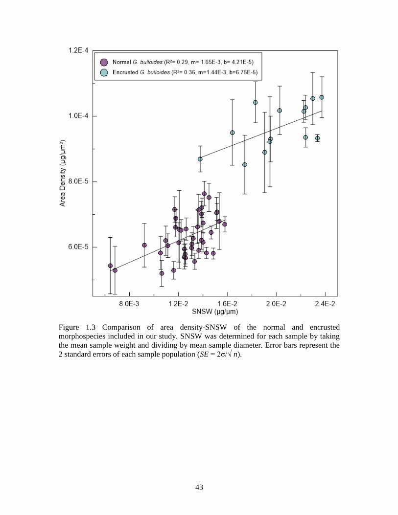
43

Figure 1.3 Comparison of area density-SNSW of the normal and encrusted

morphospecies included in our study. SNSW was determined for each sample by taking

the mean sample weight and dividing by mean sample diameter. Error bars represent the

2 standard errors of each sample population (SE = 2σ/√ n).

44

Figure 1.4 SEM images of normal (upper panels) and visually distinct encrusted (lower panels) whole shells, external surface textures

and pore density imaged from the inner shell wall.

45

Figure 1.5 G. bulloides δ18O derived calcification depths (red circles) plotted here with contoured measured temperatures (0-100 m)

with the 12.5˚C isotherm (dashed red) highlighted as the mean calcification temperature determined for this time-series. This dataset

excludes three 18O enriched samples from the strong upwelling period in 2008. The dates of coinciding hydrographic data are marked

on the upper x-axis as “X” with the three excluded samples marked by a “+”.

46

Figure 1.6 Normal and encrusted area density time-series and 1/16th split abundance counts. The Pacific Fisheries Environmental

Laboratory upwelling index is plotted as an indicator of upwelling strength and estimates of in situ [CO32-] determined from measured

temperature and oxygen indicate shifts in [CO32-] SEM images illustrate the difference in shell wall thickness from a non-upwelling

(A) and an upwelling (B) sample.

47

Figure 1.7 Left: Measured in situ sea surface temperature and estimates of surface [CO32-] from the SBB (1955-2005). Right: Down

core shell diameter and area density over the last century.

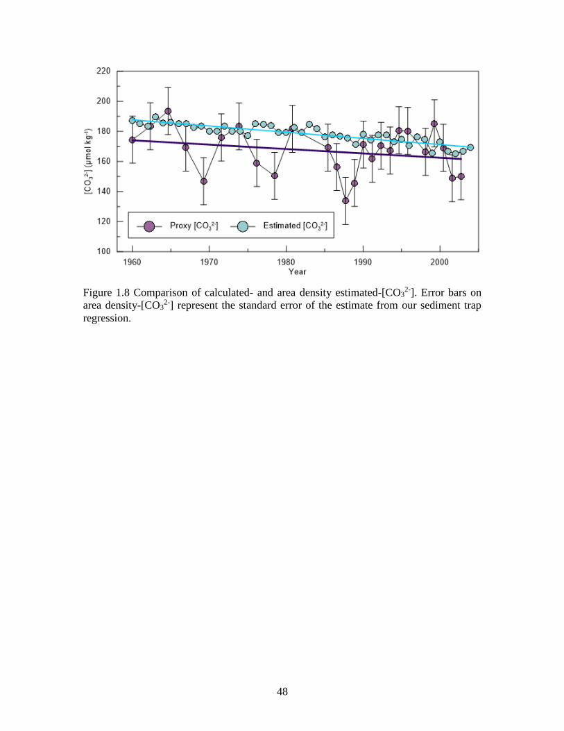
48

Figure 1.8 Comparison of calculated- and area density estimated-[CO32-]. Error bars on

area density-[CO32-] represent the standard error of the estimate from our sediment trap

regression.

49

Figure 1.9 The linear relationship observed between normal and encrusted G. bulloides

area density and [CO32-] from our sediment trap analyses. Error bars represent 2 standard

errors (SE = 2σ/√ n).

50

Figure 1.10 Comparison of area density calibrations for G. bulloides (normal and

encrusted) (this study) and G. ruber and G. sacculifer [Marshall et al., 2013]

51

CHAPTER 2

NATURAL AND ANTHROPOGENIC OCEAN ACIDIFICATION IN THE CALIFORNIA

CURRENT AND CONSEQUENCES FOR MARINE CALCIFIERS

52

2.1 ABSTRACT

The oceanic uptake of anthropogenic carbon mitigates climate change, but also

results in global ocean acidification, i.e., an increase in ocean acidity and a corresponding

reduction in the carbonate ion concentration ([CO32-]). While the global-mean changes

are well constrained by the changes in atmospheric CO2, much less is known about the

regional evolution of ocean acidification. Here, we use the calcification history recorded

by fossil shells of calcifying zooplankton to reconstruct the progression of surface ocean

acidification over the last century in the central California Current Ecosystem. Our

records indicate a 20% reduction in calcification since ~1900, translating to a 35%

decline in [CO32-] over this period. This larger than expected decrease is the result of a

substantial regional modification of the global mean trends, driven primarily by stronger

upwelling. This is supported by distinct signals in the concurrently recorded 13C/12C and

18O/16O isotopic composition of the carbonates. Our record also reveals a substantial

interannual to decadal modulation of ocean acidification in the California Current

Ecosystem by the Pacific Decadal Oscillation and the El Niño Southern Oscillation,

modulations that are expected to continue influencing the future evolution. Based on the

historic record, we predict that an unabated increase in atmospheric CO2 will lead to a

strong reduction in calcification of planktonic foraminifera.

2.2 INTRODUCTION

Over the last 150 years fossil fuel consumption, land use change and cement

production have caused annual mean atmospheric CO2 to increase from preindustrial

levels of ~280 ppm to more than 400 ppm (Figure 2.1). At the same time an estimated

53

equivalent of 73 ppm of atmospheric CO2 has been sequestered by the ocean (Khatiwala

et al., 2013; Le Quéré et al., 2015) resulting in a 0.1 reduction in global mean surface pH

(Sabine et al., 2004; Brewer, 1997; Le Quéré et al., 2014). The rate of CO2 release has

increased exponentially over this time period with the vast majority (>80%) of

anthropogenic CO2 emissions having occured over the last century, particularly since the

year 1960. As the marine carbonate system has shifted to accommodate more carbon, the

concentration of the dissolved carbonate ion (CO32-) has decreased significantly as it is

consumed via buffering reactions to maintain seawater pH (Figure 2.1). Many marine

calcifiers that depend on the availability of CO32- to precipitate their calcium carbonate

(CaCO3) shells and skeletons respond adversely to the wide-scale changes occurring in

the surface ocean (Feely et al., 2004; Sabine et al., 2004; Orr et al., 2005; Ries et al.,

2009). Field studies of corals, coccolithophores, pteropods, and foraminifera, the ocean’s

major pelagic calcium carbonate producing organisms, have repeatedly indicated

calcification stress in response to declining [CO32-] (e.g. De’ath et al., 2009; Meier et al.,

2014; Moy et al., 2009; de Moel et al., 2009; Bednarsek et al., 2014; 2016).

Marine calcifiers depend on the availability of dissolved ions in seawater,

predominantly Ca2+ and CO32-, to form their shells and skeletons. Studies have shown

that the reduced availability of CO32- results in inhibited calcification for a host of

calcifying organisms, including but not limited to corals, mussels, oysters, pteropods and

foraminifera, all of which are found in the CCS (Fabry et al., 2008; Hauri et al., 2009;

Ries et al., 2009; Kroeker et al., 2013). While the reduction in the availability of CO32-

hinders the ability of many organisms to form CaCO3, the associated decline in pH as a

54

result of increasing [H+] (Eq. 1) corresponds with a reduction in carbonate saturation state

of seawater and dissolution of CaCO3 (Eq. 2).

(1)

(2)

Planktonic foraminifera are ubiquitous calcite-secreting zooplankton that live for

approximately 1 month and form their calcite shells in the upper several hundred meters

of the water column. A recent plankton survey indicated that Rhizaria, a protist super-

group of which foraminifera are a predominant constituent, comprise on average 30% of

the total zooplankton population in the upper 500 meters of the water column in the

global ocean, with estimates as high as 80% for the coastal upwelling zone off of

California (Baird et al., 2016). Zooplankton represent the trophic level between primary

producers and upper-trophic levels and therefore play a key role in marine food webs

(Doney et al., 2012). Foraminifera are a particularly important group of calcifying

zooplankton in that they that are responsible for a significant portion of the pelagic

calcium carbonate flux (Schiebel, 2002; Kucera, 2007; Lebrato et al., 2010). Calcium

carbonate and opal biominerals and dust particles act as mineral ballasts that facilitate the

flux of organic carbon to the deep ocean that provides a net sink for atmospheric CO2 on

centennial time-scales (Armstrong et al., 2002). A global compilation of sediment trap

data indicate that calcium carbonate biominerals account for an estimated 80% of

particulate organic carbon flux below 1000 m due to the abundance and high density of

CaCO3 (Klaas & Archer, 2002)

55

Both modeling studies and observations suggest that ocean acidification (OA) will

be particularly acute in coastal upwelling systems due to the low buffer capacity of these

waters and natural upwelling processes that bring CO2-rich intermediate waters to the

ocean surface (Orr et al., 2005; Feely et al., 2008, 2010, 2016; Fabry et al., 2009; Hauri et

al., 2009; Gruber et al., 2012). The California Current Ecosystem (CCE), a highly

productive coastal upwelling system, has been identified as one of these vulnerable

regions based on both observational and modeling studies (Feely et al., 2008; Gruber et

al., 2012; Hauri et al., 2013; Turi et al., 2016). In situ measurements over the last decade

indicate a considerable decline in [CO32-] in the CCE and shoaling of the saturation

horizons for each of the CaCO3 mineral polymorphs (calcite Ωcal and aragonite Ωarg),

reducing the volume of the surface ocean suitable for calcification. Model simulations

suggest the aragonite saturation horizon in the CCE has already shoaled an estimated 150

meters since around 1850 (Gruber et al., 2012; Hauri et al., 2013; Turi et al., 2016).

Model results are supported by observations of malformed and dissolved shells of

aragonite-forming zooplankton (pteropods), particularly during periods of strong

upwelling when the saturation horizon at times intersects with the sea surface (Bednarsek

et al., 2014, 2016).

Direct observations of the marine carbonate system in the CCE are limited to the

last decade (CalCOFI; 2009-Present) and initial surveys of the global ocean took place in

the late 1970’s as a part of the Geochemical Ocean Sections Study (GEOSECS), well

after anthropogenic carbon began altering the marine carbonate system (GEOSECS;

Takahashi et al., 1982). GEOSECS has been followed up by a number of globally distributed

long-term monitoring programs, which have invariably indicated that the mean surface water pH

56

and [CO32-] have declined over the last several decades as a result of increasing pCO2 (Bates et

al., 2014). While these observational records are critically important to our understanding

of ocean chemistry, they do not provide a sufficiently long historical insight to this

problem. Model simulations can close this gap but without constraints from in situ and/or

proxy measurements, their validity remains unknown, especially with regard to their

ability to capture variability. With atmospheric CO2 concentrations projected to reach

anywhere from less than 500 to more than 900 ppm by the close of the 21st century,

understanding how pH and [CO32-] have declined over the last century is central to

projecting how the marine carbonate system will respond in the future (IPCC AR5

Report). The lack of long-term OA records currently limits our ability to put recent

observations into the context of past changes and hinders assessing how natural decadal

climate variability affects the marine carbonate system. Here, we provide the first

century-long OA record for the CCE, which has been shown to be particularly susceptible

when it comes to OA. This century-long record of [CO32-] is in agreement with in situ

measurements collected during the last decade and confirms the progression of OA

suggested by models. In addition, our results show large variations in [CO32-] associated

with Pacific Decadal Oscillation (PDO) climatic forcing. If the relationship between PDO

and OA is a widespread phenomenon, then we can expect OA will be modulated by this

climatic state, thereby shifting the time of emergence of the anthropogenic signal into the

future. Despite this modulation, the anthropogenic signal is large, with the past history

implying very low CO32- levels in the near future.

57

2.3 METHODS

2.3.1 CALCIFICATION INTENSITY

A recent sediment trap study conducted in the Santa Barbara Basin, California

found that calcification of the surface-mixed layer planktonic foraminifera species,

Globigerina bulloides, is strongly controlled by ambient [CO32-] (Osborne et al., 2016).

This study as well as others demonstrate that shell wall thickness varies as a function of

[CO32-] and therefore this shell characteristic can be used as a proxy for [CO3

2-] (Spero et

al., 1997; Bijma et al., 1999; Barker & Elderfield, 2002; Marshall et al., 2013; Osborne et

al., 2016). Foraminiferal calcification intensity, represented by both rate and efficiency of

calcification, is defined as the amount of calcite deposited relative to the size of the

individual and thereby generally reflects shell thickness (Weinkauf et al., 2013). In order

to properly estimate foraminiferal calcification intensity, size-normalization is of vital

importance because shell size, which inherently effects overall shell weight, is not

controlled by ambient [CO32-] but rather seawater temperature.

While several shell weight size-normalization techniques used to estimate

calcification intensity exist, we chose to use the area density method, which is an area-

normalizing shell weight method that uses individual rather than bulk population

measurements (Marshall et al., 2013). This method is currently the most effective size-

normalization technique (compared to measure-based weights and sieve-based weights)

that best constrains shell thickness. Approximately 40 individual G. bulloides shells were

picked from the >150 µm size-fraction of each sediment sample for area density analyses.

Individual G. bulloides shells with abnormally formed shells or that had visible clay

and/or organic material were excluded from our analyses as these characteristics could

58

effect weight and area measurements. While there can still be a considerable amount of

variability within a single sediment sample, statistical analyses by Osborne et al. (2016)

indicate that taking the average of at least 40 individuals significantly decreases the

standard error of the mean. Each shell is individually weighed in a copper weigh boat

using a high precision microbalance (Mettler Toledo XP2U; ±0.43 µg) in an

environmentally controlled weigh room. Next, each individual is photographed

positioned umbilical side up using a binocular microscope (Zeiss Stemi 2000-C) fitted

with a camera (Point Grey Research Flea3 1394b). The microscopic imaging program

(Orbicule Macnification 2.0) was used to analyze shells photos for length (Feret

diameter) and the 2-D surface area or silhouette. The Macnification 2.0 program uses the

RGB images to calculate a region of interest and generates an outline of the shell image,

which is then used to estimate a pixel 2-D area. Pixel measurements are converted to

lengths (µm) and areas (µm2) by calibrating an image of a 1 mm microscale taken at the

same magnification and working distance as shell photos. Individual shell weights were

then divided by their corresponding areas and a mean area density value was calculated

for each sample population.

The presence of an encrusted cryptic morphospecies of G. bulloides has been

documented in the Santa Barbara Channel (Sautter and Thunell, 1991; Darling et al.,

2003; Bemis et al., 2002). Further investigation indicated that the less abundant and cool

water loving “encrusted” morphospecies calcifies and fractionates stable carbon and

oxygen isotopes differently than the more abundant “normal” morphospecies (Bemis et

al., 2002; Osborne et al., 2016). Due to the offset in calcification intensity and the

intention to use these G. bulloides shells for later stable isotope analyses, morphometric

59

measurements collected during area density processing are also used to identify and

remove encrusted individuals from our sample populations (Osborne et al., 2016;

Marshall et al., 2015). The species-specific area density response of the normal

Globigerina bulloides morphospecies to ambient [CO32-] has been constrained using

individuals collected in the Santa Barbara Basin (SBB) by a sediment trap time-series

(Equation 2). Stable isotope results from this 3.5-year sediment-trap analysis indicate that

on average G. bulloides calcify in the 40 m depth range, although seasonal variability in

depth habit does occur in association with upwelling.

Calcification Intensity (µg/µm2) = 1.92-7 ([CO32-]) + 4.19-5 (1)

2.3.2 STABLE ISOTOPE MEASUREMENTS

At least 100µg (30-40 individuals) of G. bulloides used for area density analyses

were pooled to measure the stable oxygen (δ18O) and carbon (δ13C) isotopic composition.

Foraminifera were cleaned for 30 minutes in 3% H2O2 followed by a brief sonication and

acetone rinse prior to analyses. Stable isotope measurements were carried out on an

Isoprime isotope ratio mass spectrometer equipped with a carbonate preparation system.

The long-term standard reproducibility is 0.07‰ for δ18O and 0.06‰ for δ13C. Results

are reported relative to Vienna Pee Dee Belemnite (V-PDB).

2.3.3 BOX CORE SEDIMENTS

A 0.5-meter long box-core collected in the Santa Barbara Basin was used for the down

core analyses included in this study (SBB; 34˚14’N, 120˚02’W; 580 m water depth). An

age model for this core was developed using 210Pb geochronology with an error of less

than 1 year (Osborne et al., 2016). The lowermost sediments date back to the year 1895

and the uppermost sediments represent the year 2005 (average sedimentation rate 0.34

60

cm yr-1). The upper 10 centimeters of the core was sampled at half-centimeter resolution

and the lower 40 centimeters were sampled at centimeter resolution. High-resolution

sampling allows for nearly annual resolution for the upper 20 years of the core and

roughly ~2 year resolution for the lower 80 years of the core.

2.3.4 MARINE CARBONATE SYSTEM CALCULATIONS

The marine carbonate system for the historic record was calculated using the

proxy [CO32-] estimates and a salinity-based estimate of total alkalinity (Fassbender et al.,

2016). We estimate the seawater boron concentration using a chlorinity relationship

derived for North Pacific (Lee et al., 2010) and then determine the concentration of

[HCO3-] using the formulation for total alkalinity (Equation 2). In order to estimate DIC

we sum the estimated [CO32-] with the derived [HCO3

-] and assume that any

concentration of [CO2] is less than 1% of DIC (Zeebe and Wolf-Gladrow, 2001; Equation

3). We assume a constant seawater temperature and salinity based on the mean surface

temperature from the Santa Barbara Basin and salinity from Scripps Pier (salinity) Shore

Stations 50 year time-series and assume surface pressure of 1 for these calculations

(T=16 ˚C, S=33.5 ppt, P=1 atm).

Total Alkalinity = [HCO3-]+2[CO3

2-]+[B(OH)4-] (2)

Dissolved Inorganic Carbon = [HCO3-]+[CO3

2-] (3)

For the projection of the carbonate system in to the future we use projected

atmospheric CO2 to estimate pCO2 following Henry’s Law and again assume a constant

total alkalinity. Henry’s Law constants (K0) were determined using the R package by

Jean-Marie Epitalon, Aurelien Proye, and Jean-Pierre Gattuso. The K0 determined as a

61

part of this package follow the formulation of Weiss (1974) and account for changes in

temperature, salinity and pressure. We assume a constant seawater temperature, salinity

and pressure for these calculations (T=16 ˚C, S=33.5 ppt, P=1 atm).

pCO2(µatm)=XCO2(ppm)(pAtm-pH2O)

XCO2= Projected [CO2]

pAtm= 1

pH2O= determined in R according to Weiss, (1974)

The saturation state of seawater was calculated using the proxy [CO32-] values for

the historic record or the predicted [CO32-] values for the forward projection. Calculations

were made using the CO2Sys program assuming that the concentration of calcium in

seawater has remained constant (10.28 mmol kg-1; Broecker and Peng, 1982).

Stoichiometric solubility constants determined by Mucci (1983) for each mineral were

used in these calculations. We again assume a constant seawater temperature, salinity and

pressure for these calculations (T=16 ˚C, S=33.5 ppt, P=1 atm).


2.4.1 CALCIFICATION AND THINNING SHELLS OVER THE LAST CENTURY

The calcification intensity of nearly 2,000 individual G. bulloides shells was

measured using 52 sediment samples from a 0.5-meter long box-core collected in the

Santa Barbara Basin (SBB; 34˚14’N, 120˚02’W; 580 m water depth; Table 2.1). The G.

bulloides used for our calcification intensity measurements were also used for oxygen

and carbon stable isotopic composition analyses. Down core calcification intensity and

62

shell size measurements indicate that G. bulloides produced 20% thinner and 7% larger

shells, respectively, by the close of the 20th century relative to those from 1900. The

relationship between increasing shell size and warming sea surface temperatures is

evident in the comparison of shell diameter and the oxygen isotopic composition of the

same G. bulloides shells (Figure 2.2) Globigerina bulloides calcification intensity was

converted to [CO32-] using the relationship derived for this species from the SBB

(Osborne et al., 2016).

Estimates of [CO32-] from calcification intensity indicate an ~35% decline in

surface ocean [CO32-] over the 20th century (271 to 173 ±16 µmol kg-1) or nearly a 100

µmol kg-1 change (Figure 2.3). The decline in calcification is apparent in scanning

electron micrographs of shell wall cross sections of similarly sized G. bulloides from the

top and bottom of the sediment core (Figure 2.3). Our proxy-based [CO32-] estimates are

compared to results from a hindcast model simulation determined for various depths

within the SBB water column from 1979 to 2012. These simulations of the carbonate

system are based on an eddy-resolving ocean biogeochemical model forced with

observation-based variations of wind stress and fluxes of heat and freshwater (Turi et al.,

2016). The modeled long-term trend is in agreement with our proxy record. However, the

model simulations indicate overall lower [CO32-] values relative to our estimates based on

calcification intensity, in part due an overall negative bias in the model (Hauri et al.,

2013). Recent in situ surface ocean [CO32-] measurements from the Santa Barbara Basin

by the California Cooperative Oceanic Fisheries Investigation (CalCOFI; 2009-2015) and

NOAA’s Ocean Acidification Program (2011-2013) are in excellent agreement with the

trend of our estimated [CO32-] values although these datasets do not overlap with our

63

sediment record. An additional comparison to the oligotrophic North Pacific (Hawaii

Ocean Time-series) also shows a similar long-term decline albeit with significantly

higher [CO32-] values, reflecting the subtropical location of this time-series. This regional

difference illustrates the inherently low [CO32-] conditions in the CCE.

Because the relative concentrations of the dissolved inorganic carbon species

(DIC; CO2, HCO3−, CO3

2-) co-vary in a predictable nature so do the variables of the

marine carbonate system (DIC, Total Alkalinity, pH, pCO2). Six equations with 4

unknowns represent the variables of the marine carbonate system, and therefore

knowledge of two variables can be used to determine the remainder of the system. Using

our down core [CO32-] values and salinity-based estimate of total alkalinity (Fassbender

et al., 2016) we estimated how pH has evolved over the last century (Table 2.2). We

estimate that the [H+] of seawater has increased by 90%, translating to a 0.25 unit decline

in pH in this region (8.17-7.92), thereby exceeding the global average of 0.1 units by

more than a factor of two. Our estimated decadal rate of pH decline for this region over

the last century (-0.025 dec-1) is slightly higher than the rate of pH decline modeled

recently for the entire California Current System (-0.020 dec-1; 1979-2012; Turi et al.,

2016), and more broadly with observations for the North Pacific (-0.017 dec-1; 1991-

2006; Byrne et al., 2010) and the HOT time-series (-0.019 dec-1). Regional model

simulations for the CCE emphasize that the central portion of the system, where our

study region is located, has experienced a large decline in pH as a result of focused strong

upwelling (Gruber et al., 2012; Turi et al., 2016).

The saturation state of seawater with respect to calcium carbonate (Ω) was also

quantified using our [CO32-] estimates. Because the concentration of calcium in seawater

64

([Ca2+]; 10.28 mmol kg-1) is conservative, [CO32-] can be considered the dominant control

on Ω. An Ω value of 1 indicates that the water mass is saturated with respect to CaCO3,

while values above 1 represent supersaturated conditions where calcification is favored

and values below 1 indicate an undersaturated environment where CaCO3 preferentially

dissolves. The long-term trend in our reconstruction indicates that Ω of the mineral form

calcite (Ωcal) decreased by 1.5 units (4.6-3.1), while the Ω of the mineral aragonite

(Ωarg) decreased by 1 unit (3.0-2.0) representing a 50% decline in saturation states since

1900. Episodic acidification events result in saturation states that can be as low as 2.43

Ωcal and 1.56 Ωarg. The decadal rate of decline in Ωarg recorded in our proxy

reconstruction (-0.10 dec-1) is comparable to model estimates for the upper 60 m of the

water column spanning the last ~35 years for the entire CCS (-0.12 dec-1; 1979-2012;

Turi et al., 2016).

2.4.1 CLIMATIC MODULATION OF OCEAN ACIDIFICATION

While we attribute the long-term decline in [CO32-] to anthropogenic CO2-driven

ocean acidification, there is also considerable decadal and sub-decadal scale variability

around the long-term trend. In order to best visualize this variability, we have removed

the long-term anthropogenic trend in [CO32-] and compare the detrended [CO3

2-] record to

a Pacific Decadal Oscillation index (Hare et al., 1996). This comparison reveals that

decadal fluctuations in [CO32-] co-vary with shifts between positive and negative phases

of PDO (Figure 2.4). During positive (warm) phases of PDO the carbonate system shifts

to a higher [CO32-] state, while negative (cool) phases of PDO coincide with overall

lower [CO32-] values (Figure 2.4a). PDO is associated with changes in the strength of the

Aleutian Low, resulting in basin-wide temperature, pressure and wind stress anomalies in

65

the Pacific (Mantua and Hare, 2002). Within the CCE, the positive (warm) phase of PDO

coincides with weaker Aleutian Low winds, resulting in decreased coastal upwelling,

warmer sea surface temperatures and reduced productivity. Conversely, the negative

(cold) phase of PDO produces the opposite set of conditions.

Since coastal upwelling controls the amount of acidic subsurface waters that reach

the surface and PDO regulates the strength of upwelling, we hypothesize that this

mechanism alters the surface carbonate system on decadal time-scales. We use a two-

pronged approach to test if decadal shifts in upwelling strength are recorded in our study

region and if they are found in association with PDO shifts. First we use the stable

oxygen isotopic composition (δ18O) as a temperature proxy to compare values recorded

by a surface (G. bulloides) and a deep (Neogloboquadrina incompta) dwelling

foraminifera species. An increased offset (∆δ18O) in the temperatures recorded by the

surface and deep dwelling species represents an increase in stratification or a decline in

upwelling strength (Pak and Kennett, 2002). The ∆δ18O is positively correlated with the

PDO index; positive phases are marked by a higher ∆δ18O, which represent decreased

upwelling/increased stratification (Figure 2.4b). A reduction in upwelling of low pH

waters would alleviate the bottom-up stress on the surface carbonate system, giving rise

to higher surface [CO32-]. We also use the stable carbon isotopic composition (δ13C) of G.

bulloides shells, which records the isotopic composition of DIC (Ferguson et al., 2013).

The seasonal signal in δ13C recorded by G. bulloides in our study region varies inversely

with upwelling strength (Figure 2.5); lower δ13C coincides with peak upwelling when the

subsurface DIC that is 12C-enriched due to remineralization is introduced to the surface.

After removing the long-term decline in δ13C due to the 13C Suess Effect (Keeling et al.,

66

1979; Figure 2.6), we find that the residual changes in δ13C positively correlate with PDO

and our ∆δ18O record (Figure 2.4b). This confirms that upwelling weakens in the CCE

during positive PDO resulting in higher than expected [CO32-] during these periods and

strengthens during negative phases of PDO resulting in lower than expected [CO32-].

These upwelling records also indicate a long-term increase in stratification (Figure 2.7),

which is supported by CalCOFI (1950-present) observations of warming sea surface

temperatures, deepening of the thermocline depth and declining zooplankton biomass

(Roemmich and McGowan, 1995; McGowan et al., 2003; Di Lorenzo et al., 2003).

The El Niño Southern Oscillation (ENSO) also correlates with sub-decadal shifts

in the [CO32-] record. El Niño events, typically lasting 6-18 months, produce similar

anomalies as positive PDO phases and are marked by decreased windstress, reduced

upwelling, and elevated [CO32-], while La Niña events are similar to negative PDO

phases and coincide with lower [CO32-]. Five years of continuous observations from a

mooring in the SBB observed the progression of the 2010 La Niña confirming the

relationship between La Niña, increased coastal upwelling and increased acidity of

surface waters off the continental shelf of California (Nam et al., 2011). We observe

several rapid, extreme acidification events that unexpectedly coincide with the three

largest El Niño events of the last century (1997/1998, 1982/1983 and 1986/1987) (Figure

2.8). The anomalous declines in [CO32-] associated with these specific El Niño events are

also captured in the hindcast model simulations for the SBB (Turi et al., 2015; Figure

2.9). This deviation from the typical trend of elevated [CO32-] in association with El Niño

events is likely owing to the substantial shift in surface current dynamics that occur

during exceptionally strong El Niño conditions that result in the advection of low pH

67

waters from the Equatorial Pacific to the coastal California region (Bograd and Lynn,

2001; Di Lorenzo et al., 2005; Nam et al., 2015). This phenomenon suggests that not only

chemical but also physical processes play an important role in marine carbonate system

dynamics in this region.

2.4.1 FUTURE IMPLICATION OF OCEAN ACIDIFICATION ON PLANKTON CALCIFICATION

Our record of foraminiferal calcification intensity and [CO32-] during the last

century provides insight as to how the carbonate system in the CCE may vary in the

future. Projections of [CO32-] through the end of the 21st century are generated based on

the four atmospheric CO2 Representative Concentration Pathways (RCP) scenarios

(Table 2.3; Figure 2.10) described by the IPCC AR5 report (Chapter 12). RCPs represent

a range of scenarios including a significant decline in CO2 emissions (RCP 2.6, 421 ppm)

to “business as usual” emissions (RCP 8.5, 936 ppm). The projections made here

represent a baseline change that can be expected for this region and are in excellent

agreement with global modeled carbonate system projections (Bopp et al., 2013; Table

2.4). However, a hindcast estimation of [CO32-] using this technique indicates the net

change in the marine carbonate system is underrepresented compared to our proxy

reconstruction for this region. This is likely due to the fact that projections based only on

atmospheric CO2 concentrations and seawater alkalinity cannot represent the regional

influence of upwelling. Therefore these projections represent a conservative estimate for

the progression of ocean acidification in the CCE and large variations around the

projected long-term trend should be expected based on the response of this system to

climatic forcing observed in the historic record.

68

We highlight the results for the 538 ppm scenario (RCP 4.5) as it is an optimistic

projection that meets the carbon emission and mean temperature goals (2˚ C temperature

cap) set forth during the 2015 Paris climate agreements. Despite efforts to abate carbon

emissions, under this scenario, [CO32-] decreases by an additional 25% by the close of the

21st century, representing a 54% decline in [CO32-] relative to the year 1900. Surface

waters will likely remain supersaturated with respect to both aragonite and calcite on

average, although modulation by PDO may result in undersaturation during negative

PDO phases with episodic undersaturation in concert with strong El Niños and other

extreme events (Hauri et al., 2013). Likewise, pH decreases by an additional 0.14 units

over the course of the 21st century, resulting in a net 0.39 unit decline in pH since the

beginning of the 20th century. Marine calcifiers that depend on the availability of [CO32-]

will likely respond adversely to such conditions, with estimates for G. bulloides

indicating at least a 30% reduction in calcification from 1900 to 2100. Under the business

as usual scenario (RCP 8.5) scenario where CO2 more than triples preindustrial values to

936 ppm, [CO32-] will likely decrease by 70% resulting in a 40% reduction in

calcification. Episodic undersaturation as a result of climatic modulation becomes

increasingly more likely as [CO32-] nears undersaturation thresholds under this scenario

and permanent aragonite undersaturation in the surface ocean is likely by the close of the

21st century.

2.5 CONCLUSIONS

Our 20th century reconstruction of [CO32-] for the central CCE region underlines

the significant shifts that have already occurred in the marine carbonate system over the

last century in response to anthropogenic CO2. This record also indicates that the marine

69

carbonate system experiences considerable variability, which we associate with shifts in

costal upwelling strength related to PDO and ENSO. Over decadal time-scales

positive/negative phases of PDO correlate with an overall elevated/reduced [CO32-] state,

indicating that anthropogenic acidification will be both amplified and dampened in

association with decadal shifts in this climatic mode. Over shorter time-scales, ENSO

correlates with [CO32-] in the same fashion (El Niño/La Niña, elevated/reduced [CO3

2-]).

However very strong El Niño events produce anomalous conditions that deviate from the

typical trend and are instead associated with dramatic and rapid acidification events.

Various emission scenarios for the coming century indicate that [CO32-] will continue to

decline in response to anthropogenic CO2 nearing permanent surface ocean

undersaturation. The projected decline in calcification of planktonic foraminifera and

other calcifiers will likely result in a reduction of the fraction of organic carbon reaching

the seafloor via these ballasting minerals, consequently producing a positive feedback for

CO2 accumulation in the atmosphere and ocean. The response of the marine carbonate

system is considerably different between each scenario indicating that reducing emissions

is key to maintaining a surface ocean that is a suitable habitat for marine calcifiers. While

projections of [CO32-] are important for understanding how the system may progress in

the future, our past record indicates [CO32-] will not decline linearly and that modulation

by climatic forcing will be important in the coming century.

70

Table 2.1 Down core ages and morphometric measurements

Sample

Number

Core

Depth

(cm)

Age n Area

Density

Weight

(ug)

Area

(um2)

Diameter

(um)

5 2.5 2002 39 7.38E-05 4.46 58373 307

6 3.0 2001 39 7.35E-05 4.79 64730 327

7 3.5 1999 38 7.90E-05 5.70 71948 340

8 4.0 1998 38 8.19621E-

05 5.99 70435 339

9 4.5 1997 38 7.65E-05 4.81 62072 316

10 5.0 1996 29 6.56E-05 3.18 47321 267

11 5.5 1995 40 8.23E-05 4.72 57106 306

12 6.0 1994 40 8.24E-05 7.13 85885 381

13 6.5 1992 40 7.85E-05 6.20 77636 359

14 7.0 1991 39 7.94E-05 6.25 79605 364

15 7.5 1990 40 7.70E-05 4.53 56804 301

16 8.0 1989 37 8.01E-05 7.11 88434 385

17 8.5 1988 37 6.72E-05 3.93 53465 294

18 9.0 1987 17 3.57 52906 287

19 9.5 1986 40 7.55E-05 4.51 59296 313

20 10.0 1984 40 7.91E-05 5.13 64606 328

21 11.0 1982 28 6.80E-05 2.54 36812 242

22 12.0 1980 38 8.27E-05 6.87 83249 374

23 13.0 1977 40 7.39E-05 3.44 45509 270

24 14.0 1975 29 7.62E-05 3.32 43502 260

25 15.0 1973 38 8.32E-05 6.39 76960 355

26 16.0 1971 39 8.10E-05 5.47 68269 334

27 17.0 1968 18 7.30E-05 3.62 50341 278

28 18.0 1966 23 7.91E-05 3.67 45552 269

29 19.0 1964 34 8.63E-05 6.13 73619 346

30 20.0 1961 37 8.32E-05 6.29 79173 357

31 21.0 1959 40 8.06E-05 6.00 74304 352

32 22.0 1957 37 7.71E-05 5.52 78096 355

33 23.0 1954 40 7.83E-05 5.29 67781 334

34 24.0 1952 38 8.20E-05 4.26 59167 310

35 25.0 1950 32 8.90E-05 6.53 72870 349

36 26.0 1947 40 7.94E-05 5.73 72136 342

37 27.0 1945 36 8.08E-05 5.73 70943 342

38 28.0 1943 39 9.24E-05 5.04 54511 299

39 29.0 1941 38 9.63E-05 6.00 67339 331

40 30.0 1938 39 8.94E-05 4.87 62358 321

71

41 31.0 1936 40 9.39E-05 4.57 56911 305

42 32.0 1934 34 9.51E-05 3.73 45452 265

43 33.0 1931 27 9.75E-05 4.45 51212 285

44 34.0 1929 33 9.83E-05 4.15 54732 294

45 35.0 1927 37 8.49E-05 3.11 36889 242

46 36.0 1924 39 9.84E-05 4.84 57141 300

47 37.0 1922 40 9.56E-05 5.34 63047 323

48 38.0 1920 25 9.35E-05 4.48 55287 302

49 39.0 1917 38 8.99E-05 5.44 61554 318

50 40.0 1915 36 8.40E-05 4.64 57970 304

51 41.0 1913 38 8.28E-05 5.07 61423 324

52 42.0 1911 39 8.14E-05 5.77 65143 329

53 43.0 1908 39 8.40E-05 4.38 56820 307

54 44.0 1906 38 8.88E-05 5.83 70591 339

55 45.0 1904 23 9.25065E-

05 4.33 47869 279

56 46.0 1901 27 9.71E-05 6.01 66762 324

72

Table 2.2 Down core estimates of the marine carbonate system

Year Salinity Temp

(˚C)

TA

(mmol/kgSW)

TCO2

(mmol/kgSW) pH

CO32-

(mmol/kgSW) ΩCa ΩAr

2003 33.5 16 2250.0 2083.6 7.93 126.1 3.04 1.95

2002 33.5 16 2250.0 2085.4 7.93 125.0 3.01 1.93

2000 33.5 16 2250.0 2056.6 7.99 142.5 3.43 2.20

1999 33.5 16 2250.0 2031.7 8.05 157.9 3.80 2.44

1998 33.5 16 2250.0 2060.5 7.98 140.1 3.38 2.17

1997 33.5 16 2250.0 2141.5 7.78 93.0 2.24 1.44

1996 33.5 16 2250.0 2039.5 8.03 153.0 3.69 2.37

1995 33.5 16 2250.0 2039.0 8.03 153.4 3.70 2.37

1993 33.5 16 2250.0 2059.1 7.99 140.9 3.39 2.18

1992 33.5 16 2250.0 2054.5 8.00 143.8 3.46 2.22

1991 33.5 16 2250.0 2067.2 7.97 136.0 3.28 2.10

1990 33.5 16 2250.0 2053.4 8.00 144.5 3.48 2.23

1989 33.5 16 2250.0 2089.7 7.92 122.5 2.95 1.89

1988 33.5 16 2250.0 2105.7 7.88 113.1 2.73 1.75

1987 33.5 16 2250.0 2075.1 7.95 131.2 3.16 2.03

1985 33.5 16 2250.0 2056.4 7.99 142.6 3.44 2.21

1983 33.5 16 2250.0 2113.9 7.85 108.4 2.61 1.68

1981 33.5 16 2250.0 2037.4 8.03 154.4 3.72 2.39

1978 33.5 16 2250.0 2083.3 7.93 126.3 3.04 1.95

1976 33.5 16 2250.0 2071.2 7.96 133.6 3.22 2.07

1974 33.5 16 2250.0 2034.9 8.04 155.9 3.76 2.41

1972 33.5 16 2250.0 2046.1 8.01 148.9 3.59 2.30

1969 33.5 16 2250.0 2088.1 7.92 123.4 2.97 1.91

1967 33.5 16 2250.0 2056.4 7.99 142.6 3.44 2.21

1965 33.5 16 2250.0 2018.6 8.07 166.1 4.00 2.57

1962 33.5 16 2250.0 2034.7 8.04 156.0 3.76 2.41

1960 33.5 16 2250.0 2048.4 8.01 147.5 3.55 2.28

1958 33.5 16 2250.0 2066.9 7.97 136.2 3.28 2.11

1955 33.5 16 2250.0 2060.6 7.98 140.1 3.37 2.17

1953 33.5 16 2250.0 2041.1 8.03 152.1 3.66 2.35

1951 33.5 16 2250.0 2004.9 8.10 174.8 4.21 2.70

1948 33.5 16 2250.0 2054.5 8.00 143.8 3.46 2.22

1946 33.5 16 2250.0 2047.4 8.01 148.1 3.57 2.29

1944 33.5 16 2250.0 1987.1 8.13 186.2 4.48 2.88

1942 33.5 16 2250.0 1966.9 8.17 199.1 4.80 3.08

1939 33.5 16 2250.0 2002.9 8.10 176.1 4.24 2.72

1937 33.5 16 2250.0 1978.9 8.15 191.4 4.61 2.96

1935 33.5 16 2250.0 1972.9 8.16 195.2 4.70 3.02

1932 33.5 16 2250.0 1960.5 8.18 203.3 4.90 3.14

1930 33.5 16 2250.0 1956.5 8.19 205.8 4.96 3.18

1925 33.5 16 2250.0 1955.5 8.19 206.5 4.97 3.19

1923 33.5 16 2250.0 1970.1 8.16 197.0 4.75 3.05

1921 33.5 16 2250.0 1981.0 8.14 190.0 4.58 2.94

1918 33.5 16 2250.0 2000.1 8.11 177.9 4.29 2.75

73

1916 33.5 16 2250.0 2030.7 8.05 158.5 3.82 2.45

1914 33.5 16 2250.0 2036.8 8.03 154.7 3.73 2.39

1912 33.5 16 2250.0 2000.4 8.11 177.6 4.28 2.75

1909 33.5 16 2250.0 2030.9 8.05 158.4 3.82 2.45

1907 33.5 16 2250.0 2005.5 8.10 174.4 4.20 2.70

1905 33.5 16 2250.0 1986.4 8.13 186.6 4.49 2.89

1902 33.5 16 2250.0 1962.6 8.18 201.9 4.86 3.12

1898 33.5 16 2250.0 1977.3 8.15 192.5 4.64 2.98

74

Table 2.3 Projected changes in the marine carbonate system based on AR5 RCP scenarios

CO2

Year

RCP

2.6

RCP

4.5

RCP

6.0

RCP

8.5

2000 368.87 368.87 368.87 368.87

2005 378.81 378.81 378.81 378.81

2010 389.29 389.13 389.07 389.32

2020 412.07 411.13 409.36 415.78

2030 430.78 435.05 428.88 448.83

2040 440.22 460.85 450.70 489.44

2050 442.70 486.54 477.67 540.54

2060 441.67 508.87 510.63 603.52

2070 437.48 524.30 549.82 677.08

2080 431.62 531.14 594.26 758.18

2090 426.00 533.74 635.65 844.80

2100 420.90 538.36 669.72 935.87

pCO2

Year

RCP

2.6

RCP

4.5

RCP

6.0

RCP

8.5

2000 355.37 355.37 355.37 355.37

2005 364.95 364.95 364.95 364.95

2010 375.04 374.89 374.84 375.08

2020 396.99 396.09 394.38 400.57

2030 415.02 419.13 413.19 432.41

2040 424.12 443.98 434.21 471.53

2050 426.50 468.74 460.19 520.77

2060 425.51 490.25 491.95 581.44

2070 421.48 505.12 529.70 652.31

2080 415.83 511.71 572.52 730.44

2090 410.42 514.21 612.39 813.90

2100 405.50 518.66 645.22 901.64

CO3

2-

Year

RCP

2.6

RCP

4.5

RCP

6.0

RCP

8.5

2000 167.52 167.52 167.52 167.52

2005 164.48 164.48 164.48 164.48

2010 161.39 161.44 161.46 161.38

2020 155.08 155.33 155.80 154.10

2030 150.26 149.21 150.74 145.90

2040 147.95 143.13 145.46 136.97

75

2050 147.35 137.57 139.44 127.20

2060 147.60 133.08 132.74 116.96

2070 148.61 130.15 125.58 106.93

2080 150.05 128.89 118.36 97.71

2090 151.46 128.42 112.35 89.49

2100 152.77 127.59 107.85 82.23

pH

Year

RCP

2.6

RCP

4.5

RCP

6.0

RCP

8.5

2000 8.08 8.08 8.08 8.08

2005 8.07 8.07 8.07 8.07

2010 8.06 8.06 8.06 8.06

2020 8.04 8.04 8.04 8.03

2030 8.02 8.01 8.02 8.00

2040 8.01 7.99 8.00 7.97

2050 8.01 7.97 7.98 7.93

2060 8.01 7.96 7.95 7.89

2070 8.01 7.94 7.93 7.85

2080 8.02 7.94 7.90 7.80

2090 8.02 7.94 7.87 7.76

2100 8.03 7.93 7.85 7.72

76

Table 2.4 Absolute values and relative changes of carbonate system parameters

reconstructed for the 20th century from G. bulloides calcification intensity and projected

parameters based on atmospheric CO2 predictions. Only relative changes in projected pH

are reported here due to high error propagation of calculating pH.

Year

1900

Year

2000

Δ2000-

1900

RCP

2.6

Δ2100-

2000

RCP

4.5

Δ2100-

2000

RCP

6.0

Δ2100-

2000

RCP

8.5

Δ2100-

2000

CO2 (ppm) 296 370 73 421 51 538 169 670 300 936 566

[CO32-] (µmol/kgsw) 271 173 -98 153 -20 128 -45 108 -65 82 -91

Ωarg 3.0 2.0 -1.0 1.8 -0.2 1.4 -0.6 1.1 -0.9 0.7 -1.3

Ωcal 4.6 3.1 -1.5 2.8 -0.4 2.2 -1.0 1.7 -1.4 1.1 -2.1

pH 8.19 7.92 -0.25

-0.05

-0.14

-0.23

-0.36

pH (Bopp et al., 2013)

-0.07

-0.15

-0.22

-0.33

77

Figure 2.1 The increase in atmospheric CO2 due to fossil fuel burning, land use change

and cement production increases surface ocean CO2 and causes a redistribution of

dissolved inorganic carbon species (Le Quéré et al., 2015). CO2 quickly reacts with water

to form carbonic acid (H2CO3; not shown above), which almost instantaneously

dissociates into a bicarbonate ion (HCO3-) and releases a hydrogen ion (H+). The increase

in H+ as a result of this reaction lowers seawater pH (pH=-log(H+)), causing ocean

acidification. Carbonate ion (CO32-) reacts with increasingly concentrated H+ to alleviate

seawater acidity thereby forming more HCO3-. The decreased availability of CO3

2-

adversely affects marine organisms that use this ion to build their CaCO3 shells and

skeletons. Images of planktonic foraminifera, pteropod and coccolithophore shells

illustrate the effect of CO32- on shell formation (Images National Geographic Society,

Müller et al., 2015).

78

Figure 2.2 The long-term shift in G. bulloides shell diameter increases in concert with

warming sea surface temperatures. We compare the relative changes that are recorded G.

bulloides δ18O to a Northern Hemisphere Temperature anomaly for the 1900-2000 period

and see a good agreement between temperature trends recorded in these records (Jones et

al., 2013). We also compared G. bulloides δ18O to in situ sea surface temperature

measurements made in the SBB (1955-Present; Shore Stations Program) and see an

excellent agreements between sea surface temperature and the δ18O recorded in our G.

bulloides shells.

79

1900 2000 100µm20µm 20µm

a b c

Figure 2.3 Estimated [CO32-] derived from G. bulloides area density (1895-2000) compared to model simulations at 0, 30 and 50

meters (1979-2012) and in situ measurements from the Santa Barbara Basin made by CalCOFI and NOAA’s West Coast OA Cruises

and Hawaii Ocean Time-series (HOT) data from the oligotrophic North Pacific. (a) SEM images show a typical G. bulloides specimen

from the SBB and shell wall cross-sections of similarly sized shells from the (b) upper- and (c) lower-most samples of the box-core

clearly illustrating the difference in shell wall thickness over the past century.

80

Figure 2.4 Upper panel shows the [CO32-] record with the long-term anthropogenically-

driven decline removed. The detrended dataset is shown with the Pacific Decadal

Oscillation (PDO) index indicating a correlation between high/low [CO32-] and

positive/negative PDO phases. Both data sets are shown as 5-period running means. The

lower panel shows detrended ∆δ18ON. incompta-G. bulloides and G. bulloides δ13C again to

highlight the natural variability not associated with anthropogenic ocean acidification.

These datasets are plotted again with the PDO index indicating a relationship between

weakened/strengthened upwelling and positive/negative PDO phase.

81

Figure 2.5 δ13C of G. bulloides recorded in a year long (October 2013-October 2014) set

of sediment trap samples from the Santa Barbara Basin. These data are plotted with an

upwelling index from the Pacific Fisheries Environmental Laboratory (PFEL) with higher

values indicating increased upwelling strength. Note that the δ13C data are plotted on an

inverted axis, therefore δ13C and upwelling strength are inversely related. The more

negative δ13C values are associated with stronger upwelling of subsurface waters that are

relatively 12C-enriched due to remineralization of organic matter.

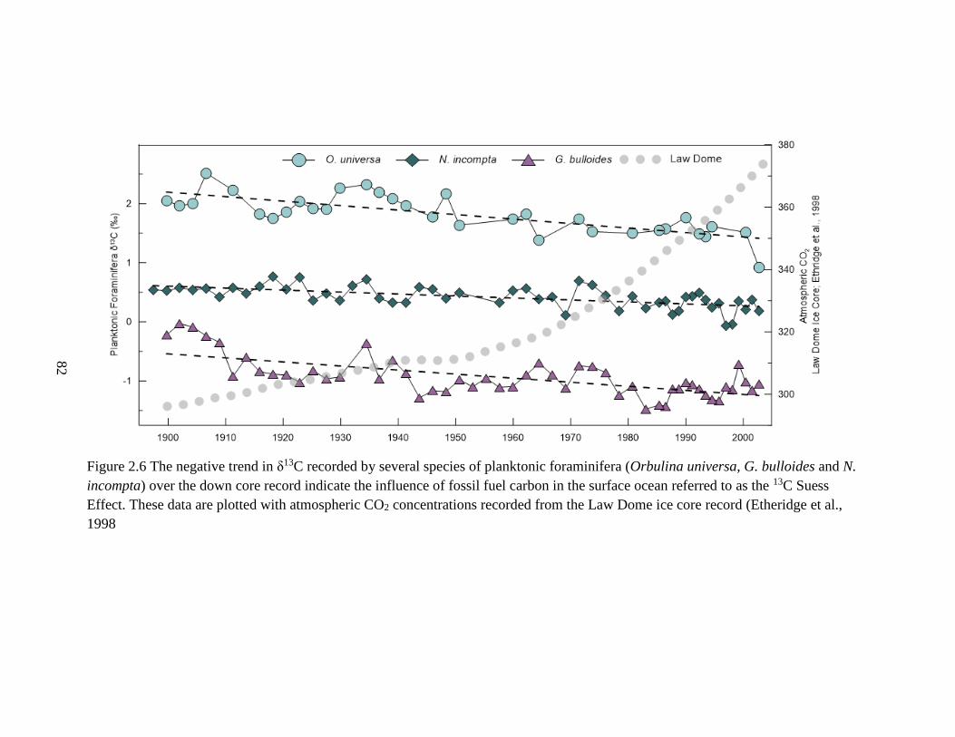
82

Figure 2.6 The negative trend in δ13C recorded by several species of planktonic foraminifera (Orbulina universa, G. bulloides and N.

incompta) over the down core record indicate the influence of fossil fuel carbon in the surface ocean referred to as the 13C Suess

Effect. These data are plotted with atmospheric CO2 concentrations recorded from the Law Dome ice core record (Etheridge et al.,

1998

83

Figure 2.7 δ18O of G. bulloides (surface-mixed layer) and N. incompta (sub-thermocline) measured over the last century. Because δ18O

and temperature are negatively correlated, these data are plotted on an inverted y-axis. δ18O values for G. bulloides at present are more

negative relative to values from 1900 indicating surface ocean warming. N. incompta δ18O indicates the opposite trend suggesting that

the calcification temperature for each of these species has diverged over the last century which we interpret here as an increase in

stratification.

84

Figure 2.8 Three rapid acidification events recorded in the [CO32-] reconstruction occur

anomalously in association with strong El Niño events (1982/1983, 1986/1987 and

1997/1998). These data are shown with the Multivariate ENSO index (inverted axis).

These events deviate from the typical relationship between positive MEI (El Niño) and

elevated [CO32-] which, for example, can be seen here from 1990-1995 when elevated

[CO32-] coincides with El Niño conditions.

85

Figure 2.9 Comparison of detrended proxy [CO32-] values to detrended modeled [CO3

2-]

values for the 1975-2005 interval when the three large El Nino events occur. While the

exact timing of the 1982/3 and 1986/7 do not align as well as the 1997/8 event, errors in

the age of the sediment samples suggest that the negative carbonate excisions could well

overlap.

86

Figure 2.10 Projections of [CO32-] in association with the four RCP CO2 pathways

outlined in the IPCC AR5 Report. Historic atmospheric CO2 concentrations from the

Mauna Loa Time-Series and the Law Dome Ice Core as well as our proxy [CO32-]

reconstruction are shown as a historical reference to the CO2 model projections. The

[CO32-] at which aragonite and calcite become undersaturated are highlighted as dashed

lines (Broecker and Peng, 1982).

87

CHAPTER 3

BORON CONCENTRATION OF NON-DINOFLAGELLATE HOSTING PLANKTONIC

FORAMINIFERA CALCITE AND SEAWATER CARBONATE CHEMISTRY

88

3.1 ABSTRACT

The concentration of boron in marine carbonates (B/Ca ratio) has been proposed

to covary with seawater carbonate chemistry. However, a number of studies have

evaluated the B/Ca proxy in planktonic foraminifera and found that boron incorporation

may not be a straightforward process. The majority of previous research has focused on

tropical species that host large photosynthetic symbionts, which interfere with ambient

carbonate chemistry and the incorporation of boron into the calcite lattice. This study

focuses on evaluating the boron concentration of subtropical and subpolar species that are

asymbiontic or host small intra-shell non-dinoflagellate symbionts. (Globigerina

bulloides, Neogloboquadrina incompta and Neogloboquadrina dutertrei) collected as

part of a time series sediment trap study in the Santa Barbara Basin (SBB). Replicate

measurements of B/Ca ratios across size-fractions generally indicate no size-dependent

uptake of boron that has previously been recorded for dinoflagellate symbiont bearing

species. Both Neogloboquadrina species indicate strong correlation with the calcite

saturation of seawater, carbonate ion concentration and pH. However the relationship

between G. bulloides and these variables is more complex. The presence of two

morphospecies of G. bulloides (encrusted and normal) in our sampling population may

account for high B/Ca ratios and poor duplicates that occur in samples collected during

winter and peak upwelling months when the encrusted morphospecies is present in the

SBB. A further analysis of individual G. bulloides of each morphospecies from this study

region is essential to determining if trace element offsets exist and to assess the influence

that cryptic morphospecies have on bulk B/Ca ratios. Down core measurements of N.

incompta B/Ca indicate a steady decline over the last century as a result of ocean

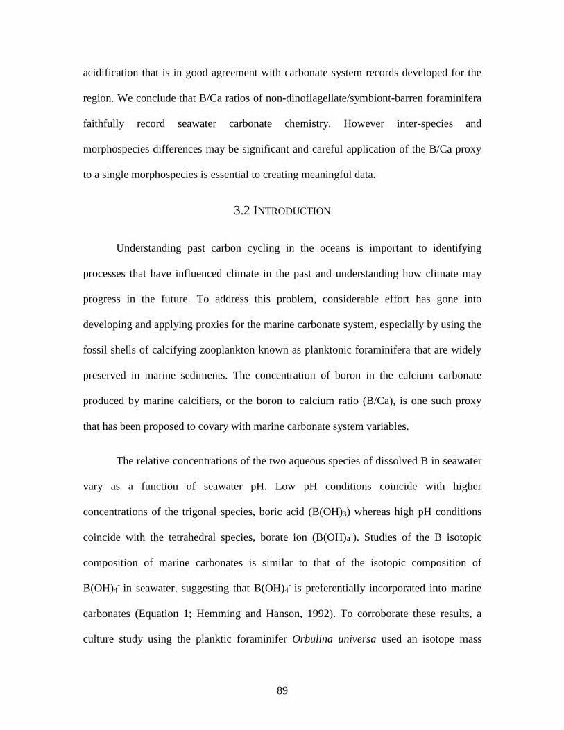
89

acidification that is in good agreement with carbonate system records developed for the

region. We conclude that B/Ca ratios of non-dinoflagellate/symbiont-barren foraminifera

faithfully record seawater carbonate chemistry. However inter-species and

morphospecies differences may be significant and careful application of the B/Ca proxy

to a single morphospecies is essential to creating meaningful data.

3.2 INTRODUCTION

Understanding past carbon cycling in the oceans is important to identifying

processes that have influenced climate in the past and understanding how climate may

progress in the future. To address this problem, considerable effort has gone into

developing and applying proxies for the marine carbonate system, especially by using the

fossil shells of calcifying zooplankton known as planktonic foraminifera that are widely

preserved in marine sediments. The concentration of boron in the calcium carbonate

produced by marine calcifiers, or the boron to calcium ratio (B/Ca), is one such proxy

that has been proposed to covary with marine carbonate system variables.

The relative concentrations of the two aqueous species of dissolved B in seawater

vary as a function of seawater pH. Low pH conditions coincide with higher

concentrations of the trigonal species, boric acid (B(OH)3) whereas high pH conditions

coincide with the tetrahedral species, borate ion (B(OH)4-). Studies of the B isotopic

composition of marine carbonates is similar to that of the isotopic composition of

B(OH)4- in seawater, suggesting that B(OH)4

- is preferentially incorporated into marine

carbonates (Equation 1; Hemming and Hanson, 1992). To corroborate these results, a

culture study using the planktic foraminifer Orbulina universa used an isotope mass

90

balance approach to estimate the fraction of boric acid incorporated for a low pH culture

when boric acid incorporation would hypothetically be highest and found that only 3-8%

of the total B was from boric acid (Allen et al., 2011). Therefore the concentration of B

in planktic foraminifera should be positively correlated with seawater pH; higher pH,

higher proportion of B(OH)4-, higher B/Ca. A theoretical framework for how B

incorporates in to foraminiferal shells poses that the charged B(OH)4- is attracted to the

growth surface where it is de-hydroxylated to a trigonal form (BO33-) during

incorporation into the calcite structure (Equation 1; Hemming et al., 1995, 1998). This

mechanism explains how a tetrahedral ion replaces a trigonal ion space in the calcite

lattice and why the 𝛿11B of foraminifera shells reflect the 𝛿11B of the tetrahedral rather

than the trigonal form of B. Further, synchotron x-ray spectromicroscopy of foraminiferal

shells indicate B hosted in shell calcite is solely trigonal BO3 (Branson et al., 2015).

(1)

Developing the B/Ca carbonate chemistry proxy, particularly for foraminifera, has

been the focus of many core-top, culture and sediment trap studies. Culture experiments

using three tropical spinose species of planktic foraminifera that harbor dinoflagellate

symbionts (Orbulina universa, Globigerinoides sacculifer and Globigerinoides ruber

(pink)) found that B/Ca ratios respond positively to increases in pH (Allen et al., 2011,

2012). These studies also showed that foraminiferal B/Ca had no significant response to

large changes in temperature (∆˚C 6-8) and a minor positive response to large increases

in salinity (∆ 33-40). Shell wall profiles of cultured Orbulina universa and benthic

Amphistegina lessonii documented high and low B banding within the shell wall that are

anti-correlated with Mg/Ca banding (Allen et al., 2011; Branson et al., 2015). Banding

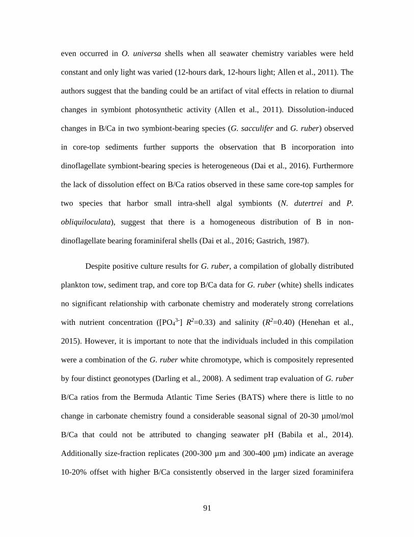
91

even occurred in O. universa shells when all seawater chemistry variables were held

constant and only light was varied (12-hours dark, 12-hours light; Allen et al., 2011). The

authors suggest that the banding could be an artifact of vital effects in relation to diurnal

changes in symbiont photosynthetic activity (Allen et al., 2011). Dissolution-induced

changes in B/Ca in two symbiont-bearing species (G. sacculifer and G. ruber) observed

in core-top sediments further supports the observation that B incorporation into

dinoflagellate symbiont-bearing species is heterogeneous (Dai et al., 2016). Furthermore

the lack of dissolution effect on B/Ca ratios observed in these same core-top samples for

two species that harbor small intra-shell algal symbionts (N. dutertrei and P.

obliquiloculata), suggest that there is a homogeneous distribution of B in non-

dinoflagellate bearing foraminiferal shells (Dai et al., 2016; Gastrich, 1987).

Despite positive culture results for G. ruber, a compilation of globally distributed

plankton tow, sediment trap, and core top B/Ca data for G. ruber (white) shells indicates

no significant relationship with carbonate chemistry and moderately strong correlations

with nutrient concentration ([PO43-] R2=0.33) and salinity (R2=0.40) (Henehan et al.,

2015). However, it is important to note that the individuals included in this compilation

were a combination of the G. ruber white chromotype, which is compositely represented

by four distinct geonotypes (Darling et al., 2008). A sediment trap evaluation of G. ruber

B/Ca ratios from the Bermuda Atlantic Time Series (BATS) where there is little to no

change in carbonate chemistry found a considerable seasonal signal of 20-30 µmol/mol

B/Ca that could not be attributed to changing seawater pH (Babila et al., 2014).

Additionally size-fraction replicates (200-300 µm and 300-400 µm) indicate an average

10-20% offset with higher B/Ca consistently observed in the larger sized foraminifera

92

samples (Babila et al., 2014). The authors conclude that increasing photosynthetic

activity of dinoflagellate symbionts hosted on G. ruber spines elevate the ambient pH in

the microevnrionment around the foraminifera so that larger individuals that host a

greater number of symbionts have higher B/Ca ratios (Babila et al., 2014).

An additional sediment trap study (G. ruber (pink), O. universa and G.

truncatulinoides) indicated a positive relationship between shell thickness (measured by

area density) and B/Ca ratios, and concluded that carbonate chemistry did not exert

control on B/Ca ratios but rather calcification rate (Salmon et al., 2016). Foraminiferal

area density (measure of how much calcite is deposited relative to shell size) has been

linked to calcification intensity, which reflects both calcification rate and efficiency

(Osborne et al., 2016; Weinkauf et al., 2016; Marshall et al., 2013). Correlations between

calcification rate and B/Ca ratios have also previously been reported in both foraminiferal

core-top assessments and synthetic inorganic calcite precipitation studies (Ni et al., 2007;

Uchikawa et al., 2015; Kaczmarek et al., 2015). Interestingly, studies that have applied

the area density proxy thus far have shown that carbonate ion concentration is the main

control on calcification intensity (area density), and therefore a correlation with B/Ca

would inherently suggest a correlation with carbonate chemistry (Marshall et al., 2013;

Weinkauf et al., 2016; Osborne et al., 2016).

A recent study of symbiont-barren foraminifera (Neogloboquadrina incompta and

Globigerina bulloides) from North Pacific core-top samples found a strong positive

correlation between B/Ca ratios and pH, carbonate ion concentration and the calcite

saturation of seawater (Quintana Krupinaski et al., submitted). The positive result with

asymbiontic foraminifera substantiates that B/Ca ratios of species that harbor

93

dinoflagellate symbionts should not be used as seawater carbonate chemistry proxies. In

this study, we further evaluate B/Ca ratios of the asymbiotic species N. incompta and G.

bulloides and also study N. dutertrei using sediment trap material from the Santa Barbara

Basin (SBB), California. While N. incompta (non-spinose) and G. bulloides (spinose) are

classified as symbiont-barren foraminifera, N. dutertrei (non-spinose) harbors small

intracellular symbionts that could affect B incorporation (Hemleben et al., 1989).

3.3 MATERIALS AND METHODS

3.3.1 SEDIMENT TRAP AND DOWN CORE MATERIAL

Planktonic foraminifera (N. dutertrei, N. incompta and G. bulloides) used in this

study were collected as part of an ongoing sediment trap time series in the center of the

SBB (34˚14’N, 120˚02’W, ~580 m water depth; Thunell; et al., 1995, 2007; Thunell,

1998; Figure 1.1). McLean Mark VII-W automated sediment traps equipped with 0.5 m2

funnel openings are deployed for 6-month periods and samples are collected continuously

on a bi-weekly basis. Of the two sediment traps on the mooring (~150 and ~480 m water

depth), we primarily use samples collected by the upper trap. Sediment trap sample

bottles are buffered and poisoned with a sodium azide solution prior to deployment.

Recovered sediments have historically been split and archived using a sodium borate

buffered solution. However, the main sample suite used in this study was collected in

2013-2015 and was split using unbuffered deionized water in order to prevent B

contamination. These samples were immediately washed over a 125 µm sieve and dried

in a 40˚C oven. Cleaning tests conducted on samples that were archived in sodium borate

94

buffer for varying amounts of time (6 months to 7 years) were used to determine if

contamination as a result of the sodium borate archival process could be resolved.

Water column hydrographic and chemical data conducted on a monthly basis at

the site of the sediment trap mooring by the Plumes and Blooms Program

(http://www.oceancolor.ucsb.edu/plumes_and_blooms) were used in this study.

However, because the Plumes and Blooms Program does not routinely measure carbonate

chemistry variables, we use model simulations of the marine carbonate system for

comparison with our foraminiferal geochemical data. Model simulations were developed

for various depths using an eddy-resolving ocean biogeochemical model forced with

observation-based variations of wind stress and fluxes of heat and freshwater (Turi et al.,

2016). While the trends in modeled carbonate variables are in good agreement with in

situ measurements, the overall values are not (Osborne et al., unpublished; Figure 3.1). A

negative bias in the model has already been identified and has been attributed to the over

emphasis of wind observations, which drive a stronger upwelling signal and result in

lower pH carbonate system (Hauri et al., 2013). A comparison of surface calcite

saturation values measured by the CalCOFI time-series in SBB indicates a relatively

consistent offset of higher measured Ω calcite values compared to mean annual model

data (Figure 3.2). A complication of in situ sea surface [CO32-] measurements from 2007-

2010 to coeval daily values estimated by the model also indicates an average offset in

[CO32-] that equate to a nearly identical Ω calcite offset observed in the annual time-

series comparison. For the period when there are available in situ measurements of

carbonate system variables and model datasets overlap (2007-2015), the mean offset

between measured and model data are used to correct model values.

95

A down core record was also generated of B/Ca ratios of N. incompta that spans

the last century. The 0.5 m box-core used in this study was collected in 2012 near the

SBB sediment trap mooring and has been used for shell weight and stable isotope

analyses of G. bulloides and stable isotope analyses of N. dutertrei. Due to this previous

work, sediment material containing only N. incompta remained for down core trace

element analyses. An age model was developed for this core using radiogenic activities of

210Pb and137Cs and indicates that the lowermost sediments in the core date back to the

year ~1900 (Osborne et al., 2016).

3.2.2 TRACE ELEMENT ANALYSES

Typically 150-200 µg of foraminiferal calcite was pooled for each trace element

analysis. Samples smaller than 100 µg often times did not provide sufficient material

after the sample loss that occurs during the cleaning procedure. Foraminifera were picked

from discrete size-fractions (150-250 µm, 250-355 µm, 355-425 µm and >425 µm) so

that duplicate measurements for each species and sample could be measured when

material was available. For G. bulloides and N. incompta, individuals from the smallest

two size-fractions were only available and for some sampling periods only a single size-

fraction was available due to low foraminiferal flux. Although it has been noted that two

distinct genotypes of G. bulloides are present within the SBB (Darling et al., 2003), these

cryptic morphospecies were not identified and separated for our trace element analyses.

Each sample was weighed and loaded in to 1.5 ml polypropylene centrifuge tube

for sample cleaning. Samples were cleaned following the method of Boyle and Kegwin

(1985). For the borate-buffered sediment trap samples used for the cleaning test portion

96

of the study, additional reductive and acid leach treatments were conducted. Prior to the

final acid leach, cleaned samples were transferred to new 1.5 ml polypropylene vials that

had been cleaned in a quartz-distilled 10% hydrochloric acid (HCl) reflux bath and rinsed

with B-free MQ water. Sample cleaning and preparation took place in an over-pressured

flow hood equipped with B-free HEPA filters to minimize atmospheric B contamination.

All acids and 18.3 Mega-Ohm MQ water were mannitol-distilled using a Teflon

distillation setup and stored in Teflon containers. Distillation of a 500 ml volume using 2

grams of mannitol would typically take place over the course of a week due to the low

sub-boiling distillation temperature (80-90˚C).

Five gravimetrically prepared multi-element standard solutions were prepared for

foraminiferal trace element analyses. Standard solutions were prepared using a fixed

calcium concentration with varying concentrations of trace elements (Li, B, Mg, Al, Mn,

Fe, Zn, Sr, Cd, U). Standard 0 was mixed with only calcium and is used analytically as

the blank for Standards 1-4. Concentrations of the trace elements mixed in Standards 1-4

were chosen based on the previously measured ranges in planktonic foraminifera. Stock

standard solutions were prepared at 1000 ppm calcium and stored in Teflon containers in

a clean laboratory with controlled environmental conditions. Working standards were

diluted to the desired calcium concentration to match sample calcium concentrations

(typically 20 or 30 ppm) on the day of sample analysis using the same batch of acid used

for sample preparation.

Trace element analyses were conducted using a Thermo Element II HR-ICP-MS.

Instrumental settings and our analytical methods were adapted from Misra et al. (2014) In

order to minimize the difficulty of measuring B in marine carbonates., specialized

97

equipment and analytical techniques were used in this study. The overall low

concentration of B in foraminiferal calcite and high instrumental blank are addressed by

using hydrofluoric acid (HF) in our mixed acid matrix. The use of HF limits the

adsorption of B onto instrumental surfaces. Therefore the use of HF significantly reduces

instrumental B blanks. A specialized Teflon spray chamber, platinum injector and

platinum sample (normal) and skimmer (H) cones were used for B analyses due to their

resistance to degradation as a result of prolonged contact with HF. A sample and standard

mixed acid matrix of 0.1 N HNO3 + 0.06 N HF were used in our analyses. A lower

concentration of HF is used in our study relative to Misra et al. (2014; 0.1N HNO3 +

0.3N HF) due to the instability of the high calcium concentration samples analyzed in our

study. When the 0.3N HF mixed acid matrix was used in standard dilutions, back-to-back

calibrations resulted in shifting Ca concentrations due to the reaction of HF with calcite

and the formation of calcium fluoride precipitates in solution. When we attempted to use

the 0.3N HF mixed acid matrix with our foraminiferal samples, calcium fluoride

precipitates formed and would not redissolve. Results from Misra et al. (2014) indicate

that a 0.06N HF concentration in the acid matrix still effectively washes out residual B in

the system resolving the issue of carry over between sample analyses while maintaining a

low B blank.

Dip checks, which are used to determine the calcium concentration of each

sample, are essential to matrix-matching foraminiferal trace element samples to standards

(Yu et al., 2005). Because calcium dominates foraminifera-based sample solutions,

significant variations in calcium concentrations result in significant matrix effects. The

low ionization potential of B has been illustrated by measuring a standard solution at

98

varying calcium concentrations, which results in lower B/Ca ratios being measured at

higher calcium concentrations due to matrix induced mass-related discrimination (Yu et

al., 2005; Misra et al., 2014). For this reason, using a sufficient sample size is also

important to minimizing matrix effects. Small sample size results in a low calcium

concentration of the stock sample dilution that is dissolved in 2% HNO3. Therefore the

sample dilution used for analysis has a relatively higher HNO3 normality and lower HF

normality due to the smaller volume of the mixed acid matrix used for dilution, resulting

in matrix effects for these samples.

Just prior to analysis, samples are dissolved in 100 µl of mannitol-distilled 2%

HNO3 to create a concentrated stock of each sample. Acidified samples then are placed in

a sonication bath for 30 minutes and individually vortexed to ensure full dissolution of

sample material. Dip checks are conducted using a 10 µl aliquot of each concentrated

sample stock and diluted up to a 200 µl volume using the 0.1N HNO3 + 0.06N HF (20x

dilution factor). The calcium concentration of each sample is determined relative to a 10

ppm calcium dilution of Standard 0. Calcium concentrations of the concentrated sample

stocks are then used to create a sample dilution to the target calcium concentration for

that analytical run. Typically the target calcium concentration for our foraminiferal

analyses is 20 ppm however for N. dutertrei analytical runs, a 30 ppm calcium

concentration is used due to the lower B concentration in this species. Sample dilutions

are made in quartz-distilled HCL refluxed 1.5 ml polypropylene vials that are sonicated

with mannitol-distilled B-free MQ immediately prior to use. The total volume of sample

dilution ranged from 250-500 µl depending on the concentration and volume of solution

needed of the concentrated stock sample. Down core dilutions were always measured in

99

400-500 µl dilutions due to unusual matrix effects that occurred in smaller sample

dilutions of core samples.

Each analytical run began with a 5-minute acid matrix washout to minimize

instrumental B blank. Following the washout a total of 4 acid matrix blanks and typically

4 procedural blanks in 1.5 ml polypropylene sample vials were measured. Standard

solutions were then measured back-to-back in order of increasing multi-element

concentration. Each foraminiferal sample was bracketed with a “dip” where the sample

probe is immersed in a 15 ml vial of the acid matrix and then a sample-specific acid

matrix blank after a take up time of 2.5 minutes. Sample specific blanks were prepared in

quartz-distilled HCL refluxed 1.5 ml polypropylene vials that were sonicated with

mannitol-distilled B-free MQ immediately prior to use. While the instrumental boron

blank accounts on average for 20% of the B measured for a given sample, the standard

deviation of blanks measured during a single analytical run are extremely consistent with

standard deviations of repeat measurements representing only 5% of the blank value.

Procedural blanks measured at the beginning of the first analytical run for that sample

batch are almost always within error of instrumental blanks. Standard 2, which contains

the multi-element concentrations most like the samples, was measured after every third

sample as an internal consistency standard. A maximum of 15 samples were measured in

a single analytical run so that drift would not affect the relationship between the standards

measured at the beginning of the run and samples measured at the end of the run

(approximately 2.5 hour sequence).

To assess the analytical precision of our B method for calcite matrix samples, we

created a homogenized foraminifera standard. The foraminifera (Globorotalia menardii)

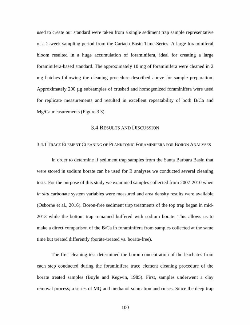
100

used to create our standard were taken from a single sediment trap sample representative

of a 2-week sampling period from the Cariaco Basin Time-Series. A large foraminiferal

bloom resulted in a huge accumulation of foraminifera, ideal for creating a large

foraminifera-based standard. The approximately 10 mg of foraminifera were cleaned in 2

mg batches following the cleaning procedure described above for sample preparation.

Approximately 200 µg subsamples of crushed and homogenized foraminifera were used

for replicate measurements and resulted in excellent repeatability of both B/Ca and

Mg/Ca measurements (Figure 3.3).


3.4.1 TRACE ELEMENT CLEANING OF PLANKTONIC FORAMINIFERA FOR BORON ANALYSES

In order to determine if sediment trap samples from the Santa Barbara Basin that

were stored in sodium borate can be used for B analyses we conducted several cleaning

tests. For the purpose of this study we examined samples collected from 2007-2010 when

in situ carbonate system variables were measured and area density results were available

(Osborne et al., 2016). Boron-free sediment trap treatments of the top trap began in mid-

2013 while the bottom trap remained buffered with sodium borate. This allows us to

make a direct comparison of the B/Ca in foraminifera from samples collected at the same

time but treated differently (borate-treated vs. borate-free).

The first cleaning test determined the boron concentration of the leachates from

each step conducted during the foraminifera trace element cleaning procedure of the

borate treated samples (Boyle and Kegwin, 1985). First, samples underwent a clay

removal process; a series of MQ and methanol sonication and rinses. Since the deep trap

101

sits in suboxic waters, treatments aimed at eliminating manganese-rich overgrowths that

may form under low oxygen conditions (reductive step; sodium hydroxide buffered 4%

hydrazine) and any organic matter retained on the surface or inside of foraminifera shells

(oxidative step; sodium hydroxide buffered 1% hydrogen peroxide) were performed. The

final step was a weak acid leach (0.001% nitric acid) in a 30 second to 1 minute

sonication bath that is aimed at removing any chemical residues produced during the

cleaning procedure. Due to the fact that high boron concentrations were anticipated for

this test, we decided to repeat each of the cleaning steps. This would also help to devise a

specialized cleaning procedure for borate treated samples by determining if doubling any

of the cleaning steps would be more effective at removing the borate contamination. A

400 µl leachate aliquot from the final rinse after each cleaning step was acidified to a

0.1N HNO3 + 0.06 HF matrix and measured on the Element HR-ICP-MS.

The boron concentrations of the leachates decreased significantly (~50%) from

the initial to final cleaning step (Figure 3.4). This suggests that borate contamination is

not restricted to the surface of foraminiferal shells, as evidenced by initial rinses during

the clay removal step accounting for approximately half of the boron removal. The next

largest decrease in boron concentration occurs after the first reductive step accounting for

approximately one-quarter of the boron removal. The aggressive nature of the chemical

solution used in the reductive step typically results in the majority of calcite lost during

the cleaning procedure and likely removes outer calcite layers that contain a considerable

fraction of the boron contamination. An increase in boron concentration of the leachate

from the first oxidative treatment is likely due to boron being mobilized from organic

material that is oxidized during this step. The general consistency in boron concentration

102

between the two final acid leaches suggests that the boron in these leaches is the primary

foraminiferal shell signal rather than contamination.

For the next cleaning test we compare the B/Ca ratios of G. bulloides and N.

dutertrei calcite from a sample that had been stored in borate for six months. This sample

was divided into four equal fractions for G. bulloides and five fractions of N. dutertrei.

Due to the larger shell size and robustness during cleaning, there was more sample

material available to conduct tests using N. dutertrei. Each fraction underwent different

chemical cleaning steps (reductive, oxidative, acid leach). For both species, the first

fraction underwent only clay and reductive treatments, the second underwent clay,

reductive and oxidative treatments and the third fractions underwent clay, reductive,

oxidative and varying levels of acid leach treatments. These results are compared to time-

equivalent top trap samples that were not borate buffered and indicate that final B/Ca

values for the buffered samples are within error of the non-buffered samples. For both

species rigorous acid leach is essential for removing all of the B contamination.

Neogloboquardina dutertrei required three 1 minute acid leaches and G. bulloides needed

three 30-second acid leaches before the outer contaminated calcite layers were removed

(Figure 3.5). Mg/Ca ratios were also measured for these samples and indicate that a more

rigorous cleaning results in significantly lower Mg/Ca ratios, especially for N. dutertrei

due to the fact that outer calcite layers are enriched in Mg and removal of this layer

effects the whole shell Mg/Ca signal (Barker et al., 2003). However, boron is

incorporated more homogenously through foraminiferal shells therefore preferential

removal of the outer surface during more rigorous cleaning does not significantly affect

the whole shell B/Ca ratios.

103

Based on the results of these cleaning tests, we applied a modified cleaning

procedure to a series of borate-treated samples from the 2007-2010. In addition to the

traditional cleaning protocol we added a second reductive treatment and a triple acid

leach treatment. Despite this more aggressive cleaning, boron concentrations of G.

bulloides from the borate buffered samples from 2007-2010 were often more than two

times higher than expected B/Ca values (Figure 3.6). Based on these results we conclude

that there is a time-dependent factor to how the borate buffer alters the original

foraminiferal B/Ca. Therefore we suggest that samples archived in sodium borate buffer

are not suitable for boron analyses even when additional cleaning steps are used.

3.4.2 SEDIMENT TRAP B/CA RATIOS IN NEOGLOBOQUADRINA SPECIES

A total of 26 sediment trap samples from October 2013-October 2014 were used

to generate a year-long time-series of B/Ca ratios for both N. dutertrei (Figure 3.7) and N.

incompta (Figure 3.8). Ekman-induced upwelling that begins in February and persists

through July results in an overall lower flux of both species during this period and

produces some gaps in the B/Ca time-series. When sufficient sample material was

available, replicate measurements of B/Ca ratios were made on different size-fractions

(11 out of 19 N. dutertrei samples and 3 out of 17 N. incompta samples). The greater size

range and larger individual mass of N. dutertrei easily allowed for replicate

measurements, while the lower abundance and smaller individual size (generally

restricted to the 150-255 µm size-fraction) of N. incompta hampered sample replication.

Replicate measurements indicate that both species generally yield B/Ca ratios

within error regardless of shell size (Figure 3.7 and 3.8). This differs from previous

104

studies of dinoflagellate symbiont-bearing foraminifera that demonstrated that

photosynthetic activity of symbionts result in poor replicate measurements across size-

fractions (Babila et al., 2014). The result for N. dutertrei is particularly interesting due to

the fact that this species does in fact harbor symbionts. However, the dinoflagellate

symbionts hosted by some spinose foraminifera typically range from 8-12 µm in size,

while many non-spinose species including N. dutertrei host coccoid alga that are 1.5-3.5

µm in size (Gastrich, 1987; Fehrenbacher et al., 2011). Our results reinforce that the

relative activity of these small intracellular symbionts, which are limited by light, is much

less than the large dinoflagellate symbionts that are found on extracellular spines of

surface dwelling species (Gastrich, 1987).

The large errors associated with N. dutertrei B/Ca replicates in March and August

2014 are the result of small sample sizes (n = 4, <100µg) for each measurement (Figure

3.7). As with other foraminiferal geochemical analyses (δ18O, Mg/Ca), ideally a large

number of individuals are included in bulk measurements to reduce the noise of

intersample variability (Killingley et al., 1981; Ganssen et al., 2011; Schiffelbein and

Hills, 1984). In order to further demonstrate that size-fraction does not affect B/Ca ratios,

replicate measurements using individuals spanning all size-fractions (150µm-425µm)

were made on three samples from October-December 2013 when N. dutertrei were

highly abundant,. These broad size-fraction replicates produced values within error of the

other sample replicates. The excellent replication of B/Ca values for various sized N.

dutertrei indicates that the presence of symbionts in this species does not influence the B

signal.

105

We compare B/Ca ratios of each species to modeled water column data to assess

the relationship between shell geochemistry and seawater carbonate chemistry. Previous

studies have shown that it is important to use water column properties from the depth of

calcification in order to establish the best relationship between shell geochemistry and

seawater conditions. A study from the Southern California Bight indicate that the δ13C of

N. incompta (also referred to as N. pachyderma (right coiling)) and N. dutertrei from this

region are in equilibrium with δ13C at the thermocline or sub-thermocline depths, which

range between 25-40 meters water depth during non-upwelling periods when these

species are most abundant (Sautter and Thunell et al., 1991; Figure 3.9). MOCNESS tows

conducted in the Equatorial Pacific collected N. dutertrei from the sea surface to over

1,000 meters water depth but oxygen and carbon isotopic results indicate that N. dutertrei

calcite is in equilibrium with seawater at ~30 meters water depth (Fairbanks et al., 1982).

This suggests that N. dutertrei produce the majority of their shell calcite at ~30 meters

water depth and then descend through the water column during later life stages

(Fairbanks et al., 1982). A δ18O study of N. incompta from core-top samples from our

study region suggest that the mean calcification depth of this species is also ~30 meters

water depth (Quintana Krupinaski et al., submitted). Calcification depths for both species

in the Santa Barbara Basin were estimated using Mg/Ca derived temperatures ](Figure

3.9). Using the Anand et al (2003) Mg/Ca:temperature equation for N. dutertrei and a

mixed calibration for non-symbiont bearing species, we estimate average calcification

depths for N. dutertrei and N. incompta of ~30 m and ~40 m respectively, over the course

of the sediment trap sampling period.

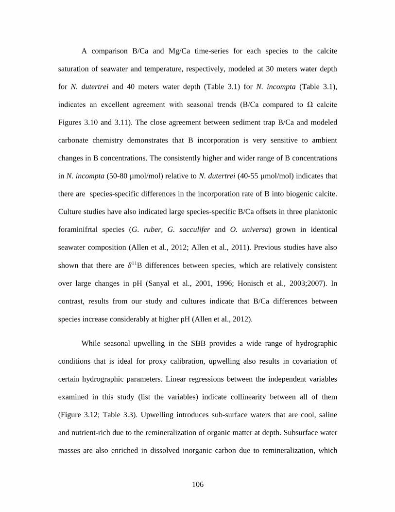
106

A comparison B/Ca and Mg/Ca time-series for each species to the calcite

saturation of seawater and temperature, respectively, modeled at 30 meters water depth

for N. dutertrei and 40 meters water depth (Table 3.1) for N. incompta (Table 3.1),

indicates an excellent agreement with seasonal trends (B/Ca compared to Ω calcite

Figures 3.10 and 3.11). The close agreement between sediment trap B/Ca and modeled

carbonate chemistry demonstrates that B incorporation is very sensitive to ambient

changes in B concentrations. The consistently higher and wider range of B concentrations

in N. incompta (50-80 µmol/mol) relative to N. dutertrei (40-55 µmol/mol) indicates that

there are species-specific differences in the incorporation rate of B into biogenic calcite.

Culture studies have also indicated large species-specific B/Ca offsets in three planktonic

foraminifrtal species (G. ruber, G. sacculifer and O. universa) grown in identical

seawater composition (Allen et al., 2012; Allen et al., 2011). Previous studies have also

shown that there are 𝛿11B differences between species, which are relatively consistent

over large changes in pH (Sanyal et al., 2001, 1996; Honisch et al., 2003;2007). In

contrast, results from our study and cultures indicate that B/Ca differences between

species increase considerably at higher pH (Allen et al., 2012).

While seasonal upwelling in the SBB provides a wide range of hydrographic

conditions that is ideal for proxy calibration, upwelling also results in covariation of

certain hydrographic parameters. Linear regressions between the independent variables

examined in this study (list the variables) indicate collinearity between all of them

(Figure 3.12; Table 3.3). Upwelling introduces sub-surface waters that are cool, saline

and nutrient-rich due to the remineralization of organic matter at depth. Subsurface water

masses are also enriched in dissolved inorganic carbon due to remineralization, which

107

results in naturally lower in pH, [CO32-] and Ω calcite of upwelled waters. Positive

correlation between temperature and B/Ca observed in both species suggests that

temperature may exert some control B/Ca ratios. However, temperature and the carbonate

system parameters (pH, [CO32-] and Ω calcite) also are tightly correlated; therefore

correlations with temperature may be spurious. A strong correlation between Mg/Ca

(temperature proxy) and B/Ca ratios for both species illustrates the covariation of the

independent variables that control shell geochemistry (Figure 3.13). Culture experiments

indicate that temperature has a negligible effect on B/Ca in planktonic foraminifera

(Allen et al., 2011, 2012) and North Pacific core-top results for G. bulloides and N.

incompta indicate that the relationship between temperature and B/Ca ratios is spurious

(Quintana Krupinaski et al., submitted). Inorganic calcite precipitation studies have also

indicated negative or insignificant influence of temperature on B/Ca ratios (Mavromatis

et al., 2015; Kaczmarek et al., 2016). A negative correlation between B/Ca ratios and

salinity differs from previous results that suggest that salinity strongly influences B/Ca in

the planktic species G. ruber (Henehan et al., 2015). Culture results indicate that salinity

has some positive influence on B incorporation, however the opposite sign of this

relationship in our dataset indicates the influence of salinity is minor relative to carbonate

system variables (Allen et al., 2012). Nutrient concentration is also negatively correlated

with B/Ca ratios in our dataset unlike the positive correlation observed in globally

distributed core-tops for the symbiont-bearing species G. ruber (Henehan et al., 2015).

No significant correlation between N. incompta and nutrient concentration was observed

in North Pacific core-tops, perhaps due to the lack of symbionts in this species (Quintana

Krupinaski et al., submitted).

108

The highest correlation coefficients observed in our study are between B/Ca and

each of the carbonate system parameters (pH, [CO32-] and Ω calcite) (Table X). The

slightly higher correlation coefficient observed between Ω calcite and B/Ca observed in

both species supports the core-top results from the North Pacific (Quintana Krupinaski et

al., submitted). This core-top study covered a wide range of hydrographic regimes and

clearly demonstrated that B/Ca is most significantly correlated with Ω calcite (Quintana

Krupinaski et al., submitted). The authors suggest that the Ω calcite of seawater exerts the

strongest control on B/Ca ratios because of the mechanistic relationship between

calcification rate and B incorporation into foraminiferal calcite (Quintana Krupinaski et

al., submitted). The surface entrapment model proposes that faster crystal growth (which

occurs at higher Ω calcite) reduces the time available for boron to escape via diffusion

therefore resulting in more B being retained in newly formed calcite (Watson, 2004).

The relationships between B/Ca of N. dutertrei and N. incompta and modeled Ω calcite

values are highly significant (Figure 3.14). A comparison of the N. incompta regression

developed as a part of this study with the North Pacific core-top data indicates an

excellent agreement between the two sample sets.

3.4.3 THE INFLUENCE OF MIXED GENOTYPES ON G. BULLOIDES B/CA

A sediment trap time-series of B/Ca ratios for G. bulloides was developed using both the

October 2013-October 2014 samples included in the study of Neogloboquadrina species

and an additional samples collected during the first half of 2015. A total of 29 out of 39

sediment trap samples from this period had sufficient material to make B/Ca

measurements. All but three samples from the October 2013-2014 period provided

enough material for size fraction replicates (150-250 µm and 250-355 µm). El Niño

109

conditions that started in 2015 resulted in overall lower foraminifera fluxes. Therefore G.

bulloides from the 150-355 µm size fraction were used for geochemical analyses.

Although two morphotypes of G. bulloides have previously been identified in our study

region (Sautter and Thunell, 1991; Bemis et al., 2002) we did not distinguish between

morphotypes for the trace element analyses. The G. bulloides B/Ca ratios generally

duplicate well across size-fractions with the exception of during winter months and peak

upwelling periods in the spring (Figure 3.15). This is likely due to an increase in the

abundance of the encrusted G. bulloides morphospecies during these periods (Darling et

al., 2003; Osborne et al., 2016). Sediment trap studies from the Southern California Bight

indicate that the normal G. bulloides is found in abundance throughout the year while the

encrusted morphotype is seasonally associated with cool periods (Sautter and Thunell

1991; Darling et al., 2003; Osborne et al., 2016). Down core studies from the SBB also

indicate an increased abundance in encrusted individuals associated with glacial periods

(Hendy and Kennett, 2000; Bemis et al., 2002). Using a combination of shell weight, area

and diameter, it is possible to distinguish the two morphotypes of G. bulloides (Osborne

et al., 2016). We applied this technique to a winter trap sample that had poor duplicates

and found that encrusted individuals dominate this sample (Figure 3.16).

The additional sediment trap samples from December 2014-April 2015 included

in our G. bulloides analyses demonstrates a similar seasonal range and trend for the

winter to early spring sampling months. A comparison of G. bulloides B/Ca ratios to

modeled Ω calcite and Mg/Ca to modeled temperature illustrates that higher than

expected B and Mg values occur during winter and peak upwelling when encrusted

individuals are typically found in greater abundance (B/Ca ratios versus Ω calcite; Figure

110

3.17). Quintana Krupinaski et al. (submitted) observe encrusted G. bulloides in some

core-top samples and determined that the encrusted individuals have a higher B

concentrations than the normal morphospecies. A difference in trace element

concentrations is not surprising since offsets in stable isotopes have already been

observed for the two forms (Osborne et al., 2016; Bemis et al., 2002). Laser ablation

results from an Arabian Sea plankton tow reveal that individual G. bulloides have Mg/Ca

offsets differences of 3 mmol/mol within a single sampling population which the authors

attribute to the presence of two morphotypes (Sadekov et al., 2016). Analysis of trace

element concentrations in individual specimens of the two G. bulloides morphotypes in

our study region would be helpful for quantifying the geochemical differences that exist

between these forms and determining the effect of pooling these individuals for

paleoclimatic reconstructions. If encrusted forms have higher Mg and B concentrations,

the inclusion of these individuals in down core reconstructions has the potential to

significantly mute estimated changes in paleo-temperatures and carbonate system

variables as a result of higher abundances of encrusted individuals during cold periods.

3.4.4 DOWN CORE N. INCOMPTA B/CA IN RELATION TO CARBONATE CHEMISTRY RECORDS

In order to further examine the potential of symbiont-barren foraminifera B/Ca

ratios as a paleo-carbonate system proxy, we developed a record of B/Ca spanning the

last 100 years for a box core from the SBB. This sediment core was previously used for

area density and stable isotope analyses of G. bulloides and stable isotope analyses of N.

dutertrei and N. incompta (Osborne et al., 2016); therefore only limited sample material

of N. incompta was available for trace element analyses. There is a steadily decline in

B/Ca ratios from ~1900 through ~1980, at which time B/Ca ratios increase dramatically

111

(Figure 3.18). Coincident with the increase in B increases in Fe and Al. Clay particles

trapped on the surfaces of foraminifera shells represents a significant contamination

source of boron and increases in Al/Ca and Fe/Ca ratios indicate that clay contamination

was not effectively removed for the upper core samples. Shell morphology measurements

of G. bulloides indicate a significant increase in shell surface area in the upper part of the

core and this could be responsible for the increased clay contamination over the last 30

years of the record. Regardless, samples that indicated elevated Al/Ca and Fe/Ca ratios

were excluded from the down core B/Ca record. A comparison of N. incompta B/Ca-

estimated Ω calcite to G. bulloides area density-estimated Ω calcite indicate excellent

agreement between these two reconstructions (Figure 3.19).

3.5 CONCLUSIONS

Our work suggests that B/Ca ratios of non-dinoflagellate bearing foraminifera have the

potential to serve as a carbonate system proxy, specifically for Ω calcite of seawater.

However, careful selection of individuals included in trace element analyses and

application of appropriate calibration relationships is important. The offset between

normal and encrusted G. bulloides from our study region suggests that vital effects can be

significant (even between morphospecies) and genotype-specific calibrations are likely

important. A global compilation of planktonic foraminifera genotypes indicate that G.

bulloides is a highly cryptic species with seven sequenced genotypes to date. The

diversity identified within the G. bulloides species concept highlights the need for

additional geotype-specific work to assess consistency geochemical tracers on this

112

species. However, genetic work on Neogloboquadrina indicate these species are far less

cryptic, for instance only a single genotype of N. incompta has been found in the Pacific

and a second genotype in the Atlantic (Darling et al., 2008). The present state of

foraminiferal B research indicates that B/Ca is strongly affected by species-specific and

maybe even geotype-specifc vital effects while 𝛿11B seems to be less affected, explaining

why B/Ca and 𝛿11B results oftentimes conflict. Future work to assess the influence of

species-specific vital effects and resulting offsets in trace element incorporation is

essential to further developing the B/Ca proxy prior to application to the fossil record.

113

Table 3.1 Neogloboquadrina dutertrei size fraction replicates and mean B/Ca values and

Mg/Ca data

Tra

p ID

Cu

p Date

Average

B/Ca

(umol/mol

)

250-

355u

m

355-

425u

m

>425u

m

>150u

m

B/Ca

Error

Mg/Ca

(mmol/mol

)

39 1

10/23/1

3 55.59 53.87 57.31 55.63 3.44 1.678

39 2 11/8/13 55.87 55.61 56.01 55.98 54.50 1.41 1.686

39 3

11/24/1

3 53.77 53.58 54.40 53.35 52.86 1.29 1.685

39 4

12/10/1

3 51.61 53.23 50.39 51.22 2.93 1.667

39 5

12/26/1

3 49.87 49.87 2.49 1.641

39 6 1/11/14 50.68 51.10 50.25 1.20 1.602

39 7 1/27/14 51.82 51.34 52.29 1.35

39 8 2/12/14 49.23 49.99 48.47 2.15 1.567

39 9 2/28/14 46.68 42.72 50.63

11.1

8

39 10 3/16/14 44.73 44.73 2.24 1.553

39 11 4/1/14 1.523

39 12 4/17/14 41.15 41.15 2.06

39 13 5/3/14 43.34 43.34 2.17

40 1 5/24/14 1.517

40 2 6/4/14 1.506

40 3 6/16/14

40 4 6/27/14 47.23 47.23 2.36 1.588

40 5 7/9/14 45.19 43.57 46.80 4.57 1.671

40 6 7/20/14 51.56 51.61 51.51 0.14

40 7 8/1/14 54.06 56.44 51.68 6.73 1.615

40 8 8/12/14 1.651

40 9 8/24/14 51.18 51.18 2.56

40 10 9/4/14

40 11 9/16/14 53.93 52.70 55.16 3.47 1.672

40 12 9/27/14 57.07 57.07 2.85 1.661

40 13 10/9/14

114

Table 3.2 Neogloboquadrina incompta size fraction replicates and mean B/Ca values and

Mg/Ca data.

Trap

ID Cup Date

Average

B/Ca

(umol/mol)

150-

250 um

250-

355um

B/Ca

Error

Mg/Ca

(mmol/mol)

39 1 10/23/13 64.78 66.69 62.87 2.70 1.49

39 2 11/8/13 70.41 67.50 73.32 4.12 1.61

39 3 11/24/13 72.37 72.37 3.62 1.64

39 4 12/10/13 75.21 75.21 3.76 1.65

39 5 12/26/13 78.51 78.51 3.93 1.78

39 6 1/11/14 1.57

39 7 1/27/14 69.24 69.24 3.46

39 8 2/12/14 64.05 64.05 3.20 1.47

39 9 2/28/14 1.40

39 10 3/16/14 57.46 57.46 2.87

39 11 4/1/14 59.12 59.12 2.96 1.46

39 12 4/17/14 1.28

39 13 5/3/14 51.50 51.50 2.58

40 1 5/24/14

40 2 6/4/14

40 3 6/16/14

40 4 6/27/14 57.84 57.84 2.89 1.50

40 5 7/9/14 69.11 69.11 3.46

40 6 7/20/14 73.93 73.93 3.70 1.62

40 7 8/1/14 1.58

40 8 8/12/14

40 9 8/24/14 1.56

40 10 9/4/14 59.52 59.52 2.98 1.48

40 11 9/16/14 65.29 65.29 3.26 1.49

40 12 9/27/14 70.60 70.60 3.53 1.68

40 13 10/9/14 75.65 78.24 73.06 3.66

115

Table 3.1 Simle linear regression data of monthly resolved hydrographic data indicating

cross-correlations between independent variables

Date Salin

ity

Te

mp

NO

3

pH

in

pCO

2

(mat

m)

HCO3

(mmol/kg

SW)

CO3

(mmol/kg

SW)

CO2

(mmol/kg

SW)

B Alk

(mmol/kg

SW)

W

Ca

6/15/

13

33.3

9

11.

21

16.

44

7.

83

672.

37 2046.43 83.91 29.51 41.81

2.7

9

7/15/

13

33.3

5

11.

55

15.

39

7.

83

669.

01 2041.32 84.97 29.08 42.24

2.8

2

8/15/

13

33.1

8

12.

88

10.

25

7.

89

569.

92 1991.31 100.07 23.92 49.23

3.1

8

9/15/

13

33.1

0

13.

88

6.1

8

7.

95

499.

47 1950.62 113.82 20.40 55.56

3.5

1

10/15

/13

33.0

5

14.

41

4.4

6

7.

97

471.

88 1931.52 120.27 19.00 58.46

3.6

6

11/15

/13

32.9

9

14.

80

3.6

5

7.

98

458.

70 1920.56 123.84 18.37 60.02

3.7

5

12/15

/13

33.0

6

14.

10

3.4

2

7.

99

443.

75 1916.62 127.30 17.77 61.67

3.8

3

1/15/

14

33.1

3

13.

79

2.3

8

8.

01

423.

90 1905.60 133.08 16.84 64.42

3.9

7

2/15/

14

33.1

0

13.

47

6.7

4

7.

94

504.

22 1958.65 112.06 20.92 54.89

3.4

7

3/15/

14

33.1

3

12.

56

10.

08

7.

90

554.

37 1990.61 100.41 23.58 49.63

3.1

9

4/15/

14

33.2

1

11.

43

13.

86

7.

86

624.

17 2024.67 88.97 27.22 44.31

2.9

2

5/15/

14

33.3

5

11.

28

15.

93

7.

84

650.

15 2037.47 86.92 28.32 43.27

2.8

7

6/15/

14

33.2

2

12.

22

12.

35

7.

86

617.

48 2014.87 92.60 26.21 45.78

3.0

0

7/15/

14

33.1

1

13.

37

8.3

9

7.

92

530.

08 1969.74 107.45 22.04 52.73

3.3

6

8/15/

14

33.0

7

14.

18

5.4

9

7.

96

480.

05 1939.11 118.23 19.48 57.65

3.6

1

9/15/

14

33.0

7

14.

37

4.8

6

7.

96

473.

29 1934.59 119.95 19.08 58.40

3.6

6

10/15

/14

33.0

6

14.

87

3.5

9

7.

98

458.

36 1921.30 124.99 18.20 60.56

3.7

8

11/15

/14

33.0

2

15.

91

2.8

2

7.

99

447.

15 1910.39 128.79 17.54 62.15

3.8

7

12/15

/14

33.1

3

16.

67

1.0

6

8.

01

423.

14 1880.29 143.17 15.73 67.96

4.2

1

116

Figure 3.1 Comparison of in situ measurements of surface [CO32-] (data from CalCOFI and Osborne et al., 2016) compared to

modeled values. Note that the in situ data are plotted on the left y-axis and the model data are plotted on the right-hand y-axis due to

the offset in the range of values. An offset in [CO32-] was determined for each sample equaling an average of 33 µmol/mol. The

conversion of this carbonate value to Ω calcite values yields the same average offset as the CalCOFI comparison shown in the below

Figure #.

117

Figure 3.2 Comparison of in situ surface omega calcite values from the CalCOFI time-

series compared to model estimates of surface omega calcite for the 2009-2015 period

when these datasets over lap. The offset between these datasets is used to correct model

values that are used in the B/Ca calibration portion of this study.

118

Figure 3.3 Replicate B/Ca and Mg/Ca measurements of a foraminifera matrix-specific

standard. Globorotalia menardii shells from a 2-week-long sediment sample from the

Cariaco Basin (150 meter depth) are used for our foraminiferal standard. Error bars

represent fully propagated 2-sigma errors.

119

Figure 3.4 The leachates of each of the cleaning steps for 3 sediment trap samples that

were archived in the sodium borate buffer are shown here in counts per second of boron.

120

Figure 3.5 B/Ca ratios of G. bulloides and N. dutertrei from a single borate buffered (6-

months) sediment trap sample. Foraminiferal populations were split into 4 to 5 fractions

in order to evaluate how the borate buffer contamination is progressively removed from

treated samples. The robust nature of N. dutertrei shells required an additional acid leach

treatment of 3-times for 1 minute. The final acid leach treatments yield B/Ca ratios for

both species that are comparable to those measured on populations from a time

equivalent non-buffered sample.

121

Figure 3.6 Comparison of B/Ca ratios of rigorously cleaned foraminifera that were

preserved in a sodium borate buffer for 6-7 years with the B/Ca ratios of foraminifera that

were not treated with sodium borate. This result indicates that prolonged storage of

foraminifera in sodium borate inhibits the removal of the borate contamination.

122

Figure 3.7 Time-series of N. dutertrei B/Ca measurements from sediment trap samples

collected from October 2013-October 2014. Replicate measurements were made using

three size-fractions and for several samples replicates were made without restricting size-

fraction. Error bars on replicate means indicate 2-sigma errors of replicate measurements.

When no replicates were made error bars represent the fully propagated analytical error

associated with each measurement.

123

Figure 3.8 Time-series of N. incompta B/Ca measurements from sediment trap samples

collected from October 2013-October 2014. Generally N. incompta was only found in

abundance in the 150-250 µm size fraction. However, a limited number of replicate

measurements were made using the 250-355 µm fraction. When no replicates were made

error bars represent the fully propagated analytical error associated with each

measurement. Error bars on replicate means indicate 2-sigma errors of replicate

measurements.

124

Figure 3.9 Temperature profiles 0-80 meters water depth from 2013-2014 modeled data

throughout a seasonal cycle in the SBB. Open circles and squares indicate the Mg/Ca-

derived calcification temperatures of N. incompta and N. dutertrei compared to the

temperature profiles.

125

Figure 3.10 Mean replicate B/Ca ratios of N. dutertrei (pink circles) compared to modeled 30 meter Ω calcite. Model data is shown

here as daily (gray circles) and monthly mean (blue diamonds) values.

126

Figure 3.11 Mean replicate B/Ca ratios of N. incompta (navy circles) compared to modeled 30 meter Ω calcite. Model data is shown

here as daily (gray circles) and monthly mean (light blue diamonds) values.

127

Figure 3.12 Matrix of linear regressions showing the relationship between the B/Ca ratios

of Neogloboquadrina species and the monthly mean value determined for each

independent variables. Histograms are included to show range and frequency for each

variable.

128

Figure 3.13 Correlations between Mg/Ca (a temperature proxy) and B/Ca ratios for both

species support that temperature and carbonate system variables are collinear in our

dataset.

129

Figure 3.14 Calibration relationships for N. incompta and N. dutertrei from SBB

sediment trap results. Final calibration equation presented here is pooled data from this

study’s sediment trap results and core-top results for the North Pacific (unpublished data,

Quintana Krupinaski et al., in review).

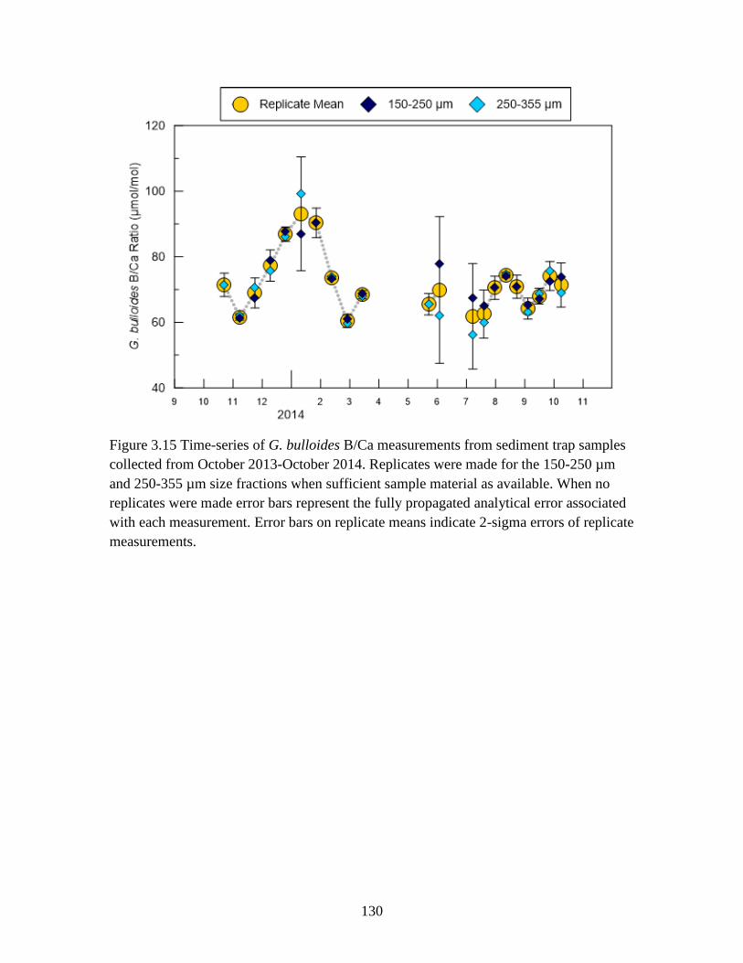
130

Figure 3.15 Time-series of G. bulloides B/Ca measurements from sediment trap samples

collected from October 2013-October 2014. Replicates were made for the 150-250 µm

and 250-355 µm size fractions when sufficient sample material as available. When no

replicates were made error bars represent the fully propagated analytical error associated

with each measurement. Error bars on replicate means indicate 2-sigma errors of replicate

measurements.

131

Figure 3.16 Morphometric analyses used to determine the presence of the normal and encrusted cryptic G. bulloides morphospecies

during the January 2014 sampling period. The trend in weight-area and grouping of morphospecies in the area density-diameter

analyses are shown here with previously identified morphospecies groups from the SBB (Osborne et al., 2016).

132

Figure 3.17.Mean B/Ca ratios of G. bulloides (yellow circles) compared to modeled 40-meter Ω calcite. A mean calcification depth of

40 meters was determined using G. bulloides 𝛿18O temperature estimates for a 3-year SBB sediment trap study (Osborne et al., 2016).

Model data is shown here as daily (gray circles) and monthly mean (light blue diamonds) values. Red circles highlight samples that

likely include encrusted individuals based on a comparison of B/Ca and Mg/Ca to Ω calcite and temperature, respectively.

133

Figure 3.18 Down core measurements of boron, aluminum and iron to calcium ratios.

Measurements are shown here as counts per second (CPS) indicating the intensity of the element

concentration measured by the HR-ICP-MS. Grayed area indicates the sampling period when clay

contamination is indicated by elevated Fe/Ca and Al/Ca.

134

Figure 3.19 Down core estimates of Ω calcite from N. incompta B/Ca ratios and G.

bulloides area density measurements.

135

REFERENCES

Aldridge, D., C. J. Beer, and D. A. Purdie (2012), Calcification in the planktonic

foraminifera Globigerina bulloides linked to phosphate concentrations in surface

waters of the North Atlantic Ocean, Biogeosciences, 9(5), 1725–1739,

doi:10.5194/bg-9-1725-2012.

Alin, S. R., R. A. Feely, A. G. Dickson, J. M. Hernandez-Ayon, L. W. Juranek, M. D.

Ohman, and R. Goericke (2012), Robust empirical relationships for estimating the

carbonate system in the southern California Current System and application to

CalCOFI hydrographic cruise data (2005–2011), Journal of Geophys. Research,

117.

Allen, K., B. Hönisch, S. Eggins, J. Yu, H. Spero and H. Elderfield (2011), Controls on

boron incorporation in cultured tests of planktic foraminifera Orbulina universa,

Earth Planet Sci. Lett. 309, 291-301.

Allen, K., B. Hönisch, S. Eggins and Y. Rosenthal (2012), Environmental controls on

B/Ca in calcite tests of the tropical planktic foraminifera species Globigerinoides

ruber and Globigerinoides sacculifer, Earth Planet Sci. Lett. 351-352, 270-280.

Anand, P., H. Elderfield, and M. H. Conte (2003), Calibration of Mg/Ca thermometry in

planktonic foraminifera from a sediment tap time series, Paleoceanography,

18(2), 1050, doi:10.1029/2002PA000846.

Armstrong, R. A., Lee, C., Hedges, J. I., Honjo, S. & Wakeham, S. G. (2002) A new,

mechanistic model for organic carbon fluxes in the ocean based on the

quantitative association of POC with ballast minerals. Deep-Sea Res. II 49, 219–

236.

Babila, T., Rosenthal, Y., and Conte, M. H., (2014) Evaluation of the biogeochemical

controls on B/Ca of Globigerinoides ruber white from the Ocean Flux Program,

Bermuda, Earth Planet Sci. Lett. 404, 67-76.

Barker, S., and H. Elderfield (2002), Foraminiferal Calcification Response to Glacial-

Interglacial Changes in Atmospheric CO2, Science 297, 833-836.

136

Bates, N.R., Y. M. Astor, M.J. Church, K. Currie, J. E. Dore, M. González-Dávila, L.

Lorenzoni, F. Muller-Karger, J. Olafsson, and J. M. Santana-Casiano (2014), A

time-series view of changing ocean chemistry due to ocean uptake of

anthropogenic CO2 and ocean acidification. Oceanography 27(1):126–141

Bé, A. W. H., S. M. Harrison, and L. Lott (1973), Orbulina universa d'Orbigny in the

Indian Ocean, Mar. Micropaleontol., 19(2), 150–192.

Bé, A. W. H. (1977), An ecological, zoogeographic and taxonomic review of recent

planktonic Foraminifera, in Oceanic Micropalaeontology, edited by A. T. S.

Ramsay, pp. 1–100, Academic Press, London, New York, San Francisco.

Bednaršek, N., Tarling, G. A., Bakker, D. C., Fielding, S., & Feely, R. A. 2014,

Dissolution Dominating Calcification Process in Polar Pteropods Close to the

Point of Aragonite Undersaturation, PloS One, 9(10), e109183.

Bednaršek, N., C. J. Harvey, I. C. Kaplan, R. A. Feely, J. Mozina (2016) Pteropods on

the edge, Cumulative effects of ocean acidification, warming and deoxygenation,

Progress in Oceanography 145, 1-24

Beer, C. J., R. Schiebel, and P. A. Wilson (2010a), Testing planktic foraminiferal shell

weight as a surface water [CO32-] proxy using plankton net samples, Geology,

38(2), 103–106.

Beer, C. J., R. Schiebel, and P. A. Wilson (2010b), Technical note: On methodologies for

determining the size-normalised weight of planktic foraminifera, Biogeosciences,

7(7), 2193–2198, doi:10.5194/bg-7-2193-2010.

Bemis, B. E., H. J. Spero, J. Bijma, and D.W., Lea (1998), Reevaluation of the oxygen

isotopic composition of planktonic foraminifera: Experimental results and revised

paleotemperature equations: Paleoceanography 13, 150–160.

Bemis, B. E., H. J. Spero, and R. C. Thunell (2002), Using species-specific

paleotemperature equations with foraminifera: a case study in the Southern

California Bight, Marine Micropaleo., 46, 405-430.

Berger, W. H. (1971) Sedimentation of planktonic foraminifera, Marine Geology, 11,

325-358.

Biard, T., L. Stemmann, M. Picheral, N. Mayot, P. Vandromme, H. Hauss, G. Gorsky, L.

Guidi, R. Kiko, F. Not (2016) In situ imaging reveals the biomass of giant protists

in the global ocean, Nature Letter 532, 504-506, doi:10.1038/nature17652.

137

Bijma, J., H.J. Spero, and D.W. Lea (1999) Reassessing foraminiferal stable isotope

geochemistry: Impact of the oceanic carbonate systems (experimental results). Pp.

489–512 in Use of Proxies in Paleoceanography: Examples from the South

Atlantic. G. Fisher and G. Wefer, eds., Springer-Verlag, New York, NY.

Bijma, J., B. Honisch, and R.E. Zeebe (2002) Impact of the ocean carbonate chemistry on

living foraminiferal shell weight: Comment on “Carbonate ion concentration in

glacial-age deep waters of the Caribbean Sea” by W. S. Broecker and E. Clark,

Geochemistry Geophysics Geosystems, 3(11), doi:10.1029/2002GC000388.

Bograd S. and R. J. Lynn (2001) Physical-biological coupling in the California Current

during the 1997-99 El Nino-La Nino cycle, Geophys. Res. Lett., 28 (2), 275-278.

Bopp, L., L. Resplandy, J. C. Orr, S. C. Doney, J. P. Dunne, M. Gehlen, P. Halloran, C.

Heinze, T. Ilyina, R. Seferian, J. Tjiputra, and M. Vichi (2013) Multiple stressors

of ocean ecosystems in the 21st century: projections with CMIP5 models,

Biogeosciences, 10, 6225-6245, doi:10.5194/bg-10-6225-2013.

Boyle, E. A., and L. D. Keigwin (1985), Comparison of Atlantic and Pacific

paleochemical records for the last 215,000 years: Changes in deep ocean

circulation and chemical inventories, Earth Planet. Sci. Lett., 76, 135–150,

doi:10.1016/0012-821X(85)90154-2.

Branson, O., K. Kaczmarek, S. A. T. Redfern, S. Misra, G. Langer, T. Tyliszczak, J.

Bijma, H. Elderfield (2015) The coordination and distribution of B in

foraminiferal calcite, Earth and Planetary Science Letters, 416, 67-72,

Brewer, P.G. (1997), Ocean chemistry of the fossil fuel CO2 signal: The haline signal of

“business as usual”: Geophysical Research Letters, v. 24, p. 1367–1369, doi:

10.1029/97GL01179.

Broeker, W. and T-H Peng (1982) Tracers in the Sea, Lamont-Doherty Geological

Observatory, Columbia University, Palisades, New York.

Broecker, W., and E. Clark (2001), A dramatic Atlantic dissolution event at the onset of

the last glaciation, Geochem. Geophys. Geosyst., 2(11), 1065,

doi:10.1029/2001GC000185.

Bruland, K. W., 1974, Pb-210 geochronology in the coastal marine environment [Ph.D.

dissert.]:La Jolla, Univ. California, San Diego, 106 p.

Byrne RH, Mecking S, Feely R a and Liu X (2010) Direct observations of basin-wide

acidification of the North Pacific Ocean, Geophys. Res. Lett. 37 1–5.

138

Cai, W.-J., X. Hu, W.-J. Huang, L.-Q. Jiang, Y. Wang, T.-H Peng, and X. Zhang (2010)

Alkalinity distribution in the western North Atlantic Ocean margins. J. Geophys.

Res., 115(C8): C08014.

Carter, M.W. and A.A. Moghissi (1977), Three Decades of Nuclear Testing, Health

Physics., 33, 55-71.

Chen, B., W.-J. Cai, and L. Chen (2015), The marine carbonate system of the Arctic

Ocean: Assessment of internal consistency and sampling considerations, summer

2010, Marine Chemistry, 176, 174-188.

Curry, W, B and R. K. Matthews (1981), Equilibrium 18O fractionation in small size

fraction planktic foraminifera: Evidence from Recent Indian Ocean sediments,

Mar. Micropaleontol., 6, 327-337.

Dai, Y., J. Yu, and H. J. H. Johnstone (2016), Distinct responses of planktonic

foraminiferal B/Ca to dissolution on seafloor, Geochem. Geophys. Geosyst., 17,

1339–1348, doi:10.1002/2015GC006199.

Darling, K.F., Wade, C.M., Kroon, D., Leigh Brown, A.J., Bijma, J., (1999) The diversity

and distribution of modern planktonic foraminiferal small subunit ribosomal RNA

genotypes and their potential as tracers of present and past ocean circulations.

Paleoceanography 14, 3–12.

Darling, K.F.,Wade, C.M., Steward, I.A., Kroon, D., Dingle, R., Leigh Brown, A.J.,

(2000) Molecular evidence for genetic mixing of Arctic and Antarctic subpolar

populations of planktonic foraminifers. Nature 405, 43–47.

Darling, K.F., Kucera, M.,Wade, C.M., von Langen, P., Pak, D., (2003) Seasonal

occurrence of genetic types of planktonic foraminiferal morphospecies in the

Santa Barbara Channel, Paleoceanography 18, 1032.

doi:10.1029/2001PA000723.

Darling, K. F., and C. M. Wade (2008), The genetic diversity of planktic foraminifera

and the global distrubtion of ribosomal RNA genotypes, Marine Micropaleo, 67,

216-238.

Dittert, N., and R. Henrich (2000), Carbonate dissolution in the South Atlantic Ocean:

evidence from ultrastructire breakdown in Globigerina bulloides, Deep-Sea

Resrarch, Part I, 47, 603-620.

de Moel, H., G. M. Ganssen, F. J. C. Peeters, S. J. A. Jung, D. Kroon, G. J. A. Brummer,

and R. E. Zeebe (2009) Planktic foraminiferal shell thinning in the Arabian Sea

due to anthropogenic ocean acidification? Biogeosciences, 6, 1917–1925.

139

de Villiers, S. (2004), Optimum growth conditions as opposed to calcite saturation as a

control on the calcification rate and shell-weight of marine foraminifera, Mar.

Biol., 144(1), 45–49, doi:10.1007/s00227-003-1183-8.

De’ath, G., J. M. Lough, K. E. Fabricius (2009), Declining coral calcification on the

Great Barrier Reef, Science 342 (6158) 599, doi: 10.1126/science.1165283.

Di Lorenzo E, Miller AJ, SchneiderNand McWilliams JC (2005) The warming of the

California current system: dynamics and ecosystem implications, J. Phys.

Oceanogr. 35 336–62.

Dickson, A.G., and F.J. Millero, (1987), A comparison of the equilibrium constants for

the dissociation of carbonic acid in seawater media. Deep-Sea Research 34,

1733–1743.

Dickson, A.G. (1990), Standard potential of the reaction: AgCl(s) + ½H2(g) = Ag(s) +

HCl(aq), and the standard acidity constant of the ion HSO4 in synthetic sea water

from 273.15 to 318.15 K, J. Chem. Thermodyn. 22: 113–127.

Doney, S. C., M. Ruckelshaus, J. E. Duffy, J. P. Barry, F. Chan, C. A. English, H. M.

Galindo, J. M. Grebmeier, A. B. Hollowed, N. Knowlton, J. Polovina, N. N.

Rabalais, W. J. Sydeman, L. D. Talley (2012) Climate change impacts on marine

ecosystems, Annu. Rev. Mar. Sci. 2012. 4:11–37, 10.1146/annurev-marine-

041911-111611.

Etheridge, D.M., L.P. Steele, R.L. Langenfelds, R.J. Francey, J.-M. Barnola, and V.I.

Morgan. (1996), Natural and anthropogenic changes in atmospheric CO2 over

the last 1000 years from air in Antarctic ice and firn. Journal of Geophysical

Research, 101, 4115-4128.

Fabry, V., Seibel, B., Feely, R., and Orr, J., 2008. Impacys of ocean acidification on

marine fauna and ecosystem processes, ICES Journal of Marine Science 65, 414-

432.

Fairbanks, R.G., M. Sverdlove, R. Free, P.H. Wiebe, and A.W.H. Bé, (1982), Vertical

distribution and isotopic fractionation of living planktonic foraminifera from the

Panama Basin, Nature 298, 841–844. doi:10.1038/298841a0.

Feely, R. A., Sabine, C. L., Lee, K., Berelson, W., Kleypas, J., Fabry, V. J., Millero, F. J.

(2004) Impact of Anthropogenic CO2 on the CaCO3 System in the Oceans.

Science 305, 362-366.

140

Feely, R. A., C. L. Sabine, J. M. Hernandez-Ayon, D. Ianson, and B. Hales (2008)

Evidence for Upwelling of Corrosive ‘Acidified’ Water onto the Continental

Shelf. Science 320 (5882), 1490–92. doi:10.1126/science.1155676.

Feely, R. A, S. R. Alin, J. Newton, C. L. Sabine, M. Warner, A. Devol, C. Krembs, C.

Maloy (2010) The combinded effects of ocean acidification, mixing, and

respiration on pH and carbonate saturation in an urbanized estuary. Estuarine,

Coastal and Shelf Science 88 (4), 442-449.

Fehrenbacher, J. S., H. J. Spero and A. D. Russell (2011) Observations of living non-

spinose planktic foraminifers Neogloboquadrina dutertrei and N. pachyderma

from specimens grown in culture, AGU Fall Meeting 2011, Abstract #PP41A-

1724.

Ferguson, J. E., K. R. Johnson, G. Santos, L. Mayer, A. Tripati (2013) Investigating δ13C

and Δ14C within Mytilus californianus shells as proxies of upwelling intensity,

Geochem. Geophys. Geosys., 14 (6) 1856-1865, doi:10.1002/ggge.20090.

Field, D., D. Cayan, and F. Chavez (2006) Secular warming in the California Current and

North Pacific, CalCOFI Rep., 47.

Foster, G.L. (2008), Seawater pH, pCO2 and [CO32-] variations in the Caribbean Sea over

the last 130 kyr: a boron isotope and B/Ca study of planktic foraminifera, Earth

and Planetary Science Letters, 271, 254.

Fassbender, A. J., S. R. Alin, R. A. Feely, A. J. Sutton, J. A. Newton, R. H. Byrne (2016)

Estimating total alkalinity in the Washington State Coastal Zone: Complexities

and surprising utility for ocean acidification research, Estuaries and Coasts,

doi:10.1007/s12237-016-0168-z.

Friddell, J. E., R. C. Thunell, T. P. Guilderson, and M. Kashgarian (2003), Increased

northeast Pacific climatic variability during the warm middle Holocene, Geophys.

Res. Lett., 30, 1560, doi:10.1029/2002GL016834, 11.

Ganssen, G., and M. Sarnthein (1983), Stable isotope composition of foraminifers: The

surface and bottom water record of coastal upwelling, in Coastal Upwelling: Its

Sedimentary Record, Part A, edited by J. Thiede and E. Suess, pp. 99-121,

Plenum, New York.

Ganssen, G. M., F. J. C. Peeters, B. Metcalfe, P. Anand, S. J. A. Jung, D. Kroon, AND

G.-J. Brummer (2011) Quantifying sea surface temperature ranges of the Arabian

Sea for the past 2000 years, Climate of the Past, 7:1337–1349.

141

Gastrich, M. D. (1987), Ultrastructure of a new intracellular symbiotic alga found within

planktonic foraminifera1, J. Phycol., 23(4), 623–632.

Gonzalez-Mora, B., F. J. Sierro, and J. A. Flores (2008), Controls of shell calcification in

planktonic foraminifers, Quat. Sci. Rev., 27(9–10), 956–961,

doi:10.1016/j.quascirev.2008.01.008.

Gruber, N., C. Hauri, Z. Lachkar, D. Loher, T.L. Frölicher, and G. Plattner (2012) Rapid

Progression of Ocean Acidification in the California Current System, Science 337,

220-223.

Hauri, C., Gryver, N., Plattner, G., Alin, S., Feely, R. A., Hales, B., Wheeler, P. A., 2009,

Ocean acidification in the California Current System, Oceanography 22, 60-71.

Hauri, C., N. Gruber, A. M. P. McDonnell, M. Vogt (2013) The intensity duration and

severity of low aragonite saturation state events on the California continental shelf

Geophysical Research Letters 40, 3424-3429, doi:10.1002/grl.50618, 2013.

Hare, S. R. (1996): Low frequency climate variability and salmon production. Ph.D.

Dissertation. Univ. of Washington, Seattle, WA, 306 pp.

Hecht, A. D. (1976), An ecologic model for test size variation in recent planktonic

foraminifera: Applications to the fossil record, J. Foraminiferal Res., 6(4), 295–

311, doi:10.2113/gsjfr.6.4.295.

Hemleben, C., M. Spintiler, and O. R. Anderson, Modern Planktonic Foraminifera, 363

pp., Springer-Verlag, New York, 1989.

Hemming, N.G., Hanson, G.N. (1992), Boron isotopic composition and concentration in

modern marine carbonates. Geochim. Cosmochim. Acta 56, 537–543.

Hemming, N. G., R. J. Reeder, and G. N. Hanson (1995), Mineral-fluid partitioning and

isotopic fractionation of boron in synthetic calcium carbonate, Geochim.

Cosmochim. Acta, 59(2), 371–379, doi:10.1016/0016-7037(95)00288-B.

Hemming, N. G., R. J. Reeder, S. R. Hart (1998) Growth step selective incorporation of

boron on the calcite surface, Geocim. Cosmochim. Acta, 62, 2915-2922.

Hendershott, M. and C. Winant (1996), Surface circulation in the Santa Barbara Channel,

Oceanography 9, 114-121.

Hendy, I. and J. Kennett (1999), Latest Quaternary North Pacific surface-water responses

imply atmosphere-driven climate instability, Geology, 27(4)291-294.

142

Hendy, I. L., and J. P. Kennett (2000) Dansgaard-Oeschger cycles and the California

Current System: Planktonic foraminiferal response to rapid climate change in

Santa Barbara Basin, Ocean Drilling Program hole 893A, Paleoceanography, 15,

30– 42.

Henehan, M., J. Rae, G. Foster, J. Erez, K. Prentice, M. Kucera, H. Bostock, J. Milton, P.

Wilson, B. Marshall, and T. Elliott (2013) Calibration of the boron isotope proxy

in the planktonic foraminifera Globigerinoides ruber for use in paleo-CO2

reconstruction, Earth and Planetary Sciences Letters 364, 111-122.

Henehan, M.J., Foster, G.L., Rae, J.W.B., Prentice, K.C., Erez, J., Bostock, H.C.,

Marshall, B.J., Wilson, P.A., (2015) Evaluating the utility of B/Ca ratios in

planktic foraminifera as a proxy for the carbonate system: a case study of

Globigerinoides ruber. Geochemistry, Geophys. Geosystems 1–

18.doi:10.1002/2014GC005514

Honisch, B., J. Bijma, A. D. Russell, H. J. Spero, M. R. Palmer, R. E. Zeebe, and A.

Eisenhauer (2003), The influence of symbiont photosynthesis on the boron

isotopic composition of foraminifera shells, Mar. Micropaleontol., 49(1–2), 87–

96, doi:10.1016/S0377-8398(03)00030-6.

Honisch, B., N. G. Hemming, B. Loose (2007) Comment on “A critical evaluation of the

boron isotope-pH proxy: the accuracy of ancrient ocean pH estimates” by M.

Pagani, D. Lemarchand, A. Spivack and J. Gaillardet, Geochim. Cosmochim.

Acta, 71, 1636-1641.

Huang, W.-J., Y.Wang, and W.-J. Cai (2012) Assessment of sample storage techniques

for total alkalinity and dissolved inorganic carbon in seawater. Limnol. Oceanogr.

Methods 10: 711-717.

Hut, G., (1987), Stable isotope reference samples for geochemical and hydrological

investigations, International Atomic Energy Agency, Vienna.

Jansen, H., R. E. Zeebe, and D. A. Wolf-Gladrow (2002), Modeling the dissolution fo

settling CaCO3 in the ocean, Global Biogeochem. Cycles, 16(2).

Jørgensen, B. B., J. Erez, N. P. Revsbech and Y. Cohen (1985), Symbiotic photosynthesis

in a planktonic foraminiferan, Globigerinoides sacculifer (Brady), studied with

microelectrodes. Limnol. Oceanogr., 30(6), 1253-1267.

Kaczmarek, K., Nehrke, G., Misra, S., Bijma, J., Elderfield, H., 2016. Investigating the

effects of growth rate 910 and temperature on the B/Ca ratio and δ11B during

inorganic calcite formation. Chem. Geol. 421, 81–92.

doi:10.1016/j.chemgeo.2015.12.002

143

Keeling, C. D. (1979), The Suess effect: 13Carbon-14Carbon interrelations, Environ. Int.,

2(4–6), 229–300, doi:10.1016/0160-4120(79)90005-9.

Khatiwala, S., Tanhua, T., Mikaloff Fletcher, S., Gerber, M., Doney, S. C., Graven, H.

D., Gruber, N., McKinley, G. A., Murata, A., Ríos, A. F., and Sabine, C. L.

(2013), Global ocean storage of anthropogenic carbon, Biogeosciences, 10, 2169–

2191, doi:10.5194/bg-10-2169-2013.

Killingley, J. S., R. F. Johnson, AND W. H. Berger (1981), Oxygen and carbon isotopes

of individual shells of planktonic foraminifera from Ontong-Java Plateau,

Equatorial Pacific. Palaeogeography, Palaeoecology, Palaeoclimatology,

33:193–204.

Kincaid, E., R. Thunell, C. Lange, and A. Weinheimer (2000) Plankton fluxes in the

Santa Barbara Basin: response to seasonal and interannual changes, Deep-Sea

Research 47, 1157-1176.

Kinsey, D. W. and P. J. Davies (1979) Effects of elevated nitrogen and phosphorous on

coral reef growth, Limnol. Oceanog., 24, 935– 940.

Klaas, C. & Archer, D. (2002) Association of sinking organic matter with various types

of mineral ballast in the deep sea: implications for the rain ratio. Global

Biogeochem. Cy. 16, 63. DOI:10.1029/2001GB001765).

Koide, M., A. Soutar, and E. D. Goldberg (1972), Marine geochronology with Pb-210,

Earth and Planetary Sci. Letters, 14, 422-446.

Krishnaswami, S., D. Lai, S. Amin, and A. Soutar (1973), Geochronological studies in

Santa Barbara Basin: Fe-55 as a unique tracer for particulate settling, Limnology

and Oceanography, 18, 763-770.

Kroeker, K. J., R. L. Kordas, R. Crim, I. E. Hendriks, L. Ramajo, G. S. Singh, C. M.

Duarte, J-P. Gattuso (2013) Impacts of ocean acidification on marine organisms:

quantifying sensitivities and interaction with warming, Global Change Biology 19

(6) 1884-1896, 10.1111/gcb.12179.

Kroon, D., and G. Ganssen (1988) Northern Indian Ocean upwelling cells and the stable

isotope composition of living planktic foraminifers, in Planktonic Foraminifers as

Tracers of Ocean-Climate History, edited by G.-J. Brummer and D. Kroon, pp.

299-317, Free University Press, Amsterdam, 1988.

144

Kučera M. Planktonic Foraminifera as tracers of past oceanic environments. In: Hillaire-

Marcel C, de Vernal A, Chamley H, editors. Proxies in late Cenozoic

paleoceanography. vol. 1 of Developments in Marine Geology. Amsterdam:

Elsevier; 2007. pp. 213–262.

Le Quéré, C., and others (2015) Global Carbon Budget 2015, Earth Syst. Sci. Data, 7,

349-396, DOI doi:10.5194/essd-7-349-2015.

Lebrato, M. D. Inglesias-Rodriguez, R. A. Feely, D. Greenley, D. O. Jones, N. Suarez-

Bosche, R. S. Lampitt, J. A. Cartes, D. R. H. Green, B. Alker (2010) Global

contribution of echinoderms to the marine carbon cycle: CaCO3 budget and

benthic compartments, Ecological Monographs80 (3), 441-467.

Lee, K., T.-W. Kim, R. H. Byrne, Y.-M. Liu (2010), The universal ratio of boron to

chlorinity for the North Pacific and North Atlantic Oceans, Geochimica et

Cosmochimia Acta, 74(6), 1801-1811.

Lewis, E., and D.W.R. Wallace (1998) Program Developed for CO2 System

Calculations, ORNL/CDIAC-105, Carbon dioxide Inf.Anal. Cent. Oak Ridge Nat.

Lab., U.S. Dep. of Energy, Oak Ridge, Tenn..

Lin, Y.-P., and P. C. Singer (2006) Inhibition of calcite precipitation by orthophosphate:

speciation and thermodynamic considerations, Geochim. Cosmochim. Ac., 70,

2530–2539.

Lombard, F., J. Erez, E. Michel, and L. Labeyrie (2009) Temperature effect on

respiration and photosynthesis of the symbiont-bearing planktonic foraminifera

Globigerinoides ruber, Orubulina universa, and Globigerinella siphonifera,

Limnol. Oceanogr., 54(1), 210-218.

Lombard, F., R. E. da Rocha, J. Bijma, and J. P. Gattuso (2010), Effect of carbonate ion

concentration and irradiance on calcification in planktonic foraminifera,

Biogeosciences, 7(1), 247–255, doi:10.5194/bg-7-247-2010.

McGowan, J., S. Bograd, R. J. Lynn, and A. J. Miller, 2003: The biological response to

the 1977 regime shift in the California Current. Deep-Sea Res., 50, 2567–2582.

Manno, C., N. Morata, and R. Bellerby (2012), Effect of ocean acidification and

temperature increase on the planktonic foraminifer Neogloboquadrina

pachyderma (sinistral), Polar Biol., 35, 1311–1319.

Mantua, N. J. and S. R. Hare (2002) The Pacific decadal oscillation, J. Oceanogr. 58 35–

44, doi:10.1023/A:1015820616384.

145

Marshall, B.J., R. Thunell, M. Hennehan, Y.Astor, and K. Wejnert (2013) Planktonic

foraminiferal area density as a proxy for carbonate ion concentration: A

calibration study using the Cariaco Basin ocean time series, Paleoceanography

28, 1-14, doi:10.1002/palo.20034.

Marshall, B. J., R. C. Thunell, H. J. Spero, M. J. Henehan, L. Lorenzoni, and Y. Astor

(2015) Morphometric and stable isotopic differentiation of Orbulina universa

morphotypes from the Cariaco Basin, Venezuela, Marine Micropaleo., 120, 46-

64.

Mavromatis, V., Montouillout, V., Noireaux, J., Gaillardet, J., Schott, J., (2015)

Characterization of boron incorporation and speciation in calcite and aragonite

from co-precipitation experiments under controlled pH, temperature and

precipitation rate. Geochim. Cosmochim. Acta, 150, 299–313.

doi:10.1016/j.gca.2014.10.024

Mehrbach, C., C.H. Culberson, J.E. Hawley, and R.N. Pytkowicz (1973) Measurement of

the apparent dissociation constants of carbonic acid in seawater at atmospheric

pressure, Limnology and Oceanography, 18, 897–907.

Meier, K. J. S., L. Beaufort, S. Heussner, P. Ziveri (2014) The role of ocean acidification

in Emiliania huxleyi coccolith thinning in the Mediterranean Sea, Biogeosciences

11, 2857-2869, doi:10.5194/bg-11-2857-2014.

Mekik, F., and L. Raterink (2008), Effects of surface ocean conditions on deep-sea calcite

dissolution proxies in the tropical Pacific, Paleoceanography, 23, PA1216,

doi:10.1029/2007PA001433.

Milliman, J. D., P. J. Troy, W. M. Balch, A. K. Adams, Y.-H. Li, and F. T. Mackenzie

(1999) Biologically mediated dissolution of calcium carbonate above the

chemical lysocline? Deep Sea Res., Part I, 46, 1653– 1669.

Misra, S., M. Greaves, R. Owen, J. Kerr, A. C. Elmore, and H. Elderfield (2014),

Determination of B/Ca of natural carbonates by HR-ICP-MS, Geochem. Geophys.

Geosyst., 15, doi:10.1002/2013GC005049.

Moore, W. S. (1984), Radium isotope measurements using germanium detectors, Nuclear

Instruments & Methods in Physics Research 223 (2-3), 407-411.

Moy, A.D., W.R. Howard, S.G.Bray, and T.W. Trull (2009) Reduced calcification in

modern Southern Ocean planktonic foraminifera, Nature Geoscience 2, 276–280.

146

Mucci, A. (1983) The solubility of calcite and aragonite in seawater at various salinities,

temperatures and one atmosphere total pressure, American Journal of Science,

283, 780-799.

Nam, S., H-J Kim, and U. Send (2011) Amplification of hypoxic and acidic events by La

Nina conditions on the continental shelf off California, Geophys. Res. Lett., 38,

doi:10.1029/2011GL049549.

Ni, Y., G. L. Foster, T. Bailey, T. Elliott, D. N. Schmidt, P. Pearson, B. Haley, and C.

Coath (2007), A core top assessment of proxies for the ocean carbonate system in

surface-dwelling foraminifers, Paleoceanography, 22, PA3212,

doi:10.1029/2006PA001337.

Orr, James C., Victoria J. Fabry, Olivier Aumont, Laurent Bopp, Scott C. Doney, Richard

A. Feely, Anand Gnanadesikan, et al. (2005). Anthropogenic Ocean Acidification

over the Twenty-First Century and Its Impact on Calcifying Organisms. Nature

437 (7059), 681–86. doi:10.1038/nature04095.

Osborne, E. B., R. C. Thunell, B. J. Marshall, J. A. Holm, E. J. Tappa, C. Benitez-Nelson,

W.-J. Cai, and B. Chen(2016), Calcification of the planktonic foraminifera

Globigerina bulloides and carbonate ion concentration: Results from the Santa

Barbara Basin, Paleoceanography, 31, doi:10.1002/2016PA002933.

Pak, D. K., and J. P. Kennett (2002) A Foraminiferal Isotopic Proxy for Upper Water

Mass Stratification, The Journal of Foraminiferal Research 32 (3), 319–27.

Pak, D. K., D. W. Lea, and J. P. Kennett (2004), Seasonal and interannual variation in

Santa Barbara Basin water temperatures observed in sediment trap foraminiferal

Mg/Ca, Geochem. Geophys. Geosyst., 5, Q12008, doi:10.1029/2004GC000760.

Pak, D. K., D. W. Lea, and J. P. Kennett (2012), Millennial scale changes in sea surface

temperature and ocean circulation in the northeast Pacific, 10–60 kyr BP,

Paleoceanography, 27, PA1212, doi:10.1029/2011PA002238.

Paasche, E. and S. Brubank (1994) Enhanced calcification in the coccolithophorid

Emiliania huxleyi (Haptophyceae) under phosphorus limitation, Phycologia, 22,

324–330.

Peeters, F., E. Ivanova, S. Conan, G.-J. Brummer, G. Ganssen, S. Troelstra, and J. van

Hinte (1999), A size analysis of planktic Foraminifera from the Arabian Sea, Mar.

Micropaleontol., 36(1),31–61.

147

Pierrot, D., Lewis, E., Wallace, D.W.R. 2006. MS Excel Program Developed for CO2

System Calculations. ORNL/CDIAC-105a. Carbon Dioxide Information Analysis

Center, Oak Ridge National Laboratory, U.S. Department of Energy, Oak

Ridge,Tennessee. Prell, W. L., and W. B. Curry, Faunal and isotopic indices of

monsoonal upwelling: Western Arabian Sea, Oceanol. Acta, 4, 91-98, 1981.

Prell, W. L., and W. B. Curry (1981) Faunal and isotopic indices of monsoonal

upwelling: Western Arabian Sea, Oceanol. Acta, 4, 91-98.

Quintana Krupinaski, N. B., A. D. Russell, D. K. Pak and A. Paytan (submitted) Core-top

calibration of B/Ca in Pacific Ocean Neogloboquadrina incompta and

Globigerina bulloides as a surface water carbonate system proxy, Earth and

Planetary Sci. Letters.

Rae, J. W. B., G. L. Foster, D. N. Schmidt, and T. Elliott (2011) Boron isotopes and B/Ca

in benthic foraminifera: proxies for the deep ocean carbonate system, Earth

Planet. Sci. Lett. 302, 403–413.

Reimers C.E., M. Kastern, and R. E. Garrison (1990) The role of bacteria mats in

phosphate mineralization with particular reference to the Monterey Formation, p.

300-311. W. C. Burnett & S. R. Riggs [eds.], Phosphate deposits of the world. V.

3. Cambridge.

Ries, J. B., A. L. Cohen, and D. C. McCorkle (2009), Marine calcifiers exhibit mixed

responses to CO2-induced ocean acidification, Geology, 37(12), 1131–1134,

doi:10.1130/G30210A.1.

Rink, S., M. Kuhl, J. Bijma, and H. J. Spero (1998) Microsensor studies of

photosynthesis and respiration in the symbiotic foraminifer Orbulina universa,

Mar. Biol., 131, 583–595.

Ritchie, J. C., and J. R. McHenry (1989) Application of radioactive fallout Cesium-137

for measuring soil erosion and sediment accumulations rates and patterns: A

review, J. Environ. Qual., 19, 215-233.

Roemmich, D. and J. McGowan (1995) Climatic warming and the decline of zooplankton

in the California Current. Science, 267, 1324–1326.

Sabine C. L., Feely, R.A., Gruber, N., Key, R. M., Lee, K., Bullister, J. L., Wannikhof,

R., Wong, C. S., Wallace, D. W. R., Tilbrook, B., Millero, F. J., Peng, T., Kozyr,

A., Ono, T., Rios, A. F. (2004) The Oceanic Sink for Anthropogenic CO2. Science

305, 367-371.

148

Sadekov, A. Y., et al. (2016), Geochemical imprints of genotypic variants of Globigerina

bulloides in the Arabian Sea, Paleoceanography, 31, doi:10.1002/2016PA002947.

Salmon, K. H., P. Anand, P. F. Sexton, M. Conte (2016) Calficaition and groth processes

in planktonic foraminifera complicate the use of B/Ca and U/Ca as carbonate

chemistry proxies, Earth and Planetary Sci. Lett., 449, 372-381.

Sanyal, A., N. G. Hemming, W. S. Broecker, D. W. Lea, H. J., Spero, G. N. Hanson,

(1996) Oceanic pH control on the boron isotopic composition of foraminifera:

evidence from culture experiments. Paleoceanography 11, 513-517.

Sanyal, A., J. Bijma, H. J. Spero, D. W. Lea (2001) Empirical relationship between pH

and the boron isotopic composition of G. sacculifer: inplications for the boron

isotope paleo-pH proxy, Paleoceanography, 16, 515-519.

Sautter, L. R., and R.C. Thunell (1991a), Planktonic foraminiferal response to upwelling

and seasonal hydrographic conditions: Sediment trap results from San Pedro

Basin, Southern California Bight: J. of Foram. Research, 21(4), 347-363.

Sautter, L. R., and R.C. Thunell (1991b), Seasonal Variability in the δ18O and δ13C of

planktonic foraminifera from an upwelling environment: Sediment trap results

from the San Pedro Basin, Southern California Bight: Paleoceanography, 6(3),

307-334.

Schiebel, R. (2002) Planktonic foraminiferal sedimentation and the marine calcite budget,

Global Biogeochem Cycles 16(4),13-1–13-21.

Schiffelbein, P., and S. Hills (1984), Direct assessment of stable isotope variability in

planktonic foraminifera populations. Palaeogeography, Palaeoclimatology,

Palaeoecology, 48:197–213.

Schmidt, D. N., S. Renaud, J. Bollmann, R. Schiebel, and H. R. Thierstein (2004), Size

distribution of Holocene planktic foraminifer assemblages: Biogeography,

ecology and adaptation, Mar. Micropaleontol., 50(3-4), 319-338,

doi:10.1016/S0377-8398(03)00098-7.

Spero, H.J., J. Bijma, D.W. Lea, and B.E. Bemis (1997), Effect of seawater carbonate

concentration on foraminiferal carbon and oxygen isotopes, Nature 390(6659),

497–500.

Takahashi, T., R.T. Williams, and D.L. Bos. (1982) Carbonate chemistry. Pp. 77–83 in

GEOSECS Pacific Expedition, vol. 3, Hydrographic Data 1973–1974. W.S.

Broecker, D.S. Spencer, and H. Craig, eds, National Science Foundation,

Washington, DC.

149

Thiede, J., Skeletal plankton and nekton in upwelling water masses off northwestern

South America and northwestern Africa, in Coastal Upwelling: Its Sedimentary

Record, Part A, edited by J. Thiede and E. Suess, pp. 183-208, Plenum, New

York, 1983.

Thunell, R., R. S. Keir, and S. Honjo (1981), Calcite dissolution: An in situ study from

the Panama Basin, Science 212 (4495), 659-661.

Thunell, R., E. Tappa, and D. Anderson (1995), Sediment fluxes and varve formation in

Santa Barbara Basin, offshore California, Geology 23, 1083-1086.

Thunell, R. (1998), Particle fluxes in a coastal upwelling zone: sediment trap results from

Santa Barbara Basin, California, Deep-Sea Research 45, 1863-1884.

Thunell, R., C. Benitez-Nelson, R. Varela, Y. Astor, and F. Muller-Karger (2007),

Particulate Organic Carbon Fluxes Along Upwelling-Dominated Continental

Margins: Rates and Mechanisms, Global Biogeochemical Cycles, 21, GB1022,

doi:1029/2006GB002793.

Thunell, R. C., E. Tappa, C. Pride, and E. Kincaid (1999) Sea-surface temperature

anomalies associated with the 1997-1998 El Niño recorded in the oxygen isotope

composition of planktonic foraminifera, Geology, 27(9), 843-846.

Turi , G., Z. Lachkar, N. Gruber, M. Munnich (2016) Climatic modulation of recent

trends in ocean acidification in the California Current System, Environ. Res. Lett.

11, doi:10.1088/1748-9326/11/1/014007.

Uchikawa, J., Penman, D.E., Zachos, J.C., Zeebe, R.E., 2015. Experimental evidence for

kinetic effects on B/Ca in synthetic calcite: Implications for potential B(OH)4−

and B(OH)3 incorporation. Geochim. Cosmochim. Acta 150, 171–191.

doi:10.1016/j.gca.2014.11.022

Watson, E.B., (2004) A conceptual model for near-surface kinetic controls on the trace-

element and stable isotope composition of abiogenic calcite crystals. Geochim.

Cosmochim. Acta 68, 1473–1488. doi:10.1016/j.gca.2003.10.003

Weinkauf, M. F. G., T. Moller, M. C. Koch, and M. Kučera (2013), Calcification

intensity in planktonic Foraminifera reflects ambient conditions irrespective of

environmental stress, Biogeosciences, 10(10), 6639–6655.

Weinkauf, M. F. G., J. G. Kunze, J. J. Waniek, and M. Kučera (2016), Seasonal variation

in shell calcification of planktonic Foraminifera in the NE Atlantic reveals

species-specific response to temperature, productivity, and optimum growth

conditions, PLOS ONE, 11(2), e148363.

150

Weiss R. F. (1974) Carbon dioxide in water and seawater: the solubility of a non-ideal

gas. Marine Chemistry 2, 203-215.

Yu, J., J. Day, M. Greaves, and H. Elderfield (2005), Determination of multiple

element/calcium ratios in foraminiferal calcite by quadrupole ICP-MS, Geochem.

Geophys. Geosyst., 6, Q08P01, doi:10.1029/2005GC000964.

Yu, J., H. Elderfield, and B. Honisch (2007) B/Ca in planktonic foraminifera as a proxy

for surface seawater pH. Paleoceanography 22, 1-17.

Yu, J., G.L. Foster, H. Elderfield, W.S. Broecker, and E. Clark (2010) An evaluation of

benthic foraminiferal B/Ca and δ11B for deep ocean carbonate ion and pH

reconstructions, Earth Planet. Sci. Lett., 293 (1–2), 114–12

Zeebe, R. E. and D. A. Wolf-Gladrow (2001), CO2 in Seawater: Equilibrium, Kinetics,

Isotopes. Elsevier Oceanography Series, 65, pp. 346, Amsterdam.

151

APPENDIX A – SUPPORTING INFORMATION FOR CHAPTER 1

Introduction

Supporting text are in-depth descriptions of methodologies and statistical assessments

that are referenced and briefly described in the main text. Supporting figures supplement

data trends described in the text. Datasets include the sediment trap calibration data, age

model radioisotope counts and historic approximation of the marine carbonate system.

Text S1. Approximately 2 grams from each sample were freeze dried and used for

radioisotope measurements. Wet weights, recorded prior to freeze drying, and dry

weights were used to estimate sample porosity and correct for compaction. Freeze dried

sediments were ground, loaded into counting vials and sealed with epoxy for 3 weeks

prior to counting. Each sample was measured (3-5 days) for 210Pb, 214Pb and 137Cs via

gamma decay counting using a high purity germanium well detector [Moore, 1984].

The excess 210Pb (210Pbex), reflective of atmospheric deposition rather than

supported 210Pb (210Pbsupp) from the decay of 226Ra, was determined by subtracting the

activity of 214Pb (assumed to be in secular equilibrium with 210Pbsupp; mean 3.7 dpm/gm)

from the activity of 210Pb. The exponential decay of 210Pbex observed in the core

sediments (Figure 3) used to determine ages for the core using a combination of Constant

Initial Concentration (CIC) and Constant Rate of 210Pb Supply (CRS) models. An offset

of approximately ±1 year between models is used to represent the error on sample age

152

estimates. Using these age constraints an average sedimentation rate of 0.43 cm

yr-1; and an average mass accumulation rate of 5.84 g cm2 yr-1 was determined for the

core. The sedimentation rate determined from the 210Pbex is relatively uniform over the

entire 0.5 m core and is also in good agreement with previously determined radioisotope

chronologies for the SBB [Koide et al., 1972; Krishnaswami et al., 1973, Bruland et al.,

1974]. The increase in 137Cs activity at 19 cm (Figure 3) is used as an independent age

marker horizon for the year 1964 and represents the peak in radioactive fallout from

atmospheric nuclear bomb testing [Carter and Moghissi, 1977; Ritchie and McHenry,

1989]. The depth of the 137Cs spike was shallower than expected using both the CRS and

CIC models when assuming a 2012 collection year as the core top age. We therefore

conclude that the upper several centimeters of sediments were not preserved when this

box-core was collected. As such, we applied a 6 year age correction that anchored the 19

cm 137Cs spike to a depositional year of 1964. These age constraints indicate that the 0.5

meter core extends back to ~1895 and the uppermost sediments contained in the core

represent the year ~2006.

Text S2. Water samples used for TA and DIC analysis were poisoned with HgCl2 and

stored in borosilicate glass narrow-neck bottles with ground stopper tops sealed with

vacuum grease prior to analysis. TA samples were analyzed using an automated titrator

(AS-A2, Apollo Scitech, USA) following the method detailed in Cai et al. [2010].

Briefly, a 25‐ mL seawater sample was used for each titration in an open‐ cell setting.

Variable amounts of 0.1 N HCl were added to the seawater samples until they reached a

pH value of 3.8. Then, equal volumes of HCl were added six times to the titration vessel

until a final pH value of <3 was reached. The titration end‐ point was determined by a

153

linear function, i.e., Gran titration method. Water samples, standards, titrants, and

titration vessels were all kept at 22.0°C using water jackets. Each sample was titrated at

least twice with an overall precision of better than ±0.1%. DIC was measured using a

DIC analyzer (AS-C3, Apollo Scitech, USA) following the method detailed in Huang et

al. [2012] and Chen et al. [2015]. Seawater samples (0.75 mL) were acidified by H3PO4,

and the released CO2 was subsequently quantified by a nondispersive infrared CO2

detector. Two to three duplicates were measured. The method has a precision of better

than ±0.1%. Certified Reference Materials (CRMs) from A. Dickson (SIO, UCSD) were

used throughout the sample analysis to insure an accuracy of ±0.1% for both TA and DIC

data.

Text S3. Multicollinearity occurs when two or more predictor variables are inter-related

causing difficulty in determining the influence of a single independent variable on the

dependent variable response. Collinearity diagnostics such as tolerance and variance

inflation factor can be used to identify if bivariate relationships exist between the

predictor variables. Tolerance (1-R2) indicates the extent to which the independent

variable cannot be predicted by another independent variable. Tolerance values can range

from 0 to 1 with values <0.2 indicating that collinearity is an issue. The variance inflation

factor or VIF ((1-R2)-1) is another collinearity diagnostic that describes the amount that

the standard error of the independent variable will increase due to collinearity. VIF values

can range from 0 to 10, with a value of 4 indicating a doubling of the standard error.

Tolerance values close to 1 and VIF values less than 2 indicate that collinearity is not an

issue.

154

Results based on collinearity diagnostics from our dataset indicate that [CO32-]

and temperature are highly collinear, while [CO32-] and [PO4

3-] are moderately collinear.

By replacing measured values for an independent variable with residual values calculated

for that variable, SLR can be used to estimate the significance of relationships after

accounting the covariance with another predictor variable. For example, [CO32-] residuals

of [PO43-] ([PO4

3-]Cres) were estimated by using the SLR equations relating [PO43-] to

[CO32-] to determine a predicted [PO4

3-] value and then subtracting the predicted value

from the measured value of [PO43-]. This residual represents the variability in [PO4

3-] that

is unrelated to its covariance with [CO32-]. By replacing temperature and [PO4

3-]

measured values with calculated [CO32-] residuals, collinearity issues are resolved as

indicated by tolerance >0.2 and VIF <2. Note that the determination of temperature and

[PO43-] residuals for [CO3

2-] and replacing measured [CO32-] with residual [CO3

2-] values

yields the same results. Further SLR between temperatureCres and [PO43-]Cres with area

density produce insignificant relationships (p >0.05) with low correlation coefficients

(Temperature R2 = 0.07, [PO43-] R2 = 0.01).

Several hierarchical regression models (HRM) were conducted to determine the

influence of each of the predictor variables on area density in a stepwise fashion. Each

model lists the predictor variables in order of importance (X1, X2 and X3) and the change

in the correlation coefficient (∆R2) and change in significance (p∆R2) are used to identify

the importance of each subsequent variable added to the model. The measured value is

used as the input for variable X1 while the X2 and X3 variables are the residuals

calculated from variable X1. Model 1 uses [CO32-], temperatureCres and [PO4

3-]Cres as

variables X1, X2 and X3, respectively, and indicates no increase in ∆R2 when

155

temperatureCres and [PO43-]Cres are added to the model, with an insignificant change in

p∆R2 to both of these additions. Model 2 instead uses temperature as X1 and [CO32-]Tres

and [PO43-]Tres as variables X2 and X3 and indicates more than a 10% increase in ∆R2 and

a highly significant change in p∆R2 when [CO32-]Tres is added to the model. Models 3 and

4 use [PO43-] as X1 and interchange [CO3

2-]Pres and temperaturePres as variables X2 and X3.

Model 3 uses [CO32-]Pres as X2 and indicates a highly significant 25% increase in ∆R2

whereas the subsequent addition of temperaturePres X3 results in an nonsignificant change

in p∆R2 and no change in the R2 for the regression. Model 4 echo results of Model 3 and

indicates the addition of [CO32-]Pres even as the last variable added to the model results in

a considerable and significant increase in regression correlation coefficients.

Text S4. A time-series of surface ocean temperature exists in the SBB from the year

1955-present and is used to evaluate how temperature and [CO32-] have varied over the

last 50 years. Because there is no record of sea surface salinity we use a time-series of

surface salinity measurements from the Scripps Pier located just south of the SBB, which

is likely representative of salinity conditions in the SBB. We couple these in situ

measurements with total alkalinity and pCO2 to estimate surface ocean [CO32-] over the

last 50 years using the CO2Sys program. Due to the fact that alkalinity reflects the charge

balance of seawater which is unaffected by increasing seawater CO2 alkalinity should

remain relatively unchanged over this interval. We use a constant alkalinity value of 2250

µmol kg-1, based on mean surface alkalinity values determined by in situ measurements

from 2007-2010. We use measurements of atmospheric CO2 from the Mauna Loa Time-

series to estimate pCO2 assuming a constant atmospheric pressure of 1 atm and determine

a time-specific water vapor pressure according to Henry’s Law. Henry’s Law constants

156

(K0) were determined using the R package by Jean-Marie Epitalon, Aurelien Proye, and

Jean-Pierre Gattuso. The K0 determined as a part of this package follow the formulation

of Weiss [1974] and account for changes in temperature, salinity and pressure. We

evaluate our estimates of pCO2 by comparing our values to measured values from the

Hawaii Ocean Time-Series (1988-present), which indicate greater variability but good

overall agreement with our pCO2 estimates.

pCO2(µatm)=XCO2(ppm)(pAtm-pH2O)

XCO2= Measured Mauna Loa [CO2]

pAtm= 1

pH2O= determined in R according to Weiss, [1974]

Weiss R. F., 1974 Carbon dioxide in water and seawater: the solubility of a non-ideal

gas. Marine Chemistry 2, 203-215.

157

UpwellingNon-Upwelling Upwelling UpwellingNon-Upwelling Non-Upwelling

Figure A.1 Temperature (upper), [PO43-] (middle) and [CO3

2-] (bottom) contour plots

from 0-75 meters water depth measured by CTD and from water samples collected by

Niskin-bottles for the duration of the study period. Contour plots interpolate 7 water

column measurements (0, 5, 10, 20, 30, 50, 75 m) that were generally collected at montly

resolution (sampling indicated by X on upper x-axis). Periods of upwelling and non-

upwelling are defined by the shoaling of the 11˚C isotherm above 50 meters water depth.

Cross-hatched periods represent gaps in sampling that resulted in poor data interpolation

for contouring. All data shown here were collected from the Plumes and Blooms Program

Station 4 (34˚15.01N, 119˚54.38W) located adjacent to the SBB sediment trap mooring.

(Data from: http://www.oceancolor.ucsb.edu/plumes_and_blooms/). In situ

measurements from the SBB sea surface indicate that temperatures range from 12-19.5

˚C, total dissolved phosphate concentrations ([PO43-]) range from 0.13-1.06 µmol kg-1,

and [CO32-] ranges from 125-210 µmol kg-1 from 2007-2010 when the sediment trap

samples used in this study were collected.

158

Figure A.2 The left panel shows the box-core radioisotope counts of 210Pbex relative to

core depth. The exponential decay of that 210Pb recorded in the upper 30 cm of the core

was used to determine a mean sedimentation rate (0.43 cm yr-1) for the core. The right

panel shows the activities of 137Cs with core depth. A notable increase in 137Cs observed

at 19 cm is used as a even tie point to the year 1964, which represents the peak in

atmospheric nuclear bomb testing.

159

Figure A.3 The percent error as a function of the number of individuals used to generate

a mean area density value. We use actual data from three sediment trap samples that

represent a range of area density and standard deviations therefore representing the

maximum and minimun range in percent errors associated with our area density

measurements. From this test we would suggest that a pool of 30-40 individuals

represents a high degree of confidence when using a mean area density value to represent

the population mean.

160

Figure A.4 We use TA and DIC measurements from the SBB to estimate a mean calcite

saturation profile for the SBB using the CO2Sys program. Water column measurements

are limited to surface to 400 meters water depth and therefore do not provide information

about bottom water saturation. Due to the exponential decline in saturation state that

occurs through the water column, we use the natural log of these data and a log fit of the

100-400 meter water depth measurements to project the decline in saturation state below

400 meters. This projection indicates that based on mean conditions within the basin,

bottom waters at 600 meters are still supersaturated with respect to calcite in the SBB.

161

Figure A.5 A comparison of individual G. bulloides morphometric measurements from

six consecutive sediment trap samples (n =214 individual measurements) that were

included in the sediment trap calibration. A total of 15 encrusted individuals were

identified from this pool of individuals based on distinct offsets in their morphometric

characteristics.

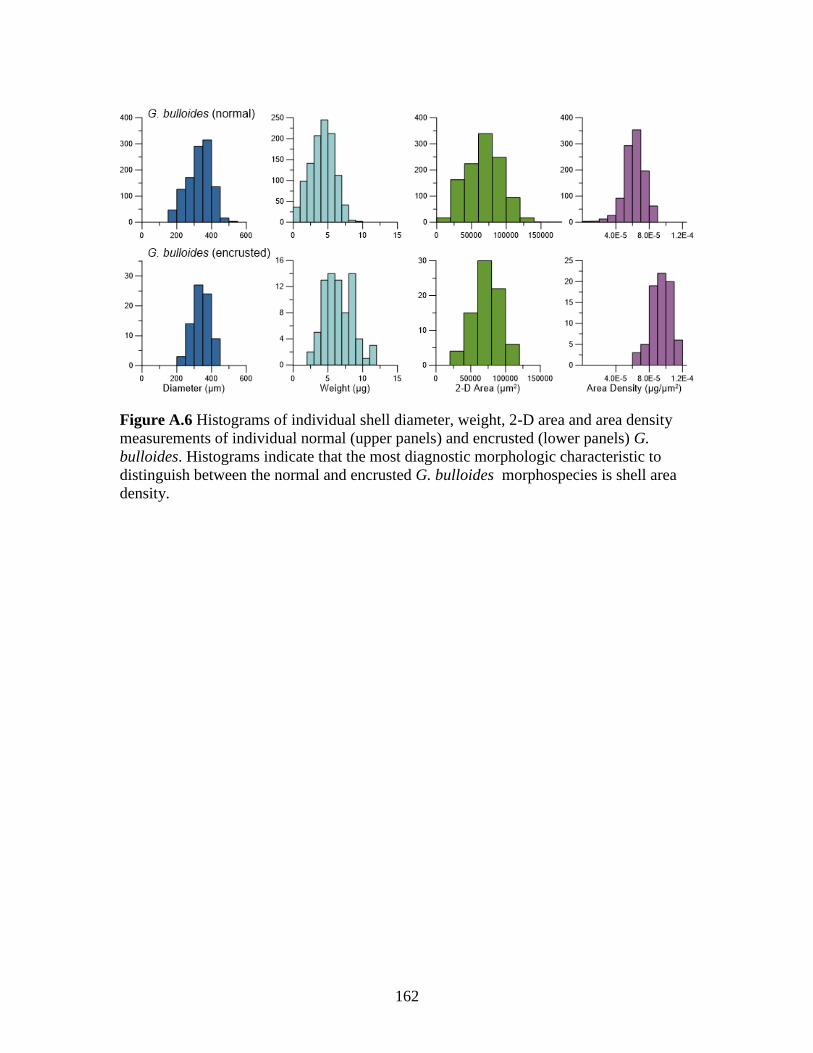
162

Figure A.6 Histograms of individual shell diameter, weight, 2-D area and area density

measurements of individual normal (upper panels) and encrusted (lower panels) G.

bulloides. Histograms indicate that the most diagnostic morphologic characteristic to

distinguish between the normal and encrusted G. bulloides morphospecies is shell area

density.

163

Figure A.7 Regressions of measured temperature and [PO43-] as independent variables

showing significant linear relationships with both normal G. bulloides area density and

measured [CO32-] indicating bivariate relationships between the in situ predictor variables

used in this study. Temperature and [CO32-] are positively correlated with area density

while phosphate and [CO32-] are negatively correlated with area density.

164

Figure A.8 Comparison of measured sea surface temperature from the SBB (1955-2000) to

temperatures derived from G. bulloides δ18O measurements. The long-term trends of each

temperature record are plotted and indicate similar declining trends although surface in

situ temperatures are warmer than G. bulloides derived temperatures. This is likely due to

the fact that the temperature relationship used to convert δ18O to temperature is a culture

derived relationship therefore the δ18O temperatures estimated here represent the

calcification, and therefore subsurface, temperature recorded by G. bulloides.

165

Figure A.9 The left panel figure compares pCO2 estimates calculated in this study

compared to the monthly and annual means of measured surface pCO2 from HOT (1988-

Present) and monthly values from the SBB (2007-2010). The right panel illustrates the

seasonal shifts in surface ocean pCO2 in the SBB that shifts dramatically in response to

upwelling. During periods of non-upwelling pCO2 is lower than atmospheric values while

upwelling pCO2 is higher than atmospheric CO2. This variability cannot be captured using

mean annual temperature and salinity values for the basin although calculated pCO2

represents integration over the seasonal cycle.

166

Table A.1 Simple linear regression results for all of the independent variables examined

in this study

Y=a+b(X)

Y X a b R2 F p

Area Density [CO32-] 4.19E-5 1.92E-7 0.80 121.41 <0.001

Temperature [CO32-] 7.57 0.04 0.86 186.85 <0.001

[PO43-] [CO3

2-] 2.33 -0.01 0.65 55.36 <0.001

Area Density Temperature 1.26E-5 4.24E-6 0.70 69.17 <0.001

[CO32-] Temperature -151.50 21.95 0.86 186.85 <0.001

[PO43-] Temperature 4.53 -0.29 0.79 110.99 <0.001

Area Density [PO43-] 7.57E-5 -1.16E-5 0.54 35.57 <0.001

[CO32-] [PO4

3-] 174.72 -58.95 0.65 55.36 <0.001

Temperature [PO43-] 14.93 -2.75 0.79 110.99 <0.001

.

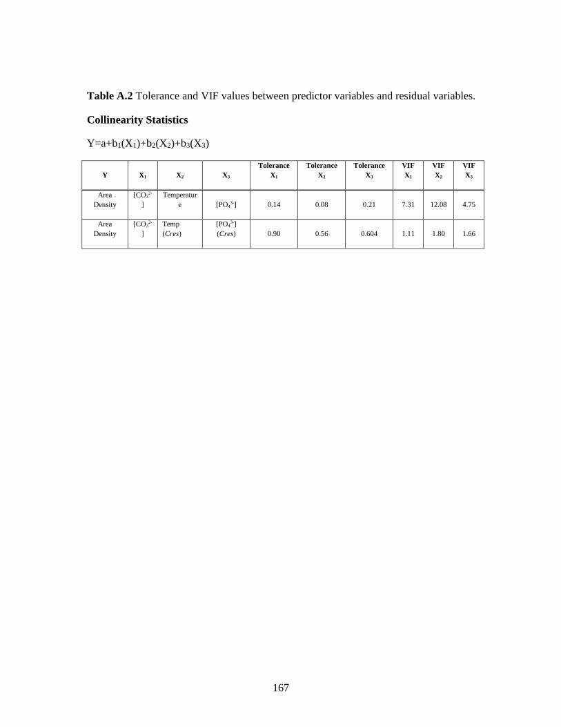
167

Table A.2 Tolerance and VIF values between predictor variables and residual variables.

Collinearity Statistics

Y=a+b1(X1)+b2(X2)+b3(X3)

Y X1 X2 X3

Tolerance

X1

Tolerance

X2

Tolerance

X3

VIF

X1

VIF

X2

VIF

X3

Area

Density

[CO32-

]

Temperatur

e [PO43-] 0.14 0.08 0.21 7.31 12.08 4.75

Area

Density

[CO32-

]

Temp

(Cres)

[PO43-]

(Cres) 0.90 0.56 0.604 1.11 1.80 1.66

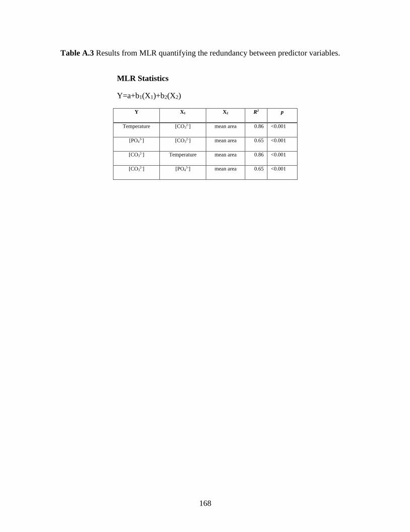
168

Table A.3 Results from MLR quantifying the redundancy between predictor variables.

MLR Statistics

Y=a+b1(X1)+b2(X2)

Y X1 X2 R2 p

Temperature [CO32-] mean area 0.86 <0.001

[PO43-] [CO3

2-] mean area 0.65 <0.001

[CO32-] Temperature mean area 0.86 <0.001

[CO32-] [PO4

3-] mean area 0.65 <0.001

169

Table A.4 Results from four hierarchical regression models that were used to evaluate

the significance of each predictor variable on area density (“ns” indicates a non

significant p value).

Hierarchical Regression Models

Y = a + b1(X1) + b2(X2) + b3(X3) Beta

Y X1 X2 X3 R2 ∆R2 F∆ p ∆R2

Beta

1

Beta

2

Beta

3

Mod

el 1

Area

Density [CO32-]

0.8

0

0.8

0

121.4

1 <0.001 0.90

[CO32-] Temp (Cres)

0.8

0

0.0

0 0.02

0.90

(ns) 0.90 0.01

[CO32-] Temp (Cres)

[PO43-]

(Cres)

0.8

0

0.0

0 0.09

0.77

(ns) 0.90 -0.01 -0.01

Mod

el 2

Area

Density

Temperatur

e

0.7

0

0.7

0 69.17 <0.001 0.84

Temperatur

e

[CO32-]

(Tres)

0.8

0

0.1

0

115.2

2 0.001 0.77 0.33

Temperatur

e

[CO32-]

(Tres)

[PO43-]

(Tres)

0.8

0

0.0

0 0.06

0.81

(ns) 0.77 0.33 -0.02

Mod

el 3

Area

Density [PO43-]

0.5

4

0.5

4 35.57 <0.001 -0.74

[PO43-]

[CO32-]

(Pres)

0.8

0

0.2

6 38.19 <0.001 -0.68 0.51

[PO43-]

[CO32-]

(Pres) Temp (Pres)

0.8

0

0.0

0 0.01

0.94

(ns) -0.68 0.52 -0.01

Mod

el 4

Area

Density [PO43-]

0.5

4

0.5

4 35.57 <0.001 -0.74

[PO43-] Temp (Pres)

0.7

0

0.1

6 14.86 0.001 -0.73 0.39

[PO43-] Temp (Pres)

[CO32-]

(Pres)

0.8

0

0.1

1 14.90 0.001 -0.68 -0.01 0.52

170

APPENDIX B –COPYRIGHT PERMISSIONS FOR CHAPTER 1

development and application of foraminiferal carbonate

Documents