developing a multiplexing assay system for the quality
TRANSCRIPT

Worcester Polytechnic InstituteDigital WPI
Major Qualifying Projects (All Years) Major Qualifying Projects
April 2017
Developing a Multiplexing Assay System for theQuality Control of Cell Therapy ProductsAmishi VairagadeWorcester Polytechnic Institute
Julia Michelle SmithWorcester Polytechnic Institute
Thai Thanh TrinhWorcester Polytechnic Institute
Follow this and additional works at: https://digitalcommons.wpi.edu/mqp-all
This Unrestricted is brought to you for free and open access by the Major Qualifying Projects at Digital WPI. It has been accepted for inclusion inMajor Qualifying Projects (All Years) by an authorized administrator of Digital WPI. For more information, please contact [email protected].
Repository CitationVairagade, A., Smith, J. M., & Trinh, T. T. (2017). Developing a Multiplexing Assay System for the Quality Control of Cell Therapy Products.Retrieved from https://digitalcommons.wpi.edu/mqp-all/4125

1
Developing a Multiplexing Assay System for the Quality Control of Cell Therapy
Products
A Major Qualifying Project Report:
Submitted to the Faculty of the Worcester Polytechnic Institute
In partial fulfillment of the requirements of the Degree of Bachelor of Science
By:
Julia Smith
Thai Trinh
Amishi Vairagade
April 27, 2017
Prof. Kristen Billiar, Ph.D., WPI
Prof. Edward Clancy, WPI
This report represents the work of WPI undergraduate students submitted to the faculty as evidence of completion of a degree requirement. WPI routinely publishes these reports on its website without editorial or peer review. For more information about
the projects program at WPI, please see http://www.wpi.edu/academics/ugradstudies/project-learning.html.

2
Abstract When used for autologous transplant, mesenchymal stem cells require extensive quality control
(QC) before being reintroduced into the body. One standard method of QC is biological assays, which
are a manually completed laboratory test for determining the concentration of foreign substances in a
cell culture solution. Biological assays have a number of limitations including time, cost, and level of
manual involvement. With these limitations in mind, a proof-of-concept device was developed to show
the potential for an automated multiplexed assay device for QC. This prototype device design can
accurately intake and dispense reagent volumes necessary for the completion of two assays, in a range
between 50 and 350 µL. The device is also capable of providing the required temperature environment
for each step of the assay process, changing between room temperature (24 °C) and 65 °C in under five
minutes.

3
Table of Contents Abstract ........................................................................................................................................................ 1
Table of Tables .............................................................................................................................................. 8
Authorship Page ............................................................................................................................................ 9
1 Introduction ........................................................................................................................................ 11
2 Background ......................................................................................................................................... 14
2.1 Regenerative Medicine ............................................................................................................... 14
2.2 Stem Cells .................................................................................................................................... 14
2.2.1 Mesenchymal Stem Cells (MSCs) ........................................................................................ 14
2.3 Applications of MSCs................................................................................................................... 15
2.3.1 Therapeutic Applications .................................................................................................... 15
2.3.2 Autologous Transplant Therapy .......................................................................................... 15
2.4 MSC Quality Control for Autologous Transplant ........................................................................ 16
2.4.1 Toxin Detection Assays ....................................................................................................... 16
2.4.2 Residual Cell Culture Material Assays ................................................................................. 17
2.4.3 Limitations of Quality Control ............................................................................................. 18
3 Project Strategy ................................................................................................................................... 20
3.1 Initial Client Statement ............................................................................................................... 20
3.2 Design Requirements .................................................................................................................. 20
3.2.1 Objectives ............................................................................................................................ 20
3.2.2 Engineering Standards ........................................................................................................ 21
3.3 Revised Client Statement ............................................................................................................ 22
3.4 Project Management Approach .................................................................................................. 22
3.4.1 Gantt Chart .......................................................................................................................... 23
3.4.2 Scrum Methodology: Daily Stand-up Meetings .................................................................. 25
3.4.3 Weekly Client Meetings ...................................................................................................... 25
3.4.4 Trello Board ......................................................................................................................... 25
4 Design Process .................................................................................................................................... 26
4.1 Needs Analysis ............................................................................................................................ 26
4.1.1 Clinical/Patient Need .......................................................................................................... 26
4.1.2 Client Need .......................................................................................................................... 27
4.1.3 Device Requirements .......................................................................................................... 27

4
4.2 Alternative Designs ..................................................................................................................... 28
4.2.1 Ideal System Architecture ................................................................................................... 28
4.2.2 Assay Plate .......................................................................................................................... 29
4.2.3 Microcontroller ................................................................................................................... 30
4.2.4 Fluid Control ........................................................................................................................ 33
4.2.5 Temperature Control .......................................................................................................... 38
4.2.6 Heat and Fluid Controller Driver ......................................................................................... 42
4.2.7 Control Mechanism ............................................................................................................. 43
4.3 Feasibility Studies and Experimental Modeling .......................................................................... 45
4.3.1 Fluidic Control System Modeling ........................................................................................ 45
4.3.2 Temperature Control System Modelling ............................................................................ 47
4.4 Final Design Approach ................................................................................................................ 54
4.4.1 Prototype Architecture ....................................................................................................... 54
4.4.2 Assay Selection .................................................................................................................... 54
4.4.3 Fluid Control ........................................................................................................................ 56
4.4.4 Temperature Control .......................................................................................................... 59
4.5 Pretotype Design ......................................................................................................................... 61
5 Design Verification .............................................................................................................................. 64
5.1 Assay Experimentation ............................................................................................................... 64
5.1.1 Mycoplasma Baseline Assay Experiment ............................................................................ 64
5.1.2 BSA Baseline Assay Experiment .......................................................................................... 67
5.2 Fluidic Control Experimentation ................................................................................................. 68
5.2.1 Syringe Pump Calibration Curve Determination Experiment ............................................. 68
5.2.2 Syringe Pump with Manifold: Dead Volumes Experiment .................................................. 70
5.2.3 Syringe Pump with Manifold: Intake Accuracies Experiment ............................................. 71
5.2.4 Syringe Pump with Manifold and Air Pump: Output Volume Loss Experiment ................. 72
5.2.5 Cross Contamination Experiment ....................................................................................... 73
5.2.6 BSA Assay Run: Water Trial Experiment ............................................................................. 74
5.3 Temperature Control Experimentation ...................................................................................... 76
5.3.1 Heating from Room Temperature to 65° C Experiment ..................................................... 76
5.3.2 Cooling from 65 °C to Room Temperature (24 °C) Experiment .......................................... 78
5.3.3 Temperature Control System Cooling Experiment ............................................................. 79

5
6 Design Validation ................................................................................................................................ 81
6.1 Prototype Validation: BSA Assay Run with System ..................................................................... 81
6.2 Prototype Validation: Mycoplasma Assay Run with System ...................................................... 82
7 Discussion ............................................................................................................................................ 84
7.1 Fluidic Control System Discussion ............................................................................................... 84
7.2 Temperature Control System Discussion .................................................................................... 85
7.3 Potential Project Impacts ............................................................................................................ 86
7.3.1 Economics ........................................................................................................................... 86
7.3.2 Environmental Impact ......................................................................................................... 86
7.3.3 Societal Influence ................................................................................................................ 86
7.3.4 Political Ramifications ......................................................................................................... 86
7.3.5 Ethical Concerns .................................................................................................................. 86
7.3.6 Health and Safety Issues ..................................................................................................... 87
7.3.7 Manufacturability ............................................................................................................... 87
7.3.8 Sustainability ....................................................................................................................... 87
8 Conclusions and Recommendations ................................................................................................... 88
9 References .......................................................................................................................................... 90
Appendices .................................................................................................................................................. 93
Appendix A: Potential Pretotype Brochure............................................................................................. 93
Appendix B: R&D Systems Mycoprobe Mycoplasma Detection Assay Kit Procedure ............................ 96
Appendix C: MyBioSource BSA Detection Assay Procedure ................................................................. 101
Appendix D: Syringe Pump Calibration Curve Determination Experiment (Full) ................................. 108
Appendix E: Syringe Pump with Manifold: Dead Volumes Experiment (Full) ...................................... 116
Appendix F: Syringe Pump with Manifold: Intake Inaccuracies Experiment (Full) ............................... 128
Appendix G: Syringe Pump with Manifold and Air Pump: Output Volume Loss Experiment (Full) ...... 130
Appendix H: BSA Water Trial Experiment: Full ..................................................................................... 133
Appendix I: System BSA Assay Experiment Data .................................................................................. 135
Appendix J: System Mycoplasma Experiment Data .............................................................................. 136

6
Table of Figures FIGURE 1 PROJECT GANTT CHART ............................................................................................................................... 24
FIGURE 2 ARCHITECTURE DRAWING OF IDEAL SYSTEM BREAKDOWN ....................................................................... 29
FIGURE 3 ARDUINO MEGA 2560 MICROCONTROLLER BOARD ................................................................................... 31
FIGURE 4 TEXAS INSTRUMENTS 16-BIT MICROCONTROLLER BOARD ......................................................................... 32
FIGURE 5 PERISTALTIC PUMPING MECHANISM. ......................................................................................................... 33
FIGURE 6 TORQUE-ACTUATED PUMP .......................................................................................................................... 34
FIGURE 7 TYPICAL OTS AUTOMATED SYRINGE PUMP. ................................................................................................ 35
FIGURE 8 ACTUONIX P16 LINEAR ACTUATOR CHOSEN FOR SYRINGE PUMP RETRIEVED FROM
HTTPS://S3.AMAZONAWS.COM/ACTUONIX/ACTUONIX+P16+DATASHEET.PDF ............................................... 36
FIGURE 9 NRESEARCH SOLENOID VALVE MANIFOLD .................................................................................................. 37
FIGURE 10 COOLDRIVE ONE SINGLE VALVE DRIVERS .................................................................................................. 38
FIGURE 11 KAPTON HEATER ........................................................................................................................................ 39
FIGURE 12 POTENTIAL HEATING SYSTEM CREATED BY TRT TEAM .............................................................................. 39
FIGURE 13 PELTIER TEC MODULE ................................................................................................................................ 40
FIGURE 14 TEMPERATURE SENSOR RETRIEVED FROM
WWW.GOOGLE.COM/SEARCH?Q=LM35&RLZ=1C1CHFX_ENUS608US608&SOURCE=LNMS&TBM=ISCH&SA=X
&VED=0AHUKEWIZVCR70ZRTAHVM2SYKHTGXDFAQ_AUIBIGB&BIW=1270&BIH=633#IMGRC=DCXCZGTS1ZYA
MM: .................................................................................................................................................................... 41
FIGURE 15 MC33926 MOTOR DRIVER SHIELD FOR ARDUINO MICROCONTROLLER BOARD ....................................... 43
FIGURE 16 PID CONTROL LOOP ................................................................................................................................... 44
FIGURE 17 NRESEARCH VALVE MANIFOLD TECHNICAL DRAWING ............................................................................. 46
FIGURE 18 TRANSIENT RESPONSE: HEAT INPUT AND CONVECTION OF ALUMINUM VS. COPPER ............................. 49
FIGURE 19 TRANSIENT COOLING RESPONSE OF ALUMINUM VERSUS COPPER .......................................................... 50
FIGURE 20 THERMAL CIRCUIT OF ALUMINUM SHEET WITH POLYSTYRENE WELL ...................................................... 51
FIGURE 21 THERMAL CIRCUIT OF A MACHINED ALUMINUM BAR AND POLYSTYRENE WELL ..................................... 52
FIGURE 22 PROTOTYPE ARCHITECTURE ...................................................................................................................... 54
FIGURE 23 FLUID CONTROL SYSTEM CONSISTING OF SYRINGE PUMP AND SOLENOID VALVE MANIFOLD ................ 56
FIGURE 24 SCHEMATIC SHOWING CONTROL OF SYRINGE PUMP AND VALVE MANIFOLD SYSTEM ........................... 57
FIGURE 25 FLUIDIC CONTROL SUBSYSTEM DETAILED SCHEMATIC ............................................................................. 58
FIGURE 26 PROTOTYPE TEMPERATURE CONTROL SYSTEM ARCHITECTURE DRAWING .............................................. 59
FIGURE 27 IMAGE OF ENTIRE TEMPERATURE CONTROL SYSTEM ............................................................................... 59
FIGURE 28 TEMPERATURE CONTROL SYSTEM SCHEMATIC ......................................................................................... 60
FIGURE 29 TEMPERATURE CONTROL SUBSYSTEM DETAILED SCHEMATIC ................................................................. 61
FIGURE 30 SOLIDWORKS DRAWING OF POTENTIAL ASSAY DEVICE (LEFT) AND POTENTIAL ASSAY DEVICE
INTEGRATED INTO A LAB BENCH SETTING (RIGHT) ............................................................................................ 62
FIGURE 31 MYCOPLASMA ASSAY INITIAL RUN RESULT WELLS. .................................................................................. 65
FIGURE 32 MYCOPLASMA ASSAY SECONDAY RUN RESULT WELLS. ............................................................................ 66
FIGURE 33 INITIAL BSA ASSAY STANDARD DILUTION CURVE COMPARE TO MANUFACTURER EXAMPLE .................. 67
FIGURE 34 INITIAL BSA ASSAY RESULT WELLS. DESCENDING CONCENTRATION FROM.............................................. 68
FIGURE 35 BASELINE BSA ASSAY STANDARD DILUTION CURVE (LEFT) AND BSA RESULTANT WELLS (RIGHT) WITH
CONCENTRATION DESCENDING FROM TOP RIGHT WELL (30,000 NG/ML) TO BOTTOM RIGHT (0NG/ML) ....... 68
FIGURE 36 GRAPH OF OUTPUT VOLUME VS. LINEAR ACTUATOR DISTANCE DATA FROM ALL EXPERIMENTAL
ITERATIONS WITHOUT OUTLIERS (LEFT). GENERATED CALIBRATION CURVE FROM ALL ITERATION DATA WITH
OUTLIERS REMOVED (RIGHT).............................................................................................................................. 70

7
FIGURE 37 VOLUME OUTPUT COMPARISON BETWEEN SYSTEM WITH AND WITHOUT MANIFOLD .......................... 71
FIGURE 38 RESULTS OF SYSTEM INTAKE EXPERIMENT: GOAL INTAKE VS. ACTUAL INTAKE (LEFT). CHANGE IN INTAKE
VOLUME VS. GOAL VOLUME INTAKE (RIGHT) .................................................................................................... 72
FIGURE 39 DISTRIBUTION OF VOLUME LOST WITH AIR PUMP INTEGRATION (LEFT) AND DISTRIBUTION OF VOLUME
LOST WITH NO AIR PUMP (RIGHT) ...................................................................................................................... 73
FIGURE 40 TOP VIEW OF CONTAMINATED WELLS (LEFT). SIDE VIEW OF CONTAMINATED WELLS (RIGHT) .............. 74
FIGURE 41 DISTRIBUTION OF VOLUMES REQUESTED VS. ACTUAL VOLUME OUTPUT FOR FOUR VOLUMES ............. 75
FIGURE 42 HEATING FROM RT TO 65°C WITH 80X80MM ATTACHED HEAT SINK ....................................................... 77
FIGURE 43 SIMULATED AND EMPIRICAL DATA FOR TRANSIENT HEATING OF THE SYSTEM ....................................... 77
FIGURE 44 COOLING FROM 65°C TO ROOM TEMPERATURE WITH 80X80MM HEAT SINK (LEFT) AND SYSTEM COOL
FROM 65°C TO ROOM TEMPERATURE WITH 60X60MM HEAT SINK (RIGHT) ..................................................... 79
FIGURE 45 COOLING STABILITY GRAPH OF COOLING THE SYSTEM FROM 60 °C TO 24 °C .......................................... 79
FIGURE 46 COMPARISON OF BASELINE ASSAY TEST RESULTS AND SYSTEM ASSAY TEST RESULTS ............................ 82
FIGURE 47 COMPARISON OF BASELINE MYCOPLASMA ASSAY RESULTS (TOP) TO SYSTEM MYCOPLASMA ASSAY
RESULTS (BOTTOM). POSITIVE CONTROLS INDICATED BY DARKER RED COLOR: LEFT WELLS. NEGATIVE
CONTROLS INDICATED BY TRANSPARENT COLOR: RIGHT WELLS. ...................................................................... 83

8
Table of Tables TABLE 1 PROJECT GANTT CHART BREAKDOWN .......................................................................................................... 23
TABLE 2 OTS BSA ASSAY TRADEOFF ANALYSIS ............................................................................................................ 55
TABLE 3 OTS MYCOPLASMA TRADEOFF ANALYSIS ...................................................................................................... 55
TABLE 4 MANUFACTURER INCLUDED OD RESULT COMPARISON (LEFT) EXPERIMENTAL OD AND RESULTS (RIGHT) 65
TABLE 5 MANUFACTURER INCLUDED O.D. RESULT COMPARISON (LEFT) EXPERIMENTAL O.D. AND RESULTS .......... 66
TABLE 6 MANUFACTURER SPECIFICATIONS FOR ASSAY RESULTS (LEFT). ................................................................... 83

9
Authorship Page
Section Main Author Main Editor
Abstract Julia Smith Julia Smith
1 Introduction Amishi Vairagade/Thai Trinh
Amishi Vairagade/Julia Smith
2 Background
2. 1 Regenerative Medicine Amishi Vairagade Amishi Vairagade/Julia Smith
2.2 Stem Cells Julia Smith Julia Smith
2.3 Application of MSCs Julia Smith Julia Smith
2.4 MSC Quality for Autologous Transplant Julia Smith/Amishi Vairagade
Amishi Vairagade/Julia Smith
3 Project Strategy
3.1 Initial Client Statement Julia Smith Julia Smith
3.2 Design Requirements Julia Smith Julia Smith
3.3 Revised Client Statement Julia Smith Julia Smith
3.4 Project Management Approach Julia Smith Julia Smith
4 Design Process
4.1 Needs Analysis Julia Smith Julia Smith
4.2 Alternative Designs Thai Trinh/Amishi Vairagade
Thai Trinh/Julia Smith
4.3 Feasibility Studies and Experimental Modeling
Thai Trinh/Amishi Vairagade
Thai Trinh/Amishi Vairagade
4.4 Final Design Approach Thai Trinh Thai Trinh/Julia Smith
5 Design Verification
5.1 Assay Experimentation Julia Smith Julia Smith
5.2 Fluid Control Experimentation Julia Smith/Amishi Vairagade
Julia Smith
5.3 Temperature Control Experimentation Thai Trinh Thai Trinh/Julia Smith
6 Design Validation
6.1 Prototype Validation: BSA Assay Run with System
Julia Smith Julia Smith
6.2 Prototype Validation: Mycoplasma Assay Run with System
Julia Smith Julia Smith
7 Discussion
7.1 Fluidic Control System Discussion Julia Smith Julia Smith
7.2 Temperature Control System Discussion Julia Smith Julia Smith
8 Conclusions and Recommendations Julia Smith/Amishi Vairagade
Julia Smith
Appendix A: Potential Pretotype Brochure Amishi Vairagade Julia Smith/Amishi Vairagade
Appendix B: R&D Systems Mycoprobe Mycoplasma Detection Assay Kit Procedure
N/A
Appendix C: MyBioSource BSA Detection Assay Procedure
N/A
Appendix D: Syringe Pump Calibration Curve Determination (Full)
Amishi Vairagade Julia Smith/Amishi Vairagade
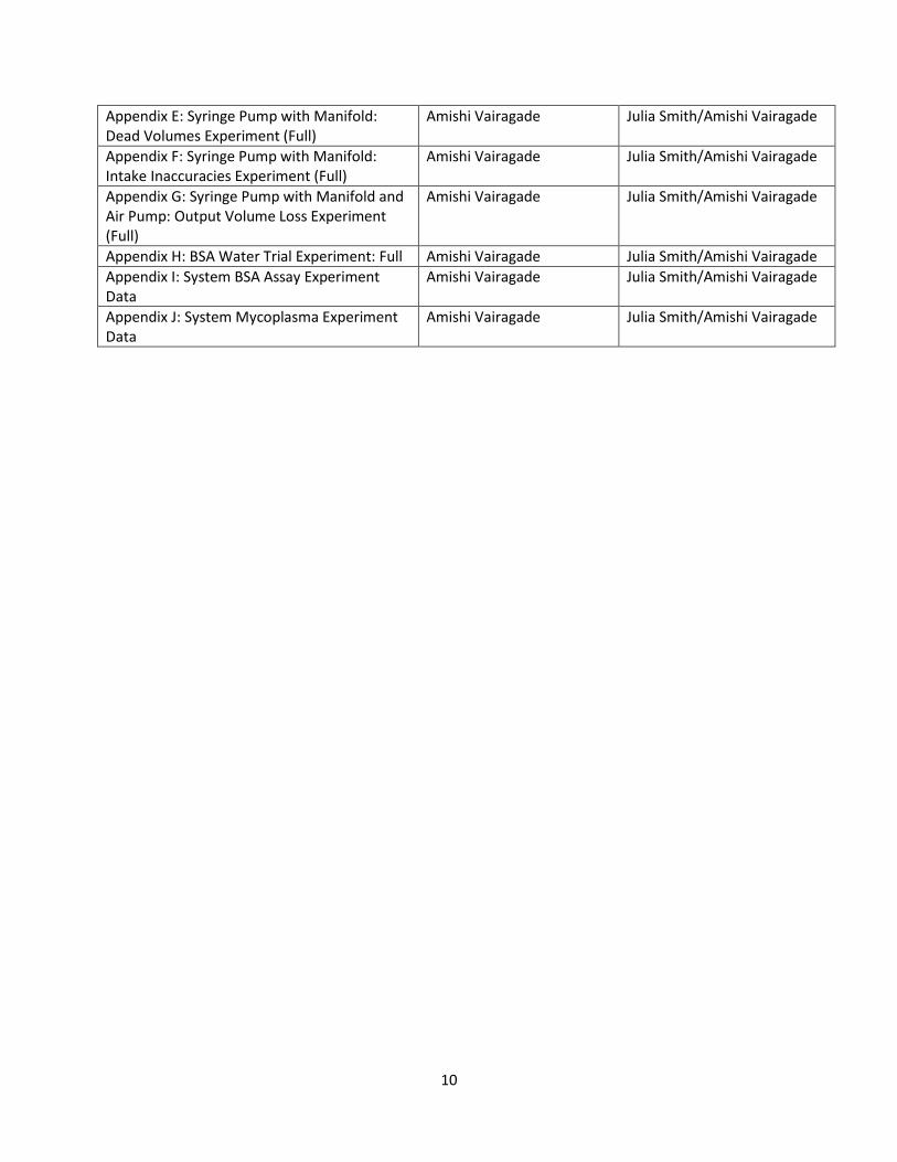
10
Appendix E: Syringe Pump with Manifold: Dead Volumes Experiment (Full)
Amishi Vairagade Julia Smith/Amishi Vairagade
Appendix F: Syringe Pump with Manifold: Intake Inaccuracies Experiment (Full)
Amishi Vairagade Julia Smith/Amishi Vairagade
Appendix G: Syringe Pump with Manifold and Air Pump: Output Volume Loss Experiment (Full)
Amishi Vairagade Julia Smith/Amishi Vairagade
Appendix H: BSA Water Trial Experiment: Full Amishi Vairagade Julia Smith/Amishi Vairagade
Appendix I: System BSA Assay Experiment Data
Amishi Vairagade Julia Smith/Amishi Vairagade
Appendix J: System Mycoplasma Experiment Data
Amishi Vairagade Julia Smith/Amishi Vairagade
11
1 Introduction With current medical treatments, it is often difficult to target the source as well as the
symptoms of chronic diseases, which are due to malfunctioning or aging cells. This results in inefficient
and high cost medical treatment for patients. One possible solution is regenerative medicine. This area
of medicine focuses on treating the fundamental causes of the diseases rather than only the symptoms.
Specifically, regenerative medicine aims to improve, repair, or regenerate damaged tissues by replacing
them with healthy tissues or cells (Alliance for Regenerative Medicine, 2013). For example, when
diagnosed with Type 1 Diabetes Mellitus, a patient is most often treated by continuously introducing
insulin to body due to the malfunctioning of the pancreas. However, using regenerative medicine
strategies, scientists are researching how to recover pancreatic cells and return them to a healthy,
insulin-producing condition. The patient’s body can then naturally produce insulin without life-long
treatment (United State Government Accountability Office, 2015).
Currently, there are many important regenerative medicine technologies used in the healthcare
industry, including cell-based therapy, gene therapy, and tissue engineering. Among these technologies,
cell-based therapy is the most prominent, as it is currently involved in more than 1,900 clinical trials
worldwide (Alliance for Regenerative Medicine, 2013). Cell-based therapy is a subsection of
regenerative medicine that involves harvesting stem cells and progenitor cells such as mesenchymal
stem cells or neural stem cells. This therapy also includes isolating differentiated adult cells from human
body such as fibroblasts, osteoblasts, and myocytes. These healthy cells are then introduced into a
patient’s body in order to replace non-functioning and damaged cells (Alliance for Regenerative
Medicine, 2014).
Cell-based therapy is a promising area in the medical field and can be used to treat many
conditions and diseases, such as heart failure, cancer, and spinal cord injuries. Cell-based technologies
have contributed to the treatment of more than 160,000 patients. From 2008 to 2013, 12 cell therapy
products have received approval by various regulatory agencies (Alliance for Regenerative Medicine,
2013). Some cell therapy products that have been approved by the U.S. Food & Drug Administration
(FDA) are Fibroblasts from Fibrocell Technologies, Inc. and Clevecord, which is HPC (Hematopoietic
Progenitor Cell) Cord Blood from the Cleveland Cord Blood Center (U.S. Food & Drug Administration,
2017).

12
These cell-based technologies usually use three major types of cells: autologous, allogeneic, and
pluripotent cells (National Cell Manufacturing Consortium, 2016). Autologous cells are the patient’s own
cells, which are used as a personalized treatment. These can be used to recover the patient’s ability to
produce blood cells after chemotherapy in order to help treat blood cancers such as leukemia and
myeloma. Moreover, using the patient’s own cells reduces the risk of cellular incompatibility and graft
vs. host conditions. Allogeneic cells are stem cells that harvested from a compatible donor. These cells
can also help the patient to recover blood cell production after chemotherapy but has a high risk for
immune rejection (Cancer Treatment Centers of America, 2017). Pluripotent cells can differentiate
themselves into any of three basic body layer cell groups: ectoderm, endoderm, and mesoderm. As a
result, pluripotent stem cell can produce any cell or tissue, which is useful for cell replacement for
damaged organs or tissues (Boston Children’s Hospital, 2017).
Though cell manufacturing has the potential to greatly benefit patients, the cells used in the cell-
based products require intense maintenance and quality control to ensure their viability and safety. It is
very crucial to ensure that the cells injected into the patient’s body are safe and uncontaminated.
Current methods of stem cell quality control include models, assays, and sensors to gauge the quality of
the cells. These methods can be not only be expensive but also time consuming. There are other
challenges associated with the current quality control methods such as difficulty with obtaining
reproducibly accurate results, which can lead to potentially harmful errors. Inaccurate results not only
compromise the quality of the cells but can also be dangerous and even life threatening for the patient
(National Cell Manufacturing Consortium, 2016).
The purpose of our project is to overcome these quality control challenges by designing and
creating a proof-of-concept device to demonstrate the ability of multiplexing assays used for testing
mesenchymal stem cells (MSCs), which will be used for autologous transplant. The current quality
control of MSCs has several challenges associated with it. The current quality control tests using assays
are performed manually by a laboratory technician and involve steps such as pipetting, transferring, and
incubating. Because of the cost of the off-the-shelf assay kits as well as the manual labor involved in
these tests, the cost of quality control is very high and one of the most expensive aspects of the cell
therapy process. Furthermore, running these assays can be time consuming as each assay can take up to
seven hours to complete, resulting in higher labor costs and extensive time spent on this area. Another
limitation of running these assays manually is that it may result in human errors like reproducibility,
false negatives and false positives. False negatives are particularly dangerous because if contaminated
cells are reintroduced into the body, severe side effects can take place for the patient and health could

13
be compromised. False positives can result in viable cells being discarded leading to a waste of cells,
time, and cost associated with the tests. Thus, it is important to build and design a device that can
multiplex these assays while reducing the costs involved in the quality control and reducing the time
involved in running these tests.
For this project, our MQP team created a proof-of-concept device to show the potential for an
automated, multiplexing assay device that our client, Triple Ring Technologies, could further develop in
the future. Because of the early stage of this project, the prototype was unable to reach all goals laid out
due to time constraints but we see this device being capable of solving many of the aforementioned
problems after future development and implementation. This device ideally would be able to
simultaneously perform key quality control assays on a single patient’s MSC sample to ensure that the
cells are healthy and viable before reintroduction into the body. The device would require little manual
involvement and would consequently result in lower labor costs, reduced time spent on quality control,
and higher reproducibility and accuracy. This product could eventually be a marketable device that can
greatly assist with the quality control of cell therapy products.

14
2 Background
2.1 Regenerative Medicine
The medical field has advanced through the years and has seen innovation in treating various
diseases. One such important advancement in the medical field is regenerative medicine. Regenerative
medicines are used for the treatment of a part of the body that has damage due to a health condition or
aging. Regenerative medicine is focused on treating the root of the health condition in order to address
it. Though still a growing field with much room for improvement, regenerative medicine is an important
innovation in the healthcare industry as it has led to effective health care treatment. Regenerative
medicines include a wide spectrum of approaches involving cell-based therapies, gene therapy, biologics
and small molecules, tissue engineering, stem cells, and biobanking to treat many serious conditions.
(Alliance for Regenerative Medicine, 2013).
Cell-based therapies are a subset of regenerative medicine in which healthy cells are used to
heal the impaired part of the body. This method of treatment promotes and strengthens the body’s
immune system by redeveloping and renewing the body’s cells. Cell based therapies usually use
hematopoietic stem cells and mesenchymal stems cells which are undifferentiated adult stem cells.
These cells differentiate to form other cell types such as intestinal cells, muscle cells, and blood cells.
Because of the variety of cells that MSCs are able to differentiate into, they are very versatile and have
almost unlimited potential for applications in a wide range of diseases (Bender, 2016)
2.2 Stem Cells
Stem cells are undifferentiated cells that are found throughout most tissues in the body. These
cells are capable of differentiating into a large variety of different cell types depending on their location
and the function of the surrounding tissues. Because of their renewable properties, stem cells can repair
themselves and are often responsible for the repair of the surrounding tissue by differentiating into the
appropriate type of cell, depending on the tissue’s needs. (NIH, 2016).
2.2.1 Mesenchymal Stem Cells (MSCs)
This project focuses on mesenchymal stem cells and their potential applications in research and
the treatment of a variety of diseases. Mesenchymal stem cells are valuable because of their ability to
differentiate into a large range of cell types. The applications for these cells and their potential to treat a
variety of different diseases and disorders make them very valuable to the scientific research
community. Some current applications research include the treatment of cardiovascular diseases,
neurodegenerative disorders such as Parkinson’s and Alzheimer’s, and autoimmune diseases including
rheumatoid arthritis and type 1 diabetes. However, these cells become less capable of differentiating

15
quickly with increasing cell culture passages, therefore all cells collected must be put to use because it is
difficult to ensure a constant supply of viable cells. (Ullah, et al, 2015).
The particular stem cells that are the focus of this project are mesenchymal stem cells (MSCs).
These stem cells are derived from an adult human and were originally thought to be found only in bone
marrow (NIH, 2016). However, more recently, scientists have shown that they are found in virtually
every tissue in the body including adipose tissue, amniotic fluid, and even umbilical cords. Depending on
their location, MSCs have the potential to differentiate into a range of other cell types, in particular,
bone, cartilage, fat, and even occasionally neural cells (Ullah, et al, 2015). Additionally, they can also
differentiate into stromal cells which are assistive in the support of blood production (NIH, 2016).
2.3 Applications of MSCs
2.3.1 Therapeutic Applications
Stem cell therapy is a relatively new area of medicine and its possible applications are seemingly
limitless, though most areas of research have not been advanced past clinical trial stages of treatment.
Research conducted in recent years has shown that cell therapy treatments can assist with healing of
bone and cartilage diseases; this process required infusion of MSC rich bone marrow into the affected
area to help combat both osteogenesis imperfecta and hypophosphatasia. This therapy can also be used
to address various cardiovascular diseases which is highly beneficial given the non-regenerative nature
of cardiovascular cells. Infusion of MSCs in the affected region can assist in recovering from heart
disease, heart failure, and myocardial infarction. Autoimmune disease such as Crohn’s disease and
Rheumatoid arthritis can also benefit from the anti-inflammatory properties of the MSCs. (Kim, Cho,
2013).
2.3.2 Autologous Transplant Therapy
The application of MSCs for this project is in autologous MSC transplant therapy. Autologous
transplant therapy is a method of cell therapy in which a patient’s own cells are harvested, preserved,
and reinjected into the body after a period of time. This therapy is most often used as a treatment for
blood conditions or cancers like lymphoma or leukemia. Because the chemotherapy required to treat
these condition destroys cancer cells as well as blood forming cells found in bone marrow, it is helpful to
resupply the body with healthy and unaffected stem cells to quicken the time it takes for the body to
regenerate the lost blood cells.
The process for autologous transplant consists of multiple steps: harvesting, preservation,
quality control, and reinjection into the body. MSCs are collected from the bone marrow when the
patient is relatively healthy or just prior to chemotherapy or radiation treatment (Leukemia &

16
Lymphoma Society, 2017). Stem cells are typically collected using apheresis, where they are isolated
from the bone marrow. The collected stem cells are then either cryogenically preserved until needed or
cultured to expand the number of cells available and then cryogenically preserved until required. If the
stem cells are cultured, they must undergo extensive quality control to ensure purity before
reintroduction to the body.
Once the cells are required, generally after cancer treatment has been completed, the stem cells
are reinfused into the body, typically through a central venous catheter. Once the cells have been
reintroduced, there is a period of time necessary for the engraftment of the saved cells in which they
are required to replace all cells that had died during treatment. After this period of time has passed, the
cells are able to regrow and regenerate as required. (Memorial Sloan Kettering Cancer Center, 2017).
2.4 MSC Quality Control for Autologous Transplant
In the biotechnology field, when biomedical products such as MSCs are to be used in human or
animal therapeutics, they need to be appropriately purified from contaminants to prevent health risks.
Contamination in the final product can come from outside sources or excess amounts of residual
substances used during the cell culture process. Therefore, it is important to ensure that the
concentration of residual substances or contaminants in the final product are within FDA approved
limits. Biological assays are one method used to identify presence of specific contaminants in a cell
solution.
2.4.1 Toxin Detection Assays
During the cell culture process, it is possible for the cultures to be contaminated by certain
toxins, such as bacteria. These toxins can be very harmful and can fully compromise the culture and all
cells being grown because of the potentially harmful effects they could have on the cells and on the
patient who would be receiving the cells. Therefore, it is very important that the MSCs used for
autologous transplant are rigorously tested for these toxins to ensure maximum safety for the patient.
2.4.1.1 Toxin Detection Assays: Mycoplasma
One of the most common biological contaminants is mycoplasma. Mycoplasma is a
microorganism that has the capacity to modify certain properties of the cell it infects, including its
development patterns. It is also capable of inducing the spread of viruses and yield in the infected cell
culture. (Ryan, 2008).
Mycoplasma is a dangerous contaminant because its microscopic size allows it to easily infect
cultures and remain potentially undetected. Additionally, these small microorganisms have the ability to
replicate themselves and, because they lack cell walls, can quickly reproduce and infect the cell culture.

17
Mycoplasma colonies are hearty and difficult to destroy which enables them to grow rapidly in a healthy
cell culture environment. Because of these characteristics and the potential for health risks for patients,
it is very important that cells be tested for mycoplasma before they are reintroduced into the body.
(Ryan, 2008).
2.4.1.2 Toxin Detection Assays: Endotoxin
Another toxin that is important to test MSCs for is endotoxin. Endotoxin is a complex
lipopolysaccharide found in gram negative bacteria and is released upon both cell death and
reproduction of the bacteria. Endotoxin infection can cause a number of problems in both in vitro and in
vivo environments, making it very important to identify its presence as soon as possible. In an in vitro
environment, endotoxin can cause a multitude of problems with cell cultures as it affects production of
macrophages and can inhibit colony formation of the desired cell type. In vivo, endotoxin infection can
result in inflammatory and pyrogenic responses, beginning with fever and chills and sometimes
worsening to potentially fatal septic shock. (Sigma Aldrich, 2017). Endotoxin is carried on laboratory
equipment because of its affinity for hydrophobic surfaces such as cell culture plates. This toxin is
particularly problematic because of its high stability and resistance to heat, which makes it difficult to
eradicate using normal sterilization methods, particularly autoclaving. (Sigma Aldrich, 2017).
2.4.2 Residual Cell Culture Material Assays
In order to ensure the purity of the cells, it is important to test for residual cell culture materials.
Some cell cultures may involve use of residual cell culture material derived from animal sources,
particularly bovine or porcine. These may cause contamination of the cells with adventitious agents.
Thus, it is important to test for residual cell culture materials to confirm the viability and purity of the
cells. (Bioreliance, 2017).
2.4.2.1 Residual Cell Culture Material Assays: Bovine Serum Albumin (BSA)
One such substance cell culture is tested for is Bovine Serum Albumin (BSA). Serum is an
important part in tissue engineering and cell culture as it is used to supply nourishment to the culture. It
also acts as a carrier for essential compounds like hormones, growth factors, and nutrients. (Francis,
2010).
It has been observed that BSA infusion can have ill-effects on health. It has been observed that
albumin can result in increased capillary permeability, excessive circulation, and pulmonary edema.
(Drummond & Ludlam, 1999). Additionally, it is important to be cautious with the use of any animal
based products when culturing cells that will be reintroduced to the human body, as this can also have
ill effects. In general, animal derived serums an lead to many problems with human MSC culture
18
including introducing variability in the culture, changing cell growth patterns, and contaminating the
culture with cytotoxic factors found in the serum. It can also be a risk for introducing viruses, bacteria,
prions, bacteria, and other contaminants into the cell solutions. These contaminants can compromise
the health of the cells and the patient if the cells are reintroduced into the blood stream. Finally, the use
of animal based serum can disrupt the adhesion of the cells and cause hindrance of the cell growth. This
disruption may result in disturbing the stability of the cells and further interfere cell growth and function
(Tekkatte, et al., 2011).
2.4.2.2 Residual Cell Culture Material Assays: Trypsin
Trypsin is a material that is formed in the pancreas and is very commonly used in adherent cell
culture (Sigma Aldrich, 2017). Its main purpose is to cleave peptides on lysine and arginine side chains
which effectively breaks the bonds between adherent cells and the cell culture plate in which they grew
(Worthington Biochemical Corporation, 2017).
Trypsin is typically taken from either bovine or porcine sources when used in cell culture. This is
an important material to test for as residual material because of its non-human source. It is risk-inducing
to reintroduce cells into the body that have been exposed to an animal based material. Trypsin can carry
viruses that are prevalent and difficult to eradicate in the porcine population. It can additionally be
contaminated with other adventitious agents that can cause changes in cell cultures and difficulties with
creating a suitable biological product. (European Medicines Agency, 2014).
2.4.3 Limitations of Quality Control
Biological assays are some of the most popular laboratory methods for detecting potentially
hazardous substances in cell solutions. They are used in hospitals, laboratories, industry and research to
identify the presence and concentration of particular substances in a cell solution including proteins,
antibodies, and hormones. These tests perform based on the principles of the binding ability of
antibodies, which are proteins generated by the immune system in response to the presence of foreign
agents like bacteria. Due to their high specificity to bind to certain molecular structures, antibodies are
used in some assays to detect certain biological molecules. (ImmunoChemistry Technologies, 2017).
However, these assays have significant room for improvement. The main concerns with these assays are
the high cost, time commitment, and possibility for human error involved.
Off-the-shelf (OTS) assay kits are expensive and vary greatly in cost range. For example, the R&D
Systems' Proteome Profiler Human Kidney Biomarker Array price per kit is $495, which breaks down to
$125 per sample and $3.28 for each data point. R&D Systems' Fluorokine® MAP Multiplex Human
Inflammation 12-plex kit costs $2,390, which breaks down to $30 per sample and $2.5 for each data

19
point (Biocompare, 2011). In addition to these examples, there are hundreds of other assay kits on the
market with costs that range from hundreds to thousands of dollars. These OTS assay kits are also very
time consuming to perform. For example, the MycoProbe® Mycoplasma Detection Kit from R&D
Systems requires five hours to run the whole assay (R&D Systems, 2016), not including sample and
reagent preparation time. Another example is the MyBioSource BSA Detection Assay kit, which takes up
to two hours to complete, with additional time again required for preparation (MyBioSource, 2016).
Finally, a considerable amount of manual work is involved in executing assays, which involves manual
procedures like pipetting, washing, and transferring of solutions. Moreover, running the assay
procedures manually may introduce risk for human error and difficulties in reproducibility. An
experienced operator is required to ensure that the assays are correctly executed. It is crucial to ensure
the assay procedure is performed correctly since the therapeutic applications rely on the stable and
accurate data.
With consideration of the above limitations, an automated system to perform all the
aforementioned assay procedures would be extremely beneficial to help reduce expenses and increase
confidence in results. This device could be used to execute assays by utilizing automated fluid and
temperature control, reducing manual involvement. Additionally, more accurate and consistent results
could be accomplished by testing the repeatability of such a device. Furthermore, the device can
decrease costs related to instruments required to run the assay. Finally, by scaling reactions to use
smaller volumes of reagents can be used to further reduce the costs involved in QC.

20
3 Project Strategy
3.1 Initial Client Statement
The client for this project was Triple Ring Technologies (TRT), a research and development firm
that specializes in medical devices, in vitro diagnostics, and imaging. TRT created this project as a
continuation of previous work done within the In Vitro Technologies department. The original client
statement for this MQP is as follows.
“The goal of this project is to develop a concept and prototype device that demonstrates
multiplexed assays used in the quality control (QC) testing of stem cells manufactured for autologous
transplant. Because these QC tests are currently performed manually with separate technologies, they
are one of the more expensive components of the stem cell manufacturing process. We would like to
significantly reduce the cost of QC by developing a system that bundles a number of tests into a
compact, automated cartridge.”
Using this client description, the project team was able to initiate background research to
become familiar with the field of quality control testing and potential solutions to the problem at hand.
3.2 Design Requirements
3.2.1 Objectives
At the project outset, TRT provided a number of design requirements for the device. These
objectives were necessary to guide the group through the brainstorming and design process to ensure
that the eventual prototype addressed the client’s needs for the product. Though this project is one that
will be continued after the completion of our work, our group worked to incorporate as many of the
constraints and specifications as possible so that the continuing work would proceed toward final
product success.
The assay instrument or device should be capable of multiplexing assays simultaneously in one
device. The design and system architecture of the device should consider proper temperature control
for incubation areas and time. It should also consider reagent mixing and fluid motion to ensure all
assays run in the device are completed correctly and without contamination with each other. The
instrument should possess proper fluidics control and be able to manage temperatures within the
device. For this project, a proof-of-concept prototype device should be created to show that this
potential design could be possible in the future.
The pretotype portion of the project should be a product concept of the product as it could be
far in the future. This pretotype should have all objectives met by the device in order to show how the
product could be a useful and necessary addition in labs. Additionally, it can include drawings in order to

21
illustrate product concept and workflow or potentially 3D mockups of the system. Therefore, potential
clients and buyers can better visualize and see the need for this product and realize its future
advantages over the gold standard QC methods on the market now.
3.2.2 Engineering Standards
During the engineering design process, it is vital to consider the industry and engineering
standards that are relevant to the system at hand. Because this system is meant to prove that cells are
useable in the human body, there are strict guidelines that it must conform to in order to be considered
safe and effective. For this project, it was necessary to look at standards regarding sterility, testing,
electrical limitations as well as other areas. The group did research to determine the standards in these
areas according to ISO standards, FDA requirements, ASTM standards, and IEC standards.
One of the standards used to ensure the quality and the safety of the device is ISO (International
Organization for Standardization) 11737-2:2009- Sterilization of medical devices. This standard states
important testing required to avoid any contaminants on the medical device thus ensuring patients’
safety (ISO 11737, 2009).
IEC 60601-1 is a standard covering electrical equipment for medical use. This standard regulates
safety requirements for electrical connections like plug insulation and flexibility of power cords.
Moreover, there is a subsection describing constraints for medical electrical equipment including risk
management, testing methods, and classification. With this standard, we have a guideline for how to
prevent potential harm like electrical shock to users (IEC 60601-1, 2015).
IEC 60083 provides information about plugs system and socket-outlets in several countries
around the world. For example, it gives information about pole numbers, shape, alignment, voltage and
current for sockets in Australia, Austria, and other countries. Knowing this data, it is helpful for us to
specify the compatibility of our product’s power usage with the power system in different countries.
IEC 60252-1 provides information about safety requirements for AC motor capacitors, which
includes performance, testing and rating. Some details can be mentioned are the phase system,
frequency specifications and capacitor types. Since our project involves pumping, which may result in
usage of motors, it is important to consider these constraint to the product so as to prevent possible
damage (IEC 60252, 2010).
ISO 9001: International Organization for Standardization (ISO) specifies ISO 9001:2015, which
incorporates/includes quality management system in any field in over 170 countries. This standard helps
in customer satisfaction by ensuring the quality of the products (ISO 9000, 2017).

22
ISO 13485: It is very essential to bind to medical device standards in order to ensure safety of
the patients. Another very important standard is ISO 13485, which ensures the quality management of
the system. This standard is applicable for organizations which are involved in design,
manufacturing/production, distribution, installation or servicing of medical devices or anything similar
or related (ISO 13485, 2016).
ISO 14001: 2015 is an environment management ISO standard. The standard identifies the impact
of the medical device on the environment. It recognizes the effects of manufacturing the device and its
parts on the environment. This helps ensure a safety environment for the company and its employees as
well (ISO 14000, 2015).
3.3 Revised Client Statement
During the initial research period, our MQP team was able narrow our project focus by working
with TRT to ensure that client needs would be met by our design. The revised client statement below
was a result of this work.
“The goal of this project is to develop a concept and prototype device that demonstrates semi-
automated fluidic and temperature control to show potential for a multiplexed assay device to be used
in the quality control (QC) testing of mesenchymal stem cells (MSCs) manufactured for autologous
transplant. The assays of concern in this project test for mycoplasma and bovine serum albumin
(BSA). We would like to significantly reduce the cost of QC by developing a system that bundles these
tests into a compact, automated system with easy-to-read, absorbance based results. Additionally, this
automated device would be required to meet the minimum requirements for FDA level sensitivities for
the results of these performed assays.”
3.4 Project Management Approach
This project was a three term project conducted both on campus at WPI and onsite at the
client’s facility in Newark, CA. It consisted of a preparation period (seven weeks prior to arrival), an
implementation period (eight weeks onsite) and concluded with a completion and documentation
period (seven weeks after the project duration). A number of methods were employed to ensure good
planning and time management for the duration of the project.
During the preparation term, the team worked to develop an understanding of the project
background and be more prepared for the onsite portion of the project. The team had weekly meetings
with our TRT project liaisons: Director of In Vitro Technologies (Roger Tang), Practice Lead of In Vitro
Technologies (Ryan McGuinness), and a Senior Scientist (Optical Technologies) and WPI alumnus (Jen
Keating). These meetings were meant for the team to present progress and pose questions to our

23
liaisons for the coming week’s research. Additionally, the TRT team provided a number of resources to
expedite the process, including documentation of current research and the current state of the project.
TRT also provided documents regarding the motivation behind the project, namely reports on
regenerative medicine, the market potential for this field, and discussion on its future developments.
In the future, it would be beneficial for the project to incorporate a Pre-Qualifying Project (PQP)
official course registration in order to ensure that the students are prepared for the background
research and preparation that needs to be completed before arriving onsite at the company. Because
this project was the first of its kind, there was not a registered PQP and despite weekly meetings and
information sharing with TRT liaisons, our group was unable to complete the required preparation work
and research because of time limitations due to academic course load. Therefore, future MQP teams
could benefit from a scheduled PQP to ensure that scheduling other academic courses can be balanced
with the preparation work for the project.
3.4.1 Gantt Chart
Upon arrival at TRT, the group worked to compile a Gantt chart with a potential outline of the
term and the tasks that would be required to complete the project in a timely manner. This chart can be
seen in Table 1 and Figure 1 below.
Table 1 Project Gantt Chart Breakdown

24
Figure 1 Project Gantt Chart

25
3.4.2 Scrum Methodology: Daily Stand-up Meetings
Per the suggestion of the TRT team, the team implemented a specific facet of agile development
and scrum methodology, mainly the daily stand-up. Scrum methodology refers to the highly iterative
process of discussing daily what was achieved the previous day, what the goals for that day are, and
what is standing in the way of progress. The MQP team had a short daily meeting with the TRT team to
discuss these daily goals and ensure that progress was being made as expected by addressing problems
as soon as they arose. These meetings were helpful in more specifically breaking down tasks and
creating the agenda for the day’s work. This type of organization was necessary because of the short
nature of the onsite portion of the project and the need for maximum progress as fast as possible.
3.4.3 Weekly Client Meetings
A weekly meeting, with the TRT team, MQP team, and WPI advisors was also a tool to stay
organized and on-track. This project was required to satisfy the WPI MQP requirements for the
Biomedical Engineering and Electrical and Computer Engineering departments. Therefore the team had
an academic advisor from each department to gauge progress of the project in both areas. These
meetings were helpful in showing the progress the team had made over the last week while also
allowing the opportunity for feedback and questions on the work done.
3.4.4 Trello Board
For additional organization, the team created a more detailed breakdown of tasks using an
online project management tool called Trello. Trello facilitates digital implementation of agile
development including the ability to add tasks with detailed checklists, assign tasks to individual team
members, upload results, and conduct discussions through comments on tasks.
The use of Trello allowed for easy parallelization of work through distribution of work to all
team members. Tasks in Trello are easily modifiable and were actively modified to incorporate
additional items needed to complete work. The tasks were organized and broken down roughly
according to the part of the prototype system that was affected by the task: fluid control, temperature
control, and assay experimentation and design. Once specific tasks were completed, they could be
checked off and new tasks could be added so that progress could be made and monitored.
26
4 Design Process
4.1 Needs Analysis
4.1.1 Clinical/Patient Need
Every year, almost 60,000 stem cell transplants are performed all over the world. These
transplants are performed for treating disorders like cancer and blood related conditions (Alliance for
Regenerative Medicine, 2013). According to the Alliance for Regenerative Medicine Annual Report
(ARM), the cell therapy industry generated over $900 million for bio-therapeutic companies in 2012. The
clinical need for this project revolves around the necessity for quality control for the transplanted cells.
If this quality control process is ineffective, the patient’s health could be compromised, which remains
the main concern and motivation behind these tests. Because these biological assays are currently
performed by hand, human error can be introduced into the QC process, which can have dangerous side
effects for the patient involved. For example, if because of human error a toxin detecting assay comes
back with a false negative and the cells are wrongly assumed to be safe for reintroduction into the body,
the patient’s health could be compromised. In the case of a toxin such as endotoxin, presence of the
toxin in an in vivo environment can have serious consequences including fevers, chills, immune
responses, and potentially fatal septic shock (Sigma Aldrich, 2017). Therefore it is crucial that these tests
be performed reproducibly and without error. Additionally, in a more economic view, false positives can
also present issues during QC. If false positives are present, the cells in question would need to be
disposed of and would not be approved to be used as a therapy. However, if the contaminant in
question was not actually present and the cells were healthy and uninfected, a significant amount of
time and cost would be wasted and the patient would lose the opportunity to have the cells reinjected.
These biological assays are also cost and time intensive. Assay kits can be expensive, with coast
and amount of included reagents varying greatly from kit to kit. For example, the R&D Systems’
Proteome Profiler Human Kidney Biomarker Assay can cost $495 per kit, while the R&D Systems’
Fluorokine MAP Multiplex Human Inflammation 12-plex kit can cost $2390 per kit (Biocompare, 2011).
The time involved is also high, as one of these assay runs typically takes a minimum of three hours of
total time with intermittent manual involvement. Some OTS assays like the Mycoprobe Mycoplasma
Detection Kit can take up to four and a half hours to complete with additional manual steps that can
increase the total time (R&D Systems, 2016). In the case of autologous transplant, each round of QC
would have to be performed separately because of the risk of cross-contamination between the cell
types. Therefore, because each set of cells would have to be tested separately, the time cost involved in
the process is problematic and greatly increases the cost of the process as a whole. The high cost of
27
these OTS kits coupled with the assay completion time and manual labor costs cause QC to be the most
expensive part of autologous cell therapy process. If the time and cost involved with completing these
assays was reduced using an automated, multiplexed system, research and QC laboratories could greatly
increase throughput, lessen QC total cost, and have greater assurance of the accuracy and reliability of
the test results.
4.1.2 Client Need
The client need for this project is motivated by the creation of a new TRT medical device that
can be released to the market in the future. In the short term view, TRT looked at this project as the
opportunity to progress the device enough ahead to apply for the California regenerative medicine grant
to ensure that the research and testing necessary to develop this product could be funded for the
foreseeable future. Our client hoped that our MQP team could accomplish a proof-of-concept device
that would assist in applying for the grant and showing the potential of this product in the future.
4.1.3 Device Requirements
The requirements for this device were in a way rather non-specific because of the early stage of
the project. Because our team was developing a prototype/proof-of-concept device, it was often
necessary for the team to create logical specifications that were unspecified by the assay manufacturers
or the TRT team.
The first consideration was the necessity for a properly coated surface on which to run the
assays inside the device. Because some assays, especially the ELISA (enzyme linked immunosorbent
assay) category, require a modified surface that will allow for specific bindings to take place, it was
necessary to the device to possess the correct type of plate for these reactions. Additionally, TRT’s goal
was to have all result collection completed by an absorbance microplate reader, a standard machine in
most biological labs, in order to simplify the device slightly. Therefore, it is necessary that whatever
surface the assays are conducted on can be moved and fit into a standard reader for data collection.
For the quality control biological assays to be able to be run correctly, the created device would
be required to move the manufacturer specified volumes of each reagent around the device, as
necessary. These volume specifications can be found in the OTS assay inserts and range from 50-350 µL.
The exact volumes for each reagent vary depending on the kit being used, but in general this range of
volumes would need to be accurately controlled by the system. There was no specific flow rate or time
of output necessary for this subsystem of the device but the team wanted to be able to replicate the
flow and time of the reagent through the system to closely resemble those of an actual lab pipette.
Additionally, there could be no splashing or cross-contamination between the wells so the team would

28
also have to ensure that there was enough control over the fluid to limit these areas as much as
possible.
The assay kits also have a specified temperatures at which the reagent mixtures must incubate
in order for the chemical reactions to be completed successfully. Most kits that our team researched did
not have specific tolerances so the group decided that the temperature system should be able to heat to
within 2-3 °C of the required temperature to reduce the possibility of error due to the temperature
level. The team also had to decide on what length of time was acceptable for the heating system to have
to heat up and cool down to the desired temperatures. These specifications were decided based on the
incubation time and temperature required by the assay kits. For example, for a temperature of 65 °C
that would incubate for one hour, the team decided that the system should take no more than five
minutes to heat and cool to and from room temperature to ensure that solutions would be at the
appropriate temperature for as close to the required time as possible.
4.2 Alternative Designs
During the project design process, the group came up with a variety of different options and
solutions to the problem at hand. Many possible components were considered before final decisions
were made and used in the prototype. These options were either researched, discussed, and found to
be ill-fitting for the design or were experimented with to determine their potential usefulness to the
design. All of these options were considered and contributed to the design process in some way to
ensure that the final design had the most appropriate and useful components. The main areas for which
different options were considered were in regards to assay plates, fluid control, and temperature
control.
4.2.1 Ideal System Architecture
During the brainstorming process, the team decided to create a long-term, end-goal
architecture for the system to have a more definite idea of what components were necessary for the
prototype. Though this architecture describes a number of subsystems that our team was not able to
address, it provided an idea of how our prototype could develop more in the future and what areas
would need to be implemented and improved. Figure 2 below shows the whole system architecture and
lists the subsystems and components we deemed necessary to have a potentially successful final
product.

29
Figure 2 Architecture Drawing of Ideal System Breakdown
4.2.2 Assay Plate
One option that the team considered for the assay plates needed to run these tests was to
create a PDMS cartridge using a 3D printed negative mold to form fluidic channels. The assay reagents
would be pumped through various parts of the cartridge and heated appropriately when required.
However, one major flaw with this potential design was the necessity of duplicating the surface
chemistry that is present in OTS kit assay plates. Since the assays of concern are ELISA based assays, they
require a specifically coated surface on which the appropriate binding and reactions can take place.
Because of the proprietary nature of the assay kits, these surfaces are very difficult to replicate.
Attempting to do so would require an extensive amount of time to determine the correct substances
while also experimenting to ensure that the correct bindings take place.
To avoid recreating the surface chemistry on the assay plates, the team also looked at using the
existing OTS assay plates to see how they could be integrated into a potential device. Using the
preexisting plates would allow for correct binding and would remove one potential area for error in the
device. The plates included in the kits were also stripwell plates which was another benefit because the
assays typically only need 8-16 wells, or 1-2 strips of 8 wells, on which to run the assay. Therefore, the
other wells would not have the potential of being contaminated because only the needed number could
30
be removed. Finally, these plates already fit a standard absorbance plate reader. This would eliminate
the need for creating a cartridge that had the proper dimensions to fit in the reader correctly.
4.2.3 Microcontroller
Since the two main blocks of our project, temperature and fluid control, must be automated the
heart of the whole system should be something that allows user to give instructions to the system
through a friendly interface. Moreover, we also wanted to have data recorded from these systems to
facilitate testing protocol. Lastly, the control system should be small enough to fit into a device that
would fit comfortably on a standard lab bench. As a result, one device that can satisfy all above
requirements is a microcontroller. A microcontroller is a system on chip that has an integrated circuit
(IC) built inside. A microcontroller has both input and output port peripherals that allows the device to
communicate with several external devices, which in our case would be the temperature and fluid
control systems. Moreover, it also has program memory inside that allows the programmer to upload
digital instructions to execute commands using common programming languages such as C or C++. In
addition, since we were developing a prototype for proof-of-concept rather than a marketable product,
we did not want to design our own circuit board or microcontroller to perform aforementioned tasks. As
a result, one of the most important features needed was a microcontroller board with a user friendly
integrated development environment (IDE). This IDE could save time by introducing powerful and
convenient programming functions that allow the team to integrate communication between the
microcontroller and the temperature and fluid systems without being concerned about how to setup
the communication protocol between these devices.
In this section, the team describes some options for microcontroller development board that are
widely available on market and were considered for this project.

31
4.2.3.1 Arduino Mega 2560
Figure 3 Arduino Mega 2560 microcontroller board
Retrieved from: https://www.arduino.cc/en/Main/arduinoBoardMega
The Arduino Mega 2560, seen in Figure 3 above, is a development board that has an 8-bit chip
ATmega2560 powered by 5 V. This board has 54 digital I/O pins along with 16 analog input pins. This
number is very impressive since it has a lot of available pins to allow for additional communication with
the temperature and fluidic systems. The board also has 8 KB of RAM memory with maximum clock
speed of 16 MHz. Moreover, it has a built-in flash memory of 256 KB that allows user to store the
program inside the board, even after disconnecting the power to Arduino board. Therefore, whenever
we turn on this device, our automated system will be on without having to reprogram it. Additionally,
the Arduino Mega 2560 can be powered through two possible ports of 5 V. One is via USB cable port
which is a convenient option because it allows us to study the current draw and power consumption of
the system before selecting an appropriate battery. After we are familiar with how much power the
system consumes, we can purchase a 5 V battery and connect through Arduino’s battery port, which
makes the system relatively independent of computer and can become a separate device. Lastly,
Arduino LLC has developed its own IDE with the Arduino language. This programming language is a
higher level version of C/C++ that combines several C/C++ system instructions to communicate with
devices into simpler and more compact commands for the user. For example, Arduino’s digitalRead()
function is actually a combination of several C commands such as configuring register pin data being
read from, accessing ram memory, storing data read from digital pin to memory location and so on.

32
4.2.3.2 MSP430F5529 USB LaunchPad Evaluation Kit
Another option for the system’s microcontroller is the MSP430F5529, which is a 16-bit
microcontroller board from Texas Instruments (TI) and can be seen in Figure 4 below. It is low power
and connects to a PC through a USB 2.0 port. It supports 40 pins to allow communication with external
devices. Maximum clock speed 25 mHz with 128 KB flash memory and 8 KB RAM. This board has several
built-in external devices such as 12-bit analog to digital converter (ADC) and a temperature sensor,
which are necessary for the thermal function of our system. In terms of hardware efficiency, this board
is more advanced than the Arduino Mega 2560 since it consumes less power, while supporting powering
options between 5 V to 3.3 V. Moreover, the higher clock speed can improve the system execution if
there are too many processes required to be competed simultaneously in the final design. The 12-bit
ADC also introduces better resolution to the user than the 10-bit ADC of the Arduino Mega 2560, which
can result in more precise data collection for temperature values or linear actuator syringe data. Similar
to Arduino, this board also has its own IDE called Code Composer Studio. This is similar to a C/C++
program interface that has a built-in driver setup to be compatible with the board. However, this IDE is
much more advanced than Arduino since it allows user to trace down value in each pin register, setting a
break point and real time operating system design.
Figure 4 Texas Instruments 16-bit microcontroller board
Retrieved from: http://www.ti.com/tool/msp-exp430f5529lp
In terms of hardware consideration, the MSP430F5529 definitely has more benefits than the
Arduino Mega 2560. It can execute programs faster and it also has more bit range (16 bits) in the core
than the 8-bit ATmega2560 chip. With more instruction and data bus, the process of making decisions,
accessing memory, and configuring hardware interface with external devices will be faster.
MSP430F5529 also has lower price of $13, compared to $40 for the Arduino Mega 2560. However, one

33
significant drawback of MSP430F5529 is that the programming content of TI board is much more
complicated. It requires the programmer to access each bit of register ports to turn them on or off in
order to setup different modes of that port, which can be the input port, output port and other
functions such as internal clock setup. Moreover, to communicate with external devices, the
programmer needs to know about the protocol associate with it such as SPI, I2C or UART. Setting up the
drivers for these protocol is complicated and time consuming, which was not suitable for the seven
week time constrain the team had on the project. Given that time is the most important concern and
other hardware or price drawbacks are not as significant, the Arduino Mega 2560 was chosen.
4.2.4 Fluid Control
Usual fluid control involves applying pressure to push or vacuum the fluid inside a fluid path.
Therefore, this section discusses what fluid control mechanisms we considered for generating these
pressure forces while also being compatible with our system requirements.
4.2.4.1 Pumping Options
One of the first options the team looked at was a peristaltic pump, which consists of a rotating
wheel leaning against a tube, as seen in Figure 5 below. These continuous sealing actions against the
tube result in a vacuum force, which can draw fluids from one end into interior tubing system. When the
sealing releases pinches at the other end, the fluid will be drawn out. As a result, if we put reagents
reservoir at one tube end, this pump can deliver them into a microfluidic channel at the other end. In
terms of automation, by controlling the rotating speed of the wheel, we can manage the flow rate that
is appropriate for the fluidic systems.
Figure 5 Peristaltic pumping mechanism.
Retrieved from http://www.verderflex.com/en/how-do-peristaltic-pumps-work/
Another option is torque-actuated pump. This design, seen in Figure 6, is from the Hong Kong
University journal. The system has a screw in red and a base in grey. The base has threads that allow the
screw to introduce fluid into the system. When the screw is rotated clockwise, the solution flows from
the red section into a microfluidic channel; when the screw is rotated counterclockwise, the fluid in the

34
microfluidic channel is vacuumed back into the reservoir. One advantage of this system is its compact
and simple design. Moreover, this design is suitable for a microfluidic system, which is one of the most
challenging feature of our desired system. The main drawback is that since the screw system is manually
controlled, we would have to create an external piece that can attach to the screw to automate it.
Moreover, since the design is not off-the-shelf it would require selecting appropriate materials to 3D
print.
Figure 6 Torque-actuated pump
Retrieved from https://www.researchgate.net/publication/286652883_Simple_Cost-
Effective_3D_Printed_Microfluidic_Components_for_Disposable_Point-of-Care_Colorimetric_Analysis
Lastly, the syringe pump is one of the most popular pumping techniques. As seen in Figure 7, the
syringe plunger usually attaches to a linear actuator that is capable of shortening and expanding. These
actions of compressing and expanding will result in push and pull actions on syringe plunger, thereby
allowing for the intake or output fluids from the syringe. The movable linear actuator is usually driven by
a motor with controllable pumping or vacuuming speed. One of the advantages of the syringe pump is
its friendly interface with the linear actuator, which is available off-the-shelf product. The design is fairly
simple, yet can maintain good accuracy of fluid dispensing.
Given the short amount of time and for the sake of the proof-of-concept, the team wanted to
choose a design that consists of widely available OTS components. This requirement, however, does not
fit well to either the peristaltic or torque actuated pumps. Both of these would require external

35
mechanical parts to allow for automation of the pumps which would also require many calculations and
experiments before the system would become usable. Moreover, for the peristaltic pump, the rotating
wheel is not a popular component and therefore the team would most likely have to design and 3D print
the appropriate piece. As a result, the syringe pump was chosen. This choice was made because syringes
and linear actuators are easily bought OTS and the interface between these components is straight
forward and easy to control.
Figure 7 Typical OTS automated syringe pump.
Retrieved from: http://www.kdscientific.com/products/infusion-syringe-pumps.html
4.2.4.2 Motor
After careful consideration, the team determined that in order to generate pressure force into
the fluidic path, we needed to have an automated push/pull mechanism. These types of automation
usually involve the usage of motor control. There are several motor options available on the market and
we had to decide on which is our best option. Below are three of the most popular motor options
available:
A DC motor is based on continuous shaft rotation motor driven by DC voltage signal through
power and ground connection only. This power signal is usually controlled by Pulse Width Modulation
(PWM) signal. PWM signal with more duty cycles will result in more power delivered to the motor,
increasing the motor’s speed and force. This motor is the most simple and easiest to drive with only
relays. However, the shaft progression only stops when power is off, which can result in errors.
Servo motors are usually DC motors with external components such as a control circuit and
position sensor to facilitate more precise actuating. Servo motors do not rotate freely but are based on a

36
control input signal. This control signal commands the DC motor when to stop rotating and stay at the
desired position. This will prevent any external forces that can push or pull the actuator, thereby
preventing possible error during operations. PWM is also used to control the servo motor operations.
Stepper motor uses a base motor that has several toothed electromagnets with a central gear in
between. Similar to servomotor, stepper motor has external circuit to control each electromagnet,
thereby turning the motor shaft. This electromagnet control is simply switching power on or off to
energize and cause rotation from one electromagnet to the adjacent one, which is called a step.
Therefore, the precision of motor rotation is higher with separate electromagnets arranged in one full
circle. Moreover, this design allows stepper motor to hold position by torque rather than power like the
DC motor or servo motor, thereby introducing less error and less energy consumption.
With the purpose for proof-of-concept, which requires control of current draw to the linear
actuator as well as control of the linear actuator position, the servo motor is the most ideal one. Servo
motors usually include both a position sensor and a current sensor that the DC motor does not have.
These sensors record important information that is necessary to select the proper moving range and
moving speed for dispensing and inputting reagents into fluidic system. In addition, the simpler rotary
mechanism of servo motor comparing to the more complicated mechanism of stepper motors can
facilitate our short project time.
4.2.4.3 Syringe Pump Motor
One important requirement for the motor was that it should be compatible with an Arduino
motor driver controller board that is available on the market, which means the sensor signal should be
within the maximum voltage range of Arduino (5 V). To satisfy this requirement, the team selected an
Actuonix P16 linear actuator. The P16 is among the most popular and cost effective devices that
combines both linear actuator and servo motor. This product, seen in Figure 8, requires 12 V DC to allow
push/pull operations with built-in position feedback. The feedback system consists of a simple
potentiometer wiper with 5 V power to a positive reference rail and ground to a negative reference rail.
Figure 8 Actuonix P16 linear actuator chosen for syringe pump Retrieved from
https://s3.amazonaws.com/actuonix/Actuonix+P16+Datasheet.pdf

37
The steel bar is an actuator attached to a servo motor. This bar can move in and out, thereby
pushing or pulling a syringe plunger if it is attached to the actuator. The electrical wires include power
and ground wires. There are also position feedback wires that can feed data into Arduino analog pin to
keep track of the position of steel bar. The distance information is sampled through a 10-bit DAC built in
the device, which is capable of reporting actuator position in the range from 0 to 210. These numbers
are the values will be reported from sensor to microcontroller and 210 represents the largest distance
the P16 can travel, which is 50 mm.
4.2.4.4 Solenoid Valve Manifold
One concern we had when we were working on the prototype was how to reduce the size of the
device as much as possible. Therefore, it was undesirable to a have a single syringe pump to handle one
reagent only. For the assays of concern in this project, there can be up to eight different reagents that
need to be dispensed but having eight syringe pumps is undesirable. As a result, we needed to have a
mechanical part that can act as an interface between one syringe pump and several reagent reservoirs.
After inquiring with TRT employees, we were able to find a part, the NResearch solenoid valve manifold
which is available OTS, in an onsite lab and readily available for use.
Figure 9 NResearch Solenoid valve manifold
Retrieved from: http://www.nresearch.com/
As we can see from Figure 9 above, this piece is 12 V solenoid valve manifold from NResearch.
The manifold consists of four 3-way solenoid valves. Each hole, seen on the front side of the manifold,
are input channels which would attach via tubing to reagent reservoirs. There are also input and output
holes at the top and bottom of white part that we cannot see in this picture. These solenoid valves are
controlled by applying 12 V DC power to two power lines, resulting in an on or off state. As a result, by
connecting four reservoirs to four side channels, with the syringe pump connected to the input hole and
an assay plate at the output hole, we can utilize only one syringe pump to deliver four reagents to a

38
well. We were informed that NResearch can customize their products so this piece could be
implemented with as many as eight valves in order to control all eight reagents through only one syringe
pump. However, that is the goal for future. For our purpose of proof-of-concept, we decided to make us
of the available four-way solenoid valves manifold in the TRT lab and justify how well it can work in our
system. However, another problem arose since these solenoid valves operate at 12 V, which is too large
compared to our Arduino Mega 2560 pin’s maximum voltage rate of 5 V. However, NResearch also
provides electronic drivers along with the solenoid valves, which are the CoolDrive One Single Valve
Drivers.
Figure 10 CoolDrive One single valve drivers
Retrieved from: http://www.nresearch.com/Images/Drivers/CoolDriveONE.pdf
This driver, seen in Figure 10, is a printed circuit board with IC chips built-in that can regulate 12
V power delivered from power supply to the solenoid valve driver. In the driver, there is logic chip that
accepts 5 V digital signal from Arduino pin. The board basically then acts like a switch. If it receives 5 V
from digital output of Arduino, it closes the switch and allows 12 V power to pass through. If it receives
less than 0.8 V, it disconnects the switch and solenoid valve turns off.
4.2.5 Temperature Control
For the temperature control subsystem of our prototype, the team had to consider a number of
different heating and cooling mechanisms to accurately control the incubation environment for the
assays. The various options that were considered are discussed in the following sections.
4.2.5.1 Kapton heaters
The first option for temperature control was inherited from previous TRT work on this project,
where they chose to use Kapton polyimide film, seen in Figure 11, from OMEGA Engineering Inc.,
attached to aluminum blocks as a heat source. This was used in parallel with a Minco CT325 microheater
controller which utilized a RTD/thermistor sensor to better control the temperature. The operating
voltage range is 4.75 V to 60 V DC while RTD input should be from 100 Ω to 1000 Ω and the thermistor
input should be 50 kΩ. The power source provides energy to heater up to 240 watts and the RTD sensor

39
can detect temperature from 2° C to 200° C. The thermistor can detect temperature from 25° C to 75° C.
The temperature is read with a voltmeter connecting to the left-most two pins with calibration of 0.010
V/°C.
Figure 11 Kapton heater
Retrieved from: http://www.omega.com/pptst/KHR_KHLV_KH.html
The Minco controller delivers power through red electrical wire to a dark orange thermofoil.
These thermofoils are taped to a metal bar, which converts electrical power to heat. By controlling the
amount of current delivered to the metal bar, the temperature can be adjusted. The entire temperature
control setup can be seen in Figure 12 below.
Figure 12 Potential heating system created by TRT team

40
However, the film has an area of 1 in x 3 in and energy density of 10 W/in2 and 115 V power.
Since it has such a high voltage requirement, it was expected that it would take a significant amount of
time to reach the desired temperature when connected to the 20 V power supply.
4.2.5.2 Peltier Thermoelectric Heating and Cooling
One of the most popular heat control method is the Peltier TEC module, seen in Figure 13. The
Peltier TEC makes use of the Peltier effect to generate heat flux across a p-n junction. The p-n junction is
sandwiched between two ceramic plates, where one plate is bonded to the hot side of Peltier and the
other is bonded to the cold side. When the Peltier module is provided with electrical energy, it will heat
up one side and cool the other side. Moreover, this hot and cold effect can be opposite if we reverse the
polarity of delivered energy. One of the most popular as well as reasonably priced Peltier modules is the
TEC1-12706. It has dimensions of 40 x 40 x 3.8 mm and can operate from -30 °C to 83 °C, which includes
all temperatures required for this project. The max voltage allowed is 12 V with a corresponding max
current draw of 6.1 A.
Figure 13 Peltier TEC module
Retrieved from: https://www.amazon.com/TEC1-12706-Thermoelectric-Peltier-Cooler-Volt/dp/B002UQQ3Q2
When used to heat an 82 x 34 x10 mm aluminum bar, the previously mentioned Kapton heater
took almost 20 minutes to heat the block from room temperature (24 °C) to 37 °C. Since we needed the
temperature transition to take less than five minutes, the Kapton heater option was discarded because of
this long temperature change time. The group then tested the Peltier TEC to determine if the time for
temperature change could be less than that of the Kapton heater. By attaching the hot side of the module
to the same sized aluminum bars, the Peltier could heat up the aluminum bar from room temperature (24
°C) to 37 °C in two minutes and from room temperature (24 °C) to 65 °C in five minutes. With this

41
preliminary sample data, we concluded that the Peltier TEC module was appropriate for our design
requirements. The TEC can also produce cold in order to stop the heating process and cool down the
aluminum block back down to room temperature, which was another requirement for the heating system.
This could speed up the cooling process compared to passive cooling that would be the method cooling
used if the Kapton polyimide film heaters were selected. Finally, the TEC module is much cheaper than
the polyimide film. As a result, with considerations of efficiency, price, and availability, we decided to
select the TEC1 12706 Peltier TEC module as the temperature source.
4.2.5.3 Temperature Sensor
The device also required a temperature sensor to show the actual temperature of the heating
block during the temperature control process. We wanted a sensor that can operate within the range of
our assay temperatures, meaning it would have to maintain good performance at and beyond 65° C.
Moreover, the temperature should communicate easily with the Arduino without requiring further
implement of a driver setup or other communication protocol. One of the most popular and cost
effective temperature sensors is the LM35, which can be seen in Figure 14.
Figure 14 Temperature Sensor Retrieved from
www.google.com/search?q=lm35&rlz=1C1CHFX_enUS608US608&source=lnms&tbm=isch&sa=X&ved=0ahUKEwiZvcr70ZrTAh
VM2SYKHTgxDfAQ_AUIBigB&biw=1270&bih=633#imgrc=dCxcZGTs1zyamM:
This LM35 temperature sensor has an operation range from -55 °C to 150 °C, which is much larger
than our maximum temperature requirement of 65° C. It also has a 0.5 °C accuracy at the ambient room
temperature of 25 °C, which is adequate for our purpose of proof-of-concept. Moreover, current
consumption of this sensor is only 60 μA and operating voltage ranges from 4 V to 30 V. Finally, it has
simple communication with the Arduino via the analog input pin.

42
4.2.6 Heat and Fluid Controller Driver
After consideration and selection, we had chosen the three most important components for the system:
o Arduino Mega 2560 is the brain of the system, carrying out instructions to communicate
and gather data from peripheral devices.
o P16 Linear Actuator, which will be attached to a syringe holder that can push or pull the
syringe plunger to handle fluidic flow. Position data will feed back to the Arduino serial
monitor and will be used to correspond how much volume associates with distance
traveled.
o Peltier TEC module is used to generate heat to the metal block. The amount of heat or
cold generated will be determined through power magnitude that we provide to the
Peltier TEC module.
However, one problem in this design was that P16 Linear actuator requires 12 V power, while the
Peltier TEC requires 8 V. Both these values exceed the 5 V limit of the Arduino and if they are connected
directly to the Arduino pins, the Arduino will be immediately and irreparably damaged. Therefore, we
needed an interface between the Arduino and these devices to regulate the power through the 5 V
instructions of the Arduino. Moreover, another common feature between these two devices is that they
need to be able to reverse and forward the polarity of voltage applied to them. For the linear actuator,
forward drives the steel bar out, vacuuming the reagents into fluidic system, and reverse drives the steel
bar in, dispensing the reagents to the 96-well plate. For the Peltier TEC module, forward makes the site
facing the metal block heat up, and reverse makes that same site cool down, bringing the metal block
back to room temperature (24° C). One of the most common circuitry that allows for this specification is
an H-Bridge. Conveniently, we were able to retrieve an OTS motor driver controller board, a Pololu Dual
MC33926 Motor Driver Shield for Arduino, from the TRT lab, seen in Figure 15 below.

43
Figure 15 MC33926 Motor driver shield for Arduino microcontroller board
Retrieved from: https://www.pololu.com/product/2503
This driver board can handle voltage from 5 V to 28 V delivered to external devices and has a
current limit draw of 3 A, while the maximum voltage for the actuator is only 12 V. With this number, we
were not afraid of current overload with the 6 A breakdown limit of Peltier TEC module that can damage
the Peltier. Moreover, this driver board is compatible with Arduino and therefore the board can be
powered through the 5 V pin from the Arduino and receive the Arduino command to increase or decrease
current draw to devices, and forward or reverse energy polarity to meet requirements. One of the most
significant features of this board is its robust drivers that can limit over current draw, over temperature
shutdown, under voltage shutdown, and short circuit protection. All of these power protections are not
present in the Arduino, which is why the Arduino is very sensitive to power surge, which can damage the
board. Finally, Pololu created a library that simplifies communication protocol between the Arduino and
the MC33926 board. The user only needs to call a single line of code to control delivered power and power
polarity which saves a significant amount of time in integrating the system using this motor driver board.
4.2.7 Control Mechanism
One problem with the Peltier TEC module was that if it continually received full energy draw from
the power supply, it would continue to heat up and will eventually reach its max operating temperature
and break. Moreover, we wanted to keep the system to be stable at specific assay temperature of 37 °C
and 65 °C. Lastly, it was desirable to not only heat up the metal bar but also cool it down to room
temperature (24 °C) or even below for future application of freezing samples. As a result, we needed an
automated controlling method that can vary energy delivery to the Peltier module as well as be able to
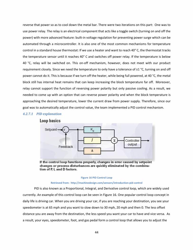
44
reverse that power so as to cool down the metal bar. There were two iterations on this part: One was to
use power relay. The relay is an electrical component that acts like a toggle switch (turning on and off the
power) with more advanced feature: built-in voltage regulation for preventing power surge which can be
automated through a microcontroller. It is also one of the most common mechanisms for temperature
control in a standard house thermostat: If we use a heater and want to reach 40° C, the thermostat tracks
the temperature sensor until it reaches 40° C and switches off power relay. If the temperature is below
40 °C, relay will be switched on. This on-off mechanism, however, does not meet with our product
requirement closely. Since we need the temperature to only have a tolerance of ±1 °C, turning on and off
power cannot do it. This is because if we turn off the heater, while being full powered, at 40 °C, the metal
block still has internal heat remains that can keep increasing the block temperature far off. Moreover,
relay cannot support the function of reversing power polarity but only passive cooling. As a result, we
needed to come up with an option that can reverse power polarity and when the block temperature is
approaching the desired temperature, lower the current draw from power supply. Therefore, since our
goal was to automatically adjust the control value, the team implemented a PID control mechanism.
4.2.7.1 PID explanation
Figure 16 PID Control Loop
Retrieved from: http://machinedesign.com/sensors/introduction-pid-control
PID is also known as a Proportional, Integral, and Derivative control loop, which are widely used
currently. An example of this control loop can be seen in Figure 16. One popular control loop concept in
daily life is driving car. When you are driving your car, if you are reaching your destination, you see your
speedometer is at 65 mph and you want to slow down to 30 mph, 20 mph and then 0. The less offset
distance you are away from the destination, the less speed you want your car to have and vice versa. As
a result, your eyes, speedometer, foot, and gas pedal form a control loop that allows you to adjust the

45
car speed properly. In a similar way, the PID controller computes the output (speed) to be based on the
input error of travel distance. In PID, we can control three parameters:
Proportional factor: This factor controls the regulated output by multiplying the measured input
error and a certain gain factor. This control type allows the system, if far away from desired
goal, to approach the goal faster. However, one problem is if the gain factor is too large, it can
cause overshoot, meaning that the system can go above the desired goal level. In addition, it
takes long time for system to stabilize from that oscillation. Moreover, when error is small, the
control loop cannot detect it well and barely any output appears. Therefore, for a more accurate
control system, using proportional factor alone is not enough.
Integral factor: This factor considers the offset error and duration of offset. From that, the
integral factor integrates the error over time and based on that sum, changes output to reduce
that error sum of the previous calculation. On the other side, as the ‘I’ factor takes into
consideration of past error, it can result in overshoot to the desired goal.
Derivative factor: This generates a rate of error instantaneously and computes the product of
that rate with a certain gain factor. The derivative factor deals with how fast the error is
changing over time so it can compensate the stability of the control system. Therefore, we can
use this factor for stabilizing the system but not for approaching desired goal fast as
proportional system.
Since our heating systems has requirements of reaching assay temperature (37 °C, 65 °C, room
temperature (24 °C) with an offset allowance of 2 °C, we only consider proportional factor since it can
satisfy above goals while also being the easiest factor to tune.
4.3 Feasibility Studies and Experimental Modeling
4.3.1 Fluidic Control System Modeling
Because of the nature of the requirements for this project, it was difficult to perform a feasibility
study on the fluidic control portion of the device. Because of the early stage and proof-of-concept
nature of the device, there was no specification for flowrate, time of fluid control, tubing diameter, size
constraints, or other such areas of concern. As such, the feasibility of the device had to be determined
through empirical and experimental methods. However, the team did analyze the solenoid valve
manifold system to determine what effects the internal pathway of the valve manifold used would have
on the system by creating spaces for fluid dead volumes and cross contamination. Later in the project,
we found through experimentation that this value was not consistent and varied with different

46
conditions. The architecture of the valve manifold can be seen in Figure 17 and full calculations are
below.
Figure 17 NResearch valve manifold technical drawing: modified by MQP team to highlight path lengths
Retrieved from http://www.nresearch.com/
In order to calculate or analyze the internal pathway in the solenoid valve manifold, the
following steps were performed. In order to calculate the total length of the common passage, the
length of the common passage consisting of diagonal path was calculated.
Length of common passage (Diagonal paths= x, x/2)
x =√0.662 + 0.662 = 0.93 in
x/2 = 0.467 in
Total Length of the common passage can be calculated by using the following equation:
= (x*3)+(x/2*2)= (0.93*3)+(0.467*2) in = 3.72 in
Inlet Passages consists of horizontal and vertical lengths. In order to calculate the total length of the
inlet Passage, both the horizontal and the vertical lengths were added.

47
Horizontal length= 0.66/2 = 0.33 in
Vertical length= 0.81/2= 0.406 in
Total Length of the Inlet passage can be calculated by using the following equation:
=(vertical length of each inlet passage +horizontal length of each inlet passage)*4
=(0.406+0.33)*4 = 2.944 in
Internal Volume for the common passage = 91 uL (Given in the drawing)
Internal Volume each inlet port = 32.5 uL (Given in the drawing)
The area of the common passage can be calculated by dividing total volume by total length. The
following equation was used to calculate the area of common passage:
Area of the common passage (𝐴1) = Total Volume/Total Length = 91 uL/ 3.72 in
= 0.00556 𝑖𝑛3/ 3.72 in = 0.00149 𝒊𝒏𝟐
The diameter of the common passage was calculated by using the area of the common passage.
Diameter of the common passage
= √(4 ∗ 𝐴1)/𝜋 = √(4 ∗ 0.0014)/𝜋= 0.042 in
Similarly, the area and diameter of the inlet passage was calculated using the following equations:
Area of each inlet (𝐴2) = Volume in each inlet passage/ Length of each inlet passage
= 32.5uL/0.736in = 0.0198 𝑖𝑛3/ 0.736 in = 0.0269 𝒊𝒏𝟐
Diameter of each inlet= √(4 ∗ 𝐴2)/𝜋 = √(4 ∗ 0.0269)/𝜋 = 0.185 in
Since resistance of the flow is directly proportional to length, the team tried to reduce the length of the
wire tube connecting the manifold. The team used 1/32 in diameter tube. In order to lower the
resistance of the flow, the smaller diameter tube can be used for the prototype.
4.3.2 Temperature Control System Modelling
The general idea was to heat the 96-well plate with samples inside by placing it on a heat-
conducting platform. This platform would be required to be a good conductor, easily machined, and
simple to interface with a 96-well plate. The first step in this process was selecting material for the
heating platform. Two of the most common heat-conducting materials are aluminum and copper.
48
Therefore, it was important to carry out a rough analysis on the heat conduction characteristics, namely,
how fast the material can heat up 96-well plate from room temperature (24° C) to the final desired assay
temperature of 37 °C and 65 °C as well as how fast can it cool the 96-well plate from the desired assay
temperature back to room temperature. Lastly, given the selected material, it was necessary to decide
on how to machine the metal block so that it could facilitate heat conduction between the Peltier TEC
module and the block, and between the block and the 96-well plate. Given our short time range at TRT,
we cannot conduct all testing to determine which part to choose or which material to choose.
Therefore, this modelling section would provide theoretical calculation that can help us select an option
without experimental testing. This gave us an educated starting point and provided more insight for
future improvement.
4.3.2.1 Transient Model for Heating: Aluminum vs. Copper
First, a modelling for transient response of how temperature versus time behavior between
copper and aluminum was conducted. In this model, we used the transient equation as follows:
Ɵ =𝐸𝑖𝑛
h ∗ A+ (Ɵ𝑖 −
𝐸𝑖𝑛
h ∗ A) ∗ 𝑒−𝑡/𝑇𝑎𝑢
Ɵ is the temperature difference between current temperature and ambient temperature, which
was chosen to be 25 °C. Ɵi is the initial temperature difference which we assumed was 0 °C because the
metal block had remained at room temperature for some time. Ein is power delivered to the Peltier TEC
module. Since we used 8 V from power supply and we had 1.5 A current draw on average, the energy
value was calculated as:
𝐸𝑛𝑒𝑟𝑔𝑦 = 𝑉 ∗ 𝐼 = 8 ∗ 1.5 = 12 𝑊𝑎𝑡𝑡𝑠
For the purpose of proof-of-concept, we only used three rows of wells, each row having eight
wells, for each assay. Therefore, to reduce the time and effort in machining metal block, we chose the
size of block that could fit three rows of wells. The dimension found by rough estimation gave the area
of metal block as 0.006954 m2. The value h is a heat transfer coefficient, which were advised by a
mechanical engineer in TRT to be 30 W
K∗m2.. Tau value in here represents time versus temperature
relationship of different metals. The equation we used for tau calculation was:
Tau =m ∗ c
h ∗ A
Tau calculated for aluminum was 196.29 seconds and for copper was 278 seconds. The variable
m is the mass of the metal block. The mass of the aluminum block was chosen to be 0.045 kg and the
mass of copper block was chosen to be 0.15 kg. These mass values were calculated using the same area
of 0.006954 m2 as above. C is the specific heat capacity value for copper and aluminum, which are 390

49
J
Kg∗K. and 910
J
Kg∗K. respectively. Putting those values into above Ɵ transient equation, we could find the
temperature of metal block by:
𝑀𝑒𝑡𝑎𝑙 𝑇𝑒𝑚𝑝𝑒𝑟𝑎𝑡𝑢𝑟𝑒 = Ɵ + Initial Metal Temperature = Ɵ + 25
Figure 18 Transient Response: Heat Input and Convection of Aluminum vs. Copper
As we can see from Figure 18 above, aluminum in red takes less time to heat up than copper in
blue. From this graph, we predicted that aluminum can bring the heat station from room temperature
(24 °C) to assay temperature faster than copper. However, it was also required to make sure that the
system is capable of returning to room temperature since there are assay steps incubating samples at
room temperature. As a result, the following section will study the cooling capability between the two
materials before making decision.
4.3.2.2 Transient Model for Cooling: Aluminum vs. Copper
In this model, we used the transient equation based on Newton’s law of cooling as follows:
𝑇(𝑡) = 𝑇𝑒𝑛𝑣 + (𝑇(0) − 𝑇𝑒𝑛𝑣) ∗ 𝑒−𝑡
𝑡0
The ambient temperature (Tenv) was chosen to be 22 °C based on room temperature in TRT
station at that time. The block was assumed to be near 54 °C at the beginning (T(0)). All other values,
such as heat coefficient and tau values were kept the same as the previous modelling. Putting these
numbers into T(t) equation, we had cooling characteristics of aluminum and copper as seen in the graph
below.
0
10
20
30
40
50
60
70
0 50 100 150 200 250 300
Tem
pe
ratu
re (°C
)
Time Elapsed (s)
Transient Response: Heat Input and Convection
Al
Cu
50
Figure 19 Transient Cooling Response of aluminum versus copper
As we can see from Figure 19 above, aluminum in blue cools down faster than copper in red
from 54° C. From these cooling and heating experiments, testing with both aluminum and copper blocks
with the same surface area and thickness, we concluded that aluminum can both heat up and cool down
faster than copper. Therefore, aluminum was chosen as the material for heating station.
4.3.2.3 Thermal Conductance Circuit
After selecting aluminum as the material for the heating block, it was important to decide how
we should machine the metal block to facilitate the best heat conduction between the metal block and
the 96-well plate. The first idea was to use a thin aluminum sheet as can be seen from the diagram
below. In this method, we would attach the Peltier TEC module to one end of the block surface so it can
transfer the heat to the aluminum sheet and then place the polystyrene well plate onto the sheet, near
the Peltier TEC. We will justify this configuration’s thermal resistance in a generalized system. It should
be noted that for the purpose of simplicity of the model, air resistance was disregarded and thermal
contact conductance was assumed to have one constant value of 20000 W
K∗m2., which was advised by a
TRT mechanical engineer. Moreover, since the internal design of Peltier TEC is a p-n junction, which is
complicated to model, we also disregarded the Peltier TEC internal heat resistance.

51
Figure 20 Thermal circuit of aluminum sheet with polystyrene well
A typical thermal system usually breaks down into a resistance circuit similar to an electrical
resistor circuit and can be used to study thermal behavior. The heat source, similar to a power source,
delivers energy through several blocks of resistances. In our system, the thermal resistance circuit
represents how much of the original heat will remain after going through the Peltier-metal block contact
resistance, internal metal block resistance, and so on until it reaches the output. The output of this
system is the temperature inside the polystyrene wall. As we can see from Figure 20 above, we have
four resistors in series. We can calculate the value of each resistance as following:
RAB: Peltier-Aluminum sheet thermal contact resistance. Hc is the thermal contact
conductance is: 20000 W
K∗m2.. A is the surface area of Peltier TEC module. From that, we can
find the thermal contact resistance with our Peltier TEC module area as:
𝑅𝑃𝑒𝑙𝑡𝑖𝑒𝑟𝐶𝑜𝑛𝑡𝑎𝑐𝑡 = 1
ℎ𝑐 ∗ 𝐴=
1
20000 ∗ 0.0016= 0.03125
𝐾
𝑊
RBC: Aluminum sheet thermal conductance across the sheet for the heat to transfer from
Peltier TEC to the well plate position. This can be calculated using following equation:
𝑅𝑆ℎ𝑒𝑒𝑡 = 𝑥
𝐴 ∗ 𝑘= 6.9686
𝐾
𝑊

52
In this equation, x is length of material that is parallel to heat flow, which we found to be 0.035
m. K is thermal conductivity of material. For aluminum, this number is 205 W
K∗m.. A is the cross-sectional
area that is perpendicular to heat transfer flow, which in our case is, 0.0000245 m2.
RCD: Aluminum sheet – single polystyrene well thermal contact resistance. In here we have
the similar equation as above:
𝑅𝐶𝑜𝑛𝑡𝑎𝑐𝑡 = 1
ℎ𝑐 ∗ 𝐴=
1
20000 ∗ 1.01203 ∗ 𝑒−5= 4.94055
𝐾
𝑊
RDE: This is the thermal resistance for the heat to travel across the polystyrene wall of well
plate to reach the water/solution inside the well.
𝑅𝑃𝑜𝑙𝑦𝑠𝑡𝑦𝑟𝑒𝑛𝑒 = 𝑥
𝐴 ∗ 𝑘= 933.083
𝐾
𝑊
Here we assumed that the temperature right at the inner layer of the polystyrene well will be
the same as that of the fluid contained in the well in order to simplify our calculation. The system,
starting from RAB and ending at RDE, is a series of thermal resistors with the end of each resistor as the
start of next resistor. With this series resistance circuit, we can calculate the total thermal resistance by
adding up RAB, RBC, RCD and RDE to be 945.023 𝐾
𝑊 for the first set up of heat block.
In the second setup, instead of a thin aluminum sheet, we used a thicker metal block in which
we drilled holes that could hold the wells and reach halfway up the well wall. The same simplification for
the thermal system analysis was kept similar to the above setup.
Figure 21 Thermal circuit of a machined aluminum bar and polystyrene well

53
As we can see from Figure 21 above, we have four resistors in series with each other. We
can calculate the value of each resistance value as follow:
RAB: Peltier-Aluminum block thermal contact resistance. We can find the thermal contact
resistance with our Peltier TEC module area as:
𝑅𝑃𝑒𝑙𝑡𝑖𝑒𝑟𝐶𝑜𝑛𝑡𝑎𝑐𝑡 = 1
ℎ𝑐 ∗ 𝐴=
1
20000 ∗ 0.0016= 0.03125
𝐾
𝑊
RBC: Aluminum sheet thermal conductance across the sheet for the heat to transfer from the
Peltier TEC to the well plate. This can be calculated using following equation:
𝑅𝑆ℎ𝑒𝑒𝑡 = 𝑥
𝐴 ∗ 𝑘= 0.813
𝐾
𝑊
RCD: Aluminum block – single polystyrene well thermal contact resistance. Here we have similar
equation as above:
𝑅𝐶𝑜𝑛𝑡𝑎𝑐𝑡 = 1
ℎ𝑐 ∗ 𝐴=
1
20000 ∗ 0.00021= 0.41
𝐾
𝑊
RDE: This is the thermal resistance for the heat to travel across the polystyrene wall of well plate
to reach the water/solution inside the well.
𝑅𝑃𝑜𝑙𝑦𝑠𝑡𝑦𝑟𝑒𝑛𝑒 = 𝑥
𝐴 ∗ 𝑘= 409.96
𝐾
𝑊
The second system is also a series of thermal resistors. We can calculate the total thermal resistance by
adding up RAB, RBC, RCD and RDE, whose sum ends up with the total thermal resistance of 411.216
𝐾
𝑊 for the second set up of the heat block.
As we can see after calculating the value for each heat block setup, even though we have a thicker
metal block for second setup, it only results in 411.216 𝐾
𝑊 compared to 945.023
𝐾
𝑊 from the first setup.
The second configuration is only 43.5% resistance compared to the first one. This difference is because
when we introduce more contact area between the aluminum block and polystyrene well by insertion,
we facilitate more heat transfer between them. Therefore, the contact area increases, thereby decreasing
the thermal resistance value. Moreover, by fitting each well into metal block, each polystyrene row can
be kept more tightly rather than taping into aluminum sheet like in setup one. As a result, we decided to
select the second setup for the heat station.

54
4.4 Final Design Approach
4.4.1 Prototype Architecture
After creating an ideal system architecture, the team also created a basic architecture drawing
of the prototype system itself to have a simplified view of the various subsystems that made up the
device. This representation can be seen in Figure 22 below.
Figure 22 Prototype Architecture
4.4.2 Assay Selection
In order to meet our objective to create a prototype device, which could perform multiplexed
assay for the cells, our team looked into different potential substances (contaminants) affecting MSCs
during quality control. To accomplish this goal, the team researched various OTS assay kits for
mycoplasma, trypsin, endotoxin and BSA. Due to the time constraints of the seven week term and for
the sake of proof-of-concept, only mycoplasma and BSA Assay kits were chosen, with the thought that
other assays could be implemented in the future. Though a number of manufacturers sell assay kits to
detect these contaminants, they differ in terms of sensitivity, time to run the assay, cost, read-outs,
temperature, and procedure steps for the assay. After comparing these parameters, the most similar
assay kits were chosen based on parameters like read-outs and procedure steps. The comparison tables
for both OTS shelf assays can be seen in Table 2 and Table 3 below; the team’s choices for each assay
are indicated by italics.

55
Table 2 OTS BSA Assay Tradeoff Analysis
Parameter Cygnus Technologies MyBioSource
Sensitivity 0.124 ng/mL 85.5 ng/mL
Time 2 hours 2 hours
Cost $525 $430
Principle ELISA ELISA
Read-out Absorbance Absorbance
Sample Preparation Sample dilution Supernate preparation
Table 3 OTS Mycoplasma Tradeoff Analysis
Parameter Roche Thermo Fisher
ATCC R&D Systems
Sensitivity 10 CFU/mL 4 CFU/mL Unavailable 15 CFU/mL
Time 5 hours 5 hours Unavailable 4.5 hours
Cost $1000 $3000 Unavailable $380
Principle Polymerase Chain Reaction (PCR)
PCR PCR DNA hybridization/ELISA
Read-Out Fluorescence, impedance
Fluorescence Fluorescence, impedance
Absorbance
Sample Preparation Lysis solution Lysis solution Lysis solution Lysis solution
Additionally, the chosen kits came with precoated assay plates, appropriate for each assay.
These assay plates were in stripwell form so the team could continue with the goal of using only the
necessary amount of wells for each assay run. It also allowed for easy transfer to a standard absorbance
microplate reader.

56
4.4.3 Fluid Control
After extensive iterations and analysis of potential components, the team chose appropriate
components to make up the final fluid control subsystem. The system can be seen in Figure 23 below.
Figure 23 Fluid control system consisting of syringe pump and solenoid valve manifold
After the previously discussed iterations and research, the team decided to utilize a simple
syringe pump system that was created in house at TRT. This syringe pump consisted of a machined
aluminum platform that supported a Hamilton gas tight 1 mL syringe. The glass syringe plunger is
attached to a P16 Actuonix linear actuator. At the syringe tip, we connected 1/32 in outer diameter
tubing into the NResearch solenoid valve manifold, which was controlled by the CoolDrive One Single
Valve Driver. The whole system was controlled through the MC33926 motor driver shield from Pololu
and an Arduino microcontroller board. This option for fluid control was chosen because of its immediate
availability and simple design that would lead to minimizing testing time and more thoroughly showing
proof-of-concept for the device. An in-house pump was used because of the cost and time it would
require to purchase an OTS pump; however, if a syringe pump was used in the future for the final design
of the device, a much more precise and well-manufactured pump would be used instead.
The fluid control system also consisted of a removable vacuum pump that was used to flush the
system between additions of reagents. This pump remained removable and was only attached to the
system when needed because of difficulty had with attaching the pump without adding large amounts
of excess tubing pathways. This pump was retrieved from a TRT lab and was controlled by a direct
connection to a 12 V power source.
Syringe Pump
Arduino Control
Setup
Solenoid Valve
Manifold

57
4.4.3.1 Fluid Control System Schematic
Figure 24 Schematic showing control of syringe pump and valve manifold system
The schematic, seen in Figure 24, was drawn using Fritzing software, which is an open-source
tool online that allows the user to draw schematics for the Arduino and the most popular Arduino
components. From the above figure, we show a more detailed representation about how each
component communicates with each other. Here the MC33926 Motor controller Arduino Shield is
replaced with a MD03A Motor Driver since there is not schematics library for the MC33926 version and
the MD03A is the closest match inside software library. Therefore, we replaced the MD03A as our motor
driver and specified the correct name in the picture. As we can see on the motor driver board, the two
ports in middle are connected to a 12 V power source so as to drive the P16 Actuonix Linear Actuator
through two top terminals. By sending commands from the Arduino to the motor driver to the M1PWM
pin, we can control how fast or slow, reverse or forward mode the linear actuator should travel. Since
the valve manifold we use has four single valves inside it, we tried to replicate with four motors, naming
them valve1, valve2, valve3 and valve4. The motor and valve driver have the same design of two
connections into positive and negative rails of power supply, as we observe the black and red wires in
the picture. These four valves will be turned on and off through four separate 8-pin CoolDrive One valve
driver as represented in four green 8-pin headers. The input to pin 1 and pin 2 will be 12 V of power to

58
power the valve when on through pin 8 and 9. This power delivery is turned on and off through the 5 V
digital signal from Arduino feeding into pin 5 of the valve driver. A more detailed schematic of the
resistances and voltages at each step during this process can be seen in Figure 25.
Figure 25 Fluidic control subsystem detailed schematic
59
4.4.4 Temperature Control
4.4.4.1 Temperature Control System Architecture
Figure 26 Prototype temperature control system architecture drawing
Figure 27 Image of entire temperature control system
Figure 26 presents a block diagram for the heat control system flow and Figure 27 shows the
experimental setup of the temperature control system. As we can see, the MC33926 motor controller
driver will receive Arduino command for how much power should be drawn from the power supply and
fed into the Peltier TEC module. This amount of power in blue then flows into the Peltier TEC, triggering

60
the Peltier effect across the p-n junction and generating heat flow in red to the machined aluminum plate.
The plate temperature will be reported back to the Arduino in order to readjust power magnitude so as
to make the metal plate stays consistently near the desired assay temperature. The heat/cold flow in red
on the other side will be absorbed through the heatsink and then blown away by air flow in green from a
DC cooling fan. This method is to prevent change in temperature on the opposite site facing heatsink from
disturbing heating process at aluminum plate.
4.4.4.2 Temperature Control System Schematic
Figure 28 Temperature Control System Schematic
Similar to the previous shown schematics for fluidic control, the MC33926 Motor controller
Arduino Shield is replaced with a MD03A Motor Driver since there is not a schematics library for MC33926
version. As we can see on the motor driver board, the two ports in middle are connected to an 8 V battery
to drive the Peltier TEC module through the two top terminals. Power magnitude and polarity are also
controlled through Arduino commands. Additionally, the LM35 temperature sensor reports data through
analog input pin 3 on the Arduino. Moreover, the DC cooling fan is controlled through a switch-like NPN
transistor. When digital pin 31 writes a high signal to the middle terminal of NPN transistor, the cooling
fan yellow negative terminal is connected to both ground and turn on. On the other site, if the digital
61
signal is low, the negative terminal is connected to the open circuit and no power can flow across the DC
fan. The entire schematic for the temperature control system can be seen in Figure 28 and a more detailed
schematic of the resistances and voltages at each junction can be seen below in Figure 29.
Figure 29 Temperature control subsystem detailed schematic
4.5 Pretotype Design
The team’s client statement included creating both a prototype of the proof-of-concept device
and a pretotype for the potential future product. A pretotype is a future concept describing the
completed product as it could be in the future, upon completion of the project, with all goal product
objectives met. The objectives for this device include that the device be automatable, multiplexed, time

62
efficient, cost efficient, scalable, regulation compliant, and used for autologous transplant of MSCs. The
pretotype describes the ideal sub-sections of the device, consisting of a sample preparation area,
reagent distribution system, temperature control regions, proper reagent storage, waste storage and
removal system, and finally the assay plate itself where the assays will be performed. A SolidWorks
mock-up of a potential design for this device can be seen in Figure 33 below.
Figure 30 SolidWorks drawing of potential assay device (left) and potential assay device integrated into a lab bench setting (right)
In this device, the cell sample to be tested would be pipetted into the designated reservoir in
the sample preparation section. After pipetting, the compartment door would be closed using the
“open/close” button on the device. The sample preparation section would contain a centrifuging and
supernatant collection region and a cell lysis solution creation region in order to transfer the correct cell
solution into the assay plate. This section will also be capable of creating standard dilutions or control
solutions as needed for the assays. After sample preparation, the reagents will be transferred
automatically from the sample preparation section to the assay completion system, using fluid controls
that are completely contained within the unit. This section would be temperature controlled as per the
assay requirements. The assay reagents are stored in temperature regulated reservoirs that adhere to
the appropriate storage conditions. The system is also equipped with pumping and valve controls to
transfer the reagents from the storage reservoirs to the assay plate with controlled flowrate and
pressure. A waste region would also be contained in the device for the collection of any waste or
residual reagents from the assay. The assays would be completed on a 96-well disposable plate, which
will be pre-coated with the necessary surface chemistry required to run each assay. The plate has a
separate section for each assay to be completed, namely BSA, mycoplasma, endotoxin and trypsin.
Finally, the device would be equipped with a user-interface screen indicating the conditions within the
device, including pressure and temperature, and the status of the assay completion. Upon completion

63
the device will indicate “complete” on the UI screen. The assay plate would be removed and placed in a
standard absorbance microplate reader to obtain the results.
The team also created a potential brochure (Appendix A) for advertising the device and its
advantages over the current methods of quality control. There would many advantages of using the
device by automating the device to multiplex these four assays simultaneously. Multiplexing the assays
would largely reduce the labor, time, and cost involved during the assay process, especially since each
cell sample for autologous transplant must be tested separately. The device would be affordable as well
as easy to use and conveniently sized in order to fit on a standard lab bench. By automating the assays,
the results will have increased accuracy and will greatly reduce the chance of errors and false results
from the tests because human error would be almost entirely removed. The device would be very
efficient and would not require any additional equipment.

64
5 Design Verification
This chapter will discuss the experiments that the team conducted to test various parts of the
device to ensure functionality of each subsystem. These experiments were planned and conducted with
proof-of-concept in mind and were designed to show that this design was feasible and can be pushed
forward in the future. These experiments were created specifically for this project but in the future
when the device has been refined further, the group would recommend adhering to standard methods
of testing for this type of device, based on the engineering standards referenced in section 3.2.2. As a
medical device, the system must meet these standards in order to be introduced onto the market and
into testing laboratories in the future.
5.1 Assay Experimentation
5.1.1 Mycoplasma Baseline Assay Experiment
During the assay experimentation process, the team decided that it would be necessary to run a
baseline assay test for each of the chosen assays using the manufacturer’s procedure and standard
laboratory equipment. There were no automated steps used in the baseline assay experiments and all
fluid handling was completed by hand with standard pipettes. Temperature control was accomplished
with a water bath and a standard incubator, as specified by the manufacturer instructions. The results
from these baseline assays could later be used as a comparison against the results of the assay run using
the system to show the system’s level of effectiveness. These assays were run solely with the controls
included with the kits because no cells were used in the duration of the project.
5.1.1.1 Initial Mycoplasma Assay Run
The team first ran the R&D Systems Mycoprobe Mycoplasma Detection assay using the
manufacturer insert procedure (Appendix B) as well as standard methods and lab equipment for volume
dispensing, incubation, and transfer. The kit that was used for this baseline test was already available in
the lab, as a leftover from the previous TRT that had already been completed. The team used this kit
because of its availability. A new kit was ordered from the manufacturer but had not yet arrived at that
time.
During this experiment, the team encountered a number of setbacks which led to inconclusive
and unusable results. The experimental plan called for three wells of the positive control and three wells
of the negative control. However, there was only enough positive control left in the kit for one full well
to be run. Additionally, this assay kit had been stored for about six months in the lab, which was three
months longer than the manufacturer insert claimed the kit would be usable for. The assay was run as

65
described despite these problems in order to become more familiar with the process for the next
experiment.
After completion of the assay, the wells were read in a standard microplate reader at 450nm
wavelength and a color change should have occurred but was not visible, as can be seen in Figure 31
below. A successful assay run would have resulted in the positive control wells turning a dark red color
and the negative control wells remaining clear. Use of the microplate reader yields the optical density
(OD) of each well, which was required to be above or below a certain threshold, as described by the
manufacturer, to be deemed acceptable. At the completion of this experiment, the team decided that
the data was not accurate enough to be used as a baseline and that the experiment would need to be
run again.
Table 4 Manufacturer included OD result comparison (left) Experimental OD and results (right)
Figure 31 Mycoplasma Assay Initial Run Result Wells.
Right two wells: positive control; left three wells: negative control
Experimental Condition Optical Density Result
Positive Control 0.0106 Negative
Positive Control 0.00934 Negative
Negative Control 0.0102 Negative
Negative Control 0.00648 Negative
Negative Control 0.00934 Negative
OD Values Result
<0.05 Mycoplasma Negative
0.05-0.1 Inconclusive
>0.1 Mycoplasma Positive

66
5.1.1.2 Secondary Mycoplasma Assay Run
In this experiment, the team used a new R&D Systems mycoplasma detection kit to ensure that
the baseline data was accurate. The manufacturer insert was again followed and standard laboratory
procedures were used to conduct the assay. At the conclusion of the experiment, the wells were again
read in a microplate reader to determine the optical densities of the solutions. The assay was successful
during this experiment and the positive and negative controls reacted as expected with the appropriate
optical densities present, as seen in Figure 32 below.
It is important to note that for both baseline mycoplasma assay runs, there was a slight
misinterpretation of data due to human error. The plates are meant to be read at 490nm and then again
at 600nm, with the second value being subtracted from the first value to get the final optical density of
the value. This difference is meant to account for the optical imperfections in the well plate and is
recommended by the manufacturer. Upon further inquiry with the manufacturer after this mistake was
made, the team decided that these results were acceptable because had the difference been taken, the
negative controls would have been in the correct range to represent a negative value. This decision was
also necessary because of the time and material constraints that the team was under.
Table 5 Manufacturer included O.D. result comparison (left) Experimental O.D. and results
Figure 32 Mycoplasma Assay Seconday Run Result Wells.
Left three wells: positive control; right three wells: negative control
Experimental Condition Optical Density Result
Positive Control 2.05 Positive
Positive Control 2.02 Positive
Positive Control 2.16 Positive
Negative Control 0.161
Incon-clusive
Negative Control 0.1
Incon-clusive
Negative Control 0.113
Incon-clusive
O.D. Values Result
<0.05 Mycoplasma Negative
0.05-0.1 Inconclusive
>0.1 Mycoplasma Positive

67
5.1.2 BSA Baseline Assay Experiment
The team also ran a baseline assay experiment for the BSA assay to have results to compare to
once the project was successfully completed. The team used the MyBioSource BSA Detection Kit in this
experiment and the manufacturer insert instructions (Appendix C) were followed accordingly. This
assay, different than the previous, used a standard dilution curve as a control. The experiment was run
only with the standard curve and again with no cells.
5.1.2.1 Initial BSA Assay Run
The first assay run was conducted with a previously used kit obtained from the TRT prior work
and therefore again presented potential errors because of the length of storage time. Despite this
excess of time, the experiment was conducted as planned with the standard BSA dilution curve run in
duplicate. The assay kit included a graph of an expected BSA standard curve that could be used as a
reference for the curve created from the experimental assay and can be seen in green in Figure 33.
At the completion of this experiment, the wells were read at 490nm wavelength and the results
were analyzed according to the manufacturer, graphing the optical density versus the log of BSA
concentration. The resulting standard curves, shown compared to the manufacturer example in Figure
34 below, were intended to have a gradient from virtually clear to dark yellow but this result was not
present. The standard curves were both inaccurate and could not be considered as appropriate baseline
data to compare to in the future. Therefore, the team again decided to rerun the experiment to achieve
better results.
Figure 33 Initial BSA Assay Standard Dilution Curve compare to manufacturer example
0
0.5
1
1.5
2
2.5
3
3.5
4
4.5
5
0 0.5 1 1.5 2
Log
of
Co
nce
ntr
atio
n
Optical Density Experimental Wells: Row 1 Experimental Wells: Row 2
Manufacturer Example

68
Figure 34 Initial BSA assay result wells. Descending concentration from
left-most well (30,000 ng/mL) to right-most well (0ng/mL)
5.1.2.2 Secondary BSA Assay Run
The second iteration of the BSA detection assay was successful and able to be used as baseline
data for future comparison. The team used a new MyBioSource BSA detection kit for this experiment
and followed standard laboratory procedures and the manufacturer instructions. At the completion of
the assay, a decided gradient could be seen in the wells. However, there was a limited amount of the
dilution reagent which only allowed for one standard curve to be run rather than two. The absorbance
readings were again analyzed and graphed and the results can be seen in Figure 35 below. The wells at
the conclusion of the experiment can also be seen in Figure 39.
Figure 35 Baseline BSA Assay Standard Dilution Curve (left) and BSA resultant wells (right) with concentration descending
from top right well (30,000 ng/mL) to bottom right (0ng/mL)
5.2 Fluidic Control Experimentation
5.2.1 Syringe Pump Calibration Curve Determination Experiment
5.2.1.1 Purpose
The purpose of this experiment was to find correlation between linear actuator distance and
volume of water dispensed by the automated syringe pump. Using this correlation, a calibration curve
could be generated that related this distance and volume and integrated into the Arduino code. After
0
1
2
3
4
5
0 0.5 1 1.5 2
Log
of
Co
nce
ntr
atio
n
Optical DensityExperimental Curve Manufacturer Example

69
integrating this calibration into the Arduino code, ideally the system would be much more accurate in
dispensing the desired amount of volume.
5.2.1.2 Experimental Procedure
This experiment was performed using the pre-existing syringe pump assembly consisting of a
1mL glass syringe and linear actuator in a machined aluminum frame. The assembly was connected to a
programmed Arduino Uno controller board to initiate and terminate movement of the linear actuator.
The Arduino code was programmed to prompt the user for a position value that the linear actuator
would then travel to.
The first step in this experiment was to determine the maximum volume that the syringe could
intake. Though it was a 1 mL syringe, the aluminum frame restricted full movement of the syringe so it
was unable to reach capacity. The group achieved this by taking water into the system to the linear
actuator’s limit and measuring the mass difference of the reservoir the water was taken from. The
average intake was measured at 768 µL.
To measure the calibration between linear actuator distance and volume output the team filled the
syringe to capacity, input randomly chosen linear actuator positions, and measured the output volume
of fluid dispensed. A total of 12 linear actuator positions were tested and the entire experiment was
repeated three times with these volumes to ensure accurate data. A full description of the experimental
procedure can be found in Appendix D.
5.2.1.3 Experimental Results and Analysis
At the conclusion of the experiment, the group transferred the collected data to Excel for
analysis. To create the calibration curve, the distance travelled by the linear actuator was plotted against
the volume output at that position. To achieve the most accurate curve, data points from all three
experimental iterations were included in this plot but major outliers were removed. These outliers were
removed because they were most likely due to human error and did not reflect on the effectiveness of
the system. The graph in Figure 36 below shows the calibration curve between the linear actuator
distance and the volume dispensed with outliers removed. The full data set and graph including outliers
can be seen in Appendix D. The calibration curve created in this experiment was then integrated into the
Arduino code so the team could input a value into the code and know with relative certainty what
volume would be dispensed.

70
Figure 36 Graph of output volume vs. linear actuator distance data from all experimental iterations without outliers (left).
Generated calibration curve from all iteration data with outliers removed (right).
5.2.2 Syringe Pump with Manifold: Dead Volumes Experiment
5.2.2.1 Purpose
The purpose of this experiment was to empirically determine the volume lost in the solenoid
valve manifold when various volumes of fluid were dispensed by the syringe pump system. This
information would be used to factor in to the volume entered into the Arduino code to be dispensed by
the system.
5.2.2.2 Experimental Procedure
The procedure for this experiment was similar to that of the previous experiment, with the main
difference being the integration of the solenoid valve manifold into the syringe pump system. The
system was filled to capacity and randomly chosen output volumes were entered into the Arduino code.
The subsequent output volume was compared to the goal output volume to create another curve for
the system with the integrated manifold. This experiment was performed with the 12 chosen volumes
from the previous experiment to output and the entire experiment was performed three times. A fully
detailed description of the experimental procedure can be found in Appendix E.
5.2.2.3 Experimental Results and Analysis
The data was collected and analyzed in Excel. The goal volume output is compared
graphically to the actual volume output of the system. This curve was then compared to the previously
created calibration curve to identify any discrepancies or offsets. This comparison can be seen in Figure
37. The team observed that the offset between the curve created without the manifold and the curve
created with the manifold was not uniform. It was initially hypothesized that the valve manifold would
have a constant volume lost within it. However, the data showed that the amount of volume lost in the
0
200
400
600
800
1000
0 500 1000
Vo
lum
e O
utp
ut
(uL)
Distance Traveled (Unitless)
Iteration 1 Iteration 2 Iteration 3
y = 0.7455x + 51.358R² = 0.9835
0
200
400
600
800
1000
0 500 1000
Vo
lum
e O
utp
ut
(uL)
Distance Traveled (Unitless)
Combined Tests Linear (Combined Tests)

71
system slightly increased as the volumes dispensed increased. The full data set from this experiment can
be found in Appendix E.
Figure 37 Volume output comparison between system with and without manifold
5.2.3 Syringe Pump with Manifold: Intake Accuracies Experiment
5.2.3.1 Purpose
The goal of this experiment was to determine the accuracy of the fluid intake of the syringe
pump and valve manifold system. This information would show the team if the system was capable of
taking in the goal amount of volume or if there was volume not taken in by the system.
5.2.3.2 Experimental Procedure
To perform this experiment, the team used the syringe pump system with the integrated valve
manifold as described in previous sections. A fluid reservoir was then filled with water and weighed. A
range of randomly selected volumes between 0 and 700 µL were chosen as intake volumes and entered
into the Arduino code. After the syringe pump, which began fully empty, had taken in the entered
volume of fluid, the mass difference of the reservoir was measured to determine the actual intake of the
system. 12 volumes were tested and the experiment was repeated three times. A fully detailed
description of the experimental procedure can be found in Appendix F.
5.2.3.3 Experimental Results and Analysis
Once the data was collected, it was transferred to Excel for analysis. The team compared the
goal volume input values to the actual volume taken in by the system, as seen in Figure 42. However,
this graph is not an accurate representation of the experimental results because its relatively linear
y = 0.92x - 7.31R² = 0.99
y = 0.99x + 13.96R² = 0.99
0
100
200
300
400
500
600
700
800
0 100 200 300 400 500 600 700 800
Act
ual
Vo
lum
e O
utp
ut
(uL)
Goal Volume Output (uL)
With manifold Without Manifold Linear (With manifold) Linear (Without Manifold)

72
relationship is misleading. The team then plotted the goal input volumes against the change in volume
that corresponded to each data point. This graph signified the difference between the goal intake
volume and the actual intake volume to show how much volume was not taken in by the system, as
seen in Figure 38. This graph shows that the intake loss was not uniform but was consistent over the
three iterations of the experiment. These results were disappointing as there was such a large difference
between the goal intake and actual intake of the system. The full data set from this experiment can be
found in Appendix F.
Figure 38 Results of system intake experiment: goal intake vs. actual intake (left). Change in intake volume vs. goal volume
intake (right)
5.2.4 Syringe Pump with Manifold and Air Pump: Output Volume Loss Experiment
5.2.4.1 Purpose
The purpose of this experiment was to determine the effectiveness of an attached air pump
used to flush the valve manifold of volumes left behind after dispensing. If seen as effective, this
attached air pump could be used to more accurately dispense volumes and ensure that all fluid was
removed from the manifold.
5.2.4.2 Experimental Procedure
In this experiment, an air pump was integrated into the system between the valve manifold and
syringe pump. The procedure for this experiment was similar to previously described experiments,
beginning with a full syringe and dispensing to a range of randomly chosen volume values. After
dispensing the volume of fluid, as in previous experiments, the air pump was turned on for 1-2 seconds
to allow all residual fluids to be flushed from the system and into the collection reservoir. The reservoir
was then weighed to identify the mass difference and final output volume from the system. This
experiment consisted of 12 volume data points and the entire experiment was performed three times. A
detailed description of the procedure can be found in Appendix G.
y = 1.03x - 89.42R² = 0.99
0
200
400
600
800
0 100 200 300 400 500 600 700 800
Act
ual
Vo
lum
e I
nta
ke (
uL)
Goal Volume Intake (uL)
Combined
0
20
40
60
80
100
0 100 200 300 400 500 600 700 800 900
ΔV
olu
me
(u
L)
Goal Volume Intake (uL)Test 1 Test 2 Test 3
73
5.2.4.3 Experimental Results and Analysis
Upon completion of the experiment, the data was collected and transferred to Excel for analysis.
Upon further analysis of the data, it was seen that the air pump did assist with increasing the amount of
volume that was dispensed from the system. When comparing the amount of volume lost in the system
when using the air pump to the amount of volumes lost in the system when the air pump was not
integrated, as seen in Figure 39 below, the group saw that the volumes lost became less varied upon
integration of the pump. However, the team decided against integrating the pump into the system
because of the excess amount of tubing required to attach the air pump. Because the previous intake
experiment proved to be rather unsuccessful, the team did not want to integrate any more unnecessary
tubing that could decrease the intake accuracy even more. Therefore, it was decided to implement the a
vacuum air pump instead, only as needed, in order to fully flush out the system between reagent
additions. Therefore, it would not introduce additional tubing during intake but could still assist with
ridding the system of the left behind volumes.
Figure 39 Distribution of volume lost with air pump integration (left) and distribution of volume lost with no air pump (right)
5.2.5 Cross Contamination Experiment
5.2.5.1 Purpose
One of the final experiments that the team conducted was a qualitative cross contamination
test to determine if the system was being fully cleared out by the integrated vacuum. This was necessary
in order to lessen the chance of mixing between the reagents and compromising of the assay.
5.2.5.2 Experimental Procedure
During this experiment, the team used yellow dyed water to fully fill the system and then
dispense all volume into a 96-well plate, as can be seen in the bottom row of Figure 40 below. This
water was not contaminated because it was the first color through the system. We then disconnected
the manifold from the syringe pump and fully vacuumed it out, opening all valves and leaving the
-100
-50
0
50
100
150
0 100 200 300 400 500 600 700 800 900
Vo
lum
e L
ost
(u
L)
Goal Volume Output (uL)Iteration 1 Iteration 2 Iteration 3
-100
-50
0
50
100
150
0 100 200 300 400 500 600 700 800 900
Vo
lum
e L
ost
(u
L)
Goal Volume Output (uL)
Iteration 1 Iteration 2 Iteration 3

74
vacuum on until no liquid was seen leaving the manifold. The syringe pump itself, still separate from the
manifold was filled and emptied with uncolored water 3 times to ensure that any residual color was
eradicated. The system was then filled with red colored water and the emptying process was repeated.
Finally, yellow water was taken in and pumped out of the system again and the resultant wells were
observed for any color change that might have occurred from residual red colored water. We repeated
the whole process again with yellow colored water as the base again but then followed with green
colored water as the secondary color.
5.2.5.3 Experimental Results and Analysis
The team saw that the residual volume removal did not fully clear out the system as we had
hoped. Even after extensive vacuuming of the valve manifold, we saw that both red and green colored
water affected the yellow colored water that followed it. However, the concentration of the
contaminated color did lessen in later wells but the color was still present. The results from this
experiment can be seen in Figure 40, where the top/left wells were the result of the green colored water
contamination, the middle wells were the result of the red colored water contamination, and the
right/bottom wells are the result of no contamination for comparison. This was a qualitative experiment
due to lack of time. However, though the results were only obtained visually, the team believed the
outcome was still helpful for the project.
Figure 40 Top view of contaminated wells (left). Side view of contaminated wells (right)
5.2.6 BSA Assay Run: Water Trial Experiment
5.2.6.1 Purpose
The purpose of this experiment was to determine if the system was able to correctly intake and
dispense the specific volumes needed to run the BSA detection assay. This experiment was run as a
mock assay trial using water instead of reagents to ensure that materials did not go to waste if there
was a flaw in the system. For this experiment, the system that was used was our final prototype system,
containing the syringe pump, solenoid valve manifold, and detachable vacuum.

75
5.2.6.2 Experimental Procedure
To complete this experiment, the team followed the MyBioSource kit insert instructions to
determine what volumes would be necessary for the BSA assay. The system was then used to intake and
output water in the same way that would be used in the actual assay run, namely using the automated
pumping system to intake and output fluid but with manual control over tubing to ensure accuracy in
delivering the fluid. The desired intake volume was entered into the Arduino code and after the intake
was completed, the system would be returned to position zero to empty the contents into the desired
well. The intake and output was performed on four volumes dispensing into six wells and the entire
experiment was completed three times. A full description of this experimental procedure and a table of
the volumes used in this experiment can be found in Appendix H.
5.2.6.3 Experimental Results and Analysis
At the completion of the experiment, the team saw that the system was consistently dispensing
less volume than had been requested. However, a relatively consistent amount of water was lost at each
of these volumes, as seen in Figure 41 below, which allowed the team to be able to account for the
volume loss at each point. Based on the data collected, the team decided to integrate a volume buffer
into the volume value that was entered into the Arduino software. After averaging the output losses and
differences in volume intake at volume point, the volume buffer was determined to be 15 µL. The full
data set can be found in Appendix H.
Figure 41 Distribution of volumes requested vs. actual volume output for four volumes

76
5.3 Temperature Control Experimentation
5.3.1 Heating from Room Temperature to 65° C Experiment
5.3.1.1 Purpose
The purpose of this experiment was to determine the time it took to heat the control system
from 24 °C to the maximum incubation temperature, 65 °C, and vice versa. It was also necessary to
determine if there was a major difference in heating times when the system was connected to an 80x80
mm heatsink or a 60x60 mm heat sink.
5.3.1.2 Experimental Procedure
To complete this experiment, the temperature control system was set up with a temperature
sensor attached to the aluminum assay strip well platform for monitoring its surface temperature. The
Peltier module was connected to the aluminum plate on the side that would be generating heat and to a
heat sink on the other, which would be diffusing heat and cooling. Either side of the Peltier module can
be used to heat or cool depending on the voltage and polarity applied to it. There were two size options
for the heat sink: 80x80 mm and 60x60 mm and the system was tested with both in order to identify any
major differences between the two. In addition, other specifications such as block mass, block area,
Peltier module area, and polystyrene well was kept the same as discussed in the modelling section.
This experiment was completed by controlling the system with a motor driver board and an
Arduino Mega microcontroller board. Energy was delivered to the Peltier module to heat up the
aluminum plate by controlling the “speed” parameter of motor driver board. This speed is the output of
the PID control system, which is implemented inside the Arduino. The input of the PID control loop is the
temperature data from the temperature sensor. In general, the Arduino PID control loop continuously
keeps track of how far the plate is from the goal temperature. For example, to go from RT (~24 °C) to 65
°C, the PID control will tell the motor controller to allow full current draw from the Peltier at 8 V. As the
aluminum gets closer to the desired temperature, the current draw to the Peltier module decreases
until the temperature is reached.
It is important to note that this test was carried out by filling 75% volume of each well with
water. Each well volume is 360 µL maximum. The well strip was placed in the aluminum block for
heating and was open to room temperature air with a temperature of about 24 °C. The temperature
sensor LM35 was used to measure the metal block temperature, data of which was then recorded into
Arduino serial monitor. For parallel monitoring, we dipped a Fluke thermocouple into the water of one
well and double checked that when the metal block stabilizes at the assay temperature, the water
should be at the same temperature too.

77
5.3.1.3 Experimental Results and Analysis
The data collected from the Arduino during the experiment showed that the temperature
control system reached its goal temperature and remained there after about four minutes. The goal for
the system was that it should be able to heat to the desired temperature in less than five minutes.
Figure 42 Heating from room temperature (24 °C) to 65 °C with 80 x 80 mm attached heat sink
Figure 43 Heating from room temperature (24 °C) to 65 °C with 60 x 60 mm attached heat sink
As we can see from Figure 42 and Figure 43 above, the heating characteristics of both graphs are
similar. From room temperature of 25 °C heating to 55 °C, we have a nearly linear increment. This is due
to the PID controller seeing that aluminum block is still far from the desired heat goal so it allows full
current draw from Peltier TEC module. From 55 °C to 60 °C, the PID starts decreasing current draw
0
10
20
30
40
50
60
70
0 100 200 300 400 500 600 700
Tem
pe
ratu
re (
°C)
Time (s)
Series1
78
allowance, which results in a non-linear curve of temperature that stabilizes upon reaching goal
temperature. In general, the heat system can go from room temperature to 65 °C in less than five
minutes, which meets the temperature transition goal.
Because the heating behavior of system with two different heat sinks, 60x60 mm and 80x80
mm, is very similar, we can assume that the size of the heatsink does not affect significantly the heating
performance of the system. Therefore, to determine which heatsink to use, more experiments needed
to be conducted.
5.3.2 Cooling from 65 °C to Room Temperature (24 °C) Experiment
5.3.2.1 Purpose
The purpose of this experiment was to ensure that the system was capable of cooling the
aluminum block from the highest incubation temperature, 65 °C, to 24 °C within the specified amount of
time, five minutes. It also provided more data on which heat sink was a better option for the system.
5.3.2.2 Experimental Procedure
After reaching 60 °C, we turned off the power delivered to Peltier module and turned on the
cooling fan. However, as mentioned earlier, one of the problem with this is that Peltier’s job is to
maintain a heat difference across two plates. For example, if the allowed temperature difference
between the two surfaces is 70 °C and the hot side temperature is currently 30 °C, it allows the cold side
to be -40 °C. However, this is not always true. Since the heating effect on cold side is significant that it
will keep increasing the heat much faster than the cold side, the cold side need to go back to -20 °C, -10
°C, 0 °C and start going above 0 °C again. Even though we already implemented a heatsink and cooling
fan for this problem it does not go away entirely. As a result, the longer we reverse energy delivered, the
more heat we may get later instead of cold, which can slow down our cooling process. Therefore,
triggering this reverse action at lower temperature definitely saves more power usage than at 60 °C. As
a result, we decided to only turn off the Peltier module and use DC cooling fan for the first few minutes
of cooling. We observed that with this approach, the cooling process still dropped fast until reaching 29
°C. At 29 °C, since the temperature is close to room temperature, the cooling process slows down. At
that point, we then start reversing the energy delivered to Peltier module, while the DC cooling fan
remains on the whole time.
5.3.2.3 Experimental Results and Analysis
Below is the experimental data of this method for the two sizes of available heatsinks. As we can
see from Figure 44, the small heatsink can get the system to cool down faster. Take a point at 200

79
seconds, the small heatsink decrease the system to 27 °C while at 200 seconds, the larger heatsink cools
the system down to 30 °C only. From this result, we chose the 60x60 mm heatsink as the better option.
Figure 44 Cooling from 65 °C to room temperature with 80x80 mm heat sink (left) and system cool from 65 °C to room
temperature with 60x60 mm heat sink (right)
5.3.3 Temperature Control System Cooling Experiment
After doing testing on all options that we have: aluminum versus copper, aluminum sheet versus
machined aluminum block, and 60 x 60 mm versus 80 x 80 mm heatsink, we finalized the components in
each of the conclusions discussed in the Final Design section. We also knew that the system can remain
stable around 65 °C, which is the max temperature needed for the assays Therefore, the team
performed an experiment with this final design to test if it can stay stable at room temperature after
cooling down from 65 °C.
Figure 45 Cooling stability graph of cooling the system from 60 °C to 24 °C
0
10
20
30
40
50
60
0 200 400 600
Tem
pe
ratu
re (
°C)
Time (sec)Series1 Series2
0
10
20
30
40
50
60
0 200 400 600
Tem
pe
ratu
re (
°C)
Time (sec)65 to max LOW, 60 x 60mm heatsink Series2
0
10
20
30
40
50
60
0 100 200 300 400 500 600 700 800
Tem
pe
ratu
re (
°C)
Time (s)
Series1

80
As we can see from Figure 45, the heat block went down from 55 °C to room temperature of 24 °C
and stayed there from time 400 seconds to time 690 seconds, which showed that the system was
capable of keeping the metal block stable at room temperature.
It was important to note that in these experiments, we had 60 °C instead of 65 °C because of the
offset between the temperature sensor feeding data to the Arduino versus the true temperature of
metal block. The true temperature was measured through a more sensitive sensor, which was a Fluke
thermistor. By placing both sensor in the same location, we observed that when the Fluke thermistor
claims 65 °C, the LM35 sensor sees 60 °C. Moreover, some of the cooling graphs start from 55 °C instead
of 60 °C. This change was because when we turned off the power supply and changed the desired
temperature in the Arduino to room temperature, it took around five seconds for the data collecting
monitor to start recording. These 5 seconds resulted in the previous 5 °C drop from 60 °C that we cannot
monitor.

81
6 Design Validation
Device validation is necessary to show that the design created is effective and meets the goals
that were originally set out at the outset of the project. Typically, validation for a medical device would
take place in a clinical setting where it would be put to use as a replacement for the system being
improved. However, for this project, the designed device was not able to be used in a clinical setting
because the final goal was proof-of-concept rather than immediate clinical application. Therefore, the
team validated the system as much as possible by showing that the system was capable of accurately
running the assays that the final device would automatically run in a clinical setting. Running these
assays with the system shows that the device is capable of the fluid and temperature control necessary
for the assays and therefore proves that this idea is feasible and can be moved forward in the future.
6.1 Prototype Validation: BSA Assay Run with System
The first assay run to show validation of the designed system was the BSA detection assay. The
manufacturer procedure was followed using the system instead of typical laboratory equipment,
including pipettes and incubators. During this experiment, the team ran the included BSA standard
dilution curve to show completion of the assay. No cell solution was tested in the experiment, as the
main goal was only proof-of-concept. The standard dilution curve was created by hand, using standard
laboratory tools. We chose this method of creating the standard curve because in the future device, a
separate sample preparation station will be responsible for this task. Because we were only
demonstrating proof-of-concept for the reagent distribution system, the team decided that the curve
should be created by hand to ensure that it was as accurate as possible before the system was used.
Once the dilutions were created, the subsequent steps of the assay were completed in duplicate using
the system with manual control of tubing as necessary. This device is only semi-automated and
therefore all fluidic output and intake was automated but it was necessary to move the intake/output
tubes into the subsequent wells and reagent reservoirs by hand. This step would be automated in the
future but the project was unable to reach that stage during the seven week time period.
Once the assay was successfully completed, the plate was read in an absorbance plate reader at
450 nm and the values were plotted against the log of the BSA concentration in each well, as seen in
Figure 46 below and the full data set can be found in Appendix I. The resulting curves showed a
descending concentration, as necessary, but offset from the baseline assay run data. Iteration 1 was
significantly more uniform and more accurately showed the desired results. The curve representing
Iteration 2 was offset and unpredictable, showing that the device had the ability to correctly control
fluids dispensed but was not consistent in doing so. The team believed the explanation for the offset of

82
the curves was due to the system consistently dispensing about 15 µL more than required. This volume
offset would also increase the concentration of the reagents added to the various wells, which would
cause the entire curve to be slightly offset. However, for the sake of consistency, the group did not
modify the system to account for this 15 µL offset during this or the next experiment.
Figure 46 Comparison of baseline assay test results and system assay test results
6.2 Prototype Validation: Mycoplasma Assay Run with System
The team also completed the mycoplasma detection assay using the system instead of the usual
laboratory tools. To complete this assay, again no cell solutions were used and only the
positive/negative controls were run to show proof-of-concept. The manufacturer kit instructions were
closely followed. Three wells of each positive and negative control were run and the results were
compared to those of the baseline mycoplasma assay results. The results of the system assay run
showed that the 15 µL volume offset again increased the concentration of the wells. The colorimetric
differences between the baseline assay wells and the system assay wells can be seen in Figure 47 below.
0
1
2
3
4
5
0 0.5 1 1.5 2 2.5 3 3.5
Log
of
Co
nce
ntr
atio
n
Optical Density
Baseline System Test Iteration 1 System Test Iteration 2

83
Figure 47 Comparison of baseline mycoplasma assay results (top) to system mycoplasma assay results (bottom). Positive
controls indicated by darker red color: left wells. Negative controls indicated by transparent color: right wells.
The resulting assay wells were read in an absorbance plate reader at both 490nm and 600nm
and this data set can be found in Appendix J. The optical densities measured at 600nm were then
subtracted from the readings at 490nm to account for the optical imperfections in the assay plate, as
instructed by the assay manufacturer. These final optical densities were then compared to a table
provided by the manufacturer that specified what optical densities corresponded to a positive, negative,
or inconclusive result. The results and the manufacturer information can be seen in Table 5 below.
Table 6 Manufacturer specifications for assay results (left). Optical density comparison between baseline and system assay results (right)
Experimental Condition Average Optical Density (490 nm –600 nm)
Result
Baseline Assay Run: Positive Control
1.14 Positive
Baseline Assay Run: Negative Control
-0.127 Negative
System Assay Run: Positive Control
3.02 Positive
System Assay Run: Negative Control
0.269 Positive
O.D. Values (490 nm – 600 nm)
Result
<0.05 Mycoplasma Positive
0.05-0.1 Inconclusive
>0.1 Mycoplasma Positive

84
7 Discussion The results of this project were positive overall and showed that the device created is a
legitimate first step in designing a fully automated, multiplexed assay machine but would need
significant improvement in the future. Because the team’s main goal was basic proof-of-concept, the
created prototype reached this goal but could not meet all expectations because of the limited span of
time in which the project was completed. The biggest obstacle that the team faced was the time
constraint of the seven week onsite portion of the project. Because of this short span of time in which to
complete the project, it was vital that the team waste no time and use as many available resources as
possible. As such, it was necessary to use components that were not ideal but were necessary because
of their immediate availability. If the project were to be continued in the future, the ideas and
knowledge gained by this proof-of-concept device could be applied to better, more appropriate
components to make the device significantly more reliable and successful.
Another important aspect of this project was the level of automation of the system. Since it was
designed to be a proof-of-concept device, the system was only semi-automated and did require a high
level of manual control, including tubing control and Arduino code prompts, in order to perform
successfully. However, had time allowed, the team is confident that the system would be able to
become significantly more automated.
Additionally, the long term goal for this device is to greatly reduce time and labor costs because
of the automated nature of the device. At this stage of project development and because the device was
only semi-automated, we were not able to show a reduction of time spent on completing the assays and
therefore this area of concern could be improved in the future. However, if work on this project
continues, the group is confident that a large reduction in manual involvement time would occur. This
time reduction would also greatly lessen labor costs because a laboratory technician’s time could be
spent working on other areas and not focusing solely on completing the QC tests.
7.1 Fluidic Control System Discussion
The fluidics control portion of the device was only partially successful and therefore would
require significant improvement in the future when this project is developed further. The team’s
extensive testing showed that the system was capable of controlling the volumes of fluids necessary to
run the assays but was often inconsistent in doing so accurately. Therefore, different components would
have to be integrated into the system in the future in order to increase the accuracy and consistency of
the device.
85
One of the main issues with this design was the solenoid valve manifold, used to intake volumes
into the syringe pump and output them into a specific well. When the solenoid valve manifold was
integrated into the system, intake and output both became more difficult because of the tortuous inner
pathway of the manifold. The design of the manifold was such that the internal path was a zigzag
between the valve ports, which led to extensive volume loss and inconsistencies with the
measurements. The manifold was particularly problematic in regards to volume intake into the system.
Looking at the experimental results, the team saw up to about a 30% volume loss of the volumes taken
into the system. A potential reason for these inaccuracies is that the syringe pump was not large enough
or powerful enough to generate enough of a vacuum to overcome the tortuous manifold pathway and
bring the desired volume into the system. This discrepancy between goal and actual intake and output
would not be acceptable in a final design and therefore would have to be addressed.
Additionally, the valve manifold greatly increased the risk of cross contamination because of the
number of places in which fluids could remain, even after pumping and vacuuming out the system. It is
crucial to the success of the assays that preemptive reagent mixing is very limited or lacking entirely. The
system was still able to complete the assays relatively successfully despite this problem, but it would
definitely need to be addressed in future iterations of the design.
The system also had significant difficulty accurately dispensing smaller volumes of fluid. Because
of the length of the internal manifold pathway, moving from one valve to another often required a
higher volume of fluid than was supposed to be dispensed. To address this problem, the system was
filled with the reagent of choice and then the smaller volumes were pumped out after a number of
“blank” volumes were dispensed. In an ideal system, this internal loss could be accounted for accurately
in order to not waste reagents. Since the team was so limited by the time constraints of the project, this
problem was not a high priority to address as long as the system could be manipulated to work
correctly.
7.2 Temperature Control System Discussion
The temperature control portion of the device remained very successful throughout the duration
of the project. The integration of the Peltier heating modules greatly increased speed and efficiency of
both heating and cooling of the system and allowed for greater control over the temperatures involved.
The system acted as an appropriate replacement for the typical incubator or water bath for heating of
the assay plates. It was able to reach necessary temperature, whether by heating or cooling, within five
minutes, meeting the goal the team had put in place.

86
7.3 Potential Project Impacts
This section discusses the potential impacts our project could have on certain aspects of society.
These considerations are necessary to ensure that this project will be beneficial in all areas.
7.3.1 Economics
This device would ideally have a positive impact on the economics of the medical device
industry. It would lead to collaborations between assay manufacturers and the device manufacturer.
Additionally, cost of quality control would greatly decrease because of the limited minimal involvement
needed to use this equipment. Therefore, the laboratories in which it was used would save expenses on
quality control that could be implemented elsewhere, giving business to more companies and positively
impacting this field.
7.3.2 Environmental Impact
This device will have a positive environmental impact because of the reduction of disposable
pieces used when the device is fully automated and functional. Because there is a reduction of human
error, there will be less waste of any disposable pieces used by the machine. Additionally, the device will
be mostly made up of reusable parts that will not be disposed of after every use, which also increases its
level of positive environmental impact.
7.3.3 Societal Influence
If stem cell therapy becomes the norm in the future, then this device would have the capacity to
have a very positive societal influence by increasing the safety and reliability of this method of
treatment.
7.3.4 Political Ramifications
Political ramifications would be a minor issue for this device. There is little about this device that
would cause it to cause any political ramifications because of its generally scientific and non-
controversial applications. One potential concern that could be raised is that the automatic nature of
this device could remove jobs for those who do these tests manually currently. However, with the
introduction of this device, those employees would be able to focus on increasing throughput of cell
quality control in the lab and would be able to expand their field of interest.
7.3.5 Ethical Concerns
This device does not have any major associated ethical concerns. Whenever this device would
be used, it would be with the direct consent of the patient whose cells were being cultured and
transplanted. A potential ethical concern for this device is if it was expanded to the quality control of
embryonic stem cells or a similar type of currently controversial cell type. However, the device itself

87
would only be acting as a method of QC and therefore should not be associated with the ethical
concerns of the cells themselves.
7.3.6 Health and Safety Issues
Health and safety were the main concerns of this project because of the effects these cells can
have on the patients they are reintroduced into. The goal of this device was to decrease human error
and increase reproducibility to ensure that the cells were healthy and acceptable to be used as a
treatment. If the cells have a false negative result, the patient’s safety can be at risk because of the
effects these contaminants can have in an in vivo environment. Therefore, with the reduction of human
error, this device will help to decrease the number of false negative results and better assure the
usability of the stem cells for transplant.
7.3.7 Manufacturability
Because this device will be utilizing a number of currently existing technologies and subsystems
combined into one device, manufacturability should be a minor concern. Because many pieces of the
device are already manufactured separately, it would be relatively simple to assemble these parts into
the final device.
7.3.8 Sustainability
The system would be made up of reusable and durable parts that would allow for long-term use.
The final device subsystems would ideally utilize materials that would not degrade over time with
regular use. Because of the expensive nature of the device, it would be necessary that it be a one-time
purchase for laboratories because of the likely high cost involved.

88
8 Conclusions and Recommendations
The goal of this project was to create a semi-automated proof-of-concept device that could
demonstrate the ability to control the fluidic and temperature environment requirements for specific
biological assays to be run correctly. In the future, this project will hopefully be advanced to a fully
automated, multiplexed device that is capable of running the four key quality control assays, to detect
mycoplasma, trypsin, endotoxin, and BSA, with high quality, reproducible results.
Overall, we were able to create a proof-of-concept prototype that was capable of controlling
fluids and temperature in such a way that allowed for successful completion of these biological assays.
The fluidic control system would be required to be improved in the future because it was only relatively
consistent with taking in and dispensing fluids from the system into the assay plate. A more accurate
and consistent pumping system would have to be implemented. There was minimal cross contamination
in the system, though some was present. Additionally, the correct temperature environment was
provided by the temperature control system and the system was able to heat from room temperature
to a maximum of 65 °C in less than five minutes and remain stable at this temperature for as long as
required. It was also able to cool back down to room temperature in the same amount of time. Using
these systems along with some manual involvement, the mycoplasma and BSA detection assays were
able to be completed with acceptable results using only the system.
Though we completed the goals set out at the beginning of the project, there is still a large area
for improvement in the future. In regards to the fluid control system, it would be beneficial for the
device to have a much more capable and accurate pumping and valve separation system. One potential
option would be to integrate a peristaltic pumping droplet mechanism system. This type of system could
greatly increase the level of control over the volumes released and decrease the chance of volume
offsets. Another potential replacement for the syringe pump is a network of pinch valves connected to
T-valves, each corresponding to a specific and separate reagent. Using built up pressure in the system,
opening one valve for a specific amount of time would release a known amount of volume into the
system. This idea would again yield higher control and less chance for inaccuracies with the volumes
dispensed.
The temperature control system could also be advanced in the future by integrating a storage
system with the proper environment for reagents, which require specific freezing or refrigeration
conditions if they are intended to be contained in the device itself. The device is designed to be as self-
sufficient as possible so including the reagents in the system would be a beneficial addition to the
device.

89
In the future, the system would also benefit from being much more automated than the current
prototype device. Because of the time constraints of the project, it was higher priority for the team to
ensure that the processes themselves were working rather than concentrating on automating a system
that might not be functional. Therefore, now that the system has proved functional, it would be
beneficial to integrate additional steps into the Arduino code to greatly lessen the amount of manual
involvement necessary for the system to function correctly.
In conclusion, our MQP was relatively successful in showing proof-of-concept of the created
system. However, there were some complications and many areas have room for improvement in the
future. Therefore, further development of this device could potentially result in a fully automated,
multiplexed assay system that minimizes cost and manual involvement while also increasing reliability
and reproducibility.

90
9 References
Alliance for Regenerative Medicine. (2014). Regenerative Medicine Annual Industry Report. Anderson, N. (n.d.). Biotin Streptavidin | Innova Biosciences. Retrieved January 23, 2017, from (https://www.innovabiosciences.com/innova/biotin-streptavidin.html) Bender, Eric. (2016). Cell-based theryapy: Cells on trial. Nature. 540:106-108. (http://www.nature.com/nature/journal/v540/n7634_supp/full/540S106a.html) Bioreliance. Raw Material Testing. (2017). (http://www.bioreliance.com/us/services/biopharmaceutical-services/raw-material-testing) Boston Children’s Hospital. (2017). About Stem Cells: Pluripotent Stem Cells 101. (http://stemcell.childrenshospital.org/about-stem-cells/pluripotent-stem-cells-101/) BSA ELISA kit; All Bovine Serum Albumin (BSA) ELISA Kit. (n.d.). (https://www.mybiosource.com/prods/ELISA-Kit/All/Bovine-Serum-Albumin-BSA/BSA/datasheet.php?products_id=2000242#QLINFO) Cancer Treatment Centers of America. (2017). How We Treat Cancer: Find Treatments at our Hospitals. (http://www.cancercenter.com/treatments/) Chan, H. N., et al. (2016). Simple, Cost-Effective 3D Printed Microfluidic Components for Disposable, Point-of-Care Colorimetric Analysis. ACS Sensors, 1(3), 227-234. doi:10.1021/acssensors.5b00100 Chandana, T., Gunasingh, G. P., Cherian, K.M., Sankaranarayanan, K.(2011). “Humanized” Stem Cell Culture Techniques: The Animal Serum Controversy. Stem Cells International. 504723. (https://www.ncbi.nlm.nih.gov/pmc/articles/PMC3096451/) Drummond, G. & Ludlam, C. (1999). Is Albumin Harmful?. British Journal of Haematology. 106(2). 266-9 (https://www.researchgate.net/publication/12838543_Is_albumin_harmful) Francis, G. L. (2010). Albumin and mammalian cell culture: implications for biotechnology applications. Cytotechnology, 62(1), 1-16. (https://www.ncbi.nlm.nih.gov/pmc/articles/PMC2860567/) ImmunoChemistry Technologies. (2017). Back to Basics: What is an immunoassay?. (https://immunochemistry.com/2016/07/07/back-basics-immunoassay/) International Organization for Standardization. (2009). ISO 11737 Sterilization of Medical Devices. (http://www.iso.org/iso/iso_catalogue/catalogue_tc/catalogue_detail.htm?csnumber=44955) International Organization for Standardization. (2017). ISO-9000 Quality Management. (https://www.iso.org/iso-9001-quality-management.html) International Organization for Standardization. (2016). ISO-13485 Medical Device- Quality Management Systems. (https://www.iso.org/standard/59752.html)

91
International Organization for Standardization. (2015). ISO-14000 Environmental Management. (https://www.iso.org/iso-14001-environmental-management.html) International Organization for Standardization. (2015). IEC 60601-1-11:2015 Medical Electrical Equipment. (https://www.iso.org/standard/65529.html) Kim, N., & Cho, S. G. (2013). Clinical applications of mesenchymal stem cells. The Korean journal of internal medicine, 28(4), 387-402. Leukemia & Lymphoma Society. (2017). Autologous Stem Cell Transplantation. (https://www.lls.org/treatment/types-of-treatment/stem-cell-transplantation/autologous-stem-cell-transplantation) Memorial Sloan Kettering Cancer Center. (2017). Autologous Stem Cell Transplant: A Guide for Patients & Caregivers. (https://www.mskcc.org/cancer-care/patient-education/autologous-stem-cell-transplant-guide-patients-caregivers) MyBioSource. (2016). Enzyme-linked Immunosorbent Assay for Bovine Serum Albumin (BSA). (https://www.mybiosource.com/prods/ELISA-Kit/General/Bovine-Serum-Albumin-BSA/BSA/datasheet.php?products_id=2000242) National Cell Manufacturing Consortium. (2016). Achieving Large-Scale, Cost-Effective, Reproducible Manufacturing of High Quality Cells: A Technology Roadmap to 2025. National Institutes of Health (NIH). (2016). Stem Cell Basics IV. U.S. Department of Health and Human Services. (https://stemcells.nih.gov/info/basics/4.htm) Perkel, J. (2011). Multiplexed Protein Assays. Biocompare. (http://www.biocompare.com/Editorial-Articles/41806-Multiplexed-Protein-Assays/) R&D Systems. (2016). Mycoprobe Mycoplasa Detection Kit. (https://resources.rndsystems.com/pdfs/datasheets/cul001b.pdf) Ryan, J. (2008). Understanding and Managing Cell Culture Contamination. Corning Incorporated Life Sciences. (http://www.level.com.tw/html/ezcatfiles/vipweb20/img/img/20297/contamination-COR.pdf) Sigma Aldrich. (2017). What is Endotoxin? (http://www.sigmaaldrich.com/life-science/stem-cell-biology/3d-stem-cell-culture/learning-center/what-is-endotoxin.html) Sigma Aldrich. (2017). Trypsin: Physical Properties and In Vivo Processing. (http://www.sigmaaldrich.com/technical-documents/articles/biology/trypsin.html) Smith, C. (2012). Get the Blight Out: 5 Common Methods of Mycoplasma Detection. Biocompare. (http://www.biocompare.com/Editorial-Articles/122209-Mycoplasma-Detection/) Stacey, G. N. (2011). Cell culture contamination. Cancer cell culture: methods and protocols, 79-91. (https://www.ncbi.nlm.nih.gov/pubmed/21516399)

92
Thermonamic. Specification of Thermoelectric Module. (http://www.thermonamic.com/TEC1-12706-English.PDF) Ullah, I., Subbarao, R. B., & Rho, G. J. (2015). Human mesenchymal stem cells-current trends and future prospective. Bioscience reports, 35(2), e00191. (https://www.ncbi.nlm.nih.gov/pmc/articles/PMC4413017/) U.S. Food & Drug Administration. (2017). Marketed Products. Office of Cellular, Tissue and Gene Therapies. (https://www.fda.gov/biologicsbloodvaccines/cellulargenetherapyproducts/approvedproducts/default.Htm) United State Government Accountability Office. (2015). Regenerative Medicine: Federal Investment, Information Sharing, and Challenges in an Evolving Field. Report to Congressional Requesters. Volokhov, D. V., Graham, L. J., Brorson, K. A., & Chizhikov, V. E. (2011). Mycoplasma testing of cell substrates and biologics: review of alternative non-microbiological techniques. Molecular and cellular probes, 25(2), 69-77. (http://europepmc.org/abstract/MED/21232597) Worthington Biochemical Corporation. (2017). Trypsin. (http://www.worthington-biochem.com/try/) Zhang, X., Chen, Z., & Huang, Y. (2015). A valve-less microfluidic peristaltic pumping method. Biomicrofluidics, 9(1), 014118. doi:10.1063/1.4907982

93
Appendices
Appendix A: Potential Pretotype Brochure

94
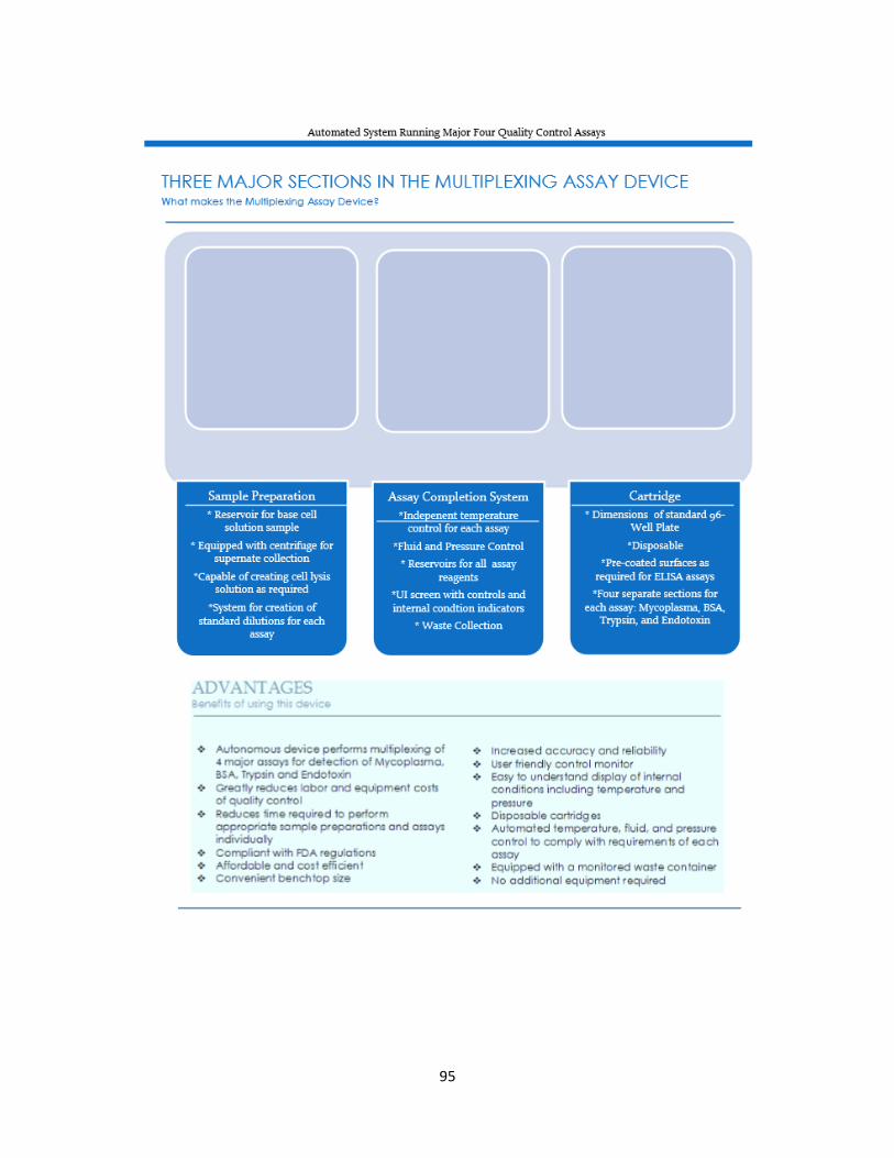
95

96
Appendix B: R&D Systems Mycoprobe Mycoplasma Detection Assay Kit
Procedure

97

98

99

100
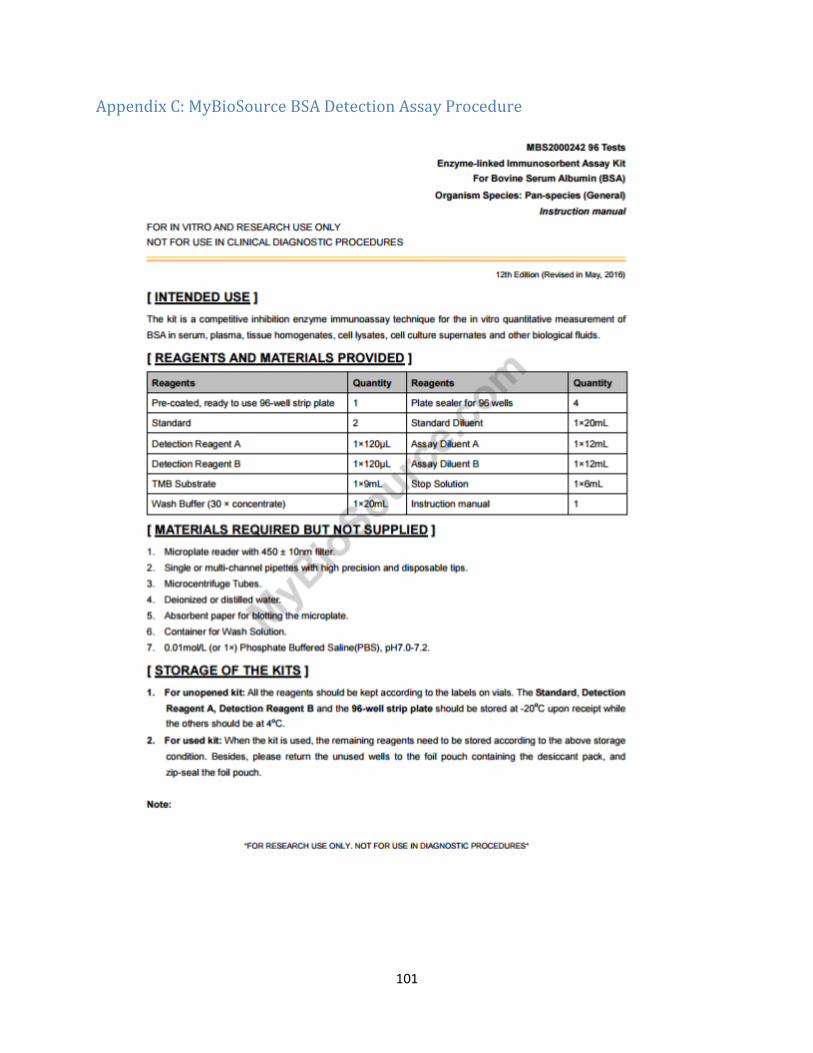
101
Appendix C: MyBioSource BSA Detection Assay Procedure

102

103

104

105
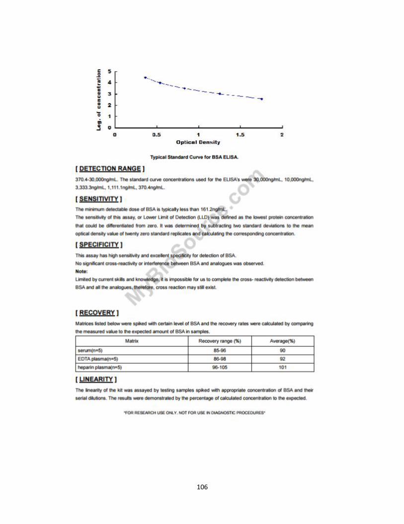
106

107

108
Appendix D: Syringe Pump Calibration Curve Determination Experiment (Full) To perform this experiment, the group used the pre-existing syringe pump assembly consisting
of a 1ml glass syringe and linear actuator enclosed in a metal assembly. The assembly was connected to a programmed Arduino Uno controller board to initiate and terminate movement of the linear actuator. The Arduino code was programmed to prompt the user for a position value that the linear actuator would then travel to. Open the Arduino software program “PumpAndValve.ino” on the computer and enter “0” value for the position of the linear actuator to bring the linear actuator to initial position corresponding to zero volume in the syringe. Then, press “x” to confirm and enter the value. NOTE: Press “x” after entering the desired value. After entering the position, enter the desired speed of the linear actuator to “150” and enter “x” to run the system. NOTE: Always enter each digit of the desired value individually for both position and speed (Example: 150, Enter). Later enter “x” after inputting the desired value for both location and speed (Example: 150, Enter, x). The program will ask for an input for the speed of the linear actuator only at the start of the program (after inputting the first desired location of the position of the linear actuator). The linear actuator will run at the same entered speed (here 150) for different input value positions of the linear actuator until the Arduino program is closed and re-run. Measuring the maximum volume of the glass syringe in the syringe pump assembly: In order to do so, first tare the mass scale to zero with the doors closed. Place a water filled glass vial (vial A) on the scale (capped). Close the scale doors and record the mass. NOTE: Record the mass when the “g” symbol appears on the scale. Uncap the vial A and place the tube connected to the glass syringe into the vial A to pump water from the vial A into the glass syringe within the syringe pump assembly. Within the same Arduino Software Program window input “1000” value for the position of the linear actuator to fill the syringe with water from the vial A. NOTE: The tube from the glass syringe is placed into the filled and weighed glass vial. After entering each digit of “1000” individually (Example: 1000. Enter) enter “x” to run the program (Example: 1000. Enter, x). The pump will start to pull water from the filled vial to the glass syringe. Now take another empty vial (vial B) and empty out water from the glass syringe to the empty vial by entering “0” for the position of the linear actuator. This will pump out all the water from the syringe. Now measure the weight of the vial A with the remaining water using the scale (Ensure to cap the vial and close the doors of the scale before measuring). Calculate the amount of water filled in the glass syringe= total weight of the filled vial A– weight of the vial A with remaining water. Perform the test 3 times and calculate the mean of water filled in the glass syringe. Calibration Curve Experiment Maximum Syringe Volume Intake Results
Total weight of the filled vial (g) Vial weight after filling the syringe (g)
Maximum volume intake of the syringe (uL)
13.4468 12.6602 787
12.6602 11.8738 786
11.8738 11.0892 785
11.0892 10.3002 789
Mean Volume Intake: 0.7866g=787uL Setting up an empty vial to collect the output volume from the Syringe Pump Assembly: In order to do so, we first enter “0” (in the Arduino software program) for the position of the linear actuator to ensure all the water is out of the system. Press “x” and enter to run the program. Take another filled glass vial (vial C). Uncap the water filled vial and place the glass syringe tube into the water filled glass vial. Enter “1000” for the position of the linear actuator to fill the glass syringe within the syringe pump to its maximum capacity. Press “x” and enter to run the program. Now take an empty glass vial (vial D)

109
and record the mass of the empty vial. NOTE: Ensure to tare the scale before measuring the mass of the empty vial. Also close the scale doors while measuring the weight of the vial. Now replace the glass vial C with an empty glass vial (vial D). In the same Arduino software program “Enter position of linear actuator” on the computer, input random positions of the linear actuator. NOTE: Input random values from “0” (Initial position of the linear actuator) to “1000” (Maximum distance traveled by the linear actuator within the syringe pump assembly). Collect the pumped water in the vial D. Measure the total mass of the vial D. Calculate the mass of the water dispensed at the input random location= total mass of the vial D - mass of the empty vial D. Repeat the previous steps for twelve random positions for the linear actuator. Repeat the previous step two more times for the same 12 positions of the linear actuator. Experimental Results and Analysis
Calibration Curve Experiment Iteration 1 Results
Start Position Input Position Actual End Position Distance Traveled Volume Output (uL)
1000 0 0 1000 775
1000 38 57 943 753
1000 281 306 694 583
1000 324 339 661 552
1000 417 (incorrect) N/A N/A 486
1000 500 518 482 418
1000 622 639 361 318
1000 635 655 345 385
1000 773 784 216 218
1000 815 836 164 168
1000 873 884 116 123
1000 950 956 44 66
Calibration Curve Experiment Iteration 2 Results
Start Position Input Position Actual End Position Distance Traveled Volume Output (uL)
1000 0 17 983 772
1000 38 43 957 772
1000 281 296 704 583
1000 324 336 664 562
1000 450 472 528 460
1000 500 517 483 320
1000 622 631 369 332
1000 635 656 344 312
1000 773 799 201 210
1000 815 833 167 167
1000 873 892 108 224
1000 950 951 49 63

110
Calibration Curve Experiment Iteration 3 Results
Start Position Input Position Actual End Position Distance Traveled Volume Output (uL)
1000 0 0 1000 793
1000 38 54 946 763
1000 281 299 701 580
1000 324 341 659 (outlier) 101(outlier)
1000 417 421 579 498
1000 500 528 472 412
1000 622 636 364 265
1000 635 648 352 313
1000 773 792 208 205
1000 815 819 181 189
1000 873 892 108 114
1000 950 955 45 63
Volume vs. Distance Traveled for Iterations 1, 2, and 3 Outliers are highlighted in the table above but removed from graph
Calibration curve experiment volume output vs distance traveled for iterations 1-3 with outliers
removed
Data Test 1 (With Outlier)
Test 2 Test 3 (With Outlier)
y=mx+c y = 0.7429x + 56.842 y = 0.7277x + 61.484 y = 0.6918x + 34.281
y = 0.75x + 51.36R² = 0.98
0
100
200
300
400
500
600
700
800
900
0 250 500 750 1000
Vo
lum
e O
utp
ut
(uL)
Distance Travelled
Linear (Volume Output )
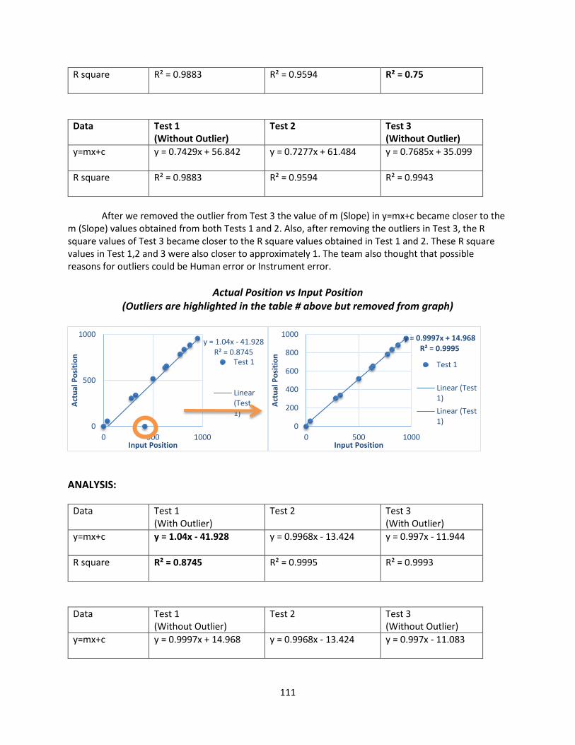
111
R square R² = 0.9883 R² = 0.9594 R² = 0.75
Data Test 1 (Without Outlier)
Test 2 Test 3 (Without Outlier)
y=mx+c y = 0.7429x + 56.842 y = 0.7277x + 61.484 y = 0.7685x + 35.099
R square R² = 0.9883 R² = 0.9594 R² = 0.9943
After we removed the outlier from Test 3 the value of m (Slope) in y=mx+c became closer to the
m (Slope) values obtained from both Tests 1 and 2. Also, after removing the outliers in Test 3, the R square values of Test 3 became closer to the R square values obtained in Test 1 and 2. These R square values in Test 1,2 and 3 were also closer to approximately 1. The team also thought that possible reasons for outliers could be Human error or Instrument error.
Actual Position vs Input Position (Outliers are highlighted in the table # above but removed from graph)
ANALYSIS:
Data Test 1 (With Outlier)
Test 2 Test 3 (With Outlier)
y=mx+c y = 1.04x - 41.928 y = 0.9968x - 13.424 y = 0.997x - 11.944
R square R² = 0.8745 R² = 0.9995 R² = 0.9993
Data Test 1 (Without Outlier)
Test 2 Test 3 (Without Outlier)
y=mx+c y = 0.9997x + 14.968 y = 0.9968x - 13.424 y = 0.997x - 11.083
y = 1.04x - 41.928R² = 0.8745
0
500
1000
0 500 1000
Act
ual
Po
siti
on
Input Position
Test 1
Linear(Test1)
y = 0.9997x + 14.968R² = 0.9995
0
200
400
600
800
1000
0 500 1000
Act
ual
Po
siti
on
Input Position
Test 1
Linear (Test1)
Linear (Test1)

112
R square R² = 0.9995
R² = 0.9995 R² = 0.9993
After removing the outlier from Test 1 the value of m(Slope) in y=mx+c are close to the slope
values obtained from Test 2 and 3. Also, after removing the outliers, the values of R square for Test 1, 2, and 3 are pretty close and are also close to approximately 1. The reasons for the outliers are Human error possibly, because the outlier’s actual position wasn’t written down (indication N/A in Test1).
Syringe Pump with Manifold: Dead Volumes Experiment
The previous steps with Manifold attached to the syringe pump. NOTE: While filling the syringe to its complete capacity, remove the manifold and fill the syringe with similar procedure. Connect the manifold right after inputting water. And continue the next steps. Syringe pump with manifold dead volumes experiment results: Iteration 1
Desired Output Volume(uL)
Actual Output Volume (uL)
Goal Position Actual Position
30 0 959 959
50 49 932 933
90 99 878 880
100 118 865 n/a*
150 164 798 n/a*
200 198 731 733
300 274 596 600
350 263 529 534
500 455 327 n/a*
600 543 193 194
700 562 59 60
796 741 0 1
*Due to human error, actual position was not recorded Syringe pump with manifold dead volumes experiment results: Iteration 2
Desired Output Volume(ul) Actual Output Volume (uL)
Goal Position Actual Position
30 0 959 957
50 45 932 933
90 48 878 n/a*
100 108 865 866
150 122 798 800
200 134 731 734
300 67 596 n/a*
350 234 529 532
500 722 327 330
600 595 193 194

113
700 629 59 60
796 729 0 1
*Due to human error, actual position was not recorded Syringe pump with manifold dead volumes experiment results: Iteration 3
Desired Output Volume(ul) Actual Output Volume (ul)
Desired Position Actual Position
30 13 959 959
50 49 932 933
90 88 878 880
100 107 865 867
150 129 798 799
200 167 731 732
300 264 596 600
350 305 529 533
500 467 327 331
600 553 193 196
700 646 59 n/a*
796 737 0 1
*Due to human error, the actual position was not recorded
Syringe pump with manifold dead volumes experiment goal vs actual output results for iterations 1-3
Observations:
y = 0.9153x - 7.3076R² = 0.9866
0
100
200
300
400
500
600
700
800
0 100 200 300 400 500 600 700 800 900
Act
ual
Ou
tpu
t (u
L)
Goal Output (uL)
Actual Output (Combined) Linear (Actual Output (Combined))

114
Data Test 1 Test 2 Test 3 (With Outlier)
y=mx+c y = 0.8686x + 9.0011 y = 1.0158x - 41.19 y = 0.9287x - 5.4455
R square R² = 0.983 R² = 0.8722 R² = 0.9982
Data Test 1 Test 2 Test 3 (Without Outlier)
y=mx+c y = 0.8686x + 9.0011 y = 0.9483x - 26.35 y = 0.9287x - 5.4455
R square R² = 0.983 R² = 0.9838 R² = 0.9982
ANALYSIS: R²: After removing the outlier the R² value for Test 2 changed from 0.8722 to 0.9838. It can be observed that the values of R² are very close to 1 after removing the outliers in Test 2. Also, the combined tests have R² = 0.9866. SLOPE: The graphs obtained are pretty linear and the slope values for Test 1 and 3 are relatively close. After removing the outlier from Test 2, the slope values for Test 2 are relatively close to the test values of Test 1 and Test 3. The combined tests have slope (m)= 0.9153. OUTLIERS: There exist 2 significant outliers in Test 2. The possible reasons for outlier are either human error or instrument error.
Observations:
Data Test 1 Test 2 Test 3 (With Outlier)
y=mx+c y = 0.7346x - 12.517 y = 0.8025x + 30.689 y = 1.0221x - 15.657
R square R² = 0.4009 R² = 0.5578 R² = 0.998
Data Test 1 Test 2 Test 3 (Without Outlier)
y=mx+c y = 1.0002x + 1.7836 y = 0.9994x + 1.5498 y = 0.9982x + 3.2175
R square R² = 1 R² = 1 R² = 1
0
100
200
300
400
500
600
700
800
900
1000
0 200 400 600 800 1000
Act
ual
Po
siti
on
Goal Position
Combined Tests Goal Position vs. Actual Position
Combined

115
OUTLIERS: There exist 5 significant outliers in Test 1, 2, and 3. The possible reasons for outlier was that the Actual Position wasn’t recorded (HUMAN ERROR). R²: After removing the outliers, the R² value for Test 1, Test 2 and Test 3 = 1. SLOPE: After removing the outliers, the slope is pretty linear and the values for the Test 1,2 and 3 are close. Comparison of with and without manifold volume outputs
Volume output comparison between system with and without manifold
y = 0.9153x - 7.3076R² = 0.9866
y = 0.9903x + 13.957R² = 0.9959
0
100
200
300
400
500
600
700
800
0 100 200 300 400 500 600 700 800
Act
ual
Ou
tpu
t (u
L)
Goal Output (uL)
Goal Volume Output vs. Actual Volume Output
With manifold Without Manifold Linear (With manifold) Linear (Without Manifold)

116
Appendix E: Syringe Pump with Manifold: Dead Volumes Experiment (Full) The purpose of this experiment was to determine volume lost in the valve manifold Steps: In order to perform this test, we took the already existing Syringe pump assembly consisting of 1ml glass syringe and linear actuator enclosed using metal assembly and connected it to the Solenoid manifold using a 1/32 inch tube. We connected it to the Arduino and the power supply. We also connected a 1/32 inch diameter tube to the manifold assembly to pump water out.
Setting up Arduino Software Program: Open the Arduino software program “PumpAndValve.ino” on the computer and enter “0” value to move the syringe to initial position corresponding “0” volume in the syringe. Enter “x” in the Arduino software to confirm. After entering the volume, enter the desired speed of the linear actuator to “150” and enter “x” to run the system. NOTE: Always enter each digit of the desired value individually for both volume and speed. (Example: 150, Enter). Always enter “x” after inputting the desired value for both volume and speed. (Example: 150, Enter, x). The program will ask for an input for the speed of the linear actuator only at the start of the program (after inputting the first desired volume). The linear actuator will run at the same entered speed (here 150) for different values of volumes until the Arduino program is closed and re-run. Setting up an empty vial to collect the output volume from the Syringe Pump Assembly (Without Manifold): Take a filled glass vial (vial A). Uncap the water filled vial A and place the glass syringe tube into the water filled glass vial. Enter “796” in the same Arduino program: “B: Enter volume” to fill the syringe at its maximum capacity. Enter “x” to run. Now take an empty glass vial (vial B) and record the mass of the empty vial. NOTE: Ensure to tare the scale before measuring the mass of the empty vial (capped). Also close the scale doors while measuring the weight of the vial. Now replace the glass vial A with an empty glass vial (vial B). (Place the syringe tube into vial B). Subtract a desired volume from 796 (maximum capacity of the syringe). (Example: 50 ul = 796-50=746). Enter the volume value (calculated) to be dispensed in the glass vial B. Enter “x” to run the program. NOTE: The test will be performed at the volumes in the following tables:
ASSAY VOLUME (ml)
BSA/Mycoplasma 0.05ml
BSA 0.09ml
BSA 0.10ml
Mycoplasma 0.15ml
Mycoplasma 0.20ml
BSA/Mycoplasma 0.30ml
BSA 0.35ml
BSA 0.60ml
Record the total mass of the vial B with the dispensed water. Calculate the mass of the output water = total mass of the water filled vial B - mass of the empty vial B. Repeat the previous steps for all the different volumes in the tables above. Repeat the previous step two more times for the same volumes.
(Without Manifold) Re-run the test two times and record the data in the following table:
MINIMUM (mL)
MAXIMUM (mL)
0.03 0.8
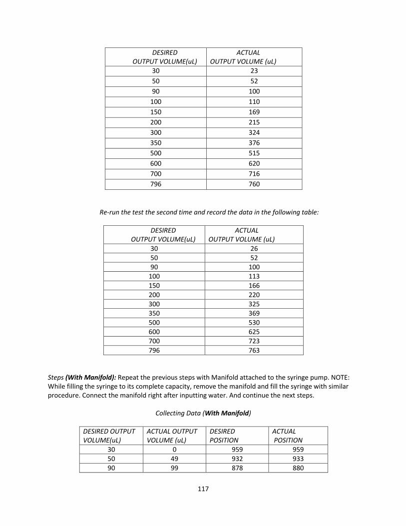
117
DESIRED OUTPUT VOLUME(uL)
ACTUAL OUTPUT VOLUME (uL)
30 23
50 52
90 100
100 110
150 169
200 215
300 324
350 376
500 515
600 620
700 716
796 760
Re-run the test the second time and record the data in the following table:
DESIRED OUTPUT VOLUME(uL)
ACTUAL OUTPUT VOLUME (uL)
30 26
50 52
90 100
100 113
150 166
200 220
300 325
350 369
500 530
600 625
700 723
796 763
Steps (With Manifold): Repeat the previous steps with Manifold attached to the syringe pump. NOTE: While filling the syringe to its complete capacity, remove the manifold and fill the syringe with similar procedure. Connect the manifold right after inputting water. And continue the next steps.
Collecting Data (With Manifold)
DESIRED OUTPUT VOLUME(uL)
ACTUAL OUTPUT VOLUME (uL)
DESIRED POSITION
ACTUAL POSITION
30 0 959 959
50 49 932 933
90 99 878 880

118
100 118 865 n/a
150 164 798 n/a
200 198 731 733
300 274 596 600
350 263 529 534
500 455 327 n/a
600 543 193 194
700 562 59 60
796 741 0 1
Repeat step two more times.
DESIRED OUTPUT VOLUME(uL)
ACTUAL OUTPUT VOLUME (uL)
DESIRED POSITION
ACTUAL POSITION
30 0 959 957
50 45 932 933
90 48 878 n/a
100 108 865 866
150 122 798 800
200 134 731 734
300 67 596 n/a
350 234 529 532
500 722 327 330
600 595 193 194
700 629 59 60
796 729 0 1
DESIRED OUTPUT VOLUME(uL)
ACTUAL OUTPUT VOLUME (uL)
DESIRED POSITION
ACTUAL POSITION
30 13 959 959
50 49 932 933
90 88 878 880
100 107 865 867
150 129 798 799
200 167 731 732
300 264 596 600
350 305 529 533
500 467 327 331
600 553 193 196
700 646 59 n/a
796 737 0 1

119
ACTUAL VS GOAL VOLUME OUT- WITHOUT MANIFOLD Test 1 and 2
Observations:
Data Test 1 Test 2
y=mx+c y = 0.9863x + 13.911 y = 0.9943x + 14.004
R square R² = 0.996 R² = 0.9958
R²: It can be observed that the values of R² are very close to 1. SLOPE: The graphs obtained are pretty
linear and the slope values for Test 1 and 2 are close. OUTLIERS: The graphs don’t have any significant
outliers.
y = 0.9863x + 13.911
R² = 0.996
0
100
200
300
400
500
600
700
800
900
0 100 200 300 400 500 600 700 800 900
Act
ual
Ou
tpu
t
Goal Output
Combined Linear (Combined)
y = 0.9863x + 13.911R² = 0.996
0
100
200
300
400
500
600
700
800
900
0 100 200 300 400 500 600 700 800 900
Act
ual
Ou
tpu
t
Goal Output
Test 1 Linear (Test 1)
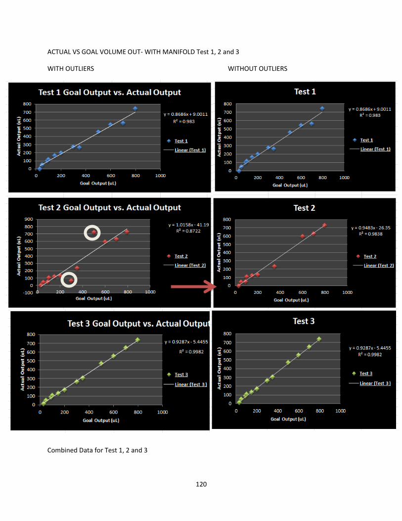
120
ACTUAL VS GOAL VOLUME OUT- WITH MANIFOLD Test 1, 2 and 3
WITH OUTLIERS WITHOUT OUTLIERS
Combined Data for Test 1, 2 and 3

121
y = 0.9153x - 7.3076R² = 0.9866
0
100
200
300
400
500
600
700
800
0 100 200 300 400 500 600 700 800 900
Act
ual
Ou
tpu
t (u
L)
Goal Output (uL)
Actual Output (Combined) Linear (Actual Output (Combined))
Observations:
Data Test 1 Test 2 Test 3 (With Outlier)
y=mx+c y = 0.8686x + 9.0011 y = 1.0158x - 41.19 y = 0.9287x - 5.4455
R square R² = 0.983 R² = 0.8722 R² = 0.9982
Data Test 1 Test 2 Test 3 (Without Outlier)
y=mx+c y = 0.8686x + 9.0011 y = 0.9483x - 26.35 y = 0.9287x - 5.4455
R square R² = 0.983 R² = 0.9838 R² = 0.9982
ANALYSIS: R²: After removing the outlier the R² value for Test 2 changed from 0.8722 to 0.9838. It can be observed that the values of R² are very close to 1 after removing the outliers in Test 2. Also, the combined tests have R² = 0.9866. SLOPE: The graphs obtained are pretty linear and the slope values for Test 1 and 3 are relatively close. After removing the outlier from Test 2, the slope values for Test 2 are relatively close to the test values of Test 1 and Test 3. The combined tests have slope (m)= 0.9153. OUTLIERS: There exist 2 significant outliers in Test 2. The possible reasons for outlier are either human error or instrument error.

122
ACTUAL VS GOAL POSITION- WITH MANIFOLD Test 1, 2 and 3
WITH OUTLIERS WITH OUTLIERS
NOTE: Removed 2 outliers from the previous volume analysis for Test 2

123
Observations:
Data Test 1 Test 2 Test 3 (With Outlier)
y=mx+c y = 0.7346x - 12.517 y = 0.8025x + 30.689 y = 1.0221x - 15.657
R square R² = 0.4009 R² = 0.5578 R² = 0.998
Data Test 1 Test 2 Test 3 (Without Outlier)
y=mx+c y = 1.0002x + 1.7836 y = 0.9994x + 1.5498 y = 0.9982x + 3.2175
R square R² = 1 R² = 1 R² = 1
OUTLIERS: There exist 5 significant outliers in Test 1, 2, and 3. The possible reasons for outlier was that the Actual Position wasn’t recorded (HUMAN ERROR). R²: After removing the outliers, the R² value for Test 1, Test 2 and Test 3 = 1. SLOPE: After removing the outliers, the slope is pretty linear and the values for the Test 1,2 and 3 are close. Test3: Air Pump Integration The purpose of this experiment was to determine if using an air pump helped lessen dead volumes by flushing the remaining dead volumes left behind. Steps: In order to perform this test, we took the already existing Syringe pump assembly consisting of 1ml glass syringe and linear actuator enclosed using metal assembly and connected it to the Solenoid manifold using a 1/32 inch tube. We connected it to the Arduino and the power supply. We also connected a 1/32 inch diameter tube to the manifold assembly to pump water out. We also connected the air pump to manifold and syringe pump. Setting up an empty vial to collect the output volume from the Manifold: Take a filled glass vial (vial A). Uncap the water filled vial A and place the glass syringe tube into the water filled glass vial. Enter “799” in the same Arduino program: “B: Enter volume” to fill the syringe at its maximum capacity. Enter “x” to run. Now take an empty glass vial (vial B) and record the mass of the empty vial. NOTE: Ensure to tare the scale before measuring the mass of the empty vial (capped). Also close the scale doors while measuring the weight of the vial. Connect the manifold to the syringe pump tube. NOTE: Fill the syringe pump at its full capacity directly using syringe pump tube instead of connecting it to the manifold. Now replace the glass vial A with an empty glass vial (vial B). (Place the manifold tube into vial B). Subtract a desired volume from 799 (maximum capacity of the syringe). (Example: 50 ul = 799-50=749). Enter the volume value (calculated) to be dispensed in the glass vial B. Enter “x” to run the program. NOTE: The test will be performed at the volumes in the following tables:

124
ASSAY VOLUME (ml)
BSA/Mycoplasma 0.05ml
BSA 0.09ml
BSA 0.10ml
Mycoplasma 0.15ml
Mycoplasma 0.20ml
BSA/Mycoplasma 0.30ml
BSA 0.35ml
BSA 0.60ml
Enter “y” in the Arduino code to start the air pump. Stop the air pump by entering “s” in the Arduino code. Stop after 1 second. Record the total mass of the vial B with the dispensed water. Calculate the mass of the output water = total mass of the water filled vial B - mass of the empty vial B. Repeat the previous steps for all the different volumes in the tables above. Repeat the previous step two more times for the same volumes. Collecting Data
DESIRED OUTPUT VOLUME(uL)
ACTUAL OUTPUT VOLUME (uL)
30 15.1
50 13.1
90 25.6
100 63.3
150 110.8
200 179.8
300 293.4
450 (Instead of 350) 398.6
500 393.7
600 576.6
700 670.9
799 500.3
DESIRED OUTPUT VOLUME(uL)
ACTUAL OUTPUT VOLUME (uL)
30 16.1
50 31.8
90 77.1
100 70.8
150 144.4
200 182.7
MINIMUM (mL)
MAXIMUM (mL)
0.03 0.8

125
y = 0.8351x - 6.1035R² = 0.9215
0
100
200
300
400
500
600
700
800
0 500 1000
Act
ual
Vo
lum
e O
utp
ut
(uL)
Goal Volume Output (uL)
Test 1
Series1
Linear (Series1)
y = 0.9743x - 11.069R² = 0.9938
0
100
200
300
400
500
600
700
800
0 500 1000Act
ual
Vo
lum
e O
utp
ut
(uL)
Goal Volume Output (uL)
Test 2
Test2
Linear (Test2)
y = 1.0333x - 30.847R² = 0.9861
0
100
200
300
400
500
600
700
800
0 500 1000
Act
ual
Vo
lum
e O
utp
ut
Goal Volume Output
Test 1
Test1
Linear (Test1)
y = 0.9743x - 11.069R² = 0.9938
0
100
200
300
400
500
600
700
800
0 500 1000Act
ual
Vo
lum
e O
utp
ut
(uL)
Goal Volume Output (uL)
Test 2
Test2
Linear (Test2)
300 265.7
350 343.8
500 494
600 599.6
700 692.3
799 718.6
Goal Output VS Actual Output WITH OUTLIERS IN TEST WITHOUT OUTLIERS IN TEST 1
DESIRED OUTPUT VOLUME(uL)
ACTUAL OUTPUT VOLUME (uL)
30 -1.8
50 10.9
90 69.6
100 68.6
150 130.7
200 146.9
300 289
350 330.5
500 489.7
600 581.6
700 672.6
799 703.6

126
y = 0.9727x - 22.607R² = 0.9927
0
100
200
300
400
500
600
700
800
0 500 1000
Act
ual
Vo
lum
e O
utp
ut
(uL)
Goal Volume Output (uL)
Test 3
Test3
Linear (Test3)
y = 0.9727x - 22.607R² = 0.9927
0
100
200
300
400
500
600
700
800
0 500 1000
Act
ual
Vo
lum
e O
utp
ut
(uL)
Goal Volume Output (uL)
Test 3
Test3
Linear (Test3)
Data Test 1 (With Outlier)
Test 2 Test 3
y=mx+c y = 0.8351x - 6.1035 y = 0.9743x - 11.069 y = 0.9727x - 22.607
R square R² = 0.9215 R² = 0.9938 R² = 0.9927
Data Test 1 (Without Outlier)
Test 2 Test 3
y=mx+c y = 1.0333x - 30.847 y = 0.9743x - 11.069 y = 0.9727x - 22.607
R square R² = 0.9861 R² = 0.9938 R² = 0.9927
Observations: OUTLIERS: There exist 2 significant outliers in Test 1. The possible reasons for outlier are human error or instrument error. R²: After removing the outlier the R² value for Test 1 changed from 0.9215 to 0.9861. It can be observed that the values of R² are very close to 1 after removing the outliers in Test 2.

127
SLOPE: The graphs obtained are pretty linear and the slope values for Test 2 and 3 are relatively close. After removing the outlier from Test 1, the slope value for Test 1 is relatively close to the test values of Test 2 and Test 3.

128
Appendix F: Syringe Pump with Manifold: Intake Inaccuracies Experiment
(Full) In order to perform this test, we took the already existing Syringe pump assembly consisting of
1ml glass syringe and linear actuator enclosed using metal assembly and connected it to the Solenoid manifold using a 1/32 inch tube. We connected it to the Arduino and the power supply. We also connected a 1/32 inch diameter tube to the manifold assembly to intake water. Open the Arduino software program “PumpAndValve.ino” on the computer and enter “0” value to move the syringe to initial position corresponding “0” volume in the syringe. Enter “x” to confirm. After entering the position, enter the desired speed of the linear actuator to “150” and enter “x” to run the system. NOTE: Always enter each digit of the desired value individually for both volume and speed. (Example: 150). Always enter “x” after inputting the desired value for both volume and speed. (Example: 1, Enter, 5, Enter, 0, Enter, x). The program will ask for an input for the speed of the linear actuator only at the start of the program (after inputting the first desired volume). The linear actuator will run at the same entered speed (here 150) for different values of volumes until the Arduino program is closed and re-run.
Start with full glass vial of water. Weigh on tared scale to get total mass. NOTE: Ensure to tare the scale before measuring the mass of the vial (capped). Also close the scale doors while measuring the weight of the vial. Start syringe at volume 0. Put tubing into glass vial and input desired volume into Arduino interface. Begin program so pump fills syringe. When syringe is full to desired volume position, weigh the vial again to see how much water is actually taken into the syringe
Input volume 0 into the Arduino software to empty out all contents of the syringe into the same vial. Weigh again to see how much volume was dispensed. We chose a range of volumes between 0 and 700 to ensure that the pump is consistent. We also ensured appropriate values to reflect the values we’ll need for the assays.
Goal Intake (uL) Actual Intake (uL) Iteration 1
Actual Intake (uL) Iteration 2
Actual Intake (uL) Iteration 3
30 1 5 3
50 5 1 1
90 21 20 19
100 27 38 26
150 78 72 69
200 114 115 111
300 200 203 199
350 247 402 246
500 401 400 403
600 510 528 509
799 773 765 767

129
Results of system intake experiment: goal intake vs. actual intake
Results of system intake experiment: Change in intake volume vs. goal volume intake
We obtained a pretty linear relationship for Actual Intake vs. Goal Intake with y= 1.03x-89.42. Also the value of R square equals 0.99, close to 1. After obtaining another graph representing Difference in Volume vs. Goal Volume Intake, we observed that a constant volume difference wasn’t observed. Also, after looking at the graph, constant trend of loss of volume wasn’t observed.
y = 1.03x - 89.42R² = 0.99
0
100
200
300
400
500
600
700
800
0 100 200 300 400 500 600 700 800
Act
ual
In
take
(u
L)
Goal Intake (uL)
Goal Intake vs. Actual Intake
Combined Linear (Combined)
0
20
40
60
80
100
0 100 200 300 400 500 600 700 800 900
ΔV
olu
me
(u
L)
Goal Volume Intake (uL)Test 1 Test 2 Test 3 Poly. (Test 1) Poly. (Test 3)

130
Appendix G: Syringe Pump with Manifold and Air Pump: Output Volume Loss
Experiment (Full) In order to perform this test, we took the already existing Syringe pump assembly consisting of
1ml glass syringe and linear actuator enclosed using metal assembly and connected it to the Solenoid manifold using a 1/32 inch tube. We connected it to the Arduino and the power supply. We also connected a 1/32 inch diameter tube to the manifold assembly to pump water out. We also connected the air pump to manifold and syringe pump. Take a filled glass vial (vial A). Uncap the water filled vial and place the glass syringe tube into the water filled glass vial. Enter “799” in the same Arduino program: “PumpAndValve.ino” to fill the syringe at its maximum capacity. Enter “x” to run. Now take an empty glass vial (vial B) and record the mass of the empty vial. NOTE: Ensure to tare the scale before measuring the mass of the empty vial (capped). Also close the scale doors while measuring the weight of the vial. Connect the manifold to the syringe pump tube. NOTE: Fill the syringe pump at its full capacity directly using syringe pump tube instead of connecting it to the manifold. Now replace the glass vial A with an empty glass vial (vial B). (Place the manifold tube into vial B). Subtract a desired volume from 799 (maximum capacity of the syringe). (Example: 50 µl = 799-50=749). Enter the volume value (calculated) to be dispensed in the glass vial B. Enter “x” to run the program. NOTE: The test will be performed at the volumes in the following tables:
Assay Volume (uL)
Minimum 30
BSA/Mycoplasma 50
BSA 90
BSA 100
Mycoplasma 150
Mycoplasma 200
BSA/Mycoplasma 300
BSA 350
BSA 600
Maximum 800
Enter “y” in the Arduino code to start the air pump. Stop the air pump by entering “s” in the Arduino code. Stop after 1 second. Record the total mass of the vial B with the dispensed water. Calculate the mass of the output water = total mass of the water filled vial B - mass of the empty vial B. Repeat the previous steps for all the different volumes in the tables above. Repeat the previous step two more times for the same volumes.
Experimental Results and Analysis
Desired Output Volume (uL)
Actual Output Volume: Iteration 1 (uL)
Actual Output Volume: Iteration 2 (uL)
Actual Output Volume: Iteration 3 (uL)
30 15.1 16.1 -1.8
50 13.1 31.8 10.9
90 25.6 77.1 69.6
100 63.3 70.8 68.6

131
150 110.8 144.4 130.7
200 179.8 182.7 146.9
300 293.4 265.7 289
350 398.6* 343.8 330.5
500 393.7 494 489.7
600 576.6 599.6 581.6
700 670.9 692.3 672.6
799 500.3 718.6 703.6
*In Iteration 1, value measured at 450µL due to human error.
Goal Output VS Actual Output (Outliers highlighted in table # but removed from graph)
Data Test 1 (With Outlier)
Test 2 Test 3
y=mx+c y = 0.8351x - 6.1035 y = 0.9743x - 11.069 y = 0.9727x - 22.607
R square R² = 0.9215 R² = 0.9938 R² = 0.9927
Data Test 1 (Without Outlier)
Test 2 Test 3
y=mx+c y = 1.0333x - 30.847 y = 0.9743x - 11.069 y = 0.9727x - 22.607
R square R² = 0.9861 R² = 0.9938 R² = 0.9927
Observations: OUTLIERS: There exist 2 significant outliers in Test 1. The possible reasons for outlier are human error or instrument error. R²: After removing the outlier the R² value for Test 1 changed from 0.9215 to 0.9861. It can be observed that the values of R² are very close to 1 after removing the outliers in Test 2.
y = 0.9153x - 7.3076R² = 0.9866
0
100
200
300
400
500
600
700
800
900
0 100 200 300 400 500 600 700 800 900
Act
ual
Ou
tpu
t (u
L)
Goal Output (uL)
Syringe Pump and ManifoldGoal Output vs. Actual Output
Combined Linear (Combined)

132
SLOPE: The graphs obtained are pretty linear and the slope values for Test 2 and 3 are relatively close. After removing the outlier from Test 1, the slope value for Test 1 is relatively close to the test values of Test 2 and Test 3.

133
Appendix H: BSA Water Trial Experiment: Full Purpose: Determine if proof-of-concept device has the accuracy and precision to dispense volumes required for BSA assay. The trial was run with water rather than reagents. Open the Arduino software program “PumpAndValve.ino” on the computer and enter “0” value to move the syringe to initial position corresponding “0” volume in the syringe. Enter “x” in the Arduino software to confirm. After entering the volume, enter the desired speed of the linear actuator to “250” and enter “x” to run the system. Enter the goal intake volume into the Arduino code; the goal volumes are listed in the following table: NOTE: 50uL input buffer is used because of variability. NOTE: Air Pump after pumping each reagent. Enter the volumes to intake in the Arduino code as listed in the table above, and begin to fill the syringe from the manifold input/output valve ports (which manifold input ports are designated for which reagent volumes). Now dispense the volume in the same input/output valve port from syringe pump into each well using manual tubing control. Calculate the actual output volumes using mass difference calculations. Repeat each run with 6 wells at each volume three times. The intake and output w/ buffer volume was calculated as listed in the following table:
Intake w/ buffer volume
100uL 150uL 350uL 140uL
Average Intake Volume (uL)
36 81 270 72
Average Intake Difference (uL)
62 69 80 57
Overall CV of Intake Volume (%)
70 10 2 8
Reagent Volume
Detection Reagent A 50uL
Detection Reagent B 100uL
Wash Buffer 300uL
Substrate Solution 90uL
Stop Solution 50uL

134
Output w/ buffer Volume
100uL 150uL 350uL 140uL
Average Ouput Volume (uL)
18 54 209 52
Average Output Volume Lost (uL)
15 15 11 8
Overall CV of Output Volume (%)
48 24 6 2
Average Intake Difference (uL) 70uL
Average Output Losst (uL) 15uL
The following volumes were calculated to ensure requested volumes achieve desired output volume:
Goal Output Volume Actual Arduino Input (uL) Rounded Arduino Input (uL)
50uL 127 130
90uL 155 170
100uL 174 180
300uL 391 380
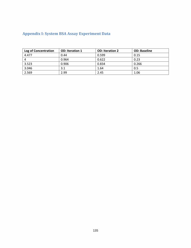
135
Appendix I: System BSA Assay Experiment Data
Log of Concentration OD: Iteration 1 OD: Iteration 2 OD: Baseline
4.477 0.44 0.599 0.15
4 0.964 0.622 0.23
3.523 0.906 0.834 0.266
3.046 3.1 1.64 0.5
2.569 2.99 2.45 1.06

136
Appendix J: System Mycoplasma Experiment Data
Mycoplasma Baseline Assay System Mycoplasma Assay
Positive Control Readings at 490nm 2.05 2.02
2.16
4.49 4.57 4.34
Negative Control Readings at 490nm 0.161 0.1 0.113
0.354 0.334 0.516
Positive at 600nm 0.874 0.948 0.916
1.48 1.48 1.38
Negative at 600nm 0.0822 0.0575 0.0736
0.116 0.113 0.168
Difference Positive 1.123 1.109 1.191
3.01 3.09 2.96
Difference Negative 0.0252 -0.011 -0.141
0.238 0.221 0.348