develop of the dynamic model of gb for transient stability

DEVELOP OF THE DYNAMIC MODEL OF GBFOR TRANSIENT STABILITY IN RSCAD

MASTER THESIS

German Fabricio VELEZ TERREROS

DEVELOP OF THE DYNAMIC MODEL OF GB FORTRANSIENT STABILITY IN RSCAD

MASTER THESIS

by

German Fabricio VELEZ TERREROS

Student Number: 4518519

in partial fulfillment of the requirements for the degree of

Master of Sciencein Electrical Engineering

(Electrical Sustainable Energy)

at the Delft University of Technology,to be defended publicly on Monday August 22, 2017 at 10:00 AM.

Supervisor: Asst. Prof. dr. ir. J. L. Rueda Torres

Thesis committee: Prof. dr. P. Palensky

Dr. Armando Rodrigo Mor

An electronic version of this dissertation is available athttp://repository.tudelft.nl/.

http://repository.tudelft.nl/

Life is like an infinite road with no end; you decide to walk through or stand on theroadside. When you find someone who goes in the same direction, never let it go. This

project is dedicated to my family who supports me in every project, my new and oldfriends, and in special to my road companion my wife Ana...

Fabricio Velez

Acknowledgment

I would like to express my gratitude to the University of TU Delft for allowing me to con-tinue my Master studies; It has been a challenge and a pleasure to be here. In addition, Iwould like to express my gratitude to Dr. ir. Jose Rueda. Throughout this two years, youhave been a mentor. And during the thesis project, your guidance has been essential foraccomplishing this work. Next, I would like to express my gratitude to Prof. dr. P. Palenskyfor your valuable feedback which helps me to improve my work. Last but not the least, Iwould like to thank Dr. A. Rodrigo Mor for accepting to be part of the thesis committee.Finally, I would like to thank the scholarship program by the Secretariat of Higher Edu-cation, Science, Technology and Innovation of the Republic of Ecuador who provided mewith financial support for conducting my master studies at the University of TU Delft.

vii

Abstract

Increasing wind generation causes displacement of conventional power plants with Syn-chronous Generators in electrical power systems. This condition leads to less inertia, lesscontrollability and a degraded damping performance in the electrical systems. Studies ofstability of the power system attempt to analyze this issues. Rotor angle stability studiesusing real time digital simulation requires the use of data mining to obtain an insightabout the coherency of the system with the variation of the time series data. However, thelimitations of the simulation systems as well as the magnitude of the models can lead intodifficult study scenarios. By modeling the power systems in real time simulators, electricalstudies can be performed faster than with conventional offline simulators. In this the-sis project, the Britain baseline system was modeled in the Real Time Digital Simulator(RTDS) using as a starting point and initialization reference, the electrical power modeldeveloped for the simulator Power Factory. The model then was reduced using coherencyanalysis by clustering time-series-data. The same modeling considerations were appliedfor implementing future scenarios of the GB in the RTDS. For reduction purposes, threemain areas describing the North, Central, and South parts of the system were consideredin the GB model. The results show that while the area of study is considered constant theother two areas can be replaced by the coherent areas. Thus, less use of racks is required foranalyzing the model in the simulator. This study contributes to the analysis of the powerelectrical systems, by providing valuable insights in how to reduce electrical models fortheir study in the RTDS.

ix

CONTENTS

List of Figures xiii

List of Tables xv

1 Introduction 11.1 Introduction . . . . . . . . . . . . . . . . . . . . . . . . . . . . . . . . 11.2 Literature Review . . . . . . . . . . . . . . . . . . . . . . . . . . . . . . 21.3 Problem Definition . . . . . . . . . . . . . . . . . . . . . . . . . . . . . 31.4 Background . . . . . . . . . . . . . . . . . . . . . . . . . . . . . . . . . 31.5 Objective and Research Questions . . . . . . . . . . . . . . . . . . . . . 41.6 Research Approach . . . . . . . . . . . . . . . . . . . . . . . . . . . . . 41.7 Outline . . . . . . . . . . . . . . . . . . . . . . . . . . . . . . . . . . . 5

2 GB Model in RTDS 72.1 Description . . . . . . . . . . . . . . . . . . . . . . . . . . . . . . . . . 72.2 Real Time Digital Simulator . . . . . . . . . . . . . . . . . . . . . . . . . 7

2.2.1 RTDS Hardware . . . . . . . . . . . . . . . . . . . . . . . . . . . 82.2.2 RTDS Software . . . . . . . . . . . . . . . . . . . . . . . . . . . . 9

2.3 GB Model in RTDS . . . . . . . . . . . . . . . . . . . . . . . . . . . . . 112.3.1 Baseline . . . . . . . . . . . . . . . . . . . . . . . . . . . . . . . 112.3.2 Transition scenarios . . . . . . . . . . . . . . . . . . . . . . . . . 152.3.3 Components . . . . . . . . . . . . . . . . . . . . . . . . . . . . . 152.3.4 Limitations. . . . . . . . . . . . . . . . . . . . . . . . . . . . . . 222.3.5 Implementing the GB System in the RTDS . . . . . . . . . . . . . . 252.3.6 Initialization Comparison . . . . . . . . . . . . . . . . . . . . . . 25

3 Reduction of GB system for study of Transient Stability in RSCAD 323.1 Background . . . . . . . . . . . . . . . . . . . . . . . . . . . . . . . . . 323.2 Dynamic coherency for reduction. . . . . . . . . . . . . . . . . . . . . . 33

3.2.1 Coherency analysis . . . . . . . . . . . . . . . . . . . . . . . . . 333.2.2 Coherency Analysis . . . . . . . . . . . . . . . . . . . . . . . . . 343.2.3 Clustering Identification . . . . . . . . . . . . . . . . . . . . . . . 353.2.4 k-mean algorithm . . . . . . . . . . . . . . . . . . . . . . . . . . 363.2.5 Elbow Method . . . . . . . . . . . . . . . . . . . . . . . . . . . . 38

3.3 Application of the Coherency Analysis to the GB System . . . . . . . . . . 393.3.1 Disturbances in the RTDS . . . . . . . . . . . . . . . . . . . . . . 393.3.2 Coherency Analysis in Matlab . . . . . . . . . . . . . . . . . . . . 42

xi

xii CONTENTS

4 Analysis Results 444.1 Areas of Study . . . . . . . . . . . . . . . . . . . . . . . . . . . . . . . . 454.2 North Area Analysis . . . . . . . . . . . . . . . . . . . . . . . . . . . . . 474.3 Central Area Analysis . . . . . . . . . . . . . . . . . . . . . . . . . . . . 504.4 South Area Analysis . . . . . . . . . . . . . . . . . . . . . . . . . . . . . 52

5 Conclusions 535.1 Answer to Research Questions . . . . . . . . . . . . . . . . . . . . . . . 545.2 Future Work. . . . . . . . . . . . . . . . . . . . . . . . . . . . . . . . . 55

6 References 56References . . . . . . . . . . . . . . . . . . . . . . . . . . . . . . . . . . . . 56

7 Annexes 597.1 Annex 1: Scripts and Macros . . . . . . . . . . . . . . . . . . . . . . . . 597.2 Annex: Initial Parameter Tables . . . . . . . . . . . . . . . . . . . . . . . 777.3 ANNEX: Tables GONE GREEN SCENARIOS . . . . . . . . . . . . . . . . . 807.4 Annex: Assignation Clustering Tables . . . . . . . . . . . . . . . . . . . . 86

LIST OF FIGURES

1.1 Research flow . . . . . . . . . . . . . . . . . . . . . . . . . . . . . . . . . . . . 51.2 Thesis Work Flow . . . . . . . . . . . . . . . . . . . . . . . . . . . . . . . . . . 6

2.1 GB network representation of 29 Zones [1, 2] . . . . . . . . . . . . . . . . . . 82.2 Rack Components . . . . . . . . . . . . . . . . . . . . . . . . . . . . . . . . . 92.3 Draft Module in RTDS . . . . . . . . . . . . . . . . . . . . . . . . . . . . . . . 102.4 RunTime Module in RTDS . . . . . . . . . . . . . . . . . . . . . . . . . . . . . 102.5 GB model in Power Factory [3] . . . . . . . . . . . . . . . . . . . . . . . . . . 122.6 GB model in Power Factory [3] . . . . . . . . . . . . . . . . . . . . . . . . . . 132.7 Synchronous Generator RTDS [3] . . . . . . . . . . . . . . . . . . . . . . . . 162.8 Transformer in RTDS [3] . . . . . . . . . . . . . . . . . . . . . . . . . . . . . . 172.9 Bus modelling in RTDS [3] . . . . . . . . . . . . . . . . . . . . . . . . . . . . . 182.10 Transmission Line in RTDS [3] . . . . . . . . . . . . . . . . . . . . . . . . . . 182.11 Tline Setup in RTDS . . . . . . . . . . . . . . . . . . . . . . . . . . . . . . . . 192.12 Electrical parameters of Tline in RTDS . . . . . . . . . . . . . . . . . . . . . 202.13 Transmission line selector process in RTDS . . . . . . . . . . . . . . . . . . . 212.14 Shunt Capacitor in RTDS [3] . . . . . . . . . . . . . . . . . . . . . . . . . . . . 212.15 Dynamic Load as Constant Load in RTDS . . . . . . . . . . . . . . . . . . . . 222.16 Processors behavior in the RTDS per subsystem . . . . . . . . . . . . . . . . 242.17 GB mounted in the RTDS . . . . . . . . . . . . . . . . . . . . . . . . . . . . . 262.18 Representation of Zones in RTDS . . . . . . . . . . . . . . . . . . . . . . . . . 272.19 Comparison a Zone in RTDS and Power Factory . . . . . . . . . . . . . . . . 282.20 Comparison of Voltage Magnitude between systems . . . . . . . . . . . . . 292.21 Comparison of Voltage Angle between systems . . . . . . . . . . . . . . . . 30

3.1 Algorithm of Coherency Analysis . . . . . . . . . . . . . . . . . . . . . . . . . 343.2 Algorithm of Clustering Identification . . . . . . . . . . . . . . . . . . . . . . 363.3 Elbow Method . . . . . . . . . . . . . . . . . . . . . . . . . . . . . . . . . . . . 393.4 Algorithm implemented in Matlab to determine "k" by elbow method . . . 403.5 Implementation of Faults in the RTDS . . . . . . . . . . . . . . . . . . . . . . 403.6 Configuration of the line breaker in RTDS . . . . . . . . . . . . . . . . . . . . 42

4.1 Areas of GB System . . . . . . . . . . . . . . . . . . . . . . . . . . . . . . . . . 464.2 Number of Clusters determined by faults in the North Area . . . . . . . . . 474.3 Cluster Assignation of P by Bus Fault in Z1 . . . . . . . . . . . . . . . . . . . 484.4 Cluster Visualization of P by Bus Fault in Z2 . . . . . . . . . . . . . . . . . . 494.5 Number of Clusters of P in the Central Area . . . . . . . . . . . . . . . . . . . 514.6 Cluster Visualization of P by Bus Fault in Z9 . . . . . . . . . . . . . . . . . . 51

xiii

xiv LIST OF FIGURES

4.7 Number of Clusters of P in the South Area . . . . . . . . . . . . . . . . . . . 52

LIST OF TABLES

2.1 GB System Baseline 2016[4] . . . . . . . . . . . . . . . . . . . . . . . . . . . . 14

7.1 Load Input Table . . . . . . . . . . . . . . . . . . . . . . . . . . . . . . . . . . 777.2 Transmission Line Parameter . . . . . . . . . . . . . . . . . . . . . . . . . . . 787.3 Buses Distribution in Areas . . . . . . . . . . . . . . . . . . . . . . . . . . . . 797.4 GONE GREEN 2020 [4] . . . . . . . . . . . . . . . . . . . . . . . . . . . . . . . 817.5 GONE GREEN 2025[4] . . . . . . . . . . . . . . . . . . . . . . . . . . . . . . . 827.6 GONE GREEN 2030[4] . . . . . . . . . . . . . . . . . . . . . . . . . . . . . . . 837.7 GONE GREEN 2035[4] . . . . . . . . . . . . . . . . . . . . . . . . . . . . . . . 847.8 CLuster Elements Z1 . . . . . . . . . . . . . . . . . . . . . . . . . . . . . . . . 857.9 Clustering by P as a response of Bus Faults in the North Area . . . . . . . . 877.10 Clustering by P as a response of Bus Faults in the Center Area . . . . . . . . 887.11 Clustering by P as a response of Bus Faults in the South Area . . . . . . . . 897.12 Clustering by P as a Response of Line Switching in the North Area . . . . . 907.13 Clustering by P as a Response of Line Switching in the Center Area part1 . 917.14 Clustering by P as a Response of Line Switching in the Center Area part2 . 927.15 Clustering by P as a Response of Line Switching in the South Area part1 . . 937.16 Clustering by P as a Response of Line Switching in the South Area part2 . . 947.17 Clustering by P as a Response of Load Increasing in the North Area . . . . 957.18 Clustering by P as a Response of Load Increasing in the Center Area . . . . 967.19 Clustering by P as a Response of Load Increasing in the South Area . . . . 97

xv

1INTRODUCTION

1.1. INTRODUCTIONFor the future years, several changes are expected in the electrical power system of GreatBritain (GB)[4]. One of the changes involves the installation of wind generation for sup-ply future energy demand the zones. However, with the increasing installation of windgeneration, a displacement of conventional power plants with synchronous generatorsis expected. As a response to this change of generation in the GB area, less inertia andcontrollability will be presented in the power system leading to stability problems[5]. Inorder to deal with future stability issues caused by the replacement of generation andthe interconnected nature of power systems, it is necessary to perform studies of thestability of the systems in the present using expected scenarios for the future. In theGB system, several studies have been performed in order to analyze the behavior of thesystem. Moreover, different electrical models have been developed to perform differ-ent kind of studies; One of the studies and the focus of the present project is the elec-tromagnetic transient (EMT) phenomena, caused by faults, switching operations, loadfluctuations and lightning strikes which causes transients in the system[5]. Due to thefast nature of this phenomena, not only a specific model has been required but also aspecific simulator with enough processing capacity to deal with this phenomena. RealTime Digital Simulator (RTDS), is a powerful software/hardware simulator developed tothe study of EMT in electrical power systems. In the present thesis project, the electri-cal power model of the GB system will be implemented in the RTDS to perform futurestudies in the network. EMT studies in the GB system involves a considerable high useof hardware resources of the RTDS. Due to the limitations of the RTDS acquired for theuniversity of TU Delft and considering the parallel projects using the RTDS, it is requireda reduction of the system after implemented.

The RTDS system installed in TU Delft has six racks used to deal with the simulationof the electrical projects. When implemented the GB system, it consumes four racksleaving only two available racks for the rest project. The reduction of the system mustallow reducing the consumption of the racks of the RTDS while maintaining the behavior

1

1

2 1. INTRODUCTION

of the zones of the GB system. One way to deal with the reduction of the electrical powersystem is to find generators which have similar behavior when disturbances are appliedto it. Thus, generators with similar behavior can be clustered and the system can bereduced.

Clustering analysis has been used to form groups of elements which oscillate simi-larly when subjected to disturbances. There are several techniques to cluster differentsignals. Indeed, time series data can be used to group elements of the electrical system.Once determined the number of clusters and the elements which are part of it, the ag-gregated elements can be represented as an equivalent of the group. These equivalentsallow the reduction of the size of the system when the study conditions require it.

With the reduction of the network, it is possible to work with fewer areas. Indeed, itallows focusing on determined areas while maintaining the rest of the system as equiv-alents maintaining the performance of the original system. RTDS does not provide aneigenvalue analysis tool included in the software. Due to, the manipulation of time-series data is extracted from the RTDS and send to Matlab in order to find the clusters ofgenerators which will lead to a reduction of the system.

The output of the project will provide the GB model and the future scenarios imple-mented in the RTDS. Additionally, the algorithms developed in Matlab for the Coherencyanalysis. Finally, the insight for reducing the model in order to use fewer resources of theRTDS.

1.2. LITERATURE REVIEW

In the study performed by [6], a method for dynamic reduction of power systems is pro-posed, similar projects identifying generators coherent generators were presented by [7],and [8]. Next, two branches of the study appear for determine the coherency of the sys-tems as shown in the book [9]. One of the studies uses a modal-based approach as shownin the book [10], and the studies conducted by G. Troullinos in [11], [12], and [13]. Andthe other type uses a measurement-based presented by [9] and [8]. The model-basedstudies require the use of eigenvalues and well known of the system topology. As theeigenvalue analysis requires the use of the state matrix [5] to perform the study, and theRTDS system does not allow to extract the state matrix at the moment. However, somestudies indicate the possibility of extracting enough information from system files to ex-ternally build the state matrix [14], and using that information perform eigenvalue analy-sis [15]. Nevertheless, using the measurement-based with the time-series data extractedit is possible to perform the coherency analysis. In the book [9], a great distinction be-tween the different methods to perform the reduction using this method are explained.Additional studies have been performed using graph theories [16], independent compo-nent analysis [17], and hierarchical clustering [18] with the incorporation of the PMU sig-nals, among others. For the project, with the implementation of the GB in the RTDS, themechanism selected for finding the clusters is the use of a hierarchical method. Differentoptions involving the use of a hierarchical method for performing clusters of time-seriessignals are possible[19]. One of the oldest ways for performing the cluster assignation isthe use of the kmean method[20] [21]. Using this mechanism based on the signals ex-

1.3. PROBLEM DEFINITION

1

3

tracted from the RTDS[3], it is possible to perform a cluster assignation which will resultin a reduction of the system.

1.3. PROBLEM DEFINITION

The continuously increase in demand of developed countries, added to the expectationof using renewable sources, set new strategies to provide solutions to the balance of elec-trical energy of the nations. It is expected for the next years an increment of wind genera-tion in the GB zone. Nevertheless, with the increasing incorporation of renewable energysources (RES), conventional power plants using synchronous generators have been dis-placed. This shift of generation brings several sustainable advantages such as the lackof conventional fuels dependability and the use of renewable sources. Although, it alsoproduces challenges for the control and operation of electrical power systems.

Synchronous generators provide major contributions to keep the stability of electri-cal power systems in comparison to wind generators. These contributions are related toparameters such as inertia and damping. Both parameter values are considerably higherin synchronous generators than in wind generators. Indeed, synchronous generatorsalso present a better control performance over the system.

Considering Areas with only synchronous generators is possible to analyze the be-havior of the system. For big areas, transient stability analysis is focused on small por-tions of the net. Even though, for areas of the size of GB, it is necessary to reduce themodels in order to analyze the network under different perspectives.

Develop a dynamic reduction of the system using real-time digital simulators, it iscrucial to handle time-series data. Using this information, determine coherent areasfor implementation of the GB system would be optimal. Data mining techniques couldhelp to get insight about coherency variation using time series data. Then, a tool whichallows to automatically handle data-series information in order to process and obtaincoherency areas of the system is required.

1.4. BACKGROUND

GB system model was delivered to TU Delft as part of the MIGRATE project for the stud-ies in the incorporation of wind generators in the GB system for the future years. Addi-tional to the GB model, several scenarios were presented for future modifications in thedispatch and generators. The model acquired for the project is specified for the simu-lator Power Factory DigSilent. The model consists of 29 electrical zones distributed inthe area of the GB. Indeed, this model is a reduction of the original system employedfor power electrical studies. The first task in the master thesis project is to implementthe 29 zones model in the RTDS acquired for TU Delft. The RTDS consist in a simulatorwhich incorporates software and hardware to perform EMT studies. With the aim to getinto account with the RTDS, a first model was implemented using to study the Kundurtwo area model. Once implemented the model in the RTDS and Power Factory, an ini-tialization parameters comparison was performed. The results demonstrate that bothsoftware simulators can provide the same initialization results when performed a power

1

4 1. INTRODUCTION

flow simulation. Both software is compatible as a first instance. Even though due to themagnitude of the GB system and the limitations explained in the next chapter, it is re-quired a cluster evaluation with the aim of reducing the system to make possible futureincorporations and modifications in the model.

1.5. OBJECTIVE AND RESEARCH QUESTIONS

The primary objective of the present thesis is to develop a model of the GB system forthe use in the RTDS software simulator. The GB system took as a base is the one mod-eled in Power Factory Digsilent; it consists of 29 zones, and it will be specified in the nextchapter. After implemented the model, reduce it using cluster methodology in order toallow different transient studies. The next research questions will be answered at the endof this project:

• How to ensure that power flow results and initialization obtained in power factory andRTDS are comparable?

• Is there any limitation in the RTDS for implementing the GB Model?

• How to reduce the GB system model in RSCAD while preserving acceptable accuracy?

• Is it possible to perform cluster analysis based on the time-series data from the RTDS?

1.6. RESEARCH APPROACH

Given the GB system as a model in the Power Factory, the first approach was to imple-ment each element of the model in the RTDS simulator. Most of the elements were im-plemented following the same characteristics described in Power Factory. Nevertheless,wind generators and transmission lines require a more deep analysis. For the trans-mission lines, the model used in Power Factory differs with the model implemented inthe RTDS due to the necessity of incorporating the parameter of distance for travelingwaves model. While for generators, even though wind generators are already availablein the library of the RTDS, their use requires more processing effort and the models ofthe GB system are still under development. Due to, wind generators were replaced bysynchronous generators in the RTDS.

Once implemented the GB model in the RTDS, an initialization analysis will be per-formed comparing the power flow of both simulators. With the system implemented,the requirement of reducing the system for future element addition is recognized. A setof disturbances is implemented in the GB system for different conditions. This distur-bance will produce the responses of different electrical parameters of the generators toperform the clustering assignations.

The clustering analysis will be performed by the use of the time-series signals sim-ulated in the RTDS. The extraction of the signals required will be performed runningscripts developed in the RTDS environment, to later import those signals to Matlab. Mat-lab is a powerful tool used in the treatment of signals for their analysis. Due to the facility

1.7. OUTLINE

1

5

to import signals to it and the implemented tools for hierarchical clustering, it was se-lected to continue with the second part of the project.

In Matlab, the signals are processed using a hierarchical cluster analysis by the useof kmean method, once defined the number of clusters per event. An iterative process iscommanded to determine the cluster assignation of each zone to the convenient cluster.The last analysis will be performed by the division of the system into three main areaswhen keeping one area as constant named area of study, the other two areas will bereplaced by coherent areas.

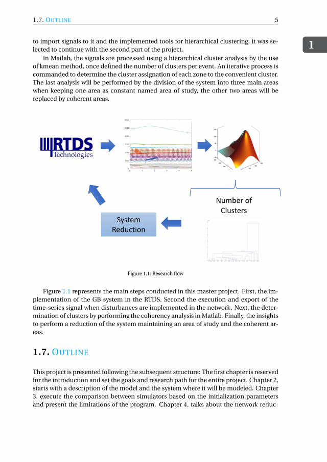
Figure 1.1: Research flow

Figure 1.1 represents the main steps conducted in this master project. First, the im-plementation of the GB system in the RTDS. Second the execution and export of thetime-series signal when disturbances are implemented in the network. Next, the deter-mination of clusters by performing the coherency analysis in Matlab. Finally, the insightsto perform a reduction of the system maintaining an area of study and the coherent ar-eas.

1.7. OUTLINE

This project is presented following the subsequent structure: The first chapter is reservedfor the introduction and set the goals and research path for the entire project. Chapter 2,starts with a description of the model and the system where it will be modeled. Chapter3, execute the comparison between simulators based on the initialization parametersand present the limitations of the program. Chapter 4, talks about the network reduc-

1

6 1. INTRODUCTION

tion, from extracting the information from RTDS to use time-series data to cluster theelements. Chapter 5, present the results of the clustering and the GB model with spec-ifications for studies. Chapter 6, detail the conclusions and recommendations of theproject, plus possible applications for future work. Finally, the scripts and annexes areattached.

Figure 1.2: Thesis Work Flow

2GB MODEL IN RTDS

2.1. DESCRIPTION

The Great Britain (GB) model already implemented in Power Factory consists of twenty-nine zones interconnected by nineteen nine transmission lines with one single circuitand forty-nine double circuits. This representation was delivered to TU Delft as part ofthe Migrate project, and it represents the dynamic model of GB. In the model, northareas have a nominal voltage of 275 kV while the center and south areas have 400 kV.Parameters of each element (generators, buses, lines, transformers, compensators, andloads) were specified for this model. Indeed, this model represents a reduction of thesystem; it could be confirmed analyzing the transmission lines, all lines have a length ofone kilometer which is a representation performed for dynamic purposes.

Figure 2.1 shows the geographic GB model with the 29 zones distributed in their area.This image just describes an overall view of the system, the red lines are in 275kV, whilethe blue lines are the circuits in 400kV. It must be mentioned that this model does notrepresent any interconnection outside the twenty-nine zones.

Detailed information about the GB system, as well as their representation in theRTDS will be presented in this chapter. Table 7.2, reveals the values of parameters usedto their model in Power Factory.

2.2. REAL TIME DIGITAL SIMULATOR

Real Time Digital Simulator (RTDS) is world’s first real time digital power system simu-lator. It consists of two main components custom software and hardware designed forthe study of Electro-Magnetic Transient simulations (EMT). The real time requires par-allel processing in order to compute the state of the system during the time step defined.Time steps are in the order of 25µs to 50µs. One of the main advantages in comparisonwith other software simulators is the possibility of performing studies faster than with

7

2

8 2. GB MODEL IN RTDS

Figure 2.1: GB network representation of 29 Zones [1, 2]

offline simulators [3]. Even though RTDS is also used for closed loop testing of controlcomponents and protections, that characteristic will not be mentioned in the presentproject.

Another characteristic of the RTDS is the capacity of scalability due to the incorpo-ration of new processors or elements according to the purpose of the final user. As thecomponents are mounted to the network, several users can work in parallel to run dif-ferent simulations. Hardware components and software description will be presentedbelow.

2.2.1. RTDS HARDWARE

RTDS have a modular design, which allows the incorporation of more cubicles accordingto the necessities of the user. TU Delft has installed four cubicles, and in each cubicle areinstalled two racks. Main elements which are part of the rack are presented in figure 2.2.where:

GTWIF, is in charge of data exchange between the commands sent from the user tothe system as well as the results from the system to the user. It makes possible the in-terconnection between six other racks via fiber optic. Moreover, It enables the parallelconnections between hardware and workstations via Ethernet. PB5, this card allows toprocess the network solution; it can handle 72 single phase nodes and 100 single phase

2.2. REAL TIME DIGITAL SIMULATOR

2

9

Figure 2.2: Rack Components

switches per rack. Nevertheless, the number of nodes can be doubled to 144 adding asecond PB5 processor to the rack. GBH, it is in charge of keeping and handle the sametime-step for the racks. Finally, GTNETx2, allows the communication with external de-vices and handle IEC 61850 protocol.

2.2.2. RTDS SOFTWARE

SOFTWARE: RTDS is formed by seven different modules which allow the system to build,design and run circuits. All these modules contain a graphic interface and a user-friendlymanage. The use of the modules is related mainly to the finality of the user, even throughDraft and RunTime modules are indispensables to create and execute simulations.

Draft Module: It is the environment to design the network, as well as other simulatorsthe function of drag and drop is able. Single point connection or three-phase connec-tions provide facility to interconnect elements. All elements are found in the library, andnew libraries can be developed. In this module, the parameters of the system must beinput, as well as the time step and the subnetwork division. Figure 2.3 presents the spacefor modelling at the left and the library at the right of the figure.

RunTime module and Multiplot, after designing the network another environmentcalled RunTime allows executing the simulation. Moreover, control and export the re-sults of the simulations. Additionally, it also offers a graphic editor to present the resultsin different ways. Included in this module, the possibility to execute scripts to start, stopand control of the parameter and elements of the simulation is enabled. These scripts

2


are in C-programming language which makes easy the execution. Figure 2.4 representsa plot and controls for a circuit modeled in RTDS. FileManager module, it provides anorganized way to keep different simulations. All archives created or imported are visibleand accessible from this module. T-line module and Cable, it allows creating detailedmodels of the transmission lines, it is important to take into account that names of linesin draft mode must match the names from the t-line creation. Finally, CBuilder, it createscomponents under the requirement of the user. A graphical representation and controlover the menus can be added.

Figure 2.3: Draft Module in RTDS

Figure 2.4: RunTime Module in RTDS

2.3. GB MODEL IN RTDS

2

11


The version of GB model which is considered as an input for this thesis is the one mod-eled in Power Factory. In the model, there are 29 interconnected zones representing thedynamic network behavior of the GB system. The first challenge in modeling the GB sys-tem in the RTDS is the lack of conversion tool from Power Factory to the RTDS. Due to,the system was modeled from scratch using the information available from the elementsin power factory.

While implementing the GB system in RTDS several drawbacks and limitations ap-pear. The limited number of racks and processors available in the system, the high pro-cessor consumption when modeling wind turbines and the size of the system does notallow a full implementation of the model in the RTDS. The next subsection will explainthe limitations of the RTDS when conducted the project as well as the solutions and as-sumptions developed for overcoming the restrictions.

2.3.1. BASELINEThe model of the GB system in Power Factory was delivered to TU Delft as part of theMigrate Project. It consists of 29 electrical zones interconnected as presented in the fig-ure 2.5. The baseline scenario contemplates a dispatch considering the actual elementswhich are part of the GB system. The baseline reflects a dispatch in the year 2016. Themodel with lines and voltage levels were extracted from the "Electricity Ten Year State-ment 2016" from UK electricity transmission[4].

This scenario is the main focus of the project, the complete scenario will be mod-eled in the RTDS under certain restrictions and assumptions developed in this chapter.In the figure 2.5, each block represents an electric area mainly integrated by a bus bar,generators, loads, transformers, and compensators. The figure describes the size andinterconnection in the GB network. A similar output will be obtained in the RTDS, withthe use of subsystem as detailed next. The dispatch, as well as the characteristics of themodel, were extracted from the model in Power Factory. The table 2.1 presents the gen-eration and load values implemented as a dispatch in the RTDS. Figure 2.5 presents thedistribution of the zones in the GB system. Each zone corresponds to a substation, dueto in each of the zones generators, buses, transformers, loads, and compensators are in-stalled. In zones one, two and three, and four the voltage level is 275kV. In the rest ofthe areas, the voltage level is 400kV. Figure 2.6 is an example of how a zone is displayedin the RTDS. Additional to the elements of the substation, fault points and fault logicpoint must be added to allow simulate faults in the system. Fault points and logic will beexplained later in the chapter.

2


Figure 2.5: GB model in Power Factory [3]


2

13

Figure 2.6: GB model in Power Factory [3]

2


Table 2.1: GB System Baseline 2016[4]

Baseline Case 2016

Region Substation

SynchoGen-erator(GW)

WindGen-erator(GW)

ActiveLoad(GW)

ReactiveLoad(MVAr)

WindGen-eratorDis-patch(GW)

SynchroGen-eratorDis-patch(GW)

Scotland

1 1.08 0.8646465 0.53 110.25 0.856 0.943742 1.08 0.8684848 0.53 110.25 0.8598 0.947933 1.08 0 0.53 110.25 0 04 1.08 0.849798 0.53 110.25 0.8413 0.927535 1.08 0 0.53 110.25 0 06 1.08 0 0.53 110.25 0 07 1.08 0.8512121 0.53 110.25 0.8427 0.929088 1.08 0 0.53 110.25 0 0

NorthEng-land

9 3.78 0.725 3.25 682.50 0.71775 0.79132

10 3.78 0.725 3.25 682.50 0.71775 0.7913211 3.78 0.725 3.25 682.50 0.71775 0.7913216 3.78 0.725 3.25 682.50 0.71775 0.79132

WestEng-land

12 3.77 0.2 2.17 455.00 0.198 0.2183

13 3.77 0 2.17 455.00 014 3.77 0.2 2.17 455.00 0.198 0.218315 3.77 0 2.17 455.00 017 3.77 0 2.17 455.00 018 3.77 0 2.17 455.00 0

EastEng-land

19 1.95 0.5495 1.88 393.75 0.544005 0.5997

20 1.95 0.55 1.88 393.75 0.5445 0.6003SouthEng-land

21 1 0 2.06 431.67 0

22 1 0 2.06 431.67 023 1 0.497 2.06 431.67 0.49203 0.542424 1 0 2.06 431.67 025 1 0 2.06 431.67 026 1 0.504 2.06 431.67 0.49896 0.550127 1 0 2.06 431.67 028 1 0 2.06 431.67 029 1 0.4995 2.06 431.67 0.494505 0.54519


2

15

2.3.2. TRANSITION SCENARIOS

As extracted from the electricity ten-year statement 2016 [4], two different type of sce-narios are developed fo the future of the GB system. These scenarios are centered on theexpected behavior of the BG system for the coming years. Even though one of the focuspoints is to reach the 2050 carbon reduction target, one of the scenarios does not havehigh expectation in the increasing installation of renewable sources of energy. This sce-nario is called NO PROGRESSIVE and although consider new renewable installations, itdoes not consider that the increment will be drastic.

On the other hand, the second scenario called GONE GREEN proposes a series ofpolicies interventions, as well as, innovations to reduce greenhouse gas emissions. Thisscenario assumes an investment of more money and more focus in the long-term greenambition [4]. Due to limitations in collecting information, the NO PROGRESSIVE sce-narios will not be modeled in the RTDS. Moreover, the GONE GREEN scenarios will beimplemented in the RTDS as well as the baseline model.

GONE GREEN scenarios present four future scenarios for the coming years 2020,2025, 2030 and 2035. The replacement of synchronous generation, also the installationof more wind generation will describe the characteristics of this new scenarios. Table7.4, table 7.5, table 7.6, and table 7.7 presented in the Annex 7.3: GONE GREEN TABLES,will present the dispatch and the type of generation for each of the future scenarios.

2.3.3. COMPONENTS

The 29 Zones of the GB system developed in Power Factory contain several elements tobe modeled in the RTDS. Due to keeping the scope of the thesis to synchronous gener-ators and the lack of wind generator models in the RTDS. An important assumption re-garding the replacement of wind generators by synchronous generators is explained inthis section. The rest of the GB system components are presented next to a small detailof the menus for modeling each element. The majority of the parameters were extractedfrom the Power Factory and implemented in the RTDS using as guide [3].

SYNCHRONOUS MACHINE MODEL

The RTDS Library offers several types of models for generators. Each of them has theirown characteristics and are used depending on the type of generation and the proper-ties required by the user. Figure 2.7, represent the model used in the RTDS, this model,as well as the model in Power Factory, correspond to the 7th order. The name of the gen-erator is "RTDS_SHARC_MAC_V31", and can be located in the main library in the draftmode. Additional to the generator an exciter, governor, and PSS can be coupled.

For study convenience, the parameters of the Generator, as well as the AVR and Gov-ernor controllers were adjusted as close as possible to the elements from the Power Fac-tory. Even though, all controllers can be modified in function of future studies. An ad-vantage of using this model is that it has incorporated the possibility of automaticallyconnecting a transformer at its output. The internally connected transformer not onlyreduce the number of connections, but also three single electrical nodes can be saved.

2


In most of the cases, this transformer was not used due to the limitation of only allow tochoose a delta-Y connection for the transformer.

Figure 2.7: Synchronous Generator RTDS [3]

It must be taking in consideration the importance of the selection of signals for futureplot and analysis. A complete guide for configuration of each parameter of the generatoris presented in [3]. Parameters like apparent power, voltage and frequency were kept asthe same as the parameters presented in Power Factory.

WIND GENERATORS

Wind Generators are part of the baseline model of the GB system for the year 2016. Animportant assumption was made with the wind generators. As the modeling of windgenerators in the RTDS are part of a different study. It was discussed the possibility ofrepresenting the wind generators as synchronous generators with active power and re-active power constant. It was also discussed that inertia must be reduced in order toadjust as much as possible to the wind generator behavior. It is expected in future tasksthe integration of wind generator model to the GB system in the RTDS.

TRANSFORMER

As well as Generators there are diverse types of transformers available in the library ofthe RTDS. The transformer selected is as similar as the transformer in Power Factory,the model in the library of the RTDS is the "TRF3P2W". It is a three phase two windingtransformer model; it has three modes: ideal, linear and saturation. And it can be used inany of the modes depending on the information assigned as input. This transformer alsohas the possibility of addition tap changer. Even though no tap changers were modeledfor the simulations.


2

17

For the simulations, the transformer was modeled as an ideal transformer, where themagnetizing inductance is neglected, and the only reactance take into account is theleakage reactance. RTDS also neglect the winding resistances; it assumes these as thevalue of zero. Figure 2.8a presents the symbol of the transformer in the RTDS wherethe winding configuration can be modified. Fig 2.8b is the representation of the idealtransformer used by the RTDS with no magnetizing path.

(a) Transformer Model RTDS (b) Ideal Transformer in RTDS

Figure 2.8: Transformer in RTDS [3]

BUS BAR

There was no difference in the type of bus bar in the RTDS and Power Factory. The onlydifference is the way of each software to define the type of bus. while in Power Factory thetype of bus is defined by the generator or load connected to it, in RTDS it is necessary todefine the type internally in each bus. Figure 2.9, present the input menu for configuringa bus bar in the RTDS. The parameters Vd and Ad will display the values of the power flowresult in voltage magnitude and angle when a power flow is run in the draft mode.

TRANSMISSION LINE

In RTDS there are two types of transmission lines available in the library, depending onthe study to perform and the own characteristic of the lines to model. Travelling wavemodel and Pi section model represent the behaviour of transmission lines in the RTDS.Nevertheless, the different representation implies that PI model uses lumped parame-ters, while travelling waves uses distributed parameters. One of the advantages of usingtravelling wave models is the reduced processor consumption compared with the PI sec-tion model. Travelling wave models are also required in order to interconnect bus barsfrom different subsystems.

In the Figure 2.10, three elements are presented for a transmission line in the RTDS.The calculation block, where it is possible to define the type of transmission line, andthe send and reception side of the transmission line. Using the PI model is plausible.Nevertheless, integration time step of the system must be taking into account. In orderto work correctly, the travel time step defined for the transmission line must be at least

2


Figure 2.9: Bus modelling in RTDS [3]

Figure 2.10: Transmission Line in RTDS [3]


2

19

equal to the single integration time implemented. It is compulsory to mention that alltransmission lines distances in Power Factory were set as 1 Km, due to traveling wavemodels will be implemented the in RTDS and will be discussed in the next chapter. Thefinal distances of transmission lines, as well as the equivalent parameters of reactance,capacitance, and susceptance, are presented in table 7.2.

Additional to the information provided in DRAFT mode of the RTDS, it is necessaryto create transmission lines to input the parameters of the lines. RTDS use a comple-mentary interface called "Tline setup". figure 2.11 and figure 2.12 present the interfacewere the electrical parameters of the transmission line must be entered. RTDS allows toinput physical information about the lines and configuration; Even though, it will not beused for the GB model.

Figure 2.11: Tline Setup in RTDS

The transmission line selected for the project due to the use of multiple subsystemsis the traveling wave. In order to select this type of line, some basic concepts must betaken into consideration: subsubsectionSimulation Time Step It is the time required forthe system to process data[3] Based on electromagnetic waves the Propagation of thevelocity is defined by the equation 2.1, and the traveling time by the equation 2.2.

V p =√

1

L∗C(2.1)

t p =p

L∗C (2.2)

Due to system requirements citemanual, in order to handle and manage data, if trav-eling time in a transmission line is less than the simulation time step. Then a Pi modeltransmission line can be used. It must also be considered that Pi model transmission

2


Figure 2.12: Electrical parameters of Tline in RTDS

lines do not allow connection between subsystems. For that reason, if it’s required to usetraveling waves a readjustment of the distance and the parameters of the line is compul-sory.

For example, assuming a propagation velocity equal to the speed of the light and asimulation time step of 50 µ s, then, the minimum distance for a transmission line tobe modelled as traveling wave is 15 Km. If it is not the case in base of that distance thecapacitance and inductance of the transmission line must be recalculated. Figure 2.13shows the algorithm used for selecting transmission line types in the RTDS.

As required for the several interconnections between subsystems, and taking intoconsideration that traveling waves produce less computational effort. All lines weremodeled as traveling waves. Power Factory model keeps all transmission lines with alength of 1km, then all parameters of the transmission lines were recalculated as well asnew distances are presented. Table 7.2 presented as a show the new values and distancesof the transmission lines that were used to model in the RTDS.

CAPACITOR AND REACTOR

Capacitors and Reactors are defined by their capacitance and inductance value. Thisvalues were taken from Power Factory, and converted from MVAR to capacitance valuesµ F. Figure 2.14, present the menu to implement the capacitor in the RTDS.

LOADS

There are several classes of loads available in the library of the RTDS, According to thePower Factory, all loads are constant for this model. To simulate the same behavior inthe RTDS, static loads were selected at the beginning of the model. Even though, if the


2

21

Figure 2.13: Transmission line selector process in RTDS

Figure 2.14: Shunt Capacitor in RTDS [3]

2


simulation involves an increase or decrease of the load, it is necessary to change manu-ally the parameters and not from the runtime. This drawback was solved, using dynamicloads with fixed set values of active and reactive power. To give flexibility to the loads,it is set +−50% of the set value for the maximum and minimum limit of the load. If it’snot required the values of the minimum and maximum limits could be the same as theinitial. Figure 2.15, present the window were the parameter of the load can be modifiedin the RTDS.

Figure 2.15: Dynamic Load as Constant Load in RTDS

2.3.4. LIMITATIONS

As reviewed at the beginning of the chapter, using RTDS has many advantages regardingprocessing and velocity that are not possible to achieve with a different kind of software,due to the physical particular hardwe equipment it handles. Nevertheless, as all of theequipment, there are limitations which dictate the way to use the system. These limita-tions are specified for the system used for the preparation of the document. There aretwo main drawbacks founded in the use of the RTDS to simulate the GB system.

• The number of calculations must not overpass the time step specified.

When working with big systems, it is distributed in several subsystems. Even thoughthere is the possibility to have as many elements and controls as it is allowed, butthe system can not handle to complete the process by the end of the time step. Ifthat is the case, then it must be considered to reduce the number of calculationswith a new distribution of the elements. If it is not possible to reduce the elements,then the time step must be increased to let the system more time to handle withthe calculations. It must be noticed that a new time step will affect the system ifthere are transmission lines modeled as traveling waves. Then the transmissionlines must be recalculated as showed in the last section. In order to simulate faultsthe time step was increased from 50us to 60 us for simulation purposes.

• The system can not handle an infinite number of electrical nodes


2

23

The system can not handle an infinite number of electrical nodes. As the majorityof the simulators, there are limitations in the number of elements. As presentedat the beginning of the chapter, the RTDS used in the thesis is composed by sixracks, each rack has the PB5 processor card which allows handling a maximumof 72 single phase nodes and 100 single phase switches. Even though it was alsomentioned that the number of nodes could be doubled to 144 adding a second PB5processor. It mus be noticed that the main drawback trying to use less quantity ofracks for modeling the GB system was the processors that the RTDS can handleper card. Figure 2.16, is an example of the use of cards with the processors in asubsystem. If the number of processors is higher than the system capabilities, theuse of a new subsystem is required.

2

242

.GB

MO

DE

LIN

RT

DS

Figure 2.16: Processors behavior in the RTDS per subsystem


2

25

Due to this limitations, the version of the GB system in the RTDS uses four racks. Usethis number of racks is not the best solution taking into consideration that the universityhas a total of 6 racks. Due to this model, a reduction of the system must be recommendedif future analysis requires incorporating new elements like dynamic loads or wind gen-erators. Next chapter will develop a coherency analysis to provide recommendations forthe future use of the GB model in the RTDS.

.

2.3.5. IMPLEMENTING THE GB SYSTEM IN THE RTDS

Knowing the components available and the limitations of the RTDS. The GB model wasimplemented in the draft mode of the RTDS, all parameters and configurations weretaken from the Power Factory model. Then the system is implemented in four subsys-tems (4 racks). The distribution of the zones in the RTDS system was determined aspresented next:

• Subsystem 1: Zone 1, Zone 2, Zone 3, Zone 4, Zone 5, Zone 6, Zone 7.

• Subsystem 2: Zone 8, Zone 9, Zone 10, Zone 11, Zone 12, Zone 13, Zone 14, Zone 15.

• Subsystem 3: Zone 16, Zone 17, Zone 18, Zone 19, Zone 20, Zone 21, Zone 22, Zone23.

• Subsystem 4: Zone 24, Zone 25, Zone 26, Zone 27, Zone 28, Zone 29.

The first version of the model keeps the system with visible interconnections betweenZones. Four subsystems are used to implement the model. Figure 2.17 represents thefirst version of the GB model in the RTDS, it is notable that each of the squares repre-sents a subsystem. Even though this version allows a fast supervision of the system; it isnot practical when new elements or modifications are required in it. A new where eachzone can be independent of the other allows to implement new components as well asdelete or modify unnecessary ones. This new modeling design is important for a fastimplementation of the rest of scenarios described for the GB system.

A final version of the system was modeled with the substitution of wind generatorsby synchronous generators, achieving a balance between generation and load. In thisversion, the zones present independent connection due to the use of traveling wavestransmission lines for interconnection between zones. This version allows moving areasto another subsystem which will represent a huge advantage in future studies. Figure2.18 presents a subsystem where the zones are separated and modeled inside each ownbox. Once finalized the modeling both systems must have similar behaviors. However, aparameter initialization comparison is required in order to confirm that all parameters,as well as the model, represent the GB model of the Power Factory in the RTDS.

2.3.6. INITIALIZATION COMPARISON

Figure 2.19 presents a zone modeled in power factory and the same zone modeled inRTDS. The main difference is that in power factory the generator controllers are designed

2


Figure 2.17: GB mounted in the RTDS


2

27

Figure 2.18: Representation of Zones in RTDS

inside the generator, while in the RTDS all controllers have a graphical representation.When all elements of the power system are modeled and interconnected. The initializa-tion of the parameters used for each element must be tested. To evaluate the balancebetween generation and load, and obtain the values of voltage magnitude and voltageangle it is required to perform a power flow. RTDS and Power factory allow simulating apower flow using the same method called Newton Raphson [22]. Due to this character-istic in the RTDS it is possible to compare that initialization values are compatible withthe values obtained in Power Factory.

As the model in power factory is running with no problem, it is feasible to extract theresults of a power flow as a text file. This advantage is not possible at the moment in theRTDS; however, there are some files in the RTDS which make possible to compare thepower flow without the necessity of review inside each of the bus bars the results of thepower flow.

In order to obtain the power flow from the RTDS, two files must be taking into con-sideration: ".rtp file" and ".dtp file". ".rtp file" is the file wich contains the parametersof the dynamic devices of the system modeled in RTDS, is it similar to ".raw" file used inPSS/E; both files have the same sequence. ".dtp file" it contains the network of the mod-eled system, it also contains the information of the buses and generators after running apower flow.

Using the ".dtp file", it is possible to extract the voltage angle and magnitude of eachbus bar of the network. A macro developed in Excel called "PowerFlow_extraction" al-lows extracting the information of the power system using the file which can be found inthe folder where the simulation is running, or it can be exported from the draft mode toany location in the system. The macro is attached as Annex 7.1 to the project.

2


Figure 2.19: Comparison a Zone in RTDS and Power Factory

Annex 7.1, locate the bus bars in the file extracted from the RTDS, once locatedthe bus bars it select the values of voltage angle and magnitude after the power flowis achieved. When the voltages in magnitude and angle are available from both systems,they are compared in order to demonstrate that the initialization parameters are com-patible in both systems.

Figure 2.20, present the voltage magnitude in both systems when a power flow isperformed in both systems. It can be noticed that the generator of the Zone 10 is theslack bus bar of the system. All magnitudes are similar with the magnitudes in PowerFactory. Even though, the system in RTDS replace the wind generators by synchronousgenerators.

Figure 2.21, is the angle magnitudes in the bus bars of the electrical power system.It can be noticed that not only the voltages are similar in both systems, the angle mag-nitudes have a slight difference due to the loss in conversion of the parameters of thetransmission lines. Even though the values are compatible, and the power flow does notpresent any major difference in both systems.

2.3

.GB

MO

DE

LIN

RT

DS

2

29

Figure 2.20: Comparison of Voltage Magnitude between systems

2

302

.GB

MO

DE

LIN

RT

DS

Figure 2.21: Comparison of Voltage Angle between systems


2

31

In this chapter, the GB model was presented. Additionally, the limitations of the sys-tem define the numbers of resources to use. Afterwards, the GB system was modeled inthe draft mode of the RTDS, a power flow simulation was performed in order to com-pare the initialization results of voltage angle and magnitude with the results obtainedin Power Factory. Figure 2.20 and figure2.21 present the power flow solutions for theBaseline case of the GB system. Nevertheless, due to future developments and studiesinvolving the system, and future element integrations to the network; It is required tosuggest a possibility on how to perform studies over the same model by reducing thenumber of racks used to simulate and evaluate the system. Next section will demon-strate the possibility of reducing the GB system in the RTDS using the time-series signalswhich are an output of the simulators due to the lack of Modal analysis.

Finally, as an extension of the project, Gone Green scenarios for the years 2020, 2025,2030 and 2035 were also modeled in the draft mode of the RTDS. The gone green scenar-ios represent modifications not only in the dispatch of the generation and consumptionof the loads but also in the replacement of the synchronous generators with wind gener-ators in the system. All values used to model the future scenarios were taking from thetable 7.4, table 7.5, table 7.6, table 7.7 for the years 2020, 2025, 2030 and 2035 respec-tively [4]. Gone green scenarios will also be considered in the suggestions for reducingthe size of the power network due to the same limitations presented in the resources ofthe simulator.

3REDUCTION OF GB SYSTEM FOR

STUDY OF TRANSIENT STABILITY IN

RSCAD

3.1. BACKGROUND

Once modeled the GB system in the RTDS, and due to the hardware limitations pre-sented in the last chapter. It is required to reduce the model in order to use it for tran-sient studies. Transient studies are focused in the fast response of the elements of a spe-cific area when subjected to disturbances, more than the general response of the wholesystem. GB model contains 29 zones, using a total of four racks for the simulation inthe RTDS. With the finality of using fewer components of the hardware, and focus thestudies in smaller areas; A reduction of the system is presented in this chapter. Severalconcepts about reduction will be presented, as well as the methodology to apply it in themodel.

To start with the reduction of the system, it must be taking into account that unlikePower Factory, RTDS does not offer the possibility of extracting the state matrix, or per-form an eigenvalue analysis. The state matrix of the system is under development, andeven though is not the topic of the chapter, it can be referred to [23] for further informa-tion. As RTDS is limited in the eigenvalue analysis, a method using information providedfrom the RTDS is presented. The method will make use of the time-series signals whichcan be extracted from RTDS. The signals will be imported to Matlab to perform a clusteranalysis.

32

3.2. DYNAMIC COHERENCY FOR REDUCTION

3

33


The high computational effort required in order to perform transient stability analysis,derive on the focus of the study to small areas leaving the rest of the system to be con-sidered as external areas. Under this consideration not only the computational require-ments can be more relaxed, but also faster responses can be expected. The identificationof the areas must be considered when a strong coupling can be detected with different el-ements inside the area. If there is no strong coupling between the elements, then thoseelements are part of different areas. Different theories and computational algorithmshave been developed to identify, and aggregate elements to clusters [24]. Most of themmake use of the state matrix and eigenvalue analysis. As explained RTDS does not allowsuch facilities to perform those mechanisms. Nevertheless, clustering time-series sig-nals could fulfill the requirements to determine the cluster identification; furthermore,the system reduction.

3.2.1. COHERENCY ANALYSIS

In order to speed up the computation times due to specific vulnerabilities, the systemwill be analyzed by zones. Once selected the focusing area, this is modeled with enoughdetail to represent the behavior of the area. The rest of the areas connected to it arereplaced by dynamic equivalents sufficient to reproduce the same influence as the orig-inals. A general method for determining dynamic equivalents for system reduction con-sist of three steps [24]:

• Cluster identification: The first step in the reduction of electrical power systems is theidentification of generators and bus bars which have a coherent behavior. Thereare two main groups of mechanisms based on the elements used to perform thistask. The model-based coherency identification, and the measurement-base co-herency identification. As mention before, the first method [10, 25] requires aknowledge of the state of the system in order to perform an eigenvalue analysisof the linearized model. The second group is based on measurements, in order toidentify coherency based on signals from the system more than the state of it. Dueto the lack of state matrix from the system the method selected rely on the signalswhich should be extracted from the system.

The coherency identification based on time-series analysis is performed using twoparameters of the system the rotor velocity and the active power magnitude at theterminals of the machine. Both parameters are extracted from the system as aresponse of the system when applied several contingencies. Later, with help ofmathematical tools (Matlab), clustering analysis are performed in order to deter-mine the number of clusters and elements which are part of them, based on thesignals extracted from the system. The methodology used for performing the clus-ter analysis is presented in the next section.

• Element aggregation:

3

34 3. REDUCTION OF GB SYSTEM FOR STUDY OF TRANSIENT STABILITY IN RSCAD

When identified the coherency of the system, (using the clustering analysis); anequivalent Generator and Bus Bar is placed in order to represent the behavior ofthe cluster it belongs. According to the topology, different clusters with differentelements could be founded [26]. All results and conclusions of the analysis will bepresented in the next chapter.The element aggregation of generators consists ofaggregate the coherent machine group into a single equivalent machine, to nexteliminate load buses from external systems. After the aggregation, the system willbe reduced [9].

• Estimation of parameters:

Finalized the determination of clusters, the elements which belong to each of it,and the selection of equivalent elements, the GB system will be reduced. In com-parison with the 29 Zone model, the expected result will be a system where mainareas can be distinguished and modeled to perform rotor angle stability studies.

3.2.2. COHERENCY ANALYSIS

Figure 3.1: Algorithm of Coherency Analysis

Figure 3.1, present the coherency identification steps performed in the project. The


3

35

first part in the RTDS the operation condition is defined taking into account the modelof the system and preparing the system to run disturbances on it. After evaluating thatthere are no initialization problems, the scripts developed in the RunTime mode are ex-ecuted.

Several scripts were prepared to extract the information from the RTDS. Most of thescripts have the same format. The variables must be initialized; next, the simulationstarts. Subsequently, the disturbances are executed and finally, the signals from the plotsare stored on the local machine. The simulation time for all simulations is 5s. It is consid-ered for bus-fault contingencies, it is necessary to define the logic of the fault (presentedin chapter 2) and connect the fault point in each bus bar. The faults in the buses are setto occur at the 1.25s of the simulation time with a duration of 150ms. For Line Switching,it is necessary to modify all transmission lines adding a switch to each side of the line.The logic defined will open both sides of the line at the same time. Finally, the load willbe increased by 50% of the active power of each load.

SIGNALS EXTRACTION:

The first step to export signals is prepared the network for running different disturbances.Fault points are mounted in each bus of the system, as well as switches in lines and slidesfor modifying the loads. Later, the script is developed in RTDS in order to plot in the onegraph the response of active power of each generator. And in another graph the rotorvelocity of each of the generators. Both graphs reflect the response of the generatorsof each area when subjected to 3 phase fault in each bus-bar, line disconnection, andan increase of fifty percent in each of the loads. Once the plots are produced, it will beimported to Matlab as will be explained in the next section.

Main concepts, as well as the implementation of each algorithm, are explained bel-low. It must be stressed that in order to develop a baseline case, the model of the systemready in RTDS and the disturbances conditions must be evaluated before. Figure 3.1,presents the algorithm designed to run the cluster analysis.

3.2.3. CLUSTERING IDENTIFICATION

The second part of the algorithm showed on blue in the figure 3.1, was performed inMatlab. The coherency identification uses as input the signals extracted from the RTDSin the last step. In this section not only the clustering algorithm used will be presented,but also the way of how it was performed with the baseline scenario 2016. Importantconcepts of the clustering determination will be reviewed next.

EUCLIDEAN DISTANCE

The Euclidean distance is a metric function; it is commonly used as a basic measure fortime series similarity. Equation 3.1 represent the basic equation for calculating the dis-tance between two points, where a[i ] and b[i ] are two distant points. When a series ofsequences need to be compared, the equation 3.2 is used; where A, is the matrix con-taining the series of sequences, with the same length (in the project case time), and Bis the signal or set of signals to compare, the result will be a matrix with the distances

3


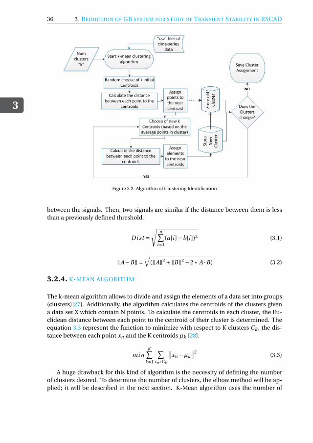
Figure 3.2: Algorithm of Clustering Identification

between the signals. Then, two signals are similar if the distance between them is lessthan a previously defined threshold.

Di st =√

n∑i=1

(a[i ]−b[i ])2 (3.1)

‖A−B‖ =√

(‖A‖2 +‖B‖2 −2∗ A ·B) (3.2)

3.2.4. K-MEAN ALGORITHM

The k-mean algorithm allows to divide and assign the elements of a data set into groups(clusters)[27]. Additionally, the algorithm calculates the centroids of the clusters givena data set X which contain N points. To calculate the centroids in each cluster, the Eu-clidean distance between each point to the centroid of their cluster is determined. Theequation 3.3 represent the function to minimize with respect to K clusters Ck , the dis-tance between each point xn and the K centroids µk [28].

mi nK∑

k=1

∑xnεCk

∥∥xn −µk∥∥2 (3.3)

A huge drawback for this kind of algorithm is the necessity of defining the numberof clusters desired. To determine the number of clusters, the elbow method will be ap-plied; it will be described in the next section. K-Mean algorithm uses the number of


3

37

clusters and first, it define the centroids (center of a cluster), it is determined by an itera-tive process where the distance between signals are used, and the minimum distance tothe other elements is so-called centroid. By an iterative process, each signal is comparedwith the other to determine the similitude between them. Once obtained the similitudebetween signals, those who present more similar behavior (shape) are grouped into acluster.

In order to solve equation 3.3, it is required to use an iterative method, as the methodpresented by Lloyd’s [28]. This algorithm converges in few steps finding a solution fora local minimum. The method as can be seen in the equations 3.4 and 3.5, consists intwo steps: First, check and set centroids for each of the clusters, once the centroids µk

have been established, the clusters are updated in function of the closest points to eachcentroid. Finally, with the set of clusters placed, the centroids are recalculated in orderto set as the mean of all points who belong to the cluster.

Ck = Xn :∥∥Xn −µk

∥∥É al l∥∥xn −µl

∥∥ (3.4)

µk = 1

Ck

∑xnεCk

xn (3.5)

Figure 3.2, presents the "kmean" algorithm used for determine the number of clus-ters [28]. The algorithm uses the time-series signals extracted from the RTDS 7.6 as inputas well as the number of clusters as discussed in the kmean algorithm. Later, the methodto determine the number of clusters will be presented.

The algorithm assumes the number of clusters is known and fixed. When the inputvariables are determined, the first step of the algorithm starts selecting random centroids(center of the clusters) per each cluster. Using the centroids the algorithm calculates thedistance between each point to the centroids. Additionally, the algorithm will aggregatethe points to the closest centroid and it will store the cluster.

In the second step, a new set of centroids is calculated based on the average pointsinside each cluster. New distances are calculated between the points of the signal andthe new centroids. The process continues normally grouping the elements to the nearcentroids and store the new cluster. The cluster stored from the first step is comparedwith the one in the second step if there are no changes in the clusters the algorithm finishrunning and save the final cluster. Nevertheless, if the cluster from the second step isdifferent from the cluster in the first step, the cluster from the second step is stored anda third step is executed.

The algorithm will repeat the steps until the last cluster is equal or tolerably similarto the cluster stored in the previous step. The algorithm is performed in Matlab usingthe command "kmeans", it returns the assignation of the signals to the clusters, but thenumber of clusters must be defined at the beginning of the process. In order to obtainthe number of clusters “k”, in the first instance, the same algorithm is used. The algo-rithm must be run several times with different values of "k".

3


3.2.5. ELBOW METHOD

This method is one of the oldest methods considered to find the number of clusters nec-essary for initialization parameters of the kmean algorithm. Elbow method is developedto find an "optimal" number of clusters based on the k-mean cluster algorithm reviewbefore [29, 30]. It uses the k-mean algorithms varying "k" to find the "optimal" or moreadjuster value of "k". It is a visual method which plots the distortion in function of thenumber of clusters selected. At the end, the curve obtained presents the distortion whichdecreases when using more number of clusters. The method reviews the graph obtainedand determine when an elbow is present. After that point, the distortion does not varyconsiderably. So the point when the curve changes from a rapid difference of distortionto a slow difference is called elbow, and the number of clusters of that point is selectedfor the case.

Even though, one of the drawbacks to taking into account is the computational effortas well as the time consuming for converging into a result. The results can be presentedas a curve in a two-dimensional graph of number of clusters vs. variance, where thesudden change in the curve represents the "optimal" number of clusters to take. Thefigure 3.3 is a representation of the elbow method handle for one of the data-series ofthe project. As can be noticed from the figure, at some point aggregate more clusters donot represent a significant increase in the percentage of variance[29, 30]. Elbow methoduses the f-test[30], which is the result of the group variance over the total variance 3.8, toplot the curve vs the number of clusters.

Dk = ∑xi εCk

∑x j εCk

∣∣∣∣xi −x j∣∣∣∣2 = 2nk

∑x j εCk

∣∣∣∣xi −x j∣∣∣∣2 (3.6)

Wk =K∑

k−1

1

2nkDk (3.7)

Using the concept of Euclidean distance review before, it is possible to determineintra-distances between points in a cluster. Equation 3.6, represent the sum of intra-cluster distances between points inside a cluster Ck , with nk elements. While equation3.7, measure the compactness of the cluster using the sum of squares. Wk is the variancequantity which allows determining the optimal number of clusters.

For the implementation in Matlab, the k-means method is used from k=1 to k= totalnumber of elements, after saving the results of all possible clusters, and using the elbowmethod the optimal number of clusters is determined. Then, with the "k" value discov-ered, the k-mean method is used getting the elements of each of the clusters. This algo-rithm is performed for each of the contingencies presented. The results are presentedin a matrix, where the first row represents the number of clusters for that scenario, andeach cell below is the element assigned to a cluster. The algorithm used in Matlab isdescribed in 3.4.

3.3. APPLICATION OF THE COHERENCY ANALYSIS TO THE GB SYSTEM

3

39

Figure 3.3: Elbow Method

Per cent ag e o f V ar i ance = bet ween g r oup var i ance

tot al var i ance(3.8)

3.3. APPLICATION OF THE COHERENCY ANALYSIS TO THE GBSYSTEM

Once reviewed the methods to perform a coherency analysis using time-series signals. Itwill be explained how the methods were applicated to the GB system signals.

3.3.1. DISTURBANCES IN THE RTDSRTDS does not offer a friendly interface to simulate disturbances. In most of the cases,the model must be altered to add elements or able switches. Later the simulations canbe controlled by the RunTime environment of the RTDS.

FAULT IN BUSES

A failure point and fault logic need to be connected to each bus bar in the power systemmodel. The failure point allows determining the type of failure to simulate ( 1 phase, 2phases, 3 phases and grounded or not), while the logic allows controlling the pulse du-

3


Figure 3.4: Algorithm implemented in Matlab to determine "k" by elbow method

ration and additional logics to control the disturbance. Both elements are implementedusing the library and modeled in the Draft-mode of the RTDS. Figure 3.5 present theelements to simulate a three phase fault in the RTDS.

(a) Fault Logic (b) Fault Point

Figure 3.5: Implementation of Faults in the RTDS

To all buses of the system with exception to the buses modeled as intern bus, a pointof fail plus a fail logic were connected. It must be considered that each variable musthave a unique name to handle the system. After connected all points, in the draft mode,the rest of the process is conducted in the RunTime mode. In RunTime mode, the signalsto export must be selected and presented in a Plot.

For the project, the Active Power (P) and the rotor angle (W)were selected to analyzethe behavior after disturbances. Due to, two different plots were prepared to export theactive power behavior and the rotor angle when applied a 3 phase fault to each of thebuses of the system. Once implemented the fault points and the logic. 3-phase faults of


3

41

100ms duration at 25% of the simulation time are set in all buses. Another benefit of theRTDS is the possibility of performing scripts to automatize the simulations. The scriptsmust be written in "C-language" and can control the entire RunTime environment.

Two scripts were developed to run and extract information of the RTDS system whenthe fault occurs in each of the buses. The script "P_busfault_Cases" and "W_busfault_Cases"are attached as an annex to the project.

The last part of the name of the scripts is "Cases," it makes reference to each timea fault is applied to a bus bar a Case is created for P and W. Each "Case" contains a setof signals for all the generators in the system. For Bus Fault in the Power System, thereare 62 cases extracted; it means that a fault was applied to each of the 62 bus bars in thesystem. And each case is stored in a folder organized by the name assigned from case 1to case62 for P and W, to create a database of signals for future analysis.

Annex 7.2 and annex 7.3, present the scripts which were developed in C language.Due to the extension of the script, there are just 3 cases uploaded. Even though therest of the script is the same for the rest of buses. The script starts with the definitionof variables. Then, with the command "Start" the Runtime Start the simulation of thepower system. After a pause to let the system stabilize after turning it on, the first fault isapplied to the fist bus bar in the system. Finally, a command to export the signals fromthe plot is executed and turn off the simulation. This script repeats the same actionsto each of the buses for the 62 Cases. At the end two files are stores ".out" and ".mpb’.The file ".out" contain the simulation with the signals which will be processed later. Thebehavior of both scripts, the main difference is the output. While the first case extractseach P of the generator, the second case extract W of each one.

LINE SWITCHING

The procedure with this type of disturbance is similar to the bus fault, but instead ofsetting fault points, the switches on each side of a line must be turned on. It must betaking into consideration the limitation of the number of switches per subsystem. Eventhough, the signal for opening and closing the switches can be used for both sides of thetransmission line. Figure 3.6, present the window where the switching will be configured.In the project, all lines were set with switches to able the opening and close. And thesame signal sends the order to command both sides of the switch at the same time.

Scripts in the annex7.4 and annex 7.5 obtain the cases for P and W when a line isopened in the system. There are 101 Cases for P and Q, due to most of the lines aredouble circuits, and the model was changed to switch one of the circuits per time. InRTDS is not possible to model parallel lines as a simple element, so two elements wererequired.

LOAD VARIATION

As reviewed in the last chapter, the loads used in the RTDS are dynamic loads with aconstant value of active and reactive power. The maximum and minimum limits of the

3


Figure 3.6: Configuration of the line breaker in RTDS

loads were configured with a possibility increasing of the active and reactive power con-sumption in and +- 50%. Due to this condition, the disturbance selected for a load wasan increase of 50% of the active power consumption. Scripts in the annex7.7, and theannex 7.9 present the structure to increase each load and collect the response of P andW in the system. There are 29 Cases, one per each load increased the value. Annex showspart of the script, even though the logic is the same for all loads.

3.3.2. COHERENCY ANALYSIS IN MATLAB

CLUSTERING IDENTIFICATION

Calculated k, which it was calculated using the elbow method, the algorithms will try toassign the elements to each of the k clusters defined by the centroids. First, initializeassigning the elements randomly to the centroids using the following algorithm, whichallows improving the Lloyd’s algorithm [28], according to the work developed by Arthurand Vassilvitskii [27]. One element is selected randomly from the dataset to be the firstcentroid (c1). Then, calculate the distances from each element (c j ) to the first centroidselected as (c1). The distance between an element (c j ) to the centroid m is defined asd(xm ,c j ). Then, new centroid is selected also randomly from the data set with the prob-ability determined by equation 3.9, where (cn1) is the new centroid . In order to find thecenter j, the distances from each element to each centroid are calculated, and suddenlyassigned to the closest centroid.

An iterative process involving all elements computation is executed to determine thedistance between each element to the closest center, until k centroids are determined.Once calculated the distances between all elements to each of the centroids, the ele-ments are assigned to the closest centroid. Finally, an iterative process of calculationof the average number of elements in each cluster to get k new centroids is performed.The process is repeated from the determination of the distance between elements andcentroids until the cluster assignment does not change.


3

43

cn1 = d 2(xm ,c1)∑nj=1 d 2(x j ,C1)

(3.9)

Figure 3.4 is a representation of the algorithm applied to determine the signals of thedata-series to their corresponding cluster. As can be appreciated, the number of clusters"k" is already assumed. Nevertheless, the value of "k" is calculated and demonstrated inthe next subsection.

The script uses the Euclidean distances to define the signals that can be clustered.Annex 7.8, calls one by one the cases extracted from the RTDS, then execute the algo-rithm of k-mean. It uses iteratively as input for "k" values from 1 to the maximum ofelements to be a cluster, and then using the variance curve, it obtains the optimal k(number of clusters). After that, it executes one more time the k-mean algorithm us-ing the optimal k founded in the last step. All elements of the case are then associatedwith a cluster and finally, creates a matrix where each column corresponds to a case andeach row to an element evaluated. The first row is the optimal number of clusters foundfor the case.

4ANALYSIS RESULTS

In the last chapter, the methodology to determine the number of clusters in the GB sys-tem was presented. For the necessity of reducing the size of the GB system to consumefewer resources of the RTDS, coherent areas were determined. The coherent areas repre-sent the cluster assignation of the zones which are not studied to model it with the studyarea. Additionally, different disturbances were applied in the elements of the completesystem, leading to the extraction of three variables of the generators, which represent thebehavior of the system.

This chapter presents the results obtained in the previous chapters plus an analysisfor the baseline case and future scenarios. In chapter 2, the GB system modeled with 29zones [2] was implemented in the RTDS. As a result, the 29 zones were distributed in 4subsystems. Nevertheless, it is necessary to reduce the number of subsystems (racks), toperform future analysis. Several cases will be presented to determine different ways ofreduction the GB system depending on the variables to analyze and the type of contin-gencies simulated in the system.

There are three types of contingencies applied to the model in order to evaluate thebehavior of the system. Such as faults applied in each of the bus bars of the system,switching of the transmission lines, and increasing of the active power of the loads. Allthese contingencies were considered in the baseline case and the scenarios. The finalgoal of the chapter is to determine the reduction of the GB system based in differentstudy cases using the method explained in the last chapter. The results were obtained foreach area of study, each clustering area is in function of the disturbance applied to thesystem, and the variable selected from the zones (voltage terminals, active power, andvelocity of the rotor). The algorithm implemented in Matlab allows to run the clusteringanalysis in each area, the output is the number of clusters determined for the rest of thesystem, and the assignation of each zone to a coherent area. When considering a studyarea, the columns presented in the next tables represent the disturbances applied on thezones of the area selected. For the baseline case, the disturbances applied in the systemwere the fault in bus bars, switching of the transmission lines, and the variation of the

44

4.1. AREAS OF STUDY

4

45

active power of the loads. Nevertheless, for the GONE GREEN scenarios, the variationof voltage was not performed due to the necessity of creating a new model just for thatdisturbance. Moreover, the study was conducted only with the fault in bus bars andswitching of the lines, but, the variables extracted to represent the behavior of the systemare the same as in the baseline scenario.

4.1. AREAS OF STUDY

In the previous chapters, the GB system was presented as a model with 29 Zones [2]. Dueto the magnitude of the model, and the limitations of the RTDS system, a reduction isrequired for performing transient stability studies. For analysis purposes, in this chapterthree areas are selected as the focus of future studies. The areas were selected based ongeographic zones. Each area has multiple zones associated as presented next:

• Scotland Zone which will be called North Area and it is composed of the zone 1, zone2, zone 3, zone 4, zone 5, zone 6, zone 7 and zone 8 of the 29 zones of the GBsystem.

• North and West Zone which will be called Central Area and it is composed of zone9, zone 10, zone 11, zone 16, zone 12, zone 13, zone14, zone 15 and zone 17, andzone 18 of the 29 zones of the GB system.

• East and South Zone which will be called South Area and it is composed of zone 19,zone 20, zone 21, zone 22, zone 23, zone 24, zone 25, zone 26, zone 27, zone 28 andzone 29 of the 29 zones of the GB system.

When performing future studies in one of the three geographical areas, the area se-lected (North, Center or South) will remain complete with all zones which are part of thearea modeled, and the rest of the areas will be replaced by coherent areas determinedusing the methodology presented in the previous chapter.

The Geographic areas selected to perform the clustering analysis are presented infigure 4.1, where the areas in which the GB system was divided are shown in colors. TheNorth Area is in blue, the Central Area in red, while the South Area in Yellow. . Addition-ally, table 7.3, included in annexes present the assignation of each bus of the system tothe area for analysis. According to the table, it can be noticed that all buses are part ofthe subsystem defined in Chapter 2. The number of Case is the assignation developedin Chapter 3 when signals were extracted of the RTDS. After determining the areas, dis-turbances will be to each one to obtain coherent-areas which will allow the reduction ofthe system under contingencies or specific studies.

After presented how the GB system is split into three main areas for study, and ob-tained the results of the clustering analysis performed in the last chapter, it is necessaryto analyze the results obtained in MATLAB taking into account the response of each vari-able in the rest of the zones when applied disturbances in the area selected. The finalsystem could be implemented by modeling only one of the areas North, Center or South(only the study area), plus the coherent zones obtained for the rest of the areas. This re-duction will allow simulating the GB system in the RTDS using fewer subsystems whichwill lead in less number of racks for future studies.

4

46 4. ANALYSIS RESULTS

Figure 4.1: Areas of GB System

4.2. NORTH AREA ANALYSIS

4

47

The following sections have multiple tables as outputs; all tables will be added in theannexes part of the project, meanwhile, only a few cases will be presented in order toexplain the clustering applied. North Area Analysis The defined North Area of the GBsystem geographically belongs to Scotland. The study contemplates that several distur-bances will be applied to the zones which belong to this area to obtain different coherentareas of it. The coherent areas will allow reducing the size of the system while maintain-ing the full model of the North Area. The method of clustering was presented in Chapter3, even though in this section the algorithm implemented in Matlab will be reviewed.


Three different classes of disturbances (bus fault, line switching, and load increasing)were defined for the analysis of the GB system. Each disturbance was evaluated in allzones of each area defined. For a first approach, the first disturbance case will be evalu-ated for the North Area. Similar studies can be performed for the rest of the disturbances.

Bus Faults defined in Chapter 3 were applied in the Buses of the Zone 1, Zone 2, Zone3, Zone 4, Zone 5, Zone 6, Zone 7, and Zone 8. As the North Area would be modeledcompletely, in this case, the clustering analysis is performed in the rest of the GB system.Additionally, to the Bus fault, the three variables related to the generator are taken intoconsideration. Active power, the velocity of the rotor and the terminal voltage produce adifferent number of clusters as presented in the next graphs.

Figure 4.2: Number of Clusters determined by faults in the North Area

In the figure 4.2, the number of clusters obtained for the same disturbance are notthe same. Indeed, the number of clusters depends on the parameter analyzed. For thedifferent cases, the number of clusters varies. Moreover, the assignation of the numberof clusters is different for each case. Due to that reason, it is important to develop anautomatic algorithm to process the information. In each folder containing the time-series signals, it is also present the Clustering macro developed per each area of the GBsystem for each case. As an example, one case of cluster assignation for a disturbance inthe North Area is presented.

4


Considering a fault in a bus in the Zone 1, the first algorithm executed in Matlab 7.10iteratively reads the files which contain the time-series signals. In this example, the file"P_BusFault_Case_1" which belongs to the Bus Bar Fault in the Zone 1 will be analyzed.After the import of the signals and names of the elements, the number of an optimalnumber of clusters is calculated as presented in the last chapter. Additionally, the assig-nation of the signals to the clusters is executed. The result is stored in a matrix where thefirst row presents the names of the disturbances and the first column the elements of thesystem to be clustered. Each column represents a zone to which is assigned a number.This number is the cluster assignation given to it. The first column is the case to analyze,the number of clusters determined by the method cited in the last chapter is 5. It thefigure 4.3, it is easy to visualize the behavior of the rest of the zones when this kind offault occurs in the north zone.

Figure 4.3: Cluster Assignation of P by Bus Fault in Z1

As the visualization of the clusters by the use of the matrix is not well convenient,an additional macro must be executed in Matlab to visualize the results in a better way.This macro allows to graphically understand the new coherent areas created in base ofthe methodology of the project. One of the advantages of this case is that it prints theGB system and with different colors represent the coherent behavior in the system whilemaintaining as constant the area of study.

In the figure 4.4, a map of the GB system with different colors in the zones appear.In black the North Area which must be modeled completely, while the rest of the zonesare now part of the coherent areas. The different colors represent different clusters de-termined for this specific example. In the Central Area and South Area, seven clustershave been identified. This graph can be obtained for all disturbances cases set, and forthe three variables chosen for analysis.

In this case, can be noticed that almost all generators in the South Area have beenclustered together because they follow similar behavior when applied the fault. Thiscoherency analysis will allow reducing the use of the subsystems and number of racks inthe RTDS. According to the results presented for this particular case, the Zone North canbe modeled in one Subsystem (rack), while the rest seven coherent areas can be modeledin another subsystem (rack). The coherency applied to this concrete case would reduce


4

49

Figure 4.4: Cluster Visualization of P by Bus Fault in Z2

4


to 50% the consumption of the resources of the RTDS.

A similar analysis can be performed for the rest of the time-series cases obtainedfrom the RTDS. For practical purposes, just one case will be presented for the CentralArea and one for the South Area. The algorithms will be attached to the annexes of thedocument, as well as the matrices for the cases. For the GONE GREEN scenarios, a filecontaining the signals and matrices will be delivered with the project. In the figure 4.4,the clusters determined and presented. Most of the clusters are close, even though itmust be noticed that the Zone 10 is set as the slack bar of the system. Due to that reason,it is not completely affected by the disturbance, and his response is similar to the remoteareas.

Finally, according to the figure 4.4 three coherent areas are presented for the centraland south areas in red, green and blue. Even though for future implementation threemore areas also must be modeled. Let’s focus on the zone 10, this area belongs to thesame coherent area as the one presented at the bottom of the power system (green area).Nevertheless, the zone 10 is electrically separated from the rest of zones which are partof the green area. This result appears in all cases when the faults are performed in theNorth Area, and it happened because the zone 10 was established as the slack bus barof the GB system. Taking into account that the slack bus is located in the zone 10 is itcomprehensible that the behavior of the zone is similar to the farthest areas from thedisturbances. A similar behavior presents the zones 12 and 20; It belongs to the coherentareas blue and red respectively. Even though, the zones do not have electrical connectionwith the rest of their areas. In the final reduction, both zone 12 and zone 20, as well asthe zone which has the slack bus, must be modeled as independent coherent areas.

4.3. CENTRAL AREA ANALYSIS

Similarly as presented for the North Area, the Central Area is evaluated. In this case,the Central Area will be entirely modeled, while North and South Areas will be replacedby coherent areas. For Analysis of the Central Area, a fault bus in the zone 9 will beselected for evaluation. The rest of disturbances (line switching and load increasing) willbe attached to the folder with the final report. The responses of the system to the faultwere stored and clustered following the method explained in the last chapter. Figure 4.5,present the number of clusters obtained when taking as a focus of study the Central Area,and considering bus faults inside it.

In order to present results, the active power response when a bus fault is applied inthe Zone 9 present the following clustering response. Figure ??, represent the clustersformed in the North Area and south when a fault is applied in the zone 9 of the CentralArea. Seven clusters have been determined. Indeed, according to the figure ??, the blackpoints represent the Central Area, the other zones present the coherent areas formed bythe methodology presented in the last chapter.

According to this example, the GB system could be reduced using the full model ofthe central area, plus the coherent areas. This reduction allows implementing the GBmodel in the RTDS using two racks instead of four racks. The figure ?? was obtainedusing the same macro in Matlab, even though the Matlab files were split and attached to

4.3. CENTRAL AREA ANALYSIS

4

51

Figure 4.5: Number of Clusters of P in the Central Area

Figure 4.6: Cluster Visualization of P by Bus Fault in Z9

4


each type of disturbance.

4.4. SOUTH AREA ANALYSIS

The case presented for the last two areas is replicated for the South Area. Figure 4.7represent the clusters in the GB system when a bus fault occurs in the Central Area. Thefault selected for the study is a bus fault in the zone 19. In this specific case, the numberof clusters is 9. The South Area will remain constant while the North and Central areasare replaced by the coherent areas.

Figure 4.7: Number of Clusters of P in the South Area

The figures presenting the cluster visualization, are just a sample of the total graphs.There is a specify graph for each disturbance in each of the zones of the GB system. Forthe GONE GREEN scenarios, the methodology is similar taking into account that notonly the dispatch is different, but also the elements connected to the buses. The graphsand the matrices used to plot it are attached to the folder of the thesis project. In the nextpart graphs with the differences between each disturbance in the areas are presented.

As determined by the examples presented in this chapter and according to [8], thecoherency areas with the clusters depend not only on the type of disturbance but alsoin the location of the same. For a disturbance based only on the signals of the outputparameter of the generator, the coherent areas vary. The same behavior appears for therest of the disturbances analyzed in the thesis project. In all cases, the area of study plusthe coherent areas can be easily modeled in two racks. It will allow the incorporation ofnew elements such as wind turbines. Finally, the algorithm developed in Matlab for theclustering analysis will allow reviewing the cluster assignation of all zones in each areaof the GB model.

5CONCLUSIONS

This is a concluding chapter which answers the main research questions as well as pro-vides an insight about the thesis project elaborated.

As developed in the project, the GB system provided by the model in Power Factorycan be modeled in the RTDS. Nevertheless, some parameters and assumptions were im-plemented in the RTDS such as the change of the type of transmission lines and thereplacement of wind generators by synchronous generators with fixed active and reac-tive power. An important parameter in the RTDS is the time-step, the simulator must becapable of the process the full model during this time step. Indeed, if the time step isviolated, a new time step must be adjusted and the parameters of the model such as thetransmission lines must be recalculated.

In addition, the system initialization power flow results of the Power Factory can becomparable with the power flow of the RTDS for the same model, and the results aresimilar taking into account the assumptions applied. In Chapter 2, voltage magnitude,and voltage angle from a power flow in the Power Factory were compared with the re-sults obtained in the RTDS. The results were positives, determining that the initial con-ditions for both simulators are the same. The size of the GB system as well as the lim-ited number of RTDS racks requires the study of reduction the GB model implemented.Even though there are several possibilities to reduce the model, the use of measurement-based method was selected to perform the coherency analysis by kmean algorithm. Thealgorithm requires time-series signals obtained as the response of the system to distur-bances.

To extract the time-series data from the RTDS, the model in the RTDS must be mod-ified incorporating different elements such as point of faults, and breakers in the lines.This modification does not cause any affectation to the simulation, even though, if theelement processing time exceeds the time-step, the system parameters must be mod-ified. The execution of disturbances in the network is an iterative process of run thecontingency and collect the information of the responses as signals. This process can beautomatized by the use of scripts in the RTDS run-time environment. A k-mean cluster-

53

5

54 5. CONCLUSIONS

ing algorithm is a powerful tool for analyzing time-series information. The main draw-back for their use in electrical power systems is that the user must know the numberof clusters before performing the analysis. The elbow method uses the kmean methoditeratively to determine the number of clusters.

In Chapter 4, the results of the clustering analysis were presented dividing the sys-tem into three main areas. Each area was considered as the focus area independent ofthe others. The results establish that while the focus area must be modeled in its en-tirety, the rest of the areas can be replaced by coherent areas. In most of the cases whenapplied the coherency analysis the model present a reduction of the 50% in the usageof the resources of the RTDS. It means that the GB system instead of using 4 racks to bemodeled, it would use 2 racks. The racks which are not required can be used for futureimplementations in the model.

5.1. ANSWER TO RESEARCH QUESTIONS

How to ensure that power flow results and initialization obtained in power factory andRTDS are comparable? In power factory simulator, as well as in the RTDS the power flow

can be obtained via Newton Raphson. When the dispatch and model in both systems arethe same, as in the two area model and later in the GB model. The power flow results canbe compared. If the results of both flows are similar, it means the initialization param-eters for both simulators for the model are the same. In power factory, the extraction ofthe power flow is implemented, and a table with the values of voltage magnitude and an-gle can be exported. For the RTDS, the values are presented inside each of the bus bars.In order to compare the results with the flow of the power factory an additional step toextract the flow from a system file is required.

Is there any limitation in the RTDS for implementing the GB Model? There are

two main types of limitations that can be found in the implementation of the GB modelin the RTDS. The first limitation is related to the number of calculations or process inthe RTDS. The processing time that the RTDS uses for the total number of calculationsshould not exceed the time step defined for the project. When the time step is less thanthe time that takes the system to process the model, an output error is presented. Theeasy way to deal with this inconvenient is to use more subsystems to maintain the time-step. If there is not possible to increase the number of subsystems, the time-step must beincreased, even though, it means that the parameters defined for the transmission linesmust be replaced. The second limitation is the limited number of electrical nodes whichcan be used for simulations in the RTDS. The number of nodes, as well as the numberof processors, are limited in the RTDS. Due to, for large power systems, the solution tothis limitation is the installation of more racks or the reduction of the systems in orderto perform, specific analysis of the system.

How to reduce the GB system model in RSCAD while preserving acceptable accu-

5.2. FUTURE WORK

5

55

racy? It is possible to keep the focussing area and use coherent areas to reduce the rest

of the system. At least there are 50% reduction in the use of the racks and elements.

Is it possible to perform cluster analysis based on the time-series data from theRTDS? Yes, as reviewed in the third chapter there are two main methods to perform

cluster analysis in power electrical systems. The modal-based method which uses theeigenvalue analysis, and the measurement-base method which use time-series signalsto perform the cluster analysis. The method selected is part of the measurement-basedmethod. Indeed, the solution selected is a hierarchical method called kmeans. whichtakes the time-series signals to determine the number of clusters and the cluster assig-nation. Using the kmeans algorithm in Matlab an insight about how to cluster the zonesof the GB system was performed.

Thesis Main Objective:Develop a Model of the GB system in RTDS Simulator

The GB model has been implemented in the RTDS; it includes the main componentof the GB system. Wind Generators have been replaced by synchronous generators withconstant active and reactive power. The model uses four racks of the RTDS to performsimulations. A coherency analysis by clustering time-series-data was performed to pro-vide insight in the reduction of the power system.

The same analysis was performed for the GONE GREEN scenarios. These scenarioswere also implemented with the same limitations and assumptions as the baseline case.The coherency analysis was extended for this scenarios. And, the models with the clusteranalysis will be delivered as part of the thesis project.

5.2. FUTURE WORK

Several projects have been performed at the moment using the RTDS system. Eventhough, the following studies are proposed:

• Addition of wind generators considering special cases of coherency and generator ag-gregation and reduced network model in RSCAD. THis will allow to focus on thestudy of phenomena within an area of interest.

• Analysis of transient phenomena’s like (voltage dip influence frequency dip) relatedto MIGRATE project.

• Determine the State Matrix from the "dtp" and "dta "files to perform eigenvalue anal-ysis in RTDS.

• With the develop of dynamic loads in the RTDS, it could be incorporated to the presentGB Model for future studies

6REFERENCES

REFERENCES[1] M. Belivanis and K. Bell, Representative gb network model, in Internal report in the

Dep. of Electronic and Electrical Engineering (University of Strathclyde, Glasgow,2011).

[2] K. R. W. Bell and A. N. D. Tleis, Test system requirements for modelling future powersystems, in IEEE PES General Meeting (2010) pp. 1–8.

[3] RTDS, Manual of RTDS components (RTDS, 2013).

[4] N. G. E. Transmissions, Electricity Ten Year Statement 2016 (nationalgrid, UK, 2016).

[5] P. Kundur, Power System Stability and Control (McGraw Hill Education, India, 1994).

[6] a. M. J.E. VanNess, H.Zimmer, Reduction of dynamic models of power systems, IEEETransactions on Power Apparatus and Systems (1973).

[7] R. Podmore, Identification of coherent generators for dynamic equivalents, IEEETransactions on Power Apparatus and Systems PAS-97, 1344 (1978).

[8] F. Wu and N. Narasimhamurthi, Coherency identification for power system dynamicequivalents, IEEE Transactions on Circuits and Systems 30, 140 (1983).

[9] J. H. Chow, Power System Coherency and Model Reduction (Springer New York, NewYork, 2013).

[10] G. Rogers, Power System Oscillations (Springer, New York, 2000).

[11] G. Troullinos, J. F. Dorsey, H. Wong, J. Myers, and S. Goodwin, Estimating order re-duction for dynamic equivalents, IEEE Power Engineering Review PER-5, 42 (1985).

56

http://www.maths.ed.ac.uk/optenergy/NetworkData/reducedGB/

http://www.maths.ed.ac.uk/optenergy/NetworkData/reducedGB/

http://dx.doi.org/10.1109/PES.2010.5589807

http://dx.doi.org/ 10.1109/TPAS.1978.354620

http://dx.doi.org/ 10.1109/TPAS.1978.354620

http://dx.doi.org/10.1109/TCS.1983.1085343

http://dx.doi.org/10.1109/MPER.1985.5528624

REFERENCES

6

57

[12] G. Troullinos, J. Dorsey, C. Griffin, H. Wong, and J. Myers, Estimating order reduc-tion for large power systems, in 1986 25th IEEE Conference on Decision and Control(1986) pp. 1212–1217.

[13] G. Troullinos and J. F. Dorsey, Coherency and model reduction: state space point ofview, IEEE Transactions on Power Systems 4, 988 (1989).

[14] H. W. Dommel, Digital computer solution of electromagnetic transients in single-and multiphase networks, IEEE Transactions on Power Apparatus and Systems PAS-88, 388 (1969).

[15] B. W. H. A. Rupasinghe and U. D. Annakkage, Extracting data from the rscad elec-tromagnetic simulation platform to perform eigenvalue analysis, in 2015 IEEE 10thInternational Conference on Industrial and Information Systems (ICIIS) (2015) pp.256–260.

[16] M. A. Rios and O. Gómez, Identification of coherent groups and pmu placement forinter-area monitoring based on graph theory, in 2011 IEEE PES CONFERENCE ONINNOVATIVE SMART GRID TECHNOLOGIES LATIN AMERICA (ISGT LA) (2011) pp.1–7.

[17] M. A. M. Ariff and B. C. Pal, Coherency identification in interconnected power system- an independent component analysis approach, in 2013 IEEE Power Energy SocietyGeneral Meeting (2013) pp. 1–1.

[18] H. A. Alsafih and R. Dunn, Determination of coherent clusters in a multi-machinepower system based on wide-area signal measurements, in IEEE PES General Meeting(2010) pp. 1–8.

[19] A. K. Jain and R. C. Dubes, Algorithms for Clustering Data (Prentice-Hall, EnglewoodCliffs, 1998).

[20] J. MacQueen, Some methods for classification and analysis of multivariate obser-vations, in Proceedings of the Fifth Berkeley Symposium on Mathematical Statisticsand Probability, Volume 1: Statistics (University of California Press, Berkeley, Calif.,1967) pp. 281–297.

[21] J. A. Hartigan and M. A. Wong, Algorithm as 136: A k-means clustering algorithm,Journal of the Royal Statistical Society. Series C (Applied Statistics) 28, 100 (1979).

[22] J. J. Grainger and W. D. Stevenson, Power System Analysis (McGraw-Hill, New York,1994).

[23] B. W. H. A. Rupasinghe and U. D. Annakkage, Extracting data from the rscad elec-tromagnetic simulation platform to perform eigenvalue analysis, in 2015 IEEE 10thInternational Conference on Industrial and Information Systems (ICIIS) (2015) pp.256–260.

[24] J. H. Chow, Time-scale modelling of dynamic networks with applications to powersystems (Springer-Verlag, New York, 1982).

http://dx.doi.org/10.1109/CDC.1986.267574

http://dx.doi.org/ 10.1109/59.32589

http://dx.doi.org/10.1109/TPAS.1969.292459

http://dx.doi.org/10.1109/TPAS.1969.292459

http://dx.doi.org/ 10.1109/ICIINFS.2015.7399020


http://dx.doi.org/10.1109/ISGT-LA.2011.6083180

http://dx.doi.org/10.1109/ISGT-LA.2011.6083180

http://dx.doi.org/ 10.1109/PESMG.2013.6672186

http://dx.doi.org/ 10.1109/PESMG.2013.6672186

http://dx.doi.org/10.1109/PES.2010.5589888

http://projecteuclid.org/euclid.bsmsp/1200512992

http://projecteuclid.org/euclid.bsmsp/1200512992

http://www.jstor.org/stable/2346830



6

58 REFERENCES

[25] S. B. Yusof, G. J. Rogers, and R. T. H. Alden, Slow coherency based network partition-ing including load buses, IEEE Transactions on Power Systems 8, 1375 (1993).

[26] G. N. Ramaswamy, C. Evrard, G. C. Verghese, O. Fillatre, and B. C. Lesieutre, Ex-tensions, simplifications, and tests of synchronic modal equivalencing (sme), IEEETransactions on Power Systems 12, 896 (1997).

[27] D. Arthur and S. Vassilvitskii, K-means++: The advantages of careful seeding, in Pro-ceedings of the Eighteenth Annual ACM-SIAM Symposium on Discrete Algorithms,SODA ’07 (Society for Industrial and Applied Mathematics, Philadelphia, PA, USA,2007) pp. 1027–1035.

[28] S. Lloyd, Least squares quantization in pcm, IEEE Transactions on Information The-ory 28, 129 (1982).

[29] R. L. Thorndike, Who Belongs in the Family? (1953).

[30] R. Lomax, Statistical Concepts: A Second Course (Lawrence Erlbaum Associates,2007).

http://dx.doi.org/10.1109/59.260855

http://dx.doi.org/10.1109/59.589753

http://dx.doi.org/10.1109/59.589753

http://dl.acm.org/citation.cfm?id=1283383.1283494

http://dl.acm.org/citation.cfm?id=1283383.1283494

http://dx.doi.org/10.1109/TIT.1982.1056489

http://dx.doi.org/10.1109/TIT.1982.1056489

https://books.google.nl/books?id=p17rT373FNAC

7ANNEXES

7.1. ANNEX 1: SCRIPTS AND MACROS

Listing 7.1: PowerFlow_extract

Open folder Power_FlowImport the dft file in excel:

Open Excel>>Data>>From textSelect file with the dft solutionimport in cell B1with separator of ":"

Create new macro:Open Excel>>View>>Macros>>Record>>EditCopy the "Extract_PF_RTDS" text file in the macroPaste the macro

Run:Run the macroVoltages & Angles will be displayedCopy the results to a new page

Edit and Maintaining:Edit the macro for the internal buses created, for example:For the bus "WT01":

Range("M" & Base + ix).SelectActiveCell.FormulaR1C1 = "WT01"

temp1x = Cells(1 + Base, 3).Selecttmpx = ActiveCell.AddressSet celdax = Range("C:C").Find(What:="WT01", LookAt:=xlPart)Range("C" & celdax.Row + 41).Select'tmp2 = ActiveCell.Address

59

7

60 7. ANNEXES

Selection.CopyRange("N" & Base + ix).PasteSpecialRange("C" & celdax.Row + 42).SelectSelection.CopyRange("O" & Base + ix).PasteSpecialix = ix + 1

For the new internal buses just copy the above text and replace the,→ name in red.

Listing 7.2: Script_P_BusFault)

Writing Plot Data to an output for MatlabDescription: Fault in different Bus Bars fixed CCT=0.15

Extract PAdditional Notes: The techniques applied in this example are

,→ specificto the particular plot saved in this example. If you wish to

,→ use thisscript with a different plot, you will likely have to alter

,→ certainaspects of this script.

// Local Variables:float LGFTIME,t,PG01,PG02,PG03,PG04,PG05,PG06,PG07,PWT01,PGWT2,PGWT04

,→ ,PWT07,PG09,PG10,PG12,PG13,PG14,PG15,PWT12,PWT14,PG16,PG17,,→ PG19,PG20,PG21,PG22,PG23,PWT16,PWT19,PG24,PG25,PG26,PG27,PG28,,→ PG29,PWT26,PWT29,PG08,PG11,PG18;

int i,numCases;string datafilename,resultsfilename,dummy;//**********// Start the simulationStart;i=1;

// Wait for the system to stabilizeWait 3.0;// Print case number in the "Message Area" of Runtimefprintf(stdmsg,"Case Number %d\n",i);// Apply faultPushButton "Subsystem #1 : CTLs : Inputs : FLGT1";ReleaseButton "Subsystem #1 : CTLs : Inputs : FLGT1";

fprintf(stdmsg,"3 phase Fault on bus applied");// Save plot data for resulting power in generators after the

,→ faultfprintf(stdmsg,"Saving plot data for Case Number %d\n",i);

SavePlot "Pot_Act","C:\RTDS_USER\fileman\GB_60us\Buses\


7

61

,→ P_BusFault_Case_"::itoa(i)::".mpb";datafilename = "P_BusFault_Case_"::itoa(i)::".out";// Skip the header before parsingfscanf(datafilename,"%s%s%s%s%s%s%s%s%s%s%s%s%s%s%s%s%s%s%s%s%s%s

,→ %s%s%s%s%s%s%s%s%s%s%s%s%s%s%s%s",dummy,dummy,dummy,dummy,,→ dummy,dummy,dummy,dummy,dummy,dummy,dummy,dummy,dummy,,→ dummy,dummy,dummy,dummy,dummy,dummy,dummy,dummy,dummy,,→ dummy,dummy,dummy,dummy,dummy,dummy,dummy,dummy,dummy,,→ dummy,dummy,dummy,dummy,dummy,dummy,dummy);

//Stop the simulationStop;//New simulationStart;i=2;

// Wait for the system to stabilizeWait 3.0;// Print case number in the "Message Area" of Runtimefprintf(stdmsg,"Case Number %d\n",i);// Apply Fault on BusPushButton "Subsystem #1 : CTLs : Inputs : FLGT2";ReleaseButton "Subsystem #1 : CTLs : Inputs : FLGT2";////SetSwitch "Subsystem #1 : CTLs : Inputs : BRL0102B" = 1;fprintf(stdmsg,"3 phase Fault on bus applied");

// Save plot data for resulting power in generators after the,→ fault

fprintf(stdmsg,"Saving plot data for Case Number %d\n",i);SavePlot "Pot_Act","C:\RTDS_USER\fileman\GB_60us\Buses\

,→ P_BusFault_Case_"::itoa(i)::".mpb";datafilename = "P_BusFault_Case_"::itoa(i)::".out";// Skip the header before parsingfscanf(datafilename,"%s%s%s%s%s%s%s%s%s%s%s%s%s%s%s%s%s%s%s%s%s%s


//Stop the simulationStop;//This process will repeat for all bus bars in the model

Listing 7.3: W_BusFault_Cases

Writing Plot Data to an output for MatlabDescription: Fault in different Bus Bars fixed CCT=0.15

Extract W

7

62 7. ANNEXES

Additional Notes: The techniques applied in this example are,→ specific

to the particular plot saved in this example. If you wish to,→ use this

script with a different plot, you will likely have to alter,→ certain

aspects of this script.// Local Variables:float LGFTIME,t,W1,W02,W03,W04,W05,W06,W07,WT01,WT2,WT04,WT7,W9,W10,

,→ W11,W12,W13,W14,W15,WT12,WT14,W16,W17,W18,W19,W20,W21,W22,W23,,→ WT16,WT19,W24,W25,W26,W27,W28,W29,WT26,WT29,W8,W11,W18;

int i,numCases;string datafilename,resultsfilename,dummy;// Start the simulationStart;i=1;

// Wait for the system to stabilizeWait 3.0;// Print case number in the "Message Area" of Runtimefprintf(stdmsg,"Case Number %d\n",i);// Apply faultPushButton "Subsystem #1 : CTLs : Inputs : FLGT1";ReleaseButton "Subsystem #1 : CTLs : Inputs : FLGT1";

fprintf(stdmsg,"3 phase Fault on bus applied");// Save plot data for resulting power in generators after the

,→ faultfprintf(stdmsg,"Saving plot data for Case Number %d\n",i);//ojo en la siguiente linea con el nombre del plot "Subsystem #1|

,→ Node Voltages"SavePlot "Rotor_speed","C:\RTDS_USER\fileman\GB_60us\Buses\

,→ W_BusFault_Case_"::itoa(i)::".mpb";datafilename = "W_BusFault_Case_"::itoa(i)::".out";// Skip the header before parsingfscanf(datafilename,"%s%s%s%s%s%s%s%s%s%s%s%s%s%s%s%s%s%s%s%s%s%s

,→ %s%s%s%s%s%s%s%s%s%s%s%s%s%s%s%s%s%s",dummy,dummy,dummy,,→ dummy,dummy,dummy,dummy,dummy,dummy,dummy,dummy,dummy,,→ dummy,dummy,dummy,dummy,dummy,dummy,dummy,dummy,dummy,,→ dummy,dummy,dummy,dummy,dummy,dummy,dummy,dummy,dummy,,→ dummy,dummy,dummy,dummy,dummy,dummy,dummy,dummy,dummy,,→ dummy);

//Stop the simulationStop;//New simulationStart;i=2;


7

63

// Wait for the system to stabilizeWait 3.0;// Print case number in the "Message Area" of Runtimefprintf(stdmsg,"Case Number %d\n",i);// Apply Fault on BusPushButton "Subsystem #1 : CTLs : Inputs : FLGT2";ReleaseButton "Subsystem #1 : CTLs : Inputs : FLGT2";////SetSwitch "Subsystem #1 : CTLs : Inputs : BRL0102B" = 1;fprintf(stdmsg,"3 phase Fault on bus applied");


fprintf(stdmsg,"Saving plot data for Case Number %d\n",i);//ojo en la siguiente linea con el nombre del plot "Subsystem #1|


,→ W_BusFault_Case_"::itoa(i)::".mpb";datafilename = "W_BusFault_Case_"::itoa(i)::".out";// Skip the header before parsingfscanf(datafilename,"%s%s%s%s%s%s%s%s%s%s%s%s%s%s%s%s%s%s%s%s%s%s

,→ %s%s%s%s%s%s%s%s%s%s%s%s%s%s%s%s%s%s",dummy,dummy,dummy,,→ dummy,dummy,dummy,dummy,dummy,dummy,dummy,dummy,dummy,,→ dummy,dummy,dummy,dummy,dummy,dummy,dummy,dummy,dummy,,→ dummy,dummy,dummy,dummy,dummy,dummy,dummy,dummy,dummy,,→ dummy,dummy,dummy,dummy,dummy,dummy,dummy,dummy,dummy,,→ dummy);

//Stop the simulationStop;//This process will repeat for all bus bars in the model

Listing 7.4: Script_Switching_Lines_P_Cases

Writing Plot Data to an Excel File Script ExampleScript Developed By: Fabricio Velez

Date: 2017Description: Switching Lines

Extract PAdditional Notes: The techniques applied in this example are




// Local Variables:

7

64 7. ANNEXES

float LGFTIME,t,PG01,PG02,PG03,PG04,PG05,PG06,PG07,PWT01,PGWT2,PGWT04,→ ,PWT07,PG09,PG10,PG12,PG13,PG14,PG15,PWT12,PWT14,PG16,PG17,,→ PG19,PG20,PG21,PG22,PG23,PWT16,PWT19,PG24,PG25,PG26,PG27,PG28,,→ PG29,PWT26,PWT29,PG8,PG11,PG18;


// Wait for the system to stabilizeWait 3.0;fprintf(stdmsg,"Case Number %d\n",i);SetSwitch "Subsystem #1 : CTLs : Inputs : BRL0102" = 1;fprintf(stdmsg,"Open T/L");fprintf(stdmsg,"Saving plot data for Case Number %d\n",i);SavePlot "Pot_Act","C:\RTDS_USER\fileman\GB_60us\Buses\

,→ P_LineOut_Case_"::itoa(i)::".mpb";datafilename = "P_LineOut_Case_"::itoa(i)::".out";

fscanf(datafilename,"%s%s%s%s%s%s%s%s%s%s%s%s%s%s%s%s%s%s%s%s%s%s,→ %s%s%s%s%s%s%s%s%s%s%s%s%s%s%s%s",dummy,dummy,dummy,dummy,,→ dummy,dummy,dummy,dummy,dummy,dummy,dummy,dummy,dummy,,→ dummy,dummy,dummy,dummy,dummy,dummy,dummy,dummy,dummy,,→ dummy,dummy,dummy,dummy,dummy,dummy,dummy,dummy,dummy,,→ dummy,dummy,dummy,dummy,dummy,dummy,dummy);

SetSwitch "Subsystem #1 : CTLs : Inputs : BRL0102" = 0;//Stop the simulationStop;//New simulationStart;i=2;

// Wait for the system to stabilizeWait 3.0;// Print case number in the "Message Area" of Runtimefprintf(stdmsg,"Case Number %d\n",i);

SetSwitch "Subsystem #1 : CTLs : Inputs : BRL0102B" = 1;fprintf(stdmsg,"Open T/L");// Save plot data for resulting power in generators after the


,→ Node Voltages"SavePlot "Pot_Act","C:\RTDS_USER\fileman\GB_60us\Buses\

,→ P_LineOut_Case_"::itoa(i)::".mpb";datafilename = "P_LineOut_Case_"::itoa(i)::".out";


7

65

// Skip the header before parsingfscanf(datafilename,"%s%s%s%s%s%s%s%s%s%s%s%s%s%s%s%s%s%s%s%s%s%s


SetSwitch "Subsystem #1 : CTLs : Inputs : BRL0102B" = 0;//Stop the simulationStop;//This process will repeat for all transmission lines defined in the

,→ model

Listing 7.5: Script_Switching_Lines_W_Cases

Writing Plot Data to an Excel File Script ExampleScript Developed By: Fabricio Velez

Date: 2017Description: Switching Lines

Extract WAdditional Notes: The techniques applied in this example are




// Local Variables:float LGFTIME,t,W1,W02,W03,W04,W05,W06,W07,WT01,WT2,WT04,WT7,W9,W10,

,→ W12,W13,W14,W15,WT12,WT14,W16,W17,W19,W20,W21,W22,W23,WT16,,→ WT19,W24,W25,W26,W27,W28,W29,WT26,WT29,W8,W11,W18;



SetSwitch "Subsystem #1 : CTLs : Inputs : BRL0102" = 1; Wait

7

66 7. ANNEXES

,→ 30.0;

fprintf(stdmsg,"Open T/L");// Save plot data for resulting power in generators after the



,→ W_LineOut_Case_"::itoa(i)::".mpb";datafilename = "W_LineOut_Case_"::itoa(i)::".out";//resultsfilename = "CaseNum"::itoa(i)::"W.csv";// Skip the header before parsingfscanf(datafilename,"%s%s%s%s%s%s%s%s%s%s%s%s%s%s%s%s%s%s%s%s%s%s


SetSwitch "Subsystem #1 : CTLs : Inputs : BRL0102" = 0;//Stop the simulationStop;//New simulationStart;i=2;


SetSwitch "Subsystem #1 : CTLs : Inputs : BRL0102B" = 1;Wait 30.0;fprintf(stdmsg,"Open T/L");// Save plot data for resulting power in generators after the



,→ W_LineOut_Case_"::itoa(i)::".mpb";datafilename = "W_LineOut_Case_"::itoa(i)::".out";//resultsfilename = "CaseNum"::itoa(i)::"W.csv";// Skip the header before parsingfscanf(datafilename,"%s%s%s%s%s%s%s%s%s%s%s%s%s%s%s%s%s%s%s%s%s%s

,→ %s%s%s%s%s%s%s%s%s%s%s%s%s%s%s%s",dummy,dummy,dummy,dummy,


7

67

,→ dummy,dummy,dummy,dummy,dummy,dummy,dummy,dummy,dummy,,→ dummy,dummy,dummy,dummy,dummy,dummy,dummy,dummy,dummy,,→ dummy,dummy,dummy,dummy,dummy,dummy,dummy,dummy,dummy,,→ dummy,dummy,dummy,dummy,dummy,dummy,dummy);

SetSwitch "Subsystem #1 : CTLs : Inputs : BRL0102B" = 0;//Stop the simulationStop;//This process will repeat for all transmission lines defined in the

,→ model

Listing 7.6: Script_to_csv

Writing Plot Data to an output for excel Excel FileAdditional Notes: The techniques applied in this example are




// Local Variables:float LGFTIME,t,PG01,PG02,PG03,PG04,PG05,PG06,PG07,PG09,PG10,PG12,

,→ PG13,PG14,PG15,PG16,PG17,PG19,PG20,PG21,PG22,PG23,PG24,PG25,,→ PG26,PG27,PG28,PG29,PG08,PG11,PG18,W1,W02,W03,W04,W05,W06,W07,,→ W9,W10,W12,W13,W14,W15,W16,W17,W19,W20,W21,W22,W23,WW24,W25,,→ W26,W27,W28,W29,W8,W11,W18,Nod13a,N13,N21a,Ngt21a,N131,N3hv1,,→ N16,Ngt3a,N4hv1,N4lv1,Ngt4a,N5hv1,Ngt5a,N6hv1,Ngt6a,N7hv1,,→ Ngt7a,N8hv1,Ngt8a,N9hv1,Ngt9a,N10hv1,Ngt10a,N11hv1,Ngt11a,,→ N12hv1,Ngt12a,N13hv1,Ngt13a,N14hv1,Ngt14a,N15hv1,Ngt15a,N16hv1,→ ,Ngt16a,N17hv1,Ngt17a,Np12hv1,N18hv1,Ngt18a,N19hv1,Ngt19a,,→ N20hv1,Ngt20a,N21hv1,Ngt21a,N22hv1,Ngt22a,N23hv1,Ngt23a,N24hv1,→ ,Ngt24a,N25hv1,Ngt25a,N26hv1,Ngt26a,N27hv1,Ngt27a,N28hv1,,→ Ngt28a,N29hv1,Ngt29a;

int i,numCases;string datafilename,resultsfilename,dummy;// Initialization://PWT01,PGWT2,PGWT04,PWT07,PWT12,PWT14,PWT16,PWT19,PWT26,PWT29,Start;

i=2;// Wait for the system to stabilizeWait 3.0;// Print case number in the "Message Area" of Runtimefprintf(stdmsg,"Case Number %d\n",i);// Apply Fault on BusPushButton "Subsystem #1 : CTLs : Inputs : FLGT2";

7

68 7. ANNEXES

ReleaseButton "Subsystem #1 : CTLs : Inputs : FLGT2";////SetSwitch "Subsystem #1 : CTLs : Inputs : BRL0204B" = 1;fprintf(stdmsg,"3 phase Fault on bus applied");


fprintf(stdmsg,"Saving plot data for Case Number %d\n",i);SavePlot "Pot_Act","D:\OneDrive\Thesis_TUDelft\NewNSignls\

,→ SCENARIO\2035\P_BusFault_Case_"::itoa(i)::".mpb";datafilename = "P_BusFault_Case_"::itoa(i)::".out";// Skip the header before parsing//fscanf(datafilename,"%s%s%s%s%s%s%s%s%s%s%s%s%s%s%s%s%s%s%s%s%s

,→ %s%s%s%s%s%s%s%s%s%s%s%s%s%s%s",dummy,dummy,dummy,dummy,,→ dummy,dummy,dummy,dummy,dummy,dummy,dummy,dummy,dummy,,→ dummy,dummy,dummy,dummy,dummy,dummy,dummy,dummy,dummy,,→ dummy,dummy,dummy,dummy,dummy,dummy,dummy,dummy,dummy,,→ dummy,dummy,dummy,dummy,dummy);

Stop;

Listing 7.7: Script_Load_Variation_P_Cases

Writing Plot Data to an output for excel Excel File

Script Developed By: Fabricio VelezDate: 2017

Revised: N/ADescription: Load Increase in 50\%

Extraction PAdditional Notes: The techniques applied in this example are




// Local Variables:float LGFTIME,t,PG01,PG02,PG03,PG04,PG05,PG06,PG07,PWT01,PGWT2,PGWT04

,→ ,PWT07,PG09,PG10,PG12,PG13,PG14,PG15,PWT12,PWT14,PG16,PG17,,→ PG19,PG20,PG21,PG22,PG23,PWT16,PWT19,PG24,PG25,PG26,PG27,PG28,,→ PG29,PWT26,PWT29,PG8,PG11,PG18;



7

69

// Wait for the system to stabilizeWait 3.0;// Print case number in the "Message Area" of Runtimefprintf(stdmsg,"Case Number %d\n",i);// // Increase Load 50%SetSlider "Subsystem #1 : Loads : L01 : Pset" = 787.5;//ReleaseButton "Subsystem #1 : CTLs : Inputs : 787.5";

fprintf(stdmsg,"Increase 50% of Load");// Save plot data for resulting power in generators after the


SavePlot "Pot_Act","C:\RTDS_USER\fileman\GB_60us\Loads\,→ P_Load_Case_"::itoa(i)::".mpb";

datafilename = "P_Load_Case_"::itoa(i)::".out";// Skip the header before parsingfscanf(datafilename,"%s%s%s%s%s%s%s%s%s%s%s%s%s%s%s%s%s%s%s%s%s%s


//Stop the simulationSetSlider "Subsystem #1 : Loads : L01 : Pset" = 525;

Stop;//New simulationStart;i=2;

// Wait for the system to stabilizeWait 3.0;// Print case number in the "Message Area" of Runtimefprintf(stdmsg,"Case Number %d\n",i);// // Increase Load 50%

SetSlider "Subsystem #1 : Loads : L02 : Pset" = 787.5;//ReleaseButton "Subsystem #1 : CTLs : Inputs : 787.5";



,→ Node Voltages"SavePlot "Pot_Act","C:\RTDS_USER\fileman\GB_60us\Loads\

,→ P_Load_Case_"::itoa(i)::".mpb";datafilename = "P_Load_Case_"::itoa(i)::".out";// Skip the header before parsingfscanf(datafilename,"%s%s%s%s%s%s%s%s%s%s%s%s%s%s%s%s%s%s%s%s%s%s

7

70 7. ANNEXES



Stop;//This process will repeat for all loads defined in the model

Listing 7.8: Script_to_csv

clearclc%FinHead contain the names of the disturbances of the network.FinHead={'Fault in BusGen1','Fault in BusGen2','Fault in BusGen3','

,→ Fault in BusGen4','Fault in BusGen5','Fault in BusGen6','Fault,→ in BusGen7','Fault in Bus1','Fault in Bus2','Fault in Bus3HV',→ ,'Fault in Bus3LV','Fault in Bus4HV','Fault in Bus4LV','Fault,→ in Bus5','Fault in Bus6','Fault in Bus7','Fault in FLPS13',',→ Fault in FLG08','Fault in FLG10','Fault in FLG11','Fault in,→ BusGen9','Fault in BusGen12','Fault in BusGen13','Fault in,→ BusGen14','Fault in BusGen15','Fault in Bus8','Fault in Bus09',→ ,'Fault in Bus10','Fault in Bus11','Fault in Bus12','Fault in,→ Bus13','Fault in Bus14','Fault in Bus15','Fault in BusGen16',',→ Fault in BusGen17','Fault in BusGen18','Fault in BusGen19',',→ Fault in BusGen20','Fault in BusGen21','Fault in BusGen22',',→ Fault in BusGen23','Fault in Bus16','Fault in Bus17','Fault in,→ Bus18','Fault in Bus19','Fault in Bus20','Fault in Bus21',',→ Fault in Bus22','Fault in Bus23','Fault in FLPSB1218','Fault,→ in BusGen24','Fault in BusGen25','Fault in BusGen26','Fault in,→ BusGen27','Fault in BusGen28','Fault in BusGen29','Fault in,→ Bus24','Fault in Bus25','Fault in Bus26','Fault in Bus27',',→ Fault in Bus28','Fault in Bus29'};

% Then a pop-up window will ask for the zone to perform the analysis,→ (North, Central or South)

AreaSel=menu('Select an Area to Perform the Study','Area North','Area,→ Central','Area South','ALL');

Ars = AreaSel-1;% Area North selectedif Ars == 0%OptK and Assig: determine the final matrix output containing the

,→ number of clusters and the cluster assignation for each case.OptK=zeros(1,62);


7

71

Assig=zeros(21,62);% for loop for read each case depending of the area of studyfor i = 1:18

%import the case to openAAX = sprintf('P_BusFault_Case_%d.out', i);AAi=importdata(AAX,' ');AAx1=AAi.data;%The next section will modify the file to make it easy to work on

,→ itAA=AAx1(:,10:size(AAx1,2));

% A=readtable(AA.data);%%%select the correct heads for the data%%%

heady=strsplit(AAi.textdata{1},' ');heady2=heady(1, 2:2:end);head1 = strrep(heady2,'#1|Machines|','');head2 = strrep(head1,'#2|Machines|','');head3 = strrep(head2,'#3|Machines|','');head4 = strrep(head3,'#4|Machines|','');headx1 = strrep(head4,'"','');head = headx1(1, 10:size(headx1,2));%delete some variables not used anymore

clearvars head1 head2 head3 head4 heady heady2%select signals already importedelement=size(AA,2);x = AAi.data(:,1);y=AA(:,1:element);%normalize the signalsyy = bsxfun(@times, bsxfun(@minus,y,min(y)), 1./range(y));Aedit=[x yy];% modify the output signalsA1=transpose(Aedit);a1=size(A1,1);A2=A1(2:a1,:);

%Calculate the distance, (it can be omitted)Dist = pdist(A2,'euclidean');

%Calculate hierarchical clusters of the rows of the data based on the%Euclidean distance (it can be omitted)

Z=linkage(A2);Tic %start measuring time

%call the function opt_kmeans to find the optimal number of clusters[IDX,C,SUMD,K]=opt_kmeans(A2);

%populate final matrix with the results of k and assignation of,→ clusters

Assig(:,i)=IDX;OptK(:,i)=K;

7

72 7. ANNEXES

Toc %stop measuring time%plot of the signals and save it (it can be omitted)plot(x,yy(:,1), x,yy(:,2), x,yy(:,3),x,yy(:,4),x,yy(:,5),x,yy(:,6),x,

,→ yy(:,7),x,yy(:,8),x,yy(:,9),x,yy(:,10),x,yy(:,11),x,yy(:,12),x,→ ,yy(:,13),x,yy(:,14),x,yy(:,15),x,yy(:,16),x,yy(:,17),x,yy,→ (:,18),x,yy(:,19),x,yy(:,20),x,yy(:,21))

legend(head);saveas(1,sprintf('P_BusFault_North_%d.png',i))i %go to the next caseend%prepare the output fileFin1=[OptK;Assig];Fin2=[Fin1(:,1:18) Fin1(:,26)];headtr=transpose(head);headtr=['K';headtr];Fin3=num2cell(Fin2);Fin4=[headtr Fin3];%add the titel row to the outputNameUp=['K' FinHead(1:18) FinHead(1,26)];%Fin is the final outputFin=[NameUp;Fin4];%save the final matrix in excel format and MATLAB formatsave('P_BusFault_North.mat','Fin');

filename = 'P_BusFault_North.xlsx';xlswrite(filename,Fin);

Listing 7.9: Script_Load_Variation_W_Cases

Writing Plot Data to an output for excel Excel FileScript Developed By: Fabricio Velez

Date: 2017Revised: N/A

Description: Load Increase 50%Extraction W

Additional Notes: The techniques applied in this example are,→ specific

to the particular plot saved in this example. If you wish to,→ use this

script with a different plot, you will likely have to alter,→ certain

aspects of this script.// Local Variables:float LGFTIME,t,W1,W02,W03,W04,W05,W06,W7,WT01,WT2,WT04,WT7,W9,W10,

,→ W12,W13,W14,W15,WT12,WT14,W16,W17,W19,W20,W21,W22,W23,WT16,,→ WT19,W24,W25,W26,W27,W28,W29,WT26,WT29,W8,W11,W18;


7

73





,→ Node Voltages"SavePlot "Pot_Act","C:\RTDS_USER\fileman\GB_60us\Loads\

,→ W_Load_Case_"::itoa(i)::".mpb";datafilename = "W_Load_Case_"::itoa(i)::".out";// Skip the header before parsingfscanf(datafilename,"%s%s%s%s%s%s%s%s%s%s%s%s%s%s%s%s%s%s%s%s%s%s



Stop;//New simulationStart;i=2;




7

74 7. ANNEXES

//ojo en la siguiente linea con el nombre del plot "Subsystem #1|,→ Node Voltages"

SavePlot "Pot_Act","C:\RTDS_USER\fileman\GB_60us\Loads\,→ W_Load_Case_"::itoa(i)::".mpb";

datafilename = "W_Load_Case_"::itoa(i)::".out";// Skip the header before parsingfscanf(datafilename,"%s%s%s%s%s%s%s%s%s%s%s%s%s%s%s%s%s%s%s%s%s%s



Stop;

Listing 7.10: Clust_P_BF_ZN

clearclc%Head finalFinHead={'Fault in BusGen1','Fault in BusGen2','Fault in BusGen3','

,→ Fault in BusGen4','Fault in BusGen5','Fault in BusGen6','Fault in BusGen7','Fault in

,→ Bus1','Fault inBus2','Fault in Bus3HV','Fault in Bus3LV','Fault in Bus4HV','Fault in

,→ Bus4LV','Faultin Bus5','Fault in Bus6','Fault in Bus7','Fault in FLPS13','Fault in

,→ FLG08','Faultin FLG10','Fault in FLG11','Fault in BusGen9','Fault in BusGen12','

,→ Fault in BusGen13','Fault in BusGen14','Fault in BusGen15','Fault in Bus8','Fault in

,→ Bus09','Fault inBus10','Fault in Bus11','Fault in Bus12','Fault in Bus13','Fault in

,→ Bus14','Fault inBus15','Fault in BusGen16','Fault in BusGen17','Fault in BusGen18','

,→ Fault in BusGen19','Fault in BusGen20','Fault in BusGen21','Fault in BusGen22','

,→ Fault in BusGen23','Fault in Bus16','Fault in Bus17','Fault in Bus18','Fault in

,→ Bus19','Fault in Bus20','Fault in Bus21','Fault in Bus22','Fault in Bus23','Fault in

,→ FLPSB1218','Fault inBusGen24','Fault in BusGen25','Fault in BusGen26','Fault in BusGen27'

,→ ,'Fault in


7

75

BusGen28','Fault in BusGen29','Fault in Bus24','Fault in Bus25',',→ Fault in Bus26',

'Fault in Bus27','Fault in Bus28','Fault in Bus29'};%%%%%Select Zone to Study%%%%%%%%%AreaSel=menu('Select an Area to Perform the Study','Area North','Area

,→ Central','Area South','ALL');Ars = AreaSel-1;%%%%%%% North %%%%if Ars == 0

OptK=zeros(1,62);Assig=zeros(21,62);

for i = 1:18AAX = sprintf('P_BusFault_Case_%d.out', i);AAi=importdata(AAX,' ');AAx1=AAi.data;AA=AAx1(:,10:size(AAx1,2));

%%%select the correct heads for the data%%%heady=strsplit(AAi.textdata{1},' ');heady2=heady(1, 2:2:end);

%%%%%%%%%%%%%%%%%%%%%%%%%%%%%%%%%headx1 = strrep(head,'"','');

head = headx1(1, 10:size(headx1,2));clearvars head1 head2 head3 head4 heady heady2%%%%%head=A.Properties.VariableNames;%head(:, 1) = [];element=size(AA,2);x = AAi.data(:,1);y=AA(:,1:element);%normalize signalsyy = bsxfun(@times, bsxfun(@minus,y,min(y)), 1./range(y));Aedit=[x yy];A1=transpose(Aedit);a1=size(A1,1);A2=A1(2:a1,:);

%Calculate the distance, (just for later comparison)Dist = pdist(A2,'euclidean');

%Calculate hierarchical clusters of the rows of the data based on the%euclidean distance (just for comparison)

Z=linkage(A2);tic

%call the function opt_kmeans to find the optimal numbe of clusters[IDX,C,SUMD,K]=opt_kmeans(A2);%clusty = cluster(Z,'maxclust',K); %%para comprobar los

7

76 7. ANNEXES

,→ clusters no%necesario al momentoAssig(:,i)=IDX;OptK(:,i)=K;toc

plot(x,yy(:,1), x,yy(:,2), x,yy(:,3),x,yy(:,4),x,yy(:,5),x,yy(:,6),x,→ ,yy(:,7),x,yy(:,8),x,

yy(:,9),x,yy(:,10),x,yy(:,11),x,yy(:,12),x,yy(:,13),x,yy(:,14),x,yy,→ (:,15),x,yy(:,16),x,

yy(:,17),x,yy(:,18),x,yy(:,19),x,yy(:,20),x,yy(:,21))legend(head);saveas(1,sprintf('P_BusFault_North_%d.png',i));iendiFin1=[OptK;Assig];Fin2=[Fin1(:,1:18) Fin1(:,26)];headtr=transpose(head);headtr=['K';headtr];Fin3=num2cell(Fin2);Fin4=[headtr Fin3];

NameUp=['K' FinHead(1:18) FinHead(1,26)];%Names=Casesmat(1,1:9); %%%NameUp=num2cell(Names);Fin=[NameUp;Fin4];

save('P_BusFault_North.mat','Fin');filename = 'P_BusFault_North.xlsx';

xlswrite(filename,Fin);

7.2. ANNEX: INITIAL PARAMETER TABLES

7

77


Table 7.1: Load Input Table

BASE LINE LOADS SET IN RTDSLoad L01 L02 L03 L04 L05 L06 L07 L08P set 525 525 525 525 525 525 525 525P min 262.5 262.5 262.5 262.5 262.5 262.5 262.5 262.5Pmax 787.5 787.5 787.5 787.5 787.5 787.5 787.5 787.5Qset 110.25 0 110.25 110.25 110.25 110.25 110.25 110.25Qmin 55.125 0 55.125 55.125 55.125 55.125 55.125 55.125Qmax 165.375 0 165.375 165.375 165.375 165.375 165.375 165.375Load L09 L10 L11 L12 L13 L14 L15 L16P set 3250 3250 3250 2166.67 2166.67 2166.67 2166.67 3250P min 1625 1625 1625 1083.33 1083.33 1083.33 1083.33 1625Pmax 4875 4875 4875 3250 3250 3250 3250 4875Qset 682.5 682.5 682.5 455 455 455 455 682.5Qmin 341.25 341.25 341.25 227.5 227.5 227.5 227.5 341.25Qmax 1023.75 1023.75 1023.75 682.5 682.5 682.5 682.5 1023.75Load L17 L18 L19 L20 L21 L22 L23 L24P set 2166.67 2166.67 1875 1875 2055.56 2055.56 2055.56 2055.56P min 1083.33 1083.33 937.5 937.5 1027.78 1027.78 1027.78 1027.78Pmax 3250 3250 2812.5 2812.5 3083.33 3083.33 3083.33 3083.33Qset 455 455 393.75 393.75 431.67 431.67 431.67 0Qmin 227.5 227.5 196.875 196.875 215.835 215.835 215.835 0Qmax 682.5 682.5 590.625 590.625 647.505 647.505 647.505 0Load L25 L26 L27 L28 L29P set 2055.56 2055.56 2055.56 2055.56 2055.56P min 1027.78 1027.78 1027.78 1027.78 1027.78Pmax 3083.33 3083.33 3083.33 3083.33 3083.33Qset 431.67 431.67 431.67 431.67 431.67Qmin 215.835 215.835 215.835 215.835 215.835Qmax 647.505 647.505 647.505 647.505 647.5

7

78 7. ANNEXES

Table 7.2: Transmission Line Parameter

Line Dist[km] Req [ohm/km] Ceq[uF/km] X’eq[ohm/km] Line Dist[km] Req [ohm/km] Ceq[uF/km] X’eq[ohm/km]Line1-2_1 1 9.23 1.197068 15.13 Line20-21_2 1 1.92 0.8845195 7.68Line1-2_2 1 9.23 0.360295 15.13 Line20-26_1 1 0.56 0.4474164 3.68Line1-3_1 1 2.645 0.4377398 56.72 Line20-26_2 1 0.56 0.4474164 3.68Line1-3_2 1 2.645 0.4377398 56.72 Line21-22_1 1 0.77 0.6049798 9.76Line10-15_1 1 0.83 2.115965 10.08 Line21-22_2 1 0.3 0.2450986 1.78Line10-15_2 1 0.85 10.68926 13.36 Line21-25_1 1 0.4 0.3155406 16Line11-12_1 1 0.16 0.158773 13.6 Line21-25_2 1 0.4 0.3155406 16Line11-12_2 1 0.16 0.158773 13.6 Line22-23_1 1 0.62 0.490611 4.8Line11-13_1 1 0.64 0.529986 8.32 Line22-23_2 1 0.88 0.6899367 4.8Line11-13_2 1 0.64 0.4969772 8.32 Line22-25_1 1 0.54 0.8534843 6.56Line11-15-2 1 1.12 0.7772809 67.2 Line22-25_2 1 0.59 0.8152871 6.56Line11-15_1 1 1.58 1.141555 67.2 Line23-24_1 1 0.37 5.659359 1.12Line12-13_1 1 1.54 0.7659491 17.25 Line23-24_2 1 1.38 1.914252 1.28Line12-13_2 1 1.54 0.7659491 17.25 Line23-29_1 1 2.42 1.054402 29.12Line12-18-2 1 1.18 0.579133 14.4 Line23-29_2 1 2.42 1.054402 29.12Line12-18_1 1 1.55 0.762957 14.4 Line24-25_1 1 1.66 0.5805336 14.56Line13-14_1 1 1.71 2.336586 18.61 Line24-25_2 1 1.66 0.5805336 14.56Line13-14_2 1 1.31 2.412184 19.22 Line24-28_1 1 1.09 0.4750775 11.2Line13-15_1 1 2.62 0.2196338 36.8 Line24-28_2 1 1.09 0.4750775 11.2Line13-15_2 1 2.19 1.321591 36.8 Line25-26_1 1 0.32 1.05838 9.12Line13-18_1 1 1.34 1.543612 11.2 Line25-26_2 1 0.32 1.05838 9.12Line13-18_2 1 0.78 0.3865555 11.2 Line26-27_1 1 0.32 0.3574938 8.05Line14-15_1 1 0.29 1.108705 3.55 Line26-27_2 1 0.32 0.3574938 8.05Line14-15_2 1 0.3 1.51038 3.55 Line27-28_1 1 0.61 0.5964491 11.38Line14-16_1 1 8 0.2916673 28.8 Line27-28_2 1 0.61 0.5964491 11.38Line14-16_2 1 0.8 0.5560555 25.6 Line28-29_1 1 0.82 0.6764085 12.74Line15-16_1 1 0.13 1.5883664 1.375 Line28-29_2 1 0.82 0.6764085 12.74Line15-16_2 1 0.265 1.4061658 4.16 Line3-4_1 1 2.27 0.1851927 31.01Line16-17_1 1 1.6 0.9097615 17.15 Line3-4_2 1 2.27 0.01852564 31.01Line16-17_2 1 1.6 0.5274076 17.15 Line4-5_1 1 1.6 0.2486955 38.4Line16-19_1 1 0.9 0.8944508 22.56 Line4-5_2 1 1.6 0.2486955 38.4Line16-19_2 1 0.9 0.8944508 22.56 Line4-6_1 1 2.08 0.3497589 36.8Line16-21_1 1 2.32 1.824107 29.18 Line4-6_2 1 2.08 0.2976197 36.8Line16-21_2 1 2.32 1.824107 29.18 Line4-7_1 1 3.38 0.2335758 21.6Line16-22_1 1 2.85 1.247393 27.52 Line4-7_2 1 3.36 0.3059913 21.6Line16-22_2 1 2.85 1.671732 27.52 Line5-6_1 1 1.36 0.7610471 16.82Line17-18_1 1 0.67 0.4673107 2.88 Line5-6_2 1 2.42 1.179657 25.81Line17-18_2 1 0.67 0.4673107 2.88 Line6-7_1 1 4.8 0.5847034 320Line17-22_1 1 1.1 0.9099843 15.52 Line6-7_2 1 4.8 0.5847034 320Line17-22_2 1 1.09 0.9083928 15.52 Line6-9_1 1 1.25 0.9221119 13.63Line18-23_1 1 1.87 0.8200618 15.36 Line6-9_2 1 1.25 0.1466135 13.63Line18-23_2 1 2.21 0.960691 15.36 Line7-8_1 1 0.213333333 7.682409 0.053333333Line19-20_1 1 2.11 0.7273381 22.88 Line7-8_2 1 0.213333333 4.34493 0.053333333Line19-20_2 1 2.85 1.329358 34.08 Line8-10_1 1 1.33 1.317803 28Line19-21_1 1 0.59 0.5878865 9.44 Line8-10_2 1 1.33 1.317803 28Line19-21_2 1 0.59 0.5848944 9.44 Line9-10_1 1 7.87 0.497773 54.88Line2-3 1 22.72 0.05220282 58.23 Line9-10_2 1 5.63 0.377611 39.25Line2-4_1 1 0.15 3.749436 24.58 Line9-11_1 1 2.62 0.9684578 26.08Line2-4_2 1 0.15 4.667824 24.58 Line9-11_2 1 2.62 0.9684578 26.08Line20-21_1 1 1.92 1.392606 7.68


7

79

Table 7.3: Buses Distribution in Areas

Area1

Area2

Area3

Case Subsystem Bus Case Subsystem Bus Case Subsystem Bus1 Sub #1 FLGT1 19 Sub #2 FLG10 37 Sub #3 FLGT192 Sub #1 FLGT2 20 Sub #2 FLG11 38 Sub #3 FLGT203 Sub #1 FLGT3 21 Sub #2 FLGT9 39 Sub #3 FLGT214 Sub #1 FLGT4 22 Sub #2 FLGT12 40 Sub #3 FLGT225 Sub #1 FLGT5 23 Sub #2 FLGT13 41 Sub #3 FLGT236 Sub #1 FLGT6 24 Sub #2 FLGT14 45 Sub #3 FLN197 Sub #1 FLGT7 25 Sub #2 FLGT15 46 Sub #3 FLN208 Sub #1 FLN1 27 Sub #2 FLN09 47 Sub #3 FLN219 Sub #1 FLN2 28 Sub #2 FLN10 48 Sub #3 FLN22

10 Sub #1 FLN3HV 29 Sub #2 FLN11 49 Sub #3 FLN2311 Sub #1 FLN3LV 30 Sub #2 FLN12 51 Sub #4 FLGT2412 Sub #1 FLN4HV 31 Sub #2 FLN13 52 Sub #4 FLGT2513 Sub #1 FLN4LV 32 Sub #2 FLN14 53 Sub #4 FLGT2614 Sub #1 FLN5 33 Sub #2 FLN15 54 Sub #4 FLGT2715 Sub #1 FLN6 34 Sub #3 FLGT16 55 Sub #4 FLGT2816 Sub #1 FLN7 35 Sub #3 FLGT17 56 Sub #4 FLGT2917 Sub #1 FLPS13 36 Sub #3 FLGT18 57 Sub #4 FLN2418 Sub #2 FLG08 42 Sub #3 FLN16 58 Sub #4 FLN2526 Sub #2 FLN8 43 Sub #3 FLN17 59 Sub #4 FLN26

44 Sub #3 FLN18 60 Sub #4 FLN2761 Sub #4 FLN2862 Sub #4 FLN29

7

80 7. ANNEXES

7.3. ANNEX: TABLES GONE GREEN SCENARIOS


7

81

Table 7.4: GONE GREEN 2020 [4]

GONE GREEN 2020

Region SubstationSyncGen

(GW)

WindGen

(GW)

ActiveLoad(GW)

ReactiveLoad

(MVAr)

DispatchWind(GW)

DispatchSync(GW)

Scotland

1 1.08 0.85033 0.5000 105.00 0.856 0.96392 0 0.85 0.5000 105.00 0.8598 03 1.08 0.85 0.5000 105.00 0.8415 0.96394 0 0.85 0.5000 105.00 0.8413 05 1.08 0.85 0.5000 105.00 0.8415 0.96396 0 0.85 0.5000 105.00 0.8415 07 1.08 0.85 0.5000 105.00 0.8415 0.96398 1.08 0.65 0.5000 105.00 0.6435 0.9639

North England

9 1.512 1.558 3.0000 630.00 1.54242 1.3494610 3.78 1.558 3.0000 630.00 1.54242 1.984511 3.78 1.558 3.0000 630.00 1.54242 3.3736516 3.78 0.725 3.0000 630.00 0.71775 3.37365

West England

12 0.2 2.0000 420.00 0.198 013 2.639 0 2.0000 420.00 0 1.93966514 0.2 2.0000 420.00 0.198 015 3.77 0 2.0000 420.00 0 3.36472517 0.2 2.0000 420.00 0.198 018 3.77 0 2.0000 420.00 0 2.77095

East England19 1.755 1.3495 1.8750 393.75 1.336005 1.1056520 1.95 1.35 1.8750 393.75 1.3365 1.2285

South England

21 0.756 0.3 1.8889 396.67 0.297 0.5953522 1 0 1.8889 396.67 0 0.787523 1 0.497 1.8889 396.67 0.49203 0.787524 1 0 1.8889 396.67 0 0.787525 1 0 1.8889 396.67 0 0.787526 1 0.504 1.8889 396.67 0.49896 0.787527 1 0 1.8889 396.67 0 0.787528 1 0 1.8889 396.67 0 0.787529 1 0.4995 1.8889 396.67 0.494505 0.945

7

82 7. ANNEXES

Table 7.5: GONE GREEN 2025[4]

GONE GREEN 2025


(GW)

WindGen

(GW)

ActiveLoad(GW)

ReactiveLoad

(MVAr)

DispatchWind(GW)

DispatchSync(GW)

Scotland

1 0.864 1.85033 0.51 107.63 1.8318267 02 0 1.85 0.51 107.63 1.8315 03 1.08 1.85 0.51 107.63 1.8315 04 0 1.85 0.51 107.63 1.8315 05 1.08 1.85 0.51 107.63 1.8315 06 0 2.218 0.51 107.63 2.19582 07 1.08 1.1141 0.51 107.63 1.102959 08 1.08 2.018 0.51 107.63 1.99782 0

North England

9 0 2.658 3.00 630.00 2.63142 010 3.024 2.56 3.00 630.00 2.5344 0.060328811 3.78 2.56 3.00 630.00 2.5344 1.984516 3.78 0.725 3.00 630.00 0.71775 1.9845

West England

12 0 1.9 2.00 420.00 1.881 013 2.268 0 2.00 420.00 0 1.6669814 0 0.2 2.00 420.00 0.198 015 3.77 0 2.00 420.00 0 3.36472517 0 0.2 2.00 420.00 0.198 018 3.77 0 2.00 420.00 0 2.968875

East England19 1.85 2.4995 1.88 393.75 2.474505 020 2.145 2.5 1.88 393.75 2.475 0.1126125

South England

21 0.648 0.4 1.94 408.33 0.396 0.340222 1 0 1.94 408.33 0 0.52523 1 0.497 1.94 408.33 0.49203 0.52524 1 0 1.94 408.33 0 0.6325 1 0 1.94 408.33 0 0.6326 1 0.504 1.94 408.33 0.49896 0.787527 1 0 1.94 408.33 0 0.787528 1 0 1.94 408.33 0 0.787529 1 0.4995 1.94 408.33 0.494505 0.945


7

83


GONE GREEN 2030


(GW)

WindGen

(GW)

ActiveLoad(GW)

ReactiveLoad

(MVAr)

DispatchWind(GW)

DispatchSync(GW)

Scotland

1 0 1.85033 0.55 115.50 1.8318267 02 0 1.85 0.55 115.50 1.8315 03 0.864 0.85 0.55 115.50 0.8415 04 0 0 0.55 115.50 0 05 1.08 1.85 0.55 115.50 1.8315 06 0 2.218 0.55 115.50 2.19582 07 1.08 0 0.55 115.50 0 08 1.08 2.291 0.55 115.50 2.26809 0

North England

9 0 2.658 3.13 656.25 2.63142 010 1.512 3.35 3.13 656.25 3.3165 0.3175211 3.78 2.56 3.13 656.25 2.5344 0.793816 3.78 2.332 3.13 656.25 2.30868 0.7938

West England

12 0 1.9 2.17 455.00 1.881 013 2.18 1 2.17 455.00 0.99 1.602314 0 1.2 2.17 455.00 1.188 015 4.158 0.95 2.17 455.00 0.9405 2.2627517 0 0.2 2.17 455.00 0.198 018 4.536 0.95 2.17 455.00 0.9405 3.394125

East England19 2.34 4.1 2.00 420.00 4.059 020 3.12 6.4 2.00 420.00 6.336 0

South England

21 0 0.4 2.11 443.33 0.396 022 0 0.53 2.11 443.33 0.5247 023 1 0.497 2.11 443.33 0.49203 024 1 0 2.11 443.33 0 0.1837525 1 0 2.11 443.33 0 0.6326 1 0.504 2.11 443.33 0.49896 027 1 0.53 2.11 443.33 0.5247 0.6328 1 0.53 2.11 443.33 0.5247 0.6329 1 0.4995 2.11 443.33 0.494505 0.63

7

84 7. ANNEXES


GONE GREEN 2035


(GW)

WindGen

(GW)

ActiveLoad(GW)

ReactiveLoad

(MVAr)

DispatchWind(GW)

DispatchSync(GW)

Scotland

1 0 3.00033 0.60 126.00 2.9703267 02 0 2.85 0.60 126.00 2.8215 03 0.864 0 0.60 126.00 0 04 0 0 0.60 126.00 0 05 1.296 1.85 0.60 126.00 1.8315 06 0 2.7 0.60 126.00 2.673 07 1.08 1.85 0.60 126.00 1.8315 08 1.08 2.45 0.60 126.00 2.4255 0

North England

9 0 4.4 3.38 708.75 4.356 010 0.756 4.3 3.38 708.75 4.257 0.273067211 3.78 3.7 3.38 708.75 3.663 016 3.78 2.3 3.38 708.75 2.277 0

West England

12 0 3.4 2.33 490.00 3.366 013 0 1 2.33 490.00 0.99 014 0 1.9 2.33 490.00 1.881 015 2.268 1.75 2.33 490.00 1.7325 017 0 0.2 2.33 490.00 0.198 018 4.158 1.05 2.33 490.00 1.0395 2.18295

East England19 2.145 6.3995 2.13 446.25 6.335505 020 3.15 6.4 2.13 446.25 6.336 0

South England

21 0 0.4 2.28 478.33 0.396 022 0 0.53 2.28 478.33 0.5247 023 1.296 0.497 2.28 478.33 0.49203 024 1 0.53 2.28 478.33 0.5247 025 1 0.53 2.28 478.33 0.5247 026 1 0.504 2.28 478.33 0.49896 027 0 0.60475 2.28 478.33 0.5987025 028 1 0.60475 2.28 478.33 0.5987025 029 1 0.4995 2.28 478.33 0.494505 0


7

85

Table 7.8: CLuster Elements Z1

L01Clusters 6PG09 3PG10 6PG11 3PG12 6PG13 5PG14 6PG15 5PG16 6PG17 5PG18 3PG19 5PG20 4PG21 3PG22 2PG23 2PG24 2PG25 2PG26 1PG27 2PG28 2PG29 1

7

86 7. ANNEXES

7.4. ANNEX: ASSIGNATION CLUSTERING TABLES

7.4

.AN

NE

X:A

SS

IGN

AT

ION

CL

US

TE

RIN

GT

AB

LE

S

7

87

Table 7.9: Clustering by P as a response of Bus Faults in the North Area

Clustering by P as a response of Bus Faults in the North Area

BusG1

BusG2

BusG3

BusG4

BusG5

BusG6

BusG7

Bus1

Bus2

Bus3HV

Bus3LV

Bus4HV

Bus4LV

Bus5

Bus6

Bus7 FLPS13

FLG08

Bus8

K 5 5 5 5 5 5 5 5 5 5 5 5 5 5 5 5 5 5 5

Z9 4 2 3 3 5 5 2 1 1 5 5 3 2 4 3 4 3 5 5

Z10 1 5 5 5 1 2 4 4 4 2 3 1 5 3 2 2 2 1 2

Z11 4 2 3 3 5 5 2 1 1 5 5 3 2 4 3 4 3 5 5

Z12 2 3 4 2 3 1 1 5 2 3 2 2 4 2 1 4 5 4 1

Z13 3 4 3 3 5 4 2 1 1 1 4 4 4 5 3 1 3 3 5

Z14 2 3 4 2 3 1 1 5 2 3 2 2 4 2 1 4 5 4 1

Z15 3 4 3 3 5 4 2 1 1 1 4 4 4 5 3 1 3 3 5

Z16 2 3 4 2 3 1 1 5 2 3 2 2 2 2 1 4 5 4 1

Z17 3 4 2 3 4 3 5 2 5 4 2 4 2 5 4 3 3 2 4

Z18 5 4 2 4 1 2 4 4 4 2 3 5 5 3 4 2 1 1 2

Z19 5 1 4 2 3 1 1 5 2 3 2 2 2 2 1 4 5 4 1

Z20 3 4 2 3 5 3 5 1 5 4 2 4 2 5 4 3 3 2 4

Z21 1 5 5 1 2 2 3 4 3 2 3 1 1 1 2 2 2 1 3

Z22 1 5 5 5 2 2 3 4 4 2 3 1 5 3 2 2 2 1 3

Z26 1 5 1 5 2 2 3 3 4 2 1 1 3 3 5 5 4 1 3

Z27 1 5 5 5 2 2 3 4 4 2 3 1 5 3 2 2 2 1 3

Z28 1 5 5 5 2 2 3 4 4 2 3 1 5 3 2 2 2 1 3

Z29 1 5 1 5 2 2 3 3 4 2 1 1 3 3 5 5 4 1 3

7

887

.AN

NE

XE

S

Table 7.10: Clustering by P as a response of Bus Faults in the Center Area

Clustering by P as a response of Bus Faults in the Center Area

FLG10

FLG11

BusG 9

BusG12

BusG13

BusG14

BusG15

Bus09

Bus10

Bus11

Bus12

Bus13

Bus14

Bus15

BusG16

BusG17

BusG18

Bus16

Bus17

Bus18

K 7 8 7 8 8 8 7 7 8 7 8 8 8 8 7 7 8 7 8 8

Z1 2 4 4 1 5 7 5 7 5 7 8 4 4 3 1 2 8 5 1 5

Z2 3 5 4 2 6 7 6 3 8 2 8 7 8 4 6 3 5 5 8 7

Z3 1 8 5 5 8 3 2 2 6 5 1 6 3 2 7 6 2 2 7 2

Z4 4 7 7 6 1 1 4 5 6 1 1 6 3 2 7 1 4 2 5 2

Z5 5 2 2 4 7 6 6 6 4 3 4 3 6 5 5 3 7 7 6 4

Z6 6 6 3 3 2 5 1 4 7 7 5 8 1 1 2 4 6 6 2 3

Z7 7 3 6 4 3 2 6 6 2 7 3 5 6 5 5 7 7 4 6 4

Z8 2 6 6 4 3 2 7 6 1 6 3 2 6 5 4 3 3 3 3 8

Z19 2 6 4 2 2 5 3 3 1 7 7 1 1 8 3 5 6 6 2 3

Z20 2 6 4 2 2 5 6 3 1 7 7 1 1 8 5 3 6 6 2 3

Z21 1 1 1 7 4 4 2 1 3 4 6 6 2 6 7 1 1 1 4 1

Z22 1 1 1 7 4 4 2 1 3 1 2 6 7 6 7 1 4 1 4 1

Z23 1 1 1 7 4 4 2 1 3 1 2 6 7 6 7 1 4 1 4 1

Z24 4 7 7 8 1 8 4 5 6 1 1 6 5 7 7 1 4 2 5 6

Z25 1 1 1 7 4 4 2 1 3 1 2 6 7 6 7 1 4 1 4 1

Z26 4 7 7 8 1 1 4 5 6 1 1 6 3 2 7 1 4 2 5 2

Z27 1 1 1 7 4 4 2 1 3 1 2 6 7 6 7 1 4 1 4 1

Z28 1 1 1 7 4 4 2 1 3 1 2 6 7 6 7 1 4 1 4 1

Z29 4 7 7 8 1 1 4 5 6 1 1 6 3 2 7 1 4 2 5 2

7.4

.AN

NE

X:A

SS

IGN

AT

ION

CL

US

TE

RIN

GT

AB

LE

S

7

89

Table 7.11: Clustering by P as a response of Bus Faults in the South Area

Clustering by P as a response of Bus Faults in the South Area

BusG19

BusG20

BusG21

BusG22

BusG23

Bus19

Bus20

Bus21

Bus22

Bus23

BusG24

BusG25

BusG26

BusG27

BusG28

BusG29

Bus24

Bus25

Bus26

Bus27

Bus28

Bus 29

K 9 9 10 9 9 9 9 9 9 10 9 9 10 10 10 9 9 9 9 9 10 9

Z1 8 2 5 9 4 7 5 3 7 6 1 4 3 10 7 9 5 1 5 7 6 1

Z2 1 1 6 6 3 9 5 6 1 4 3 4 4 7 9 1 6 6 6 6 10 9

Z3 6 6 1 8 5 1 2 9 9 10 2 7 1 2 8 8 3 2 8 8 7 5

Z4 6 7 9 2 5 8 7 9 9 9 6 5 1 1 8 2 9 3 3 8 4 9

Z5 8 1 3 6 4 4 3 3 2 4 7 4 6 6 9 1 1 9 6 3 1 9

Z6 4 1 8 4 8 4 1 1 4 1 8 1 2 5 6 4 5 1 1 2 8 4

Z7 8 1 10 3 4 3 9 2 2 8 3 4 5 9 10 3 5 8 6 2 9 9

Z8 9 5 7 5 1 5 8 7 5 7 4 8 8 4 2 1 8 7 6 1 5 2

Z9 8 1 7 6 4 4 5 3 2 4 3 4 3 6 9 1 5 1 7 2 1 9

Z10 3 4 4 2 7 6 4 9 6 3 6 3 1 8 3 7 4 5 3 5 2 8

Z11 8 1 7 6 4 4 5 3 2 4 3 4 3 6 9 1 5 1 7 2 1 9

Z12 5 9 2 1 6 2 6 5 8 2 5 2 10 3 1 6 2 4 4 9 3 3

Z13 7 1 7 4 2 4 1 8 4 5 8 9 9 6 5 5 5 1 1 2 1 6

Z14 5 9 2 1 6 2 6 5 8 2 5 2 10 3 1 6 2 4 4 4 3 3

Z15 7 1 7 4 2 4 1 8 4 5 8 9 9 6 5 5 5 1 1 2 1 6

Z16 5 3 2 1 6 2 6 5 3 2 5 2 10 3 1 6 2 4 9 4 3 7

Z17 2 8 3 5 1 5 8 7 5 7 9 6 7 4 4 5 7 7 1 1 5 2

Z18 3 4 4 7 9 6 4 4 6 3 6 3 1 8 3 7 4 5 2 5 2 8

7

907

.AN

NE

XE

S

Table 7.12: Clustering by P as a Response of Line Switching in the North Area

Clustering by P as a Response of Line Switching in the North Area

L0102A

L0102B

L0103A

L0103B

L0203A

L0204A

L0204B

L0304A

L0304B

L0405A

L0405B

L0406A

L0406B

L0407A

L0407B

L0506A

L0506B

L0607A

L0607B

L0609A

L0609B

L0708A

L0708B

L0810A

L0810B

K 5 5 5 5 5 5 5 5 5 5 5 5 5 5 5 5 5 5 5 5 5 5 5 5 5

Z09 3 5 3 3 1 4 1 4 4 5 3 2 3 4 5 5 3 5 4 1 2 2 3 3 1

Z10 2 2 1 2 4 2 2 1 1 1 2 1 2 1 2 2 2 2 3 4 1 1 5 2 5

Z11 3 5 3 1 1 3 1 4 4 5 3 2 3 4 5 1 3 3 4 1 2 2 3 3 1

Z12 1 4 5 2 4 2 2 1 1 1 2 1 2 1 2 2 2 2 3 4 1 1 5 2 5

Z13 4 5 3 3 1 5 1 4 4 3 5 2 1 4 4 5 3 4 4 5 2 4 3 5 4

Z14 1 4 5 2 4 2 2 1 1 1 2 1 2 1 2 2 2 2 3 4 1 1 5 2 5

Z15 4 5 3 3 1 5 1 4 4 3 5 2 1 4 4 5 3 4 4 5 2 4 3 5 4

Z16 1 4 2 2 4 2 2 1 1 1 2 1 2 1 2 2 2 2 3 4 1 1 5 2 5

Z17 4 3 3 5 5 5 1 4 4 5 4 5 4 4 3 4 1 4 5 5 3 4 3 4 1

Z18 2 2 4 4 1 4 3 5 4 2 5 2 4 4 5 5 4 1 1 1 5 3 3 3 1

Z19 1 4 2 4 1 4 1 4 4 5 5 2 4 4 5 5 4 5 5 1 2 4 4 3 1

Z20 4 3 3 4 1 4 5 3 5 5 5 4 4 2 5 5 5 5 5 1 4 5 4 3 1

Z21 5 1 1 3 1 4 1 4 4 5 5 2 3 4 5 5 4 5 4 1 2 4 3 3 1

Z22 2 1 1 2 2 2 2 1 2 1 2 1 2 5 2 2 2 2 3 3 1 1 2 2 3

Z23 2 1 1 2 2 2 2 1 2 1 2 1 2 5 2 2 2 2 3 3 1 1 2 2 3

Z24 2 1 1 2 2 2 2 1 2 1 2 1 2 5 2 2 2 2 3 3 1 1 2 2 3

Z25 2 1 1 2 2 2 2 1 2 1 2 1 2 5 2 2 2 2 3 3 1 1 2 2 3

Z26 2 1 1 3 3 1 4 2 3 4 1 3 5 3 1 3 4 5 2 2 2 4 1 1 2

Z27 2 1 1 2 2 2 2 1 2 1 2 1 2 5 2 2 2 2 3 3 1 1 2 2 3

Z28 2 1 1 2 2 2 2 1 2 1 2 1 2 5 2 2 2 2 3 3 1 1 2 2 3

Z29 2 1 1 3 3 1 4 2 3 4 1 3 5 3 1 3 4 5 2 2 2 4 1 1 2

7.4

.AN

NE

X:A

SS

IGN

AT

ION

CL

US

TE

RIN

GT

AB

LE

S

7

91

Table 7.13: Clustering by P as a Response of Line Switching in the Center Area part1

Clustering by P as a Response of Line Switching in the Center Area part1

L0910A

L0910B

L0911A

L0911B

L1015A

L1015B

L1112A

L1112B

L1113A

L1113B

L1115A

L1115B

L1213A

L1213B

L1218A

L1218B

L1314A

L1314B

L1315A

L1315B

L1318A

K 7 7 7 7 7 7 7 7 7 7 7 7 7 7 7 7 7 7 7 7 7

Z1 1 1 6 3 7 6 1 6 2 4 3 7 5 3 2 7 1 5 7 3 2

Z2 6 2 3 6 2 3 6 6 4 7 4 7 4 5 7 5 5 6 4 7 5

Z3 2 1 1 2 2 2 6 3 5 6 1 5 3 4 7 5 5 1 4 4 1

Z4 7 5 3 5 1 7 2 7 6 1 1 4 7 4 4 3 6 2 3 4 7

Z5 4 1 5 7 2 1 6 2 5 4 1 2 3 6 1 1 5 7 4 5 6

Z6 5 6 3 6 6 7 7 4 1 5 7 5 1 1 7 3 7 1 1 4 4

Z7 7 3 3 5 1 7 2 7 6 1 1 4 6 4 4 3 6 2 3 4 7

Z8 4 1 5 6 2 5 6 6 7 3 6 7 3 7 5 5 4 1 5 6 3

Z19 5 6 3 6 6 7 7 4 1 5 7 5 1 1 7 3 7 1 1 4 4

Z20 3 7 7 4 4 7 3 5 1 4 1 3 1 4 7 2 5 1 6 4 6

Z21 1 1 3 6 2 7 7 6 1 4 1 7 3 4 7 3 5 1 1 4 2

Z22 1 4 2 1 3 4 4 1 3 2 2 1 2 2 3 4 3 3 2 1 2

Z23 1 4 2 1 3 4 4 1 3 2 2 1 2 2 3 4 3 3 2 1 2

Z24 1 4 2 1 3 4 4 1 3 2 2 1 2 2 3 4 3 3 2 1 2

Z25 1 4 2 1 3 4 4 1 3 2 2 1 2 2 3 4 3 3 2 1 2

Z26 2 1 4 2 5 2 5 3 5 6 5 6 3 4 6 6 2 4 4 2 1

Z27 1 4 2 1 3 4 4 1 3 2 2 1 2 2 3 4 3 3 2 1 2

Z28 1 4 2 1 3 4 4 1 3 2 2 1 2 2 3 4 3 3 2 1 2

Z29 2 1 4 2 5 2 5 3 5 6 5 6 3 4 6 6 2 4 4 2 1

7

927

.AN

NE

XE

S

Table 7.14: Clustering by P as a Response of Line Switching in the Center Area part2

Clustering by P as a Response of Line Switching in the Center Area part2

L1318B

L1415A

L1415B

L1416A

L1416B

L1516A

L1516B

L1617A

L1617B

L1619A

L1619B

L1621A

L1621B

L1622A

L1622B

L1718A

L1718B

L1722A

L1722B

L1823A

L1823B

K 7 7 7 7 7 7 7 7 7 7 7 7 7 7 7 7 7 7 7 7 7

Z1 2 6 6 6 7 1 6 6 5 4 3 6 5 4 6 1 2 1 5 7 1

Z2 5 5 4 4 1 4 2 7 6 3 4 7 3 3 7 3 4 2 7 2 5

Z3 5 5 7 4 1 2 7 5 6 1 6 1 3 3 4 2 5 2 3 2 5

Z4 6 4 4 1 5 7 1 3 4 5 7 4 7 7 4 6 1 2 4 5 4

Z5 4 5 1 3 6 5 7 2 4 7 6 4 3 6 2 7 6 6 3 7 5

Z6 7 7 7 6 1 2 4 1 7 2 7 1 5 5 1 4 7 5 3 7 3

Z7 6 3 4 7 5 7 1 3 4 5 7 4 7 7 4 6 1 2 4 5 4

Z8 4 5 4 6 3 3 7 1 3 7 1 3 1 3 4 2 6 7 3 1 7

Z19 7 7 7 6 1 2 4 1 7 2 7 1 5 5 1 4 7 5 3 7 3

Z20 7 7 2 6 1 2 5 1 7 6 5 1 4 3 4 5 3 3 6 4 6

Z21 4 5 4 6 1 2 4 1 4 4 7 4 5 3 4 2 2 2 3 7 5

Z22 1 1 5 5 2 1 3 4 1 4 2 5 2 2 3 1 2 1 1 3 1

Z23 1 1 5 5 2 1 3 4 1 4 2 5 2 2 3 1 2 1 1 3 1

Z24 1 1 5 5 2 1 3 4 1 4 2 5 2 2 3 1 2 1 1 3 1

Z25 1 1 5 5 2 1 3 4 1 4 2 5 2 2 3 1 2 1 1 3 1

Z26 3 2 3 2 4 6 7 5 2 1 6 2 6 1 5 2 5 4 2 6 2

Z27 1 1 5 5 2 1 3 4 1 4 2 5 2 2 3 1 2 1 1 3 1

Z28 1 1 5 5 2 1 3 4 1 4 2 5 2 2 3 1 2 1 1 3 1

Z29 3 2 3 2 4 6 7 5 2 1 6 2 6 1 5 2 5 4 2 6 2

7.4

.AN

NE

X:A

SS

IGN

AT

ION

CL

US

TE

RIN

GT

AB

LE

S

7

93

Table 7.15: Clustering by P as a Response of Line Switching in the South Area part1

Clustering by P as a Response of Line Switching in the South Area part1

L1619A

L1619B

L1621A

L1621B

L1622A

L1622B

L1722A

L1722B

L1823A

L1823B

L1920A

L1920B

L1921A

L1921B

L2021A

L2021B

L2026A

L2026B

L2122A

L2122B

L2125A

K 8 8 8 8 8 8 8 8 8 8 8 8 8 8 8 8 8 8 8 8 8

Z1 2 6 7 3 1 8 5 7 1 6 3 2 6 7 3 3 4 5 8 6 3

Z2 4 1 2 1 3 2 7 2 2 2 5 8 7 3 6 1 8 7 3 3 4

Z3 6 4 1 1 6 2 3 5 2 5 5 4 2 3 5 4 8 8 5 5 4

Z4 7 2 1 6 2 6 6 4 5 5 1 1 1 4 5 7 8 3 4 5 4

Z5 8 4 8 7 6 4 2 6 7 8 7 4 2 3 5 8 2 2 1 5 5

Z6 5 3 3 4 7 2 8 3 4 7 8 5 5 8 8 5 6 1 7 4 4

Z7 7 2 1 6 2 6 6 4 5 5 1 6 1 4 7 7 8 3 4 7 4

Z8 1 5 8 1 5 4 4 8 3 3 6 3 2 2 5 6 7 2 2 8 6

Z9 6 8 1 2 6 2 8 5 6 7 5 5 3 8 7 2 8 8 7 7 4

Z10 3 6 6 8 4 1 8 1 8 6 4 7 6 6 1 3 3 4 8 6 8

Z11 8 8 1 2 6 3 8 5 6 1 2 5 3 8 7 8 8 8 1 7 4

Z12 3 6 6 8 4 1 8 1 8 6 4 7 6 6 1 3 3 4 8 6 1

Z13 6 8 5 5 6 7 1 5 6 4 5 5 8 1 2 4 5 6 5 2 4

Z14 3 6 6 8 4 1 8 1 8 6 4 7 6 6 1 3 3 4 8 6 8

Z15 6 8 5 5 6 7 1 5 6 4 5 5 8 1 2 4 5 6 5 2 4

Z16 3 6 6 8 4 1 8 1 8 6 4 7 6 6 1 3 3 4 8 6 8

Z17 1 5 8 1 5 4 4 8 3 3 6 4 2 5 5 6 7 6 2 8 7

Z18 6 7 4 2 8 5 8 5 6 7 5 5 4 8 4 2 1 8 6 1 2

Z29 3 2 3 2 4 6 7 5 2 1 6 2 6 1 5 2 5 4 2 6 2

7

947

.AN

NE

XE

S

Table 7.16: Clustering by P as a Response of Line Switching in the South Area part2

Clustering by P as a Response of Line Switching in the South Area part1

L2125B

L2223A

L2223B

L2225A

L2225B

L2324A

L2324B

L2329A

L2329B

L2425A

L2425B

L2428A

L2428B

L2526A

L2526B

L2627A

L2627B

L2728A

L2728B

L2829A

L2829B

K 8 8 8 8 8 8 8 8 8 8 8 8 8 8 8 8 8 8 8 8 8

Z1 5 2 7 2 2 8 4 1 5 1 4 5 4 3 2 3 1 5 2 7 5

Z2 7 5 8 4 5 1 8 5 2 7 5 1 3 2 4 8 5 4 3 1 3

Z3 8 1 8 4 6 1 2 5 2 7 8 2 2 8 4 8 2 1 4 3 6

Z4 6 7 5 4 3 1 1 7 7 8 3 8 6 4 8 2 6 1 8 6 7

Z5 4 6 3 1 1 3 7 4 8 7 7 7 7 5 4 8 3 1 5 8 8

Z6 8 3 6 7 8 7 3 5 4 4 6 4 5 1 5 5 4 3 6 3 2

Z7 6 7 5 7 3 4 1 2 7 3 3 6 6 4 8 2 6 7 6 6 7

Z8 2 4 8 6 7 6 7 6 6 6 7 7 8 8 6 4 7 8 4 8 1

Z9 8 1 2 7 4 4 2 5 2 5 8 4 2 7 1 6 5 7 6 3 2

Z10 1 2 1 5 2 2 4 3 1 2 1 3 1 3 3 3 1 2 1 2 4

Z11 8 1 2 8 4 4 2 5 2 5 8 4 2 7 1 6 5 7 6 3 2

Z12 1 2 1 5 2 2 4 3 1 2 1 3 1 3 3 3 1 2 1 2 4

Z13 8 1 2 3 6 4 6 5 2 5 8 2 2 7 1 7 2 7 8 4 6

Z14 1 2 1 5 2 2 4 3 1 2 1 3 1 3 3 3 1 2 1 2 4

Z15 8 1 2 3 6 4 6 5 2 5 8 2 2 7 1 7 2 7 8 4 6

Z16 1 2 1 5 2 2 4 3 1 2 1 3 1 3 3 3 1 2 1 2 4

Z17 2 6 8 6 7 6 6 8 6 6 7 7 8 8 6 4 7 8 4 4 1

Z18 3 8 4 7 4 5 5 5 3 5 2 4 2 6 7 1 8 6 7 5 2

Z29 3 2 3 2 4 6 7 5 2 1 6 2 6 1 5 2 5 4 2 6 2


7

95

Table 7.17: Clustering by P as a Response of Load Increasing in the North Area

Clustering by P as a Response of Load Increasing in the North Area

L1 L2 L3 L4 L5 L6 L7 L8

K 5 5 6 5 5 5 6 6

Z9 5 4 4 2 5 3 5 6

Z10 4 1 3 1 2 2 1 4

Z11 5 4 4 2 5 3 5 6

Z12 5 5 4 1 2 2 1 4

Z13 5 3 6 5 1 3 4 2

Z14 5 5 4 1 2 2 1 4

Z15 5 3 6 5 1 3 4 2

Z16 5 5 4 1 2 2 1 4

Z17 1 2 5 4 5 3 5 5

Z18 3 1 3 2 3 4 3 3

Z19 5 4 1 2 4 3 5 6

Z20 1 2 5 2 5 5 5 6

Z21 2 4 2 4 5 3 6 5

Z22 4 1 3 1 2 2 1 4

Z23 4 1 3 1 2 2 1 4

Z24 2 1 2 1 2 2 1 4

Z25 4 1 3 1 2 2 1 4

Z26 2 4 2 3 5 1 2 1

Z27 4 1 3 1 2 2 1 4

Z28 4 1 3 1 2 2 1 4

Z29 2 4 2 3 5 1 2 1

7

96 7. ANNEXES

Table 7.18: Clustering by P as a Response of Load Increasing in the Center Area

Clustering by P as a Response of Load Increasing in the Center Area

L9 L10 L11 L12 L13 L14 L15 L16 L17 L18

K 8 8 8 7 8 8 8 8 8 8

Z1 6 2 6 3 1 5 6 1 6 7

Z2 6 5 3 7 3 7 7 5 7 1

Z3 3 7 5 5 5 6 5 8 5 4

Z4 6 8 8 1 4 3 8 4 2 8

Z5 5 2 4 2 2 8 2 1 2 8

Z6 8 4 2 7 7 1 4 1 3 2

Z7 6 3 8 1 4 3 8 4 2 8

Z8 1 4 7 7 7 1 3 6 7 2

Z19 7 2 2 7 2 4 6 6 3 2

Z20 2 6 2 6 7 4 8 2 4 6

Z21 6 2 7 4 7 4 8 1 1 3

Z22 3 1 1 4 6 2 1 7 1 3

Z23 3 1 1 4 6 2 1 7 1 3

Z24 3 1 1 4 6 2 1 7 1 3

Z25 3 1 1 4 6 2 1 7 1 3

Z26 4 2 7 3 8 4 6 3 8 5

Z27 3 1 1 4 6 2 1 7 1 3

Z28 3 1 1 4 6 2 1 7 1 3

Z29 4 2 7 3 8 4 6 3 8 5


7

97

Table 7.19: Clustering by P as a Response of Load Increasing in the South Area

Clustering by P as a Response of Load Increasing in the South Area

L19 L20 L21 L22 L23 L24 L25 L26 L27 L28 L29

K 8 8 8 8 8 8 8 8 8 8 8

Z1 5 5 6 7 7 8 3 8 4 3 6

Z2 6 8 8 6 5 2 5 7 8 4 8

Z3 8 7 4 2 4 1 1 1 2 5 1

Z4 2 1 7 3 2 6 7 4 7 1 4

Z5 7 5 8 1 3 4 4 5 6 6 7

Z6 4 6 1 1 8 3 2 2 1 8 6

Z7 2 1 7 3 2 6 7 4 3 1 3

Z8 7 2 8 4 8 3 6 7 6 3 5

Z9 7 5 8 1 8 2 5 5 6 2 6

Z10 1 4 4 5 1 5 1 6 2 7 1

Z11 7 5 5 1 8 2 5 5 6 2 6

Z12 1 4 5 5 1 5 1 6 2 7 1

Z13 3 3 2 8 8 2 8 5 5 2 2

Z14 1 4 4 5 1 5 1 6 2 7 1

Z15 3 3 2 8 8 2 8 5 5 2 2

Z16 1 4 5 5 1 5 1 6 2 7 1

Z17 7 2 8 4 8 3 6 7 6 3 5

Z18 7 5 3 1 6 7 5 3 6 3 6

develop of the dynamic model of gb for transient stability

Documents