develop and demonstrate a methodology using janus(a) to
TRANSCRIPT

Calhoun: The NPS Institutional Archive
Theses and Dissertations Thesis Collection
1991-06
Develop and demonstrate a methodology using
Janus(A) to analyze advanced technologies.
Wright, Jerry Vernon
Monterey, California. Naval Postgraduate School
http://hdl.handle.net/10945/28117


NAVAL POSTGRADUATE SCHOOLMonterey, California
THESISDevelop and Demonstrate a Methodology Using Janus(A) to
Analyze Advanced Technologies
by
Jerry Vernon Wright
June, 1991
Thesis Advisor:
Co- Advisor:Samuel Parry
James Hoffman
Approved for public release; distribution is unlimited
T256332


SECURITY CLASSIFICATION OF THIS PAGE
REPORT DOCUMENTATION PAGE
1a REPORT SECURITY CLASSIFICATION
Unclassified
1b RESTRICTIVE MARKINGS
2a SECURITY CLASSIFICATION AUTHORITY
2b DECLASSIFICATION/DOWNGRADING SCHEDULE
3 DISTRIBUTION/AVAILABILITY OF REPORT
Approved for public release; distribution is unlimited.
4 PERFORMING ORGANIZATION REPORT NUMBER(S) 5 MONITORING ORGANIZATION REPORT NUMBER(S)
6a NAME OF PERFORMING ORGANIZATIONNaval Postgraduate School
6b OFFICE SYMBOL(If applicable)
360
7a NAME OF MONITORING ORGANIZATION
Naval Postgraduate School
6c ADDRESS (City, State, and ZIP Code)
Monterey, CA 93943-5000
7b ADDRESS (City, State, and ZIP Code)
Monterey, CA 93943 5000
8a NAME OF FUNDING/SPONSORING
ORGANIZATION8b OFFICE SYMBOL
(If applicable)
9 PROCUREMENT INSTRUMENT IDENTIFICATION NUMBER
8c ADDRESS (City, State, and ZIP Code) 10 SOURCE OF FUNDING NUMBERS
Program tlement No Protect No Work Unit Accession
Number
1 1 . TITLE (Include Security Classification)
DEVELOP AND DEMONSTRATE A METHODOLOGY USING J ANUS) A) TO ANALYZE ADVANCED TECHNOLOGIES
12 PERSONAL AUTHOR(S) WRIGHT, JERRY V.
13a TYPE OF REPORTMaster's Thesis
13b TIME COVERED
From To
14 DATE OF REPORT (year, month, day)
JUNE 1991
15 PAGE COUNT101
16 SUPPLEMENTARY NOTATION
The views expressed in this thesis are those of the author and do not reflect the official policy or position of the Department of Defense or the U.S.
Government.
17 COSATI CODES
FIELD GROUP SUBGROUP
1 8 SUBJECT TERMS (continue on reverse if necessary and identify by block number)
Janus(A), Central Composite Design Experiments, Response Surface Methodology, Advanced
Technologies
19 ABSTRACT (continue on reverse if necessary and identify by block number)
This thesis presents a study of a methodology for analyzing advanced technologies using the Janus(A) High Resolution Combat Model. The goal of
this research was to verify that the methodology using Janusl A ) gave expected or realistic results. The methodology used a case where the results
were known: the addition of a long range direct fire weapon into a force on force battle. Both the weapon characteristics and force mixes were used
as input parameters/variables. A Central Composite Design experiment was conducted in Janusl A ) to examine the relationship between the
Long Range Tank (LRT) and the other tank killing systems in the force. The results of the research indicate that weapon system range is critically
important in the Janus (A) model as is competant tactical positioning of the forces. The LRT significantly increased the destructive capability of
the force as long as it was positioned in a tactically sound area. But, when overwhelmed by enemy forces, the LRT still contributed to the number
ofenemy kills, but the contribution to the survivability of friendly forces was not as evident. Response Surface Methodology was used to build a
mathematical model of the relationship between the response and input variables of the experiment.
20 DISTRIBUTION/AVAILABILITY OF ABSTRACT
Q UNCIASSIIIED/UNLIMITED ] SAME AS REPOR1 |J [JliC USERS
21 ABSTRACT SECURITY CLASSIFICATION
Unclassified
22a NAME OF RESPONSIBLE INDIVIDUAL
Samuel Parry
22b TELEPHONE (Include Area code)
(408)646 2786
22c OFFICE SYMBOLOR/Py
DD FORM 1473. 84 MAR 83 APR edition may be used until exhausted
All other editions are obsolete
SECURITY CLASSIFICATION OF THIS PAGE
Unclassified

Approved for public release; Distribution is unlimited
Develop and Demonstrate A Methodology UsingJanus(A) To Analyze Advanced Technologies
by
Jerry Vernon ^Vright
Captain, United States ArmyB.S., United States Military Academy, 1981
Submitted in partial fulfillment of the
requirements for the degree of
MASTER OF SCIENCE IN OPERATIONS RESEARCH
from the
NAVAL POSTGRADUATE SCHOOLJune 1991

ABSTRACT
This thesis presents a study of a methodology for analyzing advanced
technologies using the Janus (A) High Resolution Combat Model. The goal of
this research was to verify that the methodology using Janus(A) gave expected
or realistic results. The methodology used a case where the results were
known: the addition of a long range direct fire weapon into a force on force
battle. Both weapon characteristics and force mixes were used as input
parameters/variables. A Central Composite Design experiment was conducted
in Janus(A) to examine the relationship between the Long Range Tank (LRT)
and the other tank killing systems in the force. The results of the research
indicate that weapon system range is critically important in the Janus(A) model
as is competent tactical positioning of the forces. The LRT significantly
increased the destructive capability of the force as long as it was positioned in
a tactically sound area. But, when overwhelmed by enemy forces, the LRT still
contributed to the number of enemy kills, but the contribution to the
survivability of friendly forces was not as evident. Response Surface
Methodology was used to build a mathematical model of the relationship
between the response and input variables of the experiment.
in

el
THESIS DISCLAIMER
The views expressed in this thesis are those of the author and do not reflect
the official policy or position of the Department of Defense or the U.S.
Government.
The reader is further cautioned that certain vehicle system input
parameters used and portions of the computer program developed in this
research are not valid for all scenarios of interest. While every effort has been
made, within the time available, to ensure that the computer programs were
free of computational and logic errors, they cannot be considered validated.
Any application of these programs without additional verification is at the risk
of the user(s).
IV

TABLE OF CONTENTS
I. INTRODUCTION 1
II. ANALYSIS METHODOLOGY 4
A. EXPECTED RESULTS 4
B. SCENARIO 5
C. WEAPON SYSTEM CHOSEN 6
D. INPUTS 7
E. MEASURES OF EFFECTIVENESS 10
III. EXPERIMENTAL DESIGN 12
A. EXPERIMENTAL DESIGNS CONSIDERED 13
IV. CENTRAL COMPOSITE DESIGN EXPERIMENT 18
A. DESIGN CENTER POINT AND FACTOR RANGES 18
B. FACTORIAL COMPONENET OF CCD 20
C. BUILDING THE EXPERIMENTAL RUNS 21
V. DATA ANALYSIS METHODOLOGY AND RESULTS 23
A. RESPONSE SURFACE METHODOLOGY 23
B. RESPONSE SURFACE ANALYSIS AND RESULTS 26
C. CONCLUSIONS 38
D. FURTHER TESTING AND ANALYSIS 40
V. CONCLUSIONS AND RECOMMENDATIONS 47
A CONCLUSIONS 47
v

B. RECOMMENDATIONS 49
APPENDIX A. ANALYSIS FRAMEWORK 51
A. BACKGROUND 51
B. APPROACH 53
C. JANUS(A) SIMULATION 65
D. CONCLUSIONS 70
APPENDIX B. JANUS(A) TACTICAL SCENARIO 71
APPENDIX C. FIVE FACTOR CCD EXPERIMENTAL DESIGN MATRIX..78
A. DESIGN VALUE NOTATION 78
B. LRT MAXIMUM RANGE LEVELS 78
C. DESIGN MATRIX 78
APPENDIX D. RANDOM NUMBER GENERATION PROGRAM 81
A. FORTRAN RANDOM INTEGER PROGRAM 81
B. SUBROUTINE RANNUM 82
C. ASSOCIATED SYSTEM LINE NUMBERS 85
APPENDIX E. SAS OUTPUT 86
A. SAS OUTPUT - RED KILLS 86
B. SAS OUTPUT - BLUE KILLS 88
REFERENCES 90
INITIAL DISTRIBUTION LIST 91
VI

LIST OF TABLES
Table 1. CCD FACTOR LEVELS 21
Table 2. EXPERIMENTAL RESPONSE - RED KILLS 28
Table 3. RED KILLS REGRESSION MODEL SUMMARY 30
Table 4. EXPERIMENTAL RESPONSE - BLUE KILLS 31
Table 5. BLUE FORCE REGRESSION MODEL SUMMARY 33
Table 6. ANALYSIS OF VARIANCE TABLE - RED KILLS 34
Table 7. ANALYSIS OF VARIANCE TABLE - BLUE KILLS 36
Table 8. RESULTS OF ADDITIONAL RUNS 41
Vll
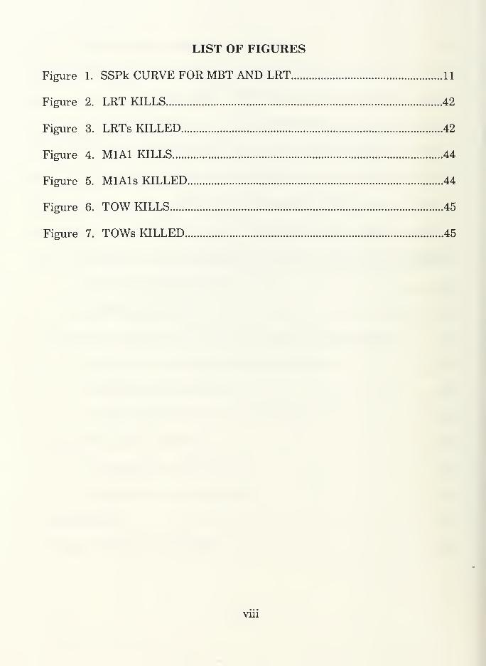
LIST OF FIGURES
Figure 1. SSPk CURVE FORMBT AND LRT 11
Figure 2. LRT KILLS 42
Figure 3. LRTs KILLED 42
Figure 4. M1A1 KILLS 44
Figure 5. MlAls KILLED 44
Figure 6. TOW KILLS 45
Figure 7. TOWs KILLED 45
viu

I. INTRODUCTION
The Army of the 21st century will be a highly technical, flexible, and
lighter force than has been seen in the past. While the size of the Army may
shrink, this reduction will not necessarily result in a loss in the destructive
capability of each unit, only the size of that unit and the number of units on
the battlefield will diminish. To meet these changes, the Army must develop
weapons that are more powerful, and require fewer soldiers (reduced crew size)
with the goal of producing a force of adequate capability.
Reduced force size comes with demands for a reduced military budget. The
control of costs, always important, can be expected to dominate all aspects of
Army operations. Significantly, cost control for the development of new
weapons will be critical as the Army moves to modernize its forces. One way
to control costs is to provide an efficient method to test new weapon concepts
before they are actually built. Those concepts which prove useful are likely
candidates for further development.
A framework for analyzing new weapon concepts which incorporates
advanced technologies was recently developed at the Operations Research
Center (ORCEN) of the Department of Systems Engineering, United States
Military Academy at West Point (see APPENDIX A). The ORCEN is used by

the Army and cadets for the analysis of system design, operations research, and
combat modelling. This framework is a logical ordering of inputs, processes,
and outputs to consider when conducting an operational analysis of a
technologically advanced weapon system using a computer simulation model.
The goal of the research presented in this thesis is to demonstrate an
analytical method for using a computer simulation that fits within the proposed
framework to perform conceptual analysis of an hypothesized advanced future
weapon system. The computer simulation selected for this study was Janus(A).
This simulation is currently being used by the Army and Marine Corps as a tool
for training and the analysis of weapons and tactics. It is used at the ORCEN
to teach cadets modelling and analysis.
There are several reasons for using Janus(A) as an analytical tool to
explore the operational implications of advanced technological weapon systems.
First, it is relatively easy for warfighters to use, not just programmers. Second,
it is supported by Army analytical agencies (Training and Analysis Command,
Institute for Defense Analysis, etc.). Third, it uses straightforward attrition
based measures of effectiveness (MOE) and measures of performance (MOP).
Also, Janus(A) uses well understood battle calculus (stochastic processes) in the
model. Using Janus(A) will allow analysts to evaluate technologies early on in
the research and development phase to assess the viability of future
technologies. Furthermore, Janus(A) is the primary high resolution analytical

model used at Training and Analysis Command-Monterey (TRAC-Mtry) and at
the ORCEN.
This thesis attempts to model an advanced technological system placed in
an actual battle and analyze its impact on the force's destructive capability as
a whole. The major objectives to accomplish this goal include:
1. Research, identify, and select those model input parameters for anadvanced weapon system that could justifiably model the
implications of technology in Janus(A).
2. Define a straight forward methodology (design an experiment) to
be used to measure the effects of the technology on the force as
a whole.
3. Build a mathematical model that approximates the relationship
between a desired response (i.e., number of enemy kills) and the
system characteristic variables (i.e., weapon range).

II. ANALYSIS METHODOLOGY
The methodology chosen to demonstrate this study was to take a case with
expected results, replicate that case in Janus(A), and compare the results. The
steps to accomplish this are to: 1) posit a case with known results, 2) select an
appropriate scenario to analyze the advanced technology, 3) select appropriate
input parameters, 4) select appropriate measures of effectiveness, 5) select an
effective and efficient experimental design, and, 5) conduct thorough data
analysis to compare the results against the expected results.
To check the feasibility of using Janus(A), a case is posited where the
answers are already known. This will enable the analyst to determine if, in
fact, Janus(A) provides expected reasonable results. The case for this study is
the addition of a long range direct fire weapon system in a desert scenario.
This is an important case because the future of advance technologies is leaning
toward smaller units capable of destroying the enemy quicker, at greater
ranges, and with less ammunition.
A. EXPECTED RESULTS.
The expected results for a long range direct fire weapon system in a long
range scenario seem trivial. It is expected that there will be more long range
kills. This will allow the force with the long range weapon to engage and kill

the enemy first, keeping the enemy further away for a longer period of time
and thus bring other weapons to bear on the enemy. While the long range
weapon may not increase the Blue (friendly) Force's survivability against
overwhelming odds, it is expected that it will create more Red (enemy)
casualties. It is expected that the long range weapon will be superior to the
current main battle tank (MBT) and tube-launched optically tracked wire
guided (TOW) anti-tank weapon system.
B. SCENARIO.
The actual scenario chosen for the analysis is a National Training Center
(NTC) battle that took place in 1988. The reason for using this battle is that
it took place on ground where long range visibility is possible. Also, this was
an actual training battle. The scenario pits a battalion level tank heavy task
force in the defense (Blue Force) against an attacking Motorized Rifle Regiment
(Red Force). The scenario was replicated into Janus(A) by CPT David Dryer
[Ref. 13]. A brief explanation of the scenario can be found in APPENDIX B.
The main reason for using this scenario is the fact that there are no biases
from the author in the development of the scenario for the study. Developing
a scenario from scratch could lend itself to tactical and doctrinal errors. This
scenario actually occurred. Commanders and soldiers influenced the battlefield
with actual decisions. The scenario begins where the units are separated,
converge, and engage in two separate battles. For this study, a simulation of

this scenario was allowed to run until the middle of the first battle. This
allowed the collection of data for the long range portion of the battle to
determine the contribution of the long range weapon to the force.
C. WEAPON SYSTEM CHOSEN.
The advanced technological weapon posited in this scenario is a direct fire,
high velocity, kinetic energy tank gun system with a maximum effective range
of 6000 meters. This weapon system would be mounted on an armored chassis
and have the capability on firing an Armor Piercing (AP) round at a velocity
and range greater than that of an existing main battle tank.
The operational requirement for this weapon system comes from the
hypothesis that it is feasible to develop a weapon system capable of engaging
enemy armored systems at a greater range than current tanks, and achieve a
greater probability of kill given a hit from the increased velocity of the round.
The Defense Science Board proposed such an advanced technology in 1984.
The envisioned system fired a high velocity, kinetic energy projectile from an
armored platform to engage enemy targets at ranges up to 6000 meters with
roughly the same probability of hit/kill and armored piercing capabilities of a
main battle tank (MBT) at 3000 meters [Ref.ll]. Sensors and engagement
systems are assumed to be more advanced than the current main battle tank
systems to allow the engagements at such extended ranges. The guidance
system for this weapon may either be heat seeking, magnetic, or laser guided.

For this study, the system will be referred to as a Long Range Tank (LRT).
D. INPUTS.
There are two types of parameters that were chosen for this study: weapon
system parameters and force mix parameters. Weapon system parameters are
those weapon system characteristics that are varied throughout the experiment
to determine what effect they might have on the response. Force mix
parameters are force ratios of one weapon system to another. The force ratios
used for this study consisted of the number of new systems replacing the old
system divided by the total number of old systems initially in the force (before
replacement). The force ratios are varied, thus replacing different quantities
of a weapon with the system under study. This allows the analyst to measure
the effect of the weapon system in relation to the force mix with another
weapon system.
The input parameters (factors) chosen for this study are: 1) ratio of
#LRT/(max # of TOWs), 2) ratio of #LRT/(max # of MTBs), 3) Main battle
tank opening range, 4) TOW opening range, and 5) LRT maximum effective
range. These were chosen because they represented the force mix issue (#1
and #2), the opening range issue (#3 and #4, to be discussed later), and the
advanced technological weapon system characteristic, maximum effective range
(#5).

A question arose as to how to put the LRT into the force structure.
Replacing all of the TOWs and MTBs with the LRT eliminates the interactive
contribution of the systems together in the force. Therefore, ratios of the
LRTs to TOWs and MBTs were decided upon as inputs in the experiment.
Also, random replacement of each TOW and MBT by the LRT removed any
bias due to positioning in the scenario. Each TOW and MBT system had an
equal probability of being replaced, thus positioning and movements for the
LRT were predetermined based on the position and movement of the system
it replace. These factors relate the number of TOWs and MBTs that were
randomly replaced by the LRTs. For each run, a specified number of TOWs
and MBTs were replaced randomly. This means that keeping everything else
constant (movement routes, firing posture, tactical position, etc.), a certain
number of TOWs and MBTs were switched and made LRTs. No run had the
same replacement as any other run. This was done with a FORTRAN random
number generation program that used the program RANNUM (uniform
distribution) to get a random number, converted that random number into an
integer, checked to insure that the integer had not been previously selected,
and repeated the process until the required number of integer numbers was
selected. The program can be seen in APPENDIX E.
Each weapon system was given a line number in the Janus(A) data base.
The forces were numbered sequentially from one to the number of elements
8

in the force size. For this random replacement, each of the TOW systems were
numbered from 1 to 23 (the initial number of TOWs in the scenario). Each of
the MBTs were numbered from 1 to 39 (the initial number of MBTs in the
scenario). The random number generator then selected a desired number of
integers from a specified range (1-23, 1-39). This random replacement
eliminated bias due to positioning. Using this ratio as a parameter provided a
measure of effectiveness of the LRT versus the TOW and MBT. It is expected
that range matters for this scenario. The longer range for a weapon is more
desirable and it will be advantageous to replace the shorter range weapons with
the LRT. It is also expected that the longer range weapons will dominate the
weaker weapons and therefore, replacement of the weaker weapons (less
survivable) will occur first.
The maximum opening range of a weapon system is a parameter that was
thought to be sensitive in Janus(A) from previous studies [Ref. 2]. Restricting
the opening range of a weapon prevents firing at maximum range (minimum
effectiveness). This restriction would improve the Ph and Pk values for a single
shot but would allow the enemy to engage with fire within his maximum range
without exposure to return fire. If a weapon opens fire at its maximum range,
two things occur: his position is potentially detectable by the blast of the
weapon, and the small Ph and P kvalues produce a minimal effect on the enemy.
Introducing the opening ranges of the TOW and MBT as inputs will hopefully

The LRT maximum range incorporates both the opening range as
described above and the maximum effectiveness of the weapon system, which
includes the effect of the hyper-velocity kinetic energy round. The values in
the P h and P k tables were not changed from those for the MBT. The range
bands associated with the values were altered to represent the maximum
effective ranges. Improving the range of the weapon system, while keeping the
Pk and Pk values the same, gives better results at the shorter ranges. Figure
1 graphically portrays the single shot probability of kill (SSPk) for the MBT
(solid line) as a function of range. The dashed and dotted lines represent the
SSPk curves for the LRT at maximum effective ranges of 4500 meters and 6000
meters (the center point and axial point for the experiment discussed later).
Within Janus(A), the maximum opening range was changed to coincide with the
Ph and Pk maximum range band.
E. MEASURES OF EFFECTIVENESS.
A measure of effectiveness (MOE) is a measure of the contribution of a
factor to the overall effectiveness of the force. It is the response variable
(dependent variable) that is a measure to quantify the results of the model
output. The MOEs selected for this experiment are:
1. Number of red kills
2. Number of blue kills
MOE #1 gives a measure of destructive capability (lethality) and MOE #2 gives
10

— mbT— LRT C CPJ
•••+
4---
RANGE C KN/O
Figure 1. SSPk Curve for MBT and LRT.
a measure of survivability. Both can easily be recorded and analyzed. These
allow an analysis to determine which of the previously discussed factors had a
significant effect on both enemy casualties and friendly survivability.
The number of RED Kills include not only those kills by the TOW,
MBT, and LRT, but also artillery kills, machine gun kills, etc. While there are
contributors to the number of red kills other than the TOW, MBT, or LRT, this
study is interested in displaying the effect of the parameters on the lethality
of the force as a whole. MOE #1 obeys the two fundamentals of MOE
selection: keep it simple and bigger is better. MOE #2 is simple and has a
direct relationship to the one theme of this study: the survivability effects of
the force by replacing the TOW or MBT.
11

III. EXPERIMENTAL DESIGN
Experiments may either confirm knowledge about a system or explore the
effect of new conditions of the system [Ref. 1: p.l]. This experiment is
expected to confirm the operational benefit of a proposed advanced
technological weapon system. Additionally, this experiment will demonstrate
how to apply force ratios to the model as parameters. Models such as Janus(A)
ultimately are a transformation of a set of inputs (the scenarios and
circumstances of combat) to a set of outputs. Using such a model equates to
selecting the inputs and then "running" the model to examine "what happens".
Because this analysis concerns the performance of a weapon which exists only
in concept, the exact value of all inputs is not known. Uncertainty in model
inputs suggest parametric analysis which is often considered a problem of
experimental design. In the context of this research, the issue is to select an
efficient design which will identify the sensitivity of scenario inputs which
express how a future technology weapon performs and how it is used. These
are questions of performance capabilities and force structure. Performance
capabilities relate to physical characteristics such as rate of fire, range or
weapons, and ability of sensors to detect targets. Force structure issues
concern the number and type of weapons which comprise a force along with
12

information about how these weapons are used.
As previously described, Janus(A) incorporates inputs which describe both
weapon performance and force structure composition. The issue for analysts
is, therefore, to select an experimental design which will demonstrate how well
a force performs given various combinations of these inputs. In this case, the
objective is to determine how changes in various performance characteristics
of a future weapon will influence the overall combat capability of the friendly
force.
A. EXPERIMENTAL DESIGNS CONSIDERED.
A level is a specific value set for the input or parameter being analyzed.
The results attained from several runs of a model at various levels of particular
factors represent the output of the model to changes of the factor.
Geometrically, this output characterizes a response surface as a function of
input parameters. There is no reason to believe that responses are linear,
therefore, at least three levels are chosen for this study. Several experimental
designs are available which provide a methodology to perform this type of
analysis. A few will be considered for this study: factorial, fractional factorial,
and central composite designs. Factorial designs are important for the
following reasons [Ref. 3: p.306]:
1. They require relatively few runs per factor; and although they are
unable to explore fully a wide region in the factor space, they can
indicate major trends and so determine a promising direction for further
13

experimentation.
2. They can be suitably augmented to form composite designs.
3. They form the basis for fractional factorial designs.
4. These designs and the corresponding fractional designs may be used as
building blocks so that the degree of complexity of the finally constructed
design can match the sophistication of the problem.
5. The interpretation of the observations produced by the designs can
proceed largely by using common sense and elementary arithmetic.
For this experiment, due to time and resources, the interest is on the
main effects of the inputs on the response with a manageable number of runs.
1. Full Factorial Design.
A full factorial design is one where all possible combinations of factors
and levels are considered. For n levels and k factors, there are nkpossible
combinations of experimental runs to consider. For this study, there are five
factors or inputs. This would require 35 = 243 experimental runs to cover all
combinations. However, time and resource constraints force the consideration
of some type of reduced factorial design.
2. Fractional Factorial Design.
A fractional factorial design is one that considers certain high-order
interactions to be negligible. Therefore, those runs which provide information
about the negligible higher order interactions are eliminated. Thus a fraction
of the full factorial design may be sufficient to capture the relevant
14

information. Fractional designs are widely used in screening experiments,
those interested in identifying those factors that have large effects [Ref. 1:
p.325]. As the goal of this research is to identify such cases, this design
warrants further consideration.
For this experiment, one half of the full factorial design is unmanageable
in terms of effort and time (120 experimental runs). One fourth fractional
designs may be more manageable but the loss of some low-order effects may be
significant. Also, for fractional designs, the interactions that will be eliminated
may be significant to this study. Therefore, another fractional factorial design
alternative will be considered and chosen.
3. Central Composite Design (CCD).
An alternative to the 3kfactorial system is a class of composite designs
called the central composite design (CCD). "This design is greatly used by
workers applying second order response surface techniques [Ref. 4: p. 126]."
The CCD is the 3kfactorial or fractional factorial design augmented with a
specific number of axial points. The center points "are experimental runs with
all factor levels set half-way between their minimum and maximum settings
[Ref. 5: pp.9-10]." Axial points are runs with a factor set at its minimum or
maximum level and all other factors set at their center point level. Therefore,
the CCD is a five level experimental design. The preceding discussion of the
CCD is a very brief and general overview of a complex class of experimental
15

designs. For additional information, the reader is encouraged to examine
Response Surface Methodology [Ref. 4] and Understanding Industrial Designed
Experiments [Ref. 5].
The Central Composite Design reduces the number of experimental runs
that would be needed if a full or fractional factorial design were used. The
number of experimental runs for this five factor experiment is 52: 32 factorial
points, 10 axial points, and 10 replications at the center point [Ref. 4: p. 153].
This is significantly less than the 243 runs required in a full factorial design.
The CCD can also be used to fit a second order response surface. Since it is
unclear what type of response surface to expect from this experiment, an
estimated response surface must be approximated. The CCD approximates a
second order response surface. It provides information about main and low-
order effects. This design is rotatable, meaning:
A design is said to be rotatable when the variance of the estimated response- that is, the variance ofy, which of course depends on a point of interest xlf
x2 , ..., xk- is a function only of the distance from the center of the design
and not on the direction [Ref. 4: p. 139].
This means that "points in the factor space which are the same distance from
the center point (origin) are treated as being equally important [Ref. 4: p.165]."
The experimental design chosen for this study was the CCD. The CCD
is perhaps the most popular class of designs used for estimating the coefficients
in a second degree model [Ref. 6: p.32]. It is difficult to physically interpret
16

what is meant by third, fourth, and, for this experiment, fifth order
interactions. Assuming those higher order interactions to be negligible
supported use of the CCD. This is reasonable because higher order interactions
(third, fourth, and fifth order) are difficult to physically interpret and are
confounded in the main and second order interaction effects. This is reasonable
because models such as Janus(A) are intended to have orthogonal inputs. Also,
the statistical techniques involved in response surface methodology are very
similar to those associated with simple linear regression analysis. Recall, two
of the objectives for this research were to design an experiment to measure the
effects of a technology on a response and then to build a mathematical model
to approximate the relationship between the response and the variable inputs.
Use of the CCD and the response surface methodology satisfies these
objectives. Response surface methodology will be discussed in more detail in
Chapter V.
17

IV. CENTRAL COMPOSITE DESIGN EXPERIMENT
This section describes how the CCD design was implemented for this
study. The CCD is a five level experimental design that assumes that higher
order interactions are confounded by the main effects and second order
interactions. The CCD is composed of three parts: the full factorial design at
the radial points (equi-distant from the center of the design), the single runs
at each axial point (the minimum and maximum points of each factor), and the
center point (average value component of each factor) replications. Given the
weapon, the scenario, the factors (parameters), and the MOEs, the levels for
each factor must be determined. The first step is to build the design, or run
matrix which defines the levels of input parameters used for each run of the
simulation.
A. DESIGN CENTER POINT AND FACTOR RANGES.
The experimental center point (CP) for each factor is determined from the
maximum and minimum values for that factor. The ranges of each factor are
determined by the experimenter. For this design, the CP is defined as:
_MINfa£tor+
MAXfactor Q)L,r
factor~
18

which is the midpoint of the range of values considered reasonable for each
factor. The minimum and maximum values for the force ratios (Xj and X2 )
were obviously set at 0.0 and 1.0. These relate to the number of elements
replaced for a given ratio. At 0.0, no TOWs or MBTs were replaced by LRTs,
while at 1.0, all of the TOWs and MBTs were replaced by LRTs. The minimum
values for the TOW and MBT opening ranges were set at 500 meters. This put
the center point at a reasonable level. The maximum ranges were the AMSAA
values in the data base (3000 meters for the MBT, 3750 meters for the TOW).
The CP for the LRT range was determined using the current MBT maximum
range (3000 meters) as its minimum opening range (hypothesizing that the
LRT was no worse that the current tank) and the hypothesized maximum
range of 6000 meters.
The CP for the force ratios (#LRT/#TOW, #LRT/#MBT) is 0.5. The CP
for the TOW and MBT opening range was determined using equation (1). The
CP values for each factor are as follows:
CPlrt/tow = O.o
CPlrt/mbt = 0.5
cp\1bt range= 1*50
CPtOW RANGE= ^1^5
^"lrt max range= 4500
The center is defined as (X„ X2 , X3 , X4 , Xg) = (0.5, 0.5, 1750, 2125, 4500).
19

B. FACTORIAL COMPONENT OF CCD.
Delta (6) is the amount a factor is varied around the CP which is the two
factor portion of the design. This is necessary to calculate the factor's
experimental levels. The following equation is used to calculate the appropriate
6 value for each factor:
r _ MAKfactor-CPfactor _ ^AXfactor'^factor(2)
factor-- =
2^78
Alpha (a) is defined as the distance from the design center point to an axial
point [Ref. 5: p.62] and is calculated by the equation (2k)1/4
, where k is the
number of factors. For this experiment, a = (25)1/4 = 2.378. The 6 values for
the factors in this study are as follows:
°LRT/TOW = U.Zl
*LRT/MBT= O.Zl
'MBT RANGE = 526 meters
5tow range = 683 meters
= 631 meters"LRT max range
The preceding discussion provides the necessary information for determining
the five levels for each factor listed in Table 1.
Determining the five levels for the LRT MAX RANGE was different from
the other levels in that each P h and Pk table is a function of range. Each table
20

is divided into five range bands. The CCD levels only consider the maximum
range. Each table was changed to reflect the appropriate range band given the
maximum range (the minimum range is zero). JANUS(A) uses a piecewise
continuous function composed of 4 line segments to describe the probabilities
of hit and kill for a given weapon as a function of range. The CCD levels for
the range bands are shown in APPENDIX D.
TABLE 1. CCD FACTOR LEVELS.
MIN CP-ft CP CP+5 MAX
LRT/TOW 0.0 0.29 0.5 0.71 1.00
LRT/MBT 0.0 0.29 0.5 0.71 1.00
MBTRG 500 1224 1750 2276 3000
TOWRG 500 1442 2125 2808 3750
LRT MAX RG 3000 3869 4500 5131 6000
C. BUILDING THE EXPERIMENTAL RUNS.
The number of experimental runs required for this experimental design
with five factors (k = 5) is 52 [Ref. 4: p. 153]. That is, there are 25 = 32 full
factorial runs, 10 axial point runs, and 10 replications at the center point. An
axial point is an experimental run with a factor set at either its minimum or
maximum level and all other factors set at their center point levels. The 10
center point runs will allow an estimate of the experimental error to be made.
Thus, a check for model adequacy is possible [Ref. 5: pp.7-62]. The complete
design matrix for this research is located in APPENDIX D.
The experimental runs were conducted by manipulating specific portions
21

of the JANUS(A) data base. The different force ratios required that individual
weapon systems be replaced by the LRT. This replacement was done randomly
for each run (as mentioned previously). This random replacement removed the
bias due to positioning of the system in the force.
A consequence of this random replacement was that certain key systems
(MBTs, TOWs) were killed immediately due to poor tactical placement of the
element. Some of the elements in the actual NTC scenario were positioned in
noncombat or tactically unsound areas due to mechanical breakdowns or poor
positioning by the force commander. In any event, certain systems were killed
immediately and others shortly after the battle began at long exposed ranges.
If those elements were picked by the random number generator to be replaced
by the LRTs, then the contribution to the survivability of the Blue force would
have to include the sound tactical employment of those weapons.
The actual manipulation of the data in Janus(A) can be accomplished by
following the instructions in the JANUS Documentation and Users Manual
[Ref. 7: p. 3-1 to 3-25].
22

V. DATA ANALYSIS METHODOLOGY AND RESULTS
The methodology used in this thesis consists of the design of the
experiment and the data analysis. This chapter contains a description of the
response surface methodology and the data analysis associated with the results
of the experiment.
A. RESPONSE SURFACE METHODOLOGY.
Response surface methodology (RSM) consists of a set of techniques used
in the empirical study of relationships between one or more responses and a
group of input variables [Ref.6:p.l]. For this study, response surface
methodology was applied to the results obtained from the CCD experiment.
RSM was used because: 1) it assumes the residual errors to follow a normal
distribution (thus permitting simple significance tests to be done), 2) it uses
least squares regression techniques allowing a mathematical model to be built
to approximate the relationship between the response and the variables, and
3) it approximates a convex surface in which the optimum operating conditions
are met [Ref.4:p.63]. The result, or response is the measure of effectiveness
(MOE) associated with each experimental run. Recall, the two MOEs selected
for this experiment were the number of RED kills and the number of BLUE
kills.
23

Response Surface Methodology (RSM) is a set of techniques designed to
find the "best" value of the response [Ref.6:p.l]. There are several reasons for
choosing RSM as a statistical technique [Ref.2:p.33]. First, RSM allows one to
develop a mathematical model to approximate the relationship between a
measurable response and the input variables over a selected region. Second,
with RSM, it is possible to identify the factors which have the most effect and
least effect on the response. Third, RSM is very similar to multiple regression
analysis, specifically the method of least squares. RSM applies regression
analysis "in an attempt to gain a better understanding of the characteristics of
the response system under study [Ref.6:p.l]." Lastly, the CCD type of
experiment and the related response surface methodology results in greater
precision in estimating the regression coefficients with a minimal of
experimental effort [Ref.4:p.l26].
1. The Response.
The response is the measurable quantity whose value is assumed to be
affected by changing the levels of the factors [Ref.6:p.2], The factors for this
study are the force ratios of LRTs to TOWs and MBTs, maximum opening
ranges of MBTs and TOWs, and LRT maximum range. The true value of the
response corresponding to any of the 52 experimental runs is denoted by rj.
The term "true response, 77" means the hypothetical value of rj that would be
obtained in the absence of experimental error [Ref.6:p.2]. However, error is
24

always present in experiments and the actual value observed for any given
combination of factor levels is Y = r} + e, where e is the experimental error.
Recall the MOEs chosen for this experiment are the number of red kills and
the number of blue kills.
2. The Response Function.
The value of the response r? depends on the levels X1,X2,...,Xk of k
quantitative factors, fpf 2>--f k-Therefore, there exists a mathematical function,
0, of X^Xj,...^, the values of which, for any given combination of factor levels,
provide the corresponding value of rj. The response function is given by
equation (3).
n=<t>(xxyK
2,...Xk ) (3)
The response function,<f>,
is called the true response function and is assumed
to be a continuous function of the X;'s [Ref.6:p.2].
3. The Response Model and Fitted Response Surface.
The second order response model of k factors takes the following
general form:
i = p.+ EPA + EEW + £ pX <4)
25

where the fy's are the regression coefficients for the first-degree terms, the fa's
are coefficients for the pure quadratic terms, the /?jm's are the coefficients for
the cross product terms and the Xs represent the experimental levels of the k
factors. The estimates and parameters are then obtained using the method of
least squares. The predicted response function is given by the following
equation:
t = * + £ bpCj ££ v^» + E bX <5)
where the b's are estimates of the /J parameters. Equation (5) can be used to
estimate values of 77 for given values of Xx, X2 ,..., Xk [Ref.6:p.2].
The discussion above is only a general overview of a complex statistical
technique. For further information concerning the response surface
methodology, one should refer to Response Surface Methodology [Ref.4] and
How to Apply Response Surface Methodology [Ref.6].
B. RESPONSE SURFACE ANALYSIS AND RESULTS.
1. Model Response.
The 52 experimental runs were executed and the total number ofRED
kills and BLUE kills were tabulated for each of the runs. The statistical
package SAS (Statistical Analysis Software) was used to calculate the fit of the
model and the significance of the variables. The experimental responses are
26

tabulated in Tables 2 and 4.
2. The Fitted Response Surface Model.
The statistical package SAS was used to perform the multiple
regression necessary to build the second order response surface model for both
RED Kills response and BLUE Kills response. The SAS outputs are displayed
in APPENDIX F. The assumption of quadratic response surface allows for the
estimation of 21 model parameters, including the intercept [Ref.5:p.7-65].
27

TABLE 2. EXPERIMENTAL RESPONSE - RED KILLS
RUN REDKILLs
RUN REDKILLs
RUN REDKILLS
RUN REDKILLS
1 63 14 44 27 42 40 44
2 47 15 62 28 43 41 51
3 59 16 39 29 42 42 48
4 45 17 59 30 43 43 44
5 63 18 39 31 61 44 41
6 51 19 45 32 35 45 51
7 60 20 39 33 50 46 43
8 47 21 66 34 43 47 59
9 48 22 37 35 44 48 43
10 41 23 51 36 60 49 45
11 50 24 39 37 47 50 47
12 48 25 51 38 42 51 52
13 55 26 39 39 52 52 38
3. RED Kills Response Surface Model.
The regression analysis for the response RED Kills produced the
following model:
r?R = 47.754 + 2.425X 1+ 2.075X2-0.125X3 + 0.475X4 +5.725X5 + 0.906X 1
X2-
0.094X1X3-0.594X 1
X4-0.156X
1X6 + 0.031X2X3 + 1.782X2X4 +1.344X2X6 +
0.281X3X4-1.531X3X5 + 0.344X4X5-0.881X 1
2 + 0.244X2
2 + 1.244X3
2-0.006X4
2-
0.256X52
(6)
28

where X, = #LRTs/#TOWs, X2= #LRTs/#MBTs, X3
=MBT Range, X4=TOW
Range, and X5= LRT max Range. Table 3 summarizes the estimated
coefficients, standard error of estimate, t-ratio, and p-value. The t-ratio and
associated p-value are used to test the null hypothesis that the coefficients (the
/3s) are equal to zero against the alternate hypothesis that the coefficients are
not equal to zero. That is:
H : ft= 0,i = l,2,...
Ha : ^0,1 = 1,2,...
If a coefficient is equal to zero at some significance level, this implies that the
variable associated with that coefficient has no effect on the fitted model. This
hypothesis test is a two-tailed t-test and the significance level (a) at which one
would reject H is established at a level of a = 0.05. Since the test is two-tailed,
the significance level becomes (a/2 = 0.025). The p-value listed in Table 3
represents the smallest level of significance, a, for which one would reject H .
The rejection region for this hypothesis test corresponds to any value of1 1 1 >
ta/2 . The table value of t 025 with 31 degrees of freedom is approximately 2.04.
Those factors marked "*" in Table 3 are significant at a = 0.05.
29

TABLE 3. RED KILLS REGRESSION MODEL SUMMARY.
VARIABLE COEFF. EST. STD. DEV. t-RATIO p-VALUE
x, 2.4250 0.9241 2.62 0.0134*
x2
2.0750 0.9241 2.25 0.0320*
x3-0.1250 0.9241 -0.14 0.8933
x40.4750 0.9241 0.51 0.6109
x5 5.7250 0.9241 6.19 0.0001*
x, 2 -0.8810 1.0164 -0.87 0.3927
x2
2 0.2439 1.0164 0.24 0.8119
X32 1.2449 1.0164 1.22 0.2302
x4
2 -0.0060 1.0164 -0.01 0.9953
x5
2 -0.2560 1.0164 -0.25 0.8028
XjX2
0.9062 1.0332 0.88 0.3872
X1X3 -0.0937 1.0332 -0.09 0.9283
XjX4-0.5937 1.0332 -0.57 0.5697
x,x5-0.1562 1.0332 -0.15 0.8808
X2X
30.0312 1.0332 0.03 0.9761
X2X
41.7812 1.0332 1.72 0.0947
X2X5 1.3437 1.0332 1.30 0.2030
X3X
4 0.2812 1.0332 0.27 0.7873
X3X5-1.5312 1.0332 -1.48 0.1484
x4x5 0.3437 1.0332 0.33 0.7416
CONSTANT 47.7540 1.8182 26.26 0.0001*
30

TABLE 4. EXPERIMENTAL RESPONSE - BLUE KILLS
RUN BLUEKILLs
RUN BLUEKILLs
RUN BLUEKILLS
RUN BLUEKILLS
1 55 14 60 27 60 40 64
2 65 15 57 28 67 41 56
3 54 16 60 29 58 42 61
4 60 17 56 30 58 43 62
5 56 18 62 31 62 44 63
6 60 19 63 32 73 45 60
7 54 20 60 33 60 46 58
8 60 21 69 34 63 47 57
9 61 22 67 35 64 48 64
10 65 23 59 36 54 49 62
11 54 24 62 37 57 50 59
12 58 25 56 38 60 51 59
13 58 26 63 39 59 52 64
4. BLUE Kills Response Surface Model.
The regression analysis for the response BLUE Kills produced the
following model:
r? B = 59. 887-1.500X1-0.100X
2-0.700X3 + 0.300X 4-1.950X5-0.312X 1
X 2 +
0.875X1X 3 + 1 .250X
1X 4-0.312X 1
X5-0.312X 2X3 + 0.937X 2X4 + 0.250X 2X5 +
0.250X 3X 4-0.437X 3X 5 + 0.187X 4X 5 + 0.544X 1
2-0.331X 2
2 + 0.044X 3
2+
0.044X4
2 + 0.294X5
2(7)
where X! = #LRTs/#TOWs, X2= #LRTs/#MBTs, X3
=MBT Range, X4=TOW
31

Range, and X5= LRT max Range. Table 5 summarizes the estimated
coefficients, standard error of estimate, t-ratio, and p-value. The table value
of t0025 with 31 degrees of freedom is the same as the RED Kills model and is
approximately 2.04. Again, those factors marked "*" in Table 3 are significant
at a = 0.05.
32

TABLE 5. BLUE KILLS REGRESSION MODEL SUMMARY.
VARIABLE COEFF. EST. STD. DEV. t-RATIO p-VALUE
x1
-1.5000 0.5626 -2.67 0.0121*
x2
-0.1000 0.5626 -0.18 0.8601
x3-0.7000 0.5626 -1.24 0.2228
x4
0.3000 0.5626 0.53 0.5977
x5-1.9500 0.5626 -3.47 0.0016*
x, 2 0.5443 0.6188 0.88 0.3858
x2
2 -0.3306 0.6188 -0.53 0.5969
X32 0.0443 0.6188 0.07 0.9433
x4
2 0.0443 0.6188 0.07 0.9433
x5
2 0.2940 0.6188 0.48 0.6376
XjX2
-0.3125 0.6290 -0.50 0.6228
XjX30.8750 0.6290 1.39 0.1741
xxx
41.2500 0.6290 1.99 0.0558
x,x5
-0.3125 0.6290 -0.50 0.6228
X2X3
-0.3125 0.6290 -0.50 0.6228
X2X
40.9375 0.6290 1.49 0.1462
X2X5 0.2500 0.6290 0.40 0.6938
X3X4
0.2500 0.6290 0.40 0.6938
X3X
5-0.4375 0.6290 -0.70 0.4919
x4x
50.1875 0.6290 0.30 0.7676
CONSTANT 59.8871 1.2069 54.10 0.0001*
33

5. Analysis of Variance - Red Kills.
For multiple regression, the analysis of variance is a technique that is
used to partition the variance and to compare models that include different sets
of variables [Ref.8:p.48]. The output provided from the SAS includes an
analysis of variance table (ANOVA). The ANOVA table corresponding to this
experiment is presented in Table 6 below.
TABLE 6. ANALYSIS OF VARIANCE TABLE - RED KILLS
SOURCE DF SS MS F-VALUE p-VALUE
REGRESSION 20 2189.69 109.48 3.55 0.0008
ERROR 31 955.29 30.81
TOTAL 51 3144.98
The total variation in the data is called the "total sum of squares", SST, and is
computed by adding the sum of squares due to the regression (SSR) and the
sum of squares of the residuals (SSE) [Ref.6:p.l0]. The degrees of freedom
associated with the SST is N-l, where N is the total number of experimental
observations (N = 52). The degrees of freedom associated with the SSR is n-l,
where n is the number of terms in the fitted model (n = 21). The degrees of
freedom for the SSE is N-n = 31.
The F statistic is used to test the null hypothesis (H ) that the fitted
response surface model does not have a significant effect on the measured
34

response. The alternate hypothesis (Ha ) is that the fitted surface model does
have a significant effect on the measure response. The Fmodel statistic is
calculated using values associated with the mean square of the regression and
the mean square of the residuals (as follows) [Ref.6:p. 11].
_, Mean Square Regression SSRf(n-l) /C v
P l/~/.i = —n z——
—
— = —
-
y&>Mean Square Residuals SSEjiN-n)
The value of FModel is compared to the table value F n .1Nna . If FModel >FnlN .na ,
then the null hypothesis is rejected at a reasonable level of significance
(a = 0.05). If FModel <
F
n .! Nn
a
, then the one fails to reject the null hypothesis at
the a level of significance. The table value for F2031005 is 1.92 for the RED
Kills.
6. Analysis of Variance - BLUE Kills.
The analysis of variance table for the BLUE Kills is shown in Table 7.
The degrees of freedom for the BLUE Kills is the same as the RED Kills. The
value of FModel is again compared to the table value Fn .1Nna . If FModel>Fn.1N_na,
then the null hypothesis is rejected at the a level of significance (a = 0.05). If
^Modei < Fn.i,N-n.a > then the one fails to reject the null hypothesis at the a level of
significance. The table value for F2031005 is 1.92 for the BLUE Kills.
35

TABLE 7. ANALYSIS OF VARIANCE TABLE - BLUE KILLS
SOURCE DF SS MS F-VALUE p-VALUE
REGRESSION 20 405.27 20.26 1.60 0.1167
ERROR 31 392.50 12.66
TOTAL 51 797.77
7. Analysis of Results,
a. RED Kills Model.
The regression model and the ANOVA table indicate that the null
hypothesis (H ) that the fitted model does not have a significant effect can be
rejected (3.55 > 1.92). Therefore, the alternate hypothesis is accepted that the
fitted model does have an effect on the response at a level of significance.
Further investigation of the regression results indicate that most of the
estimated coefficients may be zero. If the values of |t| > ta/2 for each
estimated coefficient, then the null hypothesis that the coefficient is zero can
be rejected at a level of significance. Also, the p-values for the remaining
variables are so large that H will never be rejected. The variables not
associated with the zero coefficients (see asterisks in Table 3) and for which H
is rejected are: X1(#LRT/#TOW), X
2(#LRT/#MBT), X5 (LRT max range),
and the constant. This does not mean that the other variables do not influence
the results, rather, there is not sufficient evidence to provide accurate
estimates of their effects [Ref.6:p.l2]. These three variables are all associated
36

with the LRT (force ratio and range).
b. BLUE Kills Model.
For the BLUE kills model, it was expected that the blue force would
be killed due to the RED force outnumbering the BLUE force and RED
attacking BLUE. Using the regression model and the ANOVA table for the
BLUE Kills model indicate that the null hypothesis (H ) that the fitted model
does not have a significant effect cannot be rejected (F2031a = 1.92 >
FModel= 1.60). Therefore, there is no evidence to reject the hypothesis that the
fitted model has no effect on the response at 11.67% level of significance.
Further investigation of this regression model also indicates that most of the
estimated coefficients may be zero. If the value of |t| > ta/2 for each
estimated coefficient, then the null hypothesis that the estimated coefficient
is zero can be rejected at the (a) level of significance. The table value of t48 025
is 2.01. Also, the p-values for the remaining variables are so large that H will
never be rejected. The variables not associated with the zero coefficients (see
asterisks in Table 5) and for which H is rejected (|t| > 2.01) are: Xj
(#LRT/#TOW), X5 (LRT max range), and the constant. This does not mean
that the other variables do not influence the results, rather, there is not
sufficient evidence to provide accurate estimates of their effects [Ref.6:p.l2].
Recall, this model is based on the number of BLUE Kills response. It is
desirable to keep the response as small as possible (survivability). Therefore,
37

it is hoped that the impact of the coefficients contribute to decreasing the
response variable. The sign of the significant coefficients is negative,
supporting the previous statement. As a LRT is added to the force replacing
a TOW, the response is decreased through the negativity of the coefficient for
those factors. This indicates that it is better to replace the TOW first (the
more vulnerable weapon system) but adding more LRTs to the system will
decrease the number of BLUE kills. Also, the magnitude of the coefficient for
the LRT/TOW ratio is smaller (larger negative) than the LRT/MBT ratio.
This indicates that it is better to replace the TOW first and then the MBT with
the LRT. Increasing the number of LRTs that replace the TOW increases
negatively the number of BLUE Kills more than replacing the MBTs with
LRTs.
C. CONCLUSIONS.
The results from the RED Kills model indicate that the regression model
is a fairly good predictor of the response variable. The key parameters that
influence the variation in the response are the LRT force ratios and the LRT
Max Range. This agrees with what one would instinctively believe when given
a longer range weapon. Since the regression equation is second order, it is
convex. Therefore there exist an extreme point. The nonlinear program solver
General Algebraic Modelling System (GAMS) was used to maximize the
regression equation. The result indicated that the model is maximized at the
38

upper endpoints (all variables set at their maximum level). This indicates that
JANUS(A) is sensitive to opening range and that a longer range weapon system
(in this terrain) will significantly contribute to the destructive capability of the
force. Also, the significant coefficients were all positive. This indicates that
raising the factor level for the force ratios or the LRT range will increase the
response (number of RED kills). The magnitude of the coefficient for X2was
larger than Xv This indicates that it is more beneficial to first replace the
TOW (the weaker weapon) then the MBT. All of these results agree with the
answers posited prior to conducting this experiment and support the hypothesis
that the longer the range of a weapon system and the number of those systems
in the force, the larger the contribution to the destructive capability of the
force.
The results from the BLUE Kills model were also as posited. While the
model is not as good a fit to the variation in the response and therefore not
sufficient as a basis from which to draw conclusions, the significant coefficients
are those expected. The model indicates that the non-zero coefficients X, and
X5 contribute negatively to the response variation. Recalling that the desired
response for this model is as small as possible (# of Blue Kills), this indicates
that as X! and X5 increase, the response decreases (the number of BLUE kills
decreases). This coincides with what was posited at the beginning of this
paper: that the addition of a long range weapon system will increase the
39

survivability of the owning force. One possible reason for the bad regression
model may be due to the random replacement of the LRTs for TOWs and
MBTs (as mentioned in Chapter III). Another possible explanation for this is
that as more LRTs are entered into the force, the detectability of the Blue
force by the Red force increases, thus exposing them to enemy fire sooner than
that if the LRTs were not in the force.
D. FURTHER TESTING AND ANALYSIS.
In order to determine possible reasons for the lack of the BLUE Kills
regression to model the response, a follow-on experiment was conducted. For
this experiment, a more traditional method was chosen, and ten additional
Janus(A) runs were made. The values for each of the variables were fixed at
what was felt might be the most reasonable settings if this system was inserted
into the scenario (no variation in the factors). The force ratios were set at
their center point, while the TOW and LRT were set at their maximum ranges.
The MBT opening range was set at its upper radial point. This configuration
was chosen because the Ph and Pk values for the MBT decrease rapidly at the
maximum range and it was felt that realistically, MBT gunners do not open fire
at their maximum range, but wait to get more efficient shots at the enemy.
Also, these are the values where the Ph and Pk values begin to drop off rapidly
and gunners get effective shots at long ranges. These are the posited
influential values indicated in Chapter I. Therefore, the values of the
40

parameters were (Xj = 0, X2= 0, X3
= 1 , X4= 2, X5
= 2). The results of the runs are
shown in Table 8.
TABLE 8. RESULTS OF ADDITIONAL RUNS.
RUN RED KILLS BLUE KILLS RUN RED KILLS BLUE KILLS
53 51 55 58 51 59
54 64 55 59 56 57
55 64 56 60 61 58
56 54 43 61 76 54
57 66 53 62 63 50
For these runs, as in the first 52 runs, the replacements were done randomly
for each run.
To study the effects of range on both the RED Kills and BLUE Kills, the
number of kills by weapon system was plotted in 500 meter range bands. Six
box plot graphs were developed: one for each BLUE system (LRT, TOW, MBT)
plotting the number of RED Kills versus 500 meter range bands and one for
each BLUE system plotting the number of BLUE Kills of that system versus
the range bands in which they were killed (Figures 2 through 7).
Figures 2 and 3 depict the LRT, both the number of RED kills scored by
the LRT and the number of LRTs killed by RED systems. It is apparent that
the LRT scored most of its kills at the longer ranges (5-6 kms). It is also
apparent that the RED force killed the LRTs at the RED force's maximum
ranges. This means that having a LRT in one's force will kill more enemy at
41

22
20
18
16
14
12
lO
B
6
2
D
t i i i r -i1 r t 1
1 r
JL _
"T"
RANGE BANDS Ckms^
Figure 2. LRT Kills in 500 meter Range Bands.
1 1 1 1 1 1 1 1 1 1 1
-T -
i,
JI
::::i:: ::...
T _ ------1 i i i i i i i i
D- SO SO-1 4-1.3 1 .3-3 »-3 3 I .3-J »-3 3 .3-
4
-4—4 . 3
RANGE BANDS CKmsD
Figure 3. LRTs Killed in 500 meter Range Bands.
42

greater ranges but it will also attract more enemy fire at the enemy's
maximum ranges. The LRT's long range fire exposes their positions to the
RED force, who then return fire.
Figures 4 and 5 are box plots of the kills scored by the MBT and the
number of MBTs killed by range bands. These figures indicate that the MBT
did most of its killing at the longer ranges with the main tank round. But, at
the shorter ranges, where the alternate weapon (machine gun) might be more
practical, the alternate weapon was, in fact, used. For the number of MBTs
killed by the RED force, again the enemy engages the MBTs at the earliest
possible time - the maximum range of their weapons.
Figures 6 and 7 depict the same information as discussed above for the
TOW. The significant point here is that the TOW scored such a small amount
of kills that the impact of this weapon can hardly be evaluated. The TOW uses
its antitank weapon to engage targets at the longer ranges and its machine gun
to engage targets at the shorter ranges. With such few TOWs initially in the
force and the discrete values of the number of TOWs, the significance of the
number of TOWs killed by the RED force cannot be evaluated.
Positioning of the weapon systems greatly affected the probability of the
systems being killed early on in the battle, at close or far ranges. These graphs
make it difficult to tell what is going on with the addition of the LRTs except
that the weapons on both sides attempt to kill targets at the greater ranges.
43

7 —
^ 5 h
LUcr
o —_L _L J_ _L
O- .50. 5 0-11-1 .51 .5-2 2-2.52. 5-3 3-3. 53. 5-4
RANGE BANDS C^^sD
Figure 4. MBT Kills in 500 meter Range Bands.
71 1 1
LU
B
3
^Z
10fc-cn2Ouu
9
z
1 1 1 1 1 I I I I I l
O- 3d SO-1 -»-1.3 1.3-B 0-2 3 H.3-3 3-3.9 S.3-* •^•i.S
RANGE BANDS CKms)
Figure 5. MBTs Killed in 500 meter Range Bands.
44

UJLi
o- 90 30-1 i-i3 1 a-a a-» 3 05-3 3-13 3 3-1
RANGE BANDS CKrns^
Figure 6. TOW Kills in 500 meter Range Bands.
QLU
o
s — —
« — i- —
— r -r • • —
O- 3D .30-1 1-13 13- 8 8-33 B3-1 »- 3 3 J3-1 -^-13
RANGE BANDS CK^IS}
Figure 7. TOWs Killed in 500 meter Range Bands.
45

The results depicted what was intuitively suspected and what the CCD
experiment depicted: that range matters in this scenario.
The other intuitive result from this additional research is that the more
long range weapons in a force, the larger the contribution to the destructive
capability of that force. The LRT comprised 50% of the Blue force, while the
TOW and MBT comprised 18% and 32%, respectively. The contribution by each
of the Blue systems to the total number of Red Kills was 71%, 9%, and 21%,
respectively, for the LRT, TOW, MBT. This indicates only that the most
dominate system, in term of total number of systems, does most of the killing.
There are more LRTs in the force than any other system - so they do most of
the killing. This does not mean that the LRTs are "best" overall.
Two conclusions drawn from this additional experiment are that: 1) the
results agree with the CCD experiment that range matters both to the
survivability and the destructive capability of the force, and 2) a system
exposed to the enemy will be fired upon and killed. This means that no matter
how good a system is, if it is positioned in a tactically unsound area, the
likelihood of it contributing to the overall force is small.
46

V. CONCLUSIONS AND RECOMMENDATIONS.
A. CONCLUSIONS.
The results of this study demonstrated that the CCD is an efficient and
effective experimental design in the analysis of advanced technologies using
Janus(A). Reducing the number of experimental runs while still gaining the
statistical significance of the main and second order effects allows the analyst
to obtain the important data without a large number of experimental runs.
For this study and the advanced technology chosen to demonstrate using
Janus(A) and the CCD, the results were encouraging. In almost every respect,
the Janus(A) results were those expected for this scenario. The regression
analysis and ANOVA indicated that the addition of a long range direct fire
weapon system greatly improves the destructive capability of the force. The
effect of the LRT on the survivability of the BLUE force was not as evident.
This study showed that, in fact, the TOW, and maybe the main battle tank,
may be obsolete for this scenario if this advanced technological system was
available. The LRT and its long range capability clearly dominated the effects
of the MBT and TOW. The results indicated that the impact on the blue
survivability was unclear due to the overwhelming red force and the fact that
the scenario was not run through the end of the battle. However, the addition
47

of a long range direct fire weapon system may decrease the number of blue
systems killed in this scenario.
Another result from this study was that using force ratio as a factor in the
experiment allowed the analysis of an optimal force mix for the scenario. From
the analytical results of the CCD and response surface, an optimal force mix for
this scenario was found at the upper end points of the design. For this
scenario, replacing all of the TOWs and MBTs with LRTs gave the best results
in terms of number of RED kills. Use of these force ratios enabled the model
to pick out the weaker system, both in terms of destructive capability and
survivability. The scenario was ideal for a long range armored vehicle,
therefore the TOW, the short ranged, lightly armored system, was replaced
entirely in both the RED Kills model and the BLUE Kills model.
Given the results observed by this analysis, Janus(A) may be an
appropriate simulation model to study the influence of advanced technological
weapons on battle outcomes. It was easy to use, both as an experimental tool
and as a data collector. Using the CCD enabled a manageable number of
experimental runs to be made during a short period of time. The response
surface methodology was very effective in identifying the factors which had the
most and least effect on the responses. The results supported the initially
expected outcome of this study.
48

B. RECOMMENDATIONS.
Several recommendations are presented stemming from problems and
discoveries learned by the author. As Janus(A) comes to wider uses in the
Army, more people will learn more about it. Its entire use has not yet been
explored.
It is recommended that further studies of advanced technologies using
Janus(A) be conducted. Studies involving the weapon characteristics
themselves as the isolated factors should be done. In particular, follow-up
studies of the propulsion system and target sensors on a long range direct fire
system are warranted. Aiming a weapon at greater ranges poses possible
problems with aiming errors. The type and characteristics of the propulsion of
a round to great ranges at high velocities may also pose physical problems.
These problems may be analyzed in Janus(A) early on to get an indication of
the magnitude of the effect in a force on force scenario.
This study considered only one scenario. A follow-up study should consider
this weapon, the LRT, in a wooded type terrain, where long ranges are not
abundant. Consideration for the type of mission given the force would also
warrant further study. This study considered the defensive mission given the
BLUE force. Both of these variations are of importance when considering a
weapon system for further development. If all the world were flat and open,
the LRT might be the answer, but, with various terrains, various missions,
49

various mixes of other weapon systems, the results would be different. It is
recommended that further studies of this weapon in different scenarios be
conducted.
Finally, it is evident that the CCD is an extremely efficient and effective
experimental design. It is recommended that the CCD and response surface
methodology be used more often when time and resources prevent replicated
full factorial designs. The benefit of the CCD is the amount of information
gained through a fairly small number of experimental runs.
50

APPENDIX A: ANALYSIS FRAMEWORK
This appendix describes in general terms the Analysis Framework shown
in Figure 8. While this framework can be applied to almost any simulation
model, JANUS(A), was the simulation model used for this thesis.
A. BACKGROUND.
JANUS is an interactive, two-sided, closed, stochastic, ground combat,
wargaming simulation featuring precise color graphics. It comes in several
versions. One, developed initially as a nuclear effects modelling simulation by
the Lawrence Livermore National Laboratory, is called JANUS(L). TRADOC
Analysis Command (TRAC) at White Sands Missile Range developed a version
for Army combat development needs called JANUS(T). JANUS(A) is a version
of JANUS(L) developed for the Army for use in both combat development and
training communities.
Interactive refers to the interplay between the military analysts who
decide what to do in crucial situations during simulated combat and the system
that models that combat. Two-sided refers to the two opposing forces directed
simultaneously by two sets of players. Closed means that the actions of the
opposing side are relatively unknown to each other. Stochastic refers to the
way the system determines the results of actions like direct fire engagements,
51

Input
Doctrine
Process Output
Justification o(
OperationalNeed &
Relationship to
Threat
DesignSystem
ConfigurationAlternatives
SystemPerformance &Capabilities
Compareand
Analyze
SystemTrade-offs
Required Capabilities
System Characteristics
&Performance EnvelopeEmployment Concept
Figure 8. Analysis Framework for the study ofAdvanced Technologies.
52

i.e., according to the laws of probability and chance. The principal focus of the
battle is on the ground maneuver and artillery units, but JANUS(A) is able to
model weather conditions, day and night visibility, engineer support, minefield
employment and breaching, rotary and fixed wing aircraft, resupply, and a
chemical environment. The simulation uses digitized terrain developed by the
Defense Mapping Agency and displays it with contour lines, roads, rivers,
vegetation, and urban areas. Additionally, the terrain realistically affects
visibility and movement.
A decision was made to use JANUS(A) as a research tool for the Operations
Research Center (ORCEN) and as a teaching tool for cadets at USMA.
JANUS(A) is currently used to evaluate new potential technologies in a
classroom environment. The intention is to use JANUS(A) as an actual
analytical tool for realistic advanced technologies. With a methodology
established, it is felt that the results of an analysis could be used as input into
the decision making process for further research or procurement.
B. APPROACH.
The Analysis Framework shown in Figure 8 forms the basis for
incorporating inputs, processes, and outputs into a detailed, step-by-step
process. The final output would be a report of the required capabilities, system
characteristics and performance envelope, and the employment concept for the
advanced technology being studied.
53

The initial step in this analysis is to determine the operational need, the
motivation for development of an advanced technology. There may be
doctrinal, operational, organizational, or mission changes or a newly recognized
threat that requires a material response. An exploitation of a technological or
operational advantage held by the Army or some vulnerability existing within
the threat is also valid justification of a need. TRADOC and AMC (defined
earlier) are the agencies which may have this information. With this in mind,
the analysis will be guided toward satisfying the operational need rather than
the success of the technology.
Along with the operational need, the analyst will need to have the
definitions of advanced technological approaches. These provide
information on the material options available to address a capability shortfall
or enhancement opportunity that supports the operational need. These
advanced technological approaches provide the analyst with the desired
technologies in terms of relationships between system performance (range,
reliability, endurance, lethality, survivability, etc.), system physical
characteristics (weight, size, ease of maintenance, etc.), cost, schedule for
availability, supportability factors, and technical risk [Ref.10]. It is important
to note that the performance data must be available for the analyst before
proceeding with this methodology. These advanced technologies must be
engineered and tested rather than experimental. Preferred documentation will
54

include technical and test reports from the supporting technology base effort
(Army, other service, or industry). With this in mind, the analyst can proceed
with this methodology.
1. INPUTS.
The inputs for this methodology are items (explained below) that may
be provided for the analyst. Possible sources of information are provided with
each explanation.
a. Updated Operational Need.
A current, detailed operational need translates a battlefield
deficiency or desired capability improvement into an operational concept for a
material solution. This is the underlying basis for the analysis. This can
normally be gotten from the appropriate TRADOC school/center.
b. Updated Threat.
As world events change, so changes the THREAT. An updated
threat is critical for the analyst in determining what forces the technology will
be used against. In the last year, the threat has changed from the Soviet
Union to the Middle East. The future threat is unknown and we must be
prepared for a number of different levels of threat forces. This has tremendous
impact on the way the Army thinks and operates in terms of operational need.
Updated threat information may be obtained from the Intelligence Threat
Analysis Center (ITAC) or from any TRADOC school/center.
55

c. Doctrine.
As the world events and the threat changes, our doctrine with
existing systems must change. As new weapon systems are developed, doctrine
to employ that system must be developed. New technologies may affect
current doctrines for existing systems. A structured enemy, like the Soviets,
will use a different doctrine than an unstructured enemy as we found in
Panama and the Middle East. The doctrine to fight these unstable forces must
be developed and incorporated into current doctrines. This information may
not be available and therefore must be estimated. The appropriate TRADOC
school/center for the weapon system being analyzed will be able to provide
assistance in this area.
d. Detailed Threat.
This differs from b. above in that now a complete detailed
breakdown of enemy forces, weapon systems, etcvmust be available to provide
the correct opposition for the system being analyzed. This detailed threat
should also include the scenario and terrain in which we expect the enemy to
operate. A European threat is much different than a Middle East threat.
Again, this information would be best provided by the appropriate TRADOC
school/center.
e. Realistic Scenarios.
A scenario must be built to correctly test the new technology
56

(system). The scenario must be appropriately conducted to obtain the most
realistic results possible. A system designed for the close-in battle would not
be analyzed using a deep battle scenario, theater-level scenario, etc. The
scenario must coincide with system being analyzed and its mission. The
scenario must also coincide with the threat expected for this weapon system.
A base scenario should be built, without the new system, and run to give the
analyst a basis for comparing the test results for the new system. This
information should be obtained through the appropriate TRADOC
school/center, experienced officers and analysts, and common sense.
f. Performance Characteristics.
From the definition of advanced technological approaches, the
analyst should obtain the performance characteristics. These characteristics
provide data on the material capability test results from the engineering of the
advanced technologies. This information can be obtained from the technical
and test reports from the supporting technology base effort (Army, other
service, or industry).
g. Force Structure.
A force structure must be designed to support the technology being
analyzed. This structure should be consistent with the level of operation of the
advanced technology. A theater defense system would not normally be
analyzed at the company level. An important issue here is that for JANUS(A),
57

a decision must be made to use systemic runs of the model or man-in-the-loop
runs. Systemic runs will give more consistent data than the man-in-the-loop
runs. If humans are involved, as they are in battle, the results may become
skewed due to the operators personality, lack of experience, etc. Both the level
and type of force structure should be designed to isolate and incorporate the
system being analyzed. Again, this information comes from using common
sense and the appropriate TRADOC school/center.
h. Risks.
All weapon systems have an inherent risk associated with their use.
The risks associated with an advanced technology should be defined in the
advanced technological approaches. These risks may not be quantifiable but
should be included in the analysis of the performance and capability results.
i. Manpower.
In today's Army, personnel strengths play an important part of cost
analysis. The manpower required to operate and maintain a new technology
must be included in any analysis. For this Janus(A) analysis, only the
manpower required to operate the system or technology needs to be known.
This information will come from the definition of advanced technological
approaches.
58

j. Estimated Costs.
While this study is not a Cost and Operational Effectiveness
Analysis (COEA), the cost must be included in the final analysis. This
approach concentrates on the performance and capabilities of a new technology,
but costs greatly impact the analysis of any new technology. Costs versus
capability trade-offs should be included in the final analysis. The estimated
costs can be gotten from the definition of advanced technological approaches.
2. PROCESSES.
The processes used to take the given input information and employ
various analyses and simulations will be developed by the analyst. Each piece
of input information is placed into a process, analyzed, and incorporated into
the output.
a. Assessment of Need versus Threat.
Using the updated operational need and updated threat, an
assessment of the need against the expected threat should be conducted. Does
the need adequately coincide with the threat? Is the need lacking? Does the
need sufficiently meet the threat? These are the types of questions that need
to be answered in detail during this process.
b. Assess and Prioritize.
During this process, the updated operational need, threat, and
doctrine needed to support the advanced technologies are analyzed. Each is
59

assessed and prioritized based on importance and impact on the battlefield.
This should narrow the focus of the analysis to the mission area required for
the technology.
c. Design System Configuration Alternatives.
This process allow the analyst/cadet to use the doctrine, detailed
threat, and performance characteristics and design alternatives to meet the
operational need. The alternatives may come from modifying existing systems,
off-the-shelf systems, or new systems. Another alternative that must be
addressed is the force structure. A new or advanced technology may produce
different results using different force structures. Whatever the alternative, the
design must be consistent with performance data available, engineered rather
than experimental, and possibly have an expected cost associated with each.
These alternatives will be used for the Janus(A) simulation runs.
d. Janus(A) Simulation.
With all the pertinent information, the analyst is ready to input the
data into Janus(A) and begin the runs. The details for this process will be
described later. Janus(T) Documentation and User's Guide [Ref.7] provides
specific procedures for inputting the data into Janus(A) and checking final data
prior to beginning any runs. Upon completion of the Janus(A) runs, the analyst
should be able to describe the system's performance and capabilities.
60

e. Compare and Analyze.
This process involves incorporating the inputs of risks, manpower,
and estimated costs along with the system performance and capabilities from
the Janus(A) runs to compare and analyze this information. Measures of
Effectiveness (MOEs) are verified. Data and sensitivity analysis are conducted.
All previous data is used to determine the overall system trade-offs.
3. OUTPUT.
The outputs for this methodology are the reports generated from the
processes described above. Each output contributes to the bottom line: does
the new system or advanced technology meet the operational need and required
capabilities? The final report should address the following items: required
capabilities, system characteristics, performance envelope, and employment
concept.
a. Justification of Operational Need and Relationship to
Threat.
Using the assessment of the need versus the threat, the analyst
should be able to justify the need and its relationship to the threat.
b. Identification and Priority of Missions.
After assessing and prioritizing the operational need, threat, and
doctrine, the analyst should be able to identify the battlefield functional
mission area and capability packages. The analyst should use the Janus(A)
61

results to help prioritize its missions. Each capability package has numerous
tasks that accomplish the missions. These tasks should be considered when
analyzing the system and its purpose.
c. System Performance and Capabilities.
Upon completion of a set of Janus(A) runs, the analyst should be
able to describe the system's performance and capabilities. Whether or not the
capabilities met the operational need is determined at this step. If other
alternatives need to be evaluated, the procedure returns to the design system
configuration alternatives process and another set of Janus(A) runs conducted.
Ifthe system's performance and capabilities are adequate, then the information
is used in the compare and analyze process. The system's performance and
capabilities are a major portion of the final report.
d. System Trade-Offs.
Upon completion of the analysis, a matrix of system trade-offs
should be produced. This graphically displays how parameter/performance
increases impacts other performance characteristics. This provides the decision
maker the ability to see what effect a specific capability has on the other
capabilities. The analyst should graphically examine the relationships between
each key design parameter or bands ofperformance and its associated measures
of effectiveness. The use of bands of performance rather than point estimates
is encouraged. The limits and parameters for each band should be carefully
62

defined for each appropriate characteristic or performance factor. Weighted
factors may also be included in this analysis. The operational need, capabilities,
risks, and costs of the system should always be considered in the trade-off
analysis. A faster tank might mean less accuracy with the main gun, for
example. This output depicts to the reader what the impact of possible
personal or professional desires might have on a given system.
4. FINAL REPORT.
The final output of this methodology would be the culmination of all
of the above analysis. Inputs for the final report include the justification of the
operational need and relationship to the threat, identification and priority of
missions, system performance and capabilities (as simulated by Janus(A)), and
the system trade-offs in terms of the need, required capabilities, risks, and
costs. Also included should be the advantages and disadvantages of the system
configuration alternatives, key design parameters in the system, identification
of any shortfalls or discrepancies in the advanced technology, and
recommendations for improvement to the technology. The three main areas
to be addressed should be: 1) required capabilities, 2) system characteristics
and performance envelope, and 3) employment concept.
a. Required Capabilities.
This portion of the final report should address the required
capabilities of the system to meet the operational need. Shortfalls and
63

discrepancies as related to the operational need should be detailed.
b. System Characteristics and Performance Envelope.
This section of the report will contain the recommended
characteristics of the system and the performance data achieved to meet the
operational need. Specific information such as height, weight, overall
dimensions, and weapon characteristics of the system may be included if
available. This section will include the recommended environment(s) in which
the system will operate, the number of crew members needed to operate the
system, the mission of the system, the vulnerabilities of the system, and the
expected costs of the system. The system trade-offs will be analyzed and
included in this section. This section will also include the performance data
from the Janus(A) runs, recommendations for improvement to any part of the
system, and observed Janus(A) problems or deficiencies for the system.
c. Employment Concept.
An analysis of the expected deployment and employment will have
been done prior to the Janus(A) runs. This information will allow the analyst
to decide the best employment possibilities for the system. Upon completion
of the Janus(A) runs, considering the operational need and mission of the
system, the analyst will be able to recommend employment considerations for
this system.
64

C. JANUS(A) SIMULATION.
This section of the methodology will detail the steps needed to use Janus(A)
to conduct analysis of an advanced technology. This section details the brief
discussion in paragraph B.5.d above. Following the Janus(T) Documentation
and User's Guide [Ref.7] will enable the analyst to quickly and thoroughly
enter all of the required data prior to any Janus(A) run. As with the above
methodology, there are inputs, processes, and outputs for the Janus(A) runs
(see Figure lb), described in detail below.
1. INPUTS.
As in the methodology above, prior to any process, there must be inputs
provided. These inputs, like those given above, will be provided primarily for
the analyst. There may be a situation where the analyst will have to use
his/her best judgement for the data or information. Most of the inputs are
found in the previous references but will be mentioned again in the proper
context.
a. Suitable Terrain.
Prior to inputting data into Janus(A), a decision as to the type of
terrain should be decided. Janus(A) can be used on any terrain available from
the Defense Mapping Agency. Future world situations and expected future
political climates will dictate which terrain might be suitable. Other
considerations for analysis should be time of day (or night or both), time of
65

year, weather conditions, temperature, etc. All of these should be considered
as the terrain scenarios are built.
b. Level of Operations.
The level of operations or level of force structure should be kept at
a minimum. This allows a better analysis of the impact of the system against
enemy targets (system oriented one-on-one or one-on-few simulations).
Janus(A) can model force levels from individual up to brigade level. For
individual weapons, individual soldiers can be depicted. For weapon systems,
squad, company, or battalion size forces can be depicted. The level of
operations must coincide with the purpose (or mission) of the system being
analyzed.
c. Doctrine.
As mentioned above, the doctrine of the Army must be known or
estimated for the particular system or technology being analyzed. How will the
system be deployed and employed? Information from the appropriate
school/center may be helpful. Common sense should be utilized. During the
Janus(A) runs, the doctrine decided upon should be used strictly and
consistently. This will prevent the results from being skewed due to human
variances. Realizing that in battle there will be human variations, the analyst
should attempt to produce a clean simulation (free of biases) that can be
replicated to isolate the impact of the system being analyzed to the battle.
66

d. Detailed Threat.
This step in the methodology requires specific information on the
possible threat technologies that may be available during the time being
analyzed. The future threat technologies that may counter our systems is to
be input into Janus(A) along with our advanced technologies. This information
may be more difficult to obtain and may require a modification/upgrade to the
threat system(s). Information may be obtained from the Intelligence Threat
Analysis Center (ITAC). Threat system characteristics must be input into
Janus(A) using the same procedure as for the blue (friendly) side.
e. Performance Characteristics.
The detailed weapon performance characteristics for both friendly
and threat forces must be input into Janus(A). Janus(A) uses probability of hit
and probability of kill tables, detection data, engagement ranges, and other data
to determine outcomes of engagements. Without specific data on the new
technology, values of existing data must be used and perhaps upgraded to
reflect the estimated values of the new system. A scenario must then be built
to best evaluate this system with its estimated values. The data must be
verified with the test reports. The data must also reflect the entire range of
values for a particular characteristic (range, weight, lethality, speed, muzzle
velocity). This is the most important of the steps. If incorrect data is used, the
analysis will be skewed and unreliable.
67

f. Prioritize Key Parameters.
Advanced technologies have a multitude of characteristics or
parameters. Deciding which parameters to vary and analyze is a difficult task.
Using only those parameters or bands of performance which are key and vital
to the mission and prioritizing those will allow the analyst to get a better grasp
on the analysis portion of the methodology.
2. PROCESSES.
The processes for the Janus(A) simulation consists of those events
necessary to narrow the scope of the analysis to a reasonable level. These
processes require some thought and reason. The number of parameters in an
analysis of this size may be too numerous to vary each parameter and conduct
runs for each change. Therefore, this methodology should limit the number of
runs to those critical to the design of the system.
a. Select System Trade-Offs.
Using an interaction matrix with the key parameters on each axis,
the analyst can decide which parameters or bands of performance have a
significant interaction with each other. This allows the analyst to select only
those key parameters that may have a significant interaction for the simulation
runs. A run design such as full factorial, fractional factorial, or Central
Composite Design may be used to assist in selecting the number of parameters
to analyze. Common sense and detailed analysis will contribute to this step.
68

b. Develop a Run Matrix.
With the above interaction trade-off matrix, the analyst now needs
to develop a run matrix. This is a matrix that determines which simulation
runs will be used in Janus(A) and which key parameters will be varied for each
run. One axis may have several key parameters (weapon lethality, range,
detectability, etc) while the other axis may have several trade-off parameters
(heightl versus rate of firel, height2 versus detectabilityl, etc.) from the above
matrix. Those key parameters and the key system trade-offs help determine
which Janus(A) runs to conduct. Some study in Response Surface Methodology
may be useful for this area.
c. Janus(A) Runs.
With the above matrices and all of the system characteristics, data,
doctrine, threat, terrain, etc. the simulation can be loaded and run. If possible,
several runs (using different seeds) should be made. Depending on the type of
system being analyzed, the Janus(A) runs can be done in one of several ways.
The forces could be input, deployed, employed, planned, and the battle started
without any human interaction during the battle. This provides a simulation
that can be easily replicated. Changing the seed only changes the random
occurrence of events. Using human interaction during the battle may provide
a more realistic scenario but will be harder to replicate and may make the data
more difficult to analyze due to human factors. An offensive-minded controller
69

may use more of his forces forward to defeat the enemy quicker, even on the
defense, and therefore incur more casualties but accomplish the mission
quicker that a defensive, more conservative controller. An artillery-minded
controller may use more artillery to augment a tank system than an
armor-minded controller. These examples demonstrate how data may be
skewed during the simulation runs. Output files from the Janus(A) post
processor should be recorded and analyzed. If key parameters need to be
changed to reflect the full range of values, then the input considerations need
to be re-evaluated, the processes conducted again, and another Janus(A) run
conducted. When all desired key parameters have been evaluated through the
simulation runs, the output files need to be analyzed and the system's
performance and capabilities documented.
D. CONCLUSIONS.
This methodology is a common sense approach using Janus(A) to evaluate
and analyze advanced technological approaches. This methodology uses
thought processes similar to those used in other concept analysis agencies.
This methodology is designed so the user can follow a step-by-step procedure
and use Janus(A) as the simulation model. This methodology can be used with
Janus(A) immediately as a training tool for students and researchers.
70

APPENDIX B: JANUS (A) TACTICAL SCENARIO
1. Reference.
The following information is extracted from a report by CPT (P) David
Dryer, titled, Comparison of the Janus (A) Combat Model to National Training
Center (NTC) Battle Data: Phase II. It is provided to briefly describe the
mission scenario used in this research. Anyone desiring to know more about
this study should contact the TRAC-MTRY facility at the Naval Postgraduate
School, located in Monterey, California.
2. Initial Mission Assessment.
One should get an overall picture of the battle, before getting immersedin the details. This can be done by looking at the video mission summary; the
written Take Home Packet; and a replay of the battle on LLNL's AWS, or a PCwith General-purpose NTC Analysis of Training Tool (GNATT-II), or the SunAdvanced Home Station Workstation (if available).
71

a. BLUEFOR Mission, Task Organization, and Concept ofOperation
The BLUEFOR mission and commander's intent is found in both the TakeHome Packet and the video mission summary. The task organization andconcept of operation are described in the video mission summary. In FY 91,
ARI-POM also started maintaining written mission sheets which contain the
above BLUEFOR information. In order to understand these concepts, a display
of intelligence and operational graphics, with associated names, needs to be
available. Task force operational overlays are available at the ARI-POMwarehouse for most of the missions from FY 89 to the present. Both the VAXand GNATT-II systems at ARI-POM have capability to show battlefield
graphics, but not the names associated with these graphics. The video mission
summary also displays the important battlefield graphics when talking about
the BLUEFOR concept of operation.
The NTC battle being used for illustration is a modernized armored task
force (TF) defense in sector (DIS) mission which occurred in the Siberia
training area of NTC during FY 1988. The task force's decision support
template is shown in Figure 2. Six battalion size mobility corridors are
identified. Two forward teams from the task force are to observe decision point
9 (DP9) and report which mobility corridors the enemy regiment is movingalong. The task force operational graphics are shown in Figure 3. The task
force mission was to defend in sector from PL VICTORIA to PL GERALD NLT242400 — 88 to destroy enemy forces and allow no penetration of PLLAWTON. The task force commander's intent was to deceive the enemy as to
the location ofprimary positions and fight an aggressive counter-reconnaissance
battle by positioning elements forward. After the counter-reconnaissance battle
has ended, the commander intended to shift these forces into positions in depth
in order to destroy the enemy in EA's SHARK and PIRANHA
The BLUEFOR task organization is listed in the video mission summaryand is shown in Table 1. The BLUEFOR concept of the operation is divided
into two phases. Phase one is the counter-reconnaissance battle and phase twois the defense in sector. During phase one, Tm Scout will have an infantry
platoon from Tm A and an infantry platoon from Tm F OPCON which will
occupy battle positions (BPs) 12 and 21, respectively. B Co will continue to
72

: /// / /uniitr yt rfcnp
(IK 6^\ * A \
V-'=•
: • rtWLDtW I idcc
- W vn *f y S-i
7!P.*"
Figure 2. BLUEFOR Decision Support Template
occupy BP 14. Tm Scout will screen along Phase Line (PL) Wendy. At the
end of phase one, B Co will move to BP 24 and the two forward infantry
platoons will rejoin their parent units.
During phase two, Tm A will defend from BP 22, orienting from target
reference points (TRPs) 29 to 27. D Co(-), B Co, and Tm F will defend from BP25, BP 24, and BP 21, respectively. If the enemy attacks along mobility
corridors (MCs) 1, 2, or 3, Tm F will reposition to BP 31, orienting from TRPs33 to 35. If the enemy attacks along MC 6, B Co will reposition along Route
Blue to BP 34, orienting on TRP 37, and D Co(-) will move southwest to a
firing line vicinity the center of engagement area (EA) Cuda in order to engage
73

g5fflj|j^ :
j7t
^ / '/ / / X i /ftlXr Of Kbtif I / \ 1 t
1
Figure 3. BLUEFOR Task Force Operational Graphics
the second echelon motorized rifle battalion (MRB). The Vulcan Platoon will
position in BP 25. The priority for countermobilty was shifted from Tm F andEA Shark, on order EA Piranha to EA Shark and BP 25, on order Tm F. TheTF combat trains will locate northeast of EA Piranha. The TF commander will
be with D Co(-), the TF operations officer (S-3) will be with Tm A, and the TFexecutive officer (XO) will be with the tactical operations center (TOC). A task
force FRAGO was given in matrix form and is shown in Table 2.
74

Table 1. BLUEFOR Task Organization
Tm Scout Tm A Tm FSet Pit 1/A Armor 1/A Mech2xStingers 2/A Armor 3/A Mech
2/A Mech 3/A Armor2/B Mech Stinger
BCo D Co(-) TF Control
1/B 2/D Armor Hqs Tk Sec
Armor2/B 3/D Armor A/— EN(-)
Armor3/B 1/EAT 1/A/-- EN
ArmorStinger Vul Pit
(DS)
Hvy Mtr Pit
Table 2. BLUEFOR Task Force FRAGO Matrix
PHASE TM SCT TM A TM F D CO(-) B CO
RECON/ Screen Fwd to PL Occupy BP12 Occupy BP21A Occupy BP14
CTR-RECON Wendy Orient from Orient from Orient fromEstablish OP's TRP 16-15 TRP 09-23 TRP 15-11
CTR- RECON ID Enemy Forces/ Occupy BP22 Occupy BP21 Occupy BP25Main Atk Orient from Orient from Orient fromHandover Ctr- TRP 29-27 TRP 23-26 TRP 28-27Recon Battle to O/O fromCo B/Fwd Mech TRP 26-09Pits
DEFENSE IN ID Enemy Follow- Fwd Mech Pit Fwd Mech Pit Be Prep to Occupy BP24SECTOR On Returns Returns Flex A Pit Orient from
Forces/Direction Occupy BP22 Occupy BP21 Fwd vie TRP
27 or vie526046
TRP 33-34O/O fromTRP 35-36
b. OPFOR Mission and Concept of Operation
The OPFOR mission and concept of the operation is found only in the video
task force after action review (AAR) tape. The OPFOR commander briefly
explained his concept and execution in the AAR, but no associated OPFORgraphics or written orders are maintained in the CTC ARI-POM archive.
The mission of the enemy motorized rifle regiment (MRR) was to conduct
a regimental attack from positions in contact at 25 0230 hrs. The purpose was
to penetrate forward positions, destroy the majority of BLUEFOR combat
75

power, and have enough OPFOR combat power remaining at the objective to
conduct a follow-on attack.
The OPFOR concept of the operation was to initially conduct a strong
reconnaissance effort by positioning six Division Reconnaissance Teams (DRTs)in the TF sector starting on the night of the 23d and then infiltrating the
Regimental Reconnaissance Company (RRC) and two dismounted infantry
companies during the night of the 24th. The OPFOR Forward Detachment(Fwd Det), consisting of a reinforced MRB, was to move through the WhaleGap and up to the Red Pass area. The Fwd Det was not to penetrate Red Pass,
but establish a firing line short of Red Pass to fix the BLUEFOR team in this
vicinity. The main body of the MRR was to attack on two axes: the Valley of
Death and the Langford Lake approaches and move to a decision point vicinity
Hill 466. The MRR main body would then turn behind the Fwd Det into the
least likely avenue of approach, corresponding to the BLUEFOR's MC 5 along
the Siberian Ridge and pass the MRR's second echelon through to the final
objective to the east.
c. Critical Mission Events
A narrative of mission execution is contained in the video mission summary.Critical timing and attrition information is available in this narrative, whichaids in the synchronization of the scenario. Key events are listed below:
23 Night- First part of counter-reconnaissance battle. The OPFOR has
24 Day 2 of 6 DRTs compromised and 3 T-72s destroyed attempting
to secure the Whale Gap. The BLUEFOR has 3 of 5 Scout
Bradleys destroyed
24 Night 4 BRDMs and 4 BMPs from the RRC and two dismountedinfantry companies attempt to infiltrate TF sector
24 2055 BLUEFOR Scout SC3 killed due to artillery fratricide
24 2400 BLUEFOR defend in sector mission start time25 0015 2 BMPs and 2 BRDMs destroyed
25 0056 Fwd Det crossed PL Whitley.
25 0136 Lead tank of Fwd Det entered a FASCAM minefield and wasdestroyed
25 0200 Fwd Det was vicinity the tip of the Whale25 0225 Fwd Det was vicinity TRP 11 moving northeast and the lead
elements ofthe MRR was vicinity the 37 north-south grid line
25 0245 MRR was vicinity PL Whitley and Tm F in BP 21A began to
engage the Fwd Det25 0247 A32/Tm F killed B23/Fwd Det at a range of 1530 meters
25 0300 MRR was vicinity the tip of the WhaleB Co was halted southwest of checkpoint (CP) 19
76

Tm F and D Co(-) engaging Fwd Det vicinity EA Cuda25 0330 D Co(-) had lost 5 of 10 tanks and one Improved TOW
Vehicle (ITV)
The Fwd Det was combat ineffective and the MRR wasvicinity TRP 9 and 11 beginning to swing northeast on MC 5
25 0400 Lead of MRR was vicinity EA Piranha
D Co(-), Tm F, and B Co were combat ineffective
25 0430 MRR crossed PL Abercrombie with approximately 60%strength
25 0440 BLUEFOR TF receives change of mission
77

APPENDIX C: FIVE FACTOR CCD EXPERIMENTAL DESIGN MATRIX
A. DESIGN VALUE NOTATION.
Design Values -2 -1 + 1 + 1
Real Values MINfactor
CP-6 CP CP + 6 MAX,actor
B. LRT MAX RANGE LEVELS.
CCD VALUE RANGE HEADINGS
-2 0000 500 1000 2000 3000
-1 0000 645 1290 2579 3869
0000 750 1500 3000 4500
+ 1 0000 855 1710 3421 5131
+ 2 0000 1000 2000 4000 6000
C. DESIGN MATRIX.
The following 2 pages display the design matrix used for the experimental
runs. It includes the factorial portion of the matrix (runs 1-32), the center
point replications (runs 33-42), and the axial point runs (runs 43-52).
78
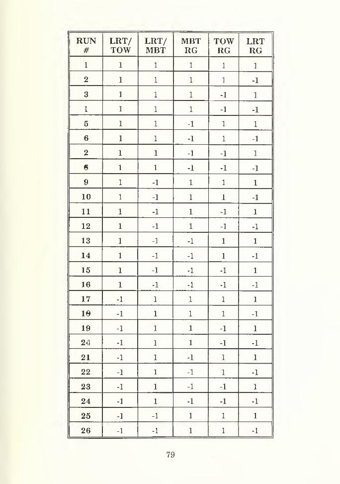
RUN#
LRT/TOW
LRT/MBT
MBTRG
TOWRG
LRTRG
1
2 -1
3 -1
4 -1 -1
5 -1
6 -1 -1
7 -1 -1
8 -1 -1 -1
9 -1
10 -1 -1
11 -1 -1
12 -1 -1 -1
13 -1 -1
14 -1 -1 -1
15 -1 -1 -1
16 -1 -1 -1 -1
17 -1
18 -1 -1
19 -1 -1
20 -1 -1 -1
21 -1 -1
22 -1 -1 -1
23 -1 -1 -1
24 -1 -1 -1 -1
25 -1 -1
26 -1 -1 -1
79

RUN#
LRT/TOW
LRT/MET
METRG
TOWRG
LRTRG
27 -1 -1 -1
28 -1 -1 -1 -1
29 -1 -1 -1 1
30 -1 -1 -1 1 -1
31 -1 -1 -1 -1
32 -1 -1 -1 -1 -1
33
34
35
36
37
38
39
40
41
42
43 2
44 -2
45 2
46 -2
47 2
48 -2
49 2
50 -2
51 2
52 -2
80

APPENDIX D: RANDOM NUMBER GENERATION PROGRAM
A. FORTRAN RANDOM INTEGER PROGRAM.
This program generates a specified number in integer numbers (without
replacement) from a uniform distribution within a set of boundaries. The
inputs are the seed, the number if desired integers, and the maximum value
of the interval (minimum set at 1).
PROGRAM UNIRAND
INTEGER SEED, B(50),I, J, Y(50,50), L, Z, MREALX,KOPEN (UNIT=ll,FILE = 'UNIOUT2')
DO 19 1 = 1,50
DO 18 J =1,50
Y(I,J) =
18 CONTINUE19 CONTINUE
PRINT VENTER THE SEED'READ ', SEEDM = l
REWIND (11)
10 PRINT VENTER THE NUMBER OF RANDOM VALUES YOU DESIRE:'
READ *,L
PRINT ','ENTER THE MAX VALUE OF THE INTERVAL:'
READ *,B(M)
IF (L. GE. B(M)) THENPRINT ', 'YOU HAVE ENTERED MORE VALUES THAN MAX.'
GO TO 50
ENDIFK=REAL(B(M))
C PRINT *, 'YOUR VALUES ARE',L,K
1 = 1
20 CALL RANNUM(1, SEED, 1.0,K,0, X)
Y(M,I) = INT(X)
IF (I .EQ. 1) GO TO 40
DO 30 J =1,1-1
IF (Y(M4) .EQ. Y(M,I)) GO TO 20
30 CONTINUE40 1=1+1
IF (I .LE L) GO TO 20
PRINT VIF YOU DESIRE ANOTHER RUN, TYPE 1.'
81

READ *,Z
IF (Z .EQ. 1) THENM =M + 1
GO TO 10
ELSEDO 100J=1,MWRITE (11,*) 'FOR\L,'RANDOM VALUES FROM 1 TO',B(J)
WRITE (11,45)(Y(J,I), I = 1,L)
100 CONTINUEENDIF
45 FORMAT (1X,20(I2,1X))
50 STOPEND
B. SUBROUTINE RANNUM.
This subroutine was written by Professor PAW Lewis, Department of
Operations Research, Naval Postgraduate School, to generate random values
for given distributions.
SUBROUTINE RANNUM(DISTN, SEED, RPARM1, RPARM2, IPARM, X)
CC THIS SUBROUTINE PROVIDES AN INTERFACE WITH THE LLRANDOMIIC ROUTINES PROVIDED IN THE NONIMSL LIBRARY. THE PARAMETERC REQUIREMENTS AND CALLING PROCEDURES ARE AS FOLLOWS:CC DISTN = DISTRIBUTION TYPE YOU WANT TO SELECTC AN INTEGER BETWEEN 1 AND 7
C SEED = THE RANDOM NUMBER SEED YOU WISH TO USEC RPARM1, RPARM2, AND IPARM ARE REAL AND INTEGER PARAMETERSC PASSED TO THE ROUTINE WITH MEANINGS WHICH VARY WTTH THEC TYPE OF DISTRIBUTION YOU DESIREC NOTE: IPARM IS CURRENTLY NOT BEING USED.C X = THE RETURNED RANDOM NUMBER rT IS ALWAYS REALCC DISTRIBUTION NUMBERS AND THE ASSOCIATED PARM DEFINITIONS:CC 1-UNIFORM ON THE INTERVAL RPARM1 TO RPARM2C 2-NORMAL WTTH MEAN RPARM1 AND VARIANCE RPARM2C 3-EXPONENTIAL WTTH RATE RPARM1C 4-COUCHY WTTH A = RPARM1 AND B = RPARM2C 5-GAMMA WITH SHAPE RPARM2 AND RATE RPARM1C 6-POISSON WTTH RATE RPARM1C 7-GEOMETRIC WTTH P = RPARM1C
REAL RPARM1, RPARM2, XINTEGER DISTN, SEED, IPARM, N
REAL TEMP, VARIAT(l)IF (DISTN.LE.0.ORDISTN.GT.8) THENWRTTECIO, •) 'ILLEGAL CALL TO RANNUM, BAD DISTN'
STOPENDIF
82

cGOTO (10, 20, 30, 40, 50, 60, 70), DISTN
CC GENERATE A UNIFORM BETWEEN RPARM1 AND RPARM210 CONTINUE
IF (RPARM1 - RPARM2.EQ.0) THENWRrTE(10, •) 'ILLEGAL EQUAL RPARMS IN RANNUM'STOP
ENDIFIF (RPARM1.GT.RPARM2) THENTEMP = RPARM1RPARM1 = RPARM2RPARM2 = TEMP
ENDIFCALL LRND(SEED, VARIAT, 1, 1, 0)
VARIAT(l) = RPARM1 + (RPARM2 - RPARM1) • VARIAT(l)GOTO 99
CC GENERATE A NORMAL WITH MEAN RPARM1 AND STDDEV RPARM220 CALL LNORM(SEED, VARIAT, 1, 1, 0)
VARIAT(l) = (VARIAT(l) * RPARM2) + RPARM1GOTO 99
CC GENERATE AN EXPONENTIAL WrTH RATE (1/MEAN) RPARM130 CONTINUE
IF (RPARM1.EQ.0) THENWRTrE(10, •) 'ILLEGAL ZERO RATE IN RANNUM'STOP
ENDIFCALL LEXPN(SEED, VARIAT, 1, 1, 0)
VARIAT(l) = VARIAT(l) / RPARM1GOTO 99
CC GENERATE A COUCHY WTTH A = RPARM1 AND B = RPARM240 CONTINUE
IF (RPARM2.LE.0) THENWRrTE(10, •) 'ILLEGAL COUCHY SPREAD IN RANNUM, B = ',RPARM2STOP
ENDIFCALL LCCHY(SEED, VARIAT, 1, 1, 0)
VARIAT(l) = (VARIAT(l) • RPARM2) + RPARM1GOTO 99
C50 CONTINUE
IF (RPARM1.LE.0) THENWRITE(10, •) 'ILLEGAL NONPOSITIVE GAMMA RATE IN RANNUM'STOP
ENDIFIF (RPARM2.LE.0) THENWRITE(10, *) 'ILLEGAL SHAPE PARAMETER IN RANNUM'STOP
ENDIFCALL LGAMA(SEED, VARIAT, 1, 1, 0, RPARM2)VARIAT(l) = VARIAT(l) • (1.0 / RPARM1)GOTO 99
C60 CONTINUE
83

IF (RPARM1.LE0) THENWRTTE(10, •) 'ILLEGAL POISSON RATE IN RANNUM'STOP
ENDIFCALL LPOIS(SEED, VARIAT, 1, 1, 0, RPARM1)GOTO 99
C70 CONTINUE
IF (RPARM1.LE.0) THENWRITE(10, ') 'ILLEGAL GEOM PROB IN RANNUM'STOP
ENDIFCALL LGEOM(SEED, VARIAT, 1, 1, 0, RPARM1)GOTO 99
C99 CONTINUE
X = VARIAT(l)END
84

C. ASSOCIATED SYSTEM LINE NUMBERS.
RANDOM#
TOWLINE#
MBTLINE#
RANDOM#
TOWLINE #
MBTLINE#
1 36 1 21 102 71
2 37 2 22 103 72
3 38 52 23 104 73
4 39 53 24 74
5 40 54 25 75
6 41 55 26 76
7 42 56 27 77
8 43 57 28 78
9 44 58 29 79
10 82 59 30 80
11 83 60 31 81
12 84 61 32 87
13 85 62 33 88
14 86 63 34 89
15 95 64 35 90
16 97 65 36 91
17 98 66 37 92
18 99 68 38 93
19 100 69 39 94
20 101 70
85

APPENDIX E: SAS OUTPUT
This APPENDIX contains the SAS output used for the multiple regression
analysis, the subsequent regression ofthe significant variables, and theANOVA
tables for both the RED Kills and BLUE Kills MOEs.
A. SAS OUTPUT - RED Kills.
The following is the SAS output for the RED Kills multiple regression:
THESIS DATA 1
14:40 MONDAY, MAY 6, 1991
GENERAL LINEAR MODELS PROCEDURE
DEPENDENT VARIABLE: Y
SOURCE DF SUM OF SQUARES MEAN SQUARE
MODEL 20
ERROR 31
CORRECTED TOTAL
2085.94447891 104.29722395
1059.03629032 34.16246098
51 3144.98076923
MODEL F = 3.05 PR > F = 0.0026
R-SQUARE C.V. ROOT MSE Y MEAN0.663261 12.1719 5.84486621 48.01923077
SOURCE DF TYPE I SS F VALUE PR > F
XI 1 235.22500000 6.89 0.0134
X2 1 172.22500000 5.04 0.0320
X3 1 0.62500000 0.02 0.8933
X4 1 9.02500000 0.26 0.6109
X5 1 1311.02500000 38.38 0.0001
xrxi 1 23.20530627 0.68 0.4161
X2*X2 1 258349868 0.08 0.7851
X3*X3 1 5054325739 1.48 0.2330
X4'X4 1 0.00704023 0.00 0.9886
X5*X5 1 2.16787634 0.06 0.8028
X1*X2 1 26.28125000 0.77 0.3872
X1*X3 1 0.28125000 0.01 0.9283
86

SOURCE DF TYPE I SS F VALUE PR > F
X1*X4 11.28125000 0.33 0.5697
X1*X5 0.78125000 0.02 0.8808
X2*X3 0.03125000 0.00 0.9761
X2'X4 101.53125000 2.97 0.0947
X2'X5 57.78125000 1.69 0.2030
X3*X4 2.53125000 0.07 0.7873
X3*X5 75.03125000 2.20 0.1484
X4'X5 3.78125000 0.11 0.7416
SOURCE DF TYPE III SS F VALUE PR > F
XI 235.22500000 6.89 0.0134
X2 172.22500000 5.04 0.0320
X3 0.62500000 0.02 0.8933
X4 9.02500000 0.26 0.6109
X5 1311.02500000 38.38 0.0001
Xl'Xl 25.66787634 0.75 0.3927
X2*X2 1.96787634 0.06 0.8119
X3'X3 51.16787634 130 0.2302
X4'X4 0.00120968 0.00 0.9953
X5*XS 2.16787634 0.06 0.8028
X1*X2 26.28125000 0.77 0.3872
X1'X3 0.28125000 0.01 0.9283
X1*X4 11.28125000 0.33 03697
X1*X5 0.78125000 0.02 0.8808
X2'X3 0.03125000 0.00 0.9761
X2'X4 10133125000 2.97 0.0947
X2*X5 57.78125000 1.69 0.2030
X3*X4 233125000 0.07 0.7873
X3'X5 75.03125000 2.20 0.1484
X4'X5 3.78125000 0.11 0.7416
T FOR HO: PR > ]T) STD ERROR OFPARAMETER ESTIMATE PARAMETER = ESTIMATE
INTERCEPT 47.75403226 26.26 0.0001 1.81825318
XI 2.42500000 2.62 0.0134 0.92415449
X2 2.07500000 2.25 0.0320 0.92415449
X3 -0.12500000 -0.14 0.8933 0.92415449
X4 0.47500000 031 0.6109 0.92415449
X5 5.72500000 6.19 0.0001 0.92415449
Xl'Xl -0.88104839 -0.87 0.3927 1.01643443
X2*X2 0.24395161 0.24 0.8119 1.01643443
X3'X3 1.24395161 1.22 0.2302 1.01643443
X4*X4 -0.00604839 -0.01 0.9953 1.01643443
X5'X5 -0.25604839 -0.25 0.8028 1.01643443
X1'X2 0.90625000 0.88 0.3872 1.03323613
X1'X3 -0.09375000 -0.09 0.9283 1.03323613
XI 'X4 -039375000 -037 03697 1.03323613
X1*X5 -0. 15625000 -0.15 0.8808 1.03323613
X2'X3 0.03125000 0.03 0.9761 1.03323613
X2'X4 1.78125000 1.72 0.0947 1.03323613
X2*X5 1.34375000 1.30 0.2030 1.03323613
X3*X4 0.28125000 0.27 0.7873 1.03323613
87

PARAMETERT FOR HO: PR > ]T] STD ERROR OFESTIMATE PARAMETER = ESTIMATE
X3'X5X4*X5
-1.53125000
0.34375000
-1.48 0.1484
0.33 0.7416
1.03323613
1.03323613
B. SAS OUTPUT - BLUE Kills.
The following is the SAS output for the BLUE Kills multiple regression:
THESIS DATA 1
14:36 MONDAY, MAY 6, 1991
GENERAL LINEAR MODELS PROCEDURE
DEPENDENT VARIABLE: Y
SOURCE DF SUM OF SQUARES MEAN SQUARE
MODEL 20
ERROR 31
CORRECTED TOTAL
405.26761787 20.26338089
39230161290 12.66134235
51 797.76923077
MODEL F = 1.60 PR > F = 0.1167
R-SQUARE0508001
C.V.
5.8964
ROOT MSE Y MEAN355827800 60.34615385
SOURCE DF TYPE I SS F VALUE PR > F
XI 1 90.00000000 7.11 0.0121
X2 1 0.40000000 0.03 0.8601
X3 1 19.60000000 155 0.2228
X4 1 3.60000000 0.28 05977
X5 1 152.10000000 12.01 0.0016
xrxi 1 9.91737892 0.78 0.3830
X2'X2 1 3.33399471 0.26 0.6115
X3'X3 1 0.10406404 0.01 0.9283
X4'X4 1 0.09712644 0.01 0.9308
X5'X5 1 2.86505376 0.23 0.6376
X1*X2 1 3.12500000 0.25 0.6228
X1'X3 1 2450000000 1.94 0.1741
X1*X4 1 50.00000000 3.95 0.0558
Xl'XS 1 3.12500000 0.25 0.6228
X2'X3 1 3.12500000 0.25 0.6228
X2*X4 1 28.12500000 2.22 0.1462
X2*X5 1 2.00000000 0.16 0.6938
X3*X4 1 2.00000000 0.16 0.6938
X3'X5 1 6.12500000 0.48 0.4919
X4'X5 1 1.12500000 0.09 0.7676
88

SOURCE Dl TYPE III SS F VALUE
XI 1 90.00000000 7.11 0.0121
X2 1 0.40000000 0.03 0.8601
X3 1 19.60000000 155 0.2228
X4 1 3.60000000 0.28 0.5977
X5 1 152.10000000 12.01 0.0016
Xl'Xl 1 9.79838710 0.77 0.3858
X2'X2 1 3.61505376 0.29 05969
X3*X3 1 0.06505376 0.01 0.9433
X4*X4 1 0.06505376 0.01 0.9433
X5*X5 1 2.86505376 0.23 0.6376
X1»X2 1 3.12500000 0.25 0.6228
X1'X3 1 2430000000 1.94 0.1741
XI *X4 1 50.00000000 3.95 0.0558
X1*X5 1 3.12500000 0.25 0.6228
X2*X3 1 3.12500000 0.25 0.6228
X2'X4 1 28.12500000 2.22 0.1462
X2*X5 1 2.00000000 0.16 0.6938
X3'X4 1 2.00000000 0.16 0.6938
X3'X5 1 6.12500000 0.48 0.4919
X4'X5 1 1.12500000 0.09 0.7676
T FOR HO: PR > ]T] STD ERROR OFESTIMATEPARAMETER ESTIMATE PARAMETER =
INTERCEPT 59.88709677 54.10 0.0001 1.1069:
XI -1.50000000 -2.67 0.0121 056261315
X2 -0.10000000 -0.18 0.8601 056261315
X3 -0.70000000 -1.24 0.2228 056261315
X4 0.30000000 053 05977 056261315
X5 -1.95000000 -3.47 0.0016 056261315
Xl'Xl 054435484 0.88 0.3858 0.61879197
X2'X2 -0.33064516 -053 05969 0.61879197
X3'X3 0.04435484 0.07 0.9433 0.61879197
X4*X4 0.04435484 0.07 0.9433 0.61879197
X5*X5 0.29435484 0.48 0.6376 0.61879197
X1*X2 -0.31250000 -0.50 0.6228 0.62902063
X1*X3 0.87500000 1.39 0.1741 0.62902063
X1'X4 1.25000000 1.99 0.0558 0.62902063
X1*X5 -0.31250000 -050 0.6228 0.62902063
X2'X3 -0.31250000 -0.50 0.6228 0.62902063
X2*X4 0.93750000 1.49 0.1462 0.62902063
X2*X5 0.25000000 0.40 0.6938 0.62902063
X3*X4 0.25000000 0.40 0.6938 0.62902063
X3'X5 4)43750000 -0.70 0.4919 0.62902063
X4*X5 0.18750000 0.30 0.7676 0.62902063
89

LIST OF REFERENCES
1. Montgomery, Douglas C, Design and Analysis of Experiments, John Wiley andSons, Inc., 1984.
2. Kowalkoski, Steven A., Parametric Sensitivity Analysis of the Janus(A) HighResolution Combat Model, Masters Thesis, Naval Postgraduate School, Monterey,
CA, March 1991.
3. Box, George E. P., Hunter, William G., Hunter, J. Stuart, Statistics for
Experimenters, John Wiley & Sons, Inc., 1978.
4. Myers, Raymond H., Response Surface Methodology, Allyn and Bacon, Inc., 1971.
5. Schmidt, Stephen R., and Launsby, Robert G., Understanding Industrial Designed
Experiments, Air Academy Press, 1989.
6. Cornell, John A., How to Apply Response Surface Methodology, American Society
for Quality Control, 1984.
7. U.S. Army TRADOC Analysis Center, Janus (T) Documentation and Users Guide,
White Sands Missile Range, NM, June 1986.
8. Weisberg, Sanford, Applied Linear Regression, John Wiley & Sons, Inc., 1985.
9. SAS Institute Inc., SAS/SAT User's Guide, Version 6, Fourth Edition, Volume 2,
Cary, NC: SAS Institute Inc., 1989.
10. Department of Defense, COEA Guidelines (DRAFT), DOD 500.1-G, Feb 1990.
11. Conversation with Starry, Donn, GEN.(Ret), Feb 1991.
12. Mendenhall, William, Mathematical Statistics with Applications, PWS Publishers,
Boston, MA, 1986.
13. Dryer, David, Subject: Comparison of the Janus(A) Combat Model to National
Training Center (NTC) Battle Data: Phase II, TRAC-MTRY, Monterey, CA, 1991.
90

INITIAL DISTRIBUTION LIST
No. Copies
1. Commander 1
U.S. Army Training and Doctrine CommandATTN: ATCDFort Monroe, VA 23651-5000
2. Deputy Undersecretary of the Army 1
for Operations Research
ATTN: Mr. Hollis
Room 2E660, The PentagonWashington, D.C. 20310-0102
3. Commander and Director 1
U.S. Army TRADOC Analysis Command-FLVNATTN: ATRCFort Leavenworth, KS 66027-5200
4. Director 1
U.S. Army TRADOC Analysis Command-WSMRATTN: ATRC-WWhite Sands Missile Range, NM 88002-5502
5. Chief 1
U.S. Army TRADOC Analysis Command-MontereyATTN: MAJ James Hoffman, USAP.O. Box 8692
Monterey, CA 93943-0692
6. Director 1
U.S. Army TRADOC Analysis Command-Ft MonroeATTN: ATRC-RPFort Monroe, VA 23561-5143
91

7. Lawerence Livermore National Library
Conflict Simulation Center
P.O. Box 808 L-315
Livermore, CA 94450
8. Library, Code 52
Naval Postgraduate School
Monterey, CA 93943-5002
9. Director
U.S. Army Concepts Analysis Agency8120 Woodmont Ave.
Bethesda, MD 20814-2797
10. Defense Technical Information Center
ATTN: DTIC,TCACameron Station
Alexandria, VA 22304-6145
11. Director
Department of Systems Engineering
United States Military AcademyWest Point, NY 10996
12. Professor Samuel Parry
Department of Operations Research
Naval Postgraduate School, Code 55PyMonterey, CA 93943-5000
13. CPT Jerry V. WrightDepartment of Systems Engineering
United States Military AcademyWest Point, NY 10996
92


ThesisW9123 Wrightc.l Develop and demonstrate
a methodology using Janus(A) to analyze advancedtechnologies.
ThesisW9123c.l
Wright
Develop and demonstratea methodology using Janus(A) to analyze advancedtechnologies.
