deterministic brownian motion dissertation

37? //B4J

DETERMINISTIC BROWNIAN MOTION

DISSERTATION

Presented to the Graduate Council of the

University of North Texas in Partial

Fulfillment of the Requirements

For the Degree of

DOCTOR OF PHILOSOPHY

By

Gyorgy Trefan, B.S.

Denton, Texas

August, 1993

Trefan, Gyorgy, Deterministic Brownian Motion. Doctor of Philosophy

(Physics) , August, 1993, 172 pp., 30 figures, references, 19 titles.

The goal of this thesis is to contribute to the ambitious program of the founda-

tion of developing statistical physics using chaos. We build a deterministic model

of Brownian motion and provide a microscpoic derivation of the Fokker-Planck

equation. Since the Brownian motion of a particle is the result of the competing

processes of diffusion and dissipation, we create a model where both diffusion and

dissipation originate from the same deterministic mechanism - the deterministic

interaction of that particle with its environment.

We show that standard diffusion which is the basis of the Fokker-Planck equa-

tion rests on the Central Limit Theorem, and, consequently, on the possibility of

deriving it from a deterministic process with a quickly decaying correlation func-

tion. The sensitive dependence on initial conditions, one of the defining properties

of chaos insures this rapid decay.

We carefully address the problem of deriving dissipation from the interaction

of a particle with a fully deterministic nonlinear bath, that we term the booster.

We show that the solution of this problem essentially rests on the linear response

of a booster to an external perturbation. This raises a long-standing problem con-

cerned with Kubo's Linear Response Theory and the strong criticism against it by

van Kampen. Kubo's theory is based on a perturbation treatment of the Liouville

equation, which, in turn, is expected to be totally equivalent to a first-order per-

turbation treatment of single trajectories. Since the boosters are chaotic, and chaos

is essential to generate diffusion, the single trajectories are highly unstable and do

not respond linearly to weak external perturbation.

We adopt chaotic maps as boosters of a Brownian particle, and therefore ad-

dress the problem of the response of a chaotic booster to an external perturbation.

We notice that a fully chaotic map is characterized by an invariant measure which

is a continuous function of the control parameters of the map. Consequently if the

external perturbation is made to act on a control parameter of the map, we show

that the booster distribution undergoes slight modifications as an effect of the weak

external perturbation, thereby leading to a linear response of the mean value of

the perturbed variable of the booster. This approach to linear response completely

bypasses the criticism of van Kampen.

The joint use of these two phenomena, diffusion and friction stemming from the

interaction of the Brownian particle with the same booster, makes the microscopic

derivation of a Fokker-Planck equation and Brownian motion, possible.

ACKNOWLEDGEMENTS

First of all I say thanks to my two advisors Professor Paolo Grigolini and

Professor Bruce J. West without who this dissertation simply would not exist. They

introduced me in the field of researches of nonlinear and chaotic dynamics and they

supported me constantly.

Special thanks go to a group of people in Pisa who helped me via their coop-

eration. Riccardo Mannella who taught me computer simulations, Marco Bianucci

who consulted me on theoretical developments, Luca Bonci who helped me in solv-

ing technical problems and David Vitali whose conversations clarified conceptual

difficulties.

It is a distinct pleasure to thank to Roberto Roncaglia from who I learned a

lot about statistical physics and who I am happy to call my friend since I met him

three years ago. I also thank to Won Gyu Kim for his friendship, Miroslaw Latka

and Ding Chen for discussions on various computer topics.

I would like to say thanks to my professors in the Department of Physics of

UNT for being conciencious teachers. I also thank the graduate students helping

me out with their everyday support.

I warmly thank my parents' support while I was working on my dissertation.

This work was supported partially by the Texas Higher Education Coordinating

Board (Texas Advanced Research Program, Project No. 003594-038).

TABLE OF CONTENTS

Page

FIGURE CAPTIONS iv

Chapter

1. INTRODUCTION 1

2. DETERMINISTIC DIFFUSION 7

§2.1 The Central Limit Theorem 8

§2.2 Deterministic Diffusion in Area Preserving Maps 16

§2.3 Deterministic Diffusion in the Standard Map using the Zwanzig

Projection Technique 27

§2.4 Deterministic Diffusion in a 1 dimensional map 38

3. LINEAR RESPONSE THEORY FOR MAPS 51

§3.1 The Linear Response Theory of van Velsen 53

§3.2 The Linear Response Theory of Kubo for 1 dimensional maps . 58

§3.3 The Linear Response Theory of Kubo for 2 dimensional area

preserving maps 69

4. THE GEOMETRICAL LINEAR RESPONSE THEORY FOR

MAPS

§4.1 The Geometrical Linear Response Theory for 1 dimensional maps 79

5. DETERMINISTIC BROWNIAN MOTION 92

§5.1 Deterministic Brownian motion with phenomenological dissipation 92

ii

§5.2 Deterministic Brownian motion - self consistent picture . . . 110

6. CONCLUSION 123

Appendix

1. THE ZWANZIG PROJECTION TECHNIQUE 127

2. PROBABILISTIC DESCRIPTION OF CHAOTIC MAPS - THE

FROBENIUS OPERATOR 133

3. THE LINEAR RESPONSE THEORY OF KUBO AND THE

GEOMETRICAL LINEAR RESPONSE THEORY FOR CLASSICAL

CONTINUOUS SYSTEMS 152

REFERENCES 167

in

FIGURE CAPTIONS

Figure 2.1.1. The distribution of the velocity v of map (2.1.11 — 12) for 100 itera-

tions. The circles show the results of numerical calculations which are compared to

the theoretical results (solid line) given by (2.1.13) 14.

Figure 2.1.2. The evolution of the variance < > of the velocity of map (2.1.11 -

12) for 1,000 iterations. The circles show the results of numerical calculations which

are compared to the theoretical results given by (2.1.14) 15.

Figure 2.2.1. The diffusion coefficient as a function of the control parameter K

for the variable v of the standard map (2.2.9) calculated from (2.2.11) using the

characteristic function technique. We considered only large values of the control

parameter K i.e. K > 10 28.

Figure 2.3.1. The diffusion coefficient of variable v of the standard map (2.2.9) as

a function of K. Again we considered only large values of the control parameter K

i.e. K > lO.The calculations are based on the Zwanzig projection method which

results equation (2.3.1) 37.

Figure 2.4-1- The 1 dimensional diffusion producing map (2.4.4) for a = 2.... 40.

Figure 2.4-2. The reduced map of map (2.4.4) for a = 2 41.

Figure 2.4.3a. Drift produced by map (2.4.4). The peak of map (2.4.4) is mapped

onto a neighboring peak 42.

Figure 2.4-3b. A periodic orbit produced by map (2.4.4). The peak of map (2.4.4)

is mapped into itself eventually. 43.

Figure 2.4-4• A diffusive orbit (0.017,0.119,0.833,-0.169,...) produced by map

(2.4.4) for a = 2 44.

Figure 4-1• The zero centered tent map (4.1) 81.

iv

Figure 4-2. The conjugating function (4.2) 82.

Figure 4-3. The conjugated map (4.5) for some values of the conjugation parameter

a, a = 1.0 (solid line, unperturbed case), a = 0.7 (long dashed line) and a = 1.3

(short dashed line) 83.

Figure 4-4• The evolution of the average of the conjugated map (4.5) for some val-

ues of the conjugation parameter a, a = 1.0 (solid line, unperturbed case), a = 0.7

(long dashed line) 84.

Figure 4-5. The response R(a) of the conjugated map (4.5) as a function of the

conjugation or perturbation parameter a. The circles show the results of numerical

calculations, the solid line is the analytical result calculated from (4.3) 85.

Figure 4-6. The zero centered logistic map (4.15) 87.

Figure ^.7. The conjugated map (4.18) with for some values of the conjugation

parameter a, a = 1.0 (solid line, unperturbed case), a = 0.7 (long dashed line) and

a = 1.3 (short dashed line) 88.

Figure 4-8. The invariant distribution (4.21) of the conjugated map (4.18). 90. for

some values of the conjugation parameter a, a = 1.0 (solid line, unperturbed case),

a = 0.7 (long dashed line) and a = 1.3 (short dashed line) 90.

Figure 4-9- The response R(a) of the conjugated map (4.18) as a function of the

conjugation (or perturbation) parameter a. The circles show the results of (4.22)

by numerical calculations, the solid line is the fitting curve (4.16) for small pertur-

bations 91.

Figure 5.1.1a. The velocity equilibrium distribution p(v) of the Brownian particle

in the small 7 case. The circles show the results of numerical simulations based

on map (5.1.39 — 41) and the solid line shows the result of the theoretical inves-

tigations calculated from (5.1.16). The parameter values we used: Tcha0s — 1-0,

< x2 > = 1/2, 7 = 0.01 and integration step h = 0.1 107.

v

Figure 5.1.1b. The velocity equilibrium distribution p(v) of the Brownian particle

in the large 7 case. The circles show the results of numerical simulations based on

map (5.1.39) and (5.1.43 — 44) and the solid line shows the result of the theoretical

investigations calculated from (5.1.16). The parameter values we used: rch.aos = 1.0,


Figure 5.1.1c. The velocity equilibrium distribution p(v) of the Brownian particle

in the modest 7 case. The circles show the results of numerical simulations based on


investigations calculated from (5.1.16). The parameter values we used: Tcha0s = 1.0,


Figure 5.2.1. Relaxation of the velocity of map (5.2.1 — 5) with reaction parameter

A = 0.01. (5.2.3) is the conjugate of the tent map . The velocity is set initially to

VQ = 100 and the average is taken over 10,000 samples. The circles show the results

of numerical calculations and the solid line represents the theoretical prediction of

(5.1.8) with (5.2.23) and (5.2.24) 118.

Figure 5.2.2. Evolution of the average velocity square from map (5.2.1 — 5) for some

values of the reaction parameter A. (5.2.3) is the conjugate of the tent map. The

velocity was initially set to VQ = 0 and the average was taken over 10,000 trajec-

tories. The circles represent the results of computer calculations and the solid line

shows the the theoretical results using (5.1.10) with (5.2.23) and (5.2.24). . . . 119.

Figure 5.2.3. Relaxation of the velocity of map (5.2.1 - 5) with reaction parameter

A = 0.01. (5.2.3) is the conjugate of the logistic map. The velocity is set initially to

v0 = 100 and the average is taken over 10,000 samples. The circles show the results


(5.1.8) with (5.2.25) and (5.2.26) 121.

Figure 5.2.4• Evolution of the average velocity square from map (5.2.1 — 5) for

VI

some values of the reaction parameter A. (5.2.3) is the conjugate of the logistic

map. The velocity was initially set to VQ — 0 and the average was taken over 10,000

trajectories. The circles represent the results of computer calculations and the solid

line shows the the theoretical results using (5.1.10) with (5.2.23) and (5.2.24).122.

Figure A2.1. The map (A2.17) for r = 3 138.

Figure A2.2. The map (A2.21) 139.

Figure A2.3. The invariant distribution (A2A9) of the logistic map (.42.48).. 148.

Figure A2-4- The iterates / 1 (x ) and f2(x) of the zero centered logistic map (.42.53).

150.

Figure A3.1. The modified Henon-Heiles potential (A3.28) 159.

Figure A3.2. The deformation of the Poincare surface of sections due to perturba-

tion. The solid line shows the boundary of the Poincare surface of sections of the

plane (-7T, £) when the motion takes place in the modified Henon-Heiles potential

(.A3.28) i.e., the motion is unperturbed. The dashed line shows the boundary of the

Poincare surface of sections of the perturbed motion 161.

vn

CHAPTER 1

INTRODUCTION

Statistical physics addresses the problem of deriving the macroscopic properties

of matter from microscopic properties. One of the most difficult problems is that of

macroscopic irreversibility versus microscopic reversibility, i.e., how one can derive

diffusion, relaxation to equilibrium and other irreversible phenomena from interac-

tions of atoms, molecules or other particles when the interactions are described by

the fundamental reversible laws of classical or quantum mechanics.

The first partial solution for the problem of reversibility-irreversibility was pro-

posed by Boltzmann (Boltzmann 1912) who, although he wanted to avoid, made

an additional assumption - the assumption of non-decreasing entropy in an isolated

physical system, which lead to relaxation and consequently to irreversibility.

Boltzmann's idea - in spite of being decades ahead of the scientific knowledge of

his contemporaries - contained the unnecessary assumption on the non-decreasing

entropy. This assumption was eliminated by Langevin (Langevin 1908) who as-

sumed an interaction between the system of interest and its environment. In this

model the environment acts upon the system with a random force and the system

of interest dissipates energy to the environment. The fluctuation and dissipation

lead the evolution of the system to equilibrium and consequently irreversibility for

arbitrary initial condition.

Although Langevin did not assume entropy in his model he introduced a ran-

dom force which is a sophisticated way of saying "I do not know the mechanism but

I can describe the reality well enough". Although stochastic theories are mathemat-

ically refined and elegant, from the point of view of a fundamental physical theory

the introduction of a random force is no better than a purely thermodynamical

and therefore phenomenological fluctuation-dissipation theory which was developed

earlier by Einstein (Einstein 1905, 1906).

Thus the idea of a stochastic environment had to be replaced with a determin-

istic environment. Nakijama, Mori and Zwanzig worked out a quantum mechanics-

like formalism (Nakijama 1958, Mori 1965, Zwanzig 1960) where they considered

a system of interest coupled to the environment which had infinitely many degrees

of freedom. They used a projection technique to derive the motion of the system

of interest. Their theory has the following, not well established assumptions: the

environment of the systems they investigate has an infinite number of degrees of

freedom, is described by linear differential equations and the environment is placed

initially in thermal equilibrium (statistical assumption) i.e. the energy of the en-

vironment follows the Maxwell-Boltzmann distribution from the initial moment of

its evolution. These three assumptions are not well justified because one finds re-

laxation in mesoscopic systems too, although they do not have nearly infinitely

many degrees of freedom. Furthermore in a conservative system described by linear

differential equations of motion the energy remains confined in the original distri-

bution and does not move from one normal mode to another, thereby preventing

the system from relaxing to the equilibrium state in which all modes have the same

energy. Finally we want to derive statistical properties from the system dynamics

rather than assuming them as an initial condition.

There is a different approach to irreversibility phenomena than the one de-

scribed and it was proposed by Fermi. Fermi realized that in a conservative system

described by linear differential equations of motion one will not find relaxation phe-

nomena. Thus, Fermi, Ulam and Pasta (Fermi et al. 1955) numerically studied a

nonlinear system hoping to find relaxation to equilibrium but instead they found a

robust periodicity with soliton solutions and no relaxation. By this attempt Fermi

showed that the nonlinearity itself is not sufficient for a conservative physical sys-

tem to reach equilibrium. The necessary and sufficient condition for a conservative

physical system to reach equilibrium is for it to be a mixing system as was proved

by Krylov (Krylov 1950). Mixing systems are better known to physicist as a kind

of chaotic system thus the idea that the foundation of statistical mechanics for clas-

sical systems should rest on chaos (Ford et al. 1963, Arnold et al. 1968, Ehrenfest

1959, Ford 1975) gradually emerged and still has not been universally accepted.

The goal of this thesis is to contribute to the ambitious program of the foun-

dation of statistical physics. We attempt to build up a model of Brownian motion

(Brown 1826) which is an important system from the point of view of irreversibility.

Since Brownian motion is the result of the competing processes of diffusion and

dissipation, we have to create a model where both diffusion and dissipation origi-

nate from the same deterministic mechanism - the interaction of a particle with its

environment. The particle which interacts with its environment is described by the

following differential equations

v = x, (1.1)

and

x = R(x, — A2v(t),...). (1.2)

Above (1.1) is the Newton equation of motion of the particle since the velocity v

of the particle changes according to the force of the environment represented by

variable x.

(1.2) is the equation of motion of the environment, where R represents a set of

functions, the term — A2v(t) represents the reaction of the particle on the environ-

ment (negative feedback) with the reaction coefficient A and the dots indicate that

the motion of the environment can depend on variables other than x and v.

The differential equations (1.1 — 2) show that when the particle does not react

on its environment i.e., A = 0, then the environment continuously gives energy

to the particle in a random way, thus diffusion with no dissipation takes place.

This process is explained in details in Chapter 2, where we use a discrete time

representation of (1.1 — 2), for instance the environment is mimicked by a chaotic

map. Chaotic maps are deterministic systems so the diffusion we obtain is termed

as deterministic diffusion.

When the particle reacts on its environment i.e., v is very large and A ^ 0,

but weak, then (1.2) immediately yields

<- ®(^) eq ~ %A < ^(^) eq • (^*^)

(1.3) shows that in this case the environment rearranges itself in a way that com-

pensates for the action caused in the environment by the Brownian particle. In

other words the environment responses to the perturbation, where the average re-

sponse linearly depends on the velocity, the reaction parameter A and coefficient x,

the generalized susceptibility. Thus as we shall show, the reaction of the Brownian

particle on its environment is intimately related to Linear Response Theory. We

use maps to mimick the dynamics of the environment, so we have to investigate

how chaotic maps respond to external perturbations. Linear Response Theory for

chaotic maps is the subject of Chapter 3.

The Linear Response Theory for chaotic maps presented in Chapter 3 is the

counterpart of Kubo's conventional Linear Response Theory (Kubo 1957). The lat-

ter theory is based on a first-order perturbative treatment of the Liouville equation.

Since the evolution of the distribution of chaotic maps is given by the Frobenius

operator, the Linear Response Theory for chaotic maps is a first-order perturbation

calculation on the Frobenius operator and it recovers Kubo's formula i.e., the sus-

ceptibility is related to the equilibrium cross-correlation function of an observable

of the unperturbed map and the perturbation variable.

As we mentioned above the conventional theory of Kubo is basically a pertur-

bative treatment of the Liouville equation which is equivalent to the perturbation

of single trajectories. Since the trajectories of chaotic systems are unstable, it

was thought by van Kampen (van Kampen 1971) that a first-order perturbation

treatment is inadequate. Applying Kubo's treatment to maps one faces the same

problem as in the case of continuous-time systems i.e., using a first-order perturba-

tion treatment on the Frobenius operator means perturbation of single trajectories.

To satisfy the criticisms of van Kampen we adopt a geometrical argument and we

build up the Geometrical Linear Response Theory for chaotic maps in Chapter 4.

In Chapter 5 we combine the deterministic diffusion and dissipation, first us-

ing a phenomenological dissipation in (1.1 — 2) so that they become the following

Langevin equation

v = x — 7i>, (1.4)

and

x = R(x,...). (1.5)

In the above Langevin equation, instead of the stochastic environment (1.5) we use

a deterministic, chaotic environment mimicked by the logistic map. The appearance

of phenomenological dissipation is not satisfactory, because a self consistent theory

should provide both diffusion and dissipation from the same mechanism, namely

the particle-environment interaction as it is given by (1.1 — 2). Thus in the rest

of Chapter 5 we realize (1.1 — 2) by a discrete time representation, actually by a 2

dimensional map. The map we present recovers the standard results of the Brown-

ian motion within the framework of a completely deterministic and self consistent

model.

CHAPTER 2

DETERMINISTIC DIFFUSION

As we mentioned in the Introduction the main goal of this dissertation is to

build up a self-contained picture of Brownian motion, without using statistical as-

sumptions, namely from rigorously deterministic equations of motion.

Brownian motion is the result of a dynamical balance between two competing

processes, diffusion and dissipation. Therefore, an exhaustive treatment of Brown-

ian motion forces us to investigate both diffusion and friction. In this chapter we

focus on diffusion, and, to keep our promise of avoiding statistical assumptions, on

deterministic diffusion.

Diffusion, according to traditional wisdom is a genuinely stochastic process,

which emerges when a physical variable collects uncorrelated, random actions.

There is, however, a wide class of deterministic systems, the chaotic systems, which

are reminiscent of random systems in certain aspects. Thus we also expect the

appearence of diffusion in certain chaotic systems. This is what we do in this Chap-

ter, namely, we address the problem of diffusion in deterministic, chaotic systems,

for the purpose of deriving an analytical expression for the quantity defining the

diffusion strength, the so-called diffusion coeficient. For any system under study we

shall derive the analytical expression of the corresponding diffusion coefficient.

In understanding diffusion the Central Limit Theorem is of primary impor-

tance. Thus we review it in §2.1 and give a physical example of how diffusion

emerges when a velocity is coupled to a chaotic environment represented by the

logistic map.

In §2.2 we present a less restrictive version of the Central Limit Theorem and

8

again we give a physical example of how diffusion emerges in the standard map with

short correlation time and how one can calculate the diffusion coefficient using the

characteristic function technique. In §2.3 we study diffusion for the standard map

using a different formalism, i.e., the Zwanzig projection technique.

Diffusion occurs not only in 2-dimensional area preserving maps, but also in

1-dimensional, chaotic maps. This is what we study in §2.4- We derive the diffusion

coefficient from dynamical considerations and by using the Frobenius operator to

determine the invariant density of the map, i.e., the equilibrium probability density.

§2.1 The Central Limit Theorem

Remark 2.1.1. As we mentioned above the Central Limit Theorem is of paramount

importance in understanding diffusion. Therefore first we cite and prove it following

the standard procedure (Gnedenko and Khinchin 1962, Bass 1966, Rozanov 1969).

Then we give a physical example of deterministic diffusion. In this example the

velocity is the collector or integrator variable which is coupled to a chaotic environ-

ment. The chaotic environment is represented by the logistic map. In this example

we show that the velocity has a Gaussian distribution whose width grows linearly

in time.

Proposition 2.1.1. If

i) we consider the random variables £i,#2> ...xn

ii) which are mutually independent,

iii) have the same mean value < Xj > = 0, where the symbol < ... > denotes

the averaging over an ensemble of realizations

iv) have the same standard deviation y < x'j > = D,

v) and have the same ensemble distribution p(xj) which vanishes quickly as

l«il 0 0

then

the quantity

vn = -^= • (xi + x2 + ... + xn) (2.1.1) V n

• is normally distributed or more precisely the probability that the sum (2.1.1)

is less than vD is I

"1 /»V lim P {-£ < v) = — = / exp (—t2/2)dt (2.1.2)

n-»00 \JJ J V27T J-oo

Proof. The characteristic function of vn is defined

$(vn) —< e x p ( — i k v n ) > = < e x p (-ik(x 1 + x 2 + ... + xn))/yfn >

n n

= < T T e x p > = T T < exp {—ikxjj^/n\ >

j=i j . i (2.1.3) n

= e x p (XT 3-1

where

Aj(k) = In < exp ( - i k x j / y / n ) >. (2.1.4)

Since n is large we expand Aj(k) in Taylor series with respect to k around k = 0

and we get

Aj(k/^/n) ^ Aj(Q)4- kAj{0) + —Aj(0) H 0{n 1^2). (2.1.5)

« Ti

10

From the definition (2.1.4) of A,{k) one sees that A,(0) = 0. The first order term

kAj(0) vanishes too because

dkAi(fc)L=o = ^ < x i > = °- (2.1.6)

The second order term (k2/2)A'<(0) = ~(k2/2n)D2 because

(j2 • -2

dk2^(fc)L=o = ^ < XJ > +'- < *; >= < x) > = -~D2 . (2.1.7)

So the characteristic function of vn becomes D2 1

< exp (—ikvn) > = exp (—ik2— + ()(-=)). n (2.1.8)

Introducing the notation

1 . ~ E < * 5 >

the characteristic function becomes

n n . 3=1

(2.1.9)

* K ) = exp ( - i f c V + 0 ( ^ ) j . (2.1.10)

By neglecting the term 0(1/Jn) one can see the characteristic function is bell-

shaped with width a/V2. After inverse Fonrier transformation of $(„„) the quantity

vn has a normal distribution according to (2.1.2).

q.e.d.

Remark 2.1.2. In the following Proposition 2.1.1 we show an example for the ap-

plication of the Central Limit Theorem to a physical system. We consider a model

11

system where the velocity of a free particle is coupled to a chaotic environment. The

chaotic environment acts upon the velocity but the velocity does not react back on

the environment. The chaotic environment causes abrupt changes in the velocity

i.e., the particle is periodically kicked. The chaotic environment is mimicked by

zero centered logistic maps. We note here that the logistic map is one of the most

studied map (Ulam and Neumann 1947, May 1976, Feigenbaum 1978, Collet and

Eckmann 1980, Eckmann and Ruelle 1985, Schuster 1988).

We now plan to study a model resulting in the diffusion of a variable v, which

can be thought of as being the velocity of the Brownian particle. This is the variable

under observation. Thus we shall refer to it as the variable of interest. The variable

x determines the time evolution of the variable of interest, under the form of abrupt

changes, or boosts. Thus we shall refer to it as the booster variable. Throughout the

whole thesis we shall use the term booster to denote a new kind of bath, one that

is: deterministic and chaotic, and has only a few degrees of freedom. To keep the

booster distinct from conventional baths, which are characterized by infinitely many

degrees of freedom, and are in well defined thermodynamical states, as a result of

an assumption, rather than of a genuinely microscopic and deterministic dynamics.


i) we consider a free particle whose velocity is constant for a time but at the

end of each time interval the velocity abruptly changes from the value vn to vn+1

= Vn 4" (2.1.11)

ii) where the change of the velocity is determined by a sequence of numbers

Xi,X2, ...,xn originates from the zero centered logistic map

12

xn+i = 1 - 2x2n, (2-1.12)

then

• after n iteration the distribution of the variable vn is

p(vn) = —F= exp ^ • (2.1.13) yxn \ n J

and

• the variance of the velocity of the kicked particles is linear in time

<v2n> = n<x )>= n/2. (2.1.14)

Proof. As we showed in Proposition A 2.6, Appendix 2 recursive application of the

zero centered logistic map (2.1.12) provides a ^-correlated sequence of numbers

< XjXo > =< x) > 6jfi (2.1.15)

i.e., the numbers xi, aj2, •••, xn are mutually independent. They also have zero mean

value

< X j > = 0, (2.1.16)

and their standard deviation is constant

< x) > = 1/2, (2.1.17)

and their probability density vanishes as |xj | —• oo i.e.,

13

lim p(xj) = 0. (2.1.18)

\xj |—KX>

Thus they fulfill the requirement of the Central Limit Theorem. In our case the vari-

able of interest v is the collector (integrator) variable. The Central Limit Theorem

states about the variable of interest v that it has a Gaussian distribution according

to

p<"", = v^exp(-^)' (2'U9)

where

a2 = n < x2j > . (2.1.20)

Substituting (2.1.20) and (2.1.17) into (2.1.19) we obtain

p(vn) = . 1 = exp f - J n2 1 = -7== exp ') • (2.1.21)

^2wn < x) > V 2 n<x)>j \ n) V )

We can calculate the evolution of the variance of the variable of interest from

the definition of the second moment i.e., from

/

OO

p(vn)dvn. (2.1.22) -OO

Substituting (2.1.21) into (2.1.22) we end up with (2.1.14).

q.e.d.

Remark 2.1.3. A computer program realized the equations (2.1.11 - 12). In the

calculations all variables of interest are initially set to 0 i.e., i>o = 0, and the booster

14

variable is initially distributed uniformly over the interval [—1,1]. The iterations

were executed for 100 steps i.e., n = 100 and the final distribution of variable i>ioo

was calculated over 50,000 samples. The distribution obtained by the numerical

calculations and the one calculated from (2.1.13) are presented in Figure 2.1.1.

0 .07

0 .05

- 0 .04

0 .03

0 . 0 2

0 . 0 1

Figure 2.1.1. The distribution of the velocity v of map (2.1.11 — 12) for 100 it-

erations. The circles show the results of numerical calculations which are compared

to the theoretical results (solid line) given by (2.1.13).

A computer program calculated the diffusion of the velocity based on equations

(2.1.11 — 12). In the calculations all variables of interest were initially set to 0

i.e., VQ — 0, and the booster variable was initially distributed uniformly over the

interval [—1,1]. The iteration was executed for 1,000 steps i.e., n = 1,000, and

15

the evolution of the variance was calculated over 10,000 samples. The evolution

obtained by numerical calculations and the one calculated from equation (2.1.14)

are presented in Figure 2.1.2.

- 3 0 0

1000

Figure 2.1.2. The evolution of the variance < v\ > of the velocity of map (2.1.11 —

12) for 1,000 iterations. The circles show the results of numerical calculations which

are compared to the theoretical results given by (2.1.14).

Definition 2.1.1. In the example above one can see that the individual trajecto-

ries of velocity v evolve in a random-like manner, but the average value of the

variance of the velocity is proportional to the discrete time n. In this case a dif-

fusion of the velocity takes place. The diffusion of the velocity is described by a

diffusion coefficient D which is defined as follows

16

D = ( lim ^-(v„ - vo)A , (2.1.23) \n-*oo i n /

where VQ is the initial value of variable v and vn denotes the value of variable v at

time n.

Remark 2.1.4• Note that the diffusion is intimately connected to the Central Limit

Theorem. Whenever a diffusion process takes place, we can consider the diffusive

variable as an accumulation of random or chaotic events with finite correlation time.

The variance of the diffusive variable is proportional to the time and its distribu-

tion function is Gaussian. On the other side when we find anomalous diffusion i.e.,

when the evolution of the variance of the diffusive variable is not linear in time, it

is an indication that the Central Limit Theorem breaks down for some reasons, for

instance the booster variable has infinite correlation time.

§2.2 Deterministic Diffusion in Area Preserving Maps

In this paragraph we first show that there are less restrictive ways than shown

in §2.1 of stating and proving the Central Limit Theorem. Then we show how one

can derive the diffusion coefficient when the chaotic environment is characterized

by a definite, not too long correlation time. Finally we show using the example of

the standard map in its chaotic regime how one can derive the diffusion coefficient

using the characteristic function technique.

Remark 2.2.1. The way we stated the Central Limit Theorem is too restrictive.

17

We can use less restrictive assumptions and at the same time we the Central Limit

Theorem. We can ease the assumptions on several points.

i) The random numbers Xi-s do not need to have zero mean value. With nonzero

mean values we get a "drift" in the variable v, i.e., the mean value of v increases

linearly with time. With the deduction of the drift the Central Limit Theorem is

easily proved.

ii) The random numbers Xj-s should not necessarily have the same distribu-

tion p(xj). For instance let us consider a sequence of random numbers where the

random numbers with odd indices have one distribution pi(x2 j+i) with standard

deviation < ^ j + i > = D and the random numbers with even indices have an-

other distribution P2{x2j) ^ Pi{%2j+i) although their standard deviations is the

same yj< > = yj< x\j > = D. The Central Limit Theorem holds true for

the random numbers with odd indices and separately for the random numbers with

even indices and trivially for their comb-like combinations.

iii) we can ease the assumption of mutual independence and still prove the

Central Limit Theorem. We prove this in the following proposition.

Proposition 2.2.1. If the impulse map reads

^n+l — -f- Xn

(2.2.1) %n+1 — /(®n)j

where / (xn) is a map with a dynamics of finite correlation time r , then

• the variable v is diffusive and

• its diffusion coefficient D is equal to half the product of the variance < x^ >

and the correlation time r

18

D = -<X)>T. (2.2.2)

Proof. The diffusion coefficient of variable v is, according to Definition 2.1.1,

( " . 3 )

where VQ is the initial value of variable v and vn is its value after n iteration of

the map (2.2.1). The difference vn - v0 can be written in terms of the difference

in consecutive velocities At* = Vi - as vn - v0 = £ ? = 1 At*. So the diffusion

coefficient (2.2.3) becomes

^ ( n ^ E E ^ ^ V (2.2.4) \ i= 1 3=1 /

We want to reduce the double sum in the expression of the diffusion coefficient so

we rewrite it in the form

1 ^ n n—i

" i f c l E ) • (2.2.5) i=l j=l-i

we can The velocities jump Avi is caused by the booster, namely Avi = Xi. Thus

express (2.2.5) m terms of the z;'s. The booster is chaotic in a way that the variable

x has a finite correlation time. Thus we can express the sum over j in (2.2.5) with,

replaced by from n = -oo to n = oo. Thus the diffusion coefficient (2.2.5)

takes the form

1 n oo

IJ: E < > (2.2.6) t= 1 —oo

19

Since the booster is ergodic the ensemble average over i can be replaced by a single

time average

1 °° ^ = 2 E (xixi+j)- (2.2.7)

j——00

Note that the correlation time r of the booster is defined as

00 ( X i X i+ j ) T = -

{X{X{)

Substituting this expression into (2.2.7) we end up with equation (2.2.2).

(2.2.8)

q.e.d.

Remark 2.2.2. The impulse maps (2.1.11) and (2.2.1) that we have been deal-

ing with so far were not derived from autonomous systems. The real challenge

is to derive diffusion in Hamiltonian systems. Since a 1-dimensional Hamiltonian

system often is represented by a 2-dimensionaI area-preserving map, i.e., by a map

whose Jacobian J = 1, we investigate the possibility of diffusion in a 2-dimensiona!

area-preserving map. One of the most widely discussed 2-dimensional maps is the

standard map

vn+i =vn + K sin(xn) (2.2.9)

•£»+1 ~ ®n "t" ^n+1*

It was observed that for certain values of the control parameter K the standard

map is chaotic (Chirikov 1979). For very large values of the control parameter K the

correlation time of variable x is practically unity, i.e., the variable x in its evolution

loses memory in a single step. Ia this case diffusion takes place in the variable v and

20

we can estimate the diffusion coefficient D. Using the result of Proposition 2.2.1

the diffusion coefficient D of the variable v of the standard map (2.2.9) is

D = \ (K2 sin(zn)2) = (2.2.10)

If the control parameter K is large but the variable x is not delta-correlated

we need more precise calculations to obtain the diffusion coefficient. The first

results in this case were obtained by Rechester and White (Rechester and White

1980), although their method was not completely deterministic. The first completely

deterministic derivation of the diffusion coefficient D as the function of the control

parameter K was determined by Cary et al. (Cary et al. 1981). Later Cary and

Meiss suggested that diffusion takes place in a wide range of deterministic maps and

the diffusion coefficient could be calculated in a way similar to that of Rechester

and White. Schell et al. (Schell et al. 1982) discussed diffusive dynamics in quite

general systems with translational symmetry. Doran and Fishman (Doran and

Fishman 1988) showed how diffusion takes place in multidimensional systems. One

of the most recent generalizations was presented by Kook and Meiss (Kook and

Meiss 1990) who showed how diffusion emerges in symplectic maps.

The case of modest values of the control parameter K, i.e., (1 < K < 10) is

a subject of intense research (Zisook 1982, Karney 1983, Lichtenberg et al. 1987).

In this case long time correlations appear and anomalous diffusion takes place as a

result of intermittencies but the phenomena is not well understood.

In Proposition 2.2.2 we use the characteristic function technique to determine

the diffusion coefficient D as the function of the control parameter K in the case of

large values of K following the idea of Rechester and White (Rechester and White

1980).

21


i) we consider the standard map

*>«+i =vn + K sin(xn)

Xn-\-1 — Xn H" ^n+1

ii) in its chaotic case, i.e., control parameter K is large (K > 10) then

• the variable v shows diffusion

• and its diffusion coefficient is

(2.2.9)

D = ^K2 [1 - 2J2(K) + 2J$(K) - 2Jl{K)} , (2.2.11)

where Jn(K) denotes the n-th order Bessel-function.

Proof. As we showed in Proposition 2.2.1 the diffusion coefficient D of an impulse

map is

1 00

D = - Y , »*+')

cx>

1 1 v~^ 1 X \ = - (AvkAvk) + - 2J (AvfcAvk+t) + - 2^ (AvkAvk+i).

(2.2.12)

1=1 l=-oo

Using the time symmetry of the correlation function the diffusion coefficient becomes

D = \ (AvkAvk) + 2 ^ (&vkAvk+i) i=i

(2.2.13)

The change in the variable v is due to the sine term in the standard map (2.2.9),

where Avk = K sin xk,

D = K2

(sin xk sin xk) + 2 ^ (sin Xk sin xk+i) i=i

(2.2.14)

22

We use exponential representation

smxk = i [exp(ixfe) - exp(-*sfc)] 2 i

and the diffusion coefficient D becomes

K2 D = ~ r [(exP(«0xfc)) + (exp(i2a:fc))] 4

K2 00

7 l(6XDfi El, -4- 7.T.U I I \ -4- / PYn/ n rn. . _\\1

1=1 (2.2.15)

K2 00

4 5 3 [(exP(ia;fc + *®Jb+0) + (exp(-zxk - ixjk+l))]

K X~ r / , + ~4~2-s l(exP(-Mk + ixk+i)) + (exp(ixk - ixk+i))].

i=i

We can rewrite the diffusion coefficient in terms of the characteristic function

the characteristic function is defined in the following way,

since

Xo(m0) = (exp(im0a:fc)) (2.2.16.a)

Xo(™>o,mi) = (exp (im0xk + imixk+i)) (2.2.16.6)

Xo("io,mi,m2) = (exp(imoXfc + imixk+i + im,2Xk+2)). (2.2.16.c)

So the diffusion coefficient becomes

OO K2 K2

d = ~4~ Ixo(o) + xo(2)] ba(i, 0 , . . . , 0,1) + xi(—1,0,..., 0, -1)] 1=1

K2 00

+ T X ! M 1 , 0 , . . . , 0, -1 ) + X i ( - l , 0 , . . . , 0,1)] 1=1

K*_ 4

00 Xo(0) + xo(2) + 2 £ ( X / ( 1 , 0 , . . . , 0 , - 1 ) - X i ( l , 0 , . . . , 0 , l ) )

1=1

(2.2.17)

23

Our goal is to simplify the above expression. The way we do is to we derive a

recursion relation for the higher order characteristic functions and to calculate the

lower order characteristic functions in a straightforward way. Therefore we rewrite

the standard map (2.2.1) in a recursive form that depends only on the variable x.

It takes the form

xn = 2xn_! - xn_2 + K sin xn_j (2.2.18)

The characteristic function is given by the definition in the following form

X(m0 ,m1 , . . . ,m f c) =

(exp(im0xn + . . . + imfc_3a;n+fc_3 + imk_2xn+k_2 + im^Xn+k^ + imkxn+k))

(2.2.19)

Substituting (2.2.18) in the last term of the expression above we get

x(rno,mi,.. . ,mfc) =

< exp(im0a;n + . . . + imfc_3xn+fc_3 + i(mk_2 - mk)xn+k_2 (2.2.20)

+ i(mk-1 +2mk)xn+k_1 + imkKsixilxn+k^)) > .

Using the Bessel function identity OO

exp(iKsinx)= Ji(K) exp(ilx) (2.2.21) fc — OO

we end up with the desired recurrence relation of the characteristic functions

Xfc(w0,m1,...,mfc) _ ^ MmkK)xk-i(m0,...,mk_3,mk_2 - mk, l=~™ (2.2.22)

mk-i + 2 mk + l).

24

Now we can evaluate the diffusion coefficient D given by (2.2.17) term by term.

The term Xo(0) is trivially unity since

Xo(0) = < exp 'Ozfc) > = 1. (2.2.23)

The term Xo(2) vanishes because

Xo(2) = < exp(i2xfc) > = 62y0 - 0. (2.2.24)

Now we explicitely write the essential terms of the diffusion coefficient D. Thus

(2.2.17) becomes

4 | 1 + 2 E t t t ( 1 . 0 o , -1) -Xi( l ,0 , . . . ,0 , l ) ] l

2

+ [^4(1,0,0,0, —1) - X4(l, 0,0,0,1) + X3(l> 0,0, - 1 ) — X3(l, 0,0,1)]

K2

+ X 2 W 1 ' ° ' _ 1 ) - X2(i, o, 1) + Xi(l, - 1 ) - Xi(l, 1)].

(2.2.25)

The term Xi(m0,mi) is calculated from the definition (2.2.16b) by setting k=-l

Xi(m0,mi) = < exp(im0x_i + «mi®0) > • (2.2.26)

Expressing x_x from the standard map (2.2.9)

X-1 =Xq-VQ

and substituting back into (2.2.26) we obtain

Xi(^o,mi) = ( J d^odxo ) ' 7 , dt^d®# exp(i(m0 + mx)xQ - im0vQ), (2.2.27)

25

where R is an invariant region of the space ( x , v ) i.e., a region which is mapped

onto itself. Evaluating the integral (2.2.27) we get

= rao,0 TOi,0) (2.2.28)

from which we conclude that

X i ( l , l ) = x i ( l , - 1 ) = 0. (2.2.29)

In the calculation of the terms X2(m0im i im2) of the diffusion coefficient (2.2.25)

we use the recursion relation (2.2.22). This takes the form

OO X 2 ( m 0 i m i i m 2 ) = M m 2 K ) x i ( m o - m 2 , m i + 2 m 2 + 1 ) . (2.2.30)

oo

Substituting (2.2.28) into (2.2.30) we end up with

X2 (^Oj ^1) ^2) — J —ml—2m,'2 (^2-^Oj (2.2.31)

from where one can see that

X 2 ( l , 0 , -1 ) = 0 (2.2.32)

and

X2(1,0,1) = 6 1 A J - 2 ( K ) = J 2 ( K ) , (2.2.33)

where we used the Bessel function identity

J_n(x) = (—l)nJn(a;). (2.2.34)

26

We calculate the contribution of the term > m% > m z) i n a similar way. The

recursion relation (2.2.22) reads

X3(mo,m1,m2,m3) = —77i i — 2mo(^0^)®^"o-m2— 2ms (^3-^0> (2.2.35)

from which we get

Xs(l, 0,0,1) = J^(K)J^(K) = Jl{K) (2.2.36)

and

X»(l, 0 ,0,-1) = J-3(K)J3(K) = -Jl(K) (2.2.37)

respectively. Finally the contribution of the terms X4(mo>TOi>m2>^ — 3,7714) is

calculated in a similar manner. We obtain

*4(1,0,0,0,1)= Y, Jl(K)Jmi)((l + 2)K) (2.2.38) i=s—00

and

X4(l, 0 , 0 , 0 , - 1 ) = Y , (2.2.39) |= — OO

respectively. Combining equations (2.2.36 - 39) and (2.2.32 — 33) and (2.2.29) with

(2.2.25) the diffusion coefficient D becomes

D = ^K2 [1 - 2J2(K) + 2J}(K) - 2Jl(K)}

i/2 00

+ T 2 £ [Ji(-K ,)Ji-4(X ,)Ja«-»)(('-2)*')-J?(*')J2 (H.i )((! + 2)lir)] f= — 00

TV-2 0 0

+ -5-253[x*(l»0».. . .0 , -1 ) - x i ( l ,0 , . . . ,0,1)]. 4 <=5

(2.2.40)

27

The Bessel functions for large values of K oscillate in a way that the terms of the

infinite sums do not provide a significant contribution to the diffusion coefficient

therefore we can neglect those terms and the diffusion coefficient D takes the form

(2.2.11).

q.e.d.

Remark 2.2.3. The diffusion coefficient as a function of the control parameter K for

the variable v of the standard map is presented in Figure 2.2.1. We considered only

large values of the control parameter K i.e., K > 10. In the figure we can observe

the oscillatory behavior of the diffusion coefficient D{K).

§2.3 Deterministic Diffusion in the Standard Map using the Zwanzig

Projection Technique

In §2.2 we showed there was a diffusion in the standard map in its chaotic

regime. In order to derive the diffusion coefficient D from the dynamics of the map

we used the characteristic function technique. There is an alternative way in which

one uses the projection operator technique in deriving the diffusion coefficient. In

the sandard map (2.2.9) we consider variable v to be the variable of interest and

variable x the booster variable. We are not interested in the evolution of variable x

thus we make a contraction over it. In order to execute the contraction over variable

x we need to use the projection operator technique (see Appendix 1). This is what

we do in this paragraph.

28

- 4 0 0

Figure 2.2.1. The diffusion coefficient as a function of the control parameter K

for the variable v of the standard map (2.2.9) calculated from (2.2.11) using the

characteristic function technique. We considered only large values of the control

parameter K i.e., K > 10.


i) we consider the standard map

vn+i =vn + K sin xn

• n+l = 2-n -f- Vn+1

ii) in the large control parameter K case (K > 10) then

• the variable v shows diffusion

• and its diffusion coefficient is

(2.2.9)

29

1 — 2\/2—7= cos(K - 77r) VK 4

(2.3.1)

Proof. The proof shown here was suggested by Hasegawa and Shapir (Hasegawa

and Shapir 1991) and was worked out in details by Grigolini (Grigolini 1993). The

standard map (2.2.9) makes the state (xn,vn) of the space (x,v) evolved into the

state (x n + i , i ; n + i )

(xn,Vn) * (- n+15 n+l)* (2.3.2)

If we consider an ensemble of states with the density p(x, v; n) they evolve in an

ensemble of states with the density p(x, v; n + 1)

p(x, v;n) —• p(x,v;n + 1) (2.3.3)

or we can write it in a formal way in terms of the evolution operator II

p(x,v;n + 1) = Ilp(x,v,n). (2.3.4)

We interpret the change in the state (x n , v n ) to (xn+\,vn+i) as being due to a

collision and a free motion. The collision takes place at the beginning of the nth

time interval and it is applied for such a short time and with such a strength that

we neglect the change in the variable x at the same time. This collisison gives

a contribution to the evolution of the density p(x, v; n) which is described by the

evolution operator exp(—Ksinx-^j). After the collision a free motion takes place

till the beginning of the next time interval while the variable v remains constant.

This process gives a contribution to the evolution of the density p{x, v; n) described

by the operator exp(—v-^). So the complete, one step evolution of the density is

given by

30

n + l ) - c M - v ~ ) e x p ( ~ K s m x ~ - ) p ( x , v , n ) . (2.3.5)

Now we apply the Zwanzig projection technique (Appendix 1) to evaluate the action

of the evolution operator upto third order and we use the result to evaluate the

diffusion coefficient of the variable v. First we take the double Fourier-transform of

the density p(x, v;n + 1)

r2ir poo p(k,w; n + 1) = / dx I dvexp(iuv) exp(ikx)p(x, v; n + 1)

J 0 J—oo /*2tt poo

= / dx dvexp(iujv)exp(ikx)exp(-v~) (2.3.6) 0 J oo dx

d x exp(—Ksinx—)p(x,v; n).

The differential operator a p ( - v £ ) can be moved to the left by integration by part

and we get

poo rj o d l /-«,d" Cxp(t,s' ey:P(iuJV'l czp(ikx)

°° d • <2-3-7) x exp(-ir sin x7^)p(x, v; n)

Since

exp ( , £ ) exp(,-fa) = ( l + » £ + £ . • £ + . . . ) exp( i f a )

= exp(?&x) exp (ikv) (2.3.8)

therefore the evolution of the density p(k,w;n) reads

f f°° P{k^n + 1) =70

dxJ_JVQMi^v)exp(ikx)exp(-Ksmxj-)p(x,v;n),

(2.3.9)

31

where the notation u* = a> + k was introduced. The operator exp (—Ksin x-^j) can

be put in the front by using integration by part and we get

p(k,u;n + 1) = J dx J dvexp ^ K s i n x exp(iu*v) exp(ikx)p(x, v;n).

(2.3.10)

exp ( k sin x-j^J exp(iu*v) = ^1 + K sin x^ + ^(K sin x)2 —• + ..

x exp(iu;*?;) = exp(iKu>* sin a:) exp(iaw) (2.3.11)

which results for p(u, k\ n + 1) in

p2w poo p(k, u; n + 1) = / dx dv exp(iu>*v) exp(ikx) exp(iKu* sin x)p(x, v; n).

Jo J—oo (2.3.12)

Using the Bessel function identity

OO exp(iKu* sin x) = ^2 Ji(Ku*)exp(ilx). (2.2.21)

Izz — OO

we rewrite the evolution equation of the density (2.3.12) and we obtain

°° p2 7T pOO p(k,u>]n + 1)= Ji(Ku*) / dx dt/exp(«u;*v)exp(i(fc + l)x)p(x,v,n).

l=-oo J°

(2.3.13)

Our goal is to express p(k, u; n +1) in terms of the p(k, u;; n). Therefore we need to

express p(x,v\n) from p(k,u;n) by a proper inverse Fourier transformation which

is

32

1 /* oo p{x,v\n) = ——z V* / do; 'exp(—iW)exp(—ixk')p(k',a/;n) (2.3.14)

(2%r

Substituting (2.3.14) into (2.3.13) and using the definition of the ^-function i.e.,

1 f°° 3(x) = 7T~ / do/exp(iu'x) (2.3.15a)

^ J — OO

and

1 f2* &k' o = — I dxexp(ik'x) (2.3.15b)

2tt Jo

we obtain the evolution of p(k, w, n) in the form of

OO /•OO p(k,u;n + 1) = £ Jz(Ka;*) / d a / % * - w)^+,,Jb»p(*:/,w'; n)

/__ _ J — OO

~ (2-3.16)

= J ] J,(tfw*)p(* + J,a;*;n). i= —OO

Since we have the evolution law of the density function p(k,u>-,n) in the |fc, to > rep-

resentation we need to express the evolution operator II in the same representation.

The scalar product is defined

j*2ir poo (k,w\F(x,v)) = I dx dvexp(iuv)ex.p(ikx)F(x,v). (2.3.17)

Jo J—oo

In terms of the scalar product the evolution equation takes the form

p(k,u>;n + 1) = {k,u>\p(x,v;n + 1)) = (k,uj\IL\k',u'). (2.3.18)

Comparing (2.3.18) to (2.3.16) we get the form of the evolution operator in the

|A:, a; > base

33

<fc,w|II|fcV>= Y , Ji{Ku*)8k^k,8{uj*-u'). (2.3.19)

i = - o o

According to our interpretation the standard map (2.2.9) represents a collision

(2.3.2) which brings the state (x n , v n ) into the state (an+i,t>n+i). The collision

can be expressed in the corresponding frequency space as

> —• |k -4- u) *4" k > . (2.3.20)

In the dynamics given by the map (2.2.9) the variable x is fast. It is assumed to be at

equilibrium i.e., it is uniformly distributed over the interval [0,2x] which means that

in its corresponding frequency space, the k space, A; = 0 can be chosen. Actually

we are interested in the long time behavior of variable v i.e., in its corresponding

frequency space, the a> space, the range of u < 1 is ofinterest. Thus the projection

operator P is defined in the following way

P = |0,w > < 0,w| (2.3.21)

where u < 1. The projection operator over the "irrelevant space" is defined as

Q = l - P , (2.3.22)

where 1 is the identity operator i.e.,

l|fc,u; > = \k,oj > . (2.3.23)

We apply the projection operators P and Q on the density p(x,v;n + 1) along with

the evolution operator II so we get

34

Pp(x, v\ n + 1) = PILp(x, v, n) = PILlp(x, v; n)

= PU(P + Q)p(x,v,n) (2.3.24)

= PIIPp(x, v; n) + PIIQ/9(x, v, n)

and

Qp(x, v; n + 1) = QILP/>(x, v; n) + QIlQp(x, v; n). (2.3.25)

In (2.3.25) we can replace n with n — 1 and obtain

<2/>(:r, v; n) = QIIP/)(a;, v; n - 1) + QnQ/j(x, v; n — 1) (2.3.26)

which we substitute into (2.3.24) to get

Pp(x, V, n + 1) = PHPp(x, v; n) + PIIPQIIP/^x, v, n — 1)

+ PILQIlQp(x, v; n - 1).

Repeating the procedure we end up with the formal solution

(2.3.27)

(2.3.28) Pp(x, V, n + 1) = PUPp(x, v- n) + PIL ^(Qn)fcPp(x, v\n-k)

k=zl

+ (QIl)nQp(x,v, 0).

The control parameter k is large so ee observe a chaotic process. Therefore we

can make the nonrestrictive assumption that the variable x initially is equally dis-

tributed over the [0,27r] interval. Therefore

Qp(x, v; n) = 0 (2.3.29)

so the equation (2.3.28) becomes

35

Pp(x, v; n + 1) = PII y^(gn) f cP/)(x, v;n — k). (2.3.30) k=o

We approximate the sum in (2.3.30) up to third order in II i.e.,

Pp(x, v; n + 1) ~ PHPp(x, v; n) + PILQHPp(x, v, n — 1) (2.3.31)

+ PUQUQUPp(x, v) n — 2).

We can calculate the single terms of the r.h.s of (2.3.31) one by one. From (2.3.19)

we get

(0,o;|n|0,u>) = JQ(KIO) (2.3.32a)

(0,a>|IIQII|0,a>) = 0 (2.3.326)

( 0 M n Q n Q n \ 0 M = J 2 J i ( K u ) J - 2 i ( K ( u + i)). (2.3.32c)

Equation (2.3.31) becomes

Pp(x, v;n + 1) = PUPp(x, v; n) + PIIQnPQII/9(a:, v; n — 2). (2.3.33)

We assume that the time evolution from n — 2 to n is significantly driven by the

first order term of (2.3.30) i.e.,

Pp(x,v;n + 1) ~ PUPp(x,v,n — 2) = j Q ( K u ) P p ( x , v , n — 2). (2.3.34)

So (2.3.33) becomes

36

Pp(x,v;n + 1) = Jo{Ku) + £ g o JhiKup-njKju + / ) )

JQ(KV) Pp(x, v; n)

(2.3.35)

which means

p(0,u>;n +1) Jo(Ku) + EwJ2-i(Ku>)J-2l(K(u + l))

p(0,u>; n). (2.3.36) Ji(Ku)

We can find a good approximation for the diffusion coefficient D based on the

following argument. Since Ku> is small we can expand the Bessel-function Jn(Ku)

in an infinite series

n+2k

(2.3.37)

and for large arguments K(u +1) ~ Kl the Bessel-function is approximated well by

a cosine function with decreasing amplitude.

2 \ 1 / 2

COS (Kl — ^7T — i n i r ) + (2.3.38)

Substituting n = 0, A; = 0,1 into (2.3.37) and n = -2,1 = 1 into (2.3.38) respectively

(2.3.36) becomes

p(0,u>;n + 1) ' ffV ATV / 2 V / 2 rrr ^ 1 _ — + — ( T k ) « * & - ? ) p(0,u>;ri). (2.3.39)

From (2.3.39) the diffusion coefficient immediately is given

D = K2

1 - 2V2-^= cos(K - -tt) VK 4

(2.3.1)

37

q.e.d.

Remark 2.3.1. The diffusion coefficient of variable v of the standard map (2.2.9)

as a function of K is plotted in Figure 2.3.1. We consider only large values of

the control parameter K, i.e., K > 10. The plotted curve shows the result of the

theoretical prediction which is based on equation (2.3.1) (derived from the Zwanzig

projection method). Comparing Figure 2.3.1 to Figure 2.2.1 we observe that the

results on the diffusion coefficient of the standard map obtained by the Zwanzig

projection method and the characteristic function method coincide.

§2.4 Deterministic Diffusion in a 1-dimensional map

Remark 2.4.1. As we mentioned in paragraph 2.2 one can observe deterministic

diffusion in a Hamiltonian system. There are interesting non-Hamiltonian systems

which can be represented by a 1-dimensional map like Rayleigh-Benard cells (Mauer

and Libcheber 1980), anharmonic LRC circuits (Linsay 1981, Testa et al. 1982),

Josephson junctions in the presence of microwave field (Hubermann et al. 1980, Cir-

illo and Pedersen 1982, Jacob and Goldhirsch 1982), chemical reactions (Roux 1983)

and certain biological systems (May 1976) and many of them show diffusive behav-

ior. Numerous theoretical and computational efforts attempted to understand the

emergence of diffusion of the 1-dimensional maps which describe the systems above

(Grossmann and Fujisaka 1982, Geisel and Niertwetberg 1982, Fujisaka and Gross-

mann 1982, Grossmann and Thomae 1983, Geisel and Nierwetberg 1984, Geisel

and Thomae 1984, Fujisaka et al. 1985). In Proposition 2.4.1 we use the Frobenius

38

« 400

Figure 2.3.1. The diffusion coefficient of variable v of the standard map (2.2.9) as

a function of K. We consider only large values of the control parameter K i.e.,

K > 10. The plotted curve shows the result of the theoretical prediction which is

based on equation (2.3.1) (derived from the Zwanzig projection method).

operator method to show how to derive deterministic diffusion from a 1-dimensional

map. The derivation rests on the idea that the diffusion coefficient is related to the

correlation function of the map. The correlation function is a description of the

steady state properties of the map, thus the averages that appear in the correlation

calculations must be taken over the invariant distribution of the map. Consequently,

in order to obtain the correlation function, we need this invariant distribution, i.e.,

the distribution which does not change under the mapping dynamics. In order to

find the invariant distribution we have to find the operator which describes the

evolution of the distribution. This operator i.e., the operator which describes the

39

evolution of a distribution under a certain mapping dynamics is called the Frobe-

nius operator and the fixed point of the Frobenius operator provides the invariant

distribution. (For technical details on the Frobenius operator see Appendix 2).

Proposition 2.4-1 • If

i) the 1-dimensional map reads

X n + 1 = Fa(Xn) (2.4.1)

with the control parameter a;

ii) under the translation X —> X + N behaves as

Fa{X + N) = N + Fa(X), (2.4.2)

where N is integer;

iii) is odd i.e., is invariant under the reflection X —• -X

Fa(X) = -Fa(-X); (2.4.3)

iv) is characterized by Fa{X) with only one maximum and one minimum per

cell;

v) is characterized by the control parameter a large enough to map out of the

unit cell the points from the neighborhood of the extrema (assumption of chaos);

vi) and Fa(X) is a piecewise linear continuous map with the same slope almost

everywhere i.e., in the first cell (interval [0,1)) as follows

(4a -\)X f o r o < X < < 1; Fa(X) = { - (4a - 1)(X - j ^ j ) + a for ^ < X < 1 - ^ ; (2.4.4)

( 4 a - l ) ( X - l ) + l for 1- < X < 1;

40

vii) where a is positive and integer, then

• the variable X is diffusive for almost every initial condition

• and the diffusion constant D is

D = a(a — l)(2a — 1)

3(4a - 1 )

The map for a = 2 is plotted in Figure 2-4-1-

(2.4.5)

- 0 . 5

Figure 2.4-1- The 1-dimensional map (2.4.4) for a = 2 which produces diffusion.

Proof. The proof consists of two main parts. In the first part we show examples of

nondiffusive trajectories. In the second part we show that the map is chaotic for

the control parameter values a > | and the trajectories jump back and forth from

one to another contiguous cell, thereby leading in the long-time limit to diffusion

41

with no drift. The diffusion coefficient is related to the correlation function. The

correlation function is calculated by averaging over the invariant distribution of the

map (2.4.4) whose invariant distribution is obtained by the help of the Frobenius

operator.

Nondiffusive, regular trajectories

For initial conditions Xq = N and Xq = 1/2 + N, where N = 0 , ± 1 , ± 2 . . . the

map (2.4.4) provides constant consecutive values because the initial conditions are

fixed points of the map.

For values of the control parameter a larger than the critical value one can

observe regular trajectories. In order to investigate the emergence of the regular

trajectories we introduce the concept of the reduced map. The construction of the

reduced map from the map (2.4.4) is shown in Figure 2.4-2.

Figure 2.4-2. The reduced map of map (2.4.4) for a = 2.

42

For certain values of the control parameter a (e.g. for a = 1.41144) the peak of

the reduced map can be mapped onto a consecutive peak itself (see Figure 2.4.3a).

This solution results in a drift with drift velocity v = 1 because it takes 1 consecutive

step for the trajectory to jump to an equidistant point of the neighboring cell.

0.25 0.5 0.75 1.25 1.5

Figure 2.4.3a. Drift produced by map (2.4.4). The peak of map (2.4.4) is mapped

onto a neighboring peak.

max-For other values of the control parameter (e.g., for a = 1 + /2/2) the local

imum of the map is mapped onto its neighbor local minimum (see Figure 2.4.3b).

This situation results in a periodic trajectory.

From the examples above we conclude that for particular initial conditions and

certain values of the control parameter produce non-diffusional trajectories.

Diffusive trajectories

For most values of the control parameter a we find a diffusively broadening

43

- 0 . 5

Figure 2.4.3b. A periodic trajectory produced by map (2.4.4). The peak of map

(2-4.4) is mapped into itself eventually.

trajectory. A typical example of a diffusive trajectory is shown in Figure 2.4.4. In

order to calculate the diffusion coefficient we rewrite the map (2.4.4) in the form

*n+1 =Xn + fa{ Xn) = Fa(Xn),

where fa(X) is a 1-periodic function i.e.,

(2.4.6)

fa(X + 1) = fa(X). (2.4.7)

It is worthwile to rewrite the variable Xn with respect to the cell number Nn and

the relative position xn (i.e., inside the cell)

"I" 3Cn. (2.4.8)

44

Figure 2.4-4• A diffusive trajectory (0.017,0.119,0.833,-0.169,...) produced by

map (2.4.4) for a = 2.

We can rewrite the map (2.4.4) in a way that it represents two kinds of dynamics,

one is the jump between the cells and the other one is the dynamics inside a given

cell Nn as follows

Nn+1 — Nn -+• A a(xn) ,

•^n+l = 9a{%n)i (2.4.9)

where

Aa(x) — [2**a(a?)]int — Fa(x) Qa{x), (2.4.10)

where [-Fa(^)]int denotes the largest integer smaller than Fa(x).

Now we show that the map (2.4.4) does not produce drift. The drift velocity

v is defined as the average of the differences in two consecutive positions i.e.,

45

-I n—1 V= lim - V ] ( X i + 1 - X i ) . (2.4.11)

n—>oc u »=0

Substituting (2.4.6) into (2.4.11) we get

_l n—l - n—1 u = lim - Y ] (fa{Xi)) = lim - V" (/«(«<)), (2.4.12)

n-+oo fi ' n—»oo H * i = 0 i = 0

since fa(X) has the translational symmetry (2.4.7).

From equation (2.4.12) we conclude that one can study the drift of the map

(2.4.4) only by using the reduced map of it since the variable x G [0,1) and the

averaging takes place over the invariant distribution of the reduced map. As we

proved in Appendix 2, Remark A2.2 the reduced form of the map (2.4.4) has a

uniform invariant distribution

6*(x) = 1. (2.4.13)

Since fa{X) is an odd, 1-periodic function in its reduced map it has the symmetry

/«(«) = -fa{l ~ x). (2.4.14)

Therefore the drift velocity (2.4.12) becomes

1 n _ 1 f 1

v = lim — / fa(xi)e*(xi)dxi. (2.4.15) n ~ * ° °

Since 6*(x) = 1 we rewrite the drift.velocity (2.4.15) in the form of

1 ^ [ ri/2 fi v= lim - V / fa{xi)dxi+ / fa(Vi)&Vi

n~*°° n Jo J1/2

*1/2 /-l fa{Xi)dXi+ I

ilo l /° J l / 2

By substituting y = 1 — x and using the symmetry (2.4.14) (2.4.16) becomes

(2.4.16)

i ^ r z-i/2 ,o

" = , & U E /„ / . ( * + / . ( * t=0 L J1/2

46

= 0. (2.4.17)

We conclude that the map (2.4.4) produces pure diffusion since the drift velocity is

v = 0.

The diffusion coefficient is calculated from its definition

2 0 = ( < * » - < x » > > 2 ) • < 2 - 4 - 1 8 )

which can be rewritten by using equations (2.4.8) and (2.4.9) in the form of

2D = i ( ( E *•<*> - ( E ) + * . - < * « > ) ) (2.4.19) \i=0 \ i=0

Introducing the notation

6Aa(xi) = Aa(xi) - (Aa(xi)) (2.4.20)

equation (2.4.19) becomes

2D = £ (E ' E SA°(X>)) • (2.4.21)

\ t=s 0 i=0 /

Using the argument that we used in Proposition 2.2.1 the diffusion coefficient D

in (2.4.20) can be expressed in terms of the correlation function

^ ^ (8Aa(xj)6Aa(xo)) • (2.4.22) 3=0

Thus we have to calculate the correlation function

C(j) = {SAaix^SAaixo)). (2.4.23)

From the definition (2.4.10) of Aa(x) one can see that for map (2.4.4)

< A«(«) > = 0,

therefore

47

(2.4.24)

8 Aa(x) = Aa(x),

so the correlation function (2.4.23) can be written in the form of

(2.4.25)

C(j) = ( A « ( x i ) A 0 ( ® o ) ) • (2.4.26)

For the sake of simplicity let us assume that the control parameter a = 2 and let

us calculate the correlation function at "time" j = 1

C ( l ) = ( A t t ( ® 1 ) A B ( « 0 ) ) -

From (2.4.4) and (2.4.10) it follows that

(2.4.27)

Aa(^o) — ^

1 2a—11 _ ri 31 4a-l ' 4a—1J — L7' 7J

1_1 = [i 61 t - l j L7' 7J

2 a -| 4a—1' 1 ~ 4 a

(2.4.28)

1, if x0 €

-1 , if xq E

k 0, otherwise,

where we notice that the length lXo of the intervals where Aa(xo) ^ 0 is the same

for both intervals lXo = The application of the reduced map g(x) on the initial

xq yields Xi

xi = g(xQ) (2.4.29)

and the resulting Aa(xi) has the following structure. In the interval 4a1_1, j =

[ | r , | ] there are two piecies of intervals where A0(xi) = 1 and two pieces of intervals

48

where Aa(xi) = — 1. All the four intervals have the same length lXl = The same

is true for the interval [ j f z r , 1 ~ = [f, f ] • From this and from the uniform

distribution of variable x0 (See Appendix 2, Remark A2.2 for proof) we conclude

that

C( 1) = 0. (2.4.30)

By similar argument we can prove that

C(j) = 0 for every j ^ 0. (2.4.31)

We can prove by a slightly more complicated argument that for any integer a the

correlation function is

C(j) = C(0)6jfi. (2.4.32)

From (2.4.32) and (2.4.22) we see that the diffusion coefficient D for the map (2.4.4)

is

D = \ m = i ((A0(a:))2) (2.4.33)

The variance of Aa(x) can be calculated directly from its definition (2.4.10). From

(2.4.10) we see that in the interval j 0, 4®_1

(Aa(x0))2 = (n - l)2 , if XQ e n — 1 n 4a — 1' 4a — 1

(2.4.34)

Thus

49

^(Aa(x0))2^ = dx0 (Aa(x0))2 Q*{x0)

a i (2.4.35) 1 ^ 2 2 a(a — l)(2a — 1)

= to£>=3 4a — 1 » n=0

2

where we used g*(xo) = 1 and the symmetry of (Aa(xo)) give four contributions,

each of them is equal to the contribution of that of the interval |o, 4a(^_1 j , on the

entire interval [0,1]. Prom (2.4.35) and (2.4.33) the diffusion coefficient D is the

one given by (2.4.5).

q.e.d

Remark 2.4-2. In Proposition 2.4-1 we proved that map (2.4.4) produces v = 0

drift velocity. We can prove that the drift velocity is zero for a broader class of

maps. Actually maps which satisfy the assumptions i) — v) of Proposition 2.4.1 and

the invariant distribution of their reduced map have the symmetry g*(x) = £>*(1—x),

x € [0,1) have no drift as well. The proof is identical with the one we used for our

case.

Remark 2.4-3. In Proposition 2.4-1 the assumption of piecewise nonlinearity is not

essential since all the topological conjugate maps to the map (2.4.4) show similar

behavior to the one we investigated although some of them show drift and diffusion

too (Grossmann and Fujisaka 1982, Fujisaka and Grossmann 1982).

Remark 2.4-4• In Chapter 2.1 we gave an example of diffusion that resulted of

the integration of a stochastic variable using the Central Limit Theorem. In Chap-

ter 2.2-2.4 we showed how diffusion emerges in deterministic systems, where for

50

the calculations of the diffusion coefficient D we used the characteristic function,

the Zwanzig projection approach and the Frobenius operator technique respectively.

There are other techniques which derive the diffusion coefficient in chaotic, deter-

ministic systems, e.g., path integral fromalism (Jensen and Oberman 1981) but for

our further purposes the ones we showed are satisfactory.

CHAPTER 3

LINEAR RESPONSE THEORY FOR MAPS

As we have stressed in Chapter 1, the main goal of this thesis is to develop a

self-contained and deterministic picture of Brownian motion.

We have also noticed that Brownian motion is the result of the joint action of

diffusion and friction. We have also seen that friction implies the solution of the

intriguing problem of the linear response of a chaotic system to an external pertur-

bation. Indeed, as pointed out in the Introduction, the linear friction, appearing in

the standard Fokker-Planck equation, occurs as a consequence of a feedback process,

and of the wide time scale separation between system and booster. The system of

interest, with a certain velocity v, is perceived by the booster as a field determin-

ing the shape of its equilibrium distribution. The rearrangement of the booster is

virtually instantaneous compared to the time scale of the variable velocity. On the

other hand, the condition of wide time scale separation implies that the perturba-

tion perceived by the booster is weak and that a linear response approach can be

adopted. For this reason, the deterministic derivation of friction implies a rigorous

treatment of the linear response of a booster to an external perturbaton, which is

indeed the subject of this chapter.

There are several ways to perturb a chaotic map. The most obvious way is the

orbital perturbation which can be applied to maps with unbounded dynamics. The

orbital perturbation means the addition of a constant perturbative term to one of

the dynamical variables. This is what we study in §5.1 after defining the response

in terms of maps dynamics.

The orbital perturbation can not be applied to 1-dimensional chaotic maps

51

52

because it can drive the dynamical variable out of the mapping region i.e., the sim-

ple orbital perturbation can force the dynamical variable into a region where it is

not defined. A map moving beyond its natural range must be perceived as a non-

physical result. In order to obtain results that make sense from the point of view of

physics, we need to apply dynamical perturbations to 1-dimensional maps. Dynam-

ical perturbations are the ones where the perturbation depends on the actual value

of the perturbed variable. Thus in §3.2 we study the actions of dynamical pertur-

bations on 1-dimensional maps, referring ourselves to the illuminating example of

the logistic map, and we attempt to build up a Linear Response Theory along the

lines established by Kubo (Kubo, 1957) in the case of Hamiltonian system in the

continuous time representation. In §3.3 we show a refinment of the theory presented

in §3.2. Here we apply a dynamical perturbation on the logistic map and calculate

the response by a better than first order perturbation theory. In §3.4 we extend the

Linear Response Theory of Kubo for 2-dimensional maps subjected to dynamical

perturbations. We calculate the asymptotic and time-dependent susceptibility of

Arnold's map. We use in these investigations the Frobenius operator method in

order to obtain the evolution of densities associated with the maps of our interest.

Studying chaotic maps in terms of Kubo's Linear Response Theory leads to

conceptual difficulties. Since the maps are chaotic, two initially close orbits rapidly

diverge from each other. In this way diverge from one another the perturbed and

unperturbed orbits starting from the same initial condition, even for small perturba-

tions. Therefore there is no physical justification for the linearisation of individual

orbits. Although Kubo's Linear Response Theory essentially linearises the individ-

ual orbits (van Kampen 1971) surprisingly it provides correct results for the avarages

of physical quantities. The probable reason why Kubo's Linear Response Theory

works is because the chaotic systems can be associated unambigously with a proba-

53

bility density function. This probability density is smooth and it evolves smoothly

when it is perturbed. Furthermore the probability density is an analytic function of

the perturbation parameter and thus it can be expanded into a Taylor-series with

respect to the perturbation parameter. For sufficiently small perturbations it may

be approximated by linear functions. For instance the response of an observable

may be defined as an average value over a smooth probability density and thus

it can be linearized with respect to small enough perturbations which allows the

definition of linear response.

§3.1 The Linear Response Theory of van Velsen

In this paragraph we illustrate the ideas of van Velsen (van Velsen 1977) who

first addressed the problem of the Linear Response Theory of maps. In this theory

a class of area preserving maps is considered, where the perturbation is applied by

adding a constant to the r.h.s. of the equation defining the (n + l)-th value of the

variable as a function of the n-th value (orbital perturbation), so as to mimic the

procedure of the Linear Response Theory of Kubo. After defining the response, the

linear response and the generalized susceptibility for maps, we discuss the Linear

Response Theory of van Velsen.

Definition 3.1.1. Let us consider a map fa(%) with control parameter a fa(x) :

[0,1] i—• [0,1]. Let us apply an external perturbation P. The dynamics of the map,

due to the external perturbation P changes from

3J«+1 — fa(%n) (3.1.1)

54

into

xn+1(P) = fa(xn,P). (3.1.2)

The response of the map to the external perturbation P is a function of P, denoted

by R(P) which is the difference of the perturbed and unperturbed averages i.e.,

R(P) = {xn(P)) - (xn(0)), (3.1.3)

where < . . . > denotes averaging over an ensemble which is associated with an an-

alytic distribution function. Consequently note that Definition 3.1.1 is a statistical

definition of the response.

Definition 3.1.1. If the R(P) function is linear i.e.,

R(P) = XP, (3.1.4)

then the map produces a linear response to the external perturbation P and the

coefficient x is called the generalized susceptibility of the map.

Definition 3.1.2. Even if the response of the individual orbits of the map to the

external perturbation is not linear we can define a linear response. Since the per-

turbation P is small for physiscal systems the linear response is defined as

x = (3.1.5) P = 0 d P

Note that in Definition 3.1.2 we assume that the response R(P) which is an

average quantity is a differentiable function of the perturbation P.

55

Remark 3.1.1. From physical point of view it is very important to investigate

how Hamiltonian systems respond to external perturbations. Since Hamiltonian

systems are associated with area preserving maps, it is of real interest to investi-

gate the response of area preserving maps to an external perturbation P . If we

consider a map M

Vn+1 =

(3.1.6)

%n+1 = G(vn, Xn)

where F and G are analytic functions then, as BirkhofF showed (Birkhoff 1922),

in a neighborhood of an elliptic fixed point the mapping M can be brought into

the normal form

fn+1 = Vn cos(7o + 71 (vl + x\)) + xn sin (70 + 71 (t£ + x2n)) + Q4

(3.1.7) xn+1 = -Vn sin(70 + 71 (*>n + xl)) + xn COs(7o + 7i (vl + x2

n)) + i?4

by means of an area preserving (nonlinear) transformation. Here 70 and 71 are

constants, while Q4 and R4 are power series in xn and yn that begin with terms

of order four and are convergent in a neighborhood of (v,x) = (0,0).

Van Velsen showed (van Velsen 1977) that the map (3.1.7) can be rewritten in

the following area preserving form

v„+i =vn + f(xn) (3.1.8)

•^n+l — 2-n "I" d(vn+l)j

where f(x) = £ ° ^ i and g(v) = a n d 7i = 7i(«i,ck2,0:3,/3a,/?2,/53)-

The map (3.1.8) is more suitable for computer calculations than the previous ones.

The perturbation P is added in the following way to the map (3.1.8) (orbital per-

turbation)

56

^n-f 1 — "1" /(%n) "H P (3.1.9)

z„+i = x „ + s ( t / n + i ) ,

where P is a constant external force. In the following proposition we show an ex-

ample of how one can calculate the response of a map in a particular case.


i) we consider the mapping

Vn+1 =Vn + f(xn) + P (3.1.10)

2-n+l = %n "I" 9(^11+1)5

ii) where f and g are 1-periodic functions (the periods can be assumed to be

equal to unity without loss of generality),

iii) when both / and g have zero means

iv) and the initial distributions of v and x are symmetric with respect to (0,0)

then

• the response Rn(P) is

T> t T3\ / nP, for variable v /<> -i 11 \ * " ( P ) = i 0 for variable *. ( 3 ' U I )

Proof. The response Rn(P) is defined according to Definition 3.1.1

Rn(P) = MP)) ~ (Zn(0)) , (3.1.12)

where (zn(P)) denotes the average of z-s over an ensemble

< ^ ) > = ^ (3.1.13) 1=1

57

where i = 1, . . . , iV and Mn denotes n applications of the map

(3.1.10) on a given initial condition (v,x). We claim that after n application the

map takes the form

vn+x -v = nP + $n(u, x|P) (3.1.14)

xn- x = Vn(v,x\P),

where $ n and \&n are periodic functions with period unity in v, x and P.

We prove the claim above by induction. Comparing the claim to the map

(3.1.10) we see that the formula (3.1.14) is true for n = 1 and

^(v,x\P) = f(x) (3.1.15)

and

$i(v,x| P) = g(v + f(x)). (3.1.16)

Now we suppose (inductive assumption) that if (3.1.14) is true for some n > 1 then

it is also true for some n + 1 as well. Prom (3.1.10) and our inductive assumption

we have

Vn+1 = Vn + f ( x n ) + P = v + nP + $„( t / , x\P) + f ( x + ^„( i ; , x\P)) + P.

(3.1.17)

Thus

$ n + i (v, a:|P) = $n(v, x\P) + f(x + $n(v, x\P)) (3.1.18)

has the required properties, e.g. periodicity. Similarly one shows

58

¥n+i(v,x |P) = *«(</, x |P) +g(v + (n + 1 )P + $ n + i K x | P ) ) . (3.1.19)

Thus we have proved our claim. The important consequence of this result is as

follows. Since the map (3.1.10) can be written in the form of (3.1.14) we can

calculate the response of map (3.1.10) using the form (3.1.14) i.e.,

(vn) = (v) + (nP) + ($n(v,x\P)) (3.1.20)

{xn) = {x) + {yn(v,x\P)).

When / and g both have period unity a natural choice for an ensemble would be

the unit cell U\ {{x,y) : x € [—|, \],y € [—|, | ]} . For symmetric initial conditions

the only nonvanishing term in (3.1.20) is (nP). Thus the response is given by

(3.1.11).

q.e.d.

Remark 3.1.2. The Proposition 3.1.1 was checked by numerical calculations (van

Velsen 1977). Van Velsen used the map

v n + i = vn + 2 sin 2itxn + P (3.1.21)

x n + i = xn + 3sin27run+i.

He found that the response is linear in P and proportional to the "time" n in the

way formula (3.1.11) predicts.

§3.2 The Linear Response Theory of Kubo for 1-dimensional maps

Remark 3.2.1. The Linear Response Theory of Geisel et al. (Geisel et al. 1984).

59

In the previous paragraph we considered a case of perturbation when the or-

bit of a 2-dimensional map was perturbed. If we perturb a 1-dimensional map

/ : [0,1] [0,1] then, due to the perturbation the map can map out itself from

the interval [0,1] (Heldstab et al 1983, Geisel et al. 1984). Thus we have to con-

sider perturbations which keep the process being mapped in the interval [0,1]. For

these kinds of perturbations Geisel et al. (Geisel et al. 1984) developed a Linear

Response Theory which is the counterpart of the Linear Response Theory of Kubo

that is worked out in detail in Appendix 3.

Let us consider an unperturbed map f(x) with the dynamics

«»+i = f(x„) (3.2.1)

and the perturbed one with the dynamics

«n+i = / '(«», *0, (3.2.2)

where the perturbed map f'(x) is related to the unperturbed one by addition of the

perturbation A f ( x )

f'(x, n) = / ( x ) + A/(x, n). (3.2.3)

Since the trajectories of f(x) and f'(x) are expected to diverge we formulate the

response in terms of invariant densities. When we calculate the densities we have

to use the corresponding Frobenius operators P and P'n

P^ = P + APn, (3.2.4)

A A

where P'n governs the evolution of the density g'(x) of the perturbed map and P

governs the evolution of the density Q(X) of the unperturbed map respectively. The

60

perturbed density Q'{X) evolves according to

0n+l(X) = Ke'n(X)- (3-2-5)

The Frobenius operator for any observable B(x) acts as

f B{x)P'ne'n{x)dx= f B(f'(x, n))e'n(x)dx. (3.2.6) Jo J 0

Thus the integral Kernel of the Frobenius operator P'n reads (see Appendix, Remark

A2.4 and Definition A2.T).

PL(X> V, n) = 6(x - f'{y, n)). (3.2.7)

The unperturbed distribution function Qn{x) is evolved by the time independent

Frobenius operator P

Qn+l(x)=pQn(x) (3.2.8)

with kernel

P(x,y) = 6(x - /(»)). (3.2.9)

The time evolution of the distribution function g'n may be expressed by the propa-

gator i?'(n|s) in the form

e'n = R'(n\s)e'a, n > 1 (3.2.10)

A

where J2'(n|s) is given by the time-ordered product

# ( n | a ) = P'(n)P'(n - 1 ) . . . P'{s + 1), n > s (3.2.11)

R'(n\n) = 1.

61

Prom this representation we note that i?'(n|s) satisfies the equation

R'(n\no) = -R'(n|s)^'(s |n0) (3.2.12)

The time independent Frobenius operator P of the process generates the unper-

turbed propagator

ij(n|s) = P"- (3.2.13)

with kernel

R(x, n\y, s) = 6(x - fn-(y)). (3.2.14)

Because of the decomposition (3.2.4) of the perturbed Frobenius operator P' the

propagator satisfies the following equation

A n

R (n |n 0 ) = J?(n|n0) + ^ R(n\s)AP(s)R'(s - l |n 0 ) , (3.2.15)

where we assumed that the propagator ij(n |n0) is switched on at time n = To

first order in the perturbation the perturbed propagator in the last term may be

replaced by the unperturbed one i.e., - l ^ ) _ R{s _ 1(„o). T h e n ( 3 2 1 5 )

yields for the perturbed distribution

Qnix) = 6n{x) + ^2 R(n\s)AP(s)ea-1(x). (3.2.16) «=n0+l ' '

According to (3.2.7) and (3.2.9) the kernel of AP(s) is to first order in h, given by

P(x,y;s) f(v))h„ (3.2.17)

62

where hs is the external perturbation with the causality condition (hs = 0 for s < 0).

Applying the result of (3.2.17) on the distribution e*-i(x) and using (3.2.8), we have

A

es{x)hs (3.2.18)

and therefore

n

Qn(x) = Qn(x) - ^2 / R{xin\y,s) — Qa{y)dyha. (3.2.19)

s = n 0 + l J ° Qy

According to definition (3.1.3) from the perturbed distribution g'n(x) and the unper-

turbed distribution gn(x) we can calculate the response in an arbitrary observable

B(x),

(ABn) - (B(x))e,n{x) - (B(x))en(x) = B(x)[e'n(x) - 0n(ar)]dx (3.2.20)

to an external perturbation ha is given in terms of the above generalized suscepti-

bility by

(ABn) - Xn,ahs. (3.2.21) s=no+l

Substituting into (3.2.20) and comparing the result to (3.2.21) and assuming a

perturbation ha = 0(s) we obtain for the generalized susceptibility

X n , s ~ ~ L [ B(x)&(x>n \y ' s)-r[es{y)]dxdye(n-s) for n ^ s 0 J o a y (3.2.22)

X n , n : = l j

where 0(n - s) is the step function (0 for n < s and 1 for n > s). Using the

definition (3.2.19) of the unperturbed propagator .R(n|s) (3.2.22) yields

63

Xn,3 = - J ^ J 5(xn(xo))[^]^o(2/)dxody0(n) (3.2.23)

where we denoted the initial condition s = 0 and x = xs = xq and the propagator

acted upon the initial condition xq in the usual way

f B(xo)Pnq*(xo)dxo = f B ( x n ( x 0 ) ) e * ( x 0 ) d x 0 , (3.2.24) Jo Jo

where we used the assumption that the system initially is in a state which would

be in equilibrium in the absence of perturbation i.e., q'q(x) = Q*(x), where Q*{x)

denotes the equilibrium distribution of the non-perturbed system. We assume that

the external perturbation A/(x ,n) couples to the variable A. The generalized

susceptibility is according to (3.2.24) and (3.2.18)

X n ~ J f dx0dyfi(a;n(a:o)) *(*o ~ f{v))A(y)e*{y) for n > 0.

(3.2.25)

The formula (3.2.25) is the discrete counterpart of Kubo's Linear Response formula

(A3.4) in Appendix 3. Note that in the derivation of (3.2.25) we used essentially

the same assumptions as those used in the derivation of (A3A). For instance in the

definition of susceptibility (3.2.21) we assumed that the summation with respect

to the discrete time n and the integration with respect to the chaotic variable

x are interchangable. We used a first-order perturbation theory in substituting

the perturbed propagator with the unperturbed one. Furthermore the chaoticity

assumption assures the existence of a smooth invariant distribution function.

In the following proposition we show by an example how the Linear Response

Theory above works for the perturbed logistic map.

64


i) the unperturbed map is the logistic map f(x): [-1,1] [-1, l]

f(x) = 1 - 2x2

ii) the perturbation A f(x, n)

(3.2.26)

Af(x, n) = KA(X)Q(U), (3.2.27)

iii) where

A(x) = 2(x2 - x4) - 1 < K < 1 ; (3.2.28)

iv) and the perturbation parameter K is small then

• the generalized susceptibility Xn of the system

/c = 2 ^ n = 1,2... (3.2.29)

where x0 is the initial value of x and B(x) is a physical quantity whose response is

of interest.

Proof. The generalized susceptibility of the system is to be calculated from its

definition (3.2.25). Using the property of the ^-function (for example in ref. Messiah

1961)

6[f(y)] Vi) (3.2.30)

with f ( y i ) = 0 and f'(yt) ^ 0 the generalized susceptibility X n (3.2.24) after inte-

gration with respect to y becomes

65

/ I ften R K K ) ) (y<(s o)) g* fafon))

-1 dar0 ^ | / ' (yj(^o)) | ' (3.2.31)

where yi(x) denotes the roots of equation x = f(y) = 1 - 2y2,

i.e.,

(3.2.32)

*5

V u l = ± S ] ~ 2 ^ ' (3.2.33)

Substituting (3.2.33) and (3.2.28) into (3.2.31) and using the invariant distribution

e'(x) of the unpeturbed logistic map (3.2.26) ( s-(x) is given by Remark A2.9,

Appendix 2)

e " ( x ) - Xl (3.2.34)

the generalized susceptibility Xn is

X» - dx0B (*„(*„))

K f 1 1

2 I IXN(%O)) XQ .

J ^ XQ

(3.2.35)

Identifying the invariant distribution (3.2.34) of the unperturbed logistic map (3.2.

26) in (3.2.35) we can rewrite the generalized susceptibility as a cross correlation

function between the observable B and initial condition xQ

K f 1

X N = 2 J dx0B(xN(X0 ))X0Q*(X0)

K , _ 1 (3.2.36) ~ o" (-® (xn(%o)) ®o) •

66

q.e.d.

Remark 3.2.2.11 we consider the assumptions of the Proposition 3.2.1 and the phys-

ical quantity whose response we are intersted in is the variable * itself then the

response is given as

Xn - 2 { V q ) (3.2.37)

As we proved m Proposition A2.6, Appendix 2 the logistic map (3.2.35) is 8-

correlated so the generalized susceptibility is a 1-step vanishing function of

"time" n

Ix2) x " - (3.2.38)

Remark 3.2.3. The Linear Response Theory of Grossmann (Grossmann 1984).

The Linear Response Theory of Geisel et al. (see above) can be refined as was

shown by Grossmann (Grossmann 1984). It is because the Linear Response Theory

of Geisel et al., following Kubo's idea developed for continuous systems, is a first-

order pertubation theory. The first-order perturbation was introduced when we

assumed that in (3.2.15) the perturbed propagator R(s - 1|„0) can be replaced by

the unperturbed propagator R(, - 1 K ) . jf w e d o n o t M t h i s ^ ^

keep the perturbed propagator and we use for the initial distribution an estimate

better than that for the equilibrium distribution f of the unperturbed map, then

we can get a more precise result for the generalized susceptibility x „ i.e., (3.2.25)

becomes

67

ni ^ dxodyB(xn(xo) ^ ~ f{v))A{y)Q*K{y) for n > 0

(3.2.39)

where ^K(y) is the above mentioned better estimate for the equilibrium distribution

of the perturbed map. In the following Proposition 3.2.2 we show how this method

works for the logistic map and its dynamical perturbation of Proposition 3.2.1.

Poroposition 3.2.2. If

i) the unperturbed map is the logistic map f(x): [-1,1] [-1, l]

f(x) = 1 - 2a:2, (3.2.26)

ii) and the perturbation A f(x, n)

Af(x,n) = KA(x)Q(n), (3.2.27)

iii) where

A(x) = 2{x2 - a:4) - - < K < 1 ; (3.2.28)

iv) the perturbation parameter K is small,

v) and we use the theory of Grossmann then

• the generalized susceptibility Xn of the system is

3/c

Xn = Y i B (Xn(xo)^D) , n = 1 ,2 . . . (3.2.40)

where 8x\ denotes x%- < x% >, with < x\ > = 1/2.

Proof. The proof consist of the evaluation of (3.2.39). In order to evaluate the

68

expression (3.2.39) we need a good estimate for the perturbed equilibrium g*K(x).

As Gyorgyi et al. showed (Gyorgyi et al. 1984) a good estimate for Q*k(x) is

q*J?) = e*{x) K

1 + £ + (i + x _ 2a:2) + 0(h*) Z o

(3.2.41)

where g*(x) is the equilibrium distribution (3.2.34) of the unperturbed logistic map

(3.2.26).

Using the (3.2.30) property of the ^-function the generalized susceptibility

(3.2.39) becomes

x„ = k / ' dx„B ( i . ( x 0 ) ) - p - Y , A ( V f Z ' } ) ? ( n1 I O > ) , J-i d*o ^ | f'K ( y i ( x 0 ) ) |

where yi(x) denotes the roots of the equation

(3.2.42)

Zo = fn{y) = 1 - 2 y 2 + 2K(y 2 - y4),

i.e.,

yi,2 = ±1 w (3.2.43)

(3.2.44)

Substituting (3.2.41), (3.244) and (3.2.27) into (3.2.42) and doing some lengthy but

straightforward algebra we find that (3.2.42) becomes

Xn ^ (*^ti(®o)) y£*(zo) + y 0*(zo)<foo (3.2.45)

where g*(x0) is the equilibrium distribution (3.2.34) of the unperturbed map and

8x1 = Xq- < XQ > . (3.2.46)

69

After the integration with respect to XQ we end up with (3.2.40) for the generalized

susceptibility.

q.e.d.

§3.3 The Linear Response Theory of Kubo for 2-dimensional area pre-

serving maps

Remark 3.3.1. The Linear Response Theory of Breyman et al. (Breyman et al.

1992).

In §3.i we investigated how certain 2-dimensional area preserving maps respond

to a constant external perturbation. In §3.2 we were interested in the response

of the logistic map to a dynamical perturbation i.e., the perturbation depended

on the actual state of the logistic map itself. The dynamical perturbations are of

paramount importance because in an interaction between a system of interest and

its environment (or booster) the booster is subjected to a dynamical perturbation

originating with the system of interest. In this paragraph we consider Arnold's map

(Arnold 1968) subjected to dynamical perturbation. First we calculate the response

at very long times, then the time dependent linear response following the procedure

as worked out by Breyman et al. (Breyman et al. 1992).


i) the map f(x): [0,1] x [0,1] [0,1] x [0,1]

xn+i =xn + yn modi (3.3.1)

yn+1 = 2 yn modi

ii) is subjected to an additive perturbation ah(x) so it yields the map fa(z'):

70

[0,1] x [0,1] i-+ [0,1] x [0,1]

z«+i =xn + Vn + ah(x) modi

yn+1 = 2yn modi,

iii) where a is the perturbation parameter, and

(3.3.2)

, / x / X, for 0 < x < \ /« o o\ h W = \ l - x , for | < x < 1 , <3-3 '3 '

then

• the asymptotic response i.e., the response for very long times is

(6(x)) = £ (3.3.4)

and

(%)> = 0 (3.3.5)

respectively.

Proof. The central idea of the proof is that if we can determine the invariant

densities of the cat map (3.3.1 — 2) then we can calculate any steady state averages

of an observable by averaging over the invariant distributions. Therefore our goal is

to determine the invariant distributions of the unperturbed and the perturbed maps

(3.3.1 — 2). We calculate the invariant distribution by finding it as the fixed point of

the Frobenius operator. The proof consist of two parts. In the first part we calculate

the invariant distributions of the unperturbed and the perturbed maps g*(x,y)

and g'*(x,y), respectively. In the second part, knowing g*(x, y) and g'*(x, y), the

response of an observable is calculated from its definition. The formalism we use in

this proof is similar to the one we used in Remark 3.2.1.

71

Arnold's cat map (3.3.1) is chaotic (see Tabor 1989 for proof). The perturbation

(3.3.2) preserves its chaoticity. (Actually one can show that both the perturbed and

the unperturbed maps are mixing systems, Lasota et al. 1985). The consequence of

the chaoticity or more precisely of the mixing property is that both the perturbed

and unperturbed systems have a unique invariant distribution q'*{x, y) and Q*(x, y),

respectively.

The invariant distribution of the unperturbed and perturbed maps. We claim

that the invariant distribution g*(x,y) of Arnold's cat map is

e*(i,») = 1. (3.3.6)

We have to show that the Frobenius operator of the unperturbed map P(x,y) acts

upon Q*(x, y) in the following way

PQ*(x,y) = P I = Q*(x,y) = 1. (3.3.7)

The Frobenius operator P is given by Definition A2.29 that we apply on the density

g*(x,y) = 1, so (-42.9) is

P I = 55^- f f ldsdj, (3.3.8) SxSy J 7 / - . ( |„ , , |X|M )

The integral (3.3.8) has a geometrical interpretation. It is a volume element whose

height is unity and the base is the area of the preimage of the rectangle [a, a:] x [6, y].

The map (3.3.1) is area preserving therefore the rectangle [a, x\ x [b,y] and its

preimage / - 1 ( [ a , a:] X [ft, y] have the same area so

[ [ ldsdt = l l ldsdt = (x — a)(y — b) J ./[a,z]x[&,j/] J Jf~x([a,x]x\b,y] (3.3.9)

— xy — ax — by + ab.

72

Substituting (3.3.9) into (3.3.8) we obtain

d2 P1 = ~ax~by + ab) = 1. (3.3.10)

Thus we showed that the invariant distribution Q*(x,y) = 1 is invariant under the

action of the Frobenius operator P of the unperturbed map.

The invariant distribution of the perturbed map is calculated along the same

line as those adopted above. According to these calculations the invariant distribu-

tion of the perturbed map is

t*f \ ( for 0 < a: < «<«•»>-{i («•")

The response. Now, since we know the perturbed an unperturbed invariant

distributions e*(x,y) and g'*{x,y) respectively it is straightforward to calculate the

responses. The response of the variable x is defined by

(Sir) = (x)e,m - (x)e., (3.3.13)

where from (3.3.11) we substitute the invariant distribution g'*(x,y) so

rl pi -i±2. .J (x)e„ = / dx dyg'*(x,y)x = / dx dy-

Jo Jo J o J o 1 + ft

+ / dx f dy-l—x = - + I Jkts. Jo 1 - a 4 2

x

(3.3.14)

and we use equation (3.3.6) for averaging over the invariant distribution 6*(x,y) of

the unperturbed cat map in order to calculate (:x) , so

= Jo d x L dye*(x,y^x ~ J dx J dylx = (3.3.15)

73

Prom (3.3.13), (3.3.14) and (3.3.15) clearly

(S x ) = f • (3.3.16)

Similarly the long time response of y is given by

(sv) = {y)e». - {y)e., (3.3.17)

where

1-f-g j

< 3 - 3 - 1 8 )

and

<»)«• = JQ dxJQ

dyly = (3.3.19)

where we used the invariant distribution (3.3.11) for g'* and (3.3.6) for g* respec-

tively. (3.3.18) and (3.3.19) with (3.3.17) yield for the response in observable y

(SV) = °- (3.3.20)

q.e.d.

Remark 3.3.2. Previously we investigated the asymptotic response of the system

due to a perturbation. It is more interesting to know how an observable B{x, y)

reaches its asymptotic value in time. In order to do it we assume the system is in

unperturbed equilibrium at time n = 0. The unperturbed equilibrium is character-

ized by the invariant distribution of the unperturbed system g*(x,y). We assume

74

furthermore that the perturbation ah(x) couples to variable x and it is switched

on n = 0. Then the system evolves untill it reaches its new equilibrium which is

characterized by the perturbed invariant distribution p'*(x, y). The evolution of the

perturbed distribution g'n(x,y) is governed by the perturbed Frobenius operator P'

eh+i (®, y) = P'e'n(x> v)- (3.3.21)

The time dependent response {SB)n of observable B to a perturbation is defined as

the difference between the average of observable B taken over the actual distribution

g'n(x,y) of the perturbed map

- U dxdyB(x,y)e'n(x,y) (3.3.22) rl /»1

'0 Jo

and the average of the observable B taken over the invariant distribution Q*{x,y)

of the unperturbed map

(B)„- = I I dxdyB(x,y)e*(x,y) (3.3.23)

(6B)n = (B)e,n - (B)e.. (3.3.24)

In the following Proposition 3.3.2 we show that the response of an observable

B{x,y) consist of two parts — a stationary one and a vanishing, time dependent

part.


i) the map f(x) : [0,1] x [0,1] [0,1] x [0,1]

75

xn+i =xn + yn modi (3.3.1)

yn+i = 2 yn modi

ii) is subjected to an additive perturbation ah(x) so it yields the map /a(x) :

[0,1] x [0,1] w. [0,1] x [0,1]

a^ri+i =xn + yn + ah(x) modi

Vn+1 = 2 yn modi,

iii) where a is the perturbation parameter, and

(3.3.2)

for 0 < x < | for | < x < 1 , (3.3.3)

then

• the response of an observable B(x,y)

(6B)en = {8B)e„ + (6B)n, (3.3.25)

where (6B)e„ is the stationary part and (SB)n is the time dependent part with

(SB) = a [ dx [ dyB(x,y)siga.(x - i ) (3.3.26a) Jo Jo *

(SB)n = -a f1 dx f1 dyB(x, y)Pnsign(x - h. (3.3.266) Jo Jo *

Proof. To calculate the response, the perturbed Frobenius operator P' is approxi-

mated to first order in the perturbation parameter a

P'c-P + aP'W, (3.3.27)

76

where P 'M denotes the first order term of the power series expansion of P ' in a.

Therefore for the time-evolution operator for n time steps one finds to first order in

a

n P ' n = P n + a ^ 2 p n —p'( 1 )p— 1 , (3.3.28)

5=1

which is the counterpart of (3.2.15). The time-dependent response of an observable

B ( x , y ) is given by (3.3.24) into which substituting (3.3.28) we get

( 6 B ) n = a Y , t d x f 1 d y B ( x , y ) P » - p M (3.3.29) s=l J 0 J0

where we used that g'Q = g* and P k g * = q* i.e., assumptions iv) and v). In order to

evaluate the expression P ' ^ g * we express the perturbed map as a conjugation of

the unperturbed map and we associate a Frobenius operator with the conjugation

function. We express the operator P ' ^ in terms of the new Frobenius operator

which allows us to calculate P'Wg*.

We consider that the perturbed map (3.3.2) is related to the unperturbed map

(3.3.1) by a conjugation described by a conjugating function ga (see e.g. Appendix

2)

fa ~ 9a o f o ga 1 . (3.3.30)

According to the conjugation we can build up the Frobenius operator P ' of the

perturbed map fa

P' = P a P p ; \ (3.3.31)

where P is the Frobenius operator of the unperturbed map and P a is the Frobenius

77

operator related to the conjugating function ga- To first order in a the Frobenius

operator is given

p/(i) _ p + o ( p 0 ) p _ pp(i)) + 0{a2). (3.3.32)

Comparing (3.3.32) to (3.3.27) and substituting P'W into (3.3.29) we get for {SB)n

(6B)n = a f ] f ' d x fiyB(x,y)P"'(Pil'ip - P P ^ ) e ' ( x , y ) J<> J«

= " ° E l d x f i v B ( x , y ) P n - ( i - P)PP)e"(x,y), (3.3.33) J o J o

A A (1\ where I denotes the identity operator. P„ g* can be evaluated from the Definition

A2.6, Appendix 2 which gives

P ^ V = —sign(x - i ) . (3.3.34)

Substituting (3.3.34) into (3.3.33) we end up with (3.3.25) and (3.3.26).

q.e.d.

CHAPTER 4

THE GEOMETRICAL LINEAR RESPONSE THEORY FOR MAPS

In this chapter we develop the Geometrical Linear Response Theory for 1 di-

mensional maps. The reason why we call this method geometrical is because the

main idea behind it is derived from a paper (Bianucci et al. 1993a), where the

geometrical nature of the method is evident. They (Bianucci et al. 1993a) have

faced the problem of the resoponse of a Hamiltonian system to an external petur-

bation, adopting a method to which the criticism of van Kampen might not apply

(van Kampen 1971). These authors noticed that a Hamiltonian system which is

chaotic and mixing is expected to be ergodic and therefore to have a microcanon-

ical equilibrium distribution. If the perturbation acts in the form of a field K

changing the potential that drives the dynamics of the system without affecting its

ergodic properties, then the equilibrium distribution can be expressed as a continu-

ous function of K. This makes it possible to adopt a perturbation expansion of the

distribution around K = 0, thereby bypassing van Kampen's criticism regarding the

impossibility of using perturbation methods within the context of chaotic systems

characterized by orbit instabilities. It is evident from the arguments of Bianucci et

al. (1993a) that the stability of the distributions is compatible with the instabilities

of the trajectories.

Here, we shall adopt this geometrical method to the case of 1 dimensional maps.

This has been the subject of a very recent paper (Bianucci et al., 1993b). It has

been observed that by a suitable transformation, the conjugation transformation,

controlled by a parameter a called the conjugation parameter, the zero-centered

tent map is changed into a different map, with the invariant distribution of the tent

78

79

map changing into a corresponding transformed, or conjugated, distribution. This is

reminiscent of the microcanonical distribution of the Hamiltonian case which upon

changes of the field K adopts itself smoothly to the new geometry of the phase

space. Here the invariant distribution is a continuos function of the conjugation

parameter a, as, in the truly geometrical case, the microcanonical distribution is a

continuous function of K. The conjugation transformation can also break the sym-

metry of the tent map so as to result in a new invariant measure which is no longer

symmetric with respect to the center of the map domain. Let us imagine that at

a = ao, the map is symmetric, and results in a symmetric invariant distribution.

Then the mean value of x will turn out to be a continuous function of a, vanishing

at a = ao. Thus the parameter a — ao plays the role of an external perturba-

tion, and with criteria reminiscent of the geometrical criteria adopted by Bianucci

et al. (Bianucci et al. 1993a) it turns out to be easy to evaluate the corresopobd-

ing susceptibility of the map. All this is illustrated in the following Proposition 4.1.

§4. The Geometrical Linear Response Theory for 1 dimensional maps

Proposition 4-1- If

i) the unperturbed map f(t) : [—1,1] [—1,1] is the zero centered tent map

tn+1 — /(^n) — 1 ~ 2|in | (4-1)

(see Figure 4-1),

ii) it is subjected to a conjugation with the conjugation function

80

x = )>{*)-J + / a ' - ( ' + 1 - a ) 2 , for —1 < t < a — 1 ; 11 — \ /(2 — a)2 — (t + 1 — a)2, for a — 1 < t < 1

with a € [0,2] (see Figure 4-2),

iii) and the initial values of t are uniformly distributed over the interval [-1,1]

then

• the response R(a) of the map

R ( a ) = ( | - i ) (« - 1) (4.3)

• and the generalized susceptibility is

( I - 1 ) - <4-4>

Proof. The response of the conjugated map is calculated from its definition. Since

the unperturbed map is the zero centered tent-map (4.1) and the perturbed map is

the conjugated map

ga(x) = ho f oh'1, ( 4 . 5 )

(see Figure 4-3) the response R(a) is given

R(a) = (x) - (t), (4.6)

81

- 0 . 5 •

Figure 4-1- The zero centered tent map (4.1).

where the averaging takes place over the invariant distributions Q*(x) and g*(t)

respectively.

We can use the invariant distributions instead of the time dependent distributions

in averaging because we assumed (assumption iii)) that the tent map is initially

uniformly distributed over the interval [—1,1] thus the conjugated map reaches

its invariant distribution instantly after the application of the perturbation i.e.,

conjugation. (In Figure 4-4 the evolution of (xn) is plotted for several values of the

perturbation or conjugation parameter a.

The figure shows that (xn) does not depend on time n. This is numerical evidence

that the perturbation causes instant response in the variable x). As we showed in

82

V

jC

- 0 . 5

Figure 4-2. The conjugating function (4.2) for some values of the conjugation pa-

rameter a, a — 1.0 (solid line, unperturbed case), a = 0.7 (long dashed line) and

a = 1.3 (short dashed line).

Proposition A 2.1, Appendix 2 the invariant distribution of the tent map is uniform

i.e., the invariant distribution g*(t) of the map (4.1) is

' • W = 2 ' (4.7)

where t € [— 1,1]. Thus

(t) = J ^tg*(t)dt = y\idt = 0,

that means the response R(a) is the average of x

(4.8)

i2(o) = (x). (4.9)

83

l

0.75

0.5

0.25

0

-0.25

-0.5

-0.75

-1

I

II / n

' W l * \ * \ * V * V \ i %

\

sn v \

X s A " ^ N \ \

v x \

-0.75 -0.5 -0.25 0 0.25 0.5 0.75 1 x

Figure 4-3. The conjugated map (4.5) for some values of the conjugation parameter

a, a — 1.0 (solid line, unperturbed case), a = 0.7 (long dashed line) and a = 1.3

(short dashed line).

In order to calculate (x) we explore the fact that x is the conjugate of t therefore,

as we proved in Proposition A2.4, Appendix 2 the invariant density g*(x) is given

in terms of the invariant density of the tent map and the Jacobian of the inverse of

the conjugating function x = h(t)

Qg(x) = e*Ah 1 ( x ) ) dh x(x)

da; (4.10)

From (4.2)

t _ r i f T ) _ / a - 1 - Va2-(x + !)2> t - n W - j a _ 1 + v / ( 2 _ a ) 2 _ ( x _ 1 ) 2 )

for —1 < x < a — 1; for a — 1 < x < 1.

(4.11)

84

0.4

0.2

K 0 v

-0.2

-0.4

2.5 5 7.5 10 12.5 15 17.5 20 n

Figure 4-4• The evolution of the average of the conjugated map (4.5) for some values

of the conjugation parameter a, a = 1.0 (solid line, unperturbed case), a — 0.7 (long

dashed line), and a = 1.3 (short dashed line).

We can see from (4.11) that h~1(x) is monotonously increasing therefore

« s w = i Id h 1(x)

(4.12) i g K ~ ' 2 dx

where we substituted Q*f(t) from (4.7) into (4.10). Now the respone R(a) in (4.9)

becomes

R(a) = (x) = J xg*(x)dx

= \ ~ h~1(x)dx = ( a - l ) ( l -

The response as a function of a is plotted in Figure 4.5.

(4.13)

85

-0.4

-0.6

0.25 0.5 0.75 1.25 1.5 1.75

Figure \.5. The response R(a) of the conjugated map (4.5) as a function of the

conjugation or perturbation parameter a. The circles show the results of numerical

calculations, the solid line is the analytical result calculated from (4.3).

From (4.13) we can see that the response R(a) is proportional to the perturbation

parameter a. The perturbation parameter a represents no perturbation when a = 1

as can be seen from (4.11) thus when we calculate the generalized susceptibility we

compute the value of the derivative at a — 1. Finally the susceptibility is

d R(a) da a=l

d-B(a) _ 7r da 2'

(4.14)

q.e.d.

86

Remark 4-2- The response R(a) is not always proportional to the perturbation

a, or actually the real perturbation a — 1. An example of this kind is shown in the

following Proposition 4-2.

Proposition 4-2. If

i) the unperturbed map f(t) : [-1,1] [-1,1] is the zero centered logistic

map

*»+i = f{tn) = 1 - 2 ^ (4.15)

(see Figure ^.6),

ii) it is subjected to a conjugation with the conjugation function

x h(t\ = I -1 + \/a2-(t + l - a)2, for —1 < t < a — 1 ; 11 — \/(2 - a)2 — (t + 1 - a)2, for a — 1 < t < 1

with a e [0,2] (see Figure 4.2),

iii) and the initial values of t are uniformly distributed over the interval [—1,1]

then

• the response R(a) of the map for small perturbations, i.e., a « l

R(a) « 0.4404(a — 1) (4.16)

• and the generalized susceptibility is

dR(a) X - da

= 0.4404. (4.17) a=l

Proof. The proof is given in the same spirit as that adopted for the zero-centered

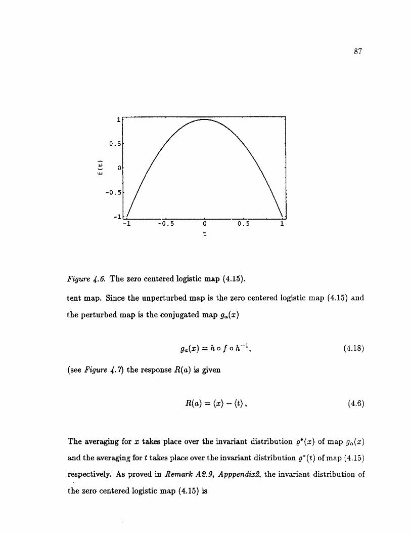
87

0.5

- 0 . 5

Figure 4-6. The zero centered logistic map (4.15).

tent map. Since the unperturbed map is the zero centered logistic map (4.15) and

the perturbed map is the conjugated map ga(x)

g«(x) = ho f oh 1, (4.18)

(see Figure 4.1) the response R(a) is given

R(a) = {x) - (t), (4.6)

The averaging for x takes place over the invariant distribution g*(x) of map ga(x)

and the averaging for t takes place over the invariant distribution g*(t) of map (4.15)

respectively. As proved in Remark A2.9, Apppendix2, the invariant distribution of

the zero centered logistic map (4.15) is

88

x Oi

0.25

0.25

0.75

-0.75 -0.5 -0.25 0 0.25 0.5 0.75 1

Figure 4-7. The conjugated map (4.18) with for some values of the conjugation

parameter a, a = 1.0 (solid line, unperturbed case), a = 0.7 (long dashed line) and

a — 1.3 (short dashed line).

e'it) tiV l — t2'

which is an even function on the interval t € [—1,1], thereby leading to

<t>= [ tg*(t)dt= [ t—.1 dt = 0.

J . i 7-1 T From (4.6) and (4.20) the response is

(4.19)

(4.20)

R(a) =< x > . (4.21)

In order to calculate < x > we need the equilibrium distribution g*(x) of the

perturbed map (4.18). As we proved in Proposition A2.4, Appendix 2 the invariant

89

density of the conjugated map Q*(x) is related to the invariant density e*(t) of the

unperturbed map via

<$(*) = e',(h-Hx)) d h 1(x)

dx (4.22)

From (4.2) we get for the inverse conjugating function

t _ h - i ( x ) _ J a - 1 - V a 2 - + !)2> for —1 < x < a — 1; ( > \ a — 1 + \/(2 — a)2 — (x — l)2 , for a — 1 < < 1.

(4.11) shows that h~1(x) is monotonously increasing thus (4.22) becomes

g*(x) = - < 7T

y,l-(o-l—v/a2-(a:+l)2)3 Va2-(a:+l)2 ' — i 11 i, i y • 1~?,, , . for a — 1 < x < 1.

k -y 1—(a—l+-y/(2—a)2—(x—l)2)2 y(2—a)2—(x—1)?

for —1 < x < a — 1;

(4.23)

The invariant distribution g*(x) (4.23) is plotted in Figure 4-8.

Thus the response (4.9) becomes

x 1 1 S + l R(a) = - I x f = y

0 . - (a - 1 - y/a? - (x + l)2)2 V f l 2 - (® + !)2 dx

+ 1 — x i r i

— I y , " 1 1 , , , * ^/ l - (a - 1 + </(2 - a ) 2 - ( x ^ l ) 2 ) 2 \ / ( 2 - a) 2 - ( x - i)1

:dx.

(4.24)

We could not evaluate this expression analytically so we used a numerical integration

provided by the program package Mathematica (Wolfram 1988) and we fitted a

curve to the numerical results for small values of the perturbation parameter a — 1

(see Figure 4-9)- We found that the response is for small perturbation i.e., for

a - l < 1

90

Figure 4-8. The invariant distribution (4.23) of the conjugated map (4.18) for some

values of the conjugation parameter a, a = 1.0 (solid line, unperturbed case), a = 0.7

(long dashed line) and a = 1.3 (short dashed line).

R(a) « 0.4404(a - 1). (4.16)

From (4.16) the generalized susceptibility is

d R{a) da a=l

0.4404. (4.17)

q.e.d.

91

OH

0.25 0.5 0.75 1 1.25 1.5 1.75 2

-0.2

Figure 4.9. The response R(a) of the conjugated map (4.18) as a function of the

conjugation (or perturbation) parameter a. The circles show the results of (4.24)

by numerical calculations, the solid line is the fitting curve (4.16) for small pertur-

bations.

CHAPTER 5

DETERMINISTIC BROWNIAN MOTION

In this chapter we fulfill the main goal of this work. We present two models for

deterministic Brownian motion. After recalling the traditional wisdom on Brownian

motion, in the first paragraph (§5.1) we present a model where the Brownian particle

is coupled to a chaotic booster which is mimicked by the zero centered logistic map.

The particle loses energy via a phenomenological dissipation. We use a stochastic

technique for the analytical treatment and an algorithm for the numerical solution

of the equations of motion.

In §5.2 we present the self consistent picture of the deterministic Brownian

motion. Here the Brownian particle interacts with a chaotic booster. The result of

the interaction is the fluctuation and dissipation of the energy of the particle. We

test the velocity of the Brownian motion by investigating the fluctuation-dissipation

and the relaxation properties. We show the deterministic Brownian motion for two

kinds of chaotic boosters, the zero-centered logistic and tent maps.

§5.1 Deterministic Brownian motion with phenomenological dissipation

Remark 5.1.1. The traditional wisdom on the Brownian motion

As we mentioned in the Introduction Brownian motion is a result of two com-

peting processes - the fluctuation and the dissipation. The fluctuation takes into

account the action of the environment or booster on the system of interest.

In this traditional picture one assumes that the booster is robust and can have

many — possibly an infinite number of — degrees of freedom and is considered to be

92

93

i n t h e r m o d y n a m i c e q u i l i b r i u m ( s t a t i s t i c a l a s s u m p t i o n ) . So t h e b o o s t e r a c t s u p o n

t h e s y s t e m of i n t e r e s t i n a n e r r a t i c m a n n e r - t h i s a c t i o n is d e s c r i b e d b y m e a n s of a

r a n d o m f o r c e w h i c h c a u s e s d i f f u s i o n .

W e a s s u m e t h a t t h e s y s t e m of i n t e r e s t is s m a l l c o m p a r e d t o t h e b o o s t e r t h e r e -

f o r e in i t s i n t e r a c t i o n w i t h t h e r o b u s t b o o s t e r i t o n l y s l i gh t ly p e r t u r b s t h e d y n a m i c s

of t h e b o o s t e r . T h e r e a c t i o n of t h e s y s t e m t o t h e b o o s t e r t a k e s p l a c e in a d i s s ipa -

t i v e m a n n e r . T h e d i s s i p a t i o n is a s s u m e d t o b e p r o p o r t i o n a l t o t h e v e l o c i t y of t h e

p a r t i c l e .

W h e n w e a s s u m e t h a t t h e s y s t e m of i n t e r e s t is s m a l l c o m p a r e d t o t h e b o o s t e r

w e u s e a k e y a s s u m p t i o n t h a t b e i n g t h e m o t i o n of t h e b o o s t e r is f a s t c o m p a r e d

t o t h e s y s t e m . I n o t h e r w o r d s t h e r e is a t i m e - s c a l e s e p a r a t i o n b e t w e e n t h e s y s t e m

of i n t e r e s t a n d t h e b o o s t e r . D u e t o t h i s t i m e - s c a l e s e p a r a t i o n t h e C e n t r a l L i m i t

T h e o r e m is a p p l i c a b l e a n d o n e r ecove r s t h e G a u s s i a n e q u i l i b r i u m d i s t r i b u t i o n of

t h e ve loc i ty . I n t h i s s e c t i o n w e sha l l e x a m i n e t w o e x a m p l e s , w h e n t h e r e is n o t i m e -

sca l e s e p a r a t i o n b e t w e e n t h e b o o s t e r a n d t h e v a r i a b l e of i n t e r e s t a n d w e c a n n o t

r e c o v e r t h e G a u s s i a n d i s t r i b u t i o n .

T h e r e s u l t of t h e c o m p e t i t i o n b e t w e e n t h e r a n d o m fluctuations a n d t h e dis-

s i p a t i o n is a d y n a m i c a l e q u i l i b r i u m b e t w e e n t h e t w o p r o c e s s e s in a w a y t h a t t h e

b o o s t e r p u m p s a s m u c h e n e r g y i n t o t h e s y s t e m of i n t e r e s t a s i t r ece ives f r o m i t b y

d i s s i p a t i o n . T h e s y s t e m of i n t e r e s t h a s a fixed a v e r a g e e n e r g y w h i c h is p r o p o r t i o n a l

t o t h e p r o d u c t of t h e d i f f u s i o n coef f i c ien t D* a n d t h e d i s s i p a t i o n r a t e 7 ( E i n s t e i n

1905)

\m{v2) = ^rnD* 7 (5 .1 .1)

T h e m o d e l a b o v e w a s first e x p r e s s e d in t e r m s of a s t o c h a s t i c m a t h e m a t i c a l for -

94

malism by Langevin (Langevin 1908). Langevin considered a 1-dimensional system

where two kinds of forces act on a particle of mass m - the dissipative force Fd

which is proportional to the velocity v i.e., Fa = - r v and a random force £(£). The

equation of motion reads

mi) = — Tv + £(i). (5.1.2)

After deviding by mass m (5.1.2) becomes

v = —'yv + x(t), (5.1.3)

where 7 = T/m and x = £/ra respectively and x(t) is assumed to be delta-correlated

in time

(s(*)s(0)) = 2 D6(t) (5.1.4)

with a Gaussian distribution

P(®) = (5*1*5)

and zero average value

(x(t)) = 0. (5.1.6)

The equation (5.1.3) has the formal solution

v(t) = v0e+ e-f* f ei*'x{t')ed', (5.1.7) J 0

where VQ denotes the initial value of the velocity •u(O) = VQ. After averaging over

an ensemble of realizations of the random force (5.1.7) becomes

95

{ v ( t ) ) = voe-t* (5.1.8)

where we used (5.1.6) in the averaging. For the average of the second moment we

obtain from equation (5.1.7)

( v 2 { t ) ) = v l e - ^ t + e ~ ^ t f ' d t ' f d t " { x ( t ' ) x { t " ) ) e * W \ (5.1.9) Jo Jo

Substituting equation (5.1.4) into (5.1.9) and integrating with respect to t' and t"

we get

( v 2 ( t ) ) = ^ + (vg - ~ ) e 2 j \ (5.1.10)

which shows that the average of the square velocity and therefore the kinetic energy

reaches the equilibrium value

{ v 2 ( o o ) } = ^ (5.1.11)

which is the fluctuation-dissipation relation derived from the Langevin equation.

We note here that the apparent difference between Einstein's fluctuation-dissipation

relation (5.1.1) and (5.1.11) is the result of the fact that in (5.1.1) D* denotes the

diffusion coefficient while in (5.1.11) D denotes the correlation coefficient of the

stochastic force divided by the mass. Although D and D* are proportional to each

other they are not the same. In the following we shall use equation (5.1.11) as a

fluctuation- dissipation relation.

In order to obtain the evolution of the probability density p ( v ; t ) of the velocity

we have to solve the Fokker-Planck equation (Fokker 1915, Planck 1917). The

Fokker-Planck equation which corresponds to the equation (5.1.3) is (Grigolini 1991)

96

? £ W 1 = { ^ + d ^ ) " ^ < 5 1 - 1 2 >

whose solution is

i n*-")8

p(v;t) =—====e 2(x-e 27i) . (5.1.13) ^ 2 * 2 (1 - e-2T")

For long times the solution (5.1.13) of the Fokker-Planck equation approaches the

Maxwell-Boltzmann-distribution i.e.,

1

p(v,co) = — e (5.1.14)

The above results represent the traditional understanding of Brownian motion.

Remark 5.1.2. From Remark 5.1.1 we can see that the action of the booster on

the velocity of the Brownian particle is represented by a random force. The chaotic

and stochastic processes are similar to each other in the sense that both of them

produce erraticaly evolving observables although the chaotic one originates form a

deterministic system. Therefore it is a reasonable idea to substitute the random

force, i.e., the stochastic booster in the Langevin equation (5.1.3), with a chaotic

booster. In the following Proposition 5.1.1 we show how deterministic Brownian

motion emerges when a light particle interacts with a deterministic (but chaotic)

booster.


i) the the motion of a particle takes place in one dimension,

ii) it is described by the equation of motion

97

v = — yv + x(t), (5.1.14)

where v denotes the velocity of the particle and x(t) is a chaotic variable which

originates from the zero centered logistic map in its fully chaotic regime

x(t + 1) = 1 — 2x2(t) (5.1.15)

then

• the velocity v reaches the equilibrium distribution p(v; oo) = p(v; t —> oo)

2 2

p(v; oo) = Z - 1 [1 - 2LH-] , (5.1.16)

where Tchaoa is the characteristic time of the chaotic booster

= (5.1.17)

and Z~l is the normalizing constant.

Proof. The proof rests on the idea that the logistic map as a booster can be mimicked

by a dichotomous noise which has the same variance and characteristic time that

the booster has. So we replace the chaotic x(t) in (5.1.3) with a dichotomous noise

and we obtain a stochastic differential equation from which we obtain the evolution

of the distribution function p(v;t).

The chaotic booster is the logistic map. As we showed in Proposition A2.5,

Appendix 2 the zero centered logistic map (5.1.15) has an invariant i.e., equilibrium

distribution

e*(x) = —7f===f' (5.1.18) 7TV 1 ~ X 2

98

the so called U-shaped distribution. It means that most of the time the booster

provides values close to ±1 and it switches back and forth between them in an

erratic manner. Since the variance of the booster variable x is

{x2) = f x2g*(x)dx=^-, (5.1.19) J o ^

we substitute the booster with the dichotomous noise

f(t) = ±a, (5.1.20)

where a = ^ and the mean value of f(t)

= 0 (5.1.21)

and the correlation function of f(t) is

(/(«)/( 0)> = a'e~"T', (5.1.22)

where rc is the correlation time of the dichotomous noise. Thus we replace the

Langevin-equation (5.1.3) with the stochastic differential eqation

i) = - -yV + f(t). (5.1.23)

We solve equation (5.1.23) by following the procedure developed by Lindenberg and

West (Lindenberg and West 1990).

From the definition of the dichotomous noise f(t) we can conclude that the

conditional probability Prob{/(t + r) = a\f(t) = a} i.e., the probability that f(t +

T) = a at time t + r if f(t) = a at time t is

99

Prob{/(f + r) = a\f(t) = a} = Prob{/(< + r) = -a\f(t) = - a }

_ | ( l + « - / * . ) (5.1.24)

and

Prob {f(t + r) = a\f(t) = - a } = Prob{/(t + r ) = -a\f(t) = a}

= 5 ( x ~ e~T/T°) • (5.1.25)

From (5.1.24) and (5.1.25) we can write the master equation for the dichotomous

noise

d_ dt

^d_ rcdt

W(a,t\f0) — — — 7^W(a,t\fo) —VT(—a,i|/o) rc dt

(5.1.26)

and

| w ( - < M l / o ) = -L2-W(-a,t\f0) + (5.1.27) dt v ' "u/ tc dt

where W(a,t\f0) denotes the condiditional probability that f(t) = a at time t if

f{t) = fo a t time t = 0. Equations (5.1.26 — 27) can be rewritten in operatorial

form

8 (5.1.28)

where

11, = - - 1 1 1 - 1 (5.1.29)

Similarly we can write the master equation for the Langevin equation (5.1.3) as

100

d_ dt

W(v,f,t\v0,f0) = - £ ( - 7 « + / ) + H/ (5.1.30)

where W(v, / , t|fo ? /o) denotes the conditional probability that v(t) = v and f(t) =

/ at time t if v(0) = VQ and /(0) = /o at time t = 0. Substituting (5.1.20) into

(5.1.30) and averaging over the initial distribution P(/o) we get

$ d 1 —W(v,a,t\v0) = [-7^ + a] W(t;,a,*|t;o) - — W(v,a,t\v0)

+ — W(v,-a,t\v0) rc

(5.1.31)

d_ dt

() W(v, -a,t\v0) = - — [~7V - a] W(v, —a,t|v0) - 7"W(v, —a,t|v0)

+ — W(v,a,t\v0). (5.1.32)

Introducing the sum and difference distributions Wt{v,t\vo) and St(v,t\vQ) respec-

tively (5.1.31 - 32) become

9 Wt(v,t\v0) = i^vWt{v,t\vQ) - a-j^St(v,t\v0) dt (5.1.33)

d_ dt

St(v,t\vQ) = - 2_ TC

d ' W

d St(v,t\v0) - a—Wt(v,t\v0). (5.1.34)

We are looking for the steady state solutions Ws(v) and Ss(v) i.e., solutions, where

the left hand sides of (5.1.33 — 34) vanish and they become

= a±S.(v) (5.1.35)

2 a — - J V Tc OV

101

0 Ss(v) = -a—ws(v) (5.1.36)

dv

Prom (5.1.35) with zero flux boundary conditions we find

s*(v) = (5.1.37)

Substituting this relation into (5.1.36) and solving it again subject to zero flux

boundary condition finally yields

= (5.1.38)

where Z' 1 is the normalizing constant. After performing the integration in (5.1.38)

and using (5.1.19 - 22) i.e., < a;2 > = a2 = 1/2 we obtain (5.1.16).

q.e.d


i) the motion of a particle takes place in one dimension,

ii) it is described by the equation of motion

v = -1V + x(t), (5.1.3)

where v denotes the velocity of the particle and x(t) the chaotic variable which

originates from the zero centered logistic map in its fully chaotic regime

xn+i = l-2x2n (5.1.15)

then

102

the evolution of the discretized velocity is given by

*>«+i = \ + v££i) , (5.1.39)

to accuracy 0(h3), where

v»+i = v n ~ hTVn + Vhxn (5.1.40)

Vi+1 =Vn- fryvi+l + Vhxn, (5.1.41)

with integration step h and

Tchaos < 1 / 7 (5.1.42)

• the evolution of the discretized velocity is given by

*>n+i = \ ( v % + , (5.1.39)

to accuracy 0(h3), where

wi+i =vn~ h(xn - ivn) (5.1.43)

Un+1 ~• vn + h(xn — 7^i+i)j (5.1.44)

with h integration step and

Tchaos > 1/7- (5.1.45)

103

Proof. Proposition 5.1.1 gives the algorithm to solve equation (5.1.3) numerically.

The equation (5.1.3) is a linear stochastic equation thus a modified Euler method

(Gerald 1970) provides a satisfactory accuracy as a numerical solution of equation

(5.1.3). The modified Euler method is a predictor-corrector method where we use

the result of the Euler method as a predictor and we use this predicted value in the

calculation of the corrector (Press et al. 1990). In order to show how the modified

Euler-method works we consider the differential equation

Yt = /(»)• I5-1-46)

The Euler method gives an estimate of y^+i knowing yn

Vn+1 = Vn + h^ ^ =yn + hf(yn). (5.1.47)

Another estimate y^h ig provided by calculating the derivative at the point t =

tn h

Vn+l =Vn + h^j =Vn + hf{Vn+1). (5.1.48) QZ t~tn -f- h

In order to calculate f(yn+1) we should know yn+i exactly but we do not know it.

Thus we approximate it by y^+i- So (5.1.46) becomes

= »n + hf(y%). (5.1.49)

We get a good estimate for yn+1 by taking the arithmetic mean of the predictor

Vn+l a n d corrector y ^

104

yn+l = \ ( y { n l 1 + y i n h ) . (5.1.50)

In the case of rchaos > 1 / 7 the chaotic variable changes slowly, i.e., x(t) is adiabatic

variable. The addition of an adiabatic x(t) to the right hand side of (5.1.46) changes

(5.1.47 — 48) into the following form

Vnh =Vn + hf(yn) + hxn (5.1.51)

and

2/n+l — Vn + hfil/n+l) + hxn. (5.1.52)

respectively. Identifying y = v and f(y) = -7t> (5.1.50 - 52) become (5.1.39) and

(5.1.43 — 44) respectively.

In the case of Tchaos I / 7 the chaotic variable is fast therefore it is considered

to be a random-like variable. The averaging over x for a time of length h takes

place as it is done over the random variables. In order to do so let us consider the

differential equation

y = x(t) , (5.1.53)

where x(t) is a delta-correlated stochastic variable with zero mean value

(x(<)x(0)) = 2 D6(t). (5.1.54)

We know from the Central Limit Theorem (Proposition 2.1.1) that in this case the

variable y shows diffusion

(y2(t)) = 2 Dt (5.1.55)

105

and at the same time y changes randomly thus it can written as

y(t) = V2Dt£(t) (5.1.56)

where £(t) is a random variable with Gaussian distribution and variance (Z2(t)) = 1.

Therefore the stochastic equation (5.1.53) can be discretized in the form of

Vn+1 =yn + V2Dh£(t) = yn + Vhxn, (5.1.57)

where h is the integration step.

In the case of Tcj%aos I / 7 the differential equation (5.1.3) is discretized by

combining the discretization of the deterministic part v = — f v and the random-like

part v == x(t). The discretization of the deterministic part takes place by identifying

y — v and f(y) = —^v in (5.1.47), while (5.1.57) provides the discretization for the

chaotic part. Thus the predictor of (5.1.3) is

Vn+1 =vn~ hjvn + Vhxn (5.1.40)

and the corrector is (5.1.41). predictor (5.1.40) and the corrector (5.1.41) yields

The only thing left to complete the proof is to show that the algorithm (5.1.39 —

41) and (5.1.39), (5.1.43 - 44) is correct to order 0(h3). From (5.1.47) and (5.1.48)

we get that the discretized form of (5.1.46) is

h Vn+1 = yn + - [ f ( y n ) + f(yn + hf(yn))]. (5.1.58)

Expanding the term f(yn + hf(yn)) in a Taylor-series and neglecting higher than

linear terms in the expansion we realize that the algorithm we presented above

106

provide an accuracy of order h2 which is satisfactory for the linear system (5.1.3)

with a proper choice of integration step h.

q.e.d.

Remark 5.1.3. The algorithm we showed in Proposition 5.1.2 was originally pro-

posed by Rao et al. (Rao et al. 1974) and it was developed further by Sanchez

(Sanchez 1982), Mannella et al. (Mannella et al. 1989) and Gard (Gard 1988) in

several forms. For instance the algorithm of Mannella et al. was succesfully applied

for multiplicative and additive noises in nonlinear systems as well (Mannella 1989,

Bonci et al. 1991).

We applied the algorithm of Proposition 5.1.2 in 3 cases: 7 = 0.01, 7 = 10.0

and 7 = 3.0. We calculated the equilibrium-distribution of the velocity v from

10,000 trajectories with integration step h = 0.01. The equilibrium distributions

of the velocity v are plotted in Figures 5.1.1a-c for the three different dissipation

parameters 7. The results of the numerical calculations are compared to the results

of the theoretical investigations (5.1.16). The characteristic time of the chaotic

booster (5.1.15) is calculated by (5.1.17). Since the logistic map (5.1.15) is 8-

correlated (see Proposition A2.6), thus rcha0s = 1-

For the small 7 case i.e., when 7 = 0.01 so T c h a o s < 1 / 7 there is a large time-

scale separation between the time-scale of the booster characterized by Tchaoa = 1

and the motion of the particle characterized by time-scale 1/7 = 100. Thus the

particle accumulates the fluctuations of the booster and its energy or velocity-

square eventually reaches the Maxwell-Boltzmann distribution which implies that

the velocity follows the Gaussian distribution (see Figure 5.1.1a).

107

0 .08

0 . 0 6

£ 0.04

0 . 0 2

Figure 5.1.1a. The velocity equilibrium distribution p(v) of the Brownian particle

in the small 7 case. The circles show the results of numerical simulations based on

map (5.1.39 — 41) and the solid line shows the result of the theoretical investigations

calculated from (5.1.16). The parameter values we used: Tchaos — 1.0, < x2 > = 1/2,

7 = 0.01 and integration step h = 0.1.

In cases when the motion of the particle is faster than that of the booster (large

7) the particle is fast enough to trace the motion of the booster in a rescaled manner.

Thus the equilibrium distribution of the velocity is more similar to the equilibrium

distribution of the booster (see Figure A2.3 for the equilibrium distribution of the

booster). We calculated the large 7 case with 7 = 10.0 and plotted the result in

Figure 5.1.1b.

108

-o. i - 0 . 0 5 0 . 0 5

Figure 5.1.1b. The velocity equilibrium distribution p(v) of the Brownian particle

in the large 7 case. The circles show the results of numerical simulations based on


investigations calculated from (5.1.16). The parameter values we used: Tchaos — 1-0,

< x2 > = 1/2, 7 = 10.0 and integration step h = 0.001.

In the case of intermediate dissipation, i.e., when the Tchaos is comparable to

I /7 the situation is a mixture of the above two cases. The equilibrium distribution

of the velocity shows the properties of the booster as long as it inherits the U-

shape of the equilibrium distribution of the booster but it is less steep and starts

broadening. We investigated the case of 7 = 3.0 and plotted the results in Figure

5.1.1c.

109

»• •

-0.3 -0.2 -0.1 0 0.1 0.2 0.3 v

Figure 5.1.1c. The velocity equilibrium distribution p(v) of the Brownian particle

in the modest 7 case. The circles show the results of numerical simulations based on


investigations calculated from (5.1.16). The parameter values we used: Tcha0s = 1.0,

< x2 > = 1/2, 7 = 3.0 and integration step h = 0.01.

The theoretical results are in good agreement with the results of the numerical

calculations for the small 7 case, while the other cases show apparent deviations.

This is expected since the theory so fcr discussed is a stochastic theory and it only

works well, where the genuine stochastic properties dominate (e.g. Central Limit

Theorem). In the cases, where the system is more deterministic-like we should

mimick the booster with a different estimate of the statistical properties, especially

as far as the second moment is concerned.

110

One could also wonder why the equilibrium distribution of the velocity is so

different from the usual Gaussian distribution in the large and modest 7 cases. The

system is overdamped since it is strongly coupled to the booster and the velocity

does not have time to accumulate the random actions of the booster. In other words

it relaxes too fast compared to the booster.

Remark 5.1.4. There has been some efforts to derive deterministic Brownian motion

(Beck 1990, Prakash et al. 1991, Trefan et al. 1991) although all of them share a

common disadvantage - the presence of a phenomenological dissipation term —jv.

The appearance of a phenomenological dissipation term is an ad hoc assumption

which forces the system from outside to obey the fluctuation- dissipation theorem.

In order to have a self-consistent physical picture we need to build up a model

where the dissipation is the result of the reaction of the particle on the booster and

fluctuations are the result of the action of the chaotic booster on the particle. We

develop this theory in the following paragraph.

§5.2 Deterministic Brownian motion - self consistent picture

Remark 5.2.1. As we pointed out in Remark 5.1.4 the model of the Brownian

motion where a phenomenological dissipative term is assumed is not satisfactory,

because the dissipation is an ad hoc assumption. We now build up a model where

both the dissipation and the fluctuation originates from the interaction of a particle

with a booster. This is our goal in the present chapter, where we follow the idea

developed by the author and his collegues in (Bianucci et al. 1993b).

We consider a 1-dimensional model where a light particle interacts with a

chaotic booster. On one side the chaotic booster has a short characteristic time

I l l

Tchaos and we assume that the action of the booster abruptly changes the velocity

of the Brownian particle at the end of each time interval with length Tchaos i e.,

the particle receives an erratic kick from the booster at equidistant instants. The

chaotic kicks on the particle lead to the diffusion of the velocity as we discussed

earlier.

On the other side the light particle reacts on the booster. The reaction is a

negative feedback which is proportional to the velocity. This feedback perturbes

the booster and slightly moves it out of equilibrium. For instance, for large nega-

tive velocities the booster gives a series of chaotic kicks with positive mean values.

Thus the booster produces a drift in the velocity towards its equilibrium which is a

dissipation from the point of view of the velocity. This dissipation limits the oth-

erwise unbounded growth of the velocity diffusion and as a result of the competing

diffusion and dissipation the velocity of the Brownian particle reaches dynamical

equilibrium with the booster. So does its average kinetic energy.

This model is expressed in mathematical form by a 2-dimensional impact map-

ping where the actual velocity is a sum of its previous value and a kick of a fully

chaotic 1-dimensional map. The dynamics of the booster is given by a 1-parameter

conjugated map of a fully chaotic map where the conjugation parameter is nega-

tively proportional to the velocity. This conjugation, as we shall see in the following

Proposition 5.2.1, creates the reaction or feedback which leads to a dissipation.


i) the 1-dimensional dynamics of a particle

ii) is given by the following 2-dimensional impact mapping

^n+l ~ Vn "I" (5.2.1)

112

* n+1 — 9a{^n)i (5.2.2)

iii) where ga(x) is the conjugation of a zero-centered, fully chaotic map f(t) :

[—1,1] »-+• [—1,1], t € [-1,1] i.e.,

ga(x) = hao f oh~x(x), (5.2.3)

iv) where the conjugating function ha(t) is

x h (+\ - ! ~l + Va2 ~ (t-a + l)2, for - 1 < t < a - 1; ( . a { ) ~ 11 - V ( 2 - a ) > - ( t - a + l)a, for a - 1 < t < 1; (5-2<4)

where a 6 [0,2],

v) and the conjugation parameter is negatively proportional to the velocity

a- 1 = - A 2 v , (5.2.5)

where A is a small reaction coefficient then

• the velocity v is indistinguishable from the velocity of a Brownian particle.

Proof. When we want to show that the velocity is that of a Brownian particle we

have to show that from the map we can derive the Langevin equation

v = - 7 v + x(t) (5.2.6)

or the Fokker-Planck equation

§ i e M = T ^ v + D ^ e ( v ; t ) . (5.2.7)

We show this claim in the following way. First we show that (5.2.1) results in diffu-

sion of the velocity therefore it is equivalent to an equation v - x(t), where x(t) is

113

a random force with short correlation. Then we show that the feedback (5.2.2 - 5)

is equivalent to the action of a dissipative term —jv in (5.2.6).

The diffusion. The fully chaotic map f(t) : [-1,1] _• [-1,1] is subjected to a

conjugation. The conjugation preserves the Lyapunov spectrum (Devaney 1989)

therefore it preserves the chaoticity as well. Since the feedback is small the correla-

tion properties of the map (5.2.2) do not differ significantly from the unperturbed

m a P 9a=i(%) ~ apart from a small drift term. Since the unpertrubed map ga=\(x)

is symmetric, as we proved in Proposition A2.6 and Remark A2.ll, its correlation

function vanishes in one step i.e., it is delta-correlated. Thus the consecutive values

xn,x n+1, . . . represent a sequence of short correlated kicks with same correlation

time. The correlation time Tiooster of the booster is defined according to (2.2.8)

Tbooster — ]Cn=0 ^ xnx0 >

< xl > (2.2.8)

Since

(5.2.8)

where

2D =< xl >, (5.2.9)

therefore

Tbooster ~ 1• (5.2.10)

Equation (5.2.1) shows that the velocity is the collector variable of the chaotic

kicks with short correlation (5.2.8). Therefore the velocity v of (5.2.1) fulfills the

requirements of the Central Limit theorem (Proposition 2.1.1) i.e., the velocity is

114

diffusive. Thus (5.2.1) mimicks the Langevin equation (5.2.6) without the dissipa-

tion term —jv.

The dissipation. The feedback or the reaction of the particle on the booster is de-

fined by equations (5.2.3 - 5). From the definition (5.2.3 - 4) of the conjugation

function we can see that for a = 1 the conjugation function ha(t) is antisymmetric

K=i{-t) = -ha=1(t), (5.2.11)

so the conjugated map ga(x) is symmetric for a = 1.

9a= l ( - x ) = ga=l (x). (5.2.12)

Thus the map ga(x) with a = 1 produces a sequence of x-s with zero mean value

< Xn >a=1 = 0, (5.2.13)

where < . . . > a = 1 denotes the averaging over an ensemble of the dynamics of

9a=i(xn) when a = 1. We refer to the case with a = 1 as the unperturbed booster or

the booster with unperturbed dynamics. From (5.2.5) we can see that the dynamics

is unperturbed when the velocity v = 0.

Now let us see what happens when the velocity reaches a large positive value.

When v is large and positive then from (5.2.5) the perturbation parameter a - 1 is

small

l a ~ L (5.2.14)

It means that the dynamics of the booster ga(x) is subjected to a small, negative

perturbation. In this case the booster provides a series of x-s with a modest negative

mean

115

< xn > a < 1 < 0. (5.2.15)

From (5.2.5) the perturbation is negatively proportional to the velocity v. To small

perturbations the booster responds proportionally to the strength of the perturba-

tion a - 1

< xn > =< ga(xn) > = (a - l)x, (5.2.16)

where x denotes the generalized susceptibility

d<xn> A,

da

From (5.2.16 - 17) and (5.2.5) we obtain

a= 1 (5.2.17)

<xn>=< ga(xn) > = - A 2 x < vn > . (5.2.18)

From (5.2.1) we can see that this negative mean (5.2.18) is accumulated in the

velocity v thus forcing the velocity from its large positive value to tend to zero.

This mechanism is the dissipation. Since the booster variable x couples directly to

the velocity v we can identify the coefficient - A 2 * as the dissipation parameter 7

i.e.,

7 = a 2 X (5.2.19)

From the aboves we can conclude that the impact map (5.2.1 - 5) represents a

Langevm equation with the dissipation coefficient (5.2.19) and fluctuation coefficient

1 2 ^booster (2.2.2)

£> = - < - 2

116

Thus the fluctuation - dissipation relation for map (5.2.1 — 5) reads

< u2 > = — = 1 < xo > Tboos te r (5.2.20) 7 2 A2x

q.e.d

Remark 5.2.2. In the followings we show two examples for the realization of Propo-

sition 5.2.1.

In the first example we consider the case where the map (5.2.2) is the conjugate

of the zero-centered tent map

tn+1 = 1 - 2|tn | (4.1)

with the conjugation function (5.2.3 — 4). If the velocity is that of a Brownian

particle then, as we showed in Remark 5.1.1, its average relaxes according to (5.1.8)

< vn > = voe~yn (5.1.8)

and the average kinetic energy or average velocity square evolves according to

(5.1.10)

< v 2n > = ^ + ( v l - ^ ) e ~ 7 n , (5.1.10)

where n denotes the discrete time.

We can determine the fluctuation coefficient D from (2.2.2), where < x\ >

denotes the variance of the unperturbed dynamics of the conjugated map. Using

the results of (4.12) < XQ > becomes

117

< x% > = J ^ xle*g{xo)dxo = \J_i ^ o ^ d x l °^dX°' (5-2.21)

where /i_1(x) is the inverse of the conjugation function (5.2.4) given by (4.11)

,_i/ x {a-l-^/a2-(x +1)2, for - 1 < x < a 1; (41-n h W - \ a - l + V ( 2 - a ) 2 - ( x - l ) ^ for a — 1 < as < 1.

Substituting (4.11) into (5.2.21) and evaluating the integral for the unperturbed

case (a = 1) we get

< x\ > = 1 + J xy/l - (x + l)2dx - J xy/l - (x — l)2da; = ^ - - = 0.0959. _ 1 (5.2.22)

Prom (2.2.22), (5.2.22) and (5.2.10) the fluctuation coefficient D is

2 \ 3 2 / 0.0480. (5.2.23)

The dissipation coefficient 7 we determine from (5.2.19). We showed in Proposition

4.1 that if the zero centered tent map is subjected to perturbation by conjugation

with the conjugating function (5.2.4) then the generalized susceptibility x is

X = \ ~ I- (4-4)

Thus from (5.2.19) and from (4.4) the dissipation coefficient is

7 = - A 2 ( | - 1). (5.2.24)

We executed computer calculations to monitor the relaxation of the average velocity.

The initial velocity vq was chosen to be vq = 100, the reaction parameter A was

118

chosen to be small in order to keep the perturbation small and the booster was

initially placed into the equilibrium of the unperturbed map. The way to place the

booster in unperturbed equilibrium is to place the tent map in equilibrium initially

i.e., to start the evolution of the tent map from uniformly distributed random initial

values on the interval [—1,1]. The average was taken over 10,000 different initial

conditions. The resulting velocity relaxation is plotted in Figure 5.2.1. The results

of the computer calculations are compared to the theoretical results obtained from

(5.1.8) with (5.2.23) and (5.2.24).

20000 40000 60000 80000 100000 n

Figure 5.2.1. Relaxation of the velocity of map (5.2.1 - 5) with reaction parameter

A = 0.01. (5.2.3) is the conjugate of the tent map . The velocity is set initially to



(5.1.8) with (5.2.23) and (5.2.24).

119

We also calculated the evolution of the average kinetic energy for some values

of the reaction parameter. A was chosen to be 0.005, 0.006,... , 0.01. The velocity

was initially set to vq = 0 and the booster started its evolution from its unperturbed

equilibrium. The results on the evolution of the average velocity square are plotted

in Figure 5.2.2. We compared the results of computer calculations to the theoretical

results calculated from (5.1.10) with (5.2.23) and (5.2.24).

5 0 0 0

4 0 0 0

3 0 0 0

OJ > 2000

1000

0

0 . 0 0 5

• •••••••••• ? i • • • S S • • • •

* 11 * * •* * * *

. A =

• • • V 9 • \

o . o a

10

2 A n

Figure 5.2.2. Evolution of the average velocity square from map (5.2.1 - 5) for

some values of the reaction parameter A. (5.2.3) is the conjugate of the tent map.

The velocity was initially set to v0 = 0 and the average was taken over 10,000


line shows the the theoretical results using (5.1.10) with (5.2.23) and (5.2.24).

The second example is where map (5.2.2) is the conjugate of the zero-centered

logistic map

120

t n + 1 = 1 - 2 t » (4.15)

with the conjugating function (5.2.3 — 5). Here again we monitor the the evolution

of the average velocity square and the relaxation of the average velocity. In order

to do so we need the fluctuation coefficient D and dissipation coefficient 7.

The fluctuation coefficient D is determined from (2.2.22), where in the calcula-

tion of the variance < xjj > the average must be taken over the invariant distribution

(4.21). The inverse conjugation function is (4.11) so for D we obtain

D = 0.1134. (5.2.25)

The dissipation coefficient 7 was determined from (5.2.19) using the result of Propo-

sition 4-2, where we showed that the generalized susceptibility x of the perturbed

logistic map, if the perturbation was represented by the conjugating function (5.2.4),

is

X = 0.4404. (5.2.26)

We realized (5.2.1 — 5) on the computer and monitored the relaxation of the

average velocity starting from a non-equilibrium position v0 = 100. The reaction

parameter was chosen to be small, A = 0.01 and the booster started to evolve from

its unperturbed equilibrium. The average was taken over 10,000 samples. The

results are plotted in Figure 5.2.3.

We also monitored the evolution of the velocity square when the velocity was

set initially to VQ = 0. We used several values of the reaction parameter A and

plotted the results in Figure 5.2.4•

121

100

A 6 0

v 40

20000 40000 60000 80000 100000 n

Figure 5.2.3. Relaxation of the velocity of map (5.2.1 — 5) with reaction parameter

A = 0.01. (5.2.3) is the conjugate of the logistic map. The velocity is set initially to



(5.1.8) with (5.2.25) and (5.2.26).

From Figures 5.2.1-4 w e c a n s e e that the results of numerical calculations and

the theory are in good agreement.

122

12000 0 . 0 0 5

10000

* 8000

6000

4000

2000 A = 0.01

2 Att

Figure 5.2.4• Evolution of the average velocity square from map (5.2.1 - 5) for

some values of the reaction parameter A. (5.2.3) is the conjugate of the logistic

map. The velocity was initially set to i>o = 0 and the average was taken over 10,000


line shows the the theoretical results using (5.1.10) with (5.2.23) and (5.2.24).

CHAPTER 6

CONCLUSION

We have shown that a rigorously microscopic derivation of the Fokker-Planck

equation rests on the rigorously microscopic derivation of both diffusion and friction

from the interaction of the system of interest with the same "thermal bath".

The problem of deriving diffusion from a deterministic process has been ad-

dressed and successfully solved by many groups (Chirikov 1979, Rechester and

White 1980, Cary et al. 1981, Schell et al. 1982, Doran and Fishman 1988).

We have shown that the standard diffusion behind the Fokker-Planck equation es-

sentially rests on the Central Limit Theorem, and, consequently, on the possibility

of deriving from a deterministic process of a given variable x a decaying correlation

function. The so called sensitive dependence of chaos on initial conditions insures

this possibility.

The problem of deriving friction from the interaction with a fully deterministic

bath, that we term booster, was much more difficult to solve. We have carefully ad-

dressed this problem and we have shown that the solution of this problem essentially

rests on the linear response of a booster to an external perturbation.

This raises a long-standing problem, that of the Kubo linear response theory

and of the strong criticism by van Kampen against this theory. The Kubo linear

response theory is based on a perturbation treatment of the Liouville equation,

which, in turn, is expected to be totally equivalent to a first-order perturbation

treatment of single trajectories. Since the boosters are chaotic, and chaos is essential

to generate dffusion, the single trajectories are highly unstable and do not respond

linearly to weak external perturbation.

123

124

To deal with this intriguing problem we have replaced the continuous-time

representation with a discrete-time picture. In other words, we have adopted maps

as boosters of our Brownian particle, and we have therefore addressed the problem

of the response of a chaotic booster to an external perturbation.

We have noticed that a chaotic mapping is characterized by an invariant mea-

sure which is a continuous function of the control parameters of the map. Conse-

quently if the external perturbation is made to act on a control parameter of the

map, we have that the booster distribution undergoes slight modifications as an

effect of weak external perturbation, thereby leading to a linear response of the

mean value of the perturbed variable of the booster. This approach to the linear

response bypasses completely the criticism of van Kampen.

The joint use of these two ingredients, diffusion and friction stemming from

the interaction of the Brownian particle with the same booster, making possible for

us to derive (Bianucci et al. 1993b) what, to the best of our knowledge, must be

considered as being the microscopic derivation of a Fokker-Planck equation.

The comparision of the analytic to the simulation results are extremely good.

We can construct a fully chaotic deterministic process as close as we want to the

dynamical behavior of a Fokker-Planck equation. However, there are many problems

left for future investigation. First of all, we have shown how to derive a linear

response to a chaotic system, in spite of the warnings of van Kampen. The warnings

of van Kampen focus on the adoption of a perturbation approach to the linear

response, and do not concern the possibility itself of deriving a linear response out

of a chaotic system.

Thus, we have now to face the problem of whether or not our approach to the

linear response conflicts with the approach of Kubo. There are preliminary results

showing that the Kubo approach to the derivation of the time asymptotic value of

125

the susceptibility leads to an exact result. We believe that the theoretical analysis

carrried out in this dissertation proves to be of fundamental importance in explain-

ing why it is so. We have indeed shown that the invariant distributions are stable

against external perturbation and this stability makes it possible to succesfully

adopt a perturbation treatment.

Encouraged by these results, we do hope that we shall be able to successfully

address a more difficult problem, that of deriving the Fokker-Planck equation from

a fully Hamiltonian picture, within a continuous time representation.

The problem of deriving statistical mechanics form chaos, as we have tried to

do it in this dissertation, cannot be really carried out if we ignore that microscopic

dynamics is in fact driven by quantum mechanics. For the foundation of statisti-

cal physics one needs to use chaotic systems, thus the classically chaotic quantum

systems are of paramount interest from the point of view of statistical physics. In

fact, the manifestation of chaos in classically chaotic quantum systems is a subject

of active research (Casati et al. 1979, Izrailev 1990). On the other hand the origin

of irreversibility in quantum mechanics is a very difficult problem.

This difficulty lies in the fact that in classical systems chaoticity means that

two, initially close orbits depart from each other in an exponential manner. This

very rapid divergence of orbits results in the motions of two, initially close orbits

becoming independent of each other in a short time. Thus a chaotic environment

behaves like a random environment which results in irreversibility. The correspond-

ing quantum mechanical average orbits follow the classical path, but the overlap of

the orbits grows exponentially like the divergence of averages. The overlap keeps the

wave functions of the corresponding classical orbits in phase and it provides a robust

cohesion of the wavefunction. Thus the exponential separation of classical orbits

does not result in dephasing, i.e., uncorrelated motion, thus a classically chaotic

126

quantum system does not produce relaxation. In other words quantum mechanics

means that the instability of trajectories is lost, and that the long-range correla-

tions, in time and space, are established. Consequently the problem of quantum

irreversibility is very difficult, nevertheless there have been successful attempts at

describing irreversibility in classically chaotic quantum systems (Bonci et al. 1992,

Roncaglia 1992). Thus this disseration is the first step on a long road whose end

is the extremely difficult enterprise of establishing a dynamical basis of quantum

statistical mechanics.

A promising way of approaching the problem of irreversibility of quantum

mechanical origin is to study classical systems of weak chaos. Quantum uncer-

tainty tends to spread all over the region of the classical phase space occupied by

chaotic clouds. For this reason, an approach to the canonical equilibrium distribu-

tion through the Fokker-Planck equation, which do not rest on the total ergodicity

of the system, can be very useful. The traditional approach to the canonical equi-

librium distribution, is, more or less, as follows. One asssumes ergodicity first. This

means a microcanonical equilibrium distribution. Then, one makes a contraction

over the irrelevant degrees of freedom of this microcanonical equilibrium distribu-

tion, and one gets a canonical equilibrium distribution. From the point of view

of quantum mechanics the microcanonical distribution might become an enormous

quantum cloud. If we derive the canonical equilibrium distribution by means of our

Fokker-Planck approach, we can rederive the classical statistical mechanics as well.

Another possible direction of research could be exploring quantum maps (Berry

et al. 1979, Tabor 1983), where one could attempt to understand what the conju-

gation means and if it is possible to build up a feedback by conjugation in quantum

maps.

APPENDIX 1

THE ZWANZIG PROJECTION TECHNIQUE

127

128

In Chapter 2, §2.3 we studied the deterministic diffusion in the standard map

and we derived the diffusion coefficient using the Zwanzig projection technique. The

Zwanzig projection technique, which is a quantum mechanics-like formalism, was

developed originally for continuous classical systems (Nakajima 1958, Zwanzig 1960)

and it was applied to various physical systems (Grabert 1982). In this appendix we

show the basic ideas and definitions. We introduce the projection operator and we

derive a master equation using it. Then we show how a memory kernel arises in

simple cases and how one can calculate the averages of observables of interest.

Let us consider a classical physical system with a set of "relevant" variables or

variables of interest a and a set of "irrelevant" variables or variables of the envi-

ronment b. Since the system is classical the equations of motion for the probability

distribution p is given in terms of the Liouville-operator L

^ p ( a , b; t) = Lp(a, 6; t). (-A1.1)

Let us assume that L may be written as

L = La + Li + L/, (.*41.2)

where La and Lb describe the evolution of the distribution due to variables a and A.

b, and Lj expresses the evolution of p due to the interaction between the variables

a and b. Let us assume furthermore that Lb admits an equilibrium distribution

Lbpeq(b) = 0. (41.3)

Thus the projection operator P is defined

Pp(a, 6; t) = peq(b)a(a; t) = peq(b) J dbp(a, b; t). (^41.4)

129

If Peqip) is normalized the operator P is idempotent

p 2 = P- (41.5)

We introduce the densities pi and p2 which correspond to the projection operator

P and its conjugate Q in the following way

P = Pi+P2, (41.6)

where

Pi = pP (41.7)

and

P2=QP = (1- P)p. (41.8)

Thus the evolution eqution (41.1) becomes

d

—p = L(Pl +p2). (41.9)

Applying operators P and Q on both sides of (41.9) becomes

d foPi — PL{pi + P2) (41.10)

and

d

0jp2 = QL(pi + p2). (41.11)

Equation (41.11) is a first order inhomogenious equation with the formal solution

130

p2(t) = eQLtQp(0)+ f dse^LaQLPp(t-s)p(0). (41.12)

J 0

Substituting (41.12) into (.41.10) we obtain the master equation

d ~ r* . . -^Pi (t) = PLPp(t) + / dsPLeQ L sQLPp(t - s) + PLeQltQp(0). (>11.13)

J 0

Equation (>11.13) can be rewritten in terms of the memory kernel

K(t) - PLeQLtQLP (41.14)

in the form

OtPii1) - PLPp(t) + f dsK(s)p(t - s) + PLeQLtQp(0). (41.15) J o

In the Markovian approximation the kernel (41.14) is a ^function and in some

cases the inhomogenious term can be neglected (Grigolini 1976).

The Markovian assumption can not be applied always but we can express the

memory kernel in terms of the correlation functions of the variables of interest. In

order to do so we shall use the interaction picture instead of the Schrodinger picture

(41.1.). In the interaction picture the equation of motion of the density p reads

d jtP{t) = Lj^pit), (4 i . i 6 )

where

P = eLotP (41.17)

and

131

h i t ) = e ^ U e 1 * 1 (41.18)

where Lq denotes

to = La + Lb. (A1.19)

Repeating the calculations (.41.1 - 13) we obtain obtain the master equation

3_

dt Pp(t) = PLT(t)Pp(t) + J dsPL/^Sxp J dsiQL/(Sl)

+ PLi(t)&cp j J d sQLi ( s )

QLI(s)Pp(s)

Qp( o).

(41.20)

The roughest approximation is to replace the time ordered exponential with unity

and if the inhomogeneous term can be neglected too the master equation (>11.20)

becomes

d_„

dt P\{t)= [ d s P L i ( t ) L I ( s ) p { s ) . (41.21)

Jo

In deriving (>11.21) we assumed that PLj(t)P = 0. Using the general properties

of the projection operator P and Lb that e^btP = P and Pe^bt = P the memory

kernel becomes

K(t -s) = ell^-^Kb{t - s), (vll.22)

where

Kb(t -s) = P L j e ^ + ^ ' - ^ L / P . (>11.23)

132

Kb(t) is a correlation operator providing information on the relaxtion properties of

the bath.

The average value of an observable A, where A depends on the variables of

interest a, by definition is

( A ( t ) ) = J A(a)p(a, b;t)dadb = J A 0)J dadft. (A1.24)

Since observable A depends only on the variables of interest a in calculating <

A(t) > one may use the reduced density a(a;t) so (vll.24) becomes

( A ( t ) ) = J Aa(a-,t)da, (.41.25)

where a(a\t) is defined by the projection operator P in (-A1.4) which we rewrite in

the following form

a(5-,t) = Pl(3'^\ (A1.26) Peqip)

where p\ (a, b; t) is the part of interest of p(a, b; t) defined by (A1.7). Since p\ (a, b; t)

is given as the solution of the master equation (^41.13) we can calculate (A(t)) from

(A1.25) and (A1.2G) by solving (^41.13).

APPENDIX 2

PROBABILISTIC DESCRIPTION OF CHAOTIC MAPS

THE FROBENIUS OPERATOR

133

134

Chaotic motion of physical observables means an erraticly evolving variable.

In this sense the chaotic motion is reminiscent of the stochastic motion. Therefore

it is a good idea to use the probabilistic formalism in the discription of chaotic

phenomena.

In this Appendix we present a probabilistic description of chaotic maps. Since

in the study of stochastic processes the quantities of primary importance are the

probability density and correlation functions we define density functions for maps

and investigate its evolution in an operatorial formalism. Several, practically useful

definitions of the evolution operator are given for 1- and 2-dimensional maps.

Because the conjugation plays an important role in studies of maps we study

the conjugation and its action on the density and the correlation properties of maps.

Finally we prove that all the symmetric maps have quickly vanishing correlation

functions.

Definition A2.1. Let us consider a map f(x): [0,1] i—• [0,1] i.e.,

®n+1 = : /(-^n)? (-A2.1)

where xn e [0,1]. The asymptotic density function g*(x) is defined as

n—1

P*(x)= lim lim V x i l f j M ] , (42.2) m(I)—*0 n—• OO ' \ /

3=0

where x0 is the initial condition, m(I) denotes the Lebesque measure of interval

I C [0,1] and xi its characteristic function (1 if x inside of I, 0 elsewhere). The

asymptotic density function Q*{x) is a useful tool of calculations for instance the

average of x denoted by < x > is calculated as

<x>= xe*(x)dx. (42.3) ./all possible x

135

Remark A 2.1. Consecutive applications of a map on a set of initial condiditons

which is described by an initial distribution have the density function evolved.

Our goal is to derive the evolution of an initial density function in terms of an

operatorial formalism. Therefore let us consider a large number N of initial states

^ 2 , , x°N. The evolution takes place by the application of map (>12.1)

x\ = f(x$), x\ = f(x%), ...,x]f = f(x%). (A2A)

We approximate the density function eo(%) °f the initial state with the characteristic

function Xl0(x^)i f° r every (not too small) interval I C [0,1]

f 1 N

/ eo(«)dtt (*?)• (A2.5) J l ° j=i

Similarly the density function ei(x) °f the states x^x®,... ,x°N satisfies, for I C

[0,1]

r i N

J^ ^(w)dw = — (A2.Q)

For any I C [0,1]

Xj € I if and only if Xj e / _ 1 ( / ) , (^42.7)

where / - 1 ( I ) denotes the preimage of I i.e., the set of points which are mapped

into I by applying 1 iteration

/"'(/) = {x:/(»)€/}. (A2.S)

So we have the relation

136

*/(/(*)) = Xf-t(i)(x). (>12.9)

with which we can rewrite equation (>12.6) in the form

f 1 N

(,42.10) i=i

We note that our choice of I0 and I are arbitrary so we can use the choice

I q - f 1 ( I ) . (A2.ll)

With this choice the right-hand sides of (A2.5) and (>12.10) are equal therefore

^ gi(ti)dtt = J eo(u)du. (>12.12)

The relationship (>12.12) expresses the conservation of states under the evolution

dynamics (>12.1).

If I is an interval, say I = [a, x] we can obtain an explicit representation for qi

since equation (-A2.12) becomes

/ Qi(u)du= [ Qo(u)du. (>1213)

and differentiating with respect to x gives

e i i x ) = U f - , M ^ u } d u - (-4214)

This observation leads us to the following definition.

Definition A.2.2. The Frobenius operator which describes the evolution of a density

function under the dynamics / is defined

137

d f 6n+i(x) = Pen{x) = T~ / 6n(u)du. (A2.15)

d x «//_1([0,x])

Definition A.2.3. The density function g*(x) which is unchanged under the action

of the Frobenius operator, i.e.,

Pe*(x) = e*(x) (A2.1Q)

is called the invariant distribution function. The invariant distribution in stationary

deterministic systems plays the role of a probability density.

Proposition A2.1. If

i) we consider dynamics / : [0,1] i-+ [0,1] given by

")

f(x) = rx mod 1, (^42.17)

iii) where r is integer then

• the invariant distribution of / is the uniform distribution i.e.,

e*(x) = 1. (i42.18)

The map (A2.17) for r = 3 is shown in Figure A2.1.

Proof. We pick up an arbitrary interval [0, x] C [0,1]. So the preimage of the

interval [0, x] is given by

r 1 ( [0 ,x ] ) = u r - 01 [ ^ + ^]. (A2.19)

Figure A2.1. The map (A2.17) for r = 3.

Applying the Frobenius operator on the uniform density we get

A r _ 1 /••*• + * J ' —•»

t=U r

r—1 X

dx f—' r t = 0

1,

138

(42.20)

which means that the uniform distribution is invariant under the evolution of map

(>12.17).

q.e.d.

Remark A2.2. In a very similar way we can prove that

i) linear piecewise maps f(x): [0,1] [0,1] composed of n branches

ii) where the i-th branch maps the interval Ii = [a;, &;] onto the interval [0,1]

i.e., Ii = [ai,6i] i-+ [0,1]

iii) in a way that /(a*) = 0 or /(a») = 1 and /(&;) = 0 or f(bi) = 1

139

iv) and a^+i = bi

v) and within a branch the map has the same nonzero slope i.e., it is not broken

within the unit circle (A2.21)

then

• map (A2.21) has a uniform invariant distribution.

A map like this is shown in Figure A2.2.

Figure A2.2. The map (>12.21).

Remark A 2.3. If we restrict ourselves to maps which are invertible we can give

different definitions for the Frobenius operator. In the following propositions we

show that those definitions are equivalent.

140

Definition A2.4. The Frobenius operator P for an invertible and differentiable map

/ : [0? 1] 1-4 [0,1] is defined

Pq(x) = eif 1(x)) da

[ r V ) ] (A2.22)

Proposition A 2.2. If

i) the map / : [0,1] [0,1] is invertible

ii) and / is differentiable

then

• Definitions A.2.2 and A2.4 of the Frobenius operator are equivalent.

Proof. Suppose that / is an increasing function. Then

/ ([a,x])=[f-1(a),f-1(x)]

and from the Definition A2.2. i.e., from equation (>12.15)

(42.23)

P s ( x ) ~ ^ = £ W r ' M ) - * ( / - • (* ) ) ] (42.24)

where R(s) denotes the indefinite integral function of g(s). If / is decreasing the

sign of the right hand side is reversed. Thus in the general 1-dimensional case

Pe(x) = e(f~Hx)) _d_ da; r \ x ) (42.25)

q.e.d.

141

— - A

Definition A2.5. The Frobenius operator P for an invertible and differentiate 1-

dimensional map / : [0,1] [0,1] is defined by

Pe(x) = Q ( / - 1 (x) ) J - 1 ( x ) (42.26)

where J - 1 (x) denotes the Jacobian of the of the inverse map.

Proposition A2.3 If

i) the map / : [0,1] 1-4 [0,1] is invertible

ii) and differentiable

then

• Definition A2.4 and Definition A2.5 of the Frobenius operator are equivalent.

Proof. For 1-dimensional dynamical systems the Jacobian is defined as

J(x) (42.27)

Introducing the notation J 1(a;) for the Jacobian of the inverse map

d J~\x) - (A2.2S)

and comparing (42.28) to equation (42.25) we end up with equation (42.26).

q.e.d.

Remark A2-4- The Definition A2.5 is important from the point of view of general-

ization since the Frobenius operator is defined for more than 1-dimensional systems

too, where we have to use the Jacobian and the preimage of a given n-dimensional

volume element.

142

Definition A2.6. The Frobenius operator P of a 2-dimensional map f(x,y) is acting

on a density function g(x, y)

Pe^y) = [ f e(s,t)dsdt, (A2.29) Oxdy J Jf-i([a,x]x[b,y])

where / - 1 ([a, x] x [b,y]) denotes the preimage of the rectangle [a,x] x [b,y].

Remark A2.4- Besides the Definition A2.2 and Definition A2.4 we can give another

definition for the Frobenius operator. It is based on the idea that maps are com-

pletely deterministic and their evolution can be expressed in terms of a 6-function.

Thus the evolution of the density function can be given in terms of ^-function too.

Qn+i{x) = J 6(x-f(y))g(y)dy (>12.30)

Using the properties of the ^-functions (for example in Messiah 1961) (>12.30) can

be written in the form of

Qn+1 (X) = £ ' (42.31)

where yi(x) are the solutions of the equation

x = f(y). (A2.32)

Thus we can define the Frobenius operator as follows:

Definition A2.7. Let us consider a map / : [0,1] i-» [0,1]. The Frobenius oper-

ator P is given by its action

* - ( * ) = = (j42.33)

143

where yi(x) are the solutions of the equation (4.2.32).

Remark A 2.5. Definition A2.7 allows us to generalize the Frobenius operator for

2-dimensional maps.

Definition A2.8. Let us consider the 2-dimensional invertible map / = f(x,y) f :

[0,1] x [0,1] i-* [0,1] x [0,1]. The Frobenius operator is given by its action on a

density function gn(x,y)

6n+i(x,y) = pQn{x,y) = , r6n ( / 1 (^,2/)), (42.34) \DeWf\f-i(x,y)\

where f~x(x,y) denotes the inverse of map f(x,y) and |DetD/| denotes the Jaco-

bian of map / .

Remark A2.6. The knowledge of the Frobenius operator and the evolution of a

density function is important. It is also important to know how the map evolves

in a tarnsformed space. This is what we investigate in the next few statements fol-

lowing the idea of Halmos (Halmos 1956), Ulam (Ulam 1960), Smale and Williams

(Smale and Williams 1976) and Grossmann (Grossmann 1979).

Definition A 2.9. Let us consider a map / : 11-» I which is defined on variable t £ I

tn+i = f(tn) (42.35)

and let us consider a map g : J t-* J which is defined on variable x € J. Maps /

and g are conjugate if there exist a one-to-one map h : 11-+ J such that

144

g(x) = h (/ [h 1(x)])=hofoh ^z ) . (.42.36)

Remark A2.7. In the following Proposition A2.3 we show an example of conju-

gated maps.


i) the tent map / : [0,1] [0,1]

t n + 1 = f { t n ) = 1 - 2

ii) is subjected to a conjugation via the conjugating function

2 t n (42.37)

x = h(t) = sin2(^f) (.42.38)

then

• the conjugated map g(x) is the logistic map

Xn+1 = g{xn) = 4zn( l - xn). (42.39)

Proof. We can obtain the conjugated map g(x) from its definition (42.36). First

we need to calculate h~1(x) then / [/i-1(x)] finally h ( / [/i-1(a;)]). We get from

(42.38)

2 t = h~x (x) = — arcsin \fx. (42.40)

7T

Thus

145

/ [h 1(x)] = 1 - 2

Finally for h ( / [/i -1 (x)]) we get

arcsin 7T

in \[x (A2.41)

g(x) = h(f [h 1(x)]) = sin2 ^ ^1 — 2 — — arcsin yfx ^ j

= cos ^ ^ — ~arcsin \fx 7r = cos2 — 2arcsin ^/x^j

sin2 (2 arcsin y/x) = 4 sin2 (arcsin y/x) cos2 (arcsin \ f x )

Ax{\ — x).

(A2A2)

q.e.d.

Remark A2.8. The conjugation is a useful tool from practical point of view since

say we have a complicated map but we can find a conjugation which results in a

simpler map. Then we do our investigations on the simple map and by an inverse

conjugation we transform the results back to the space of the complicated map. For

instance in the case of chaotic maps the quantity of paramount importance is the

density function. In the next Proposition A2-4 we show how the density behaves

under conjugation.

Proposition A2.4- If

i) the map f(t) = / 1(-*• J, t € I

tn+1 — /(^n) (42.43)

ii) has the invariant density £?/(<),

146

iii) a conjugation t = h(x) h : I J

iv) results in map g(x) = g : J i-> J, x € J

v) and the map g has an invariant density Qg{x)

then

• the invariant densities Qg(x) and Qf(t) are related via

dhr\x) Qg{v) = Qf[h 1(«)]

dx (42.44)

Proof. The probability P(x) that x is between x and x + &x

P(x) = e9(x)dx. (A2.45)

Similarly the probability P(t) that t is between t and t + dt

P(t) = 6f(t)dt. (A2A6)

From the conservation of probabilities

P(x) = P(t), (42.47)

which after susbstituting the conjugation function t = h~l (x) immediately leads us

to the result (42.44).

Remark A 2.9. Now we show an example how one can find the invariant density

of the logistic map, which is difficult to obtain by a straightforward calculation,

with the help of a proper conjugation.

147


i) we consider the logistic map g : [0,1] [0,1]

Xn+I = g(xn) = 4a:n(l - xn) (42.48)

then

• its invariant density is

^ <42'49)

Proof. As we proved in Proposition A2.3 the logistic map (.42.48) is the conjugate

of the tent map (.42.37) with the conjugation function (.42.38). In Proposition A2.1

we proved that the tent map (A2.37) has a uniform distribution

ef(t) = 1. (A2.50)

Thus from Proposition A 2.4 we get

Qg{x) = 1

From (.42.38) we get

d h 1{x) dx

(42.51)

d h 1(x) 2 d . r 1 —;; = - j - arcsin Vx = (42.52)

dx 7r dx iry/x(l - x) v '

Substituting (42.52) into (42.51) we obtain (.42.49). The invariant distribution

(42.49) of the logistic map (.42.48) is presented in Figure A2.3.

148

q.e.d.

Figure A2.3. The invariant distribution (42.49) of the logistic map (42.48).

Remark A2.10. As we mentioned in Remark A2.8 the quantity of p r i m a r y impor-

tance of chaotic maps is their invariant density functions. From the point of view

of dynamics it is also important to know their correlation properties. In the next

Proposition A2.6 we show how one can obtain the correlation function of the logistic

map.

Proposition A 2.6. If

149

i) we consider the zero centered logistic map f(x) : [—1,1] [—1,1]

Xn+1 = f(xn) = 1-2x1 (42.53)

then

• its correlation funcion

~~ (^n^o) = (XQ) 3n,0> (42.54)

where Sn<o denotes the Kronecker symbol.

Proof. The proof is based purely on symmetry arguments. The correlation function

is an equilibrium property therefore we have to assume that the initial values x0

are distributed according to the invariant density

o ' ( x ) = (A2'55) X

The invariant density (42.55) of the zero centered logistic map is obtained by a

simple rescaling from the invariant density (42.49) of the non-zero centered logistic

map. We observe that (42.55) is an even function.

g*(x) = 6*(-x) x € [-1,1]. (42.56)

Thus the correlation function from its definition is given as

Co = (XQXQ) = (X2q) = J ^xle*(x0)dx0 (42.56)

and

150

ci = (xiajo) = (f(xQ)x0) = J f(x0)x0Q*(x0)dx0 = 0, (42.57)

because f(xo) and f?*(xo) are even and xo is odd function. Thus the integrand is an

odd function whose integral on the interval [—1,1] vanishes. Since all the further

iterates fn(xo) (n > 1) are even (see for instance Figure A2-4), the argument above

is valid and

cn — (xnx0) — 0 for n > 1 (42.58)

q.e.d.

x u-4 U-4

X - 0 . 5

Figure A2.4. The iterates f1 (x) and f2(x) of the zero centered logistic map (42.53).

151

Remark A2.ll. The results of Proposition A2.6 are obviously generalized to sym-

metric maps

f(x) = f(-x) x € [—1,1]. (A2.59)

All the fully chaotic symmetric maps have 1-step vanishing correlation func-

tions.

APPENDIX 3

THE LINEAR RESPONSE THEORY OF KUBO AND THE

GEOMETRICAL LINEAR RESPONSE THEORY

FOR CLASSICAL CONTINUOUS SYSTEMS

152

153

In this Appendix first we review the conventional Linear Response Theory of

Kubo. Then we show the difficulties emerge in the justification of this theory. In

the second part of the Appendix we show how one can bypass the difficulties of

the conventional theory of Kubo by presenting the Geometrical Linear Response

Theory.

Proposition A3.1. The Linear Response Theory of Kubo.

If

i) the considered physical system is a classical N particle system i.e., its phase

space T

r = {QjiPj} j = 1? 2 , . . . , N, (A3.1)

ii) its unperturbed dynamics is described by the Hamiltonian Ho

HQ = Ho(qj,pj), (A3.2)

iii) it is subjected to a perturbation KH\

KHX = Hi({qj,pj},t), (A3.3)

where the perturbation parameter is K,

iv) the perturbation is small i.e., a first order perturbation calculation can be

applied,

v) the integration with respect to time and the phase space variables indepen-

dent,

vi) and initially (before the perturbation) the system is in equilibrium of the

unperturbed system

154

then

the generalized susceptibility %(t) with respect to observable A = A(T) is

X(t) = [ cWA(tf)Li) U3-4) J0 x ' e«q(r)

where L\ is the Liouville operator associated with the perturbation Hamiltonian

H\ and £eq(r) is the equilibrium phase space density of the unperturbed system

and < >eeq(r) denotes the averaging over the density £?eq(r).

Proof. We follow the method of Kubo (Kubo 1957) in the proof. The above con-

sidered physical system evolves under the action of the total Hamiltonian H

H ^ H o + K H i . (A3.5)

The evolution of the phase space density #(r, t) is given by the Liouville-operator

L(t)

^ ^ • = L(t)e(r,t)=[Lo + KL1(t)]e(r,t), (-43.6)

where

Loe(r,t) = {Ho,e(r,t))Poi„m = | (A3.t)

and

= = *£ (^4 " w£) e(r'ty

(A3.8) A /V

The total Liouville operator L is separated into two parts, LQ which describes the

evolution of the density p(r, t) of the unperturbed system and L\ which describes

155

the evolution of the density Q\ (r, T) purely due to the perturbation respectively. In

terms of the densities the total density ^(r , T) consist of two parts, the equilibrium

density of the unperturbed system £>eq(r) and the density Q\ (r, T) which is the result

of the perturbation itself

E(T,T) = EEQ(T) + GI(R,T) ( A Z . 9 )

Substituting (A3.9) into the evolution equation (A3.6) we obtain

+ M M = i 0 ( ? e q ( r ) + K I I { T ) E ^ I T ) + IOEI(T,T) + x l , («)<>, ( r , t ) .

(A3.10)

The equilibrium condition reads

dffeq(r')

DT

Thus the Liouville equation for the perturbed density Q\ (r, T) becomes

a - ioffeq ( r ) = 0. (j43.11)

= ^ i i ( ( ) f c , ( r ) + i o f t ( r , ! ) + i i : i 1 ( ( )? i ( r , i ) . U 3 i 2 )

The last term is considered to be of second order therefore it is neglected so the

Liouville equation for Q\ (r, T) becomes

^ ^ • = K U ( t ) e ^ ( T ) + Lot1(T,t) . (.43.13)

We use the assumption VI) that the perturbation is applied at time T = 0 and before

this instant the density Q is the equilibrium density of the unperturbed dynamics

E-PHO

0i(r,o) = 0eq(r) = — , (A3.14)

156

where

P = - j ^ f (43.15)

with kB the Boltzmann-constant and T absolute temperature and Z is the partition

function

Z = Lnr d^dPje~^H°(^,Pj} • (A3.16)

The assumption above allows us to rewrite the perturbation operator KLi(t) in the

form of

KL1(t) = KL1(t)e(t), (A3.17)

where we separated the phase space and time dependent parts by introducing the

step-function 0(t). With this notation the Liouville equation (A3.13) becomes

Of = -^W-£l<?eq(r) + LoQ\(T,t) (A3.18)

whose formal solution is

EI (r, T) = K d F T , ( r ) . (43.19)

Now we can calculate the response with respect to an observable A. The observable

A of the perturbed system at time t has the mean value < A >e where < > e denotes

the averaging over a distribution g

< A>8= F DRA(I>(R,*). Jail r 'all r

Since

(A3.20)

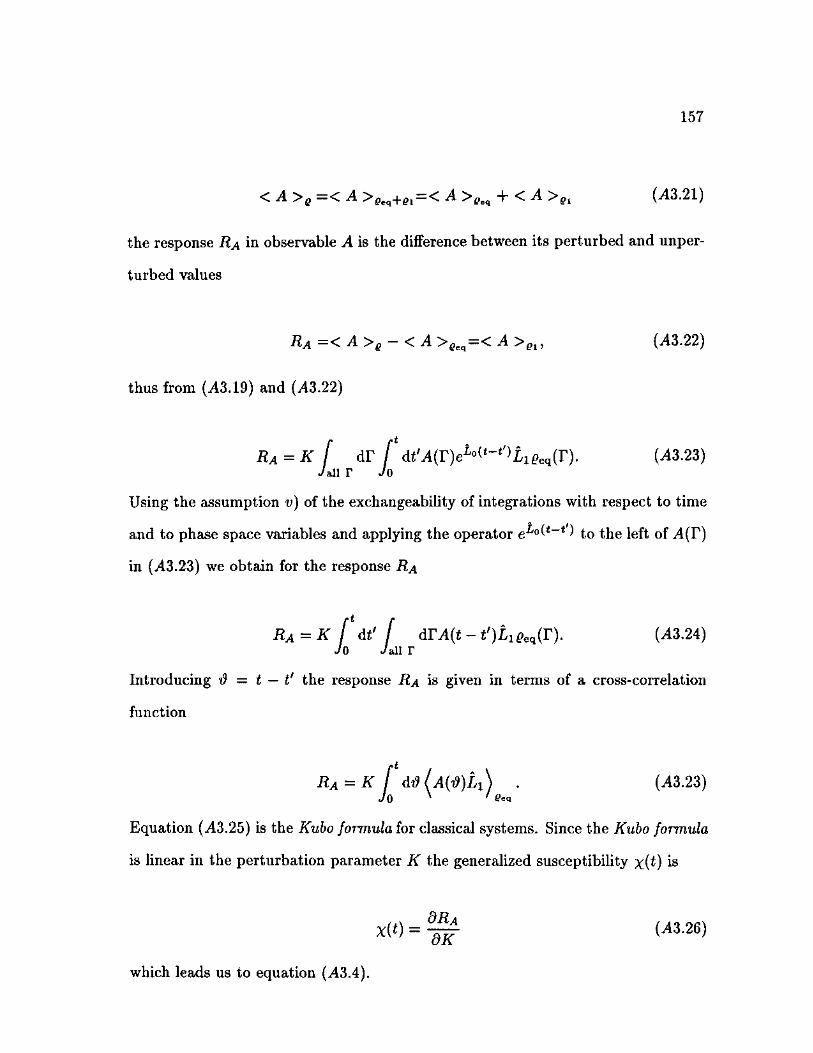
157

< A >q =< A >geq+ei—< A >geq + < A > e i (A3.21)

the response RA in observable A is the difference between its perturbed and unper-

turbed values

RA=<A>e-<A>6e(l=<A>ei, (A3.22)

thus from (A3.19) and (A3.22)

Ra = K [ d r f dt'AWe^-^hge^T). (A3.23) J all r Jo

Using the assumption t>) of the exchangeability of integrations with respect to time

and to phase space variables and applying the operator to the left of A(F)

in (A3.23) we obtain for the response RA

RA = K [ dt' [ drA(*-*')£i0eq(r). (A3.24) Jo Jail r /

rt

< 0 Jail r

Introducing •& = t — t' the response RA is given in terms of a cross-correlation

function

Ra = K f dti/A^Li) . (A3.23)

JO ^ ' <?eq

Equation (A3.25) is the Kubo formula for classical systems. Since the Kubo formula

is linear in the perturbation parameter K the generalized susceptibility %(*) is

X(t) = (-13.26)

which leads us to equation (A3.4).

158

q.e.d.

Remark A3.1. Kubo's linear response formula (A3.4) is an approximate result

based on a first order perturbation theory. There are two important assumption

in the derivation of it. One of them is the exchangeability of the integration with

respect to time and phase space variables. The other assumption is that one can

neglect the term Li(t)gi(T,t) in the evolution of the distribution. Neither of these

two assumptions are well established. Especially the latter one was criticized by

van Kampen (van Kampen 1971) who pointed out that the neglect of the term

Li(t)gi(T, t) is essentially a linearization of the trajectories. Although linearization

of the trajectories can yield correct results only in linear systems at the same time

these systems do not produce relaxation to equilibrium.

In the following Proposition A3.2 we show a linear response theory which recov-

ers Kubo's Linear Response Theory without linearizing the individual trajectories.

In Proposition A3.2 we follow the way was developed by Bianucci et al. (Bianucci

et al 1993b).

Proposition A3.2. The Geometrical Linear Response Theory.

If

i) the considered unperturbed physical system is described by the Hamiltonian

tfo = ^ + ^ + tfo(£,0, (A3.27)

ii) where the potential {/(£,£) is a modified Henon-Heiles potential (see Figure

A3.1)

159

C«({.0 = V + V + « 2 - + f 4 C , «2 c2

2 2 (43.28)

2 u(£,?)

Figure A3.1. The modified Henon-Heiles potential (43.28).

iii) the perturbed physical system is described by the Hamiltonian

H = H0 + U0{{,Q-Kt9(t),

where 0(t) is the step-function,

iv) and the unperturbed system is chaotic i.e., the parameters

(43.29)

mi = 1; m 2 = 0.54; E = H0 = 0.8 (43.30)

160

then

• the generalized susceptibility x = x(°°) with respect to the perturbation

parameter K

{ A m

where and ( l are the largest and smallest values of variable £ in the Poincare

surface of sections of plane (7r,£).

Proof. The proof is based on the following idea. The pertubation is applied to

the variable £. The action of the perturbation is monitored in its action upon the

Poincare surface of section of the plane (71", £) with ( and v fixed. The Poincare

surface of sections in the unperturbed case gives a uniformly filled circle in the

(7r, £) plane which is stretched along the £ axis due to the perturbation (see Figure

A3.2). This distortion is manifested in

( -^0)perturbed ^ ( £ ( ^ 0 ) u n p e r t u r b e d = ( J 4 3 . 3 2 )

from which the generalized susceptibility x is determined in the usual way

X = m - ( « ^ ) U « . u r b e d ) | w (*>-32)

The Poincare surface of sections and the average values of the physical quantities

are calculated within the framework of the microcanonical formalism.

Thus the proof consist of two parts. First we calculate the dominion of the

Poincare surface of sections using the energy conservation then we calculate the

161

1.5

1

0.5

K 0

-0.5

-1

-1.5 -1 -0.5 0 0.5 1 1.5 2

5

Figure A3.2. The deformation of the Poincare surface of sections due to perturba-

tion. The solid line shows the boundary of the Poincare surface of sections of the

plane when the motion takes place in the modified Henon-Heiles potential

(A3.28) i.e., the motion is unperturbed. The dashed line shows the boundary of the

Poincare surface of sections of the perturbed motion.

response with the help of this dominion.

Determination of the dominion of the Poincare surface of sections.

Let us consider the system with the Hamiltonian (.43.27)

H q = + + ^ c ) { A Z 2 7 )

The parameters m\, 777,2 and the total energy E are chosen in a way that the system

is chaotic (see assumption Hi)). This chaotic system is microcanonical (Rasetti

1986, Katok et al. 1986). We assume also that the system is ergodic which is an

162

obvious assumption. Thus the time average of a variable can be replaced by an

average over the microcanonical density distribution which is defined by

S(E - H((, *,(,<>))<%dirdCdi,

J6(E-H((, 7T, (, i/))dfdxd<df' ( A 3 3 3 )

Therefore the probability that the system explores a certain region of the phase

space is proportional to the volume of this region. So the mean value < /(£) > is

< / ( 0 > = J d/x/(0, (A3.34)

where dfi is given by (>13.33).

The energy E is a constant of motion so we can eliminate one of the phase

space variables say v. The ^-function in (>13.33) is rewritten in terms of v

6{E - H0) = 6^V~V\ (>13.35)

where

P = J - ( E -y m2 V

mi7r2

2

Thus the microcanonical density distribution (>13.33) becomes

1 d ^ d c

P K , 0 ) . (43.36)

V f dfdirdC Jf f1(E) u

= 1 d£dnd( (>13.37)

/_2_ ( E _ 2.11*1 _ IJU ^ ftl(E) I . d^d*d<; « ' V m * v 2 Q ) yj^ ( e - s ^ - u u , o )

where Sl(E) is the integration domain i.e., the domain of space £, (, 7r, where

v2 > 0. (>13.38)

163

The domain Sl(E) is bounded by a surface S = S(E). The surface S(E) is defined

by the region of the space where

v = 0 (A3.39)

i.e., the region, where

C) = 0. (A3.40)

Prom the surface S(E) and (A3.40) we can determine the range of integration of

variable %. It is

7T € [ TEJTTJS], (A3.41)

where

0 = \I—(E-U(t 0 ) . (X3.42) V m i

Thus the mean value < /(£) > i.e., (A3.34) can be written

/n,pn 4^d£d£d7r < /(£) > = JQ(E> u — _

^ f d£d<dir Jfl(E) v

Si" d< SlR d f / ( 0 / .

n(E) p At CtRAtt(e\ f*E dx

t*E y ^ ( E - = ¥ i - i r « . o )

/ c " d ^ / a d « / - f d* ( j 1 3 ' 4 3 > d7T. -TtE

J^(e-^-V (f.o)

Jfa d< //"(C)1 d^<^> / q d< F f a K ) ) - - n a t O ) ]

/ a d< / w o d< J a dC I M 0 - W O ]

164

where F(£) is the indefinite integral function of /(£), £r(C) and £l(C) are the

solutions of the equation

E-U(t C) = 0 (>13.44)

so it is considered being the extrema of the range of integration of £ with E and

C fixed, Cl and ( r are the extrema of the range of integration of the variable ( at

fixed energy E.

Now we can calculate the average value < /(£) > only using the Poincare

surface of sections of the system. Sl(E) is a 3-dimensional range of the phase space

(£> C> Tf)- Fixing ( = (* and plotting the phase space coordinates (£, 7r) whenever

the trajectory hits the plane C = C* fr°m the same direction, we get a closed domain

of the (£, 7r) plane which is uniformly filled. This domain of the phase space is the

Poincare surface of section.

From (A3.43) we can see that the invariant measure derived by the Poincare

map d/x(£, (*) with respect to variable £ corresponds to a uniformly distributed £

{ A 3 A 5 )

Thus from (A3.45) and (^43.43) we get average < /(£) >

, { 0 > " € » ( { • ) - & « • ) ( " 3 ' 4 6 )

which in the case of /(£) = £ is simplified to

< £ > = i ( 6 i ( 0 +«£«*)) • (X3.47)

1 6 5

Determination of the linear response

In order to determine the generalized susceptibility we need to calculate the

average of £ with the perturbation acting which value is denoted by < £ >k- The

average of £ for the unperturbed case is given by (A3.47). We can determine < £ >k

using the energy conservation and the calculations above.

At time t = 0 the perturbation starts acting although the system remains

conservative as the Hamiltonian (A3.29) shows. The Hamiltonian also shows that

the energy Ep of the perturbed system is

Ep = E + K(£ - £(0)), (43.48)

where £(0) denotes the value of the variable £ at time t — 0.

Now we can repeat the calculations we did previously using the energy Ep.

Thus the corresponding equations to equation (43.44) becomes

E - £T(£, C) - K(t - £ ( 0 ) ) = 0 , ( 4 3 . 4 9 )

from which £r(C*) and £l(C*) can be determined.

From the definition (43.32) and from (43.46) we can see that the generalized

susceptibility x becomes

X 2 dUC) + dZUC)

dK k=o dK K=0 ( 4 3 . 5 0 )

In order to obtain the susceptibility x w e also need

S s J C i „ _ w ( 2 £ r > t - m ( A 3 m dK dK{8(' £=£, U'(W) + K «=& KM-al>

and

06t(C*) dK

df ( d l r i V «£/

f - «») siref £=(» u'((,C) + K £=£r

166

(A3.52)

where

u'(U") = -^u((,C)- (A3.53)

Substituting (A3.51) and (A3.52) into (A3.50) the generalized susceptibility x takes

the simple form of

X = " 2

£r - £(0) + €L - £(o) (A3.54)

U'(ZR,C) U'((L,C) J '

where £R(C*) and £L((*) denote the extrema of the domain accessible of the unper-

turbed map.

Since our potential fulfills the symmetry

u'(U,C) = -u'(a,C),

the generalized susceptibility is simplified to (A3.31).

(A3.55)

q.e.d.

REFERENCES

Arnold V.I. and Avez A. 1968, Ergodic Problems of Classical Mechanics, W.A. Ben-

jamin, New York.

Bass J. 1966, Elements of Probability Theory, Academic Press, New York.

Beck C. 1990, Physica A, 169, 324.

Berry M.V., Balazs N.L., Tabor M., and Voros A. 1979,Ann. Phys. NY, 122, 26.

Bianucci M., Mannella R., Fan X., Grigolini P., and West B.J. 1993a, Phys. Rev.

A, 47, 1510.

Bianucci M., Bonci L., Trefan Gy., West B.J., and Grigolini P. 1993b, Phys. Lett.

A, 174, 377.

Birkhoff G.D. 1922, Acta Math., 43, 1.

Boltzmann L. 1912; Vorlesungen uber Gastheorie, 2Bde, J.A. Barth, Leipzig.

Bonci L., Grigolini P., Mannella R., Trefan Gy., and Vitali D. 1991, Phys. Rev. A,

43, 2624.

Bonci L., Roncaglia R., West B.J., and Grigolini P. 1991, Phys. Rev. Lett., 67,

2593.

Breyman W. and Thomae H., Linear response of two-dimensional area-preserving

maps, (unpublished).

Cary J.R., Meiss D.J., and Bhattacharjee A. 1981, Phys. Rev. A, 23, 2744.

Casati G. and Ford J. (eds.) 1977, Stochastic Behaviour in Classical and Quantum

Hamiltonian Systems, Como, Lecture Notes Phys. 93, Springer, Berlin.

Cirillo M. and Pedersen N.F. 1982, Phys. Lett. A, 90, 150.

Chirikov B.V. 1979, Phys. Rep., 52, 263.

Collet P. and Eckmann J.-P. 1980, Iterated Maps on the Interval as dynamical Sys-

167

168

Devaney R. L. 1989, An introduction to chaotic dynamical systems, Addison-Wesley,

Redwood City, California.

Doron E. and Fishman S. 1988, Phys. Rev. A, 37, 2144.

Eckmann J.-P. and Ruelle D. 1985, Rev. Mod. Phys., 57, 617.

Ehrenfest P. and Ehrenfest T. 1959, The conceptual foundation of the Statistical

Approach in Mechanics, Cornell Univ. Press, Ithaca.

Einstein A. 1905, Ann. Phys. (Leipzig), 17, 756.

Einstein A. 1906, Ann. Physik, 119, 371.

Feigenbaum M. 1978, J. Stat. Phys., 19, 25.

Fermi E., Pasta J. and Ulam S.M. 1955, Studies in Nonlinear problems, Tech. Rep.,

LA-1940, Los Alamos Sci. Lab.

Fokker A.D. 1915, Ann. Phys. (Leipzig), 43, 310.

Ford J. and Waters J. 1963, J. Math. Phys., 4, 1293.

Ford J. 1975, Fundamental Problems in Statistical Mechanics 1, ed. by E.D.G. Co-

hen, North-Holland, Amsterdam.

Fujisaka H. and Grossmann S. 1982, Z. Phys. B, 48, 261.

Fujisaka H. and Grossmann S., and Thomae S. 1985, Zeitschr. fur Naturforsch.,

40a, 867.

Gard T.C. 1988, Introduction to Stochastic Differential Equations, Marcel Dekker,

Inc., New York.

Gardiner C.W. 1985, Handbook of Stochastic Methods for Physics, Chemistry and

Natural Sciences, Springer, Berlin.

Gerald C.F. 1970, Applied Numeical Analysis, Addison-Wesley Series in Mathemat-

ics, Addison- Wesley Publishing Comp., Inc., Reading.

Geisel T. and Niertwetberg J. 1982, Phys. Rev. Lett., 48, 7

Geisel T. and Nierwetberg J. 1984, Phys. Rev. A, 29, 2305.

169

Geisel T. and Thomae S. 1984, Phys. Rev. Lett., 52, 1936.

Geisel T., Heldstab J., and Thomas H. 1984, Zeitschr. Phys. B, 55, 165.

Gnedenko B.V. and Khinchin A. Y. 1962, An Elementary Introduction to the The-

ory of Probability, Dover Publ. Inc., New York.

Grabert H. 1982, Projection Operator Techniques in Nonequilibrium Statistical Me-

chanics, in Springer Tracts in Modern Physics 95, Springer-Verlag, Berlin.

Grigolini P. 1976, Theoretical Foundations, in Memory Function Approaches to

Stochastic Problems in Condensed Matter, ed. M.W Evans, P. Grigolini and G.P.

Parravicini, Advances in Chemical Physics 62, An Interscience Publication, U.S.A.

Grigolini P. 1991, Lecture Notes on Nonequlibrium Statistical Mechanics, (unpub-

lished).

Grigolini P. 1993, Quantum Irreversibility and Measurement, World Scientific Pub.,

Singapore.

Grossmann S., and Thomae S. 1977, Z. Naturforsch., 32a, 1353.

Grossmann S. and Fujisaka H. 1982, Phys. Rev. A, 26, 1779.

Grossmann S. and Thomae S. 1983, Phys. Lett. A, 97, 263.

Grossmann S. 1984, Zeitschr. Phys. B, 57, 77.

Gyorgyi G. and Szepfalussy P. 1984, J. Stat. Phys., 34, 451.

Halmos P.R. 1956, Lectures on Ergodic Theory, Chelsea Pub. Comp., New York.

Hasegawa H.H. and Shapir W.C. 1991, in Solitons and Chaos, ed. by Antoniou J.

and Lambert F., Springer, Berlin.

Heldstab J., Thomas H., Geisel T., and Radons G. 1983, Zeitschr. Phys. B, 50,

141.

Hubermann B.A., Crutchfield J.P. and Packard N.H. 1980, Applied Phys. Lett.,

37, 750.

Izrailev F.M. 1990, Phys. Rep., 196, 299.

170

Jacob E.B., Goldhirsch J., Imry Y., and Fishman S., Phys. Rev. Lett., 49, 1599.

Jensen R.V. and Oberman C.R. 1981, Phys. Rev. Lett., 46, 1547.

Karney F.F. 1983, Physica D, 8, 360.

Katok A. and Strelcyn J.M. 1986, Lecture Notes in Mathematics 1222, Springer,

Berlin.

Kook H. and Meiss D.J. 1990, Phys. rev. A, 41, 4143.

Krylov N.S. 1950, Raboty po obosnovaniiu stastisticheskoi fiziki, Moscow, Works on

the foundations of statistical physics, Princeton Univ. Press, Princeton 1979.

Kubo R. 1957, J. Phys. Soc. Japan, 12, 570.

Langevin P. 1908, Comptes. Rendues, 146, 530.

Lasota A. and M.C. Mackey 1985, Probabilistic properties of deterministic systems,

Cambridge Univ. Press, Cambridge.

Leven R.W. and Koch B.P. 1981, Phys. Lett. A, 86, 71.

Lichtenberg A.J., Liebermann M.A. and Murray N.W. 1987, Physica D, 28, 371.

Lindenberg K. and West B.J. 1990, The Nonequilibrium Statistical Mechanics of

Open and Closed Systems, VCH Publishers.

Linsay P.S. 1981, Phys. Rev. Lett., 47, 1349.

Mannella R. 1989, Computer experiments in non-linear stochastic physics, in Noise

in nonlinear Dynamial Systems, 3, Experiments and Simulations, ed. F. Moss and

P.V.E. McClintock, Cambridge Univ. Press, Cambridge.

Mannella R. and Palleschi V. 1989, Phys. Rev A, 40, 3381.

Mauer and Libchaber A. 1980, J. Phys. C, 41, 3.

May R.M. 1976, Nature (London), 261, 459.

Messiah A. 1961, Quantum Mechanics I, pp. 469, North Holland Publ. Comp.,

Amsterdam.

Mori H. 1965, Prog. Theor. Phys., 33, 424.

171

Nakajima S. 1958, Prog. Theor. Phys., 20, 948.

Planck M. 1917, Sitzungsber. Preuss. Akad. Wiss. Phys. Math. Kl., 325.

Prakash S., Peng C.-K., and P. ALstrom 1991, 43, 6564.

Press W. H., Flannery B.P., Teukolsky S.A., and Vetterling W.T. 1990, Numerical

Recipes in C The Art of Scientific Computing, Cambridge Univ. Press, Cambridge.

Rao N.J., Borwanker J.D., Ramkrishna 1974, SIAM (Soc. Ind. Appl. Math.) J.

Control, 12, 124.

Rasetti M. 1986, Modern Methods in Equilibrium Statistical Mechanics, Series on

Advances in Statistical Mechanics 2, World Scientific, Singapore.

Rechester A.B. and White R.B. 1980, Phys. Rev. Lett., 44, 1586.

Roncaglia R. 1992, Studies of Classically Chaotic Quantum Systems within the

Pseudo-Probability Formalism, Ph.D. Dissertation, University of North Texas, Den-

ton.

Roux J.-C. 1983, Physica D, 7, 57.

Rozanov Y.A. 1969, Probability Theory: A concise Course, Dover Pub. Inc., New

York.

Sancho J.M., San Miguel M., Katz S.L., and Gunton J.D. 1982, Phys. Rev. A, 26,

1589.

Schell M., Eraser S., and Kapral R. 1982, Phys. Rev. A, 26, 504.

Schuster H.G. 1988, Deterministic Chaos, An Introduction, VCH Verlagsgesellschaft

mbH, Weinheim.

Smale S. and Williams R.F. 1976, J. Math. Biol., 3, 1.

Tabor M. 1983, Physica D, 6, 195.

Tabor M. 1989, Chaos and Integrability in Nonlinear Dynamics - an Introduction,

J. Wiley & Sons, New York.

Testa J., Perez J. and Jeffries C. 1982, Phys. Rev. Lett., 48, 714.

172

Trefan Gy., Grigolini P., and West B.J. 1992, Phys. Rev. A, 45, 1249.

Ulam S.M. and Neuman von J. 1947, Bull. Amer. Math. Soc., 53, 1120.

Ulam S.M. 1960, A collection of Mathematical Problems, Interscience Tracts in Pure

and Applied Mathematics 8.

van Kampen N.G. 1971, Phys. Norv., 5, 279.

van Velsen J.F.C. 1978, Phys. Rep., 41, 135.

Wolfram S. 1988, Mathematica - A System for doing Mathematics by Computer,

Addison - Wesley Publ., Inc., Redwood City, California.

Zisook A.B. 1982, Phys. Rev. A, 25, 2289.

Zwanzig R. 1960, J. Chem. Phys., 33, 1338.

deterministic brownian motion dissertation

Documents