determining significant factors for earthmoving in the ...docs.trb.org/prp/13-4940.pdf · 1...

Kim et al.

1

Determining Significant Factors for Earthmoving in the Bridge Construction 1

2

Seonghoon Kim, Ph.D. 3

Assistant Professor 4

1007 Carruth Building 5

Department of Construction Management and Civil Engineering Technology 6

Georgia Southern University 7

Statesboro, GA 30460 8

Phone: (912) 478-7289 9

Fax: (912) 478-1853 10

E-mail: [email protected] 11

(Corresponding Author) 12

13 Yong Bai, Ph.D., P.E. 14

Chair, Professor 15

Department of Construction Engineering & Management 16

North Dakota State University 17

1530 W. 15th Street, 2135-B Learned Hall 18

Lawrence, KS 66045 19

Tel: (785) 864-2991 20

Fax: (785) 864-5631 21


23

Yang-Ki Jung, Ph.D. 24

Deputy Director 25

Transport Safety & Welfare Division 26

Ministry of Land, Transport and Maritime Affairs 27

Gwacheon, South Korea 427-712 28

Tel: (822) 2110-8677 29

Fax: (822) 504-9199 30


32

33

34

Submit data: November 15th

, 2012 35

Word count: 7,479 (Text: 4,729; Figures and Tables: 11 × 250 = 2,750) 36

37

TRB 2013 Annual Meeting Paper revised from original submittal.

Kim et al.

2

ABSTRACT 1 Urban earthmoving operations are analyzed to identify significant factors that impact relatively 2

low productivity. The research project was conducted in the urban interchange reconstruction of 3

Interstate Highway 235 (I-235) in Des Moines, Iowa. By using observational studies and a 4

statistical analysis method, the factors were identified, including match factor, number of passes, 5

and loading cycle time per bucket. Number of truck, match factor, travel time, and hauling 6

distance were identified as the unique factors for the off-site earthmoving project, while the start 7

time and travel time were significant factors for the on-site project. This research also identified 8

significant factors for the truck bunching and showed that the match factor from the urban 9

earthmoving project does not linearly correlate with the productivity of each truck. Reducing the 10

hauling distance for urban earthmoving projects was the principal method for improving 11

productivity. Based on the research results, a pre-planning and execution method was proposed 12

to improve earthmoving productivity for urban interchange reconstruction. 13

14

Key words: Earthmoving, Highway, Productivity, Schedule, Iowa. 15

16

17


Kim et al.

3

INTRODUCTION 1

Earthmoving productivity has long been a major research subject in the area of construction 2

engineering and management for the following reasons: (1) Earthmoving is included in most 3

construction projects, such as highways, buildings, dams, harbors, airports, sewage and drainage 4

systems, and industrial plants; (2) Earthmoving requires intensive equipment operations; (3) 5

Estimating the earthmoving productivity not only determines the efficiency of operation but also 6

identifies the significant factors that impact productivity. Proper planning and scheduling 7

minimize waiting time and other delays, making the earthmoving process more productive, and 8

decreasing the risk of cost overrun [1]. 9

The efficiency of earthmoving operations varies widely, depending on properties of earth 10

such as rugged earth, moisture content, and swelling and shrinkage factors. A computer program 11

[2] was used to determine the coefficients in order to calculate the haul unit performance in an 12

efficient, accurate, and convenient manner. Farid and Koning [3] proposed that maximum 13

earthmoving productivity will be determined by the productivity of loading facilities regardless 14

of the size, number, and speed of the hauling units. Christian and Xie [1] categorized the factors 15

of earthmoving operations into machine selection, production, and cost based on a survey of 16

industry data, as well as the opinions of experts. Smith [4] identified the factors that influence 17

earthmoving operations by using linear regression techniques. Such factors include bucket 18

capacity, match factor, and the total number of trucks being used. Simulation methods were 19

utilized to identify optimized earthmoving operations for minimizing the total project cost, and 20

the overall project duration, and the equipment idle time [5, 6]. Global positioning system (GPS) 21

equipment became methods to improve progress control and productivity for earthmoving 22

operations [7, 8] 23

24

Urban Highway Earthmoving Productivity on I-235 in Des Moines 25

The purpose of the reconstruction of I-235 was to widen and replace about 80 overpass 26

bridges, install noise barriers and retaining walls, and reconstruct about 20 interchanges, main 27

line pavements, and utility works. This project began in 2002 and was completed in 2007. The 28

total cost of the project was expected to be $429 million [9]. The earthmoving involved in this 29

project constituted 20 percent of the total project cost. 30

31

TABLE 1. Earthmoving Productivity for I-235 Reconstruction 32

Project Type

(1)

No. of

Projects

(2)

Quantity

(yd³)

(3)

Working Period

(days)

(4)

Productivity

(yd³/day)

(5)

Rural Projects 17 1,392,000 432 3,222

I-235 Urban Projects 13 832,548 609 1,367

Note: Quantities for the I-235 project were based on the as-built quantity until June 2004. 33

34

The average earthmoving productivity of the thirteen I-235 reconstruction projects, 35

located in the urban areas, was lower than the average rate of the seventeen rural highway 36


Kim et al.

4

projects based on the data provided by the Iowa Department of Transportation (Iowa DOT). 1

Table 1 shows the difference between the two project groups. The daily average productivity 2

was 3,222 yd³ per day for seventeen rural projects. The average for the thirteen I-235 projects 3

was 1,367 yd³ per day, or approximately 40 percent of the rural earthmoving productivity. This 4

comparison was based on the projects with volumes of less than 200,000 yd³ of earthmoving 5

quantity per project and normal type of earth materials, such as loam, silt, gumbo, peat, clay, soft 6

shale, sand, and gravel. Because of low productivity in the urban interchange projects, bidding 7

prices ranged from 2 to 3 times higher than those of rural projects. 8

Iowa Department of Transportation (Iowa DOT) focused on two main factors for 9

successful completion of the entire I-235 corridor, which were to (1) decrease adverse effects 10

due to delays from previous projects and (2) encourage the projects to collaborate worksites. 11

The reconstruction projects are performed in the urban area of Des Moines where features 12

contribute to lower production rates than those of rural areas. To succeed in the urban projects, 13

the possibility of improving productivity for each project becomes a key issue. A comprehensive 14

literature review showed that there were a few techniques that could be used to improve 15

productivity for urban highway projects. O’Connor and El-Diraby [10] provided methods for 16

optimizing urban bridge construction. Lee et al. [11] reported the most economical traffic 17

closure scenario for urban highway paving projects so that transportation agencies and 18

contractors achieved minimum construction costs and user road costs. However, there is a 19

limited amount of literature on urban earthmoving productivity improvement, although there 20

have been many research projects which focused on earthmoving productivity improvement. 21

Thus, it is important to conduct research to identify factors that have a significant impact upon 22

urban earthmoving productivity and to develop methods to improve the productivity. 23

24

RESEARCH OBJECTIVE AND SCOPE 25

The primary objective of this research was to identify factors that impact earthmoving 26

productivity in urban interchange reconstruction projects. A secondary objective was to develop 27

a preplanning method to improve the productivity. The required data were collected via 28

construction documents, site observations, and interviews with earthmoving contractors and 29

inspectors. Forty-five earthmoving operations in the I-235 reconstruction project were observed 30

and recorded using the time-study method, then statistical analysis was conducted to determine 31

the cause and effect factors. The data were gathered from two interchange reconstruction sites. 32

33

METHODOLOGY 34

An urban earthmoving operation is defined as construction in an area where there is an increased 35

density of man-made structures in comparison to the surrounding areas. In this research, two 36

projects were selected from I-235 urban interchange reconstruction projects, both of which began 37

and ended in 2004. Four different types of earthmoving operations were randomly selected from 38

these interchange reconstruction projects. Equipment fleet for those operations included trucks 39

and an excavator. 40

The time-scaled data were collected during weekly site visits after literature review. A 41

multiple regression modeling was used for data analyses to determine factors that impacts 42

earthmoving productivity, or the response variable. A total of nine explanatory variables were 43

gathered from job sites and these variables were used to estimate productivity for earthmoving 44


Kim et al.

5

operations. Explanatory variables in this research were the number of trucks, bucket capacity, 1

start time, the number of passes, loading cycle time, truck spot time, truck travel time, truck 2

dump time, and lastly, hauling distance. From this point forward, the nine collected data were 3

used to determine the significant factors that impact the productivity. In addition, eight 4

calculated variables were included in the analysis. 5

The number of loader was not included as an explanatory variable because the collected 6

data were all single loader operations. Rolling resistance and grade resistance were not 7

considered for calculating earthmoving productivity in this research, because this research 8

assumed that most of the hauling roads were composed of asphalt paving and low gradient. Thus, 9

total resistance, the sum of these two resistances could be considered to be the same for I-235 10

earthmoving projects according to the Caterpillar Performance Handbook [12]. 11

12

Match Factor and Estimating Productivity 13

Under conventional theories, the capacity of each truck will determine overall output and output 14

will linearly increase as more trucks are added until the loader production capacity is reached. 15

This conventional theory has been used to estimate the productivity of truck-loader fleets for 16

many years. The Match Factor (MF) is indicative of the suitability of the size of the truck fleet; 17

it is used to determine the efficiency of the fleet. Mogan and Peterson [13] developed the match 18

factor to estimate the appropriate number of trucks and number of loaders: 19

20

)1(TimeCycleHaulerLoadersofNumber

TimeCycleLoaderHaulersofNumberFactorMatch

21 When the match factor equals 1, the operation is referred to as the ideal condition for 22

determining the number of machines and the cycle time of equipment. If MF < 1, the operation 23

indicates that less than the ideal number of hauling units are employed. If MF > 1, it indicates 24

that there are more haulers than the operation needs. Consequently, the overall efficiency will be 25

no longer increased if MF > 1 [14]. 26

In an earthmoving operation, three different productivity levels could be estimated based 27

upon data gathered. These are maximum productivity, possible productivity, and actual 28

productivity. Possible productivity depends on loader production and actual productivity 29

depends on hauling unit production. The maximum productivity can be calculated using the 30

following formula. 31

32 3

max ( /10 ) ( ) (2)P Load Cycle Rate loads hours Load Volume per Cycle m 33

Possible productivity will be lower than maximum productivity when the number of available 34

hauling units is insufficient to keep the loader busy. 35

36

max

max

1

1 (3)

possible

possible

P P MF for MF

P P for MF

37

Actual productivity is determined by the following equation: 38

39

)4()()10/( 3mVolumeLoadhourscyclesRateCycleHaulerPactual 40

With the calculations above, the bunch factor is determined by the following equation: 41


Kim et al.

6

1

)5(possible

actual

P

PFactorBunch 2

Bunching certainly occurs in a system of a loader and its correlating fleet of trucks. If a 3

truck has a greater cycle time due to the loader’s delay, this delay time affects either the queue or 4

the fleet cycle time. Therefore, many contractors consider the bunch factor to be a valid measure 5

of earthmoving productivity. 6

The truck possible productivity can reach 100 percent if the match factor is equal to or 7

greater than 1 as illustrated in Figure 1. Unlike the possible productivity, the operation 8

efficiency of 100 percent does not correspond to MF=1. The match factor for 100 percent 9

operation efficiency is reached at 1.8 as the efficiency increases by adding more haulers. Even if 10

the efficiency is at 100 percent, this efficiency level is not considered at its optimal level because 11

the additional haulers increase the cost more than they increase profits [4]. The previous 12

research [15] demonstrated that optimal cost fleets can have operational efficiency as low as 50 13

percent. 14

15

16

17

FIGURE 1 Match Factor vs. Operation Efficiency [4] 18

19

DATA COLLECTION 20

A total of 45 earthmoving operations from four urban earthmoving projects were observed. 21

Time studies were conducted using a stopwatch to collect the raw data. Additional information 22

on site conditions, project sizes, and site features were obtained through site visits, interviews 23

with inspectors and contractors, and through the inspection of documents from the Iowa 24

0%

20%

40%

60%

80%

100%

0 0.2 0.4 0.6 0.8 1 1.2 1.4 1.6 1.8

Match Factor

Op

era

tio

n E

ffic

ien

cy

Trucks possible efficiency

Trucks actual efficiency

Loader Efficiency


Kim et al.

7

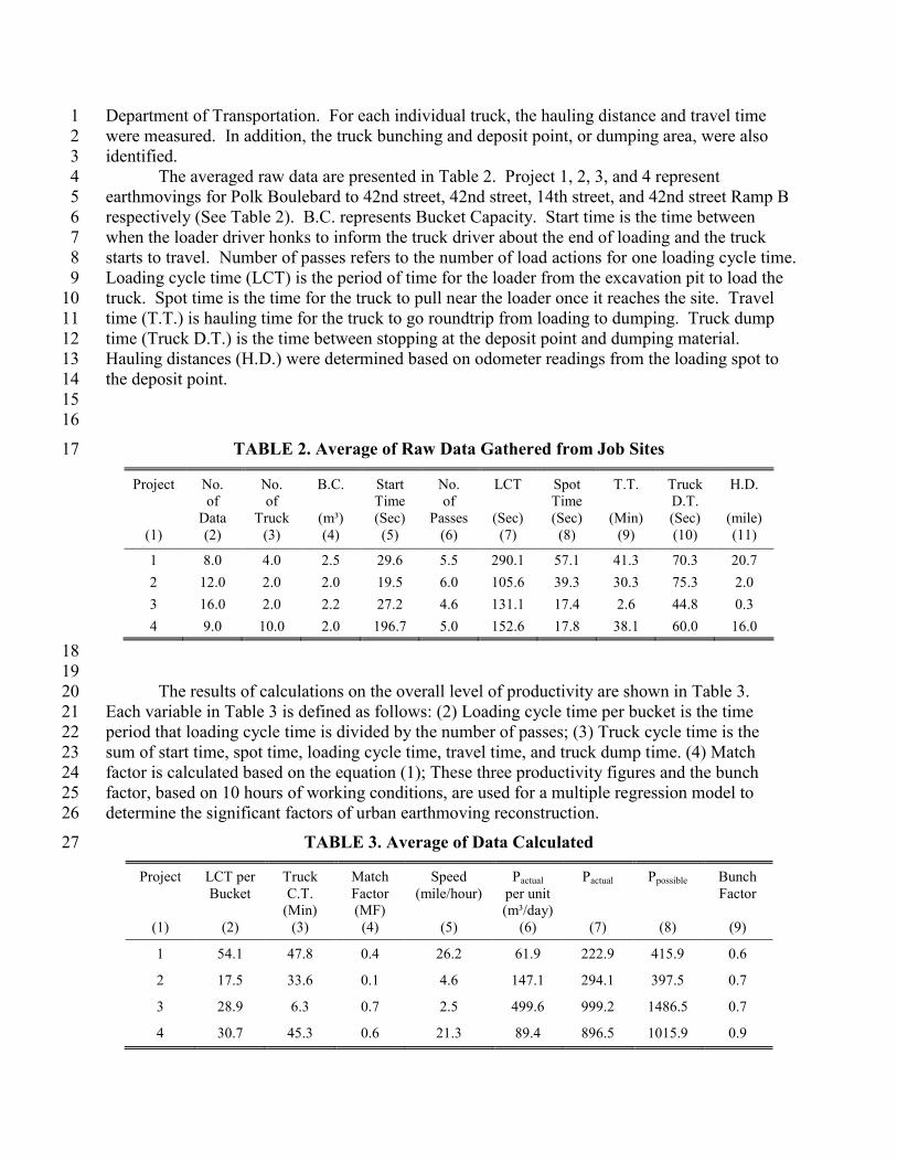
Department of Transportation. For each individual truck, the hauling distance and travel time 1

were measured. In addition, the truck bunching and deposit point, or dumping area, were also 2

identified. 3

The averaged raw data are presented in Table 2. Project 1, 2, 3, and 4 represent 4

earthmovings for Polk Boulebard to 42nd street, 42nd street, 14th street, and 42nd street Ramp B 5

respectively (See Table 2). B.C. represents Bucket Capacity. Start time is the time between 6

when the loader driver honks to inform the truck driver about the end of loading and the truck 7

starts to travel. Number of passes refers to the number of load actions for one loading cycle time. 8

Loading cycle time (LCT) is the period of time for the loader from the excavation pit to load the 9

truck. Spot time is the time for the truck to pull near the loader once it reaches the site. Travel 10

time (T.T.) is hauling time for the truck to go roundtrip from loading to dumping. Truck dump 11

time (Truck D.T.) is the time between stopping at the deposit point and dumping material. 12

Hauling distances (H.D.) were determined based on odometer readings from the loading spot to 13

the deposit point. 14

15

16

TABLE 2. Average of Raw Data Gathered from Job Sites 17

Project

(1)

No.

of

Data

(2)

No.

of

Truck

(3)

B.C.

(m³)

(4)

Start

Time

(Sec)

(5)

No.

of

Passes

(6)

LCT

(Sec)

(7)

Spot

Time

(Sec)

(8)

T.T.

(Min)

(9)

Truck

D.T.

(Sec)

(10)

H.D.

(mile)

(11)

1 8.0 4.0 2.5 29.6 5.5 290.1 57.1 41.3 70.3 20.7

2 12.0 2.0 2.0 19.5 6.0 105.6 39.3 30.3 75.3 2.0

3 16.0 2.0 2.2 27.2 4.6 131.1 17.4 2.6 44.8 0.3

4 9.0 10.0 2.0 196.7 5.0 152.6 17.8 38.1 60.0 16.0

18

19

The results of calculations on the overall level of productivity are shown in Table 3. 20

Each variable in Table 3 is defined as follows: (2) Loading cycle time per bucket is the time 21

period that loading cycle time is divided by the number of passes; (3) Truck cycle time is the 22

sum of start time, spot time, loading cycle time, travel time, and truck dump time. (4) Match 23

factor is calculated based on the equation (1); These three productivity figures and the bunch 24

factor, based on 10 hours of working conditions, are used for a multiple regression model to 25

determine the significant factors of urban earthmoving reconstruction. 26

TABLE 3. Average of Data Calculated 27

Project

(1)

LCT per

Bucket

(2)

Truck

C.T.

(Min)

(3)

Match

Factor

(MF)

(4)

Speed

(mile/hour)

(5)

Pactual

per unit

(m³/day)

(6)

Pactual

(7)

Ppossible

(8)

Bunch

Factor

(9)

1 54.1 47.8 0.4 26.2 61.9 222.9 415.9 0.6

2 17.5 33.6 0.1 4.6 147.1 294.1 397.5 0.7

3 28.9 6.3 0.7 2.5 499.6 999.2 1486.5 0.7

4 30.7 45.3 0.6 21.3 89.4 896.5 1015.9 0.9


Kim et al.

8

REGRESSION MODEL AND ANALYSIS 1

A multiple linear regression model was developed to predict the productivity per hauling unit for 2

the urban earthmoving operation and to determine factors that made a significant impact upon 3

that productivity. The productivity per hauling unit represented how effectively the earthmoving 4

operation was executed in the field. Thus, the productivity per hauling unit was selected as the 5

response variable against 11 explanatory variables, which were the number of truck, match factor, 6

bucket capacity, start time, number of passes, loading cycle time (LCT), spot time, travel time, 7

truck dump time, hauling distance, and loading cycle time per bucket. The cycle time was not 8

selected as an explanatory variable, because the variable was composed of four variables 9

included in the 11 explanatory variables. The regression model on the bunch factor was also 10

developed to determine the factor that impacted the actual productivity. 11

In this research, data from the four earthmoving projects were analyzed, and then the data 12

sets according to the range of productivity per hauling unit were divided into two categories: (1) 13

productivity less than 350 m3/day, and (2) productivity between 350 m

3/day and 750 m

3/day. 14

Table 4 shows the coefficients of determination as well as the number of observations for 15

each data set. The range of the coefficients of determination is from 0.94 to 0.99. For example, 16

the coefficient of determination (R²) of 0.94 from the four earthmoving projects indicates that 94 17

percent of the variation in the explanatory variables can be explained by the regression model. 18

The coefficients for each data set were close to 1, meaning that the regression line was a valid 19

explanation of the variations in this model. 20

21

22

TABLE 4. R2 and the Number of Observation for Each Data Set 23

Data Set

(1)

Unit Production Bunch Factor

R Square

(2)

Observations

(3)

R Square

(4)

Observations

(5)

Earthmoving (4 projects) 0.94 45 0.97 45

Production (0 – 350 m³/day) 0.95 29 0.98 29

Production (350 – 750 m³/day) 0.99 16 0.98 16

24

25

The t-statistic is the ratio of the coefficient to its standard error to test the significance of 26

the regression model. In the Table 5, the t-statistic of the match factor is 27

477.529/186.205 2.565t and the value is greater than the critical t-value at a level of 28

significance of 5 percent, t(0.025;n-p-1)=2.04. Since the corresponding probability of 0.015 is less 29

than the P-value 0.05, the null hypothesis (H0), which is 1 0 , can be rejected. Accordingly, 30

other two explanatory variables, No. of passes and LCT per bucket, were selected as significant 31

factors at the 95 percent confidence level (α=0.05). The predicted productivity ˆiy can be 32

estimated by the following mathematical formula based on the coefficients of three explanatory 33

variables (bold text) in Table 5. The intercept in a multiple regression model is often labeled the 34

constant and the mean for the response when all of the explanatory variables take on the value 0. 35

36


Kim et al.

9

TABLE 5. Parameter Estimates on Productivity per Hauling Unit 1

Variables

(1)

Coefficients

(2)

Standard

Error

(3)

t-Statistic

(4)

P-value

(5)

Lower

95%

(6)

Upper

95%

(7)

Intercept 671.400 903.600 0.743 0.463 -1166.987 2509.787

No of Truck -24.323 30.205 -0.805 0.426 -85.776 37.130

Match Factor 477.529 186.205 2.565 0.015 98.692 856.365

Bucket Capacity (m³) 37.693 382.767 0.098 0.922 -741.052 816.438

Start -0.147 0.242 -0.607 0.548 -0.639 0.345

No. of Passes -89.895 31.106 -2.890 0.007 -153.181 -26.610

Loading Cycle Time 0.856 0.636 1.346 0.188 -0.438 2.149

Spot 0.137 1.604 0.085 0.932 -3.126 3.400

Travel Time (Min) -0.866 0.726 -1.193 0.241 -2.344 0.611

Truck D.T(Sec) 0.139 0.913 0.152 0.880 -1.718 1.996

Hauling Distance (mile) -3.618 11.407 -0.317 0.753 -26.826 19.590

LCT per Bucket -8.307 3.017 -2.753 0.010 -14.445 -2.169

2

)9(307.8895.89529.477400.671ˆ321 iiii xxxy 3

BucketperTimeCycleLoadingx

PassesofNox

FactorMatchx

i

i

i

:

.:

:

3

2

1

4 5

6

An ANOVA (Analysis of Variance) test determined whether the regression model for the 7

four earthmoving projects was statistically significant. The F value of 47.4 revealed that the 8

entire regression was significant because the test statistic F value was greater than the critical F 9

value (Fcritical = F0.05; 11, 33 = 2.13 for a significance level of 0.05). It means that at least one of 11 10

variables was not zero, indicating that we rejected the null hypothesis of H0: β1 = β2 = ∙∙∙ = β11 = 11

0. Consequently, the urban earthmoving productivity and the explanatory variables in Table 6 12

were linearly correlated. 13

14

TABLE 6. ANOVA Table on Productivity for the Four Projects 15

Source

(1)

Df

(2)

SS

(3)

MS

(4)

F

(5)

F(0.05)

(6)

Regression 11 1726970.5 156997.3 47.4 2.13

Residual 33 109314.3 3312.6

Total 44 1836284.8

16

This research garnered results similar to the previous research in terms of the significant 17

factors for earthmoving productivity. The significant factors in the earthmoving operations 18

determined from the previous research were the number of trucks, bucket capacity, match factor, 19


Kim et al.

10

truck travel time, and hauling distance [4]. In Table 7, significant factors for earthmoving 1

productivity per hauling unit with the coefficients are presented. Number of truck, match factor, 2

travel time, and hauling distance were identified as significant factors in the urban earthmoving 3

project with productivity ranged from 0 to 350 m³. For the on-site project with productivity from 4

350 to 750 m³, start time and travel time are significant factors. Number of passes, match factor, 5

and loading cycle time per bucket also proved significant for the four earthmoving projects. In 6

this research, on-site project represents earthmoving operation performed in the job site. In 7

addition, loading in off-site projects was carried out on the job site but dumping occurred outside. 8

9

TABLE 7. Significant Factors on Earthmoving Productivity per Hauling Unit 10

Variables

(1)

Coefficients

Off-site

Earthmoving

0 – 350 (m³)

(2)

On-site

Earthmoving

350 – 750 (m³)

(3)

Earthmoving

(4 projects)

(4)

Intercept 400.461 1523.759 671.400

No of Truck -13.042

M.F. 178.529 477.529

Bucket Capacity (m³)

Start -4.252

No. of Passes -89.895

Loading C.T.

Spot

Travel Time (Min) -1.380 -201.386

Truck D.T. (Sec)

H.D. (mile) -3.248

LCT per Bucket -8.307

11

12

The difference between this research and previous studies was that the number of passes 13

was a statistically significant factor. The number of passes was a negative factor that reduced the 14

productivity as the number of passes increased. The regression model for the bunch factor was 15

not defined in previous research [4]. During this research, explanatory variables correlated with 16

the bunch factor were tested except for the productivity range from 350 to 750 m3. However, 17

other regression models were not defined by the bunch factor (see Table 8). 18

19

20

21

22

23

24


Kim et al.

11

TABLE 8. Significant Factors on Bunch Factor 1

Variables

(1)

Coefficients

Off-site

Earthmoving

0 – 350 (m³)

(2)

On-site

Earthmoving

350 – 750 (m³)

(3)

Earthmoving

(4 projects)

(4)

Intercept 1.704 5.297

No of Truck 0.0469 -0.054

M.F.

B.C (m³)

Start

No. of Passes -0.184 -0.236

Loading C.T 0.0016 0.002

Spot 0.0022 0.002

Travel Time (Min)

Truck D.T (Sec)

H.D (mile) -0.0218 0.025

LCT per Bucket -0.0067 -0.011

2

Figure 2 illustrates the relationship between the overall efficiency of earthmoving 3

operations and the match factor. The data for urban earthmoving productivity does not match the 4

possible productivity, which increases the overall efficiency as the match factor increases until it 5

reaches one. As previously described on the match factor, the productivity is the highest when 6

the match factor is approximately 1.8 after truck bunching is taken into account. However, the 7

match factors for the 14th St. earthmoving project, the best practices observed within those data, 8

were only 0.7 in the average, indicating that the project needs more hauling resources based on 9

the previous research. In practice, the hauling units were employed in enough numbers since 10

there was continuous queuing by trucks due to the space restriction. Space limitations, one of the 11

features in urban interchange reconstruction, should be considered for match factor because the 12

restricted space often limits room for additional hauling equipment. For example, the average 13

match factor in the 14th Street project was 0.7, even if only a little bunching was found and was 14

relatively well-executed in small enough space where no more equipment could be employed. 15

16


Kim et al.

12

1

FIGURE 2 Match Factor vs. Bunch Factor 2

3

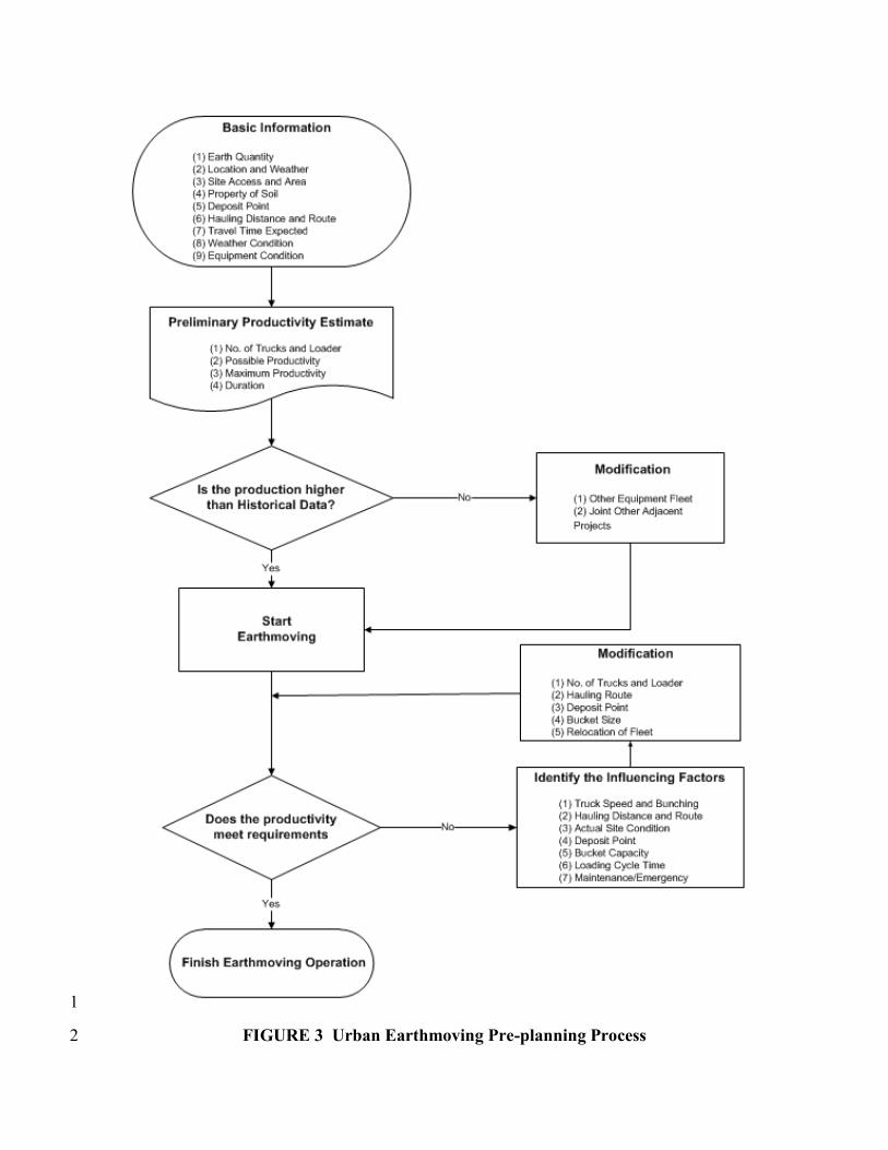
URBAN EARTHMOVING PRE-PLANNING FLOW CHART 4

The urban earthmoving pre-planning flow chart was developed based on the result of this 5

research, as shown in Figure 3. During the development, several assumptions were made: (1) 6

earthmoving is performed in the urban area; and (2) in most cases, excavators and trucks are 7

used for the urban earthmoving operation except for the intermittent use of scrapers. 8

To use this chart, the first step is to study the basic information of a job site, such as earth 9

quantity, location, accessibility, trafficability, borrow pit, deposit point, equipment fleet, 10

operation method, and hauling distance. The information can be readily identified by the 11

earthmoving contractor in advance through drawings, specifications, and site visits. Based on 12

the useful information, project managers will be able to estimate the expected productivity 13

(Preliminary Productivity) that includes possible productivity and maximum productivity. Once 14

these productivity figures are high enough in comparison to the company’s historical data 15

observed from similar cases, earthmoving can be started. In the case of an unsatisfied condition, 16

managers need to consider if another equipment fleet could be selected. 17

Once earthmoving begins, the project manager will be able to determine actual 18

productivity and factors that impact the productivity. Actual productivity can be calculated 19

based on field operations. The manager can determine factors by observing truck queuing and 20

loader operations. Then, the next stage is to check if the actual productivity meets the target 21

value. If yes, the earthmoving operation will continue as planned. If the target value is not met, 22

modification will be needed. 23

24

0%

20%

40%

60%

80%

100%

0.0 0.2 0.4 0.6 0.8 1.0 1.2 1.4 1.6 1.8

Match Factor

Bu

nc

h F

ac

tor

Bunch Factor

Theoritical Bunch Factor


Kim et al.

13

1

FIGURE 3 Urban Earthmoving Pre-planning Process 2


Kim et al.

14

CONCLUSION AND RECOMMENDATIONS 1 Earthmoving in urban interchange construction faces many potential barriers that can increase 2

the project duration and costs. Identifying significant factors involved in productivity and site 3

observations coupled with time studies provided useful information on the causes of low 4

productivity in urban interchange reconstruction projects. 5

Match factor, loading cycle time per bucket, and number of passes were identified as 6

significant factors for urban earthmoving. Number of truck, match factor, travel time, and 7

hauling distance were identified as the unique factors for off-site earthmoving projects, while the 8

start time and travel time were significant factors for on-site projects. 9

The bunch factor and the match factor were defined differently in the urban earthmoving 10

project. The bunch factor was defined by regression modeling, whereas in the previous research, 11

the bunch factor could not defined by the multiple regression model. The number of trucks, 12

number of passes, loading cycle time, spot, hauling distance, and loading cycle time per bucket 13

were all significant for the bunch factors. 14

Hauling distance is a negative factor for off-site earthmoving productivity, indicating two 15

important concepts: (1) reducing the hauling distance is the key point in increasing earthmoving 16

productivity, and (2) in multiple urban highway projects, as in the I-235 project in Des Moines, a 17

productivity study with the proper pre-planning is essential for balancing earth in overall job 18

sites. Consequently, the pre-planning phase is an appropriate time to consider these two 19

concepts. In other words, establishing an adequate stockpile or deposit point on-site is an 20

important method for improving earthmoving productivity in urban interchange reconstruction. 21

Match factor is not necessary when truck access is limited by utility work, small 22

excavation quantity, and restricted space. It is a possible assumption that the match factor can be 23

better used in the linear earthmoving and mass excavation site, such as harbor construction, new 24

main-line highway projects, and airport construction. When applying the match factor for 25

productivity analysis of urban interchange reconstruction, the job site area should be spatial 26

enough for the earthmoving to be executed in a continuous manner. In several projects in the I-27

235 urban interchange reconstruction, the researchers found that maintaining a match factor of 1 28

through the employment of more trucks was ultimately not worthwhile. Using the research 29

results, a pre-planning flow chart was proposed to solve the problems encountered during 30

earthmoving in urban interchange reconstruction. 31

Additional significant factors for urban earthmoving operations might have been 32

identified if the scope of data was extended. Although several significant variables were not 33

identified in this research, the optimal amount of equipment on the job site, the contractor 34

management skill level, the specific variables of the area itself in terms of restricted deposit 35

points, the work space, access time to hauling route, and the traffic open scenario could be 36

considered. These variables could be additional significant factors to earthmoving productivity 37

for urban interchange reconstruction. 38

39


Kim et al.

15

ACKNOWLEDGEMENTS 1 The authors would like to thank the Iowa Department of Transportation and contractors involved 2

in the I-235 reconstruction project for supporting this research by providing financial resources, 3

project notes, documents, and access to the construction sites. 4


Kim et al.

16

REFERENCES. 1

2

1. Christian, J. and T.X. Xie. More realistic intelligence in earthmoving estimates. 1994. 3

University Park, PA, USA: Computational Mechanics Publ, Southampton, Engl. 4

2. Hicks, J.C., Haul-unit performance. Journal of Construction Engineering and Management, 5

1993. 119(3): p. 646-653. 6

3. Farid, F. and T.L. Koning, Simulation verifies queuing program for selecting loader-truck 7

fleets. Journal of Construction Engineering and Management, 1994. 120(2): p. 386-404. 8

4. Smith, S.D., Earthmoving productivity estimation using linear regression techniques. 9

Journal of Construction Engineering and Management, 1999. 125(3): p. 133-141. 10

5. Tromposch, E. and J.H. Armitage, Design-construction of Fox Hollow pedestrian bridge. 11

PCI Journal, 1997. 42(6): p. 50-59. 12

6. Marzouk, M. and O. Moselhi, Object-oriented Simulation Model for Earthmoving 13

Operations. Journal of Construction Engineering and Management, 2003. 129(2): p. 173-14

181. 15

7. Christoffersen, J., et al., Innovative cable-stayed bridge. Concrete (London), 1998. 32(7): p. 16

32-34. 17

8. Navon, R. and Y. Shpatnitsky, Field Experiments in Automated Monitoring of Road 18

Construction. Journal of Construction Engineering and Management, 2005. 131(4): p. 487-19

493. 20

9. Swanson, J.A. and J. Windau, Rapid rehabilitation. Modern Steel Construction, 2004. 44(6): 21

p. 53-54. 22

10. Abou-Zeid, A., et al., Data flow model for communications between project participants in a 23

highway bridge project. Canadian Journal of Civil Engineering, 1995. 22(6): p. 1224-1234. 24

11. SAS. 25

12. Liu, B., X.-Y. Huang, and N.-N. Yan, Construction of manufacturing execution system and 26

its application at Shougang. Kang T'ieh/Iron and Steel (Peking), 2006. 41(12): p. 79-82. 27

13. Woo, D.-C., Robotics in highway construction & maintenance. Public Roads, 1995. 58(3): p. 28

26-30. 29

14. Nichols, M.E. Applications for satellite positioning technology in the construction industry. 30

1996. Atlanta, GA, USA: IEEE, Piscataway, NJ, USA. 31

15. Yang, D.-L., W.-H. Kuo, and M.-S. Chern, Multi-family scheduling in a two-machine 32

reentrant flow shop with setups. European Journal of Operational Research, 2008. 187(3): p. 33

1160-1170. 34


determining significant factors for earthmoving in the ...docs.trb.org/prp/13-4940.pdf · 1...

Documents