HAL Id: hal-02080379https://hal.archives-ouvertes.fr/hal-02080379

Submitted on 26 Mar 2019

HAL is a multi-disciplinary open accessarchive for the deposit and dissemination of sci-entific research documents, whether they are pub-lished or not. The documents may come fromteaching and research institutions in France orabroad, or from public or private research centers.

L’archive ouverte pluridisciplinaire HAL, estdestinée au dépôt et à la diffusion de documentsscientifiques de niveau recherche, publiés ou non,émanant des établissements d’enseignement et derecherche français ou étrangers, des laboratoirespublics ou privés.

Determining permeability tensors of porous media: Anovel ‘vector kinetic’ numerical approach

Yann Jobic, Prashant Kumar, Frédéric Topin, Rene Occelli

To cite this version:Yann Jobic, Prashant Kumar, Frédéric Topin, Rene Occelli. Determining permeability tensors ofporous media: A novel ‘vector kinetic’ numerical approach. International Journal of Multiphase Flow,Elsevier, 2019, 110, pp.198-217. 10.1016/j.ijmultiphaseflow.2018.09.007. hal-02080379

1

Determining permeability tensors of porous media: a novel

‘vector kinetic’ numerical approach

Y Jobic1, P Kumar1, F Topin1 and R Occelli1

1Aix-Marseille Université, IUSTI, CNRS UMR 7343

5, Rue Enrico Fermi, 13453 Marseille Cedex 13, France

E-mail: yann.jobic@univ-amu.fr

Abstract. New structurally tailored porous materials are nowadays used in many engineering

applications due to several attractive properties. Knowledge of pressure losses or flow structures

in such complex media and their relationship with geometrical parameters are thus critical for

various applications. Precise determination of local flow behavior and macroscale properties of

natural media (soils, biomass....) are increasingly needed. It is therefore important to simulate

the complex and unsteady flows by reliable numerical methods and to determine intrinsic

macroscopic hydraulic properties on porous structures. The availability of low cost, easy-to use

High-performance computational resources lead to generalization of pore scale numerical

simulations in various fields. The recent development of innovative scheme like LBM to

overcome the classical drawback of commercial softwares (VF, EF) in achieving high accuracy,

shows the potential of kinetic based methods for producing efficient and accurate solvers. An

alternative vector kinetic method is proposed to solve Incompressible Navier-Stokes equations

at pore scale and eventually determine permeability tensors of complex porous media. A moment

based (vs discrete velocities), non-diffusive, explicit, parallel implementation was implemented

and successfully used on several totally different complex geometries. Excellent results at low

Re number were obtained, the method is thus well suited for permeability tensors determination

of complex heterogeneous media. The code was validated against classical benchmark as well

as experimental and numerical permeability data obtained on different porous media of variable

1Y Jobic: yann.jobic@univ-amu.fr.

2

porosity namely (i) foams (virtual model structures and real samples), (ii) sandstone and (iii)

wood.

3

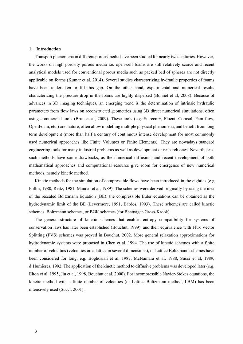
1. Introduction

Transport phenomena in different porous media have been studied for nearly two centuries. However,

the works on high porosity porous media i.e. open-cell foams are still relatively scarce and recent

analytical models used for conventional porous media such as packed bed of spheres are not directly

applicable on foams (Kumar et al, 2014). Several studies characterizing hydraulic properties of foams

have been undertaken to fill this gap. On the other hand, experimental and numerical results

characterizing the pressure drop in the foams are highly dispersed (Bonnet et al, 2008). Because of

advances in 3D imaging techniques, an emerging trend is the determination of intrinsic hydraulic

parameters from flow laws on reconstructed geometries using 3D direct numerical simulations, often

using commercial tools (Brun et al, 2009). These tools (e.g. Starccm+, Fluent, Comsol, Pam flow,

OpenFoam, etc.) are mature, often allow modelling multiple physical phenomena, and benefit from long

term development (more than half a century of continuous intense development for most commonly

used numerical approaches like Finite Volumes or Finite Elements). They are nowadays standard

engineering tools for many industrial problems as well as development or research ones. Nevertheless,

such methods have some drawbacks, as the numerical diffusion, and recent development of both

mathematical approaches and computational resource give room for emergence of new numerical

methods, namely kinetic method.

Kinetic methods for the simulation of compressible flows have been introduced in the eighties (e.g

Pullin, 1980, Reitz, 1981, Mandal et al, 1989). The schemes were derived originally by using the idea

of the rescaled Boltzmann Equation (BE): the compressible Euler equations can be obtained as the

hydrodynamic limit of the BE (Levermore, 1991, Bardos, 1993). These schemes are called kinetic

schemes, Boltzmann schemes, or BGK schemes (for Bhatnagar-Gross-Krook).

The general structure of kinetic schemes that enables entropy compatibility for systems of

conservation laws has later been established (Bouchut, 1999), and their equivalence with Flux Vector

Splitting (FVS) schemes was proved in Bouchut, 2002. More general relaxation approximations for

hydrodynamic systems were proposed in Chen et al, 1994. The use of kinetic schemes with a finite

number of velocities (velocities on a lattice in several dimensions), or Lattice Boltzmann schemes have

been considered for long, e.g. Boghosian et al, 1987, McNamara et al, 1988, Succi et al, 1989,

d’Humières, 1992. The application of the kinetic method to diffusive problems was developed later (e.g.

Elton et al, 1995, Jin et al, 1998, Bouchut et al, 2000). For incompressible Navier-Stokes equations, the

kinetic method with a finite number of velocities (or Lattice Boltzmann method, LBM) has been

intensively used (Succi, 2001).

4

Meanwhile, the simplicity of LBM has enabled it to be successfully applied to a wide range of

problems (Aidun, 2010). LBM used for complex geometries structure such as foams is still challenging

(Liu, 2015) and some limitations of the formalism such as numerical instability at low viscosities,

(Lallemand et al, 2000) or boundary position dependence on variable viscosity, (e.g. Narváez et al, 2010)

has been raised. A lot of efforts have been made to overcome these limitations. For example, dubbed

regularized LBM has been developed to improve numerical stability (Succi, 2001). The multiple

relaxation time (MRT) collision operator has been used to improve the numerical stability by separating

the relaxation rates of the hydrodynamic (conserved) and non-hydrodynamic (non-conserved) moments

(d’Humières et al, 2002). Unfortunately, it destroys the entropy compatibility.

The use of special velocity lattices and particular Maxwellians that are not entropy compatible also

contribute to the loss of robustness (Chikatamarla et al, 2009). Indeed, as it was shown in Yong et al,

2005, usual LBM (as opposed to entropic LBM, see for instance Karlin et al, 1998, Succi et al, 2002) is

not able to comply with any entropy theorem, and the study of stability must be performed with

additional difficulties.

Our work takes its roots in (Natalini et al, 2008) where a limited number of velocity directions are

used, in accordance with (Bouchut, 2002). Even if we start from kinetic considerations, we use the

approach of (Bouchut et al, 2006) to write a simple explicit finite volume/difference scheme on the

macroscopic moments themselves, thus finally avoiding the kinetic aspects. This approach enables to

analyze the accuracy in a simple way, and lead to simple, and physical interpretation of boundary

conditions. Moreover, the implementation requires less memory consumption than a discrete velocities

approach. Eventually the explicit scheme insures the good scalability of parallel software

implementation. We end up with a BGK-FVS method that is second-order accurate without any special

choice of the velocities and with standard forward Euler time stepping. Indeed, it is just the Lax-

Friedrichs scheme applied to a scaled compressible isentropic system. It satisfies a discrete entropy

inequality under a CFL (Courant Friedrichs Lewy) condition involving only the viscosity, and a sub-

characteristic condition that can be interpreted as saying that a cell Reynolds number associated to the

grid size is less than one.

As compared to classical LBM type method, this one is non-diffusive, explicit, parallel and

successfully used on several totally different complex geometries. Moreover, from practical point of

view, the main advantages of our method are:

• Boundary condition implementation is direct and easy (moment-based scheme).

• Explicit stability conditions allow a priori evaluation of mesh/time step requirements.

• The implementation requires less memory consumption than a discrete velocities approach,

eventually the explicit scheme insures the good scalability of parallel software implementation.

5

• The moment base scheme is naturally written in term of physical quantities (obviously it could

be made non-dimensional), which could help its use in other communities such as porous media

or biomedical domain.

This kinetic approach is presented and used to solve transport equations at local (pore) scale. The

macroscopic permeability of the porous media is eventually obtained from volume averaging and

correlated with morphological characteristics of different foam samples as well as

complex/heterogeneous media.

2. Numerical method

We solve the Incompressible Navier-Stokes Equations (INSE):

𝜕𝒗

𝜕𝑡+ 𝒗 ∙ 𝛻𝒗 = −𝛻𝑝 + 𝜈𝛻2𝒗

𝛻 ∙ 𝒗 = 0, (1)

With 𝒗 the velocity, 𝜈 the viscosity, and 𝑝 the pressure. We therefore developed a numerical method

called "FVS-BGK" which comes from a rigorous use of the kinetic theory. The idea, summarized in

Figure 1, is to solve a hyperbolic system of conservation law with a kinetic method based on a BGK

collisional operator, approximated by a transport/projection algorithm. The time (explicit Euler) and

space discretization are achieved on a constant cell approximation similar to a finite volume method.

The discrete velocities are calculated using a 2-D point stencil on a regular structured mesh (e.g. 6 points

for 3 dimensional problems). A parabolic rescaling is then applied to the kinetic variables to solve an

Incompressible Euler system. Finally, the INSE diffusion term is added by matching the real fluid

viscosity to the numerical diffusion of the scheme. The entropy existence is carefully analyzed at each

construction step of this method, and gives directly a stability condition, which ensures the existence

and uniqueness of the solution. This method is fully detailed in Bouchut et al, 2018.

2.1. Kinetic relaxation to compressible models

We first solve a hyperbolic system of conservation laws, defined as:

𝜕𝑡𝑾+∑𝜕

𝜕𝑥𝑗𝐹𝑗(𝑾)

𝐷𝑗=1 = 0, (2)

with 𝑾 the vector of unknown (density, velocity) and D the space dimension. We used a kinetic

method based on a vectorial BGK (simpler collisional operator of the Boltzmann equation) (Krook et

al, 1954). Those kinds of methods add a kinetic variable 𝜉, which describe the direction of the particle’s

velocity. It can be written as:

6

𝜕𝑡𝒇 +1

𝜖𝑎𝑑𝑣𝐯(𝜉) ⋅ ∇𝐱𝑓 =

1

𝜖𝑐𝑜𝑙𝑙(𝑴[𝑾] − 𝒇), (3)

with f the probability density function (pdf), 𝜖𝑎𝑑𝑣 and 𝜖𝑐𝑜𝑙𝑙 small positive parameters that will tend to

zero in a special way. 𝑾 is a vector, corresponding to the moments of the Maxwellian equilibrium 𝑴.

For equation (3) to be consistent with (2), we must impose the following conditions to 𝑴 (which are the

mass and flux conservation):

∫𝑴[𝑾](𝜉)𝑑𝜉 = 0, (4)

∫ 𝑣𝑗(𝜉)𝑴[𝑾](𝜉)𝑑𝜉 = 𝐹𝑗(𝑾), (5)

naming 𝐹𝑗 the flux of 𝑾.

The challenging task is then to define 𝑴 so that the model conserves the good properties of the

original kinetic scheme, i.e. a convex entropy 𝜂, as well at the continuous level than at discrete level.

The chosen form of 𝑴 is linear with respect to 𝑾 and 𝐹𝑗. The existence of the associated entropy 𝜂 (and

her flux) will give a special condition, called sub-characteristic condition, which will greatly simplify

the stability analysis of the scheme.

2.2. Discrete scheme

We will solve equation (3) by a transport-projection algorithm (Bouchut, 2002). The idea is that in

equation (3), if 𝜖𝑐𝑜𝑙𝑙 tends toward zero, a bounded solution implies that 𝒇 tends toward 𝑴[𝑾]. Therefore,

at each step, 𝒇 is Maxwellian, and thus we can rewrite equation (3) with a change of variables:

𝜕𝑡𝒘+ 𝑣(𝜉) ⋅ ∇𝑥𝒘 = 𝟎,

∀𝜉,𝒘(𝑡𝑛, 𝒙, 𝜉) = 𝑾𝑛(𝒙). (6)

This algorithm has some interesting features; the most important one is that all the kinetic variables

will be eliminated in the final scheme, using only the dimensional macroscopic physical variables

(density, velocity). We consider a Cartesian mesh, with a discrete velocity set of 2 times D velocities

for 𝜉, and constant data in each cell as in the finite volume method. Then the transport/projection

algorithm is interpreted as a Flux Vector Splitting (FVS) method. That means that the flux is

decomposed in separated directions: 𝑭𝑗(𝑾) = 𝑭𝑗+(𝑾) + 𝑭𝑗

−(𝑾). We have chosen the Lax-Friedrichs

decomposition in order to define Fj±(W) (Bouchut, 2018). This will enable to import the continuous

kinetic entropy condition to the discrete level. The resulting scheme, using the above discretization,

becomes:

7

𝑾𝒊

𝑛+1 −𝑾𝒊𝑛 +

Δ𝑡

Δ𝑥∑ (𝑭

𝒊+𝒆𝑗

2

𝑛 − 𝑭𝒊−𝒆𝑗

2

𝑛 )𝐷𝑗=1 = 𝟎,

𝑭𝒊+𝒆𝑗

2

𝑛 = 𝑭𝑗+(𝑾𝒊

𝑛) + 𝑭𝑗−(𝑾𝒊+𝒆𝑗

𝑛 ). (7)

2.3. Parabolic rescaling

We search the limit of equation (2) using two different steps. We first set 𝜖𝑎𝑑𝑣 ≈ √𝜖𝑐𝑜𝑙𝑙, which

explains why we call it the “parabolic rescaling”. We can note that when 𝜖𝑐𝑜𝑙𝑙 → 0, 𝜖𝑎𝑑𝑣 is greater than

𝜖𝑐𝑜𝑙𝑙. We can then fix 𝜖𝑎𝑑𝑣 and let 𝜖𝑐𝑜𝑙𝑙 tends toward zero. This limit is well known (Bouchut et al,

2000), and the system in this asymptotic limit tends toward a classical system of conservation laws:

𝜕𝑡𝜌 + ∇𝒙 ⋅ (𝜌𝒖) = 0,

𝜕𝑡(𝜌𝒖) + ∇𝒙 ⋅ (𝜌𝒖⊗ 𝒖 +𝑃(𝜌)−𝑃(𝜌)

𝜖𝑎𝑑𝑣2 𝑰) = 𝟎,

(8)

with 𝜌 the reference density. We choose the state equation as:

𝑃(𝜌) = 𝑐𝑠2𝜌 (9)

with 𝑐𝑠 the speed sound. We want the solution to be bounded when 𝜖𝑎𝑑𝑣 tends toward zero, therefore

equation (8) and (9) lead to keep 𝜌 in the neighbourhood of 𝜌: 𝜌 = 𝜌 + 𝑂(𝜖𝑎𝑑𝑣2 )

Defining p as the physical pressure by:

𝜌 → ,𝑃(𝜌)−𝑃()

𝜖2→ 𝑝. (10)

Therefore equation (7) becomes the Incompressible Euler equations:

𝜕𝑡𝜌 + ∇𝒙 ⋅ (𝜌𝒖) = 0,

𝜕𝑡(𝜌𝒖) + ∇𝒙 ⋅ (𝜌𝒖⊗ 𝒖 + 𝑝𝑰) = 𝟎. (11)

2.4. Adding diffusion

To obtain incompressible Navier-Stokes equations (INSE), we need to add the diffusive term. We

define the numerical diffusion coming out from the discrete numerical scheme, and fix it accordingly

the free parameters of the current scheme to the desired physical diffusion leading to the following

formula (consistency):

𝜖 =𝑐Δ𝑥

2𝜈. (12)

As the scheme is explicit in time, CFL can be described as:

2𝐷𝜈Δ𝑡

Δ𝑥2≤ 1. (13)

8

Finally, the numerical scheme in terms of density and dimensioned physical velocity is written as:

𝜌𝒊

𝑛+1 = (1 − 2𝐷𝜈Δ𝑡

Δ𝑥2) 𝜌𝒊

𝑛 +𝜈Δ𝑡

Δ𝑥2∑ 𝜌𝑖−𝑒𝑗

𝑛 +Δ𝑥

2𝜈(𝜌𝒖𝑗)𝒊−𝒆𝒋

𝑛 + 𝜌𝒊+𝒆𝒋𝑛 −

Δ𝑥

2𝜈(𝜌𝒖𝑗)𝒊+𝒆𝒋

𝑛𝐷𝑗 ,

(𝜌𝒖)𝒊𝑛+1 = (1 − 2𝐷

𝜈Δ𝑡

Δ𝑥2) (𝜌𝒖)𝒊

𝑛

+𝜈Δ𝑡

Δ𝑥2∑ ((𝜌𝒖)𝒊−𝒆𝑗

𝑛 +Δ𝑥

2𝜈(𝜌𝒖𝑗𝒖)𝒊−𝒆𝑗

𝑛 +2𝜈

Δ𝑥

𝑃(𝜌𝒊−𝒆𝒋𝑛 )

𝑐2𝒆𝑗

𝐷𝑗

+(𝜌𝒖)𝒊+𝒆𝑗𝑛 +

Δ𝑥

2𝜈(𝜌𝒖𝑗𝒖)𝒊+𝒆𝑗

𝑛 +2𝜈

Δ𝑥

𝑃(𝜌𝒊+𝒆𝑗𝑛 )

𝑐2𝒆𝑗) .

(14)

For each moment the sum over j corresponds to the projection step (𝑓 is forced to be Maxwellian).

Finally, considering the Cell Reynolds Number:

𝑅𝑒𝑚 =Δ𝑥

2𝜈max𝑖,𝑗=1…𝐷

|𝑢𝑖𝑗|. (15)

The sub-characteristic stability condition is then:

𝑐𝑠

1−𝑅𝑒𝑚≤ 𝑐. (16)

The initialization of parameters is as follows: we fix 𝜖 = 1 (this parameter having no influence in the

final scheme), we find c with the consistency equation (12), we then fix the ratio 𝑐𝑠/𝑐 = 1 (numerical

tests proved this choice to provide good accuracy) giving the last parameter 𝑐𝑠.

The formulation, which is written in term of moments, encompass the kinetic origin of the continuous

scheme. The pdfs are Maxwellian at each time step, thus allowing us to write the transport-projection

scheme in term of physical macroscopic variables. Eventually, the scheme (equation 14) is implemented

similarly to a classical FVM one (see figure 1).

As the scheme is only written in term of moments, the boundary conditions are treated as in FVM or

finite difference method. For applying Dirichlet boundary conditions, we use the standard ghost cells

method. Some well-chosen values are assigned on an extra cell outside the domain. For example, the

wall boundary condition corresponds to setting zero Dirichlet condition to the normal velocity. The

ghost cell method is also used for the Neumann boundary condition. The Combinations of Dirichlet and

Neumann conditions are also possible, like setting Dirichlet conditions for some components of W, and

Neumann to the other components (see Bouchut, 2018 for details).

3. Macroscopic equations

3.1. Darcy equation

The first observations of monophasic flows through sand soils (Darcy, 1856) have shown that there

is a linear relationship between the pressure drops and the filtration velocity at low Reynolds. The Stokes

9

equation can be averaged (neglecting the Brinkman correction and gravity) for Darcy's law (Whitaker,

1986):

−𝐾𝐷 𝛻⟨𝑃⟩𝑓 = 𝜇𝑓⟨𝑉⟩, (17)

where 𝜇𝑓 is the fluid viscosity and ⟨𝑉⟩ is the average fluid velocity over all the volume of the sample,

𝐾𝐷 is the permeability tensor It is a second order symmetric positive and definite tensor, it’s an intrinsic

property of the medium and a constant throughout the domain it also does not depend on the shape of

the domain.

3.2. Extraction of the permeability tensor

To identify 𝐾𝐷 (a positive defined symmetric tensor) we use the method described in Bear, 1972 and

Renard, 2001. A block shaped domain meshed with constant size cartesian 3D mesh was built for each

sample either from CAD or tomographic images. We then solve the flow problem (INSE) at pore scale

then extract the averaged velocity and pressure gradients. In 3D, one solution at pore scale for a given

situation with given boundary condition leads to a system of 3 equations with 3 unknowns (the

components of 𝐾𝐷 ). We use equation 15 to write:

[ 𝐾𝑥𝑥𝐾𝑥𝑦𝐾𝑥𝑧𝐾𝑦𝑥𝐾𝑦𝑦𝐾𝑦𝑧𝐾𝑧𝑥𝐾𝑧𝑦𝐾𝑧𝑧 ]

=

[ ∇𝑃𝑥

1 ∇𝑃𝑦1 ∇𝑃𝑧

1

0 0 00 0 0

0 0 0∇𝑃𝑥

1 ∇𝑃𝑦1 ∇𝑃𝑧

1

0 0 0

0 0 00 0 0∇𝑃𝑥

1 ∇𝑃𝑦1 ∇𝑃𝑧

1

∇𝑃𝑥2 ∇𝑃𝑦

2 ∇𝑃𝑧2

0 0 00 0 0

0 0 0∇𝑃𝑥

2 ∇𝑃𝑦2 ∇𝑃𝑧

2

0 0 0

0 0 00 0 0∇𝑃𝑥

2 ∇𝑃𝑦2 ∇𝑃𝑧

2

∇𝑃𝑥3 ∇𝑃𝑦

3 ∇𝑃𝑧3

0 0 00 0 0

0 0 0∇𝑃𝑥

3 ∇𝑃𝑦3 ∇𝑃𝑧

3

0 0 0

0 0 00 0 0∇𝑃𝑥

3 ∇𝑃𝑦3 ∇𝑃𝑧

3] −1

[ 𝑉𝑥1

𝑉𝑦1

𝑉𝑧1

𝑉𝑥2

𝑉𝑦2

𝑉𝑧2

𝑉𝑥3

𝑉𝑦3

𝑉𝑧3]

. (18)

In system 17, subscripts 𝑥, 𝑦, 𝑧 describe the directions while superscripts 1,2,3 describe the numerical

simulation performed each time in each direction. In case of isotropic foams, diagonal components of

permeability tensors are equal while the other components are zero.

To obtain the tensor, we need to solve 3 flow problems with different orientations of the mean flow

imposed by the boundary condition, we then have to solve a linear system of 9 equations and 9

unknowns. We choose to prescribe pressure difference between two opposite faces of the domain while

other faces were set as symmetry planes. This was done 3 times with the pressure difference imposed

successively along x, y and z.

3.3. Determination of principal directions

10

Two additional treatments are introduced to check the quality of the results and eventual bias induced

by the extraction method:

• We suppress the « numerically induced» very low gradients (< 1/1000 main gradient) to

avoid the apparition of non-physical term linked to matrix inversion. These terms appear in

directions perpendicular to the main flow. Generally speaking, this phenomenon occurs for

weakly anisotropic objects. The order of magnitude of these gradients is comparable to the

numerical accuracy of the results. In some cases, taking them into account leads to non-

physical results. Their suppression is natural in these cases. We systematically assess the

impact of their removal on the final result. It has been found that only the non-diagonal terms

were changed.

• We force the symmetry of the permeability tensor. The equations (19) below are combined

with the system (18), thus leading to 9 equations 6 unknown over-determined system (20).

𝐾𝑥𝑦 = 𝐾𝑦𝑥𝐾𝑥𝑧 = 𝐾𝑧𝑥𝐾𝑦𝑧 = 𝐾𝑧𝑦

, (19)

𝐾𝐷 =

[ 𝐾𝐷

𝑥𝑥

𝐾𝐷𝑥𝑦

𝐾𝐷𝑥𝑧

𝐾𝐷𝑦𝑦

𝐾𝐷𝑦𝑧

𝐾𝐷𝑧𝑧 ]

= 𝜇𝑓

[ ∇𝑃𝑥

1 ∇𝑃𝑦1 ∇𝑃𝑧

1

0 ∇𝑃𝑥1 0

0 0 ∇𝑃𝑥1

0 0 0∇𝑃𝑦

1 ∇𝑃𝑧1 0

0 ∇𝑃𝑦1 ∇𝑃𝑧

1

∇𝑃𝑥2 ∇𝑃𝑦

2 ∇𝑃𝑧2

0 ∇𝑃𝑥2 0

0 0 ∇𝑃𝑥2

0 0 0∇𝑃𝑦

2 ∇𝑃𝑧2 0

0 ∇𝑃𝑦2 ∇𝑃𝑧

2

∇𝑃𝑥3 ∇𝑃𝑦

3 ∇𝑃𝑧3

0 ∇𝑃𝑥3 0

0 0 ∇𝑃𝑥3

0 0 0∇𝑃𝑦

3 ∇𝑃𝑧3 0

0 ∇𝑃𝑦3 ∇𝑃𝑧

3] −1

.

[ 𝑉𝑥1

𝑉𝑦1

𝑉𝑧1

𝑉𝑥2

𝑉𝑦2

𝑉𝑧2

𝑉𝑥3

𝑉𝑦3

𝑉𝑧3]

. (20)

We systematically compare the 3 tensors (full tensor (FT), symmetric (S), without small

gradient(WSG)) and results are always similar. Note that the overdetermined system is solved to the last

square sense. For all tested cases, the diagonal terms do not change significantly (usually less than 0.1%)

while the other terms may change more significantly.

In all cases, we compute eigenvalues 𝜆𝑖 and associated Eigenvectors 𝒘𝑖 of the tensor which constitute

principal values and direction of the permeability (Bear, 1972):

𝐷 × 𝒘𝑖 = 𝜆𝑖𝒘𝑖. (21)

This decomposition is useful for comparing the tensor characterizing different samples as the value

in the (arbitrary defined) basis of original samples are not comparable. We will also test the

11

orthogonality of the 𝒘𝑖 vectors. If these are orthogonal, then in the basis composed of the 𝒘𝑖 vectors,

the permeability tensor will be orthotropic, with 𝜆𝑖 as elements of the diagonal.

Moreover, the values of 𝒘𝑖 will give an information about the orientation of the original basis (i.e.

the basis associated to the real sample and its 3D images) compared to the one composed of the

eigenvectors. As it is generally impossible to know beforehand the orientation of permeability tensor,

the basis used during either experiments or 3D image acquisition is arbitrary oriented relative to the

permeability one. Determining principal basis give the real orientation of the permeability tensor and

allow direct comparison between samples or measurement methods as well as correlate anisotropy of

such tensor to physical phenomena.

3.4. First application example: Permeability tensor of sandstone

We consider a sandstone sample of porosity 13.5 % (see section 4.3 for details). The first step is to

solve system (18). We obtain:

𝐹𝑇 = (9.75 0.355 0.2360.293 7.76 −0.1380.791 0.149 7.49

) × 10−13 𝑚2, (22)

with the eigenvalue/eigenvector decomposition in table 1. The second step is to nullify the very low

gradient induced by residual numerical noise. We then have the following permeability tensor:

𝑊𝑆𝐺 = (9.75 0.354 0.2360.293 7.76 −0.1390.791 0.149 7.49

) × 10−13 𝑚2, (23)

with the eigenvalue/eigenvector decomposition in table 2. In this case, the tensor is nearly identical

to the previous one as expected because numerical noise is low on these calculations. Note that in both

case the tensors are not symmetrical. This is due to numerical error during inversion, linked to the low

degree of anisotropy and the fact that principal direction basis is close to the image one. Finally, we

force the symmetry of the tensor (system 20). Then new tensor is then:

𝑆 = (9.78 0.306 0.5080.306 7.74 −0.00920.508 −0.0092 7.49

) × 10−13 𝑚2, (24)

with the eigenvalue/eigenvector decomposition in table 3. For all the cases, we checked that the

eigenvector basis is orthogonal, giving the final permeability tensor:

𝐷 = (9.92 0 00 7.71 00 0 7.37

) × 10−13 𝑚2, (25)

12

in the 𝒘1, 𝒘2, 𝒘3 basis. See Table 9 for eigenvalues and eigenvectors.

The tensors obtained using the 3 cases are close; indeed, forcing the symmetry induce a small change

(~1%) on diagonal terms. Nevertheless, this tensor is symmetric by nature thus the difference are

probably dues to numerical error during inversion process.

As the λi are relatively close (only 25.8% of relative difference), we can conclude that the sandstone

is only slightly anisotropic (and this anisotropy is generally not characterized in experimental studies

due to technical limitations). Moreover, it appears clearly that permeabilities along 𝒘2 and 𝒘3 are very

close, which mean that the sample structure characteristic size is significantly different only along the

other direction 𝒘1. This could be linked to the formation of this natural rock under influence of gravity

that lead to a compression along one direction.

The present study focuses only on Darcian regime although the inertial effects can be significant

even at low Reynolds number and a Forchheimer law (quadratic relation between velocity and pressure

gradient) may be a more accurate model for fluid flow. It is necessary to determine permeability in

Darcy regime and check the flow regime based on explored velocity range to choose the flow law in a

coherent way (Kumar et al, 2014). In case of non-Darcy flow, equation (16) could be used considering

an apparent (velocity dependent) permeability tensor. This latter is constituted by the sum of two tensors,

the first one being the Darcian permeability tensor, and the second one relative to the inertia effects (see

Soulaine, 2014 for a detailed discussion). The procedure used here could thus still be applied and the

flow law parameters are essentially extracted in the same way although some additional complexity

arise due to the inertia terms dependency on both magnitude and relative orientation of the velocity.

We validate the computed permeability against literature permeability data (see Hugo et al, 2012;

Vicente et al, 2006; Zinszner et al, 2007 and Talon et al, 2006) for two different kinds of samples: a high

porosity metallic foam (manufactured medium) as well as a sample of low porosity natural medium, a

Fontainebleau sandstone. We then study the influence of geometrical anisotropy (elongation) on the

permeability tensor using Kelvin-like structure unit cells, which are simultaneously elongated and

compressed differently for each direction. Finally, we study the permeability tensor of a piece of wood

(redwood tree).

4. Global hydraulic results

The pore scale numerical method has been extensively validated against classical CFD

(Computational Fluid Dynamics) benchmarks such as Poiseuille flow and Taylor-Green vortex problem,

which are analytical ones (Jobic, 2016). We also use numerical Benchmarks as the backward facing step

flow and the Von Karman vortex shedding over a square obstacle. Those benchmarks results showed

that this method is well suited for relatively low Reynolds number (less than 100) to achieve excellent

13

accuracy on relatively “small” meshes. At higher Reynolds, the cell number should be increased

(equation 15), and therefore computing cost may become prohibitive compared to other methods.

We perform some extensive calculations on real domains reconstructed from micro-tomographic

images (μCT) as well as over idealized domains, which are by construction already discrete and fixed.

The original image resolution defines the maximum Reynolds number compatible with adequate

accuracy. And thus, limit the present work to the Darcy regime. The dimension of representative volume

element (side >5 cell size) to perform numerical simulations was chosen to optimize results’ reliability

and computational time (see Brun et al, 2009). The simulations were stopped when 𝐾𝐷 converge

asymptotically with less than 0.1% variation. Moreover, we also systematically checked mass in-balance

at pore scale both over the entire domain (i.e. between inlet and outlet) and between several cross

sections inside the domain. Additionally, we also analyzed qualitatively the local velocity pattern

looking for local aberrations (e.g. in highly deformed zone of natural media).

4.1. Periodic-idealized Kelvin-like cell

The final purpose of this work is to find a good correlation between some quantitative easily

measurable geometrical parameters and the intrinsic permeability property without carrying out 3D

numerical calculation on a case-by-case basis. (see Kumar et al, 2017).

To produce such correlations, a permeability database has to be created along with a morphological

one. A representative simplified structure (here kelvin-like unit cell) was chosen, then several key

geometric parameters such as strut cross-section, porosity, strut and cell size, were varied individually.

On each of these virtual samples, we solve Navier-Stokes equations and extract macro-scale properties.

At first, we study structure with constant diameter struts then extend this analysis to variable cross-

section along the strut axis.

4.1.1. Constant cross section ligament

The computational domain is built from a 3D CAD model generated using the inbuilt function of

commercial software, StarCCM+. The foam structure is constructed simply by extruding a sketch along

the edge of a truncated octahedron. The sketch (circle of diameter 𝑑𝑠 corresponding to strut diameter)

is set at the midpoint between 2 nodes of polyhedron and orthogonal to the node-to-node line. It was

then swept along this half-strut skeleton up to the node. This procedure is repeated from the four half-

struts intersecting at a node. Then, the planes bisecting each angle -constituted by a pair of struts and

parallel to the third one- were used to slice the excess length of each strut. These 4 half struts structure

were iteratively duplicated by symmetry along the original sketches until a whole cell (plus additional

outward half-struts) was constituted. Further, a Boolean intersection with the cubic unit cell is realized.

14

This procedure was fully parameterized in terms of strut diameter and cell size (Figure 2-left). As the

influence of the unit cell size own permeability -K~ 𝑑𝑑𝑐𝑒𝑙𝑙2 - is already well known, (see. Bonnet, 2008)

the node-to-node length (𝐿𝑁 = √2 mm) is kept fixed for entire calculations giving a fixed cell size

(𝑑𝑐𝑒𝑙𝑙 = 2√2𝐿𝑁 =4 mm).

Based on the construction method described above, strut diameter has been used as a control

parameter to generate foams of chosen porosities. This allows creating only (in a periodic unit cell) 36

struts that are along the edge of the truncated octahedron. Note that, the strut ligament diameter does not

vary along its axis (Figure 2-left). Upon increasing the diameter of the strut, one would reach a point

where the structure degenerate and will not be a foam anymore (i.e. the centerline skeleton of the created

shape will differ from the truncated octahedron, and some faces between adjacent pores may collapse).

We increase progressively the size of strut diameter until the shape degenerates. This point is referenced

as a limiting porosity, below which Kelvin-like foam structure having circular cross-section does not

exist anymore.

The morphological parameters of virtual Kelvin-like foam structures are numerically measured from

CAD data (surface and volume of the structure) and thus, do not induce any significant bias (see Table

4). Note that, the same base mesh size (mesh cells average size) is used for all CFD calculations.

Nevertheless, the mesh is constructed for each strut size and local refinement is used to capture properly

the geometrical features of the sample.

4.1.2. Influence of mesh resolution

We carried out a detailed study of mesh convergence. There are 2 different aspects that play a role

in this case. The CAD mesh used to generate the geometry and the cartesian regular grid on which VFS-

BGK calculations are done. This latter is dependent on the quality of the CAD one. As expected, coarse

meshing does not provide accurate results as morphological errors are very important. Then the results

converge with mesh resolution. Finally, over-meshing lead to adverse results mainly linked to numerical

limits of the CAD mesher (numerical accuracy, and creation of poorly conformed cells in small acute

zones. These latter lead to generations of unrealistic very small surface corrugations). Consequently, the

procedure reaches the point where geometrical structure is poor and INSE solver becomes prohibitively

time consuming.

The first step is to verify the impact of the geometric discretized resolution (voxel size) on porosity

(ε0), surface porosity (𝜀𝑠𝑢𝑟𝑓), specific surface area (ac) and permeability (KD) values of the Kelvin-like

foam sample of cylindrical strut shape (𝜀0 = 0.6 and 0.95) as presented in Figure 3

It can be observed that the morphological parameters start to converge at higher resolution to capture

precisely the 3D foam structure reported in the works of (Kumar et al, 2014). On the other hand, the

15

main flow topology is well captured despite the lack of resolution (stairs effect as shown in Figure 4). It

is a well-known phenomenon (see Inamuro et al, 1997; Clague et al, 2000; Bernsdorf, 2008), which

comes from the fact that the specific surface area is nearly the same for all resolutions.

As expected, the calculated permeability converges when mesh resolution increases. To perform

parametric studies, a domain constituted of 1603 mesh cells is chosen to perform CPU/memory cost

optimized numerical simulations without compromising significantly accuracy of the data (see Table 6).

4.1.3. Variable cross section ligament

We extended our analysis to variable diameter ligament (Figure 3). The foam structure is constructed

in the same way than the constant diameter one. The only difference being that the initial sketch (circle

of diameter 𝑑𝑠,2 corresponding to strut diameter at the middle of strut) is set at the midpoint between 2

nodes and orthogonal to the strut axis. It was then swept along this half-strut skeleton with a draft angle

up to the node. Again, his procedure was fully parameterized in terms of strut diameter, cell size and,

draft angle (Figure 2-right). Here, the draft angle is positive and mean outward draft during extrusion.

It thus led to produce a structure with a bigger strut diameter (𝑑𝑠,1) near the node junction while a smaller

diameter (𝑑𝑠,2) at the middle of the ligament. Such ligament occupies a large volume at node intersections

while a small volume at the center of the ligament. This allows us to vary for example the strut size

(average) at constant porosity and cell size by changing the draft angle. We also now dispose of

representative cells for the most commonly encountered type of solid foams commercially available and

used in various industry fields.

Remark: Measurements on real foam samples from different producer clearly shows that according

to the manufacturing process (e.g. coating for ceramic one, electrodeposition for metals) solid foam may

or may not exhibit “lump” in the vicinity of node junction. Also, several strut cross sections could be

produced, and variations of strut diameter are observed or not, either from intentional manufacturing

technique (in case of additive fabrication for example) or simply as a consequence of a cost optimized

production for specific applications.

The morphological parameters i.e. strut diameter at the middle of ligament (𝑑𝑠,2), porosity (𝜀𝑜),

specific surface area (𝑎𝑐), and pore diameter (𝑑𝑝) of 32 virtual Kelvin-like foam samples using classical

CAD approach are measured (see Table 5).

4.1.4. Results and discussion

The current numerical results obtained from VFS-BGK on structured grid were compared against

numerical results of Kumar et al, (2014) obtained on commercial software (StarCCM+) on polyhedral

unstructured mesh.

16

The classical formula of Ergun, 1952: 𝐾𝐷 =𝐷𝑝2𝜖3

150∗(1−𝜖)2 (where 𝐷𝑝 is equivalent particle diameter) is

also compared to these results as it is often used for foam permeability prediction. This latter was

originally developed for packed bed of spheres and there is no real agreement in literature about its use

(and exact formulation) for the case of foam. Most commonly, permeability was linked to two

parameters i.e. pore size and porosity for isotropic and commercially available foams.

Table 7 present several calculated permeability values using FVS-BGK method on constant as well

as variable cross section of foam samples.

Our data are in perfect agreement with those from Kumar and Topin, 2014 for the constant strut

Kelvin cells (Figure 5). We can note that (Kumar et al, 2014) used a nonstandard Darcy formalism, by

considering the mean pressure gradient on the bulk phase, not on the fluid phase (see equation 16).

Therefore, a scaling factor (surface porosity) has been applied to their results to retrieve the permeability

value with the exact definition. On figure 5 the porosity offset between the 2 dataset is due to the

difference in geometric discretization of the original images and is a function of resolution. The proposed

discretization method causes errors at the walls according to the resolution where original solid-fluid

interfaces are not aligned with voxel faces (figure 4).

The second important point is that the Ergun-like formulation clearly (i) is out of range and (ii) do

not follow the same trend than measured/calculated data and thus, cannot be applied -in this form- to

open-cell foams. Note that on Figure 5 the Ergun formula values are out of range and have been

graphically rescaled to compare the shape of the curve with the actual data.

Several experimental works are reported in term of Ergun ’like formulation. As the available foam

sample cover a very narrow range of porosity (typically 0.85 -0.95) - also pore/struts shape may depend

on cell diameter - no experimental study covers a wide range of porosity. Thus, for the limited accessible

range, the Ergun formulation was adapted using a specific “pore diameter” -different depending on case

study - and the discrepancy between Ergun formulation and Foam permeability behavior in respect with

porosity was not apparent.

4.2. Real high porosity foam samples

Metallic foams are a class of materials that are attractive for numerous applications, as they present

high porosity, high effective thermal conductivity of the solid phase and of the bulk samples. Moreover,

they also promote mixing and have excellent specific mechanical properties. Metallic foams are thus

used in the field of compact heat exchangers, reformers, two-phase cooling systems, and spreaders.

Foams have also been used in high-power compact batteries and catalytic-reactor applications such as

fuel cell systems (see e.g. METFOAM, 2015).

17

A commercial foam sample (NC 1723 Recemat foam see Figure 6a) has been chosen as previous

experimental and numerical studies of pressure drop are available (Bonnet, 2008, Brun, 2009). The

geometry has been reconstructed from the µCT tomographic images using 198x198x342 voxels.

It appears clearly that these foams present a rather low specific surface, a large pore diameter, and a

very high porosity in comparison to classical porous media. It has been demonstrated (Vicente et al,

2006) that the cells are spatially organized (common mean orientation) but some defects appear in this

arrangement. Cells of different orientation and size materialize these defects. They appear to

accommodate topological constraints associated with plateau border angles, space filling, and

constraints produced by manufacturing processes. The corresponding computing domain incorporates

those defects, in order to include the representative elementary volume (REV), as in (Brun et al, 2009).

It is important to note that, we have the used the same real sample for the experimental and numerical

studies. The numerical domain is however a fraction of the experimental one. This is due to the chosen

voxel size for µCT imaging (necessary to capture strut geometry), which leads to a limited field of view.

A representative elementary volume of 1.1 × 1.1 × 2 cm3 was used.

We compare our results against different literature data:

1. Experimental data (Bonnet et al, 2008), extrapolated by a Forchheimer law, which finds 𝐾𝐹 =

2.23 × 10−8 m2 (here, 𝐾𝐹 represents Forchheimer permeability and is not Darcian

permeability, see Kumar and Topin, 2017).

2. Numerical data, also using a Forchheimer law, giving 𝐾𝐹 = 2.8 × 10−8 m2 for an LBM code,

and 𝐾𝐹 = 5.6 × 10−8 m2 for a Finite Volume code (E. Brun, 2009). The discrepancy between

this latter value and the other one is attributed to data treatment and boundary conditions

handling.

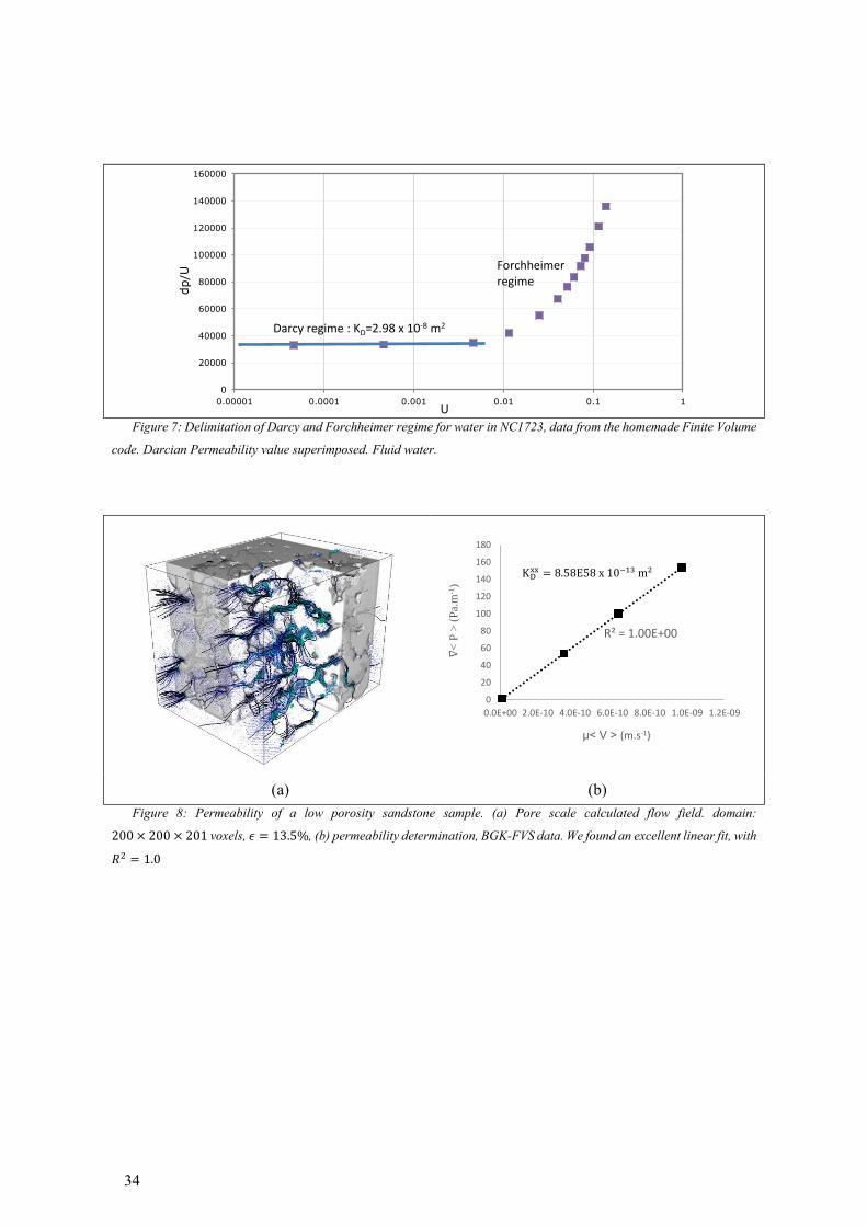
Using BGK-FVS scheme, we found 𝐾𝐷 = 3.03 × 10−8 m2(see figure 6). An excellent agreement is

obtained with both experimental and numerical results. Note that the pressure gradient versus velocity

curve is a perfect line (R2 = 1.00, Figure 6b), as expected for Darcian regime, showing that the viscous

flow is indeed well captured. In literature, the reported permeability (either experimentally or

numerically obtained) is often Forchheimer permeability (see Kumar and Topin, 2017), while the

permeability obtained here is Darcian permeability. It is difficult to assess accurately the bias between

Darcian and Forchheimer permeability, which explains the small differences. However, as the raw data

generated using the in-house Finite Volume code are available, we calculate the Darcian permeability

from original pressure and velocities data in order to obtain a more representative comparison with our

calculations. We obtain 𝐾𝐷 = 2.98 × 10−8 𝑚2 (figure 7). The relative difference for this permeability

and the one obtains with the BGK-FVS method is at about 1.6%, showing an excellent agreement.

18

Applying the methodology described in Section 3 for the determination of the permeability tensor,

we find, the permeability tensor in the basis 𝒘1, 𝒘2, 𝒘3:

𝐷 = (3.32 0 00 3.13 00 0 3.14

) × 10−8 𝑚2. (26)

We have max𝑖,𝑗,𝑖≠𝑗

|𝑤𝑖 ∙ 𝑤𝑗| = 1.86 × 10−13 𝑚2. That means that the principal basis composed of the

eigenvectors is orthogonal, and, the basis orientation is very close to the one of the tomographic images.

As the foam cells come from the bubbles produced during the foaming of the original polymer precursor

that are aligned with the main direction of original bloc (and gravity) this indicates (for this sample) that

the manufacturing process respect this orientation. A careful visual analysis of all our sample sheets has

shown that their faces are nearly parallel to cell alignment.

The values of the eigenvalues and eigenvectors can be found in Table 8. As the diagonal terms of the

tensor 𝜆𝑖 are very close (only 5.7% of relative difference), we can conclude that the NC1723 sample is

only slightly anisotropic. From geometrical point of view this foam is also nearly isotropic and cells are

slightly elongated along one direction only (see. Brun, 2009). The structure of permeability tensor that

exhibit the same trend is clearly governed by the pore characteristic size along its principal axes.

4.3. Low porosity natural media sample

The Fontainebleau sandstone is often used as a benchmark, because of the exceptional quality of the

porosity/permeability relation (27) given by Zinszner et al, 2007.

A µCT image of 5003.voxel – 3x3x3 mm3, spatial resolution 6 𝜇𝑚 – was acquired from a core sample

of porosity 14.5%. After normalization and filtering, the grey-level density 3D image was binarized to

segment pore and solid volume using a threshold set at the minimum between the two peaks of the gray

level histogram (Talon et al, 2006). The binarized sample presents a porosity of 14.1%. The difference

with the core bulk porosity could be attributed to both heterogeneity of the sample (µCT image is only

a small fraction of the core) and bias linked to the thresholding process.

We then use a bloc of side 1.2 𝑚𝑚3 - porosity 13.5%- about 1/8 of the original image, to produce a

2003 cells mesh (figure 8a). The flow problem was solved, and permeability tensor was extracted (see

section 3).

We can compare the permeability values to literature experimental data or correlation. An

experimental law corresponding to a Fontainebleau sandstone is given in (Zinszner, 2007), which is:

log 𝐾𝐷 = 𝑎(log 𝜖)3 + 𝑏(log 𝜖)2 + 𝑐(log 𝜖) + 𝑑, (27)

19

with the parameters values in Table 10. In this expression, the porosity 𝜖 is expressed in percentages

and gives the permeability in 𝑚𝐷. Talon et al, 2006 give the confidence interval of this law

(RMSE=0.31), for porosity 14.5%.

For example, it gives the following experimental permeability, for a porosity of 13.5%, 𝐾𝑒𝑥𝑝 =

5.68 ± 1.76 × 10−13 𝑚2. We have however no information on the flow direction used to create the

power law function. Permeability values associated to the porosity of the sample at different stage of the

analysis have been synthesized in Table 11.

On Figure 9, we compare the permeabilities computed with the BGK-FVS method with the

experimental values given by Talon, (2006). Unfortunately, our method could not be tested against the

other samples that were not available for a more detailed comparison. The calculated values are in good

agreement with experimental one, although these latter are widely spread and exhibit some clear

uncertainties both for porosity and permeability.

4.4. Application to anisotropic tailored media (orthotropic case)

Based on the comparison and validations performed on idealized and real open cell foams of different

porosities, the proposed method gives reliable permeability values. It can thus be very interesting to

obtain permeability tensors on orthotropic foams, as available literature data are very scarce (see Hugo,

2012). Moreover, anisotropic materials could be used to optimize many components or system. For

example, tailoring high permeability in one direction while keeping a slightly lower one in the other

would be very interesting for heat sink design (e.g. electronic cooling applications).

Orthotropic anisotropy of the original foam sample was realized by elongating and compressing

simultaneously in two orthogonal directions by a factor √𝛺 and 1/√𝛺 respectively while the third

direction is kept unaffected to conserve porosity. Some anisotropic Kelvin-like foam samples presenting

circular strut shape are shown in Figure 10, as well as fluid velocity field (sections in the x, y and z-

directions).

The calculations were repeated imposing the flow successively along the three directions to

determine permeability tensors. Results are presented in Figure 11 and Table 12. First, the case where

Ω = 1 is isotropic by construction, meaning that Kxx = Kyy = Kzz. Moreover, also by construction, the

basis composed of the eigenvectors is identical to the one of the computing domains, namely e1, e2,

e3. We have then Kxx = Kw1, Kyy = Kw2, Kzz = Kw3.

The result’s interpretation of the permeability variation as a function of the deformation is complex

as the geometry and the foam angles are varying for each case. It can however be observed that:

20

• for Ω ∈ [1,2], the x-direction permeability increases with elongation deformation, while along the

other two directions (i.e. y and z) the permeability decreases (due to the compression

deformation).

• for Ω ∈ [2,9], the permeabilities along all directions are decreasing. This could come from the

increase of the specific surface area or the effect of struts orientations and cross section

deformation.

These first results validate the use of the BGK-FVS method for this class of problems; a systematic

study of deformation vector on permeability tensor is carried out and will be the object of further

publication.

4.5. Complex real geometries: determination of a wood sample properties

4.5.1. Generation of computing domain from raw images

We obtained the image data from LBNL (Lawrence Berkeley National Laboratory) in the frame of

the ESM effort at NASA, thanks to Francesco Panerai. It is microtomographic images of redwood

sample coming from Mendocino forest, California. The whole sample contains 18003 cells, which

represent a volume of 5.8 mm3 (see raw images on Figure 12a for example). Obviously, there is no

certainty that this particular sample is representative enough to extract properties of the wood as a

material. On the other hand, it could be used to check our INSE solver capability as well as our method

of permeability characterization on a complex medium.

Binarization from direct thresholding on the raw data gives unsatisfactory results, as shown in Figure

12b. We can observe a lot of small isolated white voxels (false solid voxels). These speckles come from

artefact during image acquisition and need to be suppressed to correctly reconstruct the sample

geometry.

We used the iMorph (http://www.imorph.fr/, Brun et al, 2008) software developed at IUSTI, in order

to clean up the data and reconstruct the 3D topology. The first treatment was to apply a median filter,

which suppress the speckle noise, and then we only conserved the connected components, thus

suppressing the free unconnected false solid voxels that are obviously artefacts.

Moreover, as shown in Figure 12a, the images seem mis-oriented compared to the wood apparent

structure. A rotation (50 degrees) around z axis has been applied to align visible structure with basis

directions. We show with Figure 12c an example of cleaned images. One could clearly observe the

suppression of the unwanted voxels.

As it is a recurrent problem in µCT reconstruction, it is interesting to highlight the sensibility of the

porosity value to the threshold level during binarization. We plot the cumulative normed histogram of

the gray level of the sample image (Figure 13). We observe a strong porosity variation (from 85.7% up

21

to 89%) for a 5% variation of the threshold. Choosing the right threshold is tricky (as there is often no

independent comparable porosity data) and this value has a great influence on the resulting mesh.

Eventually, the whole sample computational domain represents 23 billion of unknowns (18003 cells

with four unknowns per cells), which is difficult to solve considering the current available computing

power.

We have therefore chosen to work on subdomain of smaller size and cut three different domain, at

different location of the sample. The first one is a cube of 150 cells edges. As expected, the computing

time is very low (37 minutes on 96 processors). The post-processing is easy. However, this subdomain

is not representative of the sample (it is not a Representative Element Volume, REV).

The second subdomain is a cube of 200 cells edges and is taken at another (non-overlapping) arbitrary

location. The last one is a cube of 600 cells edges that overlaps partially the previous ones, which

represent the third of the original sample along each direction or 1/27 of sample volume; see Table 13

for a general presentation of the samples).

For each subdomain, we study its homogeneity, and determine the permeability tensor to check the

properties at different scale and try to quantify the representative elementary volume size for such

material.

4.5.2. Subdomain 1: 1503 cells

The homogeneity of the subdomain was analyzed first. We extract 2D porosity of 3 planes that were

swept across the entire domain. This operation was realized for 3 perpendicular planes corresponding to

each face of the subdomain. The results are reported on figure 14a, the abscissa is the position of the

plane relative to its original position.

We first note that the porosity variation of the z direction has less amplitude than the other two. This

comes from the fact that the vessels (or pores) are organized by cells that transport the sap in the

hardwoods. They are located longitudinally in the timber and may or may not be juxtaposed. In our

sample, they are oriented in the z direction.

Moreover, we clearly observe, still in Figure 14a, that near the corner of the sample away from the

origin, the porosity is abnormally high. As shown on Figure 15a, this is due to a default in the subdomain

-a big hole- leading to two different structures in the region of interest. The first one has a kind of

regularity in the vessel organization, the other part contains only the hole. Plotting the contour of the

flow in this subdomain confirms (Figure 15b) that the velocity is higher in the region containing the

hole. As this default is a local artefact and not a feature of the whole sample, this first subdomain is

probably not representative of the whole sample.

22

Applying the methodology described before for the determination of the permeability tensor, and for

simplicity rename the 𝒘1, 𝒘2, 𝒘3 basis by x,y,z. The permeability tensor in this basis is then:

𝐷 = (1.43 0 00 6.65 00 0 9.72

) × 10−11 𝑚2, (28)

with the values of the eigenvalues and eigenvectors in Table 14. The anisotropy, as expected, is very

high, with more than 30% difference between the z and y direction, and a ratio superior to six between

the z and x direction. The flow is much easier in the z direction, the one of the vessels. There is however

a significant difference between the x and y direction. This indicates that opening size measured in plane

x-z are smaller than in plane y-z. This is probably linked to the natural growth of the wood

microstructure. These results indicate that we are able to solve INSE equations and extract a permeability

tensor from a complex heterogeneous sample.

4.5.3. Subdomain 2: 2003 cells

The homogeneity of the 200 cells edge’s subdomain was again checked (Figure 14b). We observe

two small special regions, where the porosity is quite low, at around 75%. However, those two regions

are very limited in space compared to the subdomain size (and some similar region were found at other

location in the whole sample). Unlike the previous one, this subdomain is not composed of two regions,

and look way more homogeneous, as a confirmation of the homogeneity study. Moreover, the porosity

along the z axis is quite regular, between 84 and 88 %, which is an expected behavior due to vessels

orientation along z direction (see Figure 16a). We can conclude that this subdomain is probably

representative of the whole sample, at least more representative than the previous one.

Figure 16b -with a different view angle from 16a to show a small hole in the sample- shows iso-

contours of the velocity magnitude field for a pressure gradient (and thus a main flow) imposed along z

direction. These iso-contours are mainly tubular, the flow is similar to Poiseuille flow in parallel tube as

expected from the wood structure. Nevertheless, patterns, characteristic of tube connection, are visible

near the front vertical edge of the view.

Figure 17 shows iso-contours of velocity magnitude for a gradient imposed in transverse direction.

In this case, we lose the tubular behavior of the velocity magnitude, for a more erratic one. The fluid

crosses the sample by passing from one vessel to the other across opening (of smaller dimension than

the vessel) that are not aligned.

We determined the permeability tensor in the x,y,z basis:

𝐷 = (2.22 0 00 3.83 00 0 7.72

) × 10−11 𝑚2, (29)

23

with the values of the eigenvalues and eigenvectors in Table 15. This tensor is slightly different from

previous one. There is nearly a factor two between the z and y direction, and a factor 4 between the z

and x direction. We can still recover the fact that the vessels are oriented in the z direction. We can

conclude that our method captures well the main feature of flow field and relation of permeability tensor

with geometrical feature even for complex situations.

4.5.4. Subdomain 3: 6003 cells

The same analysis was repeated to the biggest subdomain. Figure 14c shows a different porosity

behavior than the previous ones, as the variation around the mean porosity value is clearly lower. The

subdomain 1 and 2 present porosities varying between 73% and 93%. For subdomain 3, the porosity

variation amplitude is nearly 2.5 time lower (82% to 90%). This clearly indicates that the first 2

subdomains are representative of a local zone and not of the whole sample.

The x and y directions present oscillations around the z axis, retrieving again the vessels orientation

in the z direction (see Figure 18a).

We do not observe high porosity peaks; the biggest subdomain is more regular than the smaller ones

(local defaults); in particular it contains no hole. We can conclude that this sample is fairly

homogeneous.

From Figure 18b, we can observe that the flow contour of the velocity magnitude is mainly tubular

as expected, the vessels being oriented in the z direction. We find the permeability tensor is the x,y,z

basis:

𝐷 = (1.44 0 00 4.08 00 0 7.51

) × 10−11 𝑚2, (30)

with the values of the eigenvalues and eigenvectors in Table 16. The anisotropy is comparable to the

previous smaller samples.

4.5.5. Representative Element Volume considerations

The question is then: is the 6003 cells subdomain enough to approximate the permeability of the

whole sample?

First, subdomain 3 is homogeneous, which at first may looks good, but as we have seen before it

does not have holes that the whole sample has. Cutting a smaller part of it should possess the same

"imperfections". Secondly, it is interesting to plot the evolution of the diagonal permeability tensor

elements, namely Kxx, Kyy and Kzz for the samples. From Figure 19, we can observe that the variation for

Kzz and Kyy is less than 10% from subdomain 2 to subdomain 3. Kxx seems to vary, for more than 32%

24

from subdomain 2 to subdomain 3. It is therefore difficult to say if this subdomain size is a reasonable

REV. In order to check the global behavior for the intermediate structures, we generate and analyze a

sample of 3503 voxel cut in the 6003 one. The obtained permeability tensor is similar to those of

subdomain 2 and 3.

To conclude on REV considerations, the whole imaged sample is of about 6 mm edges, while the

diameter of the tree is between 3 to 4.5 meters (average values). Therefore, the permeability values may

be strongly dependent on the sample position.

As the BGK-FVS tools is well adapted to deal with such complex geometry, a detailed and systematic

study will be carried out in order to extract representative properties of the wood using several (i.e.

sampled at different tree position) and bigger (i.e. constituting a “true” REV) samples.

5. Conclusion

We designed a kinetic BGK equation which corresponds to a hyperbolic system. Then, we used a

transport-projection method to approximate the RHS of the designed BGK, enabling to use a moment-

based equation rather than discrete velocities ones. As this method can be seen as a Flux Vector Splitting

one, we analyzed the moment-based equation with the tools of the FVS method, without involving any

kinetic model. The entropy is kept at each step of the formal developments, from the continuous scheme

to the discrete level. Then, the consistency and accuracy of the BGK-FVS method for application to

INSE equations leads to flux/moment derivative conditions. These latter are satisfied by adjusting a free

parameter and eventually allows to obtain second-order accuracy. In other words, we controlled the

known diffusivity of the discrete scheme by adjusting it to the physical viscosity. The stability analysis

is ensured with the entropy, which imposes that the computed moments remain in the stability region of

the open set of admissible moments. Finally, the discrete entropy inequality holds under three different

stability conditions: one coming from the CFL of the time discretization of the hyperbolic system, two

from the stability region: the cell Reynolds number and the sub-characteristic condition. This means that

the grid size must be small enough to satisfy all of them. However, the implementation requires less

memory consumption than a discrete velocities approach, eventually the explicit scheme insure the good

scalability of parallel software implementation.

We have shown that this new numerical scheme is well suited for accurate calculation of pressure

and velocity field and find natural application in determination of macroscopic properties of complex

geometries samples. Current numerical results showed that the new method characterizes precisely the

Darcian permeability tensors, demonstrating its accuracy and robustness, for various porous media, from

high to low porosities, both natural and manufactured media such as wood, soil or metallic foams. Those

3D complex structures may come from either binarized microtomographic images or CAD geometry,

25

which can have small imperfections, leading to meshing difficulties for commercial software. Moreover,

such softwares use numerical schemes that may have difficulties in presence of isolated -closed- pores.

We have seen that the BGK-FVS method does not have these two problems, showing excellent results

in different media. In the present form, our proposed method is limited to intrinsic permeability of

different porous media. The development of inertial effects is currently under development and will be

presented in the near future.

Acknowledgement

We would like to thank Daniela BAUER for sending us the microtomographic images used in (L.

Talon et al, 2006). This work was granted access to the HPC resources of Aix-Marseille Université

financed by the project Equip@Meso (ANR-10-EQPX-29-01).

26

References

Aidun C.K., and Clausen J.R., 2010, “Lattice-Boltzmann Method for Complex Flows”. Annu. Rev.

Fluid 42. DOI: 10.1146/annurev-fluid-121108-145519

Bardos C., Golse F., and Levermore C.D., 1993, “Fluid dynamic limits of kinetic equations-II

Convergence proofs for the Boltzmann-equation”. Comm. Pure Appl. Math. 46, pp. 667-753

Bear J., 1972, Dynamics of Fluids in Porous Media. Dover publications

Bernsdorf J.,2008, “Simulation of complex flows and multi-physics with the lattice-boltzmann method”.

PhD thesis. Amsterdam’s Univerity, p.114, p. 76

Boghosian B. and Levermore C., 1987, “A cellular automaton for Burgers’s equation”. Complex

Systems 1, pp. 17-30

Bonnet J.P., Topin F., and Tadrist L., 2008, “Flow laws in metal foams: compressibility and pore size

effects”. Transport in Porous Media 73 pp. 233-254

Bouchut F., 1999, “Construction of BGK Models with a Family of Kinetic Entropies for a Given System

of Conservation Laws”. Journal of Statistical Physics 95.1-2, pp. 113-170

Bouchut F., Guarguaglini F.R., and Natalini R., 2000, “Diffusive bgk approximations for nonlinear

multidimensional parabolic equations”. Indiana Univ. Math. J. 49, pp. 723-749

Bouchut F., 2002, “Entropy satisfying flux vector splittings and kinetic BGK models”. Numerische

Mathematik 94.4, pp. 623-672

Bouchut F. and Frid H., 2006, “Finite difference schemes with cross derivatives correctors for

multidimensional parabolic systems”. J. Hyp. Diff. Eq. 3, pp. 27-52

Bouchut F., Jobic Y., Natalini R., Occelli R., Pavan V., 2018, “Second-order entropy satisfying BGK-

FVS schemes for incompressible Navier-Stokes equations”. SMAI-Journal of computational

mathematics, 4, p. 1-56, doi: 10.5802/smai-jcm.28

Brun E., Vicente J., Topin F., and Occelli R., 2008, “IMorph: A 3D morphological tool to fully analyse

all kind of cellular materials”. Cellmet08 Dresden, Germany

Brun E., Vincente J., Topin F., Occelli R., and Clifton M.J., 2009, “Microstructure and Transport

Properties of Cellular Materials: Representative Volume Element”. Advanced material Engineering 11,

pp. 805–810

Chen G.Q., Levermore C.D., and Liu T.-P., 1994, “Hyperbolic conservation laws with stiff relaxation

terms and entropy”. Comm. Pure Appl. Math. 47, pp. 787-830

Chikatamarla S. and Karlin I., 2009, “Lattices for the lattice Boltzmann method”. Phys. Rev. E 79, p.

046701

Clague D. S., Kandhai B. D., Zhang R., 2000, “Hydraulic permeability of (un)bounded fibrous media

using the lattice Boltzmann method”. Phys. Rev. E 61, pp. 616–625

27

Darcy H. P. G., 1856, “Exposition et application des principes à suivre et des formules à employer dans

les questions de distribution d'eau. Les fontaines publiques de la ville de Dijon”. Paris, Victor Delmont

Elton B., Levermore C., and Rodrigue G., 1995, “Convergence of convective-diffusive lattice

Boltzmann methods”. SIAM J. Numer. Anal. 32, pp. 1327–1354

Ergun S., 1952, “Fluid flow through packed columns,” Chem. Engineering Progress, vol. 48, pp. 89-94

Liu H., Kang Q., Leonardi C.R., 2015, “Multiphase lattice Boltzmann simulations for porous media

applications”. Computational Geosciences, pp. 1-29

Hugo J-M, 2012, “Transferts dans les milieux cellulaires à forte porosité”. PhD thesis. Université Aix-

Marseille.

d’Humières D., 1992, “Generalized lattice-Boltzmann equations in Rarefied Gas Dynamics: Theory and

Simulations”. AIAA Progress in Astronautics and Astronautics 159, pp. 450-458

d’Humières D., Ginzburg I., Krafczyk M., Lallemand P., and Luo L.S., 2002, “Multiple-relaxation-time

lattice Boltzmann models in three dimensions”. Phil. Trans. Royal Soc. London series A-Math. Phys.

Eng. Sci. 360,pp. 437-451

Inamuro T., Yoshino M., and Ogino F., 1997, “Accuracy of the lattice Boltzmann method for small

Knudsen number with finite Reynolds number”. Phys. Fluids 9, p. 3535

Jin S., Pareschi L., and Toscani G., 1998, “Diffusive relaxation schemes for multiscale discrete-velocity

kinetic equations”. SIAM J. Numer. Anal. 35, pp. 2405-2439

Jobic Y., 2016, “Numerical approach by kinetic methods of transport phenomena in heterogeneous

media”. PhD thesis. Université Aix-Marseille.

Karlin I.V., Gorban A.N., Succi S., and Boffi V., 1998, “Maximum entropy principle for lattice kinetic

equations”. Phys. Rev. Lett. 81, pp. 6–9

Kumar P. and Topin F., 2014, “Micro-structural Impact of Different Strut Shapes and Porosity on

Hydraulic Properties of Kelvin-Like Metal Foams”. Transport in Porous Media 105.57-81

Kumar P, Topin F, 2017, “Predicting pressure drop in open-cell foams by adopting Forchheimer

number”. International Journal of Multiphase Flow 94, 123-136

Krook M., Bhatnagar P.L., Gross E.P., 1954, “A model for collision processes in gases”. Phys. Rev. 94,

p. 511

Lallemand P. and Luo L.S., 2000, “Theory of the lattice Boltzmann method: dispersion, dissipation,

isotropy, Galilean invariance, and stability”. Phys. Rev. E 61, pp. 6546-6562

Levermore D., Bardos C.; Golse F., 1991, “Fluid dynamical limits of kinetic equations, I : Formal

derivation”. J. Statist. Phys. 63, pp. 323-344

McNamara G.R. and Zanetti G., 1988, “Use of the Boltzmann-equation to simulate lattice-gas

automata”. Phys. Rev. Letters 61, pp. 2332-2335

28

Mandal J.C. and Deshpande S.M., 1989, “Higher order accurate kinetic flux vector splitting method for

Euler equations, in Nonlinear Hyperbolic Equations – Theory, Computation Methods, and

Applications”. Notes on Numerical Fluid Mechanics Series 24, pp. 384-392

METFOAM, 2015, international conference on porous media and metallic foams. Barcelona

Narváez A., Zauner T., Raischel F., Hilfer R., and Harting J., 2010, “Quantitative analysis of numerical

estimates for the permeability of porous media from lattice-Boltzmann simulations”. Journal of

Statistical Mechanics: theory and experiment P11026

Natalini R., Carfora M., 2008, “A discrete kinetic approximation for the incompressible Navier-Stokes

equations”. ESAIM: M2AN 42, pp. 93-112

Pullin D.I., 1980, “Direct simulation methods for compressible inviscid idealgas flow”. J. Comput. Phys.

34, pp. 231-244

Renard P., Genty A., and Stauffer F., 2001, “Laboratory determination of the full permeability tensor”.

J. Geophysical Res. 106.B11, pp. 26443-26452

Reitz R.D., 1981, “One-dimensional compressible gas dynamics calculations using the Boltzmann

equations”. J. Comput. Phys. 42, pp. 108-123

Soulaine C., Quintard M., 2014, “On the use of a Darcy–Forchheimer like model for a macro-scale

description of turbulence in porous media and its applicationto structured packings”, International

Journal of Heat and Mass Transfer 74 88–100

Succi S., Foti E., and Higuera F., 1989, “3-dimensional flows in complex geometries with the lattice

Boltzmann method”. Europhys. Letters 10, pp. 433-438

Succi S., 2001, “The lattice Boltzmann equation for fluid dynamics and beyond. Numerical Mathematics

and Scientific Computation”, Oxford Science Publications, the Clarendon Press, Oxford University

Press, New York

Succi S., Karlin I.V., and Chen H., 2002, “Role of the H theorem in lattice Boltzmann hydrodynamic

simulations”. Rev. Mod. Phys. 74, pp. 1203-1220

Talon L., Bauer D., Gland N., Youssef S., Auradou H., and Ginzburg I., 2006, “Assessment of the two

relaxation time Lattice-Boltzmann scheme to simulate Stokes flow in porous media”. Water Resources

Research 48.4

Vicente J., Topin F., Daurelle J-V., and Rigollet F., 2006, “Thermal conductivity of metallic foam:

simulation on real X-ray tomographied porous medium and photothermal experiments”. IHTC13, 13TH

International Heat Transfer Conference, Sydney

Whitaker S., 1986, “Flow in porous media 1: a theoretical derivation of Darcy’s law”. Transport in

Porous Media, vol. 1, pages 3–25

29

Yong W.A. and Luo L.S., 2005, “Nonexistence of H theorem for some lattice Boltzmann models”. J.

Stat. Phys. 121, pp. 91-103

Zinszner B. and Pellerin F.M., 2007, “A geoscientist’s guide to petrophysics”. IFP Publication

30

Figure 1: Block-diagram of the FVS-BGK scheme: A hyperbolic system of conservation laws is solved by a kinetic

method using a BGK operator. The RHS of the designed BGK is approximated by a transport/projection algorithm, which

can be interpreted as a flux vector splitting, enabling a moment-based scheme; the space discretization is done by a Finite

Volume scheme, and the velocity discretization by a fixed set of discrete velocity. Then, after a parabolic rescaling we obtain

the incompressible Euler equation, and diffusion is added by making a controlled numerical diffusion matching the physical

viscosity, solving finally the Navier-Stokes equations. Entropy is conserved at each step, from the continuous scheme to the

discrete level.

Figure 2: Presentation of a node and four struts of a foam sample (left) constant cross section of diameter, 𝑑𝑠 and half strut

length, 𝐿𝑠/2; (center) node to node length, 𝐿𝑁; (right) variable cross section of diameter, 𝑑𝑠,2 at the middle of the ligament and

half strut length 𝐿𝑠*/2.

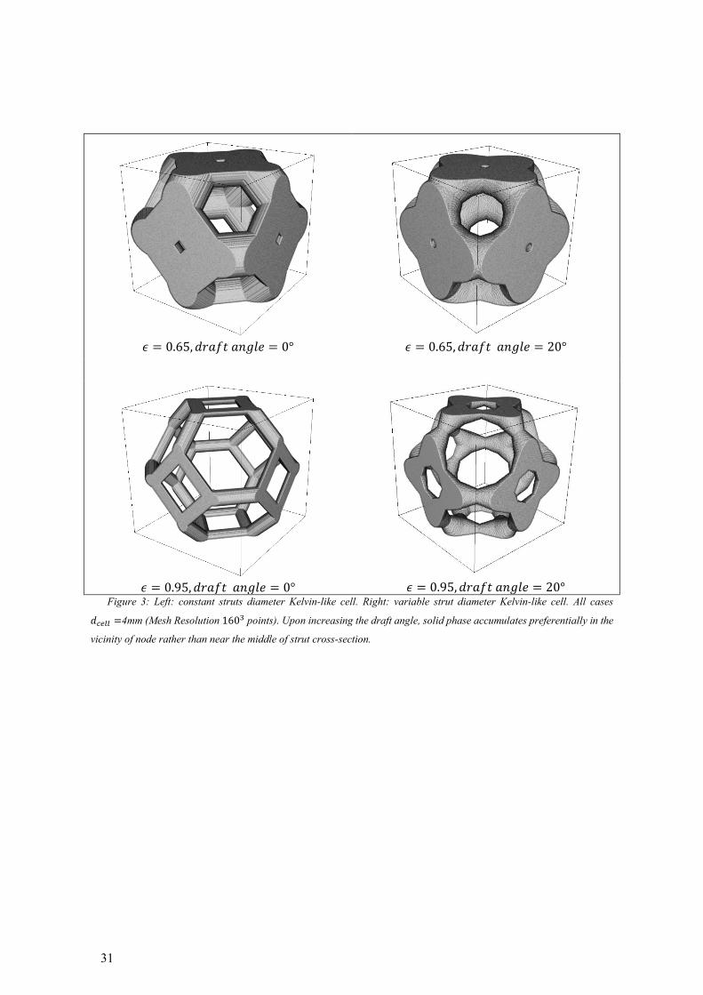
31

𝜖 = 0.65, 𝑑𝑟𝑎𝑓𝑡 𝑎𝑛𝑔𝑙𝑒 = 0°

𝜖 = 0.65, 𝑑𝑟𝑎𝑓𝑡 𝑎𝑛𝑔𝑙𝑒 = 20°

𝜖 = 0.95, 𝑑𝑟𝑎𝑓𝑡 𝑎𝑛𝑔𝑙𝑒 = 0°

𝜖 = 0.95, 𝑑𝑟𝑎𝑓𝑡 𝑎𝑛𝑔𝑙𝑒 = 20°

Figure 3: Left: constant struts diameter Kelvin-like cell. Right: variable strut diameter Kelvin-like cell. All cases

𝑑𝑐𝑒𝑙𝑙 =4mm (Mesh Resolution 1603 points). Upon increasing the draft angle, solid phase accumulates preferentially in the

vicinity of node rather than near the middle of strut cross-section.

32

(a1) (a2) (a3) (a4)

(b1) (b2) (b3) (b4) Figure 4: Velocity field in a cross section perpendicular to main flow axis located at the middle of a unit cell for various

resolutions, from 403 to 3203 voxels, and porosity (𝜖 =0.6 up and 0.95 down)

Figure 5: Validation and comparison of Darcian permeability variations as a function of porosity for a given cell size

(𝑑𝑐𝑒𝑙𝑙 =4mm), with variable and constant strut sections. Note that Ergun formula values are out of range and have been

graphically rescaled in order to compare the shape of the curve with the actual data.

2.00E-09

5.20E-08

1.02E-07

1.52E-07

2.02E-07

2.52E-07

3.02E-07

3.52E-07

4.02E-07

0.5 0.55 0.6 0.65 0.7 0.75 0.8 0.85 0.9 0.95 1

Per

mab

ility

(m

2 )

Porosity

Variable strut: Kinetic

Variable strut: Starccm+

Constant strut: Kinetic

Constant strut: Starccm+

rescaled Ergun

33

Figure 6. Left: 3-D reconstruction and flow field in a NC1723 foam sample (𝜀𝑜 =0.87); Right: Extraction of

permeability by linear regression and comparison with literature.

34

Figure 7: Delimitation of Darcy and Forchheimer regime for water in NC1723, data from the homemade Finite Volume

code. Darcian Permeability value superimposed. Fluid water.

(a) (b)

Figure 8: Permeability of a low porosity sandstone sample. (a) Pore scale calculated flow field. domain:

200 × 200 × 201 voxels, 𝜖 = 13.5%, (b) permeability determination, BGK-FVS data. We found an excellent linear fit, with

𝑅2 = 1.0

0

20000

40000

60000

80000

100000

120000

140000

160000

0.00001 0.0001 0.001 0.01 0.1 1

dp/U

U

Darcy regime : KD=2.98 x 10-8 m2

Forchheimerregime

R² = 1.00E+00

0

20

40

60

80

100

120

140

160

180

0.0E+00 2.0E-10 4.0E-10 6.0E-10 8.0E-10 1.0E-09 1.2E-09

∇<

P >

(P

a.m

-1)

μ< V > (m.s-1)

KDxx = 8.58E58 x 10−13 m2

35

Figure 9: BGK-FVS permeability results compared to experimental data and literature correlation; sandstone sample

of porosity 13.5%

Kxx (FVS-BGK)Kyy (FVS-BGK)Kzz (FVS-BGK)

36

(√1.2, 1,1/√1.2)

(√1.6, 1,1/√1.6)

(√2, 1,1/√2)

(√2.5, 1,1/√2.5)

(√2.75, 1,1/√2.75)

(√3, 1,1/√3)

(√3.5, 1,1/√3.5)

(2,1,1/2)

(√5, 1,1/√5)

(√9, 1,1/√9)

(√3.5, 1,1/√3.5) Figure 10: Kelvin-like samples (circular strut) for various elongations; Pore scale fluid flow result shown on the last

figure (streamlines and velocity magnitude cut off)

37

Figure 11: Permeability tensors diagonal components versus elongation factor Ω. Kelvin like foam sample.

(a) (b) (c) Figure 12: Redwood structure micro-tomographs (a) Raw image (b) Direct thresholding on the raw data-> gives a lot

of false solid voxels (c) Thresholding after a cleaning stage (removal of non-connected components). The remaining small

white voxels are connected to other slices.

0.000E+00

2.000E-08

4.000E-08

6.000E-08

8.000E-08

1.000E-07

1.200E-07

1.400E-07

0 1 2 3 4 5 6 7 8 9 10

Per

mea

bili

ty (

m2 )

Transformation factor Ω

Kxx

Kyy

Kzz

38

Figure 13: Impact of thresholding on porosity: sensibility study. For a threshold variation

of 5%, we obtain a variation of about 2% of porosity in the vicinity of chosen threshold value.

0

10

20

30

40

50

60

70

80

90

100

0 50 100 150 200 250

po

rosi

ty (

%)

grey level

87.7%

79±5%

39

(a)

(b)

(c)

Figure 14: 2D Porosity variations along each direction: (a) subdomain 1(1503 cells). The z

direction has less porosity variation than the other 2, giving the visual result that the wood fibers

are oriented in this direction. (b) subdomain 2 (2003 cells). Some small dense regions appear

(c) subdomain 3 (6003 cells). A more homogeneous distribution is observed.

73

78

83

88

93

0 50 100 150

po

rosi

ty (

%)

position in voxel

X

Y

Z

73

78

83

88

93

0 50 100 150 200

po

rosi

ty (

%)

position in voxel

X

Y

Z

73

78

83

88

93

0 100 200 300 400 500 600

po

rosi

ty (

%)

position in voxel

X

Y

Z

40

(a) (b)

Figure 15: Subdomain 1 (1503 cells). (a) Structure, the wood fibers are oriented up to the z direction. There

is a hole in the structure. (b) Pore scale flow pattern. The image view-angle is different; see the hole in the wood

structure. 3D iso-contours of velocity magnitude. The main flow is in the same direction than the wood fibers.

Pressure difference imposed along z

41

(a) (b)

Figure 16: Subdomain 2 (2003 cells): (a) The wood fibers are oriented up to the z direction. (b) Iso-contours of velocity

magnitude for a different view-angle. The flow presents a tubular aspect as expected from the vessels structure. Pressure

difference imposed along z

42

Figure 17: Subdomain 2. Iso-contours of velocity magnitude for a different

view-angle. The flow presents a rather convoluted path. Pressure difference

imposed along x.

43

(a) (b)

Figure 18: Subdomain 3 (6003 cells). (a) The wood fibers are oriented up to the z direction. (b) Iso-contours of velocity

magnitude for a different view-angle. The flow presents a tubular aspect as expected from the vessels structure. Pressure

difference imposed along z

44

Figure 19: Evolution of the diagonal component of permeability tensor versus the subdomain size.

Kz and Ky show good convergence, whereas Kx seems to vary. Globally a REV size of 2003 voxels

seems acceptable.

1.0E-11

2.0E-11

3.0E-11

4.0E-11

5.0E-11

6.0E-11

7.0E-11

8.0E-11

9.0E-11

1.0E-10

100 200 300 400 500 600 700

per

mea

bili

ty (

m2 )

Edge length (voxels)

Kx

Ky

Kz

45

Table 1: Eigenvalues and eigenvectors for the permeability tensor of the sandstone

sample, direct extraction method without treatment 𝐹𝑇

𝜆1(10−13) 𝒘𝟏 𝜆2(10

−13) 𝒘𝟐 𝜆3(10−13) 𝒘𝟑

9.87

-0.941

7.71

-0.320

0.175

-0.110

-0.163 0.853 0.496

0.175 -0.037 -0.984

Table 2: Eigenvalues and eigenvectors for the permeability tensor of the sandstone

sample, direct extraction method with small gradient cancelation 𝑊𝑆𝐺

𝜆1(10−13) 𝒘𝟏 𝜆2(10

−13) 𝒘𝟐 𝜆3(10−13) 𝒘𝟑

9.87

-0.941

7.71

-0.320

7.43

-0.110

-0.163 0.853 0.496

0.175 -0.037 -0.984

Table 3: Eigenvalues and eigenvectors for the permeability tensor of the sandstone

sample, forced symmetry extraction method 𝑆

𝜆1(10−13) 𝒘𝟏 𝜆2(10

−13) 𝒘𝟐 𝜆3(10−13) 𝒘𝟑

9.92

0.970

7.71

0.202

7.37

0.135

0.227 -0.951 -0.210

0.086 0.234 -0.968

46

Table 4: Morphological parameters of virtual Kelvin-like

foam, circular struts, constant cross-section.

𝜀𝑜(−) 𝑎𝑐 (𝑚−1) 𝑑𝑝 (𝑚𝑚) 𝑑𝑠 (𝑚𝑚)

0.60 982 0.694 1.212

0.65 979 0.822 1.110

0.70 960 0.951 1.006

0.75 926 1.083 0.900

0.80 873 1.223 0.789

0.85 796 1.372 0.669

0.90 686 1.541 0.534

0.95 515 1.749 0.367

Table 5: Morphological parameters of various virtual Kelvin-

like foam with variable cross-section of the struts.

𝜃(°) 𝑑𝑠,2(𝑚𝑚) 𝜀𝑜(−) 𝑎𝑐(𝑚−1) 𝑑𝑝(𝑚𝑚)

2.5 0.7885 0.78 878.7 1.1298

5.0 0.7885 0.76 887.1 1.0786

7.5 0.7885 0.75 899.9 1.0402

10.0 0.7885 0.73 918.0 1.0125

12.5 0.7885 0.71 942.0 0.9940

15.0 0.7885 0.69 973.1 0.9841

17.5 0.7885 0.67 1012.5 0.9823

20.0 0.7885 0.65 1061.7 0.9884

2.5 0.3673 0.94 559.9 1.6297

5.0 0.3673 0.92 599.8 1.5498

7.5 0.3673 0.91 638.5 1.4889

10.0 0.3673 0.89 678.4 1.4443

12.5 0.3673 0.87 721.1 1.4132

15.0 0.3673 0.85 768.4 1.3945

17.5 0.3673 0.83 822.5 1.3875

20.0 0.3673 0.81 885.5 1.3919

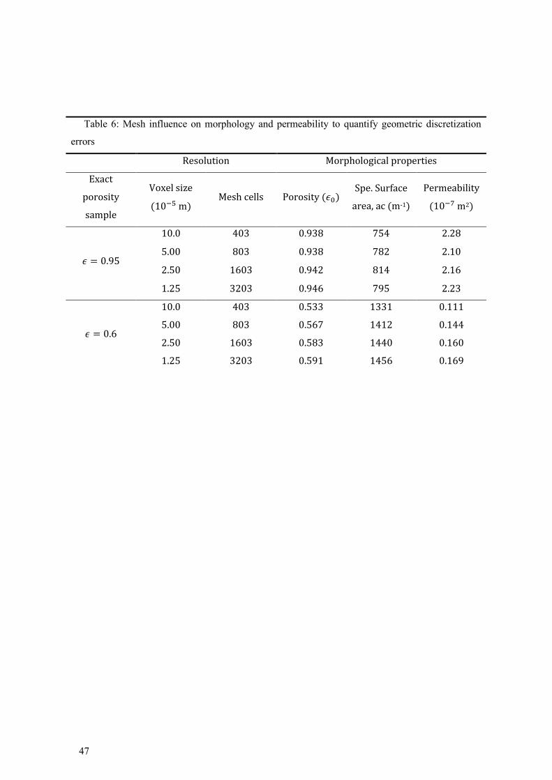
47

Table 6: Mesh influence on morphology and permeability to quantify geometric discretization

errors

Resolution Morphological properties

Exact

porosity

sample

Voxel size

(10−5 m) Mesh cells Porosity (𝜖0)

Spe. Surface

area, ac (m-1)

Permeability

(10−7 m2)

𝜖 = 0.95

10.0 403 0.938 754 2.28

5.00 803 0.938 782 2.10

2.50 1603 0.942 814 2.16

1.25 3203 0.946 795 2.23

𝜖 = 0.6

10.0 403 0.533 1331 0.111

5.00 803 0.567 1412 0.144

2.50 1603 0.583 1440 0.160

1.25 3203 0.591 1456 0.169

48

Table 7: Morphological parameters and permeability values of virtual foam samples (obtained

with the FVS-BGK method).

VFS-BGK StarCCM+

Type of

foams

Porosity, 𝜀𝑜

(−)

Permeability,

𝐾𝐷 (10−8 𝑚2)

Porosity, 𝜀𝑜

(−)

Permeability, 𝐾𝐷

(10−8 𝑚2)

Foam

samples

based on

constant

strut

diameter,

angle 0°

0.631 3.65 0.65 4.26

0.683 4.90 0.7 5.59

0.736 6.50 0.75 7.28

0.786 8.56 0.8 9.52

0.837 11.30 0.85 12.56

0.890 15.50 0.9 17.05

0.943 22.80 0.95 24.79

Foam

samples

based on

variable

strut

diameter,

angle 20°

0.518 1.85

0.564 2.50 0.58 2.42

0.612 3.32

0.660 4.38 0.68 4.98

0.709 5.76 0.73 6.50

0.760 7.63 0.78 8.35

0.815 10.30 0.83 11.95

0.875 14.80 0.89 16.26

Table 8: Eigenvalues and eigenvectors for the permeability tensor of the NC1723

sample

𝜆1(10−8) 𝒘𝟏 𝜆2(10

−8) 𝒘𝟐 𝜆3(10−8) 𝒘𝟑

3.32

-0.944

3.13

0.331

3.14

0

0.331 0.944 -0.001

0 0.001 1

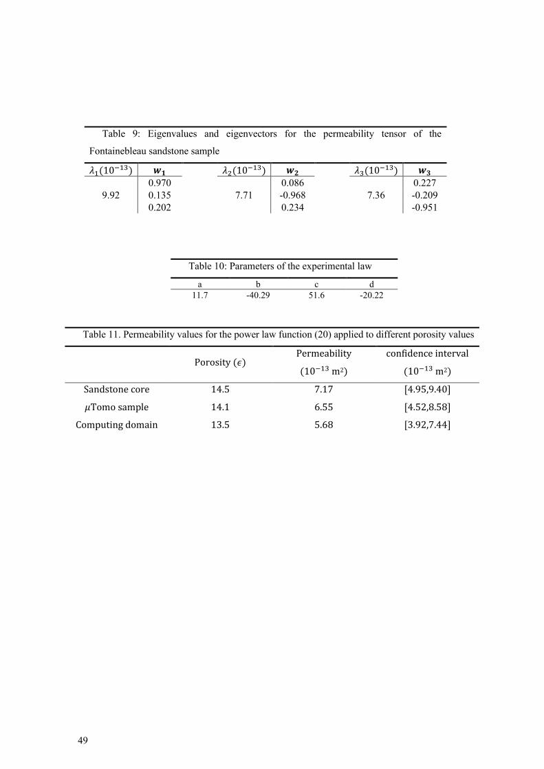
49

Table 9: Eigenvalues and eigenvectors for the permeability tensor of the

Fontainebleau sandstone sample

𝜆1(10−13) 𝒘𝟏 𝜆2(10

−13) 𝒘𝟐 𝜆3(10−13) 𝒘𝟑

9.92

0.970

7.71

0.086

7.36

0.227

0.135 -0.968 -0.209

0.202 0.234 -0.951

Table 10: Parameters of the experimental law

a b c d

11.7 -40.29 51.6 -20.22

Table 11. Permeability values for the power law function (20) applied to different porosity values

Porosity (𝜖) Permeability

(10−13 m2)

confidence interval

(10−13 m2)

Sandstone core 14.5 7.17 [4.95,9.40]

𝜇Tomo sample 14.1 6.55 [4.52,8.58]

Computing domain 13.5 5.68 [3.92,7.44]

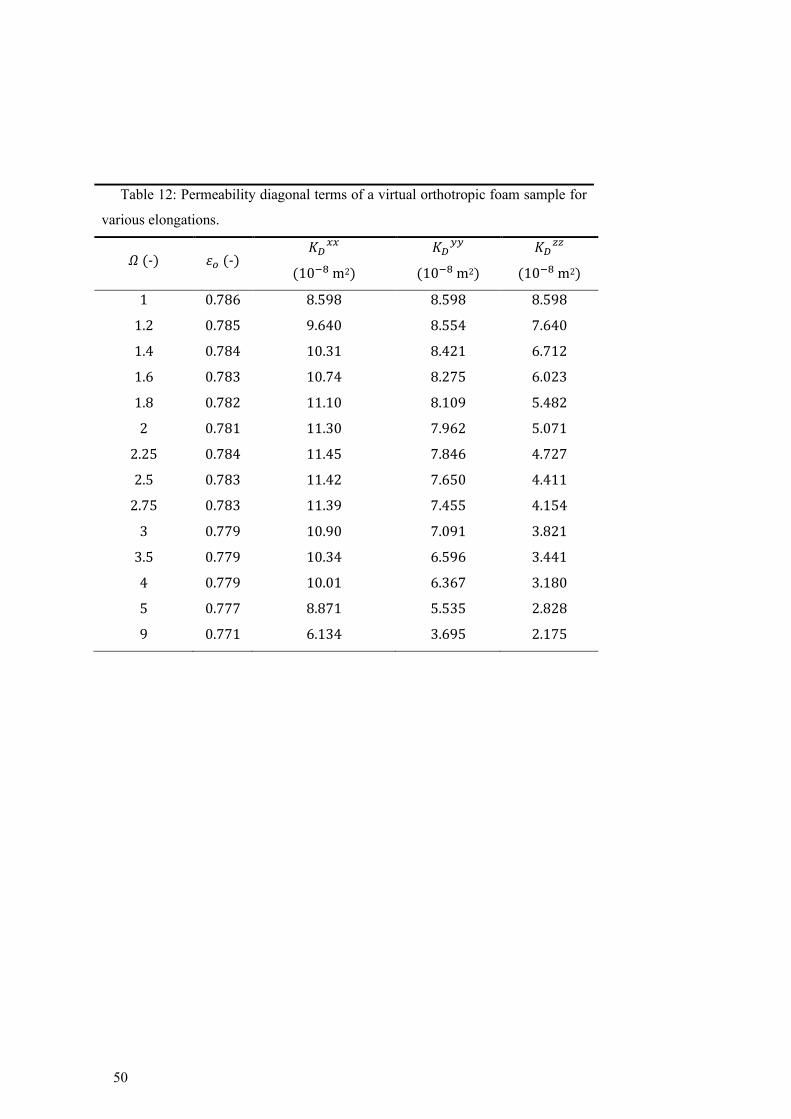
50

Table 12: Permeability diagonal terms of a virtual orthotropic foam sample for

various elongations.

𝛺 (-) 𝜀𝑜 (-) 𝐾𝐷

𝑥𝑥

(10−8 m2)

𝐾𝐷𝑦𝑦

(10−8 m2)

𝐾𝐷𝑧𝑧

(10−8 m2)

1 0.786 8.598 8.598 8.598

1.2 0.785 9.640 8.554 7.640

1.4 0.784 10.31 8.421 6.712

1.6 0.783 10.74 8.275 6.023

1.8 0.782 11.10 8.109 5.482

2 0.781 11.30 7.962 5.071

2.25 0.784 11.45 7.846 4.727

2.5 0.783 11.42 7.650 4.411

2.75 0.783 11.39 7.455 4.154

3 0.779 10.90 7.091 3.821

3.5 0.779 10.34 6.596 3.441

4 0.779 10.01 6.367 3.180

5 0.777 8.871 5.535 2.828

9 0.771 6.134 3.695 2.175

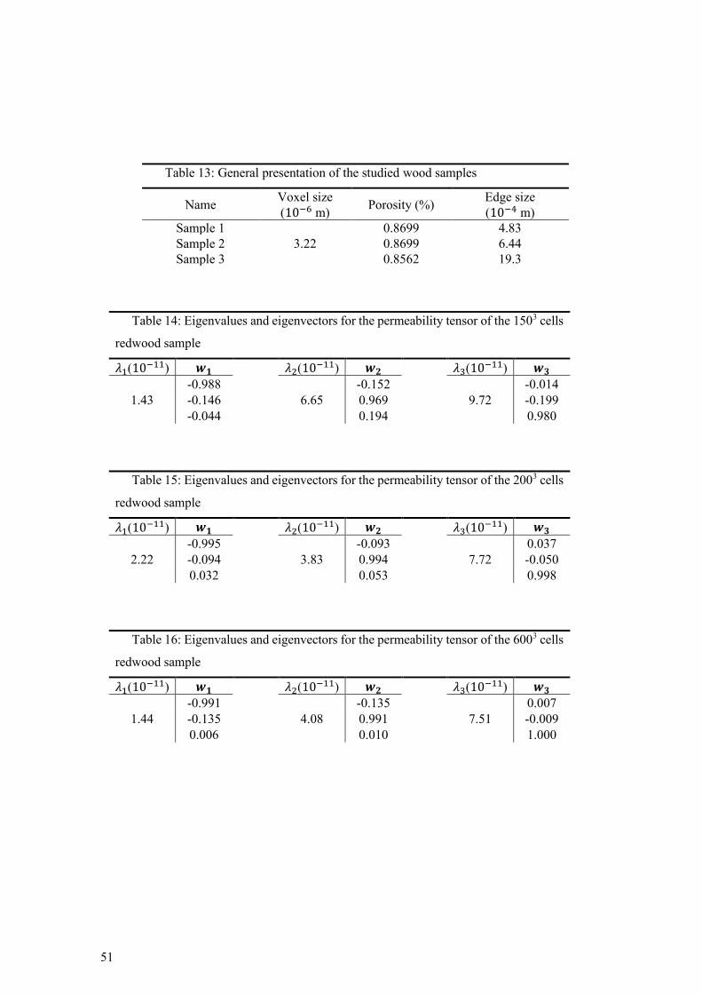
51

Table 13: General presentation of the studied wood samples

Name Voxel size

(10−6 m) Porosity (%)

Edge size

(10−4 m)

Sample 1

3.22

0.8699 4.83

Sample 2 0.8699 6.44

Sample 3 0.8562 19.3

Table 14: Eigenvalues and eigenvectors for the permeability tensor of the 1503 cells

redwood sample

𝜆1(10−11) 𝒘𝟏 𝜆2(10−11) 𝒘𝟐 𝜆3(10−11) 𝒘𝟑

1.43

-0.988

6.65

-0.152

9.72

-0.014

-0.146 0.969 -0.199

-0.044 0.194 0.980

Table 15: Eigenvalues and eigenvectors for the permeability tensor of the 2003 cells

redwood sample

𝜆1(10−11) 𝒘𝟏 𝜆2(10−11) 𝒘𝟐 𝜆3(10−11) 𝒘𝟑

2.22

-0.995

3.83

-0.093

7.72

0.037

-0.094 0.994 -0.050

0.032 0.053 0.998

Table 16: Eigenvalues and eigenvectors for the permeability tensor of the 6003 cells

redwood sample

𝜆1(10−11) 𝒘𝟏 𝜆2(10−11) 𝒘𝟐 𝜆3(10−11) 𝒘𝟑

1.44

-0.991

4.08

-0.135

7.51

0.007

-0.135 0.991 -0.009

0.006 0.010 1.000