determining appropriate loss coefficients for use in the
TRANSCRIPT
Determining appropriate loss coefficients for use in the nozzle-model of a stage-by-stage
turbine model
Prepared By:
Alton Cadle Marx
MRXALT001
Department of Mechanical Engineering
University of Cape Town
Supervisor: Prof. Wim Fuls
January 2019
Submitted to the Department of Mechanical Engineering at the University of Cape Town in partial fulfilment of the academic requirements for a Masters of
Science degree in Mechanical Engineering
Key Words: Turbine loss coefficient, Flownex, Stage-by-stage turbine nozzle-model,
Loss coefficient algorithm
Univers
ity of
Cap
e Tow
n

The copyright of this thesis vests in the author. No quotation from it or information derived from it is to be published without full acknowledgement of the source. The thesis is to be used for private study or non-commercial research purposes only.
Published by the University of Cape Town (UCT) in terms of the non-exclusive license granted to UCT by the author.
Univers
ity of
Cap
e Tow
n

i
Declaration
I, Alton Cadle Marx, know the meaning of plagiarism and declare that all the work in the document,
save for that which is properly acknowledged, is my own. This dissertation has been submitted to the
Turnitin module (or equivalent similarity and originality checking software) and I confirm that my
supervisor has seen my report and any concerns revealed by such have been resolved with my
supervisor.
_______________
Alton Cadle Marx

ii
Abstract
A previously developed turbine modelling methodology, requiring minimal blade passage
information, produced a customizable turbine stage component. This stage-by-stage turbine nozzle-
model component was derived from the synthesis of classical turbine theory and classical nozzle
theory enabling the component to accurately model a turbine stage. Utilizing Flownex, a thermo-
hydraulic network solver, the turbine stage component can be expanded to accurately model any
arrangement and category of turbine.
This project focused on incorporating turbine blade passage geometrical information, as it relates to
the turbine specific loss coefficients, into the turbine stage component to allow for the development
of turbine models capable of predicting turbine performance for various structural changes,
anomalies and operating conditions.
The development of turbine loss coefficient algorithms as they relate to specific blade geometry data
clusters required the investigation of several turbine loss calculation methodologies. A stage-by-stage
turbine nozzle-model incorporating turbine loss coefficient algorithms was developed and validated
against real turbine test cases obtained from literature.
Several turbine models were developed using the loss coefficient governed turbine stage component
illustrating its array of capabilities. The incorporation of the turbine loss coefficient algorithms clearly
illustrates the correlation between turbine performance deviations and changes in specific blade
geometry data clusters.

iii
Acknowledgements
I would like to express my sincere gratitude to the following individuals and organizations:
• The Eskom Power Plant Engineering Institute (EPPEI) program and the UCT ATProM team.
• Everyone who assisted in making this study possible, notably Prof. Pieter Rousseau and my
engineering managers; Joe Roy-Aikins and Kapil Sukhnandan.
• My industrial mentor, Gary de Klerk, for his guidance that lead me towards my post-graduate
studies.
• My wife, Candice Marx, for her endless love, encouragement and willingness to proofread
engineering jargon.
• My supervisor, Prof. Wim Fuls, without who’s outstanding professional guidance, continuous
patience and enthusiastic discussions, this study would not be possible.
• My late grandfather, Brian Samuel, Weil ich dir so viel verdanke.
iv
Table of Contents
Declaration .............................................................................................................................................. i
Abstract .................................................................................................................................................. ii
Acknowledgements ............................................................................................................................... iii
List of Figures ........................................................................................................................................ vi
List of Tables ......................................................................................................................................... ix
List of Nomenclature .............................................................................................................................. x
Chapter 1 Introduction .......................................................................................................................... 1
1.1 Background ................................................................................................................................... 1
1.2 Research objectives and limitations ............................................................................................ 2
1.3 Dissertation outline ...................................................................................................................... 3
Chapter 2 Literature Review .................................................................................................................. 4
2.1 Turbine fundamentals .................................................................................................................. 4
Turbine classification considerations .................................................................................... 5
Turbine blade design nomenclature ................................................................................... 10
Impulse and reaction turbines ............................................................................................ 13
2.2 Turbine performance ................................................................................................................. 15
Turbine performance visualization ..................................................................................... 15
Turbine loss coefficients ..................................................................................................... 17
Loss coefficient methodology selection ............................................................................. 20
Carry-over and reheat analysis ........................................................................................... 23
2.3 Nozzle-model review .................................................................................................................. 25
Turbine modelling methods ................................................................................................ 25
Flownex network solver overview ...................................................................................... 27
The Stage-by-stage nozzle model overview ....................................................................... 29
2.4 Case study data classification ..................................................................................................... 32

v
Chapter 3 Research Methodology ....................................................................................................... 33
3.1 Nozzle model adaptation methodology ..................................................................................... 33
3.2 Loss coefficient input variables .................................................................................................. 34
3.3 Loss coefficient algorithms ......................................................................................................... 36
Primary profile loss ............................................................................................................. 36
Secondary Loss .................................................................................................................... 42
Fan Loss ............................................................................................................................... 45
Tip Leakage Loss .................................................................................................................. 46
Moisture Losses .................................................................................................................. 49
LSB Losses ........................................................................................................................... 50
3.4 Off-design loss coefficient algorithm ......................................................................................... 51
3.5 Loss coefficient output variables ............................................................................................... 55
Chapter 4 Algorithm Validation: AGARD Test Case ............................................................................. 57
Chapter 5 Design and Off-Design Evaluation ....................................................................................... 62
5.1 Steam turbine model.................................................................................................................. 62
5.2 Off-Design impact assessment ................................................................................................... 69
Chapter 6 Turbine Blade Design Impact .............................................................................................. 73
6.1 Blade profile design upgrade ..................................................................................................... 73
6.2 Turbine blade degradation ......................................................................................................... 76
6.3 Turbine blade shrouding variation ............................................................................................. 79
6.4 LSB interconnection impact ....................................................................................................... 81
Chapter 7 Conclusion & Recommendation ......................................................................................... 84
7.1 Conclusion .................................................................................................................................. 84
7.2 Recommendation ....................................................................................................................... 86
References ........................................................................................................................................... 87
Appendix A: Experimental Data ........................................................................................................... 91
Appendix B: Abbreviated Loss Coefficient Algorithms ........................................................................ 98
Appendix C: Ethics in Research Assessment ...................................................................................... 106

vi
List of Figures
Figure 2-1: Coal-fired Power Station Illustration - Adapted from [3] .................................................... 4
Figure 2-2: HP Steam Turbine Cross Section - Adapted from [6] .......................................................... 5
Figure 2-3: HP ST Cascade Sizing Indication - Adapted from [6] ........................................................... 7
Figure 2-4: LP ST Cascade Sizing Indication - Adapted from [6] ............................................................ 7
Figure 2-5: HP/IP/LP Steam Turbine Layout - Adapted from [6] ........................................................... 9
Figure 2-6: Turbine Cross-Section Geometry Indication ..................................................................... 10
Figure 2-7: Turbine Blade Cross-Section Geometry Indication ........................................................... 11
Figure 2-8: Turbine Blade Profile Design Guide - Adapted from [15] .................................................. 11
Figure 2-9: Blade Profile Parameters Identification Process ............................................................... 12
Figure 2-10: Impulse and Reaction Turbine Comparison – Adapted from [11] .................................. 13
Figure 2-11: Impulse Turbine Velocity Triangle Diagram – Adapted from [18] .................................. 13
Figure 2-12: Reaction Turbine Velocity Triangle Diagram– Adapted from [19] .................................. 14
Figure 2-13: Two Turbine Stages Enthalpy-Entropy Diagram .............................................................. 16
Figure 2-14: Turbine Loss Indication [13] ............................................................................................ 17
Figure 2-15: 5 Multistage Turbine Carry-over and Reheat Factor Visualization – Adapted from [37] 23
Figure 2-16: Carry-Over Indication ...................................................................................................... 24
Figure 2-17: Fluid Flow Conditions ...................................................................................................... 26
Figure 2-18: 1D, 2D & 3D Modelling - Adapted from [19], [41]& [42] respectively ........................... 26
Figure 2-19: Stage-by-stage Nozzle-model Custom Compound Components [1] ............................... 27
Figure 2-20: Stage-by-stage Nozzle-model Component [1] ................................................................ 29
Figure 2-21: Moving Nozzle Analogy - Adapted from [1] .................................................................... 29
Figure 3-1: Stage-by-stage nozzle-model with Loss Coefficient Algorithm Implemented .................. 33
Figure 3-2: Loss Coefficient Algorithm Script Architecture ................................................................. 33
Figure 3-3: Stator Fluid Properties Input Variables ............................................................................. 34
Figure 3-4: Stator Profile Blade Geometry Input Variables ................................................................. 35
Figure 3-5: Traupel's profile loss chart [29] ......................................................................................... 37

vii
Figure 3-6: Mach number correction factor chart [29] ....................................................................... 37
Figure 3-7: Reynolds number correction factor chart [29] .................................................................. 38
Figure 3-8: Reynolds Correction Curve for Re<2∙105 ........................................................................... 39
Figure 3-9: Reynolds Correction Curve for Re>2∙105 ........................................................................... 39
Figure 3-10: Trailing edge area illustration – Adapted from [29] ........................................................ 41
Figure 3-11: Trailing Edge loss diagram [29] ........................................................................................ 41
Figure 3-12: Flow correction factor chart – Adapted from [29] .......................................................... 43
Figure 3-13: Fan loss chart [29]............................................................................................................ 45
Figure 3-14: Unshrouded Correction Coefficient Chart ....................................................................... 47
Figure 3-15: Blade Shroud Seal Designs – Adapted from [11] ............................................................. 48
Figure 3-16: Single stage model utilizing Flownex’s labyrinth seal component [1] ............................ 48
Figure 3-17: Moisture Loss to Pressure Ratio ...................................................................................... 49
Figure 3-18: LSB Interconnection Geometry – Adapted from [29] ..................................................... 50
Figure 3-19: Rotor and Stator Inlet Angle Orientation ........................................................................ 52
Figure 3-20: Cascade coefficient reference guide – Adapted from [24] ............................................. 53
Figure 3-21: Off-design Turbine Stator Inlet Angle Triangles .............................................................. 54
Figure 3-22: Loss Coefficient Algorithm Results Display...................................................................... 55
Figure 3-23: Loss Coefficient Algorithm Output Display ...................................................................... 56
Figure 4-1: AGARD 4-Stage Turbine Cross-section View [45] .............................................................. 57
Figure 4-2: AGARD Flownex Model Layout .......................................................................................... 58
Figure 4-3: AGARD Total & Static Pressure Comparison ..................................................................... 59
Figure 4-4: AGARD Turbine Loss Distribution ...................................................................................... 61
Figure 5-1: LP Turbine Cross-Section - Adapted from [6] .................................................................... 62
Figure 5-2: LPST Flownex Model Layout .............................................................................................. 63
Figure 5-3: Full Load LPST Total Pressure Comparison ........................................................................ 65
Figure 5-4: Overall Full Load LPST Loss Distribution ............................................................................ 65
Figure 5-5: LPST Stage 3B & 4B Loss Comparison ................................................................................ 66
Figure 5-6: Full & Partial Load Section B Loss Distribution Comparison ............................................. 68

viii
Figure 5-7: Cascade Coefficient Determination Example .................................................................... 70
Figure 5-8: Full & Partial Load Work Per Stage Comparison ............................................................... 71
Figure 5-9: LPST Rotors Inlet Angles ................................................................................................... 72
Figure 6-1: Single Stage LCNM ............................................................................................................. 73
Figure 6-2: Turbine Blade Profile Improvement Example ................................................................... 73
Figure 6-3: Blade Geometry Cluster - Turbine Losses Correlation ...................................................... 75
Figure 6-4: Blade Geometry Cluster - Turbine Losses Correlation ...................................................... 75
Figure 6-5: Blade Degradation Illustration - Adapted from [13] ......................................................... 76
Figure 6-6: Blade Geometry Cluster - Turbine Losses Correlation ...................................................... 78
Figure 6-7: Blade Degradation Loss Comparison ................................................................................. 78
Figure 6-8: Shrouded and Unshrouded Blade – Adapted from [13] ................................................... 79
Figure 6-9: Shrouded and Unshrouded Blade Loss Distribution ......................................................... 80
Figure 6-10: LSB Interconnection Types - Adapted from [13] ............................................................. 81
Figure 6-11: LSB Interconnection Turbine Losses Distribution ............................................................ 83

ix
List of Tables
Table 2-1: Specific Heat Ratio Values [7] ............................................................................................... 6
Table 2-2: HP/IP/LP Comparison – Adapted from [13] .......................................................................... 9
Table 2-3: Loss Coefficient Comparison - Adapted from [27] ............................................................. 22
Table 2-4: Flownex Component Classification – Images Adapted from [43] ...................................... 28
Table 2-5: Turbine performance data categories ................................................................................ 32
Table 3-1: LSB Interconnection Drag Coefficient ................................................................................. 51
Table 4-1: AGARD Pressure Result Comparison .................................................................................. 59
Table 4-2: AGARD Temperature Result Comparison ........................................................................... 60
Table 4-3: AGARD Turbine Loss Performance Data ............................................................................. 60
Table 5-1: LPST Full Load Result Comparison ...................................................................................... 64
Table 5-2: Full Load LPST Section B Loss Performance Data ............................................................. 65
Table 5-3: 60% Partial Load LPST Result Comparison ......................................................................... 67
Table 5-4: 60% Partial Load LPST Section B Loss Performance Data .................................................. 67
Table 5-5: Off-design Total Pressure & Temperature Comparison ..................................................... 70
Table 5-6: Off-design LSB Comparison ................................................................................................. 71
Table 6-1: Blade Upgrade Performance Comparison .......................................................................... 74
Table 6-2: Blade Upgrade Performance Data ...................................................................................... 75
Table 6-3: Blade Fouling Degradation Performance Data ................................................................... 77
Table 6-4: Blade Erosion Degradation Performance Data ................................................................... 77
Table 6-5: Shrouded and Unshrouded Blade Performance Data ........................................................ 80
Table 6-6: LSB Interconnection Performance Data ............................................................................. 82

x
List of Nomenclature
General Symbols h Enthalpy kJ/kg
s Entropy kJ/kg∙K
ρ Density kg/m3
μ Dynamic Viscosity kg/ms
p Pressure MPa, kPa
cp Specific Heat at Constant Pressure kJ/kg∙K
cv Specific Heat at Constant Volume kJ/kg∙K
ks Surface Finish mm
u Blade Speed, Turbine Rotational Speed m/s, rpm
T Temperature ˚C / K
V Volume m3
v Working Fluid Velocity m/s
Δv Difference in Working Fluid Velocities m/s
w Work MW, kW
Subscripts co Carry-over
s Ideal, Isentropic
0,1, 2, 3… Position Indication
r Relative
Stg Stage
x, y, z Turbine Stage Indication
Superscripts
’ Stator Blade Row / Fixed Blades / Nozzles
’’ Rotor Blade Row / Moving Blades / Buckets
Dimensionless Parameters kco Carry-over ratio
xDf Dryness Fraction
ζ Enthalpy Loss Coefficient
η Efficiency %
Ma Mach Number
nBld Number of Blades per Row
N Number of Stages
CD Restrictor Contraction Coefficient
CL Restrictor Loss Coefficient
Y Pressure Loss Coefficient

xi
Dimensionless Parameters Continued
R Degree of Reaction %
Re Reynolds Number
RF Reheat Factor
k Specific Heat Ratio
cw Change in Flow Velocity Ratio
Blade Geometry Symbols Dm Mean diameter m, mm
Dn Hub diameter m, mm
Ds Tip diameter m, mm
l Blade height m, mm
υ Blade diameter hub to tip ratio
SWdth Blade width m, mm
Schrd Blade chord length m, mm
δgap Blade row gap width m, mm
δBld Maximum blade thickness m, mm
δTe Trailing edge thickness m, mm
O Throat width m, mm
τ Blade tip clearance m, mm
ω Shrouded tip leakage mass flow ratio
ϒ Shrouded tip leakage velocity ratio
φ Unshrouded tip leakage mass flow ratio
Kτ Unshrouded correction coefficient
DLSB Last Stage Blade interconnection diameter m, mm
lLSB Last Stage Blade interconnection length m, mm
dLSB Last Stage Blade interconnection thickness m, mm
wLSB Last Stage Blade interconnection width m, mm
fhcc
Height of the curvature of the camberline m, mm
CLine Camberline m, mm
Angles
α0 Inlet Angle ˚
α1 Outlet Angle ˚
αInc Incidence angle ˚
βs Blade stagger angle ˚
Areas
ABldGap Blade spacing area m2
AFlow Overall flow area m2

xii
Abbreviations AGARD The Advisory Group for Aerospace Research and Development
AT Acceptance Test
GT Gas Turbine
HBD Heat Balance Diagram
HP High Pressure Turbine
IP Intermediate Pressure Turbine
LSB Last Stage Blade
LP Low Pressure Turbine
LS Live Steam
LTA Life Time Assessment
RHS Reheat Steam
rpm Revolution per Minute
ST Steam Turbine
Introduction 1
Chapter 1 Introduction
1.1 Background
Power production performance modelling and simulations have become a vital everyday component
of the energy engineering sector. The evaluation of seemingly unrelated performance variations of
power plant components as they relate to distant structural anomalies has become common
practice. This has been made possible by the tedious evolution from the complex hand calculation
performed in the past to the present spectrum of computerized applications that has many shapes,
structures and formats.
Turbine performance modelling plays a key role in power production performance evaluations.
Although turbines very simply put only convert energy from one format to another the modelling
thereof is a slightly more complex matter. For this reason, many methodologies exist to accurately
model turbines. A dominant theme throughout literature is the determination and prediction of
turbine efficiency and loss quantification.
Combining turbine performance modelling with plant operation data and turbine specific design
information it becomes possible to identify location specific anomalies and suggest improvements to
affected turbine sectors. This, in turn, could inform maintenance procedures, assist in accurate
lifetime assessments (LTA) of steam path components (such as blading, seals and diaphragms) and
thus benefit overall turbine operation and performance.
Small anomalies can contribute to significant performance losses and develop into more severe
problems that can affect the lifespan of components and the entire turbine. Evaluating performance
consistency across the stages of a turbine allows for the isolation of specific problem areas within the
turbine.
This study builds upon a previously developed turbine modelling methodology, requiring minimal
blade passage information, that produced a customizable turbine stage component [1]. This stage-
by-stage turbine nozzle-model component was derived from the synthesis of classical turbine theory
and classical nozzle theory enabling the component to accurately model a turbine stage. Utilizing
Flownex, a thermo-hydraulic network solver, the turbine stage component can be applied to
accurately model any arrangement and category of an axial turbine.
This study aims to incorporate additional turbine blade passage geometrical information, as it relates
to the turbine specific loss coefficients, into the turbine stage component. This inclusion will allow
for the development of turbine models capable of predicting turbine performance for various
structural changes, anomalies and operating conditions, without requiring assumptions or
calibrations of the loss coefficient.

Introduction 2
1.2 Research objectives and limitations
A need was identified for the investigation and determination of the most beneficial loss coefficient
sets that would provide the greatest possible advance to the existing stage-by-stage turbine nozzle-
model component [1]. For this reason, this study is focused on the development of turbine loss
coefficient algorithms, as they relate to specific blade geometry data clusters, whilst maintaining a
minimal geometric data input requirement.
Listed below are key approach orientated objectives that define the backbone of the study:
• Investigation of turbine loss methodologies.
• Determine appropriate loss coefficients for design conditions.
• Determine the best loss coefficient or correction factor for off-design conditions.
• Investigate the implementation possibility of Carry-over and Reheat factor.
• Develop a comprehensive loss coefficient calculation algorithm.
• Implement algorithms into the nozzle-model and test model’s structural soundness.
• Construct a case study model in Flownex for validation and verification purposes
• Construct a case study model of an existing operational steam turbine to illustrate modelling
ability for both design and off-design conditions.
• Utilizing a developed steam turbine model, display the ability to predict offset performance
conditions resulting from turbine component variance.
• Demonstrate how the new loss coefficients can help to quantify the impact of design and
operational variation on the overall turbine performance.
• Develop a practical user-friendly interface and listing procedure for the loss coefficient algorithm
script architecture in the nozzle model.
The greatest impediment for the study was the availability of sensitive design information. Due to
the intellectual property rights that govern the majority of the turbine design and manufacturing
sector, obtaining information has been limited. This limiting factor restricts the extent and range of
the validation and testing of the loss coefficient algorithms. Unfortunately, while some data have
been obtained, the source and some specifics may not be disclosed.
Additionally, this study only extends to axial flow gaseous turbines: air, steam.
Introduction 3
1.3 Dissertation outline
This dissertation is comprised of a further eight chapters consisting of the following content:
Chapter 2: Literature Review
Establishes an overview of turbine fundamentals, designs and performance modelling as to orient
the reader to the general focus area of this study. This is followed by an in-depth review of key focus
areas, notably carry-over and reheat factor, turbine loss coefficients and turbine blade design.
Chapter 3: Research Methodology
Builds on the focus areas discussed in Chapter 2 by analysing how all the various components fit
together, before providing a numerical evaluation required for the development of the loss
coefficient algorithm. The implementation of the loss coefficient algorithm into the stage-by-stage
turbine nozzle-model component completes the chapter.
Chapter 4: Algorithm Validation
Acts as a validation case study that compares the published AGARD air turbine test case, utilizing the
loss coefficient algorithms, against comparable turbine models and the original turbine test case
measurements.
Chapter 5: Design and Off-Design Evaluation
Evaluates the ability of the stage-by-stage turbine nozzle-model component, governed by turbine
loss coefficient algorithms, to model an actual steam turbine. The case study compares the
performance of the turbine model against the actual turbine for both design and off-design
conditions.
Chapter 6: Turbine Blade Design Deviation Impact
Investigates the information that can be obtained for a single turbine stage model with focus placed
on specific turbine blade geometry data clusters as they relate to turbine loss coefficients. Four
different case study are evaluated: Blade profile design improvement, Blade profile degradation,
Blade shrouding variations and LSB Interconnection impact.
Each case study examines the impact that deviating from an original blade design has on stage
performance.
Chapter 7: Conclusion & Recommendation
This chapter concludes the dissertation, drawing together significant findings, performance
correlations, model features and capabilities made possible by the turbine loss coefficient algorithm
implementation. Recommendations for further investigation completes the chapter.
Literature Review 4
Chapter 2 Literature Review
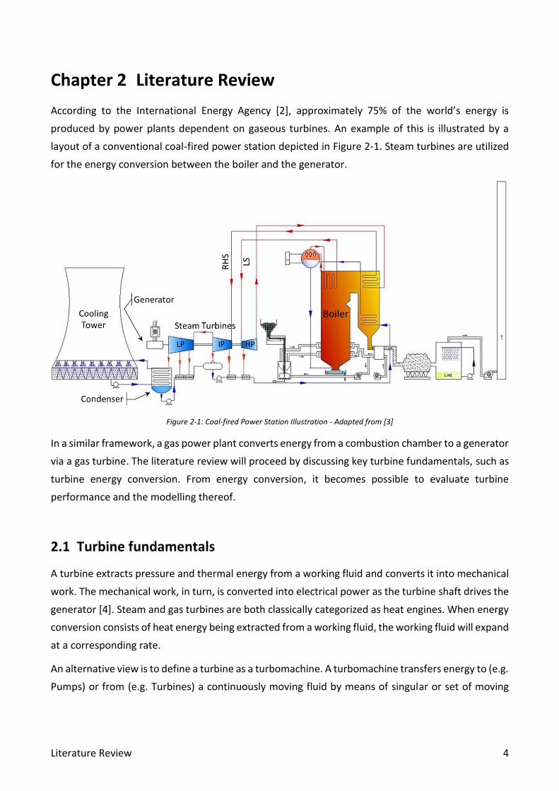
According to the International Energy Agency [2], approximately 75% of the world’s energy is
produced by power plants dependent on gaseous turbines. An example of this is illustrated by a
layout of a conventional coal-fired power station depicted in Figure 2-1. Steam turbines are utilized
for the energy conversion between the boiler and the generator.
Figure 2-1: Coal-fired Power Station Illustration - Adapted from [3]
In a similar framework, a gas power plant converts energy from a combustion chamber to a generator
via a gas turbine. The literature review will proceed by discussing key turbine fundamentals, such as
turbine energy conversion. From energy conversion, it becomes possible to evaluate turbine
performance and the modelling thereof.
2.1 Turbine fundamentals
A turbine extracts pressure and thermal energy from a working fluid and converts it into mechanical
work. The mechanical work, in turn, is converted into electrical power as the turbine shaft drives the
generator [4]. Steam and gas turbines are both classically categorized as heat engines. When energy
conversion consists of heat energy being extracted from a working fluid, the working fluid will expand
at a corresponding rate.
An alternative view is to define a turbine as a turbomachine. A turbomachine transfers energy to (e.g.
Pumps) or from (e.g. Turbines) a continuously moving fluid by means of singular or set of moving

Literature Review 5
blade rows. For turbines the moving blade rows are defined as a rotor assembly, consisting of a shaft
with blades intricately connected to each other and the shaft.
In addition to the rotor assembly gas, steam and hydro turbines consist of a stator assembly, that
constricts and guides the working fluid. The stator assembly consists of a casing with stationary blade
rows intricately connected [5]. The combination of both stator and rotor set is termed a turbine stage.
Figure 2-2 presents a cross-section drawing of a modern turbine rotor and stator assembly.
Figure 2-2: HP Steam Turbine Cross Section - Adapted from [6]
Several design conditions and physical parameters dictate the complexity of turbine design. For this
reason, it is important to understand how energy is converted in turbines and how to define turbine
classifications.
Turbine classification considerations
Turbine cascade development is a vital design consideration. As the working fluid enters the turbine
(from a boiler or a combustion chamber) it consists of high pressure and temperature at a given mass
flow rate. The working fluid then passes through a turbine stage causing the working fluid to expand.
This expansion must be accommodated for in the turbine design. For each stage, the working fluid
expands at a ratio defined by the specific volume condition.
As the pressure decrease, the volume will increase and vice versa. For most cases, it can be assumed
that gaseous working fluids in turbines hold to polytropic expansion during operation [7]. Thus,
holding to the gas law stated in equation [2.1.1].
1 1 2 2
k kp V p V = [2.1.1]

Literature Review 6
The value of the specific heat ratio (k) is determined as an isentropic ideal gas relation for both gas
and steam turbines. Equation [2.1.2] defines the isentropic condition in terms of the specific heat at
constant pressure (cp) and constant volume (cv).
p
v
ck
c= [2.1.2]
For steam turbines specifically there exists low-pressure operating conditions where the steam
moves across the vapour line requiring a unique calculation, this is accomplished with Zeuner’s
relation [2.1.3]. This relation utilizes the initial dryness fraction value (xDf) of the steam. During the
occurrence of this phase change in the steam there exist a unique phenomenon namely
supersaturation that will be discussed in section 3.3 .
(1.035 )10
Dfxk = + [2.1.3]
Table 2-1 provides values of specific heat ratio for steam and gas turbines under different physical
conditions. The specific heat ratio plays a significant role in both turbine design and performance
analysis.
Table 2-1: Specific Heat Ratio Values [7]
Working Fluid Specific Heat Ratio (k)
Air1 1.4
Most Combustion Gasses 1.333
Superheated Steam 1.3
Saturated Steam 1.135
Wet Steam See equation [2.1.3]
The rate of expansion, on the other hand, has several input considerations (e.g. bleed points or
reheats) but is always driven by the fixed mass flow rate that must move through the turbine. The
increase in volume per stage requires longer blading and hence a larger casing diameter.
1 The Specific heat ratio (k) of Air is 1.4 for moderate temperature. Slight changes in the specific heat ratio of
Air occur with changes in temperature.

Literature Review 7
This sizing increase per stage for a high-pressure steam turbine in comparison with a low-pressure
steam turbine section is displayed in Figure 2-3 and Figure 2-4 respectively.
Figure 2-3: HP ST Cascade Sizing Indication - Adapted from [6]
Figure 2-4: LP ST Cascade Sizing Indication - Adapted from [6]
The number of stages (N) of a turbine can be determined as the ratio of total enthalpy drop (ΔhTotal(ss))
across a turbine compared to the desired average ideal enthalpy drop of a single stage (hDesign(s)).
( )
( )
Total ss
Design s
hN
h
= [2.1.4]
Equation [2.1.4] assumes an identical design enthalpy drop across all stages of a turbine. When
calculating the number of stages as a design step the value is rounded down if the cost was the
primary criteria whilst rounding up if efficiency is more important [8]. The enthalpy drop of a stage
indicates the loading per stage. Some other design considerations may result in an un-even stage
loading as is found especially in low-pressure turbines.
Notably, the reheat factor, discussed in section 2.2.4 could be used by turbine designers for turbine
stage loading design evaluation [9].

Literature Review 8
Thermal expansion must be mentioned as a design consideration for turbine cascade development.
As metals expand when heated so will turbine cylinders and rotors. Turbine thermal expansion
predominately occurs during the start-up operational phases of a turbine. The thermal expansion
generated from the heat exchange between the working fluid and the composition materials of a
turbine will induce metal stresses. These stresses related to the turbine operational lifetime
expectancy design consideration [10].
The laws of linear expansion state that for a given rise in temperature, the larger the original size of
metal, the greater its expansion [11]. The following linear thermal expansions are defined for turbine
design:
▪ Differential expansions: the difference in expansion between the rotor and the stator.
▪ Relative expansion: the rate of expansion between the rotor and the stator of the turbine.
▪ Absolute expansion: This is the total expansion of the turbine shaft and casing trains from the
fixation point(s).
Differential expansion must be carefully controlled during the operation of turbines. During turbine
warming, the rotor will heat faster than the turbine casing due to the differences in their respective
physical design parameters. The clearance between the stator and rotor turbine blades are very
small to minimize losses. Hence precautions must be taken to prevent contact [12].
Thermodynamic design considerations alone do not account for the mechanical integrity of turbine
design. Mechanical reliability and safety design considerations must be implemented alongside all
other design factors such as thermal, performance and cost.
The mechanical design limitations associated with the working fluid pressure and density
transformations, across a turbine and its stages, determine the principal design layout of a turbine
unit. Larger pressure differentials invoke higher material stresses, greater component deflections and
more axial thrust. The magnitudes of the mechanical design limitations are determined and
evaluated as they account for the final sizing and arrangement of a turbine and its components [11].
Three common pressure region sizing classifications are used: High-Pressure (HP), Intermediate-
Pressure (IP) and Low-Pressure (LP). The combination, type and number of classifications are all
dependent upon requirements and the design preference of the specific manufacturer. Nuclear
turbines tend to have much larger LP turbines, whilst smaller industrial turbines combine HP and IP
sections into one turbine casing.
Notably, gas turbines are often comprised of high-temperature ceramic blades with intercooling thus
voiding pressure region sizing classification. Blade intercooling has not been included in this study.

Literature Review 9
The turbine train in Figure 2-5 consists of a single HP turbine, a double flow IP turbine and two double
flow LP turbines. All the turbines are connected onto one rotating a shaft that drives the generator.
Figure 2-5: HP/IP/LP Steam Turbine Layout - Adapted from [6]
Table 2-2 provides a comparative overview of the three steam turbine classifications.
Table 2-2: HP/IP/LP Comparison – Adapted from [13]
High-Pressure
Turbines
Intermediate-Pressure
Turbines
Low-Pressure
Turbines
Highest steam temperatures and pressures
Primarily only found on power stations with reheat
Exhausts to lower pressure (Condenser vacuum)
Largest thermal expansion Exhausts to LP turbine Often operates in wet steam conditions
Efficiency Range: +/- 88% Efficiency Range: +/- 92% Efficiency Range: +/- 85%
Mostly single flow direction design
Varies single or double flow based on design requirement
The blades twist between reaction and impulse design
The last point to mention is that of extraction points which are used to extract steam from the turbine
to the feed-heaters. The number and sizing of extraction points are all dependent upon plant thermal
requirements and turbine design considerations. Before assessing the detail of turbine blade design
a brief clarification is required between impulse and reaction turbines.
Literature Review 10
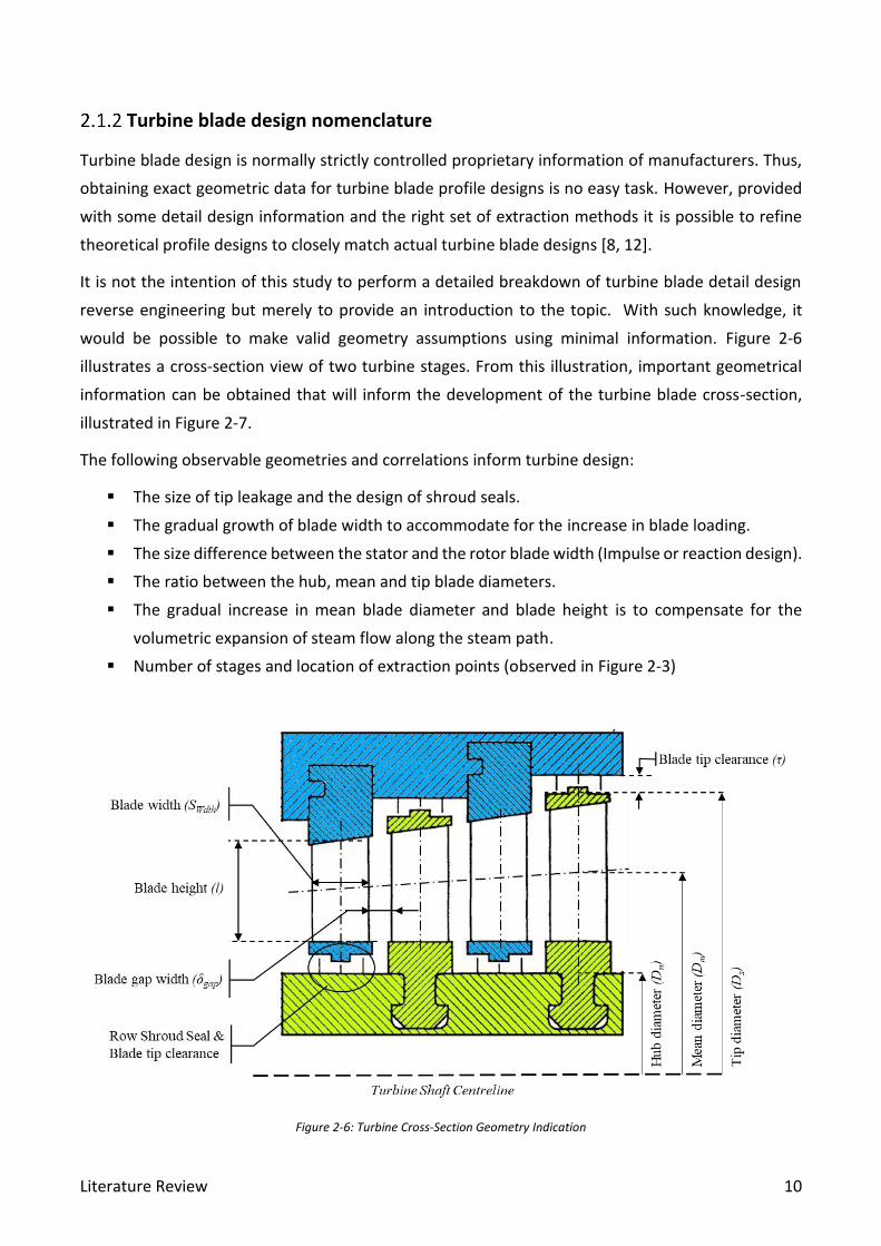
Turbine blade design nomenclature
Turbine blade design is normally strictly controlled proprietary information of manufacturers. Thus,
obtaining exact geometric data for turbine blade profile designs is no easy task. However, provided
with some detail design information and the right set of extraction methods it is possible to refine
theoretical profile designs to closely match actual turbine blade designs [8, 12].
It is not the intention of this study to perform a detailed breakdown of turbine blade detail design
reverse engineering but merely to provide an introduction to the topic. With such knowledge, it
would be possible to make valid geometry assumptions using minimal information. Figure 2-6
illustrates a cross-section view of two turbine stages. From this illustration, important geometrical
information can be obtained that will inform the development of the turbine blade cross-section,
illustrated in Figure 2-7.
The following observable geometries and correlations inform turbine design:
▪ The size of tip leakage and the design of shroud seals.
▪ The gradual growth of blade width to accommodate for the increase in blade loading.
▪ The size difference between the stator and the rotor blade width (Impulse or reaction design).
▪ The ratio between the hub, mean and tip blade diameters.
▪ The gradual increase in mean blade diameter and blade height is to compensate for the
volumetric expansion of steam flow along the steam path.
▪ Number of stages and location of extraction points (observed in Figure 2-3)
Figure 2-6: Turbine Cross-Section Geometry Indication
Literature Review 11
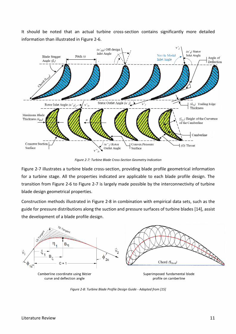
It should be noted that an actual turbine cross-section contains significantly more detailed
information than illustrated in Figure 2-6.
Figure 2-7: Turbine Blade Cross-Section Geometry Indication
Figure 2-7 illustrates a turbine blade cross-section, providing blade profile geometrical information
for a turbine stage. All the properties indicated are applicable to each blade profile design. The
transition from Figure 2-6 to Figure 2-7 is largely made possible by the interconnectivity of turbine
blade design geometrical properties.
Construction methods illustrated in Figure 2-8 in combination with empirical data sets, such as the
guide for pressure distributions along the suction and pressure surfaces of turbine blades [14], assist
the development of a blade profile design.
Figure 2-8: Turbine Blade Profile Design Guide - Adapted from [15]
Literature Review 12
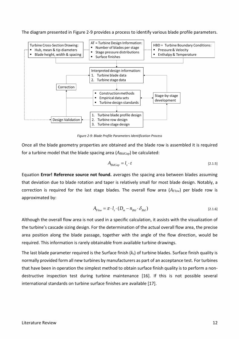
The diagram presented in Figure 2-9 provides a process to identify various blade profile parameters.
Figure 2-9: Blade Profile Parameters Identification Process
Once all the blade geometry properties are obtained and the blade row is assembled it is required
for a turbine model that the blade spacing area (ABldGap) be calculated:
BldGap sA l t= [2.1.5]
Equation Error! Reference source not found. averages the spacing area between blades assuming
that deviation due to blade rotation and taper is relatively small for most blade design. Notably, a
correction is required for the last stage blades. The overall flow area (AFlow) per blade row is
approximated by:
( )Flow s m Bld BldA l D n = − [2.1.6]
Although the overall flow area is not used in a specific calculation, it assists with the visualization of
the turbine’s cascade sizing design. For the determination of the actual overall flow area, the precise
area position along the blade passage, together with the angle of the flow direction, would be
required. This information is rarely obtainable from available turbine drawings.
The last blade parameter required is the Surface finish (ks) of turbine blades. Surface finish quality is
normally provided form all new turbines by manufacturers as part of an acceptance test. For turbines
that have been in operation the simplest method to obtain surface finish quality is to perform a non-
destructive inspection test during turbine maintenance [16]. If this is not possible several
international standards on turbine surface finishes are available [17].
Literature Review 13
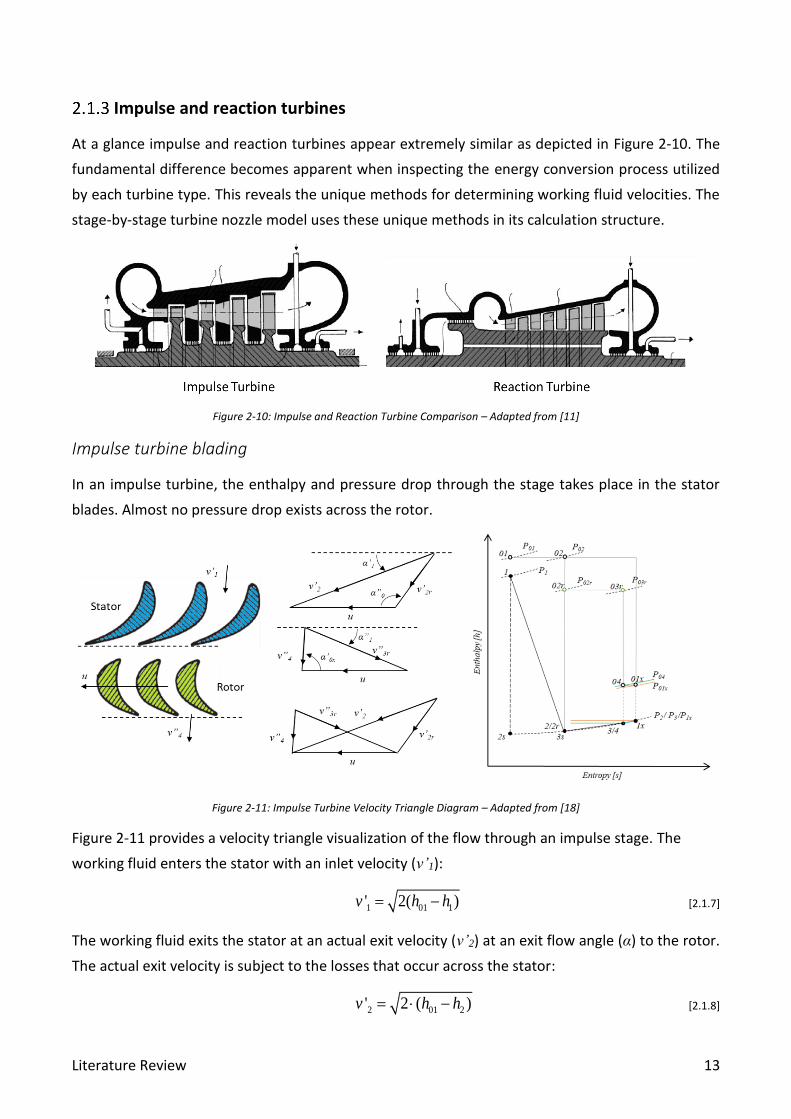
Impulse and reaction turbines
At a glance impulse and reaction turbines appear extremely similar as depicted in Figure 2-10. The
fundamental difference becomes apparent when inspecting the energy conversion process utilized
by each turbine type. This reveals the unique methods for determining working fluid velocities. The
stage-by-stage turbine nozzle model uses these unique methods in its calculation structure.
Figure 2-10: Impulse and Reaction Turbine Comparison – Adapted from [11]
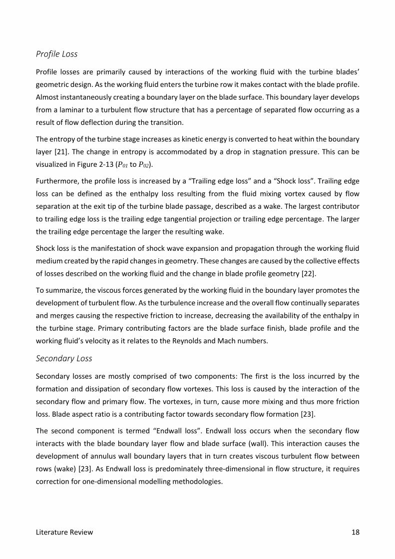
Impulse turbine blading
In an impulse turbine, the enthalpy and pressure drop through the stage takes place in the stator
blades. Almost no pressure drop exists across the rotor.
Figure 2-11: Impulse Turbine Velocity Triangle Diagram – Adapted from [18]
Figure 2-11 provides a velocity triangle visualization of the flow through an impulse stage. The
working fluid enters the stator with an inlet velocity (v’1):
1 01 1' 2( )v h h= − [2.1.7]
The working fluid exits the stator at an actual exit velocity (v’2) at an exit flow angle (α) to the rotor.
The actual exit velocity is subject to the losses that occur across the stator:
2 01 2' 2 ( )v h h= − [2.1.8]

Literature Review 14
The fluid enters the rotor at a relative velocity (v’2r) and flow angle (α1). This considers the relative
movement between the rotor blade speed (u) and the stators actual exit velocity (v’2) at an exit flow
angle (α). Utilizing the velocity triangle and the laws of trigonometry:
2 2
2 2 2 1' ' 2 ' cos( )rv u v v u = + − [2.1.9]
The working fluid exits the rotor blades at a relative exit velocity (v”3r). The rotor relative total
enthalpy stays constant (h03r=h02r) so in a loss-less rotor, the relative rotor inlet velocity (v’2r) and
exit velocity (v”3r) would be the same. The rotor relative exit velocity with losses and before work
extraction occurs is:
3 02 3'' 2 ( )r rv h h= − [2.1.10]
The rotor absolute exit velocity after work extraction has taken place:
4 04 4" 2( )v h h= − [2.1.11]
The working fluid enters the next stage stator with an inlet velocity (v’1x) after incorporating carry-
over losses:
1 01 1' 2( )x x xv h h= − [2.1.12]
The carry-over effect this is discussed in section 2.2.4 .
For clarification, point 3, illustrated in all h-s diagrams presented, is a fabricated point associated with
the calculation of the fictitious kinetic energy component discussed in section 2.3.3 .
Reaction turbine blading
Figure 2-12: Reaction Turbine Velocity Triangle Diagram– Adapted from [19]

Literature Review 15
From Figure 2-12 it becomes apparent that the same velocity calculation methods used for an
impulse turbine stage can be used to calculate the reaction turbine stage. The most significant
difference is that v”3r is substantially bigger than v’2r, since the flow is further accelerated through
the rotor passages. This difference is dependent upon the reaction ratio.
For a reaction turbine, the enthalpy conversion and pressure drop, across a stage, are split between
the stator and rotor blades. The ratio of this spilt is determined by the degree of reaction (R) defined
as:
R
Stg
hR
h
=
[2.1.13]
The degree of reaction is indicated as a percentage value. The conventional reaction turbines
discussed in literature consists of all the stages having a nominal 50% reaction design. Actual turbines
are often designed with a wide range of reaction values.
Design factors that may impact on the level of reaction per stage may be the available enthalpy within
the working fluid, the turbine shaft length, material constraints, material and manufacturing costs
and the manufacturers’ proprietary designs preferences [8]. A 0% reaction stage experiences no
change in enthalpy across the rotor, this differs from an impulse stage that experiences no change
in pressure across the rotor [20].
2.2 Turbine performance
As the working fluid, be it steam or gas, flows through the turbine blade channel contained in the
turbine casing, heat energy is converted into kinetic energy. Turbine designs have evolved over time
to maximize the utilization of this energy conversion thus improving turbine performance.
Turbine performance visualization
Turbine performance is ideally characterized by an enthalpy-entropy diagram. The diagram illustrates
the thermodynamic process, indicating the heat losses in relation to the functional energy converted
(work output).
Figure 2-13 presents the turbine working fluid flow performance on an enthalpy-entropy (h-s)
diagram for two consecutive stages. An equivalent turbine cross section was added, to the top right
corner, as to orientate the reader to the physical locations depicted.
This configuration will assist in the clarification of concepts such as; loss coefficients, carry-over and
off-design condition modelling. This section attempts to present a comprehensive visualization of
turbine performance.

Literature Review 16
Figure 2-13: Two Turbine Stages Enthalpy-Entropy Diagram
An ideal turbine blade passage (Δh’s & Δh”s) consists of no losses, whilst actual turbines (Δh’)
experience losses. The nozzle losses (Δh’ζ & Δh” ζ) are discussed in section 2.2.2 while the carry-over
loss (Δh’’c) is discussed in section 2.2.4 . Turbine efficiencies are used to indicate the ratio between
ideal and actual performance. Total-to-total, total-to-static and static-to-static are three efficiencies
defined by classical turbine theory [20].
Total-to-total efficiency is the ratio between the actual work performed by a multistage turbine
relative to the ideal work output whilst operating at fixed back pressure:
01 04
01 04
tt
ss
h h
h h
−=
− [2.1.14]
Total-to-static efficiency is the adiabatic efficiency that incorporates the loss of exit kinetic energy
(exit velocity). Ideally suited for single stage or last stage blade calculations:
01 04
01 3
ts
ss
h h
h h
−=
− [2.1.15]

Literature Review 17
Static-to-static efficiency occurs when the inlet velocity of a stage equals the exit velocity:
1 3
1 3
ss
ss
h h
h h
−=
− [2.1.16]
The isentropic nozzle efficiency for a single turbine stator and rotor row is defined as:
01 2
01 2
's
h h
h h
−=
− [2.1.17]
02 3
02 3
" r
r s
h h
h h
−=
− [2.1.18]
Equation [2.1.17] (Stator nozzle efficiency) and [2.1.18] (Rotor nozzle efficiency) are used as a core
framework property in the stage-by-stage nozzle-model component [1].
The following sections provide an overview of turbine losses and categorize them into the most
widely acknowledged groups. This provides the premise for the evaluation of loss coefficients for
both design and off-design conditions. Loss coefficients provide a turbine row and the stage specific
analysis methodologies. To complete the required evaluation of a turbine, an overview of turbine
performance evaluation is required. This is discussed in section 2.2.4 .
Turbine loss coefficients
The collective loss experienced by each row or stage can be characterized into the following loss
categories depicted in Figure 2-14:
Figure 2-14: Turbine Loss Indication [13]
Literature Review 18
Profile Loss
Profile losses are primarily caused by interactions of the working fluid with the turbine blades’
geometric design. As the working fluid enters the turbine row it makes contact with the blade profile.
Almost instantaneously creating a boundary layer on the blade surface. This boundary layer develops
from a laminar to a turbulent flow structure that has a percentage of separated flow occurring as a
result of flow deflection during the transition.
The entropy of the turbine stage increases as kinetic energy is converted to heat within the boundary
layer [21]. The change in entropy is accommodated by a drop in stagnation pressure. This can be
visualized in Figure 2-13 (P01 to P02).
Furthermore, the profile loss is increased by a “Trailing edge loss” and a “Shock loss”. Trailing edge
loss can be defined as the enthalpy loss resulting from the fluid mixing vortex caused by flow
separation at the exit tip of the turbine blade passage, described as a wake. The largest contributor
to trailing edge loss is the trailing edge tangential projection or trailing edge percentage. The larger
the trailing edge percentage the larger the resulting wake.
Shock loss is the manifestation of shock wave expansion and propagation through the working fluid
medium created by the rapid changes in geometry. These changes are caused by the collective effects
of losses described on the working fluid and the change in blade profile geometry [22].
To summarize, the viscous forces generated by the working fluid in the boundary layer promotes the
development of turbulent flow. As the turbulence increase and the overall flow continually separates
and merges causing the respective friction to increase, decreasing the availability of the enthalpy in
the turbine stage. Primary contributing factors are the blade surface finish, blade profile and the
working fluid’s velocity as it relates to the Reynolds and Mach numbers.
Secondary Loss
Secondary losses are mostly comprised of two components: The first is the loss incurred by the
formation and dissipation of secondary flow vortexes. This loss is caused by the interaction of the
secondary flow and primary flow. The vortexes, in turn, cause more mixing and thus more friction
loss. Blade aspect ratio is a contributing factor towards secondary flow formation [23].
The second component is termed “Endwall loss”. Endwall loss occurs when the secondary flow
interacts with the blade boundary layer flow and blade surface (wall). This interaction causes the
development of annulus wall boundary layers that in turn creates viscous turbulent flow between
rows (wake) [23]. As Endwall loss is predominately three-dimensional in flow structure, it requires
correction for one-dimensional modelling methodologies.

Literature Review 19
Tip Leakage Loss
Tip leakage loss occurs across the clearances between the stator blades and the shaft and the rotor
blades and the turbine casing. The tip leakage loss is primarily created by the mixing of the working
fluid flow through the blade passage and the flow across the respective tip leakage regions. The
mixing occurs at the exit blade region and progresses into the blade spacing gap.
The loss severity is reliant on the pressure difference between interacting flows as well as the sizing
of the clearances. A contribution to tip leakage loss severity is whether the blade is shrouded or
unshrouded [11].
Incidence Loss
Incidence loss is caused by the deviation from the ideal inlet angle of the working fluid onto the blade
profile. The incidence angle indicates the deviation from the design angle. The impact of this
deviation results in the increase of the profile losses experienced. Dependent on the cause of the
incidence the working fluid can be directed either towards the convex or concave side of the blade
passage. Each incidence angle orientation has its own corresponding loss effect [24].
Moisture loss
Moisture loss is a steam turbine specific attribute, primarily occurring in the last stage blades of a
low-pressure turbine and under the right conditions for water droplets to form. Wet steam is the
term used to describe the condition of water droplet formation within steam as a working fluid.
Moisture loss has been the focus of immense study [25]. For simplification, moisture loss will be
broken into two categories: thermodynamic loss and mechanical loss.
Thermodynamic moisture loss occurs when sudden condensation occurs after the steam condition
has crossed the saturation line. Described as the heat loss resulting from a phase transition between
supercooling and equilibrium states [7].
Mechanical moisture loss is comprised out of two components. “Braking Loss” resulting from the
difference in velocity profiles of the formed water droplets and the unchanged steam. As both phases
are bound by the same velocity triangles yet have a different velocity constitution the heavier liquid
particles will obstruct and slow the lighter vapour particles.
As a secondary effect of the braking loss, “Drag Loss” occurs because of the frictional loss generated
between the water droplets and steam. The larger the water droplets the larger the mechanical loss
[26].

Literature Review 20
Other Losses
For the purpose of this study, two additional losses are investigated, specifically “Fan loss” and “Last
Stage Blade losses”. Fan loss is a correction coefficient that incorporates the additional losses
incurred due to the blade spacing not being constant over the row radius from hub to tip [27].
Last stage blade losses specifically add losses incurred due to the unique interconnection designs of
last stage blade. Uniquely “Exhaust loss” is specifically excluded as it relates to overall heat cycle
performance.
It should be noted that the turbine losses discussed do not define all possible classifications or
combinations of losses. The exact combination of losses is dependent upon the specific
methodology’s requirements.
A comparative loss coefficient study was conducted and is discussed in the next sections for design
and off-design conditions. The selected loss coefficient methodologies are evaluated in the next
chapter.
Loss coefficient methodology selection
Turbine losses are expressed by means of loss coefficients. Loss coefficients either utilize pressure
loss coefficients (Y) or enthalpy loss coefficients (ζ). Each loss coefficient methodology relates back
to turbine performance in a specific method although a lot of similarities are present.
An example of the this can be observed when comparing the loss coefficient equations for a stator
developed by Denton [28], equation [2.1.19], with that of Traupel [29], equation [2.1.20].
2 2
01 2
' sDenton
h h
h h
−=
− [2.1.19]
2 2
01 2
' sTraupel
s
h h
h h
−=
− [2.1.20]
It is possible to incorporate multiple loss coefficients methodologies into a single modelling
methodology, provided the methodologies are correctly linked and do not overlap in terms of the
effects that are incorporated.
It is possible to convert pressure loss coefficients to enthalpy loss coefficients and vice versa [30],
but the implementation of this conversion into a modelling scheme increases the required processing
time and tends to create evaluation overlap.
Literature Review 21
Numerous turbine loss coefficient methodologies have been developed over time. A comprehensive
comparison study was conducted by Ning [27]. The most notable methodologies are:
▪ Soderberg’s [31]: developed one of the first loss coefficient methodologies, it incorporated profile
and secondary losses. It is often viewed as a foundation for other methodologies.
▪ Ainley & Mathieson [32]: established, by means of detailed turbine performance experiments, a
pressure loss coefficient turbine performance prediction methodology.
▪ Craig & Cox [33]: developed a methodology based on linear turbine blade cascade testing focused
on predicting losses in turbine stages. With the incorporation of “Other losses”, a greater overall
efficiency accuracy was obtained.
▪ Dunham & Came [34]: produced a methodology by improving upon the “Ainley & Mathieson”
methodology made possible by the improvement of measured experimental data.
▪ Traupel [35]: developed a one-dimensional empirical modelling methodology that incorporates
various flow distributions generated by turbine blades and accompanying turbine blade
components. The empirical data was extracted from an array of experiments and data sets.
▪ Kacker & Okapuu [36]: the methodology is a combination and advancement of the “Ainley &
Mathieson” and “Dunham & Came” methodologies, with the incorporation of “Shock losses”.
▪ Denton [28]: produced a methodology based on the relationship between turbine loss causes and
the respective increases of entropy. The method is based on the theoretical evaluation of losses
formulated from the conservation equations and other turbine specific governing equations.
A selection criterion was developed that compares the amount of functional performance data a loss
coefficient methodology would produce compared to the amount of blade geometry it requires. The
selection criteria scoring is determined by adding value per turbine loss type and deducting value per
blade geometry parameter required relative to the total number of possibilities per section:
_ _ _ _
_ _ _ _
Number of Losses Number of Geometries
Total Possible Losses Total Blade GeometriesScore
= −
A higher score implies that loss coefficient requires an amount of geometrical data input but
produces a higher level of detailed loss coefficient result. Table 2-2 provides the loss coefficient
methodologies comparison result.

Literature Review 22
Table 2-3: Loss Coefficient Comparison - Adapted from [27]
Year Author Types of losses Design (D) /
Off-Design (OD) Score
1949 Soderberg TT=PR+SE+TL D 62%
1951 Ainley & Mathieson TT=PR+SE+TL+TE D+OD 53%
1960 Steward et al PR, SE D 52%
1965 Smith TT OD 55%
1968 Baljé & Binsley TT=PR+SE+TL D 60%
1969 Mukhtarov & Krichakin TT=PR+SE+TL D+OD 53%
1970 Craig &Cox TT=PR+SE+OL D+OD 40%
1970 Dunham & Came TT=PR+SE+TL+TR D+OD 60%
1971 Kroon & Tobiasz TT D+OD 55%
1977 Traupel TT=PR+SE+FA+TL+TE+OL D 74%
1980 Zehner PR OD 55%
1981 Macchi & Perdichizzi TT D+OD 55%
1982 Kacker & Okapuu TT=PR+SE+TL+TE D+OD 51%
1987 Sharma & Butler SE D 58%
1990 Moustapha et al PR, SE OD 62%
1992 Okan & Gregory-Smith SE D 61%
1992 Schobeiri & Abouelkheir PR OD 55%
1993 Denton TT=PR+SE+TL+TE D 57%
TT - Total losses
PR - Profile loss
SE - Secondary loss
FA - Fan loss
TL - Tip Leakage loss
TE - Trailing Edge loss
OL - Other losses
From the comparisons in Table 2-3, it was determined that Traupel [29] is the most advantageous
loss coefficient methodology. Traupel’s loss coefficient methodology is comprised of profile loss,
secondary loss, fan loss, tip leakage loss and trailing edge loss.
Additionally, one can incorporate Last stage blade losses as well as moisture loss into this loss
coefficient methodology. It has the benefit of having an enthalpy loss coefficient format that is similar
to the Soderberg methodology [1] utilized in the stage-by-stage turbine nozzle-model component.
The disadvantage of the Traupel’s methodology is that it does not evaluate turbine losses for off-
design conditions. Fortunately, Zehner [24] developed a methodology that provides an off-design
correction for Traupel’s methodology. Zehner provides an expansion of Traupel’s methodologies by
integrating turbine blade cascade characteristics and incidence loss into Traupel’s profile loss.
Furthermore, the “Moisture loss” used in Traupel’s methodology is expanded and improved upon by
the incorporations of Gyarmathy’s [26] moisture loss calculation, that is based on wet-steam turbine
theory, and a correction methodology for moisture loss development compiled by Hiroyuki et al [25].

Literature Review 23
Carry-over and reheat analysis
Turbine “Carry-Over” and “Reheat Factor” do not form part of the primary loss coefficient algorithm
but offer an additional performance evaluation methodology. Figure 2-15 provides a visualization of
Carry-over and Reheat factor for multiple stages.
Figure 2-15: 5 Multistage Turbine Carry-over and Reheat Factor Visualization – Adapted from [37]
Carry-over
As the working fluid passes from one stage to the next, point 4 to 1x in Figure 2-16, across the
diaphragm (gap), a portion (kco) of the available kinetic energy is lost and converted back into fluid
static temperature [37].

Literature Review 24
Figure 2-16: Carry-Over Indication
This conversion is caused by the rapid expansion and turbulence of the working fluid leaving a stage.
The decrease in working fluid pressure relates to the energy conversion into heat, this generates an
increasing of the enthalpy and entropy generally termed stage reheat. This energy conversion is
referred to as “Carry-over” (h”C) [38].
1 4x cov k v= [2.1.21]
1 4'' ' ''C xh h h = − [2.1.22]
Equation [2.1.21] and [2.1.22] govern the Carry-over effect. The Carry-over (h”C) for a single
stage-to-stage can be expressed in terms of the carry-over ratio (kco) as:
( )2
2 4" 12
C co
vh k
= −
[2.1.23]
The Carry-over effect enables all stages, except the first stage, to benefit to an extent from the
inefficiency of the preceding stages. Carry-over is utilized in the stage-by-stage turbine nozzle-model
to accommodate for the reheat phenomena as discussed in section 2.2.2 .
Reheat factor
Reheat factor is a measure of inefficiency across multiple stages or a complete turbine of steam
turbine resulting from steam’s deviation from the ideal gas law. Defined as the ratio of total enthalpy
drop relative to ideal enthalpy drop during the expansion phases of a turbine. Reheat factor tends to
be between 1.03 and 1.08 for most steam turbines [20]. Reheat factor presents a correlation between
isentropic and polytropic turbine efficiencies.

Literature Review 25
The reheat factor indicates, in part, the overall impact turbine losses have on performance. For a
complete turbine consisting of x stages the reheat factor is:
1 2 ...s s xs
ss
h h hRF
h
+ + +=
[2.1.24]
If the reheat factor is not provided in the in the turbine performance data it can be determined after
an initial nozzle-model evaluation has been completed. The Reheat factor indicates that the sum of
all the isentropic enthalpy drops across individual stages, of a multi-stage turbine, is greater than the
total adiabatic enthalpy drop of the turbine [20]. This can be observed in Figure 2-15 and is
characterized by:
5
1
is
i
ss
h
RFh
=
=
The reheat factor depends largely on the turbine design with regards to stage loading and expansion
design [37]. It is significantly impacted by the initial inlet and exhaust conditions as illustrated in
Figure 2-15.
Notably, limited documentation was found on the relationships between Turbine loss, Carry-over
and Reheat factor. From obtained literature, it appears that the correlations between the
methodologies have not been well researched. Both Carry-over and Reheat factor allow for
alternative evaluation of turbine performance.
2.3 Nozzle-model review
Before looking at the inner workings of the stage-by-stage turbine nozzle-model some information is
required regarding turbine process modelling. Specifically, the software used and the framework
required for the stage-by-stage nozzle-model component.
Turbine modelling methods
Turbine blade passages have a notoriously complex design causing a multitude of intricate unsteady
fluid flow conditions. Figure 2-17 illustrates a collection of fluid conditions. Almost every
combination, of these conditions, is possible across an entire turbine. These combinations, in turn,
lead to a variety of physical actions from material stress to shock waves to immense heat transfer
[39].

Literature Review 26
Figure 2-17: Fluid Flow Conditions
Due to the complexity of the thermohydraulic flow through a turbine blade passage, the precise
modelling thereof is equally complex. Turbine model formats are primarily defined in the following
three categories:
One-dimensional (1D) flow simulation: utilizes velocity triangles as the calculation foundation and
applies corrections for losses and efficiencies [19]. Largely empirically based correction factors and
loss coefficients improve the accuracy of the modelling methodologies [40]. Loss coefficients and
correction factors are reviewed in section 2.2.2
Two-dimensional (2D) cascade simulation: places focus on the angular momentum of the working
fluid as it passes through the blade passages. The modelling methodologies either uses an axial-
tangential cartesian or a cylindrical coordinate system. Allowing for a row-by-row modelling
arrangement (cascade) [41]. Loss coefficients and correction factors are also incorporated for
improved accuracy.
Three-dimensional (3D) computational fluid dynamics (CFD): requires exact turbine geometric data
as to enable the replication and thus analysis of a turbine. CFD determines the turbine performance
losses by calculating the unsteady fluid flow conditions more commonly named secondary flows.
Additionally, 3D meshing ads to the complexity of CFD modelling [39]. Most modern research
focusses on applying CFD modelling for turbine analysis.
Figure 2-18: 1D, 2D & 3D Modelling - Adapted from [19], [41]& [42] respectively
Literature Review 27
With each additional dimension, the modelling design complexity increases. This comes at the cost
of numerical processing time, advanced modelling knowledge and detailed information required but
with the benefit of a possible increased accuracy and fidelity. Although the stage-by-stage turbine
nozzle-model methodologies is a 1D modelling method it achieves a high level of accuracy [1].
The incorporation of loss coefficient algorithms into the stage-by-stage turbine nozzle-model aims to
add to the accuracy of the turbine performance modelling method, whilst maintaining lower
processing time and requiring minimal turbine geometric data.
Flownex network solver overview
A brief overview of Flownex SE follows as to provide fundamental background information regarding
the stage-by-stage nozzle-model component’s workings and compositions. It should be noted that in
no way does this overview do justice to the complete workings, complexity or vast capabilities of
Flownex.
Flownex SE is defined as a one-dimensional thermo-hydraulic network solver. Flownex utilizes an
isolated algorithm solving structure governed primarily by the conservation of mass, energy and
momentum equations. It solves these governing equations on a node to node network structure for
both steady state and transient simulations. Integrated on top of these equations are component
specific algorithms, defining the physics required for their modelling [43].
Once a Flownex network is constructed with all the specific components required for an accurate
model, a fluid is assigned to the network. The fluid properties can be drawn from a prepopulated
library or customized to requirements. Flownex can integrate Excel, Ansys, Matlab and MathCad into
simulations, to mention a few compatible application [43]. The network solver allows for solving
criteria to be adjusted, enabling greater model stability, accuracy and control.
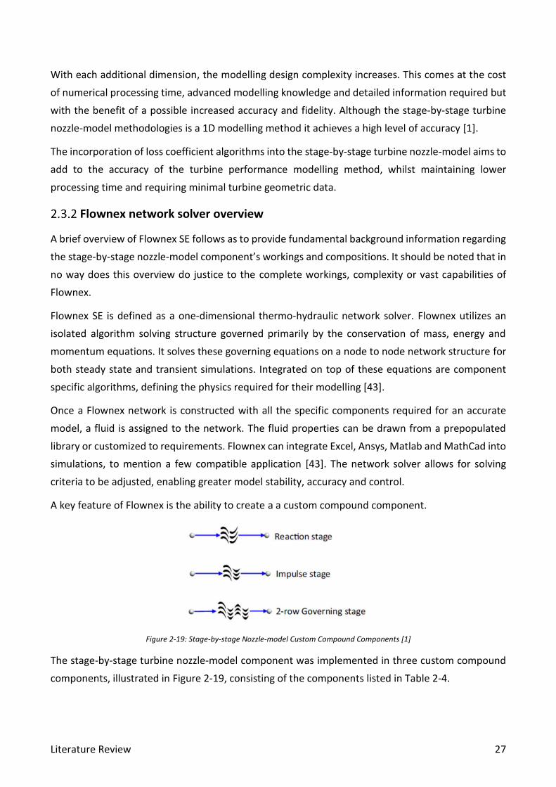
A key feature of Flownex is the ability to create a a custom compound component.
Figure 2-19: Stage-by-stage Nozzle-model Custom Compound Components [1]
The stage-by-stage turbine nozzle-model component was implemented in three custom compound
components, illustrated in Figure 2-19, consisting of the components listed in Table 2-4.
Literature Review 28
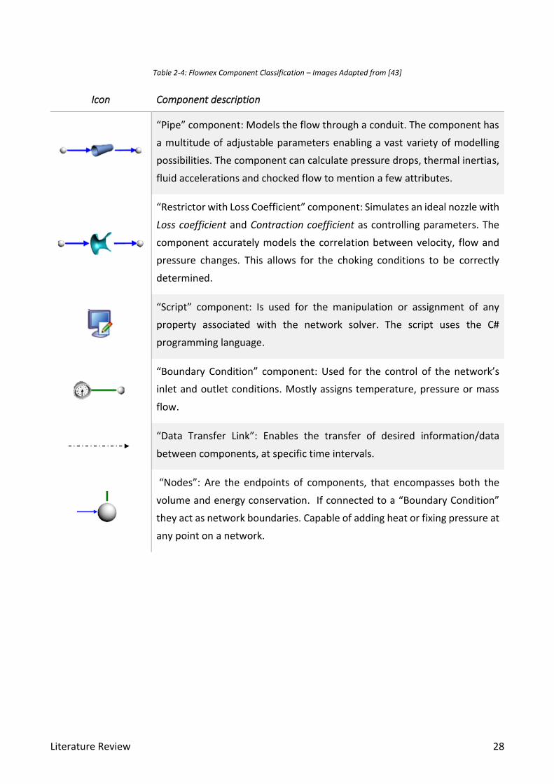
Table 2-4: Flownex Component Classification – Images Adapted from [43]
Icon Component description
“Pipe” component: Models the flow through a conduit. The component has
a multitude of adjustable parameters enabling a vast variety of modelling
possibilities. The component can calculate pressure drops, thermal inertias,
fluid accelerations and chocked flow to mention a few attributes.
“Restrictor with Loss Coefficient” component: Simulates an ideal nozzle with
Loss coefficient and Contraction coefficient as controlling parameters. The
component accurately models the correlation between velocity, flow and
pressure changes. This allows for the choking conditions to be correctly
determined.
“Script” component: Is used for the manipulation or assignment of any
property associated with the network solver. The script uses the C#
programming language.
“Boundary Condition” component: Used for the control of the network’s
inlet and outlet conditions. Mostly assigns temperature, pressure or mass
flow.
“Data Transfer Link”: Enables the transfer of desired information/data
between components, at specific time intervals.
“Nodes”: Are the endpoints of components, that encompasses both the
volume and energy conservation. If connected to a “Boundary Condition”
they act as network boundaries. Capable of adding heat or fixing pressure at
any point on a network.

Literature Review 29
The Stage-by-stage nozzle model overview
The Reaction Stage custom compound component illustrated in Figure 2-19 is comprised of the
components illustrated in Figure 2-20.
Figure 2-20: Stage-by-stage Nozzle-model Component [1]
The stage-by-stage turbine nozzle-model is grounded on building a turbine stage based on nozzle
theory. For the simplification of this concept, a moving nozzle analogy is utilized [1], illustrated in
Figure 2-21.
Figure 2-21: Moving Nozzle Analogy - Adapted from [1]
The “Restrictor with Loss Coefficient” component is used to simulate the turbine stator and rotor
blade rows. This enables the modelling of a turbine stage as a combination of two nozzles. The
restrictor Loss coefficient and Contraction coefficient is used to incorporate the nozzle losses.

Literature Review 30
The restrictor Loss Coefficient is derived from [43] for a stator and rotor:
21
2 2 2
01 2
' 1 rL
vC
p p
= −
− [2.2.1]
21
2 3 4
02 3
" 1L
r
vC
p p
= −
− [2.2.2]
Whilst the Contraction Coefficients are derived by Fuls [1] in terms of row efficiencies and densities
for a stator and rotor:
2
2
' 'D
s
C
= [2.2.3]
3
3
" "D
s
C
= [2.2.4]
The inclusion of row efficiency allows for the integration of turbine loss coefficients into the nozzle-
model. Fuls [1] utilizes a loss coefficient methodology equivalent to equation [2.1.19]. Through
algebraic manipulation of [2.1.17] and [2.1.19] the relation between row nozzle-model efficiency
(ηNM) and turbine loss coefficients (ζNM) is found as:
1
1NM
NM
=+
[2.2.5]
Notably, this relationship is fundamental to the adaptation of the nozzle-model. The velocity triangle
equations expressed in 2.1.3 along with the stage performance visualization of the working fluid,
Figure 2-21, contains the basis of the stage-by-stage turbine nozzle-model component. This is
facilitated in the “Script” component.
Important calculations performed by the nozzle-model script are for the correction of the relative
inlet (v’2r) and exit rotor velocities (v”3r), as they are impacted by the rotor rotational blade speed
(u).
Other important calculations performed are that of work extraction (w) and carry-over effect. Before
being able to calculate work extraction the nozzle-model script must first calculate the fictitious
kinetic energy component (v3):
( )3 01 32v h h= − [2.2.6]
For clarification, up until point 3, no work has been extracted from the working fluid by the nozzle-
model. This implies that the total rotor exit enthalpy is identical to that of the inlet condition,
although the static enthalpy had decreased. This results in the development of a kinetic energy
component (v3).

Literature Review 31
The nozzle-model script calculates the fictitious kinetic energy component from the total rotor inlet
enthalpy assuming the rotor blades have not extracted any energy from the working fluid.
The work extraction calculation is performed by the “Script” in one of two methods. If blade efficiency
(ηb) is known:
212 3bw v= [2.2.7]
Or more practically utilizing the stator and rotor velocities and angles:
' "
2 1 3 1( cos( ) cos( ) )rw u v v u = + − [2.2.8]
The carry-over effect, discussed in section 2.2.4 , is simulated by a “Pipe” component which acts as a
diffuser. The “Pipe” receives variable values from the “Script” enabling the nozzle-model component
exit condition correction for the next stage [1]. These variables consist of the derived inlet and outlet
diameter:
4
3 4
in
mD
v
= [2.2.9]
4
1 4 co
out
x
m
kD
v
= [2.2.10]
As well as, a “Pipe” component specific property, a “Pressure drop coefficient” (Kloss) that describes
an approximation of desired total pressure drop whilst retaining the static pressure
2 1
3
1 xloss coK k
= − [2.2.11]
The continuous control and calculation of corrections, coefficients and variables form part of the
“Script” component’s function. The timeframe or phase in which the calculations must be performed
is reliant upon the “Data Transfer Links” that communicate information between the “Script” and all
the other components.
The examination of the workings of the stage-by-stage turbine nozzle-model component enables the
development and implementation of an adaption methodology. This is the topic of the next chapter
along with the examination and implementation of the selected loss coefficients.

Literature Review 32
2.4 Case study data classification
Before proceeding, it is required to discuss the categories of data used for the generation and
simulation of turbine test cases. Table 2-5 provides a summary.
Table 2-5: Turbine performance data categories
Information Description
Turbine design data ▪ Original equipment manufacturer (OEM) design information.
▪ Measured information obtained over the lifetime of the
component.
▪ Recorded design changes.
Acceptance tests (AT) ▪ Provides a comprehensive data set of the plant design and
performance information.
▪ Usually obtained during the commissioning phase of plant life.
▪ Can be used as an ideal plant condition.
▪ Are physical measurements, typically at a higher accuracy than
operating plant data.
Heat balance diagrams
(HBD)
▪ Heat balance diagrams provide steam cycle overview
information.
▪ HBD are often available for various loads. Allowing for off-design
or varied operational performance guidelines.
▪ If provided by OEM it may be used as a model verification check.
▪ Are typically predicted, not measured, and would in some cases
contain margins of conservatism.
Operational plant data ▪ Operational plant data is actual measurements and observations
of plant performance information.
▪ The information is regularly available although less reliable and
often incomplete.
▪ Can be utilised for actual plant performance evaluations.

Research Methodology 33
Chapter 3 Research Methodology
This chapter will first describe the adaptation methodology implemented by illustrating the Flownex
script architecture. Second, it will evaluate the selected loss coefficients obtained from literature and
convert them into a digital/mathematical form for implementation into a programming algorithm.
Finally, it will review the results of the adaptation.
3.1 Nozzle model adaptation methodology
A Flownex “Script” is utilized to interact with the nozzle-model component, as illustrated in Figure
3-1. The script consists of the converted turbine loss coefficient algorithms. The C# script code format
allows for validation and stability control measure to be implemented in the program architecture.
Figure 3-1: Stage-by-stage nozzle-model with Loss Coefficient Algorithm Implemented
The diagram illustrated in Figure 3-2 provides a structural format diagram to indicate the general
requirements of the algorithm script.
Figure 3-2: Loss Coefficient Algorithm Script Architecture

Research Methodology 34
The loss coefficient algorithm script architecture is comprised of three sections:
▪ Input: User defined turbine design data and data transfer link information from the nozzle-model
components, as indicated in Figure 3-2.
▪ Script functions: Check validity of data, maintain the script program during processing, calculated
loss coefficients and format results to feedback to nozzle-model.
▪ Output: Returns script values to nozzle-model script per processing step and displays final values
obtained.
The following section is comprised first of a description of the turbine loss coefficient input variables,
followed by the evaluation and conversion of design and off-design loss coefficient into
programmable algorithms.
Notably, the initial loss coefficient algorithms were developed in Mathcad, an engineering calculation
software, that was used for methodology verification and validation purposes. An initial attempt to
directly implement a MathCad scripts into a Flownex model presented processing complication and
delays.
3.2 Loss coefficient input variables
The turbine loss coefficient input variables are comprised of two categories as indicated in Figure 3-2,
namely “user defined” and “nozzle model defined”. The working fluid properties required are linked
to the stage-by-stage turbine nozzle-model components via data transfer links. The stator and rotor
restrictors send working fluid properties to the loss algorithm script as the variables indicated in
Figure 3-3.
Figure 3-3: Stator Fluid Properties Input Variables
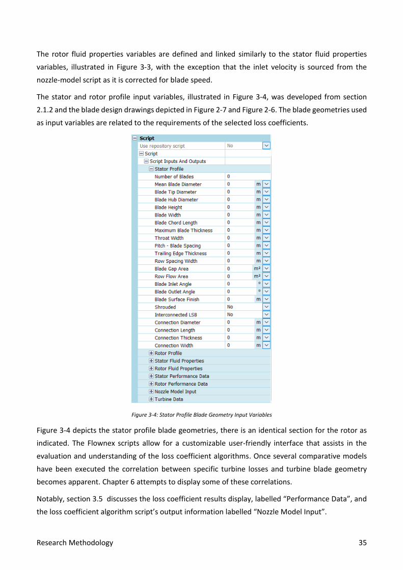
Research Methodology 35
The rotor fluid properties variables are defined and linked similarly to the stator fluid properties
variables, illustrated in Figure 3-3, with the exception that the inlet velocity is sourced from the
nozzle-model script as it is corrected for blade speed.
The stator and rotor profile input variables, illustrated in Figure 3-4, was developed from section
2.1.2 and the blade design drawings depicted in Figure 2-7 and Figure 2-6. The blade geometries used
as input variables are related to the requirements of the selected loss coefficients.
Figure 3-4: Stator Profile Blade Geometry Input Variables
Figure 3-4 depicts the stator profile blade geometries, there is an identical section for the rotor as
indicated. The Flownex scripts allow for a customizable user-friendly interface that assists in the
evaluation and understanding of the loss coefficient algorithms. Once several comparative models
have been executed the correlation between specific turbine losses and turbine blade geometry
becomes apparent. Chapter 6 attempts to display some of these correlations.
Notably, section 3.5 discusses the loss coefficient results display, labelled “Performance Data”, and
the loss coefficient algorithm script’s output information labelled “Nozzle Model Input”.
Research Methodology 36
3.3 Loss coefficient algorithms
This section will evaluate the selected loss coefficients that are largely comprised of reworkings of
Traupel’s turbine loss methodology [29] and show how they were systematically adapted into the
loss coefficient algorithm script component.
The Traupel enthalpy loss coefficient (ζTLC) is the sum of a Primary profile loss (ζP), a Secondary loss
(ζS), a Tip Leakage or Seal loss (ζTl), a Fan loss (ζF), an LSB loss (ζLSB) and a Moisture loss (ζM).
TLC P S Tl F LSB M = + + + + + [3.3.1]
Traupel enthalpy loss coefficient (ζTLC) relates back to nozzle efficiency by:
1nozzle TLC = − [3.3.2]
Each enthalpy loss component is evaluated as a collective of its parts.
Primary profile loss
The primary profile loss (ζP) is determined by
0 ReP P M Te C = + + [3.3.3]
ζP0 – Profile loss
χM – Mach number correction factor
χRe – Reynolds number correction factor
ζTe – Trailing edge loss
ζC – Carnot shock loss
Profile loss
The profile loss (ζP0) is caused by the friction that occurs on the blade surfaces as a result of the flow
separation of the boundary layers. A thicker boundary layer creates greater flow separation primarily
on the blade suction surface.
The inlet and outlet velocity angles largely impact the boundary layer formation. The profile loss (ζP0)
is obtained from empirical correlations between the inlet and outlet flow angles as illustrated in
Figure 3-5.

Research Methodology 37
Figure 3-5: Traupel's profile loss chart [29]
The profile loss chart, Figure 3-5, was converted into a series of polynomials which are linearly
interpolated for a given angle:
1_
77
0 0[ , 1] 0
1Position
i
P P i
i
M −
+
=
= [3.3.4]
Equation [3.3.4] is utilized for both stator and rotor with the correct angle orientations required. A
model algorithm validation and stability control measure is required at this point to correct for values
entered outside of the curve functions indicated in Figure 3-5.
Mach number correction factor
The Mach number correction factor (χM) considers the free stream velocity across the blade profile
and utilizes the Mach number along with the diagram shown in Figure 3-6.
Figure 3-6: Mach number correction factor chart [29]

Research Methodology 38
Mach number correction factor curve types, illustrated in Figure 3-6, are described as:
▪ Curve 1 - Relates to a conventional high-speed grid
▪ Curve 2 - Applies to a strongly accelerating grid
▪ Curve 3 - Corresponds to a constant-pressure impeller grid with rounded entry edge
▪ Curve 4 - Corresponds to a constant-pressure impeller grid which has a relatively pointed,
forward-drawn entry edge for high Mach numbers.
Curve 1 is most often selected in the determinization of the Mach number correction factor. Curve 1
best correlates to the conditions experienced by power utility turbines [35]. The Mach number
correction chart is converted into the following algorithms:
1M = for Ma<0.8 [3.3.5]
5 4 3 2344.9 1763 3690.8 3744.7 1878.6 374.2M Ma Ma Ma Ma Ma = − + − + − + for Ma≥0.8 [3.3.6]
The Mach number is determined by Flownex and is linked to the loss coefficient algorithm script.
Reynolds number correction factor
The Reynolds number correction factor (χRe), determined by utilizing Figure 3-7, describes the
influence that the Reynolds number (Re) and surface finish or roughness (ks) has on the blade profile
loss. The relationship between profile loss and the Reynolds number correction factor is indicated by
the correlation the Reynolds number has with the boundary layer thickness and the flow separation
as defined by classical fluid dynamics [22].
Figure 3-7: Reynolds number correction factor chart [29]

Research Methodology 39
From the chart, it becomes apparent that the Reynolds number correction factor is exclusively
dependant on the working fluids Reynolds number below the transition point (Re<2∙105). Whilst
above the transition point the turbine blade surface finish will exclusively determine the Reynolds
number correction factor. Only line (a) is turbine specific for the Reynolds number correction factor,
lines (b) and (c) are used for compressors. A clearer concept of Figure 3-7 is provided in Figure 3-8
and Figure 3-9.
Figure 3-8: Reynolds Correction Curve for Re<2∙105
It is apparent from Figure 3-8 that a lower Reynolds (Re<2∙105) number will increase the profile loss.
Figure 3-9: Reynolds Correction Curve for Re>2∙105
Figure 3-9 indicates that a larger Reynolds number (Re>2∙105) has no impact on the profile loss but
that the relative blade surface finish will increase the profile loss.

Research Methodology 40
The Reynolds number indicates the ratio between inertia and viscous forces within the working fluid
flow and is determined by:
ReRe
v D
= [3.3.7]
ρ – Blade outlet fluid density
v – Blade outlet fluid velocity
DRe – Blade spacing area diameter
μ – Blade outlet dynamic viscosity
The blade spacing area diameter (DRe) is determined for the Reynolds number calculation by
converting the blade spacing area (ABldGap), determined by equation [2.1.5], into hydraulic diameter
[35]:
Re
4 BldGapAD
= [3.3.8]
Traupel provides a rough guide for surface finishes values to be used [35]:
▪ 0 to 0.002 mm for ground and polished blades.
▪ 0.005 to 0.010 mm for standard milled and drawn blades
▪ 0.01 to 0.03 mm for lightly rusted blades
▪ 0.03 to 0.06 mm for heavily rusted sheet metal blades
▪ 0.03 to 0.10 mm for raw casting blades
The Reynolds number correction can then be calculated using the following equation:
For Re<2∙105
2 0.491718
Re 4.1542 10 Re −= [3.3.9]
For Re≥2∙105
3 2
8 5 3
Re 2.04381 10 1.34009 10 2.00593 10 0.565005chrd chrd chr
s
d
s sk k k
S S S
= − + + +
[3.3.10]
The loss coefficient algorithm section for Mach number and Reynolds number correction factors have
validation checks. These checks only allow valid value transfer, thus excluding extreme values fed
from the nozzle-model during iteration processes.
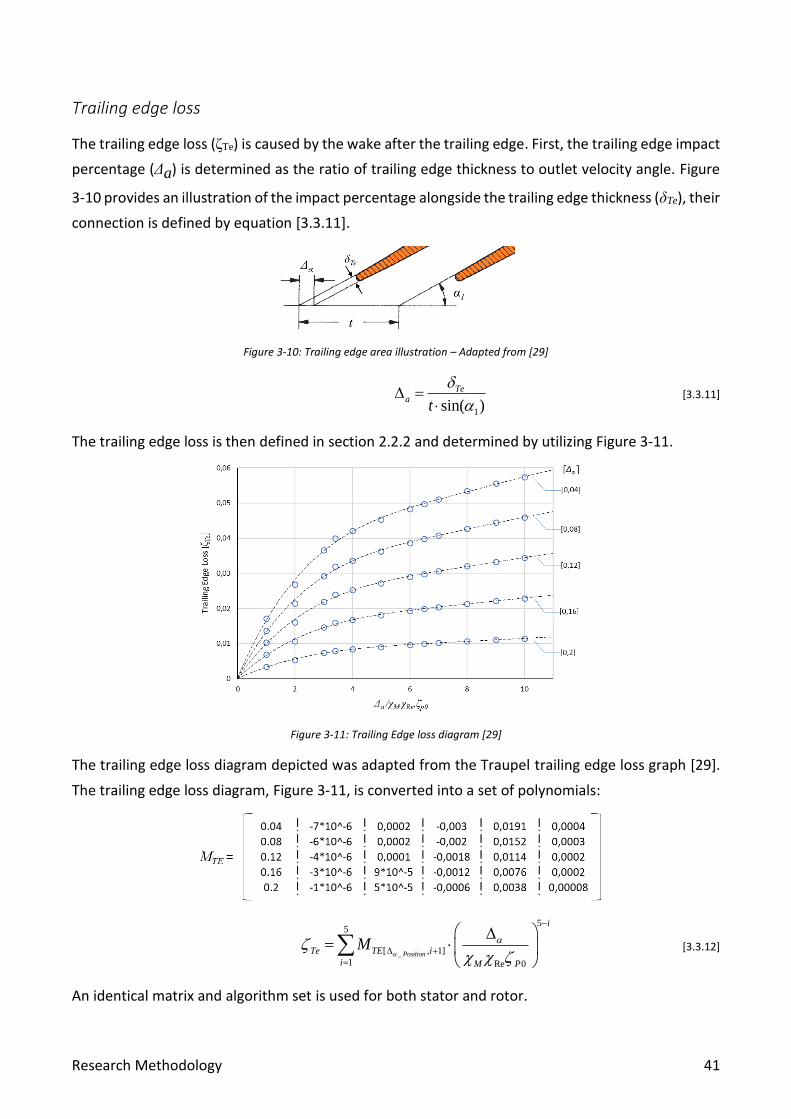
Research Methodology 41
Trailing edge loss
The trailing edge loss (ζTe) is caused by the wake after the trailing edge. First, the trailing edge impact
percentage (Δa) is determined as the ratio of trailing edge thickness to outlet velocity angle. Figure
3-10 provides an illustration of the impact percentage alongside the trailing edge thickness (δTe), their
connection is defined by equation [3.3.11].
Figure 3-10: Trailing edge area illustration – Adapted from [29]
1sin( )
Tea
t
=
[3.3.11]
The trailing edge loss is then defined in section 2.2.2 and determined by utilizing Figure 3-11.
Figure 3-11: Trailing Edge loss diagram [29]
The trailing edge loss diagram depicted was adapted from the Traupel trailing edge loss graph [29].
The trailing edge loss diagram, Figure 3-11, is converted into a set of polynomials:
_
55
[ , 1]
1 Re 0Position
i
Te TE i
i M P
M
−
+
=
=
[3.3.12]
An identical matrix and algorithm set is used for both stator and rotor.
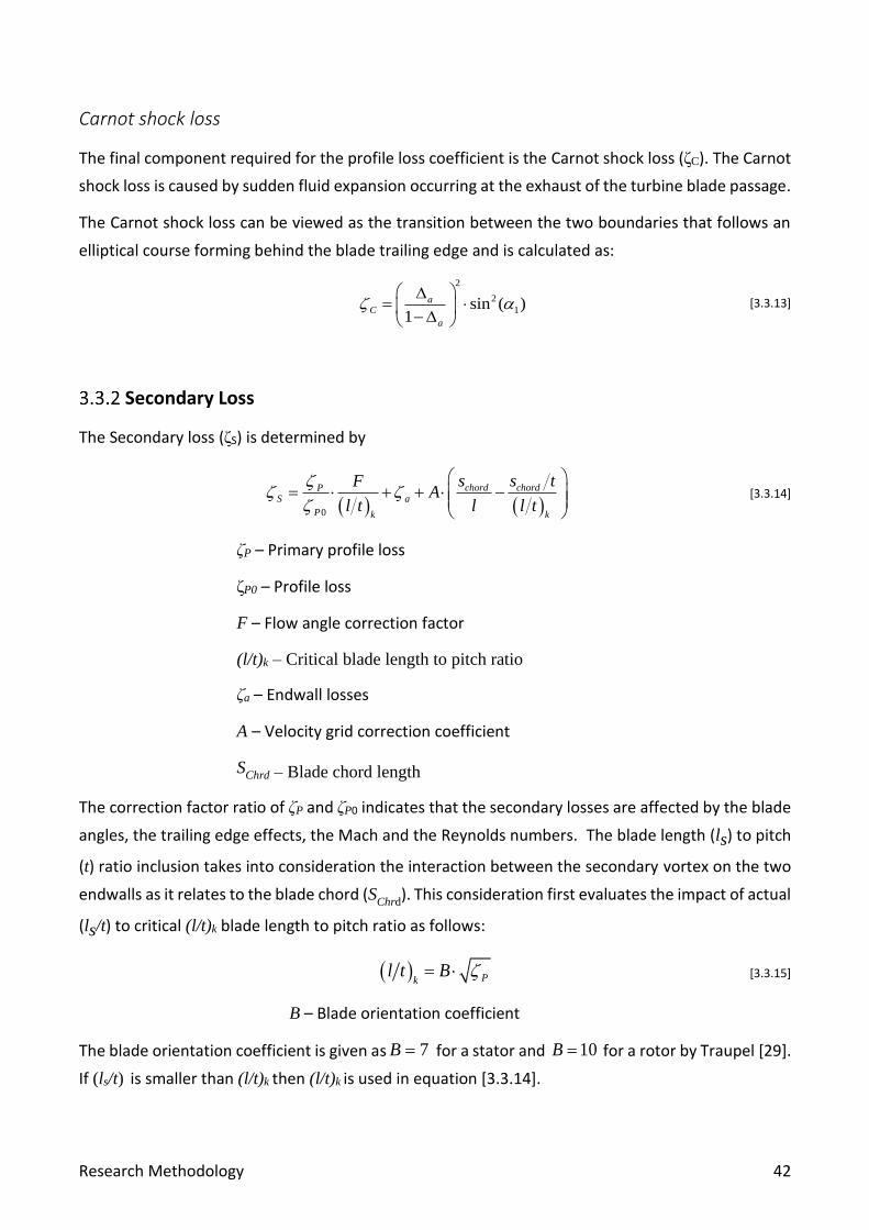
Research Methodology 42
Carnot shock loss
The final component required for the profile loss coefficient is the Carnot shock loss (ζC). The Carnot
shock loss is caused by sudden fluid expansion occurring at the exhaust of the turbine blade passage.
The Carnot shock loss can be viewed as the transition between the two boundaries that follows an
elliptical course forming behind the blade trailing edge and is calculated as:
2
2
1sin ( )1
aC
a
= −
[3.3.13]
Secondary Loss
The Secondary loss (ζS) is determined by
( ) ( )0
chord chordPS a
P k k
s s tFA
l t l l t
= + + −
[3.3.14]
ζP – Primary profile loss
ζP0 – Profile loss
F – Flow angle correction factor
(l/t)k – Critical blade length to pitch ratio
ζa – Endwall losses
A – Velocity grid correction coefficient
SChrd – Blade chord length
The correction factor ratio of ζP and ζP0 indicates that the secondary losses are affected by the blade
angles, the trailing edge effects, the Mach and the Reynolds numbers. The blade length (ls) to pitch
(t) ratio inclusion takes into consideration the interaction between the secondary vortex on the two
endwalls as it relates to the blade chord (SChrd
). This consideration first evaluates the impact of actual
(ls/t) to critical (l/t)k blade length to pitch ratio as follows:
( ) Pkl t B = [3.3.15]
B – Blade orientation coefficient
The blade orientation coefficient is given as 7B = for a stator and 10B = for a rotor by Traupel [29].
If (ls/t) is smaller than (l/t)k then (l/t)k is used in equation [3.3.14].

Research Methodology 43
Flow correction factor
The change in flow angle correction factor (F) is an indication of how the secondary flow is affected
by the difference between the inlet and the outlet flow angles (α0 ,α1) and the respective velocities.
This relationship is observed in Figure 3-12.
Figure 3-12: Flow correction factor chart – Adapted from [29]
Figure 3-12 indicates that the greater the difference between inlet and outlet angles (Δα - change
of flow angle) the greater the secondary loss will be impacted by the flow correction factor.
Similarly, the smaller the change in flow velocity ratio (cw) the greater the impact.
0 1 = − [3.3.16]
/w in outc v v= [3.3.17]
The flow correction factor diagram, Figure 3-12, is converted into a set of polynomials applicable to
both stator and rotor:
55
1_[ , 1]
i
F
iw Positionc iF M
−
=+= [3.3.18]
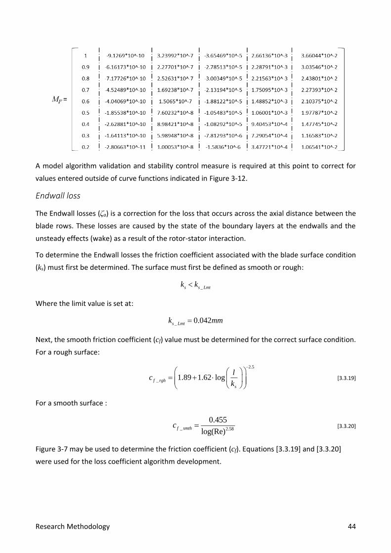
Research Methodology 44
A model algorithm validation and stability control measure is required at this point to correct for
values entered outside of curve functions indicated in Figure 3-12.
Endwall loss
The Endwall losses (ζa) is a correction for the loss that occurs across the axial distance between the
blade rows. These losses are caused by the state of the boundary layers at the endwalls and the
unsteady effects (wake) as a result of the rotor-stator interaction.
To determine the Endwall losses the friction coefficient associated with the blade surface condition
(ks) must first be determined. The surface must first be defined as smooth or rough:
_s s Lmtk k
Where the limit value is set at:
_ 0.042s Lmtk mm=
Next, the smooth friction coefficient (cf) value must be determined for the correct surface condition.
For a rough surface:
2.5
_ 1.89 1.62 logf rgh
s
lc
k
−
= +
[3.3.19]
For a smooth surface :
_ 2.58
0.455
log(Re)f smthc = [3.3.20]
Figure 3-7 may be used to determine the friction coefficient (cf). Equations [3.3.19] and [3.3.20]
were used for the loss coefficient algorithm development.
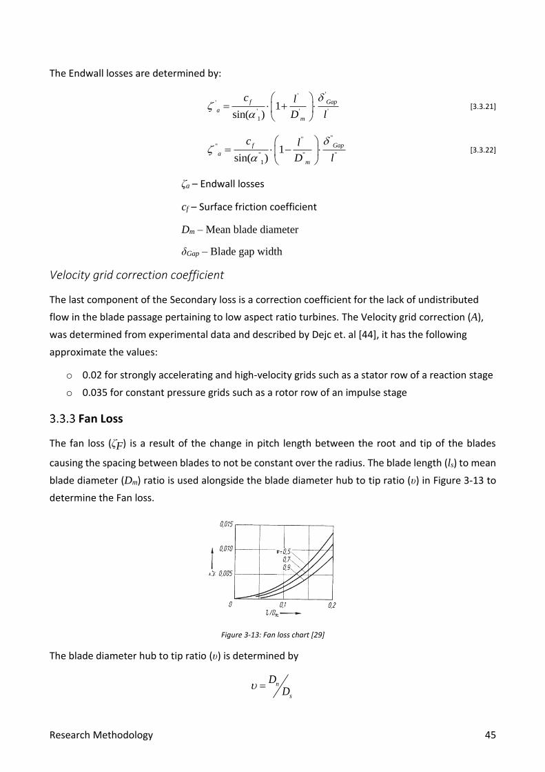
Research Methodology 45
The Endwall losses are determined by:
'''
' ' '
1
1sin( )
f Gap
a
m
c l
D l
= +
[3.3.21]
""
"
" " "
1
1sin( )
f Gap
a
m
c l
D l
= −
[3.3.22]
ζa – Endwall losses
cf – Surface friction coefficient
Dm – Mean blade diameter
δGap – Blade gap width
Velocity grid correction coefficient
The last component of the Secondary loss is a correction coefficient for the lack of undistributed
flow in the blade passage pertaining to low aspect ratio turbines. The Velocity grid correction (A),
was determined from experimental data and described by Dejc et. al [44], it has the following
approximate the values:
o 0.02 for strongly accelerating and high-velocity grids such as a stator row of a reaction stage
o 0.035 for constant pressure grids such as a rotor row of an impulse stage
Fan Loss
The fan loss (ζF) is a result of the change in pitch length between the root and tip of the blades
causing the spacing between blades to not be constant over the radius. The blade length (ls) to mean
blade diameter (Dm) ratio is used alongside the blade diameter hub to tip ratio (υ) in Figure 3-13 to
determine the Fan loss.
Figure 3-13: Fan loss chart [29]
The blade diameter hub to tip ratio (υ) is determined by
n
s
DD
=

Research Methodology 46
The fan loss increases independently with the increase in blade hub to tip ratio and the blade length
to mean diameter ratio. A simple set of polynomials were used for the development of the fan loss
component:
3
3
[ , 1]
1
( )Position
i
F Fl i
i m
lM
D −
+
=
= [3.3.23]
Due to the sizing of the graph, a stricter control measure is required to restrict extreme values for
both stator and rotor.
Tip Leakage Loss
The Tip Leakage loss (ζTl) is caused by the energy dissipation of the working fluid across the blade tip
and the mixing of the tip leakage flow with the exiting main flow. Traupel [29] provides empirical
approximations for tip leakage loss for turbine blades, classified into two groups namely unshrouded
and shrouded.
Unshrouded
Traupel presents a tip leakage loss approximation function for unshrouded turbine blades based on
experimental results obtained from the ETH Institute of Thermal Turbomachinery [29]. The
approximation function is comprised of an extensive list of variables. The tip leakage for an
unshrouded stator and an unshrouded rotor is determined respectively as:
' ' '' 2
' ' 1
' ' '
( 0.002 )2(1 )
2
Chrd nTl
m
S DR vK
l D
−− +=
[3.3.24]
" " "" 2 2
" " 2
" " "
( 0.002 )2 1
2
Chrd srTl
m
S DR v uK
l D
−+ − +=
[3.3.25]
Where the tip leakage gap mass flow percentage (φ) was determined by relating blade tip area to the
blade flow area:
' '
' n
Flow
D
A
=
[3.3.26]
" "
" s
Flow
D
A
=
[3.3.27]
An unshrouded correction coefficient (Kτ) is used in the approximation function.

Research Methodology 47
Figure 3-14: Unshrouded Correction Coefficient Chart
The unshrouded correction coefficient can be determined by using Figure 3-14 adapted from 4
diagrams provided by Traupel [29] or approximated using a set of linear curves:
22
[( 0.002) , 1]1 Position
Chrd
i
Ki
i wS
vK M
c
−
− +=
=
[3.3.28]
Figure 3-14 provides a reference guide for approximate correct value zones based on the row outlet
velocity (sin α1), this attribute must be included as a model algorithm validation function.
Shrouded
Tip leakage loss for shrouded blades incorporates the Shrouded tip leakage mass flow ratio (ω); that
indicates the portion of mass flow through the seals and the Shrouded tip leakage velocity ratio (ϒ);
that implements a correction for the tip leakage losses resulting from the inlet-outlet velocity ratio
occurring at design inlet and outlet flow angles.
Traupel [35] provides a value estimation table for the shrouded tip leakage velocity ratio (ϒ) as it
relates to the shrouded tip leakage mass flow ratio and the pressure distribution range between LP
and HP turbines.

Research Methodology 48
Both the shrouded tip leakage mass flow ratio and the derived shrouded tip leakage velocity ratio
can be determined for the stator and rotor accordingly:
1
=
− [3.3.29]
21,5318 1,3854 0,1244 = + + [3.3.30]
Then the Shrouded tip Leakage loss is calculated as:
( )
2
' 2
' ' 1
2
1
2 1 1Tl
vv
Rv
v
− = − −
[3.3.31]
2
" 3
" " 2
3
2
1
r
rTl
r
r
vv
vv
− = −
[3.3.32]
The Traupel shrouded tip leakage loss coefficient uses a generalized evaluation method and does not
incorporate exact blade seal design geometries, illustrated in Figure 3-15, into its determination.
Figure 3-15: Blade Shroud Seal Designs – Adapted from [11]
Notably, due to the complex nature of tip leakage experimental measurements, evaluation and
accuracy of theoretical approximations, it is regarded as the weak point for the loss coefficient
algorithm. A sensible amount of validation checks and stability corrections have been implemented
to improve the tip leakage approximation.
An alternative tip leakage loss modelling method is proposed by Fuls [1]. Gland seal leaks, bypass
flows and clearance leaks can be modelled in Flownex’s by utilizing a labyrinth seal component in
combination with the nozzle components, as illustrated in Figure 3-16.
Figure 3-16: Single stage model utilizing Flownex’s labyrinth seal component [1]
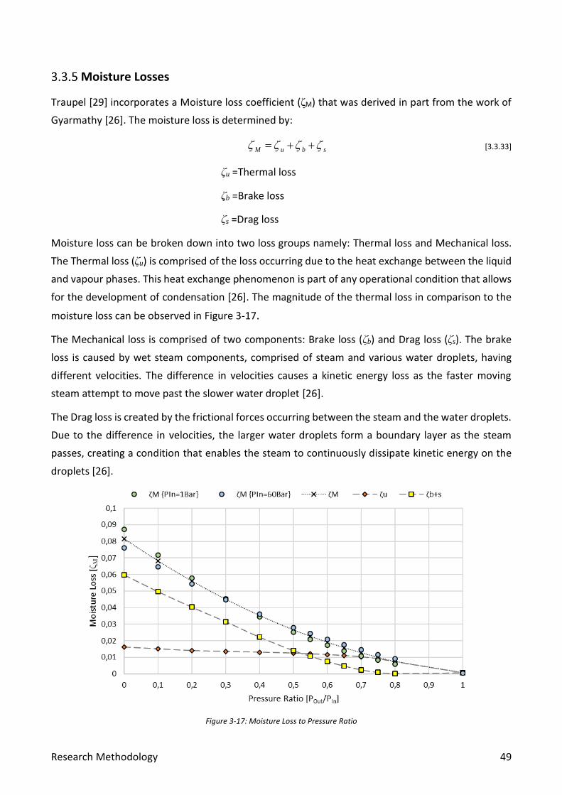
Research Methodology 49
Moisture Losses
Traupel [29] incorporates a Moisture loss coefficient (ζM) that was derived in part from the work of
Gyarmathy [26]. The moisture loss is determined by:
M u b s = + + [3.3.33]
ζu =Thermal loss
ζb =Brake loss
ζs =Drag loss
Moisture loss can be broken down into two loss groups namely: Thermal loss and Mechanical loss.
The Thermal loss (ζu) is comprised of the loss occurring due to the heat exchange between the liquid
and vapour phases. This heat exchange phenomenon is part of any operational condition that allows
for the development of condensation [26]. The magnitude of the thermal loss in comparison to the
moisture loss can be observed in Figure 3-17.
The Mechanical loss is comprised of two components: Brake loss (ζb) and Drag loss (ζs). The brake
loss is caused by wet steam components, comprised of steam and various water droplets, having
different velocities. The difference in velocities causes a kinetic energy loss as the faster moving
steam attempt to move past the slower water droplet [26].
The Drag loss is created by the frictional forces occurring between the steam and the water droplets.
Due to the difference in velocities, the larger water droplets form a boundary layer as the steam
passes, creating a condition that enables the steam to continuously dissipate kinetic energy on the
droplets [26].
Figure 3-17: Moisture Loss to Pressure Ratio

Research Methodology 50
The work of Gyarmathy [26] and Hiroyuki et. al. [25] was used to improve on the correlation provided
by Traupel [35] producing the Moisture loss to pressure ratio chart in Figure 3-17. The Moisture loss
can then be determined by:
2
0.0581 0.139 0.0815out outM
in in
p p
p p
= − +
[3.3.34]
A model algorithm validation function is used to only initiate the Moisture loss function if the steam
quality drops below 99% and the pressure ratios are within limits.
Note that the unique phenomenon of supersaturation must be incorporated into the validation
function. Supersaturation occurs when the steam state does not follow the exact equilibrium curves
when crossing the saturation line whilst travelling inside a blade passage.
This deviation results from the condensation phase experiencing a delay that is followed by a sudden
phase shift, creating an instantaneous collapse from steam to droplet state requiring the initiation of
the Moisture Loss function.
LSB Losses
The Last Stage Blade loss coefficient (ζLSB), specific to the loss coefficient algorithm, is solely
comprised of the loss incurred by the last stage blades interconnections. The loss is based on the
frictional and separation flow forces generated by the reduction in flow area and the respective flow
disturbance resulting from the interconnection [29]. Figure 3-18 provides an LSB interconnection
geometry guide.
Figure 3-18: LSB Interconnection Geometry – Adapted from [29]
The LSB loss is determined for both stator and rotor by:
2
2
1 2 2 28 Sin LSB LSB
LSB LSB
LSB s n
D dtx
l D D
=
− [3.3.35]

Research Methodology 51
The last stage blade interconnection shape specific drag coefficient (xLSB) is determined from the drag
coefficient values illustrated in Table 2-1 [35]. The loss coefficient algorithm has a manual input
validation check and correction requirement for xLSB.
Table 3-1: LSB Interconnection Drag Coefficient
The turbine blade interconnection script input variables are indicated at the end of Figure 3-4
This concludes all the components required for the design condition modelling section of the loss
coefficient algorithm. All the loss coefficient components are calculated and combined as indicated
in equation [3.3.1] to form the master equation of the loss coefficient algorithm.
3.4 Off-design loss coefficient algorithm
The loss coefficient developed by Traupel [29] can be corrected for off-design conditions by
implementing Zehner’s [24] loss coefficient methodology. The Zehner loss coefficient (ζP_Z) focuses
on determining turbine performance at off-design conditions. Traupel's loss coefficient is used as the
basis for Zehner's loss coefficient, thus utilizing the same primary profile enthalpy loss (ζP) coefficient
characteristics determined in section 3.3 .
The Zehner loss coefficient applies the following correction on the zero-incidence design profile loss
condition determined by Traupel’s loss coefficient [24]:
_ 1 (1 )Zb
aZ i
P Z P − = − − [3.3.36]
ζP_Z – Zehner Profile loss coefficient
ζP – Traupel Profile loss
Δi – Difference in angle of attack from design
Za & Zb – Cascade geometry character correction

Research Methodology 52
The Zehner correction requires first the determination of the incidence angle (αInc). Figure 3-19
indicates the working fluid inlet angle conventions for both the rotor and the stator blade rows. The
inlet angles are adjusted to illustrate the incidence angles for off-design turbine speeds (-u, +u) with
regards to design speed (u).
Notably, the turbine speed and off-design speeds are configured into the loss coefficient algorithm
script under the “Turbine Data” section illustrated in Figure 3-4.
Figure 3-19: Rotor and Stator Inlet Angle Orientation
The negative incidence angles move towards the convex pressure blade surface whilst the positive
incidence angle moves towards the concave suction blade surface. The incidence angle is determined
as the difference between the converted design inlet angle (α0) and the off-design inlet angle (αOD):
0(180 )Inc OD = − − [3.3.37]
The difference to the design angle of attack (Δi) is then determined with regards to the impact the
incidence angle has. If 0 0Inc − , then:
0
180
Inc
Inc
i
− =
− [3.3.38]
Otherwise:
0 Inc
Inc
i
− =
− [3.3.39]
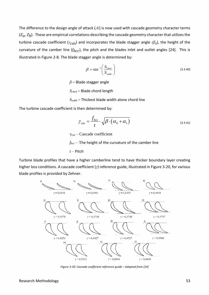
Research Methodology 53
The difference to the design angle of attack (Δi) is now used with cascade geometry character terms
(Za, Zb). These are empirical correlations describing the cascade geometry character that utilizes the
turbine cascade coefficient (γcas) and incorporates the blade stagger angle (βs), the height of the
curvature of the camber line (fhcc), the pitch and the blades inlet and outlet angles [24]. This is
illustrated in Figure 2-8. The blade stagger angle is determined by:
1sin chrd
wdth
S
S − =
[3.3.40]
β – Blade stagger angle
Schrd – Blade chord length
Swdth – Thickest blade width alone chord line
The turbine cascade coefficient is then determined by:
( )0 1hcc
cas
f
t = + [3.3.41]
γcas – Cascade coefficient
fhcc – The height of the curvature of the camber line
t – Pitch
Turbine blade profiles that have a higher camberline tend to have thicker boundary layer creating
higher loss conditions. A cascade coefficient (γ) reference guide, illustrated in Figure 3-20, for various
blade profiles is provided by Zehner.
Figure 3-20: Cascade coefficient reference guide – Adapted from [24]

Research Methodology 54
Figure 3-20 is used as a validation check platform. Za and Zb cascade geometry character correlations
are determined as follow:
If 0i , then:
22.587 0.426 1.21a cas casZ = − − [3.3.42]
24.175 10.802 13.881b cas casZ = − − [3.3.43]
Else
20.446 3.82 2.899a cas casZ = − − [3.3.44]
22.413 10.38 10.116b cas casZ = − − [3.3.45]
The Off-Design loss coefficient (ζTZLC) is now determined by rewriting Traupel’s enthalpy loss
coefficient as a function of Zehner’s profile loss correction.
_TZLC P Z S Tl F LSB M = + + + + + [3.3.46]
Additionally, a model algorithm stability function is required to ensure that the incidence angles are
within limits and orientated correctly for both stator and rotor. The inlet stator row is excluded from
the off-design coefficient algorithm, whilst the remainder has a simple inlet angle check function.
Figure 3-21: Off-design Turbine Stator Inlet Angle Triangles
The check function utilizes Figure 3-21 and the law of sines. For -u < u:
0
1
Sin( ' ) Sin( ' )
"
Inc
xu v
=
[3.3.47]
An equivalent approach is used for the overspeed (+u > u) of a turbine and the rotor inlet angle check
function.
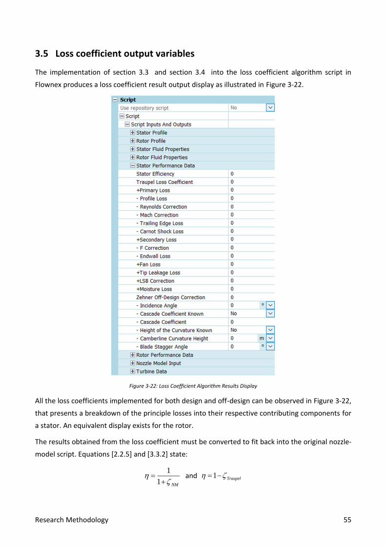
Research Methodology 55
3.5 Loss coefficient output variables
The implementation of section 3.3 and section 3.4 into the loss coefficient algorithm script in
Flownex produces a loss coefficient result output display as illustrated in Figure 3-22.
Figure 3-22: Loss Coefficient Algorithm Results Display
All the loss coefficients implemented for both design and off-design can be observed in Figure 3-22,
that presents a breakdown of the principle losses into their respective contributing components for
a stator. An equivalent display exists for the rotor.
The results obtained from the loss coefficient must be converted to fit back into the original nozzle-
model script. Equations [2.2.5] and [3.3.2] state:
1
1 NM
=+
and 1 Traupel = −
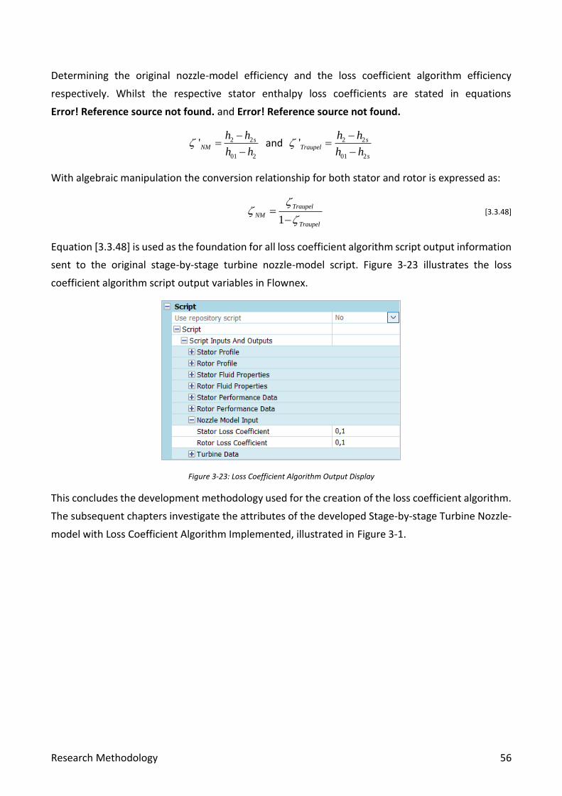
Research Methodology 56
Determining the original nozzle-model efficiency and the loss coefficient algorithm efficiency
respectively. Whilst the respective stator enthalpy loss coefficients are stated in equations
Error! Reference source not found. and Error! Reference source not found.
2 2
01 2
' sNM
h h
h h
−=
− and 2 2
01 2
' sTraupel
s
h h
h h
−=
−
With algebraic manipulation the conversion relationship for both stator and rotor is expressed as:
1
Traupel
NM
Traupel
=
− [3.3.48]
Equation [3.3.48] is used as the foundation for all loss coefficient algorithm script output information
sent to the original stage-by-stage turbine nozzle-model script. Figure 3-23 illustrates the loss
coefficient algorithm script output variables in Flownex.
Figure 3-23: Loss Coefficient Algorithm Output Display
This concludes the development methodology used for the creation of the loss coefficient algorithm.
The subsequent chapters investigate the attributes of the developed Stage-by-stage Turbine Nozzle-
model with Loss Coefficient Algorithm Implemented, illustrated in Figure 3-1.

Algorithm Validation: AGARD Test Case 57
Chapter 4 Algorithm Validation: AGARD Test Case
This chapter serves as a validation case study for the implementation of the loss coefficient algorithm
into the nozzle-model. The stage-by-stage nozzle model was tested against a well calibrated and
measured gas turbine test case of the Advisory Group for Aerospace Research and Development
(AGARD). The AGARD gas turbine test case presents a rare validation opportunity in the sense that the
loss coefficient algorithm could be tested against the stage-by-stage nozzle model [1] and an extensively
well-documented turbine validation case [45].
Upon further investigation, it was found that the AGARD report [45] provides a range of different
compressor and turbine test cases. The test case utilized for validation (E/TU-4) is an air turbine rig
comprised of four stator-rotor stages, illustrated in Figure 4-1. E/TU-4 was predominantly developed
for the investigation of industrial turbine characteristics.
Figure 4-1: AGARD 4-Stage Turbine Cross-section View [45]
The E/TU-4 test case consisted of seven test scenarios. Each scenario investigates the turbine
thermodynamic parameters and performance for a specific combination of mass flow rate and
turbine rotational speed.
A previous study, conducted by Pottas [40], provides detailed turbine blade geometries for the
AGARD E/TU-4 test case. The blade geometries where developed by interpolating various turbine
coordinate data points, that describe the blade profiles, obtained from the AGARD report [45].

Algorithm Validation: AGARD Test Case 58
The AGARD test case E/TU-4 has the following attributes that further justify its use as a validation case:
▪ The turbine rig has an open loop configuration that measures mass flow upstream from the turbine
inlet with a venturi tube.
▪ The Inlet, exhaust and the inter-stage air pressures, temperatures and flow velocities were
measured with a traversing probe.
▪ Turbine rotational speed and torque are measured in association with a connected
dynamometer.
▪ Each stage has identical blade profile designs.
The development and validation of an equivalent loss coefficient algorithm model aims to show the
comparative modelling ability between the original nozzle-model (with calibrated and fixed loss
coefficients) and the loss coefficient nozzle-model (with calculated and variable loss coefficients).
Additionally, the loss coefficient nozzle model should display additional row specifics information
resulting from the inclusion of turbine blade geometry.
The case study evaluation requirements were:
▪ Validate the loss coefficient stage-by-stage turbine nozzle-model methodology.
▪ Display additional attributes obtained by the implementation of the loss coefficient
algorithms.
Note: The following abbreviations used for the result tables and graphs:
▪ NM - Stage-by-stage turbine nozzle-model
▪ LCNM - Loss coefficient stage-by-stage turbine nozzle-model
▪ Test - AGARD gas turbine test case
Model development
Figure 4-2 depicts the AGARD E/TU-4 loss coefficient nozzle model Flownex configuration.
Figure 4-2: AGARD Flownex Model Layout
The turbine geometric information required along with the turbine performance information was
obtained from the AGARD test case [45, 40].

Algorithm Validation: AGARD Test Case 59
The boundary conditions and nozzle areas were set identical to the original nozzle-model [1] and
then slightly adjusted to achieve the desired mass flow at the design condition. No calibration was
made to the loss coefficients. Carry-over losses were defined the same as for the nozzle model.
AGARD Gas Turbine Boundary Conditions
Inlet Total Pressure: 257,6 kPa Working fluid: Air
Inlet Temperature: 131,5 ˚C Mass flow calibration: 6.45 kg/s
Exhaust Total Pressure: 105 kPa RPM: 7500
Results and Discussion
The first result reviewed is the comparison of total and static pressure across the turbine stages of
Test and LCNM. From Table 4-1 an average total and static pressure error of 0.29% and 0.95% is
observed respectively. When comparing LCNM and NM similar results are obtained, an overall
deviation of 0.38% is observed.
Table 4-1: AGARD Pressure Result Comparison
Po
int Total Pressure [kPa]
Test
|LC
NM
D
iff.
[%
]
NM
|LC
NM
D
iff.
[%
]
Static Pressure [kPa]
Test
|LC
NM
Dif
f. [
%]
NM
|LC
NM
Dif
f. [
%]
Test NM LCNM Test NM LCNM
0 257,6 257,6 257,5 0,04 0,04 252,9 252,9 253,0 0,05 0,05
1 211,9 212 211,9 0,02 0,06 206,6 209,4 209,5 1,41 0,06
2 170 170,3 169,0 0,61 0,79 165,6 168,0 166,7 0,66 0,77
3 134,6 134,8 133,6 0,77 0,92 130,9 132,8 131,6 0,56 0,87
4 105 105 105,0 0,00 0,00 101,3 103,0 103,4 2,08 0,39
A total and static pressure comparative graph is illustrated in Figure 4-3.
Figure 4-3: AGARD Total & Static Pressure Comparison

Algorithm Validation: AGARD Test Case 60
Table 4-2 presents a temperature and velocity comparison. The temperature obtained an error range
of between 0.28% to a maximum of 3.14%. The comparative studies found that the there is a high
level of accuracy obtained by the LCNM. With the only exception is the comparison of velocities,
where a sizable average difference of 22% was obtained between Test and LCNM. Whilst an average
error of 0.8% is obtained between LCNM and NM.
Table 4-2: AGARD Temperature Result Comparison
Po
int Temperature [˚C]
Test
|LC
NM
D
iff.
[%
]
NM
|LC
NM
Dif
f. [
%]
Velocity [m/s]
Test
|LC
NM
D
iff.
[%
]
Test
|LC
NM
D
iff.
[%
]
Test NM LCNM Test NM LCNM
0 131,5 131,5 132,0 0,38 0,38 65,6 65,5 65,2 0,61 0,46
1 111,7 111,8 112,0 0,28 0,19 75 52,5 51,8 30,93 1,33
2 90,0 91,6 90,7 0,82 0,94 74,8 54,7 54,1 27,67 1,10
3 67,2 70,6 69,3 3,14 1,83 74,2 54,6 55,2 25,61 1,10
4 47,8 48,4 48,0 0,34 0,91 82,7 58,2 58,1 29,75 0,17
The velocity differences can in part be accredited to the slightly larger deviation obtained in the static
pressure values compared to the total pressure values. The correlation between static pressure and
velocity is significant enough that if the model was to be more finely tuned to better predict static
pressure it could be presumed that a better velocity correlation could be obtained. Further
investigation of different AGARD E/TU-4 models indicates similar velocity deviation percentages.
Since losses mainly affect the temperatures, one can conclude that the nozzle loss coefficients as
calculated by the LCNM are trustworthy. The loss coefficient algorithm additionally produced turbine
performance data related to turbine losses, presented in Table 4-3.
Table 4-3: AGARD Turbine Loss Performance Data
Performance Data Stage 1 Stage 2 Stage 3 Stage 4
Stator Rotor Stator Rotor Stator Rotor Stator Rotor
Efficiency [%] 91,34 91,66 93,05 90,29 92,95 90,58 92,73 89,33
Row Loss Coefficient 0,087 0,083 0,069 0,097 0,071 0,094 0,073 0,107
+Primary Loss 0,034 0,043 0,029 0,057 0,029 0,052 0,028 0,048
- Profile Loss 0,028 0,042 0,027 0,057 0,026 0,052 0,026 0,049
- Reynolds Correction 1,089 0,962 0,925 0,953 0,919 0,944 0,914 0,935
- Mach Correction 1,000 1,000 1,000 1,000 1,000 1,000 1,000 1,000
- Trailing Edge Loss 0,004 0,002 0,004 0,002 0,004 0,002 0,005 0,002
- Carnot Shock Loss 0,0001 0,0002 0,0002 0,0002 0,0002 0,0002 0,0002 0,0002
+Secondary Loss 0,035 0,013 0,022 0,012 0,021 0,012 0,020 0,012
- F Correction 0,049 0,027 0,039 0,030 0,042 0,029 0,042 0,029
- Endwall Loss 0,0004 0,0001 0,0003 0,0001 0,0002 0,0001 0,0002 0,0002
+Fan Loss 0,010 0,012 0,014 0,016 0,018 0,020 0,022 0,024
+Tip Leakage Loss 0,007 0,015 0,004 0,013 0,003 0,011 0,002 0,024

Algorithm Validation: AGARD Test Case 61
From the turbine loss performance data, it is determined that the overall turbine efficiency is 91.49%
that compares favourably with the AGARD Test case data result of 91.3%. The AGARD loss coefficient
nozzle-model obtains an efficiency prediction accuracy of 99.3%.
Additionally, a visual turbine overall loss distribution graph is illustrated in Figure 4-4.
Figure 4-4: AGARD Turbine Loss Distribution
It can be inferred that the largest contributing factors to the turbine performance loss are associated
with the losses occurring from boundary layer development and the subsequent kinetic energy
losses. This is indicated by the loss distribution illustrated in the turbine losses data, Table 4-3.
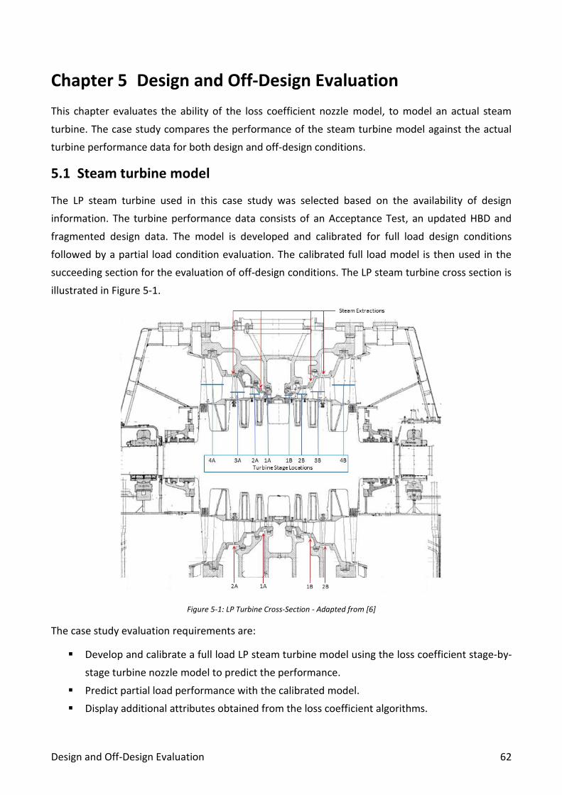
Design and Off-Design Evaluation 62
Chapter 5 Design and Off-Design Evaluation
This chapter evaluates the ability of the loss coefficient nozzle model, to model an actual steam
turbine. The case study compares the performance of the steam turbine model against the actual
turbine performance data for both design and off-design conditions.
5.1 Steam turbine model
The LP steam turbine used in this case study was selected based on the availability of design
information. The turbine performance data consists of an Acceptance Test, an updated HBD and
fragmented design data. The model is developed and calibrated for full load design conditions
followed by a partial load condition evaluation. The calibrated full load model is then used in the
succeeding section for the evaluation of off-design conditions. The LP steam turbine cross section is
illustrated in Figure 5-1.
Figure 5-1: LP Turbine Cross-Section - Adapted from [6]
The case study evaluation requirements are:
▪ Develop and calibrate a full load LP steam turbine model using the loss coefficient stage-by-
stage turbine nozzle model to predict the performance.
▪ Predict partial load performance with the calibrated model.
▪ Display additional attributes obtained from the loss coefficient algorithms.

Design and Off-Design Evaluation 63
Model Development
Figure 5-2 depicts the LP steam turbine loss coefficient nozzle model Flownex configuration. Four
distinctive steam extraction points are indicated, correlating to the LP steam turbine design
configuration. Note that the double-flow arrangement is modelled as two parallel turbines, each
with their individual extractions. This is because the extractions are not symmetrical between the
two flows.
Figure 5-2: LPST Flownex Model Layout
For the determination of the turbine loss coefficients each stage’s blade geometry variables are
required as per Figure 3-4. The blade geometries were extrapolated using methods discussed in
section 2.1.2 from obtained information.
The general turbine rotor, casing and blade diameters, widths and spacings were measured from a
turbine cross-section illustration. Further motivation for the use of this specific turbine case was the
availability of blade specific information such as the number of blades and the blade surface finish.
The LP turbine the pitch, blade throat, blade chord length and other stator blade profiles parameters
were estimated from literature [8]. This enabled the determination of the blade design inlet and
outlet angles as well as the remainder of the required blade variables.
The assumption was made to determine the blade angles across the mean blade diameter line.
Additionally, the specification and spacing of the blade shrouding were available in the design data
along with the LSB interconnection design information.
The model boundary conditions are obtained from the design information and heat balance diagram
[6]. The steam temperatures and pressures at the four extraction points are used as validation
parameters, whilst the mass flow is used as a boundary condition calibration value.

Design and Off-Design Evaluation 64
The design information of the LP turbine indicated identical inlet conditions for both flow directions.
Once the model was developed it was calibrated according to the method discussed in section 3.5
LPST Full Load Boundary Conditions
Inlet Total Pressure: 400 kPa Working fluid: Steam
Inlet Temperature: 147.9 ˚C Mass flow calibration: 88.72 kg/s
Exhaust Total Pressure: 5,35 kPa RPM: 3000
Extraction 1A: 3.867 kg/s Extraction 2A: 0.967 kg/s
Extraction 1B: 4.136 kg/s Extraction 2B: 0.967 kg/s
Note: The following abbreviations used for the result tables and graphs:
▪ LCNM - LPST Loss coefficient stage-by-stage turbine nozzle-model
▪ LPST – Low-pressure steam turbine acceptance test dated 1970
▪ HBD – Based on an updated turbine performance review dated 1990
▪ LCNMPL – Partial load LPST Loss coefficient stage-by-stage turbine nozzle-model
Results and Discussion
The first set of results, presented in Table 5-1, compare the total pressure and temperature for the
various boundary points at full load conditions.
Table 5-1: LPST Full Load Result Comparison
Point
Total Pressure [kPa]
LPST
-LC
NM
D
iff.
[%
]
HB
D-L
CN
M
Dif
f. [
%] Temperature [˚C]
LPST
-LC
NM
D
iff.
[%
]
HB
D-L
CN
M
Dif
f. [
%]
LPST HBD LCNM LPST HBD LCNM
Inlet 400 400 400,0 0,00 0,00 150 147,9 147,9 1,40 0,00 Extraction 1a 144 149 148,4 3,07 0,39 110 111,0 110,5 0,46 0,40 Extraction 1b 48,5 48,8 48,6 0,21 0,41 80 80,4 81,2 1,50 1,00 Extraction 2a 15,3 15,7 16,1 5,36 2,68 54 54,7 54,9 1,67 0,46 Extraction 2b 15,3 15,7 16,2 5,95 3,25 54 54,7 54,9 1,67 0,46
Exhaust 5,35 5 5,0 6,54 0,00 33,75 32,0 32,9 2,59 2,73
From Table 5-1 average errors of 1.12%, for total pressure, and 1.55 %, for temperature, are observed
between the HDB and the LCNM. The loss coefficient nozzle-model achieves a high level of accuracy
against both acceptance test and HBD conditions. The model indicates that the turbine should
produce 35.25 MW, which compares reasonably to the initial rating of 36 MW.
Figure 5-3 provides a visual comparison of the total pressure and temperature. Notably, the model
produces results comfortably within the range of the of assessment values.

Design and Off-Design Evaluation 65
Figure 5-3: Full Load LPST Total Pressure Comparison
In addition to the general thermodynamic parameters, the loss coefficient algorithm produced
turbine performance data related to turbine losses. Presented in Table 5-2 is a subset of data
comparing the loss profiles for one side of the LP steam turbine, the complete set is provided in
Appendix A. Figure 5-4 presents an overall turbine loss distribution.
Figure 5-4: Overall Full Load LPST Loss Distribution
Table 5-2: Full Load LPST Section B Loss Performance Data
Performance Data
Stage 1B Stage 2B Stage 3B Stage 4B
Stator Rotor Stator Rotor Stator Rotor Stator Rotor
Efficiency [%] 89,41 83,55 91,15 88,30 94,52 89,44 87,23 81,30
Row Loss Coefficient 0,106 0,165 0,089 0,117 0,055 0,106 0,128 0,187
Primary Loss 0,026 0,048 0,027 0,062 0,022 0,048 0,032 0,044
Secondary Loss 0,056 0,018 0,039 0,010 0,015 0,004 0,011 0,003
Fan Loss 0,000 0,000 0,000 0,001 0,007 0,008 0,026 0,027
Tip Leakage Loss 0,024 0,039 0,023 0,045 0,011 0,026 0,017 0,020
LSB Correction 0,000 0,000 0,000 0,000 0,000 0,000 0,000 0,024
Moisture Loss 0,000 0,000 0,000 0,000 0,000 0,000 0,032 0,069
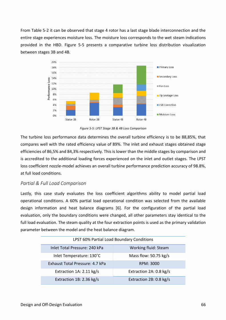
Design and Off-Design Evaluation 66
From Table 5-2 it can be observed that stage 4 rotor has a last stage blade interconnection and the
entire stage experiences moisture loss. The moisture loss corresponds to the wet steam indications
provided in the HBD. Figure 5-5 presents a comparative turbine loss distribution visualization
between stages 3B and 4B.
Figure 5-5: LPST Stage 3B & 4B Loss Comparison
The turbine loss performance data determines the overall turbine efficiency is to be 88,85%, that
compares well with the rated efficiency value of 89%. The inlet and exhaust stages obtained stage
efficiencies of 86,5% and 84,3% respectively. This is lower than the middle stages by comparison and
is accredited to the additional loading forces experienced on the inlet and outlet stages. The LPST
loss coefficient nozzle-model achieves an overall turbine performance prediction accuracy of 98.8%,
at full load conditions.
Partial & Full Load Comparison
Lastly, this case study evaluates the loss coefficient algorithms ability to model partial load
operational conditions. A 60% partial load operational condition was selected from the available
design information and heat balance diagrams [6]. For the configuration of the partial load
evaluation, only the boundary conditions were changed, all other parameters stay identical to the
full load evaluation. The steam quality at the four extraction points is used as the primary validation
parameter between the model and the heat balance diagram.
LPST 60% Partial Load Boundary Conditions
Inlet Total Pressure: 240 kPa Working fluid: Steam
Inlet Temperature: 130˚C Mass flow: 50.75 kg/s
Exhaust Total Pressure: 4.7 kPa RPM: 3000
Extraction 1A: 2.11 kg/s Extraction 2A: 0.8 kg/s
Extraction 1B: 2.36 kg/s Extraction 2B: 0.8 kg/s

Design and Off-Design Evaluation 67
Results and Discussion
The results presented in Table 5-3 compare the total pressure and steam quality for the various
boundary points at 60% partial load conditions. The pressure boundary condition results indicate an
average error of 2.86%, with the largest deviations occurring at extraction points 2A and 2B.
Temperature was excluded from the comparison as the HDB only provides a possible steam quality
for the extraction points. The steam quality comparison indicates an approximate error of 1.24%.
Table 5-3: 60% Partial Load LPST Result Comparison
Point
Total Pressure [kPa] HBD-LCNMPL Diff. [%]
Steam Quality HBD-LCNMPL Diff. [%]
HBD LCNMPL HBD LCNMPL
Inlet 240 240,0 0,00 130˚C 130˚C 0,00
Extraction 1a 88 88,2 0,19 0,96 0,980 1,72
Extraction 1b 29,8 29,5 0,95 0,93 0,938 1,04
Extraction 2a 10,1 10,9 7,59 0,91 0,923 1,41
Extraction 2b 10,1 11,0 8,43 0,91 0,924 1,52
Exhaust 4,7 4,7 0,00 0,89 0,901 1,78
The 60% partial load model indicates a power production of 20,3 MW at an overall turbine efficiency
of 87,96%. This equates to 57,7% of the full load 35,25MW LCNM power production. The partial load
operational condition reduces the overall LCNM turbine efficiency by 1.1%.
The partial load LCNM results compare favourably with the HBD partial load values. The actual LPST
power production rating at 60% partial load is unknown but is estimated to be 21.3MW equating to
an estimated 5.9% error made by the 60% partial load LCNM.
Table 5-4 presents the 60% partial load LPST loss performance data comparable to the full load
equivalent presented in Table 5-2. It can be observed that both stage 3B and 4B experiences moisture
loss. The additional moisture loss corresponds to the increased wet steam condition indicated by the
HBD.
Table 5-4: 60% Partial Load LPST Section B Loss Performance Data
Performance Data
Stage 1B Stage 2B Stage 3B Stage 4B
Stator Rotor Stator Rotor Stator Rotor Stator Rotor
Efficiency [%] 89,40 83,63 89,65 88,37 92,22 89,44 87,48 78,88
Row Loss Coefficient 0,106 0,164 0,104 0,116 0,078 0,106 0,125 0,211
Primary Loss 0,026 0,048 0,027 0,062 0,022 0,048 0,038 0,066
Secondary Loss 0,056 0,017 0,039 0,010 0,015 0,004 0,013 0,004
Fan Loss 0,000 0,000 0,000 0,001 0,007 0,008 0,026 0,027
Tip Leakage Loss 0,024 0,039 0,023 0,044 0,011 0,046 0,017 0,020
LSB Correction 0,000 0,000 0,000 0,000 0,000 0,000 0,000 0,024
Moisture Loss 0,000 0,000 0,000 0,000 0,001 0,004 0,043 0,069

Design and Off-Design Evaluation 68
Figure 5-6 provides a visual comparison between the 60% partial load (PL) and full load (FL) LPST
performance loss distributions presented in Table 5-4 and Table 5-2 respectively.
Figure 5-6: Full & Partial Load Section B Loss Distribution Comparison
The largest increase in turbine loss can be observed in the 60% partial load rotor 4B. Whilst an
incremental formation of moisture loss can be observed on stator 3B and rotor 3B. The 60% partial
load LPST LCNM evaluation presents the loss coefficient algorithms reasonable ability to predict
partial load performance with minimal model configuration requirements.
This LPST design case model will be used in the following section as the calibrated model and used
for the comparison between design and off-design conditions.

Design and Off-Design Evaluation 69
5.2 Off-Design impact assessment
Power utility turbines are often designed to run at only one optimal spin or rotational speed that
corresponds to a power grids unique operating frequency. For a 50Hz power grid, the optimal design
values are either 3000-rpm or 1500-rpm, depending on whether the generator is a 2-pole or 4-pole
machine. When a turbine deviates from design speed it is usually cause for concern.
Most power utilities will allow, for a short correctable time period, a slight deviation in output power
frequency. Predetermined trip values, for turbine-generator sets, activate when the unit operates
outside of optimal or safe conditions. For a 50Hz network, a deviation of ±5Hz is tolerable for a very
limited time period due to the extreme risk associated with the respective operational conditions.
For this reason, the off-design conditions corresponding to 45Hz and 55Hz will be investigated here.
The 5% frequency deviation correlates to the turbine critical speeds. Turbine critical speeds are
defined as the specific turbine spin speeds that induce turbine shaft resonance. Resonance typically
occurs when the frequency, magnitude and orientation of an oscillating excitation force, acting on a
rotor, corresponds with a natural frequency. The critical speeds are set at a 10% separation margin
from the design speed [46]. For a 3000-rpm turbine, the critical speeds are associated with 2700-rpm
and 3300-rpm.
The off-design assessment uses the LP steam turbine model developed for design conditions in the
prior section. The Flownex model and actual turbine configurations can be observed in Figure 5-1 and
Figure 5-2. The case study evaluation requirements are:
▪ Predict the performance deviation of a LP steam turbine caused by a change in turbine
operational speed. Test for multiple operational conditions comparing to measured Off-
Design Condition data
▪ Display additional attributes obtained by the implementation of the loss coefficient
algorithms: Focused on “Incidence Angle”.
Note: The following abbreviations used for the result tables and graphs:
▪ LCNM – Design condition Loss coefficient stage-by-stage turbine nozzle-model
▪ 2700, 3300 – Off-design condition Loss coefficient stage-by-stage turbine nozzle-model
Model development
The model boundary conditions are set to heat balance diagram [6] values. No other changes were
done to the calibrated design LP steam turbine model. The turbine speed was adjusted to the off-
design evaluation parameters. The LP steam turbine model spin speed, for all LCNM components,
can be controlled via a Flownex data link that fixes the spin speed to the desired value.

Design and Off-Design Evaluation 70
LPST Off-Design Boundary Conditions
Inlet Total Pressure: 400 kPa Working fluid: Steam
Inlet Temperature: 147.9 ˚C Mass flow calibration: 88.725 kg/s
Exhaust Total Pressure: 5 kPa RPM: 3000
+10% rpm: 3300 [55Hz] -10% rpm: 2700 [45Hz]
Additionally, the Cascade coefficient input values are required for the determination of the off-design
performance losses. The Cascade coefficient plays a significant role in the Zehner correction factor,
see section 3.4 . For this the turbine blade profiles can be compared to the Cascade coefficient
reference guide, presented in Figure 3-20, or calculated by equation [3.3.41].
Figure 5-7: Cascade Coefficient Determination Example
Results and Discussion
Table 5-5 presents the off-design findings related to total pressure and temperature. From these
results an average temperature deviation of 2,49% and 2,97% were observed for the 2700rpm and
3300rpm speeds respectively.
Table 5-5: Off-design Total Pressure & Temperature Comparison
Point
Total Pressure [kPa] Temperature [˚C]
LCNM 2700 3300 LCNM 2700 3300
Inlet 400 399,9 399,9 147,9 148 148,9 Extraction 1a 148,4 143,9 144,1 110,5 109,8 110,1 Extraction 1b 48,60 48,39 48,38 81,2 80,5 80,4 Extraction 2a 16,12 17,06 18,3 54,9 58,5 58,16 Extraction 2b 16,21 18,02 18,7 54,9 57,87 58,8 Exhaust 5 5,2 5,16 32,88 33,58 34,10
The largest pressure deviation occurs at the low-pressure extraction points for different operational
speeds, which correspondence to higher temperature conditions.

Design and Off-Design Evaluation 71
An interesting comparison between the amount of work produced per stage at various operational
speeds are presented in Figure 5-8.
Figure 5-8: Full & Partial Load Work Per Stage Comparison
Both the 3300rpm and 2700rpm operational speeds are less efficient than the turbine design
condition efficiency, at 88.3% and 87.8% respectively. Stage 1A produces slightly less power than
stage 1B ( 0.3MW) this is accredited to the location of the steam extraction point 1A as illustrated
in Figure 5-1.
Table 5-6: Off-design LSB Comparison
Performance Data
LSB LCMN LSB 2700 LSB 3300
Stator Rotor Stator Rotor Stator Rotor
Efficiency [%] 87,23 81,50 84,65 81,33 84,46 81,4 Primary Loss 0,032 0,044 0,032 0,044 0,032 0,044 Secondary Loss 0,011 0,003 0,011 0,002 0,011 0,002 Fan Loss 0,026 0,027 0,026 0,027 0,026 0,027 Tip Leakage Loss 0,017 0,020 0,030 0,020 0,030 0,020 LSB Correction 0,000 0,024 0,000 0,024 0,000 0,024 Moisture Loss 0,043 0,069 0,042 0,069 0,042 0,069 Zehner Off-Design Correction 0,000 0,000 0,154 0,187 0,155 0,186 Incidence Angle [˚] 0,000 0,000 -30,47 -25,17 30,57 27,20
Table 5-6 evaluates a sample section of the turbine loss performance information tabled in Appendix
A. The evaluation compares the last stage blade performances for the three operational speeds.
Emphasized are the incidence angles created by the variation from design speed, generating
additional off-design losses. It is determined that the overall turbine loss for the last stage blade is
increased by 4.67% and 5.26% for 2700rpm [45Hz] and 3300rpm [55Hz] respectively.
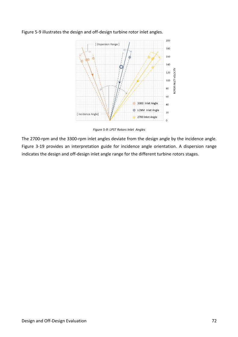
Design and Off-Design Evaluation 72
Figure 5-9 illustrates the design and off-design turbine rotor inlet angles.
Figure 5-9: LPST Rotors Inlet Angles
The 2700-rpm and the 3300-rpm inlet angles deviate from the design angle by the incidence angle.
Figure 3-19 provides an interpretation guide for incidence angle orientation. A dispersion range
indicates the design and off-design inlet angle range for the different turbine rotors stages.

Turbine Blade Design Impact 73
Chapter 6 Turbine Blade Design Impact
This chapter investigates the information that can be obtained from a single turbine stage model.
The emphasis is placed on the correlation between turbine losses as they relate to specific turbine
blade geometry data clusters. Four different case studies are evaluated:
▪ Blade profile design improvement
▪ Blade profile degradation
▪ Blade shrouding variations
▪ Last stage blades interconnection effects
Each case study examines the impact that deviating from an original blade design has on stage
performance. All models developed in this chapter are based on a single stage configuration
illustrated in Figure 6-1.
Figure 6-1: Single Stage LCNM
All parameters are kept identical except for the ones required for specific evaluations, thus ensuring
the accuracy of compatibility. Each case has unique boundary conditions and evaluation parameters.
6.1 Blade profile design upgrade
This case study aims to show the ability of the loss coefficient nozzle-model to quantify the
improvement impact on turbine performance in upgrading a blade profile.
Figure 6-2: Turbine Blade Profile Improvement Example

Turbine Blade Design Impact 74
An actually recorded blade improvement installation is used for the case study [6]. Turbine blading
information along with process information was partially available, for both the original and
upgraded blades. The remainder of the information was obtained by methods discussed in section
2.1.2 . The case study evaluation requirements are:
▪ Predict the performance improvement generated by the upgrade of the turbine blade profile.
▪ Display additional attributes obtained by the implementation of the loss coefficient
algorithms: Focused on blade geometry data clusters.
Note: The following abbreviations used for the result tables and graphs:
▪ 1960 – Original blade design Loss coefficient stage-by-stage turbine nozzle-model
▪ 2000 – Upgraded blade design Loss coefficient stage-by-stage turbine nozzle-model
All components are identical except for specific blade geometries. The upgraded blade changes
consisted of the following properties: Throat, Max blade thickness, Flow area, Trailing Edge
Thickness, Blade Chord Length.
Model development
The performance and boundary conditions were obtained, calculated and inferred from design
drawings, acceptance tests and HDB’s. Only the first stage of the IP steam turbine was evaluated as
it consisted of the most complete design. First, the 1960 model nozzle area was calibrated and then
used for the 2000 model by means of only adjusting the blade profile properties. The actual turbine
blade upgrades improved the overall turbine power output from 365 MW to 400 MW.
Stage Upgrade Boundary Conditions
Inlet Total Pressure: 3,32 MPa Working fluid: Steam
Inlet Temperature: 490 ˚C Mass flow calibration: 148 kg/s
RPM: 3000 IP Steam Turbine
Results & Discussion
Table 6-1 presents a performance comparison between the documented values and the loss
coefficient nozzle model. It was determined that an error of between 1 - 2,5% was experienced.
Table 6-1: Blade Upgrade Performance Comparison
Performance Component 1960’s 2000’s
Actual Overall Turbine MW 365 400
Actual 1st IP ST Stage MW 3,765 4,483
Flownex LCNM 1st Stage MW 3,726 4,373
1st Stage Actual|LCNM MW Diff [%] 1,015 2,455
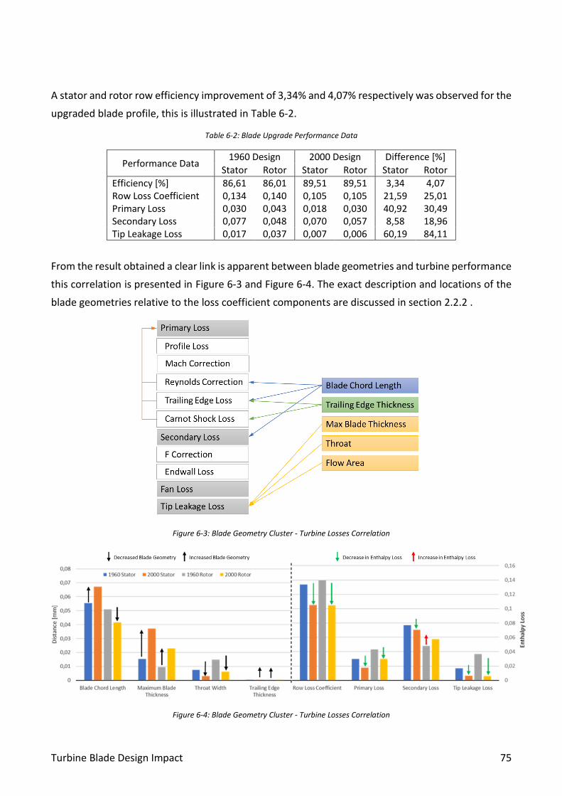
Turbine Blade Design Impact 75
A stator and rotor row efficiency improvement of 3,34% and 4,07% respectively was observed for the
upgraded blade profile, this is illustrated in Table 6-2.
Table 6-2: Blade Upgrade Performance Data
Performance Data 1960 Design 2000 Design Difference [%]
Stator Rotor Stator Rotor Stator Rotor
Efficiency [%] 86,61 86,01 89,51 89,51 3,34 4,07 Row Loss Coefficient 0,134 0,140 0,105 0,105 21,59 25,01 Primary Loss 0,030 0,043 0,018 0,030 40,92 30,49 Secondary Loss 0,077 0,048 0,070 0,057 8,58 18,96 Tip Leakage Loss 0,017 0,037 0,007 0,006 60,19 84,11
From the result obtained a clear link is apparent between blade geometries and turbine performance
this correlation is presented in Figure 6-3 and Figure 6-4. The exact description and locations of the
blade geometries relative to the loss coefficient components are discussed in section 2.2.2 .
Figure 6-3: Blade Geometry Cluster - Turbine Losses Correlation
Figure 6-4: Blade Geometry Cluster - Turbine Losses Correlation

Turbine Blade Design Impact 76
Figure 6-4 indicates that the overall stage loss decreases (green arrows) with the upgraded blade
design (black arrows). Notably the rotor secondary loss increases (red arrow) with the upgrade. It can
be assumed that the overall improvement of the rotor performance justified the additional
secondary loss associated with the upgraded blade design.
The results provide clear motivation for the consideration of blade profile improvements. The loss
coefficient nozzle-model has shown that it is able to predict possible performance improvements
generated by upgraded changes in blade geometries.
6.2 Turbine blade degradation
Various particles can be present in the turbine working fluid creating undesirable operational
conditions for turbine components. Solid particle erosion (SPE) is the study of material erosion caused
by the surface impact of hard particles. SPE alters the blade profile inlet and discharge areas, on both
the stator and rotor, creating undesirable working fluid pressures and velocities.
Figure 6-5: Blade Degradation Illustration - Adapted from [13]
Fouling, on the other hand, describes the accumulation of particles on compromised surface areas.
Creating the same performance degradation mechanics associated with SPE. Fouling, Material
deformation, SPE, Moisture impact erosion and Corrosive pitting are but a few turbine degradation
mechanisms. This case study demonstrates the Loss coefficient stage-by-stage turbine nozzle model’s
ability to predict performance loss associated with blade profile degradation mechanisms.
The case study evaluation requirements are:
▪ Predict the performance losses incurred by the fouling and erosion of turbine blades.
▪ Display additional attributes obtained by the implementation of the loss coefficient
algorithms: Focused on “surface finish” and corresponding blade geometries.
Note: The following abbreviations used for the result tables and graphs:
▪ Polished – Loss coefficient stage-by-stage turbine nozzle-model with design blade conditions
▪ Fouling – Loss coefficient stage-by-stage turbine nozzle-model with severe deposit formations
▪ Erosion –Loss coefficient stage-by-stage turbine nozzle-model with severe erosion.

Turbine Blade Design Impact 77
Model development
This case study is a theoretical assessment to test the loss coefficient nozzle model’s ability to predict
the performance losses incurred by a common plant problem. The maintenance and operation guide
produce by Sanders [11] was used in the development of the case studies boundary conditions and
blade geometry parameters.
An initial ideal turbine stage was developed against which the two degradations mechanisms, Fouling
and Erosion, could be compared. Each degradation mechanism evaluation assumes identical blade
area degradation and surface finish deformations on both the stator and rotor. All parameters are
identical between the three models with the exception listed in the boundary conditions. The ks
values were conservatively selected from a best practices steam turbine operational guide [47].
Stage Degradation Boundary Conditions
Inlet Total Pressure: 8000 kPa Working fluid: Steam
Inlet Temperature: 510 ˚C Mass flow calibration: 300 kg/s
RPM: 3000 Theoretical Stage Condition
Fouling [ks]: 0.1 m Erosion [ks]: 0.06 m
Results & Discussion
Table 6-3: Blade Fouling Degradation Performance Data
Performance
Polished Fouling Polished | Fouling
Diff. [%]
Stator Rotor Stator Rotor Stator Rotor
Work [kW] 10290,4 9594,5 6,76
Efficiency [%] 86,62 88,30 68,00 73,63 21,5 16,6
Row Loss Coefficient 0,134 0,117 0,320 0,264 139,3 125,4
Primary Loss 0,030 0,043 0,098 0,149 224,9 245,5
Secondary Loss 0,077 0,048 0,195 0,090 153,7 85,7
Fan Loss 0,010 0,012 0,010 0,012 0,000 0,000 Tip Leakage Loss 0,017 0,014 0,017 0,014 3,91 2,38
Table 6-4: Blade Erosion Degradation Performance Data
Performance
Polished Erosion Polished | Erosion
Diff. [%]
Stator Rotor Stator Rotor Stator Rotor
Work [kW] 10290,4 10089,0 1,96
Efficiency [%] 86,62 88,30 71,98 76,90 16,9 12,9
Row Loss Coefficient 0,134 0,117 0,280 0,231 109,5 97,4
Primary Loss 0,030 0,043 0,078 0,124 159,4 187,5
Secondary Loss 0,077 0,048 0,175 0,082 127,7 69,4
Fan Loss 0,010 0,012 0,010 0,012 0,000 0,000
Tip Leakage Loss 0,017 0,014 0,017 0,014 2,82 1,66

Turbine Blade Design Impact 78
Table 6-3 and Table 6-4 compare the turbine stage performance of the Polished stage with the
Fouling and Erosion degradation stages respectively. The stage performance experiences a decline of
6,76% caused by Fouling. Whilst a 1,96% decline in performance is caused by blade Erosion. The
correlation between stage performance and blade geometry clusters is illustrated in Figure 6-6.
Figure 6-6: Blade Geometry Cluster - Turbine Losses Correlation
Figure 6-7 provides a visual comparison of the turbine loss distribution incurred by blade degradation.
It is apparent from the results that minute changes in surface finish and blade profile area may lead
to extensive performance losses.
Figure 6-7: Blade Degradation Loss Comparison
Notably from Figure 6-7, it can be observed that the stator experiences a dominant increase in
Secondary loss, whilst the rotor experiences a dominant increase in Primary loss (yellow arrows).
This is accredited to the specific turbine loss configurations associated with stator and rotor blades
as described in section 3.3
Although this case study used extreme theoretical conditions it showed the ability of the loss
coefficient algorithm to predict turbine performance loss associated with blade profile degradation
mechanisms.
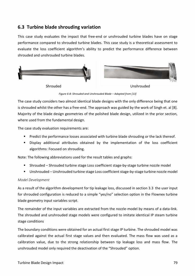
Turbine Blade Design Impact 79
6.3 Turbine blade shrouding variation
This case study evaluates the impact that free-end or unshrouded turbine blades have on stage
performance compared to shrouded turbine blades. This case study is a theoretical assessment to
evaluate the loss coefficient algorithm’s ability to predict the performance difference between
shrouded and unshrouded turbine blades.
Figure 6-8: Shrouded and Unshrouded Blade – Adapted from [13]
The case study considers two almost identical blade designs with the only difference being that one
is shrouded whilst the other has a free-end. The approach was guided by the work of Singh et. al [8].
Majority of the blade design geometries of the polished blade design, utilized in the prior section,
where used from the fundamental design.
The case study evaluation requirements are:
▪ Predict the performance losses associated with turbine blade shrouding or the lack thereof.
▪ Display additional attributes obtained by the implementation of the loss coefficient
algorithms: Focused on shrouding.
Note: The following abbreviations used for the result tables and graphs:
▪ Shrouded – Shrouded turbine stage Loss coefficient stage-by-stage turbine nozzle model
▪ Unshrouded – Unshrouded turbine stage Loss coefficient stage-by-stage turbine nozzle model
Model Development
As a result of the algorithm development for tip leakage loss, discussed in section 3.3 the user input
for shrouded configuration is reduced to a simple “yes/no” selection option in the Flownex turbine
blade geometry input variables script.
The remainder of the input variables are extracted from the nozzle-model by means of a data-link.
The shrouded and unshrouded stage models were configured to imitate identical IP steam turbine
stage conditions
The boundary conditions were obtained for an actual first stage IP turbine. The shrouded model was
calibrated against the actual first stage values and then evaluated. The mass flow was used as a
calibration value, due to the strong relationship between tip leakage loss and mass flow. The
unshrouded model only required the deactivation of the “Shrouded” option.

Turbine Blade Design Impact 80
Shrouded/Unshrouded Boundary Conditions
Inlet Total Pressure: 4000 kPa Working fluid: Steam
Inlet Temperature: 400 ˚C Mass flow calibration: 150 kg/s
RPM: 3000 Theoretical Stage Condition
Results & Discussion
Table 6-5 presents the performance comparison between the shrouded and the unshrouded turbine
stage models under the theoretical conditions. The results confirm that the shrouded blades enable
a turbine stage to produce approximately 1.17% more work than the unshrouded blades under
identical conditions. Accordingly, shrouded blades produce an overall better stage efficiency.
Table 6-5: Shrouded and Unshrouded Blade Performance Data
Performance Shrouded Unshrouded
Shrouded | Unshrouded Diff. [%]
Stator Rotor Stator Rotor Stator Rotor
Work [kW] 3840,857 3796,144 1,164
Efficiency [%] 86,626 88,287 83,787 79,644 3,277 9,789
Row Loss Coefficient 0,134 0,117 0,162 0,204 21,224 73,782
Primary Loss 0,030 0,043 0,030 0,043 0,000 0,000
Secondary Loss 0,077 0,048 0,077 0,048 0,000 0,000
Fan Loss 0,010 0,012 0,010 0,012 0,000 0,000
Tip Leakage Loss 0,017 0,014 0,045 0,100 171,4 614,0
Notably, the removal of the rotor shrouding results in an increase from 0.014 kJ/kg to 0.1 kJ/kg Tip
leakage loss. Figure 6-9 convincingly illustrates the impact unshrouded turbine blades have on
turbine loss distribution.
Figure 6-9: Shrouded and Unshrouded Blade Loss Distribution
This case study used reasonable theoretical blade geometries and suitable operational conditions.
The ability to predict performance deviation based on tip leakage losses can be finely tuned for actual
turbine modelling requirements. The loss coefficient algorithm nozzle-model exhibited the ability to
predict turbine performance associated with shrouded and unshrouded blade designs.

Turbine Blade Design Impact 81
6.4 LSB interconnection impact
The last case study of this chapter investigates the impact various last stage blade interconnections
have on stage performance. Interconnections are a physical strength and stability requirement, due
to the sizing and operational conditions of last stage blades.
Figure 6-10: LSB Interconnection Types - Adapted from [13]
Figure 6-10 illustrates the three different types of interconnection commonly used by turbine
manufactures. The case study compares the three interconnection types against each other in a
similar modelling approach as used in the previous section.
The case study evaluation requirements are:
▪ Predict the stage performances associated with last stage blade interconnections.
▪ Display additional attributes obtained by the implementation of the loss coefficient
algorithms: Focused on LSB interconnection blade geometry illustrated in Figure 3-18.
Note: The following abbreviations used for the result tables and graphs:
▪ Arcade Binding – Square interconnection LSB Loss coefficient turbine nozzle model
▪ Lacing Wire – Round interconnection LSB Loss coefficient turbine nozzle model
▪ Lacing Rods – Oval interconnection LSB Loss coefficient nozzle model
Model development
The last stage models were developed from the last stage blade designs used in Chapter 5 . The three
different last stage blade interconnection geometries are based on the design information provided
by Singh et. al [8] and EPRI [47]. The interconnection geometries are as follows:
LSB Interconnection Geometry
Arcade Binding
Lacing Wire
Lacing Rods
Connection Thickness [m] 0,02 0,01 0,01
Connection Width [m] 0,01 0,01 0,02

Turbine Blade Design Impact 82
All three interconnection blade designs have the same blade-to-blade length and are located on the
same diameter height. For simplification of the test case, only single strand interconnections are
evaluated. Only the last stage rotor blades will be interconnected for this case study as per the LPST
stage 4B design.
Last stage blade interconnections information is presented in Figure 3-18. The boundary conditions
are set to mimic the operational conditions of stage 4B, location illustrated in Figure 5-1.
Last Stage Boundary Conditions
Stage Inlet Pressure: 15,3 kPa Working fluid: Steam
Inlet Temperature: 55 ˚C Turbine Exhaust Pressure: 5,35 kPa
RPM: 3000 Mass flow calibration: 31.5 kg/s
Results & Discussion
Table 6-6 presents a comparison of the LSB interconnection modelling results. The results indicate
that Lacing rods are the most beneficial at an 85,45% stage efficiency, followed by Lacing wire at
84,84 %.
Table 6-6: LSB Interconnection Performance Data
Performance
Lacing Rods Arcade Binding Lacing Wire
Stator Rotor Stator Rotor Stator Rotor
Efficiency [%] 91,35 79,56 91,22 74,76 91,32 78,36
Row Loss Coefficient 0,086 0,204 0,088 0,252 0,087 0,216
Primary Loss 0,025 0,055 0,025 0,055 0,025 0,055
Secondary Loss 0,007 0,003 0,007 0,003 0,007 0,003
Fan Loss 0,026 0,027 0,026 0,027 0,026 0,027
Tip Leakage Loss 0,011 0,020 0,011 0,020 0,011 0,020
LSB Correction 0,000 0,024 0,000 0,073 0,000 0,036
Moisture Loss 0,020 0,069 0,022 0,069 0,021 0,069
Figure 6-11 provides a comparative illustration of the LSB interconnection types based on their
respective turbine loss distributions. It is apparent that the Arcade Binging interconnection would be
the poorest interconnection selection for this specific blade design, based on thermal performance
evaluation alone.

Turbine Blade Design Impact 83
Figure 6-11: LSB Interconnection Turbine Losses Distribution
This case study illustrates the loss coefficient algorithms ability to determine performance deviation
based on LSB interconnection geometries, enabling the nozzle-model to more accurately predict last
stage performance.
Conclusion & Recommendation 84
Chapter 7 Conclusion & Recommendation
7.1 Conclusion
The study set out to determine an appropriate loss coefficient model for use in the stage-by-stage
turbine nozzle model. Research into turbine loss methodologies produced a functional comparative
grouping of turbine loss coefficients that could be used in conjunction with the nozzle model.
The greatest selection criteria for the loss coefficients was integrability and clear correlation to
turbine blade geometries. The correlation between losses and geometries are key to obtaining
greater functionality from the loss coefficient algorithm.
Traupel’s loss coefficient methodology was selected for the loss coefficient algorithm “design”
condition section with corrections provided for moisture loss. Zehner’s loss correction was used for
the development of the loss coefficient algorithm for “off-design” section.
The fundamental group of loss coefficients were comprised of a profile loss, a secondary loss, a fan
loss and a tip leakage loss. These losses are associated with the majority of turbine loss
methodologies. The second group was aimed at off-design performance predictions and was added
as a correction to the fundamental group losses. The final group was focused on specialized losses,
specifically last stage blade interconnection losses and moisture loss.
The selected loss coefficients methodologies enabled the development of a loss coefficient algorithm
script in Flownex that integrates with the stage-by-stage turbine nozzle model. The algorithm script
incorporated structural stability and validation control measures to assist during solving.
Once a model has been developed it requires calibration. Several calibration methods are possible,
all dependant on the amount and type of information that is available. Calibration can be performed
by fixing the inlet and exhaust pressure and temperature boundary conditions and then configuring
the nozzle-model throat area until the correct mass flow is obtained.
A validation and verification case study illustrated the validity of the loss coefficient algorithms by
obtaining an average efficiency prediction accuracy of 99.3%. The case study compared the loss
coefficient nozzle-model’s results to a well-documented actual AGARD gas turbine test case, as well
as to the results obtained from the initial stage-by-stage turbine nozzle model.
The validation leads to the successful construction of an operational steam turbine case study model.
The low-pressure steam turbine loss coefficient nozzle model obtained an overall performance
prediction accuracy of 98.8%. The low-pressure steam turbine model was constructed from an actual
operational steam turbine, for which the majority of the design information was available. The test
case evaluated both full and partial load operational conditions.
Conclusion & Recommendation 85
The comparison between full and partial load (60%) results confirmed the loss coefficient algorithm’s
ability to predict turbine performance as well as turbine loss distributions.
From the low-pressure steam turbine model, an off-design design evaluation became possible. The
off-design evaluation investigated the impact of operating a turbine at off-normal spin speeds has on
overall turbine performance. The loss coefficient algorithm determined the loss in performance, for
(90% and 110%) critical speed operation, by calculating the impact off-design incidence angles have
on turbine performance. This, in turn, illustrates the loss coefficient algorithm’s ability to model both
design and off-design conditions.
Additional case studies displayed the loss coefficient nozzle model's ability to predict offset
performance conditions resulting from turbine geometry variance. Four turbine blade design
alterations were evaluated. The first evaluation investigated the impact of a change in profile design
has on overall stage performance. This was achieved by modelling and comparing the performance
of an actual old blade profile designs with its upgrade blade profile design. The loss coefficient nozzle-
model was able to predict the change in turbine stage performance resulting from the change in the
blade profile design.
The second evaluation investigated the impact of degradation mechanisms have on turbine
performance. The evaluation used theoretical Fouling and Erosion blade degradation scenarios. The
loss coefficient nozzle-model was able to predict the decline in turbine performance caused by the
degradation mechanisms, as well as indicate how the turbine loss distribution related to specific
changes in blade profile geometries.
The third evaluation determined the difference in turbine performance related to shrouded and
unshrouded blade designs. The focus of this evaluation was to determine the loss coefficient nozzle
model’s ability to predict tip leakage loss. The final evaluation followed by investigating the impact
that last stage blade interconnections have on turbine performance. The third and fourth blade
design evaluations displayed the loss coefficient’s abilities to predict turbine performance variations
related to specific blade design characteristics.
This study has shown that the implementation of the loss coefficient algorithm has enabled the stage-
by-stage turbine nozzle model to predict turbine performance, as well as turbine loss distributions,
from the incorporation of turbine blade geometries.

Conclusion & Recommendation 86
7.2 Recommendation
The loss coefficient has the following shortfalls and opportunities for further research:
▪ The loss coefficient algorithm requires the addition of turbine blade-intercooling into the gas
turbine performance analysis methodology.
▪ Incorporating detail blade shroud design and configurations into the determination of tip
leakage instead of a generalized mass flow methodology utilized.
▪ The implementation of a blade profile selection user interface would further advance the
ability of the nozzle-model, similar to the data presented in Figure 3-20.
▪ The unification of the nozzle-model script and the loss coefficient algorithm script into one
streamlined compressed script would improve the overall model processing speed.
References 87
References
[1] W. Fuls, “Accurate stage-by-stage modelling of axial turbines using an appropriate nozzle
analogy with minimal geometric data,” Applied Thermal Engineering, vol. 116, pp. 134-146,
2017.
[2] IEA, “Key World Energy Statistics 2018,” International Energy Agency, Paris, France, 2018.
[3] R. U. ATProM, “Applied Thermofluid Process Modelling,” University of Cape Town, Mechanical
Engineering Department, 2018. [Online]. Available: http://www.atprom.uct.ac.za. [Accessed
October 2018].
[4] T. Croft, Steam Turbine Principles and Practice 1st Edition, New York: McGraw-Hill Book
Company Inc., 1923.
[5] T. Wright, Fluid machinery : performance, analysis, and design, Boca Raton: CRC Press LLC,
1999.
[6] Undisclosed, Undisclosed Steam Turbine Information, Undisclosed, 2010.
[7] S. Sandler, Chemical and Engineering Thermodynamics 3rd Edition, Weinheim: John Wiley &
Sons Inc, 1999.
[8] M. L. G. Singh, Blade Design and Analysis for Steam Turbines, New York: The McGraw-Hill
Companies, 2011.
[9] O. Singh, Applied Thermodynamics 3rd Edition, New Delhi: New Age International (P) Ltd., 2009.
[10] V. Vullo and F. Vivio, Rotors: Stress Analysis and Design, Rome: Springer, 2013.
[11] W. Sanders, “Turbine steam path: Maintenance and Repair Vol.2,” Pennwell Publishing
Company, 2002.
[12] H. S. M. Bloch, Steam Turbines: Design, Applications, and Rerating 2nd Edition, Milan: The
McGraw-Hill Co., 2009.

References 88
[13] F. Woell, Steam Turbine Thermodynamic Velocity Triangle and Blade Design, Johannesburg:
EPPEI, 2016.
[14] G. Azad, J. Hart and S. Teng, “Heat Transfer and Pressure Distribution on a Gas Turbine Blade,”
NASA Glenn Research Center, Texas, 2000.
[15] M. Schobeiri, “Turbomachinery Flow Physics and Dynamic Performance 2nd Edition,” Springer,
Heidelberg, 2012.
[16] S. Egorova, A. Kapitanova and D. Loktevb, “Turbine Blades Profile and Surface Roughness
Measurement,” Elsevier, ScienceDirect, vol. International Conference on Industrial Engineering,
2017.
[17] ISO, “ISO 14661 / ISO 3977 / ISO 2314:2009,” International Standard, 2000.
[18] R. Gorla, Turbomachinery Design and Theory, New York: Marcel Dekker Inc., 2003.
[19] M. Smith, “A simple correlation of turbine efficiency,” Journal of Royal Aeronautical Society,
1965.
[20] S. Dixon and C. Hall, Fluid Mechanics and Thermodynamics of Turbomachinery, Oxford: Elsevier
Inc, 2014.
[21] B. Lakshminarayana, Fluid Dynamics and Heat Transfer of Turbomachinery, Chichester: John
Wiley & Sons Inc., 1996.
[22] I. Shames, Mechanics of Fluids, 4th Edition, Madrid: McGraw-Hill, 2003.
[23] O. Sharma and T. Butler, “Predictions of Endwall Losses and Secondary Flows in Axial Flow
Turbine Cascades,” Journal of Turbomachinery, vol. 109, no. April, p. 229, 1987.
[24] P. Zehner, “Calculation of Four-Quadrant Characteristics of Turbines,” The American Society of
Mechanical Engineers, no. 80-GT-2, 1980.
[25] K. Hiroyuki, O. Akihiro, S. Naoki and N. Yoshiki, “Development of Moisture Loss Models in Steam
Turbines,” Heat Transfer-Asian Research, vol. 42, no. 10.1002/htj.20395., 2013.
References 89
[26] G. Gyarmathy, Grundlagen einer Theorie der Nassdampfturbine, Zürich, Switzerland: ETH Zurich
Research Collection, 1962.
[27] N. Wei, “Significance of Loss Models in Aerothermodynamic Simulation for Axial Turbines,”
Royal Institute of Technology: Department of Energy Technology - Division of Heat and Power
Technology, Stockholm, 2000.
[28] J. Denton, “Loss mechanisms in turbomachines,” Journal of turbomachinery, , vol. 115, 1993.
[29] W. Traupel, Thermische Turbomaschinen: Erster Band, Zürich: Springer Verlag Berlin
Heidelberg, 1977.
[30] J. Horlock, Axial Flow Turbine, Butterwoth Published, 1966.
[31] C. Soderberg, “Unpublished Gas Turbine Laboratory notes,” Massachusetts Institute of
Technology, 1949.
[32] D. Ainley and G. Mathieson, A Method of performance estimation of axial flow turbines, 1951.
[33] H. Craig and H. Cox, Performance estimation of axial flow turbines., Instititution of mechanical
engineers, 1970.
[34] J. Dunham and P. Came, “Improvements to the Ainley-Mathieson method of turbine
performance prediction,” Journal of engineering for power, vol. 92, pp. 252-256, 1970.
[35] W. Traupel, “Thermische Turbomaschinen: Zweiter Band,” Springer Verlag Berlin Heidelberg,
Zürich, 1977.
[36] S. Kacker and U. Okapuu, “A mean line prediction method for axial flow turbine efficiency,”
Journal for engineering for power, vol. 104, pp. 111-119, 1982.
[37] S. McBrinie, Marine Steam Engines and Turbines 4th Ed, Wellington, New Zealand: The
Butterworth Group Ltd, 1980.
[38] W. Kearton, Steam turbine theory and practice, Pitman, 1951.
[39] M. Leonid, Y. Govoruschenko and P. Pagur, “Axial turbine stages design: 1D/2D/3D simulation,
experiment, optimization,” in Turbo Expo, Nevada, 2005.

References 90
[40] R. J. H. Pottas, “A row-by-row axial turbine process model based on a one-dimensional
thermofluid network approach,” University of Cape Town, Cape Town, 2016.
[41] R. I. Lewis, Turbomachinary Performance Analysis, Elsevier Science & Technology Books, 1996.
[42] NASA, “NASA Glenn Research Center,” NASA, 2012. [Online]. Available:
https://www.grc.nasa.gov/www/5810/rvc/tcgrid.htm. [Accessed 2018].
[43] M-Tech_Industrial, “Flownex Simulation Environment: General User Manual,” May 2017.
[Online]. Available: https://www.flownex.com/. [Accessed 2018].
[44] M. Dejc and B. Trojanovskij, “ Untersuchung und Berechnung axialer Turbinenstufen,” Berlin ,
1973.
[45] AGARD, “Test Cases for Computation of Internal Flows in Aero Enginre Components,” AGARD:
Propulsion and Energetics, NATO Nations, 1990.
[46] API, “API Starndard 612: Special purpose steam turbines for industrial services,” American
Petroleum Institute, Washington, 1995.
[47] EPRI, “Collection of Journal Articles on Steam Turbine Blades,” Electrical Power Research
Institute.

Appendix A: Experimental Data 91
Appendix A: Experimental Data
AGARD Case Study
Description Stator Rotor Stator Rotor Stator Rotor Stator Rotor
Number of Blades 39 39 39 39 39 39 39 39
Mean Blade Diameter [m] 0,330379 0,33543 0,34123 0,346281 0,35208 0,357132 0,362931 0,367982
Blade Tip Diameter [m] 0,390758 0,400061 0,412459 0,421762 0,434161 0,443463 0,455862 0,465165
Blade Hub Diameter [m] 0,27 0,27 0,27 0,27 0,27 0,27 0,27 0,27
Blade Height [m] 0,062406 0,067069 0,073281 0,077944 0,084156 0,088819 0,095031 0,099694
Blade Width [m] 0,045455 0,039174 0,046792 0,038393 0,04802 0,037668 0,049135 0,037
Blade Chord Length [m] 0,055294 0,051025 0,056266 0,052215 0,057156 0,05343 0,057963 0,054662
Maximum Blade Thickness [m] 0,015393 0,009459 0,015632 0,008983 0,015847 0,008514 0,016038 0,008053
Throat Width [m] 0,0075 0,0148 0,0107 0,01365 0,01453 0,01359 0,01818 0,01438
Pitch - Blade Spacing [m] 0,035951 0,035334 0,037218 0,036538 0,038448 0,037733 0,039638 0,038909
Trailing Edge Thickness [m] 0,0004 0,00048 0,000482 0,000512 0,000462 0,000526 0,000548 0,000522
Row Spacing Width [m] 0,009673 0,017286 0,008894 0,016532 0,008169 0,015831 0,007492 0,03959
Blade Gap Area [m2] 0,000453 0,000961 0,000762 0,001034 0,001192 0,001177 0,001688 0,001401
Row Flow Area [m2] 0,017658 0,037466 0,029714 0,040328 0,046486 0,045895 0,065835 0,054639
Blade Inlet Angle [˚] 79,90363 31,47247 79,90363 24,05564 79,90363 16,13911 79,90363 7,901738
Blade Outlet Angle [˚] 19,53035 67,06804 20,163 67,7347 20,78783 68,37578 21,41185 68,99137
Blade Surface Finish [m] 0,00001 0,00001 0,00001 0,00001 0,00001 0,00001 0,00001 0,00001
Shrouded Yes Yes Yes Yes Yes Yes Yes Yes
Interconnected LSB No No No No No No No No
Efficiency [%] 91,3387 91,66072 93,05028 90,28629 92,9471 90,5845 92,73315 89,33202
Traupel Loss Coefficient [kJ/kg] 0,086613 0,083393 0,069497 0,097137 0,070529 0,094155 0,072668 0,10668
Primary Loss [kJ/kg] 0,03405 0,043082 0,029479 0,056551 0,028588 0,051531 0,028421 0,047703
Profile Loss [kJ/kg] 0,027808 0,042315 0,026903 0,057016 0,026368 0,052181 0,025833 0,048558
Reynolds Correction 1,089312 0,96174 0,92467 0,952651 0,918966 0,943787 0,914016 0,935209
Mach Correction 1 1 1 1 1 1 1 1
Trailing Edge Loss [kJ/kg] 0,003626 0,002195 0,004421 0,002033 0,004202 0,002083 0,004603 0,002106
Carnot Shock Loss [kJ/kg] 0,000132 0,00019 0,000181 0,000202 0,000155 0,0002 0,000206 0,000185
Secondary Loss [kJ/kg] 0,035312 0,013231 0,022176 0,012455 0,020864 0,01244 0,019631 0,011512
F Correction 0,049498 0,026684 0,039317 0,029591 0,041658 0,02943 0,04238 0,029498
Endwall Loss [kJ/kg] 0,000396 0,000142 0,000296 0,000113 0,00023 9,31E-05 0,000183 0,000202
Fan Loss [kJ/kg] 0,01028 0,011779 0,013944 0,015577 0,01792 0,019659 0,022143 0,023962
Tip Leakage Loss [kJ/kg] 0,006971 0,015302 0,003899 0,012553 0,003157 0,010525 0,002473 0,023502
Stage 1 Stage 2 Stage 3 Stage 4

Appendix A: Experimental Data 92
LPST – Theoretical Geometries2
LPST - Full Load Case Study
LPST - 60% Partial Load Case Study
2 The LPST geometries displayed are not exact and are in part derived from theory.
Description Stator Rotor Stator Rotor Stator Rotor Stator Rotor Stator Rotor Stator Rotor Stator Rotor Stator Rotor
Number of Blades 30 30 30 30 30 30 30 30 30 30 30 30 30 30 30 30
Mean Blade Diameter [m] 1,79 1,79 1,81 1,81 1,85 1,85 2,2 2,2 1,79 1,79 1,81 1,81 1,85 1,85 2,2 2,2
Blade Tip Diameter [m] 1,85 1,855 1,97 1,99 2,29 2,34 2,83 2,83 1,85 1,855 1,97 1,99 2,29 2,34 2,83 2,83
Blade Hub Diameter [m] 1,705 1,705 1,71 1,71 1,69 1,68 1,57 1,57 1,705 1,705 1,71 1,71 1,69 1,68 1,57 1,57
Blade Height [m] 0,07 0,07 0,12 0,14 0,3 0,306 0,61 0,63 0,07 0,07 0,12 0,14 0,3 0,306 0,61 0,63
Blade Width [m] 0,056 0,034 0,07 0,034 0,1 0,052 0,16 0,086 0,056 0,034 0,07 0,034 0,1 0,052 0,16 0,086
Blade Chord Length [m] 0,0672 0,0415 0,0861 0,0422 0,125 0,0655 0,208 0,1049 0,0672 0,0415 0,0861 0,0422 0,125 0,0655 0,208 0,1049
Maximum Blade Thickness [m]0,0192 0,0119 0,0246 0,012 0,0357 0,0187 0,0594 0,03 0,0192 0,0119 0,0246 0,012 0,0357 0,0187 0,0594 0,03
Throat Width [m] 0,0095 0,019 0,012 0,018 0,0192 0,0186 0,023 0,0196 0,0095 0,019 0,012 0,018 0,0192 0,0186 0,023 0,0196
Pitch - Blade Spacing [m] 0,0384 0,0384 0,0384 0,0384 0,0386 0,0388 0,041 0,043 0,0384 0,0384 0,0384 0,0384 0,0386 0,0388 0,041 0,043
Trailing Edge Thickness [m] 0,0005 0,0005 0,0005 0,0005 0,0005 0,0005 0,0005 0,0006 0,0005 0,0005 0,0005 0,0005 0,0005 0,0005 0,0005 0,0006
Row Spacing Width [m] 0,018 0,07 0,02 0,11 0,03 0,16 0,076 0,152 0,018 0,07 0,02 0,11 0,03 0,16 0,076 0,152
Blade Inlet Angle [˚] 80 30 80 25 82 28 80 25 80 30 80 25 82 28 80 25
Blade Outlet Angle [˚] 20 70 20 65 25 72 20 80 20 70 20 65 25 72 20 80
Blade Surface Finish [m] 0,01 0,01 0,01 0,01 0,01 0,01 0,01 0,01 0,01 0,01 0,01 0,01 0,01 0,01 0,01 0,01
Shrouded Yes Yes Yes Yes Yes Yes No No Yes Yes Yes Yes Yes Yes No No
Interconnected LSB No No No No No No No Yes No No No No No No No Yes
Connection Diameter [m] - - - - - - - 2,69 - - - - - - - 2,69
Connection Length [m] - - - - - - - 0,048 - - - - - - - 0,048
Connection Thickness [m] - - - - - - - 0,01 - - - - - - - 0,01
Connection Width [m] - - - - - - - 0,02 - - - - - - - 0,02
Stage B2 Stage B3 Stage B4Stage A1 Stage A2 Stage A3 Stage A4 Stage B1
Stator Rotor Stator Rotor Stator Rotor Stator Rotor Stator Rotor Stator Rotor Stator Rotor Stator Rotor
Efficiency [%] 89,407 84,09 91,146 88,328 94,524 89,441 91,612 81,301 89,407 83,546 91,1474 88,30483 94,52414 89,44059 87,2263 81,30075
Traupel Loss Coefficient [kJ/kg] 0,1059 0,1591 0,0885 0,1167 0,0548 0,1056 0,0839 0,187 0,1059 0,1645 0,088526 0,116952 0,054759 0,105594 0,127737 0,186992
Primary Loss [kJ/kg] 0,0262 0,0477 0,0265 0,0618 0,0218 0,0479 0,0318 0,0437 0,0262 0,0477 0,026514 0,061757 0,021792 0,047902 0,031905 0,043723
Profile Loss [kJ/kg] 0,0252 0,0431 0,0269 0,057 0,0224 0,0522 0,0253 0,0547 0,0252 0,0431 0,026903 0,057016 0,022425 0,052181 0,025315 0,054746
Reynolds Correction 0,8658 1,0535 0,7995 1,0456 0,7262 0,8736 1,0937 0,7572 0,8658 1,0535 0,799469 1,045607 0,726232 0,873555 1,099314 0,757232
Mach Correction 1 1 1 1 1 1 1 1 1 1 1 1 1 1 1 1
Trailing Edge Loss [kJ/kg] 0,0042 0,0021 0,0048 0,002 0,0053 0,0021 0,0039 0,0021 0,0042 0,0021 0,00483 0,001959 0,00531 0,002123 0,003897 0,0021
Carnot Shock Loss [kJ/kg] 0,0001 0,0002 0,0002 0,0002 0,0002 0,0002 0,0002 0,0002 0,0001 0,0002 0,000176 0,000182 0,000196 0,000196 0,000179 0,000168
Secondary Loss [kJ/kg] 0,0561 0,0168 0,039 0,0097 0,0152 0,0041 0,0105 0,0025 0,0561 0,0175 0,038959 0,009715 0,015163 0,004058 0,010548 0,002663
F Correction 0,0981 0,0321 0,1226 0,0312 0,1199 0,0324 0,1209 0,0437 0,0981 0,0335 0,122615 0,031283 0,119928 0,032445 0,120906 0,046672
Endwall Loss [kJ/kg] 0,0004 0,0006 0,0003 0,0004 0,0002 0,0003 0,0003 0,0001 0,0004 0,0006 0,000289 0,000421 0,000168 0,000282 0,000306 0,000118
Fan Loss [kJ/kg] 0,0007 0,0008 0,0005 0,0009 0,0007 0,0008 0,0026 0,0027 0,0007 0,0008 0,000499 0,000859 0,00701 0,007508 0,025623 0,027356
Tip Leakage Loss [kJ/kg] 0,0237 0,0947 0,0226 0,0444 0,0108 0,0461 0,016 0,0196 0,0237 0,0399 0,022555 0,044621 0,010794 0,046125 0,01657 0,019595
LSB Correction [kJ/kg] 0 0 0 0 0 0 0 0,0242 0 0 0 0 0 0 0 0,024169
Moisture Loss [kJ/kg] 0 0 0 0 0 0 0 0 0 0 0 0 0 0 0,04309 0,069486
Stage 3B Stage 4BStage 2BPerformance Data
Stage 1A Stage 2A Stage 3A Stage 4A Stage 1B
Stator Rotor Stator Rotor Stator Rotor Stator Rotor Stator Rotor Stator Rotor Stator Rotor Stator Rotor
Efficiency [%] 89,396 83,681 88,587 88,377 92,089 89,439 90,805 85,909 89,396 83,626 89,645 88,375 92,218 89,439 87,476 78,884
Traupel Loss Coefficient [kJ/kg] 0,106 0,163 0,114 0,116 0,079 0,106 0,092 0,141 0,106 0,164 0,104 0,116 0,078 0,106 0,125 0,211
Primary Loss [kJ/kg] 0,026 0,048 0,027 0,062 0,022 0,048 0,038 0,066 0,026 0,048 0,027 0,062 0,022 0,048 0,038 0,066
Profile Loss [kJ/kg] 0,025 0,043 0,027 0,057 0,022 0,052 0,025 0,055 0,025 0,043 0,027 0,057 0,022 0,052 0,025 0,055
Reynolds Correction 0,866 1,054 0,799 1,046 0,726 0,874 1,348 1,167 0,866 1,054 0,799 1,046 0,726 0,874 1,357 1,175
Mach Correction 1,000 1,000 1,000 1,000 1,000 1,000 1,000 1,000 1,000 1,000 1,000 1,000 1,000 1,000 1,000 1,000
Trailing Edge Loss [kJ/kg] 0,004 0,002 0,005 0,002 0,005 0,002 0,003 0,002 0,004 0,002 0,005 0,002 0,005 0,002 0,003 0,002
Carnot Shock Loss [kJ/kg] 0,000 0,000 0,000 0,000 0,000 0,000 0,000 0,000 0,000 0,000 0,000 0,000 0,000 0,000 0,000 0,000
Secondary Loss [kJ/kg] 0,056 0,017 0,039 0,010 0,015 0,004 0,012 0,004 0,056 0,017 0,039 0,010 0,015 0,004 0,013 0,004
F Correction 0,098 0,033 0,123 0,031 0,120 0,032 0,121 0,045 0,098 0,033 0,123 0,031 0,120 0,032 0,121 0,049
Endwall Loss [kJ/kg] 0,000 0,001 0,000 0,000 0,000 0,000 0,000 0,000 0,000 0,001 0,000 0,000 0,000 0,000 0,000 0,000
Fan Loss [kJ/kg] 0,000 0,000 0,000 0,001 0,007 0,008 0,026 0,027 0,000 0,000 0,000 0,001 0,007 0,008 0,026 0,027
Tip Leakage Loss [kJ/kg] 0,024 0,098 0,023 0,044 0,011 0,046 0,016 0,020 0,024 0,099 0,023 0,044 0,011 0,046 0,017 0,020
LSB Correction [kJ/kg] 0,000 0,000 0,000 0,000 0,000 0,000 0,000 0,024 0,000 0,000 0,000 0,000 0,000 0,000 0,000 0,024
Moisture Loss [kJ/kg] 0,000 0,000 0,000 0,000 0,001 0,004 0,032 0,069 0,000 0,000 0,000 0,000 0,001 0,004 0,032 0,069
Stage 1B Stage 2B Stage 3B Stage 4BPerformance Data
Stage 1B Stage 2A Stage 3A Stage 4A

Appendix A: Experimental Data 93
Off-Design Case Study
Efficiency [%] 88,64 83,204 89,908 87,65 93,024 89,423 88,875 88,294 88,64 82,587 89,909 87,621 93,024 89,422 84,648 81,333
Traupel Loss Coefficient [kJ/kg]0,105 0,1679 0,0883 0,1235 0,0547 0,1058 0,0982 0,117 0,105 0,1741 0,0883 0,1238 0,0547 0,1058 0,1404 0,1866
Primary Loss [kJ/kg] 0,0262 0,0477 0,0265 0,0618 0,0218 0,0479 0,0317 0,0437 0,0262 0,0477 0,0265 0,0618 0,0218 0,0479 0,0319 0,0437
Profile Loss [kJ/kg] 0,0252 0,0431 0,0269 0,057 0,0224 0,0522 0,0253 0,0547 0,0252 0,0431 0,0269 0,057 0,0224 0,0522 0,0253 0,0547
Reynolds Correction 0,8658 1,0535 0,7995 1,0456 0,7262 0,8736 1,091 0,7572 0,8658 1,0535 0,7995 1,0456 0,7262 0,8736 1,0971 0,7572
Mach Correction 1 1 1 1 1 1 1 1 1 1 1 1 1 1 1 1
Trailing Edge Loss [kJ/kg] 0,0042 0,0021 0,0048 0,002 0,0053 0,0021 0,0039 0,0021 0,0042 0,0021 0,0048 0,002 0,0053 0,0021 0,0039 0,0021
Carnot Shock Loss [kJ/kg] 0,0001 0,0002 0,0002 0,0002 0,0002 0,0002 0,0002 0,0002 0,0001 0,0002 0,0002 0,0002 0,0002 0,0002 0,0002 0,0002
Secondary Loss [kJ/kg] 0,0555 0,018 0,039 0,0107 0,0152 0,0042 0,0105 0,0022 0,0555 0,0189 0,039 0,0108 0,0152 0,0042 0,0105 0,0023
F Correction 0,0969 0,0344 0,1226 0,0347 0,1199 0,0339 0,1209 0,0375 0,0969 0,0363 0,1226 0,0349 0,1199 0,0339 0,1209 0,0398
Endwall Loss [kJ/kg] 0,0004 0,0006 0,0003 0,0004 0,0002 0,0003 0,0003 0,0001 0,0004 0,0006 0,0003 0,0004 0,0002 0,0003 0,0003 0,0001
Fan Loss [kJ/kg] -5E-05 -5E-05 0,0005 0,0009 0,007 0,0075 0,0256 0,0274 -5E-05 -5E-05 0,0005 0,0009 0,007 0,0075 0,0256 0,0274
Tip Leakage Loss [kJ/kg] 0,0234 0,1023 0,0223 0,0501 0,0107 0,0461 0,0303 0,0196 0,0234 0,1075 0,0223 0,0504 0,0107 0,0461 0,0303 0,0196
LSB Correction [kJ/kg] 0 0 0 0 0 0 0 0,0242 0 0 0 0 0 0 0 0,0242
Zehner Off-Design 0,1136 0,168 0,1009 0,1235 0,0698 0,1058 0,1112 0,1171 0,1136 0,1741 0,1009 0,1238 0,0698 0,1058 0,1535 0,1867
Incidence Angle (°) -25,77 -12,61 -22,77 -11,23 -24,67 -13,88 -30,56 -24,12 -25,77 -12,61 -22,67 -11,17 -24,63 -13,85 -30,47 -25,17
Efficiency [%] 88,553 85,836 89,74 88,956 92,865 89,442 88,675 88,349 88,553 85,45 89,74 88,957 92,865 89,442 84,464 81,4
Traupel Loss Coefficient [kJ/kg]0,1049 0,1416 0,0888 0,1104 0,0548 0,1056 0,0985 0,1164 0,1049 0,1454 0,0888 0,1104 0,0548 0,1056 0,1406 0,1859
Primary Loss [kJ/kg] 0,0262 0,0477 0,0265 0,0618 0,0218 0,0479 0,032 0,0437 0,0262 0,0477 0,0265 0,0618 0,0218 0,0479 0,0321 0,0437
Profile Loss [kJ/kg] 0,0252 0,0431 0,0269 0,057 0,0224 0,0522 0,0253 0,0547 0,0252 0,0431 0,0269 0,057 0,0224 0,0522 0,0253 0,0547
Reynolds Correction 0,8658 1,0535 0,7995 1,0456 0,7262 0,8736 1,1021 0,7572 0,8658 1,0535 0,7995 1,0456 0,7262 0,8736 1,109 0,7572
Mach Correction 1 1 1 1 1 1 1 1 1 1 1 1 1 1 1 1
Trailing Edge Loss [kJ/kg] 0,0042 0,0021 0,0048 0,002 0,0053 0,0021 0,0039 0,0021 0,0042 0,0021 0,0048 0,002 0,0053 0,0021 0,0039 0,0021
Carnot Shock Loss [kJ/kg] 0,0001 0,0002 0,0002 0,0002 0,0002 0,0002 0,0002 0,0002 0,0001 0,0002 0,0002 0,0002 0,0002 0,0002 0,0002 0,0002
Secondary Loss [kJ/kg] 0,0554 0,0144 0,039 0,0087 0,0152 0,004 0,0106 0,0016 0,0554 0,015 0,039 0,0087 0,0152 0,004 0,0106 0,0016
F Correction 0,0968 0,0274 0,1226 0,0278 0,1199 0,0322 0,1209 0,0272 0,0968 0,0284 0,1226 0,0278 0,1199 0,0322 0,1209 0,0272
Endwall Loss [kJ/kg] 0,0004 0,0006 0,0003 0,0004 0,0002 0,0003 0,0003 0,0001 0,0004 0,0006 0,0003 0,0004 0,0002 0,0003 0,0003 0,0001
Fan Loss [kJ/kg] -5E-05 -5E-05 0,0005 0,0009 0,007 0,0075 0,0256 0,0274 -5E-05 -5E-05 0,0005 0,0009 0,007 0,0075 0,0256 0,0274
Tip Leakage Loss [kJ/kg] 0,0234 0,0795 0,0228 0,0391 0,0108 0,0461 0,0303 0,0196 0,0234 0,0828 0,0228 0,0391 0,0108 0,0461 0,0303 0,0196
LSB Correction [kJ/kg] 0 0 0 0 0 0 0 0,0242 0 0 0 0 0 0 0 0,0242
Zehner Off-Design 0,1145 0,1416 0,1026 0,1104 0,0713 0,1056 0,1133 0,1165 0,1145 0,1455 0,1026 0,1104 0,0713 0,1056 0,1554 0,186
Incidence Angle (°) 25,812 12,789 22,823 11,727 24,754 14,298 30,654 25,88 25,812 12,789 22,708 11,666 24,694 14,262 30,574 27,195
2700
3330

Appendix A: Experimental Data 94
Blade Design Upgrade
Stator Rotor Stator Rotor
Number of Blades 39 39 39 39
Mean Blade Diameter [m] 0,330379 0,33543 0,330379 0,33543
Blade Tip Diameter [m] 0,390758 0,400061 0,390758 0,400061
Blade Hub Diameter [m] 0,27 0,27 0,27 0,27
Blade Height [m] 0,062406 0,067069 0,062406 0,067069
Blade Width [m] 0,045455 0,039174 0,056 0,034
Blade Chord Length [m] 0,055294 0,051025 0,0672 0,04148
Maximum Blade Thickness [m] 0,015393 0,009459 0,03714 0,022822
Throat Width [m] 0,0075 0,0148 0,003109 0,006134
Pitch - Blade Spacing [m] 0,035951 0,035334 0,0384 0,0384
Trailing Edge Thickness [m] 0,0004 0,00048 0,00045 0,000475
Row Spacing Width [m] 0,009673 0,017286 0,009673 0,017286
Blade Inlet Angle [˚] 79,90363 31,47247 79,90363 31,47247
Blade Outlet Angle [˚] 19,53035 67,06804 19,53035 67,06804
Blade Surface Finish [m] 0,00001 0,00001 0,00001 0,00001
Shrouded Yes Yes Yes Yes
Efficiency [%] 0,031905 0,043723 0,031854 0,043723
Row Loss Coefficient [kJ/kg] 0,010548 0,002663 0,010531 0,002288
Primary Loss [kJ/kg] 0,025623 0,027356 0,025623 0,027356
Secondary Loss [kJ/kg] 0,01657 0,019595 0,03034 0,019595
Tip Leakage Loss [kJ/kg] 0,04309 0,069486 0,042082 0,069486
2000’s1960’sDescription

Appendix A: Experimental Data 95
Blade Degradation
Description Stator Rotor Stator Rotor Stator Rotor
Number of Blades 39 39 39 39 39 39
Mean Blade Diameter [m] 0,330379 0,33543 0,330379 0,33543 0,330379 0,33543
Blade Tip Diameter [m] 0,390758 0,400061 0,390758 0,400061 0,390758 0,400061
Blade Hub Diameter [m] 0,27 0,27 0,27 0,27 0,27 0,27
Blade Height [m] 0,062406 0,067069 0,062406 0,067069 0,062406 0,067069
Blade Width [m] 0,045455 0,039174 0,045455 0,039174 0,043 0,038
Blade Chord Length [m] 0,055294 0,051025 0,055294 0,051025 0,053 0,048
Maximum Blade Thickness [m] 0,015393 0,009459 0,016 0,01 0,015 0,009
Throat Width [m] 0,0075 0,0148 0,007 0,013 0,0078 0,0175
Pitch - Blade Spacing [m] 0,035951 0,035334 0,035951 0,035334 0,035951 0,035334
Trailing Edge Thickness [m] 0,0004 0,00048 0,00042 0,0005 0,00039 0,00046
Row Spacing Width [m] 0,009673 0,017286 0,009673 0,017286 0,0098 0,0175
Blade Inlet Angle [˚] 79,90363 31,47247 79,90363 31,47247 79,90363 31,47247
Blade Outlet Angle [˚] 19,53035 67,06804 19,53035 67,06804 19,53035 67,06804
Blade Surface Finish [m] 0,00001 0,00001 0,0001 0,0001 0,00006 0,00006
Efficiency [%] 86,62435 88,2997 67,99743 73,6261 71,97822 76,89786
Row Loss Coefficient [kJ/kg] 0,133757 0,117003 0,320026 0,263739 0,280218 0,231021
Primary Loss [kJ/kg] 0,03001 0,043082 0,097514 0,148841 0,077844 0,123869
Secondary Loss [kJ/kg] 0,076873 0,048191 0,194988 0,089501 0,175031 0,081654
Fan Loss [kJ/kg] 0,01028 0,011779 0,01028 0,011779 0,01028 0,011779
Tip Leakage Loss [kJ/kg] 0,016594 0,013951 0,017243 0,013619 0,017063 0,013719
ErosionFouledPolished

Appendix A: Experimental Data 96
Shrouded & Unshrouded Case Study
Description Stator Rotor Stator Rotor
Number of Blades 52 52 52 52
Mean Blade Diameter [m] 0,330379 0,33543 0,340481 0,345532
Blade Tip Diameter [m] 0,390758 0,400061 0,409363 0,418665
Blade Hub Diameter [m] 0,27 0,27 0,27 0,27
Blade Height [m] 0,062406 0,067069 0,071731 0,076394
Blade Width [m] 0,045455 0,039174 0,045455 0,039174
Blade Chord Length [m] 0,055294 0,051025 0,055294 0,051025
Maximum Blade Thickness [m] 0,015393 0,009459 0,015393 0,009459
Throat Width [m] 0,0075 0,0148 0,0075 0,0148
Pitch - Blade Spacing [m] 0,035951 0,035334 0,035951 0,035334
Trailing Edge Thickness [m] 0,0004 0,00048 0,0004 0,00048
Row Spacing Width [m] 0,009673 0,017286 0,009673 0,017286
Blade Inlet Angle [˚] 79,90363 31,47247 79,90363 31,47247
Blade Outlet Angle [˚] 19,53035 67,06804 19,53035 67,06804
Blade Surface Finish [m] 0,00001 0,00001 0,00001 0,00001
Shrouded Yes Yes No No
Efficiency [%] 86,62574 88,28655 83,78714 79,64409
Traupel Loss Coefficient [kJ/kg] 0,133743 0,117135 0,162129 0,203559
Primary Loss [kJ/kg] 0,03001 0,043082 0,03001 0,043082
Profile Loss [kJ/kg] 0,027808 0,042315 0,027808 0,042315
Reynolds Correction 0,930957 0,96174 0,930957 0,96174
Mach Correction 1 1 1 1
Trailing Edge Loss [kJ/kg] 0,003989 0,002195 0,003989 0,002195
Carnot Shock Loss [kJ/kg] 0,000132 0,00019 0,000132 0,00019
Secondary Loss [kJ/kg] 0,076896 0,0482 0,076896 0,048199
F Correction 0,123266 0,09807 0,123266 0,09807
Endwall Loss [kJ/kg] 0,000263 9,48E-05 0,000263 9,47E-05
Fan Loss [kJ/kg] 0,01028 0,011779 0,01028 0,011779
Tip Leakage Loss [kJ/kg] 0,016557 0,014075 0,044943 0,1005
Shrouded Unshrouded

Appendix A: Experimental Data 97
LSB Interconnection Case Study
Description Stator Rotor Stator Rotor Stator Rotor
Number of Blades 30 30 30 30 30 30
Mean Blade Diameter [m] 2,2 2,2 2,2 2,2 2,2 2,2
Blade Tip Diameter [m] 2,83 2,83 2,83 2,83 2,83 2,83
Blade Hub Diameter [m] 1,57 1,57 1,57 1,57 1,57 1,57
Blade Height [m] 0,61 0,63 0,61 0,63 0,61 0,63
Blade Width [m] 0,16 0,086 0,16 0,086 0,16 0,086
Blade Chord Length [m] 0,208 0,10492 0,208 0,10492 0,208 0,10492
Maximum Blade Thickness [m]0,059429 0,029977 0,059429 0,029977 0,059429 0,029977
Throat Width [m] 0,023 0,0196 0,023 0,0196 0,023 0,0196
Pitch - Blade Spacing [m] 0,041 0,043 0,041 0,043 0,041 0,043
Trailing Edge Thickness [m] 0,00053 0,00055 0,00053 0,00055 0,00053 0,00055
Row Spacing Width [m] 0,076 0,152 0,076 0,152 0,076 0,152
Blade Inlet Angle [˚] 80 25 80 25 80 25
Blade Outlet Angle [˚] 20 80 20 80 20 80
Blade Surface Finish [m] 0,01 0,01 0,01 0,01 0,01 0,01
Shrouded Yes No Yes No Yes No
Interconnected LSB No Yes No Yes No Yes
Connection Diameter [m] - 2,69 - 2,69 - 2,69
Connection Length [m] - 0,048 - 0,048 - 0,048
Connection Thickness [m] - 0,01 - 0,02 - 0,01
Connection Width [m] - 0,02 - 0,01 - 0,01
Efficiency [%] 91,35111 79,55595 91,2166 74,75997 91,31794 78,35657
Traupel Loss Coefficient [kJ/kg]0,086489 0,204441 0,087834 0,2524 0,086821 0,216434
Primary Loss [kJ/kg] 0,022418 0,061012 0,022418 0,06062 0,022418 0,060918
Profile Loss [kJ/kg] 0,025315 0,054746 0,025315 0,054746 0,025315 0,054746
Reynolds Correction 0,661731 1,076321 0,661731 1,069095 0,661731 1,074581
Mach Correction 1 1 1 1 1 1
Trailing Edge Loss [kJ/kg] 0,005487 0,00192 0,005487 0,001923 0,005487 0,00192
Carnot Shock Loss [kJ/kg] 0,000179 0,000168 0,000179 0,000168 0,000179 0,000168
Secondary Loss [kJ/kg] 0,007482 0,002822 0,007482 0,002835 0,007482 0,002825
F Correction 0,120906 0,035455 0,120906 0,03587 0,120906 0,035559
Endwall Loss [kJ/kg] 0,000285 0,000125 0,000285 0,000124 0,000285 0,000125
Fan Loss [kJ/kg] 0,025623 0,027356 0,025623 0,027356 0,025623 0,027356
Tip Leakage Loss [kJ/kg] 0,010774 0,019595 0,010782 0,019595 0,010776 0,019595
LSB Correction [kJ/kg] 0 0,024169 0 0,072508 0 0,036254
Moisture Loss [kJ/kg] 0,020191 0,069486 0,021528 0,069486 0,020521 0,069486
Arcade Binding Lacing WireLacing Rods

Appendix B: Abbreviated Loss Coefficient Algorithms
98
Appendix B: Abbreviated Loss Coefficient Algorithms
Loss Coefficient Algorithm C# Script
//Flow Area Calculation
sAbgp.Value=Math.Atan(sO/sDm)*(sDs*sDs-sDn*sDn)/4;
sAf.Value=sAbgp*sNb;
rAbgp.Value=Math.Atan(rO/rDm)*(rDs*rDs-rDn*rDn)/4;
rAf.Value=rAbgp*rNb;
//Traupel Loss Coefficient Calculations
sζ.Value=sPL+sSL+sFL+sTL+sLSB+sML;
rζ.Value=rPL+rSL+rFL+rTL+rLSB+rML;
//Primary Loss
sPL.Value=(sPrf*sReC*sMaC)+sTe+sCs;
rPL.Value=(rPrf*rReC*rMaC)+rTe+rCs;
//Profile Loss
double []α0={sα0,rα0};
double []α1={sα1,rα1};
double []Prf={sPrf,rPrf};
{double [,]PrfM={ {(Math.PI*10/180),0,0,-1.6414*10E-9,5.22727*10E-7,-6.49224*10E-5,7.1513*10E-3}
,{(Math.PI*15/180),-7.19149*10E-13,3.49129*10E-10,-6.69342*10E-8,6.34078*10E-6,-3.13043*10E-4,1.02567*10E-2}
,{(Math.PI*20/180),-1.17977*10E-12,5.62751*10E-10,-1.06216*10E-7,9.92353*10E-6,-4.74289*10E-4,1.23335*10E-2}
,{(Math.PI*25/180),-1.49757*10E-12,7.07226*10E-10,-1.32412*10E-7,1.23126*10E-5,-5.8547*10E-4,1.40457*10E-2}
,{(Math.PI*30/180),-1.55815*10E-12,7.38388*10E-10,-1.397*10E-7,1.32036*10E-5,-6.406*10E-4,1.51418*10E-2}
,{(Math.PI*35/180),-1.96059*10E-12,9.16953*10E-10,-1.70609*10E-7,1.58261*10E-5,-7.52811*10E-4,1.69495*10E-2}
,{(Math.PI*45/180),-4.23568*10E-12,1.73797*10E-9,-2.80328*10E-7,2.24533*10E-5,-9.30707*10E-4,1.84516*10E-2}};
for (int i = 0; i < Prf.Length; i++)
{ double x0,x1;
double []PrfX= new double[6];
double []PrfY= new double[6];
if (α1[i]<=PrfM[0,0])
{ for (int k = 1; k < 7; k++)
{ PrfX[k-1]=PrfM[0,k]*Math.Pow((α0[i]*180/Math.PI),6-k); }
Prf[i]=PrfX[0]+PrfX[1]+PrfX[2]+PrfX[3]+PrfX[4]+PrfX[5];}
else if (α1[i]>=PrfM[6,0])
{ for (int k = 1; k < 7; k++)
{ PrfX[k-1]=PrfM[6,k]*Math.Pow((α0[i]*180/Math.PI),6-k);}
Prf[i]=PrfX[0]+PrfX[1]+PrfX[2]+PrfX[3]+PrfX[4]+PrfX[5]; }
else
{for (int j = 0; j < 5; j++)
{if ((α1[i]>=PrfM[j,0]) && (α1[i]<PrfM[j+1,0]))
{for (int k = 1; k < 7; k++)
{PrfX[k-1]=PrfM[j,k]*Math.Pow((α0[i]*180/Math.PI),6-k);
PrfY[k-1]=PrfM[j+1,k]*Math.Pow((α0[i]*180/Math.PI),6-k);}
x0=PrfX[0]+PrfX[1]+PrfX[2]+PrfX[3]+PrfX[4]+PrfX[5];
x1=PrfY[0]+PrfY[1]+PrfY[2]+PrfY[3]+PrfY[4]+PrfY[5];
Prf[i]=((x1-x0)*(α1[i]-PrfM[j,0])/(PrfM[j+1,0]-PrfM[j,0]))+x0;}}}}}
sPrf.Value=Prf[0];
rPrf.Value=Prf[1];

Appendix B: Abbreviated Loss Coefficient Algorithms
99
//Reynolds Number Correction
double []Re={sRe,rRe};
double []Ks={sksf/sSchrd,rksf/rSchrd};
double []ReC=new double[2];
sRe.Value=sρ*V2*(Math.Sqrt(sAbgp/Math.PI))/sμ;
rRe.Value=rρ*V3*(Math.Sqrt(rAbgp/Math.PI))/rμ;
for (int i = 0; i < Re.Length; i++)
{if (Re[i]<200000)
{ReC[i]=415.42*Math.Pow(Re[i],-0.491718);}
else
{ReC[i]=(-2.04381*10E7*Ks[i]*Ks[i]*Ks[i])+(1.34009*10E4*Ks[i]*Ks[i])+(2.00593*10E2*Ks[i])+(0.565005);}}
sReC.Value=ReC[0];
rReC.Value=ReC[1];
//Mach Number Correction
double []Ma={sMa,rMa};
double []MaC=new double[2];
for (int i = 0; i < Ma.Length; i++)
{if (Ma[i]>0.8)
{MaC[i]=(-344.92*Math.Pow(Ma[i],5))+(1796.3*Ma[i]*Ma[i]*Ma[i]*Ma[i])+(-
3690.8*Ma[i]*Ma[i]*Ma[i])+(3744.7*Ma[i]*Ma[i])+(-1878.6*Ma[i])+374.2;}
else
{MaC[i]=1.0;}}
sMaC.Value=MaC[0];
rMaC.Value=MaC[1];
//Trailing Edge Loss
double []Tep=new double[2];
double []Te=new double[2];
double []δte={sδte,rδte};
double []t={st,rt};
double []TeX=new double[2];
double []TeY=new double[2];
for (int i = 0; i < Te.Length; i++)
{Tep[i]=δte[i]/(t[i]*Math.Sin(α1[i]));
TeX[i]=Tep[i]/(Prf[i]*ReC[i]*MaC[i]);
if (TeX[i]<3.4)
{TeY[i]=0.9697*TeX[i]+0.7461;}
else
{TeY[i]=-0.014548*TeX[i]*TeX[i]+0.457829*TeX[i]+2.61156;}}
double [,]TeM={{0.04,500,-6*10E-17},{0.08,250,-6*10E-17},{0.12,166.6667,0},{0.16,125,-6*10E-17},{0.2,100,4*10E-17}};
for (int i = 0; i < Te.Length; i++)
{double x0,x1;
if (Tep[i]<=TeM[0,0])
{Te[i]=(TeY[i]-TeM[0,2])/TeM[0,1]; }
else if (Tep[i]>=TeM[4,0])
{Te[i]=(TeY[i]-TeM[4,2])/TeM[4,1]; }
else
{for (int j = 0; j < 3; j++)
{if ((Tep[i]>=TeM[j,0]) && (Tep[i]<TeM[j+1,0]))
{x0=(TeY[i]-TeM[j,2])/TeM[j,1];
x1=(TeY[i]-TeM[j+1,2])/TeM[j+1,1];
e[i]=((x1-x0)*(Tep[i]-TeM[j,0])/(TeM[j+1,0]-TeM[j,0]))+x0;}}}}
sTe.Value=Te[0];
rTe.Value=Te[1];

Appendix B: Abbreviated Loss Coefficient Algorithms
100
//Carnot Shock Loss
double []Cs={sCs,rCs};
sCs.Value=(Tep[0]/(1-Tep[0]))*(Tep[0]/(1-Tep[0]))*Math.Sin(sα1)*Math.Sin(sα1);
rCs.Value=(Tep[1]/(1-Tep[1]))*(Tep[1]/(1-Tep[1]))*Math.Sin(rα1)*Math.Sin(rα1);
//-----Primary Loss Complete----//
//Secondary Loss
sSL.Value=(sPL/sPrf)*(sFc/ltx[0])+sEw+0.02*((sSchrd/sls)-((sSchrd/st)/ltx[0]));
rSL.Value=(rPL/rPrf)*(rFc/ltx[1])+rEw+0.02*((sSchrd/sls)-((sSchrd/st)/ltx[1]));
double []B={7,10}; //B=7 for Stator, B=10 for Rotor
double [] lt={(sls/st),(rls/rt)};
double []ltk={(B[0]*Math.Sqrt(sPL)),(B[1]*Math.Sqrt(rPL))};
double []ltx=new double[2];
for (int i = 0; i < lt.Length; i++)
{ltx[i]=ltk[i]>lt[i]?ltk[i]:lt[i];}
// Coefficient A = 0.02 for strongly accelerating and high velocity grids & 0.035 for constant pressure impeller grids
// F Correction
double []Fc=new double[2];
double []cw={(V1/V2),(V2r/V3)}; //!!!!!!!Check research for accuracy
double []dα={((α0[0]-α1[0])*180/Math.PI),((α1[1]-α0[1])*180/Math.PI)};
{double [,]FcM={{1,-9.1269*10E-11,3.23992*10E-8,-3.65469*10E-6,2.66136*10E-4,3.66044*10E-3},
{0.9,-6.16173*10E-11,2.27701*10E-8,-2.78513*10E-6,2.28791*10E-4,3.03546*10E-3},
{0.8,-7.17726*10E-11,2.52631*10E-8,-3.00349*10E-6,2.21563*10E-4,2.43801*10E-3},
{0.7,-4.52489*10E-11,1.69238*10E-8,-2.13194*10E-6,1.75095*10E-4,2.27393*10E-3},
{0.6,-4.04069*10E-11,1.5065*10E-8,-1.88122*10E-6,1.48852*10E-4,2.10375*10E-3},
{0.5,-1.85538*10E-11,7.60232*10E-9,-1.05483*10E-6,1.06001*10E-4,1.97787*10E-3},
{0.4,-2.62881*10E-11,8.98421*10E-9,-1.08292*10E-6,9.40453*10E-5,1.47745*10E-3},
{0.3,-1.64113*10E-11,5.98948*10E-9,-7.81293*10E-7,7.29054*10E-5,1.16583*10E-3},
{0.2,-2.80663*10E-12,1.00053*10E-9,-1.5836*10E-7,3.47721*10E-5,1.06541*10E-3}};
for (int i = 0; i < Fc.Length; i++)
{double x0,x1;
double []FcX= new double[5];
double []FcY= new double[5];
if (cw[i]>=FcM[0,0])
{ for (int k = 1; k < 6; k++)
{FcX[k-1]=FcM[0,k]*Math.Pow(dα[i],5-k);}Fc[i]=FcX[0]+FcX[1]+FcX[2]+FcX[3]+FcX[4];}
else if (cw[i]<=FcM[8,0])
{ for (int k = 1; k < 6; k++)
{FcX[k-1]=FcM[8,k]*Math.Pow(dα[i],5-k);}
Fc[i]=FcX[0]+FcX[1]+FcX[2]+FcX[3]+FcX[4];}
else
{for (int j = 0; j < 8; j++)
{if ((cw[i]<FcM[j,0]) && (cw[i]>=FcM[j+1,0]))
{for (int k = 1; k < 6; k++)
{FcX[k-1]=FcM[j,k]*Math.Pow(dα[i],5-k);
FcY[k-1]=FcM[j+1,k]*Math.Pow(dα[i],5-k);}
x0=FcX[0]+FcX[1]+FcX[2]+FcX[3]+FcX[4];
x1=FcY[0]+FcY[1]+FcY[2]+FcY[3]+FcY[4];
Fc[i]=((x1-x0)*(cw[i]-FcM[j,0])/(FcM[j+1,0]-FcM[j,0]))+x0;}}}}}
sFc.Value=Fc[0];
rFc.Value=Fc[1];

Appendix B: Abbreviated Loss Coefficient Algorithms
101
//Endwall Loss
double ksfL=0.042;
double []ksf={sksf,rksf};
double []ls={sls,rls};
double []Dm={sDm,rDm};
double []cf=new double[2];
{for (int i = 0; i < cf.Length; i++)
{if (ksf[i]<ksfL)
{cf[i]=0.445/Math.Pow((Math.Log(Re[i])),2.58);}
else
{cf[i]=Math.Pow((1.89+1.62*(Math.Log((ls[i]/ksf[i])))),-2.5);}} }
sEw.Value=(cf[0]/Math.Sin(sα1))*(1+(sls/Dm[0]))*(sδgp/sls);
rEw.Value=(cf[1]/Math.Sin(rα1))*(1-(rls/Dm[1]))*(rδgp/rls);
//----Secondary Loss Complete----//
//Fan Loss
double []υ={(sDn/sDs),(rDn/rDs)};
double []lsD={(sls/sDm),(rls/rDm)};
double []FL=new double[2];
double [,]FLM={{0.5,3.53074*10E-2,-2.08139*10E-4,1.28485*10E-5},
{0.7,3.20866*10E-2,-7.03983*10E-4,6.39394*10E-6},
{0.9,2.99004*10E-2,-1.49509*10E-3,7.86364*10E-6}};
for (int i = 0; i < FL.Length; i++)
{double x0,x1;
double []FLX= new double[5];
double []FLY= new double[5];
if (υ[i]>=FLM[2,0])
{ for (int k = 1; k < 4; k++) {
FLX[k-1]=FLM[2,k]*Math.Pow(lsD[i],3-k);}
FL[i]=FLX[0]+FLX[1]+FLX[2];}
else if (υ[i]<=FLM[0,0])
{ for (int k = 1; k < 4; k++)
{FLX[k-1]=FLM[0,k]*Math.Pow(lsD[i],3-k);}
FL[i]=FLX[0]+FLX[1]+FLX[2];}
else
{for (int j = 0; j < 2; j++)
{if ((υ[i]>=FLM[j,0]) && (υ[i]<FLM[j+1,0]))
{for (int k = 1; k < 4; k++)
{FLX[k-1]=FLM[j,k]*Math.Pow(lsD[i],3-k);
FLY[k-1]=FLM[j+1,k]*Math.Pow(lsD[i],3-k);}
x0=FLX[0]+FLX[1]+FLX[2];
x1=FLY[0]+FLY[1]+FLY[2];
FL[i]=((x1-x0)*( υ[i]-FLM[j,0])/(FLM[j+1,0]-FLM[j,0]))+x0;}}}}
sFL.Value=FL[0];
rFL.Value=FL[1];
//
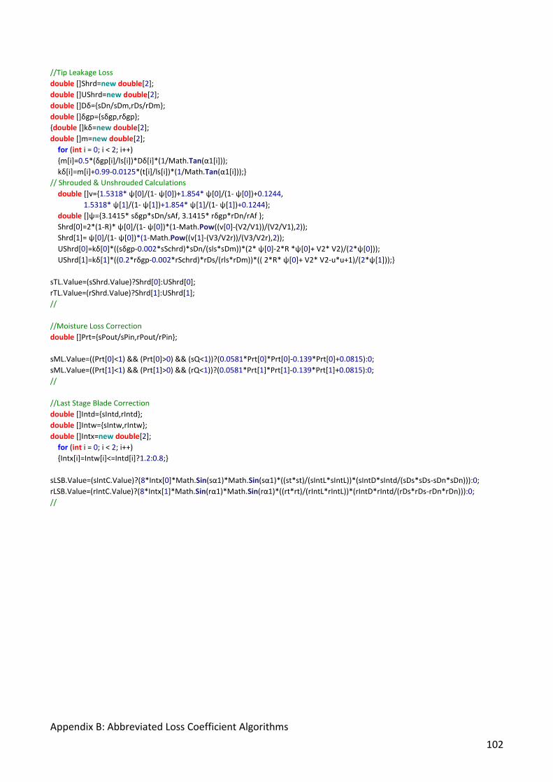
Appendix B: Abbreviated Loss Coefficient Algorithms
102
//Tip Leakage Loss
double []Shrd=new double[2];
double []UShrd=new double[2];
double []Dδ={sDn/sDm,rDs/rDm};
double []δgp={sδgp,rδgp};
{double []kδ=new double[2];
double []m=new double[2];
for (int i = 0; i < 2; i++)
{m[i]=0.5*(δgp[i]/ls[i])*Dδ[i]*(1/Math.Tan(α1[i]));
kδ[i]=m[i]+0.99-0.0125*(t[i]/ls[i])*(1/Math.Tan(α1[i]));}
// Shrouded & Unshrouded Calculations
double []v={1.5318* ψ[0]/(1- ψ[0])+1.854* ψ[0]/(1- ψ[0])+0.1244,
1.5318* ψ[1]/(1- ψ[1])+1.854* ψ[1]/(1- ψ[1])+0.1244};
double []ψ={3.1415* sδgp*sDn/sAf, 3.1415* rδgp*rDn/rAf };
Shrd[0]=2*(1-R)* ψ[0]/(1- ψ[0])*(1-Math.Pow((v[0]-(V2/V1))/(V2/V1),2));
Shrd[1]= ψ[0]/(1- ψ[0])*(1-Math.Pow((v[1]-(V3/V2r))/(V3/V2r),2));
UShrd[0]=kδ[0]*((sδgp-0.002*sSchrd)*sDn/(sls*sDm))*(2* ψ[0]-2*R *ψ[0]+ V2* V2)/(2*ψ[0]));
UShrd[1]=kδ[1]*((0.2*rδgp-0.002*rSchrd)*rDs/(rls*rDm))*(( 2*R* ψ[0]+ V2* V2-u*u+1)/(2*ψ[1]));}
sTL.Value=(sShrd.Value)?Shrd[0]:UShrd[0];
rTL.Value=(rShrd.Value)?Shrd[1]:UShrd[1];
//
//Moisture Loss Correction
double []Prt={sPout/sPin,rPout/rPin};
sML.Value=((Prt[0]<1) && (Prt[0]>0) && (sQ<1))?(0.0581*Prt[0]*Prt[0]-0.139*Prt[0]+0.0815):0;
sML.Value=((Prt[1]<1) && (Prt[1]>0) && (rQ<1))?(0.0581*Prt[1]*Prt[1]-0.139*Prt[1]+0.0815):0;
//
//Last Stage Blade Correction
double []Intd={sIntd,rIntd};
double []Intw={sIntw,rIntw};
double []Intx=new double[2];
for (int i = 0; i < 2; i++)
{Intx[i]=Intw[i]<=Intd[i]?1.2:0.8;}
sLSB.Value=(sIntC.Value)?(8*Intx[0]*Math.Sin(sα1)*Math.Sin(sα1)*((st*st)/(sIntL*sIntL))*(sIntD*sIntd/(sDs*sDs-sDn*sDn))):0;
rLSB.Value=(rIntC.Value)?(8*Intx[1]*Math.Sin(rα1)*Math.Sin(rα1)*((rt*rt)/(rIntL*rIntL))*(rIntD*rIntd/(rDs*rDs-rDn*rDn))):0;
//
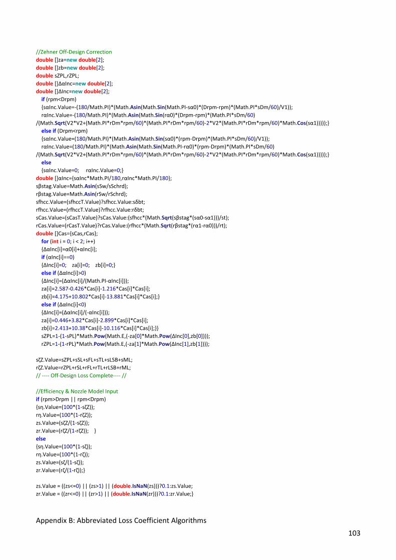
Appendix B: Abbreviated Loss Coefficient Algorithms
103
//Zehner Off-Design Correction
double []za=new double[2];
double []zb=new double[2];
double sZPL,rZPL;
double []ΔαInc=new double[2];
double []ΔInc=new double[2];
if (rpm<Drpm)
{sαInc.Value=-(180/Math.PI)*(Math.Asin(Math.Sin(Math.PI-sα0)*(Drpm-rpm)*(Math.PI*sDm/60)/V1));
rαInc.Value=-(180/Math.PI)*(Math.Asin(Math.Sin(rα0)*(Drpm-rpm)*(Math.PI*sDm/60)
/(Math.Sqrt(V2*V2+(Math.PI*rDm*rpm/60)*(Math.PI*rDm*rpm/60)-2*V2*(Math.PI*rDm*rpm/60)*Math.Cos(sα1)))));}
else if (Drpm<rpm)
{sαInc.Value=(180/Math.PI)*(Math.Asin(Math.Sin(sα0)*(rpm-Drpm)*(Math.PI*sDm/60)/V1));
rαInc.Value=(180/Math.PI)*(Math.Asin(Math.Sin(Math.PI-rα0)*(rpm-Drpm)*(Math.PI*sDm/60)
/(Math.Sqrt(V2*V2+(Math.PI*rDm*rpm/60)*(Math.PI*rDm*rpm/60)-2*V2*(Math.PI*rDm*rpm/60)*Math.Cos(sα1)))));}
else
{sαInc.Value=0; rαInc.Value=0;}
double []αInc={sαInc*Math.PI/180,rαInc*Math.PI/180};
sβstag.Value=Math.Asin(sSw/sSchrd);
rβstag.Value=Math.Asin(rSw/rSchrd);
sfhcc.Value=(sfhccT.Value)?sfhcc.Value:sδbt;
rfhcc.Value=(rfhccT.Value)?rfhcc.Value:rδbt;
sCas.Value=(sCasT.Value)?sCas.Value:(sfhcc*(Math.Sqrt(sβstag*(sα0-sα1)))/st);
rCas.Value=(rCasT.Value)?rCas.Value:(rfhcc*(Math.Sqrt(rβstag*(rα1-rα0)))/rt);
double []Cas={sCas,rCas};
for (int i = 0; i < 2; i++)
{ΔαInc[i]=α0[i]+αInc[i];
if (αInc[i]==0)
{ΔInc[i]=0; za[i]=0; zb[i]=0;}
else if (ΔαInc[i]>0)
{ΔInc[i]=(ΔαInc[i]/(Math.PI-αInc[i]));
za[i]=2.587-0.426*Cas[i]-1.216*Cas[i]*Cas[i];
zb[i]=4.175+10.802*Cas[i]-13.881*Cas[i]*Cas[i];}
else if (ΔαInc[i]<0)
{ΔInc[i]=(ΔαInc[i]/(-αInc[i]));
za[i]=0.446+3.82*Cas[i]-2.899*Cas[i]*Cas[i];
zb[i]=2.413+10.38*Cas[i]-10.116*Cas[i]*Cas[i];}}
sZPL=1-(1-sPL)*Math.Pow(Math.E,(-za[0]*Math.Pow(ΔInc[0],zb[0])));
rZPL=1-(1-rPL)*Math.Pow(Math.E,(-za[1]*Math.Pow(ΔInc[1],zb[1])));
sζZ.Value=sZPL+sSL+sFL+sTL+sLSB+sML;
rζZ.Value=rZPL+rSL+rFL+rTL+rLSB+rML;
// ---- Off-Design Loss Complete---- //
//Efficiency & Nozzle Model Input
if (rpm>Drpm || rpm<Drpm)
{sη.Value=(100*(1-sζZ));
rη.Value=(100*(1-rζZ));
zs.Value=(sζZ/(1-sζZ));
zr.Value=(rζZ/(1-rζZ)); }
else
{sη.Value=(100*(1-sζ));
rη.Value=(100*(1-rζ));
zs.Value=(sζ/(1-sζ));
zr.Value=(rζ/(1-rζ));}
zs.Value = ((zs<=0) || (zs>1) || (double.IsNaN(zs)))?0.1:zs.Value;
zr.Value = ((zr<=0) || (zr>1) || (double.IsNaN(zr)))?0.1:zr.Value;}

Appendix B: Abbreviated Loss Coefficient Algorithms
104
Loss Coefficient Algorithm Script Variables Definitions
Blade Geometry Input Variables
sNb_=_StatorProfile_:_NumberofBlades
sDm_=_StatorProfile_:_MeanBladeDiameter
sDs_=_StatorProfile_:_BladeTipDiameter
sDn_=_StatorProfile_:_BladeHubDiameter
sls_=_StatorProfile_:_BladeHeight
sSw_=_StatorProfile_:_BladeWidth
sSchrd_=_StatorProfile_:_BladeChordLength
sδbt_=_StatorProfile_:_MaximumBladeThickness
sO_=_StatorProfile_:_ThroatWidth
st_=_StatorProfile_:_Pitch-BladeSpacing
sδte_=_StatorProfile_:_TrailingEdgeThickness
sδgp_=_StatorProfile_:_RowSpacingWidth
sAbgp_=_StatorProfile_:_BladeGapArea
sAf_=_StatorProfile_:_RowFlowArea
sα0_=_StatorProfile_:_BladeInletAngle
sα1_=_StatorProfile_:_BladeOutletAngle
sksf_=_StatorProfile_:_BladeSurfaceFinish
Bool_sShrd_=_StatorProfile_:_Shrouded
Bool_sIntC_=_StatorProfile_:_InterconnectedLSB
sIntD_=_StatorProfile_:_ConnectionDiameter
sIntL_=_StatorProfile_:_ConnectionLength
sIntd_=_StatorProfile_:_ConnectionThickness
sIntw_=_StatorProfile_:_ConnectionWidth
rNb_=_RotorProfile_:_NumberofBlades
rDm_=_RotorProfile_:_MeanBladeDiameter
rDs_=_RotorProfile_:_BladeTipDiameter
rDn_=_RotorProfile_:_BladeHubDiameter
rls_=_RotorProfile_:_BladeHeight
rSw_=_RotorProfile_:_BladeWidth
rSchrd_=_RotorProfile_:_BladeChordLength
rδbt_=_RotorProfile_:_MaximumBladeThickness
rO_=_RotorProfile_:_ThroatWidth
rt_=_RotorProfile_:_Pitch-BladeSpacing
rδte_=_RotorProfile_:_TrailingEdgeThickness
rδte_=_RotorProfile_:_RowSpacingWidth
rAbgp_=_RotorProfile_:_BladeGapArea
rAf_=_RotorProfile_:_RowFlowArea
rα0_=_RotorProfile_:_BladeInletAngle
rα1_=_RotorProfile_:_BladeOutletAngle
rksf_=_RotorProfile_:_BladeSurfaceFinish
Bool_rShrd_=_RotorProfile_:_Shrouded
Bool_rIntC_=_RotorProfile_:_InterconnectedLSB
rIntD_=_RotorProfile_:_ConnectionDiameter
rIntL_=_RotorProfile_:_ConnectionLength
rIntd_=_RotorProfile_:_ConnectionThickness
rIntw_=_RotorProfile_:_ConnectionWidth
Fluid Properties
V1_=_StatorFluidProperties_:_InletVelocity
V2_=_StatorFluidProperties_:_OutletVelocity
sRe_=_StatorFluidProperties_:_ReynoldsNumber
sMa_=_StatorFluidProperties_:_MachNumber
sT_=_StatorFluidProperties_:_Temperature
sρ_=_StatorFluidProperties_:_Density
sμ_=_StatorFluidProperties_:_Viscosity
sPin_=_StatorFluidProperties_:_InletPressure
sPout_=_StatorFluidProperties_:_OutletPressure
V2r_=_RotorFluidProperties_:_InletVelocity
V3_=_RotorFluidProperties_:_OutletVelocity
rRe_=_RotorFluidProperties_:_ReynoldsNumber
rMa_=_RotorFluidProperties_:_MachNumber
rT_=_RotorFluidProperties_:_Temperature
rρ_=_RotorFluidProperties_:_Density
rμ_=_RotorFluidProperties_:_Viscosity
rPin_=_RotorFluidProperties_:_InletPressure
rPout_=_RotorFluidProperties_:_OutletPressure

Appendix B: Abbreviated Loss Coefficient Algorithms
105
Calculated Loss Coefficients
sη_=_StatorPerformanceData_:_StatorEfficiency
sζ_=_StatorPerformanceData_:_TraupelLossCoefficient
sPL_=_StatorPerformanceData_:_+PrimaryLoss
sPrf_=_StatorPerformanceData_:_-ProfileLoss
sReC_=_StatorPerformanceData_:_-ReynoldsCorrection
sMaC_=_StatorPerformanceData_:_-MachCorrection
sTe_=_StatorPerformanceData_:_-TrailingEdgeLoss
sCs_=_StatorPerformanceData_:_-CarnotShockLoss
sSL_=_StatorPerformanceData_:_+SecondaryLoss
sFc_=_StatorPerformanceData_:_-FCorrection
sEw_=_StatorPerformanceData_:_-EndwallLoss
sFL_=_StatorPerformanceData_:_+FanLoss
sTL_=_StatorPerformanceData_:_+TipLeakageLoss
sLSB_=_StatorPerformanceData_:_+LSBCorrection
sML_=_StatorPerformanceData_:_+MoistureLoss
sζZ_=_StatorPerformanceData_:_ZehnerOff-DesignCorrection
sαInc_=_StatorPerformanceData_:_-IncidenceAngle
Bool_sCasT_=_StatorPerformanceData_:_-
CascadeCoefficientKnown
sCas_=_StatorPerformanceData_:_-CascadeCoefficient
sCasBool_sfhccT_=_StatorPerformanceData_:_-
HeightoftheCurvatureKnown
sfhcc_=_StatorPerformanceData_:_-
CamberlineCurvatureHeight
sβstag_=_StatorPerformanceData_:_-BladeStaggerAngle
rη_=_RotorPerformanceData_:_RotorEfficiency
rζ_=_RotorPerformanceData_:_TraupelLossCoefficient
rPL_=_RotorPerformanceData_:_+PrimaryLoss
rPL_=_RotorPerformanceData_:_-ProfileLoss
rReC_=_RotorPerformanceData_:_-ReynoldsCorrection
rMaC_=_RotorPerformanceData_:_-MachCorrection
rTe_=_RotorPerformanceData_:_-TrailingEdgeLoss
rTerCs_=_RotorPerformanceData_:_-CarnotShockLoss
rSL_=_RotorPerformanceData_:_+SecondaryLoss
rFc_=_RotorPerformanceData_:_-FCorrection
rEw_=_RotorPerformanceData_:_-EndwallLoss
rFL_=_RotorPerformanceData_:_+FanLoss
rTL_=_RotorPerformanceData_:_+TipLeakageLoss
rLSB_=_RotorPerformanceData_:_+LSBCorrection
rML_=_RotorPerformanceData_:_+MoistureLoss
rζZ_=_RotorPerformanceData_:_ZehnerOff-DesignCorrection
rαInc_=_RotorPerformanceData_:_-IncidenceAngle
Bool_rCasT_=_RotorPerformanceData_:_-
CascadeCoefficientKnown
rCas_=_RotorPerformanceData_:_-CascadeCoefficient
Bool_rfhccT_=_RotorPerformanceData_:_-
HeightoftheCurvatureKnown
rfhcc_=_RotorPerformanceData_:_-
CamberlineCurvatureHeight
rβstag_=_RotorPerformanceData_:_-BladeStaggerAngle
Loss Coefficient Algorithm Output Variables
zs_=_NozzleModelInput_:_StatorLossCoefficient
zr_=_NozzleModelInput_:_RotorLossCoefficient
Drpm_=_TurbineData_:_TurbineDesignSpeed
rpm_=_TurbineData_:_OperatingSpeed
sQ_=_StatorFluidProperties_:_Quality
rQ_=_RotorFluidProperties_:_Quality
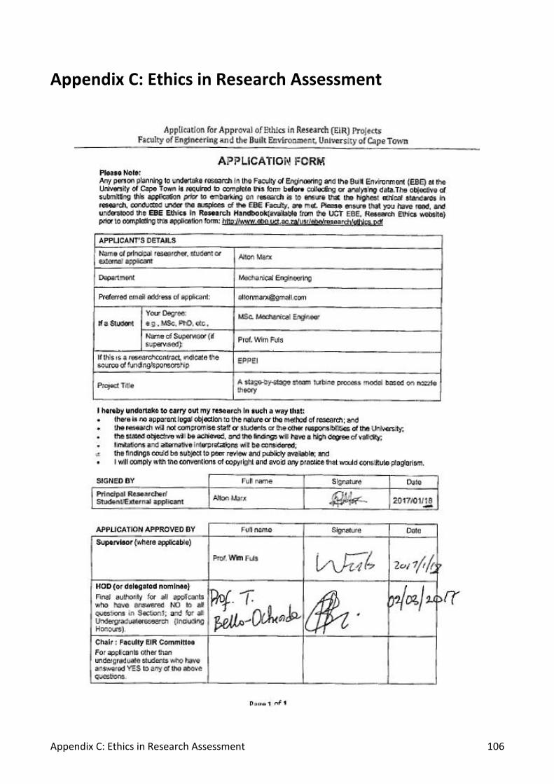
Appendix C: Ethics in Research Assessment 106
Appendix C: Ethics in Research Assessment