determination of the thermal properties and heat...
TRANSCRIPT

1
DETERMINATION OF THE THERMAL PROPERTIES AND HEAT TRANSFER CHARACTERISTICS OF HIGH CONCENTRATION ORANGE PULP
By
JUAN FERNANDO MUÑOZ HIDALGO
A THESIS PRESENTED TO THE GRADUATE SCHOOL OF THE UNIVERSITY OF FLORIDA IN PARTIAL FULFILLMENT OF THE
REQUIREMENTS FOR THE DEGREE OF MASTER OF SCIENCE
UNIVERSITY OF FLORIDA
2012

2
© 2012 Juan Fernando Muñoz Hidalgo

3
To my wife Carolina who supported and helped me to achieve my goals throughout my graduate studies

4
ACKNOWLEDGMENTS
I would like to thank my family and friends for their support and encouragement. I
also thank my academic advisor Dr. Reyes for sharing his knowledge, for encouraging
me to work independently, and for giving me the tools to overcome hurdles during my
research. I would also like to thank my graduate committee members, Dr. Teixeira and
Dr. Ehsani for their valuable contributions to this work. Finally, I would like to give
special thanks to all who helped me throughout my research and graduate studies:
Shelley Jones, John Henderson, Sabrina Terada, Elyse Payne, Thao Nguyen,
Giovanna Iafelice, and Zhou Yang.

5
TABLE OF CONTENTS page
ACKNOWLEDGMENTS................................................................................................. 4
LIST OF TABLES........................................................................................................... 8
LIST OF FIGURES ........................................................................................................ 9
LIST OF ABBREVIATIONS .......................................................................................... 12
ABSTRACT.................................................................................................................. 15
CHAPTER
1 LITERATURE REVIEW ......................................................................................... 17
Introduction............................................................................................................ 17
Theoretical Background ......................................................................................... 18
Orange Pulp and High Concentration Orange Pulp ......................................... 18
Thermal Properties of Foods ........................................................................... 20
Specific heat ............................................................................................. 21
Thermal conductivity ................................................................................. 22
Thermal diffusivity ..................................................................................... 23
Principles of Heat Transfer in Fluids ................................................................ 23
Heat transfer by conduction ...................................................................... 23
Heat transfer by convection ...................................................................... 24
Overall heat transfer coefficient ................................................................ 25
Steady-state and unsteady-state heat transfer .......................................... 26
Flow of Fluids – Concepts Relevant to this Study ............................................ 27
The Reynolds number ............................................................................... 27
Literature Review................................................................................................... 28
Functional and Nutritional Properties of Citrus Pulp ........................................ 28
Orange Pulp Industrial Applications................................................................. 29
Pasteurization of Orange Pulp ......................................................................... 30
Flow Characteristics of HCP and other Viscous Fluids .................................... 31
Thermal Properties of Fruit Pulps and of other Viscous Fluids ........................ 34
Heat Transfer Coefficient of Fruit Pulps and other Viscous Fluids ................... 36
Alternative Technologies for Pasteurizing Fruit Pulps, Purees, and other Viscous Products ......................................................................................... 37
Research Objectives ............................................................................................. 40
Figures and Tables ................................................................................................ 42
2 THERMAL PROPERTIES OF HIGH CONCENTRATION ORANGE PULP ........... 44
Introduction............................................................................................................ 44
Materials and Methods .......................................................................................... 44
6
Sample Preparation ........................................................................................ 44
Pulp Concentration Adjustment ....................................................................... 45
Moisture Content ............................................................................................. 45
Density ............................................................................................................ 46
Specific Heat Capacity .................................................................................... 46
Thermal Diffusivity ........................................................................................... 48
Thermal conductivity ....................................................................................... 50
Statistical Analysis .......................................................................................... 50
Results and Discussion ......................................................................................... 50
Moisture Content and Density ......................................................................... 50
Thermal Properties of Orange Pulp ................................................................. 51
Specific heat capacity ............................................................................... 51
Thermal diffusivity ..................................................................................... 52
Thermal conductivity ................................................................................. 53
Conclusion............................................................................................................. 54
Figures and Tables ................................................................................................ 55
3 DETERMINATION OF HEAT TRANSFER COEFFICIENTS AND HEAT TRANSFER CHARACTERISTICS OF HIGH CONCENTRATION ORANGE PULP ..................................................................................................................... 59
Introduction............................................................................................................ 59
Materials and Methods .......................................................................................... 60
Samples Preparation ....................................................................................... 60
Experimental Setup ......................................................................................... 60
Determination of Local and Overall Heat Transfer Coefficients ....................... 62
Temperature Profiles ....................................................................................... 64
Pressure Drop ................................................................................................. 65
Regression Analysis ........................................................................................ 65
Results and Discussion ......................................................................................... 65
Determination of Heat Transfer Coefficients .................................................... 65
Temperature Profiles ....................................................................................... 72
Pressure Drop Determinations ........................................................................ 76
Conclusions ........................................................................................................... 78
Significance of this Research ................................................................................ 79
Overall Conclusions ............................................................................................... 81
Future Work ........................................................................................................... 82
Figures and Tables ................................................................................................ 84 APPENDIX
A COMPARISON BETWEEN THE HEAT TRANFER COEFFICIENTS OBTAINED IN THE HEATING AND COOLING SECTIONS OF THE HEAT EXCHANGER ... 100
B COMPARISON BETWEEN THE PRESSURE DROPS OBTAINED IN THE HEATING AND COOLING SECTIONS OF THE HEAT EXCHANGER ................ 102

7
LIST OF REFERENCES ............................................................................................ 104
BIOGRAPHICAL SKETCH ......................................................................................... 108

8
LIST OF TABLES
Table page 1-1 Specific heat capacity and thermal conductivity of viscous fluids and other
common liquid foods. ........................................................................................ 43
1-2 Heat transfer coefficient of viscous fluids and other common liquid foods. ........ 43
2-1 Average (n = 3) moisture content and density of orange pulp at different concentrations ................................................................................................... 57
2-2 Experimental values obtained for the calorimeter´s heat capacity ..................... 58
2-3 Mean values of the thermal properties of orange pulp at selected concentrations ................................................................................................... 58
3-1 Experimental flow rates and velocities used for determining the heat transfer coefficients for different pulp concentrations. ..................................................... 87
3-2 Calculated local and overall heat transfer coefficients for different pulp concentrations and velocities, in the heating section of a tubular heat exchanger. ........................................................................................................ 88
3-3 Calculated local heat transfer coefficients for different pulp concentrations and velocities, in the cooling section of a tubular heat exchanger...................... 89
9
LIST OF FIGURES
Figure page 1-1 Simplified flow diagram for industrial production of orange juice, low
concentration orange pulp (LCP), and high concentration orange pulp (HCP). Modified from Braddock (1999). ........................................................................ 42
1-2 Combined convective and conductive heat transfer (Singh and Heldman 2009). ................................................................................................................ 42
2-1 FMC Quick Fiber Test instrument used for determining orange pulp concentration ..................................................................................................... 55
2-2 Experiment setup for determining specific heat capacity of orange pulp samples ............................................................................................................. 55
2-3 Time-temperature graph for determining orange pulp specific heat capacity. .... 56
2-4 Time-temperature graph for determining the heat loss to the surroundings to calculate the specific heat capacity. .................................................................. 56
2-5 Materials and methods used to determine the thermal diffusivity of orange pulp. .................................................................................................................. 57
3-1 Schematic representation of equipment setup for determination of temperature profiles and heat transfer coefficients of high concentration orange pulp. ...................................................................................................... 84
3-2 Schematic representation of set of thermocouples inserted at different radial directions of the inner pipe and thermocouple attached to the pipe´s surface to measure the wall temperature. ...................................................................... 84
3-3 Set of thermocouples inserted at different radial directions at the pipe´s exit ..... 85
3-4 Schematic representation of the temperature profile when orange pulp flows in the heating section of a tubular heat exchanger. ........................................... 85
3-5 Data acquisition board used to record data ....................................................... 86
3-6 Equipment setup ............................................................................................... 86
3-7 Local heat transfer coefficients as function of velocity in the heating section of heat exchanger, for pulp concentrations of 516 (♦), 617 (■), 712 (▲), and 801 (Х) g L-1. ..................................................................................................... 90

10
3-8 Local heat transfer coefficients as function of velocity in the cooling section of heat exchanger, for pulp concentrations of 516 (♦), 617 (■), 712 (▲), and 801 (Х) g L-1. ............................................................................................................ 90
3-9 Overall heat transfer coefficients as function of velocity in the heating section of heat exchanger, for pulp concentrations of 516 (♦), 617 (■), 712 (▲), and 801 (Х) g L-1. ..................................................................................................... 91
3-10 Local (♦) and overall (■) heat transfer coefficients as function of velocity in the heating section of heat exchanger, for pulp concentrations of 516, and 617 g L-1. ........................................................................................................... 92
3-11 Local (♦) and overall (■) heat transfer coefficients as function of velocity in the heating section of heat exchanger, for pulp concentrations of 712, and 801 g L-1. ........................................................................................................... 93
3-12 Temperature profiles obtained for 516 ± 6 g L-1 orange pulp concentration in the heating section of a tubular heat exchanger at flow rates of 4.4 (♦), 5.3 (■), 6.4 (▲), and 7.9 (Х) x 10-4 m3 s-1. ............................................................... 94
3-13 Temperature profiles obtained for 516 ± 6 g L-1 orange pulp concentration in the cooling section of a tubular heat exchanger at flow rates of 4.4 (♦), 5.4 (■), 6.3 (▲), and 7.5 (Х) x 10-4 m3 s-1. ............................................................... 94
3-14 Temperature profiles obtained for 617 ± 7 g L-1 orange pulp concentration in the heating section of a tubular heat exchanger at flow rates of 4.5 (♦), 5.6 (■), 6.4 (▲), and 7.6 (Х) x 10-4 m3 s-1. ............................................................... 95
3-15 Temperature profiles obtained for 617 ± 7 g L-1 orange pulp concentration in the cooling section of a tubular heat exchanger at flow rates of 3.8 (♦), 4.4 (■), 5.3 (▲), and 6.9 (Х) x 10-4 m3 s-1. ............................................................... 95
3-16 Temperature profiles obtained for 712 ± 12 g L-1 orange pulp concentration in the heating section of a tubular heat exchanger at flow rates of 3.9 (♦), 4.4 (■), 5.9 (▲), and 7.4 (Х) x 10-4 m3 s-1. ............................................................... 96
3-17 Temperature profiles obtained for 712 ± 12 g L-1 orange pulp concentration in the cooling section of a tubular heat exchanger at flow rates of 2.7 (♦), 3.7 (■), 6.0 (▲), and 6.7 (Х) x 10-4 m3 s-1. ............................................................... 96
3-18 Temperature profiles obtained for 801 ± 13 g L-1 orange pulp concentration in the heating section of a tubular heat exchanger at flow rates of 2.4 (♦), 3.5 (■), 4.1 (▲), and 5.1 (Х) x 10-4 m3 s-1. ............................................................... 97
3-19 Temperature profiles obtained for 801 ± 13 g L-1 orange pulp concentration in the cooling section of a tubular heat exchanger at flow rates of 2.1 (♦), 2.9 (■), 3.6 (▲), and 4.8 (Х) x 10-4 m3 s-1. ............................................................... 97

11
3-20 Hypothesized mixed flow of HCP ...................................................................... 98
3-21 Pressure drop as function of flow rate in the heating section of heat exchanger, for pulp concentrations of 516 (♦), 617 (■), 712 (▲), and 801 (Х) g L-1. .................................................................................................................. 98
3-22 Pressure drop as function of flow rate in the cooling section of heat exchanger, for pulp concentrations of 516 (♦), 617 (■), 712 (▲), and 801 (Х) g L-1. .................................................................................................................. 99

12
LIST OF ABBREVIATIONS
Area (m2)
Inside surface area of the pipe (m2)
Outside surface area of the pipe (m2)
Specific heat capacity (J kg-1 K-1)
Specific heat of the reference liquid (J kg-1 K-1)
Diameter (m)
Friction factor
Gravity acceleration (9.81 m·(s2)-1)
Proportionality factor for gravitational force (1 kg m (s2 N)-1)
Local heat transfer coefficient (W m-2 °C-1)
HCP High concentration orange pulp
HDP High density orange pulp
Heat capacity of the calorimeter (J K-1)
Consistency coefficient (Pa·s)
Thermal conductivity (W m-1 K-1)
Length (m)
LCL Low concentration orange pulp
Mass (kg)
Reference liquid weight (kg)
Sample weight (kg)
Flow behavior index
Pressure at the inlet of the pipe (kPa)

13
Pressure at the outlet of the pipe (kPa)
Heat (J)
Rate of heat transfer (W)
Total heat content at the final state (J)
Total heat content at the initial state (J)
Radius (m)
Reynolds number
nRe Reynolds number for power law fluids in laminar flow
Temperature (°C)
Final equilibrium temperature (K)
Outlet temperature of the product (°C)
Inlet temperature of the cold fluid or product (°C)
Outlet temperature of the heating media (°C)
Inlet temperature of the heating media (°C)
Reference liquid initial temperature in calorimetric analysis (K)
Sample initial temperature in calorimetric analysis (K)
Tw Apparent wall temperature (°C)
Time required to reach equilibrium temperature (s)
Overall heat transfer coefficient (W m-2 °C-1)
Overall heat transfer coefficient based on the inside area of a pipe (W m2 °C-1)
Velocity (m s-1)
Average velocity (m s-1)

14
Weight (kg)
Length or thickness (m)
Elevation (m)
Thermal diffusivity (m2 s-1)
∆P Pressure drop (kPa)
∆P/L Pressure drop per unit of length (kPa m-1)
Temperature difference (K or °C)
Logarithmic mean temperature difference
Heat loss rate, temperature variation over time (°C s-1)
γ Shear rate (s-1)
Density (kg m-3
)
σ Shear stress (Pa)
σo Yield stress (Pa)
Viscosity (Pa·s)

15
Abstract of Thesis Presented to the Graduate School of the University of Florida in Partial Fulfillment of the Requirements for the Degree of Master of Science
DETERMINATION OF THE THERMAL PROPERTIES AND HEAT TRANSFER
CHARACTERISTICS OF HIGH CONCENTRATION ORANGE PULP By
Juan Fernando Muñoz Hidalgo
August 2012
Chair: José I. Reyes-De-Corcuera Major: Food Science and Human Nutrition
Orange pulp strongly contributes to the sensory and texture properties of fruit
juices and other beverages. High concentrated pulp (HCP) is difficult to pasteurize
because its high apparent viscosity results in laminar flow regimes. Therefore, heat
transfer occurs mostly by conduction. Determination of the thermal properties and heat
transfer characteristics of HCP is essential for modeling and optimizing the thermal
process of this fluid. Specific heat capacity (Cp), thermal diffusivity (α), and thermal
conductivity (k), were determined for orange pulp concentrations of ≈ 500 to 800 g L-1.
Specific heat was between 4025 and 4068 J kg-1 K-1; α ranged from 1.50 to 1.56 x 10⁻⁷
m2 s-1; and k was between 0.63 and 0.66 W m-1 K-1. For Cp, α, and k, no significant
differences (p>0.05) were found among the different pulp concentrations. Local and
overall heat transfer coefficients, radial temperature profiles, and pressure drops were
determined by heating and cooling the pulp in a tubular heat exchanger at selected flow
rates. The local heat transfer coefficients ranged from 1342 to 7755 W m-2 °C-1, while
the overall heat transfer coefficients were between 1241 and 6428 W m-2 °C-1. These
values increased with velocity and decreased with pulp concentration. Pressure drop
was between 147 and 244 kPa for a pipe length of 3.4 m. Pressure drop was higher for

16
more concentrated pulp, and increased with flow rate. The information obtained in this
study can be used to optimize equipment design and process conditions to maximize
heat transfer and minimize pressure drop, for processing HCP aseptically.

17
CHAPTER 1 LITERATURE REVIEW
Introduction
The demand for minimally processed and fresh-like foods has continuously
increased in recent years. Beverage and juice consumers are demanding products that
have closer sensory characteristics and nutritional properties to freshly hand-squeezed
juices (Berlinet and others 2007). Orange pulp, a by-product obtained from the industrial
production of orange juice, strongly contributes to the aroma, flavor, and texture
properties of unprocessed and fresh-like juices (Rega and others 2004). The increase in
demand for orange pulp in the market, particularly in Asia, has raised the need to study
the product's physical properties and heat transfer characteristics for industrial
optimization of handling and pasteurization systems. The types of orange pulp that are
commercially available are: unwashed, washed, and wholesome juice vesicles. Washed
pulp refers to juice vesicles obtained after the juice and soluble solids have been
recovered from pulp or pulpy juice streams by water extraction. Wholesome juice
vesicles are very difficult to produce (Kimball 1991). Unwashed pulp, which is the focus
of this literature review and this research, will be explained in further detail and will be
referred to as orange pulp in this thesis. In 2010/11 season, an estimate of 700
thousand metric tons of orange pulp were produced in the United States (USDA 2011),
which correspond to an estimated value of $520 million.
To-date, many citrus processors produce orange pulp at concentrations around
500 g L-1 as determined by the quick fiber test. Commercializing pulp with higher
concentrations is economically more efficient, since reduces shipping and storage
costs. However, pulp at concentrations above 500 g L-1, also referred to as high

18
concentration orange pulp (HCP) or high density pulp (HDP) is difficult to handle in
conventional equipment due to its high apparent viscosity. High concentration pulp
today is generally not produced aseptically because the pressure drop in tubular
pasteurizers is very high. In most cases pulp is pasteurized at around 500 g L-1, then
concentrated in a non-aseptic finisher, stored and sold as a frozen product. Storage of
frozen pulp involves high energy costs and higher risk of spoilage (Levati 2010;
Braddock 1999).
Optimization of equipment design for production of aseptic HCP requires to
determine the heat transfer characteristics of this fluid, and to obtain its thermophysical
properties. This information has not been published. The overall objective of this study
was to determine HCP´s thermal properties and heat transfer characteristics at different
flow rates, in the heating and cooling sections of a tubular heat exchanger. This
information is essential for modeling processing operations involving heat transfer and
for designing and optimizing equipment to produce HCP aseptically. This chapter
presents the theoretical background on orange pulp processing as well as the
fundamentals of thermal properties and heat transfer in tubular heat exchangers,
relevant concepts on flow of fluids, and a review of the studies that have been published
regarding citrus pulp and other viscous fluids such as juice concentrates, fruit purees
and pastes. The specific objectives of this study are also presented in this section.
Theoretical Background
Orange Pulp and High Concentration Orange Pulp
Orange pulp is the dispersion of burst juice vesicles in a small fraction of juice that
is obtained from the orange juice finishing and centrifugation process. This fraction of
fruit is rich in sugars, and also contains fibers and other residual substances (Tripodo

19
2004). Orange pulp contains an average of 19.7% of total solids, and represents
approximately 5% of the weight of fresh oranges (Martínez and Carmona 1980; Kimball
1991). Figure 1-1 shows a general flow diagram of the industrial process for obtaining
orange juice and pulp from the orange fruit.
After extraction, orange juice is pumped to finishers for separation of part of the
ruptured juice vesicles, or pulp. The aim of recovering pulp is to manufacture large pulp
sacs from the pulpy juice stream, with most of the juice removed (Braddock 1999).
Minimum residual juice in the pulp is necessary for transportation purposes. Depending
on the market value of pulp and juice, juice processors favor the yield of one or the
other product, by adjusting finishing conditions.
When the pulpy juice passes through the first finisher, the pulp in the extracted
juice is concentrated to approximately 500 g L-1. In the industry, this semi-concentrated
pulp is pasteurized using a tubular heat exchanger. Pasteurization is generally
conducted at 90 °C, for 0.5 to 1.0 min, followed by cooling to 2 to 5 °C. Due to the
difficulties for pumping the semi-concentrated pulp, heat exchangers with large
horizontal tubes and spiral baffles are necessary for efficient pasteurization (Braddock
1999). After chilling, the semi-concentrated pulp-juice mixture can be further
concentrated to what is referred as “high density pulp” (600 to 900 g L-1) in a second
finisher. Because this finisher is not aseptic, after packaging the concentrated pulp is
stored at frozen temperatures to inhibit any residual enzyme activity as well as microbial
growth (Kimball 1991). From a practical and economic standpoint, pulp with this
concentration level is preferred by the industry, since high concentrated pulp results in
lower transportation and storage costs.

20
The most common process for obtaining high concentration orange pulp has some
disadvantages. It requires two steps for concentration, since high concentration pulp is
difficult to handle in conventional tubular pasteurizers due to its high viscosity, its
rheology and its flow characteristics. Pulp concentrations above 500 g L-1 are difficult to
mix uniformly resulting in high temperature differences within the fluid; therefore, it is
difficult to achieve uniform thermal treatment conditions (Levati 2010). In addition,
pumping in conventional tubular heat exchangers results in high pressure drop when
handling very viscous fluids. Another drawback of this process is that in the
pasteurization of the pre-concentrated pulp (500 g L-1), the carrier juice contained in the
mixture juice-pulp (approximately 50% juice) is over-exposed to high temperatures
when achieving the required pasteurization conditions for the pulp. This temperature
over-exposure may affect the juice´s sensory characteristics (Yeom and others 2000;
Levati 2010).
Thermal Properties of Foods
Thermophysical properties are necessary for the design and prediction of heat
transfer operations during handling, processing, canning, and distribution of food.
Theoretical and empirical relations used to design and operate processes involving heat
transfer require knowledge of the thermal properties of foods under consideration.
Thermal properties can be defined as those properties that control the transfer and
storage of heat in a particular food (Lozano 2005). In this research, the thermal
properties that are relevant to the design of heat exchangers were studied: Specific heat
capacity, thermal diffusivity and thermal conductivity. This section is based on Lozano
(2005) and Singh and Heldman (2009).
21
Water content significantly influences all thermophysical properties. Some thermal
properties can be calculated directly from the water content of a food. However, most
foods are complex materials, and their contents of proteins, fats, and carbohydrates
highly differ from one food to another. Therefore, food composition has variable effects
on the thermal properties of a composite food material. Thermal properties are also
dependent on the temperature, as well as the chemical composition and physical
structure of food. Some models have been developed to predict the thermal properties
of foods. Some of these models take into account the food composition, and also
assess a physical representation of the food under study. However, often the values
estimated by these models have significant discrepancies when compared to
experimental values. These differences are mainly due to the complex physicochemical
structure of food products; for example the complex interactions that occur between the
different components of a food, or the physical changes that some food components
undergo with temperature variations. (Mercali and others 2011).
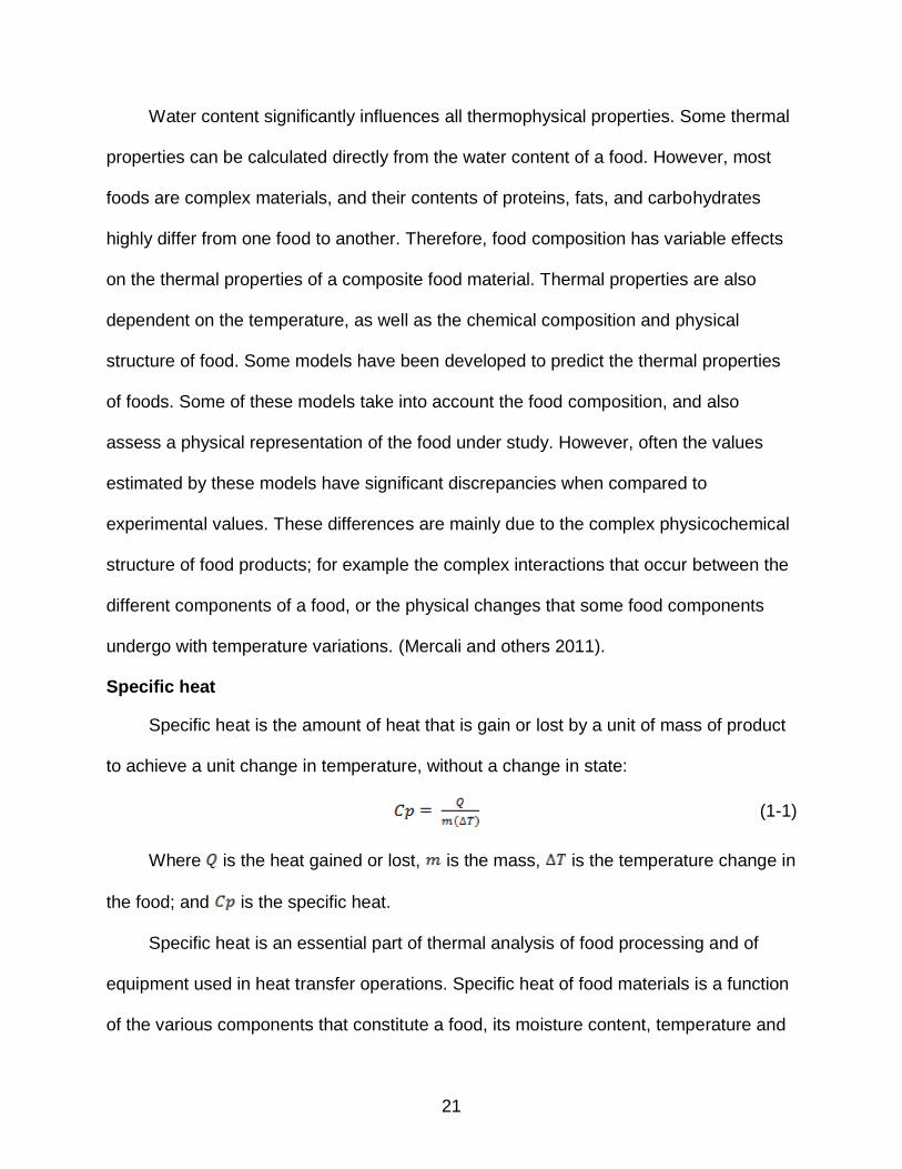
Specific heat
Specific heat is the amount of heat that is gain or lost by a unit of mass of product
to achieve a unit change in temperature, without a change in state:
(1-1)
Where is the heat gained or lost, is the mass, is the temperature change in
the food; and is the specific heat.
Specific heat is an essential part of thermal analysis of food processing and of
equipment used in heat transfer operations. Specific heat of food materials is a function
of the various components that constitute a food, its moisture content, temperature and

22
pressure. Specific heat increases as the food´s moisture content increases. Since in
most food processing applications pressure is kept constant, specific heat at constant
pressure is used. Specific heat can be estimated by using predictive equations, which
are empirical mathematical models mainly based in the major components of foods.
Another method used for specific heat measurement is differential scanning calorimetry
(DSC). The advantages of DSC are that measurement is rapid, only a very small
sample is needed for analysis, and the results are comparable to those obtained from
standard calorimeters. Specific heat can also be determined using a calorimeter, where
a known amount of a reference liquid of known specific heat capacity and initial
temperature is placed in contact with a known amount of sample at different
temperatures, allowing them to reach an equilibrium temperature. An energy balance
based on equation 1-1, and that takes into account the heat losses to the surroundings,
allows calculating the specific heat of the sample (Hwang and Hayakawa 1979). This
method will be explained in detail in Chapter 2.
Thermal conductivity
Thermal conductivity ( is an intrinsic property of a material, and represents the
amount of heat that is conducted per unit of time through a unit thickness of the material
if a unit temperature difference exists across the thickness. The SI unit for thermal
conductivity is:
(1-2)
Most foods with high moisture contents have thermal conductivity values closer to
that of water. Several empirical models have been proposed to estimate thermal
conductivity of foods. Some of the simplest models consider that the different

23
components of foods are arranged in layers either parallel or normal to the heat flow.
Most of the empirical expressions proposed to calculate the thermal conductivity of
foods are functions of temperature, and/or water content.
Thermal diffusivity
Thermal diffusivity ( ) is a ratio between thermal conductivity, density, and
specific heat:
(1-3)
Physically, the thermal diffusivity represents the change in temperature produced
in a unit volume of unit surface and unit thickness, containing a unit of matter, by heat
flowing in a unit of time under unit temperature differences between opposite faces. The
units of thermal diffusivity are m2 s
-1.
Principles of Heat Transfer in Fluids
Heat transfer by conduction
Conduction is the mode of heat transfer where energy is transferred at a molecular
level. One theory that describes conductive heat transfer states that as molecules of a
material accumulate thermal energy, they vibrate with higher amplitude of vibration
while confined in their lattice. These vibrations are transmitted from one molecule to
another without translatory movement of the molecules. Heat is conducted from regions
of higher temperature to regions of lower temperature. Another theory states that
conduction takes place at a molecular level due to the movement of free electrons,
which carry thermal and electrical energy. In conductive heat transfer, there is no
movement of the material undergoing heat transfer.
The rate of heat transfer by conduction can be expressed by Fourier´s law:

24
(1-4)
Where is the rate of heat flow in the direction of heat transfer by conduction; is
the thermal conductivity; is the area through which heat flows; is the temperature;
and is length.
Heat transfer by convection
When a flowing fluid is heated or cooled by coming into contact with a solid body
that is at a different temperature than the fluid, heat exchange will occur between the
fluid and the solid body. This mode of heat transfer is known as convection. There are
two forms of convective heat transfer: Forced convection, which involves the use of
mechanical means to induce the movement of the fluid. And free convection, when
there is a temperature gradient caused by density differences within the system; these
differences in density produce fluid movement. Both forms of convection may result in
laminar or turbulent flow of the fluid, but turbulence generally happens under forced
convection heat transfer. Natural convection only occurs in a gravitational field.
When a flowing fluid comes into contact with the surface of a flat plate, the rate of
heat transfer from the solid body to the fluid is proportional to the surface area of the
solid in contact with the fluid, and the temperature difference between them. The
convective heat transfer coefficient can be expressed by an equation called Newton´s
law of cooling. The heat transfer coefficient is a mathematical explanation of the
temperature difference between the fluid and the surface of the solid that arises from
the movement of the fluid:
(1-5)

25
Where is the rate of heat transfer; is the convective heat coefficient; is the
surface area of the solid; Ts is the temperature of the solid surface; and T∞ is the
temperature of the fluid.
The convective heat transfer coefficient is not a property of the material. This
coefficient depends on some properties of the fluid such as density, viscosity, specific
heat, and thermal conductivity; the velocity of the fluid; geometry and roughness of the
surface of the solid body in contact with the fluid.
Overall heat transfer coefficient
Conductive and convective heat transfer may occur simultaneously in many heat
transfer applications. For example, when a fluid with a temperature higher than
environment temperature flows inside a pipe, heat is first transfer by forced convection
from the inside fluid to the inside surface of the pipe, then through the pipe wall material
by conduction, and finally from the outer pipe surface to the surrounding environment by
free convection. Figure 1-2 shows the temperature profile of combined conductive and
convective heat transfer for the described example of the fluid flowing inside a pipe.
Equation 1-6 can be used to calculate the overall heat transfer coefficient:
(1-6)
Where is the overall heat transfer coefficient based on the inside area of the
pipe; is the inside surface area of the pipe; is the inside convective heat transfer
coefficient; and are the inside and outside radius respectively; is the pipe´s
length; is the thermal conductivity of the pipe material; is the convective heat
transfer coefficient at the outside surface of the pipe; and is the outside surface area
of the pipe.

26
The overall heat transfer coefficient ( can also be expressed as:
(1-7)
Integrating this equation in order to apply it to the entire area of the heat
exchanger, the logarithmic mean temperature difference ( ) is introduced. To use
the , it is assumed that: the overall heat transfer coefficient is constant; the
specific heat of the heating or cooling media and of the fluid are constant; the heat
dissipated to the ambient is negligible; and the flow is steady, either parallel or
countercurrent (McCabe and others 1985):
(1-8)
Where the logarithmic mean temperature difference is calculated as:
(1-9)
Where is the inlet temperature of the heating media; is the product inlet
temperature; is the outlet temperature of the heating media; and is product outlet
temperature.
Steady-state and unsteady-state heat transfer
When studying heat transfer of foods, the conditions may be steady-state or
unsteady-state. Steady-state occurs when time does not affect the temperature
distribution within the material, although temperature may be different at different
locations within the object. Unsteady-state conditions imply that temperature changes
with time at a particular location. Even though, strictly speaking, steady-state conditions
are not common, their mathematical analysis is much simpler. Therefore, steady-state
conditions are often assumed to analyze problems involving heat transfer and to obtain
useful information for designing equipment and processes.

27
Flow of Fluids – Concepts Relevant to this Study
The Reynolds number
The Reynolds number is a dimensionless number used for describing
quantitatively the flow characteristics of a fluid flowing in a pipe or on the surface of
objects of different shapes. The Reynolds number allows predicting the flow regime, i.e.
laminar or turbulent, under selected flow conditions. Reynolds number states that the
critical velocity at which laminar flow changes into turbulent flow, depends on the
following parameters: The diameter of the pipe ( ) , and the viscosity ( ), density ( )
and average velocity ( ) of the fluid. These factors were combined in the following
expression, which allows obtaining a definite value to specifically identify the kind of flow
that a Newtonian fluid will have under certain flow conditions (McCabe and others 1985;
Singh and Heldman 2009):
(1-10)
The transition from laminar to turbulent flow may occur over a wide range of
Reynolds numbers. For Newtonian fluids, below Reynolds numbers of 2100, laminar
flow is always identified, but this type of flow can still be encountered up to Reynolds
numbers of several thousand under special conditions. Under normal conditions, the
flow is turbulent above 4000. A transition region is found between 2100-4000, where the
flow can be laminar or turbulent depending upon the conditions at the pipe´s inlet and
on the distance from the inlet (McCabe and others. 1985).
For non-Newtonian fluids, the generalized Reynolds number for power law fluids
( ) can be calculated with the following expression:
(1-11)

28
Where is the flow behavior index; and is the consistency coefficient, which are
the power law parameters obtained from rheological and viscosity determinations. For
non-Newtonian fluids, turbulent flow regimes occur at Reynolds numbers above 2100
with pseudoplastic fluids, for which < 1.
Literature Review
Functional and Nutritional Properties of Citrus Pulp
The increasing market demand for orange pulp in recent years is mainly due to its
contribution to aroma, flavor, and texture of unprocessed and fresh-like juices. Pulp has
a strong effect on the sensory perception and texture properties of citrus juices and
other beverages. It influences aroma and taste perceptions. This may be explained by
physicochemical and cognitive effects. The former due to the fact that fresh pulp
contains high amounts of key aroma compounds such as acetaldehyde and terpenes.
The cognitive effects may be explained by the tactile properties of pulp that impart a
particular tactile sensation in the mouth of juice consumers (Rega and others 2004;
Berlinet and others. 2007). From the total volatile compounds of fresh squeezed orange
juice, it was found that orange pulp represented 80% (Brat 2003). It was also reported
that most citrus pulps had relatively high contents of carotenoids, influencing the color of
citrus juices (Agocs and others 2007).
Besides its functionality in beverage applications, some nutritional properties have
been attributed to orange pulp in a number of publications. The nutritional compounds
found in citrus juices were also found in citrus by-products such as pulp. Orange pulp is
a source of phenolic compounds, dehydroascorbic and ascorbic acids, which are well-
known antioxidants (Gil-Izquierdo and others 2002). There are some discrepancies in
literature related to the dietary fiber content in orange pulp. While some authors stated

29
that orange pulp had relatively low fiber content, others emphasized the nutritional
benefits that orange pulp may have on diet, due to its fiber content. Larrea and others
(2005) reported that orange pulp contained approximately 24% of solid material, which
included 9.8% of proteins, 2.4% of lipids, 2.7% of ash contents, 9.3% of total
carbohydrates from which 74.9% was dietary fiber (consisting of 54.8% of insoluble
dietary fiber and 20.1% of soluble dietary fiber). Ingestion of foods containing dietary
fiber has been recommended for weight loss. According to these authors, pectin, which
is the main source of soluble fiber in orange pulp, had effects in reducing the
absorption of carbohydrates in the small intestine, thus, reducing the level of serum
glucose (Larrea and others 2005). However, orange pulp fiber contribution depends in
the amount of pulp that is included in a particular product formulation.
Orange Pulp Industrial Applications
Due to the functional properties of orange pulp, the primary use of this product is
for mixing with juice concentrates and beverage bases to impart texture, body, and
pulpy characteristics to reconstituted juices and drinks. Some patents have been
published detailing product formulation based on citrus pulps and other citrus by-
products. A method for producing a clouding agent from orange pulp and orange peel
for applications in soft drink beverages was patented (Lashkajani 1999). This clouding
agent contributed to the opaqueness and particular flavor of citrus juice beverages.
Orange pulp has volatile compounds that contribute to flavor, aroma and also adjusts
the viscosity of beverages.
Currently, frozen unwashed pulp containing natural juice solids is the most
frequently used material for product formulation. Orange pulp has been proposed as
constituent for formulating jams, gel-like desserts, and glaze coatings. Frozen pulp has
30
also been used for preparing aerated frozen fruit desserts (Braddock 1999). Citrus pulps
have a high water and oil holding capacity. For this reason, orange pulp may be used as
thickener and gelling agent in beverages and gels-type products, and for formulating
low caloric foods. Orange pulp has been used for formulating baked products such as
cookies and cakes as a substitute for some of the flour, with good results in flavor,
excellent water binding capacity, and less calories than the original formula (Passy and
Mannheim 1983).
In other studies, biscuits formulated with 15% of extruded orange pulp had higher
preference levels compared to the control, in terms of flavor, texture, and general
acceptance. The total fiber content in biscuits formulated with extruded orange pulp was
also higher than the control (Larrea and others 2005). The use of extrusion process to
improve the functional and nutritional properties of orange pulp has also been reported,
making it more suitable for food applications. These and other applications show that
there are several potential uses for citrus pulp as a functional ingredient for a variety of
food products.
Pasteurization of Orange Pulp
To-date, high concentration orange pulp is generally not produced aseptically due
to the difficulties to handle this fluid in conventional tube pasteurizers. In very viscous
fluids, heat is transferred mostly by conduction, and radial temperature gradients result
in non-uniform process. In conventional tube heat exchangers high pressure drops
occur when handling viscous fluids. High concentration pulp is mainly commercialized
frozen, which involves high energy costs and lower shelf life compared to aseptic pulp.
If the product is abused during manufacture or thawing, microbiological problems may
occur, as yeasts and molds can utilize the sugars present in the pulp (Braddock 1999).

31
The main purpose of citrus products pasteurization is to inactivate the enzyme
pectin methylesterase (PME), which is responsible for some undesirable changes
during storage. Pectin methylesterase affects the colloidal stability of citrus juices and
promotes the browning effect in citrus products during storage (Nikdel and others 1993).
This enzyme causes cloud loss of orange juice by deesterification of pectin. Heat
pasteurization of orange products is used to inactivate PME, which has higher thermal
resistance than vegetative microorganisms. Between 90 and 100% reduction of the
PME activity is normally achieved through heat pasteurization (Yeom and others. 2000).
Publications detailing the process conditions for pasteurizing orange pulp and high
concentration orange pulp are limited. A standard pasteurization process for low
concentration orange pulp was reported by Gil-Izquierdo and others (2002), by heating
the product to 95 °C for 30 s, followed by refrigeration at 4 °C. Braddock (1999) reported
similar conditions for microbe and enzyme inactivation in orange pulp: Pasteurization at
90 °C for 0.5-1.0 min, followed by cooling to 2-5 °C, using heat exchangers with large
horizontal tubes and spiral baffles. For 850 g L-1 concentration pulp, Levati (2010)
reported a pasteurization treatment of 98 °C for 90 s using a JBT tubular heat
exchanger with static mixers. The product was then filled aseptically. However, Levati
stated in his study that it is a current challenge to process high concentration pulp in
tubular heat exchangers, due to the high pressure drop resulting from its high viscosity,
its particular rheological behavior, and the difficulties to achieve a uniform thermal
treatment.
Flow Characteristics of HCP and other Viscous Fluids
For optimum design of continuous heat processing plants, it is fundamental to
understand the flow properties of fluids over an adequate temperature range (Cabral
32
and others 2010). Since the rheological parameters of fluids change significantly with
temperature and concentration, modeling and optimization of heat transfer operations is
a major challenge (Gabs and others 2003). Studies with high concentration orange pulp
showed that the rheological characteristics of this fluid varied significantly with
temperature and concentration. High concentration pulp presented a clear non-
Newtonian behavior, and showed the behavior of a shear thinning (pseudoplastic) fluid
when plotting shear rate and shear stress (Payne 2011). This means that its apparent
viscosity decreased with increasing rate of shear stress (Tavares and others 2007).
Payne (2011) also found that orange pulp with concentrations between 600 to 900 g L-1
had laminar flow when flowing inside tubular pipes. Levati (2010) also reported that
HCP flowed under laminar regime when conducting flow simulations in circular pipes
and annular heat exchanger. In laminar flow, time dependence is manifested due to the
structural changes that the product has during flow (Gabs and others 2003). For HCP,
these structural changes may be explained by the gelation process that occurs in the
pulp when heated. The realignment of the pulp inside the pipe, and the separation of
fibers and liquid while flowing at high temperatures (above 50 °C) may cause erratic
results when measuring and calculating different parameters such as temperature
profiles, velocity, and heat transfer coefficients (Levati 2010). It was reported that HCP
presented slippage when flowing in tubular pipes. Slippage refers to separation of liquid
from the solid particles at the wall surface of the pipe. It was found that the slippage
coefficient increased with higher flow rates, and with higher shear stress at the wall
(Payne 2011).
33
In the reviewed publications regarding the rheological and flow properties of
viscous fluids, the authors determined which mathematical model was more suitable for
describing each fluid´s behavior. For non-Newtonian fluids, one of the most widely used
is the Ostwald-De Waele model, also known as the power-law model:
σ = Kγn (1-12)
Where σ is the shear stress; K is the consistency index; γ is the shear rate; and n
is the flow behavior index.
When fluids are concentrated, an additional resistance flow may affect, which is
represented by the yield stress σo. This is known as the Herschel-Bulkley model (Telis-
Romero and others 1999):
σ = σo + Kγn (1-13)
For high concentration orange pulp, Levati (2010) reported that the rheological
behavior of this fluid was well described by the power law model. However, Payne
(2011) stated that HCP was a power law fluid only at very low shear rates. With the
presence of slippage, HCP no longer behaved as a power law fluid. Regarding other
fluids, Telis-Romero and collaborators (1999) reported that concentrated orange juice
behaved as a pseudoplastic fluid with yield stress. Its rheological behavior was best
represented by the Herschel-Bulkley model. They also found that as long as there were
temperature changes during flow, the rheological properties of the fluid were not
constant along the tube length. In another study with frozen concentrated orange juice
(FCOJ) with 46.6 to 65.0 °Brix, it was found that the shear rate - shear stress data at all
concentrations was best described by the power law model (Tavares and others 2007).
In other publications, authors stated that the power law model best described the flow of

34
tomato concentrates, concentrated orange juice, concentrated kiwi juice, peach and
plum puree, and other fruit purees. For guava pulp, the rheological properties were well
described by power law with yield stress, exhibiting highly non-Newtonian nature
(Harnanan and others 2001).
Thermal Properties of Fruit Pulps and of other Viscous Fluids
Knowing the thermophysical properties of food is necessary for research and
engineering applications such as pumping, heating, cooling, freezing, drying and
evaporation. Thermal properties are essential for modeling, simulation and optimization
of heat transfer operations in food processing (Mercali and others 2011). During
processing, properties like density, thermal conductivity and specific heat capacity, may
go through significant changes depending on composition, temperature, and physical
structure of food. These properties can be predicted as a function of temperature and
the major components of foodstuffs: Water, protein, fat and carbohydrates. But
significant discrepancies may exist between the estimated and the experimental values
due to the complex physicochemical structure of foods (Bon and others 2010).
Therefore, experimental methods are necessary to determine the thermal properties of
foods more accurately.
Orange pulp´s thermal properties have not been reported. Values of specific heat
capacity and thermal conductivity for other viscous fluids and common liquids are
presented in Table 1-1. In a study with banana puree with an average soluble solid
concentration of 22 °Brix, the specific heat and thermal conductivity were estimated
using the puree´s composition. The estimated value for specific heat was 3642.5 J kg-1
K-1, and for thermal conductivity was 0.595 W m-1 K-1 (Ditchfield and others 2007).

35
In a study with mango pulp, the thermal conductivity was determined using a cell
where the heat transmitted by conduction was measured (by electrical resistance)
across the sample placed between two concentric copper cylinders. Thermal
conductivity was measured at different temperatures and water contents. It was found
that thermal conductivity was more dependent of moisture content than of temperature.
The values obtained ranged from 0.377 to 0.622 W m-1 K-1, increasing significantly with
mango pulp´s water content. The specific heat capacity for mango pulp was also
determined using the same experimental set-up as for the thermal conductivity, but
using a different mathematical solution. The values obtained ranged between 2730 to
4093 J kg-1 K-1, varying significantly with moisture content (Bon and others 2010).
The thermal properties of acerola and blueberry pulps were determined by Mercali
and others (2011). The specific heat was determined using a calorimeter. For acerola
pulp with 8% solids content, the specific heat was 4172.4 J kg-1 K-1 for an average
temperature of 37 °C. There was no significant difference between the values of acerola
pulp specific heat and the theoretical values for water. The specific heat for blueberry
pulp with 16% of solids was 3720.9 J kg-1 K-1 for an average temperature of 38 °C.
There was significant difference between the values found for blueberry pulp and those
of water. It was also found that as moisture content increased in the product, its specific
heat was higher (Mercali and others 2011).
The thermal diffusivity of acerola and blueberry pulps was determined based on
the analytical solution for the heat diffusion equation in a long cylinder. The thermal
conductivity of these pulps was calculated using equation 1-3. The thermal diffusivity of
acerola pulp was 1.53 x 10⁻⁷ m2 s-1, while for blueberry pulp a value of 1.51 x 10⁻⁷ m2 s-1

36
was obtained. The thermal conductivity of acerola pulp at 40 °C was 0.65 W m-1 K-1,
while for blueberry pulps, the values were 0.57 and 0.64 W m-1 K-1, for pulps with 14%
and 16% of solid content respectively. It was found that thermal conductivity was more
dependent on moisture content than on temperature (Mercali and others 2011).
Heat Transfer Coefficient of Fruit Pulps and other Viscous Fluids
Determination of heat transfer coefficients is essential to model aseptic
processing of fluids that have a complex rheological behavior, such as high
concentration orange pulp. The heat transfer coefficients for citrus pulps have not been
published. Studies with other viscous fluids have shown that the heat transfer coefficient
depends on the fluid thermophysical properties and flow regime, as well as on operating
conditions for a particular heat exchanger (geometry and surface roughness) (Ditchfield
and others 2007). Several expressions can be found in the literature to determine the
heat transfer coefficient, but experimental determinations that include process
parameters are few. Equipment design largely depends on reliable equations to explain
heat transfer, pressure loss, and energy requirements. Hence, it is imperative to
calculate the heat transfer coefficients considering real process parameters (Ditchfield
and others 2006) Table 1-2 shows heat transfer coefficients values found in literature for
some common liquids and viscous fluids such as fruit purees and pulps.
In a study with orange juice during pasteurization in a plate heat exchanger, the
heat transfer coefficients were calculated. The values for orange juice varied from 983
to 6500 W m-2 °C-1, while for water (using the same processing conditions as OJ)
ranged from 8387 to 24245 W m-2 °C-1. The heat transfer coefficient was correlated as a
linear function of orange juice viscosity and the channel velocity in the plate heat
exchanger (Kim and others 1999). In a study with a model sucrose solution in a falling
37
film evaporator, the values obtained for the heat transfer coefficient ranged between
1908 to 6168 W m-2 °C-1. The main source of variation was the stage (effect) of
evaporation; the heat transfer coefficient decreased as the sucrose solution became
more concentrated (Prost and others 2006). For tomato pulp, the heat transfer
coefficients were calculated when heating the pulp in a scraped surface heat
exchanger. The heat transfer coefficient varied between 625 and 911 W m-2 °C-1. The
authors found that the values obtained were affected by the flow rate, rotor speed and
steam temperature (Sangrame and others 2000).
Ditchfield and others (2007) calculated the heat transfer coefficients of banana
puree with a soluble solid concentration of 22 °Brix in a tubular heat exchanger. The
heat transfer coefficients obtained ranged from 655 to 1070 W m-2 °C-1. The authors
found that all variables studied: flow rate, steam temperature and length / diameter (L/D)
ratio, significantly affected the heat transfer coefficient. The heat transfer coefficient
increased at higher flow rates, smaller L/D ratios, and higher heating medium
temperatures. It was also found that there was a significant temperature difference
between the banana puree that was near the pipe´s wall and the product located at the
center, and that this difference was smaller at lower flow rates (Ditchfield and others
2007).
Alternative Technologies for Pasteurizing Fruit Pulps, Purees, and other Viscous Products
The use of thermal treatment for pasteurizing citrus products may cause
irreversible alterations of the fresh-like flavor, reduction of nutrients, and the initiation of
undesirable browning reactions in the juice (Berlinet and others 2007; Yeom and others
2000). In a study where orange pulp was pasteurized at 90 °C for 30 s, it was found that

38
the thermal process significantly reduced the total phenolic compounds content.
Thermal pasteurization of pulp also caused a loss of 58% and 79% of total vitamin C
and L-ascorbic acid respectively, and a loss of 47% of pulp´s antioxidant capacity,
mainly due to the loss of phenolic compounds (Gil-Izquierdo and others 2002). It has
also been found that exposure of pulps to high temperatures caused overdrying of pulp
and affected the dietary fiber and protein content (Passy and Mannheim 1983).
The use of alternative processing technologies to obtain food products and
beverages that are safe for consumption and that retain most of their initial quality in
terms of nutrition, sensory characteristics, and functionality is currently being
researched. A number of recent studies regarding the denominated emerging
technologies as alternatives for pasteurizing diverse food products have been
published. Some of these not-conventional processes are: Microwave energy, ohmic
heating, and high pressure technology. Currently, most of these technologies are
relatively expensive and various technical issues still remain unclear. However, it is
important to encompass these technologies and consider them as an alternative for
processing viscous fluids and other foods containing solid particles.
The use of microwave energy to pasteurize citrus beverages and concentrated
juices has been reported. This technology has the following advantages: Food is directly
heated, no heat-transfer films are used, the temperature is easier to control, and foods
retain more nutritional components than in thermal processing (Nikdel and others 1993).
Nickdel and others (1993) reported that pasteurization of pulpy orange juice with
microwave energy gave promising results in terms of enzyme inactivation,
microorganism’s destruction, and sensory evaluation. In this study, by using microwave
39
heating, PME was inactivated in 98.5 and 99.5% at temperatures near 75 °C for 10-15 s
of residence time. This was compared to 99% of PME inactivation by traditional
pasteurization at 90.5 °C for 15 s. The authors concluded that pasteurization using
microwave energy in continuous mode was effective for pulpy juice pasteurization. As of
most of these relatively new technologies, more research is necessary to apply
microwave energy at industrial scales.
Pasteurization of fruit purees by ohmic heating has been studied. Ohmic heating is
based on the direct passage of electrical current through the food, with heat generated
as a result of electrical resistance. The main advantage of this process over thermal
processing, is rapid and uniform heating, resulting in less thermal damage to the
product (Rahman 2007). Ohmic heating is suitable for pumpable foods, and it can be
used for sterilization of liquid and viscous products (Icier and Ilicali 2005). Ohmic
heating has been found to be effective for microorganism destruction in foods such as
fruit purees. However, the electrical conductivity of fruit purees depends strongly on
temperature, ionic concentration, moisture content, and pulp concentration. Thus,
mathematical models have to be developed for determining the optimal process
conditions (temperature, voltage) and the properties of different foods (heat resistance,
electrical conductivity) to be used for pasteurization of foods (Icier and Ilicali 2005).
The application of high pressure processing (HPP) as an alternative to thermal
treatment for inactivation of PME and preservation of citrus products has been studied.
It was found that the activation of PME in orange juice and concentrated orange juice
depended on the pressure level used, on the pressure holding time, and on the acidity
and soluble solids content of the product (Basak and Ramaswamy 1996). In another

40
study, it was found that stabilization of pulpy orange juice with high pressure processing
required a minimum of 500 MPa to sufficiently reduce PME activity. It was also reported
that inactivation of PME was enhanced by combining HPP with thermal treatment of 50
°C, and that the orange juice treated with HPP retained its fresh-like quality for several
months when stored at 4 °C (Nienaber and Shellhammer 2001). But the use of
pressures above 500 MPa may require expensive equipment, which is a drawback for
using this technology now days.
The reviewed literature showed that there is potential for the use of these
technologies for pasteurization and for aseptically processing highly viscous products
such as orange pulp, fruit purees, and pastas. However, most of these emerging
technologies are relatively expensive today. In addition, the need for future research in
these fields is still very extensive.
Research Objectives
The overall objective of this study was to determine the main parameters needed
to optimize the design of a pasteurization system for producing high concentration
orange pulp aseptically. The specific objectives of this research were (1) to determine
the thermal properties of high concentration orange pulp: Specific heat capacity, thermal
diffusivity, and thermal conductivity; and (2) to determine the heat transfer
characteristics of HCP in tubular heat exchangers: Calculate the local heat transfer
coefficients in the heating and cooling section of a the heat exchanger for different pulp
concentrations and fluid velocities; calculate the overall heat transfer coefficients for the
selected processing conditions in the heating section of the heat exchanger; and obtain
the temperature profiles and pressure drops when heating and cooling orange pulp with
different concentrations at selected flow rates.

41
Determining the specific heat capacity is important for thermal analysis of food
processing and of equipment where heat transfer operations are involved, e.g. for
determining the amount of energy required to heat a food to pasteurization
temperatures. In addition, the specific heat capacity was used to calculate the heat
transfer coefficients of HCP. The thermal diffusivity was used to calculate the thermal
conductivity. Thermal conductivity is necessary for calculations involving rate of
conductive heat transfer in food processing operations and equipment design.
Determining the heat transfer coefficients is necessary to design and optimize
equipment dimensions such as the pipe length and diameter of a heat exchanger, or
process conditions such as flow rate, required for accomplishing a desired rate of heat
transfer. The temperature profiles allowed determining the way heat flowed across the
radial layers of HCP flowing in a tubular pipe, and to assess the type of flow regime in
which HCP flowed for the selected experimental conditions. This information, combined
with the pressure drop determinations, can be used to optimize the design of tubular
heat exchangers to produce HCP aseptically, with minimum pressure drop and
maximum heat transfer. This information can also be used to assess if tubular heat
exchangers are the most suitable equipment to pasteurize highly-concentrated orange
pulp.

42
Figures and Tables
Figure 1-1. Simplified flow diagram for industrial production of orange juice, low concentration orange pulp (LCP), and high concentration orange pulp (HCP). Modified from Braddock (1999).
Figure 1-2. Combined convective and conductive heat transfer (Singh and Heldman
2009).
Defects
Chiller
Oranges
Extractor
Pulpy juice and defects
Finisher
Juice
LCP
500 g/L Pasteurizer
Finisher
Package
Frozen Storage
HCP
600-1000 g/L
Pulpy juice
Cyclone
Juice

43
Table 1-1. Specific heat capacity and thermal conductivity of viscous fluids and other common liquid foods.
Fluid Specific Heat Capacity J kg-1 K-1
Thermal Conductivity W m-1 K-1
1. Banana puree (22 °Brix) 2. Mango pulp 3. Acerola pulp 3. Blueberry pulp with 14% solids 3. Blueberry pulp with 16% solids 4. Strawberry pulp 4. Blackberry pulp 4. Red raspberry pulp 4. Blueberry pulp 5. Blueberry syrup 5. Tomato soup concentrate 5. Honey 5. Apple sauce 5. Apple Juice 5. Orange juice 5. Water at 20°C 5. Water at 25°C 5. Water at 60°C 5. Water at 65°C
3643 2730-4093
4172 4050 3721
3755-3967 3542-3754 3528-3836 3717-3931
3445 3676
- - -
3882 -
4181 -
4188
0.595 0.377-0.622
0.650 0.570 0.640
- - - - - -
0.502 0.516 0.436 0.431 0.597
- 0.658
-
1. (Ditchfield and others 2007) 2. (Bon and others 2010) 3. (Mercali and others 2011) 4. (Souza and others 2008) 5. (Singh and Heldman 2009)
Table 1-2. Heat transfer coefficient of viscous fluids and other common liquid foods.
Fluid Flow Rate m3 s-1
Heat Transfer Coeff. W m-2 K-1
1. Banana puree 2.3-5.1 x10⁻⁵ 655-1070 Local h, in a tubular heat exchanger 2. Tomato pulp 6.5-8.5 x10⁻⁴ 625-911 Overall U, in scrap surf. evaporator 3. Sucrose solution 6.7-5.2 x10⁻⁵ 1908-6168 Overall U, in falling film evaporator
4. Orange juice 1.5-3.5 x10⁻⁴ 983-6500 Overall U, in plate heat exchanger 4. Water 2.2-2.6 x10⁻³ 8387-24245 Local h, in plate heat exchanger
1. (Ditchfield and others 2007) 2. (Sangrame and others 2000) 3. (Prost and others 2006) 4. (Kim and others 1999).

44
CHAPTER 2 THERMAL PROPERTIES OF HIGH CONCENTRATION ORANGE PULP
Introduction
Thermal properties are those that control the transfer and storage of heat in a
particular food (Lozano 2005). Thermal properties of most foods are significantly
influenced by water content. These properties are also affected by temperature and by
the chemical composition and physical structure of food. Therefore, experimental
methods are necessary to accurately determine the thermal properties of food. The
objective of this study was to determine the thermal properties of HCP that are relevant
to the design of heat exchangers for aseptic processing of this fluid. Specific heat
capacity, thermal diffusivity, and thermal conductivity, were determined for orange pulp
concentrations of ≈ 500, 600, 700, and 800 g L-1
. The specific heat capacity obtained in
this study was used to further calculate the heat transfer coefficients of HCP flowing in a
tubular heat exchanger. In addition, knowledge of these properties is necessary for
modeling, simulation and optimization of process operations which involve heat transfer.
Materials and Methods
Sample Preparation
Orange pulpy juice was obtained by juicing Valencia oranges in FMC extractors
(JBT model 591, Lakeland, Florida) at the Citrus Research and Education Center
(CREC) pilot plant. The pulpy juice was pasteurized in a stainless steel tubular heat
exchanger (Feldmeier Equipment, Inc. Syracuse, NY.). Pasteurization was conducted at
90 °C for a minimum holding time of 60 s and then cooling to 4 °C, to inactivate the
enzyme pectin methylesterase (PME). Inactivation of PME was important to avoid
deesterification of pectin, which caused a rapid separation of liquid from the fibers when

45
pulp was stored and changes in pulp concentration due to product gelation. After
pasteurization, the pulp was separated from the juice using a FMC screw finisher (JBT
Model 35, Hoopeston, Illinois) at 50 psi with a J.U. 52 mesh screen. Orange pulp with a
concentration of 920 g L-1 was obtained, as determined using a FMC Quick Fiber Test.
Sodium benzoate was added to the pulp (0.5%) as an anti-mold agent. Pulp was stored
in a cold room at 8 °C before taking samples for conducting the different tests.
Pulp Concentration Adjustment
To adjust pulp concentration, 920 g L-1 pulp was diluted with pasteurized orange
juice to concentrations of 801 ± 13, 712 ± 12, 617 ± 7, and 516 ± 6 g L-1. Pulp
concentration was determined using a FMC Quick Fiber Test instrument (Figure 2-1).
Approximately 500 mL of pulp were weighted and placed in the 20 mesh screen of the
Quick Fiber apparatus. After 2 minutes of mechanical shaking, the pulp and the screen
were weighted, and by subtracting the weight of the screen, the weight of the pulp was
obtained. Pulp concentration was determined as:
(2-1)
Moisture Content
Orange pulp moisture content was determined in triplicate for each of the pulp
concentrations studied. Approximately five grams of sample were weighted in a small
aluminum pan using an analytical balance (Denver Instrument Co., Denver, Colorado).
The aluminum pan containing the sample was placed in an oven (Central Scientific Co,
New York) at 75 °C, and it was weighted each hour until stable weight was reached
(seven hours). Pulp moisture content was measured as:
(2-2)

46
Where is the weight of the sample after reaching steady weight, and is the
initial weight of the sample. Density
Orange pulp density for each of the pulp concentrations studied was determined in
triplicate at 20 °C using a 25-mL volumetric cylinder (TEKK, USA) and an analytical
balance (Denver Instrument Co., Denver, Colorado).
Specific Heat Capacity
The specific heat capacity was determined using a method developed by Hwang
and Hayakama (1979) and adapted by Mercali and others (2011) with minor
modifications: An insulated stainless steel double wall 0.3 L thermo flask (Thermos,
Rolling Meadows, Illinois) was adapted to be used as a calorimeter. A thermocouple
type K was inserted into its geometric center. Approximately 200 g of water at 70 °C
(reference liquid) were weighted and placed inside the calorimeter. The system was
closed and placed on a shaker (New Brunswick Scientific Co, Edison, New Jersey) for
15 minutes, allowing the temperatures of the water and of the calorimeter to equilibrate.
Approximately 75 g of pulp, which were previously placed in low-density polyethylene
bags and stored in a refrigerator overnight, were placed inside the calorimeter at an
initial temperature of ≈ 10 °C, in indirect contact with the reference liquid. The
polyethylene bag was used because of the pulp hygroscopic characteristics, which may
affect the heat analysis of the experiment as the pulp would dissolve in the reference
water and incorporate it into its matrix (Hwang and Hayakawa 1979). In addition, the
plastic bag helped drop the sample rapidly and easily into the calorimeter, minimizing
heat dissipation during sample addition. The system was maintained with constant
agitation until reaching a final equilibrium temperature (Figure 2-2). An energy balance,

47
based on the law of energy conservation, allowed calculating the specific heat capacity
of the sample:
(2-3)
(2-4)
Where is the total heat content at the initial state; is the total heat content at
the final state; and is the heat loss factor (heat dissipation to the surroundings).
Replacing equation 2-4 in 2-3 and rearranging as done by Hwang and Hayakama
(1979):
(2-5)
Where is the specific heat of the sample; is the specific heat of the
reference liquid; and are the masses of the sample and reference liquid
respectively; and are the initial temperatures of the sample and reference
liquid respectively; is the final equilibrium temperature; is the time required for
the sample to reach an equilibrium temperature with the calorimeter; is the heat
capacity of the calorimeter; and is the heat loss rate.
The temperature was recorded using a data acquisition board (National
Instruments, model NI TB-9214) and a computer program written in LabVIEW 10.0.
The final equilibrium temperature ( ) and the time required to reach this
temperature ( ) were obtained from the linear portion of the time-temperature graph of
each experiment (Figure 2-3). The specific heat capacity was calculated in triplicate for
each of the studied orange pulp concentrations using equation 2-5.

48
To determine the heat capacity of the calorimeter ( ) and the energy loss rate
( , the method described above was used, but using distilled water as the sample:
Approximately 200 g of water at 70 °C (reference liquid) were weighted and placed
inside the calorimeter. About 100 g of water at room temperature (sample) were
weighted, and its initial temperature was measured. The sample water was poured
inside the calorimeter in contact with the reference water. The system was immediately
closed and kept in the shaker for constant agitation until reaching equilibrium
temperature. To measure the heat loss to the surroundings, the system was left in the
shaker for approximately 60 min, and from the slope of the linear portion of the
temperature vs. time graph (Figure 2-4), the heat loss rate was obtained as ∆T/∆t. The
heat capacity of the calorimeter ( ) was obtained by using equation 2-5 and solving for
:
(2-6)
Using the mean value of obtained from 10 replicates, the experimental
apparatus was validated by conducting experiments to determine the specific heat
capacity of distilled water, and comparing these values with the ones obtained in the
literature. These results are presented in the Results and Discussion section.
Thermal Diffusivity
The thermal diffusivity was determined based on the method used by Mercali and
others (2011). This technique is based on the analytical solution for the heat diffusion
equation in a cylinder. A copper cylinder (40 mm length and 20 mm diameter) was used
for this experiment (Figure 2-5a). At one end of the cylinder, a thermocouple type K was
inserted into its geometric center through a rubber stopper and sealed with marine
49
epoxy. On the other end, the cylinder was filled with pulp sample and a rubber stopper
was placed to seal the system.
The cylinder filled with pulp sample was immersed in a water bath at ≈ 25 °C until
reaching constant temperature. After reaching equilibrium, the initial temperature was
recorded, and the system was transferred to another thermostatic bath with a
temperature of ≈ 55°C. The cylinder was immersed in this bath until reaching
equilibrium temperature with the water. Throughout the experiment, the temperature
was recorded using the same data acquisition system and program as for the specific
heat capacity determination.
Integrating as a function of radius the analytical solution of the energy
conservation equation for cylindrical coordinates in a non-steady state, as done by
Mercali and others (2011), the following equation was obtained:
(2-7)
Where is the temperature as function of time and radius of the cylinder; is
the initial temperature, is the equilibrium temperature; is the thermal diffusivity;
is the radius of the cylinder; is the time to reach equilibrium temperature; and is a
constant.
Adjusting the temperature data versus time to equation 2-7, a linear correlation
between ln vs. time was obtained. By determining the slope of the linear
portion of this curve, the thermal diffusivity of the sample can be calculated:
(2-8)

50
The thermal diffusivity at 40 °C was calculated in triplicate for each of the studied
orange pulp concentrations. The temperature of 40 °C was the average between the
initial bath temperature (25 °C) and the second bath temperature (55 °C). Figure 2-5b
shows a time vs. dimensionless temperature graphs used for determining the slope and
calculating the thermal diffusivity of orange pulp.
Thermal conductivity
Thermal conductivity of the studied orange pulp concentrations was calculated
using equation 1-3 and solving for :
(2-9)
Where is the thermal conductivity (W m-1 K-1); is the thermal diffusivity (m2 s-1);
is the density (kg m-3); and is the specific heat capacity (J kg-1 K-1).
Statistical Analysis
To determine the effect of pulp concentration on specific heat, thermal diffusivity,
and thermal conductivity, 1-way ANOVA (p < 0.05) was carried out using statistical
software (JMP® Version 9.0.2, SAS Institute Inc., Cary, NC, USA). If the effect was
found to be significant, Student´s t-test with 95% confidence level was carried out to
determine significant differences among pulp concentrations.
Results and Discussion
Moisture Content and Density
Orange pulp moisture content and density for the different pulp concentrations are
presented in Table 2-1. The moisture content and density values obtained were very
similar for all concentrations. For pulp concentrations of 617, 712, and 801 g L-1, the
moisture content was between 82.0 ± 0.001 and 82.1 ± 0.002 %, while for 516 g L-1, it
was slightly higher: 82.7 ± 0.001 %. These values were in agreement with the literature.

51
Martinez and Carmona (1980) reported that orange pulp had an average moisture
content of 80.3%, while Kimball (1991) reported a range of 80-85% moisture content for
this product. Compared to other fruit pulps, the values obtained were also within the
same range. Blueberry pulp had an average moisture content of 82% (Mercali and
others 2011), while mango pulp had an average moisture content of 83.7% (Bon and
others 2010). Moisture content did not vary with pulp concentration. Since orange juice
contains approximately 12% of soluble solids (similar soluble solids content as in pulp),
when pulp was concentrated in the finisher, the soluble solids contained in the juice
were also removed from the concentrated pulp. This may explain why the water content
was similar for the different pulp concentrations.
With all pulp concentrations having almost the same moisture content, similar
density values were expected for the different pulp concentrations. Orange pulp density
at 20 °C ranged between 1.03 ± 0.004 and 1.06 ± 0.001 g mL-1. The values were close
to the density of water. It was expected that orange pulp had slightly higher density than
water, due to its solid content of ≈ 18%. The density values obtained were also similar
to that of other fruit pulps. Mercali and others (2011) reported density values between
0.97 and 1.03 g mL-1 for acerola pulp, and between 0.98 and 1.05 g mL-1 for blueberry
pulp. In this study, the values varied with temperature and the product´s water content.
Thermal Properties of Orange Pulp
Specific heat capacity
The results obtained for the calorimeter´s heat capacity (Hk) determination are
shown in Table 2-2. The average value of Hk was 60.1 ± 10.2 J K-1. This value was
validated by determining water´s specific heat capacity at ≈ 30 °C using the calorimeter.
An average value of 4187.3 J kg K-1 was obtained for water, which deviated by less

52
than 0.1% from water´s Cp values reported in the literature (Table 1-2). Therefore, the
calorimeter was validated for determining orange pulp´s specific heat capacity.
The experimental results for the determination of orange pulp´s specific heat
capacity are shown in Table 2-3. The specific heat capacity at ≈ 30 °C for the 4 pulp
concentrations ranged from 4025.0 to 4068.4 J kg-1 K-1. The statistical analysis
indicated that there was no significant difference (p > 0.05) among the specific heat of
the different pulp concentrations. However, there was significant difference between the
specific heat of orange pulp and water (p < 0.05), meaning that it will not be correct to
assume the Cp of water as the Cp of orange pulp for further calculations. Since
moisture content in all pulp concentrations was between 82 and 83%, and the specific
heat capacity strongly depends on water content, it was expected that Cp would be
similar for all pulp samples.
Orange pulp´s specific heat has not been reported in the literature. Comparing
with other fruit pulps, orange pulp´s specific heat was similar to some of the reported
values for mango pulp (Bon and others 2010) and acerola pulp (Mercali and others
2011), and higher compared to the reported values of blueberry, strawberry, red
raspberry, and blackberry pulps (Souza and others 2008). The specific heat capacity for
this group of fruit pulps, which are shown in Table 1-2, ranged from 3528 to 3967 J kg
K-1. In general, specific heat increased with higher product moisture content.
Thermal diffusivity
The average thermal diffusivity at 40 °C for 516 g L-1 pulp was 1.50 ± 0.01 x 10⁻⁷
m2 s-1, while for pulp concentrations between 617 and 801 g L-1 the mean thermal
diffusivity values were between 1.55 ± 0.07 and 1.56 ± 0.04 x 10⁻⁷ m2 s-1 (Table 2-3).
The thermal diffusivity of water at 30 °C is 1.48 x 10⁻⁷ m2 s-1 (Singh and Heldman 2009).

53
Since semi-concentrated pulp (≈ 500 g L-1) had slightly higher moisture content than
higher pulp concentrations, its thermal diffusivity may be closer to that of water.
However, statistical analysis indicated that there were not significant differences (p >
0.05) between the thermal diffusivity values obtained for the different pulp
concentrations.
Orange pulp´s thermal diffusivity values were close to the ones reported for other
fruit pulps. The thermal diffusivity values for acerola, blueberry, and tomato pulp were:
1.53, 1.51, and 1.48 x 10⁻⁷ m2 s-1 respectively (Mercali et al. 2011; Singh and Heldman
2009). As the products´ moisture content increased, the thermal diffusivity was lower,
becoming closer to that of water.
Thermal conductivity
The calculated thermal conductivity for the different orange pulp concentrations is
presented in Table 2-3. The values obtained for pulp concentrations between 516 and
801 g L-1 were between 0.63 and 0.66 W m-1 K-1, showing no significant differences
between them (p > 0.05). There were no significant differences (p > 0.05) either with
water.
Thermal conductivity for orange pulp has not been reported. However, the values
obtained were within the range reported for other fruit pulps. For mango pulp with 9%
moisture content (dry basis), a thermal conductivity ranging between 0.59 and 0.62 W
m-1 K-1 was reported (Bon and others 2010). Mercali and others (2011) reported values
of 0.65, 0.57, and 0.64 W m-1 K-1 for acerola, blueberry pulp with 14% solids, and
blueberry pulp with 16% solids respectively. As for the other thermal properties, thermal
conductivity was dependent on the product´s moisture content.

54
Conclusion
In this study, moisture content, density, specific heat capacity, thermal diffusivity,
and thermal conductivity were determined for orange pulp concentrations of ≈ 500 to
800 g L-1. For all pulp concentrations moisture content was between 82.1 and 82.7%.
Density values ranged from 1.03 to 1.06 g mL-1. For all pulp concentrations, specific
heat capacity was between 4025.0 to 4068.4 J kg-1 K-1; thermal diffusivity ranged from
1.50 to 1.56 x 10⁻⁷ m2 s-1; and thermal conductivity was between 0.63 and 0.66 W m-1 K-
1.
The thermophysical properties of food strongly depend on moisture content. Since
moisture content was very similar for all pulp concentrations, there were no significant
differences (p > 0.05) between the mean values obtained for specific heat capacity,
thermal diffusivity, and thermal conductivity for the different pulp concentrations.
Thermal conductivity of pulp was not significantly different (p > 0.05) compared to that of
water. However, the specific heat was significantly different (p < 0.05) from the values
reported for water.
The results of the thermal properties of orange pulp fell in a similar range of values
that have been reported for other fruit pulps with similar moisture content. The
reproducibility of results in this study (Table 2-3) showed that the methods used for
determining the thermal properties of orange pulp are valid and can be used for
determining the thermal properties of other food products. The values obtained for
thermal conductivity and specific heat capacity of orange pulp can be used to obtain the
thermal characteristics of this product, and to optimize process operations involving
heat transfer.

55
Figures and Tables
Figure 2-1. FMC Quick Fiber Test instrument used for determining orange pulp
concentration. Photo courtesy of author.
Figure 2-2. Experiment setup for determining specific heat capacity of orange pulp
samples. Photos courtesy of author.

56
Figure 2-3. Time-temperature graph for determining orange pulp specific heat capacity.
Figure 2-4. Time-temperature graph for determining the heat loss to the surroundings to
calculate the specific heat capacity.

57
a)
b)
Figure 2-5. Materials and methods used to determine the thermal diffusivity: a) Copper cylinder (photo courtesy of the author) and b) Time vs. dimensionless temperature graph. The slope of the linear portion of this curve allowed calculating the thermal diffusivity of orange pulp.
Table 2-1. Average (n = 3) moisture content and density of orange pulp at different
concentrations. Errors were calculated as standard deviations. Pulp Concentration
g L-1 Moisture Content
% Density at 20 °C
kg m-3
516 ± 6 82.7 ± 0.001 1037.0 ± 4.4 617 ± 7 82.1 ± 0.002 1056.5 ± 1.0 712 ± 12 82.0 ± 0.002 1038.7 ± 7.5 801 ± 13 82.1 ± 0.001 1033.7 ± 1.5

58
Table 2-2. Experimental values obtained for the calorimeter´s heat capacity (n=10).
Test Calorimeter´s heat capacity (Hk)
J K-1
1 65.98 2 72.10 3 66.86 4 68.93 5 48.31 6 48.82 7 47.57 8 55.41 9 54.08 10 72.67
Mean 60.07 Std. Deviation 10.23
Table 2-3. Mean values of the thermal properties of orange pulp at selected
concentrations. Errors represent standard deviations (n=3) Pulp Concentration
g L-1 Specific Heat Capacity
J kg-1 K-1 Thermal Diffusivity
m2 s-1 Thermal Conductivity
W m-1 K-1
516 ± 6 4025.0 ± 37.1 1.50 ± 0.01 x 10⁻⁷ 0.63 617 ± 7 4051.2 ± 64.1 1.55 ± 0.02 x 10⁻⁷ 0.66
712 ± 12 4055.7 ± 32.1 1.56 ± 0.04 x 10⁻⁷ 0.66 801 ± 13 4068.4 ± 12.5 1.55 ± 0.07 x 10⁻⁷ 0.65

59
CHAPTER 3 DETERMINATION OF HEAT TRANSFER COEFFICIENTS AND HEAT TRANSFER
CHARACTERISTICS OF HIGH CONCENTRATION ORANGE PULP
Introduction
Determination of heat transfer coefficients is essential to model aseptic processing
of fluids that have a complex rheological behavior, such as high concentration orange
pulp. The heat transfer coefficients and heat transfer characteristics of orange pulp have
not been reported. The heat transfer coefficient is not a property of a material. It
depends on thermophysical properties of a fluid such as density, viscosity, specific heat,
and thermal conductivity, the velocity and flow regime of the fluid, the geometry and
roughness of the surface of the solid body in contact with the fluid (Singh and Heldman
2009). Several expressions can be found in the literature to determine the heat transfer
coefficient. However, for equipment design, it is imperative to calculate the heat transfer
coefficients considering real process parameters (Goldstein and others 2005).
The objectives of this study were: (1) to determine the local and overall heat
transfer coefficients for orange pulp concentrations of approximately 500, 600, 700, and
800 g L-1 at different velocities in a concentric pipe heat exchanger; (2) to obtain the
radial temperature profiles when heating and cooling orange pulp at the selected
concentrations, in order to explain how heat is transferred in this fluid; and (3) to
determine the pressure drop that results from the flow of orange pulp at selected
concentrations in tubular pipes, at different flow rates. This information is necessary to
optimize equipment design and the process conditions for producing high concentration
orange pulp (HCP) aseptically.

60
Materials and Methods
Samples Preparation
Orange pulp with concentrations of 516 ± 6, 617 ± 7, 712 ± 12, and 801 ± 13 g L-1
was obtained as detailed in the Materials and Methods section of Chapter 2. Since pulp
concentration tends to increase with extended processing, its concentration was
measured and adjusted, if necessary, after every three experimental runs.
Experimental Setup
Experiments were conducted in a stainless steel double tube heat exchanger
(Feldmeier Equipment, Inc. Syracuse, NY) located at the CREC at University of Florida.
Figure 3-1 shows the schematic equipment setup used in this study. Approximately 40 L
of orange pulp with concentrations of 516, 617, 712, and 801 g L-1 were pumped from a
feeding tank into the heat exchanger using a diaphragm pump (Hypro, model 9910-
D1064, New Brighton, MN). Tests were run in the heating and cooling sections of the
heat exchanger for each pulp concentration. The length and diameter of each section
were 3.40 m and 0.0254 m (1 in) respectively. An electromagnetic flow meter
(Rosemount, model 8732, Chanhassen, MN) was used to measure the flow rate. Flow
rates were adjusted with a glove valve on a by-pass that diverted part of the inlet flow
back to the feeding tank. For each pulp concentration and heat exchanger section,
experiments were run at minimum five different flow rates. Two pressure transducers
(Omegadyne Inc., models PX43EO-060GI and PX44EO-500GI, Sunbury, OH) were
mounted at the inlet and outlet of the heat exchanger´s experimental section to measure
the initial and final pressure.
Pulp initial temperature (Ti) was measured with a thermocouple type K, placed in
the bottom of the feeding tank. To measure pulp average final temperature, a set of five

61
thermocouples (T0 – T4) type K were inserted at the exit of each section (heating and
cooling) using multiconductor feedthroughs (Omega, Stamford, CT), as shown in
Figures 3-2 and 3-3. These thermocouples were inserted at a radial distance of 12.7,
10.0, 7.0, 4.0, and 1.0 mm from the pipe wall. At first, a static mixer with a thermocouple
attached to its end was placed at the exit of the pipe to mix the pulp uniformly and
measure its final temperature. However, the static mixer did not produce a uniform
temperature and pulp average final temperature measurements were not accurate.
Therefore, we removed the static mixer and determined pulp final temperature as the
arithmetic mean of the temperatures obtained with the set of five thermocouples
described above. For experiments conducted in the heating section, hot water (heating
media) temperature was set at 76 ± 1 °C; for tests conducted in the cooling section
water temperature was set at 4 ± 1 °C. Due to the heat exchanger design, the flow of
the heating media was countercurrent to the product´s flow, while the flow of the cooling
media was parallel.
To measure the apparent wall temperature (Tw), an exposed junction
thermocouple type K was well attached to the inner pipe´s external surface at the exit of
the heating and cooling sections. The whole tube at the exit was insulated with foam
pipe insulation to avoid heat losses to the surroundings and reasonably approximate the
actual wall temperature (Figure 3-2). It was assumed that the temperature difference
between the internal and external surfaces of the pipe was negligible. Figure 3-4 shows
a schematic representation of how heat flowed when pulp was flowing in the heating
section of the heat exchanger, and where the wall temperature was measured. We
selected this point to measure Tw because it was not possible to place the thermocouple

62
inside the pipe´s wall without getting it in contact with the heating media or the product.
Hence there was no other practical way of determining such temperatures. However, it
is clear that this temperature was only an approximation to the actual wall temperature.
For each experiment run, pulp at room temperature was pumped into the system
only once (without recirculation), and temperatures, flow rate, and pressures were
recorded after reaching steady state, using a data acquisition board model NI TB-9214,
and a computer program written in LabVIEW 10.0 both from National
Instruments,(Austin, TX) (Figure 3-5). A total of 48 experiments were conducted, and
each condition was carried out once (Table 3-3). A picture of the equipment setup is
shown in Figure 3-6.
Determination of Local and Overall Heat Transfer Coefficients
The conventional definition of the heat flow for a fluid flowing in the heating or
cooling section of a pipe, and the energy balance equation applied to a section of a
pipe, were combined to calculate the local heat transfer coefficients (Gratão and others
2006; Ditchfield and others 2007):
(3-1)
Where, is the heat transferred; is the heat transfer coefficient; is the heat
transfer area; is the wall temperature; and is pulp average final temperature. is
pulp specific heat capacity; is pulp density; and is the volume of the heat
exchanger.
Rearranging and integrating equation 3-1 as done by Ditchfield and others (2007),
resulted in the following expression:
(3-2)

63
Where is pulp inlet temperature; is the pipe diameter; is the velocity; and
is the tube length.
Orange pulp density and specific heat capacity were determined as explained in
Chapter 2. The average velocity was calculated dividing the volumetric flow rate by the
pipe´s cross section area. To calculate the local heat transfer coefficient using equation
3-2, we assumed the following: Pulp density, thermal conductivity, and specific heat
were constant throughout the range of temperatures of the experiments; natural
convection effects were negligible; and steady flow was reached. The relationship
between the calculated heat transfer coefficients with velocity and pulp concentration
was determined.
Due to the difficulties involved in measuring accurately the wall surface
temperature to calculate h, the overall heat transfer coefficient (U) was also calculated
for each pulp concentration and flow rate in the heating section of the heat exchanger.
These values were compared to those obtained for h in order to obtain a more
conservative approach for future calculations involving the heat transfer coefficient.
The overall heat transfer coefficient was calculated using equation 1-7 and solving
for U:
(3-3)
Where was calculated using equation 2-4, and the logarithmic mean temperature
difference was calculated as follows:
(3-4)

64
Where is the inlet temperature of the heating media; is pulp inlet
temperature; is the outlet temperature of the heating media; and is pulp average
outlet temperature.
The outlet temperature of the heating media ( ) was measured for pulp
concentrations of ≈ 600 and 700 g L-1 with a temperature sensor located at exit of the
heat exchanger. This temperature was measured at selected flow rates ranging from
3.1 x 10⁻⁵ to 6.5 x 10⁻⁴ m3 s-1. The values were plotted as function of flow rate, and
an equation obtained from linear regression analysis (R2=0.9935) was used to estimate
values for the rest of pulp concentrations and flow rates covered in this research.
Temperature Profiles
Temperature profiles in the radial direction of the pipe, which is the same direction
as heat flow, where determined with the temperatures measured with the set of five
thermocouples located at the exit of the heat exchanger´s section (Figure 3-2). For each
experimental run, these temperatures were plotted as function of distance from the pipe
wall. The differences between the curves obtained for the different pulp concentrations
and flow rates were analyzed in terms of flow regime and heat transfer.
To assess the flow regimes for each experiment, the Reynolds number was
estimated using the friction factor, which was calculated using Bernoulli´s equation:
(3-5)
(3-6)
Where is the friction factor; and are the outlet and inlet pressures; is the
pulp density; is the gravity acceleration; is the elevation; is the proportionality

65
factor for gravitational force; is the velocity; is the pipe diameter; and is the pipe
length.
Pressure Drop
The pressure drop for each experimental run was determined with the pressure
difference between the pressure at the inlet and the pressure at the outlet of the heat
exchanger section:
(3-7)
The obtained pressure drop values were plotted as function of pulp concentration
and flow rate, to determine the type of relationship between these variables.
Regression Analysis
Regression analysis was performed to determine the relationship between velocity
and the heat transfer coefficients obtained for the different pulp concentrations, in both
sections of the tubular heat exchanger.
Results and Discussion
Determination of Heat Transfer Coefficients
Local heat transfer coefficients obtained in the heating section for the different pulp
concentrations and flow rates ranged from 1342 to 7765 W m-2 °C-1. For the cooling
section, the local heat transfer coefficients ranged from 1441 to 7757 W m-2 °C-1. The
ranges were very similar for both sections. For the heating section, the calculated
overall heat transfer coefficient values were between 1241 and 6428 W m-2 °C-1, a bit
lower than the range obtained for the local heat transfer coefficients. Table 3-2 shows
the local and overall heat transfer coefficients obtained in the heating section, and Table
3-3 shows the local heat transfer coefficients obtained in the cooling section for the
different pulp concentrations and flow rates. These values were obtained for velocities
66
between 0.3 and 1.7 m s-1, that correspond to flow rates between 1.6 and 8.5 x 10⁻⁴ m3
s-1 (Table 3-1).
For all pulp concentrations, the heat transfer coefficient increased with increasing
velocities. Figures 3-7 and 3-8 show the calculated heat transfer coefficients as a
function of velocity and pulp concentration, for the heating and cooling sections
respectively. In the heating section, similar heat transfer coefficient values were
obtained for pulp concentrations of 516 and 617 g L-1 at similar velocities. For 712 g L-1
pulp, the heat transfer coefficients were lower compared to those obtained for lower
pulp concentrations at similar velocities, and were close to the values obtained for 801 g
L-1 pulp at similar velocities. Figure 3-7 shows that the range of heat transfer coefficients
obtained for 801 g L-1 pulp was very narrow (1342 to 2549 W m-2 °C-1) compared to the
other concentrations. This was in part due to the fact that at this concentration, it was
not possible to reach the same range of flow rates as for the other concentrations. As
flow rate (velocity) affects the heat transfer coefficient, the range of h values became
narrower as the range of flow rates for a particular pulp concentration was smaller.
Figure 3-8 shows that in the cooling section, a similar trend was obtained as for
the heating section. However, the range of local heat transfer coefficients obtained for
the 617 and 712 g L-1 concentrations was narrower compared to those obtained for
these concentrations in the heating section. In addition, in contrast with the heating
section, there was a pronounced difference at the higher velocities between the values
obtained for the 516 g L-1 and for 617 g L-1 concentrations. The differences obtained for
different pulp concentrations will be explained further in this section. Figures A-1 and A-
2 (Appendix A) show a comparison between the local heat transfer coefficients obtained

67
in the heating and in the cooling section for each pulp concentration. These graphs
suggest that for all pulp concentrations, the relationship between heat transfer
coefficient and velocity may be described with a linear equation. Linear regression
showed that a correlation coefficient R2 above 0.95 was obtained for all linear fits,
except for ≈ 700 g L-1 pulp in the cooling section and for ≈ 800 g L-1 pulp in both
sections, where R2 was between 0.92 and 0.94. At higher pulp concentrations, it was
more difficult to achieve steady flow rates due to its higher apparent viscosity, which
might explain why the relation was less linear for these concentrations (Payne 2011).
Tables 3-2 and 3-3 also show the slopes and intercepts obtained from the linear
regression analysis. In the heating section, the slopes obtained from the local heat
transfer coefficient vs. velocity curves (h/ ) ranged between 4370 to 5615 for pulp
concentrations of ≈ 500 to 700 g L-1, with standard error ranging from ± 233 to ± 405.
For the same concentrations, the slopes obtained from the overall heat transfer
coefficient vs. velocity curves (U/ ) were between 3410 to 5262, with an error between
± 172 to ± 393. For ≈ 800 g L-1 pulp, the slopes were considerably lower than for lower
concentrations. For h/ and U/ , the slopes were 2024 ± 300 and 1704 ± 361
respectively. The slopes for 800 g L-1 pulp were lower because the flow rates reached
for this concentration were smaller, hence obtaining a narrower range of heat transfer
coefficients. In the cooling section, the slope h/ for ≈ 500 g L-1
concentration was 7235
± 608, much higher compared to the slopes obtained for the higher concentrations. For
≈ 600 to 800 g L-1 pulp, the slopes obtained were similar; they ranged from 1273 to
2927 with an error between ± 201 to ± 433. For these concentrations, the range of heat
transfer coefficients was narrower compared to ≈ 500 g L-1, which explains why their

68
slopes were closer. Regarding the intercepts, we expected that these values would be
close to zero. However, for some pulp concentrations, large negative or positive values
were obtained. This was found for ≈ 600 and 700 g L-1 concentrations in the heating
section, and for ≈500 to 700 g L-1 in the cooling section. Probably at very low flow rates,
the relationship between the heat transfer coefficients with velocity is less linear, or it
varies at a different rate compared to higher flow rates. The intercepts obtained for ≈
800 g L-1 concentrations were more reasonable, probably because at this concentration
very low velocities were reached, which allow predicting better the h and U values that
will be obtained when velocity is zero.
In general, the local heat transfer coefficients were lower in the cooling than in the
heating section for the same pulp concentrations at similar flow rates. McCabe and
others (1985) explained that for very viscous fluids, when heated, the lower viscosity
near the wall makes the velocity profile more like a plug flow, with a steep gradient near
the wall and a smaller gradient near the center, leading to higher rate of heat transfer. In
the other hand, when a viscous fluid is cooled, the velocity gradient at the wall
decreases, resulting in lower rate of heat transfer. The differences in the heat transfer
coefficients were also due to differences in flow rate. Payne (2011) reported that orange
pulp had laminar flow at concentrations between 500 to 850 g L-1. Levati (2010) also
reported laminar flow for 850 g L-1 orange pulp. As pulp concentration increased, pulp
had higher apparent viscosity and behaved more like a paste, making it impossible to
achieve the same flow rates with the diaphragm pump compared to the lower
concentrations, resulting in lower heat transfer coefficients. At higher velocities, the
movement of the product particles inside the pipe was higher compared to lower
69
velocities, which favored heat transfer from the heating media to the product and within
the product. This was evidenced by the wall temperature measurements. At high flow
rates, the wall temperature varied considerably after each experiment compared to its
initial value. While for low flow rates, the wall temperature after each experiment was
close to its initial measurement. This indicated that at higher velocities, the rate of heat
exchange between the heating / cooling media and the product increased, causing
higher temperature differences in the wall´s surface.
Figures 3-7 and 3-8 show that local heat transfer coefficients were higher for pulp
concentrations of 516 and 617 g L-1, compared to those obtained for 712 and 801 g L-1
at similar velocities. These graphs also show that for the lower pulp concentrations, at
velocities above 1.5 m s-1 the heat transfer coefficients tended to increase faster (higher
slope) compared to the other concentrations. This was particularly observed for
concentrations of 516 and 617 g L-1 in the heating section, and for 516 g L-1 in the
cooling section. Pulp at higher concentrations, especially ≈ 800 g L-1, flowed like a solid
block inside tubular pipes. The radial movement of particles and fluid near the wall for
this concentration was minimum compared to lower pulp concentrations such as ≈ 500
and ≈ 600 g L-1, which was not favorable for heat transfer. This caused a larger
temperature gradient between the pulp at the center of the pipe and the wall, affecting
the rate of heat transfer for higher pulp concentrations. However, the lower flow rates
that were obtained for higher pulp concentrations played a major role on the differences
found for the heat transfer coefficients, as explained previously.
The local heat transfer coefficients obtained for low and high concentration orange
pulp were higher compared to values that have been reported for other pulps and

70
purees. Ditchfield and others (2007) reported local heat transfer coefficients of 654.8 to
1070.4 W m-2 °C-1 for banana puree in a tubular heat exchanger. However, the range of
velocities used in this study ranged from 0.2 to 0.4 m s-1, much lower than the velocities
that we used for orange pulp (0.3 to 1.7 m s-1). For velocities close to 0.4 m s-1,
Ditchfield and others (2007) obtained heat transfer coefficients between 800 and 1070
W m-2 °C-1. For similar velocities, the heat transfer coefficients obtained for HCP were
between 969 and 1441 W m-2 °C-1, which were close to the values obtained for banana
puree. In our study, these low velocities were only obtained for orange pulp
concentrations of 801 g L-1. In the same study with banana puree, the authors also
found that heat transfer coefficients increased at higher flow rates, smaller L/D ratios,
and higher heating medium temperatures. In addition, there was a high temperature
difference between the banana puree that was near the pipe´s wall and the product
located at the center, especially at lower flow rates, which was in agreement to what we
found for orange pulp. For tomato pulp, Sangrame and others (2000) reported overall
heat transfer coefficients of 625 to 911 W m-2 °C-1 in a thin film scrapped surface
evaporator, for flow rates of approximately 6.5 to 8.5 x 10⁻⁴ m3 s-1. These values were
considerably smaller compared to the overall heat transfer coefficients obtained for
orange pulp at similar flow rates. These differences were probably due to the different
equipment and operating conditions used in each experiment, and due to tomato pulp
higher apparent viscosity (100,000 to 250,000 cP) compared to orange pulp (33,000 to
234,000 cP for concentrations between 503 and 795 g L-1) (Payne 2011). Prost and
others (2005) reported overall heat transfer coefficients ranging from 983 to 6500 W m-2
°C-1 for sucrose solutions in a falling film evaporator. The obtained values varied with

71
operating conditions and with sugar concentrations. This range of overall heat transfer
coefficient is close to the one obtained for orange pulp.
Figure 3-9 shows the overall heat transfer coefficients obtained in the heating
section for the different pulp concentrations and velocities. The range of values obtained
was similar to that obtained for the local heat transfer coefficients in the heating section.
The overall heat transfer coefficients were very similar for concentrations of 516, 617,
and 712 g L-1. For 801 g L-1, the overall heat transfer coefficients were lower, mainly due
to the lower flow rates reached at this concentration. Figures 3-10 and 3-11 show a
comparison between the local and overall heat transfer coefficients obtained for each
pulp concentration, as a function of velocity. These graphs show that the difference
between the local and the overall heat transfer coefficients was greater for the lower
concentrations, while for 712 and 801 g L-1 concentrations, both heat transfer
coefficients were similar. For concentrations of 516 and 617 g L-1, the difference
between h and U ranged from 1250 to 2240, and from 802 to 1375 W m-2 °C-1
respectively. For 712 and 801 g L-1, the difference between h and U was between 184
to 463, and 59 to 278 W m-2 °C-1 respectively. Since at high pulp concentration the
laminar flow regime occurred throughout the cross section of the pipe, the predominant
way of heat transfer for these concentrations was conduction. This may explain why the
overall convective heat transfer coefficient became very similar to the convective local
heat transfer coefficient at high pulp concentrations. Laminar flow and heat transfer by
conduction will be discussed in the next section of this chapter. For the local heat
transfer coefficient calculation, it was assumed that the flow rate of the heating media
was much larger than the flow rate of the product. Hence, it was assumed that the

72
temperature variation in the heating media was negligible, and it was not considered for
the calculation of h. However, the temperature of the heating media did change with the
product´s flow rate. When pulp flowed at higher velocities, after reaching steady
conditions, the inlet and outlet temperature of the hot water changed in relation to its
initial values. As concentrations of ≈ 500 to 600 g L-1 flowed at higher velocities than
lower concentrations, the temperature of the heating media dropped more for these
concentrations. For example, for 516 g L-1 pulp flowing at 7.9 x 10⁻⁴ m s-1, the
temperature of the heating media decreased approximately 7 °C after reaching steady
state, while for 712 g L-1 pulp flowing at 3.9 x 10⁻⁴ m s-1, the temperature dropped about
1 °C. This also explains why the overall heat transfer coefficient varied more for lower
pulp concentrations in relation to the local heat transfer coefficient. Since for high
concentration pulp the values were very similar, either the overall or the local heat
transfer coefficients can be used for design and optimization of equipment and process
operations.
Temperature Profiles
The temperature profiles in a radial direction of the tubular pipe were obtained for
every experimental condition. Figures 3-12 to 3-19 show the temperature profiles
obtained for each pulp concentration in the heating and cooling sections of the heat
exchanger, at selected flow rates. All graphs show that when the pulp was heated, its
temperature was maximum at the wall, and decreased towards the center. And when
the pulp was cooled, the temperature was minimum at the wall and increased towards
the center of the pipe. This was obviously expected since heat flowed in a radial
direction, from the heating media to the wall, from the wall to the product, and within the
product (McCabe and others 1985). For all experiments, the temperature of pulp at the

73
center of the pipe was close to its initial temperature. Since we only used one heating or
one cooling section of 3.40 m each, the distance was too short to cause a higher
increase in temperature in the center of the pipe at the flow rates reached in this study.
In general, the temperature of pulp at the wall was close to the wall´s surface
temperature at the lower flow rates, but as flow rates were higher, the difference
between these temperatures increased. This was expected because at lower flow rates
the residence time was longer, allowing the pulp temperature at the wall to become
closer to that of the heating surface.
In the heating section, for pulp concentrations of 516 and 617 g L-1, the
temperature profile was linear at lower flow rates (4.4 to 5.6 x 10⁻⁴ m3 s-1). At higher flow
rates (6.4 to 7.9 x 10⁻⁴ m3 s-1) the difference between the temperatures measured at 1,
4, and 7 mm from the pipe´s wall decreased, and the curve became less steep at these
points, resulting in a less linear profile compared to the lower flow rates. As flow rate
increased, there was more molecular movement in the flowing product, favoring heat
transfer and consequently equilibrating more the temperatures measured in a radial
direction (Bhamidipati and Singh 1994).
In the cooling section, for all pulp concentrations, the temperature profiles were
also more linear for the lower than for the higher flow rates. However, a marked division
was observed between the first two points that are closer to the wall (1 and 4 mm from
the wall) and the rest. For all pulp concentrations and for most flow rates, the
temperature between these two points was relatively close, and after the third point (7
mm from the wall), the temperature curves became steeper. This effect may be
attributed to the presence of slippage at the wall that was reported by Payne (2011) for

74
low and high concentration orange pulp in tubular pipes. When slippage at the wall is
manifested, a thin layer of liquid is formed at the interface of the fluid and the wall,
causing a “lubrication” effect in a small portion of product that is close to the wall
(Barnes 1995). Slippage caused a mixed flow, which may have induced changes in
viscosity between both faces and thus, changes in the velocity and temperature profiles.
Probably this type of temperature profile was mainly observed in the cooling section
because as explained by McCabe and others (1985), the velocity gradient at the wall is
different for a viscous fluid that is heated than for a viscous fluid that is cooled.
The temperature profiles obtained for the higher pulp concentrations (712 and 801
g L-1) in the heating section were different compared to those obtained for the lower
concentrations. For higher concentrations, the temperature difference between the pulp
at the wall and the pulp at the center was larger. This was due in part to the lower flow
rates reached at these concentrations, but probably also due to the lower rate of heat
transferred within more concentrated pulp. In contrast to the temperature profiles
obtained in the heating section for the lower pulp concentrations, for ≈ 700 and ≈ 800 g
L-1, the temperature profile became less linear at lower flow rates (2.4 to 3.9 m3 s-1).
However, this very low range of flow rates was only obtained for these concentrations.
For concentrations of 712 and 801 g L-1, the temperature curve was steep for the points
located at 1, 4, and 7 mm from the wall, and then the temperature measurements were
close between the points located at 10 and 12.7 (center) mm from the wall. For these
latter points, their temperatures were very similar to the pulp´s inlet temperature,
indicating that the rate of heat transfer was lower for higher concentrations. This means
that at these concentrations, heat was mainly transmitted to the radial space located at
75
7 mm from the wall, but from this distance to the center, the temperature was almost the
same as the initial temperature. This was not observed for the lower pulp concentrations
in the heating section. This suggests that for high concentration pulp, heat was
transferred mostly by conduction, and that the convective heat transfer to the liquid
layer at the surface of the pipe was small.
The Reynolds number was estimated for each condition that was carried out in this
study, to assess the type of flow regime that was obtained in each case. All the
estimated Reynolds numbers were between 3 and 90, indicating laminar flow for all pulp
concentrations. This confirmed what was found by Levati (2010) and Payne (2011), who
reported laminar flow for low and high concentration orange pulp. In laminar flow, heat
transfer occurs by conduction. In general, most temperature profiles obtained in this
study were linear, which is in agreement with laminar flow. As discussed, the
temperature profiles became less linear for the highest flow rates at the lower
concentrations, or for very low flow rates at the higher concentrations. For the lower
concentrations, even though the flows were predominantly laminar, there may be a
certain degree of turbulence that allowed reaching higher flow rates and increased the
rate of heat transfer. The higher flow rates reached at the lower concentrations caused
more movement of particles when the product flowed inside the pipe. This explains why
the heat transfer coefficients were higher at these conditions, and this may explain why
the temperature profiles were less linear. McCabe and others (1985) explained that flow
is truly laminar only in conditions were temperature changes and viscosity gradients are
small. But variations in viscosity across the tube distort the velocity-distribution profile of
laminar flow. When a fluid is heated, the layer near the wall has a lower viscosity than

76
the layers near the center, causing an increase in the velocity gradient at the wall. In
addition, the temperature “layers” generate density gradients that may cause natural
convection to set in, distorting the flow lines of the fluid. Regarding the less-linear
temperature profiles obtained for very low flow rates at high pulp concentrations,
McCabe and others (1985) stated that in laminar flow at low velocities and at large
temperature drops, natural convection may occur to a very high extent. The effects of
natural convection in tubes is found almost entirely in laminar flow, since at very low
velocities, the fluid is not able to overcome the “soft” currents of natural convection. The
different factors discussed: Slippage, probable natural convection, density and viscosity
gradients, may have contributed to obtain distorted temperature profiles for some of the
conditions carried out in this research. Figure 3-20 shows the hypothesized mixed flow
of HCP, where heat was probably transferred by convection at the liquid layer at the
wall, and by conduction at the thick “plug” of pulp flowing under laminar regime.
Pressure Drop Determinations
The pressure drops that resulted from pumping orange pulp with concentrations of
≈ 500 to 800 g L-1 in the heating and cooling sections of a tubular heat exchanger were
plotted as function of flow rate in Figures 3-21 and 3-22. The pressure drop increased
with higher flow rates for all pulp concentrations. As shown in the graphs, the pressure
drop was higher for lower pulp concentrations. In the heating section, the pressure drop
ranged from 147 to 157 kPa for 516 g L-1, from 159 to 175 kPa for 617 g L-1, from 184 to
207 kPa for 712 g L-1, and from 159 to 169 kPa for 801g L-1. For this last concentration,
the pressure drop values were not as high as expected due to the lower flow rates that
were reached for this concentration. The same occurred for the cooling section, were

77
the pressure drops were between 168 to 189 kPa for 516 g L-1, 196 to 220 kPa for 617
g L-1, 217 to 253 kPa for 712 g L-1, and 170 to 210 kPa for 801 g L-1.
Figures B-1 and B-2 (Appendix B) show that for all pulp concentrations the
pressure drop was considerably higher in the cooling section than in the heating
section. It was expected that pressure drop would be higher in the cooling section, for
higher pulp concentrations, and at higher flow rates. At higher temperatures and lower
concentrations the apparent viscosity of the liquid phase probably decreased; this
facilitated the movement of particles, generating less pressure while flowing. At higher
flow rates, there was more interaction of particles within the fluid, generating more
friction, and thus, more resistance to flow. Consequently, the pressure drop was higher
with increasing flow rates (Singh and Heldman 2009).
Comparing to the pressure drops per unit of pipe length (∆P/L) obtained by Payne
(2011) for orange pulp concentrations between 529 and 870 g L-1 flowing in the same
tubular heat exchanger, the values obtained in our study were higher but in the same
order of magnitude. In the cooling section of the heat exchanger, Payne (2011) obtained
experimental ∆P/L ranging between 37.9 and 56.3 kPa m-1, while in the heating section,
the values obtained were between 8.5 and 50.5 kPa m-1. We obtained ∆P/L values
ranging between 49.4 and 74.4 kPa m-1 in the cooling section, and between 43.2 and
60.9 kPa m-1 in the heating section. The higher pressure drops per length unit obtained
in our study can be attributed to the fact that in Payne´s experiments, pulp flowed
through the heat exchanger at constant temperature, while we heated or cooled the
pulp. Since changes in apparent viscosity with temperature are exponential, it is
reasonable that the differences in ∆P/L were larger in the heating than in the cooling

78
section. In addition, the variability between orange pulp used in each study (e.g. source,
different extraction and finishing processes) probably also contributed to the differences
found between these studies.
The pressure drops obtained in our study were higher compared to values
reported for other viscous fluids such as fruit purees. For apricot, apple, nectarine, and
strawberry purees, pressure drops of approximately 55 to 120, 35 to 180, 10 to 50, and
10 to 45 kPa were reported respectively (Yeow and others 2002). The correspondent
range of flow rates for these pressure drops was from 2.8 x 10⁻⁵ to 1.6 x 10⁻³ m3 s-1. The
flow rates used for orange pulp in our study fell in the range of flow rates reported by
Yeow and others (2002). In this study, a pipe with 0.025 m diameter and 7 m length was
used, which doubled the length used in the experiments with HCP. The authors did not
report the apparent viscosity of the purees; probably these values were greater for
orange pulp, which may be the main cause for the pressure drop differences found. For
850 g L-1 orange pulp, Levati (2010) reported pressure drops between 375 to 500 kPa
at flow rates from 1.4 to 1.8 x 10⁻³ m3 s-1 in a tubular pipe with 0.025 m diameter, at 50
°C. These values were higher compared to the values that we obtained for pulp
concentrations between 712 and 801 g L-1 in the heating section (163 to 207 kPa).
However, the flow rates reported by Levati were much higher than the ones reached in
this study for HCP. The pressure drops obtained in this research can be used in
combination with heat transfer data obtained, for modeling and optimization of heat
transfer operations for HCP.
Conclusions
For orange pulp concentrations of approximately 500, 600, 700 and 800 g L-1
flowing in the heating and cooling sections of a tubular heat exchanger, the heat

79
transfer coefficients varied linearly with velocity. As velocity increased, higher heat
transfer coefficients were obtained. The local heat transfer coefficients were higher for
lower pulp concentrations, mainly due to the higher velocities that were reached at
these concentrations, which favored heat transfer. Orange pulp with concentrations
close to 800 g L-1 flowed like a solid block in tubular pipes. This caused that the flow
rates reached for this concentration were very low, hence reducing the rate of heat
transfer within the fluid. The overall heat transfer coefficients obtained in the heating
section for the different pulp concentrations at different velocities, did not vary
considerably compared to the local heat transfer coefficients. The values of h and U
were very close for concentrations of ≈700 and 800 g L-1. At these concentrations, heat
was transferred mostly by conduction, which explained why the local and overall
convective heat transfer coefficients were very similar. The temperature profiles and
estimated Reynolds numbers indicated that orange pulp with concentrations from 500 to
800 g L-1 flowed under laminar regime. These curves also indicated the presence of
slippage at the wall surface, which distorts the temperature profiles at the distances
located near the wall. The pressure drop measured in the heat exchanger increased at
higher flow rates, and was higher for more concentrated pulp. Also, higher pressure
drops were found in the cooling section of the heat exchanger.
Significance of this Research
In this research, the thermal properties, heat transfer coefficients, and heat
transfer characteristics of HCP in tubular heat exchangers were determined. This
information had not been previously published. This data can be used to evaluate
process operations which involve heat transfer, to design and optimize equipment
dimensions and characteristics for thermal processing of HCP, and to obtain HCP heat

80
transfer characteristics with different equipment and processing conditions. For
example, the specific heat of HCP can be used to obtain energy balances using the
conventional definition of heat flow (equation 2-4). We can determine the energy
required to heat HCP from an initial temperature to a desired final temperature at a
given mass flow rate. With this energy requirement, it is possible to determine the
required mass flow rate and temperature of the heating or cooling media in the
equipment under evaluation. The specific heat capacity can also be used to calculate
the heat transfer coefficients for other types of heat exchangers, or other process
conditions. The thermal conductivity is useful to calculate the rate of conductive heat
transfer along the radial direction of a tubular pipe. Since in HCP heat is mostly
transferred by conduction, the thermal conductivity plays a major role for designing and
optimizing thermal processes and equipment for this fluid, e.g. to calculate the required
heat transfer area to heat HCP from Ti to Tf in a tubular pipe.
The results from this study showed that for HCP, turbulent flow was not possible to
achieve under the conditions carried out in these experiments. The relatively low heat
transfer coefficients obtained for highly-concentrated pulp, the high temperature
gradients within the product, and the high pressure drops, indicated that the heat
exchanger dimensions and pump characteristics used in this research were not suitable
for pasteurizing HCP. The heat transfer coefficients obtained for HCP can be used to
determine the required equipment dimensions and characteristics to pasteurize this
fluid. Applying the same equations used in this research, the minimum pipe length and
diameter that will allow reaching pasteurization temperatures for HCP flowing in a
tubular pipe can be calculated. Nonetheless, the required dimensions might not be

81
applicable from a practical and commercial standpoint. The obtained temperature
profiles suggested that we would probably need a very long pipe to reach the desired
temperature in the pulp located at the center of the pipe. In addition, a very high power
pump would probably be required to overcome the pressure drop built inside the pipe,
and induce turbulent flow to enhance heat transfer. Therefore, tubular heat exchangers
are probably not the most suitable equipment to pasteurize highly-concentrated pulp.
The heat transfer coefficients and thermal properties obtained in this research can still
be used for design and optimization purposes, especially for optimizing equipment to
handle orange pulp with lower concentrations (< 700 g L-1).
Overall Conclusions
The thermal properties of orange pulp with concentrations of approximately 500,
600, 700, and 800 g L-1 were determined in this research. The specific heat capacity,
thermal diffusivity, and thermal conductivity, were not significantly different (p > 0.05)
among pulp concentrations. Orange pulp specific heat capacity was significantly
different (p < 0.05) compared to water, while the thermal conductivity was not
significantly different (p > 0.05) from to the values reported for water.
The local and overall heat transfer coefficients of low and high concentration
orange pulp, increased linearly with fluid velocity, and decreased with pulp
concentration. Heat transfer coefficients were lower for highly-concentrated pulp due to
its “solid like” flow that caused higher temperature gradients within the product. The
radial temperature profiles suggested that HCP flowing in tubular pipes presented
slippage at the wall, flowed under laminar regime, and that heat in this fluid was mainly
transferred by conduction. The estimated Reynolds numbers confirmed laminar flow for
all pulp concentrations. Pressure drop for HCP flowing in a tubular heat exchanger

82
increased with flow rate and with pulp concentration. Pressure drop was higher in the
cooling than in the heating section of the heat exchanger, for same pulp concentrations
and similar flow rates.
The process conditions and equipment used in this research did not allow
reaching turbulence for HCP. In order to induce turbulent flow and enhance heat
transfer, high power pumps and larger equipment dimensions would probably be
required. Hence, scraped surface heat exchangers can be an alternative to tubular
pasteurizers, for producing highly-concentrated pulp aseptically.
Future Work
In this study, we did not cover the higher range of orange pulp concentrations:
from 850 to 1000 g L-1, because it was not possible to pump pulp concentrations above
800 g L-1 with the diaphragm pump used in these experiments. Another type of pump
such as a progressive cavity pump, would allow determining the heat transfer
coefficients and temperature profiles for this higher range of concentrations, which
would be valuable information for citrus processors and equipment designers. For future
studies involving heat transfer in tubular heat exchangers, it would be useful to measure
the inlet and outlet temperature of the heating or cooling media in order to calculate
accurately the overall heat transfer coefficients in both sections.
As discussed in the “Significance of this Research” section, the results obtained in
this study will allow calculating the required equipment dimensions and process
conditions for pasteurizing HCP in tubular pipes. However, it is possible that these
requirements might not be applicable from a commercial and practical standpoint.
Therefore, it would be useful to combine the pressure drop, heat transfer data, and
thermal properties obtained in this research, to determine the equipment requirements,

83
utility consumption, potential capacities, in order to minimize pressure drop and
maximize heat transfer. This information may lead to conduct further experiments with
other types of heat exchangers, or to experiment with different pipe dimensions, in order
to find the optimal equipment to produce HCP aseptically.

84
Figures and Tables
Figure 3-1. Schematic representation of equipment setup for determination of
temperature profiles and heat transfer coefficients of high concentration orange pulp.
Figure 3-2. Schematic representation of set of thermocouples inserted at different radial directions of the inner pipe (at 12.7, 10.0, 7.0, 4.0, and 1.0 mm from the pipe wall), and thermocouple attached to the pipe´s surface to measure the wall temperature.

85
Figure 3-3. Set of thermocouples inserted at different radial directions at the pipe´s exit.
Photo courtesy of author.
Figure 3-4. Schematic representation of the temperature profile when orange pulp flows
in the heating section of a tubular heat exchanger.

86
Figure 3-5. Data acquisition board used to record data. Photo courtesy of author.
Figure 3-6. Equipment setup. Photo courtesy of author.

87
Table 3-1. Experimental flow rates and velocities used for determining the heat transfer coefficients for different pulp concentrations.
Pulp concentration
g L-1
Heating Section Cooling Section
Flow Rate x 10-4 m3 s-1
Velocity m s-1
Flow Rate x 10-4 m3 s-1
Velocity m s-1
516 ± 6 1 4.4 0.9 4.4 0.9 5.3 1.0 5.4 1.1 6.4 1.3 5.9 1.2 7.2 1.4 6.3 1.2 7.9 1.6 7.5 1.5 8.3 1.6 7.8 1.5
617 ± 7 4.2 0.8 3.8 0.7 4.5 0.9 3.9 0.8 4.9 1.0 4.4 0.9 5.6 1.1 5.3 1.0 6.4 1.3 5.6 1.1 7.0 1.4 6.9 1.4 7.6 1.5 7.3 1.4
712 ± 12 3.9 0.8 2.7 0.5 4.4 0.9 3.1 0.6 5.9 1.2 3.7 0.7 7.4 1.5 6.0 1.2 8.5 1.7 6.3 1.2 - - 6.7 1.3
801 ± 13 2.1 0.4 1.6 0.3 2.4 0.5 2.1 0.4 3.5 0.7 2.9 0.6 4.1 0.8 3.6 0.7 4.8 0.9 4.8 1.0 5.1 1.0 - -
1 The errors shown for pulp concentration are the correspondent standard deviations.

88
Table 3-2. Calculated local and overall heat transfer coefficients for different pulp concentrations and velocities, in the heating section of a tubular heat exchanger. Data obtained from regression analysis is also shown.
Pulp concentration
g L-1
Velocity ( )
m s-1
Local heat transfer coefficient (h)
W m-2
°C-1
Overall heat transfer coefficient (U)
W m-2
°C-1
Slope h /
Intercept h /
R2
Slope U /
Intercept U /
R2
516 ± 6 1 0.9 4044 2788
Slope 4370 ± 331 Interc. 354 ± 440
R2 0.98
Slope 3410 ± 151 Interc. -157 ± 200
R2 0.99
1.0 5162 3417
1.3 5849 4190
1.4 6414 4718
1.6 6978 5022
1.6 7765 5525 617 ± 7 0.8 3285 2483
Slope 5615 ± 405 Interc. -1092 ± 468
R2 0.97
Slope 4582 ± 393 Interc. - 1134 ± 455
R2 0.96
0.9 3869 3130
1.0 4619 3447
1.1 5447 3889
1.3 5739 4548
1.4 6486 4845
1.5 7401 6027 712 ± 12 0.8 1670 1486
Slope 4693 ± 233 Interc. -1725 ± 287
R2 0.99
Slope 5262 ± 172 Interc. -2477 ± 212
R2 0.99
0.9 2434 2214
1.2 3922 3642
1.5 5160 4993
1.7 5964 6428 801 ± 13 0.4 1342 1241
Slope 2024 ± 300 Interc. 469 ± 226
R2 0.92
Slope 1704 ± 361 Intercept 514 ± 272
R2 0.85
0.5 1468 1408
0.7 1587 1360
0.8 2252 2059
0.9 2348 2070
1.0 2549 2301 1 The errors shown for pulp concentration are the correspondent standard deviations.
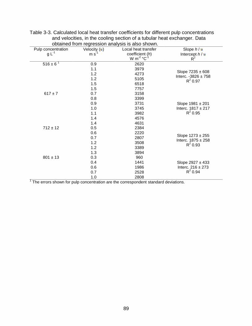
89
Table 3-3. Calculated local heat transfer coefficients for different pulp concentrations and velocities, in the cooling section of a tubular heat exchanger. Data obtained from regression analysis is also shown.
Pulp concentration g L
-1
Velocity ( )
m s-1
Local heat transfer coefficient (h)
W m-2
°C-1
Slope h /
Intercept h /
R2
516 ± 6 1 0.9 2620
Slope 7235 ± 608 Interc. -3826 ± 758
R2 0.97
1.1 3979
1.2 4273
1.2 5105
1.5 6518
1.5 7757 617 ± 7 0.7 3158
Slope 1981 ± 201 Interc. 1817 ± 217
R2 0.95
0.8 3399
0.9 3731
1.0 3745
1.1 3982
1.4 4576
1.4 4631 712 ± 12 0.5 2384
Slope 1273 ± 255 Interc. 1875 ± 258
R2 0.93
0.6 2220
0.7 2807
1.2 3508
1.2 3389
1.3 3894 801 ± 13 0.3 960
Slope 2927 ± 433 Interc. 216 ± 273
R2 0.94
0.4 1441
0.6 1986
0.7 2528
1.0 2808 1 The errors shown for pulp concentration are the correspondent standard deviations.

90
Figure 3-7. Local heat transfer coefficients as function of velocity in the heating section
of heat exchanger, for pulp concentrations of 516 (♦), 617 (■), 712 (▲), and 801 (Х) g L
-1.
Figure 3-8. Local heat transfer coefficients as function of velocity in the cooling section
of heat exchanger, for pulp concentrations of 516 (♦), 617 (■), 712 (▲), and 801 (Х) g L-1.
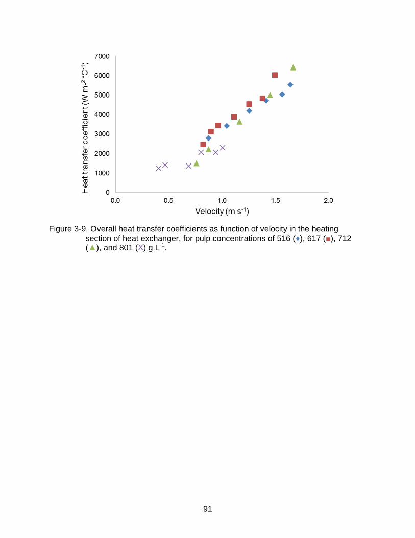
91
Figure 3-9. Overall heat transfer coefficients as function of velocity in the heating
section of heat exchanger, for pulp concentrations of 516 (♦), 617 (■), 712 (▲), and 801 (Х) g L-1.
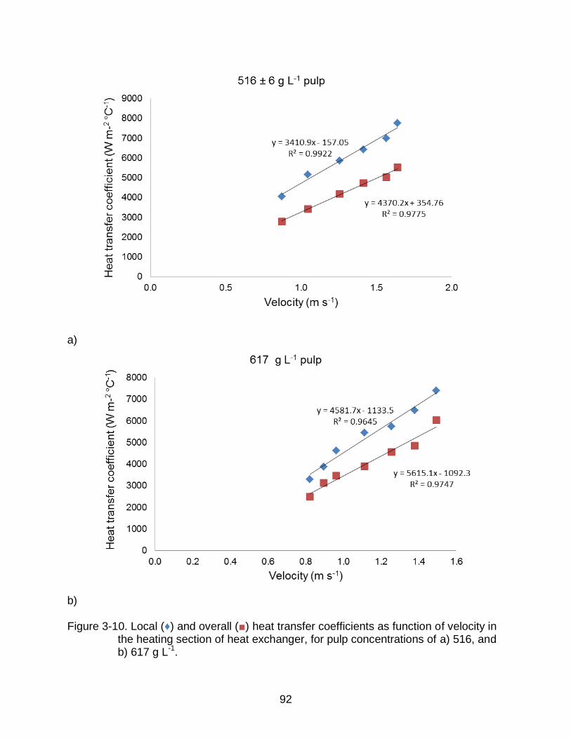
92
a)
b) Figure 3-10. Local (♦) and overall (■) heat transfer coefficients as function of velocity in
the heating section of heat exchanger, for pulp concentrations of a) 516, and b) 617 g L-1.

93
a)
b) Figure 3-11. Local (♦) and overall (■) heat transfer coefficients as function of velocity in
the heating section of heat exchanger, for pulp concentrations of a) 712, and b) 801 g L-1.

94
Figure 3-12. Temperature profiles obtained for 516 ± 6 g L-1 orange pulp concentration
in the heating section of a tubular heat exchanger at flow rates of 4.4 (♦), 5.3 (■), 6.4 (▲), and 7.9 (Х) x 10-4 m3 s-1.
Figure 3-13. Temperature profiles obtained for 516 ± 6 g L-1 orange pulp concentration
in the cooling section of a tubular heat exchanger at flow rates of 4.4 (♦), 5.4 (■), 6.3 (▲), and 7.5 (Х) x 10-4 m3 s-1.
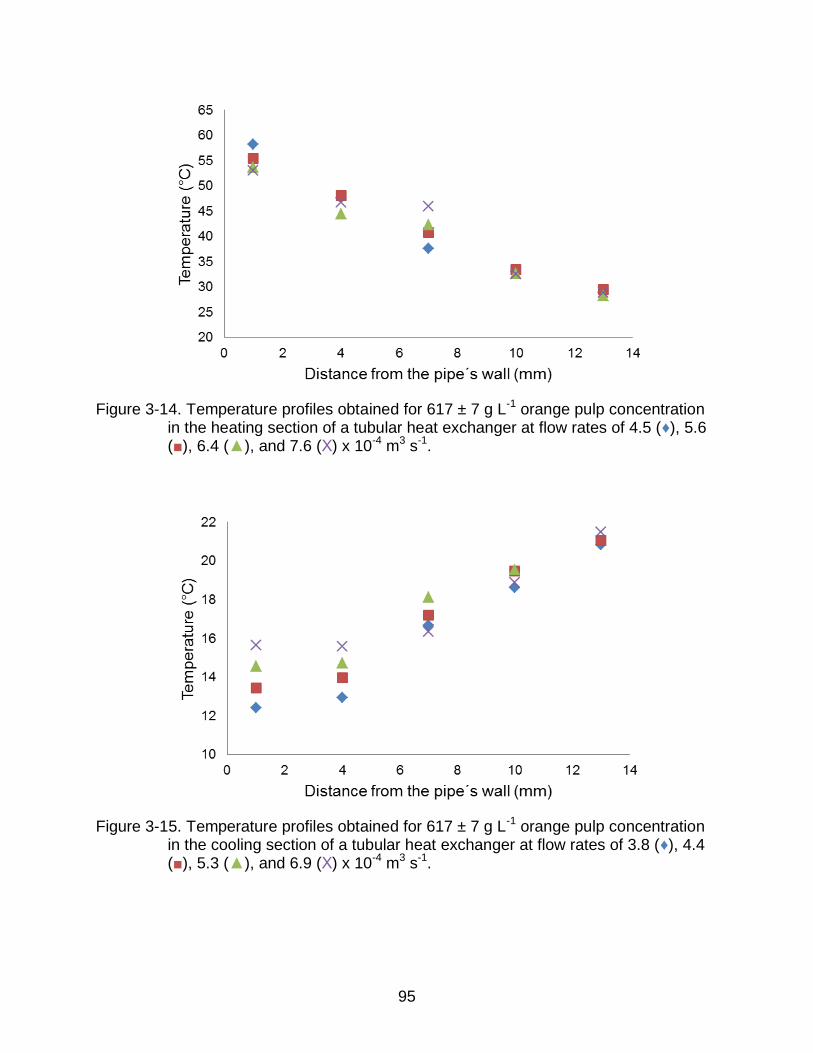
95
Figure 3-14. Temperature profiles obtained for 617 ± 7 g L-1 orange pulp concentration
in the heating section of a tubular heat exchanger at flow rates of 4.5 (♦), 5.6 (■), 6.4 (▲), and 7.6 (Х) x 10-4 m3 s-1.
Figure 3-15. Temperature profiles obtained for 617 ± 7 g L-1 orange pulp concentration
in the cooling section of a tubular heat exchanger at flow rates of 3.8 (♦), 4.4 (■), 5.3 (▲), and 6.9 (Х) x 10-4 m3 s-1.

96
Figure 3-16. Temperature profiles obtained for 712 ± 12 g L-1 orange pulp concentration
in the heating section of a tubular heat exchanger at flow rates of 3.9 (♦), 4.4 (■), 5.9 (▲), and 7.4 (Х) x 10-4 m3 s-1.
Figure 3-17. Temperature profiles obtained for 712 ± 12 g L-1 orange pulp concentration
in the cooling section of a tubular heat exchanger at flow rates of 2.7 (♦), 3.7 (■), 6.0 (▲), and 6.7 (Х) x 10-4 m3 s-1.

97
Figure 3-18. Temperature profiles obtained for 801 ± 13 g L-1 orange pulp concentration
in the heating section of a tubular heat exchanger at flow rates of 2.4 (♦), 3.5 (■), 4.1 (▲), and 5.1 (Х) x 10-4 m3 s-1.
Figure 3-19. Temperature profiles obtained for 801 ± 13 g L-1 orange pulp concentration
in the cooling section of a tubular heat exchanger at flow rates of 2.1 (♦), 2.9 (■), 3.6 (▲), and 4.8 (Х) x 10-4 m3 s-1.

98
Figure 3-20. Hypothesized mixed flow of HCP. A thin layer of liquid (slippage) was
formed close to the pipe surface, where heat was transferred by convection. While a thick plug of pulp flowed under laminar regime and heat was transferred mostly by conduction.
Figure 3-21. Pressure drop as function of flow rate in the heating section of heat
exchanger, for pulp concentrations of 516 (♦), 617 (■), 712 (▲), and 801 (Х) g L-1.

99
Figure 3-22. Pressure drop as function of flow rate in the cooling section of heat
exchanger, for pulp concentrations of 516 (♦), 617 (■), 712 (▲), and 801 (Х) g L-1.

100
APPENDIX A COMPARISON BETWEEN THE HEAT TRANSFER COEFFICIENTS OBTAINED IN
THE HEATING AND COOLING SECTIONS OF THE HEAT EXCHANGER
a)
b) Figure A-1. Heat transfer coefficients as a function of velocity in the heating (■) and cooling (♦) sections of heat exchanger for: a) 516 and b) 617 g L-1 orange pulp concentration.

101
a)
b) Figure A-2. Heat transfer coefficients as a function of velocity in the heating (■) and cooling (♦) sections of heat exchanger for: a) 712 and b) 801 g L-1 orange pulp concentration.

102
APPENDIX B COMPARISON BETWEEN THE PRESSURE DROPS OBTAINED IN THE HEATING
AND COOLING SECTIONS OF THE HEAT EXCHANGER
a)
b) Figure B-1. Pressure drop as a function of flow rate for a) 516, and b) 617 g L-1 pulp concentrations, in the heating (■) and cooling (♦) sections of a tubular heat exchanger.
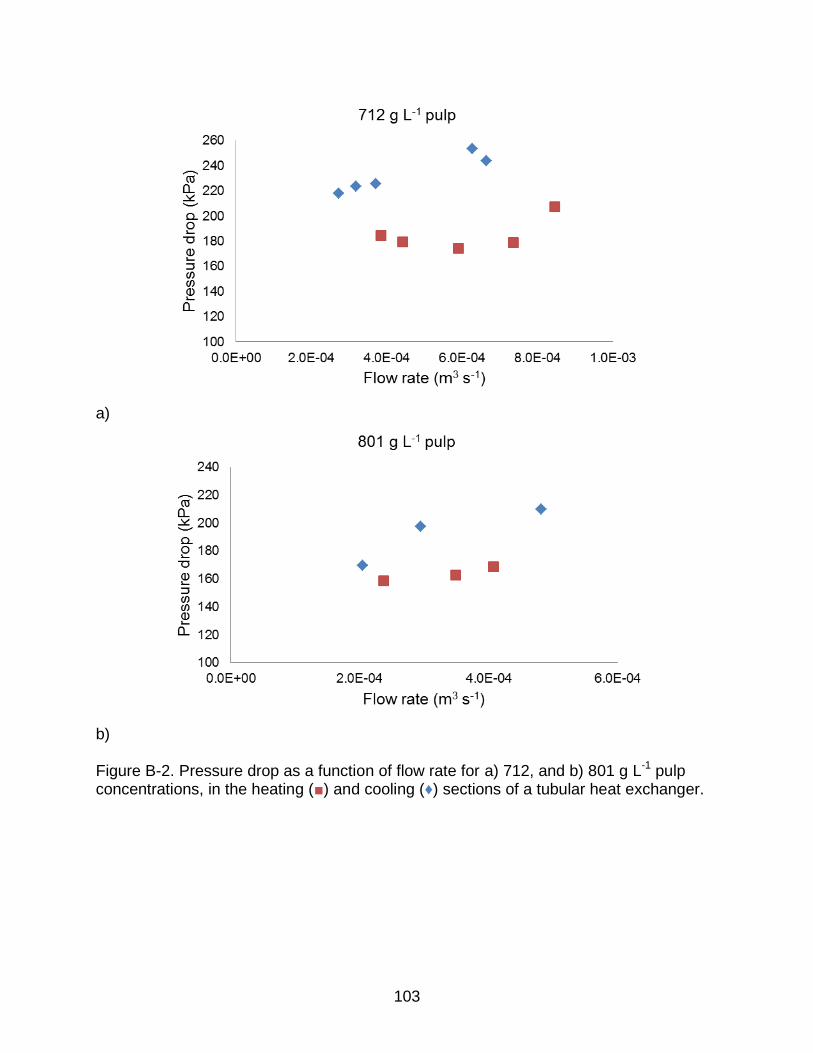
103
a)
b) Figure B-2. Pressure drop as a function of flow rate for a) 712, and b) 801 g L-1 pulp concentrations, in the heating (■) and cooling (♦) sections of a tubular heat exchanger.

104
LIST OF REFERENCES
Agocs A, Nagy V, Szabo Z, Mark L, Ohmacht R & Deli J. 2007. Comparative study on the carotenoid composition of the peel and the pulp of different citrus species. Innovative Food Science & Emerging Technologies 8(3):390-394.
Barnes HA. 1995. A review of the slip (wall depletion) of polymer-solutions, emulsions and particle suspensions in viscometers - its cause, character, and cure. Journal of Non-Newtonian Fluid Mechanics 56:221-251.
Basak S & Ramaswamy HS. 1996. Ultra high pressure treatment of orange juice: a kinetic study on inactivation of pectin methyl esterase. Food Research International 29(7):601-607.
Berlinet C, Guichard E, Fournier N & Ducruet V. 2007. Effect of pulp reduction and pasteurization on the release of aroma compounds in industrial orange juice. J Food Sci 72(8):S535-S543.
Bhamidipati S & Singh RK. 1994. Thermal time distributions in tubular heat exchangers during aseptic processing of fluid foods. Biotechnology Progress 10(2):230-236.
Bon J, Váquiro H, Benedito J & Telis-Romero J. 2010. Thermophysical properties of mango pulp (Mangifera indica L. cv. Tommy Atkins). Journal of Food Engineering 97(4):563-568.
Braddock RJ. 1999. Handbook of citrus by-products and processing technology. John Wiley.
Brat P. 2003. Distribution of Volatile Compounds in the Pulp, Cloud, and Serum of Freshly Squeezed Orange Juice J Agr Food Chem 51:3442-3447.
Cabral RAF, Gut JAW, Telis VRN & Telis-Romero J. 2010. Non-Newtonian flow and pressure drop of pineapple juice in a plate heat exchanger. Braz. J. Chem. Eng. 27(4):563-571.
Ditchfield C, Tadini CC, Singh RK & Toledo RT. 2006. Velocity and temperature profiles, heat transfer coefficients and residence time distribution of a temperature dependent Herschel-Bulkley fluid in a tubular heat exchanger. Journal of Food Engineering 76(4):632-638.
Ditchfield C, Tadini CC, Singh RK & Toledo RT. 2007. Heat transfer during thermal processing of a temperature dependent non-Newtonian fluid in a tubular heat exchanger. Chemical Engineering and Processing 46(5):472-476.

105
Gabs AL, Telis VRN, Tadini CC & Telis-Romero J. 2003. Effect of time-dependant rheological behavior on the laminar flow of frozen concentrated orange juice (FCOJ) in a circular pipe at subzero temperatures. 2nd Mercosur Congress on Chemical Engineering. 4th Mercosur Congress on Process Systems Engineering. Rio de Janeiro, Brasil. p. 1-10.
Gil-Izquierdo A, Gil M & Ferreres F. 2002. Effect of Processing Techniques at Industrial Scale on Orange Juice Antioxidant and Beneficial Health Compounds. J Agr Food Chem 50:5107-5114.
Goldstein RJ, Eckert ERG, Ibele WE, Patankar SV, Simon TW, Kuehn TH, Strykowski PJ, Tamma KK, Bar-Cohen A, Heberlein JVR, Davidson JH, Bischof J, Kulacki FA, Kortshagen U, Garrick S & Srinivasan V. 2005. Heat transfer--a review of 2002 literature. International Journal of Heat and Mass Transfer 48(5):819-927.
Gratão ACA, Silveira JV & Telis-Romero J. 2006. Laminar forced convection to a pseudoplastic fluid food in circular and annular ducts. International Communications in Heat and Mass Transfer 33(4):451-457.
Harnanan SW, Tejinder S & Bains GS. 2001. Effect of processing, preservation and storage on rheology of guava pulp. Journal of Texture Studies 32(4):271-284.
Hwang MP & Hayakawa K-I. 1979. A Specific Heat Calorimeter for Foods. J Food Sci 44(2):435-448.
Icier F & Ilicali C. 2005. Temperature dependent electrical conductivities of fruit purees during ohmic heating. Food Research International 38(10):1135-1142.
Kim HB, Tadini CC & Singh RK. 1999. Heat transfer in a plate exchanger during pasteurization of orange juice. Journal of Food Engineering 42(2):79-84.
Kimball DA. 1991. Citrus Processing-Quality Control and Technology. New York.
Larrea M. 2005. Effect of some operational extrusion parameters on the constituents of orange pulp. Food Chemistry 89(2):301-308.
Larrea M, Chang Y & Martinezbustos F. 2005. Some functional properties of extruded orange pulp and its effect on the quality of cookies. LWT - Food Science and Technology 38(3):213-220.
Lashkajani H, inventor. 1999 Oct 12, 1999. Method for producing a clouding agent using citrus pulp. United States patent 5,965,177.
Levati M. 2010. Rheological Behavior of Citrus Pulp and its Application to Aseptic Processing. JBT FoodTech. Parma, Italy. p. 32-46.
Lozano JE. 2005. Food Engineering. In: Barbosa-Cánovas, G., editor). Enciclopedia of Life Support Systems. Paris: EOLSS Publishers/UNESCO 2005. p. 45-64.

106
Martínez J & Carmona F. 1980. Composition of Citrus Pulp. Animal Feed Science and Technology 5(1):1-10.
McCabe WL, Smith JC & Harriot P. 1985. Unit Operations of Chemical Engineering,Fourth Edition ed. Singapore: McGraw-Hill International Book Co.
Mercali GD, Sarkis JR, Jaeschke DP, Tessaro IC & Marczak LDF. 2011. Physical properties of acerola and blueberry pulps. Journal of Food Engineering 106(4):283-289.
Nienaber U & Shellhammer TH. 2001. High-Pressure Processing of Orange Juice: Combination Treatments and a Shelf Life Study. J Food Sci 66(2):332-336.
Nikdel S, Chen CS, Parish ME, MacKellar DG & Friedrich LM. 1993. Pasteurization of citrus juice with microwave energy in a continuous-flow unit. J Agr Food Chem 41(11):2116-2119.
Passy N & Mannheim H. 1983. The Dehydration, Shlef Life and Potential Uses of Citrus Pulps. Journal of Food Engineering 2:19-34.
Payne E. 2011. Rheological Properties of High and Low Density Orange Pulp. Lake Alfred: University of Florida.
Prost JS, González MT & Urbicain MJ. 2006. Determination and correlation of heat transfer coefficients in a falling film evaporator. Journal of Food Engineering 73(4):320-326.
Rahman S. 2007. Food Preservation Aspects of Ohmic Heating. In: Rahman, S., editor). Handbook of Food Preservation Second ed. Boca Raton, Florida: CRC Press. Taylor and Francis Group. p. 742-748.
Rega B, Fournier N, Nicklaus S & Guichard E. 2004. Role of pulp in flavor release and sensory perception in orange juice. J Agr Food Chem 52(13):4204-4212.
Sangrame G, Bhagavathi D, Thakare H, Ali S & Das H. 2000. Performance evaluation of a thin film scraped surface evaporator for concentration of tomato pulp. Journal of Food Engineering 43(4):205-211.
Singh P & Heldman D. 2009. Introduction to Food Engineering,Fourth ed. Burlington, MA. USA: Elsevier Inc.
Souza D, Marczak LDF & Tessaro IC. 2008. Estudo das Propriedades Físicas de Polpas e Néctares de Pequenos Frutos. Porto Alegre: Universidade Federal do Rio Grande do Sul. p. 168-170.

107
Tavares DT, Alcantara MR, Tadini CC & Telis-Romero J. 2007. Rheological Properties of Frozen Concentrated Orange Juice (FCOJ) as a Function of Concentration and Subzero Temperatures. International Journal of Food Properties 10(4):829-839.
Telis-Romero J, Telis VRN & Yamashita F. 1999. Friction factors and rheological properties of orange juice. Journal of Food Engineering 40(1-2):101-106.
Tripodo M. 2004. Citrus waste recovery: a new environmentally friendly procedure to obtain animal feed. Bioresource Technology 91(2):111-115.
USDA. 2011. Citrus Fruits 2011 Summary. Chicago.
Yeom HW, Streaker CB, Zhang QH & Min DB. 2000. Effects of pulsed electric fields on the quality of orange juice and comparison with heat pasteurization. J Agr Food Chem 48(10):4597-4605.
Yeow YL, Perona P & Leong YK. 2002. A Reliable Method of Extracting the Rheological Properties of Fruit Purees from Flow Loop Data. J Food Sci 67(4):1407-1411.

108
BIOGRAPHICAL SKETCH
Juan Fernando Muñoz was born in Quito, Ecuador. In 2003, he obtained a Food
Engineering degree in Universidad San Francisco de Quito. From 2003 to 2010, he
worked in the food industry, mainly in the R&D field developing vegetable fats and oils
for industrial applications and food products for mass consumption. In 2010, J.F. Muñoz
began his graduate studies at University of Florida to pursue a master´s degree in Food
Science and Human Nutrition. He is expected to complete his studies in August 2012,
and intends to return to the industry to work in what he feels more passionate about:
Research and development.