determination of the energy–momentum densities of aluminium...

J. Phys.: Condens. Matter11 (1999) 3645–3661. Printed in the UK PII: S0953-8984(99)01098-X

Determination of the energy–momentum densities ofaluminium by electron momentum spectroscopy

M Vos†, A S Kheifets†, E Weigold†, S A Canney‡, B Holm§,F Aryasetiawan‖ and K Karlsson¶† Research School of Physical Sciences and Engineering, Institute of Advanced Studies, ANU,Canberra, A.C.T. 0200, Australia‡ Electronic Structure of Materials Centre, Flinders University of South Australia, GPO Box2100, Adelaide, S.A. 5001, Australia§ Department of Applied Physics, Chalmers University of Technology and Goteborg University,S-412 96 Goteborg, Sweden‖ Joint Research Centre for Atom Technology, Angstrom Technology Partnership, 1-1-4 Higashi,Tsukuba, Ibaraki 305, Japan¶ Department of Natural Science, Hgskolan i Skovde, 541 28 Skovde, Sweden

Received 20 January 1999

Abstract. The energy-resolved momentum densities of thin polycrystalline aluminium films havebeen measured using electron momentum spectroscopy (EMS), for both the valence band and theouter core levels. The spectrometer used for these measurements has energy and momentumresolutions of around 1.0 eV and 0.15 atomic units, respectively. These measurements should, inprinciple, describe the electronic structure of the film very quantitatively, i.e. the dispersion andthe intensity can be compared directly with theoretical spectral momentum densities for both thevalence band and the outer core levels. Multiple scattering is found to hamper the interpretationsomewhat. The core-level intensity distribution was studied with the main purpose of settingupper bounds on these multiple-scattering effects. Using this information we wish to obtain afull understanding of the valence band spectra using different theoretical models of the spectralfunction. These theoretical models differ significantly and only the cumulant expansion calculationthat takes the crystal lattice into account seems to describe the data reasonably well.

1. Introduction

A large amount of information on the electronic structure of solids has been acquired over thepast thirty years, both theoretically and experimentally. The vast majority of these theories usedfor the interpretation of experiments are in terms of effective one-particle models. Exchangeand correlation effects are acknowledged, but are assumed to only modify the effective potentialprobed by the electrons. This potential is usually obtained from some form of the densityfunctional theory.

A proper way of calculating one-particle excitation spectra is to use the Green functiontheory. Central to this theory is the spectral function describing the final state of the systemin terms of momentum and energy after the sudden removal of an electron. These spectralfunctions show dispersing structures rather similar to those obtained in the effective one-particletheories. However, they differ in two important respects.

Firstly, the calculated dispersing structures have (except right at the Fermi level) a finitebut significant width, i.e. lifetime broadening due to decay of the state created by the removal

0953-8984/99/183645+17$19.50 © 1999 IOP Publishing Ltd 3645

3646 M Vos et al

of an electron. Secondly, they give a significant fraction of the intensity (about 25%) atenergy/momentum values well away from the dispersing quasi-one-electron structures. Thesesatellites are often referred to as intrinsic plasmons, and are rooted in the screening of thecreated hole by the system, and hence are related to the electron–electron correlations.

There is only limited experimental evidence to test these theories. Lifetime widths can beobtained from photoelectron spectroscopy. The satellites are probed by photoemission as well,but their intensity is superimposed on intensity from extrinsic satellites excited by the outgoingelectron as it propagates to the surface. For aluminium, measured values of the intensity ratioof the intrinsic satellite to the core level range from 0.11 to 0.34 [1]. The valence band case iseven more complicated, as the excitation cross section in photoemission depends strongly onthe angular momentum of the initial state. Moreover, these measurements determine dispersion(binding energy versus crystal momentum) and do not resolve momentum densities directly.

The momentum density is probed by Compton scattering. It measures the projection ofthe momentum density of the target electrons on the scattering vector. If a series of differentdirections are measured, one can reconstruct the 3D momentum distribution. The effect ofelectron–electron correlation on the measured momentum distribution is a reduction in size ofthe discontinuity at the Fermi momentum as well as a tail extending the momentum distributionto larger values. There is currently a discrepancy between the size of the measured discontinuityand the theoretically predicted one [2,3].

In Compton scattering a photon transfers a large amount of energy to a target electron.Due to the fact that this electron is not detected one measures the momentum density of thetarget electron projected on the scattering vector. Attempts are being made to fully resolvethe momentum density by measuring the emerging electron in coincidence with the scatteredphoton. In these(γ, eγ ) experiments multiple scattering becomes a problem. The ejectedelectron should not transfer momentum on its way out of the solid. This requires thin free-standing films. This technique is still under development [4,5]. However, using photons, thisseems to be as far as one can go. It does not seem feasible with the current techniques to obtainenergy information as well as momentum information.

The Compton experiments rely on impulsive collisions. The ejected electron is assumed tohave such a large energy that it leaves the system without further interaction with the(N −1)-electron system left behind. This approximation is generally expected to be quite good forenergies of the ejected electron of 1 keV or more [6].

Instead of photons one can use electrons as the incoming particles. The interaction ofan electron with the target is much stronger than that of the photon (Møller versus Klein–Nishina cross sections [5]), and the electrons can be conveniently analysed for both energyand momentum using electrostatic analysers. This makes resolution of energy and momentumsimultaneously feasible, opening the possibility of completely measuring the (occupied partof the) spectral function. This technique is referred to as electron momentum spectroscopy(EMS) [7, 8]. EMS is an (e, 2e) experiment performed under conditions such that the plane-wave impulse approximation is valid, i.e. in the limit of high energy and momentum transfer.

However, the price that one pays is that in these EMS experiments, due to the strongerinteraction of the electron with the target, multiple scattering is an even larger problem than inthe(γ, eγ ) case, even for the thinnest of films. Indeed, only a small fraction of coincidences arerelated to clean events (i.e. without multiple scattering). In this paper we examine how muchinformation about the spectral function one can obtain in spite of these multiple-scatteringeffects, using aluminium as an example.

There are a number of favourable factors. Firstly, the interaction of keV electrons witha solid is relatively simple and well understood, and can be described to a certain extent in asemiclassical way as straight trajectories separated by elastic (with the ion cores) or inelastic

Determination of the energy–momentum densities of aluminium 3647

(with the electrons) collisions. The average separation of these collisions is described by theelastic and inelastic mean free path. In this way one can model fairly accurately the multiple-scattering effects and attempt to correct for them.

Secondly, we have to describe three quantities i.e. the intensity at a certain mom-entum/binding energy combination. As we will see, this is a very stringent test, i.e. nocalculated spectral function gives a perfect fit to the data even if one tries to adjust someof the parameters such as the elastic and or inelastic mean free path, film thickness etc. Thedisagreement between experiment and theory can be due to imperfections in either one orboth of them. This makes it a stringent test case, and it will be interesting to see whetherdevelopments in experimental and theoretical techniques will resolve these differences.

The remainder of the paper is organized as follows. In the next section we establish theconnection between the spectral function and the measured (e, 2e) intensity for a free-electrongas. Subsequently we present the (e, 2e) measurement over a wide energy range and seehow we can use the core levels to get some upper limits on the multiple-scattering effects.Finally we concentrate on the valence band and see how different calculations compare withthe measurements.

2. The relation between EMS and the spectral function

Previously we have compared EMS results with band-structure calculations. For the case ofaluminium this was done by Canneyet al [9, 10]. Briefly one solves the electronic structureof the solid in terms of Bloch functions

9k =∑G

cGe(k+G)·R.

Each Bloch function has a well defined energy and contributes to the EMS intensity at thisenergy and at a momentumk +G by an amount proportional to|cG|2. In order to see whatchanges if we want to take correlation effects explicitly into account, we briefly review thetheory of electron momentum spectroscopy in solids so that we can get some insight into thenature of the approximations made in comparing the EMS results with a spectral function.

One can think of EMS as a high-energy EELS (electron energy-loss spectroscopy) exp-eriment with the measured intensity restricted by an additional coincidence requirement. Inan EELS experiment an incoming electron (energyE0, momentumk0) scatters from a targetsystem containingN electrons and emerges with energyE1 and momentumk1. We useω forthe transferred energy (ω = E0 − E1) andk for the transferred momentum (k = k0 − k1).

In the first Born approximation, which is valid at high energies, the scattering cross sectionof an EELS experiment can be written as

dσ

dω d�= Ck k1

k0S(k, ω) (1)

withCk a term that depends on the particle–particle interaction and the momentum transfer [11].For electrons it can be written as (we use atomic units throughout)

Ck = 4

k4N. (2)

whereN is the number of electrons in the system. (Here we assume that 1/k4� 1/k41). It is a

constant for a given measurement geometry. The second term is determined by the electronicstructure of the target. It describes the time dependence of the density–density correlationsand can be written as

S(k, ω) = 1

2πN

∫ ∞−∞

dt eiωt 〈ρk(t)ρ−k(0)〉 (3)

3648 M Vos et al

with ρk(t) ≡ eiHtρke−iHt andρk the Fourier transform of the electron density in coordinatespace andH the Hamiltonian of theN -electron system. Equation (1) is the central formulaused in the interpretation of EELS experiments, and was first derived by Van Hove [12]. Itassumes the sudden limit, i.e. no interaction between the outgoing (scattered) electron and thesystem left behind in an excited state.

In general a difference between an EMS experiment and a traditional EELS experimentis that the transferred momentumk in the latter is much smaller thank0, usually not more than1 au. In EMS our aim is to measure momentum densities and thus we want to scatter fromindividual electrons. The size of the area from which we scatter is of the order of 1/k. Thusin order to have these binary collisions we need large momentum transfer, perhaps even up tothe maximum possible,k0/

√2.

In the case of high momentum transfer in a binary collision both the scattered and ejectedelectron can be approximated by a free electron. Thus for the final state we can write

|αN 〉 = |k2αN−1〉. (4)

wherek2 is the momentum of the ejected electron. This means that there is no interactionof the outgoing electrons with the(N − 1)-electron system left behind, i.e. the reaction takesplace in the sudden limit with respect to the ejected electron as well. Intuitively it is clear thatthe validity of this approximation is better for faster outgoing electrons.

Plane waves are the natural basis for a homogeneous (free-electron-like) system. (If oneconsidered the crystal lattice, one would of course use Bloch waves.) Letaq anda†

q be theannihilation and creation operators for an electron with momentumq. Further define

aq(t) = eiHtaqe−iHt . (5)

The electron density componentρ±k can be written as

ρk =∑q

a†qaq+k ρ−k =

∑q

a†q+kaq. (6)

Using this notation we can write

〈0|ρk(t)ρ−k(0)|0〉 =∑q,q′〈0|a†

q(t)aq+k(t)a†q′+k(0)aq′(0)|0〉. (7)

Consider a system in the ground state|0〉. The momentum densities decrease rapidlyabovekF (kF being the Fermi momentum), even for an interacting electron gas. Those termsin the sum with eitherq or q ′ � kF do not contribute to the sum, as these matrix elements areevaluated in the ground state. Thus for those terms that contribute,|q + k| � kF , as we areinterested in large values of the transferred momentumk, and we can write

〈0|a†q(t)aq+k(t)a

†q′+k(0)aq′(0)|0〉 = e−iεq+k t 〈0|a†

q(t)aq′(0)aq+k(0)a†q′+k(0)|0〉 (8)

Here

εq+k = k2/2 + (q · k) + q2/2

i.e. the time dependence ofaq+k(t) (the ejected electron) is taken to equal that of a free electronwith that momentum.a†

q′+k creates an electron with momentumq′ + k with probability 1 asthis level is unoccupied in the ground state due to the large magnitude ofk (and the smallmagnitude ofq′). The matrix element is zero unless this electron is annihilated byaq+k. Thismeans thatq′ = q. Thus we are left with∑

q,q′〈0|a†

q(t)aq+k(t)a†q′+k(0)aq′(0)|0〉 =

∑q

〈0|a†q(t)aq(0)|0〉e−iεq+k t . (9)

Substituting this back in equation (3), the familiar results of a Compton profile being measuredin a high-momentum-transfer EELS experiment are obtained [13]. In our case we measure


the ejected electron as well. This means that we determineq +k, and hence instead of a sum-mation overq in equation (9) only the term withq = k1 + k2 − k0 contributes. The energyanalysis of the ejected electron determinesεq+k. Thus we can write the energy-resolved crosssection of an (e, 2e) experiment using equation (3), equation (5) and equation (9) as

dσ 4

dE1 dE2 d�1 d�2=(

1

2π

)5k1k2

k0|V (k)|2

∫ ∞−∞

dt

2π〈0|a†

q(t)aq(0)|0〉e−i(E0−E1−E2)t . (10)

HereV (k) = 4π/k2 is the Fourier transform of the Coulomb potential. Note that the integralis a real quantity, as the contribution att is the complex conjugate of the contribution at−t .

In the sudden approximation there is no interaction after the collision between the systemand the emerging electrons. The measured energyε = E0−E1−E2 is thus the energy of thestate created att = 0 with momentumq. Now compare this expression with the definition ofthe (retarded) Green’s function:

G−(q, t) = −i2(t)〈0|a†q(t)aq(0)|0〉

G−(q, ε) = −i∫ ∞

0〈0|a†

q(t)aq(0)|0〉e−iεt dt(11)

with 2(t) = 0 for t < 0 and 1 fort > 0. G−(q, ω) is complex. However, from the structureof these equations it is clear that this function is closely related to the (e, 2e) cross section:

dσ 4

dE1 dE2 d�1 d�2= 1

(2π)5k1k2

k0|V (k)|2(−π)−1 ImG−(q, ε). (12)

The same result was obtained by D’Andrea and Del Sole, in the context of (e, 2e) measurementsof reconstructed surfaces [14]. This is the central equation for the interpretation of the EMSresults of a many-electron interacting system. The measured intensity is proportional to aconstant which depends on the kinematics of the experiment and the imaginary part of theone-particle Green’s function (spectral function). Thus instead of comparing the EMS resultssimply with the modulus of the square of the wave function in momentum space, as is done insingle-particle theories, we have to compare the EMS results with the spectral function whichis a key element of the many-body formalism.

This relation between the spectral function and the measured intensity is a directconsequence of the impulse approximation. The above derivation is given mainly to bring outtwo important differences between photoemission experiments and these electron scatteringexperiments. In EMS there are no different matrix elements for different electrons (s, petc). Also the measurement of dispersion does not rely on the crystal periodicity, as crystalmomentum does not appear in the above derivation. The latter reason makes EMS a probethat can test jellium-type calculations of free-electron-like materials such as aluminium, as thecrystal potential is not an essential part of the excitation process.

3. Spectral functions for aluminium

In this paper we use four different spectral functions. First we use a linear muffin-tin orbital(LMTO) calculation of the aluminium band structure based on the local density approximationof the density functional theory (model A). In this model correlation effects are assumed toaffect only the effective one-particle Hamiltonian. This calculation was used in the previouspaper describing these experiments [9]. As our sample is polycrystalline, the results of thecalculation are averaged over all directions.

As this is a one-particle theory, there is no lifetime broadening of the Bloch states. It wasfound in [9] that if empirical lifetime broadening was added (taken from Levinsonet al [15]),

3650 M Vos et al

it could describe the data from the Fermi level to the bottom of the band quite well, but failed athigher binding energies. Thus the empirical lifetime broadening is included again in model A.

As much as 30 years ago it was predicted theoretically that the sudden removal of anelectron from a free-electron gas may result in the excitations of plasmons in the system. Thefinal state then has a larger energy, not just the binding energy of the electron removed from afree-electron gas, and hence there are satellites at higher binding energy in the spectrum.The simplest model that abandons the effective one-particle assumption and incorporatesthese satellites is theG0W calculation as described by Lundqvist [16]. This is our modelB. This model neglects the lattice (it is a jellium model). Satellites appear now at higherbinding energies and the quasi-particle part of the spectral function has lifetime broadening.However, it is known from photoemission data that the satellite position predicted by model

0 10 20 30 400 10 20 30 40

0<q<0.1

0.1<q<0.2

0.2<q<0.3

0.3<q<0.4

0.4<q<0.5

0.5<q<0.6

0.6<q<0.7

0.7<q<0.8

0.8<q<0.9

0.9<q<1.0

Binding Energy (eV)

Inte

nsity

(ar

b. u

nits

)

0 10 20 30 40

ABCD

0 10 20 30 40

Figure 1. Four different spectral functions of aluminium as derived from the four different theoriesA–D as described in the text. The theories are convoluted with the experimental energy (1.5 eV)and momentum resolution (0.15 au). They are all normalized to equal height of the quasi-particlepeak at zero momentum.


B (at'1.5× the plasmon energy) is not supported by experiment. The model is reproducedhere for completeness.

The third model (model C) is a more recent calculation using cumulant expansiontechniques [17–21] as described in references [22, 23]. For reasons that will be apparentwhen we compare our theoretical model with the experimental spectrum, we have used thecumulant expansion in anon-self-consistent manner. Using a cumulant expansion scheme, theproblem with the satellite energy seems to be rectified. It is again a model that neglects thecrystal lattice.

Finally, model D is the result of a cumulant expansion calculation including the crystallattice. Again it is averaged over all directions. Calculations were done for 30 differentk-pointsin the first Brillouin zone.

Near the Fermi level the spectral function is sharply peaked. The energy step size incalculation C and the coarseness of thek-grid in calculation D seem to affect the area of the peakheight obtained near the Fermi level somewhat. The four different theories, after convolutionwith the experimental energy (1.5 eV) and momentum resolution (0.15 au), are plotted infigure 1 for momentum values from 0 to 1 au. Binding energies in this and the followingfigures are relative to the Fermi level. In spite of our modest resolutions, the differencesbetween the different models should be well resolved with the present spectrometer.

4. Experimental procedure

The experimental procedure was described extensively in reference [9]. In brief, we evaporateda thin aluminium layer ('40 Å) onto a free-standing carbon membrane ('60 Å thick). Thesample was transferred under UHV (ultra-high vacuum) to the EMS spectrometer and measuredfor a period of 2–3 days. The EMS spectrometer uses an asymmetric geometry, with a relativelyslow ejected electron (20 keV incoming beam, 18.8 keV fast (scattered) outgoing electron,1.2 keV slow (ejected) outgoing electron). Due to a relatively low energy of the slow electronthe experiment is mainly sensitive to one side of the sample (the one covered with aluminium).For events occurring at large depths (in the carbon layer) the probability of the slow electronescaping without elastic and/or inelastic scattering is extremely small. In no case did weobserve a clear signature of the carbon layer in the spectra. Of course, (e, 2e) events occurringin the carbon substrate can contribute to the rather structureless background due to multiplescattering. Their contribution to the spectrum decreases due to the small mean free path forboth elastic and inelastic scattering of the slow electron created during the (e, 2e) events.

As we will discuss later, the core levels show some indication of the presence of theinitial stages of the oxidation of aluminium. In order to show that the contributions of eithercarbon and/or aluminium oxide are small, we present in figure 2 a spectrum of Al, Al2O3 andamorphous carbon, both at zero momentum and at a relatively high momentum (near 1.5 au).All energies are relative to the Fermi level. The aluminium spectrum does not extend far beyond1 au (for aluminiumkf = 0.97 au). Much of the intensity measured at higher momentumvalues is due to (e, 2e) events with additional elastic scattering of the incoming and/or outgoingelectrons, and hence it has no clear structure. Both the Al2O3 and the amorphous C spectraextend to larger momenta. If a substantial amount of either of these spectra were to be presentin the measured Al valence band spectrum, it would be visible at high momentum. Multiplescattering in the carbon layer will however influence the shape of the background of the Alvalence band. These processes are included in the Monte Carlo simulations, to be discussedlater. More details on the oxidation of Al, as seen by EMS, can be found in [24] and on EMSof amorphous carbon in [25].

3652 M Vos et al

1.4<|q|<1.6

0<|q|<0.2

Amorphous Carbon

1.4<|q|<1.6

0<|q|<0.2'Al

2O

3'

Inte

nsity

(ar

b. u

nits

)

0 10 20 30

Binding Energy (eV)

1.4<|q|<1.6

0<|q|<0.2

Aluminium

Figure 2. The spectra of amorphous carbon, aluminium oxide and aluminium for momentumvalues near zero and near 1.5 au. The distinct features in the aluminium spectra extend only upto 1.0 au and from these spectra it is clear that neither aluminium oxide or carbon contributessignificantly to the aluminium spectra.

5. Experimental results

5.1. Introduction

In figure 3 (left-hand panel) we show the experimental EMS data over a binding energy rangeof 140 eV. The data show the measured intensity integrated over different momentum ranges.For small momenta (<0.5 au) the main peak is in the valence band region, although othersharp features (namely the 2s and 2p core levels) are also present at larger binding energies. Athigher momenta the valence band features become less pronounced, whereas the intensity ofthe core levels persists. In this plot we also show the intensity as predicted by a single-particletheory, without multiple scattering. For the theory the valence band structure was obtainedfrom an LMTO calculation with empirical lifetime broadening (model A), whereas the core-level momentum distributions were taken to be equal to those for the atomic case and the


0

100

200

300

400

500

600

700

800Scan 1

Scan 20.0<q<0.5 a.u.

Al. valence

Al 2pAl 2s

0

80

160

240

320

400

480

560 0.5<q<1.0 a.u.

Inte

nsity

(ar

b. u

nits

)

Scan 1

Scan 20.0<q<0.5 a.u.

Al. valence

Al 2pAl 2s

0.5<q<1.0 a.u.

0

100

200

300 1.0<q<1.5 a.u. 1.0<q<1.5 a.u.

0

100

2001.5<q<2.0 a.u. 1.5<q<2.0 a.u.

0

100

200

0 20 40 60 80 100 120

2.0<q<2.5 a.u.

0 20 40 60 80 100 120

2.0<q<2.5 a.u.

Binding Energy (eV)

Figure 3. A scan for an aluminium film over a wide energy range that includes both the valenceband and the outer core levels. The data are integrated over five momentum ranges, as indicated.In the left-hand panel we compare the data with a theory (LMTO calculation) that does notinclude multiple-scattering effects. In the right-hand panel the theoretical intensity is correctedapproximately for multiple scattering.

binding energies of the core levels were taken from photoemission data. The intensity ratio ofthe core level and valence band is, however, not a free parameter since all the wave functionsare normalized to the total number of electrons in that level. The calculations were convolutedwith the experimental energy and momentum broadening. Additional lifetime broadening wasadded for the 2s level to obtain agreement with the experimental width of 2 eV FWHM. (For

3654 M Vos et al

the 2p level, lifetime broadening is not resolved.)In all cases there is a sharp feature in the measured spectrum at the positions predicted by

the calculations. However, it is obvious from this plot that the large majority of events are notdirectly related to either the core levels or the valence band. In these cases the (e, 2e) eventwas not the only interaction of the electrons with the solid. Inelastic scattering has occurred aswell, and has shifted the intensity to lower binding energies. Indeed the highest peaks in thelower-momentum ranges are not in the valence band region, but occur just below the valenceband region.

It is interesting to note that in EMS the valence band dominates the spectrum at lowmomentum. As these valence wave functions are extended in real space they are confined tothe low-momentum region in momentum space, and hence have a relatively high intensity atlow momentum. The much more localized core levels are confined in real space, and thusextended in momentum space, and consequently have smaller intensities in the experiment.The ratio of the valence band to core-level intensity in the experiment is of the same orderas the calculated one. The ratio of the valence to core levels is completely different for EMScompared to the one obtained in XPS (x-ray photoelectron spectroscopy). In the latter casethe core levels are by far the most intense features. This fact reflects the great differences inthe excitation processes of the two techniques.

Thus, although there is a clear signature of the spectral momentum densities in these plots,it is also clear that the majority of events are not directly related to it. In these cases additionalscattering occurred for either the incoming or outgoing electron trajectories. These effects canbe modelled using semi-empirical models of electron propagation in solids. We carried outMonte Carlo simulations as described by Vos and Bottema [26]. Briefly, their method usesinelastic and elastic mean free paths for the distribution of the elastic and inelastic collisions.The magnitudes of the deflections due to elastic collisions are derived from the cross sectionof elastic scattering of an electron from an atom. The energy loss is set equal to the plasmonenergy (with a spread around the mean corresponding to the experimentally determined width).

In the present simulations we included surface plasmons as well. The probability ofsurface plasmon creation can be obtained from theory (see e.g. Stern and Ferrel [27], or thesummary given by Egerton [28]). However, the appearance of the surface plasmon componentis coupled to a reduction of the bulk plasmon component. This means that the excitationprobability of the bulk plasmon near the surface is smaller, i.e. its mean free path shouldincrease near the surface. This is not easily implemented in our Monte Carlo code and was notattempted. Instead we used bulk plasmon creation rates everywhere, and hence overestimatethe bulk plasmon creation rate slightly.

The results are shown in figure 3 (right-hand panel). The simulation was normalized tothe experiment using the same normalization factor for all five momentum intervals, obtainedby setting the valence peak height equal to the experimental one for the lowest momentuminterval. Clearly the theory together with the simulations predicts intensity all the way downto high binding energies. However, the measured intensity is still larger than the calculatedintensity, especially for small momentum values, and for binding energies between 15 and60 eV.

5.2. Core levels

It is clear that even after including multiple scattering with Monte Carlo simulations, theagreement with the measurement is still poor. Let us now focus on the 2p core level. This isthe sharpest structure (in energy) in the experiment, with a momentum distribution which issupposedly very close to the atomic one. These results are shown in figure 4. In the central


sim

ulat

ed in

tens

ity

55 60 65 70 75 80 85 90 95

Binding Energy (eV)

Inte

nsity

(ar

b. u

nits

)

Figure 4. In the central panel we show the Al 2p core level as measured by EMS. The intensitywas integrated from 0 to 2.5 au of momentum. Four different contributions can be distinguishedwith increasing binding energy: the main component, a contamination-related component and thesurface and the bulk plasmon components. The top panel shows the 2p intensity, as predicted bythe Monte Carlo simulations as discussed in the text. The lower panel shows the result of exposureof the aluminium film to 600 L of O2.

panel we show the experimental data. These coincidence experiments have rather low countrates and the data shown are the result of a two-day measurement. In spite of a vacuum below1.0× 10−10 Torr there is still a tail on the high-binding-energy side of the 2p peak. A smallpart of the intensity on the high-binding-energy side will be due to the non-resolved spin–orbitsplitting and the asymmetry of the Doniach–Sunjic lineshape, which was not incorporated inthe fit. However, for the largest part it will be due to some oxidation of the surface. The exactarea of this contribution is difficult to estimate, but for the fit shown it is'25% of the mainline, which we consider as an upper limit.

It should be noted that in the case of the graphite 1s core level a very similar tail, extendingto higher binding energies, was observed [29]. This is the only other core level that has beenstudied in detail with the current spectrometer. Thus the impurity satellite could as well be an

3656 M Vos et al

artefact of the spectrometer.In the lowest panel we show the effect of purposely exposing a fresh Al film, prepared in

an identical manner, to 600 L of oxygen. In this case the effects of oxidation are much morepronounced. Full details of a systematic study of the oxidation of an aluminium surface byEMS were given by Canneyet al [24].

The main 2p structure has a width of 1.5 eV. The spin–orbit splitting ('0.4 eV) is thus notresolved. However, it sets an upper limit of the resolution of the spectrometer (and stabilityover a two-day period) of about 1.3 eV. There is no reason that this resolution should not applyto the valence band data, as they are taken under identical circumstances. However, to besomewhat conservative we use the value of 1.5 eV for our assumed valence band resolution.

There are two more structures visible in figure 4. One is 15.6 eV away from the mainline, hence related to the plasmon satellite, and has 69% of the intensity of the main line. Theother is shifted by 10.6 eV, which corresponds to the surface plasmon and it has 28% of theintensity of the main line.

In order to obtain the intensities of the different components we fitted the background witha second-order polynomial. This background above the Al 2p level can only have its origin in(e, 2e) events with the valence band (in the carbon or aluminium layer) plus additional energy-loss events. We would like to point out that there is an intrinsic danger in this procedure. If thereare very broad satellites to the core level then we may incorporate these features inadvertentlyin the background originating from the valence electrons.

Next we want to use the core-level intensity obtained as a test of the validity of theMonte Carlo simulations. In the simulations we can ‘turn off the valence band’ contributionto the measured spectrum (and at the same time change nothing in the elastic and/or inelasticscattering behaviour). We obtain then an intensity of the Al 2p core level and its associatedplasmon and surface plasmon. The result of this simulation is shown in the top panel of figure 4.

In discussions of the plasmon intensity of core levels in photoemission experiments, oneusually uses the three-step model, i.e. one assumes that it is possible to separate the excitationstep from the propagation to the surface and subsequent escape steps. It is then possible,in principle, to distinguish between intrinsic and extrinsic plasmons, i.e. those created duringexcitation and those created during subsequent propagation of the photoelectron to the surface.In the above analysis we do not include intrinsic plasmons. One should thus consider thesimulations to give only an upper bound of the contributions of extrinsic loss processes. Valuesof the creation rates of intrinsic plasmons as compiled by Hufner for the Al 2p core level rangefrom 0.11 to 0.34 relative to the main line [1]. The reduction in the bulk plasmon creation dueto the surface, which is not taken into account in the simulations, is theoretically estimatedto be close to half the creation rate of the surface plasmon [30]. The reasonable agreementobtained in the simulation could thus be due to the fact that the contribution of the intrinsicplasmon, and the reduction of the extrinsic bulk plasmon, due to surface effects, are of similarmagnitude.

Besides giving a good description of the energy spectra, the simulations also have todescribe the observed momentum distributions. For the Al 2s and 2p lines this is shown infigure 5. First the spectra were integrated over a large momentum range. Then the mainline was fitted with one Gaussian component only. The energy positions and widths of thepeaks were determined and subsequently kept fixed. The spectra were then fitted over smallermomentum intervals, with only the shape of the background and the peak height allowed tovary. The resulting intensities showed a local minimum for the 2p level at zero momentum,whereas the 2s level has maximum intensity at zero momentum. The (atomic) Al 2p wavefunction itself has a node at zero momentum, and hence the atomic 2p density is zero at zeromomentum (solid curves in figure 5). The residual intensity of the 2p level at zero momentum


0 0.5 1 1.5 2 2.5 3

0 1 2 3 4 5

0 1 2 3

0 1 2 3 4 5

Momentum (a.u.)

Inte

nsity

(ar

b. u

nits

)

Momentum (Å -1)

105 110 115 120 125

0.0<q<3.0 a.u.

Al 2s

60 65 70 75 80

Inte

nsity

(ar

b. u

nits

)

0.0<q<3.0 a.u.

Al 2p

Binding Energy (eV)

Figure 5. In the top two panels we show the Al 2p and Al 2s levels fitted with one Gaussiancomponent. The position and width of this Gaussian was kept fixed and was used to determine thepeak area of these lines as a function of momentum (error bars, lower two panels). The atomic 2pand 2s momentum densities are each indicated with a solid curve; the expected intensity based onthe atomic momentum densities and an estimate of the effects of multiple scattering are indicatedby the dashed curves.

cannot be explained by finite momentum resolution. Monte Carlo simulations as describedabove seem to predict the observed shapes fairly well, as is shown by the dashed curves. Themeasured intensity of the 2p level near zero momentum appears thus to be an effect of elasticscattering (i.e. the incoming and/or one of the outgoing electrons was deflected by an ion core,causing the wrongq-value to be inferred from the momentum conservation equation).

Thus the core-level spectra seem to be described reasonably well, if we correct for multiplescattering, both in energy and momentum space. If anything, the Monte Carlo simulations

3658 M Vos et al

overestimate the aluminium plasmon-loss peak, as the current analysis does not take intoaccount the possible existence of intrinsic plasmons.

5.3. The valence band

We now return to the valence band results. They differ, of course, from those for the corelevels in that the binding energy depends on momentum. This dispersion is well describedby the band-structure calculations, which are now done routinely even for complicated solids.Our band-structure calculations are linear muffin-tin orbital (LMTO) calculations, using theatomic sphere approximation (model A). As our sample is polycrystalline, the results of thecalculation have to be averaged over all directions. It was found by Canneyet al [9] thatthe spherically averaged calculations were in good agreement with the experiment in thenear-valence-band region, but that they underestimate the intensity at higher binding energies,even after inclusion of multiple-scattering effects [9]. The dispersing structure was, withinexperimental error, indistinguishable from a free-electron parabola—i.e. aluminium, as far asour experiment is concerned, seems to be a good example of an electron gas [9]. However, theintensity at large binding energies was underestimated by this approach.

LMTO+life-time broadening (model A)G

0W

0 Calculation, Jellium (model B)

Cumulant Expansion, Jellium (model C)Cumulant Expansion, Lattice (model D)

Inte

nsity

(ar

b. u

nits

)

-10 0 10 20 30 40

Binding Energy (eV)

Inte

nsity

(ar

b. u

nits

)

Figure 6. The valence band of aluminium for zero momentum. In the top panel we show thespectral function for zero momentum for the different theories as indicated. After including thesame multiple-scattering effects as for the core level, we obtained the curves in the lower panel asa theoretical estimate of the measured intensity (error bars). All have been normalized to the samequasi-particle peak height atε ' 11 eV.


This was the reason for the use of models B to D for comparison with our experiment, inthe hope that these more sophisticated theories will give a better description of the experiment.First we plot again the spectral function at zero momentum (but now without broadening dueto finite energy and momentum resolution) atq = 0 (figure 6, upper panel).

As lifetime broadening is an essential component in these many-body theories, let us firstcompare the width of the quasi-particle peak as a function of binding energy. The empiricalbroadening is larger than the one obtained from theories. Canneyet al [9] found that theempirical lifetime broadening based on the measurement of Levinsonet al [15] described ourexperimental data very well. Nearq = 0 the assumed broadening was 3.5 eV FWHM. Thetheoretical spectral function has a width nearq = 0 of 1.7 eV for model B [16] and 2.4 eVfor model C [23], whereas model D is closest to the empirical values (about 3 eV). Thus the

0 10 20 300 10 20 30 0 10 20 30

0.6<q<0.7

0.7<q<0.8

0.8<q<0.9

0.9<q<1.0

1.0<q<1.1

1.1<q<1.2

0 10 20 30

Binding energy (eV)

Inte

nsity

(ar

b. u

nits

)

0.0<q<0.1 a.u.

0.1<q<0.2

0.2<q<0.3

0.3<q<0.4

0.4<q<0.5

0.5<q<0.6

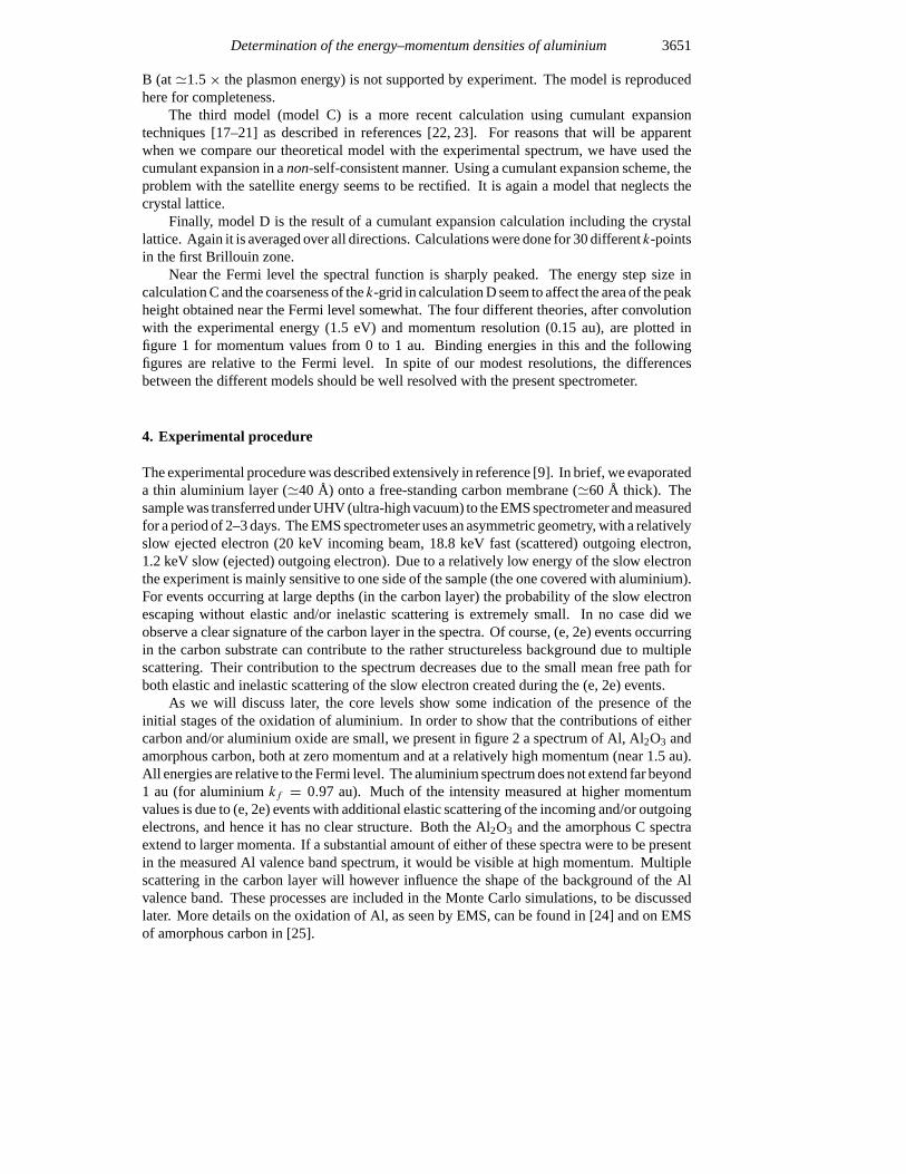
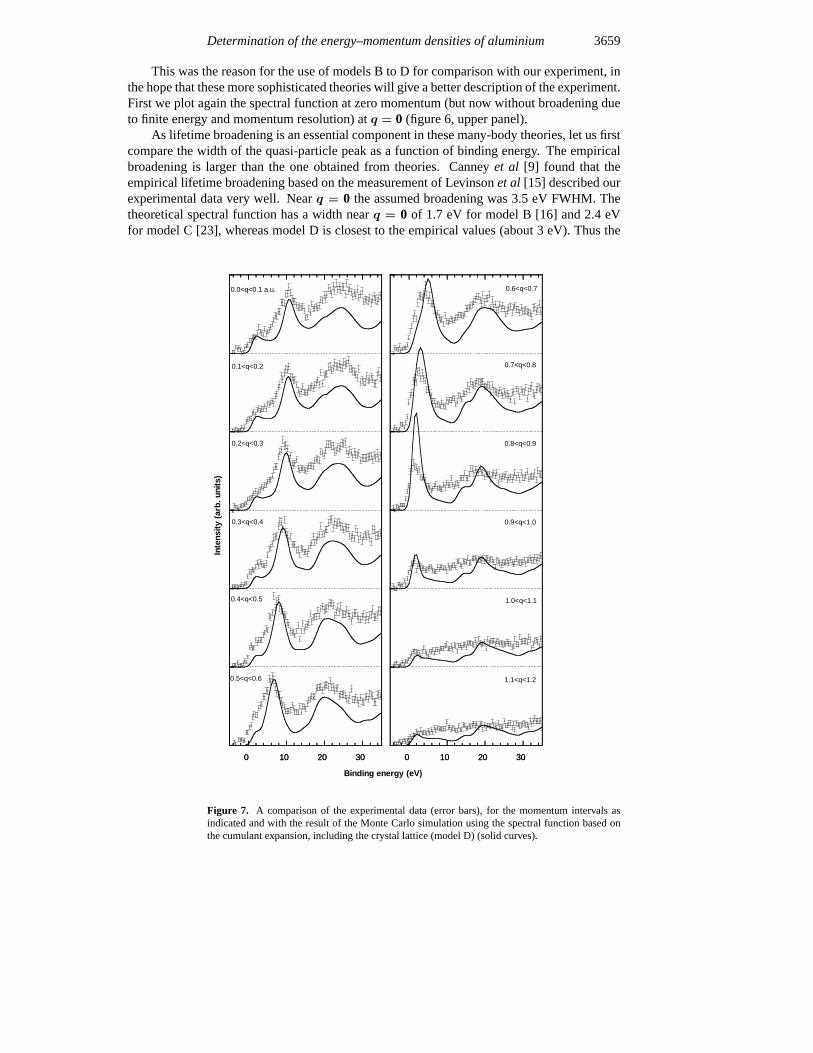
Figure 7. A comparison of the experimental data (error bars), for the momentum intervals asindicated and with the result of the Monte Carlo simulation using the spectral function based onthe cumulant expansion, including the crystal lattice (model D) (solid curves).

3660 M Vos et al

crystal lattice (included in model D but not in model C) seems to increase the quasi-particlewidth significantly and also appears to affect the exact position of the intrinsic satellite.

In figure 6 (lower panel) we show the simulated experiment, based on these theories andusing Monte Carlo simulations for the multiple scattering. All parameters of the simulationswere identical to those describing the core levels. The simulated intensities were normalized,for convenience, to equal peak height at the quasi-particle peak. As expected, the quasi-particlepeaks are too narrow for the jellium theories (models B and C) and slightly too narrow formodel D. TheG0W0 calculation (model B) predicts a sharp peak at 34 eV for which there areno indications in the experiment. The cumulant expansion theory predicts a peak near 27 eVbinding energy, at somewhat higher binding energy and more pronounced than that found inthe experiment. The separation of the satellite from the quasi-particle peak is very close tothe plasmon energy here ('15.5 eV) and therefore extrinsic and intrinsic losses combine toa well defined peak in the simulations. The general shape of model D (cumulant expansionincluding the lattice) agrees best with the experiment. Due to the larger width of the quasi-particle peak (compared to those found from models B and C) the intensity at high bindingenergy approaches the quasi-particle peak height. Also, due to the fact that the intrinsic satelliteappears at a slightly lower energy than the plasmon satellite, extrinsic and intrinsic satellitescombine to a rather broad feature, very much as in the experiment.

To get an impression of the overall performance of model D, not only forq = 0, weplot the results of the simulations over a whole series of momentum values (figure 7). As theoccupied states of Al extend outside the first Brillouin zone, but the calculations were donewithin the reduced zone, the resulting spectra for momenta near the Fermi wave vector areless reliable. The overall agreement, especially up to 0.8 au, is surprisingly good. The generalshape of the spectra is reproduced nicely.

6. Conclusions

In this paper we investigated the energy-resolved momentum densities for both the core leveland the valence band of aluminium. There seems to be a clear difference between the two partsof the spectrum. For the core level the plasmon-related satellites appear less intense than themain peak, whereas for the valence band part the intensity is as high in the plasmon-loss areaas for the valence band itself. This conclusion is evident from the raw data, and thus does notrely on the analysis of the multiple-scattering contributions.

The simulations seem to give a reasonable description of the core-level region. Onlythe cumulant expansion theory, taking the lattice into account (model D), gives an adequatedescription of the measured valence band. Thus both electron–electron correlation and thelattice have to be considered to get a good description of the measurement. Surprisinglythe measurement is not sensitive for the crystal lattice as far as the dispersion of the quasi-particle theory is concerned (it cannot distinguish it from a free-electron parabola for thesepolycrystalline samples) but the lattice seems to have a significant effect on the width of thequasi-particle peak. Also the fact that in model D the maximum in the satellite intensity isseparated from the quasi-particle peak by less than the plasmon energy seems to be supported bythe experiment. A similar broadening of the quasi-particle peak was found for Na (compare [23](without a lattice) and [22] (with a lattice)).

A slight further improvement of the agreement would be obtained if the lifetime broadeningin model D was slightly larger. However, given the purity of the sample and the approximatenature of the multiple-scattering simulations, the level of agreement seems quite satisfactory.

EMS seems to be an excellent probe for testing the calculations of spectral functions,especially if multiple-scattering effects can be reduced. This is possible by increasing the


energy of the incoming and outgoing electrons, which leads to an increase in the mean freepath (at the expense of the cross section of the process). A high-energy spectrometer is currentlyunder construction at the Australian National University.

Acknowledgments

The experimental work at Flinders University was done at a Special Research Centre fundedby the Australian Research Council. We acknowledge the contribution of the entire staff ofthe Centre to the work described here. BH acknowledges a post-doctoral fellowship at thematerials and surface group at Chalmers/GU.

References

[1] Hufner S 1995Photoelectron Spectroscopy(Berlin: Springer) ch 4[2] Schulke W, Statz G, Wohlert F and Kaprolat A 1996Phys. Rev.B 5414 381[3] Kr alik B, Delaney P and Louie S G 1998Phys. Rev. Lett.804253[4] Kurp F F, Tschentscher Th, Schulte-Schrepping H, Schneider J R and Bell F 1996Europhys. Lett.3561[5] Kurp F F, Vos M, Tschentscher Th, Kheifets A S, Schneider J R, Weigold E and Bell F 1997Phys. Rev.B 55

5440[6] McCarthy I E and Weigold E 1991Rep. Prog. Phys.54789[7] Dennison J R and Ritter A L 1996J. Electron Spectrosc. Relat. Phenom.7799[8] Vos M and McCarthy I E 1995Rev. Mod. Phys.67713[9] Canney S A, Vos M, Kheifets A S, Clisby N, McCarthy I E and Weigold E 1997J. Phys.: Condens. Matter9

1931[10] Canney S A, Kheifets A S, Vos M and Weigold E 1998J. Electron Spectrosc. Relat. Phenom.88–91247[11] Schnatterley S E 1979Solid State Physicsvol 34 (New York: Academic) p 275[12] Van Hove L 1954Phys. Rev.95249[13] Platzman P M and Tzoar N 1965Phys. Rev.139A410[14] D’Andrea A and Del Sole R 1978Surf. Sci.71306[15] Levinson H J, Greuter F and Plummer W 1983Phys. Rev.B 27727[16] Lundqvist B I 1968Phys. Kondens. Mater.7 117[17] Langreth D C 1970Phys. Rev.B 1 471[18] Bergersen B 1973Can. J. Phys.51102[19] Hedin L 1980Phys. Scr.21477[20] Almbladh C-O and Hedin L 1983Handbook on Synchroton Radiationvol 1, ed E E Koch(Amsterdam: North-

Holland) p 686[21] Gunnarsson O, Meden V and Schonhammer K 1994Phys. Rev.B 5010 462[22] Aryasetiawan F, Hedin L and Karlsson K 1996Phys. Rev. Lett.772268[23] Holm B and Aryasetiawan F 1997Phys. Rev.B 5612 825[24] Canney S A, Vos M, Kheifets A S, Guo X, McCarthy I E and Weigold E 1997Surf. Sci.382241[25] Vos M, Storer P J, Cai Y Q, McCarthy I E and Weigold E 1995Phys. Rev.B 511866[26] Vos M and Bottema M 1996Phys. Rev.B 545946[27] Stern E A and Ferrel R A 1960Phys. Rev.120130[28] Egerton R F 1986Electron Energy Loss Spectroscopy(New York: Plenum)[29] Canney S A, Brunger M J, McCarthy, I E, Storer P J, Utteridge S, Vos M and Weigold E 1997J. Electron

Spectrosc. Relat. Phenom.8365[30] Ritchy R H 1957Phys. Rev.120130

determination of the energy–momentum densities of aluminium...

Documents