Citation: Okorie, Ikechukwu (2010) Determination of potentially toxic elements (PTEs) and an assessment of environmental health risk from environmental matrices. Doctoral thesis, Northumbria University.

This version was downloaded from Northumbria Research Link: http://nrl.northumbria.ac.uk/1502/

Northumbria University has developed Northumbria Research Link (NRL) to enable users to access the University’s research output. Copyright ©  and moral rights for items on NRL are retained by the individual author(s) and/or other copyright owners. Single copies of full items can be reproduced, displayed or performed, and given to third parties in any format or medium for personal research or study, educational, or not-for-profit purposes without prior permission or charge, provided the authors, title and full bibliographic details are given, as well as a hyperlink and/or URL to the original metadata page. The content must not be changed in any way. Full items must not be sold commercially in any format or medium without formal permission of the copyright holder. The full policy is available online: http://nrl.northumbria.ac.uk/policies.html

Determination of potentially toxic elements

(PTEs) and an assessment of environmental

health risk from environmental matrices

Ikechukwu Alexander Okorie

The thesis submitted in partial fulfilment of the

requirements of Northumbria University, Newcastle upon

Tyne for the degree of Doctor of Philosophy

June 2010

ii

Declaration

This thesis records the results of experiments conducted by myself in the School of Applied

Sciences, Northumbria University under the supervision of Prof. John R. Dean and Dr Jane

Entwistle between September 2006 and June 2010. It is of my own composition and has not

previously been submitted in part, or in whole, for a higher degree.

iii

Abstract

A former industrial site now used for recreational activities was investigated for total PTE

content, uptake of the PTEs by foraged fruits and mobility of the PTEs using single extraction

such as HOAc and EDTA. In order to evaluate the health risks arising from ingestion of the

PTE contaminated soil, the oral bioaccessibility using in vitro physiologically based

extraction test (PBET) and tolerable daily intake (TDI) or mean daily intake (MDI) was used.

The PBET simulates the transition of the PTE pollutants in the soil into human

gastrointestinal system while the TDI or MDI is the mass of soil that a child would require to

take without posing any health risk. In addition to the former industrial site, an investigation

of the urban road dust from Newcastle city centre and its environs was undertaken with the

view to looking into the PTE content, oral bioaccessibility and the platinum group elements

(PGEs).

Optimized microwave procedure was applied to 19 samples obtained from a former industrial site (St

Anthony‟s lead works) in Newcastle upon Tyne. Of the range of PTEs potentially present at the

site as a consequence of former industrial activity (As, Cd, Cr, Cu, Ni, Pb and Zn), the

majority of top soil samples indicated elevated concentrations of one or more of these PTEs.

In particular, data obtained using either inductively coupled plasma mass spectrometry (ICP-

MS) or flame atomic absorption spectroscopy (FAAS) indicates the high and wide

concentration of Pb on the site (174 to 33,306 mg/kg). Comparing the resulting PTEs data

with UK Soil Guidelines Values (SGVs) suggests at least parts of the site represent areas of

potential human health risk. It was found that Pb soil values exceeded the SGV on 17 out of

the 19 sampling sites; similarly for As 7 out of 19 sampling sites exceeded the SGV. While

for Cd and Ni the soil levels were below the stated SGVs.

Samples of foraged fruits collected from the same site were also analysed for the same PTEs.

The foraged fruit was gathered over two seasons along with samples of soil from the same

sampling areas, acid digested using a microwave oven, and then analysed by ICP-MS. The

foraged fruits samples included blackberries, rosehips and sloes which were readily available

on the site. The concentration levels of the selected elements in foraged samples varied

between not detectable limits and 24.6 mg/kg (Zn). Finally, the soil-to plant transfer factor

was assessed for the 7 elements. In all cases, the transfer values obtained were below 1.00,

iv

except Cd in 2007 which is 1.00, indicating that the majority of the PTE remains in the soil

and that the uptake of PTE from soil to plant at this site is not significant.

The determination of total or pseudo total PTE content of soil is often insufficient to assess

the risk to humans. A range of extraction protocols were applied to the 19 samples urban

topsoils, and report on the correlations between pseudo total PTE content and results obtained

following a physiologically-based extraction procedure (oral bioaccessibility), EDTA and

HOAc extraction protocols (reagent-specific available fraction), for a broad range of PTEs

(As, Cd, Cu, Cr, Ni, Pb, Zn). Results of the single-reagent extraction procedures did not, in

general, provide a good indication of oral bioaccessibility but shows positive correlation with

the pseudo total PTE content. The bioaccessibility data shows that considerable variation

exists both spatially across the site, and between the different PTEs, but correlates well with

the pseudo-total concentrations for all elements (r2 exceeding 0.8). One of the main

objectives of this work is to show the role of bioaccessibility in generic risk assessment.

Comparison of the pseudo-total PTE concentrations with SGV or generic assessment criteria

(GAC) indicated that all of the PTEs investigated need further action, such as receptor

exposure modelling. If we refine our generic risk assessment using the PTE bioaccessibility

data then a very different picture of the site emerges; one where 5 out of the 7 PTEs

investigated indicate the need for a more detailed site-specific risk assessment showing that

bioaccessible fraction instead of pseudo total PTE content allows a more considerable

approach to human health risk assessment to be made.

Potential health risk from the site was also calculated to estimate the mass of soil a child

would require to ingest to reach the estimated TDI or MDI. From the results for a child with

geophagy (50 g/day) behaviour the levels of all PTEs are exceeded except Cr (III). In contrast

for a child with pica behaviour (1 g/day) only two PTE exceeds the TDI value i.e. Cd and Pb;

in addition, for As, the IDoral value and the MDI values are exceeded. Based on the

unintentional consumption of 0.1 g of soil, only Pb and As exceed the guideline value (TDI

and IDoral respectively) for this type of samples.

The pseudo-total and bioaccessible concentration of 6 PTEs in urban street dust from nine

sampling sites across Newcastle upon Tyne city centre and its environs was investigated.

Typical pseudo-total concentrations across the sampling sites ranged from 4.4 to 8.6 mg/kg

for As, 0.2 to 3.6 mg/kg for Cd, 25 to 217 mg/kg for Cu, 14 to 46 mg/kg for Ni, 70 to 4261

v

mg/kg for Pb, and, 111 to 652 mg/kg for Zn. This data compared favourably with other urban

street dust samples collected and analysed in a variety of cities globally, the exception was

the high level of Pb determined in a specific sample in this study. The concentration of PTEs

in the samples has been compared to estimated tolerable daily and mean daily intakes values

against recommended ingestion values for geophagy behaviour, soil-pica behaviour and

unintentional consumption. Based on the unintentional consumption of dust samples (0.1

g/day) no PTE exceeded the guidelines values. The oral bioaccessibility of PTEs in street

dust was assessed using PBET. Based on a worst case scenario the PBET approach estimated

that Cd and Zn had the highest % bioaccessible fractions (> 45%) while the other PTEs i.e.

As, Cu, Ni and Pb had lower % bioaccessible fractions (< 30%). It was postulated that Cd

and Zn were more likely to be derived from anthropogenic sources whereas the other PTEs

were more indicative of both anthropogenic and natural sources. The bioaccesible

concentration was compared to the guideline values based on the unintentional consumption

(0.1 g/day). In all cases the bioaccessible concentration values were well below the guideline

values.

The concentrations of PGE (Rh, Pd and Pt) were measured in the 9 sampled points of urban

road dust from the Newcastle city centre. The result reveals that the concentration of Rh

ranges from 1.2 to 54.8 ng/g, Pd from 2.7 to 203.7 ng/g and Pt from 8.1 to 118.5 ng/g. The

mean value of Pd (79.8 ng/g) is significantly higher than those of Rh (17.6 ng/g) and Pt (38.2

ng/g) showing a shift from Pt to Pd in its use in the construction of catalytic converters. The

grain size analysis was carried out using three dust samples. The three samples were

fractionated into six size fractions with their sedimentological equivalent in parenthesis:

1000-2000 µm (very coarse sand), 500-1000 µm (coarse sand), 250-500 µm (medium sand),

125-250 µm (fine sand), 63-125 µm (very fine sand) and <63 µm (silt and clay). The typical

relationship in grain size analysis is that concentration of the metal increases with decreasing

grain size. On this basis, most of the dominant fraction analysed for PGEs in soils by many

researchers is the <63 µm size fractions. However, this assumption is called into question in

the present study as the result obtained shows that reasonable concentration of PGEs can be

obtained in other size fractions especially the 63-125 µm hence analysis of only < 63 µm

fraction will underestimate the PGE concentration in the environmental sample.

vi

Acknowledgements

I would like to express my gratitude to Northumbria University for the ORS scholarship

awarded for my PhD study. Nnamdi Azikiwe University, Awka, Nigeria is also

acknowledged for the study leave granted to me to complete this study.

I am very grateful to Prof. John R. Dean, my principal supervisor, and Dr Jane Entwistle my

second supervisor for their invaluable guidance and support during the course of my research.

Mr. P. Hartley and L. Bramwell (Newcastle City Council) are acknowledged for providing

access to the site and valuable background information. Mr Michael Elund also of Newcastle

City Council is acknowledged for his assistance in the provision of traffic data. Also worthy

of acknowledgement is Dr Chris Ottley of Durham University for his assistance in the

analysis of platinum group elements. The technical support of Mr. Gary Askwith, Mr. Dave

Osborne, Geochemistry Research Group and all members of the School of Applied Sciences,

Northumbria University is highly appreciated.

Finally but most importantly, I would like to thank my wife (Ogechi Chiamaka), my daughter

(Chinaemerem) and my son (Bradley Chigozirim) for giving me the time, being there at all

times for me with continuous support, patience, and love.

vii

Contents

Declaration ii

Abstract iii

Acknowledgements vi

Contents vii

List of Tables xii

List of Figures xv

Chapter One: Environmental significance of PTEs in urban soils/dust

1.1 Introduction 1

1.2 Solid phase partitioning 2

1.3 PTEs in urban soils and dust 3

1.3.1 Arsenic (As) 3

1.3.2 Cadmium (Cd) 6

1.3.3 Chromium (Cr) 6

1.3.4 Copper (Cu) 7

1.3.5 Nickel (Ni) 8

1.3.6 Lead (Pb) 9

1.3.7 Zinc (Zn) 10

1.3.8 Platinum group elements (PGEs) 10

1.4 Contaminated Land Legislation 11

1.5 Assessment of environmental risk to humans using oral bioaccessibility 12

1.6 Aims and objectives of the research 13

References 15

Chapter Two: Instrumental methods of measuring PTEs and microwave

optimisation

2.1 Introduction 22

viii

2.1.1 Inductively Coupled Plasma Mass Spectroscopy (ICP-MS) 22

2.1.2 Flame Atomic Absorption Spectroscopy (FAAS) 25

2.1.3 X ray Fluorescence (XRF) 26

2.2 Principal sources of uncertainty in environmental trace analysis 29

2.2.1 Sample preparation 30

2.2.2 Sample collection and storage 31

2.3 Optimisation of microwave digestion 32

2.4 Experimental 33

2.4.1 Central Composite Design (CCD) 33

2.4.2 Instrument and reagents 34

2.4.3 Microwave digestion protocol 34

2.4.4 ICP-MS protocol 36

2.5 Results and discussion 36

2.5.1 Microwave optimisation 36

2.5.2 ICP-MS analysis of soil CRM 38

2.6 Conclusion 41

References 42

Chapter Three: Evaluation of PTEs contamination at a former industrial

site (St Anthony’s) in Newcastle upon Tyne

3.1 Introduction 47

3.1.1 Site description 49

3.2 Experimental 52

3.2.1 Sampling and sample preparation 52

3.2.2 Instrument and Reagents 52

3.2.3 Soil pH 55

3.2.4 Soil organic matter content 55

ix

3.2.5 Cation Exchange Capacity (CEC) 55

3.2.6 Pseudo total PTE content of soil from former St Anthony‟s lead works 57

3.2.7 Total PTE content in foraged fruits by ED-XRF 57

3.2.8 Single extraction using EDTA 59

3.2.9 Single extraction using HOAc 59

3.3 Results and discussion 60

3.3.1 Soil properties (pH, % LOI, CEC) 60

3.3.2 ICP-MS of soil CRM 60

3.3.3 Pseudo-total PTE content of soil from former St Anthony‟s lead works 62

3.3.4 Mobility of PTEs from former St Anthony‟s lead work 66

3.3.5 Quality control for foraged fruit measurement 73

3.3.6 Foraged fruits elemental concentration 74

3.3.7 Soil plant transfer factor 78

3.4 Conclusion 81

References 82

Chapter Four: The use of the physiologically-based extraction test to assess

oral bioaccessibility of PTEs from an urban recreational site

4.1 Introduction 87

4.2 Experimental 88

4.2.1 The study site 88

4.2.2 Reagents 88

4.2.3 Preparation of extraction reagents for the in vitro extraction test 89

4.2.4 Preparation of samples using BARGE method 90

4.2.5 Microwave digestion protocol/ICP-MS analysis of sample 91

4.2.6 Determination of oral bioaccessibility 91

4.3 Results and Discussion 91

4.3.1 Evaluation of the BARGE approach: Application to soil CRM 91

4.3.2 Characterization of study site topsoils 92

4.3.3 Evaluation of the BARGE approach: Application to an urban recreational site 92

x

4.3.4 Generic risk assessment and the role of bioacessibility data 97

4.3.5 Estimation of bioaccessibility of soil using TDI and MDI 99

4.4 Conclusion 101

References 102

Chapter Five: Natural and anthropogenic PTE input to urban street dust

and the role of oral bioaccessibility testing

5.1 Introduction 106

5.2 Experimental 107

5.2.1 Sampling and Sample preparation 107

5.2.2 Instrument and reagents 107

5.2.3 Pseudo total PTE concentration 107

5.2.4 Procedure for in vitro physiologically based extraction test 108

5.3 Results and Discussion 108

5.3.1 Quality Control 108

5.3.2 Pseudo total PTE concentration 111

5.3.3 PTE concentration/traffic volume 119

5.3.4 Inter-element relationship to road dust 119

5.3.5 Bioaccessibility of PTEs in urban street dust 119

5.3.6 Bioaccessibility of PTEs in urban street dust by TDI or MDI 121

5.4 Conclusion 124

References 126

Chapter Six: Influence of particle size on the distribution of platinum

group elements (PGEs) in urban street dust/sediments

6.1 Introduction 135

6.1.1 Accumulation and mobility of PGEs 137

6.1.2 Health risk effects of PGEs 138

6.2 Experimental 139

6.2.1 Sampling and sample preparation 139

6.2.2 Instrument and reagents 141

xi

6.2.3 Preparation of cation exchange resin and separation columns 141

6.2.4 Microwave digestion and column separation for PGE analysis 142

6.2.5 Analysis of PGEs using ICP-MS 142

6.3 Results and discussion 143

6.3.1 Isotope selection and interferences 143

6.3.2 Quality control using certified reference material 144

6.3.3 PGE concentration in road dust 145

6.3.4 Grain-size partitioned PGE concentration and mass loading 147

6.3.5 Correlation coefficient of PGE and PTEs concentration in road dust 150

6.3.6 PGE ratios for determining emission source 152

6.4 Conclusion 152

References 153

Chapter Seven: Conclusion and future work 160

7.1 Conclusion 160

7.2 Future work 161

Appendix A 163

Appendix B 170

Appendix C 173

Appendix D 176

Appendix E 179

Appendix F 182

xii

List of Tables

Table 1.1: Industrial uses of some PTEs 3

Table 1.2: Toxicity of major potentially toxic elements (PTEs) in polluted soils 4

Table 2.1: Comparison of mass analysers figure of merit 24

Table 2.2: Comparison of Elemental Techniques 29

Table 2.3: Upper and lower limit of the variables for computing conditions for standard runs 34

Table 2.4: Experimental design which shows the range of conditions for the variables 35

Table 2.5: Operating conditions for ICP-MS 36

Table 2.6: ICP-MS calibration data for PTEs Cr, Ni, Cu, Pb and Zn 38

Table 2.7: Concentration of PTEs measured by ICP-MS in Ouseburn soil samples 39

Table 2.8: Statistical treatment of individual PTE data using multilinear regression 40

Table 2.9: PTEs statistically significant at 95 % confidence interval 41

Table 2.10: Total PTE concentration (mg/kg) in soil Certified Reference Materials by

ICP-MS/FAAS 41

Table 3.1: Site Description of former St Anthony‟s lead work 49

Table 3.2: Description of sampling site & sample 53

Table 3.3: Calibration Data As, Cd, Cr, Cu and Ni on ICP-MS and Pb, Zn on FAAS 58

Table 3.4: Soil Properties at St Anthony‟s Lead Works (SAL) 61

Table 3.5: Typical CEC values for different soils 62

Table 3.6 : Single Extraction for BCR 700 63

Table 3.7: PTEs concentration in rural soil with no local PTE input mg/kg dry soil 64

Table 3.8:Pseudo-total PTE concentration of soil from former St Anthony‟s lead works 65

Table 3.9: Component matrix for data of St Anthony‟s Lead Works 66

Table 3.10: Total PTE concentration (mg/kg, dry weight) in a plant certified reference

material 74

Table 3.11: Analysis of foraged fruits from Site (SAL) (mg/kg, dry weight) (September

2007) 75

xiii

Table 3.12: Comparison of own data with literature values for Black berry from SAL 5 76

Table 3.13: ICP-MS Analysis of foraged fruits from site (SAL)* (mg/kg, dry weight)

(September 2008) 77

Table 3.14: Analysis of PTEs in soil from the site (SAL)* (mg/kg, dry weight) 79

Table 3.15: Transfer values for PTE uptake over two successive seasons 80

Table 4.1: Analysis of soil certified reference material (GBW 07401) using microwave

digestion and the BARGE method 93

Table 4.2: Topsoil properties (n = 19). PTE concentration (mg/kg, dry weight) 94

Table 4.3: Summary of stage related bioaccessibility and residual fraction of PTEs in all

topsoils 95

Table 4.4: Amount (µg) of PTE ingested from the sampled SAL soil calculated from the

content of potentially toxic elements (mg/kg) 100

Table 5.1: Sample location, driving style and traffic volume 109

Table 5.2: Analysis of PTE content of dust certified reference material (BCR 723) using

microwave digestion-ICP-MS 111

Table 5.3: Normality test on the < 250 µm size fraction of street dust 112

Table 5.4: Global PTE concentrations (mg/kg) in street dust 114

Table 5.5: Inter-element correlation matrix for street dust 120

Table 5.6: Indicative, pseudo-total, stage related bioaccessible and residual fractions of

PTEs in BCR 723 122

Table 5.7: Summary of Stage related bioaccessibility and residual fraction of PTEs in road

dust 123

Table 5.8: Amount (µg) of PTE ingested from the sampled urban road dust calculated from

the content of PTEs (mg/kg) 125

Table 6.1: PGE supply by application (worldwide) 136

Table 6.2: Palladium demand by application in Europe (kg) 137

Table 6.3: Platinum demand by application in Europe (kg) 137

Table 6.4: Sample location/descriptions 140

Table 6.5: Operating conditions for ICP-MS 143

Table 6.6: Calibration Data for the PGEs 143

xiv

Table 6.7: Concentration of PGEs in Dust Reference Material BCR 723 145

Table 6.8: Concentration of PGEs in >250 and <250µm (ng/g) 145

Table 6.9: Descriptive statistics for PGEs in the >250 and the <250µm size fraction of road

dust samples (ng/g) 146

Table 6.10: The Non parametric Mann-Whitney test results of >250 and <250 µm size

fraction for the concentration of PGEs 146

Table 6.11: Global concentration of PGE in Road Dust (ng/g) 148

Table 6.12: PTE concentration road dust (mg/kg) 151

Table 6.13: Relationship of PGEs with PTEs 151

xv

List of Figures

Figure 1.1: Exposure linkage of contaminant to receptor 11

Figure 1.2: Overview of the study 14

Figure 2.1: Mechanism of conversion of a droplet to positive ion in the ICP 22

Figure 2.2: Major components of ICP-MS system 23

Figure 2.3: Block diagram of atomic absorption spectrometer 26

Figure 2.4: The principle of XRF and the typical XRF detection arrangement 28

Figure 2.5: Flow chart for inorganic environmental analysis including a rough error

estimation of the different analytical procedure 29

Figure 3.1: Sample locations for soil samples at former St Anthony‟s lead works 50

Figure 3.2: Sample locations for foraged fruits collected from former St Anthony‟s lead

works 51

Figure 3.3: Box plot of PTE concentration in soil from former St Anthony‟s 66

Figure 3.4: Biplot of the first two principal components 67

Figure 3.5: Percentage/concentration (mg/kg) of As extracted in EDTA and HOAc 68

Figure 3.6: Percentage /concentration (mg/kg) of Cd extracted in EDTA and HOAc 69

Figure 3.7: Percentage /concentration (mg/kg) of Cr extracted in EDTA and HOAc 70

Figure 3.8: Percentage /concentration (mg/kg) of Cu extracted in EDTA and HOAc 71

Figure 3.9: Percentage /concentration (mg/kg) of Ni extracted in EDTA and HOAc 72

Figure 3.10: Percentage /concentration (mg/kg) of Pb extracted in EDTA and HOAc 72

Figure 3.11: Percentage /concentration (mg/kg) of Zn extracted in EDTA and HOAc 73

Figure 3.12: Boxplot showing seasonal variation in concentration for seven PTEs for 2007

and 2008 78

Figure 3.13: Box plot for transfer factors for the two seasons 2007 and 2008 81

Figure 4.1: Box plot for bioaccessibility of As, Cd, Cr, Cu, Ni, Pb and Zn in topsoils 96

Figure 5.1: Map showing sampling points for the urban road dust 108

xvi

Figure 5.2: Box plot of total PTE concentration in street dust 112

Figure 5.3: Pseudo total content of As in the <250 µm particle size fraction of dust sample

collected from Newcastle city centre 113

Figure 5.4: Pseudo total content of Cd in the <250 µm particle size fraction of dust sample

collected from Newcastle city centre 116

Figure 5.5: Pseudo total content of Cu in the <250 µm particle size fraction of dust sample

collected from Newcastle city centre 116

Figure 5.6: Pseudo total content of Ni in the <250 µm particle size fraction of dust sample

collected from Newcastle city centre 117

Figure 5.7: Pseudo total content of Pb in the <250 µm particle size fraction of dust sample

collected from Newcastle city centre 118

Figure 5.8: Pseudo total content of Zn in the <250 µm particle size fraction of dust sample

collected from Newcastle city centre 118

Figure 5.9: Box plot for oral bioaccessibility in road dust 124

Figure 6.1: Comparison between the <250 and > the 250 µm size fraction for the PGEs 147

Figure 6.2: PGE concentration in road dust 148

Figure 6.3: Grain-size (µm) partitioned PGEs concentration in three road dust sample(Site 8,

14 and 15) from Newcastle City Centre 149

Figure 6.4: Relative PGE mass loading for sites 8, 14 and 15 across the 6 determined size

fractions. 150

1

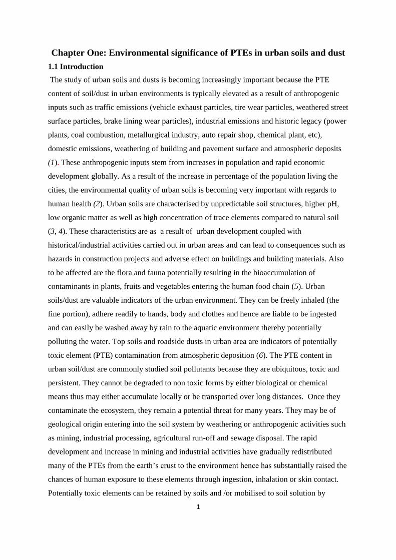
Chapter One: Environmental significance of PTEs in urban soils and dust

1.1 Introduction

The study of urban soils and dusts is becoming increasingly important because the PTE

content of soil/dust in urban environments is typically elevated as a result of anthropogenic

inputs such as traffic emissions (vehicle exhaust particles, tire wear particles, weathered street

surface particles, brake lining wear particles), industrial emissions and historic legacy (power

plants, coal combustion, metallurgical industry, auto repair shop, chemical plant, etc),

domestic emissions, weathering of building and pavement surface and atmospheric deposits

(1). These anthropogenic inputs stem from increases in population and rapid economic

development globally. As a result of the increase in percentage of the population living the

cities, the environmental quality of urban soils is becoming very important with regards to

human health (2). Urban soils are characterised by unpredictable soil structures, higher pH,

low organic matter as well as high concentration of trace elements compared to natural soil

(3, 4). These characteristics are as a result of urban development coupled with

historical/industrial activities carried out in urban areas and can lead to consequences such as

hazards in construction projects and adverse effect on buildings and building materials. Also

to be affected are the flora and fauna potentially resulting in the bioaccumulation of

contaminants in plants, fruits and vegetables entering the human food chain (5). Urban

soils/dust are valuable indicators of the urban environment. They can be freely inhaled (the

fine portion), adhere readily to hands, body and clothes and hence are liable to be ingested

and can easily be washed away by rain to the aquatic environment thereby potentially

polluting the water. Top soils and roadside dusts in urban area are indicators of potentially

toxic element (PTE) contamination from atmospheric deposition (6). The PTE content in

urban soil/dust are commonly studied soil pollutants because they are ubiquitous, toxic and

persistent. They cannot be degraded to non toxic forms by either biological or chemical

means thus may either accumulate locally or be transported over long distances. Once they

contaminate the ecosystem, they remain a potential threat for many years. They may be of

geological origin entering into the soil system by weathering or anthropogenic activities such

as mining, industrial processing, agricultural run-off and sewage disposal. The rapid

development and increase in mining and industrial activities have gradually redistributed

many of the PTEs from the earth‟s crust to the environment hence has substantially raised the

chances of human exposure to these elements through ingestion, inhalation or skin contact.

Potentially toxic elements can be retained by soils and /or mobilised to soil solution by

2

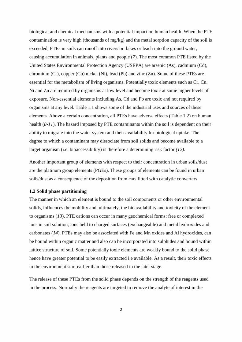
biological and chemical mechanisms with a potential impact on human health. When the PTE

contamination is very high (thousands of mg/kg) and the metal sorption capacity of the soil is

exceeded, PTEs in soils can runoff into rivers or lakes or leach into the ground water,

causing accumulation in animals, plants and people (7). The most common PTE listed by the

United States Environmental Protection Agency (USEPA) are arsenic (As), cadmium (Cd),

chromium (Cr), copper (Cu) nickel (Ni), lead (Pb) and zinc (Zn). Some of these PTEs are

essential for the metabolism of living organisms. Potentially toxic elements such as Cr, Cu,

Ni and Zn are required by organisms at low level and become toxic at some higher levels of

exposure. Non-essential elements including As, Cd and Pb are toxic and not required by

organisms at any level. Table 1.1 shows some of the industrial uses and sources of these

elements. Above a certain concentration, all PTEs have adverse effects (Table 1.2) on human

health (8-11). The hazard imposed by PTE contaminants within the soil is dependent on their

ability to migrate into the water system and their availability for biological uptake. The

degree to which a contaminant may dissociate from soil solids and become available to a

target organism (i.e. bioaccessibility) is therefore a determining risk factor (12).

Another important group of elements with respect to their concentration in urban soils/dust

are the platinum group elements (PGEs). These groups of elements can be found in urban

soils/dust as a consequence of the deposition from cars fitted with catalytic converters.

1.2 Solid phase partitioning

The manner in which an element is bound to the soil components or other environmental

solids, influences the mobility and, ultimately, the bioavailability and toxicity of the element

to organisms (13). PTE cations can occur in many geochemical forms: free or complexed

ions in soil solution, ions held to charged surfaces (exchangeable) and metal hydroxides and

carbonates (14). PTEs may also be associated with Fe and Mn oxides and Al hydroxides, can

be bound within organic matter and also can be incorporated into sulphides and bound within

lattice structure of soil. Some potentially toxic elements are weakly bound to the solid phase

hence have greater potential to be easily extracted i.e available. As a result, their toxic effects

to the environment start earlier than those released in the later stage.

The release of these PTEs from the solid phase depends on the strength of the reagents used

in the process. Normally the reagents are targeted to remove the analyte of interest in the

3

specific phase either by exchange process or dissolution of the target phase. The solid phase

partitioning depends greatly in soil pH and organic matter content (13).

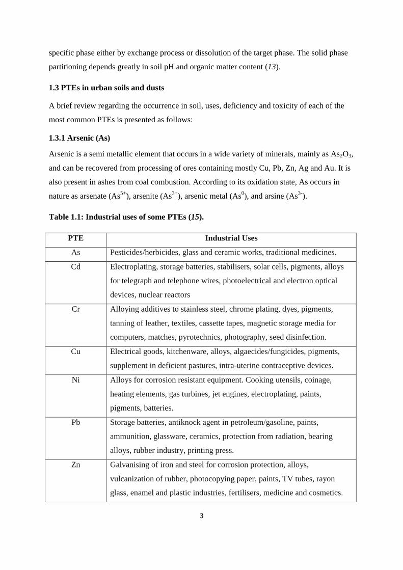
1.3 PTEs in urban soils and dusts

A brief review regarding the occurrence in soil, uses, deficiency and toxicity of each of the

most common PTEs is presented as follows:

1.3.1 Arsenic (As)

Arsenic is a semi metallic element that occurs in a wide variety of minerals, mainly as As2O3,

and can be recovered from processing of ores containing mostly Cu, Pb, Zn, Ag and Au. It is

also present in ashes from coal combustion. According to its oxidation state, As occurs in

nature as arsenate (As5+

), arsenite (As3+

), arsenic metal (As0), and arsine (As

3-).

Table 1.1: Industrial uses of some PTEs (15).

PTE Industrial Uses

As Pesticides/herbicides, glass and ceramic works, traditional medicines.

Cd Electroplating, storage batteries, stabilisers, solar cells, pigments, alloys

for telegraph and telephone wires, photoelectrical and electron optical

devices, nuclear reactors

Cr Alloying additives to stainless steel, chrome plating, dyes, pigments,

tanning of leather, textiles, cassette tapes, magnetic storage media for

computers, matches, pyrotechnics, photography, seed disinfection.

Cu Electrical goods, kitchenware, alloys, algaecides/fungicides, pigments,

supplement in deficient pastures, intra-uterine contraceptive devices.

Ni Alloys for corrosion resistant equipment. Cooking utensils, coinage,

heating elements, gas turbines, jet engines, electroplating, paints,

pigments, batteries.

Pb Storage batteries, antiknock agent in petroleum/gasoline, paints,

ammunition, glassware, ceramics, protection from radiation, bearing

alloys, rubber industry, printing press.

Zn Galvanising of iron and steel for corrosion protection, alloys,

vulcanization of rubber, photocopying paper, paints, TV tubes, rayon

glass, enamel and plastic industries, fertilisers, medicine and cosmetics.

4

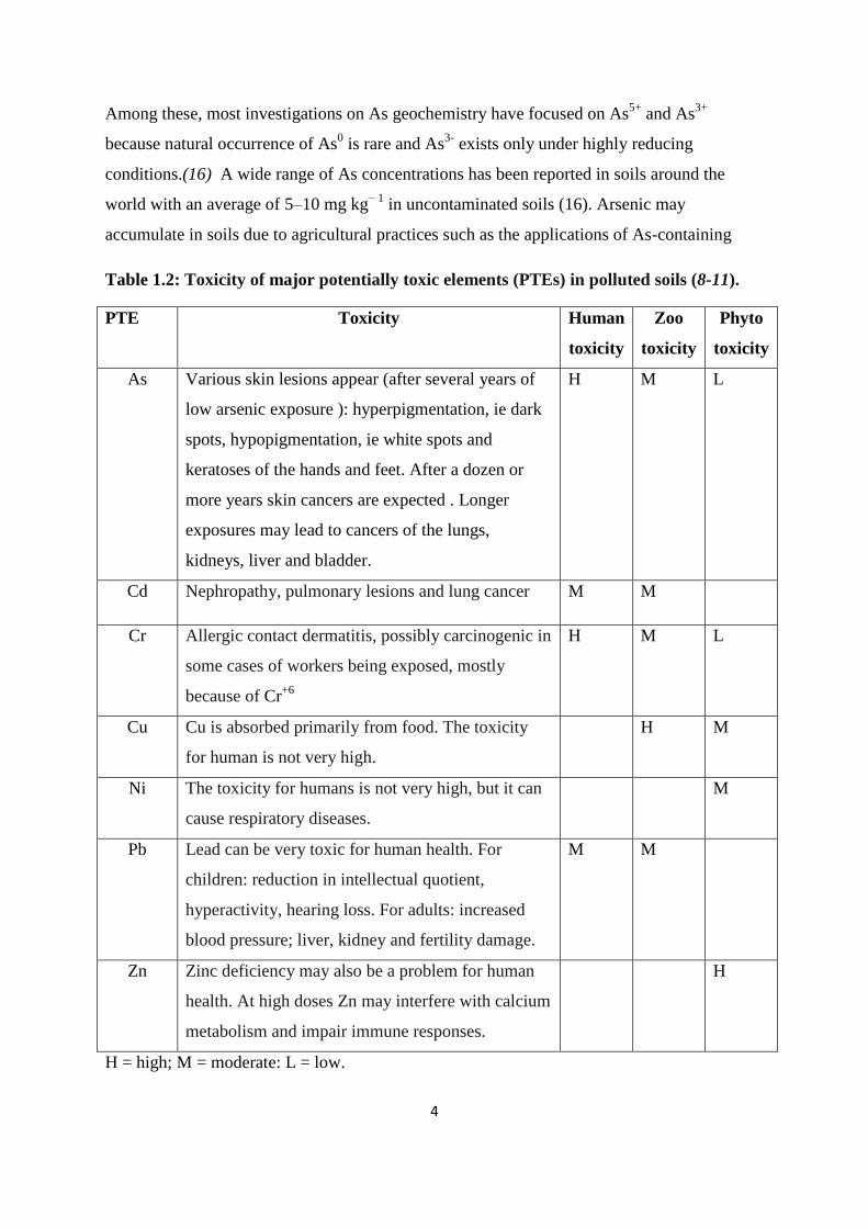
Among these, most investigations on As geochemistry have focused on As5+

and As3+

because natural occurrence of As0 is rare and As

3- exists only under highly reducing

conditions.(16) A wide range of As concentrations has been reported in soils around the

world with an average of 5–10 mg kg− 1

in uncontaminated soils (16). Arsenic may

accumulate in soils due to agricultural practices such as the applications of As-containing

Table 1.2: Toxicity of major potentially toxic elements (PTEs) in polluted soils (8-11).

PTE Toxicity Human

toxicity

Zoo

toxicity

Phyto

toxicity

As Various skin lesions appear (after several years of

low arsenic exposure ): hyperpigmentation, ie dark

spots, hypopigmentation, ie white spots and

keratoses of the hands and feet. After a dozen or

more years skin cancers are expected . Longer

exposures may lead to cancers of the lungs,

kidneys, liver and bladder.

H M L

Cd Nephropathy, pulmonary lesions and lung cancer M M

Cr Allergic contact dermatitis, possibly carcinogenic in

some cases of workers being exposed, mostly

because of Cr+6

H M L

Cu Cu is absorbed primarily from food. The toxicity

for human is not very high.

H M

Ni The toxicity for humans is not very high, but it can

cause respiratory diseases.

M

Pb Lead can be very toxic for human health. For

children: reduction in intellectual quotient,

hyperactivity, hearing loss. For adults: increased

blood pressure; liver, kidney and fertility damage.

M M

Zn Zinc deficiency may also be a problem for human

health. At high doses Zn may interfere with calcium

metabolism and impair immune responses.

H

H = high; M = moderate: L = low.

5

pesticides and herbicides, pig manure, and phosphorus fertilizers, thereby raising concerns

about the risk of As to the environment and human health (16-21). The accumulated As in

soils can distribute among different soil components, such as organic matter, Fe and Mn

oxides, carbonates and sulphides, and such distribution could affect its mobility,

bioavailability and toxicity (16, 22-24).

Though both aqueous As5+

and As3+

are highly toxic to organisms, As3+

has 200 times higher

toxicity than As5+

at the same concentration (25, 26). In addition to its toxicity, As3+

has

enhanced mobility in natural water system and this mobility increases as pH increases (27,

28). Under reducing conditions As3+

dominates, existing as arsenite (AsO33-

) and its

protonated forms: H3AsO3, H2AsO3-, HAsO3

2-. Arsenite can adsorb or co-precipitate with

metal sulphides and has a high affinity for other sulphur compounds.

In aerobic environments, As5+

is dominant, usually in the form of arsenate (AsO43-

) in various

protonation states: H3AsO4, H2AsO4 -, HAsO4

2-, AsO4

3-. Arsenate, and other anionic forms

of As behave as chelates and can precipitate when metal cations are present (29). As5+

is

readily immobilized on soil and sediment particles by adsorption on and co-precipitation with

oxides of Mn, Al and Fe under acidic and moderately reducing condition (30, 26). Arsenate

(As5+

) can also be mobilized under reducing conditions that encourage the formation of As3+

,

under alkaline and saline conditions, in the presence of other ions that compete for sorption

sites, and in the presence of organic compounds that form complexes with As (27, 28).

Arsenates can be leached easily if the amount of reactive metal in the soil is low.

Studies on the geochemical behaviour of As during the past decade have revealed that

microorganisms play a significant role in electrochemical speciation and cycling of As in

nature by mediating the transformation of As and As-adsorbents (31, 26). Elemental arsenic

and arsine, AsH3, may be present under extreme reducing conditions. Sorption and

coprecipitation with hydrous iron oxides are the most important removal mechanisms under

most environmental conditions (28, 32, 33).

Tolerable daily intake (TDI) and mean daily intake (MDI) indicates the quantity of soil a

child is required to take in a day without running the risk of being harmed. These values have

been used to assess the potential health risk to a child. In the case of As, a non-threshold

carcinogen, TDI is inappropriate hence an oral index dose (IDoral) has been proposed of 0.3

6

µg/kg bw/day (34). Therefore the IDoral value based on an assumed body weight of 10 kg

child is 3 µg/day and MDI 5 µg/day based on 20 kg child (34).

1.3.2 Cadmium (Cd)

Cadmium is soluble in acids but not in alkalis. It is similar in many respects to Zn but it forms

more complex compounds. Cadmium occurs naturally in the form of cadmium sulphide or

carbonate (CdS or CdCO3). It is recovered as a by-product from the mining of sulphide ores

of Pb, Zn and Cu. Sources of Cd contamination include plating operations and the disposal of

Cd-containing wastes (27, 28). The most common form of Cd include Cd2+

, cadmium-

cyanide complexes, or Cd(OH)2 solid sludge (27, 28). Adsorption mechanism is the primary

source of Cd removal from the soil (35,36). The chemistry of cadmium in the soil

environment is to a great extent controlled by pH. Under acidic conditions Cd solubility

increases and very little adsorption of Cd by soil colloids, hydrous oxide and organic matter

takes place. At pH values greater than 6, Cd is adsorbed by the soil solid phase or is

precipitated, and the solution concentration of Cd is greatly reduced. Cd forms soluble

complexes with inorganic and organic ligands, in particular Cl-. The formation of these

complexes will increase the mobility of Cd in soil. Hydroxide and carbonate of Cd solids

dominate at high pH. Cadmium will also precipitate in the presence of phosphate, arsenate,

chromate and other anions. Cadmium is relatively mobile in surface water and ground-water

systems and exists primarily as hydrated ions or as complexes with humic acids and other

organic ligands (28). Sorption is also influenced by the cation exchange capacity (CEC) of

clays, carbonate minerals, and organic matter present in soils and sediments. Under reducing

conditions, precipitation as CdS controls the mobility of cadmium (27, 28). Cadmium salts

with low solubility includes cadmium phosphate (Cd3(PO4)2), sulphide (CdS), hydroxide

(Cd(OH)2 and carbonate (CdCO3). The solubilities of these Cd salts will increase with

decreasing pH.

The TDI for Cd based on a 10 kg child is 5 µg/day (37) and for MDI is 28.7 µg/day based on

a 20 kg child (38).

1.3.3 Chromium (Cr)

Chromium does not occur naturally in elemental form but only in compounds. It is mined as a

primary ore product in the form of the mineral chromite, FeCr2O4. Major sources of Cr

contamination include releases from electroplating processes and the disposal of Cr

7

containing wastes (27). Chromium is unstable in O2, it immediately produces a thin oxide

layer that is impermeable to oxygen and protects the metal below. Chromium exists in the

environment in two stable oxidation states, Cr6+

and Cr3+

, which have different toxicity and

transport characteristics.

Chromium in oxidation state of +6 is the form of Cr commonly found at contaminated sites

(28). Hexavalent chromium, Cr6+

, typically exists as the oxyanion chromate (CrO42−) and

dichromate (Cr2O72-

) and precipitate readily in the presence of metal cations such as Ba2+

,

Pb2+

, and Ag+. Chromate and dichromate also adsorb on soil surfaces especially Fe and Al

oxides. The hexavalent Cr has a high solubility in soils (at a high soil pH) and waters and

tends to be mobile in the environment. Additionally, it is acutely toxic, subject to biological

uptake, and also carcinogenic (39). Chronic exposure to hexavalent Cr is reported to induce

renal failure, anaemia, haemolysis and liver failure.

In contrast, Cr3+

, is the dominant form of Cr at low pH (<4). Chromium in oxidation state of

+3 has a limited hydroxide solubility and forms strong complexes with ions such as NH4+,

Cl-, F

-, CN

-, SO4

2- making it relatively immobile and less available for biological uptake. Cr

+3

is an essential trace element to humans and shortages may cause heart conditions, disruptions

of metabolisms and diabetes. Uptake of excess Cr3+

can cause health effects e.g. skin rashes.

Therefore, reduction of Cr6+

to Cr3+

is considered an important remediation strategy for

reducing the deleterious effects of this pollutant. Cr6+

can be reduced to Cr3+

by soil organic

matter, S2-

and Fe2+

ions under anaerobic conditions.

The TDI of Cr3+

based on a 10 kg child is 50 µg/day for soluble compounds and 50,000

µg/day for metallic and insoluble compounds (37). The MDI for Cr3+

is 60.2 µg/day and 6.7

µg/day for Cr6+

(38).

1.3.4 Copper (Cu)

Copper is a very common substance that occurs naturally in the environment and is

distributed through natural phenomena (wind-blown dust, decaying vegetation, forest fires

and sea spray) and human activities (mining, metal production, wood production and

phosphate fertilizer production). Copper is mined as a primary ore product from CuS and

oxide ores. Mining activities are the major source of Cu contamination. Other sources of Cu

include algaecides and Cu pipes. Copper has low chemical reactivity. In moist air it slowly

8

forms a greenish surface; this coating protects the metal from further attack. Copper can be

found in many kinds of food, in drinking water and in air; as a result we absorb quantities of

Cu each day by eating, drinking and breathing. The absorption of Cu is necessary, because it

is a trace element that is essential for human health. Solution and soil chemistry strongly

influence the speciation of Cu. In aerobic, sufficiently alkaline systems, CuCO3 is the

dominant soluble copper species. The cupric ion, Cu2+

, and hydroxide complexes, CuOH+

and Cu(OH)2, are also commonly present. When copper ends up in soil it strongly attaches to

organic matter and minerals over a wide range of pH values. As a result of this, it does not

travel very far after release and it hardly ever enters groundwater (28). The affinity of Cu for

humates increases as pH increases and ionic strength decreases. Copper does not break down

in the environment and because of that it can accumulate in plants and animals when it is

found in soils. On copper-rich soils only a limited number of plants have a chance of survival.

Copper can interrupt the activity in soils, as it negatively influences the activity of

microorganisms and earthworms. The decomposition of organic matter may seriously slow

down because of this. In anaerobic environments, when S2 is present CuS(s) will form. The

cupric ion (Cu2+

) is the most toxic species of Cu. Toxicity has also been demonstrated for

CuOH+ and Cu2(OH)2

2+ (28, 40). Acute inhalation of Cu dust or fumes at concentration of

0.075-0.12mg/m3 may cause metal fume fever with symptoms such as cough, chills and

muscle ache (41). The TDI for Cu based on a 10 kg child is 1400 µg/day (37) and for MDI

7000 µg/day based on a 20 kg child (38).

In plants, Cu is essential in seed production, disease resistance and regulation of water.

Copper in excess can be phytotoxic to plants and it has been used as an algaecide to control

algal blooms. It can cause plant damage if, for example, it is present at too high concentration

in sewage sludge which is applied to agricultural land. Copper is required by humans in trace

level in order to help haemoglobin formation and carbohydrate metabolism

1.3.5 Nickel (Ni)

The most important oxidation state of the Ni is +2. It also exists as certain compounds in

which the oxidation state of the metal is between -1 and +4. It is used in stainless steel

production, nickel-cadmium batteries, alloys, and electroplating. Nickel is resistant to

corrosion by air and water under ambient conditions and combines readily with other metals

including Cr, Cu, Fe and Zn to form alloys (42). Nickel contamination may occurs from

emissions of metal mining, smelting, and refining operations; Nickel plating and alloy

9

manufacturing; land disposal of sludge, and disposal of effluents. Nickel is found in the

environment combined primarily with oxygen or sulphur as oxides or sulphides. Nickel is a

potent skin sensitiser (that is, able to cause allergic reaction in humans) and as many as 1 –

4% of men and 8 – 20 % of women in the general population may be Ni sensitive (43). The

TDI for Ni based on a 10 kg child is 500 µg/day (37) and for MDI 130 µg/day based on a 20

kg child (43). Direct contact of Ni leads to skin rash which is the most common type of

reaction to Ni exposure (44). Ingestion of Ni can cause skin reactions in previously sensitised

individuals. The other main concern for oral exposure to Ni is its developmental toxicity

potential, which has been observed in experimental animal studies (43). Soluble Ni salts and

the mixture of Ni sulphides and oxides present in refinery dust are carcinogenic to the lung

and nasal tissues in humans (43). Other toxic effects of Ni observed following inhalation

exposure include chronic bronchitis, emphysema, reduced vital capacity and asthma. Nickel

is present in a number of enzymes in plants and microorganisms. In humans, Ni influences Fe

absorption and metabolism, and may be an essential component of the haemopoietic process.

1.3.6 Lead (Pb)

The primary industrial sources of Pb contamination include metal smelting and processing,

Pb battery manufacturing, pigment and chemical manufacturing and Pb contaminated wastes.

Widespread contamination due to the former use of Pb in gasoline is also of concern. Lead

released to groundwater, surface water and land is usually in the form of elemental Pb, lead

oxides and hydroxides, and lead metal oxyanion complexes (27). Lead occurs most

commonly with an oxidation state of 0 or +2. Pb2+

is the more common and reactive form of

lead and forms mononuclear and polynuclear oxides and hydroxides. Under most conditions

Pb2+

and lead-hydroxy complexes are the most stable forms of Pb (27, 28). Low solubility

compounds are formed by complexation with inorganic (Cl-, CO3

2- , SO4

2-, PO4

3- ) and

organic ligands (humic and fulvic acids, EDTA, amino acids) (28, 29). Lead carbonate solids

form above pH 6 and PbS is the most stable solid when high sulphide concentrations are

present under reducing conditions. Most Pb that is released to the environment is retained in

the soil (45). The primary processes influencing the fate of Pb in soil include adsorption, ion

exchange, precipitation, and complexation with sorbed organic matter. These processes limit

the amount of Pb that can be transported into the surface water or groundwater. The relatively

volatile organo lead compound tetramethyl lead may form in anaerobic sediments as a result

of alkylation by microorganisms (27). The amount of dissolved Pb in surface water and

10

groundwater depends on pH and the concentration of dissolved salts and the types of mineral

surfaces present. In surface water and ground-water systems, a significant fraction of Pb is

undissolved and occurs as precipitates (PbCO3, Pb2O, Pb(OH)2, PbSO4), sorbed ions or

surface coatings on minerals, or as suspended organic matter. Lead can be very toxic for

human health. For children: reduction in intellectual quotient, hyperactivity, hearing loss. For

adults: increased blood pressure; liver, kidney and fertility damage. The TDI for Pb based on

a 10 kg child is 36 µg/day (37).

1.3.7 Zinc (Zn)

Zinc is a fairly reactive metal that will combine with oxygen and other non-metals, and will

react with dilute acids to release hydrogen. Zinc does not occur naturally in elemental form. It

is an essential trace element which is present in soil and can be toxic when exposure exceeds

physiological needs. It is usually extracted from mineral ores to form ZnO. The primary

industrial use for Zn is as a corrosion-resistant coating for iron or steel (27, 28). Metallic Zn

is mixed with other metals to form alloys such as brass and bronze and also used to make dry

cell batteries. Zinc oxide is used in the manufacture of paints, rubber, ceramic and many other

products. The main source of exposure to zinc is from food though there might be oral

exposure arising from working in industries where Zn is used as source of raw materials. Zinc

usually occurs in the +II oxidation state and forms complexes with a number of anions,

amino acids and organic acids. Zn may precipitate as Zn(OH)2(s), ZnCO3(s), ZnS(s), or

Zn(CN)2(s). Zinc is one of the most mobile PTEs in surface waters and groundwater because

it is present as soluble compounds at neutral and acidic pH values. At higher pH values, Zn

can form carbonate and hydroxide complexes which control its solubility. Zinc readily

precipitates under reducing conditions and in highly polluted systems when it is present at

very high concentrations, and may co-precipitate with hydrous oxides of iron or manganese

(27, 28). Sorption to sediments or suspended solids, including hydrous iron and manganese

oxides, clay minerals, and organic matter, is the primary fate of Zn in aquatic environments.

At high doses Zn may interfere with calcium metabolism and impair immune responses. The

TDI for Zn based on a 10 kg child is 5000 µg/day (37) and for MDI 27000 µg/day based on a

20 kg child (38)

1.3.8 Platinum group elements (PGEs)

The PGEs consists of iridium (Ir), osmium (Os), palladium (Pd), platinum (Pt), rhodium (Rh)

and ruthenium (Ru). These elements are all transition metals lying in the d-block (Group 8, 9

11

and 10 and period 5 and 6). Platinum and Pd are found in pure state in nature (46). The other

four elements Ir, Os, Rh and Ru occur as alloys of Pt and Au (47). The concentration of PGEs

in the lithosphere is very low, with the average estimated to be in the range of 0.001–0.005

mg/kg for Pt; 0.015 mg/kg for Pd; 0.0001 mg/kg for Rh; 0.0001 mg/kg for Ru; 0.005 mg/kg

for Os; and 0.001 mg/kg for Ir (48). Of the six PGEs, the ones of interest for this study are

Pd, Pt and Rh because of their use in the construction of catalytic converters used in the

automobiles. Platinum group elements released from the catalytic converters are primarily

bound to aluminium oxide particles (49). They were until recently, regarded as inert elements

but recent studies have shown that they may be soluble and quite reactive (50). The details of

PGEs are discussed in chapter six.

1.4 Contaminated Land Legislation

The legal definition of 'contaminated land', as provided by Part IIA of the Environmental

Protection Act 1990 (51) is: “Land which appears to the local authority in whose area it is

situated to be in such a condition, by reason of substances in, on or under the land that a)

significant harm is being caused or there is a significant possibility of such harm being

caused or b) pollution of controlled water is being, or is likely to be, caused”. This Act come

into force in England and Scotland in 2000 and in Wales 2001. The Act creates a framework

to identify and clean up contaminated land, where contamination poses unacceptable risks to

human health or the environment. The UK follows a non-statutory Contaminated Land

Exposure Assessment Model (CLEA) which details a standard approach in dealing with

contaminated land and associated human health risk assessment for England and Wales. The

approach is risk based and involves an assessment which is carried out to determine whether

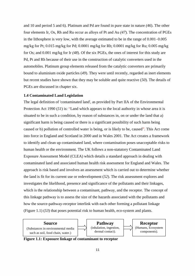
the land is fit for its current use or redevelopment (52). The risk assessment explores and

investigates the likelihood, presence and significance of the pollutants and their linkages,

which is the relationship between a contaminant, pathway, and the receptor. The concept of

this linkage pathway is to assess the size of the hazards associated with the pollutants and

how the source-pathway-receptor interlink with each other forming a pollutant linkage

(Figure 1.1) (53) that poses potential risk to human health, eco-system and plants.

Figure 1.1: Exposure linkage of contaminant to receptor

Source

(Substances in environmental media

such as soil, food chain, water.)

Pathway (inhalation, ingestion,

dermal contact).

Receptor (Humans, Ecosystem

components).

12

To evaluate the degree of soil contaminant using the risk-based approach there is set

guidelines by the Environmental Agency and DEFRA, Soil Guideline Values (SGV). Soil

guideline values give an indication of the representative average levels of contamination in

soil below which the long-term human health risks should be minimal and above it there may

be a cause for concern and possibility of posing significant risk to human health. The SGV

has been modelled for three main land uses: (a) residential (b) allotments and (c)

commercial/industrial. They are designed to be applicable across the range of site conditions

and contaminant forms that are typically encountered on the UK (54). It is a generic risk

assessment criteria which can be used in the preliminary assessment of the risk to human

health from chronic exposure to contaminated soil. Soil guideline values are derived using the

contaminated land exposure assessment model (CLEA). The CLEA model is based on

comparing predicted contaminant exposure levels with established toxicological levels (or

Health Criteria Values: HCV). The basic assumption in using the CLEA model to derive

SGVs is that contaminant released from the soil is taken up into the body to the same extent

as from the medium or organism used to derive the HCV. In a situation where the HCV is

determined using organisms other than human or contaminants are present as recalcitrant

compounds, the above assumptions using CLEA model may not necessarily be true (55). At

present SGVs are available for only As, Cd and Ni among the metals being studied with the

rest being either recently withdrawn or not available. Generic assessment criteria published

by CEIH and LQM (38) are available for a range of other metals.

1.5 Assessment of environmental risk to humans using oral bioaccecibility

There are several methods of assessing environmental risk of soil contaminants to humans. In

England, DEFRA supports the use of CLEA model i.e SGVs and generic risk assessment as

outlined in section 1.2. The Scottish and Northern Ireland Forum for Environmental Research

(SNIFFER) proposed method for deriving site-specific human health assessment criteria for

contaminants in soil and is adapted in Scotland and Northern Ireland. In all these methods,

the assumption is that the total metal concentration in the soil ingested is equal to that

absorbed by the body. None of these methods until very recently considered the internal

exposure or dose which is the actual fraction of the total amount of ingested contaminant

from the soil that reaches the systemic circulation; hence the risk from soil intake with

regards to metal contamination may be overestimated.

13

Oral bioaccessibility can be determined by either in vivo or an in vitro method. The in vivo

method requires direct tests with human or suitable animal models as a surrogate for humans.

The use of humans for bioaccessibility testing is understandably not feasible on ethical

grounds. The routine use of animals is also challenging in terms of cost, time, facilities and

ethical issues (56). On the basis of the above, in vitro method of measuring oral

bioaccessibility has been developed. The principle underlining in vitro methods is that uptake

of a contaminant depends on the rate and extent of its dissolution in the gut (56). There are

different types of in vitro models (57). The in vitro bioaccessibility test mimics the digestive

system of humans by using reagents/enzymes. The digestive system of humans consists of the

mouth, stomach and the small intestine. The mouth compartment of the digestive system in

most of the in vitro methods is omitted because of the short time the contaminant spends in

the mouth. The stomach and the small intestine is therefore the major compartment of the

system and where the contaminant spends most of the time hence the definition of oral

bioaccessibility as the fraction that is soluble in the gastrointestinal environment and

available for absorption (58). The major problem facing in vitro method is the issue of

validation, reproducibility and robustness for regulatory acceptance in risk assessment. At

present, none of the in vitro methods has been approved by regulators in the UK and the

bioaccessible fraction obtained largely depends on the applied in vitro method. The

Bioaccessibility Research Group of Europe (BARGE) unified method (which is batch based)

focuses on digestion characteristics as a method of separation was used in this work. This

method has recently undergoing a unification process and it is anticipated that it should

provide a standard method that will produce a conservative estimate of the oral bioaccessible

fraction of contaminants from soil to be used in human health risk assessment.

In vitro bioaccessibility testing should be validated with the in vivo method. Unfortunately,

no UK soil samples have undergone in vivo testing hence the true or acceptable

bioaccessibility values of the metal contaminants in UK soils are still unknown.

1.6 Aims and objective of the research.

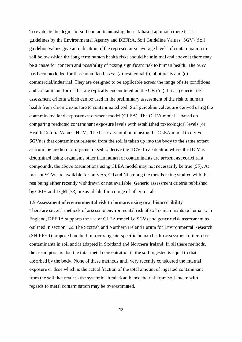
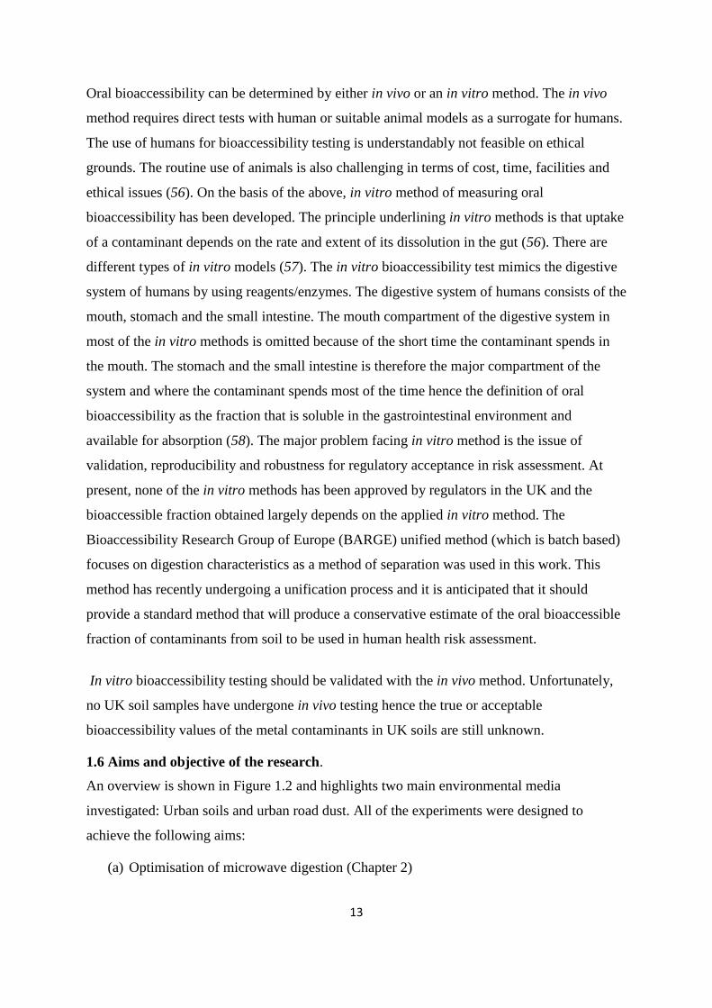
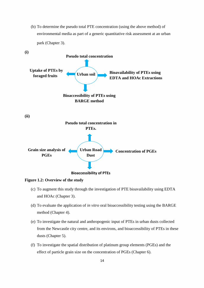
An overview is shown in Figure 1.2 and highlights two main environmental media

investigated: Urban soils and urban road dust. All of the experiments were designed to

achieve the following aims:

(a) Optimisation of microwave digestion (Chapter 2)

14

(b) To determine the pseudo total PTE concentration (using the above method) of

environmental media as part of a generic quantitative risk assessment at an urban

park (Chapter 3).

(i)

(ii)

Figure 1.2: Overview of the study

(c) To augment this study through the investigation of PTE bioavailability using EDTA

and HOAc (Chapter 3).

(d) To evaluate the application of in vitro oral bioaccessibility testing using the BARGE

method (Chapter 4).

(e) To investigate the natural and anthropogenic input of PTEs in urban dusts collected

from the Newcastle city centre, and its environs, and bioaccessibility of PTEs in these

dusts (Chapter 5).

(f) To investigate the spatial distribution of platinum group elements (PGEs) and the

effect of particle grain size on the concentration of PGEs (Chapter 6).

Urban soil

Pseudo total concentration

Uptake of PTEs by

foraged fruits Bioavailability of PTEs using

EDTA and HOAc Extractions

Bioaccessibility of PTEs using

BARGE method

Urban Road

Dust

Pseudo total concentration in

PTEs.

Grain size analysis of

PGEs Concentration of PGEs

Bioaccessibility of PTEs

15

References

1 Binggan, W., Linsheng, Y. (2010). A review of heavy metal contaminations in urban

soils, urban road dust and agricultural soils from China. Microchemical Journal, 94,

99 – 107.

2 Ying, L., Zitong, G., Ganlin, Z., Wolfgang, B. (2003). Concentrations and chemical

speciations of Cu, Zn, P band Cr of urban soils in Nanjing, China. Geoderma, 115,

101 – 111.

3 Daniela, S., Massimo, A., Adriana, B., Rodolfo, N., Mario, S. (2002). Heavy metals in

urban soils: a case study from the city of Palermo (Sicily), Italy. Science of the Total

Environment, 300, 229-243.

4 Bretzel, F., Calderisi, M. (2006). Metal contamination in urban soils of coastal

Tuscany (Italy). Environmental Monitoring and Assessment, 118, 319-335.

5 Thorton, I. (1991). Metal contaminants of soils in urban areas in Bullock, P &

Gregory, J.P (ed). Soils in the urban environment. Blackwell Scientific Oxford.

6 Xiangdong, Li., Chi-sun, P., Pui Sum, L. (2001). Heavy metal contamination of urban

soils and street dusts in Hong Kong. Applied Geochemistry, 16, 1361-1368.

7 Mulligan, C.N., Yong, R.N., Gibbs, B.F. (2001). Remediation technologies for metal-

contaminated soils and groundwater: an evaluation. Engineering Geology, 60, 193–

207.

8 Davydova, S. (2005). Heavy metals as toxicantsin big cities. Microchemical Journal,

79, 133-136.

16

9 Merian, E., Anke, M., Ihnat, M., Stoeppler, M. (2004). Elements and their compounds

in the environment – vol 2. Metals and their compounds (pp 20-48). Germany: Wiley-

VCH.

10 Pierzynsky, G.M., Sims, J.T., Vance, G.F. (2005). Soils and environmental quality.

New York, USA: CRC Press.

11 Poggio. L. Vrscaj. B, Rainer. S, Erwin. H. Ajmone. F. (2009). Metals pollution and

human bioaccessibility of topsoils in Grugliasco (Italy). Environmental pollution, 157,

680-689.

12 Scott, F. Matthew, J.L., Guangchao, L. (2004). Temporal changes in soil partitioning

and bioaccessibility of As, Cr and Pb. Journal of Environmental Quality, 33, 2049 –

2055.

13 Bacon, J.R., Davidson, C.M. (2008). Is there future for sequential chemical

extraction? Analyst, 133, 25-46.

14 Rule, J.H. (1998). Trace metal cation adsorption in soils: selective chemical

extractions and biological availability. Studies in Surface Science and Catalysis, 120,

319-349.

15 Alloway, B.J. (1995). The origin of heavy metals in soils. In B.J. Alloway (Ed.),

Heavy metals in soils, (pp. 38–57).London, UK: Blackie Academic and Professional.

16 Feng, L., Yuan-Ming, Z., Ji-Zheng, H. (2009). Microbes influence the fractionation

of arsenic in paddy soils with different fertilization regimes. Science of the total

environment, 407, 2631-2640.

17 Gregory, R.P., Ross, F.M., Thomas, J. (1996). Environmental aspect of arsenic

toxicity, Critical Review Clininical Laboratory Science, 33, 457–493.

17

18 Chirenje, L.Q., Chen, M., Zillioux, E.J. (2003). Comparison between background

concentrations of arsenic in urban and non-urban areas of Florida. Advanced

Environmental Research, 8, 137-146.

19 Brouwere, K.D., Smolders, E., Merclox, R. (2004). Soil properties affecting solid–

liquid distribution of As(V) in soils, European Journal of Soil Science, 55, 165-173.

20 Camm, S.G ., Glass, J.H., Bryce, W.D., Butcher, A.R. (2004). Characterisation of a

mining-related arsenic-contaminated site. Journal of Geochemical Exploration, 82, 1-

15.

21 Li, X.Y., Chen, B.T. (2005). Concentrations of additive arsenic in Beijing pig feeds

and the residues in pig manure. Resource Conservation Recycle, 45, 356-367.

22 Cumming, E.D., Caccavo, F., Fendorf, S., Rosenzweig, F.R. (1999). Arsenic

mobilization by the dissimilatory Fe(III)-reducing bacterium Shewanella alga BrY.

Environmental Science Technology, 33, 723-729.

23 Islam, F.S., Gault, G.A., Boothman, C ., Polya, A.D., Chamock, M.J., Chartterjee, D.

(2004). Role of metal-reducing bacteria in arsenic release from Bengal Delta

sediments. Nature, 430, 68-71.

24 deLemos, J. L., Bostick, C.B., Renshaw, E.C., Sturup, S., Feng, H.S. (2006). Landfill-

stimulated iron reduction and arsenic release at the Coakley Superfund Site.

Environmental Science Technology, 40, 67-73.

25 Williams, J.W., Silver, S. (1984). Bacterial resistance and detoxification of heavy

metals. Enzyme Microbiology Technology, 6, 530–537.

18

26 Jung, U., Sang, W., Hyo, T., Kyoung, W., Jin, S. (2009) Enhancement of Arsenic

mobility by indigenous bacteria from mine tailing as response to organic supply.

Environment International, 35, 496-501.

27 Smith, L.A., Means, J.L., Chen, A., Alleman, B., Chapman, C.C., Tixier, J.S.,

Brauning, S.E., Gavaskar, A.R., Royer, M.D. (1995). Remedial options for metals-

contaminated sites: Boca Raton: Lewis Publishers.

28 Cynthia, E., David, D. (1997). Remediation of metals-contaminated soil and

groundwater. Technology Evaluation Report (TE-97-01) in Groundwater

Remediation Technologies Analysis Centre (GWRTAC) E series.

29 Bodek, I., Lyman, W.J., Reehl, W.F., Rosenblatt, D.H. (1988). Environmental

Inorganic Chemistry: Properties, Processes and Estimation Methods, Pergamon Press,

Elmsford, NY.

30 Mok, M.W., Wai, M.C. (1994). Mobilization of arsenic in contaminated river waters.

In: J.O. Nriagu, Editor, Arsenic in the environment, Wiley, New York 99-117.

31 Newman, K.D., Ahmann, D., Morel, M.F. (1998). A brief review of microbial

arsenate respiration. Journal of Geomicrobiology, 15, 255-268.

32 Krause, E., Ettel, V.A. (1989). Solubilities and Stabilities of Ferric Arsenate

Compounds. Hydrometallurgy, 22, 311-337.

33 Pierce, M.L., Moore, C.B. (1982), Adsorption of Arsenite and Arsenate on

Amorphous Iron Hydroxide. Water Resources, 16, 1247-1253.

34 Environmental Agency. (2010). Contaminants in soil: updated collation of

toxicological data and intake values for humans inorganic arsenic. Science report:

SC050021/TOX 1.

19

35 Dudley, L.M., MacLean, J.E., Sims, R.C., Jurinak, J.J. (1988). Sorption of Copper

and Cadmium from the water soluble fraction of an acid mine waste by two

calcareous soils. Soil Science, 145, 207 -214.

36 Joan, E. M., Bert, E. B. (1992). Ground water issue: Behaviour of metals in soils.

EPA/540/S-92/018.

37 Ljung, K., Selinus, O., Otabbong, E., Berglund, M. (2006).. Metal and arsenic

distribution in soil particle sizes relevant to soil ingestion by children. Applied

Geochemistry, 21, 1613-1624.

38 Nathanail, P., McCaffrey, C., Ashmore, M., Cheng, Y., Gillett, A., Ogden, R., Scott,

D. (2009). The LQM/CIEH Generic Assessment Criteria for Human Health Risk

Assessment 2nd

edition pp 4-1 – 8-10. Land quality press UK.

39 Bianchi, V., Levis, A.G. (1987). Recent advances in chromium genotoxicity.

Toxicology Environmental Chemistry, 15, 1-24.

40 LaGrega, M.D., Buckingham, P.L., Evans, J.C. (1994). Hazardous Waste

Management. McGraw Hill, New York.

41 Yasir, F., Tufail, M., Tayyeb, J.M., Chaudhry, M.M., Siddique, N.(2009). Road dust

pollution of Cd, Cu, Ni, Pb and Zn along Islamabad Expressway, Pakistan.

Microchemical Journal 92, 186 – 192.

42 Kabata-Pendias, A., Mukherjee, A.B. (2007). Trace Elements from soil to human.

Berlin Spinger – Verlag.

20

43 Environmental Agency (2010). Contaminants in soil: updated collation of

toxicological data and intake values for humans. Nickel. Science Report

SC050021/SR TOX8.

44 Russell, A.M., Lee, K.L. (2005). Co and Ni: Structure-property relations in

nonferrous metals. Wiley Inter Science, John Wiley & Sons.

45 Evans, L.J. (1989). Chemistry of metal retention by soils. Environmental Science

Technology 23, 1046-1056.

46 Kalavrouziotis, I. K., Koukoulakis, P.H. (2009). Environmental impact of platinum

group elements (Pt, Pd and Rh) emitted by the automobile catalyst converters. Water

Air Soil Pollution, 196, 393 – 402.

47 Hartley, F.R. (1991). Chemistry of platinum group metals, recent development.

Amsterdam. Elsevier publishers.

48 Greenwood, N.N., Earnshaw, A. (1989). Chemistry of the elements. Oxford.

Pergamon Press p 1242 – 1363.

49 Moldovan, M., Gomez, M.M., Palacios, M. (1999). Determination of platinum,

rhodium and palladium in car exhaust fumes. Journal of Analytical Atomic

Spectrometry, 14, 1163 – 1169.

50 Klaassen, C. (1996). The basic science of poisons. 5th

edition NewYork: McGraw-

Hill. 725-726.

51 Scottish Environmental Protection Agency (SEPA)

www.sepa.org.uk/land/contaminated. March, 2010.

21

52 Nathanail, P., Bardos, S. (2004). Reclamation of contaminated land. Wiley & Sons

Ltd.

53 DEFRA & Environmental Agency (2002). Contaminants in soil: Collation of

Toxicological data and intake values of humans. Lead. www.environmental

agency.gov.uk February, 2010.

54 Nathanail, C.P., McCaffrey, C. (2003). The use of oral bioaccessibility in assessment

of risks to human health from contaminated land. Land Contamination and

Reclamation, 11, 309-313.

55 Hursthouse, A., Kowalczyk, G. (2009). Transport and dynamics of toxic pollutants in

the natural environment and their effect on human health: research gaps and

challenge. Environmental Geochemistry and Health, 31, 165-187.

56 Sohel, S., Bob, B., David, W. (2007). A review of laboratory results for

bioaccessibility values of arsenic, lead and nickel in contaminated UK soils.

Environmental Science and Health Part A, 42, 1213 – 1221.

57 Van de wiele, T.R., Oomen, A.G., Wragg, T., Cave, M., Minekus, M., Hack, A.,

Cornelis, C., Rompelberg, C.M., De Zwart, L.L., Klinck, B., Van wijnen, J.,

Verstraete, W., Sips, A.J.A.M.(2007). Comparison of five in vitro digestion models to

in vivo experimental results: Lead bioaccessibility in the human gastrointestinal tract.

Environmental Science and Health Part A, 42, 1203 – 1211.

58 Paustenbach, D. J. (2000). The practice of exposure assessment: a state of the art

review. Toxicology and Environmental Health Part B, 3, 179 – 291.

22

Chapter Two: Instrumental methods of measuring PTEs and microwave

optimisation

2.1 Introduction

In most inorganic analytical laboratories, trace element analysis is usually performed using

instrumental techniques such as flame atomic absorption spectroscopy (FAAS), X-ray

fluorescence spectroscopy (XRF), graphite furnace atomic absorption spectroscopy

(GFAAS), inductively coupled plasma-atomic emission spectroscopy (ICP-AES), inductively

coupled plasma-mass spectroscopy (ICP-MS). These analytical techniques differ in terms of

sensitivity, requirements for sample preparation, sample throughput and costs of analysis.

Most of the instrument is dedicated to the analysis of either a liquid or solid samples.

Instruments in which solid samples are introduced directly during measurement cover with

difficulty needs usually required in environmental applications such as determinations of

elements at trace or ultra-trace concentrations hence the need to transform the sample into

liquid form before introduction to the instrument. For the purpose of this study, three

instrumental techniques will be discussed (i.e. FAAS, XRF and ICP-MS) by focussing on the

principles, basic components, the mode of operations and limitations of each of these

techniques drawing out the strength and weaknesses of each of the technique rather than the

detailed description of the techniques.

2.1.1 Inductively Coupled Plasma Mass Spectroscopy (ICP-MS)

Principle

ICP-MS involves the dissociation of the sample (which must be in liquid form) into its

constituent atoms or ions. The ions are extracted from the plasma and passed into the mass

spectrometer, where they are separated based on their atomic mass-to-charge ratio by a

quadrupole. The sample is pumped at 1 mL/min into a nebulizer where it is converted into a

fine aerosol with Ar gas at about 1 L/min. The fine droplets of the aerosol, which represent

only 1 - 2% of the sample, are separated from larger droplets using a spray chamber. The fine

aerosol then emerges from the exit tube of the spray chamber and is transported into the

plasma torch via a sample injector where the processes shown in Figure 2.1 take place.

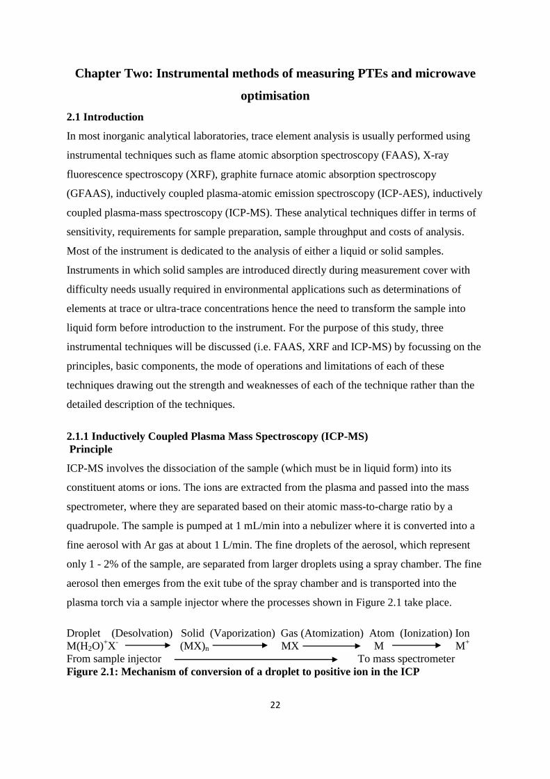
Droplet (Desolvation) Solid (Vaporization) Gas (Atomization) Atom (Ionization) Ion

M(H2O)+X

- (MX)n MX M M

+

From sample injector To mass spectrometer

Figure 2.1: Mechanism of conversion of a droplet to positive ion in the ICP

23

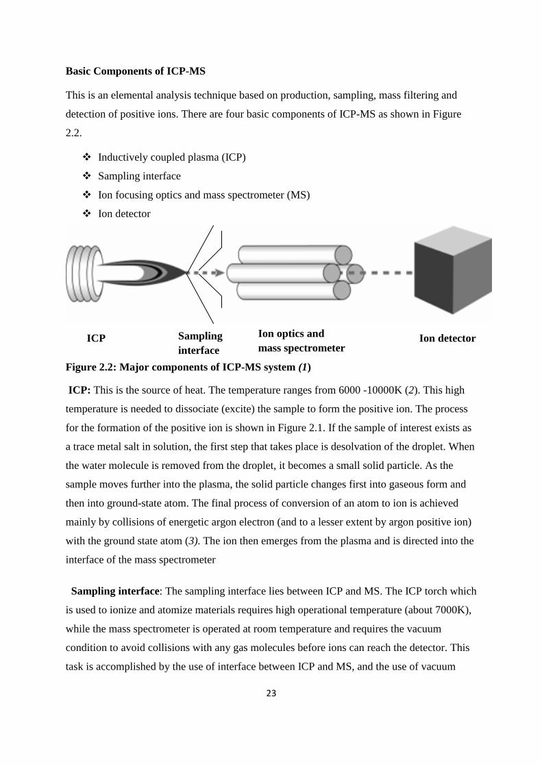
Basic Components of ICP-MS

This is an elemental analysis technique based on production, sampling, mass filtering and

detection of positive ions. There are four basic components of ICP-MS as shown in Figure

2.2.

Inductively coupled plasma (ICP)

Sampling interface

Ion focusing optics and mass spectrometer (MS)

Ion detector

Figure 2.2: Major components of ICP-MS system (1)

ICP: This is the source of heat. The temperature ranges from 6000 -10000K (2). This high

temperature is needed to dissociate (excite) the sample to form the positive ion. The process

for the formation of the positive ion is shown in Figure 2.1. If the sample of interest exists as

a trace metal salt in solution, the first step that takes place is desolvation of the droplet. When

the water molecule is removed from the droplet, it becomes a small solid particle. As the

sample moves further into the plasma, the solid particle changes first into gaseous form and

then into ground-state atom. The final process of conversion of an atom to ion is achieved

mainly by collisions of energetic argon electron (and to a lesser extent by argon positive ion)

with the ground state atom (3). The ion then emerges from the plasma and is directed into the

interface of the mass spectrometer

Sampling interface: The sampling interface lies between ICP and MS. The ICP torch which

is used to ionize and atomize materials requires high operational temperature (about 7000K),

while the mass spectrometer is operated at room temperature and requires the vacuum

condition to avoid collisions with any gas molecules before ions can reach the detector. This

task is accomplished by the use of interface between ICP and MS, and the use of vacuum

ICP Sampling

interface

Ion optics and

mass spectrometer Ion detector

24

pumps to remove nearly all the gas molecules in the space between the interface and the

detector.

Ion optics: The ion optics are positioned between the skimmer cone of the sampling interface

and the mass separation device. The function of the ion optic system is to take ions from the

hostile environment of the plasma at atmospheric pressure via the interface cones and steer

them into the mass analyzer, which is under high vacuum. Another important role of the ion

optic system is to stop particulates, neutral species, and photons from getting through to the

mass analyzer and the detector. These species cause signal instability and contribute to

background levels, which ultimately affect the performance of the system.

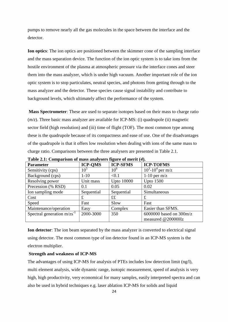
Mass Spectrometer: These are used to separate isotopes based on their mass to charge ratio

(m/z). Three basic mass analyzer are available for ICP-MS: (i) quadrupole (ii) magnetic

sector field (high resolution) and (iii) time of flight (TOF). The most common type among

these is the quadrupole because of its compactness and ease of use. One of the disadvantages

of the quadrupole is that it offers low resolution when dealing with ions of the same mass to

charge ratio. Comparisons between the three analysers are presented in Table 2.1.

Table 2.1: Comparison of mass analysers figure of merit (4).

Parameter ICP-QMS ICP-SFMS ICP-TOFMS

Sensitivity (cps) 105 10

6 10

3-10

4 per m/z

Background (cps) 1-10 <0.1 1-10 per m/z

Resolving power Unit mass Upto 10000 Upto 1500

Precession (% RSD) 0.1 0.05 0.02

Ion sampling mode Sequential Sequential Simultaneous

Cost £ ££ £

Speed Fast Slow Fast

Maintenance/operation Easy Complex Easier than SFMS.

Spectral generation m/zs-1

2000-3000 350 6000000 based on 300m/z

measured @20000Hz

Ion detector: The ion beam separated by the mass analyzer is converted to electrical signal

using detector. The most common type of ion detector found in an ICP-MS system is the

electron multiplier.

Strength and weakness of ICP-MS

The advantages of using ICP-MS for analysis of PTEs includes low detection limit (ng/l),

multi element analysis, wide dynamic range, isotopic measurement, speed of analysis is very

high, high productivity, very economical for many samples, easily interpreted spectra and can

also be used in hybrid techniques e.g. laser ablation ICP-MS for solids and liquid

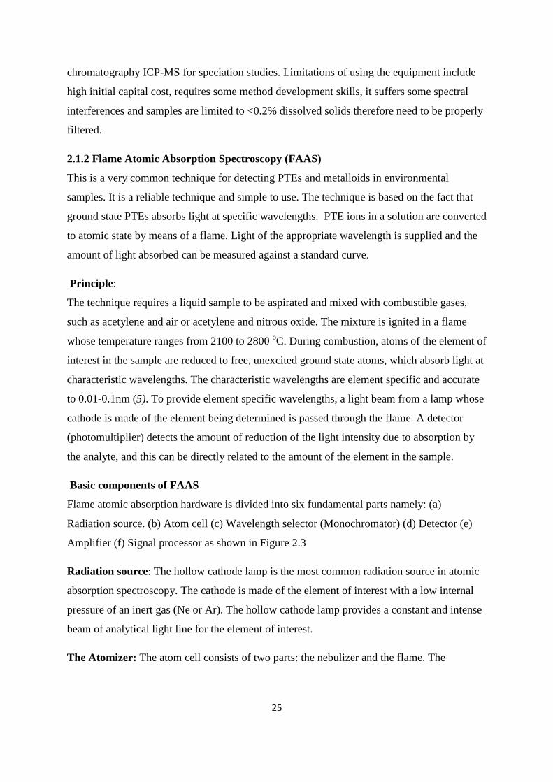
25

chromatography ICP-MS for speciation studies. Limitations of using the equipment include

high initial capital cost, requires some method development skills, it suffers some spectral

interferences and samples are limited to <0.2% dissolved solids therefore need to be properly

filtered.

2.1.2 Flame Atomic Absorption Spectroscopy (FAAS)

This is a very common technique for detecting PTEs and metalloids in environmental

samples. It is a reliable technique and simple to use. The technique is based on the fact that

ground state PTEs absorbs light at specific wavelengths. PTE ions in a solution are converted

to atomic state by means of a flame. Light of the appropriate wavelength is supplied and the

amount of light absorbed can be measured against a standard curve.

Principle:

The technique requires a liquid sample to be aspirated and mixed with combustible gases,

such as acetylene and air or acetylene and nitrous oxide. The mixture is ignited in a flame

whose temperature ranges from 2100 to 2800 oC. During combustion, atoms of the element of

interest in the sample are reduced to free, unexcited ground state atoms, which absorb light at

characteristic wavelengths. The characteristic wavelengths are element specific and accurate

to 0.01-0.1nm (5). To provide element specific wavelengths, a light beam from a lamp whose

cathode is made of the element being determined is passed through the flame. A detector

(photomultiplier) detects the amount of reduction of the light intensity due to absorption by

the analyte, and this can be directly related to the amount of the element in the sample.

Basic components of FAAS

Flame atomic absorption hardware is divided into six fundamental parts namely: (a)

Radiation source. (b) Atom cell (c) Wavelength selector (Monochromator) (d) Detector (e)

Amplifier (f) Signal processor as shown in Figure 2.3

Radiation source: The hollow cathode lamp is the most common radiation source in atomic

absorption spectroscopy. The cathode is made of the element of interest with a low internal

pressure of an inert gas (Ne or Ar). The hollow cathode lamp provides a constant and intense

beam of analytical light line for the element of interest.

The Atomizer: The atom cell consists of two parts: the nebulizer and the flame. The

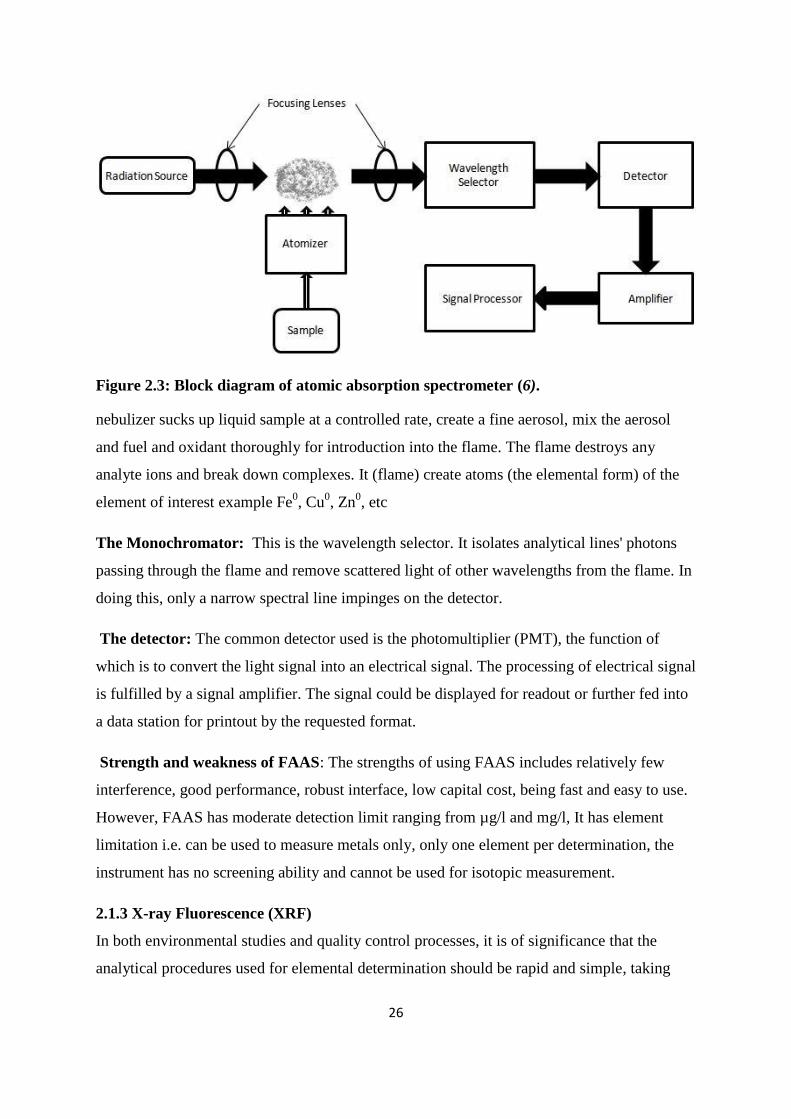
26

Figure 2.3: Block diagram of atomic absorption spectrometer (6).

nebulizer sucks up liquid sample at a controlled rate, create a fine aerosol, mix the aerosol

and fuel and oxidant thoroughly for introduction into the flame. The flame destroys any

analyte ions and break down complexes. It (flame) create atoms (the elemental form) of the

element of interest example Fe0, Cu

0, Zn

0, etc

The Monochromator: This is the wavelength selector. It isolates analytical lines' photons

passing through the flame and remove scattered light of other wavelengths from the flame. In

doing this, only a narrow spectral line impinges on the detector.

The detector: The common detector used is the photomultiplier (PMT), the function of

which is to convert the light signal into an electrical signal. The processing of electrical signal

is fulfilled by a signal amplifier. The signal could be displayed for readout or further fed into

a data station for printout by the requested format.

Strength and weakness of FAAS: The strengths of using FAAS includes relatively few

interference, good performance, robust interface, low capital cost, being fast and easy to use.

However, FAAS has moderate detection limit ranging from µg/l and mg/l, It has element

limitation i.e. can be used to measure metals only, only one element per determination, the

instrument has no screening ability and cannot be used for isotopic measurement.

2.1.3 X-ray Fluorescence (XRF)

In both environmental studies and quality control processes, it is of significance that the

analytical procedures used for elemental determination should be rapid and simple, taking

27

into account the number of samples to be analyzed. Atomic spectroscopy, including FAAS

and ICP-MS are common techniques used for PTE determination in environmental samples

(7, 8). However, these techniques require a prior destruction of the matrix by mineral acids

which may lead to problems of contaminants by reactants employed or disturbances of the

measured concentration by element losses due to incomplete solubilization and/or

evaporation (9, 8). Moreover, the method of matrix destruction used strongly depends on the

chemical composition of the sample and on the element to be determined (10). In view of

these problems, the use of other methods for direct and multi-elemental analysis of samples

has been increasing over the last few years, including X-ray fluorescence spectrometry (XRF)

(11). Simplicity of sample preparation, minimum manipulation, speed, cost effectiveness,

application to a wide range of concentrations from 100% to few part per million (ppm) and

the chance of analyzing some elements such as sulphur that can hardly be determined by

other techniques have promoted XRF as a useful alternative to conventional spectroscopic

techniques.

Principle

In XRF Spectrometry, high-energy primary X-ray photons are emitted from a source (X-ray

tube) and strike the sample. The primary photons from the X-ray tube have enough energy to

knock electrons out of the innermost, K or L, shell. When this occurs, the atoms become ions,

which are unstable. An electron from an outer shell, L or M, will move into the newly vacant

space at the inner shell to regain stability. As the electron from the outer shell moves into the

inner shell space, it emits an energy known as a secondary X-ray photon. This phenomenon is

called fluorescence. The secondary X-ray produced is characteristic of a specific element.

The energy (E) of the emitted fluorescent X-ray photon is determined by the difference in

energies between the initial and final shell of the individual transitions. This is described by

equation 2.1

E = hc/λ 2.1

Where h is Planck's constant; c is the velocity of light; and λ is the characteristic wavelength

of the photon. Energies are inversely proportional to the wavelengths; they are characteristic

for each element.

Basic components of XRF

The setup of XRF instrumentation (Figure 2.4) consists of four basic components (a) An

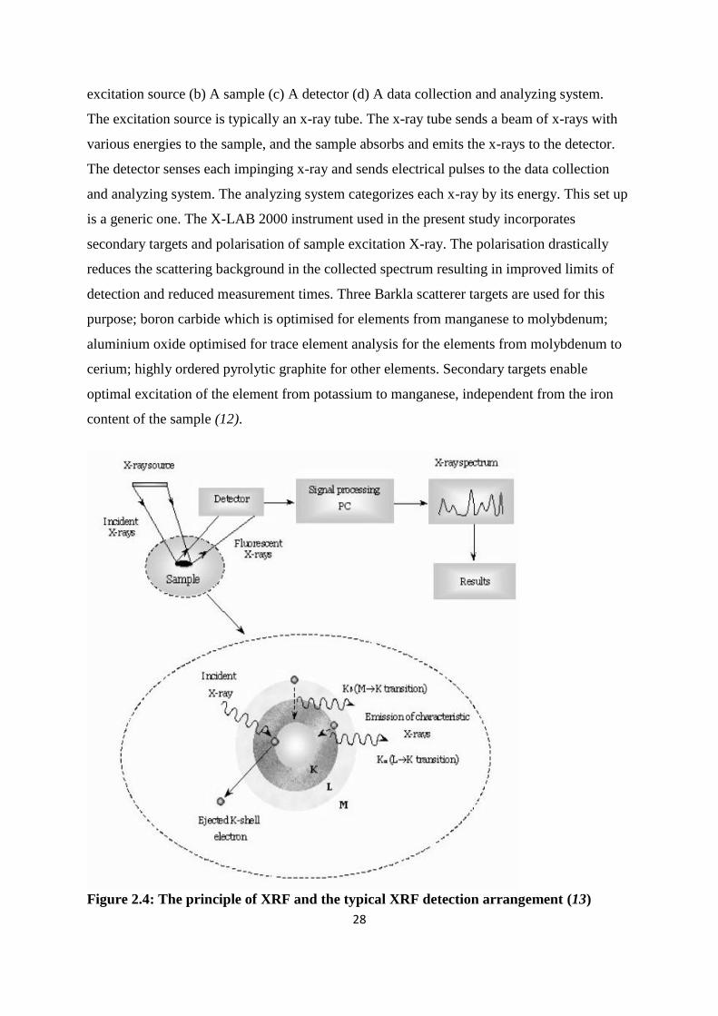
28

excitation source (b) A sample (c) A detector (d) A data collection and analyzing system.

The excitation source is typically an x-ray tube. The x-ray tube sends a beam of x-rays with

various energies to the sample, and the sample absorbs and emits the x-rays to the detector.

The detector senses each impinging x-ray and sends electrical pulses to the data collection

and analyzing system. The analyzing system categorizes each x-ray by its energy. This set up

is a generic one. The X-LAB 2000 instrument used in the present study incorporates

secondary targets and polarisation of sample excitation X-ray. The polarisation drastically

reduces the scattering background in the collected spectrum resulting in improved limits of

detection and reduced measurement times. Three Barkla scatterer targets are used for this

purpose; boron carbide which is optimised for elements from manganese to molybdenum;

aluminium oxide optimised for trace element analysis for the elements from molybdenum to

cerium; highly ordered pyrolytic graphite for other elements. Secondary targets enable

optimal excitation of the element from potassium to manganese, independent from the iron

content of the sample (12).

Figure 2.4: The principle of XRF and the typical XRF detection arrangement (13)

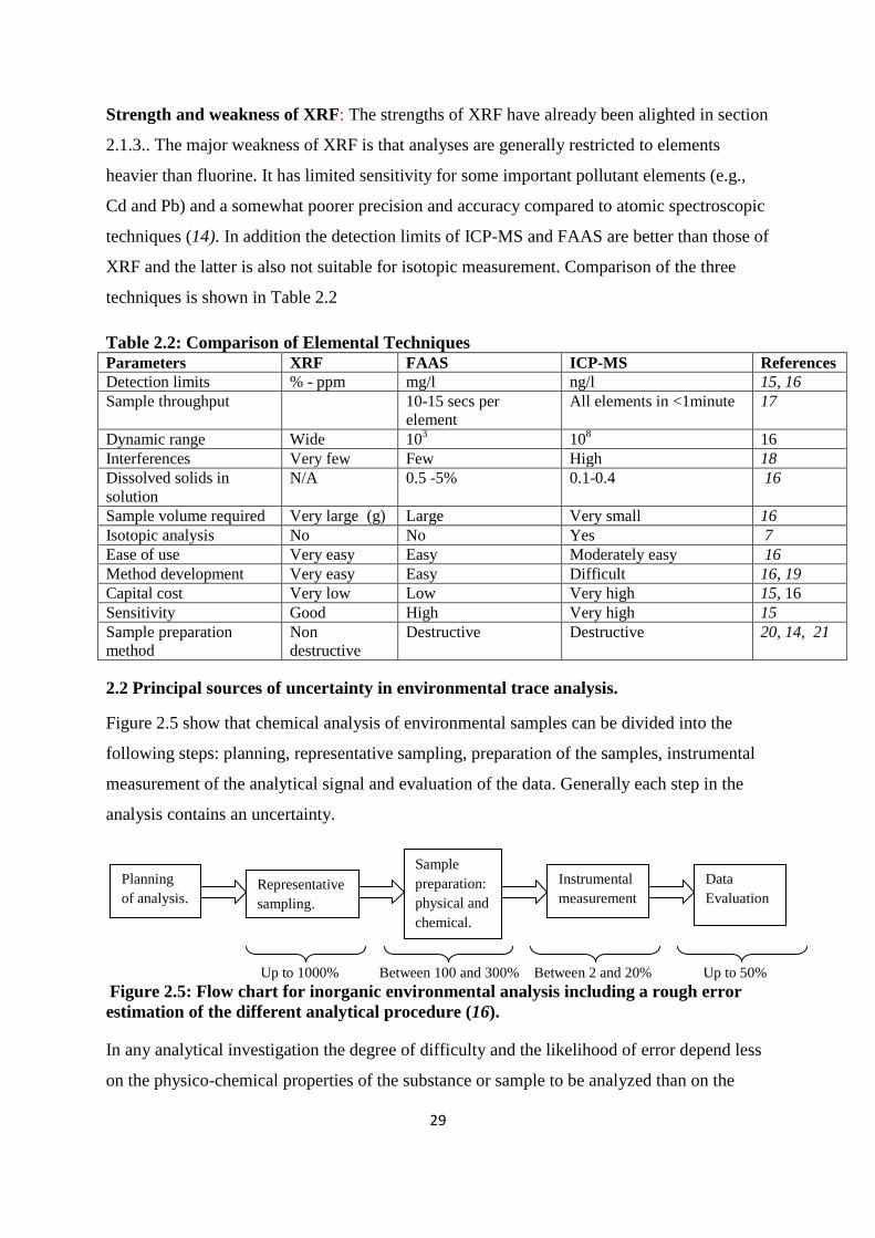
29

Strength and weakness of XRF: The strengths of XRF have already been alighted in section

2.1.3.. The major weakness of XRF is that analyses are generally restricted to elements

heavier than fluorine. It has limited sensitivity for some important pollutant elements (e.g.,

Cd and Pb) and a somewhat poorer precision and accuracy compared to atomic spectroscopic

techniques (14). In addition the detection limits of ICP-MS and FAAS are better than those of

XRF and the latter is also not suitable for isotopic measurement. Comparison of the three

techniques is shown in Table 2.2

Table 2.2: Comparison of Elemental Techniques

Parameters XRF FAAS ICP-MS References

Detection limits % - ppm mg/l ng/l 15, 16

Sample throughput 10-15 secs per

element

All elements in <1minute 17

Dynamic range Wide 103 10

8 16

Interferences Very few Few High 18

Dissolved solids in

solution

N/A 0.5 -5% 0.1-0.4 16

Sample volume required Very large (g) Large Very small 16

Isotopic analysis No No Yes 7

Ease of use Very easy Easy Moderately easy 16

Method development Very easy Easy Difficult 16, 19

Capital cost Very low Low Very high 15, 16

Sensitivity Good High Very high 15

Sample preparation

method

Non

destructive

Destructive Destructive 20, 14, 21

2.2 Principal sources of uncertainty in environmental trace analysis.

Figure 2.5 show that chemical analysis of environmental samples can be divided into the

following steps: planning, representative sampling, preparation of the samples, instrumental

measurement of the analytical signal and evaluation of the data. Generally each step in the

analysis contains an uncertainty.

Up to 1000% Between 100 and 300% Between 2 and 20% Up to 50%

Figure 2.5: Flow chart for inorganic environmental analysis including a rough error

estimation of the different analytical procedure (16).

In any analytical investigation the degree of difficulty and the likelihood of error depend less

on the physico-chemical properties of the substance or sample to be analyzed than on the

Planning

of analysis. Representative

sampling.

Sample

preparation:

physical and

chemical.

Instrumental

measurement

Data

Evaluation

30

concentration range in which the substance to be determined occurs in the sample (4).

Whereas % and ppm ranges can often be determined without much trouble and as a matter of

routine, at ppb and even more at ppt levels present a problem.

2.2.1 Sample preparation

In the analysis of environmental samples, one of the most common sources of error which

analysts encounter are those emanating from preparation steps. Sample preparation is the

most critical part of the analysis because it is responsible for the most and often hidden

sources of errors. It is usually time-consuming and many errors influencing the reliability of

the final results may be introduced at this stage (22). Errors due to contaminations may be

usually overcome if necessary precautions are taken concerning reagents, equipment and the

manner of working. Contaminations, frequently observed, are due to systematic or random

introduction of non-negligible amounts of the analyte during different steps of the analysis.

The choice of the sample preparation procedure will depend on the measurement technique

used. Sample preparation involves several stages. For solid samples, the stages includes

drying (air, laboratory oven 39 to 42oC), homogenization (mixing/crushing), grinding (mills,

mortars), followed by a sub sampling, mineralization and dissolution of a subsample. Most of

these steps performed in the laboratory may be sources of contaminations, essentially due to

the type of vessels and purity of reagents, used. Drying protects the sample material against

microbial decomposition during subsequent storage and acquires constant reference value by

determining the dry weight as opposed to the fresh weight, which is difficult to quantify.

Samples that cannot be dried immediately can be kept in a refrigerator at 4°C before being

processed further (23). To obtain a representative sample and increase the surface area of the

sample, the solid sample has to be split into smaller parts by applying a mechanical force.

The size of the sample is reduced further by grinding. Grinding generally applied to solid

samples prior to the dissolution procedure, may contaminate the sample by abrasion of the

mortar or milling parts with certain hardness (24). Sample preparation steps necessitate the

use of reagents and vessels made in porcelain, glass, quartz, PTFE, platinum or various

plastics. Impurities present in reagents are important (and often systematic) sources of

contaminations, in particular if they are added in great amounts. Total dissolution of samples

cannot be achieved in one step using a single reagent. In practice, a number of steps and

reagents is dictated by the matrix composition. The dissolution process can lead to

volatilization of the analyte arsing from high temperature (eg dry ashing) or volatilization of

31

chlorine ions as nitrosyl chloride (NOCl) as in acid digestion, adsorption, coprecipitation of

the analyte with a precipitate formed by a main matrix element within the reactive mixture

(2). Incomplete dissolution as a result of wrong choice of reagent can lead to error. The good

choice of the sample preparation procedure, the quality of its application and a suitable

laboratory environment become therefore the most critical points for a successful trace

element analysis.

The matrix of a sample is responsible for the degree of difficulties encountered during

analyses because it will impose constraints not only in the analyte determination but also

during preparation steps (8). In view of elevated concentrations of analyte, the sample matrix

is the factor responsible for interference observed during measurements of other elements

present at lower concentrations.

Samples collected for environmental monitoring fall into different categories as a function of

the analytical difficulty associated to the complexity of the matrix and/or concentration levels

to determine: Waters (drinking, surface, ground, and rain); Soils, sediments, suspended

particulate matter collected in natural waters, dusts; Plant samples; Seawater (ultra-trace

concentrations), biological fluids (very complex matrix: blood, milk, or highly variable

matrix: urine); Wastes (urban or industrial) (8). Depending on the instrument for

measurement, the sample can be introduced either in solid or liquid form. Very few

techniques allow solid samples to be introduced directly into the instrument for analysis

therefore analysis of solid samples by other methods involve bringing them into a solution in

order to satisfy needs of introduction systems of most analytical techniques utilized in routine

laboratories.

2.2.2 Sample collection and storage

Sampling is the first and one of the most important steps, in analysis and has the role of

ensuring the representativity of the sample in the context studied. For this reason also, it

represents the most potential source of errors. A representative sample is one that is evenly

distributed, and is required for the analysis. One of the special problems of environmental

analysis is that the quantity of the original sample may be in kilogramme or tonne range and

out of this only a few hundred milligrams can be put into the equipment for the actual

analysis (7). In other words, there is very considerable reduction in bulk from the original

32

sample to the sample used for measurement. Nevertheless, it has to be ensured that the

sample used in analysis has the same mean chemical composition as the original sample.

Depending on the samples to analyze and elements to be determined, the sampling tools,

filtration devices and storage vessels have to be carefully chosen and cleaned to minimize

risks of possible contamination (22). All vessels to be used should thus be washed, rinsed and

then soaked overnight in 1–10% (v/v) analytical grade nitric acid. Finally, before use all

vessels should be rinsed in high purity deionised water. Sample collection and storage is

associated with the risk of contamination especially when the sampling is to do with low

concentration of the analyte (8). In order to minimize analyte losses by adsorption of metal

ions on the vessel or on the suspended particles, the samples collected can be stored for a

short time in a refrigerator, and for longer periods in a freezer. For the same purpose, aqueous

solutions are generally acidified immediately after sampling (generally at pH 1.5 with nitric

acid) (16). This treatment is generally sufficient to prevent the adsorption of trace elements

on to walls of the vessel for relatively long term storage. Another means to avoid adsorption

losses is immediate freezing of the sample collected and its thawing just before

measurements. This is the best method for storage of natural waters because an acidification

may mobilize into solution some trace elements associated with particulate matter present in

the sample.

2.3 Optimisation of microwave digestion

Acid digestion or wet decomposition is routinely employed for the determination of elements

in solids in order to transfer the analytes into solution so that they can be introduced into the

instrumentation (e.g. ICP-MS, AAS) in liquid form (25, 26). Acid digestion involves the use

of acid and heat to destroy the organic matrix, carbonate bound fractions and sorbed fractions

of a sample to liberate the metal content. It measures the total or pseudo-total (depending on

the reagent used for the digestion) concentration of the metal present in the sample matrix. In

this study, acid digestion was carried out using aqua regia (HCl: HNO3 3:1 v/v) and

microwave system to heat the sample. Microwave radiation is a non-ionising radiation in the

frequency range of 300 and 300,000 MHz (27). The frequency of 2450 MHz is used

throughout in every microwave oven apparatus (27, 28). The interaction between sample and

microwave radiation is due to two processes (29, 30).The first process is the dipole rotation

as a function of the oscillating electromagnetic field. At 2450 MHz, the dipole aligns and

randomises five billion times a second. In the second process the ionic conduction

33

mechanism takes place whereby the ionic species migrate in the direction of the electric field.

These two processes produce intense heating which is faster than the convection and thermal

conduction used in classical heating methods. Thus, heating efficiency depends on the

presence of polar molecules (e.g. water) and ions in the sample environment. High

temperatures can be reached at relatively low pressures (31, 32). Microwave digestion is

therefore a rapid and efficient method of sample decomposition prior to determination of

trace metals. The advantages of microwave digestion involve higher recovery of the analyte,

shorter extraction time and use of smaller quantities of solvent (33, 34). A large number of

different acid mixtures have been used for microwave digestion e.g. HNO3 /HCl,

HNO3/H2SO4, HNO3/HClO4 and sometimes HF. In this work, an acid mixture of HCl/HNO3

(3:1 v/v) was used and the degree of dissolution during microwave digestion was examined

by investigating four variables, namely acid volume (V), digestion time (t), microwave power

input (P) and temperature (T). The optimised conditions of these variables were used in the

digestion of soil reference material and its concentration determined to ascertain the accuracy

of the method

2.4 Experimental.

2.4.1 Central Composite Design (CCD).

Central composite design (CCD) is required in order to establish the optimum conditions and

also to obtain information about the inter-relationships between the variables (35). A central

composite randomised design was set up to obtain the various reaction conditions for each

run. Twenty eight standard runs were obtained from the CCD. Each of the variables had

limits set at five coded levels: -α, -1, 0, +1 and +α (36). The variables identified were

temperature, time, power and volume of solvent. The use of a CCD allows all operating

parameters to be investigated individually, as squared terms, and to consider interaction

effects (36). The results of the CCD were evaluated using multilinear regression. The range

of metals for which this technique has been applied are Cr, Cu, Ni, Pb and Zn. Table 2.3

shows the minimum and maximum values for each of the variables which were employed to

generate the equation of a straight line used in the computation of the various values for each

run. The experimental design for the 28 standard runs using the four variables was set up and

is shown in Table 2.4. To fully understand the way in which microwave system affects

digestion, individual operating variables were considered along with nonlinear effects and

interaction terms. The operating variables were studied using a full second order central

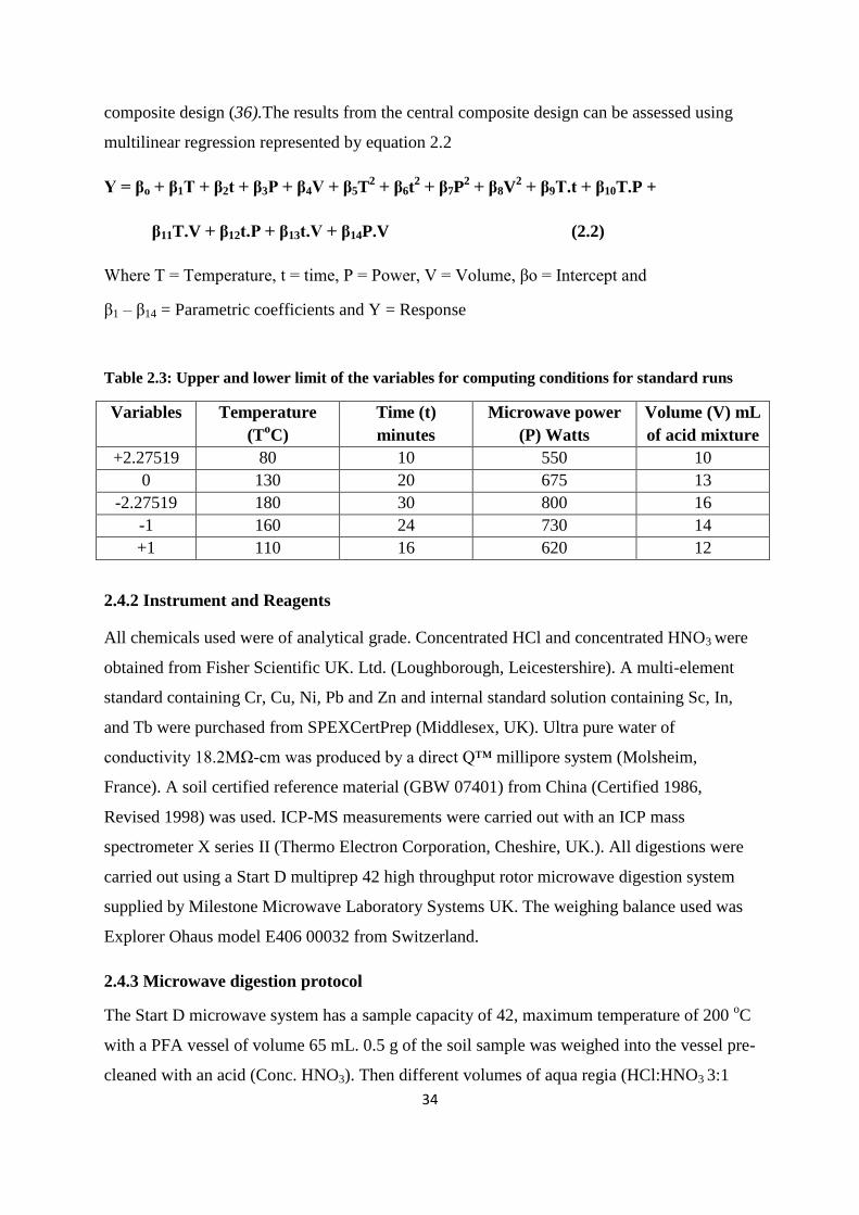
34

composite design (36).The results from the central composite design can be assessed using

multilinear regression represented by equation 2.2

Y = βo + β1T + β2t + β3P + β4V + β5T2 + β6t

2 + β7P

2 + β8V

2 + β9T.t + β10T.P +

β11T.V + β12t.P + β13t.V + β14P.V (2.2)

Where T = Temperature, t = time, P = Power, V = Volume, βo = Intercept and

β1 – β14 = Parametric coefficients and Y = Response

Table 2.3: Upper and lower limit of the variables for computing conditions for standard runs

Variables Temperature

(ToC)

Time (t)

minutes

Microwave power

(P) Watts

Volume (V) mL

of acid mixture

+2.27519 80 10 550 10

0 130 20 675 13

-2.27519 180 30 800 16

-1 160 24 730 14

+1 110 16 620 12

2.4.2 Instrument and Reagents

All chemicals used were of analytical grade. Concentrated HCl and concentrated HNO3 were

obtained from Fisher Scientific UK. Ltd. (Loughborough, Leicestershire). A multi-element

standard containing Cr, Cu, Ni, Pb and Zn and internal standard solution containing Sc, In,

and Tb were purchased from SPEXCertPrep (Middlesex, UK). Ultra pure water of

conductivity 18.2MΩ-cm was produced by a direct Q™ millipore system (Molsheim,

France). A soil certified reference material (GBW 07401) from China (Certified 1986,

Revised 1998) was used. ICP-MS measurements were carried out with an ICP mass

spectrometer X series II (Thermo Electron Corporation, Cheshire, UK.). All digestions were

carried out using a Start D multiprep 42 high throughput rotor microwave digestion system

supplied by Milestone Microwave Laboratory Systems UK. The weighing balance used was

Explorer Ohaus model E406 00032 from Switzerland.

2.4.3 Microwave digestion protocol

The Start D microwave system has a sample capacity of 42, maximum temperature of 200 oC

with a PFA vessel of volume 65 mL. 0.5 g of the soil sample was weighed into the vessel pre-

cleaned with an acid (Conc. HNO3). Then different volumes of aqua regia (HCl:HNO3 3:1

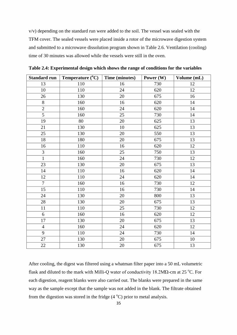
35

v/v) depending on the standard run were added to the soil. The vessel was sealed with the

TFM cover. The sealed vessels were placed inside a rotor of the microwave digestion system

and submitted to a microwave dissolution program shown in Table 2.6. Ventilation (cooling)

time of 30 minutes was allowed while the vessels were still in the oven.

Table 2.4: Experimental design which shows the range of conditions for the variables

Standard run Temperature (oC) Time (minutes) Power (W) Volume (mL)

13 110 16 730 12

10 110 24 620 12

26 130 20 675 16

8 160 16 620 14

2 160 24 620 14

5 160 25 730 14

19 80 20 625 13

21 130 10 625 13

25 130 20 550 13

18 180 20 675 13

16 110 16 620 12

3 160 25 750 13

1 160 24 730 12

23 130 20 675 13

14 110 16 620 14

12 110 24 620 14

7 160 16 730 12

15 110 16 730 14

24 130 20 800 13

28 130 20 675 13

11 110 25 730 12

6 160 16 620 12

17 130 20 675 13

4 160 24 620 12

9 110 24 730 14

27 130 20 675 10

22 130 20 675 13

After cooling, the digest was filtered using a whatman filter paper into a 50 mL volumetric

flask and diluted to the mark with Milli-Q water of conductivity 18.2MΏ-cm at 25 oC. For

each digestion, reagent blanks were also carried out. The blanks were prepared in the same

way as the sample except that the sample was not added in the blank. The filtrate obtained

from the digestion was stored in the fridge (4 oC) prior to metal analysis.

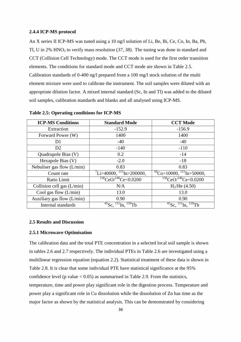
36

2.4.4 ICP-MS protocol

An X series II ICP-MS was tuned using a 10 ng/l solution of Li, Be, Bi, Ce, Co, In, Ba, Pb,

Tl, U in 2% HNO3 to verify mass resolution (37, 38). The tuning was done in standard and

CCT (Collision Cell Technology) mode. The CCT mode is used for the first order transition

elements. The conditions for standard mode and CCT mode are shown in Table 2.5.

Calibration standards of 0-400 ng/l prepared from a 100 mg/l stock solution of the multi

element mixture were used to calibrate the instrument. The soil samples were diluted with an

appropriate dilution factor. A mixed internal standard (Sc, In and Tl) was added to the diluted

soil samples, calibration standards and blanks and all analysed using ICP-MS.

Table 2.5: Operating conditions for ICP-MS

ICP-MS Conditions Standard Mode CCT Mode

Extraction -152.9 -156.9

Forward Power (W) 1400 1400

D1 -40 -40

D2 -140 -110

Quadrupole Bias (V) 0.2 -14

Hexapole Bias (V) -2.0 -18

Nebuliser gas flow (L/min) 0.83 0.83

Count rate 7Li>40000,

115In>200000,

238U>300000

59Co>10000,

115In>50000,

238U>100000. The soil sample

from St Anthony was digested

using the optimised microwave

procedure described in 4.2.3.

The ICP-MS was tuned by the

procedure detailed in 4.2.4 and

the tuning conditions as shown

in table 3 of 4.2.4 for both CCT

and Standard mode. The

calibration equation is shown in

table 3. Lead and Zn were

analysed using FAAS by

preparing calibration standard

from 1000 mg/kg of the stock

solution. The concentration of

the metal (Pb and Zn) were

measured at λ = 217 and 398.8

nm respectively.

Ratio Limit 156

CeO/140

Ce<0.0200 156

CeO/140

Ce<0.0200

Collision cell gas (L/min) N/A H2/He (4.50)

Cool gas flow (L/min) 13.0 13.0

Auxiliary gas flow (L/min) 0.90 0.90

Internal standards 45

Sc, 115

In, 159

Tb 45

Sc, 115

In, 159

Tb

2.5 Results and Discussion

2.5.1 Microwave Optimisation

The calibration data and the total PTE concentration in a selected local soil sample is shown

in tables 2.6 and 2.7 respectively. The individual PTEs in Table 2.6 are investigated using a

multilinear regression equation (equation 2.2). Statistical treatment of these data is shown in

Table 2.8. It is clear that some individual PTE have statistical significance at the 95%

confidence level (p value < 0.05) as summarised in Table 2.9. From the statistics,

temperature, time and power play significant role in the digestion process. Temperature and

power play a significant role in Cu dissolution while the dissolution of Zn has time as the

major factor as shown by the statistical analysis. This can be demonstrated by considering

37

temperature and power for Cu recovery. At the highest power of 800 watts and a moderate

temperature of 130 oC (Standard run 24), the Cu recovery is 208.4 mg/kg while keeping the

time constant at 20 minutes and volume of 13 mL. This recovery is very close to the highest

value of Cu obtained in all the runs (the optimised run). At the highest temperature of 180 oC

and power of 675 watts (Standard run 18), Cu recovery is 168 mg/kg at constant time and

volume of 20 minutes and 13 mL respectively though not too close to the optimum value but

goes a long way in showing that the majority of the dissolution in this case comes more from

temperature than from power. Similarly, the recovery for Zn is poor (418 mg/kg) when the

lowest time of 10 minutes was applied in the digestion (standard run 21). At other lower t of

16 minutes, the recovery varies depending on the temperature, power and volume of solvent

used. Example standard run 7 had Zn recovery of 759 mg/kg when a time of 16 minutes is

used. The temperature used for the dissolution is 160 oC and the power is 730 watts which is

high enough to produce such a reasonable recovery in 16 minutes. The highest recovery of Pb

(506.7 to 659.9 mg/kg) occurs mainly between the temperatures of 130 to 160 oC (Standard

runs 25, 3, 24, 17 and 7). For a constant t of 20 minutes, volume of 13 mL and temperature of

130 oC, the recovery for Pb for runs 25, 24 and 17 are 506.7, 522.8 and 556.0 mg/kg

respectively while the high temperature of 160 oC for time of 25 minutes and also volume of

13 mL for standard run 3 gave 659.9 mg/kg. Though the standard run 7 was operated at high

temperature of 160 oC the recovery for Pb in this run is lower than that of run 3 because the

time of operation (16 minutes) was lower. Standard run 3 gave the highest recovery in all of

the elements (Cr. Cu, Ni, Pb and Zn) studied. The optimised values are 97.0, 250.5, 98.9,

659.9 and 998.3 mg/kg for Cr, Cu, Ni, Pb and Zn respectively (Table 2.7). The optimised

conditions that gave the optimum values are temperature of 160 °C, a time of 25 minutes,

power of 750 watts and a volume of 13 mL (standard run 3). These conditions were used in

the microwave digestion of subsequent samples. In comparison with literatures, it is observed

that the microwave conditions vary depending on the mass of the sample used in the

digestion and the manufacturer / model of the microwave. For instance Navarro et al., 2008

(39) used a Start D model with 0.3 g mass of sample and conditions were 500 W for 10

minutes and 450 W for 18 minutes making a total of 28 minutes for the digestion and the

volume of aqua regia used was 15 mL while operating at a temperature of 160oC. Yasemin et

al., 2007 (40) used a Perkin Elmer Multiwave 3000 with 0.5 g mass of sample with a power

of 600 W, digestion time of 30 minutes and aqua regia volume of 12 mL. Nouri et al., 2007

(41) used a 0.1 g mass of sample in two microwave models: ETHOS and MARS 5

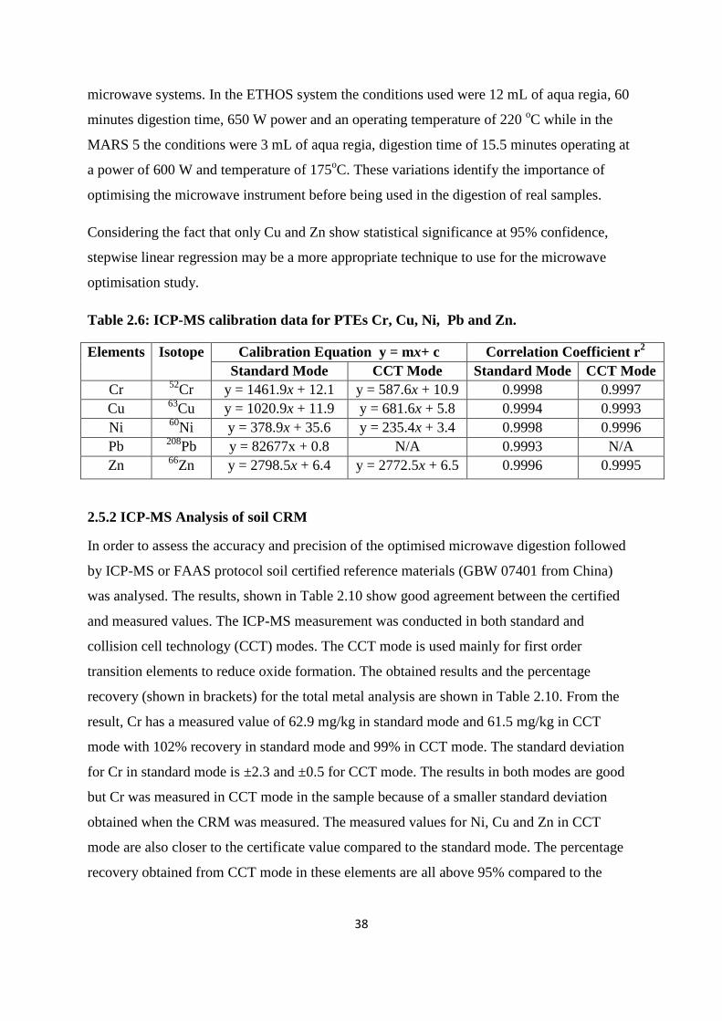
38

microwave systems. In the ETHOS system the conditions used were 12 mL of aqua regia, 60

minutes digestion time, 650 W power and an operating temperature of 220 oC while in the

MARS 5 the conditions were 3 mL of aqua regia, digestion time of 15.5 minutes operating at

a power of 600 W and temperature of 175oC. These variations identify the importance of

optimising the microwave instrument before being used in the digestion of real samples.

Considering the fact that only Cu and Zn show statistical significance at 95% confidence,

stepwise linear regression may be a more appropriate technique to use for the microwave

optimisation study.

Table 2.6: ICP-MS calibration data for PTEs Cr, Cu, Ni, Pb and Zn.

Elements Isotope Calibration Equation y = mx+ c Correlation Coefficient r2

Standard Mode CCT Mode Standard Mode CCT Mode

Cr 52

Cr y = 1461.9x + 12.1 y = 587.6x + 10.9 0.9998 0.9997

Cu 63

Cu y = 1020.9x + 11.9 y = 681.6x + 5.8 0.9994 0.9993

Ni 60

Ni y = 378.9x + 35.6 y = 235.4x + 3.4 0.9998 0.9996

Pb 208

Pb y = 82677x + 0.8 N/A 0.9993 N/A

Zn 66

Zn y = 2798.5x + 6.4 y = 2772.5x + 6.5 0.9996 0.9995

2.5.2 ICP-MS Analysis of soil CRM

In order to assess the accuracy and precision of the optimised microwave digestion followed

by ICP-MS or FAAS protocol soil certified reference materials (GBW 07401 from China)

was analysed. The results, shown in Table 2.10 show good agreement between the certified

and measured values. The ICP-MS measurement was conducted in both standard and

collision cell technology (CCT) modes. The CCT mode is used mainly for first order

transition elements to reduce oxide formation. The obtained results and the percentage

recovery (shown in brackets) for the total metal analysis are shown in Table 2.10. From the

result, Cr has a measured value of 62.9 mg/kg in standard mode and 61.5 mg/kg in CCT

mode with 102% recovery in standard mode and 99% in CCT mode. The standard deviation

for Cr in standard mode is ±2.3 and ±0.5 for CCT mode. The results in both modes are good

but Cr was measured in CCT mode in the sample because of a smaller standard deviation

obtained when the CRM was measured. The measured values for Ni, Cu and Zn in CCT

mode are also closer to the certificate value compared to the standard mode. The percentage

recovery obtained from CCT mode in these elements are all above 95% compared to the

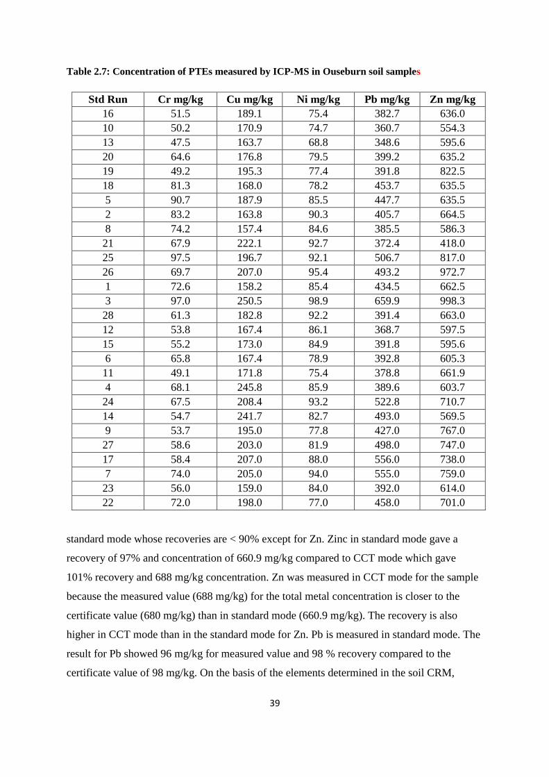
39

Table 2.7: Concentration of PTEs measured by ICP-MS in Ouseburn soil samples

Std Run Cr mg/kg Cu mg/kg Ni mg/kg Pb mg/kg Zn mg/kg

16 51.5 189.1 75.4 382.7 636.0

10 50.2 170.9 74.7 360.7 554.3

13 47.5 163.7 68.8 348.6 595.6

20 64.6 176.8 79.5 399.2 635.2

19 49.2 195.3 77.4 391.8 822.5

18 81.3 168.0 78.2 453.7 635.5

5 90.7 187.9 85.5 447.7 635.5

2 83.2 163.8 90.3 405.7 664.5

8 74.2 157.4 84.6 385.5 586.3

21 67.9 222.1 92.7 372.4 418.0

25 97.5 196.7 92.1 506.7 817.0

26 69.7 207.0 95.4 493.2 972.7

1 72.6 158.2 85.4 434.5 662.5

3 97.0 250.5 98.9 659.9 998.3

28 61.3 182.8 92.2 391.4 663.0

12 53.8 167.4 86.1 368.7 597.5

15 55.2 173.0 84.9 391.8 595.6

6 65.8 167.4 78.9 392.8 605.3

11 49.1 171.8 75.4 378.8 661.9

4 68.1 245.8 85.9 389.6 603.7

24 67.5 208.4 93.2 522.8 710.7

14 54.7 241.7 82.7 493.0 569.5

9 53.7 195.0 77.8 427.0 767.0

27 58.6 203.0 81.9 498.0 747.0

17 58.4 207.0 88.0 556.0 738.0

7 74.0 205.0 94.0 555.0 759.0

23 56.0 159.0 84.0 392.0 614.0

22 72.0 198.0 77.0 458.0 701.0

standard mode whose recoveries are < 90% except for Zn. Zinc in standard mode gave a

recovery of 97% and concentration of 660.9 mg/kg compared to CCT mode which gave

101% recovery and 688 mg/kg concentration. Zn was measured in CCT mode for the sample

because the measured value (688 mg/kg) for the total metal concentration is closer to the

certificate value (680 mg/kg) than in standard mode (660.9 mg/kg). The recovery is also

higher in CCT mode than in the standard mode for Zn. Pb is measured in standard mode. The

result for Pb showed 96 mg/kg for measured value and 98 % recovery compared to the

certificate value of 98 mg/kg. On the basis of the elements determined in the soil CRM,

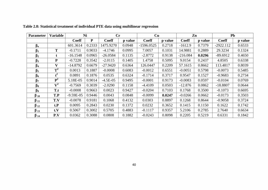
40

Table 2.8: Statistical treatment of individual PTE data using multilinear regression

Parameter Variable Ni Cr Cu Zn Pb

Coeff P

value

Coeff p value Coeff p value Coeff p value Coeff p value

βo 601.3614 0.2333 1475.9270 0.0948 -1596.0525 0.2718 -1612.9 0.7379 -2922.112 0.6533

β1 T -0.1711 0.9033 -4.1746 0.0995 7.0057 0.1031 14.9881 0.2889 29.3234 0.1324

β2 t -16.1548 0.0965 -26.0584 0.1135 -2.8772 0.9138 -216.084 0.0296 -89.6912 0.4650

β3 P -0.7228 0.3542 -2.0115 0.1405 1.4758 0.5095 9.0154 0.2437 4.8505 0.6338

β4 V -14.8792 0.6679 -27.9420 0.6364 126.0447 0.2209 57.1615 0.8662 113.4817 0.8039

β5 T2 0.0013 0.1887 -0.0008 0.6083 -0.0012 0.6551 -0.0051 0.5798 -0.0073 0.5485

β6 t2 0.0891 0.1876 0.0535 0.6324 -0.1714 0.3717 0.9547 0.1527 -0.9683 0.2734

β7 P2 5.18E-05 0.9014 -4.5E-05 0.9495 -0.0001 0.9173 -0.0083 0.0597 -0.0104 0.0769

β8 V2 -0.7569 0.3039 -2.0290 0.1158 -4.4109 0.0503 -12.876 0.0862 -18.8807 0.0644

β9 T.t -0.0008 0.9663 0.0023 0.9427 -0.0204 0.7103 0.1768 0.3500 -0.1073 0.6695

β 10 T.P -9.59E-05 0.9446 0.0043 0.0848 -0.0099 0.0247 -0.0266 0.0662 -0.0173 0.3503

β 11 T.V -0.0078 0.9181 0.1068 0.4132 0.0303 0.8897 0.1268 0.8644 -0.9058 0.3724

β 12 t.P 0.0095 0.2843 0.0230 0.1372 0.0232 0.3652 0.1415 0.1150 0.1622 0.1742

β 13 t.V 0.5067 0.3002 0.5705 0.4883 -0.1117 0.9357 5.2106 0.2785 2.7640 0.6634

β 14 P.V 0.0362 0.3088 0.0808 0.1882 -0.0243 0.8098 0.2205 0.5219 0.6331 0.1842

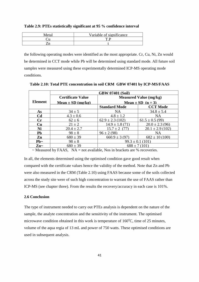
41

Table 2.9: PTEs statistically significant at 95 % confidence interval

Metal Variable of significance Cu T.P Zn t

the following operating modes were identified as the most appropriate. Cr, Cu, Ni, Zn would

be determined in CCT mode while Pb will be determined using standard mode. All future soil

samples were measured using these experimentally determined ICP-MS operating mode

conditions.

Table 2.10: Total PTE concentration in soil CRM GBW 07401 by ICP-MS/FAAS

Element

GBW 07401 (Soil) Certificate Value

Mean ± SD (mg/kg)

Measured Value (mg/kg)

Mean ± SD (n = 3) Standard Mode CCT Mode

As 34 ± 5 NA 34.8 ± 5.4 Cd 4.3 ± 0.6 4.8 ± 1.2 NA Cr 62 ± 6 62.9 ± 2.3 (102) 61.5 ± 0.5 (99) Cu 21 ± 2 14.9 ± 1.8 (71) 20.0 ± 2.3 (96) Ni 20.4 ± 2.7 15.7 ± 2 (77) 20.1 ± 2.9 (102) Pb 98 ± 8 96 ± 2 (98) NA Zn 680 ± 39 660.9 ± 3 (97) 682 ± 10 (100) Pb~ 98 ± 8 99.3 ± 0.1 (101) Zn~ 680 ± 39 688 ± 7 (101)

~ Measured by FAAS, NA = not available, Nos in brackets are % recoveries.

In all, the elements determined using the optimised condition gave good result when

compared with the certificate values hence the validity of the method. Note that Zn and Pb

were also measured in the CRM (Table 2.10) using FAAS because some of the soils collected

across the study site were of such high concentration to warrant the use of FAAS rather than

ICP-MS (see chapter three). From the results the recovery/accuracy in each case is 101%.

2.6 Conclusion

The type of instrument needed to carry out PTEs analysis is dependent on the nature of the

sample, the analyte concentration and the sensitivity of the instrument. The optimised

microwave condition obtained in this work is temperature of 160oC, time of 25 minutes,

volume of the aqua regia of 13 mL and power of 750 watts. These optimised conditions are

used in subsequent analysis.

42

References

1 Nelms, S. ICP-MS: What is it, how does it work and how do you apply it to clinical

analysis? http//www.thermo.com/eThermo/CMA/PDFs/Various/File_26531. February

2010.

2 Dean, J.R. (2005). Practical Inductively Coupled Plasma Spectroscopy. John Wiley &

Sons, Chichester UK.

3 Hasegawa, T., Haraguchi, H., Abdullah, M. (1988). Inductively coupled plasma in

analytical atomic spectrometry-excitation mechanisms and analytical feasibilities.

Pure and Applied Chemistry, 60(5), 685 – 696.

4 Cornelis, R., Caruso,J., Crews, H., Heumann, K. (2003). Handbook of elemental

speciation Techniques and methodology. John Wiley, Chichester UK.

5 Reynolds, R.J., Aldous, K., Thompson, K.C. (1970). Atomic absorption spectroscopy:

a practical guide. Banes and Noble, New York.

6 http://en.wikipedia.org/wiki/Atomic_absorption_spectroscopy. February 2010

7 Baffi, C., Bettinelli, M., Beone, G.M., Spezia, S. (2002). Comparison of different

analytical procedures in the determination of trace elements in lichens. Chemosphere,

48, 299 -306.

8 Hoenig, M. (2001). Preparation steps in environmental trace element analysis-facts

and traps. Talanta, 54, 1021 – 1938.

9 Hoenig, M., Baeten, H., Vanhentenrijk, S., Vassileva, E., Quevauviller, Ph. (1998).

Critical discussion on the need for an efficient minerilization procedure for the

analysis of plant material by atomic spectrometric methods. Analytica Chimica Acta,

358, 85-94.

43

10 Polkowska-Mortrenko, H., Danko, B., Dybczynski, R., Koster, A., Bode, P. (2000).

Effect of acid digestion method on cobalt determination in plant materials. Analytica

Chimica Acta, 408, 89-95.

11 Potts, P.J., Ellis, A.T., Kregsamer, P., Marshall, J., Streli, C., West, M.,

Wobrauschek, P. (2004). Atomic spectrometry update. X- ray florescence

spectrometry. Journal of Analytical Atomic Spectrometry, 19, 1397 - 1419.

12 Dean, J.R., Deary, M.E., Gbefa, B.K., Scott, W.C. (2004). Characterisation and

analysis of persistent organic pollutants and major, minor and trace elements in

calabash chalk. Chemosphere, 57, 21-25.

13 XRF Laboratory. Elemental Analysis using the XRF technique.

http//omega.physics.uoi.gr/Xrf/english/the_Xrf_technique. February 2010.

14 Margui, E., Queralt, I., Hidalgo, M. (2009). Application of X-ray florescence

spectrometry to determination and quantitation of metals in vegetal material. Trends

in Analytical Chemistry, 28, 362 – 372.

15 Madson, G.P., Marco, A.Z. (2003). Trends in preconcentration procedures for metal

determination using atomic spectrometry techniques. Microchimica Acta, 141, 115 –

131.

16 Markert, B. (1995). Sample preparation for trace element analysis in plant matrices.

Science of the Total Environment, 176, 45 – 61.

17 Thermo elemental. AAS, GFAAS, ICP or ICP-MS? Which technique should I use?

An elementary overview of elemental analysis. http://www.thermo.com February

2010.

18 Gupta, J.G., Bertrand, N.B. (1995). Direct ICP-MS of trace and ultratrace elements in

geological materials after decomposition in a microwave oven. Talanta, 42, 1947-

1957.

44

19 Muynck, D., Vanhaecke, F. (2009). Development of method based on ICP-MS for the

simultaneous determination of elements in bone and dental tissue. Spectrochimica

Acta Part B, 64, 408-415.

20 Margui, E., Hidalgo, M., Queralt, I. (2005). Multielemental fast analysis of vegetation

simple by X-ray florescence spectrometry: Possibilities and drawbacks.

Spectrochemica Acta Part B, 60, 1363-1372.

21 Makinen, E., Korhonen, M., Liisa, E., Haapamaki, S., Jarvinen, M. (2005).

Comparison of XRF and FAAS in the analysis of chromate copper arsenate in

contaminated soils. Water, Air and Soil Pollution, 171, 95 – 110.

22 Zoltan, M., Ralph, S. (2004). Sample preparation for trace element analysis In:

Comprehensive analytical chemistry. Spectrochemica Acta, part B 59, 1943 – 1944.

23 Dean, J.R. (1998). Extraction methods for environmental analysis. John Wiley &

Sons, Chichester, UK.

24 Arabinda, K.S., Ruma, C., Cervera, L.M., Miguel, G. (1995). Metal speciation in solid

matrices. Talanta, 42, 1007-1030.

25 Pranar, K., Shankararaman, C. (2007). Microwave digestion ICP-MS for elemental

analysis in ambient airborne fine particulate matter. Analytica Chimica Acta, 599,

170-176.

26 Ute, K., Sandra, J., Jurgen, K and Eckard, J (2005). Determination of arsenic species

in fish Oil after acid digestion. Microchimica Acta, 151, 249-255.

27 Radmila, M., Blaz, K. (2003). Determination of Zn, Cu, Pb, Ni and Cr in some

Slovenian food stuffs. Eur. Food Res. Technology, 217, 211-214.

45

28 Amjad, H.E and Jamal, A. S (2007). A rapid and simple microwave-assisted digestion

procedure for Spectrophotometric determination of titanium dioxide photo catalyst on

activated carbon. Talanta, 71, 1867-1872.

29 Richter, R.C., Link, D. Kingston, H.M. (2001). Microwave-enhanced chemistry.

Analytical Chemistry, 73, 31A-37

A.

30 Pranar, K., Shankararaman, C., David, W.M. (2007). Microwave-assisted extraction

of rare earth elements from Petroleum refining catalysts and ambient fine aerosols

prior to inductively coupled plasma- mass spectrometry. Analytica Chimica Acta, 581,

247-259.

31 Sturgeon, R.E., Willie, S.N. (1995). Continous flow microwave assisted digestion of

environmental samples using atomic spectrometric detection. Journal of Analytical

Atomic Spectrometry, 10, 981-986

32 Melaku, S., Gelaude, I., Vanhacke, F., Moens, L., Richard, D. (2003). Comparison

of Pyrolysis and Microwave Acid Digestion techniques for the Determination of

Mecury in Biological and Environmental Materials. Microchimica Acta, 142, 7-12.

33 Charun, Y., Farmer, J.G. (2006). A comparative study of acid-extractable and total

digestion methods for the determination of inorganic elements in peat material by

inductively coupled plasma-optical emission spectrometry. Analytica Chimica Acta,

557, 296-303.

34 Zlotorzynski, A. (1995). The application of microwave radiation to analytical

Chemistry, Critical Review in Analytical Chemistry, 25, 43-76.

35 Mohd, A.A., Dean, J.R., Tomlinson, W.R. (1992). Factorial Design Approach to

Microwave Dissolution. Analyst, 117, 1743-1748.

36 Norashikin, S, Dean, J.R., Pauzi, M.A., Zuriati, Z. (1998). An Experimental design

Approach for the Determination of Polycyclic Aromatic Hydrocarbons from Highly

46

Contaminated Soil Using Accelerated Solvent Extraction. Analytical Chemistry, 70,

420-424.

37 Intawongse, M., Dean, J.R. (2008). Use of the physiologically-based extraction test to

assess the oral bioaccessibility of metals in vegetable plants grown in contaminated

soil. Environmental Pollution, 152(1), 60 - 72.

38 Melaku, S., Richard, D., Moens, L. (2005). Determination of trace elements in

agricultural soil samples by inductively coupled plasma-mass spectrometry:

Microwave acid digestion versus aqua regia extraction. Analytica Chimica Acta ,543,

117-123.

39 Navarro, P., Arana, G., Etxebarria, N., Dean, J.R. (2008). Evaluation of the

physiologically based extraction test as an indicator of metal toxicity in mussel tissue.

Analytica Chimica Acta, 622, 126 – 132.

40 Yasemin, S., Fikri, B., Seref, G. (2007). ICP-MS analysis of a series of metals in

environmental samples. Food Chemistry, 105, 395-399.

41 Nouri, M., Hassan, P., Rasmussen, E., Valbonna, C. (2007). Analysis of

environmental samples using microwave assisted digestion and ICP-MS: Maximizing

total element recoveries. Water, Air Soil Pollution, 178, 323-334.

47

Chapter Three: Evaluation of PTE contamination at a former industrial

site (St Anthony’s Lead Work) in Newcastle upon Tyne

3.1 Introduction

PTEs are well-known for their toxic effects and therefore information on their concentrations

and distribution in the environment is important. Pollution of the environment by these

elements can pose a serious threat to plants, animals and even human beings because of

bioaccumulation, non-biodegradable properties and toxicity of the contaminants even at low

concentrations. Since these elements are non-biodegradable, their pollution is long lasting.

Different approaches are used for soil and sediment analysis, many of them focussed on

pollutant desorption from the solid phase; others on the pollutant adsorption from a solution

by the solid phase. Among the approaches based on desorption, leaching procedures are the

most widely accepted and used (1). Leaching involves two processes: - (a) Mobilization of

the target metal from the solid particle and (b) Dissolution of metal-containing solid phases

(e.g. Al, Fe, Mn oxides or hydroxides, organic matter and silicate minerals). The dissolution

process is a three step mechanism involving (1) fast ligand adsorption onto surface functional

groups of solid particles (2) slow mineral metal detachment and (3) fast protonation restoring

the original surface functional groups (2, 3). Changes in environmental conditions, whether

natural or anthropological, can strongly influence the behaviour of both essential and

potentially toxic elements by altering the forms in which they occur. The transfers of metals

from soil to plants pose potential health risks because they can enter the food chain and the

environment (4 ). Plant uptake is one of the major pathways by which heavy metals enter the

food chain (5, 6).The uptake of PTEs by plants from soils is of interest because excess

dietary intakes are detrimental to human health.

Of the leaching extraction processes, single and sequential extraction has been the most

widely accepted and used. Sequential extraction provides more detailed information about

the different availabilities of PTEs partitioning among different geochemical phases, enabling

differentiation between several physical forms of speciation: exchangeable, carbonates,

oxide, organic-bound and residual forms. The most widely used method for determining

sequential extraction are those proposed by Tessier et al. 1979 (7) and modified by Rauret et

al. 1999 (8). The former method has four steps, where four fractions of extractable PTEs are

released from the sample:- exchangeable (ion exchange PTEs), associated with carbonates

(acid soluble PTEs), associated with Fe-Mn oxides (reducible PTEs) and associated with

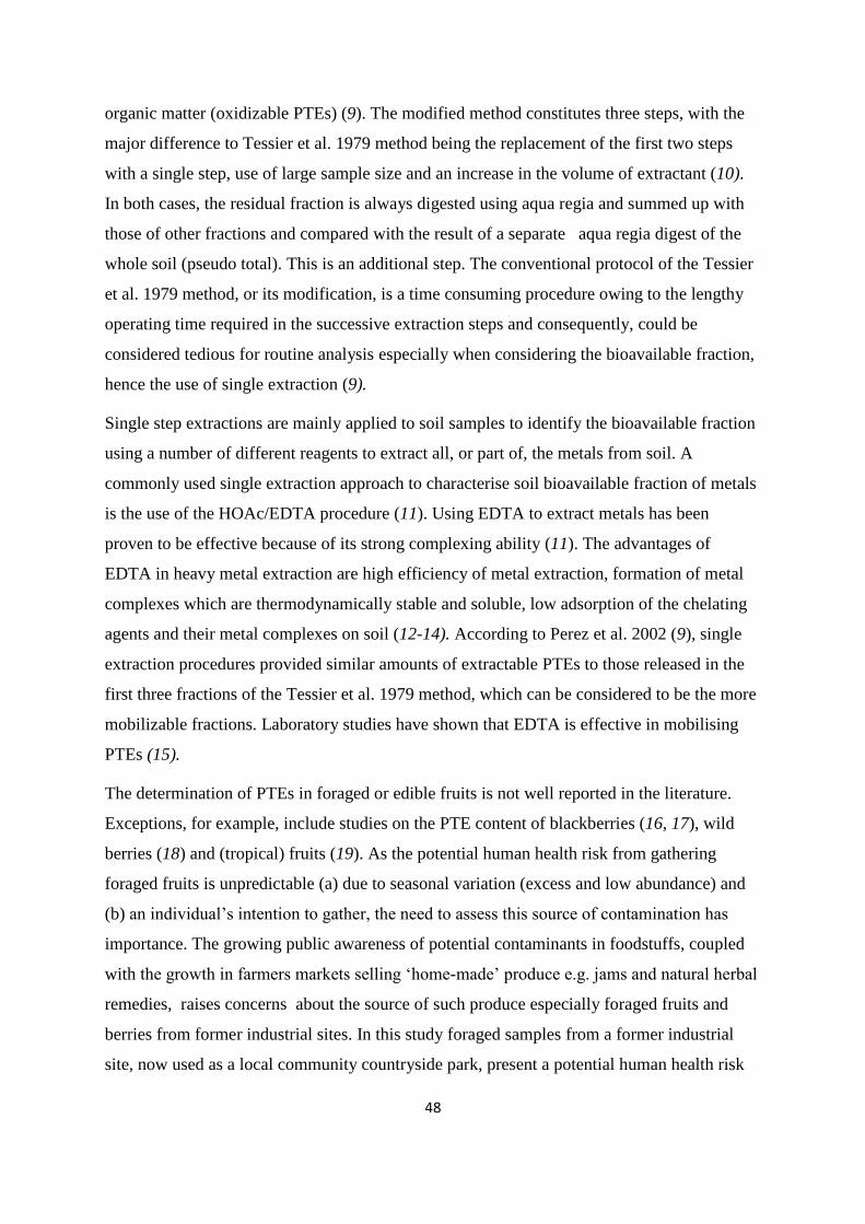
48

organic matter (oxidizable PTEs) (9). The modified method constitutes three steps, with the

major difference to Tessier et al. 1979 method being the replacement of the first two steps

with a single step, use of large sample size and an increase in the volume of extractant (10).

In both cases, the residual fraction is always digested using aqua regia and summed up with

those of other fractions and compared with the result of a separate aqua regia digest of the

whole soil (pseudo total). This is an additional step. The conventional protocol of the Tessier

et al. 1979 method, or its modification, is a time consuming procedure owing to the lengthy

operating time required in the successive extraction steps and consequently, could be

considered tedious for routine analysis especially when considering the bioavailable fraction,

hence the use of single extraction (9).

Single step extractions are mainly applied to soil samples to identify the bioavailable fraction

using a number of different reagents to extract all, or part of, the metals from soil. A

commonly used single extraction approach to characterise soil bioavailable fraction of metals

is the use of the HOAc/EDTA procedure (11). Using EDTA to extract metals has been

proven to be effective because of its strong complexing ability (11). The advantages of

EDTA in heavy metal extraction are high efficiency of metal extraction, formation of metal

complexes which are thermodynamically stable and soluble, low adsorption of the chelating

agents and their metal complexes on soil (12-14). According to Perez et al. 2002 (9), single

extraction procedures provided similar amounts of extractable PTEs to those released in the

first three fractions of the Tessier et al. 1979 method, which can be considered to be the more

mobilizable fractions. Laboratory studies have shown that EDTA is effective in mobilising

PTEs (15).

The determination of PTEs in foraged or edible fruits is not well reported in the literature.

Exceptions, for example, include studies on the PTE content of blackberries (16, 17), wild

berries (18) and (tropical) fruits (19). As the potential human health risk from gathering

foraged fruits is unpredictable (a) due to seasonal variation (excess and low abundance) and

(b) an individual‟s intention to gather, the need to assess this source of contamination has

importance. The growing public awareness of potential contaminants in foodstuffs, coupled

with the growth in farmers markets selling „home-made‟ produce e.g. jams and natural herbal

remedies, raises concerns about the source of such produce especially foraged fruits and

berries from former industrial sites. In this study foraged samples from a former industrial

site, now used as a local community countryside park, present a potential human health risk

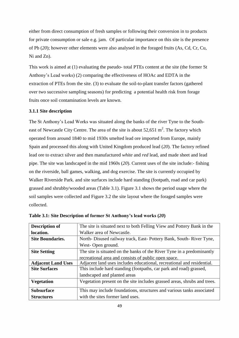
49

either from direct consumption of fresh samples or following their conversion in to products

for private consumption or sale e.g. jam. Of particular importance on this site is the presence

of Pb (20); however other elements were also analysed in the foraged fruits (As, Cd, Cr, Cu,

Ni and Zn).

This work is aimed at (1) evaluating the pseudo- total PTEs content at the site (the former St

Anthony‟s Lead works) (2) comparing the effectiveness of HOAc and EDTA in the

extraction of PTEs from the site. (3) to evaluate the soil-to-plant transfer factors (gathered

over two successive sampling seasons) for predicting a potential health risk from forage

fruits once soil contamination levels are known.

3.1.1 Site description

The St Anthony‟s Lead Works was situated along the banks of the river Tyne to the South-

east of Newcastle City Centre. The area of the site is about 52,651 m2. The factory which

operated from around 1840 to mid 1930s smelted lead ore imported from Europe, mainly

Spain and processed this along with United Kingdom produced lead (20). The factory refined

lead ore to extract silver and then manufactured white and red lead, and made sheet and lead

pipe. The site was landscaped in the mid 1960s (20). Current uses of the site include:- fishing

on the riverside, ball games, walking, and dog exercise. The site is currently occupied by

Walker Riverside Park. and site surfaces include hard standing (footpath, road and car park)

grassed and shrubby/wooded areas (Table 3.1). Figure 3.1 shows the period usage where the

soil samples were collected and Figure 3.2 the site layout where the foraged samples were

collected.

Table 3.1: Site Description of former St Anthony’s lead works (20)

Description of

location.

The site is situated next to both Felling View and Pottery Bank in the

Walker area of Newcastle.

Site Boundaries. North- Disused railway track, East- Pottery Bank, South- River Tyne,

West- Open ground.

Site Setting The site is situated on the banks of the River Tyne in a predominantly

recreational area and consists of public open space. Adjacent Land Uses Adjacent land uses includes educational, recreational and residential.

Site Surfaces This include hard standing (footpaths, car park and road) grassed,

landscaped and planted areas

Vegetation Vegetation present on the site includes grassed areas, shrubs and trees.

Subsurface

Structures

This may include foundations, structures and various tanks associated

with the sites former land uses.

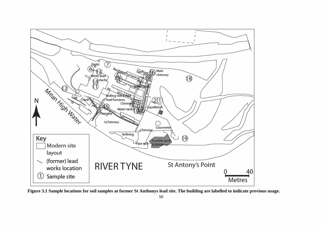
50

Figure 3.1 Sample locations for soil samples at former St Anthonys lead site. The building are labelled to indicate previous usage.

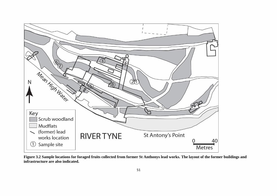
51

Figure 3.2 Sample locations for foraged fruits collected from former St Anthonys lead works. The layout of the former buildings and

infrastructure are also indicated.

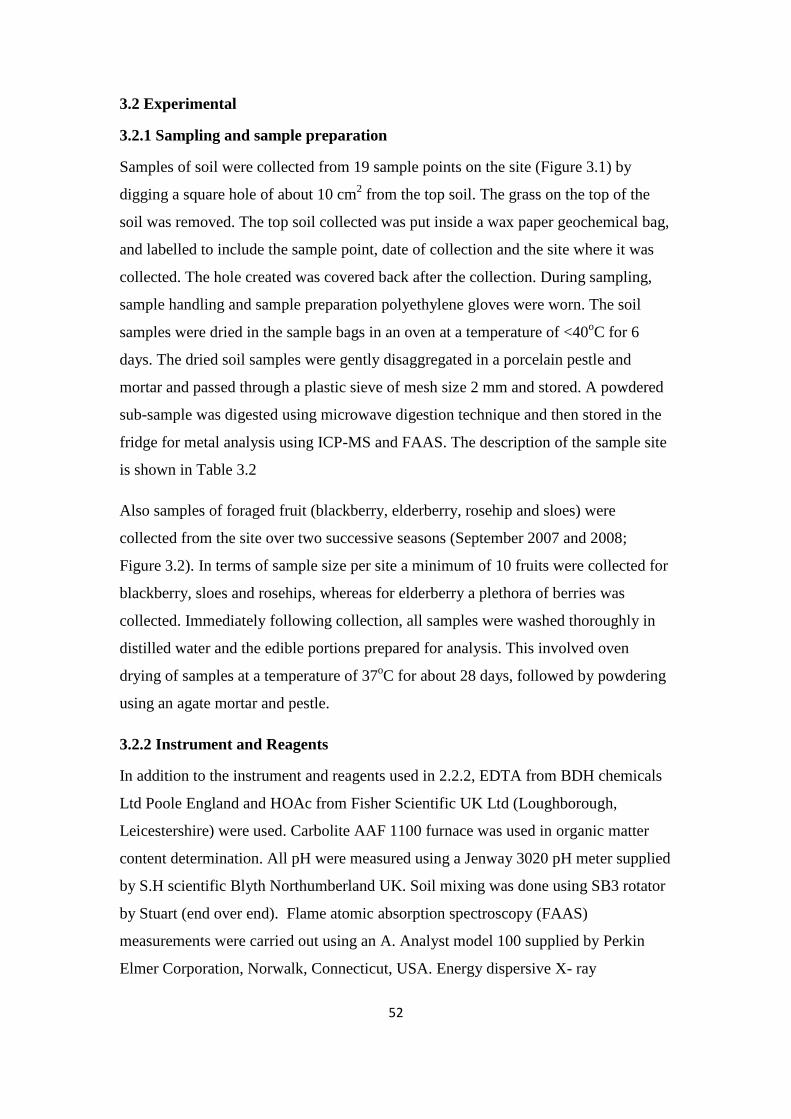
52

3.2 Experimental

3.2.1 Sampling and sample preparation

Samples of soil were collected from 19 sample points on the site (Figure 3.1) by

digging a square hole of about 10 cm2 from the top soil. The grass on the top of the

soil was removed. The top soil collected was put inside a wax paper geochemical bag,

and labelled to include the sample point, date of collection and the site where it was

collected. The hole created was covered back after the collection. During sampling,

sample handling and sample preparation polyethylene gloves were worn. The soil

samples were dried in the sample bags in an oven at a temperature of <40oC for 6

days. The dried soil samples were gently disaggregated in a porcelain pestle and

mortar and passed through a plastic sieve of mesh size 2 mm and stored. A powdered

sub-sample was digested using microwave digestion technique and then stored in the

fridge for metal analysis using ICP-MS and FAAS. The description of the sample site

is shown in Table 3.2

Also samples of foraged fruit (blackberry, elderberry, rosehip and sloes) were

collected from the site over two successive seasons (September 2007 and 2008;

Figure 3.2). In terms of sample size per site a minimum of 10 fruits were collected for

blackberry, sloes and rosehips, whereas for elderberry a plethora of berries was

collected. Immediately following collection, all samples were washed thoroughly in

distilled water and the edible portions prepared for analysis. This involved oven

drying of samples at a temperature of 37oC for about 28 days, followed by powdering

using an agate mortar and pestle.

3.2.2 Instrument and Reagents

In addition to the instrument and reagents used in 2.2.2, EDTA from BDH chemicals

Ltd Poole England and HOAc from Fisher Scientific UK Ltd (Loughborough,

Leicestershire) were used. Carbolite AAF 1100 furnace was used in organic matter

content determination. All pH were measured using a Jenway 3020 pH meter supplied

by S.H scientific Blyth Northumberland UK. Soil mixing was done using SB3 rotator

by Stuart (end over end). Flame atomic absorption spectroscopy (FAAS)

measurements were carried out using an A. Analyst model 100 supplied by Perkin

Elmer Corporation, Norwalk, Connecticut, USA. Energy dispersive X- ray

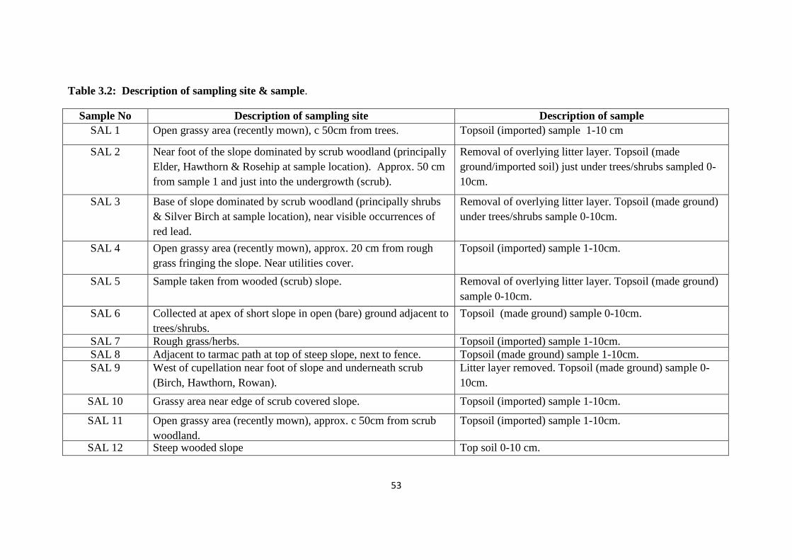
53

Table 3.2: Description of sampling site & sample.

Sample No Description of sampling site Description of sample

SAL 1 Open grassy area (recently mown), c 50cm from trees. Topsoil (imported) sample 1-10 cm

SAL 2 Near foot of the slope dominated by scrub woodland (principally

Elder, Hawthorn & Rosehip at sample location). Approx. 50 cm

from sample 1 and just into the undergrowth (scrub).

Removal of overlying litter layer. Topsoil (made

ground/imported soil) just under trees/shrubs sampled 0-

10cm.

SAL 3 Base of slope dominated by scrub woodland (principally shrubs

& Silver Birch at sample location), near visible occurrences of

red lead.

Removal of overlying litter layer. Topsoil (made ground)

under trees/shrubs sample 0-10cm.

SAL 4 Open grassy area (recently mown), approx. 20 cm from rough

grass fringing the slope. Near utilities cover.

Topsoil (imported) sample 1-10cm.

SAL 5 Sample taken from wooded (scrub) slope. Removal of overlying litter layer. Topsoil (made ground)

sample 0-10cm.

SAL 6 Collected at apex of short slope in open (bare) ground adjacent to

trees/shrubs.

Topsoil (made ground) sample 0-10cm.

SAL 7 Rough grass/herbs. Topsoil (imported) sample 1-10cm.

SAL 8 Adjacent to tarmac path at top of steep slope, next to fence. Topsoil (made ground) sample 1-10cm.

SAL 9 West of cupellation near foot of slope and underneath scrub

(Birch, Hawthorn, Rowan).

Litter layer removed. Topsoil (made ground) sample 0-

10cm.

SAL 10 Grassy area near edge of scrub covered slope. Topsoil (imported) sample 1-10cm.

SAL 11 Open grassy area (recently mown), approx. c 50cm from scrub

woodland.

Topsoil (imported) sample 1-10cm.

SAL 12 Steep wooded slope Top soil 0-10 cm.

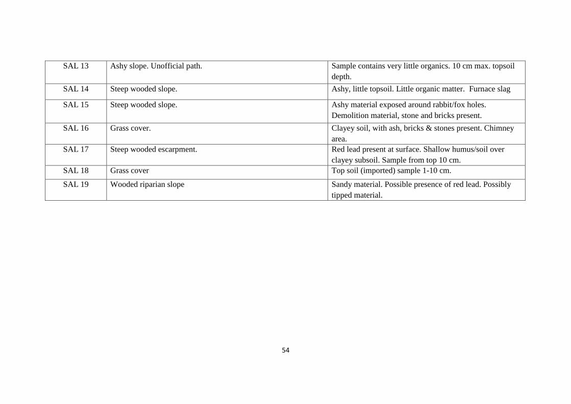
54

SAL 13 Ashy slope. Unofficial path. Sample contains very little organics. 10 cm max. topsoil

depth.

SAL 14 Steep wooded slope. Ashy, little topsoil. Little organic matter. Furnace slag

SAL 15 Steep wooded slope. Ashy material exposed around rabbit/fox holes.

Demolition material, stone and bricks present.

SAL 16 Grass cover. Clayey soil, with ash, bricks & stones present. Chimney

area.

SAL 17 Steep wooded escarpment. Red lead present at surface. Shallow humus/soil over

clayey subsoil. Sample from top 10 cm.

SAL 18 Grass cover Top soil (imported) sample 1-10 cm.

SAL 19 Wooded riparian slope Sandy material. Possible presence of red lead. Possibly

tipped material.

55

fluorescence spectroscopy (ED-XRF) analysis was performed on a Spectro Analytical

X-Lab 2000 instrument fitted with a Gresham Si (Li) detector. Flame photometer used

was from Evans Electroselenium LTD, Essex, UK. Carbolite AAF 1100 furnace was

used in % loss of ignition (LOI) determination. An end-over-end shaker (Stuart

Rotator SB3) was used for the single extraction (Barloworld Scientific Ltd.,

Staffordshire, UK).

3.2.3 Soil pH

The pH was determined in a soil: deionised water suspension 1: 2.5 w/v (21) as

follows; 10 g of soil sample was accurately weighed into a 50 mL Sarstedt extraction

tube. 25 mL of deionised water was added to the soil. The sample was placed on a

shaker and agitated at 30 rpm for 10 minutes. Then, the sample was left to stand for

10 minutes and the pH recorded. The pH was measured using pH meter after being

calibrated with buffer solutions of pH 4 and 7.

3.2.4 Soil organic matter content

Soil organic matter content was determined using the method of LOI as described by

Baize 1993 (22). 5 g of soil sample was accurately weighed into a pre-weighed

crucible. The weight of soil (W) and the weight of soil and crucible (W1) were

recorded. The sample was placed in a pre-heated muffle furnace (400 °C) for 4 hours

and then cooled in a desiccator. The sample was re-weighed and the weight was

recorded (W2). The % LOI was calculated using equation 3.1.

% LOI = W1 - W2 x 100 3.1

W

3.2.5 Cation exchange capacity (CEC)

Soil testing laboratories do not provide direct measurement of CEC rather an estimate

of it based on exchangeable cations. Effective CEC as a preferred nomenclature was

determined according to the procedure described by Robertson et al., 1999 (23). It

involves measurement of exchangeable cations which include both the base cations

(K+, Ca

2+, Mg

2+, and Na

+) and the acid cation (H

+).Other cations such as NH4

+ and

trace metals are usually present in minor amounts and can be effectively ignored.

56

Base cations measurement

4 g sample of fresh sieved soil was weighed into a 50 mL Sarstedt extraction tube. 40

mL of 1 M NH4OAc, pH 7.0 (77.1 g NH4OAc was added to 950 mL deionised water,

adjusted pH to 7.0 with HOAc or aqueous ammonia, and made up the volume to 1.0 L

with deionised water) was added to the sample. The sample was agitated on a shaker

at 30 rpm for 1 hr, after which it was centrifuged at 1000 g for 10 minutes. The

supernatant was removed and filtered through a Whatman No.41 filter paper for

analysis using Flame Atomic Absorption Spectrometer (FAAS) for Ca2+

/ Mg2+

and a

Flame Photometer for Na+/ K

+. The base cations were calculated from equations 3.2

and 3.3.

Gravimetric basis – Element mass

mg element / kg soil = (C x V) 3.2.

W

Where

C = concentration of ion in extract in mg/L, V = volume of extractant

W = dry mass of soil.

Gravimetric basis – Element moles of charge

cmolc element / kg = (Cg x n) 3.3

(10 x A)

Where

Cg = element mass on gravimetric basis, as mg element /kg soil

n = valence of ion, A = atomic mass of ion

Exchangeable acidity

10 g sample of fresh sieved soil was weighed into a 100 mL extraction tube. 25 mL of

1 M KCl was added to the sample. The sample was shaken thoroughly and was

allowed to sit for 30 minutes after which it was sieved in a 2 mm mesh size. The

moisture content of a separate sub sample was determined as detailed in 3.2.4. The

sieved solution was filtered through a Buchner funnel and the residue washed with

five successive 25 mL aliquot of I M KCl for a total of 150 mL KCl per soil sample.

To the filtrate was added five drops of phenolphthalein and titrated with 0.1 M NaOH

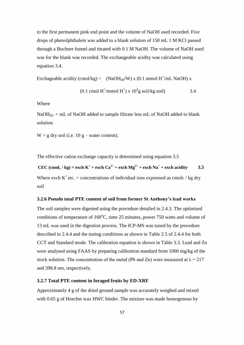
57

to the first permanent pink end point and the volume of NaOH used recorded. Five

drops of phenolphthalein was added to a blank solution of 150 mL 1 M KCl passed

through a Buchner funnel and titrated with 0.1 M NaOH. The volume of NaOH used

was for the blank was recorded. The exchangeable acidity was calculated using

equation 3.4.

Exchageable acidity (cmol/kg) = (NaOHdif/W) x (0.1 mmol H+/mL NaOH) x

(0.1 cmol H+/mmol H

+) x 10

3g soil/kg soil) 3.4

Where

NaOHdif = mL of NaOH added to sample filtrate less mL of NaOH added to blank

solution

W = g dry soil (i.e. 10 g – water content).

The effective cation exchange capacity is determined using equation 3.5

CEC (cmolc / kg) = exch K+ + exch Ca

2+ + exch Mg

2+ + exch Na

+ + exch acidity 3.5

Where exch K+

etc. = concentrations of individual ions expressed as cmolc / kg dry

soil

3.2.6 Pseudo total PTE content of soil from former St Anthony’s lead works

The soil samples were digested using the procedure detailed in 2.4.3. The optimised

conditions of temperature of 160oC, time 25 minutes, power 750 watts and volume of

13 mL was used in the digestion process. The ICP-MS was tuned by the procedure

described in 2.4.4 and the tuning conditions as shown in Table 2.5 of 2.4.4 for both

CCT and Standard mode. The calibration equation is shown in Table 3.3. Lead and Zn

were analysed using FAAS by preparing calibration standard from 1000 mg/kg of the

stock solution. The concentration of the metal (Pb and Zn) were measured at λ = 217

and 398.8 nm, respectively.

3.2.7 Total PTE content in foraged fruits by ED-XRF

Approximately 4 g of the dried ground sample was accurately weighed and mixed

with 0.65 g of Hoechst wax HWC binder. The mixture was made homogenous by

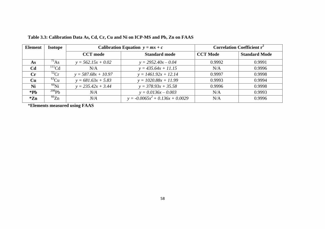
58

Table 3.3: Calibration Data As, Cd, Cr, Cu and Ni on ICP-MS and Pb, Zn on FAAS

Element Isotope Calibration Equation y = mx + c Correlation Coefficient r2

CCT mode Standard mode CCT Mode Standard Mode

As 75

As y = 562.15x + 0.02 y = 2952.40x – 0.04 0.9992 0.9991

Cd 111

Cd N/A y = 435.64x + 11.15 N/A 0.9996

Cr 52

Cr y = 587.68x + 10.97 y = 1461.92x + 12.14 0.9997 0.9998

Cu 63

Cu y = 681.63x + 5.83 y = 1020.88x + 11.99 0.9993 0.9994

Ni 60

Ni y = 235.42x + 3.44 y = 378.93x + 35.58 0.9996 0.9998

*Pb 208

Pb N/A y = 0.0136x – 0.003 N/A 0.9993

*Zn 66

Zn N/A y = -0.0065x2

+ 0.136x + 0.0029 N/A 0.9996

*Elements measured using FAAS

59

shaking in a Retsch MM 200 shaker for 3 mins at 30 cycles per second. The

homogenous mixture was packed in a stainless steel compartment and then formed in

to a 32 mm pellet using a hydraulic press (Graseby Specac) by applying a pressure of

< 10 bar. The pressed pellet was placed inside the ED-XRF instrument and its

elemental composition determined

3.2.8 Single extraction using EDTA

0.05 M EDTA was prepared as ammonium salt solution by adding in a beaker 14.61 g

EDTA to 80 mL deionised water. The dissolution was achieved by gradually adding

13 mL of ammonia solution (25%). The solution was then transferred to a 1.0 L

Polyethylene container and approximately 900 mL of deionised water was added. The

pH of the solution was adjusted to 7.0 by adding a few drops of NH3 or HCl as

appropriate and the solution was made up to 1.0 L with deionised water. 2 g of soil

CRM (BCR 700) was weighed into a 50 mL centrifuge tube and 20 mL of 0.05 M

EDTA (pH 7.0) was added. The mixture obtained was shaken in an end-over-end

shaker at 30 rpm for 1 hr at room temperature. The mixture was centrifuged for 10

minutes at 3000 g and the supernatant was decanted, filtered through a Whatman No

41 filter paper and stored in a polyethylene bottle at 4oC. The extract was analysed

using ICP-MS. The same procedure was adopted on the samples.

3.2.9 Single extraction using HOAc

0.43 M HOAc was prepared by adding 25 mL glacial HOAc to about 500mL of

deionised water in a 1.0 L polyethylene container. The solution was then made up to

1.0 L with deionised water. 20 mL of 0.43 M HOAc was added to 0.5 g of soil CRM

(BCR 700) in a 50 mL centrifuge tube and the mixture extracted by shaking with an

end-over-end shaker at 30 rpm for 16 hrs at ambient temperature (overnight) making

sure that there was no delay between the addition of the extractant solution and the

beginning of the shaking. The mixture was centrifuged for 10 minutes at 3000 g and

the supernatant was decanted and filtered through a Whatman no 41 filter paper and

stored in a polyethylene bottle at 4oC until analysis with ICP-MS. This procedure was

applied to the samples.

60

3 .3 Results and Discussion

3.3.1 Soil properties (pH, % LOI, CEC)

The behaviour of heavy metals varies for different types of soil and so characterising

the soil sample is important. Table 3.4 shows the properties of the soil collected from

former St Anthony‟s lead works. The soil characteristics such as pH, % LOI and CEC

have a direct influence on the mobility and availability of PTEs (24-27).

Soil pH is one of the most important factors in the control of the absorption, mobility

and bioavailability of PTEs in the soil solution (27). A high pH contributes to a

decrease of PTE mobility by the formation of precipitates, which increases the

number of adsorption sites and decreases the competition of H+

for adsorption,

thereby increasing the PTE stability with humic substance. The pH was carried out in

water. The average pH measurement in the sampled points from the site is 7.3

There is only limited variability in the % LOI except with that of SAL 18 where the %

LOI is much higher. The average % LOI is 11.47%. The % LOI contributes to the soil

CEC and a high value of % LOI results in a high value of CEC, which will have direct

impact on the availability of metals.

CEC indicates the number of cation exchange sites and the value gives an idea of the

number of cation adsorption sites in the soil (23). PTEs in soils of low CEC are more

susceptible to leaching. Table 3.5 shows the typical CEC values for different soils.

From Table 3.5, it can be seen that the CEC values at former St Anthony‟s lead works

(SAL) (Table 3.4) falls within the normal range, except for SAL 18, which has a high

value of 161 cmol/kg. The cation adsorption potential of PTEs in this case will be

high because of the high CEC. According to Cameron, (28) CEC values are

considered low if below 12 cmol/kg.

3.3.2 ICP-MS of soil CRM

The soil certified reference material (BCR 700) was analysed in two different modes

(Standard and CCT) using inductively coupled plasma mass spectrometer (ICP-MS)

for both HOAc and EDTA extraction. The results obtained are shown in Table 3.6. As

noted previously, the CRM was run to check the accuracy and precision of the

instrument. The CRM was run three times for each extractant (for a precision

estimate) and the mean taken. The result of the CRM showed good agreement

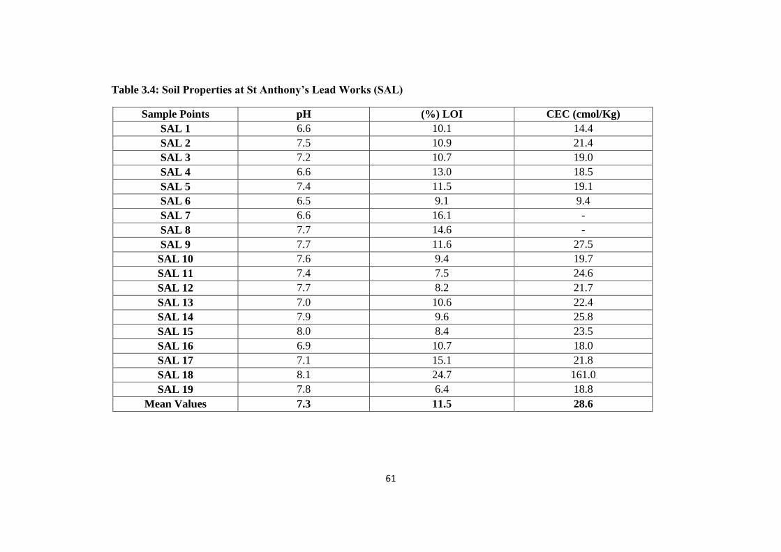
61

Table 3.4: Soil Properties at St Anthony’s Lead Works (SAL)

Sample Points pH (%) LOI CEC (cmol/Kg)

SAL 1 6.6 10.1 14.4

SAL 2 7.5 10.9 21.4

SAL 3 7.2 10.7 19.0

SAL 4 6.6 13.0 18.5

SAL 5 7.4 11.5 19.1

SAL 6 6.5 9.1 9.4

SAL 7 6.6 16.1 -

SAL 8 7.7 14.6 -

SAL 9 7.7 11.6 27.5

SAL 10 7.6 9.4 19.7

SAL 11 7.4 7.5 24.6

SAL 12 7.7 8.2 21.7

SAL 13 7.0 10.6 22.4

SAL 14 7.9 9.6 25.8

SAL 15 8.0 8.4 23.5

SAL 16 6.9 10.7 18.0

SAL 17 7.1 15.1 21.8

SAL 18 8.1 24.7 161.0

SAL 19 7.8 6.4 18.8

Mean Values 7.3 11.5 28.6

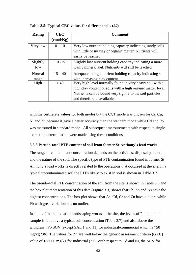
62

Table 3.5: Typical CEC values for different soils (29)

Rating CEC

(cmol/Kg)

Comment

Very low 0 – 10 Very low nutrient holding capacity indicating sandy soils

with little or no clay or organic matter. Nutrients will

easily be leached.

Slightly

low

10 -15 Slightly low nutrient holding capacity indicating a more

loamy mineral soil. Nutrients will still be leached.

Normal

range

15 – 40 Adequate to high nutrient holding capacity indicating soils

with increasing clay content. High + 40 Very high level normally found in very heavy soil with a

high clay content or soils with a high organic matter level.

Nutrients can be bound very tightly to the soil particles

and therefore unavailable.

with the certificate values for both modes but the CCT mode was chosen for Cr, Cu,

Ni and Zn because it gave a better accuracy than the standard mode while Cd and Pb

was measured in standard mode.. All subsequent measurements with respect to single

extraction determination were made using these conditions.

3.3.3 Pseudo-total PTE content of soil from former St Anthony’s lead works

The range of contaminant concentration depends on the activities, disposal patterns

and the nature of the soil. The specific type of PTE contamination found in former St

Anthony‟s lead works is directly related to the operations that occurred at the site. In a

typical uncontaminated soil the PTEs likely to exist in soil is shown in Table 3.7.

The pseudo-total PTE concentration of the soil from the site is shown in Table 3.8 and

the box plot representation of this data (Figure 3.3) shows that Pb, Zn and As have the

highest concentrations. The box plot shows that As, Cd, Cr and Zn have outliers while

Pb with great variation has no outlier.

In spite of the remediation landscaping works at the site, the levels of Pb in all the

sample is far above a typical soil concentration (Table 3.7) and also above the

withdrawn Pb SGV (except SAL 1 and 11) for industrial/commercial which is 750

mg/kg (30). The values for Zn are well below the generic assessment criteria (GAC)

value of 188000 mg/kg for industrial (31). With respect to Cd and Ni, the SGV for

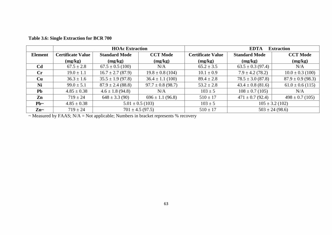
63

Table 3.6: Single Extraction for BCR 700

HOAc Extraction EDTA Extraction

Element

Certificate Value

(mg/kg)

Standard Mode

(mg/kg)

CCT Mode

(mg/kg)

Certificate Value

(mg/kg)

Standard Mode

(mg/kg)

CCT Mode

(mg/kg)

Cd 67.5 ± 2.8 67.5 ± 0.5 (100) N/A 65.2 ± 3.5 63.5 ± 0.3 (97.4) N/A

Cr 19.0 ± 1.1 16.7 ± 2.7 (87.9) 19.8 ± 0.8 (104) 10.1 ± 0.9 7.9 ± 4.2 (78.2) 10.0 ± 0.3 (100)

Cu 36.3 ± 1.6 35.5 ± 1.9 (97.8) 36.4 ± 1.1 (100) 89.4 ± 2.8 78.5 ± 3.0 (87.8) 87.9 ± 0.9 (98.3)

Ni 99.0 ± 5.1 87.9 ± 2.4 (88.8) 97.7 ± 0.8 (98.7) 53.2 ± 2.8 43.4 ± 0.8 (81.6) 61.0 ± 0.6 (115)

Pb 4.85 ± 0.38 4.6 ± 1.8 (94.8) N/A 103 ± 5 108 ± 0.7 (105) N/A

Zn 719 ± 24 648 ± 3.3 (90) 696 ± 1.1 (96.8) 510 ± 17 471 ± 0.7 (92.4) 498 ± 0.7 (105)

Pb~ 4.85 ± 0.38 5.01 ± 0.5 (103) 103 ± 5 105 ± 3.2 (102)

Zn~ 719 ± 24 701 ± 4.5 (97.5) 510 ± 17 503 ± 24 (98.6)

~ Measured by FAAS; N/A = Not applicable; Numbers in bracket represents % recovery

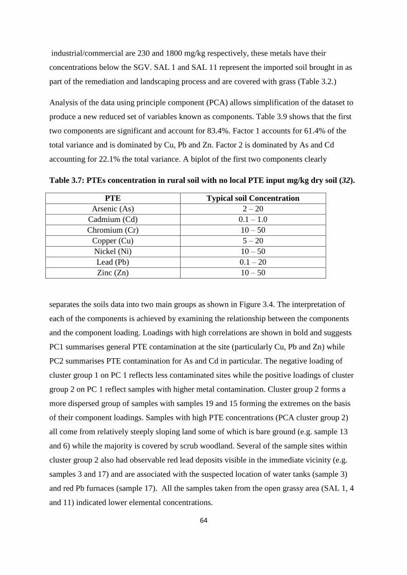
64

industrial/commercial are 230 and 1800 mg/kg respectively, these metals have their

concentrations below the SGV. SAL 1 and SAL 11 represent the imported soil brought in as

part of the remediation and landscaping process and are covered with grass (Table 3.2.)

Analysis of the data using principle component (PCA) allows simplification of the dataset to

produce a new reduced set of variables known as components. Table 3.9 shows that the first

two components are significant and account for 83.4%. Factor 1 accounts for 61.4% of the

total variance and is dominated by Cu, Pb and Zn. Factor 2 is dominated by As and Cd

accounting for 22.1% the total variance. A biplot of the first two components clearly

Table 3.7: PTEs concentration in rural soil with no local PTE input mg/kg dry soil (32).

PTE Typical soil Concentration

Arsenic (As) 2 – 20

Cadmium (Cd) 0.1 – 1.0

Chromium (Cr) 10 – 50

Copper (Cu) 5 – 20

Nickel (Ni) 10 – 50

Lead (Pb) 0.1 – 20

Zinc (Zn) 10 – 50

separates the soils data into two main groups as shown in Figure 3.4. The interpretation of

each of the components is achieved by examining the relationship between the components

and the component loading. Loadings with high correlations are shown in bold and suggests

PC1 summarises general PTE contamination at the site (particularly Cu, Pb and Zn) while

PC2 summarises PTE contamination for As and Cd in particular. The negative loading of

cluster group 1 on PC 1 reflects less contaminated sites while the positive loadings of cluster

group 2 on PC 1 reflect samples with higher metal contamination. Cluster group 2 forms a

more dispersed group of samples with samples 19 and 15 forming the extremes on the basis

of their component loadings. Samples with high PTE concentrations (PCA cluster group 2)

all come from relatively steeply sloping land some of which is bare ground (e.g. sample 13

and 6) while the majority is covered by scrub woodland. Several of the sample sites within

cluster group 2 also had observable red lead deposits visible in the immediate vicinity (e.g.

samples 3 and 17) and are associated with the suspected location of water tanks (sample 3)

and red Pb furnaces (sample 17). All the samples taken from the open grassy area (SAL 1, 4

and 11) indicated lower elemental concentrations.

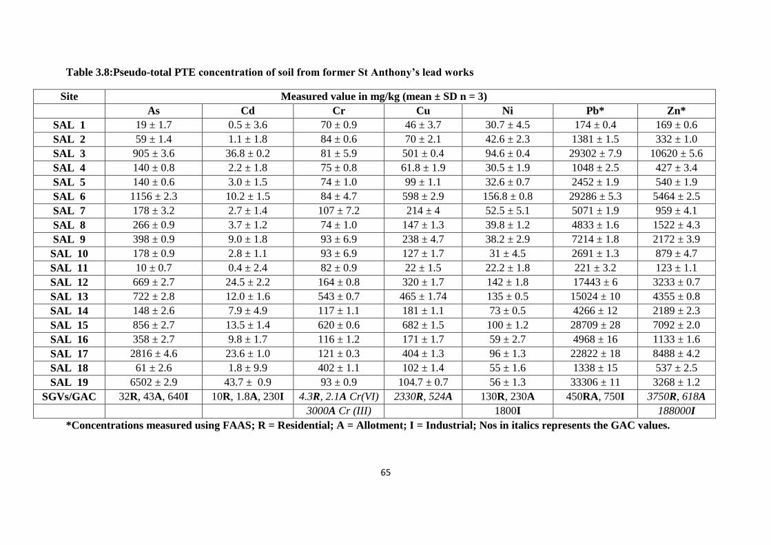
65

Table 3.8:Pseudo-total PTE concentration of soil from former St Anthony’s lead works

Site Measured value in mg/kg (mean ± SD n = 3)

As Cd Cr Cu Ni Pb* Zn*

SAL 1 19 ± 1.7 0.5 ± 3.6 70 ± 0.9 46 ± 3.7 30.7 ± 4.5 174 ± 0.4 169 ± 0.6

SAL 2 59 ± 1.4 1.1 ± 1.8 84 ± 0.6 70 ± 2.1 42.6 ± 2.3 1381 ± 1.5 332 ± 1.0

SAL 3 905 ± 3.6 36.8 ± 0.2 81 ± 5.9 501 ± 0.4 94.6 ± 0.4 29302 ± 7.9 10620 ± 5.6

SAL 4 140 ± 0.8 2.2 ± 1.8 75 ± 0.8 61.8 ± 1.9 30.5 ± 1.9 1048 ± 2.5 427 ± 3.4

SAL 5 140 ± 0.6 3.0 ± 1.5 74 ± 1.0 99 ± 1.1 32.6 ± 0.7 2452 ± 1.9 540 ± 1.9

SAL 6 1156 ± 2.3 10.2 ± 1.5 84 ± 4.7 598 ± 2.9 156.8 ± 0.8 29286 ± 5.3 5464 ± 2.5

SAL 7 178 ± 3.2 2.7 ± 1.4 107 ± 7.2 214 ± 4 52.5 ± 5.1 5071 ± 1.9 959 ± 4.1

SAL 8 266 ± 0.9 3.7 ± 1.2 74 ± 1.0 147 ± 1.3 39.8 ± 1.2 4833 ± 1.6 1522 ± 4.3

SAL 9 398 ± 0.9 9.0 ± 1.8 93 ± 6.9 238 ± 4.7 38.2 ± 2.9 7214 ± 1.8 2172 ± 3.9

SAL 10 178 ± 0.9 2.8 ± 1.1 93 ± 6.9 127 ± 1.7 31 ± 4.5 2691 ± 1.3 879 ± 4.7

SAL 11 10 ± 0.7 0.4 ± 2.4 82 ± 0.9 22 ± 1.5 22.2 ± 1.8 221 ± 3.2 123 ± 1.1

SAL 12 669 ± 2.7 24.5 ± 2.2 164 ± 0.8 320 ± 1.7 142 ± 1.8 17443 ± 6 3233 ± 0.7

SAL 13 722 ± 2.8 12.0 ± 1.6 543 ± 0.7 465 ± 1.74 135 ± 0.5 15024 ± 10 4355 ± 0.8

SAL 14 148 ± 2.6 7.9 ± 4.9 117 ± 1.1 181 ± 1.1 73 ± 0.5 4266 ± 12 2189 ± 2.3

SAL 15 856 ± 2.7 13.5 ± 1.4 620 ± 0.6 682 ± 1.5 100 ± 1.2 28709 ± 28 7092 ± 2.0

SAL 16 358 ± 2.7 9.8 ± 1.7 116 ± 1.2 171 ± 1.7 59 ± 2.7 4968 ± 16 1133 ± 1.6

SAL 17 2816 ± 4.6 23.6 ± 1.0 121 ± 0.3 404 ± 1.3 96 ± 1.3 22822 ± 18 8488 ± 4.2

SAL 18 61 ± 2.6 1.8 ± 9.9 402 ± 1.1 102 ± 1.4 55 ± 1.6 1338 ± 15 537 ± 2.5

SAL 19 6502 ± 2.9 43.7 ± 0.9 93 ± 0.9 104.7 ± 0.7 56 ± 1.3 33306 ± 11 3268 ± 1.2

SGVs/GAC 32R, 43A, 640I 10R, 1.8A, 230I 4.3R, 2.1A Cr(VI) 2330R, 524A 130R, 230A 450RA, 750I 3750R, 618A

3000A Cr (III) 1800I 188000I

*Concentrations measured using FAAS; R = Residential; A = Allotment; I = Industrial; Nos in italics represents the GAC values.

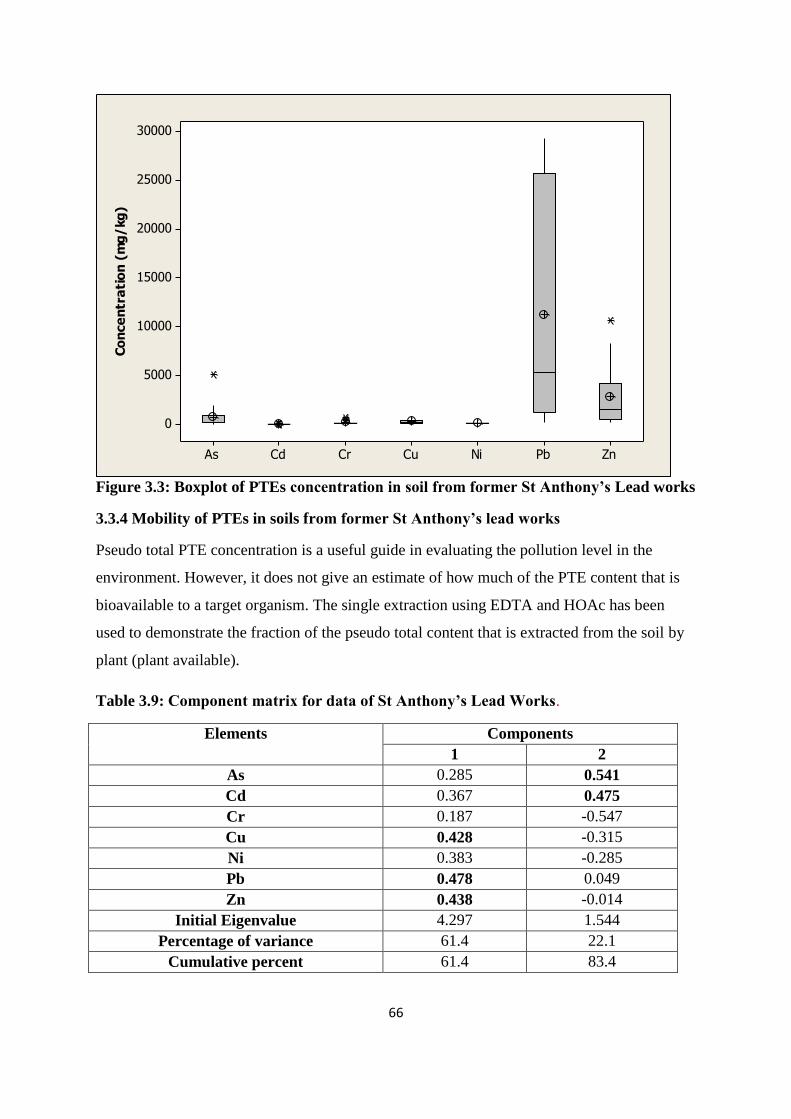
66

ZnPbNiCuCrCdAs

30000

25000

20000

15000

10000

5000

0

Co

nce

ntr

ati

on

(m

g/

kg

)

Figure 3.3: Boxplot of PTEs concentration in soil from former St Anthony’s Lead works

3.3.4 Mobility of PTEs in soils from former St Anthony’s lead works

Pseudo total PTE concentration is a useful guide in evaluating the pollution level in the

environment. However, it does not give an estimate of how much of the PTE content that is

bioavailable to a target organism. The single extraction using EDTA and HOAc has been

used to demonstrate the fraction of the pseudo total content that is extracted from the soil by

plant (plant available).

Table 3.9: Component matrix for data of St Anthony’s Lead Works.

Elements Components

1 2

As 0.285 0.541

Cd 0.367 0.475

Cr 0.187 -0.547

Cu 0.428 -0.315

Ni 0.383 -0.285

Pb 0.478 0.049

Zn 0.438 -0.014

Initial Eigenvalue 4.297 1.544

Percentage of variance 61.4 22.1

Cumulative percent 61.4 83.4

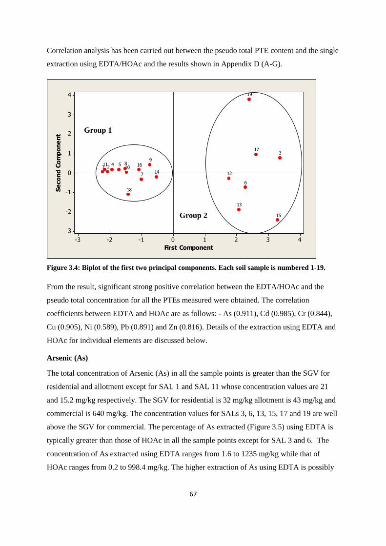
67

Correlation analysis has been carried out between the pseudo total PTE content and the single

extraction using EDTA/HOAc and the results shown in Appendix D (A-G).

43210-1-2-3

4

3

2

1

0

-1

-2

-3

First Component

Se

co

nd

Co

mp

on

en

t

19

18

17

16

15

14

13

12

11 10

9 8

7

6

5 4

3

2 1

Figure 3.4: Biplot of the first two principal components. Each soil sample is numbered 1-19.

From the result, significant strong positive correlation between the EDTA/HOAc and the

pseudo total concentration for all the PTEs measured were obtained. The correlation

coefficients between EDTA and HOAc are as follows: - As (0.911), Cd (0.985), Cr (0.844),

Cu (0.905), Ni (0.589), Pb (0.891) and Zn (0.816). Details of the extraction using EDTA and

HOAc for individual elements are discussed below.

Arsenic (As)

The total concentration of Arsenic (As) in all the sample points is greater than the SGV for

residential and allotment except for SAL 1 and SAL 11 whose concentration values are 21

and 15.2 mg/kg respectively. The SGV for residential is 32 mg/kg allotment is 43 mg/kg and

commercial is 640 mg/kg. The concentration values for SALs 3, 6, 13, 15, 17 and 19 are well

above the SGV for commercial. The percentage of As extracted (Figure 3.5) using EDTA is

typically greater than those of HOAc in all the sample points except for SAL 3 and 6. The

concentration of As extracted using EDTA ranges from 1.6 to 1235 mg/kg while that of

HOAc ranges from 0.2 to 998.4 mg/kg. The higher extraction of As using EDTA is possibly

Group 1

Group 2

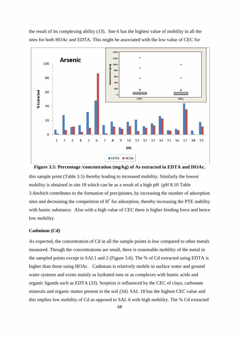
68

the result of its complexing ability (13). Site 6 has the highest value of mobility in all the

sites for both HOAc and EDTA. This might be associated with the low value of CEC for

Figure 3.5: Percentage /concentration (mg/kg) of As extracted in EDTA and HOAc.

this sample point (Table 3.5) thereby leading to increased mobility. Similarly the lowest

mobility is obtained in site 18 which can be as a result of a high pH (pH 8.10 Table

3.4)which contributes to the formation of precipitates, by increasing the number of adsorption

sites and decreasing the competition of H+

for adsorption, thereby increasing the PTE stability

with humic substance. Also with a high value of CEC there is higher binding force and hence

low mobility.

Cadmium (Cd)

As expected, the concentration of Cd in all the sample points is low compared to other metals

measured. Though the concentrations are small, there is reasonable mobility of the metal in

the sampled points except in SAL1 and 2 (Figure 3.6). The % of Cd extracted using EDTA is

higher than those using HOAc. Cadmium is relatively mobile in surface water and ground

water systems and exists mainly as hydrated ions or as complexes with humic acids and

organic ligands such as EDTA (33). Sorption is influenced by the CEC of clays, carbonate

minerals and organic matter present in the soil (34). SAL 18 has the highest CEC value and

this implies low mobility of Cd as opposed to SAL 6 with high mobility. The % Cd extracted

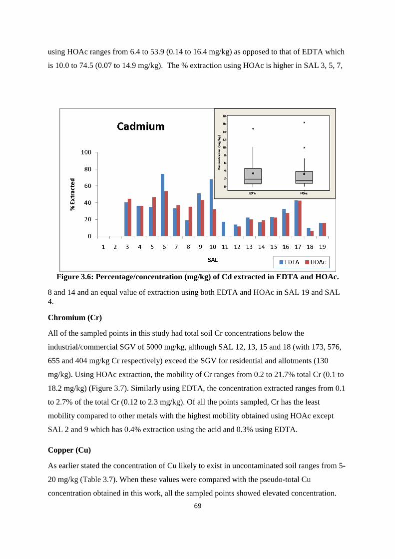
69

using HOAc ranges from 6.4 to 53.9 (0.14 to 16.4 mg/kg) as opposed to that of EDTA which

is 10.0 to 74.5 (0.07 to 14.9 mg/kg). The % extraction using HOAc is higher in SAL 3, 5, 7,

Figure 3.6: Percentage/concentration (mg/kg) of Cd extracted in EDTA and HOAc.

8 and 14 and an equal value of extraction using both EDTA and HOAc in SAL 19 and SAL

4.

Chromium (Cr)

All of the sampled points in this study had total soil Cr concentrations below the

industrial/commercial SGV of 5000 mg/kg, although SAL 12, 13, 15 and 18 (with 173, 576,

655 and 404 mg/kg Cr respectively) exceed the SGV for residential and allotments (130

mg/kg). Using HOAc extraction, the mobility of Cr ranges from 0.2 to 21.7% total Cr (0.1 to

18.2 mg/kg) (Figure 3.7). Similarly using EDTA, the concentration extracted ranges from 0.1

to 2.7% of the total Cr (0.12 to 2.3 mg/kg). Of all the points sampled, Cr has the least

mobility compared to other metals with the highest mobility obtained using HOAc except

SAL 2 and 9 which has 0.4% extraction using the acid and 0.3% using EDTA.

Copper (Cu)

As earlier stated the concentration of Cu likely to exist in uncontaminated soil ranges from 5-

20 mg/kg (Table 3.7). When these values were compared with the pseudo-total Cu

concentration obtained in this work, all the sampled points showed elevated concentration.

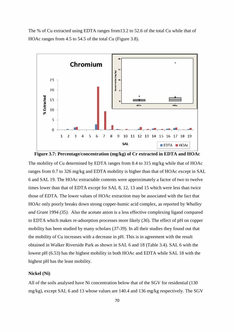
70

The % of Cu extracted using EDTA ranges from13.2 to 52.6 of the total Cu while that of

HOAc ranges from 4.5 to 54.5 of the total Cu (Figure 3.8).

Figure 3.7: Percentage/concentration (mg/kg) of Cr extracted in EDTA and HOAc

The mobility of Cu determined by EDTA ranges from 8.4 to 315 mg/kg while that of HOAc

ranges from 0.7 to 326 mg/kg and EDTA mobility is higher than that of HOAc except in SAL

6 and SAL 19. The HOAc extractable contents were approximately a factor of two to twelve

times lower than that of EDTA except for SAL 8, 12, 13 and 15 which were less than twice

those of EDTA. The lower values of HOAc extraction may be associated with the fact that

HOAc only poorly breaks down strong copper-humic acid complex, as reported by Whalley

and Grant 1994 (35). Also the acetate anion is a less effective complexing ligand compared

to EDTA which makes re-adsorption processes more likely (36). The effect of pH on copper

mobility has been studied by many scholars (37-39). In all their studies they found out that

the mobility of Cu increases with a decrease in pH. This is in agreement with the result

obtained in Walker Riverside Park as shown in SAL 6 and 18 (Table 3.4). SAL 6 with the

lowest pH (6.53) has the highest mobility in both HOAc and EDTA while SAL 18 with the

highest pH has the least mobility.

Nickel (Ni)

All of the soils analysed have Ni concentration below that of the SGV for residential (130

mg/kg), except SAL 6 and 13 whose values are 140.4 and 136 mg/kg respectively. The SGV

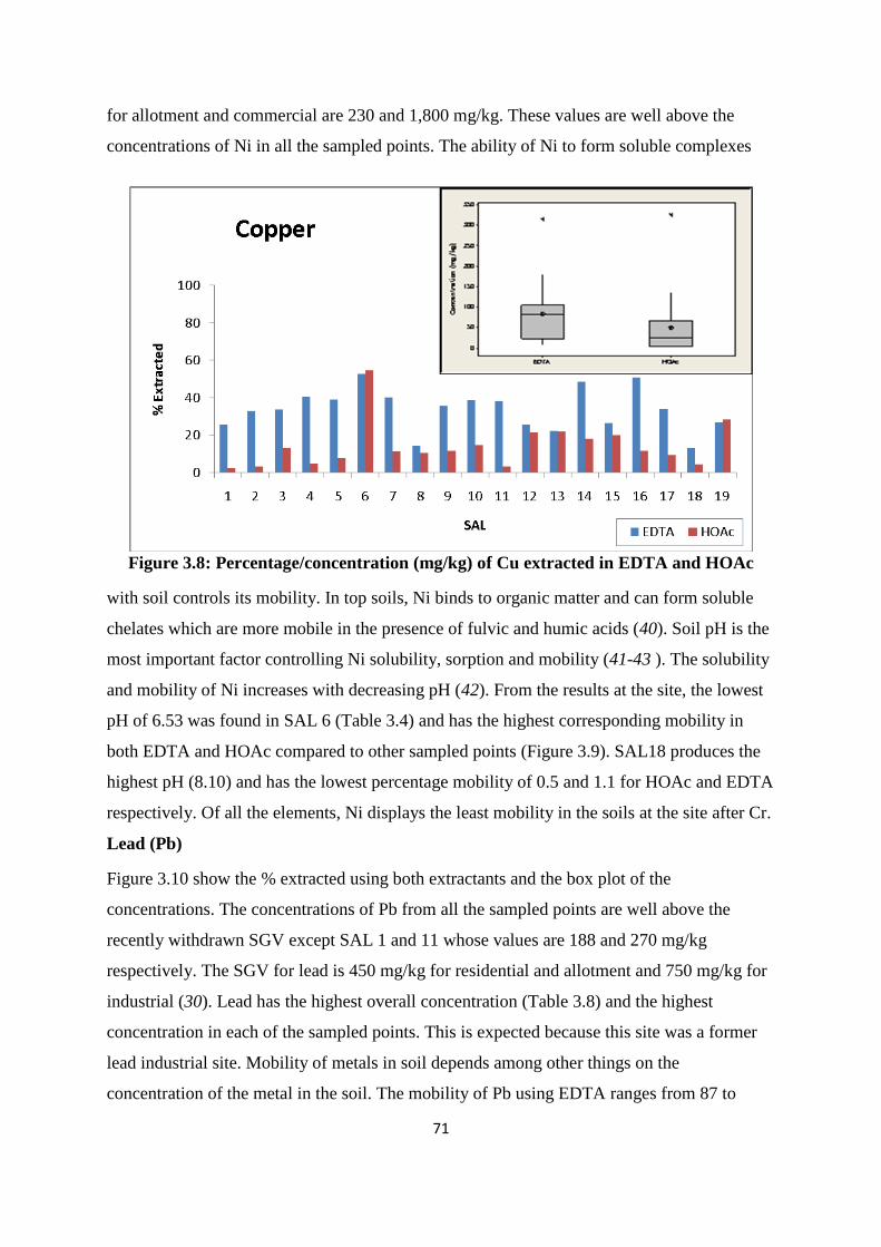
71

for allotment and commercial are 230 and 1,800 mg/kg. These values are well above the

concentrations of Ni in all the sampled points. The ability of Ni to form soluble complexes

Figure 3.8: Percentage/concentration (mg/kg) of Cu extracted in EDTA and HOAc

with soil controls its mobility. In top soils, Ni binds to organic matter and can form soluble

chelates which are more mobile in the presence of fulvic and humic acids (40). Soil pH is the

most important factor controlling Ni solubility, sorption and mobility (41-43 ). The solubility

and mobility of Ni increases with decreasing pH (42). From the results at the site, the lowest

pH of 6.53 was found in SAL 6 (Table 3.4) and has the highest corresponding mobility in

both EDTA and HOAc compared to other sampled points (Figure 3.9). SAL18 produces the

highest pH (8.10) and has the lowest percentage mobility of 0.5 and 1.1 for HOAc and EDTA

respectively. Of all the elements, Ni displays the least mobility in the soils at the site after Cr.

Lead (Pb)

Figure 3.10 show the % extracted using both extractants and the box plot of the

concentrations. The concentrations of Pb from all the sampled points are well above the

recently withdrawn SGV except SAL 1 and 11 whose values are 188 and 270 mg/kg

respectively. The SGV for lead is 450 mg/kg for residential and allotment and 750 mg/kg for

industrial (30). Lead has the highest overall concentration (Table 3.8) and the highest

concentration in each of the sampled points. This is expected because this site was a former

lead industrial site. Mobility of metals in soil depends among other things on the

concentration of the metal in the soil. The mobility of Pb using EDTA ranges from 87 to

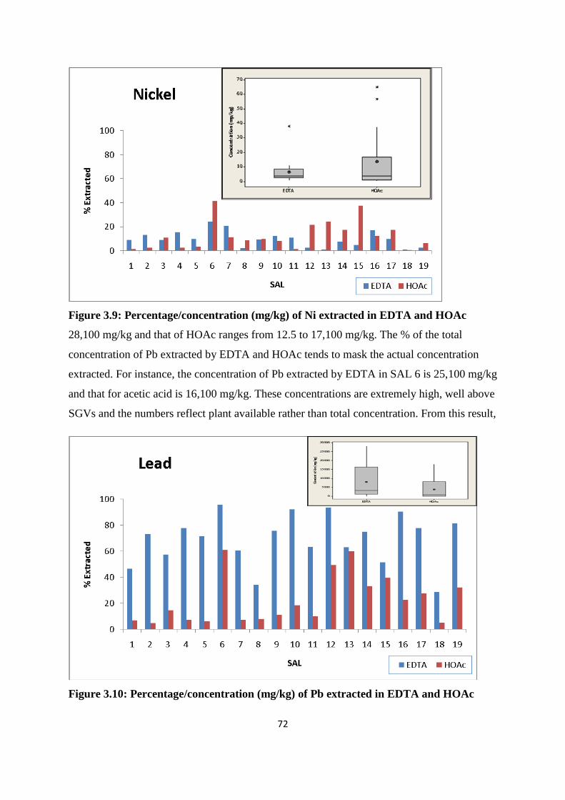
72

Figure 3.9: Percentage/concentration (mg/kg) of Ni extracted in EDTA and HOAc

28,100 mg/kg and that of HOAc ranges from 12.5 to 17,100 mg/kg. The % of the total

concentration of Pb extracted by EDTA and HOAc tends to mask the actual concentration

extracted. For instance, the concentration of Pb extracted by EDTA in SAL 6 is 25,100 mg/kg

and that for acetic acid is 16,100 mg/kg. These concentrations are extremely high, well above

SGVs and the numbers reflect plant available rather than total concentration. From this result,

Figure 3.10: Percentage/concentration (mg/kg) of Pb extracted in EDTA and HOAc

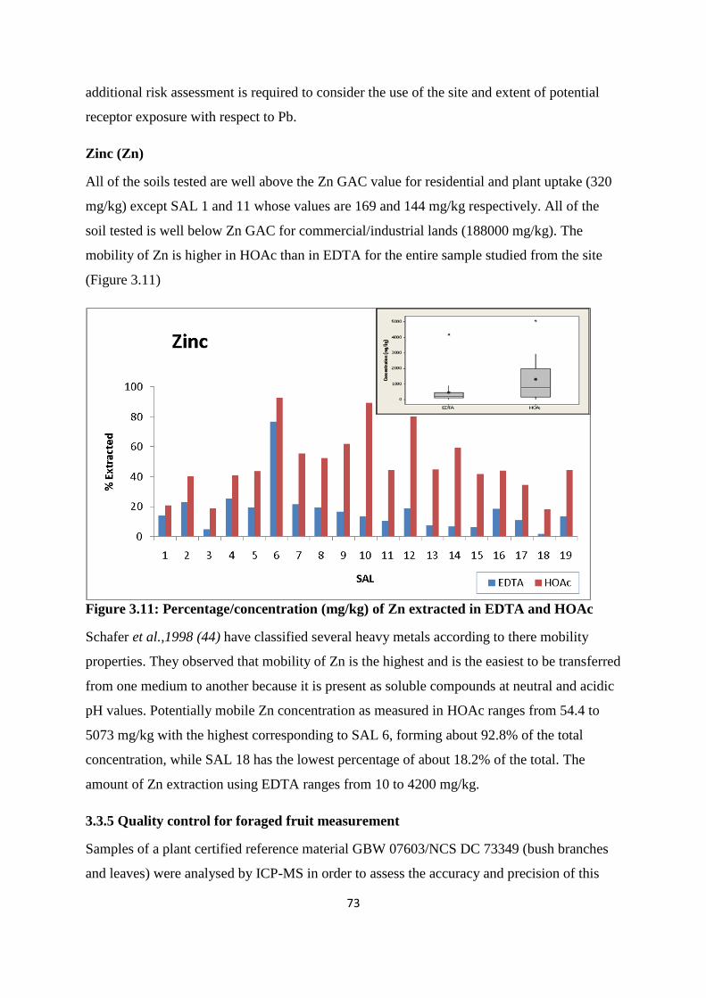
73

additional risk assessment is required to consider the use of the site and extent of potential

receptor exposure with respect to Pb.

Zinc (Zn)

All of the soils tested are well above the Zn GAC value for residential and plant uptake (320

mg/kg) except SAL 1 and 11 whose values are 169 and 144 mg/kg respectively. All of the

soil tested is well below Zn GAC for commercial/industrial lands (188000 mg/kg). The

mobility of Zn is higher in HOAc than in EDTA for the entire sample studied from the site

(Figure 3.11)

Figure 3.11: Percentage/concentration (mg/kg) of Zn extracted in EDTA and HOAc

Schafer et al.,1998 (44) have classified several heavy metals according to there mobility

properties. They observed that mobility of Zn is the highest and is the easiest to be transferred

from one medium to another because it is present as soluble compounds at neutral and acidic

pH values. Potentially mobile Zn concentration as measured in HOAc ranges from 54.4 to

5073 mg/kg with the highest corresponding to SAL 6, forming about 92.8% of the total

concentration, while SAL 18 has the lowest percentage of about 18.2% of the total. The

amount of Zn extraction using EDTA ranges from 10 to 4200 mg/kg.

3.3.5 Quality control for foraged fruit measurement

Samples of a plant certified reference material GBW 07603/NCS DC 73349 (bush branches

and leaves) were analysed by ICP-MS in order to assess the accuracy and precision of this

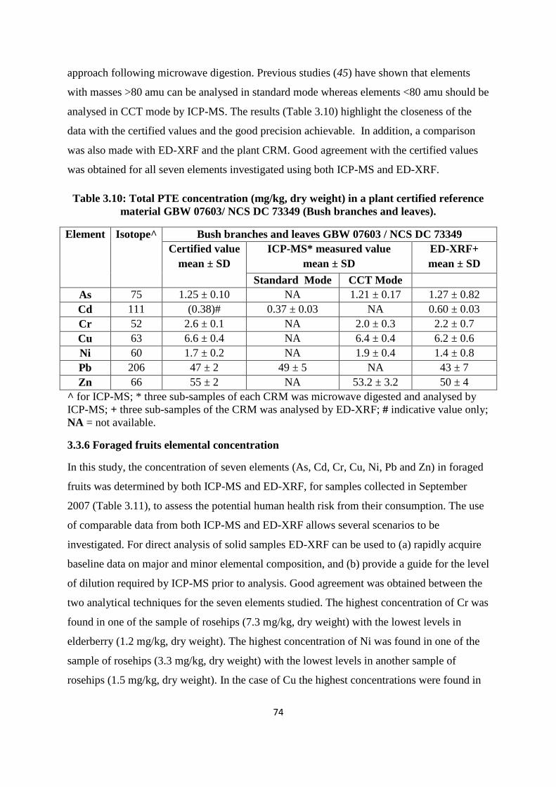
74

approach following microwave digestion. Previous studies (45) have shown that elements

with masses >80 amu can be analysed in standard mode whereas elements <80 amu should be

analysed in CCT mode by ICP-MS. The results (Table 3.10) highlight the closeness of the

data with the certified values and the good precision achievable. In addition, a comparison

was also made with ED-XRF and the plant CRM. Good agreement with the certified values

was obtained for all seven elements investigated using both ICP-MS and ED-XRF.

Table 3.10: Total PTE concentration (mg/kg, dry weight) in a plant certified reference

material GBW 07603/ NCS DC 73349 (Bush branches and leaves).

Element Isotope^ Bush branches and leaves GBW 07603 / NCS DC 73349

Certified value

mean ± SD

ICP-MS* measured value

mean ± SD

n = 3

ED-XRF+

mean ± SD

n = 3 Standard Mode CCT Mode

As 75 1.25 ± 0.10 NA 1.21 ± 0.17 1.27 ± 0.82

Cd 111 (0.38)# 0.37 ± 0.03 NA 0.60 ± 0.03

Cr 52 2.6 ± 0.1 NA 2.0 ± 0.3 2.2 ± 0.7

Cu 63 6.6 ± 0.4 NA 6.4 ± 0.4 6.2 ± 0.6

Ni 60 1.7 ± 0.2 NA 1.9 ± 0.4 1.4 ± 0.8

Pb 206 47 ± 2 49 ± 5 NA 43 ± 7

Zn 66 55 ± 2 NA 53.2 ± 3.2 50 ± 4

^ for ICP-MS; * three sub-samples of each CRM was microwave digested and analysed by

ICP-MS; + three sub-samples of the CRM was analysed by ED-XRF; # indicative value only;

NA = not available.

3.3.6 Foraged fruits elemental concentration

In this study, the concentration of seven elements (As, Cd, Cr, Cu, Ni, Pb and Zn) in foraged

fruits was determined by both ICP-MS and ED-XRF, for samples collected in September

2007 (Table 3.11), to assess the potential human health risk from their consumption. The use

of comparable data from both ICP-MS and ED-XRF allows several scenarios to be

investigated. For direct analysis of solid samples ED-XRF can be used to (a) rapidly acquire

baseline data on major and minor elemental composition, and (b) provide a guide for the level

of dilution required by ICP-MS prior to analysis. Good agreement was obtained between the

two analytical techniques for the seven elements studied. The highest concentration of Cr was

found in one of the sample of rosehips (7.3 mg/kg, dry weight) with the lowest levels in

elderberry (1.2 mg/kg, dry weight). The highest concentration of Ni was found in one of the

sample of rosehips (3.3 mg/kg, dry weight) with the lowest levels in another sample of

rosehips (1.5 mg/kg, dry weight). In the case of Cu the highest concentrations were found in

75

Table 3.11: Analysis of foraged fruits from Site (SAL) (mg/kg, dry weight) mean ± SD n=3 (September 2007)

Element SAL 1 SAL 2 SAL 3 SAL 4 SAL 5 SAL 6

ICP-MS* EDXRF+ ICP-MS* EDXRF+ ICP-MS* EDXRF+ ICP-MS* EDXRF+ ICP-MS* EDXRF+ ICP-MS* EDXRF+

As 0.32 ± 0.19 ND 0.32 ± 0.05 ND 0.19 ± 0.27 ND ND ND 0.23 ± 0.10 ND ND ND

Cd 0.5 ± 0.03 0.5 ± 0.58 0.6 ± 0.04 0.5 ± 0.5 0.7 ± 0.02 0.4 ± 0.6 ND ND 0.7 ± 0.02 0.8 ± 0.3 0.7 ± 0.03 0.6 ± 0.5

Cr 1.2 ± 0.4 1.4 ± 0.2 2.4 ± 0.6 2.3 ± 0.1 3.1 ± 0.4 3.7 ± 0.1 7.3 ± 0.2 6.7 ± 0.05 2.2 ± 0.1 2.5 ± 0.1 5.5 ± 0.1 5.8 ± 0.1

Cu 9.4 ± 0.3 9.6 ± 0.06 6.2 ± 0.2 6.4 ± 0.1 6.7 ± 0.2 7.2 ± 0.1 5.4 ± 0.03 5.6 ± 0.09 14.4 ± 0.1 15.1 ± 0.1 5.3 ± 0.1 5.9 ± 0.1

Ni 2.1 ± 0.04 1.8 ± 0.3 1.7 ± 0.1 1.5 ± 0.4 2.2 ± 0.2 2.7 ± 0.2 2.2 ± 0.2 2.4 ± 0.26 3.2 ± 0.2 3.3 ± 0.2 3.2 ± 0.2 3.1 ± 0.2

Pb ND ND 0.9 ± 0.12 0.8 ± 1.0 0.8 ± 0.08 0.8 ± 0.50 1.1 ± 0.3 1.6 ± 0.58 0.5 ± 0.6 0.5 ± 1.0 0.9 ± 0.03 1.0 ± 0.9

Zn 19.0 ± 6.3 19.3± 0.03 12.3 ± 5.1 14.8 ± 0.04 12.4 ± 2.3 16.4 ± 0.04 12.5 ± 2.2 13.4 ± 0.04 22.8 ± 3.3 26.1 ± 0.03 13.0 ± 2.3 13.4 ± 0.04

NOTE: SAL 1 = Elderberry, SAL 2 = Rosehips, SAL 3 = Rosehips, SAL 4 = Rosehips, SAL 5 = Black berry, SAL 6 = Sloes, * three sub-samples of

foraged fruit were microwave digested and analysed by ICP-MS; + one sub-sample of foraged fruit was analysed three times by ED-XRF; ND = not detected

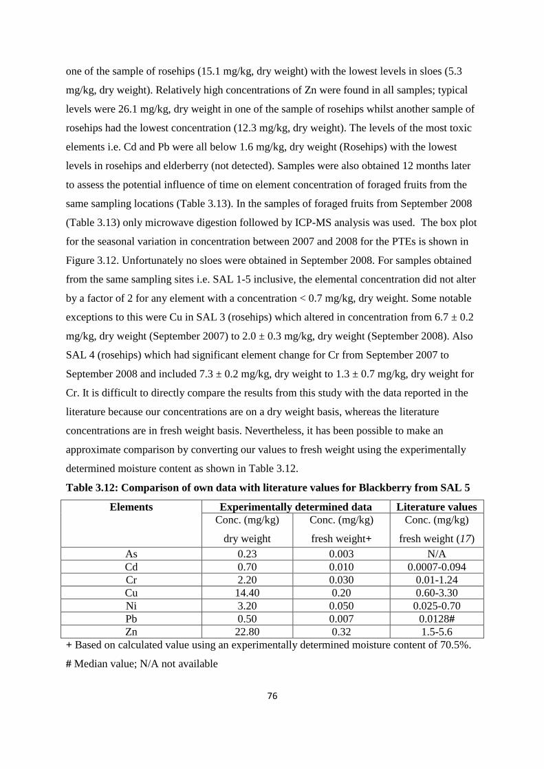
76

one of the sample of rosehips (15.1 mg/kg, dry weight) with the lowest levels in sloes (5.3

mg/kg, dry weight). Relatively high concentrations of Zn were found in all samples; typical

levels were 26.1 mg/kg, dry weight in one of the sample of rosehips whilst another sample of

rosehips had the lowest concentration (12.3 mg/kg, dry weight). The levels of the most toxic

elements i.e. Cd and Pb were all below 1.6 mg/kg, dry weight (Rosehips) with the lowest

levels in rosehips and elderberry (not detected). Samples were also obtained 12 months later

to assess the potential influence of time on element concentration of foraged fruits from the

same sampling locations (Table 3.13). In the samples of foraged fruits from September 2008

(Table 3.13) only microwave digestion followed by ICP-MS analysis was used. The box plot

for the seasonal variation in concentration between 2007 and 2008 for the PTEs is shown in

Figure 3.12. Unfortunately no sloes were obtained in September 2008. For samples obtained

from the same sampling sites i.e. SAL 1-5 inclusive, the elemental concentration did not alter

by a factor of 2 for any element with a concentration < 0.7 mg/kg, dry weight. Some notable

exceptions to this were Cu in SAL 3 (rosehips) which altered in concentration from 6.7 ± 0.2

mg/kg, dry weight (September 2007) to 2.0 ± 0.3 mg/kg, dry weight (September 2008). Also

SAL 4 (rosehips) which had significant element change for Cr from September 2007 to

September 2008 and included 7.3 ± 0.2 mg/kg, dry weight to 1.3 ± 0.7 mg/kg, dry weight for

Cr. It is difficult to directly compare the results from this study with the data reported in the

literature because our concentrations are on a dry weight basis, whereas the literature

concentrations are in fresh weight basis. Nevertheless, it has been possible to make an

approximate comparison by converting our values to fresh weight using the experimentally

determined moisture content as shown in Table 3.12.

Table 3.12: Comparison of own data with literature values for Blackberry from SAL 5

Elements Experimentally determined data Literature values

Conc. (mg/kg)

dry weight

Conc. (mg/kg)

fresh weight+

Conc. (mg/kg)

fresh weight (17)

As 0.23 0.003 N/A

Cd 0.70 0.010 0.0007-0.094

Cr 2.20 0.030 0.01-1.24

Cu 14.40 0.20 0.60-3.30

Ni 3.20 0.050 0.025-0.70

Pb 0.50 0.007 0.0128#

Zn 22.80 0.32 1.5-5.6

+ Based on calculated value using an experimentally determined moisture content of 70.5%.

# Median value; N/A not available

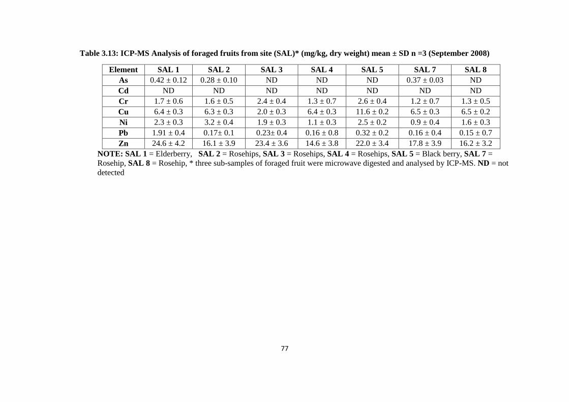
77

Table 3.13: ICP-MS Analysis of foraged fruits from site (SAL)* (mg/kg, dry weight) mean ± SD n =3 (September 2008)

Element SAL 1 SAL 2 SAL 3 SAL 4 SAL 5 SAL 7

SAL 8

As 0.42 ± 0.12 0.28 ± 0.10 ND ND ND 0.37 ± 0.03 ND

Cd ND ND ND ND ND ND ND

Cr 1.7 ± 0.6 1.6 ± 0.5 2.4 ± 0.4 1.3 ± 0.7 2.6 ± 0.4 1.2 ± 0.7 1.3 ± 0.5

Cu 6.4 ± 0.3 6.3 ± 0.3 2.0 ± 0.3 6.4 ± 0.3 11.6 ± 0.2 6.5 ± 0.3 6.5 ± 0.2

Ni 2.3 ± 0.3 3.2 ± 0.4 1.9 ± 0.3 1.1 ± 0.3 2.5 ± 0.2 0.9 ± 0.4 1.6 ± 0.3

Pb 1.91 ± 0.4 0.17± 0.1 0.23± 0.4 0.16 ± 0.8 0.32 ± 0.2 0.16 ± 0.4 0.15 ± 0.7

Zn 24.6 ± 4.2 16.1 ± 3.9 23.4 ± 3.6 14.6 ± 3.8 22.0 ± 3.4 17.8 ± 3.9 16.2 ± 3.2

NOTE: SAL 1 = Elderberry, SAL 2 = Rosehips, SAL 3 = Rosehips, SAL 4 = Rosehips, SAL 5 = Black berry, SAL 7 =

Rosehip, SAL 8 = Rosehip, * three sub-samples of foraged fruit were microwave digested and analysed by ICP-MS. ND = not

detected

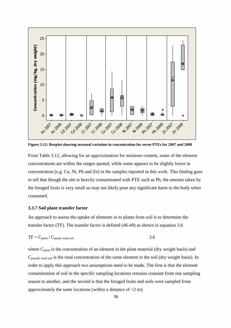
78

Zn 200

8

Zn 200

7

Pb 200

8

Pb 200

7

Ni 200

8

Ni 200

7

Cu 200

8

Cu 200

7

Cr 200

8

Cr 200

7

Cd 200

8

Cd 200

7

As 200

8

As 200

7

25

20

15

10

5

0

Co

nce

ntr

ati

on

(m

g/

kg

, d

ry w

eig

ht)

Figure 3.12: Boxplot showing seasonal variation in concentration for seven PTEs for 2007 and 2008

From Table 3.12, allowing for an approximation for moisture content, some of the element

concentrations are within the ranges quoted, while some appears to be slightly lower in

concentration (e.g. Cu, Ni, Pb and Zn) in the samples reported in this work. This finding goes

to tell that though the site is heavily contaminated with PTE such as Pb, the amount taken by

the foraged fruits is very small so may not likely pose any significant harm to the body when

consumed.

3.3.7 Soil plant transfer factor

An approach to assess the uptake of elements in to plants from soil is to determine the

transfer factor (TF). The transfer factor is defined (46-49) as shown in equation 3.6

TF = Cplant / Cpsudo total-soil 3.6

where Cplant is the concentration of an element in the plant material (dry weight basis) and

Cpseudo total-soil is the total concentration of the same element in the soil (dry weight basis). In

order to apply this approach two assumptions need to be made. The first is that the element

contamination of soil in the specific sampling locations remains constant from one sampling

season to another, and the second is that the foraged fruits and soils were sampled from

approximately the same locations (within a distance of <2 m).

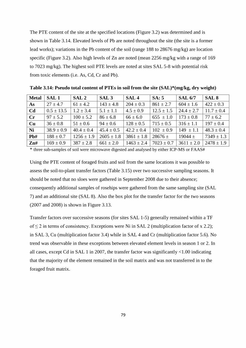
79

The PTE content of the site at the specified locations (Figure 3.2) was determined and is

shown in Table 3.14. Elevated levels of Pb are noted throughout the site (the site is a former

lead works); variations in the Pb content of the soil (range 188 to 28676 mg/kg) are location

specific (Figure 3.2). Also high levels of Zn are noted (mean 2256 mg/kg with a range of 169

to 7023 mg/kg). The highest soil PTE levels are noted at sites SAL 5-8 with potential risk

from toxic elements (i.e. As, Cd, Cr and Pb).

Table 3.14: Pseudo total content of PTEs in soil from the site (SAL)*(mg/kg, dry weight)

Metal

s

SAL 1 SAL 2 SAL 3 SAL 4 SA: 5 SAL 6/7 SAL 8

As 27 ± 4.7 61 ± 4.2 143 ± 4.8 204 ± 0.3 861 ± 2.7 604 ± 1.6 422 ± 0.3

Cd 0.5 ± 13.5 1.2 ± 3.4 5.1 ± 1.1 4.5 ± 0.9 12.5 ± 1.5 24.4 ± 2.7 11.7 ± 0.4

Cr 97 ± 5.2 100 ± 5.2 86 ± 6.8 66 ± 6.0 655 ± 1.0 173 ± 0.8 77 ± 6.2

Cu 36 ± 0.8 51 ± 0.6 94 ± 0.6 128 ± 0.5 715 ± 0.5 316 ± 1.1 197 ± 0.4

Ni 38.9 ± 0.9 40.4 ± 0.4 45.4 ± 0.5 42.2 ± 0.4 102 ± 0.9 149 ± 1.1 48.3 ± 0.4

Pb# 188 ± 0.7 1256 ± 1.9 2605 ± 1.8 3861 ± 1.8 28676 ±

13

19044 ±

10

7349 ± 1.3

Zn# 169 ± 0.9 387 ± 2.8 661 ± 2.0 1463 ± 2.4 7023 ± 0.7 3611 ± 2.0 2478 ± 1.9

* three sub-samples of soil were microwave digested and analysed by either ICP-MS or FAAS#

Using the PTE content of foraged fruits and soil from the same locations it was possible to

assess the soil-to-plant transfer factors (Table 3.15) over two successive sampling seasons. It

should be noted that no sloes were gathered in September 2008 due to their absence;

consequently additional samples of rosehips were gathered from the same sampling site (SAL

7) and an additional site (SAL 8). Also the box plot for the transfer factor for the two seasons

(2007 and 2008) is shown in Figure 3.13.

Transfer factors over successive seasons (for sites SAL 1-5) generally remained within a TF

of ≤ 2 in terms of consistency. Exceptions were Ni in SAL 2 (multiplication factor of x 2.2);

in SAL 3, Cu (multiplication factor 3.4) while in SAL 4 and Cr (multiplication factor 5.6). No

trend was observable in these exceptions between elevated element levels in season 1 or 2. In

all cases, except Cd in SAL 1 in 2007, the transfer factor was significantly <1.00 indicating

that the majority of the element remained in the soil matrix and was not transferred in to the

foraged fruit matrix.

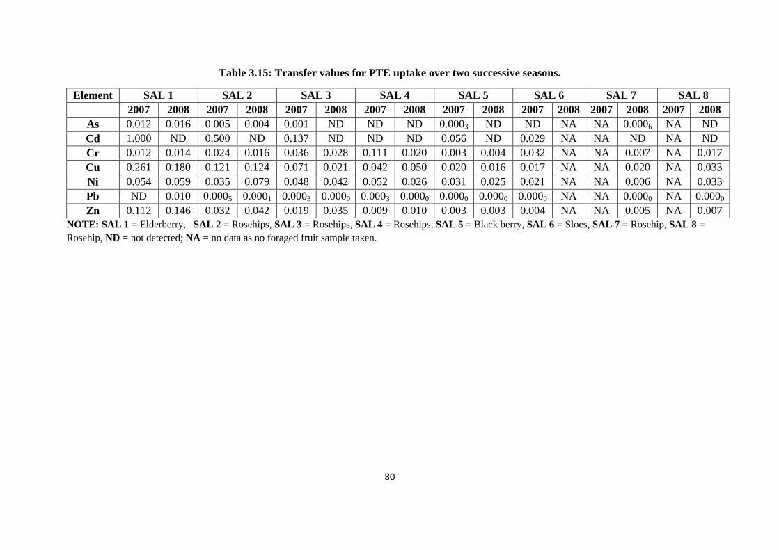
80

Table 3.15: Transfer values for PTE uptake over two successive seasons.

Element SAL 1 SAL 2 SAL 3 SAL 4 SAL 5 SAL 6

SAL 7 SAL 8

2007 2008 2007 2008 2007 2008 2007 2008 2007 2008 2007 2008 2007 2008 2007 2008

As 0.012 0.016 0.005 0.004 0.001 ND ND ND 0.0003 ND ND NA NA 0.0006 NA ND

Cd 1.000 ND 0.500 ND 0.137 ND ND ND 0.056 ND 0.029 NA NA ND NA ND

Cr 0.012 0.014 0.024 0.016 0.036 0.028 0.111 0.020 0.003 0.004 0.032 NA NA 0.007 NA 0.017

Cu 0.261 0.180 0.121 0.124 0.071 0.021 0.042 0.050 0.020 0.016 0.017 NA NA 0.020 NA 0.033

Ni 0.054 0.059 0.035 0.079 0.048 0.042 0.052 0.026 0.031 0.025 0.021 NA NA 0.006 NA 0.033

Pb ND 0.010 0.0005 0.0001 0.0003 0.0000 0.0003 0.0000 0.0000 0.0000 0.0000 NA NA 0.0000 NA 0.0000

Zn 0.112 0.146 0.032 0.042 0.019 0.035 0.009 0.010 0.003 0.003 0.004 NA NA 0.005 NA 0.007

NOTE: SAL 1 = Elderberry, SAL 2 = Rosehips, SAL 3 = Rosehips, SAL 4 = Rosehips, SAL 5 = Black berry, SAL 6 = Sloes, SAL 7 = Rosehip, SAL 8 =

Rosehip, ND = not detected; NA = no data as no foraged fruit sample taken.

81

Zn 200

8

Zn 200

7

Pb 200

8

Pb 200

7

Ni 200

8

Ni 200

7

Cu 200

8

Cu 200

7

Cr 200

8

Cr 200

7

Cd 200

8

Cd 200

7

As 200

8

As 200

7

1.0

0.8

0.6

0.4

0.2

0.0

Tra

nsfe

r fa

cto

r

Figure 3.13: Box plot for transfer factors for the two seasons 2007 and 2008

3.4 Conclusion and implications for human health

The following conclusions can be drawn from this study

(1) The site ranges from weakly acidic to neutral soil with low organic matter content

while cation exchange capacity was within the normal range except SAL 18 (160.98

cmol/kg) which is above normal.

(2) Elemental concentrations across the site are highly variable

(3) Concentration plots and PCA analysis of the data from the site reveals that soil sample

points SAL 3, 6......SAL 19 have the highest PTE concentrations with Pb, As and Zn

in excess of SGVs.

(4) Table 3.8 shows that the concentration of most of the metals investigated exceed the

SGVs/GAC. However, site specific circumstances such as the environmental

pathways and site usage patterns of human receptors needs to be taken into account as

exceedence does not necessarily imply that there is an actual risk to health. The

particular chemical form and hence its extractability is also important. Chapter four

details future work investigating the supplementary evidence to support risk

assessment at such sites using oral bioaccessibility testing.

82

(5) The plant availability estimated using EDTA/AcOH varies across the sampled points

but correlates positively with pseudo total PTE concentration.

(6) The elemental composition of foraged fruit over two sampling seasons shows that

while the level of metal contamination in the soil is relatively high for some elements

e.g. Pb, Zn and As the suspected risk to human health based on soil-to-plant transfer

ratio is negligible.

References

1 Rauret, G. (1997). Extraction procedures for the determination of heavy metals in

contaminated soil and sediment. Talanta, 46, 449 – 455.

2 Lim, T.T., Tay, J.H., Wang, J.Y. (2004). Chelating-agent-enhanced heavy metal

extraction from a contaminated acidic soil. Environmental Engineering, 130, 59 – 66.

3 Polettini, A., Pomi, R., Rolle, E. (2007). The effect of operating variables on chelant-

assisted remediation of contaminated dredged sediment. Chemosphere, 66, 866 – 877.

4 Ghanedi, M., Shokrollahi, A., Kianfar, A.H., Mirsadeghi, A.S., Pourfarokhi, A.,

Soylak, M. (2008). The determination of some heavy metals in food samples by flame

atomic absorption spectrometry after their separation – preconcentration on bis salicyl

aldehyde 1, 3 propandiimine (BSPDI) loaded on activated carbon. Journal of

Hazardous Material, 154, 128 – 134.

5 Chaney, R.L. (1990). Public health and sludge utilization. Biocycle, 30, 68 – 73.

6 Muhammad, K.J., Tasneem, G.K., Muhammad, B.A., Hassan, I.A., Nosrat, J.,

Ghulam, A.K., Abdul, Q.S., Jameel, A.B. (2009). Heavy metal accumulation in

different varieties of wheat (Triticum aestiyum) grown in soil amended with domestic

sewage sludge. Journal of Hazardous Materials, 164, 1386 – 1391.

7 Tessier, A., Campell, P.G.C., Bisson, M. (1979). Sequential extraction procedure for

the speciation of particular trace metals. Analytical Chemistry, 51, 844 – 850.

8 Rauret G, Lopez-Sanchez, J, Sahuquillo, A, Rubio, R, Davidson, C, Ure, A.,

Quevauviller, P. (1999). Improvement of the BCR three step sequential extraction

procedure prior to certification of new sediment and soil reference materials. Journal

of Environmental Monitoring, 1, 57- 61.

83

9 Perez, C. B., De Jesus, G.M., Gomez, E. (2002). Comparison of single extraction

procedures and the Tessier sequential extraction method for the fractionation of heavy

metals from environmental samples. The Analyst, 127, 681-688.

10 Bacon, J.R., Davidson, C.M. (2008). Is there a future for sequential chemical

extraction? The Analyst, 133, 25-46.

11 Samani, Z., Hu, S., Hanson, A.T., Heil, D.M. (1998). Remediation of lead

contaminated soil by column extraction with EDTA. Water, Air and Soil Pollution,

102, 221 – 238.

12 Abumaizar, R.J., Smith, E.H. (1999). Heavy metal contaminants removal by soil

washing. Journal of Hazardous Material, B70, 71 -86.

13 Peters, R.W. (1999). Chelant extraction of heavy metals from contaminated soils.

Journal of Hazadous Materials, 66, 151 – 210.

14 Tandy, S., Bossart, K., Mueller, R., Ritschel, J., Hauser, L., Schulin, R. and Nok, B.

(2004). Extraction of heavy metals from soils using biodegradable chelating agents.

Environmental Science and Technology, 38, 937 – 944.

15 Sun, B., Zhao, F.J., Lombi, E., McGrath, S.P. (2001). Leaching of heavy metals from

contaminated soils using EDTA. Environmental Pollution, 113, 111- 120.

16 MAFF UK. (2000). Multi-element survey of wild edible fungi and blackberries (sheet

199), Food Standards Agency. http://www.informaworld.com/smpp/content Feb 2010

17 Weeks C.A., Croasdale, M., Osborne, M.A., Hewitt, L., Miller, P.F., Robb, P., Baxter,

M.J., Warriss, P.D., Knowles, T.G. (2006). Multi-element survey of wild edible fungi

and blackberries in the UK. Food Additives and Contaminants, 23(2), 140-147.

18 Barcan, V.S., Kovnatsky, E.F., Smetannikova, M.S. (1998). Absorption of heavy

metals in wild berries and edible mushrooms in an area affected by smelter emissions.

Water, Air and Soil Pollution, 103(104), 173-195.

19 Leterme, P., Buldgen, A., Estrada, F., Lodono, A. (2006). Mineral content of tropical

fruits and unconventional foods of the Andes and the rain forest of Colombia. Food

Chemistry, 95, 644-652.

84

20 Newcastle City Council (2006). PHEP Environment and Culture Directorate. Former

St Anthony‟s Lead Works Site Desktop Study 3-6.

21 Strowbel, B. W., Borggaard, O. K., Hansen, H. C. B., Andersen, M. K., Raulund-

Rasmussen, K. (2005). 'Dissolved Organic Carbon and Decreasing pH Mobilize

Cadmium and Copper in Soil'. European Journal of Soil Science, 56, 189-196.

22 Baize, D. (1993). Soil Science Analyses: A Guide to Current Use. John Wiley & Sons,

Chichester UK.

23 Robertson, G. P., Sollins, P., Ellis, B. G., Lajtha, K. (1999).Standard soil methods for

long term ecological research: Exchangeable Ions, pH, and Cation Exchange

Capacity. in Robertson, G. P., Coleman, D. C., Bledsoe, C. S. Oxford University

Press.

24 Narwal, S.B., Salbu, B. (1999). Association of cadmium, zinc, copper and nickel with

components in naturally heavy metal rich soils studied by parallel and sequential

extractions. Communications in Soil Science and Plant analysis,30, 1209-1230.

25 Illera, V., Walker, I., Souza, P., Cala, V. (2000). Short-term effects of biosolids and

municipal solid waste application on heavy metals distribution in a degraded soil

under a semi- arid environment. Science of Total Environment, 255, 29-44.

26 Kabala, C., Singh B.R. (2001). Fractionation and mobility of copper, lead and zinc in

soil profiles in the vicinity of a copper smelter. Environmental Quality, 30, 485-492.

27 Walid, B.A., Noureddine, G., Abdelbasset, L., Gijs, D.L., Tahar, G. (2009). Effect

of a 5-year application of municipal solid waste compost on the distribution and

mobility of heavy metals in a Tunisian calcareous soil. Agriculture, Ecosystem and

Environment, 130, 156-163.

28 Cameron, R.E. (1992). Guide to site and soil description for hazardous waste site

characterisation. Volume 1 Metals. Environmental Protection Agency

EPA/600/491/029

29 Lancrop Laborateries, Yara Analytical Services Technical Bulletin York

www.phosyn.com. August 2009.

85

30 Environment Agency (2002). Soil guidelines values for metal contamination, R&D

Publication SGV. Available at: http://www.environment-agency.gov.uk/.

31 Nathanial, C P., Mc Affrey, C., Ashmore, M., Cheng, Y., Gilett, A., Hooker, P. and

Ogden, R C. (2009) Generic Assessment Criteria for Human Health Risk Assessment,

2nd

Ed., Nottingham, UK: Land Quality Press.

32 Sezgin, N., Ozcan, H.K., Demir, G., Nemlioglu, S., Bayat, C. (2003). Determination

of heavy metal concentrations in street dusts in Istanbul E-5 highway. Environmental

International, 29, 979 – 985.

33 Callahan, M.A., Slimak, M.W., Gabel, N.W. (1979). Water-Related Environmental

Fate of 129 Priority Pollutants, Vol.1, Introduction and Technical Background,

Metals and Organics, Pesticides and PCBs. Report to U.S.EPA, Office of Water

Planning and Standards, Washington, D.C.

34 Smith, L.A., Means, J.L., Chen, A., Alleman, B., Chapman, C.C., Tixier, J.S.,

Brauning, S.E., Gasvaskar, A.R., Royer, M.D. (1995). Remedial Options for Metals-

Contaminated Sites. Lewis Publishers, Boca Raton, Florida.

35 Whalley, C., Grant, A. (1994). Assessment of the phase selectivity of the European

Community Bureau of Reference (BCR) sequential extraction procedure for metals in

sediments. Analytica Chimica Acta, 291, 287 -295.

36 Schramel, O., Michaike, B., Kettrup, A. (2000). Study of the copper distribution in a

column in contaminated soils of hop fields by single and sequential extraction

procedures. The Science of the Total Environment, 263, 11-22.

37 Lucia, D.T., Murray, B.M.(1982). Mobility and extractability of cadmium, copper

nickel and zinc in organic and mineral soil column. Plant and Soil, 134(3), 198-205.

38 Linn, J. H., Elliott, H. A. (1998). Mobilization of copper and zinc in contaminated soil

by nitriloacetic acid. Water, Air and Soil Pollution, 37, 449 -458.

39 Reddy, K.J, Wang, L., Gloss. S. P. (1995). Solubility and mobility of copper, zinc and

lead in acidic environment. Plant and Soil, 171, 53-58.

86

40 Kabata-Pendias, A., Mukherjee, A. B. (2007). Trace elements from soil to humans.

Berlin: Springer-Verlag.

41 Ge, Y., Murray, P., Hendershot, W.H. (2000). Trace metal speciation and

bioavailabilty in urban soils. Environmental Pollution, 107, 137-144.

42 McGrath, S.P. (1995). Nickel In Heavy metals in soils (2nd

edition) (ed B.J Alloway)

London. Blackie Academic and Professional Press.

43 Suave, S., Hendershot, W., Allen, H.E. (2000). Solid-solution partitioning of metals in

contaminated soils. Environmental Science and Technology, 34(7), 1125-1131.

44 Schafer, J., Hannker, D., Eckhardt, D.J., Stuben, D. (1998). Uptake of traffic related

heavy metals and platinum group elements (PGE) by plants. The Science of the Total

Environment, 215, 59 – 67.

45 Intawongse, M., Dean J.R., 2008. Use of the physiologically-based extraction test to

assess the oral bioaccessibility of metals in vegetable plants grown in contaminated

soil, Environmental Pollution, 152, 60-72.

46 Sauerbeck, D.R. (1991). Plant, element and soil properties governing uptake and

availability of heavy metals derived from sewage sludge. Water, Air and Soil

Pollution, 57-58, 227-237.

47 Gray, C.W., McLaren, R.G., Roberts, A.H.C., Condron, L.M. (1999). Cadmium

phytoavailability in some New Zealand soils. Australian Journal of Soil Research, 37,

461-477.

48 Cui, Y-J, Zhu, Y-G, Zhai, R-H, Chen, D-Y, Huang, Y-Z, Qiu, Y., Liang, J-Z. (2004).

Transfer of metals from soil to vegetables in an area near a smelter in Nanning, China.

Environment International, 30, 785-791.

49 Chojnacka, K., Chojnacki, A., Gorecka, H., Gorecki, H. (2005). Bioavailability of

heavy metals from polluted soils to plants. Science of the Total Environment,

337,175-182.

87

Chapter Four: The use of the physiologically-based extraction test to assess

oral bioaccessibility of PTEs from an urban recreational site

4.1 Introduction

In the UK, the environmental health risk to humans of metals from contaminated land sites

are currently assessed using the non-statutory Contaminated Land Exposure Assessment

(CLEA) model (1). The model was developed to allow a comparison between predicted

contamination exposure levels and known toxicological or Health Criteria Values (HCVs), to

derive a Soil Guideline Value (SGV) which is both site and contaminant dependant (2).

These SGVs are generic assessment criteria that assess the risks to human health from

chronic exposure to contaminated soil. On that basis SGVs are classed as intervention values

and any exceedance may indicate an unacceptable human health risk from that contaminated

site (3). Derivation of SGVs using the CLEA model assumes that the contaminant is released

from the soil and is taken up by the human body to the same extent as the model which has

been used to determine the HCV (for that contaminant) (3); this assumption may, of course,

not be true as the HCVs may have been determined using non-human material and more

soluble form of the contaminant (4). Therefore basing the human health risk of contaminants

from contaminated soils on SGVs assumes that all the contaminant is taken up by the

systemic circulation; this over-simplification negates both the insolubility of the contaminant

and its potential sequestration within the soil (5). Researchers are therefore investigating

alternate approaches that allow a better representation of the likely oral bioaccessibility (i.e.

extractable in the human gut) of contaminants (6). Any estimation of the oral bioavailability

of soil-bound contaminants is based on the principle that uptake (i.e. absorption) of the

contaminant depends on its release (i.e. bioaccessibility) in the gastro-intestinal (GI) track (7,

8). The approaches are often described using in vitro method. It is therefore important in

assessing human health risk assessment to consider the oral bioaccessibility of the

contaminant, determined using in vitro methodology, from contaminated land sites.

A range of in vivo approaches have been evaluated to assess the bioavailability of PTEs for

humans from a variety of matrices including soil, dust and food (9-11), the information

obtained using these approaches cannot always be related to humans due to differences in

physiology, contaminant and the matrix itself (12). So while some work does continue on in

vivo approaches considerable barriers exist not least relating to ethical governance issues as

well as financial constraints, such that in vitro approaches are becoming more prevalent. The

88

in vitro approaches have been developed to simulate both the stomach and intestinal juices. A

number of comparative studies have suggested that the bioaccessibility results obtained are

largely dependent on the specific in vitro conditions used, the actual contaminant under

investigation and the sample matrix (1, 7-8). As the new CLEA model software (13-14)

allows greater functionality and the incorporation of bioaccessibility data into site specific

risk assessments the development of robust and agreed protocols is appropriate and timely.

This work investigates the oral bioaccessibility of PTEs in soil from a former industrial site

which is now an open access urban green space used for recreational purposes in Newcastle

upon Tyne. While much of the literature reported data on bioaccessibilty has focused on As

and Pb, this study investigates a broad range of elements (As, Cd, Cr, Cu, Ni, Pb and Zn), all

of which may be present in elevated concentrations due to the sites known industrial legacy.

In addition, the magnitude and spatial variability across the site of the oral bioaccessible

fraction is also of inherent interest.

4.2 Experimental

4.2.1 The study site

The study site, sample collection strategy and preparation along with soil characterisation as

well as the apparatus needed for the experiment has already been described in 3.1.1, 3.2.1-

3.2.5.

4.2.2 Reagents

In addition to the reagents used in 3.2.2, for the physiologically-based extraction test the

following reagents were required. Sodium hydrogen phosphate (NaH2PO4) and potassium

hydrogen phosphate (KH2PO4) were obtained from Baker Scientific, UK. Sodium chloride

(NaCl), potassium thiocyanate (KSCN), anhydrous sodium sulphate (Na2SO4), potassium

chloride (KCl), calcium chloride (CaCl2.2H2O), ammonium chloride (NH4Cl), sodium

bicarbonate (NaHCO3), magnesium chloride (MgCl2.6H2O), sodium hydroxide (NaOH),

hydrochloric acid (HCl), 30% hydrogen peroxide, urea, uric acid, anhydrous D+ glucose, D-

glucosaminehydrochloride, pepsin (pig), bovine serum albumin (BSA) and pancreatin (pig)

and concentrated nitric acid (69%, HNO3) were all obtained from Merck (Poole, England).

Mucin (pig) was obtained from Carl Roth, Germany. D-glucuronic acid (Fluka) and

-amylase (bacillus species), lipase (pig) and bile salts (bovine) were obtained from Sigma.

89

4.2.3 Preparation of extraction reagents for the in vitro extraction test

The in vitro extraction test is based on the BARGE method (15). Essentially simulated saliva

fluid was prepared by first adding 145 mg of amylase, 50.0 mg mucin and 15.0 mg uric acid

to a 2 L HDPE screw top bottle. Then, 896 mg of KCl, 888 mg NaH2PO4, 200 mg KSCN,

570 mg Na2SO4, 298 mg NaCl and 1.80 mL of 1.0 M HCl was added into a 500 mL volume

container and made up to the mark with water (inorganic saliva components). In to a second

500 mL volume container was added 200 mg urea and made up to the mark with water

(organic saliva components). Then, the 500 mL of inorganic and 500 mL of organic saliva

components was simultaneously poured in to the 2 L HDPE screw top bottle. The entire

content of the screw top bottle was shaken thoroughly and the pH of the solution (gastric

simulated saliva fluid) measured and was found to be within the range 6.5 ± 0.5.

Simulated gastric fluid was prepared by first adding 1000 mg of bovine serum albumin, 3000

mg mucin and 1000 mg pepsin to a 2 L HDPE screw top bottle. Then, 824 mg of KCl, 266

mg NaH2PO4, 400 mg CaCl2, 306 mg NH4Cl, 2752 mg NaCl and 8.30 mL of 37% HCl were

added separately into a 500 mL volume container and made up to the mark with water

(inorganic gastric components). In to a second 500 mL volume container was added 650 mg

glucose, 20.0 mg glucuronic acid, 85.0 mg urea and 330 mg glucosamine hydrochloride and

made up to the mark with water (organic gastric components). Then, the 500 mL of inorganic

and 500 mL of organic components were poured simultaneously in to the 2 L HDPE screw

top bottle. The entire content of the screw top bottle was shaken thoroughly and the pH of the

solution (gastric simulated fluid) measured. The pH was found to be within the range 0.9-1.0.

The combination of mixed saliva fluid (1 mL) and gastric fluid (1.5 mL) was checked and

was in the range of pH 1.2 – 1.4.

Simulated duodenal fluid was prepared by first adding 200 mg of CaCl2, 1000 mg bovine

serum albumin, 3000 mg pancreatin and 500 mg lipase to a 2 L HDPE screw top bottle. Then,

564 mg of KCl, 80 mg KH2PO4, 50.0 mg MgCl2, 5607 mg NaHCO3, 7012 mg NaCl and 180

µL of 37% HCl was separately added into a 500 mL volume container and made up to the

mark with water (inorganic duodenal components). In to a second 500 mL volume container

was added 100 mg urea and made up to the mark with water (organic duodenal

components). Then, 500 mL of inorganic and 500 mL of organic duodenal components was

simultaneously poured in to the 2 L HDPE screw top bottle. The entire content of the screw

90

top bottle was thoroughly shaken and the pH of the solution (simulated duodenal fluid) was

measured. The pH was found to be within the range 7.4 ± 0.2.

Simulated bile fluid was prepared by first adding 222 mg of CaCl2, 1800 mg bovine serum

albumin and 6000 mg bile to a 2 L HDPE screw top bottle. Then, 376 mg of KCl, 5785 mg

NaHCO3, 5259 mg NaCl and 180 µL of 37% HCl was separately added in to a 500 mL

volume container and made up to the mark with water (inorganic bile components). In to a

second 500 mL volume container was added 250 mg urea and made up to the mark with

water (organic bile components). Then, 500 mL of inorganic and 500 mL of organic bile

components was simultaneously poured in to the 2 L HDPE screw top bottle. The entire

content of the screw top bottle was shaken thoroughly and the solution allowed to stand for

approximately 1 hour, at room temperature, to allow for complete dissolution of solid

reagents. The pH of this solution (simulated bile fluid) was measured and was found to be

within the range 8.0 ± 0.2. The pH for the combined saliva fluid (1.0 mL), gastric fluid (1.5

mL), 3.0 mL duodenal fluid and 1.0 mL bile fluid was checked to be within the range 6.3 ±

0.5.

4.2.4 Preparation of samples using BARGE method

‘Gastric’ Extraction. An accurately weighed sample (0.6 g) was placed into a 50 mL screw-

cap Sarstedt tube and treated with 9 mL of simulated saliva fluid by manually shaking the

soil-fluid mixture in the screw-cap vessel. Then, after 5 – 15 mins 13.5 mL of simulated

gastric fluid was added. This was followed by shaking the mixture on an end-over-end shaker

maintained at 37 ± 2°C for 1 h. At that stage the pH of each soil suspension was checked (the

pH should be maintained between 1.2 -1.7). The solution was then centrifuged at 3000 rpm

for 5 min and a 1.0 mL aliquot of supernatant removed. Finally, 9.0 mL of 0.1 M HNO3 was

added to the supernatant and the extract stored at < 8 C prior to analysis by ICP-MS.

‘Gastric + Intestine’ Extraction. An accurately weighed sample (0.6 g) was placed into a

50 mL screw- cap Sarstedt tube and treated with 9 mL of simulated saliva fluid by manually

shaking the soil-fluid mixture in the screw-cap vessel. Then, after 5 – 15 mins 13.5 mL of

simulated gastric fluid was added. The mixture was then shaken on an end-over-end shaker

maintained at 37 ± 2°C for 1 hour. Then, the pH of the soil suspensions was checked such

that the pH was maintained between 1.2 -1.7. Following this 27.0 mL of simulated duodenal

fluid and 9.0 mL of simulated bile fluid were added by manually shaking the soil-fluid

91

mixture in the screw-cap vessel. The pH of the resultant suspension was adjusted to 6.3 ± 0.5,

by the dropwise addition of 37% HCl, 1 M or 10 M NaOH, as required. The mixture was

again shaken on an end-over-end shaker maintained at 37 ± 2°C for 4 h. Then, the soil

suspension was removed and its pH measured (and record); the pH should be maintained

between 6.3 ± 0.5. The soil suspension was then centrifuged at 3000 rpm for 5 min and a 1.0

mL aliquot of supernatant removed. Finally, 9.0 mL of 0.1 M HNO3 was added to the

supernatant and it was stored at < 8 C prior to analysis by ICP-MS.

4.2.5 Microwave digestion protocol/ICP-MS analysis of sample

See sections 2.4.3 and 3.2.6.for details

4.2.6 Determination of oral bioaccessibility

The oral bioaccessibility of PTEs from soil can be determined using the BARGE procedure.

The percentage bioaccessible fraction (% BAF) can be calculated using equation 4.1

Bioaccessible fraction (%) = CBioaccessibility × 100 4.1

Cpseudo total

Where, CBioaccessibility = Concentration of PTE released from soil (mg/kg) obtained via

BARGE stage I (gastric) or stage II (gastric + intestinal); Cpseudo total = Pseudo total

concentration of PTE in soil (mg/kg).

4.3 Results and Discussion

4.3.1 Evaluation of the BARGE approach: Application to soil CRM

At the moment, there is no CRM for bioaccessibility testing as a result, the assessment to the

accuracy of the BARGE was derived using a mass balance type approach adopted and

applied to a soil certified reference material (GBW 07401). Initially, using the microwave

digestion approach, the CRM was analysed for 7 PTEs under investigation and the results

compared to the certified values. The results (Table 4.1) show good accuracy (and precision,

based on triplicate determinations) between the measured and certified values for all PTEs

studied. Then, the BARGE protocol was followed on the same CRM and data obtained on the

PTE content (using ICP-MS) for both the gastric digest (stage I) and gastric + intestinal

digest (stage II). Finally, the residual fraction from stage II was acid digested using the

microwave protocol described above and also analysed by ICP-MS. In terms of the mass

balance it is noted that the sum of stage II and the residual fraction digest are in close

agreement with both the certified CRM values and the pseudo-total PTE content, determined

92

using the microwave digestion protocol, with recoveries between 80.4 and 123.3% (compared

to certified values) and 81.6 and 110.4% (compared to pseudo-total values). The sum of stage

II and the residual fraction show increased imprecision in data as might be expected, based on

cumulative errors. It is noted that the largest percentage bioaccessibility fraction (% BAF) is

obtained for stage II digests for all PTEs considered, however, the % BAF varies according to

the PTE ranging from 6.8% for Cr to 83.3 for Cd.

4.3.2 Characterization of study site topsoils

Each of the soils collected in this study was characterised for pH, loss on ignition (as

indicative of soil organic matter content) and cation exchange capacity. The results, shown in

Table 4.2, indicate that the pH of the soils from the study site were largely neutral (pH range

6.5 – 8.1, with a median pH value of 7.4) while the loss on ignition data indicated soil organic

contents ranging from 6.4 to 24.7 %, with a median value of 10.7 %. Finally, the cation

exchange capacity (CEC) of the soil ranged from 9.4 to 161.0 cmolc/kg with a median value

of 21.4 cmolc/kg. Also in Table 4.2 is a summary of the PTE concentration across the site for

the 7 elements studied.

4.3.3 Evaluation of the BARGE approach: Application to an urban recreational site

The summary data of bioaccessibility for the 19 topsoils are presented (Table 4.3). Reporting

bioaccessibility data as % BAF conceals the actual concentration of the element in the extract

and is also highly dependent on the determined total concentration, which itself may be liable

to the vagaries of the extraction technique (i.e. total v pseudo-total). As such the minimum,

median and maximum metal concentration determined for each extraction stage are presented

and the % BAF is only presented for the worst-case scenario sample (i.e. for the maximum

determined PTE concentration at each extraction stage; Table 4.3). For completeness the

amount of PTE that remained in the soil after gastric + intestinal digest is also shown i.e. the

concentration of PTE that remained in the residual digest. As might be expected, the % BAF

varies across the range of PTEs as well as the individual sample locations. The extraction

stage (i.e. the gastric or the gastric and intestinal stage) which exhibited the highest

concentration, and hence highest % BAF was consistently the gastric and intestinal stage (see

Appendix A). Of the 19 topsoils, all the PTEs investigated predominantly indicated higher

extracted PTE content following the gastric and intestinal stage compared to gastric stage

only.

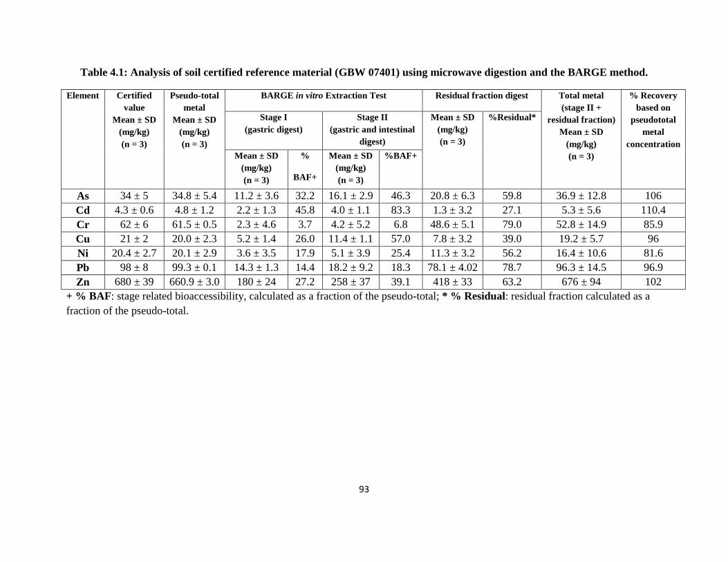
93

Table 4.1: Analysis of soil certified reference material (GBW 07401) using microwave digestion and the BARGE method.

Element Certified

value

Mean ± SD

(mg/kg)

(n = 3)

Pseudo-total

metal

Mean ± SD

(mg/kg)

(n = 3)

BARGE in vitro Extraction Test Residual fraction digest Total metal

(stage II +

residual fraction)

Mean ± SD

(mg/kg)

(n = 3)

% Recovery

based on

pseudototal

metal

concentration

Stage I

(gastric digest)

Stage II

(gastric and intestinal

digest)

Mean ± SD

(mg/kg)

(n = 3)

%Residual*

Mean ± SD

(mg/kg)

(n = 3)

%

BAF+

Mean ± SD

(mg/kg)

(n = 3)

%BAF+

As 34 ± 5 34.8 ± 5.4 11.2 ± 3.6 32.2 16.1 ± 2.9 46.3 20.8 ± 6.3 59.8 36.9 ± 12.8 106

Cd 4.3 ± 0.6 4.8 ± 1.2 2.2 ± 1.3 45.8 4.0 ± 1.1 83.3 1.3 ± 3.2 27.1 5.3 ± 5.6 110.4

Cr 62 ± 6 61.5 ± 0.5 2.3 ± 4.6 3.7 4.2 ± 5.2 6.8 48.6 ± 5.1 79.0 52.8 ± 14.9 85.9

Cu 21 ± 2 20.0 ± 2.3 5.2 ± 1.4 26.0 11.4 ± 1.1 57.0 7.8 ± 3.2 39.0 19.2 ± 5.7 96

Ni 20.4 ± 2.7 20.1 ± 2.9 3.6 ± 3.5 17.9 5.1 ± 3.9 25.4 11.3 ± 3.2 56.2 16.4 ± 10.6 81.6

Pb 98 ± 8 99.3 ± 0.1 14.3 ± 1.3 14.4 18.2 ± 9.2 18.3 78.1 ± 4.02 78.7 96.3 ± 14.5 96.9

Zn 680 ± 39 660.9 ± 3.0 180 ± 24 27.2 258 ± 37 39.1 418 ± 33 63.2 676 ± 94 102

+ % BAF: stage related bioaccessibility, calculated as a fraction of the pseudo-total; * % Residual: residual fraction calculated as a

fraction of the pseudo-total.

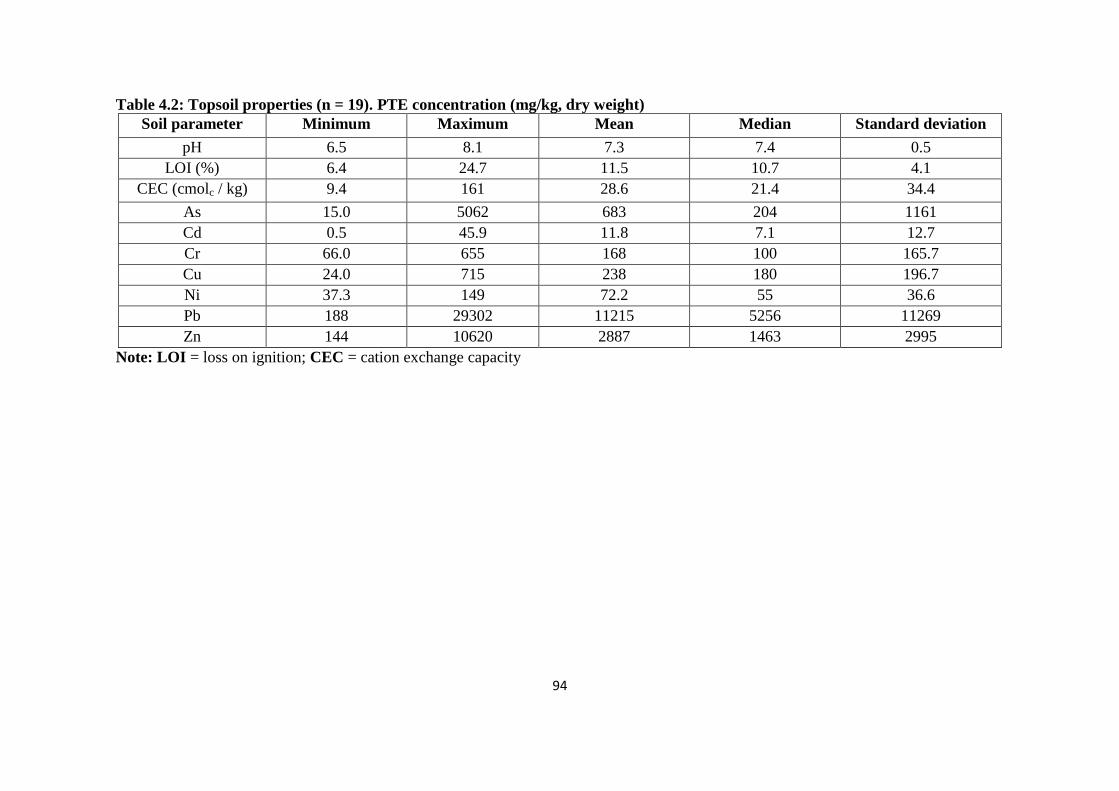
94

Table 4.2: Topsoil properties (n = 19). PTE concentration (mg/kg, dry weight)

Soil parameter Minimum Maximum Mean Median Standard deviation

pH 6.5 8.1 7.3 7.4 0.5

LOI (%) 6.4 24.7 11.5 10.7 4.1

CEC (cmolc / kg) 9.4 161 28.6 21.4 34.4

As 15.0 5062 683 204 1161

Cd 0.5 45.9 11.8 7.1 12.7

Cr 66.0 655 168 100 165.7

Cu 24.0 715 238 180 196.7

Ni 37.3 149 72.2 55 36.6

Pb 188 29302 11215 5256 11269

Zn 144 10620 2887 1463 2995

Note: LOI = loss on ignition; CEC = cation exchange capacity

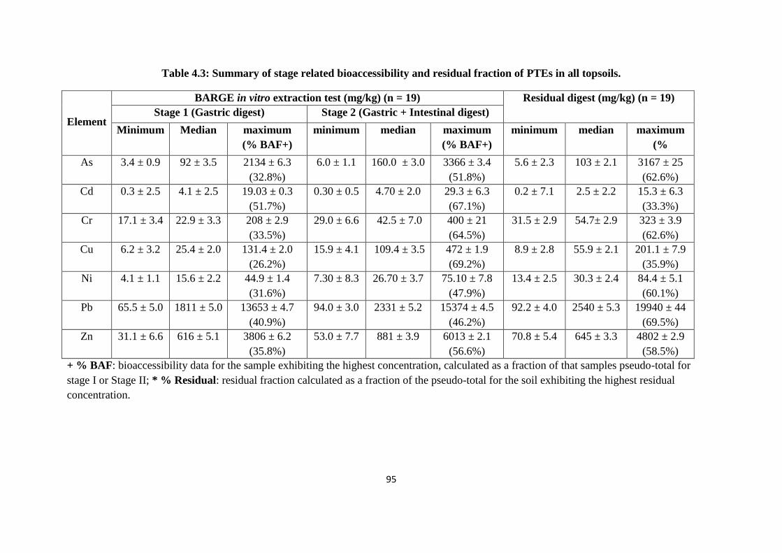
95

Table 4.3: Summary of stage related bioaccessibility and residual fraction of PTEs in all topsoils.

Element

BARGE in vitro extraction test (mg/kg) (n = 19) Residual digest (mg/kg) (n = 19)

Stage 1 (Gastric digest) Stage 2 (Gastric + Intestinal digest)

Minimum Median maximum

(% BAF+)

minimum median maximum

(% BAF+)

minimum median maximum

(%

residual*) As 3.4 ± 0.9 92 ± 3.5 2134 ± 6.3

(32.8%)

6.0 ± 1.1 160.0 ± 3.0 3366 ± 3.4

(51.8%)

5.6 ± 2.3 103 ± 2.1 3167 ± 25

(62.6%)

Cd 0.3 ± 2.5 4.1 ± 2.5 19.03 ± 0.3

(51.7%)

0.30 ± 0.5 4.70 ± 2.0 29.3 ± 6.3

(67.1%)

0.2 ± 7.1 2.5 ± 2.2 15.3 ± 6.3

(33.3%)

Cr 17.1 ± 3.4 22.9 ± 3.3 208 ± 2.9

(33.5%)

29.0 ± 6.6 42.5 ± 7.0 400 ± 21

(64.5%)

31.5 ± 2.9 54.7± 2.9 323 ± 3.9

(62.6%)

Cu 6.2 ± 3.2 25.4 ± 2.0 131.4 ± 2.0

(26.2%)

15.9 ± 4.1 109.4 ± 3.5 472 ± 1.9

(69.2%)

8.9 ± 2.8 55.9 ± 2.1 201.1 ± 7.9

(35.9%)

Ni 4.1 ± 1.1 15.6 ± 2.2 44.9 ± 1.4

(31.6%)

7.30 ± 8.3 26.70 ± 3.7 75.10 ± 7.8

(47.9%)

13.4 ± 2.5 30.3 ± 2.4 84.4 ± 5.1

(60.1%)

Pb 65.5 ± 5.0 1811 ± 5.0 13653 ± 4.7

(40.9%)

94.0 ± 3.0 2331 ± 5.2 15374 ± 4.5

(46.2%)

92.2 ± 4.0 2540 ± 5.3 19940 ± 44

(69.5%)

Zn 31.1 ± 6.6 616 ± 5.1 3806 ± 6.2

(35.8%)

53.0 ± 7.7 881 ± 3.9 6013 ± 2.1

(56.6%)

70.8 ± 5.4 645 ± 3.3 4802 ± 2.9

(58.5%)

+ % BAF: bioaccessibility data for the sample exhibiting the highest concentration, calculated as a fraction of that samples pseudo-total for

stage I or Stage II; * % Residual: residual fraction calculated as a fraction of the pseudo-total for the soil exhibiting the highest residual

concentration.

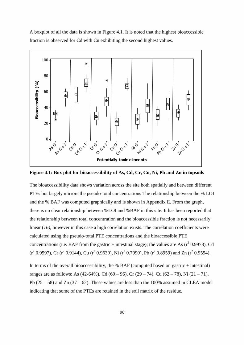
96

A boxplot of all the data is shown in Figure 4.1. It is noted that the highest bioaccessible

fraction is observed for Cd with Cu exhibiting the second highest values.

Zn G +

I

Zn G

Pb G

+ I

Pb G

Ni G +

INi G

Cu G

+ I

Cu G

Cr G +

ICr

G

Cd G

+ I

Cd G

As G +

I

As G

100

80

60

40

20

0

Potentially toxic elements

Bio

acce

ssib

ility

(%

)

Figure 4.1: Box plot for bioaccessibility of As, Cd, Cr, Cu, Ni, Pb and Zn in topsoils

The bioaccessibility data shows variation across the site both spatially and between different

PTEs but largely mirrors the pseudo-total concentrations The relationship between the % LOI

and the % BAF was computed graphically and is shown in Appendix E. From the graph,

there is no clear relationship between %LOI and %BAF in this site. It has been reported that

the relationship between total concentration and the bioaccessible fraction is not necessarily

linear (16), however in this case a high correlation exists. The correlation coefficients were

calculated using the pseudo-total PTE concentrations and the bioaccessible PTE

concentrations (i.e. BAF from the gastric + intestinal stage); the values are As (r2 0.9978), Cd

(r2 0.9597), Cr (r

2 0.9144), Cu (r

2 0.9630), Ni (r

2 0.7990), Pb (r

2 0.8959) and Zn (r

2 0.9554).

In terms of the overall bioaccessibility, the % BAF (computed based on gastric + intestinal)

ranges are as follows: As (42-64%), Cd (60 – 96), Cr (29 – 74), Cu (62 – 78), Ni (21 – 71),

Pb (25 – 58) and Zn (37 – 62). These values are less than the 100% assumed in CLEA model

indicating that some of the PTEs are retained in the soil matrix of the residue.

97

Most researchers observed high bioaccessibility of some metals in the stomach phase

example: Roussel et al., 2009 (17) observed that Cd, Pb and Zn are more bioaccessible in the

stomach with %BAF of 68, 62 and 47 respectively, Lamb et al., 2009 (18) in their study

discovered that Pb is more bioaccessible in the stomach with %BAF of over 80 while the rest

(Cu,Zn and Cd) was more in the intestinal phase, Turner et al., 2007 (19) observed more Cd

and Zn in the stomach phase, Poggio et al., 2009 (20) observed higher bioaccessibility of Pb

and Zn in the stomach while Cu and Ni were in the intestinal phase. In the present research,

high bioaccessibility is observed in the intestinal phase (G+I) than in the stomach phase for

all the metals studied. This is not surprising considering the fact that absorption normally

occurs in the intestine and bioaccessibility actually measures the fraction which is absorbed

in the blood stream during digestion.

4.3.4 Generic risk assessment and the role of bioacessibility data

As noted in section 1.4, the UK uses the widely accepted source–pathway–receptor paradigm

of pollutant linkage to assess human health risks from contaminated land (21-22). On that

basis the key exposure pathways that are considered appropriate for this site have been

identified as follows: (i) direct ingestion of soil (while the site is largely vegetated it does

have exposed soil particularly on the steep-sloped shrubby/wooded areas); (ii) direct

ingestion/inhalation of dust (dust generation, via digging at the site) the potential for

accumulation of soil material on footwear and its subsequent transport into buildings where it

may be inhaled is limited, however, dust is more likely risk); and (iii) ingestion of soil

attached to „vegetables‟ (the seasonal foraging of wild fruits and berries does occur). These

aspects will be considered based on the measured data.

It is possible to compare the BAF results from this work with the published SGVs. However,

following a review of SGVs (3) only a limited number of values are available for use in

generic risk assessment. Of relevance to this work SGVs are available for As, Cd and Ni (23-

25). However, generic assessment criteria (GAC) values have been published for Cr, Cu and

Zn (16) and so have been used to compare the data against. The lack of an updated SGV for

Pb means that the data in this work for Pb have been compared with the previous value (that

was withdrawn in July 2008) (1). On that basis a generic quantitative risk assessment for this

site was able to be carried out. It should also be noted that an urban recreational space is not

considered as part of the land scenarios inherent within the SGV/GAC values. On that basis

the data on this work was compared to SGV/GAC values for both allotment and residential

98

land use scenarios. [Note: Exceedance of SGV/GAC values of the total elemental

concentration in soil is indicative of a potential risk to human health for users of the site.

However, in this case (an urban recreational site) the assumptions on which the SGV/GAC

values are determined (i.e. age, sex and frequency of use) may not be the most appropriate].

A comparison of the determined pseudo-total element concentrations with the SGV/GAC

guidelines provides the following observations. In the case of As, 17 out of 19 samples

exceed the lower SGV (residential scenario) of 32 mg/kg; also 17 samples exceed the higher

SGV (allotment scenario) of 43 mg/kg with 5 soil samples exceeding the SGV (allotment

scenario) by almost 20 times. For Cd, 16 out of 19 soil samples exceed the lower SGV

(allotment scenario) of 1.8 mg/kg, and 7 out of 19 samples exceed the higher (residential

scenario) SGV of 10 mg/kg. For Cr, if the concentration represents Cr (VI) then all soil

samples exceed the residential scenario of 4.3 mg/kg, as well as the allotment scenario of 2.1

mg/kg with all samples having more than 15 times the GAC values in both scenarios. If

however, the concentration represents Cr (III) then none of the soils exceed even the lowest

GAC value of 3,000 mg/kg (allotment scenario). For Cu, 2 out of 19 soil samples exceed the

lower GAC (allotment scenario) of 524 mg/kg; none of the soil samples exceed the higher

GAC (residential) of 2,330 mg/kg. For Ni, 3 out of 19 samples exceed the lower SGV

(residential scenario) of 130 mg/kg; however, none of the 19 samples exceeds the higher

SGV (allotment scenario) of 230 mg/kg. For Pb, 17 out of 19 soil samples exceed the

allotment & residential scenario of 450 mg/kg, with concentrations in 17 soils at more than

twice the SGV and a maximum soil concentration of 33,306 mg Pb/kg. While finally for Zn,

13 out of 19 soil samples exceed the lower GAC value (allotment scenario) of 618 mg/kg; 5

soil samples also exceed the higher (residential scenario) of 3,750 mg/kg, with concentrations

more than twice the GAC value (i.e. maximum soil concentration of 10,620 mg Zn/kg).

Therefore based on the generic risk assessment criteria, a high percentage of soil samples, for

all of the 7 elements investigated, indicate further investigation may be required.

Unfortunately, as already indicated, differences between this site conceptual model and the

inherent assumptions within the generic land use scenarios mean that the estimated exposure

could well be different. The use of oral bioaccessibility data may therefore contribute to a

better understanding of the generic risk assessment. Also, as previously highlighted, the

SGVs (except Pb) all assume that the contaminants are completely available to the receptor

99

following exposure; as this is unlikely it will lead to an overestimate of the exposure from the

soil.

Consideration of the bioaccessible data, based on the concentration of element in the gastric +

intestinal stage (rather than the value for %BAF), allows a modified view to emerge for some

elements. In terms of Cr, and specifically Cr (VI) and Cr (III), no changes occur as a result of

using the bioaccessible data i.e. all data exceeds the GAC values for residential and allotment

scenarios. In summary, in the case of As, 15 samples still exceed residential and allotment

scenarios (a change of two fewer); for Cd, 1 sample fewer exceeds the allotment scenario and

3 fewer the residential scenario; for Cu and Ni, no samples exceed the allotment or residential

scenarios; for Pb, 16 still exceed the allotment & residential scenario; while for Zn, 3 fewer

exceed the allotment scenario and 4 fewer exceed the residential scenario. It is concluded that

while only a small shift in emphasis is made by the use of bioaccessibility data the approach

does have merit. This is because the assumptions made about the use of SGV/GAC values

and the land scenarios (allotment and residential) may not adequately reflect the urban

recreational site chosen to study in this work. In addition, it should be borne in mind that the

generic SGVs are based on the following soil type: a sandy loam soil with 6 % soil organic

matter content (26). The current site soil property data identifies typically higher organic

matter content, based on the loss on ignition values being indicative of soil organic matter

(Table 4.2). This, coupled with the high cation exchange capacity values, is likely to make

the soils more naturally retentive of the elements under investigation than those in the generic

models (22).

4.3.5 Estimation of bioaccessibility of soil using TDI and MDI

The potential health risk of soil ingestion can be assessed by calculating the mass of sample

that a child would require to ingest to reach the estimated tolerable daily intake (TDI) or

mean daily intake (MDI) for each of the potentially toxic elements investigated. The values

of the TDI are shown in Table 4.4 and are based on a 10 kg child, while the values for the

MDI are based on a child aged between 5-6 years of age and which corresponds to a weight

of 20 kg (27). In the case of As, a non-threshold carcinogen, a TDI is inappropriate. An oral

index dose (IDoral) has been proposed of 0.3 µg kg-1

bw day-1

for As (28). Therefore based on

the IDoral value and an assumed body weight of a 10 kg child the ingestion value is assumed

to be 3 µg/day. The US EPA (29) has recommended values for daily soil (including soil and

outdoor settled dust), indoor settled dust and soil plus dust ingestion for children.

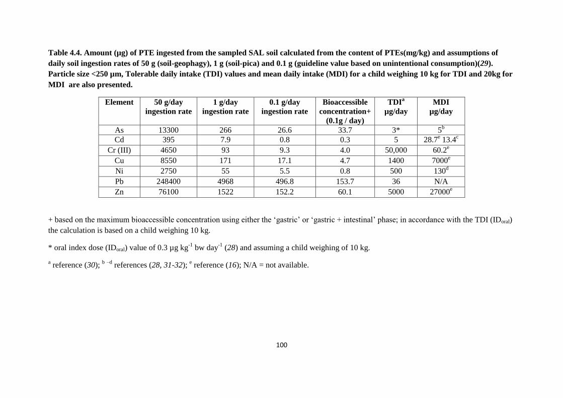
100

Table 4.4. Amount (µg) of PTE ingested from the sampled SAL soil calculated from the content of PTEs(mg/kg) and assumptions of

daily soil ingestion rates of 50 g (soil-geophagy), 1 g (soil-pica) and 0.1 g (guideline value based on unintentional consumption)(29).

Particle size <250 µm, Tolerable daily intake (TDI) values and mean daily intake (MDI) for a child weighing 10 kg for TDI and 20kg for

MDI are also presented.

Element 50 g/day

ingestion rate

1 g/day

ingestion rate

0.1 g/day

ingestion rate

Bioaccessible

concentration+

(0.1g / day)

TDIa

µg/day

MDI

µg/day

As 13300 266 26.6 33.7 3* 5b

Cd 395 7.9 0.8 0.3 5 28.7e 13.4

c

Cr (III) 4650 93 9.3 4.0 50,000 60.2e

Cu 8550 171 17.1 4.7 1400 7000e

Ni 2750 55 5.5 0.8 500 130d

Pb 248400 4968 496.8 153.7 36 N/A

Zn 76100 1522 152.2 60.1 5000 27000e

+ based on the maximum bioaccessible concentration using either the „gastric‟ or „gastric + intestinal‟ phase; in accordance with the TDI (IDoral)

the calculation is based on a child weighing 10 kg.

* oral index dose (IDoral) value of 0.3 µg kg-1

bw day-1

(28) and assuming a child weighing of 10 kg.

a reference (30);

b –d

references (28, 31-32); e reference (16); N/A = not available.

101

The recommended guideline value for soil and dust ingestion has been assessed to be 100

mg/day for children between the age 1 and <6 years. In addition, for children up to age 14

who may exhibit soil-pica behaviour the estimates range from 400 to 41,000 mg/day with a

recommended upper percentile soil pica ingestion rate of 1,000 mg/day (pica was defined in

the report (29) as the recurrent ingestion of unusually high amounts of soil); while the

recommended upper percentile geophagy soil estimate is 50,000 mg/day (geophagy was

defined in the report (29) as the intentional ingestion of earths, usually associated with

cultural practices). Therefore on the basis of these recommendations, the amount of PTE

ingested from the soil sample was calculated based on 50 g/day (geophagy), 1 g/day (soil-

pica) and 0.1 g/day (guideline value based on unintentional ingestion). The values obtained

were compared with the TDI (or IDoral in the case of As) and MDI values to assess the risk of

the PTE to the child. From the results for a child with geophagy behaviour the levels of all

PTEs are exceeded except Cr (III). In contrast for a child with pica behaviour (1 g/day) only

two PTE exceeds the TDI value i.e. Cd and Pb; in addition, for As, the IDoral value and the

MDI values are exceeded. Based on the unintentional consumption of 0.1 g of soil, only Pb

and As exceed the guideline value (TDI and IDoral respectively) for this type of samples.

Though these calculations can help to estimate the potential risk from the urban environment

studied they only assume ingestion (oral) as the means of exposure. Inhalation and

subsequent transfer to the gastro-intestinal tract via coughing up and re-swallowing may also

be relevant to consider.

4.4 Conclusion

Our generic quantitative risk assessment highlighted that exceedances of the SGV (for either

residential or allotment landuse) were present for all of the 7 PTEs based on pseudo-total

concentrations. Site-specific circumstances, such as critical pathways, receptors, site-usage

patterns and activities, need to be taken into account and so exceedence does not necessarily

imply that there is an actual risk to health.

One objective of this work was to apply a robust in vitro GI procedure to soils sampled across

a former industrial site in NE England, and to highlight the role of such data for use in human

health risk assessment. The results indicated that the bioaccessibility of PTEs investigated in

soils across the site is less than the 100% assumed by the CLEA model. Cadmium however,

indicated a much higher %BAF than other analytes with over 50 % of the pseudo-total Cd

concentration bioaccessible in all the 19 soils investigated. The bioaccessibility data indicated

102

both elemental and spatial differences and highlight total soil concentration to be a rather

crude estimate of the fraction that is potentially extractable in the body and hence potentially

taken into the blood stream. Given too that the generic land use categories (allotments and

residential) are a very conservative screening tool for an area of public open space a detailed

qualitative risk assessment is recommended as part of the on-going risk assessment at this

site, along with a detailed user study to identify exposure duration of the various receptor

groups. Site-specific SGVs/GAC need to be refined on the basis of soil type, the PTE

bioaccessibility data, and receptors behaviours, as this might lower or increase their

exposures. Bioaccessibiliy data are an additional tool towards a more holistic

multidisciplinary approach to understanding human health risk at contaminated site.

References

1 Environment Agency (2002). Soil guidelines values for metal contamination, R&D

Publication SGV. Available at: http://www.environment-agency.gov.uk/. March 2009.

2 Nathanail, C.P., McCaffrey, C. (2003). The use of oral bioaccessibility in assessment

of risks to human health from contaminated land. Land Contamination and

Reclamation, 11, 309-313.

3 DEFRA (Department for Environment, Food and Rural Affairs) (2006). Assessing

risks from land contamination – a proportionate approach. Soil guideline values: The

Way Forward. Available at: http://www.defra.gov.uk/. June 2009.

4 Hursthouse, A., Kowalczyk, G. (2009). Transport and dynamics of toxic pollutants in

the natural environment and their effect on human health: research gaps and

challenge. Environmental Geochemistry and Health, 31, 165-187.

5 Davis, A., Ruby, M.V., Bloom, M., Schoof, R., Freeman, G., Bergstrom, P.D. (1996).

Mineralogic constraints on the bioavailability of arsenic in smelter-impacted soils.

Environmental Science and Technology, 30, 392-399.

6 Paustenbach, D.J. (2000). The practice of exposure assessment: A state of the art

review. Journal of Toxicology and Environmental Health, Part B, Critical Reviews, 3,

179-291.

103

7 Oomen, A.G., Hack, A., Minekus, M., Zeijdner, E., Schoeters, G., Verstraete, W.,

Wiele, T.V.D., Wragg, J., Rompelberg, C.J.M., Sips, A.J.A.M., Wijnen, J.H.V.

(2002). Comparison of Five in vitro Digestion Models to Study the Bioaccessibility

of Soil Contaminants. Environmental Science and Technology, 36, 3326–3334.

8 Environment Agency (2007). In-vitro Bioaccessibility Testing: Current Science and

Way Forward (Environment Agency Science Update 2). Available at:

http://www.environment-agency.gov.uk/.May 2008.

9 Freeman, G. B., Scooff, R.A., Ruby, M.V., Davis, A.O., Dill, J.A., Liao, S.C., Lapin,

C.A., Bergstrom, P.D. (1995). Bioaccessibility of arsenic in soil and house dust

impacted by smelter activities following oral administration in cynomolgus monkeys.

Fundamental and Applied Toxicology, 28, 215 – 222.

10 Casteel, S. W., Cowart, R. P., Weis, C. P., Henninhsen, G. M., Hoffman, E., Brattin,

W. J., Guzman, R. E., Startost, M. F., Payne, J. T., Stockham, S. L., Becker, S. V.,

Drexler, J. W., Turn, J. R, (1997). Bioavailability of lead to juvenile swine dosed with

soil from the Smuggler Mountain NPL site of Aspen, Colorado. Fundamental and

Applied Toxicology, 36, 177 – 187.

11 Rodriguez, R. R., Basta, N. T., Casteel, S. W., Pace, L. W. (1999). An in vitro

gastrointestinal method to estimate bioavailable arsenic in contaminated soils and

solid media. Environmental Science and Technology, 33, 642–649.

12 Scoof, R. A. (2004). Bioavailability of soil-borne chemicals: method development and

validation. Human and Ecological Risk Assessment, 10(4), 637–646.

13 Environment Agency (2009). CLEA Software (Version 1.04) Handbook. Science

Report SC050021/SR4.

14 Environment Agency (2009). CLEA Software version 1.04.

15 Wragg, J., Cave, M., Oomen, A. (2009). Chemical and biological hazards programme

open report OR/07/027.

16 Nathanial, C P., Mc Affrey, C., Ashmore, M. (2009). Generic Assessment Criteria for

Human Health Risk Assessment, 2nd

Ed., Nottingham, UK. Land Quality Press.

104

17 Roussel, H., Waterlot, C., Pelfrere, A., Pruvot, C., Mazzuca, M., Douay, F. (2010).

Cd, Pb and Zn oral bioaccessibility of urban soils contaminated in the past by

atmospheric emissions from two lead and zinc smelters. Archives of Environmental

Contamination and Toxicity, 58, 945-954.

18 Lamb, D.T., Ming, H., Megharaj, M., Naidu, R. (2009). Heavy metal (Cu, Zn, Cd and

Pb) partitioning and bioaccessibility in uncontaminated and long term contaminated

soils. Journal of Hazardous Materials, 171, 1150-1158.

19 Turner, A., Ka-Hei, I.P.(2007). Bioaccessibility of metals in soil: Application of a

physiologically based extraction test. Environmental Science and Technology, 41,

7851-7856.

20 Poggio, L., Vrscaj, B., Schulin, R., Hepperle, E., Marson, F.A. (2009). Metals

pollution and human bioaccessibility of topsoils in Grugliasco (Italy). Environmental

Pollution, 157, 680-689.

21 Environment Agency (2009). Human health toxicological assessment of contaminants

in soil. Science Report SC050021/SR2.

22 HPA (Health Protection Agency) (2009). An Introduction to Land Contamination for

Public Health Professionals. HPA, Cardiff. Available at: http://www.hpa.org.uk/

August 2009.

23 Environment Agency (2009) Soil Guideline Values for nickel in soil Science Report

SC050021 / Nickel SGV.

24 Environment Agency (2009). Soil Guideline Values for cadmium in soil Science

Report SC050021 / Cadmium SGV.

25 Environment Agency (2009). Soil Guideline Values for arsenic in soil Science Report

SC050021 / Arsenic SGV.

26 Environment Agency (2009). Human health toxicological assessment of contaminants

in soil. Science Report SC050021/SR2.

27 DEFRA and EA. (2002). Contaminants in soil: Collation of toxicological data and

intake values for humans. R & D Publication CLR 9.

105

28 Environmental Agency. (2010). Contaminants in soil: updated collation of

toxicological data and intake values for humans inorganic arsenic Science report:

SC050021/TOX 1.

29 U.S. EPA. (2008). Child-Specific Exposure Factors Handbook (Final Report) 2008.

U.S. Environmental Protection Agency, Washington, DC, EPA/600/R-06/096F.

30 Ljung, K.; Selinus, O.; Otabbong, E.; Berglund, M. (2006). Metal and As distribution

in soil particle sizes relevant to soil ingestion by children. Applied Geochemistry, 21,

1613-1624.

31 Environmental Agency. (2010). Contaminants in soil: updated collation of

toxicological data and intake values for humans inorganic cadmium. Science report:

SC050021/TOX 3.

32 Environmental Agency. (2010). Contaminants in soil: updated collation of

toxicological data and intake values for humans inorganic Nickel. Science report:

SC050021/TOX 8.

106

Chapter Five: Natural and anthropogenic PTE input to urban street dust

and the role of oral bioaccessibility testing

5.1 Introduction

Dust is solid matter which comprises soil, anthropogenic metallic constituents and natural

biogenic materials (1). The soil component of urban street dusts is a mixture of mineral

constituents and organic matter; the anthropogenic materials are vehicle exhaust particles,

lubricating oil residues and tyre, brake and engine wear components while the natural

biogenic materials are tree leaves and other plant matter pulverized by traffic and general

weathering (2-4). Some of the most common elements associated with automobile industries

include As, Cd, Cu, Ni, Pb and Zn, either within the fabrication of a vehicle, component parts

(e.g. brake pads), as additives (e.g. in lubricants) for engine operation or resulting from

automobile corrosion (5, 6). For example, Cu compounds are used in lubricants as anti-wear

agents, by providing a protective layer on engine surfaces to reduce friction and prevent

damages due to continuous rubbing between engine parts. Historically, lead compounds (lead

tetraethyl (C2H5)4Pb) were added as antiknock agents in petrol prior to their cessation in the

UK in 1999 (7). The now wide spread use of unleaded fuels however, has not put a stop to

the use of lead compounds in motoring activities; for example, lead compounds are used as

anti-wear agents in lubricant oils for engines (5). Among the alternatives added into lubricant

oils are Zn compounds (5). For example, zinc dialkyldithiophosphate (ZDDP) is added as an

agent to provide additional protection under extreme-pressure or in a heavy-duty performance

situation to protect the lubricant itself from oxidative breakdown and to prevent the formation

of deposits in engines (5, 8, 9). Metals such as Ni are also used for plating the outer part of a

vehicle, such as, the tyre rims or as an alloy for plating the surface of the cylinder and pistons

of an engine (10). The source of Ni in road dust is believed to result from corrosion of these

components over the lifetime of the vehicle (11-13).

Road dust can be a particular risk to humans due to its small particle size and its inherent

mobility in windy weather conditions leading to the possibility of direct and indirect

exposure; direct exposure from dust can occur by inhalation while indirect exposure results

from contact with exposed skin and outer clothing which in turn can be accidentally ingested

(14). Young children (up to 5 years of age) are more likely to ingest significant quantities of

dust than adults because of the behaviour of mouthing non-food objects and repetitive hand /

finger sucking during outdoor activities (15). Also children have a much higher absorption

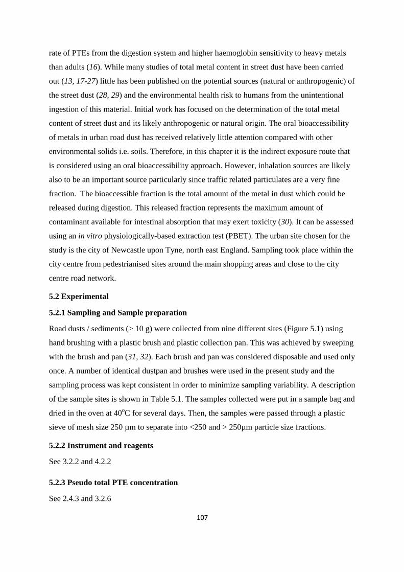
107

rate of PTEs from the digestion system and higher haemoglobin sensitivity to heavy metals

than adults (16). While many studies of total metal content in street dust have been carried

out (13, 17-27) little has been published on the potential sources (natural or anthropogenic) of

the street dust (28, 29) and the environmental health risk to humans from the unintentional

ingestion of this material. Initial work has focused on the determination of the total metal

content of street dust and its likely anthropogenic or natural origin. The oral bioaccessibility

of metals in urban road dust has received relatively little attention compared with other

environmental solids i.e. soils. Therefore, in this chapter it is the indirect exposure route that

is considered using an oral bioaccessibility approach. However, inhalation sources are likely

also to be an important source particularly since traffic related particulates are a very fine

fraction. The bioaccessible fraction is the total amount of the metal in dust which could be

released during digestion. This released fraction represents the maximum amount of

contaminant available for intestinal absorption that may exert toxicity (30). It can be assessed

using an in vitro physiologically-based extraction test (PBET). The urban site chosen for the

study is the city of Newcastle upon Tyne, north east England. Sampling took place within the

city centre from pedestrianised sites around the main shopping areas and close to the city

centre road network.

5.2 Experimental

5.2.1 Sampling and Sample preparation

Road dusts / sediments (> 10 g) were collected from nine different sites (Figure 5.1) using

hand brushing with a plastic brush and plastic collection pan. This was achieved by sweeping

with the brush and pan (31, 32). Each brush and pan was considered disposable and used only

once. A number of identical dustpan and brushes were used in the present study and the

sampling process was kept consistent in order to minimize sampling variability. A description

of the sample sites is shown in Table 5.1. The samples collected were put in a sample bag and

dried in the oven at 40oC for several days. Then, the samples were passed through a plastic

sieve of mesh size 250 µm to separate into <250 and > 250µm particle size fractions.

5.2.2 Instrument and reagents

See 3.2.2 and 4.2.2

5.2.3 Pseudo total PTE concentration

See 2.4.3 and 3.2.6

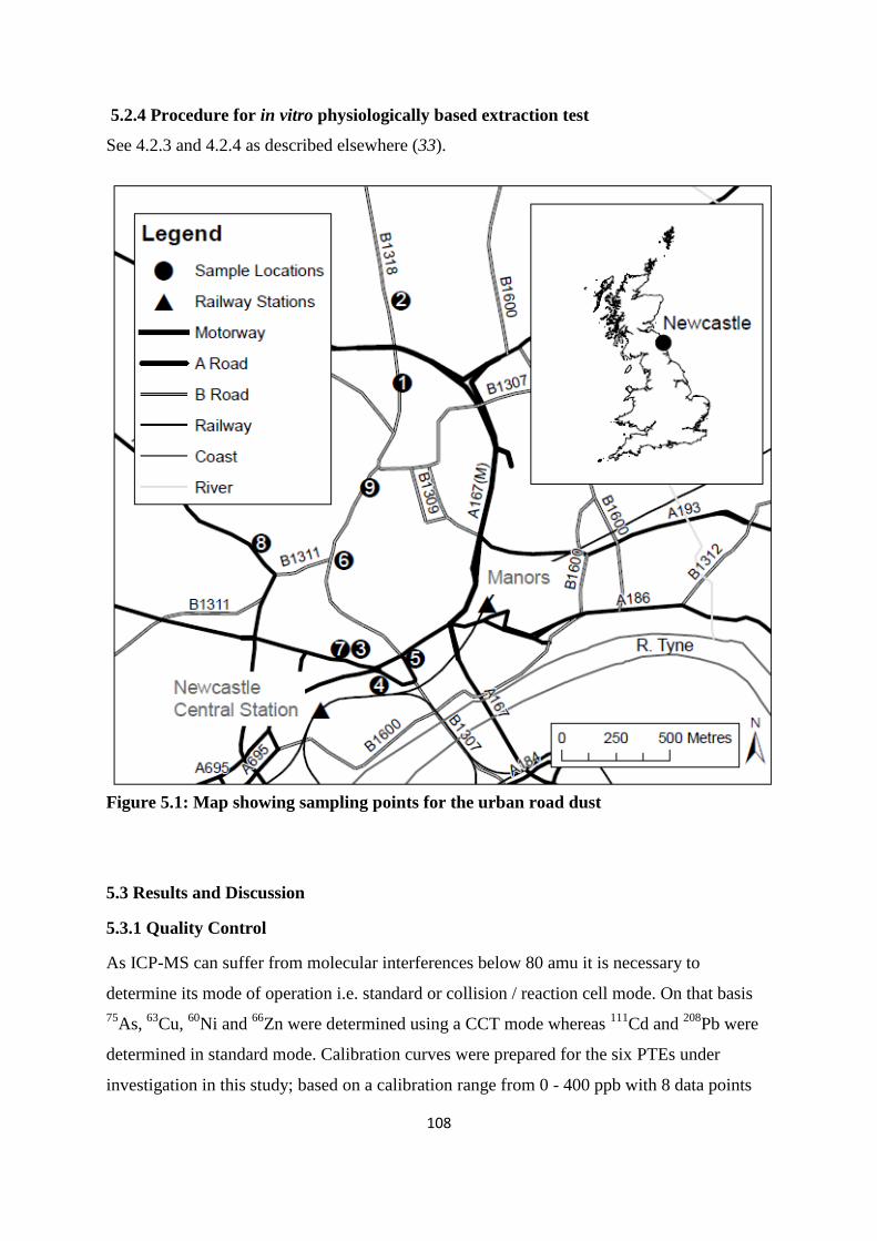
108

5.2.4 Procedure for in vitro physiologically based extraction test

See 4.2.3 and 4.2.4 as described elsewhere (33).

Figure 5.1: Map showing sampling points for the urban road dust

5.3 Results and Discussion

5.3.1 Quality Control

As ICP-MS can suffer from molecular interferences below 80 amu it is necessary to

determine its mode of operation i.e. standard or collision / reaction cell mode. On that basis

75As,

63Cu,

60Ni and

66Zn were determined using a CCT mode whereas

111Cd and

208Pb were

determined in standard mode. Calibration curves were prepared for the six PTEs under

investigation in this study; based on a calibration range from 0 - 400 ppb with 8 data points

109

Table 5.1: Sample location, driving style and traffic volume

Site

number

Location No of

vehicles /

day*

Driving Style Description/sources Possible receptors

1 Robinson

Library,

Claremont Road

14,091 Constant

Speed

North of City Centre air quality Management

area (AQMA). Entrance to Claremont bridge

(over the Great North Road B1318) directly

opposite entrance to Robinson library. Ivy

(Hedera sp.) forming a semi protected area in

which soil/dust can accumulate. Matrix

comprising soil from adjacent landscaped area

and curb-side dust.

Busy pedestrian

thorough fair with

cyclist

2 Brandling Park,

Forsyth Road

28885 Constant

Speed

North of City Centre AQMA. Park adjacent

(to the east) of the Great North Road B1318.

Sample taken from a rectangular seating area.

Matrix comprising soil from adjacent

landscaped area and general urban inputs;

sloppy sediment overlain by leaf litter.

Urban parkland.

Receptors include

dog walkers,

pedestrians and

those using the site

as a general

recreation area

3 Grainger Street

opposite St

John‟s Church

3338 Stop and Start Sample collect from corners either side of 3

doorways and recessed areas between two

buildings. Matrix: street dust and „rubbish‟

(cigarette ends, litter & other detritus of plant

and animal origin).

Busy pedestrian

route to and from

station. Busy with

vehicular traffic.

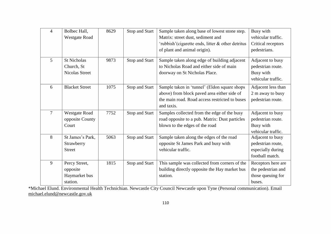
110

4 Bolbec Hall,

Westgate Road

8629 Stop and Start Sample taken along base of lowest stone step.

Matrix: street dust, sediment and

„rubbish‟(cigarette ends, litter & other detritus

of plant and animal origin).

Busy with

vehicular traffic.

Critical receptors

pedestrians.

5 St Nicholas

Church, St

Nicolas Street

9873 Stop and Start Sample taken along edge of building adjacent

to Nicholas Road and either side of main

doorway on St Nicholas Place.

Adjacent to busy

pedestrian route.

Busy with

vehicular traffic.

6 Blacket Street

1075 Stop and Start Sample taken in „tunnel‟ (Eldon square shops

above) from block paved area either side of

the main road. Road access restricted to buses

and taxis.

Adjacent less than

2 m away to busy

pedestrian route.

7 Westgate Road

opposite County

Court

7752 Stop and Start Samples collected from the edge of the busy

road opposite to a pub. Matrix: Dust particles

blown to the edges of the road

Adjacent to busy

pedestrian route.

Busy with

vehicular traffic.

8 St James‟s Park,

Strawberry

Street

5063 Stop and Start Sample taken along the edges of the road

opposite St James Park and busy with

vehicular traffic.

Adjacent to busy

pedestrian route,

especially during

football match.

9 Percy Street,

opposite

Haymarket bus

station.

1815 Stop and Start This sample was collected from corners of the

building directly opposite the Hay market bus

station.

Receptors here are

the pedestrian and

those queuing for

buses.

*Michael Elund. Environmental Health Technichian. Newcastle City Council Newcastle upon Tyne (Personal communication). Email

michael.elund@newcastle.gov.uk

111

typical correction coefficients (r2) for all elements were in excess of 0.99. The dust certified

reference material (BCR 723) was digested using the microwave protocol described in 3.2.3

and 4.2.6 and then its PTE content determined using ICP-MS. As the CRM has no certified

values for the PTEs under investigation in this study only its indicative values could be used.

The results are shown in Table 5.2. Excellent agreement was obtained with the known

indicative values (Cd, Ni, Pb and Zn); no values were available for As and Cu.

Table 5.2: Analysis of PTE content of dust certified reference material (BCR 723) using

microwave digestion-ICP-MS

Element Indicative value

(mg/kg)

Measured values (mg/kg) Mean ± SD (n = 3)

Standard Mode CCT Mode

As NA NA 10.3 ± 2.1

Cd 2.5 ± 0.4 2.4 ± 1.1 NA

Cu NA NA 175 ± 3.1

Ni 171 ± 3 NA 171 ± 3.5

Pb 866 ± 16 867 ± 2.3 NA

Zn 1660 ± 100 NA 1602 ± 3.7

5.3.2 Pseudo total PTE concentration

Dust samples were analysed using < 250 µm particle size as this is the fraction that is most

likely to adhere to hands and thus most likely to be involuntarily ingested (34). A summary of

the overall data in the form of a box plot is shown in Figure 5.2. The mean concentrations of

As, Cd, Cu, Ni, Pb and Zn are 6.4, 1.0, 132, 26, 992 and 421 mg/kg, respectively. A major

outlier in the data occurs for Pb at site 5 (4000 mg/kg); outside the cathedral church of St.

Nicholas and located on a major road artery through the city centre. Statistical evaluation of

the data (normality test) indicates that majority of the elements display a normal distribution

(p-values >0.05), except for Cd and Pb (Table 5.3). As a result of this normal distribution, the

mean is shown for As, Cu, Ni and Zn while the median is used for Cd and Pb for non-

parametric alternative (see Figures 5.2-5.8). It therefore appears that based on the normality

test and coefficient of variation (CV) that the examined elements can be classified into two

groups: Cd and Pb whose CVs are higher than 100 and the other PTEs (As, Cu, Ni and Zn)

whose CVs are lower than 100 (35).

The concentrations of each of the elements across the samples are shown in Figures 5.2-5.8.

In addition, global road dust concentrations of the PTEs under consideration have been

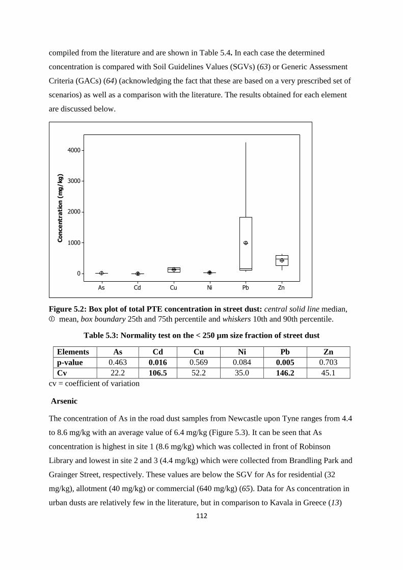
112

compiled from the literature and are shown in Table 5.4. In each case the determined

concentration is compared with Soil Guidelines Values (SGVs) (63) or Generic Assessment

Criteria (GACs) (64) (acknowledging the fact that these are based on a very prescribed set of

scenarios) as well as a comparison with the literature. The results obtained for each element

are discussed below.

ZnPbNiCuCdAs

4000

3000

2000

1000

0

Co

nce

ntr

ati

on

(m

g/

kg

)

Figure 5.2: Box plot of total PTE concentration in street dust: central solid line median,

mean, box boundary 25th and 75th percentile and whiskers 10th and 90th percentile.

Table 5.3: Normality test on the < 250 µm size fraction of street dust

Elements As Cd Cu Ni Pb Zn

p-value 0.463 0.016 0.569 0.084 0.005 0.703

Cv 22.2 106.5 52.2 35.0 146.2 45.1

cv = coefficient of variation

Arsenic

The concentration of As in the road dust samples from Newcastle upon Tyne ranges from 4.4

to 8.6 mg/kg with an average value of 6.4 mg/kg (Figure 5.3). It can be seen that As

concentration is highest in site 1 (8.6 mg/kg) which was collected in front of Robinson

Library and lowest in site 2 and 3 (4.4 mg/kg) which were collected from Brandling Park and

Grainger Street, respectively. These values are below the SGV for As for residential (32

mg/kg), allotment (40 mg/kg) or commercial (640 mg/kg) (65). Data for As concentration in

urban dusts are relatively few in the literature, but in comparison to Kavala in Greece (13)

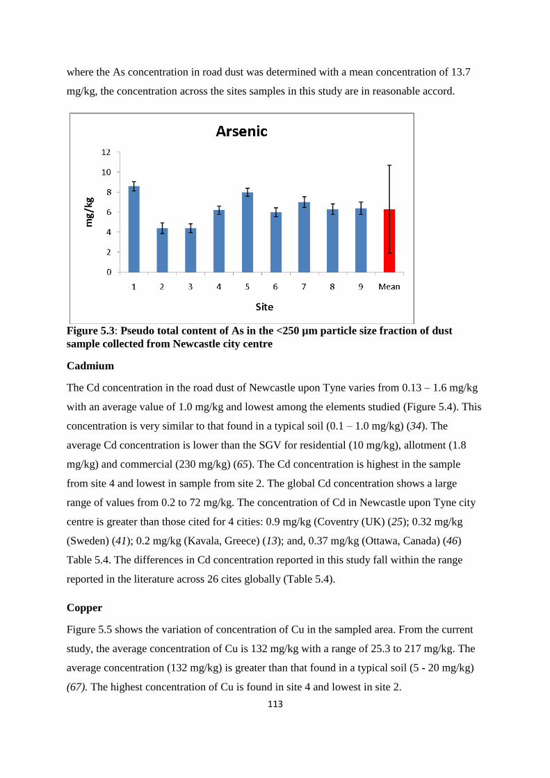
113

where the As concentration in road dust was determined with a mean concentration of 13.7

mg/kg, the concentration across the sites samples in this study are in reasonable accord.

Figure 5.3: Pseudo total content of As in the <250 µm particle size fraction of dust

sample collected from Newcastle city centre

Cadmium

The Cd concentration in the road dust of Newcastle upon Tyne varies from 0.13 – 1.6 mg/kg

with an average value of 1.0 mg/kg and lowest among the elements studied (Figure 5.4). This

concentration is very similar to that found in a typical soil (0.1 – 1.0 mg/kg) (34). The

average Cd concentration is lower than the SGV for residential (10 mg/kg), allotment (1.8

mg/kg) and commercial (230 mg/kg) (65). The Cd concentration is highest in the sample

from site 4 and lowest in sample from site 2. The global Cd concentration shows a large

range of values from 0.2 to 72 mg/kg. The concentration of Cd in Newcastle upon Tyne city

centre is greater than those cited for 4 cities: 0.9 mg/kg (Coventry (UK) (25); 0.32 mg/kg

(Sweden) (41); 0.2 mg/kg (Kavala, Greece) (13); and, 0.37 mg/kg (Ottawa, Canada) (46)

Table 5.4. The differences in Cd concentration reported in this study fall within the range

reported in the literature across 26 cites globally (Table 5.4).

Copper

Figure 5.5 shows the variation of concentration of Cu in the sampled area. From the current

study, the average concentration of Cu is 132 mg/kg with a range of 25.3 to 217 mg/kg. The

average concentration (132 mg/kg) is greater than that found in a typical soil (5 - 20 mg/kg)

(67). The highest concentration of Cu is found in site 4 and lowest in site 2.

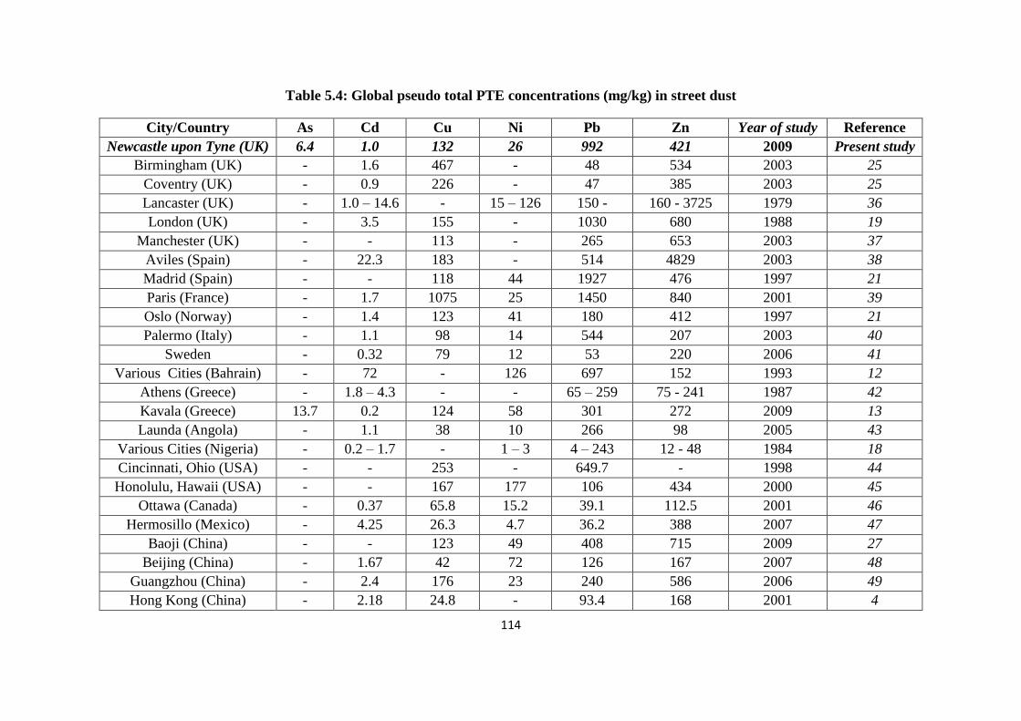
114

Table 5.4: Global pseudo total PTE concentrations (mg/kg) in street dust

City/Country As Cd Cu Ni Pb Zn Year of study

ofoofof

Reference

Newcastle upon Tyne (UK) 6.4 1.0 132 26 992 421 2009 Present study

Birmingham (UK) - 1.6 467 - 48 534 2003 25

Coventry (UK) - 0.9 226 - 47 385 2003 25

Lancaster (UK) - 1.0 – 14.6 - 15 – 126 150 -

15000

160 - 3725 1979 36

London (UK) - 3.5 155 - 1030 680 1988 19

Manchester (UK) - - 113 - 265 653 2003 37

Aviles (Spain) - 22.3 183 - 514 4829 2003 38

Madrid (Spain) - - 118 44 1927 476 1997 21

Paris (France) - 1.7 1075 25 1450 840 2001 39

Oslo (Norway) - 1.4 123 41 180 412 1997 21

Palermo (Italy) - 1.1 98 14 544 207 2003 40

Sweden - 0.32 79 12 53 220 2006 41

Various Cities (Bahrain) - 72 - 126 697 152 1993 12

Athens (Greece) - 1.8 – 4.3 - - 65 – 259 75 - 241 1987 42

Kavala (Greece) 13.7 0.2 124 58 301 272 2009 13

Launda (Angola) - 1.1 38 10 266 98 2005 43

Various Cities (Nigeria) - 0.2 – 1.7 - 1 – 3 4 – 243 12 - 48 1984 18

Cincinnati, Ohio (USA) - - 253 - 649.7 - 1998 44

Honolulu, Hawaii (USA) - - 167 177 106 434 2000 45

Ottawa (Canada) - 0.37 65.8 15.2 39.1 112.5 2001 46

Hermosillo (Mexico) - 4.25 26.3 4.7 36.2 388 2007 47

Baoji (China) - - 123 49 408 715 2009 27

Beijing (China) - 1.67 42 72 126 167 2007 48

Guangzhou (China) - 2.4 176 23 240 586 2006 49

Hong Kong (China) - 2.18 24.8 - 93.4 168 2001 4

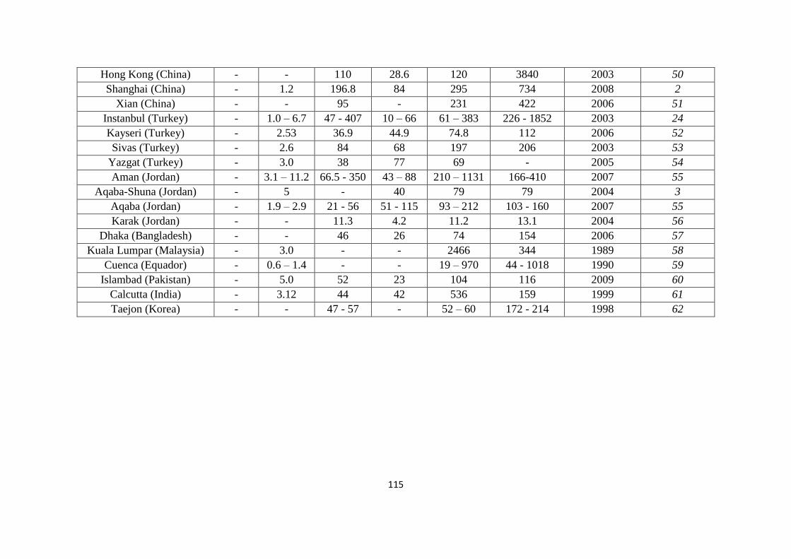
115

Hong Kong (China) - - 110 28.6 120 3840 2003 50

Shanghai (China) - 1.2 196.8 84 295 734 2008 2

Xian (China) - - 95 - 231 422 2006 51

Instanbul (Turkey) - 1.0 – 6.7 47 - 407 10 – 66 61 – 383 226 - 1852 2003 24

Kayseri (Turkey) - 2.53 36.9 44.9 74.8 112 2006 52

Sivas (Turkey) - 2.6 84 68 197 206 2003 53

Yazgat (Turkey) - 3.0 38 77 69 - 2005 54

Aman (Jordan) - 3.1 – 11.2 66.5 - 350 43 – 88 210 – 1131 166-410 2007 55

Aqaba-Shuna (Jordan) - 5 - 40 79 79 2004 3

Aqaba (Jordan) - 1.9 – 2.9 21 - 56 51 - 115 93 – 212 103 - 160 2007 55

Karak (Jordan) - - 11.3 4.2 11.2 13.1 2004 56

Dhaka (Bangladesh) - - 46 26 74 154 2006 57

Kuala Lumpar (Malaysia) - 3.0 - - 2466 344 1989 58

Cuenca (Equador) - 0.6 – 1.4 - - 19 – 970 44 - 1018 1990 59

Islambad (Pakistan) - 5.0 52 23 104 116 2009 60

Calcutta (India) - 3.12 44 42 536 159 1999 61

Taejon (Korea) - - 47 - 57 - 52 – 60 172 - 214 1998 62

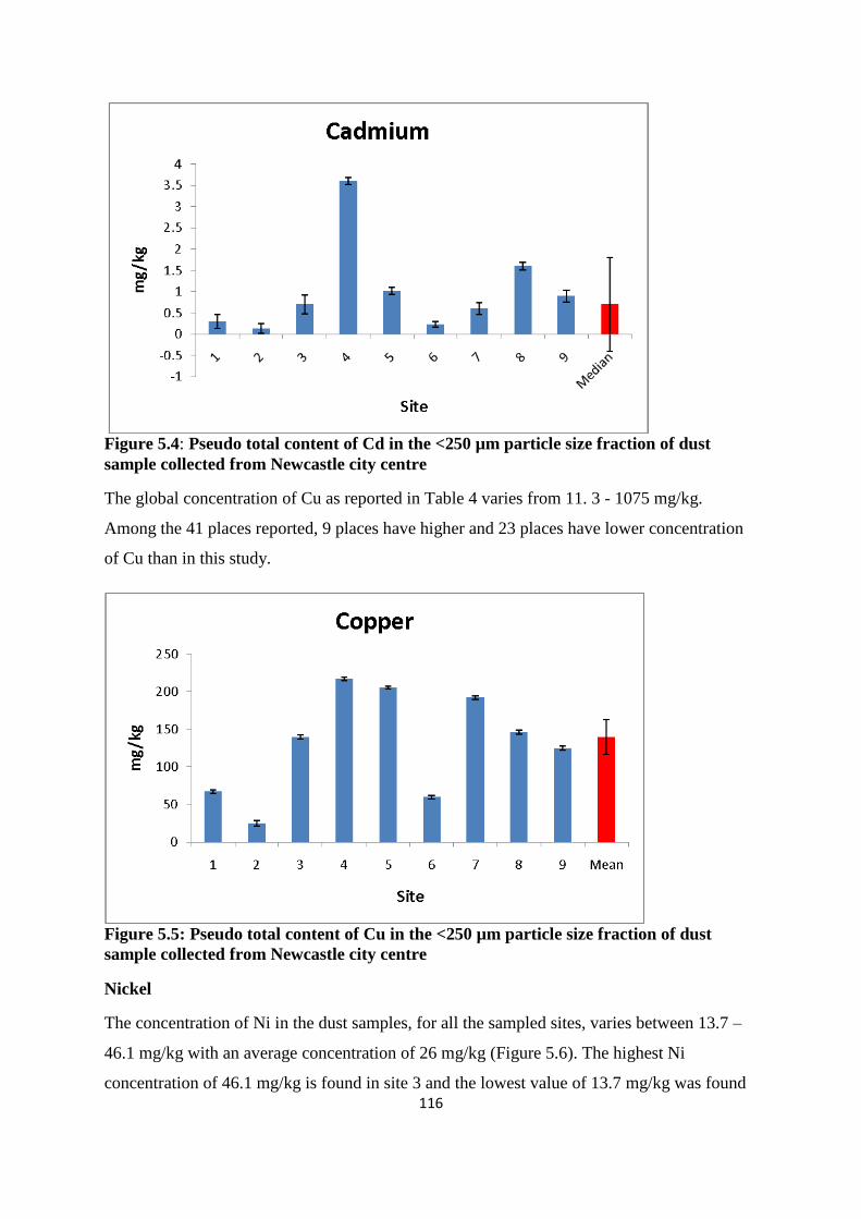
116

Figure 5.4: Pseudo total content of Cd in the <250 µm particle size fraction of dust

sample collected from Newcastle city centre

The global concentration of Cu as reported in Table 4 varies from 11. 3 - 1075 mg/kg.

Among the 41 places reported, 9 places have higher and 23 places have lower concentration

of Cu than in this study.

Figure 5.5: Pseudo total content of Cu in the <250 µm particle size fraction of dust

sample collected from Newcastle city centre

Nickel

The concentration of Ni in the dust samples, for all the sampled sites, varies between 13.7 –

46.1 mg/kg with an average concentration of 26 mg/kg (Figure 5.6). The highest Ni

concentration of 46.1 mg/kg is found in site 3 and the lowest value of 13.7 mg/kg was found

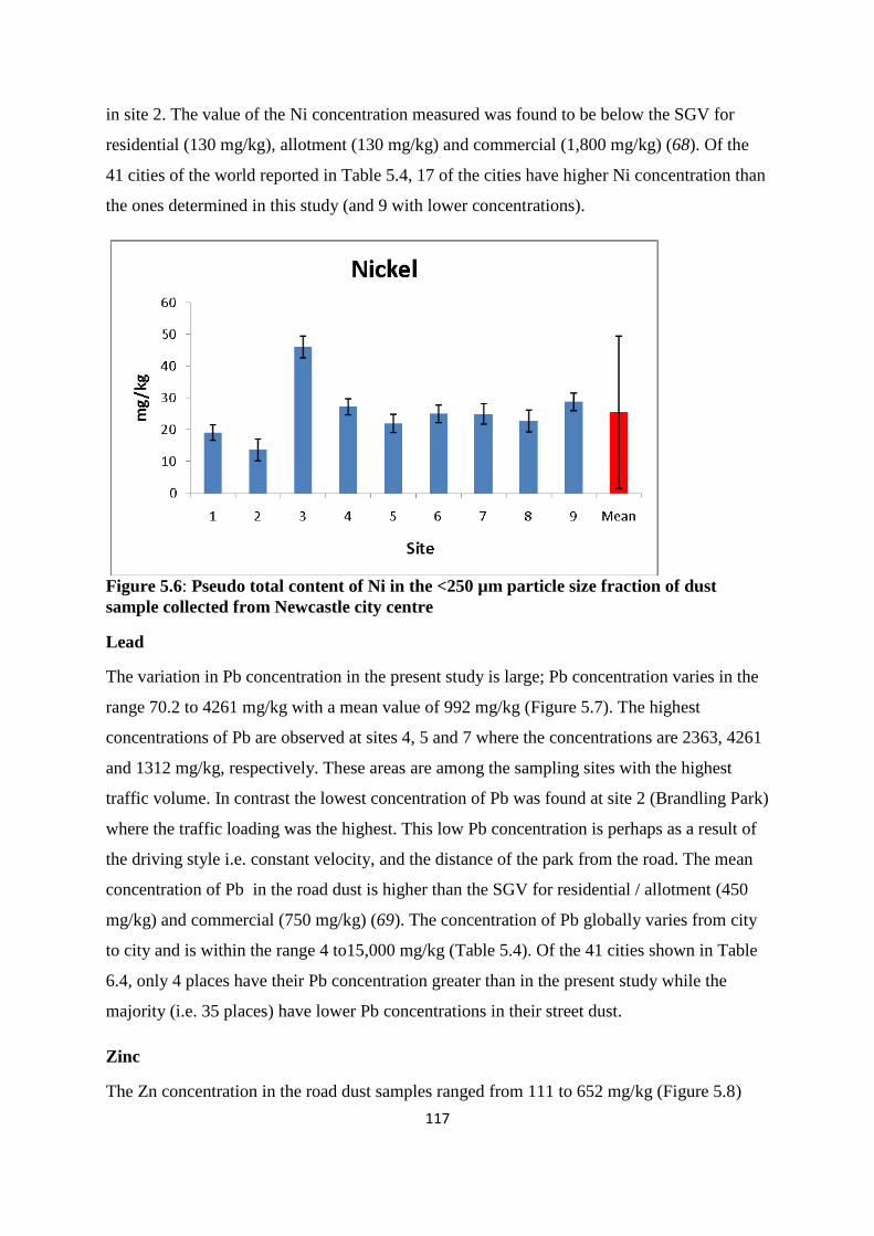
117

in site 2. The value of the Ni concentration measured was found to be below the SGV for

residential (130 mg/kg), allotment (130 mg/kg) and commercial (1,800 mg/kg) (68). Of the

41 cities of the world reported in Table 5.4, 17 of the cities have higher Ni concentration than

the ones determined in this study (and 9 with lower concentrations).

Figure 5.6: Pseudo total content of Ni in the <250 µm particle size fraction of dust

sample collected from Newcastle city centre

Lead

The variation in Pb concentration in the present study is large; Pb concentration varies in the

range 70.2 to 4261 mg/kg with a mean value of 992 mg/kg (Figure 5.7). The highest

concentrations of Pb are observed at sites 4, 5 and 7 where the concentrations are 2363, 4261

and 1312 mg/kg, respectively. These areas are among the sampling sites with the highest

traffic volume. In contrast the lowest concentration of Pb was found at site 2 (Brandling Park)

where the traffic loading was the highest. This low Pb concentration is perhaps as a result of

the driving style i.e. constant velocity, and the distance of the park from the road. The mean

concentration of Pb in the road dust is higher than the SGV for residential / allotment (450

mg/kg) and commercial (750 mg/kg) (69). The concentration of Pb globally varies from city

to city and is within the range 4 to15,000 mg/kg (Table 5.4). Of the 41 cities shown in Table

6.4, only 4 places have their Pb concentration greater than in the present study while the

majority (i.e. 35 places) have lower Pb concentrations in their street dust.

Zinc

The Zn concentration in the road dust samples ranged from 111 to 652 mg/kg (Figure 5.8)

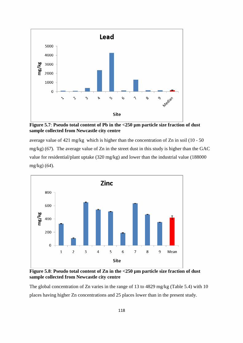
118

Figure 5.7: Pseudo total content of Pb in the <250 µm particle size fraction of dust

sample collected from Newcastle city centre

average value of 421 mg/kg which is higher than the concentration of Zn in soil (10 - 50

mg/kg) (67). The average value of Zn in the street dust in this study is higher than the GAC

value for residential/plant uptake (320 mg/kg) and lower than the industrial value (188000

mg/kg) (64).

Figure 5.8: Pseudo total content of Zn in the <250 µm particle size fraction of dust

sample collected from Newcastle city centre

The global concentration of Zn varies in the range of 13 to 4829 mg/kg (Table 5.4) with 10

places having higher Zn concentrations and 25 places lower than in the present study.

119

5.3.3 PTE concentration/traffic volume

Some researchers (70-71) have suggested a direct relationship between PTE levels and traffic

volume in the roadside environment while others (70) have demonstrated that driving style

may be more influential in affecting metal concentration. The results from this study suggest

that there appears to be no straightforward correlation between traffic volume and PTE

concentration. In general, higher PTE concentrations are found at sites where the

predominant driving style is stop/start (i.e. intersection and traffic lights); these locations

form either a major route to the city centre or are within the city centre and thus subject to

frequent traffic congestion. In contrast, the lower PTE concentrations were from samples with

high traffic volumes i.e. 14091 and 28885 vehicles per day at site 1 and site 2, respectively

(Table 5.1). At these sites the traffic is generally a constant flow. In addition, sample site 6

has the lowest volume of traffic but a higher PTE concentration than those with the highest

traffic flow (sites 1 and 2). This suggests that driving style has the most significant effect on

metal contamination in road side dust compared to traffic volume. Graphical relationship

between the traffic volume and pseudo total concentration of urban road dust is shown in

appendix F.

5.3.4 Inter-element relationship in road dust

In order to investigate any inter-element relationship in the road dust samples correlation

analysis was performed (Table 5.5). From the matrix generated (Table 5.5) it is evident that

some correlation exists between most PTEs investigated, except As. Strong positive

correlations exist between Cu and Cd (0.680), Pb and Cu (0.736), Zn and Cu (0.856) (Table

5.5). These significant positive correlation values may indicate that road dust contamination

by these PTEs (Cd, Cu, Ni, Pb and Zn) originated from common sources (e.g. automobiles)

while the lack of correlation between As and the other PTEs may be indicative of multiple or

independent sources. The moderate correlation value of 0.404 between As and Pb may imply

at least one common source e.g. traffic related.

5.3.5 Bioaccessibility of PTEs in urban street dust

The oral bioaccessibility of PTEs from the dust reference material (BCR 723) and the urban

dust samples were assessed using the in vitro PBET procedure. The percentage bioaccessible

fraction (% BAF) was calculated using the equation 4.1.

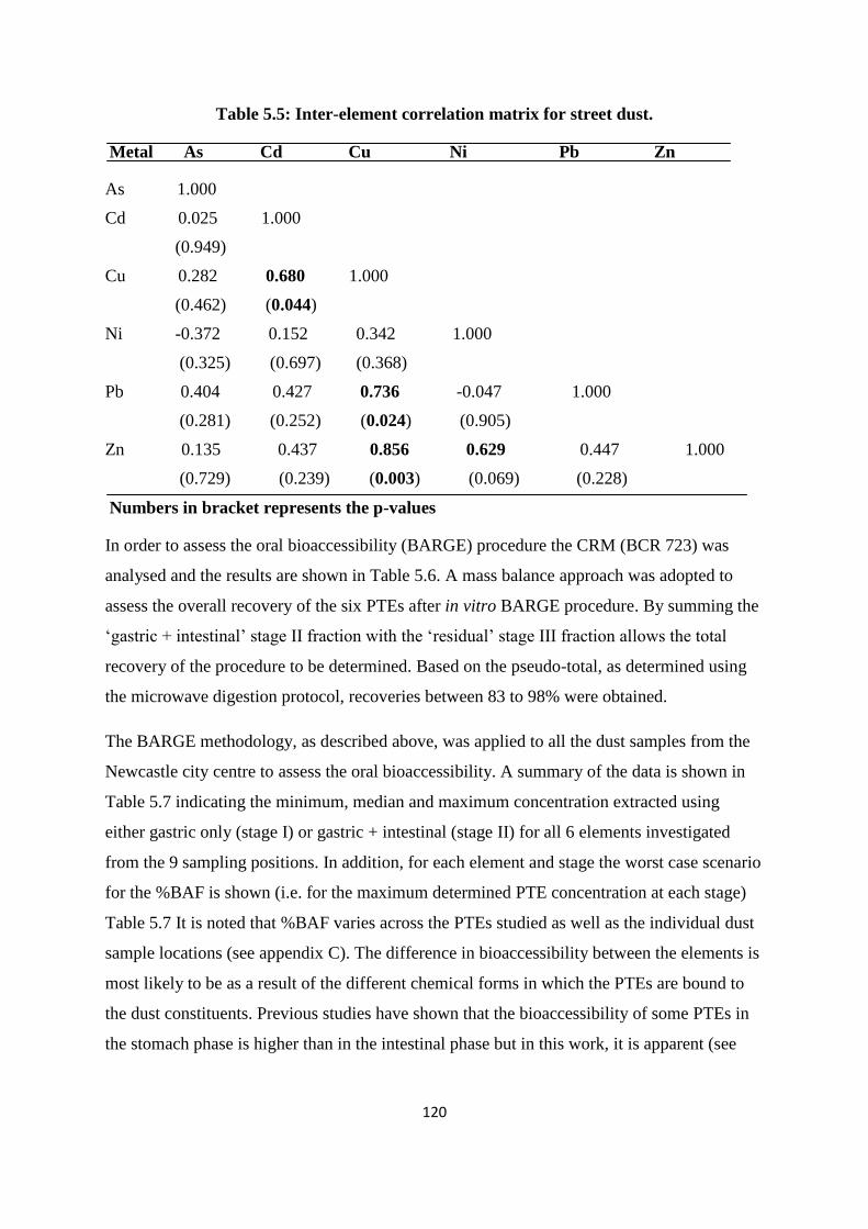
120

Table 5.5: Inter-element correlation matrix for street dust.

Metal As Cd Cu Ni Pb Zn

As 1.000

Cd 0.025 1.000

(0.949)

Cu 0.282 0.680 1.000

(0.462) (0.044)

Ni -0.372 0.152 0.342 1.000

(0.325) (0.697) (0.368)

Pb 0.404 0.427 0.736 -0.047 1.000

(0.281) (0.252) (0.024) (0.905)

Zn 0.135 0.437 0.856 0.629 0.447 1.000

(0.729) (0.239) (0.003) (0.069) (0.228)

Numbers in bracket represents the p-values

In order to assess the oral bioaccessibility (BARGE) procedure the CRM (BCR 723) was

analysed and the results are shown in Table 5.6. A mass balance approach was adopted to

assess the overall recovery of the six PTEs after in vitro BARGE procedure. By summing the

„gastric + intestinal‟ stage II fraction with the „residual‟ stage III fraction allows the total

recovery of the procedure to be determined. Based on the pseudo-total, as determined using

the microwave digestion protocol, recoveries between 83 to 98% were obtained.

The BARGE methodology, as described above, was applied to all the dust samples from the

Newcastle city centre to assess the oral bioaccessibility. A summary of the data is shown in

Table 5.7 indicating the minimum, median and maximum concentration extracted using

either gastric only (stage I) or gastric + intestinal (stage II) for all 6 elements investigated

from the 9 sampling positions. In addition, for each element and stage the worst case scenario

for the %BAF is shown (i.e. for the maximum determined PTE concentration at each stage)

Table 5.7 It is noted that %BAF varies across the PTEs studied as well as the individual dust

sample locations (see appendix C). The difference in bioaccessibility between the elements is

most likely to be as a result of the different chemical forms in which the PTEs are bound to

the dust constituents. Previous studies have shown that the bioaccessibility of some PTEs in

the stomach phase is higher than in the intestinal phase but in this work, it is apparent (see

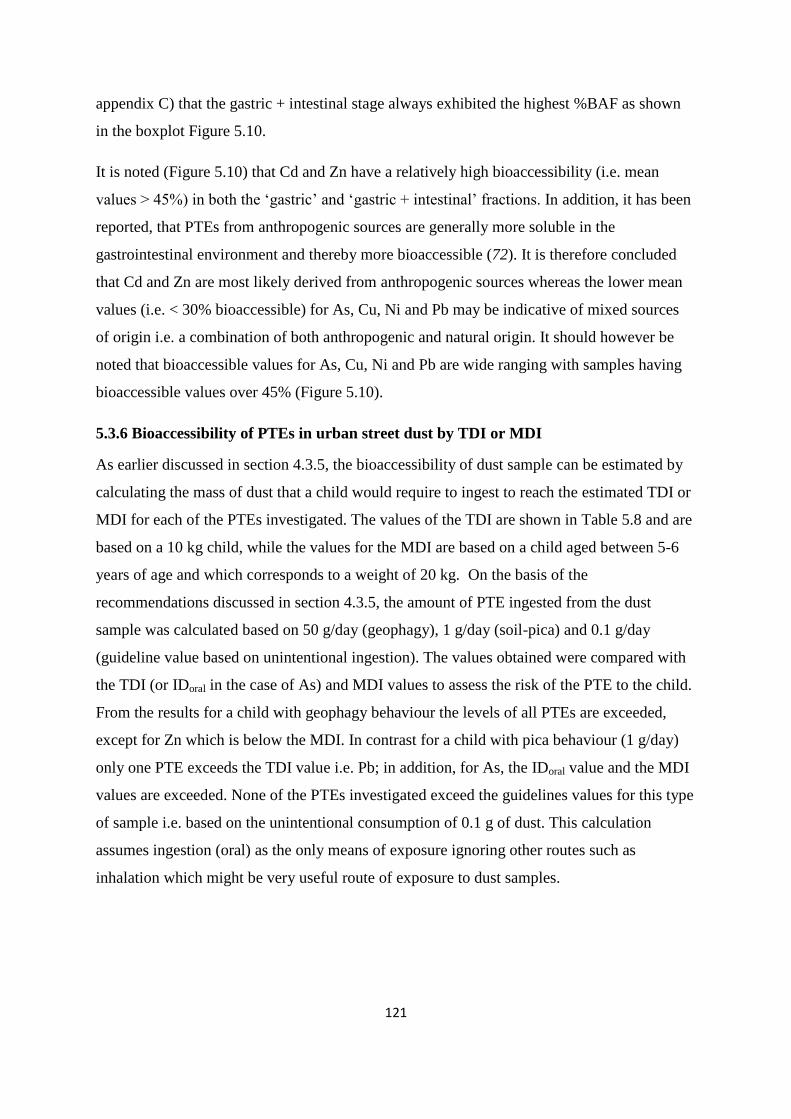
121

appendix C) that the gastric + intestinal stage always exhibited the highest %BAF as shown

in the boxplot Figure 5.10.

It is noted (Figure 5.10) that Cd and Zn have a relatively high bioaccessibility (i.e. mean

values > 45%) in both the „gastric‟ and „gastric + intestinal‟ fractions. In addition, it has been

reported, that PTEs from anthropogenic sources are generally more soluble in the

gastrointestinal environment and thereby more bioaccessible (72). It is therefore concluded

that Cd and Zn are most likely derived from anthropogenic sources whereas the lower mean

values (i.e. < 30% bioaccessible) for As, Cu, Ni and Pb may be indicative of mixed sources

of origin i.e. a combination of both anthropogenic and natural origin. It should however be

noted that bioaccessible values for As, Cu, Ni and Pb are wide ranging with samples having

bioaccessible values over 45% (Figure 5.10).

5.3.6 Bioaccessibility of PTEs in urban street dust by TDI or MDI

As earlier discussed in section 4.3.5, the bioaccessibility of dust sample can be estimated by

calculating the mass of dust that a child would require to ingest to reach the estimated TDI or

MDI for each of the PTEs investigated. The values of the TDI are shown in Table 5.8 and are

based on a 10 kg child, while the values for the MDI are based on a child aged between 5-6

years of age and which corresponds to a weight of 20 kg. On the basis of the

recommendations discussed in section 4.3.5, the amount of PTE ingested from the dust

sample was calculated based on 50 g/day (geophagy), 1 g/day (soil-pica) and 0.1 g/day

(guideline value based on unintentional ingestion). The values obtained were compared with

the TDI (or IDoral in the case of As) and MDI values to assess the risk of the PTE to the child.

From the results for a child with geophagy behaviour the levels of all PTEs are exceeded,

except for Zn which is below the MDI. In contrast for a child with pica behaviour (1 g/day)

only one PTE exceeds the TDI value i.e. Pb; in addition, for As, the IDoral value and the MDI

values are exceeded. None of the PTEs investigated exceed the guidelines values for this type

of sample i.e. based on the unintentional consumption of 0.1 g of dust. This calculation

assumes ingestion (oral) as the only means of exposure ignoring other routes such as

inhalation which might be very useful route of exposure to dust samples.

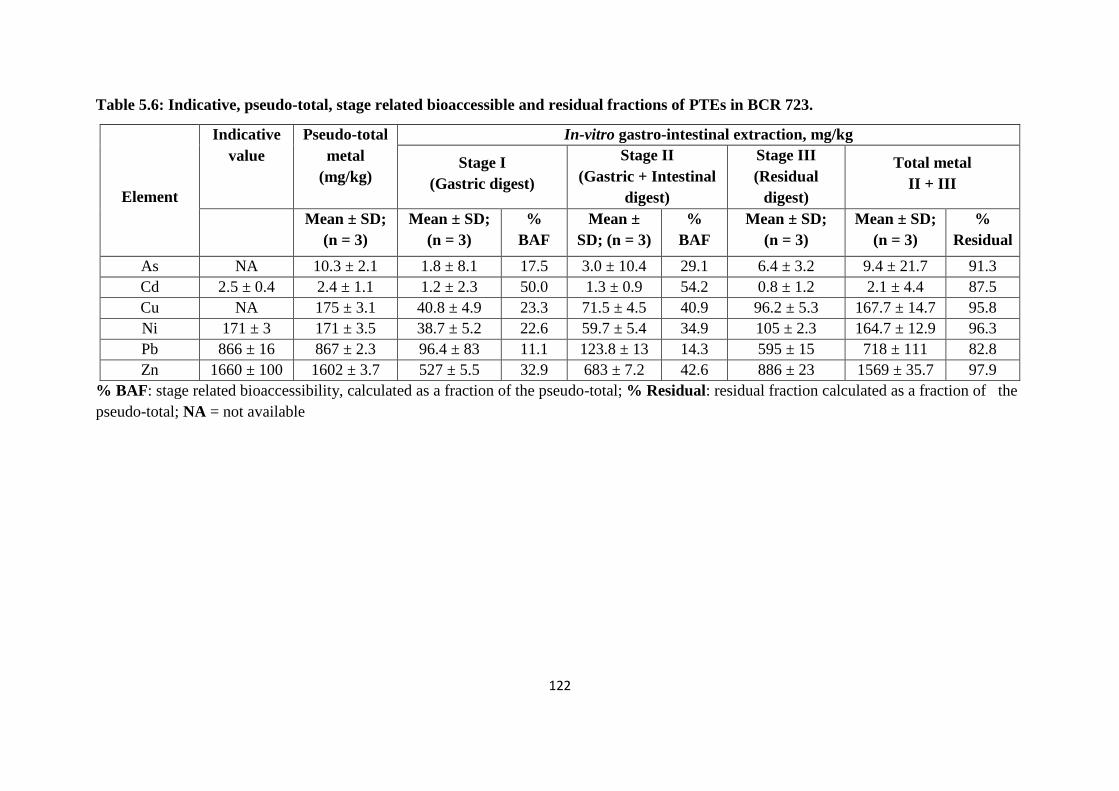
122

Table 5.6: Indicative, pseudo-total, stage related bioaccessible and residual fractions of PTEs in BCR 723.

Element

Indicative

value

Pseudo-total

metal

(mg/kg)

In-vitro gastro-intestinal extraction, mg/kg

Stage I

(Gastric digest)

Stage II

(Gastric + Intestinal

digest)

Stage III

(Residual

digest)

Total metal

II + III

Mean ± SD;

(n = 3)

Mean ± SD;

(n = 3)

%

BAF

Mean ±

SD; (n = 3)

%

BAF

Mean ± SD;

(n = 3)

Mean ± SD;

(n = 3)

%

Residual

As NA 10.3 ± 2.1 1.8 ± 8.1 17.5 3.0 ± 10.4 29.1 6.4 ± 3.2 9.4 ± 21.7 91.3

Cd 2.5 ± 0.4 2.4 ± 1.1 1.2 ± 2.3 50.0 1.3 ± 0.9 54.2 0.8 ± 1.2 2.1 ± 4.4 87.5

Cu NA 175 ± 3.1 40.8 ± 4.9 23.3 71.5 ± 4.5 40.9 96.2 ± 5.3 167.7 ± 14.7 95.8

Ni 171 ± 3 171 ± 3.5 38.7 ± 5.2 22.6 59.7 ± 5.4 34.9 105 ± 2.3 164.7 ± 12.9 96.3

Pb 866 ± 16 867 ± 2.3 96.4 ± 83 11.1 123.8 ± 13 14.3 595 ± 15 718 ± 111 82.8

Zn 1660 ± 100 1602 ± 3.7 527 ± 5.5 32.9 683 ± 7.2 42.6 886 ± 23 1569 ± 35.7 97.9

% BAF: stage related bioaccessibility, calculated as a fraction of the pseudo-total; % Residual: residual fraction calculated as a fraction of the

pseudo-total; NA = not available

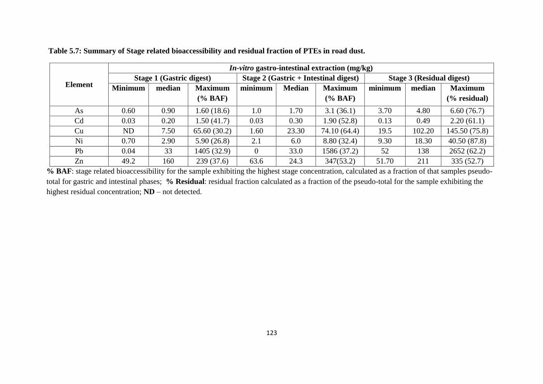
123

Table 5.7: Summary of Stage related bioaccessibility and residual fraction of PTEs in road dust.

Element

In-vitro gastro-intestinal extraction (mg/kg)

Stage 1 (Gastric digest) Stage 2 (Gastric + Intestinal digest) Stage 3 (Residual digest)

Minimum median Maximum

(% BAF)

minimum Median Maximum

(% BAF)

minimum median Maximum

(% residual)

As 0.60 0.90 1.60 (18.6) 1.0 1.70 3.1 (36.1) 3.70 4.80 6.60 (76.7)

Cd 0.03 0.20 1.50 (41.7) 0.03 0.30 1.90 (52.8) 0.13 0.49 2.20 (61.1)

Cu ND 7.50 65.60 (30.2) 1.60 23.30 74.10 (64.4) 19.5 102.20 145.50 (75.8)

Ni 0.70 2.90 5.90 (26.8) 2.1 6.0 8.80 (32.4) 9.30 18.30 40.50 (87.8)

Pb 0.04 33 1405 (32.9) 0 33.0 1586 (37.2) 52 138 2652 (62.2)

Zn 49.2 160 239 (37.6) 63.6 24.3 347(53.2) 51.70 211 335 (52.7)

% BAF: stage related bioaccessibility for the sample exhibiting the highest stage concentration, calculated as a fraction of that samples pseudo-

total for gastric and intestinal phases; % Residual: residual fraction calculated as a fraction of the pseudo-total for the sample exhibiting the

highest residual concentration; ND – not detected.

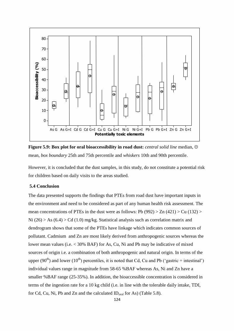
124

Zn G+IZn GPb G+IPb GNi G+INi GCu G+ICu GCd G+ICd GAs G+IAs G

80

70

60

50

40

30

20

10

0

Potentially toxic elements

Bio

acce

ssib

ility

(%

)

Figure 5.9: Box plot for oral bioaccessibility in road dust: central solid line median,

mean, box boundary 25th and 75th percentile and whiskers 10th and 90th percentile.

However, it is concluded that the dust samples, in this study, do not constitute a potential risk

for children based on daily visits to the areas studied.

5.4 Conclusion

The data presented supports the findings that PTEs from road dust have important inputs in

the environment and need to be considered as part of any human health risk assessment. The

mean concentrations of PTEs in the dust were as follows: Pb (992) > Zn (421) > Cu (132) >

Ni (26) > As (6.4) > Cd (1.0) mg/kg. Statistical analysis such as correlation matrix and

dendrogram shows that some of the PTEs have linkage which indicates common sources of

pollutant. Cadmium and Zn are most likely derived from anthropogenic sources whereas the

lower mean values (i.e. < 30% BAF) for As, Cu, Ni and Pb may be indicative of mixed

sources of origin i.e. a combination of both anthropogenic and natural origin. In terms of the

upper (90th

) and lower (10th

) percentiles, it is noted that Cd, Cu and Pb („gastric + intestinal‟)

individual values range in magnitude from 58-65 %BAF whereas As, Ni and Zn have a

smaller %BAF range (25-35%). In addition, the bioaccessible concentration is considered in

terms of the ingestion rate for a 10 kg child (i.e. in line with the tolerable daily intake, TDI,

for Cd, Cu, Ni, Pb and Zn and the calculated IDoral for As) (Table 5.8).

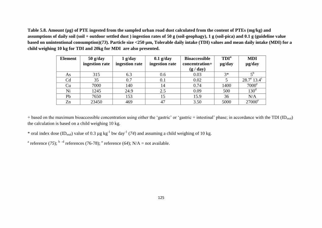
125

Table 5.8. Amount (µg) of PTE ingested from the sampled urban road dust calculated from the content of PTEs (mg/kg) and

assumptions of daily soil (soil + outdoor settled dust ) ingestion rates of 50 g (soil-geophagy), 1 g (soil-pica) and 0.1 g (guideline value

based on unintentional consumption)(73). Particle size <250 µm, Tolerable daily intake (TDI) values and mean daily intake (MDI) for a

child weighing 10 kg for TDI and 20kg for MDI are also presented.

Element 50 g/day

ingestion rate

1 g/day

ingestion rate

0.1 g/day

ingestion rate

Bioaccessible

concentration+

(g / day)

TDIa

µg/day

MDI

µg/day

As 315 6.3 0.6 0.03 3* 5b

Cd 35 0.7 0.1 0.02 5 28.7e 13.4

c

Cu 7000 140 14 0.74 1400 7000e

Ni 1245 24.9 2.5 0.09 500 130d

Pb 7650 153 15 15.9 36 N/A

Zn 23450 469 47 3.50 5000 27000e

+ based on the maximum bioaccessible concentration using either the „gastric‟ or „gastric + intestinal‟ phase; in accordance with the TDI (IDoral)

the calculation is based on a child weighing 10 kg.

* oral index dose (IDoral) value of 0.3 µg kg-1

bw day-1

(74) and assuming a child weighing of 10 kg.

a reference (75);

b –d

references (76-78); e reference (64); N/A = not available.

126

The results range between 0.02 and 15.9 g / day. In all cases, except for Pb, the bioaccessible

concentration is significantly below the guideline values based on unintentional consumption

(0.1 g / day). On that basis use of the bioaccessible concentration offers an alternate basis for

assessing risk to humans

References

1 Ferreira, B.L., DeMiguel, E. (2005). Geochemistry and risk assessment of street dust

in Launda, Angola: a tropical urban environment. Atmospheric Environment, 39, 4501

– 4512.

2 Shi, G., Chen, Z., Xu, S., Zhang, J., Wang, L., Bi, C., Teng, J. (2008). Potentially

toxic metal contamination of urban soils and roadside dust in Shanghai, China.

Environmental Pollution, 156, 251 – 266.

3 Howari, F.M., Abu-Rukah, Y., Goodell, P.C. (2004). Heavy metal pollution of soils

along north Shuna-Aqaba highway, Jordan. International Journal of Environment and

Pollution, 22, 597 – 607.

4 Li, X., Poon, C.S., Liu, P.S. (2001). Heavy metal contamination of urban soils and

street dusts in Hong Kong. Applied Geochemistry, 16, 1361 – 1368.

5 Mang, T., Dresel, W. (Ed.) (2007). Lubricants and Lubrication, 2nd

Ed., Wiley-VCH,

Weinheim, Germany.

6 Haus, N., Zimmermann, S., Wiegand, J., Sures, B. (2007). Occurrence of platinum

and additinoal traffic related heavy metal in sediments and biota. Chemosphere, 66(4),

619-629.

7 Barlow, P.L. (1999). The lead ban, lead replacement petrol, and the potential for

engine damage. Anti-Corrosion Methods and Materials, 46, 439-449.

8 Hu, X. (2002). Study of friction and wear performance of zinc dialkyldithiphosphate

in the presence of trace ketone. Tribology Letters, 12 (1), 67-74.

9 Yong, W. (2008). Synergistic lubricating effects of ZDDP with a hetrocyclic

compound. Industrial Lubrication and Tribology, 60(6), 317 – 320.

127

10 Hidayah, S., Amran, A.M. (2008). Comparison of Pt, Rh, Cu, Zn, Pb and Ni

concentration I road dust samples of genting sempah tunnel, Pahang. The Malaysian

Journal of Analytical Science, 12(2), 291-301.

11 Ferguson, J.E., Kim, N. (1991). Trace elements in street and house dusts source and

speciation. Science of the Total Environment, 100, 125 – 150.

12 Akhter, M.S., Madany, I.M. (1993). Heavy metal in street and house dust in Bahrain.

Water, Air and Soil Pollution, 66, 111 – 119.

13 Achilleas, C., Nikolaos, S. (2009). Heavy metal contamination in street dust and

roadside soil along the major national road in Kavalas region, Greece. Geoderma,

151, 257 – 263.

14 Abrahams, P.W. (2002). Soils: their implications to human health. Science of the

Total Environment, 291, 1 – 32.

15 Mielke, H.W., Gonzalez, C.R., Smith, M.K., Mielke, P.W. (1999). The urban

environment and children‟s health: Soil as an integrator of lead, zinc and cadmium in

New Orleans, Louisiana, USA. Environmental Research, 81, 117 – 129.

16 Emanuela, M., Daniela, V., Gaetano, D. (2006). Metal distribution in road dust

samples collected in an urban area close to a petrochemical plant at Gela, Sicily.

Atmospheric Environment, 40, 5929 – 5941.

17 Al-shayep, S.M., Seaward, M.R.D. (2001). Heavy metal content of roadside soils

along ring road in Riyadh, Saudi Arabia. Asian Journal of Chemistry, 13, 407 – 423.

18 Ndiokwere, C.L. (1984). A study of heavy metal pollution from motor vehicle

emissions and its effect on roadside soil, vegetation and crops in Nigeria.

Environmental Pollution, 7, 35 – 42.

19 Schwar, M.J.R., Moorcroft, J.S., Laxen, D.P.H., Thomson, M., Armorgie, C. (1988).

Baseline metal-in-dust concentrations in Greater London. Science of the Total

Environment, 68, 25 – 43.

128

20 Chen, T.B., Wong, J.W., Zhou, H.Y., Wong, M.H. (1997). Assessment of trace metal

distribution and contamination in surface soils of Hong Kong. Environmental

Pollution, 96, 61 – 68.

21 De Miguel, E., Llamas, J.F., Chacon, E., Berg, T., Larssen, S., Royset, O., Vadset, M.,

(1997). Origin and pattern of distribution of trace elements in street dust: unleaded

petrol and urban lead. Atmospheric Environment, 31(17), 2733 – 2740.

22 Wang, W.H., Wong, M.H., Leharne, S., Fisher, B. (1998). Fractionation and

biotoxicity of heavy metals in urban dusts collected from Hong Kong and London.

Environmental Geochemistry and Health, 20, 185 – 198.

23 Al-Khashman, O.A. (2007). Determination of metal accumulation in deposited street

dusts in Amman, Jordan. Environmental Geochemistry and Health, 29(1), 1 – 10.

24 Sezgin, N., Ozcan, H.K., Demir, G., Nemlioglu, S., Bayat, C. (2003). Determination

of heavy metal concentrations in street dusts in Istanbul E-5 highway. Environment

International, 29, 979 – 985.

25 Charlesworth, S., Everett, M., McCarthy, R., Ordonez, A., de Miguel, E. (2003). A

comparative study of heavy metal concentration and distribution in deposited street

dusts in large and small urban areas: Birmingham and Coventry, West Midlands, UK.

Environment International, 29, 563 – 573.

26 Faruque, A., Hawa,B.M., Hiroaki, I.(2007). Environmental assessment of Dhaka City

(Bangladesh) based on trace metal contents in road dusts. Environmental Geology, 51,

975 – 985.

27 Lu, X., Wang, L., Lei, K., Huang, J., Zhai, Y.(2009). Contamination assessment of

copper, lead, zinc, manganese and nickel in street dust of Baoji, NW China. Journal

of Hazardous Materials, 161, 1058 – 1062.

28 Ljung, K., Otabbong, E., Selinus, O. (2006). Natural and anthropogenic metal inputs

to soils in urban Uppsala, Sweden. Environmental Geochemistry and Health, 28, 353-

364.

129

29 Rodrigues, S., Urquhart, G., Hossack, I., Pereira, M.E., Duarte, A.C., Davidson, C.,

Hursthouse, A., Tucker, P., Robertson, D. (2009). The influence of anthropogenic and

natural geochemical factors on urban soil quality variability: a comparison between

Glasgow, UK and Aveiro, Portugal. Environmental Chemistry Letters, 7, 141-148.

30 Oomen, A.G., Hack, A., Minekus, M., Zeijdner, E., Schoeters, G., Verstraete, W.,

Wiele, T.V.D., Wragg, J., Rompelberg, C.J.M., Sips, A.J.A.M., Wijnen, J.H.V.

(2002). Comparison of Five in vitro Digestion Models to Study the Bioaccessibility of

Soil Contaminants. Environmental Science and Technology, 36, 3326 – 3334.

31 Lesniewska, B.A., Godlewska-Zylkiewicz, B., Bocca, B., Caimi, S., Hulanicki, A.

(2004). Platinum, Palladium and rhodium content in road dust, tunnel dust and

common grass in Bialystok area (Poland): A pilot study. Science of the Total

Environment, 321, 93 – 104.

32 Robertson, D.J., Taylor, K.G. (2007). Temporal variability of metal contamination in

urban road-deposited sediment in Manchester UK: Implications for urban pollution

Monitoring. Water, Air and Soil Pollution, 186, 209-220.

33 Wragg, J., Cave, M., Tayor, H., Basta, N., Brandon, E., Casteel, S., Oomen, A.

(2009). Inter-laborattory trial of a unified bioaccessibility procedure. Chemical and

biological hazards programme open report OR/07/027.

34 Bornschein, R.L., Succop, P.A., Kraft, K.M., Clark, C.S., Peace, B., Hammond, P.B.

(1987) Exterior surface dust lead, interior house dust lead and childhood lead

exposure in an urban environment. In: Hemphill, D.D. (Editor). Trace Substances in

Environmental Health XX: Proceedings of University of Missouri's 20th

Annual

Conference, Vol. 20, Columbia, MO, June 1986, pp. 322-332.

35 Han, Y., Du, P., Cao, J., Eric, S.P. (2006). Multivariate analysis of heavy metal

contamination in urban dusts of Xi an Central China. Science of the Total

Environment, 355, 176 – 186.

36 Harrisson, R.M. (1979). Toxic Metals in street and household dusts. Science of the

Total Environment, 11, 89 – 97.

130

37 Robertson, D.J., Taylor, K.C., Hoon, S.R. (2003). Geochemical and mineral magnetic

characterization of urban sediment particulates, Manchester, UK. Applied

Geochemistry, 18, 269 – 282.

38 Ordonez, A., Loredo, J., de Miguel, E., Charlesworth, S. (2003). Distribution of heavy

metals in street dust and soils of an industrial city in Northern Spain. Archives of

Environmental Contamination and Toxicology, 44, 160 – 170.

39 Pagotto, C., Remy, N., Legret, M., LeCloirec, P. (2001). Heavy metal pollution of

road dust and roadside soil near a major rural highway. Environmental Technology,

22, 307 – 319.

40 Varrica, D., Dongarra, G., Sabatino, G., Monna, F. (2003). Inorganic geochemistry of

roadway dust from the metropolitan area of Palermo, Italy. Environmental Geology,

44, 222 – 230.

41 Hjortenkrans, D., Bergback, B., Haggerud, A. (2006). New metal emission patterns in

road traffic environments. Environmental Monitoring and Assessment, 117, 85 – 98.

42 Yassoglou, N., Kosmas, C., Asimacopoulos, J., Kallianou, C. (1987). Heavy metal

contamination of roadside soils in the Greater Athens Area. Environmental Pollution,

47, 293 – 304.

43 Baptista, L.F., De Miguel, E. (2005). Geochemistry and risk assessment of street dust

in Launda, Angola. A tropical urban environment. Atmospheric Environment, 39(25),

4501 – 4512.

44 Tong, S.T.Y. (1998). Indoor and outdoor household dust contamination in Cincinnati,

Ohio, USA. Environmental Geochemistry and Health, 20, 123 – 133.

45 Sutherland, R.A., Tolosa, C.A. (2000). Multi-element analysis of road deposited

sediment in an urban drainage basin, Honolulu, Hawaii. Environmental Pollution,

110, 483 – 495.

46 Rasmussen, P.E., Subramanian, S.K., Jessiman, B.J. (2001). A multi-element profile

of house dust in relation to exterior dust and soils in the city of Ottawa, Canada.

Science of the Total Environment, 267, 125 – 140.

131

47 Meza-Figueroa, D., O-Villanueva, M.D., Parra, M.L.D. (2007). Heavy metal

distribution in dust from elementary schools in Hermosillo, Sonora, Mexico.

Atmospheric Environment, 41, 276 – 288.

48 Han, L., Zhuang, G., Cheng, S., Wang, Y., Li. J. (2007). Characteristics of re-

suspended road dust and its impact on the atmospheric environment in Beijing.

Atmospheric Environment, 41, 7485 – 7499.

49 Duzgoren-Aydrin, N.S., Wong, C.S.C., Aydin, A., Song, Z., You, M., Li, X.D.

(2006). Heavy metal contamination and distribution in the urban environment of

Guangbzhou, SE China. Environmental Geochemistry and Health, 28, 375 – 391.

50 Yeung, Z.L.L., Kwok, R.C.W., Yu, K.N. (2003). Determination of multi-element

profiles of street dust using energy dispersive X-ray florescence EDXRF. Applied

Radiation and Isotopes, 58, 339 – 346.

51 Yongming, H.D., Junji, C., Posmentier, E.S. (2006). Multivariate analysis of heavy

metal contamination in urban dusts of Xian, Central China. Science of the Total

Environment, 355, 176 – 186.

52 Tokalioglu, S., Kartal, S. (2006). Multivariant analysis of the data and speciation of

heavy metals in street dust samples from the organized industrial district in Kayseri,

Turkey. Atmospheric Environment, 40, 2797 – 2805.

53 Elik, A. (2003). Heavy metal accumulation in street dust samples in Sivas.

Communications in Soil Science and Plant Analysis, 34, 145 – 156.

54 Divrikli, V., Soylak, M., Elic, L., Dogan, M. (2005). Trace heavy metal levels in

street dust sample from Yozgat city centre, Turkey. Journal of Trace and Microprobe

Techniques, 21, 351 – 361.

55 Al-Khashman, O.A. (2007). Investigation of metal concentrations in street dust

samples in Aqaba city, Jordan. Environmental Geochemistry and Health, 29(1), 197 –

207.

132

56 Al-Khashman, O.A. (2004). Heavy metal distribution in dust, street dust and soils

from the work place in Karak Industrial Estate, Jordan. Atmospheric Environment, 38,

6803 – 6812.

57 Ahmed, F., Ishiga, H. (2006). Trace metal concentrations in street dusts of Dhaka city

in Bangladesh. Atmospheric Environment, 40, 3835 – 3844.

58 Ramain, M.N., Badri, M.A. (1989). Heavy metals in tropical city street dust and

roadside soils: a case of Kuala Lumpur, Malaysia. Environmental Technology Letters,

10, 435 – 444.

59 Hewitt, C.N., Candy, G.B.B. (1990). Soil and street dust heavy metal concentrations

in and around Cuenca, Ecuador. Environmental Pollution, 63, 129 – 136.

60 Yasir, F., Tufail, M., Tayyeb, J.M., Chaudhry, M.M., Siddique, N. (2009). Road dust

pollution of Cd, Cu, Ni, Pb and Zn along Islamabad Expressway, Pakistan.

Microchemical Journal, 92, 186 – 192.

61 Chatterjee, A., Banerjee, R.N. (1999). Determination of lead and other metals in

residential area of greater Calcutta. Science of the Total Environment, 227, 175 – 185.

62 Kim, K.M., Myung, J.H., Ahn, J.S., Chon, H.T. (1998). Heavy metal speciation in

dusts and stream sediments in Taejon area, Korea. Journal of Geochemical

Exploration, 64, 409 – 419.

63 Environment Agency (2002). Soil guidelines values for metal contamination, R&D

Publication SGV. Available at: http://www.environment-agency.gov.uk/. March 2009.

64 Nathanial, C P., Mc Affrey, C., Ashmore, M., Cheng, Y., Gilett, A., Hooker, P.,

Ogden, R C. (2009). Generic Assessment Criteria for Human Health Risk

Assessment, 2nd

Ed., Nottingham, UK. Land Quality Press.

65 Environmental Agency (2009). Soil Guideline Values for arsenic in soil. Science

Report SC050021/Arsenic SGV.

66 Environmental Agency (2009). Soil Guideline Values for cadmium in soil. Science

Report SC050021/Cadmium SGV.

133

67 Sezgin, N., Ozcan, H.K., Demir, G., Nemlioglu, S., Bayat, C. (2003). Determination

of heavy metal concentrations in street dusts in Istanbul E-5 highway. Environmental

International, 29, 979 – 985.

68 Environmental Agency (2009). Soil Guideline Values for nickel in soil. Science

Report SC050021/Nickel SGV.

69 DEFRA (Department for Environment, Food and Rural Affairs). The Environmental

Agency (2002). Soil Guideline Values for lead contamination. R&D publication SGV

10.

70 Whiteley, J. D., Murray, F. (2003). Anthropogenic metal concentrations in road dusts

and roadside soils from Perth, Western Australia. Science of the Total Environment,

317, 121-135.

71 Ely, J. C., Neal, C. R., Kulpa, C. F., Schneegurt, M. A., Seidler, J. A., Jain, J. C.

(2001). Implications of metal accumulation along U. S. roads from catalytic converter

attrition. Environmental Science Technology, 35, 3816-3822.

72 Ljung. K., Oomen. A., Duits. M., Selinus. O., Berglund. M. (2007) Bioaccessibility

of metals in urban playground soils. Journal of Environmental Science and Health

Part A, 42, 1241-1250.

73 U.S. EPA. (2008). Child-Specific Exposure Factors Handbook (Final Report) 2008.

U.S. Environmental Protection Agency, Washington, DC, EPA/600/R-06/096F.

74 Environmental Agency. (2010). Contaminants in soil: updated collation of

toxicological data and intake values for humans inorganic arsenic. Science report:

SC050021/TOX 1.

75 Karin, L., Olle, S., Erasmus, O., Marika, B. (2006). Metal and arsenic distribution in

soil particle sizes relevant to soil ingestion by children. Applied Geochemistry, 21,

1613-1624.

76 Environmental Agency (2010). Contaminants in soil: updated collation of

toxicological data and intake values for humans inorganic arsenic. Science report:

SC050021/TOX 1.

134

77 Environmental Agency (2010). Contaminants in soil: updated collation of

toxicological data and intake values for humans inorganic cadmium. Science report:

SC050021/TOX 3.

78 Environmental Agency (2010). Contaminants in soil: updated collation of

toxicological data and intake values for humans inorganic Nickel. Science report:

SC050021/TOX 8.

135

Chapter Six: Influence of particle size on the distribution of platinum

group elements (PGEs) in urban street dust/sediments

6.1 Introduction

The PGEs comprise iridium (Ir), osmium (Os), palladium (Pd), platinum (Pt), rhodium (Rh)

and ruthenium (Ru). These elements are all transition metals lying in the d-block (Group 8, 9

and 10 and period 5 and 6). Platinum and Pd are found in their pure state in nature (1). The

other four elements Ir, Os, Rh and Ru occur as alloys of Pt and Au (2). Platinum group

elements are mined in South Africa, Siberia and Sudbury, Ontario. The concentration of

PGEs in the lithosphere is among the lowest, with the average estimated to be in the range of

0.001–0.005 mg/kg for Pt; 0.015 mg/kg for Pd; 0.0001 mg/kg for Rh; 0.0001 mg/kg for Ru;

0.005 mg/kg for Os; and 0.001 mg/kg for Ir (3, 2, 4). Worldwide production of PGEs has

been steadily increasing since 1970. This reflects the growing worldwide use of PGEs (5). Of

the six PGEs, the ones of interest for this study are Pd, Pt and Rh because of their use in the

construction of catalytic converters used in the automobiles. The total worldwide supply in

1999 and 2000, as shown in Table 6.1, was 265 and 238 tonnes for Pd; 156 and 164 tonnes

for Pt; 14.9 and 16.2 tonnes for Rh; respectively (6). In 2001 the highest published value for

Pt in road dust was 2.252 mg/kg (7) and that of Pd was 0.556 mg/kg (8).The use of PGEs,

reported in literature, is a cause of concern because relatively little is known about the

mobility, toxicity and bioaccumulation processes of PGEs (9).

Platinum group elements have various applications one of which is their use in the

construction of catalytic converters. The properties of PGEs which makes them suitable to be

used as catalytic converter include: - (i) outstanding catalytic properties (ii) resistance to

chemical attack (iii) stable electrical properties (iv) high corrosion resistance (v) low

coefficient of thermal expansion (vi) high melting point (vii) high mechanical strength.

Platinum group elements released from the catalytic converters are primarily bound to

aluminium oxide particle (10, 11). They were until recently, regarded as inert elements but

recent studies have shown that they may be soluble and quite reactive (12).

The main emissions of automobile engines are N2, CO2 and H2O. These emissions are mainly

non harmful to human health however, because combustion is never perfect, smaller amounts

of more harmful emissions are also produced namely carbon monoxide (CO), hydrocarbons

(HC) or volatile organic compounds (VOCs) and oxides of nitrogen (NOx). These gases are

the largest source of ground level ozone which is responsible for smog formation, respiratory

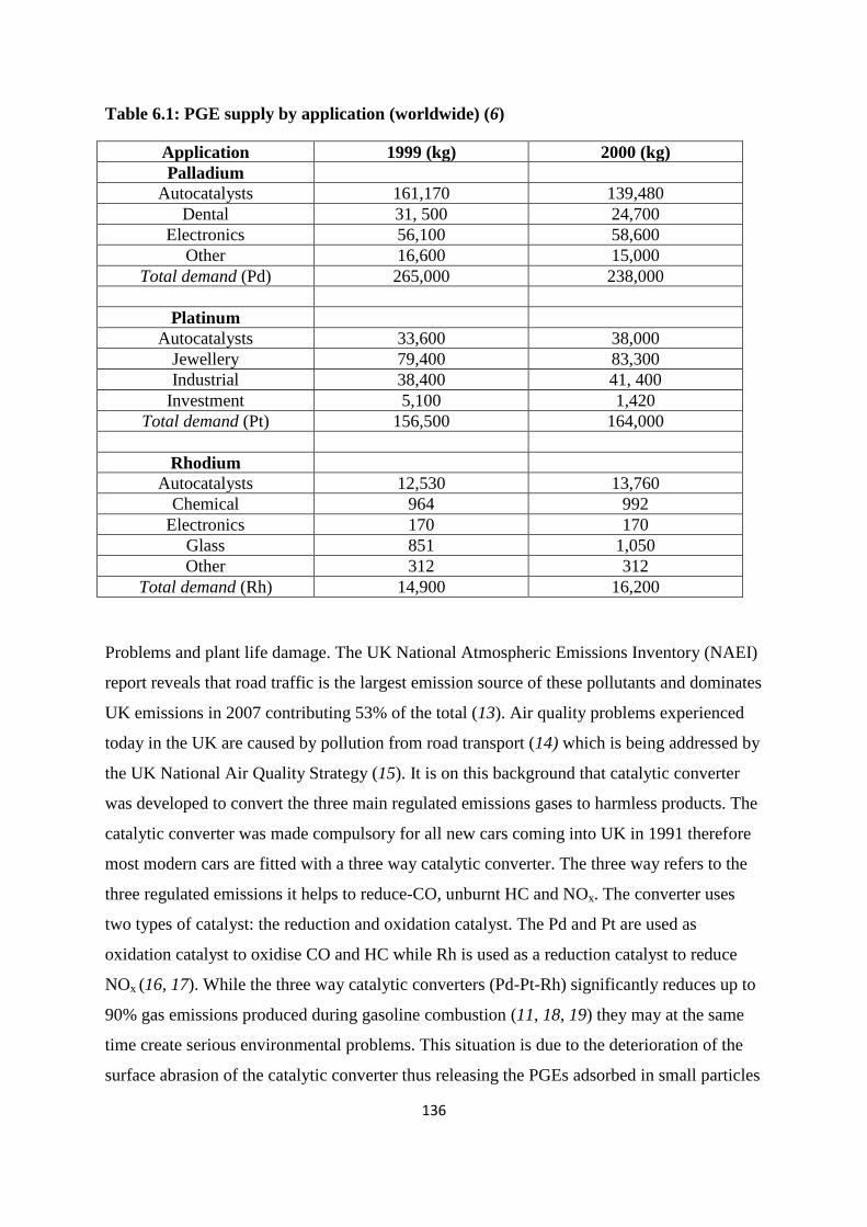
136

Table 6.1: PGE supply by application (worldwide) (6)

Application 1999 (kg) 2000 (kg)

Palladium

Autocatalysts 161,170 139,480

Dental 31, 500 24,700

Electronics 56,100 58,600

Other 16,600 15,000

Total demand (Pd) 265,000 238,000

Platinum

Autocatalysts 33,600 38,000

Jewellery 79,400 83,300

Industrial 38,400 41, 400

Investment 5,100 1,420

Total demand (Pt) 156,500 164,000

Rhodium

Autocatalysts 12,530 13,760

Chemical 964 992

Electronics 170 170

Glass 851 1,050

Other 312 312

Total demand (Rh) 14,900 16,200

Problems and plant life damage. The UK National Atmospheric Emissions Inventory (NAEI)

report reveals that road traffic is the largest emission source of these pollutants and dominates

UK emissions in 2007 contributing 53% of the total (13). Air quality problems experienced

today in the UK are caused by pollution from road transport (14) which is being addressed by

the UK National Air Quality Strategy (15). It is on this background that catalytic converter

was developed to convert the three main regulated emissions gases to harmless products. The

catalytic converter was made compulsory for all new cars coming into UK in 1991 therefore

most modern cars are fitted with a three way catalytic converter. The three way refers to the

three regulated emissions it helps to reduce-CO, unburnt HC and NOx. The converter uses

two types of catalyst: the reduction and oxidation catalyst. The Pd and Pt are used as

oxidation catalyst to oxidise CO and HC while Rh is used as a reduction catalyst to reduce

NOx (16, 17). While the three way catalytic converters (Pd-Pt-Rh) significantly reduces up to

90% gas emissions produced during gasoline combustion (11, 18, 19) they may at the same

time create serious environmental problems. This situation is due to the deterioration of the

surface abrasion of the catalytic converter thus releasing the PGEs adsorbed in small particles

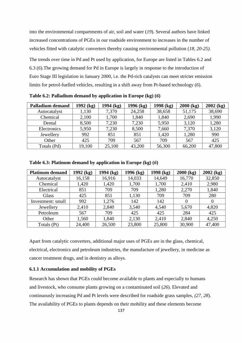
137

into the environmental compartments of air, soil and water (19). Several authors have linked

increased concentrations of PGEs in our roadside environment to increases in the number of

vehicles fitted with catalytic converters thereby causing environmental pollution (18, 20-25).

The trends over time in Pd and Pt used by application, for Europe are listed in Tables 6.2 and

6.3 (6).The growing demand for Pd in Europe is largely in response to the introduction of

Euro Stage III legislation in January 2000, i.e. the Pd-rich catalysts can meet stricter emission

limits for petrol-fuelled vehicles, resulting in a shift away from Pt-based technology (6).

Table 6.2: Palladium demand by application in Europe (kg) (6)

Palladium demand 1992 (kg) 1994 (kg) 1996 (kg) 1998 (kg) 2000 (kg) 2002 (kg)

Autocatalyst 1,130 7,370 24,258 38,658 51,175 38,690

Chemical 2,100 1,700 1,840 1,840 2,690 1,990

Dental 8,500 7,230 7,230 5,950 3,120 1,280

Electronics 5,950 7,230 8,500 7,660 7,370 3,120

Jewellery 992 851 851 1,420 1,280 990

Other 425 709 567 709 567 425

Totals (Pd) 19,100 25,100 43,200 56,300 66,200 47,800

Table 6.3: Platinum demand by application in Europe (kg) (6)

Platinum demand 1992 (kg) 1994 (kg) 1996 (kg) 1998 (kg) 2000 (kg) 2002 (kg)

Autocatalyst 16,158 16,916 14,033 14,649 16,770 32,850

Chemical 1,420 1,420 1,700 1,700 2,410 2,980

Electrical 851 709 709 1,280 2,270 1,840

Glass 425 851 1,130 709 709 280

Investment: small 992 1,276 142 142 0 0

Jewellery 2,410 2,840 3,540 4,540 5,670 4,820

Petroleum 567 709 425 425 284 425

Other 1,560 1,840 2,130 2,410 2,840 4,250

Totals (Pt) 24,400 26,500 23,800 25,800 30,900 47,400

Apart from catalytic converters, additional major uses of PGEs are in the glass, chemical,

electrical, electronics and petroleum industries, the manufacture of jewellery, in medicine as

cancer treatment drugs, and in dentistry as alloys.

6.1.1 Accumulation and mobility of PGEs

Research has shown that PGEs could become available to plants and especially to humans

and livestock, who consume plants growing on a contaminated soil (26). Elevated and

continuously increasing Pd and Pt levels were described for roadside grass samples, (27, 28).

The availability of PGEs to plants depends on their mobility and these elements become

138

mobile under acidic soil water conditions, a fact which increases their uptake by plants (1).

PGEs emitted into the environment, may form soluble compounds able to be absorbed by

plants, thus creating the possibility for their presence in the food chain. Catalyst converter

emitted PGEs, may undergo rapid transformations in the environment, and subsequently

behave similarly to soluble PGE salts (21). Hoppstock and Sures 2004 (29) in their review

demonstrated biological availability of soluble and particle bound PGEs to plants and

animals. Laboratory studies with mussels exposed to road dust revealed an increasing

biological availability of PGEs in the following order: Rh > Pt > Pd (30). Similar results

were obtained by Schafer and Punchelt 1998 (31) when demonstrating that plants can

assimilate Pd, Pt and Rh. Tankari et al. 2007 (32) found that Pd and Rh concentrations

increased with the time of plant exposure to PGE pollution.

6.1.2 Health risk effects of PGEs

The health effect of PGEs toxicity is exemplified by Pt. Platinum was believed to be

chemically inert. However, this was not true as recent evidence suggests that Pt in the

environment can be ionized into forms that are environmentally and biologically active (12).

Platinum group elements which are released from catalytic converters are primarily bound to

aluminium oxide particles (10). Up to 36% of these particles have a size <3 μm (33), and

therefore reach lung alveolaries. Platinum in road dust can be solubilized, and enters the

waters, sediments, soils and the food chain. Certain Pt compounds are also known to be

cytotoxic and have mutagenic and carcinogenic effects which will have some effects on

microorganisms at very low concentrations (5, 34). In addition, some Pt complexes can bind

to N and S in proteins producing a reduction in enzymatic activity (6). Though initially

automobile emitted PGEs were thought of as being inert biologically, recent studies have

shown the biological availability of not only soluble, but also of particle bound PGEs, to

plants and animals (35, 30).

Adverse occupational health effects following exposure to complex salts of Pt were first

observed in 1911 in a photographic studio (1). Studies conducted on precious metal workers

in four British Pt refineries revealed that 52 out of 91 persons had symptoms of sneezing,

wheezing and shortness of breath (36). Platinum compounds, especially the soluble salts,

such as ammonium tetrachloroplatinite(II) and ammonium hexachloroplatinate(IV) used in

the production of industrial catalysts (37) are toxic, and chronic industrial exposure to them is

139

responsible for the development of a syndrome known as Platinosis, which is characterized

by the respiratory and cutaneous hypersensitivity (34).

The first efforts towards understanding the PGEs risk effects was to analyze the body fluids

for the basic three noble elements in people occupationally involved in PGEs manufacturing.

Employees exposed during the production and recycling of Pt-based catalytic converters

revealed Pt levels in urine and blood up to 100 times higher than those of non-exposed

individuals (34). In general the Pt(II), Pt(V) and Pd (II) toxic effects on the cellular level are

comparable to the toxic effects of Cd(II) and Cr(VI), sometimes even exceeding the damage

induced by the above species of Cd and Cr (38).

Whereas numerous studies have concentrated on the heavy metal (e.g. Pb or Cd)

concentration in the environment, relatively few studies focus on PGE (30). Following the

potential health risk associated with PGEs and the accumulation and mobility of these

precious metals in environmental matrices, this work focuses on PGE concentration in the

environmental matrix of urban road dust and the influence of particle size on the distribution

of these elements.

6.2 Experimental

6.2.1 Sampling and sample preparation

The sampling procedure is as described in 5.2.1 and sample location shown in Figure 5.1

Apart from the simplicity of using hand via sweeping, as opposed to a vacuum cleaner, part

of this study was to investigate the PGE concentration according to particle size and the

vacuum cleaner only samples particles finer than 250 µm thereby excluding the coarse

particles needed for grain size analysis. Description of the sample sites are shown in Table

6.4. The dried samples were sieved through a plastic sieve of mesh size 2 mm to remove

gravel, refuse and stones. Fractional size coarser than 2 mm was of limited importance when

considering metal contaminants (39, 9). Only 3% of labile Pb is held in the 1000 – 2000 µm

fractions and the remaining 97% labile Pb is in the 0 – 1000 µm fractions (9). It was on this

basis that some of the samples (8, 14 and 15: the large ones) were fractionated into six size

fractions with their sedimentological equivalent in parenthesis: 1000-2000 µm (very coarse

sand), 500-1000 µm (Coarse sand), 250-500 µm (medium sand), 125-250 µm (fine sand), 63-

125 µm (very fine sand) and <63 µm (silt and clay). All the samples (8, 9, 11, 13-15, 17-19)

were passed through the 250 µm mesh size to separate between <250 and >250 µm. The dry

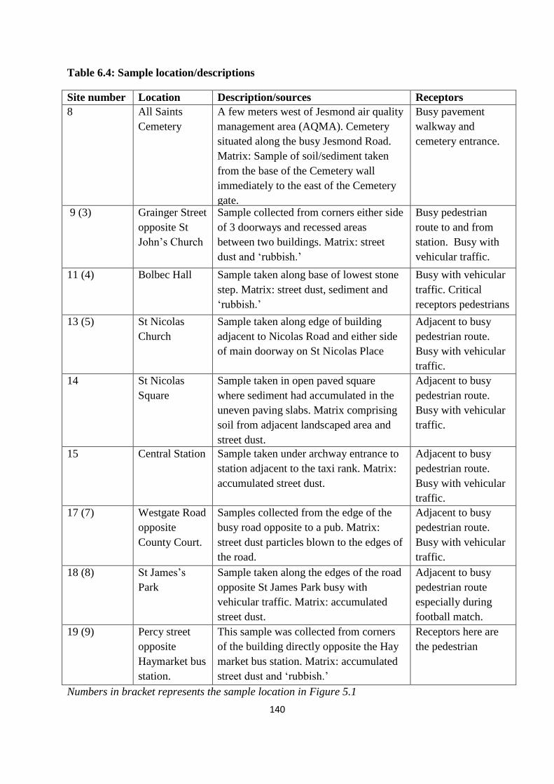
140

Table 6.4: Sample location/descriptions

Site number Location Description/sources Receptors

8 All Saints

Cemetery

A few meters west of Jesmond air quality

management area (AQMA). Cemetery

situated along the busy Jesmond Road.

Matrix: Sample of soil/sediment taken

from the base of the Cemetery wall

immediately to the east of the Cemetery

gate.

Busy pavement

walkway and

cemetery entrance.

9 (3) Grainger Street

opposite St

John‟s Church

Sample collected from corners either side

of 3 doorways and recessed areas

between two buildings. Matrix: street

dust and „rubbish.‟

Busy pedestrian

route to and from

station. Busy with

vehicular traffic.

11 (4) Bolbec Hall

Sample taken along base of lowest stone

step. Matrix: street dust, sediment and

„rubbish.‟

Busy with vehicular

traffic. Critical

receptors pedestrians

13 (5) St Nicolas

Church

Sample taken along edge of building

adjacent to Nicolas Road and either side

of main doorway on St Nicolas Place

Adjacent to busy

pedestrian route.

Busy with vehicular

traffic.

14 St Nicolas

Square

Sample taken in open paved square

where sediment had accumulated in the

uneven paving slabs. Matrix comprising

soil from adjacent landscaped area and

street dust.

Adjacent to busy

pedestrian route.

Busy with vehicular

traffic.

15 Central Station

Sample taken under archway entrance to

station adjacent to the taxi rank. Matrix:

accumulated street dust.

Adjacent to busy

pedestrian route.

Busy with vehicular

traffic.

17 (7) Westgate Road

opposite

County Court.

Samples collected from the edge of the

busy road opposite to a pub. Matrix:

street dust particles blown to the edges of

the road.

Adjacent to busy

pedestrian route.

Busy with vehicular

traffic.

18 (8) St James‟s

Park

Sample taken along the edges of the road

opposite St James Park busy with

vehicular traffic. Matrix: accumulated

street dust.

Adjacent to busy

pedestrian route

especially during

football match.

19 (9) Percy street

opposite

Haymarket bus

station.

This sample was collected from corners

of the building directly opposite the Hay

market bus station. Matrix: accumulated

street dust and „rubbish.‟

Receptors here are

the pedestrian

Numbers in bracket represents the sample location in Figure 5.1

141

sieved samples were sub-sampled using cone and quarter prior to undergoing further analysis.

6.2.2 Instrument and reagents

Concentrated HCl and HNO3 were obtained from Romil Limited Cambridge. A multi-

element standard containing Ir, Pd, Pt and Rh was purchased from SPEXCertPrep

(Middlesex, UK). Ultra pure water of conductivity 18.2MΩ-cm was produced by a direct Q™

millipore system (Molsheim, France). A road dust certified reference material was used (BCR

723 No 114) supplied by the institute for reference materials and measurements (Certified

2002, Revised 2008). Poly-prep chromatography columns and AG® 50W-X8 cation exchange

resin 200 – 400 mesh size from Bio-rad laboratories Hercules Canada were used. An

evaporating unit for Reacti-Therm™ heating models (containing Reacti-vap™ teflon®

coated needles 4” (102 mm) x 19 gauge and Reacti-Therm™ heating module) and vortex

mixer were from Fisher Scientific UK Ltd. (Loughborough, Leicestershire). Other

instruments were specimen tubes made of soda glass with stopper, retort stand with clamps,

glass measuring cylinder (A grade), volumetric flask (A grade) and eppendorf micro pipette.

Dust samples were collected from locations across Newcastle city centre and local environs.

ICP-MS measurements were carried out with an ICP mass spectrometer X series II (Thermo

Electron Corporation, Cheshire, UK). All digestions were carried out using a Start D

multiprep 42 high throughput rotor microwave digestion system supplied by Milestone

Microwave Laboratory Systems UK. The weighing balance used was Explorer Ohaus model

E406 00032 from Switzerland.

6.2.3 Preparation of cation exchange resin and separation columns

All plastic containers used were soaked in an acid bath for about one week prior to the

preparation. They were rinsed with ultra pure water and allowed to dry before being used.

250g of AG 50 – X8 200 -400 mesh cation exchange resin was placed into a pre-cleaned one

litre plastic container. 250 mL 6M HCl was added to the container and was shaken to allow

mixing. This solution was allowed to stand overnight. The next morning the 6M HCl was

decanted from the mixture and replaced by 250 mL 8M HNO3. The new solution was shaken

and allowed to stand overnight. The next morning the 8M HNO3 was decanted from the

mixture and replaced by 250 mL 6M HCl. This process of mixing and decanting 6M HCl and

8M HNO3 was repeated three times. After the third time, the resin was finally stored in 250

mL 6M HCl and was ready for use (C.Ottley, personal communication 2009). The retort

stands with the clamps were arranged such that the Poly-prep chromatographic column will

142

be held tightly and in a convenient position. The entire set up was placed in a well secured

place to avoid shaking and other forms of interferences such as dust from external sources

getting into the column. Once the column was set, 4 mL of freshly shaken resin was added to

the column and the solution allowed to drain through. 10 mL of 6M HCl was added to the

settled resin and the solution allowed to drain through, after which the solution was

equilibrated using 15 mL of 0.5M HCl. A pre-cleaned acid washed specimen tube was placed

beneath each column prior to the loading of the sample.

6.2.4 Microwave digestion and column separation for PGE analysis

The sample was digested using the microwave method, as outline in 2.2.3 and 3.2.6 except

that 20 mL of aqua regia (HCl: HNO3 3:1 v/v), made from Romil acid, was used instead of 13

mL and the temperature raised to 200oC for 10 minutes. This is because catalyst-derived

particles which carry PGEs are usually in a form difficult to digest (40).The filtrate from the

microwave aqua regia digest was vortex mixed and sub-sampled by removing 4 mL from

each sample and blank. The sample and the blank were evaporated to dryness under a stream

of N2 and heat. The residue was re-dissolved using 5 mL of 6M HCl , evaporated in stream of

nitrogen and heat and then re-constituted using 2 mL of 0.5M HCl. After re-dissolving the re-

constituted residue, the solution was added to the cation exchange column. The low affinity

of PGE-anion complexes for the cation resin means that they begin to elute almost

immediately. The eluent is collected in a pre- cleaned acid washed specimen tubes made of

soda glass with poly stopper. To the same residue, further 2 mL of 0.5M HCl was added,

vortex mixed and then poured to the cation exchange column. The eluent was collected in the

same specimen tubes. A further 6 mL 0.5M HCl was added to the column and the eluent

collected in the same specimen tubes. The process of washing the residue in the column with

2 mL and 6 mL of 0.5M HCl was repeated. Experiments have shown that this was sufficient

to wash all PGEs of interest off the column while all major cations were retained (Al, Ca, Fe,

K, Mg, Mn, Na and Ti) (41). The solution containing PGEs and other anion complexes from

the column were evaporated to dryness under stream of N2 and heat. To the dry residue was

added two drops 16M HNO3 to remove organics and then vortex mixed. This mixture was

evaporated to dryness in a stream of N2 and heat. The final residue was made up to 2 mL

using 3% HNO3, vortex mixed and stored in the fridge (4oC) for ICP-MS analysis.

6.2.5 Analysis of PGEs using ICP-MS

The analytical method adopted for this work follows that of Sutherland et al. 2007 (41). The

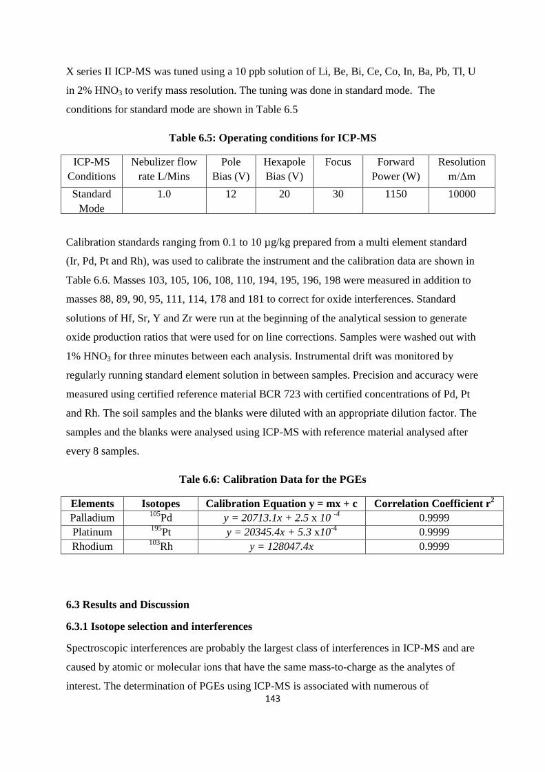
143

X series II ICP-MS was tuned using a 10 ppb solution of Li, Be, Bi, Ce, Co, In, Ba, Pb, Tl, U

in 2% HNO3 to verify mass resolution. The tuning was done in standard mode. The

conditions for standard mode are shown in Table 6.5

Table 6.5: Operating conditions for ICP-MS

ICP-MS

Conditions

Nebulizer flow

rate L/Mins

Pole

Bias (V)

Hexapole

Bias (V)

Focus Forward

Power (W)

Resolution

m/Δm

Standard

Mode

1.0 12 20 30 1150

10000

Calibration standards ranging from 0.1 to 10 µg/kg prepared from a multi element standard

(Ir, Pd, Pt and Rh), was used to calibrate the instrument and the calibration data are shown in

Table 6.6. Masses 103, 105, 106, 108, 110, 194, 195, 196, 198 were measured in addition to

masses 88, 89, 90, 95, 111, 114, 178 and 181 to correct for oxide interferences. Standard

solutions of Hf, Sr, Y and Zr were run at the beginning of the analytical session to generate

oxide production ratios that were used for on line corrections. Samples were washed out with

1% HNO3 for three minutes between each analysis. Instrumental drift was monitored by

regularly running standard element solution in between samples. Precision and accuracy were

measured using certified reference material BCR 723 with certified concentrations of Pd, Pt

and Rh. The soil samples and the blanks were diluted with an appropriate dilution factor. The

samples and the blanks were analysed using ICP-MS with reference material analysed after

every 8 samples.

Tale 6.6: Calibration Data for the PGEs

Elements Isotopes Calibration Equation y = mx + c Correlation Coefficient r2

Palladium 105

Pd y = 20713.1x + 2.5 x 10 -4

0.9999

Platinum 195

Pt y = 20345.4x + 5.3 x10-4

0.9999

Rhodium 103

Rh y = 128047.4x 0.9999

6.3 Results and Discussion

6.3.1 Isotope selection and interferences

Spectroscopic interferences are probably the largest class of interferences in ICP-MS and are

caused by atomic or molecular ions that have the same mass-to-charge as the analytes of

interest. The determination of PGEs using ICP-MS is associated with numerous of

144

interference problems. This spectroscopic interference, arising from major constituents of the

sample, complicates PGE determination (42). It is particularly severe when analysing

catalytic converter pollution products due to the common use of Sr and Zr substrate in the

catalysts which generates unusually high and significant levels of oxide interferences on the

PGE masses of interest (41). ICP-MS is used in the determination because of its multi-

element capacity and the extent of the isotopic information one is able to produce.

The analytical isotopes 105

Pd, 195

Pt and 103

Rh were selected based on the natural abundances

of the analytical isotopes and the ascertainment of relative abundances of the potential atomic

and molecular interfering ions along with the resolution required to separate analyte masses

from interfering masses (43). Palladium has 105, 106 and 108 isotopes with abundances of

22.3%, 27.3% and 26.5% respectively. The 106 and 108 suffers from isobaric monoatomic

interference of Cd ion while 105

Pd does not suffer any monoatomic ion interference hence is

the chosen isotope for analysis.

Platinum 195 was chosen as the preferred isotope for measurement because it has the highest

abundance (33.8%) compared to the other isotopes. Platinum 194 has abundance of 32.9%.

Some of the interfering ions are quantitatively retained by the cation column relative to PGEs

thus effectively separating them and causing reduced problems for example 87

Sr16

O, 86

Sr17

O

for 103

Rh and 89

Y16

O for 105

Pd ( 41). Hafnium and Zr behave as anion complexes (44, 45) and

hence elute with the PGE from the cation column causing serious interferences. Oxides of

these elements interfere on the Pd mass spectrum with respect to Zr and in the Pt mass

spectrum for Hf. Oxides of these elements were reduced by the use of a nebuliser which

maintains oxide generation levels below 0.05% of the total mass signal. Example, Zr signals

of > 106 cps produces

90Zr

16O signal of 500cps or less which can easily be corrected from

PGE analyte signals that are normally > 10,000 cps. Interferences linked to other metals e.g.

Cu, Zn and Pb, can be separated in the resolution mode of 4000 cps which is well below that

for PGEs of 10,000 cps (46). Interferences not separated from instrumental manipulations

and treatment stages were corrected mathematically by estimating the contribution of

interfering species to the PGEs signal through the analysis of single element standard

solutions of interferents as published in (10, 46, 47).

6.3.2 Quality control using certified reference material

Validation was performed by analysing dust reference material BCR 723. 0.5g of the CRM

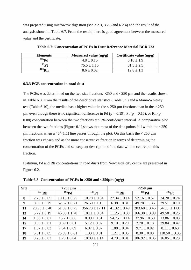
145

was prepared using microwave digestion (see 2.2.3, 3.2.6 and 6.2.4) and the result of the

analysis shown in Table 6.7. From the result, there is good agreement between the measured

value and the certificate.

Table 6.7: Concentration of PGEs in Dust Reference Material BCR 723

Elements Measured value (ng/g) Certificate value (ng/g) 105

Pd 4.8 ± 0.16 6.10 ± 1.9 195

Pt 75.5 ± 1.16 81.3 ± 2.5 103

Rh 8.6 ± 0.02 12.8 ± 1.3

6.3.3 PGE concentration in road dust

The PGEs was determined on the two size fractions >250 and <250 µm and the results shown

in Table 6.8. From the results of the descriptive statistics (Table 6.9) and a Mann-Whitney

test (Table 6.10), the median has a higher value in the < 250 µm fractions than in the > 250

µm even though there is no significant difference in Pd (p = 0.19), Pt (p = 0.15), or Rh (p =

0.08) concentration between the two fractions at 95% confidence interval. A comparative plot

between the two fractions (Figure 6.1) shows that most of the data points fall within the <250

µm fractions when a 45o

(1:1) line passes through the plot. On this basis the < 250 µm

fraction was chosen and as the more conservative fraction in terms of determining the

concentration of the PGEs and subsequent description of the data will be centred on this

fraction.

Platinum, Pd and Rh concentrations in road dusts from Newcastle city centre are presented in

Figure 6.2.

Table 6.8: Concentration of PGEs in >250 and <250µm (ng/g)

Site >250 µm <250 µm 103

Rh 105

Pd 195

Pt 103

Rh 105

Pd 195

Pt

8 2.73 ± 0.05 10.15 ± 0.25 10.78 ± 0.34 27.34 ± 0.14 52.16 ± 0.57 24.20 ± 0.74

9 8.83 ± 0.29 52.57 ± 0.71 26.59 ± 1.18 6.38 ± 0.31 49.78 ± 1.36 29.51 ± 0.19

11 28.93 ± 0.40 51.59 ± 0.75 356.73 ± 17.11 41.32 ± 0.49 203.68 ± 3.46 54.36 ± 1.60

13 5.72 ± 0.19 46.08 ± 1.70 18.11 ± 0.34 11.25 ± 0.38 166.38 ± 3.99 49.58 ± 0.25

14 1.88 ± 0.07 15.2 ± 0.06 8.09 ± 0.51 54.75 ± 0.14 37.96 ± 0.50 13.86 ± 0.03

15 0.08 ± 0.01 0.59 ± 0.01 5.12 ± 0.02 9.19 ± 0.20 2.70 ± 0.13 29.84 ± 0.47

17 1.37 ± 0.03 7.64 ± 0.09 6.07 ± 0.37 1.88 ± 0.04 9.71 ± 0.02 8.11 ± 0.63

18 5.01 ± 0.05 23.39 ± 0.61 1.33 ± 0.01 1.21 ± 0.05 8.30 ± 0.03 118.50 ± 3.33

19 3.23 ± 0.03 1.79 ± 0.04 18.89 ± 1.14 4.79 ± 0.01 186.92 ± 0.85 16.05 ± 0.23

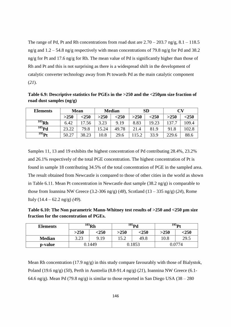
146

The range of Pd, Pt and Rh concentrations from road dust are 2.70 – 203.7 ng/g, 8.1 – 118.5

ng/g and 1.2 – 54.8 ng/g respectively with mean concentrations of 79.8 ng/g for Pd and 38.2

ng/g for Pt and 17.6 ng/g for Rh. The mean value of Pd is significantly higher than those of

Rh and Pt and this is not surprising as there is a widespread shift in the development of

catalytic converter technology away from Pt towards Pd as the main catalytic component

(21).

Table 6.9: Descriptive statistics for PGEs in the >250 and the <250µm size fraction of

road dust samples (ng/g)

Elements Mean Median SD CV

>250 <250 >250 <250 >250 <250 >250 <250 103

Rh 6.42 17.56 3.23 9.19 8.83 19.23 137.7 109.4 105

Pd 23.22 79.8 15.24 49.78 21.4 81.9 91.8 102.8 195

Pt 50.27 38.23 10.8 29.6 115.2 33.9 229.6 88.6

Samples 11, 13 and 19 exhibits the highest concentration of Pd contributing 28.4%, 23.2%

and 26.1% respectively of the total PGE concentration. The highest concentration of Pt is

found in sample 18 contributing 34.5% of the total concentration of PGE in the sampled area.

The result obtained from Newcastle is compared to those of other cities in the world as shown

in Table 6.11. Mean Pt concentration in Newcastle dust sample (38.2 ng/g) is comparable to

those from Ioannina NW Greece (3.2-306 ng/g) (48), Scotland (13 – 335 ng/g) (24), Rome

Italy (14.4 – 62.2 ng/g) (49).

Table 6.10: The Non parametric Mann-Whitney test results of >250 and <250 µm size

fraction for the concentration of PGEs.

Elements 103

Rh 105

Pd 195

Pt

>250 <250 >250 <250 >250 <250

Median 3.23 9.19 15.2 49.8 10.8 29.5

p-value 0.1449 0.1853 0.0774

Mean Rh concentration (17.9 ng/g) in this study compare favourably with those of Bialystok,

Poland (19.6 ng/g) (50), Perth in Austrelia (8.8-91.4 ng/g) (21), Ioannina NW Greece (6.1-

64.6 ng/g). Mean Pd (79.8 ng/g) is similar to those reported in San Diego USA (38 – 280

147

ng/g) (51), Germany (1 – 146 ng/g) (52), Perth in Austrelia (58.1-440.4 ng/g) (21), and

Goteborg in Sweeden (80 ng/g) (7).

Figure 6.1: Comparison between the <250 and > the 250 µm size fraction for the PGEs

6.3.4 Grain-size partitioned PGE concentration and mass loading

Three road dust samples (8, 14 and 15) were separated into six grain size fractions. The

variation in Pd, Pt and Rh concentrations across these particle size fractions is shown in

Figure 6.3. A common assumption is that the <63 µm fraction is the most highly

concentrated, as the typical relationship is an increase in element concentration with

decreasing grain size (e.g.53, 54). This assertion reveals why most of the dominant fraction

analysed for PGEs in soil by many researchers is the <63 µm size fraction

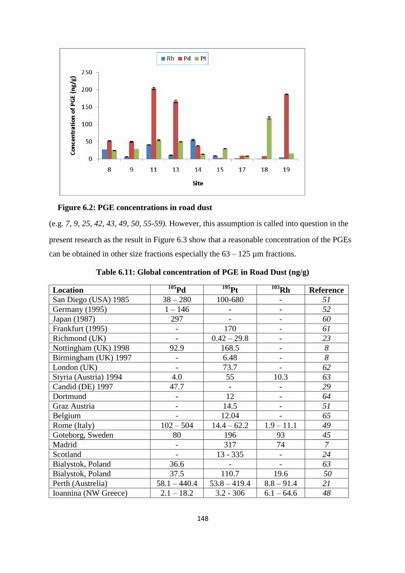
148

Figure 6.2: PGE concentrations in road dust

(e.g. 7, 9, 25, 42, 43, 49, 50, 55-59). However, this assumption is called into question in the

present research as the result in Figure 6.3 show that a reasonable concentration of the PGEs

can be obtained in other size fractions especially the 63 – 125 µm fractions.

Table 6.11: Global concentration of PGE in Road Dust (ng/g)

Location 105

Pd 195

Pt 103

Rh Reference

San Diego (USA) 1985 38 – 280 100-680 - 51

Germany (1995) 1 – 146 - - 52

Japan (1987) 297 - - 60

Frankfurt (1995) - 170 - 61

Richmond (UK) - 0.42 – 29.8 - 23

Nottingham (UK) 1998 92.9 168.5 - 8

Birmingham (UK) 1997 - 6.48 - 8

London (UK) - 73.7 - 62

Styria (Austria) 1994 4.0 55 10.3 63

Candid (DE) 1997 47.7 - - 29

Dortmund - 12 - 64

Graz Austria - 14.5 - 51

Belgium - 12.04 - 65

Rome (Italy) 102 – 504 14.4 – 62.2 1.9 – 11.1 49

Goteborg, Sweden 80 196 93 45

Madrid - 317 74 7

Scotland - 13 - 335 - 24

Bialystok, Poland 36.6 - - 63

Bialystok, Poland 37.5 110.7 19.6 50

Perth (Austrelia) 58.1 – 440.4 53.8 – 419.4 8.8 – 91.4 21

Ioannina (NW Greece) 2.1 – 18.2 3.2 - 306 6.1 – 64.6 48

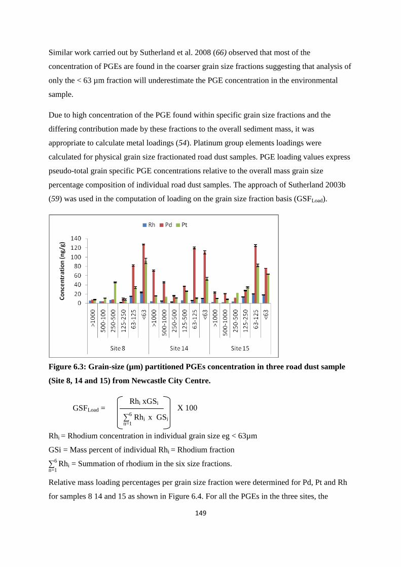
149

Similar work carried out by Sutherland et al. 2008 (66) observed that most of the

concentration of PGEs are found in the coarser grain size fractions suggesting that analysis of

only the < 63 µm fraction will underestimate the PGE concentration in the environmental

sample.

Due to high concentration of the PGE found within specific grain size fractions and the

differing contribution made by these fractions to the overall sediment mass, it was

appropriate to calculate metal loadings (54). Platinum group elements loadings were

calculated for physical grain size fractionated road dust samples. PGE loading values express

pseudo-total grain specific PGE concentrations relative to the overall mass grain size

percentage composition of individual road dust samples. The approach of Sutherland 2003b

(59) was used in the computation of loading on the grain size fraction basis (GSFLoad).

Figure 6.3: Grain-size (µm) partitioned PGEs concentration in three road dust sample

(Site 8, 14 and 15) from Newcastle City Centre.

Rhi xGSi

∑6 Rhi

x GSi

n=1

Rhi = Rhodium concentration in individual grain size eg < 63µm

GSi = Mass percent of individual Rhi = Rhodium fraction

∑6

Rhi = Summation of rhodium in the six size fractions. n=1

Relative mass loading percentages per grain size fraction were determined for Pd, Pt and Rh

for samples 8 14 and 15 as shown in Figure 6.4. For all the PGEs in the three sites, the

X 100 GSFLoad =

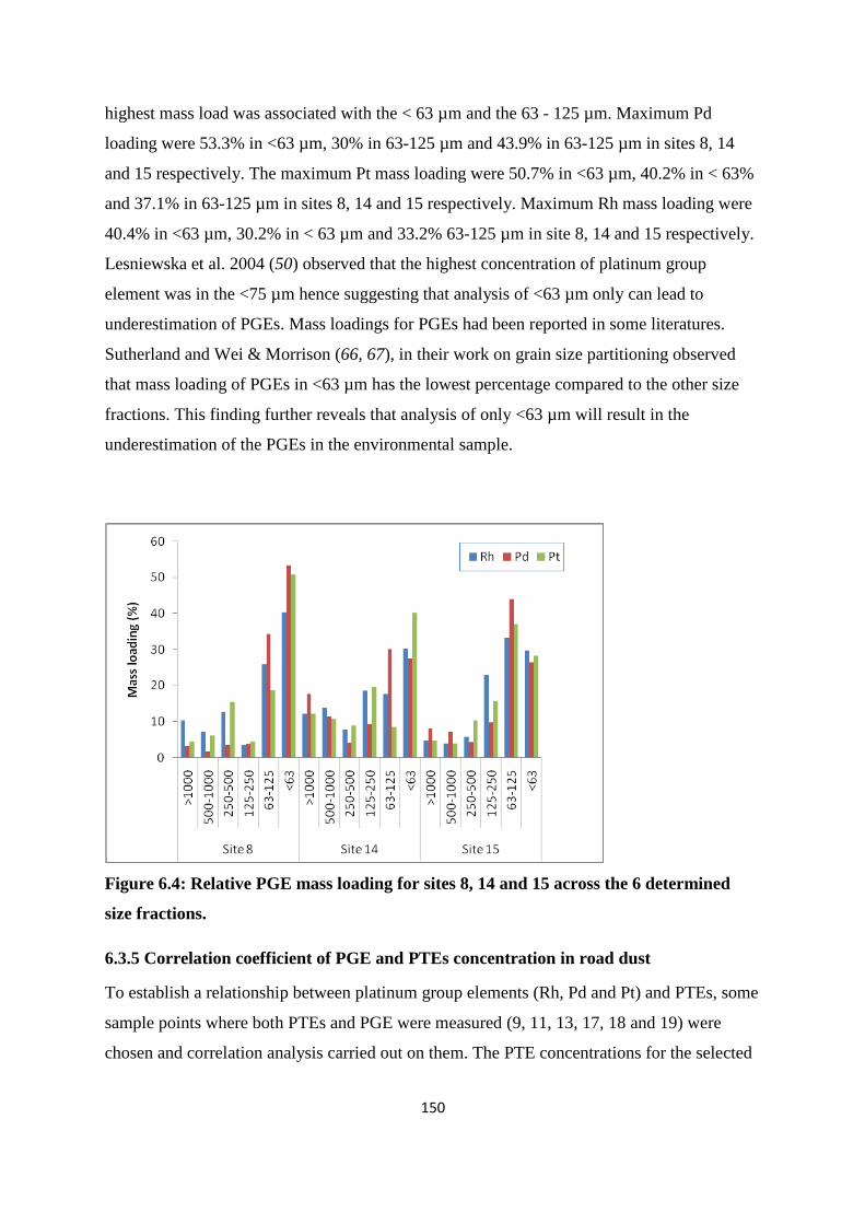
150

highest mass load was associated with the < 63 µm and the 63 - 125 µm. Maximum Pd

loading were 53.3% in <63 µm, 30% in 63-125 µm and 43.9% in 63-125 µm in sites 8, 14

and 15 respectively. The maximum Pt mass loading were 50.7% in <63 µm, 40.2% in < 63%

and 37.1% in 63-125 µm in sites 8, 14 and 15 respectively. Maximum Rh mass loading were

40.4% in <63 µm, 30.2% in < 63 µm and 33.2% 63-125 µm in site 8, 14 and 15 respectively.

Lesniewska et al. 2004 (50) observed that the highest concentration of platinum group

element was in the <75 µm hence suggesting that analysis of <63 µm only can lead to

underestimation of PGEs. Mass loadings for PGEs had been reported in some literatures.

Sutherland and Wei & Morrison (66, 67), in their work on grain size partitioning observed

that mass loading of PGEs in <63 µm has the lowest percentage compared to the other size

fractions. This finding further reveals that analysis of only <63 µm will result in the

underestimation of the PGEs in the environmental sample.

Figure 6.4: Relative PGE mass loading for sites 8, 14 and 15 across the 6 determined

size fractions.

6.3.5 Correlation coefficient of PGE and PTEs concentration in road dust

To establish a relationship between platinum group elements (Rh, Pd and Pt) and PTEs, some

sample points where both PTEs and PGE were measured (9, 11, 13, 17, 18 and 19) were

chosen and correlation analysis carried out on them. The PTE concentrations for the selected

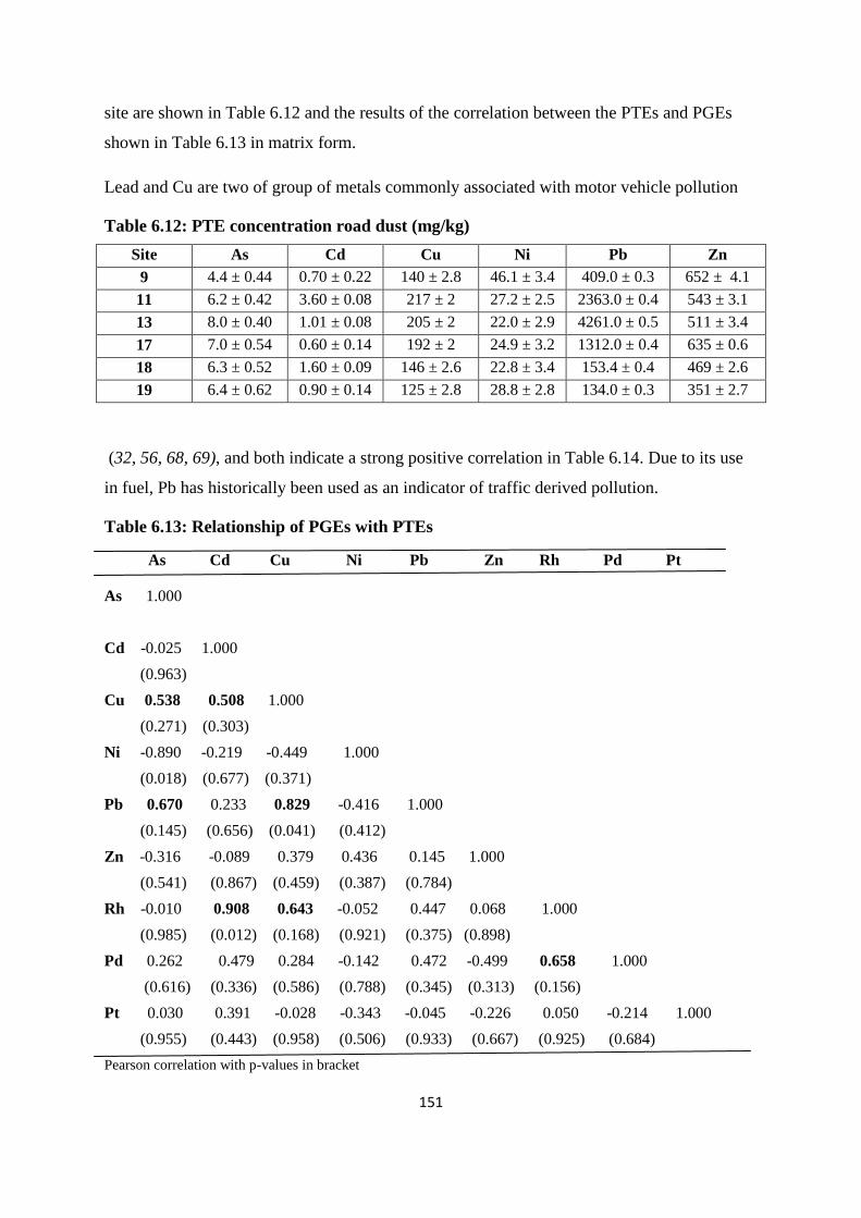
151

site are shown in Table 6.12 and the results of the correlation between the PTEs and PGEs

shown in Table 6.13 in matrix form.

Lead and Cu are two of group of metals commonly associated with motor vehicle pollution

Table 6.12: PTE concentration road dust (mg/kg)

Site As Cd Cu Ni Pb Zn

9 4.4 ± 0.44 0.70 ± 0.22 140 ± 2.8 46.1 ± 3.4 409.0 ± 0.3 652 ± 4.1

11 6.2 ± 0.42 3.60 ± 0.08 217 ± 2 27.2 ± 2.5 2363.0 ± 0.4 543 ± 3.1

13 8.0 ± 0.40 1.01 ± 0.08 205 ± 2 22.0 ± 2.9 4261.0 ± 0.5 511 ± 3.4

17 7.0 ± 0.54 0.60 ± 0.14 192 ± 2 24.9 ± 3.2 1312.0 ± 0.4 635 ± 0.6

18 6.3 ± 0.52 1.60 ± 0.09 146 ± 2.6 22.8 ± 3.4 153.4 ± 0.4 469 ± 2.6

19 6.4 ± 0.62 0.90 ± 0.14 125 ± 2.8 28.8 ± 2.8 134.0 ± 0.3 351 ± 2.7

(32, 56, 68, 69), and both indicate a strong positive correlation in Table 6.14. Due to its use

in fuel, Pb has historically been used as an indicator of traffic derived pollution.

Table 6.13: Relationship of PGEs with PTEs

As Cd Cu Ni Pb Zn Rh Pd Pt

As 1.000

Cd -0.025 1.000

(0.963)

Cu 0.538 0.508 1.000

(0.271) (0.303)

Ni -0.890 -0.219 -0.449 1.000

(0.018) (0.677) (0.371)

Pb 0.670 0.233 0.829 -0.416 1.000

(0.145) (0.656) (0.041) (0.412)

Zn -0.316 -0.089 0.379 0.436 0.145 1.000

(0.541) (0.867) (0.459) (0.387) (0.784)

Rh -0.010 0.908 0.643 -0.052 0.447 0.068 1.000

(0.985) (0.012) (0.168) (0.921) (0.375) (0.898)

Pd 0.262 0.479 0.284 -0.142 0.472 -0.499 0.658 1.000

(0.616) (0.336) (0.586) (0.788) (0.345) (0.313) (0.156)

Pt 0.030 0.391 -0.028 -0.343 -0.045 -0.226 0.050 -0.214 1.000

(0.955) (0.443) (0.958) (0.506) (0.933) (0.667) (0.925) (0.684)

Pearson correlation with p-values in bracket

152

Whereas some studies have demonstrated strong positive correlation between the PGEs and

Pb (32, 70), in this study Pb has no strong mathematical correlation with any of the PGEs.

The lack of a strong correlation between PGE and Pb is not surprising as the introduction and

growth of the use of catalytic converters in automobiles reduces drastically the emission of

Pb from the automobile to the environment. Rhodium has a strong correlation with Cu and

Cd (Table 6.13) as well as Pd. A common source is likely and possibly anthropogenic, e.g.

automobiles.

6.3.6 PGE ratios for determining emission source

Platinum group element ratios are of great importance in determining automotive catalysts as

emission sources (71). Commonly bivariate PGE ratios in a given sample media are

compared to those associated with typical values in autocatalysts (66). Similarities between

them have been used as evidence to infer anthropogenic contamination from catalytic

converters (66). Three common ratio fields for three way catalytic converters (TWC) have

been defined as follows:- Pt/Pd 1 – 2.5; Pt/Rh 5 – 16 and Pd/Rh 4 – 9 (70). The Pt/Pd, Pt/Rh

and Pd/Rh observed in the present study are 0.56, 4.08 and 7.27 respectively. These values

are obtained on n = 24 sample size. The Pt/Pd and Pt/Rh ratio in this study are not in

agreement with the potential catalytic converter ratio defined by Ely et al., 2001 (70) and

Whitney and Murray 2003 (21). This result appears to support the earlier assertion (section

6.1) of shift from Pt to Pd as component of TWC (6). The high Pd in our analysis results in

the lower ratio of Pt/Pd, and the lower Pt results in the lower Pt/Rh ratio. The ratio of Pd/Rh

is in agreement with that of Ely et al. 2001 (70). This suggests that the presence of Pd and Rh

in the sampled points must have come from the automobile as a result of the deterioration of

the TWC converter fitted at the exhaust of the motor vehicles.

6.4 Conclusion

From the present research, the following findings were made:-

1. Platinum group elements (Pd, Pt and Rh) for <250µm fraction of 9 urban street

dust/sediment and 3 grain size fractionated samples from Newcastle city centre all indicate a

strong anthropogenic signal.

2. The grain size analysis reveals that values of PGE are influenced by the size of the fraction

analysed.

153

3. From grain size analysis, the highest concentration lies within the <63 and 63-125 µm size

fraction. Therefore analysis of only the <63 µm will underestimate auto catalyst PGE.

4. There is a strong positive correlation between Pd and Rh and the Pd/Rh ratio (7.27) for

Newcastle City Centre samples falls within the ratio field (4 – 9) defined by Ely et al. 2001 as

indicative of TWC (70).

5. The low value of the Pt/Pd and the Pt/Rh ratio of the samples in comparison with other

authors give an indication of a possible recent shift in the composition of the TWC converters

from Pt towards Pd.

References

1 Kalavrouziotis, I. K., Koukoulakis, P.H. (2009). Environmental impact of platinum

group elements (Pt, Pd and Rh) emitted by the automobile catalyst converters. Water

Air Soil Pollution, 196, 393 – 402.

2 Hartley, F.R. (1991). Chemistry of platinum group metals, recent development.

Amsterdam. Elsevier publishers.

3 Greenwood, N.N., Earnshaw, A. (1989). Chemistry of the elements. Oxford.

Pergamon Press p 1242 – 1363.

4 Wedepohl, K.H. (1995). The composition of the continental crust. Geochimica Et

Cosmochimica Acta, 59, 1217 – 1232.

5 WHO (1991). Environmental Health Criteria 125 – Platinum. Geneva: World Health

Organization, International Programme on Chemical Safety. 1991.

6 Ravindra, K., Bencs, L., Grieken, R. (2004). Platinum group elements in the

environment and their health risk. The Science of the Total Environment,318, 1 – 43.

7 Gomez, B., Gomez, M., Sanchez, J.L., Fernandez, R., Palacios, M.A. (2001).

Platinum and rhodium distribution in airborne particulate matter and road dust. The

Science of the Total Environment, 261, 131 – 144.

8 Hutchinson, E.J., Farago, M.E., Simpson, P.R. (1999). Changes in platinum emissions

from motor vehicles. In: Zereini F, Alt F, editors. Anthropogenic platinum – group

element emissions. P 57 – 64.

9 Sutherland, R.A. (2003a). A first look at platinum in road – deposited sediments and

roadside soils, Honolulu, Oahu, Hawaii. Archives of Environmental Contamination

and Toxicology, 44, 430 – 436.

154

10 Moldovan, M., Gomez, M.M., Palacios, M. (1999). Determination of platinum,

rhodium and palladium in car exhaust fumes. Journal of Analytical Atomic

Spectrometry, 14, 1163 – 1169.

11 Palacios, M.A., Gomez, M.M., Maldovan, M., Morrisson, G., Rauch, S., McLead, C.

(2000). Platinum group elements: Quantification in collected exhaust fumes and

studies of catalyst surfaces. The Science of the Total Environment, 257, 1 – 15.

12 Klaassen, C. (1996). Casarett and Doulls toxicology. The basic science of poisons. 5th

edition NewYork: McGraw-Hill. 725-726.

13 http://www.naei.org.uk. March 2009.

14 Haibo, C., Anil, N., Margaret, B. (2008). Classification of road traffic and roadside

pollution concentrations for assessment of personal exposure. Environmental

Modelling & Software, 23, 282 – 287.

15 Department of the Environment, Transport and the Regions DETR. (2000). The Air

Quality Strategy for England, Scotland, Wales and Northern Ireland: Working

Together for Clean Air. Transport and the Regions. Department of the Environment,

London.

16 Morton, O., Puchelt, H., Hemandez, E., Lounezeva, E. (2001). Traffic related

platinum group elements (PGEs) in soils from Mexico City. Journal of Geochemical

Exploration, 72, 223-227.

17 Lucena, P., Vadillo, J.M., Laserna, J.J. (1999). Mapping of platinum group metals in

automotive exhaust three way catalysts using laser induced breakdown spectrometry.

Analytical Chemistry,71, 4385 – 4391.

18 Barefoot, R.R. (1999). Distribution and speciation of platinum group elements in the

environmental matrices. Trends in Analytical Chemistry, 18, 702 – 707.

19 Zereini, F., Wiseman, C., Beyer, J.M., Artelt, S., Urban, H. (2001). Platinum, Lead

and Cerium concentrations of street particulate matter (Frankfurt AM Main,

Germany). Journal of Soils and Sediments, 3, 188 – 195.

20 Barbante, C., Veysseyre, A., Ferrari, C., Van de Velde, K., Morel, C., Capodaglio, G.

(2001). Greenland snow evidence of large scale atmospheric contamination for

platinum, palladium and rhodium. Environmental Science and Technology, 35, 835 -

839.

21 Whitely, J.D., Murray, F. (2003). Anthropogenic platinum group elements (Pt, Rh,

Pd) concentrations in road dust and road side soils from Perth Western Australia. The

Science of the Total Environment ,317, 121 – 135.

155

22 Gagnon, Z.E., Newkirk, C., Hicks, S. (2006). Impact of platinum group metals on the

environment. A toxological, genotoxic and analytical chemistry study. Journal of

Environmental Science and Health Part A, 41, 397 – 414.

23 Farago, M.E., Kavanagh, P., Blanks, R., Kelly, J., Kazantzis, G., Thornton, I. (1998).

Platinum concentrations in urban road dust and soil and in blood and urine in the

United Kingdom. The Analyst, 123, 451 – 454.

24 Higney, E., Olive, V., MacKenzie, A.B., Pulford, I.D. (2002). Isotope dilution ICPMS

Analysis of platinum in road dusts from west central Scotland. Applied Geochemistry,

17, 1123 – 1129.

25 Kylander, M.E., Rauch, S., Morrison, G.M., Andam,K. (2003). Impact of automobile

emissions on the levels of platinum and lead in Accra, Ghana. Journal of

Environmental Monitoring, 5, 91 – 95.

26 Alloway, B.J., Ayres, D.C. (1997). Chemical Principle of Environmental Pollution.

London. Blackie Academic and Professional p 147.

27 Hees, T., Wenclawiak, B., Lustig, S., Schramel, P., Schwarzer, M. (1998).

Distribution of platinum group elements (Pt, Pd and Rh) in environmental and clinical

matrices: Composition, analytical techniques and scientific outlook – status report.

Environmental Science Pollution Resources, 5, 105 – 111.

28 Schuster, M., Schwarzer, M., Risse, G. (2000). Determination of palladium in

environmental samples. In: Zereini ,F., Alt, F. ditors. Anthropogenic platinum group

element emissions. Their impact on man and environment. Berlin: Springer – Verlag

p 173 – 182.

29 Hoppstock, K., Sures, B. (2004). Platinum group metals. In E, Merian. M. Anke and

M. Stoeppler (Eds), Elements and their Compounds in their environment. Wiley p

1047 – 1086.

30 Zimmermann, S., Messerschmidt, J., Von, B.A., Taraschewski, H., Sures, B. (2002).

Biological availability of traffic related platinum group elements (palladium, platinum

and rhodium) to the zebra mussel in water containing road dust. Environmental

Toxicology Chemistry, 21, 2713 – 2718.

31 Schafer, J., Punchelt, H. (1998). Platinum-group metal (PGM) emitted from

automobile catalytic converters and their distribution in roadside soils. Geochemistry

Exploration, 64, 307 – 314.

32 Tankari. D.B.A., Ducoulombier, C.C., Soligot, C., Feidt, C., Rychen, G. (2007).

Deposition of platinum group elements and polycyclic aromatic hydrocarbons on rye

grass exposed to vehicular traffic. Agronomy for Sustainable Development, 27, 261 –

266.

156

33 Konig, H.P., Hertel, R.F., Koch, W., Rosner, G. (1992). Determination of the

platinum emissions from three way catalysts – quipped with gasoline engine.

Atmospheric Environment, 26, 741 – 745.

34 Bunger, J., Stork, J., Stalder, K. (1996). Cyto- and genotoxic effects of co-ordination

complexes of platinum, palladium and rhodium in vitro. International Archives of

Occupational Environmental Health, 69, 33 – 38.

35 Gebel, T., Lantzsch, H., Plebow, K., Dunkelberg, K. (1997). Genotoxicity of platinum

and palladium compounds in human and bacterial cells. Mutation Resource, 389, 183

– 190.

36 Paolucci, C., Ponti, J., Fabbri, M.V., Breda, D., Sabbioni, E., Burastero, S.B. (2007).

Platinum group elements allergic immune response on dendritic cells. Allergy and

Immunology, 143, 1 – 2.

37 Hughes, E.G. (1980). Medical surveillance of platinum refinery workers. Society of

Occupational Medicine, 30, 27-30.

38 Schmid, M., Zimmerman, S., Krug, F., Sures, B. (2007). Influence of platinum,

palladium and rhodium as compared with cadmium, nickel and chromium on cell

viability and oxidative stress in human bronchial epithelial cell. Environment

International, 33, 385 – 390.

39 Stone, M., Marsalek, J. (1996). Trace metal composition and speciation in street

sediment: Sault Ste, Marie, Canada. Water Air and Soil Pollution, 87, 149-169

40 Niemela, M., Peramaki, P., Piispanen, J., Poikolainen, J. (2004). Determination of

platinum and rhodium in dust and plant samples using microwave-assisted sample

digestion and ICP-MS. Analytica Chimica Acta, 521, 137-142.

41 Sutherland, R.A., Pearson, D.G., Ottley, C.J. (2007). Platinum-group elements (Ir, Pd,

Pt and Rh) in road-deposited sediments in two urban watersheds, Hawaii. Applied

Geochemistry, 22, 1485 – 1501.

42 Gomez, B., Palacios, M.A., Gomez, M., Sanchez, J.L., Morrison, G., Rauch, S.,

McLeod, C., Ma, R., Caroli, S., Alimonti, A., Petrucci, F., Bocca, B., Schramel, P.,

Zischka, M., Petterson, C., Wass, U. (2002). Levels and risk assessment for humans

and ecosystems of platinum-group elements in the airborne particles and road dust of

some European cities. The Science of the Total Environment, 299, 1 – 19.

43 Motelica-Heino, M., Rauch, S., Morrison, G.M., Donard, O.F. (2001). Determination

of palladium, platinum and rhodium concentrations in urban road sediments by laser

ablation-ICP-MS. Analytica Chimica Acta, 436, 233 – 244

44 Ely, J.C., Neal, C.R., ONeill, J.A., Jain, J.C. (1999), Quantifying the platinum group

elements (PGEs) and gold in geological samples using cation exchange pretreatment

157

and ultrasonic nebulisation inductively coupled plasma-mass spectrometry (USN-

ICP-MS). Chemical Geology, 157, 219 – 234.

45 Pearson, D.G., Woodland, S.J. (2000). Solvent extraction/anion exchange separation

and determination of PGEs (Os, Ir, Pt, Pd, Ru) and Re-Os isotopes in geological

samples by isotope dilution ICP-MS. Chemical Geology, 165, 87 – 107.

46 Gomez, M.B., Gomez, M.M., Palacios, M.A. (2000). Control of interferences in the

determination of Pt, Pd and Rh in airborne particulate matter by inductively coupled

plasma mass spectrometry. Analytica Chimica Acta, 404, 285 – 294.

47 Rauch, S., Lu, M., Morrison, G. (2001). Heterogeneity of platinum group metals in

airborne particles. Environmental Science Technology, 35, 595 – 599.

48 Tsogas, G.Z., Giokas, D.L., Vlessidis, A.G., Aloupi, M., Angelidis, M.O. (2009).

Survey of the distribution and time-dependent increase of platinum-group element

accumulation along urban roads in Ioannina (NW Greece). Water, Air and Soil

Pollution, 201, 265 – 281.

49 Petrucci, F., Bocca, B., Alimonti, A., Caroli,S. (2000). Determination of Pd, Pt and

Rh in airborne particulate and road dust by high resolution ICP-MS: a preliminary

investigation of the emission from automotive catalysts in the urban area of Rome.

Journal of Analytical Atomic Spectroscopy, 15, 525 – 528.

50 Lesniewska, B.A., Godlewska-Zylkiewicz, B., Bocca, B., Caimi, S., Hulanicki, A.

(2004). Platinum, Palladium and rhodium content in road dust, tinnel dust and

common grass in Bialystok area (Poland): A pilot study. The Science of the Total

Environment, 321, 93 – 104.

51 Hodge, V.F., Stallard, M.O. (1986). Platinum and palladium in roadside dust.

Environmental Science Technology, 20, 1058 – 1060.

52 Schafer, J., Eckhardt, J.D., Puchelt, H. (1996). Traffic related nobel metal emissions

in southwest Germany. VM Goldschmidt Conference, Journal conference Abstract 1:

536.

53 Horowitz, A.J. (1991). A primer on sediment –trace Element Chemistry. Lewis

Publishers. Inc. Chelsea, Mi.

54 Robertson, D.J., Taylor, K.G. (2007). Temporal variability of metal contamination in

urban road-deposited sediment in Manchester UK: Implications for urban pollution

Monitoring. Water, Air and Soil Pollution, 186, 209-220.

55 Gomez, B., Gomez, M., Palacios, M.A. (2003). ICP-MS determination of Pt, Pd and

Rh in airborne and road dust after tellurium co precipitation. Journal of Analytical

Atomic Spectroscopy, 18, 80 – 83.

158

56 Jarvis, K.E., Parry, S.J., Piper, J.M. (2001). Temporal and spatial studies of

autocatalyst-derived trace elements in the environment. Environment Science

Technology, 35, 1031 – 1036.

57 Kan, S.F., Tanner, P.A. (2004): Determination of platinum in roadside dust samples

by dynamic reaction cell-inductively coupled plasma mass spectrometry. Journal of

Analytical Atomic Spectrometry, 19, 1 – 6.

58 Whiteley, J.D. (2005). Seasonal variability of platinum, palladium and rhodium

(PGE) levels in road dusts and roadside soils, Perth, Western Australia. Water, Air

and Soil Pollution, 160, 77 – 93.

59 Sutherland, R.A. (2003b). Lead in grain fractions of road-deposited sediment.

Environmental Pollution, 121, 229-237.

60 Helmers, E., Schwarzer, M., Schuster, M. (1998). Comparison of palladium and

platinum in environmental matrices: palladium pollution by automobile emissions.

Environmental Science Pollution Resources,5, 44 – 50.

61 Zereini, F., Skerstupp, B., Alt, F., Helmers, E., Urban, H . (1997a). Geochemical

behaviour of platinum group metals (PGE) in particulate emissions by automobile

exhaust catalysts: experimental results and environmental investigations. The Science

for the Total Environment, 206, 137 – 146.

62 Jin, X., Zhu, H. (2000). Determination of platinum group elements and gold in

geological samples with ICP-MS using a sodium peroxide fusion and tellurium co-

precipitation. Journal of Analytical Atomic Spectrometry, 15, 747 – 751.

63 Godlewska-Zylkiewicz, B., Zaleska, M. (2002). Preconcentration of palladium I a

flow-through electrochemical cell for determination by graphite furnace atomic

absorption spectrometry. Analytica Chimica Acta, 462, 305 – 312.

64 Beirohr, E., Lee, M.L., Tschopel, P., Tolg, G. (1993). Determination of platinum in

biotic and environmental samples by graphite furnace atomic absorption spectrometry

after its electro deposition into graphite tube packed with reticulated vitreous carbon.

Journal of Analytical Chemistry 346, 689 – 692.

65 Parent, M., Vanhoe, H., Moens, Dams, R. (1996). Determination of low amounts of

platinum in environmental and biological materials using thermospray nebulisation

inductively coupled plasma mass spectrometry. Journal of Analytical Chemistry, 354,

664 – 667.

66 Sutherland, R.A., Pearson, G.D., Ottley, C.J. (2008): Grain size partitioning of

platinum-group elements in road-deposited sediments: Implications of anthropogenic

flux estimates from autocatalysts. Environmental Pollution, 151, 503 – 515.

159

67 Wei, C., Morrison, G.M. (1994b). Platinum in road dusts and urban river sediments.

The Science of the Total Environment, 146/147, 169 – 174.

68 Ogunsola, O.J., Oluwole, A.F., Asubiojo, O.I., Olaniyi, H.A., Akeredolu, F.A.,

Akanle, O.A., Spyrou, N.M., Ward, N.I., Ruck, W. (1994). Traffic pollution:

preliminary elemental characterisation of roadside dust in Lagos Nigeria. The Science

of the Total Environment, 146/147, 175 – 184.

69 Legret, M., Pagotto, C. (1999). Evaluation of Pollutant loadings in runoff waters from

a major rural highways. The Science Total of the Environment, 235, 143 – 150.

70 Ely, J.C., Neal, C.R., Kulpa, C.F., Schneegurt, M.A., Seidler, J.A., Jain, C.J. (2001).

Implication of Platinum –Group Element Accumulation along U.S. Roads from

Catalytic-Converter Attrition. Environmental Science Technology, 35, 3816 – 3822.

71 Zereini, F., Dirksen, F., Skerstupp, B., Urban, H. (1998). Platinum group element in

the environment – Anthropogenic impact. Environmental Science and Pollution

Resources, 5(4), 223 – 230.

160

Chapter Seven: Conclusion and future work

7.1 Conclusion

This research aimed to investigate the oral bioaccessibility of 7 PTEs (As, Cd, Cr, Cu, Ni, Pb

and Zn) from former industrial site (St Anthony‟s lead works) now used for recreational

activities. The pseudo total content, uptake by the foraged fruits and mobility of these PTEs

by single extraction using EDTA and HOAc were examined. Furthermore, an investigation of

the urban street dust from Newcastle city centre and its environs was performed to determine

the elemental content, oral bioaccessibility and platinum group elements.

To achieve the research aims, the experiment were designed into sub-experiments. The first

experiment was on the former industrial site and dealt with pseudo total PTE content and

mobility of the PTEs using EDTA and HOAc. In addition, pH, organic matter contents, and

CEC of the soil from the former site were measured. The mean pH, %LOI and CEC are 7.32,

11.47 and 28.61cmolc/kg respectively. The pseudo total PTE concentration varied from one

sample point to the other across the site with Pb and Zn exhibiting the highest concentration

in all the sampled points. The highest concentration of Pb, Zn and As from the sampled point

is 33.306, 10,620 and 6,502 mg/kg respectively. Extractions of PTEs in the soils using

chemical selective extractants (EDTA and HOAc) also varied across the sampled points but

correlates positively with the pseudo total PTE concentration. The lowest percentage

extraction was found in Cr (< 25%) and Ni (< 45%).

In the second experiment, foraged fruits obtained from the site for two seasons were analysed

for pseudo total PTE content so as to assess the amount of PTEs taken up by the fruits. The

PTEs availability for the foraged fruits was assessed by measuring the transfer factor (TF). It

was found that the TF in all the sampled points (except Cd in SAL 1 in 2007) are

significantly <1.00 in both seasons indicating that the majority of the element remained in the

soil matrix. Therefore while the level of PTE in the soil is relatively high for some elements

e.g. Pb, Zn and As, the suspected risk to human health based on soil-to-plant transfer ratio is

negligible.

The possible implication to human health associated with accidental ingestion of the

contaminated soil was assessed using the BARGE method in the third experiment. The results

indicated that the bioaccessible fraction varied across the site and between the different PTEs

but correlates positively with the pseudo total PTE content. All the PTEs measured have their

161

bioaccessibility more in the gastric + intestinal phase. Other types of measuring

bioaccessibility used in this work such as single extraction and TDI/MDI relate differently to

the BARGE experiment. Lead is the PTE of great concern in this site because the

bioaccessible concentrations are higher than a typical soil intake required by a child to pose a

risk. The work also shows that cautious estimates of bioaccessibility based on BARGE, have

a role to play in the estimation of oral exposure during the development of site-specific

assessment criteria. However, this use of conservatively estimated bioaccessibility should be

justified on a site by site and substance by substance basis.

The fourth experiment was on the determination of pseudo total PTE content and their

bioaccessibilty through oral ingestion on road dust from the Newcastle city centre and ite

environs. The result obtained from the study indicates that the concentrations of the PTEs

compared favourably with those of other cities in the world. The mean concentration

decreases in the order: Pd (992 mg/kg) > Zn (421 mg/kg) > Cu (132 mg/kg) > Ni (26 mg/kg)

> As (6.4 mg/kg) > Cd (1.0 mg/kg) with driving style (stop/start at intersections or traffic

lights) having a more significant impact on the concentration than the volume of traffic. The

bioaccessibility of road dust based on the worst case scenario indicates that Cd and Zn had

the highest % bioaccessible fractions (> 45%) while As, Cu, Ni and Pb had lower %

bioaccessible fractions (< 35%). None of the PTE measured was above the unintentional

consumption of 0.1 g/day when compared with the TDI or MDI values hence are generally

low to pose a risk.

The fifth experiment dealt on the evaluation of PGE and the effect of particle size on its

distribution in urban road dust. The result obtained shows that the mean concentration

deceases in the order: Pd (79.8 ng/g) > Pt (38.2 ng/g) > Rh (17.6 ng/g). Also the garin size

analysis shows that most of the PGEs are found in the particle sizes 63-125 µm and < 63 µm

therefore analyzing particle size of only 63 µm as practiced by most researchers will

underestimate the PGE concentration in the environmental samples.

7.2 Future Work

The present work dealt on oral ingestion as the exposure pathway for assessing risk from

metal contaminated site. However, development of tests to mimic the processes of other

pathways such as inhalation leading to bioaccessibility via the lungs and dermal absorption

leading to skin depot bioavailability need to be considered. Also bioaccessibility of other

162

contaminants such as organic substances and the platinum group elements need to be

investigated in both sample matrices. Furthermore, a clear understanding of the interactions

and mechanisms governing the contaminants dissolution from soil/dust in the human gastro

intestinal tract also need to be investigated.

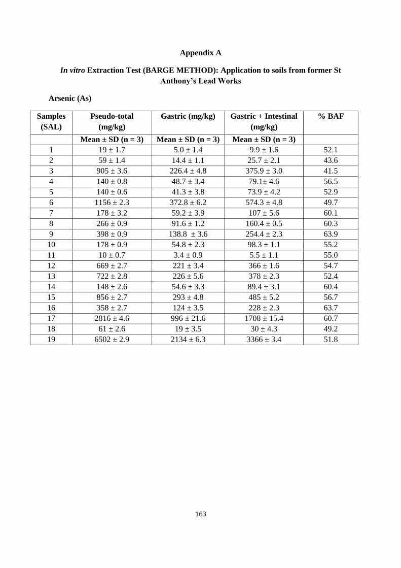
163

Appendix A

In vitro Extraction Test (BARGE METHOD): Application to soils from former St

Anthony’s Lead Works

Arsenic (As)

Samples

(SAL)

Pseudo-total

(mg/kg)

Gastric (mg/kg) Gastric + Intestinal

(mg/kg)

% BAF

Mean ± SD (n = 3) Mean ± SD (n = 3) Mean ± SD (n = 3)

1 19 ± 1.7 5.0 ± 1.4 9.9 ± 1.6 52.1

2 59 ± 1.4 14.4 ± 1.1 25.7 ± 2.1 43.6

3 905 ± 3.6 226.4 ± 4.8 375.9 ± 3.0 41.5

4 140 ± 0.8 48.7 ± 3.4 79.1± 4.6 56.5

5 140 ± 0.6 41.3 ± 3.8 73.9 ± 4.2 52.9

6 1156 ± 2.3 372.8 ± 6.2 574.3 ± 4.8 49.7

7 178 ± 3.2 59.2 ± 3.9 107 ± 5.6 60.1

8 266 ± 0.9 91.6 ± 1.2 160.4 ± 0.5 60.3

9 398 ± 0.9 138.8 ± 3.6 254.4 ± 2.3 63.9

10 178 ± 0.9 54.8 ± 2.3 98.3 ± 1.1 55.2

11 10 ± 0.7 3.4 ± 0.9 5.5 ± 1.1 55.0

12 669 ± 2.7 221 ± 3.4 366 ± 1.6 54.7

13 722 ± 2.8 226 ± 5.6 378 ± 2.3 52.4

14 148 ± 2.6 54.6 ± 3.3 89.4 ± 3.1 60.4

15 856 ± 2.7 293 ± 4.8 485 ± 5.2 56.7

16 358 ± 2.7 124 ± 3.5 228 ± 2.3 63.7

17 2816 ± 4.6 996 ± 21.6 1708 ± 15.4 60.7

18 61 ± 2.6 19 ± 3.5 30 ± 4.3 49.2

19 6502 ± 2.9 2134 ± 6.3 3366 ± 3.4 51.8

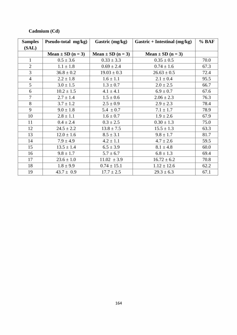
164

Cadmium (Cd)

Samples

(SAL)

Pseudo-total mg/kg) Gastric (mg/kg) Gastric + Intestinal (mg/kg) % BAF

Mean ± SD (n = 3) Mean ± SD (n = 3) Mean ± SD (n = 3)

1 0.5 ± 3.6 0.33 ± 3.3 0.35 ± 0.5 70.0

2 1.1 ± 1.8 0.69 ± 2.4 0.74 ± 1.6 67.3

3 36.8 ± 0.2 19.03 ± 0.3 26.63 ± 0.5 72.4

4 2.2 ± 1.8 1.6 ± 1.1 2.1 ± 0.4 95.5

5 3.0 ± 1.5 1.3 ± 0.7 2.0 ± 2.5 66.7

6 10.2 ± 1.5 4.1 ± 4.1 6.9 ± 0.7 67.6

7 2.7 ± 1.4 1.5 ± 0.6 2.06 ± 2.3 76.3

8 3.7 ± 1.2 2.5 ± 0.9 2.9 ± 2.3 78.4

9 9.0 ± 1.8 5.4 ± 0.7 7.1 ± 1.7 78.9

10 2.8 ± 1.1 1.6 ± 0.7 1.9 ± 2.6 67.9

11 0.4 ± 2.4 0.3 ± 2.5 0.30 ± 1.3 75.0

12 24.5 ± 2.2 13.8 ± 7.5 15.5 ± 1.3 63.3

13 12.0 ± 1.6 8.5 ± 3.1 9.8 ± 1.7 81.7

14 7.9 ± 4.9 4.2 ± 1.1 4.7 ± 2.6 59.5

15 13.5 ± 1.4 6.5 ± 3.9 8.1 ± 4.8 60.0

16 9.8 ± 1.7 5.7 ± 6.7 6.8 ± 1.3 69.4

17 23.6 ± 1.0 11.02 ± 3.9 16.72 ± 6.2 70.8

18 1.8 ± 9.9 0.74 ± 15.1 1.12 ± 12.6 62.2

19 43.7 ± 0.9 17.7 ± 2.5 29.3 ± 6.3 67.1

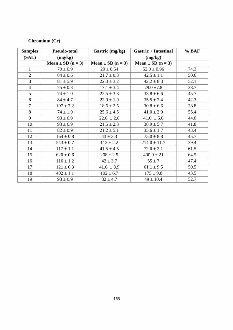
165

Chromium (Cr)

Samples

(SAL)

Pseudo-total

(mg/kg)

Gastric (mg/kg) Gastric + Intestinal

(mg/kg)

% BAF

Mean ± SD (n = 3) Mean ± SD (n = 3) Mean ± SD (n = 3)

1 70 ± 0.9 29 ± 0.54 52.0 ± 0.96 74.3

2 84 ± 0.6 21.7 ± 0.3 42.5 ± 1.1 50.6

3 81 ± 5.9 22.3 ± 3.2 42.2 ± 8.3 52.1

4 75 ± 0.8 17.1 ± 3.4 29.0 ±7.8 38.7

5 74 ± 1.0 22.5 ± 3.8 33.8 ± 6.6 45.7

6 84 ± 4.7 22.9 ± 1.9 35.5 ± 7.4 42.3

7 107 ± 7.2 18.6 ± 2.5 30.8 ± 6.6 28.8

8 74 ± 1.0 25.6 ± 4.5 41.0 ± 2.9 55.4

9 93 ± 6.9 22.6 ± 2.6 41.0 ± 5.8 44.0

10 93 ± 6.9 21.5 ± 2.3 38.9 ± 5.7 41.8

11 82 ± 0.9 21.2 ± 5.1 35.6 ± 1.7 43.4

12 164 ± 0.8 43 ± 3.3 75.0 ± 8.8 45.7

13 543 ± 0.7 112 ± 2.2 214.0 ± 11.7 39.4

14 117 ± 1.1 41.5 ± 4.5 72.0 ± 2.1 61.5

15 620 ± 0.6 208 ± 2.9 400.0 ± 21 64.5

16 116 ± 1.2 42 ± 3.7 55 ± 7 47.4

17 121 ± 0.3 41.6 ± 3.9 61.1 ± 9.5 50.5

18 402 ± 1.1 102 ± 6.7 175 ± 9.8 43.5

19 93 ± 0.9 32 ± 4.7 49 ± 10.4 52.7

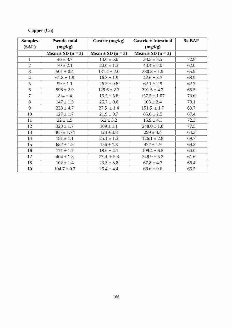
166

Copper (Cu)

Samples

(SAL)

Pseudo-total

(mg/kg)

Gastric (mg/kg) Gastric + Intestinal

(mg/kg)

% BAF

Mean ± SD (n = 3) Mean ± SD (n = 3) Mean ± SD (n = 3)

1 46 ± 3.7 14.6 ± 6.0 33.5 ± 3.5 72.8

2 70 ± 2.1 20.0 ± 1.3 43.4 ± 5.0 62.0

3 501 ± 0.4 131.4 ± 2.0 330.3 ± 1.9 65.9

4 61.8 ± 1.9 16.3 ± 1.9 42.6 ± 3.7 68.9

5 99 ± 1.1 26.5 ± 0.8 62.1 ± 2.9 62.7

6 598 ± 2.9 129.6 ± 2.7 391.5 ± 4.2 65.5

7 214 ± 4 15.5 ± 5.8 157.5 ± 1.07 73.6

8 147 ± 1.3 26.7 ± 0.6 103 ± 2.4 70.1

9 238 ± 4.7 27.5 ± 1.4 151.5 ± 1.7 63.7

10 127 ± 1.7 21.9 ± 0.7 85.6 ± 2.5 67.4

11 22 ± 1.5 6.2 ± 3.2 15.9 ± 4.1 72.3

12 320 ± 1.7 109 ± 1.1 248.0 ± 1.8 77.5

13 465 ± 1.74 123 ± 3.8 299 ± 4.4 64.3

14 181 ± 1.1 25.1 ± 1.3 126.1 ± 2.8 69.7

15 682 ± 1.5 156 ± 1.3 472 ± 1.9 69.2

16 171 ± 1.7 18.6 ± 4.1 109.4 ± 6.5 64.0

17 404 ± 1.3 77.9 ± 5.3 248.9 ± 5.3 61.6

18 102 ± 1.4 23.3 ± 3.8 67.8 ± 4.7 66.4

19 104.7 ± 0.7 25.4 ± 4.4 68.6 ± 9.6 65.5

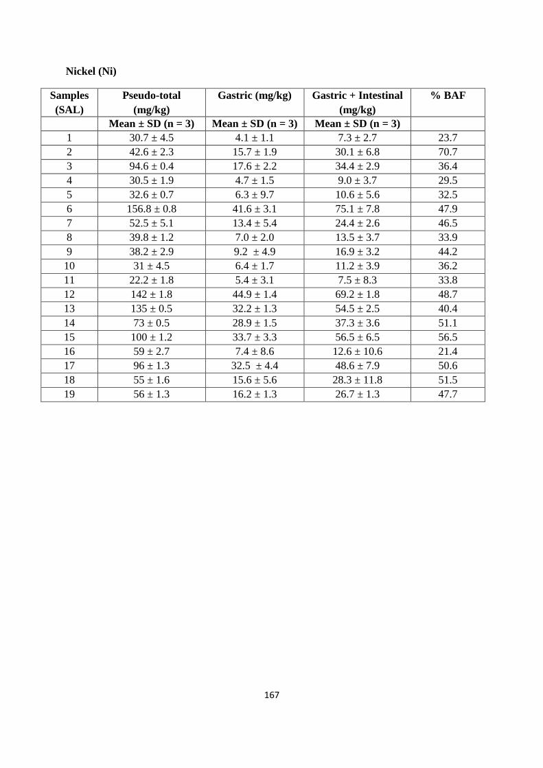
167

Nickel (Ni)

Samples

(SAL)

Pseudo-total

(mg/kg)

Gastric (mg/kg) Gastric + Intestinal

(mg/kg)

% BAF

Mean ± SD (n = 3) Mean ± SD (n = 3) Mean ± SD (n = 3)

1 30.7 ± 4.5 4.1 ± 1.1 7.3 ± 2.7 23.7

2 42.6 ± 2.3 15.7 ± 1.9 30.1 ± 6.8 70.7

3 94.6 ± 0.4 17.6 ± 2.2 34.4 ± 2.9 36.4

4 30.5 ± 1.9 4.7 ± 1.5 9.0 ± 3.7 29.5

5 32.6 ± 0.7 6.3 ± 9.7 10.6 ± 5.6 32.5

6 156.8 ± 0.8 41.6 ± 3.1 75.1 ± 7.8 47.9

7 52.5 ± 5.1 13.4 ± 5.4 24.4 ± 2.6 46.5

8 39.8 ± 1.2 7.0 ± 2.0 13.5 ± 3.7 33.9

9 38.2 ± 2.9 9.2 ± 4.9 16.9 ± 3.2 44.2

10 31 ± 4.5 6.4 ± 1.7 11.2 ± 3.9 36.2

11 22.2 ± 1.8 5.4 ± 3.1 7.5 ± 8.3 33.8

12 142 ± 1.8 44.9 ± 1.4 69.2 ± 1.8 48.7

13 135 ± 0.5 32.2 ± 1.3 54.5 ± 2.5 40.4

14 73 ± 0.5 28.9 ± 1.5 37.3 ± 3.6 51.1

15 100 ± 1.2 33.7 ± 3.3 56.5 ± 6.5 56.5

16 59 ± 2.7 7.4 ± 8.6 12.6 ± 10.6 21.4

17 96 ± 1.3 32.5 ± 4.4 48.6 ± 7.9 50.6

18 55 ± 1.6 15.6 ± 5.6 28.3 ± 11.8 51.5

19 56 ± 1.3 16.2 ± 1.3 26.7 ± 1.3 47.7

168

Lead (Pb)

Samples

(SAL)

Pseudo-total

(mg/kg)

Gastric (mg/kg) Gastric + Intestinal

(mg/kg)

% BAF

Mean ± SD (n = 3) Mean ± SD (n = 3) Mean ± SD (n = 3)

1 174 ± 0.4 65.5 ± 5.0 94.0 ± 3.0 54.0

2 1381 ± 1.5 445 ± 4.0 683 ± 2.1 49.5

3 29302 ± 7.9 7110 ± 7.1 11916 ± 4.5 40.7

4 1048 ± 2.5 177 ± 8.5 262 ± 2.4 25.0

5 2452 ± 1.9 644 ± 4.3 1121 ± 1.7 45.7

6 29286 ± 5.3 6007 ± 28 10360 ± 26 35.4

7 5071 ± 1.9 1981 ± 6.9 2959 ± 5.2 58.4

8 4833 ± 1.6 1811 ± 4.4 2331 ± 0.9 48.2

9 7214 ± 1.8 2044 ± 4.5 3115 ± 1.1 43.2

10 2691 ± 1.3 666 ± 3.6 995 ± 1.1 37.0

11 221 ± 3.2 73 ± 8.7 119 ± 8.5 53.8

12 17443 ± 6 5013 ± 2.8 7020 ± 8.3 40.2

13 15024 ± 10 3445 ± 1.6 4448 ±9.6 29.6

14 4266 ± 12 1277 ± 6.5 1695 ± 9.2 39.7

15 28709 ± 28 8363 ± 63 686 ± 58 31.5

16 4968 ± 16 1417 ± 8.3 2652 ± 5.5 53.4

17 22822 ± 18 7377 ± 7.1 10962 ± 37.4 48.0

18 1338 ± 15 553 ± 4.6 700 ± 5.8 52.3

19 33306 ± 11 13653 ± 4.7 15374 ± 4.9 46.2

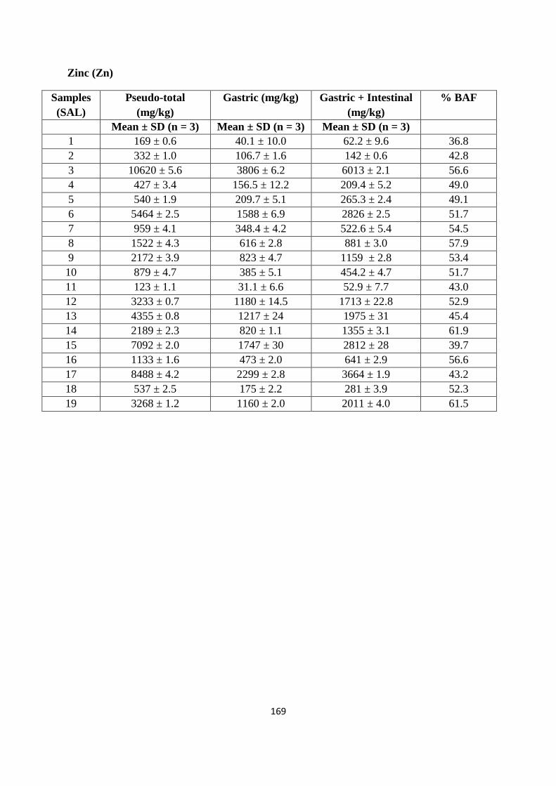
169

Zinc (Zn)

Samples

(SAL)

Pseudo-total

(mg/kg)

Gastric (mg/kg) Gastric + Intestinal

(mg/kg)

% BAF

Mean ± SD (n = 3) Mean ± SD (n = 3) Mean ± SD (n = 3)

1 169 ± 0.6 40.1 ± 10.0 62.2 ± 9.6 36.8

2 332 ± 1.0 106.7 ± 1.6 142 ± 0.6 42.8

3 10620 ± 5.6 3806 ± 6.2 6013 ± 2.1 56.6

4 427 ± 3.4 156.5 ± 12.2 209.4 ± 5.2 49.0

5 540 ± 1.9 209.7 ± 5.1 265.3 ± 2.4 49.1

6 5464 ± 2.5 1588 ± 6.9 2826 ± 2.5 51.7

7 959 ± 4.1 348.4 ± 4.2 522.6 ± 5.4 54.5

8 1522 ± 4.3 616 ± 2.8 881 ± 3.0 57.9

9 2172 ± 3.9 823 ± 4.7 1159 ± 2.8 53.4

10 879 ± 4.7 385 ± 5.1 454.2 ± 4.7 51.7

11 123 ± 1.1 31.1 ± 6.6 52.9 ± 7.7 43.0

12 3233 ± 0.7 1180 ± 14.5 1713 ± 22.8 52.9

13 4355 ± 0.8 1217 ± 24 1975 ± 31 45.4

14 2189 ± 2.3 820 ± 1.1 1355 ± 3.1 61.9

15 7092 ± 2.0 1747 ± 30 2812 ± 28 39.7

16 1133 ± 1.6 473 ± 2.0 641 ± 2.9 56.6

17 8488 ± 4.2 2299 ± 2.8 3664 ± 1.9 43.2

18 537 ± 2.5 175 ± 2.2 281 ± 3.9 52.3

19 3268 ± 1.2 1160 ± 2.0 2011 ± 4.0 61.5

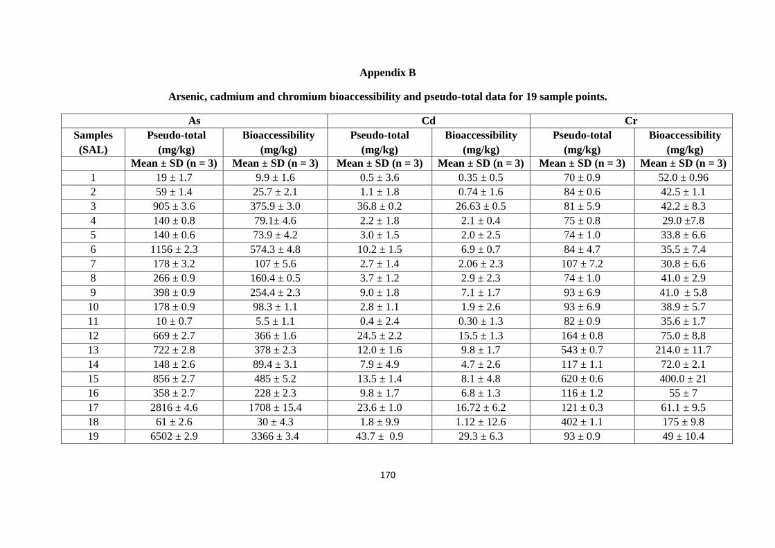
170

Appendix B

Arsenic, cadmium and chromium bioaccessibility and pseudo-total data for 19 sample points.

As Cd Cr

Samples

(SAL)

Pseudo-total

(mg/kg)

Bioaccessibility

(mg/kg)

Pseudo-total

(mg/kg)

Bioaccessibility

(mg/kg)

Pseudo-total

(mg/kg)

Bioaccessibility

(mg/kg)

Mean ± SD (n = 3) Mean ± SD (n = 3) Mean ± SD (n = 3) Mean ± SD (n = 3) Mean ± SD (n = 3) Mean ± SD (n = 3)

1 19 ± 1.7 9.9 ± 1.6 0.5 ± 3.6 0.35 ± 0.5 70 ± 0.9 52.0 ± 0.96

2 59 ± 1.4 25.7 ± 2.1 1.1 ± 1.8 0.74 ± 1.6 84 ± 0.6 42.5 ± 1.1

3 905 ± 3.6 375.9 ± 3.0 36.8 ± 0.2 26.63 ± 0.5 81 ± 5.9 42.2 ± 8.3

4 140 ± 0.8 79.1± 4.6 2.2 ± 1.8 2.1 ± 0.4 75 ± 0.8 29.0 ±7.8

5 140 ± 0.6 73.9 ± 4.2 3.0 ± 1.5 2.0 ± 2.5 74 ± 1.0 33.8 ± 6.6

6 1156 ± 2.3 574.3 ± 4.8 10.2 ± 1.5 6.9 ± 0.7 84 ± 4.7 35.5 ± 7.4

7 178 ± 3.2 107 ± 5.6 2.7 ± 1.4 2.06 ± 2.3 107 ± 7.2 30.8 ± 6.6

8 266 ± 0.9 160.4 ± 0.5 3.7 ± 1.2 2.9 ± 2.3 74 ± 1.0 41.0 ± 2.9

9 398 ± 0.9 254.4 ± 2.3 9.0 ± 1.8 7.1 ± 1.7 93 ± 6.9 41.0 ± 5.8

10 178 ± 0.9 98.3 ± 1.1 2.8 ± 1.1 1.9 ± 2.6 93 ± 6.9 38.9 ± 5.7

11 10 ± 0.7 5.5 ± 1.1 0.4 ± 2.4 0.30 ± 1.3 82 ± 0.9 35.6 ± 1.7

12 669 ± 2.7 366 ± 1.6 24.5 ± 2.2 15.5 ± 1.3 164 ± 0.8 75.0 ± 8.8

13 722 ± 2.8 378 ± 2.3 12.0 ± 1.6 9.8 ± 1.7 543 ± 0.7 214.0 ± 11.7

14 148 ± 2.6 89.4 ± 3.1 7.9 ± 4.9 4.7 ± 2.6 117 ± 1.1 72.0 ± 2.1

15 856 ± 2.7 485 ± 5.2 13.5 ± 1.4 8.1 ± 4.8 620 ± 0.6 400.0 ± 21

16 358 ± 2.7 228 ± 2.3 9.8 ± 1.7 6.8 ± 1.3 116 ± 1.2 55 ± 7

17 2816 ± 4.6 1708 ± 15.4 23.6 ± 1.0 16.72 ± 6.2 121 ± 0.3 61.1 ± 9.5

18 61 ± 2.6 30 ± 4.3 1.8 ± 9.9 1.12 ± 12.6 402 ± 1.1 175 ± 9.8

19 6502 ± 2.9 3366 ± 3.4 43.7 ± 0.9 29.3 ± 6.3 93 ± 0.9 49 ± 10.4

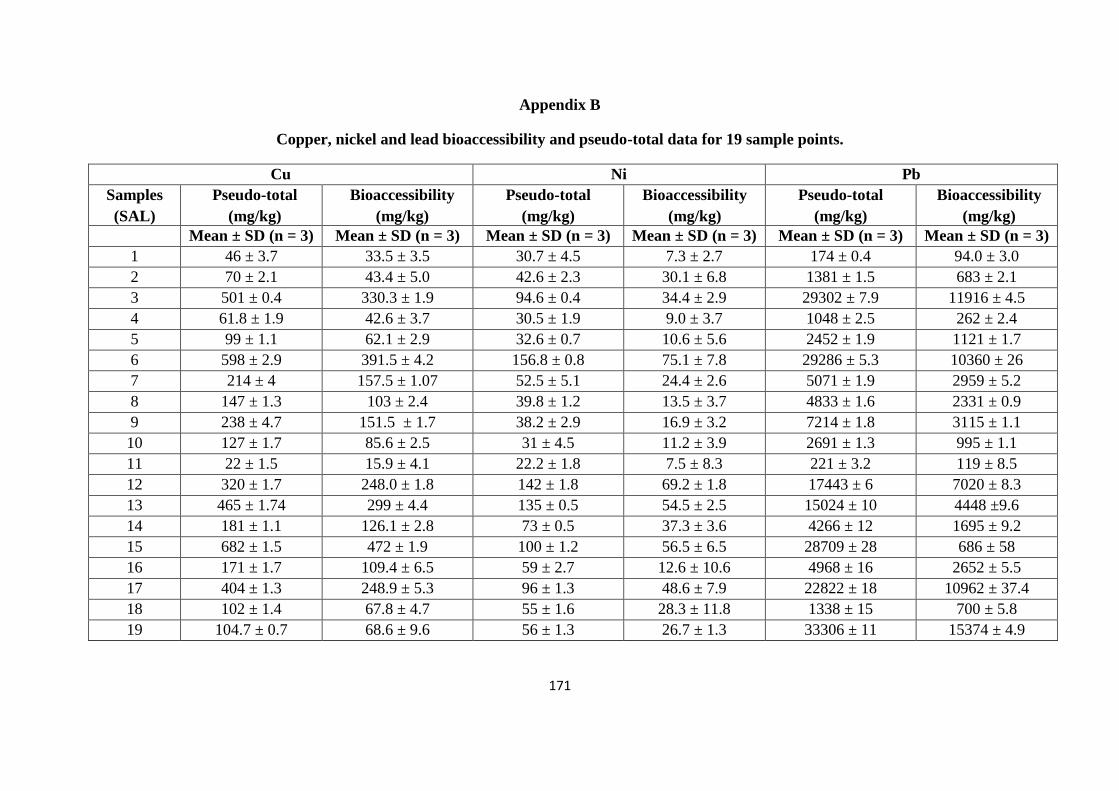
171

Appendix B

Copper, nickel and lead bioaccessibility and pseudo-total data for 19 sample points.

Cu Ni Pb

Samples

(SAL)

Pseudo-total

(mg/kg)

Bioaccessibility

(mg/kg)

Pseudo-total

(mg/kg)

Bioaccessibility

(mg/kg)

Pseudo-total

(mg/kg)

Bioaccessibility

(mg/kg)

Mean ± SD (n = 3) Mean ± SD (n = 3) Mean ± SD (n = 3) Mean ± SD (n = 3) Mean ± SD (n = 3) Mean ± SD (n = 3)

1 46 ± 3.7 33.5 ± 3.5 30.7 ± 4.5 7.3 ± 2.7 174 ± 0.4 94.0 ± 3.0

2 70 ± 2.1 43.4 ± 5.0 42.6 ± 2.3 30.1 ± 6.8 1381 ± 1.5 683 ± 2.1

3 501 ± 0.4 330.3 ± 1.9 94.6 ± 0.4 34.4 ± 2.9 29302 ± 7.9 11916 ± 4.5

4 61.8 ± 1.9 42.6 ± 3.7 30.5 ± 1.9 9.0 ± 3.7 1048 ± 2.5 262 ± 2.4

5 99 ± 1.1 62.1 ± 2.9 32.6 ± 0.7 10.6 ± 5.6 2452 ± 1.9 1121 ± 1.7

6 598 ± 2.9 391.5 ± 4.2 156.8 ± 0.8 75.1 ± 7.8 29286 ± 5.3 10360 ± 26

7 214 ± 4 157.5 ± 1.07 52.5 ± 5.1 24.4 ± 2.6 5071 ± 1.9 2959 ± 5.2

8 147 ± 1.3 103 ± 2.4 39.8 ± 1.2 13.5 ± 3.7 4833 ± 1.6 2331 ± 0.9

9 238 ± 4.7 151.5 ± 1.7 38.2 ± 2.9 16.9 ± 3.2 7214 ± 1.8 3115 ± 1.1

10 127 ± 1.7 85.6 ± 2.5 31 ± 4.5 11.2 ± 3.9 2691 ± 1.3 995 ± 1.1

11 22 ± 1.5 15.9 ± 4.1 22.2 ± 1.8 7.5 ± 8.3 221 ± 3.2 119 ± 8.5

12 320 ± 1.7 248.0 ± 1.8 142 ± 1.8 69.2 ± 1.8 17443 ± 6 7020 ± 8.3

13 465 ± 1.74 299 ± 4.4 135 ± 0.5 54.5 ± 2.5 15024 ± 10 4448 ±9.6

14 181 ± 1.1 126.1 ± 2.8 73 ± 0.5 37.3 ± 3.6 4266 ± 12 1695 ± 9.2

15 682 ± 1.5 472 ± 1.9 100 ± 1.2 56.5 ± 6.5 28709 ± 28 686 ± 58

16 171 ± 1.7 109.4 ± 6.5 59 ± 2.7 12.6 ± 10.6 4968 ± 16 2652 ± 5.5

17 404 ± 1.3 248.9 ± 5.3 96 ± 1.3 48.6 ± 7.9 22822 ± 18 10962 ± 37.4

18 102 ± 1.4 67.8 ± 4.7 55 ± 1.6 28.3 ± 11.8 1338 ± 15 700 ± 5.8

19 104.7 ± 0.7 68.6 ± 9.6 56 ± 1.3 26.7 ± 1.3 33306 ± 11 15374 ± 4.9

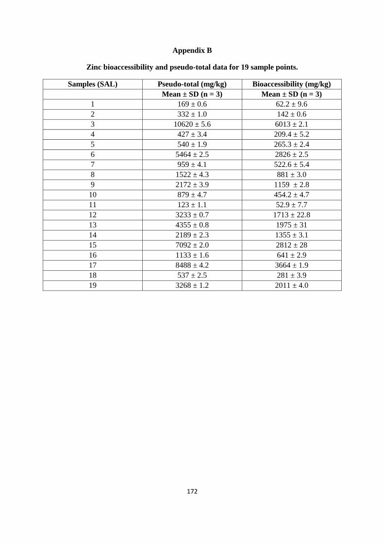
172

Appendix B

Zinc bioaccessibility and pseudo-total data for 19 sample points.

Samples (SAL) Pseudo-total (mg/kg) Bioaccessibility (mg/kg)

Mean ± SD (n = 3) Mean ± SD (n = 3)

1 169 ± 0.6 62.2 ± 9.6

2 332 ± 1.0 142 ± 0.6

3 10620 ± 5.6 6013 ± 2.1

4 427 ± 3.4 209.4 ± 5.2

5 540 ± 1.9 265.3 ± 2.4

6 5464 ± 2.5 2826 ± 2.5

7 959 ± 4.1 522.6 ± 5.4

8 1522 ± 4.3 881 ± 3.0

9 2172 ± 3.9 1159 ± 2.8

10 879 ± 4.7 454.2 ± 4.7

11 123 ± 1.1 52.9 ± 7.7

12 3233 ± 0.7 1713 ± 22.8

13 4355 ± 0.8 1975 ± 31

14 2189 ± 2.3 1355 ± 3.1

15 7092 ± 2.0 2812 ± 28

16 1133 ± 1.6 641 ± 2.9

17 8488 ± 4.2 3664 ± 1.9

18 537 ± 2.5 281 ± 3.9

19 3268 ± 1.2 2011 ± 4.0

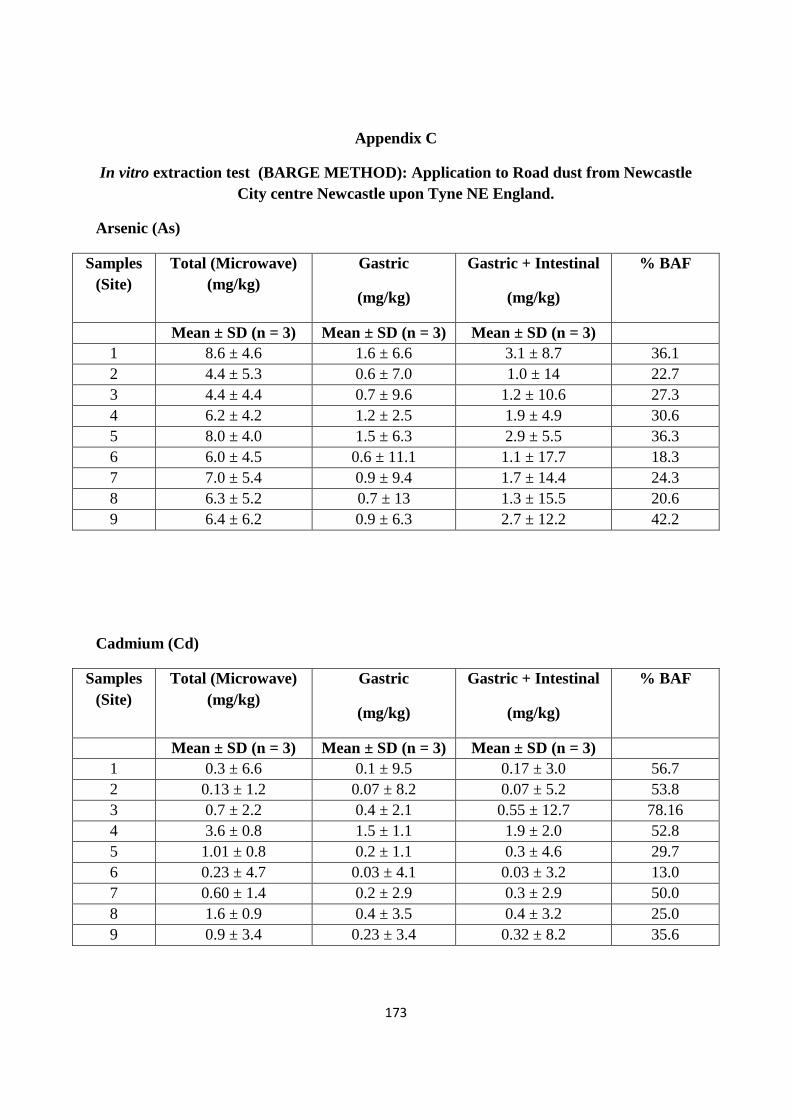
173

Appendix C

In vitro extraction test (BARGE METHOD): Application to Road dust from Newcastle

City centre Newcastle upon Tyne NE England.

Arsenic (As)

Samples

(Site)

Total (Microwave)

(mg/kg)

Gastric

(mg/kg)

Gastric + Intestinal

(mg/kg)

% BAF

Mean ± SD (n = 3) Mean ± SD (n = 3) Mean ± SD (n = 3)

1 8.6 ± 4.6 1.6 ± 6.6 3.1 ± 8.7 36.1

2 4.4 ± 5.3 0.6 ± 7.0 1.0 ± 14 22.7

3 4.4 ± 4.4 0.7 ± 9.6 1.2 ± 10.6 27.3

4 6.2 ± 4.2 1.2 ± 2.5 1.9 ± 4.9 30.6

5 8.0 ± 4.0 1.5 ± 6.3 2.9 ± 5.5 36.3

6 6.0 ± 4.5 0.6 ± 11.1 1.1 ± 17.7 18.3

7 7.0 ± 5.4 0.9 ± 9.4 1.7 ± 14.4 24.3

8 6.3 ± 5.2 0.7 ± 13 1.3 ± 15.5 20.6

9 6.4 ± 6.2 0.9 ± 6.3 2.7 ± 12.2 42.2

Cadmium (Cd)

Samples

(Site)

Total (Microwave)

(mg/kg)

Gastric

(mg/kg)

Gastric + Intestinal

(mg/kg)

% BAF

Mean ± SD (n = 3) Mean ± SD (n = 3) Mean ± SD (n = 3)

1 0.3 ± 6.6 0.1 ± 9.5 0.17 ± 3.0 56.7

2 0.13 ± 1.2 0.07 ± 8.2 0.07 ± 5.2 53.8

3 0.7 ± 2.2 0.4 ± 2.1 0.55 ± 12.7 78.16

4 3.6 ± 0.8 1.5 ± 1.1 1.9 ± 2.0 52.8

5 1.01 ± 0.8 0.2 ± 1.1 0.3 ± 4.6 29.7

6 0.23 ± 4.7 0.03 ± 4.1 0.03 ± 3.2 13.0

7 0.60 ± 1.4 0.2 ± 2.9 0.3 ± 2.9 50.0

8 1.6 ± 0.9 0.4 ± 3.5 0.4 ± 3.2 25.0

9 0.9 ± 3.4 0.23 ± 3.4 0.32 ± 8.2 35.6

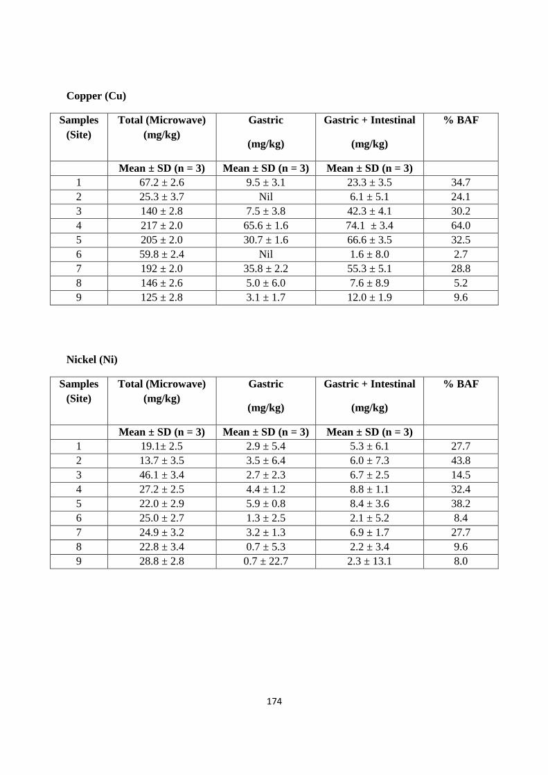
174

Copper (Cu)

Samples

(Site)

Total (Microwave)

(mg/kg)

Gastric

(mg/kg)

Gastric + Intestinal

(mg/kg)

% BAF

Mean ± SD (n = 3) Mean ± SD (n = 3) Mean ± SD (n = 3)

1 67.2 ± 2.6 9.5 ± 3.1 23.3 ± 3.5 34.7

2 25.3 ± 3.7 Nil 6.1 ± 5.1 24.1

3 140 ± 2.8 7.5 ± 3.8 42.3 ± 4.1 30.2

4 217 ± 2.0 65.6 ± 1.6 74.1 ± 3.4 64.0

5 205 ± 2.0 30.7 ± 1.6 66.6 ± 3.5 32.5

6 59.8 ± 2.4 Nil 1.6 ± 8.0 2.7

7 192 ± 2.0 35.8 ± 2.2 55.3 ± 5.1 28.8

8 146 ± 2.6 5.0 ± 6.0 7.6 ± 8.9 5.2

9 125 ± 2.8 3.1 ± 1.7 12.0 ± 1.9 9.6

Nickel (Ni)

Samples

(Site)

Total (Microwave)

(mg/kg)

Gastric

(mg/kg)

Gastric + Intestinal

(mg/kg)

% BAF

Mean ± SD (n = 3) Mean ± SD (n = 3) Mean ± SD (n = 3)

1 19.1± 2.5 2.9 ± 5.4 5.3 ± 6.1 27.7

2 13.7 ± 3.5 3.5 ± 6.4 6.0 ± 7.3 43.8

3 46.1 ± 3.4 2.7 ± 2.3 6.7 ± 2.5 14.5

4 27.2 ± 2.5 4.4 ± 1.2 8.8 ± 1.1 32.4

5 22.0 ± 2.9 5.9 ± 0.8 8.4 ± 3.6 38.2

6 25.0 ± 2.7 1.3 ± 2.5 2.1 ± 5.2 8.4

7 24.9 ± 3.2 3.2 ± 1.3 6.9 ± 1.7 27.7

8 22.8 ± 3.4 0.7 ± 5.3 2.2 ± 3.4 9.6

9 28.8 ± 2.8 0.7 ± 22.7 2.3 ± 13.1 8.0

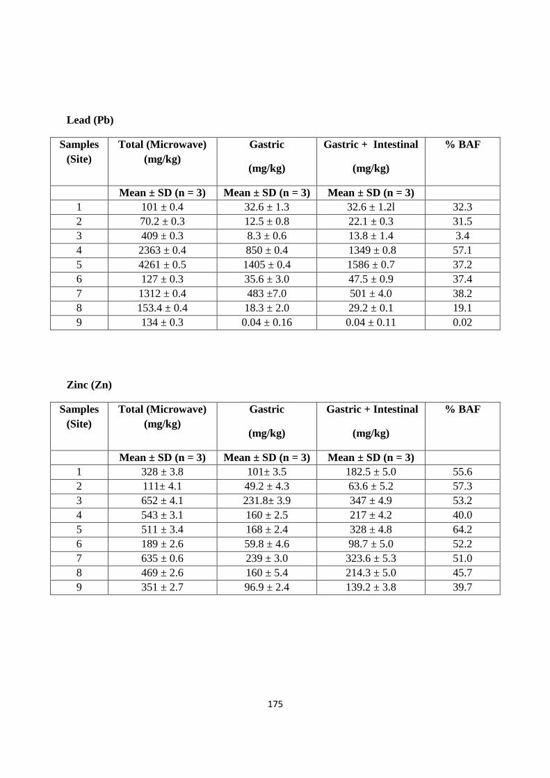
175

Lead (Pb)

Samples

(Site)

Total (Microwave)

(mg/kg)

Gastric

(mg/kg)

Gastric + Intestinal

(mg/kg)

% BAF

Mean ± SD (n = 3) Mean ± SD (n = 3) Mean ± SD (n = 3)

1 101 ± 0.4 32.6 ± 1.3 32.6 ± 1.2l 32.3

2 70.2 ± 0.3 12.5 ± 0.8 22.1 ± 0.3 31.5

3 409 ± 0.3 8.3 ± 0.6 13.8 ± 1.4 3.4

4 2363 ± 0.4 850 ± 0.4 1349 ± 0.8 57.1

5 4261 ± 0.5 1405 ± 0.4 1586 ± 0.7 37.2

6 127 ± 0.3 35.6 ± 3.0 47.5 ± 0.9 37.4

7 1312 ± 0.4 483 ±7.0 501 ± 4.0 38.2

8 153.4 ± 0.4 18.3 ± 2.0 29.2 ± 0.1 19.1

9 134 ± 0.3 0.04 ± 0.16 0.04 ± 0.11 0.02

Zinc (Zn)

Samples

(Site)

Total (Microwave)

(mg/kg)

Gastric

(mg/kg)

Gastric + Intestinal

(mg/kg)

% BAF

Mean ± SD (n = 3) Mean ± SD (n = 3) Mean ± SD (n = 3)

1 328 ± 3.8 101± 3.5 182.5 ± 5.0 55.6

2 111± 4.1 49.2 ± 4.3 63.6 ± 5.2 57.3

3 652 ± 4.1 231.8± 3.9 347 ± 4.9 53.2

4 543 ± 3.1 160 ± 2.5 217 ± 4.2 40.0

5 511 ± 3.4 168 ± 2.4 328 ± 4.8 64.2

6 189 ± 2.6 59.8 ± 4.6 98.7 ± 5.0 52.2

7 635 ± 0.6 239 ± 3.0 323.6 ± 5.3 51.0

8 469 ± 2.6 160 ± 5.4 214.3 ± 5.0 45.7

9 351 ± 2.7 96.9 ± 2.4 139.2 ± 3.8 39.7

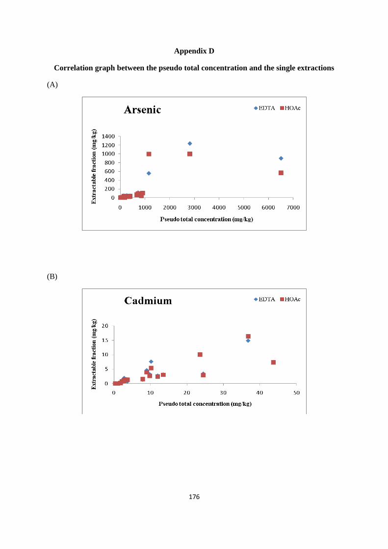
176

Appendix D

Correlation graph between the pseudo total concentration and the single extractions

(A)

(B)

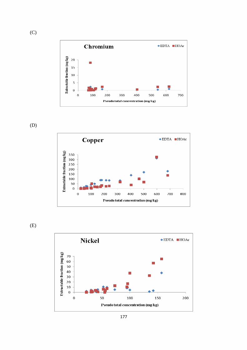
177

(C)

(D)

(E)

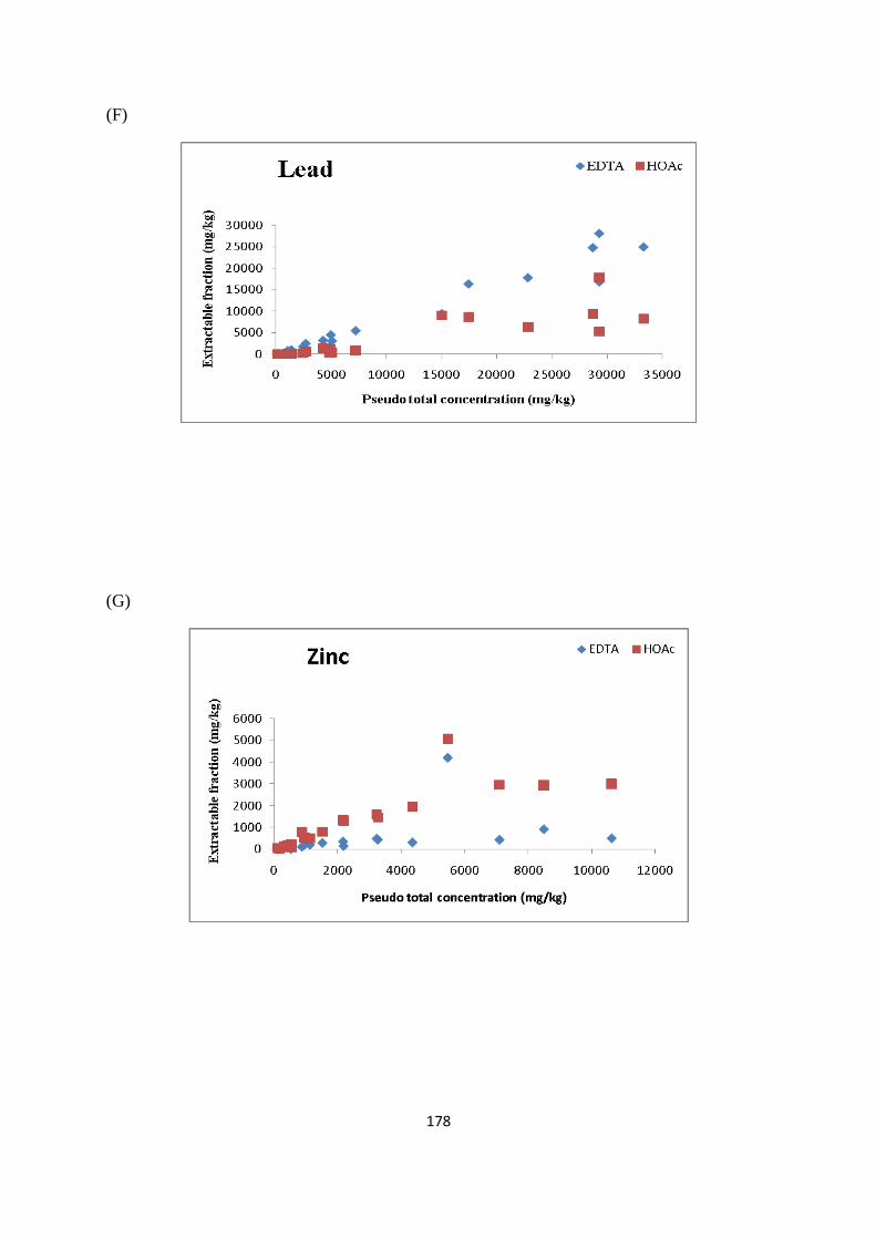
178

(F)

(G)

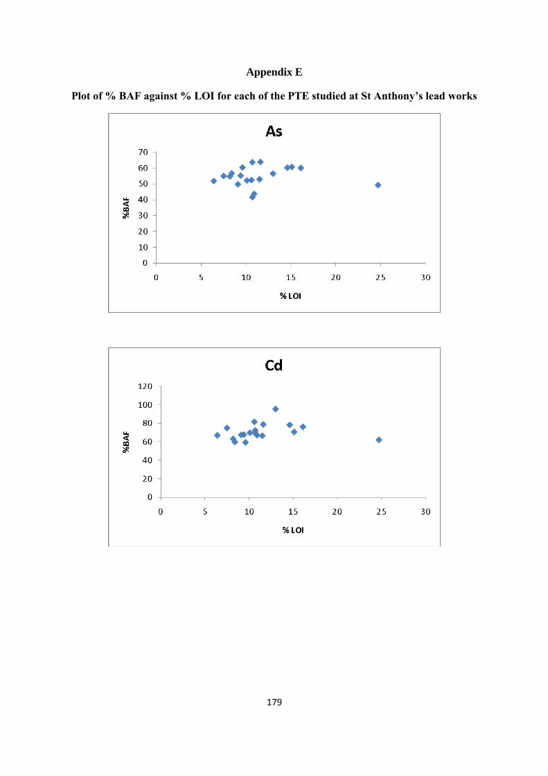
179

Appendix E

Plot of % BAF against % LOI for each of the PTE studied at St Anthony’s lead works

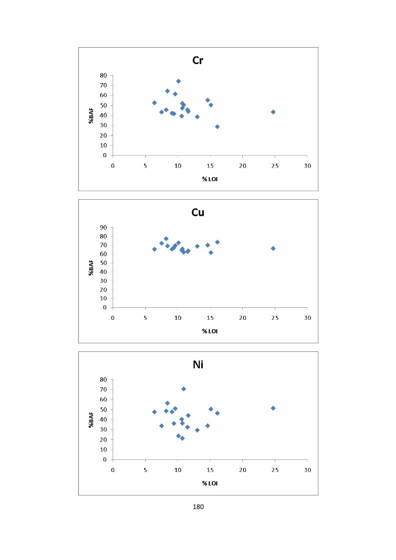
180

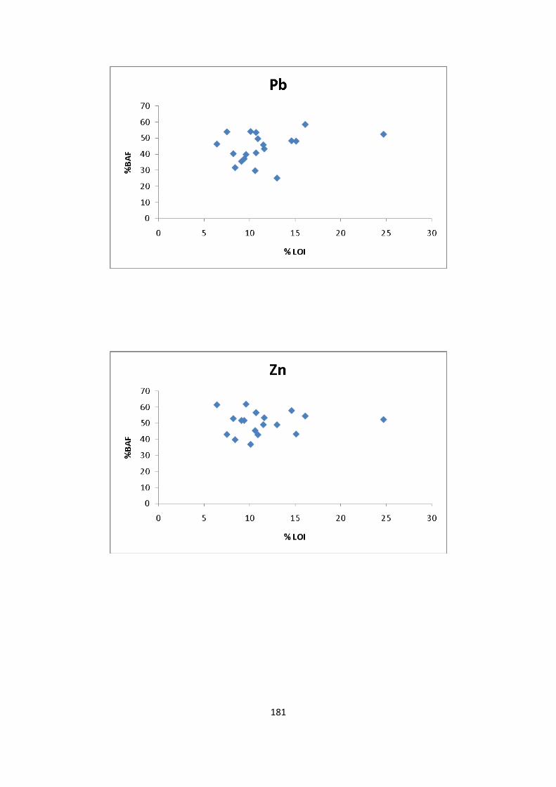
181

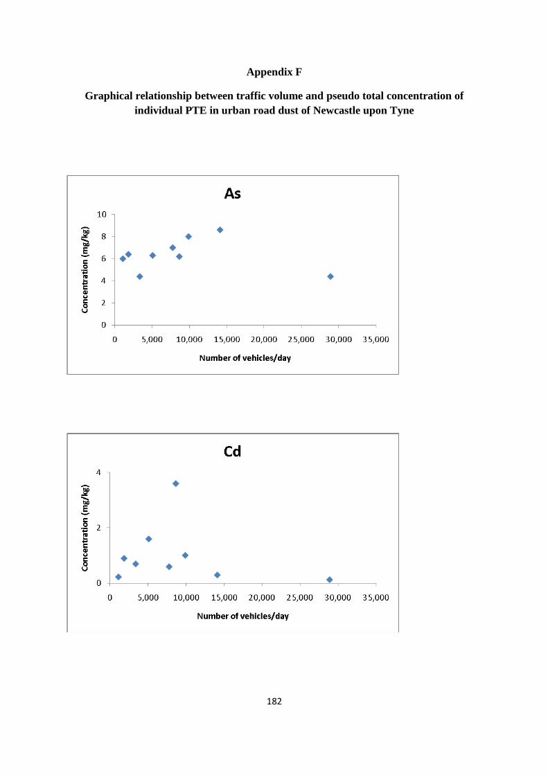
182

Appendix F

Graphical relationship between traffic volume and pseudo total concentration of

individual PTE in urban road dust of Newcastle upon Tyne

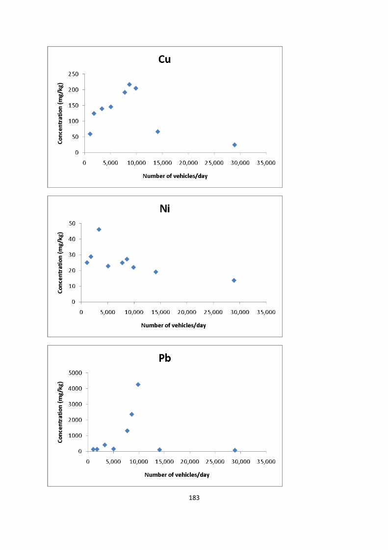
183

184