DETERMINATION OF MILLIMETRIC SIGNAL ATTENUATION DUE TO RAIN USING RAIN RATE AND RAINDROP SIZE

DISTRIBUTION MODELS FOR SOUTHERN AFRICA

by

Senzo Jerome Malinga

A THESIS

submitted in fulfillment of the requirements for the degree

PhD (ELECTRONIC ENGINEERING)

School of Engineering

College of Agriculture, Engineering, and Science

UNIVERSITY OF KWAZULU-NATAL

Durban, South Africa

March 2014

Supervisor: Professor Thomas Joachim Odhiambo Afullo

ii

Approved by:

Supervisor: Professor Thomas Joachim Odhiambo Afullo

As the candidate’s Supervisor I agree to the submission of this thesis.

Signed………………………………………Date………………………………………..

iii

COLLEGE OF AGRICULTURE, ENGINEERING AND SCIENCE

Declaration 1 - Plagiarism

I Senzo Jerome Malinga declare that

1. The research reported in this thesis, except where otherwise indicated, is my original research.

2. This thesis has not been submitted for any degree or examination at any other university.

3. This thesis does not contain other persons’ data, pictures, graphs or other information, unless

specifically acknowledged as being sourced from other persons.

4. This thesis does not contain other persons' writing, unless specifically acknowledged as being

sourced from other researchers. Where other written sources have been quoted, then:

a. Their words have been re-written but the general information attributed to them has been

referenced

b. Where their exact words have been used, then their writing has been placed in italics and inside

quotation marks, and referenced.

5. This thesis does not contain text, graphics or tables copied and pasted from the Internet, unless

specifically acknowledged, and the source being detailed in the thesis and in the References

sections.

Signed…………………………………………………..Date………………………………………………

iv

COLLEGE OF AGRICULTURE, ENGINEERING AND SCIENCE

Declarations 2 - Publications

DETAILS OF CONTRIBUTION TO PUBLICATIONS that form part and/or include research presented

in this thesis (include publications in preparation, submitted, in press and published and give details of the

contributions of each author to the experimental work and writing of each publication).

Journal Publications

1. Senzo J. Malinga and Pius A. Owolawi, “Obtaining Raindrop Size Model Using the Method of

Moments and Its Applications for South African Radio Systems,” PIER B Journal, Vol. 46, pp.

119-138, 2013.

In this paper, the Raindrop Size Distribution (DSD) modeling and analysis are presented. Drop sizes are

classified into different rain types, namely: drizzle, widespread, shower and thunderstorm. The gamma

and Lognormal distribution models are employed using the method of moments estimator, considering

the third, fourth and sixth order moments. The results are compared with the existing raindrop size

distribution models such as the three parameter lognormal distribution proposed by Ajayi and his

colleagues and Singapore’s modified gamma and Lognormal models. This is then followed by the

implementation of the proposed raindrop size distribution models on the computation of the specific rain

attenuation. Finally, the paper suggests a suitable DSD model for the region with its expressions. The

proposed models are very useful for the determination of rain attenuation for terrestrial and satellite

systems.

2. Senzo J. Malinga, P.A. Owolawi and T.J.O. Afullo, “Determination of Specific Rain Attenuation

using Different Total Cross Section Models for Southern Africa,” – Africa Research Journal

Vol. 104, No. 3, 2013 (accepted).

Electromagnetic waves whose frequency is beyond 10 GHz are severely attenuated by rain. This is true in

both satellite and terrestrial links. The rain attenuation is mainly manifested in the form of scattering and

absorption. In the paper presented here, various total cross section models are used to calculate the

v

specific attenuation due to rain for the frequencies between 1 to 100 GHz. The DSD modelling is done

using the Method of Moments, from which the specific attenuation due to rain is computed. Comparisons

are then drawn between the models proposed, well known models in existence, and theoretical results for

three different polarizations at 19.5 GHz frequency.

Conference Publications

1. P.A. Owolawi, S.J. Malinga and T.J.O. Afullo, “Estimation of Terrestrial Rain Attenuation at

Microwave and Millimeter Wave Signals in South Africa Using the ITU-R Model,” PIERS

Proceedings, Kuala Lumpur, Malaysia, March 27-30, 2012, pp. 952-962.

In this paper, experimental rain rate measurements are presented together with rain attenuation results

computed via the application of the International Telecommunication Union’s Recommendations (ITU-R)

model for attenuation due to rain in terrestrial links in South Africa. A total of nineteen case study

locations, at least every province in South Africa represented by one, are used for this presentation. The

paper specifically presents results of the total path and specific attenuation for terrestrial links for three

different types of polarizations in the frequencies ranging from 1 to 400 GHz. The implications of rain

attenuation to the system designers are evaluated by finding link distance chart, and design link-budget at

the chosen frequency range. The results of this work can be used in planning links for both microwave

and millimeter broadband wireless networks in South Africa such as Local-Multipoint-Distributed-

Services (LMDs).

2. Mulangu, C.T.; Malinga, S.J.; Afullo, T.J.O., "Impact of rain on microwave radars," 2012

International Conference on Electromagnetics in Advanced Applications (ICEAA), vol., no.,

pp.1088,1091, 2-7 Sept. 2012, Cape Town

The most important source of disturbance in microwave links is caused by precipitation attenuation due to

mainly snow and rain via scattering and absorption. In this paper, two year experimental rain rate data is

used to perform the reflectivity profile of radar at various rain rates using the lognormal DSD model for

Durban.

3. S.J. Malinga, P.A. Owolawi, and T.J.O. Afullo, “Estimation of Rain Attenuation at C, Ka, Ku, and

V Bands for Satellite Links in South Africa,” PIERS Proceedings, Taipei, Taiwan, March 25-28,

2013, pp. 948-958.

vi

The fast growth in telecommunications, increased demand for bandwidth, congestion in lower frequency

bands and miniaturization of communication equipment have forced the designers to employ higher

frequency bands such as the C (4 to 8 GHz), Ka (26.5 to 40GHz), Ku (12-18 GHz) and V (40-75 GHz)

bands. Rain is the most deleterious to signal propagation in these bands. The contribution of rain

attenuation to the quality of signal in these bands, especially in the tropical and subtropical bands in

which South Africa is located, need to be studied. The aims of this paper are to estimate the magnitude of

rain attenuation using the ITU-R model, carry out link performance analysis, and then propose

reasonable, adequate fade margins that need to be applied for all provinces in South Africa.

4. S.J. Malinga, P.A. Owolawi, and T.J.O. Afullo, “Computation of Rain Attenuation through

Scattering at Microwave and Millimeter Bands in South Africa,” PIERS Proceedings, Taipei,

Taiwan, March 25-28, 2013, pp. 959-971.

In this presentation, both measured and calculated rain attenuation are obtained using two methods. These

methods are the Pruppacher-Pitter technique (non-spherical method) and the Mie Scattering technique

(spherical method). Incorporation of available DSD data and measured rain rate with the derived

scattering amplitude coefficients is then done to estimate the total and specific attenuation due to rain for

the South Africa region. Comparison between the results obtained with the few known rain attenuation

models and one-year attenuation measurement data in South Africa (Durban) are then drawn. Further, the

results obtained are tested for both satellite and terrestrial radio links at particular rain rates and specific

frequencies.

5. P.A. Owolawi, S.J. Malinga, T.J.O. Afullo “Computation of rain scattering properties at SHF and

EHF for radio wave propagation in South Africa”, URSI Commission F Triennial, April 30 –

May 3, 2013, Ottawa, Canada.

In this paper computation of scattering parameters at 1 – 100 GHz frequencies under the influence of a

rainy medium are presented. The characteristics of scattering parameters at these frequencies are

integrated and computed with lognormal raindrop size distribution for four rain types, and the results are

used to compute the specific attenuation due to rain as well as the associated specific phase shift. The

calculated specific attenuation due to rain and its phase shift results are compared with tropical and

temperate regions’ counterparts. In addition, analytical coefficients of the fundamental specific rain

attenuation and specific phase shift are derived in the same frequency range of different rain types in

Southern Africa.

vii

6. Chrispin T. Mulangu, Senzo J. Malinga, Thomas J. Afullo, “Prediction of Radar Reflectivity along

Radio Links”, PIERS Proceedings, pp. 264 – 267, Taipei, March 25 – 28, 2013

Radiowaves propagating through a rain zone will be scattered, depolarized, absorbed and delayed in

time. All these effects of rain on the wave propagation are related to the frequency at which the signal

is transmitted and polarization of the wave as well as to the rain rate, which influences the form and

size distribution of the raindrop. The average power received by the bistatic radar is proportional to

the product of reflectivity and attenuation. These can be measured in practice but sometimes there is a

need to determine them separately. In order to determine radar reflectivity, the backscattering

coefficient needs to be estimated. This study makes predictions about the backscattering coefficient

caused by hydrometeors along terrestrial radio links, operated at wide bandwidth of 10 – 140 GHz

frequencies. The scattering properties of the spherical raindrops are calculated for different sizes of

raindrops. From the scattering properties, the back cross-sections for the spherical raindrops are

determined for different frequencies. These are integrated over different established raindrop-size

distribution models to formulate radar reflectivity and fitted to generate power-law models.

Signed:……………………………………….Date…………………………………….

viii

Acknowledgements

First and foremost, I wish to thank the Almighty God for giving me energy, good health, and the right

state of mind and wisdom that has enabled me to pursue this dream to the end.

This journey has been long and would not have been possible without the unrelenting supervision

accorded by my supervisor, Prof. Thomas Joachim Odhiambo Afullo. I am very grateful for the many

times we shared, discussing tirelessly the progress made on this study, and the constructive criticism and

inputs rendered at different stages of this work. Without his guidance and unrelenting support, this work

would not have come to a successful completion.

Additionally, I wish to convey my sincere gratitude to my wife, Lucia Babongile Malinga, for her

understanding and support during the most grueling periods of the dream. Her care and love have for sure

been a source of strength and inspiration in all that I undertake to do.

Also, I would wish to thank all those who assisted in one way or the other during the compilation and

editing of this work. Most notably, I wish to acknowledge, Dr. P.A. Owolawi, Mr. Chrispin Mulangu and

Mr. Abraham Nyete for their editing assistance and critic of the write up.

There are many other people, who assisted in many other ways, but all their names cannot fit here,

nonetheless, to all of you, may God continue to bless you so that you may also touch other people’s lives.

ix

Abstract

The advantages offered by Super High Frequency (SHF) and Extremely High Frequency (EHF) bands

such as large bandwidth, small antenna size, and easy installation or deployment have motivated the

interest of researchers to study those factors that prevent optimum utilization of these bands. Under

precipitation conditions, factors such as clouds, hail, fog, snow, ice crystals and rain degrade link

performance. Rain fade, however, remains the dominant factor in the signal loss or signal fading over

satellite and terrestrial links especially in the tropical and sub-tropical regions within which South Africa

falls. At millimetre-wave frequencies the signal wavelength approaches the size of the raindrops,

adversely impacting on radio links through signal scattering and absorption. In this work factors that may

hinder the effective use of the super high frequency and extremely high frequency bands in the Southern

African region are investigated. Rainfall constitutes the most serious impairment to short wavelength

signal propagation in the region under study. In order to quantify the degree of impairment that may arise

as a result of signal propagation through rain, the raindrops scattering amplitude functions were calculated

by assuming the falling raindrops to be oblate spheroidal in shape. A comparison is made between the

performance of the models that assume raindrops to be oblate spheroidal and those that assume them to be

spherical.

Raindrops sizes are measured using the Joss-Waldvogel RD-80 Distrometer. The study then proposes

various expressions for models of raindrops size distributions for four types of rainfall in the Southern

Africa region. Rainfall rates in the provinces in South Africa are measured and the result of the

cumulative distribution of the rainfall rates is presented. Using the information obtained from the above,

an extensive calculation of specific attenuation and phase shift in the region of Southern Africa is carried

out. The results obtained are compared with the ITU-R and those obtained from earlier campaigns in the

West African sub region. Finally, this work also attempts to determine and characterize the scattering

process and micro-physical properties of raindrops for sub-tropical regions like South Africa. Data

collected through a raindrop size measurement campaign in Durban is used to compare and validate the

developed models.

Table of Contents

Declaration 1 - Plagiarism…………………………………………………………………………………iii

Declaration 2-Publications………………………………………………….…….………………………..iv

Acknowledgements……..…………………………………………………………...……………………viii

Abstract …………………………………………………………………………….…….………………..ix

Table of Contents………………………………………………………..….…….……….…………….....x

List of Figures…………………………….…………..………………………………..……………..…..xiv

List of Tables ............................................................................................................................................ .xvi

Chapter 1………………………………………………………………………………………….......….…1

Introduction....................................................................................................................................................1

1.1 Research Question....................................................................................................................................1

1.2 Aims and Objectives................................................................................................................................2

1.3 Methodological Approach........................................................................................................................2

1.4 Significance of the Study.........................................................................................................................2

1.5 Contributions…………………………………………………………………………………...……….3

1.6 Organization of the Thesis……………………………………………………………………..……….3

Chapter 2 ....................................................................................................................................................... 5

Background Literature Review ..................................................................................................................... 5

2.0 Introduction ................................................................................................................................. 5

2.1 Tropospheric Propagation Effects ............................................................................................... 6

2.1.1 Clear-air Effects ...................................................................................................................... 6

2.1.2 Diffraction fading .................................................................................................................... 6

2.1.3 Multipath propagation (fading) ............................................................................................... 7

2.1.4 Absorption by Atmospheric Gases ......................................................................................... .9

2.1.5 Scintillation ........................................................................................................................... 10

2.1.5.1 Karasawa, Yamada and Allnut Model..................................................................................10

2.1.5.2 The ITU-R Scintillation Model……………………………………………….…………..12

2.1.6 Hydrometeor Effects ............................................................................................................. 12

2.2 Modeling of Different Propagation Impairments ...................................................................... 12

2.2.1 Rain Attenuation ................................................................................................................... 12

xi

2.2.2 Cloud Attenuation………………………………………………………………….……..…14

2.2.2.1 Liebe Model…………………………………………………… ……… ……………..….14

2.2.2.2 Altshuler Model……………………………..……………………………………….…..…15

2.2.2.3 Gunn and East Model………..…………….……………………………………….….…..15

2.2.2.4 Staelin Model………………………….…………………..………….….………….....…16

2.2.2.5 Slobin Model………………………….…………………..……….…….………….….…16

2.2.3 Melting Layer Attenuation………………………….…………………………………..…..16

2.3 The Current South African Situation ......................................................................................... 17

2.4 Chapter Summary and Conclusion ............................................................................................ 20

Chapter 3 ..................................................................................................................................................... 21

Characterization of Rain Attenuation in Terrestrial and Satellite Links in Southern Africa ...................... 21

3.0 Introduction ............................................................................................................................... 21

3.1 Terrestrial Rain Attenuation at Microwave and Millimetre Frequencies in South Africa ........ 21

3.1.1 Introductory Concepts in Rain Attenuation...............................................................................21

3.1.2 Cumulative Distribution of Rain Rate………………………………………………………....23

3.1.3 Specific Rain Attenuation Distribution for All Provinces in South Africa………………..…..25

3.1.4 Estimation of Total Path Attenuation for South African Provinces………………………...…27

3.2 Rain Attenuation at C, Ka, Ku and V Bands for Satellite Links in South Africa......................31

3.2.1 Introduction to earth-space links in South Africa………………………………………….….32

3.2.2 Rain Height ……………………………………………………………..……….……….……33

3.2.3 Slant Path Rain Attenuation Models…………………………………………………….….…34

3.2.3.1 ITU-R Rain Attenuation Model……………………………………………………….….…34

3.2.4 Earth-Space Rain Attenuation…………………………………………………………….…...43

3.3 Chapter Summary and Conclusion………………………………………………………….…49

Chapter 4………………………………………………………………………………………….….…...51

Raindrop Size Modelling Using Method of Moments and its Applications for South Africa Radio

Systems........................................................................................................................................................51

4.0 Introduction............................................................................................................................................51

4.1 Raindrop Size Distribution Modelling……………………...………………………….……….……..51

4.2 Experimental Setup and Data Sorting………….. ……………………………..………………...…....53

4.3 DSD Models with the Method of Moments (MoM)………………………………….....….…….…...55

4.4 Gamma Distribution Model and MoM…………………………………………………..…....…....…56

xii

4.5 Lognormal Distribution Model and MoM………………………………………….…………….…...59

4.6 Comparison and Validation of Results………………………………………….………….…………62

4.7 Specific Rain Attenuation………………………………………………………………………..……64

4.8 Chapter Summary and Conclusion……………………………………………………….……..….....68

Chapter 5 ..................................................................................................................................................... 70

Specific Rain Attenuation Computation Using Different Total Cross Section Models .............................. 70

5.0 Introduction ................................................................................................................................. ….70

5.1 Rain Drop Size Modelling ............................................................................................................... 70

5.2 Data Collection and Modelling…………….………………………………………………..……..72

5.3 Application of Rainfall Regimes……………………………………….……………………...…..74

5.4 Comparison of DSD Models in South Africa and West African Countries…………….......……..75

5.5 Scattering Properties of Distorted Raindrops………………………………..……………….……75

5.6 Scattering Coefficients…………………………………………………………………..…….…...75

5.7 Total Scattering Cross Section………………………………………………………………...…...77

5.8 Specific and Total Rain Attenuation…………………………………………………………...…..81

5.9 The Olsen Model for Specific Rain Attenuation .............................................................................. 88

5.10 Chapter Summary and Conclusion...................................................................................................91

Chapter 6 ..................................................................................................................................................... 92

Specific Attenuation and Phase Shift due to Rain ...................................................................................... 92

6.0 Introduction…………………………………………………..…………...…………….……….…..92

6.1 The physics of the rain structure.........................................................................................................93

6.2 Method of Moments and the three-parameter Lognormal Distribution………..............................…95

6.3 Specific Rain Attenuation and Phase Shift: Pruppacher-Pitter Theory..............................................95

6.4 Comparative studies of specific attenuation and phase shift with existing models……….…….....102

6.5 Power Law regression for specific attenuation and phase shift……………….………………...…104

6.6 Chapter Summary and Conclusion ................................................................................................... 108

Chapter 7. .................................................................................................................................................. 109

Conclusions and Recommendations for Future Work……………………………………….....………..109

7.0 Conclusions……………………...………..……………………………………………….….….…..109

7.1 Recommendations for Future Work……..……………………………….…………………………..111

xiii

References ................................................................................................................................................. 112

xiv

List of Figures

Figure 2.1: Specific Attenuation due to Atmospheric Gases………………………………..…….………11

Figure 2.2 Specific attenuation caused by rain [7]. ..................................................................................... 14

Figure 3.1 Map of South Africa [7]………..……………...…………………………………..…………..22

Figure 3.2: Average cumulative time distribution of the rain rate in all provinces in South Africa ........... 23

Figure 3.3: Specific Rain Attenuation (Horizontal polarization) for the Provinces in South Africa .......... 26

Figure 3.4: Specific Rain Attenuation (Vertical polarization) for the Provinces in South Africa .............. 26

Figure 3.5a: Total Path Attenuation for vertically polarized signals at various frequencies ...................... 28

Figure 3.5b: Total Path Attenuation for horizontally polarized signals at various frequencies .................. 28

Figure 3.6a: Predicted Rain Attenuation (VP) against Availability ............................................................ 30

Figure 3.6b: Predicted Rain Attenuation (CP) against Availability ............................................................ 31

Figure 3.6c: Predicted Rain Attenuation (HP) against Availability ............................................................ 31

Figure 3.7: Slant path through rain [17] ...................................................................................................... 34

Figure 3.8a: Rain Attenuation at 0.01% exceedence for all regions for Circular Polarization ................... 40

Figure 3.8b: Rain Attenuation at 0.01% exceedence for all regions for Horizontal Polarization ............... 40

Figure 3.8c: Rain Attenuation at 0.01% exceedence for all regions for Vertical Polarization ................... 41

Figure 3.9a: Effective path length for all regions for Circular Polarization ............................................... 41

Figure 3.9b: Effective path length for all regions for Horizontal Polarization ........................................... 42

Figure 3.9c: Effective path length for all regions for Vertical Polarization ................................................ 42

Figure 3.10a: Rain Attenuation at C-band for Horizontal Polarization for all locations at 4 GHz ............ 44

Figure 3.10b: Rain Attenuation at C-band for Horizontal Polarization for all locations at 8 GHz ............ 45

Figure 3.11a: Rain Attenuation at Ku-band for Vertical Polarization for all locations at 12 GHz ............ 45

Figure 3.11b: Rain Attenuation at Ku-band for Vertical Polarization for all locations at 18 GHz ............ 46

Figure 3.12a: Rain Attenuation at Ka-band for Circular Polarization for all provinces at 26.5 GHz ....... 46

Figure 3.12b: Rain Attenuation at Ka-band for Circular Polarization for all provinces at 40 GHz….….47

Figure 3.13a: Rain Attenuation at V-band at 75 GHZ for all Provinces for Horizontal Polarization …...47

Figure 3.13b: Rain Attenuation at V-band at 75 GHZ for all Provinces for Vertical Polarization ……..48

Figure 3.13c: Rain Attenuation at V-band at 75 GHZ for all Provinces for Circular Polarization……....48

Figure 4.1: Block diagram of the JWD-RD 80 Distrometer [115]………………..………………………53

Figure 4.2: Distrometer enclosure on Durban site……………..……….............................………………54

Figure 4.3: Scatter plots for shower: Gamma parameters against rain rate………………...……......……58

Figure 4.4: Scatter plots for widespread: Lognormal parameters against rain rate………………...…..…61

Figure 4.5: Comparative studies of the proposed model with existing ones at different rain rate....….….63

xv

Figure 4.6a: Specific rain attenuation for different rain types and general model…………………….….67

Figure 4.6b: Specific rain attenuation for different rain types and general model……………….........….67

Figure 4.6c: Specific rain attenuation for different rain types and general model……………….........….68

Figure 4.6d: Specific rain attenuation for different rain types and general model………….................….68

Figure 5.1: Scattergrams of estimated Lognormal parameters (a) NT (b) μ and (c) 𝜎2, versus the rain rate

for the thunderstorm rain type………………………………………………………………………….…73

Figure 5.2: Comparison of extinction cross-sections of MC, P-P, and Mie models at horizontal and

vertical polarization versus mean drop radius at (a) 7.8 GHz (b) 13.6 GHz (c) 19.5 GHz (d) 34.8

GHz (e) 140 GHz (f) 245.5 GHz ………………………………………………………………....…80

Figure 5.3: Specific attenuation due to rain versus frequency for different rain types: (a) Drizzle, (b)

Widespread, (c) Shower and (d) Thunderstorm…………………………………………………..…...…. 84

Figure 5.4: Specific rain attenuation against rain-rate for (a) 7.8 GHz (b) 19.5 GHz (c) 34.8 GHz and (d)

140 GHz ……………………………………………………………………………………………..…....87

Figure 5.5: Coefficient k against frequency (Note: the Spheroidal model is the M-C model) ………......88

Figure 5.6: Coefficient α against frequency (Note: the Spheroidal model is the M-C model) …………..89

Figure 6.1: Characteristics for the complex refractive index of water at 3 different temperatures

…………………………………………………………………………………………………..….…......94

Figure 6.2: Lognormal DSD for: (a) Drizzle (b) widespread (c) Shower, and (d)

Thunderstorm……………………………………………………………………………….………..…...97

Figure 6.3: Specific Attenuation for: a) Drizzle (b) Widespread (c) Shower (d) Thunderstorm................99

Figure 6.4: Specific Phase Shift: (a) Drizzle (b) Widespread (c) Shower (d) Thunderstorm…….…......101

Figure 6.5: Percentage difference in specific attenuation due to rain for different rain rates in different

regions with respect to the ITU-R model……………………………………………………….….……102

Figure 6.6: Percentage difference in phase shift for different rain rates in different regions with respect to

the ITU-R model…………………………………………………………………………………………103

xvi

List of Tables

Table 2.1: Monthly rain attenuation models for a 6.3 km link in Durban, South Africa, for 2004. ........... 19

Table 2.2: Analysis of the logarithmic and power regression estimates for the measured minimum,

average and maximum attenuation values .............................................................................. ………19

Table 3.1: Rain rate at 0.01% for all the Provinces in South Africa ......................................................... ..24

Table 3.2: The specific attenuation parameters given by ITU-R [20] ...................................................... ..25

Table 3.3: Average rain rate at 0.01% for all provinces in South Africa .................................................. ..33

Table 3.4: Characteristics for Locations in South Africa at 0.01% time of exceedance ............... ………..39

Table 4.1: Summary of gamma Parameter Model for Raindrop Size Distribution in Durban……….......59

Table 4.2: Summary of Lognormal Parameter Model for Raindrop size Distribution in Durban….….....62

Table 4.3: RMSE for different raindrop size distribution models in Percentage..............................…....64

Table 4.4: specific rain attenuation power law coefficients for different rain types……………………..66

Table 5.1: Coefficients of Lognormal DSD parameters in Equation (5.6, 5.7) for Southern Africa (SA)

and West Africa (WA)………………………………………………………………………………….…74

Table 5.2: Error analysis (RMSE in %) of the proposed Lognormal model and West Africa model….....74

Table 5.3: Comparison of rain attenuation for P-P and MC model against the Mie model at different rain

rates at 100 GHz….......................................................................................................................................81

Table 5.4: Comparison of the P-P and M-C models to the Mie model at different frequencies………….85

Table 5.5: Power law model parameters for the three drop-size models ………………………….…...…90

Table 5.6: Modelled coefficient k…………………………………………………………..……….….…90

Table 5.7: Modelled coefficient α…………………………………………………………..………..……90

Table 6.1: The values of a and b given for the frequency range 1-100 GHz for the Southern African

Region………………………………………………………………………………..…………………..105

Table 6.2: The values of and for frequencies range 1-1000 GHz for South Africa region.................107

1

Chapter 1

Introduction

1.1 Research Question

Propagation impairments arising from signal attenuation and phase shift due to rain and cloud effects,

absorption by atmospheric gases, and tropospheric refractive effects adversely compromise the quality

of millimetric band signals thereby resulting in appreciable digital transmission errors. While rain

fade, essentially a non-clear-air tropospheric effect that is characterized by variations in signal

amplitude and phase, is the dominant impairment at frequencies above 10 GHz, clear-air tropospheric

effects like gaseous absorption and tropospheric scintillation are also appreciable impairments at these

frequency ranges. These impairments result in the degradation on the Quality of Service (QoS) in

terrestrial and satellite communications links. Modeling of these effects is essential for

communications service providers in accurately predicting propagation impairments as a necessary

basis for mitigation planning through approaches like adaptively selecting appropriate power levels,

coding and modulation schemes.

The study is focused on the effects of rain on millimetric waves at frequencies of 10 – 100 GHz where

the presence of rain degrades the performance of communication systems. Congestion at lower

frequency bands and the increased use of digital techniques and orthogonally polarized frequency

channels have made it imperative for communications service providers to migrate to higher

frequency bands. However, at these frequency bands the wavelength of the transmitted signal

approaches the size of the raindrops, which results in the degradation of the communication link when

these signals interact with the raindrops. This degradation is in the form of signal amplitude

attenuation and phase change caused by signal absorption and scattering due to displacement currents

in the rain drops and the raindrops’ high dielectric constants at high frequencies [1]. To determine the

magnitude of signal degradation, the detailed scattering process and microphysical properties of

raindrops must be known.

Most of the work that has been done in this subject has been in temperate regions and to some extent

in tropical regions of West Africa and South America, which has made it necessary for similar work

to be done for sub-tropical regions like South Africa. A raindrop size distribution measurement

campaign for Southern Africa has been accomplished through the work led by Afullo [2] from which

was suggested the use of the log-normal distribution for raindrop sizes for South Africa due to the

over-estimation of the small diameter raindrops emanating from the use of the Laws and Parsons [3]

exponential distribution models. Moupfouma and Tiffon [4] also suggested a modified form of the

2

Marshall and Palmer distribution for the equatorial regions due to the similar limitations of the Laws

and Parsons model.

This study presents calculated rain attenuation obtained using two raindrop shape models. These

models are the Pruppacher-Pitter technique [5] (non-spherical method) and the Mie Scattering

technique (spherical method) [6]. The two methods are chosen by virtue of the frequency band of

interest in this work (10 – 100 GHz). The Mie technique has been chosen over the Rayleigh technique

since the latter is best suited for frequencies between 1 and 3 GHz while the Mie scattering technique

is best suited for higher frequencies, see for example [7] for more elaborate details on the

consideration of each of these techniques. The available DSD data and measured rain rates are

combined with the derived scattering amplitude coefficients to estimate the total and specific

attenuation due to rain for the South Africa region. The results obtained are compared with existing

rain attenuation models and the one-year attenuation measurement campaign in Durban, South Africa.

This study further looks at the scattering amplitude of rain, signal attenuation, and phase shift due to

rain. The approach of Pruppacher and Pitter, that assumes that the shape of raindrops is oblate

spheroidal, is used for signal wavelengths in the millimeter range that approach the dimensions of the

raindrop sizes. Results of the computation of the scattering amplitudes for varying angles of incidence

for application in terrestrial links and for the vertical and horizontal polarizations for application in

satellite links are presented. Results are also presented for the specific attenuation and phase shift.

1.2 Aims and Objectives

This research work focuses on the modeling of rain attenuation and depolarization effects over

terrestrial and satellite communication links.

1.3 Methodological Approach

(i) Data collection: Daily rainfall data for the period 2001 to 2010 was collected from the South

African Weather Services’ archives.

(ii) Data sorting, processing, interpretation and statistical analysis.

(iii) Development of rain attenuation models for spherical and non-spherical raindrops.

(iv) Application of models and optimization.

1.4 Significance of the Study

Rain attenuation is the main drawback in the design of wireless networks that are highly reliable and

optimal in performance. This is so because rain causes attenuation of the signal with varying degrees

3

of severity depending on the intensity, raindrop size, rain rate as well as the frequency of

transmission. High rain rates at frequencies of operation beyond 10 GHz pose a serious challenge to

the optimal performance of radio links and often cause complete signal outages (total unavailability of

service). Thus there is a need to determine accurately the amount of attenuation caused by varying

raindrop sizes and rain rates in both satellite and terrestrial links. Although some work has been done

in this area in Southern Africa, it is hardly enough and is not conclusive in any way. Thus, there is the

need for continued campaigns to determine accurate models of rain attenuation, raindrop size

distributions, rain rates and the phase shift and depolarization effects caused by raindrops along the

radio links. Much of the previous work was concentrated mainly on spherical raindrops and rain rate

conversions. This work is focused on both spherical and non-spherical rain drops, as well as the

depolarization effects and phase shift caused by non-spherical raindrops with emphasis on the oblate

spheroidal raindrops. Similar rainfall attenuation studies have been done in Brazil [8, 9], Malaysia

[10, 11], Singapore [12, 13] and Nigeria [14-16], among other regions albeit on a smaller scale.

1.5 Contributions

The following are the contributions in this work:

1. Both Gamma and Lognormal models for the rain drop size distributions have been developed using

the method of moments.

2. Determination of measured and computed rain attenuation models for spherical and oblate

spheroidal rain drops using the Mie scattering approach and the Pruppacher and Pitter rain drops

shape technique for both terrestrial and satellite links for Southern Africa.

3. Characterization of depolarization effects and phase shift due to hydrometeors in radio links in

South Africa.

1.6 Organization of the Thesis

The rest of this thesis is organized as follows:

In Chapter Two, a review of tropospheric precipitation and clear-air effects is presented. The different

models that describe each of the different effects are presented. A short preview of the current

situation on the work done so far by various authors in the area of rain fading in terrestrial and

satellite links is also presented here.

In Chapter Three, rain attenuation in terrestrial and satellite links is presented. Rain rate experimental

measurements are applied to compute the rain attenuation in terrestrial and satellite links. A total of

nineteen sites are used for this case study, which employs the ITU-R models. In both the satellite and

4

terrestrial links, both the specific and total rain attenuation along the path is determined. This is done

for vertical, circular and horizontal polarization at different frequencies.

In Chapter Four, rain drop size distribution models for the drizzle, widespread, shower and

thunderstorm rain types are determined. These include the Lognormal and Gamma models which are

developed using the method of moments. The models are validated by comparing them with others

existing models in West Africa and Singapore using the root mean square error criterion. The models

obtained are then applied in the determination of specific rain attenuation.

In Chapter Five, different total cross section models are employed in the computation of the specific

attenuation. The method of moments is used in the raindrop size distribution modeling, while various

extinction coefficients are used to calculate the specific rain attenuation. The total scattering cross

section models of Morrison and Cross, Pruppacher and Pitter as well as the Mie technique are used.

The results obtained are compared using the percentage difference between them.

In Chapter Six, oblate spherical raindrop models are applied to determine the scattering amplitude,

scattering cross section and total cross section. The specific attenuation and phase shift due to rain at

varying frequencies are then modeled and calculated using scattering amplitude and integrated over

all the lognormal raindrop size distribution models using different rain types.

5

Chapter 2

Background Literature Review

2.0 Introduction

Today, there are a variety of roles played by satellites, among them are for forecasting of weather,

Global Positioning Systems, In data gathering, earth observation, and, the most important ones being

for communication purposes, navigation systems, and surveillance systems, and so on.

Communication via satellite is applied in three main areas: fixed satellite, mobile satellite and

broadcast satellite services. Current advancements in satellite technology have led to the emergence of

new applications for satellite that include IP-based communications which support digital video

services [17].

In the past, satellite communications took place in frequency bands like L (1/2 GHz), S (2/4 GHz) and

C (4/6 GHz). As mentioned above, more and more advanced satellite applications have led to the

congestion of the lower frequency bands, and utilization of higher frequency bands has become a

necessity so as to support advanced services like video streaming, data communications and voice

services, which form the bulk of today’s communication needs. The current efforts are targeted

towards the exploitation of the Ku band (12/14 GHz), the Ka band (20/30 GHz) and the V band

(40/50 GHz) for better satellite service delivery. Thus, a full knowledge of the merits offered by these

higher bands is necessary for service providers to fully tap into them. The higher bands offer the

following benefits; larger bandwidth, frequency reuse, and better spectrum availability.

On a general scale, at these frequency bands, signal degradation as a result of atmospheric effects is a

major issue mainly at frequency bands above 7 GHz in tropical and sub-tropical regions, and above 10

GHz in temperate regions. This in turn causes the level of system performance to drop. The

atmospheric effects that are responsible for the signal degradation in satellite links occur in the

troposphere as well as the ionosphere. Given that the effects that are originating from the ionosphere

are only dominant at frequencies below 3 GHz, this frequency band forms part of the already

congested lower frequency band. However, the effects that originate from the troposphere are the

main concern of this work since they are dominant at frequencies greater than 3 GHz. The main

sources of signal degradation at frequencies greater than 10 GHz include absorption by gases,

attenuation due to clouds and fog, melting layer attenuation, attenuation due to rain, intersystem

interference, sky noise effect, depolarization by rain and ice, scintillation effects, multipath fading and

diffraction effects. Among these sources of signal degradation, attenuation due to rain, occurring

mainly through scattering and absorption processes is the most predominant on both earth-space and

terrestrial links [7, 18 – 32].

6

2.1 Tropospheric Propagation effects

The troposphere is the lowest layer of the atmosphere, situated between the earth and the stratosphere,

in which there is a relatively large change in temperature with height. This is the region where

convection is active and where clouds form. This region contains about 80% of the total air mass of

the atmosphere and has a thickness that varies seasonally from 10 km in the polar regions to about 18

km in the tropical regions. This is the region where much of terrestrial propagation takes place. Some

of the tropospheric effects in both clear air and precipitation conditions are discussed below.

2.1.1 Clear-air Effects

Tropospheric propagation clear-air effects are broadly categorized into atmospheric gaseous

absorptive effects and refractive effects. Absorptive effects refer to molecular absorption of signal

energy, leading to signal fading, by water vapour and oxygen in the troposphere. Refractive effects

refer to the effects caused by the variation of the tropospheric refractive index with height,

temperature, atmospheric pressure, relative humidity as well as atmospheric turbulence. These effects

manifest themselves in terms of diffraction fading, multipath propagation, gaseous absorption and

scintillation.

2.1.2 Diffraction fading

Diffraction fading (k-factor fading) takes place when the signal travelling from the transmitting

antenna to the receiving antenna is intercepted by any obstacle. This kind of fading is a direct

consequence of the refraction of radio wave as they traverse the lower atmosphere. As such, the radio

path should be clear of any obstacles or a minimum path clearance criterion should be adhered to

during terrestrial line of sight link planning as outlined in ITU-R Recommendation P.530-14 [33]. The

degree of wave bending will determine whether or not electromagnetic waves are likely to be

intercepted by obstacles along the radio link path. The degree of bending is usually modeled through

the effective earth radius factor (k-factor). However, other quantities like the atmospheric radio

refractivity, the atmospheric refractive index or the vertical refractivity gradient can also be used to

characterize the refractive properties of the atmosphere. The refractive index, , is the primary

parameter used to describe refraction in the atmosphere. It is defined as the ratio of the velocity of an

electromagnetic wave travelling in air to that in a vacuum (free space). It is given by [34]:

√ (2.1)

where is the velocity of an electromagnetic wave in a vacuum (free space), is the speed of a radio

wave in air, is the relative permeability of air, is the relative permittivity of air.

7

Since the refractive index is very close to unity in the troposphere, =1.000312, the atmospheric

radio refractivity, , which defines the refractive index in parts per million is usually used to define

the refraction and is given by [35, 36]:

( )

(2.2)

where is the atmospheric pressure (hPa), is the water vapour pressure (hPa), and is the absolute

temperature (K).

From the foregoing equations, the point k-factor, , is obtained from the following expression [37]:

[

⁄ ]

(2.3)

where

is the vertical refractivity gradient.

Atmospheric pressure, temperature, and water vapour content decrease with height above the

earth’s surface in the troposphere, but temperature will also increase with height in layers

with temperature inversion in the troposphere. The decrease in dry air pressure and water

vapour pressure is usually approximated as an exponential function of height. The variation

of the tropospheric refractivity can also, as a result of these approximations, be approximated

by an exponential function of height, as follows [38]:

⁄ ( )

where h is the height above the ground level, Ns is the surface level refractivity and H is the

applicable scale height.

2.1.3 Multipath propagation (fading)

Multipath propagation occurs when a signal travelling from the transmitter to the receiver takes

different paths. The main signal, that is the straight path signal, is then received together with other

multiple copies that are delayed and attenuated. The delays and attenuations suffered will vary from

one copy of the signal to the other depending on the route taken to the receiver, which at times could

involve multiple reflections arising from the signal encountering obstacles along the path that are

8

much greater than its wavelength. Depending on the way the signals superimpose at the receiver, the

net effect could be destructive (multipath fading) or constructive (multipath enhancement).

In [33], the ITU-R proposes three methods for the determination of multipath fading and enhancement

in terrestrial line of sight links. They include:

1. Method for small percentages of time.

2. Method for all percentages of time.

3. Method for predicting enhancement.

For the small precentages method, both gross and detailed planning cases are considered. For the

gross planning case, the percentage of time, , a fade depth, , that is exceeded in the average worst

month is given by [33]:

( | |)

(2.5)

where is the path inclination factor in radians, is the frequency in GHz, is the altitude of the

smaller of the transmitting antenna and the receiving antenna and K is the geoclimatic factor, and is

obtained using the following equation [33]:

( ) (2.6)

where is the refractivity gradient in the lowest 65 m of the atmosphere not exceeded for 0.01% of

the time of an average year.

For detailed link design, the percentage of time, , a fade depth, , is exceeded in the average worst

month is given by [33]:

( | |)

(2.7)

where all parameters are as defined in Equation (2.5), except K, the geoclimatic factor, which is

obtained using the following equation [22]:

( )( ) (2.8)

where is as defined in Equation (2.6) and is the terrain roughness factor.

9

Large signal enhancements are usually experienced under ducting conditions and for cases where the

value is above 10 dB, the following equation is used [33]:

( ) (2.9)

where is the enhancement in dB, is as defined in (2.5) and is the attenuation exceeded for

0.01% of the time.

Thus, we can conclude that multipath fading is affected by the following [33, 39]:

a) Point atmospheric refractivity gradient

b) Frequency of operation

c) Percentage of time a particular fade depth is exceeded.

d) The height of the antennas

e) The terrain roughness factor

f) Inclination of the path

2.1.4 Absorption by Atmospheric Gases

Below 10 GHz electromagnetic wave signal absorption caused by atmospheric gases is negligible.

There are three absorption peaks for the frequencies that are of interest to this study: an absorption

peak at about 22 GHz due to water vapour, and two peaks due to absorption by oxygen that occur at

about 60 GHz and at around 118 GHz.

The specific gaseous attenuation, , is given by [30]:

( ) (2.10)

where is the specific attenuation due to dry air, is the specific attenuation due to water vapour,

is the frequency in GHz, and ( ) is the complex frequency-dependent refractivity imaginary part,

and is given by [30]:

( ) ∑ ( ) (2.11)

is the strength of the i-th line, is the shape factor of the line, and the sum extends over all the

lines (for frequencies, , above 118.75 GHz, only the oxygen lines above 60 GHz should be included

in the summation), and ( ) is the dry continuum due to pressure-induced nitrogen absorption and

the Debye spectrum.

10

The strength of the line is given by [30]:

( ) for oxygen (2.12a)

( ) for water vapour (2.12b)

where p is the pressure of dry air (hPa), is the partial pressure of the water vapour (hPa) and

are coefficients.

2.1.5 Scintillation

This is another propagation effect associated with variations in the tropospheric refractive index,

which results from changes in the refractive index with atmospheric turbulence. Atmospheric

turbulence develops from wind shear due to a transfer of energy from larger to smaller eddies in the

atmosphere. Associated with the turbulent eddies is a corresponding time-variable structure of

temperature, water vapour density, and refractive index. The turbulent structure of the troposphere is

largely responsible for the scattering of electromagnetic waves (the so-called troposcatter). For

satellite communications our interest is in scintillation, phase fluctuations, and angle-of-arrival

variations, which are effects of propagation through turbulent regions of the troposphere [40, 41, 42].

Some of the different models of scintillation are discussed below:

2.1.5.1 Karasawa, Yamada and Allnutt Model

This scintillation model is based on measurements that were carried out in Yamaguchi, Japan in the

year 1983 at an elevation angle of using an antenna of diameter 7.6m at the frequency range

11.5 to 14.23 GHz. The following model was developed [41]:

𝜎 ( ) √ ( ) (2.13)

where 𝜎 is the predicted scintillation intensity, is the wet part of the radio refractivity, is the

frequency in GHz, ( ) is the antenna averaging function, is the antenna effective diameter and

is the angle of elevation.

11

Figure 2.1: Specific Attenuation due to atmospheric gases [19]

12

2.1.5.2 The ITU-R Scintillation Model

This model is proposed for the frequency range 7 – 14 GHz and the averaging antenna aperture effects

and the theoretical frequency dependence are used to estimate the average intensity of the

scintillation, 𝜎 , over a minimum period of one month. The model is summarized by the following

equation [40]:

𝜎 [( )

( )]

( ) (2.14)

where 𝜎 is the scintillation variance, ( ) is the Haddon and Vilar antenna averaging

function. All other parameters are as defined in (2.13) above.

2.1.6 Hydrometeor Effects

The atmosphere, due to the many different gases, water and particles contained therein, which are

collectively referred to as hydrometeors, absorbs and transmits many different wavelengths of

electromagnetic radiation. Hydrometeors appear to radiowaves as lossy capacitors suspended in the

atmosphere, causing both signal scattering and absorption that ultimately results in the reduction of

channel capacity. The wavelengths that are able to penetrate the atmosphere without undergoing any

absorption comprise what is known as the "atmospheric windows." Rain attenuation constitutes the

main atmospheric effect here. At frequencies lower than 10 GHz, fading due to rain is not that

pronounced, but, at higher frequencies, it is the main cause of poor link performance, especially in

regions where rainfall is heavy. Additionally, apart from attenuation of signals, rain and other

hydrometeors tend to cause depolarization [7, 43, 44].

2.2 Modeling of Different Propagation Impairments

The most important tropospheric effects that affect satellite communications at Ku- and Ka-band

frequencies, together with their modelling based on ITU-R recommendations, are detailed below.

2.2.1 Rain Attenuation

Most communication systems at microwave and millimeter bands may experience a loss due to rain

attenuation which temporarily makes the link unavailable for use at a given time. Rain attenuation

depends on rain rate characteristics, rain shape, rain drop size, and volume density. In instances where

the rain attenuation measurements are not available, the rain rate becomes an important parameter for

estimating the level of fade due to the rain. An empirical relationship between the rain rate R (mm/hr)

and the specific attenuation (dB/km) is given as [7, 31, 45]:

( ) (2.15)

13

where a and b are regression coefficients which depend on the drop shape of the falling raindrops, the

raindrop density, the polarization and the frequency. The regression coefficients in equation (2.17) are

computed by using ITU-R P.838-3 [31]:

( ) (2.16)

( ) (2.17)

where τ is the polarization tilt angle relative to the horizontal, is the path elevation angle, is

the constant for the coefficient for horizontal polarization, is the constant for the

coefficient for vertical polarization. In the case of linear vertical or horizontal polarization used for

radio link transmission, the polarization tilt angle for vertical polarization and for

horizontal polarization and for circular polarization. The path elevation angle as it is

assumed that the angles of arrival and launch make an angle of with the ground [33].

The total path attenuation is given as the product of specific attenuation γ (dB/km) and effective path

length (km) between the transmitter and the receiver [7, 47]:

( ) ( ) (2.18)

where,

⁄ ( ) and (2.19)

where d is the path length and is the rain rate exceeded in 0.01% of the time. The fade depth is

given at any desired availability for latitudes greater than 30 degrees, North or South as [7, 47]:

( ) (2.20)

where:

( )[ ( )] (2.21a)

( ) (2.21b)

( ) (2.21c)

GHzf

GHzffC

1012.0

1010/log4.012.08.0

100 (2.21d)

14

where p is the desired probability (100% availability) often expressed as a percentage.

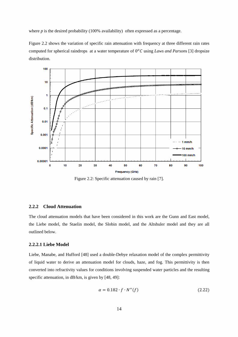
Figure 2.2 shows the variation of specific rain attenuation with frequency at three different rain rates

computed for spherical raindrops at a water temperature of using Laws and Parsons [3] dropsize

distribution.

Figure 2.2: Specific attenuation caused by rain [7].

2.2.2 Cloud Attenuation

The cloud attenuation models that have been considered in this work are the Gunn and East model,

the Liebe model, the Staelin model, the Slobin model, and the Altshuler model and they are all

outlined below.

2.2.2.1 Liebe Model

Liebe, Manabe, and Hufford [48] used a double-Debye relaxation model of the complex permittivity

of liquid water to derive an attenuation model for clouds, haze, and fog. This permittivity is then

converted into refractivity values for conditions involving suspended water particles and the resulting

specific attenuation, in dB/km, is given by [48, 49]:

( ) ( )

15

where is the frequency (GHz) and ( ) is the loss spectrum (in parts per million), a function of

frequency.

2.2.2.2 Altshuler Model

Altshuler [49, 50], realising the difficulty of measuring vertical liquid water and vapour profiles,

correlated data of absolute surface humidity with measurements of zenith cloud attenuation and

derived the following empirical equation [49, 50]:

[

] ( ) ( )

where λ is the wavelength (mm), ρ1 is the surface absolute humidity (g/m3), and α is the zenith

attenuation (dB).

The total attenuation is obtained by multiplying this empirical equation by the distance D(θ) through

the clouds, as defined below [49]:

( ) for θ > 80 (2.24a)

( ) ( )

for θ ≤ 80: (2.24b)

where is the elevation angle, is the effective earth radius (8 497 km), = 6.35 – 0.302ρ is the

effective cloud height (km) and ρ is the surface absolute humidity (g/m3).

2.2.2.3 Gunn & East Model

This model is based on Mie’s theory for spherical particles in a non-absorbing medium where

Rayleigh approximation was used to calculate the total absorption cross-section of a spherical particle

of water that is small compared to the wavelength of incident signal. In this model, cloud attenuation

in dB/km, is given by [49, 51]:

(

) [

] ( )

where ε is the complex relative dielectric constant of water, λ is the wavelength (cm), ρd is the

density of water (g/cm3); ρ1 is the liquid water content of the cloud (g/m

3), and denotes the

imaginary part

16

2.2.2.4 Staelin Model

The Staelin model was developed from the classical theoretical work of Rayleigh and explicitly

established that cloud attenuation is dependent on temperature. This is valid for frequencies between

10 GHz and 40 GHz and is given, in dB/km [49]:

( )

( )

where ρ1 is the cloud liquid water density (g/m3), is the temperature (K); and is the wavelength

(cm).

2.2.2.5 Slobin Model

The Slobin model makes use of the Staelin model where it divides clouds into twelve density

categories, from clear air to heavy clouds, such as lighter cloud, light cloud, medium cloud, heavy

cloud, heavier cloud, etc. [49].

2.2.3 Melting Layer Attenuation

A one-dimensional and stationary model was proposed by Salonen et al [52] in which the melting

layer is assumed to be composed of spherical melting snow particles that are a mixture of ice, air and

water. At the 00 C isotherm (at the top of the layer) the particles are a mixture of ice and air, and

below the bottom all the melting particles have turned to raindrops. A one-to-one relationship between

the melting particle and the corresponding raindrop is assumed where the particle mass is assumed to

be invariant during the melting process. Size distribution and the average dielectric constant are used

to characterize the melting particle.

The specific attenuation and zenith attenuation are then found by either using the Mie scattering

theory or an approximation [52]:

∫ ( ) ( ) ( )

where λ is the wavelength (mm) , (S) is the imaginary part of the scattering amplitude in the

forward direction and ( ) ( ), is the modified Gamma distribution for raindrops.

17

2.3 The Current South African Situation

In South Africa the initial contributions by Owolawi [19] focused on the modeling of the

characteristics of rain for both satellite and terrestrial links. His study focused on the rainfall rate

integration time conversions, cumulative distributions, rain rate modelling as well as the raindrop size

modelling. The author developed a factor for converting rainfall data from five-minute to one-minute

integration time. Using the combined characteristics of three rain rate integration time techniques,

viz., the empirical method, the physical method and the analytical method, he was able to develop a

hybrid method for converting the rainfall rate data of long integration time to short integration time

for South Africa and its surrounding Islands.

By letting be the number of models generating different one-minute rain rate cumulative

distributions, and be the probabilities of rain rate exceedences; then the conversion factors ( ), for

are given by [19]:

( ( )

( )) (

( )

( )) (

( )

( )) ( )

( ( )

( )) (

( )

( )) (

( )

( )) ( )

( ( )

( )) (

( )

( )) (

( )

( )) ( )

With the assumption that the hybrid conversion factor

∑ , and

the hybrid conversion factors for each exceedence percentage are , , …

respectively, then a general expression for the hybrid conversion factor is given by [19]:

∑ ( )

where ∑ is the rain rates ratio sum exceeded for a given percentage of time for

rainfall with integration times minutes and one minute for each number of distributions .

Using the developed hybrid method, the author was able to demonstrate the superiority of his method

in converting rain rate data from five-minute to one-minute integration time locally in Durban, South

Africa. Additionally, the author was able to suggest a new classification of rain zones for South Africa

18

and the surrounding Islands using both Crane and ITU-R designations. Further, the author came up

with simple models of the raindrop size distribution by employing the maximum likelihood estimation

technique.

Odedina [7] dealt extensively with semi-empirical modelling of rain attenuation using rain rate,

raindrop size distribution and signal level measurements on a 19.5 GHz link in Durban, South Africa.

The choice of the semi-empirical technique was informed by the scattering nature of raindrops on

electromagnetic waves. Various scattering raindrop amplitudes were determined at varying

frequencies, by employing the Mie scattering approach on raindrops which are spherically shaped.

From the said scattering amplitudes, different extinction cross-sections for the raindrops were

computed.

For the real part of the computed extinction cross-sections, power-law regression was applied to

determine the power-law coefficients at the different frequencies considered. The power-law model

developed was then integrated over the raindrop size distribution models for the sake of developing

theoretical models of rain attenuation. The empirical models, shown in Table 2.1, are the rain

attenuation models obtained for the rainy months in Durban in the year 2004 using measurements on a

6.3 km long radio link.

19

Table 2.1: Monthly rain attenuation models for a 6.3 km link in Durban, South Africa, for 2004.

Calendar months Empirical models

February A=0.0004R3-0.012R

2+0.1642R+2.6184

March A=0.0027R3-0.0661R

2+0.8102R+0.1009

April A=-0.0019R3+0.0536R

2-0.0704R+0.9264

October A=0.0002R3-0.0149R

2+0.6024R-0.9477

November A=0.1201R2-0.1764R+1.3416

December A=0.484R1.0992

The author was also able to develop empirically the annual power and logarithmic estimates for the

measured minimum, average and maximum attenuation values. These equations are shown in Table

2.2 below.

Table 2.2: Analysis of the logarithmic and power regression estimates for the measured minimum,

average and maximum attenuation values

Measured

attenuation

bound

Logarithmic equation Regression

coefficient

(Logarith

mic)

Power equation Regression

coefficient

(Power) Minimum A = 2.503Ln(R)-1.157 0.922 A = 0.578R0.789

0.886

Average A = 4.947Ln(R)-1.966 0.917 A = 1.892R0.618

0.948

Maximum A = 8.399Ln(R)-3.226 0.887 A = 3.112R0.6275

0.891

Rain attenuation results obtained from the measurements on a 19.5 GHz link that is horizontally

polarized in Durban, South Africa were then compared with those obtained using other existing

models for validation purposes. The author was also able to classify rain types in South Africa into

four classes: thunderstorm, shower, widespread and drizzle.

B.T Maharaj [53], in his paper dwelt on the application of fade countermeasures to alleviate rain fade

attenuation on earth-space links.

While the work in [7, 9, 53] is focused on rain rate conversions, raindrop size distributions, rain

attenuation modelling for spherical raindrops and application of fade countermeasures to alleviate rain

fade attenuation on earth-space links, determination of rain drop size distributions for Southern Africa

for oblate spheroidal raindrops, and its use in the determination of signal attenuation through

scattering and depolarization needs to be covered for Southern Africa. This is the main contribution in

the current study.

20

2.4 Chapter Summary and Conclusion

In this chapter, a review of clear-air effects, scintillation effects, gaseous absorption, cloud

attenuation and rain attenuation are been presented. Under clear-air effects, multipath and diffraction

fading have been discussed. Two scintillation models have also been reviewed as well as five

different cloud attenuation models. Gaseous attenuation has also been treated to a reasonable extent.

Rain attenuation models have also been discussed with special mention of the specific and total

attenuation. Finally, a summary of the current situation in South Africa has also been done with

special mention of the main contributions in the PhD studies of Owolawi [19] and Odedina [7] in the

same area. Overall, we conclude that rain attenuation presents the biggest threat to the design of

reliable terrestrial and satellite links of high availability in South Africa.

21

Chapter 3

Characterization of Rain Attenuation in Terrestrial and Satellite

Links in Southern Africa

3.0 Introduction

The first section of this chapter presents the application of results found in a rain rate characterizations

study in South Africa and their application to terrestrial links. It further provides an analysis on rain

fade in the light of the link distance chart and how it relates to the link budget. The outcomes are

incorporated into the link budget to determine the maximum link distance and other performance

parameters.

In the second section, an estimation is presented of the magnitude of attenuation due to rain at various

frequencies for earth-space links based on the ITU-R model using the database of rainfall of over ten

years for all provinces in South Africa. A link performance analysis using Intelsat IS 17 data is carried

out for all provinces in South Africa from which are proposed reasonable, but adequate fade margins

for all provinces in South Africa. Specific attention in terms of application is given to Ku and Ka

bands which are of interest to communication systems designers in South Africa.

3.1 Terrestrial Rain Attenuation at Microwave and Millimetre-wave Frequencies in

South Africa

This section presents the rain rate experimental measurements with the application of the International

Telecommunication Union’s Recommendations (ITU-R) on rain attenuation model in South Africa.

Nineteen sites were chosen for this study, with at least one site from each province in South Africa.

Figure 3.1 shows the map of South Africa. The parameters presented in this section are specific

attenuation and total path attenuation for signals of horizontal, circular, and vertical polarizations and

frequency in the range from 1 to 400 GHz through rain. The impact of rain attenuation on the system

is evaluated by finding the link distance chart, and designing the link-budget at the chosen frequency

range. The results of this work are useful in the planning of both microwave and millimeter-wave

broadband wireless networks in South Africa such as Local-Multipoint-Distributed-Services (LMDS).

3.1.1 Introductory Concepts in Rain Attenuation

The interest of many telecommunication companies to provide high speed wireless internet access,

broadcast multimedia information, multimedia file transfer, remote access to a local network,

interactive video conference and Voice-Over-IP has forced migration from lower frequency bands

22

which are already congested to higher frequency bands such as microwave and millimeter-wave

bands.

Figure 3.1: Map of South Africa [7]

The choice of these bands has become the key solution to today’s needs because of large bandwidth

availability, small device size and wide range of spectrum availability. Whilst there are a number of

advantages that result from operating at these bands, rain, however, compromises optimum

performance and usage of these bands. Rain attenuation results in outages that compromise the quality

of signal and link availability rendering it as a prime factor to be considered in designing both

terrestrial and satellite links. This means that the design of any communication device in this spectrum

range requires knowledge of rain fade in order to provide optimum link availability and robust and

reliable link to any telecommunication systems that offer the aforementioned benefits [28].

The performance metric considered mostly in link analysis is the system availability. That is, the time

percentage the link is providing service either at or below the specified given bit error rate. It has been

confirmed that at frequencies just above 5 GHz, the rain fade depth becomes noticeable and severe at

frequencies above 10 GHz [54]. Rain rate measurement is one of the key aspects of rain needed to

estimate the amount of rain fade, which is frequency and location dependent. The extensive work

23

carried out on the rainfall characteristics at different locations in South Africa has confirmed a

dynamic distribution of rain rate in the region [19].

This section presents the application of results found in a rain rate characteristics study in South

Africa as documented in [19] and their application to terrestrial links.

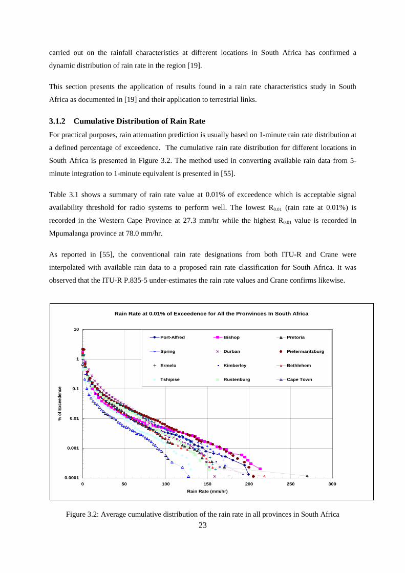
3.1.2 Cumulative Distribution of Rain Rate

For practical purposes, rain attenuation prediction is usually based on 1-minute rain rate distribution at

a defined percentage of exceedence. The cumulative rain rate distribution for different locations in

South Africa is presented in Figure 3.2. The method used in converting available rain data from 5-

minute integration to 1-minute equivalent is presented in [55].

Table 3.1 shows a summary of rain rate value at 0.01% of exceedence which is acceptable signal

availability threshold for radio systems to perform well. The lowest R0.01 (rain rate at 0.01%) is

recorded in the Western Cape Province at 27.3 mm/hr while the highest R0.01 value is recorded in

Mpumalanga province at 78.0 mm/hr.

As reported in [55], the conventional rain rate designations from both ITU-R and Crane were

interpolated with available rain data to a proposed rain rate classification for South Africa. It was

observed that the ITU-R P.835-5 under-estimates the rain rate values and Crane confirms likewise.

Figure 3.2: Average cumulative distribution of the rain rate in all provinces in South Africa

Rain Rate at 0.01% of Exceedence for All the Pronvinces In South Africa

0.0001

0.001

0.01

0.1

1

10

0 50 100 150 200 250 300

Rain Rate (mm/hr)

% o

f E

xce

ed

en

ce

Port-Alfred Bishop Pretoria

Spring Durban Pietermaritzburg

Ermelo Kimberley Bethlehem

Tshipise Rustenburg Cape Town

24

Also, rain rate contour map predicted using Crane and ITU-R rain rate models at 0.01% of

exceedences are presented in [55]. In the contour maps, the inverse distance weighting (IDW)

technique is employed because of its inherent advantage in the consistency of selecting grid points.

Table 3.1: Rain rate at 0.01% for all the Provinces in South Africa

South Africa

Province/Site

Rain Rate at

0.01%

mm/hr

Eastern Cape

Fort Beaufort

Bhisho

Umthatha

Port-Alfred

53.0

57.0

70.0

58.0

Gauteng

Pretoria

Spring

61.0

75.0

KwaZulu-Natal

Durban

Ladysmith

Pietermaritzburg

63.0

75.0

79.0

Mpumalanga

Ermelo

Belfast

Nelspruit

76.0

79.0

78.0

Northern Cape

Kimberley

59.0

Free-State

Bethlehem

Bloemfontein

60.0

67.0

Limpopo

Tshipise

50.0

North West

Klerksdorp

Rustenburg

67.0

70.0

Western Cape

Cape Point

Cape Town

Beaufort

20.0

25.0

37.0

25

3.1.3 Specific Rain Attenuation Distribution for all the Provinces in South Africa

The distributions of specific rain attenuation of all the provinces in South Africa are shown in Figures

3.3 to 3.5 for horizontal, vertical and circular polarizations respectively. The results on the graphs are

calculated using Table 3.2 coupled with the respective individual province rain rate at 0.01% of

exceedences. The highest specific rain attenuations are recorded in Mpumalanga (Ermelo) and

KwaZulu-Natal (Durban) provinces while the lowest is observed in the Western Cape (Cape Town).

This is attributed to the low rain rate experienced by Cape Town. For horizontally polarized signals,

the peak specific rain attenuation is observed at 200 GHz with the value of 28.65 dB/km and the

lowest is 13.32 dB/km at the same frequency.

The majority of the provinces have their specific rain attenuation from 23.00 to 24.00 dB/km at the

same frequency of 200 GHz. Using Figures 3.3 to 3.5, at the same frequency, it is observed that for

horizontal, circular and vertical polarization predicted specific rain attenuation decreases respectively,

though by small values. In addition, the figures confirm the expected increase in specific attenuation

as rain rate increases. It seems constant above 100 GHz for the individual province rain rate. The

reason may be due to the degree of impulse of raindrop shape to fast moving poles of electromagnetic

waves at such high frequencies may not synchronise with each other.

Table 3.2: The specific attenuation parameters given by ITU-R [31]

Frequency

GHz Ha Va Hb Vb

1 0.000387 0.00000352 0.912 0.880

2 0.00154 0.000138 0.963 0.923

4 0.000650 0.000591 1.121 1.075

6 0.00175 0.0155 1.308 1.265

7 0.00301 0.00265 1.332 1.312

8 0.00454 0.00395 1.327 1.310

10 0.0101 0.00887 1.276 1.264

12 0.0188 0.0168 1.217 1.200

15 0.0367 0.0335 1.154 1.128

20 0.0751 0.0691 1.099 1.065

25 0.124 0.113 1.061 1.030

30 0.187 0.167 1.021 1.000

35 0.263 0.233 0.979 0.963

40 0.350 0.310 0.939 0.929

45 0.442 0.393 0.903 0.897

50 0.536 0.479 0.873 0.868

60 0.707 0.642 0.826 0.824

70 0.851 0.784 0.793 0.793

80 0.975 0.906 0.769 0.769

90 1.06 0.999 0.753 0.754

100 1.12 1.06 0.743 0.744

120 1.18 1.13 0.731 0.732

150 1.31 1.27 0.710 0.711

200 1.45 1.42 0.689 0.690

300 1.36 1.35 0.688 0.689

400 1.32 1.31 0.683 0.684

26

Figure 3.3: Frequency characteristics of specific rain attenuation for horizontally polarized signals for

the Provinces in South Africa

Figure 3.4: Frequency characteristics of specific rain attenuation for vertically polarized signals for

the Provinces in South Africa

Specific Rain Attenuation(Horizontal Polarization) in all provinces in South Africa

0.0001

0.001

0.01

0.1

1

10

100

0 50 100 150 200 250 300 350 400

Frequency(GHz)

Sp

ecif

ic R

ain

Att

en

uati

on

(dB

/km

)

Eastern Cape (Port-Alfred) Gauteng(Pretoria)

KZN(Durban) Mpumalaga(Ermelo)

Northern Cape(Kimberley) Free-State(Bethlehem)

Limpopo(Tshipise) North-West(Klerksdorp)

Western-Cape(Cape Town)

Specific Rain Attenuation(Vertical Polarization) for all Provinces in South Africa

0.0001

0.001

0.01

0.1

1

10

100

0 50 100 150 200 250 300 350 400

Frequency (GHz)

Sp

ecif

ic R

ain

Att

en

ua

tio

n(d

B/k

m)

Eastern Cape (Port-Alfred) Gauteng(Pretoria)

KZN(Durban) Mpumalaga(Ermelo)

Northern Cape(Kimberley) Free-State(Bethlehem)

Limpopo(Tshipise) North-West(Klerksdorp)

Western-Cape(Cape Town)

27

3.1.4 Estimation of total path attenuation for South African Provinces

The expected fade depth is calculated using Equation (2.20) with an effective path length. The

characteristics of the fade depth at different polarization orientations in Durban with respect to

propagation frequencies are shown in Figures 3.6a to 3.6c. The fade depth is observed at different

distance ranges from 1 km to 60 km which is the valid ITU-R distance for the model. The steps to

estimate rain attenuation using the ITU-R method are summarized as follows [56]:

1. Determine the rain rate at 0.01% of exceedence. This is done by measurement at 1-minute

integration time as specified by the ITU-R or by using ITU-R P.837. In this work the

former is considered to estimate the rain attenuation.

2. Compute specific rain attenuation at given polarizations, and rain rate of interest as given

in Equations (2.17) – (2.19).

3. Compute the effective path length by as given in Equation (2.21), which will lead to the

estimated path attenuation at 0.01% of exceedence in dB.

4. Estimate the attenuation exceeded for other percentages by using Equations (2.22) and

(2.23).

According to ITU-R P.530-15, the prediction procedure outlined above is considered to be valid in all

parts of the world at least for frequencies up to 100 GHz and path lengths up to 60 km.

The ratio of attenuation at any given percentage to attenuation at 0.01% of exceedence is given as

0.07 for p equal to 1.0, and for p equal to 0.1, 0.01, 0.001, the ratios are 0.36, 1.0 and 1.44

respectively. Here the fade margins are estimated for availability at 99.99% and at any availability

that meets the needs of the operator.

Figures 3.5a – 3.5c show that the estimated total path attenuation increases with propagation

frequencies up to 40 GHz as recommended by the ITU-R and this can be valid up to a hop length of

60 km. From 40 GHz to 200 GHz, the total path attenuation slightly increases with frequency with a

dependency on the value of rain rate. There is a slight variation in total path attenuation with

frequency above 100 GHz and the curves eventually level off, though not fully. Such small

deviations could be due to errors associated with the measurements. These characteristics are

visible in the three major polarization orientations of propagating signals at frequencies above 10

GHz.

South Africa falls under two important latitudes of ITU-R classifications as expressed in Equations

(2.22) and (2.23). The majority of the provinces lie under the latitude that is less than 30 degrees and

28

the Eastern Cape and the Western Cape are the only provinces whose latitude is greater than 30

degrees.

Figure 3.5a: Total path attenuation for vertically polarized signals at various frequencies

Figure 3.5b: Total path attenuation for horizontally polarized signals at various frequencies

Expected Fade Depth( VP) against Frequency at a given Distance(km) In KwaZulu-Natal

0

50

100

150

200

250

300

350

400

0 50 100 150 200 250 300 350 400

Propagation Frequency (GHz)

Esti

mate

d F

ad

e D

ep

th (

dB

)

1km 5km 10km 15km 20km 25km 30km

35km 40km 45km 50km 55km 60km

Expected Fade Depth(HP) against Frequency at a given Distance (km) in KwaZulu-Natal

0

50

100

150

200

250

300

350

0 50 100 150 200 250 300 350 400

Propagation Frequency (GHz)

Es

tim

ate

d F

ad

e D

ep

th (

dB

)

1km 5km 10km 15km 20km 25km 30km

35km 40km 45km 50km 55km 60km

29

Figures 3.5a and 3.5b represent KwaZulu-Natal province (Durban). In general, it is observed that the

fade depth progressively increases starting from the vertical polarization, circular polarization and the

highest fade depth is observed in horizontal polarization. This is because of the shape factor of the

raindrop whose longer semi-major axis lies in the horizontal plane and that will result in the

horizontally polarized signal travelling through a longer path length through water, thereby

experiencing higher attenuation.

In the case of Durban, at 50 GHz, the fade depth is recorded as 18.81 dB for the 1 km path length for

vertical polarization, while it is 19.0 dB and 20.90 dB for circular and horizontal polarization

respectively. In another scenario in Durban, at 50 GHz, the fade depth is recorded as 255.4 dB for the

60 km path length in vertical polarization, while it is 202.12 dB and 222.30 dB for circular and

horizontal polarization respectively. At 1 km path length, it is observed that the fade depth for Durban

is more than what is recorded at Port-Alfred (that lies at latitude greater than 30 degrees) by an

average of 14.78%.

In Figures 3.6a and 3.6b, the attenuation values at a defined availability percentage with the given

frequency are presented. These were done for the two polarization states specifically for the Durban

site in the KwaZulu-Natal Province and the Port Alfred site in the Eastern Cape Province. As shown

in Figures 3.6a and 3.6b, the attenuation values at 99.999% availability for 20 GHz are 10.09 dB and

12.09 dB for vertical and horizontal polarization respectively for Durban. In the case of Port-Alfred

the attenuation values at 99.999% availability for 20 GHz are 11.69 dB and 13.92 dB for vertical and

horizontal polarization respectively. 99.999% availability, which translates to an outage of

approximately 5 minutes a year, was used here as an illustration of the required fade margins at this

stringent upper limit. In normal applications, fade margins for 99.99%, which translates to an outage

of 53 minutes per year, suffice.

At the 30 GHz, the obtained attenuation values at 99.999% availability are 18.37 dB, 18.66 dB and

21.54 dB for vertical, circular and horizontal polarization respectively for Durban. For the Eastern

Cape (Port-Alfred) the attenuation values at 99.999% availability are 21.62 dB, 21.95 dB and 25.26

dB for vertical, circular and horizontal polarization respectively. It can be seen that attenuation values

decrease as the degree of availability decreases. For example in the case of Durban, the attenuation

value is 10.09 dB at 99.999% and 2.55 dB at 99.9%. In addition, it is observed that attenuation values

at latitudes less than 30 degree are less when compared with values at latitudes greater than 30

degrees as reflected in the figures at equal performance. The percentage differences between

KwaZulu-Natal (Durban) and Eastern Cape (Port-Alfred) at an availability of 99.999% falls within

15.86% and for the 99.9% the least percentage difference is 25.75%.

30

For easy application of these results, any link design engineer can use frequency scaling to find the

estimated attenuation value for the undetermined frequency in the reading as given in ITU-R P.530.

Based on ITU-R link outages performance yard stick, 99.99% availability translates to approximately

53-minutes of outage per year while 99.999% availability translates to approximately 5-minutes of

outage per year.

Figure 3.6a: Predicted Rain Attenuation (VP) against Availability

Predicted Attenuation (VP) against Availability in Percentage in KwaZulu-Natal

0

5

10

15

20

25

30

35

40

45

0.001 0.01 0.1 1

Percentage of Availability

Pre

dic

ted

Att

en

uati

on

in

dB

1GHz 2GHz 4GHz 6GHz 7GHz 8GHz

10GHz 12GHz 15GHz 20GHz 25GHz 30GHz

35GHz 40GHz 45GHz 50GHz 60GHz 70GHz

80GHz 90GHz 100GHz 120GHz 150GHz 200GHz

300GHz 400GHz

31

Figure 3.6b: Predicted Rain Attenuation (CP) against Availability

Figure 3.6c: Predicted Rain Attenuation (HP) against Availability

3.2 Rain Attenuation at Ka, Ku and V Bands for Satellite Links in South Africa

Despite the fact that over twenty (20) fibre optic cable networks have been rolled out in

Africa, the satellite infrastructure continues to fulfill an important role in providing

Predicted Attenuation (CP) against Availability in Percentage in KwaZulu-Natal

0

5

10

15

20

25

30

35

40

45

0.001 0.01 0.1 1

Percentage of Availability

Pre

dic

ted

Att

en

uati

on

in

dB

1GHz 2GHz 4GHz 6GHz 7GHz 8GHz

10GHz 12GHz 15GHz 20GHz 25GHz 30GHz

35GHz 40GHz 45GHz 50GHz 60GHz 70GHz

80GHz 90GHz 100GHz 120GHz 150GHz 200GHz

300GHz 400GHz

Predicted Attenuation (HP) against Availability in Percentage in KwaZulu-Natal

0

10

20

30

40

50

0.001 0.01 0.1 1

Percentage of Availability

Pre

dic

ted

Att

en

ua

tio

n i

n d

B

1 GHz 2GHz 4GHz 6GHz 7GHz 8GHz

10GHz 12GHz 15GHz 20GHz 25GHz 30GHz

35GHz 40GHz 45GHz 50GHz 60GHz 70GHz

80GHz 90GHz 100GHz 120GHz 150GHz 200GHz

300GHz 400GHz

32

communication access to rural, remote and inland areas across the globe. The fast growth in

telecommunications, increased demand for bandwidth, congestion in lower frequency bands

and miniaturization of communication equipment have forced the designers to employ higher

frequency bands such as the Ku (12 to 18 GHz), Ka (26.5 to 40 GHz), and V (40 to 75 GHz)

bands. Rain is the most deleterious source to signal propagation in these bands. The

contribution of rain attenuation to the quality of signal in these bands, especially in the

tropical and subtropical bands in which South Africa is located, needs to be studied. The aims

of this section are to estimate the magnitude of rain attenuation using the ITU-R model, carry

out link performance analysis, and then propose reasonable, adequate fade margins that need

to be applied for all provinces in South Africa.

3.2.1 Introduction to earth-space links in South Africa

Consumer diversity, demands for bandwidth, and service convergence have led to a tremendous

growth in communication systems. These have resulted in congestion at lower frequency bands, and

consequently increased the need for higher frequency band usage. At these frequencies, however, the

presence of rain causes degradation of signals, especially above 10 GHz [54]. The many advantages

of telecommunications systems operating at higher frequencies include: large bandwidth, increased

frequency reuse, small device size and wide range of spectrum availability. The major obstacle to

these frequency ranges is rain. In South Africa, extensive studies done by Owolawi [55] have revealed

the existence of different climatic zones in the country. In recent years, the roll-out of fibre optic

networks has not diminished the importance of satellite communication systems, especially for rural,

remote and inland cities across the globe. The earlier satellite networks operate at L, S, C, and X

bands, while the recent ones start operating at Ku, K, Ka, Q and V bands.

Demand for broadband service is exhausting the available capacity of existing C- and Ku-band

satellite networks. The recent motivation by Hughes to support Vodacom South Africa in their latest

coverage expansion, by providing the first Ka-band satellite that will provide broadband internet

access to South Africa and other African countries, is the key reason behind this work. The impacts of

rain rate along the satellite path in Southern Africa, where mixed climate conditions of tropical, sub-

tropical and temperate are common, demand special attention with respect to rain attenuation

modeling [28, 57]. Electromagnetic waves passing through rain at any of these frequency bands will

be absorbed or scattered. This scattering and absorption processes constitute rain attenuation. The

attenuation caused by the rain depends on parameters such as the size of raindrops, rain temperature,

drop velocity, polarization, rain rate, drop orientation and transmitting frequency. Since rain

attenuation is the primary obstacle to good quality and availability of signal at these bands, the

development of rain attenuation models has been the focus of many researchers, and several

33

measurement campaigns, theoretical and analytical models have been established. Many rain

attenuation models, both for terrestrial and satellite paths, are semi-empirical in nature due to the lack

of accurate characterization of the various sources that produce the impairments. Rain attenuation is

estimated by integrating the specific attenuation along the earth-space path. The specific rain

attenuation is mathematically calculated by using empirical parameters such as the cumulative

distribution of one-minute rain rate at a given probability of exceedence. In this section, estimated

specific rain attenuation at various satellite frequency bands is proposed, based on the ITU-R

recommendations [33, 58], using a database of rainfall of over ten years in all the provinces in South

Africa. Specific attention is given to Ku and Ka bands, which are of interest to systems designers and

telecommunications operators alike.

3.2.2 Rain Height

The estimation of rain attenuation along a slant-path in a satellite link requires an understanding of the

rain height. The method, adopted by ITU-R, assumes the rain structure to be uniform from the ground

level to the 00 C isotherm height,

Rh , simply termed the effective rain height. Often, an empirical

formula is used to estimate the value of Rh due to the scarcity of measured data. Most of the

referenced rain height experiments were done in Europe and Asia, and very little data is available in

Africa except in West Africa [32, 59 – 62]. As a result, the current work uses the latest ITU

Recommendation P.839-3 [32]. Though the model is less accurate, it is widely employed to calculate

the average rain height. The mean rain height above mean sea level is expressed as [32]:

kmhhR 36.00 (3.1)

where 0h is the average annual C00 isotherm height. If the 0h is not available from local data, a

global contour map is used, as presented in reference [32], and bilinear interpolation is used to

determine any unavailable grid line on the map.

Table 3.3: Average rain rate at 0.01% for all provinces in South Africa

South Africa Province/Site Rain Rate at 0.01% (mm/hr) Lat/Long

Eastern Cape (Fort Beaufort) 53 mm/hr -32.7/26.6

Gauteng (Pretoria) 61 mm/hr -25.7/28.1

KwaZulu-Natal (Durban) 63 mm/hr -29.9/30.9

Mpumalaga (Ermelo) 76 mm/hr -26.4/29.9

Northern Cape (Kimberley) 59 mm/hr -28.7/24.7

Free-State (Bethlehem) 60 mm/hr -33.9/18.9

Limpopo (Tshipise) 50 mm/hr -22.6/30.1

North West (Klerksdorp) 67 mm/hr -26.8/26.6

Western Cape (Cape Town) 25 mm/hr -33.9/18.6

34

3.2.3 Slant Path Rain Attenuation Models

In this subsection, a rain attenuation model is presented that has performed well for temperate regions

and different rain types. This rain attenuation model is the ITU-R model, which is the most widely

accepted international method and benchmark for comparative studies. This model is semi-empirical

and often employs the local climatic parameters at a desired probability of exceedence.

3.2.3.1 ITU-R Rain Attenuation Model

Figure 3.7: Slant path through rain [28]

The ITU-R 618-10 [28] gives summarized procedures for the computation of rain attenuation on a

satellite path. In order to compute the slant-path rain attenuation using point rainfall rate, the

following parameters are required [28, 57]:

:f the frequency of operation in GHz

: the elevation angle to the satellite, in degrees

: the latitude of the ground station, in degrees N and S

:sh the height of the ground station above sea level, in km

35

:eR effective radius of the Earth (8 500 km)

:01.0R point rainfall rate for the location of interest for 0.01% of an average year (mm/hr)

Step-by-step procedures for the computation of the rain attenuation along the slant-path of a satellite

system are summarized as follows [28, 57]:

Step 1: Determine the rain height, Rh , as given in (3.1) and contour map in Recommendation ITU-R

P.839 [32].

Step 2: Determine the slant-path length and the horizontal projection.

The slant-path length sL , expressed in km, is calculated from [28]:

{

( )

( )

√( ( )

)

( ) (3.2)

The horizontal projection is then expressed as [28]:

)cos(sG LL (3.3)

where GL and sL are in km.

Step 3: Determine the rain rate at 0.01% for the location of interest over an average year. In this work,

Table 3.3 is used, which is a derived rain rate at one-minute integration time at 0.01% of

exceedance from long-term local data.

Step 4: Calculate the specific attenuation, a function of desired frequency, polarization and rain rate

using (2.17).

Step 5: Calculate the horizontal reduction factor, 01.0r at 0.01% probability, expressed as [28]:

)1(38.078.01

1

2

01.0

GLRG ef

Lr

(3.4)

Note: GL is the horizontal projection as determined in Step 2 and f is the operating frequency

measured in GHz.

36

Step 6: Calculate the vertical adjustment factor, 01.0v , for 0.01% of the time [28, 57]:

45.0131)sin(1

1

2

)1/(

01.0

f

Le

v

RRx

(3.5)

forkmhh

forkmrL

LsR

G

R

sin

)(

cos

01.0

(3.6)

and

reesrL

hh

G

sR degtan01.0

1

(3.7)

360

36deg36

for

forreesx (3.8)

Step 7: The effective path length is then computed from [28, 57]:

kmvLL RE 01.0 (3.9)

Step 8: Calculate the attenuation exceeded for 0.01% of an average year [28, 57]:

dBLA ER01.0 (3.10)

The attenuation value for other percentages of exceedence is determined by using the expression

below [28, 57]:

dBp

AA

pAp

p

)sin()1()ln(045.0)ln(033.0655.0

01.0

01.0

01.0

(3.11)

where,

otherwise

andandpif

orpif

sin25.48.1)36(005.0

2536%1)36(005.0

36%10

00

0

(3.12)

The results obtained in this section make use of the Intelsat 17 (IS-17) satellite located at 66° E, as its

service footprint covers the area of study adequately. The geo-characteristic parameters for each

37

location are shown in Table 3.4. In this table the attenuation values (in dB) that are expected for

0.01% of the time and the effective path lengths (in km) for frequencies ranging from C-band up to V-

band for circular, horizontal, and vertical polarizations are shown.

The elevation angle for each region is also shown (in degrees). The elevation angle is the angle

between the horizontal along the earth’s surface and the center line of the satellite’s transmission

beam as shown in Figure 3.8. This angle translates into the visibility (coverage) of the horizon to the

satellite’s beam, with an angle of zero degrees, ensuring visibility from all directions (ideal case).

Rainfall attenuation, however, is strongly dependent on two factors: the operating frequency and the

local rain rate. The results in Table 3.4 show that the area with the lowest rain rate at 0.01%

exceedence (Cape Town with a value of 25 mm/h) will experience the least attenuation for the same

percentage of exceedence at a given frequency. Conversely, it is true that the area with the highest

rain rate at 0.01% exceedence (Ermelo with a value of 76 mm/h) experiences the highest signal

degradation for the same percentage of exceedence at a given frequency.

The results of Table 3.4 are also displayed graphically in Figure 3.9 and Figure 3.10. Figure 3.9 shows

the variation of the attenuation at 0.01% of exceedence with frequency, for all the areas under study.

The effects of polarization are also shown as this is a consideration for antenna polarity needed by

system designers.

The effective path length for each region is determined and its dependency on frequency and elevation

angle is evident. This length is used instead of the actual geometric length due to the non-uniformity

of rain density as the signal travels through a rainy medium. The location with the lowest elevation

angle exhibits the longest effective path length (Cape Town with an elevation angle of 26.4 degrees).

However, the results in Table 3.4 suggest that the variability of local rain rate has an influence on the

effective path length. Notwithstanding this observation, the general conclusion can still be drawn that

areas of high elevation exhibit short effective path lengths given the small contribution due to varying

local rain rates. Unlike attenuation, the effective path length depends strongly on elevation angle and

frequency of operation. These results are displayed graphically in Figure 3.9 to show the variability of

the effective path length with frequency for each location.

The elevation angles give designers an idea as to the positioning of ground station antennas for

maximum energy transfer with little to no tracking required (considering geostationary orbit

satellites). All the areas under study have an elevation angle above 25 degrees, which permits the use

of the approximation given in the first condition of Equation (3.2).

38

Figures 3.8 (a) – 3.8 (c) show the attenuation expected to be exceeded for 0.01% of the time in an

average year. The fade margins are higher for horizontally polarized signals as expected while the

vertical polarization gives lower fade margins. Circularly polarized electromagnetic waves (EM)

experience a fade margin whose value lies between that of horizontally and vertically polarized

signals. Different polarizations are chosen by service providers for different reasons such as cross-

polarization discrimination and frequency reuse.

Figures 3.9 (a) – 3.9 (c) show how the effective path length changes as the frequency of operation

changes. At lower frequencies, such as C-band, the effective path length is quite long but decreases

almost exponentially around Ku-band frequencies. As frequency increases into the Ka-band

frequencies, the effective path length maintains a uniform value. It also appears that at V-bands, the

effective path length begins to increase consistently with increasing frequency. The increase is,

however, steady but could be rapid at millimetre bands.

39

Table 3.4: Characteristics for Locations in South Africa at 0.01% time of exceedence

Attenuation for 0.01% of time and Effective path length

Location

R0.01

Frequency

(GHz)

Elevation

Angle (°)

Circular Horizontal Vertical

(dB) (km) (dB) (km) (dB) (km)

Bethlehem

60 mm/hr

4

8

12

18

26.5

40

48

75

26.7°

0.4609

7.3072

16.2329

30.1983

50.9177

80.8603

95.0743

127.9248

10.1799

6.6407

6.0082

5.7685

5.6110

5.6080

5.7014

6.1725

0.7474

7.8191

17.4814

32.8390

54.7199

84.6843

98.7186

130.1286

9.9343

6.4013

5.7842

5.5319

5.4154

5.4842

5.6002

6.1247

0.4163

6.7780

15.1020

27.9804

47.2461

77.0819

91.4850

125.7473

10.2298

6.9178

6.2317

5.9885

5.8180

5.7377

5.8060

6.2207

Cape Town

25 mm/hr

4

8

12

18

26.5

40

48

75

26.4°

0.1487

3.7325

8.3613

16.3508

28.7665

48.5640

58.6595

83.0914

10.7497

11.4095

8.4816

7.7663

7.3542

7.1193

7.1351

7.5077

0.1972

4.2487

8.8294

17.3737

30.5685

50.5434

60.5617

84.2548

10.6436

11.7503

8.2262

7.5455

7.1546

6.9941

7.0352

7.4621

0.1468

3.4142

7.9403

15.4870

27.0192

46.6038

56.7809

81.9398

10.7542

11.6610

8.7469

7.9725

7.5667

7.2507

7.2384

7.5538

Durban

63 mm/hr

4

8

12

18

26.5

40

48

75

38.4°

0.4816

8.1321

17.3709

31.6598

52.6433

82.1961

95.9097

127.0373

8.1551

5.6319

5.1296

4.9314

4.8044

4.8207

4.9088

5.3261

0.8218

8.7098

18.8020

34.6613

56.8030

86.2863

99.7862

129.3459

7.9794

5.4286

4.9335

4.7227

4.6357

4.7139

4.8211

5.2840

0.4259

7.5383

16.0839

29.1568

48.6474

78.1667

92.1017

124.7595

8.1937

5.8699

5.3265

5.1265

4.9835

4.9327

4.9996

5.3686

Ermelo

76 mm/hr

4

8

12

18

26.5

40

48

75

39.7°

0.5138

8.6734

18.2123

32.8177

54.1693

84.0374

97.8242

129.0140

8.2385

5.6807

5.1343

4.9020

4.7560

4.7618

4.8466

5.2551

0.8933

9.3008

19.7456

35.9913

58.5035

88.2608

101.8174

131.3815

8.1325

5.4813

4.9401

4.6949

4.5891

4.6563

4.7596

5.2133

0.4516

8.0292

16.8361

30.1757

50.0101

79.8791

93.9033

126.6785

8.2636

5.9142

5.3293

5.0957

4.9330

4.8727

4.9365

5.2973

Fort

Beaufort

53 mm/hr

4

8

12

18

26.5

40

48

75

33.3°

0.3368

6.1075

13.7248

25.7554

43.7342

70.0710

82.6717

111.8571

8.7993

6.5913

5.8600

5.5977

5.4298

5.4034

5.4802

5.8989

0.5302

6.5193

14.7515

27.9455

46.9708

73.3646

85.8119

113.7500

8.5952

6.3420

5.6521

5.3837

5.2515

5.2908

5.3884

5.8556

0.3080

5.6892

12.7973

23.9189

40.6136

66.8201

79.5812

109.9874

8.8367

6.8905

6.0690

5.7971

5.6188

5.5215

5.5752

5.9428

Kimberley

59 mm/hr

4

8

12

18

26.5

40

48

75

34.1°

0.4044

7.0987

15.4464

28.3315

47.3760

74.8319

87.8138

117.6630

9.1377

6.6031

5.8288

5.5074

5.3057

5.2650

5.3380

5.7461

0.6622

7.6019

16.6621

30.8583

50.9807

78.4266

91.2260

119.7047

9.0411

6.3706

5.6238

5.2936

5.1294

4.1535

5.2468

5.7029

0.3649

6.5850

14.3513

26.2182

43.9060

71.2862

84.4577

115.6469

9.1579

6.8785

6.0346

5.7067

5.4926

5.3819

5.4323

5.7898

Klerksdorp

67 mm/hr

4

8

12

18

26.5

40

48

75

36.7°

0.4595

7.8934

16.8355

30.5508

50.6980

79.3005

92.6614

123.1336

8.7393

6.1563

5.4876

5.2029

5.0245

5.0047

5.0828

5.4896

0.7769

8.4615

18.2102

33.3944

54.6579

83.1990

96.3537

125.3321

8.6536

5.9418

5.2882

4.9925

4.8531

4.8962

4.9938

5.4472

0.4091

7.3117

15.5996

28.1783

46.8923

75.4586

89.0329

120.9639

8.7591

6.4086

5.6877

5.3992

5.2063

5.1184

5.1748

5.5325

Pretoria

61 mm/hr

4

8

12

18

26.5

40

48

75

38.6°

0.3939

7.2004

15.5001

28.2984

47.1866

74.2932

87.0530

116.2884

8.5060

6.3954

5.6288

5.3134

5.1179

5.0802

5.1512

5.5450

0.6509

7.7052

16.7346

30.8635

50.8224

77.9035

90.4749

118.3257

8.4249

6.1648

5.4299

5.1070

4.9486

4.9732

5.0635

5.5031

0.3541

6.6892

14.3913

26.1584

43.6930

70.7361

83.6904

114.2777

8.5232

6.6732

5.8294

5.5065

5.2976

5.1925

5.2418

5.5873

Tshipise

50 mm/hr

4

8

12

18

26.5

40

48

75

42.0°

0.2892

6.1332

13.1683

24.2786

40.8491

65.1933

76.8522

103.8973

8.1758

7.1756

6.0126

5.6065

5.3637

5.2841

5.3400

5.7128

0.4560

6.4849

14.1444

26.3346

43.8846

68.2654

79.7687

105.6321

8.1145

6.8410

5.8061

5.4034

5.1957

5.1782

5.2536

5.6713

0.2654

5.8419

12.2962

22.5650

37.9347

62.1679

73.9868

102.1854

8.1871

7.6677

6.2252

5.7980

5.5431

5.3955

5.4295

5.7548

40

Figure 3.8 (a): Rain Attenuation at 0.01% exceedence for all regions for Circular Polarization

Figure 3.8 (b): Rain Attenuation at 0.01% exceedence for all regions for Horizontal Polarization

0

1

10

100

1000

0 20 40 60 80

0.0

1%

Att

enuat

ion (

dB

)

Frequency (GHz)

Bethlehem

Cape Town

Durban

Ermelo

Fort Beaufort

Kimberley

Klerksdorp

Pretoria

Tshipise

0

1

10

100

1000

0 20 40 60 80

0.0

1%

Att

enuat

ion (

dB

)

Frequency (GHz)

Bethlehem

Cape Town

Durban

Ermelo

Fort Beaufort

Kimberley

Klerksdorp

Pretoria

Tshipise

41

Figure 3.8 (c): Rain Attenuation at 0.01% exceedence for all regions for Vertical Polarization

Figure 3.9 (a): Effective path length for all regions for Circular Polarization

0

1

10

100

1000

0 20 40 60 80

0.0

1 %

Att

enuat

ion (

dB

)

Frequency (GHz)

Bethlehem

Cape Town

Durban

Ermelo

Fort Beaufort

Kimberley

Klerksdorp

Pretoria

Tshipise

0

2

4

6

8

10

12

14

8 28 48 68 88

effe

ctiv

e p

ath l

ength

(km

)

Frequency (GHz)

Bethlehem

Cape Town

Durban

Ermelo

Fort Beaufort

Kimberley

Klerksdorp

Pretoria

Tshipise

42

Figure 3.9 (b): Effective path length for all regions for Horizontal Polarization

Figure 3.9 (c): Effective path length for all regions for Vertical Polarization

0

2

4

6

8

10

12

14

8 28 48 68 88

Eff

ecti

ve

pat

h l

ength

(km

)

Frequency (GHz)

Bethlehem

Cape Town

Durban

Ermelo

Fort Beaufort

Kimberley

Klerksdorp

Pretoria

Tshipise

0

2

4

6

8

10

12

14

8 28 48 68 88

Eff

ecti

ve

pat

h l

ength

(km

)

Frequency (GHz)

Bethlehem

Cape Town

Durban

Ermelo

Fort Beaufort

Kimberley

Klerksdorp

Pretoria

Tshipise

43

3.2.4 Earth-Space Rain Attenuation

Earlier satellites have been offering services at C-band frequencies but the demand for increased

bandwidth has seen this band exhausted and inadequate in supporting the fast data rates associated

with modern applications. The inherent advantages at these bands are quite evident from Figure 3.11

which depicts low attenuation levels even at high availability requirements. In this section, maximum

fade depths were determined for probabilities ranging from 0.001% to 5%. Evidently, as the

availability increases, so does the required rain fade margin. The variability of rainfall attenuation

with availability is location as well as frequency dependent. For the two frequencies considered in

Figure 3.10 (lower and upper bounds for C-band), as discussed in Subsection 3.2.5, Cape Town has

the least attenuation for all the percentage availabilities considered. It also follows that, given the local

rain rates, that Ermelo experiences the highest rainfall attenuation within the range of the probabilities

considered. The results are consistent with the notion that higher rain rates require high fade margins.

This may be true for terrestrial radio links where the elevation angle is considered to be uniform

(zero) for all locations. However, the effect of elevation angle on attenuation (Equations (3.6) through

(3.11)), is such that locations of higher rain rate may have lower attenuation as compared to those

with lower rain rates for 0.01% of the time. This means that areas having the same rain rate do not

necessarily have to have equal fade margins. The dependency of rainfall attenuation on geographical

location plays an important role in this analysis.

The effect of effective path length on rain attenuation is observed in Figure 3.10 (a). For probabilities

of outage above 2% of the time (availability of 98% or less), there is a noticeable overlapping

behaviour amongst the graphs. The graph for Tshipise prominently displays this scenario. This is a

result of different effective path lengths for different locations. The same scenario is less prominent in

Figure 3.10 (b), which is probably nullified by the higher frequency of 8 GHz. It is even clearer at Ku-

, Ka-, and V-band frequencies as shown in Figures 3.11, 3.12, and 3.13 respectively.

The Intelsat 17 (IS-17) provides good coverage in South Africa, transmitting at Ku-band frequencies

with vertical polarization with a beam peak of up to 53.3 dBW. The uplink frequencies range from

13.75 – 14.50 GHz with the downlink range of 10.95 – 11.70 GHz [IS-17 factsheet]. The increased

demand for bandwidth for greater data flow and the over-crowding of the electromagnetic spectrum

may see this provision inadequate for the numerous applications of satellite systems. The trend

recently has been to utilize Ka-band frequencies for satellite communications, with uplink frequencies

of 30 GHz and downlink frequencies of 20.2 GHz [63].

Despite the obvious merits that include less propagation losses (due to hydrometeors), less free space

loss and the ability to penetrate foliage, lower frequencies do not provide for restrictions in power

44

requirements, easy transmit-to-receive isolation, and antenna aperture size. Utilization of Ka-band

frequencies and even higher can provide spectral relief for satellite applications with reasonably sized

antennas and reduced power requirements. Figures 3.11 and 3.12 show that operating at Ka- and V-

bands requires a considerable amount of fade margin as compared to operating at lower bands. The

worst case difference, as expected, is between the vertical and horizontal polarizations, with a value of

4.7 dB at 75 GHz for Ermelo. For linear polarization, precision alignment is required for the earth

station antenna to maximize reception from the satellite. Given the height of the satellite above the

earth, transmission latencies are imminent. Since the satellite is of geostationary type, it has a fixed

radius of orbit of about 42 242 km. Its height above the earth surface is therefore given by [57]:

kmhGEO 35864)637842242( (3.13)

Unlike C- and Ku-bands, Ka-band employs multiple spot beams which makes it attractive in terms of

focus and frequency reuse. Over a wide geographical area, the same frequency range can be reused

many times provided adjacent spot beams use a different frequency.

Figure 3.10 (a): Rain Attenuation at C-band for Horizontal Polarization for all locations at 4 GHz

0.0001

0.001

0.01

0.1

1

10

95 96 97 98 99

Rai

nfa

ll A

tten

uat

ion (

dB

)

Availability

BethlehemCape TownDurbanErmeloFort BeaufortKimberleyKlerksdorpPretoriaTshipise

45

Figure 3.10 (b): Rain Attenuation at C-band for Horizontal Polarization for all locations at 8 GHz

Figure 3.11 (a): Rain Attenuation at Ku-band for Vertical Polarization for all locations at 12 GHz

0.01

0.1

1

10

100

95 96 97 98 99

Rai

nfa

ll A

tten

uat

ion (

dB

)

Availability

BethlehemCape TownDurbanErmeloFort BeaufortKimberleyKlerksdorpPretoriaTshipise

0.1

1

10

100

95 96 97 98 99

Rai

nfa

ll A

tten

uat

ion (

dB

)

Availability

BethlehemCape TownDurbanErmeloFort BeaufortKimberleyKlerksdorpPretoriaTshipise

46

Figure 3.11 (b): Rain Attenuation at Ku-band for Vertical Polarization for all locations at 18 GHz

Figure 3.12 (a): Rain Attenuation at Ka-band for Circular Polarization for all provinces at 26.5 GHz

0.1

1

10

100

95 95.5 96 96.5 97 97.5 98 98.5 99 99.5

Rai

nfa

ll A

tten

uat

ion (

dB

)

Availability

BethlehemCape TownDurbanErmeloFort BeaufortKimberleyKlerksdorpPretoriaTshipise

0.1

1

10

100

95 96 97 98 99

Rai

nfa

ll A

tten

uat

ion (

dB

)

Availability

BethlehemCape TownDurbanErmeloFort BeaufortKimberleyKlerksdorpPretoriaTshipise

47

Figure 3.12 (b): Rain Attenuation at Ka-band for Circular Polarization for all provinces at 40 GHz

Figure 3.13 (a): Rain Attenuation at V-band at 75 GHz for all provinces for Horizontal Polarization

1

10

100

95 96 97 98 99

Rai

nfa

ll A

tten

uat

ion (

dB

)

Availability

Bethlehem

Cape Town

Durban

Ermelo

Fort Beaufort

Kimberley

Klerksdorp

Pretoria

Tshipise

1

10

100

95 96 97 98 99

Rai

nfa

ll A

tten

uat

ion (

dB

)

Availability

Bethlehem Cape Town

Durban Ermelo

Fort Beaufort Kimberley

Klerksdorp Pretoria

Tshipise

48

Figure 3.13 (b): Rain Attenuation at V-band at 75 GHz for all provinces for Vertical Polarization

Figure 3.13 (c): Rain Attenuation at V-band at 75 GHz for all provinces for Circular Polarization

1

10

100

95 96 97 98 99

Rai

nfa

ll A

tten

uat

ion (

dB

)

Availability

Bethlehem Cape Town

Durban Ermelo

Fort Beaufort Kimberley

Klerksdorp Pretoria

Tshipise

1

10

100

95 96 97 98 99

Rai

nfa

ll A

tten

uat

ion (

dB

)

Availability

Bethlehem Cape Town

Durban Ermelo

Fort Beaufort Kimberley

Klerksdorp Pretoria

Tshipise

49

3.3 Chapter Summary and Conclusion

Section 3.1 presents rain attenuation estimation using both the ITU-R model and measured regional

rain rate data collected over 10 years. In addition, the results of 1-year rain attenuation measurements

are used to design a link budget for the University of KwaZulu-Natal microwave links. Also, the hop

distance chart is used to estimate the maximum hop distance a defined link can have under a pre-

defined rain fade margin and system gain. The results will be useful in the proper planning of radio

links by radio network planners in South Africa. They will improve precision in the estimation of link

availability, link performance, link budget and management of the link frequency between the ranges

from 1 GHz to 400 GHz.

Section 3.2 presents results that are based on the Intelsat 17 (IS-17) satellite characteristics which

operate at C- and Ku-band and projections are made into higher frequency bands. Across all the

frequency bands from C-band up to V-band, rainfall attenuation, elevation angle, and effective path

length have been determined for satellite link applications in South Africa. Consideration has been

given to link availabilities from 95% up to 99.999% of the time. It is noted that the severity of the

degradation of the propagating signal increases with increasing availability. However, for a given

percentage availability, the signal degradation increases with an increase in operating frequency of the

satellite link. It is observed for example in Figure 3.6 (a) and more clearly from Table 3.4, that a fade

margin in excess of 50.7 dB is required for 99.99% availability in Klerksdorp considering circular

polarization at 26.5 GHz. For the same location, availability, and polarization, a fade margin of 79.3

dB is required for the operating frequency of 40 GHz.

Results displayed in Table 3.4 show that areas of lower elevation angles have longer effective path

lengths. These areas are expected to suffer higher loss in dB during operation since signals traverse a

longer atmosphere and the overall slant path is increased. For any of the locations studied, the

effective path length varies inversely proportional to the frequency of operation up to 40 GHz.

Beyond this frequency a direct proportionality relationship is observed consistently up to 75 GHz. It

can thus be inferred that this relationship is valid for even higher frequencies not under consideration

in this thesis.

Considering all the locations under study for South Africa, Cape Town is associated with the lowest

fade margin at all frequencies and availabilities. Conversely, Ermelo had the highest fade margin at all

frequencies and availabilities. A number of other locations also experience almost the same level of

degradation as Ermelo. The two notable ones are Bethlehem and Durban. In comparison with Ermelo,

at 75 GHz, Bethlehem is lower by 1.25 dB, while Durban is 2.04 dB lower for horizontal polarization.

For circular polarization Bethlehem and Durban are lower by 1.09 dB and 1.97 dB, respectively,

50

while for vertical polarization they are lower by 0.93 dB and 1.92 dB, respectively. It should be noted

that all these comparisons are made for 99.99% availability. Despite having the smallest elevation

angle of 26.4 degrees, Cape Town maintains a low fade margin requirement and this can only be

attributed to its significantly low local rain rate of 25 mm/h. Tshipise has the highest elevation angle

of 42 degrees and local rain rate of 50 mm/h (twice that of Cape Town). It remains in need of higher

fade margins as compared to Cape Town though less prone to degradation as compared to the other

locations in the country.

At the lower bound of the Ka-band, 26.5 GHz, it is observed that the lowest rain attenuation of about

27 dB (for Cape Town) is obtained with the highest value of 50 dB obtained for Ermelo for 0.01% of

the time. For the same demand at 40 GHz, the minimum and maximum fade margins required are

46.6 dB and 79.9 dB respectively. So 27 dB and 80 dB can be considered the minimum and the

maximum attenuation levels at Ka-bands for 99.99% availability for satellite communications links in

South Africa.

51

Chapter 4

Raindrop Size Modelling Using Method of Moments and Its Applications

for South Africa Radio Systems

4.0 Introduction

In this chapter, raindrop size distribution (DSD) modelling and analysis are presented. Rainfall is

classified into four main categories, namely: drizzle, widespread, shower and thunderstorm,

depending on the rain rate. The Gamma and Lognormal distribution models are employed using the

method of moments estimator and considering the third, fourth and sixth order moments. The models

obtained are compared with the existing raindrop size distribution models. This is then followed by

the implementation of the proposed raindrop size distribution models on the computation of the

specific rain attenuation. Finally, suitable raindrop size distribution models are proposed for the South

African region. The proposed models are very useful for the determination of rain attenuation for

terrestrial and satellite systems.

4.1 Raindrop Size Distribution Modelling

The quest for a huge bandwidth for higher data rates coupled with the congestion of lower frequencies

has forced communication systems designers to explore the higher frequency bands. The higher

frequencies such as microwave and millimeter waves are available and allow multi-Gbit/second signal

transmission in terrestrial, satellite and wireless communications. The other advantages that are

associated with the frequencies in this range are the immunity to interference, short range capacity

coverage, frequency reuse, large bandwidth and easy deployment. At these higher frequencies,

attenuation due to environmental factors such as atmospheric gases, oxygen absorption, foliage

blockage, scattering effect (diffused and specular reflection), fog, clouds and precipitation [1, 64-67]

is more pronounced. The chief contributor to impairment at these frequencies is the raindrop, which

has roughly the same size as the radio wavelength at higher frequency, and thus causes scattering of

the radio signal [65].

The microwave and millimeter wave attenuation depends considerably on rain rate and raindrop size

distribution [65]. In view of the complexity of communication systems required to meet the demands

of today’s users, adequate knowledge of the rain characteristics of these bands is required in order to

appropriately compensate for the associated signal loss [1, 64 – 67].

In the field of climatology, meteorology, hydrology and radio communications, the spatial and

temporal studies of rainfall characteristics such as rain rate and raindrop size distribution are

important [68]. The reason lies in the unpredictability and stochastic behaviour of climatic parameters.

52

Several researchers have solved this problem by employing empirical, analytical and statistical

approaches [19, 69, 70]. The measurement of raindrop size distribution is very much a statistical

process which depends on the data collected [69]. There are several measurement methods that have

been used in the past for sampling the raindrop size distribution such as the filter paper method, the

Doppler radar method, the Opto-electronic method and the electromechanical method. The latter is

considered in this paper by using the Joss-Waldvogel RD-80 distrometer [19, 69]. The limitation of

such equipment is in the spatial and temporal variation of raindrop size distribution. This limitation

can be overcome through the use of radar equipment or employing advanced mathematical techniques

to extrapolate point measurements by a Distrometer [1]. It should be noted that the most common

reference available for calculating rain attenuation often uses rain intensity R, probably because of a

scarcity of rain drop size data. The relationship between rain rate and drop size distribution N (D) is

given as [70]:

dDDNDvDR )()(1060

34

(4.1)

where ( ) represents the terminal velocity of raindrops in still air and is measured in meters per

second, and D is the equivalent spherical diameter in millimetres.

To account for the total attenuation at higher frequency in a system, the first step is to calculate the

specific rain attenuation which depends on rain rate and the raindrop size. Extensive work in the

South African context has been done by Owolawi [19] on raindrop size distributions which are simply

expressed by using statistical distribution expressions such as the Power law, exponential distribution,

gamma and lognormal distribution. It is widely known that three popular distribution functions are

used to describe raindrop size spectra. The models of Laws and Parsons [3] and Marshall and Palmer

[71] are based on exponential distribution, and are generally used in temperate regions. The other two

models, the Lognormal and modified Gamma models are appropriate for tropical and sub-tropical

regions [72 – 76]. Researchers from Brazil [8, 9, 74], India [77], Malaysia [10, 11, 78], and Nigeria

[15, 79], all from the tropical regions, have employed the latter two distribution functions to model

the raindrop size for all kinds of rainfall characteristics in their respective regions. It has been

established that the exponential method may not be suitable for tropical and sub-tropical regions, in

which South Africa falls [15, 69,]. The traditional modeling method with experimental DSD data is

achieved by fitting the raw data which may result in large discrepancies between the modeled and the

measured DSD data. The method of moments is often used to represent an estimated DSD input

parameter.

The aim of the present work is to employ the method of moments to obtain the DSD parameters and

apply the appropriate statistical distributions such as the Lognormal and modified Gamma functions.

The results are tested against the existing models and true DSD population spectra. The model

53

parameters are further employed to determine the specific attenuation coefficients from 5 to 100 GHz

using the proposed Lognormal models, and the extinction cross-sections that are based on Mie

scattering for different rain rate regimes.

4.2 Experimental Setup and Data Sorting

In this work, the raindrop size distribution data is measured by the J-W RD-80 Distrometer. The

equipment is capable of measuring raindrop diameters between 0.3 mm and 5 mm with an accuracy of

±5%. The JWD is an impact distrometer that has two main components: a sensor and a processor, as

shown in Fig. 4.1. The sensor is an electro-mechanical unit that measures the vertical momentum of

raindrops as they impact on it, and then transforms this momentum into a pulsed signal that is

processed by the processor by relating the amplitude of the pulses from the sensor to the raindrop

sizes. The sensor further sorts the drop diameters into 127 channels, each representing the number of

drops in a size interval, and this data is further compressed into 20 classes. 4 classes are then averaged

every minute and stored. The resultant DSDs are then available in the output form of a table, graph, or

plot using DISDRODATA software.

Figure 4.1: Block diagram of the JWD-RD 80 Distrometer [115]

54

The equipment is positioned on the roof top of the School of Electrical, Electronics and Computer

Engineering, Durban, South Africa. The geographical coordinates of where the equipment is

positioned are latitude 290

52’S and longitude 300

58’E, with an altitude of 139.7 meters above sea

level. At this height, the windy conditions are taken into consideration. It is noted from many

literature sources that windy condition serves as the largest single factor degrading measurement

accuracy. It is often observed that small drops may pass the observing sensor area at low angles

without falling in the sampling area. This problem has led to false terminal velocity [80 – 84]. In order

to minimize this problem, the Distrometer is placed within two rectangular wall enclosures as

presented in Figure 4.2. Since the sampling area of a Distrometer is 50 cm2, the inner rectangular wall

(2m × 2m × 0.8m) is to prevent birds from damaging the cone part of the Distrometer and the outer

rectangular wall (3m × 4.14 m × 11.6m) is to prevent the wind from drifting the rain drops away from

reaching the sampling sensor area.

Figure 4.2: Distrometer enclosure on Durban Site

The data were collected over a period of two years and grouped into four rain regimes based on the

rain rate and the general regime where all the raindrop size data is combined. The details of data

sorting are described in reference [73]. Reference [73] and this work used the same database but the

focus of [73] was on the employment of the maximum likelihood estimator approach with lognormal

distribution to model the dropsize distribution for Durban while the focus of this work has been on the

classification of drop sizes into different rain types, namely: drizzle, widespread, shower and

thunderstorm, and the employment of the gamma and Lognormal distribution models using the

Outer rectangular wall

Inner rectangular wall

Distrometer

55

method of moments estimator, considering the third, fourth and sixth order moments. Several authors

have employed rain rate for the classification of raindrop size distribution into their respective rain

types such as drizzle, widespread, shower and thunderstorm [2, 79, 85 – 89]. As presented by Afullo

[2], raindrop size is classified into the four classes based on the characteristic of unimodal and

bimodal effects on the probability density of the drop size distribution in South Africa. Based on this

reason, the same classes of rain rate classes are employed in this paper to categorize the raindrop size

distribution into the following types:

Drizzle (0.1 mm/hr < R < 5 mm/hr)

Widespread (5 mm/hr ≤ R < 10 mm/hr)

Shower (10 mm/hr ≤ R < 40 mm/hr)

Thunderstorm (R ≥ 40 mm/hr)

It should be noted that the rain rate sampling rate is at 1-minute integration time as recommended by

the ITU-R. The drop density decreases from drizzle to thunderstorm regime progressively, i.e. drizzle

records over 46 000 samples while the thunderstorm sample number is less than 34.

4.3 DSD Models with the Method of Moments (MoM)

In this section, two main statistical distributions are considered using the method of moments to

describe the probability density distribution of the raindrop size data as classified in section one of the

paper. The two distributions are the Lognormal and modified Gamma functions. The general

expression to describe the rain rate, R, (in mm/hr) from the distrometer is given in [75]:

i

i

i nDST

R

20

1

3

6

3600

(4.2)

where S is the area of the sensitive surface of the distrometer in m2 (S = 0.005 m

2) , T is the time

interval for the measurements in seconds (the standard value of the T = 60s was used) and ni is the ith

channel with diameter Di in mm. Note that the distrometer measured raindrop size distribution N(Di)

(m-3

mm-1

) based on the semi-empirical expression is:

ii

i

iDTSDv

nDN

)(

10)(

6

(4.3)

where ni is the number of drops measured in drop size class i during the time interval T, ΔDi is the

diameter interval of drop size class i, and ( ) is the terminal velocity of rain drop in based on

the Gunn and Kinzer expression [90]. The equivalent general model using any form of distribution

function is summarized as in [73]:

56

)()( DpdfNDN T (4.4)

where is the raindrop concentration per unit volume of rainfall drops for the different rain regimes

and pdf(D) is the probability density function of the raindrop distribution. In this chapter, we limit the

discussion to the two distributions mentioned earlier to describe the ( ). The advantages inherent

in the application of MoM includes the simplicity of analytical application on the DSD parameters,

and physical interpretation of the chosen function parameters of the DSD.

The statistical moment at order moment is theoretically expressed as [91]:

ii

i

n

ii

D

D

n

in dDDNDdDDNDM )()(20

1

max

min

(4.5)

where and are 5 mm and 0.3 mm for the J-W RD-80 . To compute raindrop size

distribution parameters from the distrometer, Equation (4.5) is employed and re-expressed as [92]:

n

ii

n

in mmmDvTS

niDM 3

20

1 )(

(4.6)

Equation (4.6) is applied to the distrometer measured data and the collected data are then equated to

the statistical equivalent at the chosen order of the moment.

4.4 Gamma Distribution Model and MoM

In this study, J-W RD-80 distrometer data was fitted using a modified gamma distribution by

employing an estimator method of moments. The modified Gamma distribution technique is

considered because of its ability to represent DSD parameters at low and high diameter of drops. The

general expression for the Gamma distribution model for raindrop size distribution is given as [2, 75,

93]:

( ) ( ) ( ) (

⁄ ) (4.7a)

where:

( ) [

]

( )

(4.7b)

where the DSD parameters ( ), , and ( ) are the intercept, shape and slope

parameters respectively. Note that is the shape parameter, is the scale parameter, and is a

57

constant that depends on and as shown in Equation (4.7b) above. By equating in Equation

(4.6) to Equation (4.7a), the resulting solution for the constants of the modified gamma distribution

considering the moment order n = 3, 4, and 6, as presented in [76], is:

√ ( )

( ) (4.8)

where:

(4.9a)

( )

(4.9b)

( ) (4.10)

In this chapter, the statistical relationship between rain rate and DSD parameters are employed in

order to explain the characteristics of raindrop size distributions as demonstrated by many authors in

the past. Popular among them are, Marshall-Palmer [71], Ulbrich [93], Timothy et al. [94], Ajayi et

al.[79], Fišer et al [85] and Afullo [2]. These constants are computed with the available raindrop size

distribution data, and the scatter plots obtained are shown in Figure 4.3. For simplicity, the results are

fitted with their respective suitable relationships as presented in Table 4.1. The same approach is

applied to all the rain regimes and only the shower category is presented as a sample. It is observed

that the results produced weak correlation coefficients (R2), hence the second distribution (Lognormal

distribution) is considered and used in this chapter due to the improvement in the value of the

correlation coefficients. Based on the rain regimes discussed in Section 4.2 of this chapter, the scatter

plots for the shower rain type are presented in Figure 4.3. The summary of the fitted raindrop

distribution parameters for gamma are presented in Table 4.1.

The presence of different forms of relationships between rain rate and DSD parameter as presented in

Table 4.1 may be due to secondary peaks/bimodal and shifts that are present in the DSD spectral as

confirmed by several authors [2, 95]. The types of relationships chosen are often used based on the

best correlation coefficients by authors who had worked on the microphysics of DSD [75 – 87]. Based

on the reasons stated earlier, the choice of different relationships between rain rate and DSD

parameters is considered in fitting the DSD parameters. It consists of a mix of power, logarithm,

polynomial (2nd order) and linear relationships.

58

Figure 4.3: Scatter plots for shower: Gamma parameters against rain rate

y = 0.0066x2 - 0.303x + 11.82

-10

0

10

20

30

40

50

60

70

10 15 20 25 30 35 40 45

DSD

sh

ape

par

ame

ter

µ

Rain Rate (mm/hr)

y = 15.326x-0.33

0

5

10

15

20

25

10 15 20 25 30 35 40 45

Slo

pe

par

ame

ter

^

Rain Rate (mm/hr)

y = -246.6ln(x) + 1497.3

1

10

100

1000

10000

100000

10 15 20 25 30 35 40 45

Log

Rai

nd

rop

C

on

cen

trat

ion

NT

Rain Rate (mm/hr)

y = 2E+13x-6.587

0.000001

10000

1E+14

1E+24

1E+34

1E+44

1E+54

10 15 20 25 30 35 40

Inte

rce

pt

par

ame

ter

NO

Rain Rate (mm/hr)

59

Table 4.1: Summary of gamma Parameter Model for Raindrop Size Distribution in Durban

Rain regime Raindrop

Count

Raindrop

Concentration NT

Intercept NO Slope parameter, DSD slope Parameter µ

Thunderstorm 531.39R0.0912

639.31Ln(R) -1679

106R0.2727

13.697R-0.316

0.0028R2+0.390R-5.7139

Shower 403.89R0.1

-246.6Ln(R) +1497.3

2×10+13R-6.587

15.326R-0.33

0.0066R2+0.303R+11.82

Widespread 284.31R0.3317

2×1044R-2×1044

6×1058 (Ln( R) -1)

8×10+12Ln(R)- 2×1013

9×10+12 Ln (R) - 2×1013

Drizzle 250.93R0.424

1045R-3×1044

-6×1029 Ln (R)+ 2×10296

9×10+13 Ln (R) - 2×1014

-2×1015R2+8×1014R-6×1013

General 270.36R0.407

-2×1044 (Ln ( R) +1)

7×10270R2- 5×10272R+3×10273

-3×1012 (Ln ( R) +1)

2×1010R2-1012R-1012

It is noted that the raindrop counts are well represented by the power law while other parameters are

fitted with different relationship types attaining the best correlation coefficients. The correlation

coefficient in the gamma distribution is weak; this may be due to the clusters of the data used. It is

observed in Figure 4.3 that the spread of variability of DSD parameters decreases as the rain rate

progressively increases. The reduction in variability of DSD parameters observed may be as a result

of reduction in the DSD parameter range.

It should be noted that the relationship between R and different DSD parameters are fitted using the

least-squares criterion, after the method of moments has been used to deduce the values of the DSD

parameters from the raindrop size spectra, which take into account the third, fourth and sixth order

moments.

4.5 Lognormal Distribution Model and MoM

The probability density function of the three-parameter lognormal distribution is considered here with

a little modification of the distribution input variables. The three-parameter lognormal distribution is

expressed as [96] :

( ) ( 𝜎) (4.11)

where the random variable mean droplet diameter, is said to have a three-parameter lognormal

distribution if the random variable ( ), where is greater than , is normally distributed

( 𝜎 ), and 𝜎 is considered to be greater than zero. The probability density function of the three-

parameter lognormal distribution is then given by Pan et al. [97] as:

( 𝜎)

√ ( )

( ) (4.12)

𝜎

60

Equation (4.11) will be zero if the conditions in Equation (4.12) are not met. Parameter 𝜎 is the

variance of ; it defines the shape parameter of , where is the mean of . The method of moments

is considered with a condition that , with an expression such that [96]:

*

( 𝜎) + (4.13)

Using the same moment order as presented in the gamma distribution, the three input parameters are

expressed as follows [51, 96]:

( ) (4.14)

( ) (4.15)

𝜎 ( ) (4.16)

where , , and represent the natural logarithms of the measured moments , and

respectively.

In the case of Lognormal distribution, the scatter plot for widespread rain is chosen and presented in

Figure 4.4. The lognormal model parameters are fitted with different laws as with the case of the

gamma distribution, the only change is in the correlation coefficients, which is better compared to the

gamma distribution. Table 4.3 shows a summary of the fitted lognormal model parameters for

different rain regimes.

61

Figure 4.4: Scatter plots for widespread: Lognormal parameters against rain rate

y = 0.0017x2 - 0.025x + 0.1662

0

0.1

0.2

0.3

0.4

5 6 7 8 9 10

Sigm

a σ

Rain Rate (mm/hr)

y = 284.31x0.3317

0

500

1000

1500

2000

2500

3000

3500

5 6 7 8 9 10

Rai

nd

rop

Co

un

ts

Rain Rate (mm/hr)

y = 0.0019x2 + 0.0072x - 0.0609

-1

-0.5

0

0.5

1

1.5

2

5 6 7 8 9 10

Mie

u µ

Rain Rate (mm/hr)

62

Table 4.2: Summary of Lognormal Parameter Model for Raindrop size Distribution in Durban

Rain regime Raindrop

Count

Raindrop Concentration NT Mieu, µ Sigma, σ

Thunderstorm 531.39R0.0912

0.051R2- 4.0654+ 662.28

0.17R0.2727

2×10-5R2- 0.003R + 0.1895

Shower 403.89R0.1

-0.0619R2+ 0.5595R + 518.44

0.0003R2 + 0.0269R + 0.0034

0.0644R0.0738

Widespread 284.31R0.3317

-5.7183R2+ 76.034R+ 411.78

0.0017R2-0.025R+ 0.1662

0.0019R2+0.0072R-0.0609

Drizzle 250.93R0.424

-856.82R2+1381.5R+33.89

-5.6587R2+3.22R- 0.8686

-0.5759R2+0.3181R+0.0286

General 270.36R0.407

221.45R0.354

0.1504ln(R) -0.2594

0.0088 Ln (R) + 0.0742

4.6 Comparison and Validation of Results

The accuracy of the proposed models can be evaluated by performing the Root Mean Square Error

(RMSE) test as a percentage. The performance technique is employed as prescribed and used by

several authors who have worked in this area of study [75, 76, 87]. The expression is presented as:

√

∑ ( ) ( )

( )

where ( ) is the calculated droplet size of the measured data, and denotes the number of

channels provided by the distrometer measurement system. The modeled ( ) represents the

proposed and existing models from other regions of the world. Although, the RMSE is used in this

work because it is widely employed to describe the average model performance, nevertheless, it has

been reported to be inappropriate and could lead to misinterpretation of the average error [98].

Figure 4.5 shows the measured DSD data and existing models like the modified gamma distribution

model [99, 100] (Singapore model) and lognormal model [15] (proposed and West African model)

and the proposed gamma model. Table 4.3 gives a summary of the percentage of RMSE for different

rain rates and raindrop size distribution models. Table 4.3 shows that the RMSE ranges between

3.72% and 52.73%. The table reveals that as the rain rate increases, the RMSE increases progressively

in all the compared models. The highest value of RMSE is recorded in the modified gamma model

(Singapore) and the least RMSE is observed in the proposed lognormal model. Based on the RMSE,

the best performance of the proposed and existing models are presented as follows: modified gamma

63

model (Singapore), Lognormal model (Singapore), proposed gamma model, Lognormal model (West

Africa) and proposed Lognormal model.

Figure 4.5: Comparative studies of the proposed model with existing ones at different rain rate

1E-09

1E-08

0.0000001

0.000001

0.00001

0.0001

0.001

0.01

0.1

1

10

100

1000

0 1 2 3 4 5 6

Rai

nd

rop

siz

e d

istr

ibu

tio

n (

m-3

mm

-1)

Mean diameter of rainfall drops(mm)

Comparison of Measured and Predicted DSD at 5 mm/hr

Measured data

Lognormal Mode(West Africa)

Proposed Lognormal Model

Modified Gamma model (Singapore model)

Modified Gamma model(Europe model)

Proposed Gamma model

0.00001

0.0001

0.001

0.01

0.1

1

10

100

1000

10000

0 1 2 3 4 5 6

Rai

nd

rop

siz

e d

istr

ibu

tio

n (

m-3

mm

-1)

Mean diameter of rainfall drops (mm)

Comparison of Measured and Predicted DSD at 100 mm/hr

Measured data

Lognormal Model(West Africa)

Proposed Lognormal Model

Modified Gamma model (Singapore model)

Modified Gamma model(Europe model)

Proposed Gamma Model

64

Table 4.3: RMSE for different raindrop size distribution models in Percentage

Rain

Rate

(mm/hr)

Lognormal

Model:

West Africa

Lognormal

Model:

Singapore

Modified

Gamma:

Singapore

Proposed

Lognormal

Model for

South Africa

Proposed

Gamma

Model for

South Africa

5 7.99 11.89 9.05 3.72 9.14

10 9.23 14.90 12.19 4.21 11.15

25 10.85 19.49 19.55 4.72 13.92

100 13.73 28.33 52.73 6.38 17.94

4.7 Specific Rain Attenuation

In this chapter, we used the Mie Scattering theory to calculate specific rain attenuation using local rain

rate and drop size distribution data collected in Durban, South Africa. Since in this chapter our

interest is to study the characteristics of the specific attenuation in different rain classes, the adoption

of the Mie Scattering has been considered. The polarization independent specific rain attenuation

denoted by ( ) is calculated by integrating the raindrop size distribution models and is

given, as in [95, 96, 101], by:

∫ ( ) ( )

(4.18)

where is the total extinction cross-section in which depends on the drop diameter , the

wavelength , and the complex refractive index of the raindrop . The refractive index of the

raindrop also depends on the propagating frequency, temperature and drop size distribution. is

given as:

))(12(Re2

),,(1

2

n

nn banmDQ

(4.19)

where Re is the real part of the expression (18) , and are the Mie scattering coefficients which

depend on the drop diameter, wavelength and the complex refractive index of the raindrops. The

complex refractive index is determined by using the Liebe model [95]. The average maximum

temperature of in Durban is adopted. Using the general power law, the specific rain attenuation

is equivalent to that shown in Equation (2.17).

In order to determine the coefficients and , in Equation (2.17), Equations (4.18) and (4.19) are

used for specific attenuation computations and the results fitted as a function of rainfall rate via the

regression technique. The specific attenuation is determined for different rain types by using the Liebe

complex refractive index model, the terminal velocity and the different raindrop size distribution

models based on the rain type regimes. Due to the non-spherical shape of raindrops, a circular

polarization is assumed. In order to determine the coefficients for the power law relationship between

65

specific attenuation and rain rate R (mm/hr), the non-linear optimization regression method is used

as recommended by ITU-R P.838-3 [ 31] and the same approach has been employed by several

authors [45, 102]. Thus, the coefficients and for different rain types are developed considering

circular polarization. Table 4.4 gives a summary of the coefficients with respect to the corresponding

rain types. It is noticed that the value of coefficient decreases progressively as the trend moves

from drizzle to the thunderstorm raindrop regime. In the case of the coefficient , the reverse is the

case. As a function of frequency, as the frequency increases, the coefficient increases as well, while

the coefficient b decreases with the increase in frequency in each rain regime.

Figure 4.6 (a) – 4.6(d) represent the specific rain attenuation for the drizzle, widespread, shower,

thunderstorm and the models compared with the general model derived from the combined rain drop

size data, and ITU-R P.838-3 specific rain attenuation for the frequency range 1 – 100 GHz [31]. It is

worth mentioning here that the ITU-R model is based on the Laws-Parsons DSD model, which may

not be adequate in a region such as Durban, which is located in the sub-tropical region of the country.

It is observed from Figure 4.6 that the specific rain attenuation increases with frequency. The most

pronounced specific rain attenuation is recorded in the thunderstorm rain regime while the least value

of the specific rain attenuation is found in the drizzle regime.

Considering the frequency of 5 GHz at rain rates of 4 mm/hr, 9 mm/hr, 30 mm/hr and 100 mm/hr, the

specific rain attenuation will increase by 67% between the drizzle rain regime and the widespread rain

regime. In the case of drizzle and thunderstorm regimes, the increase is approximately 2145 %.

At the same specified rain rates and frequency of 50 GHz, the drizzle/widespread increase is 69%,

while drizzle/thunderstorm increase records approximately 1182%. At 100 GHz, the least percentage

difference is observed for the drizzle/widespread and drizzle/thunderstorm; the values are 35% and

431% respectively. In the case of the general models, the results obtained for drizzle shows about

10% increase in specific attenuation compared to that obtained using the dedicated drizzle model. For

rain rates of 9 mm/hr, 30 mm/hr and 100 mm/hr, the specific rain attenuation is less compared to that

obtained through the corresponding regime dedicated models for widespread, shower and

thunderstorm respectively. Another notable point in Figure 4.6 is that the ITU-R model overestimated

almost in all rain regimes with a less discrepancy at low rain rates. The progressive increase in the

differences between the ITU-R model and the proposed models with increased rain rate is an

indication of the difference between the proposed DSD models and the Laws-Parsons DSD model.

66

Table 4.4: Specific rain attenuation power law coefficients for different rain types

Frequency

(GHz)

Drizzle

Widespread

Shower

Thunderstorm

General

a b a b a b a b a b

5 0.0008 0.9679 0.0007 0.905 0.0004 1.0816 0.0003 1.18 0.00055 1.0336

10 0.0047 1.0554 0.0034 1.199 0.0026 1.2983 0.0029 1.2661 0.0034 1.2048

15 0.0152 1.1032 0.0127 1.177 0.0143 1.1396 0.0177 1.0833 0.01497 1.1258

20 0.0333 1.072 0.0287 1.112 0.0302 1.0989 0.0377 1.0392 0.03247 1.0807

25 0.0591 1.0303 0.0523 1.037 0.0482 1.069 0.0568 1.0252 0.0541 1.0405

30 0.0937 1.0125 0.086 0.989 0.0772 1.0296 0.0906 0.9871 0.0868 1.0046

35 0.1368 1.004 0.1302 0.955 0.1196 0.9871 0.143 0.9394 0.1324 0.9713

40 0.1872 0.9934 0.1849 0.917 0.1709 0.9473 0.2053 0.8984 0.18707 0.9391

50 0.3094 0.9591 0.3373 0.806 0.2889 0.8621 0.3176 0.8371 0.3133 0.8662

60 0.4665 0.9271 0.5784 0.681 0.4621 0.7592 0.4363 0.7752 0.4858 0.7856

70 0.6538 0.9086 0.9017 0.589 0.7272 0.6632 0.6185 0.7072 0.7253 0.7171

80 0.8273 0.9003 1.2113 0.541 1.0107 0.6028 0.8267 0.6571 0.969 0.6753

90 0.932 0.8967 1.4023 0.520 1.196 0.5735 0.9659 0.6312 1.12405 0.6554

100 0.9586 0.8954 1.457 0.512 1.2534 0.5625 1.0071 0.6215 1.16902 0.6479

ITU-R,P.838-3 [31]

Frequency (GHz) )(Horizontala )(Horizontalb

)(Verticala

)(Verticalb

5 0.0002162 1.6969 0.0002428 1.5317

10 0.01217 1.2571 0.01129 1.2156

15 0.04481 1.1233 0.05008 1.0440

20 0.09164 1.0568 0.09611 0.9847

25 0.1571 0.9991 0.1533 0.9491

30 0.2403 0.9485 0.2291 0.9129

35 0.3374 0.9047 0.3224 0.8761

40 0.4431 0.8673 0.4274 0.8421

50 0.6600 0.8084 0.6472 0.7886

60 0.8606 0.7656 0.8515 0.7486

70 1.0315 0.7345 1.0253 0.7215

80 1.1704 0.7115 1.1668 0.7021

90 1.2807 0.6944 1.2795 0.6876

100 1.3671 0.6815 1.3680 0.6765

67

Figure 4.6a: Specific rain attenuation for different rain types and general model

Figure 4.6b: Specific rain attenuation for different rain types and general model

1E-06

1E-05

0.0001

0.001

0.01

0.1

1

10

0 10 20 30 40 50 60 70 80 90 100

Spe

cifi

c R

ain

Att

en

uat

ion

(d

B/k

m)

Frequency (GHz)

Drizzle SA 0.1 mm/hr Drizzle SA 3 mm/hr

Drizzle SA 4 mm/hr General Drizzle Model SA 0.1 mm/hr

General Drizzle Model SA 3 mm/hr General Drizzle Model SA 4 mm/hr

ITU-R P.838-3 ( H ) SA 0.1 mm/hr ITU-R P.838-3 ( H ) SA 3 mm/hr

ITU-R P.838-3 ( H ) SA 4 mm/hr ITU-R P.838-3 ( V ) SA 0.1 mm/hr

ITU-R P.838-3 ( V ) SA 3 mm/hr ITU-R P.838-3 ( V ) SA 4 mm/hr

0.001

0.01

0.1

1

10

0 10 20 30 40 50 60 70 80 90 100

Spe

cifi

c R

ain

Att

en

uat

ion

(d

B/k

m)

Frequency (GHz)

Widespread SA 5 mm/hr Widespread SA 7 mm/hr

Widespread SA 9 mm/hr General Widespread Model SA 5 mm/hr

General Widespread Model SA 7 mm/hr General Widespread Model SA 9 mm/hr

ITU-R P.838-3 ( H ) SA 5 mm/hr ITU-R P.838-3 ( H ) SA 7 mm/hr

ITU-R P.838-3 ( H ) SA 9 mm/hr ITU-R P.838-3 ( V ) SA 5 mm/hr

ITU-R P.838-3 ( V ) SA 7 mm/hr ITU-R P.838-3 ( V ) SA 9 mm/hr

68

Figure 4.6c: Specific rain attenuation for different rain types and general model

Figure 4.6 d: Specific rain attenuation for different rain types and general model

4.8 Chapter Summary and Conclusion

In this chapter, raindrop size distribution data is modeled using the method of moments and fitted with

Lognormal and modified Gamma distributions. The former is considered because of its average

0.001

0.01

0.1

1

10

100

0 10 20 30 40 50 60 70 80 90 100

Spe

cifi

c R

ain

Att

en

uat

ion

(d

B/k

m)

Frequency (GHz)

Shower SA 10 mm/hr Shower SA 20 mm/hr

Shower SA 30 mm/hr General Shower Model SA 10 mm/hr

General Shower Model SA 20 mm/hr General Shower Model SA 30 mm/hr

ITU-R P.838-3 ( H ) SA 10 mm/hr ITU-R P.838-3 ( H ) SA 20 mm/hr

ITU-R P.838-3 ( H ) SA 30 mm/hr ITU-R P.838-3 ( V ) SA 10 mm/hr

ITU-R P.838-3 ( V ) SA 20 mm/hr ITU-R P.838-3 ( V ) SA 30 mm/hr

0.01

0.1

1

10

100

0 10 20 30 40 50 60 70 80 90 100

Spe

cifi

c R

ain

Att

en

uat

ion

(d

B/k

m)

Frequency ( GHz)

Thunderstorm SA 40 mm/hr Thunderstorm SA 70 mm/hr

Thunderstorm SA 100 mm/hr General Thunderstorm Model SA 40 mm/hr

General Thunderstorm Model SA 100 mm/hr ITU-R P.838-3 ( H ) SA 40 mm/hr

ITU-R P.838-3 ( H ) SA 70 mm/hr ITU-R P.838-3 ( V ) SA 40 mm/hr

ITU-R P.838-3 ( V ) SA 70 mm/hr ITU-R P.838-3 ( V ) SA 100 mm/hr

69

correlation coefficients. The results of the proposed model are compared with two sub-tropical and

tropical models: West Africa’s Lognormal model and Singapore’s modified Gamma and Lognormal

model. The results show that the proposed model performs better at all chosen rain types.

The proposed rain dropsize models are applied to determine specific rain attenuation coefficients for

different rain types and compared to the general model which comprises of all raindrop size

distributions. With the exception of the drizzle rain type, the value of the specific rain attenuation

obtained using the general model is less compared to the one obtained through their respective

dedicated models. The specific rain attenuation for drizzle is 10% higher when employing the general

model as opposed to that obtained from the dedicated model. The results of the proposed raindrop size

distribution models and specific rain attenuation coefficients may be of great interest to satellite and

terrestrial systems designers in Southern Africa.

70

Chapter 5

Specific Rain Attenuation Computation Using Different Total Cross

Section Models

5.0 Introduction

In this chapter, the specific attenuation due to rain is computed using different total cross section

models, while the raindrop size distribution is characterized for different rain regimes in the frequency

range between 1 and 100 GHz. The Method of Moments is used to model raindrop size distributions,

while different extinction coefficients are used to compute the specific rain attenuation. Comparison

of theoretical results of the existing models and the proposed models against experimental outcomes

for horizontal and vertical polarizations at different rain rates are presented.

5.1 Rain Drop Size Modelling

The advantages offered by Super High Frequency (SHF) and Extremely High Frequency (EHF) bands

such as large bandwidth, small antenna size, and easy installation or deployment have motivated the

interest of researchers to study various factors that prevent optimum utilization of these bands. Factors

such as cloud, hail, fog, snow, ice crystals, and rain degrade terrestrial and satellite link performance

at these frequencies. Rain fade remains the dominant factor in signal fading over satellite and

terrestrial links, especially in the tropical and sub-tropical regions like South Africa. In this chapter,

the focus is on signal attenuation due to absorption and scattering by rain. While other types of

hydrometeors such as water vapour, snowfall, and hail are considered secondary deleterious factors to

link design at these frequency bands, attenuation due to rain is a fundamental quantity in the

estimation of signal degradation in the presence of precipitation for terrestrial and satellite links. As

presented in several articles, a simple power-law relationship of specific rain attenuation as given in

equation (2.17) is widely used, and the values of the coefficient parameters k and α are listed in the

International Telecommunication Union Recommendation ITU-R P.838.3 [31].

It is evident from several contributors in this area of research [15, 103, 104] that the parameters k and

α in Equation (2.17) vary with the raindrop size distribution (DSD). It is observed as well that the rain

DSD is location and climate dependent. In order to account for the degree of rain attenuation or rain

fade in a link, two methods are often considered: the direct method (which refers to direct

measurements at the receiver using a spectrum analyzer), and the statistical method (which involves

rain rate and raindrop size measurement). The rain rate and raindrop size measurements allow for the

estimation of rain attenuation in a cost-effective way as compared with the direct method. Regional

and global efforts have been made to obtain suitable distribution functions and related parameters for

the raindrop size distribution (DSD). The early DSD models were based on exponential [3]

71

distribution functions which poorly represented the very small and very large raindrops. The other

distribution functions that have been suggested are the Lognormal [15, 87], the Weibull [95, 105], and

the gamma [106] distribution functions. There are several ways of fitting measured DSD data, of

which the method of moments [107] and maximum likelihood estimation [108] are the most popularly

used by many authors. While DSD measurement campaigns have been reported over a considerable

period of time in West Africa [65, 109], less work has been done in this particular area in Southern

Africa [2, 73].

One of the aims of this chapter is to give a report on the current DSD modelling for the South African

region and its application using different extinction cross section models. The resulting fitted DSD is

integrated over the scattering cross section to calculate the specific attenuation due to rain. In order to

estimate the total cross sectional area of raindrops, the choice of rain shape is the key parameter.

Morrison and Cross [110] fitted the rain drop shape with a spheroidal model, using the least-squares

method. The contribution of Pruppacher and Pitter [5], presented theoretical results of raindrops at

different sizes, while Li et al. [111, 112] further simplified Pruppacher and Pitter’s model, with the

expression:

( ) [ ( )

( )]

{ ( ) *

+

( ) *

+

} (5.1)

where,

(5.2a)

(5.2b)

(5.2c)

( )

(

) (5.2d)

( ) *

(

)+ (5.2e)

where a0 denotes the mean raindrop radius, theoretically given as 0.25 mm to 3.00 mm with an

incremental interval of 0.25 mm, and H(θ) denotes the step function. Equations (5.1) to (5.2) represent

the spherical raindrop size model. Another approach with a new formula was presented [113] - in

which case the scattered electromagnetic fields were deemed due to spheroidal raindrops. Considering

spheroidal raindrop scatterers, the surface of the drops is described by [113]:

√ *

+ (5.3)

72

where (( ) ) , and a and b represent the raindrop’s minor and major semi-axes

respectively, and are measured in centimeters. In [113] Oguchi’s method was used to obtain a and b

from the mean drop size radius that was developed to determine the specific rainfall attenuation.

Oguchi [114] assumed that:

;

(

) (5.4)

The other method presented in [113] is that of Morrison and Cross [110], which assumes that:

;

(5.5)

The parameters obtained using the method of Morrison and Cross have shown reasonably consistent

results when considering larger raindrops as opposed to that proposed by Oguchi [114]. In this

chapter, the aforementioned total scattering cross section of Morrison and Cross [110], alongside the

Pruppacher and Pitter model [5] as well as the Mie scattering model, are used to compute the specific

attenuation due to rain for Southern Africa.

5.2 Data Collection and Modelling

For the purpose of this work, two-year DSD data was collected using the Joss-Waldvogel RD-80

disdrometer (JWD) [115] at an integration time of one minute. This equipment is placed at latitude

30058’ E and longitude 29

052’ S on top of the Electrical, Electronic, and Computer Engineering

building, University of KwaZulu-Natal, at an altitude of 139.7 m above sea-level. It measures

raindrop diameters in the range of 0.3 mm to 5 mm in 20 different bins, with the accuracy of ±5%.

The expressions used to estimate the measured rain rate (mm/hr) by the equipment is presented in the

JWD manual as in (4.2, 4.3). With the nature of rain distribution in Southern Africa, the rain rate is

used to classify the raindrop size distribution models into four classes as given in Section 4.2. The

rain rate is estimated from the modelled N(Di) for each class of rain rate type, as given in Equation

(4.1). Comparative studies of the measured N(Di) and modelled N(Di), are done using the percentage

RMSE as given in Equation (4.17). The MoM method is then used to determine the three parameter

Lognormal DSD model (refer to Section 4.5).

73

(a) (b)

(c)

Figure 5.1: Scattergrams of estimated Lognormal parameters (a) NT (b) μ and (c) 𝜎2, versus the rain

rate for the thunderstorm rain type

Figure 5.1 presents logarithmic scattergrams of Lognormal DSD parameters versus rain rate for the

thunderstorm rain type. These parameters are derived from Equations (4.14) –(4.16). For the other

rain types such as drizzle, widespread and shower, Table 5.1 and expressions presented in Equations

(5.6) and (5.7) give details of Lognormal DSD parameters and their coefficients for the Southern

African region as summarized in the expressions below:

(5.6)

(5.7)

y = 0.063ln(x) + 0.298

0.1

1

40 60 80 100 120 140

Rain Rate(mm/hr)

μ

Lo

g1

0 µ

y = 41.319x0.625

100

1000

40 60 80 100 120

Rain rate (mm/hr)

NT

Power (NT)

Lo

g1

0 N

T (

m-3

)

y = 0.022ln(x) + 0.013

0.01

0.1

1

40 60 80 100 120

Rain rate (mm/hr)

σ2

Log. (σ2)

Lo

g 1

0 σ

2

74

5.3 Application of Rainfall Regimes

It has been established that the raindrop size distribution varies considerably for different types of

rainfall regimes or classes. These rainfall types, as defined in Section 4.2, are: drizzle, widespread,

shower and thunderstorm. The corresponding parameters of their Log-normal distributions are shown

in Table 5.1. A general distribution model has often been used by many researchers. However, there is

a notable difference in the specific attenuation due to rain produced by the general model, hence the

need to develop regime-specific rain attenuation models [86, 96].

Table 5.1: Coefficients of Lognormal DSD parameters in Equation (5.6, 5.7) for Southern Africa (SA)

and for West Africa (WA) [33]

Rain

Type

a0 b0 Aμ Bμ Aσ Bσ

SA WA SA WA SA WA SA WA SA WA SA WA

Drizzle

212.3 718.00 0.387 0.399 -0.281 -0.51 0.131 0.128 0.086 0.038 0.013 0.013

Shower

258.3 137.00 0.095 0.370 -0.321 -0.41 0.242 0.234 0.072 0.223 0.005 -0.03

Wide

spread

322.4 264.00 0.102 -0.23 -0.392 -0.47 0.249 0.174 0.083 0.161 -0.003 0.018

Thunder

storm

41.3 63.00 0.625 0.491 0.299 -0.18 0.063 0.195 0.014 0.209 0.022 -0.03

General

model

220.0 108.00 0.392 0.363 -0.267 -0.20 0.137 0.199 0.077 0.137 0.010 -0.01

Table 5.2: Error analysis (RMSE in %) of the proposed Lognormal model and West Africa model

Rain Type Lognormal

model

(West Africa)

Proposed

Lognormal

Model

Drizzle 8.01 4.03

Shower 9.85 4.53

Widespread 10.98 5.01

Thunderstorm 13.15 6.95

General 11.49 4.14

75

5.4 Comparison of DSD models in South Africa and West African countries

The performance test analysis of the proposed Log-normal model and its counterpart from West

Africa [86] are evaluated using Equation (4.17). The comparison is done by substituting the

coefficients in Tables 5.1a and 5.1b into Equations (5.6, 5.7) with measurements carried out in

Durban as discussed in section 4.2.

The RMSE model performance test is carried out by taking at least three rain rate samples of each rain

type, with the average RMSE in percentage then calculated for each rain type. The proposed Log-

normal model performs better than its counterparts across all the rain regimes. The test results agree

with RMSE results presented in [96].

The slight deviations of RMSE values recorded are due to the optimum best fit function employed

(such as linear, power law, and exponential fits) in [96] and the averaged RMSE calculated for each

rain type. The summary of the RMSE performance test is presented in Table 5.2.

5.5 Scattering Properties of Distorted Raindrops

The investigation and successful prediction of the attenuation of plane electromagnetic waves caused

by a rainy medium involves an assumption of a particular physical model for the raindrop shape. The

total scattering cross-section (extinction cross-section) of the raindrop depends to a great deal on this

physical model. Many researchers have adopted a simple approach that assumes raindrops to be

spherical in shape and employed the Mie theory to obtain the specific attenuation due to rain.

However, it has been established through photographic measurements [116, 117] that realistic

raindrops become oblate spheroidal in shape as the drop size gets larger. Raindrops of fairly large size

experience severe distortion, and as such, they are no longer spheroidal in shape but look like

hamburgers [118, 119]. This loss of shape is accompanied by a loss of symmetry along their axes. The

assumption that raindrops are spherical, as adopted by many researchers, is therefore valid only for

small raindrops.

5.6 Scattering Coefficients

Scattering coefficients can be obtained by considering different orders of approximations, with the

zeroth-order scattering from the spheroid representing the Mie scattering from a sphere [112, 120]. Li

et al [112, 120] discuss two approaches for obtaining the first-order scattering approximation. The

first approach is to modify the scattering coefficients ( ) and

( ) through the use of an

effective radius of the spheroid, while the second approach involves the modification of the spherical

vector wave functions to the spheroidal ones. The second approach involves lengthy and error-prone

76

calculations hence it is much easier and more realistic to use the first approach. This approach

suggests that the variability of the raindrop shape merely translates to the variability of the effective

raindrop radius. For spherical raindrops, the scattering coefficients are expressed in terms of the mean

drop radius of the sphere.

The following equation was thus considered to represent the surface of an arbitrarily-distorted

scatterer [112, 120]:

( ) (5.8)

where and represent the zenith and the azimuth angles of the incident waves at which reflection

occurs. The above equation clearly shows that for small values of v, This implies that the

second term in the above equation represents a distortion with respect to a sphere of radius a. It can

therefore be considered that the term ( ) represents the effective radius of an

arbitrarily-shaped scatterer [112, 120].

The scattering coefficients are thus given by [100, 101, 109]:

( ) ( ) ( ) ( )

( )* ( )

( )+

( )( ) ( )

(5.9)

( ) ( ) ( ) ( )

( )

( ) ( ) ( )* ( )

( )+ (5.10)

and the parameter D is given by:

( ) (5.11)

where k0 is the free space wave number and α is the incidence angle.

The parameter D is analogous to the size parameter commonly used in the Mie calculations. Once the

shape of the raindrops is known the scattering coefficients can be determined. The extinction (total)

cross-section is then calculated based on the different shapes for different models as follows [110,

114]:

∑ ( )

( ) ( )

(5.12)

where is the effective raindrop radius given by [114, 115]:

√ (5.13)

77

5.7 Total Scattering Cross Section

In this chapter, the total scattering cross-section is evaluated and plotted against the mean raindrop

radius for three different raindrops shape models. We consider the Morrison and Cross (M-C) model

for spheroidal raindrops; the Pruppacher and Pitter (P-P) model for raindrops of any size and shape;

and the Mie model for spherical rain drops. The first two models are polarization dependent while the

third model is polarization independent. In order to evaluate the effect of polarization using the three

total cross-section models, the following six frequencies are used: 7.8 GHz, 13.6 GHz, 19.5 GHz, 34.8

GHz, 140 GHz, and 245.5 GHz. The corresponding complex refractive indices of water at a

temperature of 20 degrees Celsius using the method of Liebe et al for these frequencies are:

(8.3614+i1.697), (7.5307+i2.4231), (6.7189+i2.7566), (5.2534+i2.8091), (2.9701+i1.5635), and

(2.5945+i1.1046), respectively.

Fig. 5.2 shows that the different models are in agreement in terms of the extinction cross section for

small raindrop diameters and lower frequencies. As the drop diameter increases, a noticeable

difference is observed among the models. The Mie model gives the lowest values of extinction cross-

section while the higher values are obtained from the M-C and P-P models due to the degree of the

raindrops’ distortion. The results confirm the inability of the Mie model to realistically represent the

raindrop shape, reducing it to a smaller sized sphere in comparison with the realistic spheroid of the

M-C and P-P models. Figure 5.2 confirms that different polarizations have different effects on the

total cross section. The horizontally-polarized wave records a larger value of total cross-section than

its vertical counterpart.

By using the percentage difference between the P-P model and the Mie model at 7.8 GHz, it

confirmed that at lower diameters, the percentage difference is minimal. At a diameter of 2 mm, it is

seen that the percentage difference with respect to vertical polarization is 11.76%. In the case of

horizontal polarization, a similar trend is observed, with the percentage difference of 18.99% at the

same diameter. The lower percentage difference is recorded in the M-C model against the Mie model.

At a diameter of 2 mm, the percentage differences between the M-C model and the Mie model are

5.60% and 12.23% for vertical and horizontal polarization, respectively. At a frequency of 245.5

GHz, in Figure 5.2(f), the same trend is observed as was the case for the lower frequency (7.8 GHz).

The percentage difference at the 245.5 GHz frequency is approximately twice the values reported at

the lower frequency.

78

1,E-06

1,E-05

1,E-04

1,E-03

1,E-02

1,E-01

1,E+00

0 0,5 1 1,5 2 2,5 3 3,5E

xtinction C

ross s

ection (

cm

2)

Raindrop mean radius (mm)

Qt(P-P-H)

Qt(P-P-V)

Qt(Mie)

Qt(MC-V)

Qt(MC-H)

(a) 7.8 GHz

1,E-05

1,E-04

1,E-03

1,E-02

1,E-01

1,E+00

0 0,5 1 1,5 2 2,5 3 3,5

Extinction c

ross s

ection (

cm

2)

Raindrop mean radius (mm)

Qt(P-P-H)

Qt(P-P-V)

Qt(Mie)

Qt(MC-V)

Qt(MC-H)

(b) 13.6 GHz

79

1,E-05

1,E-04

1,E-03

1,E-02

1,E-01

1,E+00

1,E+01

0 0,5 1 1,5 2 2,5 3 3,5

Extinction c

ross s

ection (

cm

2)

Raindrop mean radius (mm)

Qt(P-P-H)

Qt(P-P-V)

Qt(Mie)

Qt(MC-V)

Qt(MC-H)

(c) 19.5 GHz

1,E-04

1,E-03

1,E-02

1,E-01

1,E+00

0 0,5 1 1,5 2 2,5 3 3,5

Extinction c

ross s

ection (

cm

2)

Raindrop mean radius (mm)

Qt(P-P-H)

Qt(P-P-V)

Qt(Mie)

Qt(MC-V)

Qt(MC-H)

(d) 34.8 GHz

80

1,E-03

1,E-02

1,E-01

1,E+00

0 0,5 1 1,5 2 2,5 3 3,5

Extinction c

ross s

ection (

cm

2)

Raindrop mean radius (mm)

Qt(P-P-H)

Qt(P-P-V)

Qt(Mie)

Qt(MC-V)

Qt(MC-H)

(e) 140 GHz

1,E-03

1,E-02

1,E-01

1,E+00

1,E+01

0 0,5 1 1,5 2 2,5 3 3,5

Extinction c

ross s

ection (

cm

2)

Raindrop mean radius (mm)

Qt(P-P-H)

Qt(P-P-V)

Qt(Mie)

Qt(MC-V)

Qt(MC-H)

(f) 245.5 GHz

Figure 5.2: Comparison of extinction cross-sections of MC, P-P, and Mie models at horizontal and

vertical polarization versus mean drop radius at (a) 7.8 GHz; (b) 13.6 GHz; (c) 19.5 GHz; (d) 34.8

GHz; (e) 140 GHz; (f) 245.5 GHz

81

5.8 Specific and Total Rain Attenuation

The prediction of rainfall attenuation is achieved through the numerical integration of the following

equation:

∫ ( ) ( )

(5.14)

where ( ) represents the extinction cross section as given in Equation (5.12) above. N(D) is the

mean drop size distribution of the rainfall drops. The impact of distorted raindrops on attenuation due

to rain is determined for the P-P model, M-C-model, and Mie model for frequencies up to 100 GHz.

The results are plotted on the same set of axes for ease of comparison. As indicated in Section 5.4,

comparisons are made by using different total scattering cross-section models at circular polarization

to determine specific rain attenuation as shown in Figure 5.3. The choice of circular polarization is

considered because of its popularity in satellite communications at SHF and EHF ranges. In order to

investigate the variability of specific rain attenuation, a single rain rate has been chosen from each

rainfall regime to show the degree of the attenuation impact on the link operating at a given

frequency, as shown in Figures 5.3 (a) to 5.3(d).

To highlight the worst case scenarios, the upper band of rain rate values were used for each rain type,

namely: 5 mm/hr, 10 mm/hr, 40 mm/hr, and 100 mm/hr for drizzle, widespread, shower, and

thunderstorm rain types, respectively. The percentage difference between the specific attenuation due

to Mie model and that due to the M-C model is high compared to the difference due to the Mie and

the P-P models. The highest average percentage difference in specific attenuation is thus obtained for

the thunderstorm rain type with the M-C model, giving a value of 31.47%; while its P-P model

counterpart gives a difference of 30.95%. The lowest difference in specific attenuation is observed

with the drizzle rain type, returning values of 9.27% and 15.11% between the Mie and the P-P model

and the Mie and the M-C model, respectively.

Table 5.3: Comparison of rain attenuation for P-P and MC model against the Mie model at different

rain rates at 100 GHz

Rain Type

Attenuation Percentage

Difference (%) between Mie

and P-P and MC-model

P-P model MC model

Drizzle 4.36 8.98

Widespread 5.96 10.81

Shower 15.35 17.83

Thunderstorm 30.95 31.47

82

The specific attenuation due to rain in an area gives the radio planner information about the extent to

which the transmitted signal will be degraded in the presence of rain. The choice of operating

frequency of a radio link is influenced by the rain attenuation and availability stipulations for the

service on offer. Figure 5.3 shows the frequency characteristics of the specific rain attenuation for a

radio link operating in the four different rain types. It is clear that the severity of signal degradation

increases with increasing frequency. This translates into higher fade margin requirements at high

frequencies to ensure reliable service for radio link users. Of the three models used in this study, the

Mie model stipulates lower fade margin demands at all frequencies, while the M-C model calls for the

highest fade margin requirements for all frequencies. The P-P model gives fade margins that lie in

between these two.

Considering the specific attenuation due to the different rain types, we can see that the three models

are in reasonably good agreement as shown in Fig. 5.3(a) for the drizzle rain type. The drizzle rain

type is characteristically dominated by small rain drops and rain rate of at most 5 mm/hr. This is in

keeping with the notion that small rain drops are almost spherical in shape. The effective raindrop

radius, of the P-P and M-C models, reduces to nearly that of the spherical model, giving almost

the same attenuation levels as those due to the Mie model. However, as the raindrop size increases,

the difference in the results from the three models becomes more noticeable. A summary of the

percentage differences in specific attenuation between the P-P and M-C models on the one hand, with

the Mie model on the other, is shown in Table 5.3. The comparison is made at the frequency of 100

GHz. More importantly, this comparison gives insight into the validity of the widely accepted Mie

model.

The positive values in the table indicate that the values obtained using the Mie model are less than

those of its counterparts. Table 5.3 clearly indicates that the difference between the values obtained

using the Mie model and its counterparts increase with increasing rain rate.

83

0,0001

0,001

0,01

0,1

1

10

0 20 40 60 80 100

Spec

ific

Atte

nuat

ion

(dB/

km)

Frequency (GHz)

Drizzle

P-P Model

M- C Model

Mie

(a) Drizzle

0,0001

0,001

0,01

0,1

1

10

0 20 40 60 80 100

Spec

ific

Atte

nuat

ion

(dB/

km)

Frequency (GHz)

Widespread

P-P Model

M-C Model

Mie

(b) Widespread

84

0,0001

0,001

0,01

0,1

1

10

100

0 20 40 60 80 100

Spec

ific

Atte

nuat

ion (

dB/k

m)

Frequency (GHz)

Shower

P-P Model

M-C Model

Mie

(c) Shower

0,0001

0,001

0,01

0,1

1

10

100

0 20 40 60 80 100

Spec

ific

Atte

nuat

ion

(dB/

km)

Frequency (GHz)

Thunderstorm

P-P Model

M-C Model

Mie

(d) Thunderstorm

Figure 5.3: Specific attenuation due to rain versus frequency for different rain types: (a) Drizzle;

(b) Widespread; (c) Shower; and (d) Thunderstorm

85

The specific attenuation due to rain varies considerably with operating frequency. Figures 5.4(a) to

5.4(d) show how the specific rain attenuation varies with rain rate for the three models. For both the

M-C and the P-P models, the plotted graphs are presented for both vertical and horizontal

polarizations. The effect of raindrop distortion is investigated once more and compared with the

spherical model of Mie. The results presented in Table 5.4 represent the average percentage

differences in specific attenuation between the Mie model and its two counterparts for several

frequencies in the range 1 ≤ f ≤ 245.5 GHz. It is seen from Table 5.4 that the percentage difference of

specific attenuation decreases with increasing frequency. The highest percentage difference of 35.90%

is obtained between the Mie model and the P-P model, while a difference of 28.85% is obtained

between the Mie model and the M-C model at 7.8 GHz. On the other hand, the lowest percentage

difference is observed at a frequency of 140 GHz, with values of 0.81% and 1.04 % for the M-C

model (vertical polarization) and the P-P model (vertical polarization), respectively. All the values in

Table 5.4 are determined for an extreme rain rate of 100 mm/hr. This result is more evident in Figure

5.3, where small gaps between the graphs are noticeable at lower frequencies. At high frequencies, the

graphs seem to attain close values. This implies that the three models are in reasonably good

agreement at high frequencies. The Mie model thus gives a good representation of the drop shape

even at high frequencies, while a considerable difference is observed at lower frequencies.

Table 5.4: Comparison of the P-P and M-C models to the Mie model at different frequencies

Frequency

(GHz)

Average Attenuation Percentage

difference (%)

P-P V

Model

P-P H

Model

M-C V

Model

M-C H

Model

7.8 17.36 35.90 10.20 28.85

13.6 9.19 18.00 10.25 19.04

19.5 7.26 15.80 4.79 13.32

34.8 10.99 22.59 5.67 17.25

140 1.04 10.47 0.81 8.46

245.5 2.47 13.55 1.71 9.18

86

0.001

0.01

0.1

1

10

0 20 40 60 80 100

Sp

ecif

ic A

tten

uatio

n (d

b/k

m)

Rain Rate (mm/h)

f=7.8 GHzM-C V

M-C H

P-P-H

P-P-V

Mie

(a) 7.8 GHz

0.01

0.1

1

10

0 20 40 60 80 100

Sp

ecif

ic A

ttenuatio

n (d

B/k

m)

Rain Rate (mm/h)

f=19.5 GHz

M-C V

M-C H

P-P-H

P-P-V

Mie

(b) 19.5

87

0.01

0.1

1

10

100

0 20 40 60 80 100

Sp

ecif

ic A

ttenuatio

n (d

B/k

m)

Rain Rate (mm/h)

f=34.8 GHz M-C V

M-C H

P-P-H

P-P-V

Mie

(c) 34.8 GHz

0.1

1

10

100

0 20 40 60 80 100

Sp

ecif

ic A

ttenuatio

n (d

B/k

m)

Rain Rate (mm/h)

f=140 GHzM-C V

M-C H

P-P-H

P-P-V

Mie

(d) 140 GHz

Figure 5.4: Specific rain attenuation against rain-rate for (a) 7.8 GHz (b) 19.5 GHz (c) 34.8

GHz and (d) 140 GHz

88

5.9 The Olsen Model for Specific Rain Attenuation

The ITU-R recommends the use of the power law relationship to determine the specific attenuation

due to rain, provided the local rain rate is known. In this chapter, the results of specific rain

attenuation obtained using the Lognormal DSD are modelled using the power law relationship. As

mentioned earlier on, the coefficients k and α vary with both frequency and location-dependent rain

drop size distribution. These coefficients are determined and presented in Table 5.5 for Durban, which

lies on the east coast of South Africa. In this section circular polarization is assumed. Once again,

three raindrop size models are considered, one being the popular spherical drop shape of Mie, while

the other two take into account distortion during the drop fall. The power law model parameters are

presented in Table 5.5 with subscripts m, p, and s representing Mie, P-P, and M-C models

respectively.

Figure 5.6 shows the parameter α modelled for the frequency range 0 < f ≤ 100 GHz. The results in

Tables 5.6 and 5.7 can be used to determine the power law coefficients at any desired frequency in the

range 1 ≤ f ≤ 100 GHz. The specific rain attenuation can thus be determined at all frequencies in this

range of desired rain rates.

Figure 5.5: Coefficient k against frequency (Note: the Spheroidal model is the M-C model)

0.0

0.5

1.0

1.5

2.0

2.5

0 10 20 30 40 50 60 70 80 90 100

Coef

fici

ent,

k

Frequency (GHz)

Mie Model

P-P Model

Spheroidal Model

89

Figure 5.6: Coefficient α against frequency (Note: the Spheroidal model is the M-C model)

The following general model is realized:

(5.16)

(5.17)

where A1 and A2 represent the fourth coefficient of the polynomial, B1 and B2 represent the third

coefficient, C1 and C2 represent the second coefficient, D1 and D2 represent the first coefficient, and E1

and E2 represent the constant of the polynomial. Substituting the coefficients shown in Table 5.6 and

5.7 into Equations (5.16) and (5.17) enables the determination of k and α for different frequencies.

0.0

0.2

0.4

0.6

0.8

1.0

1.2

1.4

0 10 20 30 40 50 60 70 80 90 100

Coef

fici

ent,

α

Frequency (GHz)

Mie Model

P-P Model

Spheroidal Model

90

Table 5.5: Power law model parameters for the three drop-size models

Frequency

(GHz)

Mie Model P-P Model M-C Model

1 0.00006 0.7595 0.00006 0.7759 0.00006 0.7758

2 0.0002 0.7836 0.0002 0.8043 0.0002 0.8040

4 0.001 0.8663 0.001 0.9064 0.001 0.9039

5 0.0016 0.9239 0.0016 0.9776 0.0017 0.9779

6 0.0025 0.9859 0.0025 1.0500 0.0026 1.0448

8 0.0052 1.0797 0.0053 1.1319 0.0056 1.1291

10 0.0099 1.1168 0.0103 1.1574 0.0109 1.1562

12 0.0172 1.1180 0.0179 1.1442 0.019 1.1424

20 0.0714 1.0471 0.0736 1.0667 0.0776 1.0636

30 0.1914 0.9692 0.1975 0.9835 0.2088 0.9807

40 0.382 0.9145 0.3928 0.9239 0.4137 0.9208

50 0.6226 0.8427 0.6364 0.8489 0.6682 0.8441

60 0.929 0.7638 0.9477 0.7687 0.9951 0.7637

80 1.6774 0.6631 1.7026 0.6692 1.7705 0.6672

90 1.9331 0.6412 1.954 0.6471 2.014 0.6459

100 2.053 0.6266 2.0686 0.6325 2.1186 0.6319

Table 5.6: Modelled coefficient k

Fit Model Mie P-P M-C

Fourth

Order

Polynomial

1 ≤ f ≤ 100

GHz

4th -7E-8 -7E-8 -7E8

3rd

1E-5 1E-5 1E-5

2nd

-1E-4 -1E-4 -1E-4

1st 3.3E-3 3.3E-3 3.2E-3

constant -0.0114 -0.0115 -0.0113

Table 5.7: Modelled coefficient α

Polynomial Fit Mie P-P M-C

4th Order

Polynomial

1 ≤ f ≤ 10 GHz

4th - 8E-5 8E-5

3rd -9E-4 -2.8E-3 -2.7E-3

2nd 1.43E-2 2.81E-2 2.76E-2

1st -1.65E-2 -4.4E-2 -4.28E-2

constant 0.7638 0.7964 0.7954

3rd Order

Polynomial

10 < f ≤ 100 GHz

3rd 5E-7 4E-7 4E-7

2nd -4E-5 -3E-5 -2E-5

1st -6.3E-3 -7.6E-3 -7.7E-3

constant 1.1923 1.232 1.232

91

5.10 Chapter Summary and Conclusion

This chapter presents realistic raindrops based on their extinction total cross section and the specific

attenuation due to rain using three models, namely, the M-C (or spheroidal) model, the P-P model,

and the Mie (or spherical) model. The chapter further investigates the validity of the Mie spherical

raindrops model that is used by many researchers. It is observed that while the extinction cross-

section varies considerably with raindrop size, the three models show a close agreement for small

raindrop diameters but differ as the drop size increases.

The Mie model thus remains accurate for fade margin determination for small raindrop diameters; this

model therefore gives reliable specific rain attenuation predictions in regions dominated by drizzle

rainfall, but will considerably underestimate the attenuation in regions dominated by shower and

thunderstorm rain types.

The results also show that the raindrop extinction cross section for the three models agree at the lower

frequencies while as the frequency increases, a noticeable difference is observed. The effect of

polarization is noticed in the M-C model and the P-P model, with the horizontal polarization returning

the higher percentage difference compared to the Mie model.

The specific attenuation due to rain for different total cross-sections (P-P, M-C and Mie models) with

circular polarization for different rain types shows a progressive increase in the average percentage

differences (with respect to the Mie model) from drizzle through widespread to thunderstorm. The

average specific attenuation percentage difference for the P-P model is low compared to the M-C

model. The results further show that the power law model parameters, k and α, can be modelled using

the fourth order polynomial as shown by Equations (5.16) and (5.17). The specific rain attenuation

can thus be determined using the power law model for frequencies up to 100 GHz and rain rate up to

100 mm/h. In regions where there is a high presence of large raindrops (as is the case in tropical and

sub-tropical regions like South Africa), it will be inadequate to employ the Mie model in the

determination of local rain fade margins. However, this model is acceptable for regions dominated by

the drizzle rain type due to the large number of small drops.

92

Chapter 6

Specific Attenuation and Phase Shift due to Rain

6.0 Introduction

As the communication services increase in Southern Africa, the congestion at lower frequency bands

has forced service providers to employ higher frequencies such as the millimeter wave band. In view

of this, a finer model is required to estimate the militating factors that cause impairments in the

transmitted signals at this frequency band. This chapter focuses on the calculation of specific

attenuation and phase shift due to depolarization effects of rain at frequencies between 1 and 100 GHz

using oblate spheroidal raindrop model for the region. The scattering characteristics at four different

rain types are integrated to compute the specific attenuation and specific phase shift due to rain. The

applicability of the results derived from this study is confirmed through comparison with results of

specific attenuation and phase shift obtained by using the ITU-R standard and other well-known

models for tropical and sub-tropical regions.

The demands due to emerging technologies has forced communications service providers and

researchers to explore the higher frequency bands where some of the advantages are frequency reuse,

device miniaturization, and huge bandwidth. At the frequency bands above 7 GHz for tropical regions

and above 10 GHz for temperate regions rain attenuation is a dominant contributor to the signal

impairments. However, as the transmitted signal wavelength approaches the size of the raindrops,

then the interaction between the transmitted signals and raindrops results in the degradation of the

communication link through signal absorption and scattering due to displacement currents in the rain

drops and the raindrops’ high dielectric constants at high frequencies [1]. To determine the magnitude

of signal degradation, i.e., signal attenuation, rain-induced signal depolarization, etc, the detailed

scattering process and microphysical properties of raindrops must be known.

Raindrop scattering properties and its attenuation of radio waves have attracted many scholars’

contributions, especially in temperate and tropical regions of the globe [121]. In temperate regions,

just to name but a few, the contribution by Crane [122], Olsen [123], Oguchi [124 –126] and

Medhurst [127] gave an in-depth knowledge in the field of radio propagation in a rainy medium and

further comparative studies in the tropical regions. In the tropical regions, the contribution of few

authors such as Ajayi and Ofoche [14], and Ajewole et al. [128] in West-Africa and also the

contribution by Kunhikrishnan et al., [129] in India have detailed comparative studies of rain

attenuation distributions for different regions in the globe. In Southern Africa too, studies have been

initiated in this important area of radio propagation, see for example [130-132].

93

6.1 The physics of the rain structure

The refractivity of raindrops largely depends on their temperature and the frequency of the radio

signal propagating through it. In calculating the scattering properties of raindrops, it is imperative to

know the complex refractive index, given by [133]:

(6.1)

where √ . The complex permittivity is related to the complex refractive index by √ ( )

where the complex permittivity of water is given by [133]:

( ) ( ) ( ) (6.2)

The complex permittivity, also referred to as the dielectric constant, of water is also a function of

temperature. A model for calculating the temperature-dependent complex permittivity of water across

the frequency range 1 GHz to 1000 GHz that uses a double-Debye relaxation approximation is given

in [133]. This model is based on non-linear, multi-parameter, least-squares fitting of experimental

data to the dielectric properties of water. The real and the imaginary parts of the complex permittivity

in (6.2) are given by [133]:

( ⁄ )

( ⁄ ) (6.3)

( )

( ⁄ )

( )

( ⁄ ) (6.4)

where: is the frequency in GHz, real part of the complex permittivity, imaginary part of

the complex permittivity,and

( ) (6.5a)

(6.5b)

( ) ( ) (6.5c)

( ) (6.5d)

⁄ (6.5e)

(6.3) and (6.4) are valid for frequencies up to 1000 GHz and temperatures between 100C and 30

0C.

The real part is responsible for the change of phase of the radiowave passing through it and the

imaginary part is responsible for the signal absorption.

94

As shown in Figure 6.1, the real part of the complex refractive index of water decreases with

increasing frequency whilst the imaginary part attains its maxima in the frequency range between 15

GHz and 30 GHz for the different temperatures, that is, at 0 0C the peak is at 15 GHz, at 10

0C the

peak is at 20 GHz, and at 20 0C the peak occurs at 30 GHz.

The dielectric properties of water for millimetric radio wave signals are governed by resonance

absorption in water that occurs at particular frequencies. The frequency at which this absorption

occurs primarily varies with temperature as the effect of impurities that may be present in rain water

becomes negligible for microwave and millimetric radio signals.

Apart from the refractivity, the shape of raindrops, which is a function of surface tension and

aerodynamic forces as the drops fall onto the ground, also contributes to signal attenuation due to rain.

It has been shown [130] that the shape of falling raindrops depends on the rain drop size, with small

rain drops having spherical shapes while larger rain drops are spheroidal in shape. It should be noted

that in this work the model of oblate spheroidally shaped raindrops at 20 0C temperature is adopted.

Figure 6.1: Characteristics for the complex refractive index of water at 3 different temperatures

0

1

2

3

4

5

6

7

8

9

10

1 10 100 1000

Re(

N).

Im

(N)

Frequency (GHz)

Re(T=0)

Im(T=0)

Re(T=10)

Im(T=10)

Re(T=20)

Im(T=20)

95

6.2 Method of moments and the three-parameter Lognormal Distribution

In estimating the specific rain attenuation and phase shift, a reliable model of raindrop size is

required. In this section, the method of moments is suggested to estimate the three parameters of the

lognormal raindrop size distribution. The reader is referred to Sections 4.5, 5.2, 5.6, and 5.8 for the

procedure employed in data collection, modelling of the DSD for oblate spheroidal rain drops, the

mathematics of the said rain drops, the MoM technique and the Lognormal distribution, and specific

rain attenuation and the Pruppacher-Pitter Theory on Oblate Spheroidal is used in this chapter.

Figure 6.2 shows drop size distribution patterns for various rain types. At the drop diameter less than

1 mm, the patterns are similar at different rain rates whereas above 1 mm, the divergence of

distribution is well noticed and further as the rain rate increases.

6.3 Specific Rain Attenuation and Phase Shift: Pruppacher-Pitter Theory

The specific phase shift at a given frequency is represented with the imaginary part of the complex

forward scattering amplitude )0(S and expressed as [112]:

)/()())(12(Im100.91

2

24 kmdBdDDNban

n

nn

(6.6)

where and are the raindrops’ minor and major semi-axes, respectively, and ( ) is the mean

raindrop size distribution.

The specific rain attenuation due to different rain classes in South Africa has been evaluated in the

frequency range 1 – 100 GHz, for a path length of 1 km, drops’ temperature of 20 0C and the oblate

spheroidal raindrop shape considered. Figure 6.3 shows values of specific rain attenuation at

recommended specifications for different rain types: drizzle, widespread, shower and thunderstorm. In

general, specific rain attenuation increases with increase in frequency and also rain rate for all types of

rain. At 100 GHz it decreases in rate and tending to attain a bit of stability as the frequency further

increases irrespective of rain type, this might be due to the saturation state of the total cross section

and scattering cross section of scattering parameters or properties employed at the higher frequencies.

The same trend of distribution pattern is recorded for a specific phase shift as presented in Figure 6.4.

96

(a)

1E-05

0.0001

0.001

0.01

0.1

1

10

100

1000

0 0.2 0.4 0.6 0.8 1 1.2 1.4 1.6

N(D

) (m

m -3

mm

-1)

Raindrop radius (mm)

R = 0.75 mm/h R = 3.00 mm/h

R = 2.00 mm/h R = 4.00 mm/h

R = 4.50 mm/h

1E-05

0.0001

0.001

0.01

0.1

1

10

100

1000

0 0.5 1 1.5 2 2.5 3 3.5

N(D

) (m

m -3

mm

-1)

Raindrop radius (mm)

R = 5.00 mm/h

R = 6.00 mm/h

R = 7.00 mm/h

R = 8.00 mm/h

R = 9.00 mm/h

R = 10.0 mm/h

97

(b)

(c)

(d)

Figure 6.2: Lognormal DSD for: (a) Drizzle (b) Widespread (c) Shower, and (d) Thunderstorm

1E-05

0.0001

0.001

0.01

0.1

1

10

100

1000

0 0.5 1 1.5 2 2.5 3 3.5

N(D

) (m

m -3

mm

-1)

Raindrop radius (mm)

R = 15.00 mm/h R = 20.0 mm/h

R = 25.0 mm/h R = 30.0 mm/h

R = 35.00 mm/h R = 40.00 mm/h

1E-05

0.0001

0.001

0.01

0.1

1

10

100

1000

0 0.5 1 1.5 2 2.5 3 3.5

N(D

) (m

m -3

mm

-1)

Raindrop radius (mm)

R = 45.00 mm/h R = 60.0 mm/h

R = 80.00 mm/h R = 90.00 mm/h

R = 100.00 mm/h R = 120.00 mm/h

98

(a)

(b)

0.00001

0.0001

0.001

0.01

0.1

1

10

1 10 100

Spe

cifi

c at

ten

uat

ion

, dB

/km

Frequency, GHz

R = 5 mm/hr

R = 2 mm/hr

R = 1 mm/hr

R = 0.25 mm/hr

0.0001

0.001

0.01

0.1

1

10

1 10 100

Spe

cifi

c at

ten

uat

ion

, dB

/km

Frequency, GHz

R = 10 mm/hr

R = 9 mm/hr

R = 7 mm/hr

R = 5 mm/hr

99

(c)

(d)

Figure 6.3: Specific Attenuation for: a) Drizzle (b) Widespread (c) Shower (d) Thunderstorm

0.0001

0.001

0.01

0.1

1

10

100

1 10 100

Spe

cifi

c at

ten

uat

ion

, dB

/km

Frequency, GHz

R = 40 mm/hr

R = 30 mm/hr

R = 20 mm/hr

R = 10 mm/hr

0.0001

0.001

0.01

0.1

1

10

100

1 10 100

Spe

cifi

c at

ten

uat

ion

, dB

/km

Frequency, GHz

R = 100 mm/hr

R = 80 mm/hr

R = 60 mm/hr

R = 40 mm/hr

100

(a)

(b)

0.01

0.1

1

10

100

1 10 100

Spe

cifi

c p

has

e s

hif

t, d

eg/

km

Frequency, GHz

R = 5 mm/hr

R = 2 mm/hr

R = 1 mm/hr

R = 0.25 mm/hr

0.1

1

10

100

1 10 100Spe

cifi

c p

has

e s

hif

t, d

eg/

km

Frequency, GHz

R = 10 mm/hr

R = 9 mm/hr

R = 7 mm/hr

R = 5 mm/hr

101

(c)

(d)

Figure 6.4: Specific Phase Shift: (a) Drizzle (b) Widespread (c) Shower (d) Thunderstorm

0.1

1

10

100

1000

1 10 100

Spe

cifi

c p

has

e s

hif

t, d

eg/

km

Frequency, GHz

R = 40 mm/hr

R = 30 mm/hr

R = 20 mm/hr

R = 10 mm/hr

1

10

100

1000

1 10 100

Spe

cifi

c p

has

e s

hif

t, d

eg/

km

Frequency, GHz

R = 100 mm/hr

R = 80 mm/hr

R = 60 mm/hr

R = 40 mm/hr

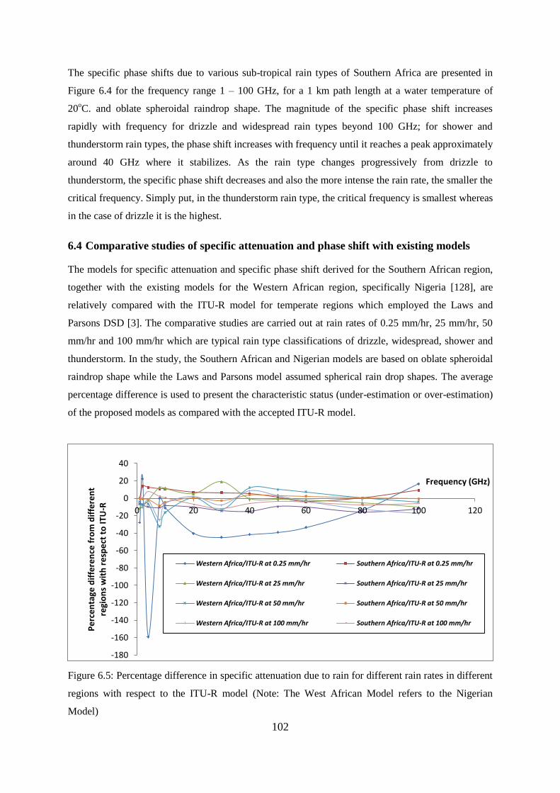
102

The specific phase shifts due to various sub-tropical rain types of Southern Africa are presented in

Figure 6.4 for the frequency range 1 – 100 GHz, for a 1 km path length at a water temperature of

20oC. and oblate spheroidal raindrop shape. The magnitude of the specific phase shift increases

rapidly with frequency for drizzle and widespread rain types beyond 100 GHz; for shower and

thunderstorm rain types, the phase shift increases with frequency until it reaches a peak approximately

around 40 GHz where it stabilizes. As the rain type changes progressively from drizzle to

thunderstorm, the specific phase shift decreases and also the more intense the rain rate, the smaller the

critical frequency. Simply put, in the thunderstorm rain type, the critical frequency is smallest whereas

in the case of drizzle it is the highest.

6.4 Comparative studies of specific attenuation and phase shift with existing models

The models for specific attenuation and specific phase shift derived for the Southern African region,

together with the existing models for the Western African region, specifically Nigeria [128], are

relatively compared with the ITU-R model for temperate regions which employed the Laws and

Parsons DSD [3]. The comparative studies are carried out at rain rates of 0.25 mm/hr, 25 mm/hr, 50

mm/hr and 100 mm/hr which are typical rain type classifications of drizzle, widespread, shower and

thunderstorm. In the study, the Southern African and Nigerian models are based on oblate spheroidal

raindrop shape while the Laws and Parsons model assumed spherical rain drop shapes. The average

percentage difference is used to present the characteristic status (under-estimation or over-estimation)

of the proposed models as compared with the accepted ITU-R model.

Figure 6.5: Percentage difference in specific attenuation due to rain for different rain rates in different

regions with respect to the ITU-R model (Note: The West African Model refers to the Nigerian

Model)

-180

-160

-140

-120

-100

-80

-60

-40

-20

0

20

40

0 20 40 60 80 100 120

Pe

rce

nta

ge d

iffe

ren

ce f

rom

dif

fere

nt

regi

on

s w

ith

re

spe

ct t

o IT

U-R

Frequency (GHz)

Western Africa/ITU-R at 0.25 mm/hr Southern Africa/ITU-R at 0.25 mm/hr

Western Africa/ITU-R at 25 mm/hr Southern Africa/ITU-R at 25 mm/hr

Western Africa/ITU-R at 50 mm/hr Southern Africa/ITU-R at 50 mm/hr

Western Africa/ITU-R at 100 mm/hr Southern Africa/ITU-R at 100 mm/hr

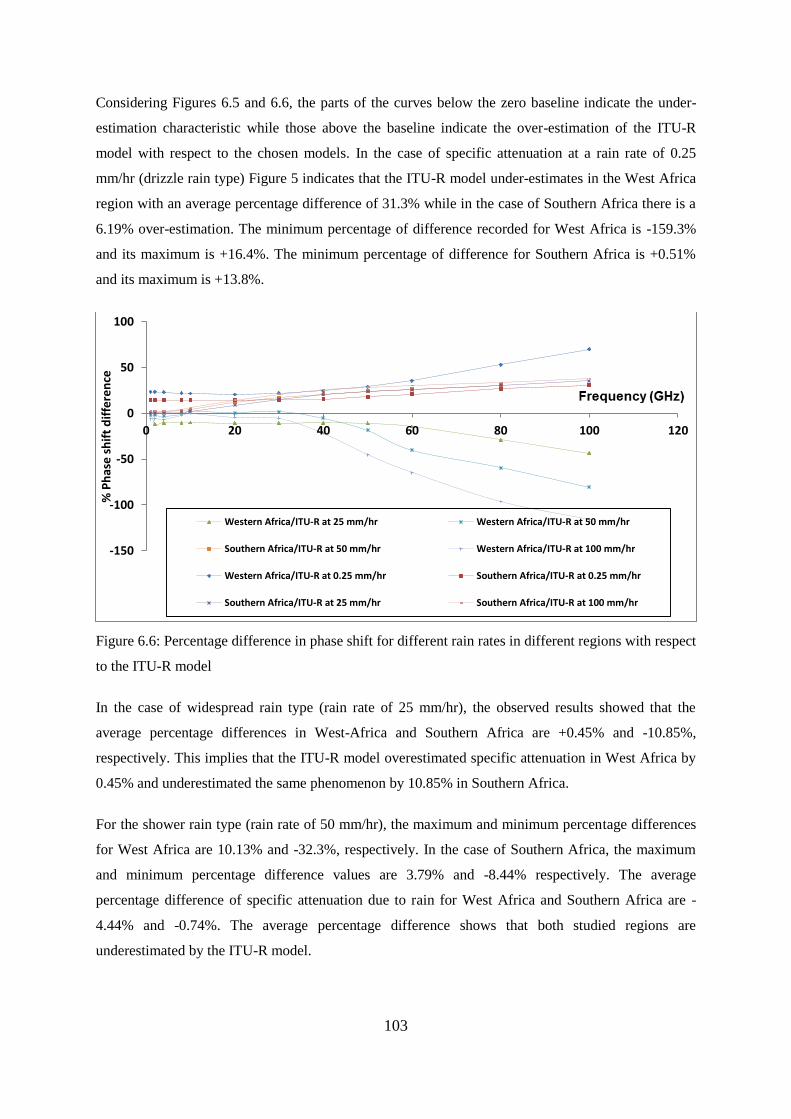
103

Considering Figures 6.5 and 6.6, the parts of the curves below the zero baseline indicate the under-

estimation characteristic while those above the baseline indicate the over-estimation of the ITU-R

model with respect to the chosen models. In the case of specific attenuation at a rain rate of 0.25

mm/hr (drizzle rain type) Figure 5 indicates that the ITU-R model under-estimates in the West Africa

region with an average percentage difference of 31.3% while in the case of Southern Africa there is a

6.19% over-estimation. The minimum percentage of difference recorded for West Africa is -159.3%

and its maximum is +16.4%. The minimum percentage of difference for Southern Africa is +0.51%

and its maximum is +13.8%.

Figure 6.6: Percentage difference in phase shift for different rain rates in different regions with respect

to the ITU-R model

In the case of widespread rain type (rain rate of 25 mm/hr), the observed results showed that the

average percentage differences in West-Africa and Southern Africa are +0.45% and -10.85%,

respectively. This implies that the ITU-R model overestimated specific attenuation in West Africa by

0.45% and underestimated the same phenomenon by 10.85% in Southern Africa.

For the shower rain type (rain rate of 50 mm/hr), the maximum and minimum percentage differences

for West Africa are 10.13% and -32.3%, respectively. In the case of Southern Africa, the maximum

and minimum percentage difference values are 3.79% and -8.44% respectively. The average

percentage difference of specific attenuation due to rain for West Africa and Southern Africa are -

4.44% and -0.74%. The average percentage difference shows that both studied regions are

underestimated by the ITU-R model.

-150

-100

-50

0

50

100

0 20 40 60 80 100 120

% P

has

e s

hif

t d

iffe

ren

ce

Western Africa/ITU-R at 25 mm/hr Western Africa/ITU-R at 50 mm/hr

Southern Africa/ITU-R at 50 mm/hr Western Africa/ITU-R at 100 mm/hr

Western Africa/ITU-R at 0.25 mm/hr Southern Africa/ITU-R at 0.25 mm/hr

Southern Africa/ITU-R at 25 mm/hr Southern Africa/ITU-R at 100 mm/hr

104

Lastly on the comparative studies of specific rain attenuation, using the percentage differences for the

thunderstorm rain type also confirmed that the ITU-R model underestimated specific attenuation due

to rain by -6.66% in West Africa and by -2.83% in the Southern Africa.

Figure 6.6 presents a characteristic percentage differences in the specific phase shift between the

West African model and the ITU-R model, and the Southern African model and the ITU-R model.

For the drizzle rain type, the average percentage difference for West Africa and Southern Africa are

30.64% and 17.85% respectively. This implies that the ITU-R model used to determine specific phase

shift overestimates for the small rain drops for these two regions. In the case of widespread rain

(rain rate of 25 mm/hr) the average percentage difference between the West African model

and the ITU-R model shows an under-estimation of 14.14% and for the Southern African

region there is an over-estimation of 13.84%. The trend of under-estimation by the ITU-R

model in the West African region cuts across the shower and thunderstorm rain types by

17.35% and -31.22% respectively, while in the case of Southern Africa, an overestimation

trend by 14.83% and 17.40% respectively was observed for the shower and thunderstorm rain

types.

6.5 Power Law regression for specific attenuation and phase shift

The results obtained from the computations of specific attenuation and specific phase shift

due to rain are modeled using a power law regression scaling at different frequencies and rain

types in the region of Southern Africa. Table 6.1 shows the coefficients of power law

expressions in Equations (2.17) and (6.7) for specific attenuation and phase shift due to rain

for the region respectively.

(6.7)

where and are coefficients of the phase shift and R in hrmm/ is the rain rate for a

defined rain type for the region. With reference to Equation (2.17), Table 6.1 shows that the

values of a are less sensitive to the type of rain chosen and the same also applies, to some

extent, in the case of parameter b for the frequency range 1 GHz7 .

As presented by various authors [45, 134], the analytical expressions of a, b , and can be

used conveniently by radio planners and system designers to estimate both specific

attenuation and phase shift due to rain. Based on Equations (2.17) and (6.7) for Southern

Africa and for the different rain types, general equations are summarized in Equations (6.8) to

105

(6.15) for specific attenuation and Equations (6.16) to (6.23) denote expressions for the

specific

Table 6.1: The values of a and b given for the frequency range 1-100 GHz for the Southern African

Region

GHzfffaDrizzle 1001..............................0048.00017.00002.0 2 (6.8)

GHzfffbDrizzle 1001.........................9651.00053.0101 24 (6.9)

GHzfffaWidespread 1001.......................0124.00006.00002.0 2 (6.10)

GHzffb

GHzffb

Widespread

Widespread

10011..................................................7183.1

101...........................................631.00582.0

2.0

(6.11)

Freq(GHz) Drizzle Widespread Showers Thunderstorm

a b R2 a b R

2 a b R

2 A b R

2

1 2x10-5

0.9309 0.9738 3x10-5

0.719 0.999 2x10-5

0.8291 0.999 2x10-5

0.8714 1

2 0.0001 0.936 0.9749 0.0001 0.7465 0.9988 8x10-5

0.8671 0.999 7x10-5

0.9161 1

3 0.0002 0.9441 0.9767 0.0003 0.7887 0.9986 0.0002 0.9234 0.9999 0.0001 0.981 1

4 0.0005 0.9549 0.9789 0.0005 0.8421 0.9984 0.0003 0.9938 0.9999 0.0002 1.0643 0.9999

5 0.0008 0.9679 0.9813 0.0007 0.9051 0.9981 0.0004 1.0816 0.9998 0.0003 1.18 0.9999

6 0.0012 0.983 0.9839 0.001 0.9766 0.9979 0.0006 1.1785 0.9998 0.0004 1.2871 0.9999

7 0.0018 1 0.9864 0.0014 1.0503 0.9979 0.0008 1.2556 0.9999 0.0006 1.3351 1

8 0.0025 1.0184 0.9888 0.0019 1.1174 0.9981 0.0011 1.302 0.9999 0.001 1.3392 1

9 0.0035 1.0372 0.9909 0.0025 1.1662 0.9986 0.0017 1.3087 1 0.0017 1.3077 1

10 0.0047 1.0554 0.9925 0.0034 1.1997 0.9991 0.0026 1.2983 1 0.0029 1.2661 1

12 0.0079 1.0835 0.9945 0.006 1.2113 0.9997 0.0055 1.246 1 0.0067 1.1918 0.999

15 0.0152 1.1032 0.9956 0.0127 1.1771 1 0.0143 1.1396 1 0.0177 1.0833 0.999

20 0.0333 1.072 0.9935 0.0287 1.1129 0.9999 0.0302 1.0989 1 0.0377 1.0392 0.9999

25 0.0591 1.0303 0.9897 0.0523 1.0376 0.997 0.0482 1.069 1 0.0568 1.0252 0.9999

30 0.0937 1.0125 0.9876 0.086 0.9894 0.9996 0.0772 1.0296 1 0.0906 0.9871 0.999

35 0.1368 1.004 0.9865 0.1302 0.955 0.9997 0.1196 0.9871 1 0.143 0.9394 0.999

40 0.1872 0.9934 0.9849 0.1849 0.9173 0.9997 0.1709 0.9473 1 0.2053 0.8984 0.9999

45 0.2445 0.9776 0.9825 0.2523 0.8674 0.9996 0.2266 0.907 1 0.2645 0.8659 0.9999

50 0.3094 0.9591 0.9792 0.3373 0.8065 0.9995 0.2889 0.8621 1 0.3176 0.8371 0.9999

60 0.4665 0.9271 0.9723 0.5784 0.6811 0.9994 0.4621 0.7592 1 0.4363 0.7752 1

70 0.6538 0.9086 0.9675 0.9017 0.5896 0.9996 0.7272 0.6632 0.9999 0.6185 0.7072 1

80 0.8273 0.9003 0.9652 1.2113 0.5413 0.9999 1.0107 0.6028 0.9998 0.8267 0.6571 0.9999

90 0.932 0.8967 0.9641 1.4023 0.5202 0.9999 1.196 0.5735 0.9998 0.9659 0.6312 0.9999

100 0.9586 0.8954 0.9638 1.457 0.5122 1 1.2534 0.5625 0.9998 1.0071 0.6215 0.9999

106

GHzfffaShower 1001....................0072.00008.00001.0 2 (6.12)

GHzffb

GHzfeb

Widespread

f

Shower

1009................................................7795.1

81..................................................7616.0

189.0

0694.0

(6.13)

GHzffa rmThundersto 1001................................................2889.2 14.0 (6.14)

GHzffb

GHzfeb

rmThundersto

f

rmThundersto

1008..................................................8095.1

71...............................................7934.0

193.0

0766.0

(6.15)

The expressions in equations (6.8) - (6.15) are fitted by the regression equations optimized by the

minimum correlation coefficients 2R with the values closer to 1. The weak value of

2R are observed

with the expression for b especially in widespread and shower rain types with a value that is less than

0.8.

The same regression technique employed in estimating the coefficients of a and b in the case of

specific attenuation is used in determining the coefficients of and for the specific phase shift as

presented in Table 6.2 for four rain types in the Southern African region.

The results tabulated in Table 6.1 and 6.2 add value in link design in that engineers will be able to

determine both specific attenuation and specific phase shift due to rain for the frequency range 1 –

100 GHz. On the other hand, Equations (6.8) – (6.23) are easy-to-use analytical expressions that can

present any error that might arise in the case of interpolation of a given frequency to determine

unspecified frequencies and their coefficients.

In some cases the analytical expressions are split into two different expressions based on the optimum

peaks in order to improve the regression results and correlation coefficients.

GHzff

GHzff

Drizzle

Drizzle

10080............................................624.90

701............................................0753.0

623.0

0402.1

(6.16)

GHzfff

GHzfff

Drizzle

Drizzle

10035.................9756.00016.0107

301...............9278.00006.0104

26

26

(6.17)

GHzff

GHzff

Widespread

Widespread

10080............................................154

701........................................0823.0

641.0

0805.1

(6.18)

GHzfff

GHzfff

Widespread

Widespread

10035..................9408.00083.0104

301.................7024.00041.0108

25

25

(6.19)

107

GHzff

GHzff

Shower

Shower

10080................................................06.153

701..................................................0563.0

662.0

1234.1

(6.20)

GHzfff

GHzfff

Shower

Shower

10035.........................0513.10095.0104

301........................805.00064.00002.0

25

2

(6.21)

GHzff

GHzff

rmThundersto

rmThundersto

10080...........................................56.131

701...........................................0475.0

672.0

1414.1

(6.22)

GHzfff

GHzfff

rmThundersto

rmThundersto

10035..............001.10075.0103

301...........8437.00075.00003.0

25

2

(6.23)

Table 6.2: The values of and give for frequencies range 1-1000GHz for Southern Africa

Region

Frequency(GHz) Drizzle Widespread Showers Thunderstorm

R2 R2 R2 R2 1 0.078 0.929 0.973 0.093 0.709 0.999 0.069 0.816 0.999 0.059 0.855 1

2 0.157 0.929 0.973 0.187 0.71 0.999 0.137 0.817 0.999 0.119 0.857 1

3 0.237 0.929 0.973 0.281 0.712 0.999 0.206 0.82 0.999 0.177 0.861 1

4 0.317 0.93 0.973 0.374 0.715 0.999 0.273 0.824 0.999 0.234 0.866 1

5 0.397 0.93 0.973 0.467 0.719 0.999 0.34 0.83 0.999 0.289 0.873 1

6 0.479 0.931 0.974 0.56 0.723 0.998 0.405 0.836 0.999 0.344 0.88 1

7 0.561 0.932 0.974 0.653 0.728 0.998 0.47 0.842 0.999 0.4 0.886 1

8 0.645 0.933 0.974 0.746 0.733 0.998 0.538 0.846 0.999 0.462 0.887 1

9 0.729 0.934 0.974 0.839 0.737 0.998 0.605 0.85 0.999 0.521 0.891 1

10 0.815 0.935 0.974 0.936 0.739 0.998 0.677 0.852 0.999 0.583 0.892 1

12 0.988 0.936 0.975 1.133 0.742 0.999 0.829 0.851 0.999 0.723 0.888 1

15 1.251 0.935 0.974 1.427 0.743 0.998 1.015 0.862 0.999 0.875 0.902 1

20 1.702 0.937 0.975 1.935 0.749 0.998 1.418 0.857 0.999 1.281 0.885 1

25 2.16 0.943 0.976 2.433 0.764 0.999 1.9 0.85 1 1.865 0.856 1

30 2.599 0.943 0.976 2.966 0.756 0.999 2.406 0.829 1 2.451 0.825 1

35 3.008 0.938 0.975 3.529 0.732 0.999 2.904 0.801 1 2.96 0.796 1

40 3.458 0.928 0.973 4.247 0.69 0.999 3.468 0.761 1 3.394 0.767 1

45 4 0.916 0.97 5.225 0.635 0.999 4.225 0.708 0.999 3.863 0.733 1

50 4.547 0.907 0.967 6.296 0.585 0.999 5.12 0.656 0.999 4.395 0.698 1

60 5.538 0.896 0.964 8.295 0.522 0.999 7.05 0.577 0.999 5.718 0.634 0.999

70 6.116 0.892 0.963 9.44 0.5 1 8.325 0.541 0.999 6.801 0.596 0.999

80 6.063 0.892 0.963 9.404 0.496 1 8.385 0.534 0.999 6.906 0.586 0.999

90 5.539 0.892 0.963 8.57 0.498 1 7.667 0.535 0.999 6.387 0.584 0.999

100 4.943 0.892 0.963 7.587 0.504 1 6.704 0.545 0.999 5.552 0.596 0.999

108

6.6 Chapter Summary and Conclusion

In this chapter, the determination of signal attenuation and signal phase shift due to the interaction of

the signal with a passing rain envelope was done. Signal depolarization is itself due to rain attenuation

either as a result of scattering or absorption, resulting in a phase change on exit from the rain medium.

The advantages inherent at these bands, such as high bandwidth, miniaturization of radio equipment

and antenna, easy deployment and large coverage area, are offset by propagation impairments due to

rain at these bands. The focus of this chapter is to study and model the rain microstructure and classify

it into its various rain types based on regional data such as drizzle, widespread, shower and

thunderstorm. Oblate spheroidal rain shape is assumed with the P-P model used to compute scattering

amplitude, scattering cross section and total cross section, thus specific attenuation and specific phase

shift due to rain at 20 0C and a frequency range of 1 – 100 GHz are determined. The specific

attenuation and specific phase shift due to rain are calculated using scattering amplitude and

integrated over all the lognormal raindrop size distribution models using different rain types.

In order to evaluate the characteristics of estimated specific attenuation and phase shift for Southern

Africa, percentage difference is employed to compare the obtained results with the ITU-R model. A

further comparison is made with results obtained using the model derived for West Africa with results

obtained using the ITU-R model to see the effect of different regions on the ITU-R results. From these

results, we conclude that the ITU-R model under-estimates in some cases and overestimates in other

cases, which might be due to the raindrop shape assumed in the computation. The power relation

expressions obtained, together with their respective coefficients will add value in link design in the

region.

109

Chapter 7

Conclusions and Recommendations for Future Work

7.0 Conclusions

In the first part of this study, the rain attenuation estimation is presented using both the ITU-R model

and measured regional rain rate data collected over 10 years in South Africa. The results obtained in

the second part of this study are based on the Intelsat 17 (IS-17) satellite characteristics which operate

at C- and Ku-band and projections are made into higher frequency bands.

Across all the frequency bands from C-band up to V-band, rainfall attenuation, elevation angle, and

effective path length have been determined for satellite link applications in South Africa. A

consideration has been made for link availabilities from 99.99% up to 99.999% of the time. It is noted

that the severity of the degradation of the propagating signal increases with increasing availability.

However, for a given percentage availability, the signal degradation increases with an increase in

operating frequency of the satellite link.

In the third part of this study we proposed a simple and regionally based model for the calculation of

the specific rain attenuation at different rain rates and frequencies up to 100 GHz. The key parameters

are “regional rain drop size distribution model” and “rain rate”. The results presented show the

suitability and adaptability of the model for the Southern African region. This makes it possible to

calculate specific rain attenuation and thus total attenuation at a defined distance of less than 60 km.

The statistical tests confirmed the suitability of other models such as the modified Gamma model. For

the optimum calculation of the attenuation, a rain attenuation model for non-spherical raindrops is

proposed. This result will serve as a good tool for radio planning engineers and technicians especially

in the Southern African region where no comprehensive work has been carried out in the field of radio

propagation through rain.

The fourth part of this study presented realistic raindrops based on their extinction total cross section

and the specific attenuation due to rain using three models, namely, the Morrison and Cross (or

spheroidal) model, the Pruppacher-Pitter model, and the Mie (or spherical) model. A further

investigation of the validity of the Mie spherical raindrops model that is used by many authors was

carried out. It is observed that while the extinction cross-section varies considerably with raindrop

size, the three models show a close agreement for small raindrop diameters but differ as the drop size

increases. The Mie model thus remains accurate for fade margin determination for small raindrop

diameters; this model therefore gives reliable specific rain attenuation predictions in regions

110

dominated by drizzle rainfall, but will considerably underestimate the attenuation in regions

dominated by shower and thunderstorm rain types.

The results also show that the raindrop extinction cross section for the three models agree at the lower

frequencies while a noticeable difference is observed as the frequency increases. The effect of

polarization is noticed in the M-C model and the P-P model, with the horizontal polarization returning

the higher percentage difference compared to the Mie model.

The specific attenuation due to rain for different total cross-sections (P-P, M-C and Mie models) with

circular polarization for different rain types shows a progressive increase in the average percentage

differences (with respect to the Mie model) from drizzle through widespread to thunderstorm rain

types. The average specific attenuation percentage difference for the P-P model is low compared to

the M-C model. The results further show that the power law model parameters, k and α, can be

modelled using a fourth order polynomial. The specific rain attenuation can thus be determined using

the power law model for frequencies up to 100 GHz and rain rate up to 100 mm/hr. In regions where

there is a high presence of large raindrops (as is the case in tropical and sub-tropical regions like

South Africa), it is inadequate to employ the Mie model in the determination of local rain fade

margins. However, this model is acceptable for regions dominated by the drizzle rain type due to a

high presence of small drops.

In the fifth and last part of this study the focus was to study and model the rain microstructure and

classify it into its various rain types based on regional data such as drizzle, widespread, shower and

thunderstorm. Oblate spheroidal rain shape is assumed with the P-P model used to compute scattering

amplitude, scattering cross section and total cross section, thus specific attenuation and specific phase

shift due to rain at 20 0C and a frequency range of 1 – 100 GHz are determined.

The raindrop size models for each rain type are presented by their respective expressions. The results

determined here will improve the accuracy of specific attenuation and specific phase shift due to rain

in the sense that each unnoticed peak that might be peculiar with the general expression is being

identified. The specific attenuation and specific phase shift due to rain are calculated using scattering

amplitude and integrated over all the lognormal raindrop size distribution models using different rain

types.

In order to evaluate the characteristics of estimated specific attenuation and phase shift for Southern

Africa, percentage difference is employed to compare the obtained results with the accepted ITU-R

model. A further comparison is made with results obtained using the model derived for West Africa

with results obtained using the ITU-R model to see the effect of different regions on the ITU-R

results. It is observed that the ITU-R model either under-estimated in some cases or overestimated the

rain attenuation in the South African region, which might be due to the raindrop shape assumed in the

111

computation (spherically-shaped raindrop). The phase shift and specific attenuation power relation

expressions obtained will be useful in improved link design in the South African region.

7.1 Recommendations for Future Work

Rain attenuation in both terrestrial and satellite links remains under-researched in Southern Africa.

The dynamic nature of the seasonal as well as annual rain patterns still presents a new frontier for

research, with regard to their impact on link performance. As such, much of the work involving

attenuation computation in South Africa using rainfall data as well as confirmation measurements

have only been extensively carried out in Durban. The same needs to be extended to cover more areas.

The limitation of the JWD with regard to the smallest raindrop size it can measure has meant that

raindrops that are smaller than 0.3 mm have not been included in the development of rain DSDs. To

mitigate this limitation, it will be necessary to develop parameterizations that will correct the JWD

measurements through factoring in raindrops of small diameters for the Southern African region. This

could be done through a transformation that will focus on correcting the DSDs measured. Also,

different types of measurement equipment need to be used concurrently so as to draw comparisons

with the results obtained using the Joss-Waldvogel RD-80 distrometer used in the current study.

112

References

[1] G.O. Ajayi, S. Feng, S.M. Radicella, B.M. Reddy (Eds.): Handbook on radio propagation related

to satellite communications in tropical and subtropical countries, (ICTP, 1996).

[2] T.J.O. Afullo, “Raindrop Size Distribution Modelling for Radio Link Design along the Eastern

Coast of South Africa,” PIER B, Vol.34, pp. 345-366, 2011.

[3] J.O. Laws and D.A Parsons, “The relation of raindrop-size to intensity,” Trans. Amer. Geophys.

Union, Vol.24, pp.452-460, 1943.

[4] F. Moupfouma, & J. Tiffon, “Raindrop size distribution from microwave scattering measurements

in equatorial and tropical climates,” Electronic Letters, Vol. 18, pp. 1012 – 1014, 1982.

[5] H.R. Pruppacher, and R.L. Pitter, “A semi-empirical determination of shape of cloud and rain

drops,” J. Atmos. Science, Vol. 28, pp. 86-94, 1971.

[6] Mie, “Contributions to the optics of turbid media particularly of colloidal metal solutions,”

Annalen Dr Physiq, Vol 25 (3), pp. 377-445, 1908.

[7] M.O. Odedina, A Semi-Empirical Formulation for Determination of Rain Attenuation on

Terrestrial Radio Links, Ph.D. Thesis, School of Electrical, Electronics and Computer Engineering,

University of KwaZulu Natal, Durban, South Africa, 2010.

[8] O. Massambani,, and C. A, M. Rodriquez, “Specific attenuation as inferred from drop size

distribution measurements in the tropics,” in Proceedings of URSI Commission F symposium, pp. 25 –

28, Rio de Janeiro, Brazil, 3-7 December, 1990.

[9] L. R. Maciel, and M. S. Assis, “Tropical rainfall drop-size distribution,” Int. J. Sat. Commun., 8,

181 – 186, 1990.

[10] Zainal, A. R., I. A. Glover, and P. A. Watson, “Rain rate and drop size distribution measurements

in Malaysia,” in Proceedings of IEEE International Geoscience and Remote Sensing Symposium pp.

309 – 311, 1993.

[11] R. MD Islam, Y. A Abdulrahman and T. A Rahman, “An improved ITU-R rain attenuation

prediction model over terrestrial microwave links in tropical region,” EURASIP Journal on Wireless

Communications and Networking, 2012:189, pp. 1-9, 2012.

113

[12] T. S. Yeo, P. S. Kooi, and M. S. Leong, and S. S. Ng , “Microwave attenuation due to rainfall at

21.255 GHz in the Singapore Environment,” Electron. Lett., 26(14), 1021 – 1022, 1990.

[13] Z. X. Zhou, L. W. Li, T. S. Yeo, and M. S. Leong , “Cumulative distributions of rainfall rate and

microwave attenuation in Singapore’s tropical region,” Radio Science, 35(3), 751 – 756, 2000.

[14] G. O. Ajayi, and E. B. C. Ofoche, “Some tropical rainfall rate characteristics at Ile-Ife for

microwave and millimeter Wave Application,” J. Climate and Appl. Meteor., 23(4), 562 – 567, 1983.

[15] G. O. Ajayi, and R. L. Olsen, “Modeling of a tropical raindrop size distribution for microwave

and millimeter wave applications,” Radio Sci. J., 20(20), 193 –202, 1985.

[16] G. O. Ajayi, and S. U. B. Ezekpo, “Development of climatic maps of rainfall rate and attenuation

for microwave application in Nigeria,” The Nigerian Engineer 23(4), 13 – 30, 1988.

[17] G. Giambene, Resource Management in Satellite Networks: Optimization and Cross-layer

design. Springer, ISBN 978-0-387-36897-9, 2007.

[18] W. Dissanayake, “Ka-Band propagation Modeling for Fixed Satellite Application,” Online

Journal of Space Communication Issue No.2, Fall 2002.

[19] P.A. Owolawi, Characteristics of Rain at Microwave and Millimetric Bands for Terrestrial and

Satellite Links Attenuation in South Africa and Surrounding Islands, Ph.D. Thesis, School of

Electrical, Electronics and Computer Engineering, University of KwaZulu Natal, Durban, South

Africa, 2010.

[20] M.O. Odedina, and T.J.O. Afullo, “Determination of Rain Attenuation from Electromagnetic

Scattering by Spherical Raindrops: Theory and Experiment,” Radio Science 45: RS1003, 2010.

[21] A. Dissanayake, J. Allnutt, and F. Haidara, “A Prediction Model that Combines Rain Attenuation

and Other Propagation Impairments along Earth-Satellite Paths,” IEEE Trans. Antennas and

Propagation, vol. 45, No. 10, 1997, pp. 1546 – 1557.

[22] L. Castanet et al., “Comparison of Various Methods for Combining Propagation Effects and

Predicting Loss in Low Availability Systems in the 20-50 GHz Frequency Range,” Int’l. J. Satell.

Commun., vol. 19, 2001, pp. 317–34.

[23] L. J. Ippolito, Satellite Communications System Engineering, 1st Ed., John Wiley and Sons,

2008, Chapter 8.

114

[24] D. B. Hodge, “An Improved Model for Diversity Gain on Earth-Space Propagation Paths,” Radio

Sci., vol. 17, no. 6, 1982, pp. 1393–99.

[25] A. D. Panagopoulos, P.-D. M. Arapoglou, and P. G. Cottis, “Satellite communications at Ku, Ka

and V bands: Propagation impairments and mitigation techniques,” IEEE Commun, Surv. Tutor., Oct.

2004, 3rd

Quart.

[26] M. Filip and E. Vilar, “Adaptive Modulation as a Fade Countermeasure, An OLYMPUS

Experiment,” Int’l. J. Satell. Commun., vol. 8, 1990, pp. 31–41.

[27] C. Chu and K.S. Chen, “Effects of Rain Fading on the Efficiency of the Ka-band LMD system in

the Taiwan Area,” IEEE Trans. On Vehicular Technology, Vol.54, No.1, 2005.

[28] ITU-R Recommendation P.618.10, Propagation data and prediction methods required for the

design of Earth-space telecommunication systems, 10/2009, Geneva, Switzerland.

[29] ITU-R Recommendation P.840-4, Attenuation due to clouds and fog, 10/2009 Geneva,

Switzerland.

[30] ITU-R Recommendation P.676-10, Attenuation by atmospheric gases, Geneva, Switzerland.

[31] ITU-R Recommendation P.838-3, Specific attenuation model for rain for use in prediction

methods, 09/2005, Geneva, Switzerland.

[32] ITU-R Recommendation P.839-3, Rain height model for prediction methods, 02/2001, Geneva,

Switzerland.

[33] ITU-R Recommendation P.530-12, Propagation data and prediction methods required for the

design of terrestrial Line-of-Sight Systems, 2012, Geneva, Switzerland.

[34] R. L. Freeman, Radio system design for telecommunications, Third Edition, WILEY-

INTERSCIENCE: John Wiley & Sons Inc., New York, 2007.

[35] S.M. Babin, “A case study of subrefractive conditions at Wallops Island, Virginia,” Journal of

Applied Meteorology, vol. 34, pp. 1028-1038, 1995.

115

[36] COST Project 255, Radiowave Propagation Modeling for Satcom Services at Ku band and

Above, Final Report, ESA Publication Division, 2002.

[37] N.K. Chaudhary, D.K. Trivedi and R. Gupta, “The impact of k-factor on the wireless link in

Indian semi-desert terrain,” International Journal Advanced Networking and Applications, vol. 2,

Issue 04, pp. 776-779, 2011.

[38] B.G Ayantunji, P.N Okeke, J.O Urama and Y. Najib, “A semi-empirical model for extrapolation

of surface refractivity over Nigeria,” African Review of Physics, vol. 6, No. 14, pp. 121-128, 2011.

[39] P.K. Odedina and T.J.O Afullo, “Multipath propagation modeling and measurement in clear-air

environment for LOS link design application,” Southern Africa Telecommunication Networks and

Applications Conference Proceedings, 2009.

[40] N.B.A. Rahim, Dao, H., Islam, M.R., and Ibrahim, A.F.I., “Prediction of the tropospheric

scintillation for earth to satellite link in tropical climate,” 4th International Conference on

Mechatronics (ICOM), 17-19 May 2011, Kuala Lumpur, Malaysia.

[41] Karasawa, Y., M. Yamada and J. E. Allnutt, “A New Prediction Method for Tropospheric

Scintillation on Earth-Space Paths,” IEEE Trans. Antennas Propagat., pp. 1608-1614, 1988.

[42] Ippolito L.J., Radiowave Propagation in Satellite Communications, van Nostrand Reinhold

Company, 1986.

[43] K. Harb, A. Srinivasan, H. Changcheng, and B. Cheng, “Prediction Method to Maintain QoS in

Weather-impacted Wireless and Satellite Networks,” Proceedings of the 2007 ISIC IEEE

International Conference on Systems, Man and Cybernetics.

[44] R.K. Crane, “Prediction of the Effects of Rain on Satellite Communication Systems,”

Proceedings of the IEEE, vol. 65, No. 3, pp. 456 – 474, March 1977.

[45] R. Olsen, D. Rogers, and D. Hodge, “The relation in the calculation of rain attenuation,”

IEEE Trans. Antennas Propag., Vol. 26, no. 2, pp. 318–329, 1978.

116

[46] Y. T. Karasawa and T. Matsudo, “Characteristics of fading on low-elevation angle Earth-space

paths with concurrent rain attenuation and scintillation,” IEEE Transactions on Antennas and

Propagation, vol. 39, No. 5, pp. 657 – 661, 1991.

[47] M. P. H. Hall, L. W. Barclay, and M.T. Hewitt (1996), Propagation of Radiowaves, IEE Press,

London.

[48] H. J. Liebe, T. Manabe, and G. A. Hufford, “Millimetre Wave Attenuation and Delay Rates Due

to Fog/Cloud Conditions,” IEEE Transactions on Antennas and Propagation, December 1989, vol.

37, No. 12, pp. 1617 – 1623.

[49] S.I.S. Hassan, Satellite link impairment due to rain and other climatic factors, Department of

Electrical and Electronic Engineering, Universiti Sains Malaysia, Available on

http://www.aprsaf.org/data/aprsaf12_data/day2/csa/6_Dyed_csawg.pdf, last accessed on 16th October

2013.

[50] E.A. Altshuler and R.A. Marr, “Cloud attenuation of millimetre wavelengths,” IEEE

Transactions on Antennas and Propagation, 1989, vol. 37, pp. 1473 – 1479.

[51] A. W. Dissanayake, J. Allnut, and F. Haidara, “Cloud attenuation modelling for SHF and EHF

applications,” International Journal of Satellite Communications, 2001, Vol. 19, pp. 335 – 345.

[52] E. Salonen, “Prediction models of atmospheric gases and clouds for slant path attenuation,”

Olympus Utilization Conference, Sevilla, 1993, pp. 615 – 622.

[53] B.T Maharaj, “Application of fade countermeasures to alleviate rain fade attenuation on earth-

space links,” Satnac 1998.

[54] F.Moupfouma, “Improvement of a rain attenuation prediction method for terrestrial microwave

links,” IEEE Transactions on Ant .and prop., Vol. AP-32, No.12, pp.1368-1372, 1984.

[55] P.A. Owolawi, “Rainfall rate probability density evaluation and mapping for the estimation of

rain attenuation in South Africa and surrounding islands,” PIERS Online, Vol.112, pp.155-181, 2011.

117

[56] P.A. Owolawi, S.J. Malinga and T.J.O. Afullo, “Estimation of Terrestrial Rain Attenuation at

Microwave and Millimeter Wave Signals in South Africa Using the ITU-R Model,” PIERS

Proceedings, Kuala Lumpur, Malaysia, March 27-30, 2012, pp. 952-962.

[57] S.J. Malinga, P.A. Owolawi, and T.J.O. Afullo, “Estimation of Rain Attenuation at C, Ka, Ku,

and V Bands for Satellite Links in South Africa,” PIERS Proceedings, Taipei, Taiwan, March 25-28,

2013, pp. 948-958.

[58] ITU-R Recommendation P.618-8, Propagation data and prediction methods required for the

design of Earth-space telecommunication systems, ITU, Geneva, Switzerland, 2003.

[59] N.C. Mondal, S.K. Sarkar, “Rain height in relation to 0- C isotherm height for satellite

communication over the Indian Subcontinent,” Theoretical and Applied Climatology, Vol. 76, 89–

104, 2003.

[60] J.T. Ong, K.I. Timothy, F.B.L. Choo, W.L. Carron, “Effective rain height statistics for slant path

attenuation prediction in Singapore,” Electronic Letters 36 (7), pp. 661–663, 2000.

[61] S. Parshoatam, I.S. Hudiara, M.L. Singh, “Estimation of effective rain height at 29 GHz at

Amritsar (tropical region),” IEEE Transaction on Antennas and Propagation 55 (5), 1463–1465,

2007.

[62] G. O. Ajayi, and F. Barbaliscia, “Prediction of attenuation due to rain: Characteristics of the

Co0 isotherm in temperate and tropical climates," International Journal of Satellite Communication,

Vol. 8, pp. 187-196, 1990.

[63] J. S. Seybold, Introduction to RF Propagation, John Wiley & Sons, Hoboken, NJ, 2005, pp. 255-

270.

[64] R.K Crane, Electromagnetic wave propagation through rain, John Wiley,1996.

[65] S.Das, A. Maitra , A.K. Shukla, “Rain attenuation modelling in the 10 – 100 GHz frequency

using drop size distributions for different climate zones in tropical India,” PIER B, 25, pp. 211-224,

2010.

118

[66] K.S. Chen, C.Y. Chu, Y.C. Tseng, “A semi-empirical model of rain attenuation at Ka-band in

Northern Taiwan,” PIER M, 16, pp. 213-223, 2011.

[67] J.S. Mandeep, J.E. Allnut, “Rain attenuation prediction at Ku-band in South East Asian

countries,” PIER, Vol. 76, pp. 65-74, 2007.

[68] A. Berne, and R. Uijlenhoet, “A stochastic model of range profiles of raindrop size distributions:

Application to radar attenuation correction,” Geophys. Res. Lett., 32, L10803, doi:

10.1029/2004GL021899, 2005a.

[69] A.R. Jameson and A.B. Kostinski, “What is a Raindrop Size Distribution?,” Bulletin of the

American Meteorological Society , Vol.82, pp.1169-1177, 2001.

[70] R. Uijlenhoet, J.A. Smith, and M. Steiner “Microphysical Structure of Extreme precipitation as

inferred from Ground-based Raindrop spectra,” Journal of the Atmospheric Sciences, Vol. 60, pp.

1220-1238, 2003.

[71] J.S. Marshall. and W.M. Palmer, “The distribution of raindrops with size,” Journal of

Meteorology, Vol.5, pp. 165-166, 1948.

[72] R.G. Quimpo and A.B Brohi, “On the frequency distribution of raindrop sizes,” Journal of

Irrigation and Drainage Engineering, Vol.112, No.2, pp. 119-127, May 1986.

[73] P.A Owolawi, “Raindrop Size Distribution Model for the Prediction of Rain Attenuation in

Durban,”PIERS Online, Vol.7, No.6, pp. 516-523, 2011.

[74] L.R. Maaciel and M.S. Assis, “Tropical rainfall drop size distribution,” International Journal of

Satellite Communications, Vol.8, pp. 181-186, 1990.

[75] L.S. Kumar, Y.H. Lee, and J.T Ong, “Truncated Gamma Drop Size Distribution Models for Rain

Attenuation in Singapore,” IEEE Transactions of Antennas and Propagation, Vol.58, No.4, April

2010.

[76] L.S. Kumar, Y.H. Lee, and J.T. Ong, “Two-Parameter Gamma Drop Size Distribution Models

for Singapore,” IEEE Transactions on Geoscience and Remote Sensing, Vol.549, No.4, September

2011.

119

[77] B.S. Jassal A. K. Verma and Lal Singh, “Raindrop size distribution and attenuation for Indian

climate,” Indian Journal of Radio and Space Physics, Vol.23, Iss.3, pp. 193-196, June 1994.

[78] A.R. Tharek and J. Din, “Rainfall drop size distribution measurements in Malaysia,” Proc. URSI

Comm. F. 1992 Symposium on Wave Propagation and Remote Sensing, Ravenscar, North Yorkshire,

UK,8-12 June,1992, pp 1.2.1-1.2.5.

[79] G.O. Ajayi and A. Adimula, “Variations in raindrop size distribution and specific attenuation in a

tropical environment,” URSI Comm. F Symposium, La Londe-less Maures, France, pp. 811-814,

September 1989.

[80] B. Sevruk, , and W. R. Hamon, International comparison of national precipitation gauges with a

reference pit gauge. WMO Instrument and Observing Methods Rep. 17, 1984. [Available from World

Meteor. Org., Case Postale 2300, CH-1211, Geneva, Switzerland].

[81] B. Sevruk, “Wind induced measurement error for high-intensity rains. Proc. International

Workshop on Precipitation Measurement,” WMO Tech. Document 328, 199–204, 1989. [Available

online at http://www.wmo.ch.].

[82] P. Y. Groisman, and D. R. Legates, “The accuracy of United States precipitation data,” Bull.

Amer. Meteor. Soc., Vol. 75, 215-227, 1994.

[83] V. Nešpor, , and B. Sevruk,: “Estimation of wind-induced error of rainfall gauge measurements

using a numerical simulation,” J. Atmos. Oceanic Technol.,Vol. 16, 450–464, 1999.

[84] B. Sevruk, , M. Ondras and B. Chvila, “The WMO precipitation measurement intercomparisons,”

Atmos. Res., Vol. 92, 376-380, 2009.

[85] O. Fiser, M . Schoenhuber, and P. Pesice, “First results of DSD measurement by video

distrometer in the Czech Republic in 1998–1999,” Studia Geophysica et Geodetica, 46, 3, 485–505,

2002.

[86] I.A Adimula and G.O. Ajayi, “Variation in raindrop size distribution and specific attenuation due

to rain in Nigeria,” Ann. Telecom, Vol.51, No. 1-2, pp. 87–93, 1996.

120

[87] K.I. Timothy, J.T. Ong and E.B.L. Choo, “Raindrop size distribution using method of moments

for terrestrial and satellite communication applications in Singapore,” IEEE Trans. Antennas

Propagat., vol. 50, pp. 1420–1424, October 2002.

[88] J.S. Mandeep and K. Tanaka; “Effect of atmospheric parameters on satellite links,” Int. Journal

Millimeter wave, 2007, 28(10), pp. 789-795.

[89] L.S. Kumar, Y.H. Lee, J.X. Yeo and J.T. Ong., “Tropical rain classification and estimation of

rain from Z-R (Reflectivity-rain rate) relationships,” PIER B, Vol.32,107-127, 2011.

[90] R. Gunn and G.D. Kinzer, “The terminal velocity of fall for water droplets in stagnant air,”

Journal Atmos. Sci., Vol.6, No.4, pp. 243-248, 1949.

[91] J. Vivekanandan, G. Zhang, and E. Brandes, “Polarimetric radar rain estimators based on

constrained gamma drop size distribution model,” J. Appl. Meteorology., Vol.43, No.2, pp. 217-230,

2004.

[92] T. Kozu, and K. Nakamura., “Rainfall parameter estimation from dual-radar measurements

combining reflectivity profile and path-integrated attenuation,” J.Atmos. Oceanic Tech., 1991, Vol.

8(2), pp. 259-270.

[93] C.W. Ulbrich, “Natural variation in the analytical form of the raindrop size distribution,” J.

Climate Appl. Meteoro., Vol. 22, pp. 1764-1775, 1983.

[94] K.I. Timothy, S. Sharma, M. Devi and A.K. Barbara, “Tropical raindrop size distribution (RDS):

Prediction and modeling its effects on microwave propagation,” Proceedings of 9th International

Conference on Antennas and Propagation, Eindhoven, The Netherlands, 4-7 April 1995, pp. 244-248.

[95] H. Jiang, M. Sano and M. Sekine, “Weibull Raindrop-size distribution and its application to rain

attenuation,” IEE Proc., Microwave, Antenna Propagation., Vol.144, No.3, pp.197-200, June 1997.

[96] S. J. Malinga and P. A. Owolawi, “Obtaining raindrop size model using the method of moments

and its applications for South African radio systems,” PIER B Journal, Vol. 46, pp. 119-138, 2013.

121

[97] W. Pan, Leung, P., Huang, W and Wei Liu, W. “On interval estimation of the coefficient of

variation for three-parameter Weibull, lognormal and gamma distribution: A simulation-based

approach,” European Journal of Operational Research, 164, pp. 367-377, 2005.

[98] C.J. Willmott and K. Matsuura., “Advantages of the mean absolute error (MAE) over the root

mean square error (RMSE) in assessing average model performance”, Climate Research , Vol.30, pp.

79-82, December ,2005.

[99] J. T. Ong and Y. Y. Shan, "Raindrop size distribution models for Singapore: comparison with

results from different regions,” Proc. 10th Intl. Conf. on Ant. & Prop., Vol. 436, 2.281-2.285, 1997.

[100] J. T. Ong et al., “Studies on tropical rainfall structure with RAL S-band radar, TRMM PR and

radiosonde-inter comparison,” Proc. European Geophysical Society, XXVI General Assembly, France,

Mar. 2001.

[101] T.S. Yeo, P.S. Kooi, M.S. Leong, and L.W. Li, “Tropical raindrop size distribution for the

prediction of rain attenuation of microwaves in the 10-40 GHz band,” IEEE Transactions on Antennas

and Propagation, Vol.49, No.1, 80-82, January 2001.

[102] L. da Silva Mello and M.S. Pontes., “Unified method for the prediction of rain attenuation in

satellite and terrestrial links,” Journal of Microwaves, Optoelectronics and Electromagnetic

Applications, Vol.11, No.1, June 2012.

[103] F. Moupfouma, “A new theoretical formulation for calculation of the specific attenuation due to

precipitation particles on terrestrial and satellite radio links,” International Journal of Satellite

Communications, Vol. 15, pp. 89-99, 1997.

[104] I. Seishiro, “Rain attenuation at millimeter wavelength of 1.33 mm,” International Journal of

Infrared and Millimeter waves, Vol. 25, No.10, pp. 1495-1501, October 2004.

[105] M. Sekine, C. Chen, and T. Musha, “Rain attenuation from log-normal and Weibull raindrop-

size distributions,” IEEE Trans. Antenna and propagation, Vol. AP-35, No.3, pp. 358-359, March

1987.

[106] D.A. De Wolf, “On the Law-Parsons distribution of raindrop sizes,” Radio Science, Vol. 36,

No.4, pp. 639-642, June/August 2001.

122

[107] T. Kozu, Estimation of raindrop size distribution from space borne radar measurements, Ph.D.

dissertation, Univeristy of Kyoto, Japan, 1991.

[108] P.W. Mielke Jr., “Simple iterative procedures for two parameter gamma distribution maximum

likelihood estimates,” Journal. Appl. Meteor. Vol. 15, pp. 181-183, 1976.

[109] S. Moumouni, M. Gosset, and E. Houngninou, “Main features of rain drop size distributions

observed in Benin, West Africa, with optical distrometers,” Geophysical Research Letters, Vol. 35,

No. 23, L23807, doi: 10.1029/2008GL035755, December 2008.

[110] J.A Morrison and M.J. Cross, “Scattering of a plane electromagnetic wave by axisymmetric

raindrops,” Bell Syst. Tech, J., Vol. 53, pp. 955-1019, July-August, 1974.

[111] L.W. Li, P.S. Kooi, M.S. Leong, T.S. Yeo, and M.Z. Gao, “Microwave attenuation by

realistically distorted raindrops: Part I-Theory,” IEEE Trans. Antenna Propagation, Vol. 43, No.8, pp.

811-821, 1995.

[112] L.W. Li, P.S. Kooi, M.S. Leong, and T.S. Yeo, “Integral Equation Approximation to

Microwave Specific Attenuation by Distorted Raindrops: The Pruppacher-and-Pitter Model,”

Proceedings of IEEE Singapore International Conference, 3-7 Jul 1995, pp. 600-604, ISBN: 0-7803-

2579-6.

[113] L.W. Li, P.S. Kooi, M.S. Leong, and T.S. Yeo, “Integral Equation Approximation to

Microwave Specific Attenuation by Distorted Raindrops: The Spheroidal Model,” Proceedings of

IEEE Singapore International Conference, 3-7 Jul 1995, pp. 658-662, ISBN: 0-7803-2579-6.

[114] T. Oguchi, “Attenuation of electromagnetic wave due to rain with distorted raindrops,” J. Radio

Res. Labs., Vol. 7, pp. 467-485, 1960.

[115] Distromet Ltd., Distrometer RD-80 instructional manual, Basel, Switzerland, June 20, 2002.

[116] T.J. Schuur et al., “Drop Size Distribution Measured by a 2D Video Disdrometer: Comparison

with Dual-Polarization Radar Data,” Journal of Applied Meteorology, Vol. 40, pp. 1019 – 1034, June,

2001.

123

[117] H. R. Pruppacher and K. V. Beard, “A wind tunnel investigation of the internal circulation and

shape of water drops falling at terminal velocity in air,” Quart. J. R. Met. Soc., Vol. 96, pp. 247-256,

April 1970.

[118] T. Oguchi, “Electromagnetic wave propagation and scattering in rain and other hydrometeors,”

Proc. IEEE, Vol. 71, Issue 9, pp. 1029-1078, Sept. 1983.

[119] L. W. Li et al., “On the simplified expression of realistic raindrop shapes,” Microwave &

Optical Technol. Letters, Vol. 7, Issue 4, pp. 201–205, March 1994.

[120] S.J. Malinga, P.A. Owolawi and T.J.O. Afullo, “Determination of specific rain attenuation using

different total cross-section models for Southern Africa,” SAIEE Africa Research Journal, Vol. 105,

No. 1, pp. 20-30, 2014.

[121] M. Marzuki, T. Kozu, and T. Shimomai, “Diurnal Variation of Rain Attenuation Obtained from

Measurement of Raindrop Size Distribution in Equatorial Indonesia,” IEEE Transactions on Antennas

and Propagation, Vol. 57, 1191-1196, 2009.

[122] R.K. Crane, “Propagation phenomena affecting satellite communication systems operating in

centimeter and millimeter wavelength bands,” IEEE Transactions on Antennas and Propagation., AP-

26, No.2, 318-329, 1978.

[123] D.V. Rogers and R.L. Olsen, “Calculation of radiowave attenuation due to rain at frequencies

up to 1000 GHz,” Communications Res. Centre, Dept. of Communications, Ottawa, ON, Canada,

CRC Rep. 1299, 1976.

[124] T. Oguchi, “Attenuation of Electromagnetic wave due to rain with distorted raindrops (Part II)”,

Journal of Radio Labs (Japan), 11, 19–44, 1964.

[125] T. Oguchi, “Scattering and absorption of a millimeter wave due to rain and melting hailstones”,

Journal of Radio Labs (Japan). 13, 141–172, 1966.

[126] T. Oguchi, “Effect of incoherent scattering on microwave and millimeter wave communication

through rain”, Electronics Letter, 27, 759–760, 1991.

124

[127] R.G. Medhurst, “Rainfall attenuation of centimeter waves: Comparison of theory and

measurement,” IEEE Transactions on Antennas and Propagation, AP-13, 550-564, 1965.

[128] M.O. Ajewole, L.B. Kolawole and G.O. Ajayi, “Theoretical study of effect of different types of

tropical rainfall on microwave and millimeter-wave propagation,” Radio Science, 34, 1103–1124,

1999.

[129] P.K. Kunhikrishnan, R. Sivaraman, and D.P. Alappattu, “A case study of rain drop size

distribution over a tropical Indian station,” 36th COSPAR Scientific Assembly, 16-23 July, Beijing

China, 2006.

[130] P.A. Owolawi: Rain at SHF and EHF for Radio Link in South Africa: Characteristics of Rain at

SHF and EHF for Terrestrial and Satellite Links in South Africa, LAP LAMBERT ACEDEMIC

Publishing, ISBN: 9783846596548, 2011.

[131] K. Naicker and S.H. Mneney, “Propagation Measurememt and modelling for terrestrial line-of-

sight links at 19.5 GHz,” IEEE Africon 2004, Gaborone, Botswana, pp. 95-100, 2004.

[132] M.O. Fashuyi and T.J.Afullo, “Rain attenuation prediction and modelling for LOS links on

terrestrial paths in South Africa,” Radio Science, Vol.42, RS003618, 2007.

[133] H.J. Liebe, “MPM – An atmospheric millimeter wave propagation model,” International

Journal of Infrared and Millimetre Waves, Vol. 10, No. 6, pp. 631 – 650, 1989.

[134] J. Goldhirsh, “Two-dimension visualization of rain cell structure,” Radio Science, Vol. 35, pp.

713-729, 2000.